INTERNATIONAL JOURNAL OF GEOMAGNETISM AND AERONOMYVOL. 7, GI3005, doi:10.1029/2007GI000169, 2008

Comparison and validation studies related to themodeling ionospheric convection and the Europeanincoherent scatter observations in the polar cap

R. Lukianova,1 A. Kozlovsky,2 and T. Turunen2

Received 24 May 2007; accepted 14 February 2008; published 1 3 March 2008.

[1] We use the ionospheric velocity measurements obtained by the European incoherentscatter (EISCAT) Svalbard radar (ESR) for comparison with the electric field distributionpredicted by the new ionospheric convection model based on realistic maps of field-alignedcurrents. The comparative analysis of model output and observations is based on the datacontained both the north–south and east–west components of the ionospheric electric field.Such a comparison provides an independent check of the model. It is shown that the modelrepresents accurately the large-scale features of statistical electric field inferred from the ionvelocity measured by the ESR. From observations and modeling we quantitatively determinethe dependence of the ionospheric electric field strength on the IMF conditions and howthis varies with magnetic local time. For specification of the relationship we derive averageconvection patterns for sorting by the magnitude and direction of the IMF. The dependenceis clearly seen by contrasting the results for two magnitudes of the IMF strength (BT = 1and 5 nT), for two opposite directions of the IMF Bz component, and for By+, By−. Themagnitude of the IMF has the main impact on the average flows under southward IMFconditions. The sign of IMF By is the most important factor influenced the convectionsystem under the IMF northward. For By− the northward component is negative duringa major part of the day indicating counterclockwise plasma flow around the pole. ForBy+, the situation is opposite, the electric field is directed poleward and the plasma rotateclockwise. These are confirmed nicely by the ESR observations. INDEX TERMS: 2409 Ionosphere:

Current systems; 2411 Ionosphere: Electric fields; 2475 Ionosphere: Polar cap ionosphere; 6969 Radio Science:

Remote sensing; KEYWORDS: EISCAT observation, ionospheric convection model, polar cap, field-aligned

currents.

Citation: Lukianova, R., A. Kozlovsky, and T. Turunen (2008), Comparison and validation studies related to the modeling iono-

spheric convection and the European incoherent scatter observations in the polar cap, Int. J. Geomagn. Aeron., 7, GI3005,

doi:10.1029/2007GI000169.

1. Introduction

[2] Convection electric fields are observed regularly in thehigh-latitude ionosphere. Over this wide region the polarcap still has the poorest observational coverage that makesdifficult the investigation of a number of phenomena. Inparticular, the IMF By− related electric field and FAC areexpected in the polar cap. Indeed, the polar-orbiting satel-lites such as the Orsted, Magsat, Champ, Iridium [Ander-

1Arctic and Antarctic Research Institute, St. Petersburg,Russia

2Sodankyla Geophysical Observatory, Sodankyla, Finland

Copyright 2008 by the American Geophysical Union.

1524–4423/08/2007GI000169$18.00

son and Korth, 2007; Christiansen et al., 2002; Papitashviliet al., 2001, 2002; Waters et al., 2001] detect intense FACabove +75◦ magnetic latitude (m.l.). These current den-sity numbers are comparable with the current density of thecorresponding pair of R1 currents. Some researchers believethat the entire near-pole area is always filled with widespreadFACs irrespective of the IMF [e.g., Kustov et al., 2000, andreferences therein; Papitashvili et al., 2001].

[3] The near-pole FAC imply large and variable electricfields in the polar cap, which is not presented adequatelyin the statistical convection models published up to now[Heppner and Maynard, 1987; Papitashvili and Rich, 2002;Rich and Hairston, 1994; Ruohoniemi and Greenwald, 2005;Weimer, 2005]. That is mainly because more data from near-pole region is needed for sorting out in relation to season andIMF strength and direction. Even the assimilative mapping

GI3005 1 of 11

GI3005 lukianova et al.: modeling ionospheric convection GI3005

of the ionospheric electrodynamics (AMIE) [Richmond andKamide, 1988], a technique to obtain high-latitude electro-dynamics combining a wide variety direct and indirect obser-vations from ground magnetometer, radar and near surfacesatellites for individual events, assumes that the data cover-age can be not good (X. Cai et al., unpublished data, 2006).A precise classification of the convection behavior with thesolar wind parameters continues to be an actual task. In par-ticular, it would certainly give more insight in the IMF By

effect in magnetospheric convection.[4] Recently, a new approach for modeling the global dis-

tribution of ionospheric electric potentials utilizing high-precision maps of FACs derived from measurements by theOrsted, Magsat and Champ satellites as input to a com-prehensive numerical scheme has been presented [Lukianovaand Christiansen, 2006]. On the conductivity side, both thesolar contribution and auroral precipitation contribution aretaken into account. It is also able to isolate the effects ofconductivity variations and of IMF. Comparison with ex-isted convection models shows that the convection patternsobtained on the basis of numerical simulation under differ-ent IMF and seasonal conditions are in agreement with thecommonly accepted understanding of large-scale convection.The model includes the polar cap effects and may be usedfor statistical studies.

[5] However, we should also compare with and validate themodel by independent measurements. The European inco-herent scatter (EISCAT) Svalbard radar (ESR) can be usedfor this. To carry out the study, we need measurements ofthe ionospheric convection vector velocity in the high lati-tudes (> 75◦ m.l.). Both the north-south (meridional) andthe east–west (azimuthal) components of the velocity areimportant. First, such a comparison provides an indepen-dent check of the convection model based on FAC. Also, wequantitatively determine the dependence of the near-poleelectric field strength on the IMF conditions and how thisvaries with magnetic local time (MLT). Such dependence areclearly seen by contrasting the results for two magnitudes ofthe IMF strength, for two opposite directions of the IMF Bz

component, and for By+, By− under positive Bz condi-tions. For specification of the dependence we derive averageconvection patterns for sorting by magnitude and orienta-tion of IMF. In this paper we present a comparison of modeloutput and results of ESR measurements of high-latitudeconvection electric fields.

2. Data

[6] The European incoherent scatter (EISCAT) Svalbardradar (ESR) is located in Longyearbyen (geographic coor-dinates are 78.15◦N, 16.03◦E) at the CGM latitude 75.3◦.The radar is able to probe the ionospheric F region by trans-mitting a signal and receiving back-scattered signals. Theline-of-sight (LOS) plasma velocity is derived from spectrumof the back-scattered signal by using the Grand Unified In-coherent Scatter Design and Analysis Package (GUISDAP)[Lehtinen and Huuskonen, 1996]. There is one steerable ESRantenna. Vector of the plasma flow velocity can be measured

when the antenna is scanning al low elevation between twodirections (the beam-swinging mode).

[7] We got the data from the MADRIGAL database, whichcontains analyzed ESR data starting from the beginning ofthe radar operation in 1996. Mostly, the radar measuredalong a fixed direction to the north or south, which does notallow obtaining the velocity component along the east-westdirections. The beam-swinging mode was used sometimes,and the vector flow can be derived in this cases. However,the data at high latitudes (above 75◦ m.l.) are obtained onlyin the cases when the antenna is pointed northward. Alto-gether, there was 110 h of such observation during 2001–2002. These data have been selected for the present study.In the selected cases, the radar was measuring at an eleva-tion of 30◦ from the horizon swinging between two azimuths,−31.25◦ and −16.75◦ (negative angle means turning from Nto W), which are about the direction toward the geomag-netic north. As a rule, the radar was measuring in eachthe position during 1.5–2 min (i.e., the full cycle was 3–4min). We use the LOS plasma velocity averaged over theheight from 250 to 350 km, so that the data are obtainedfrom about 78◦ m.l. We assumed the field-aligned ion ve-locity to be zero. Actually, this velocity does not exceed100 m s−1 which leads to an uncertainty of about 15 m s−1

in the transverse (perpendicular to the magnetic field line)velocity measurements. This error is small enough to beneglected. Vectors of the plasma velocity were calculatedby combining the line-of-sight velocities from the two beamdirections. Effectively, it is assumed that the plasma flowis constant along the L-shell over the distance between thebeams, which is about 140 km. Thus, the obtained data areaveraged over the area of 140 by 170 km in space and over3–4 min in time. For this mode of radar operation, accuracyof the obtained northward velocity component is essentiallybetter than that of the east-west component.

[8] For a long time (since 1996 when the ESR was es-tablished) this radar was mostly used for observations alongthe north-south direction. Only recently, in January andDecember 2004, two campaigns have been performed to ob-serve the azimuthal plasma flow with a good accuracy. Dur-ing these campaigns the ESR steerable antenna was directedto the east or west along the corrected geomagnetic (CGM)latitude (i.e., at an azimuth angle of 70◦ or 250◦ from thegeographic north) at an elevation angle of 45◦. The mea-surements were made in the dayside (0600–1600 MLT) dur-ing 60 h, altogether. These data which include only theeast-west flow component measured at 75.3◦ m.l. are alsoused in the present study. The data used are from ESRobservations under arbitrary IMF conditions. Winter andequinox data are almost equally represented, with respec-tively about 40h and 60h of data, whereas summer is lessrepresented, with only 10h of data. We sum up the observa-tions over many events irrespective to the season that resultin extensive coverage. The data is then selected satisfyingthe IMF intensity 0.5 nT< BT = (B2

z +B2y)1/2 < 3 nT (BT1

case), 3 nT≤ BT < 7 nT (BT5 case) and BT ≥ 7 nT and di-vided in four main IMF clock angles in the GSM Y −Z planeΨ = 45◦ (Bz+, By+), Ψ = 135◦ (Bz+, By−), Ψ = 225◦

(Bz−, By−), and Ψ = 315◦ (Bz−, By+). The associatedclock angle is assumed to belong to one of the main clock an-

2 of 11

GI3005 lukianova et al.: modeling ionospheric convection GI3005

gles if it lays within the interval +45◦ centered at certain Ψ.This gives the ionospheric electric field responses to changesin the IMF Bz and By components separately.

[9] To obtain basic convection patterns, we applythe FAC-based model of the ionospheric electric fields[Lukianova and Christiansen, 2006]. Maps of FAC derivedfrom high-precision magnetic field survey data from thesatellites Orsted, Magsat, and Champ [Papitashvili et al.,2002] serve as the ionospheric convection model input. Torepresent the seasonal dependence, we utilize FAC distribu-tion over the northern hemisphere collected into 3-monthintervals centered at the solstices and equinoxes. The set ofFAC maps for each season is then collected into two intervalssatisfying the IMF conditions BT1 and BT5 and divided infour main IMF clock angles as described above. From theconductivity side we use the following approach. The totalconductivity distribution is combined from solar irradiancecontribution [Robinson and Vondrak, 1984] and auroral con-tribution [Hardy et al., 1987]. The former is calculated byaveraging the daily distribution over 2-month intervals cen-tered at the solstices and equinoxes, other parameters aretaken UT= 1040, F10.7 = 150. The latter contribution de-pends on the Kp index. Taking into account the variationof average Kp with the IMF clock angle and strength, wechoose Kp = 1 for BT1, Kp = 2 for BT5 if Bz > 0, andKp = 3 for BT5 if Bz < 0.

3. Results

3.1. Modeled Convection Patterns

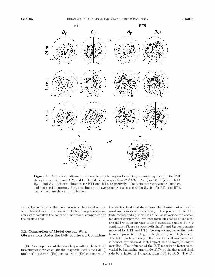
[10] First, we consider the electric field behavior undersouthward IMF conditions. Convection patterns are calcu-lated for winter, summer, equinox for IMF magnitude BT1,BT5 and for the IMF clock angles Ψ = 225◦ and 315◦ (Fig-ure 1). Figure 1a shows the equipotentials obtained in thenorthern polar region for BT1. From top to bottom theplots represent winter, summer, and equinoctial patterns forthe IMF By− (Figure 1a, left) and By+ (Figure 1a, right),respectively. Figure 1b is organized in the same manneras Figure 1a but gives the result for IMF magnitude BT5.All panels expectedly show that the two-cell convection sys-tem is typical for IMF Bz negative irrespective of the seasonand By sign. The duskside vortex occupies bigger area andslightly extends to dawn side likely due to the effect of day-night conductivity gradient. Under equinoctial conditionsthe duskside vortex extension in near-pole region is morepronounced than that during winter or summer. Despite theIMF By-related distortion of plasma flow on the dayside israther small, it is clearly seen that change of the By polaritydoes not produced simple mirrored patterns. The IMF By

positive conditions are much more favorable for the expan-sion of duskside vortex at the dayside than the opposite signof By for the expansion of dawnside vortex across the noonmeridian. However, despite these season- and By-related dif-ferences in convection patterns the two-cell system contin-ues to be fairly dominating. Thus, three factors influenced

the convection patterns can be ranged in following order: amagnitude of IMF, a By sign, a season. That allows us tospecify the dependence of the electric potential distributionmainly on IMF magnitude. We obtain the generalized pat-terns for BT1 and BT5 by averaging over a season and aBy sign. The result is shown in two bottom plots, left andright plots reproduce maps for BT1 and BT5, respectively.For both levels of the IMF strength the convection vorticeskeep its shape, but the voltage of them is expectedly differ-ent. Specifically, the voltages of negative/positive cell are−21/ + 21 kV and −32/ + 27 kV for BT1 and BT5, respec-tively. The cross-polar potential drop increases by a factorof 1.4 while the IMF strengthens from BT1 up to BT5.

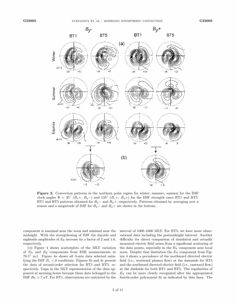
[11] To obtain basic characteristics of the convection underthe northward IMF condition, we perform a binding by sea-son, IMF magnitude and clock angle in a manner analogousto that for southward IMF. Winter, summer and equinoc-tial convection patterns are calculated for BT1, BT5 andΨ = 45◦, 135◦. The results, consisting of 12 patterns in to-tal, are illustrated in Figure 2. In contrast to Figure 1, aBy sign is taken as a primarily factor whereas the IMF mag-nitude is secondary factor. Two left columns (where one isfor BT1 and other is for BT5) and two right columns repre-sent By− and By+ patterns, respectively. Figure 2 shows arather complicated combination of three effects, specifically,a By sign, a season, and a magnitude of IMF. For weakerIMF BT1, the patterns can be described as two-cell for allorientation of By. For stronger IMF BT5, a pronounced ex-pansion of the dusk (dawn) cell for By− (By+) across thenoon is seen. With strengthening of the IMF the intensifica-tion of the pole-round vortices depending on the sign of By

becomes more and more evident. From seasonal side the fol-lowing features should be mentioned. The winter dusk cellgenerally dominates irrespective to By sign, whereas an iso-lated cell extending from the prenoon (for By−) or postnoon(for By+) sector is clearly identified in the dayside near-poleregion. During summer and equinox the foci of dominatingvortex is located almost at the pole, so that the plasma flowsclockwise or counterclockwise around the pole depending ona By sign. Inspection of the patterns presented in Figure 2shows that a By sign effect dominates over the IMF magni-tude and seasonal effects. Thus, we construct the generalizedpatterns for different orientation of By by averaging over aseason and a magnitude of IMF. Resulted patterns are pre-sented in two bottom plots, left and right plots show themaps for By− and By+, respectively. These reproduce themain features of the convection under the northward IMFconditions including the crescent-shaped dawn (dusk) cellfor negative (positive) sign of By and the expansion of cor-responding cell across the noon meridian. Also, elongateddawn (dusk) cell extends further across the midnight merid-ian indicating global counterclockwise (clockwise) rotationof whole convection system with growth of magnetic activ-ity.

[12] From the results of simulation we conclude that themagnitude of IMF has the main impact on the average flowsunder southward IMF conditions while the sign of IMF By

is the most important factor influenced the convection sys-tem under the IMF northward. This allows us utilizing theobtained set of four convection patterns (Figures 1, bottom,

3 of 11

GI3005 lukianova et al.: modeling ionospheric convection GI3005

Figure 1. Convection patterns in the northern polar region for winter, summer, equinox for the IMFstrength cases BT1 and BT2, and for the IMF clock angles Ψ = 225◦ (Bz−, Bz−) and 315◦ (Bz−, Bz+).By− and By+ patterns obtained for BT1 and BT5, respectively. The plots represent winter, summer,and equinoctial patterns. Patterns obtained by averaging over a season and a By sign for BT1 and BT5,respectively are shown in the bottom.

and 2, bottom) for further comparison of the model outputwith observations. From maps of electric equipotentials wecan easily calculate the zonal and meridional components ofthe electric field.

3.2. Comparison of Model Output WithObservations Under the IMF Southward Conditions

[13] For comparison of the modeling results with the ESRmeasurements we calculate the magnetic local time (MLT)profile of northward (EN) and eastward (EE) component of

the electric field that determines the plasma motion north-ward and clockwise, respectively. The profiles at the lati-tude corresponding to the EISCAT observations are chosenfor direct comparison. We first focus on change of the elec-tric field with an increase of IMF magnitude under Bz < 0conditions. Figure 3 shows both the EN and EE componentsmodeled for BT1 and BT5. Corresponding convection pat-terns are presented in Figures 1a (bottom) and 1b (bottom).The MLT profiles clearly reflect the two-cell system whichis almost symmetrical with respect to the noon/midnightmeridian. The influence of the IMF magnitude factor is re-vealed by increasing amplitude of EN at the dawn and duskside by a factor of 1.4 going from BT1 to BT5. The EE

4 of 11

GI3005 lukianova et al.: modeling ionospheric convection GI3005

Figure 2. Convection patterns in the northern polar region for winter, summer, equinox for the IMFclock angles Ψ = 45◦ (Bz+, By−) and 135◦ (Bz+, By+) for the IMF strength cases BT1 and BT5.BT1 and BT5 patterns obtained for By− and By+, respectively. Patterns obtained by averaging over aseason and a magnitude of IMF for By− and By+ are shown in the bottom.

component is maximal near the noon and minimal near themidnight. With the strengthening of IMF the dayside andnightside amplitudes of EE increase by a factor of 2 and 1.6,respectively.

[14] Figure 4 shows scatterplots of the MLT variationof EN and EE components from ESR measurements at78.5◦ m.l. Figure 4a shows all 3-min data selected satis-fying the IMF Bz < 0 conditions. Figures 4b and 4c presentthe data of second-order selection for BT1 and BT5, re-spectively. Gaps in the MLT representation of the data ap-peared at morning hours because these data belonged to theIMF BT > 7 nT. For BT1, observations are restricted by the

interval of 1000–2400 MLT. For BT5, we have more obser-vational data including the postmidnight interval. Anotherdifficulty for direct comparison of simulated and actuallymeasured electric field arises from a significant scattering ofthe data points, especially in the EN component near localnoon. Despite that limitation the EN component from Fig-ure 4 shows a prevalence of the northward directed electricfield (i.e., westward plasma flow) at the dawnside for BT5and the southward directed electric field (i.e., eastward flow)at the duskside for both BT1 and BT5. The regularities ofEN can be more clearly recognized after the appropriatedfourth-order polynomial fit as indicated by thin lines. The

5 of 11

GI3005 lukianova et al.: modeling ionospheric convection GI3005

Figure 3. The MLT profiles of northward (EN) and east-ward (EE) components of the electric field modeled for BT1and BT5. Corresponding convection patterns are presentedin two bottom plots of Figure 1.

fitted curves keep a sine-like shape associated with the an-tisunward transpolar plasma flow, the amplitude increasesby a factor of ∼ 1.5 with the growth of the IMF strengthfrom BT1 up to BT5. For comparison, the modeled electricfield from Figure 3 is given by thick lines in each panel. Thedata points of the EE component are much less scattered.Figure 4 (right) shows that the electric field is eastward andwestward on the dayside and nightside, respectively. Thinlines give the second-order polynomial fit. For both BT1and BT5, the simulated EE (thick lines) generally agrees indirection and in intensity with observations.

3.3. Comparison of Model Output WithObservations Under the IMF NorthwardConditions

[15] As shown above, under the IMF northward condi-tions a sign of IMF By becomes crucial for the convection

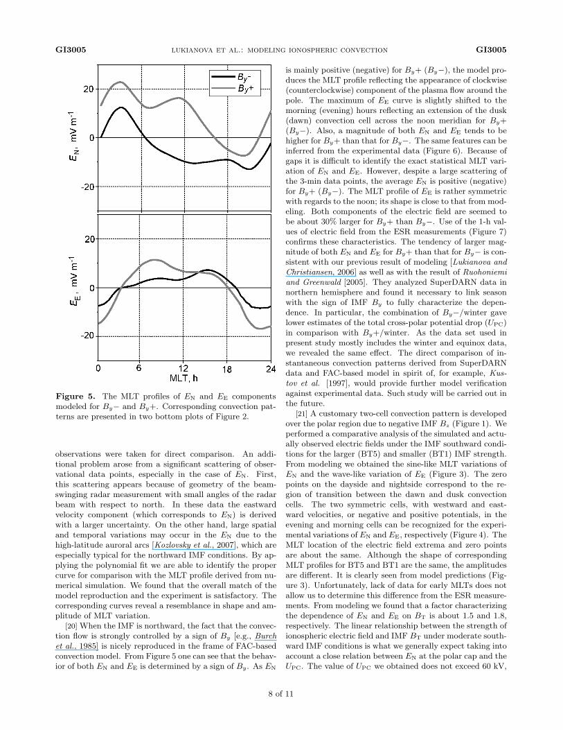
system at high latitudes while the IMF magnitude remainssecond-order factor. We now return to consideration of theelectric field variations associated with change of By direc-tion if Bz > 0. Figure 5 shows the modeled MLT profiles ofboth the EN and EE components for By− and By+. Thecomponents are calculated at 80◦ from corresponding elec-tric potential distribution presented in Figure 2 (bottom).From Figure 5 one can see that for By− the northwardcomponent EN is negative during ∼ 3/4 part of the day in-dicating clockwise plasma flow around the pole. For By+,the situation is opposite, the electric field is directed pole-ward and the plasma rotates counterclockwise. At the sametime, the zonal component EE is changed insignificantly, itsbehavior is similar to that in the Bz < 0 case.

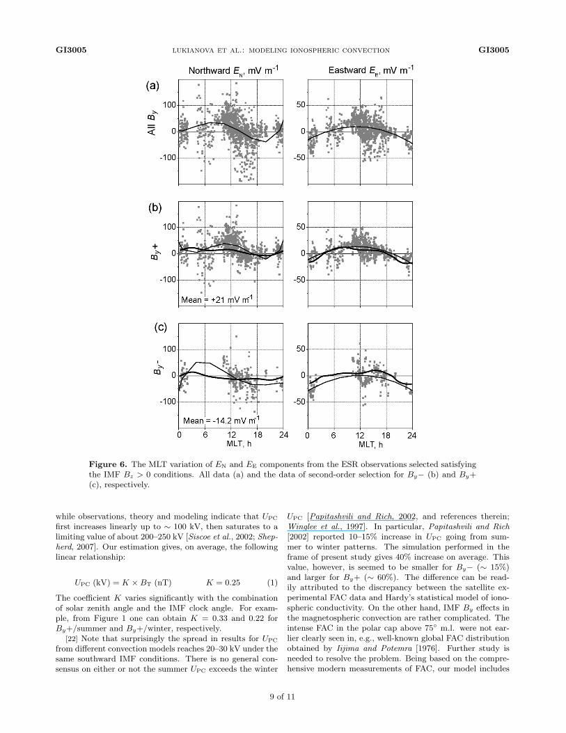
[16] To go further in quantitative comparison of the modeloutput with radar measurements, Figure 6 gives the MLTvariation of EN and EE from the ESR observations at78.5◦ m.l. Figure 6 is organized in the similar manner as Fig-ure 4, but for the data selected satisfying the IMF northwardconditions and sorted out by a sign of By. Figure 6a showsall 3-min data from our data set for Bz > 0. Figures 6b and6c present the data of secondary order selection for By+and By−, respectively. The data points corresponding tothe IMF BT > 7 nT have been removed. There remainsa significant scattering of the data points for both EN andEE components. However, the general tendencies relatedto the sign of By can be recognized, specifically a domina-tion of positive or negative values of EN as shown by thinsolid lines indicating the second-order polynomial fit of theoriginal data. The mean value of observational data of EN is+21 and −14.2 mV m−1 for By+ and By−, respectively. Forcomparison, the MLT profiles (thick lines) from Figure 5 areadded to each plot of Figure 6. One can see the satisfactoryagreement between two curves, especially for By+.

[17] In order to make the By dependence more evident wereproduce in Figure 7 the 1-h values of EN and EE compo-nents from the ESR. Two special campaigns performed inwinter 2004 provided observations of the azimuthal plasmaflow at 75.3◦ m.l. These data included only the east-westflow component but with a good accuracy. Figure 7 repre-sents the measurements under By+ and By− conditions.The MLT profiles of EN are combined from observations at78.5◦ and 75.3◦ m.l. To distinguish between the data pointfrom higher and lower latitudes, the former is marked withthe squares, and the latter is marked with the open circles.One can clearly see a pronounced difference in behavior ofEN associated with a sign of By. Values of EN are mostlynegative for By− with the mean of about −22 mV m−1

(= 78.5◦ m.l.) and −7.5 mV m−1 (= 75.3◦ m.l.). Posi-tive values of EN dominate for By+, the means are +24.3and +12 mV m−1 at 78.5◦ and 75.3◦, respectively. The EE

component is mainly positive on the dayside irrespective tothe By polarity. For By+ the electric fields is seemed tobe stronger (the mean of EE is equal +11.3 mV m−1) thanthat for By− (the mean is equal +7.5 mV m−1). The elec-tric field derived from the FAC-based model shows the sameregularity. Figure 2 gives the cross polar potentials equalto 28 kV and 32 kV for By+ and By−, respectively. Theamplitudes of both EN and EE components from Figure 5are larger for By+.

6 of 11

GI3005 lukianova et al.: modeling ionospheric convection GI3005

Figure 4. The MLT variation of EN and EE components from ESR measurements selected satisfyingthe IMF Bz < 0 conditions. All data (a) and data of second-order selection for BT1 (b) and BT5 (c).Thin and thick lines represent the polynomial fit of observational data and the modeled MLT profile,respectively.

4. Summary and Discussion of ComparisonResults

[18] In this study we use the two very different techniquesto derive the horizontal ionospheric electric field in the polarcap. First one is the modeling of convection patterns basedon realistic maps of FAC measured under the ionosphere bymodern constellation of satellites. Another technique is theradar measurements of ionospheric plasma velocities whichgenerate information on corresponding electric fields. Fromthe beginning of operation the ESR was mostly used for ob-servations along the north-south direction which does notallow obtaining the velocity component along the east-westdirections. In the MADRIGAL database one were able to

select only about 110 h in 2001–2002 when the antenna waspointed northward and the data at high latitudes could beobtained. And recently, in 2004, two campaigns have beenspecially performed to observe the azimuthal plasma flow.These observations formed a database containing two com-ponents of electric field and provided an opportunity to com-pare the model predictions with the measurements that arenot a part of the model input data.

[19] We simulated the convection systems under differ-ent IMF conditions. After appropriate sorting of patternsby magnitude and direction of IMF, the transverse EN andEE components of electric field were calculated for the fourcombinations of IMF, specifically for By− and By+, whenBz > 0, and for BT ∼ 1 nT and BT ∼ 5 nT, when Bz < 0.The profiles along MLT at the latitude corresponding to ESR

7 of 11

GI3005 lukianova et al.: modeling ionospheric convection GI3005

Figure 5. The MLT profiles of EN and EE componentsmodeled for By− and By+. Corresponding convection pat-terns are presented in two bottom plots of Figure 2.

observations were taken for direct comparison. An addi-tional problem arose from a significant scattering of obser-vational data points, especially in the case of EN. First,this scattering appears because of geometry of the beam-swinging radar measurement with small angles of the radarbeam with respect to north. In these data the eastwardvelocity component (which corresponds to EN) is derivedwith a larger uncertainty. On the other hand, large spatialand temporal variations may occur in the EN due to thehigh-latitude auroral arcs [Kozlovsky et al., 2007], which areespecially typical for the northward IMF conditions. By ap-plying the polynomial fit we are able to identify the propercurve for comparison with the MLT profile derived from nu-merical simulation. We found that the overall match of themodel reproduction and the experiment is satisfactory. Thecorresponding curves reveal a resemblance in shape and am-plitude of MLT variation.

[20] When the IMF is northward, the fact that the convec-tion flow is strongly controlled by a sign of By [e.g., Burchet al., 1985] is nicely reproduced in the frame of FAC-basedconvection model. From Figure 5 one can see that the behav-ior of both EN and EE is determined by a sign of By. As EN

is mainly positive (negative) for By+ (By−), the model pro-duces the MLT profile reflecting the appearance of clockwise(counterclockwise) component of the plasma flow around thepole. The maximum of EE curve is slightly shifted to themorning (evening) hours reflecting an extension of the dusk(dawn) convection cell across the noon meridian for By+(By−). Also, a magnitude of both EN and EE tends to behigher for By+ than that for By−. The same features can beinferred from the experimental data (Figure 6). Because ofgaps it is difficult to identify the exact statistical MLT vari-ation of EN and EE. However, despite a large scattering ofthe 3-min data points, the average EN is positive (negative)for By+ (By−). The MLT profile of EE is rather symmetricwith regards to the noon; its shape is close to that from mod-eling. Both components of the electric field are seemed tobe about 30% larger for By+ than By−. Use of the 1-h val-ues of electric field from the ESR measurements (Figure 7)confirms these characteristics. The tendency of larger mag-nitude of both EN and EE for By+ than that for By− is con-sistent with our previous result of modeling [Lukianova andChristiansen, 2006] as well as with the result of Ruohoniemiand Greenwald [2005]. They analyzed SuperDARN data innorthern hemisphere and found it necessary to link seasonwith the sign of IMF By to fully characterize the depen-dence. In particular, the combination of By−/winter gavelower estimates of the total cross-polar potential drop (UPC)in comparison with By+/winter. As the data set used inpresent study mostly includes the winter and equinox data,we revealed the same effect. The direct comparison of in-stantaneous convection patterns derived from SuperDARNdata and FAC-based model in spirit of, for example, Kus-tov et al. [1997], would provide further model verificationagainst experimental data. Such study will be carried out inthe future.

[21] A customary two-cell convection pattern is developedover the polar region due to negative IMF Bz (Figure 1). Weperformed a comparative analysis of the simulated and actu-ally observed electric fields under the IMF southward condi-tions for the larger (BT5) and smaller (BT1) IMF strength.From modeling we obtained the sine-like MLT variations ofEN and the wave-like variation of EE (Figure 3). The zeropoints on the dayside and nightside correspond to the re-gion of transition between the dawn and dusk convectioncells. The two symmetric cells, with westward and east-ward velocities, or negative and positive potentials, in theevening and morning cells can be recognized for the experi-mental variations of EN and EE, respectively (Figure 4). TheMLT location of the electric field extrema and zero pointsare about the same. Although the shape of correspondingMLT profiles for BT5 and BT1 are the same, the amplitudesare different. It is clearly seen from model predictions (Fig-ure 3). Unfortunately, lack of data for early MLTs does notallow us to determine this difference from the ESR measure-ments. From modeling we found that a factor characterizingthe dependence of EN and EE on BT is about 1.5 and 1.8,respectively. The linear relationship between the strength ofionospheric electric field and IMF BT under moderate south-ward IMF conditions is what we generally expect taking intoaccount a close relation between EN at the polar cap and theUPC. The value of UPC we obtained does not exceed 60 kV,

8 of 11

GI3005 lukianova et al.: modeling ionospheric convection GI3005

Figure 6. The MLT variation of EN and EE components from the ESR observations selected satisfyingthe IMF Bz > 0 conditions. All data (a) and the data of second-order selection for By− (b) and By+(c), respectively.

while observations, theory and modeling indicate that UPC

first increases linearly up to ∼ 100 kV, then saturates to alimiting value of about 200–250 kV [Siscoe et al., 2002; Shep-herd, 2007]. Our estimation gives, on average, the followinglinear relationship:

UPC (kV) = K ×BT (nT) K = 0.25 (1)

The coefficient K varies significantly with the combinationof solar zenith angle and the IMF clock angle. For exam-ple, from Figure 1 one can obtain K = 0.33 and 0.22 forBy+/summer and By+/winter, respectively.

[22] Note that surprisingly the spread in results for UPC

from different convection models reaches 20–30 kV under thesame southward IMF conditions. There is no general con-sensus on either or not the summer UPC exceeds the winter

UPC [Papitashvili and Rich, 2002, and references therein;Winglee et al., 1997]. In particular, Papitashvili and Rich[2002] reported 10–15% increase in UPC going from sum-mer to winter patterns. The simulation performed in theframe of present study gives 40% increase on average. Thisvalue, however, is seemed to be smaller for By− (∼ 15%)and larger for By+ (∼ 60%). The difference can be read-ily attributed to the discrepancy between the satellite ex-perimental FAC data and Hardy’s statistical model of iono-spheric conductivity. On the other hand, IMF By effects inthe magnetospheric convection are rather complicated. Theintense FAC in the polar cap above 75◦ m.l. were not ear-lier clearly seen in, e.g., well-known global FAC distributionobtained by Iijima and Potemra [1976]. Further study isneeded to resolve the problem. Being based on the compre-hensive modern measurements of FAC, our model includes

9 of 11

GI3005 lukianova et al.: modeling ionospheric convection GI3005

Figure 7. The 1-h values of EN and EE components from the ESR. Measurements under By+ (top)and By− (bottom) conditions, respectively. The MLT variation of EN is combined from observations at78.5◦ (black squares) and 75.3◦ m.l. (gray open circles).

these polar cap effects and, hence, may be well used to studystatistically the IMF By effects. Validation of the model byindependent measurements of the European incoherent scat-ter (EISCAT) Svalbard radar (ESR) credits a confidence insimulated EN and EE providing further proof that the modelis accurately calculating the electric potential distribution atthe polar cap.

5. Conclusion

[23] Under different IMF conditions the north-south andeast-west components of the electric field have been derivedand compared using the ionospheric velocity measurementsfrom ESR and the new ionospheric convection model basedon realistic maps of field-aligned currents. An agreement isfound regarding the MLT variation of the transverse compo-nents of the electric field inferred from the radar data andmodeling. This result shows quantitatively the capabilityof the model to determine statistical characteristics of theionospheric electric field, at least in the region of the radarfield of view.

[24] The main conclusions of the present study can beformulated as follows:

[25] 1. The ESR measurements of the ionospheric convec-tion vector velocity in the high latitudes (> 75◦ m.l.) allowobtaining the velocity component along both the east-westand north-south directions.

[26] 2. The modeling and observations show that underthe moderate southward IMF conditions the factor charac-terizing a dependence of the amplitude of the ionosphericelectric field on the IMF strength is about 1.5. Underthe northward IMF conditions the electric field tends to behigher for By+ than for By−.

[27] 3. The model predicts that the cross-polar cap poten-tial drop increases on average by a factor of 1.4 going fromsummer to winter convection patterns. The value, however,is smaller for By− (∼ 1.1) and larger for By+ (∼ 1.6).

[28] 4. It is necessary to link the solar zenith angle withthe IMF clock angle to fully characterize the convection pat-terns.

[29] Acknowledgments. We are indebted the Director and

staff of EISCAT for operating the facility and supplying the data.

EISCAT is an International Association supported by Finland

(SA), France (CNRS), Germany (MPG), Japan (NIPR), Norway

(NFR), Sweden (VR), and the United Kingdom (PPARC). The

study was supported by the Academy of Finland. The work of

R.L. was supported by the RFBR (grant 06-05-64311-a) and IN-

TAS (grant 06-1000013-8823).

References

Anderson, B. J., and H. Korth (2007), Saturation of globalfield-aligned currents observed during storms by the Iridium

10 of 11

GI3005 lukianova et al.: modeling ionospheric convection GI3005

satellite constellation, J. Atmos. Sol. Terr. Phys., 69(1–2),166, doi:10.1016/j.jastp.2006.06.013.

Burch, J. I., P. H. Reiff, J. D. Menetti, and R. A. Heelis (1985),IMF By-dependent plasma flow and Birkeland currents in thedayside magnetosphere: 1. Dynamic Explorer observations, J.Geophys. Res., 90(A2), 1577, doi:10.1029/JA090iA02p01577.

Christiansen, F., V. O. Papitashvili, and T. Neubert (2002),Seasonal variations of high-latitude field-aligned currents in-ferred from �rsted and Magsat observations, J. Geophys. Res.,107(A2), 1029, doi:10.1029/2001JA900104.

Hardy, D. A., M. S. Gussenhoven, R. Raistrick, andW. J. McNeil (1987), Statistical and functional repre-sentation of the pattern of auroral energy flux, number fluxand conductivity, J. Geophys. Res., 92(A11), 12,275.

Heppner, J. P., and N. C. Maynard (1987), Empirical high-latitude electric field model, J. Geophys. Res., 92(A5), 4467.

Iijima, T., and T. A. Potemra (1976), Large-scale characteristicsof field-aligned currents associated with substorm, J. Geophys.Res., 81, 3999.

Kozlovsky, A., A. Aikio, T. Turunen, H. Nilsson, T. Sergienko,V. Safargaleev, and K. Kauristie (2007), Dynamics and elec-tric currents of morningside Sun-aligned auroral arcs, J. Geo-phys. Res., 112, A06306, doi:10.1029/2006JA012244.

Kustov, A. V., V. O. Papitashvili, G. J. Sofko, A. Schiffler,Y. I. Feldstein, L. I. Gromova,, A. E. Levitin, B. A. Belov,R. A. Greenwald, and M. J. Ruohoniemi (1997), Daysideionospheric plasma convection, electric fields, and field-alignedcurrents derived from the SuperDARN radar observations andpredicted by the IZMEM model, J. Geophys. Res., 102(A11),24,057.

Kustov, A. V., W. B. Lyatsky, G. J. Sofko, and L. Xu (2000),Field-aligned currents in the polar cap at small IMF Bz andBy derived from SuperDARN radar observations, J. Geophys.Res., 105, 205.

Lehtinen, M. S., and A. Huuskonen (1996), General incoherentscatter analysis and GUISDAP, J. Atmos. Sol. Terr. Phys.,58, 435, doi:10.1016/0021-9169(95)00047-X.

Lukianova, R., and F. Christiansen (2006), Modeling of theglobal distribution of ionospheric electric fields based on re-alistic maps of field-aligned currents, J. Geophys. Res., 111,A03213, doi:10.1029/2005JA011465.

Papitashvili, V. O., and F. J. Rich (2002), High-latitude iono-spheric convection models derived from Defense Meteorologi-cal Satellite Program ion drift observations and parameterizedby the interplanetary magnetic field strength and direction, J.Geophys. Res., 10(A8), 1198, doi:10.1029/2001JA000264.

Papitashvili, V. O., F. Christiansen, and T. Neubert (2001),Field-aligned currents during IMF 0, Geophys. Res. Lett.,28(15), 3055.

Papitashvili, V. O., F. Christiansen, and T. Neubert (2002), Anew model of field-aligned currents derived from high-precisionsatellite magnetic field data, Geophys. Res. Lett., 29(14), 1683,doi:10.1029/2001GL014207.

Rich, F. J., and M. Hairston (1994), Large-scale convectionpatterns observed by DMSP, J. Geophys. Res., 99, 3827.

Richmond, A. D., and Y. Kamide (1988), Mapping electrody-namic features of the high-latitude ionosphere from localizedobservations: Technique, J. Geophys. Res., 93(A6), 5741.

Robinson, R. M., and R. R. Vondrak (1984), Measurements ofE region ionization and conductivity produced by solar illumi-nation at high latitudes, J. Geophys. Res., 89, 3951.

Ruohoniemi, J. M., and R. A. Greenwald (2005), Dependenciesof high-latitude plasma convection: Consideration of IMF, sea-sonal, and UT factors in statistical patterns, J. Geophys. Res.,110, A09204, doi:10.1029/2004JA010815.

Siscoe, G. L., N. U. Crooker, and K. D. Siebert (2002), Trans-polar potential saturation: Roles of region 1 current system andsolar wind ram pressure, J. Geophys. Res., 107(A10), 1321,doi:10.1029/2001JA009176.

Shepherd, S. G. (2007), Polar cap potential saturation: Ob-servations, theory, and modeling, J. Atmos. Sol. Terr. Phys.,69(3), 234, doi:10.1016/j.jastp.2006.07.022.

Waters, C. L., B. J. Anderson, and K. Liou (2001), Estima-tion of global field-aligned currents using the Iridium systemmagnetometer data, Geophys. Res. Lett., 28(11), 2165.

Weimer, D. R. (2005), Improved ionospheric electrodynamicmodels and application to calculating Joule heating rates, J.Geophys. Res., 110, A05306, doi:10.1029/2004JA010884.

Winglee, R. M., V. O. Papitashvili, and D. R. Weimer (1997),Comparison of the high-latitude ionospheric electrodynamicsinferred from global simulations and semiempirical models forJanuary 1992 GEM campaign, J. Geophys. Res., 102(A12),26,961.

R. Lukianova, Arctic and Antarctic Research Institute, 38Bering str., St. Petersburg 199397, Russia. (renata@aari.nw.ru)

A. Kozlovsky and T. Turunen, Sodankyla Geophysical Obser-vatory, Sodankyla, Finland.

11 of 11