Asian Journal

of Research in

Business Economics

and

Management Asian Journal of Research in Business Economics and Management Vol. 5, No. 3, March 2015, pp. 51-64.

ISSN 2249-7307

51

www.aijsh.org

Asian Research Consortium

Comparing the Forecasting Power of Multivariate Var and Univariate Arima Models: A Case of Groundnut Prices in

Bikaner District of Rajasthan

Richard Kwasi Bannor*; Sharma Amita**

*Ph.D Scholar,

Institute of Agribusiness Management,

SK Rajasthan Agricultural University,

Bikaner, India.

**Assistant Professor,

Institute of Agribusiness Management,

SK Rajasthan Agricultural University,

Bikaner, India. DOI NUMBER-10.5958/2249-7307.2015.00057.2

Abstract

This study explored modelling and forecasting of wholesale groundnut monthly prices in Bikaner district of Rajasthan using the Autoregressive Integrated Moving Average (ARIMA) model and Vector Autoregressive model (VAR). Augmented Dickey fuller test, DF-GLS test and Philips Perron test were used to test for unit root in price series. Autocorrelation (ACF) and Partial autocorrelation (PACF) functions were estimated to assist in deciding the appropriate orders of the Autoregressive model of order p (AR) and Moving Average model of order q (MA). The BIC test was conducted because we were considering several ARIMA models and the model (0, 1, 0) which had the lowest BIC value of 11.612 with R square figure of 84.7% and the mean absolute percentage error of 7.602% was chosen as the best fit model. Vector Autoregressive model used in Model factored in Jaipur, Jodhpur monthly groundnut market prices and cumulative rainfall and rain days per month over the period of 2005-2014. VAR model showed high forecasting error with MAPE of 0.769% compared to ARIMA model of 2.745%.Indiacting, VAR model has high forecasting accuracy compared to ARIMA. The Lagrange Multiplier test of VAR showed that there is no serial correlation in the model whereas Jacque-Bera test also indicated, the residuals of the VAR model is normally distributed indicating a good fit model.

Keywords: ARIMA model, Vector Autoregressive model, Autocorrelation function, Forecasting accuracy, Bikaner, Groundnut, Mean Absolute Percentage Error. ________________________________________________________________________________

Bannor & Amita (2015). Asian Journal of Research in Business Economics and Management,

Vol. 5, No. 3, pp. 51-64.

52

Introduction

India is the largest producer of oilseeds in the world and the oilseed sector occupies an important position in the country’s economy. India accounts for 12- 15 per cent of global oilseeds area, 6-7 per cent of vegetable oils production, and 9-10 per cent of the total edible oils consumption (FAOSTAT, 2011). Oilseed crops contribute a significant proportion to the agricultural GDP. In 2010-11 the area under nine oilseed crops was 26.82 m ha with production of 32.48 Mt, and the total edible oils production in the country stood at 6.63 Mt. Oilseeds area and output are concentrated in the central and southern parts of India, mainly in the states of Madhya Pradesh, Gujarat, Rajasthan, Andhra Pradesh and Karnataka. One important oilseed, groundnut, is use for edible and non-edible purposes. About 81.6% of the total production is crushed and used for edible purpose. The remaining production goes for seed (12%), feed (5.3%) and exports (1.1%). (Anonymous, 2006-07). The governments of Rajasthan understanding the importance of groundnut has been promoting groundnut farming; hence not surprising Rajasthan and Maharastra groundnuts has been assisting greatly in controlling the increasing price of oil in the country (Ananymous 2015).

However the effect on farmers is groundnut market prices are still ruling below the minimum support price (MSP) currently despite NAFED procuring more than 1.1 lakh tonne of the nut from farmers, who are mostly in Gujarat and Rajasthan, under the price support scheme in the last one month. According to AGMARK data, groundnut prices in various markets in Rajasthan are around Rs 3,000 per quintal against the MSP of Rs 4,000 per quintal.

This phenomenon can be attributed to the inability to access agricultural marketing information, which has deprived most farmers the opportunity to effectively plan and market their produce. Market information and intelligence are crucial to enable farmers and traders to make informed decisions about what to grow, when to harvest, to which markets produce should be sent to sell and whether to store it or not (Burark, 2013). Nevertheless, majority of the rural producers are unable to understand and interpret the market information (Ajjan et. al. 2009).

Pingali (2006) indicated that in era of market liberalization and globalization, the returns to diversification towards high-value commodities are conditional to investment in post harvest technologies for processing, quality and food safety. It is therefore imperative to increase investment in public infrastructure (roads, markets, communication, electricity etc.) and institutions that generate widespread benefits in terms of improving access to market information and reducing transaction costs to induce private investment in agribusiness.

Undoubtedly, the most important marketing intelligence need of the farmer is price intelligence. Market information and market intelligence are two inevitable components of market led extension (Babu, 2011). Hence, the dissemination of complete and accurate marketing information is a key to achieving both operational and pricing efficiency in the marketing system (Bhardwaj 2011) which is the core reason of this research.

Farmers are still not getting forecast prices of commodities in their areas as no forecasting is done; consequently, promoting market inefficiencies and wastage of groundnut (Adetunji and Adesiyan, 2008). It is therefore not surprising, small scale groundnut farmers often sell produce either in the

Bannor & Amita (2015). Asian Journal of Research in Business Economics and Management,

Vol. 5, No. 3, pp. 51-64.

53

nearby markets or the farm gate resulting in less of share in consumer price (Kwasi and Kobina 2014).

That is to say, if agricultural growth is to be realized, Rajasthan Government has to ensure effective and efficient market information systems. Forecasting of agricultural commodity prices is of formidable challenge to farmers (Kwasi and Kobina, 2014) even though groundnut price forecast will ensure greater share to producer (farmer) of consumer price and will assist farmers in making informed marketing decisions even in production of agricultural commodities (Kwasi and Kobina, 2014). Hence, using ARIMA model and VAR model to forecast groundnut prices is very useful not only to farmers but in policy formulation and also in promoting efficiency of groundnut marketing in the State. An efficient farm marketing system due to market price information is an important means for raising the income levels of farmers and for promoting the economic development of a country (Tamimi, 1999).

Methodology

Sources of Data

The secondary data used for this study was sourced from AGMARKNET database, Rajasthan Government water resources database and India Meteorological Department (Ministry Of Earth Sciences) southwest sonsoon-2014 end of season report for Rajasthan. AGMARKNET database is under the directorate of Marketing and Inspection of the Ministry of Agriculture of Government of India. Data set of 3 markets namely Bikaner, Jaipur, Jodhpur, were sourced, covering monthly groundnut prices from January 2005 to December 2014. Rainfall and rain days data covering the same period were sourced from Rajasthan Government water resources database and Ministry of Earth sciences report. The wide data were selected to increase the potency of the models used in the analysis and also represent the availability of groundnut market price series, rainfall and rain days data.

Method of Data Analysis

The approach adopted by the researchers was shaped by the approach adopted by Mafimisebi et al 2014; Bannor and Bentil 2014; Kwasi and Kobina 2014. The data analytical techniques that were used in this study included unit root test, Autoregressive Integrated Moving Average (ARIMA) and Vector Autoregressive model (VAR). Augmented Dickey Fuller Tests (ADF) test, Philips-Perron (PP) test and DF-GLS test were used for the stationarity tests.

Test for Unit Root Test: A stationary series is one with a mean value which will not vary with the sampling period. In contrast, a non-stationary series will exhibit a time varying mean (Juselius K 2006). Before forecasting the price of groundnut in the district, it is essential to test for unit root and identify the order of stationarity, denoted as I(0) or I(1). This is necessary to avoid spurious and misleading regression estimates. The framework of ADF methods is based on analysis of the following model

(1)

Bannor & Amita (2015). Asian Journal of Research in Business Economics and Management,

Vol. 5, No. 3, pp. 51-64.

54

Here, pt is the groundnut price series being investigated for stationarity, ∆ is first difference operator, T is time trend variable, μt represents zero- mean, serially uncorrelated, random disturbances, k is the lag length; α,β, γ and δk are the coefficient vectors. Unit root tests were conducted on the β parameters to determine whether or not each of the series is more closely identified as being I(1) or I(0) process. Test statistics is the t statistics for β. The test of the null hypothesis of equation (1) shows the existence of a unit root when β=1 against alternative hypothesis of no unit root when β ≠ 1. The null hypothesis of non-stationarity is rejected when the absolute value of the test statistics is greater than the critical value. When pt is non-stationary, it is then examined whether or not the first difference of pt is stationary (i.e. to test ∆pt − ∆pt −1 ≈ (1) by repeating the above procedure until the data were transformed to induce stationarity.

Philips-Perron (PP) test for a unit root in a time series was used in addition to Augmented Dickey Fuller(ADF). The Philips-Perron (PP) test is similar to the ADF test. PP test was conducted because the ADF test mostly loses its power for sufficiently large values of “k”, the number of lags. It includes an automatic correction to the Dickey-Fuller process for auto-correlated residuals. The regression is as follows

∆yt = bo + b1yt −1 + µt (2)

Where yt is the groundnut price series being investigated for stationarity, b0 and b1 are the coefficient vectors and ut is serially correlated.

Box –Jenkins Model Identification

This approach was adopted from Kwasi and Kobina 2014. The data is examined to check for the most appropriate class of ARIMA processes through selecting the order of the consecutive and seasonal differencing required to make series stationary, as well as specifying the order of the regular and seasonal ARIMA model necessary to adequately represent the time series model. The Autocorrelation function (ACF) and the Partial Autocorrelation function (PACF) are the most important elements of time series analysis and forecasting. The ACF measures the amount of linear dependence between observations in a time series that are separated by a lag k. The PACF plot helps to determine how many auto regressive terms are necessary to reveal one or more of the following characteristics: time lags where high correlations appear, seasonality of the series, trend either in the mean level or in the variance of the series. (Brockwell and Davis, 2002)

Model Parameter Estimation

The Box and Jenkins model includes autoregressive and moving average parameters as well as differencing in the formulation of the model. The three types of parameters in the model are: the autoregressive parameters (p), the number of differencing passes (d) and moving average parameters(q). Box –Jenkins model are summarized as ARIMA (p,d,q) . For example , model described as ARIMA (0,1,0) means that this contains 0 autoregressive (p) parameter and 1 moving average (q) parameter for the times series data after it was differenced once to attain stationarity.

Bannor & Amita (2015). Asian Journal of Research in Business Economics and Management,

Vol. 5, No. 3, pp. 51-64.

55

Oder of Autoregressive Process (p)

Specifically, for an AR (1) process, the autocorrelation function should have an exponentially decreasing appearance. However, higher- order AR processes are often a mixture of exponentially decreasing and damped sinusoidal components.

Order of Moving-Average process (q)

The autocorrelation function of an MA series cut of sharply whereas as for AR series, the autocorrelation function exhibits an exponential decay. The autocorrelation function of a MA (q) process becomes zero at lag q+1 and greater, therefore we examine the autocorrelation function to see where it becomes zero. We do this by placing the 95% confidence interval for the autocorrelation function on the autocorrelation plot.

In ARIMA model, the future value of a variable is assumed to be a linear function of several past observations and random errors. That is, the underlying process that generate the time series has the form:

yt 0 1 yt1 2 yt2 ...p ytp t 1t1 2t2 ...1t1 (3)

where yt and εt are the actual value and random error at time period t, respectively; øi (i=1, 2,…, p) and θj (j=0, 1, 2,…, q) are model parameters. The integers p and q are often referred to as orders of the model. Random errors, εt , are assumed to be independently and identically distributed with a mean of zero and a constant variance of ζ 2. Equation above entails several important special cases of the ARIMA family of models. If q = 0, then (1) becomes an AR model of order p. When p = 0, the model reduces to an MA model of order q. One central task of the ARIMA model building is to determine the appropriate model order (p, q) (Zhang 2003).

Diagnostic checking for Model appropriateness Forecasting

In diagnose checking step, the residuals from the fitted model shall be examined against adequacy. This was done by correlation analysis through the residual ACF plots and the goodness-of –fit test by means of BIC and white noise using the Ljung-Box Q statistic. If the residuals are correlated, then the model should be refined as in step one above. Otherwise, the autocorrelations are white noise and the model is adequate to represent our time series. Hence, the model developed incorporates the basic statistical properties of the time series data into its parameters. This three-step model building process is typically repeated several times until a satisfactory model is finally selected. The final selected model can then be used for forecasting (Zhang 2003)

Multivariate VAR Model Specifications

To deal with forecasting which involves two or more time series, we need to go beyond the univariate ARIMA model. Vector Autoregressive model was used in forecasting wholesale groundnut prices in Bikaner. Model included Jaipur, Jodhpur market prices and cumulative rainfall and rain days per month over the period of the prices. These four time series which has effect on the price of wholesale groundnut prices were included in the model to increase the forecasting of

Bannor & Amita (2015). Asian Journal of Research in Business Economics and Management,

Vol. 5, No. 3, pp. 51-64.

56

accuracy of the model. The intent is, Groundnut prices in Bikaner district are affected by Jodhpur, Jaipur market prices and the amount of rainfall in a month and the rain days experienced by the district. In most case, an occurrence of an event is caused by multiple time series variables. Furthermore, not only that these variables are contemporaneously correlated to each other, their past values may also correlate to each others. By considering multiple time series jointly for an analysis, it utilizes the additional information in determining the dynamic relationships over time among the series (Stock and Watson 2011).

Model Specification

The number of lags is selected by applying five different multivariate lag selection criteria: the Akaike information criterion (AIC), the Hannan-Quin information criterion (HQIC), and the Schwarz’s Bayesian information criterion (SBIC), FPE and LR. This was employed in defining the appropriate lag lengths for a VAR model since they are critical in improving the accuracy of the model (Bannor and Bentil 2014).

Let RF= Cumulative monthly rainfall in mm

RD= Cumulative monthly rain days

The VAR model can be simplified as

…....4

Having estimated the five variables VAR, we denoted the estimated values of the coefficients by bs. We obtained these estimates using the data from time period 1 to end of time period (t). Now we forecast the values of Bikaner beyond sample period, t+1,t+2,….,(t+n), where n is specified.

The model for forecasting of Bikaner wholesale groundnut prices for time period (t+1) can be specified as;

…………5

Forecasting Accuracy

Measures of forecast accuracy are based on forecast errors. The difference between the actual value and the forecasted value gives you the forecast error. The researchers employed Mean Absolute Percent Error (MAPE) as a measure of accuracy for both the VAR and ARIMA models. It indicates the measured error as a percent of actual values

MAPE = 100 ∑ [|At – Ft| / At ] / T………………………………………………………………..6

Where At=Actual Values, Ft=Forecasted Values, T=number of time periods in months

Bannor & Amita (2015). Asian Journal of Research in Business Economics and Management,

Vol. 5, No. 3, pp. 51-64.

57

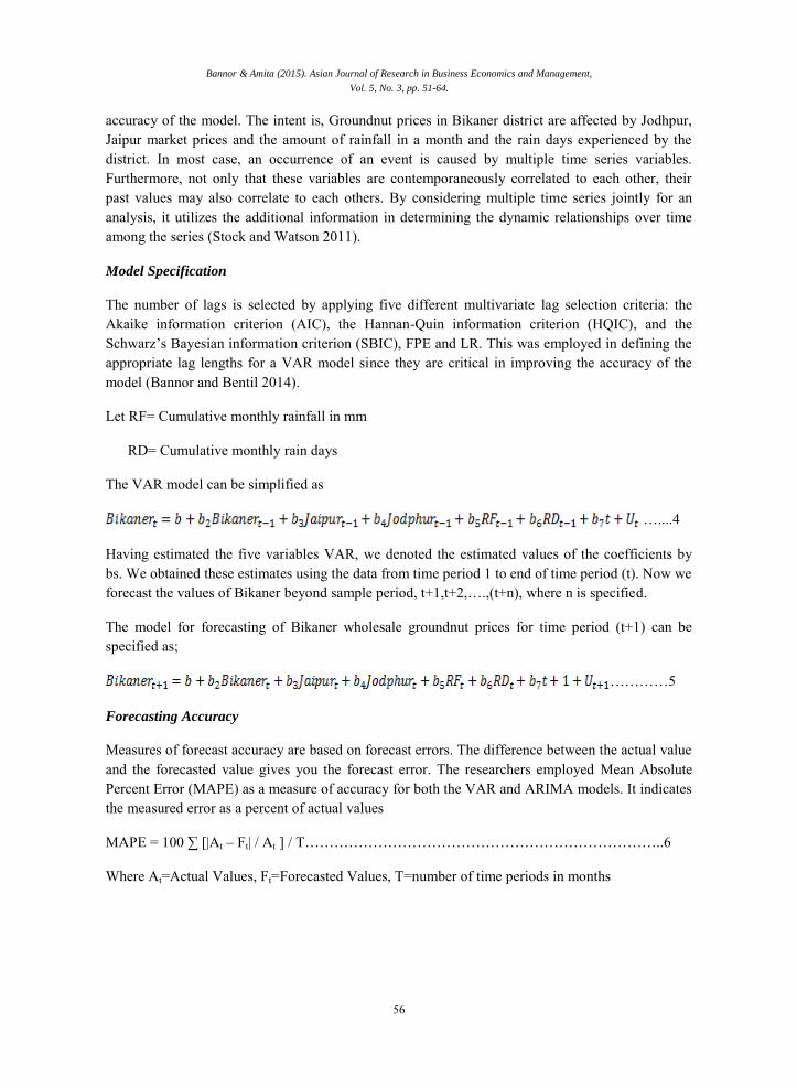
Results and Discussions

Table 2: Unit Root Testing

Variables Price Level 1(0) Intercept with Trend

Market prices ADF Statistics PP Statistics DF-GLS Test Statistics

Test

Statistics

5%

Critical

Value

Test

Statistics

5%

Critical

Value

Test

Statistics

5%

Critical

Value

Bikaner -3.717 -3.448 -3.493 -3.448 -3.480 -3.011 Jaipur -7.076 -3.448 -7.076 -3.448 -6.808 -3.011 Jodhpur -6.178 -3.448 -6.178 -3.448 -5.573 -3.011 Rainfall(mm) -6.131 -3.448 -6.131 -3.448 -5.473 -3.011 Raindays(days) -6.539 -3.448 -6.539 -3.448 -5.816 -3.011 Ho: variables are not stationary or has unit root

H1: Variables are stationary or does not have unit root

NB: If the absolute value of ADF, PP, DF-GLS Test Statistics is less than their 5% critical value we accept null hypothesis. It is also when the MacKinnon approximate p-value for Z(t) is insignificant.

The study first examined each variable time series for evidence of non-stationarity in order to be able to use it in the VAR and ARIMA models. At level 0, all the time series variables were stationary. This stationarity is due to the fact, we are only testing for the unit factoring trend in each of the test. However if we suppress the constant term in the regression, the series will not be stationary. Augmented Dickey Fuller (ADF), DF-GLS Test Statistics and Philips-Perron (PP) showed similar results as indicated above.

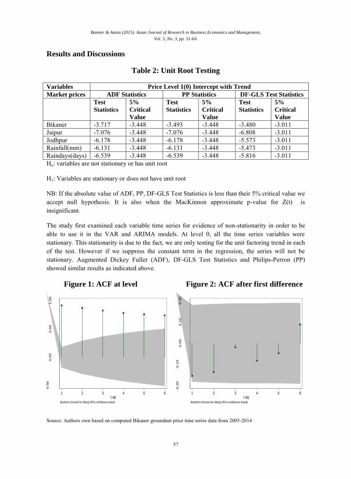
Figure 1: ACF at level Figure 2: ACF after first difference

-0.5

00.0

00.5

01.0

0

Auto

co

rrela

tio

ns o

f b

ikan

er

1 2 3 4 5 6Lag

Bartlett's formula for MA(q) 95% confidence bands

-0.2

0-0

.10

0.0

00.1

00.2

0

Auto

co

rrela

tio

ns o

f D

.bik

an

er

1 2 3 4 5 6Lag

Bartlett's formula for MA(q) 95% confidence bands

Source: Authors own based on computed Bikaner groundnut price time series data from 2005-2014

Bannor & Amita (2015). Asian Journal of Research in Business Economics and Management,

Vol. 5, No. 3, pp. 51-64.

58

Autocorrelation Function at level is shown in Figure 1. The ACF assisted the researchers on deciding the appropriate p,d,q values for the ARIMA modeling by considering the number of spikes outside the confidence bound and in our case its 0.

Figure 3: PACF at Level Figure 4: PACF after first difference

-0.5

00.0

00.5

01.0

0

Part

ial au

tocorr

ela

tions o

f b

ika

ne

r

1 2 3 4 5 6Lag

95% Confidence bands [se = 1/sqrt(n)]

-0.2

0-0

.10

0.0

00.1

00.2

0

Part

ial au

tocorr

ela

tions o

f D

.bik

ane

r

1 2 3 4 5 6Lag

95% Confidence bands [se = 1/sqrt(n)]

Source: Authors own based on computed Bikaner wholesale groundnut price time series data from 2005-2014

Figure 3 and 4 respectively shows the graph of partial correlogram of the series before and after first diffference. PACF at level cuts off aftter the first spike in Figure 1 showing non stationarity however after first difference series become statistically insignificant in figure 4. In addition to the ACF, the PACF is done to decide the appropriate orders of the Autoregressive model of order p (AR) and Moving Average model of order q (MA). Figure 6 shows PACF of AR (1) when φ < 0 Single spike at lag one (negative side) (Kwasi and Kobina,2014).

Table 4: Diagnostic Checking of ARIMA models

ARIMA

Model(p,d,q)

Schwarz

Bayesian

Criterion(BIC)

Ljung Box Q

statistics

R square(%) Maximum Absolute

Percentage Error

(MAPE)

1,1,2 11.69 0.66 0.86 7.46* 1,1,1 11.65 0.69 0.86 7.47 1,1,2 11.66 0.60 0.85 7.48 2,1,2 11.73 0.74 0.86 7.46 0,1,0 11.61* 0.66 0.85 7.60 2,1,1 11.70 0.76 0.86 7.46 2,1,0 11.69 0.58 0.85 7.48 0,1,1 11.64 0.54 0.85 7.52 Source: Author’s computation *= Most preferred according to the test

Ljung box Q statistics; Ho: No autocorrelation H1: There is autocorrelation

NB; Reject null hypothesis when p value is less than 5%

Bannor & Amita (2015). Asian Journal of Research in Business Economics and Management,

Vol. 5, No. 3, pp. 51-64.

59

The table shows various diagnostic tests done to check the adequacy of the models for ARIMA forecasting. The BIC test was conducted, because we were considering several ARIMA models as shown. The model (0,1,0) had the lowest BIC value of 11.61. In addition, the Q statistics was used to test for serial correlations in the models above. All the models shown above had no autocorrelation in the series; which means, the model is fit for forecasting. R square is also used to test the goodness of fit of the model. However Maddala and Lahiri 2009 argued, time series usually have strong trends and seasonal hence the R square is normally high making it difficult to judge the usefulness of a model by just looking at the high R square.

Furthermore MAPE, which is calculated by dividing the difference between actual value and forecasted value (known as the forecasting error) by the actual value, then resulting value is multiplied by 100 to obtain the forecasting percentage error was tested to know how good our model is for forecasting the price series. The forecasting method that minimized the MAPE within each model is considered the preferred method for forecasting the groundnut market price.

The mean absolute percentage error varies from 7.46% to 7.60% across all models. This shows the mean uncertainty in each model’s predictions or forecasting. Whether these values represent an acceptable amount of uncertainty depends on the degree of risk you are willing to accept(Kwasi and Kobina,2014). The low percentage of MAPE could be attributed to the low to volatility of the various variables used for the forecasting and the large number of data series used. This is because for ARIMA to give higher forecasting accuracy the data series should have at least 50 observations.

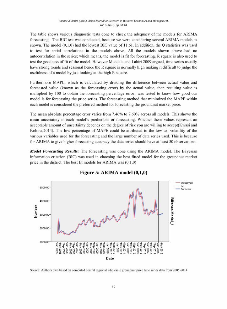
Model Forecasting Results: The forecasting was done using the ARIMA model. The Bayesian information criterion (BIC) was used in choosing the best fitted model for the groundnut market price in the district. The best fit models for ARIMA was (0,1,0)

Figure 5: ARIMA model (0,1,0)

Source: Authors own based on computed central regional wholesale groundnut price time series data from 2005-2014

Bannor & Amita (2015). Asian Journal of Research in Business Economics and Management,

Vol. 5, No. 3, pp. 51-64.

60

Figure 5 above shows the observed and forecasted trend of the best fit model ARIMA (0,1,0) of groundnut prices in Bikaner district of Rajasthan.

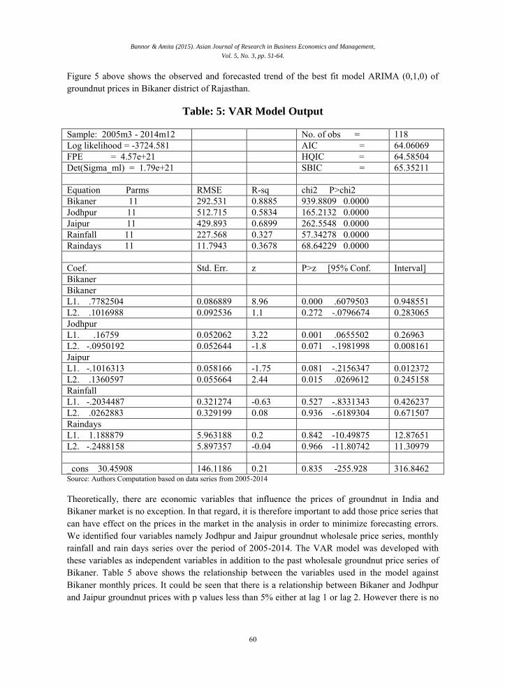
Table: 5: VAR Model Output

Sample: 2005m3 - 2014m12 No. of obs = 118 Log likelihood = -3724.581 AIC = 64.06069 FPE = 4.57e+21 HQIC = 64.58504 Det(Sigma_ml) = 1.79e+21 SBIC = 65.35211

Equation Parms RMSE R-sq chi2 P>chi2 Bikaner 11 292.531 0.8885 939.8809 0.0000 Jodhpur 11 512.715 0.5834 165.2132 0.0000 Jaipur 11 429.893 0.6899 262.5548 0.0000 Rainfall 11 227.568 0.327 57.34278 0.0000 Raindays 11 11.7943 0.3678 68.64229 0.0000 Coef. Std. Err. z P>z [95% Conf. Interval] Bikaner

Bikaner L1. .7782504 0.086889 8.96 0.000 .6079503 0.948551

L2. .1016988 0.092536 1.1 0.272 -.0796674 0.283065 Jodhpur

L1. .16759 0.052062 3.22 0.001 .0655502 0.26963 L2. -.0950192 0.052644 -1.8 0.071 -.1981998 0.008161 Jaipur

L1. -.1016313 0.058166 -1.75 0.081 -.2156347 0.012372 L2. .1360597 0.055664 2.44 0.015 .0269612 0.245158 Rainfall

L1. -.2034487 0.321274 -0.63 0.527 -.8331343 0.426237 L2. .0262883 0.329199 0.08 0.936 -.6189304 0.671507 Raindays

L1. 1.188879 5.963188 0.2 0.842 -10.49875 12.87651 L2. -.2488158 5.897357 -0.04 0.966 -11.80742 11.30979

_cons 30.45908 146.1186 0.21 0.835 -255.928 316.8462 Source: Authors Computation based on data series from 2005-2014

Theoretically, there are economic variables that influence the prices of groundnut in India and Bikaner market is no exception. In that regard, it is therefore important to add those price series that can have effect on the prices in the market in the analysis in order to minimize forecasting errors. We identified four variables namely Jodhpur and Jaipur groundnut wholesale price series, monthly rainfall and rain days series over the period of 2005-2014. The VAR model was developed with these variables as independent variables in addition to the past wholesale groundnut price series of Bikaner. Table 5 above shows the relationship between the variables used in the model against Bikaner monthly prices. It could be seen that there is a relationship between Bikaner and Jodhpur and Jaipur groundnut prices with p values less than 5% either at lag 1 or lag 2. However there is no

Bannor & Amita (2015). Asian Journal of Research in Business Economics and Management,

Vol. 5, No. 3, pp. 51-64.

61

relationship between rainfall and rain days on Bikaner prices with p values more than 5% either at lag 1 or lag 2.

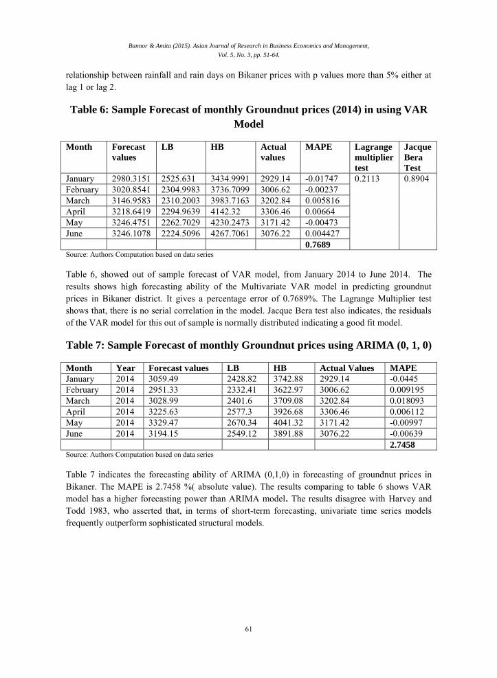
Table 6: Sample Forecast of monthly Groundnut prices (2014) in using VAR

Model

Month Forecast

values

LB HB Actual

values

MAPE Lagrange

multiplier

test

Jacque

Bera

Test

January 2980.3151 2525.631 3434.9991 2929.14 -0.01747 0.2113 0.8904 February 3020.8541 2304.9983 3736.7099 3006.62 -0.00237 March 3146.9583 2310.2003 3983.7163 3202.84 0.005816 April 3218.6419 2294.9639 4142.32 3306.46 0.00664 May 3246.4751 2262.7029 4230.2473 3171.42 -0.00473 June 3246.1078 2224.5096 4267.7061 3076.22 0.004427

0.7689

Source: Authors Computation based on data series

Table 6, showed out of sample forecast of VAR model, from January 2014 to June 2014. The results shows high forecasting ability of the Multivariate VAR model in predicting groundnut prices in Bikaner district. It gives a percentage error of 0.7689%. The Lagrange Multiplier test shows that, there is no serial correlation in the model. Jacque Bera test also indicates, the residuals of the VAR model for this out of sample is normally distributed indicating a good fit model.

Table 7: Sample Forecast of monthly Groundnut prices using ARIMA (0, 1, 0)

Month Year Forecast values LB HB Actual Values MAPE

January 2014 3059.49 2428.82 3742.88 2929.14 -0.0445 February 2014 2951.33 2332.41 3622.97 3006.62 0.009195 March 2014 3028.99 2401.6 3709.08 3202.84 0.018093 April 2014 3225.63 2577.3 3926.68 3306.46 0.006112 May 2014 3329.47 2670.34 4041.32 3171.42 -0.00997 June 2014 3194.15 2549.12 3891.88 3076.22 -0.00639

2.7458

Source: Authors Computation based on data series

Table 7 indicates the forecasting ability of ARIMA (0,1,0) in forecasting of groundnut prices in Bikaner. The MAPE is 2.7458 %( absolute value). The results comparing to table 6 shows VAR model has a higher forecasting power than ARIMA model. The results disagree with Harvey and Todd 1983, who asserted that, in terms of short-term forecasting, univariate time series models frequently outperform sophisticated structural models.

Bannor & Amita (2015). Asian Journal of Research in Business Economics and Management,

Vol. 5, No. 3, pp. 51-64.

62

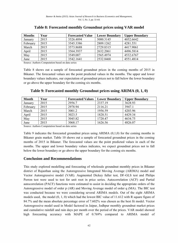
Table 8: Forecasted monthly Groundnut prices using VAR model

Months Year Forecasted Value Lower Boundary Upper Boundary

January 2015 3526.4894 3000.3145 4052.6642 February 2015 3545.3386 2809.1262 4281.551 March 2015 3573.8688 2729.8315 4417.9061 April 2015 3564.3937 2632.2061 4496.5814 May 2015 3549.087 2565.4974 4532.6767 June 2015 3542.1641 2532.8468 4551.4814 Source: Authors Computation based on data series

Table 8 shows out a sample of forecasted groundnut prices in the coming months of 2015 in Bikaner. The forecasted values are the point predicted values in the months. The upper and lower boundary values indicates, our expectation of groundnut prices not to fall below the lower boundary or go above the upper boundary for the coming six months.

Table 9: Forecasted monthly Groundnut prices using ARIMA (0, 1, 0)

Month Year Forecasted Values Lower Boundary Upper Boundary

January 2015 2956.7 2337.19 3628.93 February 2015 2978.94 2116.21 3947.1 March 2015 3001.2 1956.59 4203.96 April 2015 3023.5 1828.51 4429.34 May 2015 3045.82 1720.47 4634.75 June 2015 3068.17 1626.56 4826.07 Source: Authors Computation based on data series

Table 9 indicates the forecasted groundnut prices using ARIMA (0,1,0) for the coming months in Bikaner grain market. Table 10 shows out a sample of forecasted groundnut prices in the coming months of 2015 in Bikaner. The forecasted values are the point predicted values in each of the months. The upper and lower boundary values indicates, we expect groundnut prices not to fall below the lower boundary or go above the upper boundary for the coming six months.

Conclusion and Recommendations

This study explored modelling and forecasting of wholesale groundnut monthly prices in Bikaner district of Rajasthan using the Autoregressive Integrated Moving Average (ARIMA) model and Vector Autoregressive model (VAR). Augmented Dickey fuller test, DF-GLS test and Philips Perron test were used to test for unit root in price series. Autocorrelation (ACF) and Partial autocorrelation (PACF) functions were estimated to assist in deciding the appropriate orders of the Autoregressive model of order p (AR) and Moving Average model of order q (MA). The BIC test was conducted because we were considering several ARIMA models. Out of the eight ARIMA models used, the model (0, 1, 0) which had the lowest BIC value of 11.612 with R square figure of 84.7% and the mean absolute percentage error of 7.602% was chosen as the best fit model. Vector Autoregressive model used in Model factored in Jaipur, Jodhpur monthly groundnut market prices and cumulative rainfall and rain days per month over the period of the prices. VAR model showed high forecasting accuracy with MAPE of 0.769% compared to ARIMA model of

Bannor & Amita (2015). Asian Journal of Research in Business Economics and Management,

Vol. 5, No. 3, pp. 51-64.

63

2.745%.Indiacting, VAR model has high forecasting accuracy compared to ARIMA. The Lagrange Multiplier test also showed that there is no serial correlation in the model. Jacque-Bera test also indicated, the residuals of the VAR model is normally distributed indicating a good fit model.Whereas also the results indicated know autocorrelation in the residuals from all the ARIMA models used; Ljung Box Q statistics values are higher than 5%. This analysis is of relevance to the groundnut industry stakeholders especially farmers in determining where to sell their groundnuts considering Bikaner markets relative to other markets. Further studies should be done to determine groundnut market efficiency in the district and the state as whole to complement the forecasting of prices.

References

Adetunji MO, Adesiyan I.O. (2008). Economic Analysis of Plantain Marketing in Akinyele Local Government Area in Oyo State, Nigeria. International Journal Agricultural Economics and Rural Development. 1(1): 15-21.

Ajjan. N., Senthilanthan. S., Salvam. S., Shivakumar. K. M., and Rohini. A. (2009). Project Proposal on establishing and Networking of Agricultural Intelligence centres in India. Centre for Agricultural and Rural Development Studies, Tamil Nadu Agricultural University, Coimbatore, 118p.

Anonymous, (2015). Retrieved from http://waterresources.rajasthan.gov.in/Daily_Rainfall_Data/Rainfall_Index.htmon 31/01/2015 Anonymous, (2015). Retrieved from http://agriexchange.apeda.gov.in/News/newshome.aspx?categorycode=0501 on 1/2/2015 Anonymous, (2007). Economic Survey. Ministry of Agriculture, Govt. of India.

Babu, K.S., (2011). Market information and Intellligence as agricultural development Options.

Indian Jouranl of Agricultural Marketing. 5( 3): 83-84.

Bannor, K. R., and Kobina, B. J. (2014). Cassava markets integration analysis in the central region of Ghana. Indian Journal of Economics and Development,10(4):319-329.

Bhardwaj S. P. (2011). Singificance of Market Information System (MIS) in Agricultural Development.

Indian Journal of Agricultural Marketing. 25( 3 ):83-84.

Brockwell, P., and Davis, R. (2002). Introduction to Time Series and Forecasting. Springer International Edition.

Burark, S.S., Pant,D.C., Sharma H. and Bheel, S. (2013). Price forecast of Coriander- A case study of the Kota Market of Rajasthan.Indian Journal of Agricultural Marketing.27( 3):72.

Bannor & Amita (2015). Asian Journal of Research in Business Economics and Management,

Vol. 5, No. 3, pp. 51-64.

64

Harvey, A.C. & E.C. Todd (1983). Forecasting econometric time series with structural Box-Jenkins models (with discussion). Journal of Business and Economic Statistics.1(4):299-315. Retrieved from http://www.jstor.org/pss/1391661

Ismet M, Barkley AP, Llewelyn R.V. (1998). Government Intervention and Market Integration in ndonesian Rice Markets. Agric. Econ. 19: 283-295.

Juselius K (2006). The Co-integrated VAR Model: Methodology and Applications. Oxford University Press.

Kwasi B.R., and Kobina B.J. (2014). Forcasting Of Cassava Prices In The Central Region of Ghana Using Arima Model. Intercontinental Journal of Marketing Research Review. 2(8).

Maddalla G.S., Kajal L., (2009). Introduction to Econometrics. Fourth edtion, pp 481-506.

Mafimisebi T.E., Agunbiade B.O. and Mafimisebi O.E. 2014. Price Variability, Co-integration and Exogeniety in the Market for Locally Produced Rice: A Case Study of Southwest Zone of Nigeria. Retrieved from http://dx.doi.org/10.4172/jrr.1000118

Pingali, P. (2006). Agricultural Growth and Economic Development; A view through the globalization lens. Presidential Address to the 26th International Conference of Agricultural Economists, Gold Coast, Australia, August 12-18.

Stock J.H. & Watson, M.W. (2011). Introduction to Econometrics (3rd Edition). Boston, MA: Pearson.

Zhang P.G., (2003). Time series forecasting using a hybrid ARIMA and neural network model.

Neurocomputing. 50: 159-175.