Comparing costs and outcomes across programmes of health care

HEALTH ECONOMICS

Published online 14 February 2011 in Wiley Online Library (wileyonlinelibrary.com). DOI: 10.1002/hec.1716

COMPARING COSTS AND OUTCOMES ACROSS PROGRAMMESOF HEALTH CAREy

STEPHEN MARTINa, NIGEL RICEb,� and PETER C. SMITHc

aDepartment of Economics, University of York, Heslington, York, UKbCentre for Health Economics, University of York, Heslington, York, UK

cInstitute of Global Health Innovation, Imperial College Business School, London, UK

SUMMARY

This paper examines the expenditure choices of local health authorities operating under fixed budget constraints.It applies a theoretical model of budgeting to a data set from 303 English Primary Care Trusts (PCTs) across tenbroad programmes of health care to derive estimates of the elasticity of expenditure in each programme with respectto the total income of the PCT. The results suggest quite similar income elasticities across most programmes, in therange 0.644–1.128. The only outlier is the musculoskeletal programme with an elasticity of about 0.46. Themodelling also derives estimates of spending elasticities with respect to medical needs and thereby permitscalculation of the implicit cost of saving a life year in five programmes of care. The results are important as theyindicate to policy makers how specific programme areas might be affected by general budgetary reductions.Copyright r 2011 John Wiley & Sons, Ltd.

Received 14 January 2010; Revised 22 September 2010; Accepted 17 December 2010

KEY WORDS: allocative efficiency; budget elasticities; programme budgets; local health authorities; health outcomes

1. INTRODUCTION

A fundamental decision for collective healthcare purchasers working under a fixed budget constraint (suchas local health authorities or social health insurers) is how to allocate their aggregate budget across broadprogrammes of care. There is very little evidence on how that allocation decision is made, and whichprogrammes decision makers will augment if the purchaser is in receipt of additional funds, or contract ifexpenditure savings are required. Researchers who have examined this issue find that allocation decisionsare rarely made explicitly. Instead, incremental changes are made, often according to implicitorganisational political considerations (Mitton and Donaldson, 2004). Yet knowledge of purchasers’behavioural responses to budgetary constraints is essential if national policy makers, who set budgets andallocate funds, are to understand the implications for different care groups of their funding decisions.

Furthermore, knowledge of the marginal effectiveness of programme spending is essential if localdecision makers are to make informed decisions about budget allocations. There is a surprising lack ofreliable evidence on the nature of the link between healthcare spending and the health of the population.In their review of the evidence on whether health care saves lives, Nolte and McKee (2004) note that mostof these production function studies employ regression analysis to examine the impact of healthcare inputsand other explanatory variables on some measure of healthcare outcome. They conclude that manystudies have struggled to identify a strong and consistent relationship between healthcare expenditure and

ySupporting information may be found in the online version of this article.

*Correspondence to: Centre for Health Economics, University of York, Heslington, York YO10 5DD, UK. E-mail:[email protected]

Copyright r 2011 John Wiley & Sons, Ltd.

Health Econ. : 316–337 (2012)21

health outcomes (after controlling for other factors) whilst, in contrast, socioeconomic factors are oftenfound to be highly associated with health outcomes (Nolte and McKee, 2004, p. 58).

Nixon and Ulmann (2006) find some evidence that healthcare expenditure has a significant positiveimpact on health outcome. However, this result is not consistent across studies, and their reviewsupports the belief that it can be difficult to establish a clear positive link between healthcare inputs andhealth outcomes. These equivocal findings may in part reflect serious theoretical and statisticaldifficulties associated with such studies (Gravelle and Backhouse, 1987). In particular, a fundamentalobstacle to any statistical analysis in this field of study is the difficulty of disentangling cause and effect.Although a casual empirical analysis might reveal no correlation between mortality and spending, thismight follow not because spending has no impact on outcome, but because spending is endogenous, inthe sense that it is in part determined by the level of healthcare need. The methodological challenge is todetermine whether – after adjusting for need – extra spending gives rise to better health outcomes.

In a previous paper, we sought to address these challenges by deploying a formal theoretical model ofspending choices, and exploiting two important new data sets for the English National Health Service(NHS) (Martin et al., 2008a). Since April 2003 each local health authority has been required to allocate allof its expenditure – including expenditure on inpatient care, outpatient care, community care, primarycare and pharmaceuticals – between 23 ‘programmes’ of care. At the same time, local mortality data havealso been released for a variety of diseases. In some cases the disease coverage of the expenditure datacorresponds exactly to the disease coverage of the mortality data, while in other cases the correspondenceis less precise. The availability of both expenditure and mortality data for several programmes of careoffers an opportunity to develop empirical models of expenditure choices and health outcomes.

Martin et al. (2008a) examined the relationship between healthcare expenditure and mortality ratesfor two large programmes of care (cancer and circulatory disease). Their theoretical model involves twoequations for each programme: one which models the determinants of expenditure on the programmeand another which models the determinants of the health outcome. These were estimated usingspending and outcomes data from 295 local health authorities responsible for purchasing health care inEngland. Satisfactory expenditure and outcome equations were developed and enabled us to estimatethe expenditure in 2004/2005 required to ‘save’ an additional year of life in each disease category: about£13 100 for cancer and about £8000 for circulatory disease.

This paper uses programme budgeting data for 2005/2006 to estimate spending and outcomesequations across a large number of programmes of care in order to address two objectives: to deriveestimates of the income elasticity of spending for each programmes of care and to expand from two tofive the number of progammes for which an estimate of the cost of saving a life year is available.A further innovation is that we draw on data collected from General Practices as part of the Quality andOutcomes Framework (QOF). This was introduced in the United Kingdom in April 2004 and includes aseries of statistical indicators from which it is possible to calculate prevalence rates for various diseases,which we are able to test as potential additional indicators of need for particular care programmes.

The plan of this paper is as follows. Section 2 provides some background information aboutprogramme budgeting as well as some descriptive statistics for the FY 2005/2006 budgeting data. Theoutcome and expenditure equations are derived from a theoretical model of the budgetary problem facedby a purchasing manager seeking to allocate limited funds between competing programmes of care. Thismodel and the estimation methods are presented briefly in Section 3. Outcome and expenditure equationsare derived for several programmes and these are reported in Section 4. Section 5 summarises the results.

2. PROGRAMME BUDGETING IN ENGLAND

The English NHS is financed almost entirely from national taxation. Access to primary and secondarycare is generally free for the patient but access to secondary care and pharmaceuticals is only permitted


DOI: 10.1002/hecHealth Econ. : 316–337 (2012)21

317COSTS AND OUTCOMES ACROSS PROGRAMMES OF HEALTH CARE

via a general practitioner. The NHS is organised geographically, with most expenditure on health carebeing the responsibility of the local Primary Care Trusts (PCTs). For the years relevant to this study,there were 303 PCTs with average populations of 160 000. The sole significant source of funding for aPCT is the annual lump sum budget allocated by the national ministry, within which it is expected tomeet the expenditure on most aspects of health care, including inpatient, outpatient and communitycare, primary care and prescriptions.

Since April 2003 each PCT has reported expenditure data disaggregated according to 23 programmesof health care and, in some cases, the programme is broken down into further sub-programmes.Summary programme budgeting data for 2005/2006 are presented in Table I. The first column showsthe national average NHS expenditure per person by programme budget category in 2005/2006. AcrossEngland as a whole, NHS expenditure per person is £1286. The single largest category is the ‘other’category (programme budget category 23) with per capita expenditure of almost £168. This categoryincludes primary care expenditure, workforce training expenditure and a range of other miscellaneousexpenditure items. Of these components, primary care expenditure is by far the largest element at £145per head.

Table I. Expenditure by programme budget category, per person, all England, using cost-adjusted expenditure byPCT, 2005/2006

PCT spent per head, £, cost adjusted

Programme budget category National net spent per head, £, 2005/2006 Mean Minimum Maximum CV

1 Infectious diseases 23.7 21.77 6.54 244.02 0.872 Cancers/tumours 82.8 84.37 37.20 139.54 0.213 Blood disorders 17.4 17.00 0.31 63.07 0.414 Endocrine/metabolic 37.0 37.56 15.17 191.69 0.314a Diabetes 16.8 17.26 1.41 44.23 0.304x Other 20.1 20.67 5.28 175.79 0.515 Mental health 156.9 154.35 34.22 360.54 0.295a Substance abuse 14.0 14.63 0.46 194.40 1.385b Dementia 16.3 16.61 0.24 70.67 0.805x Other 126.7 124.47 13.44 289.20 0.336 Learning disability 44.7 45.20 3.00 277.52 0.517 Neurological system 40.8 41.69 16.57 131.69 0.298 Eye and vision 28.0 28.84 12.22 57.72 0.279 Hearing 6.2 6.33 1.82 19.29 0.4510 Circulatory 123.6 125.59 64.82 192.52 0.1911 Respiratory 69.2 70.43 5.56 145.10 0.2512 Dental 23.3 24.62 1.91 92.60 0.6813 Gastro-intestinal 80.9 82.39 39.27 132.54 0.2214 Skin 26.6 26.97 12.58 52.95 0.2515 Musculo-skeletal 74.2 75.72 33.75 177.99 0.2516 Trauma/injuries 75.9 77.41 36.53 139.28 0.2217 Genito-urinary 67.2 67.12 26.73 144.74 0.2618 Maternity/repro 59.9 59.12 25.18 163.05 0.2919 Neonate conditions 13.3 12.87 0.32 39.42 0.5320 Poisoning 14.2 14.45 5.18 35.84 0.3021 Healthy individuals 24.6 24.48 7.33 106.00 0.5522 Social care needs 27.7 26.93 0.06 158.40 0.7823 Other areas 168.1 168.45 78.42 378.89 0.1823a GMS/PMS 145.5 145.89 12.39 264.73 0.14Total expenditure 1286.2 1293.57 884.57 1871.32 0.13

Source: See the Programme Budget Section of the Department of Health’s website at http://www.dh.gov.uk/.Note: Descriptivestatistics across PCTs are unweighted and, for any given PCT, its expenditure per head figure reflects its raw population adjustedfor unavoidable cost variations. The coefficient of variation (CV) is a measure of dispersion and is calculated as the standarddeviation divided by the mean.



318 S. MARTIN ET AL.

Table I also indicates the degree of variation in expenditure levels across PCTs by programme budgetcategory. For each category, the unweighted average of the PCT per capita expenditure figures –adjusted for the unavoidable geographical variation in costs – is reported in the second column ofTable I, followed by the observed minimum and maximum spend.1 The final column shows thecoefficient of variation. The variation in the expenditure levels across PCTs in 2005/2006 isconsiderable. For example, expenditure per head on cancers and tumours averages £84 across allPCTs but this varies between £37 and over £139 per head.

To further illustrate the geographic variation in expenditure levels, Figure 1 shows (cost adjusted)expenditure per head by PCT for 2005/2006 with each PCT allocated to one of five expenditure quintiles(quintile 1 contains the 59 PCTs with the smallest spent per head).2 This shows that per capitaexpenditure is typically greatest around London and the traditional industrial heartlands in thenortheast, the northwest, West Yorkshire and the West Midlands. Figure 2 uses an age and sexstandardised mortality ratio (SMR) for people aged under 75 years to allocate PCTs to one of fivemortality quintiles (quintile 1 contains the 59 PCTs with the smallest SMR and quintile 5 contains the59 PCTs with the largest SMR).3 As was the case for expenditure, high mortality is clearly concentratedaround the traditional industrial heartlands.

Figure 1. Expenditure (2005/2006) per head by PCT quintile

1This cost adjustment reflects the fact that health economy input prices vary considerably across the country and are up to 30%higher in London and the southeast of England than elsewhere (see Department of Health, 2005).

2Both maps are Crown Copyright 2007. All rights reserved. Ordnance Survey License number 100018355. The eight PCTs forwhom we have no data are shown with no shading.

3The SMR is for people aged under 75 years and relates to all causes of death considered amenable to health care over the period2002–2004.




Any study of the impact of healthcare expenditure on outcomes should allow for the endogenousnature of the healthcare input, mentioned in Section 1. The issue is whether – after adjusting for need –extra spending gives rise to better health outcomes. The Department of Health routinely uses econometricestimates of relative NHS healthcare spending needs as part of its annual allocation of funds to PCTs(Smith et al., 2001). Some of the within-programme variation in per capita expenditure across PCTsreported in Table I will reflect different levels of the need for health care. Therefore, when the expenditureper head data in Table I are adjusted for each PCT’s need for health care, the degree of variation inexpenditure declines for most of the programme budget categories. However, this decline is relatively smalland there are still substantial differences in expenditure per head across the country even after allowing forlocal cost and need variations (Martin et al., 2007). For example, for cancer and tumours the minimumand maximum spent per head is £37 and £139 using the cost adjusted expenditure data (from Table I) butis £38 and £145 using the cost and need adjusted population data. Therefore, there is considerablegeographical variation in expenditure per head in each disease category even after adjusting for need, andan examination of the reasons for and effects of this variation lies at the heart of our analysis.

3. THEORETICAL MODEL AND ESTIMATION ISSUES

3.1. Theoretical model

Our model assumes that PCT receives an annual financial lump sum budget yi from the nationalministry and that the PCT allocates this budget across the J programmes of care to maximise a social

Figure 2. SMR (2002, 2003 and 2004) by PCT quintile




welfare function W( � ).4 This social welfare function embodies health outcomes across the Jprogrammes of care. In addition to its budget constraint, the PCT also faces a ‘health productionfunction’ fj( � ) that indicates the link between local spending xij on programme j and health outcomes inthat programme hij. The nature of the health production function will depend on two types of local PCTfactors: the clinical needs of the local population relevant to the programme of care (which we denote asnij) and broader local environmental factors zij relevant to delivering the programme of care (such asinput prices, geographical factors or other uncontrollable influences on outcomes). Both clinical andenvironmental factors may be multidimensional in nature. Thus,

hij ¼ fjðxij; nij; zijÞ;@fj@x

40;@2fj@x2

o0 ð1Þ

Each PCT allocates expenditure across the 23 programmes of care so that the marginal benefit of thelast pound spent in each programme of care is the same. Solving the constrained maximisation problemyields the result that the optimal level of expenditure in each category, x�ij, is a function of the need forhealth care in each category (ni1; ni2; . . . ; niJ), environmental variables affecting the production of healthoutcomes in each category (zi1; zi2; . . . ; ziJ) and PCT income (yi) so that:

x�ij ¼ gjðni1; . . . ; niJ; zi1; . . . ; ziJ; yiÞ; j ¼ 1; . . . ; J ð2Þ

Thus, for each programme of care there exists an expenditure equation (2) explaining expenditurechoice of PCTs and a health outcome equation (1) that models the associated health outcomes achieved.The remainder of this section describes how we approach the empirical estimation of these equations foreach care programme.

3.1.1. Estimation issue 1: simultaneous or equation-by-equation estimation? Data limitations precludethe simultaneous estimation of all 23 outcome and expenditure equations (we do not have variablesreflecting need, environmental factors and health outcomes for all 23 programmes of care). Instead weemploy two-stage least squares to estimate each expenditure and outcome equation separately for theprogrammes for which relevant data are available.

3.1.2. Estimation issue 2: the expenditure equation. There exists no programme-specific indicator of theneed for health care, so we proxy this using the ‘needs’ component of the Department of Health’sresource allocation formula. This needs element is specifically designed to adjust PCT allocations forlocal healthcare needs. The expenditure equation also requires a proxy for need across all otherprogrammes of care. In our previous study – where we were modelling only two care programmes – weemployed the circulatory mortality rate as the proxy for the need for competing programmes in thecancer expenditure equation, and the cancer mortality rate as the proxy for the need for competingprogrammes in the circulatory expenditure equation (Martin et al., 2008a). As these are bothprogrammes that attract considerable expenditure, it is not implausible that expenditure in one ofthe programmes will influence expenditure in the other and, in this study, we have retained thisapproach when re-estimating the expenditure and outcome functions for the cancer and circulatoryprogrammes for 2005/2006.

In the other expenditure equations, depending on the specification, we have employed either (a) thestandardised death rate from all causes amenable to health care for people aged under 75 years or(b) the age standardised years of life lost (SYLL) rate for all deaths of those aged under 75 as the proxy

4The allocation of the national budget between PCTs is based on an econometric analysis of actual historical NHS healthcareexpenditure at the small area level. The estimated model includes indicators of both the need for and supply of health care, andthis model is used to inform the construction of a ‘needs’ index for each PCT. The national budget is split between PCTsaccording to the relative need of each PCT and is designed to achieve equality of access for equal need. Further details of theresource allocation in the NHS can be found in Smith et al. (2001).




for other calls on resources. Although these proxy measures will include some ‘own specialty’ deaths,these will comprise a very small proportion of the total. For example, in 2004 cancer and circulatoryproblems accounted for over two-thirds of all deaths for those under 75 years of age and the thirdlargest category – respiratory problems – accounted for less than one in ten of all deaths (NCHOD,2007; ONS, 2007). We therefore feel that the ‘all causes’ mortality indices are reasonable proxies fordemands on the budget from other specialties.5

3.1.3. Estimation issue 3: the outcome equation. For each care programme, we estimate models using twoalternative measures of health outcome: the disease-specific SMR for those aged under 75 and a measureof the avoidable YLL to the disease. The latter variable is calculated by summing over ages 1–74 years thenumber of deaths at each age multiplied by the number of years of life remaining up to age 75 years. Thecrude YLL rate is simply the number of YLL divided by the resident population aged under 75 years. Likeconventional mortality rates, YLL can be standardised for age and sex to eliminate the effects ofdifferences in population demographic structures between areas, by applying the age and sex-specific YLLto a standard population. This standardised YLL rate is the second health outcome variable employed inthis study (Lakhani et al., 2006, p. 379). Both outcome indicators are for the three years 2002, 2003 and2004 combined and the expenditure data are for 2005/2006. Implicitly, our analysis assumes that PCTshave reached some sort of equilibrium in the expenditure choices they make and the outcomes they secure.

3.1.4. Estimation issue 4: OLS or 2SLS? Endogeneity tests confirmed our prior beliefs that expenditure inthe outcome equation and other programme need for health care in the expenditure equation were bothendogenous variables. Hence, we employ 2SLS rather than OLS to estimate all expenditure and outcomeequations. 2SLS involves replacing the endogenous variables in the equation of interest with their predictedvalues from an OLS regression which regresses the endogenous variable on a set of exogenous variablesincluding a subset of instruments. These instruments should be strong predictors of the endogenous variable(they are relevant) but they should be appropriately excluded from the equation of interest (they are valid).We have a number of potential instruments available, mostly derived from 2001 Population Census, andthese are described in Section A.1 in Appendix A. These indicators reflect factors, such as socio-economic deprivation and the availability of informal care in the community, that might indirectlyinfluence mortality rates and/or healthcare expenditure levels. Three of the available instruments – theproportion of households that are lone pensioner households, the proportion of the populationproviding unpaid care and the population weighted index of multiple deprivation – were selected asinstruments on the basis of their theoretical and empirical relevance and their validity. Various testsincluding those for instrument validity (using the Sargan, 1958 test), instrument relevance (Anderson,1984; Shea, 1997) and instrument strength (Cragg and Donald, 1993; Staiger and Stock, 1997; Stockand Yogo, 2002) are reported. We also test for model specification using the Pesaran and Taylor (1999)instrumental variables version of Ramsey’s (1969) reset test. Further details of these tests can be foundin Martin et al. (2008a) and the relevant first-stage regressions can be found in Martin et al. (2007).Descriptive statistics for the mortality and needs variables can be found in Section A.2 of Appendix A,and a correlation matrix for the expenditure and mortality variables can be found in Section A3.

4. EMPIRICAL RESULTS: PROGRAMMES WITH A MORTALITY INDICATOR

We have been able to construct mortality indicators for 10 of the 23 programmes of care. In this section,we report results from the estimation of expenditure and outcome equations for these ten programmes,

5We were unable to obtain the necessary detailed data to remove the death rates for particular programmes from the all causedeath rate.




together with details of the expenditure equation for three programmes for which no outcome indicatoris available. As the results for the cancer and circulatory disease programmes are similar to those usingexpenditure data for the previous year (that is, for 2004/2005: Martin et al., 2008a), updated results for2005/2006 are presented very briefly but a more detailed discussion is available in Section A.4 ofAppendix A (available from Wiley InterScience website).

4.1. Cancer programme of care

Results for the cancer programme of care are in Table II. Columns under (1) present 2SLS results usingSMRs as the measure of health outcome while columns under (2) present 2SLS estimates using theSYLL rate as the outcome measure.6,7 All variables have been log transformed and parameter estimatescan be interpreted as elasticities.8

The outcome equations suggest that expenditure on cancer services significantly reduces mortalityfrom cancer. The expenditure equations imply that the ‘other calls on resources’ variable has theanticipated negative effect on cancer expenditure, and that the budget elasticity of expenditure is about0.95. The coefficient on the cancer expenditure term in the SYLL equation can be used to calculate themarginal ‘cost’ of an extra life year. It suggests that a 1% increase in cancer expenditure per head(£82.80 in 2005/2006) gives rise, ceteris paribus, to a 0.393% reduction in YLL (which totalled 2 268 541for 2002, 2003 and 2004). This implies that an extra life year costs £13 931.

4.2. Circulatory disease programme of care

The results for circulatory problems are shown in Table III and, in general, the estimated coefficientsexhibit the same qualitative characteristics as for the cancer care programme. The expenditure equationssuggest the budget elasticity of expenditure is about 0.70, and the standard error on the total budgetterm suggests that the 95% confidence interval for the budget elasticity in the circulatory diseaseprogramme lies almost entirely below 1. Note also that the coefficient on the total budget term (between0.681 and 0.705) is lower than that for the cancer programme of care (between 0.935 and 0.968),implying that the expenditure on circulatory disease is less responsive to budget changes than is oncancer. The coefficient on the circulatory disease expenditure term in the CHD SYLL equation can beused to calculate the marginal cost of an extra life year. It suggests that a 1% increase in circulatorydisease expenditure per head (£123.6 in 2005/2006) is associated with a 1.585% reduction in life yearslost (which totalled 1 607 171 for 2002, 2003 and 2004). This implies that an extra life year costs £7279.

4.3. Neurological programme of care

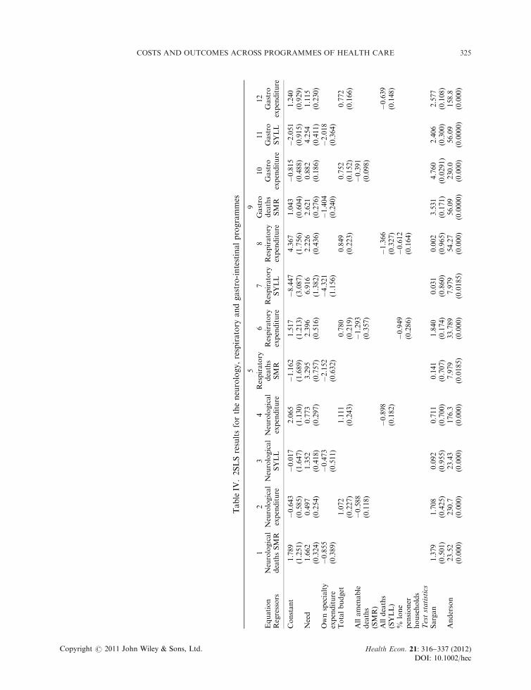
Results for the neurological programme of care with deaths caused by epilepsy as the outcome indicatorare shown in the first four columns of Table IV. Although epilepsy accounts for o10% of deathsattributable to the neurological care programme, it was the only mortality indicator available for thiscare programme at the time of writing.9 Moreover, the other major causes of death in this category –motor neuron disease, Parkinson’s disease, Alzheimer’s disease and multiple sclerosis – are notnormally considered to be amenable to or avoidable with appropriate health care and so mostexpenditure in this category is likely to be towards patient care rather than saving life.

6These SMRs are for those aged under 75 years.7This SYLL rate is calculated on the basis of a 75-year life expectancy.8The number of observations in the regression equations is 295 not 303. There are eight missing PCTs because the variables used inthe regression models were constructed at slightly different dates and between these dates there were a small number of PCTboundary changes.

9Of the 9480 all age deaths attributed to the neurological care programme in England in 2004, only 838 were due to epilepsy(NCHOD, 2007; ONS, 2007).




Table II. Results for the cancer programme of care, 2005/2006

2SLS (1) 2SLS (2)

N5 295 Cancer deaths SMR Cancer expenditure Cancer SYLL Cancer expenditure

Constant 3.546 (0.292) �0.024 (0.509) 4.100 (0.248) �0.019 (0.516)Need 0.988 (0.096) 0.652 (0.233) 0.904 (0.083) 0.703 (0.248)Cancer expenditure �0.504 (0.118) �0.393 (0.100)Total budget 0.935 (0.190) 0.968 (0.190)Circulatory deaths SMR �0.593 (0.109)Circulatory SYLL �0.576 (0.107)

Test statisticsSargan (w21) 0.403 (0.525) 0.032 (0.858) 1.164 (0.280) 0.602 (0.437)Anderson (w21) 42.01 (0.000) 213.5 (0.000) 42.01 (0.000) 176.5 (0.000)Cragg–Donald 22.27 (o0.05) 154.0 (o0.05) 22.27 (o0.05) 118.8 (o0.05)Partial R2 0.132 0.515 0.132 0.45Pesaran–Taylor (w21) 0.02 (0.883) 2.82 (0.093) 0.04 (0.837) 2.98 (0.084)

Endogeneity (w21)Cancer expenditure 55.15 (0.000) 35.63 (0.000)Circulatory deaths 4.842 (0.027)Circulatory SYLL 7.830 (0.005)

Notes: 1. Parentheses show robust standard errors for parameter estimates and p-values for the test statistics. 2. The instrument setfor cancer expenditure includes the proportion of households that are lone pensioner households and the proportion of thepopulation providing unpaid care. 3. The instrument sets for circulatory deaths (SMR) and circulatory years of life lost (SYLLrate) include the proportion of households that are lone pensioner household and the proportion of the population providingunpaid care.

Table III. Results for the circulatory disease programme of care, 2005/2006

2SLS-1 2SLS-1

N5 295 CHD deaths SMR CHD expenditure CHD SYLL CHD expenditure

Constant 1.700 (0.333) 2.098 (0.733) 1.398 (0.403) 3.440 (1.110)Need 2.459 (0.161) 0.693 (0.205) 2.819 (0.192) 0.884 (0.261)CHD expenditure �1.367 (0.159) �1.585 (0.192)Total budget 0.705 (0.142) 0.681 (0.160)Cancer deaths SMR �0.706 (0.173)Cancer SYLL �0.953 (0.248)% White ethnic group 0.180 (0.058) 0.197 (0.066)% Pop unpaid carers 0.415 (0.118) 0.363 (0.136)

Test statisticsSargan (w21) 0.016 (0.899) 3.353 (0.067) 0.013 (0.908) 2.397 (0.121)Anderson (w21) 73.2 (0.000) 82.64 (0.000) 66.3 (0.000) 44.70 (0.000)Cragg–Donald 48.02 (o0.05) 46.56 (o0.05) 41.96 (o0.05) 23.56 (o0.05)Partial R2 0.248 0.244 0.224 0.14

Pesaran–Taylor (w21) 1.75 (0.185) 0.44 (0.508) 0.10 (0.754) 0.28 (0.594)

Endogeneity (w21)CHD expenditure 103.8 (0.000) 109.5 (0.000)Cancer deaths 11.653 (0.000)Cancer SYLL 13.844 (0.000)

Notes: 1. Parentheses show robust standard errors for parameter estimates and p-values for the test statistics. 2. The instrument setfor CHD expenditure in the outcome equation using the SMR includes the population weighted index of multiple deprivationbased on ward-level IMD 2000 scores, and the proportion of residents in the white ethnic group. 3. The instrument set for CHDexpenditure in the outcome equation using the SYLL rate includes the proportion of households that are lone pensionerhouseholds, and the proportion of residents in the white ethnic group. 4. The instrument sets for cancer deaths (SMR) and cancerSYLL include the proportion of households that are lone pensioner households and the population weighted index of multipledeprivation based on ward-level IMD 2000 scores. 5. The term ‘CHD’ is used as a shorthand for ‘circulatory problems’.




TableIV

.2SLSresultsfortheneurology,respiratory

andgastro-intestinalprogrammes

59

Equation

Regressors

1Neurological

deathsSMR

2Neurological

expenditure

3Neurological

SYLL

4Neurological

expenditure

Respiratory

deaths

SMR

6Respiratory

expenditure

7Respiratory

SYLL

8Respiratory

expenditure

Gastro

deaths

SMR

10

Gastro

expenditure

11

Gastro

SYLL

12

Gastro

expenditure

Constant

1.789

(1.251)

�0.643

(0.585)

�0.017

(1.647)

2.065

(1.130)

�1.162

(1.689)

1.517

(1.213)

�8.447

(3.087)

4.367

(1.756)

1.043

(0.604)

�0.815

(0.488)

�2.051

(0.915)

1.240

(0.929)

Need

1.662

(0.324)

0.497

(0.254)

1.352

(0.418)

0.773

(0.297)

3.295

(0.757)

2.396

(0.516)

6.916

(1.382)

2.226

(0.436)

2.621

(0.276)

0.882

(0.186)

4.254

(0.411)

1.115

(0.230)

Ownspecialty

expenditure

�0.855

(0.389)

�0.473

(0.511)

�2.152

(0.632)

�4.321

(1.156)

�1.404

(0.240)

�2.018

(0.364)

Totalbudget

1.072

(0.227)

1.111

(0.243)

0.780

(0.219)

0.849

(0.223)

0.752

(0.152)

0.772

(0.166)

Allamenable

deaths

(SMR)

�0.588

(0.118)

�1.293

(0.357)

�0.391

(0.098)

Alldeaths

(SYLL)

�0.898

(0.182)

�1.366

(0.327)

�0.639

(0.148)

%lone

pensioner

households

�0.949

(0.286)

�0.612

(0.164)

Teststatistics

Sargan

1.379

(0.501)

1.708

(0.425)

0.092

(0.955)

0.711

(0.700)

0.141

(0.707)

1.840

(0.174)

0.031

(0.860)

0.002

(0.965)

3.531

(0.171)

4.760

(0.0291)

2.406

(0.300)

2.577

(0.108)

Anderson

23.52

(0.000)

230.7

(0.000)

23.43

(0.000)

176.3

(0.000)

7.979

(0.0185)

33.789

(0.000)

7.979

(0.0185)

54.27

(0.000)

56.09

(0.0000)

230.0

(0.000)

56.09

(0.0000)

158.8

(0.000)




Cragg–Donald

8.03

(o0.05)

114.2

(o0.05)

7.99

(o0.05)

78.7

(o0.05)

3.99

(o0.05)

17.54

(o0.05)

3.99

(o0.05)

29.19

(o0.05)

20.2

(o0.05)

171.3

(o0.05)

20.2

(o0.05)

103.4

(o0.05)

PartialR2

0.076

0.542

0.076

0.449

0.026

0.108

0.026

0.168

0.173

0.541

0.173

0.416

Pesaran–Taylor

0.36

(0.549)

0.05

(0.823)

1.16

(0.280)

0.02

(0.888)

0.00

(0.946)

0.99

(319)

0.41

(0.521)

0.58

(0.445)

3.14

(0.076)

0.02

(0.901)

2.47

(0.115)

1.17

(0.279)

Endogeneity

Ownspecialty

expenditure

3.04

(0.080)

0.349

(0.554)

55.78

(0.000)

84.43

(0.000)

42.57

(0.000)

41.92

(0.000)

Allamenable

deaths

2.570

(0.108)

10.83

(0.000)

4.396

(0.036)

Alldeaths

(SYLL)

12.250

(0.000)

9.298

(0.002)

8.089

(0.004)

Notes:

1.Parentheses

show

robust

standard

errors

forparameter

estimatesandp-values

forthetest

statisticsforallequations.

2.Theinstrumentsetforneurological

expenditure

includes

theproportionofhouseholdsthatare

lonepensioner

households,theproportionofthepopulationprovidingunpaid

care

andthepopulationweighted

index

ofmultiple

deprivationbasedonward-level

IMD

2000scores.

3.Theinstrumentsets

forallamenable

deaths(SMR)andalldeaths(SYLL)in

theneurological

programmeincludetheproportionofhouseholdsthatare

lonepensioner


care


ward-level

index

ofmultiple

deprivationscores.4.Neurologicaldeathsare

proxiedbytheallageindirectepilepsy

SMR

for2002–2004,andtheneurologicalSYLLrate

isproxiedbytheunder

75years

epilepsy

SYLLrate

for2002–2004.5.Theinstrumentsetforrespiratory

expenditure

includes

theproportionofthepopulationprovidingunpaid

care

andthepopulationweightedindex

ofmultiple


IMD

2000scores.6.Theinstrumentsets

forallamenable

deaths(SMR)andalldeaths

(SYLL)in

therespiratory

programmeincludetheproportionofthepopulationprovidingunpaid

care,andthepopulationweightedindex

ofmultiple

deprivationbasedon

ward-level

IMD

2000scores.7.Therespiratory

allageSMR

isaweightedaverageoftheasthma,bronchitisandpneumonia

SMRs(w

ithweights

reflectingthenumber

of

deathsin

each

category)whiletheSYLLrate

outcomeindicatoristhesum

oftheasthma,bronchitisandpneumonia

SYLLrates.8.Theinstrumentsetforgastro-intestinal

expenditure

includes


lonepensioner


care


index

ofmultiple


IMD

2000scores.

9.Theinstrumentsetforallamenable

deaths(SMR)andalldeaths(SYLL)in

thegastro-intestinal

programmeincludes


lonepensioner

householdsandthepopulationweightedindex

ofmultiple


IMD

2000scores.10.Thegastro-intestinalallageSMR

isaweightedaverageoftheliver

disease

andulcer

SMRswithweights

reflectingthenumber

ofdeathsin

each

category

whiletheSYLLrate

outcomeindicatoristhesum

oftheliver

disease

andulcer

SYLLrates.




In the outcome equation with the SMR as the dependent variable (Equation 1) both need andexpenditure are significant and have the anticipated signs. The Pesaran–Taylor test reveals no evidenceof misspecification and tests indicate that the instruments are relevant and valid. The model with theSYLL rate as the dependent variable (Equation 3) is similar to its SMR counterpart except that theexpenditure term is now statistically insignificant. For both outcome measures, Shea’s partial R2 is smalland the F-statistic from the Cragg–Donald test does not exceed the Staiger and Stock suggestedcriterion of being greater than 10. This suggests that there may be a potential problem with weakinstruments. The tabulated values of Stock and Yogo (2002), however, suggest that the expected bias of2SLS relative to OLS bias is restricted to between 10 and 20%.

As a proxy for the ‘other calls on resources’ term, we have employed either (a) the SMR from allcauses amenable to health care for those aged under 75 years or (b) the SYLL rate for all deaths of thoseaged under 75.10,11 In both of the neurological expenditure equations, all three regressors (need, totalbudget and the ‘other calls on resources’ term) have the anticipated effect on expenditure and the teststatistics reveal no evidence of misspecification. The coefficient on the total budget term in theexpenditure equation varies between 1.072 and 1.111, implying that a 10% budget change leads to asimilar change in expenditure on the neurological programme. However, the standard error for thisestimate is about 0.23 so our 95% confidence interval for the budget elasticity is quite wide at between0.64 and 1.56. A condition-specific measure of need – the epilepsy prevalence rate – is available from theQOF. However, the use of this condition-specific measure of need offers little improvement in modelperformance over the general measure of need.

The estimated coefficient (�0.473) on neurological expenditure in Equation (3) is not significant butis our best estimate of the impact of expenditure on epilepsy mortality. It could be used to infer that oneextra life year in this programme would cost £191 234, a much larger figure than that estimated for othercare programmes. However, because epilepsy deaths account for only a small proportion of all deathsattributable to neurological causes, and because much expenditure in this budgeting category will bedirected towards ‘caring’ rather than life saving, we would not recommend drawing any policyconclusions from this figure.

4.4. Respiratory problems programme of care

Results for the respiratory programme of care are shown in Equations (5)–(8) of Table IV. As themortality outcome indicator, we employ a weighted average of the SMRs for asthma, bronchitis andpneumonia with weights determined by the number of deaths attributed to each cause in 2004.12 For theSYLL rate outcome indicator, we sum the SYLL rate for each of these three causes of death. In 2004,these three causes accounted for almost 52 000 of the 65 000 all age deaths attributable to the respiratoryproblems care programme (NCHOD, 2007; ONS, 2007).

In both of the outcome equations (5 and 7), need and expenditure have the anticipated signs and aresignificant. The usual tests indicate that the instruments are relevant and valid, that expenditure isendogenous and that there is no evidence of misspecification.13 There is, however, some indication thatthe instruments may be weakly associated with expenditure. Shea’s R2 is low and the Cragg–DonaldF-statistic does not exceed Staiger and Stock’s recommended criterion of 10. Stock and Yogo do notprovide critical values for the expected ratio of 2SLS bias to OLS bias for two excluded instruments as

10See Martin et al. (2008a,b) for details of which deaths are deemed amenable to health care.11In 2002–2004 neurological deaths accounted for o2% of the 195 000 deaths from all causes amenable to health care in thoseaged below 75.

12More precisely, the respiratory SMR5 ((1160/51 700)�asthma SMR)1((21 662/51 700)�bronchitis SMR)1((28 878/51 700)�pneumonia SMR).

13The proportion of households that are lone pensioner households is not included as part of the excluded instrument set.




used here and so we cannot assess the likely extent of bias related to OLS for these models but somecaution should be exercised in the interpretation of these results.

In both of the expenditure equations (6 and 8), need, total budget and the proxy for other calls onresources all have the anticipated effect on respiratory expenditure and are significant, as is an additionalregressor: the percentage of households that are lone pensioner households. This might be indicative of anunmet needs effect or of a selection effect. Again, the usual tests indicate that the instruments are relevantand valid, that all the amenable deaths terms are endogenous, and that there is no evidence ofmisspecification. The coefficient on the total budget term in the two expenditure equations ranges between0.78 and 0.85, implying that a 10% budget change leads to about an 8.2% change in expenditure.

Two more condition-specific measures of need – the asthma prevalence rate and the chronicobstructive pulmonary disease (COPD) prevalence rate – are available from the QOF. However, interms of the plausibility and significance of the coefficient estimates and passing the relevant diagnostictests, the results generated by the use of these two condition-specific measures of need were no betterthan those available with the use of the more generic measure of need. The coefficient on theexpenditure term in the SYLL outcome equation (�4.321) can be used to calculate the marginal cost ofone extra life year in this programme. It implies that a 1% increase in expenditure (£69.2 in 2005/6) givesrise to a 4.321% reduction in life years lost (324 735 in 2002, 2003 and 2004), and this implies that oneextra life year in this category would cost £7397.

4.5. Gastro-intestinal programme of care

Results for the gastro-intestinal programme of care are shown in Equations (9)–(12) of Table IV. As themortality outcome indicator we employ a weighted average of the SMRs for liver disease and for ulcerdeaths with weights determined by the number of deaths attributed to each cause in 2004.14 For theSYLL rate outcome indicator, we sum the SYLL rate for each of these two causes of death. In 2004these two causes accounted for over 9000 of the 25 000 all age deaths attributable to the gastro-intestinalcare programme (NCHOD, 2007; ONS, 2007).

In the outcome equations (9 and 11), both need and expenditure have the anticipated signs and aresignificant. The usual tests indicate that the instruments are relevant and valid, that expenditure isendogenous and that there is no evidence of misspecification. In the expenditure equations (10 and 12),need, total budget and the proxy for other calls on resources all have the anticipated effect onexpenditure and are statistically significant. The coefficient on the total budget term in the expenditureequation is about 0.76 and this implies that a 10% budget change leads to 7.6% change in expenditure.The standard error associated with this estimate (about 0.16) suggests that the 95% confidence intervalfor this coefficient lies almost entirely below 1.

The results from the gastro-intestinal outcome model with the SYLL rate as the dependent variablecan be used to calculate the marginal cost of a single life year. The gastro-intestinal expenditurecoefficient of �2.018 implies that a 1% increase in expenditure per head (which was £80.9 in 2005/2006)is associated with a 2.018% reduction in life years lost (which totalled 316 506 for 2002, 2003 and 2004).This suggests that one extra life year would cost £19 000. However, this is likely to be an over-estimatebecause liver disease and ulcers accounted for o40% of deaths attributable to the gastro-intestinal careprogramme (NCHOD, 2007; ONS, 2007).

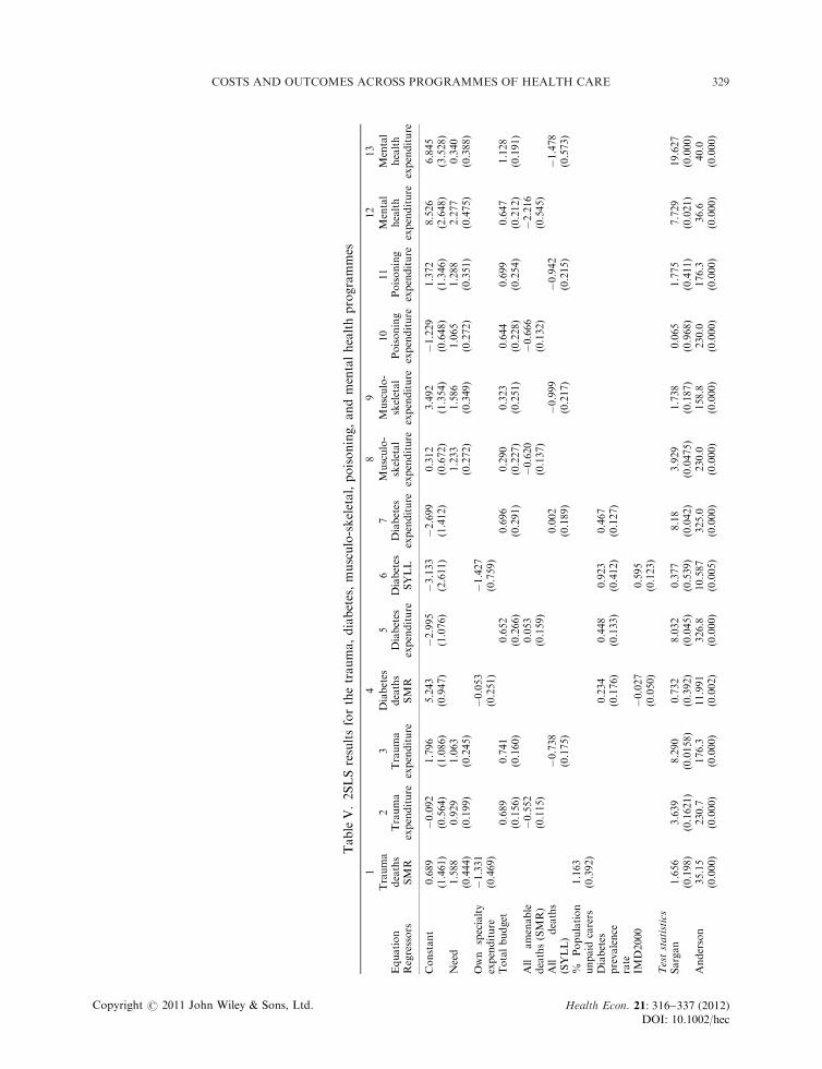
4.6. Trauma, burns and injuries programme of care

Results for the trauma, burns and injuries programme of care are shown in columns 1–3 of Table V. Forthe mortality rate outcome indicator, we employ a weighted average of the SMRs for deaths from a

14More precisely, the gastro-intestinal SMR5 ((5438/8754)�liver disease SMR)1((3316/8754)�ulcers SMR).




TableV.2SLSresultsforthetrauma,diabetes,musculo-skeletal,poisoning,andmentalhealthprogrammes

14

89

12

13

Equation

Regressors

Trauma

deaths

SMR

2Trauma

expenditure

3Trauma

expenditure

Diabetes

deaths

SMR

5Diabetes

expenditure

6Diabetes

SYLL

7Diabetes

expenditure

Musculo-

skeletal

expenditure

Musculo-

skeletal

expenditure

10

Poisoning

expenditure

11

Poisoning

expenditure

Mental

health

expenditure

Mental

health

expenditure

Constant

0.689

(1.461)

�0.092

(0.564)

1.796

(1.086)

5.243

(0.947)

�2.995

(1.076)

�3.133

(2.611)

�2.699

(1.412)

0.312

(0.672)

3.492

(1.354)

�1.229

(0.648)

1.372

(1.346)

8.526

(2.648)

6.845

(3.528)

Need

1.588

(0.444)

0.929

(0.199)

1.063

(0.245)

1.233

(0.272)

1.586

(0.349)

1.065

(0.272)

1.288

(0.351)

2.277

(0.475)

0.340

(0.388)

Own

specialty

expenditure

�1.331

(0.469)

�0.053

(0.251)

�1.427

(0.759)

Totalbudget

0.689

(0.156)

0.741

(0.160)

0.652

(0.266)

0.696

(0.291)

0.290

(0.227)

0.323

(0.251)

0.644

(0.228)

0.699

(0.254)

0.647

(0.212)

1.128

(0.191)

All

amenable

deaths(SMR)

�0.552

(0.115)

0.053

(0.159)

�0.620

(0.137)

�0.666

(0.132)

�2.216

(0.545)

All

deaths

(SYLL)

�0.738

(0.175)

0.002

(0.189)

�0.999

(0.217)

�0.942

(0.215)

�1.478

(0.573)

%Population

unpaid

carers

1.163

(0.392)

Diabetes

prevalence

rate

0.234

(0.176)

0.448

(0.133)

0.923

(0.412)

0.467

(0.127)

IMD2000

�0.027

(0.050)

0.595

(0.123)

Teststatistics

Sargan

1.656

(0.198)

3.639

(0.1621)

8.290

(0.0158)

0.732

(0.392)

8.032

(0.045)

0.377

(0.539)

8.18

(0.042)

3.929

(0.0475)

1.738

(0.187)

0.065

(0.968)

1.775

(0.411)

7.729

(0.021)

19.627

(0.000)

Anderson

35.15

(0.000)

230.7

(0.000)

176.3

(0.000)

11.991

(0.002)

326.8

(0.000)

10.587

(0.005)

325.0

(0.000)

230.0

(0.000)

158.8

(0.000)

230.0

(0.000)

176.3

(0.000)

36.6

(0.000)

40.0

(0.000)




Cragg–

Donald

18.3

(o0.05)

114.2

(o0.05)

78.7

(o0.05)

6.02

(o0.05)

147.3

(o0.05)

5.30

(o0.05)

145.9

(o0.05)

171.3

(o0.05)

103.4

(o0.05)

114.2

(o0.05)

78.7

(o0.05)

12.7

(o0.05)

14.0

(o0.05)

PartialR2

0.112

0.542

0.449

0.041

0.674

0.035

0.672

0.541

0.416

0.541

0.449

0.119

0.129

Pesaran–

Taylor

0.65

(0.420)

0.30

(0.581)

0.49

(0.483)

0.07

(0.785)

0.00

(0.962)

12.30

(0.001)

0.02

(0.900)

0.18

(0.673)

0.11

(0.739)

0.01

(0.913)

0.12

(0.728)

0.17

(0.683)

0.07

(0.791)

Endogeneity

Own

specialty

expenditure

4.421

(0.035)

0.23

(0.630)

7.16

(0.007)

All

amenable

deaths(SMR)

8.153

(0.004)

0.07

(0.786)

8.549

(0.003)

4.153

(0.041)

14.59

(0.000)

All

deaths

(SYLL)

10.73

(0.001)

0.09

(0.760)

14.625

(0.000)

6.208

(0.012)

4.582

(0.032)

Notes:

1.Parentheses

show

robust

standard

errors

forparameter

estimatesandp-values

forthetest

statistics.

2.Theinstrumentsetfortraumaexpenditure

includes

the

proportionofhouseholdsthatare

lonepensioner

householdsandthepopulationweightedindex

ofmultiple


IMD

2000scores.

3.The

instrumentsetsforallamenabledeaths(SMR)andalldeaths(SYLL)in

thetraumaprogrammeincludetheproportionofhouseholdsthatare

lonepensioner

households,the

proportionofthepopulationprovidingunpaid

care


ofmultiple


IMD

2000scores.

4.Theoutcome

indicatorin

Equation(1)isaweightedaverageofthefracturedfemurandskullfracture

SMRswithweightsreflectingthenumber

ofdeathsin

each

category.NoSYLL-based

mortality

ratesare

available

forthesedeaths.5.Theinstrumentsetfordiabetes

expenditure

includes


lonepensioner

households,the

proportionofthepopulationprovidingunpaid

care


ofmultiple

deprivationbasedonward-levelIM

D2000scores.6.Theinstrumentset

forallamenabledeaths(SMR)andalldeaths(SYLL)in

thediabetes

programmeincludes


lonepensioner

households,theproportionof

thepopulationprovidingunpaid

care,thepopulationweightedindex

ofmultiple


IMD

2000scoresandtheallspecialtyneedsindex

(not

included

asaregressorin

thesecond-stageequations).7.Thediabetes

death

measure

istheallageSMR

for2002–2004andtheSYLLrate

isforthose

aged

under

75over

the

same3-yearperiod.Theexpenditure

andoutcomedata

haveidenticalIC

D10coverage.8.Thesamplesize

forthediabetes

deathsequationis284.9.Theinstrumentsetsfor

theallamenabledeaths(SMR)andalldeaths(SYLL)variablesin

themusculo-skeletalprogrammeincludetheproportionofhouseholdsthatare

lonepensioner

households


ofmultipledeprivationbasedonward-levelIM

D2000scores.10.Theinstrumentsetsfortheallamenabledeathsandalldeathsvariables

inthepoisoningprogrammeincludetheproportionofhouseholdsthatare

lonepensioner

households,theproportionofthepopulationthatprovideunpaid

care

andthe

populationweightedindex

ofmultiple

deprivationbasedonward-levelIM

D2000scores.11.Theinstrumentsets

fortheallamenabledeathsandalldeathsvariablesin

the

mentalhealthincludetheproportionofhouseholdsthatare

lonepensioner

households,

theproportionofthepopulationthatprovideunpaid

care

andthepopulation

weightedindex

ofmultipledeprivationbasedonward-levelIM

D2000scores.12.Theresultspresentedare

forallmentalhealthexpenditure

excludingthatondem

entia(the

latter

accounts

forabout11%

ofallmentalhealthexpenditure)althoughsimilarmodelsare

obtainable

forallmentalhealthexpenditure.




fractured femur and from a skull fracture with weights determined by the number of deaths attributedto each cause in 2004.15 No SYLL rate data are available for these causes of death. In 2004 these twocauses accounted for about one-quarter of the 10 500 deaths attributable to the trauma and injuriesprogramme budgeting category (NCHOD, 2007).

In the outcome equation (1) both the need and expenditure terms have the anticipated sign andare significant. It was also necessary to add the proportion of the population, providing unpaid care asan additional regressor. It has a significant positive sign in the outcome equation and the implicationis that, ceteris paribus, areas with more unpaid carers have higher mortality rates from fractures.This might be because the availability of care allows the elderly to continue to live in their own homeand that they are more likely to fall and die from a fall at home than they are in alternativeaccommodation (such as a residential home or sheltered housing). The usual statistical tests indicatethat the instruments are relevant and valid, that expenditure is endogenous and that there is no evidenceof misspecification.

In both of the expenditure equations (2 and 3), need, total budget and the all deaths term have theanticipated effect on expenditure and are statistically significant. Again, the usual tests indicate that theinstruments are relevant and valid, that the deaths term is endogenous and that there is no evidence ofmisspecification. The coefficient on the total budget term lies between 0.689 and 0.741. The standarderror associated with this estimate (about 0.15) suggests that the 95% confidence interval for thiscoefficient lies almost entirely below 1.

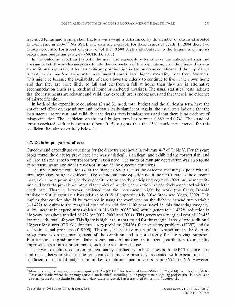
4.7. Diabetes programme of care

Outcome and expenditure equations for the diabetes are shown in columns 4–7 of Table V. For this careprogramme, the diabetes prevalence rate was statistically significant and exhibited the correct sign, andwe used this measure to control for population need. The index of multiple deprivation was also foundto be useful as an additional regressor in one of the outcome equations.

The first outcome equation (with the diabetes SMR rate as the outcome measure) is poor with allthree regressors being insignificant. The second outcome equation (with the SYLL rate as the outcomemeasure) is more promising as the expenditure term has the anticipated negative effect on the mortalityrate and both the prevalence rate and the index of multiple deprivation are positively associated with thedeath rate. There is, however, evidence that the instruments might be weak (the Cragg–Donaldstatistic5 5.30 suggesting a bias relative to OLS of approximately 30%; Stock and Yogo, 2002). Thisimplies that caution should be exercised in using the coefficient on the diabetes expenditure variable(�1.427) to estimate the marginal cost of an additional life year saved in this budgeting category.A 1% increase in expenditure (which was £16.80 in 2005/2006) would generate a 1.427% reduction inlife years lost (these totalled 66 757 for 2002, 2003 and 2004). This generates a marginal cost of £26 453for one additional life year. This figure is higher than that found for the marginal cost of one additionallife year for cancer (£13 931), for circulatory problems (£8426), for respiratory problems (£7397) and forgastro-intestinal problems (£18 999). This may be because much of the expenditure in the diabetesprogramme is on the management of the condition and is not directly for life saving purposes.Furthermore, expenditure on diabetes care may be making an indirect contribution to mortalityimprovements in other programmes, such as circulatory disease.

The two expenditure equations are reasonably satisfactory: in both cases both the PCT income termand the diabetes prevalence rate are significant and are positively associated with expenditure. Thecoefficient on the total budget term in the expenditure equation varies from 0.652 to 0.696. However,

15More precisely, the trauma, burns and injuries SMR5 ((2517/7814)�fractured femur SMR)1((5297/7814)�skull fracture SMR).These are deaths where the primary cause is ‘unclassified’ according to the programme budgeting project (that is, there is anexternal cause for the death) but the secondary cause is recorded as a fractured femur or a fractured skull.




the standard error for this estimate is about 0.28 so our 95% confidence interval for the budget elasticityis quite wide between 0.10 and 1.26. Although positive, the coefficient on the ‘other calls on resourcesterm’ is insignificant in both equations and there is no evidence of mis-specification. The endogeneitytest suggests that the ‘other calls on PCT resources’ term is not endogenous but OLS estimation of thetwo expenditure equations generates results offer no improvement on those presented in Table V.

In addition to the programmes discussed above, we sought to estimate outcome and expenditureequations for three further programmes – infectious diseases, genito-urinary problems and neonateconditions – for which a relevant mortality indicator is available. However, we met with less success inmodelling these other budgeting categories. For example, the coefficients in both the expenditure andoutcome equations for the genito-urinary programme were counterintuitive. This lack of success isperhaps not surprising as the specialty coverage of the outcome measure – the mortality rate fromchronic renal failure (ICD10 code N18) – is considerably smaller than that of the expenditure data(which relates to ICD10 codes A50–A64, N00–N99, Q500–Q649, R30–R39, R86–R87), and renalfailure accounts for less than one-fifth of all deaths that fall within the genito-urinary programme.In addition, there are relatively few deaths from this condition: over the 3-year period 2002–2004 therewere on average 1406 deaths per year which is less than five deaths per PCT per annum. Similar smallnumber issues also arise with the infectious diseases and neonate conditions categories.

For some budgeting categories, no relevant mortality indicator is available and thus we were unableto estimate an outcome (death rate) equation. However, expenditure equations can still be estimated(see, for example, equations 8–13 in Table V) and the budget elasticities for the three categories forwhich plausible results were derived are summarised below. Further discussion of the results for thesethree categories can be found in Section A.5 of Appendix A (available from Wiley InterScience website)but, in summary, we obtained:

� a budget elasticity of 0.461 for expenditure in the musculo-skeletal programme of care (95%confidence interval ranging from 0.11 to 0.81);

� a budget elasticity of about 0.670 for expenditure in the poisoning programme of care (95%confidence interval ranging from 0.19 to 1.15) and

� a budget elasticity of 0.647 for expenditure in the mental health programme of care (95%confidence interval ranging from 0.23 to 1.07).

The estimated costs of an extra life year presented above are in terms of an unadjusted life year.As an indication of how they might be adjusted to yield the cost of a quality-adjusted life year (QALY),we have employed the utility scores made available by the HODaR project (HODaR, UniversityHospital of Wales) using the UK EQ-5D scoring algorithm.16 Quality of life scores are available byICD10 code, and the data set includes the number of patients whose responses are attributed to eachcode. These scores can be assigned to programme budget categories using the ICD10 code. Taking aweighted average of utility scores across the relevant ICD10 codes generated the following averages:0.663 for cancer, 0.578 for circulatory disease, 0.625 for gastro-intestinal problems, 0.558 for respiratoryproblems and 0.562 for diabetes. Thus, our estimate of the cost of:

(a) a cancer QALY is £21 012 (5 £13 931/0.663);(b) a circulatory disease QALY is £12 593 (5 £7279/0.578);(c) a respiratory QALY is £13 256 (5 £7397/0.558);(d) a gastro-intestinal QALY is £30 400 (5 £19 000/0.625) and(e) a diabetes QALY is £47 069 (5 £26 453/0.562).

16For details of this data set, see https://www.jiscmail.ac.uk/cgi-bin/webadmin?A25 ind0409&L5HEALTHECON-DIS-CUSS&F5&S5&P5 6725). We are grateful to Dr Craig Currie, Director and Senior Lecturer in Health Outcomes Research,HODaR, Cardiff Medicentre, University Hospital of Wales, for making available this data set.




5. CONCLUSIONS

This study has attempted to estimate expenditure and outcome equations for 23 programmes of care.Satisfactory expenditure equations have been developed for ten programmes of care, which representmost of the major spending categories. One focus of this study has been on the expenditure elasticitywith respect to the global PCT budget (income), and similar values have been obtained across mostprogrammes, in the range 0.644–1.128. The only outlier is the musculoskeletal programme with arelatively low-income elasticity of expenditure of about 0.46. With the exception of the neurological andmental health programmes, all of our budget elasticities are o1.0.

Assuming that the budget is fully spent each year, this implies that some of the budget elasticities forthe programmes for which we have been unable to derive a satisfactory expenditure equation are likelyto be greater than 1.0. These programmes – which include infectious diseases, blood disorders, learningdisability, vision problems, hearing problems, dental problems, skin problems, genito-urinary problems,maternity, neonate conditions, healthy individuals, social care needs and general practice – accountedfor 44% of the total expenditure in 2005/2006. These might represent services where efficiency gains aremore easily achieved or programmes where the purchaser’s perception of the cost-effectiveness ofmarginal expenditure is lowest.

Our results suggest that policy-makers seeking to impose budget reductions on local purchasers canexpect to see different expenditure reductions in different services. Future work might seek to explain whythese variations exist. Furthermore, the results indicate the likely behavioural response to less directconstraints on expenditure, such as the ‘ring fencing’ of some element of PCT expenditure for implementingmandatory treatment guidelines. At the margin, satisfying such mandates may require reductions inservices elsewhere, and these results indicate the scale of reductions likely to be seen in some services.

In this modelling, we have assumed that the response of PCTs to budget reductions will be equal andopposite to those found under the budget increases. It can be plausibly argued that this may not occur inpractice, because in some services PCTs may experience more ‘friction’ in seeking expenditure changesin one direction than the other. For example, expenditure reductions may be made more difficult insome services than others because of redundancy payment liabilities. Similarly, the elasticities calculatedhere are for marginal changes, but marginal changes in budgets may not be feasible for someprogrammes. Expenditure may be lumpy and the interval elasticity may be different from the pointelasticity.17 Future work might seek to model any asymmetry of this type.

Satisfactory outcome equations, using SMRs, have been estimated for seven programmes of care:cancer, circulatory problems, neurological problems, respiratory problems, gastro-intestinal problems,trauma and injuries, and diabetes. They show that healthcare expenditure has a demonstrably positiveeffect on outcomes. Our lack of success with three other categories – infectious diseases, genito-urinaryproblems and neonatal care – is probably because outcome indicator (death) is not a common outcomefor these categories, or because the specialty coverage of the mortality data fails to match closely enoughthe coverage of the budgeting data.

The results presented here confirm and considerably extend the preliminary findings presentedpreviously for the cancer and circulatory disease programmes (Martin et al., 2008a). They confirm thatthe marginal cost of a ‘life year’ saved is quite low at:

� £13 931 for cancer;� £7279 for circulatory problems;� £7397 for respiratory problems;� £18 999 for gastro-intestinal problems and� £26 453 for diabetes.

17We are indebted to an anonymous referee for this point.




These figures suggest that expenditure on different programmes yields somewhat different benefits interms of life years saved. However, it is quite likely that the variations we observe between the costsin the different programmes can in part be explained by: (a) interventions, such as cancer palliativecare, that yield benefits that cannot be measured to any great extent in increased life expectancy and(b) differences in the extent to which the specialty coverage of the mortality data corresponds to thecoverage of the budgeting data. Nevertheless, after a rudimentary adjustment for quality of life, theseestimates do appear to be in line with the sum of £30 000 for a QALY commonly attributed to the UK’sNational Institute for Health and Clinical Excellence (NICE) as the threshold for accepting newtechnologies (Appleby et al., 2009).

However, the modelling in this paper does have limitations. First, we have modelled outcome datafor the three years 2002, 2003 and 2004, along with expenditure data for the one year 2005/2006. Morerealistically, current health outcomes will be the result of current and previous years of expenditure bylocal PCTs. Implicitly, our analysis assumes that PCTs have reached some sort of equilibrium in theexpenditure choices they make and the outcomes they secure. This is probably not an unreasonableassumption, given the relatively slow pace at which both types of variable change. This assumption issupported by the finding that the cost of life year estimates presented here for cancer and circulatorydisease are similar to those reported previously but which were based on expenditure data for differenttime periods.18 Second, this study uses limited health outcomes data (in the form of mortality rates) andwe have been unable to adjust our estimates of the cost of a life year for variations in the proportion ofspent in each programme that is devoted to condition management (rather than extending life). Finally,we treat programmes of care independently ignoring the influence that co-morbidities acrossprogrammes might have on the relationships between expenditure and health outcomes. As new dataresources emerge, future work may be able to address some of these limitations.

APPENDIX A

A.1. Socio-economic indicators available as potential instruments for 2SLS estimation

Table AI lists the socio-economic indicators available as potential instruments for the 2SLS estimation.It also provides details of how each indicator has been constructed.

Table AI. Socio-economic indicators available as potential instruments for 2SLS estimation

Indicatorname Short description

Long description with relevant Census Key Statistic table and cellnumbers

BORNEXEU Residents born outside the EuropeanUnion

Residents born outside the European Union divided by all residents(census cell definition: KS005008/KS005001)

WHITEEG Residents in white ethnic group Population in white ethnic group divided by total population (KS0060021KS0060031KS006004)/KS006001

PCWALLTI Population of working age with illness Proportion of population of working age with limiting long-term illnessdivided by population aged 16–74 (KS008003/KS09A001)

POPPUCAR Unpaid care providers in population Proportion of population providing unpaid care (KS008007/KS008001)POPPUCA1 Unpaid care (o20 h a week) in

populationProportion of population providing unpaid care of 1–19 h a week(KS008008/KS008001)

POPPUCA2 Unpaid care (20–49 h) in population Proportion of population providing unpaid care for 20–49 h per week(KS008009/KS008001)

POPPUCA3 Unpaid care (450 h a week) inpopulation

Proportion of population providing unpaid care for over 50 h a week(KS008010/KS008001)

NQUAL174 Proportion aged 16–74 with noqualifications

Proportion of population aged 16–74 with no qualifications (KS013002/KS013001)

18In addition, we also obtained similar cost of life year estimates for cancer and circulatory disease when we re-estimated the modelusing expenditure data for 2006/2007 and mortality data for 2004, 2005 and 2006 for the new English PCTs (Martin et al., 2008b).




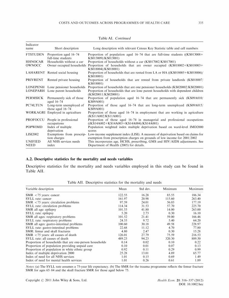
A.2. Descriptive statistics for the mortality and needs variables

Descriptive statistics for the mortality and needs variables employed in this study can be found inTable AII.

Table AI. Continued

Indicatorname Short description Long description with relevant Census Key Statistic table and cell numbers

FTSTUDEN Proportion aged 16–74full-time students

Proportion of population aged 16–74 that are full-time students ((KS0130081KS013009)/KS013001)

HHNOCAR Households without a car Proportion of households without a car (KS017002/KS017001)OWNOCC Owner occupied households Proportion of households that are owner occupied (KS0180021KS0180031

KS018004)/KS018001)LAHARENT Rented social housing Proportion of households that are rented from LA or HA ((KS0180051KS018006)/

KS018001)PRIVRENT Rented private housing Proportion of households that are rented from private landlords (KS018007/

KS018001)LONEPENH Lone pensioner households Proportion of households that are one pensioner households (KS020002/KS020001)LONEPARH Lone parent households Proportion of households that are lone parent households with dependent children

(KS020011/KS020001)PERMSICK Permanently sick of those

aged 16–74Proportion of population aged 16–74 that are permanently sick (KS09A010/KS09A001)

PC74LTUN Long-term unemployed ofthose aged 16–74

Proportion of those aged 16–74 that are long-term unemployed (KS09A015/KS09A001)

WORKAGRI Employed in agriculture Proportion of those aged 16–74 in employment that are working in agriculture(KS11A002/KS11A001)

PROFOCCU People in professionaloccupations

Proportion of those aged 16–74 in managerial and professional occupations((KS14A0021KS14A0031KS14A004)/KS14A001)

POPWIMD Index of multipledeprivation

Population weighted index multiple deprivation based on ward-level IMD2000scores

LISI2002 Exemptions from prescrip-tion charges

Low-income supplement index (LISI). A measure of deprivation based on claims forexemption from prescription charges on grounds of low income for 2001/2002

UNIFIEDNEED

All NHS services needsindex

This incorporates age, HCHS, prescribing, GMS and HIV/AIDS adjustments. SeeDepartment of Health (2005) for details.

Table AII. Descriptive statistics for the mortality and needs

Variable description Mean Std dev. Minimum Maximum

SMR o75 years: cancer 122.55 16.28 85.55 186.34SYLL rate: cancer 161.97 20.98 115.60 263.40SMR o75 years: circulation problems 97.59 24.01 56.03 177.19SYLL rate: circulation problems 114.34 31.53 57.70 225.70SMR all age: epilepsy 101.53 41.80 14.00 263.00SYLL rate: epilepsy 5.20 2.73 0.30 16.10SMR all ages: respiratory problems 101.52 21.41 59.00 166.46SYLL rate: respiratory problems 24.33 9.72 5.40 64.20SMR all ages: gastro-intestinal problems 100.60 30.18 49.58 228.97SYLL rate: gastro-intestinal problems 22.68 11.12 4.70 77.80SMR: femur and skull fractures 4.80 2.47 0.30 15.28SMR o75 years: all causes of death 126.01 27.79 75.59 216.53SYLL rate: all causes of death 489.23 94.23 320.30 889.50Proportion of households that are one-person households 0.14 0.02 0.10 0.22Proportion of population providing unpaid care 0.10 0.01 0.07 0.13Proportion of population in white ethnic group 0.92 0.11 0.29 0.99Index of multiple deprivation 2000 25.28 13.01 4.89 65.77Index of need for all NHS services 1.01 0.15 0.69 1.49Index of need for mental health services 1.01 0.26 0.61 1.89

Notes: (a) The SYLL rate assumes a 75-year life expectancy. (b) The SMR for the trauma programme reflects the femur fractureSMR for ages 65–84 and the skull fracture SMR for those aged below 75.




TableAIII.

Correlationmatrix

fortheexpenditure

andmortality

variables

x1

x2

x3

x4

x5

x6

x7

x8

x9

x10

x11

x12

x13

x14

x15

x16

x17

x18

x19

x20

x21

x22

x23

SMR

o75years:cancer

x1

1.00

SYLLrate:cancer

x2

0.95

1.00

SMR

o75years:circulation

x3

0.83

0.79

1.00

SYLLrate:circulation

problems

x4

0.82

0.79

0.98

1.00

SMR

allages:epilepsy

x5

0.36

0.34

0.35

0.36

1.00

SYLLrate:epilepsy

x6

0.22

0.21

0.18

0.20

0.70

1.00

SMR

allages:respiratory

problems

x7

0.76

0.68

0.79

0.77

0.32

0.13

1.00

SYLLrate:respiratory

problems

x8

0.79

0.75

0.86

0.86

0.39

0.20

0.82

1.00

SMR

allages:gastro-intestinal

problems

x9

0.68

0.64

0.74

0.72

0.30

0.14

0.68

0.73

1.00

SYLLrate:gastro-intestinal

problems

x10

0.73

0.69

0.77

0.77

0.32

0.17

0.67

0.77

0.91

1.00

SMR:femurandskullfractures

x11

0.32

0.29

0.31

0.29

0.05

0.05

0.21

0.21

0.26

0.29

1.00

SMR

o75years:allcausesof

death

x12

0.84

0.81

0.99

0.97

0.38

0.22

0.80

0.87

0.75

0.78

0.32

1.00

SYLLrate:allcausesofdeath

x13

0.87

0.87

0.93

0.94

0.42

0.27

0.76

0.88

0.76

0.83

0.31

0.94

1.00

Spendper

head,cancer

x14

0.25

0.28

0.13

0.15

0.16

0.18�0.01

0.15

0.11

0.15�0.01

0.13

0.23

1.00

Spendper

head,circulation

problems

x15

0.43

0.44

0.37

0.38

0.21

0.17

0.21

0.29

0.34

0.41

0.23

0.37

0.44

0.50

1.00

Spendper

head,neurological

problems

x16

0.27

0.23

0.16

0.16

0.05

0.06

0.09

0.14

0.13

0.20

0.11

0.15

0.24

0.41

0.46

1.00

Spendper

head,respiratory

problems

x17

0.60

0.57

0.53

0.53

0.22

0.16

0.45

0.50

0.47

0.54

0.35

0.54

0.57

0.34

0.75

0.39

1.00

Spendper

head,gastro-

intestinalproblems

x18

0.52

0.50

0.41

0.42

0.21

0.16

0.35

0.38

0.35

0.42

0.21

0.42

0.49

0.43

0.77

0.39

0.78

1.00

Spendper

head,trauma

x19

0.39

0.40

0.30

0.32

0.22

0.23

0.24

0.32

0.23

0.30

0.03

0.30

0.39

0.40

0.48

0.30

0.41

0.47

1.00

Spendper

head,diabetes

x20

0.34

0.33

0.39

0.38

0.10

0.03

0.23

0.26

0.22

0.28

0.20

0.37

0.37

0.22

0.42

0.15

0.42

0.28

0.17

1.00

Spendper

head,musculo-

skeletalproblems

x21

0.34

0.35

0.26

0.26

0.10

0.09

0.12

0.21

0.22

0.30

0.19

0.26

0.32

0.26

0.45

0.25

0.35

0.44

0.34

0.27

1.00

Spendper

head,poisoning

x22

0.26

0.28

0.21

0.22

0.14

0.08

0.12

0.20

0.20

0.22

0.04

0.21

0.27

0.40

0.50

0.25

0.45

0.51

0.42

0.24

0.41

1.00

Spendper

head,mental

healthexcdem

entia

x23

0.42

0.42

0.50

0.50

0.23

0.13

0.35

0.53

0.45

0.50

0.03

0.50

0.53

0.20

0.20

0.16

0.31

0.21

0.26

0.16

0.06

0.12

1.00

Note:Thespendper

headdata

are

adjusted

forunavoidable

variationsin

localinputpricesandrelate

to2005/2006.

A.3.Correlationmatrix

fortheexpenditure

andmortality

variables

Acorrelationmatrix

fortheexpenditure

andmortality

variablesem

ployed

inthisstudycanbefoundin

Table

AIII.




ACKNOWLEDGEMENTS

This study was funded by the Health Foundation under its Quest for Quality and ImprovedPerformance (QQuIP) initiative. The paper does not necessarily reflect the views of the funder. NigelRice gratefully acknowledges funding support from the Economic and Social Research Council undergrant number RES-060-25-0045. We are grateful to Hugh Gravelle, Andrew Jackson and Karl Claxtonfor helpful comments and advice.

REFERENCES

Anderson TW. 1984. Introduction to Multivariate Statistical Analysis (2nd edn). Wiley: New York.Appleby J, Devlin N, Parkin D, Buxton M, Chalkidou K. 2009. Searching for cost effectiveness thresholds in the

NHS. Health Policy 91: 239–245.Cragg JG, Donald SG. 1993. Testing identifiability and specification in instrumental variable models. Econometric

Theory 9: 222–240.Department of Health. 2005. Unified Exposition Book: 2003/04, 2004/05 and 2005/06 PCT Revenue Resource Limits.

Department of Health: London.Gravelle H, Backhouse M. 1987. International cross-section analysis of the determination of mortality. Social

Science Medicine 25(5): 427–441.Lakhani A, Olearnik H, Eayres D (eds). 2006. Compendium of Clinical and Health Indicators: Data Definitions and

User Guide for Computer Files. NCHOD: London.Martin S, Rice N, Smith PC. 2007. Further evidence on the link between health care spending and health outcomes

in England. Centre for Health Economics Research Paper 32, University of York, December 2007.Martin S, Rice N, Smith PC. 2008a. Does health care spending improve health outcomes? Evidence from English

programme budgeting data. Journal of Health Economics 27: 826–842.Martin S, Rice N, Smith PC. 2008b. The link between health care spending and health outcomes for the new

English primary care trusts. Centre for Health Economics Research Paper 42, University of York, October 2008.Mitton C, Donaldson C. 2004. The Priority Setting Toolkit: A Practical Guide to the Use of Economics in Health

Care Decision Making. BMJ Books: London.NCHOD. 2007. Figures compiled by NCHOD from Annual Mortality Extract from ONS. Supplied by Daniel

Eayres, personal communication.Nixon J, Ulmann P. 2006. The relationship between health care expenditure and health outcomes. European Journal

of Health Economics 7: 7–18.Nolte E, McKee M. 2004. Does Health Care Save Lives? The Nuffield Trust: London.ONS. 2007. VS3 mortality by cause, England, 2004 Registrations. ONS, personal communication.Pesaran MH, Taylor LW. 1999. Diagnostics for IV regressions. Oxford Bulletin of Economics and Statistics 61(2):

255–281.Ramsey JB. 1969. Tests for specification errors in a classical linear least squares regression analysis. Journal of the

Royal Statistical Society: Series B 31: 350–371.Sargan JD. 1958. The estimation of economic relationships using instrumental variables. Econometrica 26: 393–415.Shea J. 1997. Instrumental relevance in multivariate linear models: a simple measure. Review of Economics and

Statistics 79: 348–352.Smith PC, Rice N, Carr-Hill RA. 2001. Capitation funding in the public sector. Journal of the Royal Statistical

Society: Series A 164(Part 2): 217–257.Staiger D, Stock JH. 1997. Instrumental variables regression with weak instruments. Econometrica 65: 557–586.Stock JH, Yogo M. 2002. Testing for weak instruments in linear IV regression. NBER Technical Working Paper

284.




Comparing costs and outcomes across programmes of health care

Documents

Transcript of Comparing costs and outcomes across programmes of health care