Community Heterogeneity and PoliticalParticipation in American Cities∗

Daniel RubensonUdeM & LSE

daniel.rubenson@umontreal.ca

Prepared for presentation to the 2005 Canadian Political Science

Association meeting, London ON 2–4 June 2005

This version, May 2005

Abstract

This paper analyzes the effects of racial diversity on political participationin American cities. Previous work on the relationship between diversity andparticipation has produced ambiguous results. Some find that diversity sup-presses political participation while others maintain the opposite. I argue thatincentives for participation are reduced by homogeneity. Heterogeneous placesare characterized by more conflict over resources and more mobilized groups,leading to higher levels of political participation. However, I also argue that dif-ferent racial groups react differently to diversity. The paper uses data from the2000 Social Capital Community Benchmark Survey, respondents from whichwere matched with census data on their place of residence. The results of thisanalysis indicate that racial diversity affects the propensity to vote differentlyfor different racial groups and that these differences vary across communities.While white people are less likely to vote the more racially diverse their city ofresidence is, the relationship is the reverse for minority populations.

∗Earlier versions of the paper were presented to the 2004 Midwest Political Science AssociationMeetings, Chicago IL and the 2004 EPOP Confernce, Oxford, England. Thanks to Andre Blais,Torun Dewan, Keith Dowding, Francois Gelineau, Jouni Kuha, Paul Martin, Bob Putnam andChris Wlezian for comments and suggestions and to Marylin Millikin for assistance in obtainingthe geocodes for the data. The data used in this paper come from the Social Capital CommunityBenchmark Survey, available at the Roper Center. The Social Capital Community BenchmarkSurvey was designed by the Sauguaro Seminar at the John F. Kennedy School of Government,Harvard University and funded by the Ford Foundation and a number of Community Foundations.Any errors remain mine.

1. Introduction

By taking political action, citizens make their preferences known, determine who

holds public office and try to influence the decisions made by politicians. Despite

popular conceptions of the United States as a vast wasteland of apathetic and apolit-

ical citizens, the reality is that Americans are participants. While it is true that voter

turnout is lower in the US than in many other democracies, Americans are generally

more likely to contact politicians and officials, work on a campaign, belong to and

be active in political groups and participate in local politics than citizens in other

countries (Brady, Schlozman, Verba & Elms 2002).

However, the issue of declining political participation has spurred a large litera-

ture and much debate not only the United States but also in many other western

democracies. Much of the research on political participation and its decline, analyzes

changes in the characteristics of individuals that may account for decreased voter

turnout and other forms of activity. While changes in levels of education, income

and other individual-level factors are no doubt important and should be analyzed,

much of such research suffers from not taking adequate account of political and so-

cial context. This study analyzes data from a new large-scale survey and matches

respondents with information about their city of residence from various sources in

order to examine how the political and social environment in which individuals find

themselves affects their political behavior.

As Verba, Schlozman & Brady note, democracy requires both a degree of voice and

equality (1995, p. 1). However, far from all citizens make their voice known through

voting and even fewer take part in other forms of political participation. Those

that do participate are not representative of the larger population. As we know,

participants differ in fundamental ways from non-participants—education, income,

race, gender and a host of other individual-level characteristics set active citizens

apart from inactive ones. However, it is not the case that participation is equal

2

between equally rich, well educated, white males for instance. As I show in this

paper, even after controlling for many of the characteristics of individuals associated

with political participation, activity rates vary between people in different places in

the United States. So it is not just a matter of who you are, (or even who you are

connected to, as social capitalists would have us believe), but also where you are. In

order to examine the effects of context on political action I compare participation

across cities in the United States

Although cities in the Unites States vary on a large number of dimensions, in this

paper I only focus on one: racial diversity. Race is of fundamental importance to

American politics and one of the most striking trends in American society in recent

years has been the increase in racial diversity. Are people living in cities characterized

by high degrees of ethnic fractionalization more or less likely to take political action

than those living in very homogenous places?

2. The Impact of Diversity on Political Participation

While issues of race and their influence on political behavior and attitudes have long

been studied by scholars of American politics, the focus of most of this research has

been on how the race of individuals affects various outcomes. Until recently it has

been rare that race as a characteristic of community context or environment has

been taken into account (Oliver 2001). Perhaps in response to the realization that

diversity is increasing and patters of racial integration changing, there have been

a number of new studies on the impact of racial heterogeneity (eg. Alesina & La

Ferrera 2000, Costa & Kahn 2003, Oliver 2001). The majority of studies examining

heterogeneity and participation argue that increased heterogeneity is detrimental to

levels of engagement.1 The social capital literature from Putnam forward argues

1Notable exceptions are Oliver (2001) who argues that increasing racial segregation betweensuburbs is related to decreased political and civic engagement and Campbell (2002) who argues thatthe relationship between diversity and political participation is curvilinear so that political activityis lower at both extremes of diversity and homogeneity.

3

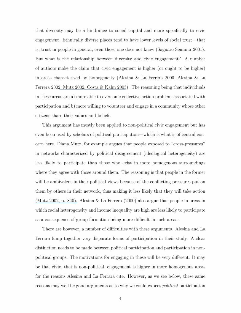
that diversity may be a hindrance to social capital and more specifically to civic

engagement. Ethnically diverse places tend to have lower levels of social trust—that

is, trust in people in general, even those one does not know (Saguaro Seminar 2001).

But what is the relationship between diversity and civic engagement? A number

of authors make the claim that civic engagement is higher (or ought to be higher)

in areas characterized by homogeneity (Alesina & La Ferrera 2000, Alesina & La

Ferrera 2002, Mutz 2002, Costa & Kahn 2003). The reasoning being that individuals

in these areas are a) more able to overcome collective action problems associated with

participation and b) more willing to volunteer and engage in a community whose other

citizens share their values and beliefs.

This argument has mostly been applied to non-political civic engagement but has

even been used by scholars of political participation—which is what is of central con-

cern here. Diana Mutz, for example argues that people exposed to “cross-pressures”

in networks characterized by political disagreement (ideological heterogeneity) are

less likely to participate than those who exist in more homogenous surroundings

where they agree with those around them. The reasoning is that people in the former

will be ambivalent in their political views because of the conflicting pressures put on

them by others in their network, thus making it less likely that they will take action

(Mutz 2002, p. 840). Alesina & La Ferrera (2000) also argue that people in areas in

which racial heterogeneity and income inequality are high are less likely to participate

as a consequence of group formation being more difficult in such areas.

There are however, a number of difficulties with these arguments. Alesina and La

Ferrara lump together very disparate forms of participation in their study. A clear

distinction needs to be made between political participation and participation in non-

political groups. The motivations for engaging in these will be very different. It may

be that civic, that is non-political, engagement is higher in more homogenous areas

for the reasons Alesina and La Ferrara cite. However, as we see below, these same

reasons may well be good arguments as to why we could expect political participation

4

to be lower in such areas. While the social capital literature argues that increased di-

versity leads to decreased generalized trust and, therefore, less political participation,

a strong case can be made that the diminished trust in diverse communities should

mean more participation. If one is distrustful of others in one’s community, it makes

sense to ensure that one’s own voice is heard through taking part in politics.

In contrast to this literature, I argue that community heterogeneity—racial het-

erogeneity in particular—should lead to a higher likelihood of people participating in

politics. One potential reason for this is that cities or communities characterized by

heterogeneity will tend to have more conflicts over resources and policies and more

mobilized groups leading to more political participation. Recent work in group con-

flict theory shows that racial attitudes and policy preferences are strongly influenced

by group identities and the perception that what other groups gain, the own group

loses. As Glaser puts it, “In essence, this theory posits that individuals have a zero-

sum view of politics, that they think in group terms, in ‘us’ and ‘them’ terms, and

that they see the possibility that their own group could lose something valued to a

rival group” (Glaser 1994, p. 23). In other words, individuals view politics, at least

in part, as a competitive struggle between groups for scarce resources and are moti-

vated to attempt “to affect the process and pattern of their distribution” (Bobo 1988,

p. 95). Not only is the individual-level race important for the development of these

attitudes and related behaviors, but the racial environment is crucial. People living

in more racially diverse areas will be inclined to express these kinds of attitudes more

than those in less heterogeneous areas (Glaser 2003). Race and racial identity become

more salient in more racially heterogeneous places.

3. Data

The convoluted nature of American local government has led to difficulties in studying

political participation and these difficulties have been exacerbated by the lack of data

5

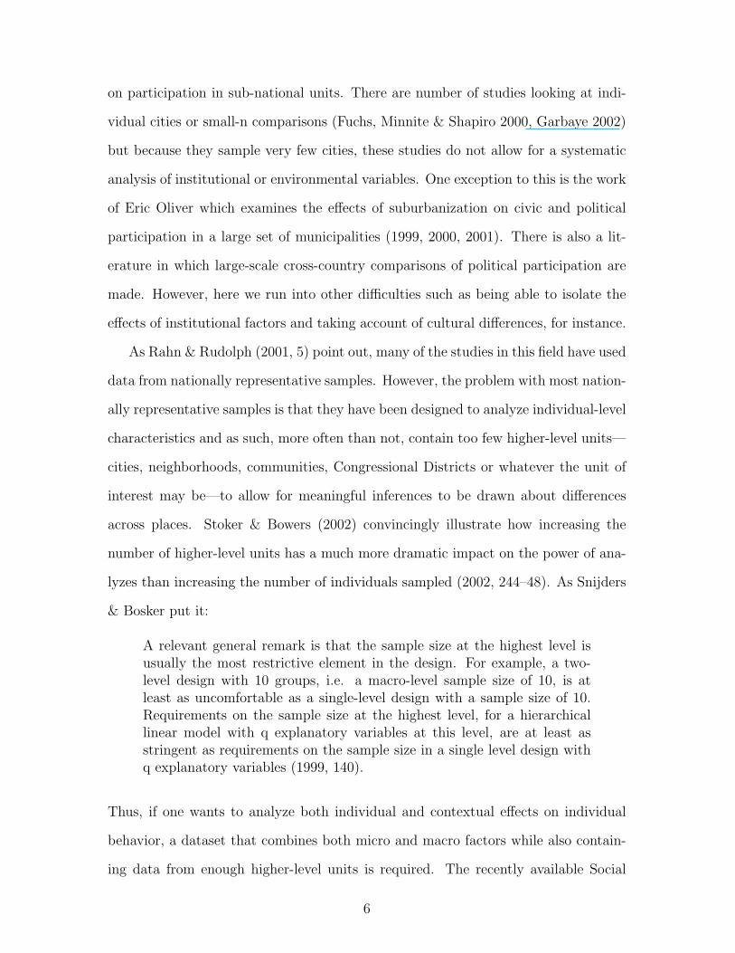
on participation in sub-national units. There are number of studies looking at indi-

vidual cities or small-n comparisons (Fuchs, Minnite & Shapiro 2000, Garbaye 2002)

but because they sample very few cities, these studies do not allow for a systematic

analysis of institutional or environmental variables. One exception to this is the work

of Eric Oliver which examines the effects of suburbanization on civic and political

participation in a large set of municipalities (1999, 2000, 2001). There is also a lit-

erature in which large-scale cross-country comparisons of political participation are

made. However, here we run into other difficulties such as being able to isolate the

effects of institutional factors and taking account of cultural differences, for instance.

As Rahn & Rudolph (2001, 5) point out, many of the studies in this field have used

data from nationally representative samples. However, the problem with most nation-

ally representative samples is that they have been designed to analyze individual-level

characteristics and as such, more often than not, contain too few higher-level units—

cities, neighborhoods, communities, Congressional Districts or whatever the unit of

interest may be—to allow for meaningful inferences to be drawn about differences

across places. Stoker & Bowers (2002) convincingly illustrate how increasing the

number of higher-level units has a much more dramatic impact on the power of ana-

lyzes than increasing the number of individuals sampled (2002, 244–48). As Snijders

& Bosker put it:

A relevant general remark is that the sample size at the highest level isusually the most restrictive element in the design. For example, a two-level design with 10 groups, i.e. a macro-level sample size of 10, is atleast as uncomfortable as a single-level design with a sample size of 10.Requirements on the sample size at the highest level, for a hierarchicallinear model with q explanatory variables at this level, are at least asstringent as requirements on the sample size in a single level design withq explanatory variables (1999, 140).

Thus, if one wants to analyze both individual and contextual effects on individual

behavior, a dataset that combines both micro and macro factors while also contain-

ing data from enough higher-level units is required. The recently available Social

6

Capital Community Benchmark Survey allows a more systematic study the effects of

contextual variables on behavior. The survey consists of a nationally representative

sample of 3003 respondents as well as 40 different sub-national representative sam-

ples. These samples had varying geographical boundaries including states and regions

within states (some were at the county level, some at the city level and some at other

regional levels determined by the local community foundation funding the project in

each area). The total sample size for the combined surveys is 29,733. Through an

agreement with the Roper Center I was able to obtain detailed geocodes for the data,

enabling me to identify respondents’ places of residence. Using these Federal Infor-

mation Processing Standards (FIPS) codes (the unique identification code used by

the Census Bureau to identify every place in Untied States) respondents were sorted

into their city of residence regardless of what sub-sample they belonged to originally,

thereby avoiding the sometimes awkward sampling geographies determined by the

sponsors. I have then matched respondents to the survey with data about their place

of residence from the US Census and US Census of Governments contained in the

County and City Data Book. This produced a file with census data on the city level

for 14,017 of the respondents who lived in 634 identifiable city areas.

“City” in this study refers to census-defined areas of populations of 25,000 or

more and only those respondents residing in such areas were selected. Some of the

missing data are due to not being able to identify a respondent’s city FIPS code;

this missingness is relatively random. There are, as if often the case with survey

data, also a number of cases at the individual level that have missing data on some

items due to non-response. This form of missing data is less random and needs to

be addressed in a way other than the common strategy of deleting cases; a strategy

that certainly leads to biased results and a loss of power in the analysis due to less

information once cases have been discarded (King, Honacher, Joseph & Scheve 2001,

p. 49). Instead of deleting cases—either listwise or pairwise—one can impute values

for the missing data. Using Joseph Schafer’s (1999) multiple imputation software,

7

NORM I imputed values for the missing data, creating 5 complete data sets on which

subsequent analyzes were carried out.2

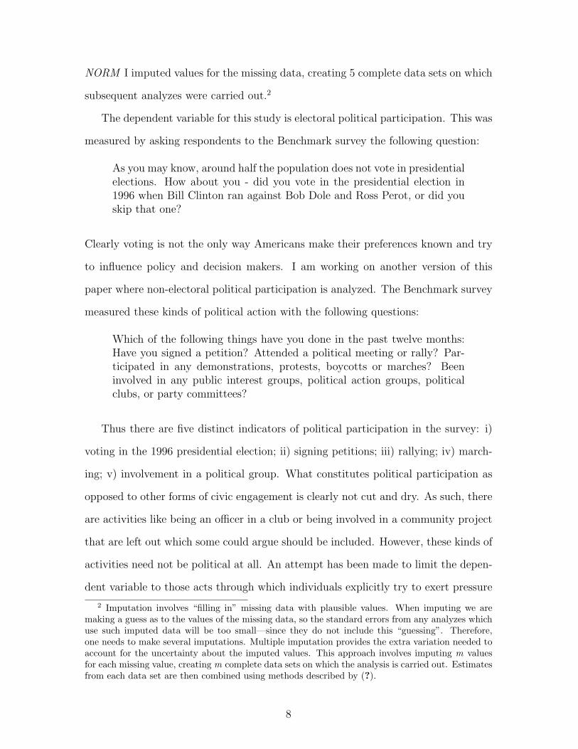
The dependent variable for this study is electoral political participation. This was

measured by asking respondents to the Benchmark survey the following question:

As you may know, around half the population does not vote in presidentialelections. How about you - did you vote in the presidential election in1996 when Bill Clinton ran against Bob Dole and Ross Perot, or did youskip that one?

Clearly voting is not the only way Americans make their preferences known and try

to influence policy and decision makers. I am working on another version of this

paper where non-electoral political participation is analyzed. The Benchmark survey

measured these kinds of political action with the following questions:

Which of the following things have you done in the past twelve months:Have you signed a petition? Attended a political meeting or rally? Par-ticipated in any demonstrations, protests, boycotts or marches? Beeninvolved in any public interest groups, political action groups, politicalclubs, or party committees?

Thus there are five distinct indicators of political participation in the survey: i)

voting in the 1996 presidential election; ii) signing petitions; iii) rallying; iv) march-

ing; v) involvement in a political group. What constitutes political participation as

opposed to other forms of civic engagement is clearly not cut and dry. As such, there

are activities like being an officer in a club or being involved in a community project

that are left out which some could argue should be included. However, these kinds of

activities need not be political at all. An attempt has been made to limit the depen-

dent variable to those acts through which individuals explicitly try to exert pressure

2 Imputation involves “filling in” missing data with plausible values. When imputing we aremaking a guess as to the values of the missing data, so the standard errors from any analyzes whichuse such imputed data will be too small—since they do not include this “guessing”. Therefore,one needs to make several imputations. Multiple imputation provides the extra variation needed toaccount for the uncertainty about the imputed values. This approach involves imputing m valuesfor each missing value, creating m complete data sets on which the analysis is carried out. Estimatesfrom each data set are then combined using methods described by (?).

8

on politicians and decision-makers, try to influence the direction and character of

policy and most obviously, have their say in the election of representatives. The five

types of political participation differ considerably in many ways and the environ-

mental factors I am interested in may indeed have different effects on different types

of political activity; therefore they ought to be modeled separately and compared,

however this paper deals only with voting.

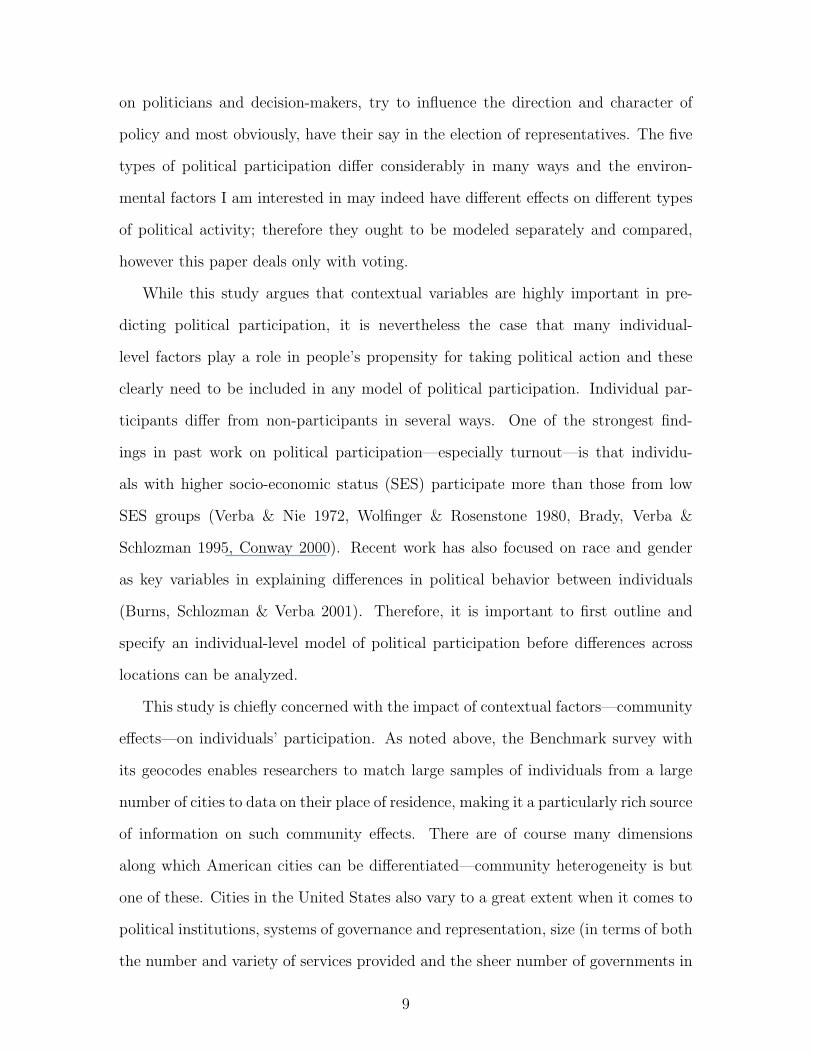
While this study argues that contextual variables are highly important in pre-

dicting political participation, it is nevertheless the case that many individual-

level factors play a role in people’s propensity for taking political action and these

clearly need to be included in any model of political participation. Individual par-

ticipants differ from non-participants in several ways. One of the strongest find-

ings in past work on political participation—especially turnout—is that individu-

als with higher socio-economic status (SES) participate more than those from low

SES groups (Verba & Nie 1972, Wolfinger & Rosenstone 1980, Brady, Verba &

Schlozman 1995, Conway 2000). Recent work has also focused on race and gender

as key variables in explaining differences in political behavior between individuals

(Burns, Schlozman & Verba 2001). Therefore, it is important to first outline and

specify an individual-level model of political participation before differences across

locations can be analyzed.

This study is chiefly concerned with the impact of contextual factors—community

effects—on individuals’ participation. As noted above, the Benchmark survey with

its geocodes enables researchers to match large samples of individuals from a large

number of cities to data on their place of residence, making it a particularly rich source

of information on such community effects. There are of course many dimensions

along which American cities can be differentiated—community heterogeneity is but

one of these. Cities in the United States also vary to a great extent when it comes to

political institutions, systems of governance and representation, size (in terms of both

the number and variety of services provided and the sheer number of governments in

9

a city) as well as how and how much they tax their residents. All of these may affect

political participation but here I specifically concentrate my attention on community

racial heterogeneity. Community heterogeneity is operationalized using a measure

of racial fractionalization for each city in the sample. Following Easterly & Levine

(1997), Alesina, Baqir & Easterly (1999), Alesina & La Ferrera (2000) and others,

racial fragmentation is measured by a Herfindahl-based index constructed from the

US Census defined as follows:

racialfractionalization = 1−∑

k

S2ki

where i represents a given city and k the following races: (i) White; (ii) Black; (iii)

American Indian, Eskimo, Aleutian; (iv) Asian, Pacific Islander; (v) Hispanic. Each

term Ski is the share of race k in the population of city i. The index measures the

probability that two randomly drawn individuals in area i belong to different races

and takes on values between 0 and 1. Higher values of the index represent more racial

heterogeneity.

4. The Multilevel Model

The data I use here are nested, or clustered, in nature. I have data on individuals

from the Benchmark survey and these individuals are clustered in cities, on which I

also have data; as such observations have not been sampled independently of each

other. As Snijders & Bosker (1999) note, dependence can be seen as both a nuisance

and as an interesting phenomenon in itself (1999, p. 6-9). The nuisance is that

dependence of observations needs to be corrected for in some way in order to avoid

drawing incorrect inferences; for example, standard errors will tend to appear smaller

than they actually are if dependence is ignored. However, I am also interested in

analyzing the effects of different city characteristics on individual behavior. That

is, I want to draw inferences on cities as well as individuals, making the clustering

10

of observations of interest. In this paper, the question is whether living in a more

ethnically diverse city affects an individual’s propensity to take political action.

There are a number of empirical strategies for handling data structures of this

kind. Steenbergen & Jones (2002, 220) note that political scientists have tended

to opt for either “dummy variable models” or “interactive models.” Dummy vari-

able models, by assigning fixed effects for each higher-level unit, are able to over-

come the statistical problems associated with dependence of observations in clus-

tered data (Steenbergen & Jones 2002, Rahn & Rudolph 2001). However, one

is often interested in how various aspects of different higher-level units impact on

lower-level units; say how different city characteristics influence individuals’ chances

of participating in politics. A dummy variable model is inadequate in this re-

spect. As Steenbergen & Jones put it, “Dummy variables are only indicators of

subgroup differences; they do not explain why the regression regimes for the sub-

groups are different” (2002, 220). Past contextual analyzes on political behavior

(Huckfeldt 1979, Huckfeldt 1984, Abowitz 1990, Oliver 1999, Oliver 2000, Oliver 2001,

e.g.) have tended to use interactive models where contextual-level independent vari-

ables are included alone or in interactions with individual-level variables in order to

account for contextual heterogeneity (Rahn & Rudolph 2001, 31). These types of

models are not ideal either. As Humphries argues, this approach to modeling mul-

tilevel data “implicitly assumes a deterministic relationship between the contextual

variable and individual-level parameters” (Humphries 2001, 684).

A more appropriate model for clustered data of the kind I have and where one

is interested in explaining different sources of contextual variation is a hierarchical,

or multilevel, model. Such a model provides robust standard errors (Raudenbush

& Bryk 2002) and is better able to capture the unmodeled city effects through the

inclusion of random effects. The multilevel model also makes adjustments to both

within and between parameter estimates for the clustered nature of the data.

11

The hierarchical model begins with a level-1 structural model.3 This model can

be expressed as follows:

yij = β0j + β1jx1ij + εij (1)

Where yij is the individual-level dependent variable for an individual i (=1,. . . ,Nj)

nested in level-2 unit (in this case city) j (=1,. . . ,J ). The term x1ij is the individual-

level variable and εij is the individual-level disturbance term. The model is in all

respects the same as the traditional regression model except for the important dif-

ference that the parameters need not be fixed. That is, they can be allowed to vary

across level-2 units as indicated by the j–subscripts on the β0j and β1j parameters.

This addition is crucial and makes possible the testing of certain hypotheses that

would be difficult or impossible otherwise. At level-2 (the city-level), I model the

individual-level regression parameters as functions of city-level predictors:

β0j = γ00 + γ01z1j + δ0j (2)

andβ1j = γ10 + γ11zj + δ1j. (3)

Equations 2 and 3 together make up the level-2 model where the γ-parameters are

the fixed level-2 parameters and the δ-parameters are disturbance terms. The full

model is achieved by substituting the expressions for β0j and β1j in (2) and (3) into

(1):

yij = γ00 + γ01zj + δ0j + (γ10 + γ11zj + δ1j)xij + εij

= γ00 + γ01zj + γ10xij + γ11zjxij + δ0j + δ1jxij + εij, (4)

where γ00 is the intercept, γ01 denotes the effect of the level-2 (city) variable, γ10

is the effect of the individual-level predictor and γ11 is the effect of the cross-level

interaction between the individual-level and city-level predictors with disturbance

3The development and notation of the multilevel model presented here draws heavily from theexcellent discussions in Raudenbush & Bryk (2002, 16–30) and Steenbergen & Jones (2002, 221–3).

12

terms represented by δ0j, δ1j and εij . In what follows I estimate three models: a

“null” model with no predictors at either individual-level or city-level; a conditional

model with fixed and randomly varying individual-level predictors; and a “full” model

with both individual-level and city-level predictors. Since the dependent variable is

binary (0 did not vote; 1 voted), the models I estimate are hierarchical generalized

linear models (HGLM). Specifically, I estimate Bernoulli models with a logit link

function (Raudenbush & Bryk 2002, 292–296).4

5. Results and Discussion

5.1. The Empty Model

Before estimating the individual-level model, it is appropriate to begin by asking

whether there in fact exists significant variation in the dependent variable across

contextual units—cities—and, if so, what proportion of the total variance is accounted

for by the city-level. To gauge the magnitude of variation between cities in political

participation it is useful to begin by estimating an unconditional or, so-called, empty

model; that is, a model with no predictors at either level. This produces point

estimates for the grand mean as well as providing information on the variance at the

individual and city-levels (Raudenbush & Bryk 2002, 24). The individual-level model

is thus simply

political participationij = β0j (5)

and the city-level model is

β0j = γ00 + δ0j, δ0j ∼ N(0, τ00). (6)

4The models presented here were estimated using the software Hierarchical Linear Models forWindows (version 5.45q) developed by Raudenbush, Bryk, Cheong & Congdon (2003). HLM pro-duces “empirical Bayes estimates of the randomly-varying level-1 [individual-level] parameters, gen-eralized least squares estimates of the level-2 [city-level] coefficients; and maximum likelihood es-timates of the variance-covariance components” (Raudenbush, Bryk, Cheong & Congdon 2002, 4).See Raudenbush & Bryk (2002) for details on estimating the various coefficients.

13

Table 1: ANOVAa

VotingParameter

Fixed EffectsIntercept (γ00) 1.101*

(0.036)Random EffectsCity-Level Variance (τ00) 0.330*

(0.025)

Intraclass correlation (ρ) 0.091-2 × Log Likelihood 38073.001

a* significant at .01%. N=14,153; J=690. Dependentvariable is “voted in 1996”. Estimates are from alogistic model estimated using restricted maximumlikelihood in HLM; robust standard errors inparentheses..

This model is equivalent to a one-way ANOVA with random effects. Here γ00 is the

average log-odds of political participation across US cities (the grand mean), while

τ00 is the variance between cities in city-average log-odds of political participation.

The results from the empty model for voting—presented in table 1—are γ00=1.101

(se=0.036), τ00=0.330 (se=0.025). Thus, for a city with a typical voting rate, that is,

for a city with a random effect δ0j=0, the expected log-odds of voting is 1.101, corre-

sponding to an odds of exp(1.101)=3.007 or a probability of 1/(1+exp(-1.101)=.750.

Table 1 also shows that there exists statistically significant variance at the city-

level for voting, making it clear that political participation is more fruitfully modeled

as a multilevel phenomena, or at the very least, that the multilevel nature of political

participation should not be ignored.5 In order to get an idea of how much of the

5To determine whether variance components are statistically significant, I perform a likelihoodratio test by comparing the deviance statistics of two models (Raudenbush & Bryk 2002, Snijders& Bosker 1999, Steenbergen & Jones 2002). The deviance is -2 × the log likelihood (Raudenbush& Bryk 2002, p. 64). First, I estimate a model with an unrestricted variance component (i.e. arandomly varying intercept), producing a deviance D1. Next, a model where the variance componentis restricted to zero is estimated, giving a deviance D0. Subtracting D0 from D1 generates a statisticwith a χ2 distribution with 1 degree of freedom, allowing me to calculate a p-value for the test.

14

overall variance in political participation is attributable to either the individual-level

or the city-level, it is useful to calculate the intraclass correlation coefficient (ICC).6

The ICC measures the proportion of the variance of the dependent variable that is

between cities. As Steenbergen & Jones note in their analysis of support for the

European Union, it is unsurprising that the individual-level accounts for a great

deal of the variance when data are measured at the individual-level, as they are in

my study (2002, p. 231). Nonetheless, the proportion of the variance in political

participation that is between cities is still considerable—for voting it is 9.1% (that is,

100× .330/(.330 + 3.29)).

5.2. The Individual-level Model

Now I turn to the conditional models. The first conditional model is as follows:

turnoutij = γ00 + Σγ10Raceij + Σγ20INDi + δ0j + Σδ1jRaceij + εij . (7)

Here Race is a set of dummy variables for the race of individual respondents and

IND is a vector of individual-level controls (gender, education, age and age squared).

Note that the effect of Race is allowed to vary randomly across cities. The estimates

from this model are presented in table 2. The results for the individual-level variables

are largely consistent with existing research. Individuals with higher socio-economic

status (SES) tend to be more likely to vote than others (Verba, Schlozman & Brady

1995, Wolfinger & Rosenstone 1980). Here education has a strong positive effect on

voting. The coefficient for the gender variable is also positive; women are more likely

6The intraclass correlation coefficient for linear multilevel models is obtained by the followingformula: ρ = τ00

τ00+σ2 where σ2 is the individual-level variance. However, in nonlinear models, suchas the logit models estimated here, this formula is less useful because the individual-level varianceis heteroscedastic (Raudenbush & Bryk 2002, p. 298). Snijders & Bosker describe an alternativedefinition of the ICC for nonlinear models as follows: ρ = τ00

τ00+π2/3 . This definition treats thedependent variable as an underlying latent continuous variable following a logistic distribution, thevariance (i.e. the individual-level variance in my models) for this distribution is π2/3 (Snijders &Bosker 1999, pp. 223–224).

15

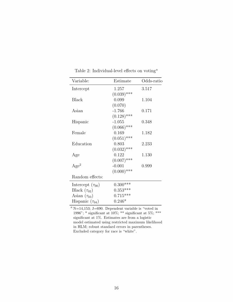
Table 2: Individual-level effects on votinga

Variable: Estimate Odds-ratio

Intercept 1.257 3.517(0.039)***

Black 0.099 1.104(0.070)

Asian -1.766 0.171(0.128)***

Hispanic -1.055 0.348(0.066)***

Female 0.169 1.182(0.051)***

Education 0.803 2.233(0.032)***

Age 0.122 1.130(0.007)***

Age2 -0.001 0.999(0.000)***

Random effects:

Intercept (τ00) 0.300***Black (τ02) 0.353***Asian (τ03) 0.715***Hispanic (τ04) 0.246*

a N=14,153; J=690. Dependent variable is “voted in1996”; * significant at 10%; ** significant at 5%; ***significant at 1%. Estimates are from a logisticmodel estimated using restricted maximum likelihoodin HLM; robust standard errors in parentheses.Excluded category for race is “white”.

16

to vote than men, controlling for other factors in the model. While some researchers

do report that women participate to a lesser extent than men, much recent research

points to the gender gap closing (Conway 2000, 36–7) (Rosenstone & Hansen 1994,

140–1). Age has a positive effect on an individual’s propensity to vote. As people

get older, it is more likely that they turn out. The squared term of Age is also

significant indicating that as people get very old, the positive effect of age on voting

tapers off. Again, the result for age is consistent with previous work (see for example

Blais 2000, Wolfinger & Rosenstone 1980).

As the results in table 2 indicate, Asians and Hispanics are both less likely to

vote than whites. The odds of Asians voting are 17% of those for whites, while

the odds of Hispanics turning out are 35% of those for whites. The coefficient for

blacks is insignificant. Examining the bottom part of the table, it is evident that

the estimates of the variance components of the random portion of the model—the

randomly varying individual-level intercept, β0j, and the randomly varying dummy

variables for race—are significant. That is, after controlling for the individual-level

factors, there still remains a significant amount of variation both in voter turnout

across cities and in the differences in voting between various racial groups across

communities in the United States. The next step is to specify a model that tries to

predict those varying slopes.

5.3. The Racial Diversity Model

Finally, I turn to the full model with both individual-level variables and city-level

predictors. This model contains the same individual-level variables as the previous

model but here I also include the measure of racial heterogeneity, or fractionalization,

described above. While the previous model estimated the slopes for each racial cate-

gory by specifying these individual-level terms as random, in the full model I attempt

to predict those slopes with my measure of racial heterogeneity. That is, I include

cross-level interaction terms between the individual-level race dummies and racial

17

fractionalization. In other words, in (7) I am testing the hypothesis that differences

in voting between groups are not constant across cities; now I want to predict this

variation using the level of racial heterogeneity in each city. The full model is as

follows:

turnoutij = γ00 + γ01RFj + Σγ10INDi + Σγ20Raceij

+ Σγ21RFj ∗Raceij + δ0j + Σδ2jRaceij + εij . (8)

Of interest here are the estimates for the effects of racial fractionalization on the

random slopes of the four race categories included at the individual-level; the cross-

level interactions. The other individual-level estimates remain largely unchanged in

this model. Turning to the variables of interest, it is instructive to first examine

the estimates of the variance components for the random effects. All the variance

components have decreased from the previous model with the addition of the city-

level factor of racial fractionalization, though only modestly, suggesting that the

new variable is doing some work in reducing the unexplained variance across cities.

The variance components remain significant, however, indicating that the city-level

variables in the model do not explain all the variance across communities.7

The cross–level interactions for whites and blacks are both significant and suggest

that racial heterogeneity affects these racial groups differently.The effect of racial

fractionalization on voting for whites is significant and negative. Increasing racial

diversity, according to this model, decreases the likelihood of voting for white people.

The Racial fractionalization×black interaction, on other hand, has a positive sign

7While the tables contain the variance components, it also instructive to consider their co-variances. In the model presented in Table 3, the intercept is positively correlated with Asian,but negatively with black and Hispanic indicating that if white participation is high, the differencebetween white and Asian tends to be relatively small, but that between white and black or Hispanicrelatively large. Note that in such a case black participation may still be relatively (compared toother cities) high, but the difference between blacks and whites is larger than usual. The correla-tions between the race effects tell a similar story. They are positive between black and Hispanicbut negative between Asian and black or Hispanic. This implies that in a city where the differencebetween white and black is large, it also tends to be large between white and Hispanic but relativelysmall between white and Asian.

18

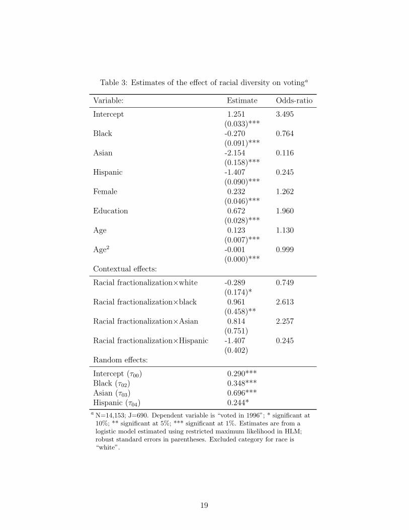
Table 3: Estimates of the effect of racial diversity on votinga

Variable: Estimate Odds-ratio

Intercept 1.251 3.495(0.033)***

Black -0.270 0.764(0.091)***

Asian -2.154 0.116(0.158)***

Hispanic -1.407 0.245(0.090)***

Female 0.232 1.262(0.046)***

Education 0.672 1.960(0.028)***

Age 0.123 1.130(0.007)***

Age2 -0.001 0.999(0.000)***

Contextual effects:

Racial fractionalization×white -0.289 0.749(0.174)*

Racial fractionalization×black 0.961 2.613(0.458)**

Racial fractionalization×Asian 0.814 2.257(0.751)

Racial fractionalization×Hispanic -1.407 0.245(0.402)

Random effects:

Intercept (τ00) 0.290***Black (τ02) 0.348***Asian (τ03) 0.696***Hispanic (τ04) 0.244*

a N=14,153; J=690. Dependent variable is “voted in 1996”; * significant at10%; ** significant at 5%; *** significant at 1%. Estimates are from alogistic model estimated using restricted maximum likelihood in HLM;robust standard errors in parentheses. Excluded category for race is“white”.

19

0.65

0.7

0.75

0.8

0.85

0.9

0.04

0.07

0.09

0.12

0.14

0.17

0.19

0.22

0.24

0.27

0.29

0.32

0.34

0.37

0.39

0.42

0.44

0.47

0.49

0.52

0.54

0.57

0.59

0.62

0.64

0.67

0.69

0.72

0.74

Racial fractionalization

Pr(vote)

whites

blacks

Figure 1: The Effect of racial diversity on the probability of voting among racialgroups

and is statistically significant. That is, racial diversity positively predicts voting

among blacks—as diversity increases, so do the odds of voting for a black person.

While the estimates from the main effects for Asian and Hispanic are significant,

the interaction terms for these with racial fractionalization fail to meet conventional

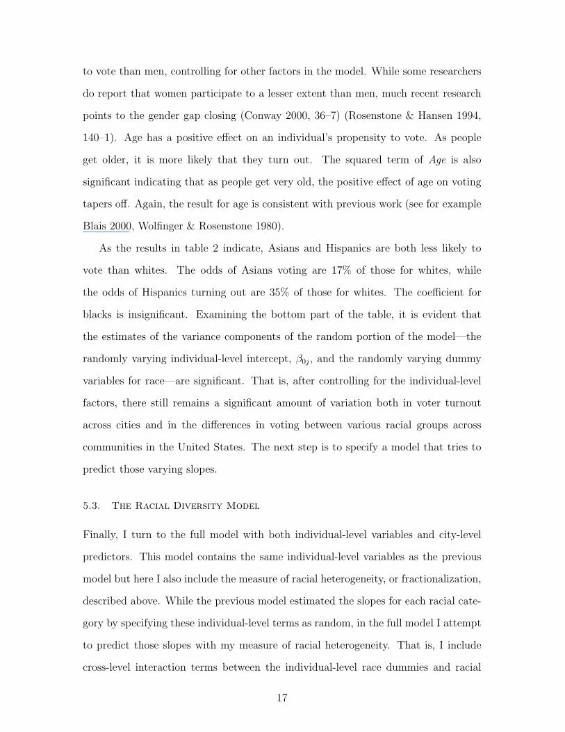
levels of statistical significance. Figure 1 illustrates graphically the effect of letting

racial diversity predict the probability of voting for blacks and whites.8 If you are

black, your odds of voting increase with increasing levels of racial diversity. The

effect on blacks of racial diversity strong enough to make blacks more likely to turn

out than whites as one moves up the racial fractionalization scale. A black person

moving from a very homogenous community with a score at the bottom of the racial

fractionalization index to a city at the high end of the diversity scale would represent a

jump in the probability of voting from .737 to .872, holding all other factors constant.

8The predicted effects are obtained by holding all independent variables at their mean andallowing the racial fractionalization index to vary over its full range found in the data.

20

For a white person, the same move entails a drop in the probability of voting from

.775 to .738. As figure 1 demonstrates, the impact of racial diversity is considerably

stronger for blacks than for whites.

6. Conclusion

Much previous research on the effects of racial diversity on civic engagement, social

capital and political participation maintains that increased levels of diversity will

serve to decrease political activity. In this paper I have argued the opposite; that

people living in more diverse communities will be more likely to participate in politics.

Inter–racial attitudes tend to be more conflictual in more diverse places where race

and racial identity are more salient. That is, individuals see race relations in terms of

a zero–sum competition over resources and their distribution. More racially diverse

places should as a result be characterized by more conflict, more issues and therefore

more political participation. I also hypothesized that the differences in voting between

racial groups will vary between cities and this variability can, in part, be explained

by racial heterogeneity.

The analysis shows that the effect of racial diversity on whites’ likelihood of voting

is negative. That is, living in a more racially diverse place tends to suppress turnout

among whites. However, when racial fractionalization was used to predict the slope

of each individual racial group, this relationship reversed for non-Hispanic blacks.

For black people, living in a more diverse community raises the probability of voting.

The results from this analysis indicate that the relationship between racial diversity

and political participation is not straightforward and that it impacts differently on

people from distinct racial groups. Specifying a model where the individual effect of

race is allowed to vary randomly across cities uncovers different results which remain

“hidden” in models where race effects are fixed. In this model, racial heterogeneity

becomes a strong predictor of participation for members of minority groups while

21

the participation of whites remains negatively related to diversity. One needs to

explicitly model the effect of diversity on separate racial groups in order to get at

these associations.

22

Data Appendix

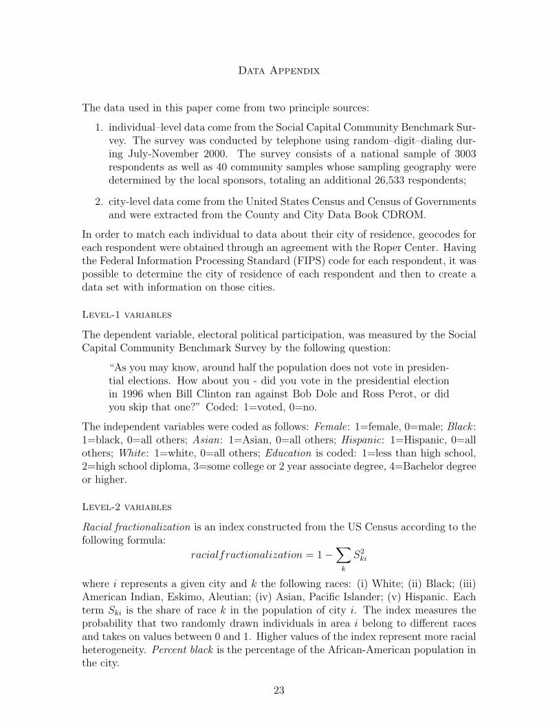
The data used in this paper come from two principle sources:

1. individual–level data come from the Social Capital Community Benchmark Sur-vey. The survey was conducted by telephone using random–digit–dialing dur-ing July-November 2000. The survey consists of a national sample of 3003respondents as well as 40 community samples whose sampling geography weredetermined by the local sponsors, totaling an additional 26,533 respondents;

2. city-level data come from the United States Census and Census of Governmentsand were extracted from the County and City Data Book CDROM.

In order to match each individual to data about their city of residence, geocodes foreach respondent were obtained through an agreement with the Roper Center. Havingthe Federal Information Processing Standard (FIPS) code for each respondent, it waspossible to determine the city of residence of each respondent and then to create adata set with information on those cities.

Level-1 variables

The dependent variable, electoral political participation, was measured by the SocialCapital Community Benchmark Survey by the following question:

“As you may know, around half the population does not vote in presiden-tial elections. How about you - did you vote in the presidential electionin 1996 when Bill Clinton ran against Bob Dole and Ross Perot, or didyou skip that one?” Coded: 1=voted, 0=no.

The independent variables were coded as follows: Female: 1=female, 0=male; Black :1=black, 0=all others; Asian: 1=Asian, 0=all others; Hispanic: 1=Hispanic, 0=allothers; White: 1=white, 0=all others; Education is coded: 1=less than high school,2=high school diploma, 3=some college or 2 year associate degree, 4=Bachelor degreeor higher.

Level-2 variables

Racial fractionalization is an index constructed from the US Census according to thefollowing formula:

racialfractionalization = 1−∑

k

S2ki

where i represents a given city and k the following races: (i) White; (ii) Black; (iii)American Indian, Eskimo, Aleutian; (iv) Asian, Pacific Islander; (v) Hispanic. Eachterm Ski is the share of race k in the population of city i. The index measures theprobability that two randomly drawn individuals in area i belong to different racesand takes on values between 0 and 1. Higher values of the index represent more racialheterogeneity. Percent black is the percentage of the African-American population inthe city.

23

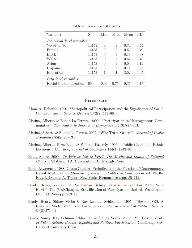
Table 4: Descriptive statistics

Variables N Min. Max. Mean S.D.

Individual–level variablesVoted in ’96 14153 0 1 0.70 0.45Female 14153 0 1 0.59 0.49Black 14153 0 1 0.18 0.38White 14153 0 1 0.61 0.48Asian 14153 0 1 0.04 0.19Hispanic 14153 0 1 0.12 0.33Education 14153 1 4 3.02 0.95

City–level variablesRacial fractionalization 690 0.04 0.75 0.35 0.17

References

Abowitz, Deborah. 1990. “Sociopolitical Participation and the Significance of SocialContext.” Social Science Quarterly 72(2):543–66.

Alesina, Alberto & Eliana La Ferrera. 2000. “Participation in Heterogeneous Com-munities.” The Quarterly Journal of Economics 115(3):847–904.

Alesina, Alberto & Eliana La Ferrera. 2002. “Who Trusts Others?” Journal of PublicEconomics 85(2):207–34.

Alesina, Alberto, Reza Baqir & William Easterly. 1999. “Public Goods and EthnicDivisions.” Quartlery Journal of Economics 114(4):1243–84.

Blais, Andre. 2000. To Vote or Not to Vote? The Merits and Limits of RationalChoice. Pittsburgh PA: University of Pittsburgh Press.

Bobo, Lawerence. 1988. Group Conflict, Prejudice, and the Paradox of ContemporaryRacial Attitudes. In Eliminating Racism: Profiles in Controversy, ed. PhyllisKatz & Dalmas A. Taylor. New York: Plenum Press pp. 85–114.

Brady, Henry, Kay Lehman Schlozman, Sidney Verba & Laurel Elms. 2002. WhoBowls? The (Un)Changing Stratification of Participation. 2nd ed. WashingtonDC: CQ Press pp. 219–42.

Brady, Henry, Sidney Verba & Kay Lehman Schlozman. 1995. “Beyond SES: AResource Model of Political Participation.” British Journal of Political Science89(2):271–94.

Burns, Nancy, Kay Lehman Schlozman & Sidney Verba. 2001. The Private Rootsof Public Action: Gender, Equality and Political Participation. Cambridge MA:Harvard University Press.

24

Campbell, David E. 2002. Getting Along vs. Getting Ahead: Contextual Influenceson Motivations for Collective Action, PhD dissertation, Harvard University.

Conway, Margaret. 2000. Political Participation in the United States. 3rd ed. Wash-ington DC: CQ Press.

Costa, Dora L. & Matthew E. Kahn. 2003. “Civic Engagement and CommunityHeterogeneity: An Economist’s Perspective.” Perspectives on Politics 1(1):103–11.

Easterly, William & Ross Levine. 1997. “Africa’s Growth Tragedy: Policies andEthnic Divisions.” 111(4):1203–50.

Fuchs, Ester R., Lorraine C. Minnite & Robert Y. Shapiro. 2000. Political Capitaland Political Participation. Paper presented to the 2000 Annual Meeting of theAmerican Political Science Association, Washington DC.

Garbaye, Romain. 2002. “Ethnic and Minority Participation in British and FrenchCities: A Historical Institutionalist Perspective.” International Journal of Urbanand Regional Research 26(3):555–70.

Glaser, James M. 1994. “Back to the Black Belt: Racial Environment and WhiteRacial Attitudes in the South.” Journal of Politics 56(1):21–41.

Glaser, James M. 2003. “Social Context and Inter-Group Political Attitudes: Experi-ments in Group Conflict Theory.” British Journal of Political Science 33(4):607–20.

Huckfeldt, Robert. 1979. “Political Participation and the Neighborhood Social Con-text.” American Journal of Political Science 23(3):579–92.

Huckfeldt, Robert. 1984. Politics in Context: Assimilation and Conflict in UrbanNeighborhoods. New York: Agathon Press.

Humphries, Stan. 2001. “Who’s Afraid of the Big, Bad Firm.” American Journal ofPolitical Science 45(3):678–99.

King, Gary, James Honacher, Anne Joseph & Kenneth Scheve. 2001. “AnalyzingIncomplete Political Science Data: An Alternative Algorithm for Multiple Im-putation.” American Political Science Review 95(1):49–69.

Mutz, Diana C. 2002. “The Consequences of Cross-Cutting Networks for PoliticalParticipation.” American Journal of Political Science 46(4):838–55.

Oliver, J. Eric. 1999. “The Effects of Metropolitan Economic Segregation on LocalCivic Participation.” American Journal of Political Science 43(1):186–212.

Oliver, J. Eric. 2000. “City Size and Civic Involvement in Metropolitan America.”American Political Science Review 94(2):361–73.

25

Oliver, J. Eric. 2001. Democracy in Suburbia. Princeton NJ: Princeton UniversityPress.

Rahn, Wendy M. & Thomas J. Rudolph. 2001. “Spatial Variation in Trust in LocalGovernment: The Roles of Institutions, Culture and Community Heterogeneity.”Paper presented to the Trust in Government Conference, Center for the Studyof Democratic Politics, Princeton University 30 November-1 December 2001.

Raudenbush, Stephen W. & Anthony S. Bryk. 2002. Hierarchical Linear Models:Applications and Data Analysis Methods. 2nd ed. Thousand Oaks CA: Sage.

Raudenbush, Stephen W., Anthony S. Bryk, Yuk Fai Cheong & Richard Congdon.2002. HLM 5: Hierarchical Linear and Nonlinear Modeling. Lincolnwood IL:Scientific Software International.

Raudenbush, Stephen W., Anthony S. Bryk, Yuk Fai Cheong & Richard Congdon.2003. HLM 5: Hierarchical Linear and Nonlinear Modeling, version 5.45q. Lin-colnwood IL: Scientific Software International.

Rosenstone, Steven & John Mark Hansen. 1994. Mobilization, Participation andDemocracy in America. New York: MacMillan.

Saguaro Seminar. 2001. “Social Capital Community Benchmark Survey: ExecutiveSummary.” Cambridge, MA: John F. Kennedy School of Government, HarvardUniversity.

Schafer, Joseph L. 1999. NORM: Multiple Imputation of Incomplete Multivariate DataUnder a Normal Model, Version 2. Software for Windows 95/98/NT. UniversityPark PA: Penn State University.

Snijders, Tom & Roel Bosker. 1999. Multilevel Analysis: An Introduction to Basicand Advanced Multilevel Modeling. London: Sage.

Steenbergen, Marco R. & Bradford S. Jones. 2002. “Modeling Multilevel Data Struc-tures.” American Journal of Political Science 46(1):218–37.

Stoker, Laura & Jake Bowers. 2002. “Designing Milti-Level Studies: Sampling Votersand Electoral Districts.” Electoral Studies 21(2):235–67.

US Department of Commerce (Census Bureau). 1994. City and County Data Book.Washington DC: US Department of Commerce.

Verba, Sidney, Kay Lehman Schlozman & Henry E. Brady. 1995. Voice and Equality:Civic Volunteerism in American Politics. Cambridge MA: Harvard UniversityPress.

Verba, Sidney & Norman H. Nie. 1972. Participation in America. San Francisco:Harper & Row.

Wolfinger, Raymond E. & Steven J. Rosenstone. 1980. Who Votes? New Haven CT:Yale University Press.

26