Combustion Chemistry and Physics of Ethanol Blends to ...

Combustion Chemistry and Physics of Ethanol Blends to Inform Biofuel Policy

by

Cesar L. Barraza Botet

A dissertation submitted in partial fulfillment

of the requirements for the degree of

Doctor of Philosophy

(Mechanical Engineering)

in the University of Michigan

2018

Doctoral Committee:

Professor Margaret S. Wooldridge, Chair

Professor André L. Boehman

Professor Hugh Scott Fogler

Associate Professor Venkatramanan Raman

Cesar L. Barraza Botet

[email protected]

ORCID iD: 0000-0002-0094-1172

© Cesar L. Barraza Botet 2018

ii

Dedication

To my wife, Naty,

and my daughter, Abbie,

for their love, patience and support

iii

Acknowledgements

Foremost, I would like to express my sincere gratitude to my advisor, Prof. Margaret S.

Wooldridge, for her continuous support during my Ph.D. studies. Her role in this journey has been

fundamental as she gave me the opportunity to join her group in the first place, provided me

guidance for my research, and allowed me to pursue my own ideas both inside and outside the

laboratory. I could not have had a better advisor and mentor than Prof. Wooldridge during my

Ph.D., as she has greatly contributed to the scientist and professional I am today.

Additionally, I would like to thank Prof. André L. Boehman, Prof. Hugh Scott Fogler and

Prof. Venkatramanan Raman for serving on my dissertation committee. Their insightful comments

and constructive recommendations were highly appreciated in shaping this dissertation.

My sincere gratitude also goes to Dr. Bradley Zigler and the Transportation & Hydrogen

Systems Center team at the National Renewable Energy Laboratory for hosting me in Golden,

Colorado and their collaboration in the data collection for this dissertation research.

I am also thankful to Prof. Joy Rhode and Prof. James Duderstadt from the Science,

Technology and Public Policy graduate certificate program at the Ford School of Public Policy.

Their constructive feedback to my policy memos for their classes greatly contributed to the policy

discussion in this dissertation.

iv

I would like to thank Dr. Scott Wagnon for his friendship and guidance in the laboratory.

Thank you also to my labmates and friends in Ann Arbor—Ripudaman Singh, Mario Medina,

Rachel Schwind, Luis Gutierrez, Dimitris Assanis, Ivan Tibavinsky, Zida Li, and many others.

I am very grateful to all my friends in Colombia for their long-distance support, including

my dear friends at the Universidad del Atlántico—Havid Escorcia, Argemiro Palencia, Jose Lopez,

Alvaro Molina, Walberto Doria and Mario Crespo. I would also like to thank my master’s advisor

at the Universidad del Norte, Prof. Antonio Bula, for encouraging me to pursue my Ph.D. in the

U.S.

I would like to acknowledge the generous financial support of the U.S. Department of

State’s Fulbright Program, the Colombian Department of Science, Technology and Innovation—

Colciencias, and the U.S. Department of Energy—Office of Basic Energy Science.

I specially thank my mom, Enelsa, my sisters, Anyily and Farleys, and my niece and

nephew, María Angélica and Thomas E., for their unconditional support during all these years. To

my dad, Luis E., and my uncle, Alfonso, who are dearly missed as I profoundly value the years we

shared!

Most importantly, I thank my wife, Nataly, and my daughter, Abigail, without whom I

would not have achieved this goal. Your love, understanding and support constantly motivate me

to pursue my dreams even when I feel insecure or overwhelmed. You two are the reason why I

am here today and the driving force that—I am sure—will take me where I have never imagined.

Thank you for believing in me! I love you two, immensely!

v

Table of Contents

Dedication ii

Acknowledgements iii

Lists of Figures vii

Lists of Tables xi

Abstract xiii

Chapter 1 Introduction 1

1.1 Ethanol and the U.S. Biofuel Policy 3

Life Cycle Analysis 4

Food versus Fuel Controversy 6

Development of Cellulosic Biofuels 7

E10 Blend Wall 9

An Alternative Biofuel Policy 11

1.2 U.S. Fuel Efficiency and GHG Emissions Standards 12

1.3 U.S. Tier 3 Motor Vehicle Emission and Fuel Standards 14

1.4 Fundamental Combustion Science for Informed Policymaking 15

Chapter 2 Experimental Setup 22

2.1 Rapid Compression Facility (RCF) 22

Ignition and High-Speed Imaging 23

Fast-gas sampling 25

Gas Chromatography Analysis 26

Speciation Uncertainty Analysis 27

2.2 Ignition Quality Tester (IQT) 30

Chapter 3 Ethanol Combustion Chemistry 34

3.1 Introduction 34

3.2 Objective 35

3.3 Experimental Methods 35

vi

3.4 Results and Discussion 35

Ignition Delay Times 35

Intermediate Species 44

3.5 Conclusions 50

3.6 Supporting Information 50

Chapter 4 Combustion Chemistry of Ethanol/Iso-Octane Blends 54

4.1 Introduction 54

4.2 Objective 56



Ignition Delay Times 57

Intermediate species 67

4.5 Conclusions 81


Chapter 5 Physico-Chemical Interactions of Ethanol and Iso-Octane 86

5.1 Introduction 86

5.2 Objective 88



Liquid Fuel (Total) and Chemical Ignition Delays 90

Physical Contributions to Ignition Delay 97

5.5 Conclusions 107


Chapter 6 Concluding Remarks 114

6.1 Technical Conclusions 114

6.2 Recommendations for Future Work 115

6.3 Policy Implications 116

Appendix A Participatory Strategy for U.S. Biofuel Policy 120

Bibliography 124

vii

Lists of Figures

Figure 1.1. 1980-2016 history of U.S. domestic gasoline and ethanol consumption in the

transportation sector. Source: U.S. Energy Information Administration (www.eia.gov). ........... 11

Figure 1.2. Schematic of material and energy (solid arrows), and information (dashed arrows)

flows on the interactions between energy/environmental policies and fundamental combustion

phenomena through regulation and technology development. Source: This figure was created

using images available online of Ford Motor Company commercial products. ........................... 17

Figure 2.1. Schematic of the UM RCF as configured for high speed imaging. Used with

permission from Wagnon [43]. ..................................................................................................... 23

Figure 2.2. Schematic of the UM RCF as configured for fast-gas sampling. Used with permission

from Wagnon [43]......................................................................................................................... 26

Figure 2.3. Quantification of concentrations, correction factors and uncertainties for speciation

experiments: (a) calibration curve of ethanol from GC-2a/FID (see Table 2.1), (b) air dilution

factor and (c) dead volume factor. ................................................................................................ 28

Figure 2.4. Schematic of the IQT combustion chamber. Taken from Bogin et al. [53]. Copyright

2016, Elsevier. .............................................................................................................................. 31

Figure 3.1. Typical pressure (black lines) and pressure derivative (red lines) time histories in the

test section for an ignition experiment using high-speed imaging. The bottom panels show the

sequence of still images from the high-speed camera at the time near ignition. Conditions for the

experiment were: Peff = 9.91 atm, Teff = 937 K, ϕ = 0.99, inert/O2 ratio = 8.29, C2H5OH = 3.43%,

O2 = 10.4%, N2 = 86.17%, Ar = 0.01%, τign = 13.15 ms. ............................................................. 37

Figure 3.2. Experimental and modeling results for ethanol ignition delay time. Results of the

ignition measurements in the UM RCF were for near stoichiometric conditions ( = 0.97) and

average dilution levels of inert/O2 ratios of 8.2 for imaging (main figure) and 7.5 for speciation

(inset) experiments. Model predictions (solid lines) are based on the reaction mechanism by Burke

et al. [51]. ...................................................................................................................................... 38

Figure 3.3. Summary of results of ignition delay time for stoichiometric mixtures of ethanol

studied in this work and available in the literature. All data are presented as reported in the

literature. No scaling was used to create this figure. ................................................................... 39

Figure 3.4. Summary of the normalized ignition delay time data for stoichiometric mixtures of

ethanol studied in this work and available in the literature. All data were normalized to P = 10 atm

and Inert/O2 = 3.76 (air level of dilution) using Equation 3.1. Model predictions (red dashed line)

based on the reaction mechanism by Burke et al. [51] and Equation 3.1 (black solid line) are

included. ........................................................................................................................................ 40

viii

Figure 3.5. Results of CHEMKIN sensitivity analysis for OH based on the reaction mechanism by

Burke et al. [51] at simulation conditions of P = 10.1 atm, T = 930 K, ϕ = 1 and (inert/O2) = 7.5.

The top 10 reactions are included in the figure. ............................................................................ 42

Figure 3.6. Comparison of the experimental data for stoichiometric ethanol experiments at 10.1

atm and inert/O2 ratio of 8.4 (main figure) and 7.5 (inset) compared with model predictions using

the reaction mechanism of Burke et al. [51], and the effects of modifying the pre-exponential

factors of R17, R19 and R369....................................................................................................... 43

Figure 3.7. Typical pressure (solid black lines) and pressure derivative (dashed black lines) time

histories in the test section for an ignition experiment using fast gas sampling. Pressure time

histories for sampling volumes 1 (solid blue lines) and 2 (solid red lines) and corresponding valve

triggering signals (colored dashed lines) are included. Conditions for the experiment were: Peff =

10.6 atm, Teff = 936 K, ϕ = 0.99, inert/O2 ratio = 7.47, C2H5OH = 3.74%, O2 = 11.36%, N2 =

79.6%, Ar = 5.3%, τign = 11.15 ms. .............................................................................................. 44

Figure 3.8. Chromatograms corresponding to Sample 2 of Figure 3.7 from (a) GC-1/FID, (b) GC-

2a/FID and (c) GC-2b/TCD. See Table 2.1 for specific technical information on each GC

configuration. ................................................................................................................................ 45

Figure 3.9. Measured and predicted (using the reaction mechanism by Burke et al. [51]) time

histories of stable intermediate species produced during ethanol autoignition: a) ethanal and b)

ethene. Average conditions for the sampling experiments were used for the model predictions

which were P = 10.1 atm, T = 930 K, ϕ = 0.99, C2H5OH = 3.75%, O2 = 11.33%, and inert/O2 =

7.5. The effects of modifying the pre-exponential factors within the respective uncertainty limits

of reactions R17, R19 and R369 are included. ............................................................................. 46

Figure 3.10. Measured and predicted (using the reaction mechanism by Burke et al. [51]) time

histories of stable intermediate species produced during ethanol autoignition: a) ethanol, b)

methane, c) ethane, d) ethyne, e) carbon monoxide, f) carbon dioxide, g) propane, h) propene, i)

1-butene, j) 1,3-butadiene. Average conditions for the sampling experiments were used for the

model predictions which were P = 10.1 atm, T = 930 K, ϕ = 0.99, C2H5OH = 3.75% O2 = 11.33%,

and inert/O2 = 7.5. The effects of modifying the pre-exponential factor within the uncertainty

limits of reaction R369 are included. ............................................................................................ 47

Figure 3.11. Schematic representation of the reaction pathway analysis for ethanol oxidation using

the reaction mechanism by Burke et al. [51]. for conditions of P = 10.1 atm and T = 930 K,

C2H5OH = 3.75%, O2 = 11.33%, N2 = 79.6% and Ar = 5.31% for time of t/ign = 0.9. ............... 49

Figure 4.1. Typical pressure (solid lines) and pressure derivative (dashed lines) time histories in

the test section for ignition experiments of E0 (red), E50 (blue) and E100 (green) using high-speed

imaging. ........................................................................................................................................ 58

Figure 4.2. Selected frames from the high-speed imaging at the time near ignition for pressure-

time histories in Figure 4.1. The frames corresponding to the maximum intensities are included.

....................................................................................................................................................... 60

Figure 4.3. Experimental results of ignition delay times for stoichiometric (ϕ = 0.99 ± 0.01)

mixtures of E0, E5, E11, E26, E50, E67, and E100 fuels. The E100 data include results from

Chapter 3. Two dilution levels were considered for the imaging (main figure, inert/O2 = 8.74 ±

0.33) and for the speciation (inset, inert/O2 = 7.48 ± 0.02) experiments. Model predictions are

ix

based on the reaction mechanism by Mehl et al. [84] (solid lines). Regression fits to the

experimental data are provided as dotted lines. ............................................................................ 61

Figure 4.4. Comparison of measured and simulated pressure and experimental pressure derivative

traces for E0 (dashed lines) and E100 (solid lines) at state conditions of ~10 atm, ~930 K and

inert/O2 = 7.5. Imaging and speciation experiments, and constant-volume, compression/heat

transfer and pyrolysis simulations are included. ........................................................................... 62

Figure 4.5. Summary of scaled ignition delay times (open symbols) of the fuel data presented in

Figure 4.3 for stoichiometric (ϕ = 0.99) mixtures at P = 10 atm and inert/O2 = 8.74. The regression

coefficient of CB for the E0–E100 blends was used to scale the ignition data to E50 blend level.

E50 data were not scaled and are presented as filled symbols. .................................................... 63

Figure 4.6. Effect of ethanol addition on ignition delay time at ~910 K and ~1000 K for P = 10

atm and molar ratio of inert/O2 = 8.74. ......................................................................................... 64

Figure 4.7. Model predictions using the Mehl et al. mechanism [84] for ignition delay times of

stoichiometric iso-octane and ethanol mixtures at 10 and 100 atm. ............................................. 65

Figure 4.8. Results of CHEMKIN sensitivity analysis for OH at P = 10 atm, T = 930 K, ϕ = 1 and

(inert/O2) = 7.5. Simulations based on the reaction mechanism by Mehl et al. [84] for E0, E50 and

E100. Reaction numbers of the top 5 reactions are according to the mechanism numeration. ... 66

Figure 4.9. Typical pressure and pressure derivative time histories in the test section for an E50

ignition experiment using fast gas sampling. Pressure time histories for the two sampling volumes

are shown along with the corresponding triggering signals. Conditions for the experiment were

Peff = 9.8 atm, Teff = 934 K, ϕ = 0.99, inert/O2 = 7.43, i-C8H18 = 0.54%, C2H5OH = 1.55%, O2 =

11.62%, N2 = 78.7%, Ar = 7.6%, and τign = 18.16 ms. ................................................................. 68

Figure 4.10. Chromatograms corresponding to Sample 2 of Figure 4.7 from (a) GC-1/FID (blue)

and GC-2a/FID (red), and (b) GC-3/MS. Features of species which were quantified in the study

are identified in the chromatograms. ............................................................................................ 69

Figure 4.11. Measured (symbols) and predicted (lines) time histories of stable intermediate species

produced during autoignition of E0, E50 and E100: a) iso-octane, b) iso-butene, c) propene, d)

ethane, e) carbon monoxide, f) ethanol, g) ethanal, h) ethene, i) methane, and j) carbon dioxide.

The effects of removing the ethanol (red dashed lines) and iso-octane (green dashed line) from the

E50 mixture in the simulation are included. ................................................................................. 71


produced during autoignition of E0, E50 and E100: a) ethyne b) acetone, c) methacrolein, d) iso-

pentene. ......................................................................................................................................... 72

Figure 4.13. Schematic representations of the reaction pathways for E0, E50 and E100 using the

reaction mechanism by Mehl et al. [84] for conditions of ϕ = 1.0, P = 10 atm and T = 930 K and

inert/O2 = 7.5 for the time of t/τign = 0.9. Percentage of fuel consumed at these conditions: E0:

61%; E50: 53% i-C8H18, 35% C2H5OH; E100: 24%. ................................................................... 77

Figure 4.14. Predicted time histories of important radical species produced during ignition delay

time of E0, E50 and E100, i.e., hydroxyl, hydroperoxyl, methyl and hydrogen radicals. ............ 78

Figure 4.15. Predicted time histories of important radical species near autoignition of E0, E50 and

E100: a) hydroperoxyl radical b) hydroxyl radical. ...................................................................... 78

x

Figure 4.16. Normalized stable intermediate species produced during autoignition of E0, E50 and

E100: a) iso-octane, b) iso-butene, c) propene, d) ethane, e) ethanol, f) ethanal, g) ethene, h)

methane. ........................................................................................................................................ 80

Figure 5.1. Typical pressure (solid lines) and pressure derivative (dashed lines) time histories in

the IQT for liquid fuel ignition experiments of E0 (red), E50 (blue) and E100 (green). ............. 91

Figure 5.2. Experimental results of liquid fuel ignition delays for stoichiometric mixtures of E0,

E25, E50, E75, and E100 fuels. Regression fits to the experimental data are provided as dash-

dotted lines. ................................................................................................................................... 93

Figure 5.3. Comparison of liquid fuel ignition delays from IQT experiments and ignition delay

times from the RCF data in Chapter 3 and Chapter 4 for stoichiometric mixtures of E0, E50 and

E100 and inert/O2 = 9.0. Model predictions are based on the reaction mechanism by Mehl et al.

[84] (solid lines). Regressions for both sets of data are provided. ............................................... 95

Figure 5.4. Summary of scaled liquid fuel ignition delays (open symbols) and chemical ignition

delay times (filled symbols) of the data presented in Figure 5.3 for stoichiometric blends at P = 10

atm and inert/O2 = 9.0. The corresponding regression coefficient of CB for each ignition delay

correlation was used to scale the E0 and E100 ignition data to E50 blend level. Model predictions

using the reaction mechanism by Mehl et al. [84] (solid lines) are provided. .............................. 96

Figure 5.5. Effects of ethanol addition on total and chemical ignition delays at ~913 K for P = 10

atm and molar ratio of inert/O2 = 9.0. ........................................................................................... 97

Figure 5.6. Comparison of typical pressure (solid lines) and pressure derivative (dot-dashed lines)

time histories in the IQT for liquid fuel ignition experiments (blue) with RCF chemical ignition

delay experiments (red)................................................................................................................. 98

Figure 5.7. Estimation method for apparent charge cooling and heat release for the IQT data

presented in Figure 5.6. ................................................................................................................. 99

Figure 5.8. Overall contribution of spray and mixing physics to total ignition delay as a function

of the carbon content in the blend (blend level) and temperature............................................... 100

Figure 5.9. Contribution to total ignition delay from spray physics (injection, breakup and

evaporation), and from turbulent mixing as function of the carbon content in the blend (blend level)

and temperature. .......................................................................................................................... 101

Figure 5.10. Summary of average chemical and physical time scales at different blend levels and

initial charge temperatures. ......................................................................................................... 103

Figure 5.11. Effects of spray Reynolds number, ethanol addition and state temperature on

convective Damköhler number for the conditions of the IQT and RCF studies. ....................... 105

Figure 5.12. Effects of apparent charge cooling, ethanol addition and charge temperature on the

turbulent mixing Damköhler number for the conditions of the IQT and RCF studies. .............. 106

Figure 6.1. Schematic of material and energy (solid arrows), and information (dashed arrows)

flows on the interactions between the technical conclusions of this dissertation and the proposed

policy structure through regulation and technology development. Text in red represents the areas

that can be informed by the results of this dissertation. Source: This figure was created using

images available online of Ford Motor Company commercial products. ................................... 117

xi

Lists of Tables

Table 1.1. 2016 worldwide production of ethanol by country/region. Source: RFA analysis of

public and private data sources [4]. ................................................................................................ 2

Table 2.1. Gas chromatograph systems, specification and operational settings. ......................... 27

Table 3.1. Summary of experimental conditions and results for ethanol autoignition. All mixture

data are provided on a mole fraction basis. Values with an asterisk (*) correspond to speciation

experiments. .................................................................................................................................. 51

Table 3.2. Summary of results for speciation experiments of stoichiometric ethanol mixtures with

an asterisk (*) in Table 3.1. Data are arranged in ascending order for t/τign. ................................ 53

Table 4.1. Best-fit regression coefficients for τign correlations of E0, E50, E100, and all fuel data

(E0-E100) fort ϕ = 0.99, P = 9.98 atm and inert/O2 = 8.74. The regression correlations have the

form of τign = A (CB)d exp(Ea/RT)................................................................................................. 61

Table 4.2. Initial mixture composition of simulations presented in Figure 4.11. ........................ 74

Table 4.3. Experimental measurements and model predictions of the total carbon represented by

the species in Figure 4.11.............................................................................................................. 74

Table 4.4. Summary of experimental conditions and results for iso-octane autoignition. All

mixture data are provided on a mole fraction basis. Values with an asterisk (*) correspond to

speciation experiments. ................................................................................................................. 82

Table 4.5. Summary of experimental conditions and results for E50 autoignition. All mixture data

are provided on a mole fraction basis. Values with an asterisk (*) correspond to speciation

experiments. .................................................................................................................................. 83

Table 4.6. Summary of experimental conditions and results for iso-octane/ethanol blend

autoignition. All mixture data are provided on a mole fraction basis. ......................................... 84

Table 4.7. Summary of results for speciation experiments of iso-octane and E50 with an asterisk

(*) in Table 4.4 and Table 4.5. Data are arranged in ascending order of t/τign for each blend. ... 85

Table 5.1. Liquid fuel properties of gasoline, iso-octane and ethanol [2,125]. ........................... 90

Table 5.2. Summary of experimental conditions and results for E0 liquid fuel autoignition in the

IQT. All mixture data are provided on a mole fraction basis. ................................................... 109





xii



Table 5.6. Summary of experimental conditions and results for E100 liquid fuel autoignition in

the IQT. All mixture data are provided on a mole fraction basis. ............................................. 113

Table A.1. Detailed roles of organizations and panels involved in the PTA and the VCC. ...... 123

xiii

Abstract

This dissertation provides new fundamental and quantitative understanding of the

combustion chemistry and physics of ethanol and ethanol blends. The results provide a means to

inform strategic energy policy-making in the transportation sector. Scientifically informed vehicle

regulation can drive the development of technologies that optimize fuel performance and minimize

pollutant emissions when using ethanol to displace gasoline.

In this work, two experimental facilities were used to study the global reactivity and

detailed ignition chemistry of ethanol, iso-octane and ethanol/iso-octane blends at conditions

relevant to advanced engine strategies. Rapid compression facility (RCF) studies were used to

quantify global reactivity in terms of ignition delay times and to provide new data on the reaction

pathways of pollutant species like aldehydes and soot precursors. The RCF ignition study of

ethanol/iso-octane blends demonstrated their reactivity tends to increase with the carbon content

in the blend within the limits defined by pure ethanol and pure iso-octane across the range of

temperatures studied. Furthermore, the reaction pathways of each fuel develop independently with

no significant fuel-to-fuel interactions, but with a shared radical pool. At the same conditions of

the RCF studies, ignition quality tester (IQT) studies of ethanol/iso-octane blends considered the

effects of spray injection physics, stratification and mixing effects on the fuel blend reactivity. The

results showed that although thermal-fluid effects reduced the overall reactivity for all the blends

studied, the chemistry effects dominate the temperature dependence for all blends and conditions

studied.

xiv

The results of these studies represent vital data for developing, validating and verifying the

combustion chemistry of detailed and reduced chemical kinetic models for ethanol blends, which

are used to predict global reactivity and pollutant formation in fundamental and applied

combustion systems. The quantitative understanding of the chemistry behind the knock resistance

attributes and pollutant formation pathways of ethanol and ethanol blends can allow regulatory

agencies to set more ambitious and simultaneously more realistic efficiency and emission

standards for integrating ethanol into the transportation infrastructure.

1

Chapter 1 Introduction

Renewable fuels (biofuels) are produced from renewable biomass with the objective of

replacing or reducing the use of fossil fuels for transportation. In general, the potential of biofuels

to reduce greenhouse gas (GHG) emissions depends on the biofuel properties, the fossil fuel they

substitute and the biomass source. Conventional biofuels—i.e., ethanol from corn starch—can

reduce GHG emissions by 19-48% [1]; advanced and cellulosic biofuels by at least 50% and 60%,

respectively; and biomass-based diesel (biodiesel) by at least 50%. On the negative side, biofuels

generally have lower energy content per volume than the fossil fuel they replace, which tends to

reduce fuel economy (miles per gallon) [2].

Ethanol is the most widely used biofuel in the transportation sector, where it is primarily

used as an additive in reformulated gasoline in the U.S. and as the main transportation fuel in

Brazil [3]. As of 2016, the U.S. is the leading ethanol producer worldwide reaching production

levels of 15.33 billion gallons (b.g.) that represent the 58% of the total ethanol produced that year,

followed by Brazil with a production share of 27% (see Table 1.1). Since 2007, ethanol production

levels in the U.S. have grown by a factor of 2.36 whereas Brazil has increased its production by a

factor of 1.45 during the same period of time [4]. Around 93% of the 2016 U.S. ethanol production

was consumed domestically, while the remaining was primarily exported to Canada (1.7%), Brazil

(1.6%) and China (1.3%) [5].

2

Table 1.1. 2016 worldwide production of ethanol by country/region. Source: RFA analysis of public and

private data sources [4].

Country/Region Millions of Gallons Production Share

United States 15,330 58%

Brazil 7,295 27%

European Union 1,377 5%

China 845 3%

Canada 436 2%

Thailand 322 1%

Argentina 264 1%

India 225 1%

Rest of World 490 2%

Total 26,584

In the U.S., the increase in ethanol consumption has been driven by biofuel policies such

as the Renewable Fuel Standard (RFS) [6] and the California's Low Carbon Fuel Standard [7].

Although commercially limited by the so-called “blend wall†” and currently blended in the U.S. at

10% ethanol with gasoline (E10), higher gasoline/ethanol blends (E20 and E30) have shown

promising results regarding lower tailpipe CO2 emissions at comparable fuel economy to E10 by

enabling higher compression ratios in turbocharged direct injection (DI) engines [8]. Higher

gasoline/ethanol blends can also significantly reduce the formation of soot, particulates and NOX

exhaust emissions in engines applications [9,10].

This introductory chapter describes important characteristics of the RFS program and

discusses the technical and political factors that have contributed to its challenging implementation

in the U.S. Complementary policies aimed to increase vehicle fuel economy and reduce emissions

of GHG and air pollutants are also discussed regarding their interactions with the RFS program

and their potential to achieve a harmonic set of regulations for fuels, vehicles and emissions.

†The so-called “E10 blendwall” is defined by the EPA as “…the volume of ethanol that can be consumed domestically

if all gasoline contains 10% ethanol and there are no higher-level blends consumed such as E15 or E85.”

3

Lastly, the role of ethanol and ethanol blend combustion chemistry to inform biofuel, fuel

efficiency and pollutant emissions policies is described, along with the methodology followed in

this dissertation.

1.1 Ethanol and the U.S. Biofuel Policy

Historically representing around one third of the U.S. total energy consumption,

transportation fuels have become the primary source of CO2 emissions as of 2016 [11]. Motivated

by the increased dependence on foreign oil, concerns of the effects of oil peaking in many

countries, interests in promoting economic development, and mitigating the anthropogenic causes

of climate change, the U.S. has implemented several strategies during the past ten years through

the enactment of the Energy Independence and Security Act (EISA) of 2007 [6]. From the EISA,

the policies that aim to reduce the GHG emissions from automotive sources include the Corporate

Average Fuel Economy (CAFE) Standards, the Renewable Fuel Standard (RFS) and investments

in biofuel research and development and infrastructure.

The U.S. Congress created the RFS program in 2005 under the Energy Policy Act (EPAct)

[12] and later expanded it under the EISA (RFS2). The program aims to achieve an annual

production of 36 b.g. of renewable fuels by 2022 and sets increasing annual volume requirements

of renewable fuels to be blended with fossil fuels by oil refineries and importers. The

Environmental Protection Agency (EPA) is responsible for implementing the program and

publishes the annual RFS volumes for total renewable fuel, advanced biofuel, cellulosic biofuel

and biomass-based diesel. The Clean Air Act (CAA) [13] provides the EPA with fuel-specific and

general waiver authorities for the RFS in case the program is found to be harming the economy or

the environment, or if there is inadequate domestic supply of renewable fuels.

4

From the beginning of the RFS program, it has been the subject of controversy between

interested stakeholders such as the oil and gas industry and automakers on one side, and the

agricultural and biofuel sectors and environmental groups on the other. Several technical

components of the program have been challenged—even in court—by both communities, e.g., oil

and gas and biofuel lobby groups [14]. The main areas of debate include: the definition of GHG

emission metrics and evaluation methodology, the accurate prediction of future production and

consumption of fossil and biofuels, the competition of fuel feedstocks with food resources (i.e.,

the “food versus fuel” debate), the assignment of RFS obligated parties to incentivize the

development of cellulosic technology, and the E10 blend wall. For each of these aspects of

controversy on the RFS program, stakeholders have repeatedly claimed that their positions are

supported by scientific data. However, as discussed below, some of the studies present

methodological discrepancies, which can undermine and misinform decision makers when they

design and implement biofuel policies.

Life Cycle Analysis

Life Cycle Analysis (LCA) is a methodological tool intended to uniformly assess the

potential environmental impacts of a product system throughout its life cycle [15]. For biofuel-

related policies in the U.S., LCA was used for the first time in the 2007 EISA as the methodology

used to evaluate the life-cycle GHG emission reductions [16]. However, with no binding

guidelines for biofuels, LCA studies in the literature are based on a range of frameworks, system

boundaries, functional units, co-product allocation approaches, impact categories, reference

systems for comparison, and assumptions for by- and co-products [17]. Consequently, available

LCA studies on energy and GHG balances of biofuels can present large discrepancies, which may

lead to contradictory policy-making [18–20]. For corn ethanol, conflicting and non-replicable

5

LCA results [20–23] have been attributed to differences in system boundaries and treatment of co-

and by-products. Luo et al. [19] studied the effects of using mass/energy, economic, or expansion

allocations for two blends of 2nd generation‡ ethanol and gasoline (E10 and E85) in a midsize car,

and proved the large dependence of the allocation approach on the LCA results of global warming

potential. Czyrnek-Delêtre et al. [17] recently recommended broadening the impact categories

beyond the traditional GHG emission and energy balances to avoid burden shifting, by including

categories such as eutrophication, acidification and land use.

Regardless of the sophistication of novel frameworks for LCA studies used for future

biofuel policies, the existence of numerous and dissimilar methodologies in the literature poses

questions of legitimacy when any of those approaches are used to inform biofuel decision-making.

Although a powerful decision-making tool with some rigorous scientific foundations, LCA

methodologies are susceptible to be adapted as an advocacy resource for certain technologies,

which poses an ethical predicament on the way scientific knowledge can be intentionally biased

to favor political or economic interests. The challenge in this area is then to guarantee a minimum

level of objectivity and standardization in the design and use of LCA methodologies, so LCA

results can be used to impartially evaluate sustainable biofuel development. Further LCA should

be developed in a manner to restrict their misuse as a means to justify stakeholder interests. Also,

a balance between the level of complexity and accuracy of the LCA frameworks should be

achieved to make their results more accessible and understandable to non-expert policy decision-

makers [24–26] and the general public [27].

‡2nd generation biofuels are produced from non-food resources, e.g. cellulosic biofuels.

6

Food versus Fuel Controversy

Between March 2007 and March 2008, some grain commodities experienced a price

increase of more than a factor of two; a time period that coincided with increasing global biofuel

production. The dramatic increase in grain costs led to speculation about increased biofuel

production being solely responsible for the surge of food prices, even though grain prices

decreased by 50% after March 2008 while biofuel production continued to grow [28]. In an effort

to clarify if claims of biofuel production being the main driver for the 2007-2008 food price

increase, Mueller et al. [28] found that the record grain prices in 2008 were primarily caused by a

speculative bubble related to high petroleum prices, a weak U.S. dollar, and increased volatility

due to commodity index fund investments. Additionally, Mueller et al. [28] concluded the

convergence of several factors contributed to high commodity prices, such as decreased grain

supply and increased demand and production costs driven by higher energy and fertilizer costs

[28]. Their analysis suggested biofuel production had a moderate contribution of 3–30% to the

2007–2008 increase of commodity food prices [28]. Similarly, Ajanovic [29] determined, even

though the use of feedstocks for biofuel is expected to increase feedstock prices due to increased

demand and corresponding marginal costs, the volatility of feedstock prices during the 2000–2009

period was not caused by biofuel production, but by oil prices and speculation. In another study,

Zhang et al. [30] differentiated the effects of biofuels on global agricultural commodity prices as

short-run and long-run impacts using time-series prices on fuels and agricultural commodities.

They concluded there was no direct long-run relationship between fuel and agricultural prices, and

there was a limited connection between fuel and agricultural prices in the short-run due to the

impact of sugar prices—as main source for ethanol—on other agricultural commodity prices,

excluding rice [30].

7

Although there are now scientific studies supporting that increased biofuel production has

no significant impact on feedstock prices [29], reports published in 2008 by the U.S. government

and international agencies speculating on 1st generation biofuels causing higher food prices

worldwide and land-use changes have harmed the public opinion on biofuels in general [31].

Regardless, new biofuel policies should focus on stimulating the development of 2nd generation

biofuels as a way to mitigate any future impact of biofuel production on food prices [28,29].

Development of Cellulosic Biofuels

The potential of conventional biofuels produced from food crops to decarbonize the

transportation sector is limited due to factors such as competition with the food industry, limited

agricultural land for crops, and the high energy requirements for agricultural chemicals (like

fertilizers, herbicides and pesticides) and harvesting [2]. As an alternative, cellulosic biofuels are

produced from agricultural and forest residues (instead of food crops), which can be cultivated on

marginal agricultural land, require less energy and less agricultural chemicals, and have the

potential to utilize residues of the food or fuel production processes as an energy source [2].

Perhaps the most visionary objective of the RFS program in 2007 was to stimulate the

commercial development of cellulosic biofuels, which up to that moment had not been produced

at an industrial scale due to technical challenges to efficiently and cost-effectively convert

cellulose to fuel [14]. To protect obligated parties in case the actual production of cellulosic fuel

did not meet the RFS volumes stipulated in EISA, the U.S. Congress provided the EPA with a

cellulosic waiver authority that allows the EPA to reduce the volume of cellulosic biofuel to the

projected level estimated by the Energy Information Administration (EIA).

Although no cellulosic ethanol was commercially available between 2010 and 2012, the

EPA set the required volume based on over-estimated predictions of production. Consequently,

8

the EPA imposed economic penalties for non-compliance on refineries and importers—the

obligated parties—that could not commercially acquire the cellulosic fuels during 2010 and 2011

[14]. This action by the EPA caused the American Petroleum Institute (API) to file a lawsuit

against the 2012 RFS Final Rule on the basis that the EPA had repeatedly exceeded its statutory

authority. The Court of Appeals for the D.C. circuit acknowledged the EPA had been applying

pressure to one industry—refineries—while the cellulosic biofuel producers benefited with the

opportunity for profit [14]. The EPA defense in the lawsuit was that the RFS mandates were as

Congress intended and were a “technology-forcing” mechanism to promote growth in the

cellulosic biofuel industry by incentivizing research and development investments and innovation

[14]. The EPA arguments were readily dismissed by the court due to the asymmetry in the

incentives for the industries involved [14].

In addition to the negative effects of penalties imposed on the obligated parties, Skolrud et

al. [32] analyzed the impacts of the EPA waiver credits obligated parties can purchase to avoid

their obligation to bend cellulosic biofuel. They found setting low waiver prices significantly

contributed to the stagnation of the cellulosic ethanol market in the context of the RFS program.

They also concluded the opportunity to purchase low-priced waivers diminishes the driving effects

of increased standards to affect the equilibrium quantity of cellulosic ethanol in the market [32].

Furthermore, the RFS program failed to increase cellulosic ethanol demand due to very little

incentive for firms to develop and adopt new technologies that would contribute to the growth of

the cellulosic ethanol sector [32].

The Court’s decision on the 2012 RFS and an extensive revision of the program by the

EPA led to the two-year delay (2014–2015) in the publication of the RFS volumes which were

finally released in late 2016. For the 2014–2016 time period, the EPA used its waiver authorities

9

for the first time to set lower volumes of cellulosic biofuels than those intended by the EISA. The

continued use of the EPA cellulosic waiver authority for the 2017 RFS—and potentially for

upcoming years—can cause high uncertainty on the cellulosic industry due to the short-term scope

of the regulation. Private investment that can contribute to increase the economic feasibility of

cellulosic technologies would likely be disincentivized under this uncertain scenario.

E10 Blend Wall

The EPA defined the E10 blend wall for the 2017 RFS as “…the volume of ethanol that

can be consumed domestically if all gasoline contains 10% ethanol and there are no higher-level

blends consumed such as E15 or E85” [33]. The blend wall then refers to the limitations on the

ability to provide end users with gasoline containing beyond 10% ethanol by volume. According

to the EPA, ethanol supply is not limited by production and import capacity, but by lower gasoline

demand than the projected in 2007, the number of retailers offering higher ethanol blends (e.g.,

E15 and E85), the number of vehicles legally and practically able to consume E15 and E85, relative

higher prices of E15 and E85 compared to E10, and the supply of gasoline without ethanol (E0)

[33]. Figure 1.1 illustrates how liquid biofuel consumption has decelerated in recent years.

Although the U.S. automotive fleet is currently able to use 10% ethanol blended in

gasoline, the petroleum industry have argued a significant number of automobiles are not approved

to use E10 blends, and use of E10 fuel would allow manufacturers to void warranties [14]. In

contrast, supporters of the biofuel industry claim that most of the fleet—particularly newer cars—

can operate on gasoline containing up to 15% ethanol, along with flex-fuel vehicles which are

designed to use up to E85 ethanol blends. Biofuel supporters also argue the challenge of the E10

blend wall can be readily addressed by increasing the offer of E15 and E85 at fueling stations and

by encouraging consumers to purchase more flex-fuel vehicles and to fuel with E85 [14].

10

However, automakers have historically opposed the use of higher blends (above E10) to power

their vehicles, particularly the older models [34].

In 2016, after the EPA delayed the enactment of the 2014–2016 RFS volumes, Americans

for Clean Energy (ACE), American Coalition for Ethanol, Growth Energy, National Corn Growers

Association, National Sorghum Producers and the Renewable Fuels Association filed a lawsuit in

the Court of Appeals for the D.C. circuit challenging the EPA’s Final Rule for the RFS. The

petitioners argued that the “EPA’s interpretation of its general waiver authority was contrary to

the statue and that by focusing on fuel distribution capacity and demand rather than supply, […]

the agency erroneously concluded that there was an inadequate supply of renewable fuel to justify

a waiver of the levels established by Congress” [14]. In its final decision, the Court granted the

petition of ACE et al. for the EPA to not use the argument of “inadequate domestic supply” to

waive the total renewable fuel volume requirements. However, the Court approved the EPA’s

decision-making approach of considering the “ability of advanced biofuels to be consumed” in the

market to use its cellulosic waiver authority [35].

As a result, the EPA has set the renewable fuel mandate for the 2017 RFS at 19.28 b.g.

(including 15 b.g. of conventional ethanol) [33] that will produce nationwide average blends of

ethanol in gasoline of ~9.8%. However, the EPA continued to use its waiver authorities for the

2017 Final Rule by reducing the volume mandates originally established by the EISA. With

respect to the EISA mandate, the repeated use of the waiver authorities for the RFS volumes [33]

will represent reductions of 20% for total renewable, 52% for advanced and 94% for cellulosic

biofuels by the end of 2017. The EPA has justified the 2017 RFS cuts on the basis of “the slower

than expected development of the cellulosic biofuel industry and constraints in the marketplace

related to supply of certain biofuels to consumers”, driven by the ethanol blend wall (supply side)

11

and the lower gasoline consumption (demand side) compared to the 2007 estimates by the EIA

[33]. Without the use of waivers, the EISA mandate for the 2017 RFS would have produced

nationwide average blends of ~14% based on EIA’s gasoline consumption estimates [36] and

considering production of conventional, advanced and cellulosic strategies ethanol.

Figure 1.1. 1980-2016 history of U.S. domestic gasoline and ethanol consumption in the transportation

sector. Source: U.S. Energy Information Administration (www.eia.gov).

An Alternative Biofuel Policy

Under the current energy policy of the U.S. administration, it is likely the EPA will keep

waiving the annual RFS goals below those originally intended by the EISA for the years 2018 to

2022, overriding the long-term objectives of the law with short-term regulatory rules. As a

response, legislators have proposed alternative policies such as The Food and Fuel Consumer

Protection Act (FFCPA) of 2016, which aims to “alleviate the ethanol blend wall” [37] by setting

the maximum total volume of ethanol contained in U.S. transportation fuels to 9.7%. This bill

intends to limit the EPA’s ruling authority and to compel the EPA to comply with established

timeframes, which would potentially reduce some of the uncertainty imposed on the oil and gas,

agricultural and biofuel industries by the EPA’s short-term RFS regulations. However, it is unclear

how the FFCPA would incentivize the deployment of biofuels with lower GHG emissions, which

12

is the penultimate objective of the RFS program. The U.S. internal ethanol production and

consumption levels (for E10, E15 and E85 blends) resulted in a 0.9 b.g. surplus of ethanol in 2016

[11], even though ethanol consumption has decelerated since 2010 (see Figure 1.1) due to stable

demand for gasoline and the E10 blend wall [36]. In this scenario, there seems insufficient demand

for the FFCPA bill to drive the growth of advanced and cellulosic ethanol industries.

1.2 U.S. Fuel Efficiency and GHG Emissions Standards

In an effort to improve the fuel efficiency and to reduce GHG emissions of the light-duty

(LD) vehicle fleet nationwide, the National Highway Traffic Safety Administration (NHTSA) and

the EPA—in collaboration with the California Air Resources Board (CARB)—implemented the

Corporate Average Fuel Economy (CAFE) and the GHG emissions standards under the legal

authority of the EISA [6] and the CAA [13]. In 2011, light-duty vehicles accounted for ~40% of

the total U.S. oil consumption and ~60% of the transportation-related GHG emissions and fuel

consumption [38]. After implementing the CAFE and GHG emissions standards for model years

(MYs) 2012–2016, the NHTSA and EPA have set progressive average fleet-wide standards for

MYs 2017–2025 that aim to achieve 48.7 – 49.7 miles per gallon (mpg) and 163 grams/mile of

carbon dioxide (g-CO2/mi) for MY 2025 [38]. The CAFE standard is expected to save ~4 billion

barrels of oil and to reduce GHG emissions by ~2 billion CO2-equivalent metric tons over the

lifetime of the light-duty vehicles produced between 2017 and 2025 [38].

For Heavy-Duty (HD) duty vehicles, similar standards aim to reduce fuel consumption and

GHG emissions in the sector, which represented the second largest contributor to transportation-

related oil consumption (20%) and GHG emissions (23%) in the U.S. in 2010 [39]. By setting

vehicle weight-rated fuel consumption and CO2 emissions standards of 21.8 – 36.7 gallons per

1,000 ton-mile and 222 – 373 g-CO2/ton-mile for MY 2017, NHTSA and EPA estimated savings

13

of ~530 million barrels of oil and to reduce GHG emissions by ~270 CO2-equivalent million metric

tons (MMT CO2eq) over the lifetime of the vehicles sold during the 2014–2018 period [40].

Further lifetime reductions in MYs 2018–2029 fuel consumption (73 – 82 billion gallons) and

GHG emissions (976 – 1,098 MMT CO2eq) are estimated to result from the more stringent phase

2 of the HD National Program [39].

Increasingly stringent fuel efficiency standards for MYs 2012-2016 have offset growth of

the transportation fleet; resulting in relatively steady gasoline consumption (see Figure 1.1), which

has also limited liquid biofuels growth (due to the limit of blending to E10 discussed above) [36].

For MY 2017 and later, the more ambitious fuel efficiency standards and the increasing volumes

of renewable fuels mandated by the RFS program are expected to increase the fraction of the U.S.

fuel supply coming from renewable sources by 2022 [38]. Since ethanol represented ~87% of the

total U.S. biofuels consumption in 2016 [11] and gasoline-powered vehicles are ~99% of the light-

and ~37% of the heavy-duty fleets [35], achieving the RFS volumes from EISA would yield

nationwide average ethanol blends of at least 22% by 2022 if gasoline consumption remains

steady.

Increasing gasoline/ethanol blend levels tends to reduce engine fuel economy (i.e. miles

per gallon) due to the significantly lower volumetric lower heating values (LHV) of ethanol with

respect to gasoline [2]. This effect is not currently accounted for in the fuel economy and CO2

emissions standards for conventional gasoline vehicles, but the effects of lower fuel economy are

included for flexible fuel vehicles (FFVs) assuming operation using E85 [38–40]—although they

could be operating on lower ethanol blends. Mid-level blends (E20 and E30) can achieve fuel

economy comparable to E10 while reducing tailpipe CO2 emissions in DI engines by taking

advantage of the increased knock resistance of ethanol compared with gasoline (e.g. through

14

turbocharging and higher compression ratios) [8]. Higher thermal efficiencies—therefore higher

fuel economy—may be possible with higher ethanol blends [8], but the potential of ethanol

depends on the engine strategy, hardware design and material selection.

1.3 U.S. Tier 3 Motor Vehicle Emission and Fuel Standards

In order to address the impact of motor vehicles and fuels on air quality and public health,

the EPA—under the legal authority of the CAA [13]—has established the Tier 3 emission and fuel

standards for light-, medium- and heavy-duty vehicles of MYs 2017 and later [41]. Over the same

timeframe of the CAFE/GHG emission standards, the Tier 3 program sets progressively more

stringent emission standards with respect to the preceding Tier 2 program for air pollutants such

as ozone precursors, particulate matter (PM), and air toxics (including NOx, CO and unburned

hydrocarbons) [41]. The program sets target tailpipe PM emissions of 6 mg/mi per-vehicle by

2019, as well as fleet-average non-methane organic gases plus nitrogen oxides (NMOG+NOX)

emissions of 30 mg/mi by 2025, which would reduce ~31% of the on-highway NMOG+NOX

emissions by 2050 [41]. In this regulation, NMOG accounts for emissions of ethanol and several

air toxic pollutants including benzene, acetaldehyde and formaldehyde, which have been identified

as carcinogenic compounds.

The EPA has acknowledged challenges to ensuring the current emission standards can be

met by the gasoline-powered vehicles approved for E15 and the growing FFV fleet (due to the

variations in ethanol content of the FFV fuels) [41]. In this regard, the lack of clarity in the

regulation could undermine the market expansion of E15–E85 fuel blends necessary to satisfying

the mandates of the RFS program [41]. E10 is set as the main reference fuel for emissions testing

and certification in the Tier 3 standards, although the effects of physical and chemical properties

of E85 blends are somehow recognized through special testing provisions for FFVs [41]. Even

15

though the actual fuel composition is the primary factor affecting on-road pollutant generation and

control in gasoline vehicles and FFVs, the regulation only requires the average fleet to comply

with the Tier 3 standards, and not the individual types of engines and corresponding fuels.

As ethanol displaces gasoline in blends used in gasoline vehicles (E10–E15) and FFVs

(E0–E85), the higher octane rating of ethanol and other thermophysical and combustion properties

lead to lower tailpipe emissions of carbon monoxide (CO) and unburned hydrocarbons (UHC)—

such as benzene [9]; although, unburned ethanol emissions are expected to increase. Fundamental

studies have also found increased emissions of acetaldehyde and formaldehyde observed in

engines fueled with ethanol blends, which are attributed to the hydroxyl moiety in ethanol and the

reaction pathways favored by ethanol [2]. In contrast, the use of ethanol in reciprocating engines

reduces soot and PM emissions compared with gasoline by displacing high carbon number

hydrocarbons that participate in soot formation and polycyclic aromatic hydrocarbon (PAH)

growth [2]. Due to the higher heat of vaporization, ethanol also tends to reduce the peak

temperature inside the combustion chamber when blended with gasoline, which reduces NOx

emissions [9]. Even though trends of the effects of ethanol blends on engine-out emissions have

been established, a quantitative understanding of their formation mechanisms is still lacking.

1.4 Fundamental Combustion Science for Informed Policymaking

The policy analysis above demonstrates that designing effective and consistent

energy/environmental policies is complex and involves a variety of technological, social, political

and economic factors—and their interactions. Such diverse factors play a major role in the

feasibility of policy implementation. Although low-carbon energy policies have technical

foundations, the decision-making process to establish biofuel and vehicle fuel economy and

emissions regulations is strongly influenced by market power and vested interests. In the case of

16

the RFS program, many of the controversial aspects have been framed as science-based

disagreements between supporters and opponents of the increased use of ethanol in gasoline

blends. Well stablished scientific methods—like LCA—have been shaped to favor both

supporting and opposing sides of the RFS legislation, and research findings from fundamental

studies have been ignored, denied or framed to support specific outcomes.

Figure 1.2 presents a schematic of material, energy and information flows of the current

interactions between energy/environmental policies and fundamental ethanol blend combustion

phenomena through vehicle technologies and vehicle and biofuel regulations. The bounded

regions in the figure represent the areas where information or technology is generated, and include

(in Figure 1.2 from outside in) policy decision-making, regulation rulemaking, technology

development and fundamental combustion science. As described above, two pieces of

legislation—the EISA and the CAA—provide the legal authority for the U.S. regulatory

agencies—the EPA and the NHTSA—to implement the regulation standards. While the EISA

defined the policy goals for the CAFE standard and the RFS program in 2007, the CAA provisions

allow EPA to set progressively stringent GHG and air pollution standard and to waive RFS

volumes. Regulation rulemaking and enforcement act as technology drivers for the automotive

industry to optimize the use of the fuel available in the market and to produce expected outputs

such as higher fuel efficiency and lower emissions. Fleet-wide fuel efficiency improvements tend

to reduce the demand for gasoline, which should be blended with an increasing supply of ethanol

dictated by the RFS program. The effects of progressively increasing ethanol content in gasoline

are not considered in the CAFE, GHG and air pollution standards, even though variations in fuel

composition can dramatically change the combustion chemistry and physics inside the chamber,

which affects engine performance and emissions. Hence, the achievement of full compliance with

17

all the existing regulation—RFS, CAFE, GHG and air pollutant standards—is uncertain since, for

example, increasing contents of ethanol in gasoline make CAFE, GHG and air pollutant standards

moving targets potentially in either beneficial or detrimental manners.

Figure 1.2. Schematic of material and energy (solid arrows), and information (dashed arrows) flows on the

interactions between energy/environmental policies and fundamental combustion phenomena through

regulation and technology development. Source: This figure was created using images available online of

Ford Motor Company commercial products.

From the policy perspective, the supply-sided approach used to design the RFS program—

where volume mandates were established based on EIA oil consumption predictions—

disconnected the policy with the demand side of the liquid fuel market. On the biofuel demand

side, characterizing the combustion properties of ethanol and ethanol blends allows to determine

the maximum potential of ethanol utilization in the transportation sector. Importantly, the

18

combustion performance must be considered in a context that guarantees compliance with

increasingly stringent fuel efficiency and air pollution standards. An example of how fundamental

combustion science can directly contribute to informed policy is via the quantitative understanding

of the chemistry behind the knock resistance attributes (e.g. through ignition delay measurements)

and the pollutant formation pathways of ethanol and ethanol blends. Such understanding allows

regulatory agencies to set realistic standards for thermal efficiency of reciprocating engines where

high fractions of the fuel supply come from ethanol. Scientifically informed regulation of the

transportation sector also enables vehicle manufacturers to better plan for the development of

technologies that optimize fuel performance and minimize pollutant emissions. By

complementing the available scientific data, new fundamental chemistry understanding can be

used to define ethanol blend levels optimized for metrics like maximum fuel economy and

minimum GHG and air toxic emissions. Such information can enable the design of policies to

stimulate the deployment of the next generation of biofuels like cellulosic technologies. A key

challenge to the scientific community is to connect the results of fundamental scientific studies in

transparent ways to regulatory outcomes like increasing fuel economy and reducing air pollution

while aiming to achieve additional environmental goals through low-carbon fuel policies such as

the RFS.

Towards the goal of informing policy decision-makers, regulatory agencies and auto

manufacturers on ethanol as a biofuel for use in the transportation sector, this dissertation provides

new fundamental and quantitative understanding of the combustion chemistry and physics of

ethanol and ethanol blends that can contribute to the effective design of strategic low-carbon fuel

policy. The rigorous experimental methods used here lay the scientific foundation to bridge

19

complementary—and sometimes conflicting—energy and environmental policies that converge at

the point of using ethanol as a transportation fuel.

In the scope of this work, two experimental facilities were used to study the ignition

characteristics of ethanol, iso-octane (a reference fuel for octane rating and an important gasoline

surrogate) and relevant ethanol/iso-octane blends at a consistent range of test conditions. The

University of Michigan rapid compression facility (UM RCF) enables experimental conditions at

homogeneous state and mixture composition conditions similar to the advanced reciprocating

engine operating strategy of homogeneous charge compression ignition (HCCI). An ignition

quality tester (IQT) at the National Renewable Energy Laboratory (NREL) enables the studies of

the effects of fuel injection, vaporization and mixing on ignition, which includes phenomena and

conditions relevant to gasoline direct injection (GDI) engine technologies. Detailed descriptions

of the experimental setups and methods used in this work are provided in Chapter 2.

Chapter 3 presents new experimental data on ethanol ignition obtained with the UM RCF,

which include stable species measurements of important pollutants—such as ethanol,

acetaldehyde, CO and CO2—and soot precursors. Ignition delay times were determined from

pressure-time histories of ignition experiments with stoichiometric ethanol-air mixtures at

pressures of ~ 3–10 atm and temperatures of 880–1150 K. High-speed imaging was used to record

chemiluminescence of homogeneous ignition events during the experiments. Speciation

experiments were performed using fast-gas sampling and gas chromatography to identify and

quantify ethanol and 11 stable intermediate species formed during the ignition delay period.

Simulations were carried out using a chemical kinetic mechanism available in the literature, and

the agreement with the experimental results for ignition delay time and the intermediate species

measured was evaluated. From the sensitivity analysis simulations, important reactions for both

20

ignition delay time and intermediate species measurements were identified at the experimental

conditions. The content in Chapter 3 has been published in the ACS Journal of Physical Chemistry

A [42].

Chapter 4 presents new experimental data on the ignition of iso-octane and ethanol fuel

blends, including measurements of pollutant species and precursors, using the UM RCF. Ignition

delay times were determined from pressure-time histories of ignition experiments for

stoichiometric mixtures of iso-octane and 5, 11, 26, 50 and 67% by volume iso-octane and ethanol

blends with air. A range of temperatures (900 – 1080 K) were studied at a pressure of 10 atm.

Speciation experiments were performed for pure iso-octane (E0) and a 50% by volume blend of

iso-octane and ethanol (E50) at 10 atm and ~930 K. Fast-gas sampling, gas chromatography and

mass spectrometry were used to identify and quantify 14 stable intermediate species formed during

the ignition delay periods for the three fuels (E0, E50 and E100). The measurements of eight

stable intermediates were considered in detail and were used to describe reaction pathways

important during iso-octane and ethanol ignition and how they were altered for iso-octane/ethanol

blends. Simulations were carried out using a detailed reaction mechanism for gasoline surrogates

available in the literature and the agreement with the ignition and speciation experiments was

evaluated. The content in Chapter 4 has been accepted for publication in Combustion and Flame.

Chapter 5 includes new measurements of liquid fuel ignition delay times of iso-octane and

ethanol fuel blend using the NREL IQT at the same experimental conditions of the UM RCF

studies in Chapter 3 and Chapter 4. Pressure-time histories were used to determine liquid fuel

ignition delays at global stoichiometric non-premixed conditions for iso-octane, ethanol and 25,

50, 75% by volume iso-octane/ethanol blends with mixtures of 10% oxygen diluted in nitrogen.

Temperature ranging from 880 to 970 K were studied at a pressure of 10 atm. By comparing total

21

ignition delay times from the IQT with chemical ignition delay times from the RCF, the

contributions of physical phenomena were quantified as representative time scales for spray

injection, breakup and evaporation processes, and for gas-phase turbulent mixing. Regression

analyses were developed for ignition time scales as function of blend level and charge temperature.

Non-dimensional analyses were also carried out to determine the relative effects of physical time

scales with respect to chemical ignition delay times. The content in Chapter 5 is under preparation

for submission to Fuel.

In Chapter 6, the technical conclusions drawn from the chemical and physical effects of

ethanol blending for engine applications are presented along with suggestions for future work.

Discussion of mechanisms to inform energy policy for the transportation sector with the results of

fundamental combustion studies is also included in Chapter 6.

22

Chapter 2 Experimental Setup

Two facilities were utilized to carry out the experimental studies on the chemistry and

physics of ethanol and ethanol blends in this work—the UM RCF and the NREL IQT. The

fundamental difference between the RCF and IQT experimental approaches is that gas-phase

reactants are pre-mixed for RCF experiments while liquid fuels are injected, vaporized and mixed

in situ in IQT studies. At the same experimental conditions, the RCF provides insights on the

global reactivity and pollutant formation under homogenous conditions whereas the IQT allows

the effects of spray and mixing physics on the overall reactivity of ethanol blends to be quantified.

The different approaches are used to isolate the effects of chemistry in the RCF results and to

quantify the physical and chemical interactions of the fuel spray and mixing in the IQT results.

2.1 Rapid Compression Facility (RCF)

Ignition delay times (τign) from the UM RCF provide direct quantification of the global

reactivity of reference compounds and their parametric correlation with a wide range of

thermodynamic state conditions. The identification of important reaction pathways is also possible

by measuring the concentrations of radical and stable intermediate species formed during ignition,

which allows the development of combustion theory and validation and improvement of chemical

kinetic models. A broad range of experimental conditions can be achieved using the UM RCF for

a variety of fuels and multicomponent blends, including end-of-compression pressures and

temperatures ranging from 0.5 – 30 atm and 500 – 1800 K, and test times from 5 – 50 ms [42]. In

this work, ignition delay times, high-speed imaging and stable intermediate species measurements

23

were applied to pure ethanol (Chapter 3), and iso-octane and ethanol/iso-octane blends (Chapter

4) and their results were compared across their reactivity and intermediate species formation

ranges.

Ignition and High-Speed Imaging

The UM RCF consists of five major components shown in Figure 2.1: the driven section,

driver section, test section, sabot (free piston) and the hydraulic control valve. The driver section—

filled with high-pressure air—and the stainless steel driven section—filled with the test mixture at

low pressure—are initially isolated from each other by the hydraulic control valve and a thin

polyester (Mylar®) film. The two-piece sabot assembly consists of a deformable ultra-high

molecular weight polyethylene nosecone and a brass counterweighted body (Delrin®) in a tight

contact with the internal walls of the driven section.

Figure 2.1. Schematic of the UM RCF as configured for high speed imaging. Used with permission from

Wagnon [43].

A pre-defined mixture with composition determined by target values of molar equivalence

ratio, molar dilution ratio, pressure and temperature is prepared in a dedicated mixing tank. An

intake manifold and a capacitance diaphragm gauge (MKS High Accuracy Baratron® Type 690A)

are utilized to sequentially fill the mixing tank based on the target partial pressures of ethanol

(C2H5OH, Decon Labs, 200 proof, 100%, anhydrous), iso-octane (i-C8H18, 2,2,4-trimethylpentane,

24

Sigma-Aldrich, 99.8%, anhydrous), oxygen (O2, PurityPlus 4.3, 99.993%), argon (Ar, PurityPlus

5.0, 99.999%), carbon dioxide (CO2, PurityPlus Laser grade 4.5, 99.995%) and nitrogen (N2,

PurityPlus 5.0, 99.999%).

As the hydraulic control valve rapidly opens, the high-pressure air in the driver section

flows through the hydraulic control valve, breaks the polyester film and pushes the sabot through

the driven section toward the test section. The compression process takes place over a period of

<100 ms [44] until the nosecone seats in an annular interference fit, sealing the test gas mixture in

the test section. The geometries of the sabot and nosecone are designed to trap the colder boundary

layer gases outside of the test section, which reduces thermal stratification and fluid mixing effects

inside the test section.

A 32-bit data acquisition system (National Instruments cDAQ-9172) and a user data-

acquisition LabView code were used to collect the data at a frequency of 100 kHz, including the

pressure-time histories measured from the test section with a piezoelectric transducer (Kistler

6125C01) coupled with a charge amplifier (Kistler 5010B). A fast Fourier transform was applied

to all pressure data to filter the high-frequency noise (over 1 kHz) caused by the sabot impact at

the end-of-compression. The definition of ignition delay time, τign, is given by the difference in

time between the maximum rate of change of the mixture pressure, (dP/dt)max, and the end of

compression. More details about components, dimensions, procedures, and characterization of the

UM RCF can be found in Donovan et al. [44,45].

For imaging experiments, a polycarbonate sheet is used as an end-wall to seal the test

section and to provide optical access for high-speed imaging. The high-speed color camera (Vision

Research Phantom v7.11) with a Navistar 50 mm lens (f/0.95) is used to record chemiluminescence

emitted during ignition, and was set at a resolution of 512 x 512 pixels, sample rates of 3,000 –

25

25,000 frames per second and an exposure time of 39.6 µs using the proprietary software (Phantom

v. 675.2). Further details on the camera specifications and settings are provided in Walton et al.

[46].

Fast-gas sampling

Fast sampling of the reacting gases during the ignition delay time is achieved by installing

a stainless-steel end-wall instrumented with two symmetrically located sampling systems as

presented in Figure 2.2. Each sampling system includes a sampling tube (ID/OD = 0.20/0.32 cm)

extending ~10 mm into the volume of the test section, a fast sampling valve (a modified Festo

MHE3 valve with a stock response time of 3 ms, 3 mm orifice), a sampling chamber (4.5 ± 0.5

mL) with a septum port (VICI Valco, low-bleed), a piezoresistive pressure transducer (Kistler

4045A2) coupled with an amplifier (Kistler 4618A0), and an isolation valve. Samples are

withdrawn from the test section into the pre-evacuated sampling chamber during average discrete

time intervals of 2.3 ±0.3 ms using a pulse generator (Stanford Research Systems DG535) and a

custom-made triggering system to power the sampling valves. The gas sample quenches as it is

collected due to rapid expansion into the evacuated sampling chamber. The chambers are

evacuated before sampling to minimize the dilution of the sample with residual air remaining in

the chambers.

The ultimate absolute pressure of each sampling chamber was ~0.2 torr. The

concentration-time histories are constructed by changing the sample triggering times of successive

ignition experiments at the same target thermodynamic state conditions. Maintaining a constant

trigger pulse width of Δt = 1.5 ms yielded temporal resolutions of ~6%, 13% and 18% of τign for

E0, E50 and E100, while allowing the collection of adequate sample volume for the gas

chromatography (GC) analysis. Two gas syringes (Hamilton Gastight #1010, 10 mL) were used

26

to extract the gas samples from the sampling chambers through the septum ports and to inject the

samples into the GC systems for analysis. In depth description and characterization of the fast-gas

sampling systems are provided in Karwat et al. [47] and Barraza-Botet et al. [42].

Figure 2.2. Schematic of the UM RCF as configured for fast-gas sampling. Used with permission from

Wagnon [43].

Gas Chromatography Analysis

Two PerkinElmer GC systems (Autosystems and Clarus 500) with three chromatographic

columns were used to identify and quantify the stable intermediate species in the gas samples.

Table 2.1 summarizes the GC systems, the technical specifications of the capillary columns and

the operational settings utilized for the gas sample analysis.

GC-1/FID was configured to target hydrocarbon species up to C5, while GC-2a/FID

quantified low volatility and high polarity species, and GC-2b/TCD was configured to target

permanent gases and light hydrocarbon species. These GC systems and configurations were used

in the pure ethanol study in Chapter 3 and Barraza-Botet et al. [42], and the GC standard calibration

compounds and procedure (as in Wagnon et al. [48,49]) have been maintained for the ethanol/iso-

octane blend study in Chapter 4.

27

Table 2.1. Gas chromatograph systems, specification and operational settings.

GC

No. Column

Length

(m)

ID

(mm)

Film

(μm)

Carrier

Gas T

column Method Detector T

detector

(°C)

1 CP-

Al2O

3/Na

2SO

4 25 0.53 10

He @32

cm/s

40°C (2 min), ↑

6°C/min, 160°C (3 min) FID 300

2a DB-WAX 30 0.25 0.25 He @70

cm/s

40°C (2 min), ↑

6°C/min, 160°C (3 min) FID 300

2b ShinCarbon

ST 2 1 N/A

He @19

mL/min

40°C (2 min), ↑

6°C/min, 160°C (3 min) TCD 100

3 Rtx-1 60 0.32 1.00 He @28

cm/s

35°C (1 min), ↑

8°C/min, 107°C MS 250

For the ethanol/iso-octane blend study, a new GC-MS system (PerkinElmer Arnel Clarus

680 GC–SQ8T MS–EI) equipped with a Restek Rtx-1 (fused silica) column was also used to

identify and quantify characteristic volatile (C5 – C8) and oxygenated hydrocarbons produced

during iso-octane ignition [50] including iso-octane, iso-butene (i-C4H8, 2-methyl-1-propene),

acetone (CH3COCH3, propanone), iso-butenal (i-C3H5CHO, methacrolein) and iso-pentene (i-

C5H10). Multi-compound calibrations were carried out for these species in the GC-3/MS to

determine calibration curves, uncertainties for concentration measurements, and saturation and

detectability limits. The diagnostic capabilities of the GC-3/MS also allowed the distinction

between co-eluting isomers such as iso-pentene and 1-pentene, which was not possible in the

previous iso-octane ignition study [50], which used only GC flame-ionization detectors.

Speciation Uncertainty Analysis

The experimental uncertainties of the sampling process and GC analysis were assessed

using a calibration process that ensured randomized, independent and replicated measurements of

the different compounds to be quantified. Linear regressions were determined to obtain calibration

curves that correlated the GC responses to the known concentrations of each compound in the

calibration mixture. The standard deviations of the data were estimated as a representation of the

28

measurement error given the normal distribution of the residuals. Figure 2.3(a) shows a GC

calibration curve for ethanol and its corresponding 95% prediction band. Since the 95% band

expands with increasing concentrations, the calibration curve was truncated at 10,000 ppm, and

that value was defined as the calibration upper limit for ethanol. A similar process was carried out

for ethanal to define its calibration upper limit of 3,000 ppm. Increased mixture dilution could be

used to improve the calibration uncertainties for ethanol and ethanal, but the dilution process would

introduce another set of uncertainties, so that approach was not used here.

Figure 2.3. Quantification of concentrations, correction factors and uncertainties for speciation

experiments: (a) calibration curve of ethanol from GC-2a/FID (see Table 2.1), (b) air dilution factor and (c)

dead volume factor.

Uncertainties in the sampling system were caused by air dilution into the sample and dead

volume in the sampling tubing. Two types of experiments were designed and executed to account

for each of the effects. Air dilution was caused by the air remaining in the sampling volume before

each sample was collected, so an inert CO2/N2 mixture was repeatedly run through the UM RCF

at 10 atm and 930 K (end of compression), the sampling system and the GCs. Since no reactions

were involved, no dead volume effects were present. An air dilution factor, FAD, was then defined

as (C0/Cm)AD, i.e., the ratio of the initial CO2 concentration in the core region to the CO2

concentration measured by the GC-2b/TCD for these air dilution experiments. Figure 2.3(b) shows

the statistical estimate of FAD and the corresponding 95% prediction band plotted against the most

29

significant independent variable evaluated for this set of experiments, in this case ΔP average

between the test section and the sample volume.

Given the constant magnitude of the dead volume—inside the sampling tubes, pyrolysis

experiments of a fixed C2H5OH concentration were executed in the UM RCF at 10 atm and 1400

K (end of compression), sampled at 8 ms after the end of compression and taken to the GCs.

According to the Burke et al. [51] mechanism, at these experimental conditions, 97% of ethanol is

consumed after 1 ms. Consequently, any ethanol detected by the GCs corresponds to the dead

volume of the sampling system. A dead volume factor, FDV, was defined as (Cm/C0)pyro, i.e., the

ratio of the ethanol concentration measured by the GC-2a/FID to the initial concentration of the

pyrolysis experiments. Figure 2.3(c) shows the statistical estimation of FDV and its 95% prediction

band plotted against the most significant independent variable evaluated for this set of

experiments, which was the end-of-compression temperature. Other important statistics are also

included in Figure 2.3 for the different uncertainty sources assessed here.

Each concentration reported in the study was corrected from its measured value, Cm,

according to Equation 2.1 where Ccore and C0 are the compound concentration in the core region

and the prepared mixture, respectively.

Ccore = FAD (Cm – FDVC0)/(1 – FAD) (2.1)

The uncertainties for concentrations in the core region reported in this work were defined

as the global standard deviation, σg of each speciation experiment and species measurement using

the law of propagation of error [52] in Equation 2.2 to combine the standard deviations of the GC

measurements, and the air dilution and dead volume factors.

σg2 = (∂Ccore/∂Cm)2. σm

2 + (∂Ccore/∂FAD)2. σAD2 + (∂Ccore/∂FDV)2. σDV

2 (2.2)

30

2.2 Ignition Quality Tester (IQT)

As seen in Figure 2.4, the NREL IQT is a bench-scale device consisting of a stainless-steel

constant-volume combustion chamber with a fuel spray injection system that enables the direct

measurement of liquid fuel ignition delay time, τign,liq. Experimental conditions such as initial

charge air pressure and temperature, overall equivalence ratio and dilution level are well

controlled. The fuel is injected into the chamber through a single-hole S-type delayed (inward-

opening) pintle nozzle connected to a pneumatically-driven mechanical fuel pump using a 1.5 mm

(ID) fuel line. A piezo-electric pressure transducer (Kistler 601B1 with coolant jacket) installed

at the opposite end of the injector measures the charge-air pressure during the experiment. The

0.21 L chamber is pressurized with a mixture of 10% O2 in N2 (Scott Specialty Gas Certified

Master Class purity, ±2% analytical accuracy) to a charge air pressure of 10 ±0.07 atm (absolute)

prior to the injection of a pre-determined amount of fuel resulting in an overall equivalence ratio

of ~1.0 for each blend. Fuel injection pressures of ~177 atm (manometric) were used for the

experiments in this study.

Nine electric cartridge heaters (Watlow Firerod, J4D-4441, each 300 W) are embedded in

the outer wall of the combustion chamber to maintain a constant temperature representative of the

bulk air prior to injection in the main portion of the chamber (see Figure 2.4). Omega K-type

thermocouples are used for temperature measurements in the IQT. The charge air temperature

(Tcharge) reported with each result corresponds to the measurement of the air back thermocouple

just before the start of injection (SOI), although the gas temperature during the ignition delay

period is lower due to the evaporative cooling of the fuel. A second thermocouple located 70 mm

closer to the injector nozzle along the axis of the chamber typically indicates temperature gradients

of 40 – 50 K exist in the chamber with respect to the location of the air back thermocouple. The

31

temperature gradient is caused by heat transfer to the cooling system of the injector nozzle and the

chamber end-cap which is exposed to ambient air. Additional thermocouples are used to monitor

the temperatures of the external surface of the chamber, the pressure transducer, and the coolant

surrounding the injector nozzle, where the latter is maintained at T < 323 K to help prevent fuel

boiling in the fuel injector. The boiling points of the fuels are provided in Table 5.1.

Figure 2.4. Schematic of the IQT combustion chamber. Taken from Bogin et al. [53]. Copyright 2016,

Elsevier.

The binary fuel blends for the IQT study were prepared gravimetrically with iso-octane

(2,2,4-trimethylpentane, Sigma-Aldrich, 99.8%, anhydrous) and ethanol (Sigma-Aldrich, 200

proof, ACS reagent, ≥99.5%) by converting the volume percentages to mass percentages—based

on the density of each fuel listed in Table 5.1. A high-precision balance (Mettler PB303-S) is used

to increasingly add each blend component up to a total blend mass of 150 g ±10 mg. The amount

of fuel blend injected into the chamber is controlled by metal shims that change the relative

positions of the fuel plunger in the variable-volume injection pump. The mass of fuel injected for

each blend experiment was determined using a mass calibration curve developed with n-heptane

32

as calibration fuel and was calculated to vary between 57 and 66 mg based on the blend density

(see Table 5.1). Bogin et al. [53] measured the actual fuel mass injected using the ASTM D6890

standard method and calculated the variability of fuel mass injected on the injection-to-injection

basis, obtaining standard deviations of 0.7–0.8 mg for 10 consecutive injections of E0, E50 and

E100 blends [53]. Based on these results, Bogin et al. [53] determined the accuracy of the mass

calibration curve varies between 0% and 6.6%, depending on the blend level (E0, E50 and E100).

The IQT was originally developed to measure liquid fuel ignition delay and to rapidly

determine the derived cetane numbers (DCN) of diesel-type fuels using the ASTM International

test method D6890 [54], which defines the ignition event at the “pressure recovery point” of 138

kPa (1.36 atm) above the pre-injection pressure. However, in order to maintain consistency with

ignition delay time measurements (τign) from the UM RCF, the liquid fuel ignition delay (τign,liq) in

this study is defined as the time interval between the start of injection (SOI) and the maximum rate

of change in the chamber pressure, (dP/dt)max. A wide-ranging set of experimental conditions can

be achieved in the NREL IQT for single- and multi-component fuels, including initial (pre-

injection) charge-air pressures from 1 to 15 atm, temperatures from 620 to 990 K, and test times

from 40 to >200 ms [53]. More details on the IQT device and setup can be found in Bogin et al.

[53,55,56].

A major advantage of the IQT for ignition studies is the high repetition rate as ignition

delay experiments can be conducted every 20 s, which allows evacuation of burned gases, re-

charging with fresh gas mixture, and achieving steady state change air temperature between

consecutive injections. Due to the heterogeneous characteristics of the spray combustion process

in the IQT, fuel ignition delay measurements comprise both physical phenomena—such as spray

breakup, vaporization and mixing—and the chemical kinetics of ignition. In Chapter 5, ignition

33

delay time measurements (τign) from the UM RCF (from Chapter 3 and Chapter 4) are compared

with liquid fuel ignition delay measurements (τign,liq) from the NREL IQT at nominally the same

experimental conditions and ethanol/iso-octane blend levels. By comparing the ignition data from

these two facilities, the contributions of the spray-related physical phenomena to the chemistry-

driven ignition time scales of ethanol/iso-octane blends are quantified.

34

Chapter 3 Ethanol Combustion Chemistry

3.1 Introduction

In spite of the well-known relevance of ethanol, there are still a limited number of

experimental studies on ethanol auto-ignition behavior at conditions expected in engine

applications and there are even fewer studies where intermediate species have been quantified.

Ignition studies, particularly when coupled with species measurements, allow a deeper

understanding of oxidation and emissions chemistry and related heat release rates. There are two

major groups of experimental conditions for ethanol ignition reported in the literature. Many of

the experimental data in the literature are from shock tube studies and include mixtures dilute in

argon with fuel-to-oxygen equivalence ratios of ϕ = 1.0, 0.5, and 2, pressures from 1 atm to slightly

higher than 10 atm, and temperatures > 1100 K [57–60]. For ethanol-air mixtures at stoichiometric

conditions, ignition delay time results for pressures higher than 10 atm and temperatures from 750-

1400 K are available from shock tube studies [61–63] and rapid compression machines [61,64].

Ethanol speciation data are available in the literature from low-pressure flames and flow and jet-

stirred reactors, mainly at high temperatures [65–76]; however, no species measurements are

currently available at intermediate pressures, and intermediate and low temperatures. From the

elementary reaction studies involving ethanol, most experiments have focused on hydrogen

abstraction from the ethanol α-carbon by hydroxyl radicals and ethanol molecular decomposition

using several diagnostic techniques at different conditions, as summarized by Sarathy et al. [2].

Additionally, several detailed chemical kinetic mechanisms can be found in the literature for

35

ethanol [57,61,67,72,77–80] and for multi-component fuel mixtures including ethanol

[2,51,59,64,81–87].

3.2 Objective

The aim of this chapter is to provide new experimental ignition and speciation data on

ethanol-air mixtures from a single facility—the UM RCF—at conditions which complement and

expand on prior studies in the literature. This work considers stoichiometric ethanol-oxygen

mixtures at moderate levels of dilution using Ar, N2 and CO2 as buffer gases, pressures from 3 to

10 atm and temperatures from 880 to 1150 K. Simulations were carried out using an updated

version of the AramcoMech kinetic model modified by Burke et al. [51,87]. High-speed imaging

was used to record chemiluminescence during ignition, and fast-gas sampling coupled with gas

chromatography was used to identify and quantify stable species during the ignition delay time of

stoichiometric ethanol-air mixtures at 10 atm and 930 K.

3.3 Experimental Methods

The results presented in this chapter were obtained using the UM RCF and following the

experimental methodology described in Section 2.1. Summaries of the initial conditions and

results for both imaging and speciation experiments can be found in Section 3.6.

3.4 Results and Discussion

Ignition Delay Times

Figure 3.1 shows a plot of the typical pressure and pressure derivative time histories from

ethanol ignition experiments carried out in this study. As a result of compression by the sabot, the

pressure of the test gas mixture increases to a local maximum (Pmax) at the end of compression,

corresponding to the time when the nosecone seats. The time at the end of compression when the

36

pressure reaches Pmax is set as zero (t = 0 ms). The gas mixture pressure slightly decreases after

the end of compression as heat is transferred to the walls of the test and extension sections and, to

a lesser extent, due to endothermic fuel pyrolysis. After a period of time, the pressure rapidly

increases due to auto-ignition of the test gas mixture. The ignition delay time, τign, for each

experiment was defined as the time from the end of compression, where P = Pmax, to the maximum

rate of change in the pressure time history, i.e. (dP/dt)max. All data exhibited similar features of a

smooth compression process, followed by relatively constant pressure before ignition.

Effective pressure (Peff) and effective temperature (Teff) for each experiment in this study

were defined as in He et al. [88], a method that as has been successfully used in many previous

UM RCF studies to represent the experimental state conditions [46–49,89–91]. The effective

pressure was calculated as the time-averaged integrated pressure from Pmax to Pmin, i.e. the

minimum pressure before ignition, in order to account for heat transfer effects. Teff was determined

by numerically integrating isentropic compression relations using Peff, the initial mixture pressure

and temperature, and the gas mixture thermophysical properties as in Karwat et al. [91]. The

appropriateness of modeling the UM RCF compression process as isentropic has been

experimentally verified by Donovan et al. [44]. The use of average conditions further removes

some of the bias towards higher temperatures and pressures that occurs when using end-of-

compression conditions, particularly when results are presented on Arrhenius diagrams, which

typically assume isobaric and isothermal reporting.

A set of still images from the high-speed imaging corresponding to the ignition experiment

is included in Figure 3.1. The chemiluminescence emission showed homogeneous ignition in the

test volume, with no indication of local ignition events, propagation of flames or reaction fronts,

or other spatial irregularities. As seen in Figure 3.1, the intensity of the emission increased to the

37

maximum at t = 13.06 ms, which corresponded to the time of the maximum pressure derivative,

i.e. τign = 13.15 ms. The observations of homogenous chemiluminescence were typical for all the

imaging experiments and provided confidence in local sampling as being representative of the

overall mixture conditions.

Figure 3.1. Typical pressure (black lines) and pressure derivative (red lines) time histories in the test section

for an ignition experiment using high-speed imaging. The bottom panels show the sequence of still images

from the high-speed camera at the time near ignition. Conditions for the experiment were: Peff = 9.91 atm,

Teff = 937 K, ϕ = 0.99, inert/O2 ratio = 8.29, C2H5OH = 3.43%, O2 = 10.4%, N2 = 86.17%, Ar = 0.01%, τign

= 13.15 ms.

Summaries of the results for ign are presented in Figure 3.2 and Table 3.1. The imaging

and sampling experiments used average inert/O2 ratios of 8.2 and 7.5, respectively. In the figure,

the symbols represent the results of the current work. The experimental uncertainties of the

measurements are represented as error bars in Figure 3.2 with an average value of ±6.7% for ign.

The horizontal error bars for temperature were calculated as the standard deviation of the

temperatures deduced from measured pressure-time history data. The vertical error bars represent

the uncertainty in determining the ignition delay time based on the pressure data. Filled symbols

38

in Figure 3.2 correspond to ignition experiments that used high-speed imaging while open symbols

correspond to speciation experiments. In Figure 3.2, the vertical error bars are included for all

data, but they are sometimes smaller than the size of the symbols. Both data sets exhibited

excellent repeatability and low scatter. The results for ign exhibited the expected trends of

increasing reactivity with increasing pressure and temperature, with clear Arrhenius behavior at

each pressure.

Figure 3.2. Experimental and modeling results for ethanol ignition delay time. Results of the ignition

measurements in the UM RCF were for near stoichiometric conditions ( = 0.97) and average dilution levels

of inert/O2 ratios of 8.2 for imaging (main figure) and 7.5 for speciation (inset) experiments. Model

predictions (solid lines) are based on the reaction mechanism by Burke et al. [51].

The UM RCF results provide new ignition data at conditions where no previous studies

have been reported, specifically for temperatures below 1200 K and pressures of 10 atm and below,

as seen in Figure 3.3 which presents a summary of the results of the current work and previous

studies of ignition delay time for stoichiometric mixtures of ethanol. The results of the current

work are in good agreement with the larger body of data which include high temperature

conditions. In particular, the current work agrees with the higher temperature studies by Natarajan

39

et al. [57], Dunphy et al. [58] and Noorani et al. [60] which were conducted at slightly higher levels

of dilution (inert/O2 = 10 - 20), but comparable pressures (1 - 10 atm). The other intermediate and

low temperature studies were conducted at approximately air levels of dilution and higher

pressures and show clear trends of increasing reactivity with increasing pressure and higher O2

concentrations.

Figure 3.3. Summary of results of ignition delay time for stoichiometric mixtures of ethanol studied in this

work and available in the literature. All data are presented as reported in the literature. No scaling was

used to create this figure.

The large body of data available for ethanol ignition delay time presented the opportunity

to explore regression analysis over the wide range of conditions and mixtures studied to see if the

data could be represented by a single, simple correlation as a function of pressure, temperature and

dilution. The composite data presented in Figure 3.3 were used to determine the following best-

fit correlation for ignition delay time:

𝜏𝑖𝑔𝑛[𝑚𝑠] = 7.02𝑥10−7[𝑚𝑠. 𝑎𝑡𝑚0.86] (𝑖𝑛𝑒𝑟𝑡

𝑂2)0.68

𝑃[𝑎𝑡𝑚]−0.86𝑒𝑥𝑝 (15,711[𝐾]

𝑇[𝐾]) (3.1)

40

Equation 3.1 was developed for data which span the range of the conditions of = 1.0, P

= 1.0 – 91.5 atm, molar dilution of inert/O2 = 3.76 – 25.33, and T = 750 – 1670 K. The quality of

the correlation at representing the data was excellent as indicated by the R2 value of 0.967. The

correlation was used to normalize the experimental data to air levels of dilution and 10 atm, and

the results are presented in Figure 3.4. Equation 3.1 is included in the figure. The extended data

set collapses well to a single trend-line for temperatures above 900 K, with slightly increasing

scatter for temperatures below 900 K.

Figure 3.4. Summary of the normalized ignition delay time data for stoichiometric mixtures of ethanol

studied in this work and available in the literature. All data were normalized to P = 10 atm and Inert/O2 =

3.76 (air level of dilution) using Equation 3.1. Model predictions (red dashed line) based on the reaction

mechanism by Burke et al. [51] and Equation 3.1 (black solid line) are included.

The experimental results were compared with model predictions using detailed reaction

chemistry. The pressures, temperatures, and mixture composition from the UM RCF experiments

were used as initial conditions for 0-dimensional adiabatic constant-volume CHEMKIN

simulations, and the time from the start of the simulation to the maximum (dP/dt)max was defined

as ign. Model predictions are shown in Figure 3.2 as solid lines for the mechanism by Burke et al.

[51], which is a detailed mechanism for C1-C3 hydrocarbon and oxygenated species oxidation.

41

The mechanism contains 1831 elementary reactions, including ethanol reaction chemistry, and has

been validated by comparison with several experimental data sets [51,64,83,87]. As seen in Figure

3.2, the predictions using the mechanism by Burke et al. [51] are in excellent agreement with the

current results, generally falling within the uncertainty of the experimental data for all pressures

and temperatures presented. The model predictions also agreed well with Equation 3.1 and the

extended data set as seen in Figure 3.4.

The excellent level of agreement between the experimental data and the model predictions

provided confidence in using reaction mechanism to interpret the reaction pathways controlling

ethanol ignition at the conditions of the UM RCF study. For this purpose, the OH radical

concentration was used as a surrogate for ign to conduct CHEMKIN sensitivity analysis using the

mechanism by Burke et al. [51]. The results for the OH sensitivity coefficients at the average

conditions of the speciation experiments, i.e., P = 10.1 atm, T = 930 K, ϕ = 0.99 and (Inert/O2) =

7.5 are presented in Figure 3.5. Two elementary reactions control ethanol ignition at these

conditions:

H2O2 (+ M) ↔ 2OH (+M) (R19)

C2H5OH + HO2 ↔ sC2H4OH + H2O2 (R369)

and to a lesser extent the reaction:

2HO2 ↔ H2O2 + O2 (R17)

where the reaction numbers are according to the Burke et al. mechanism [51]. The hydrogen

abstraction from the ethanol α-carbon site by hydroperoxyl radical (R369) was included in an

earlier version of this mechanism by Metcalfe et al. [83] who used an analogy of the rate constants

calculated by Zhou et al. [92] for n-butanol with a factor of 2.5 as the estimated uncertainty. Mittal

42

et al. [64] later adjusted the pre-exponential factor, which improved the prediction capabilities of

the mechanism for ign for their experimental data. Rate coefficients derived by Troe [93] for the

chain-branching thermal dissociation of hydrogen peroxide (R19) and by Hippler et al. [94] for

the inhibiting self-reaction of HO2 radicals (R17) each have uncertainties of ± a factor of 2.

Figure 3.5. Results of CHEMKIN sensitivity analysis for OH based on the reaction mechanism by Burke

et al. [51] at simulation conditions of P = 10.1 atm, T = 930 K, ϕ = 1 and (inert/O2) = 7.5. The top 10

reactions are included in the figure.

A CHEMKIN parametric study was carried out to quantify the effects of independently

changing the pre-exponential factors (A) of these three reactions on ign of stoichiometric ethanol

mixtures at 10.1 atm and inert/O2 ratios of 8.4 and 7.5 for the temperature range studied

experimentally. Figure 3.6 shows changes in the A-factors within the reported uncertainties for

reactions R17 [94] and R19 [93] produced relatively small variations on ign, and the model

predictions still fell within the experimental uncertainties. Only R369 showed significant effect

on ign when changing the pre-exponential factor by a factor of 2.5 (based on the original estimate

by Zhou et al. [92] for n-butanol). The uncertainty bounds for R369 include the fact that Mittal et

al. [64] increased the Zhou et al. [92] A-value by a factor of 1.75 (to AR369 = 2.45 x 10-5), but kept

the original uncertainty values unmodified. As presented in the inset of Figure 3.6, both

43

experimental repeatability and uncertainty are well captured by AR369 values ranging from 2 x10-5

to 4 x 10-5, which suggests that uncertainty factors lower than ±2.5 could be assigned to A in R369.

Figure 3.6. Comparison of the experimental data for stoichiometric ethanol experiments at 10.1 atm and

inert/O2 ratio of 8.4 (main figure) and 7.5 (inset) compared with model predictions using the reaction

mechanism of Burke et al. [51], and the effects of modifying the pre-exponential factors of R17, R19 and

R369.

Modification of the pre-exponential factor of ethanol + HO2 by Mittal et al. [64] improved

the level of agreement with the experimental results presented by Mittal et al. [64] and in this work;

however, fundamental studies of the ethanol + HO2 elementary reaction will help reduce

empiricism and improve the fundamental understanding of this important reaction. Such future

efforts will benefit from the high sensitivity of the results of this study to the ethanol + HO2

reaction, as these data can help to develop strategies to measure and validate elementary reaction

rates for ethanol + HO2.

44

Intermediate Species

Figure 3.7 shows the pressure time histories for the test section and sampling volumes as

well as the pressure derivative for the test section data of a typical speciation experiment. The

ignition delay time data derived from the sampling experiments were presented in Figure 3.2,

Figure 3.3, Figure 3.4 and Figure 3.6 and agreed well with the trends of the other experimental

data and with model predictions, indicating the collection of two samples did not affect the ignition

process. Sample times were defined for each experiment as the time corresponding to one half the

area under the sampling pressure curve starting from the time the valve was triggered to the time

of maximum sampling pressure. The uncertainty in sample timing was defined by the integration

limits, which represented the duration of the gas sampling. Average sample duration was 2.1 ms

with corresponding uncertainties of ±0.1 ms. The transport delay of ~ 1 ms, between the moment

the sample valve opened and when the pressure in the sample volume started to increase, was

accounted for to define the sample time and included in Table 3.2.

Figure 3.7. Typical pressure (solid black lines) and pressure derivative (dashed black lines) time histories

in the test section for an ignition experiment using fast gas sampling. Pressure time histories for sampling

volumes 1 (solid blue lines) and 2 (solid red lines) and corresponding valve triggering signals (colored

dashed lines) are included. Conditions for the experiment were: Peff = 10.6 atm, Teff = 936 K, ϕ = 0.99,

inert/O2 ratio = 7.47, C2H5OH = 3.74%, O2 = 11.36%, N2 = 79.6%, Ar = 5.3%, τign = 11.15 ms.

45

For this study, gas sampling data were acquired from 15 ignition experiments with average

Peff = 10.10 ±0.26 atm, Teff = 930 ±4 K and ign = 11.9 ±1.3 ms. All experiments used the same

mixture composition of C2H5OH = 3.75%, O2 = 11.33%, N2 = 79.6% and Ar = 5.31% (mole basis).

12 species were detected and quantified using the GC/FID-TCD systems and the temperature

profiles described in Table 2.1. Figure 3.8 presents typical chromatograms corresponding to the

Sample 2 (red solid line) data presented in Figure 3.7.

Figure 3.8. Chromatograms corresponding to Sample 2 of Figure 3.7 from (a) GC-1/FID, (b) GC-2a/FID

and (c) GC-2b/TCD. See Table 2.1 for specific technical information on each GC configuration.

The stable intermediate species measurements from the gas sampling and GC analysis are

presented in Figure 3.9 and Figure 3.10. In both figures, the temporal scales were normalized to

the ignition delay time of each experiment, where t/τign = 0 corresponds to the end of compression

and t/τign = 1 corresponds to autoignition. The data were normalized due to slight variations in the

end-of-compression conditions that occurs due to the interference fit used to seat the nose cone of

the sabot which affects the compression ratio of each experiment. Both normalized and non-

normalized results for the species measurements are provided in the Table 3.2. The symbols

represent the mole fractions of the stable species in the mixture collected during each sampling

interval. The horizontal error bars in Figure 3.9 and Figure 3.10 correspond to the duration (in

normalized time) of the sampling events, while vertical error bars represent the standard deviation

of each mole fraction measurement as a statistical indication of the uncertainty associated with the

46

sampling and GC measurement systems. Uncertainties in the species mole fraction measurements

come from two main sources: the measurement error of the GCs and the fast-gas sampling system.

A detailed description of the GC calibration process and the uncertainty assessment of the gas

sampling measurements are provided in Section 2.1. High concentrations of ethanal (over 3,000

ppm) and ethanol (over 10,000 ppm) saturated the GC columns, hence, ethanal and ethanol data

above their calibration limits were not included in Figure 3.9 and Figure 3.10.

Figure 3.9. Measured and predicted (using the reaction mechanism by Burke et al. [51]) time histories of

stable intermediate species produced during ethanol autoignition: a) ethanal and b) ethene. Average

conditions for the sampling experiments were used for the model predictions which were P = 10.1 atm, T

= 930 K, ϕ = 0.99, C2H5OH = 3.75%, O2 = 11.33%, and inert/O2 = 7.5. The effects of modifying the pre-

exponential factors within the respective uncertainty limits of reactions R17, R19 and R369 are included.

The stable species detected and measured in this study included ethanal (CH3CHO) and

ethene (C2H4) (presented in Figure 3.9); and ethanol (C2H5OH), methane (CH3OH), ethane (C2H6),

ethyne (C2H2), carbon monoxide (CO), carbon dioxide (CO2), propane (C3H8), propene (C3H6), 1-

butene (C4H8-1) and 1,3-butadiene (C4H6-1,3) (presented in Figure 3.10). Ethanal and ethene are

products of the two main reaction pathways expected for ethanol oxidation at the conditions

studied here. Both species were measured at peak levels of over 0.1% (mole basis). Both CO and

CO2, as final products of combustion, were produced at high levels (> 2% mole fraction each) at

times close to ignition. The experimental measurements showed ethanol was consumed relatively

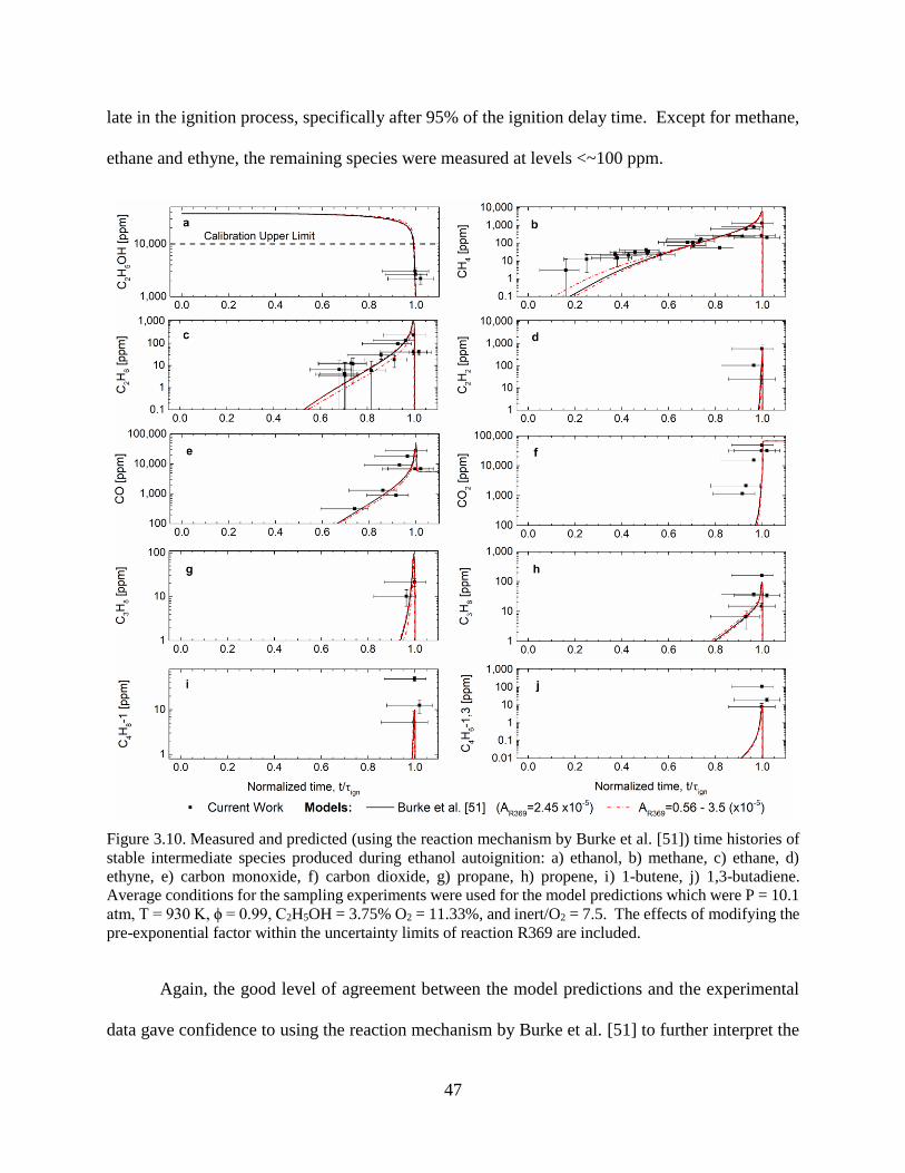
47

late in the ignition process, specifically after 95% of the ignition delay time. Except for methane,

ethane and ethyne, the remaining species were measured at levels <~100 ppm.

Figure 3.10. Measured and predicted (using the reaction mechanism by Burke et al. [51]) time histories of

stable intermediate species produced during ethanol autoignition: a) ethanol, b) methane, c) ethane, d)

ethyne, e) carbon monoxide, f) carbon dioxide, g) propane, h) propene, i) 1-butene, j) 1,3-butadiene.

Average conditions for the sampling experiments were used for the model predictions which were P = 10.1

atm, T = 930 K, ϕ = 0.99, C2H5OH = 3.75% O2 = 11.33%, and inert/O2 = 7.5. The effects of modifying the

pre-exponential factor within the uncertainty limits of reaction R369 are included.

Again, the good level of agreement between the model predictions and the experimental

data gave confidence to using the reaction mechanism by Burke et al. [51] to further interpret the

48

experimental data via reaction path analysis. The results are presented in Figure 3.11, and show

~72% of the ethanol reacted to produce ethanal as an early intermediate of the reaction sequence

initiated by hydrogen abstraction by different radicals (predominantly OH and HO2) from the α-

carbon site of ethanol and completed by the low-barrier reaction of α-hydroxyethyl radical

(sC2H4OH) and O2 [95,96]. Most of the ethanal was consumed in a series of steps to produce

methanal (formaldehyde, CH2O – not detected by the GC systems) before oxidizing to CO. The

latter carbonyls (aldehydes) are a well-known concern for the use of pure ethanol or high-ethanol

blends from the pollution control perspective in the transportation sector [97]. Methane (Figure

3.10(b)) and ethane (Figure 3.10(c)) were produced from branches of the main pathway when

ethanal reacted to form methanal. Ethene was the product of the H-atom abstraction reactions

from the secondary or β-carbon site on ethanol followed by β-scission reaction (see Figure 3.11).

The sensitivity of the model predictions for the species to changes in the pre-exponential

factors of reactions R17, R19 and R369 was also investigated. The A-factors for R17, R19 and

R369 were varied within the assigned uncertainty limits (as in Figure 3.6), and the results are

shown in Figure 3.9 for ethanal and ethene. These species showed the highest sensitivity to

changes in the A-factors of the three reactions. As seen in Figure 3.9, modifying the A-coefficients

did not significantly improve agreement for ethanal, while the agreement with ethene was

modestly improved at earlier times by reducing the A-factor for R369. Figure 3.10 includes the

results of modifying the A-factor for R369 only, and the results showed negligible changes in the

species predictions for all compounds.

The lack of sensitivity (using the conventional Chemkin sensitivity analysis) of the species

time histories to the reactions controlling the ignition delay time or the global reactivity of the

mixture at the state conditions presents a challenge and an opportunity to evaluate our

49

understanding of reaction pathways and reaction mechanisms. The strong sensitivity of the radical

pool to the reactions controlling ignition, and the corresponding sensitivity of fuel consumption to

the radical pool, eclipse or dominate the system response. Alternative methods of sensitivity

analysis may provide opportunity for intermediate species measurements to be used to validate

and verify reaction mechanisms beyond typical comparisons, such as those made here.

Figure 3.11. Schematic representation of the reaction pathway analysis for ethanol oxidation using the

reaction mechanism by Burke et al. [51]. for conditions of P = 10.1 atm and T = 930 K, C2H5OH = 3.75%,

O2 = 11.33%, N2 = 79.6% and Ar = 5.31% for time of t/ign = 0.9.

The stable intermediate species reported near t/τign = 1.00 accounted for ~92% of the carbon

initially in the mixture and corresponded well with the 87% of carbon predicted by the Burke et

al. [51] mechanism. In general, there was very good agreement between the experimental data

and the predictions from the mechanism, i.e. within the sampling interval and measurement

50

uncertainties. No significant reaction pathways were identified for the higher hydrocarbons from

the Burke et al. [51] mechanism; however, such species may provide some insight into how

reaction pathways change when ethanol is blended with gasoline and gasoline surrogates.

3.5 Conclusions

The results of the present work expand the quantitative understanding of the reactivity of

ethanol at intermediate temperatures and pressures. OH sensitivity analysis identified H-

abstraction from ethanol by HO2 (R369) as the primary reaction significantly affecting the global

reactivity of ethanol, but changing the A-factor for R369 within the uncertainty limits had small

to negligible effects on predicted intermediate species. Hence, ignition delay time data, like the

results of the current work, are a basis for improving the rate coefficient uncertainties for this

important reaction, and the speciation data provide important new information identifying and

quantifying the reaction pathways of the stable intermediate species formed during ignition.

Importantly, the results include species which are critical to predicting pollutant emissions like

aldehydes and soot precursor species. The combined measurements of ignition delay times and

intermediate species for ethanol ignition provide vital data for developing, validating and verifying

combustion chemistry. Excellent agreement between the experimental data and the model

predictions was observed in this study without modifying any of the rate coefficient data in the

original reaction mechanism developed by Burke et al. [51]. The results of the study provide direct

evidence to support high confidence in our predictive understanding of ethanol combustion,

including the detailed reaction pathways, at conditions directly relevant to modern combustion

systems.

3.6 Supporting Information

51

Table 3.1. Summary of experimental conditions and results for ethanol autoignition. All mixture data are

provided on a mole fraction basis. Values with an asterisk (*) correspond to speciation experiments.

ϕ

Test Gas Composition

Inert/O2 Peff

[atm]

Teff

[K]

τign

[ms] C2H5OH O2 N2 Ar CO2

[%] [%] [%] [%] [%]

0.98 3.41 10.47 79.81 6.31 0.00 8.23 3.04 936 46.0

0.98 3.41 10.46 73.41 12.72 0.00 8.23 2.95 961 30.6

0.96 3.38 10.55 68.18 17.88 0.01 8.16 2.70 964 29.8

0.98 3.41 10.47 70.01 16.12 0.00 8.23 2.99 979 20.9

0.98 3.40 10.46 70.91 15.23 0.00 8.24 3.08 996 13.9

0.91 3.30 10.82 63.69 22.20 0.00 7.94 2.78 1012 12.9

0.93 3.32 10.75 58.32 27.61 0.00 7.99 2.80 1044 7.2

0.90 3.26 10.92 51.73 34.08 0.01 7.86 2.73 1084 3.9

0.91 3.29 10.83 44.06 41.82 0.00 7.93 2.79 1118 2.4

0.95 3.35 10.63 43.42 42.59 0.01 8.09 2.81 1123 2.0

0.93 3.32 10.74 43.79 42.15 0.00 8.00 2.88 1124 2.0

0.95 3.37 10.59 82.84 0.02 3.18 8.12 5.33 902 57.4

0.96 3.38 10.55 82.86 0.02 3.19 8.16 5.32 902 53.8

0.97 3.40 10.49 84.09 0.01 2.01 8.21 6.03 929 27.5

0.96 3.37 10.57 80.22 5.83 0.01 8.14 5.58 952 19.1

0.99 3.43 10.40 78.33 7.85 0.00 8.29 5.46 979 11.7

0.98 3.42 10.43 78.32 7.82 0.01 8.26 5.77 992 8.9

0.95 3.37 10.59 68.95 17.10 0.00 8.12 5.53 999 7.7

0.96 3.37 10.58 65.67 20.37 0.01 8.13 5.35 1016 5.4

0.96 3.37 10.57 66.40 19.66 0.00 8.14 6.12 1023 4.3

0.96 3.38 10.56 61.73 24.34 0.00 8.15 5.83 1041 3.4

0.96 3.38 10.55 60.97 25.10 0.00 8.16 6.13 1050 2.5

0.96 3.37 10.58 56.35 29.70 0.00 8.13 5.41 1062 2.8

0.94 3.34 10.68 56.57 29.41 0.00 8.05 5.44 1063 2.6

0.94 3.34 10.68 56.57 29.41 0.00 8.05 5.44 1064 2.5

0.97 3.39 10.51 55.91 30.18 0.01 8.19 6.37 1086 1.4

0.99 3.21 9.75 77.49 9.55 0.00 8.93 8.23 961 10.2

0.99 3.21 9.75 70.71 16.34 0.00 8.93 9.64 999 4.5

0.97 3.18 9.85 70.77 16.20 0.00 8.83 9.55 997 4.6

0.99 3.29 9.94 78.59 8.17 0.01 8.73 9.13 949 11.6

0.99 3.44 10.38 83.46 0.00 2.72 8.30 11.19 907 19.6

0.99 3.43 10.39 85.88 0.00 0.30 8.29 11.94 967 6.8

0.99 3.43 10.39 65.74 20.44 0.00 8.29 8.96 1030 2.6

0.99 3.43 10.39 84.43 0.00 1.75 8.29 9.81 928 17.2

0.99 3.43 10.40 83.38 2.79 0.00 8.29 10.11 930 16.1

0.99 3.43 10.40 84.46 0.01 1.70 8.29 10.06 931 15.3

0.99 3.43 10.40 86.17 0.01 0.00 8.29 9.91 937 13.2

52

0.99 3.43 10.40 84.45 0.00 1.72 8.29 9.81 924 15.1

0.99 3.43 10.40 77.64 8.52 0.01 8.29 9.82 961 6.9

0.99 3.43 10.41 83.38 2.79 0.00 8.28 10.50 935 12.6

0.99 3.43 10.42 71.98 14.17 0.00 8.27 9.73 1000 4.5

0.98 3.42 10.43 76.38 0.01 9.76 8.26 9.83 894 33.4

0.98 3.42 10.44 78.94 0.01 7.19 8.25 9.72 909 23.7

0.98 3.42 10.44 76.08 0.01 10.05 8.25 10.60 896 28.6

0.98 3.42 10.44 73.69 12.45 0.00 8.25 9.50 994 4.7

0.98 3.41 10.45 73.69 12.45 0.00 8.24 9.32 990 4.5

0.98 3.41 10.45 73.70 12.44 0.00 8.24 9.60 997 3.9

0.98 3.41 10.46 73.99 0.01 12.13 8.23 10.38 883 38.4

0.97 3.40 10.50 83.33 2.77 0.00 8.20 10.23 929 15.9

0.99 3.75 11.33 79.61 5.32 0.00 7.50 9.77 928 13.2*

0.99 3.75 11.33 79.61 5.31 0.00 7.50 9.92 930 12.2*

0.99 3.75 11.33 79.60 5.31 0.01 7.50 10.13 932 11.2*

0.99 3.75 11.33 79.60 5.31 0.01 7.50 10.04 929 12.9*

1.00 3.77 11.33 79.59 5.31 0.00 7.49 10.26 933 9.9*

0.99 3.75 11.33 79.60 5.31 0.01 7.50 9.71 923 13.9*

1.00 3.77 11.33 79.59 5.31 0.00 7.49 10.16 931 10.8*

1.00 3.77 11.33 79.59 5.31 0.00 7.49 10.34 934 10.4*

1.00 3.77 11.33 79.59 5.31 0.00 7.49 10.00 928 12.1*

0.99 3.75 11.34 79.60 5.31 0.00 7.49 10.35 933 12.7*

0.99 3.75 11.34 79.60 5.31 0.00 7.49 9.74 923 14.0*

0.99 3.75 11.34 79.60 5.31 0.00 7.49 9.97 928 12.6*

0.99 3.75 11.34 79.60 5.31 0.00 7.49 10.13 931 12.1*

0.99 3.75 11.34 79.60 5.31 0.00 7.49 10.38 936 9.9*

0.99 3.74 11.36 79.60 5.30 0.00 7.47 10.60 936 11.2*

53

Table 3.2. Summary of results for speciation experiments of stoichiometric ethanol mixtures with an asterisk (*) in Table 3.1§. Data are arranged

in ascending order for t/τign.

time

[ms]

τign

[ms] t/τign

C2H5OH

[ppm]

C2H6

[ppm]

CH3CHO

[ppm]

C2H4

[ppm]

C2H2

[ppm]

CH4

[ppm]

CO

[ppm]

CO2

[ppm]

C3H6

[ppm]

C3H8

[ppm]

C4H8-1

[ppm]

C4H6-1,3

[ppm]

1.8 11.2 0.16 X - 66 16 - 3 - - - - - -

3.2 12.9 0.25 X - 138 33 - 12 - - - - - -

4.0 10.8 0.37 X - 188 62 - 23 - - - - - -

4.6 12.1 0.38 X - 129 30 - 15 - - - - - -

5.5 12.9 0.43 X - 226 64 - 21 - - - - - -

5.8 12.6 0.46 X - 322 91 - 31 - - - - - -

6.1 12.1 0.50 X - 360 119 - 41 - - - - - -

7.1 13.9 0.51 X - 592 100 - 28 - - - - - -

7.2 14.0 0.51 X - 659 102 - 32 - - - - - -

6.8 12.1 0.56 X - 190 62 - 22 - - - - - -

9.5 13.9 0.68 X 6 1,640 274 - 111 - - - - - -

9.3 13.2 0.70 X 4 X 247 - 105 - - - - - -

8.9 12.6 0.70 X 4 X 214 - 91 - - - - - -

8.9 12.7 0.71 X 4 X 191 - 74 - - - - - -

7.6 10.4 0.73 X 13 X 320 - 134 - - - - - -

8.3 11.2 0.74 X 12 X 385 - 168 313 - - - - -

9.9 12.1 0.82 X 6 X 121 - 57 - - - - - -

9.3 10.8 0.86 X 30 X 497 - 282 1,309 - - - - -

11.6 12.7 0.92 X 18 X 438 - 242 892 1,168 - - - -

9.2 9.9 0.93 X 95 X 845 - 646 9,193 2,148 7 - - -

12.7 13.2 0.96 X 134 946 1,099 105 822 18,217 15,411 37 10 - -

9.9 9.9 1.00 3,072 40 252 484 25 263 6,835 31,536 15 - 5 8

11.1 11.2 1.00 2,646 230 336 2,439 589 1,360 27,710 48,799 159 22 49 110

10.6 10.4 1.02 2,203 39 238 455 - 207 6,908 31,697 35 - 12 20

§ Where “X” represents measurements above the calibration limits and “-” means “below the detectable limits”.

54

Chapter 4 Combustion Chemistry of Ethanol/Iso-Octane Blends

4.1 Introduction

Iso-octane is an important primary reference fuel and is often used as a simple chemical

surrogate for gasoline. Numerous experimental studies of the low temperature (600 - 1300 K)

ignition chemistry of iso-octane can be found in the literature, in particular where shock tubes and

rapid compression machines (RCMs) were used to create the desired state conditions. Examples

of studies at the pressure relevant to the current work are briefly summarized here. Shen et al. [98]

used a shock tube to measure ignition delay times of stoichiometric iso-octane/air mixtures at 10

atm and 950 – 1250 K, and compared the results with shock-tube data by Fieweger et al. [99] and

Davidson et al. [100] at similar conditions. In those studies, no negative temperature coefficient

(NTC) behavior was observed for temperatures above 910 K, and good agreement was achieved

between the different experimental data sets and between the experimental data and modeling

results based on the iso-octane kinetic mechanism by Curran et al. [101]. Ignition of iso-octane/air

mixtures at ϕ = 1 and P = 10 atm have also been studied in RCMs by Minetti et al. [102] at T =

660 – 890 K, and Griffith et al. [103] at 900 – 950 K. The RCM data suggested the onset of NTC

behavior for iso-octane was between 800 and 850 K for P = 10 atm, which corresponded well with

simulation results based on the Mehl et al. [84] reaction mechanism for gasoline surrogates and

gasoline fuel mixtures (which includes the Curran et al. [101] sub-mechanism). Iso-octane ignition

has been extensively studied using the UM RCF through ignition delay time [88], OH time history

[104] and intermediate species [50] measurements, and by characterizing the weak and strong

ignition behavior using high-speed imaging [46,89] for a range of conditions (ϕ = 0.2 – 2.0, P = 5

55

– 23 atm, T = 810 – 1100 K). Low temperature shock tube, RCM, RCF, and other important

experimental and computational chemistry studies have led to quantitative predictive

understanding of iso-octane combustion chemistry over a broad range of pressures, temperatures

and mixture compositions. As for ethanol, such accurate understanding of iso-octane ignition is

invaluable for quantifying the effects of iso-octane as a binary blend component.

To our knowledge, only two studies in the literature have reported ignition data of binary

iso-octane/ethanol blends. Cancino et al. [82] measured ignition delay times in a shock tube for

stoichiometric ethanol and blend of 25% by volume ethanol (E25) at 30 bar and 750 – 1200 K.

They found the iso-octane reduced the reactivity of the ethanol for T > 1000, and proposed a kinetic

model that agreed well with their experimental data. Song and Song [105] used an RCM to

measure the ignition delay times of pure iso-octane (E0), E10 and E20 at 27 bar and 750 – 900 K,

and demonstrated the opposite trend—where the ethanol addition suppressed iso-octane reactivity

at low temperatures (T < 870 K), particularly in the NTC region. Additionally, shock-tube ignition

data of stochiometric multi-component surrogate mixtures blended with 40, 20 and 10% ethanol

by Fikri et al. [106] and Cancino et al. [82,107] at 10 – 50 atm and 690 – 1220 K are available,

although the effects of ethanol addition to a fixed surrogate mixture were not measured. Yahyaoui

et al. [108] evaluated the changes in reactivity of a surrogate mixture of iso-octane, toluene and 1-

hexene when adding ethanol up to 85% by volume at ϕ = 1, P = 2 atm and T = 1200 – 2000 K, and

concluded ethanol addition consistently increased the blend reactivity at the conditions studied.

Up to date, no measurements of stable intermediate species produced during the ignition of

ethanol/iso-octane blends currently exist in the literature. Such data provide direct insight into the

dominate reaction pathways of ignition of ethanol/iso-octane blends and provide high fidelity

validation of our current understanding of the reaction chemistry of these important fuel blends.

56

Although various detailed kinetic models for fuel blends that include ethanol can be found

in the literature [2,51,59,64,81–87], the kinetic model developed by Mehl et al. [84] at Lawrence

Livermore National Laboratory is widely accepted and has been extensively validated for gasoline

surrogates and mixtures. The mechanism contains 5935 elementary reactions, including iso-octane

reaction rates from Curran et al. [101] and a C1 – C4 mechanism with small alcohol chemistry from

Johnson et al. [109]

4.2 Objective

The aim of this work is to understand the effects of ethanol on the reaction pathways

important during iso-octane ignition, and to specifically identify any synergies or other interactions

between the two fuel compounds. The technical approach was to provide new experimental

ignition and speciation data on stoichiometric iso-octane/ethanol blends using the UM RCF. The

current work includes ignition data for E0, and E5, E11, E26, E50 and E67 blends (by liquid fuel

volume) at moderate levels of dilution (inert gas/O2 molar ratios of 8.74:1), temperatures ranging

from 900 to 1080 K and a nominal pressure of 10 atm. Speciation data were obtained for E0 and

E50 at the same conditions (10 atm, 930 K and inert gas/O2 molar ratios of 7.5:1) of the 100%

ethanol study presented in Chapter 3. High-speed imaging was used to record chemiluminescence

during ignition, and fast-gas sampling coupled with gas chromatography and mass spectrometry

were used to identify and quantify stable species during the ignition delay time. The experimental

results were compared with simulation results which used the Mehl et al. [84] mechanism. The

results are discussed in terms of the major reaction pathways and the changes in the reaction

processes based on the blend of ethanol with iso-octane.

57


The results presented in this chapter were obtained using the UM RCF and following the


results for both imaging and speciation experiments, and supporting information can be found in

Section 4.6.


Ignition Delay Times

Figure 4.1 presents a comparison of typical pressure and pressure-derivative time histories

of stoichiometric mixtures of pure iso-octane (E0), pure ethanol (E100) and the E50 blend. Pmax

represents the local maximum of the test gas pressure resulting from the compression of each test

mixture by the sabot. The end of the compression (i.e. when P = Pmax) corresponds to the time at

which the nosecone seated and is set as time zero (t = 0 ms). Due to heat transfer to the walls, the

pressure in the test section decreases slightly after the end of compression. After the ignition delay

period, the pressure rapidly increases when the test mixture auto-ignites. The definition of ignition

delay time, τign, is given by the difference in time between the maximum rate of change of the

mixture pressure, (dP/dt)max, and the end of compression, Pmax. All data in this study showed

similar behavior of smooth compression followed by nominally constant pressures during the

ignition delay period followed by rapid heat release due to ignition.

Time-averaged state conditions for each experiment were defined as in previous UM RCF

studies [42,88]. To account for heat transfer effects, the effective pressure was defined as the time-

averaged integration of pressure from Pmax to Pmin, where Pmin was the minimum pressure before

ignition. The effective temperature was calculated by numerical integration of the isentropic

compression relations using Peff, the initial pressure and temperature, and the gas thermophysical

58

properties of the mixture [42]. Donovan et al. [44] experimentally verified the suitability of the

isentropic compression modeling for UM RCF experiments. When compared with the end-of-

compression conditions, effective conditions have been shown to be less biased towards higher

temperatures and pressures for data presented on Arrhenius diagrams, where isobaric and

isothermal conditions are typically assumed [42]. Additionally, effective conditions are

appropriate for use as initial conditions in adiabatic simulations of the UM RCF experiments as

described in He et al. [88] and Mansfield and Wooldridge [110].

Figure 4.1. Typical pressure (solid lines) and pressure derivative (dashed lines) time histories in the test

section for ignition experiments of E0 (red), E50 (blue) and E100 (green) using high-speed imaging.

The experimental conditions were similar for each of the blends presented in Figure 4.1,

where ≈ 1.00, Peff ≈ 10.3 atm, Teff ≈ 934 K and molar dilution of inert/O2 ≈ 7.5. As seen in the

figure, the pressures were virtually identical up to and after the end-of-compression until the time

of ignition for each fuel mixture. At the time of ignition, the rate of pressure rise was also similar

for each fuel mixture; however, the ignition delay time decreased with increasing ethanol content

in the fuel. The peak pressure at the time of ignition was also lower for E100 compared with E0

and E50, reflecting the lower energy content of a stoichiometric mixture of pure ethanol compared

59

with pure iso-octane, where the heating value per stoichiometric mixture of fuel and air is 421

kJ/kgmix for ethanol compared with 555 kJ/kgmix for E50 and 648 kJ/kgmix for iso-octane.

Still images from the high-speed camera corresponding to the E0, E50 and E100 ignition

experiments in Figure 4.1 are presented in Figure 4.2. Homogeneous ignition in the test section is

verified by the chemiluminescence emission which shows no signs of spatial irregularities such as

local ignition, flame propagation or reaction fronts. Note the image sequences span 0.6 ms, and

chemiluminescence is localized to the time of ignition only. As seen in Figure 4.1, the maximum

pressure derivatives—which define τign—correspond well with the times of the maximum intensity

of emission in Figure 4.2. Consistent observations of homogenous chemiluminescence occurred

for all the experiments in this study, which is important for local sampling to represent the overall

mixture composition.

Summaries of the results for ign are presented in Figure 4.3 and Table 4.4 – Table 4.6. In

Figure 4.3, the symbols correspond to the results of this work for E0 – E67 and for some E100

data, with additional E100 data from Chapter 3. Molar inert/O2 ratios of ~8.7 and 7.5 were used

for the imaging and the sampling experiments, respectively. Experimental uncertainties of the

ignition delay time measurements (due primarily to the uncertainty in dP/dt) are shown as vertical

error bars in Figure 4.3, which vary from ±0.3 ms at higher temperatures to ±1.8 ms at lower

temperatures for all the experiments presented here (E0 – E100). Error bars for temperature were

determined as the standard deviation of the effective temperature deduced from the pressure-time

history data as in Chapter 3. The majority of the E100 data at 10 atm were taken from Chapter 3,

but additional imaging experiments were acquired in the current study at temperatures of 910 –

980 K for verification purposes.

60

Figure 4.2. Selected frames from the high-speed imaging at the time near ignition for pressure-time

histories in Figure 4.1. The frames corresponding to the maximum intensities are included.

As seen in Figure 4.3, the experimental ignition data exhibited excellent repeatability and

low scatter. The E0, E50 and E100 data sets (which span larger temperature ranges than the E5,

E11 E26 and E67 data sets) each follow clear Arrhenius trends for ign. For the range of conditions

studied, E0/100% iso-octane exhibited consistently lower reactivity than E100/100% ethanol. The

addition of small amounts of ethanol to iso-octane, e.g. E5 and E11 had negligible effect on the

ignition delay time compared with E0 (within the uncertainty of the data). However, E26 and E50

exhibited progressively faster ignition delay times in comparison with E0. The ignition delay

times for E67 were approximately within the uncertainty of the ignition delay times for E50.

61

Figure 4.3. Experimental results of ignition delay times for stoichiometric (ϕ = 0.99 ± 0.01) mixtures of

E0, E5, E11, E26, E50, E67, and E100 fuels. The E100 data include results from Chapter 3. Two dilution

levels were considered for the imaging (main figure, inert/O2 = 8.74 ± 0.33) and for the speciation (inset,

inert/O2 = 7.48 ± 0.02) experiments. Model predictions are based on the reaction mechanism by Mehl et

al. [84] (solid lines). Regression fits to the experimental data are provided as dotted lines.

Regression analysis was applied to the E0, E50 and E100 data sets and to all the ignition

data (E0 – E100) to determine the best fit for Arrhenius expressions for the ignition delay time of

the form of τign = A (CB)d exp(Ea/RT), where CB is the molar carbon content in each fuel blend.

The regression coefficients are provided in Table 4.1 and presented in Figure 4.3 and Figure 4.5.

The quality of the fit to the data was excellent and the range of temperatures for the regressions

and the R2 values are included in Table 4.1.

Table 4.1. Best-fit regression coefficients for τign correlations of E0, E50, E100, and all fuel data (E0-E100)

fort ϕ = 0.99, P = 9.98 atm and inert/O2 = 8.74. The regression correlations have the form of τign = A (CB)d

exp(Ea/RT).

Fuel A (ms) Carbon in

blend (CB) d Ea (cal/mol) T (K) R2

E0 1.21x10-6 8 0 32,013 909 – 1067 0.996

E50 5.76x10-8 3.56 0 36,616 902 – 1052 0.997

E100 8.28x10-8 2 0 35,206 883 – 1030 0.986

E0–E100 8.44x10-8 8 – 2 0.776 34,083 883 – 1067 0.991

62

Figure 4.4. Comparison of measured and simulated pressure and experimental pressure derivative traces

for E0 (dashed lines) and E100 (solid lines) at state conditions of ~10 atm, ~930 K and inert/O2 = 7.5.

Imaging and speciation experiments, and constant-volume, compression/heat transfer and pyrolysis

simulations are included.

The experimental results are also compared with model predictions in Figure 4.3 based on

the detailed chemical kinetic mechanism for gasoline surrogate mixtures developed by Mehl et al.

[84]. Average effective pressure and temperature, and mixture composition from the UM RCF

experiments were used as initial conditions in 0-D adiabatic constant-volume simulations in

CHEMKIN. τign was defined as the time from the start of each simulation to the time

corresponding to (dP/dt)max. In Figure 4.4, the difference between using an adiabatic constant

volume modeling approach compared with simulating the compression process and the end-of-

compression heat transfer losses (as an expansion process) are minimal and represent 6% and 12%

differences in τign predictions for E100 and E0, which is typically smaller than the uncertainty in

the reported ignition delay times. As seen in Figure 4.3, the agreement between the experimental

data and the model predictions is generally good, within ±50%, for all the fuels and throughout the

temperature ranges considered. However, for E0 and E50, the simulations predict slightly faster

ignition delay times (up to ~30% for E0 and ~34% for E50) at lower temperatures (T < 950 K)

than observed experimentally and slightly slower ignition delay times (up to ~48% for E0 and

~30% for E50) at higher temperatures (T > 1000 K) than observed experimentally. Note the

63

simulation results show a change in the activation energy for E0 around 950 K. For temperatures

below 950 K, the model predictions are in excellent agreement with the experimental data for

E100. Interestingly, the simulations also predict negligible difference in the reactivity of E50 and

E100 for temperatures below 950 K, which differs from the experimental results.

Figure 4.5. Summary of scaled ignition delay times (open symbols) of the fuel data presented in Figure 4.3

for stoichiometric (ϕ = 0.99) mixtures at P = 10 atm and inert/O2 = 8.74. The regression coefficient of CB

for the E0–E100 blends was used to scale the ignition data to E50 blend level. E50 data were not scaled

and are presented as filled symbols.

Ignition delay time measurements scaled to E50 for all the blends in this study (E0 – E100)

are included in Figure 4.5. The power of the carbon content (CB) from the regression analysis of

all the blends in Table 4.1 (d = 0.776) was used to scale all the data—excluding E50—to CB =

3.56. The data for all the fuels collapse to a single trend-line around the original E50 data with

little scatter. The quality of the Arrhenius fit is a good indication that no NTC behavior is present

for iso-octane, ethanol and the blends at 10 atm and 880 – 1070 K. The regression correlation for

all the blends is included in Figure 4.5 along with the model predictions using Mehl et al. reaction

64

mechanism [84]. Overall the agreement between the model predictions and the experimental data

is very good (within ±50%) where the model slightly underpredicts ign at lower temperatures.

Figure 4.6. Effect of ethanol addition on ignition delay time at ~910 K and ~1000 K for P = 10 atm and

molar ratio of inert/O2 = 8.74.

Figure 4.6 presents the ignition delay time measurements as a function of the atomic carbon

content in the blend for 10 atm, inert/O2 = 8.74 and temperatures of ~910 K and ~1000 K, along

with the regression correlation and predictions using the Mehl et al. model [84]. At both

temperatures, the experimental data show increasing reactivity (i.e. faster ignition delay times) as

more ethanol is added to the blend. The model predictions are in excellent agreement with the

experimental data for all blends for 1000 K, but the model increasingly underpredicts the reactivity

of the blends at 910 K as the amount of ethanol content decreases in the blend. Interestingly, the

model predicts weak sensitivity of ign for blends between E100 to E50, particularly for 910 K,

which is not observed experimentally. As seen in the regression expression for the fuel blends,

65

the ignition delay time is nearly proportional to the atomic carbon content in the fuel mixture, CB,

with a power of 0.776.

Figure 4.7. Model predictions using the Mehl et al. mechanism [84] for ignition delay times of

stoichiometric iso-octane and ethanol mixtures at 10 and 100 atm.

The faster reactivity of 100% ethanol compared with 100% iso-octane is particular to the

state conditions used in this study (10 atm and 900 – 1050 K). In the RCM ignition study by Song

and Song [105], the authors considered ethanol/iso-octane blends at ~27 atm and 750 – 900 K and

found ethanol addition (E0, E10 and E20) suppressed the higher reactivity of the iso-octane. This

change in the relative reactivity of the two fuels is due to the NTC behavior of iso-octane. Figure

4.7 shows model predictions based on the reaction mechanism by Mehl et al. [84] for

stoichiometric air mixtures of iso-octane and ethanol for a wider temperature range (700 – 1700

K) and pressures of 10 atm and 100 atm. The simulations show faster ign of ethanol with respect

to iso-octane for T > 800 K at 10 atm and for T > 1400 K at 100 atm, and the opposite behavior

for lower temperatures due to the NTC behavior of iso-octane. The NTC behavior and relative

66

reactivity of E0 and E100 observed by Song and Song [105] at 900 K is likely due to the higher

test pressure considered in their work.

Figure 4.8. Results of CHEMKIN sensitivity analysis for OH at P = 10 atm, T = 930 K, ϕ = 1 and (inert/O2)

= 7.5. Simulations based on the reaction mechanism by Mehl et al. [84] for E0, E50 and E100. Reaction

numbers of the top 5 reactions are according to the mechanism numeration.

Sensitivity analysis of OH—as a surrogate for ign—was conducted to identify the most

important reactions for ignition of the three fuels at nominal state conditions. CHEMKIN

sensitivity analysis was used with the mechanism by Mehl et al. [84] for E0, E50 and E100 at =

1.00, P = 10 atm, T = 930 K and inert/O2 = 7.5. Plots of the results are provided in Figure 4.8.

The most important reaction for each fuel was the chain branching reaction H2O2 (+M) ↔ OH +

OH (+M) (R16). For pure iso-octane, CH3 + HO2 ↔ CH4 + O2 (R110) was also significant;

whereas for pure ethanol, C2H5OH + HO2 ↔ C2H4OH + H2O2 (R293) was the second most

67

important reaction. For the E50 blend, the hydrogen peroxide decomposition remained the most

important reaction, and both R110 and R293 were significant. The results show H2O2 and HO2

reactions dominate the ignition behavior at these moderate/low temperatures.

Intermediate species

All speciation data were acquired at the same nominal state/end-of-compression

conditions. Figure 4.9 shows data from a typical E50 speciation experiment where two gas

samples were removed and quenched from the test section at two different sampling times during

the ignition delay period. The pressure-time histories are shown for the test section and the two

sampling volumes, and the pressure derivative is shown for the test section data. As in Chapter 3,

sample times were defined as the time corresponding to one half the area under the sampling

pressure curve starting from the time the valve was triggered (i.e. the falling edge of the triggering

signal shown in Figure 4.9) to the time of maximum sampling pressure. The uncertainty in sample

timing was defined as the duration of the gas sampling event, Δtsample, given by the integration

limits of the sampling pressure. Average sample durations were 2.2 ±0.2 ms for E0 and 2.4 ±0.3

ms for E50. Average sample durations for the E100 data from Chapter 3 were 2.1 ±0.1 ms. The

ignition delay time was determined from each speciation experiment in the same manner as

described for the imaging experiments. Tables 4.4 and 4.5 include the ignition results of the

sampling experiments.

A summary of the ignition delay time data from the sampling experiments is presented in

the inset of Figure 4.3. As seen in the figure, the τign data from the sampling experiments (open

symbols) were in excellent agreement with the τign data from the imaging experiments (filled

symbols) which indicates the collection of two gas-samples did not affect the ignition process.

This is also confirmed by pressure-time histories of E0 and E100 imaging and sampling

68

experiments at the same end of compression conditions which were virtually indistinguishable (see

Figure 4.4). The inset in Figure 4.3 also provides a comparison of the experimental results with

the model predictions at the sampling conditions using the Mehl et al. [84] reaction mechanism.

The model is in excellent agreement with the E100 data (within ~10%) and very good agreement

with the E0 data (~33% lower) and the E50 data (~31% lower) at the gas sampling conditions.

Figure 4.9. Typical pressure and pressure derivative time histories in the test section for an E50 ignition

experiment using fast gas sampling. Pressure time histories for the two sampling volumes are shown along

with the corresponding triggering signals. Conditions for the experiment were Peff = 9.8 atm, Teff = 934 K,

ϕ = 0.99, inert/O2 = 7.43, i-C8H18 = 0.54%, C2H5OH = 1.55%, O2 = 11.62%, N2 = 78.7%, Ar = 7.6%, and

τign = 18.16 ms.

For iso-octane, gas samples were collected using a nominal mixture composition of i-C8H18

= 0.93%, O2 = 11.7%, N2 = 79.5% and Ar = 7.93% (mole basis). The average conditions and

corresponding standard deviations for the E0 experiments were P = 9.65 ±0.24 atm and T = 929

±5 K with an average ignition delay time and standard deviation of τign = 34.6 ±2.5 ms. For E50,

gas samples were collected using a nominal mixture composition of i-C8H18 = 0.54%, C2H5OH =

1.55%, O2 = 11.57%, N2 = 71.39% and Ar = 14.94% (mole basis). The average conditions and

corresponding standard deviations for the E50 experiments were P = 9.82 ±0.33 atm and T = 932

±7 K, with an average ignition delay time and standard deviation of τign = 18.6 ±3.2 ms. From

Chapter 3, the average conditions and corresponding standard deviations for the E100 data were P

69

= 10.10 ±0.26 atm, T = 930 ±4 K and τign = 11.9 ±1.3 ms. The standard deviation data demonstrates

that the repeatability of all the sampling experiments was excellent.

Figure 4.10. Chromatograms corresponding to Sample 2 of Figure 4.9 from (a) GC-1/FID (blue) and GC-

2a/FID (red), and (b) GC-3/MS. Features of species which were quantified in the study are identified in

the chromatograms.

For this study, up to 14 species were detected and quantified using GC analysis. Figure

4.10 presents typical chromatograms obtained from the sampling data shown in Figure 4.9.

Features of species which were quantified in the current work are identified in Figure 4.10, where

several additional features were attributed to other intermediate species that were not quantified in

this study. The species selected for calibration and analysis were determined by the anticipated

role such species would play in the iso-octane/ethanol blend reaction pathways based on previous

studies of pure iso-octane [50,104] and ethanol. In particular, the focus was on species which

70

could be attributed to one parent fuel compound or the other, in order to determine how the iso-

octane and ethanol reaction pathways were altered in the blend mixtures.

Figure 4.11 presents the measurements of ten key stable intermediate species while

measurements of the remaining four species (ethyne, acetone, methacrolein and iso-pentene) are

presented in Figure 4.12. To eliminate small variations in the end-of-compression conditions, the

sampling times are normalized to the ignition delay time of each experiment, hence t/τign = 0

represents the end of compression and t/τign = 1 corresponds to the time of autoignition. Both

absolute and normalized time values are provided in Table 4.7. The horizontal error bars in Figure

4.11 correspond to the duration of each sampling interval, while the vertical error bars represent

the standard deviation of each mole fraction measurement. Correction factors and uncertainties

for species concentrations were determined by statistically quantifying the sources of experimental

error associated with the sampling process and the GC measurement systems. The detailed

description of the methodology is provided in Section 2.1. Saturation limits for ethanol (10,000

ppm) and ethanal (3,000 ppm) are included in Figure 4.11. Concentration data above these values

have potentially higher uncertainties than represented by the vertical error bars.

As noted earlier, the species presented in Figure 4.11 were targeted for measurement

because they are significant intermediates during ignition of pure iso-octane [50,104] and pure

ethanol (See Chapter 3 and Barraza-Botet et al. [42]). At the top of Figure 4.11 are the parent fuel

measurements for iso-octane (Figure 4.11(a), top of the left column) and ethanol (Figure 4.11(f)

top of the right column). On the left-hand side (Figure 4.11(b) and Figure 4.11(c)), the

measurements for iso-butene (i-C4H8, 2-methyl-1-propene) and propene (C3H6) are presented. Iso-

butene and propene were the most important and abundant species in the experiments by He et al.

[50] in the UM RCF study of iso-octane ignition. In the current work, for E0 at t/τign ≈ 0.7, the

71

mole fraction of i-C4H8 (~1050 ppm) is approximately three times that of C3H6 (~340 ppm), which

is consistent with results from He et al. [50] at both fuel rich and fuel lean conditions around the

same time.


produced during autoignition of E0, E50 and E100: a) iso-octane, b) iso-butene, c) propene, d) ethane, e)

carbon monoxide, f) ethanol, g) ethanal, h) ethene, i) methane, and j) carbon dioxide. The effects of

removing the ethanol (red dashed lines) and iso-octane (green dashed line) from the E50 mixture in the

simulation are included.

72


produced during autoignition of E0, E50 and E100: a) ethyne b) acetone, c) methacrolein, d) iso-pentene.

On the right-hand side of Figure 4.11 (Figure 4.11(f) – (h)), the measurements for ethanol,

ethanal (CH3CHO) and ethene (C2H4) are presented. In Chapter 3, ethanal (CH3CHO) and ethene

(C2H4) were identified as the main stable intermediates produced by early reactions in the two

primary reaction pathways of ethanol. The remaining species measurements presented in Figure

4.11 include ethane (C2H6), methane (CH4), carbon monoxide (CO) and carbon dioxide (CO2),

which are stable intermediates produced by both iso-octane and ethanol. Both CO and CO2, as

primary products of combustion, are produced at high levels (> 2% mole fraction) at times close

to ignition.

The values of the E50 speciation data consistently fell within the limiting data of pure iso-

octane and pure ethanol. For E100, the levels of iso-butene were below the detectable limits,

clearly indicating there are no major pathways for iso-butene formation from ethanol. For the

species primarily produced from iso-octane (i-C4H8 and C3H6), the E50 blend decreased the values

of the intermediate species notably. For the species produced primarily from ethanol (CH3CHO

and C2H4), the blend E50 results were much closer to the E100 data than observed for the iso-

73

octane intermediates iso-butene and propene. However, the E0 results for CH3CHO and C2H4

were dramatically lower than the data for E50 and E100, indicating a non-linear decrease in these

species as a function of iso-octane in the fuel blend. For the shared intermediate species (C2H6,

CH4, CO, and CO2), the E50 measurements were often indistinguishable (i.e. within the

experimental uncertainties) with either the E0 or the E100 data, especially at times close to

autoignition.

The species measurements are also compared with model predictions in Figure 4.11 using

the reaction mechanism by Mehl et al. [84]. For reference, the initial molar composition of the

mixtures modeled for each blend corresponding to the speciation experiments can be found in

Table 4.2 and the total carbon represented by the ten species measurements and predicted by the

model simulations are provided in Table 4.3. As seen in Figure 4.11 and Table 4.3, the level of

agreement between the experimental data and the model predictions was generally excellent

(within the experimental uncertainties and the expected model uncertainties) for all species

throughout most of the ignition delay times, with a few small discrepancies. For C2H6 for E0 and

E50, the model significantly underpredicts the experimental data at early times (t/ign < 0.2). For

E100, CH3CHO and C2H4 are also under-predicted at early times (t/ign < 0.4), and C2H4 is over-

predicted at later times (t/ign > 0.6). Lastly, the model indicates CH3CHO and C2H4 should be

formed at higher levels for E50 compared with E100 (by almost an order of magnitude) at early

times (t/ign < 0.6), but the measurements indicate comparable levels for these intermediates for

E50 and E100. These small discrepancies may be an indication of the limiting accuracy of the

simulations for predicting these intermediate species at the conditions studied.

74

Table 4.2. Initial mixture composition of simulations presented in Figure 4.11.

Blend

Molar content of

Ethanol in Fuel

Blend [%]

ϕ

Simulated Test Gas Composition

Inert/O2 i-C8H18

[%]

C2H5OH

[%]

O2

[%]

N2

[%]

E0 0 1.00 0.93 0.00 11.66 87.41 7.50

E50 74 1.00 0.55 1.56 11.52 86.38 7.50

E100 100 1.00 0.00 3.77 11.32 84.91 7.50

E50 - 0% C2H5OH 0 0.60 0.56 0.00 11.70 87.74 7.50

E50 - 0% i-C8H18 100 0.41 0.00 1.57 11.58 86.85 7.50

Based on the high quality of the model predictions, the reaction mechanism by Mehl et al.

[13] was used to identify the reactions important for the production and consumption of the species

measured in this study. Figure 4.13 presents the reaction path diagrams created from rate of

production analysis for the three fuel mixtures at a time close to ignition (t/τign = 0.9). Species in

red and green are the stable intermediates measured in the current work and which are attributed

to the reaction pathways of iso-octane and ethanol, respectively, while the species in blue are

important in the reaction pathways of both fuels. For E0 and E50, the numbers in bold represent

the relative degree of importance (0 – 100) of each reaction path relative to the maximum reaction

rate for each fuel/air mixture at the time t/τign = 0.9. For E100, the values in bold were normalized

with the maximum reaction rate of the ethanol branch of E50. The parenthetical values show the

fractional significance of the different reaction pathways.

Table 4.3. Experimental measurements and model predictions of the total carbon represented by the species

in Figure 4.11.

Fuel Blend Time of calculation Experiment Model

E0 t/ign = 0.93 57% ±9% 64%

E50 t/ign = 0.85 62% ±11% 57%

E100 t/ign = 1.00 92% ±8% 87%

As seen in Figure 4.13, H-atom abstraction from the fuels are the primary means of fuel

consumption for E0, E50 and E100, and OH is the critical radical chain carrier. Fuel + HO2

reactions are also important for fuel consumption, and furthermore the HO2 + ethanol reactions

75

play a more important role compared with HO2 + iso-octane. i-C4H8 is produced by several H-

atom abstraction reactions from iso-octane followed by several pathways that can involve scission,

oxidation or subsequent H-abstraction reactions. C3H6 is produced directly from the intermediate

i-C4H9. As expected, there are no significant pathways for formation of i-C4H8 or C3H6 from

ethanol. C2H4 and CH3CHO are formed by H-abstraction from ethanol followed by decomposition

and oxidation by O2, respectively. Similar to the iso-octane intermediates, there are no significant

pathways for formation of the ethanol intermediates C2H4 and CH3CHO from iso-octane. For both

iso-octane and ethanol, C2H6 and CH4 are primarily produced by the reaction CH3 + HO2 ↔ CH4

+ O2 and the methyl radical recombination reaction CH3 + CH3 + M ↔ C2H6 +M.

The relative reaction rates and branching fractions are also compared for the three fuels to

understand the effects of the fuel composition on the measured species. The H-abstraction reaction

pathways from the different carbon sites of iso-octane are similar in magnitude for E0 and E50.

Similarly, the H-abstraction reaction rates from the primary and secondary carbon sites of ethanol,

and the relative participation by OH in such reactions, were similar for E50 and E100. OH rate of

consumption analysis was used to determine how the OH + fuel reactions were affected by the

different fuels and the fuel blend. The results indicate the OH radical pool is shared between iso-

octane and ethanol in a roughly proportional manner (~30% to i-C8H18 and ~70% to C2H5OH) to

the initial molar fraction of the fuel blend (26% i-C8H18, 74% C2H5OH). Alternatively, the relative

participation of HO2 radicals in abstracting H atoms from the primary site on ethanol is slightly

reduced (by 7%) for E50 compared with E100, potentially due to the lower concentrations of HO2

produced in the blend (see Figure 4.14 and Figure 4.15). The slight increases in the total H-

abstraction reaction rates from both iso-octane and ethanol—and in the relative participation of

OH—for E50 with respect to E0 and E100 may be caused by the higher OH radical production in

76

the blend (see Figure 4.15). The higher OH levels may also offer an explanation for the slightly

faster τign predicted by Mehl et al. model [84] for E50 blends compared with E100 (see inset of

Figure 4.3).

Compared with E100, the effect of E50 on the ethanal (CH3CHO) reaction pathways is an

acceleration of its consumption to produce CH3CO, likely also due to the higher OH levels

predicted for E50 compared with E100. The faster rate of production of CH3CO leads to faster

production of CH3 and CO, while the model predictions for the contribution from the iso-octane

branch of the methyl radical pool remains practically the same for E50 compared with E0. Faster

CH3 radical production is predicted to increase the rate of production of CH4 and—to a lesser

extent—C2H6. Unfortunately, the predicted changes in the reaction pathways yield changes in the

measured species that are smaller than the uncertainties of the measurements of CH3CO, CH4,

C2H6 and CO.

The model simulations were also used to evaluate the effect of removing either ethanol or

iso-octane from the initial composition of the E50 blend. The results indicate if changes in the

species time histories can be attributed to simply reducing the amount of iso-octane or ethanol in

the blend compared with effects due to chemical interactions between the fuels. The initial mixture

compositions of these E50–0% C2H5OH and E50–0% i-C8H18 simulations are shown in Table 4.2.

The E50–0% C2H5OH and E50–0% i-C8H18 mixtures are more fuel lean compared with the E50

counterpart, but the dilution and initial fuel mole fraction levels for the remaining fuel are the same

as for the E50 simulation. For further reference, the changes in the fuel amounts lead to more fuel

lean conditions than the E0 and E100 experiments, and the E50–0%i-C8H18 calculations are more

fuel lean compared with the E50–0%C2H5OH calculations as seen in Table 4.2.

77

Figure 4.13. Schematic representations of the reaction pathways for E0, E50 and E100 using the reaction mechanism by Mehl et al. [84] for

conditions of ϕ = 1.0, P = 10 atm and T = 930 K and inert/O2 = 7.5 for the time of t/τign = 0.9. Percentage of fuel consumed at these conditions: E0:

61%; E50: 53% i-C8H18, 35% C2H5OH; E100: 24%.

78

Figure 4.14. Predicted time histories of important radical species produced during ignition delay time of

E0, E50 and E100, i.e., hydroxyl, hydroperoxyl, methyl and hydrogen radicals.

Figure 4.15. Predicted time histories of important radical species near autoignition of E0, E50 and E100:

a) hydroperoxyl radical b) hydroxyl radical.

The simulation results are plotted in Figure 4.11 as dashed red lines for E50 without ethanol

(E50–0%C2H5OH) and as dashed green lines for E50 without iso-octane (E50–0%i-C8H18).

Although the mixture has the same initial fuel mole fraction as E50, the E50–0%C2H5OH

simulation indicates higher production rates of the iso-octane intermediates i-C4H8 and C3H6 at

early times with respect to E50 and for the shared intermediates C2H6, CH4 and CO (comparing

the solid blue line with the dashed red line in the top left panel of Figure 4.11). For the ethanol

79

intermediates CH3CHO and C2H4 (again comparing solid blue lines with dashed red lines in Figure

4.11), the E50–0%C2H5OH simulation predicts dramatically lower concentration—levels

comparable to the E0 predictions.

The predictions for E50–0%i-C8H18 indicate all intermediate species are predicted at

significantly lower levels in comparison with E50 (comparing the solid blue line with the dashed

green line in Figure 4.11). As with the E50 calculations when the ethanol was eliminated from the

mixture, by removing the iso-octane from the E50 mixture, the contribution to the intermediates

is essentially reduced to the levels of the pure fuel alone – in this case the levels of E100 with an

offset due to the more fuel lean conditions. The dramatic reduction of i-C4H8 and C3H6 by

removing iso-octane from the E50 simulation further demonstrates ethanol will not produce C4

and C3 species; whereas iso-octane does have some small pathways to form CH3CHO and C2H4.

A method for assessing the effect of the initial concentration of the parent fuels on the

measured intermediates is shown in Figure 4.16, where the measurements and model predictions

from Figure 4.11 are normalized to the initial amount of iso-octane and ethanol in the fuel. The

normalized measurements of iso-octane and ethanol show low sensitivity of the rate of fuel

consumption to the amount of fuel in the blend, which is consistent by the model predictions.

Similarly, both normalized measurements and predictions exhibit low sensitivity of the iso-octane

intermediates (i-C4H8 and C3H6) to ethanol blending, and of the ethanol intermediates (CH3CHO

and C2H4) to iso-octane addition. Normalized mole fractions of the mutual intermediates (C2H6

and CH4) showed little sensitivity to ethanol blending in iso-octane and a slightly higher sensitivity

to the iso-octane addition to ethanol. Overall, the data show the presence of ethanol in the fuel

blend reduces the larger alkene intermediates (C3 and higher) by displacement of the iso-octane

and not by chemical interaction of the ethanol with iso-octane directly.

80

Figure 4.16. Normalized stable intermediate species produced during autoignition of E0, E50 and E100: a)

iso-octane, b) iso-butene, c) propene, d) ethane, e) ethanol, f) ethanal, g) ethene, h) methane.

The results support the concept that each blend component independently produces the

intermediates expected from ignition of the parent fuel and that the radical pool is shared without

significant preference between the fuels. Essentially the blend acts as a superposition of the

reaction chemistry of the two fuels at the conditions studied. This is attributed to the relatively

similar reactivity of the fuels for the temperature and pressure considered in the speciation

experiments. A more dramatic effect of fuel blending on the reaction pathways might be expected

at lower temperatures where the NTC behavior of iso-octane is more active, as was observed in

the UM RCF study of n-heptane and n-butanol blends by Karwat et al. [90].

81

4.5 Conclusions

The results of the present work provide important new experimental measurements of

ethanol and iso-octane fuel blends. The results of the ignition delay time measurements showed

the reactivity of the ethanol and iso-octane blends was bounded by the reaction of 100% iso-octane

as the longest reaction times and 100% ethanol as the shortest reaction times at the low

temperatures and pressure studied. Progressively higher molar ethanol content added to iso-octane

increased the reactivity of the blend almost linearly to the fast reactivity limit of 100% ethanol.

The ignition delay time and speciation results, which included sentinel alkene species for soot were

used to understand and compare the important reaction pathways of the blend and provide high

fidelity data to validate predictions. Comparison of the experimental measurements with model

predictions using the gasoline surrogate reaction mechanism by Mehl et al. [84] were generally in

excellent agreement (within the experimental and expected computational uncertainties) for both

the ignition delay time data and the speciation data. The intermediate species measurements and

model predictions indicated the reaction pathways of iso-octane and ethanol in the blend develop

independently—with no significant fuel-to-fuel interactions until common intermediates are

formed, and connected by a shared radical pool. Furthermore, the OH radical is shared in

proportion in fuel + OH reactions to the initial proportion of fuels. These conclusions are likely

due to the similar reactivity of the two fuels at the conditions studied. More synergistic fuel

component interactions may be expected if the temperature and pressures were at conditions where

NTC behavior was expected for iso-octane, as was observed in the UM RCF blend study by Karwat

et al. [90] of n-heptane and n-butanol.

82


Table 4.4. Summary of experimental conditions and results for iso-octane autoignition. All mixture data

are provided on a mole fraction basis. Values with an asterisk (*) correspond to speciation experiments.

ϕ


Inert/O2

Peff Teff τign

i-C8H18 O2 N2 Ar [atm] [K] [ms]

[%] [%] [%] [%]

1.00 0.79 9.95 83.70 5.55 8.97 10.0 947 30.1

0.99 0.79 9.95 76.68 12.58 8.97 10.1 982 16.4

1.00 0.79 9.96 83.70 5.55 8.97 9.8 940 34.6

1.00 0.79 9.96 79.42 9.84 8.97 10.1 967 21.0

1.00 0.79 9.96 88.30 0.00 8.97 10.2 920 46.0

1.00 0.79 9.96 59.38 29.87 8.96 10.4 1067 4.0

0.99 0.79 9.96 70.00 19.25 8.96 9.7 1001 13.2

1.00 0.79 9.96 87.20 0.00 8.96 9.6 909 59.1

1.00 0.79 9.96 83.70 5.55 8.96 9.7 939 35.7

1.00 0.79 9.96 87.20 0.00 8.96 10.0 917 50.8

0.99 0.79 9.96 88.30 0.00 8.96 10.3 921 46.1

1.00 0.79 9.96 63.65 25.60 8.96 9.8 1039 6.5

0.99 0.79 9.96 59.40 29.84 8.96 9.9 1056 4.7

0.98 0.84 10.71 76.78 11.66 8.26 9.5 1005 11.9

0.98 0.84 10.71 76.78 11.66 8.25 9.4 1002 12.5

0.98 0.84 10.72 76.79 11.65 8.25 9.5 1006 11.0

0.99 0.93 11.67 81.28 6.12 7.49 10.1 930 32.4

1.00 0.93 11.67 78.82 8.57 7.49 10.3 936 27.8

0.99 0.93 11.68 79.27 8.13 7.48 9.5 923 38.6

0.99 0.92 11.69 82.76 4.63 7.48 9.7 923 38.0

1.00 0.93 11.68 79.27 8.13 7.48 9.6 925 36.2

0.99 0.93 11.68 79.26 8.12 7.48 9.9 935 31.8*

0.99 0.93 11.71 79.26 8.11 7.46 9.7 930 34.6*

0.99 0.93 11.67 79.59 7.81 7.49 9.4 923 36.7*

1.00 0.93 11.67 79.59 7.81 7.49 9.4 924 37.4*

0.99 0.93 11.67 79.59 7.81 7.49 9.8 933 32.4*

83

Table 4.5. Summary of experimental conditions and results for E50 autoignition. All mixture data are

provided on a mole fraction basis. Values with an asterisk (*) correspond to speciation experiments.

ϕ


Inert/O2

Peff Teff τign

i-C8H18 C2H5OH O2 N2 Ar [atm] [K] [ms]

[%] [%] [%] [%] [%]

0.99 0.46 1.32 9.86 66.78 21.58 8.97 9.6 996 7.0

0.99 0.46 1.32 9.85 87.78 0.00 8.97 9.9 902 41.9

0.99 0.46 1.32 9.87 55.92 32.43 8.95 9.5 1052 2.3

0.99 0.47 1.32 9.86 81.17 7.18 8.96 10.4 945 18.5

0.99 0.47 1.32 9.86 81.17 7.19 8.96 11.1 959 12.1

1.00 0.47 1.32 9.86 81.17 7.19 8.96 10.9 957 13.3

0.99 0.47 1.32 9.85 61.23 27.12 8.97 10.4 1046 2.3

0.99 0.46 1.32 9.87 65.88 22.46 8.95 9.6 1022 4.0

0.99 0.46 1.32 9.86 85.11 3.25 8.97 10.4 939 19.0

1.00 0.47 1.32 9.85 87.38 0.00 8.97 9.7 915 31.2

0.99 0.54 1.55 11.56 80.06 6.29 7.47 10.4 932 18.1

0.99 0.54 1.55 11.55 80.07 6.30 7.48 10.2 926 21.2

1.00 0.55 1.55 11.54 77.59 8.77 7.48 10.1 940 16.2*

0.99 0.54 1.55 11.62 78.72 7.58 7.43 9.8 934 18.2*

1.00 0.55 1.55 11.54 66.31 20.05 7.48 9.8 929 19.9*

0.99 0.54 1.55 11.54 61.84 24.52 7.48 9.3 930 19.7*

0.99 0.54 1.55 11.55 66.30 20.05 7.47 9.4 920 24.7*

0.99 0.54 1.55 11.55 74.52 11.83 7.48 10.1 937 15.9*

0.99 0.54 1.55 11.63 74.48 11.8 7.42 10.2 938 15.9*

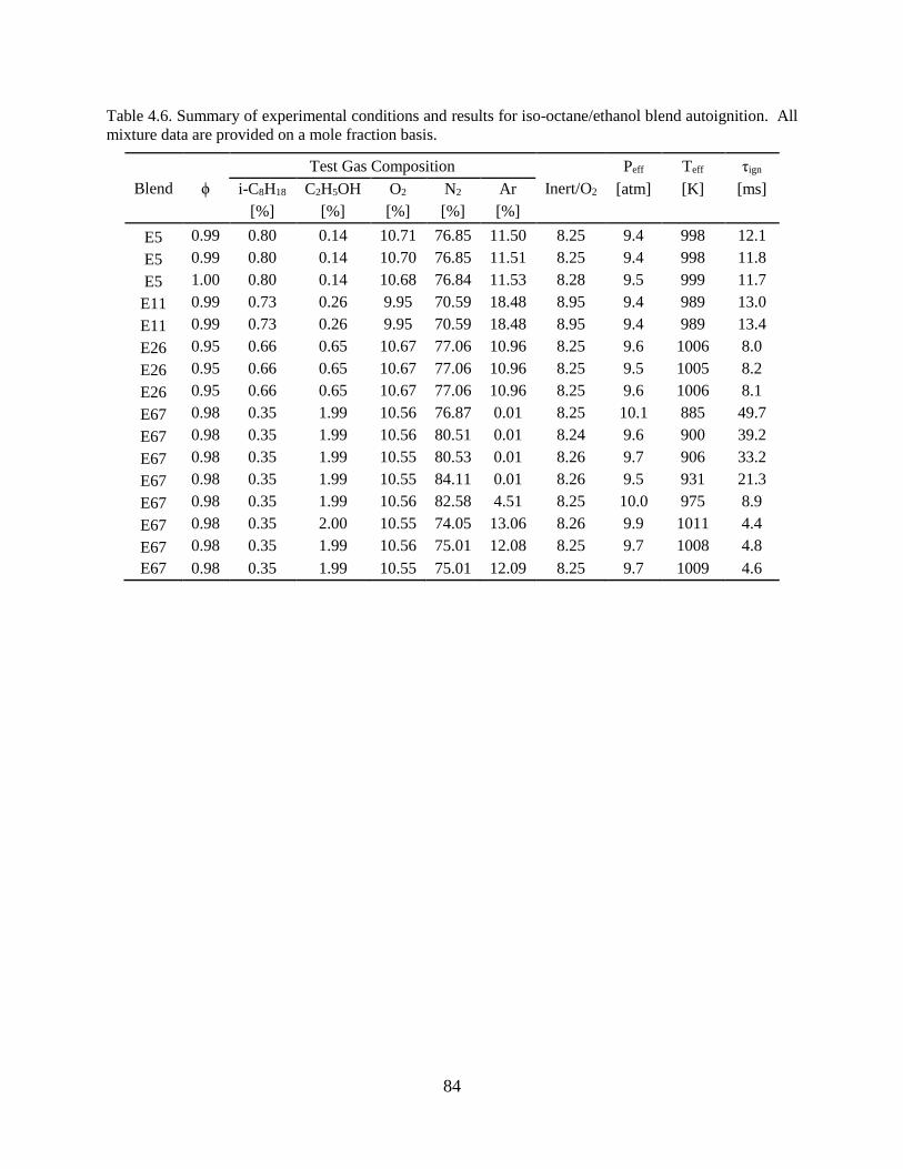
84

Table 4.6. Summary of experimental conditions and results for iso-octane/ethanol blend autoignition. All

mixture data are provided on a mole fraction basis.

Blend ϕ


Inert/O2

Peff Teff τign

i-C8H18 C2H5OH O2 N2 Ar [atm] [K] [ms]

[%] [%] [%] [%] [%]

E5 0.99 0.80 0.14 10.71 76.85 11.50 8.25 9.4 998 12.1

E5 0.99 0.80 0.14 10.70 76.85 11.51 8.25 9.4 998 11.8

E5 1.00 0.80 0.14 10.68 76.84 11.53 8.28 9.5 999 11.7

E11 0.99 0.73 0.26 9.95 70.59 18.48 8.95 9.4 989 13.0

E11 0.99 0.73 0.26 9.95 70.59 18.48 8.95 9.4 989 13.4

E26 0.95 0.66 0.65 10.67 77.06 10.96 8.25 9.6 1006 8.0

E26 0.95 0.66 0.65 10.67 77.06 10.96 8.25 9.5 1005 8.2

E26 0.95 0.66 0.65 10.67 77.06 10.96 8.25 9.6 1006 8.1

E67 0.98 0.35 1.99 10.56 76.87 0.01 8.25 10.1 885 49.7

E67 0.98 0.35 1.99 10.56 80.51 0.01 8.24 9.6 900 39.2

E67 0.98 0.35 1.99 10.55 80.53 0.01 8.26 9.7 906 33.2

E67 0.98 0.35 1.99 10.55 84.11 0.01 8.26 9.5 931 21.3

E67 0.98 0.35 1.99 10.56 82.58 4.51 8.25 10.0 975 8.9

E67 0.98 0.35 2.00 10.55 74.05 13.06 8.26 9.9 1011 4.4

E67 0.98 0.35 1.99 10.56 75.01 12.08 8.25 9.7 1008 4.8

E67 0.98 0.35 1.99 10.55 75.01 12.09 8.25 9.7 1009 4.6

85

Table 4.7. Summary of results for speciation experiments of iso-octane and E50 with an asterisk (*) in Table 4.4 and Table 4.5**. Data are arranged

in ascending order of t/τign for each blend.

Blend Time τign

t/τign i-C8H18 i-C4H8 C3H6 C2H6 CO C2H5OH CH3CHO C2H4 CH4 CO2 C2H2 CH3COCH3 i-C5H10 i-C3H5CHO

[ms] [ms] [ppm] [ppm] [ppm] [ppm] [ppm] [ppm] [ppm] [ppm] [ppm] [ppm] [ppm] [ppm] [ppm] [ppm]

E0 6.4 37.4 0.15 9,190 166 24 1 -- -- 1 10 26 -- -- -- -- --

E0 11.0 36.7 0.27 9,112 372 45 4 -- -- 0 2 43 -- -- -- -- --

E0 13.6 31.8 0.40 8,464 681 129 8 -- -- 1 6 85 -- -- -- -- --

E0 19.1 34.6 0.52 7,394 712 198 15 -- -- 4 20 104 -- -- -- -- --

E0 23.2 31.8 0.70 5,015 1,185 364 23 -- -- 21 27 203 -- -- 43 -- 36

E0 24.0 32.4 0.71 7,725 984 303 20 -- -- 10 29 182 -- -- -- -- --

E0 30.1 37.4 0.78 4,055 864 282 18 -- -- 3 26 167 -- -- -- -- --

E0 33.2 34.6 0.93 3,868 1,252 584 54 2,478 -- 131 141 477 986 -- 136 41 96

E50 3.6 19.9 0.13 5,614 24 -- 10 -- -- 39 16 14 -- -- -- -- --

E50 4.1 19.7 0.16 5,443 41 16 6 -- -- 76 13 13 -- -- -- -- --

E50 8.3 24.7 0.30 5,253 79 35 4 -- -- 725 30 27 -- -- -- -- --

E50 8.6 18.2 0.42 4,818 154 61 5 -- 13,632 219 52 50 -- -- -- -- --

E50 9.8 15.9 0.55 2,813 221 77 6 -- 9,492 650 73 85 -- -- -- -- --

E50 13.7 18.2 0.70 2,933 502 183 14 -- 12,717 765 187 189 -- -- -- -- --

E50 15.6 19.9 0.73 2,631 392 181 11 -- -- 21 136 146 -- -- -- -- --

E50 16.7 19.7 0.80 3,799 601 235 24 -- -- 259 263 313 -- -- -- -- --

E50 14.7 16.2 0.85 2,947 885 406 49 1,735 10,574 1,249 445 508 756 -- 54 20 44

E50 22.1 24.7 0.85 3,459 733 255 33 -- -- 423 318 366 -- -- -- -- 30

E50 16.8 15.9 1.00 1,756 300 230 108 7,727 4,136 794 660 834 32,262 305 -- -- --

** “--” indicates concentrations below the detectable limits of the instrument.

86

Chapter 5 Physico-Chemical Interactions of Ethanol and Iso-Octane

5.1 Introduction

The ignition of liquid fuels in ICEs involves overlapping physical processes that produce

an auto-ignitable mixture and chemical reactions that transform reactants into intermediates and

products. The distinction between the physical and chemical processes in direct-injection engines

is difficult to assess experimentally due to the complex geometry of the combustion chamber and

the high turbulence in the charge, which affect fuel distribution, spray evaporation and mixing

with the air [111]. Additionally, the changing properties of the compressed air during the ignition

delay period complicate the quantification of the effects of engine charge temperature and pressure

on the total ignition delay. Constant-volume devices, on the other hand, provide a nominally

quiescent environment before the start of injection and much smaller changes in the charge

temperature and pressure during the ignition delay period than piston engines [111]. Such

characteristics make them suitable tools to quantify the contributions of physical phenomena to

the ignition time scales of ethanol/iso-octane blends.

Direct-injection constant-volume chambers, like ignition quality testers (IQTs), are

powerful experimental tools. They have been utilized to measure liquid fuel ignition delays of

low-volatility fuels and surrogates to observe NTC behavior [53,112–116], to calculate low- and

high-temperature apparent heat release [111,112], to develop correlations for research and motor

octane numbers (RON and MON) [117–119], to assist the validation of chemical kinetic [112,120]

87

and CFD [116,121] models, and to estimate physical and chemical effects on delay periods

[111,120,122,123].

As discussed in detail below, the objective of this portion of the dissertation research was

to quantify the effects of different fuel blends on ignition measurements in an IQT. Specifically,

the data were analyzed to identify the physical and chemical contributions to the total ignition

delay time and the changes in these characteristic times as a function of the fuel composition.

Reconciliation of the results for the spray studies with the chemical kinetics measurements made

in the RCF was another goal of this part of the research. Other researchers have used IQT data to

evaluate the chemical and physical contributions to ignition behavior. Zheng et al. [111] used an

IQT to determine the physical and chemical delay periods of ultra-low sulfur diesel fuel, jet

propellant-8 fuel and two synthetic fuels by comparing the results of injecting the fuels into air

(according to the ASTM D6890-10a standard) and injecting the fuels into nitrogen at the same

charge conditions. They defined the end of the physical delay period as the point at which the two

resulting pressure traces separated, and the researchers developed Arrhenius correlations for total,

physical and chemical ignition delays to evaluate the apparent activation energies of each fuel

[111]. They concluded the physical delay period was a significant part of the total delay period,

and the chemical activation energy had an inverse relationship with the cetane number for all the

fuels tested [111]. However, Kim et al. [124] suggested using noticeable heat release as the

physics-to-chemistry transition criterion inherently over-estimates the physical delay by

attributing part of the chemical delay to physical phenomena. IQT studies of isomeric fuels

[120,122,123] have concluded that oxidation chemistry—instead of physical property variations—

is the dominating factor in changes in total ignition delay at ASTM conditions.

88

There are several previous studies of neat fuels and fuel blends using IQT systems,

including studies of iso-octane and ethanol. Osecky et al. [116] used the NREL IQT to observe

the NTC behavior of iso-octane at global equivalence ratios between 0.7 and 1.05, pressures of 1.0

and 1.5 MPa, and temperatures ranging from 653 to 996 K; and to validate single-, multi-zone and

CFD models predicting well-mixed conditions in the main part of the chamber at ~30 ms after

SOI. At similar conditions, Yang et al. [115] utilized an IQT to correlate temperature, pressure

and global equivalence ratio with iso-octane total ignition delay, obtaining an inverse relationship

between global equivalence ratio and total ignition delay in the intermediate-temperature regime.

Haas et al. [122] measured the cetane number of binary blends of ethanol with n-heptane and CF13

(a real distillate diesel fuel) in an IQT as the physical properties of the blends varied, and

demonstrated that blending up to 10% vol. alcohol into the base hydrocarbon resulted in modest

reductions of the cetane number. Bogin et al. [53] investigated the reduction of low-temperature

heat release and NTC behavior with increasing ethanol blending in iso-octane using the NREL

IQT at near-stoichiometric conditions, pressures of 0.5 – 1.5 and a temperature range of 623 – 993

K. They concluded that NTC behavior was observed for blends up to E20, that ethanol addition

produced consistently shorter ignition delays in the high-temperature region, and that increasing

ethanol content from E0 to E10 had lesser impact on ignition delays than increasing from E10 to

E20 [53].

5.2 Objective

The aim of this work is to quantify the effects of spray physics and turbulent mixing on the

global ignition chemistry of ethanol, iso-octane and ethanol/iso-octane blends at the same

experimental conditions of the ethanol and blend studies in Chapter 3 and Chapter 4. The NREL

IQT was utilized to measure liquid fuel ignition delays, τign,liq, of stoichiometric ethanol/iso-octane

89

blends—including E0, E25, E50, E75 and E100—at moderate dilution levels (N2/O2 molar ratios

of 9:1), pressures of ~10 atm, and temperatures ranging from 880 to 970 K. The overall

contribution of spray and mixing physics to the global ignition time scales were determined as a

function of blend levels and charge temperatures by directly comparing the IQT liquid fuel ignition

delay measurements with the chemistry-driven ignition data acquired in the RCF studies. By

further interrogating the pressure time histories of the IQT experiments, time scales and apparent

thermal effects of physical phenomena such as spray injection, breakup, evaporation, turbulent

mixing and heat release were also quantified. Regression analyses provided best-fit Arrhenius

correlations for total, physical and mixing time scales as functions of charge temperature and molar

carbon content in the blend (as surrogates of the different blend levels), which complement the

correlation obtained in Chapter 4 for homogeneous blend ignition. Non-dimensional analyses

connected findings on ignition time scales to fuel properties, experimental conditions, and known

physical principles. The results are discussed on a comparative basis between premixed and non-

premixed global reactivity of ethanol and iso-octane blends.


The results presented in this chapter were obtained using the NREL IQT and following the


results for ignition experiments, and supporting information are provided in Section 5.6. For

reference, the liquid fuel properties of gasoline, iso-octane and ethanol relevant for spray injection,

breakup and evaporation, and turbulent mixing processes are provided in Table 5.1.

90

Table 5.1. Liquid fuel properties of gasoline, iso-octane and ethanol [2,125].

Properties Gasoline Iso-octane Ethanol

MW 111.19 114.23 46.06

O2 (wt%) 0 0 0.35

Viscosity @ 15°C (x10-3 Pa-s) 0.37-0.44 0.47 1.19

Specific gravity @ 20°C 0.72-0.78 0.69 0.79

LHV (MJ/L) 30-33 30.5 21.4

Boiling Point (°C) 27-225 99 78

Heat of Vaporization (kJ/kg) ~351 270 1168

Specific heat @ 15°C (kJ/kg.K) 2.01 2.12 2.39

RON 88-98 100 109

MON 80-88 100 90

Flammability limits @15°C (vol. %) 1.4-7.6 0.79-5.94 4.3-19


Liquid Fuel (Total) and Chemical Ignition Delays

Figure 5.1 presents a comparison of typical pressure and pressure-derivative time histories

of stoichiometric mixtures of E0, E50 and E100 obtained from liquid fuel ignition delay

experiments in the NREL IQT. PSOI represents the pressure of the oxidizer mixture (10% O2 in

N2) inside the IQT chamber at the start of the fuel injection, which is defined as the time

corresponding to 1% of the maximum needle lift of the injector for each experiment. As the fuel

injection progresses, the pressure in the chamber decreases slightly due to the cooling effect on the

charge mixture caused by the evaporation of the fuel. After the ignition delay period, the pressure

rapidly increases as a result of auto-ignition and the associated heat release. For this study, the

liquid fuel ignition delay (τign,liq or τtotal) was defined as the time interval between the start of

injection (SOI) and the maximum rate of change in the chamber pressure, (dP/dt)max. All data in

this work presented similar behavior of post-SOI charge cooling, followed by nominally constant

pressure during the delay period and rapid heat release due ignition.

91

Figure 5.1. Typical pressure (solid lines) and pressure derivative (dashed lines) time histories in the IQT

for liquid fuel ignition experiments of E0 (red), E50 (blue) and E100 (green).

As in previous IQT studies [53,116], SOI pressure and temperature were used as the state

conditions for each experiment given the steady and homogeneous characteristics inside the IQT

chamber at SOI. The experimental conditions were similar for each of the blends presented in

Figure 5.1, with ≈ 1.00, Peff ≈ 9.9 atm, Teff ≈ 943 K and molar dilution of N2/O2 = 9.0. The

charge cooling effects are accounted for as the contribution of spray injection, spray breakup and

evaporation processes to the liquid fuel ignition delay from the start of injection to the time when

the charge pressure reaches a minimum value, Pmin. (A more detailed discussion on this approach

to defining the physical effects contributing to the liquid ignition delay time is provided in the next

section.) Figure 5.1 shows almost identical pressures until near the time of ignition for each

mixture, but with slight differences around Pmin that are attributed to variations in the cooling

effects as the composition of the fuel blends change. Figure 5.1 also shows the liquid fuel ignition

delays consistently decreased with increasing ethanol content in the blend, which corresponded

very well with the behavior observed for chemical ignition delay times in Chapter 4. During

ignition, the rates of pressure rise and the peak pressures also decreased with increasing ethanol

92

addition due to the lower energy content of pure ethanol with respect to pure iso-octane at

stoichiometric conditions.

Summaries of the results for τign,liq are presented in Figure 5.2 and Table 5.2 – Table 5.6.

Symbols in Figure 5.2 correspond to ignition delay measurements of this work for E0, E25, E50,

E75 and E100 at 9.9 atm (with an average uncertainty of –0.5 atm, which are negative as they

account for the charge cooling after SOI) and a dilution level of N2/O2 = 9.0. Four SOI charge

temperatures were measured in this study for each blend, with averages of 883 K, 913 K, 943 K

and 972 K for all the experiments. As recommended by the ASTM D6890 standard, 15 pre-

injections and 32 main injections were carried out at each set of conditions. Out of the 32 main

injections, five representative ignition events presenting the lowest injection-to-injection

temperature variability were analyzed and are presented in Figure 5.2. Experimental uncertainties

for the ignition delay measurements, presented as vertical error bars (±5.3 ms on average),

represent the accuracy of determining the time for (dP/dt)max during the heat release period of each

experiment. Temperature error bars (–12.4 K on average) were calculated as the equivalent

standard deviation of the time-varying overall charge temperature due to evaporative cooling

effects with respect to the charge temperature at SOI. Temperature-time histories were estimated

from transient adiabatic expansion calculations using the pressure-time histories from SOI to Pmin

assuming homogeneous conditions; hence, the temperature uncertainties only account for an

equivalent overall cooling effect and not for localized charge cooling in the near-spray jet zone.

The typically larger temperature error bars as ethanol content increases are consistent with the

higher specific heat and heat of vaporization of ethanol with respect to iso-octane (see Figure 5.2

and Table 5.1). For the sake of clarity, only the temperature uncertainty bars for E0, E50 and E100

are presented in Figure 5.2, although the values are consistent across blends.

93

Figure 5.2. Experimental results of liquid fuel ignition delays for stoichiometric mixtures of E0, E25, E50,

E75, and E100 fuels. Regression fits to the experimental data are provided as dash-dotted lines.

Liquid fuel ignition delay data in Figure 5.2 exhibited excellent repeatability and low

scatter of ±4.9% on average. All the data showed clear Arrhenius behavior for τign,liq within the

883 – 972 K temperature range studied, with pure iso-octane (E0) consistently presenting lower

reactivity than pure ethanol (E100). The addition of 25% of ethanol to iso-octane caused a

significant decrease on the liquid fuel ignition delay (greater than the uncertainty and scatter in the

data), while increasing the blend level from E25 to E50 produced a more modest reactivity increase

(within the uncertainty and scatter in the data). Increasing the ethanol content by 25% from E50

to E75 and E100, progressively reduced the average liquid fuel ignition delay with respect to E0,

although the E75 data fell within the uncertainties and scatter of the E50 and E100 data for all the

temperatures in this study.

To better observe τign,liq trends, a regression analysis was applied to all the liquid fuel

ignition data and a best-fit Arrhenius expression of the form τign,liq = A (CB)d exp(Ea/RT) were

determined, where CB is the molar carbon content in each fuel blend. The regression trendlines

94

for E0, E50 and E100 are included in Figure 5.2 (dash-dotted lines), along with the Arrhenius

expression. The quality of the fit to the data was excellent for the temperature range studied as

indicated by the R2 value of 0.99.

Figure 5.3 presents summaries of the liquid fuel ignition delay data from IQT experiments

(open symbols as in Figure 5.2) and ignition delay time measurements from RCF experiments

(filled symbols as in Figure 4.3) along with regression correlations and trendlines for E0, E50 and

E100. The experimental conditions for the IQT experiments—namely SOI pressures and

temperatures—were selected to match the corresponding effective conditions for RCF experiments

for a direct comparison between data sets. The effects of spray injection, breakup and turbulent

mixing in the IQT yield longer ignition delays with respect to the chemistry-driven ignition delay

times in the RCF for all the blends studied. The trend of increased reactivity with ethanol addition

for the IQT experiments was consistent with the observed behavior for the RCF experiments,

regardless of the variations of the physical properties of the fuel blend with increasing ethanol

addition. However, the lower apparent activation energy and regression coefficient of CB for IQT

data indicates that liquid fuel ignition delay is less sensitive to variations of state temperatures and

blend levels than the chemical ignition delay on a relative basis.

The experimental results are also compared with model predictions using the Mehl et al.

[84] kinetic model for 0-D adiabatic constant-volume simulations in CHEMKIN at the

corresponding state conditions for RCF and IQT experiments (see Figure 4.3). As the kinetic

model tends to predict up to ~30% faster ignition delay times for E0 and E50 at temperatures lower

than 1000 K, larger differences between liquid fuel ignition delays and chemical ignition delay

times could be mistakenly assigned as the contribution of spray and mixing physics to the global

ignition delays. Instead, either the chemical ignition delay data or the regression correlations

95

obtained in Chapter 4 provide a direct representation of the difference between liquid fuel and

chemical ignition delays within the variability of the temperature fields of the two experimental

facilities. As the onset of NTC behavior is expected for temperatures lower than 800 K for E0 at

~10 atm [53], the use of the regression should be limited to the temperature ranges of this study.

As chemical ignition delay predictions for E100 are in excellent agreement with the experimental

data and no NTC behavior is expected for lower temperatures, differences in ignition time scales

can be estimated from IQT ignition experiments and model simulations for T < 880 K with high

confidence for E100 and with good confidence for other blend compositions.

Figure 5.3. Comparison of liquid fuel ignition delays from IQT experiments and ignition delay times from

the RCF data in Chapter 3 and Chapter 4 for stoichiometric mixtures of E0, E50 and E100 and inert/O2 =

9.0. Model predictions are based on the reaction mechanism by Mehl et al. [84] (solid lines). Regressions

for both sets of data are provided.

Liquid fuel ignition delay measurements for E0 and E100 were also scaled to E50 and are

included in Figure 5.4 along with scaled chemical ignition delay data in Figure 4.5. As in Chapter

4, the power of the carbon content (CB) from the regression analysis of τign,liq (d = 0.43) was used

to scale the data to CB = 3.56 (i.e. E50). The data for E0 and E100 collapsed to a single trendline

96

around the unscaled E50 data with minor scatter, which is consistent with the RCF data. The high

quality of the Arrhenius fit included in the figure indicates that no NTC behavior is present for iso-

octane, ethanol and the blends at 10 atm and 880 – 970 K, which is also consistent with the

chemical ignition delay experiments. For reference, the model predictions using the Mehl et al.

reaction mechanism [84] are included, where the trend to slightly underpredict the chemical

ignition delay (by approximately 34%) is observed for T < 950 K.

Figure 5.4. Summary of scaled liquid fuel ignition delays (open symbols) and chemical ignition delay times

(filled symbols) of the data presented in Figure 5.3 for stoichiometric blends at P = 10 atm and inert/O2 =

9.0. The corresponding regression coefficient of CB for each ignition delay correlation was used to scale

the E0 and E100 ignition data to E50 blend level. Model predictions using the reaction mechanism by Mehl

et al. [84] (solid lines) are provided.

Figure 5.5 presents the total and chemical ignition delay measurements as a function of the

atomic carbon content in the blend for ~10 atm, inert/O2 = 9.0 and ~913 K, along with the

respective regression trendlines and predictions using the Mehl et al. model [84] similar to Figure

4.6 for RCF experiments. Both data sets show increasing reactivity as more ethanol is added to

the blend. Again, consistent longer total ignition delays with respect to chemical ignition delays

are presented for all the bends studies at ~913 K. However, the exponential relationship of τtotal

97

with inverse temperature in Figure 5.3 suggest that oxidation chemistry may also play a significant

role during the physical processes taking place right after SOI. To analyze those potential effects,

different physical time scales are analyzed as function of blend levels and charge temperature in

the next section.

Figure 5.5. Effects of ethanol addition on total and chemical ignition delays at ~913 K for P = 10 atm and

molar ratio of inert/O2 = 9.0.

Physical Contributions to Ignition Delay

In order to quantify the contribution of spray physics and turbulent mixing to the overall

ignition delay of ethanol, iso-octane and their blends, comparative metrics were defined by

overlapping the pressure and pressure-derivative time histories of IQT and RCF experiments at the

same state conditions. Figure 5.6 presents such metrics for E0 and T = 943 K, where τtotal (or

τign,liq) represents the overall ignition delay that accounts for spray, mixing and chemistry effects

as measured in the IQT while τchem only accounts for the chemical ignition delay time obtained

from homogenous ignition experiments in the RCF. As τtotal will always be larger than τchem, the

difference between the two characteristic times was defined as the contribution of physical

98

phenomena to the ignition delay, τphys, which differs from the definition of the physical delay

period used by Zheng et al. [111] where only physics—with no chemistry—take place. The

definition used in the current work acknowledges that chemical reactions may take place right after

the evaporation process starts and during the mixing process—usually where local equivalence

ratios range between 1.0 and 2.0 [126], although the heat release is not significantly observable in

the pressure trace during this time frame. Physical phenomena may continue to play a role near

the time of the ignition event as the rate of pressure rise is slower for liquid fuel ignition

experiments, potentially due to the higher mixture and thermal stratification resulting from the

mixing process.

Figure 5.6. Comparison of typical pressure (solid lines) and pressure derivative (dot-dashed lines) time

histories in the IQT for liquid fuel ignition experiments (blue) with RCF chemical ignition delay

experiments (red).

τphys can further be differentiated by the duration of the combined spray injection, breakup

and evaporation processes (τevap) and the gross of the turbulent mixing process (τmix). τevap is

defined as the period between the SOI and the time corresponding to Pmin, and strictly represents

the observable charge cooling effects caused by the evaporation of the fuel. τmix is the difference

between τphys and τevap, and corresponds to the period when the dominant physical phenomenon is

99

turbulent mixing, although chemical reactions can occur without significant heat release. In

addition to the characteristic time scales, the apparent effects of charge cooling and heat release

have been estimated by integrating the rate of pressure change (dP/dt) between SOI and Pmin, and

Pmin and the maximum pressure caused by ignition (Pmax), respectively. Figure 5.7 shows details

of the method used to estimate the apparent cooling/heat release for the IQT data presented in

Figure 5.6. The comparison of apparent heat release between the IQT and RCF experiments

presented in Figure 5.6 indicates that, although IQT experiments present a slower rate of heat

release close to the time of the ignition event, the magnitude of the heat released is comparable to

those the heat released during the RCF experiment. The effects of charge cooling on the ignition

time scales are presented in the next section.

Figure 5.7. Estimation method for apparent charge cooling and heat release for the IQT data presented in

Figure 5.6.

Figure 5.8 presents a summary of the overall physical contribution to the total ignition

delay, τphys, as a function of carbon content in the blend and temperature. Again, τphys represents

the contribution to the total ignition delay caused by spray injection, spray breakup and fuel

evaporation, and the turbulent mixing processes. τphys data were determined by subtracting

100

chemical ignition delay (τchem) data (from the RCF) from the total ignition delay (τtotal) IQT

measurements for data acquired at the same blend level and the same temperature (within the

respective uncertainties). Data presented in Figure 5.8 shows the largest value of τphys occurred at

883 K (the lowest charge temperature in the study) for all the blends, and τphys consistently

decreased as the ethanol content in the blend increased at constant charge temperatures. Increases

in charge temperatures tended to reduce τphys for each blend with the minimum values of τphys at

972 K. Increasing charge temperatures also reduced the sensitivity of τphys to ethanol addition.

Regression analysis applied to τphys data produced the best-fit Arrhenius expression included in

Figure 5.8 with an R2 value of 0.96. The lower apparent activation energy and regression

coefficient of CB for the τphys data with respect to τtotal and τchem indicate the lower sensitivity to

variations in temperatures and blend levels.

Figure 5.8. Overall contribution of spray and mixing physics to total ignition delay as a function of the

carbon content in the blend (blend level) and temperature.

In order to differentiate the effects of physical phenomena taking place during the total

ignition delay, Figure 5.9 presents two characteristic time scales for the spray injection, breakup

101

and evaporation processes, and turbulent mixing. Again, τevap is defined as the period during which

the spray injection, spray breakup and fuel evaporation processes take place as indicated by the

charge cooling effects observable in the chamber pressure data (i.e. from the time of SOI to the

time of Pmin). τmix is the result of subtracting τevap from τphys, and represents the period during

which turbulent mixing is the dominant physical phenomenon to produce a globally ignitable

mixture. Figure 5.9 shows that τevap has a relatively small contribution to τphys as well as negligible

variation with changes in the blend levels and charge temperatures when compared with those of

τmix. Hence, τevap was assumed as a constant delay period with an average value of 4.3 ±0.8 ms.

Figure 5.9. Contribution to total ignition delay from spray physics (injection, breakup and evaporation),

and from turbulent mixing as function of the carbon content in the blend (blend level) and temperature.

On the other hand, τmix showed greater sensitivity to charge temperature and blend level

changes with similar trends to τphys. The largest values of τmix were obtained at 883 K for all the

blends, and τmix progressively decreased as the ethanol content in the blend increased at constant

charge temperatures. Increases in charge temperatures also reduced τmix consistently for each

blend until reaching minimum values at 972 K, and the sensitivity of τmix to changes in ethanol

102

content. A regression analysis of τmix as a function of state temperature and carbon content in the

blend produced the Arrhenius expression presented in Figure 5.9 with an R2 value of 0.96. The

slightly higher apparent activation energy and regression coefficient of CB for the regression of

τmix regression with respect to the corresponding to τphys confirmed that turbulent mixing is the

dominating physical process that allows to achieve a globally ignitable mixture in the chamber.

When compared with the regression coefficients of τchem, the smaller Arrhenius parameters of τmix

shows its lower sensitivity to temperature and blend level variations.

Figure 5.10 presents a summary of average ignition time scales for the blends of this study

as stacked bar charts. The sum of τevap and τmix represents the physical contribution to the total

ignition delay (τphys), which added to the chemical ignition delay (τchem) provides the total ignition

delay (τtotal or τign,liq). Figure 5.10 shows that τevap remains almost constant across blends and

temperatures while increases of the ethanol content in the blends at the same state temperatures

tend to reduce both τchem and τtotal. Minimal to negligible changes are observed for τmix between

E25 and E50, and between E75 and E100 when keeping constant temperature; hence, most of the

variation of τtotal in such blends is attributed to τchem. For each blend, increases in charge

temperature progressively reduce τmix in a consistent trend with τchem as a function of increasing

temperature.

Although τchem values are consistently shorter than τmix for all the blend levels and

temperatures studied, significant oxidation chemistry is likely taking place simultaneously with

the gas-phase turbulent mixing given the exponential correlation of τmix with the inverse of charge

temperature. Since the effects of chemical reactions are not observable in the pressure time

histories as a global apparent heat release during τmix, localized reactions are expected to occur

103

instead due to mixture and thermal stratification caused by the spray injection and fuel evaporation

processes.

Figure 5.10. Summary of average chemical and physical time scales at different blend levels and initial

charge temperatures.

Since the turbulent mixing and oxidation chemistry phenomena cannot be decoupled as

sequential processes, the relative impacts of relevant liquid fuel properties on τphys and τmix were

evaluated using τchem to calculate two Damköhler numbers for convective transport and turbulent

mixing, respectively. Density, viscosity, specific heat and heat of vaporization were selected as

the most relevant liquid fuel properties that can affect ignition time scales based on the constant-

volume CFD study developed by Kim et al. [126], where the physical properties of an n-dodecane

spray were individually varied for diesel relevant conditions. Figure 5.11 and Figure 5.12 present

the effects of varying liquid blend properties on the Damköhler number corresponding to

convective transport and gas-phase turbulent mixing.

104

The convective Damköhler number (Da) relates the spray-induced convection time scales

(τphys)—deducted from comparing IQT and RCF experiments—with the chemical reaction

timescales (τchem)—obtained from the RCF—and is defined as Da = τphys/τchem. In Figure 5.11, the

Reynolds number at the nozzle exit, Respray, was used to evaluate the effects of density and

viscosity variations on Da. To calculate the Reynolds numbers (Respray = uinj.dnozzle/ν), blend

densities (ρ) and viscosities (μ) were determined using the properties of iso-octane and ethanol in

Table 5.1, and the Gambill method to determine kinematic viscosities (ν = μ/ρ). The injection

velocity was determined using Bernoulli’s equation and the coefficient of velocity (Cv = Cd = 0.8)

of the IQT injector as 𝑢𝑖𝑛𝑗 = 𝐶𝑣√2∆𝑃 𝜌⁄ , where ΔP is the pressure drop between the injector and

the chamber (Pinj – Pcharge), which was maintained at a constant value for all the IQT experiments

in this study. Hence, Respray represents the driving force for turbulent liquid-gas and gas-gas

mixing processes inside the initially quiescent chamber. Figure 5.11 presents the effects of the

fluid flow properties—given by Respray—on the contribution of physics phenomena to the total

ignition delay relative to the blend chemistry effects—defined by Da—as a function of charge

temperature and blend level.

For each temperature studied, ethanol addition to the blend increased its kinematic

viscosity and—in a lesser degree—the injection velocity producing lower Reynolds numbers,

which tended to reduce the turbulent mixing rates in the chamber. These effects are observed as

larger Damköhler numbers resulting from consistently higher physical contribution to the total

ignition delay (τphys) relative to the higher reactivity of blends with increased ethanol content

(which produce shorter chemical ignition delays, τchem). Increasing the charge temperature would

initially increase the spray air entrainment and evaporation rates, as well as the turbulent thermal

diffusivity—due to higher specific heat—of the fuel in the charge [126], which would reduce τphys.

105

However, Da is significantly increased at higher temperatures due to the exponential relationship

of τchem with inverse temperature, which consistently outweighs the effects of higher mixing rates

as the ethanol content in the blend is increased. In practical ICE applications at equivalent charge

conditions, smaller Da values should be expected for these blends due to more complex geometries

and changing volume of the combustion chamber, which generate higher turbulence in the charge.

Figure 5.11. Effects of spray Reynolds number, ethanol addition and state temperature on convective

Damköhler number for the conditions of the IQT and RCF studies.

A second Damköhler number is used for gas-gas turbulent mixing (Damix) to evaluate the

effects of different amounts of charge cooling on the mixing time scale, and is defined as Damix =

τmix/τchem. The total effect of charge cooling due to fuel vaporization is given by the amount of

heat that is transferred from the charge to the liquid droplets of fuel. The magnitude of the charge

cooling effect depends on both the heat capacity and the heat of vaporization of the liquid droplets

of fuel at the charge pressure and the temperature of each droplet during τevap. Due to the mixture

and thermal stratification caused along the axis of the chamber by fuel injection, spray breakup

and evaporation of the first fuel droplets, estimating the overall charge cooling effect using energy

106

balances and spray evaporation models becomes challenging. Instead, the values for apparent

charge cooling deduced from the IQT pressure-time histories were used to represent the combined

thermal effects of the blend injected mass, heat capacity and heat of vaporization on the gas-phase

turbulent mixing process. This approach assumes the apparent charge cooling is a global instead

of a localized effect, and that charge cooling mostly affects the gas-phase turbulent mixing after

the vaporization process has completed. The negligible contribution of τevap to τphys—both in

magnitude and variability—corresponded well with changes in liquid physical properties at

different state temperatures and blend levels. Taking place in a pseudo-sequential manner during

τevap, spray injection, spray breakup and fuel evaporation processes set the initial conditions for the

gas-phase turbulent mixing process. As seen in Figure 5.6 and Figure 5.7, the effects of charge

cooling are observed as changes in the pressure and pressure derivative in the IQT chamber. For

this discussion, the charge cooling effects were quantified for each IQT experiment by integrating

the dP/dt data over the time of charge cooling. The result was defined as the Apparent Charge

Cooling with units of pressure (atm).

Figure 5.12. Effects of apparent charge cooling, ethanol addition and charge temperature on the turbulent

mixing Damköhler number for the conditions of the IQT and RCF studies.

107

Figure 5.12 presents the determinations for Damix as a function of the Apparent Charge

Cooling for the different temperatures and blend levels studied. The Apparent Charge Cooling

increased with progressive addition of ethanol to the blend, which corresponds well with the higher

heat capacity and higher heat of vaporization of ethanol with respect of iso-octane (see Table 5.1).

There is also a slight trend of higher Apparent Charge Cooling with increasing charge temperatures

for each blend which is attributed to lower charge mixture densities while maintaining a constant

fuel mass injection for each blend.

For a given charge temperature, higher charge cooling effects caused by increasing ethanol

content in the blend produces lower local mixture temperatures, which reduces the local reactivity

of the mixture at earlier times just after fuel vaporization have taken place. As a result, longer

mixing times are required for the mixture in the chamber to achieve the degree of local reactivity

of a less thermally stratified mixture with the same homogeneous reactivity. This is mainly due to

the lower turbulent mass diffusivity caused by the higher density of ethanol. For a given blend

level, increasing the charge temperature will likely increase the turbulent thermal diffusivity due

to higher heat capacities of the charge. Once again, the combination of the previous competing

effects on τmix are overshadowed by the higher reactivity of ethanol and the exponential

relationship of τchem to the inverse temperature, which produces increasing Damix values with

ethanol addition and consistently higher charge temperatures as seen in Figure 5.12.

5.5 Conclusions

The results of this study provide new experimental data of the ignition of liquid fuel blends

of ethanol and iso-octane. The liquid fuel ignition delay time measurements showed the reactivity

of the ethanol/iso-octane blends was bounded by the ignition delays of iso-octane as the longest

delay and ethanol as the shortest delay time at the temperatures and pressures studied. Progressive

108

addition of ethanol to iso-octane increased the overall reactivity of the liquid blend to the high

reactivity limit defined by pure ethanol in a non-linear manner. These results are similar in trend

to the reactivity behavior obtained from homogeneous/chemical ignition delay times

measurements, which indicates the combustion chemistry tends to dominate the behavior of the

total ignition delay of liquid ethanol/iso-octane fuel blends as a function of temperature.

Comparative analysis of the liquid fuel and chemical ignition delays allowed estimates of physical

time scales where the fuel injection, breakup and vaporization processes and gaseous turbulent

mixing were identified as most relevant and were quantified together and separately. The

Arrhenius behavior of the turbulent mixing time scales indicated that, although no observable heat

is released, chemical reaction consistently occurred during the physical mixing time. A non-

dimensional analysis of the relative physical time scales with respect to chemical ignition delay

demonstrated that changes in the fluid flow and thermal properties—as more ethanol is added to

the blend—affect the physical time scales significantly if chemical reactivity remained unchanged.

However, the exponential relationship of the ignition time scales with temperature dominated the

total contribution of spray and mixing physics to the total ignition delay.


109

Table 5.2. Summary of experimental conditions and results for E0 liquid fuel autoignition in the IQT. All mixture data are provided on a mole

fraction basis.

ϕ mfuel-inj

Re

Target Mixture

Composition Tcharge Pcharge Apparent

Cooling τign,liq τchem τphys τevap τmix

Da i-C8H18 C2H5OH O2

[mg] [%] [%] [%] [K] [atm] [atm] [ms] [ms] [ms] [ms] [ms]

0.96 24.0 38,248 0.76 0.00 9.92 883.27 9.86 0.56 274.44 115.11 159.33 4.00 155.33 1.38

0.96 24.0 38,240 0.76 0.00 9.92 883.43 9.86 0.55 257.76 114.70 143.06 3.80 139.26 1.25

0.96 24.0 38,231 0.76 0.00 9.92 883.34 9.88 0.54 274.24 114.93 159.31 3.36 155.95 1.39

0.96 24.0 38,400 0.76 0.00 9.92 883.37 9.90 0.57 267.32 114.84 152.48 4.52 147.96 1.33

0.96 24.0 38,543 0.76 0.00 9.92 883.42 9.85 0.54 258.76 114.72 144.04 3.40 140.64 1.26

0.99 24.0 38,156 0.78 0.00 9.92 911.15 9.86 0.55 179.52 59.12 120.40 3.92 116.48 2.04

0.99 24.0 38,265 0.78 0.00 9.92 911.03 9.85 0.51 174.16 59.12 115.04 3.40 111.64 1.95

0.99 24.0 38,104 0.78 0.00 9.92 911.31 9.86 0.54 184.76 59.12 125.64 4.04 121.60 2.13

0.99 24.0 38,180 0.78 0.00 9.92 910.62 9.89 0.50 167.40 59.12 108.28 4.32 103.96 1.83

0.99 24.0 38,206 0.78 0.00 9.92 911.56 9.89 0.53 177.84 59.12 118.72 4.24 114.48 2.01

1.02 24.0 38,375 0.81 0.00 9.92 941.33 9.86 0.62 119.90 34.64 85.26 4.96 80.30 2.46

1.02 24.0 38,308 0.81 0.00 9.92 941.44 9.87 0.63 121.50 34.64 86.86 3.54 83.32 2.51

1.02 24.0 38,358 0.81 0.00 9.92 941.66 9.87 0.65 116.88 34.64 82.24 3.54 78.70 2.37

1.02 24.0 38,527 0.81 0.00 9.92 941.37 9.85 0.63 121.28 34.64 86.64 4.18 82.46 2.50

1.02 24.0 38,282 0.81 0.00 9.92 941.73 9.90 0.63 116.96 34.64 82.32 4.14 78.18 2.38

1.06 24.0 38,610 0.84 0.00 9.92 971.59 9.85 0.66 82.60 20.95 61.65 3.52 58.13 2.94

1.06 24.0 38,719 0.84 0.00 9.92 971.27 9.82 0.63 80.44 20.95 59.49 3.62 55.87 2.84

1.06 24.0 38,417 0.84 0.00 9.92 972.16 9.85 0.66 80.58 20.95 59.63 3.50 56.13 2.85

1.06 24.0 38,384 0.84 0.00 9.92 972.24 9.87 0.64 76.10 20.95 55.15 3.50 51.65 2.63

1.06 24.0 38,383 0.84 0.00 9.92 971.98 9.91 0.64 81.80 20.95 60.85 4.08 56.77 2.90

110


fraction basis.

ϕ mfuel-inj

Re

Target Mixture





0.95 26.7 29,523 0.61 0.58 9.88 883.27 9.92 0.58 201.00 80.91 120.09 4.08 116.01 1.48

0.95 26.7 29,634 0.61 0.58 9.88 883.16 9.88 0.58 210.80 81.11 129.69 3.84 125.85 1.60

0.95 26.7 29,634 0.61 0.58 9.88 883.40 9.85 0.63 186.04 80.68 105.36 3.84 101.52 1.31

0.95 26.7 29,861 0.61 0.58 9.88 883.51 9.82 0.62 205.80 80.49 125.31 4.04 121.27 1.56

0.95 26.7 29,822 0.61 0.58 9.88 883.46 9.90 0.60 203.04 80.57 122.47 3.76 118.71 1.52

0.98 26.7 29,562 0.63 0.60 9.88 912.81 9.88 0.60 120.42 43.16 77.26 3.64 73.62 1.79

0.98 26.7 29,667 0.63 0.60 9.88 912.70 9.84 0.64 132.28 43.26 89.02 4.50 84.52 2.06

0.98 26.7 29,673 0.63 0.60 9.88 912.46 9.85 0.67 139.02 43.48 95.54 3.62 91.92 2.20

0.98 26.7 29,790 0.63 0.60 9.88 912.42 9.83 0.63 134.90 43.51 91.39 3.62 87.77 2.10

0.98 26.7 29,712 0.63 0.60 9.88 912.69 9.84 0.68 136.48 43.27 93.21 3.64 89.57 2.15

1.01 26.7 29,432 0.65 0.62 9.87 942.76 9.90 0.62 87.92 23.76 64.16 4.86 59.30 2.70

1.01 26.7 29,477 0.65 0.62 9.87 942.44 9.90 0.69 90.14 23.91 66.23 3.42 62.81 2.77

1.01 26.7 29,529 0.65 0.62 9.87 942.33 9.89 0.69 90.68 23.96 66.72 3.60 63.12 2.78

1.01 26.7 29,660 0.65 0.62 9.87 942.31 9.86 0.69 88.46 23.97 64.49 4.06 60.43 2.69

1.01 26.7 29,621 0.65 0.62 9.87 942.53 9.89 0.71 95.20 23.86 71.34 4.04 67.30 2.99

1.04 26.7 29,418 0.67 0.63 9.87 972.64 9.88 0.63 63.20 13.59 49.61 3.76 45.85 3.65

1.04 26.7 29,575 0.67 0.63 9.87 972.57 9.82 0.68 62.74 13.60 49.14 4.00 45.14 3.61

1.04 26.7 29,582 0.67 0.63 9.87 972.32 9.90 0.65 62.58 13.66 48.92 3.96 44.96 3.58

1.04 26.7 29,582 0.67 0.63 9.87 972.24 9.86 0.65 67.62 13.69 53.93 3.98 49.95 3.94

1.04 26.7 29,529 0.67 0.63 9.87 972.25 9.88 0.68 64.86 13.68 51.18 3.74 47.44 3.74

111


fraction basis.

ϕ mfuel-inj

Re

Target Mixture





0.96 30.8 23,744 0.45 1.28 9.83 883.37 9.82 0.67 186.44 61.27 125.17 6.16 119.01 2.04

0.96 30.8 23,588 0.45 1.28 9.83 883.38 9.89 0.64 194.16 61.26 132.90 5.68 127.22 2.17

0.96 30.8 23,620 0.45 1.28 9.83 883.43 9.85 0.62 190.12 61.19 128.93 6.16 122.77 2.11

0.96 30.8 23,625 0.45 1.28 9.83 883.44 9.89 0.62 169.12 61.18 107.94 5.92 102.02 1.76

0.96 30.8 23,573 0.45 1.28 9.83 883.29 9.90 0.59 187.08 61.37 125.71 5.24 120.47 2.05

1.00 30.8 23,625 0.47 1.32 9.82 915.39 9.86 0.69 115.12 31.24 83.88 5.90 77.98 2.69

1.00 30.8 23,531 0.47 1.32 9.82 914.94 9.88 0.68 125.12 31.24 93.88 5.86 88.02 3.01

1.00 30.8 23,562 0.47 1.32 9.82 915.34 9.86 0.69 122.74 31.24 91.50 5.94 85.56 2.93

1.00 30.8 23,599 0.47 1.32 9.82 915.33 9.85 0.69 108.68 31.24 77.44 5.68 71.76 2.48

1.00 30.8 23,630 0.47 1.32 9.82 914.33 9.85 0.66 109.02 31.24 77.78 5.82 71.96 2.49

1.03 30.8 23,568 0.48 1.36 9.82 944.34 9.91 0.68 79.30 18.48 60.82 4.22 56.60 3.29

1.03 30.8 23,656 0.48 1.36 9.82 944.24 9.86 0.69 78.26 18.48 59.78 5.36 54.42 3.23

1.03 30.8 23,640 0.48 1.36 9.82 944.79 9.87 0.67 74.04 18.48 55.56 6.04 49.52 3.01

1.03 30.8 23,599 0.48 1.36 9.82 944.43 9.92 0.67 80.18 18.48 61.70 5.28 56.42 3.34

1.03 30.8 23,615 0.48 1.36 9.82 943.95 9.89 0.69 82.56 18.48 64.08 5.76 58.32 3.47

1.06 30.8 23,531 0.50 1.41 9.81 971.37 9.84 0.68 54.90 11.86 43.04 4.28 38.76 3.63

1.06 30.8 23,458 0.50 1.41 9.81 971.24 9.88 0.68 58.40 11.86 46.54 4.62 41.92 3.92

1.06 30.8 23,588 0.50 1.41 9.81 971.37 9.85 0.70 50.92 11.86 39.06 5.32 33.74 3.29

1.06 30.8 23,526 0.50 1.41 9.81 971.27 9.88 0.69 56.18 11.86 44.32 4.66 39.66 3.74

1.06 30.8 23,531 0.50 1.41 9.81 971.10 9.89 0.69 51.76 11.86 39.90 5.24 34.66 3.36

112


fraction basis.

ϕ mfuel-inj

Re

Target Mixture





0.92 33.8 19,487 0.24 2.02 9.77 883.34 9.82 0.72 137.88 48.47 89.41 3.92 85.49 1.84

0.92 33.8 19,377 0.24 2.02 9.77 883.28 9.85 0.71 148.72 48.54 100.18 3.84 96.34 2.06

0.92 33.8 19,385 0.24 2.02 9.77 883.39 9.87 0.70 146.88 48.42 98.46 4.32 94.14 2.03

0.92 33.8 19,338 0.24 2.02 9.77 883.41 9.85 0.70 142.00 48.40 93.60 4.48 89.12 1.93

0.92 33.8 19,478 0.24 2.02 9.77 883.41 9.86 0.70 154.64 48.40 106.24 4.36 101.88 2.19

0.96 33.8 19,308 0.25 2.09 9.77 913.03 9.84 0.74 102.76 25.78 76.98 3.54 73.44 2.99

0.96 33.8 19,193 0.25 2.09 9.77 912.30 9.91 0.74 103.64 26.17 77.47 3.54 73.93 2.96

0.96 33.8 19,338 0.25 2.09 9.77 912.62 9.86 0.76 112.74 26.00 86.74 3.48 83.26 3.34

0.96 33.8 19,270 0.25 2.09 9.77 912.88 9.90 0.74 104.32 25.86 78.46 3.54 74.92 3.03

0.96 33.8 19,240 0.25 2.09 9.77 912.96 9.88 0.74 93.84 25.82 68.02 4.02 64.00 2.63

0.99 33.8 19,423 0.25 2.16 9.76 942.89 9.85 0.74 66.98 14.22 52.76 3.52 49.24 3.71

0.99 33.8 19,330 0.25 2.16 9.76 942.64 9.87 0.77 66.28 14.29 51.99 4.08 47.91 3.64

0.99 33.8 19,355 0.25 2.16 9.76 942.73 9.84 0.75 72.52 14.26 58.26 4.14 54.12 4.08

0.99 33.8 19,347 0.25 2.16 9.76 942.23 10.00 0.78 65.92 14.40 51.52 4.14 47.38 3.58

0.99 33.8 19,347 0.25 2.16 9.76 942.73 9.87 0.77 69.88 14.26 55.62 3.56 52.06 3.90

1.02 33.8 19,300 0.26 2.23 9.75 972.20 9.85 0.76 45.88 8.22 37.66 4.64 33.02 4.58

1.02 33.8 19,338 0.26 2.23 9.75 972.49 9.84 0.76 49.00 8.17 40.83 4.02 36.81 5.00

1.02 33.8 19,338 0.26 2.23 9.75 972.40 9.86 0.73 51.74 8.19 43.55 3.52 40.03 5.32

1.02 33.8 19,347 0.26 2.23 9.75 972.64 9.86 0.74 49.00 8.15 40.85 3.46 37.39 5.01

1.02 33.8 19,308 0.26 2.23 9.75 972.06 9.85 0.78 50.76 8.24 42.52 4.04 38.48 5.16

113


fraction basis.

ϕ mfuel-inj

Re

Target Mixture





0.96 40.3 16,182 0.00 3.09 9.69 883.68 9.86 0.81 140.30 38.40 101.90 4.86 97.04 2.65

0.96 40.3 16,246 0.00 3.09 9.69 883.27 9.86 0.82 148.78 38.40 110.38 4.20 106.18 2.87

0.96 40.3 16,292 0.00 3.09 9.69 883.67 9.83 0.81 127.14 38.40 88.74 5.08 83.66 2.31

0.96 40.3 16,314 0.00 3.09 9.69 882.98 9.87 0.79 128.72 38.40 90.32 3.54 86.78 2.35

0.96 40.3 16,211 0.00 3.09 9.69 883.19 9.87 0.80 145.44 38.40 107.04 4.58 102.46 2.79

0.99 40.3 16,182 0.00 3.19 9.68 911.22 9.88 0.81 99.46 23.84 75.62 3.78 71.84 3.17

0.99 40.3 16,218 0.00 3.19 9.68 911.85 9.85 0.83 100.46 23.84 76.62 4.40 72.22 3.21

0.99 40.3 16,178 0.00 3.19 9.68 912.02 9.85 0.81 100.68 23.84 76.84 3.76 73.08 3.22

0.99 40.3 16,193 0.00 3.19 9.68 911.43 9.85 0.81 103.30 23.84 79.46 3.62 75.84 3.33

0.99 40.3 16,260 0.00 3.19 9.68 911.87 9.85 0.82 98.56 23.84 74.72 5.30 69.42 3.13

1.02 40.3 16,089 0.00 3.29 9.67 942.04 9.89 0.80 64.96 13.15 51.81 5.60 46.21 3.94

1.02 40.3 16,218 0.00 3.29 9.67 941.96 9.87 0.82 65.62 13.15 52.47 4.70 47.77 3.99

1.02 40.3 16,075 0.00 3.29 9.67 941.97 9.91 0.82 63.42 13.15 50.27 4.84 45.43 3.82

1.02 40.3 16,082 0.00 3.29 9.67 942.04 9.93 0.83 70.58 13.15 57.43 4.66 52.77 4.37

1.02 40.3 16,207 0.00 3.29 9.67 941.91 9.87 0.85 64.00 13.15 50.85 3.62 47.23 3.87

1.06 40.3 16,168 0.00 3.40 9.66 973.89 9.88 0.84 45.50 5.20 40.30 5.20 35.10 7.75

1.06 40.3 16,193 0.00 3.40 9.66 974.05 9.86 0.86 43.74 5.20 38.54 4.06 34.48 7.41

1.06 40.3 16,171 0.00 3.40 9.66 974.39 9.89 0.86 43.48 5.20 38.28 5.18 33.10 7.36

1.06 40.3 16,136 0.00 3.40 9.66 974.30 9.91 0.85 45.30 5.20 40.10 4.02 36.08 7.71

1.06 40.3 16,211 0.00 3.40 9.66 974.06 9.88 0.83 43.56 5.20 38.36 4.80 33.56 7.38

114

Chapter 6 Concluding Remarks

6.1 Technical Conclusions

This dissertation provides new fundamental and quantitative understanding of the

combustion chemistry and physics of ethanol and ethanol blends at conditions relevant to advanced

combustion strategies. Two experimental facilities—the UM RCF and the NREL IQT—were used

to study the global reactivity (through ignition delay measurements) and detailed combustion

chemistry (through stable intermediate measurements and reaction pathway analysis) of ethanol,

iso-octane and ethanol/iso-octane blends. The results of these studies represent vital quantitative

data on the combustion performance of these important fuels and the data are also critical for

developing, validating and verifying the combustion chemistry of detailed and reduced chemical

kinetic models for ethanol/iso-octane and ethanol/gasoline fuel blends. Blend combustion

chemistry is a vital part of developing predictive understanding of fuel reactivity and pollutant

formation in fundamental combustion research and applied engine research and development. The

major scientific findings of this work include:

➢ Ethanol ignition delay time data at intermediate to low temperatures and pressures indicated

the rate coefficient of the H-abstraction from the ethanol α-carbon site by HO2 should have an

uncertainty of less than a factor of ±2.5. The RCF ignition data for ethanol also indicate this

reaction drives global reactivity, but has negligible effects on predicted intermediate species.

The agreement between intermediate species measurements and model predictions using the

reaction mechanism by Burke et al. [51] demonstrated that aldehydes are characteristic

115

intermediates resulting from the main reaction pathway of ethanol combustion due to the

hydroxyl moiety of ethanol. The accurate measurement and validation of the combustion

theory leading to the formation and removal of these intermediates are important for

understanding the potential effects of ethanol on air-toxic emissions.

➢ Ignition delay time measurements of ethanol/iso-octane blends showed that blend reactivity

varies almost linearly with the molar carbon content in the blend, while limited by the

reactivities of iso-octane and ethanol at the intermediate temperatures and pressures. The

intermediate species measurements and model predictions indicated that the reaction pathways

of iso-octane and ethanol in the blend develop independently—with no significant fuel-to-fuel

interactions until common intermediates are formed—and connected by a shared radical pool.

➢ Liquid fuel ignition delay time measurements showed the addition of ethanol to iso-octane

increases the overall reactivity of the liquid blend to the high reactivity limit defined by pure

ethanol at intermediates temperatures and pressures, which agrees with the reactivity trends

obtained from homogeneous/chemical ignition delay times measurements. Characteristic

times and Damköhler number analysis demonstrated that changes in physical properties with

ethanol addition affects the physical time scales if chemical reactivity remains unchanged, but

the exponential relationship of the ignition time with temperature dominates the trends of total

ignition delay.

6.2 Recommendations for Future Work

The state conditions studied in this dissertation did not include the negative temperature

coefficient (NTC) region, which is a region of considerable interest for the development of low-

temperature combustion strategies. Additional studies emphasizing understanding the ignition

chemistry in the NTC region would be of value to improve our understanding of this chemistry

116

regime. Particularly, speciation data in the NTC region can provide valuable insights on potential

changes in the formation of characteristic pollutants.

RCF ignition and speciation studies of multi-component surrogate/ethanol blends can also

be studied in the future, for surrogate mixtures—potentially including iso-octane, n-heptane,

toluene and hexenes—that better represent the composition of pump grade gasoline. Such studies

would provide a deeper understanding of the potential chemistry effects of ethanol addition in the

reduction of soot and NOX formation, PAH growth, and UHC emissions in addition to the effect

of displacing hydrocarbon compounds contained in gasoline.

Ethanol and reference grade gasoline blend experiments in the IQT can also be used to

connect our understanding from simpler surrogate blends to the more complex composition of

pump grade gasoline blends. Lastly, bridging the findings on ethanol blends—with multi-

component surrogates and reference grade gasoline—from RCF and IQT devices to CFR engines

at equivalent conditions would provide a deeper understanding of fuel blending effects in practical

ICE applications.

6.3 Policy Implications

Figure 6.1 presents a schematic of material, energy and information flows (modified from

to the schematic presented in Figure 1.2) of the potential new interactions between the technical

conclusions of this dissertation and the recommended policy, regulation and technology

development structure for ethanol. In red text, the figure includes a list of some of the technical

conclusions of this work relevant for successful integration of ethanol into the transportation

fueling infrastructure, e.g., identifying aldehydes as characteristic intermediates from ethanol

combustion, and the effects of ethanol blending on reactivity for knock resistance, pollutant

formation and physical properties. Also included in red text are areas that can be effectively

117

informed by the technical conclusions. Identifying and quantifying the specific reaction pathways

provides necessary information for automakers to design effective mitigation and after-treatment

strategies and for regulatory agencies to predictively assess emission abatement potentials. The

quantification of the effects of ethanol blending on reactivity informs the potential for the

development of engine technologies that can take advantage of the chemical and physical

properties of ethanol, which is critical information for engine design and for setting fuel economy

standards.

Figure 6.1. Schematic of material and energy (solid arrows), and information (dashed arrows) flows on the

interactions between the technical conclusions of this dissertation and the proposed policy structure through

regulation and technology development. Text in red represents the areas that can be informed by the results

of this dissertation. Source: This figure was created using images available online of Ford Motor Company

commercial products.

118

The scientific findings of this dissertation contribute to the understanding of the technical

factors that play a major role in the successful implementation of biofuel policies to reduce the

carbon intensity and air toxic emissions in the transportation sector through ethanol blending.

Together with studies of relevant impacts in economics, agriculture, sustainability and consumer

behavior (to name a few), the results of fundamental and applied combustion scientific research

can effectively inform the design and implementation of positively impactful transportation energy

policy. The generation of scientific information on fuel composition, vehicle efficiency and

vehicle emissions, assists regulatory authorities in accounting for the interactions on vehicle

performance metrics resulting from the increase use of biofuels.

As an example of how combustion research can interact with biofuel policy, the current

U.S. policy and legislation on biofuels and the transportation sector can be considered. Having

achieved the intended volume production goals for corn-based ethanol and biodiesel in the EISA,

a new low-carbon fuel program should focus on the development of 2nd generation biofuels. In

addition to setting volumes of 2nd generation biofuels to be produced as in the RFS, a connection

with the gasoline fuel demand should be considered. In this regard, a critical goal of fundamental

and applied combustion research is to develop novel flexible fuel engine technologies capable of

achieving higher thermal efficiencies and low emissions fuel blends. Such research should focus

on providing a recommendation for maximum ethanol content in a fossil fuel blend that

simultaneously considers the goals and regulations of policies and legislation on low-carbon

biofuel supply, vehicle efficiency, and air pollution. Such an integrated approach can create a

more consistent transportation energy policy.

As mentioned before, the design of such a comprehensive biofuel policy comprises

complex interactions beyond the ones discussed in this analysis, mainly due to the multiple factors

119

and sectors of the society involved. Vehicle technology and fuel consumers, however, are often

excluded from the decision-making process, even though they play a prominent role in the success

of such policies through the consuming choices they make. The lack of expertise of the lay public

on highly technical policy issues is perhaps the major argument why there are no participatory

mechanisms in place for decision-making processes regarding biofuel policy. As an alternative, a

participatory strategy is proposed with the objective of reaching consensus between stakeholders

and the public on how to reform the RFS program. In Appendix A, the proposed decision-making

methodology is included in the format of a policy memo.

120

Appendix A Participatory Strategy for U.S. Biofuel Policy

To: United States Congress

From: Cesar Barraza-Botet, Ph.D. Candidate

Re: Participatory Technology Assessment (PTA) and Value-centered Consensus

Conference (VCC) for Reforming the U.S. Biofuel Policy

Executive Summary

The RFS†† program was designed to mitigate Greenhouse Gas (GHG) emissions by expanding the

renewable fuel industry and reducing dependence on foreign oil. The controversy over the RFS

program has revived due to the Environmental Protection Agency (EPA) using its general waiver

authority for the first time on the 2014 – 2016 RFSs. In the future, the EPA will likely keep

waiving the annual RFSs below those originally intended by the Energy Independence and

Security Act (EISA), overriding the long-term objectives of the law with short-term regulatory

rules. Under these circumstances, the U.S. Senate should take action to reform the RFS program

so it can achieve its goals. To that end, a combination of two participatory activities—PTA and

VCC—are proposed here to address this growing controversy with strong environmental and

socioeconomic implications.

Introduction

In order to explore potential approaches to reform the RFS program, the U.S. Senate should appoint

a politically-balanced non-profit organization—like the Bipartisan Policy Center (BPC)‡‡—to

oversee the execution of two participatory exercises and to advocate for the adoption of the

outcomes by decisionmakers and vested individuals and organizations.

Strategy

The goal of this two-part methodology is to reach consensus for new biofuel policies by convening

a greater and more diverse group of citizens than what previous efforts have achieved§§. To

prevent stakeholders’ excessive influence and their polarizing alliances with mutually interested

citizens, these consensus activities should differ in framings, leading roles and participants. Being

sequentially executed, the PTA should mainly reconcile technical arguments of supporters and

opponents of the RFS program; then the VCC will integrate citizen values to topics that remained

without consensus after the PTA.

†† Renewable Fuel Standard ‡‡ Bipartisan Policy Center; 1225 Eye Street, NW Suite 1000 Washington, D.C. 20005; www.bipartisanpolicy.org §§ See Final Renewable Fuel Standards for 2014, 2015 and 2016, and the Biomass-Based Diesel Volume for 2017

Documents; Response to Comments: www.epa.gov/sites/production/files/2015-12/documents/420r15024.pdf

http://www.bipartisanpolicy.org/

http://www.epa.gov/sites/production/files/2015-12/documents/420r15024.pdf

121

Given technical complexities, the EPA’s Office of Air and Radiation (OAR) should lead and

moderate the PTA assisted by academic experts on participatory policymaking (AEPP)*** selected

by the BPC. The AEPP will then coordinate and facilitate the VCC while the OAR presents the

improved briefing materials from the PTA.

Logistics

Twenty participants will constitute the panels of experts, stakeholders and citizens for the PTA,

yet the VCC will consist of one new panel of twenty lay citizens. One representative per

stakeholder†††, one from the Energy Information Administration (EIA) and one independent expert

from each relevant disciplinary field‡‡‡ should participate in the PTA. Also, lay citizens from

states with the highest CO2 emissions§§§ should be randomly invited to provide basic

socioeconomic information and statements of interest. The AEPP will then select one participant

per state with sufficient dedication and non-polarized opinions nor stakes in the controversy,

ideally resembling the U.S. population and their transportation choices.

Using a similar methodology, lay participants should be selected for the VCC with the following

variations: four participants from states with the highest CO2 emissions, four from oil-producing

states****, four from bioethanol-producing states††††, four from food agricultural states and four

randomly drawn from other states.

Each 5-day conference should include presentation of materials and arguments to the citizen

panels, allowing for Q&As and suggestions. Participants will then discuss and cross-examine

technical and value arguments aiming for compromises. Lastly, the panels would prepare

consensus reports including topics with and without agreements, conclusions and

recommendations.

Table A.1 provides detailed roles for each organization and panel involved in the activities.

*** Like the Center on Civility and Democratic Engagement at UC Berkeley directed by Prof. Larry A. Rosenthal;

www.gspp.berkeley.edu/centers/ccde ††† Six stakeholders as described in the background memo: Oil & Gas industry and Livestock sector against the

RFSs; Corn-ethanol producers, and Advanced and Cellulosic biofuel industries in favor; and Automakers and

Environmentalist groups in partial agreement with both sides. ‡‡‡ Seven experts as described in the background memo, second paragraph of the “The EPA as Decisionmaker,

Expert Agency and Stakeholder” section. §§§ Specifically, from the most densely populated areas of Texas, California, Florida, New York, Illinois and Ohio

according to the U.S. Energy Information Administration, Energy-Related Carbon Dioxide Emissions at the State

Level, 2000-2013: www.eia.gov/environment/emissions/state/analysis/ **** Specifically, from the oil industry influence areas of the five states with the highest production, i.e., Texas,

North Dakota, California, Alaska and Oklahoma according to the U.S. Energy Information Administration, 2015

Crude Oil Production: www.eia.gov/dnav/pet/pet_crd_crpdn_adc_mbbl_a.htm †††† Specifically, from the ethanol industry influence areas of the five states with the highest production, i.e., Iowa,

Nebraska, Illinois, Minnesota and Indiana according to Renewable Fuels Association (RFA), 2016 Ethanol Industry

Outlook: www.ethanolrfa.org/wp-content/uploads/2016/02/RFA_2016_full_final.pdf

http://www.gspp.berkeley.edu/centers/ccde

http://www.eia.gov/environment/emissions/state/analysis/

http://www.eia.gov/dnav/pet/pet_crd_crpdn_adc_mbbl_a.htm

http://www.ethanolrfa.org/wp-content/uploads/2016/02/RFA_2016_full_final.pdf

122

Content

Both exercises should cover the following topics:

✓ Nationwide effects of climate change

✓ Biofuels and their potential to reduce GHG emissions

✓ Land and water use

✓ Basics of the RFS program

✓ Socioeconomic impacts‡‡‡‡

✓ Roadblocks to the program§§§§

✓ Alternatives to the RFSs including carbon tax, consumer empowerment at the pump, fair

share of price volatility risk, R&D funding for low GHG biofuels, etc.

✓ Transition out of the RFS program*****

Outcomes

The OAR and AEPP should prepare a white paper for the PTA and a policy report for the VCC.

Both should include consensus analyses of technical and value aspects on the topics discussed,

identified values and citizen engagement. The reports and improved briefing materials should be

submitted to the BPC for approval, diffusion and advocacy purposes.

Advantages and Drawbacks of the Approach

Given the strong polarization around this program, this methodology is designed to achieve

compromises on particular topics and sub-topics of the controversy more than for a global

consensus. That way, the results could inform decisionmakers more accurately on technical

aspects and where their constituents stand for when making concessions, the latter being important

for elected officials to represent voters during the traditional legislative process regarding topics

without consensus.

Successfully executed, this approach will achieve a multi-level legitimization of the outcomes by

bringing together a politically influential organization, renowned experts, stakeholders and

members of the public. It also gives the results a better chance to be included in the formal political

process through advocacy efforts, transfers decision power from regulators and stakeholder to

citizens, and reduces technocracy in decision-making.

The lack of population representativeness is the most likely counterargument against this

methodology, which is partially addressed by including randomly selected citizens in the VCC.

Stakeholders and interest citizens may also argue that were intentionally excluded from parts of

the process, but the broader participation achieved can justify this approach. Finally, it can be

challenging to the OAR to convene truly independent experts willing to play a non-leading role in

the discussions, but a balanced expert panel could be a viable alternative.

‡‡‡‡ On food security, and agricultural, biofuel and oil & gas industries §§§§ EPA’s delays and waivers, RFSs v. CAFE standards, supply constraints, shocks in oil prices, the OPEC’s market

power, E10 blend wall, car warranties, etc. ***** Either now or by 2022, when the RFS program was initially intended to end.

123

Table A.1. Detailed roles of organizations and panels involved in the PTA and the VCC.

Roles PTA VCC

OAR

Host, lead and moderate; prepare and

present briefing materials; convene

experts and stakeholders; document

agreements and reasonable

disagreements

Improve and present PTA's briefing

materials; include participants' contributions

from PTA

AEPP Select the citizen panel; help make

materials understandable to lay citizens

Host, coordinate and facilitate; select the

citizen panel; help make materials

understandable to lay citizens

EIA Constitute the expert panel Represent PTA's expert panel

Stakeholder

Panel

Present arguments on controversial

topics None

Expert

Panel

Judge technical arguments; not to

overcomplicate the discussion; veto

misleading arguments

None

Citizen

Panels

Learn materials; participate in the

discussion; ask for clarification or

inclusion of information; veto

arguments not clarified; share values

Learn materials; ask for clarification; discuss

from a value perspective on PTA's

unresolved controversial topics; prepare a

consensus report

124

Bibliography

[1] M. Wang, J. Han, J.B. Dunn, H. Cai, A. Elgowainy, Well-to-wheels energy use and

greenhouse gas emissions of ethanol from corn, sugarcane and cellulosic biomass for US

use, Environ. Res. Lett. 7 (2012) 1–13.

[2] S.M. Sarathy, P. Oßwald, N. Hansen, K. Kohse-Höinghaus, Alcohol combustion chemistry,

Prog. Energy Combust. Sci. 44 (2014) 40–102.

[3] S. Baros, Brazil biofuels annual - ethanol and biodiesel, 2015.

[4] Renewable Fuels Association, World Fuel Ethanol Production, 2016:

http://www.ethanolrfa.org/resources/industry/statistics.

[5] Renewable Fuels Association, 2017 Ethanol Industry Outlook, 2017.

[6] U.S. Congress, Energy independence and security act, U.S.A, 2007.

[7] California State Assembly, Global warming solutions act, 2006.

[8] T.G. Leone, E.D. Olin, J.E. Anderson, H.H. Jung, M.H. Shelby, R.A. Stein, Effects of fuel

octane rating and ethanol content on knock, fuel economy, and CO2 for a turbocharged DI

engine, SAE Int. J. Fuels Lubr. 7 (2014) 9–28.

[9] A.K. Agarwal, Biofuels (alcohols and biodiesel) applications as fuels for internal

combustion engines, Prog. Energy Combust. Sci. 33 (2007) 233–271.

[10] M. Storch, F. Hinrichsen, M. Wensing, S. Will, L. Zigan, The effect of ethanol blending on

mixture formation, combustion and soot emission studied in an optical DISI engine, Appl.

Energy 156 (2015) 783–792.

[11] U.S. Energy Information Administration, March 2017 Monthly Energy Review, 2017.

[12] U.S. Congress, Energy Policy Act, U.S.A., 2005.

[13] U.S. Congress, Clean Air Act, U.S.A, 2004.

[14] C.M. Holman, Setbacks in Implementing the Renewable Fuel Standard Lead to Calls for

Reform, Biotechnol. Law Rep. 35 (2016) 249–257.

[15] International Organization for Standardization, Environmental management — Life cycle

assessment — Requirements and guidelines, ISO 140402006 (2006) 1–46.

[16] K. Soratana, C.L. Harden, G.G. Zaimes, D. Rasutis, C.L. Antaya, V. Khanna, A.E. Landis,

The role of sustainability and life cycle thinking in U.S. biofuels policies, Energy Policy 75

(2014) 316–326.

[17] M.M. Czyrnek-Delêtre, B.M. Smyth, J.D. Murphy, Beyond carbon and energy: The

125

challenge in setting guidelines for life cycle assessment of biofuel systems, Renew. Energy

105 (2017) 436–448.

[18] A. Benoist, D. Dron, A. Zoughaib, Origins of the debate on the life-cycle greenhouse gas

emissions and energy consumption of first-generation biofuels - A sensitivity analysis

approach, Biomass and Bioenergy 40 (2012) 133–142.

[19] L. Luo, E. Van Der Voet, G. Huppes, H.A. Udo De Haes, Allocation issues in LCA

methodology: A case study of corn stover-based fuel ethanol, Int. J. Life Cycle Assess. 14

(2009) 529–539.

[20] E. van der Voet, R.J. Lifset, L. Luo, Life-cycle assessment of biofuels, convergence and

divergence, Biofuels 1 (2010) 435–449.

[21] J. Sheehan, A. Aden, K. Paustian, K. Killian, J. Brenner, M. Walsh, R. Nelson, Energy and

environmental aspects of using corn stover for fuel ethanol, J. Ind. Ecol. 7 (2003) 117–146.

[22] D. Pimentel, Ethanol Fuels: Energy Balance, Economics, and Environmental Impacts Are

Negative, Nat. Resour. Res. 12 (2003) 127–134.

[23] D. Pimentel, T.W. Patzek, Ethanol Production Using Corn, Switchgrass, and Wood;

Biodiesel Production Using Soybean and Sunflower, Nat. Resour. Res. 14 (2005) 65–76.

[24] S.J. Cowell, R. Fairman, R.E. Lofstedt, Use of risk assessment and life cycle assessment in

decision making: A common policy research agenda, Risk Anal. 22 (2002) 879–894.

[25] S.A. Cohen, Life Cycle Assessment and the U.S. Policy Making Context, in: N. Savage,

M.E. Gorman, A. Street (Eds.), Emerg. Technol. Socio-Behavioral Life Cycle Approaches,

Taylor & Francis Group, Boca Raton, FL, 2013: pp. 217–249.

[26] Life Cycle Initiative, LCA Capability Roadmap Item: Supporting Decision Makers with

Life Cycle Assessment (LCA), 2015.

[27] R.P. Anex, W. Focht, Public participation in life cycle assessment and risk assessment: A

shared need, Risk Anal. 22 (2002) 861–877.

[28] S.A. Mueller, J.E. Anderson, T.J. Wallington, Impact of biofuel production and other supply

and demand factors on food price increases in 2008, Biomass and Bioenergy 35 (2011)

1623–1632.

[29] A. Ajanovic, Biofuels versus food production: Does biofuels production increase food

prices?, Energy 36 (2011) 2070–2076.

[30] Z. Zhang, L. Lohr, C. Escalante, M. Wetzstein, Food versus fuel: What do prices tell us?,

Energy Policy 38 (2010) 445–451.

[31] K. Kline, V.H. Dale, R. Lee, P. Leiby, Tapping Talent in a Global Economy : In Defense of

Biofuels, Done Right, Issues Sci. Technol. (2015) 1–10.

[32] T.D. Skolrud, G.I. Galinato, S.P. Galinato, C.R. Shumway, J.K. Yoder, The role of federal

Renewable Fuel Standards and market structure on the growth of the cellulosic biofuel

sector, Energy Econ. 58 (2016) 141–151.

126

[33] U.S. Environmental Protection Agency, Renewable Fuel Standard Program: Standards for

2017 and Biomass-Based Diesel Volume for 2018, 2016.

[34] A. Neuhauser, EPA Raises Fuel Requirements, Lowers Standards, Upsets Everybody, U.S.

News (2015).

[35] U.S. Court of Appeals for D.C. circuit, Americans for Clean Energy, et al. v. EPA, 2016.

[36] U.S. Energy Information Administration, Annual Energy Outlook 2017, 2017.

[37] B. Flores, Food and Fuel Consumer Protection Act of 2016, House of Representatives,

Committee on Energy and Commerce, 2016.

[38] U.S. Environmental Protection Agency, National Highway Trafic Safety Administration,

2017 and Later Model Year Light-Duty Vehicle Greenhouse Gas Emissions and Corporate

Average Fuel Economy Standards, 2012.


Greenhouse Gas Emissions and Fuel Efficiency Standards for Medium- and Heavy-Duty

Engines and Vehicles - Phase 2, 2016.


Greenhouse Gas Emissions Standards and Fuel Efficiency Standards for Medium- and

Heavy-Duty Engines and Vehicles, 2011.

[41] U.S. Environmental Protection Agency, Control of Air Pollution From Motor Vehicles: Tier

3 Motor Vehicle Emission and Fuel Standards, 2014.

[42] C.L. Barraza-Botet, S.W. Wagnon, M.S. Wooldridge, Combustion chemistry of ethanol:

Ignition and speciation studies in a rapid compression facility, J. Phys. Chem. A 120 (2016)

7408–7418.

[43] S.W. Wagnon, Chemical kinetics for advanced combustion strategies, Univeristy of

Michigan, 2014.

[44] M.T. Donovan, X. He, B.T. Zigler, T.R. Palmer, M.S. Wooldridge, A. Atreya,

Demonstration of a free-piston rapid compression facility for the study of high temperature

combustion phenomena, Combust. Flame 137 (2004) 351–365.

[45] M. Donovan, X. He, B. Zigler, T. Palmer, S. Walton, M. Wooldridge, Experimental

investigation of silane combustion and particle nucleation using a rapid-compression

facility, Combust. Flame 141 (2005) 360–370.

[46] S. Walton, X. He, B. Zigler, M. Wooldridge, A. Atreya, An experimental investigation of

iso-octane ignition phenomena, Combust. Flame 150 (2007) 246–262.

[47] D.M.A. Karwat, S.W. Wagnon, M.S. Wooldridge, C.K. Westbrook, Low-temperature

speciation and chemical kinetic studies of n-heptane, Combust. Flame 160 (2013) 2693–

2706.

[48] S.W. Wagnon, D.M.A. Karwat, M.S. Wooldridge, C.K. Westbrook, Experimental and

modeling study of methyl trans-3-hexenoate autoignition, Energy & Fuels 28 (2014) 7227–

7234.

127

[49] S.W. Wagnon, C.L. Barraza-Botet, M.S. Wooldridge, Effects of bond location on the

ignition and reaction pathways of trans-hexene isomers, J. Phys. Chem. A 119 (2015) 7695–

7703.

[50] X. He, S.M. Walton, B.T. Zigler, M.S. Wooldridge, A. Atreya, Experimental investigation

of the intermediates of isooctane during ignition, Int. J. Chem. Kinet. 39 (2007) 498–517.

[51] S.M. Burke, U. Burke, R. Mc Donagh, O. Mathieu, I. Osorio, C. Keesee, A. Morones, E.L.

Petersen, W. Wang, T.A. DeVerter, M.A. Oehlschlaeger, B. Rhodes, R.K. Hanson, D.F.

Davidson, B.W. Weber, C.-J. Sung, J. Santner, Y. Ju, F.M. Haas, F.L. Dryer, E.N. Volkov,

E.J.K. Nilsson, A.A. Konnov, M. Alrefae, F. Khaled, A. Farooq, P. Dirrenberger, P.-A.

Glaude, F. Battin-Leclerc, H.J. Curran, An experimental and modeling study of propene

oxidation. Part 2: Ignition delay time and flame speed measurements, Combust. Flame 162

(2015) 296–314.

[52] R. Willink, Measurement uncertainty and probability, Cambridge University Press,

Cambridge, 2013.

[53] G.E. Bogin, J. Luecke, M.A. Ratcliff, E. Osecky, B.T. Zigler, Effects of iso-octane/ethanol

blend ratios on the observance of negative temperature coefficient behavior within the

Ignition Quality Tester, Fuel 186 (2016) 82–90.

[54] ASTM International, Standard Test Method for Determination of Ignition Delay and

Derived Cetane Number (DCN) of Diesel Fuel Oils by Combustion in a Constant Volume

Chamber, ASTM D6890-16, (2016).

[55] G.E. Bogin, A. DeFilippo, J.Y. Chen, G. Chin, J. Luecke, M. a. Ratcliff, B.T. Zigler, A.M.

Dean, Numerical and experimental investigation of n-heptane autoignition in the ignition

quality tester (IQT), Energy and Fuels 25 (2011) 5562–5572.

[56] G.E. Bogin Jr., A.M. Dean, M.A. Ratcliff, J. Luecke, B.T. Zigler, Expanding the

experimental capabilities of the ignition quality tester for autoigniting fuels, SAE Int. J.

Fuels Lubr. 3 (2010) 353–367.

[57] K. Natarajan, K.A. Bhaskaran, An Experimental and Analytical Investigation of High

Temperature Ignition of Ethanol, Proc. 13th Internatinal Symp. Shock Tubes Waves (1981)

834–842.

[58] M.P. Dunphy, J.M. Simmie, High-temperature Oxidation of Ethanol: Part 1.-Ignition

Delays in Shock Waves, J. Chem. Soc. Faraday Trans. 87 (1991) 1691–1696.

[59] H.J. Curran, M.P. Dunphy, J.M. Simmie, C.K. Westbrook, W.J. Pitz, Shock Tube Ignition

of Ethanol, Isobutene and MTBE: Experiment and Modeling, Twenty-Fourth Symp.

Combust. Combust. Instutute (1992) 769–776.

[60] K.E. Noorani, B. Akih-Kumgeh, J.M. Bergthorson, Comparative High Temperature Shock

Tube Ignition of C1−C4 Primary Alcohols, Energy & Fuels 24 (2010) 5834–5843.

[61] C. Lee, S. Vranckx, On the Chemical Kinetics of Ethanol Oxidation: Shock Tube, Rapid

Compression Machine and Detailed Modeling Study, Zeitschrift Für Phys. Chemie 226

(2012) 1–27.

128

[62] K.A. Heufer, H. Olivier, Determination of ignition delay times of different hydrocarbons in

a new high pressure shock tube, Shock Waves 20 (2010) 307–316.

[63] L.R. Cancino, M. Fikri, A.A.M. Oliveira, C. Schulz, Measurement and Chemical Kinetics

Modeling of Shock-Induced Ignition of Ethanol−Air Mixtures, Energy & Fuels 24 (2010)

2830–2840.

[64] G. Mittal, S.M. Burke, V.A. Davies, B. Parajuli, W.K. Metcalfe, H.J. Curran, Autoignition

of ethanol in a rapid compression machine, Combust. Flame 161 (2014) 1164–1171.

[65] T. Norton, F. Dryer, An experimental and modeling study of ethanol oxidation kinetics in

an atmospheric pressure flow reactor, Int. J. Chem. Kinet. 24 (1992) 319–344.

[66] M.U. Alzueta, J.M. Hernandez, Ethanol oxidation and its interaction with nitric oxide,

Energy and Fuels 16 (2002) 166–171.

[67] J. Li, A. Kazakov, F.L. Dryer, Experimental and Numerical Studies of Ethanol

Decomposition Reactions, J. Phys. Chem. A 108 (2004) 7671–7680.

[68] T. Kasper, P. Oswald, M. Kamphus, K. Kohsehoinghaus, Ethanol flame structure

investigated by molecular beam mass spectrometry, Combust. Flame 150 (2007) 220–231.

[69] N. Leplat, A. Seydi, J. Vandooren, An Experimental Study of the Structure of a

Stoichiometric Ethanol/Oxygen/Argon Flame, Combust. Sci. Technol. 180 (2008) 519–

532.

[70] F.M. Haas, M. Chaos, F.L. Dryer, Low and intermediate temperature oxidation of ethanol

and ethanol–PRF blends: An experimental and modeling study, Combust. Flame 156 (2009)

2346–2350.

[71] P. Dagaut, C. Togbe, Experimental and Modeling Study of the Kinetics of Oxidation of

Butanol "n-Heptane Mixtures in a Jet-stirred Reactor, Energy & Fuels 23 (2009) 3527–

3535.

[72] N. Leplat, P. Dagaut, C. Togbé, J. Vandooren, Numerical and experimental study of ethanol

combustion and oxidation in laminar premixed flames and in jet-stirred reactor, Combust.

Flame 158 (2011) 705–725.

[73] H. Xu, C. Yao, T. Yuan, K. Zhang, H. Guo, Measurements and modeling study of

intermediates in ethanol and dimethy ether low-pressure premixed flames using synchrotron

photoionization, Combust. Flame 158 (2011) 1673–1681.

[74] L.S. Tran, P. a Glaude, F. Battin-Leclerc, An experimental study of the structure of laminar

premixed flames of ethanol/methane/oxygen/argon., Combust. Explos. Shock Waves 49

(2013) 11–18.

[75] L. Tran, P. Glaude, R. Fournet, F. Battin-Leclerc, Experimental and Modeling Study of

Premixed Laminar Flames of Ethanol and Methane, Energy & Fuels 27 (2013) 2226–2245.

[76] F. Herrmann, B. Jochim, P. Oßwald, L. Cai, H. Pitsch, K. Kohse-Höinghaus, Experimental

and numerical low-temperature oxidation study of ethanol and dimethyl ether, Combust.

Flame 161 (2014) 384–397.

129

[77] M.P. Dunphy, P.M. Patterson, J.M. Simmie, High-temperature Oxidation of Ethanol: Part

2.-Kinetic Modellig, J. Chem. Soc. Faraday Trans. 87 (1991) 2549–2559.

[78] F.N. Egolfopoulos, D.X. Du, C.K. Law, A Study on Ethanol Oxidation Kinetics in Laminar

Premixed Flames, Flow Reactors, and Shock Tubes, Twenty-Fourth Symp. Combust.

Combust. Inst. (1992) 833–841.

[79] N.M. Marinov, A detailed chemical kinetic model for high temperature ethanol oxidation,

Int. J. Chem. Kinet. 31 (1999) 183–220.

[80] P. Saxena, F.A. Williams, Numerical and experimental studies of ethanol flames, Proc.

Combust. Inst. 31 (2007) 1149–1156.

[81] J.C.G. Andrae, Development of a detailed kinetic model for gasoline surrogate fuels, Fuel

87 (2008) 2013–2022.

[82] L.R. Cancino, M. Fikri, A.A.M. Oliveira, C. Schulz, Ignition delay times of ethanol-

containing multi-component gasoline surrogates: Shock-tube experiments and detailed

modeling, Fuel 90 (2011) 1238–1244.

[83] W.K. Metcalfe, S.M. Burke, S.S. Ahmed, H.J. Curran, A Hierarchical and Comparative

Kinetic Modeling Study of C 1 − C 2 Hydrocarbon and Oxygenated Fuels, Int. J. Chem.

Kinet. 45 (2013) 639–673.

[84] M. Mehl, W.J. Pitz, C.K. Westbrook, H.J. Curran, Kinetic modeling of gasoline surrogate

components and mixtures under engine conditions, Proc. Combust. Inst. 33 (2011) 193–

200.

[85] B.-J. Zhong, D. Zheng, Chemical Kinetic Mechanism of a Three-Component Fuel

Composed of Iso-octane/ n -Heptane/Ethanol, Combust. Sci. Technol. 185 (2013) 627–644.

[86] B.-J. Zhong, D. Zheng, A chemical mechanism for ignition and oxidation of multi-

component gasoline surrogate fuels, Fuel 128 (2014) 458–466.

[87] S.M. Burke, W. Metcalfe, O. Herbinet, F. Battin-Leclerc, F.M. Haas, J. Santner, F.L. Dryer,

H.J. Curran, An experimental and modeling study of propene oxidation. Part 1: Speciation

measurements in jet-stirred and flow reactors, Combust. Flame 161 (2014) 2765–2784.

[88] X. He, M.T. Donovan, B.T. Zigler, T.R. Palmer, S.M. Walton, M.S. Wooldridge, A. Atreya,

An experimental and modeling study of iso-octane ignition delay times under homogeneous

charge compression ignition conditions, Combust. Flame 142 (2005) 266–275.

[89] A.B. Mansfield, M.S. Wooldridge, H. Di, X. He, Low-temperature ignition behavior of iso-

octane, Fuel 139 (2015) 79–86.

[90] D.M.A. Karwat, S.W. Wagnon, M.S. Wooldridge, C.K. Westbrook, On the combustion

chemistry of n-heptane and n-butanol blends, J. Phys. Chem. A 116 (2012) 12406–21.

[91] D.M.A. Karwat, S.W. Wagnon, P.D. Teini, M.S. Wooldridge, On the chemical kinetics of

n-butanol: ignition and speciation studies., J. Phys. Chem. A 115 (2011) 4909–21.

[92] C.-W. Zhou, J.M. Simmie, H.J. Curran, Rate Constants for Hydrogen Abstraction by HO2

from n-Butanol, Int. J. Chem. Kinet. 44 (2012) 155–164.

130

[93] J. Troe, The thermal dissociation/recombination reaction of hydrogen peroxide

H2O2(+M)<=>2OH(+M) III.. Analysis and representation of the temperature and pressure

dependence over wide ranges, Combust. Flame 158 (2011) 594–601.

[94] H. Hippler, J. Troe, J. Willner, Shock wave study of the reaction HO2+HO2→H2O2+O2 :

Confirmation of a rate constant minimum near 700 K, J. Chem. Phys. 93 (1990) 1755.

[95] J. Zádor, R.X. Fernandes, Y. Georgievskii, G. Meloni, C.A. Taatjes, J.A. Miller, The

reaction of hydroxyethyl radicals with O2: A theoretical analysis and experimental product

study, Proc. Combust. Inst. 32 (2009) 271–277.

[96] G. da Silva, J.W. Bozzelli, L. Liang, J.T. Farrell, Ethanol Oxidation : Kinetics of the alpha-

Hydroxyethyl Radical + O2 Reaction, J. Phys. Chem. A 113 (2009) 8923–8933.

[97] S.G. Poulopoulos, D.P. Samaras, C.J. Philippopoulos, Regulated and unregulated emissions

from an internal combustion engine operating on ethanol-containing fuels, Atmos. Environ.

35 (2001) 4399–4406.

[98] H.-P.S. Shen, J. Vanderover, M.A. Oehlschlaeger, A shock tube study of iso-octane ignition

at elevated pressures: The influence of diluent gases, Combust. Flame 155 (2008) 739–755.

[99] K. Fieweger, R. Blumenthal, G. Adomeit, Self-ignition of S.I. engine model fuels: A shock

tube investigation at high pressure, Combust. Flame 109 (1997) 599–619.

[100] D.F. Davidson, B.M. Gauthier, R.K. Hanson, Shock tube ignition measurements of iso-

octane/air and toluene/air at high pressures, Proc. Combust. Inst. 30 (2005) 1175–1182.

[101] H.J. Curran, P. Gaffuri, W.J. Pitz, C.K. Westbrook, A comprehensive modeling study of

iso-octane oxidation, Combust. Flame 129 (2002) 253–280.

[102] R. Minetti, M. Carlier, M. Ribaucour, E. Therssen, L.R. Sochet, Comparison of oxidation

and autoignition of the two primary reference fuels by rapid compression, Symp. Combust.

26 (1996) 747–753.

[103] J.F. Griffiths, P.A. Halford-Maw, D.J. Rose, Fundamental features of hydrocarbon

autoignition in a rapid compression machine, Combust. Flame 95 (1993) 291–306.

[104] X. He, B.T. Zigler, S.M. Walton, M.S. Wooldridge, A. Atreya, A rapid compression facility

study of OH time histories during iso-octane ignition, Combust. Flame 145 (2006) 552–

570.

[105] H. Song, H.H. Song, Ignition delay measurements of iso-octane/ethanol blend fuel in a rapid

compression machine, Eur. Combust. Meet., 2015: pp. 1–6.

[106] M. Fikri, J. Herzler, R. Starke, C. Schulz, P. Roth, G.T. Kalghatgi, Autoignition of gasoline

surrogates mixtures at intermediate temperatures and high pressures, Combust. Flame 152

(2008) 276–281.

[107] L.R. Cancino, M. Fikri, A.A.M. Oliveira, C. Schulz, Autoignition of gasoline surrogate

mixtures at intermediate temperatures and high pressures: Experimental and numerical

approaches, Proc. Combust. Inst. 32 (2009) 501–508.

[108] M. Yahyaoui, O. Mathieu, C. Dotoum, N. Chaumeix, C.-E. Paillard, Autoignition of a

131

gasoline surrogate containing various blend ratios of ethanol : Shock tube experiments and

detailed kinetic modeling, 7th Mediterr. Combust. Symp., Cagliari, Sardinia, Italy, 2011:

pp. 1–9.

[109] M. V. Johnson, S.S. Goldsborough, Z. Serinyel, P. O’Toole, E. Larkin, G. O’Malley, H.J.

Curran, A shock tube study of n- and iso-propanol ignition, Energy and Fuels 23 (2009)

5886–5898.

[110] A.B. Mansfield, M.S. Wooldridge, High-pressure low-temperature ignition behavior of

syngas mixtures, Combust. Flame 161 (2014) 2242–2251.

[111] Z. Zheng, T. Badawy, N. Henein, E. Sattler, Investigation of Physical and Chemical Delay

Periods of Different Fuels in the Ignition Quality Tester, J. Eng. Gas Turbines Power 135

(2013) 61501–1.

[112] B.T. Fisher, J.C. Allen, R.L. Hancock, J.A. Bittle, Evaluating the potential of a direct-

injection constant-volume combustion chamber as a tool to validate chemical-kinetic

models for liquid fuels, Combust. Sci. Technol. 189 (2016) 1–23.

[113] G.E. Bogin, E. Osecky, M. a. Ratcliff, J. Luecke, X. He, B.T. Zigler, A.M. Dean, Ignition

Quality Tester (IQT) Investigation of the Negative Temperature Coefficient Region of

Alkane Autoignition, Energy & Fuels 27 (2013) 1632–1642.

[114] G.E. Bogin, E. Osecky, J.Y. Chen, M.A. Ratcli, J. Luecke, B.T. Zigler, A.M. Dean,

Experiments and Computational Fluid Dynamics Modeling Analysis of Large n ‑ Alkane

Ignition Kinetics in the IgniAlsotion Quality Tester, Energy & Fuels 28 (2014) 4781–4794.

[115] S.Y. Yang, N. Naser, S.H. Chung, J. Cha, Effect of Temperature, Pressure and Equivalence

Ratio on Ignition Delay in Ignition Quality Tester (IQT): Diesel, n -Heptane, and iso -

Octane Fuels under Low Temperature Conditions, SAE Int. J. Fuels Lubr. 8 (2015) 2015-

01–9074.

[116] E.M. Osecky, G.E. Bogin, S.M. Villano, M.A. Ratcliff, J. Luecke, B.T. Zigler, A.M. Dean,

Investigation of Iso-octane Ignition and Validation of a Multizone Modeling Method in an

Ignition Quality Tester, Energy and Fuels 30 (2016) 9761–9771.

[117] P.L. Perez, A.L. Boehman, Experimental investigation of the autoignition behavior of

surrogate gasoline fuels in a constant-volume combustion bomb apparatus and its relevance

to HCCI combustion, Energy and Fuels 26 (2012) 6106–6117.

[118] T.M. Foong, K.J. Morganti, M.J. Brear, G. Da Silva, Y. Yang, F.L. Dryer, The octane

numbers of ethanol blended with gasoline and its surrogates, Fuel 115 (2014) 727–739.

[119] N. Naser, S.Y. Yang, G. Kalghatgi, S.H. Chung, Relating the octane numbers of fuels to

ignition delay times measured in an ignition quality tester (IQT), Fuel 187 (2017) 117–127.

[120] G.E. Bogin, A. DeFilippo, J.Y. Chen, G. Chin, J. Luecke, M. a. Ratcliff, B.T. Zigler, A.M.

Dean, Numerical and experimental investigation of n-heptane autoignition in the ignition

quality tester (IQT), Energy & Fuels 25 (2011) 5562–5572.

[121] A. Alfazazi, O.A. Kuti, N. Naser, S.H. Chung, S.M. Sarathy, Two-stage Lagrangian

modeling of ignition processes in ignition quality tester and constant volume combustion

132

chambers, Fuel 185 (2016) 589–598.

[122] F.M. Haas, A. Ramcharan, F.L. Dryer, Relative Reactivities of the Isomeric Butanols and

Ethanol in an Ignition Quality Tester, Energy & Fuels 25 (2011) 3909–3916.

[123] J.S. Heyne, A.L. Boehman, S. Kirby, Autoignition studies of trans- and cis-decalin in an

ignition quality tester (IQT) and the development of a high thermal stability unifuel/single

battlefield fuel, Energy and Fuels 23 (2009) 5879–5885.

[124] D. Kim, J. Martz, A. Violi, The Relative Importance of Fuel Oxidation Chemistry and

Physical Properties to Spray Ignition, SAE Int. J. Fuels Lubr. 10 (2017) 10–21.

[125] National Center for Biotechnology Information, Compound Summary: 2,2,4-

trimethylpentane, 2005: https://pubchem.ncbi.nlm.nih.gov/compound/10907#x291.

[126] D. Kim, J. Martz, A. Violi, Effects of fuel physical properties on direct injection spray and

ignition behavior, Fuel 180 (2016) 481–496.

Combustion Chemistry and Physics of Ethanol Blends to ...

Documents

Transcript of Combustion Chemistry and Physics of Ethanol Blends to ...