Cohort effects in ALDs with LCS models - 1 - PsyArXiv
59
Cohort effects in ALDs with LCS models - 1 Controlling for cohort effects in accelerated longitudinal designs using continuous- and discrete-time dynamic models Eduardo Estrada 1* Silvia A. Bunge 2 Emilio Ferrer 3 1. Department of Social Psychology and Methodology. Universidad Autónoma de Madrid (Spain) 2. Department of Psychology & Helen Wills Neuroscience Institute, University of California, Berkeley 3. Department of Psychology. University of California, Davis *Correspondence should be sent to: [email protected] Acknowledgements: This work was funded by the Ministry of Science and Innovation of Spain (ref. PID2019-107570GA-I00 / AEI / doi:10.13039/501100011033), granted to EE. Funding for data collection and curation was provided by the National Institutes of Health (National Institute of Neurological Disorders and Stroke (R01 NS057156) and the National Science Foundation (Grant BCS1558585), granted to SB and EF. The authors thank Prof. Michael D. Hunter for his assistance in the specification of the continuous time models. This manuscript has been peer-reviewed and accepted for publication in the APA journal Psychological Methods. This paper is not the copy of record and may not exactly replicate the final, authoritative version of the article. The final article will be available, upon publication, via its DOI: 10.1037/met0000427
-
Upload
khangminh22 -
Category
Documents
-
view
0 -
download
0
Transcript of Cohort effects in ALDs with LCS models - 1 - PsyArXiv
Cohort effects in ALDs with LCS models - 1
Controlling for cohort effects in accelerated longitudinal designs using continuous- and
discrete-time dynamic models
Eduardo Estrada1*
Silvia A. Bunge2
Emilio Ferrer3
1. Department of Social Psychology and Methodology. Universidad Autónoma de
Madrid (Spain)
2. Department of Psychology & Helen Wills Neuroscience Institute, University of
California, Berkeley
3. Department of Psychology. University of California, Davis
*Correspondence should be sent to: [email protected]
Acknowledgements: This work was funded by the Ministry of Science and Innovation
of Spain (ref. PID2019-107570GA-I00 / AEI / doi:10.13039/501100011033), granted to
EE. Funding for data collection and curation was provided by the National Institutes of
Health (National Institute of Neurological Disorders and Stroke
(R01 NS057156) and the National Science Foundation (Grant BCS1558585), granted to
SB and EF. The authors thank Prof. Michael D. Hunter for his assistance in the
specification of the continuous time models.
This manuscript has been peer-reviewed and accepted for publication in the APA
journal Psychological Methods. This paper is not the copy of record and may not
exactly replicate the final, authoritative version of the article. The final article will
be available, upon publication, via its DOI: 10.1037/met0000427

Cohort effects in ALDs with LCS models - 2
Abstract
Accelerated longitudinal designs (ALDs) allow examining developmental
changes over a period of time longer than the duration of the study. In ALDs,
participants enter the study at different ages (i.e., different cohorts), and provide
measures during a time frame shorter than the total study. They key assumption is that
participants from the different cohorts come from the same population and, therefore,
can be assumed to share the same general trajectory. The consequences of not meeting
that assumption have not been examined systematically. In this paper, we propose an
approach to detect and control for cohort differences in ALDs using Latent Change
Score models in both discrete and continuous time. We evaluated the effectiveness of
such a method through a Monte Carlo study. Our results indicate that, in a broad set of
empirically relevant conditions, both LCS specifications can adequately estimate cohort
effects ranging from very small to very large, with slightly better performance of the
continuous-time version. Across all conditions, cohort effects on the asymptotic level
(dAs) caused much larger bias than on the latent initial level (d0). When cohort
differences were present, including them in the model led to unbiased estimates. In
contrast, not including them led to tenable results only when such differences were not
large (d0 ≤ 1 and dAs ≤ 0.2). Among the sampling schedules evaluated, those including at
least three measurements per participant over 4 years or more led to the best
performance. Based on our findings, we offer recommendations regarding study designs
and data analysis.
Keywords: accelerated longitudinal design, state-space models, latent change score
models, continuous time models
Cohort effects in ALDs with LCS models - 3
Translational Abstract
In this paper we propose an approach to identify and control for cohort effects in
accelerated longitudinal designs. We use a simulation study to examine conditions
related to sampling design, effect size of cohort effect, parameters affected by cohort
effects, and modeling approach. Specifically, we extended a popular dynamic
longitudinal model, the Latent Change Score (LCS) model, specified in discrete- and
continuous-time. Our findings indicate that the proposed extension is effective for
detecting and controlling for cohorts effects equivalent to those documented in the
literature. Specifically, both discrete and continuous-time LCS specifications that
included parameters to account for existing cohort effects were able to estimate such
effects in all sampling conditions, particularly those with three or more measurements
per person. However, when models did not include parameters specified to account for
cohort effects, the parameter estimates were recovered with bias, which depended on the
size of the existing cohort effects in the data. Finally, in situations when cohort effects
did not exist in the data, the models that included parameters to account for cohort
effects correctly estimated them as null in most scenarios. Based on these results, when
examining ALD data in which researchers suspect there might be cohort effects, we
recommend using models that include parameters to account for such effects, especially
LCS models in continuous time.

Cohort effects in ALDs with LCS models - 4
Controlling for cohort effects in accelerated longitudinal designs by means of
continuous- and discrete-time dynamic models
Accelerated longitudinal designs (ALD; Bell, 1953, 1954; S. C. Duncan et al.,
1996), also called cohort-sequential (Nesselroade & Baltes, 1979), or cross-sequential
designs (Schaie, 1965), are particularly useful yet underused designs for conducting
longitudinal research. Their main purpose is to allow the researcher to examine the
development of a process that unfolds over a long period of time, usually spanning
years, in a much-reduced time frame. The key aspect for achieving such a purpose is the
fact that different participants enter the study at different ages (i.e., come from different
age cohorts). Each participant typically provides several repeated measures on the
variables of interest during a time frame that covers only a fraction of the total period
under study. Then, the features defining the general populational trajectory are
estimated through the aggregation of the longitudinal information provided by the
individuals, and the cross-sectional information provided by the cohorts (Bell, 1953,
1954).
In an ALD, none of the participants are followed during the complete time range
of interest. Because of this, ALDs allow conducting longitudinal research for a fraction
of the cost of a conventional study. Consider, for example, the large scale National
Institutes of Health Magnetic Resonance Imaging (NIH MRI) study of normal brain
development (Evans, 2006). This study examined the development of several cognitive
abilities and brain features. Each participant was expected to provide three repeated
measures, with an average interval of approximately two years between measures. The
mean age at time 1 was 10.6 years, (Sd = 3.6). Therefore, participants with initial age
equal to the sample mean were 10.6 years old at t1, and were measured again at ages
Cohort effects in ALDs with LCS models - 5
12.6 (t2) and 14.6 (t3), whereas participants one standard deviation above and below the
mean were 14.2, 16.2, and 18.2 years old, and 7, 9, and 11 years old, respectively. The
total duration of the study was 5 years, but the total age range spanned from 6 to 21
years, approximately. Figure 1 depicts an example of simulated trajectories in an ALD.
The top panels in Figure 1 depict the latent (left) and manifest (right) individual
trajectories if participants were followed during the whole age range. The bottom panels
depict the information from such trajectories that would be available in an ALD
spanning five years.
INSERT FIGURE 1 HERE
ALDs have been used successfully in different areas of research. For example,
various studies have used data from ALDs to examine developmental changes in a
range of cognitive abilities (McArdle et al., 2002), fluid reasoning (Ferrer, 2019; Ferrer
et al., 2009; Green et al., 2017; Wendelken et al., 2017), memory (Fandakova et al.,
2017), as well as developmental sequences linking brain structure and functioning to
general cognitive ability (Estrada et al., 2019), among others. Other implementations of
ALDs include the study of changes in adolescent alcohol use (T. E. Duncan et al.,
1994), adolescent perceptions and values associated with English and math (Watt,
2008), or the use of homophobic epithets by adolescents (Poteat et al., 2012).
Cohort equivalence
The key assumption in an ALD is that the different cohorts included in the study
come from the same population.1 Such an assumption is typically termed convergence
of the cohort-specific trajectories to the same general trajectory (Bell, 1953, 1954).
However, in the context of statistical modeling, the term “convergence” also refers to
1 ALD share other usual assumptions of between-person designs. For example, homogeneity of persons is
also built into ALDs. That is, people within a cohort are randomly equivalent to one another.

Cohort effects in ALDs with LCS models - 6
finding the optimum set of values in an iterative process of model estimation. Therefore,
in this manuscript we refer to this key assumption as cohort equivalence. Such an
assumption implies that, if we could follow the youngest participants during the whole
age range, their trajectories would be similar to those of the oldest participants.
Similarly, if we had been able to measure the oldest individuals when they were young,
they would have looked like the youngest cohort. If the age span of the study is not
much longer than its actual time span, the equivalence assumption is reasonable.
However, when the age span is much broader (e.g., in McArdle et al., 2002), the
equivalence assumption may not be tenable. In fact, if there is a large age difference
between the oldest and youngest cohorts, substantial differences between them are
possible due to various factors, such as changes in the educational system,
environmental resources, and historical events, to name a few. Although age is typically
used to define cohort, as in birth cohort, it is these social and economic factors that are
indeed responsible for differences in cohorts. Indeed, the term “cohort” can be used in
reference to any group of individuals who share a defining feature. However, because
developmental researchers are often interested in characterizing changes as a function of
biological age, in this study we use “cohort” to refer to participants born in the same
year (i.e., birth cohort), as is typically the case in ALDs.
Previous research has shown that, when the assumption of cohort equivalence is
met and thus there are no cohort differences, the parameters of the generating process
can be adequately recovered. For example, Estrada & Ferrer (2019) showed that, with
sample sizes above 200 cases, the application of various ALD sampling schedules
allowed recovering the parameters defining the population’s trajectory with a latent
change score model (LCS; McArdle, 2009). However, Estrada & Ferrer (2019) also
found that, in the presence of cohort effects, several parameters defining key features of

Cohort effects in ALDs with LCS models - 7
the population trajectory were recovered with substantial bias. This bias led to poor
confidence interval coverage rates, and was found for parameters that differed across
cohorts, and importantly, also for parameters that were cohort-invariant. That study,
however, did not include a systematic examination of how cohort effects of different
sizes, affecting different parts of the trajectory, impact the recovery of the generating
parameters. The main goal of the present study is to propose an approach to detect and
control for cohort differences in accelerated longitudinal designs. Specifically, we focus
on two theoretically-informed types of cohort differences based on the developmental
literature, in the context of cognitive development during childhood, adolescence, and
early adulthood.
Most cognitive abilities show a fast growth during the first years of life followed
by a gradual deceleration, until a maximum point somewhere between 20 and 30 years –
the exact age depends on the specific ability and the specific individual (McArdle et al.,
2002). After this point, some abilities such as processing speed, working memory
capacity, fluid reasoning, slowly decrease (Ferrer & McArdle, 2004; Kail, 1991; Kail &
Park, 1992; Kail & Salthouse, 1994; Salthouse & Kail, 1983), whereas others such as
crystallized intelligence, continue to rise at a very low rate (McArdle et al., 2002).
Many ALDs focus on development from childhood to early adulthood. In this
age range, all cognitive abilities show decelerated growth, which can be modeled as an
exponential trajectory. In this context, cohorts can differ in at least two critical aspects:
the initial mean and the maximum level. The first aspect, the initial mean, represents the
average cognitive level when t = 0. Nonequivalence in the initial mean would imply
systematic differences in ability at this timepoint between individuals born in different
years. This is depicted in the left panels of Figure 2. The second critical aspect is the
asymptotic or maximum level to which the mean trajectory tends. Non-equivalence here

Cohort effects in ALDs with LCS models - 8
would imply systematic differences in the mean peak level of ability between different
cohorts. This type of non-equivalence is depicted in the right panels of Figure 2.
INSERT FIGURE 2 HERE
The trajectories in Figure 2 represent higher average levels achieved by younger
cohorts (i.e., individuals born later). In other words, younger individuals would achieve
higher performance levels than older individuals. Effects along these lines have been
reported in the literature of cognitive abilities. For example, it is well established that IQ
scores have raised during the twentieth century (these gains are usually termed the
“Flynn Effect”; Flynn, 1984; Nisbett et al., 2012; Trahan et al., 2014). A comprehensive
meta-analysis reported a mean estimated gain of 2.31 IQ points per decade (Trahan et
al., 2014). Using as a reference the standard deviation of any given cohort (15 IQ
points), such an increase would imply a standardized difference of d = 2.31/15 = 0.15
per decade (d = .015 per year).
Latent change score models for developmental research
An increasingly large number of developmental studies, especially in the area of
cognitive development have applied Latent Change Score models (LCS, also called
latent difference score models, Ferrer & McArdle, 2003, 2010; McArdle, 2001, 2009;
McArdle & Hamagami, 2001). LCS models represent the process of interest as a
dynamical system in which the changes, instead of the levels, are the focus and are
modeled as latent variables. A path diagram of a univariate LCS is depicted in the top
left panel of Figure 3. LCS models allow examining lead-lag sequences between the
different elements of a multivariate system, and capturing dynamical auto-regressive
features that cannot be detected by means of other longitudinal models such as
multilevel linear models.

Cohort effects in ALDs with LCS models - 9
At each repeated occasion t, a latent variable representing changes (Δyt) in a
latent process (yt) is specified. Thus, at each occasion, the latent process is a function of
the initial unobserved level, yl0, plus the accumulation of changes up to that occasion.
One general specification to capture such changes is the so-called dual LCS model, in
which changes are a function of: (a) an additive linear effect captured by the latent
variable ya, and (b) a proportional effect from the latent level of the process at the
previous occasion—captured by the self-feedback parameter β. The means of the latent
initial level and slope (µ0 and µa) capture, respectively, the mean level in the process at
the first occasion, and the average additive component at every repeated occasion. The
variances of these latent variables (σ20 and σ2
a) denote individual differences in such
initial level and additive change. These two components are typically allowed to be
correlated (σ0,a expressed as a covariance, or ρl0,a as a correlation). The variance of the
measurement error, or observed variability not due to the process, is captured by the
parameter σ2e.
When modeling data on cognitive development or achievement from childhood
to early adulthood, an overall positive trend—that is, growth— is typically found in the
scores over time. In turn, the proportional effect β is negative, representing a damping
effect—that is, the process tends to an equilibrium point or asymptote. The combined
effect of the linear and proportional components of change leads to a nonlinear
exponential trajectory with less overall gains over time. For more information on LCS
models and their application to developmental change, see McArdle (2001), McArdle &
Hamagami (2001), Ferrer & McArdle (2004, 2010), Ferrer et al. (2007), and Kievit et
al. (2018).
Because the equation capturing the development is defined for the latent changes
(Δy), instead of the levels (y), multivariate LCS models specify first-order ordinary

Cohort effects in ALDs with LCS models - 10
difference equation systems in discrete time that allow capturing developmental
trajectories with various functional shapes. Another interesting feature is the fact that
they include a measurement structure that allows: a) partitioning the observed variance
of each construct into measurement error variance and latent relevant variance, and b)
specifying common latent constructs measured by multiple observed indicators
(Widaman et al., 2010, see an LCS example in Estrada et al., 2019).
However, using LCS models for data obtained in an ALD entail one important
problem: the standard LCS model is specified in discrete time (LCS-DT), and assumes
that: a) all the intervals are constant between time points and participants (i.e, the
interval between t and t-1 is always the same); and b) every measurement is taken at the
exact same time for every participant. These conditions are almost never met in ALDs.
Consider again the NIH MRI study of normal brain development as an illustrative
example: even if this study was carefully planned and the time lags were very similar
for most participants, the specific interval between any two given measurements varied
widely across cases and measures, ranging from 314 to 1588 days. Furthermore, in any
ALD, the exact time at which each individual is measured will always vary between
individuals, even if they are in the same cohort. For example, if the relevant time metric
is biological age, two participants from the same cohort, assessed in the same day, were
likely born in different days, so the actual ages can be, say, 8.15 and 8.65 years,
respectively.
In sum, the fact that the standard LCS model is defined in discrete time requires
the researcher to assume constant time points and time lags, an assumption difficult to
hold in empirical work. Previous research has shown that such an assumption leads to
nontrivial overestimation of the measurement error variance in LCS-DT models applied
to data from ALDs with nonconstant time lags (Estrada & Ferrer, 2019). This finding is
Cohort effects in ALDs with LCS models - 11
consistent with previous studies on the effects of sampling-time variation on parameter
estimation in latent growth curves (Miller & Ferrer, 2017). In the next section, we
introduce continuous-time dynamic models as a solution to this problem.
Modeling latent change in continuous time: State-space models
In recent years, various authors have proposed the use of continuous time (CT)
dynamic models for characterizing psychological processes that evolve over time
(Boker, 2001; Boker et al., 2004; de Haan-Rietdijk et al., 2017; Deboeck & Preacher,
2016; Ji & Chow, 2019; Oravecz et al., 2009, 2011; Oud & Jansen, 2000; van Montfort
et al., in press; Voelkle et al., 2012; Voelkle & Oud, 2012, 2015). These models
typically use differential equations to describe the longitudinal trajectory of the variable
of interest, which is assumed to unfold continuously. Every time-specific measure is
considered a discrete realization of that continuous process. Such observed measures are
typically linked to the latent continuous trajectory (and measurement error is partitioned
out) by means of a measurement structure, similarly to confirmatory factor analysis.
Continuous-time models offer a number of important advantages, particularly in
the context of ALDs. First, in ALDs, each individual provides only a few observations
at discrete time points, and these time points differ across individuals. Because of this
feature, CT models appear to be an optimal analytical choice for describing such
trajectories. Second, CT models make it is easier to compare parameters that were
estimated based on different time intervals. Indeed, CT models yield estimates that are
independent of the time lag and can be transformed to any specific time interval
(Voelkle et al., 2012; Voelkle & Oud, 2015). Third, most psychological processes are
assumed to unfold in continuous time. Therefore, a CT model is proposed as a more
theoretically accurate representation of those processes, as it explicitly captures this
Cohort effects in ALDs with LCS models - 12
feature (Oud & Delsing, 2010). Fourth, the LCS-DT model described in the previous
section is a specific case of an underlying CT model (Estrada & Ferrer, 2019). Such CT
model contains the same information as the DT model and more. The former accounts
for the order of measurement occasions, but also for the time interval between them.
Therefore, in many scenarios, including the case of the LCS model discussed here, the
parameters from the CT model usually contain all the necessary information to
reconstruct the DT parameters for any specific time length, whereas the opposite is not
true (Voelkle et al., 2012; Voelkle & Oud, 2015). Note, however, that not all DT models
are the discretization of a CT model (Hamerle et al., 1991; He & Wang, 1989).
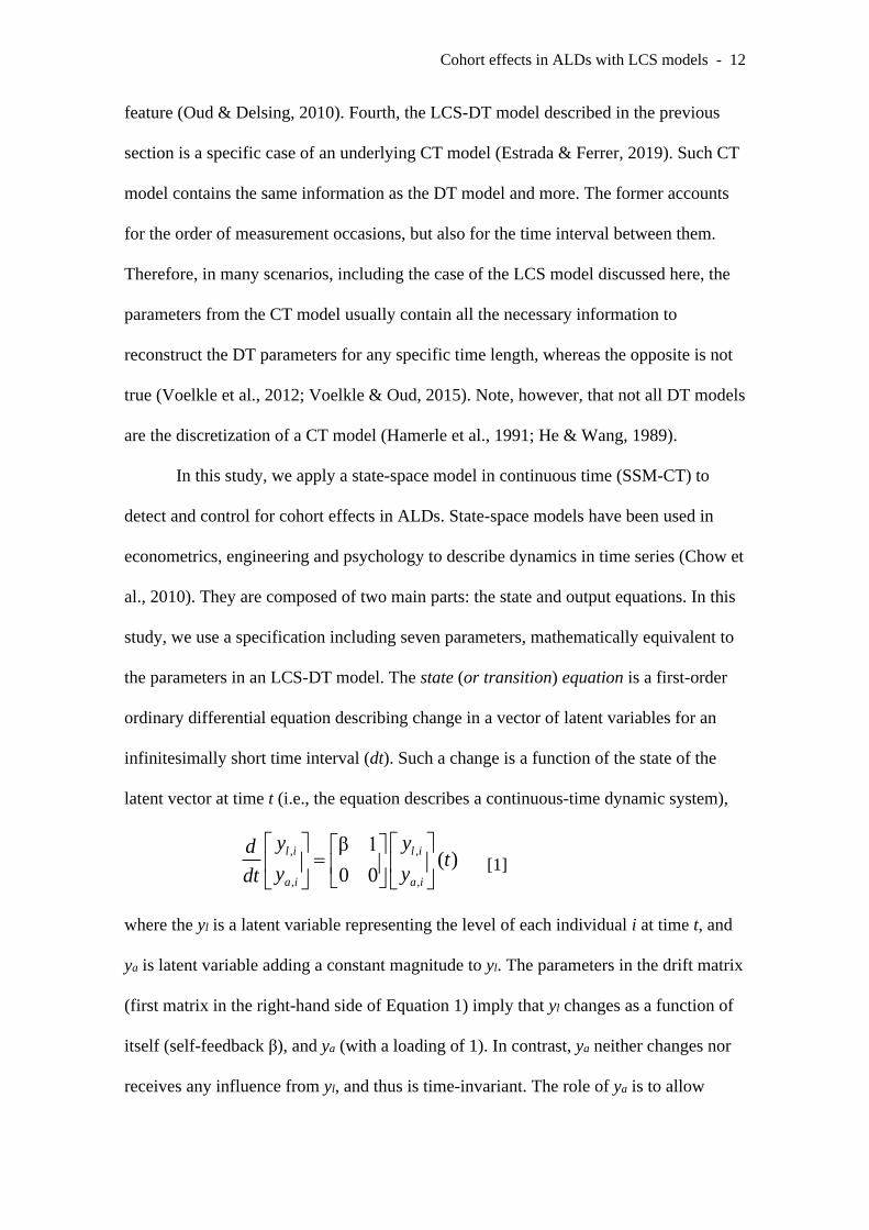
In this study, we apply a state-space model in continuous time (SSM-CT) to
detect and control for cohort effects in ALDs. State-space models have been used in
econometrics, engineering and psychology to describe dynamics in time series (Chow et
al., 2010). They are composed of two main parts: the state and output equations. In this
study, we use a specification including seven parameters, mathematically equivalent to
the parameters in an LCS-DT model. The state (or transition) equation is a first-order
ordinary differential equation describing change in a vector of latent variables for an
infinitesimally short time interval (dt). Such a change is a function of the state of the
latent vector at time t (i.e., the equation describes a continuous-time dynamic system),
, ,
, ,
β 1( )
0 0
l i l i
a i a i
y ydt
y ydt
=
[1]
where the yl is a latent variable representing the level of each individual i at time t, and
ya is latent variable adding a constant magnitude to yl. The parameters in the drift matrix
(first matrix in the right-hand side of Equation 1) imply that yl changes as a function of
itself (self-feedback β), and ya (with a loading of 1). In contrast, ya neither changes nor
receives any influence from yl, and thus is time-invariant. The role of ya is to allow

Cohort effects in ALDs with LCS models - 13
changes in the mean trajectory of yl over time. Both latent variables allow between-
individual variability (i.e., random effects), which are specified for t = 0 as
2
0 0 0 0,
2
0,
μ σ σ,
μ σ σ
l a
a a a a
yN
y
= =
μ Σ . [2]
In a univariate system, the mean trajectory tends to an asymptote with value (µa /
- β). Such asymptote is reached at t = ∞ with negative values of β, or t = -∞ with
positive values of β. Therefore, the parameter σ2a can be interpreted as capturing
individual differences in the asymptote (i.e., if σ2a = 0, all trajectories tend to the same
asymptotic level).
The time-specific observations (Yt) are linked to the latent level yt through the
output equation, which is equivalent to a measurement model in dynamic or
confirmatory factor analysis. In our case: Yit = yl,it + ei, where the variable e represents a
measurement error, with mean 0 and time-invariant variance σ2e (note that the latent
variable ya is not linked to any observation). A diagram for this SSM-CT model is
depicted in the bottom left panel of Figure 3.
This SSM-CT is an alternative parameterization to the standard LCS-DT
described above and includes the same number of parameters. However, the
interpretation of some of these parameters is different between the two models because
of their different time metrics. In an LCS-DT, the parameters β, µa, σ2a, and σl,a are
scaled for Δt = 1, whereas in an SSM-CT they are scaled for an infinitesimally short
time interval (dt). Similarly, in an LCS-DT, the parameters µ0 and σ20 refer to the first
measurement occasion, whereas in an SSM-CT they refer to t = 0, which is an arbitrary
time point, and does not necessarily correspond to the first observed occasion. For
further details on their mathematical relation, see Estrada & Ferrer (2019), Hunter
(2018), Ji & Chow (2019), Voelkle and Oud (2015), or Voelkle et al. (2012).

Cohort effects in ALDs with LCS models - 14
Purpose of the study
To the best of our knowledge, no previous study has systematically examined
the ability of dynamic models to identify and control for cohort differences in an ALD.
This is critical, because the key assumption in ALDs is the absence of such cohort
differences. If cohort effects exist, the trajectories of each cohort are not equivalent (i.e.,
in the original denomination by Bell, 1953, they do not “converge” into the same
population trajectory).
Our goal is to propose an approach to detect and control for cohort differences in
ALDs by means of LCS in discrete- and continuous-time. Specifically, we seek to
examine: a) under which conditions of cohort effects is the equivalence assumption
tenable and under which is not, and b) the performance of a methodological extension
designed to detect cohort effects influencing two key model parameters: the initial level
and asymptote.
Methods
Simulation procedure
We generated repeated measures for a latent process y which unfolds in
continuous time. The process is defined by the SSM-CT model described previously.
The parameters of this model were chosen to represent the longitudinal development of
a cognitive ability (i.e., reading ability) from childhood to early adulthood. These
parameters are reported in Table 1, and were based on previous empirical studies (Ferrer
et al., 2007, 2010; Shaywitz et al., 1990).
INSERT TABLE 1 HERE

Cohort effects in ALDs with LCS models - 15
The parameters in Table 1 were used for generating the data in all the simulation
conditions. For each condition, different cohorts provided data for different parts of the
trajectory. The generating parameters were constant across cohorts, except for the
specific parameters described below. We manipulated three simulation factors: a) type
and size of cohort effect, b) sampling schedule, and c) sample size.
a) Type and size of cohort effect. In the present study we examined cohort
effects in favor of the younger cohort equivalent to those documented in the literature
(i.e., at least the size of the Flynn effect). We included also larger effects to evaluate
how extremely adverse conditions affect the recovery of the population trajectories. We
generated nine different conditions. These are summarized in Table 2. The baseline
condition implied equal parameters for all the cohorts in the study (i.e., no cohort
effects). Four conditions generated cohort differences in the mean initial point (denoted
by d0), and four conditions in the mean asymptotic level (dAs). All the effect sizes were
computed for a 13-year difference, the largest difference in our sampling schedules (see
the following section).
In the presence of cohort effects on the initial level, the youngest cohort always
had the same mean initial level (µ0 = 10), while the rest of cohorts had lower values
(i.e., younger individuals entered the study with a higher average level). The effect size
d0 captures the mean initial difference between the oldest and youngest cohort,
computed in the metric of the standard deviation in the initial point (σ0 = 5, which was
constant across cohorts). For example, an effect of d0 = 1 implied that the t = 0 mean for
the oldest cohort was 5 points below that of the youngest cohort (d0 = [(10 – 5) / 5] = 1).
In the remaining intermediate cohorts, the value of µ0 was proportionally scaled.
Therefore, with d0=1 and 11 cohorts, the µ0 values from the youngest to the oldest
cohorts were {10, 9.5, 9, 8.5, 8, 7.5, 7, 6.5, 6, 5.5, 5}.

Cohort effects in ALDs with LCS models - 16
In the presence of cohort effects on the asymptotic level, the youngest cohort had
a mean asymptotic level of µAs = µa / -β = 6 / -(-.2) = 30. The rest of cohorts had lower
asymptotic levels. The cohort effect dAs captured the mean difference between the oldest
and youngest cohort, computed in the metric of the standard deviation in the asymptotic
level (σAs = σa / -β = 1 / -(-.2) = 5). For example, an effect of dAs = 1 implied that the
asymptotic mean for the oldest cohort was 5 points below that of the youngest cohort
(dAs = [(30 – 25) / 5] = 1). In the remaining intermediate cohorts, the value of µAs was
proportionally scaled. Therefore, with dAs =1 and eleven cohorts, the µAs values from the
youngest to the oldest cohorts were {30, 29.5, 29, 28.5, 28, 27.5, 27, 26.5, 26, 25.5, 25},
and the µa values for each cohort were {6, 5.9, 5.8, 5.7, 5.6, 5.5, 5.4, 5.3, 5.2, 5.1, 5}.
INSERT TABLE 2 HERE
b) Sampling schedule. Although many sampling schedules are possible within
the ALD framework, we restricted our selection to ALDs that are feasible in a study
spanning a maximum period of 5 years. Among them, we selected three schedules
(designs D1, D2, and D3) shown to have the best cost-effective performance in previous
studies (Estrada & Ferrer, 2019). These designs are summarized in Table 3.
INSERT TABLE 3 HERE
As a reference, we applied a “benchmark design” (D0), which included full
trajectories for every individual of every cohort, measured once per year. This design
includes 13 cohorts in which all participants are measured from ages 5 to 19. In other
words, this is an “expanded”, rather than accelerated, longitudinal study ranging for a
total of 28 years. Such design is unfeasible in real scenarios, but we included it here as a
benchmark to examine the extent to which the cohort effects can be recovered when the
full trajectories are available.
Cohort effects in ALDs with LCS models - 17
In all the designs, each participant was measured once during the corresponding
year. The exact week of the year was chosen at random with equal probability for each
of the 52 weeks in the year. This sampling procedure created random lags between and
within individuals, to reproduce the varying time lags observed in empirical ALDs
(Estrada & Ferrer, 2019).
c) Sample size. We generated samples of size 125, 250, and 500.
The combination of cohort effects, sampling schedules, and sample sizes led to 9
× 4 × 3 = 108 simulation conditions. For each of these conditions, we generated 100
replications.
Data analysis: Extension of LCS-DT and SSM-CT models to account for cohort
differences
For each sample in each condition, we estimated two versions of the two
statistical models described in our introduction (four models in total). Diagrams for
these models are depicted in Figure 3.
INSERT FIGURE 3 HERE
a) Latent Change Score model in discrete time (LCS-DT). We implemented this
model in SEM using OpenMx in R (RAM parameterization estimated with Full
Information Maximum Likelihood; cf., Ghisletta & McArdle, 2012; Neale et al., 2016).
This specification includes seven parameters and requires a discrete measurement
occasion, and not actual age, as the underlying time metric. Because the exact time lag
between measurements was different between and within cases, age bins were created in
the center of each year –i.e., at ages 5.5, 6.5, 7.5, etc. In consequence, the variability in
time lags between occasions is not specifically accounted for in the model, as it is the
case in studies using empirical data. Using discrete measurement occasions entails

Cohort effects in ALDs with LCS models - 18
creating very sparse data sets and very low coverage –or even zero– for some of the
elements in the covariance matrix. A path diagram for this model is depicted in the top
left panel of Figure 3.
b) Latent Change Score model in discrete time with cohort effects (LCS-DTc).
We extended the standard LCS model described previously by introducing the cohort
(i.e., year of birth) as an exogenous observed variable. The following additional
equations were added to the model:
y0 = τ0 + γ0 × cohort [3]
ya = τa + γa × cohort.
The youngest cohort, entering the study at age 5, was assigned a value of 0, the
next cohort, entering the study at age 6, was assigned a value of 1, and so on. The latent
initial level (y0) and additive component (ya) were regressed on this covariate2 through
the coefficients γ0 and γa. These two additional parameters were intended to capture the
corresponding linear cohort effects. Consequently, the parameters µ0 and µa are
replaced by intercepts τ0 and τa, and the variances σ20 and σ2
a become residual variances
after the cohort effect has been accounted for. A path diagram for this model is depicted
in the top right panel of Figure 3.
c) State Space Model in continuous time (SSM-CT). This model is
mathematically related to the standard LCS-DT and also includes seven parameters (see
Table 1). It is composed of two equations3:
dyt / dt = Ayt + But + qt [4]
Yt = Cyt + Dut + rt [5]
2 In our OpenMx specification, the covariates are included as definition variables. 3 We adapt here the notation in Hunter (2018), also used in OpenMx. To highlight the similarities with the
common LCS-DT specification, we changed the notation of the latent states (y) and observed variables
(Y).

Cohort effects in ALDs with LCS models - 19
Equation 4 is a more compact expression of the state equation described
previously as Equation 14. It describes how the latent states change over time with a
first-order linear differential equation: yt is an l × 1 vector of latent states, t is time. The
derivative of yt with respect to t is dyt / dt. ut is an m × 1 vector of covariates or
exogenous variables, and qt is an l × 1 vector of dynamic noise with mean zero and
covariance Q. A is an l × l matrix of autoregressive dynamics –i.e., drift matrix–, and B
is an l × m matrix of covariate effects on the latent states. Equation 5 is the output
equation. It is identical to the measurement model in the SEM framework (Chow et al.,
2010; Hunter, 2018) and describes how the latent states relate to the observed variables
at a single point in time: Yt is a n × 1 vector of observed variables or outputs at time t, rt
is an n × 1 vector of observation noise (or measurement error) with mean zero and
covariance R. C is an n × l matrix of factor loadings, and D is an n × m matrix of
covariate effects on the observed variables. In this framework, the latent initial mean
vector included in Equation 2 is noted as x0, and the latent initial covariance matrix is
noted as P0 (Hunter, 2018). A path diagram for this model is depicted in the bottom left
panel of Figure 3.
Estimation of the SSM-CT model is carried out through a set of recursive
algorithms called hybrid Kalman Filter (Boker et al., 2018; Chow et al., 2010; Hunter,
2018). This procedure iterates in cycles of one prediction step (using a Kalman-Bucy
filter) and one correction step (using a Kalman filter). For a given time t, the prediction
step makes a forecast for (the factor scores in) the state vector yt and the state
covariance matrix, based on the initial state of the system at t0, the time interval between
t and t0, and the dynamics of the system (A, B, Q and ut). The update –or correction–
step uses the observed data and the measurement model to correct the forecast from the
4 This re-expression is possible because our model does not include time-varying covariates or dynamic
noise.

Cohort effects in ALDs with LCS models - 20
previous step. The algorithm is designed to iteratively reduce the prediction error by
adjusting the parameter estimates through Maximum Likelihood prediction error
decomposition (for further details, see Boker et al., 2018; Chow et al., 2010; Hunter,
2018; Kalman, 1960; Kalman & Bucy, 1961).
We estimated this model using the functions
mxExpectationStateSpaceContinuousTime and mxFitFunctionML in OpenMx (Boker et
al., 2018; Hunter, 2018; Neale et al., 2016). In this implementation, a multiple group
model is estimated in which each person is a group with a time series of observations,
and all free parameters are constrained to be equal across “groups”. This specification
uses only the available data points and the exact time –i.e., age– at which they were
measured.
d) State Space Model in continuous time with cohort effects (SSM-CTc). The
standard SSM-CT described in the previous section was expanded by introducing the
cohort (i.e., year of birth) as an exogenous observed variable. This covariate was scaled
as explained for the LCS-DTc model, with a similar rationale. Two additional
regression parameters γ0 and γa were specified to capture linear cohort effects on the
initial and asymptotic latent levels, with the latter expressed in the latent additive
component. This resulted in a model with nine parameters. In the OpenMx SSM
specification, the x0 vector is defined to include the covariate in Equation 3 (R code for
the models in this paper can be found in
https://github.com/EduardoEstradaRs/PsychMeths2021-Cohort-effects-ALD-CT-DT).
A path diagram for this model is depicted in the bottom right panel of Figure 3.
The time metric was the same for all DT and CT models: a one-point increase
represented one year. After fitting all models to all samples, we obtained the parameter
estimates and their standard errors. In any empirical situation, and especially when
Cohort effects in ALDs with LCS models - 21
alternative statistical models are being compared, it is highly recommended to compute
various fit indices for the models and assess the extent to which the data are adequately
represented by each of them. In our study, however, the fit indices most suitable for
comparing our models – -2LogL, AIC and BIC – are completely dependent on the
number of data points available in the dataset. Consequently, the CT and DT versions of
each model are expected to achieve the exact same fit (as, in fact, they did). The
variability –i.e., standard deviation– in model fit was also fairly similar between CT and
DT versions of each model. Thus, these fit results are not reported. The standard error
for the relative biases is available from the authors upon request. The R code for
estimating the four models is available at:
https://github.com/EduardoEstradaRs/PsychMeths2021-Cohort-effects-ALD-CT-DT
Results
The models converged for all samples and conditions. Based on the estimates
and standard errors, we evaluated accuracy by computing the relative bias and 95%
confidence interval (CI) coverage of the parameters. We evaluated estimation efficiency
through the empirical standard deviation of the estimates. In addition, we also computed
the relative bias of the standard errors. Due to the space restrictions, here we include
only the results regarding relative bias, coverage, and estimation variability. Other
relevant information can be found in the Supplementary Materials.
General estimation accuracy: Overview of Relative Bias and 95% CI coverage
For each parameter in every condition, we examined estimation accuracy by
computing the parameter’s Relative Bias as RB = ( est - θ) / θ, where θ is the true
parameter value and est is the average estimated value of the parameter across all
Cohort effects in ALDs with LCS models - 22
replications in a given condition.5 Values of RB closer to zero imply unbiased estimates,
positive values imply overestimation, and negative values imply underestimation.
Previous literature has considered estimates to be substantially biased when |RB|>.10
(Flora & Curran, 2004; Rhemtulla et al., 2012). Coverage was computed as the
proportion of 95% confidence intervals around the estimated parameter value that
include the true parameter value6. As such, 95% is the optimal value of coverage,
whereas coverage below 90% is considered inadequate (Collins et al., 2001; Enders &
Peugh, 2004).
First, we provide a general overview of the models’ performance by reporting
the Root Mean Square Relative Bias as RMSRB = 2
1
K
kkRB K
= , where K is the
number of parameters in the model (either 7 for LCS-DT and SSM-CT, or 9 for LCS-
DTc and SSM-CTc). These results are reported in the top section of Figure 4. The
bottom section of Figure 4 depicts the mean coverage for each model, computed as
mean(coverage) = 1
K
kkcoverage K
= . A table with the numerical results is included in
the Supplementary materials.
INSERT FIGURE 4 HERE
The first finding worth noting in Figure 4 is that the models including cohort
effects (SSM-CTc and LCS-DTc) showed good performance in all the conditions. In
contrast, the models without parameters accounting for cohort effects (SSM-CT and
5 Due to the age binning and random time lags, when the LCS-DT models were applied, the first
measurement occasion was at 5.5 years. Thus, the parameters related to the latent initial level were
compared with the expected values for that age. They are reported in Table 1.
For γ0 and γa, θ equals zero in the conditions where the corresponding cohort effects are null. In such
conditions, computing RB would imply dividing by zero. Therefore, RB was computed in those conditions
by dividing the absolute bias by the maximum value for θ in our study: the population value for γ0 and γa
in the conditions d0 = 2.0 and dAs = 2.0, respectively.
6 Created using standard error estimates. These are Wald-type confidence intervals based on asymptotic
normal theory, not profile likelihood confidence intervals.
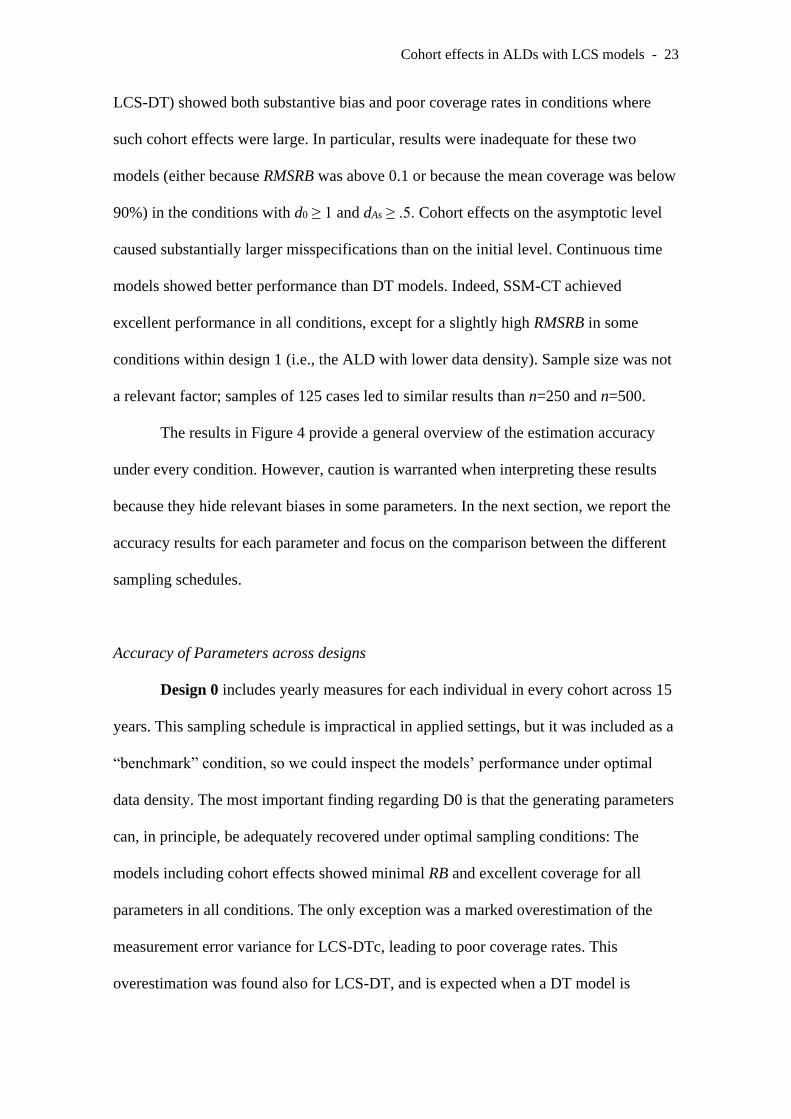
Cohort effects in ALDs with LCS models - 23
LCS-DT) showed both substantive bias and poor coverage rates in conditions where
such cohort effects were large. In particular, results were inadequate for these two
models (either because RMSRB was above 0.1 or because the mean coverage was below
90%) in the conditions with d0 ≥ 1 and dAs ≥ .5. Cohort effects on the asymptotic level
caused substantially larger misspecifications than on the initial level. Continuous time
models showed better performance than DT models. Indeed, SSM-CT achieved
excellent performance in all conditions, except for a slightly high RMSRB in some
conditions within design 1 (i.e., the ALD with lower data density). Sample size was not
a relevant factor; samples of 125 cases led to similar results than n=250 and n=500.
The results in Figure 4 provide a general overview of the estimation accuracy
under every condition. However, caution is warranted when interpreting these results
because they hide relevant biases in some parameters. In the next section, we report the
accuracy results for each parameter and focus on the comparison between the different
sampling schedules.
Accuracy of Parameters across designs
Design 0 includes yearly measures for each individual in every cohort across 15
years. This sampling schedule is impractical in applied settings, but it was included as a
“benchmark” condition, so we could inspect the models’ performance under optimal
data density. The most important finding regarding D0 is that the generating parameters
can, in principle, be adequately recovered under optimal sampling conditions: The
models including cohort effects showed minimal RB and excellent coverage for all
parameters in all conditions. The only exception was a marked overestimation of the
measurement error variance for LCS-DTc, leading to poor coverage rates. This
overestimation was found also for LCS-DT, and is expected when a DT model is

Cohort effects in ALDs with LCS models - 24
applied to a design with non-constant time lags (for details, see Estrada & Ferrer, 2019).
The models not including cohort effects led to overestimation of σ20 and σ2
a, and
simultaneous underestimation of µ0 and µa, when the corresponding cohort effect was
present. This is expected: when the between-cohort variability was not accounted for by
the model, this effect was absorbed by the variance of the latent component affected by
each type of cohort effect. Consistently, the mean differences between cohorts
introduced a negative bias in the corresponding latent mean. Due to space restrictions,
here we include figures for the three designs that are feasible in applied settings (D1,
D2, and D3). All numerical results, and a figure for D0, are available in the
Supplementary materials.
Design 1 includes two measurement occasions per individual, separated two
years apart. This is the design with the lowest data density. The results regarding RB
and coverage for this design are depicted in Figure 5. The first notable finding here is a
marked overestimation of the cohort effect on the initial level γ0 and the variance of the
latent component σ2a in the models including cohort effects. For γ0, overestimation may
happen because the model has information about the initial level for only the youngest
cohort. These biases decreased with larger sample size, especially for SSM-CTc.
Models that do not include cohort effects were especially affected by the effect on the
asymptotic level. In all the conditions, the coverage rates were excellent for the models
that included cohort effects (probably due to large standard errors). In contrast, coverage
rates were poor for the models not including cohort effects, particularly with d0 = 2 and
dAs ≥ .5. As expected, larger cohort effects led to larger bias in SSM-CT and LCS-DT.
INSERT FIGURE 5 HERE (D1)
Design 2 implies three measurement occasions per individual, separated two
years apart each, thus spanning five years. The results regarding RB and coverage for

Cohort effects in ALDs with LCS models - 25
D2 are depicted in Figure 6. This design led to better results than D1, particularly for
the models that include cohort effects. Importantly, the biases for γ0 and σ2a found in D1
were present in D2: σ2a was accurately estimated, and overestimation of γ0 was found
only for LCS-DTc with n=125, but not for SSM-CTc. Coverage rates were excellent for
SSM-CTc and LCS-DTc in all conditions. In contrast, the models not including cohort
effects led to marked bias with d0 = 2 and dAs ≥ .5.
INSERT FIGURE 6 HERE (D2)
Design 3 implies four measurement occasions per individual during four
consecutive years. Relative to D2, each participant in this design provides more data
points (4 instead of 3), but during a narrower age range (4 years instead of 5). Design 3
led to results very similar to D2. This implies that the additional measure included in D3
does not contribute to a substantial improvement in estimation accuracy. In fact, D3 led
to slightly higher bias for most parameters in all conditions, and worse coverage rates
for the measurement error variance in the DT models. Results from D3 available in the
Supplementary Materials.
Variability of the estimates
We computed SDRB as SD[(θest – θ)/ θ].7 This index allows expressing the
estimation inefficiency in the same scale for all parameters, models and designs. This
index is always positive, and values closer to zero imply less variability of the estimates
in any given condition –i.e., more efficiency. We provide a general overview of the
models’ efficiency by reporting the mean SDRB for each model, computed as
7 When comparing different models, studies on incomplete data often use a measure of efficiency based
on the ratio [variance(estimates from model0) / variance (estimates from model1)], where model0 is the
baseline model, expected to be more efficient –i.e., achieve lower variance of parameter estimates–, and
model1 is an alternative model expected to show higher variability –i.e., lower efficiency. Our Design 0
could be used as the reference condition, but because it had SDRB values below 0.1 in all conditions,
presenting the values as a quotient would lead to artificially high values for the rest of designs. Therefore,
we decided to present the raw values for each design and compare the variability with the true parameter
value, which was invariant across conditions

Cohort effects in ALDs with LCS models - 26
mean(SDRB) = 1
K
kkSDRB K
= . These results are reported in Figure 7. Results
regarding specific parameters are reported in the Supplementary materials.
INSERT FIGURE 7 HERE
A surprising finding regarding SDRB is that sample size had little relevance for
estimation efficiency. Of course, larger sample sizes led to lower SDRB, but the main
factors affecting SDRB were the specific ALD and model. As expected, D0 was the
most efficient sampling schedule, with mean values ranging approximately between .1
(models including cohort effects with n=125) and .025 (models not including cohort
effects with n=500). Among the other three designs, D1 had a clearly worse
performance in all conditions. D2 and D3 showed very similar efficiency, with
marginally better performance of D2 with the models that include cohort effects. The
models that do not include cohort effects showed better average performance than their
alternatives. Estimation variability was fairly similar for different types and sizes of
cohort effect.
An Empirical Example: Development of Abstract Reasoning from Childhood to Early
Adulthood
To illustrate the utility of the method proposed, we applied the four statistical
models discussed previously (i.e., SSM-CT, and SSM-CT with cohort effects, LCS-DT,
LCS-DT with cohort effects) to a data set from an accelerated longitudinal study.
Sample and measurement instruments
For these analyses, we use data from the Neural Development of Reasoning
Ability (NORA) study (Ferrer et al., 2009; Wendelken et al., 2011) a longitudinal
research project designed to examine the development of fluid reasoning from
childhood to adolescence. Data were collected using a cohort sequential design

Cohort effects in ALDs with LCS models - 27
involving three waves of measurement with 201, 122 and 70 participants at the first,
second and third occasion, respectively. At time 1, the participants ranged in age from
6.00 to 19.1; at time 2, the age range was 6.46 to 20.5; and at time 3 the age range was
7.75 to 21.0. Of the 201 participants, 94 (46.8%) were females and 107 (53.2%) were
males. The interval between assessments ranged between 12 and 24 months.
As part of a battery of measures, at each occasion, participants completed the
Matrix Reasoning subtest of the Wechsler Abbreviated Scale of Intelligence (WISC-R;
Wechsler, 1981). This subtest measures the ability to select the geometric visual
stimulus that accurately completes a series of stimuli that change along a particular
dimension. Such change follows one or more abstract rules that the participant must
infer. We refer to this variable as abstract reasoning.
Because this study was designed to study developmental changes in reasoning as
a function of age, we defined cohorts based on biological age. We rescaled the year of
birth to create a covariate ranging from 0 (younger participants, born later, and entering
the study at age 6) to 13 (older participants, born earlier, and entering the study at age
19). Because the DT model requires age bins, we rounded the values to the closest
integer.
Results from DT and CT models
Table 4 reports the parameter estimates from all four models. The fit statistics
for SSM-CT with cohort effects were: -2LL = 2130.5, AIC = 1398.5; for SSM-CT: -2LL
= 2143.9, AIC = 1409.9; for LCS-DT with cohort effects: -2LL = 2129.7, AIC = 1401.7;
and for LCS-DT: -2LL = 2143.5, AIC = 1411.5. The parameter estimates were
consistent in the DT and CT versions; the parameters not affected by the metrics of time
had very similar values in the DT and CT versions of the same model. For example, the
measurement error variance ranged between 8.19 (SSM-CT with cohort effects) and
Cohort effects in ALDs with LCS models - 28
8.60 (LCS-DT). Because of this consistency, we focus here on the CT models for
interpreting the results.
The most important finding in Table 4 is a significant effect of the cohort
covariate on the latent additive component, but not on the latent intercept. This finding
was replicated in the CT (γ0 = -1.46, p = .078; γa = -.125, p < .001) and DT models (γ0 =
-1.19, p = .145; γa = -.101, p = .002). The negative effect on the latent intercept implies
that participants born earlier had higher reasoning ability at age 6. However, this effect
was not statistically significant and cannot be assumed to exist in the population.
Considering that the mean of the latent additive component was positive (in SSM-CT
with cohorts, μa = 8.75), the negative effect on such component implies that, for any
given time lag, participants born later receive a larger positive constant influence. This
means that, if we were to follow the youngest cohort, in the long run they would reach
the higher asymptotic level: μAsymp = μa / (-β); in SSM-CT with cohorts, the youngest
cohort is predicted to reach a mean level of 8.75 / .240 = 36.45, whereas the oldest
cohort in the study is predicted to reach [8.75 + 13×(-.125)] / .240 = 29.68.
Taking as reference the residual variance in the latent additive component, in
SSM-CT with cohorts σ2a = .5, the difference between the youngest and oldest cohort
can be expressed as Cohen’s standardized difference d = (μa,young – μa,old) / σa = (8.75 –
7.12) / .707 = 2.30. It is also possible to standardize the regression loading to obtain the
Pearson’s correlation coefficient between cohort and additive component: rcohort,a = γa ×
(sd(cohort) / σa) = -.125 × (3.67 / .707) = -.65. Both estimates imply a very large effect
size in favor of younger cohorts. Figure 8 depicts mean predicted trajectory by the
SSM-CT without cohorts, and the cohort-specific means implied by the SSM-CT with
cohort effects, along with the observed individual data.
Cohort effects in ALDs with LCS models - 29
Comparing the SSM-CT model with and without cohort effects, the inclusion of
cohort effects on the latent intercept and additive component led to differences in the
mean and variance of both parameters; μ0, μa, σ20, σ2
a. In the model with cohort effects,
both latent means were higher, as they capture the mean level for the youngest cohort,
whereas in the model without cohort effects these parameters capture the means for the
whole sample. Regarding the latent covariances, as expected, both had lower values in
the model with cohort effects, as they represent residual variances, after considering the
effect of the cohort. Interestingly, the variance of the additive component was not
statistically different from zero in the models with cohort effects. In all cases, the latent
covariance was not significant and lead to correlations very close to zero: no relation
was found between the initial level and the additive component.
Discussion of results from empirical data
In this empirical example, we illustrated how the proposed methods can be
applied to a data set from an accelerated longitudinal design. Specifically, we examined
the development of abstract reasoning as a function of biological age, and examined the
degree to which 13 different cohorts (age at t1 from 6 to 19 years) were equivalent in
terms of their developmental trajectories. The most important finding was a significant
effect of age cohort on the additive component. This effect was negative: participants
born earlier, and who entered the study at older ages, were expected to reach lower
asymptotic levels than younger participants. Although we did not examine possible
reasons for this effect, one potential factor is the result of sampling. That is, younger
children whose parents are able to bring them to the study, thus completing hours of
cognitive and brain measurements are more likely to be on a more positive
developmental trajectory.

Cohort effects in ALDs with LCS models - 30
Note that the development of abstract reasoning can be assumed to have
exponential shape in the age range considered. However, this functional form is rather
unreasonable across the whole life span (McArdle et al., 2002). In consequence,
although the latent additive component is mathematically linked to the trajectory’s
asymptote, from a substantive standpoint it makes more sense to state that individuals
born later would reach higher peak levels than their older peers.
General Discussion
Summary of findings
In this paper, we examined the ability of LCS models, defined in both
continuous- and discrete-time, to detect and account for cohort differences in
accelerated longitudinal designs. We also examined the extent to which cohort
differences led to bias in the parameter estimates when such differences were not
controlled for.
When cohort effects were present in the data and the models included parameters
accounting for such effects (i.e., models LCS-DTc and SSM-CTc), these were
adequately estimated in all conditions, particularly those with three or more
measurements per individual. In other words, the cohort effects on the latent initial level
and latent asymptotic level (i.e., additive component) were accurately estimated, and so
were the rest of the parameters. However, when models not including cohort effects
(i.e., LCS-DT and SSM-CT) were fitted to data from an ALD with cohort differences,
the results were tenable only when such cohort differences were not large (d0 ≤ 1 and
dAs ≤ 0.2). In these conditions, most parameters were recovered with acceptable bias.
With larger cohort effects, however, the estimates from LCS-DT and SSM-CT became
untenable. Across all conditions, cohort effects on the asymptotic level (dAs) caused
much larger bias than on the latent initial level (d0).

Cohort effects in ALDs with LCS models - 31
When cohort effects were not present in the data, the models that included
parameters to account for cohort effects correctly estimated them as null in most
scenarios. In fact, these models showed better accuracy in almost every condition,
without a substantial decrease in efficiency, than those models without parameters for
cohort effects. Based on this finding, it appears reasonable to specify cohort effects in
LCS models (either in discrete- or continuous-time) when suspecting such effects in
data from ALDs. If cohort effects are present in the data, they will be correctly
estimated in the model; if they are absent, they will be identified as such, without any
bias and with only marginally larger standard errors.
Regarding the sampling schedule, Design 1 (two measures per participant,
separated two years apart, spanning 3 years) provided clearly worse results than Designs
2 (three measures taken in alternate years, spanning 5 years) and Design 3 (four
measures taken in consecutive years, spanning 4 years). In fact, Design 1 led to a
marked overestimation of the cohort effect on the latent initial level, and the variance of
the latent asymptotic level, regardless of the actual magnitude of cohort effects in the
population, particularly for samples of 125 participants. Designs 2 and 3 led to excellent
results across all the conditions. Both designs showed very similar performance, but
Design 2 was slightly better in terms of accuracy and efficiency in most conditions. In
other words, covering a wider time range with three measures per person is preferable
over having a fourth measure. Based on these results and the fact that Design 2 requires
one less measurement per participant, we recommend it over Design 3. Of course, this
recommendation applies to the conditions simulated in this study, particularly when the
researcher has reasons to assume that the model specified is correct.
Another interesting finding is that sample size had very little relevance regarding
cohort effects, at least in the conditions examined in this study. As expected, the smaller

Cohort effects in ALDs with LCS models - 32
sample size (n = 125) led to less efficient estimation across all conditions. Furthermore,
parameter biases were reduced with larger samples. However, and importantly, the
specific research design, the model specified, and the type and size of the cohort effect,
all had a much larger influence on the quality of the parameter estimates than sample
size. Based on this, we hold that samples of 125 participants are enough for conducting
ALDs in the presence of cohort effects, if the correct sampling schedule (e.g., Design 2)
is applied.
Theoretical and methodological considerations
The present work extends previous attempts to control for cohort differences in
accelerated longitudinal designs (cf., Miyazaki & Raudenbush, 2000). The procedure
proposed here intends to extend modern dynamic models so that they can account for
cohort effects. In particular, we proposed an extension of LCS models, both in discrete-
and continuous-time. This family of models has become a standard tool in
developmental research due to, among other features, its flexibility to identify lead-lag
effects between different processes, detect sources of between- and within-individual
variability, and include a measurement structure linking observed variables to latent
constructs.
Equivalence between cohorts is a key aspect in ALDs. These designs are based
on the assumption that individuals of different ages come from the same population, and
it is possible to characterize a population trajectory through the aggregation of their
individual information. However, if individuals born later differ from those born earlier
(e.g., they enter the study at a higher initial level or they reach higher level when they
exit), the equivalence assumption does not hold. The present work provides important
insights into how the model parameters are affected when such an assumption is not
tenable, and how cohort differences can be controlled for.

Cohort effects in ALDs with LCS models - 33
Cohorts can be defined in different ways depending on the context and research
question. For example, in some studies there are variables that define cohorts clearly,
such as school grade, or treatment received, among others. In contrast, the concept of
cohort may be elusive in an ALD. In this study, we used biological age to define cohorts
because a) this information is available in most ALDs, an b) age is very often the
variable of interest on which to map developmental processes. However, our proposed
approach can be readily applied to any cohort variable measured with an interval scale,
as long as it is reasonable to apply such scale as the time metric for measuring both the
age range of interest and the time range of the study.
Cohort differences have been widely documented in the literature on cognitive
abilities. One famous example is the so-called Flynn effect. During the twentieth
century, individuals born later showed systematic increases in cognitive function,
particularly fluid reasoning (Flynn, 1984, 1987; Gerstorf et al., 2015; Nisbett et al.,
2012; Pietschnig & Voracek, 2015). The smaller cohort effects in our study (d0 and dAs
= 0.2) were specifically included to reflect empirical estimates of this effect (Trahan et
al., 2014). Based on our findings (see Figures 4 to 7), we conclude that a) such “small”
cohort differences are adequately recovered by the models including cohort effects
(SSM-CTc and LCS-DTc), with a slightly better performance of the continuous-time
version; b) models not controlling for cohort effects lead to very small biases when
cohort differences affect the asymptotic level (dAs), and neglectable biases when they
affect the initial level (d0).
Across all our simulation conditions, cohort differences in the asymptotic level
caused a larger misspecification than when differences affected the initial level (in the
models not controlling for cohort effects). Relatedly, the parameter capturing cohort
differences in the initial level was harder to estimate in some conditions. Both results
Cohort effects in ALDs with LCS models - 34
are easier to interpret using Figure 2. Because the developmental process simulated here
has a much faster growth in the early years, even large cohort differences in the initial
point are compensated early on. Thus, cohort differences in the initial level are harder to
estimate, but also cause a smaller bias in the parameter estimates.
When analyzing developmental data (obtained from an ALD or otherwise), a
researcher can choose among various statistical models. In this study, we focused on
LCS models for both theoretical and methodological reasons. From a statistical
standpoint, LCS are well suited for characterizing the developmental trajectories of
cognitive and other psychological variables, which can be assumed to have exponential
shape during childhood and adolescence. From a theoretical perspective, the
determinants of change included in a dual LCS model have a direct interpretation in
terms of developmental features: the additive component is linked to the peak level and
the self-feedback parameter indicates the rate of reduction between the initial and peak
levels. For these reasons, and given our goal was not to compare different models, we
used LCS models for generating the data and also to recover the information from such
data. One consequence of this is that the fit indices for the model were uninformative
because they were entirely dependent on the number of repeated measures in a given
sampling schedule. However, when the generating process is unknown (as in empirical
data sets) it is possible to compare different statistical models. In the context of ALD,
different models could account for cohort effects differently. In such scenarios, fit
indices are not a mere function of the number of repeated measures and can be used to
compare among the different models.
Limitations and future directions
In this study, we focused on the development of a single construct over time.
Systems including dynamic interrelations between two or more processes could lead to
Cohort effects in ALDs with LCS models - 35
more complex trajectories in which, for example, there may not be asymptotic levels.
Future research should investigate the ability of our approach to recover the trajectories
in such multivariate systems.
Besides the initial and asymptotic levels, cohort differences could affect also the
rate of change. Participants from different cohorts could show faster or slower
maturation of the psychological process under study. In the LCS model, such variability
would be captured by differences in the self-feedback parameter. However, when
implementing LCS models in the standard SSM or SEM frameworks, estimating
random effects in that parameter is not always possible. Future research should examine
how to model this particular type of cohort effect.
In our analyses, we examined the recovery of key features of the population
trajectory, including cohort effects, when such effects were positive: participants born
later reached higher levels. We were interested in this type of effects because they
capture relevant empirical phenomena (e.g., Flynn effect). It is unknown whether our
results can be generalized to scenarios with cohort effects in opposing direction (i.e.,
older cohorts reaching higher levels).
In line with developmental research using ALDs, we used biological age to
define cohorts. However, other sources of between-individual variability unaccounted
for will affect the model estimates. Importantly, other definitions of cohort are also
possible, including study cohorts (participants who entered the study in a particular
year), grade cohorts (students in a particular grade), or historical cohorts (participants
with data in a given year), among others. From a modeling standpoint, it is possible to
include additional covariates for each of these types of cohorts. However, several of
them can be severely confounded. Given the particular pattern of data missingness in
ALDs, the separation of such different cohort effects may prove difficult, or even

Cohort effects in ALDs with LCS models - 36
impossible. Future research should examine the degree to which such a separation is
possible under different developmental scenarios.
Similarly, cohorts can be sometimes defined by non-monotonic categorical
variables, for example, two different groups separated several decades apart, groups
receiving different interventions, or students from different schools or countries, among
others. In principle, such qualitatively different cohorts could be modeled using LCS
models via a multiple-group specification. Another possibility would be to create
dummy variables for each category, and estimate the regression coefficients for each of
them. Future research should examine under what conditions these “qualitative” cohort
effects can be identified and controlled for. One interesting feature of the multiple-
group specification is that, in principle, it would make it possible to characterize cohort
differences (either qualitative or quantitative) in any of the model parameters. For
example, it would be possible to estimate a different self-feedback parameter for each
cohort, and test whether the different parameters can be constrained to have the same
value across groups. However, this strategy should be applied carefully in the context of
ALDs. Because the sample is divided into several cohorts, each cohort may include only
a few participants (e.g., 125 participants divided into 13 cohorts leads to 9-10
participants per cohort). Therefore, the cohort-specific estimate for a given parameter
may be inaccurate and the method may not have sufficient power to detect cohort
differences. Future research should investigate this strategy.
Other modeling approaches are available for detecting and controlling for cohort
differences. For example, Driver & Voelkle (2018) developed a Bayesian framework
for estimating hierarchical continuous-time models. In such a framework, it is possible
to specify between-individual variability in any of the model parameters. In a similar
vein, the recently developed Dynamic Structural Equation Modeling (DSEM;

Cohort effects in ALDs with LCS models - 37
Asparouhov et al., 2018; McNeish & Hamaker, 2020) allows random effects in any of
the model parameters in a discrete-time framework. Both approaches hold great promise
for detecting the type of cohort effects studied in this paper (i.e., cohort non-equivalence
in the mean and variance of the latent intercept and additive component). Importantly,
they may be useful for detecting cohort differences in other parts of the model not
studied here, such as the rate of change. However, future research should examine the
possibilities and limitations of applying these methods in the context of ALDs, with its
unique features such as high percentage of data incompleteness, random time lags
between observations, or particular shape of the developmental processes, among
others.
Conclusion
We have shown that cohort effects can be adequately recovered in the context of
ALDs. Using a simple extension of LCS models, such effects can be captured in
dynamic models including latent variables in both discrete and continuous time. Based
on our findings, and considering that that they apply to the conditions studied in our
study, we offer the following recommendations:
1. Because cohort equivalence is a key assumption in ALDs that is typically
unknown, researchers should consider the adequacy of including parameters
for cohort effects in their models. Our findings show that, when cohort
effects are linearly related to age and affect the initial and asymptotic levels,
they will be adequately recovered by LCS models in CT and DT. Note,
however, that other types of cohort effects may exist.
2. Design 1 (two measurement occasions) should be avoided because it leads to
biased parameters in most conditions. If, however, this is the only option,
using a State-Space model in continuous time with parameters for cohort

Cohort effects in ALDs with LCS models - 38
effects (bottom-right panel in Figure 3) is recommendable. The alternative
LCS model in discrete time (top-right panel in Figure 3) will likely lead to
overestimation of some parameters.
3. Designs 2 and 3 lead to similar results, with a slightly better performance of
Design 2 in most scenarios. Therefore, if the researcher can assume that the
generating model is adequately specified, and under the conditions simulated
here, Design 2 is preferable because it achieves better results with one less
measure per individual (three instead of four). Consequently, we recommend
Design 2 as the most efficient sampling schedule.
4. Consistent with previous findings (Estrada & Ferrer, 2019), investing
resources in covering a wider age range for each participant is preferable to
increasing sample size: 125 participants appear to be enough, if the right
sampling schedule is applied (e.g., Design 2).
5. Also consistent with previous research, we recommend using LCS in
continuous-time, based on State-Space modeling, with parameters to account
for potential cohort effects. Besides the advantages of CT modeling noted
elsewhere (Oud & Delsing, 2010; Voelkle et al., 2012; Voelkle & Oud,
2015), particularly in the context of ALDs (Estrada & Ferrer, 2019), this
model achieved higher accuracy than the discrete-time alternative, with only
a relatively small decrease in efficiency.
We hope that the findings reported here, and the recommendations derived from
them, will inform the design of future studies and facilitate an efficient use of the
resources available for longitudinal research.
Cohort effects in ALDs with LCS models - 39
References
Asparouhov, T., Hamaker, E. L., & Muthén, B. (2018). Dynamic Structural Equation Models.
Structural Equation Modeling: A Multidisciplinary Journal, 25(3), 359–388.
https://doi.org/10.1080/10705511.2017.1406803
Bell, R. Q. (1953). Convergence: An accelerated longitudinal approach. Child Development,
24(2), 145–152. http://dx.doi.org/10.2307/1126345
Bell, R. Q. (1954). An experimental test of the accelerated longitudinal approach. Child
Development, 25, 281–286. http://dx.doi.org/10.2307/1126058
Boker, S. M. (2001). Differential structural equation modeling of intraindividual variability. In
L. M. Collins & A. G. Sayer (Eds.), New methods for the analysis of change (pp. 3–28).
American Psychological Association.
Boker, S. M., Neale, M. C., Maes, H. H., Wilde, M. J., Spiegel, M., Brick, T. R., Estabrook, R.,
Bates, T. C., Mehta, P. D., von Oertzen, T., Gore, R. J., Hunter, M. D., & Hackett, D. C.
(2018). OpenMx User Guide. https://openmx.ssri.psu.edu/documentation
Boker, S. M., Neale, M. C., & Rausch, J. R. (2004). Latent differential equation modeling with
multivariate multi-occasion indicators. In K. van Montfort, J. H. L. Oud, & A. Satorra
(Eds.), Recent developments on structural equation models: Theory and applications
(pp. 151–174). Kluwer.
Chow, S.-M., Ho, M. R., Hamaker, E. L., & Dolan, C. V. (2010). Equivalence and Differences
Between Structural Equation Modeling and State-Space Modeling Techniques.
Structural Equation Modeling: A Multidisciplinary Journal, 17(2), 303–332.
https://doi.org/10.1080/10705511003661553
Collins, L. M., Schafer, J. L., & Kam, C.-M. (2001). A comparison of inclusive and restrictive
strategies in modern missing data procedures. Psychological Methods, 6(4), 330–351.
https://doi.org/10.1037/1082-989X.6.4.330
de Haan-Rietdijk, S., Voelkle, M. C., Keijsers, L., & Hamaker, E. L. (2017). Discrete- vs.
Continuous-Time Modeling of Unequally Spaced Experience Sampling Method Data.
Frontiers in Psychology, 8. https://doi.org/10.3389/fpsyg.2017.01849
Cohort effects in ALDs with LCS models - 40
Deboeck, P. R., & Preacher, K. J. (2016). No Need to be Discrete: A Method for Continuous
Time Mediation Analysis. Structural Equation Modeling: A Multidisciplinary Journal,
23(1), 61–75. https://doi.org/10.1080/10705511.2014.973960
Driver, C. C., & Voelkle, M. C. (2018). Hierarchical Bayesian continuous time dynamic
modeling. Psychological Methods, 23(4), 774–799.
http://dx.doi.org/10.1037/met0000168
Duncan, S. C., Duncan, T. E., & Hops, H. (1996). Analysis of longitudinal data within
accelerated longitudinal designs. Psychological Methods, 1(3), 236–248.
http://dx.doi.org/10.1037/1082-989X.1.3.236
Duncan, T. E., Duncan, S. C., & Hops, H. (1994). The effects of family cohesiveness and peer
encouragement on the development of adolescent alcohol use: A cohort-sequential
approach to the analysis of longitudinal data. Journal of Studies on Alcohol, 55(5), 588–
599. https://doi.org/10.15288/jsa.1994.55.588
Enders, C. K., & Peugh, J. L. (2004). Using an EM Covariance Matrix to Estimate Structural
Equation Models With Missing Data: Choosing an Adjusted Sample Size to Improve
the Accuracy of Inferences. Structural Equation Modeling: A Multidisciplinary Journal,
11(1), 1–19. https://doi.org/10.1207/S15328007SEM1101_1
Estrada, E., & Ferrer, E. (2019). Studying developmental processes in accelerated cohort-
sequential designs with discrete- and continuous-time latent change score models.
Psychological Methods, 24(6), 708–734. http://dx.doi.org/10.1037/met0000215
Estrada, E., Ferrer, E., Román, F. J., Karama, S., & Colom, R. (2019). Time-lagged associations
between cognitive and cortical development from childhood to early adulthood.
Developmental Psychology, 55(6), 1338–1352. https://doi.org/10.1037/dev0000716
Evans, A. C. (2006). The NIH MRI study of normal brain development. NeuroImage, 30(1),
184–202. https://doi.org/10.1016/j.neuroimage.2005.09.068
Fandakova, Y., Selmeczy, D., Leckey, S., Grimm, K. J., Wendelken, C., Bunge, S. A., & Ghetti,
S. (2017). Changes in ventromedial prefrontal and insular cortex support the

Cohort effects in ALDs with LCS models - 41
development of metamemory from childhood into adolescence. Proceedings of the
National Academy of Sciences, 201703079. https://doi.org/10.1073/pnas.1703079114
Ferrer, E. (2019). Discrete- and semi-continuous time latent change score models of fluid
reasoning development from childhood to adolescence. In E. Ferrer, S. M. Boker, & K.
J. Grimm, Longitudinal Multivariate Psychology (pp. 38–60). Routledge.
http://dx.doi.org/10.4324/9781315160542-3
Ferrer, E., & McArdle, J. J. (2003). Alternative structural models for multivariate longitudinal
data analysis. Structural Equation Modeling-a Multidisciplinary Journal, 10(4), 493–
524. https://doi.org/10.1207/S15328007SEM1004_1
Ferrer, E., & McArdle, J. J. (2004). An experimental analysis of dynamic hypotheses about
cognitive abilities and achievement from childhood to early adulthood. Developmental
Psychology, 40(6), 935–952. https://doi.org/10.1037/0012-1649.40.6.935
Ferrer, E., & McArdle, J. J. (2010). Longitudinal Modeling of Developmental Changes in
Psychological Research. Current Directions in Psychological Science, 19(3), 149–154.
https://doi.org/10.1177/0963721410370300
Ferrer, E., McArdle, J. J., Shaywitz, B. A., Holahan, J. M., Marchione, K., & Shaywitz, S. E.
(2007). Longitudinal models of developmental dynamics between reading and cognition
from childhood to adolescence. Developmental Psychology, 43(6), 1460–1473.
https://doi.org/10.1037/0012-1649.43.6.1460
Ferrer, E., O’Hare, E. D., & Bunge, S. A. (2009). Fluid reasoning and the developing brain.
Frontiers in Neuroscience, 3(1), 46–51. https://doi.org/10.3389/neuro.01.003.2009
Ferrer, E., Shaywitz, B. A., Holahan, J. M., Marchione, K., & Shaywitz, S. E. (2010).
Uncoupling of Reading and IQ Over Time: Empirical Evidence for a Definition of
Dyslexia. Psychological Science, 21(1), 93–101.
https://doi.org/10.1177/0956797609354084
Flora, D. B., & Curran, P. J. (2004). An Empirical Evaluation of Alternative Methods of
Estimation for Confirmatory Factor Analysis With Ordinal Data. Psychological
Methods, 9(4), 466–491. https://doi.org/10.1037/1082-989X.9.4.466
Cohort effects in ALDs with LCS models - 42
Flynn, J. R. (1984). The mean IQ of Americans: Massive gains 1932 to 1978. Psychological
Bulletin, 95(1), 29–51. https://doi.org/10.1037/0033-2909.95.1.29
Flynn, J. R. (1987). Massive IQ gains in 14 nations: What IQ tests really measure.
Psychological Bulletin, 101(2), 171–191. https://doi.org/10.1037/0033-2909.101.2.171
Gerstorf, D., Hülür, G., Drewelies, J., Eibich, P., Duezel, S., Demuth, I., Ghisletta, P.,
Steinhagen-Thiessen, E., Wagner, G. G., & Lindenberger, U. (2015). Secular changes in
late-life cognition and well-being: Towards a long bright future with a short brisk
ending? Psychology & Aging, 30(2), 301–310. https://doi.org/10.1037/pag0000016
Ghisletta, P., & McArdle, J. J. (2012). Latent Curve Models and Latent Change Score Models
Estimated in R. Structural Equation Modeling: A Multidisciplinary Journal, 19(4),
651–682. https://doi.org/10.1080/10705511.2012.713275
Green, C. T., Bunge, S. A., Briones Chiongbian, V., Barrow, M., & Ferrer, E. (2017). Fluid
reasoning predicts future mathematical performance among children and adolescents.
Journal of Experimental Child Psychology, 157, 125–143.
https://doi.org/10.1016/j.jecp.2016.12.005
Hamerle, A., Nagl, W., & Singer, H. (1991). Problems with the estimation of stochastic
differential equations using structural equations models. The Journal of Mathematical
Sociology, 16(3), 201–220. https://doi.org/10.1080/0022250X.1991.9990088
He, S. W., & Wang, J. G. (1989). On Embedding a Discrete-parameter {ARMA} Model in a
Continuous-parameter {ARMA} Model. Journal of Time Series Analysis, 10(4), 315–
323. https://doi.org/10.1111/j.1467-9892.1989.tb00031.x
Hunter, M. D. (2018). State Space Modeling in an Open Source, Modular, Structural Equation
Modeling Environment. Structural Equation Modeling: A Multidisciplinary Journal,
25(2), 307–324. https://doi.org/10.1080/10705511.2017.1369354
Ji, L., & Chow, S.-M. (2019). Methodological Issues and Extensions to the Latent Difference
Score Framework. In E. Ferrer, S. M. Boker, & K. J. Grimm (Eds.), Longitudinal
Multivariate Psychology (pp. 9–37). Routledge.
http://dx.doi.org/10.4324/9781315160542-2
Cohort effects in ALDs with LCS models - 43
Kail, R. V. (1991). Developmental change in speed of processing during childhood and
adolescence. Psychological Bulletin, 109(3), 490–501. http://dx.doi.org/10.1037/0033-
2909.109.3.490
Kail, R. V., & Park, Y. (1992). Global Developmental Change in Processing Time. Merrill-
Palmer Quarterly, 38(4), 525–541.
Kail, R. V., & Salthouse, T. A. (1994). Processing speed as a mental capacity. Acta
Psychologica, 86(2), 199–225. https://doi.org/10.1016/0001-6918(94)90003-5
Kalman, R. E. (1960). A New Approach to Linear Filtering and Prediction Problems. Journal of
Basic Engineering, 82(1), 35–45. https://doi.org/10.1115/1.3662552
Kalman, R. E., & Bucy, R. S. (1961). New Results in Linear Filtering and Prediction Theory.
Journal of Basic Engineering, 83(1), 95–108. https://doi.org/10.1115/1.3658902
Kievit, R. A., Brandmaier, A. M., Ziegler, G., van Harmelen, A.-L., de Mooij, S. M. M.,
Moutoussis, M., Goodyer, I. M., Bullmore, E., Jones, P. B., Fonagy, P., Lindenberger,
U., & Dolan, R. J. (2018). Developmental cognitive neuroscience using latent change
score models: A tutorial and applications. Developmental Cognitive Neuroscience, 33,
99–117. https://doi.org/10.1016/j.dcn.2017.11.007
McArdle, J. J. (2001). A latent difference score approach to longitudinal dynamic structural
analysis. In R. Cudeck, S. du Toit, & D. Sörbom (Eds.), Structural equation modeling,
present and future: A festschrift in honor of Karl Jöreskog (pp. 7–46). Scientific
Software International.
McArdle, J. J. (2009). Latent Variable Modeling of Differences and Changes with Longitudinal
Data. Annual Review of Psychology, 60(1), 577–605.
https://doi.org/10.1146/annurev.psych.60.110707.163612
McArdle, J. J., Ferrer, E., Hamagami, F., & Woodcock, R. W. (2002). Comparative longitudinal
structural analyses of the growth and decline of multiple intellectual abilities over the
life span. Developmental Psychology, 38(1), 115–142. https://doi.org/10.1037/0012-
1649.38.1.115

Cohort effects in ALDs with LCS models - 44
McArdle, J. J., & Hamagami, F. (2001). Latent difference score structural models for linear
dynamic analyses with incomplete longitudinal data. In L. M. Collins & A. G. Sayer
(Eds.), New methods for the analysis of change. (pp. 139–175). American Psychological
Association. https://doi.org/10.1037/10409-005
McNeish, D., & Hamaker, E. L. (2020). A primer on two-level dynamic structural equation
models for intensive longitudinal data in Mplus. Psychological Methods, 25(5), 610–
635. https://doi.org/10.1037/met0000250
Miller, M. L., & Ferrer, E. (2017). The Effect of Sampling-Time Variation on Latent Growth
Curve Models. Structural Equation Modeling: A Multidisciplinary Journal, 24(6), 831–
854. https://doi.org/10.1080/10705511.2017.1346476
Miyazaki, Y., & Raudenbush, S. W. (2000). Tests for linkage of multiple cohorts in an
accelerated longitudinal design. Psychological Methods, 5(1), 44–63.
https://doi.org/10.1037/1082-989X.5.1.44
Neale, M. C., Hunter, M. D., Pritikin, J. N., Zahery, M., Brick, T. R., Kirkpatrick, R. M.,
Estabrook, R., Bates, T. C., Maes, H. H., & Boker, S. M. (2016). OpenMx 2.0:
Extended Structural Equation and Statistical Modeling. Psychometrika, 81(2), 535–549.
https://doi.org/10.1007/s11336-014-9435-8
Nesselroade, J. R., & Baltes, P. B. (Eds.). (1979). Longitudinal research in the study of behavior
and development. Academic Press.
Nisbett, R. E., Aronson, J., Blair, C., Dickens, W., Flynn, J., Halpern, D. F., & Turkheimer, E.
(2012). Intelligence: New findings and theoretical developments. American
Psychologist, 67(2), 130–159. http://dx.doi.org/10.1037/a0026699
Oravecz, Z., Tuerlinckx, F., & Vandekerckhove, J. (2009). A Hierarchical Ornstein–Uhlenbeck
Model for Continuous Repeated Measurement Data. Psychometrika, 74(3), 395–418.
https://doi.org/10.1007/s11336-008-9106-8
Oravecz, Z., Tuerlinckx, F., & Vandekerckhove, J. (2011). A hierarchical latent stochastic
differential equation model for affective dynamics. Psychological Methods, 16(4), 468–
490. https://doi.org/10.1037/a0024375
Cohort effects in ALDs with LCS models - 45
Oud, J. H. L., & Delsing, M. J. M. H. (2010). Continuous Time Modeling of Panel Data by
means of SEM. In K. van Montfort, J. H. L. Oud, & A. Satorra (Eds.), Longitudinal
Research with Latent Variables (pp. 201–244). Springer. https://doi.org/10.1007/978-3-
642-11760-2_7
Oud, J. H. L., & Jansen, R. A. R. G. (2000). Continuous time state space modeling of panel data
by means of sem. Psychometrika, 65(2), 199–215. https://doi.org/10.1007/BF02294374
Pietschnig, J., & Voracek, M. (2015). One Century of Global IQ Gains: A Formal Meta-
Analysis of the Flynn Effect (1909–2013). Perspectives on Psychological Science,
10(3), 282–306. https://doi.org/10.1177/1745691615577701
Poteat, V. P., O’Dwyer, L. M., & Mereish, E. H. (2012). Changes in how students use and are
called homophobic epithets over time: Patterns predicted by gender, bullying, and
victimization status. Journal of Educational Psychology, 104(2), 393–406.
https://doi.org/10.1037/a0026437
Rhemtulla, M., Brosseau-Liard, P. É., & Savalei, V. (2012). When can categorical variables be
treated as continuous? A comparison of robust continuous and categorical SEM
estimation methods under suboptimal conditions. Psychological Methods, 17(3), 354–
373. https://doi.org/10.1037/a0029315
Salthouse, T. A., & Kail, R. V. (1983). Memory development throughout the lifespan: The role
of processing rate. In P. B. Baltes & O. G. Brin (Eds.), Life-span development of
behavior (Vol. 5, pp. 89–116). Academic Press.
Schaie, K. (1965). A general model for the study of developmental problems. Psychological
Bulletin, 64, 92–107.
Shaywitz, S. E., Shaywitz, B. A., Fletcher, J. M., & Escobar, M. D. (1990). Prevalence of
Reading Disability in Boys and Girls: Results of the Connecticut Longitudinal Study.
JAMA, 264(8), 998–1002. https://doi.org/10.1001/jama.1990.03450080084036
Trahan, L. H., Stuebing, K. K., Fletcher, J. M., & Hiscock, M. (2014). The Flynn effect: A
meta-analysis. Psychological Bulletin, 140(5), 1332–1360.
http://dx.doi.org/10.1037/a0037173
Cohort effects in ALDs with LCS models - 46
van Montfort, K., Oud, J. H. L., & Voelkle, M. C. (in press). Continuous time modeling in the
behavioral and related sciences. Springer.
Voelkle, M. C., & Oud, J. H. L. (2012). Continuous time modelling with individually varying
time intervals for oscillating and non‐oscillating processes. British Journal of
Mathematical and Statistical Psychology, 66(1), 103–126.
https://doi.org/10.1111/j.2044-8317.2012.02043.x
Voelkle, M. C., & Oud, J. H. L. (2015). Relating Latent Change Score and Continuous Time
Models. Structural Equation Modeling: A Multidisciplinary Journal, 22(3), 366–381.
https://doi.org/10.1080/10705511.2014.935918
Voelkle, M. C., Oud, J. H. L., Davidov, E., & Schmidt, P. (2012). An SEM approach to
continuous time modeling of panel data: Relating authoritarianism and anomia.
Psychological Methods, 17(2), 176–192. http://dx.doi.org/10.1037/a0027543
Watt, H. M. G. (2008). A latent growth curve modeling approach using an accelerated
longitudinal design: The ontogeny of boys’ and girls’ talent perceptions and intrinsic
values through adolescence. Educational Research and Evaluation, 14(4), 287–304.
https://doi.org/10.1080/13803610802249316
Wechsler, D. (1981). WISC-R, Wechsler Intelligence Scale for Children, Revised. Psychological
Corporation.
Wendelken, C., Ferrer, E., Ghetti, S., Bailey, S., Cutting, L., & Bunge, S. A. (2017). Fronto-
parietal structural connectivity in childhood predicts development of functional
connectivity and reasoning ability: A large-scale longitudinal investigation. The Journal
of Neuroscience, 3726–16. https://doi.org/10.1523/JNEUROSCI.3726-16.2017
Wendelken, C., O’Hare, E. D., Whitaker, K. J., Ferrer, E., & Bunge, S. A. (2011). Increased
Functional Selectivity over Development in Rostrolateral Prefrontal Cortex. Journal of
Neuroscience, 31(47), 17260–17268. https://doi.org/10.1523/JNEUROSCI.1193-
10.2011
Widaman, K. F., Ferrer, E., & Conger, R. D. (2010). Factorial Invariance Within Longitudinal
Structural Equation Models: Measuring the Same Construct Across Time. Child

Cohort effects in ALDs with LCS models - 47
Development Perspectives, 4(1), 10–18. https://doi.org/10.1111/j.1750-
8606.2009.00110.x

Cohort effects in ALDs with LCS models - 48
Table 1. Baseline generating parameters
Parameter Value in DT
(Δt=1) Value in CT Transformation
β Self-feedback -.181 -.2 βDT = β ·
e 1CT t−
μ0 Initial mean 11.795 10.0 *
μa Additive component mean 5.438 6.0 μa,DT = μa,CT ·
β ·e 1
β
CT t
CT
−
σ20 Initial variance 24.766 25.0 *
σ2a Additive component
variance .821 1.0 σ2
a,DT = σ2a,CT ·
2β ·
e 1
β
CT t
CT
−
σ0,a Initial-Additive component
covariance 3.172 3.5 σ0,a,DT = σ0,a,CT ·
β ·e 1
β
CT t
CT
−
σ2e Measurement error
variance 2.000 2.0
Implied values
μAs Asymptotic level mean 30.0 µAs = µa / -β
σ2As Asymptotic level variance 25.0 σ2
As = (σa / -β)2
ρ0,a Initial-Additive component
correlation .7 ρ0,a = σ0,a / (σ0 · σa)
* In DT, the initial mean and variance refer to the first measurement occasion. In CT,
they refer to t = 0.
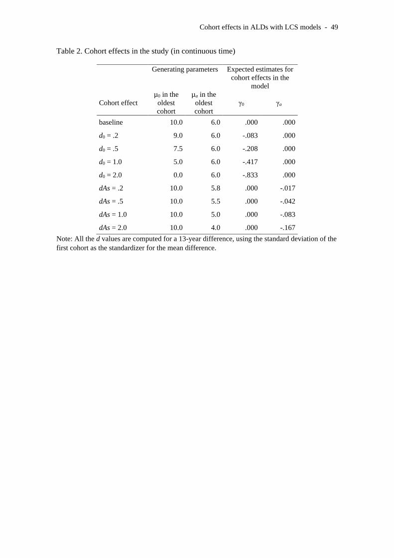
Cohort effects in ALDs with LCS models - 49
Table 2. Cohort effects in the study (in continuous time)
Generating parameters Expected estimates for
cohort effects in the
model
Cohort effect
µ0 in the
oldest
cohort
µa in the
oldest
cohort
γ0 γa
baseline 10.0 6.0 .000 .000
d0 = .2 9.0 6.0 -.083 .000
d0 = .5 7.5 6.0 -.208 .000
d0 = 1.0 5.0 6.0 -.417 .000
d0 = 2.0 0.0 6.0 -.833 .000
dAs = .2 10.0 5.8 .000 -.017
dAs = .5 10.0 5.5 .000 -.042
dAs = 1.0 10.0 5.0 .000 -.083
dAs = 2.0 10.0 4.0 .000 -.167
Note: All the d values are computed for a 13-year difference, using the standard deviation of the
first cohort as the standardizer for the mean difference.
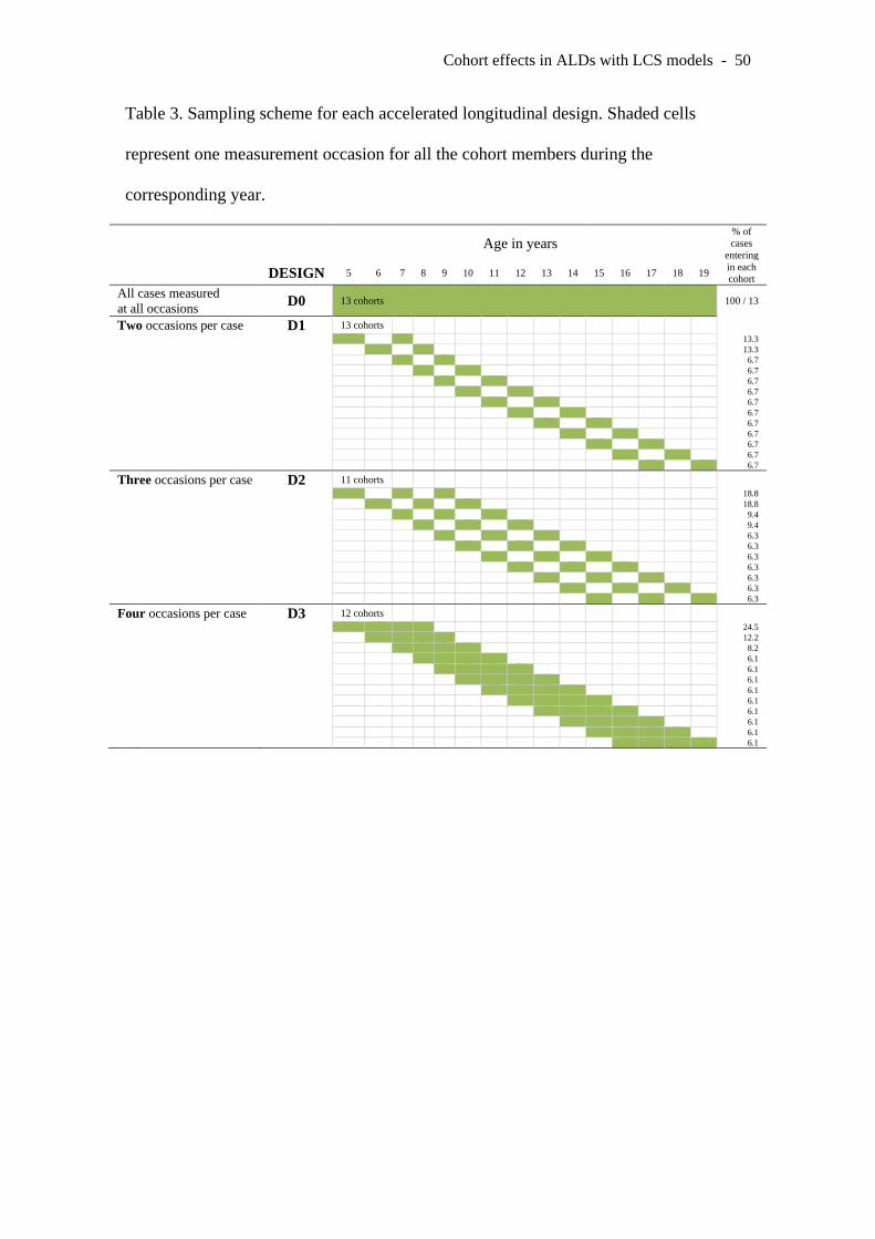
Cohort effects in ALDs with LCS models - 50
Table 3. Sampling scheme for each accelerated longitudinal design. Shaded cells
represent one measurement occasion for all the cohort members during the
corresponding year.
Age in years
% of
cases
entering
DESIGN 5 6 7 8 9 10 11 12 13 14 15 16 17 18 19 in each
cohort
All cases measured
at all occasions D0 13 cohorts 100 / 13
Two occasions per case D1 13 cohorts
13.3 13.3 6.7 6.7 6.7 6.7 6.7 6.7 6.7 6.7 6.7 6.7 6.7
Three occasions per case D2 11 cohorts
18.8 18.8 9.4 9.4 6.3 6.3 6.3 6.3 6.3 6.3 6.3
Four occasions per case D3 12 cohorts
24.5 12.2 8.2 6.1 6.1 6.1 6.1 6.1 6.1 6.1 6.1 6.1

Cohort effects in ALDs with LCS models - 51
Table 4. Parameter estimates from all four models fitted to the NORA data
SSM-CT - cohort effects SSM-CT
Parameter Estimate S.E. 95% CI p Estimate S.E. 95% CI p
Cohort → intercept γ0 -1.463 .829 -3.089 .162 .078 -
Cohort → additive γa -.125 .033 -.189 -.061 <.001 -
Self-feedback β -.240 .054 -.346 -.133 <.001 -.362 .041 -.442 -.282 <.001
Mean intercept μ0 11.115 1.465 8.244 13.987 <.001 7.826 1.434 5.016 10.636 <.001
Mean additive μa 8.747 1.267 6.263 11.230 <.001 10.665 1.029 8.649 12.682 <.001
Variance intercept σ20 69.459 20.162 29.941 108.976 .001 67.084 20.603 26.702 107.466 .001
Variance additive σ2a .500 .284 -.056 1.056 .078 1.245 .493 .279 2.212 .012
Covariance σ0a -.758 2.103 -4.880 3.365 .719 2.926 2.326 -1.633 7.485 .208
Variance error σ2e 8.190 1.099 6.037 10.344 <.001 8.495 1.106 6.328 10.662 <.001
LCS-DT - cohort effects LCS-DT
Parameter Estimate S.E. 95% CI p Estimate S.E. 95% CI p
Cohort → intercept γ0 -1.188 .814 -2.784 .409 .145 -
Cohort → additive γa -.101 .033 -.166 -.036 .002 -
Self-feedback β -.206 .048 -.300 -.113 <.001 -.293 .028 -.348 -.237 <.001
Mean intercept μ0 11.373 1.428 8.574 14.172 <.001 8.554 1.338 5.931 11.176 <.001
Mean additive μa 7.467 1.021 5.466 9.467 <.001 8.640 .687 7.293 9.987 <.001
Variance intercept σ20 63.270 18.622 26.770 99.769 .001 59.739 18.575 23.332 96.146 .001
Variance additive σ2a .374 .218 -.053 .802 .086 .861 .324 .226 1.496 .008
Covariance σ0a -.104 2.005 -4.035 3.826 .959 2.646 1.702 -.691 5.982 .120
Variance error σ2e 8.390 1.105 6.225 10.556 <.001 8.595 1.091 6.456 10.734 <.001
Note: SSM-CT = State-Space Model in continuous time. LCS-DT = Latent Change Score model
in discrete time. S.E. = Standard Error. CI = Confidence interval
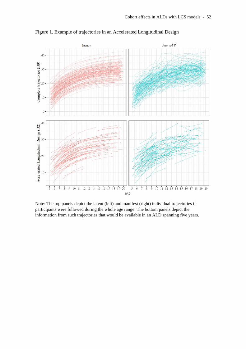
Cohort effects in ALDs with LCS models - 52
Figure 1. Example of trajectories in an Accelerated Longitudinal Design
Note: The top panels depict the latent (left) and manifest (right) individual trajectories if
participants were followed during the whole age range. The bottom panels depict the
information from such trajectories that would be available in an ALD spanning five years.
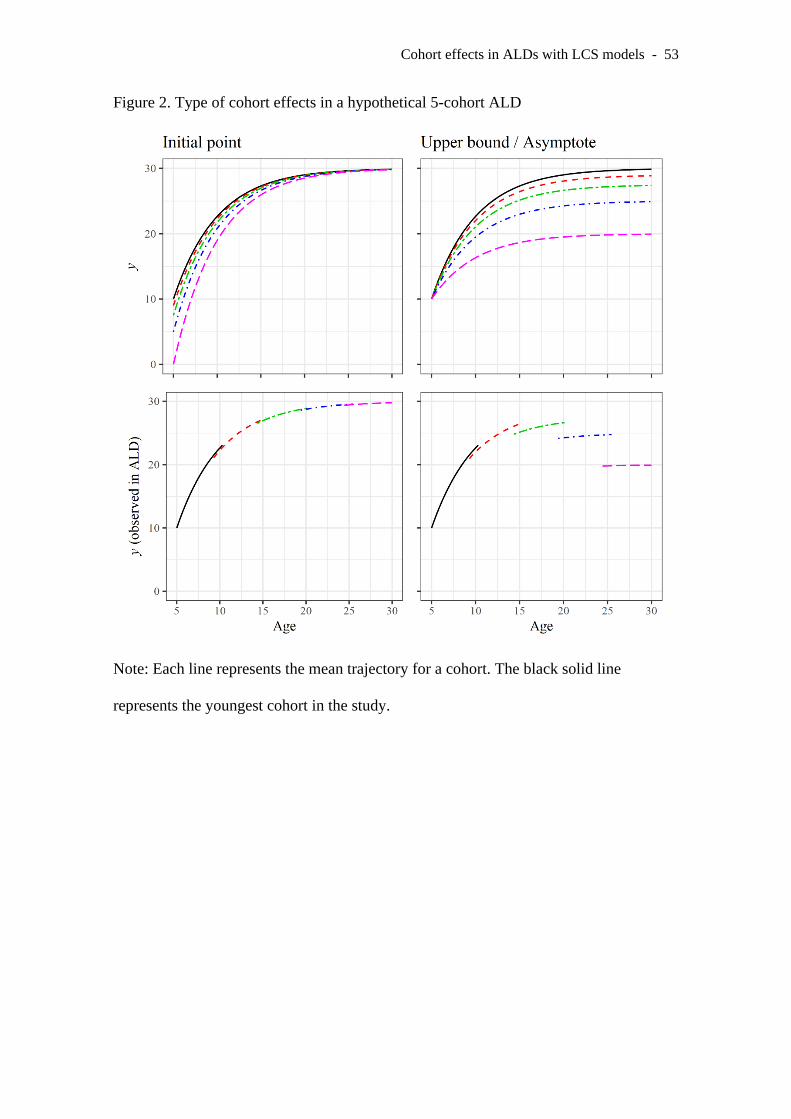
Cohort effects in ALDs with LCS models - 53
Figure 2. Type of cohort effects in a hypothetical 5-cohort ALD
Note: Each line represents the mean trajectory for a cohort. The black solid line
represents the youngest cohort in the study.
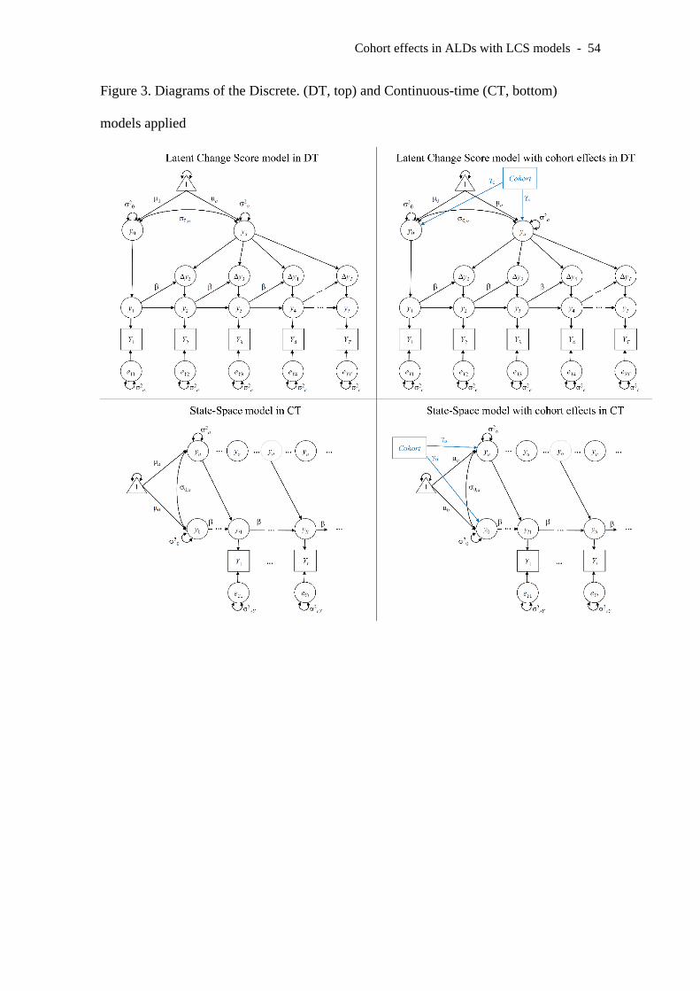
Cohort effects in ALDs with LCS models - 54
Figure 3. Diagrams of the Discrete. (DT, top) and Continuous-time (CT, bottom)
models applied
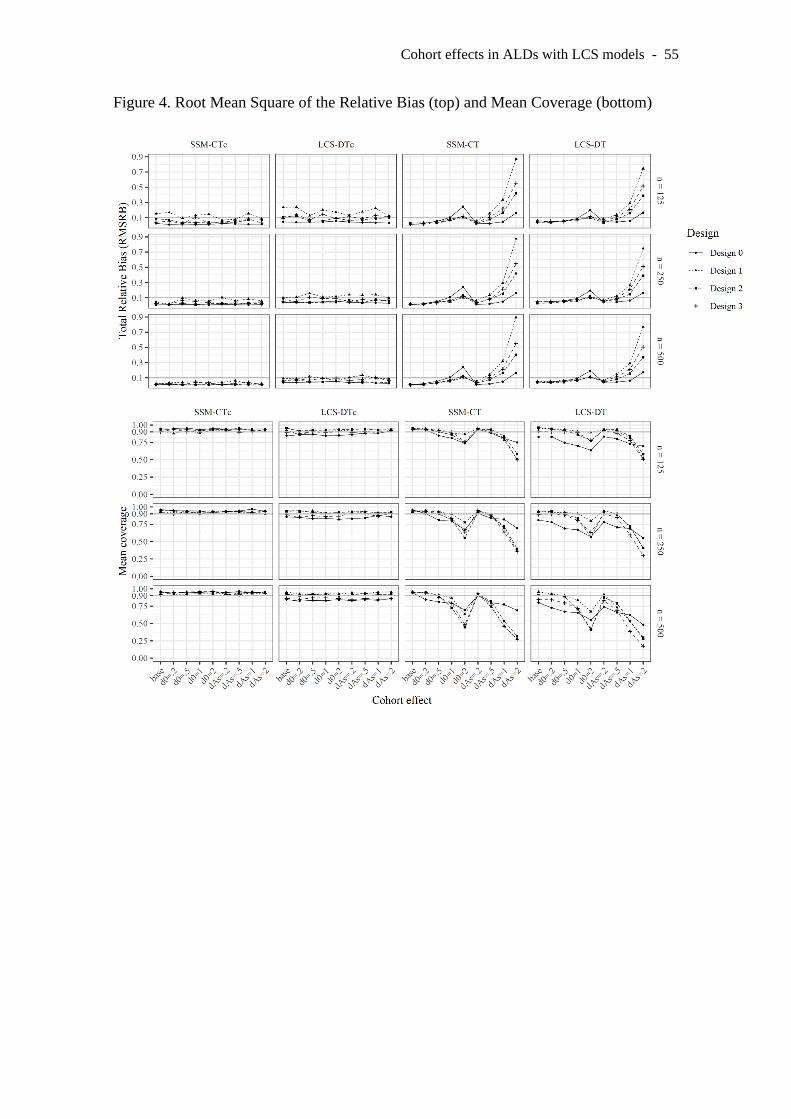
Cohort effects in ALDs with LCS models - 55
Figure 4. Root Mean Square of the Relative Bias (top) and Mean Coverage (bottom)
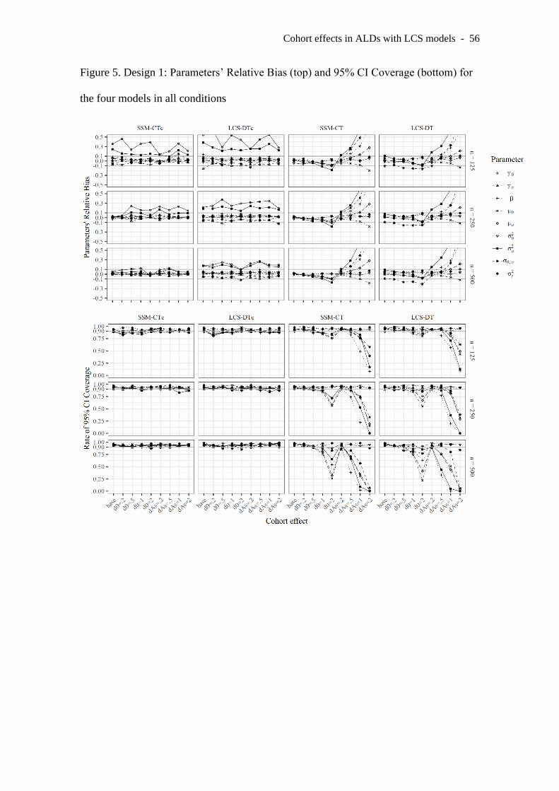
Cohort effects in ALDs with LCS models - 56
Figure 5. Design 1: Parameters’ Relative Bias (top) and 95% CI Coverage (bottom) for
the four models in all conditions
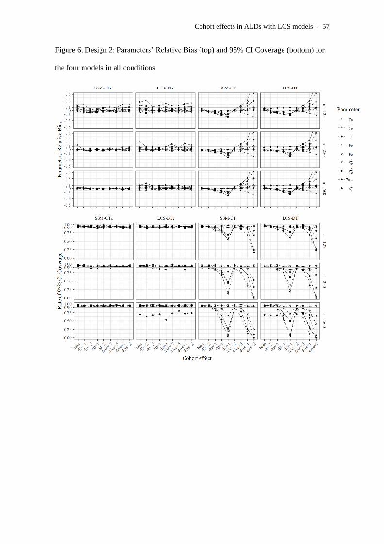
Cohort effects in ALDs with LCS models - 57
Figure 6. Design 2: Parameters’ Relative Bias (top) and 95% CI Coverage (bottom) for
the four models in all conditions
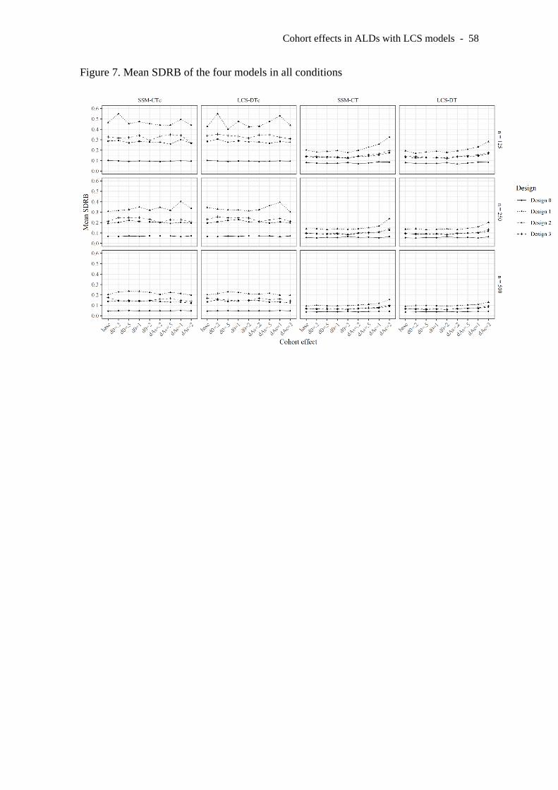
Cohort effects in ALDs with LCS models - 58
Figure 7. Mean SDRB of the four models in all conditions
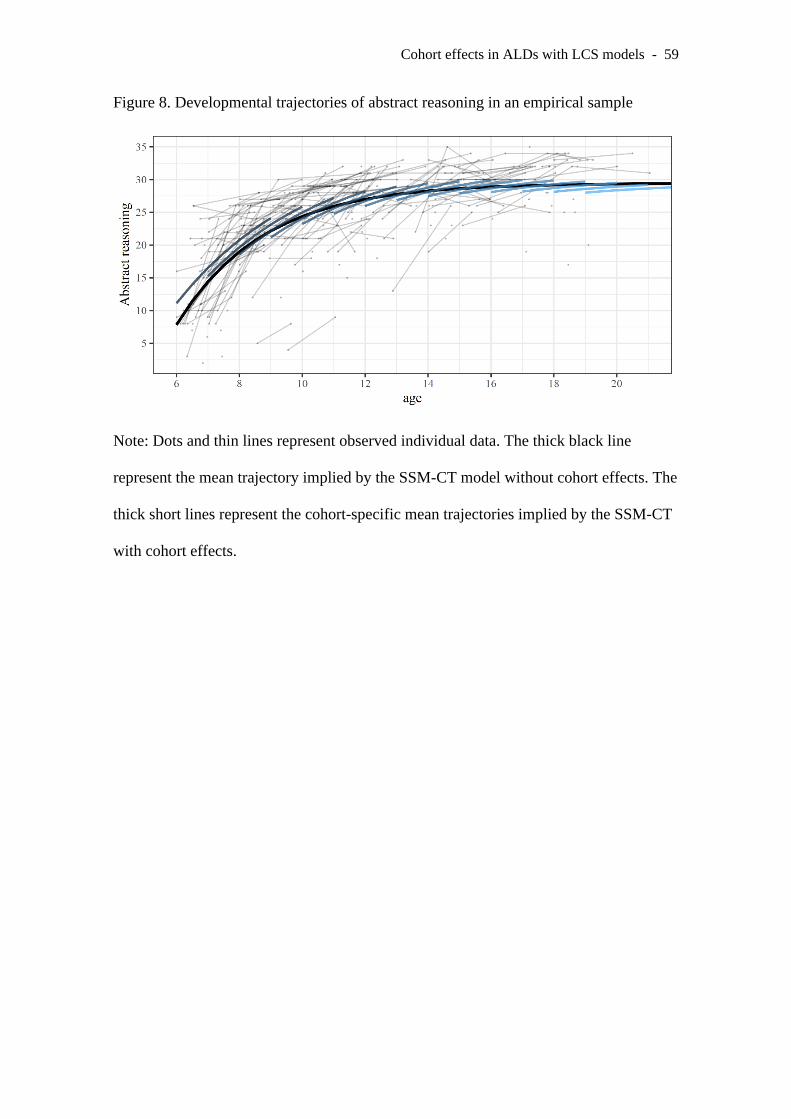
Cohort effects in ALDs with LCS models - 59
Figure 8. Developmental trajectories of abstract reasoning in an empirical sample
Note: Dots and thin lines represent observed individual data. The thick black line
represent the mean trajectory implied by the SSM-CT model without cohort effects. The
thick short lines represent the cohort-specific mean trajectories implied by the SSM-CT
with cohort effects.