Cochlea Modelling and its Application to Speech Processing
211
UNIVERSITY OF SOUTHAMPTON Faculty of Engineering and the Environment Institute of Sound and Vibration Cochlea Modelling and its Application to Speech Processing by Shuokai Pan A thesis submitted for the degree of Doctor of Philosophy June 2018
-
Upload
khangminh22 -
Category
Documents
-
view
0 -
download
0
Transcript of Cochlea Modelling and its Application to Speech Processing

UNIVERSITY OF SOUTHAMPTON
Faculty of Engineering and the Environment
Institute of Sound and Vibration
Cochlea Modelling and its
Application to Speech Processing
by
Shuokai Pan
A thesis submitted for the degree of
Doctor of Philosophy
June 2018


UNIVERSITY OF SOUTHAMPTON
ABSTRACT
FACULTY OF ENGINEERING AND THE ENVIRONMENT
INSTITUTE OF SOUND AND VIBRATION
Doctor of Philosophy
COCHLEA MODELLING AND ITS APPLICATION TO SPEECH
PROCESSING
by Shuokai Pan
Models of the cochlea provide a valuable tool for both better understanding its
mechanics and also as an inspiration for many speech processing algorithms. Real-
istic modelling of the cochlea can be computationally demanding, however, which
limits its applicability in signal processing applications. To mitigate this issue, an
efficient numerical method has been proposed for performing time domain sim-
ulations, based on a nonlinear state space formulation [1]. This model has then
been contrasted with another type of cochlear model, that is established from a
cascade of digital filters. A comparison of the responses from these two models has
been conducted, in terms of their realism in simulating the measured nonlinear
cochlear response to single tones and pairs of tones. Guided by these results, the
filter cascade model is chosen for subsequent signal processing applications because
it is significantly more efficient than the state space model, while still producing
realistic responses.
Using this nonlinear filter cascade model as a front-end, two speech processing
tasks have been investigated: voice activity detection and supervised speech sep-
aration. Both tasks are tackled within a machine learning framework, in which a
neural network is trained to reproduce target outputs. The results are compared
with those using a number of other simpler auditory-inspired analysis methods.
Simulation results show that although the nonlinear filter cascade model can be
more effective in many testing scenarios, its relative advantage against other anal-
ysis methods is small. The incorporation of temporal context information and
network structure engineering are found to be more important in improving the
performance of these tasks. Once a suitable context expansion strategy has been
selected, the difference between various front-end processing methods considered
is marginal.


Contents
List of Figures ix
List of Tables xix
Declaration of Authorship xxi
Acknowledgements xxiii
Abbreviations xxv
1 Introduction 1
1.1 Motivation . . . . . . . . . . . . . . . . . . . . . . . . . . . . . . . . 1
1.2 Thesis Contributions . . . . . . . . . . . . . . . . . . . . . . . . . . 5
1.3 Publications . . . . . . . . . . . . . . . . . . . . . . . . . . . . . . . 6
1.4 Thesis Outline . . . . . . . . . . . . . . . . . . . . . . . . . . . . . . 6
2 Background and Literature Review 9
2.1 The Cochlea . . . . . . . . . . . . . . . . . . . . . . . . . . . . . . . 9
2.1.1 Cochlea Anatomy . . . . . . . . . . . . . . . . . . . . . . . . 11
2.1.2 An Overview of Cochlear Mechanics . . . . . . . . . . . . . 12
2.1.2.1 Single Tone Responses: Compressive Amplification 15
2.1.2.2 Two-tone Suppression . . . . . . . . . . . . . . . . 18
2.2 Machine Learning and Deep Learning . . . . . . . . . . . . . . . . . 19
2.2.1 Deep Feed-forward Neural Networks . . . . . . . . . . . . . 22
2.2.2 Convolutional Neural Networks . . . . . . . . . . . . . . . . 25
2.2.3 Training of Neural Networks . . . . . . . . . . . . . . . . . . 27
2.2.3.1 Regularization . . . . . . . . . . . . . . . . . . . . 29
2.3 Summary . . . . . . . . . . . . . . . . . . . . . . . . . . . . . . . . 31
3 Comparison of Models of the Human Cochlea 33
3.1 Introduction . . . . . . . . . . . . . . . . . . . . . . . . . . . . . . . 34
3.2 Model Descriptions . . . . . . . . . . . . . . . . . . . . . . . . . . . 36
3.2.1 The Transmission-line Model . . . . . . . . . . . . . . . . . 36
3.2.2 The CAR-FAC Model . . . . . . . . . . . . . . . . . . . . . 38
3.3 Model Comparisons . . . . . . . . . . . . . . . . . . . . . . . . . . . 42
3.3.1 Derivation of the Filter Cascade Model from the TL Model . 42
v

vi CONTENTS
3.3.2 Cumulative Frequency Responses and Active Gain . . . . . . 45
3.3.3 Single-tone compression . . . . . . . . . . . . . . . . . . . . 46
3.3.4 Two-tone suppression . . . . . . . . . . . . . . . . . . . . . . 52
3.4 Discussion . . . . . . . . . . . . . . . . . . . . . . . . . . . . . . . . 56
3.5 Summary . . . . . . . . . . . . . . . . . . . . . . . . . . . . . . . . 60
4 Cochlea Modelling as a Front-end for Neural Network based VoiceActivity Detection 63
4.1 Introduction . . . . . . . . . . . . . . . . . . . . . . . . . . . . . . . 64
4.2 An Overview of Existing VAD Methods . . . . . . . . . . . . . . . . 66
4.2.1 Feature Extraction . . . . . . . . . . . . . . . . . . . . . . . 66
4.2.1.1 Acoustics features . . . . . . . . . . . . . . . . . . 66
4.2.1.2 Auditory-inspired Features . . . . . . . . . . . . . . 69
4.2.2 Decision Rules . . . . . . . . . . . . . . . . . . . . . . . . . . 72
4.2.2.1 Statistical Modelling Approaches . . . . . . . . . . 73
4.2.2.2 Machine Learning Approaches . . . . . . . . . . . . 75
4.3 Filter Cascade Spectrogram for Neural Network based VAD . . . . 78
4.4 Simulation Setup . . . . . . . . . . . . . . . . . . . . . . . . . . . . 84
4.4.1 Datasets . . . . . . . . . . . . . . . . . . . . . . . . . . . . . 84
4.4.2 Neural Network Structures and Training. . . . . . . . . . . . 89
4.4.3 Comparison with Other Methods . . . . . . . . . . . . . . . 91
4.4.4 Evaluation Metric. . . . . . . . . . . . . . . . . . . . . . . . 92
4.5 Results for Noise-dependent Training . . . . . . . . . . . . . . . . . 93
4.6 Results for Noise-independent Training . . . . . . . . . . . . . . . . 98
4.6.1 DNN Results . . . . . . . . . . . . . . . . . . . . . . . . . . 98
4.6.2 CNN results . . . . . . . . . . . . . . . . . . . . . . . . . . . 101
4.7 Further Improvements . . . . . . . . . . . . . . . . . . . . . . . . . 106
4.8 Comparison with Other Methods . . . . . . . . . . . . . . . . . . . 109
4.9 Summary . . . . . . . . . . . . . . . . . . . . . . . . . . . . . . . . 111
5 Cochlea Modelling for Supervised Speech Separation 113
5.1 Introduction . . . . . . . . . . . . . . . . . . . . . . . . . . . . . . . 113
5.2 An Overview of Classical Speech Separation Methods . . . . . . . . 114
5.2.1 Spectral Subtractive Methods . . . . . . . . . . . . . . . . . 114
5.2.2 Wiener Filter based Methods . . . . . . . . . . . . . . . . . 116
5.2.3 Statistical Model based Methods . . . . . . . . . . . . . . . 116
5.3 Supervised Speech Separation . . . . . . . . . . . . . . . . . . . . . 117
5.4 Filter Cascade Spectrogram for Supervised Speech Separation . . . 122
5.4.1 Feature Extraction . . . . . . . . . . . . . . . . . . . . . . . 122
5.4.2 Experimental Settings . . . . . . . . . . . . . . . . . . . . . 125
5.4.2.1 Datasets . . . . . . . . . . . . . . . . . . . . . . . . 125
5.4.2.2 Neural Network Structures and Training . . . . . . 126
5.4.2.3 Evaluation and Comparison . . . . . . . . . . . . . 127
5.5 Results . . . . . . . . . . . . . . . . . . . . . . . . . . . . . . . . . . 129

CONTENTS vii
5.5.1 DNN Results . . . . . . . . . . . . . . . . . . . . . . . . . . 130
5.5.2 CNN Results . . . . . . . . . . . . . . . . . . . . . . . . . . 133
5.5.3 Comparison . . . . . . . . . . . . . . . . . . . . . . . . . . . 136
5.6 Summary . . . . . . . . . . . . . . . . . . . . . . . . . . . . . . . . 141
6 Conclusions and Suggestions for Future Work 143
6.1 Conclusions . . . . . . . . . . . . . . . . . . . . . . . . . . . . . . . 143
6.1.1 Cochlear Modelling . . . . . . . . . . . . . . . . . . . . . . . 143
6.1.2 Application to Speech Processing . . . . . . . . . . . . . . . 145
6.2 Suggestions for Future Work . . . . . . . . . . . . . . . . . . . . . . 147
A Detailed Results of Supervised Speech Separation Experiments 149
B Publications 159
B.1 Time Domain Solutions for the Neely and Kim [9] Model of theCochlea . . . . . . . . . . . . . . . . . . . . . . . . . . . . . . . . . 159
B.2 Comparison of Two Cochlear Models . . . . . . . . . . . . . . . . . 159
References 169


List of Figures
2.1 The anatomy of the human ear. The cochlea is located in the innerear. Picture adapted from [22] with permission. . . . . . . . . . . . 10
2.2 Cross section of the cochlear duct (a) and the Organ of Corti (b).Subplot (a) and (b) is obtained from [28] and [29] respectively withpermission. . . . . . . . . . . . . . . . . . . . . . . . . . . . . . . . 13
2.3 Tonotopical arrangement along the human cochlea. Picture takenfrom [32] with permission. . . . . . . . . . . . . . . . . . . . . . . . 14
2.4 Input-output function of a BM site in response to characteristicfrequency tones as a function of input SPL. Responses were mea-sured before (squares) and after (triangles) trauma in a guinea pigcochlea. The solid, dashed and dotted lines represent the growthfunction that would be expected from a saturated mechanism, alinear mechanism or a combined mechanism respectively. Figureadapted from [37] with permission. . . . . . . . . . . . . . . . . . . 16
2.5 a) A family of isointensity curves representing the velocity of BMresponses to single tone pips as a function of frequency and intensity(in dB SPL). b) A family of isointensity curves representing the gainor sensitivity (velocity divided by stimulus pressure) of the BM siteto single tone pips as a function of frequency and intensity (in dBSPL), plotted using the same data as that shown in a). Figureadapted from [38] with permission. . . . . . . . . . . . . . . . . . . 17
2.6 Frequency responses of the BM at a basal and apical location. Twofamilies of sensitivity curves (ratio of BM velocity to stimulus pres-sure) were recorded at the 0.5 and 9 kHz characteristic places in thechinchilla cochlea at different stimulus frequencies and levels. Thebest frequencies and 10 dB quality factors for the highest stimuluslevel are also indicated for each location. Figure adapted from [33]with permission. . . . . . . . . . . . . . . . . . . . . . . . . . . . . . 17
2.7 Two-tone suppression of the BM velocity responses measured in thechinchilla cochlea for both (a) higher-side suppressor tones and (b)lower-side suppressor tones. Figure adapted from [40] with permission. 19
2.8 An example of deep feed-forward neural network with an inputlayer, three hidden layers, and an output layer. Picture reproducedfrom Fig. 4.1 of [20] with permission. . . . . . . . . . . . . . . . . . 23
2.9 A comparison of a biological neuron and its mathematical represen-tation in neural networks shown in Fig. 2.8. Picture reproducedfrom [19] with permission. . . . . . . . . . . . . . . . . . . . . . . . 24
ix

x LIST OF FIGURES
2.10 Illustration of a typical CNN, applied to a speech processing tasks,using a 2-dimensional time-frequency representation as input fea-tures. It consists of one convolutional layer, one pooling layer anda few fully-connected layers. Picture adapted from Fig. 3 of [54]with permission. . . . . . . . . . . . . . . . . . . . . . . . . . . . . . 27
2.11 The application of dropout to a neural network. (a) A standardneural network with 2 hidden layers. (b) The same network afterapplying dropout. Units labelled with cross have been droppedtemporarily. Picture taken from [63] with permission. . . . . . . . . 31
3.1 The box model of the human cochlea. Adapted from Fig. 2 of [88]with permission. . . . . . . . . . . . . . . . . . . . . . . . . . . . . . 36
3.2 Some example Boltzmann functions with varying values of α and β.(a) Variation of the Boltzmann function with parameter ℵ, while βis set to 1. (b) Variation of the Boltzmann function with parameterβ, while α is set to 1. . . . . . . . . . . . . . . . . . . . . . . . . . . 38
3.3 Block diagram of the micromechanical model of Neely and Kim [9]with a saturating nonlinearity in the active force. Adapted fromFig. 11 of [1] with permission. . . . . . . . . . . . . . . . . . . . . . 38
3.4 Architecture of the CAR-FAC model of the human cochlea. H1 toHN represent the transfer functions of the cascade of asymmetricresonators, modelling the BM motion with outputs y1 to yN . Damp-ing parameters of these resonators are controlled by the OHC modeland the coupled AGC smoothing filters (AGC SF), shown in dashedrectangular box, to implement fast-acting and level-dependent com-pression. The AGC module of each channel consists of a parallel-of-cascade of four first-order low-pass filters with increasing timeconstant. Smoothing filters with the same time constant are alsolaterally connected (dashed arrows), which allows a diffusion-likecoupling across both space and time. The IHC model outputs, r1
to rN , present an estimate of average instantaneous firing rates onthe auditory nerve fibres. Picture obtained by combining Fig. 15.2and Fig. 19.5 of [12] with permission. . . . . . . . . . . . . . . . . . 40
3.5 Frequency responses of the individual segments of the TL model(A, B), computed with (thin) and without (thick) the WNR termand those of the serial filters of the CAR-FAC model (C, D). Onlyevery fifth of the first 76 output channels are shown for clarity. . . . 45
3.6 Overall frequency responses at various positions for the TL model(A, B) and CAR-FAC model (C, D) when configured as fully active(thin lines) and fully passive (thick lines). Only every fifth of thefirst 76 output channels are shown for clarity. . . . . . . . . . . . . 47
3.7 Active gain provided to the travelling waves at CF in the TL andCAR-FAC models for different positions along the length of bothcochlea models. . . . . . . . . . . . . . . . . . . . . . . . . . . . . . 47

LIST OF FIGURES xi
3.8 Single-tone compression simulations at the 4 kHz characteristic placein the TL (A, B, C, D) and CAR-FAC (E, F, G, H) model. (A,E) BM motion I/O functions at a number of example frequencies,including the CF, 4 frequencies that are lower and 3 that are higherthan the CF. The straight line indicates linear growth rate of 1dB/dB for easy reference. (B, F) Sensitivity functions obtainedby normalizing the BM responses in (A, E) by the correspondingstapes velocity in the TL model and stimulus sound pressure levelin the CAR-FAC model. Stimulus intensity varied from 0 dB to100 dB in steps of 10 dB and is indicated by the thickness of thelines with the thinnest line corresponding to 0 dB and the thickestline to 100 dB. Numbers inside the circle symbol represent probeSPL divided by 10. The vertical lines indicate the place of the CFand the most sensitive frequency at the highest probe level, 100 dBSPL. (C, G) Rate-of-growth (ROG) values are shown as a functionof stimulus level for the same example frequencies as in (A) or (E).(D, H) Rate-of-growth (ROG) values are shown as a function ofstimulus frequency for some example SPLs. Line style and markermeaning in (D, H) follow that in (B, F). . . . . . . . . . . . . . . . 52
3.9 Level dependence of two-tone suppression to a 4 kHz probe tone(F1) at its characteristic place on suppressor tone frequency usingthe TL (A) and CAR-FAC (C) model. The probe tone sound pres-sure level is 30 dB. Input/output functions for a 4 kHz probe tone(F1) at its characteristic place in the absence and presence of ahigh-side, 5 kHz, suppressor tone (F2) at 5 different sound pressurelevels as indicated in the legend, in the TL (B) and CAR-FAC (D)model. . . . . . . . . . . . . . . . . . . . . . . . . . . . . . . . . . . 54
3.10 Two-tone suppression simulations using the CAR-FAC model. Re-sults are displayed from three perspectives. Column 1 (A, B, C):iso-level suppression curves for suppressors ranging from 10 to 90dB SPL in steps of 5 dB, as indicated by the line thickness, while theprobe is at 30, 50 and 70 dB SPL in rows 1, 2 and 3 respectively. 10dB suppressor levels are also marked with numbered circles: e.g.,30 dB SPL=10 times 3©. Column 2 (D, E, F): suppressor levelsnecessary to reduce the probe amplitude by 1, 10 and 20 dB, asindicated by the encircled numbers on each line. Column 3 (G, H,I): Rate of suppression (ROS) as a function of suppressor frequency,computed as the slope of the probe reduction curves shown in Fig.3.9 (C). Only every 10 dB increment in suppressor level is plottedfor better visualization. 10 dB suppressor levels are also marked. . . 57

xii LIST OF FIGURES
3.11 Two-tone suppression simulations using the TL model. Results aredisplayed from three perspectives. Column 1 (A, B, C): iso-levelsuppression curves for suppressors ranging from 10 to 90 dB SPL insteps of 5 dB, while the probe is at 30, 50 and 70 dB SPL in rows 1, 2and 3 respectively. Column 2 (D, E, F): suppressor levels necessaryto reduce the probe amplitude by 1, 10 and 20 dB. Column 3 (G, H,I): Rate of suppression (ROS) as a function of suppressor frequency,computed as the slope of the probe reduction curves shown in Fig.3.9 (a). Only every 10 dB increment in suppressor level is plottedfor better visualization. Line styles follow those in Fig. 3.10. . . . . 58
3.12 Two-tone suppression measurements from the basal region of thechinchilla cochlea. Results are displayed from three perspectives.Column 1 (A, B, C): iso-level suppression curves for suppressorsranging from 10 to 90 dB SPL in steps of 5 dB, while the probe is at8 kHz and 30, 50 and 70 dB SPL in rows 1, 2 and 3 respectively. 10dB levels are indicated with numbered symbol: e.g., 30 dB SPL=10times 3©. Column 2 (D, E, F): suppressor levels necessary to reducethe probe amplitude by 1, 10 and 20 dB (labelled as solid lines).The 1-nm iso-amplitude curve for a single tone is repeated in eachpanel (dashed line). Column 3 (G, H, I): Rate of suppression (ROS)as a function of suppressor frequency, computed as the slope of theprobe reduction curves. Only every 10 dB increment in suppressorlevel is plotted for better visualization (solid lines and numberedsymbols). The negative of the slope of single-tone I/O curves at70 dB SPL is superimposed in each panel (dashed line), where-1dB/dB is linear and 0 dB/dB is complete compression. Taken fromFigure 4 of [106] with permission. . . . . . . . . . . . . . . . . . . . 59
3.13 Maximum rate of suppression as a function of suppressor frequencyfor a 4 kHz, 30 dB SPL, probe tone at its characteristic place inthe TL and CAR-FAC model. Note that the sign of ROS valuesis inverted compared to those in Fig. 3.10, Fig. 3.11 and Fig. 3.12to facilitate comparison with experimental measurements shown inFig. 9 of [45]. . . . . . . . . . . . . . . . . . . . . . . . . . . . . . . 60
4.1 Block diagram of a typical VAD algorithm. Adapted from [108]with permission. . . . . . . . . . . . . . . . . . . . . . . . . . . . . . 65
4.2 Comparison of the computation structure of the MFCC, and PNCCalgorithms. Picture adapted from [118] with permission. . . . . . . 70
4.3 The MRCG feature. (a) Diagram of the process of extracting a 32-dimensional MRCG feature. (b) Calculation of one single-resolution8-dimensional cochleagram features in detail. Adapted from Fig. 3of [6] with permission. . . . . . . . . . . . . . . . . . . . . . . . . . 72

LIST OF FIGURES xiii
4.4 Block diagram of the IBM VAD system developed for the DARPARobust Automatic Transcription of Speech (RATS) program. Thisis a hybrid model including a DNN and a CNN sub-module and isjointly trained on multiple types of features. PLP: Perceptual Lin-ear Prediction; FDLP: Frequency Domain Linear Prediction. Fig-ure is adapted from Fig. 2 of [142] with permission. . . . . . . . . . 78
4.5 An example clean utterance from the TIMIT dataset and the sameutterance corrupted by a factory noise from the NOISEX datasetat 0 dB SNR. . . . . . . . . . . . . . . . . . . . . . . . . . . . . . . 82
4.6 Visualization of various un-normalized time-frequency representa-tions for an example clean utterance from the TIMIT dataset (rightcolumn) as shown in Fig. 4.5 and the same utterance corrupted bya factory noise from the NOISEX dataset at 0 dB SNR (left column). 83
4.7 Visualization of un-normalized MRCG representation of an exampleclean utterance from the TIMIT dataset (right column) as shown inFig. 4.5 and the same utterance corrupted by a factory noise fromthe NOISEX dataset at 0 dB SNR (left column). . . . . . . . . . . 84
4.8 Visualization of various mean-variance normalized time-frequencyrepresentations for an example clean utterance from the TIMITdataset (right column) and the same utterance corrupted by a fac-tory noise from the NOISEX dataset at 0 dB SNR (left column). . . 85
4.9 Visualization of mean-variance normalized MRCG representationof an example clean utterance from the TIMIT dataset (right col-umn) and the same utterance corrupted by a factory noise from theNOISEX dataset at 0 dB SNR (left column). . . . . . . . . . . . . . 86
4.10 A summary of the noise datasets used in experimental simulations.“Win down” refers to driving the car with windows down and “Winup” means the opposite. . . . . . . . . . . . . . . . . . . . . . . . . 88
4.11 ROC curves for six different feature types with DNN backend un-der cafe and car noises at four SNR conditions. Spec: FFT basedLog-Power spectrogram, LogMel: Log-Mel spectrogram; GTspec:Gammatone spectrogram; PNspec: Power normalized spectrogram;MRCG: multi-resolution cochleagram, FCspec: filter cascade spec-trogram. DNNs were trained noise-dependently. . . . . . . . . . . . 95
4.12 ROC curves for six different feature types with DNN backend underfactory1 and ship oproom noises at four SNR conditions. Spec: FFTbased Log-Power spectrogram, LogMel: Log-Mel spectrogram; GT-spec: Gammatone spectrogram; PNspec: Power normalized spec-trogram; MRCG: multi-resolution cochleagram, FCspec: filter cas-cade spectrogram. DNNs were trained noise-dependently. . . . . . . 96
4.13 Comparison of AUC metric for six types of spectrogram featureswith DNN backend under four types of noise and four SNR levels.DNNs are trained noise-dependently. The legend follows those inFig. 4.11 and Fig. 4.12. . . . . . . . . . . . . . . . . . . . . . . . . 97

xiv LIST OF FIGURES
4.14 Comparison of average AUC metric for six types of spectrogramfeatures with DNN backend at four SNR conditions. Average AUCvalues at each SNR were computed as the arithmetic mean of theresults shown in Fig. 4.13 across all four noise types. The legendfollows those in Fig. 4.11 and Fig. 4.12. . . . . . . . . . . . . . . . . 97
4.15 Comparison of AUC metric obtained from different spectrogrambased features with DNN backend under (matched) noise testingconditions. The legend follows those in Fig. 4.11 and DNN istrained noise-independently or multi-conditionally. . . . . . . . . . . 99
4.16 Comparison of AUC metric using different spectrogram based fea-tures with DNN backend under (unmatched) noise testing condi-tions. The legend follows those in Fig. 4.11 and DNN was trainednoise-independently or multi-conditionally. . . . . . . . . . . . . . . 100
4.17 Average AUC metric across all (matched) and (unmatched) noisetypes, obtained from different spectrogram based features with DNNbackend. Average AUC values at each SNR are computed as thearithmetic mean of the results shown in Fig. 4.15 and Fig. 4.16.Legend meanings follow those in Fig. 4.11 and DNN was trainednoise-independently or multi-conditionally. . . . . . . . . . . . . . . 100
4.18 Comparison of AUC obtained from different spectrogram featureswith CNN-SR backend under matched noise conditions. Neuralnetwork is trained using multi-conditional dataset. Results fromthe MRCG with the DNN backend are also shown. . . . . . . . . . 102
4.19 Comparison of AUC obtained from different spectrogram featureswith CNN-SR backend under unmatched noise conditions. Neu-ral network is trained using multi-conditional dataset. Results fromthe MRCG with the DNN backend are also shown. . . . . . . . . . 102
4.20 Average AUC metric across all matched and unmatched noisetypes, obtained from different spectrogram features with CNN-SR backend. Average AUC values at each SNR are computed asthe arithmetic mean of the results shown in Fig. 4.18 and Fig. 4.19.CNN is trained using multi-conditional dataset. Results from theMRCG feature with the DNN backend are also shown. . . . . . . . 103
4.21 Comparison of AUC metric obtained from different spectrogrambased features with CNN-MR backend under matched noise test-ing conditions. Neural network is trained noise-independently ormulti-conditionally. Results from the MRCG feature with a DNNbackend are also shown to facilitate comparison. . . . . . . . . . . . 103
4.22 Comparison of AUC metric obtained from different spectrogrambased features with CNN-MR backend under unmatched noisetesting conditions. Neural network is trained noise-independentlyor multi-conditionally. Results from the MRCG feature with a DNNbackend are also shown to facilitate comparison. . . . . . . . . . . . 104

LIST OF FIGURES xv
4.23 Average AUC metric across all matched and unmatched noise types,obtained from different spectrogram based features with CNN-MRbackend. Average AUC values at each SNR are computed as thearithmetic mean of the results shown in Fig. 4.21 and Fig. 4.22.CNN is trained noise-independently or multi-conditionally. Resultsfrom the MRCG feature with a DNN backend are also shown tofacilitate comparison. . . . . . . . . . . . . . . . . . . . . . . . . . . 104
4.24 Average AUC metric across all matched and unmatched noise typesand different SNR levels for four auditory spectrogram features withthree neural network classifiers, DNN, CNN-SR and CNN-MR. Re-sults from the MRCG feature with a DNN backend are also shownto facilitate comparison and all neural networks are trained noise-independently or multi-conditionally. . . . . . . . . . . . . . . . . . 105
4.25 Comparison of various strategies in capturing context informationwith the LogMel filterbank in terms of AUC under matched andunmatched noises. MRLM means adopting the same analysismethod as used in MRCG, but the Gammatone filterbank is re-placed by a LogMel filterbank. MWLLM means the spectrogramfeature is computed using multiple window lengths. . . . . . . . . . 107
4.26 Comparison of various strategies in capturing context informationwith the Gammatone filterbank in terms of AUC under matchedand unmatched noises. MWLCG means the cochleagram featureis computed using multiple window lengths. . . . . . . . . . . . . . 108
4.27 Comparison of various strategies in capturing context informationwith the filter cascade model in terms of AUC under matchedand unmatched noises. MRFC means adopting the same anal-ysis method as used in MRCG, but the Gammatone filterbank isreplaced by a filter cascade filterbank. MWLFC means the spectro-gram feature is computed using multiple window lengths. . . . . . . 108
4.28 Average AUC values obtained by applying various context expan-sion strategies to three different auditory filterbank spectrogramfeatures. The legend follows those in Fig. 4.24, Fig. 4.25, Fig. 4.26and Fig. 4.27. . . . . . . . . . . . . . . . . . . . . . . . . . . . . . . 109
4.29 Comparison of the AUC values obtained by various VAD systemsunder four noise types and SNR levels. The legend follows those inFig. 4.24, Fig. 4.25, Fig. 4.26 and Fig. 4.27. . . . . . . . . . . . . . 110
4.30 Comparison of the average AUC values across four noise types ob-tained by various VAD systems. The legend follows those in Fig.4.24, Fig. 4.25, Fig. 4.26 and Fig. 4.27. . . . . . . . . . . . . . . . . 111
4.31 Overall comparison of the average AUC values across four noisetypes and four SNR levels obtained by various VAD systems. Thelegend follows those in Fig. 4.24, Fig. 4.25, Fig. 4.26 and Fig. 4.27. 111
5.1 Comparison of the (a) conventional statistics-based method and(b, c) two types of DNN-based methods for speech separation orenhancement. Adapted from Fig. 1 of [171] with permission. . . . . 119

xvi LIST OF FIGURES
5.2 Block diagram of a typical supervised speech separation system.Common choice for Time-Frequency analysis and synthesis is theGammatone filterbank. The dashed line means that the Time-Frequency analysis representation can sometimes be used in Featureextraction module as well. . . . . . . . . . . . . . . . . . . . . . . . 121
5.3 An example clean utterance from the TIMIT dataset and the sameutterance corrupted by a factory noise from the NOISEX datasetat 0 dB SNR. . . . . . . . . . . . . . . . . . . . . . . . . . . . . . . 123
5.4 Visualization of MRCG representation of a clean utterance from theTIMIT dataset (right column) and the same utterance corrupted bya factory noise from the NOISEX dataset at 0 dB SNR (left column).124
5.5 The Ideal Ratio Mask for estimating clean speech signal shown atthe left hand side of Fig. 5.3 from its noisy counterpart shown atthe right hand side of Fig. 5.3. . . . . . . . . . . . . . . . . . . . . . 125
5.6 Comparison of STOI and three other reference objective intelligibil-ity measures in prediction of subjective speech intelligibility scores.The unprocessed noisy speech conditions are denoted by the crosses,and the ITFS-processed conditions are represented by the dots,where ITFS means ideal time frequency segregation, which is justusing ideal time-frequency mask for speech separation as introducedin section 5.3. The gray line denotes the mapping function used toconvert the objective output to an intelligibility score. Root-mean-square prediction error δ, and the correlation coefficient ρ, betweenthe subjective and objective intelligibility scores are shown in thetitle of each plot. Adapted from Fig. 1 of [190] with permission. . . 130
5.7 Average PESQ and STOI scores across matched and unmatchednoise types for DNN enhanced test utterances. A magnified view ofthe scores at 0 dB SNR is shown in the corner of each sub-plot. . . 132
5.8 Average PESQ and STOI scores over all noise types and SNR levelsfor DNN enhanced test utterances. . . . . . . . . . . . . . . . . . . 132
5.9 Average PESQ and STOI scores across matched and unmatchednoise types for single resolution CNN enhanced test utterances. Amagnified view of the scores at 0 dB SNR is shown in the corner ofeach sub-plot. . . . . . . . . . . . . . . . . . . . . . . . . . . . . . . 134
5.10 Average PESQ and STOI scores over all noise types and SNR levelsfor single resolution CNN enhanced test utterances. . . . . . . . . . 134
5.11 Average PESQ and STOI scores over matched and unmatched noisetypes for multi resolution CNN enhanced test utterances. A mag-nified view of the scores at 0 dB SNR is shown in the corner of eachsub-plot. . . . . . . . . . . . . . . . . . . . . . . . . . . . . . . . . . 135
5.12 Average PESQ and STOI scores over all noise types and SNR levelsfor multi resolution CNN enhanced test utterances. . . . . . . . . . 135
5.13 Average PESQ and STOI scores over all noise types and SNR levelsfor DNN and CNNs. . . . . . . . . . . . . . . . . . . . . . . . . . . 137

LIST OF FIGURES xvii
5.14 Comparison of average PESQ and STOI scores over matched andunmatched noise types obtained from three proposed methods andthree reference methods. . . . . . . . . . . . . . . . . . . . . . . . . 138
5.15 Comparison of average PESQ and STOI scores over all noise typesand SNR levels for three proposed methods and three referencemethods. . . . . . . . . . . . . . . . . . . . . . . . . . . . . . . . . . 138
5.16 An example of test noisy utterance and its enhancement by twosupervised learning based methods proposed in this chapter. Thetest utterance is corrupted by factory noise at 0 dB SNR. The IRMof this utterance and its clean spectrogram are shown in the toptwo plots. The estimated IRM and the corresponding enhancedspectrogram, obtained by LogMel-CNN-MR and MWLFC-CNN-MR, are shown in the middle and bottom two plots, respectively. . 139
5.17 The same test noisy utterance as used in Fig. 5.16 but enhancedby the three reference methods. The estimated IRM and the corre-sponding enhanced spectrogram, obtained by Comp Feat-DNN areshown in the top two plots, while the enhanced spectrograms ob-tained by LogMMSE and AudNoiseSup are shown in the bottomtwo plots. . . . . . . . . . . . . . . . . . . . . . . . . . . . . . . . . 140


List of Tables
4.1 List of different feature types used in this study and their dimensionsat each time frame. . . . . . . . . . . . . . . . . . . . . . . . . . . . 79
A.1 Average PESQ and STOI metrics over all noisy and enhanced testutterances obtained from all methods investigated in this work.The five noise types used to corrupt clean test utterances are thoseadopted during training and the SNR is -5 dB in this testing con-dition. Oproom: Ship operation room noise; Engine: Ship engineroom noise. . . . . . . . . . . . . . . . . . . . . . . . . . . . . . . . 150
A.2 Average PESQ and STOI metrics over all noisy and enhanced testutterances obtained from all methods investigated in this work.The five noise types used to corrupt clean test utterances are thoseadopted during training and the SNR is 0 dB in this testing con-dition. Oproom: Ship operation room noise; Engine: Ship engineroom noise. . . . . . . . . . . . . . . . . . . . . . . . . . . . . . . . 151
A.3 Average PESQ and STOI metrics over all noisy and enhanced testutterances obtained from all methods investigated in this work.The five noise types used to corrupt clean test utterances are thoseadopted during training and the SNR is 5 dB in this testing con-dition. Oproom: Ship operation room noise; Engine: Ship engineroom noise. . . . . . . . . . . . . . . . . . . . . . . . . . . . . . . . 152
A.4 Average PESQ and STOI metrics over all noisy and enhanced testutterances obtained from all methods investigated in this work.The five noise types used to corrupt clean test utterances are thoseadopted during training and the SNR is 10 dB in this testing con-dition. Oproom: Ship operation room noise; Engine: Ship engineroom noise. . . . . . . . . . . . . . . . . . . . . . . . . . . . . . . . 153
A.5 Average PESQ and STOI metrics over all noisy and enhanced testutterances obtained from all methods investigated in this work. Thefive noise types used to corrupt clean test utterances are not seenduring training and the SNR is -5 dB in this testing condition. . . . 154
A.6 Average PESQ and STOI metrics over all noisy and enhanced testutterances obtained from all methods investigated in this work. Thefive noise types used to corrupt clean test utterances are not seenduring training and the SNR is 0 dB in this testing condition. . . . 155
xix

xx LIST OF TABLES
A.7 Average PESQ and STOI metrics over all noisy and enhanced testutterances obtained from all methods investigated in this work. Thefive noise types used to corrupt clean test utterances are not seenduring training and the SNR is 5 dB in this testing condition. . . . 156
A.8 Average PESQ and STOI metrics over all noisy and enhanced testutterances obtained from all methods investigated in this work. Thefive noise types used to corrupt clean test utterances are not seenduring training and the SNR is 10 dB in this testing condition. . . . 157
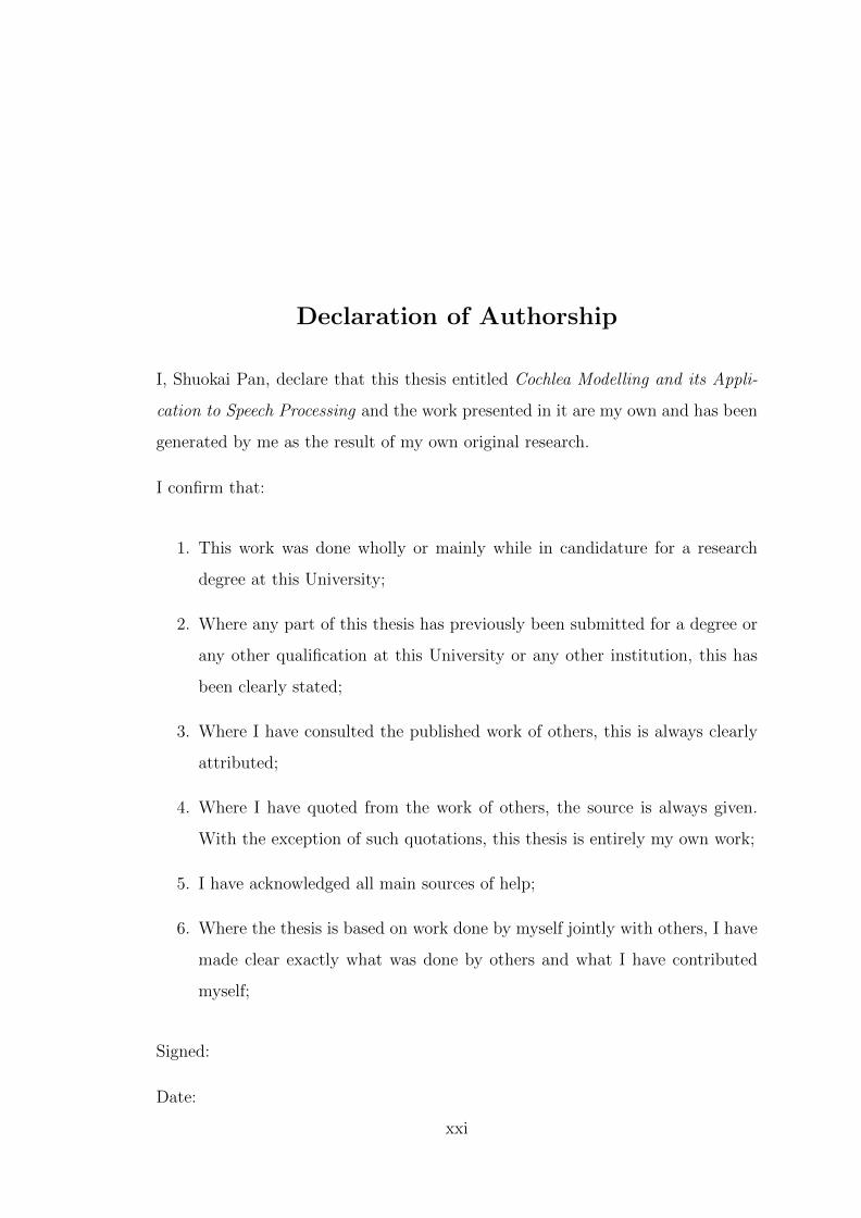
Declaration of Authorship
I, Shuokai Pan, declare that this thesis entitled Cochlea Modelling and its Appli-
cation to Speech Processing and the work presented in it are my own and has been
generated by me as the result of my own original research.
I confirm that:
1. This work was done wholly or mainly while in candidature for a research
degree at this University;
2. Where any part of this thesis has previously been submitted for a degree or
any other qualification at this University or any other institution, this has
been clearly stated;
3. Where I have consulted the published work of others, this is always clearly
attributed;
4. Where I have quoted from the work of others, the source is always given.
With the exception of such quotations, this thesis is entirely my own work;
5. I have acknowledged all main sources of help;
6. Where the thesis is based on work done by myself jointly with others, I have
made clear exactly what was done by others and what I have contributed
myself;
Signed:
Date:
xxi


Acknowledgements
I would like to express my sincere gratitude to my supervisor Professor Stephen
Elliott, without whom I would never be able to finish this challenging but re-
warding jounery of a PhD. His wisdom and passion for scientific research support
me immensely and will definitely continue to benefit me for the rest of my life. I
would also like to thank Professor Paul White for answering many of my questions
and providing additional resources that facilitate my research, and Dr Ed Craney
from Cirrus Logic for visiting me biannually and guiding my research with indus-
try expertise. Another thanks goes to Professor Stefan Bleeck who allows me to
join their weekly discussion group hosted in the Hearing and Balance Centre at
the ISVR, which greatly broadens my horizons in how auditory knowledge can be
applied in various aspects of acoustic signal processing.
Many mang thanks go to my family: my parents for their continuous and selfless
support, and my wife, Anna Deng, for accompanying me and always encouraging
me to finish my study. This thesis is devoted to all of you.
I would like to thank all of the friends I have met at the ISVR, you guys have
made my PhD a much more enjoyable experience.
Finally, I would like to thank sincerely,both EPSRC and Cirrus Logic International
Semiconductor, for providing the financial aid that helps me finish my study.
xxiii


Abbreviations
2TS Two-tone Suppression
AGC Automatic Gain Control
AMS Amplitude Modulation Spectrum
AN Auditory Nerve
AUC Area Under the Curve
BM Basilar Membrane
CASA Computational Auditory Scene Analysis
CARFAC Cascade of Asymmetric Resonators with Fast-Acting Compression
CF Characteristic Frequency
cIRM Complex Ideal Ratio Mask
CNN Convolutional Neural Network
CNN-MR Multi-resolution Convolutional Neural Network
CNN-SR Single-resolution Convolutional Neural Network
CP Characteristic frequency
DFT Discrete Fourier Transform
DNN Deep Feedforward Neural Network
FA False Alarm
IBM Ideal Binary Mask
IHC Inner Hair Cells
IRM Ideal Ratio Mask
LC Local Criterion
LPC Linear Predictive Coding
MFCC Mel Frequency Cepstral Coefficient
MLP Multilayer Perceptron
xxv

xxvi ABBREVIATIONS
MMSE Minimum Mean Square Error
MRCG Multi-Resolution Cochleagram
MSE Mean Square Error
MVN Mean Variance Normalization
MWLCG Multi-Window-Length Cochleagram
MWLFC Multi-Window-Length Filter Cascade
MWLLM Multi-Window-Length LogMel Spectrogram
OC Organ of Corti
OHC Outer Hair Cells
PESQ Perceptual Evaluation of Speech Quality
PLP Perceptual Linear Prediction
PNCC Power-Normalized Cepstral Coefficients
ReLU Rectified Linear Unit
ROC Receiver Operating Characteristic Curve
ROG Rate of Growth
ROS Rate of Suppression
SM Scala Media
SNR Signal-to-Noise Ratio
SPL Sound Pressure Level
ST Scala Tympani
STFT Short Time Fourier Transform
STOI Short-Time Objective Intelligibility
SV Scala Vestibuli
TL Transmission-Line Model
TM Tectorial Membrane
VAD Voice Activity Detection

Chapter 1
Introduction
1.1 Motivation
Speech is a natural medium for human communications. Robust and efficient pro-
cessing of speech has thus become a crucial component of many modern technolo-
gies, including telecommunication, automatic speech transcription and translation,
speaker verification, and hearing aids. Driven by the huge demand of these tech-
nologies in different scenarios, many methods have been proposed for different ap-
plications. The continuous advancement of these algorithms has greatly improved
their performance and robustness, and contributed to new generations of speech
processing applications, such as the increasingly popular voice-controlled digital
assistants, including Apple Siri, Microsoft Cortana, Google Home and Amazon
Echo. These smart systems are able to listen and respond to our speech com-
mands, for instance to retrieve answers from the internet for spoken queries and
control smart home gadgets like light switches, thermostats and TVs, usually af-
ter the detection of some specific keyword phrase(s) such as “Hey Siri” and “Hi
Alexa”. Despite the great success of these applications, a common challenge that
faces them is that, in the wide range of acoustic environments where they are em-
ployed, speech signals are often distorted by various interferences such as channel
1

2 Chapter 1 Introduction
effects, background noise, music and reverberation. These can significantly de-
grade their effectiveness and hence limit their widespread usage in practice, even
though in well-controlled clean speech conditions, they often perform very well.
However, human perception of speech is very robust against various forms of dis-
turbances. Thus the motivation of this work is to explore the benefits of using
auditory principles in developing environmentally robust speech processing algo-
rithms that could meet the increasing demand of practical applications, such as
voice controlled smart devices.
Because the complete auditory pathway is very complicated and contains a num-
ber of stages, many studies only include a small subset of auditory functionalities
and combine them with traditional signal processing techniques, while those that
integrate both low-level and more central high-level auditory principles are com-
monly known as computational auditory scene analysis or CASA [2]. In this
work, we investigate the use of characteristics of the auditory peripheral, particu-
larly the nonlinear cochlea mechanics, for speech processing, because (1) it is the
first advanced signal processing stage in the auditory pathway and is much bet-
ter understood than central auditory functions; (2) it is usually assumed that the
cochlear contributions to auditory processing, such as dynamic range compression,
frequency selectivity and sensitivity is so dominant that it largely accounts for the
properties of the entire auditory system [3]; (3) many previous studies have indeed
shown the advantages of incorporating knowledge of cochlear mechanisms [4, 5, 6,
7, 8].
The characteristics of the cochlea are integrated through a mathematical model,
which is an important area of auditory research in itself. Because it not only
provides a valuable tool for better understanding of its mechanisms, such as otoa-
coustic emissions, but also allows predictions of experiments that are difficult to
perform due to technical limitations. It is worth noting that there are mainly
two types of processing present in the cochlea: (1) the transformation of acoustic
pressure variations into mechanical vibrations along the cochlear partition through
fluid coupling, and (2) the transduction of this mechanical vibration to electrical
impulses that are transmitted to the brain by the auditory nerves, thus making

Chapter 1 Introduction 3
the physical sound perceptible to human beings. These two processes are usually
modelled separately and the complete cochlear functionality is simulated by con-
necting them together. In this work, we only focus on models of the mechanical
aspect of the cochlea that are often simply referred to as cochlear models.
Since cochlear models have been proposed in a large number of ways, the first
research direction of this work is the choice of a suitable model for subsequent
speech processing. Specifically, two types of cochlear models are investigated.
The first one is the transmission-line type of model that tries to realistically simu-
late the travelling wave inside the cochlea using differential equations. This model
is based on that originally proposed by Neely and Kim [9], but is reformulated into
the state space form by Elliott et al. [1] and retuned by Ku [10] and Young [11] to
match the properties of a human cochlea. The second model consists of a cascade
of auditory filters, called the cascade of asymmetric resonators with fast-acting
compression or CARFAC [12], that is inspired by the cochlea travelling wave. Al-
though more physiologically plausible than using parallel filterbank approaches, it
still mainly aims to reproduce the overall experimental measurements of cochlear
responses, without special considerations of the underlying biophysical mecha-
nisms. The first model is more realistic, but it is also much more computationally
demanding than the second one, especially for time domain simulations. This is
also the primary reason why this type of model is seldom adopted in practical
applications. Therefore, the first objective of this research direction is to develop
an efficient numerical method for performing time domain simulations with the
state-space model, in order to reduce the computational burden. This will benefit
its applicability to both cochlear modelling and signal processing tasks. Next, a
systematic comparison between the responses of these two models is performed in
order to assess their capabilities in reproducing cochlear nonlinearities, because
it is these nonlinearities that we are most interested in applying and exploring
their potential benefits to speech processing, and hence serves as a verification
step. Only single-tone and two-tone responses of these models are compared with
experimental measurements, because these responses reveal key aspects of the
nonlinear cochlear mechanics, that we assume are promising for speech processing

4 Chapter 1 Introduction
applications. These aspects include active amplification, dynamic compression,
and mutual suppression, which is attractive for simulating masking effects.
The next research direction of this work is to investigate the potential benefits of
integrating properties of the cochlea mechanics for speech processing applications.
There is a long history of this type of work in the speech processing field, most
notably with promising results in speech recognition [4], speech enhancement or
separation [13, 5], speech detection [6] and audio coding [7, 8]. In this work, we
consider two tasks: voice activity detection (VAD) and speech enhancement or
separation. In many previous studies [5, 6] of these two areas, the input acoustic
signals are firstly decomposed into sub-bands using a simple cochlea-like filter-
bank (mostly parallel filterbanks). Popular examples include the Mel-scale [14],
the Bark-scale [15] and the gammatone [16] filterbanks. Although they provide
representations of speech signals that are similar to those produced by a biolog-
ical cochlea, they still only offer a very crude simulation of nonlinear cochlear
mechanics. A more sophisticated cochlear model, however, has a more realistic
representation of cochlear nonlinearities and is utilised in this work to investigate
whether advanced modelling of cochlear mechanics can be more effective than
other simpler cochlea-like models for the two speech processing tasks considered.
Since 2006, one class of machine learning called deep learning [17] has began to re-
gain its popularity, and has now become the core technology behind a wide range
of signal and information processing applications. It utilizes deep architectures
that contain a hierarchy of nonlinear processing layers, which enable a machine
to learn complex concepts in the real world environments from a nested set of
simpler concepts [18]. This has been proven to be an extremely powerful learn-
ing paradigm, because algorithms based on it have been shown to significantly
outperform traditional methods in a large number of machine learning problems,
including image classification [19], speech recognition [20], voice activity detection
[6] and speech separation [5]. For these reasons, the investigation of cochlear mod-
elling for the two speech processing tasks mentioned above is carried out within
the deep learning framework.

Chapter 1 Introduction 5
1.2 Thesis Contributions
The primary contributions of this work is summarised in the following,
• Development of an efficient numerical method, that substantially reduces
the computational complexity of time domain simulations of a nonlinear,
one-dimensional, state-space, transmission-line cochlear model.
• Establishment of the theoretical relationship between the transmission-line
and filter cascade model of the cochlea and conducting a systematic com-
parison of their linear and nonlinear responses to single and two tones.
• Investigation of the advantages of using a nonlinear filter cascade cochlear
model as a front-end processor in a neural network based voice activity de-
tection task. Demonstration that the filter cascade model does not provide
significant benefits, compared to other simpler auditory filterbank features,
at least in the machine learning paradigm considered. However, the effective
incorporation of context information is proved to be more important for per-
formance improvement. Comparison with another two state-of-the-art VAD
algorithms shows that proposed methods exhibit a significantly higher level
of robustness against additive background noises.
• Investigation of the advantages of using the CARFAC filter cascade model
for supervised speech separation. in most cases, filter cascade based sys-
tems show the highest level of performance compared to standard auditory
filterbank based ones, but the advantage is rather marginal. The same set
of temporal context expansion techniques firstly investigated in the VAD
task has also been applied to supervised speech separation, but the relative
advantage of these techniques is found to be rather different. The proposed
methods also show substantially better performance than another three pre-
vious algorithms in terms of two objective metrics.

6 Chapter 1 Introduction
1.3 Publications
Some of the initial outcomes of this work have been published as a Journal paper
and a conference proceeding:
• Shuokai Pan et al. “Efficient time-domain simulation of nonlinear, state-
space, transmission-line models of the cochlea.” In: The Journal of the
Acoustical Society of America 137.6 (2015), pp. 3559-3562.
• Pan, Shuokai and Elliott, Stephen J and Vignali, Dario. “Comparison of the
nonlinear responses of a transmission-line and a filter cascade model of the
human cochlea.” In: IEEE Workshop on Applications of Signal Processing
to Audio and Acoustics (WASPAA) (2015), pp.1-5.
1.4 Thesis Outline
The remainder of this thesis is organized as follows. Chapter 2 presents the foun-
dation knowledge and literature review for the work in this thesis. This includes
an introduction to the physiology of the human auditory periphery, particularly
the cochlea, and deep learning basics that are essential for subsequent speech
processing tasks.
Chapter 3 presents a thorough investigation and comparison of two types of
cochlear models, i.e., one transmission-line model and the CARFAC model, in
terms of their realism in simulating nonlinear cochlear mechanics. The formal
connections between the linear versions of these two models is firstly explained,
followed by the comparison of the responses of the complete nonlinear models to
simple stimuli including single tones and two tones.
Guided by the results from Chapter 3, the CARFAC model is chosen, instead
of the transmission-line model, for neural network based voice activity detection
study in Chapter 4. It is compared with a number of simpler auditory-inspired
filterbank features and another two state-of-the-art algorithms in a wide range
Chapter 1 Introduction 7
of noisy test scenarios. Multiple types of context extension strategies have also
been investigated and the most effective one for each feature type has also been
identified.
Chapter 5 presents results on using the CARFAC model for supervised speech
separation. A comparison of different combinations of feature type and network
structure is carried out. Following the simulations presented in Chapter 4, the
relative advantage of various context expansion schemes is determined as well,
which is different from those observed in VAD task. A comparison of proposed
methods with another supervised learning based method and two classical speech
enhancement methods is also performed.
Chapter 6 concludes this thesis and proposes suggestions for future work.


Chapter 2
Background and Literature
Review
In this chapter, we give a brief overview of the background to this thesis, including
an introduction to the physiology and mechanics of the mammalian cochlea, and
an overview of recent developments in deep learning. The following chapters build
on this knowledge and elaborate on the problem of cochlear modelling and its
application to speech processing tasks.
2.1 The Cochlea
The human auditory system is a marvellous achievement of biological evolution,
capable of detecting and analysing sounds over a wide range of frequencies and
intensities. Humans can hear sounds over the range of approximately ten octaves
(20 Hz to 20 kHz) in frequency and 140 dB (0 to 140 dB) in sound pressure level
(SPL) [21], while possessing great sensitivity and frequency selectivity. Exten-
sive research has been carried out to understand and model various stages of this
powerful but complicated biological system. The cochlea is the first major compu-
tational element of the human auditory pathway. It is a fluid-filled organ located
in the inner ear, as shown in the illustration of the human ear in Fig. 2.1.
9

10 Chapter 2 Background and Literature Review
Figure 2.1: The anatomy of the human ear. The cochlea is located in theinner ear. Picture adapted from [22] with permission.
As can be seen in Fig. 2.1, the human ear, also called the auditory periphery, con-
sists of three stages: the outer ear, the middle ear and the inner ear. The outer ear
includes the pinna, the ear canal and the tympanic membrane or eardrum. It al-
lows efficient capture of sound impinging on the head and its directional sensitivity
provides a cue for sound localization. The middle ear is an air-filled space contain-
ing a set of three small bones, the Malleus, the Incus and the Stapes, collectively
known as the ossicles, the first of which is connected to the ear drum and the last of
which is connected to the cochlea. They act primarily as an impedance matching
mechanism between the air in the outer ear (low impedance) and the fluid in the
cochlea (high impedance), facilitating energy transfer into the cochlea. Overall,
the effects of middle ear can be well modelled by a linear mass-spring-damper sys-
tem for stimulus frequencies below 10 kHz [23] and stimulus levels below 140 dB
SPL [24]. The cochlea serves as a bridge between the physical pressure variations
and the perception of sound in our brains. It achieves this mainly through two
steps: (1) the interaction between the cochlear fluid and partition maps the input
stimuli along its longitudinal direction according to its spectral components. This
Chapter 2 Background and Literature Review 11
constitutes the so-called cochlear mechanics; (2) the conversion of the mechanical
energy into electrical impulses, through specialized sensory cells, which are sent
to the brain via the auditory nerves.
2.1.1 Cochlea Anatomy
The cochlea is one of the most delicate and complicated parts of the human body.
It has a snail-shaped structure, with about 2.5 turns and a typical length of 35
mm. The cochlear duct is divided into three compartments: the scala vestibuli
(SV), the scala media (SM) and the scala tympani (ST). The Reissner’s membrane
separates SV from SM, while the basilar membrane (BM) separates ST from SM,
as shown in Fig. 2.2 (a). Since the Reissner’s membrane is very thin and possesses
a similar density to that of cochlear fluid, it is generally assumes to have no
influence to cochlear mechanics [25], but only to separate the fluids in the SV
and the SM. The SV and ST are filled with perilymph fluid and connected at the
apex of the cochlea, called helicotrema, to allow fluid flow between them. The SM
is completely separated from the other two chambers, and filled with endolymph
fluid, that is generated in the stria vascularis. It houses an important sensory organ
that is responsible for the cochlear transduction process, called the organ of Corti
(OC), which is distributed along the length of the BM. The detailed structure of
the OC is shown in Fig. 2.2 (b). As can be seen, it consists of a range of supporting
cells and two important kinds of sensory cells, called the inner and outer hair cells,
because of their relative positions. There are one row of about 3,500 inner hair
cells (IHC) and three rows of about 12,000 outer hair cells (OHC) [26], and they
possess hair-like structure at their apical end called stereocilia. The hair bundles of
the OHCs are attached at their top to the lower surface of the tectorial membrane
(TM). Such basic structure of the OC is similar for most mammals.
These sensory cells of the cochlea interact with the nervous system through the
auditory nerve, which consists of approximately 30,000 neurons in human [27].
Most of these neurons are afferents, with their cell bodies in the spiral ganglion,
that carry information from the hair cells to the brain. The remaining small

12 Chapter 2 Background and Literature Review
amount are the efferents, which are the axons of neurons in the brainstem that
descend into the cochlea to allow central control of the cochlear transduction
process. The afferents also include two types, called type I and type II. Type I
neurons make up about 95% of the population, with one end innervates the IHCs
directly and the other end projects into the core areas of the cochlear nucleus. The
remaining around 5% afferents, called type II, innervate the OHCs instead. The
efferent neurons, however, have their cell bodies in an auditory structure in the
brainstem called the superior olivary complex and are thus called the olivocochlear
bundle. There are two groups of olivocochlear bundle neurons as well. The so-
called lateral efferents travel mainly to the ipsilateral cochlea and make synaptic
connections on the dendrites of type I afferents under the IHCs, while the medial
efferents, travel to both the ipsilateral and contralateral cochlae and make synapses
on the OHCs directly. Furthermore, the density of efferent fibers is substantially
greater for the OHCs than for the IHCs.
2.1.2 An Overview of Cochlear Mechanics
The footplate of the stapes is attached to a flexible membrane in the bony shell
of the cochlea called the oval window, that leads to the SV. The inward and
outward movements of the stapes as a result of incident sound waves create a
pressure difference across the cochlear partition, which propagates down the length
of the cochlea. Such a pressure wave deflects the BM, giving rise to the so-called
travelling wave (TW) along it. The bending of the BM results in a shear motion
between the BM and the TM, which further deflects the stereocilia of the sensory
cells. Such deflections of the hair bundles lead to transduction currents inside
the sensory cells, which for the OHCs, cause the expansion and contraction of
the cell body, a phenomenon known as somatic motility or electromobility [30]
and for the IHCs, give rise to neurotransmitter release at the IHC-auditory nerve
synaptic interface which triggers the generation of neural impulses that are sent
to the brain. The forces generated by the OHC mobility are believed to actively
amplify the TW and sharpen its response along the BM for low level inputs. Such

Chapter 2 Background and Literature Review 13
Figure 2.2: Cross section of the cochlear duct (a) and the Organ of Corti (b).Subplot (a) and (b) is obtained from [28] and [29] respectively with permission.
a biological feedback system is referred to as the cochlear amplifier, although this
amplifier is not linear but compressive, as described in more detail below.
The properties of the BM are not uniform along its length, gradually decreasing
in stiffness but increasing in width from its base (the oval window) to the apex.
Such variation causes a natural tuning of the vibration of the BM. For a pure
tone stimulus, the frequency which causes the maximum response at a particular
position along the cochlear partition decreases monotonically from the base to the
apex. This frequency is called the characteristic frequency (CF) of this specific
place, and this place is in turn called the characteristic place (CP) of this frequency.
As will be shown in later sections, the CF of a position along the cochlea tends to
decrease with increasing stimulus level, CF is usually defined as the value obtained
at very low input stimulus level, such auditory threshold. The frequencies obtained

14 Chapter 2 Background and Literature Review
Figure 2.3: Tonotopical arrangement along the human cochlea. Picturetaken from [32] with permission.
at higher input levels are often called best frequencies. In other words, each point
of the BM is best tuned to a single frequency and only a specific group of hair
cells around that point are activated for a pure tone stimulus, with high frequency
inputs mainly activating the basal section while lower frequency stimuli mainly
activating the more apical part. This tonotopical arrangement is illustrated in
Fig. 2.3, where the approximate distribution of the CFs along the BM is drawn
beside the spiral structure. Analytic expression approximating the relationship
between the characteristic frequency and place along the BM has been established
for several species in [31] and it is of the following form,
F = A(10ax − k) (2.1)
where x is the distance from the apex, A and k are constants that can be adjusted
for different species to achieve a desirable frequency range. However, constant a
is found to be roughly equal to 2.1 across many species investigated in [31], if the
distance variable x is expressed as a proportion of total cochlear partition length
(apex=0, stapes=1). Therefore, the cochlea is often treated as a spatial spectral
analyzer that decomposes the input sound signal into its frequency components
through this frequency-place mapping.

Chapter 2 Background and Literature Review 15
2.1.2.1 Single Tone Responses: Compressive Amplification
For a pure tone stimulus at the CF of the place under consideration along the
cochlea, its response is greatly amplified at low levels and behaves roughly linearly
for sound pressure levels of up to around 20 dB. However, at medium and high
levels, the BM response grows compressively, with a growth rate typically of less
than 0.5 dB/dB and can be as low as 0.2 dB/dB in very sensitive cochleae [33]. At
even higher levels, the cochlea tends to become linear again in some experiments,
but in other cases, compressive growth is maintained up to the highest intensities
tested (> 100 dB SPL) in very sensitive cochleae [33]. Fig. 2.4 shows an example
of the growth of the BM response, or the so-called input-output (I/O) function, at
the characteristic place of the single tone frequency tested for increasing stimulus
level, illustrating these three different regions of response growth. It can also be
seen that the input-output function becomes more linear and loses a large amount
of gain when the cochlea is damaged, suggesting that this behaviour only exists in
normal functioning cochlae. Such a phenomenon is commonly believed to originate
from nonlinearities residing in the cochlear amplifier [34] that is probably mediated
by the OHCs. From an engineering perspective, a normal cochlea realizes an
automatic gain control, through which the gain of the cochlear amplifier becomes
attenuated when the input intensity is increased. This compressive behaviour is
also known as self-suppression [35] and is believed to be the main reason that
allows the human auditory system to encode the remarkably large input dynamic
range of 140dB SPL in the auditory nerve firing rates, which only have a dynamic
range of 30-40 dB [36].
During the increase of stimulus intensity, the most responsive frequency and degree
of tuning at the location under consideration decreases gradually. Fig. 2.5 (a) and
(b) show two families of isointensity curves, measured at a BM site with a CF of
10 kHz in a normal chinchilla cochlea, representing the velocity and gain (velocity
divided by stimulus sound pressure) of BM responses to single tone pips as a
function of frequency and intensity (in dB SPL) respectively. It can be seen that
the BM response to single tones has a nonlinear dependence on stimulus level close

16 Chapter 2 Background and Literature Review
Figure 2.4: Input-output function of a BM site in response to characteristicfrequency tones as a function of input SPL. Responses were measured before(squares) and after (triangles) trauma in a guinea pig cochlea. The solid,dashed and dotted lines represent the growth function that would be expectedfrom a saturated mechanism, a linear mechanism or a combined mechanismrespectively. Figure adapted from [37] with permission.
to the most responsive frequency, and a more linear dependence at higher and lower
frequencies. The frequency response of the measured BM site gradually broadens
as sound level increases, becoming much more flat at the highest stimulus level. In
addition, the most responsive frequency shifts downwards by about half an octave
after raising the sound level by 90 dB. For this reason, the CF of a specific location
along the cochlea is defined at low stimulus levels, such as auditory threshold, when
the cochlea is fully active, while the most responsive frequency is usually called
the best frequency which can shift up and down as signal level changes.
There is also a clear difference between BM frequency response at the basal and
apical sites, as shown in Fig. 2.6. The apical BM response is less sharply tuned
and exhibits less gain from the cochlear amplifier compared to that of a more basal
site. In addition, the frequency of maximum sensitivity is almost independent of
stimulus level in the apical region but reduces with stimulus level in the basal
region of the cochlea.

Chapter 2 Background and Literature Review 17
Figure 2.5: a) A family of isointensity curves representing the velocity ofBM responses to single tone pips as a function of frequency and intensity (indB SPL). b) A family of isointensity curves representing the gain or sensitivity(velocity divided by stimulus pressure) of the BM site to single tone pips as afunction of frequency and intensity (in dB SPL), plotted using the same dataas that shown in a). Figure adapted from [38] with permission.
Figure 2.6: Frequency responses of the BM at a basal and apical location.Two families of sensitivity curves (ratio of BM velocity to stimulus pressure)were recorded at the 0.5 and 9 kHz characteristic places in the chinchillacochlea at different stimulus frequencies and levels. The best frequencies and10 dB quality factors for the highest stimulus level are also indicated for eachlocation. Figure adapted from [33] with permission.

18 Chapter 2 Background and Literature Review
2.1.2.2 Two-tone Suppression
The nonlinearity of the cochlear amplifier can also generate various nonlinear in-
teractions between different spectral components of more complex stimuli, such
as pairs of tones. Two-tone suppression describes the phenomenon whereby the
magnitude of the output signal in the live cochlea in response to a test tone is
reduced in the presence of another tone. It was first observed at the level of the
auditory nerve [39], where it was shown that the average discharge rate of an AN
fiber to a CF tone could be reduced by the addition of a second tone of appro-
priate frequency and sound pressure level. Analogous suppression of the overall
mechanical vibrations of the BM in response by a suppressor tone has been found
in[40]. However, [41] and [42] did not find any overall suppression, but did observe
reductions in the spectral component at the CF when a second tone was added.
A suppressor tone with a frequency higher than that of the probe tone is termed
a high-side suppressor, while the one with a lower frequency is called a low-side
suppressor. Fig. 2.7 shows an example of measured two-tone suppression in a
chinchilla cochlea for both (a) high-side suppressor tones and (b) low-side sup-
pressor tones. Each curve represents the magnitude of the BM velocity versus the
SPL of the probe tone as the level of the suppressor tone is varied. It can be seen
that as the level of the suppressor tone is increased, the intensity of the probe tone
must also increase to maintain the same BM velocity.
The most prominent difference between them is that the amount and growth
rate of suppression of the probe tone with suppressor intensities is larger and
steeper for low-side suppressors than for high-side suppressors, which is a direct
consequence of the asymmetric nature of the travelling wave in the cochlear. A
similar suppression effect has also been observed in the receptor potentials of the
IHCs [43], psychophysics experiments with human subjects [44]. Many aspects
of these phenomena are explainable by BM mechanics, except for example, the
difference between BM and auditory nerve responses due to low-side suppressions
[45].

Chapter 2 Background and Literature Review 19
Figure 2.7: Two-tone suppression of the BM velocity responses measuredin the chinchilla cochlea for both (a) higher-side suppressor tones and (b)lower-side suppressor tones. Figure adapted from [40] with permission.
2.2 Machine Learning and Deep Learning
Machine learning is the study of algorithms that are able to learn from data with-
out being explicitly programmed. It is a valuable tool for solving many tasks that
are often very difficult to be accomplished by fixed programs designed by humans.
Some examples of the tasks that machine learning has proved to be powerful in are
classification, regression, transcription, machine translation, denoising and prob-
ability distribution estimation. Generally speaking, machine learning algorithms
can be divided into two categories: supervised and unsupervised, depending on
the type of examples they are given during the learning process. In supervised
learning, the machine has access to both a training dataset and a label or target
associated with each example in the dataset. It must learn to produce the target
as close as possible, given the corresponding example, and can thus be regarded
as a function approximator. In fact, many practical problems can be formulated
as function approximation, such as the speech processing tasks addressed in this
thesis, i.e., voice activity detection (classification of speech from non-speech), and
speech separation (classification or regression depending the targets used). Unsu-
pervised learning on the other hand, refers to algorithms that are capable of learn-
ing useful properties of the structure of the training dataset without the guide of

20 Chapter 2 Background and Literature Review
targets. Examples of this category include dimensionality reduction, probability
distribution estimation and clustering. Other learning paradigms that do not be-
long to any of these two classes also exist, such as semi-supervised learning [46],
transfer learning [47] and reinforcement learning [48], although only supervised
learning is used in this work.
In most cases, a machine learning method is composed of four fundamental ele-
ments: a dataset, a model, an objective function and an optimization procedure.
The objective function measures the accuracy of the chosen model in predicting
the desired targets, given the examples in the dataset, while the optimization
procedure trains the model towards achieving optimal performance as measured
by this objective function. It is common practice to formulate such optimization
problems as minimizing the error between predicted and true targets in this field,
so the objective function is also often called the cost or loss function. The choice
of this cost function depends on the task that the machine learning algorithm is
required to solve. For instance, in classification problems, the cross entropy error
is usually chosen, while in regression problems, the mean square or mean absolute
error is often adopted. In terms of optimization, the most famous and popular
approach is the so-called method of steepest descent or gradient descent, which
modifies the parameters of a model by repeatedly taking small steps in the direc-
tion opposite to the gradient of the error function with respect to model param-
eters. Suppose we have a training dataset consists of a total number of N exam-
ples, X = {x1,x2, ...,xi, ...,xN−1,xN} and targets T = {t1, t2, ..., ti, ..., tN−1, tN},
where (xi, ti) is a single pair of example and target vectors with index i. If we
represent the model as a function, f (x;θ), with its parameters denoted as θ, and
output denoted as y, the method of gradient descent updates the model parame-
ters with the following rule,
θ(n) = θ(n− 1)− ε ∂e(Y,T)
∂θ(n− 1)(2.2)
where Y ={y1,y2, ...,yi, ...,yN−1,yN
}is the outputs of the model given the train-
ing examples, X; e(Y,T) =∑i=N
i=1 e(yi, ti) is the error measuring the difference

Chapter 2 Background and Literature Review 21
between the model outputs and the true targets over all of the training examples;
ε is a scalar learning rate parameter that determines the size of each update step;
and θ(n) represents the model parameters after the nth update. A complete pass
through all of the training examples with parameter update during the process is
called one epoch of training in machine learning.
It is important to remember that machine learning differs from pure mathematical
optimization in the sense that it must also perform well on new and previously
unseen examples, i.e., test dataset. Such an ability is called generalization and
the error measured on the test dataset is called generalization or test error. The
central challenge of machine learning is to make both training and testing error
small. Otherwise, a specific algorithm is said to be underfitting if it fails to obtain
a sufficiently small error on the training set, or overfitting when the difference
between training and testing error is too large. An excellent example illustrating
these concepts is the polynomial curve fitting problem covered in detail in Chapter
1 of [49]. In summary, the capacity of a model should be sufficiently powerful to
be able to tackle the true complexity of the task in order to prevent underfitting,
but not overly powerful which could lead to overfitting. The techniques that are
designed to reduce the test error but not the training error are collectively called
regularization, and the development of these techniques has been one of the major
research directions in machine learning.
There is a wide range of regularization techniques available for designing effective
machine learning algorithms. Probably the most classical one is the addition of
the parameter norm to the original cost function in order to penalize the size
of model parameters. The most popular choice of such regularisation is the L2
parameter norm penalty, which is the squared Euclidean distance between the
point specified by the model parameters, θ, and the origin, and is commonly
known as weight decay or leakage. But in this thesis another two regularisation
strategies are adopted: early stopping and dropout training, which are discussed
in more detail in section 2.2.3.

22 Chapter 2 Background and Literature Review
Deep learning is one type of the machine learning techniques discussed above. It
provides a powerful framework for supervised learning by representing complicated
concepts through a nested hierarchy of processing layers, with each subsequent
layer extracting a progressively more abstract representation of the input data.
By adding more layers and more units within a layer, a deep network can repre-
sent functions of increasing complexity, given sufficiently large datasets of labelled
training examples. The initial phase of deep learning research aimed to find artifi-
cial models of biological learning process, i.e., how learning happens in the brain.
This inspired a large portion of work in this field and contributed to many fa-
mous models that are critical for its recent resurgence. But modern deep learning
should not be viewed as an attempt to simulate the brain, as it draws inspiration
from many fields, especially probability, information theory, and numerical opti-
mization. Moreover, the primary objective of modern deep learning is to build
computer systems that are capable of successfully solving tasks that require intel-
ligence, rather than attempting to understand the neuroscience of how the brain
works. Deep learning has contributed to dramatic improvements in a wide range
of speech processing tasks, such as noise reduction, speech recognition and natural
language processing. This progress is made possible by a number of redeveloped or
newly proposed deep architectures, of which the most widely adopted three types
are deep feed-forward neural networks, or simply deep neural networks (DNN),
convolutional neural networks (CNN) and recurrent neural networks. In the fol-
lowing, we present a brief description of DNN and CNN only because recurrent
neural network is not utilized in this work. See [18] for a comprehensive review
and discussion on these and deep learning in general.
2.2.1 Deep Feed-forward Neural Networks
Feed-forward neural networks (FNN) are very important in the field of machine
learning and form the basis of many successful commercial applications. The most
widely used form of FNN consists of a hierarchy of many layers, with the first one,
middle one(s) and last one usually called input layer, hidden layer(s) and output

Chapter 2 Background and Literature Review 23
layer respectively. Each layer contains a number of (typically nonlinear) processing
units, called artificial neurons, as shown in Fig. 2.8. In this work, the input layer
only represents the input feature vector, while the actual signal processing layers
are the hidden layer(s) and the output layer.
Figure 2.8: An example of deep feed-forward neural network with an inputlayer, three hidden layers, and an output layer. Picture reproduced from Fig.4.1 of [20] with permission.
These models are described as neural networks because they are loosely inspired
by neuroscience. Each unit in a given layer receives a weighted combination of
activations from units in the previous layer and transforms the summed inputs to
its own output through an activation function, f(z), which is typically nonlinear
and in biological terms, represents the average firing rate of a actual neuron, as
given below,
z = Wx+b (2.3)
y = f(z) (2.4)
where x and y are the input and output vector of a given layer respectively; each
row of matrix W and each element of the column vector b contain the weights and
bias connecting the “neurons” from the previous layer to a corresponding “neuron”
24 Chapter 2 Background and Literature Review
Figure 2.9: A comparison of a biological neuron and its mathematical rep-resentation in neural networks shown in Fig. 2.8. Picture reproduced from[19] with permission.
in the current layer; and z denotes the input to the activation function computed
from an affine transformation of the input vector x using “neuron” connection
weights and bias. Fig. 2.9 shows a graphical comparison of a biological neuron and
its mathematical simplification that is widely used in machine and deep learning.
Typically, neural networks with at least two or more hidden layers are considered to
be deep, and are often simply called DNNs, while those with only one hidden layer
are traditionally referred to as multilayer perceptron (MLP). They are called feed-
forward networks because information only flows in one direction, from the input
layer, through intermediate layers, to the output layer. In other words, there are
no feedback connections in the model. However, including feedback connections
is possible and this extends them to another type of network structure called
recurrent neural network. Historically, the two most common choices of activation
function for the hidden units of neural networks are hyperbolic tangent, tanh(x),
and logistic sigmoid, δ(x), functions, which are defined and related as given below,
f(z) = tanh(z) =e2z − 1
e2z + 1(2.5)
f(z) = δ(z) =1
1 + e−z(2.6)
tanh(z) = 2δ(2z)− 1 (2.7)
But there are well-known limitations with these functions, for instance, the learn-
ing of a neural network slows down because of weak gradients when the units are
close to saturation in both very negative and very positive directions, a problem

Chapter 2 Background and Literature Review 25
known as the vanishing gradient [50]. To overcome this inherent weakness of sat-
urating nonlinearities, rectified linear neurons [51, 52, 53] have been proposed to
allow faster learning in deep networks with many layers, an example of which is
called Rectified Linear Unit (ReLU) and is shown in Eq. 2.8. Various alternative
activation functions are also available, such as the maxout function, the radial
basis function and the softplus function.
f(z) = max(z, 0) (2.8)
For the output layer, both the choice of number of units and the activation function
depend on the specific task at hand. For instance, in binary classification tasks, the
standard configuration is to have one unit with the logistic sigmoid function. The
output of this unit represents an estimate of the probability that the input data
belongs to one class, while one minus its output represents the probability estimate
of the other class. For multinomial classification problems, the convention is to use
an output layer with the same number of units as the number of categories to be
classified and estimates the conditional probability for each class with a softmax
function, given below,
p(Ck|x) = yk =ezk∑Kk=1 e
zk(2.9)
where Ck represents the kth class of a total number of K classes, x is an input
vector, zk and yk are the input and output of the kth activation function in the
output layer.
2.2.2 Convolutional Neural Networks
Convolutional neural networks (CNNs) are a specialized class of neural networks
that are inspired by mammalian visual neuroscience. They have been hugely suc-
cessful in the computer vision community since the 1990s, long before arbitrary
deep networks were considered viable, and have now been extended to the speech

26 Chapter 2 Background and Literature Review
processing domain. As its name suggests, the key element of CNN is the use of con-
volution operation with constrained connectivity patterns and parameter sharing.
This deviation from the traditional fully-connected DNN is especially useful for
high dimensionality inputs that exhibit some kind of topological structure, such as
the ordering of pixels in an image or the spectral-temporal modulation of an audio
signal. A typical CNN is composed of a convolutional layer, a pooling layer and a
few fully-connected layers, as illustrated in Fig. 2.10, which is designed for speech
processing tasks with 2-dimensional spectral-temporal features. Multiple convo-
lutional and pooling layers can be stacked on top of each other before connecting
to fully-connected layers. Such a combination of the convolutional and pooling
layer is often called the feature extracting layer as it generates data-driven fea-
tures that are directly learned from the training data. Subsequent fully-connected
layers build upon these learned features, instead of conventional hand-engineered
features, to do the final classification or recognition. Since both feature processing
and pattern recognition are jointly optimized by the learning algorithm, CNNs
generally outperform traditional techniques that tackle these two tasks separately.
The so-called convolutional layer includes a number of feature maps, each unit
of which only receives inputs from a small local 2-dimensional (2D) patch or re-
ceptive field. This receptive field shifts in one or both dimensions until it sweeps
through all vertical or horizontal channels within a context window to construct a
complete feature map. The weights of all the neurons in one feature map are usu-
ally constrained to be the same, a scheme called weight sharing. This contributes
to the shift invariance property of CNN and substantially reduces the number of
unique parameters in the whole network. Under this scheme, the forward pass
through this layer can be realized as a convolution operation between the neuron’s
weights and the input features within the context window, and hence the name
convolutional layer. The set of parameters of each neuron is similarly often called
a filter or a kernel. After the convolutional layer, nonlinear activation function as
introduced 2.2.1 is usually added as well. The pooling layer is normally used to
reduce the dimensionality of previous layer’s outputs, which can further increases

Chapter 2 Background and Literature Review 27
Figure 2.10: Illustration of a typical CNN, applied to a speech process-ing tasks, using a 2-dimensional time-frequency representation as input fea-tures. It consists of one convolutional layer, one pooling layer and a fewfully-connected layers. Picture adapted from Fig. 3 of [54] with permission.
the robustness to distortions of subsequent layers. For example, the most widely
adopted max-pooling layer involves picking the maximum value from a group of
adjacent neuron’s outputs.
2.2.3 Training of Neural Networks
As one class of machine learning techniques, training of neural network also follows
the principles discussed in section 2.2. Optimization strategies are still mostly
based on the first-order method of gradient descent, which needs the derivatives of
the cost function with respect to the weights and bias of every layer in the network.
These gradients are computed using a technique called back-propagation [55], or
simply backprop, which is essentially a repeated application of the chain rule of
calculus for computing the partial derivatives. It first computes the derivatives of
the cost function with respect to the outputs of a network, and then the gradients

28 Chapter 2 Background and Literature Review
with respect to the weights and biases of the hidden part of the network layer-
by-layer, in the reverse order, based on the chain rule, and hence the name back-
propagation. Detailed derivation of this algorithm has been given in many places,
hence is not repeated here. Please refer to Chapter 2 of [56], for instance, for such
a treatment.
After obtaining the gradients, neural network parameters can be updated using the
standard equation of gradient descent, as given in Eq. 2.2, although there are some
important points to note for effective and fast training of deep networks. First,
most optimization algorithms in deep learning only use a subset or mini-batch of
all the training examples for each gradient computation and parameter update,
which is generally called mini-batch or stochastic gradient descent. Secondly,
the learning rate is usually annealed during training. Common choices of the
decay strategy include step decay (reduce the learning rate by some factor every
few epochs), exponential decay and 1/t decay (t is the iteration number) [19].
Furthermore, the standard gradient descent can make learning slow sometimes, for
example in the case of loss function having high curvature and small gradients. The
method of momentum [57] is an approach that is often adopted to accelerate the
convergence speed when training deep networks, especially in such conditions. This
method accumulates an exponentially decaying moving average of past gradients
and continues to move the parameters in that direction. This effectively adds
inertia to the search through the parameter space and modifies Eq. 2.2 to the
following,
θ(n) = θ(n− 1) + ∆θ(n) (2.10)
∆θ(n) = m∆θ(n− 1)− ε ∂e(Y,T)
∂θ(n− 1)(2.11)
where 0 ≤ m ≤ 1 is the momentum parameter; θ(n) represents the weights and
biases of a neural network after the nth update, and e(Y,T) is the error function
as defined in Eq. 2.2. Similar to learning rate decay schedules, optimization can
sometimes benefit a little from momentum schedules, where the momentum is in-
creased in later stages of learning. A typical setting is to start with a momentum

Chapter 2 Background and Literature Review 29
at about 0.5 in a few initial epochs and increase it to 0.99 or so over multiple later
epochs [19]. A number of more sophisticated gradient descent based algorithms
have also been developed, including Nesterov momentum and adaptive learning
rate algorithms such as AdaGrad [58], RMSProp [59], AdaDelta [60] and Adam
[61]. These adaptive learning rate algorithms are different from simple learning
rate decay methods as presented above because the learning rate for each net-
work weight and bias is continuously adjusted after each parameter update during
training.
It is worth noting that the core algorithms for training deep networks have been
developed since 1980s [55], but they have not been widely used until recently be-
cause deep networks are traditionally believed to be very difficult to train. Indeed,
gradient information tends to vanish with saturating nonlinear units as it is prop-
agated backwards through several layers, making it difficult to train the lower
layers of a deep network. In the initial period of deep learning renaissance since
2006, unsupervised greedy layer-wise pretraining [62] was considered to be the key
to largely avoid bad local minima of the cost function and the vanishing gradient
problem, so that deep models can be trained effectively. But with much larger
datasets, larger models, more advanced training and regularization strategies and
more powerful computer hardware and software infrastructure, training deep net-
works has become much more viable, which in turn improves their performance
dramatically. Furthermore, the introduction of the linear rectification activation
function significantly reduces the problem of vanishing gradient. All of these make
pre-training unnecessary in most cases.
2.2.3.1 Regularization
As in general machine learning, regularisation is an important element of the train-
ing procedure, because it improves the generalization ability of a neural network
by preventing overfitting. In this thesis, we use two of these methods, called early
stopping and dropout training. Early stopping is probably the most commonly
used regularization technique in deep learning, because of its effectiveness and

30 Chapter 2 Background and Literature Review
simplicity. To use this method, a small part of the training set (usually 10-20%) is
reserved as a validation set. At the end of each training epoch, the error function
is evaluated on this separate validation set with the newly trained parameters.
This validation error is recorded and compared with those obtained at the end of
previous training epochs. If the current set of weights and biases yields the lowest
validation error, it is stored as the current optimal set of model parameters, until
they are replaced by newly trained values obtained from a later training epoch
that produces a new lowest validation error. When the validation error fails to
decrease for a consecutive certain number of epochs, 10 for instance, the train-
ing process is stopped, hence the name early stopping. Using this method, it is
typically observed that the error decreases for both training and validation sets
initially, but after a certain number of epochs, the validation error stalls and (or)
begins to increase, while the training error continues to decrease. This means that
the network is beginning to overfit the training dataset, and training should thus
be stopped at the point before it happens.
Dropout is another technique that prevents overfitting by approximately combin-
ing many different neural network architectures together efficiently. The term
“dropout” refers to temporarily removing units from the network, along with all
its incoming and outgoing connections, as shown in Fig. 2.11. The decision of
which units to drop is random, and a common practice is that each unit is re-
tained with a fixed probability, p, independent of other units [63]. This effectively
samples a sub-network from the original one, consisting of all the units that sur-
vive the dropout operation (Fig. 2.11 (b)). For each iteration of training, a new
sub-network is sampled and trained. However, during testing, the complete net-
work without dropout is used, except that the outgoing weights of the units in
this network are scaled down by a factor of the retain probability, p. This is to
ensure that the expected output of any hidden unit is the same during training
and testing [63].

Chapter 2 Background and Literature Review 31
Figure 2.11: The application of dropout to a neural network. (a) A standardneural network with 2 hidden layers. (b) The same network after applyingdropout. Units labelled with cross have been dropped temporarily. Picturetaken from [63] with permission.
2.3 Summary
In this chapter, the background to two major parts of this thesis is discussed, i.e.,
the mammalian cochlea and machine learning. Basics of cochlear anatomy are
given, followed by some discussions of nonlinear cochlear mechanics in response
to single-tones and two-tones. These are some of the key characteristics that a
reasonable model should aim to reproduce, and will be used as a reference to com-
pare the properties of two cochlear models in the next chapter. An introduction
to machine learning, with a focus on deep neural networks, is presented. Standard
network structures and training strategies that will be used in Chapters 4 and 5
have also been discussed.


Chapter 3
Comparison of a Transmission
-line and a Filter Cascade Model
of the Human Cochlea
The human auditory system is remarkably effective and robust under a wide vari-
ety of disturbances. One way of understanding its physiological mechanisms and
the resulting psychophysics is to build computational models of it. Such mod-
els have provided inspirations for effective and robust algorithms in many areas
of acoustic signal processing, such as voice activity detection, speech enhance-
ment, and speech recognition, narrowing the performance gap between the human
auditory system and machine hearing systems. Most of these modelling efforts
start from the cochlea, the first significant computational component of the au-
ditory system. In this chapter, we investigate two types of cochlear models, one
transmission-line model and one filter cascade model. The theoretical relation-
ship between their linear responses is first established. The nonlinear dynamics of
both models are then thoroughly tested and compared to experimental measure-
ments of biological cochlea responses, specifically in terms of self-suppression and
two-tone suppression (2TS) on the level of BM. This comparison serves as an im-
portant indication of the validity of a model, especially when used as a front-end
module for simulating the entire auditory system. Because modelling errors at
33

34 Chapter 3 Comparison of Models of the Human Cochlea
this step will inevitably propagate to later stages, and may also limit its capabil-
ity in signal processing applications. Single tone responses have been extensively
tested in a number of TL models [64, 65, 66] and phenomenological models [67,
68, 69]. Two-tone suppression on the level BM motion, however, have been much
less comprehensively investigated in these models. In fact, most of them only
show 2TS for a limited number of pairs of probe and suppressor tones [70, 71,
72], although neural two-tone suppression has been modelled in more detail in [73,
69]. Both self-suppression and 2TS are important in many areas of auditory signal
processing, such as the peripheral encoding of speech and music stimuli and the
determination of perceptual masking effects, such as upward spread of masking.
3.1 Introduction
Cochlear models have been formulated in numerous ways (see a comprehensive re-
view in [74]) and can be broadly divided into two classes, as discussed by Duifhuis
[75]. The first class, which includes the so-called transmission-line models [76, 77],
attempts to explicitly simulate the interaction between the fluid dynamics and
basilar membrane mechanics within the inner ear using partial differential equa-
tions. They can be computationally demanding, especially when implemented in
the time domain. The second class, often referred to as phenomenological or signal
processing models, is only concerned with reproducing the observed outputs of the
auditory system for given inputs, for example using a parallel bank of bandpass
filters, such as the gammatone [16], gammachirp [78], band-pass nonlinear [67,
71] and dual-resonance nonlinear [68] filters. The underlying biophysical processes
are not explicitly considered in these models, but they can be much more efficient
to implement. The filter cascade model [79, 80, 81, 12] sits between these two
classes, since it is both computationally efficient and, in effect, simulates the for-
ward cochlear travelling waves. To account for cochlear nonlinearity, a coupled
automatic gain control (AGC) network can be integrated into the model simulat-
ing the fast compressive responses and inter-channel interactions, giving rise to a
dynamic version of the model, called the cascade of asymmetric resonators with

Chapter 3 Comparison of Models of the Human Cochlea 35
fast acting compression or the CAR-FAC model [12]. This enjoys both the physi-
ological plausibility of TL models and the computational efficiency of filter-based
ones, achieving a good compromise between model capacity and implementation
complexity.
One weakness of the CAR-FAC model is that it does not reproduce the backward
travelling waves in the cochlea, which are believed to generate otoacoustic emis-
sions. The TL model is capable of reproducing the backward travelling waves and
hence otoacoustic emissions, particularly when small levels of random irregularities
are introduced into its parameters [82]. A price that must be paid for this feature
is that the TL model can become unstable. Whereas this can be an advantage in
the simulation of spontaneous otoacoustic emissions [83], this becomes a problem
when it limits the maximum level of active gain that can be obtained for single
tone excitations, as described below. Since the comparison between the CAR-FAC
and TL models is motivated by their use as front-end processors for signal pro-
cessing, otoacoustic emissions are not considered here and focus is put on their
abilities to model the normal responses of the mammalian auditory system at the
peripheral level.
The parameters of the filter cascades, such as the all-pole and pole-zero filter cas-
cades, have been fitted with human notched-noise masking data to predict tone-
in-masker detection thresholds based on the EQ-NL theorem by de Boer [84]. It
was shown to outperform various versions of the gammachirp filter with fewer pa-
rameters [80]. By moving its poles and zeros in the Laplace domain with input
level, it can also be adjusted to match the level-independent zero-crossing times in
the impulse responses [81], as observed from physiological measurements. Using
these fitted parameterizations and nonlinear adaptations, improved performance
has been demonstrated when using the CAR-FAC as a front-end processor, com-
pared with other standard techniques like MFCC, in a number of machine hearing
applications, e.g. content-based music retrieval [85] and large-scale cover song
recognition [86].

36 Chapter 3 Comparison of Models of the Human Cochlea
3.2 Model Descriptions
3.2.1 The Transmission-line Model
The transmission-line model used here is one-dimensional, active and nonlinear,
state-space model developed by Elliott et al. [1], that uses the micromechanical
model proposed by the Neely and Kim [9], but with parameters fitted by Young
[87]. It simplifies the biological cochlea into a symmetric fluid-filled rectangular
box, separated by a flexible partition representing the combined effect of the scala
media, the OC and the BM, as shown in Fig. 3.1.
Figure 3.1: The box model of the human cochlea. Adapted from Fig. 2 of[88] with permission.
The Neely and Kim’s micromechanical model represents an individual radial slice
of the cochlea partition by a two degree-of-freedom lumped-parameter oscillators,
as shown in Fig. 3.3. The two masses, M1 and M2, can be interpreted as the masses
of the BM and the TM respectively and they are coupled by the impedance of the
OHC. To simulate the cochlear amplifier, the OHC impedance is hypothesized to
contain two parts: a passive part, Z3 = K3/s + C3 and an active part, Z4, where
s is Laplace variable. This enables the model to replicate measured frequency
selectivity and sensitivity of biological cochlae. A total number of 500 discrete
elements are used to represent the full length of the cochlea, which is set to 35
mm. This is considered to be a sufficient number of elements in order to obtain
accurate numerical solutions of the transmission-line model, as shown in [10] and
[87]. The first 499 of them are Neely and Kim’s micromechanical elements that
simulate the cochlear partition, while the last element is a mass-damper system
simulating the boundary condition at the helicotrema, as described in the appendix
of [89]. All of these elements are locally reacting and coupled solely by the inertia
of the cochlear fluid.

Chapter 3 Comparison of Models of the Human Cochlea 37
A dimensionless factor, γ, regulates the strength of the active feedback force, so
that when γ = 1, the TL model is deemed as fully active while the model becomes
fully passive with γ = 0. The saturation of the cochlear amplifier is simulated
with a first-order Boltzmann function placed before the active impedance in the
feedback loop of each oscillator, as illustrated in Fig. 3.3. Such an arrangement
and choice of nonlinear function is to better represent the harmonic responses
and distortion products generation, while maintaining reasonable responses to
pure tones [90]. Furthermore, the input-output characteristic of the Boltzmann
function has been shown to be a good match to that of the OHCs [91, 92, 93].
The factor γ is then computed, at each element and time step, as the absolute
value of the ratio of the output and input of the Boltzmann function [83], so that
it decreases with increasing stimulus level.
γ(n, t) =
∣∣∣∣f(xd(n, t))
xd(n, t)
∣∣∣∣ (3.1)
f(xd(n, t)) = α
(1
1 + βe(−xd(n,t)/η)− 1
1 + β
)(3.2)
where n is element index, t is time step index, xd(n, t) is the relative displacement
between the two masses, f(xd(n, t)) is the Boltzmann function, whose parameter
α sets the saturation point, η affects the slope of the output, and β affects the
asymmetry of the function. In order to set the slope of the function to unity for
small input displacements, η is set to αβ(1+β)2 . Fig. 3.2 shows some examples of
Boltzmann function, with varying values of α and β.
A two-port network model of the ear canal and middle ear, based on the model in
[94] and implemented as in [10], is also included. Model responses are computed in
the time domain using a fast implementation of the modified state-space method
[95]. More details of the state-space formulation and the introduced modifications
can be found in appendix B.1, or chapter 3 of [10] and therefore are not repeated
here.

38 Chapter 3 Comparison of Models of the Human Cochlea
Figure 3.2: Some example Boltzmann functions with varying values of αand β. (a) Variation of the Boltzmann function with parameter ℵ, while β isset to 1. (b) Variation of the Boltzmann function with parameter β, while αis set to 1.
Figure 3.3: Block diagram of the micromechanical model of Neely and Kim[9] with a saturating nonlinearity in the active force. Adapted from Fig. 11 of[1] with permission.
3.2.2 The CAR-FAC Model
The CAR-FAC model [12] is based on using a cascade of local filters to simulate
the local behavior of the forward travelling waves and the overall structure of
the CAR-FAC model is shown in Fig. 3.4. A formal derivation of the underly-
ing structure of the CAR-FAC model from the above TL model is presented in
section 3.3.1. The cascade of asymmetric resonators models the forward hydro-
mechanical wave propagation on the BM. The combination of the OHC module

Chapter 3 Comparison of Models of the Human Cochlea 39
and the automatic gain control (AGC) network is used to implement the fast act-
ing compression, while the IHC model compute the mechanical-neural conversion.
The OHC module represents the instantaneous, local feedback path that adapts
the active undamping at various input SPLs, while the AGC module simulates
the slower feedback that modulates the activity of the OHC module from more
central stage of the auditory system. The outputs from asymmetric resonators
represent the BM motion (with arbitrary scale), and those of the IHC module rep-
resent an estimate of the average instantaneous firing rates on the auditory nerve
fibres. However, in this chapter only the outputs from the asymmetric resonators
are considered, as the TL model does not have a mechanical-neural transduction
module.
Each individual filter contains a complex-conjugate pole pair and a complex-
conjugate zero pair at a somewhat higher frequency in the Laplace plane. Other
pole-zero placements are also possible, such as the three-pole and two-zero filter
section proposed by Kates [96]. The transfer function of each filter stage is thus
a rational function of the Laplace transform variable s, of second order in both
numerator and denominator [81]:
H(s) =s2/ω2
z + 2ζzs/ωz + 1
s2/ω2p + 2ζps/ωp + 1
(3.3)
where ωp and ωz are the natural frequencies and ζp and ζz are the damping ra-
tios of the poles and zeros, respectively. The resulting frequency response has a
unity gain at DC, a peak in the gain around the pole frequency, simulating the
active amplification of the travelling wave and a dip around the zero frequency,
corresponding to the rapid decay of energy after the characteristic place (CP), as
shown in (C) of Fig. 3.5. The value of the peak gain is controlled by the resonator
pole damping factor, with lower damping leading to higher gain. None of the fil-
ter sections are highly resonant, but the overall system achieves a large gain and
sharp tuning from the contribution of many cascaded stages in an effect known
as “pseudo-resonance” [97]. In other words, a change of only a few percent of the
gain of each filter can alter the gain of the cumulative transfer function between

40 Chapter 3 Comparison of Models of the Human Cochlea
Figure 3.4: Architecture of the CAR-FAC model of the human cochlea. H1
to HN represent the transfer functions of the cascade of asymmetric resonators,modelling the BM motion with outputs y1 to yN . Damping parameters of theseresonators are controlled by the OHC model and the coupled AGC smoothingfilters (AGC SF), shown in dashed rectangular box, to implement fast-actingand level-dependent compression. The AGC module of each channel consistsof a parallel-of-cascade of four first-order low-pass filters with increasing timeconstant. Smoothing filters with the same time constant are also laterallyconnected (dashed arrows), which allows a diffusion-like coupling across bothspace and time. The IHC model outputs, r1 to rN , present an estimate of av-erage instantaneous firing rates on the auditory nerve fibres. Picture obtainedby combining Fig. 15.2 and Fig. 19.5 of [12] with permission.

Chapter 3 Comparison of Models of the Human Cochlea 41
the stapes and cochlear partition by several orders of magnitude, achieving a wide
range of dynamic gain control while not dramatically changing each serial filter’s
bandwidth and temporal resolution. The pole frequencies in the original imple-
mentation [98] are specified using the equivalent rectangular bandwidth scale with
50% bandwidth overlap between neighbouring sections, resulting in a total of 85
channels from 20 to 20,000 Hz. In this work, to better match cochlear mechanics,
pole frequencies are determined as the CFs of the central locations of 85 equally
divided elements along the length of the human cochlea, using the Greenwood
map [31]
F = 165.4(100.06(35−x) − 0.88) (3.4)
where F is the characteristic frequency of a position in the cochlea that is x mm
from the base. This change simply introduces a shift in the peak frequency of
the cumulative frequency response at each tap and does not influence the key
properties of the CAR-FAC model. Finally, the continuous CAR is transformed
into digital filters through pole-zero mapping using z = exp(s/fs) [81], where fs
is the model sampling frequency.
To account for the observed cochlear nonlinearity, the damping ratios of pole and
zero pairs of each section are dynamically adjusted in the CAR-FAC model in
proportion to filter outputs, to turn up or down the gain of each serial filter,
using an OHC module, in cooperation with a dedicated IHC module which is
an adaptation of that proposed by Allen [99], and a AGC network. The AGC
module of each section is a set of four first-order low-pass filters with increasing
time constant organized in a parallel-of-cascades structure (see Fig. 3.4), which
provides temporal smoothing to the outputs of the IHC module. The state of each
low-pass filters is combined with those of its nearest basal and apical neighbors
with the same time constant through weighted averaging. Such spatial smoothing
and coupling allows the activity in one channel to reduce the gains of nearby
channels, which helps to keep the gains of nearby channels in a similar range,
which in turn helps to preserve local spectra contrasts. This spatially distributed
feedback gain control is also beneficial for simulating lateral inhibition [100] and
two-tone suppression. A comprehensive description of the CAR-FAC model and

42 Chapter 3 Comparison of Models of the Human Cochlea
its software implementation can be found in [12] and [98], respectively. In the
following sections, all of the simulations with the CAR-FAC model are performed
using the default parameter values specified in [98], except that the model sampling
rate is increased from 22.05 kHz to 100 kHz in order to be the same as that of the
TL model.
3.3 Model Comparisons
3.3.1 Derivation of the Filter Cascade Model from the TL
Model
Following the long-wave approximation, the one-dimensional wave equation for the
1D box model shown in Fig. 3.1 can be derived using the principles of conservation
of mass and momentum [77] as,
∂2p(x, t)
∂x2=−2ρ
h
∂v(x, t)
∂t(3.5)
where x is the longitudinal directional along the cochlea, p(x, t) is the pressure
difference across cochlear partition, v(x, t) is the vertical velocity of the cochlear
partition, ρ is the fluid density and h is the effective height of the cochlear cham-
ber. A finite difference approximation of this equation is used in the numerical
implementation of the TL model, but its responses can also be derived analyti-
cally [77]. If the BM dynamics are assumed to be linear and characterized by the
locally-acting impedance, Zcp, Eq. (3.5) can be rewritten in the frequency domain
as,∂2p(x, ω)
∂x2+ k2(x, ω)p(x, ω) = 0 (3.6)
where p(x, ω) is the pressure difference in the frequency domain, k(x, ω) is the
wavenumber of cochlear travelling wave, which is related to the cochlear partition

Chapter 3 Comparison of Models of the Human Cochlea 43
impedance as the following,
k2(x, ω) =−2iωρ
hZcp(x, ω)(3.7)
If the model parameters vary slowly along the longitudinal direction, such that
the relative change of the wavenumber over one wavelength is not too large [77],
the WKB approximate solution [101] to Eq. (3.6) for the forward traveling waves
can be written as,
p(x, ω) = p0 k−1/2(x, ω) e−iΦ(x,ω) (3.8)
where p0 is an amplitude factor determined by the excitation and boundary condi-
tion and Φ(x, ω) is the phase integral, expressing the cumulative phase at position
x,
Φ(x, ω) =
∫ x
0
k(x′, ω) dx′ (3.9)
The vertical velocity of the cochlear partition can then be expressed as,
v(x, ω) =−p(x, ω)
Zcp(x, ω)= v0 k
3/2(x, ω) e−iΦ(x,ω) (3.10)
where v0 is related to p0 by v0 = ip0H/2ωρ. The frequency response of the BM
motion for a forward-travelling wave in a longitudinal segment of the cochlea,
extending from x0 to x0 + ∆, can thus be written as,
H∆(x0, ω) =v(x0 + ∆, ω)
v(x0, ω)=
(k(x0 + ∆, ω)
k(x0, ω)
)3/2
e−i
∫ x0+∆x0
k(x′,ω) dx′(3.11)
The responses at a sequence of positions along the cochlear partition can then be
regarded as the outputs of a cascade of filters with individual frequency response
corresponding to that given by (3.11). In [79], however, only the exponential of
the phase integral in (3.11) was considered, and the wavenumber ratio (WNR)
factor, defined below, was ignored,
WNR =
(k(x0 + ∆, ω)
k(x0, ω)
)3/2
(3.12)

44 Chapter 3 Comparison of Models of the Human Cochlea
Since the complex wavenumber changes along the length of the cochlea, this term
contributes to variations in both magnitude and phase. The influence of neglecting
this WNR term is investigated by computing two sets of magnitude and phase
responses from the linear and fully active TL model, one with and the other
without the WNR, as shown in panels (A) and (B) in Fig. 3.5 as thin and thick solid
lines respectively. The 35 mm length of the cochlear partition has been uniformly
divided into 85 sections, which is the number of channels in the CAR-FAC. The
wavenumber ratio term in Eq. 3.11 can be readily computed from the impedance
values at the starting and ending locations of each section. In order to obtain the
phase integral in Eq. 3.11, each section is further divided into 10 subsections, so
that the phase integral is computed numerically using the trapezoidal rule. This
operation effectively uses 850 discrete elements to represent the 35 mm length of
the cochlear partition. In single-tone and two-tone simulations, however, only 500
elements are used. Every fifth of the frequency responses of the first 76 sections
are shown in Fig. 3.5 for better visualization. In the TL model, it can be seen that,
the peak gains at basal sections are higher than those at more apical ones. But
if the WNR is neglected, the gain in the pass-band of each section is significantly
reduced, especially at basal sections. For comparison, panels (C) and (D) in
Fig. 3.5 show the frequency responses of the cascaded filters of the CAR-FAC
model, which are also configured as fully active and with the maximum gain.
Unlike the TL model, each serial filter in the CAR-FAC model has a smoother
high-frequency roll-off and roughly an equal amount of peak gain, which is about
7 dB. This peak gain is similar to that of the individual segment of the TL model
with the WNR term, except at a few basal sections. Thus the WNR term has
dramatic effects on the behavior of the TL model, greatly increasing its responses
at low input levels. The influences of this WNR term can be largely compensated
for by decreasing the damping, or equivalently turning up the gain, of each section
in the CAR-FAC, as is already done in the default software implementation. Thus
although the CAR-FAC filters were originally motivated only by the phase term
in Eq. 3.11, it is clear that the wavenumber ratio term is also necessary so that
the cascade filters show a more accurate representation of the cochlear responses,

Chapter 3 Comparison of Models of the Human Cochlea 45
Figure 3.5: Frequency responses of the individual segments of the TL model(A, B), computed with (thin) and without (thick) the WNR term and thoseof the serial filters of the CAR-FAC model (C, D). Only every fifth of the first76 output channels are shown for clarity.
mainly in terms of providing sufficient active gain.
3.3.2 Cumulative Frequency Responses and Active Gain
The cumulative frequency responses at a specific location or channel of the TL
(with WNR) and CAR-FAC models are shown in panels (A, B) and (C, D), re-
spectively in Fig. 3.6, when both models are linear and are either entirely passive
or entirely active. The frequency responses of every fifth of the first 76 channels
are shown for better visualization. Fully active model responses (γ = 1 in the TL
model and minimum damping in the CAR-FAC model) are shown as thin lines

46 Chapter 3 Comparison of Models of the Human Cochlea
while those for the fully passive model (γ = 0 in the TL model and maximum
damping in the CAR-FAC model) as thick lines. It can be seen that the sharpness
of tuning along the longitudinal dimension in the TL model gradually decreases
from the base to the apex, providing a better simulation of physiological results in
[33] than the CAR-FAC model which shows almost constant sharpness of tuning.
The active gain provided in the cochlear travelling waves at different locations
along the length of both models is shown in Fig. 3.7, computed as the difference in
dB in the cumulative magnitude responses at the corresponding CF between the
fully active and fully passive model settings. Channels of the CAR-FAC model
are converted to the equivalent positions along the cochlea according to their CFs
using the Greenwood map for humans, given in Eq. (3.4). At basal locations
in both models, the cumulative transfer functions have lower gains than at more
apical positions, since there is only a small number of filters to cascade. As the
travelling waves reach the middle region of the cochlea, the peak gains at CF
are greatly increased and the active gains reach their maximum values, due to
the contribution of larger number of cascaded sections. In the apical area, the
damping factors in the CAR-FAC model are gradually increased, compared to
those at more basal places, to reduce the effect of the cochlear amplifier in this
region. Thus both models are in reasonable agreement with the wide range of
experimental observations ( 20 dB to 70 dB) from different animals [33], in that
the active gain is greater at the base than at the apex. Although the detailed
distributions of the active gains along the cochlea are different between the two
models, there is currently not enough experimental evidence to justify which one
is more appropriate than the other.
3.3.3 Single-tone compression
In simulations of the nonlinear responses to single tones, the 4 kHz characteristic
place of the cochlea was taken for both models as an example for comparison of
their responses. All input stimuli had a duration of one second, with a 10 ms half-
Hanning window onset ramp. The spectral component at the stimulus frequency

Chapter 3 Comparison of Models of the Human Cochlea 47
Figure 3.6: Overall frequency responses at various positions for the TLmodel (A, B) and CAR-FAC model (C, D) when configured as fully active(thin lines) and fully passive (thick lines). Only every fifth of the first 76output channels are shown for clarity.
Figure 3.7: Active gain provided to the travelling waves at CF in the TLand CAR-FAC models for different positions along the length of both cochleamodels.

48 Chapter 3 Comparison of Models of the Human Cochlea
was obtained by a Fourier analysis of the last 0.5s of the time domain solution.
Fig. 3.8 shows the compressive growth of the BM motion to sinusoidal tones with
different frequencies and intensities in the TL and CAR-FAC [98] models. The
responses of the TL model are shown in the first column (A, B, C, D) and those
of the CAR-FAC model in the second column (E, F, G, H).
Panels (A) and (E) show the BM input/output (I/O) functions, in the TL and
CAR-FAC respectively, for some pure tones with frequencies ranging from 0.5 kHz
to 7 kHz, and with levels ranging from 0 to 120 dB SPL in steps of 5 dB. The
frequencies of these pure tones can be found in the legend of panel (G). The solid
black line in these plots represents a linear growth function. For low-level stimuli
at the characteristic frequency, 4 kHz, the response was amplified by ∼30 dB in
the TL and ∼50 dB in the CAR-FAC as indicated in Fig. 3.7. It was then highly
compressed until ∼100 dB SPL, after which both models behaved linearly. For
stimuli that are higher and lower in frequency than 4 kHz, the TL model responded
almost linearly over the entire range of levels tested, except for the ones that are
very near to the CF (e.g. 3-4.5 kHz). In the CAR-FAC model, although low
frequency stimuli showed a similar linear response pattern, the high frequency
responses also grew compressively from 0 dB to 100 dB SPL, even at frequencies
that are almost an octave above the CF, as shown more clearly in panels (G, H).
Panels (D) and (H) show the BM sensitivity curves as a function of stimulus fre-
quency with increasing input SPLs, which is represented by increasing line thick-
ness, with the thinnest line corresponding to 0 dB, thickest line to 100 dB and the
step between two neighbouring lines is 10 dB SPL. BM sensitivities were obtained
by normalizing the BM responses by the corresponding stapes velocity and sound
pressure in the TL and CAR-FAC model respectively. As can be seen, BM sen-
sitivity around the CF was reduced by ∼30 dB and more than 50 dB in the TL
and CAR-FAC model respectively, as sound pressure level was increased from 0
dB to 100 dB, broadening the BM tuning in both models. However, compared to
the CAR-FAC, the TL model is more sharply tuned and has a higher rate of high
frequency roll-off. The sensitivity for stimuli having frequencies lower and higher
than the CF remain almost constant in the TL model regardless of the stimuli

Chapter 3 Comparison of Models of the Human Cochlea 49
SPLs, while this is only the case for frequencies that are well below the CF in
the CAR-FAC model. Finally, in the filter cascade model, the most responsive
stimulus frequency, which is 4 kHz at low levels, smoothly shifts to 3.4 kHz at 100
dB SPL, equivalent to a decrease of ∼0.23 octave relative to the CF. But in the
TL model, this shift does not appear until ∼60 dB SPL, and the shift at 100 dB
SPL amounts to ∼0.68 octave lower than the CF.
To quantify the extent of compression to single tone stimuli in both models, the
rate-of-growth (ROG) functions, computed in dB/dB as the slope of the I/O func-
tions shown in panel (A, E), are shown in two different manners in panels (C,
G) and (D, H), respectively. Panels (C) and (G) mainly illustrate the variation
of ROG with probe level. In the TL model, CF response started linearly at the
lowest SPL and became compressive at ∼20 dB. Further increasing the CF level
gradually decreased the ROG to the minimum of ∼0.4 dB/dB at ∼50 dB, after
which the ROG function gradually returned back to being linear. Responses to
all the other example stimuli grew roughly linearly over the range of 120 dB SPL.
In the CAR-FAC model, however, responses to stimuli at CF and higher frequen-
cies were compressive even at at the lowest SPL tested, 0 dB. As stimulus level
was raised, the growth rates also decreased, stablizing at about 0.3 dB/dB in the
range 30 dB to 60 dB SPL. At even higher input levels, the response growth to CF
tones gradually became linear, while the responses to higher frequency pure tones
became expansive. Panels (D) and (H) show more clearly the dependence of ROG
on stimulus frequency with increasing stimulus level. As already shown above, the
TL model shows compressive growth of responses to pure tones that are within
a small region around the CF. In the CAR-FAC model, stimuli with frequencies
that are well above and below the CF are also highly compressed, especially ones
with higher frequency than the CF. In fact, compression was almost to the same
extent of the CF tones at low to mid SPLs. Although this is in disagreement with
the physiological measurements [33], the gains to these high frequency tones are
significantly lower than CF tones, and therefore is not expected to make a large
impact to the overall response.

50 Chapter 3 Comparison of Models of the Human Cochlea
Physiological measurements of mammalian cochleae from different studies and
across various species show a high degree of variation in terms of compression range
and rate. Some experiment [102] measured compressive behavior at levels as low
as 0 dB SPL in the chinchilla, while others [103, 104] did not observe compression
until the levels were above 50 dB SPL in the guinea pig. The growth rate of the BM
response in the compressive region also varies from∼0.2 to∼0.5 dB/dB [33]. Thus,
the responses of the TL and CAR-FAC models can be regarded as quantitatively
consistent with the wide range of experimental data in terms of compression start
SPL and compression rate. For the reduction in peak frequency of the normalized
BM transfer function with increasing input intensity, physiological measurements
show a decrease of 0.36-0.51 octave relative to CF [38]. Thus both models only
agree qualitatively with these measurements, as the TL exhibited a larger shift,
while the CAR-FAC model showed a smaller shift in peak frequency with stimulus
level. Furthermore, compressive responses have been observed for single tone
stimuli with frequencies that are around 30% higher and lower than the CF in
the chinchilla cochlea [38]. Both models are also not very accurate in reproducing
this, since the effective bandwidth of its “cochlear amplifier” is too limited in the
TL model and too broad in the CAR-FAC model, especially for high-side (relative
to the CF) pure tones.

Chapter 3 Comparison of Models of the Human Cochlea 51

52 Chapter 3 Comparison of Models of the Human Cochlea
Figure 3.8: Single-tone compression simulations at the 4 kHz characteristicplace in the TL (A, B, C, D) and CAR-FAC (E, F, G, H) model. (A, E)BM motion I/O functions at a number of example frequencies, including theCF, 4 frequencies that are lower and 3 that are higher than the CF. Thestraight line indicates linear growth rate of 1 dB/dB for easy reference. (B,F) Sensitivity functions obtained by normalizing the BM responses in (A, E)by the corresponding stapes velocity in the TL model and stimulus soundpressure level in the CAR-FAC model. Stimulus intensity varied from 0 dBto 100 dB in steps of 10 dB and is indicated by the thickness of the lineswith the thinnest line corresponding to 0 dB and the thickest line to 100 dB.Numbers inside the circle symbol represent probe SPL divided by 10. Thevertical lines indicate the place of the CF and the most sensitive frequency atthe highest probe level, 100 dB SPL. (C, G) Rate-of-growth (ROG) values areshown as a function of stimulus level for the same example frequencies as in(A) or (E). (D, H) Rate-of-growth (ROG) values are shown as a function ofstimulus frequency for some example SPLs. Line style and marker meaning in(D, H) follow that in (B, F).
3.3.4 Two-tone suppression
The effects of two-tone suppression from a mechanical perspective on the BM
have been demonstrated in a number of studies [40, 43, 105, 41, 42, 106, 45, 107],
although the measurements are not always consistent with each other. Ruggero
et al [40] measured suppression of the overall velocity response of the BM with
both high-side and low-side suppressors, while later experiments [105, 41, 42] only
observed reductions in the overall response for high-side suppressors. Low-side
suppressors can reduce the spectral component at the probe frequency, but never
the overall response amplitude. In addition to this “tonic” suppression (reduction
in the average response at the probe tone frequency), they also cause “phasic”
suppression where the probe tone response is suppressed in a manner that varies
with the phase of the low-side suppressor [41, 42, 45]. In this work, we adopt the
definition of two-tone suppression used in [105, 41, 42, 106, 45, 107]; as a reduction
in the magnitude of the spectral component at the probe frequency during the
simultaneous presentation of a suppressor tone. We considered the suppression
of a 4 kHz tone at its characteristic place along the cochlea. Suppressor tones
were used with frequencies from 100 Hz to 10,000 Hz, in steps of 100 Hz (except

Chapter 3 Comparison of Models of the Human Cochlea 53
at 4 kHz), and levels from 10 dB to 90 dB SPL, in steps of 5 dB. Each input
stimulus had a length of one second, but only the last 0.5 seconds of the time-
domain model outputs were used to extract the spectral component at the probe
frequency. Finally, only tonic suppression was investigated and phasic suppression
within these two models is left for future work.
The level dependent suppression of a 4 kHz probe tone, presented at 30 dB SPL,
is investigated for different suppressor frequencies and Fig. 3.9 shows a subset
of results in panels (A) and (C) for the TL and CAR-FAC models respectively.
The degree of suppression was quantified as the ratio, in dB, of the magnitude
responses at the probe frequency in the presence and absence of the suppressor,
so that 0 dB means no suppression and suppression is present when this ratio is
negative. Both low- and high-side suppressors are capable of reducing the probe
tone response, but the CAR-FAC generates greater suppression at almost all levels
of each suppressor and the suppression effect appears at lower suppressor levels.
The maximum amount of suppression is ∼30 dB in the TL model and ∼35 dB in
the CAR-FAC model, which would probably continue to increase with even higher
suppressor levels. Both models are capable of reproducing the general trend that
low-side suppressors produce higher amounts and rates of suppression than high-
side suppressors. However, in the TL model, the influence of high-side suppressors
drops off considerably quicker than that in the CAR-FAC model, with increasing
separation of the probe and suppressor frequencies.
Two-tone neural suppression in the auditory nerve has been extensively studied
[39]. One typical method to determine the amount of suppression is to calculate the
right-ward shift of AN rate-intensity functions at different suppressor intensities.
This paradigm has also often been adopted in BM two-tone suppression studies
[106, 45]. Panels (B) and (D) of Fig. 3.9 show the input/output level curves for
a 4 kHz probe tone at its characteristic place in the absence and presence of a
high-side (5 kHz) suppressor tone at 5 different SPLs. The horizontal shift in the
BM I/O functions is seen in both models, resulting in an increasingly reduced
compressive region of the probe tone growth curve at low-to-medium level as the
intensity of the suppressor tone is raised. For high-level probe tones, however, the

54 Chapter 3 Comparison of Models of the Human Cochlea
Figure 3.9: Level dependence of two-tone suppression to a 4 kHz probe tone(F1) at its characteristic place on suppressor tone frequency using the TL (A)and CAR-FAC (C) model. The probe tone sound pressure level is 30 dB.Input/output functions for a 4 kHz probe tone (F1) at its characteristic placein the absence and presence of a high-side, 5 kHz, suppressor tone (F2) at 5different sound pressure levels as indicated in the legend, in the TL (B) andCAR-FAC (D) model.
I/O function is almost linear and hardly affected by the suppressor. These results
are in good qualitative agreement with those measured experimentally, e.g. Fig.
2A of [41].
To quantify the differences between these two models, three perspectives of two-
tone suppression were computed from the complete simulation dataset and are
presented in columns 1, 2, and 3 in Fig. 3.10 for the CAR-FAC and in Fig. 3.11
for the TL model, respectively. The CF probe was presented at three different
levels, 30, 50 and 70 dB SPL, and the corresponding simulation results are shown
in rows 1, 2, and 3. Figures were plotted following the style adopted in Fig. 4 of
[106], which is also reproduced here in Fig 3.12 for easy comparison.
The first column (A, B, C) shows the iso-level suppression curves with suppressor
level increasing from 10 dB to 90 dB SPL, in increments of 5 dB. The intensity of

Chapter 3 Comparison of Models of the Human Cochlea 55
the suppressor is also coded by line thickness, with the thinnest corresponding to
10 dB SPL and the thickest to 90 dB SPL. In both models, the frequency extent
of suppression is greatly expanded for all low-side suppressors with increasing
suppressor level, while for high-side suppressors, their effects quickly decrease with
increasing frequency separation with the probe tone regardless of their levels, which
is in reasonable agreement with experimental measurements [106, 45]. The amount
of suppression exhibited in the CAR-FAC model is larger than that shown in the
TL model mainly because of the difference in active gain between the two models,
as discussed in section 3.4. Both models introduce lower level of suppression
than those measured in recent experiments in very sensitive cochleae [45], where
suppression amplitudes of more than 40-50 dB are observed for some very low
frequency suppressors (see Fig. 3(a) and 4(a) of [45]). However, the CAR-FAC
model produces responses that are very similar to the measurements of an earlier
experiment [106] (see panels (A, B, C) in Fig. 3.12). Additionally, in the TL
model, very low frequency suppressors (100, 200, 300 Hz) almost have no effect
in reducing the probe tone responses and the influence of high-side suppressors
is negligible when their frequencies are higher than around 6 kHz, equivalent to
∼0.59 octave above the probe. This is less realistic compared to the CAR-FAC
model as physiological experiments [42] have shown that low frequency suppressors
are nearly as equally effective and high-side suppression is still observable when
the suppressor frequency is nearly an octave above the probe frequency [106]. The
reduction in two-tone suppression at 2 kHz in the CAR-FAC and at 0.8 kHz, 2
kHz in the TL model when the probe tone is at 30 dB SPL is due to harmonic
distortions generated at the probe frequency, i.e. 4 kHz, by the suppressor tone.
The second column (D, E, F) shows the suppressor threshold levels for 1, 10 and
20 dB reduction of the probe response, when the probe is at 30, 50 and 70 dB SPL.
The CAR-FAC model is closer to experimental measurements than the TL model
for low-side suppression because the suppression threshold is nearly constant in
the low frequency region [106]. However, the TL model predicts better the 1 dB
threshold curve in the region around the probe frequency when the probe is at
the lowest level, 30 dB SPL. As the level of the probe tone increases, the shapes

56 Chapter 3 Comparison of Models of the Human Cochlea
of the threshold curves tend to lose their ‘tips’ (see Fig. 3.12 reproduced from
[106]), but those produced by the two models remain roughly unchanged at all
three probe levels. Furthermore, both models show suppression thresholds that
are higher than biological observations in nearly all combinations of probe and
suppressor tones simulated [106].
The third column (G, H, I) shows the rate of suppression (ROS) values as a
function of suppressor frequency, computed as the slope of the probe reduction
curves shown Fig. 3.9 (A) and (C). Only every 10 dB increment in suppressor level
is plotted for better visualization. The influence of harmonic distortions is also
visible from these plots, reducing the values of ROS and even causing an increase
of the probe spectral component when the suppressor is at very high levels, such
as 80 dB and 90 dB SPL. The maximum ROS results across all suppressor levels
are plotted in Fig. 3.13 for both models. Since experimental measurements, i.e.
Fig. 9 of [45], have shown that the maximum ROS can be as high as ∼2 dB/dB
for low-side suppression, the CAR-FAC model can be considered as more realistic
than the TL model in this aspect.
3.4 Discussion
It should be emphasized that the simulation results presented in this work are
based on the sets of model parameters described in section 3.2, and with different
sets of model parameters, the results would change to some extent. The aim of this
initial study is to objectively evaluate the performance, with the current parameter
settings, of two types of cochlear models in simulating experimentally observed
single-tone and two-tone responses. It would be interesting to further explore
whether the limitations in their responses are due to the particular choices of model
parameters, or due to more fundamental issues associated with the structures of
the two models, which is beyond the scope of the current investigation.
One obvious drawback of the TL model is that it cannot produce the same level
of active gain in the travelling waves as often measured in sensitive cochleas (see

Chapter 3 Comparison of Models of the Human Cochlea 57
Figure 3.10: Two-tone suppression simulations using the CAR-FAC model.Results are displayed from three perspectives. Column 1 (A, B, C): iso-levelsuppression curves for suppressors ranging from 10 to 90 dB SPL in steps of 5dB, as indicated by the line thickness, while the probe is at 30, 50 and 70 dBSPL in rows 1, 2 and 3 respectively. 10 dB suppressor levels are also markedwith numbered circles: e.g., 30 dB SPL=10 times 3©. Column 2 (D, E, F):suppressor levels necessary to reduce the probe amplitude by 1, 10 and 20dB, as indicated by the encircled numbers on each line. Column 3 (G, H, I):Rate of suppression (ROS) as a function of suppressor frequency, computedas the slope of the probe reduction curves shown in Fig. 3.9 (C). Only every10 dB increment in suppressor level is plotted for better visualization. 10 dBsuppressor levels are also marked.
Fig. 3.7). One method of increasing the active gain in the TL model is to increase
the dimensionless gain factor, γ, in the micro-mechanics. But this cannot be used
here, since even a slight increase in γ will causes the TL model to become unstable.
A similar limit on the active gain due to instability is also seen in other TL models
with different micro-mechanical implementations [83, 64, 65, 9]. In this respect,
the tuning of the CAR-FAC model seems to be more flexible, as system stability
is not a concern as long as poles of the individual filters are constrained to have
negative real parts.

58 Chapter 3 Comparison of Models of the Human Cochlea
Figure 3.11: Two-tone suppression simulations using the TL model. Resultsare displayed from three perspectives. Column 1 (A, B, C): iso-level suppres-sion curves for suppressors ranging from 10 to 90 dB SPL in steps of 5 dB,while the probe is at 30, 50 and 70 dB SPL in rows 1, 2 and 3 respectively.Column 2 (D, E, F): suppressor levels necessary to reduce the probe ampli-tude by 1, 10 and 20 dB. Column 3 (G, H, I): Rate of suppression (ROS) as afunction of suppressor frequency, computed as the slope of the probe reductioncurves shown in Fig. 3.9 (a). Only every 10 dB increment in suppressor levelis plotted for better visualization. Line styles follow those in Fig. 3.10.
The limited active gain in the TL model partly explains the lower amount of two-
tone suppression and lower suppression rates shown in Fig. 3.11, as the maximal
amount of suppression is given by the active gain provided to a probe tone at
its CP. For instance, at the 4 kHz CP, the active gain to a 4 kHz probe tone at
30 dB SPL is around 30 dB as illustrated in Fig. 3.8 and Fig. 3.9. The amount
of suppression of this probe tone at the highest suppressor level is also around
30 dB, as shown in Fig. 3.11. Although the CAR-FAC model can produce much
higher active gain (∼56 dB) at the 4 kHz CP, it does not introduce much larger
suppression of the probe tone than the TL model, which is a lower amount than
that measured experimentally in very sensitive cochlea [45]. This is because the
Chapter 3 Comparison of Models of the Human Cochlea 59
Figure 3.12: Two-tone suppression measurements from the basal region ofthe chinchilla cochlea. Results are displayed from three perspectives. Column1 (A, B, C): iso-level suppression curves for suppressors ranging from 10 to 90dB SPL in steps of 5 dB, while the probe is at 8 kHz and 30, 50 and 70 dBSPL in rows 1, 2 and 3 respectively. 10 dB levels are indicated with numberedsymbol: e.g., 30 dB SPL=10 times 3©. Column 2 (D, E, F): suppressor levelsnecessary to reduce the probe amplitude by 1, 10 and 20 dB (labelled assolid lines). The 1-nm iso-amplitude curve for a single tone is repeated ineach panel (dashed line). Column 3 (G, H, I): Rate of suppression (ROS) as afunction of suppressor frequency, computed as the slope of the probe reductioncurves. Only every 10 dB increment in suppressor level is plotted for bettervisualization (solid lines and numbered symbols). The negative of the slope ofsingle-tone I/O curves at 70 dB SPL is superimposed in each panel (dashedline), where-1 dB/dB is linear and 0 dB/dB is complete compression. Takenfrom Figure 4 of [106] with permission.

60 Chapter 3 Comparison of Models of the Human Cochlea
Figure 3.13: Maximum rate of suppression as a function of suppressor fre-quency for a 4 kHz, 30 dB SPL, probe tone at its characteristic place in the TLand CAR-FAC model. Note that the sign of ROS values is inverted comparedto those in Fig. 3.10, Fig. 3.11 and Fig. 3.12 to facilitate comparison withexperimental measurements shown in Fig. 9 of [45].
sensitivity of each channel of the CAR-FAC model starts to decrease at the lowest
level tested, 0 dB SPL, such that when the probe tone is at 30 dB SPL, the
active gain is reduced to ∼40 dB (Fig. 3.9 (F)), which is roughly consistent with
the amount of two-tone suppression observed in Fig. 3.11 (B). In other words,
to further increase the amount of two-tone suppression in the CAR-FAC model,
the minimum damping could be reduced, and/or the maximum damping could be
increased or a higher threshold could be set so that channel sensitivities do not
decrease until the probe levels are higher than 0 dB SPL.
3.5 Summary
This chapter compares the nonlinear responses to single-tone and two-tone stimuli
of a TL model and a filter cascade model, CAR-FAC, of the mechanics of the hu-
man cochlea. The formal connections between these two models is also explained.
The computed outputs of these two models have also been compared with exper-
imental measurements on laboratory animals, which can be quite variable. Both
models can account for the general features of these measurements, but not every
aspect of each datasets.
Chapter 3 Comparison of Models of the Human Cochlea 61
In single-tone simulations, both models quantitatively agree with the wide range
of experimental data in terms of starting SPL for compression to occur and com-
pression rate. However, they are less accurate in simulating the reduction in
peak frequency of the normalized BM transfer function with increasing input in-
tensity and the effective bandwidth of their “cochlear amplifiers”. In two-tone
suppression simulations, the CARFAC model shows reasonable amount and rate
of suppression, whereas the TL model exhibits lower amount of suppression and
lower values of ROS than those measured physiologically in very sensitive cochlae
[45], mainly because of limited amount of active gain, as discussed in section 3.4.
The TL model also shows very limited two-tone suppression for very low- and very
high-side suppressors. Finally, the suppression threshold curves predicted by both
models are not compatible with biological data, although the CAR-FAC model
produces closer results for low-side suppression. Thus, despite of its limitations,
the CAR-FAC model is found to reproduce more closely the nonlinear phenomena
observed in the auditory periphery, at least for single- and two-tone stimuli.


Chapter 4
Cochlea Modelling as a Front-end
for Neural Network based Voice
Activity Detection
In chapter 3, two types of cochlear model, a transmission-line model and a filter
cascade model, CAR-FAC, were compared in terms of their realism in simulating
some observed cochlear nonlinearities. The CAR-FAC model was found to yield
responses closer to cochlear measurements at least for single- and two-tone stim-
uli, while being much more computationally efficient. In this chapter, we explore
the potential benefits of using this filter cascade model as a front-end processor
for one speech processing application, voice activity detection (VAD), to investi-
gate whether the modelling of cochlear nonlinearity may lead to improvements in
detection accuracy, in comparison to other simpler auditory filterbank features.
Specifically, we integrate the CAR-FAC cochlear model with deep neural network
based classifiers, since, as reviewed in chapter 2, they have superior performance
compared with traditional shallow classifiers such as Gaussian Mixture Models
and Support Vector Machines in a range of pattern classification tasks.
63

64Chapter 4 Cochlea Modelling as a Front-end for Neural Network based Voice
Activity Detection
4.1 Introduction
Voice activity detection (VAD) refers to an algorithm that determines the presence
or absence of speech, usually in a distorted signal (e.g., noisy, reverberant or both).
It plays an important role in a number of modern speech signal processing appli-
cations. For instance, it improves the efficiency of speech communication system
by detecting and transmitting speech-only segments or discontinuous transmis-
sion, since about 60% of the acoustic signal produced during a normal mobile
communication contains just silence or noise [108]. It can also help many speech
enhancement systems, which rely on a VAD to decide speech absent intervals,
within which noise characteristic estimates are updated. In speech recognition
systems, VAD can be beneficial in reducing the power consumption since they
are normally computationally intensive and speech signals are only present for a
fraction of time. In high noise scenarios, where a speech enhancement module
is included for preprocessing before recognition, a VAD could also play an essen-
tial role, as discussed above. Furthermore, non-speech frame-dropping (based on
the VAD decision) from the input is also a frequently used technique in speech
recognition to reduce the number of insertion errors caused by the noise.
Motivated by the wide range of applications, VAD is subject to continuous research
and numerous approaches have been proposed. Typically, a VAD module includes
the following two main stages, as shown in Fig. 4.1: (i) feature extraction from
the recorded noisy signals in order to achieve a representation that distinguishes
speech from non-speech; (ii) a decision module that assigns a certain segment of
observation to either a speech class or a non-speech class, based on the feature
vector calculated from (i). Optionally, a third so-called hangover scheme can
also be added, which is used to smooth the decisions obtained from step (ii)
and to account for weak speech segments at the beginning and end of a speech
active region. One of the major challenges to the VAD problem is that many
of the proposed methods work satisfactorily with clean speech signals but fail
dramatically when the level of the background noise or reverberation increases.
Moreover, speech characteristics vary with time and can be affected by a series

Chapter 4 Cochlea Modelling as a Front-end for Neural Network based VoiceActivity Detection 65
of unpredictable factors, including speaker’s gender, age, temper and vocal effort.
Thus the development of a robust combination of feature vector and decision rule
has been the primary focus of almost all the more recently proposed methods for
speech detection in highly complex acoustic environments.
Figure 4.1: Block diagram of a typical VAD algorithm. Adapted from [108]with permission.
In practical operations, the recorded signal is usually divided into short frames of
10-30 ms with a frame shift of around 10 ms. For each frame, the goal of VAD
module is to determine whether it contains speech or whether it is purely noise,
i.e. the following two hypotheses,
H1 : speech present, x(i) = s(i) + n(i)
H0 : speech absent, x(i) = n(i)(4.1)
where x(i) denotes a segment of observation at frame i, s and n denote speech
and noise signals respectively and they are assumed to be additive, H0 represents
the hypothesis of noise-only frame and H1 the speech present frame. The ideal
decision for each of these two hypotheses at frame i is usually written as in Eq.
4.2, which formalizes VAD as a binary classification problem. Various algorithms
then integrate different features with a number of classification paradigms to solve
this problem. In the next section we give a brief overview of popular techniques
in the field of VAD.
decision(i) =
1, when H1 is accepted
0, when H0 is accepted
(4.2)

66Chapter 4 Cochlea Modelling as a Front-end for Neural Network based Voice
Activity Detection
4.2 An Overview of Existing VAD Methods
4.2.1 Feature Extraction
As the first step in most voice activity detection systems, numerous kinds of
features have been developed. To achieve good performance in diverse acous-
tic environments, this representation should be able to capture the discriminative
properties of the sound, and be resistant to distortions caused by various noise
sources. Additionally, noise reduction, feature compensation and normalization
techniques can be incorporated to reduce the mismatch between training and test-
ing feature vectors, although in this work, we only consider feature extraction on
its own. Early research investigated simple acoustic features such as short-term
energy and zero-crossing rate [109], which work satisfactorily in high signal-to-
noise ratio (SNR) environments, but fails significantly when the SNR decreases.
During the following decades, feature extraction method has become increasingly
sophisticated, enabling them to achieve reasonable detection accuracy in more
challenging acoustic conditions. One exception is the rise of deep learning based
methods, however, which prefer more raw feature representations like spectrograms
or even the raw waveform to more advanced hand-engineered features. There are
many ways to categorize these kinds of features, but since the aim of this work is
to investigate the use of auditory modelling in machine learning based speech pro-
cessing, we divide them into the following two classes depending on if any auditory
principle is integrated in the feature extraction process: (a) Acoustic features and
(b) Auditory-inspired features. We then briefly review some popular examples of
both classes.
4.2.1.1 Acoustics features
In this work, acoustic features refer to those features that are based on mathe-
matical transformations of the speech signals, while not explicitly relying on any
human hearing principle.
Chapter 4 Cochlea Modelling as a Front-end for Neural Network based VoiceActivity Detection 67
Harmonicity Following the source-filter model of voice production, human
speech can be regarded as the result of glottal airflows (also called the excita-
tion or source signal) that are spectrally shaped by the vocal tract that consists
of the oral, nasal, and pharyngeal resonant cavities [110]. Human speakers can
produce a wide range of sounds by manipulating the vibration pattern of the vocal
folds, or the configuration of the vocal tract above the larynx [111]. For voiced
phonemes, periodic vibration of the vocal cords modulates the airflow from the
lungs to produce a harmonically rich sound with a distinct pitch, typically between
50 and 400 Hz. This harmonic structure is one of the primary characteristics of
voiced speech and thus a reliable indicator of speech presence. Various voicing
or harmonicity based features have been developed, and a common approach is
to use the time-domain autocorrelation function (ACF). For instance, the Max-
imum Autocorrelation Peak [112] finds the magnitude of the maximum peak of
the ACF within the range of lags that correspond to the valid range of pitches of
human voices. The Autocorrelation Peak Count [113], on the other hand, counts
the number of peaks found in a certain range of lags.
Since we can treat voiced speech as a glottal pulse train filtered by the vocal tract,
several techniques can be used to first deconvolve the influence of the vocal tract
filter before characterizing the degree of harmonicity. This can be achieved by
inverse Linear Predictive Coding (LPC) filtering and the Maximum LPC Residual
Autocorrelation Peak measure simply finds the peak value of the autocorrelation
function of the LPC residual signal. Apart from LPC, cepstral analysis, as given in
Eq. 4.3, has also been used to separate the contribution of source and vocal tract
for a speech segment. Specifically, the low order cepstral coefficients characterize
the vocal tract filter, whereas the high order coefficients capture the excitation
signal and normally show a strong peak for voiced speech within the valid pitch
range. Hence the Maximum Cepstral Coefficient or Cepstral Peak [114] has also
been used as a voicing measure for VAD.
ceps = DCT (log(|FFT ((x))|2)) (4.3)

68Chapter 4 Cochlea Modelling as a Front-end for Neural Network based Voice
Activity Detection
One obvious limitation of harmonicity based features is that they cannot be ex-
pected to detect unvoiced speech phonemes, such as some fricatives, which lack
the harmonic structure. Moreover, other repetitive noises such as motor noise or
music components might be misinterpreted as speech by these measures [115].
Spectral Shape Another major characteristic of human speech is the vocal
tract filter that allows human speakers to form different phonemes. The resonance
frequencies of the varying vocal tract cavities, during speech production process,
emphasize certain sections of the spectrum, resulting in a specific shape of the
spectral envelope or formant structure for different types of phonemes. As in-
troduced in the previous section, linear prediction and cepstral analysis are two
popular ways of extracting the spectral envelope of a signal. Assuming that the
effects of human vocal tract can be approximated by an infinite impulse response
(IIR) filter, linear prediction technique aims to compute these filter coefficients
(also often called LPC coefficients), which can then be used for speech detection.
An alternative representation of the LPC coefficients is the line spectral frequencies
(LSFs), which can be interpolated while retaining stability of the corresponding
IIR filter. For this reason, LSFs are utilized in the standardized VAD procedure,
ITU-T G.729 Annex B [116], which is one of the most popular baseline methods
used for comparison in the literature. In terms of cepstral analysis, low order
cepstral coefficients can also be used. However, instead of using the discrete co-
sine transform (DCT) coefficients directly, the most popular way to compute the
cepstral coefficients is to transform the linear frequency scale to a perceptually
motivated Mel-scale [14] and compute the Mel spectrum before performing loga-
rithm compression and DCT analysis, leading to the so-call Mel frequency cepstral
coefficients, or MFCC. More details of MFCC feature extraction is given in the
next section.

Chapter 4 Cochlea Modelling as a Front-end for Neural Network based VoiceActivity Detection 69
4.2.1.2 Auditory-inspired Features
There is a long history in incorporating various auditory principles for effective
representation of speech signals for a wide range of applications, including VAD.
In this section, we briefly review some popular auditory inspired features that are
originally developed mainly for speech recognition and separation, but have also
been applied to speech detection problem and shown promising results. These
features are compared with the filter cascade spectrogram in the next section to
explore the potential advantages of filter cascade based cochlear modelling for
VAD tasks.
Mel Spectrogram and Cepstral Coefficients Probably the most popular
auditory-based feature is the Log-Mel spectrogram (LogMel) and Mel Frequency
Cepstral Coefficients (MFCC), which were first introduced in the 1980s [117]. It is
similar to standard cepstral analysis, except that it transforms the linear frequency
axis of power spectrum estimate into the perceptually motivated mel-scale [14].
Spectral components at frequency bins that are within the passband of a bank
of triangular-shaped filters (or mel-filterbank), the centre frequencies of which
are equally spaced along the mel-scale are accumulated to simulate the reduced
frequency resolution at higher frequencies in human auditory system. Taking the
natural logarithm of the mel-transformed power spectrum results in the so-called
Log-Mel spectrogram, and further taking DCT of this representation yields the
MFCC.
Power-normalized Spectrogram and Cepstral Coefficients Power normal-
ized spectrogram (PNspec) and its cepstral coefficients (PNCC) [118] represent one
of the major extensions to the original Log-Mel spectrum and MFCC. Fig. 4.2
compares the structure of PNCC processing to that of MFCC feature extraction
algorithm as presented above. As can be seen, the major innovations of PNspec
and PNCC processing include a series of modules designed to compensate adverse

70Chapter 4 Cochlea Modelling as a Front-end for Neural Network based Voice
Activity Detection
Figure 4.2: Comparison of the computation structure of the MFCC, andPNCC algorithms. Picture adapted from [118] with permission.
acoustic environments based on medium-duration temporal analysis and the re-
designed nonlinear rate-intensity function. The initial processing stages of PNCC
are quite similar to the corresponding stages of LogMel and MFCC, except that
the frequency integration is performed using gammatone filters. This is followed by
the asymmetric noise suppression and temporal masking modules that can achieve
noise reduction as well as some degree of robustness to reverberation. The final
stages of processing use a carefully-chosen power-law nonlinearity with an expo-
nent of 1/15, to approximate the nonlinear relation between signal intensity and
auditory-nerve onset firing rate, which provides superior robustness by suppressing
small signals and their variability.

Chapter 4 Cochlea Modelling as a Front-end for Neural Network based VoiceActivity Detection 71
Multi-resolution Cochleagram (MRCG) Multi-resolution cochleagram is
another auditory-inspired feature that is originally proposed for classification-
based speech separation [119] and was later applied to the VAD problem. The key
idea of MRCG is to incorporate both local and global information through multi-
resolution extraction. The local information is produced by extracting cochlea-
gram features with a small frame length or a small smoothing window (i.e., high
resolutions), while the global information is extracted with a large frame length
or a large smoothing window (i.e., low resolutions). As illustrated in Fig. 4.3(a),
MRCG is a concatenation of 4 cochleagram features with different smoothing
window sizes and frame lengths. The first and fourth cochleagram features are
generated from two N -channel gammatone filterbanks [2] with frame lengths set
to 20 ms and 200 ms respectively. The second and third cochleagram features are
calculated by smoothing each time-frequency unit of the first cochleagram feature
with two square windows that are centred at one given time-frequency unit and
have the sizes of 11 × 11 and 23 × 23. At the boundaries, where there are not
enough channels and/or frames to cover the full range of the square windows, the
overflowed parts of the windows are truncated correspondingly.
It is worth noting that the number of filters, N , in the gammatone filterbank can be
varied in different implementations, and it was set to 64 and 8 in two VAD studies
[120] and [6] respectively by the same authors. In this work, we adopt a realization
that utilizes 16 gammatone filters at each resolution, which is different from the
previous studies, the reason of which is given in section 4.3. The calculation of a
single-resolution eight-dimensional cochleagram feature in Fig. 4.3(a) is detailed in
Fig. 4.3(b). The input noisy speech is firstly filtered by an 8-channel Gammatone
filterbank, then the energy of each time-frequency unit is calculated by∑K
k=1 s2c,k,
where sc,k represents the kth sample of a given filtered frame in the cth channel
and K is frame length in samples. Finally the energy in each frame is rescaled by
the logarithm function with base of 10.

72Chapter 4 Cochlea Modelling as a Front-end for Neural Network based Voice
Activity Detection
Figure 4.3: The MRCG feature. (a) Diagram of the process of extractinga 32-dimensional MRCG feature. (b) Calculation of one single-resolution 8-dimensional cochleagram features in detail. Adapted from Fig. 3 of [6] withpermission.
4.2.2 Decision Rules
After feature extraction, the next module for most VAD algorithms is a set of
decision rules or classification schemes that partitions the feature space into two
non-overlapping regions, each of which belongs to one of the two speech activity
hypotheses. Broadly speaking, these classification methods can be grouped into
three categories, following Chapter 2.2 of [121]:
• 1. Thresholding.
• 2. Statistical modelling based approaches.
• 3. Machine learning based approaches.
Thresholding is the simplest form of the decision rule, which just uses a line or
a set of lines to divide the feature space. For instance, if the extracted feature
at the ith frame is a scalar xi, a single scalar threshold, η, can be used. To
tackle frequently changing noise condition, adaptive thresholding techniques have
also been developed [122, 123]. However, thresholding based methods essentially
Chapter 4 Cochlea Modelling as a Front-end for Neural Network based VoiceActivity Detection 73
assume that features extracted from speech and nonspeech are linearly separable,
which normally does not hold in complex acoustic environments. Thus we do not
consider it any further in this work, but briefly review the statistically modelling
and machine learning based approaches.
4.2.2.1 Statistical Modelling Approaches
For the two-hypothesis testing problem in VAD, the optimal decision rule that
minimizes the error probability is the Bayes classifier, i.e., for each frame, i, the
class selected is the one with the largest posterior probability maxjP (Hj|x), j =
0, 1, or more formally,
P (H1|x)H1
≷H0
P (H0|x) (4.4)
In the statistical modelling based framework, Eq. 4.4 is transformed to a general-
ized likelihood ratio test using the Bayes rule,
P (x|H1)
P (x|H0)
H1
≷H0
P (H0)
P (H1)(4.5)
Or equivalently,P (x|H1)
P (x|H0)
H1
≷H0
η (4.6)
where η is a tunable decision threshold. If speech, s, and background noise, n, are
assumed to independent Gaussian random processes, their discrete time Fourier
transform (DFT) coefficients at frame i, S(i) = [S(i, 1), S(i, 2), ..., S(k), ..., S(K −
1), S(K)] and N(i) = [N(i, 1), N(i, 2), ..., N(k), ..., N(K − 1), N(K)], are also
Gaussian and asymptotically independent, where k denotes the spectral bin in-
dex and K is the total number of spectral bins. The probability density functions
of the observed DFT coefficients, X(i) = [X(i, 1), X(i, 2), ..., X(i, k), ..., X(i,K −
1), X(i,K)], conditioned on the two speech activity hypotheses can thus be written

74Chapter 4 Cochlea Modelling as a Front-end for Neural Network based Voice
Activity Detection
as,
p(X(i)|H0) =k=K∏k=1
1
πλn,kexp
{−|X(i, k)|2
λn,k
}(4.7)
p(X(i)|H1) =k=K∏k=1
1
π(λs,k + λn,k)exp
{− |X(i, k)|2
(λs,k + λn,k)
}(4.8)
where λs,k and λn,k denote variances of speech and noise at the kth frequency bin
respectively. The likelihood ratio at the kth spectral bin is then defined as,
Λk =p(X(i, k)|H1)
p(X(i, k)|H0)=
1
1 + ξkexp
{γkξk
1 + ξk
}(4.9)
where ξk =λs,kλn,k
and γk = |X(i,k)|2λn,k
is referred to as a priori and a posteriori
signal to noise ratio respectively and are firstly introduced in statistical-model
based speech enhancement [124]. Finally, the likelihood ratio for the ith frame is
commonly computed from the geometric mean of the likelihood ratios for all the
frequency bins, and is then put in the logarithmic domain,
log Λ =1
K
k=K∑k=1
log Λk
H1
≷H0
η (4.10)
Here η is still the threshold parameter for choosing one of the speech activity
hypotheses. Solving the VAD problem now becomes solving the estimation of two
SNR measures, ξk and γk. Estimation of noise variance, λn,k and hence γk, can be
obtained by many noise tracking algorithms, such as the minimum statistics based
methods [125, 126] and MMSE-based approaches [127, 128]. For the a priori SNR
estimation, the decision-directed approach [124], that is originally proposed for
speech enhancement, is often adopted,
ξ(i, k) = α|S(i− 1, k)|2
λn(i− 1, k)+ (1− α)P [γ(i, k)− 1]) (4.11)
where |S(i−1, k)|2 is the speech spectral amplitude estimate of the previous frame
obtained using the MMSE estimator [124]; α is a smoothing parameter that is
usually assigned a value between 0.95 and 0.99; P is an operator that is defined

Chapter 4 Cochlea Modelling as a Front-end for Neural Network based VoiceActivity Detection 75
by,
P [x] =
x, if x ≥ 0
0, otherwise
(4.12)
Despite its simplicity and popularity, the Gaussian distribution is not an accurate
model for the distributions of speech, noise and their combination in many scenar-
ios, mainly due to speaker and acoustic environment variations. To improve the
quality of statistical modelling, a number of alternative distribution functions have
also been adopted, including the Laplacian [129], Gamma [129] and Generalized
Gaussian distribution [130]. Instead of using just one statistical model, authors in
[131] utilize a set of preferred distributions and design a switching mechanism that
automatically chooses the most suitable one in different situations based on an on-
line Komogorov-Smirmov test [132] between the observed speech samples and all
of the available distribution functions. Inspired by the same idea, Petsatodis etal.
[133] proposed a convex combination of multiple distributions to model the speech
signal in any given frame. The relative contribution of each of these models is
determined by a set of weights and the final model showed an improved modelling
capability.
4.2.2.2 Machine Learning Approaches
As reviewed in Chapter 2, machine learning techniques can automatically learn
to solve certain tasks from provided training data without being explicitly pro-
grammed. In terms of VAD, this is a classical binary pattern classification prob-
lem, for which a wide range of powerful models have been proposed. Early research
in machine learning based VAD mostly utilize shallow classifiers, such as Gaus-
sian mixture model, support vector machine, and MLP. More recently, inspired
by its huge success in various speech processing tasks such as speech recognition
and natural language processing, deep learning based methods, especially neural
networks, have become much more popular and have shown good performance
in extremely difficult scenarios. Thus we review these neural network models for
supervised VAD in more details in the following parts.

76Chapter 4 Cochlea Modelling as a Front-end for Neural Network based Voice
Activity Detection
In contrast to statistical modelling approaches that rely on explicit assumptions
about speech and noise distributions, neural network based VAD systems directly
estimate the posterior probabilities of speech and non-speech classes using several
layers of nonlinear transformations of the extracted features. They can easily
fuse the advantages of multiple feature types that capture distinct properties of
speech and non-speech and have the ability to discover the underlying regularity
within these features for the speech detection task using their hidden layers. In
the output layer, either a single sigmoid unit or two softmax units can be used. In
this work, the softmax output layer is adopted to jointly estimate speech presence
and absence probabilities. And the final VAD decision is obtained by comparing
their difference with a threshold parameter η, as shown in following function,
P (H1|x)− P (H0|x)H1
≷H0
η (4.13)
Driven by the initial interests in unsupervised layer-wise pre-training, Zhang and
Wu [134] proposed to apply the deep belief network with sigmoid hidden units to
VAD using a total number of ten classical feature types, such as MFCC, percep-
tual linear prediction, amplitude modulation spectrum and pitch based features.
In most of the noisy scenarios tested, this system was shown to outperform 11 ref-
erence VAD methods, including traditional algorithms such as G729B VAD [116]
and ETSI advanced front-end methods [135], statistical model based approaches
[136, 137, 138], Support Vector Machine based supervised methods [139] and an
unsupervised machine learning based VAD [140]. Zhang and Wang [6] further de-
veloped a deep architecture that utilises a multi-resolution stacking of an ensemble
of boosted DNNs. When trained with MRCG features, the proposed method pro-
duced considerable performance improvements compared to standard DNN based
and classical VAD algorithms.
Recently, one major research effort in machine learning based VAD is the DARPA
Robust Automatic Transcription of Speech program (RATS), the goal of which is
to develop techniques for speech activity detection, language identification, speaker
identification and keyword search in multiple languages on degraded audio signals
Chapter 4 Cochlea Modelling as a Front-end for Neural Network based VoiceActivity Detection 77
transmitted over communication channels (labelled as channel A to H) that are
extremely noisy or highly distorted [141]. The VAD module is of great importance
to this program because it serves as the first step to select speech only regions that
can be sent downstream to the other components, such as speaker identification
and keyword search, for further processing. A wide variety of features were em-
ployed for this VAD module, including most of those introduced in section 4.2.1.
In terms of acoustic modelling, initial development in phase one utilized shallow
models including Gaussian Mixture Model and MLP, and the segmentation of au-
dio signals is obtained either by a log likelihood ratio test or by treating it as a
simple speech recognition problem with a three “word” vocabulary (speech, non-
speech and non-transmission), in which an HMM based decoding is performed. In
the second and third phases of this program, deep neural network based acous-
tic models were adopted. For instance, in phase three, the IBM VAD system
[142] used a DNN model to combine multiple advanced feature extraction schemes
by concatenating their feature vectors, and a CNN model that operated on the
more raw topographical features such as Log-Mel and Gammatone filterbank en-
ergy features to allow automatic feature engineering. A hybrid model was then
created by fusing the DNN and CNN model outputs using several shared fully
connected hidden layers and a single output layer, as shown in Fig. 4.4. After
jointly training this CNN-DNN architecture, considerable performance improve-
ments were achieved compared to the systems in all previous phases. In spite of
these impressive improvements, most of the models proposed in this program are
channel-dependent, i.e., there is a separate model for each of the eight channel
degraded signal and the one selected is determined by a channel selection mod-
ule. Hence it is difficult to know exactly how well these systems can generalize in
unseen channel conditions and noise scenarios.

78Chapter 4 Cochlea Modelling as a Front-end for Neural Network based Voice
Activity Detection
Figure 4.4: Block diagram of the IBM VAD system developed for theDARPA Robust Automatic Transcription of Speech (RATS) program. This isa hybrid model including a DNN and a CNN sub-module and is jointly trainedon multiple types of features. PLP: Perceptual Linear Prediction; FDLP: Fre-quency Domain Linear Prediction. Figure is adapted from Fig. 2 of [142] withpermission.
4.3 Filter Cascade Spectrogram for Neural Net-
work based VAD
In this section, we investigate the use of the filter cascade model of human cochlea,
as introduced in previous chapter, for neural network based VAD to explore the
benefits of modelling cochlear nonlinearity in improving detection accuracy in chal-
lenging acoustic environments. To evaluate its advantages and disadvantages, the
performance of the filter cascade spectrogram feature is compared with five other
popular time-frequency representations, including short-time Fourier transform
(STFT) based Log-Power spectrogram, Log-Mel-filterbank, Gammatone spectro-
gram or Cochleagram, Power-normalized spectrogram and MRCG. Cepstral coef-
ficients are not considered in this work because it has been demonstrated in many
deep learning based speech recognition studies and also in our preliminary sim-
ulations that they are inferior to their corresponding spectrogram features when

Chapter 4 Cochlea Modelling as a Front-end for Neural Network based VoiceActivity Detection 79
Table 4.1: List of different feature types used in this study and their dimen-sions at each time frame.
neural network based acoustic modelling is adopted. As will be presented in sec-
tion 4.7, we also apply the same multi-resolution strategy as employed in MRCG
and multi-window-length extension to the above spectrogram features, which are
capable of producing further improvements to VAD system. The full list of differ-
ent feature types used in this work and their dimensions at each time frame are
shown in Table 4.1.
All input clean speech signals are sampled at 16 kHz and rescaled to 60 dB SPL
before mixing with various types of noises at a number of SNR levels. The rea-
son for such rescaling is to allow the filter cascade model to exhibit significant
nonlinearity to input signals. Different spectrogram features are computed using
an analysis window of 25 ms (or 400 samples) with a window shift of 10 ms (or
160 samples). Filter centre frequencies of various auditory filterbanks are cho-
sen to be in the range of 50 Hz to 8000 Hz, equally spaced in-between, using

80Chapter 4 Cochlea Modelling as a Front-end for Neural Network based Voice
Activity Detection
the corresponding auditory frequency scale. For the filter cascade model, this re-
sults in a total number of 66 serial sections following the default settings given in
[98]. It is worth noting that it is not very straightforward to change the channel
number in the filter cascade model. This is because its internal mechanisms for
simulating cochlear nonlinearity such as the amount of active gain, depend on the
predefined channel density, so we just follow the default settings for convenience.
For Log-Mel and Gammatone spectrograms, a 64-channel Mel filterbank and a
64-channel Gammatone filterbank is created respectively, with centre frequencies
equally spaced along the Mel scale and ERB-rate scale. This channel number is
selected to make them similar in size to the filter cascade model, so that the real
inherent difference between various time-frequency representations for the task of
VAD can be revealed. For Power-normalized spectrogram, the original authors
in [118] published an implementation with 40 channels, with its parameters and
internal processing empirically optimized for a speech recognition task . Although
this channel number can be increased to 64, our initial simulations show that this
can make VAD performance worse, probably because of parameter and filterbank
size mismatch, as also noted by the authors [118]. So we only use the original 40-
channel implementation in all following experiments. For MRCG feature, we use
16 Gammatone filters for each resolution, so that the dimension of static feature
vector is (16) 64. Note that this is in contrast with the application of MRCG in
VAD task in [120] and [6], where 64 and 8 filters were used for each resolution
respectively. The main reason for choosing such channel density is to reduce fil-
terbank size difference between various auditory models. To compute Log-Power
spectrogram, a 512-point FFT analysis is performed for each frame, from which
only the first half is selected to form a static feature vector with dimension of 257.
Finally, static feature vector of all feature types are expanded with their delta and
double-delta dynamic elements within a five-frame window, as the following,
∆xt,c =xt+1,c − xt−1,c + 2(xt+2,c − xt−2,c)
10(4.14)

Chapter 4 Cochlea Modelling as a Front-end for Neural Network based VoiceActivity Detection 81
where xt,c is the feature component at tth time frame and cth channel. The double-
Delta feature is calculated by applying Eq. 4.14 to the Delta feature ∆xt,c.
To visualize the differences between these features, Fig. 4.6 and Fig. 4.7 show an
example of each of them for a clean utterance from the TIMIT dataset [143] (left
column) and the same utterance corrupted by a factory noise from the NOISEX
dataset [144] at 0 dB SNR (right column), the waveforms of which are shown in Fig.
4.5. It can be seen that all of the auditory inspired time-frequency representations
devote more effort to represent low frequency components than high frequency
ones, compared to the traditional STFT, which is a direct consequence of the
logarithmic-like auditory frequency scale followed in these filterbanks. Compared
to Log-Mel spectrogram, Gammatone filterbank produces less sharply resolved
spectral peaks, probably because of its wide bandwidth compared to the triangular
Mel filterbank. The power normalized spectrogram is quite similar to the Gamma-
tone representation, although spectral resolution and channel activity is further
reduced, while onset of power envelop is enhanced. This is due to the asymmetric
noise suppression, temporal masking and spectral weight smoothing modules of
its implementation, which significantly reduce the effects of noise as shown in the
right column of Fig. 4.6. In the filter cascade spectrogram, both spectral energy
distribution and phoneme boundaries are smeared, and these phenomena result
from the active gain control and inter-channel interactions mechanisms within the
filter cascade model. For the MRCG feature, because the low number of filters
used for each resolution, spectral representation of speech is mostly very coarse,
but each level of resolution captures distinct characteristics of speech, which could
be beneficial for speech detection.
Under additive factory noise, the Log-Power spectrogram displays corruptions that
are more concentrated in the low frequency region, while Log-Mel feature equal-
izes such disturbance within the time-frequency (T-F) plane, showing more clearly
the harmonic structure of voiced speech. This behaviour is also observed in Gam-
matone spectrogram, although the influence in the high frequency region is more
pronounced in this case. The Power normalized spectrogram seems to have the
highest level of noise robustness, because visually speaking, the noisy features

82Chapter 4 Cochlea Modelling as a Front-end for Neural Network based Voice
Activity Detection
Figure 4.5: An example clean utterance from the TIMIT dataset and thesame utterance corrupted by a factory noise from the NOISEX dataset at 0dB SNR.
bear the highest level of resemblance to its clean counterparts compared to other
all spectrogram features. The filter cascade model, on the other hand, seems to
be the feature type that is most affected by additive noise, because almost the
entire T-F plane is filled with high level of disturbance activity. Finally, MRCG
behaves similarly to Gammatone spectrogram in the first resolution, but different
resolutions are affected by noise to different extents.
It is worth noting that all of the spectrograms shown in Fig. 4.6 and Fig. 4.7 are
feature vectors without any post processing. In this work and most other studies,
feature vectors are firstly normalized to zero mean and unit variance before using
them to train and test neural network acoustic models. Thus, it is useful to view
how various spectrograms change after this normalization procedure. Fig. 4.8 and
Fig. 4.9 show the same set of spectrogram features for the same clean and noisy
utterances but after mean and variance normalization (MVN) using sentence wide
statistics. It is worth noting that after normalization, all T-F representations are
less affected by additive noise and obtain a certain level of noise resistance. This
is best reflected in the extra resolutions included in the MRCG feature.

Chapter 4 Cochlea Modelling as a Front-end for Neural Network based VoiceActivity Detection 83
Figure 4.6: Visualization of various un-normalized time-frequency represen-tations for an example clean utterance from the TIMIT dataset (right column)as shown in Fig. 4.5 and the same utterance corrupted by a factory noise fromthe NOISEX dataset at 0 dB SNR (left column).

84Chapter 4 Cochlea Modelling as a Front-end for Neural Network based Voice
Activity Detection
Figure 4.7: Visualization of un-normalized MRCG representation of an ex-ample clean utterance from the TIMIT dataset (right column) as shown in Fig.4.5 and the same utterance corrupted by a factory noise from the NOISEXdataset at 0 dB SNR (left column).
4.4 Simulation Setup
4.4.1 Datasets
The clean speech utterances used in the following experiments are selected from the
TIMIT dataset [20], which contains in total 6,300 sentences spoken by 630 speakers
(192 females and 438 males) from 8 different dialect regions in north America, with

Chapter 4 Cochlea Modelling as a Front-end for Neural Network based VoiceActivity Detection 85
Figure 4.8: Visualization of various mean-variance normalized time-frequency representations for an example clean utterance from the TIMITdataset (right column) and the same utterance corrupted by a factory noisefrom the NOISEX dataset at 0 dB SNR (left column).

86Chapter 4 Cochlea Modelling as a Front-end for Neural Network based Voice
Activity Detection
Figure 4.9: Visualization of mean-variance normalized MRCG representa-tion of an example clean utterance from the TIMIT dataset (right column) andthe same utterance corrupted by a factory noise from the NOISEX dataset at0 dB SNR (left column).
each speaker speaking 10 sentences. There are three types of utterances in this
dataset: SA (2 sentences), SX (450 sentences) and SI (1890 sentences), and they
were specifically designed to balance the conflicting desires of compact phonetic
coverage, contextual diversity, and speaker variability. This database is already
divided into training (4620 sentences) and test (1680 sentences) subsets, with
specially chosen 24 speakers or 240 sentences from the test subset forming the so-
called core-test set. In this work, we call the utterances in the test set excluding

Chapter 4 Cochlea Modelling as a Front-end for Neural Network based VoiceActivity Detection 87
the core-test set the validation set. The average duration of an audio file is about
3 s, but it contains significantly longer duration of speech than nonspeech. To
balance the number of speech and nonspeech frames, a 0.5 s of silence was added
to both the start and end of each audio file.
To cover a wide range of practical noise scenarios, three noise datasets are consid-
ered. The first one is the well-known NOISEX-92 database [144], from where we
selected seven types of noise, including babble, tank (m109), fighter plane (F16),
two factory noises (labelled as factory1 and factory2) and two ship noises (labelled
as ship oproom and ship engine). The second noise dataset is the QUT-NOISE
corpus [145] which is specifically developed for evaluation of VAD algorithms. It
consists of five categories of noise scenarios: cafe, car, home, street and rever-
berant environment. In each category, two separate noise sessions of at least 30
minutes each were recorded at each of two different locations, for example, in
kitchen and living room in the home noise scenario, resulting in a collection of
20 noise sessions. But for the simulations performed in this work, only the four
recordings from Cafe-indoor and Car-Window down scenarios were used. Finally,
three samples of train noise recorded inside a train from the Loizou noise corpus
[146] were utilized to further enrich the noise types. Sampling frequencies of the
recordings in these three noise datasets are different, so they were all resampled
to 16 kHz before mixing with the clean speech materials in the TIMIT database
which have a sampling frequency of 16 kHz. A summary of the noise databases
and noise types used is given in Fig. 4.10,
For training and model testing, we perform both noise-dependent and noise-
independent training and testing. The term noise-dependent means that noise
type and SNR are the same in training and test sets (different noise segments are
used) , i.e., matched condition. This is to establish the upper limit of various com-
binations of features and neural networks, because training and test conditions are
fully matched. Noise-independent training means that a neural network is trained
with a large number of noise types with a wide variation of SNR levels, and it is
also tested in a range of unseen and challenging noise scenarios. This is mainly
used to evaluate the generalisation ability of different features and networks, which

88Chapter 4 Cochlea Modelling as a Front-end for Neural Network based Voice
Activity Detection
Figure 4.10: A summary of the noise datasets used in experimental simu-lations. “Win down” refers to driving the car with windows down and “Winup” means the opposite.
is one of the main goals for using machine learning in real-world applications. Ideal
targets used in all training sessions are obtain by applying the G.729B VAD al-
gorithm [116] to clean TIMIT utterances. This is considered to be reasonable, as
clean TIMIT utterances have nearly infinite signal-to-noise ratio, which ensures
high accuracy of such automatic labelling. However, the most accurate training
targets should be obtained from the phonetic transcription that accompanies each
utterance in the TIMIT database.
In noise-dependent training condition, all of the clean sentences in TIMIT dataset,
excluding the core test set (6300-240 = 6060 sentences) are used, from which 90%
of the feature vectors computed from these utterances are employed for training
neural networks, while the remaining 10% are reserved as a validation set to reg-
ularise the training process. Finally, all of the 240 sentences from the TIMIT
core-test set are employed to evaluate the performance of each trained neural net-
work model. To create noisy sentences, we select two types of noise from both the
NOISEX-92 database (Factory1 and Ship oproom) and the QUT-NOISE corpus
(Cafe and Car), so the total number of noise types is four. For each noise type,
every sentence from training and validation sets is mixed with a randomly selected
segment of either the first half of noise recordings from the NOISEX-92 database
or the first recording for noises from the QUT-NOISE corpus, at 4 SNRs of -5, 0,
5 and 10 dB. Note that SNR is computed using the original TIMIT utterances,
that is prior to the addition of extra 0.5 seconds of silence to the start and the end

Chapter 4 Cochlea Modelling as a Front-end for Neural Network based VoiceActivity Detection 89
of each audio file. The test set is created similarly, except that noise segment is
random cut from either the second half of or the second noise recording for noises
from the NOISEX-92 database and the QUT-NOISE corpus respectively. This
gives rise to a total number of 16 noisy scenarios, in each of which a DNN model
is trained to discriminate speech-in-noise from pure noise for each type of feature.
In noise-independent training, 400 clean sentences are randomly chosen from
TIMIT training set, with 50 sentences selected from each of the eight dialect
regions. The noisy utterances are created by mixing each of the clean sentences
with each of five types of noise, Cafe, Car, Factory1 , Ship oproom and Ship engine
noises, at SNR levels varying from -6 dB to 12 dB in step of 2 dB. This creates
a total number of 20,000 noisy utterances for training. The validation noisy ut-
terances are obtained in a similar way, except that only 40 clean sentences are
randomly selected from the TIMIT validation set, which gives rise to 2,000 utter-
ances. As followed in noise-dependent training scenario, noise segments added to
training and validation utterances are restricted to be selected from the first half
of the recordings for noises from the NOISEX-92 database and the first recording
for noises from the QUT-NOISE corpus. For constructing the noisy test sentences,
apart from adopting the 16 test noisy scenarios created in noise-dependent train-
ing, similar noisy set is created for Ship engine noise and five other novel noise
types, including Babble, Factory2, Tank-m109, F16 and Train noises. Since these
five new types of noise are unseen in the training set, noise segments are selected
randomly from the entire length of these recordings. Thus the total number of
noisy test sets is 40, with 10 noise types each at 4 SNR levels (-5 dB, 0 dB, 5 dB
and 10 dB).
4.4.2 Neural Network Structures and Training.
We first use a DNN to classify speech from non-speech frames given the calculated
features, which consists of one input layer, three fully connected hidden layers
each with 256 ReLU units and an output layer having two units and softmax

90Chapter 4 Cochlea Modelling as a Front-end for Neural Network based Voice
Activity Detection
nonlinearity, which presents approximate probabilities of speech presence and ab-
sence. In order to capture context information effectively and efficiently, CNN is
also adopted and we experiment with two different structures: single resolution
CNN (CNN-SR) and multi-resolution CNN (CNN-MR). The single resolution-
CNN has a standard CNN topology, whose convolutional layer is composed of 32
2-dimensional (2D) filters with size of 9×9, followed by ReLU activation function.
The multi-resolution CNN also consists of 32 2D filters with ReLU nonlinearity,
but each 8 filters of them have the following 4 resolutions: 5×5, 9×9, 15×15 and
23 × 23. Note that the sizes of multi-resolution filters are inspired by settings in
MRCG feature, because of its remarkable performance as detailed in the following
sections. Only valid convolution operation is used, meaning that no padding was
added to either the horizontal or vertical boundary of features within a context
window. Subsequently, maximum pooling along the frequency dimension only,
with size of 2 and no overlapping, is performed in all CNNs, which effectively
reduces the size of output from the convolutional layer by a factor of two. Fi-
nally, two fully connected hidden layers each with 256 ReLU units and an output
layer with two units and softmax nonlinearity are added in both CNN-SR and
CNN-MR.
Since generative model based pretraining is often found to be unnecessary, given
a large enough training dataset, we initialize our models from scratch using ini-
tialization techniques proposed in [147]. Both DNNs and CNNs are trained with
an adaptive learning rate method, Adadelta [60], to minimise the cross-entropy
cost function given the predicted and ideal target labels. Mini-batch size is set
to 256, and the maximum number of training epoch is 100. At the end of each
epoch of training, the cross-entropy loss is measured on the validation set with the
current model parameters. If the validation loss does not reduce for 10 consecutive
epochs compared to previously saved lowest validation loss, the training process is
terminated, a scheme known as early stopping. Moreover, dropout regularization
technique is also employed in each hidden layer to deactivates its units randomly
with a probability of 0.2. Both early stopping and dropout training contribute to
increasing the generalization ability of trained neural networks and reduce their
Chapter 4 Cochlea Modelling as a Front-end for Neural Network based VoiceActivity Detection 91
degree of overfitting. All implementations of these neural networks and their train-
ing and testing are realized through the Keras deep learning toolbox [148] on top
of Theano backend [149].
4.4.3 Comparison with Other Methods
To further understand the relative advantages of the systems investigated in this
work, we also compare them with VAD methods that were developed in other
studies. It worth noting that in many recent VAD researches, authors tend to
compare their proposed methods with popular but not very strong baselines, in-
cluding G729B VAD and statistical-model based VADs. In this work, we only
consider two recently developed systems, the second one of which was shown to
significantly outperform the traditional methods.
The first method is that proposed by Van Segbroeck et al. [150] as part of the
Robust Automatic Transcription of Speech program of DARPA, as introduced in
4.2.2.2, and is thus referred to as RATS-VAD in this work. This method fuses a
total number of four streams of features using a MLP classifier, including Gam-
matone Frequency Cepstral Coefficients (GFCC) [151], spectro-temporal modu-
lations extracted by Gabor filters [152], harmonicity computed from correlogram
[153] and a measure of the long-term signal variability [154]. For GFCC and
spectro-temporal modulation streams, a separate MLP is trained for each of these
two features, and the stream feature is simply the single output of each MLP,
that measures the posterior probability of speech presence in the current obser-
vation. This is the so-called neural network based data-driven feature extraction
that was initially proposed by TRAP features [155] for speech recognition. Speech
segments are then determined by thresholding the ratio of the two outputs of the
final merger MLP.
Another method is the VAD system developed by Thomas Drugman et al. [156]
and included in the Covarep (A Cooperative Voice Analysis Repository for Speech
Technologies) project [157], which is an open-source repository of advanced speech
92Chapter 4 Cochlea Modelling as a Front-end for Neural Network based Voice
Activity Detection
processing algorithms. This method also utilizes multiple types of features which
are classified as source-based and filter-based features, following the classical
source-filter model of speech production and is referred to as SF-VAD in the fol-
lowing sections. Three types of filter-based features are considered, MFCC, PLP
and the Chirp Group Delay of the zero-phase signal which is a high-resolved rep-
resentation of the filter resonances [158], although only MFCC was chosen for the
final system. Additionally, there are two sets of source-based features. The first
set is that proposed by Sadjadi and Hansen [159] also for the RATS project, which
includes 4 voicing measures that are called, harmonicity, clarity, linear prediction
gain and the harmonic product spectrum. The second set of source-related fea-
tures was not originally developed for VAD, but was selected for their robustness
properties. It consists of the Cepstral Peak Prominence [160] which is a measure
of the amplitude of the cepstral peak at the hypothesized fundamental period,
and the Summation of the Residual Harmonics [161] that quantifies the level of
voicing by taking into account the harmonics and inter-harmonics of the residual
spectrum. Each feature type was fed to a specific MLP with a single output neuron
with a sigmoid activation function producing the posterior probability of speech
presence. The trajectories from all MLPs are further merged by geometrical mean
to derive one final posterior speech probability. Note that this method is similar to
the RATS-VAD algorithm in that it utilizes neural networks to derive data-driven
features for final classification, although the final decision fusion is not carried out
by a MLP.
4.4.4 Evaluation Metric.
The effectiveness of different VAD systems investigated in this work are compared
using the area under the receiver operating characteristic (ROC) curve, i.e., the
AUC. The ROC curves show the relationship between rates of correct speech
detection or HIT rates and the rates of false speech acceptance or false alarm (FA)
rates, for varying values of decision threshold. Thus an optimal VAD algorithm
would achieve an AUC of 1. In order to obtain an operating threshold value for a

Chapter 4 Cochlea Modelling as a Front-end for Neural Network based VoiceActivity Detection 93
certain model in a specific application scenario, some optimization criterion needs
to be applied, e.g., achieving equal MISS and FA rate or equal error rate, highest
HIT-FA rate, or setting FA rate below a pre-defined value. In this work, we are
only using the AUC metric to evaluate our models. Furthermore, no hangover
scheme is used to post-process the outputs from different neural networks.
4.5 Results for Noise-dependent Training
In the noise-dependent training scenario, the test set fully matches with the train-
ing set in terms of noise type and SNR. In other words, there is one specifically
trained neural network for each combination of feature type, noise type and SNR.
Fig. 4.11 and Fig. 4.12 show all of the ROC curves for the six different spectrogram
features with DNN backend under cafe, car, factory1 and ship oproom noises at
four SNR conditions, -5 dB, 0 dB, 5 dB and 10 dB. Fig. 4.13 plots the AUC values
in all of the 16 noisy environments and Fig. 4.14 plots the average AUC values
at different SNRs across all four noise types for all of the spectrogram features
tested. It can be seen that in almost all noisy scenarios, using the MRCG fea-
tures yields the best performance in terms of AUC. The next two best performing
features are either filter cascade or Gammatone spectrogram depending on noise
type. For power normalized spectrogram, it can be nearly as effective as filter
cascade and Gammatone features under factory1 noise, but it performs the worst
in ship oproom noise condition. On average, MRCG remains the optimal feature
type across all SNR levels tested; the filter cascade and Gammatone spectrogram
features are roughly equally effective, so are the power normalized and Log-Mel
spectrogram features. Finally, log-Power spectrogram produce the lowest speech
detection accuracy in most noisy environments considered. Since the feature vector
dimension of the single resolution Gammatone spectrogram is the same as that of
MRCG, the extra performance improvements obtained from MRCG should mainly
result from the multi-resolution analysis or the inclusion of contextual informa-
tion. Although we can integrate this temporal context by simply feeding the DNN
with feature vectors concatenated from multiple frames within a temporal window,

94Chapter 4 Cochlea Modelling as a Front-end for Neural Network based Voice
Activity Detection
which is adopted in many other studies. This would result in a significant increase
in the number of parameters in the input layer. The use of dimensionality reduc-
tion techniques could mitigate this issue, but also introduces higher computational
complexity and possibly suboptimal integration of context information for the task
at hand. Thus, in the following, we investigate various types of context expansion
techniques based upon a more efficient and potentially more effective architecture,
CNN. Compared to the hand-picked smoothing coefficients in MRCG, kernel or
filter weights of CNN are directly learned from training data. It is thus reasonable
to expect that CNN based methods could produce even higher speech detection
accuracy than MRCG with DNN. Note that we do not perform experiments with
CNNs in noise-dependent training scenario, because it is of limited practical im-
portance since the training and testing conditions are fully matched. This is rarely
the case in real environment.

Chapter 4 Cochlea Modelling as a Front-end for Neural Network based VoiceActivity Detection 95
Figure 4.11: ROC curves for six different feature types with DNN back-end under cafe and car noises at four SNR conditions. Spec: FFT basedLog-Power spectrogram, LogMel: Log-Mel spectrogram; GTspec: Gamma-tone spectrogram; PNspec: Power normalized spectrogram; MRCG: multi-resolution cochleagram, FCspec: filter cascade spectrogram. DNNs weretrained noise-dependently.

96Chapter 4 Cochlea Modelling as a Front-end for Neural Network based Voice
Activity Detection
Figure 4.12: ROC curves for six different feature types with DNN back-end under factory1 and ship oproom noises at four SNR conditions. Spec:FFT based Log-Power spectrogram, LogMel: Log-Mel spectrogram; GTspec:Gammatone spectrogram; PNspec: Power normalized spectrogram; MRCG:multi-resolution cochleagram, FCspec: filter cascade spectrogram. DNNs weretrained noise-dependently.

Chapter 4 Cochlea Modelling as a Front-end for Neural Network based VoiceActivity Detection 97
Figure 4.13: Comparison of AUC metric for six types of spectrogram fea-tures with DNN backend under four types of noise and four SNR levels. DNNsare trained noise-dependently. The legend follows those in Fig. 4.11 and Fig.4.12.
Figure 4.14: Comparison of average AUC metric for six types of spectrogramfeatures with DNN backend at four SNR conditions. Average AUC values ateach SNR were computed as the arithmetic mean of the results shown in Fig.4.13 across all four noise types. The legend follows those in Fig. 4.11 and Fig.4.12.

98Chapter 4 Cochlea Modelling as a Front-end for Neural Network based Voice
Activity Detection
4.6 Results for Noise-independent Training
4.6.1 DNN Results
In this section, we present simulation results for the noise-independently trained
neural networks, to investigate how well different features generalize to unseen
noise conditions and how much they differ from their noise-dependently trained
counterparts. This is of great significance for practical applications of such sys-
tems. Results from DNN models are presented first, followed by those from CNN
models. We first test each model using utterances corrupted by matched noises,
i.e., the same types of noise used for training of neural networks, although different
random segment of each noise recording is chosen. Note that this is different from
the noise-dependent training scenario, where one neural network is trained with
only one noise type at one SNR level. In this case, a single network is trained with
multi-condition dataset that includes multiple noise types at 10 SNR levels. Next,
the model performances are evaluated under five novel and unseen noise types to
determine their generalization capabilities.
Fig. 4.15 and Fig. 4.16 show the AUC metric for all of the spectrogram features
with the DNN classifier under five matched and five unmatched noise scenarios
respectively. The average AUC values across these matched and matched noise
types are shown in Fig. 4.17. It can be seen that compared to the results obtained
from noise-dependently trained DNNs, AUC values for all features decreases in
almost all noisy conditions. This is not unexpected since the DNN is not specif-
ically trained for a certain noisy type at a specific SNR any more. However, the
MRCG remains the most effective feature type in both matched and unmatched
noise testing conditions across all SNR levels. The filter cascade spectrogram
can be nearly as effective as MRCG in matched Cafe, Factory1 and Ship engine
noises, and is the second best performing feature type in most other noisy scenar-
ios, especially at low SNR. It is interesting to observe that Gammatone feature
performs more robustly than Power-normalized spectrogram in noise-dependent
training condition, but in noise-independent training scenario, Power-normalized

Chapter 4 Cochlea Modelling as a Front-end for Neural Network based VoiceActivity Detection 99
spectrogram surpasses Gammatone and becomes the third most effective feature
type. This probably results from the noise suppression module built in its imple-
mentation, which offers some advantages in varying noisy conditions. Finally, Log
Power spectrogram, LogMel and Gammatone are the three least discriminative
features for voice detection and on average, they are basically equal in terms of
AUC metric. These experiments further confirm the benefits of including context
information for VAD task.
Figure 4.15: Comparison of AUC metric obtained from different spectro-gram based features with DNN backend under (matched) noise testing con-ditions. The legend follows those in Fig. 4.11 and DNN is trained noise-independently or multi-conditionally.

100Chapter 4 Cochlea Modelling as a Front-end for Neural Network based Voice
Activity Detection
Figure 4.16: Comparison of AUC metric using different spectrogram basedfeatures with DNN backend under (unmatched) noise testing conditions. Thelegend follows those in Fig. 4.11 and DNN was trained noise-independently ormulti-conditionally.
Figure 4.17: Average AUC metric across all (matched) and (unmatched)noise types, obtained from different spectrogram based features with DNNbackend. Average AUC values at each SNR are computed as the arithmeticmean of the results shown in Fig. 4.15 and Fig. 4.16. Legend meaningsfollow those in Fig. 4.11 and DNN was trained noise-independently or multi-conditionally.

Chapter 4 Cochlea Modelling as a Front-end for Neural Network based VoiceActivity Detection 101
4.6.2 CNN results
Driven by the remarkable performance of the MRCG feature, it is interesting
to investigate if a CNN based context expansion technique can produce further
improvements in VAD performance. Because of its low average effectiveness and
highest feature dimensionality, Log-Power spectrogram will not be considered in
the following experiments. Fig. 4.18 and Fig. 4.19 show the AUC metric for four
spectrogram features with the single resolution CNN classifier under five matched
and five unmatched noise scenarios respectively. The average AUC values across
these matched and matched noise types are shown in Fig. 4.20. In order to
facilitate the investigation of relative advantages of CNNs, the results from MRCG
feature with the DNN backend are also included in these figures. It can be seen that
with single resolution CNN, the performances of all auditory based spectrograms
have improved significantly in almost all noisy conditions, and become very close to
those of the MRCG feature. In fact, several feature types have outperform MRCG
in a number of noisy testing scenarios. For instance, in Cafe noise, the filter
cascade spectrogram produces the most accurate VAD results at most SNR levels.
In Factory1 noise, all feature types have surpassed the MRCG at all SNR levels,
except for power normalized spectrogram at the lowest SNR, -5 dB. On average,
we can observe in Fig. 4.20 that the filter cascade model produces higher AUC
values than MRCG in matched noise conditions, while in mis-matched scenario,
the filter cascade model still performs the best at low SNR levels, while at SNR of 5
dB and 10 dB, power normalized spectrogram becomes the most effective feature.
Results from multi-resolution CNN are shown in a similar way in Fig. 4.21, Fig.
4.22 and Fig. 4.23. We can see that multi-resolution CNN is able to yield more
improvements than single resolution CNN for all feature types, except for the
filter cascade model. Because of this, simple auditory inspired spectrograms are
able to outperform MRCG by a large margin in Car, Factory1 and Ship oproom
noises. Gammatone spectrogram becomes the most discriminative feature type in
nearly all ten noise types across all four SNR levels. It is surprising to see that
multi-resolution CNN can actually degrade the performance of the filter cascade
model to be even lower than that with DNN backend. Possible reasons for this

102Chapter 4 Cochlea Modelling as a Front-end for Neural Network based Voice
Activity Detection
include overfitting during training and not enough filters in the convolutional layer.
However, more simulations need to be performed to confirm this.
Figure 4.18: Comparison of AUC obtained from different spectrogram fea-tures with CNN-SR backend under matched noise conditions. Neural net-work is trained using multi-conditional dataset. Results from the MRCG withthe DNN backend are also shown.
Figure 4.19: Comparison of AUC obtained from different spectrogram fea-tures with CNN-SR backend under unmatched noise conditions. Neuralnetwork is trained using multi-conditional dataset. Results from the MRCGwith the DNN backend are also shown.
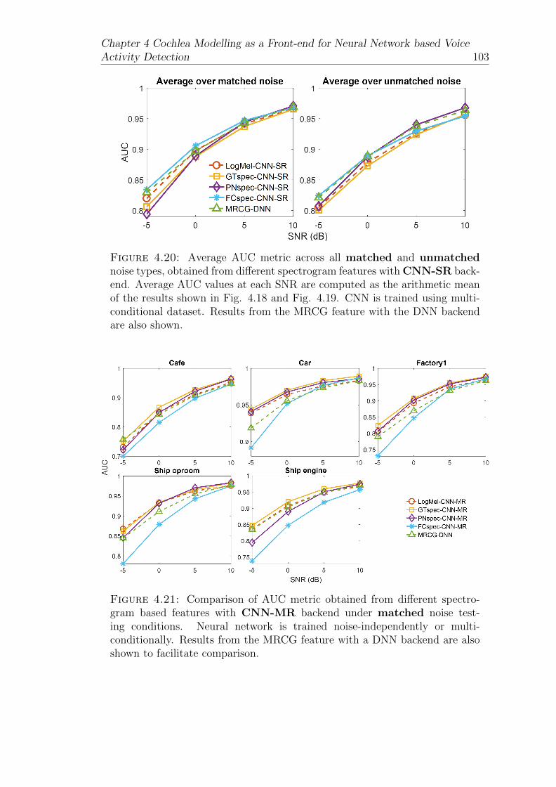
Chapter 4 Cochlea Modelling as a Front-end for Neural Network based VoiceActivity Detection 103
Figure 4.20: Average AUC metric across all matched and unmatchednoise types, obtained from different spectrogram features with CNN-SR back-end. Average AUC values at each SNR are computed as the arithmetic meanof the results shown in Fig. 4.18 and Fig. 4.19. CNN is trained using multi-conditional dataset. Results from the MRCG feature with the DNN backendare also shown.
Figure 4.21: Comparison of AUC metric obtained from different spectro-gram based features with CNN-MR backend under matched noise test-ing conditions. Neural network is trained noise-independently or multi-conditionally. Results from the MRCG feature with a DNN backend are alsoshown to facilitate comparison.

104Chapter 4 Cochlea Modelling as a Front-end for Neural Network based Voice
Activity Detection
Figure 4.22: Comparison of AUC metric obtained from different spec-trogram based features with CNN-MR backend under unmatched noisetesting conditions. Neural network is trained noise-independently or multi-conditionally. Results from the MRCG feature with a DNN backend are alsoshown to facilitate comparison.
Figure 4.23: Average AUC metric across all matched and unmatched noisetypes, obtained from different spectrogram based features with CNN-MRbackend. Average AUC values at each SNR are computed as the arithmeticmean of the results shown in Fig. 4.21 and Fig. 4.22. CNN is trained noise-independently or multi-conditionally. Results from the MRCG feature with aDNN backend are also shown to facilitate comparison.
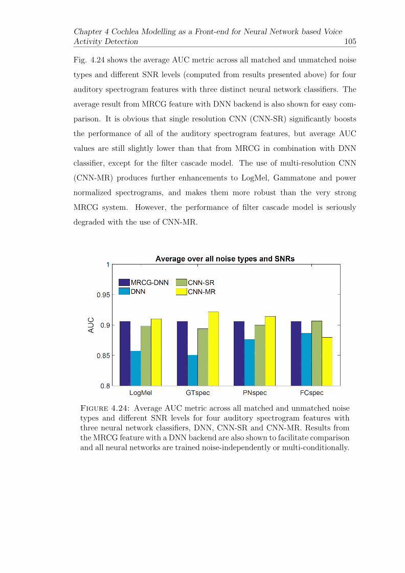
Chapter 4 Cochlea Modelling as a Front-end for Neural Network based VoiceActivity Detection 105
Fig. 4.24 shows the average AUC metric across all matched and unmatched noise
types and different SNR levels (computed from results presented above) for four
auditory spectrogram features with three distinct neural network classifiers. The
average result from MRCG feature with DNN backend is also shown for easy com-
parison. It is obvious that single resolution CNN (CNN-SR) significantly boosts
the performance of all of the auditory spectrogram features, but average AUC
values are still slightly lower than that from MRCG in combination with DNN
classifier, except for the filter cascade model. The use of multi-resolution CNN
(CNN-MR) produces further enhancements to LogMel, Gammatone and power
normalized spectrograms, and makes them more robust than the very strong
MRCG system. However, the performance of filter cascade model is seriously
degraded with the use of CNN-MR.
Figure 4.24: Average AUC metric across all matched and unmatched noisetypes and different SNR levels for four auditory spectrogram features withthree neural network classifiers, DNN, CNN-SR and CNN-MR. Results fromthe MRCG feature with a DNN backend are also shown to facilitate comparisonand all neural networks are trained noise-independently or multi-conditionally.

106Chapter 4 Cochlea Modelling as a Front-end for Neural Network based Voice
Activity Detection
4.7 Further Improvements
Since the filter cascade model yields the lowest AUC value with CNN-MR, this
motivates us to investigate alternative multi-resolution analysis strategies to close
the gap between other feature types. In the above simulations, all spectrogram
features except the MRCG use a single window size of 25 ms. In MRCG, a longer
window size of 200 ms is also employed. Thus we propose a similar strategy using
windows with multiple sizes to compute the spectrogram features. Specifically,
four different window lengths are employed, including 25 ms, 50 ms, 100ms and
200 ms, and the resulting features are called multi-window-length Cochleagram
(MWLCG), LogMel (MWLLM) and filter cascade (MWLFC) spectrograms. Note
that these window lengths are loosely inspired by the ranges of temporal context
captured by MRCG and CNNs discussed above. We have not performed this
multi-window-length analysis with the Power-normalized spectrogram because its
internal processing, such as noise suppression and temporal masking, is designed
and optimized to the short window length of around 25 ms. Thus, the use of longer
temporal window of 100 ms and 200 ms would seriously disrupt its representational
power, similar to what has been observed above when increasing its channel size.
To further confirm the relative advantage of CNN based multi-resolution anal-
ysis, the same mechanism adopted in MRCG is also applied to other features
types, by replacing the Gammatone filterbank with another auditory filterbank.
These features are referred to as MRLM and MRFC for LogMel and filter cascade
spectrograms respectively. We then train noise-independent DNN, CNN-SR and
CNN-MR models using these newly proposed features and test them in the same
manner as described above.
Fig. 4.25, Fig. 4.26 and Fig. 4.27 show the average AUC value across five matched
and five unmatched noise types obtained by applying various multi-resolution anal-
ysis methods to LogMel, Gammatone and filter cascade filterbank respectively.
Further average results across all SNR levels are shown in Fig. 4.28. For LogMel
and filter cascade filterbanks, the combination of multi-window-length spectro-
gram and CNN-MR classifier lead to the highest performance in both matched

Chapter 4 Cochlea Modelling as a Front-end for Neural Network based VoiceActivity Detection 107
and unmatched noise conditions. But for Gammatone filterbank, single-window-
length spectrogram with CNN-MR remains to be the most effective combination
for SNRs higher than 0 dB. From the average results in Fig. 4.28, it is interesting to
observe that when applying the same multi-resolution analysis adopted in MRCG,
VAD performance can also be improved for both LogMel and filter cascade models
with DNN backend. But this becomes less accurate when CNN based classifiers
are used, demonstrating the benefits of filter learning directly from the task at
hand. Overall, the most robust strategy for LogMel filterbank is MWLLM with
CNN-MR, which is slightly worse than the best strategy of Gammatone filterbank,
i.e. GTspec with CNN-MR. Finally, MWLFC with CNN-MR is the most effec-
tive combination for VAD from all of the methods tested, although the difference
between the top three strategies is not significant.
Figure 4.25: Comparison of various strategies in capturing context infor-mation with the LogMel filterbank in terms of AUC under matched and un-matched noises. MRLM means adopting the same analysis method as usedin MRCG, but the Gammatone filterbank is replaced by a LogMel filterbank.MWLLM means the spectrogram feature is computed using multiple windowlengths.

108Chapter 4 Cochlea Modelling as a Front-end for Neural Network based Voice
Activity Detection
Figure 4.26: Comparison of various strategies in capturing context informa-tion with the Gammatone filterbank in terms of AUC under matched andunmatched noises. MWLCG means the cochleagram feature is computedusing multiple window lengths.
Figure 4.27: Comparison of various strategies in capturing context infor-mation with the filter cascade model in terms of AUC under matched andunmatched noises. MRFC means adopting the same analysis method as usedin MRCG, but the Gammatone filterbank is replaced by a filter cascade fil-terbank. MWLFC means the spectrogram feature is computed using multiplewindow lengths.

Chapter 4 Cochlea Modelling as a Front-end for Neural Network based VoiceActivity Detection 109
Figure 4.28: Average AUC values obtained by applying various context ex-pansion strategies to three different auditory filterbank spectrogram features.The legend follows those in Fig. 4.24, Fig. 4.25, Fig. 4.26 and Fig. 4.27.
4.8 Comparison with Other Methods
Since both RATS-VAD and SF-VAD are also based on neural networks (although
only shallow MLP) that are trained with training data, for a fair comparison,
we test them under four noise types that are seen to none of them during train-
ing. Specifically, we choose Factory2, Tank-M109, Train and Speech-shaped (SSN)
noises, where the first three noise types are the same as those used above for un-
matched noise testing, while the SSN is taken from the Loizou noise database
[146], but solely used in this section. Babble and Factory1 noises are not used
because they were employed for training SF-VAD system as noted in the original
paper [110]. For the DNN and CNN method presented above, we choose the best
performing system that can be achieved with each of the four auditory filterbanks,
as shown in Fig .4.24 and Fig .4.28, which are the following, MWLLM-CNN-MR,
GTspec-CNN-MR, PNspec-CNN-MR, and MWLLFC-CNN-MR. Note that all of
the noise types are not seen during training for these systems either. Fig. 4.29
shows the detailed results of all of the systems compared under four noise types
and four SNR levels, Fig 4.30 shows the average results across different noises

110Chapter 4 Cochlea Modelling as a Front-end for Neural Network based Voice
Activity Detection
and Fig. 4.31 shows the average results across all noise types and SNR levels.
It can be seen that the RATS-VAD method performs significantly worse than all
other methods in almost all noisy conditions. For the SF-VAD system, although
it performs the best under Train noise at low SNRs (-5 dB, 0 dB and 5 dB), it
becomes less effective than the systems proposed in this work in nearly all other
noisy environments. On average, DNN and CNN based systems perform rather
similarly especially at high SNR levels and are more accurate than the SF-VAD to
some extent. This demonstrates the advantages of deep architectures over small
and shallow networks. But it is interesting to observe that the RATS-VAD system
is significantly less effective than other methods under comparison. One possible
reason for such lack of accuracy is that this is not the optimal method among all
of the systems developed for this project. We choose this one specifically, because
of lack of implementations of other methods and the evaluation datasets. Further-
more, this RATS-VAD was trained with audio recordings transmitted through 8
different communication channels, the distortions induced in these datasets could
be different from those that result from pure additive noise.
Figure 4.29: Comparison of the AUC values obtained by various VAD sys-tems under four noise types and SNR levels. The legend follows those in Fig.4.24, Fig. 4.25, Fig. 4.26 and Fig. 4.27.

Chapter 4 Cochlea Modelling as a Front-end for Neural Network based VoiceActivity Detection 111
Figure 4.30: Comparison of the average AUC values across four noise typesobtained by various VAD systems. The legend follows those in Fig. 4.24, Fig.4.25, Fig. 4.26 and Fig. 4.27.
Figure 4.31: Overall comparison of the average AUC values across four noisetypes and four SNR levels obtained by various VAD systems. The legendfollows those in Fig. 4.24, Fig. 4.25, Fig. 4.26 and Fig. 4.27.
4.9 Summary
In this chapter, the use of the filter cascade spectrogram has been investigated for
neural network based voice activity detection, under a wide range of noisy scenar-
ios. A number of other time-frequency representation based features have been
investigated for comparison, and simulation results show that the performance

112Chapter 4 Cochlea Modelling as a Front-end for Neural Network based Voice
Activity Detection
difference between them is generally small. Relatively large gains in detection ro-
bustness can be obtained by incorporating an appropriate form of temporal context
information for each feature type. Two types of context expansion techniques have
been investigated, one is the multi-window-length extension of spectrogram fea-
tures and the other is CNNs, which includes two versions, one has fixed size 2D
filters (single-resolution) and the other has the same number of 2D filter but with
varying sizes (multi-resolution). It is found that CNNs are almost always more
effective than DNN in speech and non-speech classification. But different fea-
tures perform the best with different temporal expansion techniques investigated.
Once the most suitable one is selected, all feature types perform rather similarly,
although the filter cascade spectrogram possess a marginal advantage.
Two other state-of-the-art voice activity detection algorithms have also been com-
pared with four of the systems proposed in this chapter. These are the ones with
optimal context expansion settings for each feature type, as determined by the
previous experiments. It is shown that these proposed systems also significantly
outperform the reference methods.

Chapter 5
Cochlea Modelling for Supervised
Speech Separation
In the previous chapter, various auditory inspired front-end processing methods
are compared in terms of their effects on the VAD tasks. In this chapter, we
further investigate their potentials for single-channel supervised speech separation
under additive noisy conditions.
5.1 Introduction
Speech is often regarded as one of the most natural and effective way of human
communication. However, speech signals can be easily corrupted by various inter-
ferences such background noise and undesirable reverberation, causing troubles to
both human and machine listeners. The set of algorithms which aim to extract
clean speech signals embedded in such sound mixtures are called speech enhance-
ment or speech separation methods. In this chapter we investigate single-channel
methods, that are based on neural networks and designed mainly for additive
noise reduction. Speech de-reverberation is out of the scope of this thesis, but has
been considered in many other studies, for instance [162]. For human listeners,
these algorithms are usually evaluated in terms of improvements to the perceived
113

114 Chapter 5 Cochlea Modelling for Supervised Speech Separation
quality and intelligibility of the separated speech signal, while for machine hear-
ing systems, these systems can be jointly optimized with a back-end stage, such
as a speech recognition engine or a natural language processing engine, so as to
optimize the complete system for the final task. In the following section, a brief
overview of existing speech separation methods is presented first, with a particular
focus on supervised learning based algorithms, which is the theme of this chapter.
Readers are referred to [146] for a comprehensive and detailed review of traditional
speech enhancement methods.
5.2 An Overview of Classical Speech Separation
Methods
5.2.1 Spectral Subtractive Methods
Probably the most classical and popular type of method in speech separation are
spectral subtractive methods. Assuming additive and uncorrelated interference,
the general idea of these methods is to recover the clean speech spectrum by
subtracting the estimated noise spectrum from the mixture spectrum. The noise-
corrupted signal, y(n) is written as,
y(n) = x(n) + d(n) (5.1)
where x(n) is the desired clean speech, d(n) is the interference signal and n is
discrete sample index. Taking discrete-time Fourier transform of both sides of Eq.
5.1 gives,
Y (ω) = X(ω) +D(ω) (5.2)

Chapter 5 Cochlea Modelling for Supervised Speech Separation 115
According to the derivations given in Chapter 5.1 of [146], the generalised form of
spectral subtraction algorithm can be written as,
|X(ω)|p = |Y (ω)|p − |D(ω)|p (5.3)
Or,
|X(ω)| = H(ω)|Y (ω)| (5.4)
H(ω) = p
√√√√(1− |D(ω)|p|Y (ω)|p
)(5.5)
where X(ω) and D(ω) are estimates of the clean speech and noise spectrum re-
spectively; p is a customisable power exponent, and popular choices are: p = 1,
giving the magnitude spectrum subtraction and p = 2, giving the power spectrum
subtraction; H(ω) is referred to as the gain or suppression function. To obtain
time-domain signal, the estimated clean speech spectrum is usually combined with
noisy phase, before using inverse Fourier transform and overlap and add method,
for example. The choice of noisy phase is partly justified by its relative insignifi-
cance in affecting speech intelligibility [163].
Despite its conceptual simplicity and ease of implementation, spectral subtraction
algorithm has several drawbacks. Since the noise spectrum has to be estimated,
inaccuracies in its estimation may lead to negative values in the subtracted spec-
trum in Eq. 5.3. Simple solutions such as half-wave-rectification can create small,
isolated and random peaks in the spectrum, giving rise to the well-known musical
noise artefacts [164]. To cope with these problems, various improvements have
been proposed to the basic spectral subtraction paradigm, such as spectral over-
subtraction with flooring [165], nonlinear spectral subtraction [166] and adaptive
gain averaging spectral subtraction [167].

116 Chapter 5 Cochlea Modelling for Supervised Speech Separation
5.2.2 Wiener Filter based Methods
Compared to the heuristics-based principles in spectral subtraction algorithms,
Wiener filtering presents an optimal linear estimate of the complex clean speech
spectrum in the sense of minimum-mean-square-error (MMSE). Assuming speech
and noise signals are wide-sense stationary, uncorrelated and have zero means, the
time domain finite-impulse-response (FIR) Wiener filter can be derived as,
h = (Rxx + Rnn)−1 rxx (5.6)
Here Rxx is the auto-correlation matrix of the clean speech signal, Rnn is the
autocorrelation matrix of the noise signal and rxx is the auto-correlation vector.
If both past and future samples of noisy speech are used to estimate the current
speech sample, the frequency domain Wiener filter can then be expressed as,
H(ω) =Pxx(ω)
Pxx(ω) + Pnn(ω)(5.7)
where Pxx(ω) and Pnn(ω) is the power spectrum of the clean speech and noise sig-
nal respectively. It can be observed that since we have access to neither the clean
speech nor the noise signal, neither their auto-correlations nor power spectra are
directly available. However, numerous techniques have been proposed for estimat-
ing these quantities from the noisy speech signal in order to perform Wiener-filter
based speech enhancement [168, 169, 170].
5.2.3 Statistical Model based Methods
As noted in Chapter 4, various statistical distributions have been employed to
model the speech and noise spectrum in order to determine speech presence likeli-
hood. In fact, these statistical models were first applied to the speech enhancement
problem, which then inspired their usage in VAD methods. The concept of a priori
and a posteriori SNRs and their estimations were first introduced and also play

Chapter 5 Cochlea Modelling for Supervised Speech Separation 117
a central role in the field of speech enhancement. As its name suggests, these
methods pose speech enhancement in a statistical estimation framework, and two
popular techniques borrowed from the estimation theory are maximum-likelihood
and Bayesian estimation. Compared to the Wiener filter introduced in the previ-
ous section, these estimators are nonlinear.
In maximum-likelihood estimation, the clean speech features we want to estimate,
for instance magnitude and phase spectra, are assumed to be unknown but deter-
ministic. In Bayesian methods, however, the parameter of interest is assumed to
be a random variable with some a priori distribution and the estimation is per-
formed based upon the Bayes’ theorem. Typically, Bayesian estimators perform
better than ML estimators, because they make use of prior knowledge. They have
been proposed in various forms, and mainly differ between each other in terms of
the target they aim to estimate (magnitude and phase, or real and imaginary parts
of complex STFT), the optimization criterion employed (MMSE or maximum a
posteriori) and speech prior distribution assumed (Gaussian, Gamma, Rayleigh
etc.). For example, Ephraim and Malah [124] developed the MMSE STFT ampli-
tude estimator by using Rayleigh distribution prior, considering the importance
of magnitude relative to phase in speech perception.
Despite their promising results, the theoretical limitations of these estimators are
that they are only optimal when the assumed statistical models are true and the
speech and noise spectral variances are known. These can be easily violated in real
data, and hence most of the statistics-based methods suffer to some extent from
inadequate noise suppression (particularly for fast varying non-stationary noises)
or introducing annoying artifacts in the recovered signal [171].
5.3 Supervised Speech Separation
Recent development in supervised speech separation originates from the field of
computational auditory scene analysis (CASA), which utilizes auditory principles

118 Chapter 5 Cochlea Modelling for Supervised Speech Separation
to analyse and understand complex acoustic environments in order to achieve near-
human performance. Based on results from psychoacoustic research, the main goal
of CASA systems was proposed to be the so-called ideal binary mask (IBM) [172],
due to its ability to yield substantial speech intelligibility improvements for noisy
speech for both normal-hearing and hearing-impaired listeners [173, 174, 175]. It
is defined using premixed target clean speech and interference signals. Specifically,
with a time-frequency (T-F) representation of a sound mixture, each T-F unit is
either preserved, with a mask value of one, or discarded, with a mask value of
zero, depending on the unit-level SNR and a local criterion. Mathematically, IBM
is expressed as the following,
IBM(t, f) =
1, if SNR(t, f) >= LC
0, otherwise
(5.8)
where SNR(t, f) denotes local SNR (in decibels) within the T-F unit at time frame
t and frequency bin or channel f ; LC is the local criterion used to determine
whether this unit is speech-dominant or interference-dominant. This effectively
formulates speech separation as a binary classification problem, opening up op-
portunities for a wide range of increasingly powerful machine learning techniques,
especially deep architectures as reviewed in Chapter 2. It worth noting that the
concept of ideal spectral masking is similar to various optimal spectral gain func-
tions or the suppression rules that many traditional methods aim to estimate, as
reviewed in section 5.2. The main difference between them is that classical ap-
proaches rely heavily on statistical assumptions on the properties of clean speech
and noise signals, whereas supervised speech separation directly learns such trans-
formation functions from training data, with little or no such assumptions. Fig.
5.1 shows a comparison of the block diagrams for these different approaches.
Although the original IBM-based supervised systems have shown great success in
improving the intelligibility of separated speech, they often results in poor percep-
tual quality, due to estimation errors and hence the removal of speech units. To
further improve their performances, various alternative training targets have been

Chapter 5 Cochlea Modelling for Supervised Speech Separation 119
Figure 5.1: Comparison of the (a) conventional statistics-based method and(b, c) two types of DNN-based methods for speech separation or enhancement.Adapted from Fig. 1 of [171] with permission.
explored, and depending on the specific choice of those targets, supervised sepa-
ration methods can be classified into two categories: (i) masking-based methods
and (ii) mapping- or regression-based methods, as also illustrated in Fig. 5.1.
As introduced above, masking-based methods aim to produce a time-frequency
mask, such as the IBM, and then use the estimated mask to separate the mixed
signal, usually by multiplying with the noisy spectrum, as indicated in Fig. 5.1 (b).
Wang etal. [176] examined a numbers of training targets and proposed an ideal
ratio mask (IRM) that should be preferred over the IBM in terms of speech quality.
This IRM is computed from the ratio of target speech energy and mixture energy,
and can be defined as in Eq. 5.9 [176], following the notation used in section
5.2.1 and Eq. 5.8. But other formulations of the ratio mask are also possible,
such as Eq. (8) in [177]. Instead of enhancing only the magnitude spectrum,
as IBM and IRM do, Williamson and Wang [178] proposed to jointly enhance
the magnitude and phase response of noisy speech by estimating the complex
ideal ratio mask (cIRM) that predicts both the real and imaginary components of

120 Chapter 5 Cochlea Modelling for Supervised Speech Separation
complex STFT spectrogram of clean speech in the Cartesian coordinate system.
Results show that it substantially outperforms the magnitude-only IRM, probably
because cIRM allows a full reconstruction of clean speech in the ideal case.
IRM(t, f) =
√X2(t, f)
X2(t, f) +D2(t, f)(5.9)
Mapping-based methods, however, learn a regression function that transforms
noisy speech features to clean speech features directly, Fig. 5.1 (c). For instance,
Xu etal. [179] proposed to use a DNN as a regression machine to estimate the
clean magnitude spectrum from the noisy magnitude spectrum. Subsequently,
the approach was extended with noise-adaptive training [180] and global variance
equalization [181] to alleviate the distortions in estimated clean magnitude spec-
trum. Since the main goal of this chapter is to investigate the benefits of advanced
modelling of cochlear nonlinearity in supervised speech separation, we only choose
the IRM as the training target in the following experiments, for its simplicity and
proved effectiveness [176], although it worth bearing in mind that more advanced
masks could change the simulation results presented below.
Apart from training target, there are another two fundamental elements in su-
pervised speech separation systems, i.e. feature extraction and backend machine
learning model, as shown in more detail in Fig 5.2. As in general machine learning
tasks, feature extraction is normally the first stage of the signal processing chain.
Early studies [182, 183] adopted pitch-based features as harmonic structure is a
prominent characteristic in voiced speech. For unvoiced speech separation, spec-
trogram statistics [184] and amplitude modulation spectrum (AMS) [185, 186, 187]
were later incorporated. To further improve speech separation robustness, various
features that were originally developed in the fields of speech and speaker recogni-
tion were also investigated, including MFCC, PLP, RASTA-PLP, GFCC, PNCC.
Using Gaussian-kernal SVMs as subband classifier, they are shown to outperform
the earlier pitch and AMS features in terms of classification accuracy and HIT-FA
rate [188]. A complementary feature set that concatenates AMS, RASTA-PLP

Chapter 5 Cochlea Modelling for Supervised Speech Separation 121
and MFCC feature vectors has also been identified as the optimal feature combi-
nation of all of the feature types tested for IBM estimation based on a group lasso
approach, and is also shown to perform the best in most of test conditions [188].
In [119], a significantly more extensive list of features were tested and the MRCG
was shown to achieve the best separation performance among all of them, even
better than the complementary feature set recommended in [188]. However, it is
worth noting that features were compared in [119] using the same type of noise for
training and testing, it is thus not clear how well can MRCG generalize to unseen
noise types for supervised speech separation, although it is indeed found to do this
effectively in VAD task as presented in Chapter 4. Since only a MLP was adopted
as a binary mask classifier, it will be worthwhile to investigate how MRCG will
interact with deep architectures, such as DNN and CNN, for speech separation,
as also pointed out in [119]. Finally, since the primary evaluation metric adopted
is the HIT-FA rate for IBM estimation, the relative advantages among various
features could change when different masks and speech separation performance
metrics were used.
Figure 5.2: Block diagram of a typical supervised speech separation system.Common choice for Time-Frequency analysis and synthesis is the Gammatonefilterbank. The dashed line means that the Time-Frequency analysis represen-tation can sometimes be used in Feature extraction module as well.

122 Chapter 5 Cochlea Modelling for Supervised Speech Separation
The final consideration is the choice of backend machine learning. Early studies
used generative models such as Gaussian Mixture Model [187] or shallow discrim-
inative models such as MLP[119] and Support Vector Machines [188] for binary
mask classification, but their practicability is somewhat limited due to the lack
of generalization ability of these systems. Motivated by their success in acous-
tic modelling for speech recognition in the last few years, recent researches focus
on deep models, including DNN, CNN, LSTM-RNN and BLSTM-RNN and they
were demonstrated to be superior to earlier systems by a large margin, even when
tested in mismatched noisy conditions. In formal listening tests, deep models en-
hanced speech shows substantial improvements in speech intelligibility for both
normal-hearing and hearing-impaired listeners. For these reasons, deep models
are adopted in the following experiments for comparing various auditory inspired
time-frequency representations for supervised speech separations.
5.4 Filter Cascade Spectrogram for Supervised
Speech Separation
5.4.1 Feature Extraction
The feature extraction procedure is basically the same as that adopted in section
4.3. Apart from the filter cascade filterbank (FCspec), four other time-frequency
representations are also considered for comparison, including FFT based Log-
Power spectrogram (Spec), Log-Mel spectrogram (LogMel), Gammatone spectro-
gram or cochleagram (GTspec) and MRCG. The Power normalized spectrogram
has also been investigated but it yielded unacceptable performance compared to
other features and hence is not considered. Different spectrogram features are
computed using an analysis window of 25 ms (or 400 samples) with a window
shift of 10 ms (or 160 samples) and feature configurations follow those detailed
in section 4.3. Moreover, multi-window-length extensions of LogMel (MWLLM),

Chapter 5 Cochlea Modelling for Supervised Speech Separation 123
Figure 5.3: An example clean utterance from the TIMIT dataset and thesame utterance corrupted by a factory noise from the NOISEX dataset at 0dB SNR.
Gtspec (MWLCG) and FCspec (MWLFC), as introduced in section 4.7, are also
included.
It is worth noting that the MRCG feature has been used in both speech detection
and speech separation tasks, but different settings were followed in these applica-
tions. In a speech detection task [6], one set of 8-channel Gammatone filterbank
was used to construct each of the four resolutions, while in speech separation, the
authors in [119] proposed to use four sets of 64-channel Gammatone filterbanks
(referred to as MRCG-64 in this chapter), making the dimensionality of static
feature vector to be 64 × 4 = 256. In this work, apart from using the original
implementation for speech separation, we also considered an variant that employs
only 16 Gammatone filters in each resolution, resulting in a static feature vector
having the size of 64. This configuration is called MRCG-16 in this chapter and is
the same MRCG feature setting as adopted in the speech detection investigation
presented in Chapter 4. It is included here for the same reason: to reduce the dif-
ference in feature dimensionality between various spectrogram features. Fig. 5.4
shows the MRCG feature with 256 channels for a clean utterance from the TIMIT
dataset [143] and the same utterance corrupted by a factory noise from the NOI-
SEX dataset [144] at 0 dB SNR, the waveforms of which are displayed in Fig.
5.3. It can be seen that the 256-channel MRCG shows much more spectral details
than its 64-channel counterpart, Fig. 4.7, but at the cost of nearly four times of
computational complexity. Since visualizations of all other spectrograms features
have been shown in Chapter 4, Fig. 4.6 and Fig. 4.7, they are not repeated here.

124 Chapter 5 Cochlea Modelling for Supervised Speech Separation
Figure 5.4: Visualization of MRCG representation of a clean utterance fromthe TIMIT dataset (right column) and the same utterance corrupted by afactory noise from the NOISEX dataset at 0 dB SNR (left column).

Chapter 5 Cochlea Modelling for Supervised Speech Separation 125
Figure 5.5: The Ideal Ratio Mask for estimating clean speech signal shownat the left hand side of Fig. 5.3 from its noisy counterpart shown at the righthand side of Fig. 5.3.
As mentioned above, the IRM is used as the training target for neural network
acoustic models in this work. Fig. 5.5 shows an example of such an IRM for the
clean utterance and its factory noise corrupted counterpart, as illustrated in Fig.
5.3, which has been computed using Eq. 5.9. Note that IRM can be computed
in different domains, such as Fourier transform and Gammatone domain. In this
work, we follow the practice adopted in [176], which formulated the IRM using a
64-channel Gammatone filterbank.
5.4.2 Experimental Settings
5.4.2.1 Datasets
In a similar way to the settings used in Chapter 4, clean speech utterances are
selected from the TIMIT [143] database. Training sentences consist of 1,600 ran-
domly chosen utterances, with 200 utterances from each of the 8 dialect region.
Another 160 utterances, with 20 from each dialect region, are also randomly se-
lected from the TIMIT validation set (original test set excluding the core test set),
to form the validation dataset. All input clean speech signals are sampled at 16
kHz and rescaled to 60 dB SPL before mixing with various types of noises at a
number of SNR levels.

126 Chapter 5 Cochlea Modelling for Supervised Speech Separation
A total number of 10 noise types are selected from three noise databases, which
are the NOISEX-92, the QUT-NOISE and the Loizou noise corpora, as shown in
Fig. 4.10. From these, five types of noise, including Cafe, Car, Factory1, Ship
oproom and Ship engine noises, are used to create a multi-condition training set,
by mixing each of the training utterances with a random segment of each noise
type at two SNR levels of -5 dB and 0 dB, which gives rise to 16,000 noisy sentences
in total. The validation dataset is obtained in a similar way, except that only 160
clean utterances are used, resulting in 1600 noisy sentences. For testing, apart
from using the five noise types that are employed in training, the other five types
of unseen noises are also adopted, consisting of Babble, Factory2, Tank-m109,
F16 and Train noises. This sets up the matched and unmatched testing scenarios.
These 10 types of noise are mixed with the 240 core test set of the TIMIT database
at four SNR levels of -5 dB, 0 dB, 5 dB and 10 dB, where 5 dB and 10 dB are two
unseen SNR conditions. Note that only noise-independent training and testing are
performed for this speech separation task, because noise-dependent training is of
limited importance for practical applications.
5.4.2.2 Neural Network Structures and Training
Both DNN and CNN architectures are used to estimate the IRM given calculated
feature vectors. The DNN is composed of one input layer, three fully connected
hidden layers, each with 1024 ReLU units and one output layer with sigmoid units.
For the CNN, both single resolution (CNN-SR) and multi-resolution (CNN-MR)
structures are adopted. The convolutional layer of CNN-SR consists of 64 2-
dimensional (2D) filters with size of 9 × 9, while that of CNN-MR also has 64
2D filters but with each 16 of them having the following 4 resolutions: 5× 5, 9×
9, 15 × 15 and 23 × 23. Valid convolution was performed between filter weights
and input features. Subsequently, after ReLU nonlinear activation and maximum
pooling along the frequency dimension with size of 2 and no overlapping, two
fully-connected hidden layers each with 1024 ReLU units and one output layer
with sigmoid units are added in both CNN-SR and CNN-MR. It can be seen that
network structures employed in this chapter are the same as those used in Chapter

Chapter 5 Cochlea Modelling for Supervised Speech Separation 127
4, except that networks sizes are increased to tackle the more challenging task of
IRM estimation (i.e. larger dimensionality of the target).
The network training procedure is essentially the same as that present in section
4.4.2, except the following changes: (a) mean-square-error (MSE) between the
predicted ratio masks and IRMs is used as the cost function. (b) The maximum
number of training epoch is set to 300 and the patience for early stopping is set
to 30, i.e., training is stopped if the validation loss does not reduce for 30 consec-
utive epochs. Note that these settings are larger than those used in VAD tasks
as presented in Chapter 4. (c) Finally, as suggested in [176] for performance im-
provement, a temporal context of 5-frame of features, centred around the current
frame, are concatenated as input to the DNN, which are in turn trained to pre-
dict the corresponding 5-frame of targets at the same time. The multiple target
estimates obtained for each frame are then averaged to produce the final mask
estimate. Note that for CNNs, there is no need for feature concatenation for the
input because context information is already included implicitly by 2D filters, but
the training targets are also the surrounding 5 frames of IRM connected together.
Therefore the output size of DNN and CNNs is 64× 5 = 320.
5.4.2.3 Evaluation and Comparison
Evaluation of the performances of various speech enhancement systems investi-
gated in this chapter are conducted by measuring the quality and intelligibility
of processed speech. Although perhaps the most reliable method for assessing
these two attributes is subjective listening tests, these tests are costly and time-
consuming. Therefore, two objective metrics are employed to predict speech qual-
ity and intelligibility of enhanced speech respectively, which are Perceptual Eval-
uation of Speech Quality (PESQ) [189] and Short-Time Objective Intelligibility
score (STOI) [190]. They are chosen because they all have been shown to be
highly correlated with subjective measurements obtained from listening tests, and
are more accurate than a number of other objective metrics in their respective
paper.

128 Chapter 5 Cochlea Modelling for Supervised Speech Separation
PESQ was originally designed for predicting quality of speech passed through
narrow-band telecommunication networks [189] and was selected as the ITU-T
recommendation P.862 [191]. To accommodate wideband signals, some changes
were made to the original narrow-band implementation and this wide-band PESQ
is documented in ITU-T recommendation P.862.2 [192]. In this chapter, we use
this wide-band version of PESQ, since all speech signals are sampled at 16 kHz.
This metric takes in both the clean reference signal and the degraded or processed
signal to produce a prediction of subject Mean Opinion Score (MOS) based on
their differences. Its computation consists of the following four main steps: (1)
pre-processing stage which is responsible for level normalization and time align-
ment of the two signals; (2) auditory transform that produces perceptual loudness
spectra; (3) symmetric and asymmetric disturbance computation between the pair
of signals and time and frequency averaging to obtain the raw PESQ score, which
ranges from -0.5 to 4.5; (4) conversion of raw PESQ score to MOS (ranges from
1 to 5) using a logistic-type function as proposed in [193]. Higher MOS means
better speech quality.
STOI also compares the clean reference signal with the degraded or processed
signal. It first decomposes both signals into one-third octave bands by grouping
frequency components obtained from STFT. After normalization and clipping of
the short-time (384 ms or 30 frames) temporal envelope of the degraded speech,
a time-frequency dependent intermediate intelligibility measure, dj,m, is obtained
for each segment j and each one-third octave band m, as the correlation coef-
ficient between the short-time temporal envelop of the clean speech and that of
the degraded speech. The global STOI score is then obtained as the average of
this intermediate intelligibility measure over all bands and all frames, and has a
monotonic increasing relationship with subjective speech intelligibility. The range
of the STOI score is from 0 to 1. It can also be mapped to actual intelligibility
score (measured as percentage of words correctly recognised), using a logistic func-
tion as proposed by its original authors [190]. The degree of correlation between
STOI and subjective intelligibility scores obtained from listening tests conducted
by Kjems et al. [194] and root-mean-square prediction errors were investigated

Chapter 5 Cochlea Modelling for Supervised Speech Separation 129
and compared with three other objective intelligibility measures in [190]. The
main results figure is reproduced in Fig. 5.6. It can be seen that STOI achieves
the highest level of correlation with subjective intelligibility scores and the lowest
prediction error. The three reference objective measures used for comparison are:
(1) DAU: metric based on a sophisticated perceptual model developed by Dau
et al. [195]; (2) NSEC: metric based on the normalized subband envelope cor-
relation [196]; (3) CSTI: normalized covariance-based Speech Transmission Index
(STI)-procedure [197].
Three other speech enhancement or separation algorithms are also employed for
comparison with the systems proposed in this chapter. The first one is a supervised
learning based method that uses the complementary feature set proposed in [188,
5] and the same DNN as adopted in this chapter to estimate the IRM (referred
to as Comp Feat-DNN). This feature set includes amplitude modulation spec-
trum, relative spectral processing with PLP, MFCC and 64-channel gammatone
filterbank energies, although the original post-processing auto-regressive moving
average filter is not used. Another two methods are classical speech enhancement
algorithms. One is the MMSE log-spectral amplitude estimator (denoted as Log-
MMSE) from [198] and the second one is the audible noise suppression algorithm
(denoted as AudNoiseSup) from [199] that aims to suppress only the audible noise
spectrum based on psychoacoustics masking principles. Implementations of these
two methods are obtained from [146].
5.5 Results
In this section, speech separation results are presented according to the neural
network acoustic model used to predict the IRMs, and only average results across
several noise types are given in order to save space. Detailed results for each
individual noise type are presented in the Appendix A.

130 Chapter 5 Cochlea Modelling for Supervised Speech Separation
Figure 5.6: Comparison of STOI and three other reference objective intelli-gibility measures in prediction of subjective speech intelligibility scores. Theunprocessed noisy speech conditions are denoted by the crosses, and the ITFS-processed conditions are represented by the dots, where ITFS means ideal timefrequency segregation, which is just using ideal time-frequency mask for speechseparation as introduced in section 5.3. The gray line denotes the mappingfunction used to convert the objective output to an intelligibility score. Root-mean-square prediction error δ, and the correlation coefficient ρ, between thesubjective and objective intelligibility scores are shown in the title of each plot.Adapted from Fig. 1 of [190] with permission.
5.5.1 DNN Results
Fig. 5.7 shows the average PESQ and STOI scores across matched and unmatched
noise types for test utterances enhanced by DNN-estimated IRMs. Since in many
scenarios, the results from different spectrogram-based features are very similar, a
magnified view of the scores around 0 dB SNR is also added in the corner of each
sub-plot. It can be seen that all systems significant improve both PESQ and STOI

Chapter 5 Cochlea Modelling for Supervised Speech Separation 131
scores at all SNR levels compared to the original noisy test utterances. However,
MRCG features do not show significant advantages compared with other standard
auditory filterbanks, which is the opposite of what has been observed in VAD
tasks in Chapter 4. In fact, MRCG-16 and MRCG-64 perform the worst in almost
all noisy scenarios, with the exception of MRCG-64, which outperforms GTspec
slightly in PESQ scores at very low SNR levels (-5 and 0 dB), although its feature
size is four times that of GTspec. The performance of GTspec is very similar to
that of MRCG-64, while being a little better in many cases. But it is worse than
the other three feature types, i.e., Spec, LogMel and FCspec. It is interesting
to note that Spec feature performs the best and better than FCspec in terms of
PESQ score under matched noise conditions, but is slightly surpassed by FCspec
under unmatched noise scenarios. For LogMel, it is the third most effective feature
type with DNN acoustic model in most cases. But it should be reminded again
that the differences between various features are very small. Fig. 5.8 shows the
average PESQ and STOI scores over all noise types and SNR levels for difference
features, indicating the same order of effectiveness as discussed above.

132 Chapter 5 Cochlea Modelling for Supervised Speech Separation
Figure 5.7: Average PESQ and STOI scores across matched and unmatchednoise types for DNN enhanced test utterances. A magnified view of the scoresat 0 dB SNR is shown in the corner of each sub-plot.
Figure 5.8: Average PESQ and STOI scores over all noise types and SNRlevels for DNN enhanced test utterances.

Chapter 5 Cochlea Modelling for Supervised Speech Separation 133
5.5.2 CNN Results
The results of PESQ and STOI scores for single resolution CNN and multi-
resolution CNN are illustrated in Fig. 5.9, Fig. 5.10 and Fig. 5.11, Fig. 5.12,
respectively. Only LogMel, GTspec, FCspec and their multi-window-length exten-
sions are used with CNN structures, while the Spec is not included, in spite of its
best performance with DNN backend, because of its much larger feature size. Sim-
ilar to DNN systems, all CNN based systems produce substantial improvements
to both PESQ and STOI scores across all SNR levels, and the performances dif-
ference between various feature types are even smaller. FCspec based features
become the most effective feature types in almost all noisy test scenarios. And it
is interesting to observe that multi-window extensions often lead to lower PESQ
and STOI scores compared to their standard filterbank counterpart, contrary to
what has been seen in VAD studies presented in Chapter 4. In particular, multi-
window-length features only show advantages relative to the standard filterbanks
in terms of PESQ under unmatched noise conditions for both CNN-SR and CNN-
MR acoustic models. But one exception is MWLFC, it produces the highest scores
across most SNR levels with CNN-MR backend. On average, we can see from Fig.
5.10 and Fig. 5.12 that multi-window-length processing is only slightly beneficial
for FCspec, but not for LogMel and GTspec.

134 Chapter 5 Cochlea Modelling for Supervised Speech Separation
Figure 5.9: Average PESQ and STOI scores across matched and unmatchednoise types for single resolution CNN enhanced test utterances. A magnifiedview of the scores at 0 dB SNR is shown in the corner of each sub-plot.
Figure 5.10: Average PESQ and STOI scores over all noise types and SNRlevels for single resolution CNN enhanced test utterances.

Chapter 5 Cochlea Modelling for Supervised Speech Separation 135
Figure 5.11: Average PESQ and STOI scores over matched and unmatchednoise types for multi resolution CNN enhanced test utterances. A magnifiedview of the scores at 0 dB SNR is shown in the corner of each sub-plot.
Figure 5.12: Average PESQ and STOI scores over all noise types and SNRlevels for multi resolution CNN enhanced test utterances.

136 Chapter 5 Cochlea Modelling for Supervised Speech Separation
5.5.3 Comparison
Before comparing with other denoising algorithms, average PESQ and STOI scores
over all noise types and SNRs for DNN and CNN acoustic models are compared
in Fig. 5.13 to better understand the difference between network structures. It
can be seen that CNNs perform slightly better than DNN for all feature types and
CNN-MR is better than CNN-SR in most cases. We can also observe more clearly
that multi-window length extensions of auditory spectrum can not provide extra
improvements in both PESQ and STOI scores, except for FCspec feature.
Fig. 5.14 and Fig. 5.15 shows the comparison of performance between three
methods that are proposed in this chapter and three other reference methods.
The three proposed methods selected are the best performing system for each
auditory filterbank feature as determined from Fig. 5.13. Traditional method like
LogMMSE is able to improve speech quality significantly as well, but not speech
intelligibility, which is a common drawback of classical approaches. However, all
of the proposed supervised learning based methods are capable of increasing both
PESQ and STOI scores by large amounts in all noisy test scenarios.
The performance of the complementary feature set with DNN acoustic model, re-
ferred to as Comp Feat-DNN, is quite poor. It can only improve objective speech
quality slightly at very low SNR levels (-5 and 0 dB) and could make processed
utterances even less intelligible compared to the original noisy ones. The audible
noise suppression algorithm also performs poorly, as it is not able to improve ei-
ther PESQ or STOI in nearly all testing conditions. To better understand their
limitations, an example noise utterance (Factory1 noise, mixed at 0 dB SNR) that
have been enhanced by proposed and reference methods is shown in Fig. 5.16
and Fig. 5.17, respectively. The IRM and clean spectrogram for this sentence are
displayed in the first row of Fig. 5.16, and the estimated IRM and enhanced spec-
trogram obtained by various methods are shown subsequently. It can be observed
that the proposed supervised algorithms are able to estimate the IRM fairly ac-
curately, although the MWLFC-CNN-MR system reduces larger amount of noise

Chapter 5 Cochlea Modelling for Supervised Speech Separation 137
than the LogMel-CNN-MR system, as judged visually from the enhanced spectro-
gram. For the reference methods, Comp Feat-DNN fails to recover a substantial
area of IRM, introducing a number of gaps within the utterance, which could ex-
plain the low scores in PESQ and STOI obtained from processed test sentences.
This also demonstrates that the more raw spectrogram based features are more ef-
fective than the more sophisticated, hand-engineered, feature extraction methods
in neural network based IRM estimation. Although the LogMMSE indeed sup-
presses a substantial amount of noise, it also distorts the spectrogram structure,
by discarding a large portion of mid-to-high frequency speech elements, which is
detrimental to speech intelligibility improvement. For AudNoiseSup algorithm, it
is strange that it destroys speech information almost completely.
Figure 5.13: Average PESQ and STOI scores over all noise types and SNRlevels for DNN and CNNs.

138 Chapter 5 Cochlea Modelling for Supervised Speech Separation
Figure 5.14: Comparison of average PESQ and STOI scores over matchedand unmatched noise types obtained from three proposed methods and threereference methods.
Figure 5.15: Comparison of average PESQ and STOI scores over all noisetypes and SNR levels for three proposed methods and three reference methods.

Chapter 5 Cochlea Modelling for Supervised Speech Separation 139
Figure 5.16: An example of test noisy utterance and its enhancement bytwo supervised learning based methods proposed in this chapter. The testutterance is corrupted by factory noise at 0 dB SNR. The IRM of this utteranceand its clean spectrogram are shown in the top two plots. The estimatedIRM and the corresponding enhanced spectrogram, obtained by LogMel-CNN-MR and MWLFC-CNN-MR, are shown in the middle and bottom two plots,respectively.

140 Chapter 5 Cochlea Modelling for Supervised Speech Separation
Figure 5.17: The same test noisy utterance as used in Fig. 5.16 but en-hanced by the three reference methods. The estimated IRM and the corre-sponding enhanced spectrogram, obtained by Comp Feat-DNN are shown inthe top two plots, while the enhanced spectrograms obtained by LogMMSEand AudNoiseSup are shown in the bottom two plots.

Chapter 5 Cochlea Modelling for Supervised Speech Separation 141
5.6 Summary
In this chapter, the use of filter cascade spectrogram feature for supervised speech
separation has been investigated. Both DNN and CNNs have been adopted to
estimate the IRMs which are then used to enhance the cochleagrams of noisy
test utterances. Similar to what has been observed in VAD studies, CNN models
almost always perform better than DNN models, so does multi-resolution CNN to
single resolution CNN, even though the amount of performance improvement is
marginal. Contrary to the findings presented in Chapter 4, multi-window-length
extension of auditory features cannot produce extra gains in performance in many
test scenarios, except for the filter cascade feature. Comparison of the systems
proposed in this chapter with three reference denoising algorithms has also been
performed, illustrating the biggest advantage of the supervised methods proposed
with respect to traditional methods is their ability to significantly improve both
speech quality and intelligibility under either seen and unseen additive noises.


Chapter 6
Conclusions and Suggestions for
Future Work
The mammalian cochlea is a fascinating sensory organ, because of the way its
nonlinearity contributes to its remarkable sensitivity and dynamic range. The
work presented in this thesis addresses the problem of nonlinear cochlea modelling
and its potential application to some aspects of speech processing. In this chapter,
important findings of this work are summarized, followed by suggestions for future
work.
6.1 Conclusions
6.1.1 Cochlear Modelling
Cochlear modelling is not only an important tool for better understanding of
cochlear functions, but also has been inspiring novel algorithms for speech pro-
cessing. A state space model of the nonlinear cochlea has been proposed by Elliott
et al. [1], based on the 1D transmission-line model developed by Neely and Kim
[9]. This reformulation allows convenient simulations of the time domain responses
of both linear and nonlinear model configurations. However, the computational
143

144 Chapter 6 Conclusions and Suggestions for Future Work
burden of this model is extremely high, seriously limiting its applicability to either
scientific or practical problems. To improve its computational efficiency, a revised
formulation of the original state space model has been developed here [95], that is
able to reduce the simulation time by around a factor of 40, by taking advantages
of the sparsity pattern of system matrices.
Even with this modified formulation, this type of cochlear model is still too compli-
cated to be applied to practical speech processing problems. Thus an alternative
nonlinear filter cascade model of the cochlea, the CARFAC model [98, 12], has
also been investigated. This filter cascade model is significantly more efficient to
run than the state space model while still being more physiologically plausible
compared to other parallel filterbank based models, because it aims to simulate
the forward travelling wave inside the cochlea, inspired by the WKB approximate
solution to the cochlear wave equation. The analytical relationship between these
two models has also been presented.
A systematic comparison of the outputs of these two nonlinear models was then
undertaken, in response to single-tones and two-tones stimuli and these are vali-
dated against experimental measurements obtained from sensitive cochleae. Re-
sults show that both models are reasonably accurate in simulating the represen-
tative characteristics of cochlear responses to single-tone stimuli, but in two-tone
suppression simulations, the CARFAC model produces results that are relatively
closer to physiological measurements than those of the transmission-line model. It
is also worth noting that both models cannot account for every aspects of the wide
range of datasets. Additionally, tuning of the parameters of the CARFAC model
is more flexible than that with the TL model, however, because of the smaller
number of free parameters and its simpler stability criterion. Given these benefits
of the CARFAC model, it is chosen as the front-end model for performing subse-
quent speech processing tasks, in comparison with other widely-used methods of
front-end processing.

Chapter 6 Conclusions and Suggestions for Future Work 145
6.1.2 Application to Speech Processing
Two types of speech processing tasks have been investigated using the CARFAC
model as a front-end processor: voice activity detection (VAD) and supervised
speech separation. For both of these tasks, the CARFAC model serves as a feature
extraction module, the output of which is fed to a neural network backend, which
is trained to produce the desire final targets using a large pool of training data. In
terms of VAD, the target is the probability of each frame of observation being either
speech or non-speech, while for speech separation, it is the ideal ratio mask of each
time-frequency unit. Since the filter cascade model provides a filterbank-based
feature, various other popular parallel filterbank-based feature extraction methods
have also been included for performance comparison. These features, although also
motivated by auditory principles, provide a less-refined representation of cochlear
functions. This offers a good opportunity to investigate whether the incorporation
of cochlear nonlinearities can be advantageous over of the use of other simpler
auditory filterbanks. Moreover, a number of network structures, including DNN
and CNNs, have been investigated for each type of feature.
Voice Activity Detection. For the voice activity detection task, both noise-
dependent and noise-independent training of neural networks have been investi-
gated, and the performances on test datasets were evaluated from the Area Under
the Receiver Operating Characteristic Curves (AUC). In noise-dependent training
scenario, only the DNN was used as the backend and it was found that the nonlin-
ear filter cascade model performed slightly better than other fixed-resolution audi-
tory filterbank-based features in terms of average AUC across all noise types. How-
ever, the best overall performance was achieved by the multi-resolution cochlea-
gram feature. Motivated by these results, CNN backends and multi-window-length
extensions were also used in noise-independent training scenario, which provides
a data-driven way of integrating multiple scales of resolutions and temporal infor-
mation. Although a similar ranking of performances of different front-ends to that
in noise-dependent training case was observed with the DNN backend, the use of
CNNs and multi-window-length extensions significantly improved the effectiveness

146 Chapter 6 Conclusions and Suggestions for Future Work
of all filterbank-based features, making them very similar in terms of overall AUC
value averaged over all noise types and SNR levels, as long as a suitable context
expansion strategy has been selected, and outperforming the MRCG with DNN
backend system. Comparison with another two recent state-of-the-art algorithms
has also demonstrated the superiority of the proposed deep network based systems.
Supervised Speech Separation. For the supervised speech separation task,
only the multi-condition noise-independent training was investigated, because the
practical importance of noise-dependent training is limited. The DNN and CNNs
(with some network structure changes), and multi-window-length extension tech-
niques that were investigated in VAD study were all used to estimate the ideal
ratio mask, that was then applied to the noisy cochleagram, from which the en-
hanced speech waveform was synthesized. The performances of different speech
separation systems were determined by two objective metrics obtained from the
enhanced speech signals: the Short Time Objective Intelligibility score and the
Perceptual Evaluation of Speech Quality. In terms of average metric values, all fil-
terbank features perform similarly, although the CARFAC model enjoys a marginal
relative advantage. However, contrary to what has been observed in VAD study,
CNN based systems are only slightly more effective than DNN based ones, which
is probably because temporal context information has been integrated in DNN as
well by concatenating features from a surrounding window of five frames. Fur-
thermore, multi-window-length extension of auditory filterbank features cannot
produce extra performance gains except for the filter cascade feature. Compari-
son with three other reference methods has illustrated that the advantage of the
proposed supervised methods, with respect to traditional ones, is their capability
in improving both intelligibility and quality of processed speech significantly.
Summary. Overall, results from these two speech processing tasks indicate that
when no temporal context information is incorporated, the filter cascade front-
end can be more effective than other simple auditory filterbanks. However, as
long as suitable context expansion strategies have been integrated, all front-end

Chapter 6 Conclusions and Suggestions for Future Work 147
processors perform rather similarly. Therefore, at least in the neural network based
framework considered in this thesis, the inclusion of temporal dynamics of speech
signals and network structure engineering seem to be more beneficial than more
refined modelling of cochlear nonlinearity in improving the performance of speech
processing algorithms.
6.2 Suggestions for Future Work
In the light of the findings of this study, the author recommends that the following
areas are worthwhile for further investigations.
• Refinement of cochlear models. In Chapter 3, we show that both the TL
and CARFAC cochlear models are capable of simulating some of the key
features of a normal cochlea. However, they also have some weaknesses
in reproducing some other aspects of cochlear mechanics. Thus it would be
beneficial to further tune the parameters of these models to make them more
compatible with experimental measurements, which could also be valuable
to speech processing tasks. Moreover, the evaluation of these models against
physiological observations is not comprehensive. For example, the following
aspects have not been investigated: the generation of harmonic distortions
and combinational tones, and the simulation of the frequency modulation or
glide in BM impulse responses. A good example of this kind of study is [3].
• Inclusion of other acoustic disturbances in speech processing tasks. For both
of the speech processing tasks investigated, only additive background noise is
dealt with. Other types of acoustic disturbances such as room reverberation
and channel mismatch are also very common and are detrimental to system
performance. Therefore, it is worthwhile to explore the potentials of cochlear
models under these environments as well. The relative advantages of different
front-end feature extractor could be changed in this case.

148 Chapter 6 Conclusions and Suggestions for Future Work
• Alternative network structures. In this work, DNN and several versions of
CNN have been integrated with a number of cochlear inspired feature vec-
tors for speech processing, which demonstrates that an important factor
for performance improvement is the effective capture of the temporal dy-
namics of speech signals. However, DNN and CNN can only incorporate a
fixed temporal context, which is computationally expensive and may also
be sub-optimal in many scenarios. Another type of neural network, called
the recurrent neural network, is able to learn a variable length of temporal
dependences according to the task at hand, by feeding back network states
from previous time steps to the current step. This is an extremely valuable
feature for speech processing tasks, especially given the results presented in
Chapter 4 and Chapter 5. Popular and successful examples of recurrent neu-
ral networks include Long Short-Term Memory [200] and Gated Recurrent
Unit networks [201].

Appendix A
Detailed Results of Supervised
Speech Separation Experiments
In Chapter 5, only the average metrics across a number of noise types are pre-
sented to provide a concise and focused representation of simulation results. In
this appendix, detailed results at each noise type and SNR level, obtained from
all methods investigated are presented. Table A.1 to A.4 show metric scores of
enhanced test utterances corrupted by seen noise types while Table A.5 to A.8
show those corrupted by unseen noise types. The results highlighted in blue are
the most effective strategy for each filterbank feature considered in this study.
They are selected to compare with another three reference methods under the
same testing scenarios, as presented in section 5.5.3. Each value in these tables is
obtain by averaging the metric scores computed from 240 testing utterances (noisy
or enhanced) created from the TIMIT core test set.
149

150 Appendix A Detailed Results of Supervised Speech Separation Experiments
Table A.1: Average PESQ and STOI metrics over all noisy and enhancedtest utterances obtained from all methods investigated in this work. The fivenoise types used to corrupt clean test utterances are those adopted duringtraining and the SNR is -5 dB in this testing condition. Oproom: Ship oper-ation room noise; Engine: Ship engine room noise.

Appendix A Detailed Results of Supervised Speech Separation Experiments 151
Table A.2: Average PESQ and STOI metrics over all noisy and enhancedtest utterances obtained from all methods investigated in this work. The fivenoise types used to corrupt clean test utterances are those adopted duringtraining and the SNR is 0 dB in this testing condition. Oproom: Ship opera-tion room noise; Engine: Ship engine room noise.

152 Appendix A Detailed Results of Supervised Speech Separation Experiments
Table A.3: Average PESQ and STOI metrics over all noisy and enhancedtest utterances obtained from all methods investigated in this work. The fivenoise types used to corrupt clean test utterances are those adopted duringtraining and the SNR is 5 dB in this testing condition. Oproom: Ship opera-tion room noise; Engine: Ship engine room noise.

Appendix A Detailed Results of Supervised Speech Separation Experiments 153
Table A.4: Average PESQ and STOI metrics over all noisy and enhancedtest utterances obtained from all methods investigated in this work. The fivenoise types used to corrupt clean test utterances are those adopted duringtraining and the SNR is 10 dB in this testing condition. Oproom: Ship oper-ation room noise; Engine: Ship engine room noise.

154 Appendix A Detailed Results of Supervised Speech Separation Experiments
Table A.5: Average PESQ and STOI metrics over all noisy and enhancedtest utterances obtained from all methods investigated in this work. The fivenoise types used to corrupt clean test utterances are not seen during trainingand the SNR is -5 dB in this testing condition.

Appendix A Detailed Results of Supervised Speech Separation Experiments 155
Table A.6: Average PESQ and STOI metrics over all noisy and enhancedtest utterances obtained from all methods investigated in this work. The fivenoise types used to corrupt clean test utterances are not seen during trainingand the SNR is 0 dB in this testing condition.

156 Appendix A Detailed Results of Supervised Speech Separation Experiments
Table A.7: Average PESQ and STOI metrics over all noisy and enhancedtest utterances obtained from all methods investigated in this work. The fivenoise types used to corrupt clean test utterances are not seen during trainingand the SNR is 5 dB in this testing condition.

Appendix A Detailed Results of Supervised Speech Separation Experiments 157
Table A.8: Average PESQ and STOI metrics over all noisy and enhancedtest utterances obtained from all methods investigated in this work. The fivenoise types used to corrupt clean test utterances are not seen during trainingand the SNR is 10 dB in this testing condition.


Appendix B
Publications
B.1 Time Domain Solutions for the Neely and
Kim [9] Model of the Cochlea
B.2 Comparison of Two Cochlear Models
159

Efficient time-domain simulation of nonlinear, state-space,transmission-line models of the cochlea (L)
Shuokai Pana) and Stephen J. ElliottInstitute of Sound and Vibration Research, University of Southampton, Highfield Campus,Southampton SO17 1BJ, United Kingdom
Paul D. TealSchool of Engineering and Computer Science, Victoria University of Wellington, P.O. Box 600,Wellington 6140, New Zealand
Ben LinetonInstitute of Sound and Vibration Research, University of Southampton, Highfield Campus,Southampton SO17 1BJ, United Kingdom
(Received 18 February 2015; revised 1 May 2015; accepted 8 May 2015)
Nonlinear models of the cochlea are best implemented in the time domain, but their computational
demands usually limit the duration of the simulations that can reasonably be performed. This letter
presents a modified state space method and its application to an example nonlinear one-
dimensional transmission-line cochlear model. The sparsity pattern of the individual matrices for
this alternative formulation allows the use of significantly faster numerical algorithms. Combined
with a more efficient implementation of the saturating nonlinearity, the computational speed of
this modified state space method is more than 40 times faster than that of the original formulation.VC 2015 Author(s). All article content, except where otherwise noted, is licensed under a CreativeCommons Attribution 3.0 Unported License. [http://dx.doi.org/10.1121/1.4921550]
[BLM] Pages: 3559–3562
I. INTRODUCTION
Active nonlinearity is an essential feature of cochlear
mechanics that is generally best modelled in the time domain.
A range of time domain numerical methods have been pro-
posed and applied to a number of models over the years
(Diependaal et al., 1987; Elliott et al., 2007). One widely
adopted two-stage strategy (Diependaal et al., 1987) first sol-
ves the model boundary value problem using the finite differ-
ence approximation, in order to compute the pressure
difference, and then uses numerical integration techniques to
solve the remaining initial value problem. More recently, a
state space matrix formulation has been proposed in Elliott
et al. (2007), which has also been applied in several studies
such as Liu and Neely (2010), Sisto et al. (2010), Rapson
et al. (2012), and Ayat et al. (2014). It expresses the model
states as a single set of coupled first-order ordinary differential
equations (ODEs), the time domain solution of which can
then be obtained using well-established ODE solvers. An extra
benefit of this approach is that it allows rigorous inspection of
the stability of linearized models, which, for instance, facili-
tates the study of spontaneous otoacoustic emissions (Ku
et al., 2009). The relation between the state space formulation
and Diependaal’s method has previously been discussed in
Rapson et al. (2012).
Despite the advantages of time domain solutions, they are
usually very computationally challenging and memory
demanding, because a sufficient spatial and time domain reso-
lution is required to ensure simulation accuracy. Taking the
standard state space method as an example, it is typically
thousands of times slower than real time when implemented in
the time domain on a desktop computer. A hybrid direct-
iterative solver was developed in Bertaccini and Sisto (2011)
to accelerate the simulation of a nonlinear feed-forward model
within the standard state space framework. This letter proposes
a modified state space (MSS) method for the time domain sim-
ulation of nonlinear one-dimensional (1D) transmission-line
cochlear models. Numerical efficiency of this MSS is com-
pared with both the standard state space (SS) and Diependaal’s
method, and it is found to be more than 40 times more efficient
than the SS and marginally faster than Diependaal’s method.
II. THE EXAMPLE COCHLEAR MODEL
The example model adopted here for comparison of algo-
rithm complexity is that reported in Ku et al. (2009), which is
a nonlinear adaptation to the linear active model originally
proposed by Neely and Kim (1986) for a cat cochlea, but with
parameters re-tuned to match human cochlear physiology.
The micromechanics of this model is represented by an array
of 500 discrete elements, with the first one modelling the mid-
dle ear, the last one the helicotrema and the remaining 498
elements modelling the cochlear partition, as shown in Fig. 4
of Elliott et al. (2007). The cochlear partition elements are
modelled as two degree-of-freedom (DOF) lumped-parameter
oscillators [Fig. 1 of Elliott et al. (2007)], coupled solely by
the cochlear fluid. The saturating active mechanism is simu-
lated by placing a compressive nonlinearity, a first-order
Boltzmann function, before the active impedance in the
micromechanical feedback loop, so that the input to the
Boltzmann function is the difference between the displace-
ments of the two masses of each oscillator. The dimensionless
factor, c, which regulates the strength of the active feedbacka)Electronic mail: [email protected]
J. Acoust. Soc. Am. 137 (6), June 2015 VC Author(s) 2015 35590001-4966/2015/137(6)/3559/4/$30.00
Redistribution subject to ASA license or copyright; see http://acousticalsociety.org/content/terms. Download to IP: 46.233.116.170 On: Sun, 23 Oct 2016 23:08:58

force, is then determined as the absolute value of the ratio of
the output and input of the Boltzmann function, as shown in
Eq. (8) of Ku et al. (2009). A two-port network model of the
ear canal and middle ear, based on the model of Kringlebotn
(1988) and programmed by Ku (2008), is also included. A
thorough description of the model and its parameter values
can be found in Ku (2008).
III. MODIFIED STATE SPACE FORMULATION
The original state space formulation proposed by Elliott
et al. (2007) used the finite difference approximation for the
1D wave propagation inside the cochlea, Eq. (1), and state
space formulation for the element micromechanics, Eqs. (2)
and (3), so that the final fluid-coupled state space equation
can be derived as Eq. (4),
FpðtÞ � €wðtÞ ¼ qðtÞ; (1)
_xðtÞ ¼ AExðtÞ þ BEpðtÞ; (2)
_wðtÞ ¼ CExðtÞ; (3)
_xðtÞ ¼ AxðtÞ þ BqðtÞ; (4)
where F is the second-order finite difference matrix, represent-
ing the coupling between the cochlear partition acceleration
vector €wðtÞ and fluid pressure difference vector p(t); q(t) is
the stapes acceleration vector, the only nonzero entry of
which is the first one; x(t) is the complete state vector;
A¼ [I�BEF�1CE]�1AE is the system matrix; and B¼ [I
�BEF�1
CE]�1BEF
�1 is the input matrix. Complete deriva-
tions and definitions of these matrices can be found in Elliott
et al. (2007). An alternative method for deriving the final state
space equation, with much better computational efficiency, is
to first combine Eqs. (2) and (3) to eliminate variable _xðtÞ,and then combine the result with Eq. (1) to eliminate depend-
ence on €wðtÞ,
€wðtÞ ¼ CE _xðtÞ ¼ CE½AExðtÞ þ BEpðtÞ�; (5)
€wðtÞ ¼ FpðtÞ � qðtÞ: (6)
Equating the right hand side of Eqs. (5) and (6) leads to the
pressure difference vector as
pðtÞ ¼ ðF� CEBEÞ�1½CEAExðtÞ þ qðtÞ�: (7)
Substituting Eq. (7) back into Eq. (2), the modified state
space equation is obtained as
_xðtÞ ¼ A0xðtÞ þ B0qðtÞ; (8)
where the new system matrix becomes A0 ¼AE
þBE(F�CEBE)�1CEAE; and new input matrix is B0
¼BE(F�CEBE)�1. This new set of state space matrices A0,B0 can be shown to be analytically identical to the original
ones A, B, using the Woodbury matrix identity for the inverse
of a sum of matrices (Henderson and Searle, 1981). Applying
this identity to the original system matrix A, we have
A ¼ ½I� BEF�1CE��1AE
¼ ½Iþ BEðF� CEBEÞ�1CE�AE ¼ A0: (9)
Similarly, for the original input matrix B, we have
B ¼ ½I� BEF�1CE��1BEF�1
¼ ½I� BEF�1CE��1BEF�1CEC�1
E
¼ ½I� BEF�1CE��1½I� ðI� BEF�1CEÞ�C�1E
¼ ½I� BEF�1CE��1C�1
E � C�1E
¼ ½Iþ BEðF� CEBEÞ�1CE�C�1
E � C�1E
¼ BEðF� CEBEÞ�1 ¼ B0: (10)
IV. NUMERICAL ADAVANTAGE OF THE MODIFIEDSTATE SPACE METHOD
As shown in Eqs. (10), (21)–(23) of Elliott et al. (2007), F
is a tri-diagonal matrix (i.e., having nontrivial elements only
on the diagonal, first sub-diagonal and first super-diagonal),
AE, BE, and CE are block diagonal matrices (in which the
diagonal elements are square matrices of any size and
off-diagonal elements are zero). It is therefore expected that
considerable memory and calculation savings can be achieved
by employing sparse matrix storage and computation methods,
especially when several hundred micro-elements are used. The
sparsity patterns of the state space matrices are shown in Fig.
FIG. 1. (Color online) Sparsity patterns, sizes, nnz, and matrix densities of state
space matrices. Only the first 20� 20 elements of each matrix are displayed for
better visualization of their internal patterns. (a) F, 500� 500, nnz¼ 1498, d� 0.599%; (b) AE, 1996� 1996, nnz¼ 4985, d� 0.125%; (c) BE, 1996� 500,
nnz¼ 500, d� 0.0501%; (d) CE, 500� 1996, nnz¼ 500, d � 0.0501%; (e)
I�BEF�1CE, 1996� 1996, nnz¼ 251496, d � 6.31%; (f) F�CEBE,
500� 500, nnz¼ 1498, d� 0.599%; (g) A or A0, 1996� 1996, nnz¼ 1 000 490,
d� 25.1%; and (h) B or B0, 1996� 500, and nnz¼ 250 000, d� 25.05%.
3560 J. Acoust. Soc. Am., Vol. 137, No. 6, June 2015 Pan et al.: Letters to the Editor
Redistribution subject to ASA license or copyright; see http://acousticalsociety.org/content/terms. Download to IP: 46.233.116.170 On: Sun, 23 Oct 2016 23:08:58

1, where the upper two rows show the individual matrices and
the bottom two rows both those inverted and the final matrices
in the state space formulation. Each square represents the
structure of a matrix and each dot denotes a nonzero element
at the corresponding location. Only the first 20� 20 elements
of each matrix are depicted for better visualization of their in-
ternal patterns. The size of each matrix for a 500-element
model, the number of nonzero entries (nnz) and sparse matrix
density, d, defined as the ratio of nnz to the total number of
entries, are also given in the figure caption. It can be seen that
more than 99% of the matrices AE, BE, CE, F, and F�CEBE
are empty, whereas this number reduces to about 75% for the
final set of state space matrices A and B. In MATLAB, sparse
algorithms (Gilbert et al., 1992) can be employed when these
matrices are defined to be sparse and the resultant sparse state
space method is about twice as efficient as the original formu-
lation. The modified state space formulation, however, can be
arranged to be even faster with sparse algorithms, because the
intermediate matrix F�CEBE is tri-diagonal and the calcula-
tion of the pressure difference vector p(t) in Eq. (7) is identical
to solving a sparse tri-diagonal linear system of the form
Ax¼ b. There exist very rapid algorithms for computing the
solution of such linear system using either iterative or direct
methods. Direct solvers based upon sparse matrix factorization
are preferable in this case due to the dimension of the model
and the nature of matrix F�CEBE. In MATLAB, the matrix left
divide operator, mldivde or backslash (\), encapsulates a host
of algorithms for solving sparse linear systems and invokes the
most suitable one according to the sparsity pattern of involved
matrices (Davis, 2006). One solver is specifically designed for
tri-diagonal systems, and direct use of this algorithm leads to a
speed improvement of at least 20 times compared to the origi-
nal formulation. But since the tri-diagonal matrix, F�CEBE,
is fixed during the entire simulation, the speed of solving this
linear system can be further increased by performing a sparse
LU decomposition beforehand. Essentially, this converts the
tri-diagonal system into a combination of a lower and an upper
triangular system which can be easily solved using forward
and backward substitution. According to (Davis, 2004), this
decomposition for the matrix F�CEBE takes the form of
F� CEBE ¼ RP�1LUQ�1; (11)
ðF� CEBEÞ�1 ¼ QU�1L�1PR�1; (12)
where L is a lower triangular matrix, U is an upper triangular
matrix, P and Q are row and column permutation matrices
used to reduce the fill-in problem during the actual factoriza-
tion process, and R is a diagonal row scaling matrix which
can lead to a sparser and more stable factorization. Thus, in
addition to using sparse matrix multiplication, the modified
state space equation is implemented as the following:
_xðtÞ ¼AExðtÞ þ �BfU�1½L�1ð�CAExðtÞÞ�g þ �qðtÞ; (13)
where �B ¼ BEQ; �C ¼ PR�1CE; and �qðtÞ ¼ BEðF�CEBEÞ�1
qðtÞ, all of which can be computed before calling
the ODE solver. Such computational advantages are not pos-
sible with the original state space method, as its intermediate
matrix, I�BEF�1CE contains significantly more nonzero
entries (more than 167 times) and is of larger size (about 16
times) than those of F�CEBE. The reduction of sparsity
mainly results from F�1, which is a completely full matrix.
V. INCLUSION OF NONLINEARITY IN THE STATESPACE EQUATIONS
Only the active feedback force needs to be compressed
with stimulus level, so the matrix AE can be decomposed into
a time-invariant passive part, AEpasand a time-varying active
part, AEact(c), which consists of all the components that are
functions of c. One way of implementing the level-dependent
nonlinearity in the time domain is to update AEact(c) every
time c changes. This involves several modifications to a
1996� 1996 matrix for every time step when using the ODE
solver and can be extremely time-consuming. By observing
that each individual block matrix inside AEact(c) only contains
nonzero entries on its first row, which also have a common
factor c, an equivalent implementation is to scale all the com-
ponents of the state vector for each cochlear partition element
by a factor c(n, t), which is given by
c n; tð Þ ¼����
f xd n; tð Þ½ �xd n; tð Þ
����; (14)
where n is the element index; xd(n, t) is the relative displace-
ment between the BM and TM; and f(x) is the Boltzmann
function. The active part of the state space equation,
AEact(c)x(t), can now be written as AEfull
xscaledðtÞ, where
AEfull¼ AEact
(c¼ 1), is a constant matrix, xscaledðtÞ¼ cðtÞ � xðtÞ, cðtÞ is a column vector including all of the
scaling factors, c(n, t), arranged in the same order as are the
elements of the complete state vector x(t) and the symbol �denotes element-by-element multiplication of the two col-
umn vectors c(t) and x(t). Therefore, the final fluid-coupled
state space equation for the nonlinear cochlear model is real-
ized as the following:
_xðtÞ ¼ AEpasxðtÞþAEfull
xscaledðtÞ þ �qðtÞþ �BfU�1½L�1ð�CðAEpas
xðtÞ þ AEfullxscaledðtÞÞÞ�g:
(15)
This method is considerably more effective than the first
one, as none of the state space matrices is changed
during the numerical integration. The original SS method
for the nonlinear model is implemented in a similar way
for comparison of numerical efficiency.
VI. RESULTS
This section presents a comparison of the computational
efficiency of four time domain numerical algorithms: the SS,
sparse state space (SSS), modified state space (MSS), and
Diependaal’s two-stage method after extending it to allow two
DOF micromechanics following the Appendix of Diependaal
et al. (1987). All of these were programmed and simulated in
MATLAB R2015a using a desktop computer with a 3.40 GHz,
quad-core Intel Core i5-3570 processor and 4 GB DDR3
RAM. The final component of all four algorithms is numerical
integration. We implemented an explicit adaptive solver,
which is a modified version of the MATLAB ode45 function,
J. Acoust. Soc. Am., Vol. 137, No. 6, June 2015 Pan et al.: Letters to the Editor 3561
Redistribution subject to ASA license or copyright; see http://acousticalsociety.org/content/terms. Download to IP: 46.233.116.170 On: Sun, 23 Oct 2016 23:08:58

removing unnecessary functionalities such as event function,
mass matrix and non-negative solutions. The relative error tol-
erance was set as 10–5 in all experiments, whereas the absolute
error tolerance was determined individually for each stimulus
to be one order of magnitude lower than the corresponding
scale of the model displacement response. This reflects the
flexibility of the adaptive solver, which can solve the model
with the required accuracy and without unnecessary effort.
The effect of the stimulus spectrum and level on program run-
time was investigated by using white noise and sinusoids hav-
ing frequencies of 2, 4, 8, 12, and 16 kHz, each of which was
sampled at 100 kHz, and had a duration of 30 ms with a 10 ms
half-Hanning window onset ramp and levels varying from 30
to 100 dB sound pressure level (SPL) in step of 10 dB.
For each stimulus, the simulation time gradually rises
with increasing input level and frequency for sinusoidal
stimuli. But the speedup factor, defined as the ratio of the SS
simulation time to that of any other method, is roughly con-
stant across most stimulus types and levels, as shown in Fig.
2 for the MSS. Similarly, the speedup factor is found to be
relatively independent of the number of microelements in
the model (not shown). Table I shows the average runtime
across different signal levels and frequencies of sinusoidal
excitations for each type of stimulus and algorithm. The
overall average runtime of all stimuli are taken as the final
metric for comparison of the computational efficiency of
each method and the overall speedup factor is shown in the
last row of Table I. It can be seen that the sparse algorithms
alone are able reduce the runtime by almost a half, but
the MSS yields a speed improvement of more than a factor
of 40 and is also about 40% quicker than the two-stage
method.
VII. CONCLUSIONS
The main contribution of this paper is the description of
the modified state space method, which has been applied here
to the nonlinear and active cochlear model developed in Ku
et al. (2009). Although analytically identical to the original
state space equation, the sparsity pattern of the constituting
matrix of this alternative formulation offers the opportunity for
considerably more efficient numerical algorithms, producing a
speedup factor of more than 40. Its computational efficiency is
on a similar scale to that of the Diependaal’s method. The
approach presented here can be readily applied to various other
1D cochlear models, such as the nonlinear and active ones
based on an array of one DOF lumped-parameter oscillators
(Sisto et al., 2010).
ACKNOWLEDGMENT
The Ph.D. work of S.P. is supported by Cirrus Logic.
Ayat, M., Teal, P. D., and McGuinness, M. (2014). “An integrated electro-
mechanical model for the cochlear microphonic,” Biocybern. Biomed.
Eng. 34, 206–219.
Bertaccini, D., and Sisto, R. (2011). “Fast numerical solution of nonlinear
nonlocal cochlear models,” J. Comput. Phys. 230, 2575–2587.
Davis, T. A. (2004). “A column pre-ordering strategy for the
unsymmetric-pattern multifrontal method,” ACM Trans. Math. Software
30, 165–195.
Davis, T. A. (2006). Direct Methods for Sparse Linear Systems (Society for
Industrial and Applied Mathematics, Philadelphia, PA), Chap. 8, pp.
135–144).
Diependaal, R. J., Duifhuis, H., Hoogstraten, H., and Viergever,
M. A. (1987). “Numerical methods for solving one-dimensional
cochlear models in the time domain,” J. Acoust. Am. Soc. 82,
1655–1666.
Elliott, S. J., Ku, E. M., and Lineton, B. (2007). “A state space model for
cochlear mechanics,” J. Acoust. Am. Soc. 122, 2759–2771.
Gilbert, J. R., Moler, C., and Schreiber, R. (1992). “Sparse matrices in
MATLAB: Design and implementation,” SIAM J. Matrix Anal. Appl. 13,
333–356.
Henderson, H. V., and Searle, S. R. (1981). “On deriving the inverse of a
sum of matrices,” SIAM Rev. 23, 53–60.
Kringlebotn, M. (1988). “Network model for the human middle ear,” Scand.
Audiol. 17, 75–85.
Ku, E. M. (2008). “Modelling the human cochlea,” Ph.D. thesis, University of
Southampton, Southampton, UK.
Ku, E. M., Elliott, S. J., and Lineton, B. (2009). “Limit cycle oscillations in
a nonlinear state space model of the human cochlea,” J. Acoust. Am. Soc.
126, 739–750.
Liu, Y.-W., and Neely, S. T. (2010). “Distortion product emissions from a
cochlear model with nonlinear mechanoelectrical transduction in outer
hair cells,” J. Acoust. Am. Soc. 127, 2420–2432.
Neely, S. T., and Kim, D. (1986). “A model for active elements in cochlear
biomechanics,” J. Acoust. Soc. Am. 79, 1472–1480.
Rapson, M. J., Tapson, J. C., and Karpul, D. (2012). “Unification and exten-
sion of monolithic state space and iterative cochlear models,” J. Acoust.
Soc. Am. 131, 3935–3952.
Sisto, R., Moleti, A., Paternoster, N., Botti, T., and Bertaccini, D. (2010).
“Different models of the active cochlea, and how to implement them in
the state-space formalism,” J. Acoust. Soc. Am. 128, 1191–1202.
FIG. 2. (Color online) Dependence of speedup factor for the modified state
space method on stimulus SPL for white noise and sinusoidal stimuli with
frequencies of 2, 4, 8, 12, and 16 kHz.
TABLE I. Comparison of average run-time in seconds, used by four algo-
rithms to solve the nonlinear 1D cochlear model with 500 discrete elements in
response to white noise and sinusoidal stimuli with frequencies of 2, 4, 8, 12,
and 16 kHz, each of which was sampled at 100 kHz, had a duration of 30 ms
with a 10 ms half-Hanning window onset ramp and levels varying from 30 to
100 dB SPL in step of 10 dB. SS: original dense state space; SSS: sparse state
space; MSS: modified state space; two-stage: Diependaal’s method.
SS SSS MSS Two-stage
Sinusoids 777.02 427.50 18.80 25.52
White noise 630.54 361.85 15.52 22.27
Average runtime 703.78 394.68 17.16 23.90
Speedup factor 1 1.78 41.01 29.45
3562 J. Acoust. Soc. Am., Vol. 137, No. 6, June 2015 Pan et al.: Letters to the Editor
Redistribution subject to ASA license or copyright; see http://acousticalsociety.org/content/terms. Download to IP: 46.233.116.170 On: Sun, 23 Oct 2016 23:08:58

2015 IEEE Workshop on Applications of Signal Processing to Audio and Acoustics October 18-21, 2015, New Paltz, NY
COMPARISON OF THE NONLINEAR RESPONSES OF A TRANSMISSION-LINE AND AFILTER CASCADE MODEL OF THE HUMAN COCHLEA
Shuokai Pan∗, Stephen J. Elliott, Dario Vignali
Institute of Sound and Vibration, University of Southampton, UK
ABSTRACT
Models of the mammalian cochlea have been proposed in a numberof ways and they have varying degree of realism and complexity.The transmission-line (TL) models are faithful to the physiology,particularly in terms of cochlear nonlinearity, but are computation-ally demanding. The pole-zero filter cascade (PZFC) model, how-ever, is much more efficient to implement, but the nonlinearity isincluded implicitly, using an automatic gain control network. Inthis study, the connection between the linear responses of these twomodels is first discussed, followed by a comparison of their nonlin-ear responses in terms of self-suppression and two-tone suppressionon the level of the basilar membrane. Both models are capable ofsimulating dynamic range compression as measured on the cochlearpartition, but the TL model is more reasonable in representing two-tone suppression, with the PZFC having lower suppression thresh-olds and over-predicting the suppression due to high-side suppres-sors. Further tuning of its parameters and structure, especially theautomatic gain control (AGC) network may be possible to make itmore compatible with these experimental observations. After adapt-ing the PZFC model to have a more realistic nonlinear behavior, itsuse for investigating auditory signal processing such as masking ef-fects, and hence as a front-end processor for acoustic signals can beenhanced, while retaining its computational efficiency.
Index Terms— Transmission-line cochlear model, pole-zerofilter cascade, self-suppression, two-tone suppression
1. INTRODUCTION
Models of the mammalian cochlea can be very beneficial, not onlyin understanding various aspects of cochlear physiology and au-ditory perception, but also in inspiring effective and robust algo-rithms for processing complex stimuli like speech and music. Thetransmission-line (TL) type of model [1] is more physiologicallybased than filterbank ones, and thus more accurate in simulatingcochlear mechanics, but it is also more computationally challengingwhen implemented in the time domain. Parallel filterbank models,on the other hand, are only concerned with reproducing measuredcochlear responses and pay little attention to the underlying bio-physics, although they can be much more efficient to implement.The pole-zero filter cascade (PZFC) model [2–4] sits between thesetwo classes, since it is directly inspired by the cochlear travelingwaves, with each serial section being a simple digital filter mod-eling the frequency response of basilar membrane (BM) vibrationsfrom one point to the next. It thus enjoys both the physiologicalplausibility of the TL models and a comparable level of numericalefficiency of parallel filterbank-based ones, achieving a good com-promise between model capacity and complexity.
∗Shuokai Pan is supported by Cirrus Logic.
The normal cochlea is known to possess an active process,which amplifies the BM responses to low-level single-tone stimuli,but gradually decreases its gain with increasing stimulus intensity.This phenomenon is known as self-suppression or dynamic-range-compression. Such nonlinearity residing in the cochlear amplifiercan cause various nonlinear interactions between different spectralcomponents of more complex stimuli, such as two tones. It has beendemonstrated that the mechanical vibrations of the BM in responseto a probe tone can be reduced by a simultaneous presence of a sec-ond tone, which is referred to as two-tone suppression. Suppressorwith frequency higher than the probe frequency is termed high-sidesuppressor, while the opposite is called low-side suppressor. Similarsuppression effect has also been observed in the receptor potentialsof the inner hair cells (IHCs) [5], the neural firing rate of auditorynerve fibers [6] and psychophysical experiments with human sub-jects [7]. Both of these nonlinear phenomena are particularly im-portant in the study of many areas of auditory signal processing,such as the peripheral encoding of speech and music stimuli and thedetermination of masking effects.
In this paper, after reviewing the formal connections betweenthe linear responses of a TL and the PZFC models, a comparisonof their nonlinear responses in terms of self-suppression and two-tone suppression on the level of BM is presented. As shown later,both models are reasonably accurate in simulating self-suppression,whereas the PZFC is less realistic than the TL model in predictingtwo-tone suppression.
2. MODEL DESCRIPTION
2.1. The Transmission-line Model
The transmission-line model adopted here is a one-dimensional,active and nonlinear one, based on the model originally proposedby Kanis and de Boer [8], but with parameters as those used byYoung [9]. It simplifies the biological cochlea into a symmetricfluid-filled rectangular box, separated by a flexible partition repre-senting the BM, as shown in Fig. 5.1 in [1]. An array of about 500discrete micro-mechanical elements are used to represent the re-sponses of the BM and organ of Corti (OC) along the 35 mm lengthof the human cochlea, each of which is a two degree-of-freedom(DOF) lumped-parameter oscillators (see Fig. 1 of [10]), coupledsolely by the cochlear fluid. The saturating cochlear amplifier issimulated explicitly with a first-order Boltzmann function placedbefore the active impedance in the feedback loop of each oscilla-tor, as illustrated in Fig. 1(b) of [11]. A two-port network model ofthe ear canal and middle ear, based on the model in [12] and pro-grammed in [13], is also included. Model responses are computedin the time domain using a fast modified state-space method [14],which is about 40 times more efficient than the original state-spacemethod [10].
978-1-4799-7450-4/15/$31.00 ©2015 IEEE
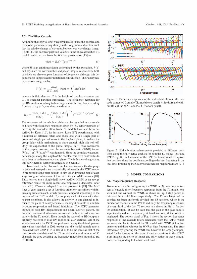
2015 IEEE Workshop on Applications of Signal Processing to Audio and Acoustics October 18-21, 2015, New Paltz, NY
2.2. The Filter Cascade
Assuming that only a long-wave propagates inside the cochlea andthe model parameters vary slowly in the longitudinal direction suchthat the relative change of wavenumber over one wavelength is neg-ligible [1], the cochlear partition velocity in the above described TLmodel can be derived from the WKB approximation [15] as,
v(x) = Bk3/2(x)e−iΦ(x) (1)
where B is an amplitude factor determined by the excitation. k(x)and Φ(x) are the wavenumber and phase integral respectively, bothof which are also complex functions of frequency, although this de-pendence is suppressed for notational convenience. Their analyticalexpressions are given by,
k2(x) =−2iωρHZcp(x)
,Φ(x) =
∫ x
0
k(x′) dx′ (2)
where ρ is fluid density, H is the height of cochlear chamber andZcp is cochlear partition impedance. The frequency response forthe BM motion of a longitudinal segment of the cochlea, extendingfrom x0 to x0 +Δ, can thus be written as,
HΔ =v(x0 +Δ)
v(x0)=
(k(x0 +Δ)
k(x0)
)3/2
e−i
∫ x0+Δx0
k(x′) dx′(3)
The responses of the whole cochlea can be regarded as a cascadeof filters with frequency responses given by (3). Other methods ofderiving the cascaded filters from TL models have also been de-scribed by Kates [16], for instance. Lyon [17] experimented witha number of different filters and chose one with a single pair ofpoles and single pair of zeros in the Laplace plane, to reduce thegroup delay while maintaining a sharp enough high-side roll-off.Only the exponential of the phase integral in (3) was consideredin that paper, however, and the wavenumber ratio (WNR) factor,(k(x0+Δ)/k(x0))
3/2, was ignored. Since the complex wavenum-ber changes along the length of the cochlea, this term contributes tovariations in both magnitude and phase. The influence of neglectingthis WNR term is further investigated in Section 3.
To account for the observed cochlear nonlinearity, the dampingsof pole and zero pairs are dynamically adjusted in the PZFC modelin proportion to the filter outputs to turn up or down the gain of eachstage using a combination of level detector and AGC network [18].Early version use a simple half-wave-rectifier (HWR) as an energyestimator, while the more recent one employed a dedicated innerhair cell (IHC) model adapted from that proposed in [19]. The AGCfilter of each stage is a set of four first-order low-pass filters with in-creasing time constant, which provides temporal smoothing to theoutputs of the IHC model. By coupling each of them with theirnearest neighbors, it also allows the activity in one channel to in-fluence the gains of nearby channels, making it possible to simulatetwo-tone suppression and lateral inhibition. The PZFC generatesoutputs of both BM displacement and neural activity pattern, butonly the mechanical vibrations are considered here in order to com-pare with the TL model. Even though the scale of its BM output isarbitrary, we refer to it as BM motion in later sections. All of thesimulations with the PZFC are performed using the default param-eter values specified in [20], except that the model sample rate isincreased from 22.05 kHz to 100 kHz, to be the same as that of thetime domain simulation of the TL model and a total number of 85channels are used covering the frequency range from around 20 Hzto 20 kHz.
Figure 1: Frequency responses of the individual filters in the cas-cade computed from the TL model (top panel) with (thin) and with-out (thick) the WNR and PZFC (bottom panel).
Figure 2: BM vibration enhancement provided at different posi-tions along the fully active cochlea for both the TL model (left) andPZFC (right). Each channel of the PZFC is transformed to equiva-lent position along the cochlea according to its best frequency in thelow-level limit using the Greenwood cochlear map for humans [21].
3. MODEL COMPARISONS
3.1. Stage Frequency Response
To examine the effect of ignoring the WNR in (3), we compute twosets of cascade filter frequency responses from the TL model, onewith and one without the WNR, as shown in Fig. 1 (top panel) asthin and thick solid lines respectively. The 35 mm length of thecochlea has been uniformly divided into 85 sections, which is thenumber of channels in the PZFC and only the frequency responsesof every third of the first 76 sections are shown in Fig. 1 for bet-ter visualization. It can be seen that the gain in the pass-band issignificantly reduced, especially at basal sections, if the WNR isneglected. The bottom panel of Fig. 1 shows the section frequencyresponses of the cascade filters calculated from the PZFC, whichare more similar to those of the TL model with WNR at low fre-quencies and those without the WNR at high frequencies. The errorintroduced by ignoring the WNR can, however, be largely compen-sated for by turning up the gain of various sections in the PZFC.Both models are set to be linear and fully active in these simula-tions, corresponding to the low-level limit.

2015 IEEE Workshop on Applications of Signal Processing to Audio and Acoustics October 18-21, 2015, New Paltz, NY
Although the peak gain of each section is very similar betweenthe two models, the decrease towards unity in the low frequencyside of each stage frequency response is more gradual in the PZFCthan in the TL model. The area of overlap in the passband region be-tween different channels is therefore larger in the PZFC. This causesthe cumulative gain at each section of the PZFC to be higher thanthat at the corresponding place along the BM of the TL model, ex-cept at the first a few stages, as shown in Fig. 2. The BM vibra-tion enhancement along the cochlea is computed at each position asthe difference in dB in the peak magnitude responses between thefully active and fully passive models. Each channel of the PZFCis converted to the equivalent position along the BM according toits best frequency in the low-level limit using the Greenwood mapfor humans [21]. Both models are in reasonable agreement with ex-perimental observations [22], in that the active gain is greater at thebase than at the apex. But the active gain decrease in the TL modelis more rapid and the PZFC probably takes a too long section of theBM to fully build up the maximum gain, due to lower amplificationprovided by initial sections of the filter cascade.
3.2. Single Tone Stimulation
Fig. 3 shows the comparison of model responses to 2 kHz pure tonewith levels ranging from 0 to 100 dB in steps of 10 dB. All stimulihad a duration of one second, with a 10 ms half-Hanning windowonset ramp and the maximum amplitude of each section of eachmodel during the whole length of the simulation time was takenfor evaluation. Panels (a) and (b) show the simulated BM vibra-tion patterns along the length of the cochlea in the TL model andPZFC, respectively. Both response patterns become broader andtheir maxima move basally as the stimulus level increases, showingqualitative agreement with measured longitudinal BM-velocity pat-terns in [23]. But the characteristic place (CP) for 2 kHz pure toneis different in the two models and the basal shift of response peak inthe TL model appears at higher stimulus SPL (70 dB) than that (30dB) in the PZFC.
Fig. 3 (c) and (d) show the derived BM input/output (I/O) levelcurves at the 2 kHz CP. In the TL model, the active mechanism of-fers an active gain of about 25 dB up to around 30 dB input SPL,and then compresses the response with a slope of 0.5 dB/dB until aninput SPL of about 80 dB, after which the model behaves linearlyagain. The PZFC, however, provides an active gain of almost 50 dBat low stimulus level, and the compression starts to take effect at 10dB SPL and does not finish until about 100 dB SPL, again with agrowth rate of about 0.5 dB/dB inbetween. Both models show al-most linear I/O functions at locations with characteristic frequencies(CFs) one octave above and below 2 kHz, i.e. about 4.5 mm to theleft or right of the CP in Fig. 3 (a) and (b). Measurements of mam-malian cochleae from different studies and across various speciesshow a high degree of variation in terms of compression range andrate. Some experiment [24] measured compressive behavior at aslow as 0 dB input SPL in the chinchilla, while others [25, 26] didnot observe it until 50 dB SPL in the guinea pig. The BM responsegrowth rate in the compressive region also varies from about 0.2 to0.5 dB/dB [22]. Thus, although the level curves of two models aredifferent, both of them are consistent with the range of experimentaldata.
3.3. Two-tone Suppression
Two-tone suppression on the level of the mechanical vibration of theBM has been demonstrated in a number of studies [27–31], but the
Figure 3: Comparison of model responses to 2 kHz pure tone withlevels ranging from 0 dB to 100 dB SPL in steps of 10 dB. (a) Max-imum BM velocity amplitudes of the TL model; (b) Maximum BMmotion amplitudes of the PZFC. Derived input/output functions ofBM vibrations at the 2 kHz CP and positions with CFs one octaveabove and below 2 kHz of the TL model (c) and PZFC (d).
measurements are not always consistent with each other. Ruggero etal [27] measured suppression to the overall velocity response of theBM with both high-side and low-side suppressors, while later ex-periments [29–31] only observed reductions in the probe frequencycomponent. In this paper, we adopt the later definition which is alsoused in [29–31], defining the two-tone suppression as a reductionin the magnitude of the spectral component at the probe frequencyduring the presentation of a suppressor tone.
Fig. 4 shows the summary of model comparisons in two-tonesuppression simulations. The stimulus also had a length of one sec-ond, but only the last 0.5 second of model outputs were used forFourier analysis to reduce the transient effects. Panels (a) and (b)show the input/output level curves for a 2 kHz probe tone in the ab-sence and presence of a 2.4 kHz suppressor tone at 5 different SPLsof the TL and PZFC models respectively. Both of them displayreduced low-level linear and mid-range compressive regions of theprobe tone growth curve as the intensity of the suppressor tone is in-creased. In contrast, for high probe tone levels, the level curves arealmost linear and hardly affected by the suppressor. These resultsare in good qualitative agreement with those measured experimen-tally and shown in Fig. 2A of [30].
The level dependence of suppression to a 2 kHz probe tone,fixed at 45 dB SPL, on different suppressor frequencies in bothmodels is then investigated and a small subset of results is displayedin panels (c) and (d) of Fig. 4. The degree of suppression was quan-tified as the ratio of the magnitude responses at the probe frequencyin the presence and absence of the suppressor. Both models arecapable of reproducing the general trend that low-side suppressorsproduce higher growth rates of suppression than high-side suppres-sors [29, 30], but the PZFC generates greater suppression at almost

2015 IEEE Workshop on Applications of Signal Processing to Audio and Acoustics October 18-21, 2015, New Paltz, NY
Figure 4: Comparison of model responses in two-tone suppressionsimulation. Input/output functions for a probe tone (F1=2 kHz) inthe absence and presence of a suppressor tone (F2=2.4 kHz) at 5different sound pressure levels of the TL model (a) and PZFC (b).Level dependence of two-tone suppression to a 2 kHz probe tone, at45 dB SPL, on suppressor tone frequency in the TL model (c) andPZFC (d). Dependence of two-tone suppression growth rate (e) andthreshold (f) on suppressor frequency in both models.
all levels of each suppressor and the suppression effect appears init at lower suppressor level. In addition, in the TL model, the influ-ence of high-side suppressors drops off considerably quicker withincreasing separation of two tone frequencies, similar to Fig. 5Aof [29], but the extent of suppression tends to reach a limit after acertain suppressor level. The PZFC continues to suppress the probetone even at the highest suppressor level, closer to the real measure-ments [29, 30], which show no sign of suppression saturation. Dif-ferences in low- and high-side suppression have also been observedin another filter cascade cochlear model by Kates [32].
To quantify these differences between the two models, Fig. 4 (e)and (f) show the dependence of two-tone suppression growth ratesand thresholds on suppressor frequency, computed from the com-plete simulation data set. Following the practice adopted in [29],suppression threshold is taken as the suppressor SPL which pro-duces 10 % suppression of the probe tone component and suppres-sion growth rate is determined as the steepest slope of the suppres-sion growth curves shown in Fig. 4 (c) and (d) above the suppression
threshold. Suppressors with thresholds higher than 100 dB SPL(e.g. F2 = 3.5 kHz in Fig. 4 (c)) are excluded from this analy-sis. The frequency of the probe tone is indicated by a dashed linein both panels. In the TL model, below-CF suppressors cause anaverage of ~0.85 dB of suppression for every dB increase in SPLand the above-CF suppressors cause a suppression growth rate of~0.41 dB/dB. In the PZFC, the average suppression growth ratesinduced by low- and high-side suppressors are ~0.95 dB/dB and~0.23 dB/dB, respectively. Both models are reasonably close toexperimentally measured growth rate values, which are ~1 dB/dBfor low-side and ~0.5 dB/dB for high-side suppressors [30], exceptthat high-side suppression growth rate in the PZFC is too low. Thisis because the PZFC allows a significant wider range of above-CFsuppressors to reduce the probe tone, the suppression growth ratesof which are rather low as shown in Fig. 4 (e). Such difference canalso be observed in Fig. 4 (f), which shows that suppressors withfrequencies higher than about 3300 Hz cease to affect the probetone in the TL model (i.e. suppression threshold higher than 100dB), while in the PZFC, two-tone suppression is still measurable forsuppressors with frequencies that are three times that of the probe.Furthermore, almost all of the suppression thresholds in the PZFCare smaller than those in the TL model, but the threshold patternis better predicted by the TL model in comparison to physiologicalmeasurements, e.g. Fig. 6 of [29], which displays roughly constantvalues around the probe tone frequency.
4. CONCLUSIONS
In this paper, we have firstly derived the frequency response of eachstage of the filter cascade from a linear TL model of the humancochlea. The error involved in ignoring the wavenumber ratio termin the original PZFC formulation can be largely compensated for byenhancing the amplification provided by each serial section, but theBM vibration enhancement at the basal sections is still smaller thanthat in the TL model.
The BM outputs of these two models in response to single-toneand two-tone stimuli have then been computed and compared withexperimental measurements on laboratory animals, although the lat-ter can be quite variable. Both models can account for the gen-eral features of these measurements, but differ in their response de-tails. The TL model produces a reasonably realistic representationof cochlear mechanics in most simulations, but is more computa-tionally intensive. The PZFC shares a similar performance in mod-eling self-suppression or dynamic-range-compression, but it over-predicts two-tone suppression due to high-side suppressor tones.Moreover, its two-tone suppression thresholds are too low and thethreshold pattern across frequency is not consistent with experimen-tal observations. But the major benefit of the PZFC is its com-putational efficiency and preliminary tests show that it is about 40times faster than the TL model when running in the time domain.It would be possible to further adjust the parameters and structureof the PZFC, especially the AGC network, based on either phys-iological data from animals or psychoacoustical experiments withhuman subjects [2, 7], to allow better representation of these non-linear phenomena that are important in peripheral auditory signalencoding and masking effects and hence enhance its suitability foreither modeling cochlear mechanics or auditory based processingof acoustic signals.

2015 IEEE Workshop on Applications of Signal Processing to Audio and Acoustics October 18-21, 2015, New Paltz, NY
5. REFERENCES
[1] E. De Boer, “Mechanics of the cochlea: modeling efforts,” inThe cochlea. Springer, 1996, pp. 258–317.
[2] R. F. Lyon, “Cascades of two-pole–two-zero asymmetric res-onators are good models of peripheral auditory function,” TheJournal of the Acoustical Society of America, vol. 130, no. 6,pp. 3893–3904, 2011.
[3] R. F. Lyon, M. Rehn, S. Bengio, T. C. Walters, andG. Chechik, “Sound retrieval and ranking using sparse audi-tory representations,” Neural computation, vol. 22, no. 9, pp.2390–2416, 2010.
[4] T. C. Walters, D. A. Ross, and R. F. Lyon, “The intervalgram:An audio feature for large-scale cover-song recognition,” inFrom Sounds to Music and Emotions. Springer, 2013, pp.197–213.
[5] M. Cheatham and P. Dallos, “Two-tone suppression in innerhair cell responses,” Hearing research, vol. 40, no. 3, pp. 187–196, 1989.
[6] B. Delgutte, “Two-tone rate suppression in auditory-nervefibers: Dependence on suppressor frequency and level,” Hear-ing research, vol. 49, no. 1, pp. 225–246, 1990.
[7] H. Duifhuis, “Level effects in psychophysical two-tone sup-pression,” The Journal of the Acoustical Society of America,vol. 67, no. 3, pp. 914–927, 1980.
[8] L. J. Kanis and E. de Boer, “Self-suppression in a locally ac-tive nonlinear model of the cochlea: A quasilinear approach,”The Journal of the Acoustical Society of America, vol. 94,no. 6, pp. 3199–3206, 1993.
[9] J. A. Young, S. J. Elliott, and B. Lineton, “Investigatingthe wave-fixed and place-fixed origins of the 2f1-f2 distor-tion product otoacoustic emission within a micromechanicalcochlear model,” The Journal of the Acoustical Society ofAmerica, vol. 131, no. 6, pp. 4699–4709, 2012.
[10] S. J. Elliott, E. M. Ku, and B. Lineton, “A state space modelfor cochlear mechanics,” The Journal of the Acoustical Societyof America, vol. 122, no. 5, pp. 2759–2771, 2007.
[11] J. A. How, S. J. Elliott, and B. Lineton, “The influence onpredicted harmonic and distortion product generation of theposition of the nonlinearity within cochlear micromechanicalmodels,” The Journal of the Acoustical Society of America,vol. 127, no. 2, pp. 652–655, 2010.
[12] M. Kringlebotn, “Network model for the human middle ear,”Scandinavian audiology, vol. 17, no. 2, pp. 75–85, 1988.
[13] E. M. Ku, “Modelling the human cochlea,” Ph.D. dissertation,University of Southampton, 2008.
[14] S. Pan, S. J. Elliott, P. D. Teal, and B. Lineton, “Efficient time-domain simulation of nonlinear, state-space, transmission-linemodels of the cochlea,” The Journal of the Acoustical Societyof America, vol. 137, no. 6, pp. 3559–3562, 2015.
[15] G. Zweig, R. Lipes, and J. Pierce, “The cochlear compro-mise,” The Journal of the Acoustical Society of America,vol. 59, no. 4, pp. 975–982, 1976.
[16] J. M. Kates, “Accurate tuning curves in a cochlear model,”Speech and Audio Processing, IEEE Transactions on, vol. 1,no. 4, pp. 453–462, 1993.
[17] R. F. Lyon, “Filter cascades as analogs of the cochlea,” in Neu-romorphic systems engineering. Springer, 1998, pp. 3–18.
[18] R. F. Lyon et al., “Using a cascade of asymmetric resonatorswith fast-acting compression as a cochlear model for machine-hearing applications,” in Autumn Meeting of the AcousticalSociety of Japan, 2011, pp. 509–512.
[19] J. Allen, “A hair cell model of neural response,” in Mechanicsof Hearing. Springer, 1983, pp. 193–202.
[20] “Cascade of asymmetric resonators with fast-acting compres-sion cochlear model,” https://github.com/google/carfac, lastaccessed: April, 2015.
[21] D. D. Greenwood, “A cochlear frequency-position functionfor several species29 years later,” The Journal of the Acous-tical Society of America, vol. 87, no. 6, pp. 2592–2605, 1990.
[22] L. Robles and M. A. Ruggero, “Mechanics of the mammaliancochlea,” Physiological reviews, vol. 81, no. 3, pp. 1305–1352, 2001.
[23] T. Ren, “Longitudinal pattern of basilar membrane vibra-tion in the sensitive cochlea,” Proceedings of the NationalAcademy of Sciences, vol. 99, no. 26, pp. 17 101–17 106,2002.
[24] W. S. Rhode and A. Recio, “Study of mechanical motions inthe basal region of the chinchilla cochlea,” The Journal of theAcoustical Society of America, vol. 107, no. 6, pp. 3317–3332,2000.
[25] E. Murugasu and I. J. Russell, “The effect of efferent stimu-lation on basilar membrane displacement in the basal turn ofthe guinea pig cochlea,” The Journal of neuroscience, vol. 16,no. 1, pp. 325–332, 1996.
[26] E. Murugasu and I. Russell, “Salicylate ototoxicity: the ef-fects on basilar membrane displacement, cochlear microphon-ics, and neural responses in the basal turn of the guinea pigcochlea,” Aud. Neurosci, vol. 1, pp. 139–150, 1995.
[27] M. A. Ruggero, L. Robles, and N. C. Rich, “Two-tone sup-pression in the basilar membrane of the cochlea: Mechanicalbasis of auditory-nerve rate suppression,” Journal of neuro-physiology, vol. 68, no. 4, pp. 1087–1099, 1992.
[28] A. Nuttall and D. Dolan, “Two-tone suppression of inner haircell and basilar membrane responses in the guinea pig,” TheJournal of the Acoustical Society of America, vol. 93, no. 1,pp. 390–400, 1993.
[29] N. Cooper and W. Rhode, “Two-tone suppression in apicalcochlear mechanics,” Auditory Neuroscience, vol. 3, no. 2, pp.123–134, 1996.
[30] N. P. Cooper, “Two-tone suppression in cochlear mechanics,”The Journal of the Acoustical Society of America, vol. 99,no. 5, pp. 3087–3098, 1996.
[31] C. D. Geisler and A. L. Nuttall, “Two-tone suppressionof basilar membrane vibrations in the base of the guineapig cochlea using low-side suppressors,” The Journal of theAcoustical Society of America, vol. 102, no. 1, pp. 430–440,1997.
[32] J. M. Kates, “Two-tone suppression in a cochlear model,”Speech and Audio Processing, IEEE Transactions on, vol. 3,no. 5, pp. 396–406, 1995.

References
[1] Stephen J. Elliott, Emery M. Ku, and Ben Lineton. “A state space model for
cochlear mechanics”. In: The Journal of the Acoustical Society of America
122.5 (2007), pp. 2759–2771.
[2] DeLiang Wang and Guy J. Brown. Computational auditory scene analysis:
Principles, algorithms, and applications. Wiley-IEEE press, 2006.
[3] Amin Saremi et al. “A comparative study of seven human cochlear filter
models”. In: The Journal of the Acoustical Society of America 140.3 (2016),
pp. 1618–1634.
[4] Richard M. Stern. “Applying physiologically-motivated models of auditory
processing to automatic speech recognition”. In: International Symposium
on Auditory and Audiological Research. 2011.
[5] Yuxuan Wang. Supervised speech separation using deep neural networks.
The Ohio State University, 2015.
[6] Xiao-Lei Zhang and DeLiang Wang. “Boosting contextual information for
deep neural network based voice activity detection”. In: IEEE/ACM Trans-
actions on Audio, Speech, and Language Processing 24.2 (2016), pp. 252–
264.
[7] Manfred R. Schroeder, Bishnu S. Atal, and J. L. Hall. “Optimizing digital
speech coders by exploiting masking properties of the human ear”. In: The
Journal of the Acoustical Society of America 66.6 (1979), pp. 1647–1652.
[8] M. Schroeder and B. S. Atal. “Code-excited linear prediction (CELP): High-
quality speech at very low bit rates”. In: IEEE International Conference on
Acoustics, Speech, and Signal Processing. Vol. 10. IEEE, 1985, pp. 937–940.
[9] Stephen T. Neely and D. O. Kim. “A model for active elements in cochlear
biomechanics”. In: The Journal of the Acoustical Society of America 79.5
(1986), pp. 1472–1480.
[10] Emery M. Ku. “Modelling the human cochlea”. PhD thesis. University of
Southampton, 2008.
169

170 REFERENCES
[11] Jacqueline Ann Young. “Modelling the cochlear origins of distortion prod-
uct otoacoustic emissions”. PhD thesis. University of Southampton, 2011.
[12] Richard F. Lyon. Human and Machine Hearing: Extracting Meaning from
Sound. Cambridge University Press, 2017.
[13] Nathalie Virag. “Single channel speech enhancement based on masking
properties of the human auditory system”. In: IEEE Transactions on Speech
and Audio Processing 7.2 (1999), pp. 126–137.
[14] Stanley S. Stevens and John Volkmann. “The relation of pitch to frequency:
A revised scale”. In: The American Journal of Psychology 53.3 (1940),
pp. 329–353.
[15] Hynek Hermansky. “Perceptual linear predictive (PLP) analysis of speech”.
In: the Journal of the Acoustical Society of America 87.4 (1990), pp. 1738–
1752.
[16] R. D. Patterson et al. “An efficient auditory filterbank based on the gam-
matone function”. In: a meeting of the IOC Speech Group on Auditory
Modelling at RSRE. Vol. 2. 7. 1987.
[17] Yann LeCun, Yoshua Bengio, and Geoffrey Hinton. “Deep learning”. In:
Nature 521.7553 (2015), pp. 436–444.
[18] Ian Goodfellow, Yoshua Bengio, and Aaron Courville. Deep Learning. http:
//www.deeplearningbook.org. MIT Press, 2016.
[19] CS231n: Convolutional Neural Networks for Visual Recognition. url:
http://cs231n.stanford.edu/.
[20] Dong Yu and Li Deng. Automatic speech recognition: A deep learning ap-
proach. Springer, 2014.
[21] Stanley A. Gelfand. Hearing: An introduction to psychological and physio-
logical acoustics. CRC Press, 2016.
[22] Anatomy of the Human Ear. Nov. 2017. url: https : / / commons .
wikimedia.org/wiki/File:Anatomy_of_the_Human_Ear_en.svg.
[23] E. M. Relkin. “Introduction to the analysis of middle-ear function”. In:
Physiology of the Ear (AF Jahn and J. Santos-Sacchi, eds.). Raven Press,
New York (1988), pp. 103–123.
[24] Jerome Pascal et al. “Linear and nonlinear model of the human middle
ear”. In: The Journal of the Acoustical Society of America 104.3 (1998),
pp. 1509–1516.
[25] Peter Dallos and Richard R. Fay. The cochlea. Vol. 8. Springer-Verlag New
York, 1996.

REFERENCES 171
[26] A. Wright et al. “Hair cell distributions in the normal human cochlea.” In:
Acta oto-laryngologica. Supplementum 444 (1987), pp. 1–48.
[27] Hans Engstrom and Jan Wersall. “Structure and innervation of the inner ear
sensory epithelia”. In: International Review of Cytology 7 (1958), pp. 535–
585.
[28] Eric R. Kandel et al. Principles of neural science. Vol. 4. McGraw-hill New
York, 2000.
[29] Tempel lab, Courses, Lectures and Handouts. Nov. 2017. url: https://
depts.washington.edu/tempelab/index.html.
[30] William E. Brownell et al. “Evoked mechanical responses of isolated
cochlear outer hair cells”. In: Science 227 (1985), pp. 194–197.
[31] Donald D. Greenwood. “A cochlear frequency-position function for sev-
eral species—29 years later”. In: The Journal of the Acoustical Society of
America 87.6 (1990), pp. 2592–2605.
[32] Cochlea anatomy. Nov. 2017. url: https : / / www . britannica . com /
science/cochlea.
[33] Luis Robles and Mario A. Ruggero. “Mechanics of the mammalian cochlea”.
In: Physiological Reviews 81.3 (2001), pp. 1305–1352.
[34] J. Ashmore et al. “The remarkable cochlear amplifier”. In: Hearing Research
266.1 (2010), pp. 1–17.
[35] Luc J. Kanis and Egbert de Boer. “Self-suppression in a locally active
nonlinear model of the cochlea: A quasilinear approach”. In: The Journal
of the Acoustical Society of America 94.6 (1993), pp. 3199–3206.
[36] Sid P. Bacon, Richard R. Fay, and Arthur N. Popper. Compression: from
cochlea to cochlear implants. Springer, 2004.
[37] B. M. Johnstone, R. Patuzzi, and G. K. Yates. “Basilar membrane measure-
ments and the travelling wave”. In: Hearing Research 22.1 (1986), pp. 147–
153.
[38] Mario A. Ruggero et al. “Basilar-membrane responses to tones at the base of
the chinchilla cochlea”. In: The Journal of the Acoustical Society of America
101.4 (1997), pp. 2151–2163.
[39] Bertrand Delgutte. “Two-tone rate suppression in auditory-nerve fibers:
Dependence on suppressor frequency and level”. In: Hearing Research 49.1
(1990), pp. 225–246.

172 REFERENCES
[40] Mario A. Ruggero, Luis Robles, and Nola C. Rich. “Two-tone suppression
in the basilar membrane of the cochlea: Mechanical basis of auditory-nerve
rate suppression”. In: Journal of Neurophysiology 68.4 (1992), pp. 1087–
1099.
[41] N. P. Cooper and W. S. Rhode. “Two-tone suppression in apical cochlear
mechanics”. In: Auditory Neuroscience 3.2 (1996), pp. 123–134.
[42] C. Daniel Geisler and Alfred L. Nuttall. “Two-tone suppression of basilar
membrane vibrations in the base of the guinea pig cochlea using “low-side”
suppressors”. In: The Journal of the Acoustical Society of America 102.1
(1997), pp. 430–440.
[43] A. L. Nuttall and D. F. Dolan. “Two-tone suppression of inner hair cell
and basilar membrane responses in the guinea pig”. In: The Journal of the
Acoustical Society of America 93.1 (1993), pp. 390–400.
[44] Hendrikus Duifhuis. “Level effects in psychophysical two-tone suppression”.
In: The Journal of the Acoustical Society of America 67.3 (1980), pp. 914–
927.
[45] William S. Rhode. “Mutual suppression in the 6kHz region of sensitive
chinchilla cochleae”. In: The Journal of the Acoustical Society of America
121.5 (2007), pp. 2805–2818.
[46] Mohamed Farouk Abdel Hady and Friedhelm Schwenker. “Semi-supervised
learning”. In: Handbook on Neural Information Processing. Springer, 2013,
pp. 215–239.
[47] Sinno Jialin Pan and Qiang Yang. “A survey on transfer learning”. In: IEEE
Transactions on Knowledge and Data Engineering 22.10 (2010), pp. 1345–
1359.
[48] Dimitri P. Bertsekas and John N. Tsitsiklis. “Neuro-dynamic programming:
an overview”. In: IEEE Conference on Decision and Control. Vol. 1. IEEE.
1995, pp. 560–564.
[49] Christopher M. Bishop. Pattern recognition and machine learning. Springer,
2006.
[50] Sepp Hochreiter et al. Gradient flow in recurrent nets: the difficulty of
learning long-term dependencies. 2001.
[51] Xavier Glorot, Antoine Bordes, and Yoshua Bengio. “Deep sparse rectifier
neural networks”. In: Proceedings of the Fourteenth International Confer-
ence on Artificial Intelligence and Statistics. 2011, pp. 315–323.

REFERENCES 173
[52] Alex Krizhevsky, Ilya Sutskever, and Geoffrey E. Hinton. “Imagenet classi-
fication with deep convolutional neural networks”. In: Advances in Neural
Information Processing Systems. 2012, pp. 1097–1105.
[53] Kaiming He et al. “Delving deep into rectifiers: Surpassing human-level
performance on imagenet classification”. In: Proceedings of the IEEE In-
ternational Conference on Computer Vision. 2015, pp. 1026–1034.
[54] Ossama Abdel-Hamid et al. “Convolutional neural networks for speech
recognition”. In: IEEE/ACM Transactions on Audio, Speech, and Language
Processing 22.10 (2014), pp. 1533–1545.
[55] David E. Rumelhart, Geoffrey E. Hinton, Ronald J. Williams, et al. “Learn-
ing representations by back-propagating errors”. In: Cognitive modeling 5.3
(1988), p. 1.
[56] Michael A. Nielsen. Neural networks and deep learning. http : / /
neuralnetworksanddeeplearning . com / chap2 . html. Determination
Press, 2015.
[57] Boris T. Polyak. “Some methods of speeding up the convergence of iter-
ation methods”. In: USSR Computational Mathematics and Mathematical
Physics 4.5 (1964), pp. 1–17.
[58] John Duchi, Elad Hazan, and Yoram Singer. “Adaptive subgradient meth-
ods for online learning and stochastic optimization”. In: Journal of Machine
Learning Research 12.Jul (2011), pp. 2121–2159.
[59] Geoffrey Hinton. Neural Networks for Machine Learning. Coursera, video
lectures. Nov. 2017. url: https://www.coursera.org/learn/neural-
networks.
[60] Matthew D. Zeiler. “ADADELTA: an adaptive learning rate method”. In:
arXiv preprint arXiv:1212.5701 (2012).
[61] Diederik Kingma and Jimmy Ba. “Adam: A method for stochastic opti-
mization”. In: arXiv preprint arXiv:1412.6980 (2014).
[62] Geoffrey E. Hinton, Simon Osindero, and Yee-Whye Teh. “A fast learn-
ing algorithm for deep belief nets”. In: Neural Computation 18.7 (2006),
pp. 1527–1554.
[63] Nitish Srivastava et al. “Dropout: a simple way to prevent neural networks
from overfitting.” In: Journal of Machine Learning Research 15.1 (2014),
pp. 1929–1958.

174 REFERENCES
[64] Sripriya Ramamoorthy, Niranjan V. Deo, and Karl Grosh. “A mechano-
electro-acoustical model for the cochlea: response to acoustic stimuli”. In:
The Journal of the Acoustical Society of America 121.5 (2007), pp. 2758–
2773.
[65] Renata Sisto et al. “Different models of the active cochlea, and how to im-
plement them in the state-space formalism”. In: The Journal of the Acous-
tical Society of America 128.3 (2010), pp. 1191–1202.
[66] Julien Meaud and Karl Grosh. “Response to a pure tone in a nonlinear
mechanical-electrical-acoustical model of the cochlea”. In: Biophysical Jour-
nal 102.6 (2012), pp. 1237–1246.
[67] Julius L. Goldstein. “Modeling rapid waveform compression on the basi-
lar membrane as multiple-bandpass-nonlinearity filtering”. In: Hearing re-
search 49.1 (1990), pp. 39–60.
[68] Enrique A Lopez-Poveda and Ray Meddis. “A human nonlinear cochlear
filterbank”. In: The Journal of the Acoustical Society of America 110.6
(2001), pp. 3107–3118.
[69] Xuedong Zhang et al. “A phenomenological model for the responses of
auditory-nerve fibers: I. Nonlinear tuning with compression and suppres-
sion”. In: The Journal of the Acoustical Society of America 109.2 (2001),
pp. 648–670.
[70] Luc-J. Kanis and Egbert De Boer. “Two-tone suppression in a locally active
nonlinear model of the cochlea”. In: The Journal of the Acoustical Society
of America 96.4 (1994), pp. 2156–2165.
[71] Julius L. Goldstein. “Relations among compression, suppression, and com-
bination tones in mechanical responses of the basilar membrane: data and
MBPNL model”. In: Hearing Research 89.1 (1995), pp. 52–68.
[72] R. Stoop and A. Kern. “Two-tone suppression and combination tone gener-
ation as computations performed by the Hopf cochlea”. In: Physical Review
Letters 93.26 (2004), p. 268103.
[73] James M. Kates. “Two-tone suppression in a cochlear model”. In: IEEE
Transactions on Speech and Audio Processing 3.5 (1995), pp. 396–406.
[74] Guangjian Ni et al. “Modelling cochlear mechanics”. In: BioMed research
international 2014 (2014).
[75] Hendrikus Duifhuis. “Comment on “An approximate transfer function for
the dual-resonance nonlinear filter model of auditory frequency selectiv-
ity”[J. Acoust. Soc. Am. 114, 2112–2117](L)”. In: The Journal of the Acous-
tical Society of America 115.5 (2004), pp. 1889–1890.

REFERENCES 175
[76] Robert Duncan Luce, Robert R. Bush, and Galanter Ed Eugene. “Hand-
book of Mathematical Psychology.” In: (1963).
[77] Egbert De Boer. “Mechanics of the cochlea: modeling efforts”. In: The
cochlea. Springer, 1996, pp. 258–317.
[78] Toshio Irino and Roy D. Patterson. “A time-domain, level-dependent au-
ditory filter: The gammachirp”. In: The Journal of the Acoustical Society
of America 101.1 (1997), pp. 412–419.
[79] Richard F. Lyon. “Filter cascades as analogs of the cochlea”. In: Neuro-
morphic systems engineering. Springer, 1998, pp. 3–18.
[80] Richard F. Lyon. “Cascades of two-pole–two-zero asymmetric resonators
are good models of peripheral auditory function”. In: The Journal of the
Acoustical Society of America 130.6 (2011), pp. 3893–3904.
[81] Richard F. Lyon et al. “Using a Cascade of Asymmetric Resonators with
Fast-Acting Compression as a Cochlear Model for Machine-Hearing Ap-
plications”. In: Autumn Meeting of the Acoustical Society of Japan. 2011,
pp. 509–512.
[82] Christopher A. Shera and John J. Guinan Jr. “Evoked otoacoustic emis-
sions arise by two fundamentally different mechanisms: a taxonomy for
mammalian OAEs”. In: The Journal of the Acoustical Society of America
105.2 (1999), pp. 782–798.
[83] Emery M. Ku, Stephen J. Elliott, and Ben Lineton. “Limit cycle oscillations
in a nonlinear state space model of the human cochlea”. In: The Journal
of the Acoustical Society of America 126.2 (2009), pp. 739–750.
[84] Egbert De Boer and Alfred L. Nuttall. “The mechanical waveform of the
basilar membrane. I. Frequency modulations (“glides”) in impulse responses
and cross-correlation functions”. In: The Journal of the Acoustical Society
of America 101.6 (1997), pp. 3583–3592.
[85] Richard F. Lyon et al. “Sound retrieval and ranking using sparse auditory
representations”. In: Neural Computation 22.9 (2010), pp. 2390–2416.
[86] Thomas C. Walters, David A. Ross, and Richard F. Lyon. “The Interval-
gram: An Audio Feature for Large-Scale Cover-Song Recognition”. In: From
Sounds to Music and Emotions. Springer, 2013, pp. 197–213.
[87] Jacqueline A. Young, Stephen J. Elliott, and Ben Lineton. “Investigating
the wave-fixed and place-fixed origins of the 2f1-f2 distortion product otoa-
coustic emission within a micromechanical cochlear model”. In: The Journal
of the Acoustical Society of America 131.6 (2012), pp. 4699–4709.

176 REFERENCES
[88] Stephen J. Elliott and Christopher A. Shera. “The cochlea as a smart struc-
ture”. In: Smart Materials and Structures 21.6 (2012), p. 064001.
[89] Emery M. Ku, Stephen J. Elliott, and Ben Lineton. “Statistics of instabil-
ities in a state space model of the human cochlea”. In: The Journal of the
Acoustical Society of America 124.2 (2008), pp. 1068–1079.
[90] Jacqueline A. How, Stephen J. Elliott, and Ben Lineton. “The influence on
predicted harmonic and distortion product generation of the position of the
nonlinearity within cochlear micromechanical models”. In: The Journal of
the Acoustical Society of America 127.2 (2010), pp. 652–655.
[91] Peter Dallos. “Overview: cochlear neurobiology”. In: The cochlea. Springer,
1996, pp. 1–43.
[92] Corne J. Kros. “Physiology of mammalian cochlear hair cells”. In: The
cochlea. Springer, 1996, pp. 318–385.
[93] Stuart L. Johnson et al. “Prestin-driven cochlear amplification is not limited
by the outer hair cell membrane time constant”. In: Neuron 70.6 (2011),
pp. 1143–1154.
[94] M. Kringlebotn. “Network model for the human middle ear”. In: Scandi-
navian Audiology 17.2 (1988), pp. 75–85.
[95] Shuokai Pan et al. “Efficient time-domain simulation of nonlinear, state-
space, transmission-line models of the cochlea”. In: The Journal of the
Acoustical Society of America 137.6 (2015), pp. 3559–3562.
[96] James M. Kates. “A time-domain digital cochlear model”. In: IEEE Trans-
actions on signal processing 39.12 (1991), pp. 2573–2592.
[97] M. Holmes and J. D. Cole. “Pseudo-resonance in the cochlea”. In: Mechan-
ics of Hearing. Springer, 1983, pp. 45–52.
[98] Cascade of asymmetric resonators with fast-acting compression cochlear
model. url: https://github.com/google/carfac.
[99] J. B. Allen. “A hair cell model of neural response”. In: Mechanics of Hear-
ing. Springer, 1983, pp. 193–202.
[100] G. von Bekesy. Sensory inhibition. Princeton University Press, 1967.
[101] George Zweig, R. Lipes, and J. R. Pierce. “The cochlear compromise”. In:
The Journal of the Acoustical Society of America 59.4 (1976), pp. 975–982.
[102] William S. Rhode and Alberto Recio. “Study of mechanical motions in the
basal region of the chinchilla cochlea”. In: The Journal of the Acoustical
Society of America 107.6 (2000), pp. 3317–3332.

REFERENCES 177
[103] Euan Murugasu and Ian J. Russell. “The effect of efferent stimulation on
basilar membrane displacement in the basal turn of the guinea pig cochlea”.
In: The Journal of neuroscience 16.1 (1996), pp. 325–332.
[104] E. Murugasu and I. J. Russell. “Salicylate ototoxicity: the effects on basilar
membrane displacement, cochlear microphonics, and neural responses in the
basal turn of the guinea pig cochlea”. In: Auditory Neuroscience 1 (1995),
pp. 139–150.
[105] Nigel P. Cooper. “Two-tone suppression in cochlear mechanics”. In: The
Journal of the Acoustical Society of America 99.5 (1996), pp. 3087–3098.
[106] William S. Rhode and Alberto Recio. “Multicomponent stimulus interac-
tions observed in basilar-membrane vibration in the basal region of the
chinchilla cochlea”. In: The Journal of the Acoustical Society of America
110.6 (2001), pp. 3140–3154.
[107] Corstiaen P. C. Versteegh and Marcel van der Heijden. “The spatial buildup
of compression and suppression in the mammalian cochlea”. In: Journal of
the Association for Research in Otolaryngology 14.4 (2013), pp. 523–545.
[108] Javier Ramirez, Juan Manuel Gorriz, and Jose Carlos Segura. “Voice ac-
tivity detection. fundamentals and speech recognition system robustness”.
In: Robust Speech Recognition and Understanding. InTech, 2007.
[109] Lawrence R. Rabiner and Marvin R. Sambur. “An algorithm for determin-
ing the endpoints of isolated utterances”. In: Bell Labs Technical Journal
54.2 (1975), pp. 297–315.
[110] Thomas Drugman et al. “Voice activity detection: merging source and
filter-based information”. In: IEEE Signal Processing Letters 23.2 (2016),
pp. 252–256.
[111] Thomas Drugman et al. “Glottal source processing: From analysis to ap-
plications”. In: Computer Speech & Language 28.5 (2014), pp. 1117–1138.
[112] Brian Kingsbury et al. “Robust speech recognition in noisy environments:
The 2001 IBM SPINE evaluation system”. In: Acoustics, Speech, and Sig-
nal Processing (ICASSP), 2002 IEEE International Conference on. Vol. 1.
IEEE. 2002, pp. I–53.
[113] Sumit Basu. “A linked-HMM model for robust voicing and speech de-
tection”. In: Acoustics, Speech, and Signal Processing, 2003. Proceed-
ings.(ICASSP’03). 2003 IEEE International Conference on. Vol. 1. IEEE.
2003, pp. I–I.
178 REFERENCES
[114] Sassan Ahmadi and Andreas S. Spanias. “Cepstrum-based pitch detection
using a new statistical V/UV classification algorithm”. In: IEEE Transac-
tions on speech and audio processing 7.3 (1999), pp. 333–338.
[115] Simon Graf et al. “Features for voice activity detection: a comparative
analysis”. In: EURASIP Journal on Advances in Signal Processing 2015.1
(2015), p. 91.
[116] Adil Benyassine et al. “ITU-T Recommendation G. 729 Annex B: a silence
compression scheme for use with G. 729 optimized for V. 70 digital simul-
taneous voice and data applications”. In: IEEE Communications Magazine
35.9 (1997), pp. 64–73.
[117] Steven Davis and Paul Mermelstein. “Comparison of parametric representa-
tions for monosyllabic word recognition in continuously spoken sentences”.
In: IEEE Transactions on Acoustics, Speech, and Signal Processing 28.4
(1980), pp. 357–366.
[118] Chanwoo Kim and Richard M. Stern. “Power-normalized cepstral coeffi-
cients (PNCC) for robust speech recognition”. In: IEEE/ACM Transactions
on Audio, Speech and Language Processing (TASLP) 24.7 (2016), pp. 1315–
1329.
[119] Jitong Chen, Yuxuan Wang, and DeLiang Wang. “A feature study for
classification-based speech separation at low signal-to-noise ratios”. In:
IEEE/ACM Transactions on Audio, Speech and Language Processing 22.12
(2014), pp. 1993–2002.
[120] Xiao-Lei Zhang and DeLiang Wang. “Boosted deep neural networks and
multi-resolution cochleagram features for voice activity detection”. In: Fif-
teenth Annual Conference of the International Speech Communication As-
sociation. 2014.
[121] Pham Chau Khoa. “Noise robust voice activity detection”. In: Master the-
sis, Nanyang Technological University 24 (2012).
[122] Javier Ramırez et al. “Efficient voice activity detection algorithms using
long-term speech information”. In: Speech Communication 42.3-4 (2004),
pp. 271–287.
[123] Georgios Evangelopoulos and Petros Maragos. “Speech event detection
using multiband modulation energy”. In: Ninth European Conference on
Speech Communication and Technology. 2005.

REFERENCES 179
[124] Yariv Ephraim and David Malah. “Speech enhancement using a minimum-
mean square error short-time spectral amplitude estimator”. In: IEEE
Transactions on Acoustics, Speech, and Signal Processing 32.6 (1984),
pp. 1109–1121.
[125] Rainer Martin. “Noise power spectral density estimation based on optimal
smoothing and minimum statistics”. In: IEEE Transactions on Speech and
Audio Processing 9.5 (2001), pp. 504–512.
[126] Israel Cohen. “Noise spectrum estimation in adverse environments: Im-
proved minima controlled recursive averaging”. In: IEEE Transactions on
Speech and Audio Processing 11.5 (2003), pp. 466–475.
[127] Richard C Hendriks, Richard Heusdens, and Jesper Jensen. “MMSE based
noise PSD tracking with low complexity”. In: IEEE International Confer-
ence on Acoustics Speech and Signal Processing. IEEE. 2010, pp. 4266–
4269.
[128] Timo Gerkmann and Richard C. Hendriks. “Unbiased MMSE-based noise
power estimation with low complexity and low tracking delay”. In: IEEE
Transactions on Audio, Speech, and Language Processing 20.4 (2012),
pp. 1383–1393.
[129] Rainer Martin. “Speech enhancement using MMSE short time spectral es-
timation with gamma distributed speech priors”. In: IEEE International
Conference on Acoustics, Speech, and Signal Processing. Vol. 1. IEEE. 2002,
pp. I–253.
[130] J. H. Chang, J. W. Shin, and N. S. Kim. “Voice activity detector employing
generalised Gaussian distribution”. In: Electronics Letters 40.24 (2004),
pp. 1561–1563.
[131] Joon-Hyuk Chang, Nam Soo Kim, and Sanjit K. Mitra. “Voice activity
detection based on multiple statistical models”. In: IEEE Transactions on
Signal Processing 54.6 (2006), pp. 1965–1976.
[132] R. Reininger and J. Gibson. “Distributions of the two-dimensional DCT
coefficients for images”. In: IEEE Transactions on Communications 31.6
(1983), pp. 835–839.
[133] Theodoros Petsatodis et al. “Convex combination of multiple statistical
models with application to VAD”. In: IEEE Transactions on Audio, Speech,
and Language Processing 19.8 (2011), pp. 2314–2327.
[134] Xiao-Lei Zhang and Ji Wu. “Deep belief networks based voice activity de-
tection”. In: IEEE Transactions on Audio, Speech, and Language Processing
21.4 (2013), pp. 697–710.

180 REFERENCES
[135] Speech Processing. “Speech processing, transmission and quality Aspects
(STQ); Distributed speech recognition; Advanced front-end feature extrac-
tion algorithm; Compression algorithms”. In: ETSI ES 202.050 (2002),
p. V1.
[136] Jongseo Sohn, Nam Soo Kim, and Wonyong Sung. “A statistical model-
based voice activity detection”. In: IEEE Signal Processing Letters 6.1
(1999), pp. 1–3.
[137] Javier Ramirez et al. “Statistical voice activity detection using a multiple
observation likelihood ratio test”. In: IEEE Signal Processing Letters 12.10
(2005), pp. 689–692.
[138] Javier Ramirez et al. “Improved voice activity detection using contextual
multiple hypothesis testing for robust speech recognition”. In: IEEE Trans-
actions on Audio, Speech, and Language Processing 15.8 (2007), pp. 2177–
2189.
[139] Ji Wu and Xiao-Lei Zhang. “Efficient multiple kernel support vector ma-
chine based voice activity detection”. In: IEEE Signal Processing Letters
18.8 (2011), pp. 466–469.
[140] Dongwen Ying et al. “Voice activity detection based on an unsupervised
learning framework”. In: IEEE Transactions on Audio, Speech, and Lan-
guage Processing 19.8 (2011), pp. 2624–2633.
[141] Jeff Ma. “Improving the speech activity detection for the DARPA RATS
phase-3 evaluation”. In: Fifteenth Annual Conference of the International
Speech Communication Association. 2014.
[142] Samuel Thomas et al. “Improvements to the IBM speech activity detection
system for the DARPA RATS program”. In: IEEE International Conference
on Acoustics, Speech and Signal Processing. IEEE. 2015, pp. 4500–4504.
[143] John S Garofolo et al. “DARPA TIMIT acoustic-phonetic continous speech
corpus CD-ROM. NIST speech disc 1-1.1”. In: NASA STI/Recon technical
report n 93 (1993).
[144] Andrew Varga and Herman J. M. Steeneken. “Assessment for automatic
speech recognition: II. NOISEX-92: A database and an experiment to study
the effect of additive noise on speech recognition systems”. In: Speech com-
munication 12.3 (1993), pp. 247–251.
[145] David B. Dean et al. “The QUT-NOISE-TIMIT corpus for the evaluation
of voice activity detection algorithms”. In: Proceedings of Interspeech 2010
(2010).

REFERENCES 181
[146] Philipos C Loizou. Speech enhancement: theory and practice. CRC press,
2013.
[147] Xavier Glorot and Yoshua Bengio. “Understanding the difficulty of training
deep feedforward neural networks”. In: Proceedings of the Thirteenth Inter-
national Conference on Artificial Intelligence and Statistics. 2010, pp. 249–
256.
[148] Francois Chollet et al. Keras. https://github.com/fchollet/keras.
2015.
[149] Theano Development Team. “Theano: A Python framework for fast com-
putation of mathematical expressions”. In: arXiv e-prints abs/1605.02688
(May 2016). url: http://arxiv.org/abs/1605.02688.
[150] Maarten Van Segbroeck, Andreas Tsiartas, and Shrikanth Narayanan. “A
robust frontend for VAD: exploiting contextual, discriminative and spectral
cues of human voice.” In: Interspeech. 2013, pp. 704–708.
[151] Yang Shao, Soundararajan Srinivasan, and DeLiang Wang. “Incorporat-
ing auditory feature uncertainties in robust speaker identification”. In:
IEEE International Conference on Acoustics, Speech and Signal Process-
ing. Vol. 4. IEEE. 2007, pp. IV–277.
[152] Bernd T. Meyer et al. “Comparing different flavors of spectro-temporal fea-
tures for ASR”. In: Twelfth Annual Conference of the International Speech
Communication Association. 2011.
[153] Svante Granqvist and Britta Hammarberg. “The correlogram: a visual dis-
play of periodicity”. In: The Journal of the Acoustical Society of America
114.5 (2003), pp. 2934–2945.
[154] Prasanta Kumar Ghosh, Andreas Tsiartas, and Shrikanth Narayanan. “Ro-
bust voice activity detection using long-term signal variability”. In: IEEE
Transactions on Audio, Speech, and Language Processing 19.3 (2011),
pp. 600–613.
[155] Hynek Hermansky and Sangita Sharma. “TRAPS-classifiers of temporal
patterns.” In: ICSLP. 1998, pp. 1003–1006.
[156] Thomas Drugman et al. “Voice activity detection: merging source and
filter-based information”. In: IEEE Signal Processing Letters 23.2 (2016),
pp. 252–256.
[157] Gilles Degottex et al. “COVAREP—A collaborative voice analysis reposi-
tory for speech technologies”. In: IEEE International Conference on Acous-
tics, Speech and Signal Processing. IEEE. 2014, pp. 960–964.

182 REFERENCES
[158] Baris Bozkurt, Laurent Couvreur, and Thierry Dutoit. “Chirp group delay
analysis of speech signals”. In: Speech Communication 49.3 (2007), pp. 159–
176.
[159] Seyed Omid Sadjadi and John HL Hansen. “Unsupervised speech activity
detection using voicing measures and perceptual spectral flux”. In: IEEE
Signal Processing Letters 20.3 (2013), pp. 197–200.
[160] James Hillenbrand and Robert A. Houde. “Acoustic correlates of breathy
vocal quality: dysphonic voices and continuous speech”. In: Journal of
Speech, Language, and Hearing Research 39.2 (1996), pp. 311–321.
[161] Thomas Drugman and Abeer Alwan. “Joint robust voicing detection and
pitch estimation based on residual harmonics”. In: Twelfth Annual Confer-
ence of the International Speech Communication Association. 2011.
[162] C. l. Doire et al. “Single-channel enhancement of speech corrupted by re-
verberation and noise”. PhD thesis. 2017. url: http://hdl.handle.net/
10044/1/43932.
[163] Kuldip K. Paliwal and Leigh D. Alsteris. “On the usefulness of STFT phase
spectrum in human listening tests”. In: Speech Communication 45.2 (2005),
pp. 153–170.
[164] Michael Berouti, Richard Schwartz, and John Makhoul. “Enhancement of
speech corrupted by acoustic noise”. In: IEEE International Conference on
Acoustics, Speech, and Signal Processing. Vol. 4. IEEE. 1979, pp. 208–211.
[165] Steven Boll. “Suppression of acoustic noise in speech using spectral subtrac-
tion”. In: IEEE Transactions on Acoustics, Speech, and Signal Processing
27.2 (1979), pp. 113–120.
[166] Philip Lockwood and Jerome Boudy. “Experiments with a nonlinear spec-
tral subtractor (NSS), hidden Markov models and the projection, for ro-
bust speech recognition in cars”. In: Speech Communication 11.2-3 (1992),
pp. 215–228.
[167] Harald Gustafsson, Sven E. Nordholm, and Ingvar Claesson. “Spectral sub-
traction using reduced delay convolution and adaptive averaging”. In: IEEE
Transactions on Speech and Audio Processing 9.8 (2001), pp. 799–807.
[168] Israel Cohen. “Speech spectral modeling and enhancement based on au-
toregressive conditional heteroscedasticity models”. In: Signal Processing
86.4 (2006), pp. 698–709.
[169] Yariv Ephraim and David Malah. “Speech enhancement using a minimum
mean-square error log-spectral amplitude estimator”. In: IEEE Transac-
tions on Acoustics, Speech, and Signal Processing 33.2 (1985), pp. 443–445.

REFERENCES 183
[170] Timo Gerkmann and Richard C. Hendriks. “Unbiased MMSE-based noise
power estimation with low complexity and low tracking delay”. In: IEEE
Transactions on Audio, Speech, and Language Processing 20.4 (2012),
pp. 1383–1393.
[171] Seyedmahdad Mirsamadi and Ivan Tashev. “Causal Speech Enhancement
Combining Data-Driven Learning and Suppression Rule Estimation.” In:
Interspeech. 2016, pp. 2870–2874.
[172] DeLiang Wang. “On ideal binary mask as the computational goal of au-
ditory scene analysis”. In: Speech separation by humans and machines.
Springer, 2005, pp. 181–197.
[173] Michael C. Anzalone et al. “Determination of the potential benefit of time-
frequency gain manipulation”. In: Ear and Hearing 27.5 (2006), p. 480.
[174] Douglas S. Brungart et al. “Isolating the energetic component of speech-
on-speech masking with ideal time-frequency segregation”. In: The Journal
of the Acoustical Society of America 120.6 (2006), pp. 4007–4018.
[175] Ning Li and Philipos C. Loizou. “Factors influencing intelligibility of ideal
binary-masked speech: Implications for noise reduction”. In: The Journal
of the Acoustical Society of America 123.3 (2008), pp. 1673–1682.
[176] Yuxuan Wang, Arun Narayanan, and DeLiang Wang. “On training targets
for supervised speech separation”. In: IEEE/ACM Transactions on Audio,
Speech and Language Processing 22.12 (2014), pp. 1849–1858.
[177] Xiao-Lei Zhang and DeLiang Wang. “A deep ensemble learning method
for monaural speech separation”. In: IEEE/ACM Transactions on Audio,
Speech and Language Processing 24.5 (2016), pp. 967–977.
[178] Donald Williamson and DeLiang Wang. “Time-Frequency Masking in
the Complex Domain for Speech Dereverberation and Denoising”. In:
IEEE/ACM Transactions on Audio, Speech, and Language Processing
(2017).
[179] Yong Xu et al. “A regression approach to speech enhancement based on
deep neural networks”. In: IEEE/ACM Transactions on Audio, Speech and
Language Processing 23.1 (2015), pp. 7–19.
[180] Yong Xu et al. “Dynamic noise aware training for speech enhancement
based on deep neural networks”. In: Fifteenth Annual Conference of the
International Speech Communication Association. 2014.
[181] Yong Xu et al. “Global variance equalization for improving deep neural net-
work based speech enhancement”. In: IEEE China Summit & International
Conference on Signal and Information Processing. IEEE. 2014, pp. 71–75.

184 REFERENCES
[182] Guoning Hu. “Monaural speech organization and segregation”. PhD thesis.
The Ohio State University, 2006.
[183] Zhaozhang Jin and DeLiang Wang. “A supervised learning approach to
monaural segregation of reverberant speech”. In: IEEE Transactions on
Audio, Speech, and Language Processing 17.4 (2009), pp. 625–638.
[184] Ron J. Weiss and Daniel P. W. Ellis. “Estimating single-channel source
separation masks: relevance vector machine classifiers vs. pitch-based mask-
ing.” In: SAPA@ INTERSPEECH. 2006, pp. 31–36.
[185] Kun Han and DeLiang Wang. “A classification based approach to speech
segregation”. In: The Journal of the Acoustical Society of America 132.5
(2012), pp. 3475–3483.
[186] Gibak Kim and Philipos C. Loizou. “Improving speech intelligibility in noise
using environment-optimized algorithms”. In: IEEE/ACM transactions on
audio, speech, and language processing 18.8 (2010), pp. 2080–2090.
[187] Gibak Kim et al. “An algorithm that improves speech intelligibility in noise
for normal-hearing listeners”. In: The Journal of the Acoustical Society of
America 126.3 (2009), pp. 1486–1494.
[188] Yuxuan Wang, Kun Han, and DeLiang Wang. “Exploring monaural features
for classification-based speech segregation”. In: IEEE/ACM Transactions
on Audio, Speech, and Language Processing 21.2 (2013), pp. 270–279.
[189] Antony W. Rix et al. “Perceptual evaluation of speech quality (PESQ)-
a new method for speech quality assessment of telephone networks and
codecs”. In: IEEE International Conference on Acoustics, Speech, and Sig-
nal Processing. Vol. 2. IEEE. 2001, pp. 749–752.
[190] Cees H. Taal et al. “A short-time objective intelligibility measure for time-
frequency weighted noisy speech”. In: IEEE International Conference on
Acoustics Speech and Signal Processing. IEEE. 2010, pp. 4214–4217.
[191] ITU-T. “Perceptual evaluation of speech quality (PESQ): An objective
method for end-to-end speech quality assessment of narrow-band telephone
networks and speech codecs, ITU-T Recommendation P.862”. In: (2000).
[192] ITU-T. “Wideband extension to recommendation P. 862 for the assessment
of wideband telephone networks and speech codecs, ITU-T Recommenda-
tion P.862.2”. In: (2007).
[193] ITU-T. “862.1: Mapping function for transforming P. 862 raw result scores
to MOS-LQO, ITU-T, Recommendation P.862.1”. In: (2003).

REFERENCES 185
[194] Ulrik Kjems et al. “Role of mask pattern in intelligibility of ideal binary-
masked noisy speech”. In: The Journal of the Acoustical Society of America
126.3 (2009), pp. 1415–1426.
[195] Torsten Dau, Dirk Puschel, and Armin Kohlrausch. “A quantitative model
of the “effective”signal processing in the auditory system. I. Model struc-
ture”. In: The Journal of the Acoustical Society of America 99.6 (1996),
pp. 3615–3622.
[196] Jesper B. Boldt and Daniel P. W. Ellis. “A simple correlation-based model
of intelligibility for nonlinear speech enhancement and separation”. In: Sig-
nal Processing Conference, 2009 17th European. IEEE. 2009, pp. 1849–
1853.
[197] Ray L. Goldsworthy and Julie E. Greenberg. “Analysis of speech-based
speech transmission index methods with implications for nonlinear opera-
tions”. In: The Journal of the Acoustical Society of America 116.6 (2004),
pp. 3679–3689.
[198] Yariv Ephraim and David Malah. “Speech enhancement using a minimum
mean-square error log-spectral amplitude estimator”. In: IEEE Transac-
tions on Acoustics, Speech, and Signal Processing 33.2 (1985), pp. 443–445.
[199] Dionysis E. Tsoukalas, John N. Mourjopoulos, and George Kokkinakis.
“Speech enhancement based on audible noise suppression”. In: IEEE Trans-
actions on Speech and Audio Processing 5.6 (1997), pp. 497–514.
[200] Sepp Hochreiter and Jurgen Schmidhuber. “Long short-term memory”. In:
Neural Computation 9.8 (1997), pp. 1735–1780.
[201] Kyunghyun Cho et al. “On the properties of neural machine translation:
Encoder-decoder approaches”. In: arXiv preprint arXiv:1409.1259 (2014).