arX

iv:c

ond-

mat

/970

6057

v1 [

cond

-mat

.sta

t-m

ech]

6 J

un 1

997

Cluster, Backbone and Elastic Backbone

Structures of the Multiple Invasion

Percolation

Roberto N. Onody and Reginaldo A. Zara

Departamento de Fısica e Informatica

Instituto de Fısica de Sao Carlos

Universidade de Sao Paulo - Caixa Postal 369

13560-970 - Sao Carlos, Sao Paulo, Brasil.

Abstract

We study the cluster, the backbone and the elastic backbone struc-tures of the multiple invasion percolation for both the perimeter and theoptimized versions. We investigate the behavior of the mass, the numberof red sites (i. e., sites through which all the current passes) and loopsof those structures. Their corresponding scaling exponents are also esti-mated. By construction, the mass of the optimized model scales exactlywith the gyration radius of the cluster - we verify that this also happens tothe backbone. Our simulation shows that the red sites almost disappear,indicating that the cluster has achieved a high degree of connectivity.

PACS numbers: 64.60.Ak; 64.60.Cn; 05.50.+q

1

1 INTRODUCTION

When a nonviscous liquid is injected into a porous medium already filled with a

viscous fluid two distinct regimes appear: one where the dominant forces are of

capillary nature and another where the viscous forces are predominant. Depend-

ing on the injection rate the system can be found in one of these regimes. The

theoretical description of such a system is based on two models: the invasion

percolation [1] and the diffusion-limited aggregation (DLA) [2]. The invasion

percolation model is indicated when the fluid flow is slow, that is, when the cap-

illary number is small. The displacement process of the fluid follows minimum

resistance paths: the smaller pores are filled or invaded first.

Grassberger and Manna [3] pointed out that the invasion percolation is a

kind of self-organizing criticality [4] exhibiting scale invariant behavior in time

and space and evolving into a natural critical state. Indeed, there are two kinds

of invasion percolation models: with and without trapping [1]. The trapping

occurs when the displaced fluid is an uncompressible fluid and it is completely

surrounded by the other. These models belong to different universality class.

The version with trapping has a fractal dimension DF ∼ 1.82 and the case

without trapping corresponds to the critical ordinary percolation [1] (DF = 9148 ).

Important applications of the invasion percolation model were found, extending

from the terciary recovery of petroleum to the fingering phenomena in soils [5].

Many modifications of the original invasion percolation model have been

proposed. They take into account the action of an external gravitational field

2

[6, 7, 8] or the flux with a privileged direction [9]. In the pioneer formulation of

the invasion percolation model [1], at each growth step only one lattice site was

allowed to be occupied. Recently [10], a more realistic model was investigated

which permits that a certain number of lattice sites can be invaded at the same

time: the multiple invasion percolation model. There are two kinds of multiple

invasion percolation: the perimeter model and the optimized model. In the

first model the cluster growth is controlled by the flux through the perimeter.

The optimized model is governed by a scaling relation between the mass and

the gyration radius of the cluster. Reference [10] studied the multiple invasion

percolation (in its site version, as in this paper) determining the abundance

of vertice type, the mean coordination number, the acceptance profile and the

fractal dimensions. An interesting burst phenomenon was detected and analyzed

in the optimized model.

The backbone is the intersection of all self-avoiding walks connecting two

points P1 and P2 of the lattice. This means that if we pass a current between

P1 and P2 the backbone is the set of points carrying current, all dangling ends are

discarded. The elastic backbone is the union of all the shortest paths between

P1 and P2. In our case P1 is the lattice center and P2 is the point where the

cluster find the frontier for the first time ( the growth process stops at this

moment). The investigation of the backbone of clusters has been of interest for

a long time. Possible applications are the conductivity of random systems [11]

and the flow of fluids in porous media [12].

3

The cluster, the backbone and the elastic backbone are the important struc-

tures of the fractal objects. The determination of the properties of such struc-

tures can lead to a better understanding of the fractal objects and even to a

classification scheme for them. But what are the relevant parameters to be

measured in these structures?. We can list the following quantities: the mass,

the minimum path, the number of red points and the number of loops. At

criticality, all them scale as a power law with the lattice size. So they can be

charactherized by their corresponding scaling exponents.

The minimum path is the shortest distance between two lattice points. The

lengths of the minimum path or ‘chemical distance’ are usually greater than

their Euclidean distance [13]. The red points are the throttle points through

which all the current pass - if they are removed the flow stops.

In the present paper we study the cluster, the backbone and the elastic

backbone structures of the multiple invasion percolation for both the perimeter

and optimized models. To determine the backbone and the elastic backbone

we employed the burning algorithm [14]. Although there are actually more effi-

cient algorithms based on artificial intelligence theory [15] or recursive algorithm

[16], we prefer the burning technique because beyond the backbone and elastic

backbone identification it also permits the determination of the red sites and

loops.

The scaling exponents for the mass, the red sites, the minimum path and the

loops are found for many values of the parameters F and D of the perimeter

4

and the optimized models. We did not strive to make these exponents very

precise. Indeed we payed more attention on the physical changes coming up

with the variation of the parameters, as long as both models were conceived to

continously interpolate from fractal to compact objects. The optimized model

reveals two amazing properties: not only the cluster but also the backbone mass

scales exactly with the gyration radius and the red points practicaly do not exist

anymore. This means that the cluster, generated with the optimized algorithm,

has acquired a high degree of connectivity without having to increase its fractal

dimension.

2 THE PERIMETER MODEL

We briefly recall the growth mechanism established for the perimeter model.

Suppose that at some growth stage t the cluster mass is Mt and that the rect-

angle area inside which the cluster is inscribed is A. The square root of A can

be interpreted as a measure of the correlation length [17]. This interpretation

comes from the fact that, as in the ordinary invasion percolation, the multiple

invasion percolation can also be thought as a kind of critical percolation model

[10]. At time t + 1, the cluster mass Mt+1 will be given by

Mt+1 = Mt + INT (4F√

A) (1)

where INT means the integer part, F is an external parameter (0 ≤ F ≤ 1)

corresponding to the fraction of the perimeter 4√

A to be invaded at time t + 1.

5

We start the growing process at the center of a square lattice.

It was numerically shown in reference [10] that for F values greater than

1/2 the cluster is compact and for (0 ≤ F ≤ 0.5) it interpolates between the

ordinary invasion percolation (with fractal dimension DF = 9148 ) and the closed

packed limit (DF = 2). We found a simple analytic demonstration of this fact.

For a lattice size L, a cluster growing compactly from its center will touch the

boundary at a time t = L2 and it will acquire the form of a square with side

l = L√2. The mass is Mt = L2

2 . At time t + 1, all available sites will be

invaded and the maximum possible mass is Mt+1 = (L+2)2

2 .Using (1) we have

the inequality

F ≤ 1

2+

1

2L(2)

which for large lattices saturate at F = 12 .

In order to obtain the scaling exponents, throughout this section we use

lattices size L = 51, 101, 201 and 401.

2.1 The Mass

The mass of fractal objects [18] scales with the lattice size L as

M ∼ LDF (3)

The cluster mass, the fractal dimension and its dependence on F were al-

ready studied [10]. Here we extend the results to the backbone and the elastic

6

backbone. The data for the backbone are of good quality and they were ob-

tained averaging over 100-2000 realizations. We get, for example, DF (F = 0) =

1.64 ± 0.01 which is completely compatible with the most extensive simulation

performed by Grassberger [16] who got 1.647± 0.004. Our results are shown in

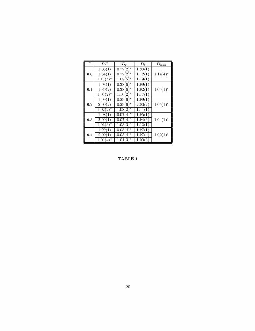
Table 1. With increasing F the backbone fractal dimension goes to 2 in a faster

way than those of the cluster itself. From Table 1 we see that around F ∼ 0.3

some exponents break their monotone behaviour. At this point the cluster has

a circular form and the corresponding gyration radius is maximum [10].

For the elastic backbone we found deviations from the straight line when

we plotted ln(M) x ln(L). This strongly indicates that corrections to scaling

are necessary. We adopted the ratio method [13] to correct them. For F = 0

we got DF = 1.17 ± 0.04 which is in fair agreement with Herrmann et al. [14]

result: 1.10 ± 0.05. When F increases, the trend is that the elastic backbone

approaches the form of a straight line connecting the lattice center to the point

where the cluster hits the frontier. The mass exponent goes to one.

2.2 The Red Sites

The number of red sites Nr scales as

Nr ∼ LDr (4)

Here again corrections to scaling are necessary. Of course, the exponents

Dr for the cluster and the backbone are the same. In the case of the ordinary

7

Table 1:To be inserted.

invasion percolation (F = 0), Dr is known exactly [19]. Coniglio used the

relations between the percolation model, Potts model and Coulomb gas to get

Dr = 34 . Our result Dr(F = 0) = 0.77±0.02 is in good agreement. As F goes to

0.5 the exponent Dr approaches zero (see Table 1). For the elastic backbone we

get Dr(F = 0) = 1.08±0.05. As we have already observed, the elastic backbone

approaches a straight line with increasing F . This means that almost every site

belonging to the elastic backbone is a red site, so Dr ∼ DF → 1 as F goes to

0.5.

2.3 The Loops

We can put a bond connecting any two nearest neighbors occupied sites. The

result is a connected graph for which the Euler relation holds: Nl = Nb−M +1

, where Nl is the number of cycles or loops number; Nb is the number of bonds

and M is the mass or the number of sites. For the burning algorithm on the

square lattice, Nl is calculated by counting the number of times that one tries

to burn a site that is already burned in the same time unit.

The number of loops Nl scales with the lattice size L as

Nl ∼ LDl (5)

The data are of very good quality and no correction to scaling was necessary.

8

Figure 1:To be inserted.

The exponent Dl approaches 2 with increasing F for both the cluster and the

backbone. This is a consequence of the Euler relation. As F increases, the

clusters become more compact, Nb approaches 2M and, for large clusters, Nl ∼

M ∼ L2. On the other hand, looking at Table 1, the exponent seems to approach

1 for the elastic backbone but this not true. In Fig.1 we show one typical cluster

with F = 0.4 and L = 401. The elastic backbone starts at the center and follows

to the right nearly as a straight line until it finds an obstacle (a site with a large

random number associated). Then a kind of a jet appears which increases the

number of loops. In the limit L → ∞ such effect can only be avoided if F ≥ 0.5.

This means that for the elastic backbone Dl goes abruptly to zero near F ∼ 0.5

as it is shown in the inset of Fig.1.

2.4 The Minimum Path

The minimum path scales as

lmin ∼ LDmin (6)

Naturally, the exponent Dmin is the same for both the cluster , backbone

and elastic backbone. Our estimate Dmin(F = 0) = 1.14 ± 0.04 is consistent

with the most precise value Dmin = 1.1307 ± 0.0004 [16]. We see from Table 1

that Dmin approaches one with increasing F .

9

3 THE OPTIMIZED MODEL

The optimized model [10] was devised in order to have a growth mechanism

obeying exactly the scaling

M ∼ (Rg)D (7)

or as near it as possible (Rg is the gyration radius and D is a real positive

external parameter that can be tuned).

Basically we use the following strategy: at each growing step we have a list

containing all the cluster perimeter sites that can be invaded and we ask for the

number of sites that should be invaded in order that (7) is verifyed as closely as

possible . This proceeding builds a fractal object which is extremely stabilized

in the sense that in any stage or size the scaling is perfectly obeyed not only

in the asymptotic limit (as usually). Another important advantage is that the

necessity of mass averages on the cluster ensemble diminishes. We hope this

can be very useful in dilute systems.

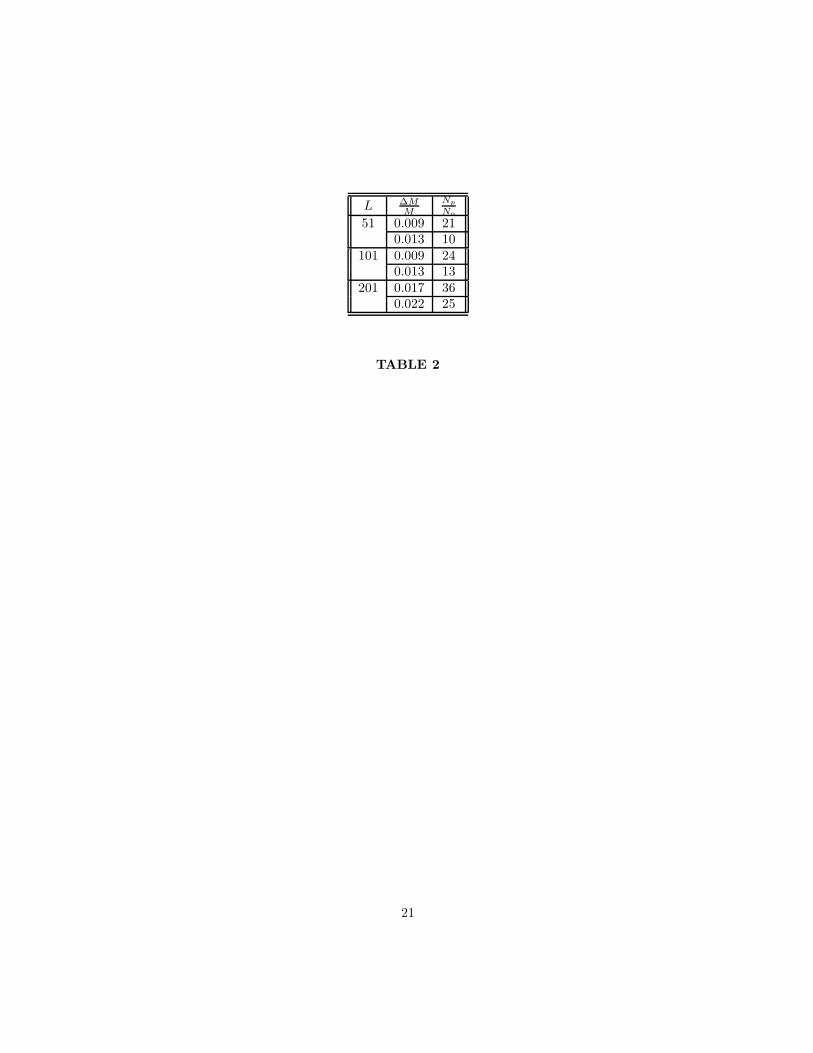
Any cluster is very representative because the mass dispersion is very small.

As an example, we compare the ratioNp

No(Np and No are the number of exper-

iments performed in the perimeter and optimized models, respectively) when

both models are simulated to achieve nearly the same relative standard devia-

tion ∆MM

. The results are shown in Table 2.

For one to one realization, we have already compared the optimized algo-

10

Table 2:To be inserted.

rithm to that of the ordinary invasion percolation. The results were even more

impressive ( see Fig.6 of ref [10]).

As shown in reference [10], when D ∈ [ 9148 , 2] it coincides with the usual

fractal dimension DF ; if 0 < D < 9148 the system is frustrated in the sense

that it tries but fails to invade less than one site; if D > 2 the system is also

frustrated but now for a different reason: the invasion cannot be faster than it

is allowed by the two dimensional lattice. In the last two situations D 6= DF .

In this paper we use the optimized algorithm to simulate only one cluster.

The growth of this unique cluster is stopped at each 50 steps. Then we measure

the mass and the loops number for both the cluster and its backbone. Their

corresponding gyration radius and the minimum path are also determined. At

each stage the rectangle in which the cluster is actually inscribed is also obtained

(up to lattice size L = 401). The lattice center and the point P2 where the

cluster touches that rectangle are used to get the minimum path. The elastic

backbone is the collection of all these paths. It is a faint structure with almost

one dimensional characteristics. When we pass from one rectangle to the next,

usually happens that P2 turns, for example, from north to south or east. So in

just one step the sites composing the elastic backbone change wildly, precluding

its determination (remember that here no averages are made).

11

Table 3:To be inserted.

We studied the optimized model only in the physical region D ∈ [9148 , 2].

Below we present our results.

3.1 The Mass

Naturally, D ≡ DF for the cluster mass. To our surprise the scaling (7) is also

perfectly obeyed by the backbone (see Fig.2(a)). Remember that the equation

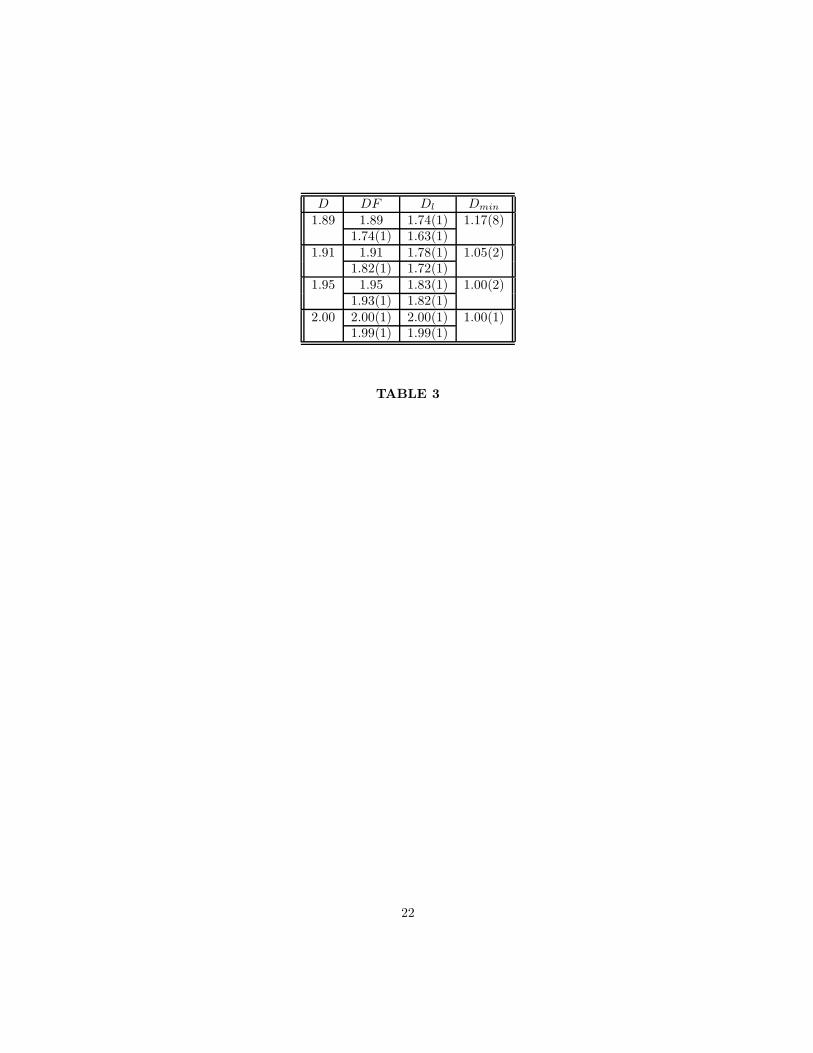
(7) was only imposed on the cluster. In Table 3 we present the fractal dimen-

sions DF for some values of D. Remember that we performed only a unique

realization. The errors bars correspond to the standard deviation calculated

along this experiment. Observe that at D = 1.89 (the fractal dimension of the

ordinary invasion percolation) we get for the backbone DF = 1.74± 0.01 which

is greater than the 1.647± 0.004 [16] of the ordinary invasion percolation. This

means that although the optimized model at D = 1.89 and the ordinary inva-

sion have the same cluster fractal dimension, they are intrinsicaly different since

their backbones are different. Conductivity properties will not be the same.

3.2 The Red Sites

An astonishing result that we got is that the number of red sites Nr of the

optimized model is very small and random. It does not obey any power law.

For example, when we grow one cluster and count the red sites number at sizes

12

Figure 2:To be inserted.

L = 51, 101, 151, 201, 251, 301, 401 we find Nr = 1, 8, 8, 1, 6, 3, 7. To investigate

this further, we simulate at D = 1.95 (just in the middle of the physical region

[1.89, 2.00]) with lattice sizes L = 51, 101, 151, 201 and the number of realizations

100, 100, 60, 15, respectively. We got < Nr >= 1.33, 1.49, 1.43, 1.87. This bring

us to the conclusion that for our optimized model the concept of red sites is not

important. The red sites number is so small that the probability of disconnecting

the cluster by removing randomly any site is pratically zero. The optimized

algorithm destroys the red sites increasing the cluster connectivity.

3.3 The Loops

The number of loops Nl scales with the gyration radius Rg in the usual way

Nl ∼ (Rg)Dl (8)

Looking the Table 3 we conclude that, as expected, both exponents go to 2

with increasing D.

To see the influence of the ensemble averages on the scaling exponents we

have performed 40 realizations of the optimized model on a lattice size L =

251 and D = 1.91. We got Dl = 1.73(4) for the cluster; DF = 1.84(1) and

Dl = 1.70(2) for the backbone and Dmin = 1.02(3). These results are fairly

good when compared to Dl = 1.78(1); DF = 1.82(1) and Dl = 1.72(1) and

13

Table 4:To be inserted.

Dmin = 1.05(2), respectively, obtained for just one realization on size L = 401.

Unfortunately, we were not able to simulate larger lattices face to the huge CPU

demand ( a unique L = 401 realization took 52 hours on a Alpha/275 station).

3.4 The Minimum Path

The minimum path scales as (6). Our results are shown in Table 3. Like in the

perimeter model, the exponent Dmin approaches 1 as the cluster becomes more

compact.

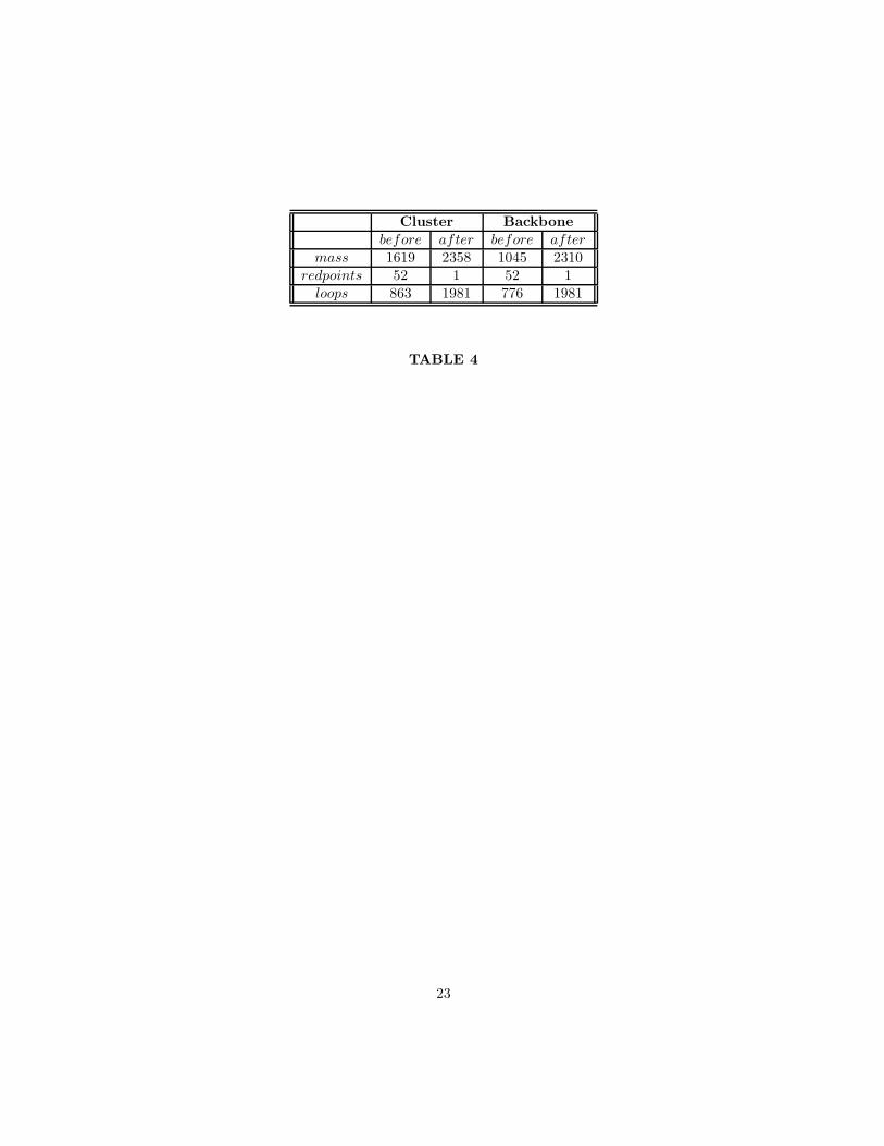
3.5 The Burst Phenomenon

We already know from reference [10] that the system is frustrated when D ∈

[0, 9148 ] (DF = 91

48 ) or D > 2 (DF = 2). In the last regime the burst phenomenon

takes place. This corresponds to an enormous and sudden mass explosion. We

simulate at D = 5.00 (L = 201) just be fore and after one of such explosions

( at time step 965, just as in Fig.11 of the reference [10] ). The results for the

cluster and the backbone are shown in Table 4. It shows a dramatic increase

(decrease) of the mass and loops (red sites).

4 CONCLUSIONS

We use the burning method to identify and analyze the cluster, the backbone

and the elastic backbone structures of the multiple invasion percolation model.

14

We determine the scaling exponents for both the perimeter and the optimized

models as well as their dependence with the parameters F and D. For those

structures we also study the behaviour of the mass, the number of red points, the

number of loops and the minimum path. The optimized model in the physical

region D = DF ∈ [ 9148 , 2] exhibited two amazing properties: the perfect scaling

of the backbone mass with its gyration radius and the red points disappearance.

This model seems to be well suited to treat dilute systems where the fluctuations

of the clusters ensemble hamper the data accuracy and overcast the reality.

Acknowledgments

We acknowledge CNPq (Conselho Nacional de Desenvolvimento Cientıfico e

Tecnologico) and FAPESP ( Fundacao de Amparo a Pesquisa do Estado de Sao

Paulo ) for the financial support.

15

References

[1] D. Wilkinson and J. F. Willemsen, J. Phys. A 16, 3365 (1983).

[2] T. A. Witten and L. M. Sanders, Phys. Rev. B 27,5686 (1983).

[3] P. Grassberger and S. S. Manna, J. Phys. 51, 1077 (1990).

[4] P. Bak, C. Tang and K. Wiesenfeld, Phys. Rev. Lett. 59, 381 (1987).

[5] R. N. Onody, A. N. D. Posadas and S. Crestana, J. Appl. Phys. 78, 2970

(1995).

[6] D. Wilkinson, Phys. Rev. B 30, 520 (1984).

[7] A. Birovljev, L. Furuberg, T. Feder, T. Jøssang , K. J. Maløay and A.

Aharony, Phys. Rev. Lett. 67, 584 (1991).

[8] P. Meakin, J. Feder, V. Frette and T. Jøssang , Phys. Rev. A 46, 3357

(1992).

[9] R. N. Onody, Int. J. Mod. Phys. C 6, 77 (1995).

[10] R. N. Onody and R. A. Zara , Physica A 231, 375 (1996).

[11] P. G. de Gennes, J. Physique Lett. 37, L1 (1976).

[12] H. E. Stanley and A. Coniglio, Phys. Rev. B 29, 522 (1984)

[13] H. J. Herrmann and H. E. Stanley, J. Phys. A 21, L829 (1988).

[14] H. J. Herrmann, D. C. Hong and H. E. Stanley, J. Phys. A 17, L261 (1984).

16

[15] D. Laidlaw, G. MacKay and N. Jan, J. Stat. Phys. 46, 507 (1987).

[16] P. Grassberger, J. Phys. A 25, 5475 (1992).

[17] U. P. C. Neves and R. N. Onody, Physica A 218, 1 (1995).

[18] B. B. Mandelbrot,The Fractal Geometry of Nature Freeman, New York

(1982).

[19] A. Coniglio, Phys. Rev. Lett. 62, 3054 (1989).

17

Tables Caption

Table 1 - The scaling exponents of the perimeter model. The order they

appear in this table corresponds to the cluster, backbone and elastic backbone

respectively. Those marked with an asterisk were calculated using the ratio

method.

Table 2 - The ratioNp

Nomeasures how many times the number of experiments

in the perimeter model Np exceeds that of the optimized No when we impose

they have the same relative standard deviation ∆MM

. The first and the second

lines correspond to the cluster and the backbone, respectively. We used No(L =

51, 101) = 100, No(L = 201) = 15.

Table 3 - The scaling exponents of the optimized model. The order they

appear in this table corresponds to the cluster and backbone respectively.

Table 4 - The abrupt variation of the mass, loops and red points at the

moment of the explosion.

18

Figures Caption

Fig.1 - In gray is a typical cluster of the perimeter model with F = 0.4 on a

lattice of size L = 401. The elastic backbone is shown in black. The inset gives

the dependence of the loops number scaling exponent with F .

Fig.2 - (a) The symbol o stands for the logarithm plot of the backbone mass

versus its gyration radius. (b) The logarithm dependence of the backbone loops

number Nl with the gyration radius.

19

F DF Dr Dl Dmin

1.88(1) 0.77(2)∗ 1.98(1)0.0 1.64(1) 0.77(2)∗ 1.72(1) 1.14(4)∗

1.17(4)∗ 1.08(5)∗ 1.19(1)1.98(1) 0.38(6)∗ 1.99(1)

0.1 1.89(2) 0.38(6)∗ 1.92(1) 1.05(1)∗

1.05(2)∗ 1.10(2)∗ 1.17(1)1.99(1) 0.29(6)∗ 1.99(1)

0.2 2.00(2) 0.29(6)∗ 2.00(2) 1.05(1)∗

1.02(2)∗ 1.08(2)∗ 1.11(1)1.98(1) 0.07(4)∗ 1.95(1)

0.3 2.00(1) 0.07(4)∗ 1.94(3) 1.04(1)∗

1.03(3)∗ 1.03(3)∗ 1.12(1)1.99(1) 0.05(4)∗ 1.97(1)

0.4 2.00(1) 0.05(4)∗ 1.97(4) 1.02(1)∗

1.01(4)∗ 1.01(3)∗ 1.00(3)

TABLE 1

20

L ∆MM

Np

No

51 0.009 210.013 10

101 0.009 240.013 13

201 0.017 360.022 25

TABLE 2

21

D DF Dl Dmin

1.89 1.89 1.74(1) 1.17(8)1.74(1) 1.63(1)

1.91 1.91 1.78(1) 1.05(2)1.82(1) 1.72(1)

1.95 1.95 1.83(1) 1.00(2)1.93(1) 1.82(1)

2.00 2.00(1) 2.00(1) 1.00(1)1.99(1) 1.99(1)

TABLE 3

22

Cluster Backbone

before after before after

mass 1619 2358 1045 2310redpoints 52 1 52 1

loops 863 1981 776 1981

TABLE 4

23

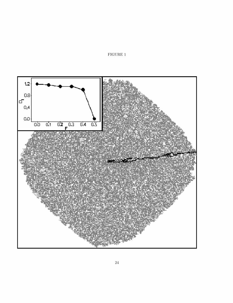
FIGURE 1

24

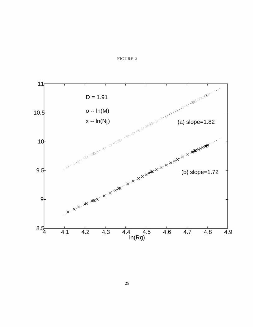
FIGURE 2

4 4.1 4.2 4.3 4.4 4.5 4.6 4.7 4.8 4.98.5

9

9.5

10

10.5

11

ln(Rg)

o -- ln(M)

D = 1.91

x -- ln(N ) (a) slope=1.82

(b) slope=1.72

l

25