Cloud Point Labelling in Optical Motion Capture Systems
124
-
Upload
khangminh22 -
Category
Documents
-
view
1 -
download
0
Transcript of Cloud Point Labelling in Optical Motion Capture Systems

Cloud Point Labelling in OpticalMotion Capture Systems
By
Juan L. Jiménez Bascones
Submitted to the department of Computer Science and Articial
Intelligence
in partial fullment of the requirements for the degree of
Doctor of Philosophy
PhD Advisor:
Prof. Dr. Manuel Graña Romay
at The University of the Basque Country
Universidad del País Vasco
Euskal Herriko Unibertsitatea
Donostia - San Sebastian
2019

ii

AUTORIZACION DEL/LA DIRECTOR/A DE TESIS
PARA SU PRESENTACION
Dr/a. _________________________________________con N.I.F.________________________
como Director/a de la Tesis Doctoral:
realizada en el Departamento
por el Doctorando Don/ña. ,
autorizo la presentación de la citada Tesis Doctoral, dado que reúne las condiciones
necesarias para su defensa.
En a de de
EL/LA DIRECTOR/A DE LA TESIS
Fdo.:

iv

CONFORMIDAD DEL DEPARTAMENTO
El Consejo del Departamento de
en reunión celebrada el día ____ de de ha acordado dar la
conformidad a la admisión a trámite de presentación de la Tesis Doctoral titulada:
dirigida por el/la Dr/a.
y presentada por Don/ña.
ante este Departamento.
En a de de
Vº Bº DIRECTOR/A DEL DEPARTAMENTO SECRETARIO/A DEL DEPARTAMENTO
Fdo.: ________________________________ Fdo.: ________________________

vi

ACTA DE GRADO DE DOCTOR
ACTA DE DEFENSA DE TESIS DOCTORAL DOCTORANDO DON/ÑA. TITULO DE LA TESIS:
El Tribunal designado por la Subcomisión de Doctorado de la UPV/EHU para calificar la Tesis Doctoral arriba indicada y reunido en el día de la fecha, una vez efectuada la defensa por el doctorando y contestadas las objeciones y/o sugerencias que se le han formulado, ha otorgado por___________________la calificación de: unanimidad ó mayoría
Idioma/s defensa: _______________________________________________________________
En a de de
EL/LA PRESIDENTE/A, EL/LA SECRETARIO/A,
Fdo.: Fdo.:
Dr/a: ____________________ Dr/a: ______________________
VOCAL 1º, VOCAL 2º, VOCAL 3º,
Fdo.: Fdo.: Fdo.:
Dr/a: Dr/a: Dr/a: EL/LA DOCTORANDO/A, Fdo.: _____________________

ix
Cloud Point Labeling in Optical Motion Capture Systems
by
Juan L. Jiménez Bascones
Submitted to the Department of Computer Science and Articial Intelligence, in partial fulllment
of the requirements for the degree of Doctor of Philosophy
Abstract
This Thesis deals with the task of point labeling involved in the overall work-
ow of Optical Motion Capture Systems. Human motion capture by optical
sensors produces at each frame snapshots of the motion as a cloud of points
that need to be labeled in order to carry out ensuing motion analysis. The
problem of labeling is tackled as a classication problem, using machine learn-
ing techniques as AdaBoost or Genetic Search to train a set of weak classiers,
gathered in turn in an ensemble of partial solvers. The result is used to feed
an online algorithm able to provide a marker labeling at a target detection
accuracy at a reduced computational cost. On the other hand, in contrast
to other approaches the use of misleading temporal correlations has been dis-
carded, strengthening the process against failure due to occasional labeling
errors. The eectiveness of the approach is demonstrated on a real dataset ob-
tained from the measurement of gait motion of persons, for which the ground
truth labeling has been veried manually. In addition to the above, a broad
sight regarding the eld of Motion Capture and its optical branch is provided
to the reader: description, composition, state of the art and related work.
Shall it serve as suitable framework to highlight the importance and ease the
understanding of the point labeling.
Keywords: Optical Motion Capture, MoCap, Marker Tracking, Ada Boost,
Genetic Search, Tree Search, Ensemble Classiers.

Acknowledgements
As pointed out in `A Short History of Nearly Everything' 1, there is no way
to make an account for the utterly entangled string of events and deeds that
brought us to reach the point we are. All things considered, '...standing
on the shoulders of giants...' is the rst quote that comes into my mind
when faced to enumerate the people I'm indebted to. That said, and in
reverse chronological order, I have to begin rendering thanks to my PhD
advisor Prof. Manuel Graña. Without his academic guidance and words of
encouragement in times of hardship, this work simply wouldn't have been
possible. There is no room here to mention all the colleagues of whom I had
the opportunity to learn so much and the few always willing to patiently
hear my professional concerns. I want to extent my gratitude to the teachers
who back in time up to primary school, infused me with the eagerness and
enjoyment of learning. And nally, all those people from dierent activities
committed to their work and with a shared wish of cooperation.
This work has been partially supported by the EC through project Cyb-
SPEED funded by the H2020 MSCA-RISE grant agreement Num. 777720.
Juan L. Jiménez Bascones
Donde canta el agua, nacen paraísos
Octavio Paz
1A book devoted to the popularisation of Science. Bill Bryson, 2003

Contents
1 Introduction 1
1.1 Motivation . . . . . . . . . . . . . . . . . . . . . . . . . . . . 1
1.1.1 Motion Capture . . . . . . . . . . . . . . . . . . . . . . 2
1.1.2 Marker labelling . . . . . . . . . . . . . . . . . . . . . 2
1.2 Overview of the Thesis Contributions . . . . . . . . . . . . . . 3
1.3 Publications . . . . . . . . . . . . . . . . . . . . . . . . . . . 5
1.4 Contents of the Thesis . . . . . . . . . . . . . . . . . . . . . . 6
2 MoCap - State of the Art 9
2.1 Interest in mocap . . . . . . . . . . . . . . . . . . . . . . . . . 9
2.2 Mocap Technologies . . . . . . . . . . . . . . . . . . . . . . . 20
2.2.1 General overview . . . . . . . . . . . . . . . . . . . . . 20
2.2.2 Wearable systems . . . . . . . . . . . . . . . . . . . . . 20
2.2.3 Markerless Optical Systems . . . . . . . . . . . . . . . 27
2.2.4 Marker-based Optical Systems . . . . . . . . . . . . . 29
3 Optical Motion Capture - Components 37
3.1 Sensors . . . . . . . . . . . . . . . . . . . . . . . . . . . . . . 37
3.1.1 Markers . . . . . . . . . . . . . . . . . . . . . . . . . . 37
3.1.2 Cameras . . . . . . . . . . . . . . . . . . . . . . . . . . 39
3.2 System deployment . . . . . . . . . . . . . . . . . . . . . . . . 42
3.2.1 System location . . . . . . . . . . . . . . . . . . . . . . 42
3.2.2 Camera Arrangement . . . . . . . . . . . . . . . . . . 43
3.3 Photogrametry . . . . . . . . . . . . . . . . . . . . . . . . . . 45
xi

xii CONTENTS
3.4 Process stages . . . . . . . . . . . . . . . . . . . . . . . . . . . 54
4 Labelling Algorithm 61
4.1 Problem Statement . . . . . . . . . . . . . . . . . . . . . . . . 61
4.2 Outline of our Approach . . . . . . . . . . . . . . . . . . . . . 64
4.3 Geometric Features and Weak Classiers . . . . . . . . . . . . 67
4.4 Labelling Without Presence of Occlusions. Ensemble of Weak
Classiers . . . . . . . . . . . . . . . . . . . . . . . . . . . . . 70
4.4.1 Training a set of weak classiers . . . . . . . . . . . . 70
4.4.2 Generating labels exploiting the ensemble of weak clas-
siers . . . . . . . . . . . . . . . . . . . . . . . . . . . 71
4.5 Ensemble of Partial Solvers . . . . . . . . . . . . . . . . . . . 73
4.5.1 The solver . . . . . . . . . . . . . . . . . . . . . . . . . 73
4.5.2 Partial solvers . . . . . . . . . . . . . . . . . . . . . . . 74
4.5.3 Training an ensemble of partial solvers . . . . . . . . . 76
4.5.4 Generating labels exploiting the ensemble of partial
solvers . . . . . . . . . . . . . . . . . . . . . . . . . . . 81
5 Results 85
5.1 Experimental Data . . . . . . . . . . . . . . . . . . . . . . . . 85
5.2 Partial Solver Performance . . . . . . . . . . . . . . . . . . . . 86
5.3 Solver Ensemble Performance . . . . . . . . . . . . . . . . . . 88
6 Conclusions 95
6.1 Achievements . . . . . . . . . . . . . . . . . . . . . . . . . . . 95
6.2 Limitations . . . . . . . . . . . . . . . . . . . . . . . . . . . . 97
6.3 Future work . . . . . . . . . . . . . . . . . . . . . . . . . . . . 99

List of Figures
2.1 Mocap in Lord of the Rings . . . . . . . . . . . . . . . . . . . 11
2.2 Helen Hayes Hospital Marker Set, from Vaughan et al. . . . . 11
2.3 Mocap playback in a swing golf analysis software named Gears
and powered by Optitrack) . . . . . . . . . . . . . . . . . . . . 14
2.4 Mocap for bike tting analysis . . . . . . . . . . . . . . . . . . 15
2.5 Example of electromechanical suite from Gypsy . . . . . . . . 21
2.6 Diagram example of an usual IMU fusion algorithm . . . . . . 23
2.7 Common IMU circuitry and in-house commercial unit device
from Xsens . . . . . . . . . . . . . . . . . . . . . . . . . . . . 24
2.8 IMU motion capture suit . . . . . . . . . . . . . . . . . . . . . 25
2.9 Kinect RGB-Depth device unit . . . . . . . . . . . . . . . . . 29
2.10 Human body kinematic model (left) and leg detail (right) . . 33
2.11 Marker based mocap suite and its 3D counterpart . . . . . . . 34
3.1 Marker specimen . . . . . . . . . . . . . . . . . . . . . . . . . 38
3.2 Lightning setup . . . . . . . . . . . . . . . . . . . . . . . . . . 38
3.3 Image marker 2D position . . . . . . . . . . . . . . . . . . . . 39
3.4 Motion capture camera with built-in IR lightning source and
its exploded view. Drawing borrowed from the Optitrack web
site . . . . . . . . . . . . . . . . . . . . . . . . . . . . . . . . . 40
3.5 Camera eld of view (FOV). . . . . . . . . . . . . . . . . . . . 41
3.6 Typical camera distribution around the capture area. . . . . . 44
3.7 Eects of lens distortion. . . . . . . . . . . . . . . . . . . . . . 46
3.8 Synthesis of 3D coordinates from 2D projections. . . . . . . . 48
xiii

xiv LIST OF FIGURES
3.9 Non intersecting projection lines. . . . . . . . . . . . . . . . . 49
3.10 Ghost markers synthesis as result of geometric coplanarity
between two cameras and two real markers. . . . . . . . . . . 50
3.11 Process stages overview. . . . . . . . . . . . . . . . . . . . . . 54
4.1 Actor wearing reective markers and corresponding digital
model . . . . . . . . . . . . . . . . . . . . . . . . . . . . . . . 62
4.2 Example of a humanoid model labelling L. . . . . . . . . . . . 63
4.3 Overall strong classier builder process . . . . . . . . . . . . 65
4.4 Overall labelling generation process . . . . . . . . . . . . . . 66
4.5 Overall solver ensemble aggregation . . . . . . . . . . . . . . 66
4.6 An example of the labelling process tree. Squares denote pos-
itive label guess and circles rejected labelling. Rejection is due
to the the ensemble classier giving a negative output on the
partial labelling. . . . . . . . . . . . . . . . . . . . . . . . . . 73
4.7 Greedy bottom up search diagram representation . . . . . . . 78
4.8 Greedy top down search diagram representation . . . . . . . 79
5.1 Accuracy and eciency assessment depending on the number
of weak classiers. . . . . . . . . . . . . . . . . . . . . . . . . 89
5.2 Graph: false assignments and false occlusions under dierent
test conditions . . . . . . . . . . . . . . . . . . . . . . . . . . 93

List of Tables
4.1 Several geometric operations . . . . . . . . . . . . . . . . . . . 68
5.1 First selected weak classiers . . . . . . . . . . . . . . . . . . 88
5.2 Experimental conditions summary . . . . . . . . . . . . . . . 90
5.3 False assignments (FA) and false occlusions (FO) results. Rows
correspond to model markers located over parts of the body. . 91
5.4 False assignments sensitivity to target marker hit rate and
number of occlusions. . . . . . . . . . . . . . . . . . . . . . . . 92
5.5 False occlusion sensitivity to target marker hit rate and num-
ber of occlusions. . . . . . . . . . . . . . . . . . . . . . . . . . 92
xv

Chapter 1
Introduction
This chapter is an overall introduction to the Thesis. First, we provide a
short motivation in section 1.1. A summary of the Thesis contents and
contributions are given in section 1.2. The publications achieved during the
work of the Thesis are listed in section 1.3. Finally, the main structure of
the Thesis is presented in section 1.4.
1.1 Motivation
Back in 1998, I got to know for the rst time the discipline ofMotion Capture.
I happened to team up, as recent post-graduate engineer, with an enthusias-
tic group of people in charge of the development of a complete optical motion
capture system industry grade solution. The project started from scratch,
almost with no previous background knowledge in the topic. The challenge
involved dealing with multiple problems such as hardware selection, cabling
setup, lightning solution, image transfer and processing, camera calibration,
bio-mechanical calculation, 3D graphic rendering ... everything dressed up
with a complex software taking care of everything.
Most of the issues could be successfully tackled with the standard knowl-
edge acquired in the engineer academical training. But it didn't take long
before the optimal solution to a particular problem arose as well above our
skills: maker identication, also known as marker tracking or marker la-
1

2 CHAPTER 1. INTRODUCTION
belling. At the time, we came out with a coarse algorithm who managed to
get away with it most of the time, but indeed the issue remained without a
satisfying solution since then.
This Thesis spreads along two main axis:
An account of the Optical Motion Capture components, stages, chal-
lenges and state-of-the art solutions.
The main motivation of this work, which is to nd a brand new method
to solve the optical marker labelling problem, appealing to the weaponry
of machine learning techniques.
1.1.1 Motion Capture
The term MOtion CAPture encompasses the processes, methods and tech-
niques that are put together to acquire, record and analyse the movement of
mainly persons, along the time. This Thesis begins covering the answer to
the what for, why and how of the Motion Capture, so that the reader may
have a broad view on the eld. The work makes also a review of the aca-
demic papers related with the subject arranged by topic, trying to highlight
the interest of the community on the eld.
Finally, a particular attention is paid to the branch of the optical marker-
based methodologies, whose composition and operation is shown in a ded-
icated chapter. This provides a good understanding of the overall picture
when it comes to the seldom discussed problem of marker labelling.
1.1.2 Marker labelling
Despite the crucial role played by the marker tracking in the whole process
of optical motion capture, at the time of writing this work the number of
published papers focused on marker labelling is scarce. Commercial systems
keep their proprietary methods unexplained, barely hinting the way they
solve the problem. On the other hand, the few papers covering the topic often
make use of predictive models exploiting the underlying kinematic model
rigid bodies and joints, predicting next marker positions from their past
1.2. OVERVIEW OF THE THESIS CONTRIBUTIONS 3
trajectories. After that, an algorithm estimates the most likely labelling by
matching the predicted trajectory against the most recently provided point
cloud.
According to our experience, marker algorithms are rather hard to tune
and lack the required reliability for an industrial solution: as soon as an
error is incurred, the subsequent tracking is likely to fail. The input data
has a high uncertainty, noise and ambiguities, and therefore machine learning
comes up as a promising approach to handle the marker labelling problem.
Consequently, the core motivation of this work is to connect the problem
and existing algorithms in a way that has never been attempted before.
1.2 Overview of the Thesis Contributions
The main contribution of the Thesis is the development of an algorithm for
the labelling of optical markers which can be embedded in the workow of
an optical motion capture system.
First, the problem of optical marker labelling is explained in the context
of the whole motion capture process. We dene a marker as a point in 3D
Cartesian space, marker model as a set of a priori dened markers and the
set of candidate points extracted from the video feed by image segmentation
and photogrammetric techniques. The dierent situations corrupting the
input data are enumerated, stating the boundary conditions the labelling
algorithm has to work with. After that, we model the actual labelling of
the candidate points as a vector of integers, so the labelling problem can be
formulated as a search in the space of labelling vectors trying to maximise a
maximise a specic criterion function under some constraints.
In order to handle the marker labelling as a classication task, we intro-
duce the concept of geometric features as geometric functions dened over
small sets of 3D points. From these geometric features we build weak clas-
siers that implement the decision `is this labelling a correct one?' over a
given cloud of candidate points. An ensemble of weak classiers are selected
and put together to build a strong classier. Weak classier selection is car-
ried out by means of a tailored implementation of the well known Ada-Boost

4 CHAPTER 1. INTRODUCTION
algorithm. The strong classier is trained over a ground truth built on pur-
pose in the context of the project and composed by actual labelled maker
samples of real moving people.
We introduce also a marker labelling solving algorithm that takes advan-
tage of the trained strong classier, proving to be able to eciently label
markers at high rates under the assumption of no occlusions.
Keeping in mind that the real data usually suers from missing data
due to occlusions and segmentation aws, a divide-and-conquer strategy is
proposed to deal with the complete problem. The concept of partial solver
comes in handy here. Indeed, strong classiers can be trained over subsets
of markers belonging to the complete model. Each strong classier is then
owned by a partial solver which can label the subset of markers up to a
given hit ratio and provided no marker from the subset is missing. As a
result, the partial solver yields a solution to the subspace spanned by the
corresponding partial marker labelling vector. In addition, the quality of a
given partial solver is determined by the number of times it correctly guesses
the right labelling over random samples of input point clouds. Such hit rate
is assessed against the ground truth and kept as attribute of the partial solver
for further use. Some interesting properties of the partial solver are stated
formally and discussed in detail in this Thesis.
It turns out that not any partial solver is equally apt to reach high hit
rates. Therefore, we develop and test and algorithm to select the elite of
partial solvers. To do so, we apply genetic algorithms where each partial
solver instance is viewed as a specimen whose genome is the subset of markers
it works over. This allows the selection to be dealt with as an evolution
process driven by a genetic algorithm, aiming to evolve the best individuals.
At the end of the evolutive process, the best ones are joint together in a
swarm of solvers forming a partial solver ensemble. A key control parameter
of the algorithm is the target hit ratio: the boundary that rules whether a
partial solver is worth to be kept alive in the genetic algorithm.
Once we count on a valid solver ensemble, the formulation of the nal
labelling algorithm follows. Each partial solver contributes with none, one
or more solutions over its subspace. An ensemble of partial solvers builds

1.3. PUBLICATIONS 5
the nal labelling algorithm. As a result, not only is each marker matched
against its candidate with the requested condence but also the ensemble
may robustly decide if, conversely, it is better to take it as occluded.
be decided to be considered as occluded or just with no enough con-
dence to guarantee the right labelling. Such algorithm is described in the
corresponding chapter and its reliability assessed against the ground truth.
A strong dependency is identied between the target hit rate and how
bold is the resulting algorithm to label markers is presence of massive missing
data: the more demanding the hit rate, the less labelled markers in exchange
for a high hit condence and vice-verse. As a side result, the denition of the
suitability of a given marker distribution is settled in terms of capturability.
Summarizing, the contributions of the Thesis are the following ones:
We provide a state of the art review up to the recent dates of the thesis
topics, namely optical marker labelling
We provide an experimental dataset which has been published as open
access repository at the following address: http://doi.org/10.5281/
zenodo.1486208
We have developed and tested an algorithm that generates the labels
of the 3D point clouds obtained by optical marker detection systems
for human motion capture. The point clouds generated at each time
instant are labelled independently, no tracking in time is required.
This algorithm is able to produce labellings in real time in the presence
of occlusions
The algorithm consists of an ensemble of classiers that are trained over
datasets from an specic motion, thus the solution has to be retrained
for each kind of motion to be analysed.
1.3 Publications
The Thesis is supported by the following achieved publications

6 CHAPTER 1. INTRODUCTION
1. J. Jiménez-Bascones and M. Graña, "Preliminary Results on an AdaBoost-
Based Strategy for Pattern Recognition in Clouds of Motion Mark-
ers," 2016 Third European Network Intelligence Conference (ENIC),
Wrocªaw, Poland, 2017, pp. 239-244.
2. Jiménez-Bascones, Juan Luis & Graña, Manuel. (2017). An Ensemble
of Weak Classiers for Pattern Recognition in Motion Capture Clouds
of Points. 201-210. 10.1007/978-3-319-59162-9_21.
3. J.L. Jiménez Bascones, Manuel Graña, J.M. Lopez-Guede. A solver-
ensemble strategy to deal with occlusions in the labelling of clouds of
motion markers. Neurocomputing (in press).
4. Jiménez Bascones, Juan Luis, & Graña Romay, Manuel. (2018). Mo-
cap gait motion samples - Optical marker trajectories (Version 1.0.1)
[Data set]. Zenodo. http://doi.org/10.5281/zenodo.1486208
1.4 Contents of the Thesis
The contents of the Thesis are organised as follows:
Chapter 2 provides a state-of-the-art review concerning the eld of mo-
cap. The why and what for questions of this technology are answered
including and account of useful applications. The main dierent exist-
ing solutions are discussed as well as that a number of publications are
mentioned to highlight the current interest of the community in this
area.
In chapter 3 a description is made regarding the main components
and stages of an optical marker-based mocap system. The purpose
is to convey a better insight of the crucial role played by the marker
labelling, which is this Thesis main contribution. Consequently, the
description is not a balanced enumeration of the parts but instead the
stages preceding the labelling stand out above the others.

1.4. CONTENTS OF THE THESIS 7
The chapter 4 is devoted to the marker labelling task and its resolution
tackled from an original approach. First of all, the problem is described
besides its boundary constraints. Afterwards, it is formulated as a
classication problem in order to be dealt with machine learning tools,
namely weak and strong classiers and tree search algorithms. In a
rst phase, an ecient algorithm is dened to solve the particular
case where no markers are occluded. In the second phase, the solving
algorithm for the generic case is presented, built on the mining of the
most worthy instances of the later.
In chapter 5 experimental results are given regarding both the eciency
and hit ratio of the presented algorithms. The methods are assessed
against the ground truth of a set of genuine capture data gathered on
purpose for this Thesis.
Finally, in chapter 6 some conclusions are considered. Achievements
and shortcomings of this Thesis contribution are identied and a draft
of future work is oered as an account for the pending todo wish list
in the future to cometh.

8 CHAPTER 1. INTRODUCTION

Chapter 2
MoCap - State of the Art
Mocap industry comprises a variety of knowledge domains to make it possi-
ble. Over the last decades the requirements and solution for specic problems
evolved and keep on doing as so did the interest of users and developers.
In this chapter we provide a general view of the state-of-the-art, existing
solutions, practical applications, as well as a review of a number of relevant
publications to highlight the growing interest of the technical an scientic
community in the eld. It will serve as foundation for a better understanding
of the marker labelling problem and its signicance by placing it in the right
context.
2.1 Interest in mocap
The use of primitive mocap forms can be traced back to the 1920s, when
the so-called rotoscoping started to be used by the Walt Disney Studios.
The artists projected live-action footage onto cell animation drawing tables,
which helped them to mimic the motion in animated cartoon characters
[9]. But it wasn't until the late 1980s and early 1990s that the modern
semi-automatic marker-based mocap turned up as part of a ourishing lm
computer animation industry. However, the systems were rather limited,
expensive and hard to operate. Way back when, the use of mocap was limited
to experts and conned in labs and research universities. But nowadays,
9

10 CHAPTER 2. MOCAP - STATE OF THE ART
improvements both in hardware and software have made possible aordable
systems that do not require specialised skills to be handled. As a proof
for that, recently many large mocap databases have been made available for
free or purchase, and even smaller studios and schools can aord multicamera
systems for production, teaching, and low-budget art projects. The mocap
potential has been unleashed on multiple applications ranging from character
animation to sport training. As a consequence, what has evolved the most
is the understanding of the medium [43] among the average public including
a wider variety of professional from dierent elds, who have started to
embraced it in the sight of its possibilities.
Movies, TV and gaming industry. Remarkable companies as Sony Im-
ageworks or Industrial Light and Magic have employed mocap to animate
background characters (crowds) as well as humanoid ctional creatures in
movies as such as Lord of The Rings (see Fig. 2.1), Titanic or Star
Wars [9]. In these productions, the movements performed by a real ac-
tor are translated into an avatar, bringing him the subtle human pose and
action nuances that articially built path trajectories do usually miss. Re-
cently, this technique broke through TV productions, where real and virtual
characters interact in real time both in live and prerecorded broadcasts.
Mocap is widely used in the production of video games. For instance,
Electronic Arts Canada has a huge in-house mocap studio1 to record motion
snippets that, once reordered and concatenated in real time on game con-
soles, they manage to reenact any motion during the game following on the
player's whims.
Medical applications. Gait analysis has been a very successful applica-
tion of human mocap, allowing ne diagnosis and follow up of treatments. An
abnormal gait movement pattern may be due to a variety of patient's lesions:
it could be at the level of the central nervous system (cerebral palsy), in the
peripheral nervous system (Charcot-Marie-Tooth disease), at the muscular
level (muscular dystrophy), or in the synovial joint (rheumatoid arthritis).
1https://www.ea.com/news/tour-the-capture-studio-at-ea-canada
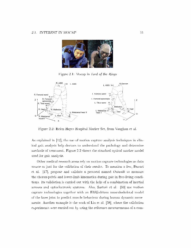
2.1. INTEREST IN MOCAP 11
Figure 2.1: Mocap in Lord of the Rings
Figure 2.2: Helen Hayes Hospital Marker Set, from Vaughan et al.
As explained in [12], the use of motion capture analysis techniques in clin-
ical gait analysis help doctors to understand the pathology and determine
methods of treatment. Figure 2.2 shows the standard optical marker model
used for gait analysis.
Other medical research areas rely on motion capture technologies as data
source or just for the validation of their results. To mention a few, Ferrari
et al. [17], propose and validate a protocol named Outwalk to measure
the thorax-pelvis and lower-limb kinematics during gait in free-living condi-
tions. Its validation is carried out with the help of a combination of inertial
sensors and optoelectronic systems. Also, Sartori et al. [50] use motion
capture technologies together with an EMG-driven musculoskeletal model
of the knee joint to predict muscle behaviour during human dynamic move-
ments. Another example is the work of Liu et al. [38], where the validation
experiments were carried out by using the reference measurements of a com-

12 CHAPTER 2. MOCAP - STATE OF THE ART
mercially available measurement system installed in a gait laboratory. The
goal was to develop a mobile force plate and 3-D motion analysis system
to measure triaxial ground reaction forces and 3-D orientations of feet. A
motion capture system, based on high-speed cameras, was adopted to sup-
port the experimental results of the developed system. Another work by
Yang et al. [61], presents a generic method to predict ground reaction forces
(GRFs). Motion capture was used to obtain postures for common standing
reaching tasks, whereas force plates were employed to record GRF informa-
tion in order to validate the prediction model. One more example is the
work of Siddiqui et al. [52], where the goal is the evaluation of decits in
exploratory behaviour in an open-eld setting using a wireless motion cap-
ture. Twenty-one stable adult outpatients with schizophrenia and twenty
matched healthy controls completed the exploration task. The motion data
were used to index participants locomotor activity and tendency for visual
and tactile object exploration. Finally, Delrobaei et al. [13] focus on the
assessment of full-body tremor as the most recognised Parkinson's Disease
(PD) symptom. The main assessment tool was an inertial measurement unit
(IMU)-based motion capture system to quantify full-body tremor and to
separate tremor-dominant from non-tremor-dominant PD patients as well as
from healthy controls. In addition, they claim that lack of a unied moni-
toring has been a major limitation to optimise therapeutic interventions for
these patients.
Sports. Human body movement is crucial when it comes to sports. No
matter if we are dealing with technical gestures, long repetitive actions or
highly stressed musculoskeletal eorts, the way the movement is developed
plays a very important role when we try to either improve the performance
or avoid sport injuries. Sports have received a lot of attention by the mocap
industry, as long as their popularity spreads among amateur sportsmen. As a
consequence, mocap systems are increasingly being used for sports training.
For example, Wan and Shan [58] collect 3D movement data to study and
identify several risk factors related to the development of muscle repetitive
stress injuries (RSIs). Based on the results, they propose a set of measures

2.1. INTEREST IN MOCAP 13
that can be applied to reduce the risk of RSIs during learning/training in
young sportsmen. Another common sportive research and development topic
is the Vertical Jump Height (VJH) and the Drop Vertical Jump (DVJ) land-
ing. While optimization of VJH is the primary target of any sport, DVJ
causes injuries on lower extremity. Therefore, in the research activity for [3],
Inertia Measurement Units (IMUs), an optical mocap system from Qualisys2
and muscle activity measurement sensors are integrated for customised DVJ
and VJH measurements.
A motion database for a large sample of penalty throws in team handball
is described by Helm et al. [25], performed by both novice and expert penalty
throwers. As well as the methods and materials used to capture the motion
data, additional information is given on the marker placement of the players
together with details on the skill level and/or playing history of the expert
group. Afterwards, this data set is employed in [24] to examine the kinematic
characteristics of captured movements by applying linear discriminant (LDA)
and dissimilarity analyses.
Fast and highly precise movements take advantage of motion capture sys-
tems too. A agship example is the golf swing (g. 2.3), where the kinematic
sequence of the movement plays an essential role. For instance, the purpose
of Cheetham et al. [10] was to compare key magnitude and timing parame-
ters of the kinematic sequence between recreational players (amateurs) and
PGA touring professionals (pros). To do so, a representative swing from
each of 19 amateurs and 19 pros was captured using three-dimensional (3D)
motion analysis techniques. All the magnitude variables showed a signi-
cant dierence between the amateurs and pros, although the mean of the
peak times showed no signicant dierence between the pros and amateurs.
The study found out that the peaking order of the body segment speeds
was dierent between pros and amateurs. Wang et al. [59] claim that in
order to understand an eective golf swing, both swing speed and impact
precision must be thoroughly and simultaneously examined. To probe their
hypothesis, seven golfers with dierent handicap levels were recorded using
high speed video cameras. Another example of the importance of capture2https://www.qualisys.com/

14 CHAPTER 2. MOCAP - STATE OF THE ART
Figure 2.3: Mocap playback in a swing golf analysis software named Gearsand powered by Optitrack)
techniques in golf is the work of Betzler et al. [6], where limitations of 3D
motion analysis in golng are described, identifying several golf-specic error
sources. Among them is marker occlusion and the clutter of high numbers
of markers in a small area, which are closely related with the problem of
marker tracking.
Bike cycling (g. 2.4) is another example of sportive activity that can
cause injuries due to repetitive movements if done in a wrong way. On the
other hand, a right biker position over the bike together with an appropriate
bike tting can signicantly improve the overall performance. Therefore,
bike tting is the perfect eld where motion analysis stands out as a cutting
edge technology, and a number of papers have been published as result of
its application. For instance, Fonda et al. [19] face the lack of consensus
on what method (dynamic vs. static ones) should be used to measure the
knee angle in bike tting, conducting a research is conducted on the validity
and reliability of dierent kinematics methods. All methods were fed with
data coming from a Vicon MX motion analysis system (Oxford metrics)
consisting of thirteen cameras recording with a sampling rate of 250 Hz
and with a residual measurement error less than 1 mm. All the dynamic
methods have been found to be substantially dierent compared to the static

2.1. INTEREST IN MOCAP 15
Figure 2.4: Mocap for bike tting analysis
measurements. Such results wouldn't be possible without the use of tracking
methods. Regarding the relevance of 2D vs 3D measurements, the main
purpose of Garcia et al. [20] was to test the validity and sensibility of two
motion capture systems (sophisticated and expensive 3D vs low-cost 2D)
to analyse angular kinematics during pedalling. The main conclusions is
that both performs well regarding angular kinematic analysis in the sagittal
plane, but only the 3D systems can analyse asymmetries between left and
right sides. Additional validity research is carried out by Bouillod et al. [8],
where the 3D motion analyser from Shimano3 and a Vicon4 are used to collect
simultaneously the movement of cyclist at dierent pedalling cadences. The
nal conclusion is that experts and scientists should use the Vicon system
for the purpose of research whereas the 3D motion analyser from Shimano
could be used for less demanding bike tting purposes. Finally, Moore et
al. [48], use motion capture techniques to prove that the bike rider uses
the upper body very little when performing normal manoeuvres, just using
steering input for bike control. The study found out that other motions such
as lateral movement of the knees were used in low speed stabilisation.
3https://www.biketting.com/4https://www.vicon.com/

16 CHAPTER 2. MOCAP - STATE OF THE ART
Activity recognition. Ongoing human action recognition is a challeng-
ing problem that has many applications, such as video surveillance, patient
monitoring, human-computer interaction, and so on. Over the last years, a
number of research papers have been published on the topic. For instance,
Patrona et al. [49] present a framework for real-time action detection, recog-
nition and evaluation of motion capture data. The automatically segmented
and recognised action instances are fed to the framework action evaluation
component, which compares them estimating their similarity. Exploiting
fuzzy logic, the framework subsequently gives semantic feedback with in-
structions on performing the actions more accurately. Similarly, Barnachon
et al. [5] show another framework to recognise streamed actions coming from
Motion Capture (mocap) data. The proposed method is based on histograms
of action poses, extracted from mocap data, that are compared according to
Hausdor distance, having the advantage of allowing some stretching ex-
ibility to accommodate for possible action length changes. Another paper
addressing the human action recognition is [26], where reconstructed 3D
data acquired by multi-camera systems is processed as 4D data (3D space +
time) to detect spatio-temporal interest points (STIPs) and local description
of 3D motion features. Local 3D motion descriptors, histogram of optical 3D
ow (HOF3D), are extracted from estimated 3D optical ow in the neigh-
bourhood of each 4D STIP and made view-invariant. The local HOF3D
descriptors are divided using spatial pyramids to capture and improve the
discrimination between arm and leg-based actions. A bag-of-words (BoW)
vocabulary of human actions is built based on these pyramids, which is com-
pressed and classied using agglomerative information bottleneck (AIB) and
support vector machines (SVMs), respectively.
In order to conduct their experiments, Ijjina et al [27] take advantage of
a number of datasets containing RGB-depth video camera motion sequences.
These video stream samples are binarized to extract silhouette information
which in turn are given as input to the convolutional neural network to learn
the discriminative features. Connected to the topic of gait analysis, Karg
et al. [30] examine the capability to gure out the mood state thought the
gait movement. By analysing the motion capture data, it is revealed that

2.1. INTEREST IN MOCAP 17
expression of aect in gait is covered by the primary task of locomotion.
In particular, dierent levels of arousal and dominance are suitable for be-
ing recognised in gait. Hence, it is concluded that gait can be used as an
additional modality for the recognition of aect.
Furthermore, Kadu et al. [29] assert that automatic classication of hu-
man mocap data has many commercial, biomechanical, and medical applica-
tions. They present a classication method that transforms the time-series
of human poses into codeword sequences, taking the temporal variations of
human poses into account. A family of pose-histogram-based classiers is
developed to examine the spatial distribution of human poses, merge their
decisions and soft scores using novel fusion methods. The results are vali-
dated on a variety of sequences from the Carnegie Mellon University5 (CMU)
mocap database. Likewise, Mao et al. [36], present a framework for recog-
nising action by means of a 3D skeleton kinematic joint model, aimed to the
eciency in terms of computational cost. To develop their research, the au-
thors use mocap samples from the Microsoft Research Redmond-Action 3D6
and the Carnegie Mellon University data bases. Tensor shape descriptor and
tensor dynamic time warping are proposed to measure joint-to-joint similar-
ity of 3D skeletal body joints. Afterwards, a multi-linear projection process
is employed to map the tensors to a lower dimensional subspace, which is
classied by the nearest neighbour classier.
The evaluation of the quality of workouts and sport performance is a
straight application of automatic movement classication. An illustrative
example is the automatic performance evaluation of dancers, studied by
Alexiadis et al. [2], using mocap data acquired from a Kinect-based hu-
man skeleton tracking. In this paper compact quaternionic vector-signal
processing methodologies are proposed. Thanks to the use of quaternionic
cross-correlations, which are invariant to rigid spatial transformations be-
tween the users, it is possible to synchronise dancing sequences from dier-
ent dancers. The nal score of the performance is done through a weighted
combination of dierent metrics, optimised using Particle Swarm Optimisa-
5http://mocap.cs.cmu.edu/6http://users.eecs.northwestern.edu/~jwa368/my_data.html
18 CHAPTER 2. MOCAP - STATE OF THE ART
tion (PSO). Similarly, Tits et al. [54] present a large 3D motion capture
data set of martial art gestures executed by participants of various skill lev-
els. The data was captured simultaneously by an optical motion capture
system from Qualisys composed by 11 cameras and a Microsoft Kinect V2
time-of-ight depth sensor. The article details the way the data has been ac-
quired, including procedures and manual cleaning. The data can be used to a
wide variety of research purposes, such as a preliminary study on extracting
morphology-independent motion features for skill evaluation [55] .
Research with mocap as primary interest. Following the interest that
mocap awakes in dierent elds, surveys on the state of the art regarding
the technologies, available commercial solutions, limitations, pros and cons,
are the primary topic of a number of publications. Indeed, the assessment of
measuring tools represents a research area by itself [4][14][46][56]. All these
works have in common the aim to assist researchers and medical doctors
in the selection of a suitable motion capture system for their experimental
set-up for a variety of applications.
Moueslund et al. [47] present a survey review on advances in human
motion capture and analysis covering over 350 publications in the period
2000-2006. The authors assert that human motion capture continues to be
the subject of an increasingly active research. The research eorts address
towards reliable markerless tracking and pose estimation in natural scenes.
The automatic understanding of human actions and behaviour is an appeal-
ing research topic too. Regarding the available technologies, Menache [43]
categorizes the most extended ones into optical, electromagnetic, and iner-
tial. Optical motion capture systems are is based on the input of several
digital CCD cameras placed around the human body. The magnetic and
inertial systems make use of small electronic devices attached to the objects
to be tracked (wearable). These receivers or sensors are connected to an
electronic control unit, in some cases by individual cables but also by wire-
less radio signals or a combination of them. Cheng et al. [11] discuss the

2.1. INTEREST IN MOCAP 19
problem of capturing human motion in a natural environment. The moti-
vation to achieve reliable markerless tracking solutions and the challenges
it entails is raised and the advantages and disadvantages of dierent meth-
ods are compared and discussed. Estevez et al. [15], refer the creation of
an open mocap data base (the Mocap-ULL), including the study of all as-
pects of mocap, from system handling (users guide) to data interpretation.
The paper also makes a review of state of the art of the motion capture tech-
nology (electromechanical, electromagnetic, optical marker-based and other)
and current elds of application.
Another matter of interest is the implementation from scratch of a com-
plete mocap system, oering a denite solution for each of the process stages.
Such ambitious goal is tackled in a number of publications. For instance,
Guerra-Filho [22] denes what optical motion capture is and its main moti-
vation and applications. Then, it lists the required resources from cameras
to a capture area and marker suits. Later, the paper presents a framework
where each of the sub-problems involved in mocap are lodged and solved in
a modular way. Such sub-problems are listed as well, being among them the
temporal correspondence problem (tracking) that involves the matching two
clouds of 3D points representing detected markers at two consecutive frames
(marker labelling). The work covers the computation of the rotational data
(joint angles) of a hierarchical human model (skeleton) and further issues
as inverse kinematics and dynamics and the use of standard output data
formats available for motion capture.
Most of the currently available mocap software packages are expensive
and proprietary. Flam et al. [18] propose a software architecture for real
time motion recording and processing, focusing on its is exibility which
would allow the addition of new optimised modules for specic parts of the
capture pipeline. The architecture encompasses the steps of initialisation,
tracking, reconstruction and data display. According to the authors, despite
lacking the robustness and precision of the compared commercial solutions,
the eorts responds to the interest for an open source solution and denitely
it serves as an incentive for future research in the area.
Another work facing the implementation of a marker-based mocap sys-

20 CHAPTER 2. MOCAP - STATE OF THE ART
tem is the thesis by Mehling [42]. This work thoroughly covers all topics
from hardware, IR lightning, camera setup, 2D blob detection, 3D camera
calibration and 3D reconstruction. When it comes to the subject of marker
tracking, the author claims that from the Cartesian marker position itself no
information can be derived to tell which object a reconstructed marker be-
longs to (i.e. labelling). Then he proposes the labelling of groups of markers
(instead of markers individually) belonging to the same rigid body (constel-
lation of markers) called tracking target. For each tracking target, a distance
matrix is computed containing all distances between its markers and such
information is used to t it among the unlabelled reconstructed points. If
the tting is good enough, the labelling follows.
2.2 Mocap Technologies
2.2.1 General overview
At the base of any motion capture system lies the physic principle for which
the movement is detected. Such detection is eventually carried out by some
form of electronic device which transforms the stimulus into signals to be
processed and transformed in raw data of dierent avours. Being the sensor
hardware the most visible part of any mocap system, they use to be classied
accordingly. But indeed, that is not the only form of classication. As long as
the main contribution of this Thesis is the description of a marker labelling
algorithm, the classication chosen here is organised to give it a special
prominence.
2.2.2 Wearable systems
Wearable mocap systems encompasses all the methods involving the attach-
ment of the sensors to the object whose movement has to be tracked. In the
case of human body capture the person to be tracked must bear the sensors
on the body, one device for each limb segment xed with glue, adhesive tapes
or velcro straps. The sensors are sometimes wired between them and to a
host computer, but the market is moving fast towards full wireless solutions

2.2. MOCAP TECHNOLOGIES 21
Figure 2.5: Example of electromechanical suite from Gypsy
in order to make the set more comfortable and less intrusive. When com-
pared to non wearables, these systems allow the person to move in larger
areas, but in exchange they turn out to be a bit annoying to carry because
of their weight and size.
Electromechanical The person must wear a special suit (see g. 2.5) with
rigid parts made of metal or plastic rods linked by potentiometers. According
to the body movement, the costume and its structures adapt to it copying its
actual position. Meanwhile, the potentiometers collect data on the degree
of openness of the joints and the collected information is transmitted back
to the software running on a host computer through wires or antennas. The
downside is that the system is rather obtrusive, lacking the ability to measure
the position of the person respect to an inertial system of reference, since
all the measurements are relative displacements between parts of the same
body.
Electromagnetic In the case of electromagnetic mocap systems, an arti-
cial low-frequency electromagnetic eld is generated all along the capture
area. A set of electromagnetic sensors, placed over the body to be tracked,
measure the orientation and intensity of electromagnetic eld and send the

22 CHAPTER 2. MOCAP - STATE OF THE ART
data to a central computer which estimates the position and orientation of
each sensor relative to the articially generated eld.
The main drawback of this method is the presence of uncontrolled elec-
tromagnetic elds or large metallic objects that may interfere with the eld
generated by the system. In addition to that, both the accuracy and the
sampling rate is rather poor when compared with other methods like the op-
tical motion capture. Finally, the movements are constrained to the volume
where the articial eld can be kept.
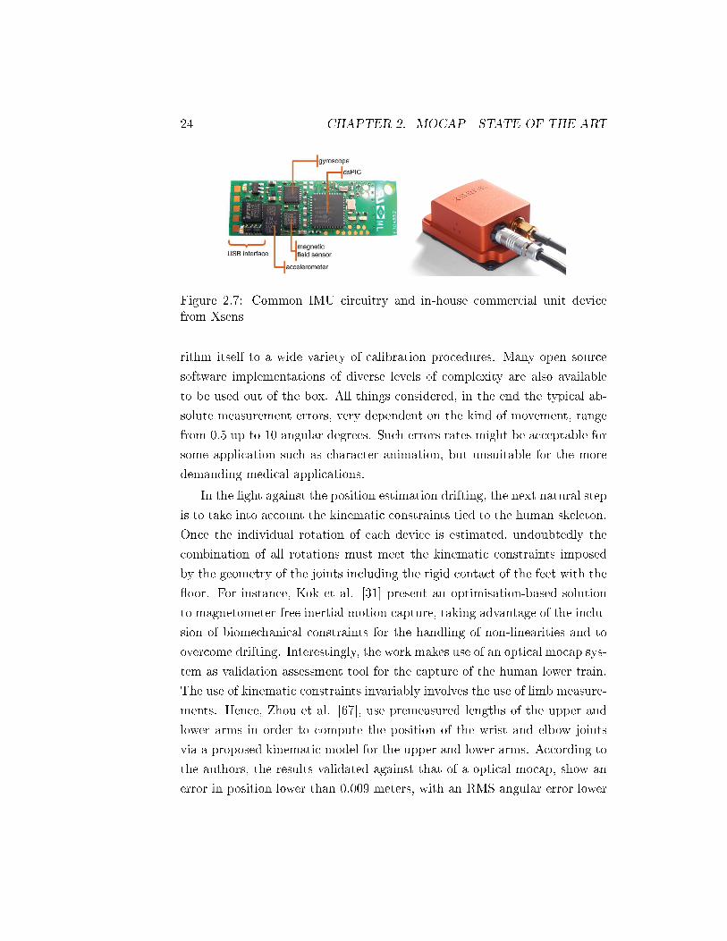
IMUs Inertial Measurement Units (inertial for short) employed in mocap
applications are small electronic devices (see g. 2.7) provided with triax-
ial accelerometers and gyroscopes. Very often, a triaxial magnetometer is
added to the set, hence getting the name of 9 axis sensor after the total
number of independent magnitudes they can measure. They are also known
as gyroscopes or just gyros, since it is the most attention grabbing part of
the hardware.
Nowadays, the motion capture based on inertial devices is probably the
best alternative to optical mocap. It gets rid of the occlusion problem in-
herent to the computation of correspondences between camera views, and
it operates in bigger areas since the person is not subjected to stay in the
eld of view of static sensors, because the sensors are attached to the body
using a sort of special suit (Fig. 2.8). Moreover, the mass production of gy-
roscopic sensors and wireless connectivity components for the mobile market
has notably reduced the price of the units increasing the diversity of avail-
able congurations regarding their characteristics and performance. When
compared to the optical solution, the inertial devices still shows two main
drawbacks: lower levels of accuracy and the inability to catch natively the
absolute position of the object to be tracked. However, both deciencies can
be partially overcomed by sophisticated reverse kinematics calculations.
The basic working principle is as follows. A triaxial gyroscope is a sen-
sor able to measure the rotational speed relative to a reference frame local
to the sensor itself. By numeric integration of the speeds, the absolute 3D
rotation can be estimated. However, despite an accurate measurement of
2.2. MOCAP TECHNOLOGIES 23
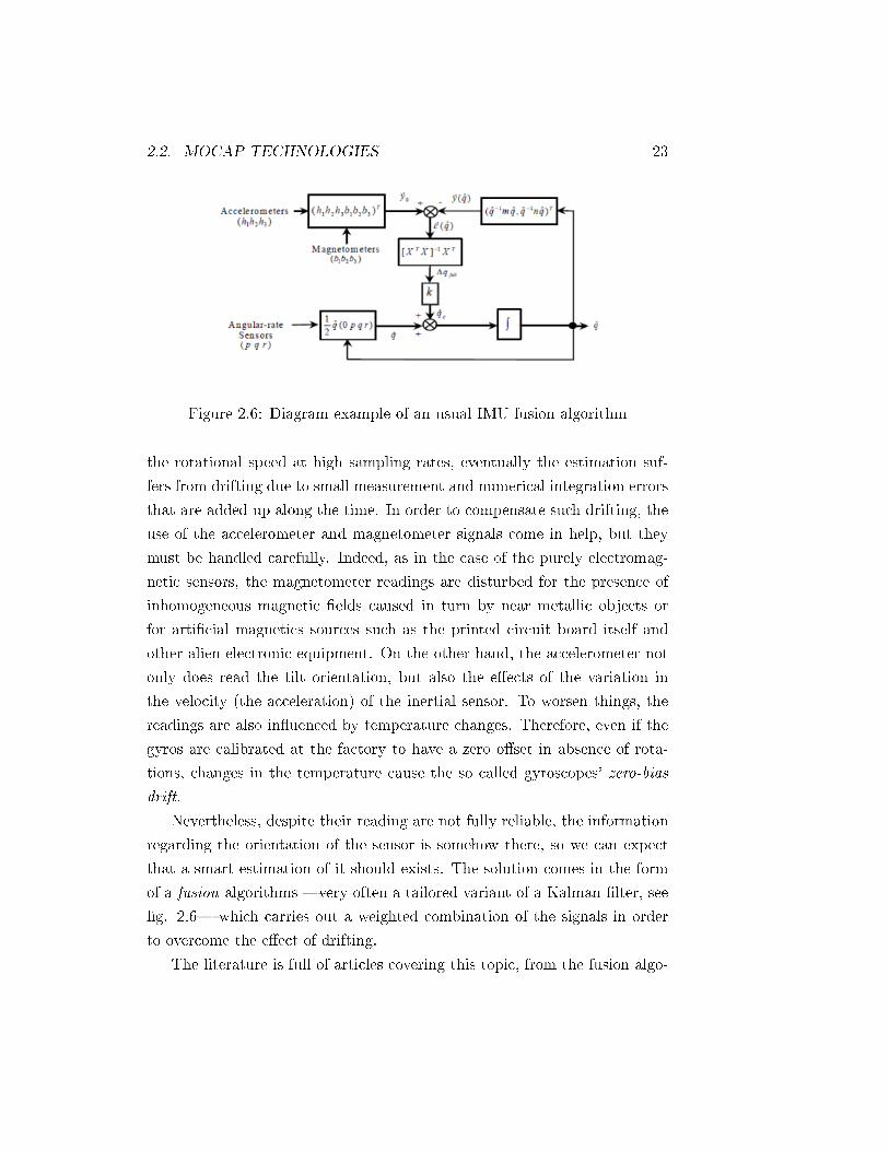
Figure 2.6: Diagram example of an usual IMU fusion algorithm
the rotational speed at high sampling rates, eventually the estimation suf-
fers from drifting due to small measurement and numerical integration errors
that are added up along the time. In order to compensate such drifting, the
use of the accelerometer and magnetometer signals come in help, but they
must be handled carefully. Indeed, as in the case of the purely electromag-
netic sensors, the magnetometer readings are disturbed for the presence of
inhomogeneous magnetic elds caused in turn by near metallic objects or
for articial magnetics sources such as the printed circuit board itself and
other alien electronic equipment. On the other hand, the accelerometer not
only does read the tilt orientation, but also the eects of the variation in
the velocity (the acceleration) of the inertial sensor. To worsen things, the
readings are also inuenced by temperature changes. Therefore, even if the
gyros are calibrated at the factory to have a zero oset in absence of rota-
tions, changes in the temperature cause the so called gyroscopes' zero-bias
drift.
Nevertheless, despite their reading are not fully reliable, the information
regarding the orientation of the sensor is somehow there, so we can expect
that a smart estimation of it should exists. The solution comes in the form
of a fusion algorithms very often a tailored variant of a Kalman lter, see
g. 2.6 which carries out a weighted combination of the signals in order
to overcome the eect of drifting.
The literature is full of articles covering this topic, from the fusion algo-
24 CHAPTER 2. MOCAP - STATE OF THE ART
Figure 2.7: Common IMU circuitry and in-house commercial unit devicefrom Xsens
rithm itself to a wide variety of calibration procedures. Many open source
software implementations of diverse levels of complexity are also available
to be used out of the box. All things considered, in the end the typical ab-
solute measurement errors, very dependent on the kind of movement, range
from 0.5 up to 10 angular degrees. Such errors rates might be acceptable for
some application such as character animation, but unsuitable for the more
demanding medical applications.
In the ght against the position estimation drifting, the next natural step
is to take into account the kinematic constraints tied to the human skeleton.
Once the individual rotation of each device is estimated, undoubtedly the
combination of all rotations must meet the kinematic constraints imposed
by the geometry of the joints including the rigid contact of the feet with the
oor. For instance, Kok et al. [31] present an optimisation-based solution
to magnetometer-free inertial motion capture, taking advantage of the inclu-
sion of biomechanical constraints for the handling of non-linearities and to
overcome drifting. Interestingly, the work makes use of an optical mocap sys-
tem as validation assessment tool for the capture of the human lower train.
The use of kinematic constraints invariably involves the use of limb measure-
ments. Hence, Zhou et al. [67], use premeasured lengths of the upper and
lower arms in order to compute the position of the wrist and elbow joints
via a proposed kinematic model for the upper and lower arms. According to
the authors, the results validated against that of a optical mocap, show an
error in position lower than 0.009 meters, with an RMS angular error lower

2.2. MOCAP TECHNOLOGIES 25
Figure 2.8: IMU motion capture suit
than 3 degrees.
A original approach is taken by Goulermas et al. in [21], where a neural
network estimates joint kinematics by taking account the proximity and gait
trajectory slope information through adaptive weighting. Multiple kernel
bandwidth parameters are used that can adapt to the local data density.
The validation is carried out by comparing the results with those given by
commercial inertial capture systems as well as an optical tracking set up.
Another major issue posed by the use of wearable fabric-embedded sen-
sors is the undesired eect of fabric motion artefacts corrupting movement
signals (and actually, this problem is faced also by the optical marker-based
mocaps). Michael and Howard [45] present a nonparametric method to learn
body movements. The undesired motion artefacts are dealt with as stochas-
tic perturbations of the sensed motion and orthogonal regression techniques
are used to build predictive models of the wearer's motion that eliminate
these artefacts in the learning process.
Alternative wearable systems There is a number of wearable solutions
developed outside the main streams of the industry trying to explore and
push the limits of alternative sensors. For instance, exible nanomateri-
als with excellent electrical properties such as carbon nanotubes, metallic
nanowires or graphene, are being used in strain sensors for the application of
human motion monitoring [63]. Thanks to its ability to be bent or twisted,
it is possible to detect complex movements combining high sensitivity and a
26 CHAPTER 2. MOCAP - STATE OF THE ART
broad sensing range, even including the detection of the pulse and heartbeat.
Zhang et al. [63] work with a wearable graphene-coated ber sensor manu-
factured on purpose for their experimental work. Particularly, the device is
tested to quantify the human body movements during sport performances.
Similarly, Koyama et al. [32] report a single-mode hetero-core optical ber
sensor manufactured and sewed to be sensitive to stretch on the weared fab-
ric. A basic setup composed by just two sets of sensors sense three kinds of
motions at the trunk, which are anteexion, lateral bending, and rotation
and provide enough information to analyse a swing golf movement.
In the line of unconventional hardware, it is possible to nd heterodox
approaches as the ones attempted by Laurijseen et al. [35], that propose
a solution based on the adoption of ultrasonic transmitters and receivers.
The transmitters simultaneously broadcast ultrasonic encoded signals from
a distributed transmitter array (which consists of at least three elements).
Such signals are caught by the receivers built of multiple mobile nodes, each
one equipped with at least three microphones. Using signal processing, a
distance can be calculated between each transmitter and microphone result-
ing in at least nine distances for each mobile node. Using these distances in
combination with the conguration of the transmitters and the microphone
array, not only the XYZ-position of the mobile node but also its rotation can
be estimated. On the other hand, Krigslund et al. [33] present a method
based on a radio frequency identication (RFID) with passive ultra high fre-
quency (UHF) tags placed on the body segments whose kinematics have to
be tracked. The basic principle lies in the fact that the inclination of each
tag can be estimated based on the polarisation of its responses caught by
dual polarised antennas.
Likewise, Baradwaj et al. [7] use IR-UWB (impulse radio-ultra wide-
band) technology to build compact and cost-eective body-worn antennas
able to locate and track human body limb movements. The UWB can be
used for positioning by utilising the time dierence of arrival (TDOA) of the
RF signals between the reference points (beacons) and the target (wearable
device), estimating the distances between them according to the time that it
takes for a radio wave to pass between the two devices. Counting on at least

2.2. MOCAP TECHNOLOGIES 27
three reference points, the calculation of the actual XYZ position follows.
The accuracy achieved with the ultra-wideband technology is several order
of magnitude greater than that of systems based on IMUs, RFID or GPS
signals. Furthermore, the signals can penetrate walls making the technol-
ogy suitable for indoor environments because UWB signals maintain their
integrity and structure even in the presence of noise and multi-path eects.
2.2.3 Markerless Optical Systems
The systems discussed so far entails the use of some kind of hardware devices
to be worn by the body to be tracked. The enticing idea of getting rid of
those obtrusive junk has been and still is a topic of steady and active
research interest. Ideally, the person to be tracked would develop free move-
ment (dancing, wrestling, hugging, ...) in any environment (i.e. no chroma
background is needed) without any item attached to its body, (i.e. excludes
tight capture suits, visual tags, ducial markers, etc) while being recorded
by calibrated, conventional colour cameras. Image segmentation and multi-
view image matching techniques are used to massively track detected salient
points over the person's skin and clothing. In the end, a human kinematic
model is tted to the cloud of the captured points satisfying kinematic, dy-
namic and/or probabilistic constraints. All in all, the huge variety of the
input data no restrictions at all when it comes to background, clothing,
scene environment, movement complexity makes the tasks really challeng-
ing.
So, in Liu et al. [39] present an algorithm able to track multiple char-
acters using a multiview markerless approach. A probabilistic shape and
appearance model exploiting multiview image segmentation is employed to
segment the input images to determine the image regions each person belongs
to, assigning each pixel uniquely to one person. The segmentation allows to
generate separate silhouette contours and image features for each person,
thus reducing the ambiguities. From the shapes and a human articulated
template, a combined optimisation scheme is applied to t each individual
pose. Afterwards, even a surface estimation is carried out to capture detailed

28 CHAPTER 2. MOCAP - STATE OF THE ART
nonrigid deformations, despite the physical model of the cloth is assumed to
be unknown.
Similarly, Zhang et al. [65] present another multi-view approach. In
this case, a multilayer search method is proposed where a new generative
sampling algorithm is introduced: instead of assuming an available body
model tting the subject, the new approach automatically creates a voxel
subject-specic 3D body model which best ts the shape and that can be
created from a large range of initial poses. Despite the parallelization of the
algorithm to speed up the calculations, real time response is limited to no
more than 9fps.
The reconstruction of the movement is carried out by a two steps algo-
rithm by Li et al. [37]. To begin with, a dense depth map estimation is
computed solving the correspondences of points across the cameras. To do
so, in addition to the similarity in the luminance, gradient and smoothness
constraints, the epipolar geometry (derived from the geometric calibration of
the the cameras) is taken into account. A numerical solution for the minimi-
sation of an energy function yields the depth maps of all the views. Finally,
in the seconds step, the point clouds of all the views are merged together
and reconstructed into a 3-D mesh using a marching cubes method with
silhouette constraints.
The emergence of aordable RGB-depth devices such as the Microsoft
Kinect (see g. 2.9, up to 35 million units sold until 2017 7), gave a fresh
starting point for many research approaches. These devices provide a RGB
image matrix together with an estimation of the depth for each pixel, which
certainly is a useful source of data when it comes to motion tracking. How-
ever, being their target market the interaction with entertaining computer
software (replacing the traditional input controllers), the depth map lacks
the required accuracy for demanding mocap applications. Nevertheless, a
number of research eorts tried to push the limits of what can be achieved
from them. For example, Liu et al. [40] present a real-time probabilistic
framework to denoise Kinect captured postures. To do so, a set of Gaussian
Processes are dened in local regions of the state space and employed to7Source: https://en.wikipedia.org/wiki/Kinect

2.2. MOCAP TECHNOLOGIES 29
Figure 2.9: Kinect RGB-Depth device unit
improve the position data obtained from Kinect. To ensure that accurately
acquired areas remain unchanged, a set of joint reliability measurements is
added into the optimisation framework together with a temporal consistency
term to, in turn, constrain the velocity variations between successive frames.
2.2.4 Marker-based Optical Systems
Marker-based optical systems are able to capture the movements of any ob-
ject by tracking special target points known as markers attached to it.
The position of the markers is detected in the images captured by cameras
equipped with an ad hoc lightning system. The markers are usually small
spheres coated with a reective material that returns back the light gener-
ated next to the camera lenses, so that the bright reective markers can be
easily segmented applying a trivial set image intensity threshold, discard-
ing all other elements such the background, skin and clothing. The planar
position of the marker within the two-dimensional BW images captured by
the cameras is estimated as the grey-level weighted centre of gravity of con-
nected pixels. Provided the cameras are calibrated, it is possible to use
photogrammetric techniques to turn a collection of 2D marker centroids into
3D absolute coordinates for each camera pair. The process is repeated over
the time at the cameras frame rate, so that the sequence of Cartesian co-
ordinates of the same marker along a period of time build up its temporal
trajectory. However, since all the markers appear identical it is required
some sort of tracking process to link the coordinates of the same physical
point in contiguous frames, thus avoiding accidental marker identity swaps

30 CHAPTER 2. MOCAP - STATE OF THE ART
that are dicult to recover from. To avoid such errors and to provide a high
coverage of the capture volume, an optical marker capture system typically
consists of around 2 to 32 cameras, or even hundred of them in high-end fa-
cilities. But a high number of cameras does not guarantee a marker identity
swap-free tracking and denitely raises the required budget as well as the
setup complexity.
Marker-based Optical Systems is doubtless the agship of mocap indus-
try. It is a well known technique and widely accepted as the reference in the
eld of animation, sports and medical analysis with dozens of successful eld
application. Despite its drawbacks (namely: expensive hardware/software,
dicult to set up, and tricky to handle), its hegemoty hasn't been beaten
in the last decades, although many attempts have been driven towards more
aordable, reliable and ease-to-use alternatives. Partly, this is due to the
advances in the industry of optical systems providing the market with af-
fordable hardware and software accessible enough to be used out-of-the-box
requiring only a short training.
By and large, most of the issues risen during the design of a optical mocap
(see Chapter 3) have been discussed in the literature and known solutions
are available for them. For instance, camera calibration (see section 3.3) is
a topic widely covered in the eld of machine vision. Biomechanical compu-
tation, in charge of turning marker XYZ components into meaningful body
parameters such as vectors, angles, degrees of freedom (Figs. 2.10 and 2.11),
has been tackled in mechanical engineering, whereas the representation of
the capture data (3D rendering, chart visualisation, ...) falls in the domain
of computer graphics and data visualisation. Regarding the hardware (cam-
eras and wires), suitable solutions including the lightning, can be borrowed
from the industrial vision machine market.
That said, however, a key problem to be solved for marker-based capture
as it is the automatic marker labelling, is seldom covered in the literature.
The most immediate consideration is that we can identify each marker in
accordance to some continuity restriction along the frames, also supported
by the kinematic constraints of the underlying human skeleton. Hence, the
natural approach [18][22] is to keep the track along the time axis using trajec-

2.2. MOCAP TECHNOLOGIES 31
tory estimators, predicting next marker positions from those in the previous
frames. In some cases, such prediction is achieved by means of a Kalman
lter tuned to t each particular marker behaviour. Given an estimation
on the movement, an energy function is formulated between the predicted
trajectory and the provided point cloud and some kind of energy minimi-
sation algorithm is applied to assign the labels. The value to optimise is
very often the mean or weighted distance between the candidates and the
predicted marker positions [44][51][41] while the minimisation algorithm is a
tailored implementation of the well known Hungarian method [34]. However
this strategy turns out to be error prone when it comes to deal with marker
occlusions (points kept out of sight of the cameras) lasting several consecu-
tive frames and have diculties to recover from small errors, often leading to
divergent behaviours. In absence of a reliable trajectory estimation the goal
function becomes untrustworthy to assess the right labelling. On the other
hand, the appraisal of future marker movement based in its recent trajectory
is simply too uncertain for very abrupt movements. As it has been pointed
out, it is like `trying to drive your car forward looking through the rear view
mirror.'
So as to strengthen the marker labelling recovery after a long lasting
occlusion, some authors take advantage of the underlying human skeleton
geometry by the identication of the markers belonging to the same body
limb. The markers can be clustered analysing the pairwise distance along
the time keeping in mind that the skin movement and other artefacts pre-
vents us from using classical rigid body restrictions. The identication of
a reappeared maker is backed up by the identication of those sharing the
same limb. This method may fail in case of massive occlusions where nearly
all markers from the same limb have been hid for too long. Some authors
[44][41] face these most adverse situations, exploiting the fact that the mark-
ers are placed over a articulated mechanism. Not only do the markers belong
to the same rigid bodies and therefore the distances among them are sup-
posed to remain the same along the time [62][42], but also the limbs are
linked between them by means of physical joints. Hence, the overall range of
movements is limited. In other words, they suggest to make use of kinematic

32 CHAPTER 2. MOCAP - STATE OF THE ART
(direct or inverse depending on the author) calculation techniques. Hence,
the number of degrees of freedom (DOF) of the underlying mechanism is re-
stricted and so is the feasible marker labelling. This contributes to identify
markers after a long time occlusion.
For instance, in [44], after standing the person to be tracked in an approx-
imate T-pose, the proposed method can estimate the skeleton conguration
through least-squares optimisation. Afterwards, a probabilistic tracking is
carried out exploiting the skeleton structure to prevent the algorithm from
drifting the it away. At each frame, the algorithm determines the maximum
likelihood skeleton conguration (pose) given the unlabelled, noisy observa-
tions of markers. The goal is to nd the conguration of the skeleton that
minimises the quadratic error, which is the quadratic distance between the
estimated position of the markers for a given conguration and the actual
marker observation. To improve the feasibility of the skeleton pose estima-
tion, penalties are included in the goal function for those joint congurations
that are outside of certain limits dened by considering the natural ranges
of the joint movement. For instance, the knee joint is constrained to a plane
(1 degree of freedom) and enclosed in a certain range that prevents it from
bending forwards. At each frame, an optimisation procedure is carried out,
usually converging after a few iterations. In the backstage lies the condence
in the correctness of the pose estimation for the previous frame, as from it
the initial estimation of the next iterative process is initialised. This depen-
dency on previous frames may lead to the failure of the convergence when
massive or lasting occlusions occurs.
Yu et al. [62] point out that the markers must be labelled along the time
in such way that a certain distances between them remain approximately
constant up to a given tolerance. Indeed this is true for markers placed over
the same limb (rigid body), assuming small shifts due to skin/mesh/clothing
artefacts. Moreover, even markers placed in dierent limbs must keep a range
of distances between them, as is the case of markers placed on the head re-
spect to markers in the hips. Therefore, for all the unlabelled markers along
the frames of a training session, the standard deviation of all possible pair
distances are computed. After that, the markers are clustered in groups

2.2. MOCAP TECHNOLOGIES 33
Figure 2.10: Human body kinematic model (left) and leg detail (right)
with a group-internal standard deviation small enough to form a rigid body
(interestingly, this links right way with the concept of feature discussed later
in 4.3). These clusters, together with their internal distances and standard
deviations, are taken into account during the labelling stage. At each consec-
utive frame, the correspondences are progressively assigned in an exhaustive
search so that the markers achieve a computed score according to how well
they t the learnt distances. To speed up the process, only a few candidates
are considered for each marker relying in the continuity of its trajectory.
Again, the correctness of the labelling in the previous frame plays a crucial
role in the overall performance.
Shubert et al. [51] also ask the person to be tracked to start in T-stance
to initialise the tracking process. However, the problem takes a more generic
shape, because their goal is the automatic initialisation of the tracking of an-
imals who will barely take notice of the system demands. In their approach,
the authors make use of a large database of previously observed poses for
the corresponding skeleton. Given a new initial frame, the set of markers are
matched across the database, scaling and rotating in whatever way it takes

34 CHAPTER 2. MOCAP - STATE OF THE ART
Figure 2.11: Marker based mocap suite and its 3D counterpart
to t a particular sample. Several considerations, some based on a k-means
algorithm, are made to speed up the whole process, discarding most of the
false matches at an early stage. After the initialisation, the tracking itself
follows. The most likely skeleton conguration is the one which minimises
the distance between the predicted marker position and the observations.
And identically, the goal function includes a quadratic joint limit cost term,
which penalises abnormal joint congurations.
The marker labelling turns up to be particularly dicult in the case of
hand tracking due to self-occlusion between the ngers. In [41], an algorithm
is presented for the fully automatic tracking of hands, where a kinematic
model of the underlying skeleton is employed to resolve ambiguities. The
method tries to t models (rigid or articulated) by minimising the overall dis-
tance error to the 3D unlabelled point data. Initially, the models are aligned
to the target by trying all possible combinations in a brute-force manner and
selecting the assignment with the lowest cost using the Hungarian method.
Afterwards, the skeleton pose is estimated by inverse kinematics, minimis-
ing an energy function that represents the least squares error between the
models and the targets. In contrast to direct kinematics, where the position
of each body in an open loop is explicitly computed from the degrees of
freedom (DOFs, mainly angles at the joints), the inverse kinematics stands
for the calculation of the DOFs from the position of the bodies (hence the
word inverse), which usually entails the solving of a system of equations.
The main advantage of the approach is a higher resilience against random

2.2. MOCAP TECHNOLOGIES 35
occlusions of markers belonging to intermediate kinematic chain segments.
Despite devoted to hand and face tracking, the overall problem of marker
tracking is perfectly stated by Alexanderson et al. [1]. In this paper, the
authors highlight the fact that in passive marker tracking the underlying
problem arises from a lack of individual discriminating features for identify-
ing the markers. When placed on rigid objects or kinematic chains (such as
human skeletons), it is possible to provide more or less invariant features that
help to solve ambiguities. However, markers placed on more exible struc-
tures such as ngers and faces yield much more ambiguous information. In
addition, the uncertainty in the spatial information is especially problematic
if temporal coherence is deteriorated due to frequent occlusions or stretches
of noisy data. To address these problems, this paper introduces two main
concepts: the generation of multiple ranked hypotheses from the spatial dis-
tribution of the unlabelled markers in each frame and a hypothesis selection
method for selecting a smooth sequence of assignments in time. That way,
the lack of information is overcome by using multiple hypotheses that post-
pone decisions until more discriminative observations arrive. The hypothesis
generation uses a collection of Gaussian Mixture Models (GMMs) to model
each marker's location in space, while hypothesis selection uses Kalman l-
ters and the Viterbi algorithm to determine the best sequence of hypotheses
in time.
In addition to the academic approaches mentioned above, there is a num-
ber of commercial solutions available for marker tracking such as Motive,
from Optitrack 8, Cortex (developed by Motion Analysis 9 ), Track Man-
ager (from Qualisys) or Clima (by s.t.t.). Little has been published about
the details of the internal tracking mechanism they implement due to the
proprietary nature of these packages. The only information is provided by
descriptive brochures or yers. For example, it is known that the software
from Qualisys10 uses a tracking algorithm (named AIM, which stands for
Automatic Identication of Markers) that basically learns from each manu-
8https://optitrack.com/products/motive/9https://motionanalysis.com/
10https://www.qualisys.com/software/qualisys-track-manager/

36 CHAPTER 2. MOCAP - STATE OF THE ART
ally veried track. What this means in practice is that after labelling each
marker the underlying model is updated. When a new track is provided to
the system, it applies the model and attempts to automatically label the
markers over the whole trial, automatically lling in gaps of certain sizes.
Apparently, huge benets are obtained when markers icker or disappear for
short periods of the movement since the AIM model automatically labels
them when they reappear.

Chapter 3
Optical Motion Capture -
Components
This chapter is devoted to provide a comprehensive knowledge of the compo-
nents of an optical capture system in order to understand the circumstances
of the labelling task, which is the main research topic of this Thesis. All other
optical capture tasks conceal issues whose solutions are pretty straightfor-
ward or requires the use of methods and algorithms already widely discussed
in the literature so they and won't be treated deeply here. We start dis-
cussing sensors, and the sensor deployment in a typical system. Next we
present the concepts of photogrammetry that allow the recovery of the 3D
position of the optical markers. The nal part of the chapter presents the
overall computational pipeline involved in the mocap system and the analysis
of the data obtained from mocap sessions.
3.1 Sensors
3.1.1 Markers
Doubtless, the emblem of the optical motion capture is the reective marker
itself (see g. 3.1). Normally it is manufactured as a little ball made out of
plastic or cork, covered with a layer of reective material very similar to the
37

38 CHAPTER 3. OPTICAL MOTION CAPTURE - COMPONENTS
Figure 3.1: Marker specimen
Figure 3.2: Lightning setup
used in the reective vests. Its main purpose is to return back the light that
falls upon its surcafe in the same direction that it arrives.
That way, the light sent by a source placed right next to the camera
hits the marker and is sent back to the camera as shown in g. 3.2, being
captured by its optics and nally reaching the camera sensor. The electronic
sensor image is composed by a 2D array of photosensitive cells producing up
a 2D grey-scale image of pixels arranged by rows and columns (see g. 3.3).
The value read from each cell is proportional to the intensity of light received
by it. After applying a threshold lter to the whole image, the pixels not

3.1. SENSORS 39
Figure 3.3: Image marker 2D position
corresponding to a marker are ruled out. The remaining ones are processes
by image connectivity analysis algorithm, yielding a list of XY centroids with
the location, in the reference frame of the image, of all the visible markers.
With the purpose of being less intrusive and to optimise the image con-
trast against the background, very often light in the infrared wave length is
used to illuminate the markers. The light source is originated in a ring of IR
LEDs arranged around the camera lens. In addition, the lenses are equipped
with a IR passband lter which reduces the ambient light noise.
3.1.2 Cameras
In contrast with the simplicity of a marker, the cameras are the more so-
phisticated elements of the electronic sensorization (like the model shown in
g. 3.4). Hence, the optical marker systems are not considered a wearable,
since the actual sensors are placed outside the object to be tracked instead
of attached to it. The main features of motion capture cameras are:
Image resolution: from VGA sizes (640x480) up to megapixel reso-
lutions (1920x1080, 2048x2048, ...), a bigger size stands for a bigger

40 CHAPTER 3. OPTICAL MOTION CAPTURE - COMPONENTS
Figure 3.4: Motion capture camera with built-in IR lightning source and itsexploded view. Drawing borrowed from the Optitrack web site

3.1. SENSORS 41
Figure 3.5: Camera eld of view (FOV).
sensitivity (metric units per pixel) to the spatial position. In addition,
it is easier to make out very proximate markers and their actual size can
be smaller. The set o is that the listing price increases accordingly;
Field of view (FOV), illustrated in 3.5: angular range of sight of the
camera. The bigger it is, the bigger is the coverage of marker detection.
In return, as the number of pixel cells remains the same, the sensitivity
level to the position goes down with larger FOVs;
Sampling rate (Hz): number of images captured per second. Com-
mon acquisition frequencies range between 50 and 100Hz, enough to
properly acquire most of human movements. However, more and more
advanced models are able to record up to 200Hz for high end appli-
cations or just to serve as distinctness towards the competence. Very
often the camera allows to look for a trade o between resolution and
frequency, a valuable feature that makes it all terrain models;

42 CHAPTER 3. OPTICAL MOTION CAPTURE - COMPONENTS
IR light source: in the case of mocap cameras the IR lighting is inte-
grated in the device housing, easing the setup and deployment;
Sync: as will be explained later, the calculation of 3D marker positions
require the simultaneous detection of the marker in at least two cam-
eras. Therefore, the images have to be acquired synchronously by the
hardware requiring a wired sync mechanism;
On-board processing: in the past, the image processing was carried out
in the host computer. However, modern mocap cameras have basic on-
board image processing software so as to extract 2D marker coordinates
right out from the raw image. This lighten the processing in the com-
puter but, best of all, it drastically reduces the data trac between
the cameras and the host, making it less prone to wired data transfer
failures;
Connectivity: all the information generated in the camera must be sent
to the host by means of some kind of communication protocol. The
most common standard used is Ethernet (both wired and WiFi) and
USB cabling, but image specic interfaces or even proprietary solutions
can be found in the market;
Control and SDK: for the remote conguration and control of the cam-
eras, the manufacturer usually provides a SDK (software development
kit), which makes possible a seamless integration in 3rd party software;
3.2 System deployment
3.2.1 System location
There are a few recommendations when it comes to choose a suitable setup
location and arrange it to avoid some basic troubles. In this section some key
ideas are given for human body motion capture, but similar considerations
might be taken for other specic applications (hand or face motion capture,
tool tracking, ...).

3.2. SYSTEM DEPLOYMENT 43
We must pick an indoor location where to place the system. Motion
capture cameras are IR light sensitive and despite some manufacturers claim
that their models are not aected by sunlight, in fact the sun turns out to
be a hassle always. For this reason, it is highly recommended to cover all
windows/hatches to block the natural daylight that might come into. The
technician must seek and remove any reective objects (shiny parts, polished
surfaces, ... non-reective tapes are his/her best friend here!) other than the
markers themselves, as well as hot light sources such as light bulbs. The
use of matte rubber carpets is often the best choice for covering reective
ooring.
The location should have room enough not only to develop the movement
but also to accommodate further equipment such as computers, screens,
tables and so on. In addition to the space needed for the movement, there is
a minimum distance between the cameras and the markers depending on the
eld of view (the smaller eld of view, the more distance is required) which
demands an extra dead unused surrounding area between human body and
cameras.
Once the system is calibrated, a process that may take some time and
annoying physical eort, any tiny unintended displacement of the cameras
would invalidate the calculation and therefore a brand new calibration pro-
cess must be carried out. To prevent such cases, the use of wall mounts
instead of tripods is a great choice. On the other hand, setting up the cam-
eras at a high elevation (typically from 220 to 260cms) enhances the coverage
of the capture volume, reducing the chance of marker occlusion and widening
the sight of view.
Last but not least, it is recommended to remove any obstacle and un-
necessary object from the capture area scene that may prevent the markers
from being detected by the cameras.
3.2.2 Camera Arrangement
The common guidelines to properly place the cameras around the capture
area for human body tracking include:

44 CHAPTER 3. OPTICAL MOTION CAPTURE - COMPONENTS
Figure 3.6: Typical camera distribution around the capture area.
to evenly place the cameras in a ring around a common centre, as show
in g 3.6;
to mount the cameras at least at the maximum height of the capture
volume;
to point the cameras inwards, adjusting the tile and heading angles
and tightening the corresponding handles and screws to prevent them
from moving;
landscape orientations of the FOV increases the horizontal coverage
area;
avoid letting any camera IR ring fall in the sight of another: otherwise
it might be taken as a legitimate marker.

3.3. PHOTOGRAMETRY 45
3.3 Photogrametry
As it has been exposed in section 3.1, the sensors will convey us an anony-
mous collection of 2D coordinates in pixel units. A dierent, unsorted list of
2D projections will be made available per camera, with no information at all
regarding the right matching among them. However, we are interested in the
3D X,Y, Z coordinates in world reference frame, where the real movement
is taking place, computed from the local pixel x, y coordinates.
Mathematical model Photogrametry is a well known topic in the eld
of machine vision, supply us with the required calculation tools to relate 2D
and 3D camera coordinates.
Let P = X,Y, Z denote a Cartesian point in R3 given in metric units,
in a inertial reference frame. Knowing the position P0 and orientation R3x3
of a camera in that reference frame allows us to evaluate the orthogonal
projection P ′ = X ′, Y ′, Z ′ of P in the camera plane.
P ′ = R (P − P0) (3.1)
The actual value of the Z ′ component is the distance from the point to
the camera, and together with the eective focal length allows us to compute
the projective coordinates x′, y′ according to the pinhole model.
x′
y′
=
f
Z ′
X ′
Y ′
(3.2)
However, in the former equality we are missing the optic distortion (g.
3.7) introduced by the camera lenses. Instead of getting x′, y′ right outfrom the sensors, what we get is its x, y distorted version. From [23], we
reproduce here a successful model for the 2D distortion:
x′r
y′r
=
x′(k1r
2 + k2r4 + . . .
)y′(k1r² + k2r
4 + . . .) (3.3)

46 CHAPTER 3. OPTICAL MOTION CAPTURE - COMPONENTS
Figure 3.7: Eects of lens distortion.
x′t
y′t
=
2p1x
′y′ + p2
(r2 + 2x′2
)p1
(r² + 2y′2
)+ 2p2x
′y′
(3.4)
where r =√x′2 + y′2. The expression 3.3 is the so called radial distor-
tion, whereas 3.4 is the tangential distortion. Putting everything together,
we can build the complete expression relating the 2D coordinates as:
x
y
=
fx(x′ + x′r + x′t
)fy(y′ + y′r + y′t
) +
x0
y0
=⇒
=⇒
x
y
= D
(x′
y′
)(3.5)
As a whole, these expressions link the 3D real coordinates of a point P
with its 2D counterpart version on each camera provided we know the nu-
meric value of its spatial position. Additionally, we need the numeric value
of the position and orientation of the camera R,P0, as well as a denite
value for f , k1,k2,... kn, p1,p2 x0 y y0. The former R y P0 are known
as extrinsic parameters, for that they dene the position of the camera in
the space. The latter, are the intrinsic parameters, which depend only on
physical characteristics of the lens and remain unchanged no matter where
the camera is placed. As explained later, the whole set of camera parame-
ters H are estimated for a camera by a process named calibration. One
particular camera is said to be calibrated if we know the right values for H.

3.3. PHOTOGRAMETRY 47
Projection Written in a compact way, we got the following equalities:
xai = gx (Xi, Yi, Zi, Ha)yai = gy (Xi, Yi, Zi, Ha)
⇒
⇒
xaiyai
= G (Xi, Yi, Zi, Ha)⇒
⇒ pai = G (Pi, Ha) (3.6)
where gx and gy are functions whose symbolic expression is known and
explicit on pai , the projection in pixel units of Pi on camera a, for which
its calibration is encoded in H. These expressions yield the values of the
projection, without the need to solve any system of equations. However,
they can play the role of equalities too, involving all the mentioned variables,
which in turn have to meet them any time:
xai = gx (Xi, Yi, Zi, Ha)yai = gy (Xi, Yi, Zi, Ha)
⇒
xai − gx (Xi, Yi, Zi, Ha) = 0
yai − gy (Xi, Yi, Zi, Ha) = 0(3.7)
Composition The inverse operation to projection is the composition, that
is to say, the reconstruction of the 3D coordinates of a point starting from its
known projections xai , yai and a valid set of calibration parameters Ha.The unknowns in this case are spatial coordinates (Xi, Yi, Zi) what in balance
with the number of equations results in 1 dimension against (indeed, such
dimension is the position along the projection line itself). So as to limit
the solution to a unique point, we need to look for more constraints and
consequently we turn to a second camera b:
pai = G (Pi, Ha)
pbi = G(Pi, H
b) =⇒
xai − gx (Xi, Yi, Zi, Ha) = 0
yai − gy (Xi, Yi, Zi, Ha) = 0
xbi − gx(Xi, Yi, Zi,
Hb)
= 0
ybi − gy(Xi, Yi, Zi,
Hb)
= 0
=⇒

48 CHAPTER 3. OPTICAL MOTION CAPTURE - COMPONENTS
Figure 3.8: Synthesis of 3D coordinates from 2D projections.
=⇒Q(pai , p
bi , Pi, H
a, Hb)
= 0 (3.8)
These constraints build up a overdetermined system of 4 equations and
3 unknowns and certainly might not have a valid solution. If not the case,
its resolution would yield a specic value for the position of the point in
3D. Due to the non-linear nature of the expressions, we have to draw on to
numeric iterative solving methods such as Newton-Raphson or Levenberg
Marquardt.
From a geometric point of view, the projection equations in 3.8 corre-
spond to the equations of a line in the space, throughout which the point is
projected into the camera. The intersection, if they meet, of to lines uniquely
determines the position of the point (gure 3.8). Otherwise, the lines skew
and denitely pai and pbi do not belong to the same real 3D point (certain 2D
mismatch, see gure 3.9).
The fullment of the equations is a necessary but not sucient condition
to take the validity of the match between pai as pbi as granted. If two 3D
points lie in the same plane simultaneously with two camera centres P ao ,
P bo , it is possible to compute up to 4 algebraic solutions for 3.8 by just the
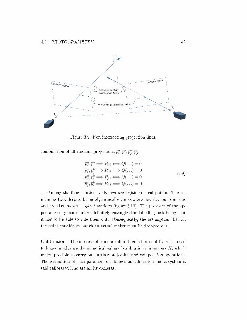
3.3. PHOTOGRAMETRY 49
Figure 3.9: Non intersecting projection lines.
combination of all the four projections pai , pbi , p
aj , p
bj :
pai , pbi =⇒ Pi,i ⇐⇒ Q(. . .) = 0
pai , pbj =⇒ Pi,j ⇐⇒ Q(. . .) = 0
paj , pbi =⇒ Pj,i ⇐⇒ Q(. . .) = 0
paj , pbi =⇒ Pj,j ⇐⇒ Q(. . .) = 0
(3.9)
Among the four solutions only two are legitimate real points. The re-
maining two, despite being algebraically correct, are not real but spurious
and are also known as ghost markers (gure 3.10). The prospect of the ap-
pearance of ghost markers denitely entangles the labelling task being that
it has to be able to rule them out. Consequently, the assumption that all
the point candidates match an actual maker must be dropped out.
Calibration The interest of camera calibration is born out from the need
to know in advance the numerical value of calibration parameters H, which
makes possible to carry out further projection and composition operations.
The estimation of such parameters is known as calibration and a system is
said calibrated if so are all its cameras.

50 CHAPTER 3. OPTICAL MOTION CAPTURE - COMPONENTS
Figure 3.10: Ghost markers synthesis as result of geometric coplanarity be-tween two cameras and two real markers.
The camera calibration is a topic widely covered by the literature in the
eld. Zhang [66] makes an excellent introduction to the epipolar geometry
and the fundamental matrix and provides a detailed review on the numerical
techniques to estimate them from 2D point correspondences even in the pres-
ence of outliers due to bad locations or false matches. The topics of ane
transformation and projective reconstruction are discussed as well, but the
lens distortion correction is marginally mentioned. In [64], the same author
introduces a brand new calibration procedure requiring just the observation
of a simple planar pattern at dierent viewing positions instead of using
expensive equipment, being this time the radial lens distortion taken into
account. In [23], a complete camera mathematical model including an ac-
curate lens distortion eect is discussed. In addition, a method is proposed
to estimate the undistorted coordinates from the natural ones. Just in ex-
change of a little but protable preprocessing, the authors show that it is
possible to build explicit symbolic expressions to do so, thus avoiding the
need of solving non linear equations.
In the end, the key when it comes to pick one method over other is the
kind of available data:

3.3. PHOTOGRAMETRY 51
do we count on 2D point and/or axis correspondences?
can those correspondences contain outliers? If so, how often?
which is the numeric condition of the data for which the numerical
methods are sensitive to? Are the samples evenly distributed or too
close?
do we count on metric information? (known point positions, distance
between points/lines, ...)
All in all, the calibration process needs to be fed with input data coming
from the camera system itself. When it comes to motion capture cameras,
the most universally adopted solution is the use of a narrow wand stick with
three markers on it as the calibration object. These three markers U , V and
W , remain aligned and at an invariable, known distance between them. The
stick is recorded roaming around the capture area covered by the sight of the
cameras. At each i-th frame a set of 2D projections are captured and, by
means of a plain identication, their correspondences can be matched across
the cameras.
After that, the 2D projections can be put into the equations 3.7, adding
up more equations restricting the known distances and forcing the unknowns
to keep in a straight line:
for each i-th frame −→
Q(paU,i, p
bU,i, PU,i, H
a, Hb)
= 0
Q(paV,i, p
bV,i, PV,i, H
a, Hb)
= 0
Q(paW,i, p
bW,i, PW,i, H
a, Hb)
= 0
‖PU,i − PV,i‖ − dU,V = 0
‖PV,i − PW,i‖ − dV,W = 0
‖PW,i − PU,i‖ − dW,U = 0
‖(PU − PV )× (PW − PV )‖ = 0
(3.10)
Again, numerical optimization methods are used to solve this set of equa-
tions. However, conversely to the case of the 3D composition the main chal-

52 CHAPTER 3. OPTICAL MOTION CAPTURE - COMPONENTS
lenge here is a) the handling of a high number of equations (16 per recorded
frame) and unknowns (13 + 9 per recorded frame) and b) the guarantee of
convergence of the numerical iterative process itself.
To deal with a), the symbolic manipulation of 3.10 manages the elimi-
nation of PU , PV , PW from the stage, following a xed number of unknowns
that wont grow with the number of samples. When it comes to b), a good
estimation for the position and orientation of the cameras can be calculated
from the fundamental matrix, which in turn can be reliably estimated from
just 2D point correspondences even in the case of outliers (see [66]).
Accuracy and sensitivity. Repeatability. As it happens with any mea-
surement tool and indeed a optical capture system is, it is possible to
wonder about the specs about it. What accuracy level can be achieved?
How sensitive is it? To answer these questions, and as a side result of the
calibration process carried out over actual data, we can get an indication for
them just by means of little extra calculation. These values will be of special
interest in some of the next stages.
The accuracy quality answers the question `how exact is the measurement
of a 3D coordinate?' Once the calibration process is nished, we can take the
calculated values for the calibration points and assess their computed dis-
tances against the actual wand stick lengths. Normally they wont perfectly
match, and the dierence is a trusty indicator of the accuracy. Moreover, as
the calibration wand stick has been recorded ideally roaming all the eld of
view, we can compute an estimation of the accuracy for each spatial location.
The less the mean error, the higher the accuracy:
mean error =1
3n
n∑i=1
∑<j,k>=U,V,W
|‖Pj,i − Pk,i‖ − dj,k|
On the other hand, the sensitivity stands for the least shift in the mea-
surement that is noticeable by the measurement tool. In our case, we are
interested for the least 3D displacement of a marker that we can detect as
an actual change in the 3D composition for a given camera setup. Actually,

3.3. PHOTOGRAMETRY 53
sensitivity is closely related with ∇f , the gradient of a scalar function f with
respect to its variables, being in our case f any of fx, fy or fz, the ones who
computes each one of the components of a 3D point depending on its local
projections in two cameras pa, pb.
f = f (pa, pb) =⇒ ∇f =
∂f
∂pax,∂f
∂pay,∂f
∂pbx,∂f
∂pby
In order to numerically estimate it, we can use the one-factor-at-a-time
(OAT) method to measure the eect on the output of moving an input
variable while keeping the others unchanged. The amount ∆p we move an
input variable is in turn the sensitivity of the system to the measurement of
local 2D coordinates, which either can be found as part of the cameras specs
or can be experimentally estimated. Thereby, sensitivity S of fxto pax is:
Spaxx = |fx (pax +∆pax, . . .)− fx (pax −∆pax, . . .)|
Up to 12 sensitivity scalar values can be computed (3 axis on 4 local
coordinates), being its average the eective sensitivity of the system at the
particular point XY Z in space, composed by the projections pa, pb:
S = S (X,Y, Z)
Finally, repeatability is and indicator of how stable is the output of the
measuring tool along successive measurements of the same measurand while
keeping all surrounding conditions unchanged. In the case of an optical
system its estimation is rather trivial: we proceed by just taking several
snapshots of a marker at a stationary position and calculating the mean
dierence of its composition respect to the average. In can be estimated
for dierent positions inside the capture sight, but in practice it remains
far below the accuracy and sensitivity as long as the lightning is even and
constant.

54 CHAPTER 3. OPTICAL MOTION CAPTURE - COMPONENTS
Figure 3.11: Process stages overview.
3.4 Process stages
In this section the basic pipeline (outlined in gure 3.11) of a motion capture
process is described, pointing out the role played by each stage in the whole
system as well as the way they link between them.
Camera settings and control Normally the hardware namely the
cameras oers a bunch of settings to govern its behaviour (see 3.1.2).
These settings can be controlled by means of the SDK run by the software
on a host controlling computer according to the user needs or wishes. Above
them is the dispatch of start/stop acquisition commands that brings the pro-
cess into play and the monitoring of potential faults in the data transfer and
hardware performance.

3.4. PROCESS STAGES 55
Acquisition Once commanded, the acquisition stage is in charge of col-
lecting the images captured from the cameras. The input data is the light
coming through the lenses, and the output are raw digitised images. In addi-
tion, capture cameras may have the functionality of processing the images to
extract the 2D marker centroids right out from them by means of an thresh-
old followed by a connectivity analysis. Being that the case, the output data
is right way a list of 2D coordinates per frame, which denitely eases the
communication with the next stage. Sometimes, the output includes further
information such as sync data with external devices (force platforms, elec-
tromyography, ...) as well as a report regarding the healthy status of the
hardware.
3D massive composition This stage is the responsible of building all the
3D points covered by the cameras sight. The input data is the 2D local
coordinates coming from each camera at each frame, as well as the current
camera calibration parameters and system accuracy and sensitivity. The
output data is the set of geometrically feasible points seen by the cameras.
Since the input 2D points are unmatched across the cameras, it is manda-
tory to compute all feasible combinations (see 3.3) to check whether they
are geometrically correct or not. In a rst screen, many wrong mismatches
are ruled out but indeed some ghost points can drain to the next stage, as
well a set of spurious compositions built from non-markers spot detection
(sunlight, shiny parts, ...).
3D Clustering and merging Just two 2D Projection are enough to build
a 3D coordinate. But very often particularly in systems composed by many
cameras it happens that the same marker is simultaneously seen by more
than two, let's say n, cameras. If that the case, that real point is repeatedly
composed up to
(n
2
)= n(n−1)
2 times. For instance, in a system of 6
cameras, up to 15 XYZ versions of the same point can be recovered.
So, the goal of this stage is to merge all the occurrences of the same point
into a single one so that there can be only one. To do so, two conditions

56 CHAPTER 3. OPTICAL MOTION CAPTURE - COMPONENTS
Algorithm 3.1 3D massive point composition algorithmInput data:
set of calibration parameter for each of a total of nc cameras H =H1, H2, . . . ,Hnc;
the set of 2D local coordinate points list per camerapa1, p
a2, . . . , p
anma
,pbi, . . . ;
accuracy calibration info;
Output data:
Praw, the set of 3D global coordinate points coherent according tophotogrametry equations up to the given tolerance;
Algorithm:
1. for each camera pair < a, b >:
(a) for each point pair < pai , pbj >:
i. synthesise corresponding 3D point P a,bi,j ;
ii. compute synthesis equations residue ra,bi,j ;
iii. is ra,bi,j below the calibration sensitivity? If so, add P a,bi,j toPraw;

3.4. PROCESS STAGES 57
Algorithm 3.2 3D clustering and merging algorithmInput data:
Praw, the set of 3D synthesised points;
sensitivity calibration info;
Output data:
C, the set of 3D merged candidate points;
Algorithm:
1. for each raw point pair < P a,bi,j , Pc,dk,l >:
(a) compute new point Pfuss as(Pa,bi,j +P c,d
k,l
)/2;
(b) is∥∥∥P a,bi,j − P
c,dk,l
∥∥∥ < S (Pfuss) ? If not so, continue to the next loop
cycle;
(c) if a=c and i6=k, continue to the next loop cycle;
(d) if b=d and j6=l, continue to the next loop cycle;
(e) add Pfuss to C;
2. add the remaining points from Praw to C:
have to be met:
1. the distance between the merged points is below a given limit, set
according to the sensitivity of the system, playing here its starring
role;
2. the merged points are not permitted to use dierent 2D projections
belonging to the same camera;
Labelling The mission of this stage is to map each marker to be tracked
to either a observed point or to a null (hidden) label with a certain level of
certainty. The input data is the set of merged points, from now on denoted
as candidates, among which can be included spurious points (those that

58 CHAPTER 3. OPTICAL MOTION CAPTURE - COMPONENTS
shouldn't be assigned to any label). It may happen as well that some real
markers be missing, due to occlusions or just because they fall out of the
sight of the cameras. The output is the labelling of each candidate point
belonging to C, stating either:
it doesn't condently match with any of the markers to be tracked;
which marker does it match, together with a condence index;
The development of a labelling algorithm is the core research topic and main
contribution of this work and is thoroughly discussed in chapter 4.
Biomechanics The job is not nished with the marker labelling. The
nal purpose of a optical capture system is the analysis of the movement
rather that the capture itself. The nal user is looking for particular data
depending on the on eld it is being applied: clinical analysis, sportive per-
formance, entertainment, character animation ... In the case of the tracking
of human bodies, a marker trajectory post-processing is carried out to turn
them into values for the joint angles (degrees of freedom DOFs) attached
to an underlying skeleton model. Such skeleton is a set of joints and bones
that emulates that of its anatomical counterpart.
This stage is performed by the biomechanics calculation, being its input
data the raw marker trajectories and the output a consistent skeleton move-
ment, given as a set of bone lengths and the evolution of DOFs along the
time. Further processing of the skeleton movement yields more sophisticated
parameters of the movement depending on the application:
gait analysis: cadence, step length, step width, walking speed, angular
knee ranges ...
golf analysis: club speed, kinematic chain curves, hip rotational speed,
...
bike tting analysis: max and min knee angles, knee over pedal spindle
(KOPS), saddle height, ...

3.4. PROCESS STAGES 59
workplace ergonomics risk assessment: repetitive tasks, angular range
of movements, ...
The goal of this paragraph is to give a sense of the tasks covered by this
stage. Among them is the need for trajectory cleaning and gap lling. As
a result of the labelling of each marker along the time, we get a 3D tra-
jectory that may contain a certain level of noise due to several sources.
Those sources are disturbances in the 2D marker detection, the lack of ac-
curacy/sensitivity/repeatability in the 3D measurement, not to mention the
obvious fact that the markers are placed over the skin instead of being di-
rectly attached to the bones. The random movement of the esh contribute
with unwanted artefacts that must be removed prior to the analysis. On the
other hand, the presence of marker occlusions or the inability of the labelling
stage to identify them (drop-outs) result in fragmented trajectory intervals.
The missing intervals must be lled by means of some ad-hoc interpolation,
so that the existing trajectory segments be sewn together coherently with
the whole set. Biomechanics is in charge of tackling these issues, adjusting
the data in order to get a movement in accordance to a real dynamic human
movement.
There is a number of paper covering this topic. Feng et al. [16], propose a
data-driven-based robust denoising approach by mining the spatial-temporal
patterns and the structural sparsity embedded in motion data. They explore
the abundant local body part posture and movement similarities to learn
motion dictionaries reformulating the human motion denoising problem as
a robust structured sparse coding problem where the temporal smoothness
property has been reinforced. C. H. Tan et al. [53], use of an alternative
matrix representation for completion is proposed to recover missing data in
mocap sequences. Similarly, G. Xia et al. [60] propose a tailored non-linear
low-rank matrix completion model for human motion recovery where at some
point kinematic constraints are added to preserve the kinematics property
of human motion.
Another task with biomechanical implications is the character mapping.
When it comes to animation applications, very often the goal is to translate

60 CHAPTER 3. OPTICAL MOTION CAPTURE - COMPONENTS
a real actor movement into a fantasy character. Normally their body mea-
surements and particularly their proportions do not match, meaning that
the DOFs can not just be applied right out from the former to the latter. A
suitable adjustment must be carried out to produce a convincing movement,
avoiding feet slips of break through solid objects (walls, scenery objects,
tools, ...).
Biomechanical event detection. Any movement have particular instants
of time it is worth to detect. For instance, the gait analysis pays especial
attention to the identication of heel strike, midstance and heel and toe
take-o times. The analysis of a golf swing relies on the identication of the
swing phases: back swing, forward swing and follow-through. The automatic
detection of these events and gestures, made possible by means of the DOF
analysis, allows to enrich the report analysis which is denitely appreciated
by the nal user.
Output data display The movement analysis results must be conveyed
by means of some human interface device:
on-screen 3D rendering: with a variable level of detail, it is interesting
for the shake of qualitative analysis that the skeleton movement can be
playback forwards, backwards or paused, everything dressed up with a
scenery, lightning, and appealing surface materials;
2D graphs: the plotting of 2D curves with biomechanical parameters
along the time, with the basic zoom/pan features;
reports: printable reports with a summarise of the main movements
parameters;
real time feedback: visual/acoustic signals produced in real time and
synced with the movement, so that the person being captured is re-
ported with the detection of an event useful for rehab and training
purposes;

Chapter 4
Labelling Algorithm
Marker labelling very often referred as marker tracking is a key step in
the mocap pipeline. The task is to link the Cartesian coordinates of the same
physical marker along the time, avoiding swaps between marker IDs due to
noise and temporary ambiguities. An apparently easy to deal with task (by
means of continuity ensuring-like methods), however the fuzzy nature of the
real world input data (occlusions, too close markers, ghost markers, random
artefacts, ...) makes it a problem hard to solve ecient and optimally. This
Chapter is devoted to the develoment of a brand new labelling algorithm
which is the core research eort of this Thesis.
4.1 Problem Statement
Optical motion capture systems using passive markers require to place a
set of n reective points markers over the object whose movement
intend to track. Each marker has a predened (and approximately con-
stant) position over the body and a unique ID, usually according to its
anatomical position. Let's denote the set of markers composing the model
as M=M1,M2, ...,Mn, where each element Mi holds descriptive names
such as 'right-shoulder ', 'left-knee' or 'left-humerus-lateral-epicondyle'. Fig-
ure 4.1 shows an actor wearing markers and suitable clothes for a motion
capture session.
61

62 CHAPTER 4. LABELLING ALGORITHM
Figure 4.1: Actor wearing reective markers and corresponding digital model
At a particular stage of the motion capture process (see 3.4), a set of
unlabelled 3D points is provided to the system. We call these points candi-
dates. They are denoted by Ct=Ct1, C
t2, ..., C
tm
, where t = 0, 1, 2, ..., T
is the time index of the frame from where they were extracted. When m 6= n
we have one of two anomalous situations, either some marker is hidden from
the cameras (occlusion) or ghost points make their appearance on the scene
(a ghost is a 3D point built from a wrong 2D image correspondence match-
ing, so that it does not correspond to a real marker). The challenge at this
stage is to correctly match the elements fromM and C using only the points
Cartesian coordinates: i.e. we do not use an a priori structural model or
the time dependences between frames. No colour codes, neither surrounding
image descriptor or ducial patterns come in assistance.
A labelling of a given frame cloud of candidate points Ct is a one-to-onecorrespondence, as shown in gure 4.2, into the cloud of the model points
M. We code the labelling as the integer vector Lt =lt1, l
t2, ..., l
tn
where:
lti ∈ N, 0 , 0 ≤ lti ≤ m (4.1)
(lti 6= 0
)⇒(lti 6= ltj ∀j ∈ 1, . . . , n − i
)(4.2)
That is to say a numeric non-zero value of lti connects the marker Mi with
candidate point Ctlti, whereas a zero value means that marker Mi has no

4.1. PROBLEM STATEMENT 63
Figure 4.2: Example of a humanoid model labelling L.

64 CHAPTER 4. LABELLING ALGORITHM
match among the candidate points (i.e. it has been occluded). Aside that, no
two elements of L contain the same non-zero integer value, since a candidate
point cannot be simultaneously assigned to two model points. Thus, the
labelling problem can be formulated as follows: given a set of candidates
and a marker model, gure out the right value for Lt.
4.2 Outline of our Approach
In contrast to the methods described in the section 2.2.4, the marker labelling
approach presented in this Thesis is completely original in that it disregards
the temporal information and works on each frame independently, stopping
the propagation of isolated mistakes. In addition, it gets rid of the traditional
rigid-body kinematic constraints, which are hard to t to the real data due to
the uncertainty of the artefacts introduced by the almost random movements
of clothing or esh.
As pointed out in section 2.2.4, the underlying problem arises from a lack
of individual discriminating features identifying the markers. However, as we
show in this Chapter, it is still possible to identify feature descriptors over
sets of markers whose value falls in a range narrow enough to tell whether a
labelling is feasible or denitively wrong. Each such feature together with its
expected range forms a weak classier, which cannot guarantee the rightness
of a labelling by itself. For instance, the distance between a marker standing
in the toe and another in the ankle should be fall in a `reasonable' range,
let's say no smaller than a cms and no bigger than b cms. Hence, if a given
labelling breaks this range, the corresponding weak classier will signal it as
incorrect.
The concept of geometric feature allows the problem to be handled as
a classication task, therefore allowing it to be solved using machine learn-
ing algorithms. Indeed, counting on a ground truth of correctly labelling
samples and a pool of descriptors, we learn the relevant geometric relations
between the markers, selecting by an AdaBoost approach (gure 4.3) the op-
timal collection of weak classiers that build a strong classier. The strong
classier proves to be reliable enough to assess whether a given labelling is

4.2. OUTLINE OF OUR APPROACH 65
Figure 4.3: Overall strong classier builder process
correct with a high condence rate.
The strong classier tells whether a labelling is correct or not, acting
as a sort of constraint to be satised. However, the unknown is a vector
of integers, which it is not dierentiable and therefore no steepest gradi-
ent descent-like methods can be applied. Instead, a tree-search algorithm
is adopted to look for the feasible labelling satisfying the strong classier
constraint. This way, the pair strong classier-search algorithm (see gure
4.4) together with some attributes as the hit ratio compose a solver , the
basic labelling algorithm, able to generate feasible labelling from scratch.
The proposed solver may fail to yield a feasible labelling in the case that
one marker is missing. To overcome this possibility, the concept of partial
solver is introduced in a divide-and-conquer strategy. Instead of working over
the whole marker model, a strong classier can be trained over a subset of
markers, so that the partial solver built upon it can generate partial labelling.
The partial labellings contributed by each partial solver are assembled (gure
4.4) in the complete unknown vector. Thereby, in case of occlusions, partial
solvers not working over the occluded marker are still able to provide feasible
links between the not-occluded makers and the candidates.
The number of partial solvers that can be dened for a given marker

66 CHAPTER 4. LABELLING ALGORITHM
Figure 4.4: Overall labelling generation process
Figure 4.5: Overall solver ensemble aggregation

4.3. GEOMETRIC FEATURES AND WEAK CLASSIFIERS 67
model is huge. Among them, we are interesting in those that, being small in
terms of the number of markers they work with, still show high hit ratios.
Finding such partial solvers can be seen as a mining process. We depict
three dierent methods are depicted below. The worthiest partial solvers
are aggregated in a solver ensemble whose union covers all the markers,
where partial solver contributes with the feasible solution to a part of L.
Acting as a whole, the ensemble of partial solvers can produce a reliable
marker labelling even in the presence of occlusions, accomplishing the nal
goal of the research.
4.3 Geometric Features and Weak Classiers
Correct labelling detection Given a marker model and a set of can-
didate points, a basic required competence is to decide whether a given
labelling L is correct or not as a whole, i.e. if one component of the vector
is wrong the whole labelling is declared incorrect. The answer is granted by
a two class classier, where class 1 stands for the correct labelling.
φ (M,Ct, Lt) =
Lt is correct−→1
is not correct −→ 0(4.3)
Anticipating the shape of the nal algorithm, our strategy is to generate
the correct labelling among all the possible ones according to Eq. 4.3, using
such classier for the detection of correct labelling. In this approach, the
correct labelling decision is made independently for each point, so we can
have an incomplete labelling (with some terms equal to zero). It is assumed
that the cloud of points corresponds to the same class of objects upon which
the classier has been trained, for example gait analysis sequences as the one
used for validation in this work.
Weak classiers Given the candidate points, it is possible to dene scalar
valued geometric functions gk : Dk → R, where Dk is the specic domain
of the function dened by the required number of points. A few examples of
geometric functions are listed in the table 4.1, but many other can be for-
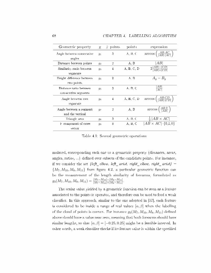
68 CHAPTER 4. LABELLING ALGORITHM
Geometric property g # points points expression
Angle between consecutive
angles
g1 3 A, B, C arccos(
AB·AC|AB|·|AC|
)Distance between points g2 2 A, B |AB|Similarity ratio between
segments
g3 4 A, B, C, D 2 |AB|−|CD||AB|+|CD|
Height dierence between
two points
g4 2 A, B Ay −By
Distance ratio between
consecutive segments
g5 3 A, B, C|AB||AC|
Angle between two
segments
g6 4 A, B, C, D arccos(
AB·CD|AB|·|CD|
)Angle between a segment
and the vertical
g7 2 A, B arccos(AB·Y|AB|
)Triangle area g8 3 A, B, C 1
2 |AB ×AC|Y component of cross
vector
g9 3 A, B, C |AB ×AC| ·0,1,0
Table 4.1: Several geometric operations
mulated, corresponding each one to a geometric property (distances, areas,
angles, ratios, ...) dened over subsets of the candidate points. For instance,
if we consider the set left_elbow, left_wrist, right_elbow, right_wrist =
M7,M10,M8,M11 from gure 4.2, a particular geometric function can
be the measurement of the length similarity of forearms, formulated as
g3(M7,M10,M8,M11) = |M7−M10|−|M8−M11||M7−M10|+|M8−M11| .
The scalar value yielded by a geometric function can be seen as a feature
associated to the points it operates, and therefore can be used to feed a weak
classier. In this approach, similar to the one adopted in [57], each feature
is considered to be inside a range of real values [α, β] when the labelling
of the cloud of points is correct. For instance g3(M7,M10,M8,M11) dened
above should have a value near zero, meaning that both forearms should have
similar lengths, so that [α, β] = [−0.25, 0.25] might be a feasible interval. In
other words, a weak classier checks if its feature value is within the specied
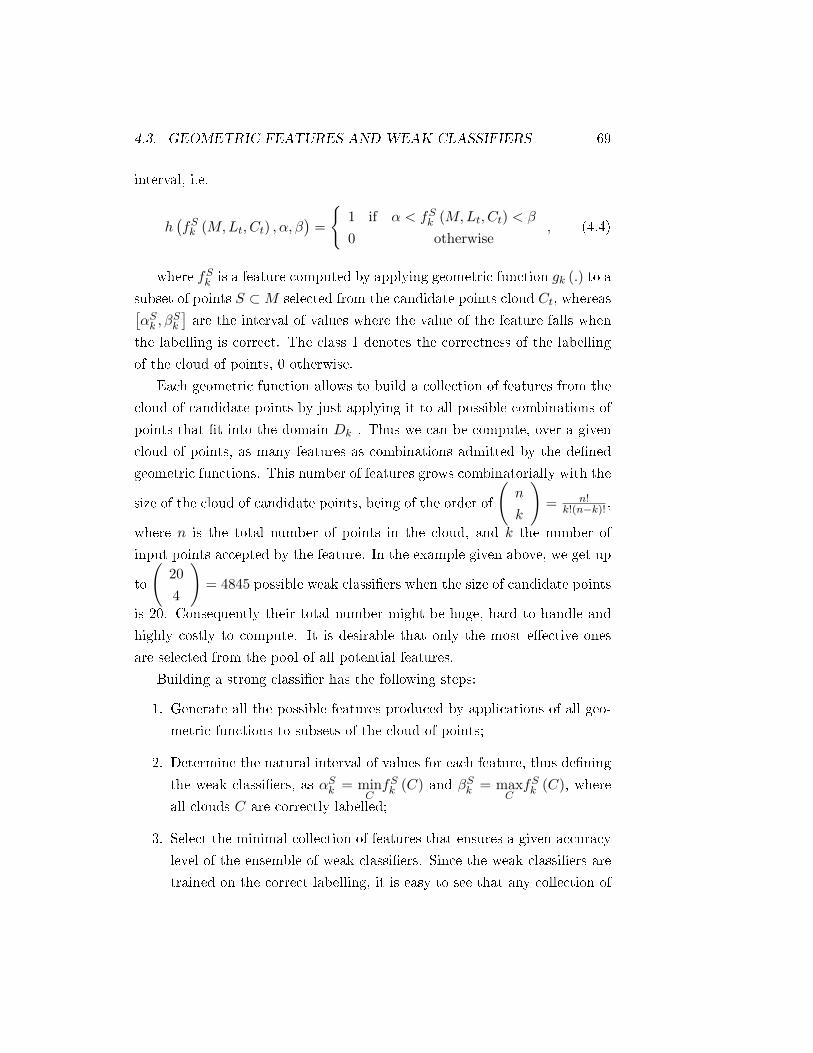
4.3. GEOMETRIC FEATURES AND WEAK CLASSIFIERS 69
interval, i.e.
h(fSk (M,Lt, Ct) , α, β
)=
1 if α < fSk (M,Lt, Ct) < β
0 otherwise, (4.4)
where fSk is a feature computed by applying geometric function gk (.) to a
subset of points S ⊂M selected from the candidate points cloud Ct, whereas[αSk , β
Sk
]are the interval of values where the value of the feature falls when
the labelling is correct. The class 1 denotes the correctness of the labelling
of the cloud of points, 0 otherwise.
Each geometric function allows to build a collection of features from the
cloud of candidate points by just applying it to all possible combinations of
points that t into the domain Dk . Thus we can be compute, over a given
cloud of points, as many features as combinations admitted by the dened
geometric functions. This number of features grows combinatorially with the
size of the cloud of candidate points, being of the order of
(n
k
)= n!
k!(n−k)! ,
where n is the total number of points in the cloud, and k the number of
input points accepted by the feature. In the example given above, we get up
to
(20
4
)= 4845 possible weak classiers when the size of candidate points
is 20. Consequently their total number might be huge, hard to handle and
highly costly to compute. It is desirable that only the most eective ones
are selected from the pool of all potential features.
Building a strong classier has the following steps:
1. Generate all the possible features produced by applications of all geo-
metric functions to subsets of the cloud of points;
2. Determine the natural interval of values for each feature, thus dening
the weak classiers, as αSk = minCfSk (C) and βSk = max
CfSk (C), where
all clouds C are correctly labelled;
3. Select the minimal collection of features that ensures a given accuracy
level of the ensemble of weak classiers. Since the weak classiers are
trained on the correct labelling, it is easy to see that any collection of

70 CHAPTER 4. LABELLING ALGORITHM
them will provide very high sensitivity (accuracy on the target class
relative to all examples of the target class) but very likely a large
number of false positives, i.e. a very low specicity. Hence, this process
is a greedy selection of the weak classier providing the biggest increase
of accuracy by decreasing the number of false positives.
4.4 Labelling Without Presence of Occlusions. En-
semble of Weak Classiers
4.4.1 Training a set of weak classiers
Let's denote O = Oi the set of learning observations Oi = Ci, Li, bicorresponding to a common model M . Each observation has a cloud of
points Ci and the labelling Li that maps it into the model. The vector biencodes the correctness of the mapping, so that bij = 0 if the label of the j-th
cloud point is incorrect, and equals 1 if it is right. The training algorithm can
easily generate incorrect labelled observations by permutation of the labels
of a correctly labelled observation. The number of permuted elements (from
2 to n, the number of markers) is an index of the severity of the simulated
labelling error. Let's denote O∗ = O∗i the incorrect samples, retaining
O = Oi for the correct ground truth observations.
The ensemble of classiers consists of a collection of features whose cor-
responding weak classier is weighted by its accuracy gain relative to the
remaining weak classiers. The output of the ensembles is computed as:
φJ (M,C,L) =
J∑j=1
wjhj(fSk (C) , αSk , β
Sk )
J∑j=1
wj
, (4.5)
where the index j refers to the order of selection of the feature for inclusion
in the ensemble, and J is the size of the ensemble.
The method follows the Adaboost strategy, as done in [57], of greedy
selection of the weak classier that maximises the accuracy, in this case the

4.4. LABELLINGWITHOUT PRESENCE OF OCCLUSIONS. ENSEMBLE OFWEAKCLASSIFIERS71
number of wrong labelling detection. Initially, all weights are set to zero
and the set of selected weak classiers is empty. In a loop all classiers are
fed with observations of dierent error severity obtained by permutations
of labels in the correct observations. If the current version of φJ (M,C,L)
does reject the incorrect sample no further process is done. Otherwise, the
weights of unselected weak classiers that reject it are updated according
to the error severity. After a number of incorrect observations is processed,
the ensemble is engrossed with the weak classier having the greatest weight.
The whole process eventually ends up when a given threshold on the accuracy
of the strong classier is reached. At the end, the elite of classiers is stored
together with the weight they got during the learning process scoring them.
4.4.2 Generating labels exploiting the ensemble of weak clas-
siers
Previous sections dealt with the answer to the question of whether a given
labelling is correct or not. In this section the aim is to generate the labels
for the cloud points using the previously trained weak classiers and the
strong ensemble classier. Given an ensemble of weak classiers φJ (M,C,L)
trained as described above, the number of weak classiers giving positive
outcome can be interpreted as a measure of how well the vector of integers
L species the matching of the model points M and the candidate points
C. Therefore, the labelling of a cloud of points can be stated as looking for
the value of L that maximises the number of positive weak classications,
where the global maxima are equivalent to the positive φJ (M,C,L) = 1.
For the sake of simplicity and without loss of generality, let's assume that
the number of point n ofM and C is the same. In other words, no marker is
occluded and no points other than the ones to be labelled are present in the
input data. In this scenario L can be any of the permutations of the integers
between 1 and n and therefore the number of possible congurations for L
is n! . Fortunately, we can exploit the structure of the strong classier as
follows:
The ensemble classier φ can be evaluated over a partial solution where

72 CHAPTER 4. LABELLING ALGORITHM
only a subset of elements of L has meaningful labels. Weak classiers
using unassigned labels are simply ignored;
A single weak classier rejecting a permutation of labels denitively
rules it out, so that not all the weak classiers composing of φ must be
computed, hence the approach takes the shape of a tree-search process;
A single weak classier can be computed from a handful of points
(usually from 2 to 6) which represents a subset of the vector L.
The huge number of possible solutions is explored following a search tree
structure. At each node (here a particular component of the vector L) a
guess li is generated on the assignment of a label li that was previously
unassigned, and the value of φ is computed over the partial labelling solution
L. If the answer is false, all the descending branches are pruned from the
search tree. More particularly, if a branch is cut o at level i of the vector
L, we avoid exploring (n− i)! labelling permutations appearing downwards
the tree. Else, if the answer to the partial labelling is true, the guess li is
accepted, and the process goes ahead with the next node in the tree. If no
correct guess is found, the process goes a step back to explore alternative
branches. The algorithm eventually terminates when all the branches have
been explored. Every branch reaching the nal node yields a feasible solution
for L. It may happen that more than one solution for L be found despite
only one is the correct, being the rest are false positives.
Figure 4.6 illustrates the algorithm process for n = 5. At level 2 the
guesses 1 and 2 are rejected by φ but accepted for 4 and 5. At level 3 the
branch corresponding to partial solution L = 3, 5, ... is cut o since
none of the 3, 5, 1, ..., 3, 5, 2, ..., 3, 5, 3, ... partial solutions are valid.
However, the algorithm eventually nds a complete valid solution through
the branch coded as 3, 4, 2, 5, 1.
This algorithm is designed to work under the assumption that no marker
is occluded, being this fact its main aw. If at some level a marker can't be
assigned to a candidate because it is actually hidden, there is no way to con-
tinue down to the next level. Many features can't be evaluated and therefore
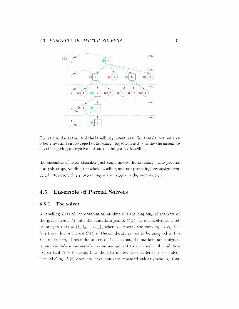
4.5. ENSEMBLE OF PARTIAL SOLVERS 73
Figure 4.6: An example of the labelling process tree. Squares denote positivelabel guess and circles rejected labelling. Rejection is due to the the ensembleclassier giving a negative output on the partial labelling.
the ensemble of weak classier just can't assess the labelling. The process
abruptly stops, voiding the whole labelling and not providing any assignment
at all. However, this shortcoming is torn down in the next section.
4.5 Ensemble of Partial Solvers
4.5.1 The solver
A labelling L (t) of the observation at time t is the mapping of markers of
the given model M into the candidate points C (t). It is encoded as a set
of integers L (t) = l1, l2, ..., lnm, where li denotes the map mi → cli , i.e.
li is the index in the set C (t) of the candidate points to be assigned to the
i-th marker mi. Under the presence of occlusions, the markers not assigned
to any candidate are encoded as an assignment to a virtual null candidate
'0', so that li = 0 means that the i-th marker is considered as occluded.
The labelling L (t) does not have non-zero repeated values (meaning that

74 CHAPTER 4. LABELLING ALGORITHM
the same candidate point cannot be labelled twice). The weak classiers
h(Ms, C (t) , LMs (t)) = T ∈ 0, 1, are decision functions whose output is
whether the partial labelling LMs (t) is correct (1) or not (0). From now on,
we assume that each data capture frame is treated independently, therefore
the time parameter t is dropped out.
We have shown in the previous section that it is possible to build up a
strong classier as an ensemble of weak classiers φ = h1, h2, ... lookingfor the minimal set of weak classiers able to decide whether a labelling is
correct (true) or not (false): φ(M,C,L) = T ∈ 1, 0. To achieve so, the
set of weak classiers is trained by means of a tailored version of AdaBoost
over a set of labelled samples extracted from a large number of frames whose
labelling relative to a given marker set has been manually veried.
The result of the algorithm discussed in 4.4.2, is a solver S (C,M, φ)
that nds the set of feasible labelling maps L = L¹, L², ..., such that
φ(M,C,Li) = true. The solver S (C,M, φ) makes use of the strong classier
φ and an ecient tree exploration method to nd all the feasible marker
labellings of the candidate points. Despite its eciency in terms of compu-
tation time, its main aw is that it cannot handle null labels. Hence, for
each labelling found Li ∈ L all of its components lj ∈ Li are positive lj > 0.
The set of labellings found by S might be the empty set L = ∅, meaning that
the solver S (C,M, φ) could not nd any feasible solution. The algorithm
of S (C,M, φ) is therefore unable to deal with occlusions: it either assigns a
candidate to each marker or to no one.
On the other hand given a solver S we can assess, by its exposition to
random samples coming from the ground truth, the hit rate P (S,mi) =
Pi(S) ∈ [0, 1] of the solver assigning any marker mi to its right candidate.
This information is precomputed and stored as an attribute of the solver S
for further usage.
4.5.2 Partial solvers
Denition A solver S = S(C,Ms, φs) is not forced to nd corresponding
candidate points to all markers of the model M . Actually, its associated
4.5. ENSEMBLE OF PARTIAL SOLVERS 75
strong ensemble classier φs can be trained to generate a partial labelling
Ls ⊆ L for a subset of markers Ms ⊆ M . Is such case, we deal with a
partial solver . Obviously, the strong ensemble classier φs only can be used
to generate labelling over the markers belonging to Ms. We designate the
dimension of the solver Ss as the number of markers that it operates upon:
dim(Ss(Ms)) = dim(Ms). The denition of hit rate per marker Pi applies
also to partial solvers, provided they can be assessed against the ground
truth.
Properties We can state several interesting properties of the hit rates of
a partial solver. Some of them were born out from experiments conducted
on the computational simulations and may be object of theoretical research
in future works.
1. If a marker mi doesn't belong to the subset Ms of the partial solver,
its hit rate remains undened: if mi /∈Ms ⇒ Pi(Ss,mi) = NaN ;
2. The hit rate for a marker mi is strictly increasing with the size of the
marker subset: if mi ∈MA ⊂MB, |MB| > |MA| ⇒ Pi(SB) ≥ Pi(SA);
3. Because the hit rates grow with with solver size, we would expect that
only big solvers may provide high hit rates. However, the empirical
nding reveals that there are also small solvers showing up high hit
rates;
4. A marker model is considered optimally designed if its labelling is fea-
sible with a 100% condent rate in absence of occlusions. In other
words, there is at least a solver whose hit rates are 100% for each
one of the markers when working over the whole set: if Ms ≡ M →∃S \ Pi(Ss(C,Ms, φs)) = Pi(S(C,M, φ)) = 1;
5. Such solver does exist for the marker set used in the experimental
tests of this work, hence the Hellen-Hayes set of markers was optimally
designed.

76 CHAPTER 4. LABELLING ALGORITHM
4.5.3 Training an ensemble of partial solvers
A partial solver ensemble is dened as a set of partial solvers such that the
union of their marker subsets covers the complete model: Ω = S1, S2, ..., SN s.t.Ms1∪Ms2 ∪ ... ∪MsN = M . The aim of dening the ensemble is to overcome the
limitation of an individual solver to give an answer when there is an occlu-
sion. If such thing happens, the unaected partial solvers (i.e. those dened
over a subset of not occluded markers) may still provide the labelling of the
unoccluded markers. More formally, let's denote M∗ the set of not occluded
markers, then we can nd a set of partial solvers Ω∗ = S∗1 , S∗2 , ..., S∗N∗ ∈ Ω
such that M∗S1∪M∗S2
∪ ...∪M∗SN⊆M∗. Given that a deterministic learning
algorithm is used for the construction of the strong classiers, two partial
solvers are dierent only if they are dened over dierent marker subsets:
SA(MA) 6= SB(MB) ⇐⇒ MA 6= MB. According to that criteria, the to-
tal number of partial solvers is the size of the markers power set P (M),
i.e.∑nm
i=1
(nm
i
), where nm = |M |.
The problem of generating marker labelling robust to occlusion is, thus,
formulated as the search for small sized partial solvers with high target rates
to compose a partial solver ensemble which can produce partial labellings
that give the best partial labelling solution when there are occlusions. The
emphasis on small sized partial solvers comes from the fact that if one is
aected by an occlusion, the solver it will not yield the labelling of its solver-
mates. The emphasis on high target rates is preferable, as that increases the
condence on the labelling. A brute force exhaustive search approach is, of
course, infeasible even for moderate sizes of the marker set. Therefore two
heuristic approaches have been explored.
Greedy search By taking advantage of the 2nd solver property stated
in the previous section hit rates strictly increase with dimension, we
can start with nm solvers of dimension 1 (one solver per marker), adding one
more extra marker at each step of the search. This is an incremental building
process that stops when the target hit rate is reached. This strategy avoids
unnecessarily big solvers, thus saving computation time. The searching al-
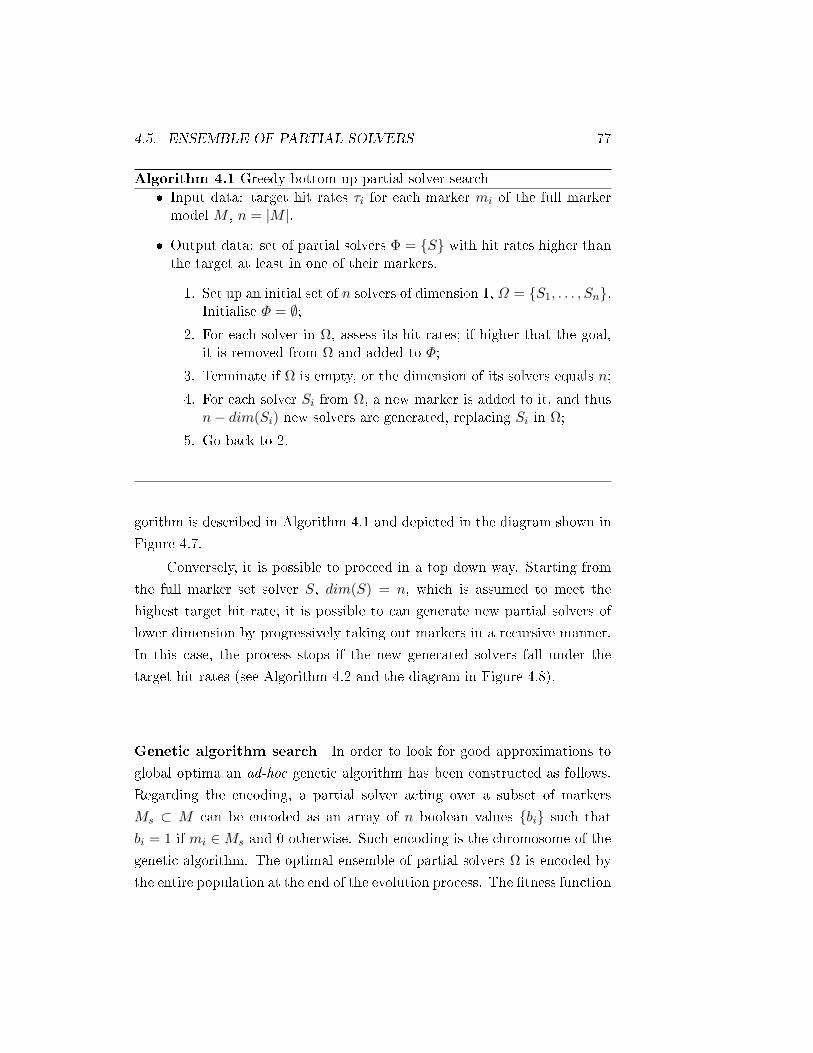
4.5. ENSEMBLE OF PARTIAL SOLVERS 77
Algorithm 4.1 Greedy bottom up partial solver search Input data: target hit rates τi for each marker mi of the full markermodel M , n = |M |.
Output data: set of partial solvers Φ = S with hit rates higher thanthe target at least in one of their markers.
1. Set up an initial set of n solvers of dimension 1, Ω = S1, . . . , Sn.Initialise Φ = ∅;
2. For each solver in Ω, assess its hit rates; if higher that the goal,it is removed from Ω and added to Φ;
3. Terminate if Ω is empty, or the dimension of its solvers equals n;
4. For each solver Si from Ω, a new marker is added to it, and thusn− dim(Si) new solvers are generated, replacing Si in Ω;
5. Go back to 2.
gorithm is described in Algorithm 4.1 and depicted in the diagram shown in
Figure 4.7.
Conversely, it is possible to proceed in a top down way. Starting from
the full marker set solver S, dim(S) = n, which is assumed to meet the
highest target hit rate, it is possible to can generate new partial solvers of
lower dimension by progressively taking out markers in a recursive manner.
In this case, the process stops if the new generated solvers fall under the
target hit rates (see Algorithm 4.2 and the diagram in Figure 4.8).
Genetic algorithm search In order to look for good approximations to
global optima an ad-hoc genetic algorithm has been constructed as follows.
Regarding the encoding, a partial solver acting over a subset of markers
Ms ⊂ M can be encoded as an array of n boolean values bi such that
bi = 1 if mi ∈Ms and 0 otherwise. Such encoding is the chromosome of the
genetic algorithm. The optimal ensemble of partial solvers Ω is encoded by
the entire population at the end of the evolution process. The tness function

78 CHAPTER 4. LABELLING ALGORITHM
Figure 4.7: Greedy bottom up search diagram representation

4.5. ENSEMBLE OF PARTIAL SOLVERS 79
Figure 4.8: Greedy top down search diagram representation

80 CHAPTER 4. LABELLING ALGORITHM
Algorithm 4.2 Greedy top down partial solver mining Input data: target hit rates τi for each marker mi of the full markermodel M , n = |M |.
Output data: set of partial solvers Φ = S with hit rates higher thanthe target at least in one of their markers.
1. Set up initial solver of dimension n, Ω = S and initialise Φ = ∅;2. For each solver Si in Ω:
(a) remove it from Ω ;(b) remove each of its marker once at a time, generating dim(Si)
new solvers stored in Ωi;(c) for each solver of Ωi, its hit rates are assessed;(d) if no solver from Ωi reaches the target rates, it is removed
from Ωi and joins Φ;(e) the remaining solver from Ωi are added to Ω;
3. If Ω is not empty, go back to 2.
of each chromosome is the maximum of the hit rates of the corresponding
partial solver.
Starting from a randomly generated population composed by a number of
partial solvers encoded as chromosomes, the following genetic operators are
applied to improve the population tness towards nding the global optimal
collection of partial solvers:
Crossover: two parent chromosomes (partial solvers) are selected ran-
domly from the population, the crossover operator generates a new
chromosome by picking randomly its genes from either one of parent
chromosomes.
Mutation: a chromosome is randomly selected and a new one is gener-
ated either by random permutation, addition or subtraction of one of
the parent's genes;
permutation: pick a pair of genes of dierent values and permute

4.5. ENSEMBLE OF PARTIAL SOLVERS 81
them. The size of the child partial solver remains the same;
addition: pick a random '0' gen and reverse its value. The size of
the child partial solver increases by one;
subtraction: pick a random '1' and reverse its value. The size of
the child partial solver decreases by one. The subtraction opera-
tion is biased towards the search of small specimens;
Selection: after application of genetic operators, the tness of the chro-
mosomes in the population are evaluated selecting those that meet the
target hit rate, when there is equal hit rate, smaller solvers are pre-
ferred. After that, a massive die out removes the 25% worse specimens.
The survivors join the ensemble of partial solvers.
Several computational experiments have been conducted in which the al-
gorithm always managed to improve the initial population after a number
of generations. The resulting solver ensembles proved to be good enough to
meet the requirements of the labelling algorithm discussed later. In any case,
the eciency of the genetic search strongly depends on its tuning parame-
ters: initial population size, crossover and mutation frequencies, number of
operations between die outs and percentage of specimens to wipe out.
4.5.4 Generating labels exploiting the ensemble of partial
solvers
At this point, we count on an optimal ensemble of partial solvers Φ = S,whose hit rates meet the targets τi for each marker. Each partial solver
is dened over a subset of the complete marker model, and the merge of
all solvers covers the complete model M . The formulation of Φ is a time
consuming training process to be done before the online execution of the
complete labelling algorithm.
During the labelling process, every time a new frame is acquired, the
list of candidate 3D points extracted from the motion capture harware is
built and exposed to each solver of the ensemble Φ of partial solvers. Each
member of the ensemble S hands over none, one or several candidate points

82 CHAPTER 4. LABELLING ALGORITHM
assigned to the markersMk within its scope. The contribution of each solver
is recorded in a labelling matrix that has as many rows as candidate points
(nc) and columns as model markers (nm), so that each matrix entry (i, j)
containsSi,js: the set of partials solvers belonging to the ensemble Φ who
suggested the i-th candidate to the j -th marker. This matrix, expected to
be sparse most of the times because the partial solvers are expected to agree
on the mappings, looks like this:
m1 m2 · · · mj · · · mnm
c1 ∅S1,2s
· · · ∅ · · · ∅
c2 ∅ ∅ · · · ∅ · · · ∅...
......
......
ci ∅ ∅ · · ·Si,js· · · ∅
......
......
...
cnc ∅ ∅ · · · ∅ · · · Snc,nms
Each columns of this matrix represents the labelling of a single marker.
A non-empty row on a given column represents the application of candidate
to be labelled as the corresponding marker. We may have the following
situations regarding the cell contents:
The most common scenario is given when the i-th row and j-th column
contain only one non-null entry. In that case a particular candidate is
assigned to j: lj = i.
A column j is empty: no solver proposes a candidate to the corre-
sponding marker. Either it might be occluded or there is not enough
condence to suggest one. In any case, we set it as occluded: lj = 0;
A column j has more than one non-null entry because two or more
solvers suggest dierent candidates. Basically this means that there is
an ambiguous assignment and therefore, from a secure point of view,
the safe choice that to set it as occluded: lj = 0.
A row has more than on non-null entry in columns j1, j2,..., which
means that a candidate point is assigned to more than one marker

4.5. ENSEMBLE OF PARTIAL SOLVERS 83
point. Again, we take a safe choice by setting all the involved marker
as occluded, i.e. lj1 = 0, lj2 = 0, ...

84 CHAPTER 4. LABELLING ALGORITHM

Chapter 5
Results
The algorithms presented in chapter 4 are designed to be applied right away
to an actual real world mocap problem. Therefore, this Thesis would be
incomplete without an assessment of the methods, in terms of hit ratio and
eciency, against real world data. Aside that, a description on the gathering
of the ground truth of a set of genuine capture motion data is given.
5.1 Experimental Data
This section presents the experimental data set that has been employed
for the computational validation experiments reported later. This database
gathers a set of real optical marker-based motion capture tracking samples.
On it, each sample corresponds to a single acquisition containing the 3D tra-
jectories of a set of markers along a continuous interval of time. Regarding
the motion, several persons were asked to walk normally while recorded using
motion capture cameras. The cameras, previously calibrated, are designed
to detect the 2D pixel image position of the markers against the background
thanks to the IR lightning ring they are provided with. The Cartesian po-
sition was afterwards recovered by means of photogrammetric methods (see
3.4 to know more), whereas the tracking was kept across the frames using
a proprietary software (CLIMA1). The data set contains only the raw 3D
1http://www.stt-systems.com/products/3d-optical-motion-capture/clima/
85

86 CHAPTER 5. RESULTS
trajectories of the aforementioned markers along the time.
The whole experimental setup corresponds to an commercial mocap set-
ting for gait analysis measurement with a equipment of six synchronised
cameras model S250e from Optitrack 2 (see gure 3.4). Their main specs
are: 800x800 pixel resolution up to 250Hz, with built in infrared lightning
and IR lter and Ethernet connectivity. The set of markers is the layout
proposed by Kadaba, Ramakrishnan, and Wootten, from the Helen Hayes
Hospital (more details can be found in [12]). The experimental data has been
manually veried, so that the collected data is guaranteed to no contain la-
belling mistakes. Altogether, the experimental data consists of 71 video
sequences recorded at 100Hz summing up to 14 dierent people of diverse
ages and body shapes walking at random paces. The average duration of
the sequences is about three seconds, so that we count on more than 20.000
frames to extract the clouds of candidate points. This database has been
made publicly accessible at Zenodo [28].
Labelled cloud samples corresponding to a correct correspondence are
categorised as class '1' for classication purposes. Point clouds with incor-
rect labelling corresponding to class '0' data samples are generated by just
applying random permutations on the labels of correct labelled data.
5.2 Partial Solver Performance
Despite a partial solver has been thought to work in an ensemble, there is
not objection to use an instance whose dimension matches that of the marker
model. It has the drawback of not providing any labelling at all if a single
marker is missing (see discussion in section 4.4.2). But in exchange for that,
the hit rate of the yielded labelling is the highest possible (2nd property of
the partial solvers, see section 4.5.2). In addition to that, the outstanding
eciency of the partial solver labelling algorithm up to 10,000 frames per
second according to the experimental results makes it very useful in real
time applications where occlusions are very unlikely.
2http://optitrack.com/

5.2. PARTIAL SOLVER PERFORMANCE 87
A set of features have been built using just a handful geometrical func-
tions (we have selected g2, g4 and g9 from Table 4.1) and applied to the
marker set of the ground truth, composed by 15 markers. Thus, a total of
665 weak classiers have been trained building the weak classier pool. The
training algorithm determines an ensemble φ = h1, h2, ... with 40 out of
665 weak classiers as the most eective to tell the correctness of a given la-
belling. To prove its accuracy, the ensemble is asked to assess the correctness
of a sample of labellings with known ground truth. The experiment shows
that the classier achieves an accuracy over 99% after the presentation of
more than 107 negative samples with diverse error severity.
Table 5.1 summarises the best weak classiers achieving over 93% accu-
racy. Apparently, the strongest weak classier is the one that prevents the
triangle right asis - left asis - sacrum from standing far from a horizontal
plane. Indeed, the set of training data involves people walking: no bend-
ing over or lying on the oor movements are being exposed to the learning
process so this restriction is full of meaning. After it, the strong classier
relies on distance features between consecutive markers. This is another way
of saying that the length of humans limbs or consecutive joints is more
limited than the distance among arbitrary parts such as the toes and the
hands. Classiers from 2 to 7 has an individual detection rate around 11%,
but, acting as a whole the classiers 1 to 7 are able to catch up with nearly
the bulk 90% of wrong labelling. This is quite remarkable, drafting a rough
idea of the strength of the approach. From the 8th classier on, the grow
of aggregated score speeds down yet being the weak classiers useful to rule
out marginal false positives.
Once a set of n weak classiers φn is built, the corresponding solver
S (C,M, φn) is assembled with it and ready to tested. In order to prove the
ensemble classier performance depending on the size of φ, multiple instances
of solver are fed with a number of candidate sets (unlabelled points) coming
from dierent frames of our dataset of gait sequences with known ground
truth and are asked to label them.
An indicator of the eciency of the algorithm is the number of required
feature evaluations: the less the numbers of evaluations, the less is the num-

88 CHAPTER 5. RESULTS
Table 5.1: First selected weak classiersWeak classier Score (%) Sum score (%)
1 TriangleNormal_Y(R_asis,L_asis,sacrum) 18.82 18.82
2 Dist(R_malleolus,R_heel) 12.91 31.74
3 Dist(L_malleolus,L_heel) 12.84 44.59
4 Dist(R_femoral_epicondyle,R_tibial_band) 11.85 56.45
5 Dist(L_femoral_wand,L_femoral_epicondyle) 11.51 67.96
6 Dist(L_tibial_wand,L_meta_h) 10.87 78.84
7 CoordDi_Y(R_femoral_wand,R_meta_h) 10.43 89.28
8 TriangleNormal_Y(sacrum,R_meta_h,L_meta_h) 1.90 91.17
9 Dist(R_femoral_wand,R_femoral_epicondyle) 1.84 93.02
ber of branches to be explored and thus the faster the search. Figure 5.1
shows how the true positive ratio grows with the number of weak classiers
used for the test of the labelling. However, as mentioned before, all classiers
up to the 40th are enough to rule out nearly all the false positives. Regarding
the eciency, the number of node evaluations apparently gets stable around
the 30th classier, requiring a mean of 3500 evaluations before running into
the right labelling. This number is rather small compared with 15! > 1012
(one trillion), which is the required number of tests in a brute-force search.
The graph that relates the number of feature evaluations with the number
of classiers is using a logarithmic vertical axis: less than 14 classiers still
require more than 100,000 evaluations.
5.3 Solver Ensemble Performance
When it comes to the solver ensemble that can successfully handle clouds of
candidate points suering occlusions, the assessment its eciency is made
according to two main performance indices:
False assignments rate (FA): number of wrong assignments of candidate
points to marker vs. total number of assignments. This is the rate of
incorrect labelling.
False occlusions rate (FO) : number of wrong occlusion assignments

5.3. SOLVER ENSEMBLE PERFORMANCE 89
Figure 5.1: Accuracy and eciency assessment depending on the number ofweak classiers.

90 CHAPTER 5. RESULTS
Test conditions
Number of markers 15
Target hit rate 99.99%
Target failure rate 0.01%
Occlusions per frame 4
Number of test frames 16384
Table 5.2: Experimental conditions summary
vs. total number of occlusion assignments
It is desirable to keep both rates low. Obviously it is desirable to avoid
wrong labelling, but not at the expense missing legitimate assignments of
not occluded markers. A good balance between both performance indices is
achieved tuning the algorithm settings.
To validate the whole process, a large set of frames are borrowed from our
dataset with known ground truth. The candidates for each frame are ran-
domly permuted to obtain wrong labelling. To simulate occlusions, between
1 to 5 candidate points are removed from the samples. The labelling gener-
ated by the approach presented above is compared with the correct labelling
and the validation statistics are continuously updated. Summary descrip-
tion of the experimental conditions is given in Table 5.2. The frames are
extracted from a gait measurement experiment, so that markers correspond
to the lower limbs of the human body.
In Table 5.3 the rates of false assignments and false occlusions are shown
for a training and validation instances where the target marker hit rate was
set to 99.99% and the number of occluded points per frame was set to 4 for a
model of 15 markers. While the false assignments stands around the 0.01%,
the rate of unassigned markers (despite being present in the candidate point
cloud) uctuates from 4.20% to 45.13% with an average of 31.16%. Some
markers are harder to catch with high condence when the rate of actual
occlusions reaches the 25%.
Repeating the above test with dierent target hit rates and dierent
number of simulated occlusions, the variation of the eciency indicators is

5.3. SOLVER ENSEMBLE PERFORMANCE 91
Marker ID FA # FA % FO # FO %
r_asis 2 0.02% 300 6.38%
l_asis 2 0.02% 254 5.55%
s2 0 0.00% 286 6.11%
r_l_thigh 0 0.00% 3564 45.03%
l_l_thigh 1 0.01% 220 4.85%
r_knee 0 0.00% 1912 30.03%
l_knee 1 0.01% 3532 44.58%
r_calf 1 0.01% 194 4.20%
l_calf 3 0.03% 218 4.71%
r_ankle 3 0.03% 2302 34.02%
l_ankle 1 0.01% 4348 49.30%
r_heel 4 0.05% 3195 42.14%
l_heel 1 0.01% 3579 45.06%
r_toe 4 0.04% 2332 34.67%
l_toe 4 0.05% 3627 45.13%
Average 1.8 0.02% 1991 31.16%
Table 5.3: False assignments (FA) and false occlusions (FO) results. Rowscorrespond to model markers located over parts of the body.

92 CHAPTER 5. RESULTS
Table 5.4: False assignments sensitivity to target marker hit rate and numberof occlusions.
False assignments rate
Target marker hit rate 99.000% 99.900% 99.990% 99.999%
Number of true occlusions
per frame
1 8.13% 1.12% 0.09% 0.04%
2 8.89% 0.94% 0.09% 0.05%
3 7.04% 0.58% 0.07% 0.02%
4 4.28% 0.34% 0.02% 0.01%
5 2.35% 0.16% 0.01% 0.00%
Table 5.5: False occlusion sensitivity to target marker hit rate and numberof occlusions.
False occlusions rate
Target marker hit rate 99.000% 99.900% 99.990% 99.999%
Number of true occlusions
per frame
1 0.25% 0.52% 12.10% 16.40%
2 5.74% 14.30% 19.96% 21.76%
3 9.56% 19.76% 25.18% 26.20%
4 13.16% 24.35% 30.90% 32.17%
5 18.25% 33.39% 39.65% 40.67%
exposed. The sensitivity of the false assignments rate (see Table 5.4), for
a constant number of simulated occlusions (the rows), when the target hit
rate increases (along the columns) the algorithm reduces dramatically the
number of false assignments. Likewise, the rate of false occlusions gets bigger
(Table 5.5, right).
These numbers are plotted in Figure 5.2. Each line corresponds to the
same number of simulated occlusions, while the dot symbol corresponds to
a given target hit rate. Low false assignment rates (x axis) correspond to
high false occlusions rate. On the other hand, when the number of simulated
occlusions gets bigger, the rate of false occlusions increases as well.
The reason behind this behaviour is the following. When it is not possible
to formulate assignments due a lack of information (occlusions), the weak
classiers can't be evaluated and consequently the strong classier loses its
strength. The intuitive interpretation is that the identication of each single
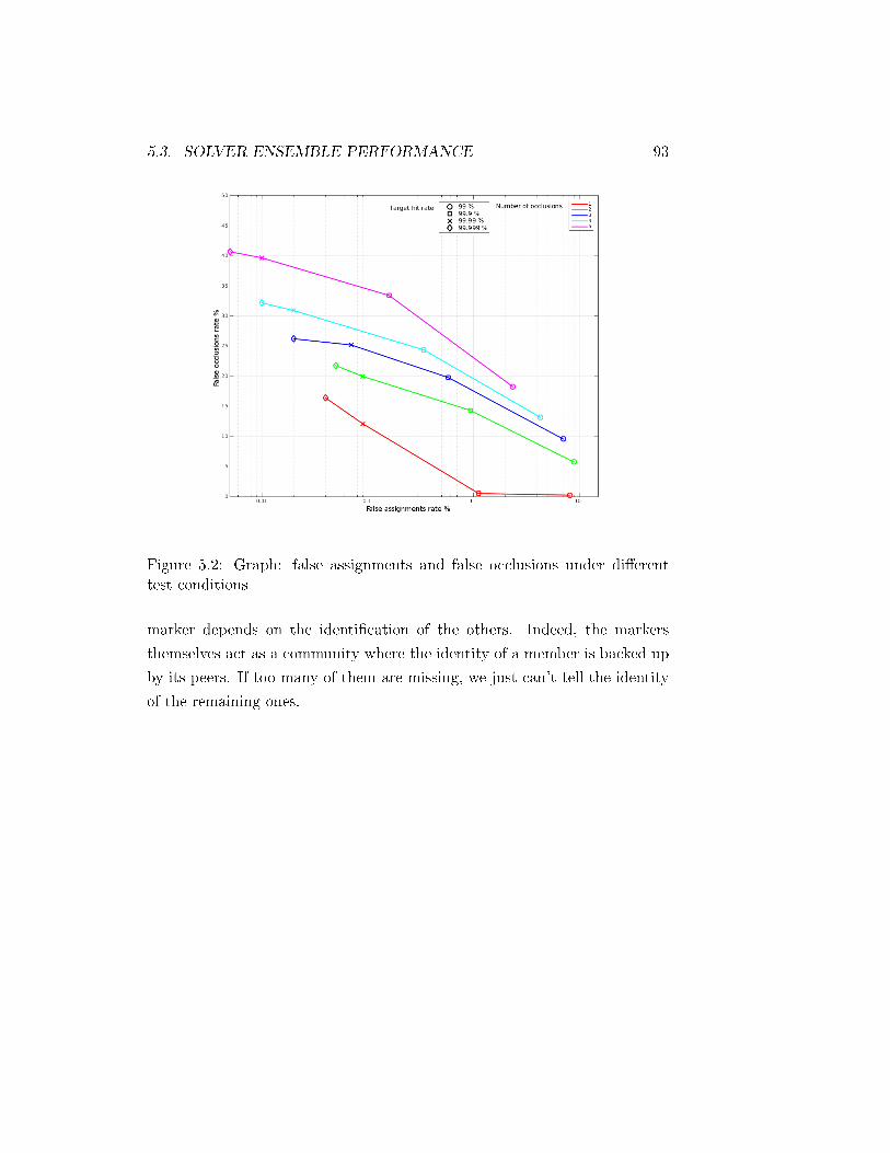
5.3. SOLVER ENSEMBLE PERFORMANCE 93
Figure 5.2: Graph: false assignments and false occlusions under dierenttest conditions
marker depends on the identication of the others. Indeed, the markers
themselves act as a community where the identity of a member is backed up
by its peers. If too many of them are missing, we just can't tell the identity
of the remaining ones.

94 CHAPTER 5. RESULTS

Chapter 6
Conclusions
In this nal chapter we present the summary and conclusions of the Thesis,
including some comments on future lines of work. The core research eort
of this work is aimed to the solution of a practical problem and therefore the
conclusions are considered from a pragmatical point of view. The accom-
plished goals and some limitations of the work are discussed in section 6.1
and section 6.2, respectively. No conclusions chapter is complete without a
list of future work guidelines that see their place in section 6.3.
6.1 Achievements
The main contribution of this Thesis is the development of a complete maker
labelling algorithm ready to be embedded in the whole pipeline of an optical
mocap system. The most appreciated requirements in such an algorithm are,
namely, a high hit ratio (percentage of right assignments), robustness against
massive and long lasting occlusions and ecient enough to be run at real time
speeds. According to the experimental results, all these requirements are met
with the set of methods here exposed.
In addition to that, the proposed solution is innovative as long as it dis-
sociates itself from the usual skeleton driven approaches followed in related
works. Instead, this work is built around the concept of weak classier as
plain geometrically based features that are evaluated over the cloud of can-
95

96 CHAPTER 6. CONCLUSIONS
didate points. This allows the problem to be tackled with the wide variety
of machine learning methods in an way who has never been explored so far.
In fact, the presented approach does not use any semantic prior structural
information, such as anatomical locations or graphs of expected relative po-
sitions. Not only does it so, but it also discards temporal information (i.e.
prior marker trajectories) that tend to mislead and break the tracking ow
in the case of frames containing ambiguities. Thus, each frame in the video
sequence is independently analysed, preventing feasible labelling mistakes
from propagating in time and turning the recovery from occlusions to be
done almost immediately.
The problem of optical marker tracking is seldom dealt in the literature.
Partly because such stage is taken as granted. Indeed, when a human eye
come across a regular unlabelled point cloud produced from the cameras,
it doesn't nd much trouble to make out who is who. In the end, our
brain is trained and used to recognise human movements. For instance,
one can easily guess who we are looking at by just the way he walks, or
even guess its mood state depending on its movement. Not to mention
the huge capacity of the brain to ll the gaps with learnt patterns when a
lasting partly occlusion takes place. Somehow, the way our mind determines
who marker is who among a collection of messy point cloud is thanks to
a entangled set of fuzzy rules born out of experience. The markers are
normally attached to the skin at best loose cloth at worst and thus they
move random and non-deterministically with respect to the corresponding
segment. Trying to write down a code or set of rules by hand is a rather
impractical undertaking for a skilled technician, unthinkable for a newbie.
In contrast, the machine learning is a natural approach as for it perfectly ts
under these circumstances, yielding decisions that mimic those of the human
brain.
A windfall obtained from the development of the algorithms is the sub-
stantiation of a slippery awareness: the markers can not be identied in-
dividually, but in strong dependency with others. The concept for partial
solvers formalises the fact that groups of markers mutually back up their
labelling. Consequently, the occlusion of a few of them may follow in the

6.2. LIMITATIONS 97
failure to assure the tag of the remaining ones, whereas a low rate in the
number of occlusions greatly increases the labelling trust. The disclosure of
such groups and the condence level they share out drove to a noticeable
eort of this work.
Another side result closely related with the above, is the settlement of a
trade o between the number of markers that can be labelled and the haz-
ard of the algorithm to make a mistake. In a cautious behaviour, the more
demanding is the hit ratio, the less the number of markers it dares to label
and vice verse. Finally, if low hit ratios are reached even in absence of occlu-
sions, we can judge a given marker model a non suitable to be tracked (for
instance it contains ambiguous symmetries or a too low number of markers
per limb). Bad designs lead to ambiguities in the labelling, therefore the
inability to achieve a robust labelling can be understood as a poor design of
marker placements. The developed methods can assist the optimal design of
marker placement as long as they are able to assess its capturability.
6.2 Limitations
In the downside, the most acute aw comes from the fact that the supervised
learning algorithms requires a number (not small) of correctly labelled frame
samples to learn from. Still counting on a basic, faulty tracking algorithm, it
takes countless hours to gather and verify the correctness of the input data.
In addition, if a negligible mismatch slips away, the overall eciency can be
weakened without almost noticing it. And if some reasonable suspicion is
established, it turns out to be pretty hard to trace back the faulty data.
On the other hand, the learning algorithm faithfully sticks to the given
examples. If the ground truth is not diverse enough, the resulting algorithm
might refuse to label a point cloud, discarding correct labelling as not feasi-
ble. A diverse enough ground truth requires the recording of a variety of per-
sons regarding their height, shape, movements technique ... a eld work that
becomes rather dicult to compile when the goal is to teach the algorithm
to track uncommon actions such as classical dance or martial arts. More-
over, even counting on a profuse data base, there is always the risk to leave

98 CHAPTER 6. CONCLUSIONS
out singular cases. Such circumstances might occur with disabled people
(clubfoot, equine foot, ...) or persons showing atypical movement disorders
(ataxic/myopathic gait, abnormal posturing, etc.). This is a particularly
severe limitation for the practical application of the developed methods, as
long as the medical community is particularly interested in these cases.
Finally, it can be sensibly argued that ruling out temporal information
can be a too extreme and harsh choice. Indeed, certain constraints could be
settled down to reduce the feasible labelling if a kind of trajectory smooth-
ness/continuity is imposed along the time. Isn't it a waste of useful infor-
mation? Happily, the answer is there is no need to exclude it at all. The
trick to accommodate those constraints in the algorithms here developed is
to consider that the geometric features are not limited to be formulated over
Cartesian coordinates belonging to the same frame. Instead of regarding the
unknown labelling as a vector of integer values Lt =ltithat associates the
i-th marker with the lti candidate at given and only one frame t (see
4.1), we could enlarge it to hold the labelling in additional frames:
LT =Lt−∆t, Lt, Lt+∆t
(6.1)
This slight problem reframe gives the weak classiers the chance to take
into account temporal information whereas the labelling for more than one
frame is simultaneously solved. But even more: geometric features are not
even limited to Cartesian positions! Certainly, the smoothness in the marker
trajectories can be formulated as constrains in its derivatives respect to the
time. And nothing prevent us from formulating geometric functions over
partial derivatives:
gk = gk(Mi,Mj , ..., Mi, ..., Mi, ...) (6.2)
being Mi = x, y, z =δxδt , ...
the rst derivative of the position of the
marker Mi respect to the time, Mithe second and so forth. From here on,
weak classiers are trained and strong classiers built with almost no change
over the original proposal. The only drawback is that the learning time can
grow signicantly, as long as the number of feasible weak classiers does alike.

6.3. FUTURE WORK 99
All in all, the methods here proposed are not forced to remain irreconcilable
with temporal constraints; instead they can be optionally embedded in the
whole formulation.
6.3 Future work
Future work guidelines come naturally from the limitations aforementioned
in the above section. To begin with, it would be really interesting and
equally challenging to feed the learning algorithms with raw, unlabelled
clouds of candidate points. Such solution would avoid the programmer the
excruciating task of gathering, verifying and cleaning the input ground truth.
A rst approach to be explored might be the possibility of an incremental
assisted human driven learning process, in a kind of semi-supervised
pipeline. Starting from a few fully supervised examples, a rst naive solver
ensemble could be trained. From that on, it is asked to label new samples and
the technician only has to manually correct its mistakes. The new labelled
samples are incorporated to the ground truth until the hit ratio reaches the
required goal.
Another path to explore is the use of weak classiers using temporal in-
formation. Undoubtedly, that should bring interesting results at the expense
of a more complex software implementation and larger learning computing
time. Only the latter halted this research work from engaging the issue that,
all in all, it is worth to be dealt.
The gait analysis is a paradigm in the interest for mocap and the reason
for what it was selected to build the experimental dataset and its ground
truth. Nevertheless, a remarkable entry in the to do list is the assessment of
the formulated methods with a variety of motion cases (jumping, dancing,
...). All things considered, once implemented it is just a matter of time to
carry out more trials to assess the algorithms after probably an appropriate
sanding and varnishing.

100 CHAPTER 6. CONCLUSIONS

Bibliography
[1] Simon Alexanderson, Carol O'Sullivan, and Jonas Beskow. Real-time
labeling of non-rigid motion capture marker sets. Computers and Graph-
ics, 69:59 67, 2017.
[2] D. S. Alexiadis and P. Daras. Quaternionic Signal Processing Techniques
for Automatic Evaluation of Dance Performances From MoCap Data.
IEEE Transactions on Multimedia, 16(5):13911406, Aug 2014.
[3] S. M. N. Arosha Senanayake and Abdul Ghani Naim. Modern Sensing
Technologies, chapter Smart Sensing and Biofeedback for Vertical Jump
in Sports, pages 6381. Springer International Publishing, 2019.
[4] Alexander M. Aurand, Jonathan S. Dufour, and William S. Marras. Ac-
curacy map of an optical motion capture system with 42 or 21 cameras
in a large measurement volume. Journal of Biomechanics, 58:237 240,
2017.
[5] Mathieu Barnachon, Saïda Bouakaz, Boubakeur Boufama, and Erwan
Guillou. Ongoing human action recognition with motion capture. Pat-
tern Recognition, 47(1):238 247, 2014.
[6] Nils Betzler, Stefan Kratzenstein, Fabian Schweizer, Kerstin Witte, and
Gongbing Shan. 3D Motion Analysis Of Golf Swings Development
And Validation Of A Golf-specic Test Set-up. In Proceedings of the
Ninth International Symposium on the 3D Analysis of Human Move-
ment, 2006.
101

102 BIBLIOGRAPHY
[7] R. Bharadwaj, S. Swaisaenyakorn, C. G. Parini, J. C. Batchelor, and
A. Alomainy. Impulse Radio Ultra-Wideband Communications for
Localization and Tracking of Human Body and Limbs Movement for
Healthcare Applications. IEEE Transactions on Antennas and Propa-
gation, 65(12):72987309, Dec 2017.
[8] Anthony Bouillod, Antony Costes, Georges Soto-Romero, Emmanuel
Brunet, and Frédéric Grappe. Validity and Reliability of the 3D Mo-
tion Analyzer in Comparison with the Vicon Device for Biomechanical
Pedalling Analysis. In icSPORTS, 2016.
[9] C. Bregler. Motion Capture Technology for Entertainment. IEEE Signal
Processing Magazine, 24(6):160158, Nov 2007.
[10] Phillip J. Cheetham, Greg A. Rose, Richard N. Hinrichs, Robert E.
Mottram, Paul D. Hurrion, and Peter F. Vint. Comparison of Kine-
matic Sequence Parameters between Amateur and Professional Golfers.
Science and Golf, 5:3036, 2007.
[11] Zhiqing Cheng, Anthony Ligouri, Ryan Fogle, and Timothy Webb. Cap-
turing Human Motion in Natural Environments. Procedia Manufac-
turing, 3:3828 3835, 2015. 6th International Conference on Applied
Human Factors and Ergonomics (AHFE 2015) and the Aliated Con-
ferences, AHFE 2015.
[12] Brian L. Davis Christopher L. Vaughan and Jeremy C. O'Connor. Dy-
namics of Human Gait. Number v. 2 in Dynamics of Human Gait.
Human Kinetics Publishers, 1992.
[13] Mehdi Delrobaei, Sara Memar, Marcus Pieterman, Tyler W. Strat-
ton, Kenneth McIsaac, and Mandar Jog. Towards remote monitoring
of Parkinson's disease tremor using wearable motion capture systems.
Journal of the Neurological Sciences, 384:38 45, 2018.
[14] Patric Eichelberger, Matteo Ferraro, Ursina Minder, Trevor Denton,
Angela Blasimann, Fabian Krause, and Heiner Baur. Analysis of accu-

BIBLIOGRAPHY 103
racy in optical motion capture A protocol for laboratory setup evalu-
ation. Journal of Biomechanics, 49(10):2085 2088, 2016.
[15] Román Estévez-García, Jorge Martín-Gutiérrez, Saúl Menéndez Men-
doza, Jonathan Rodríguez Marante, Pablo Chinea-Martín, Ovidia Soto-
Martín, and Moisés Lodeiro-Santiago. Open Data Motion Capture:
MOCAP-ULL Database. Procedia Computer Science, 75:316 326,
2015. 2015 International Conference Virtual and Augmented Reality
in Education.
[16] Y. Feng, M. Ji, J. Xiao, X. Yang, J. J. Zhang, Y. Zhuang, and
X. Li. Mining Spatial-Temporal Patterns and Structural Sparsity for
Human Motion Data Denoising. IEEE Transactions on Cybernetics,
45(12):26932706, Dec 2015.
[17] Alberto Ferrari, Andrea Giovanni Cutti, Pietro Garofalo, Michele Raggi,
Monique Heijboer, Angelo Cappello, and Angelo Davalli. First in vivo
assessment of Outwalk: a novel protocol for clinical gait analysis based
on inertial and magnetic sensors. Medical and Biological Engineering
and Computing, 48:115, 2009.
[18] D. L. Flam, D. P. d. Queiroz, T. L. A. d. S. Ramos, A. d. A. Araújo,
and J. V. B. Gomide. OpenMoCap: An Open Source Software for
Optical Motion Capture. In 2009 VIII Brazilian Symposium on Games
and Digital Entertainment, pages 151161, Oct 2009.
[19] Borut Fonda, Nejc Sarabon, and François-Xavier Li. Validity and reli-
ability of dierent kinematics methods used for bike tting. Journal of
sports sciences, 32(10):940946, 2014.
[20] Juan García-López and Pedro Abal del Blanco. Kinematic Analysis Of
Bicycle Pedalling Using 2D And 3D Motion Capture Systems. ISBS
Proceedings Archive, 35(1):125, 2017.
[21] J. Y. Goulermas, A. H. Findlow, C. J. Nester, P. Liatsis, X. J. Zeng,
L. P. J. Kenney, P. Tresadern, S. B. Thies, and D. Howard. An Instance-

104 BIBLIOGRAPHY
Based Algorithm With Auxiliary Similarity Information for the Estima-
tion of Gait Kinematics From Wearable Sensors. IEEE Transactions on
Neural Networks, 19(9):15741582, Sept 2008.
[22] Gutemberg Guerra-Filho. Optical Motion Capture: Theory and Imple-
mentation. RITA, 12:6190, 2005.
[23] Janne Heikkila and Olli Silven. A Four-step Camera Calibration Proce-
dure with Implicit Image Correction. In Proceedings of the 1997 Confer-
ence on Computer Vision and Pattern Recognition (CVPR '97), CVPR
'97, pages 1106, Washington, DC, USA, 1997. IEEE Computer Society.
[24] Fabian Helm, Jörn Munzert, and Nikolaus F. Troje. Kinematic pat-
terns underlying disguised movements: Spatial and temporal dissimilar-
ity compared to genuine movement patterns. Human movement science,
54:308319, 2017.
[25] Fabian Helm, Nikolaus F. Troje, and Jörn Munzert. Motion database
of disguised and non-disguised team handball penalty throws by novice
and expert performers. Data in Brief, 15:981 986, 2017.
[26] M. B. Holte, B. Chakraborty, J. Gonzalez, and T. B. Moeslund. A Local
3-D Motion Descriptor for Multi-View Human Action Recognition from
4-D Spatio-Temporal Interest Points. IEEE Journal of Selected Topics
in Signal Processing, 6(5):553565, Sept 2012.
[27] Earnest Paul Ijjina and Krishna Mohan Chalavadi. Human action recog-
nition in RGB-D videos using motion sequence information and deep
learning. Pattern Recognition, 72:504 516, 2017.
[28] Juan Luis Jimenez Bascones and Manuel Graña Romay. Mocap gait
motion samples - Optical marker trajectories, November 2018.
[29] H. Kadu and C. C. J. Kuo. Automatic Human Mocap Data Classica-
tion. IEEE Transactions on Multimedia, 16(8):21912202, Dec 2014.

BIBLIOGRAPHY 105
[30] M. Karg, K. Kuhnlenz, and M. Buss. Recognition of Aect Based on
Gait Patterns. IEEE Transactions on Systems, Man, and Cybernetics,
Part B (Cybernetics), 40(4):10501061, Aug 2010.
[31] Manon Kok, Jeroen D. Hol, and Thomas B. Schön. An optimization-
based approach to human body motion capture using inertial sensors.
IFAC Proceedings Volumes, 47(3):79 85, 2014. 19th IFAC World
Congress.
[32] Y. Koyama, M. Nishiyama, and K. Watanabe. A Motion Monitor Us-
ing Hetero-Core Optical Fiber Sensors Sewed in Sportswear to Trace
Trunk Motion. IEEE Transactions on Instrumentation and Measure-
ment, 62(4):828836, April 2013.
[33] R. Krigslund, S. Dosen, P. Popovski, J. L. Dideriksen, G. F. Pedersen,
and D. Farina. A Novel Technology for Motion Capture Using Pas-
sive UHF RFID Tags. IEEE Transactions on Biomedical Engineering,
60(5):14531457, May 2013.
[34] H. W. Kuhn. The Hungarian method for the assignment problem. Naval
Research Logistics Quarterly, 2(1,2):8397, 1955.
[35] D. Laurijssen, S. Truijen, W. Saeys, W. Daems, and J. Steckel. An Ul-
trasonic Six Degrees-of-Freedom Pose Estimation Sensor. IEEE Sensors
Journal, 17(1):151159, Jan 2017.
[36] J. Li, X. Mao, X. Wu, and X. Liang. Human action recognition based
on tensor shape descriptor. IET Computer Vision, 10(8):905911, 2016.
[37] K. Li, Q. Dai, and W. Xu. Markerless Shape and Motion Capture
From Multiview Video Sequences. IEEE Transactions on Circuits and
Systems for Video Technology, 21(3):320334, March 2011.
[38] T. Liu, Y. Inoue, K. Shibata, and K. Shiojima. A Mobile Force Plate
and Three-Dimensional Motion Analysis System for Three-Dimensional
Gait Assessment. IEEE Sensors Journal, 12(5):14611467, May 2012.

106 BIBLIOGRAPHY
[39] Y. Liu, J. Gall, C. Stoll, Q. Dai, H. P. Seidel, and C. Theobalt. Mark-
erless Motion Capture of Multiple Characters Using Multiview Image
Segmentation. IEEE Transactions on Pattern Analysis and Machine
Intelligence, 35(11):27202735, Nov 2013.
[40] Z. Liu, L. Zhou, H. Leung, and H. P. H. Shum. Kinect Posture Recon-
struction Based on a Local Mixture of Gaussian Process Models. IEEE
Transactions on Visualization and Computer Graphics, 22(11):2437
2450, Nov 2016.
[41] J. Maycock, T. Rohlig, M. Schroder, M. Botsch, and H. Ritter. Fully
automatic optical motion tracking using an inverse kinematics approach.
In 2015 IEEE-RAS 15th International Conference on Humanoid Robots
(Humanoids), pages 461466, Nov 2015.
[42] Michael Mehling. Implementation of a Low Cost Marker Based In-
frared Optical Tracking System. Master's thesis, TU Wien - Faculty
of Informatics - Institute of Visual Computing and Human-Centered
Technology, 2006.
[43] Alberto Menache. Understanding Motion Capture for Computer An-
imation, chapter Motion Capture Primer, pages 146. The Morgan
Kaufmann Series in Computer Graphics. Morgan Kaufmann, Boston,
second edition edition, 2011.
[44] J. Meyer, M. Kuderer, J. MÃ×ller, and W. Burgard. Online marker
labeling for fully automatic skeleton tracking in optical motion capture.
In 2014 IEEE International Conference on Robotics and Automation
(ICRA), pages 56525657, May 2014.
[45] B. Michael and M. Howard. Learning Predictive Movement Models
From Fabric-Mounted Wearable Sensors. IEEE Transactions on Neural
Systems and Rehabilitation Engineering, 24(12):13951404, Dec 2016.
[46] Emily Miller, Kenton Kaufman, Trevor Kingsbury, Erik Wolf, Jason
Wilken, and Marilynn Wyatt. Mechanical testing for three-dimensional
motion analysis reliability. Gait I& Posture, 50:116 119, 2016.

BIBLIOGRAPHY 107
[47] Thomas B. Moeslund, Adrian Hilton, and Volker Krüger. A survey of
advances in vision-based human motion capture and analysis. Computer
Vision and Image Understanding, 104(2):90 126, 2006. Special Issue
on Modeling People: Vision-based understanding of a person's shape,
appearance, movement and behaviour.
[48] Jason K. Moore, J. D. G. Kooijman, A. L. Schwab, and Mont Hubbard.
Rider motion identication during normal bicycling by means of prin-
cipal component analysis. Multibody System Dynamics, 25(2):225244,
Feb 2011.
[49] Fotini Patrona, Anargyros Chatzitos, Dimitrios Zarpalas, and Petros
Daras. Motion analysis: Action detection, recognition and evaluation
based on motion capture data. Pattern Recognition, 76:612 622, 2018.
[50] M. Sartori, M. Reggiani, E. Pagello, and D. G. Lloyd. Modeling the Hu-
man Knee for Assistive Technologies. IEEE Transactions on Biomedical
Engineering, 59(9):26422649, Sept 2012.
[51] T. Schubert, A. Gkogkidis, T. Ball, and W. Burgard. Automatic initial-
ization for skeleton tracking in optical motion capture. In 2015 IEEE
International Conference on Robotics and Automation (ICRA), pages
734739, May 2015.
[52] Ishraq Siddiqui, Gary Remington, Paul J. Fletcher, Aristotle N.
Voineskos, Jason W. Fong, Sarah Saperia, Gagan Fervaha, Susana Da
Silva, Konstantine K. Zakzanis, and George Foussias. Objective assess-
ment of exploratory behaviour in schizophrenia using wireless motion
capture. Schizophrenia Research, 195:122 129, 2018.
[53] C. H. Tan, J. Hou, and L. P. Chau. Human motion capture data re-
covery using trajectory-based matrix completion. Electronics Letters,
49(12):752754, June 2013.
[54] Mickaël Tits, Sohaïb Laraba, Eric Caulier, Joëlle Tilmanne, and Thierry
Dutoit. UMONS-TAICHI: A multimodal motion capture dataset of
expertise in Taijiquan gestures. Data in Brief, 2018.

108 BIBLIOGRAPHY
[55] Mickaël Tits, Joëlle Tilmanne, and Thierry Dutoit. Morphology Inde-
pendent Feature Engineering in Motion Capture Database for Gesture
Evaluation. In Proceedings of the 4th International Conference on Move-
ment Computing, MOCO '17, pages 26:126:8, New York, NY, USA,
2017. ACM.
[56] Eline van der Kruk and Marco M. Reijne. Accuracy of human motion
capture systems for sport applications; state-of-the-art review. European
Journal of Sport Science, 18(6):806819, 2018. PMID: 29741985.
[57] Paul Viola and Michael J. Jones. Robust Real-Time Face Detection.
International Journal of Computer Vision, 57(2):137154, May 2004.
[58] Bingjun Wan and Gongbing Shan. Biomechanical modeling as a practi-
cal tool for predicting injury risk related to repetitive muscle lengthening
during learning and training of human complex motor skills. Springer-
Plus, 5:441, 2016.
[59] Jiann-Jyh Wang, Pei-Feng Yang, Wei-Hua Ho, and Tzyy-Yuang Shiang.
Determine an eective golf swing by swing speed and impact precision
tests. Journal of Sport and Health Science, 4(3):244 249, 2015.
[60] G. Xia, H. Sun, B. Chen, Q. Liu, L. Feng, G. Zhang, and R. Hang.
Nonlinear Low-Rank Matrix Completion for Human Motion Recovery.
IEEE Transactions on Image Processing, 27(6):30113024, June 2018.
[61] J. Yang, B. Howard, A. Cloutier, and Z. J. Domire. Vertical Ground Re-
action Forces for Given Human Standing Posture With Uneven Terrains:
Prediction and Validation. IEEE Transactions on Human-Machine Sys-
tems, 43(2):225234, March 2013.
[62] Qian Yu, Qing Li, and Zhigang Deng. Online Motion Capture Marker
Labeling for Multiple Interacting Articulated Targets. Computer Graph-
ics Forum, 26(3):477483, 2007.
[63] Jinnan Zhang, Yanghua Cao, Min Qiao, Lingmei Ai, Kaize Sun, Qing
Mi, Siyao Zang, Yong Zuo, Xueguang Yuan, and Qi Wang. Human mo-

BIBLIOGRAPHY 109
tion monitoring in sports using wearable graphene-coated ber sensors.
Sensors and Actuators A: Physical, 274:132 140, 2018.
[64] Z. Zhang. A exible new technique for camera calibration. IEEE Trans-
actions on Pattern Analysis and Machine Intelligence, 22(11):1330
1334, Nov 2000.
[65] Z. Zhang, H. S. Seah, C. K. Quah, and J. Sun. GPU-Accelerated Real-
Time Tracking of Full-Body Motion With Multi-Layer Search. IEEE
Transactions on Multimedia, 15(1):106119, Jan 2013.
[66] Zhengyou Zhang. Determining the Epipolar Geometry and its Uncer-
tainty: A Review. International Journal of Computer Vision, 27(2):161
195, Mar 1998.
[67] H. Zhou and H. Hu. Reducing Drifts in the Inertial Measurements of
Wrist and Elbow Positions. IEEE Transactions on Instrumentation and
Measurement, 59(3):575585, March 2010.