Closing the gap between regional and global travel time tomography

JOURNAL OF GEOPHYSICAL RESEARCH, VOL. 103, NO. B12, PAGES 30,055-30,078, DECEMBER 10, 1998

Closing the gap between regional and global travel time tomography

Hatmen Bijwaard and Wim Spakman Vening Meinesz School of Geodynamics, Utrecht University, Utrecht, Netherlands

E. Robert Engdahl National Earthquake Information Center, U.S. Geological Survey, Denver, Colorado

Abstract. Recent global travel time tomography studies by Zhou [1996] and van der Hilst et al. [1997] have been performed with cell parameterizations of the order of those frequently used in regional tomography studies (i.e., with cell sizes of 1 ø- 2ø). These new global models constitute a considerable improvement over previous results that were obtained with rather coarse parameterizations (5 ø cells). The inferred structures are, however, of larger scale than is usually obtained in regional models, and it is not clear where and if individual cells are actually resolved. This study aims at resolving lateral heterogeneity on scales as small as 0.6 ø in the upper mantle and 1.2ø-3 ø in the lower mantle. This allows for the adequate mapping of expected small-scale structures induced by, for example, lithosphere subduction, deep mantle upwellings, and mid-ocean ridges. There are three major contributions that allow for this advancement. First, we employ an irregular grid of nonoverlapping cells adapted to the heterogeneous sampling of the Earth's mantle by seismic waves [Spakman and Bijwaard, 1998]. Second, we exploit the global data set of Engdahl et al. [1998], which is a reprocessed version of the global data set of the International Seismological Centre. Their reprocessing included hypocenter redetermination and phase reidentification. Finally, we combine all data used (P, pP, and pwP phases) into nearly 5 million ray bundles with a limited spatial extent such that averaging over large mantle volumes is prevented while the signal-to-noise ratio is improved. In the approximate solution of the huge inverse problem we obtain a variance reduction of 57.1%. Synthetic sensitivity tests indicate horizontal resolution on the scale of the smallest cells (0.6 ø or 1.2 ø ) in the shallow parts of subduction zones decreasing to approximately 20-3 ø resolution in well-sampled regions in the lower mantle. Vertical resolution can be worse (up to several hundreds of kilometers) in subduction zones with rays predominantly pointing along dip. Important features of the solution are as follows: 100-200 km thick high-velocity slabs beneath all major subduction zones, sometimes flattening in the transition zone and sometimes directly penetrating into the lower mantle; large high-velocity anomalies in the lower mantle that have been attributed to subduction of the Tethys ocean and the Farallon plate; and low-velocity anomalies continuing across the 660 km discontinuity to hotspots at the surface under Iceland, east Africa, the Canary Islands, Yellowstone, and the Society Islands. Our findings corroborate that the 660 kin boundary may resist but not prevent (present day) large-scale mass transfer from upper to lower mantle or vice versa. This observation confirms the results of previous, global mantle studies that employed coarser parameterizations.

1. Introduction

Imaging the three-dimensional velocity structure of the Earth with seismic tomography was pioneered in

Copyright 1998 by the American Geophysical Union.

Paper number 98JB02467. 0148-0227/98 / 98 JB- 02467509.00

the late 1970s. An early local tomography study by Aki et al. [1977] used a lithosphere parameterization of 20 km blocks, whereas in early global studies by Sen- gupta and Toksb'z [1976] and by Dziewonski et al. [1977] the Earth's mantle was parameterized with 10 ø cells and spherical harmonics up to degree 3 (which is in resolution comparable with 60 ø cells), respectively. In the early 1980s the global parameterization was refined

30,055

30,056 BIJWAARD ET AL.: GLOBAL TRAVEL TIME TOMOGRAPHY

considerably by Clayton and Comer [1983], who implemented 100 km thick, 5 ø wide cells. Meanwhile, spherical harmonic representations were extended to include degree 7 [Nakanishi and Anderson, 1982] and degree 8 [Woodhouse and Dziewonski, 1984]. Although the general tomography method has improved over the years in many ways, the global cell parameterization scales have, until recently, not decreased any further. For example, Inoue et at. [1990] inverted P data for velocities in 5.6 ø cells, Zhang and Tanimoto [1993] used surface wave data for a 5 ø cell model, and Vasco et al. [1995] employed P, PP, $, 2{2{, and $S-SdS phases for a model with 6 ø cells. Parameterization in terms of spherical harmonics has been extended to degree 12 [$uet at., 1994] and 16 [Masters et at., 1996], which is in resolution comparable to 15ø-11 ø cells. However, lateral heterogeneity caused by, for example, lithosphere subduction, deep mantle upwellings, and mid-ocean ridges, is expected to occur on a scale of 0.50-2 ø in the Earth's mantle. Several regional studies [e.g., Zhou and Clay- ton, 1990; Engdaht et al., 1995; $pakman et al., 1993; van der Hitst, 1995; Widiyantoro and Van der Hitst, 1996; Zhao et at., 1995] have, indeed, imaged subducting slabs at this scale, which was not resolved in the aforementioned global studies.

Only recently, model parameterizations in global P wave travel time tomography studies have been refined to a scale that approaches the small cells of the order of 1 ø that have frequently been used in regional studies. Van der Hilst et at. [1997] use 2 ø cells in a whole mantle model, and Zhou [1996] parameterizes the upper 1200 km of the Earth's mantle with a series of grids, the smallest cells of which are only 1 ø in longitude and latitude. However, neither study discusses the resolution and interpretation of structures at the smallest cell scales. van der Hitst et at. [1997] focus on lower mantle structure and mainly discuss large-scale (more than 5 ø ) high-velocity lower mantle anomalies, which they inter- pret as subducted Mesozoic ocean lithosphere that in some places seems to be connected with well-known regional slab structures. Zhou [1996] estimates resolution only on scales of 5 ø and 15 ø , and his inversion results, do in our opinion, hardly show structures on a scale of

1 ø He does show high-velocity anomalies below some subduction zones, but not all known slabs are imaged, and those that are, do not always resemble the plate-like slabs in regional studies.

The aim of this study is to take recent improvements in global tomography a step further, attempting to resolve upper mantle heterogeneity on scales as small as 0.6 ø in densely sampled regions and thereby to close the resolution gap between global and regional mantle tomography studies. Because the resolving power decreases in the lower mantle because of nongeometrical ray effects [Wietandt, 1987; Notet, 1992], we aim to resolve lower mantle structure of 1.2ø-3 ø and larger. We thereby expect to fully exploit the resolving power of the available seismic data in the entire mantle volume.

However, we do not take into account the bending of seismic rays by velocity anomalies (which may be significant for 0.6 ø cells). This is the subject of further study [Bijwaard et at., 1998].

The main contributions that lead to our advancement

are the following: First, the implementation of a model parameterization with cells of variable sizes adapted to the very inhomogeneous sampling of the Earth's mantle by the seismic rays used [$pakman and Bijwaard, 1998]. Second, the implementation of the reprocessed global data set of Engdaht et at. [1998] (which was also used by van der Hitst et at. [1997]) that is computed against the reference Earth model (ak135) of Kennett et at. [1995]. Finally, we combine all P, pP, and pwP data into nearly 5 million narrow ray bundles such that averaging over large mantle volumes is avoided while the signal-to-noise ratio is improved. The combination of these contributions leads to a better determined in-

verse problem. Apart from improving on the global modeling done

so far, there are several advantages of our global model over the existing set of regional models. The global mantle model corroborates findings in regional mantle studies and tectonic implications inferred from these (such as the fate and behavior of subducted lithosphere and the deep origins of hotspots) in a global framework, and it enables us to compare regions in which similar tectonic processes take place. Furthermore, it also shows detailed upper mantle features of well-sampled regions that have never been studied in detail such as the Scotia Sea, northwest Africa, Iran, and the Solomon Islands. In addition, the proposed model can serve as input for several other types of study, such as tectonic reconstructions and global 3-D earthquake relocation. Finally, regional solutions can be influenced by the signal and noise of teleseismic data acquired outside the model region [Masson and Trampert, 1997]. It turns out that the differences between our global model and existing regional solutions [e.g., $pakman et at., 1993; van der Hitst et at., 1993] are largest in the lower mantle part of the regional models, which may indicate the mapping of structure from outside these regions into the regional models. This does, however, not affect the major findings of these studies.

This paper should be considered an introduction to our global mantle model of P wave velocity heterogeneity and the applied method. Detailed interpretations and further comparisons with results from sensitivity analyses will be given elsewhere. Our primary aim is to present the model and to show the improvement obtained in imaging global mantle structure. In our opinion the results close the resolution gap with regional mantle studies.

2. Data

We exploit a reprocessed version of the International Seismological Centre (ISC) data set supplemented with

BIJWAARD ET AL' GLOBAL TRAVEL TIME TOMOGRAPHY 30,057

recent data from the U.S. Geological Survey's National Earthquake Information Center and from several tem- porary deployments of seismic stations [Engdahl et al., 1998]. The data processing included phase reidentification, travel time recalculation through the ak135 reference model [Kennett et al., 1995], and hypocenter redetermination (including P and $, PKiKP, PKPdf, and the teleseismic depth phases pP, pwP, and sP in the location procedure). The data set comprises over 82,000 well-constrained earthquakes and a total of 12 million first- and later-arriving seismic phases observed in the period 1964-1995. Engdahl et al. [1998] conclude from regionally systematic location shifts and a reduction of scatter in Wadati-Benioff zone seismicity that hypocenter locations have been significantly improved. Further- more, density plots of travel time residuals against epicentral distance no longer display the well-known de- pendence of ISC delay times on epicentral distance that indicates deviations of the reference model velocities

from the layer-averaged real Earth. From this database, we select 7.6 million teleseismic (i.e., from epicentral distances larger than 25 ø) P, pP, and pwP data with travel time residuals between -3.5 and +3.5 s and re-

gional (< 25 ø) P phases with absolute residuals smaller than 7.5 s. For pP and pwP phases, only events with hypocenters deeper than 35 km are included. All data are corrected for the Earth's ellipticity and station ele- vations, and the pP and pwP data are also corrected for bounce point topography and water depth, respectively.

The data set of Engdahl et al. [1998] has also been used for tomographic purposes by van der Hilst et al. [1997], who grouped the P and pP data into summary rays. In general, the use of ray bundles reduces the number of data and thus leads to a smaller inverse problem. Furthermore, the combined data are distributed more equally through the model, and the signal-to-noise ratio is increased. We therefore bundle the rays as well, but we combine the data into composite rays [Spakman and Nolet, 1988] constructed from I to 220 individual rays (the maximum number of single rays in the data set that fall within a ray bundle). A summary ray is a single ray that represents some average of a ray bundle; a composite ray is a ray bundle forged from all rays from an event cluster volume of, in our case, 30 x 30 x 30 km to a single station. A summary ray intersects only the cells traversed by the single ray it is represented by, whereas a composite ray intersects all cells traversed by rays in the ray bundle. We calculate composite ray residuals as the average of the original delays, allowing rays with sharp initial onsets to weigh twice as heavily as those with emergent onsets. Furthermore, P (and Pn), pP, and pwP phases are weighted with their specific standard deviations as determined from the raw data (1.3, 1.4, and 1.4 s, respectively). The small event cluster volume of our composite rays leads to many more, narrow ray bundles (4.7 million) than the number of summary rays that have been used by van der Hilst et al. [1997] (namely, 500,000). This prevents the averaging of data

over large ray bundle volumes, which is prerequisite for achieving small-scale resolution.

The clustering of the 7.6 million single rays into 4.7 million composite rays divided over 34,000 event clusters reduces the data variance by 16.7%. In order to adapt to the different ray bundle sizes, we weighted the data used prior to inversion:

-

w71- ' (1)

where Wrb represents the ray bundle weight, wi is the weight of ray i in the ray bundle, dti is the delay of ray i, and dt is the average delay of the ray bundle. The total weights of the different composite rays were, however, restricted to vary over one order of magnitude only. Residual density plots for the data used are shown in Figures la and lc. Although the data distribution is fiat, we still observe small fluctuations in the averages as a function of epicentral distance (denoted by the dashed white lines), indicating small deviations of the reference model from the best possible average for the data used.

0 10 20 30 40 50 60 70 80 90 100

epicentral distance (degrees)

0 ]::.::i:' li}i•ii•iii[•..{!ii:!•jii•IJ•/ 7000 composite rays

0 10 20 30 40 50 60 70 80 90 100

epicentral distance (degrees)

0 I' .!}!?•i!Ii!i•iI•i!•I"iiJ!i• 200 composite rays

Figure 1. Density plots of (a) P delays before inversion, (b) P delays after inversion, (c) pP delays before inversion, and (d) pP delays after inversion. Dashed white lines denote average residual per epicentral distance.

30,058 BIJWAARD ET AL.- GLOBAL TRAVEL TIME TOMOGRAPHY

5O0 km

-x x

Plate 1. Selected whole Earth layer solutions centered around [0øN, 145øE] (slightly smoothed over distances of 0.6 ø) from the final model. Contour scales range from -X to +X with respect to ak135 [Kennett et al., 1995]. Values outside this range obtain the color of the nearest value inside this range. Depths are (a) 200 km (X=2%), (b) 500 km (X=1.5%), (c) 810 km (X=1%), (d) 1325 km (X=0.5%), (e) 1900 km (X=0.5%), and (f) 2805 km (X=0.5%).

BIJWAARD ET AL- GLOBAL TRAVEL TIME TOMOGRAPHY 30,059

132•

-x x

Plate 1. (continued)

30,060 BIJWAARD ET AL.- GLOBAL TRAVEL TIME TOMOGRAPHY

To estimate the noise level in the data, we examined the delay time variance in ray bundles which are decreasing in width (following Gudmundsson et al. [1990]). For perfect measurements one expects the residual variance to drop to zero in infinitely narrow bundles, but by extrapolation of the values for the narrowest ray bundles we arrive at a limit value for the standard deviation

of approximately 0.3 s (Figure 2). According to Gud- roundsson et al. [1990] this represents an upper limit for the standard error'in the applied data leading to a signal-to-noise ratio of almost 4. This ratio is approximately 2 for the original ISC data, which indicates that the reprocessed data are more accurate.

3. Parameterization and Inversion

The two most popular classes of basis functions for model parameterization in global seismic tomography are spherical harmonic functions [e.g., $uet al., 1994; Masters et al., 1996; Tanimoto, 1990; Woodhouse and Dziewonski, 1984] and local discrete cell functions [e.g., Inoue et al., 1990; Vasco et al., 1995; Zhang and Tan- imoto, 1993; Zhou, 1996; van der Hilst et al., 1997; Grand et al., 1997]. A disadvantage of a parameterization based on spherical harmonics is that the relatively low degree truncation of the spherical harmonic expan- sion of the slowness field may lead to spectral leakage as a result of the uneven sampling of the mantle by seismic rays [$nieder et al., 1991; Trampert and $nieder, 1996]. Cell parameterizations for tomography studies aiming at a global solution have up to now constituted either regular grids, based on an equiangular division in longitude and latitude [e.g., Inoue ½t al., 1990; van der Hilst et al., 1997] or equal surface area (ESA) grids [e.g., Hager et al., 1985; Vasco et al., 1995]. The disadvantage of using regular or ESA cell grids is that when aiming at resolving s omall-scale structure (i.e., using small cells)

•- 1.0

õ 0.5

• CLO 350 300 250 200 150 1 O0 50 0

ray bundle width (degrees)

Figure 2. Standard deviation of residuals in decreasing ray bundles, following the approach of Gudmunds- son et al. [1990]. The dashed line denotes extrapolation to zero width.

4:: ::t----:]-4.t .I-t--l-I--f-I..f-I.:l:.:l-:-b::• :-•" .•.::j:.:•.:.•:.:•::.t.:•.:.•:::l•.•..:•.:.•:.:i.:.•:.:•.:.I:..•.:.f:.:•.:.•:.:•.:•.:.:•:.:•::.:•.::T.::.•:::•.:.•:::•.:.•:.:•.:.•:.:•...•:::•::.•:.:•.:.•:.:•:::•:.:[:• •::--::--] ]..l.'l--t-t-4-1:-f.l..I.I--t.• '•az•--•::•-':] ::: •.•:.:•::.•:.:V•:•:•:.:i.:.•:.:•.::•:•.h:.•:•:•.:.•:•:•:::•.:•:.:•.:::•:::•::•:•::.]:::•:::•.:.•.:•.:.•:.:•.::•:.:•:.•:•:•:.f:::•.:.•:•

•:. l:4.. I---'l.:.l:..i..-l:..t.-.i-::l...• 1..i ..... • '•••]%:•;•t-.- I--.]:.: I.::l;:;I..•:::l::-k.:.h'f.:4-::[::'•;::•.: •::;b:.k..l:-: I--.1:::]--.i:.:t.-. I'-'l-::l:--I.':l::'l.'.l-:'l:::l;.'[:l E:-•:-•l-:' i:'; I::.l.':l:.'l.- ' -.••'•" "•••: :': ..•-::½:-:t:::•'• :::::::::::::::::::::::::::::::::::::::::::::::::::::::::::::::::::::::::::::::::::::::::::::•::.•:•.•.::•..:•:.:•:•

• •.•J:•:l•::J-:-i.:.J.,-i,,-iJi:•::,•::.l;..t.,j-t i t r [ [ [•"•'L FJ••-'•• '> ::::::::::::::::::::::::::::::::::::::::::::::::::::::::::::::::::::::::::::::::::::::::::::::::::::::::::::::::::::::::: .: .:. ================================================================================================================================================================================= :..: •.•.•.• i•.• .. =============================================================== :.: :..•...•..•:.•- ••s•:•:•::•::•:::a;:.•:::l:::•:.:t.:.•:.:•.:.l:.:•::.•:l

• ....... •<•;: • :.• :::::::::::::::::::::::::::::::::::::::::::::::::::::::::::: .• .•::•:::•.••_•• • •s•::a ::•: :•: ]:::•: is:: ;- ::::::::::::::::::::::::::::::::::::::::::: :•: •: :J: 1::. ;•: a: :]: ::::::::::::::::::::::::::::::: •::•::.•::•:.•:•::•:::•:•:•.:. f :-:t.:.l:-:l-:-•: • • •::•]•:•:•:]•:::]:::l:•;•.•:•:::•g:E:•:•:::t:::•:::•:::•:•:•;•::p: ::;J: :::::::::::::::::::::::::::::::::::::::::::::::::::::::::::::::::::::::::::::::::::::::::::::::::::: :::: •• •.• ...... ::::::::::::::::::::::::::::::::::::::::::::::::::::::::::::::::::::::::::: ::::::::::::::::::::::::::::::::::::::::::::::::::::::::::::::::::::::: ==================================================== .... ,-. ........... , ..................... +.. r.-•.-.t.-l--.t..•...l...i.-.t.-•...t.-•---r.-•.-;•-.-•;-;•-;• •.•-- •;.•--•..•;•:s•:,•: * ;::a:::•<a:.:•-:.•:-:l-:-•.-:l-:-t:l

• •:.: i--] :•$•:]•:•:•:•.• __•:•:•E:•:•;t:;:•:•E:•:•:•:t::. I::: f'::]•:• I-::.1::• •:•:•:•t•3•3•:•:•t•:•3•:•?•:•:•:E•::•.:•:•:•]:•:•:• :•: •:• ::: {:: ::: ::: •:• :•

'-- i::1.:1.:1:::1:: i:::l::t :i::•::•::•i:::•::igi••$i:I:i$i:•::•:;:i;s•::•i:i*i:ii:i•:•:•:•i:ii:•:•:ii% .... • --• ':•P'-•' •!;:• ½::l:::l::: ::: ::: ::: ::::

1:1-::1:-'t-:-I:.:•-:-1.1.:J:.:l.-l-I--I. t ½ • •'••••(• :•::•:;•;•::•:;:g::•:•:;:•.:•::•.[;;•f::$;:•:::•:::•:::•::•::•:::•.•.:: ':' :': ::' :': ':' :': ':': I:.: I.:-I:-: I.:-I- I--1 .'t..I.I. 4-•--I- I' •'•:•'•' .••:½•:i :•=:t:::•:::[:::½:':•::: f::'[::'•'"l .'1-'-I:-: I-:: I:.: I.:.•:.:t-:-•:-:1.:4: .:- '.: •.>;.:•.•..•:.:.z.:.::.•.•::.;:•:•4:•:•:.•:.:[..•:.•::•:::•:•;•:•:•R;•::•:•;••:::•:::b::•::•.:.•.:•:h:.• I.-:.l-;.J;.:l-:.l:.:t.:.•:.'l-:-I:-:l-:•+ .•

'--: '- .... ': ..... ::•.H-½..t:-•.-.I..r-;-t:.:•.•: F.•4•:•:•••:::•:•.': ß [.' -....i.-I--I.-::l..l:. ::::::::::::::::::::::::::: .:: :-::: ::--:. 5 T; .z i = •. • •. •...• ..•..1:.:•.:.½.:,.;.v.;,.:.½.:,...,:.:,.;•..,.,.,...,..•.,..., ...... ,-.,...,.,.,,,...,..., .......... , ,. ,. ,.,,, r. •... r..•.. •..• ............. . ,.., ..,.,

25

120 130 140 150 160

longitude (degrees)

Figure 3. Hit count plots of the Caribbean for a 0.6 ø regular grid (top plot) and the irregular grid used (bottom plot) at 200 km depth. Notice how the variable cell sizes in the bottom plot lead to much smaller differences in hit count between cells than observed in

the top plot. Cell sizes range in the bottom plot from 0.6 ø to 6.0 ø .

large mantle volumes are severely overparameterized as compared to their poor ray sampling. This also holds for the complex cell model of Zhou [1996], which con- stitutes a stack of regular grids with different cell sizes. Furthermore, in the type of parameterization applied by Zhou [1996], the solution in small and large cells is not independent, which may lead to the projection of small-scale structure on an overlapping large cell. Over- parameterization will, in general, .necessitate the use' of rather severe regularization to constrain the solution in sparsely sampled regions.

In order to reduce overparameterization, but at the same time retain the possibility to resolve structure at small scales where allowed by the data, a method has been developed for the parameterization of large linear inverse problems using irregular cells. The irregular cell model used in the present study will be discussed in detail elsewhere. Underlying the grid construction algorithm is the idea to build nonoverlapping larger cells from a regular network of small cells [Abets and Roecker, 1991]. The irregular grid is constructed in a completely automated way using hit count as a constraint on cell volume. In short, we employ a mantle grid of nonoverlapping cells in which cell dimensions vary from 0.6øx0.6øx35 km up to 9.0øx9.0øx400 km such that the cell volumes minimize the variation of cell hit count

(i.e., the number of rays traversing a cell) between adja-

BIJWAARD ET AL.: GLOBAL TRAVEL TIME TOMOGRAPHY $0,061

cent cells. The cells can have irregular shapes; the only restriction is that each cell is constructed from an in-

teger number of basic (0.6 ø ) cells. Because of that, hit count cannot be equalized completely, but differences between cells are reduced considerably. This leads to a model with small cells in densely sampled regions and large cells in regions of low ray density (illustrated in Figure 3). Of course, hit count does not imply resolution, but it can be used to yield a parameterization in which each model parameter is constrained by about the same number of data. In the upper mantle each irregular cell is traversed by at least 500 composite rays (with the exception of extremely poorly sampled regions such as the Pacific); in the lower mantle this limit is raised to 1000 composite rays per cell. This effectively limits the minimum cell size in the lower mantle to 100

km. Regarding the expected width of Fresnel zones for the data used in the lower mantle [Nolet, 1992], it will be impossible to resolve smaller cells. The construction and implementation of the irregular grid goes at the expense of a negligible amount of computation time compared to the usual investment when using regular grids, and it does not complicate the inversion [$pakman and Bijwaard, 1998]. The main advantage of using sampling dependent cell grids is that they reduce the number of parameters thereby improving the con- ditioning of the inverse problem while still allowing for the resolution of small detail wherever warranted by the data. A regular cell grid based on the smallest cell sizes we use (laterally 0.6 ø in the upper mantle, 1.2 ø up to 1100 km depth, and 1.8 ø down to the core-mantle boundary (CMB) and varying in thickness from 35 km in the upper mantle to 200 km in the lower mantle) would contain 2.5 million cells. Instead, our irregular cell model consists of only 277,000 cells which is, for instance, comparable to the 275,000 cells in the regular cell model of van der Hilst et al. [1997]. However, in the upper mantle about 25 0.6øx0.6øx35 km cells can be fitted in their 2 ø x2øx 100 km cells, allowing for a much more detailed solution where possible.

The actual inversion of the travel time residuals is

based on the approach of $pakman and Nolet [1988], who aim for a joint inversion of cell slowness anomalies, relocation vectors (including origin time shifts), and station statics. We determine an approximate least squares solution of the following matrix equation:

A /•D ) S-«m'- ( d 0 ) (2) where A contains arc lengths of rays in cells and relocation and station coefficients,/• is a damping factor that increases with depth from 2000 to 15,000, D is a matrix of damping coefficients, S is a diagonal scaling matrix, m • is the scaled model vector: m • = S1/2m, m is the model vector (consisting of 277,000 cell slow- nesses, 4x34,000 event cluster relocation parameters, and 5000 station parameters), and d is the data vector (consisting of 4.7 million weighted composite delays).

The scaling matrix S has been implemented to experiment with the weighting of model parameters in the inversion [$pakman and Nolet, 1988]. This is useful, because only an approximate solution can be computed in a reasonable amount of CPU time. We obtain this so-

lution after a limited number of iterations (200) of the least squares solver LSQR [Paige and Saunders, 1982]. Within this number of iterations the scaling can weigh some model parameters down and accentuate others in the solution. With cell volume scaling one can, for example, weigh large cells down, which prevents the long ray arc lengths in these cells from dominating the inversion and allows for a better solution in small cells.

It turned out that an inversion with hit count scaling (to weigh the generally better sampled cells of the lower mantle down) in combination with cell volume scaling gives a good result (for cell j, $jj = hjvj, where h and v are hit count and cell volume, respectively), that is, an acceptable resolution for both large and small cells in the upper or lower mantle, with a small emphasis on the convergence of the solution in the smaller cells as these potentially contain the most interesting part of the solution.

Although the use of a sampling dependent cell parameterization may result in a better conditioned inverse problem, hit count is not a sufficient criterion for optimal design of model space structure [Curtis and Snieder, 1997]. Explicit regularization is still needed to constrain underdetermined model parameters and to suppress the influence of data errors (both explicit reading errors and implicit modeling/linearization errors). After extensive testing we have adopted a lateral second-derivative regularization that generally increases with depth (governed by/• in (2)) and cell volume. The following damping equation has been implemented for irregular cell k:

I N Vk(lrtk -- •ETrtl) -- 0 (3)

/:1

where vk is a factor depending on cell volume between 0.7 and 1.0, mk is the model parameter for cell k and the sum extending over all (N) laterally adjacent cells of cell k in the irregular grid. Equation (3) is restricted to lateral regularization only in order to obtain maximum depth resolution.

Implicitly, cell volume relates to the degree of resolution expected. Our synthetic experiments indicate that a regularization independent of cell volume degrades spatial resolution of the smaller detail in the model. The weights v• are such that they impose stronger regularization on the solution in larger cells. Together with damping coefficients for the relocation and station parameters (which are chosen such that these obtain reasonable values), the v• make up the rows of matrix D in (2).

This type of parameterization-dependent regularization does not impair the main advantages of using an


irregular cell grid. Furthermore, features of the solution that are described below could be identified in test in-

version results with various types of regularization and are thus taken to be robust with respect to the influence of damping on the solution.

4. Data Fit and Model Resolution

On top of the 16.7% variance reduction obtained from the grouping of data into composite rays, we gain an- other 57.1% variance reduction in the inversion. Al-

though the total variance reduction amounts to aprox- imately 70% with respect to the original (ISC) data, it still implies that a large part of the residuals remains unexplained, which is very common in seismic tomography. For example, Inoue et al. [1990] obtained 34% variance reduction; Vasco et al. [1995] obtained 35% (for the P data); Zhou [1996] obtained only 20%; and van der Hilst et al. [1997] obtained almost 50% variance reduction. The residual standard deviation after

inversion is 0.9 s, which is considerably larger than the estimated average data error (0.3 s). This is probably due to underparameterization of small-scale structure (model errors), approximations in the inversion procedure, and nonlinear wave front healing effects that are not accounted for. On the basis of results of Gudmunds-

son et al. [1990], $pakman [1993] estimates the amount of positive delay that is consumed by wave front healing at approximately 0.5 s for a ray at 70 ø epicentral distance, which is in good agreement with values obtained by $nieder and Sambridge [1992].

Figures lb and ld display the P and pP density plots of all residuals after inversion. By comparison with the density plots before inversion (Figures la and lc) the 57.1% variance reduction is clearly visible as the decreased spread of the data for all epicentral distances. The dashed white lines (which are very similar for P and pP) represent the averages of all residuals per epicentral distance. These (nonzero) averages have decreased in the inversion, implying that small but systematic deviations from the reference model may have been mapped into the inversion result [van der Hilst and $pakman, 1989].

Owing to the size of the inverse problem it is impossible to calculate a resolution matrix to formally assess the reliability of the results. In large-scale tomography studies, model resolution is therefore usually estimated using sensitivity analysis [$pakma• a•d Nolet, 1988; Humphreys and Clayton, 1988]. In such an analysis, travel time residuals caused by synthetic heterogeneity of an artificial input model are calculated for the employed seismic rays. After the addition of normally distributed noise the inversion algorithm is applied to the synthetic residuals in an attempt to recover the synthetic structures. This method, however, overestimates the resolving power of the data. It neglects nonlinear errors due to the bending of seismic rays by velocity anomalies (which probably is significant for 0.6 ø cells),

reference model biases, and systematic earthquake mis- locations [$pakman, 1991; van der Hilst et al., 1993]. Furthermore, it has been shown by L•v•que et al. [1993] that small-scale resolution, implied by a synthetic test with small-scale anomalies, does not guarantee resolution on larger scales. Finally, such tests do not measure model uncertainty: the normally distributed noise is a poor substitute for (systematic) data inconsistencies because of model parameterization and linearization or station errors that may account for biases in the solution [$pakman, 1991; van der Hilst et al., 1993]. Model uncertainty can be addressed with so-called permuted data tests [$pakman and Nolet, 1988; $pakman, 1991], which test the hypothesis that the actual data are pure noise. In a permuted data test the elements of the delay time vector are randomly permuted, while keeping the order of the matrix equation fixed. With this ac- tion any correlation between ray paths and delay times is destroyed, and the permuted data can be considered pure noise with exactly the same bulk statistics (average, variance, and frequency distribution) as the actual data. We performed five of these tests to construct variance maps much like those previously obtained from the inversion of normally distributed noise by Inoue et al. [1990]. These maps (not shown) indicate that the estimated errors, which should be regarded as upper limits for model uncertainty, are throughout the model much smaller than the anomaly amplitudes. The average error is 0.21% (of the background velocity) with a standard deviation of 0.16%.

A very popular sensitivity experiment to estimate model resolution is the so-called checkerboard test [e.g., Inoue et al., 1990; Fukao et al., 1992; Vasco et al., 1995; Zhou, 1996], in which a (3-D) checkerboard pattern of high- and low-velocity anomalies is used as a synthetic input model. However, in regions where the pattern of the checkerboard is reproduced but not its amplitude, this test does not permit one to infer that the along- ray-path smearing of anomalies causes the amplitudes to be underestimated. We therefore prefer impulse re- sponse or "spike" tests [$pakman and Nolet, 1988], in which anomalous cells of alternately positive and negative sign are spaced a few cells apart in every direction thus enabling us to investigate the smearing of the spiked anomalies by the inversion. The spike models we apply are generated on an ESA grid and then projected onto the irregular cells. Wherever spikes are smaller than the irregular cells, the irregular cells reflect the cell-volume-averaged value of all spikes they contain. Wherever spikes are larger than the irregular cells, each irregular cell simply obtains the spike value. Examples of such irregular spike models are shown in Figure 4.

For the following implemented cell sizes: 0.6 ø , 1.2 ø , 1.8 ø , 2.4 ø , 3.0 ø , 4.2 ø , and 6.0 ø , we perform these spike tests using normally distributed noise with a standard deviation of 0.5 s added to the synthetic data, aiming to resolve spikes with amplitudes of 5%. In general, these tests show reasonably good recovery (i.e., the pattern

BIJWAARD ET AL.- GLOBAL TRAVEL TIME TOMOGRAPHY 30,063

:;• ,•.... ;.• -•..]....•::::-'.- ...... • ................ •.:;.:.:" """:'•• •- ..... ,... ............ .: ..................... .-.:

ß :.-.•,' "•.'-'.:--:-:'-'-'-:..:...-•::'i.-';.--.•: ..... '• '• ......... ••'"'"'•'

i;•$' ;•!.-'::i::;::•i; ...... ;i;::•i•-•.-:i•ii•..' ..... :.'.:::.':.•5•;•i; ...... •:;-- •;•--",..:;,.'-•...-,:::'•"Y':"•i'•

i• ........... :::•:••!•i:• ........ ::.:•'•':"•]•:: ...... ' "•11 ••:..............•.••i:•::•::::•::"'•'•-' '"'"'" "":•--"•. ß ,•]i] .... . ....... ... ..... ...:< .,...:. ......... .:.:. •:.: .:..:. •':.•,.. ,..:..• ...... .:.:.•.:..•.:..•.:78

.... ::;:::::•:::::::. ..

-.0O/o I ..... :::::::::::::::::::::::::::::::::::::::::::::::::::::::::::::::::

Figure 4. Synthetic spike models and inversion results for southeast Asia: (a) 0.6 ø spike model at 200 km depth, (b) 1.2 ø spike model at 710 km depth, and (c) 1.8 ø spike model at 1325 km depth. (d), (e), and (f) plots show the corresponding inversion results. (g), (h), and (i) plots are for spike models of 1.8 ø, 2.4 ø, 3.0 ø and (j), (k), and (1) plots for their inversion results, respectively. In general, the first six plots show input and output at the lower resolution boundary, the last six depict spikes of sizes that are well-resolved.

$0,064 BIJWAARD ET AL.: GLOBAL TRAVEL TIME TOMOGRAPHY

is clearly visible, but smearing may reduce the amplitudes) on all scales within small cells in the top 300 km, that is, in all subduction zones plus most of Eurasia (with the exception of northern Siberia) and the United States (an example for southeast Asia is shown in Fig- ure 4). Only in a few areas we obtain smallest scale (65 km) recovery which decreases slowly below 300 km to about 100 km at the 660 km discontinuity, but the total recovered area (on a scale of 250 km) increases and includes parts of Africa, Australia, and the northern At]antic. In the upper part of the lower manfie the area recovered on a scale of 150-300 km becomes larger and includes the boundaries of the oceans, entire Aus- tralia and northern Siberia. In the middle of the lower

mantle, nearly the entire northern hemisphere and Aus- tralia, and southeast Asia are resolved on a scale of 300 km. In the lowermost manfie, spike resolution decreases to a scale of about 350 km for the best sampled regions in Eurasia and parts of the Indian Ocean. In the Pacific we observe at this depth severe streaking effects due to an anisotropic distribution of ray directions.

Apart from spike tests we perform a series of tests more dedicated to the shapes and amplitudes imaged in the inversion of the actual data. These tests are much

like the frequently used slab tests [e.g., Spakman et al., 1989; Fukao et al., 1992; van der Hilst, 1995]. However, slab tests are not aimed at investigating whether the internal continuity of the inferred slab is real or whether it may be due to smearing along rays. We therefore follow a slightly different approach. For our tests, synthetic models are constructed from the real solution. This is

done in the following way: we remove all positive (or negative) anomalies, smooth the model, and add a background anomaly value to obtain a zero mean. We then remove all anomalies at specific depth intervals which leads to a layer cake type of synthetic model (see, e.g., Figures 5a and 5c). We compute synthetic data for this model and finally add normally distributed noise.

We can make two inferences on the basis of the inver-

sion results obtained with this kind of synthetic input models. First, the observed decrease in amplitude with depth in the real solution (see section 5) is not ampli-

0 3 6 9 12 15 18 21 0 3 6 9 12 15 18 21

.... ............:•!!!iii•i::i•ii•i!i•!i!•i•iii!•?:i•i•!i!!!ii•..:•iiii..•i•..:•...•!!!•!•!•!i!•!•!•!•{•!ii•i!!?•?•i•i!•i•i•?•ii•?•?•i•i•i•i!!•ii•iiiiii:..•{....:•ii•f.:.•..1:• :.. - ... .... .:.... :::::: •.:: ::i :: :::::.-'::::.-'-.-::::'-:::::: ::::-<'..-.-::-.::::::::?•:: :-'.:i::::•:..i:.: -,•,4 ...... . ........... :::-:( :::::::::::::::::::::::::::::::::::::::::::::::::::::::::::::::::::::::::::::::::•...:..::::::::•?...: {i!•}ii::}ii!;!i!i! ::,il} i;:;.::.i.:.i:i:iz.z....: ..........

1200

Figure 15. (a) and (c) input and (b) and (d) output of a synthetic test to investigate vertical resolution in subduction zones. The left plots ([40øN, 120øE] - [34.8øN, 147øE]) depict the Japan subduction zone; the right plots ([16øN, 135øE] - [18.5øN, 157.9øE]) the Marianas. The smearing in the upper mantle part of the Marianas subduction zone is caused by rays preferentially traveling obliquely downward (in the Japan subduction zone this is compensated by many upward rays).

BIJWAARD ET AL.: GLOBAL TRAVEL TIME TOMOGRAPHY 30,065

fled in the synthetics and may thus be genuine, which indicates that lower mantle wavespeed heterogeneity is of smaller amplitude than upper mantle heterogeneity. This is consistent with the findings of Vasco et al. [1995], Gudmundsson et al. [1990], and Inoue et al. [1990], who find upper mantle heterogeneity of the order of 2-3% and lower mantle heterogeneity of the order of 0.5-1%. These values are probably both underestimates of the real amplitudes, because of the applied damping and possibly wave front healing. This also holds for our solution, but the synthetic tests indicate that amplitudes are estimated fairly well.

Second, the layer cake model allows us to investigate the vertical smearing of heterogeneity in realistic structures such as slabs and plumes. The results indicate vertical smearing (over 35-65 km thick layers) in regions of the upper mantle where the predominant ray direction is near vertical (see, e.g., Figures 5c and 5d) but indicate better recovery in regions with more diverse ray directions (see, e.g., Figures 5a and 5b). In the lower mantle the layer cake models (with 100-200 km thick layers) seem to be well-resolved in regions with adequate ray sampling. In general, we shall only show and discuss model features for which the synthetic spike tests and tests dedicated to specific structures indicate that they are resolved on the scale of the discussed structure un-

less indicated otherwise.

5. Results

From the matrix inversion we obtain the model vec-

tor, which consists of station corrections, cluster relocation vectors, origin time errors, and cell slowness anomalies. The station corrections correlate well with

average station residuals before inversion. This implies that they mainly serve to remove average station residuals (i.e., the average of all composite ray residuals from phases recorded at the station). The average station residuals are regionally systematic (not shown) and thus are not due to random station errors. For stations with

substantial azimuthal coverage they probably represent real, shallow structure directly beneath the station.

The event cluster relocation vectors are of the same

order of magnitude (10 km) as the formal hypocentral errors determined by Engdahl et al. [1998]. In general, they neither increase nor decrease the amount of clustering of hypocenters, though the original locations were determined with the inclusion of $, sP, PKiKP, and PKPdf, which are not included in the inversion. We compared the original and the new locations of a sub- set of 111 events for which the real locations are known

from independent data (e.g., explosions). The average length of the 3-D mislocation vector (9.9 kin) for these events is, compared to their original mislocation in ak135, reduced in the inversion by 18%. Furthermore, for the other event clusters the direction of relocation

is regionally systematic. The systematic trends are the combined result of mislocation due to 3-D heterogeneity and station network geometry for a particular cluster.

An example of the pattern of horizontal relocations is shown in Figure 6: in the Japan and Izu-Bonin subduction zones, we observe a trend in the relocations from mostly relocation to the northwest beneath Hokkaido, to the west beneath Honshu, and to the southwest in the Izu-Bonin subduction zone. In general, the origin time shifts show a strong correlation with the depth relocation (not shown), which illustrates the well-known trade-off between hypocenter depth and origin time.

The imaged velocity heterogeneity is depicted in the form of layer solutions (smoothed over distances of 0.6 ø ) for a few selected depths in Plate 1. Above the transition zone (0-410 km depth) the anomalies are mainly confined to the continents, where most seismic stations reside (with the exception of Antarctica), and the subduction zones, where most events originate. The oceanic parts and the mid-ocean ridges (with the ex-

45

40

• 35 .M

30

25 • 135

, , I .,_ I

140 145

longitude (degrees)

Figure 6. Horizontal relocations for subcrustal events beneath Japan and in the Izu-Bonin subduction zone. Circles denote the locations before inversion; lines point in the direction of relocation and have exaggerated lengths (3 x). Notice the systematic patterns with relocations mainly to the northwest beneath Hokkaido, to the west beneath Honshu, and to the southwest in the Izu-Bonin subduction zone.


ception of the North Atlantic Ridge) are scarcely illumi- nated by seismic rays, and even large cells (where implemented) have a relatively low hit count and are therefore not resolved. The applied regularization pushes the solution toward the reference model in these areas.

Below the transition zone (660 km - CMB) the subo- ceanic regions are better sampled, and the tomographic image becomes more complete, although large parts of the southern hemisphere remain poorly sampled.

Above the transition zone (Plate la) we observe underneath large parts of the continents high-velocity anomalies with amplitudes of 3-4% and roots extending to 300-400 km (not shown), although depth resolution is generally insufficient to determine the exact depth extent. These zones correspond with continental shields in Fennoscandia, Baltica, Arabia, southern Africa, Aus- tralia, Canada, and Greenland, which have previously been identified in several other global travel time tomography models [e.g., van der Hilst et al., 1997; Zhou, 1996; Vasco et al., 1995] but which are usually better resolved in lateral extent by surface wave studies [e.g., Zhang and Tanimoto, 1993]. A prominent shield that is not imaged in our model lies beneath the Amazon where ray sampling is very poor.

The best sampled mid-ocean ridge, in the north- ernmost Atlantic, is characterized by very low velocities (consistent with, for example, Vasco et al. [1995]; Zhou [1996]; Inoue et al. [1990]) throughout the upper mantle. We also find negative anomalies beneath the tectonically active regions of the Dead Sea transform, the Red Sea spreading zone, and the east Africa rift. Other prominent, shallow low velocities can be associated with orogenic belts (e.g., in Europe, in Asia Minor, and in North America) and back arc basins associated with major subduction zones (e.g., the Aegean, the Java and Banda Seas, parts of the South China and East China Seas, the Japanese and Philippine Seas, the Aleutian Basin, the South Fiji Basin, and parts of the Caribbean). Many of these features have been observed in several regional studies [$pakman et al., 1993; Mohan and Rai, 1995; Widiyantoro and van der Hilst, 1996; Fukao et al., 1992; Engdahl and Cubbins, 1987; van der Hilst, 1995; van der Hilst and Spakman, 1989] and in previous global studies, though usually with less detail [e.g., van der Hilst et al., 1997; Zhou, 1996; Vasco et al., 1995; Suet al., 1994].

The most striking features above the transition zone are the narrow, elongated high-velocity anomalies corresponding with the major subduction zones. In previous global studies many of these slabs could not be identified in a coarse cell model, because they were "sand- wiched" between low-velocity anomalies associated with back arc basins and possible contributions from frictional heating. As an example, we compare our solution in southeast Asia in Plate 2 with the model of van

der Hilst et al. [1997]. Anomalies associated with subduction beneath the Sunda and Banda arcs, the Philip- pines, the Marianas, and New Guinea are either faintly

visible or totally absent in Plate 2a [van der Hilst et al., 1997] but are clearly present in Plate 2b (our solution).

In general, we find clear, approximately 150 km thick plate-like anomalies that confirm and that can be compared with regional studies of the zones of large-scale subduction of Tonga-Kermadec [van der Hilst, 1995], Indonesia [Fukao et al., 1992; Puspito et al., 1993; Widiyantoro and van der Hilst, 1996], Japan [Zhou, 1988; $pakman et al., 1989; Zhou and Clayton, 1990; van der Hilst et al., 1991; Fukao et al., 1992; van der Hilst et al., 1993], the Aleutians [Engdahl and Gub- bins, 1987], Cascadia [VanDecar, 1991], the Caribbean' [van der Hilst and Spakman, 1989; van der Hilst, 1990], South America [Engdahl et al., 1995], and the Mediter- ranean [Spakman, 1991; Blanco and Spakman, 1993; Spakman et al., 1993]. Two examples of a comparison between a regional study and our model are shown in Figure 7 (locations of all cross sections discussed here can be found in Figure 8). Notice that the lower parts of the sections from the regional models show small-scale anomalies that are not present in the global solution. This may indicate the mapping of structure from outside the study region into the model [Masson and Tram- pert, 1997]. We can add to the total sum of these regional (subduction zone) models some less well-studied subduction zones like those beneath the Solomon Is-

lands (connecting Vanuatu subduction to New Guinea), the Scotia Sea, Pakistan (Makran subduction zone), and Algeria where we observe slab signatures as well (see Figure 9). We note, however, that although the geometry of these anomalies seems to be resolved, their internal structure is not. Vertical resolution is limited in

these areas where most rays travel obliquely downward. Apart from these major subduction zones we detect

in a few areas small isolated anomalies that might be associated with localized subduction. In the western

part of the Aleutians we observe in Figure 10a north of the slab below the trench a low-amplitude, high-velocity anomaly below the Koryakskoye mountains of Russia, coinciding with a seismically active region. Similar features are observed in Figures 10b and 10c northwest of Kamchatka and in northeast Borneo. Sensitivity tests indicate that these anomalies are real, but their exact geometry is not resolved. In the continental collision zones in India and Iran we observe high velocities indicating a thickened lithosphere (up to 300 kin) and again very localized subduction in the Pamir region in northern India [e.g., Roecker, 1993; Mohan and Rai, 1995], in northern Burma, and possibly in the Elburz in north Iran (displayed in Figure 11). The anomalies associated with localized subduction are reasonably well-resolved in lateral extent but suffer from vertical smearing between 350 and 660 km depth.

As noted by several authors [e.g., $uet al., 1994; Masters et al., 1996], the overall picture changes considerably in the transition zone (410-660 km depth). The signature of the continental shields has disappeared, and we observe a very different pattern of high and low


25•

-1.5% +1.5%

Plate 2. Comparison of the solution for southeast Asia ([90øE-160øE]x[20øS-50øN]) at 250 km depth between (a) the model of van der Hilst et al. [1997] and (b) our model (unsmoothed).

velocities (see Plate lb). The main positive anomalies now underlie Europe and the large subduction zones. Most of the negative back arc anomalies have been re- placed by broad positive anomalies caused by the ap- parent flattening of subduction in the transition zone [van der Hilst et al., 1991; Fukao et al., 1992]. Sensitiv- ity tests indicate that the broad, positive anomalies are reasonably well-resolved in lateral extent in the major subduction zones of the Mediterranean, of the Pamir, of the Sunda and Banda arcs, below the Philippines, below the Marianas, and below Taiwan, in the Japanese and Ochotsk Seas, below the eastern part of the Aleu- tians, in the Caribbean, below the Andes, in the Sco- tia Sea, below the Solomon Islands, and to the west of Tonga. This indicates that the observed blurring is not due to lack of resolution. However, at this depth the model may be biased by a few tenths of percent as a result of the aforementioned nonzero data aver-

ages. Furthermore, misidentifiec• phases resulting from the overlapping of travel time curve triplications related to the seismic discontinuities at 410 and 660 km may also affect the solution.

The large low-velocity anomalies can partly be spatially correlated to rifts (east Africa) and hotspots (Ice- land, Hawaii, and the Deccan traps), but it may also be possible that the reference velocities are biased to higher values by the preferential (subduction zone) sampling of the seismic rays that were used in constructing the reference model (although care was taken by Ken- nett et al. [1995] to avoid this). This could be the cause of some of the low velocities we observe around sub-

duction zones, although frictional heating could also be important. Synthetic tests indicate that the low velocities surrounding the slabs are not artefacts caused by, for instance, a possible instability in the inversion.

In general, the image is much more diffuse than in the upper 400 km. This does not seem to be caused by lack of lateral resolution. Although resolution for the 0.6 ø cells is limited, we can still by ray geometry resolve 1.2 ø structures in large areas, but this is at the limit of what physically can be resolved regarding the Fresnel zone width for teleseismic rays at this depth.

We observe a general continuity of structures across the 660 km discontinuity. Especially, the prominent subduction-related anomalies can easily be traced into the lower mantle, where they continue to widen. This widening may have multiple causes: the gradual decrease in resolving power with depth, the broadening of Fresnel zones with ray length [Nolet, 1992], and/or a possible slowing down of the slab at the phase boundary with its associated viscosity jump. Around 800 km depth (Plate lc) many positive anomalies can still be clearly associated with subducted slabs in the upper mantle, although most have lost their plate-like geometry. The subducted lithosphere around Indonesia con- verges into one huge high-velocity anomaly (lateral resolution is of the order of 2.4ø), the anomalies associated with Vanuatu and Tonga-Kermadec subduction seem to merge at this depth (in accord with van der Hilst [1995]), and the high-velocity anomalies beneath South America now continue across the Caribbean well into

North America as a remnant of the subducted Faral-

$0,068 BIJWAARD ET AL.: GLOBAL TRAVEL TIME TOMOGRAPHY

j'i,, ,'350 k'm I .....

-0.5% +0.5%

Plate 3. Comparison of the solution for the Tethys region at 1350 km depth in an oblique geographical projection (centered along a great circle starting at [45øN, 15øW] with azimuth 50 ø and length 190 ø) between (a) the model of van der Hilst et al. [1997] and (b) our model (unsmoothed).

BIJWAARD ET AL.: GLOBAL TRAVEL TIME TOMOGRAPHY $0,069

0 3 6 9 12 15

'•A•. '"•':" ' . .............. ::':::"•:•,:. ........ -::";g .............. ;;:•;il;iiii•i•,•,i,li':""•:.•$:ii•;•ii•i'•'•i?•i$iii•:•;

I•-'-'---•.----.':•-•:......--•.... -•• .................................... - .......................... -,• ....... •••--.-.'.-•.••.:-:••...•••.'.-.::.•:., .,-:-.',,•i:•,•.:..-..-•,• •:•*..*•`•...::`.?.`.....`......•...;•!•i•:??•s•...•.....:•..::`.`.?a•*:•*i•iiii•i$•iii:•i•ii•i•iii•:•ii:iiii•iiii•i:;•i•i .... !:ii*'"'"---'::•u•!i!•;•..-.'i•:i•!.;.:!i!iii•,i •: •aoo • , , I , , , I , , , I , , , ,

..::.::::::::::. .• .......... .....?.: ........... :......-?.-::----:- =========================== . ......... :... •- ':' , , -.::•:•..-:•:f ......... .. , , , , •ii!i?:i::iiii.:.'•!i .................... - ,, '% :<•.:•i:•:•.' ....................... ========================= ..... '.".";'. ..... :::i?;..:.'J•?•i!i•i•i:.• .......... •:.•i:•i•i:•]...:•.::i!. ',, .:.:-i•/•i ..... :::::ii::•: .:'•'-'•111iiii:i?' .... •:•'::::s ........ •::•::iiiii::.:-:•!i::•::•::•i-:..-'ii•::•i•::•!i::!•i':•.."!•-....:•" ..•, ..... A::ii•:::•:•:• ............... ::::::::::::::::::::::::::::::::::: ......... ..:::?i!L" •. .:: :!..!:.:;•.:'.'•i •-'."f•::::':' .........

40 :::::::::::::::::::::::::::::::::::::::::::::::::::::::::::::::::::::::::::::::::::::::::::::::::::::::::::::::::::::::::::::::::::::::::::::::::::::::::::::::: '•i'-'.'i•?:i!i•i ::!!ii!!!.:.-i !i!?:::::i::i::iii!?:ili•::iiii:::.-:'i•i::iii•ii::::111::i•!U* ............... •a,•:,:'-

:::..::•:..:.•.:.•.:..: ::::::::::::::::::::::::::::::::::::::::::::::::::::::::::::::::::::::::::::: . ,....:.•..:..:.,g.-•:•:•:•;.., .•:::.::::: :::.•:::.: .!

....... • ......... : ...... :....`.......:.•:.....•...``..•:!.....:..`..•:...:•*•*•:•:•:>::•:!:•:i:i:•:•:•:i:!:!:•:i...•:.....:::.`....•......•.. '-'•.:S.% .' e,•:q::!::: •.-'..• <..-. ....... •:::•::!::::,::::::'. .......... .•.•:.•..::i...:•.:....•.•!•...>.•..:..:...•.•.::•.•`:•f*`````....`•.•::••.••••..`..!:i*•.`..:•*:•::}•:...•`•i:.• .:.,•:•:i:.•:•,i::-::•S•.:.-!:'.-.-'.:•:•:•:-'.:.:•-:•-.':•i .......... :•,:

ß ..• .•...•.•...•.• .•...-..:... -..• •!j :*:':':':':' ......... :..,., ............................................ 1200

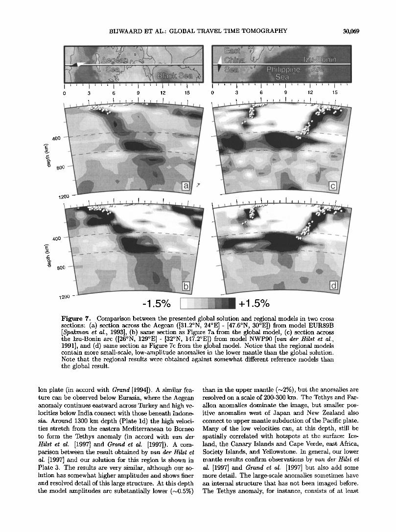
Figure 7. Comparison between the presented global solution and regional models in two cross sections: (a) section across the Aegean ([31.2øN, 24øE] - [47.6øN, 30øE]) from model EUR89B [Spakman et al., 1993], (b) same section as Figure 7a from the global model, (c) section across the Izu-Bonin arc ([26øN, 129ø-E] - [32øN, 147.2øE]) from model NWP90 [van der Hilst et al., 1991], and (d) same section as Figure 7c from the global model. Notice that the regional models contain more small-scale, low-amplitude anomalies in the lower mantle than the global solution. Note that the regional results were obtained against somewhat different reference models than the global result.

lon plate (in accord with Grand [1994]). A similar feature can be observed below Eurasia, where the Aegean anomaly continues eastward across Turkey and high velocities below India connect with those beneath Indone-

sia. Around 1300 km depth (Plate ld) the high velocities stretch from the eastern Mediterranean to Borneo

to form the Tethys anomaly (in accord with van der Hilst et al. [1997] and Grand et al. [1997]). A comparison between the result obtained by van der Hilst et al. [1997] and our solution for this region is shown in Plate 3. The results are very similar, although our solution has somewhat higher amplitudes and shows finer and resolved detail of this large structure. At this depth the model amplitudes are substantially lower (•0.5%)

than in the upper mantle (•2%), but the anomalies are resolved on a scale of 200-300 km. The Tethys and Far- allon anomalies dominate the image, but smaller positive anomalies west of Japan and New Zealand also connect to upper mantle subduction of the Pacific plate. Many of the low velocities can, at this depth, still be spatially correlated with hotspots at the surface: Ice- land, the Canary Islands and Cape Verde, east Africa, Society Islands, and Yellowstone. In general, our lower mantle results confirm observations by van der Hilst et al. [1997] and Grand et al. [1997] but also add some more detail. The large-scale anomalies sometimes have an internal structure that has not been imaged before. The Tethys anomaly, for instance, consists of at least


9O

6O

3O

-3O

-6O

.... :-' .... 12def :.;.:...:.:.:...:_..:.:.:-.---. - - - ......... ............. ......... .: ...........................

'" .......................... 11a

I'11'c 11b

-90 I • I • I • • I: •' I • I • -150 -120 -90 -60 90 120 150 180 -30 0 30 60

longitude (degrees)

Figure 8. Overview of the locations of cross sections shown in Figures 7, 9-12 and in Plates 4, 5. All cross sections have a small map with a compass needle (white pointing north) for orientation.

o

• • ........ •ii::i:::• ......... • .-,-,.½..4,,

'":i::i'.-:..:½:..i':Jil-'..';:.."..i•i•i';i".-:,:,i::: '.============================================= ..!:.......•.:.............•.:•i:.:..i::?`::::::•;•::•:•i:..•:::..:..•:..•ii:;•..;•..•..•:..::i•:•!•::•..•::•i........?..:•i....•.. . 'v '.:

•i!$::ii•i!i•!! •.•-': •?•;.-ii'..".--;-;".-!ii:.-i •Jj-'..'•-.:i:•]•½:!ii(i•½;.i:..=.'ii•i ' .:j•!,•'"". ..... ; ,• .... :::::::::::::::::::::::::::::::::::::::::::::::::::::i:::.-:::::::½::::!::::

8OO

::::::::::::::::::::::::::::::::::::::::::::::::::::::::::::::::::::::::::::::::::::::::::::::::::::::::::::::::::::::::::::::::::::::::::::::::::::::::::::::::::::::::::::: "!!".-".-ii';".-".-'.-:.-'"'"" :"'•:•:';:•!i•".-i;'-.":;":';!•!•i :;'...':';½..'?..i•! .... ß

•:.• ...... ................ • •-• 1200

3 6 9 12 15 0 3 6 9 % 12 15

Figure 9. Cross sections through (a) the Maltran subduction zone (Paidstart) ([22.5øN, 60øE] - [36.8øN, 65.1øE]) and (b) the Scotia Sea subduction zone (South Sandwich Islands) ([57.5øS, 43øW] - [54.5øS, 16.5øW]). The geometry of these anomalies is resolved, but their internal structure is not.

BIJWAARD ET AL.. GLOBAL TRAVEL TIME TOMOGRAPHY 30,071

i liiiiiii!!ii':':•:':':'"•::::ii•iii•i!11iiiiiii?,ii i i:•!•--;:: ::•::::::•:;• ::::::::::::::::::::::::: i:,:,::?: !i i i i?,:: i• ?:i:,?: i:: i•i•i'-i•i:i::?i•i•i•i ::,•i•i•i ::----[' --'-'-' ••-"•••:-•.... '""•:' "':'" "'"'•

0 3 6 9 12 15

0 3 6 9 12 15

400

800

:½!ii::::i::•[ii::-:.::i*•::'•" .:•ii•i•i•i•:;..•ii•ii•i•...:.ii•ii•:•..•i•i•i..•i•i•i•;1..:...1ii:..i:•iiiik :i•i:: ½::::i:•ii::iiiii:: ::::iii":--'-':. i-':.......'•.. i:..½•" :!:.: ::':':.' :•".. ;' :: .:V?" ':: :::½ ;7 +•:::: ::::::::::::::::::::::::::::::::::::::::::::: :: !h ?:::i.'j:i:i:i:: :j::i:iii:..-?';4:'--•:....:.-'.....i....-'::'..'•{'" '•"':'}:-- ß ß :'-'•..-.:-':.'.'i_•.:.• .... -:-•

,,,:,,I , i , , , ! , , , ! , , , i , , , I .... 0 3 6 9 12 15

:ilililili:!i• :iii: iii!!i!i{ i: •2'.'illlllil!! i•i:i: :i: i::..'•. :i: :i:.":i. ::: :•: :i½' :::: :• i iiiiiiiiii: :::i:ii::iii:iii:•iiii!½iiii !: :i: :::::::::::::::::::::: ::::::::::::::::::::::::::::::::::: ...... {•:-."-'•;•i•:•:...j:ii•:ii::"'::---:-•il}ii:•!'-""i•i:{" :':':%?•:..??,'• i •}•i!!•i•i•..........•.:•:•..•iiii•i;•.:.......:..•i•ii!ii•i•i!•iii..•i•!•i•i•?• ":"•:i

0 3 6 9 12 15

400

BOO

0 3 6 9 12 15

-• 4oo

BOO

Figure 10. Cross sections through (a) the Aleu- tian arc ([51øN, 166øE] - [66øN, 166øE), (b) Kamchatka Figure 11. Cross sections through (a) the Elburz ([63øN, 146.5øE] - [49.4øN, 158øE]), and (c) Borneo Mountains (northern Iran' ([30øN, 59øE] - [43.9øN, ([2øS, 112.5øE] - [9.5øN, 122.2øE]). In all three sections 51.9øE]), (b) Burma and Bangladesh ([23.5øN, 87øE] we observe peculiar high-velocity anomalies (apart from - [22.7øN, 103.3øE]), and (c) the Pamir (Himalayas) the obvious slab related anomalies) that might be re- ([28øN, 72øE] - [43øN, 72øE]) displaying continental lated to subduction. The presence of these anomalies is subduction. Lateral resolution is reasonable; smearing resolved, but their exact extent is not. in the vertical direction occurs between 350 and 660 km.


two segmented parallel and linear high-velocity bands: one stretching from Turkey to India and on to Bor- neo and the other stretching from Greece across Arabia into the Indian Ocean. These may reflect the complex history of subduction of the Tethys ocean. An expla- nation could be that these parallel zones result from the subduction of two major parts of the Tethys ocean, separated by a ridge system of unknown geometry. The more southerly located anomaly would then be the image of the former northern segment of the Tethys, which was subducted first. The northern anomaly would re- suit from the subduction of the southern part of the Tethys, which connected to northern India and which has overridden the already subducted northern segment. The distinction between northern and southern

neo-Tethys basins follows from the fact that the Indian continent was attached to the southern Tethys and that the last active subduction of Tethyan age lithosphere presently occurs below the Aegean and below the central Sunda arc. Other intriguing features are the low- velocity anomalies connecting the Cape Verde and Ca- nary Islands hotspots across northwest Africa with the Hoggar hotspot [Dautria, 1988] and the low velocities beneath western Europe, where remnants of recent vol- canic activity are present in the Massif Central [Gcanet et al., 1995] and the Eifel, connecting with the low velocities below the Iceland hotspot.

Up to 1800 km depth the picture hardly changes, and the main features can easily be traced, but the amplitudes decrease and around 1900 km the image consists of many small and low-amplitude anomalies (Plate le). van dec Hilst et al. [1997] raise the question of whether this part of the lower mantle might be a transitional interval in which downwellings transform from a planar geometry to a more cylindrical one. There are, however, only two seemingly planar anomalies identified in the lower mantle immediately above this interval: the Tethys and Farallon anomalies. The absence of the large sheet-like Tethys and Farallon anomalies in the lower part of the mantle may just reflect that the bulk of the lithosphere material has not reached this depth yet. If one would remove these prominent anomalies from the model, the anomaly pattern from 1300 to 1800 km would show similar scale and amplitude anomalies as deeper in the lower mantle. Moreover, we do not observe a change towards a more cylindrical shape for all high-velocity anomalies that continue across the 1800-2300 km interval. For instance, the high-velocity anomaly beneath Siberia (see Plate le) that is imaged from about 1500 km depth to the CMB has a distinct, elongated Z shape that persists all the way to the D" layer, where it joins a large high-velocity anomaly. This Z-shaped anomaly may have resulted from older subduction than that of the Tethys and Farallon plates and hence has had more time to reach the lower part of the mantle. Hence in our model we find no clear evidence

for a transitional interval between 1800 and 2300 kin.

From about 2200 km to the CMB the pattern grows

toward the often observed degree 2 pattern [e.g., $uet al., 1994] with low velocities beneath Africa and most of the Pacific and high velocities below Asia and the Americas (Plate If). These huge anomalies with somewhat higher amplitudes than we observe in the middle of the lower mantle do exhibit some internal structure, but resolution is rather limited at this depth, and severe streaking effects are visible in the northwest Pacific because of preferential ray directions. The elongated linear high-velocity anomaly below the Americas resem- bles a subduction-related anomaly, but the anomaly is not connected with the Farallon anomaly. The observed high velocities beneath Asia and the northwest Pacific may locally be connected with the subducting slab beneath Japan (in accord with van dec Hilst et al. [1997]), which corroborates the slab graveyard origin of these anomalies (see Wysession [1996] for a review of this hypothesis).

We refrain from interpreting the imaged lower mantle heterogeneity in terms of temperature, pressure, or compositional anomalies. Although it is evident that P wave velocity depends on these three parameters, we feel there is at present insufficient information to sensi- bly quantify the relative contributions of temperature, pressure, and compositional anomalies to seismic wave speed.

As mentioned before, a global high-resolution model enables us to compare small-scale tectonic features and to put them in a global perspective. The most detailed parts of our model are the densely sampled subduction zones and different types of slabs are imaged in these regions (see Plate 4), but the continuity and extent of these slabs are not always sufficiently resolved. In the slab cross sections shown in Figures 8-11 and in Plate 4, we do not, in general, show well-known major subduction zones, but instead we focus on smaller, less well-known slabs that often have not been imaged on a regional scale before. Where subduction has continued over longer time spans, we observe deep slabs, flattening in the transition zone underneath the western Mediterranean (Plate lb), the Banda arc, northern Philippines, the Solomon Islands (Plate 4a), and the Izu-Bonin trench. Resolution may be questionable beneath the Solomon Islands, but these flattenings can be resolved beneath the western Mediterranean and also

below the Banda arc and in the Izu-Bonin subduction

zone where they were previously identified by Puspito et al. [1993], Widiyantoro and van der Hilst [1996], and van der Hilst et al. [1991]. Subduction-related anomalies penetrate the 660 km discontinuity underneath Java [Fukao et al., 1992; Puspito et al., 1993; Widiyantoro and van dec Hilst, 1996] and the Marianas (Plate 4b) [van der Hilst et al., 1991], and they penetrate the 660 km discontinuity, after initial flattening in the transition zone, underneath the Kuriles [Fukao et al., 1992] and Tonga (Plate 4c) [van der Hilst, 1995]. Vertical resolution is mediocre in the upper mantle beneath Java, the Marianas, and Tonga, but we seem to be able to identify

BIJWAARD ET AL.- GLOBAL TRAVEL TIME TOMOGRAPHY 30,073

3 6 9 12 15 0

I . , . I , , , i , , I .

i i i i iiii ii ! • 1200

15 0

• ; I

1200 "'

3 6 9 12 15

$00 "'

1200 -1.5%

Plate 4. Cross sections displaying different types of subduction below (a) the Solomon Islands ([19øS, 151øEl - [4.9øS, 156.1øE]) (flattening on top of the 660 km discontinuity), (b) the Marianas ([16øN, 135øE] - [18øN, 150.6øE]) (penetrating into the lower mantle), (c) Tonga-Fiji ([19.5øS, 172øE] - [17.5øS, 172.3øW]) (penetrating after flattening), (d) Peru ([13øS, 78øW] - [12.5øS, 62.6øW]) (kinking at shallow depth), (e) New Guinea ([12øS, 143øE] - [2.5øS, 146.8øE]) (slab splitting (?) at the 660 km discontinuity), and (f) Spain ([43øN, 9øW]-[31.5øN, 3.2øE]) (possibly detachment). See text for resolution aspects.


their lower mantle continuations. In several subduction

zones other forms of slab deformation occur. Below

Venezuela and below the Peru-Bolivia region (Plate 4d) we observe a kink in the high-velocity anomaly [Eng- dahl et al., 1995] that seems to be resolved. Below New Guinea (Plate 4e) we may be imaging the splitting of a slab at the 660 km discontinuity, but the northward extending, upper mantle high-velocity part may also be the result of smearing along rays. We find anomalies suggesting possible detachment of slabs below Ecuador, southern Mexico, Italy, and Albania (consistent with Spakman et al. [1993]) and south Spain (Plate 4f) (consistent with Blanco and $pakman [1993]). Resolution may not be sufficient beneath Mexico and Ecuador, but it probably is sufficient beneath parts of southern Eu- rope. We do not find any indication of detachment underneath Sumatra [ Widiyantoro and van der Hilst, 1996, 1997], where we do seem to have enough vertical resolution to detect such a feature. We do also not de-

tect detachment beneath Greece, but estimates of the vertical resolution in this region are not as good as obtained by $pakman et al. [1993], who also used a large amount of regional data.

The dynamics behind some of the different types of slab behavior have been investigated through numerical modeling and laboratory experiments. In these studies the observed flattening and/or penetration at the 660 km discontinuity has been suggested to be caused by different rates of trench migration [Griffiths et al., 1995; Christensen, 1996; Olbertz et al., 1997]. Numer- ical modeling has indicated that detachment of slabs may occur shortly after the cessation of subduction [O1- bertz, 1997; Wong A Ton and Wortel, 1997].

As previously stated, some of the slab-related anomalies connect in the global perspective to anomalies at 1300 km depth (under southeastern Europe, Indonesia, Tonga, Central America, and Japan). Figure 12 demonstrates the continuation of the high-velocity anomalies beneath Central America and Japan all the way down to the CMB. This is consistent with the results of van

der Hilst et al. [1997] and Grand et al. [1997]. Results of tests dedicated to specific structures (Figures 12b, 12c, 12e, and 12f) show that these continuations of subduction to the CMB are not caused by a lack of vertical resolution.

Although low-velocity regions are, in general, not as well-resolved as high-velocity subduction zones, it is still possible to observe the surface expression and the deep roots of some of these anomalies. The low velocities un-

derneath the Afar Triangle and the African rift valley seem to extend several hundreds of kilometers down-

ward and appear to have a common root under central Africa (where horizontal resolution is limited to 30-6 ø ) which extends all the way to the CMB. This root has been observed by many other global tomography studies [e.g., Inoue et al., 1990; $uet al., 1994; Vasco et al., 1995; van der Hilst et al., 1997] but without a con- nection to the upper mantle. We find similar though

smaller-scale anomalies underneath the Canary Islands, Yellowstone, and Iceland, extending to at least 1200 km, 1500 km, and the CMB, respectively, but only Iceland is reasonably well-resolved in our model. Plate 5 dis- plays a section across Iceland together with a sensitivity result which clearly demonstrates the presence of a con- tinuous low-velocity anomaly from the upper mantle to the CMB beneath Iceland. Smearing could be significant in the upper mantle, but a local tomography study [Wolfe et al., 1997] has already demonstrated the presence of low velocities in the upper mantle below Iceland to at least 400 km depth.

We suspect that the approximately 400-700 km wide low-velocity anomaly observed below Iceland is the blurred image of an even narrower rising plume. The con- duits of plumes are usually estimated to have a diameter of some 100-200 km [e.g., Ribe and Christensen, 1994], which would be difficult to image. However, B. Stein- berger (Plumes in a convecting mantle: Models and observations for individual hotspots, submitted to Journal of Geophysical Research, 1998) argues that especially Iceland may not be a typical plume, but rather a more broad upwelling, because it does not seem to have a hotspot track. In any case, our result in Plate 5 gives seismological evidence for the presence of a relatively narrow low-velocity channel all across the (lower) mantle. The upwelling is tilted toward the south-southeast and has a broad root zone that extends to below the

western Atlantic and Greenland.

Figure 12 and Plate 5 constitute important evidence for the continuation of both high and low velocities across the 660 km discontinuity, a depth that is quite well-resolved in the model. These observations again [e.g., van der Hilst et al., 1997; Grand et al., 1997] indicate that the 660 km discontinuity may resist but not prevent (present day) large-scale mass transfer from the upper to the lower mantle and vice versa.

6. Conclusions

The lack of sampling in large parts of the Earth's mantle due to the uneven distribution of earthquakes and seismic stations prevents a detailed solution for the entire model space. However, the irregular cell parameterization applied with cell sizes adapted to the degree of local sampling together with the application of a vast amount of reprocessed ISC data allows for the first time for a simultaneous solution for long-wavelength structures and small-scale details wherever warranted by the resolving power of the data. The irregular parameterization not only reduces the number of unknowns drasti- cally, it probably better conditions the inverse problem of determining seismic wave velocities, event cluster relocation parameters, and station parameters from 4.7 million narrow composite rays.

The limited sampling of the lower mantle together with the broad Fresnel zones of the seismic waves [Nolet, 1992] and probably wave front healing effects [Wielandt,


0 5 10 15 20 25 30 35 40 45 0 5 10 15 20 25 30 35 40 45

. •,,,I,,,I,,.I

'•!::• ....... . ............. •: .......... .::::•:: i::i•:.::..:.•iii•.'--: ....... ""-:...::....m-- • '"'•" ":..'..':'...'f.•]i::

.:- ..... . ...... :• ::!i!::i ":::."'-•. '.. -'•-•i!i?:11!i..-'•:(,;.•i•!•":.•:• •::= ..... ,::i:ii]iJi[i•.?.•:•[[jj ::ji:[ii!!j!:!:: ":.- :::::::::!?:::::' "!iii!;i:..iii::?:•.. "-'"•f:•i::::::

%

• oo •?.'.:::...'!"':'"'::::ii

,zsoø , . , I , , •... ,:.....!.....!....•.., , I, . , • , , ._•,.-.J,::J::J.....L.L.......•, , ½ ........ ::.: :::...•.:.? -'-::-:•:•*i:!:•:•::..':; :•:i'.":':. -.,:'.. :-:-"•4i½:;.- .:::•,':•i.:.'-'.i'.:.." .......... !:i[;i:-•:i•:.....':•":;.'i"'"" "'""'" "'"" ' ""'"'""'" ' ' '"'" ' "'•••••:i• .............. •........•.....:•i•?>•.......•i!?:iiiiiii•?•.•..............i?.... .`.•.``.•..••.:.:•••••••..:•;•;.:i

.•..•.•...::i?•i!::...:•::.:...•i....... ..:.......`.... ...•..i:•......•:`.•:•:.:•:•:.....".•.....`..`.•••••.•.•••••:•i•.....:•

====================================================================================== .... :::::::::::::::::::::::::::::::::::::::::::::::::::::::::::::::::::::::::::::::: ........

• ':'::[[:i:•i[[i?..:..:.".".•i:'"'""'"':;•[B[:i?;f."J.?•. ....... ":.:::::.---.', ..................... . ............ ::::::!::i.'"'"':•{[:i:::![:::::':•[!

• •ooO - • :-....--.:.,•....•...........•.:..,.•.:••••:.......•................, ======================= .,.,......:.,............•....•.....-•,,•••... ........................... ================================

Figure 12. Cross sections across (a)-(c) Central America ([12øN, 96øW] - [33.6øN, 52.6øW]) and (d)-(f) Japan ([51øN, 97øEI - [30.2øN, 151.5øE1). Figures 12a and 12d show the solutions, Figures 12b and 12e show synthetic input models, and Figures 12c and 12f show the synthetic solutions. Notice that vertical resolution ranges from 50 to 200 km in these sections, indicating that the continuity of structures in our real solution is not caused by smearing.


25

I

3O

BoO

•00

2.0OO

?..•oo

-0.5% +0.5%

Plate 5. Cross sections through Iceland ([64øN, 44øW] - [54.7øN, 14.5øE]): (a) real solution, (b) synthetic input, and (c) synthetic output. Notice that nearly all layers in the lower mantle can be resolved separately, indicating that the continuity of the low- velocity plume in Plate 5a is not caused by vertical smearing.

1987] prevent a very detailed solution in the lower mantle part of the model. This part of our model confirms and adds more detail to recent results obtained by van der Hilst et al. [1997] and Grand et al. [1997]. Apart from the huge Tethys and Farallon plate anomalies several low-velocity anomalies are imaged, which continue from the lower mantle up to the Earth's surface. Al- though the resolution of these features is usually less than for subduction zones, their continuation seems to be resolved. Below Iceland we have imaged a relatively narrow low-velocity anomaly, the image of possibly a mantle plume, stretching all the way from the CMB to the surface. This may be the first (blurred) image of a narrow plume. This continuity of both positive and negative anomalies clearly points to the occurrence of mass transport across the 660 km discontinuity.

In the upper mantle we are able to resolve structures locally on a scale of 65 km, which is comparable to and in some cases better than results from regional mantle studies. For the first time, detailed upper mantle

structures are imaged adequately on the global scale. The global model confirms many regionally obtained results (especially in the upper mantle), puts them in a global framework, and adds several reasonably resolved regions such as the Scotia Sea, parts of northwest Africa, Iran, and the Solomon Islands for which detailed tomography results have never been published before. Furthermore, it allows for the comparison of the structure of different regions (such as subduction zones) without being hampered by different inversion methods or limited model extent. In comparison with our global model, regional mantle studies often exhibit small-scale anomalies in their lower mantle parts, which may be caused by signal and noise acquired by teleseismic data outside the model space.

In general, all subduction zones are well resolved in lateral extent and some also in depth extent, which allows for the detailed observation and comparison of slab behavior. Above the transition zone, slabs may show kinks (Venezuela and Peru-Bolivia), perhaps slabs can split (not well resolved below New Guinea), and they may detach (Spain, Italy, and Albania), which confirms several regional results. At the 660 km discontinuity we find clear continuations into the lower mantle (e.g., below Java, southeastern Europe, the Marianas, Japan, Central America, and Tonga) as well as flattening on top of it (e.g., below the western Mediterranean, the Banda arc, and the Izu-Bonin trench) and penetration after flattening (e.g., below Tonga and the Kuriles). These findings are in general agreement with results from regional studies and indicate that the 660 km discontinuity may resist but not prevent penetration of slabs into the lower mantle.

Here we have tried to give an overview of the most striking observations in our global mantle model of P wave velocity heterogeneity. This should be considered an introduction to the model and the applied method. Detailed interpretations and further comparisons with


results from sensitivity tests will be given elsewhere as these would make this paper unduly long. Our primary aim was to present the model and to show the improvement obtained in the global imaging of mantle structure. The results close the resolution gap with regional mantle studies, which is an important step toward a better understanding of the dynamics and interaction of upper and lower mantle.

Acknowledgments. We are grateful for support from the Netherlands Geosciences Foundation (GOA) with fi- nancial aid from the Netherlands Organization for Scien- tific Research (NWO) through Pioneer project PGS 76-144, through hardware grant NWO-750.396.02, and for support of H.B. through grant NWO-750.195.13. We thank R. D. van der Hilst and an anonymous referee for helpful comments and R. D. van der Hilst for supplying us with an early version of the data set. H.B. thanks dr. Kok, a naive reader, for critical comments on an early version of the manuscript. This work was conducted under the program of the Vening Meinesz School of Geodynamics.

References

Abers, G. G., and S. W. Roecker, Deep structure of an arc- continent collision: Earthquake relocation and inversion for upper mantle P and S wave velocities beneath Papua New Guinea, J. Geophys. Res., 96, 6379-6401, 1991.

Aki, K., A. Christoffersson, and E. S. Husebye, Determi- nation of the three-dimensional seismic structure of the lithosphere, Geophys. J. R. Astron. So½., 82, 277-296, 1977.

Bijwaard, H., W. Spakman, and E. R. Engdahl, Preliminary results from nonlinear global travel-time tomography (abstract), Ann. Geophys. 16, 33, 1998.

Blanco, M. J., and W. Spakman, The P-wave velocity structure of the mantle below the Iberian Peninsula: Evidence for subducted lithosphere below southern Spain, Tectono- physics, 221, 13-34, 1993.

Christensen, U. R., The influence of trench migration on slab penetration into the lower mantle, Earth Planet. $ci. Lett., 1•0, 27-39, 1996.

Clayton, R. W., and R. P. Comer, A tomographic analysis of mantle heterogeneities from body wave travel times (abstract), EOS Trans. AGU, 6• (•5), 776, 1983.

Curtis, A., and R. Snieder, Reconditioning inverse problems using the genetic algorithm and revised parameterization, Geophysics, 62, 1524-1532, 1997.

Dautria, J.-M., Relations entre les h•tdrog•n•ites du man- teau sup•rieur et le magmatisme en domaine continental distensif: Exemple des basaltes alcalins du Hoggar (Sa- hara Central, Alg•rie) et de leurs enclaves, Ph.D. thesis, Cent. Gdol. et Gdophys. de Montpellier, Montpellier, France, 1988.

Dziewonski, A.M., B. H. Hager, and R. J. O'Connell, Large- scale heterogeneities in the lower mantle, J. Geophys. Res., 82, 239-255, 1977.

Engdahl, E. R., and D. Gubbins, Simultaneous travel time inversion for earthquake location and subduction zone structure in the central Aleutian Islands, J. Geophys. Res., 92, 13,855-13,862, 1987.

Engdahl, E. R., R. D. van der Hilst, and J. Berrocal, Imaging of subducted lithosphere beneath South America, Geo- phys. Res. Left., 22, 2317-2320, 1995.

Engdahl, E. R., R. D. van der Hilst, and R. P. Buland, Global teleseismic earthquake relocation with improved travel times and procedures for depth determination, Bull. Seismol. Soc. Amer., 88, 722-743, 1998.

Fukao, Y., M. Obayashi, H. Inoue, and M. Nenbai, Sub- ducting slabs stagnant in the mantle transition zone, J. Geophys. Res., 97, 4809-4822, 1992.

Grand, S. P., Mantle shear structure beneath the Americas and surrounding oceans, J. Geophys. Res., 99, 11,591- 11,621, 1994.

Grand, S. P., R. D. van der Hilst, and S. Widiyantoro, Global seismic tomography: A snapshot of convection in the Earth, GSA Today, 7, 1-7, 1997.

Granet, M., G. Stoll, J. Dorel, U. Achauer, G. Poupinet, and K. Fuchs, Massif Central (France): New constraints on the geodynamical evolution from teleseismic tomography, Geophys. J. Int., 121, 33-48, 1995.

Griffiths, R. W., R. I. Hackney, and R. D. van der Hilst, A laboratory investigation of effects of trench migration on the descent of subducted slabs, Earth Planet. $ci. Lett., 133, 1-17, 1995.

Gudmundsson, O., J. H. Davies, and R. W. Clayton, Stochas- tic analysis of global traveltime data: Mantle heterogeneity and random errors in the ISC data, Geophys. J. Int., 102, 25-43, 1990.

Hager, B. H., R. W. Clayton, M. A. Richards, R. P. Comer, and A. M. Dziewonski, Lower mantle heterogeneity, dy- namic topography and the geoid, Nature, 313, 541-545, 1985.

Humphreys, E., and R. W. Clayton, Adaptation of back projection tomography to seismic travel time problems, J. Geophys. Res., 93, 1073-1085, 1988.

Inoue, H., Y. Fukao, K. Tanabe, and Y. Ogota, Whole mantle P-wave travel time tomography, Phys. Earth Planet. Inter., 59, 294-328, 1990.

Kennett, B. L. N., E. R. Engdahl, and R. Buland, Con- straints on seismic velocities in the Earth from traveltimes, Geophys. J. Int., 122, 108-124, 1995.

Ldv•que, J.-J., L. Rivera, and G. Wittlinger, On the use of the checker-board test to assess the resolution of tomographic inversions, Geophys. J. Int., 115, 313-318, 1993.

Masson, F., and J. Trampert, On ACH, or how reliable is regional teleseismic delay time tomography?, Phys. Earth Planet. Inter., 102, 21-32, 1997.

Masters, G., S. Johnson, G. Laske, and H. Bolton, A shear- velocity model of the mantle, Philos. Trans. R. $oc. Lon- don $er. A, 35•, 1385-1411, 1996.

Mohan, G., and S.S. Rai, Large-scale three-dimensional seismic tomography of the Zagros and Pamir-Hindukush regions, Tectonophysics, 2•2, 255-265, 1995.

Nakanishi, I., and D. L. Anderson, Worldwide distribution of group velocity of mantle Rayleigh waves as determined by spherical harmonic inversion, Bull. Seismol. Soc. Am., 72, 1185-1194, 1982.

Nolet, G., Imaging the deep earth: technical possibilities and theoretical limitations, in Proceedings of the 25th ESC Symposium Barcelona 1990, edited by A. Rocca and D. Mayer-Rosa, pp. 107-115, Servei Geolbgic de Catalunya, Barcelona, Spain, 1992.

Olbertz, D.C., The long-term evolution of subduction zones: A modelling study, Ph.D. thesis, Utrecht Univ., Utrecht, Netherlands, 1997.

Olbertz, D.C., M. J. R. Wortel, and U. Hansen, Trench migration and subduction zone geometry, Geophys. Res. Lett., 2•, 221-224, 1997.

Paige, C. C., and M. A. Saunders, LSQR: An algorithm for sparse linear equations and sparse least squares, A CM Trans. Math. Soft., 8, 43-71, 1982.

Puspito, N. T., Y. Yamanaka, T. Miyatake, K. Shimazaki, and K. Hirahara, Three-dimensional P-wave velocity structure beneath the Indonesian region, Tectonophysics, 220, 175-192, 1993.

Ribe, N.M., and U. R. Christensen, Three-dimensional


modeling of plume-lithosphere interaction, J. Geophys. Res., 99, 669-682, 1994.

Roecker, S. W., Tomography in zones of collision: Practi- cal considerations and examples, in: Seismic Tomography: Theory and Practice, edited by H. M. Iyer and K. Hira- hara, pp. 584-612, Chapman and Hall, New York, 1993.

Sengupta, M., and M. N. ToksSz, Three-dimensional model of seismic velocity variation in the Earth's mantle, Geo- phys. Res. Lett., $, 84-86, 1976.

Snieder, R., and M. Sambridge, Ray perturbation theory for traveltimes and ray paths in 3-D heterogeneous media, Geophys. J. Int., 109, 294-322, 1992.

Snieder, R., J. Beckers, and F. Neele, The effect of small- scale structure on normal mode frequencies and global inversions, J. Geophys. Res., 96, 501-515, 1991.

Spakman, W., Delay-time tomography of the upper mantle below Europe, the Mediterranean, and Asia Minor, Geo- phys. J. Int., 107, 309-332, 1991.

Spakman, W., Iterative strategies for non-linear travel time tomography using global earthquake data, in: Seismic To- mography: Theory and Practice, edited by H. M. Iyer and K. Hirahara, pp. 190-226, Chapman and Hall, New York, 1993.

Spakman, W., and H. Bijwaard, Irregular cell parameterization of tomographic problems, Ann. Geophys. 16, 28, 1998.

Spakman, W., and G. Nolet, Imaging algorithms, accuracy and resolution in delay time tomography, in: Mathemati- cal Geophysics, edited by N.J. Vlaar et al., pp. 155-187, D. Reidel, Norwell, Mass., 1988.

Spakman, W., S. Stein, R. D. van der Hilst, and R. Wortel, Resolution experiments for NW Pacific subduction zone tomography, Geophys. Res. Lett., 16, 1097-1100, 1989.

Spakman, W., S. van der Lee, and R. D. van der Hilst, Travel-time tomography of the European-Mediterranean mantle down to 1400 km, Phys. Earth Planet. Inter., 79, 3-74, 1993.

Su, W., R. L. Woodward, and A.M. Dziewonski, Degree 12 model of shear velocity heterogeneity in the mantle, J. Geophys. Res., 99, 6945-6980, 1994.

Tanimoto, T., Long-wavelength S-wave velocity structure throughout the mantle, Geophys. J. Int., 100, 327-336, 1990.

Trampert, J., and R. Snieder, Model estimations biased by truncated expansions: possible artifacts in seismic tomography, Science, 271, 1257-1260, 1996.

VanDecar, J. C., Upper-mantle structure of the Cascadia subduction zone from non-linear teleseismic travel-time

inversion, Ph.D. thesis, 165 pp., Univ. of Wash., Seattle, 1991.

van der Hilst, R. D., Tomography with P, PP and pP delay- time data and the three-dimensional mantle structure be-

low the Caribbean region, Ph.D. thesis, Utrecht Univ., Utrecht, Netherlands, 1990.

van der Hilst, R. D., Complex morphology of subducted lithosphere in the mantle beneath the Tonga trench, Na- ture, $7•, 154-157, 1995.

van der Hilst, R. D., and W. Spakman, Importance of the reference model in linearized tomography and images of subduction below the Caribbean plate, Geophys. Res. Lett., 16, 1093-1096, 1989.

van der Hilst, R. D., E. R. Engdahl, W. Spakman, and G. Nolet, Tomographic imaging of subducted lithosphere below northwest Pacific island arcs, Nature, 353, 37-43, 1991.

van der Hilst, R. D., E. R. Engdahl, and W. Spakman, To- mographic inversion of P and p? data for aspherical mantle structure below the northwest Pacific region, Geophys. J. Int., 115, 264-302, 1993.

van der Hilst, R. D., S. Widiyantoro, and E. R. Engdahl, Evidence for deep mantle circulation from global tomography, Nature, 386, 578-584, 1997.

Vasco, D. W., L. R. Johnson, R. J. Pulliam, Lateral varia- tions in mantle velocity structure and discontinuities determined from P, PP, S, SS, and SS-SdS travel time residuals, J. Geophys. Res., 100, 24,037-24,059, 1995.

Widiyantoro, S., and R. D. van der Hilst, Structure and evolution of lithospheric slab beneath the Sunda arc, In- donesia, Science, 271, 1566-1570, 1996.

Widiyantoro, S., and R. D. van der Hilst, Mantle structure beneath Indonesia inferred from high-resolution tomographic imaging, Geophys. J. Int., 130, 167-182, 1997.

Wielandt, E., On the validity of the ray approximation for interpreting delay times, in: Seismic Tomography, edited by G. Nolet, pp. 85-98, D. Reidel, Norwell, Mass., 1987.

Wolfe, C. J., I. Th. Bjarnason, J. C. VanDecar, and S.C. Solomon, Seismic structure of the Iceland mantle plume, Nature, 385, 245-247, 1997.

Wong A Ton, S. Y. M., and M. J. R. Wortel, Slab detachment in continental collision zones: An analysis of con- trolling parameters, Geophys. Res. Lett., 2•, 2095-2098, 1997.

Woodhouse, J. H., and A.M. Dziewonski, Mapping the upper mantle: Three-dimensional modelling of Earth structure by inversion of seismic waveforms, J. Geophys. Res., 89, 5953-5986, 1984.

Wysession, M. E., Imaging cold rock at the base of the mantle: The sometimes fate of slabs?, in: Subduction: Top to Bottom, Geophys. Monogr. Ser. Vol. 96, edited by G. E. Bebout et al., pp. 369-384, AGU, Washington, D.C., 1996.

Zhang, Y., and T. Tanimoto, High-resolution global upper mantle structure and plate tectonics, J. Geophys. Res., 98, 9793-9823, 1993.

Zhao, D., D. Christensen, and H. Pulpan, Tomographic imaging of the Alaska subduction zone, J. Geophys. Res., 100, 6487-6504, 1995.

Zhou, H., How well can we resolve the deep seismic slab with seismic tomography?, Geophys. Res. Lett., 15, 1425-1428, 1988.

Zhou, H., A high-resolution P wave model for the top 1200 km of the mantle, J. Geophys. Res., 101, 27,791- 27,810, 1996.

Zhou, H., and R. W. Clayton, P and S wave travel time inversions for subducting slab under the island arcs of the northwest Pacific, J. Geophys. Res., 95, 6829-6851, 1990.

H. Bijwaard, and W. Spakman, Vening Meinesz School of Geodynamics, Faculty of Earth Sciences, Utrecht Uni- versity, Budapestlaan 4, P.O. Box 80021, 3508 TA Utrecht, Netherlands. ([email protected]; [email protected])

E. R. Engdahl, National Earthquake Information Center, U.S. Geological Survey, Denver Federal Center, Box 25046, MS 967, Denver, CO 80225. ([email protected])

(Received January 26, 1998; revised June 30, 1998; accepted July 20, 1998.)

Closing the gap between regional and global travel time tomography

Documents

Transcript of Closing the gap between regional and global travel time tomography