Clinical research of dexmedetomidine in healthy volunteers

Clinical research of dexmedetomidine in healthy volunteers

Mia Bäckström

University of Helsinki

Faculty of Pharmacy

Division of Pharmaceutical Biosciences

and

University of Turku

Institute of Clinical Medicine

Department of Anesthesiology and Intensive Care

2017

TABLE OF CONTENTS 1 INTRODUCTION ................................................................................................................. 1

2 LITERATURE REVIEW ..................................................................................................... 2 2.1 Autonomic nervous system .................................................................................................... 2 2.1.1 Parasympathetic nervous system ............................................................................................. 3 2.1.2 Sympathetic nervous system ........................................................................................................ 5

2.2 Adrenergic receptors ................................................................................................................. 6 2.2.1 Beta adrenergic receptor ................................................................................................................ 7 2.2.2 Alpha-‐1 adrenergic receptor ........................................................................................................ 8 2.2.3 Alpha-‐2 adrenergic receptor ........................................................................................................ 8

2.3 Alpha-‐2 adrenoceptor agonists ............................................................................................... 9 2.3.1 Mechanism of action ...................................................................................................................... 10

2.4 Dexmedetomidine .................................................................................................................... 14 2.4.1 Pharmacological effects ............................................................................................................... 15 2.4.3 Therapeutic use of dexmedetomidine ................................................................................... 20

2.5 Pharmacokinetics (PK) ........................................................................................................... 21 2.6 PK-‐analysis methods ............................................................................................................... 22 2.6.1 NCA and compartmental methods ......................................................................................... 22 2.6.2 Pharmacometrics ............................................................................................................................ 26 2.6.3 Basics of population PK ................................................................................................................ 26

2.7 Components of the population PK model ........................................................................... 28 2.7.1 Structural model ............................................................................................................................. 30 2.7.2 Statistical model .............................................................................................................................. 32 2.7.3 Covariate model .............................................................................................................................. 33

2.8 Previous population PK modeling of IV dexmedetomidine ............................................ 34

3. EXPERIMENTAL PART: CLINICAL RESEARCH OF DEXMEDETOMIDINE ON HEALTHY VOLUNTEERS ................................................................................................... 38 3.1 Aim of the study and perspectives ....................................................................................... 38 3.2 Materials and Methods ............................................................................................................ 40 3.2.1 Volunteer study ............................................................................................................................... 40 3.2.2 Blood samples and their handling ........................................................................................... 41 3.2.3 Analysis of dexmedetomidine concentrations ................................................................... 42 3.2.4 Explorative and non-‐compartment data analysis ............................................................ 42 3.2.5 Pharmacometric analysis ............................................................................................................ 45

3.3 Results ........................................................................................................................................ 47 3.3.1 Pharmacokinetics of dexmedetomidine from NCA .......................................................... 47 3.3.2 Population pharmacokinetics of dexmedetomidine ....................................................... 52

3.4 Discussion .................................................................................................................................. 57 3.5 Conclusion ................................................................................................................................. 61

4 REFERENCES ..................................................................................................................... 62

APPENDIX I

Tiedekunta - Fakultet - Faculty

Faculty of Pharmacy

Laitos - Institution – Department

Pharmaceutical Biosciences

Tekijä - Författare - Author

Mia Bäckström

Työn nimi - Arbetets titel - Title

Clinical research of dexmedetomidine in healthy volunteers

Oppiaine - Läroämne - Subject

Biopharmacy

Työn laji ja ohjaaja(t) - Arbetets art och handledare – Level and instructor

Master´s Thesis-Teijo Saari and Arto Urtti

Aika - Datum - Month and year

May 2017

Sivumäärä - Sidoantal - Number of pages

70

Tiivistelmä - Referat - Abstract

Background: Dexmedetomdine is a α2–adrenergic receptor agonist, which by binding to the α2–adrenergic receptor in the sympathetic nervous system exhibits sedative effect. Additionally, it has an analgesic and anxiolytic effect. Dexmedetomidine is registered as a sedative for use in the intensive care unit and in USA, additionally, in surgical settings. The study was conducted to characterize the pharmacokinetics in healthy volunteers through pharmacokinetic analysis methods. Methods: The clinical study was conducted on healthy 10 voluntary subjects each receiving dose of 1 µg/kg both intravenously (IV) and subcutaneously (SC). The study session lasted for 10 hours, with a wash-out period of at least 7 days between consecutive administrations. Arterial blood samples were taken to determine the plasma concentrations of dexmedetomidine. The pharmacokinetics of the IV and SC dose were determined by noncompartmental analysis (NCA) and, additionally, population modeling using nonlinear mixed effects model (NONMEM) was used to determine the pharmacokinetics of the IV dose. Results: The population´s mean clearance after the IV dose was 40.0 L/h and for SC 45.6 L/h. The elimination half-life was 2 hours for IV, whereas terminal half-life was 9 hours for the SC dose. The SC bioavailability was 120 %. From the population modeling the typical elimination clearance, volume of distribution in central compartment, inter-compartmental clearance, and volume of distribution in the second compartment were 39.6 L/h, 13.7 L, 116 L/h, and 77 L, respectively.

Conclussion: The obtained pharmacokinetic parameter values from NCA for IV were in line with the results from previous studies. For the SC dose the pharmacokinetic parameter values had high SD indicating high inter-individual variations. However, when the 8th subject was excluded from data analysis less SD was obtained and the result resembled more the results from other extravascular studies. The pharmacokinetic population results for IV dexmedetomidine were similar to previous studies on healthy subjects. Weight was used as a covariate, and was modeled by allometrically scaling the parameters. From the results it is shown that the covariate improved the model´s goodness of fit.

Avainsanat – Nyckelord - Keywords

Dexmedetomidine; pharmacokinetics; population modeling; nonlinear mixed effects model; α2-‐agonist

Säilytyspaikka - Förvaringsställe - Where deposited

Department of biopharmacy and pharmacokinetics Muita tietoja - Övriga uppgifter - Additional information

Teijo Saari University of Turku; Arto Urtti, University of Helsinki

Tiedekunta - Fakultet - Faculty

Farmaceutiska fakulteten

Laitos - Institution – Department

Biofarmaci och farmakokinetik

Tekijä - Författare - Author

Mia Bäckström

Työn nimi - Arbetets titel - Title

Klinisk studie av dexmedetomidin hos friska frivilla individer

Oppiaine - Läroämne - Subject

Biofarmaci och farmakokinetik

Työn laji ja ohjaaja(t) - Arbetets art och handledare – Level and instructor

Pro gradu avhandling-Teijo Saari och Arto Urtti

Aika - Datum - Month and year

Maj 2017

Sivumäärä - Sidoantal - Number of pages

71

Tiivistelmä - Referat - Abstract

Bakgrund: Dexmedetomidine är en α2–adrenergisk receptor agonist, som genom att binda till α2–adrenergiska receptorn i sympatiska nervsystemet utövar en sedative effekt. Utöver det har den även uppvisat ha smärtlindrande och ångestdämpande verkan. Dexmedetodine är registrerad för användning på intensiv avdelningen, men i USA även vid kirurgiska ingrepp. Studien gick ut på att karakterisera dexmedetomidins farmakokinetik i friska frivilliga individer genom farmakokinetiska analytiska metoder.

Metoder: Den kliniska studien genomfördes på tio friska frivilliga individer, där vardera individ fick en dos på 1 µg/kg både intravenöst och subkutant. Studien pågick i 10 timmar, med en elimineringsperiod på åtminstone 7 dagar mellan de två administrationerna. Arteriella blodprov togs för att kunna bestämma dexmedetomidins plasmakoncentration. Icke-kompartmental analys användes för att bestämma farmakokinetiken efter både intravenös och subkutan administrering. Utöver det så användes nonlinear mixed effects model” (NONMEM), för att fastställa intravenösa dosens farmakokinetik. Resultat: Gruppens clearance medeltal efter intravenösa dosen var 40,0 L/h, medan den var 45,6 L/h efter subkutana dosen. Eliminationens halveringstid var för IV dosen 2 timmar och för SC dosen hela 9 timmar. Biotillgängligheten för subkutana dosen var 120 %. Resultaten från populationsanalysen var följande: eliminerings clearance 39,6 L/h, centrala distributionsvolymen 13,7 l, clearance mellan kompartment ett och två 116 L/h och distributionsvolymen i kompartment två 77 l. Sammanfattning: Farmakokinetik parametervärdena som erhölls i icke kompartment analysen påminde om resultaten från tidigare studier. Farmakokinetik parametervärdena för subkutana dosen hade höga standard avvikelser, vilket tyder på variation mellan individerna. Då åttonde indviden togs bort var samtliga standard avvikelser mindre och resulaten påminde mera de resultat som framkommit i tidigare studier då dexmedetomidine tillförts extravasculärt. Farmakokinetik resultaten från populationsanalysen påminde om resultaten från andra studier på friska frivilliga individer. Vikt användes som kovariat och togs i beaktande i modellen genom att allometriskt skala parametrarna. Från resulatetn kan man se att kovariaten förbättrade modellen.

Avainsanat – Nyckelord - Keywords

Dexmedetomidine; pharmacokinetics; population modeling; nonlinear mixed effects model; α2-‐agonist

Säilytyspaikka - Förvaringsställe - Where deposited

Biofarmaceutiska och farmakokinetiska avdelningen Muita tietoja - Övriga uppgifter - Additional information

Teijo Saari, Turun Yliopisto; Arto Urtti, Helsingin Yliopisto

1

1 INTRODUCTION

Patients receiving palliative care often suffer from pain, anxiety and depression.

Therefore, in the final stage of their life they may need sedation to ease anxiety.

Several drugs, such as opioids, benzodiazepines, antidepressants or particular

antipsychotics are used to ease anxiety (Devlin and Roberts 2011). However, all

these drugs dispose dose-‐related adverse effects, and to reduce these, a

multimodal therapy is often used to decrease individual drug doses or to achieve

synergistic interaction. This means that several drugs affecting via different

receptor-‐systems are combined. Especially opioids but also benzodiazepines are

associated with adverse effects such as tolerance, nausea, constipation and

respiratory depression (Barr et al. 2001: Swart et al. 2006). Hence, there is a

clinical need for alternative drug regimens to treat palliative care patients.

Alpha-‐2-‐agonists, which stimulate the α2-‐adrenergic receptors in the sympathetic

nervous system, have gained recent interest due to their sedative, analgesic,

anxiolytic and sympatholytic effects (Scheinin et al. 1989: Hunter et al. 1997:

Buerkle and Yaksh 1998: Sallinen et al. 1998). Dexmedetomidine, a recently found

alpha-‐2-‐agonist, has been demonstrated to induce dose-‐dependent sedation

without any risk of ventilatory depression (Ebert et al. 2000: Petroz et al. 2006).

Theoretically and based on published case reports and uncontrolled series

dexmedetomidine may provide benefits for the palliative patient, as it induces

analgesia and sedation with no risk of respiratory depression. Dexmedetomidine

exhibits poor oral bioavailability (Anttila et al. 2003) and, therefore, alternative

administration routes are needed. Previous studies have shown that

dexmedetomidine is well absorbed intranasally (Iirola et al. 2011),

intramuscularly and buccally (Scheinin et al. 1992; Anttila et al. 2003). However,

there are currently no data on the pharmacokinetics of dexmedetomidine after

subcutaneous administration.

The following literature review gives an insight on the anatomy and physiology of

the autonomic nervous system and α2-‐adrenergic receptors as a part of it. My aim

2

is to describe the mechanism of action of α2-‐receptor ligands, and the

pharmacokinetics, pharmacodynamics and therapeutic uses of dexmedetomidine.

Finally, basic knowledge of pharmacometric analysis, modeling and simulation is

provided.

In the experimental part of this thesis, the pharmacokinetics of subcutaneously

and intravenously administered dexmedetomidine in healthy volunteers are

investigated using pharmacokinetic analysis methods. Both explorative-‐ and

noncompartmental pharmacokinetic analyses were conducted to obtain estimates

for the pharmacokinetic parameters after subcutaneously and intravenously

administered dexmedetomidine. Additionally, the pharmacometric analysis is

performed to characterize the relationship between individual covariate effects

and observed drug exposure.

2 LITERATURE REVIEW

2.1 Autonomic nervous system

The autonomic nervous system is the part of the nervous system that regulates

essential body functions. It consists of nerves and nerve cells (Gabella 2001),

which principally innervate the smooth musculature of all organs, the heart and

the endocrine glands (Jänig 1989). Therefore, the autonomic nervous system

mediates regulation of the internal milieu in the body. Compared to the somatic

nervous system, which is under voluntary control, the autonomic nervous system

is generally not voluntary controlled.

Functionally, the autonomic nervous system can be divided into sympathetic-‐ and

parasympathetic nervous system (Jänig 1989). Both the sympathetic and the

parasympathetic systems consist of preganglionic-‐ and postganglionic neurons,

which transmit impulses to the effector tissue from the CNS (McCorry 2007).

Furthermore, the autonomic nervous system consists of another part; the enteric

3

nervous system, which is confined to the gastrointestinal tract (Jänig 1989). It

regulates the motility and secretory activities in the gastrointestinal tract.

However, it functions independently and no extrinsic input from the spinal cord

and brainstem is needed.

An autonomic nervous system consists of central and peripheral components

(Gabella 2001). In the central nervous system (CNS), nuclei in the hypothalamus,

brainstem and spinal cord connect with afferent nerves to the peripherally located

ganglia and further on with peripheral autonomic nerves. The nerves emerging out

of the brainstem and spinal cord consist of a preganglionic-‐ and postganglionic

neuron, and the autonomic ganglion, located outside the CNS, connects these two

neurons by a synapse (McCorry 2007). The preganglionic neurons are afferent

neurons projecting from the nuclei in the CNS. The postganglionic neurons are

axons projected from the ganglia to the peripheral tissues, such as smooth muscle

cells, cardiac muscle and secretory cells (Jänig 1989).

The autonomic nervous system is involved in the regulation of several organs in

the body. It controls, for example, the contraction and relaxation of the heart and

arteries, movement of the iris and lens in the eye, urination in the lower urinary

tract, and movement of hair and the secretion of sweat in the skin (Gabella 2001).

Furthermore, it mediates regulation in the gastrointestinal tract, genital tract and

part of the airways. Many tissues are innervated by both the parasympathetic and

the sympathetic nervous system, which typically possess opposing effects on a

given tissue (McCorry 2007). For example, in the heart the sympathetic system

increases the heart rate, whereas the parasympathetic system decreases it.

2.1.1 Parasympathetic nervous system

The parasympathetic preganglionic neurons emerge out from several nuclei of the

brainstem and from the sacral region of the spinal cord, segments S2-‐S4, as can be

seen in Figure 1 (McCorry 2007). The preganglionic axon of the neuron is long and

4

synapses with the ganglia, which is near or in the effector organ (Figure 1). The

postganglionic neuron is, on the other hand, very short and is the neuron that

provides input to the cells of the effector tissue.

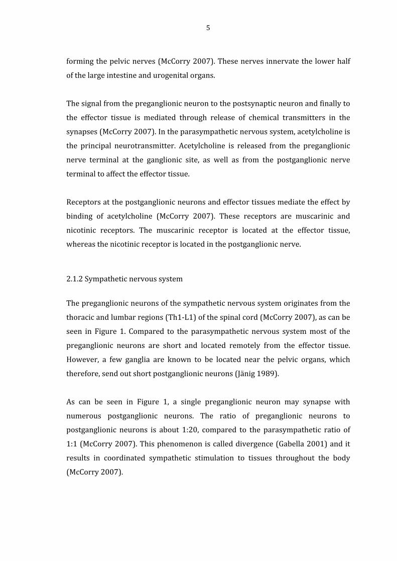
Figure 1. The sympathetic and parasympathetic branches of the autonomic nervous system. The sympathetic preganglionic nerves (red) emerge out from the thoracic and lumbar regions of the spinal cord (segment T1 to L2). The preganglionic nerves connect to the postganglionic nerve/nerves (light red), by synapsis in the ganglia, which further innervates the effector organ. The parasympathetic preganglionic nerves (dark grey) emerge out from the brainstem and sacral region of the spinal cord (segment S2 to S4). The preganglionic nerve connects to the postganglionic nerve (light grey), by synapsis in the ganglia, which further innervates the effector organ. (Adapted from Jänig, 1989)

In the brainstem the emerging neurons exit the CNS through the cranial nerve

(McCorry 2007). The oculomotor nerve (III) innervates the eyes; the facial nerve

(VII) innervates the lacrimal gland, the salivary glands and the mucus membranes

of the nasal cavity; the glossopharyngeal nerve (IX) innervates the parotid

(salivary) gland; and the vagus nerve (X) innervates the viscera of the thorax and

the abdomen, for example, heart, lungs, stomach, pancreas, small intestine, upper

half of the large intestine and liver. The preganglionic neurons from the sacral

region of the spinal cord exit the CNS separately and are later united (Figure 1),

5

forming the pelvic nerves (McCorry 2007). These nerves innervate the lower half

of the large intestine and urogenital organs.

The signal from the preganglionic neuron to the postsynaptic neuron and finally to

the effector tissue is mediated through release of chemical transmitters in the

synapses (McCorry 2007). In the parasympathetic nervous system, acetylcholine is

the principal neurotransmitter. Acetylcholine is released from the preganglionic

nerve terminal at the ganglionic site, as well as from the postganglionic nerve

terminal to affect the effector tissue.

Receptors at the postganglionic neurons and effector tissues mediate the effect by

binding of acetylcholine (McCorry 2007). These receptors are muscarinic and

nicotinic receptors. The muscarinic receptor is located at the effector tissue,

whereas the nicotinic receptor is located in the postganglionic nerve.

2.1.2 Sympathetic nervous system

The preganglionic neurons of the sympathetic nervous system originates from the

thoracic and lumbar regions (Th1-‐L1) of the spinal cord (McCorry 2007), as can be

seen in Figure 1. Compared to the parasympathetic nervous system most of the

preganglionic neurons are short and located remotely from the effector tissue.

However, a few ganglia are known to be located near the pelvic organs, which

therefore, send out short postganglionic neurons (Jänig 1989).

As can be seen in Figure 1, a single preganglionic neuron may synapse with

numerous postganglionic neurons. The ratio of preganglionic neurons to

postganglionic neurons is about 1:20, compared to the parasympathetic ratio of

1:1 (McCorry 2007). This phenomenon is called divergence (Gabella 2001) and it

results in coordinated sympathetic stimulation to tissues throughout the body

(McCorry 2007).

6

The sympathetic nervous system regulates essentially the same organs and tissues

as the parasympathetic nervous system (Figure 1). The sympathetic neurons

additionally innervate the skin, its blood vessels and sweat glands, controlling the

sweating and the tonus of the vascular smooth muscle (McCorry 2007). These

effects are only regulated by the sympathetic nervous system. Furthermore, the

sympathetic neurons also innervate adipose tissue, the liver (Jänig 1989) and the

adrenal medulla (McCorry 2007).

In the sympathetic nervous system, the short preganglionic neurons are

cholinergic and the long postganglionic neurons are adrenergic neuron (McCorry

2007). Acetylcholine is released into the synaptic cleft from the preganglionic

neuron to transport the signal to the postsynaptic sites, whereas in the

postganglionic neuron terminal noradrenaline is released to mediate the effect on

the target tissue.

2.2 Adrenergic receptors

Adrenergic receptors are located in a large number of tissues, and connect the

central-‐ and peripheral nervous systems (McCorry 2007). The numerous metabolic

and neuroendocrine effects of the catecholamines, noradrenaline and adrenaline,

are mediated through interactions with two major classes of adrenergic receptors

(Bylund 1992: Strosberg 1993). These two classes are the alpha (α-‐) and the beta

(β)-‐adrenergic receptor (Ahlquist 1948), which were discovered in 1948 by

Alhquist based on the order of potency of several catecholamine analogues.

In 1986, Dixon and his co-‐workers discovered that the β-‐adrenergic receptor, like

rhodopsin, obtained a seven-‐transmembrane structure (7TM) (Dixon et al. 1986).

The discovery leads to the idea that a large gene family of receptors existed. This

gene family was later named the G-‐protein-‐coupled receptor (GPCR) –superfamily,

to which all adrenergic receptors nowadays belong (Bylund 1992: Storsberg

1993). The amino acids that build up the transmembrane receptor crosses the cell

7

membrane seven times and incorporates hydrophilic and hydrophobic areas

(Khan et al. 1999). Additionally, to the seven hydrophobic transmembrane

segments, the intracellular carboxyl terminus and the extracellular amino

terminus are the common structural feature for the different GPCRs (Kobilka

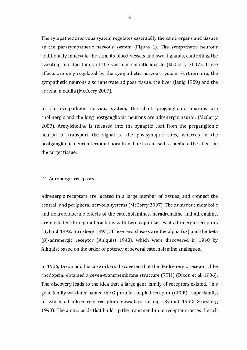
2007). A cartoon of a GPCR can be seen in Figure 2.

Figure 2. A GPCR with its seven hydrophobic transmembrane segments (H1-H7), extracellular amino terminus (COOH-) and intracellular carboxyl terminus (NH3

+). (Adapted from Lodish et al. 2000)

The α-‐adrenergic receptor is further divided into α1-‐ and α2-‐ adrenergic receptors

(Langer 1974: Bylund and U´Prichard 1983: Molinoff 1984), which gives a total of

three types of adrenergic receptors, namely, α1, α2 and β. The different adrenergic

receptors are 42-‐45 % identical in terms of the amino acid sequence in the

membrane domain (Khan et al. 1999). This implies that the diversity in the amino

sequence in the transmembrane region is important for the selectivity of ligand

binding.

2.2.1 Beta adrenergic receptor

The β-‐adrenergic receptors can further be divided into β1-‐ and β2-‐ adrenergic

receptor (Arnold et al. 1966: Lands et al. 1967a: Lands et al. 1967b). The β1-‐

receptors are located in the heart, brain, and adipose tissues and have high affinity

for both noradrenaline and adrenaline (Molinoff 1984). For example, β1-‐adrenergic

stimulation in the heart and kidneys increase cardiac output and renin release,

8

respectively (Giovannitti et al. 2015). β2-‐receptors are located in vascular and

other smooth muscles, for example, bronchial smooth muscle cells (Giovannitti et

al. 2015) and show low affinity for noradrenaline (Molinoff 1984). The

physiological functions of the β2 receptors in the vascular and bronchial smooth

muscles cells are vasodilatation and relaxation (Giovannitti et al. 2015). An

additional subtype of the β-‐adrenergic receptor has been discovered, giving rise to

three subtypes of the β-‐adrenergic receptor. The β3-‐receptor has been found to

regulate the lipid metabolism in adipose tissue, which is very distinct from the

other β-‐adrenergic receptor subtypes (Strosberg 1997: Giovannitti et al. 2015).

2.2.2 Alpha-‐1 adrenergic receptor

Similar to the β2-‐receptors, the α1–adrenergic receptors are located in the

postsynaptic site (Molinoff 1984) of the vascular smooth muscle cells Giovannitti

et al. 2015). However, the effects of the α1-‐receptors are different as they are

involved in the vasoconstriction of the vascular smooth muscle cells.

2.2.3 Alpha-‐2 adrenergic receptor

The α2-‐receptors have been located at both post-‐ and presynaptical site in the

central-‐ and peripheral nervous system (Langer 1981, Gertler et al. 2001). In the

CNS the presynaptical receptors are located in sympathetic nerve endings and in

noradrenergic neurons, where they inhibit the release of noradrenaline when

stimulated (Langer 1981). In the peripheral the α2-‐receptors are also located in

noradrenaline nerve endings and inhibit the noradrenaline release. Furthermore,

α2-‐receptors exist peripherally in numerous tissues, for example in the liver,

pancreas, platelets, kidney, eye and the adipose tissue (Khan et al. 1999).

Depending on the location, the physiologic responses mediated through the α2-‐

receptor vary significantly.

9

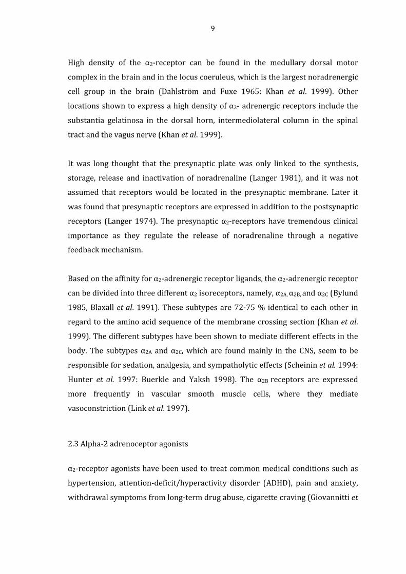
High density of the α2-‐receptor can be found in the medullary dorsal motor

complex in the brain and in the locus coeruleus, which is the largest noradrenergic

cell group in the brain (Dahlström and Fuxe 1965: Khan et al. 1999). Other

locations shown to express a high density of α2-‐ adrenergic receptors include the

substantia gelatinosa in the dorsal horn, intermediolateral column in the spinal

tract and the vagus nerve (Khan et al. 1999).

It was long thought that the presynaptic plate was only linked to the synthesis,

storage, release and inactivation of noradrenaline (Langer 1981), and it was not

assumed that receptors would be located in the presynaptic membrane. Later it

was found that presynaptic receptors are expressed in addition to the postsynaptic

receptors (Langer 1974). The presynaptic α2-‐receptors have tremendous clinical

importance as they regulate the release of noradrenaline through a negative

feedback mechanism.

Based on the affinity for α2-‐adrenergic receptor ligands, the α2-‐adrenergic receptor

can be divided into three different α2 isoreceptors, namely, α2A, α2B, and α2C (Bylund

1985, Blaxall et al. 1991). These subtypes are 72-‐75 % identical to each other in

regard to the amino acid sequence of the membrane crossing section (Khan et al.

1999). The different subtypes have been shown to mediate different effects in the

body. The subtypes α2A and α2C, which are found mainly in the CNS, seem to be

responsible for sedation, analgesia, and sympatholytic effects (Scheinin et al. 1994:

Hunter et al. 1997: Buerkle and Yaksh 1998). The α2B receptors are expressed

more frequently in vascular smooth muscle cells, where they mediate

vasoconstriction (Link et al. 1997).

2.3 Alpha-‐2 adrenoceptor agonists

α2-‐receptor agonists have been used to treat common medical conditions such as

hypertension, attention-‐deficit/hyperactivity disorder (ADHD), pain and anxiety,

withdrawal symptoms from long-‐term drug abuse, cigarette craving (Giovannitti et

10

al. 2015). Recent research has focused on the sedative, analgesic, anxiolytic and

sympatholytic effects of the α2-‐receptor agonists (Scheinin et al. 1989: Hunter et al.

1997: Buerkle and Yaksh 1998).

Clonidine was the first α2-‐adrenoceptor agonist on the market, and several α2-‐

receptor agonists have since been developed (Gertler et al. 2001). Clonidine was

introduced to the market as a nasal decongestant (Giovannitti et al. 2015), but it

caused severe hypotension, after which it gained a new clinical use in treating

hypertension (Gertler et al. 2001). Clonidine has also been used to treat anxiety,

ADHD, chronic pain, withdrawal symptoms and postoperative shivering

(Giovannitti et al. 2015). Lately it has also been used as pretreatment for surgical

patients with anxiety (Hall et al. 2006) and for procedural sedation in children

(Cao et al. 2009).

Other α2-‐adrenoceptor agonists currently used in clinical practice are tizanidine,

medetomidine and dexmedetomidine. These possess the sedative, anxiolytic, and

analgesic properties similar to those of clonidine (Scheinin et al. 1989: Giovannitti

et al. 2015; Gertler et al. 2001). Tizanidine has been used for treatment of muscle

spasm and cramps, myofascial pain disorders of head and neck, and spasticity of

cerebral palsy (Giovannitti et al. 2015). Medetomidine is nowadays mainly used in

veterinary medicine to sedate cats and dogs (Scheinin et al. 1989).

Dexmedetomidine is the pharmacologically active d-‐enantiomer of medetomidine

(Savola and Virtanen 1991) and it is used as a sedative in the intensive care unit

(ICU) (Approval letter: Precedex® 1999).

2.3.1 Mechanism of action

As previously mentioned the clinical effects of the α2-‐adrenoceptor agonists are

produced after binding to the α2-‐adrenoceptor. All subtypes of the α2-‐receptor are

GPCR (Bylund 1992: Storsberg 1993), and the effect is mediated through activation

of G-‐ (guanine-‐nucleotide regulatory binding) proteins (Freissmuth et al. 1989)

11

These G-‐proteins consist of three subunits; the beta subunit; the gamma subunit;

and the alpha subunit, which binds the guanine nucleotides, guanosine

diphosphate (GDP) and guanosine triphosphate (GTP) (Codina et al. 1987:

Freissmuth et al. 1989).

At a resting state, when the α2-‐receptor is not activated, the GDP is bound to the

alpha subunit of the G-‐protein, and the G-‐protein is not attached to the receptor

(Khan et al. 1999). After an agonist binds to the receptor, a structural change

occurs, and the G-‐protein is coupled to the receptor. The activation results in

decreased affinity for GDP and subsequently GDP is replaced by GTP, causing the

dissociation of the alpha subunit from the beta and gamma subunit, thus

generating a separate alpha subunit and a beta-‐gamma complex (Codina et al.

1987: Neer and Clapham 1988).

Activated G-‐protein (or Gi-‐protein) inhibits adenylyl cyclase (Freissmuth et al.

1989), which further results in decreased formation of 3´5´-‐ cyclic adenosine

monophosphate (cAMP) (Figure 3). The inhibition of adenylyl cyclase is an almost

ubiquitous effect seen in many different G-‐protein associated receptors (Khan et al.

1999). However, all physiological effects mediated by α2 adrenergic receptor

cannot be explained by the decrease of intracellular cAMP.

α2-‐receptor activation also results in the hyperpolarization of the cell membrane,

which is caused by the modulation of ion channel activity. The activation of the G1-‐

protein, which gates the potassium channels, results in efflux of potassium ions

(Figure 3) (Codina et al. 1987) The efflux of potassium ions causes

hyperpolarization of the cell membrane and prevents neuronal firing (Aghajanian

and VanderMaelen, 1982).

12

Figure 3. Stimulation of the presynaptic α2ABC adrenergic receptor. When the presynaptic α2 adrenergic receptor binds its ligand, the G-protein, consisting of the alpha, beta and gamma subunit, is coupled to the receptor. This results in a) inhibition of adenylyl cyclase, which decreases the formation of 3,5-cyclic adenosine monophosphate (cAMP). b) efflux of potassium, causing hyperpolarization and c) dissociation of the alpha subunit from the beta and gamma subunit, which results in inhibition of calcium influx by the beta and gamma subunit. (Adapted from Gilsbach and Hein 2008)

Neurotransmitter release from the synapse is controlled by voltage-‐dependent

calcium ion channels, which are coupled to the G-‐protein G0 (Bean 1989:

Birnbaumer et al. 1990). When activated the subunits of the G-‐protein dissociate,

and the beta-‐gamma complex mediates the effect of α2–agonists further on to the

calcium ion channel (Figure 3) (Herlitze 1996: Ikeda 1996). The beta-‐gamma

complex inhibits calcium influx through the calcium ion channel, resulting in

inhibition of neurotransmitter release. Hence, the negative feedback mechanism

mediated by the α2–agonists prevents the nerve from constant firing and inhibits

the release of neurotransmitters, both of which cause a reduction of the activity in

the ascending noradrenergic pathways.

The α2-‐adrenoceptor agonist affects both central and peripheral nervous systems

by modulating autonomic nervous system functions. The central effects can be

seen in attenuating sympathetic responses like hypertension and tachycardia by

13

stimulation of the α2-‐adrenoceptor located post-‐synaptically (Gertler et al. 2001).

The sedative and analgesic actions of α2-‐adrenoceptor agonists are mediated

through the α2A-‐adrenergic receptor subtype in the CNS (Hunter et al. 1997:

Lakhlani et al. 1997), whereas the anxiolytic effect is mediated through the α2C-‐

adrenergic receptor subtype (Figure 4) (Sallinen et al.1998). The sedative effect is

mediated through locus coeruleus, which is an important modulator of

wakefulness (Scheinin and Schwinn 1992: Gertler et al. 2001). The analgesic

effects are mediated through the substantia gelatinosa of the dorsal horn in the

spinal cord (Kuraishi et al. 1985), and through the descending medullospinal

noradrenergic pathway, which has its origin in locus coeruleus. (Marwaha et al.

1983: Gertler et al. 2001).

Activation of the peripherally located α2-‐adrenergic receptors causes various

physiological effects. In the gastrointestinal tract the effects include decreased

salvation, endocrine secretion, and bowel motility (Khan et al. 1999: Gertler et al.

2001). Inhibition of renin release, increased glomerular filtration, and increased

secretion of sodium and water are seen in the kidney. α2-‐adrenergic stimulation

decreases intraocular pressure and insulin release from the pancreas, and

contracts vascular and other smooth muscle. The release of growth hormone is

increased, and α2-‐adrenergic receptors inhibit the lipolysis of adipose tissue,

decrease the amount of circulating catecholamines in plasma, and it has also been

shown that a high concentration of the α2-‐adrenoceptor agonists causes platelet

aggregation (Khan et al. 1999).

In opposite to the centrally located α2-‐adrenoceptors, which by sympatholysis

mediates hypotension and bradycardia (Gertler et al. 2001), the peripherally

located α2-‐adrenoceptors generates vasoconstriction. It is the α2B-‐adrenergic

receptor subtype that is responsible for this effect, and it is located

postsynaptically in the vascular smooth muscle cells (van Meel et al.1981: Link et

al. 1997). Additional receptor subtypes and their effects are shown in Figure 4.

14

Figure 4. The pharmaceutical effects of α2-adrenoceptor agonist in various organs in the human body mediated through different α2-adrenoceptor subtypes. Sedation and anxiolysis are mediated through the binding to α2A- and α2C-adrenoceptors, respectively, located in the CNS. The analgesic effect is mediated through the binding of the agonist to the α2A-adrenoceptor subtype in the spinal cord. Vasoconstriction is mediated through the α2B-adrenoceptor subtype, whereas vasodilation is mediated through sympatholysis, however, unsure of the subtype. The bradycardic effect is mediated through the α2A-adrenoceptor subtype, whereas it is not certain if tachycardia is mediated through the α2B-adrenoceptor subtype. The mechanism for anti-shivering and diuresis are unknown. (Adapted from Kaur M, Singh P-M, 2011)

2.4 Dexmedetomidine

Dexmedetomidine (Figure 5) is the pharmacologically active enantiomer of the α2-‐

adrenoceptor agonist medetomidine (Savola and Virtanen 1991), and it is a

specific and potent α2-‐adrenoceptor agonist (Aantaa et al. 1993) with a wide range

of pharmacological properties, such as sympatholysis, sedation, anxiolysis, and

analgesia (Gertler et al. 2001). The high selectivity of dexmedetomidine results

from its greater affinity for the α2-‐adrenoceptor compared to clonidine.

Dexmedetomidine is approximately eight times more selective to the α2-‐

15

adrenoceptor than clonidine, as clonidine has a specificity of 220:1 to the α2-‐

adrenoceptor, compared to 1620:1 with dexmedetomidine (Gertler et al. 2001).

Figure 5. The chemical structure of dexmedetomidine (Product monograph: Precedex® 2016)

2.4.1 Pharmacological effects

The primary and desired pharmacological effects of dexmedetomidine are

mediated through binding of the agonist to the α2-‐adrenergic receptor located in

CNS. The binding of dexmedetomidine in CNS causes sedation, analgesia,

anxiolysis and sympatholysis by the mechanism previously described. Thereby, it

can be used in a wide range of clinical settings.

The dose-‐dependent sedative effect of dexmedetomidine has been well

documented (Afonso and Reis 2012). Dexmedetomdine has also been described to

produce even anesthesia when increased doses are given, which suggested that it

could be used as an intravenous (IV) anesthetic (Ebert et al. 2000). Furthermore,

the sedation induced by dexmedetomidine showed similarity with natural sleep, as

the sleeping pattern is identical with the natural course of sleep (Nelson et al.

2003).

After dexmedetomidine dosing, a brief biphasic and dose-‐dependent stimulatory

effect on the cardiovascular system is observed (Bloor et al. 1992, Penttilä et al.

2004). First, a short hypertensive phase is seen followed by hypotension. The

initial increase in blood pressure and reflectory decrease in the heart rate are seen

after a bolus dose of 1 μg/kg (Bloor et al. 1992). The hypertensive effect to the

16

hemodynamics is caused by stimulation of the α2B-‐adenoceptor in the vascular

smooth muscle, whereas the observed decrease in blood pressure after 5-‐10

minutes is due to the induction of the sympathetic tone (Bloor et al. 1992: Link et

al. 1997). Furthermore, the dose-‐dependent bradycardic effect is also primarily

meditated by sympatholysis (Gertler et al. 2001). However, with doses ranging

from 0.25 μg/kg to 0.5 μg/kg only a slight reduction of blood pressure was

obtained (Bloor et al. 1992).

Dexmedetomidine has a minimal effect on the respiratory system, which should be

considered as a major advantage compared with other anesthetic drugs (Ebert et

al. 2000: Petroz et al. 2006). Even when plasma concentrations are up to 15 times

higher than the therapeutic range, only limited respiratory effects result, which

gives dexmedetomidine wide safety margins (Venn et al. 2000). When

dexmedetomidine is used in ICU, no adverse effects on respiratory rate and gas

exchange have been demonstrated on the spontaneously breathing surgical

patients. Additionally, it is suggested that dexmedetomidine possesses

neuroprotective properties by reducing catecholamine release (Ding et al. 2015). It

also reduces cerebral blood flow and cerebral oxygen consumption (Kaur and

Singh 2011).

2.4.2 Pharmacokinetics

When dexmedetomidine is administered at the recommended dose range of 0.2 to

0.7 μg/kg/hr it exhibits linear pharmacokinetics (Product monograph: Precedex® 2016), in other words, a constant fraction of the drug is eliminated per hour

instead of a constant fraction of the drug per hour. The onset of dexmedetomidine

effect after an IV administration varies from 10-‐15 minutes (Product monograph:

Precedex® 2016), and during continuous infusion a peak concentration is usually achieved within 1 hour (Afonso and Reis 2012). Other administration modalities

can also be used, since dexmedetomidine is sufficiently absorbed after

intramuscular (IM), oral, buccal, transdermal and intranasal (IN) administration

(Kivistö et al. 1994; Anttila et al. 2003).

17

Dexmedetomidine exhibits a plasma protein binding of 94 %, which has shown to

be constant over the concentration range of 0.85 to 85 ng/ml (Dexdor® INN-‐dexmedetomidine). It is bound to both α1-‐glycoprotein and human serum albumin,

to which the latter majority of the binding occurs.

The bioavailability of the different administration routes has been characterized

(Anttila et al 2003) and the highest bioavailability was obtained from the IM route,

with a value of 104 %. However, in another study a bioavailability of 73 % was

obtained for the IM route (Dyck et al. 1993b). The oral bioavailability for

dexmedetomidine is low, 15.6 % after oral administration. However, after buccal

administration dexmedetomidine shows high bioavailability (82 %). The

bioavailability for transdermal and IN administrations have also been studied. The

bioavailability of transdermally administered dexmedetomidine from the

transdermal patch was 51 %. However, after dexmedetomidine was released from

the preparation and localized transdermally it showed a bioavailability of 88 %

(Kivistö et al. 1994). In the bioavailability study of IN administered

dexmedetomidine the median absolute bioavailability was obtained for

dexmedetomidine, with a value of 65 % (Iirola et al. 2011). However, there was a

large inter-‐individual variation, as the values range from 35 % to 93 %. Yoo et al.

(2015) have also studied the intranasal administration route through population

modeling. The obtained bioavailability was higher, namely 82 %. The results from

previously mentioned studies have been summarized in Table 1.

18

Table 1. The bioavailability for different administration routes. Dyck et al. 1993b1), Kivistö et al. 1994 2), Anttila et al. 20033), Iirola et al. 2011 4), Yoo et al. 2015 5)

Route of administration F (%)

IM 103.6 3) 73 1)

Buccal 81.8 3)

Intranasal 65.4 4), 82 5)

Transdermal 88 2)

Peroral 15.6 3)

Due to its high lipophilicity, dexmedetomidine is rapidly distributed into tissues

with a distribution half-‐life of approximately 6 minutes, which explains the rapid

onset of action (Karol and Maze 2000, based on the Abbott Laboratories internal

report by Karol 1998: Anttila et al. 2003: Product monograph: Precedex® 2016). The steady-‐state volume of distribution (Vss) varies according to these authors

from 97.3 ± 29 l to 121 ± 20 l.

In previous studies, clearance (CL) for the different administration routes were

obtained and shown in Table 2. The values range between 39 and 49.2 L/h after IV

administration, whereas apparent clearance (CL/F) for IN, transdermal and IM

varies from 41.8 to 63 L/h. In Table 2 the elimination half-‐life (t1/2) is additionally

shown. The elimination half-‐lives varied from 1.9 h to up to 5.6 h. However, the

elimination half-‐life average from the previous studies was approximately 2.5 h.

19

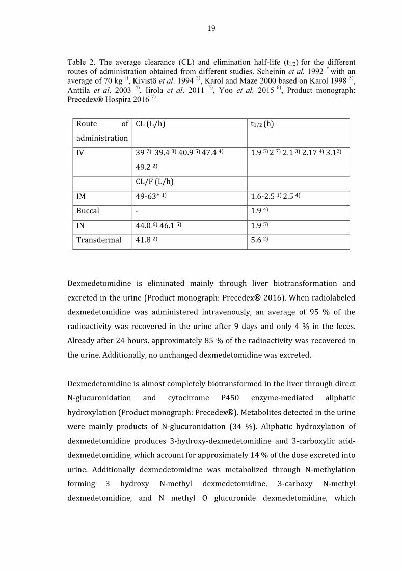
Table 2. The average clearance (CL) and elimination half-life (t1/2) for the different routes of administration obtained from different studies. Scheinin et al. 1992 * with an average of 70 kg 1), Kivistö et al. 1994 2), Karol and Maze 2000 based on Karol 1998 3), Anttila et al. 2003 4), Iirola et al. 2011 5), Yoo et al. 2015 6), Product monograph: Precedex® Hospira 2016 7)

Route of

administration

CL (L/h) t1/2 (h)

IV 39 7) 39.4 3) 40.9 5) 47.4 4)

49.2 2)

1.9 5) 2 7) 2.1 3) 2.17 4) 3.12)

CL/F (L/h)

IM 49-‐63* 1) 1.6-‐2.5 1) 2.5 4)

Buccal -‐ 1.9 4)

IN 44.0 6) 46.1 5) 1.9 5)

Transdermal 41.8 2) 5.6 2)

Dexmedetomidine is eliminated mainly through liver biotransformation and

excreted in the urine (Product monograph: Precedex® 2016). When radiolabeled dexmedetomidine was administered intravenously, an average of 95 % of the

radioactivity was recovered in the urine after 9 days and only 4 % in the feces.

Already after 24 hours, approximately 85 % of the radioactivity was recovered in

the urine. Additionally, no unchanged dexmedetomidine was excreted.

Dexmedetomidine is almost completely biotransformed in the liver through direct

N-‐glucuronidation and cytochrome P450 enzyme-‐mediated aliphatic

hydroxylation (Product monograph: Precedex®). Metabolites detected in the urine were mainly products of N-‐glucuronidation (34 %). Aliphatic hydroxylation of

dexmedetomidine produces 3-‐hydroxy-‐dexmedetomidine and 3-‐carboxylic acid-‐

dexmedetomidine, which account for approximately 14 % of the dose excreted into

urine. Additionally dexmedetomidine was metabolized through N-‐methylation

forming 3 hydroxy N-‐methyl dexmedetomidine, 3-‐carboxy N-‐methyl

dexmedetomidine, and N methyl O glucuronide dexmedetomidine, which

20

accounted for approximately 18% of the dose in urine. The aliphatic hydroxylation

is primarily mediated through CYP 2A6, whereas CYP1A2, CYP2E1, CYP2D6 and

CYP2C19 only have a minor role.

Due to the extensive liver metabolism, dose reductions should be considered for

patients with liver impairment. Compared to healthy subjects, clearance was

lowered by 53, 64 and 74 percent in adults with mild, moderate, and severe

hepatic dysfunction, respectively (Product monograph: Precedex®, 2016). In patients with severe renal dysfunction the pharmacokinetics of dexmedetomidine

did not significantly change compared to healthy subjects.

2.4.3 Therapeutic use of dexmedetomidine

In 1999, dexmedetomidine was approved for human use in the USA by the Food

and Drug Administration (FDA) (Approval letter: Precedex® 1999).

Dexmedetomidine was approved to the ICU setting for sedation of intubated and

mechanically ventilated patients. The indication has since been extended sedation

of non-‐intubated patients prior to and/or during surgical and other procedures

(Hospira Press Release 2008). In September 2011, dexmedetomidine was

approved in Europe by the European Medicine Agency (EMA) (EPAR summary for

the public: Dexdor® 2011). However, in Europe the dexmedetomidine is approved

for sedation of adult patients in ICUs only.

Dexmedetomidine is currently mainly used in the ICUs and in surgical units as an

analgosedative (Yu 2012). Compared with other sedatives, such as GABA (gamma-‐

aminobutyric acid)ergic drugs, dexmedetomidine induced sedation is

characterized with arousability. This unique characteristic allows the medical

study to communicate with the patient, thus improving the patient’s care and

outcome. Furthermore, dexmedetomidine has been proven to maintain sufficient

sedation without respiratory depression and hemodynamic instability (Siobal et al.

2006).

21

2.4.4 Off-‐label therapeutic uses of dexmedetomidine

As previously mentioned, dexmedetomidine is approved only for ICU-‐sedation and

in USA additionally for sedation prior to and/or during surgical or other

procedures. However, dexmedetomidine has been shown to be useful in other

clinical settings outside the approved therapeutic indications.

Dexmedetomidine is increasingly used off-‐label to treat delirium in the ICU as a

recent study suggested dexmedetomidine having a beneficial effect on the

postoperative complication delirium (McLaughlin and Marik 2016). Additionally,

dexmedetomidine is used to prevent shivering during spinal anesthesia after a

study demonstrated that dexmedetomidine infusion during perioperative period

decreased the shivering associated with the spinal anesthesia (Usta et al. 2011).

Dexmedetomidine product approval includes only adult patients. However,

dexmedetomidine is increasingly used off-‐label on pediatric patients. Currently

dexmedetomidine has been administered in the ICU for sedation and analgesia and

in ambulatory anesthesia e.g. for sedation during non-‐invasive procedures in

radiology (Phan and Nahata 2008). Furthermore, it is also used for postoperative

delirium and shivering in pediatric patients.

2.5 Pharmacokinetics (PK)

Pharmacokinetics is the study of the time course of a drug and its metabolites

passing through the body. During the passage the amount of drug changes due to

absorption, distribution, metabolism and elimination. These four phases (ADME)

influence the drug concentration and the total drug exposure to the tissue, thereby,

affecting the pharmacological activity of the drug in the body. Hence, it is crucial to

determine the biological fate of the drug.

22

To describe and predict pharmacokinetic parameters, such as bioavailability, area

under the plasma concentration-‐time curve (AUC), clearance, and elimination half-‐

life are calculated and used in pharmacokinetic studies. Bioavailability describes

the fraction or percentage of the given drug that has been absorbed to the blood

circulation after an extravascular (EV) dose, AUC is the total systemic exposure to

the drug, clearance the volume of the drug being eliminated per unit of time and

elimination half-‐life is the time it takes to eliminate half of the dose. Additional

parameters, for example, the maximum concentration (Cmax) and the time at

maximum concentration (Tmax), are also determined in pharmacokinetic analyses.

2.6 PK-‐analysis methods

2.6.1 NCA and compartmental methods

Both non-‐compartmental analysis (NCA) and compartmental modeling belong to

the classical PK analyses (Sherwin et al. 2014). The statistical moments derived

from the time course of the drug concentration data are the foundation for the

NCA, whereas compartmental modeling is being based on the mass balance

equations of the compartments.

NCA is used to obtain pharmacokinetic parameters without using a specific

compartment model (Gabrielsson and Weiner 2012). The total drug exposure is

determined from the AUC, which in NCA is usually calculated by the trapezoidal

rule (Gabrielsson and Weiner 2012). In the trapezoidal rule the measured data

points are used to split the curve into a series of segments, thus forming trapezoids

except the first, which forms a triangle (Figure 6). All following equations are

based on Gabrielsson and Weiner 2012.

23

Figure 6. The measured plasma concentration points split the curve in to segments forming trapezoids, except for the first forming a triangle. The area of a segment is calculated by the use of the equation:

𝐴𝑟𝑒𝑎 = !!!!!!!!!!

×(𝑡!!! − 𝑡!), (1)

where the Cpn is the plasma concentration in the nth time point trapezoid, Cpn+1 is

the plasma concentration in the following time point trapezoid, tn+1 the time at the

n+1 time point trapezoid, and tn the time at the nth time point trapezoid. However,

the area for the last segment, last concentration time-‐point to infinity, is calculated

by dividing the concentration at that time-‐point with the elimination rate constant.

The areas of all the segments are then summarized to obtain the AUC.

After AUC has been estimated, both clearance (CL) and bioavailability (F) can be

calculated. To calculate percentage bioavailability (F%) AUC for both IV and

extravascular (EV) doses ought to be calculated. The following equation is used:

𝐹% = 100 × !"#!"!"#!"

× !!"!!" , (2)

where AUCev and AUCiv are the AUC from the EV dose and IV dose, respectively,

and Div and Dev are the given IV and EV dose, respectively.

24

The IV clearance is calculated by dividing the given dose with AUC0-‐∞ as in the

following equation:

𝐶𝐿 = !"#$!"!"!!!!

, (3)

When IV data is not available the apparent extravascular clearance (CL/F) is

obtained by dividing the extravascular (EV) dose with the extravascular AUC0-‐∞ as

can be seen in the following equation:

𝐶𝐿/𝐹 = !"#$!"!"#!!!

(4)

The elimination half-‐life is obtained by dividing the constant 0.693 with the

elimination rate constant, ke, as in the following equation:

t !/! =!.!"#!! (5)

To obtain the Cmax and Tmax no equations are needed, since both values are read

from the concentration time data.

In the PK compartment model analysis models are used to describe the time-‐

course of drug exposure after administration of different doses, and to give

estimates for pharmacokinetic parameters such as clearance and volume of

distribution (Mould and Upton 2012). PK models are based on simple structural

compartments, for example, the central compartment, peripheral compartment,

and elimination compartment, which are then connected to each other with first-‐

order processes. These parameters may be used to simulate the drug

concentration obtained by a given dose in different compartments during a given

time interval. Therefore, one can obtain the estimated drug concentration in

plasma at a given time, the concentration eliminated at a given time and other

valuable information after administration of a given amount of the drug.

25

As can be seen in Figure 7, describing the drug transport from the apical-‐ to the

basolateral side of the lumen, the model consist of compartments representing

given physical entities, which are connected to each other by mathematical

formulas or given parameter values to be able to simulate the drug movement. The

construction is very simple and it gives a good understanding of the time course of

the drug exposure in the basolateral side of the lumen.

Figure 7. PK model in Stella software simulating paracetamol transport from the apical- to the basolateral side in lumen. Apical and basolateral boxes represent the apical and basolateral side of the lumen. The circles represent parameters, such as permeability (Papp), area of the lumen (area), concentration in the apical side (C1), the volume in the apical- and basolateral side (volume apical/volume baso), which through mathematical formulas aid to obtain the concentration of paracetamol (C2) in the basolateral compartment at given time points.

In a PK model the compartments are typically abstract concepts not automatically

representing a particular region of the body (Mould and Upton 2012). Hence,

physiology-‐based PK models (PBPK) are being used to represent given organs of

the body, which then are connected by the vascular system according to the

anatomic structure (Nestorov 2007).

26

2.6.2 Pharmacometrics

Pharmacometrics is a science branch involving mathematical models of

pharmacology, disease, biology and physiology for describing and quantifying

interactions, both beneficial-‐ and side effects, between xenobiotics and patients

(Barrett et al. 2009). In the beginning pharmacometrics was described as the

methodology for evaluating population based data, especially population

pharmacokinetics (Williams and Ette 2007). Nowadays it has a much broader

definition, since the term pharmacometrics has become the overall term for

describing modeling and simulation for PK, exposure-‐response relationships, and

disease progression (Sherwin et al. 2014).

Pharmacometrics uses data from animals, healthy subjects and patients to

understand the drug behavior, disease progression and its effect on individual

patients (Sherwin et al. 2014). Additionally, pharmacometrics is utilized to

personalize medicine to specific groups of patient population, thereby, improving

the efficacy and minimizing toxicity of the drug.

Pharmacometrics has become an important tool in drug development. It combines

data, knowledge, and mechanisms to help make reasonable decisions regarding

drug use and development (Mould and Upton 2012). The models are

representations of the system being evaluated. The models are highly simplified

representations, however, it is the simplification that makes them useful. Thus,

depending on the aim of the study the best fitted model is being used. Since the

most important factor is how well the model describes the phenomena, not if the

model is right or true.

2.6.3 Basics of population PK

A drug exhibits variability in exposure between patients leading to variability in

the clinical response across the population (Weber and Rüppel 2013 originated

27

from Rowland et al. 1985). To be able to estimate the PK variability across patients

large data is required, typically more than 100 patients. Traditionally the

population parameters have been estimated by the “two-‐stage approach”, where

the individuals’ data were first fitted separately. Then mean population

parameters were calculated summing up the individual parameter estimates.

Another method, called “naïve pool approach”, fits all individual data together like

there were no individual kinetic differences (Sheiner and Beal 1980). In 1977,

Sheiner and co-‐workers suggested a method for investigating the PK of a drug in a

population (Weber and Rüppel 2013). The method does not need a large data set,

instead sparse and unbalanced data can be used to investigate the typical PK of a

drug. Hence, parameter estimates can be obtained for individuals for whom there

are too few observations for standard parameter estimation methods (Mould and

Upton 2012). Various settings can be modeled with pharmacometric methods,

such as a “sparse” data with as little as one observation per subject, “rich” data

with many observations per subject or a combination of both, where many

samples are collected for some subjects and only a few samples for the others

(Bonate 2011).

The population PK is based on nonlinear mixed effect modeling (Sherwin et al.

2014), which is used to model and identify variability in drug concentrations or

pharmacological effects between individuals (Mould and Upton 2012: Mould and

Upton 2013). It uses the structural simplicity of the classical compartment PK

models but manages to associate the PK parameters to different covariates such as

age, gender, body weight etc. (Sherwin et. al. 2014). All of these physiological

factors affect the exposure of a drug (Mould and Upton 2012), for example, both

clearance and volume of distribution is affected by body weight (Sherwin et. al.

2014). These factors vary between subjects, generating variation in drug exposure

(Mould and Upton 2012). Therefore, it is of great interest to identify and quantify

the intra-‐ and inter-‐individual variability for a given drug. Additionally, the

population model is useful for rationalizing drug development and to establish

optimal dosing strategies for specific patient groups, which cannot otherwise be

studied (e.g. intensive care patients and infants (Struys et al. 2011).

28

Pharmacometric models are used to simultaneously evaluate the data from all

individuals in a population (Bonate 2011). The data is associated with a nonlinear

mixed effect model, using repeated measures trial design (Aarons 2014). The

computer software (NONMEM, Icon Software) implementing the nonlinear mixed

effect model is written in FORTRAN and was developed by Beal and Sheiner (Beal

and Sheiner 1980).

2.7 Components of the population PK model

In nonlinear mixed effects modeling, as the name “nonlinear” implies, the function

under consideration is nonlinear to the model parameter, more precisely the

dependent variable is nonlinearly related to the model parameters and

independent variables (Bonate 2011). The model incorporates both fixed effects

and random effects, hence the name mixed effects modeling. The fixed effect model

incorporates the individual pharmacokinetic parameters, identified covariates,

thereby, the known sources of inter-‐individual variability (Sherwin et. al. 2014).

The random effects, on the other hand, include the unidentified sources of

variability. In the nonlinear mixed effects model one achieves to model the

correlation between a set of independent variables and some dependent variable

(Bonate 2011). The dependent variable is concentration and the independent

variables are dose, time and possibly covariates like weight and age. The structure

of a population mixed effects model is thus:

𝑌!! = 𝑓 𝑥!" ,𝜃, 𝜂! + 𝜀! (6)

where the jth estimated drug concentration for an individual i (𝑌!") is a function of:

a vector of pharmacokinetic parameters (𝜃), individual characteristics (fixed

effects, 𝑥!" ), inter-‐individual or between subject variability (IIV or BSV) and

random effects described by residual error (𝜀!). However, nonlinear mixed effects

modeling can be used to model and simulate various dependent variables from

pharmacodynamic studies and clinical trials.

29

The nonlinear mixed effects model is composed of structural-‐, statistical-‐, and

covariate models (Figure 8) (Mould and Upton 2013). The structural models

describe the concentration time course within the population, whereas the

statistical models clarify the unaccountable random effects within the population

(Bonate 2011). The covariate models stand for the variability due to subject

physiologic characteristics (covariates). These models and the data are then

brought together by the nonlinear mixed effects modeling software (NONMEM).

Thereby, giving parameters to the describing structural, statistical, and covariate

models.

Figure 8. Principles of population modeling. A. Population models consist of several components: structural models, statistical models, and covariate models. Functions that describe the time course of a measured response (e.g. concentrations) build of the structural model. The statistical model describes the variability in the observed data, whereas the covariate model describes the influence of physical factors such as weight, height, age etc. on the individual time course of the response. B. A pharmacokinetic study with two subjects (red lines), where each subject has received a single intravenous dose. Fixed and random-‐effect parameters are both included in population modeling and are, therefore, called “mixed-‐effect” models. The structural model (blue line) represents the fixed effects by parameters that have the same value for every subject (θPOP). Each

30

subject (i) is then described by individual parameter values (yi), and can be seen as red lines. The difference between an individual’s parameter value and the population value is accounted by the random effects (ηi). The difference between the observed data for an individual (Cij) and the model’s prediction for each measurement (j) is described by residual or unexplained error (εij). C. To describe the pharmacokinetics a one-‐compartment model is used. The covariate model indicates that clearance (CLPOP) scales linearly with body weight (WT), thereby, the variability in this parameter can be described by covariate, body size. The statistical model incorporates the influence of residual error and random effects. To calculate the population (CPRED) and individual (CIPRED) predicted concentrations the model equations are used. Population models can be employed to simulate scenarios after clinically relevant dosing schemes. Figure D shows the effect of age on simulated concentration-‐time course of oxycodone after IV bolus dosing. Adapted from Olkkola et al. 2013

2.7.1 Structural model

A structural model is equivalent to systemic models and absorption models, which

are models describing the kinetics after IV dosing and drug uptake into the blood

circulation after extravascular dosing, respectively (Mould and Upton 2013). The

structural model may consist of one, or several compartments depending on the

number of exponential phases obtained by plotting concentration versus time. To

estimate the amount of compartments needed in the structural model one can plot

log concentration versus time, as each distinct declining linear phase generally

demands its own compartment. It is of great importance to choose the right

number of compartments in the structural model, because too few compartments

will describe the data poorly, giving a higher OFV (objective function value),

whereas too many compartments will show improvement in OFV, poor precision

in parameter estimation and the additional peripheral compartment parameters

will converge on values that have minimal influence on the plasma concentrations

(Mould and Upton 2013). OFV describes how well the model predictions match the

data, the lowest OFV equals the best fit.

The order of the elimination needs to be taken in consideration when the model is

being developed (Mould and Upton 2012). When the drug exhibits first-‐order

elimination the rate of elimination is proportional to concentration and clearance

31

is constant. In zero-‐order elimination systems the rate of elimination is

independent of concentration and clearance depends on the dose administered.

Generally, as the concentration increase the elimination moves progressively from

first-‐order elimination to zero-‐order elimination, thereby, showing a saturation of

the elimination pathways. However, pharmacokinetic data collected from subjects

receiving a single dose are seldom sufficient to quantify and confirm saturable

elimination, but several doses may be needed.

When a drug is given through extravascular routes it exhibits an absorption phase,

which ought to be taken into consideration. Therefore, a structural model

component representing absorption is needed, where two factors, bioavailability

and absorption rates, are the key processes affecting the total concentration

(Mould and Upton 2013). Total bioavailability can only be calculated when both IV

and extravascular data are available. The amount of unabsorbed drug depend on

the route of administration and the drug, for example, the drug does not penetrate

the gastrointestinal wall, is metabolized during absorption or precipitates or

aggregates at the injection site.

Secondly, which earlier mentioned, is the effect of the absorption rate on the total

concentration. Most extravascular administered drugs exhibit an absorption

process, called first-‐order absorption, which is described by the absorption rate

constant ka (Mould and Upton 2013). This absorption rate constant represents the

absorption as a passive process, which is driven by the concentration gradient

between the absorption site and blood. Thereby, resulting in a descending

concentration gradient with time as the drug, in an exponential manner, is

depleted at the absorption site. In cases where the drug in the blood is delayed, a

lag time in the absorption may be added to the model. However, some drugs

exhibit zero-‐order absorption, as in drug elimination, where the drug is absorbed

with constant rate. This is due to either a saturable absorption process or where

the release of the drug in the drug reservoir is constant.

32

2.7.2 Statistical model

To describe the variability associated with the structural model a statistical model

is being used (Mould and Upton 2013). In population pharmacokinetic models

there are two principal sources of variability: inter-‐individual or between subject

variability (BSV) and the residual variability (RUV). BSV is the variance of a

parameters across individuals, whereas RUV is the unexplained variability after

other sources of variability have been excluded.

The parameter values from the structural model typically exhibit variability

between every subject. In the statistical model the BSV is described by

parametrization, which is mostly based on the type of data being evaluated (Mould

and Upton 2013). In the structural model, a population value described by the

Greek letter θ, is obtained for a given pharmacokinetic parameter. To describe the

deviation from the population value for a given subject the Greek letter η is being

used. The description of BSV can be done by using the additive function: θ = θ1+

η1i, where θ1 is the population value and η1i is the deviation for the ith subject.

However, the assumption that η values are normally distributed with a mean of 0

and variance ω2 is not always correct. Therefore, when η values have skewed or

kurtotic distribution transformation is necessary to obtain normal distribution of η

values. Log-‐normal distribution is often assumed in pharmacokinetics because

parameters must be positive and often right-‐skewed (Lacey et al. 1997: Limpert et

al.2001). In a log-‐normal distribution a parameter value, e.g. clearance for a given

subject, CLi, can be described with the function: Cli= θ1 * exp(n1i), where θ1 is the

population clearance and n1i is the deviation from the population for the ith

subject (Mould and Upton 2013).

Assay variability, errors in sample time collection, and model misspecification are

sources creating residual variability in the population (Mould and Upton 2013).

The residual variability is described by the Greek letter ε. Analogous to BSV the

type of data being evaluated determines the selection of RUV model. Several

functions, for example additive, proportional and a combination of both, are being

33

used to describe RUV. The combined additive and proportional error models are

often utilized in dense pharmacokinetic data, whereas in pharmadynamic data the

additive error model is suitable. The additive formula is expressed as follows: Y=

f(θ, Time) + ε, where f (θ, Time) is the function describing the time-‐dependent

behavior of pharmacokinetic parameters (THETA). As with the BSV models the

term describing RUV, ε, is assumed to be normally distributed, independent, and

with a mean of 0 and a variance σ2. Notwithstanding, the assumption of η and ε

being independent is often incorrect, which for example can clearly be seen in the

proportional error model; Y= f (θ, η, Time) x (1+ε). However, this interaction can

be accounted for in the likelihood estimation. When the RUV is not normally

distributed, but kurtotic or right-‐skewed, transformation is necessary, similar to

BSV.

2.7.3 Covariate model

A covariate model explains the predicted variability (Mould and Upton 2013).

These predicted variabilities are important to identify in population

pharmacokinetic evaluations. The first step is to select potential covariates, which

is usually based on known properties of the drug, drug class, or physiology. For

example, when a drug is highly metabolized, covariates such as weight, liver

enzymes, and genotype will be included. The next step is to preliminarily evaluate

the selected covariates. However, the run times can occasionally be extensive and,

therefore, it is often necessary to limit the number of covariates evaluated in the

model. Different covariate screening methods aid in determining the importance of

selected covariates and, thereby, reduces the number of evaluations. The final step

is to build the covariate model. If covariate screening has been conducted only the

covariates identified in the screening are evaluated separately and the relevant

covariates are included. However, if covariate screening was not conducted, all

covariates are tested separately and those covariates meeting the inclusion criteria

are counted.

34

The covariates can either be continuous or discrete (Mould and Upton 2012). The

continuous covariates have values which are uninterrupted, for example weight,

whereas discrete values are distinct classes or unconnected values, for example

sex. These two classes of covariates are handled differently. The effect of

continuous covariates can be included in the population model by using a variety

of functions, such as, linear, power, or exponential function. CL= (θ1+ (Weight) x

θ2) x exp(n1) is a linear function and describes the effect of the covariate, weight,

on CL. The discrete covariates can either be; dichotomous, taking one of two

possible values such as sex; or polychotomous, taking on of several possible values

such as race. The dichotomous covariates are set to 0 for the reference

classification and 1 for the other classification, whereas polychotomous covariates

can be classified using different factors for each classification against a reference

value or be grouped into two categories. When the covariates are of inherent

order, for example, the degree of kidney failure is defined as mild, moderate,

severe and very severe (CKD stages: The renal association), they can be described

as mild=0 and very severe=4.

2.8 Previous population PK modeling of IV dexmedetomidine

Population pharmacokinetics of IV dexmedetomidine has previously been

described in several studies. The first study was conducted by Dyck et al. (1993ab)

in healthy males, and the most recent model was published last year (Kuang et al.

2016). Different covariates have been tested, and both healthy volunteers and

patients have been studied. An overview of the previously published population

pharmacokinetic models of IV dexmedetomidine is shown in Table 3.

35

Table 3. . An overview of the previous published population pharmacokinetics of IV dexmedetomidine. ALB=albumin, ALT=alanine transaminase, AST aspartate transaminase, BMI= body mass index, BSA= body surface area, CL= clearance, CO= cardiac putout, FAT= fat mass, FFM= fat-‐free mass, HGT= height, HV= healthy volunteers, LBM=lean body mass, N=number of subjects, CL2=inter-‐compartmental clearance, V= apparent volume of distribution, WGT= weight Study

(year)

Population/N Patient

characteristics

age/WGT/HGT

average (range)

Tested

covariates

Covariate

models

Dyck et

al.(1993a)

plus data

from 1993b

Male HV N:10

(from study

1993b)+6

31.5 years (27-‐

40)

82 kg (71-‐98)

Age, WGT,

HGT

3-‐

compartment,

with HGT as

the covariate

on CL

Talke et al.

(1997)

Female

postoperative

patients

N:8

36 years

(23-‐44)

69 kg (62-‐79)

166 cm (157-‐178)

Age, WGT,

HGT

2-‐

compartment

model with no

significant

influence of

tested

covariates

Dutta et al.

(2000)

Male HV

N: 10

24 years

(20-‐27)

78 kg (68-‐89)

177 cm

(170-‐185)

CO 2-‐

compartment

model with CO

as a covariate

on CL

Venn et al.

(2002)

Postoperative

ICU patients

N: 10

68 years

(35-‐80)

-‐ 2-‐

compartment

model with no

tested

covariates

reported

36

Lin et al.

(2011)

Chinese

postoperative

patients

N:22

46 years

(22-‐69)

60 kg (46-‐78)

165 cm

(155-‐178)

Age, WGT,

HGT, sex,

BSA, BMI,

LBM

3-‐

compartment

model with

HGT as a

covariate on

CL

Iirola et al.

(2012)

ICU patients

N:21

60 years

(22-‐85)

85 kg

(53-‐120)

174 cm

(160-‐181)

ALB: 13.5

(6.6-‐30.5)

Age, WGT,

HGY, sex,

BMI, LBM

2-‐

compartment

model with age

as a covariate

on CL and ALB

on V2

Lee et al.

(2012)

Korean HV

N: 24

27 years

71 kg

174 cm

Age, WGT,

HGT, serum

creatinine,

AST, ALT,

ALB

2-‐

compartment

model with

ALB as a

covariate on

CL and age on

V1

Välitalo et al.

(2013)

Critically ill

patients (phase

III trials)

N: 527

62 years

80 kg

65 % males

ALB: 23.4 g/L

Age, WGT,

creatinine

clearance,

bilirubin,

AST, ALB

1-‐

compartment

model with

weight as a

covariate on

CL and ALB on

V1

37

Cortínez et

al. (2015)

Obese and non-‐

obese

laparoscopic

surgery patients

N: 20 obese/ 20

non-‐obese

34/40 years

115/75 kg

165/166 cm

Age, WGT,

FFM, normal

fat mass,

intra-‐

operative

2-‐

compartment

model with

FFM as a

covariate on

CL, CL2, V1 and

V2. With FAT

as a covariate

on CL and

intra-‐operative

state as a

covariate on V1

and V2

Hannivoort

et al. (2015)

HV

N: 18 x 2

sessions

20-‐70 years

51-‐110 kg

9 male, 9 female

Age stratified

cohorts

(18-‐34/35.54/55-‐

72 years)

Age, WGT,

HGT, BMI,

sex

3-‐

compartment

model with

weight as a

covariate on

CL, CL2, V1, V2,

V3

Kuang et al.

(2016)

Chinese patients

under spinal

anesthesia

N: 19 young/16

elderly

33 vs. 69 years

71 vs. 54 kg

172 vs. 158 cm

ALT 49 vs. 20 U/L

Male:female

7:12 vs. 15:1

Age, WGT,

HGT, sex,

BMI, AST,

ALT,

creatinine

clearance

3-‐

compartment

model with

ALT as

covariate on

CL, age on V1,

and weight on

V2

38

3. EXPERIMENTAL PART: CLINICAL RESEARCH OF DEXMEDETOMIDINE ON HEALTHY VOLUNTEERS

3.1 Aim of the study and perspectives

The aim of this study, conducted on healthy volunteers, was to explore the

pharmacokinetics of subcutaneously and intravenously administered

dexmedetomidine. To determine the pharmacokinetic parameters after

subcutaneously and intravenously administered dexmedetomidine both

explorative and non-‐compartmental pharmacokinetic analysis were done with

Excel. Additionally, population modeling, using the nonlinear mixed effects

model, is used to determine the pharmacokinetics of intravenously administered

dexmedetomidine.

The pharmacokinetics of intravenously administered dexmedetomidine has been

determined in several studies and we will, therefore, be able to compare our

results with the previous studies. The values of intravenous clearance and

elimination half-‐life from five different studies are shown in Table 2. In the NCA

we will be able to determine pharmacokinetic parameter values for

subcutaneously administered, but won´t be able to compare them to other

studies, since no previous study has been conducted on subcutaneously

administered dexmedetomidine. Scheinin et al. (1992), Kivistö et al. (1994),

Anttila et al. (2004), Iirola et al. (2011), Yoo et al. 2015 have all conducted

pharmacokinetic studies on extravascularly administered dexmedetomidine on

healthy subjects. Hence, we can compare the result with the result from these

studies and get an understanding of how good the subcutaneous route is

compared to the other extravascular routes.

In the population PK modeling we will determine population pharmacokinetics

through a compartment model using the nonlinear fixed effects model. We will,

additionally, characterize the relationship between individual covariate effects

and observed drug exposure. Thereby, determination of the covariate, weight, is

39

affecting the pharmacokinetics of dexmedetomidine. These findings can then be

compared to previous results of PK population modeling. Previously, many

population PK studies of intravenously administered dexmedetomidine have

been conducted (Table 3).

It is important to take physiological factors, such as age, weight, height, hepatic-‐

and kidney functions, into consideration when administering drugs. By using

covariate models we might find associations between the covariates and

pharmacokinetics. These findings might in the future lead to individual drug

dosages and, thereby, achieving better drug effect and less adverse effects.

Dexmedetomidine registered in ICU for sedative use only and in the USA

additionally for surgical procedures. However, patients in their final stage of life

might need medication to ease pain and anxiety, hence, the anxiolytic, sedative,

and analgesic effect of dexmedetomide could be used. The products, Precedex® and Dexdor®, are registered for intravenous administration only. Even though plenty of pharmacokinetic studies have been conducted on intravenously

administered dexmedetomidine, it is not the most suitable administration route

in many cases. Therefore, there is a need for additional administration routes.

Orally administrated dexmedetomidine did not achieve sufficient bioavailability

and, hence, the investigation of other administration routes is important. If

subcutaneously administered dexmedetomidine shows good pharmacokinetics it

could, for example, be used in drug pumps for cancer patients in their final stage

of life.

40

3.2 Materials and Methods

3.2.1 Volunteer study

The clinical phase of the study was conducted in ten voluntary subjects

compatible with the inclusion and exclusion criteria. The inclusion criteria of the

study were: fluent skills in the Finnish language in order to be able to give

informed consent and communicate with the study personnel, age of 18 years or

older, male gender, a weight of 60 kg or more, and a written informed consent

from the subject. The exclusion criteria included everything from donation of

blood and participation in any other clinical study to existing or recent

significant disease.

The trial design was an open, two period, cross-‐over design with balanced

randomization, with a wash-‐out period of at least 7 days between consecutive

administrations. The study was conducted with two study sessions where the

subjects received dexmedetomidine either IV or SC at the first session and vice

versa in the second study session. However, two subjects out of ten did only

receive the SC administered dose. Prior to the first study session, a screening of

the participating subjects was conducted. The screening consisted of both a

review of medical history and a physical examination. Also a 7-‐day follow-‐up

after both study sessions by telephone contact or visit was conducted.

The preparation for the study session was to confirm whether the ten subjects

were healthy and still fulfilled the inclusion and exclusion criteria. This was

conducted by contacting the subjects by telephone in the evening preceding the

first study session. The subjects were informed to fast from midnight before both

study sessions and only water intake was allowed during this period.

The general study outline was as follows: In the morning of the first study

session, a venous catheter was inserted into a large forearm vein for safety

reasons and an arterial catheter was inserted into the radial artery for blood

41

sampling and blood pressure monitoring. Additionally, ECG, invasive blood

pressure and SpO2 were continuously monitored.

The subjects were given a single 1 μg/kg dose of dexmedetomidine either IV or

SC. The administered dexmedetomidine (dexmedetomidine hydrochloride 100

μg /ml) was the product Dexdor® developed by Orion. The SC dose was administered undiluted and the IV dose administered diluted in 10 ml of sodium

chloride solution at a constant rate during 10 min using an infusion pump.

The subjects remained in a semi-‐recumbent position after cannulation until the

end of the study, excluding time for bio-‐breaks (rest-‐room visiting and meals). At

4 and 8 hours after dexmedetomidine administration, standard meals were

served to the subjects.

At 10 hours after administration, a follow up was initiated if the subjects fulfilled

the surgical outpatient discharged criteria used at Turku University Hospital

they were allowed to leave the study facility.

This general study outline was repeated at the second study session, where the

subjects received the other dose of dexmedetomidine, either IV or SC depending

on the first study session.

3.2.2 Blood samples and their handling

Arterial blood samples, with a volume of 5 ml, were collected from the subjects

immediately prior to administration of dexmedetomidine and, thereafter, at 5,

10, 15, 20, 30, 45, 60, 90, 120, 180, 240, 300, 360, 480 and 600 min after

administration to determine plasma concentrations of dexmedetomidine. The

same procedure was repeated at the second treatment session adding up to a

total of 160 ml blood per subject.

The collected blood samples were immediately placed in ice to be kept cooled.

Subsequently a refrigerated centrifugation was used to separate the plasma from

42

the collected blood samples. The separated plasma from each 5 ml of blood was

stored in two aliquots and stored at a temperature -‐70 C.

3.2.3 Analysis of dexmedetomidine concentrations

To measure the concentration of dexmedetomidine in plasma a validated liquid

chromatographic/mass spectrometric method was used. These measurements

were conducted at the Department of Pharmacology, Drug Development and

Therapeutics at University of Turku.

The measurement method of dexmedetomidine is based on a previously

published method by Ji et al. (2004), namely; reverse-‐phase high-‐performance

liquid chromatography with tandem mass spectrometric detection (HPLC-‐

MS/MS) (Shimadzu Prominence HPLC connected to an AB Sciex API4000 mass

spectrometer). The mobile phase in liquid chromatography consisted of 0,1 %

formic acid in a mixture of 1:1:1 (v/v/v) methanol/acetonitrile/water. HPLC-‐

MS/MS is a sensitive method, and a lower quantitation limit of 0.02 ng/ml was

obtained.

3.2.4 Explorative and non-‐compartment data analysis

The explorative data analysis was conducted on Excel, where all data for each

subject were tabled and plotted. Pharmacokinetic parameter values were

obtained through NCA in Excel. Additionally, the compartment models for IV and

SC administered dexmedetomidine were determined.

In the NCA the AUC0-‐10 (from zero to 10 hours) and AUC0-‐∞ (zero to infinity) were

calculated by using the trapezoidal rule (Equation 1). The AUC0-‐∞ takes the

concentration from 10 hours onward in consideration, whereas AUC0-‐10 only

calculates the total drug exposure to time-‐point 10 hours. The last segment was

calculated by dividing the concentration at time-‐point 10 hours with the

elimination rate constant, ke, which was obtained by using regression analysis on

the three last points. The both AUCs were calculated for all subjects after both IV

43

and SC doses. However, AUC0-‐∞ is further used in the calculations. Since subject 9

and 10 did not receive the IV dose no IV pharmacokinetic parameters could be

calculated. The average AUCs for the IV and SC administered doses of all subjects

and the standard deviation were additionally calculated.

After the AUC0-‐∞ had been calculated the bioavailability for the SC dose was

calculated for each subject. Equation 2 was used to obtain the percentage

bioavailability (𝐹%). Clearance for the IV dose and apparent clearance for the SC

dose were calculated for each subject by using Equation 3 and 4, respectively.

The mean values for clearance and bioavailability for the SC and IV administered

doses were also calculated by using the two-‐stage approach.

Through NCA additional pharmacokinetic parameters were obtained. The

obtained elimination rate constant, ke, was used to calculate elimination half-‐

life, 𝑡!/!, by the use of Equation 5. The values for Tmax and Cmax after IV and SC

doses were read from the concentration-‐time tables in Excel. Averages and

standard deviations of the parameters values were additionally calculated.

Excel was also used to aid in determining the amount of compartments to be

used in the population modeling. From the plotted graphs one can determine the

compartment model for IV and SC dexmedetomidine. Hence, if it is a one-‐

compartment model the plotted graph of the plasma concentration versus time

shows an exponential curve and when plotted on a semilogarithmic scale a linear

curve is obtained (Figure 9).

44

Figure 9. Plots of plasma concentration versus time for drug showing a one-compartment model. a) The plasma concentration versus time showing an exponential curve, whereas b) is the plasma concentration in semilogarithmic scale versus time showing a linear curve. (Dhillon and Gill 2006)

To determine if it is a two-‐compartment model, the plasma concentration versus

time is plotted in the same manner as previously mentioned, however, a

different plot is obtained if it is a two-‐compartment model. As can be seen in

Figure 10, a biexponential curve is obtained in plot (a), resembling the curve (a)

in Figure 9. However, when plotting in a semilogarithmic scale a two-‐phased

linear curve is obtained, which indicates that it is a two-‐compartment model.

Every obtained phase indicates the amount of compartments. Therefore, a three-‐

phased linear curve indicates that the drug exhibits a three-‐compartment model.

Figure 10. Plots of concentration versus time for a drug showing a two-compartment model. a) The plasma concentration versus time showing an exponential curve, whereas b) is the plasma concentration in semilogarithmic scale versus time, showing a two-phased linear curve. (Dhillon and Gill 2006)

45

3.2.5 Pharmacometric analysis

In the pharmacometric analysis the time course of the dexemedetomidine

concentrations after IV administration were analyzed through a two-‐

compartment linear model, using nonlinear mixed effect modeling (NONMEM

7.1.3, ICON Development Solutions, Ellicott City, MD, USA). Additionally, a three-‐

compartment linear model was tested to determine if three-‐compartment data

describes the data better.

To be able to analyze the original IV concentration data with NONMEM an input

data file, where the data were set in a certain way, had to be constructed. In the

input data file the columns were built up with different data items and the rows

had the recorded values. The following columns were used in our input data file;

identification (ID), where we numbered the subjects from one to ten; dependent

value (DV), which equals concentration; time (TIME); amount given (AMT),

which ought to be set in mass units; missing dependent value (MDV), which gets

a value of 1 whenever a drug dose is given; the rate of the infusion (RATE); and

the covariate’s weight (WT).

After the data file was set correctly, the following step was to build up a record,

which can be translated with the NONMEM translator (NM-‐TRAN). This record is

called control file and was built up with blocks, which by codes describe given

things. Every separate block was marked with a dollar sign, for example; $PROB,

which stated the problem we were going to solve; $INPUT, which is the names of

the data records in the input data file; and block $DATA, which is the name of the

input data file developed earlier. With NONMEM one can use pre-‐written models

from the flexible library to solve pharmacokinetic problems. This library is called

Predictions for population pharmacokinetics (PREDPP), which consists of

several models named ADVAN subroutines (ADVAN1-‐12). Furthermore, each

ADVAN can have a specified TRAN subroutine, which determines the parameters

that ought to be defined in the $PK block.

46

After the data file was set correctly, a NONMEM control-‐file guiding the modeling

was built up. The data was modeled with the pre-‐defined model ADVAN3, which

is a two-‐compartment linear model, without oral absorption. The TRANS4 model

was used, to transform the rate constants to the pharmacokinetic parameters CL,

V1, Q, and V2. V1 is the volume of distribution in the central compartment, V2

the volume of distribution in the second compartment, Q the inter-‐

compartmental CL between compartment one and two, and CL the elimination

clearance. The population parameter values (THETAS) for CL, V1, Q, and V2 were

all determined through the analysis. In the pharmacokinetic model the

population parameter values were scaled with covariate body weight (WT) as

follows; TVCL=THETA(1)*(WT/78)**0.75, for CL; TVV=THETA(2)*(WT/78)**1

for CL; Q=THETA(3)*(WT/78)**0.75, Q; and V2=THETA(4)*(WT/78)**1, for V2.

The inter-‐individual variabilities (ETA1 and ETA 2) for the pharmacokinetic

parameters CL and V1 were modeled by exponential random effects: CL=

TVCL*EXP(ETA(1)) and V1=TVV*EXP(ETA(2)), respectively. The residual intra-‐

individual variance (THETA(5)) was modeled in the $ERROR block using a

combined additive and proportional error model.

The same was conducted for the three-‐compartment model. However, in this we

used the PREDPP ADVAN11, which is a three-‐compartment linear model without

an absorption phase, and additional PK parameters (Q3 and V3) had to be

determined in this PREDPP model. Q3 is the inter-‐compartmental clearance from

the third compartment to the first compartment, and V3 the volume of

distribution in the third compartment.

After the control files were properly built up with all necessary blocks, the NM-‐

TRAN was used. The NM-‐TRAN reads and translates the input, the data file and

the built record, together with a fortran compiler to a format compatible with

NONMEM to do the modeling. During the translation the NM-‐TRAN translates the

records into several NONMEM input files. Subsequently the NONMEM step itself

was run.

47

3.3 Results

3.3.1 Pharmacokinetics of dexmedetomidine from NCA

In the explorative data analysis both plasma concentrations (ng/mL) for the IV

administrated dose and the SC administered dose were plotted against time (h)

to obtain graphs. For each subject the plasma concentration, after both IV and SC

administered dexmedetomidine, are plotted against time and shown in Figure

11. For subject 9 and 10 only the SC dose was administered. As can be seen, IV

dose achieved much higher concentrations than the SC administered dose. The

highest plasma concentration (Cmax) after the IV dose was achieved in subject 2

with a value of 2.82 ng/mL, whereas the lowest plasma concentration was

achieved in subject 5 with a value of 1.72 ng/mL. The highest plasma

concentration after the SC dose was achieved in subject 10 with a value of 0.485

ng/mL, whereas the lowest value was seen in subject 4, 0.112 ng/mL.

After the SC dose the highest plasma concentration is for the majority of the

subjects achieved at 15 minutes (0.25 hours), however, for subject 3 and 9 at 30

minutes (0.5 hours). For the majority of the subjects the Tmax were achieved 10

minutes (0.1667 hours) after the IV administration rather than at the first time-‐

point (0.083 hours/ 5 minutes). This is because the dose was given as a 10 min

infusion, not as a bolus injection.

48

Figure 11. The plasma concentration of IV and SC administered dexmedetomidine versus time for all subjects. In subject 9 and 10 only the SC plasma concentration was obtained. On the y-axis is the concentration in mcg/L and on the x-axis the time in hours.

49

Additionally, all the subjects’ concentration-‐time curves were combined to a

unified graph, to easily clarify the difference among the subjects (Figure12).

a)

b)

Figure 12. The combined plasma concentration-time for all subjects after both IV and SC administered dexmedetomidine. On the y-axis is the concentration in mcg/L and on the x-axis the time in hours. Every subject has its own curve shown in different colors.

0

0,5

1

1,5

2

2,5

3

0 2 4 6 8 10 12

Cp (ng/mL)

Time (h)

IV

Subject 1

Subject 2

Subject 3

Subject 4

Subject 5

Subject 6

Subject 7

Subject 8

0

0,1

0,2

0,3

0,4

0,5

0,6

0 2 4 6 8 10 12

Cp (ng/mL)

Time (h)

SC

Subject 1

Subject 2

Subject 3

Subject 4

Subject 5

Subject 6

Subject 7

Subject 8

Subject 9

50

Through NCA the AUC0-‐∞ and AUC010 were calculated for all subjects both after

the IV and the SC dose, and are shown in Table 4. Additional pharmacokinetic

parameters can be seen in Table 4.

Table 4. The calculated PK parameter values through NCA. a) The calculated values for AUC0-∞, AUC0-10, CL, and t1/2 for all eight subjects after the IV dose. b) The calculated values for AUC0-∞, AUC0-10, CL/F, terminal half-life, F, F% for all ten subjects after the SC dose. F, F%, and CL were not able to calculate for subject 9 and 10.

a)

Subject 1 2 3 4 5 6 7 8

AUC0-‐∞ (ng*min/mL)

0.031 0.040 0.024 0.032 0.043 0.031 0.036 0.034

AUC0-‐10 (ng*min/mL)

0.031 0.039 0.0240 0.031 0.042 0.030 0.035 0.033

CL (L/h) 38 35 51.8 45 35 43 33 39

t 1/2 (h) 1.40 2.2 2.0 2.2 1.9 2.3 2.3 2.3

b)

Subject 1 2 3 4 5 6 7 8 9 10

AUC0-‐∞ (ng*min/ml)

0.022 0.023 0.026 0.014 0.039 0.032 0.028 0.13 0.031 0.044

AUC0-‐10 (ng*min/ml)

0.018 0.017 0.019 0.0086 0.026 0.024 0.022 0.020 0.022 0.031

F 0.72 0.65 1.1 0.58 0.91 1.0 0.78 3.8 -‐ -‐

F% 72 65 108 58 91 104 78 376 -‐ -‐

CL/F (L/h)

53 54 48 78 38 42 42 10 44 30

Terminal

half-‐life (h) 3.8 5.8 5.5 8.8 6.2 5.2 4.0 40 6.1 5.7

51

Finally, the population mean parameter values and standard deviations (SD)

were calculated for all PK parameters after the IV and the SC dose, and are

shown in Table 5.

Table 5. Mean PK parameter values and standard deviations (SD) for a) IV and b) SC administered dexmedetomidine.

a)

b)

The average AUC0-‐∞ value for IV and SC showed similarities, indicating same

total drug exposure. However, the AUC0-‐∞ values for the SC dose have high SDs,

and as can be seen in Table 4 the values range from 0.0143 to 0.129 ng*min/ml.

The value of apparent clearance was higher after the SC dose, and also a higher

SD was obtained, indicating significant variability (Table 5). The terminal half-‐

life is much longer after the SC administration, 9 hours versus 2 hours.

Additionally, the SD for the elimination half-‐life after the SC dose is 10 hours,

whereas it is only 0.3 hours for the IV dose. The calculated average F % shows a

high bioavailability, however, the standard deviation is very high.

Pharmacokinetic parameters

Mean SD

AUC 0-‐∞ (ng*min/ml) 0.039

0.031

F 1.2 1.2 F% 119 99

CL/F (L/h) 44

16

T 1/2 (h) 9.1 10 Tmax (h) 0.32

0.097

Cmax (ng/mL) 0.29 0.096

Pharmacokinetic parameters

Mean SD

AUC 0-‐∞ (ng*min/ml) 0.034 0.0055

CL (L/h) 40 5.9 T 1/2 (h) 2.1 0.30 Tmax (h) 0.15 0.036

Cmax (ng/mL) 2.4 0.34

52

3.3.2 Population pharmacokinetics of dexmedetomidine

In the population modeling, data from eight healthy volunteers were used. They

were all males, with ages ranging from 19 to 22, weight ranging from 71 to 91 kg.

Only the covariate, weight, was taken into account in the final covariate model.

The effect of the covariate was modeled by allometrically scaling the parameters.

The original data of IV administered dexmedetomidine exhibited at least two

linear phases when plotted as log concentration versus times (Figure 13).

Because we were not sure of the third linear phase in the middle we decided to

test both a two-‐compartment and a three-‐compartment model in our analysis.

However the three-‐compartment model did not fit properly. Thereby, a two-‐

compartment PK model, with allometrically scaled parameters, on a log-‐scale

was used to describe our data.

Figure 13. Log plasma concentration plotted against time to determine the amount of compartments we should use in the IV population model. *= the possible third phase. The concentrations are the mean plasma concentrations for all 8 subjects at given time points.

The estimated population pharmacokinetic parameters of the final model are

shown in Table 6. As can be seen all four pharmacokinetic parameters, CL1 (θ1),

CL2 (θ3), V1 (θ2) and V2 (θ4), the inter-‐individual variability, and the residual

variability (θ5) was obtained. Median predicted errors (MDPE) and median

absolute predicted errors (MDAPE), describing the model´s goodness of fit is also

0,01

0,1

1

10

0 2 4 6 8 10 12

Log Cp (ng/mL)

Time (h)

Series1

Phase I

Phase II *

53

seen in Table 6. As can be seen from the standard of error (SE) values, the

pharmacokinetic parameters and inter-‐individual variabilities were estimated

with good precision. Additionally, from the inter-‐individual variability values,

one can determine that BSV is low.

Table 6. Population pharmacokinetic parameters for the IV model of dexmedetomidine. SE, standard error of estimates; CI, confidence interval; DV, dependent value; IPRED, individual prediction; PRED, population prediction.

A bootstrap analysis with 1000 replications was conducted to evaluate

parameter ambivalence. The median and 95 % confidence intervals (CI) from the

bootstrap analysis can be seen in Table 6. Since the bootstrap analysis gave

parameter values in line with the obtained values, we can assume that the model

is robust and the parameter values are good estimates for the population.

To evaluate the final population model several diagnostic plots, were plotted:

observations vs. prediction, individual weighted residual (IWRES), conditional

Parameter Covariate model Population estimates

Bootstrap results

Mean SE Median 95 % CI θ1 = THETA1 (L/h) CL1= THETA

(1)*(WT/78)**0.75 39,6 2,02 38,8 34.7, 42.3

θ2 = THETA2 (L) V1= THETA (2)* (WT/78)**1

13,7 0,987 14,1 12.8, 16.5

θ3 = THETA3 (L/h) CL2= THETA (3)*(WT/78)**0.75

116 6,77 116,2 103.1, 129.1

θ4 = THETA4 (L) V2=THETA (4)* (WT/78)**1

77 3,14 76,2 69.5, 81.1

θ5 =THETA5 (ng/ml) 0,0155 0,0179 0,1595 0.131, 0,185 Interindividual variability

ω21 0,0154 0,00699 0,01299 0.00334, 0.02736 ω22 0,0163 0,00203 0,02184 0.00715, 0.05343 Median prediction erros

DV vs PRED (%) -‐0,29 DV vs IPRED (%) 1,65 Median absolute prediction errors

DV vs PRED (%) 13,12 DV vs IPRED (%) 8,26

54

weighted residuals (CWRES), observed/predicted versus time graphs and visual

predicted check.

In Figure 14, it can be seen that the observed plasma concentrations are in line

with the predicted individual and population plasma concentrations, thereby,

showing that the structural model fits the data. The values for median prediction

error (MDPE) describing the bias and median absolute prediction error

(MDAPE) describing the amount of variance, are small for both population and

individual predictions, also indicating a good quality of fit for the model.

a) b)

Figure 14. Observed dexmedetomdine concentrations versus a) indvidual and b) population predictions. Median predicted errors (MDPE) and median absolute predicted errors (MDAPE) are stated in both graphs.

The individual weighted residuals and the conditional weighted residuals are

shown in Figure 15, to evaluate the residual error model. All values lie inside the

given ranges, thereby, indicating that the structural and residual error models

describe the data properly.

●●

●

●

●

●

●●

●●●

●●●●

●

●

●

●

●

●

●●●

●●

●●●●

●

●

●

●

●

●●

●●

●●●●●●

●

●

●

●

●●●

●●●

●●●●●

●

●●

●

●

●●

●●

●●

●●

●●

●

●

●

●

●●●

●●

●●

●●●●

●

●

●

●

●●●

●●

●●

●●●●

●

●

●

●

●

●●

●●

●●

●●●●

MDPE 1.65 %MDAPE 8.26 %

●●

●

●

●

●

●●

●●●

●●●●

●

●

●

●

●

●

●●●

●●

●●●●

●

●

●

●

●

●●

●●

●●●●●●

●

●

●

●

●●●

●●●

●●●●●

●

●●

●

●

●●

●●

●●

●●●●

●

●

●

●

●●●

●●

●●

●●●●

●

●

●

●

●●●

●●

●●

●●●●

●

●

●

●

●

●●

●●

●●

●●●●

MDPE −0.29 %MDAPE 13.12 %

●

●

●

●

●

●

●

●●

●

●

●

●

●

●

●

●●

●

●

●

● ●

●●

●

●

●

●

●

●

●

●

●●

●● ●●

● ●

●

● ●

●

●

●

●

●●●

●

●

●

●

●

● ●

●●

●

●

●

●

●

●

●

●

●

●

●

●

●●

●

●

●

●

●

●●●

●●

● ●●

●

● ●

●

●●

●●●●

●●

● ●●

●

●●

●

●

●

●

●

●● ●

●

● ●

●

●

●

●

●

●

●

●

●

●

●

●●

●

●

●

●

●

●

●

●●

●

●

●

●●

●●

●

●

●

●

●

●

●

●

●●

●●●●

●●

●

●●

●

●

●

●

●●●

●

●

●

●

●

●●

●●

●

●

●

●

●

●

●

●

●

●

●

●

●●

●

●

●

●

●

●●●

●●

●●●●

●●

●

●●

●●

●●

●●

●●●●

●●

●

●

●

●

●

●●●

●

●●

●

●

●

●

●

●

●

●

●

●

●

●●

●

●

●

●

●

●

●

●●

●

●

●

● ●

●●

●

●

●

●

●●

●

●

●●

●● ●●

● ●●

● ●

●

●

●

●

●●●

●●

●

●

●

●●

●●

●

●

●

●

●

●

●

●

●

●

●

●

●●

●

●

●

●

●

●●●

●●

● ●●

●

● ●

●

●●●●●●

●●

● ● ●●

● ●●

●

●

●

●

●● ●

●

● ●

●

●

●

●

●

●

●

●

●

●

●

●●

●

●

●

●

●

●

●

●●

●

●

●

●●

●●

●

●

●

●

●●

●

●

●●

●●●●

●●●

●●

●

●

●

●

●●●

●●

●

●

●

●●

●●

●

●

●

●

●

●

●

●

●

●

●

●

●●

●

●

●

●

●

●●

●

●●

●●●●

●●

●

●●●

●●●

●●

●●●●

●●●

●

●

●

●

●●●

●

●●

●

●

●

●

0

1

2

3

0

1

2

3

−4

−2

0

2

4

−4

−2

0

2

4

−4

−2

0

2

4

−4

−2

0

2

4

0 1 2 3 0 1 2 3

0 2 4 6 8 10 0 1 2 3

0 2 4 6 8 10 0 1 2 3

Individual Predicted (ng/mL) Population Predicted (ng/mL)

Time (min) Population Predicted (ng/mL)

Time (min) Individual Predicted (ng/mL)

Obs

erve

d C p

(ng/

mL)

Obs

erve

d C p

(ng/

mL)

CWRE

S

CWRE

S

IWRE

S

IWRE

S

55

a)

b)

Figure 15. a) Individual weighted residuals (IWRES), where the residuals are obtained from the individual model. The IWRES is both plotted against the independent value, time, (left), and the dependent value, concentration (right). b) Conditional weighted residuals (CWRES), plotted against the independent value, time, (left), and the dependent value, concentration (right).

Observed/predicted versus time graphs are plotted for both population (right)

and individual (left) in Figure 16. When the observed values equal the predicted

values, straight lines are obtained. As can been seen straight lines are obtained,

indicating that the data fits the model properly.

●●

●

●

●

●

●●

●●●

●●●●

●

●

●

●

●

●

●●●

●●

●●●●

●

●

●

●

●

●●

●●

●●●●●●

●

●

●

●

●●●

●●●

●●●●●

●

●●

●

●

●●

●●

●●

●●

●●

●

●

●

●

●●●

●●

●●

●●●●

●

●

●

●

●●●

●●

●●

●●●●

●

●

●

●

●

●●

●●

●●

●●●●

MDPE 1.65 %MDAPE 8.26 %

●●

●

●

●

●

●●

●●●

●●●●

●

●

●

●

●

●

●●●

●●

●●●●

●

●

●

●

●

●●

●●

●●●●●●

●

●

●

●

●●●

●●●

●●●●●

●

●●

●

●

●●

●●

●●

●●●●

●

●

●

●

●●●

●●

●●

●●●●

●

●

●

●

●●●

●●

●●

●●●●

●

●

●

●

●

●●

●●

●●

●●●●

MDPE −0.29 %MDAPE 13.12 %

●

●

●

●

●

●

●

●●

●

●

●

●

●

●

●

●●

●

●

●

● ●

●●

●

●

●

●

●

●

●

●

●●

●● ●●

● ●

●

● ●

●

●

●

●

●●●

●

●

●

●

●

● ●

●●

●

●

●

●

●

●

●

●

●

●

●

●

●●

●

●

●

●

●

●●●

●●

● ●●

●

● ●

●

●●

●●●●

●●

● ●●

●

●●

●

●

●

●

●

●● ●

●

● ●

●

●

●

●

●

●

●

●

●

●

●

●●

●

●

●

●

●

●

●

●●

●

●

●

●●

●●

●

●

●

●

●

●

●

●

●●

●●●●

●●

●

●●

●

●

●

●

●●●

●

●

●

●

●

●●

●●

●

●

●

●

●

●

●

●

●

●

●

●

●●

●

●

●

●

●

●●●

●●

●●●●

●●

●

●●

●●

●●

●●

●●●●

●●

●

●

●

●

●

●●●

●

●●

●

●

●

●

●

●

●

●

●

●

●

●●

●

●

●

●

●

●

●

●●

●

●

●

● ●

●●

●

●

●

●

●●

●

●

●●

●● ●●

● ●●

● ●

●

●

●

●

●●●

●●

●

●

●

●●

●●

●

●

●

●

●

●

●

●

●

●

●

●

●●

●

●

●

●

●

●●●

●●

● ●●

●

● ●

●

●●●●●●

●●

● ● ●●

● ●●

●

●

●

●

●● ●

●

● ●

●

●

●

●

●

●

●

●

●

●

●

●●

●

●

●

●

●

●

●

●●

●

●

●

●●

●●

●

●

●

●

●●

●

●

●●

●●●●

●●●

●●

●

●

●

●

●●●

●●

●

●

●

●●

●●

●

●

●

●

●

●

●

●

●

●

●

●

●●

●

●

●

●

●

●●

●

●●

●●●●

●●

●

●●●

●●●

●●

●●●●

●●●

●

●

●

●

●●●

●

●●

●

●

●

●

0

1

2

3

0

1

2

3

−4

−2

0

2

4

−4

−2

0

2

4

−4

−2

0

2

4

−4

−2

0

2

4

0 1 2 3 0 1 2 3

0 2 4 6 8 10 0 1 2 3

0 2 4 6 8 10 0 1 2 3

Individual Predicted (ng/mL) Population Predicted (ng/mL)

Time (min) Population Predicted (ng/mL)

Time (min) Individual Predicted (ng/mL)

Obse

rved

Cp (

ng/m

L)

Obse

rved

Cp (

ng/m

L)

CWRE

S

CWRE

S

IWRE

S

IWRE

S

●●

●

●

●

●●

●●●●

●●●●

●

●

●

●

●

●●

●●●

●●●●●

●

●

●

●

●

●●●

●●●●●●●

●

●

●

●

●●●

●●●

●●●●●

●

●●●

●

●●

●●

●●●●●●

●

●

●

●

●●●

●●

●●●●●●

●

●

●

●

●●●●

●●

●●●●●

●

●

●

●

●●●

●●●

●●●●●

MDPE 1.65 %MDAPE 8.26 %0

1

2

3

4

0 1 2 3 4Individual Predicted (µg/mL)

Obs

erve

d C p

(µg/

mL)

●●

●

●

●

●●

●●●●

●●●●

●

●

●

●

●

●●

●●●

●●●●●

●

●

●

●

●

●●●

●●●●●●●

●

●

●

●

●●●

●●●

●●●●●

●

●●●

●

●●

●●

●●●●●●

●

●

●

●

●●●

●●

●●●●●●

●

●

●

●

●●●●

●●

●●●●●

●

●

●

●

●●●

●●●

●●●●●

MDPE −0.29 %MDAPE 13.12 %0

1

2

3

4

0 1 2 3 4Population Predicted (µg/mL)

Obs

erve

d C p

(µg/

mL)

●

●

●

●

●

●

●

●●

●

●

●

●

●

●

●

●●

●

●

●

● ●

●●

●

●

●

●

●

●

●

●

●●

●● ●●

● ●

●

● ●

●

●

●

●

●●●

●

●

●

●

●

●●

●●

●

●

●

●

●

●

●

●

●

●

●

●

●●

●

●

●

●

●

●●●

●●

● ●●

●

● ●

●

●●

●●●●

●●

● ●●

●

●●

●

●

●

●

●

●● ●

●

● ●

●

●

●

●

−4

−2

0

2

4

0 2 4 6 8 10Time (hr)

CWRE

S

●

●

●

●

●

●

●

●●

●

●

●

●

●

●

●

●●

●

●

●

●●

●●

●

●

●

●

●

●

●

●

●●

●●●●

●●

●

●●

●

●

●

●

●●●

●

●

●

●

●

●●

●●

●

●

●

●

●

●

●

●

●

●

●

●

●●

●

●

●

●

●

●●●

●●

●●●●

●●

●

●●

●●

●●

●●

●●●●

●●

●

●

●

●

●

●●●

●

●●

●

●

●

●

−4

−2

0

2

4

0 1 2 3 4Population Predicted (µg/mL)

CWRE

S

56

a) b)

Figure 16. Observed/predicted versus time for a) individual and b) population data.

In Figure 17, the results of a visual predictive check (VPC) are shown. VPC was

performed to evaluate the predictability of the model. This was performed by

simulating 1000 data sets. For the model to be good all observed data should lie

inside the 95% confidence interval of the simulated data. As Figure 17 shows,

this was the case with the model presented here.

Figure 17. Graph plotting the results of visual predictive check (VPC). Observed concentrations are shown with gray dots together with median (black line) and 95% confidence interval (dotted line) of the observed data. The blue areas describe the 95% confidence interval of the median and 95% confidence interval bounds of 1000 simulations obtained using the final pharmacokinetic model.

0

1

2

3

0.0 2.5 5.0 7.5 10.0TIME

DV

●

●

●

●

●

●

●

●●

●

●

●

●

●

●

●

●●

●

●

●

● ●

●●

●

●

●

●

●●

●

●

●●

●● ●●

● ●●

● ●

●

●

●

●

●●●

●

●

●

●

●

●●

●●

●

●

●

●

●

●

●

●

●

●

●

●

●●

●

●

●

●

●

●●●

●●

● ●●

●

● ●

●

●●●●●●

●●

● ● ●●

● ●●

●

●

●

●

●● ●

●

● ●

●

●

●

●

−4

−2

0

2

4

0 2 4 6 8 10Time (hr)

IWRE

S

●

●

●

●

●

●

●

●●

●

●

●

●

●

●

●

●●

●

●

●

●●

●●

●

●

●

●

●●

●

●

●●

●●●●

●●●

●●

●

●

●

●

●●●

●

●

●

●

●

●●

●●

●

●

●

●

●

●

●

●

●

●

●

●

●●

●

●

●

●

●

●●●

●●

●●●●

●●

●

●●●

●●●

●●

●●●●

●●●

●

●

●

●

●●●

●

●●

●

●

●

●

−4

−2

0

2

4

0 1 2 3 4Individual Predicted (µg/mL)

IWRE

S

0.1

0.2

1

5

10

0 2 4 6 8 10Time (hr)

Obs

erve

d/Pr

edict

ed

Individual

0.1

0.2

1

5

10

0 2 4 6 8 10Time (hr)

Obs

erve

d/Pr

edict

ed

Population

57

3.4 Discussion

In the study we investigated the pharmacokinetics of dexmedetomidine after

both IV and SC doses in healthy volunteers. In the NCA both IV and SC

pharmacokinetic parameters were calculated. From the individual data one can

clearly see that there are variations in drug exposure between subjects. To

clarify the variability in plasma concentrations, the plasma concentration-‐time

graphs of all subjects were combined (Figure 12). These variabilities may be due

to different factors, for example, physiological factors such as weight and hepatic

function (Mould and Upton 2012). However, it was not possible to determine the

factors affecting the variability in NCA.

The average pharmacokinetic values after IV dexmedetomidine showed much

smaller SD values than after the SC dose, and as can be seen in Figure 12 the

plasma concentration curves for the IV doses resembled each other much more

than the SC plasma concentrations. Since the drug is injected IV no absorption

phase is seen and, therefore, every subject was administered the same amount of

drug per kg into the blood. This might be one factor why the inter-‐individual

variation is less than after the SC dose. The parameter values from the IV dose

are in line with the previous studies, which were both conducted on healthy

subjects. For example, the elimination half-‐life varied from 2.0 to 3.1 hours and

clearance from 39 to 49.2 L/h (Table 1).

The pharmacokinetic parameter values obtained for the SC administered dose

showed apparent inter-‐individual variation. This can be assumed from the high

SD values in Table 5 and also seen in Figure 12. Since the drug is administered SC

it ought to be absorbed into the blood. The absorption phase can, additionally, to

other factors, differ from subject to subject, therefore, giving a higher variation

than after the IV dose. However, in this case the main reason for the high

variation is not due to inter-‐individual variability between all subjects. Instead it

is the data from subject 8 that makes these high SD values. As can be seen from

Figure 12 the plasma concentration curve differ greatly from the others curves in

the elimination phase. In the elimination phase the curve starts to ascend,

58

therefore, giving an AUC0-‐∞ value of 0.13 ng*min/mL, which is multiple times

bigger than the others AUC0-‐∞ values. The bioavailability value of 376 % for the

8th subject is also tremendously affecting the bioavailability average. The mean

pharmacokinetic parameter values, when the 8th subject is removed, are shown

in Table 7, and it can clearly be seen that the SD are lower. Additionally, the

bioavailability value was significantly lower, 82 % compared to 119 %. One

reason for the ascending phase in subject 8 could be that an amount of the dose

was left at the injection site and later absorbed to the blood.

Table 7. The mean pharmacokinetic parameter values for IV dose when subject 8 is removed.

Pharmacokinetic

parameters

Average SD

AUC0-‐∞ (ng*min/mL) 0.029 0.0085

F 0.82 0.18

F% 82 17.9

CL/F (L/h) 48 12

T 1/2 (h) 5.7 1.4

Tmax (h) 0.73 1.2

Cmax (ng/mL) 0.30 0.095

The obtained mean values for clearance and elimination half-‐life after IV are in

line with results from previous studies (Kivistö et al. 1994: Karol and Maze 2000:

Anttila et al. 2003: Iirola et al. 2011, Product monograph: Precedex® Hospira 2016). This can, additionally, be seen when comparing Table 2 and Table 5a. The

obtained mean pharmacokinetic parameter values after SC can, however, cannot

be compared to other studies. Clearance is in line with the values for other

administration routes, but the mean elimination half-‐life is far away from the

elimination half-‐lives of other administration routes. When the 8th subject was

removed, the elimination half-‐life was shortened from 9 hours to 5.5 hours. This

is in line with the elimination half-‐life of transdermal administration (Kivistö et

al. 1994). The bioavailability of 119 %, indicating a total absorption, is not either

59

in line with the other administration routes. The closest is the IM bioavailability

of 103.6 %, also indicating total absorption (Anttila et al. 2003). However, when

the 8th subject was removed the bioavailability was lowered to 82 %, more in

line with the other administration routes (Table 1).

Population modeling, with nonlinear mixed effect modeling, was utilized to study

the pharmacokinetics of dexmedetomidine after IV dose. The aim of the study

was also to investigate the pharmacokinetics of the SC dose through population

modeling, however, this was not conducted due to lack of time. It would have

been interesting to conduct population modeling on subcutaneously

administered dexmedetomidine, since population modeling has never been done

on SC administered dexmedetomidine. IV population modeling has, on the other

hand, been utilized before.

Both three-‐compartment and two-‐compartment models were constructed, but

the two-‐compartment model described the concentration of dexmedetomdine

better. The final two-‐compartment population model showed good quality of fit,

as can be seen in Figure 14-‐17. The two-‐compartment model has also been used

in previous studies (Table 3). However, both three-‐compartment models and

one-‐compartment models have also been used (Table 3).

The elimination clearance value was almost identical with the mean clearance

value obtained through NCA, but had less variation than in the NCA. When the

parameter values are compared with previous PK population analysis one can

see that our values are similar to previous studies. The elimination clearance is

almost identical with the value obtained in the study conducted by Välitalo et al.

(2013) (Table 8). The inter-‐compartmental clearance that we obtained in our

study was 116 L/h, a value, which in previous studies has ranged from 82.2 L/h

to 183 L/h. The value for the volume of distribution in compartment one is in

line with the results from studies conducted by Talke et al. (1997) and Iirola et

al. (2012), whereas the volume of distribution for compartment two is less than

in all previous mentioned studies (Table 8).

60

All of these studies were conducted on patients in the ICU, whereas ours were

conducted on healthy volunteers. The physiology in patients and healthy

volunteers may differ because differences in regional blood flow (Venn et al.

2002).

Table 8. Parameter values obtained in population pharmacokinetic studies in patients. CL= elimination clearance, CL2= inter-compartmental clearance, V1= central volume of distribution, V2= volume of distribution in second compartment.

Studies have also been done on healthy volunteers and our elimination clearance

parameter value resembles more the results obtained in these studies (Table 9).

The volume of distribution of compartment one is almost similar to the value

obtained in the study conducted by Dutta and colleagues (2000). Also our second

volume of distribution value resembles the result in this study. The two others

have much lower volume of distribution values in compartment two, but this

might be because the model was built as a three-‐compartment model.

Table 9. Parameter values obtained in population pharmacokinetic studies in healthy volunteers. CL= elimination clearance, CL2= inter-compartmental clearance, V1= central volume of distribution, V2= volume of distribution in second compartment. Parameters Dyck et al. (1993b) Dutta et al. (2002) Hannivoort et al.

(2015)

C1 (L/h) 25.1 33 41.2

C2 (L/h) 136 50 179

V1 (L) 7.99 13 1.8

V2 (L) 13.8 55 30.3

Parameters Talke et al.

(1997)

Venn et al.

(2002)

Iirola et al.

(2012)

Välitalo et al.

(2013)

C1 (L/h) 45.1 49.2 57.0 39

C2 (L/h) 82.2 135 183 -‐

V1 (L) 16.6 44.1 12.3 104

V2 (L) 85.5 105 132

61

The only covariate taken into account in our study was the body weight. The

effect of weight was on clearance and volume of distribution was modeled using

allometry. From the result, lower OFV, we can determine that the covariate,

weight, improved the model´s goodness of fit. Additionally, lowering the inter-‐

individual variability, as can be seen from the low values in Table 6. However,

since the study was conducted on young and healthy volunteers we could not

determine any other covariate effects on pharmacokinetic parameters. In the

study conducted by Talke and colleagues (1997) they could not determine the

effect of weight on the pharmacokinetic parameters. However, it has in several

studies been shown that weight affects the pharmacokinetic parameters. For

example, in the study conducted by Välitalo et al. (2013) on critically ill patients

it was shown that weight affected clearance and central volume of distribution,

and in the study conducted by Hannivoort et al. (2015) on healthy volunteers

was it also shown that weight had an influence on the pharmacokinetic

parameters CL, CL2, V1, and V2.

3.5 Conclusion

The obtained pharmacokinetic parameters from NCA for IV were in line with the

results from previous studies. For the SC dose the pharmacokinetic parameter

values had high SD indicating high inter-‐individual variations. However, when

the 8th subject was removed less SD was obtained and the result resembled

more the results from other studies where dexmedetomidine has been

administered extravascularly. The pharmacokinetic population results for IV

dexmedetomidine were similar to previous studies on healthy subjects. Weight

was used as a covariate, where it was modeled by allometrically scaling the

parameters. From the results it is shown that the covariate improved the model´s

goodness of fit.

62

4 REFERENCES

Aantaa R, Kallio A, Virtanen R: Dexmedetomidine, a novel alpha 2-‐adrenergic agonist. A review of its pharmacodynamic characteristics. Drugs Future 18: 49-‐56, 1993

Aarons L: Population pharmacokinetics: theory and practice. Br. J. Clin. Pharmac 32: 669-‐670, 1991

Afonso J, Reis F: Dexmedetomidine: Current Role in Anesthesia and Intensive Care. Rev Bras Anestesiol 62:118-‐133, 2012

Aghajanian G, VanderMaelen C: Alpha 2-‐adrenoceptor-‐mediated hyperpolarization of locus coeruleus nerons: intracellular studies in vivo. Scince 215:1394-‐1396, 1982

Ahlquist R: A study of the adrenotropic receptors. Am. J. Physiol. 153: 586-‐600, 1948

Anttila M, Penttilä J, Helminen A, Vuorilehto L, Scheinin H: Bioavilability of dexmedetomidine after extravascular doses in healthy subjects. Br J Clin Pharmaco 56:691-‐693, 2003

Approval Letter: Precedex®. Food and Drug Administration, 1999. Loaded 12.1.2017 http://www.accessdata.fda.gov/drugsatfda_docs/nda/99/21-‐038_Precedex_Approv.pdf

Arnold A, McAuliff J, Luduena F, Brown T Jr, Lands A. Fed. Proc 25: 500, 1966

Barr J, Zomorodi K, Bertaccini EJ, Shafer SL, Geller E. A double-‐blind, randomized comparison of i.v. lorazepam versus midazolam for sedation of ICU patients via a pharmacologic model. Anesthesiology 95:286-‐98, 2001 Barrett J, Fossler M, Cadieu K, Gastonguay M: Pharmacometrics: A multidisciplinary field to facilitate critical thinking in drug development and translational research settings. Journal of clinical pharmacology 48:632-‐649, 2008

Bean B: Neurotransmitter inhibition of neuronal calcium channels by changes in channel voltage dependence. Nature.340:153–156, 1989

Birnbaumer L, Abramowitz J, Brown Arthur: Receptor-‐effector coupling by G proteins. Biochimica et Biophysica Acta 1031:163-‐224, 1990

63

Blaxall H, Murphy T, Baker J, Ray C, Bylund D: Characterization of the alpha-‐2C adrenergic receptor subtype in the opossum kidney and in the OK cell line. Journal Pharmacol. Exp. Ther. 259:323-‐329,1991

Bloor B, Ward D, Belleville J, Maze M: Effects of intravenous dexmedetomidine in humans. II. Hemodynamic changes. Anesthesiology 77:1134-‐1142, 1992

Bonate P: Nonlinear Mixed Effects Models: Theory. In book: Pharmacokinetic-‐ Pharmacodynamic Modeling and Simulation, page 233-‐302, 2:nd edition. Authors: Bonate PL. Springer, New York, Dordrecht, Heidelberg, London, 2011

Buerkle H, Yaksh T: Pharmalogica evidence for different alpha2-‐adrenergic receptor sites mediation analgesia and sedation in the rat. Br J Aneasth 81:208-‐215, 1998

Bylund D: Heterogenity of alpha-‐2 adrenergic receptors. Pharmacology Biochemistry and behavior 22:835-‐843, 1985

Bylund B: Subtypes of alpha-‐1-‐ and alpha-‐2-‐adrenergic receptors. FASEB journal 6:832-‐839, 1992

Bylund D, U'Prichard D: Characterization of alpha-‐1 and alpha-‐2 adrenergic receptors. Int Rev Neurobiol, 24:343–422, 1983

Cao J, Shi X, Miao X, Xu J. Effects of premedication of midazolam or clonidine on perioperative anxiety and pain in children.Biosci Trends . 3:115–118, 2009 CKD: The renal association. Loaded 29.4.2017 http://www.renal.org/information-‐resources/the-‐uk-‐eckd-‐guide/ckd-‐stages#sthash.20Du2osb.dpbs

Codina J, Yatani A, Grenet D, Brown AM, Birnbaumer: The alpha subunit of the GTP binding protein Gk opens atrial potassium channels. Science 236:442-‐445, 1987

Cortínez L, Anderson B, Holford N, Puga V, de la Fuente N, Auda H, Solari S, Allende F, Ibacache M: Dexmedetomidine pharmacokinetics in the obese. European Journal of clinical pharmacology 71:1501-‐1508, 2015

Dahlström A, Fuxe K. Acta Physiol. Scand. Supp. 232 62, 1965

Devlin J, Roberts R: Pharmacology of commonly used analgesics and sedatives in the ICU: benzodiazepines, propofol, and opioids. Anesthesiol Clin 29: 567-‐85, 2011

64

Dexdor® INN-‐dexmedetomidine. Loaded 11.4.2017 http://ec.europa.eu/health/documents/community-‐register/2015/20151103133410/anx_133410_en.pdf

Dhillon S, Gill K: Basic Pharmacokinetics. In book: Clinical Pharmacokinetics, figure 1.4-‐1.5. Editors: Dhillon S and Kostrzewski A. Pharmaceutical Press, London 2006

Ding L, Zhang H, Mi W, Wang T, He Y, Zhang X, Ma X, Li H: Effects of dexmedetomidine on anesthesia recovery period and postoperative cognitive function of patients after robot-‐assisted laparoscopic radical cystectomy. Int J Clin Exp Med 8:11288-‐11395, 2015

Dixon R, Kobilika B, Strader D, Benovic J, Dohlman H, Frielle T, Bolanowski M, Bennett C, Rands E, Diehl R, Mumford R, Slater E, Sigal I, Caron M, Lefkowitz R, Strader C: Cloning of the gene and cDNA for mammalian beta-‐adrenergic receptor and homology with rhodopsin. Nature 321:75-‐79, 1986

Dutta S, Lal R, Karol M, Cohen T, Ebert T: Influence of cardiac output on dexmedetomidine pharmacokinetics. Journal of pharmaceutical science 89:519-‐527, 2000

Dyck J, Maze M, Haack C, Azarnff D, Vuorilehto L, Shafer S: Computer-‐controlled infusion of intravenous dexmedetomidine hydrochloride in adult human volunteers. Anesthesiologu 78:821-‐828, 1993a

Dyck J, Maze M, Haack C, Vuorilehto L, Shafer S: The pharmacokinetics and Hemodynamic effects of intravenous and intramuscular dexmedetomidine hydrochloride in adult human volunteers. Anesthesiology 78:813-‐820, 1993b

Ebert T, Hall J, Barney J, Uhrich T, Colinco M: The effects of increasing plasma concentrations of dexmedetomidine in humans. Anesthesiology. 93:382-‐94,2000

EPAR summary for the public: Dexdor®. European Medicines Agency, 2011. Loaded 12.1.2017 http://www.ema.europa.eu/docs/en_GB/document_library/EPAR_-‐_Summary_for_the_public/human/002268/WC500115633.pdf

Freissmuth M, Casey P, and Gilman A: G proteins control diverse pathways of transmembrane signaling. The FASEB Journal 3:2125-‐2131, 1988

Gabella, G: Autonomic Nervous System. Editor: In Life Science. John Wiley & Sons, Ltd: Chichester, 2001

65

Gabrielsson J, Weiner D: Non-‐compartmental Analysis. In book: Computational Toxicology, page 277-‐389, 1st Edition. Editors: Reisfeld A, Mayeno A. Springer Science+ Business Media, New York, 2012

Gertler R: Dexmedetomidine: a novel sedative-‐analgesic agent. BUMC Proceedings 14:13-‐21, 2001

Gilsbach R, Hein L: Presynaptic Metabotropic Receptors for Acetylcholine and Adrenaline/Noradrenaline. In book: Pharmacology of Neurotransmitter Release, page 261-‐288. Editors: Sudhof T and Starke K. Springer-‐Verlag, Berlin Heidelberg 2008

Giovannitti J, Thoms S, Crawford J: Alpha-‐2 Adrenergic Receptor Agonists: A Review of Current Clinical Applications. Anesth Prog 62:31-‐38, 2015

Hall D, Rezvan E, Tatakis D, Walters J: Oral clonidine pretreatment prior to venous cannulation. Anesth Prog . 53:34–42, 2006

Hannivoort L, Eleveld D, Proost J, Reyntjens K, Absalom A, Vereecke H, Struys M: Development of an optimized pharmacokinetic model of dexmedetomidine using target controlled infusion in healthy volunteers. Anesthesiology 132:357-‐367, 2015

Herlitze S, García DE, Mackie K, Hille B, Scheuer T, Catterall W: Modulation of Ca2+ channels by G-‐protein βγ subunits. Nature. 380:258–262, 1996

Hospira Press Release. Loaded 11.4.2017 http://phx.corporate-‐ir.net/phoenix.zhtml?c=175550&p=irol-‐newsArticle_print&ID=1219872

Hunter J, Fontana D, Hedley L, Jasper J, Lewis R, Link R, Secchi R, Sutton J, Eglen R: Assessment of the role of the alpha 2-‐adrenoceptor subtypes in the antinoceptive, sedative an hypotermic action of dexmedetiomidine in transgenic mice. Br J Pharmacol. 122:1339-‐1344, 1997

Iirola T, Vilo M, Manner T, Aantaa R, Lahtinen M, Schenin M, Olkkola KT: Bioavailability of dexmedetomidine after intranasal administration. Eur J Clin Pharmacol 67:825-‐831, 2011

Iirola T, Ihmsen H, Laiti R, Kentala E, Aantaa R, Kurvinen J-‐P, Scheinin M, Schwilden H, Schuttler J, Olkkola K: Population pharmacokinetics of dexmedetomidine during long-‐term sedation in intensive care patiens. British Journal of Anaesthesia 208:460-‐468, 2012

Ikeda S: Voltage-‐dependent modulation of N-‐type calcium channels by G-‐protein βγ subunits. Nature. 380:255–258, 1996

66

Jänig W: The autonomic nervous system. In book: Human Physiology, page 333-‐370, 2:nd edition. Authors: Schmidt R and Thews R. Springer-‐Verlag, Berlin Heidelberg 1989

Ji Q, Zhou J, Gonzales R, Gage E, El-‐Shourbagy T: Simultaneous quantitation of dexmedetomidine and glucuronide metabolites (G-‐Dex-‐1 and G-‐Dex-‐2) in human plasma utilizing liquid chromatography with tandem mass spectrometric detection. Rapid Commun Mass Spectrom 18:1753–1760, 2004

Karol M: Overview and summary of the human pharmacokinetics an biopharmaceutics of dexmedetomidine. Internal Report Abbott Laboratories, 1998

Karol M, Maze M: Pharmacokinetics and interaction pharmacodynamics of dexmedetomidine in humans. Bailliere´s Clinical Anaesthesiology 14:261-‐269, 2000

Kaur M, Singh P-‐M: Current role of dexmedetomidine in clinical anesthesia and intensive care. Anesthesia, Essays and Researches 5:128-‐133, 2011

Khan Z, Ferguson C, Jones R: Alpha-‐2 and imidazoline receptor agonists. Their pharmacology and therapeutic role. Anaesthesia 54:146-‐165, 1999

Kivistö K, Kallio A, Neuvonen PJ: Pharmacokinetics and pharmacodynamics of transdermal dexmedetomidine. Eur J Clin Pharmacol 46:345-‐349, 1994

Kobilka B: G protein coupled receptor structure and activation. Biochimica et Biophysica Acta 176:794-‐807, 2007

Kuraishi Y, Hirota N, Sato Y, Kaneko S, Satoh M, Takagi H: Noradrenergic inhibition of the release of substance P from the primary afferents in the rabbit spinal dorsal horn. Brain Res 359:177-‐182, 1985

Lacey L, Keene O, Prichard J, Bye A: Common noncompartmental pharmacokinetic variables: are they normally or log-‐normally distributed. J. Biopharm. Stat 1997:171-‐178, 1997

Lakhlani P, MacMillan L, Gou T, McCool B, Lovinger D, Maze M, Limbird L: Substitution of a mutant alpha2A-‐adrenergic receptor via ´hit and run´gene targeting reveals the role of this subtype in sedative, analgesic, and anesthetic-‐sparing responses in vivo. Proc Natl Acad 949950-‐9955, 1997

Lands A, Arnold A, McAuliff J, Luduena F, Brown T Jr: Differentiation of receptor systems activated by sympathomimetic amines. Nature. 214:597–598, 1967a

67

Lands A, Luduena P, Buzzo H: Differentiation of receptors responsive to isoproterenol. Life Sciences 6:2241-‐2249, 1967b

Langer S: Presynaptic regulation of catecholamine release. Biochem. Pharmacol. 23:1793-‐1800, 1974

Langer S: Presynaptic regulation of the release of catecholamines. Pharmacol Review 32:337-‐62, 1981

Kuang Y, Xiang Y-‐X, Guo C-‐X, Zhang R-‐R, Tang G-‐P, Hou G-‐F, Tan H-‐Y, Huang L, Huang J, Ouyang W, Duan K.M, Wang S-‐Y, Li J-‐L, Pei Q: Population pharmacokinetics study of dexmedetomidine in Chinese adult patients during spinal anesthesia 54:200-‐207, 2016

Lee S, Kim B-‐H, Lim K, Stalker D, Wisemandle W, Shin S-‐G, Jang I-‐J, Yu K-‐S: Pharmacokinetics and pharmacodynamics of intravenous dexmedetomidine in healthy Korean subjects. Journal of clinical pharmacy and therapeutics 37:698-‐703.

Limpert E, Stahel W, Abbt M: Log-‐normal distribution in the longitudinal mixed effects model. Bioscience 51:341-‐351, 2001

Lin L, Guo X, Zhang M-‐Z, Qu C-‐J, Sun Y, Bai J: Pharmacokinetics of dexmedetomidine in Chinese post-‐surgical intensive care unit patients. Acta Anaesthesiol Scandinavia 55:359-‐367, 2011

Link R, Desai K, Hein L, Stevens M, Chruscinski A, Bernstein D, Barsh G, Kobilka B: Cardiovascular regulation in mice lackinga2-‐adrenergic receptor subtypes b and c. Science 273 : 803–805, 1996

Lodish H, Berk A, Zipursky S, Matsudaira P, Baltimore D, Darnell J: G Protein-‐Coupled Receptors and Their Effectors. In book: Molecular Cell biology, section 20.3, Figure 20-‐10. Authors: Lodish H, Berk A, Zipursky S, Matsudaira P, Baltimore D, Darnell J. W.H Freeman New York, 2000

Marwaha J, Kehne J, Commissaris R, Lakoski J, Shaw W, David M: Spinal clonidine inhibits neural firing in locus coeruleus. Brain Research 276: 379-‐382, 1983

McCorry L: Physiology of the Autonomic Nervous System. Am J Pharm Educ. 71:1-‐11, 2007

McLaughlin M, Marik P: Dexmedetomidine and delirium. Ann Transl Med. 4:224, 2016

Molinoff P: Alpha-‐ and beta-‐adrenergic receptor subtypes properties, distribution and regulation. Drugs 28 suppl 2:1-‐15, 1984

68

Mould D, Upton R: Basic concepts in population modeling, simulation, and model-‐based drug development. CPT: Pharmacometrics and Systems pharmacology 1:6-‐, 2012

Mould D, Upton R: Basic concepts in population modeling, simulation, and model-‐based drug development-‐ Part 2: Introduction to pharmacokinetic modeling methods. CPT: Pharmacometrics and Systems pharmacology 2:38-‐, 2013

Neer E and Clapham D: Roles of G protein subunits in transmembrane signaling. Nature 33:129-‐134, 1988

Nelson L, Lu J, Guo T, Saper C, Franks N, Maze M: The alpha2-‐ adrenoceptor agonist dexmedetomidine converges on an endogenous sleep-‐promoting pathway to exert its sedative effects. Anesthesiology 98:428-‐436, 2003

Nestorov I: Whole-‐body physiologically based pharmacokinetic models. Expert Opinion on Drug Metabolism and Toxicology 3:235-‐249, 2007

Olkkola K, Kontinen V, Saari T, Kalso E: Does pharmacology of oxycodone justify its increasing use as an analgesic? Trends in Pharmalogical Sciences 34:206-‐214, 2013

Penttilä J, Helminen A, Anttila M, Hinkka S, Scheinin H: Cardiovascular and parasympathetic effects of dexmedetomidine in healthy subjects. Canadian Journal of Physiology and Pharmacology 82:359-‐362, 2004

Petroz G, Sikich N, James M, van Dyk H, Shafer S, Schily M, Lerman J: A phase I, two-‐center study of the pharmacokinetics and pharmacodynamics of dexmedetomidine in children. Anesthesiology. 105:1098-‐110, 2006

Phan H, Nahata M: Clinical uses of dexmedetomdine in pediatric patients. Pediatric drugs 10:49-‐69,2008

Product monograph: Precedex®. Hospira, 2016. Loaded 8.3.2017 https://www.hospira.ca/en/images/Precedex_June2016%20PM_tcm87-‐99274.PDF

Rowland M, Sheiner L, Steimer J-‐L, Sandoz A: Variability in drug therapy: description, estimation, and control: a Sandoz workshop. Editors: Rowland M, Sheiner L, Steimer J-‐L, Raven Press, Michigan, 1985

Sallinen J, Haapalinna A, Viitamaa T, Kobilka B, and Scheinin M: Adrenergic a2c-‐receptors modulate the acoustic startle reflex, prepulse inhibition, and aggression in mice. Journal of Neuroscience 18:3035-‐3042, 1998

69

Savola J-‐H, Virtanen R: Central alpha2-‐adrenoceptors are highly steroselective for dexmedetomidine, the dextro enantiomer of medetomidine. European Journal of Pharmacology 195:193-‐199, 1991

Sheiner L, Beal S: Evaluation of methods for estimating population pharmacokinetic parameters. I. Michaelis-‐ menten model: Routine clinical pharmacokinetic data. Journal of Pharmacokinetics and Biopharmaceutics 8:553-‐571, 1980

Scheinin M, Schwinn: The locuscoeruleus: site of hypnotic actions of the alpha 2-‐ adrenoceptor agonist? Anesthesiology 76:827-‐875, 1992

Scheinin H, Virtanen R, MacDonald E, Lammintausta R, Scheinin M: Medetomidine-‐ A novel alpha2-‐adrenoceptor agonist: A review of its pharmacodynamic effects. Prog. Neuro-‐Psychopharmacol and Biol. Psychiat 13:645-‐651, 1989

Scheinin H, Karhuvaara S, Olkkola KT, Kallio A, Anttila M, Vuorilehto L, Scheinin M: Pharmacodynamics and pharmacokinetics of intramuscular dexmedetomidine. Clin Pharmacol Ther. 52:537-‐46, 1992

Scheinin M, Lomasney J, Hayden-‐Hixson D, Schambra U, Caron M, Lefkowitz R, Fremeau R,Jr: Distribution of alpha2-‐adrenergic receptor subtype gene expression in rat brain. Mol. Brain Res. 21: 133-‐149, 1994

Sherwin K, Xiaofeng W, Derendorf H: Introdiktion to pharmacometrics and quantitative pharmacology with an emphasis on physiologically based pharmacokinetics. In book: Applied pharmacometrics, pages 1-‐64. Editors: Schmidt S and Derendorf H. Springer New York, Heidelberg, Dordrech, London, 2014

Siobal M, Kallet R, Kivett V, Tang J; Use of dexmedetomidine to facilitate extubation in surgical intensive-‐care-‐unit patients who failed previous weaning attempts following prolonged mechanical ventilation: a pilot study. Respir Care. 51:492-‐6, 2006

Strosberg A: Structure, function, and regulation of adrenergic receptors. Protein Science 2:1198-‐1209, 1993

Strosberg A: Structure and function of the β3-‐adrenergic receptor.Annu. Rev. Pharmacol. Toxicol 37:421-‐450, 1997

Struys M, Sahinovic M, Lichtenbelt B, Vereecke H, Absalom A: Optimizing intravenous drug administration by applying pharmacokinetic/pharmacodynamics concepts. British Journal of Aneasthesia 107:28-‐47, 2011

Swart E, Zuideveld KP, de Jongh J, Danhof M, Thijs LG, Strack van Schijndel RM: Population pharmacodynamic modeling of lorazepam-‐ and

70

midazolam-‐induced sedation upon long-‐term continuous infusion in critically ill patients. Eur J Clin Pharmacol. 62:185-‐94, 2006

Talke P, Richardsson C, Scheinin M, Fisher D: Postoperative pharmacokinetics and sympatholytic effects of dexmedetomidine. Anest Analg. 85:1136-‐1142, 1997

Usta B, Gozdemir M, Demircioglu R, Muslu B, Sert H, and Yaldız A: Dexmedetomidine for the preventin of shivering during spinal anesthesia. Clinics (Sao Paulo) 66:1187-‐1191, 2011

Van Meel J, De Jonge A, Timmermans P, Van Zwieten P: Selectivity of Some Alpha Adrenoceptor Agonists for Peripheral Alpha-‐i and Alpha-‐2 Adrenoceptors in the Normotensive Rat. The Journal of pharmacology and experimental therapeutics 219:760-‐766, 1981

Venn R, Hell J, Grounds R: Respiratory effects of dexmedetomidine in the surgical patient requiring intensive care. Crit Care 4:302-‐308, 2000

Venn R, Karol M, Grounds R: Pharmacokinetics of dexmedetomidine infusion for sedation of postoperative patients requiring intensive care. Br J Anaesth, 88:669-‐675, 2002

Välitalo P, Ahtola-‐Sätilä T, Wighton A, Sarapohja T, Pohjanjousi P, Garratt C: Population pharmacokinetics f dexmedetomidine in critically ill patients. Clin. Drug Investing 33:579-‐587, 2013

Weber W, Rüppel D: Population pharmacokinetics. In book: Drug discovery and evaluation: Safety and pharmacokinetic assays, pages 121-‐1218. Editors: Vogel H, Maas J, Hock F, Mayer D. Springer Berlin Heidelberg, 2013

William P, Ette E: Pharmacometrics: Impacting drug development and pharmacotherapy. In book: Pharmacometrics: The Science of Quantitative Pharmacology, pages 1-‐21. Editors: Ette E, Williams P. John Wiley & Sons, Hoboken, 2007

Yoo H, Iirola T, Vilo S, Manner T, Aantaa R, Lehtinen M, Scheinin M, Olkkola K, Jusko W: Mechanism-‐based population pharmacokinetics and pharmacodynamic modeling of intravenous and intranasal dexmedetomdine in healthy subjects. European Journal of Clinical Pharmacology 71:1197-‐1207, 2015

Yu Soo-‐Bong: Dexmedetomidine sedation in ICU. Korean J Anesthesiol. 62:405-‐411, 2012

Clinical research of dexmedetomidine in healthy volunteers

Documents

Transcript of Clinical research of dexmedetomidine in healthy volunteers