United States Department of Agriculture

Forest Service

Southeastern Forest Experiment Station

General Technical Report SE-65

Climate Var·abil.ty and Ecosystem espo s Proceedings of a Long-Term Ecological Research Workshop

Boulder, Colorado August 21 - 23, 1988

Cover photo: Hurricane Hugo, which snapped trees and dumped salt water on South Carolina forests in September 1989, suddenly and dramatically altered a pine ecosystem. W.T. Swank photo was taken in the vicinity of the North Inlet LTER Site.

These proceedings have been prepared using copy supplied by the authors. Authors are responsible for the content and accuracy of their papers.

October 1990

Southeastern Forest Experiment Station P·.O. Box 2680

Asheville, North Carolina 28802

CLIMATE VARIABILITY

AND ECOSYSTEM RESPONSE

Proceedings of a Long-Term Ecological Research Worl<shop

Niwot Ridge/Green Lal<es Valley L TER Site

Mountain Research Station

University of Colorado

Boulder, Colorado

August 21-23, 1988

Edited by David Greenland and Lloyd W. Swift, Jr.

Department of Geography, University of Colorado, Boulder, CO and Coweeta Hydrologic Laboratory, Forest Service, Otto, NC

The Workshop and this publication were supported by the Long-Term Ecological Research Site Coordinating Grant from the Division of Biotic Resources, National Science Foundation in cooperation with the Southeastern Forest Experiment Station, USDA Forest Service, Asheville, NC.

CONTENTS

Introduction to LTER Workshop on Climate Variability and Ecosystem Response JJavid GreenlBIJd BIJd Lloyd ft'. Swift, Jr. . . . . . . . . . .

Change, Persistence, and Error in Thirty Years of Hydrometeorological Data at Hubbard Brook

C. Anthony Federer . . . .

Application of the Z-T Extreme Event Analysis Using Coweeta Streamflow and Precipitation Data

Lloyd ft'. Swift, Jr., Jack B. f'laide BIJd JJavid L. White

Variation in Microclimate Among Sites and Changes of Climate With Time in Bonanza Creelt Experimental Forest

Leslie A. Viereck BIJd Phyllis C. AdBI11s . .

Climatic Variability and Salt Marsh Ecosystem Response: Relationship to Scale ft'.K. Michener, JJ.M. Allen, E.R. Blood, T.A. Hiltz, B. Kjerfve BIJd F. H. Sklar

Lakes as Indicators of and Responders to Climate Change JJale ft~ Robertson . . . . .

Availability and Quality of Early Weather Data, and Implications for Climate Change Assertions -- the Illinois Example

Wayne M. WendlBIJd ...... . .

Long- Term Climate Trends and Agricultural Productivity in Southwest Michigan JB111es R. CrUJD, G. Philip Robertson and Fred Nurnberger . . . ...

Climate Variability at Niwot Ridge in the Twentieth Century JJavid Greenland . . . . . . .

Climate Variability in the Short grass Steppe Timothy G.F. Kittel .....

Climate Change and Ecosystem Dynamics at the Virginia Coast Reserve 18,000 D.P. and During the Last Century

Bruce P. Hayden

Overvie1~ of Climate Variability and Ecosystem Response JJavid Greenland BIJd Lloyd W. Swift, Jr.

1

3

13

19

27

38

47

53

59

67

76

85

iii

INTRODUCTION TO LTER WORKSHOP

ON CLIMATE VARIABILITY AND ECOSYSTEM RESPONSE

David Greenland and Lloyd W. Swift Jr. 1

The Intersite Climate Committee of the Long­Term Ecological Research (LTER) Program, which is sponsored by the National Science Foundation, has the mission of facilitating investigations of the atmospheric environment in LTER ecosystems. The Committee has developed standards for meteorological measurements at LTER sites (Greenland 1986; Swift and Ragsdale 1985) and has summarized the climates at the first 11 LTER sites (Greenland 1987). This climate summary demonstrated the obvious: very different ecosystems have very different climates. This report, and discussions at the LTER Data Processing Workshop at Las Cruces in January 1986, suggested that moisture (including soil moisture) and climate variability were distinctive forcing variables at each site. The Climate Committee decided to defer investigations of water budgets and to concentrate first on climate variability. This decision recognized the LTER network's potential importance to research on the global climate change question and the growing public interest in that question.

Eleven of the 15 sites then in the LTER network attended a workshop on Climate Variability and Ecosystem Response. Ten sites are represented by papers in this volume. Each site was invited to examine its longest time series of climatic data for temporal variability and to comment on the relation of that variability to ecosystem responses. The variability of many data sets was characterized by multiyear climatic periods punctuated by strong and dramatic responses to specific weather events. All sites found duration of record and spatial representativeness to be limiting factors in assessing variability.

The workshop was held in August 1988 at the Mountain Research Station of the University of Colorado, the field headquarters for the Niwot Ridge-Green Lakes Valley LTER site. The keynote address on Global Warming and Ecosytem Response was given by Dr. Stephen Schneider of the National Center for Atmospheric Research. Following this and formal presentations of papers, the authors and Dr. Gary Cunningham from the Jornada LTER site met as the LTER Climate Committee to review the

1 Professor of Geography, University of Colorado, Boulder, CO; and Research Meteorologist, Coweeta Hydrologic Laboratory, Forest Service, U.S. Department of Agriculture, Otto, NC.

research and our understanding of climate variability and ecosystem responses of the LTER sites. The discussions reported in the overview chapter concluded that recognition and utilization of time and space scales are keys to understanding response phenomena.

The papers in this volume represent a variety of ecosystems, environments, and approaches to our topic. This variety represents one of the riches of the LTER program, .although it makes standardization and generalization difficult. The volume starts with information from three forest sites. Federer examines the record at the Hubbard Brook Experimental Forest in New Hampshire in order to determine whether real variation in the climate can be deduced from existing records. A powerful statistical technique, the Z-T extreme event analysis, is employed by Swift and others to determine the uniqueness, or return period, of extreme events in streamflow and precipitation data from the Coweeta Hydrologic Laboratory in North Carolina. Viereck and Adams infer effects of climate warming on vegetation patterns from data on spatial variation in microclimate and related plant successional development at the Bonanza Creek Experimental Forest.

Aquatic ecosystems were represented by the North Inlet South Carolina and the Northern Lakes Wisconsin LTER sites. Michener and others show impacts of chronic and acute climate events upon the estuary ecosystem and how the scale of climatic variability affects productivity. This paper was written before the North Inlet site was severely impacted by Hurricane Hugo in September 1989. At the Wisconsin site, Robertson demonstrates how historical data for fresh-water lakes can be used as a measure of longer term climatic change. Predominantly agricultural landscapes were addressed by Wendland and by Crum. Wendland summarizes the history and quality of Illinois weather observations that supported the former Illinois Rivers LTER site. Crum found little or no indication of climate change in 100-year temperature and precipitation records and was able to relate corn yield to midsummer precipitation at the Kellogg Michigan LTER site.

Three sites represented landscapes where extreme climates limit vegetation cover. Greenland describes a marked variation in the temperature and precipitation record on the alpine tundra at the Niwot Ridge-Green Lakes Valley Colorado site, but this variation was not well correlated to obvious ecosystem responses. In contrast, Kittel reports that climate variability

in the shortgrass steppe ecosystem at the Central Plains Experimental Range site in Colorado is well related to ecosystem function. The final site paper, by Hayden, describes how storm events at the Virginia Barrier Island site move and reform coastal terrain and influence vegetation distribution. The latter point was a good demonstration of the contrast between time and space scales, which must be recognized in any attempt to relate climate variability to ecosystem response.

LITERATURE CITED

Greenland, D. 1986. Standardized meteorological measurements for Long-Term Ecological Re.search sites. Bulletin of the Ecological Society of America. 67(4):275-277.

Greenland, D., ed. 1987. The climates of the Long­Term Ecological Research sites. Occasional Paper Number 44. Boulder, CO: University of Colorado, Institute of Arctic and Alpine Research. 81 pp.

Swift, Lloyd W., Jr.; Ragsdale, Harvey L. 1985.

2

Meteorological data stations at long-term ecological research sites. In: Hutchison, B. A.; Hicks, B. B., eds. The forest-atmosphere interaction: proceedings of the forest environment measurements conference; 1983 October; Oak Ridge, TN. D. Reidel Publishing Company. pp. 25-37.

CHANGE, PERSISTENCE, AND ERROR

IN THIRTY YEARS

OF HYDROMETEOROLOGICAL DATA

AT HUBBARD BROOKl/,

C. Anthony Federe~/

Abstract.--Daily precipitation, air temperature, and solar radiation data have been collected on the Hubbard Brook Experimental Forest, New Hampshire, for over 30 years. A tradeoff occurs between cost and accuracy. Various instrument errors can make real climatic variation difficult to detect. Periods of above or below "normal" temperature or precipitation persist for up to several years, but their ecosystem effect is probably slight. Rare hurricanes cause the greatest ecological response to any weather events.

Keywords: Temperature, precipitation, solar radiation.

INTRODUCTION

The Hubbard Brook Experimental Forest (HBEF) in New Hampshire is a recent addition to the Long-term Ecosystem Research (LTER) network, but its weather records and its research history extend for more than 30 years. Only in the last couple of years has the Hubbard Brook weather record been organized on a computer in such a way that long-term analysis is relatively simple.

In this paper I will examine possible long-term change or variation in the Hubbard Brook record, to see whether real variation can be separated from errors. The possible effects of climatic variation on the ecosystem are briefly discussed.

The differences among weather, climatic variation, and climate change are differences of time scale. The climate of a place is usually defined in terms of means over a 30-year period. Climate change, therefore, takes place over decades; weather, on the other hand, over days to weeks. This leaves open the question of whether a drought or cold period of several to many months should be considered as weather or climate. Though I would prefer such phenomena

l/Presented at the LTER Climate Committee Workshop on' Climate Variability and Ecosystem Response, Nederland, CO, August 22-23, 1988.

l/Principal Meteorologist, USDA Forest Service, Northeastern Forest Experiment Station, P.O. Box 640, Durham, NH 03824

to be classed as weather variation, the term "climatic variation" is now commonly used for such phenomena that have time scales of months to several years.

Variation or Error?

Most of us know, when we read an instrument, that the rea·ding may be slightly incorrect. With weather instruments and data analysis, there are several sources of error, some of which can be confused with climatic variation and even climate change.

Mistakes are human-induced by misreading or miscopying. If they are large enough, they may be caught by eye or by a computer program, but smaller ones will always exist and will be merged in with the randomness inherent in weather data. Modern electronic data collection systems may be able to eliminate mistakes. The effect of random mistakes on analysis of climatic variation and change is probably negligible. However, persistent mistakes that bias data could be interpreted as real variation.

Other sources of error are more important when evaluating climate variation. Sensor calibrations change, sensors are replaced, instrument exposure changes or instruments are moved, and processing procedures change. Each of these error sources causes apparent, but not real, long-term variation in the data. I will point out several possible instances in the Hubbard Brook data set.

There is little question about how to minimize such errors in weather data. With enough equipment and technicians (i.e.

3

money), highly accurate and complete data could be produced. But at ecological research sites, our main objective is not data collection but research. We must decide on the tradeoff between accuracy and cost. We must decide what sort of error rate or amount is tolerable. At Hubbard Brook over 30 years, the demand for or use of weather data, aside from watershed precipitation, has been minimal, though not quite non-existent. We have put a great deal of effort into collecting some data that have never been used. Concern for error reduction is wasted on data that will not be used.

HUBBARD BROOK HISTORY

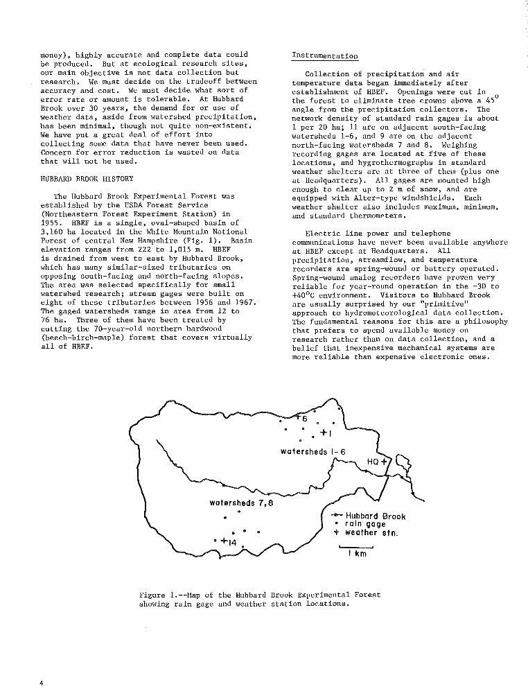
The Hubbard Brook Experimental Forest was established by the USDA Forest Service (Northeastern Forest Experiment Station) in 1955. HBEF is a single, oval-shaped basin of 3,160 ha located in the White Mountain National Forest of central New Hampshire (Fig. 1). Basin elevation ranges from 222 to 1,015 m. HBEF is drained from west to east by Hubbard Brook, which has many similar-sized tributaries on opposing south-facing and north-facing slopes. The area was selected specifically for small watershed research; stream gages were built on eight of these tributaries between 1956 and 1967. The gaged watersheds range in area from 12 to 76 ha. Three of them have been treated by cutting the 70-year-old northern hardwood (beech-birch-maple) forest that covers virtually all of HBEF.

Instrumentation

Collection of precipitation and air temperature data began immediately after establishment of HBEF. Openings were cut in the forest to eliminate tree crowns above a 45° angle from the precipitation collectors. The network density of standard rain gages is about 1 per 20 ha; 11 are on adjacent south-facing watersheds 1-6, and 9 are on the adjacent north-facing watersheds 7 and 8. Weighing recording gages are located at five of these locations, and hygrothermographs in standard weather shelters are at three of them (plus one at Headquarters). All gages are mounted high enough to clear up to 2 m of snow, and are equipped with Alter-type windshields. Each weather shelter also includes maximum, minimum, and standard thermometers.

Electric line power and telephone communications have never been available anywhere at HBEF except at Headquarters. All precipitation, streamflow, and temperature recorders are spring-wound or battery operated. Spring-wound analog recorders have proven very reliable for year-round operation in the -30 to +40°C environment. Visitors to Hubbard Brook are usually surprised by our "primitive" approach to hydrometeorological data collection. The fundamental reasons for this are a philosophy that prefers to spend available money on research rather than on data collection, and a belief that inexpensive mechanical systems are more reliable than expensive electronic ones.

-Hubbard Brook • rain gage + weather stn.

li<m

Figure 1.--Hap of the Hubbard Brook Experimental Forest showing rain gage and weather station locations.

4

Data Processing

Data processing, on the other hand, has changed drastically over time. In the SO's and early 60's, all data were picked from charts by eye and tabulated manually using rotary calculators. In 1964, we began digitizing streamflow charts and processing data by computer. Over the years, we have used six different mainframe and mini computers (GE-265, IBM 1620, IBM 360, DEC-10, PRIME-750, and DG-MV4000).l/ Our Fortran programs migrated rather easily. Input and output data were stored for many years on punch cards. Now, most of our streamflow and meteorological data are stored on magnetic tapes in ASCII files; this method has been chosen because it moves easily to new machines,

Precipitation and temperature data continue to be read from charts by eye, but are processed by computer. Only daily total precipitation and daily maximum and minimum temperatures are obtained routinely.

In early years, when the amount of data was less and labor was cheap, every data point and every calculation \vas checked by a second person. Now computer programs catch only the grossest errors. There is certainly a possibility that our random error rate now is higher than it used to be.

Headquarters Weather Station

At Hubbard Brook, we emphasize what happens on the gaged watersheds. The foot of the lowest and closest of these is 3 km away and 200 m higher than our Headquarters (HQ) office, Though a weather station has been maintained at Headquarters, data from it have not ahmys been processed. For instance, we have miles of unprocessed charts from a tipping bucket rain gage, and from an anemometer and wind vane. Headquarters data provide neither complete nor representative values for weather on the gaged watershed areas. This raises a question of which weather station or stations to use as a climatic standard for HBEF.

A weather station meeting LTER Level 2 standards was established at HQ (where power is available) in 1981. A variety of problems

liThe use of trade, firm, or corporation names in this publication is for the information and convenience of the reader. Such use does not constitute an official endorsement or approval by the U.S. Department of Agriculture or the Forest Service of any product or service to the exclusion of others that may be suitable.

have beset this system, and there are many gaps in the record. For example, a week was lost once when I forgot to push the ON button. Sensors, tape recorder, and data logger all fail occasionally. Lightning damage has been frequent, though we keep trying to improve protection. Repair and maintenance of this station has not had top priority. Although the daily data that it produces have sometimes been used, there have never been any requests for its hourly data.

Data Amount and Availability

Data piles up over the years. About one and a half million values are now contained in the routine hydrometeorological data set at Hubbard Brook (Table 1). And each of these has a time and location attached to it. Yet, we still get requests to "send us all your precipitation and streamflow data!"

Our philosophy has been to provide this data to anyone who requests it. We have recently established the Hubbard Brook Bulletin Board. Anyone with an MS-DOS microcomputer and a modem (300, 1200, or 2400 baud) can obtain many of the files containing this data by calling 603-868-1006 outside of normal working hours. Routine or long-term data from many cooperating scientists in the Hubbard Brook Ecosystem Study will gradually be added to the Bulletin Board. Data are provided to users in exactly the same ASCII files that are produced by the scientists.

SOLAR RADIATION

Daily total solar radiation has been measured at Headquarters since 1960. Se~7ors have included successively a Belfort-- pyranograph, a Weather Measure pyranograph, and two LiCor pyranometers. The pyranographs were calibrated occasionally against a Kipp pyranometer. Averaging the pyranograph charts by eye over 2-hour intervals provides good daily totals. For the LiCor sensors, the manufacturer's calibration has been used and hourly integrals are obtained by the data logger. Comparisons among the various sensors generally have shown differences of less than 5%.

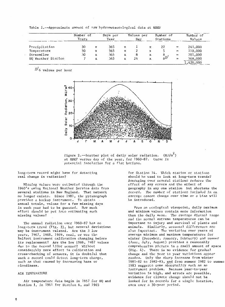
The scatter of data by day of the year shows two problems (Fig. 2). A few data points exceed the potential insolation but are not obvious errors and have not been eliminated. Second, the midsummer maximum daily values are only 80-85% of potential, though 90% would be expected for clear days. The site horizon is elevated up to 15° in the northeast and northwest by nearby trees. These trees have been growing gradually taller, and presumably reducing daily solar radiation gradually, especially in summer. Should we cut down the trees or move the sensor? Or would that destroy any usefulness the

5

6

Table I.--Approximate amount of raw hydrometeorological data at HBEF

Precipitation Temperature Streamflow HQ Weather Station

~/6 values per hour

N E 40 ' ., ~

~ 30 .... " "<<

~ 20 ... " 0

(/) 10 >.

" Cl

0

Number of Years

30 X

30 X

30 X

7 X

Days per Values per Number of Number of Year Day Stations Values

365 X 1 X 22 241,000 365 X 2 X 5 110,000 365 X 8 X 8 701,000 365 X 24 X ~I 368,000

1,420,000

Figure 2.--Scatter plot of daily solar radiation. (MJ/m2) at HBEF versus day of the year, for 1960-87. Curve is potential insolation for a flat horizon.

long-term record might have for detecting real change in radiation?

Missing values were estimated through the 1960's using National Weather Service data from several stations in New England. That net,vork no longer exists. Since 1981, the pyranograph provides a backup instrument. To obtain annual totals, values for a few missing days in each year had to be guessed. How much effort should be put into estimating such missing values?

The annual radiation over 1960-87 has no long-term trend (Fig. 3), but several deviations may be instrument related. Are the 3 low years, 1967, 1968, 1969, real, or was the Belfort instrument calibration changing before its replacement? Are the low 1986, 1987 values due to the second LiCor sensor? Without considerably more effort in calibration and cross-checking of sensors, it is doubtful that such a record could detect long-term change, such as that caused by increasing haze or cloudiness.

AIR TEMPERATURE

Air temperature data begin in 1957 for HQ and Station 1, in 1961 for Station 6, and 1965

for Station 14. Which station or stations should be used to look at long-term trends? Averaging over several stations reduces the effect of any errors and the effect of geography in any one station but shortens the record. The number of stations included in an average cannot change over time or a bias will be introduced.

From an ecological viewpoint, daily maximum and minimum values contain more information than the daily mean. The average diurnal range and the normal extreme temperatures can be important to injury and survival of plants and animals. Similarly, seasonal differences are also important. The variation over years of average minimum and maximum temperatures for winter (December, January, February) and suimner (June, July, August) provides a reasonably comprehensive picture in a small amount of space (Fig. 4). There is no evidence for gradual change and the year to year variations appear random. Only the sharp increase from winter 1981-82 to 1982-83, and from summer 1982 to summe1 1983 suggests some abnormality such as an instrument problem. Because year-to-year variation is high, and errors are possible, evidence for climate change should not be looked for in records for a single location, even over a 30-year period.

NE 6000~~~~~~-L~~-L~~~~~~~~~ ..... .., ::'li!

~ 4000 ... 0

'0 0

0:: 2000

0 1960 70

YEAR 80 90

Figure 3.--Annual solar radiation (MJ/m2) at HBEF for 1960-87. Arrows show times of sensor changes.

WINTER MAX . ........... ,.~ .... ,, .. ,.,·'''"''"' ..... ,., ... ,, .......... "·'"··· ... '· "· ..... , ........ .

YEAR

Figure 4.--Average summer (June, July, August) and winter (December, January, February) maximum and minimum daily temperatures for Stations 1, 6, and HQ at HBEF, 1961-87.

Individual Stations

The deviations of individual stations from the averages described above may be partly due to instrument calibration (Fig. 5). The hygrothermographs are currently readjusted and rotated annually in spring. In earlier times, an instrument stayed in the same location for several to many years. Standard and max-min thermometers are read weekly at each weather station, but the hygrothermograph data are not corrected to agree closely with the thermometers. In general, we have expected that errors of · ±1°C were likely. The analysis for this paper of year-to-year variation within a station shows a range of about 2°C (Fig. 5). The sudden sharp drop in Station 1 summer maximum from 1970 to 1971 is suspicious, but is not evident in the summer mlnlmum. The 1969 winter data for Station 1 are also suspect. For other years or

stations, abrupt changes do not occur, but gradual shifts of stations with respect to each other do occur. For instance, winter temperatures at Station 6 were about lOG higher than Station 14 in the early record, but '\vere about the same after the mid 1970' 8. l~atershed 4, in which Station 6 is located, was strip clearcut in 1970-74. It is tempting to attribute some change to cutting, but such change is not obvious. We have strongly discouraged interstation comparison of temperatures, because of this lack of accuracy. Yet the general order of temperatures from highest to lowest--HQ, Station 1, Station 6, Station 14--is in the expected inverse relation to elevation. HQ and Station 14 differ by about 3°C in maximum temperature, and by 470 m in elevation, just what is expected from the lapse rate. The data may be better than we think.

7

8

2

0

LIJ 2 c.!)

Summer Max.

ct

~ 0 c.:.~·:·. -:~.~;::::_\:?7~:(/< ~\;.~;~~~-·-~.---'"'',' ct-2 Summer Min. ~

~ 2 I.L

z 0 0

' ·,,_, ... ,. ........

HQ ,._,, ', ........ , __ ,,•"'""·~ ............ ~· , ... .

!; -2

> ~ 2

,, ,. 6 ..... . ... -~ .... ~ .. -·--< .. ~ .. ~.~~..:.··;......-.:..~ ..... ~_>·:

Wlnte;·-~o~. \. __ . - 14

0

-2 Winter Min.

1960 70 80 90 YEAR

Figure 5.--Deviation by station of summer and winter maximum and minimum temperatures from the average values in Figure 4.

Persistence

Ecologists customarily use monthly or annual averages to evaluate abnormality in weather, but this ignores or discards the important information contained in the daily values, If July was 1°C above normal, does that mean that each day was 1°C above normal or that a few days were many degrees above normal? If a summer is characterized as "hot", what does that really mean in terms of distribution of temperature over time?

In work with tree rings in the Northeast, I first began looking at accumulated deviation of daily mean temperature from its normal. I was struck by the apparent persistence for months of below or above normal periods, and by the abrupt transitions from one "regime" to another. Station 1 at Hubbard Brook shows such behavior over its 31 years (Fig. 6). In such a plot, also used by Barry (1985), positive slope indicates above normal conditions and negative slope below normal.

On a year-to-year time scale, below normal temperature persisted from mid-1964 to early 1968, and from early 1980 to late 1982.

Conditions were generally above normal from early 1968 to early 1976, and from late 1982 to early 1985. A comparison with regional weather data used in our tree-ring studies shows that these persistence regimes are regional in scope.

On a month-to-month time scale, regimes occur '"ith a persistence of several months (Fig. 7). November 1969 through April 1970 was almost uniformly below normal. The use of daily data shows that transition between these regimes can be very abrupt, and can often be pinpointed to a particular day. The intensity of the persistence regimes is no~ great. Regimes of about 1°C above or below normal are most common, with few extended periods reaching more than 2°C difference from normal,

Time series analysis of this data yields nothing more than a lag 1-day autocorrelation of about 0.5. The series is like taking two steps in one direction and sliding back one before deciding randomly on the next direction and step size, Persistence of the type shown here is characteristic of a random walk, or lag 1 autocorrelation. Nonetheless, it is tempting

400 0 • • 200

ci .... 0 Ul

z 0 -200 .... ct

\"·•"'' > -400 w 0

::E -600 :;)

0 ~ -800

-1000 1960 65 70 75 80 85

YEAR

Figure 6.--Accumulated deviation of daily mean temperature for Station 1 from its normal for that day of the year, for 1957-87.

u • -200

ct .... Ul

~-400 .... ct > w 0

i -600 :;) u 0 c:(

1967 1968 1969 1970 1971

Figure 7.--Accumulated deviation of daily mean temperature for Station 1 from its normal for that day of the year, for 1967-71.

to believe that the transition from one regime to another is forced by regional or even global weather patterns, such as jet stream movement (Blackmon et al. 1977), that may be produced by El Nino Southern Oscillation episodes, or North Pacific sea surface temperature anomalies (Namias et al. 1988), which have similar persistence.

PRECIPITATION

Persistence

Persistence behavior occurs for precipitation as well as for temperature (Fig. 8).

The "normal" precipitation for a given day of the year needs to be smoothed because the actual values have large day-to-day variation. We used a cubic smoothing spline with a cutoff of 50 days. The accumulated deviation tends to go upward rapidly and in big jumps, due to individual large storms, and come downward more slowly. Because of the skewed distribu·tion of daily precipitation, normal time series modeling cannot be done.

The 31-year record for Watershed 1 shows a single below-normal period from late 1960 through mid-1966 (the well-known northeastern drought), and above-normal conditions from early

9

::E 200 ::E

0 1/)

!I: -200 z 0

-400 .... "' 1:; -600 0

:::E -800 ::;)

0 ~-1000

-12 00 +-.-.-.-r-r-.-...--r-r..,-,-.--.--M-r..,-,-r-.-..--r-.-,.......-.-.-r-r.....-+ 1960 65 70 75 80 85

YEAR

Figure B.--Accumulated deviation of daily precipitation for Watershed 1 from its smoothed normal for that day of the year, for 1957-87.

1972 through mid-1978 (Fig. 8). The magnitude of deviation in the persistent regimes is on the order of 30 mm from normal per month, or about 30%.

Station Differences

Daily data from individual standard rain gageshave not been entered onto the computer before 1965, so longer-term comparisons can only be made on a 'vatershed basis. Both double mass comparison of one watershed with another and plotting of deviations from means show various, mostly unexplained, blips and kinks in the data. I have looked for one specific effect here. The cutting of Watershed 4 in 1970-74 altered the three rain gages in it so that they were in the open rather than in openings. Watershed 4 precipitation does seem slightly reduced in the period 1972-77, and then drifts upward (Fig. 9). The reduction is only about 2% and may be meaningless. There is a slight tendency for Watersheds 1 and 3 to drift downward while 6 and, recently, 4, drift upward. There is no obvious reason for such drift to exist. The data are dependent only on standard rain-gage catch, so no sensor or calibration error is involved. Exposure change by tree growth around the opening is possible; the openings ~re occasionally enlarged to compensate for ingrowth at the edges. Vegetation within the openings is cut only every several years. Should we put any more effort into examining these possible drifts and correcting for them?

10

ECOSYSTEM EFFECTS

Weather Variation

Weather variation has many effects on a forest ecosystem. These effects a:re often understood qualitatively, but are poorly quantified. We believe that drought reduces tree growth, but cannot specify how much. We know temperature affects photosynthesis and respiration, but cannot relate growing season temperature to net primary productivity. Recently I tried to relate ring widths of red spruce in New England to physiologically-based weather variables, with no success (Federer et al. 1988). Red spruce seems to be affected more by injurious winter conditions than by summer conditions (Johnson et al. 1986). But quantifying the weather conditions that cause winter conifer injury has proven elusive. Similarly, weather is known to affect outbreaks of pathogens, but quantification and modeling of the interactions are in their infancy. In general, we know that the variations in weather discussed in this paper affect the ecosystem, but we cannot say by how much.

Most effects of weather and climate variation on ecosystem processes are complex and non-linear. But many analyses of the relationships assume simple linear additive responses to monthly precipitation and mean temperature. The question of whether the available data is appropriate to the research problem is often avoided. For instance, precipitation data, or even Palmer drought

~ ~ p..,

~ ~ 1.0 0 E-< 0

~

...... , /' , ............ ,"', wss I\ ,' ', // \\ ,' ....... \

,/ ',,,' .. ',, ,/ '\ ............................. .. ' ' , ' , . ,, ws 4 ............................... . ... ··· .. . . .·· ............. ·· .............. ········ ... ,,.,"', . ········ ..... ·

• I '\.' •, ,,,,,, ... •••·••· ,i ..... · .. ·· ~ ··~ .... ---·

\ ...... ..

WSI

1970 YEAR

1980

Figure 9.--Ratio of annual precipitation on each watershed to the mean of watersheds 1, 3, 4, and 6, for 1964-86.

index, are not good substitutes for soil-water deficits in terms of drought effects.

favor certain species of plants or animals over competing species, but demonstration and quantification of such cause and effect would be quite difficult. With respect to known Hubbard Brook

history, the single weather event vlith the most impact on the ecosystem was probably the New England Hurricane of September 21, 1938. Enough trees were uprooted to induce the USDA Forest Service to carry out salvage logging in the Hubbard Brook basin. This was the only severe weather-related disturbance since the area was heavily cut prior to 1920. Hurricanes and local wind storms cause both regional and local disturbance at irregular intervals. However, treethrow mounds are common at Hubbard Brook; treethrow provides both soil mixing and seedbed for certain species;

The 30-year \Veather record at Hubbard Brook is too short to detect climatic change if climate is defined by a 30-year mean. Climatic change is very difficult to detect in any event; elaborate examination of many studies and data sets has not been able to prove the existence of a co

2-induced ~Varming trend (Ellsaesser et al.

1986). Looking for climate change in data

Fire is another weather-related event with potentially severe ecosystem impact. Fires that burn surface litter are fairly common in northeastern forests in early spring. These have some effect on nutrient cycling. Only one such fire, of a fe1v ha, has occurred in the last 30 years at Hubbard Brook. More severe crown fires are very rare, with prehistoric return periods of hundreds of years, but ecosystem impacts obviously would be severe.

Climatic Variation and Change

Climatic variation, as evidenced by persistence in the temperature and precipitation records, occurs essentially continuously at Hubbard Brook. Periods of months to years occur ~Vith temperature 1°C above or belo~V normal, or precipitation 30% above or belo~V normal. Such persistence may

sets from LTER sites is futile. Nevertheless, climate change has and ~Vill affect Hubbard Brook. Hubbard Brook is at the temperate forest-boreal forest ecotone. Climatic temperature changes of a couple of degrees C may greatly change the ratio of spruce-fir to northern hard~Voods and, thereby, the structure and function of the ~Vhole ecosystem. Changes in the ecosystem itself may become evident long before the weather data can prove that the climate has changed.

Chemical Climate

Although excluded from this paper, changes in the chemistry of the atmosphere may have greater effects on the ecosystem than changes in physical \Veather and climate. Acid precipitation, ozone and SO levels, and heavy metal deposition can Be considered. part of \Veather and climate in their larger sense. Acid precipitation and related air pollution have certainly increased considerably in the northeastern United States over the past 100 years. More recently at Hubbard Brook, sulfate input in precipitation has decreased as regional sulfate emissions are reduced (Likens

11

et al. 1984). Lead deposition to the forest floor also has decreased recently. The ecosystem impacts of these pollutants therefore, have been partially reversed. The chemical climate at Hubbard Broqk probably is changing. The impacts via acidification of soils and water and consequent ecosystem effects are receiving considerable attention at Hubbard Brook and elsewhere.

CONCLUSIONS

Climatic data collection and processing has changed almost incredibly over the past 30 years. We cannot predict what the next 30 years will bring, but need to expect more great changes.

In spite of the electronic age, mechanical weather sensors may still be more reliable than hi-tech equipment unless funds are made available for a full~time electronic technician and data analyst, backup equipment, and careful calibration.

For temperature and solar radiation, if not for precipitation, weather variation, persistence, and climatic change may be difficult to separate from error. Replication of sensors and systems can help.

Where long-term records already exist, it may be better to continue with existing instruments, methods, and exposure than to make changes that will alter long-term mean values.

12

There is a tradeoff between accuracy of weather data and costs. Where ecological research is the top priority, weather data should not be expected to detect climatic change.

Ecological systems may be affected more by occasional extreme events than by long-term changes in mean weather or climate.

Our knowledge of the quantitative relations between weather and ecosystem processes lags far behind our ability to collect reasonably good weather data. We should be spending much more money and time on research and maybe much less on instrumentation.

ACKNOWLEDGMENTS

Many people have contributed to collection and processing of Hubbard Brook weather data: Vincent Levasseur, Don Buso, and Wayne Martin deserve special recognition.

LITERATURE CITED

Barry, Roger G. 1985. Growing season temperature characteristics, Niwot Ridge and East Slope of the Front Range, Colorado, 1953-1982. CULTER/DR-85/6. Boulder, CO: Institute of Arctic and Alpine Research, University of Colorado.

Blackmon, Maurice L.; Wallace, John M.; Lan, Ngar-Cheung; Mullen, Steven L. 1977. An observational study of the northern hemisphere wintertime circulation. Journal of Atmospheric Sciences 34:1040-1053.

Ellsaesser, Hugh W.; MacCracken, Michael C.; Walton, John J.; Grotch, Stanley L. 1986. Global climatic trends as revealed by the recorded data. Review of Geophysics 24:745-792.

Federer, C.A.; Tritton, L.M.; Hornbeck, J.W.; Smith, R.B. 1989. Physiologically based dendroclimate models for effects of weather on red spruce basal-area growth. Agricultural and Forest Meteorology 46:159-172.

Johnson, Arthur H.; Friedland, Andrew J.; Dushoff, Johnathan G. 1986. Recent and historic red spruce mortality: evidence of climatic influence. Water, Air, and Soil Pollution 30:319-330.

Likens, G.E.; Bormann, F.H.; Pierce, R.S.; Eaton, J.S.; Munn, R.E. 1984. Long-term trends in precipitation chemistry at Hubbard Brook, New Hampshire. Atmospheric Environment 18:2641-2647.

Namias, Jerome; Xiaojun Yuan; and Cayan, Daniel R. 1988. Persistence of North Pacific sea surface temperature and atmospheric flow patterns. Journal of Climate 1:682-703.

APPLICATION OF THE Z-T EXTREME EVENT ANALYSIS

USING COWEETA STREAMFLOW AND PRECIPITATION DATA1

Lloyd W. Swift, Jr., Jack B. Waide, and David L. White2

Abstract.-- A technique for drought or flood analysis, after Zelenhasi6 and Todorovi6, promises to improve the definition of both duration and magnitude of extreme flow events for river-sized basins. The technique has been applied to a smaller basin at the Coweeta LTER Site using both streamflow data and a longer precipitation record. This report illustrates the technique and describes needed adjustments to apply the method to stream-sized basins.

Keywords: LTER, drought, duration, recurrence interval.

INTRODUCTION

Long-Term Ecological Research (LTER) sites are mandated to sponsor research in five core areas. One core area deals with natural and human-caused disturbances and their impacts on ecosystems. For most sites, common natural disturbances are driven either by short-term meteorological events such as storms and droughts or by long-term climate episodes. In either case, the researcher wants to be able to state how an apparently unique event or trend fits with past experience. In hydrology, traditional analyses of extreme value data are based upon flow magnitude and often use only the most extreme annual event (Chow 1964, Section BI). These analyses yield little information about duration of the event and ignore other unusal but less extreme events falling within the same year. Duration is incorporated in the Palmer Drought Index, but the ability to deal with probability of return interval is not. Zelenhasi6 and Salvai (1987), who extend work by Todorovi6 and Zelenhasi6 (1970), illustrate a method that considers the entire data record and allows statements to be made about the recurrence intervals of both the magnitude and duration of an extreme event.

1 Presented at the LTER Workshop on Climate Variability and Ecosystem Response, August 21-24, 1988 at Niwot Ridge-Green Lakes LTER Site, CO.

2 Research Meteorologist, Coweeta Hydrologic Laboratory, Otto, NC., Principal Research Ecologist, Forest Hydrology Laboratory, Oxford, MS, and Ecologist, Southeastern Forest Experiment Station, Clemson, SC, all Forest Service, U.S. Department of Agriculture.

Their illustration is based on a 8 BOO 000-ha river basin. We propose that the method can be applied to smaller basins if certain refinements in technique are made which allow for greater responsiveness of streams compared to rivers.

Our application of the Z-T method seeks to describe the southeastern drought of 1985-1988 and its significance to the Southern Appalachian Mountains and the Coweeta LTER site. Questions appropriate to the drought disturbance are: how dry was this period? how long did it last? and how does it rank with other droughts on record? In order to apply the Z-T method, we had to determine whether the technique could function with data from a smaller (approximately 1/lO,OOOth) basin and whether the technique could be used with precipitation data. If the latter were feasible, the period of record could be doubled to over 100 years and comparison of the 1925 and 1986 droughts would be possible.

CONCEPT OF THE Z-T METHOD

For droughts, the Z-T method analyzes deficit events created by dividing a continuous streamflow record into periods of unusually low flow alternating with periods of all higher flow rates. The separation is made around a derived flow reference value, Q,. A sequence of deficit and inter-deficit flow periods may contain intervals of normal flow that are separated by short, small deficits. Likewise, an extended low-flow sequence may contain periods when flow rates are temporarily above Q,. These minor excursions above or below Q, are culled from the analysis by averaging them into the adjacent flow periods. Statistical tests for validity and serial correlation are applied to the resulting set of

13

largest deficits and curves are fitted to the cummulative relative frequencies of the deficits and their durations. From these fits, recurrence intervals are calculated for the most extreme events.

THE Z-T PROCEDURE

Mean daily streamflow values for Coweeta Watershed 8 (WS08) from January 1936 through December 1988 provided the data for the streamflow test of the method. Watershed 8 is a forested headwater basin of 760 ha draining into the Little Tennessee River. Mean annual precipitation of 1988 mm is evenly distributed through the year, and flow averages 1163 mm per year.

Selecting Qr

All daily flow values for Coweeta WS08 were ranked in descending order without regard to date; Qr is the value occurring at the "r" percent interval. For this work, Qr was selected as the flow rate ranked just under 90 percent of all larger daily streamflow values. Monthly Q90 values were also selected by ranking daily flows separately by months. Q90 may be appropriate for slowly changing data but responsive or flashy streams may require a Q80 or even larger reference value. The periods of consecutive days when flow was below Qr are the deficit events (Figure 1). The required data for the following analyses are

:X D ..J "­>: .. w Cl ,_ "'

TRUNCA liON OF A FLOW SERIES INTO DISCRETE DEFICH EVENTS

Cura~lalive Defici l flo" Amount

HHE

Figure I.--Separation of a period of streamflow by Qr into flow deficit events.

the durations of these deficits (T) and the period,sums of the differences between Qr and recorded flow (D).

The seasonal cycle of streamflow suggests that low flow is relative; a level that is unusually low in the spring wet season·might be a moderate level for the fall season. Using a single Q90 for the whole year confines most deficits to the low­flow season (see days 270-310 in Figure 2). However, an atypically low flow, such as occurred in the spring of 1985, could have significant impact upon stream ecology. To include such cases, a separate Q90 was calculated and applied

14

to each month's flow data; thereafter, deficits were identified in all seasons. Because a smooth transition between months was not possible when adjacent monthly Q90 were quite different, a curve was fitted to the monthly Qr and reference values calculated for each day of the year. Figure 3

1>,---------------------------------------, H

13

12

11 10

100 200

JULIAN MY

300 400

Figure 2.--Daily streamflow for Coweeta WS08 for 1985 showing reference values for annual and monthly 090•

compares the distribution of deficit periods in 1986 derived by the three types of Qr and suggests that the extra effort needed to apply daily varying Qr was not justified by these data.

Culling Minor Events

The chronologie series of daily streamflow was transformed by subtraction into excess flows above Qr and deficit flows below Qr• Each unbroken series of deficit days was summed, defining a deficit event with duration T and cummulative. deficit (deviation from Qr) D. Similarly, excess days were summed. Low-flow periods may be

WI FEB MAR .1/'R MAY JUN JULY AUQ SEP OCT NOV DEC

Figure 3.--Average flow for deficit and inter­deficit periods in 1986 as separated by annual, monthly, and daily varying Qr•

punctuated by short events of flow above the reference value, usually caused by storms that briefly raise streamflow but have no lasting effect upon accumulating drought conditions. The next step was to remove these brief excess· periods and to combine adjacent deficit periods that effectively function as a single event. The rules for combining were: (l) the magnitude of the excess had to be less than the absolute value of each of the adjacent deficits, and (2) the absolute sum of the two deficits had to be greater than three times the magnitude of the excess. The duration of the combined deficit event was the sum of the three durations and the cumulative deficit was the algebraic sum of the excess and two deficits. Iterative passes were made through the series of alternating deficit and excess events until no further minor excess events met the criteria for combining. A drought period extending through the end of the year was listed as falling in the year containing more than half of the duration. In the event of an even split, then the drought period was listed in the year having more than half of the deficit.

We believe that the same iterative process also should be used to eliminate minor deficit events. The function fit to the cumulative relative frequency, to be described later, was sensitive to the number of very small events. The goal was to obtain a list of separate and independent events drawn from the lowest 10 percent of flows on record. From this, lists of drought duration events and drought magnitude (cumulative deficit below the Qr value) events became the data points for the analytical steps.

Statistical Tests

Several tests were applied to ensure that the selected deficit events were independent, identically distributed random variables. First, a chi-square test determined whether the distribution of the number of droughts in each year differed from the distribution of a time­dependent Poisson process. Then the list of deficits and the list of durations were each tested to ensure that the events were not serially correlated and that the lists did not include runs of consistently increasing or decreasing values. Finally, the drought deficits were ranked, the drought durations were ranked, and the correlation between rank numbers for each event was tested to confirm that both measures of drought severity ranked the same events in essentially the same order.

The number of droughts each year should fit the Poisson distribution. For this test, we calculated the overall mean annual number of deficits and counted the number of years having O,l,2, ••• k deficits each. For each class, k, the expected frequency was calculated as

Fexp = Y * e(-Nu) * N1,/ / k!, where

Y = total number of years, Nu = mean annual number of deficits, and k =class interval of 0,1,2, •.• deficits/year.

The sum of Fexp * k must equal the total number of deficits. If the sum of (Fobs - F exp) 2/F exp

across all k classes was less than the chi-square value for the number of classes minus 2, the list of selected deficits was judged to not differ from the Poisson distribution.

Serial correlation was tested on the chronological list of deficit magnitudes and on the list of durations. Three correlations were calculated for each list: (l) each event with the event following, (2) each event with the second following, and (3) each event with the third following. For a serial correlation calculation of two offset sequences of the same data, we used the variance of all events in the denominator rather than the usual product-moment formula. If all six correlations were nonsignificant, then the lists of deficits and durations were judged to be acceptably free of serial correlation. If not, then we started over, revising our rules for culling minor events to effect more combining of adjacent drought periods. Alternatively, selecting a larger Qr may reduce serial correlation for some data sets.

The runs test determined whether the chronological lists of deficits or durations contained trends or cycles. Each list was searched for groups of sequential values that formed runs of increasing.or decreasing magnitude. Runs may consist of single values that reverse the previous and succeeding trends. Adjacent pairs of identical values were considered part of the same run. If r is the number of runs and n is the total number of values in the list, then the parameter for a t-test is approximated (Sokal and Rohlf 1969, pg. 628) by

tr = {r- [(2n- l)/3]} / {(16n - 29)/90}112 ,

where most lists would contain enough events to test against t ,05 = l. 96. If tr was greater than 1.96 and the number of runs was low, the test suggested a systematic trend or bias in the list. If the number of runs was high, cycles in the data were suspected.

The two lists of deficits and durations were individually ranked and rank numbers assigned to the drought events in each list. Thus, any particular drought event might have different rank numbers for its deficit and its duration. The correlation between these pairs of rank numbers is a measure of the consistency of the data. Zelenhasi6 and Salvai (1987) found that reducing Qr increased the rank correlation. High correlation was not required for the frequency analysis but would be an important criteria if the results of this analysis were used to construct a synthetic drought series.

Recurrence Interval of Drought

The end product of this analysis is the recurrence intervals of the largest drought events based upon the deficits selected and tested by the preceding steps. To calculate recurrence intervals we required: the lists of deficits (D) and durations (T), each ranked in ascending order; the total number of droughts (N); the mean annual number of droughts (NM); and the values of the mean deficit (DM) and mean duration (TM). The

15

same calculation procedures, described below for the list of deficits, were applied also to the list of durations.

The cumulative relative frequency (CRF) was calculated by dividing the rank number of each deficit by the total number of droughts+!; CRF therefore approached 1.00 for the very largest deficit. The expected distribution for CRF is

CRFexp = 1 - e(-DIDM),

where D was each value from the list of deficits. The Kolmogorov-Smirnov goodness of fit test (Ostle 1963, pg. 471) was used to verify that the observed CRF was not significantly different from the expected distribution of CRF. For acceptance, the maximum difference between CRFobs and CRF exp had to be less than the K-S parameter of 1.36I(N) 1' 2 for the 0.05 level. Instead of

1.2

lj' " 1.0 ., :> 0" t! 0.8 u.. ., ~ IJ 0.6 Oi

0::: .. ~ 0.4 IJ '5 E 0.2 " u

20 40 60 80 100 Deficit ( area mm )

Figure 4.--0bserved points and expected curve for cumulative relative frequency of Coweeta WS08 streamflow deficits.

calculating all possible differences to find the maximum, one could select the most likely range of values from graphs drawn to visually verify the fit (Figure 4). If the distributions were not different, then the formula for the expected CRF could be used to represent the observed data.

Because recurrence interval is usually stated in years, we calculated the distribution function of the largest annual deficit, which is an extension of the function for CRF exp• as

Fexp(D) = e[-NM * e(-DIDM)] where NM was the mean number of deficits per year and D was as in CRF exp• The goodness of fit of this frequency distribution also could be verified by testing the maximum difference between the Fexp and a set of observed cumulative relative frequencies recalculated from an abbreviated list, omitting lesser deficits for years having more than one. The recurrence interval

RI = 1 I [1 - Fexp(D)]

was calculated for the largest deficits. Also, the estimated deficit for a selected return interval was calculated as:

DR1 = -DM * ln[ -ln(l -liRI) I NM].

16

ILLUSTRATION OF THE Z-T METHOD

Table 1 lists the 44 drought periods selected from Watershed 8 daily flow records for the 53 years from 1936 through 1988. Droughts were not defined in 29 of the years. The distribution of droughts per year and two variations on the Poisson calculation are shown in Table 2. The first set of columns produce a chi-square sum much larger than the critical value of 9.49 for 6-2=4 classes at 0.95 probability. Ostle ( 1963, pg. 127) recommends combining classes in cases

Table 1.--coweeta Watershed 8 drought periods based upon a Q90 truncation applied to daily flows in area-mm for 1936-1988.

Year Julian Date Dur Def Rank CRF Expected CRF obs-exp Begin Hid End T D T D T D T D T D

:::::::::::::::::::::::::::::::::::::::::::::::::::::::::::::::::::::::::::::::::::

39 283 344 40 123 54.1 41 43 . 911 . 956 .966 .996 -.055 -.041 40 46 47 48 3 1.5 1 8 .022 .167 .079 .144 -.057 .023 40 54 72 89 35 17.2 32 39 .711 .867 .617 .832 .094 .035 40 93 95 97 5 1.8 3 13 .056 .278 .128 .170 -.073 .lOB 40 104 107 109 6 2.3 5 18 .111 .400 .152 .212 -.041 .JOB 41 34 JOB 181 147 40.9 43 42 .956 .933 .982 .986 -.027 -.052 41 284 292 299 16 1.0 20 2 .433 .033 .355 .099 .078 -.065 42 123 129 134 11 1.1 11 3 .244 .067 .260 .JOB -.016-.041 43 346 352 358 13 2.2 15 17 .322 .367 .300 .204 .121 .163 44 23 31 39 17 6.0 22 26 .478 .578 .373 .463 .105 .115 45 27 35 43 16 3.2 20 22 .433 .489 .355 .282 .078 .206 45 177 216 255 78 8.5 40 31 .889 .689 .882 .586 .007 .103 52 204 211 217 14 1.4 17 6 .378 .122 .319 .135 .059 -.013 52 296 310 323 27 2.2 29 17 .644 .367 .523 .204 .022 .163 53 278 301 323 45 6.1 36 27 -~ .600 .709 .469 .091 .131 54 255 293 331 76 10.7 39 34 .867 .756 .876 .670 -.009 .OBS 54 334 336 338 5 1.4 3 6 .056 .122 .128 .135 -.073 -.013 54 355 358 361 7 2.0 7 14 .156 .311 .175 .187 -.019 .124 55 13 23 32 20 8.9 24 32 .533 .711 .422 .603 .lll .JOB 56 361 14 32 37 13.3 33 37 .733 .822 .637 .748 .. 096 .074 56 334 340 346 13 1.7 15 11 .322 .233 .300 .162 -.019 .072 58 340 350360 21 4.2 26 25 .567 .556 .438 .353 .129 .202 59 9 12 14 6 1.6 5 9 .111 .200 .152 .153 -.041 .047 59 56 60 63 8 1.7 8 11 .178 .233 .197 .162 .022 .072 63 46 55 63 17 6.9 22 29 .478 .644 .373 .511 .105 .133 63 106 112 117 12 2.1 13 15 .289 .333 .280 .196 .009 .138 65 351 360 4 18 3.0 23 21 .511 .467 .389 .267 .122 .199 66 19 30 40 21 7.2 26 30 .567 .667 .438 .526 .129 .141 67 9B 105 lll 14 1.8 17 13 .378 .278 .319 .170 .059 .lOB 68 56 63 69 14 3.9 17 24 .378 .533 .319 .333 .059 .201 78 279 300 320 42 3.5 35 23 .778 .511 .684 .304 .094 .207 81 354 14 40 53 23.6 37 41 .822 .911 .766 .913 .056 -.002 81 66 77 OB 23 16.3 27 38 .600 .844 .468 .816 .132 .029 81 100 115 129 29 6.4 30 28 .667 .622 .548 .485 .118 .137 81 264 280 295 31 2.6 31 20 .689 .433 .573 .236 .ll6 .197 Bl 312 318 323 11 1.0 11 2 .244 .033 .260 .099 -.016 -.065 85 20 25 30 11 2.6 11 20 .244 .433 .260 .236 -.016 .197 85 68 81 94 26 9.2 28 33 .622 .733 .510 .615 .113 .119 85 99 102 104 6 1.5 5 8 .111 .167 .152 .144 -.041 .023 85 109 144 179 70 11.4 38 36 .844 .800 .853 .693 -.009 .107 86 B 147 285 277 92.0 44 44 .978 .978 . 999 1.000 -.022 -.022 86 289 293 297 9 1.3 9 4 .200 .089 .219 .126 -.019 -.037 OB 53 73 93 41 11.3 34 35 .756 .778 .675 .690 .OBI .OOB 88 116 181 246 131 21.7 42 40 .933 .889 .972 .895 -.039 -.006

-----------------------------------------------------------------------------------Mean duration 36.48 days Maximum deviation = .129 .207 Mean deficit 9.64 mm Number of years 53 Number of droughts 44

such as this where small counts and high chi­square values invalidate the test. The recalculation in the right side of Table 2, with 3 or more deficits per year in the final class, yields a chi-square under the critical value of 5.99. Thus, the distribution of droughts per year is judged to not differ from the Poisson distribution.

Table 2.--Test for fit of number of droughts per year to the Poisson distribution.

Class Expected Observed Obs-Exp Chi -Sq Observed Obs-Exp Chi-Sq k years years years

0 23.11 29 5.89 1.50 29 5.89 1.50 1 19.18 12 7.18 2.69 12 7.18 2.69 2 7.96 8 0.04 0.00 8 0.04 0.00 3 2.20 1 1.20 0.65 4 1.80 1.47 4 0.46 2 1.54 5.16 5+ 0.08 1 0.92 10.58

Sum= 20.58 5.66

Table 3 gives the results of the serial correlation tests on drought duration and deficit. All values of r are small. The runs test confirms the conclusion that neither the duration nor deficit lists are serially correlated. Each list contains 28 runs, thus the t-value by the approximate formula equals -0.37.

Table 3.--Serial correlation (r) to the third level for drought durations and deficits,

Level

i X i+l i X i+2 i X i+3

N

43 42 41

Duration Deficit

-.003 -.057 -.097 -.023

.206 .106

The columns for duration in days (T) and deficit in mm (D) in Table 1 were each ranked in ascending order. The correlation between the two rank numbers for each drought was 0.84. At this point, the lists of selected droughts had met all the statistical tests and recurrence intervals could be determined.

The cumulative relative frequencies (CRF) of durations and deficits were calculated by dividing rank numbers by 45 (Table 1). Based on the mean number of droughts, 0.83 per year, the expected CRF and the difference between observed and expected CRF were calculated. The largest deviation in durations was 0.129, well below the Kolmogorov-Smirnov criteria of 0.205 for 44 observations, How'ever 1 the largest deviation of deficits from the expected distribution was just barely above the K-S criteria. Figure 4 shows the result of this borderline fit in the mid­range of CRF for drought deficits. The penalty for a weak fit, as seen below, was an outrageous estimate of recurrence interval for the most

extreme drought. Table 4 gives the estimated recurrence intervals for the eight most extreme droughts. Although we resisted accepting the recurrence intervals estimated for 1986, both the analyses and Figure 4 underscored the fact that 277 consecutive days with streamflow in the lowest 10 percent of all recorded daily flows was a highly unusual event. Figure 4 suggests that reducing the number of small droughts would pull the curve for observed data closer to the estimated distribution. A quick recalculation of selected CRFs, after we arbitrarily culled the four smallest droughts, decreased both the observed and expected CRF and their difference in midrange and cut the recurrence interval for the 1986 deficit in half. Users of the Z-T method should seek to improve the fit of the CRF distribution by experimenting with several levels of combining small events or by trying other Qr values.

Ten different years accounted for all the most extreme drought events in the Coweeta Watershed 8 record. Table 4 lists the recurrence intervals for eight deficits and eight durations. Years 1939, 1941, 1986, and 1988 ranked high in both lists. For the WSOB data, a 100-year drought was estimated to last 161 days and have an accumulated deficit of 42. 5 mm below the Q90 flow level.

Table 4.--Estimated recurrence intervals (RI) for the largest drought events from 1936 through 1988.

Year Our days

86 277 41 147 88 131 39 123 45 78 54 76 85 70 81 53

RI years

2392 68 44 36 11 10 9 6

PRECIPITATION COMPARISON

Year

86 39 41 81 88 40 81 56

Def mm

92.0 54.1 40.9 23.6 21.7 17.2 16.3 13.3

RI years

16813 330

84 14 12 8 7 5

Climate histories of the Southern Appalachian Mountains place the last major drought about 1925, a decade before the beginning of the climate record at Coweeta. A precipitation history began at Highlands, NC, in November 1877. This is a station in the U.S. Historical Climatology Network of the National Weather Service, 20.4 km east of Coweeta at the same elevation as the upper portion of Watershed B. The Z-T method was applied to the 111-year Highlands record to determine whether precipitation could be used to compare the severity of the 1986 drought with that of 1925.

Because precipitation is an event phenomenon, daily values could not be used as was done with continuous streamflow data. When monthly totals were analyzed, almost all durations were one month because individual storms would interrupt and mask otherwise dry periods. Streamflow is the

17

cumulative response of past precipitation input and evapotranspiration. As a test to simulate the timelag nature of streamflow, we used for each monthly value of precipitation the moving average of that month and the preceding three months. This technique identified 69 droughts with durations of 1 to 7 months. The 1925 drought was identified by Highlands precipitation as the driest period (Table 5). Four of the 10

Table 5.--Estimated recurrence intervals (RI) for the largest drought events identified by Highlands, NC, precipitation data, 1878-1989.

Year

1925 1954 1883 1939 1879 1941 1878 1981 1955 1986

Deficit RI mm years

168.1 154.7 136.4 135.9 108.2 99.0 94.1 92.5 83.4 78.2

334 218 122 121 50 38 32 31 23 20

most extreme events occurred before the Coweeta record began. Both the Highlands and Coweeta precipitation records identify the mid-1950's as a more important drought period than did WSOB streamflow. Precipitation data certainly does not rank the 1985-86 period as the most extreme.

CONCLUSIONS

The Z-T method of drought analysis seemed complex as presented by Zelenhasic and Salvai (1987) with all the derivations. In application, the procedure is a series of logical steps and statistical tests to confirm that the data fit the assumed distributions. A purpose of our work was to determine whether the Z-T method could be applied to a fourth-order stream. We determined that the method could be used, but found that the responsiveness of our stream, compared to the large river, required careful selection of both the reference value Q, and the techniques for culling small events and combining them into adjacent extended wet or dry periods. An unsatisfactory fit to the cumulative relative frequency distribution was purposely included to illustrate the importance of obtaining a data series that fits the assumptions.

A second purpose was to determine whether a longer precipitation record could be used to extend our interpretation of a 53-year streamflow record. Precipitation was not a perfect analog for streamflow, but this test showed that some form of time-averaging of precipitation can simulate the storage and release characteristics of the watershed.

The third purpose of this application was to describe the 1986 drought at Coweeta and compare

18

it with previous events. This analysis shows conclusively that duration and deficit of 1986 low flows were unique in the 53-year streamflow record of Coweeta Watershed 8. The cumulative effects of drought extended into 1988. However, the 1939 through 1941 period contained three separate drought periods that together must have had a severe impact on mountain watersheds and ecosystems. The extended precipitation record also identifies these same drought sequences but rates the 1925 drought as having the greatest rainfall deficit. Diaries and newspaper accounts report a dry period in the late 1800's, and this is supported by the Highlands precipitation record. The low precipitation in 1954 does not appear as a major streamflow drought. Although the May-through-October period in 1954 established the all-time minimum growing season total for this station, average or above-average precipitation before and after these months apparently maintained soil moisture at levels sufficient to sustain streamflow. This may suggest that a longer moving average time base would be appropriate for precipitation data used to simulate streamflow drought periods.

LITERATURE CITED

Chow, Ven Te. 1964. Handbook of applied hydrology. New York: McGraw-Hill Book Co., Inc.

Ostle, Bernard 1963. Statistics in research. 2d ed. Ames: Iowa State University Press. 585 pp.

Sokal, R.R; Rohlf, F.J. 1969. Biometry, the principles and practice of statistics in biological research. San Francisco: Freeman.

Todorovic, P.; Zelenhasic, E. 1970. A stochastic model for flood analysis. Water Resources Research 6:1641-1648.

Zelenhasic, E.; Salvai, A. 1987. A method of streamflow drought analysis. Water Resources Research 23:156-168.

VARIATION IN NICROCLIMATE A~lONG SITES AND CHANGES OF CLIMATE

WITH TIME IN BONANZA CREEK EXPERIMENTAL FOREsrlf

Leslie A. Viereck and Phyllis C. Adams2/

Abstract.--The microclimate in Bonanza Creek Experimental Forest varies with slope and aspect and with the stage of forest succession. Examination of the climate record from nearby Fairbanks shows that there has been an increase in mean annual temperature since the mid-1970s. Climate warming would most likely result in a shift in distribution

· of permafrost and existing vegetation types with an expansion of the more productive forest types.

Keywords: Boreal forest, taiga, permafrost, climate change, Alaska, forest succession,

SITE DESCRIPTION AND VEGETATION

The Bonanza Creek Experimental Forest (BCEF) is a 5045 ha research area located approximately 20 km west of Fairbanks in interior Alaska. The area includes a section of the Tanana River floodplain at an elevation of approximabely 120 m and adjacent uplands rising to a ridge crest of 470 m.

Upland forest types vary from highly productive aspen (Populus tremuloides Michx.), paper birch (~ papyrifera Marsh.), and white. spruce (Picea ~ (Moench) Voss) stands on south-facing, well drained slopes, to permafrost and moss-dominated black spruce (~ mariana B.S.P.) forests of low productivity on north facing and lower toe slopes. Floodplain stands of balsam poplar (Populus balsamifera L.) and white spruce comprise productive forests on recently deposited river alluvium, where permafrost is absent; slow-growing black spruce stands and bogs occupy the older terraces, which are underlain by permafrost (Viereck and others 1983).

1/Presented at the Long-Term Ecological Research Workshop into Climate Variability and Ecosystem Response, University of Colorado, August 21-23, 1989.

2/Prinicipal Plant Ecologist, USDA Forest Service, Institute of Northern Forestry, 308 Tanana Drive, Fairbanks, AK 99775; Research Technician, Forest Soils Laboratory, School of Agriculture and Land Resources Management, University of Alaska, Fairbanks, AK 99775.

Successional communities are dominant within BCEF both in the uplands and on the floodplain. In the uplands there are three ages of forest resulting from wildfires in 1983, 1915, and approximately 1800. The youngest, early successional stands are primarily in the herbaceous, shrub, and sapling stages of recovery (Foote 1983); the middle aged stands (75-years-old), on upland slopes, are in a dense aspen and birch stage, often with an understory of white spruce; mature stands are of white spruce or a mixture of white spruce and paper birch, On poorly drained sites in the upland, and on older river terraces, fire in black spruce stands has usually resulted in the reoccurrence of black spruce stands, although on some sites black spruce has been replaced by paper birch (Foote 1983).

On the floodplain of the Tanana River, erosion and silt deposition result in primary succession which begins with willows and alders and is followed first by balsam poplar and then by white spruce, Following one to several generations of white spruce, the floodplain sites develop permafrost and the productive white spruce stands are replaced by low productivity black spruce stands.

SYNOPTIC REVIEW OF BCEF CLIMATE

Climatic data reported here come from the National Weather Service observation station at the Fairbanks International Airport (lat. 64°48' N., long. 147°52' W.). The airport is on the floodplain of the Tanana River approximately 20 to 25 km northeast of the BCEF and at an elevation of 132 m. Data collected at the

19

airport are most representative of the climate of the floodplain section of BCEF.

The climate of BCEF is strongly continental and is characterized by temperature extremes from -50 to +35 °c, The region lies within a rain shadow created by the Alaska Range, The physical barrier created by the mountains prevents the area from receiving precipitation from coastal storms and also results in rapid warming in winter as 11chinook 11 type winds flow down the north slope of the mountains. The mean annual temperature of -3.3 °C at Fairbanks results in the formation of permanently frozen soils (permafrost) on north-facing slopes and poorly drained lowlands. Thus the Forest is in a zone of discontinuous permafrost (Ferrians 1965). At Fairbanks, strong temperature inversions occur 80 percent of the time during December and January, with gradients as steep as 21 °C/100 m of elevation during periods of extreme cold (Benson and Rizzo 1979). July is the warmest month with a mean daily temperature of 16.4 °C and January is the coldest with an average temperature of -24.9 °C. Because of its location at high latitude, BCEF experiences extremes of day length and sun angle which result in large differences in available solar radiation. At winter solstice, day length is 3 hgurs, 42 minutes with a maximum sun angle of 1 42', while at summer solstice there are 21 hours, 50 minut5s of sunlight and the maximum sun angle is 48 42 1 • This result2 in average daily solar radiation of2231 KJ/m /day in December and 22,375 KJ/m /day in June,

The average annual precipitation at BCEF is 269 mm. Most precipitation falls as rain in the summer months, a result of short-duration thunder storms and moist air masses that move in from the Bering Sea. Approximately 37 percent of the annual precipitation falls as snow from mid-October through April and remains as a permanent cover for 6 to 7 months each year. Maximum snow depths, averaging 75 em, are commonly reached in February and March. The water equivalent at this time averages 11 em. According to the Thornthwaite (1948) classification the climate of BCEF is semiarid, mesothermal, with little or no water surplus, and temperature efficiency normal to warm microthermal (D C12dc 12),

VARIATION IN MICROCLIMATE At10NG SITES IN BONANZA CREEK EXPERIMENTAL FOREST

Low sun angles, coupled with the continental climate, tend to make slope and aspect extremely important in the distribution of vegetation types, Permafrost also exerts strong controls over vegetation distribution by acting as a barrier to soil drainage, thereby creating wet or waterlogged soils. Presence or absence of permafrost is partially controlled by slope and aspect, These gradients of soil temperature and soil moisture are reflected in the distribution of plant communities and the productivity of forests and, in turn, result in a wide array of

20

microclimatic conditions within BCEF. The presence of permafrost on north-facing slopes, lower toe slopes, and old river terraces results in sharp contrasts with well-drained permafrost-free upland and floodplain soils. Consequently, sharp vegetation boundaries and a broad array of vegetation types are observed within close proximity to each other. Low productivity black spruce stands are formed on cold, wet permafrost-dominated soils and productive white spruce and successional hardwood stages occur on warm, mesic sites (Viereck and others 1983). The long hours of sunlight during the summer months offset to some extent the shortness of the growing season, which averages 111 frost-free days,

Although sharp contrasts exist among vegetation types on different slopes and aspects, air temperatures on opposing north- and south-facing slopes at the same elevation do not differ significantly (Slaughter and Long 1975). Soil temperatures do differ appreciably and, in addition to resulting in the presence or absence of permafrost, greatly influence vegetation distribution. It has been shown that there is a good correlation between annual soil temperature sums and forest productivity (Viereck and Van Cleve 1984).

In order to obtain more information on the effects of slope and aspect on microclimates, vegetation distribution, and productivity within BCEF we examined some microclimatic features of four stands along a gradient from hot and dry to cold and wet. These four stands were: (1) an open aspen-grassland with sage brush (Artemisia frigida Willd.) on a steep (75 percent) south-facing slope, (2) a mature white spruce stand on a 25 percent south-facing slope at an elevation of 396 m, (3) a mature paper birch on a 32 percent east-facing slope at 381 m, and (4) a black spruce stand on a 30 percent north-facing slope at an elevation of 400 m.

The following parameters were measured in the four stands during the growing season: air temperature at 1.2 min a standard weather shelter, soil temperature at depths of 5, 10, 20, and 50 em, and soil moisture in the organic layer and at 5 and 10 em in the mineral soil. For comparison of sites we used cumulative degree days for air and soil temperature. We present here a portion of the data collected, specifically for 1978 and 1979, which show some of the trends that were apparent along the environmental gradient.

In figure 1, the monthly average air temperatures for the four sites are shown. Although there are some differences in extreme temperatures among the sites, the average monthly temperatures show very little difference, ~lean annual temperatures for the four sites for the period April 1978 to May 1979 were: aspen -0.08, white spruce -069, paper birch -2.0, and black spruce -1.4 C. During the same period the mean annual temperature at the Fairbanks Airport was -2.6 °c, Air

30

20

10

0 0

w -10

ffi a -20 ~y,

-30

-40

-60 J I 11 1 J 1 ,--, 1 I 1 r 1 r J 1 r 1 1 J 1 1 1-r Jl •-r rJ I r t r-J r1 1 I/ I I I I J I' I I J I'' If

~ May Jill Jl.d hlg Sap Oct NaY Deo Jan Feb Mar

MONTH +-++ WhiiB Spruce _,__ Bich e 8 B Black Spruce

Figure 1.--Average monthly air temperatures for four stands in Bonanza Creek Experimental Forest for the period April 1978 through March 1979.

temperature degree day sums (based on 5 °C) also show no major differences among the four sites and Fairbanks.

~~!~e;~~~~~a~~~~sa~i~ ~:fz~~~e~l~~e0agg)a:~~ct. the period April 1978 through September 1979 ranged from 3966 at the aspen stand to 922 in the black spruce stand. At 20 em, temperature sums were 2393 at the aspen stand and only 539 in the black spruce stand, Of the four stands, only the black spruce stand was underlain by permafrost. In figures 2 and 3 soil temperatures are shown for the four sites for 20 em depth.

Soil moisture also showed large differences among the sites. In the steep, south-facing aspen stand, during an extended dry period in July and August of 1978, soil moisture in the mineral soil layer remained below 10 percent for over a month and reached a minimum of 2 percent. During the same period soil moisture was at 20 to 25 percent in the white spruce stand, and 25 to 60 percent in the birch stand. The mineral soil in the black spruce site remained frozen but the organic soils overlying the permafrost had a moisture content of between 440 and 700 percent (based on oven-dry weight).

It has also been shown that the snowpack and the time of snow melt differed considerably at these four sites (Slaughter and Viereck 1986), Snowpack was deepest on the black spruce site and remained nearly a month and a half longer than at the aspen site, which was snow-free by the end of March.

30

20

0

I 10

a

0

-10 I'. 11 I,., I I I I •• -. I I' I 1 I I,- I,.,,,-,,-, I'., I I I I I I l I 1 I I I' I' I I I' I 'T

~ May Jill Jl.d hlg Sap Oct NaY Doo Jan Feb Mar

MONTH e 8 8 Black Spruce

Figure 2.--Monthly average soil temperatures at 20 em depth for four stands in Bonanza Creek Experimental Forest for the period April 1978 through March 1979.

Figure 3.--Soil temperature sums (based on 0 °C) for 20 em depth in four stands in Bonanza Creek Experimental Forest for the period April 1978 through March 1979.

CHANGES IN MICROCLIMATE WITH SUCCESSIONAL CHANGES

1. Upland Secondary Succession Following Fire

There are significant changes in soil temperatures with time in both upland and floodplain succession. In previous studies (Van

21

A. ll m I!t :lZ: lli llii

0 0

0 = . 0 c 0

"' 0 8 .. 0

0 0 0 : .,

c ~

g . 0 ! & 0 c . u 0

E c :;;

" Q .

w c a: 0

" u.

0-1 2-5 6-25 26-50 51-100 100-200 200-250+ Age (years)

"' B. . c.

.:! 2500 D Heat Sum

o Forut Floor Oepth

~ 2 2000 0

b 1500

0-1 2-5 6-25 26-50 51-100 100-200 200-250+ Age (years)

Figure 4.--A. Forest succession following fire on upland south-facing slopes in BCEF. Numbers in boxes refer to llturning points11 to be studied under the LTER program. B. Soil degree day sums and organic layer thickness for the seven successional stages in 12a (modified from Van Cleve and Viereck 1983).

Cleve and others 1980, Van Cleve and Viereck 1983) we have shown that one result of fire in spruce stands in interior Alaska is warming of the soil profile. This increase in temperature results from a removal of the moss and dead organic layer and a change in the surface albedo. These changes in the soil surface allow for more abs9rption of heat. Figures 4A and 4B illustrate successional stages of the forest following fire on south aspect slopes with corresponding changes in organic layer thickness and soil degree day sums. As forest succession develops following fire, the organic layer on the forest floor also thickens, and soil temperatures gradually decrease. A significant turning point in the successional sequence is the establishment of feathermosses on the forest floor under spruce. The insulating effect of the feathermosses results in lower soil temperatures, and in black spruce sites, the reestablishment of a shallow thaw layer (active layer) above the permafrost. In our LTER study we will examine soil temperatures and soil moisture at three critical points in the successional sequence leading to the development of productive white spruce stands in the uplands of BCEF. These are (1) early succession, typified by the colonizing species which arrive

22

A. Ill IV VII VIII IX XI XII

0-1 1-2 2-5 5-10 20~40 00-100 125-175 2oo-300 300-500 600-IOOOt·

AguoiSuJiaca(YoaiS)

B. -----25 ----

........ •I)!~

. -J~-···

Figure 5.--A. Forest succession on the floodplain of the Tanana River. Numbers in boxes refer to nturning pointsn to be studied under the LTER program. B. Soil degree day sums and organic layer thickness for the twelve successional stages in 13a (modified from Van Cleve, Dyrness, and Viereck 1980).

within 5-10 years following fire; (2) mid-succession turning point, characterized by the shift from aspen and birch to spruce dominance with the establishment of the feathermoss layer on the forest floor; and (3) late succession, represented by a mature white spruce stand with a well developed organic layer (figure 4A) •

2. Primary Succession of the Tanana Floodplain

Similar trends in soil temperatures with time have been shown for the successional sequence that develops on the floodplain of the Tanana River following the deposition of new sand bars. Twelve stages of forest development on the floodplain have been described (Viereck 1989). The sequence begin's with the establishment of willows on recently deposited alluvium, proceeds through an alder shrub stage to a balsam poplar stage which, in turn, is slowly replaced by stands of white spruce, As feathermosses develop beneath the spruce canopy, the organic layer increases in thickness and soil temperatures become lower (figures 5A and 5B). In later stages the white spruce is replaced by black spruce and permafrost develops in the soils. At 10 em depth in the soil the degree day (DD) sums decrease from approximately 1500 DD in early stages to 480 DD in the black spruce stands,

In the LTER study we will examine changes in soil temperature and other microclimatic factors at four critical points. These are (1) newly colonized alluvial deposits, with young willows and herbs; (2) dense willow and alder stands in transition to closed balsam poplar stands; (3) decadent balsam poplar intermixed with canopy-height white spruce and a developing feathermoss layer; and (4} mature white spruce stands with intermittent permafrost.

LONG TERM RECORDS AND CLIMATIC VARIABILITY

Climatic data used for examining long term trends were obtained from the National Weather Service station at the Fairbanks International Airport because there are no long term climatic records from BCEF. Climatic records for Fairbanks go back to 1907 but a reliable record extends back to only 1917. However, several site changes since 1917 make analysis of long term trends suspect. Two papers in a recent symposium on the effects of climate changes in Alaska (Bowling 1984, Juday 1984) analyzed long term climatic records from Alaska. Both authors showed that 1970-1980 has been warmer than previous decades for much of Alaska, but neither presented conclusive evidence about whether the changes are cyclic or indicate a significant, long-term warming trend. Most models of predicted climatic change resulting from the "greenhouse effect11 predict greater warming at northern latitudes than at middle latitudes. Recently, Bowling has presented information which show that winters in Fairbanks hav~ ~en well above the 30-year average since 1975. She also has shown that the mean annual temperature of three cities in Alaska has been above average for the same period.

The mean annual temperature for Fairbanks for the 70 years of the reliable record, 1917 to 1987 is -3.1 °C, close to ~he 30-year average from 1951 to 1980 of -3.3 c. In contrast the mean annual temperatuse for the decade 1979 through 1988 is -1.8 c. If the warming trend of the past decade continues, the new 30-year average, from 1961 to 1990, will be considerably higher than the previous 30-year average. Although the increase in mean annual temperature may be small, because it is close to 0 °C it could have significant effects on permafrost distribution and subsequently on vegetation.

VIe have analyzed the National Weather Service climate records from the Fairbanks International Airport from the year following the last site change, 1951 through 1988. Data sets of average annual temperature were created to examine temporal variation. Annual temperatures at the Fairbanks Airport from 1951 to 1988 are quite variable with a standard deviation of 16.2 around a mean of -3.0 °C, The linear trend over this time period indicates an increase of 0.06

31 Fairbanks Daily News Miner, Sunday, January 17, 1988.

0

-1

0

~ -2

ffi -3 0

-4

-5

-6

1960 1960 1970

YEAR

1960 1990

Figure 6.--Average yearly temperatures at the Fairbanks \>leather Service station for the period 1951 to 1987 with a fitted quadratic regression curve,

°C per year while the quadratic regression curve fit to the annual temperatures shows a general increase in mean annual temperatures (figure 6), To further examine this trend, we subjected this data set to smoothing techniques. Unlike regression, smoothed data points are derived only from nearby points, and remove the influence of a single extreme value, These smoothing algorithms are described by Tukey (1977) and were applied as follows: repeated medians of 3 (with end value smoothing), splitting peaks and valleys, splitting peaks and valleys again, the Hanning algorithm, and medians of 3. Smoothing was done by means of a SAS macro program (SAS Institute 1985) written by Janet Nelson at the Forestry Sciences Laboratory, Portland, Oregon. The time series plot of this smoothed curve (figure 7) shows that the average yearly temperature has increased since the mid-1970s. Some of this increase may be due to building construction and other human activities around the airport which has resulted in the extension of the Fairbanks "heat island" to the airport environs in recent years (Bowling and Benson 1978),

We also created data sets of mean temperature values for winter months and for summer months. Winter data consisted of temperatures for December, January, and February and summer data included June, July, and August. These data sets were subjected to the smoothing techniques described above and plotted as time series. Plots of the average winter temperatures show a steady increase from a low in the late 1960s (figure 8). The summer temperatures show less variability than winter temperatures, with a noticable increase beginning in the mid 1980s (figure 9).

Another long term record of interest for the Bonanza Creek site is the record of ice break-up

23

0

-6

-6 1,.-~~~~...-.~~~~.--.-~~~~..-~~-r~~~-rT-~ .-,

1950 1960 1970 1960

YEAR

Figure 7.--Average yearly temperatures (smoothed) at the Fairbanks Weather Service station for the period 1951 to 1987.

1990

on the Tanana River at Nenana, about 50 km down-river from the LTER floodplain site (figure 10), The exact month, day, minute, and second of break-up has been determined for an annual gambling pool, The river break-up seems to integrate a number of climatic factors including severity of past winter and depth of winter snorr accumulation. In addition, weather conditions during April have a strong influence, making predictive modeling of the break-up date difficult. Although we have not analyzed these data for trends, during the warmer period of the last decade there have been an above average number of 11 early 11 (on or before May 1) break-up dates.

PREDICTIONS OF CLIMATIC VARIABILITY AND ECOSYSTEM RESPONSE

The principal objective of this workshop was to discuss ways in which the LTER ecosystems might respond to climatic variability. In a previous paper, the senior author and Van Cleve (Viereck and Van Cleve 1984) discussed the possible effects of a predicted climatic warming of 5 °C on the taiga ecosystems of interior Alaska. The following discussion is largely derived from that paper.

There are a number of possible scenarios that might occur with a climatic warming in interior Alaska, but we discuss only two here: one in which a mean annual increase is spread throughout the year with no change in precipitation, and a second in which most of the increase in temperature is in the winter and and there is an increase in summer precipitation. Most models predict an increase in precipitation along with a temperature increase as open water replaces sea ice. Also, a warmer period in the northern Yukon Territory between 11,000 and 8,900 BP rras reported to be a wetter period than

24

21

20

19

18

ov t

w18 1 (!l ~ ' gf15~r ~.,rt'>l<#

14

13

12

111,--r~~~~.--,-~~~~..,-,~~~~~·--,~r~-~~ •-r-r

1950 1960 1970 1960 1990

YEAR

Figure 8.--Average summer (June, July, and August) temperatures (smoothed) for the Fairbanks Weather Service station for the period 1951 to 1987.

present (Cwynar 1982),

A general warming of 5 °C will probably have little overall effect on the species present or the composition of the existing plant communities in the taiga in interior Alaska. Pollen records show no discernible change in past warmer and colder periods (the warmer Hypsithermal and the colder Little Ice Age) for interior Alaska (Ager 1975). Increased temperatures would, however, most likely change the distribution of vegetation types.

Higher summer temperatures with no change in precipitation would likely increase the frequency of naturally occurring wildfires, This in turn rrould increase the proportion of the vegetation in early stages of succession and decrease the area of mature stands of white and black spruce, Paper birch would invade many of the colder sites now dominated by black spruce. With a change toward a warmer and drier climate, an expansion of the steppe-like grass type and aspen types would be expected, The closed spruce forest would expand at the expense of the open forest types on wet sites. Open forest types, in turn, would invade some of the bog sites,

One significant effect of climatic rrarming would be the thawing of permafrost on some sites and an increase in the active layer thickness on others. This would result in the expansion of forest types now found on permafrost-free sites and those with a thick active layer. An increase in soil temperatures, especially on the colder sites, rrould result in a more rapid turn-over of nutrients and increased ecosystem productivity,

It is more difficult to predict the changes resulting from climatic warming if there is little change in summer temperatures but an

-16

-17

-18

-19

0-20

m -~ C!l ~ -22

-23

-24

-25

-m~~~~~~~~~~~~~~~~~~~·~ 1950 1960 1970 1960 1900

YEAR

Figure 9.--Average winter (December, January, and February) temperatures (smoothed) for the Fairbanks Weather Service station for the period 1951 to 1987 •

increase in precipitation. With an increase in precipitation the frequency of fire should decrease; early successional stages of vegetation would decrease while mature vegetation types would increase. Increased summer precipitation might also result in an expanded moss layer with a shallower depth of thaw on some permafrost sites, resulting, in turn, in an expansion of open black spruce forests and some bog and fen types. On the other hand, increased precipitation could result in higher nutrient turnover and more biological activity in some soils. The overall trend would be toward higher forest productivity and larger standing crops of biomass and nutrients.

REFERENCES CITED

Ager, T.A. 1975. Late Quaternary environmental history of the Tanana Valley, Alaska. Institute of Polar Studies Rep. 54. Columbus, OH: The Ohio State University Research Foundation. 117 p.

Benson, C.S.; Rizzo, K.R. 1979. Air pollution in Alaska. In: Weller, G., ed. Alaska weather and climate. UAGR-269. Fairbanks, AK: Geophysical Institute, University of Alaska: 94-113.

Bowling, Sue Ann. 1984. The variability of the present climate of interior Alaska. In: McBeath, Jenifer H., ed. The potential effects of carbon dioxide-induced climatic changes in Alaska: The proceedings of a conference. Misc. Publ. 83-1. Fairbanks, AK: School of Agriculture and Resources Management, University of Alaska-Fairbanks: 67-75.

OOMAY

15MAY

25MAY~~~~~~~~~~~~~~~~~~~ ~ ~ ~ ~ ~ ~ ~ ~ ~

YEAR

Figure 10.--Break-up dates for the Tanana River at Nenana from 1917 to 1988.

Bowling, S.A.; Benson, C.S. 1978. Study of the subarctic heat island at Fairbanks, Alaska. EPA-600/4-78-027. Research Triangle Park, NC: u.s. Environmental Protection Agency, Environmental Sciences Research Laboratory. 150 p.

Cwynar, L.C. 1982. A late-Quaternary vegetation history from Hanging Lake, Northern Yukon. Ecological Monographs. 52(1): 1-24.

Ferrians, O.J., Jr. 1965. Permafrost map of Alaska. Misc. Geol. Invest. Map 1-445. Washington, DC: U.S. Geological Survey. 1 sheet.

Foote, M. Joan. 1983. Classification, description, and dynamics of plant communities after fire in the taiga of interior Alaska. Res. Pap, PNW-307. Portland, OR: u.s. Department of Agriculture, Forest Service, Pacific Northwest Forest and Range Experiment Station. 108 p.

Juday, Glenn Patrick, 1984. Temperature trends in the Alaska climate record: problems, update and prospects. In: McBeath, Jenifer H., ed. The potential effects of carbon dioxide-induced climatic changes in Alaska: The proceedings of a conference. Misc. Publ. 83-1. Fairbanks, AK: School of Agriculture and Resources Management, University of Alaska-Fairbanks: 76-91.

SAS Institute Inc. 1985. SAS language guide for personal computers. Version 6 Edition. Cary, NC: SAS Institute Inc. 429 p.

Slaughter, C.W.; Long, K.P. 1975. Upland climatic parameters on subarctic slopes, central Alaska. In: Climate of the Arctic. Fairbanks, AK: Geophysical Institute, University of Alaska: 276-280.

25

Slaughter, C.W.; Viereck, L.A. 1986, Climatic characteristics of the taiga in interior'Alaska. In: Van Cleve, K.; Chapin, F.S., III; Flanagan, P.W.; Viereck, L.A.; Dyrness, C.T., eds. Forest ecosystems in the Alaskan .taiga: a synthesis of structure and function. Ecological Studies 57. New York: Springer Verlag: 9-21.

Thornthwaite, C.W. 1948. An approach toward a rational classification of climate, Geographic Review. 38(1): 55-94.

Tukey, John W. 1977. Exploratory data analysis. Reading, MA: Addison-Wesley Publishing Company. 506 p.

Van Cleve, K.; Dyrness, C.T.; Viereck, L.A. 1980. Nutrient cycling in interior Alaska floodplains and its relationship to regeneration and subsequent forest development. In: Hurray, M.; Van Veldhuizen, R.M., eds. Forest regeneration at high latitudes. Gen. Tech, Rep. PNW-107. Portland, OR: Pacific Northwest Forest and Range Experiment Station: 11-18.

Van Cleve, K.; Viereck, L.A. 1983. A comparison

26

of successional sequences following fire on permafrost-dominated and permafrost-free sites in interior Alaska. In: Permafrost: Fourth international conference proceedings; 18-22 July 1983. Fairbanks, AK. Washington, DC: National Academy of Science Press: 1286-1291.

Viereck, L.A. 1989. Flood-plain succession and vegetation classification in interior Alaska. In: Fergusen, Dennis E.; Morgan, Penelope; Johnson, Frederic D., comps. Proceedings--land classification based on vegetation: applications for resource management; 1987 November 17-19; Moscow, ID. Gen. Tech, Rep. INT-257. Ogden, UT: u.s. Department of Agriculture, Forest Service, Intermountain Research Station: 197-203.

Viereck, L.A.; Dyrness, C,T.; Van Cleve, K.; Foote, M.J. 1983. Vegetation, soils, and forest productivity in selected forest types in interior Alaska. Canadian Journal of Forest Research, 13(5): 703-720,

Viereck, L.A.; Van Cleve, K. 1984. Some aspects of vegetation and temperature relationshiips in the Alaska Taiga. In: McBeath, Jenifer H., ed. The potential effects of carbon dioxide-induced climatic changes in Alaska: The proceedings of a conference, Misc. Publ, 83-1. Fairbanks, AK: School of Agriculture and Resources Management, University of Alaska-Fairbanks: 129-142.

INTRODUCTION

CLIMATIC VARIABILITY AND SALT MARSH ECOSYSTEM RESPONSE:

RELATIONSHIP TO SCALEl

W. K. Michener, D. M. Allen, E. R. Blood, T. A. Hiltz, .B. Kj erfve, F. H. Sklar2

Abstract. Small scale spatial variability in rainfall, seasonal changes in wind velocity and directionality, and hydrometeoro­logically induced intrusions of freshwater are characteristic features of the North Inlet Estuary. Precipitation resulting from hurricanes or tropical storms is an integral component of the regional water balance. The 1986 drought was a regional scale phenomenon which significantly altered estuarine productivity.

Keywords: Crassostrea virginica settlement, drought, fish community structure, hurricanes, puimary production, Spartina alterniflora, tropical storms, water budget

The North Inlet marsh-estuarine system is located along the northeast-southwest oriented coastline, 70 km northeast of Charleston, South Carolina. Research facilities are located on Hobcaw Barony (a 7085 ha tract of maritime forest; Fig. 1) 8 km east of Georgetown, SC. The primary research areas are a 2,630 ha high-salinity Spartina alterniflora marsh and 715 ha of tidal creeks and intertidal flats which are separated from the Atlantic Ocean by sandy barrier islands. The estuary is bordered on the west by loblolly and long leaf pine forests. Hydrographic characteristics include an annual average seasonal salinity range of 30 to 34 ppt (monthly mean salinities average 19 to 36 ppt), average channel depth of 3 m, and a seasonal water temperature range of 3" to 33" C). Wetland habitats include exposed and sheltered sandy beaches; intertidal flats and oyster beds; submerged macroalgal mats; sand, shell, and mud benthic habitats; shell middens; and bird rookery islands. At mean tide, Spartina alterniflora comprises 73.0 percent, tidal creeks 20.6 percent, oyster reefs 1.0 percent and exposed mud flats 5.4 percent of the marsh-estuarine zone (Dame et al., 1986). More than 1200 ha of brackish and freshwater marshes border the Winyah Bay side of Hobcaw Barony.

1Presented at the LTER Workshop on Climate Variability and Ecosystem Response, Mountain Research Station, University of Colorado, August 21-24, 1988.

2LTER Project Investigators, Belle W. Baruch Institute for Marine Biology and Coastal Research, University of South Carolina, Columbia, SC 29208.

Figure 1. Hobcaw Barony and the North Inlet Estuary (Rain gauges Rl-R8; Haulover Creek, HC; No Man's Friend, NMF; South Jones Creek, SJ; Town Creek, TC).

27

The North Inlet temperate-subtropical climate is greatly influenced by the low elevation of this coastal site. Temperatures are moderated by the proximity of the Atlantic Ocean and the Gulf Stream which produce both relatively higher temperature minima and lower temperature maxima than would be found farther inland. The mean annual temperature (1951-1980) is 18.06° C. Temperatures range from an average of 8.44° C in January to 26.94° C in July. Record high temperature was recorded July 10, 1977 at 40.56° C and record low of -11.67° C on December 11, 1962. The number of days with temperatures 32.22° C (90° F) and above average 45 per year and days with temperatures below oo C average 35 days. The mean number of frost free days is 253, extending from mid-March to mid-November.

Precipitation in the study area (1951-1980) averaged 130 em per year (NOAA, 1985). Annual precipitation patterns are highly variable due to the episodic occurrence of frontal passages, tropical storms and hurricanes. Storm size and frequency for a given season are quite variable. Winter and spring are drier (20 and 21 percent of annual precipitation) averaging 4.8 and 4 storms per month, respectively. Fall is wetter (24 percent of annual precipitation) with 4 storms per month. Summer is the wettest season (35 percent o£ annual precipitation) with the greatest variation in storm frequency and size being due to the frequent occurrence of tropical storms and hurricanes. On an annual basis, over 30 percent of the storms result in less than 1 em precipitation, but comprise less than 5 percent of the total annual rainfall. Because of the high probability of tropical storms, the return frequency for storms >10 em in 24 hours is only 2 years (Purvis and McNab, 1985). The average (1935-1986) water budget for Georgetown indicates a slight deficit (1 to 17 mm) occuring from April to August.

North Inlet is the only tidal pass between the marsh-estuarine system and the ocean. Four smaller connections (South Jones, No Man's Friend, Sign, and Haulover Creeks) at the southern end of the system support tidal exchange with the Winyah Bay Estuary (Fig. 1). Despite its relatively small surface area (30 square miles) Winyah Bay has the largest estuarine drainage area in the southeastern US (9,511 square miles; Dowgiallo et al, 1987). The primary water exchange occurs between Town Creek at North Inlet and the ocean (79 percent), but inputs from Winyah Bay occur during southwesterly winds and/or during high river discharge. Twenty-one percent of the water exchange in the North Inlet Estuary occurs through South Jones and No Man's Friend (Kjerfve et al., 1982). Of that volume, 80 percent of the exchange occurs through South Jones (Kjerfve, 1978). Sign Creek flows into the lower portion of South Jones Creek. Haulover Creek is narrow and shallow, therefore, restricting flow to within a few hours of high tide (Michener and Allen, 1982). Exchange between the North Inlet and Winyah Bay estuaries is restricted and opposing tidal flows meet at relatively fixed nodal points under most conditions (Schwing and Kjerfve, 1980).

Major factors affecting southeastern coastal

28

environments include the recurrence of large rainfall deficits (droughts) and rainfall excesses (tropical storms and hurricanes). Precipitation conditions affect the water budget and primary production, as well as vertebrate and invertebrate communities. Objectives of this paper include examination of spatial variation in rainfall, temporal variation in wind speed and directionality, hurricane frequency, and effects of moisture conditions on the water budget and primary production. We will characterize the 1986 drought and examine its impact on oyster settlement and fish community structure. In addition, we will examine the conditions which lead to intrusion of Winyah Bay waters into the North Inlet Estuary and the related changes in nutrient availability.

METHODS AND MATERIALS

Meteorological Data

Real-time monitoring and archival of meteorological conditions at North Inlet have been implemented with a meteorologic system designed by the Climatronics Corporation and software developed in-house. The Climatronics system is designed to measure, transmit, and store wind speed, wind direction, air temperature, barometric pressure, solar radiation, precipitation, water level, water temperature and water conductivity data. The system is comprised of a 10 meter aluminum tower, individual sensors, mainframe with power supply and modem, a multiplexing recorder, and a microprocessor-based cassette data acquisition system. The software scans, edits, reformats and summarizes these data by hour for subsequent archival. The meteorological station was deployed June 1982 at Oyster Landing dock in Crab Haul Creek (Fig. 1).

Belfort Universal Series gauges (model #5-780) were used to record rainfall amounts (inches) at various locations on Hobcaw Barony (Fig. 1). All gauges were situated with at least a 45 opening in the forest canopy above the gauge. Six gauges (Rl, R2, R5, R6, R7, R8) recorded data from 1978 through 1982.

Water Budget Calculations

Water surpluses and deficits, determined from a monthly water balance, are fundamental to the comprehension of important hydrologic variables such as flood duration, runoff rates, soil moisture changes, and freshwater inflows to bays and estuaries. The water balance components developed by Thornthwaite and Mather (1955) provide quantitative estimates of these variables in a form that can be easily compared with biological or chemical processes occurring in a watershed. There are seven components in the Thornthwaite and Mather water budget: (1) potential evapotranspiration, PE; (2) soil moisture storage, ST; (3) actual evapotranspiration, AE; (4) precipitation, P; (5) deficit, D; (6) surplus, S; and (7) runoff, RO. PE is defined as the maximum amount of evapotranspiration that would be possible if the

soil surface was covered by vegetation and there were no soil moisture shortages within the root zone. PE estimates are calculated from the empirical relationships between air temperatures, daylight hours, and the heat index (Thornthwaite and Mather, 1957).

Calculations of surpluses and deficits were based on the daily temperature and precipitation data for the Georgetown weather station supplied by John Purvis at the Office of State Climatology. The North Inlet temperature data were taken from the Climatronics meteorological system at Oyster Landing. Precipitation at Oyster Landing was measured daily at 10:00 am with a standard Belfort 5-700 Series rain gauge. The sandy soils along the coastal regions are generally well drained and were assumed to have very high soil moisture storages (16 inches).

Nutrient Data and Winyah Bay Intrusion

Water samples are collected daily at 10:00 am (eastern standard time) from one foot below the surface at Clambank Creek and at Oyster Landing adjacent to the meteorological station. Samples are transported immediately to the laboratory. Approximately 200 ml of each sample is filtered through precombusted Whatman GF/F glass fiber filters. Ammonia and nitrate/nitrite are preserved with phenol and mercuric chloride, respectively, stored below 4" C and analyzed within two weeks to minimize loss due to sample storage. Aliquot& for total nitrogen and phosphorus were frozen in digestion tubes and stored separately. Ammonia, nitrate/nitrite, and total N and P were measured by automated colorimetric tests with a Technicon Autoanalyzer II or Orion Scientific Autoanalyzer System. Ammonia was determined by the phenate method (Technicon Industrial Method No. 154-71W) and nitrate/nitrite by cadmium reduction (Technicon Industrial Method No. 158-71W). Total N and P were determined using Technicon Industrial Method No. 329-74W following persulfate digestion (Glibert and Loder, 1977).

Nutrient concentration data were log transformed to achieve normality and induce homogeneity of variances (Sokal and Rohlf, 1981). Regression analysis (SAS, 1985a) was then performed on the transformed data to remove any seasonal bias. Harmonic regression terms (Chatfield, 1984) which adjusted for seasonal (365.25), lunar (29.0), and tidal (14.5) periodicities were included in the initial model (R2 = 0.05, p=O.OOOl). Exploratory analyses included principal component analysis and stepwise regression. Graphical analysis of residual error terms were utilized to eliminate problems associated with collinearity of predictor variables and to arrive at the reduced model used in the final analysis (Draper and Smith, 1981; SAS, 1985a). Analysis of variance was performed on the reduced model to examine the influence of individual parameters and their interaction on residual nutrient concentrations during 1983 (SAS, 1985a). Frequency analysis of salinity data collected at Clambank Creek (1981-1987) indicated that 25 percent of the recorded salinities were

less than or equal to 31 ppt (SAS, 1985b). For this analysis, we therefore defined low salinity at Clambank Creek to be at or below 31 ppt. Further, a low salinity event was defined as any period from one to multiple consecutive days during which low salinities were recorded.

Oyster Settlement

American oyster (Crassostrea virginica) spat settlement was monitored at three stations (Town Creek, Oyster Landing, and Old Man Creek; see Fig. 1) from 1983 to 1986 (Kenny et al., 1989). Salinity typically remains high at Town Creek and Old Man Creek. Current velocities are generally lower at Oyster Landing and the site receives periodic freshwater runoff from the nearby forest and salinities may be depressed for extended periods.

At each station two to four vertically oriented rope harnesses were used to maintain 225 cm2 , 5 mm thick asbestos plates in a horizontal plane at three different levels: 30, 70 em above mean low and 30 em below mean low tide. The harnesses were suspended from PVC pipes which were located approximately 3 m from the bank and concrete blocks held the arrays in place. Plates at each level were approximately 30 em apart. One side of each plate was slightly textured and was placed on the top side throughout the study. The plates were replaced every 2 weeks (14 +/- 2 days) in the settlement season and every four weeks in winter. They were transported to the lab in upright slotted trays to prevent abrasion. If necessary the plates were gently rinsed with water to remove excess sediment. Counts of spat were made on the entire top and bottom sides of all plates with a dissecting microscope (5X). Plates were wire brushed under. running water prior to reuse.

Analysis of variance (SAS, 1985a) was performed on log transformed count data (loglO (total harness count+l)) utilizing a complete block design for the statistical model (Sokal and Rohlf, 1981). Tukey's Studentized Range Test was used for all multiple comparison tests (Mize and Schultz, 1985). Post hoc reduction of the number of multiple comparisons examined was not performed to ensure that all statistical interpretations were conservative.

Fish Community Structure

Biweekly seine collections of fishes, shrimps, and crabs from a tidal pool were initiated April 15, 1983 and continued through the present. The sampling site (Fig. 1; adjacent to OL) is located near the meteorological station at Crabhaul Creek and consists of a depression in the creek bed, which is isolated during low tide. The pool is approximately 10 m in diameter with a maximium depth of 1 m. The bottom substrate is primarily muddy with scattered oyster shells. The pool is surrounded by Spartina alterniflora along the steepest banks and live oyster reefs occur at the pool's inflow and outflow. Salinity ranges from 1 ppt during heavy rains to 33 ppt during droughts,

29

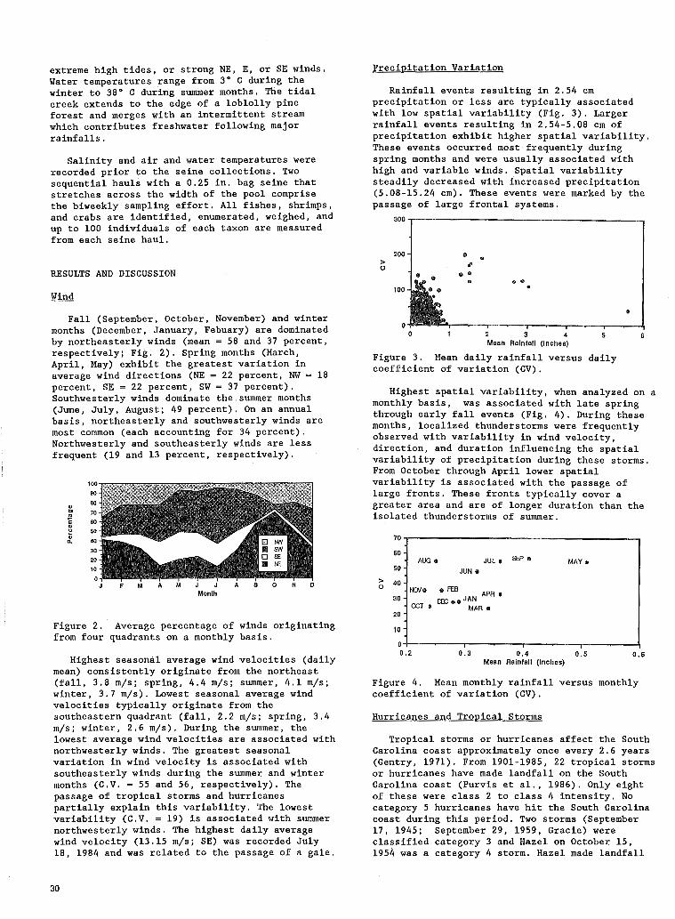
extreme high tides, or strong NE, E, or SE winds. Water temperatures range from 3" C during the winter to 38" C during summer months. The tidal creek extends to the edge of a loblolly'pine forest and merges with an intermittent stream which contributes freshwater following major rainfalls.

Salinity and air and water temperatures were recorded prior to the seine collections. Two sequential hauls with a 0,25 in. bag seine that stretches across the width of the pool comprise the biweekly sampling effort. All fishes, shrimps, and crabs are identified, enumerated, weighed, and up to 100 individuals of each taxon are measured from each seine haul.

RESULTS AND DISCUSSION

Fall (September, October, November) and winter months (December, January, Febuary) are dominated by northeasterly winds (mean = 58 and 37 percent, respectively; Fig. 2). Spring months (March, April, May) exhibit the greatest variation in average wind directions (NE = 22 percent, NW = 18 percent, SE = 22 percent, SW = 37 percent). Southwesterly winds dominate the summer months (June, July, August; 49 percent). On an annual basis, northeasterly and southwesterly winds are most common (each accounting for 34 percent). Northwesterly and southeasterly winds are less frequent (19 and 13 percent, respectively).

100

90

so " "' 70 " c so ~ 50

" 40 0.

30

20

10

Month

Figure 2. Average percentage of winds originating from four quadrants on a monthly basis.

Highest seasonal average wind velocities (daily mean) consistently originate from the northeast (fall, 3.8 mjs; spring, 4.4 mjs; summer, 4.1 m/s; winter, 3.7 m/s). Lowest seasonal average wind velocities typically originate from the southeastern quadrant (fall, 2.2 mjs; spring, 3.4 m/s; winter, 2.6 m/s). During the summer, the lowest average wind velocities are associated with northwesterly winds. The greatest seasonal variation in wind velocity is associated with southeasterly winds during the summer and winter months (C.V. =55 and 56, respectively). The passage of tropical storms and hurricanes partially explain this variability. The lowest variability (C.V. = 19) is associated with summer northwesterly winds. The highest daily average wind velocity (13.15 mjs; SE) was recorded July 18, 1984 and was related to the passage of a gale.

30

Precipitation Variation

Rainfall events resulting in 2.54 em precipitation or less are typically associated with low spatial variability (Fig. 3). Larger rainfall events resulting in 2.54-5.08 em of precipitation exhibit higher spatial variability. These events occurred most frequently during spring months and were usually associated with high and variable winds. Spatial variability steadily decreased with increased precipitation (5.08-15.24 em). These events were marked by the passage of large frontal systems.

300

200 " > .,. 0

• " . .. .. 100 .

2 3 4 5 6 Mean Rainfall (Inches)

Figure 3. Mean daily rainfall versus daily coefficient of variation (CV).

Highest spatial variability, when analyzed on a monthly basis, was associated with late spring through early fall events (Fig. 4). During these months, localized thunderstorms were frequently observed with variability in wind velocity, direction, and duration influencing the spatial variability of precipitation during these storms. From October through April lower spatial variability is associated with the passage of large fronts. These fronts typically cover a greater area and are of longer duration than the isolated thunderstorms of summer.

70;--------------------------------------, 60

AUG 111 JUL o SEP" MAYo 50 JUNo

> 40 0 f'0./111 30

CCT e

oFEB IE eo JAN APR e

MAR 111 20

10

0 0.2 0.3 0.4 0.5 0.6

Mean Rainfall (Inches)

Figure 4. Mean monthly rainfall versus monthly coefficient of variation (CV).

Hurricanes and Tropical Storms

Tropical storms or hurricanes affect the South Carolina coast approximately once every 2.6 years (Gentry, 1971). From 1901-1985, 22 tropical storms or hurricanes have made landfall on the South Carolina coast (Purvis et al., 1986). Only eight of these were class 2 to class 4 intensity. No category 5 hurricanes have hit the South Carolina coast during this period. Two storms (September 17, 1945; September 29, 1959, Gracie) were classified category 3 and Hazel on October 15, 1954 was a category 4 storm. Hazel made landfall

near Little River, South Carolina with 106 mph winds and tides up to 16.9 feet. Gracie made landfall on St. Helena Island and maintained hurricane strength more than 100 miles inland. Damage occurred from Beaufort to Charleston with heavy rains. Prior to 1900 three hurricanes with direct impact to the North Inlet system occurred in 1822, 1854, and 1893 (Purvis et al., 1986). The 1854 storm caused severe flooding with the Waccamaw Neck inundated with salt water from Waverly to Pee Dee. The great storm of 1893 occurred August 28 with winds approximately 120 mph. The storm struck at high tide and submerged whole islands. Two other hurricanes that affected the Georgetown area occurred on October 3 and 13 in 1893. Heavy rains were associated with both storms.

Hurricanes or tropical storms are an annual threat to Georgetown County. For any particular year there is a 46 percent chance of a tropical cyclone (34 or more knots wind speed) and a 13 percent chance of 2 such storms occurring in a given year (Purvis and McNab, 1985). The calculated return frequency of a 14 foot storm surge is approximately 100 years (Myers, 1975). The hurricane season along coastal South Carolina is June to October with the maximum storm occurrence frequency from September 24-30 (Purvis and McNab, 1985). The predominant storm direction is from the southwest.

During the period 1935-1986, 31 tropical storms or hurricanes passing within 75 miles of Georgetown resulted in precipitation at the Georgetown National Weather Service monitoring station. The percentage of Georgetown's total annual precipitation due to tropical storms or hurricanes ranges from 0 to 24 percent (Fig. Sa). During years when these storms occur, they are responsible for an average of 12.3 percent of the total annual rainfall. Total annual precipitation averages 128.8 em during years affected by tropical storms or hurricanes versus 120.0 em for those years not affected (Fig. Sb).

Water Budget Results

The water balance is not consistent from year to year. Although North Inlet usually has high winter surpluses and high summer deficits, there can be periods when precipitation exceeds PE during summer (1985; Fig. 6) and when PE exceeds precipitation during winter (1984-85, Fig. 6).

Drought conditions at North Inlet are not the norm. When comparing the average water budget at North Inlet with that of Georgetown (8 km away), it was found that the winter surpluses were approximately the same; however, the deficits of summer were far more extensive at North Inlet. Differences between sites were a function of the time period that was used in our comparisons (1937-1986 for Georgetown, 1979-1986 for North Inlet) and not differences due to location. Regression analysis of precipitation data revealed a highly significant correspondence between Georgetown and North Inlet (R~0.883).

25

(!) 20 Cl ell ... c: 15 (!) 0 .... (!) 10 c.

5

0 II II hi I I II

200

'E ~ c: 150 .2 'lU ~ ·;:;

100 <ll

a.

• 5 1935194019451950195519601965197019751980198

Year

Figure 5. (A) Percentage of annual precipitation due to hurricanes and tropical storms (first storm=black, second storm=open). (B) Total annual precipitation for Georgetown, SC.

14

12

1979

" 12

""'

- PE - RAIN

Ill Derick

Iii SU!pkJS

1980 1981

,, ..

.,. PE IIJI Defldt

- RAIN D. &Jrpkis

1985 1986

Figure 6. Water budget for Hobcaw Barony and North Inlet, SC.

Primary Production Measurements

North Inlet marsh grass, Spartina alterniflora, production and biomass have been measured by Dame and Kenny (1986) using the harvest technique and by Morris and Haskin (1988) using the census method. The two techniques produce similar estimates of standing biomass that range from a low of 50 gjm2 in midwinter to a high of 1000 g/m2

in early fall. Spatial and temporal differences of live standing biomass can however, be very significant. Dame and Kenny (1986) found that maximum creekside biomass ranged from 500 g/m2 to

31

1150 gjm2 during October to November, while maximum highmarsh biomass (i.e. areas not frequently inundated by tides) ranged from 280 gjm2 to 350 gjm2 during September to October. Spatial and temporal differences in biomass can be accounted for by differences in hydrodynamic forcing and the energy subsidies associated with tides and flooding frequencies (Odum et al. 1979, Conner et al. 1981).

Relationships between variation in marsh biomass and climatic events such as El Nino, are implied in the work of Dame and Kenny (1986). Climatic variations can produce annual differences in marsh salinities, hyrodology, and nutrient distributions. According to Dame and Kenny (1986), maximum biomass in the North Inlet creekside marsh occurred in 1983 (1150 g/m2 ) and 1984 (1100 g/m2

)

when winter surpluses of rainwater were extremely high and when mean winter salinities were extremely low (15 ppt). What must also be included in this climatic equation however, is the power of the wind to move river water past the tidal node thereby altering the spatial and temporal distribution of nutrients, sediments, and productivity in North Inlet. This is discussed later in more detail.

The standing stock of marsh grass is only indicative of marsh productivity. A more direct measurement of marsh production in North Inlet was done by Morris and Haskin (1988). They followed the growth and decay of every single blade of grass in six 100 cm2 plots. They found a maAimum production rate of 270+/-87 g/m2 in the midmarsh habitats of North Inlet in July of 1985 (Fig. 7). They also found that production rates peak one or two months before peak standing stocks, productivity has been decreasing since 1985, and annual trends in production at different sites are parallel. Although no climatological interactions are analyzed, Morris and Haskin conclude: "Parallel growth trends between sites, both annual and seasonal, suggest that productivity is responding to at least a regional scale phenomenon." We see good evidence for their conclusion. For example, salinity data at North Inlet indicated bay water intrusions during periods of maximum production, water quality data in the bay indicated high nitrogen concentrations (55 ug At./1), and water budget data indicated water surpluses during maximum production with increasing drought conditions after 1985. Other factors such as high phosphorus concentrations in the creek waters or variations in sea level and sediment salinity (Morris 1988) during 1985 could explain the high productivities, but these parameters are also indirectly controlled by climatic variables.

Drought

Droughts are a normal part of the climate in the southeast and have occurred 17 times in the past 100 years (Guttman and Plantico, 1987). Drought conditions occurred during 20 to 25 percent of the months from 1895 to 1986. Droughts in South Carolina last from a year and a half to seven years. Major droughts occurred in the 1920's, 1930's, 1950's, and late 1980's. The most

32

~ 300

0

~ .§ 200

E f! .9 c 0 100 ·~ ::J 'C e D.

1984 1985 1986 1987

Figure 7. Spartina alterniflora monthly primary production estimates ± 1 S.E.

persistent drought extended from 1952 to 1957. The end of the 1950's drought was marked by a rapid shift to wet conditions which persisted until the late 1970's. The 1980's brought a return to drier conditions.

The 1986 drought affected the entire southeast coast. Although not unusually long (one year), this drought was the most severe on record since precipitation records began in 1876 (Dowgiallo et al., 1987) and especially affected the Carolinas and Georgia. During April (the month most deficient in rainfall for the southeast), Charleston, SC had a 73 percent increase in the number of clear days and the number of clear days for the year was greater than the long-term average (Dowgiallo et al., 1987). Air temperatures during 1986 averaged 3" F above normal in Charleston, SC (Dowgiallo et al., 1987). In addition, Charleston had 83 days with maximum temperatures above 32.22" C for 1986 compared to the long-term average of 49.

Monthly precipitation was consistently below average from January through July and the maximum deviation was recorded in July (107 mm; Fig. 8). A slight positive deviation from normal was observed in August and was related to the passage of a single storm. Drier conditions returned in September and October. Air temperatures were above average during 10 months in 1986 (Fig. 9). High positive temperature deviations were recorded in Febuary and November (3.3 and 3.2 C, respectively). Annual flow of the Pee Dee River was 50 percent of normal (Dowgiallo et al., 1987).

Spat settlement

Spat settlement started in late April or mid May and ended in late October or mid November during each of the four years. Settlement was initiated during a narrow range of water temperatures (21.6 - 23.2 C) and was continuous with two or more peaks during most summers. The first peak typically occured in early June and the second occured in late July or early August. The second peak was usually more intense and generally accounted for 30 percent of annual set. Spat settlement was significantly higher in 1984 (p<0.05) at both Town Creek and Old Man Creek (Fig. 10). Oyster Landing also exhibited highest settlement in 1984 although total settlement was not significantly higher than that observed in

:iii c o; a:

60

40

20

0

·20

-40

·60

.so -100

·120 +---.--.--.,..--.---,--.----,--,---,,---,--.,..---,-.., J F M A M J J A S 0 N D

J FMAI.!JJASOND

Figure 8. (A) Deviation in 1986 monthly precipitation values from 30 year average. (B) Monthly precipitation during 1986 (shaded) and 30 year average (open).

4

~ 3

2! 2

.;! r! ., D. 0 E .,

·1 1-

·2

·3 J F M A M A s 0 N D

30

~ .,

20 B '" ~ D. E 10 ., 1-

0 J F M A M J A S 0 N D

Figure 9. (A) Deviation in 1986 monthly temperature values from 30 year average. (B) Monthly temperature during 1986 (shaded) and 30 year average (open).

1983. Settlement was lowest during 1986 at all three sites and this pattern could be related to the absence of a late summer pulse in late July and early August. The presence of high densities of late stage larvae in the water column in late July indicated reproductive success, but a corresponding settlement peak did not follow.

July and early August water temperatures were substantially higher in 1986 than values recorded for the previous three years (Fig. 11). Also, salinities were high and unusually stable during this period. The combined effect of high temperatures and high stable salinities was likely

responsible for the absence of a late summer settlement peak. The interaction of high temperature and high salinity has been demonstrated to cause high mortality in Ostrea edulis larvae (Robert, et al., 1988). In addition, high intertidal air temperatures and dessication stress may have adversely affected spat survivorship in the intertidal zone .

1983 1984 1985 1986

Figure 10. Mean total annual spat settlement per harness (Oyster Landing, OL; Old Man Creek, OM; Town Creek, TC).

30

~ 28 Q)

26 .... :::J .... co 24 .... Q)

a. 22 E ~ 20

18

38

li: 34 a.

....... 30 ~ ·c: 26 ~ 22

18

0 10

June

0 10

20 30 40 50 60 70 80 90

July

20 30 40 50 60 70 80 90

F-igure 11. Mean daily temperatures and salinities observed at Clambank Creek, Town Creek, and Oyster Landing during summer 1986. Bars represent monthly means ± 2 S.D. for the period 1983-1985.

The area from Charleston SC to Beaufort SC experienced heavy oyster mortalities in 1986 as a result of Dermo disease (Perkinsus marinus). The dieoffs followed drought and high temperatures and may have been related to reduced nutrients, temperature and salinity stress enhancing oyster susceptibility to disease (Dowgiallo et al., 1987).

Fish Community Structure

Biweekly collections of the more than 40 species of fishes, penaeid shrimps, and crabs which utilize high marsh creeks as "nursery" habitat have indicated that community composition and population dynamics are influenced by

33

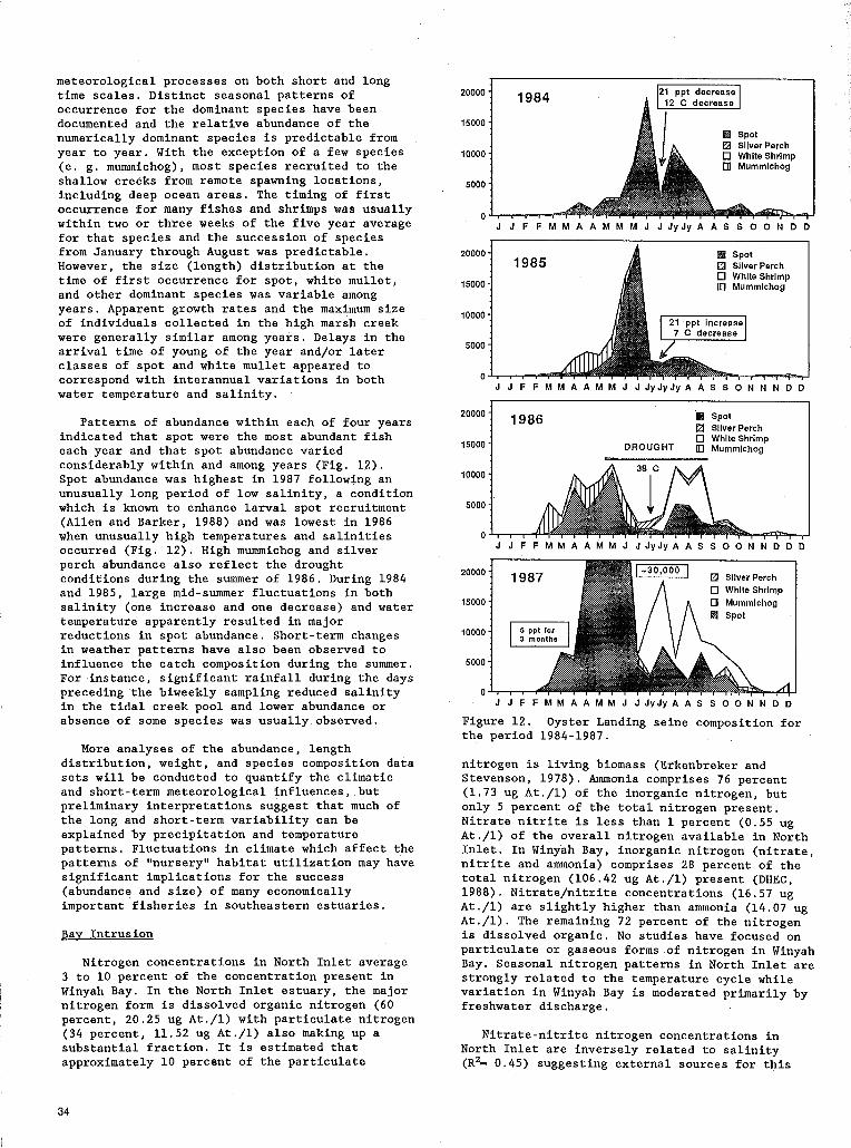
meteorological processes on both short and long time scale's, Distinct seasonal patterns ·of occurrence for the dominant species have been documented and the relative abundance of the numerically dominant species is predictable from year to year. With the exception of a few species (e. g. mummichog), most species recruited to the shallow creeks from remote spawning locations, including deep ocean areas. The timing of first occurrence for many fishes and shrimps was usually within two or three weeks of the five year average for that species and the succession of species from January through August was predictable. However, the size (length) distribution at the time of first occurrence for spot, white mullet, and other dominant species was variable among years. Apparent growth rates and the maximum size of individuals collected in the high marsh creek were generally similar among years. Delays in the arrival time of young of the year and/or later classes of spot and white mullet appeared to correspond with interannual variations in both water temperature and salinity.

Patterns of abundance within each of four years indicated that spot were the most abundant fish each year and that spot abundance varied considerably within and among years (Fig. 12). Spot abundance was highest in 1987 following an unusually long period of low salinity, a condition which is known to enhance larval spot recruitment (Allen and Barker, 1988) and was lowest in 1986 when unusually high temperatures and salinities occurred (Fig. 12). High mummichog and silver perch abundance also reflect the drought conditions during the summer of 1986. During 1984 and 1985, large mid-summer fluctuations in both salinity (one increase and one decrease) and water temperature apparently resulted in major reductions in spot abundance. Short-term changes in weather patterns have also been observed to influence the catch composition during the summer. For instance, significant rainfall during the days preceding the biweekly sampling reduced salinity in the tidal creek pool and lower abundance or absence of some species was usually observed.

More analyses of the abundance, length distribution, weight, and species composition data sets will be conducted to quantify the climatic and short-term meteorological influences, but preliminary interpretations suggest that much of the long and short-term variability can be explained by precipitation and temperature patterns. Fluctuations in climate which affect the patterns of "nursery" habitat utilization may have significant implications for the success (abundance and size) of many economically important fisheries in southeastern estuaries.

Bay Intrusion

Nitrogen concentrations in North Inlet average 3 to 10 percent of the concentration present in Winyah Bay. In the North Inlet estuary, the major nitr~gen form is dissolved organic nitrogen (60 percent, 20.25 ug At./1) with particulate nitrogen (34 percent, 11.52 ug At./1) also making up a substantial fraction. It is estimated that approximately 10 percent of the particulate

34

20000

15000

10000

5000

10000

5000

1984 21 ppt decrease 12 C decrease

1111 Spot f::l Sliver Perch 0 White Shrimp [D Mummichog

J F F M M A A M M M J J Jy Jy A A S S 0 0 N D D

DROUGHT

1111 Spot EJ Sliver Perch 0 White Shrimp lD Mummichog

N N D D

1111 Spot 0 Sliver Perch 0 White Shrimp lD Mummichog -----

0 Sliver Perch 0 White Shrimp [] Mummichog 11!1 Spot

D D

J J F F M M A A M M J J Jv Jy A A S S 0 0 N N D D

Figure 12. Oyster Landing seine composition for the period 1984-1987.

nitrogen is living biomass (Erkenbreker and Stevenson, 1978). Ammonia comprises 76 percent (1.73 ug At./1) of the inorganic nitrogen, but only 5 percent of the total nitrogen present. Nitrate nitrite is less than 1 percent (0.55 ug At./1) of the overall nitrogen available in North Inlet. In Winyah Bay, inorganic nitrogen (nitrate, nitrite and ammonia) comprises 28 percent of the total nitrogen (106.42 ug At./1) present (DHEC, 1988). Nitrate/nitrite concentrations (16.57 ug At./1) are slightly higher than ammonia (14.07 ug At./1). The remaining 72 percent of the nitrogen is dissolved organic. No studies have focused on particulate or gaseous forms of nitrogen in Winyah Bay. Seasonal nitrogen patterns in North Inlet are strongly related to the temperature cycle while variation in Winyah Bay is moderated primarily by freshwater discharge.

Nitrate-nitrite nitrogen concentrations in North Inlet are inversely related to salinity (R~ 0.45) suggesting external sources for this

nutrient. Two sampling stations affected by freshwater runoff are Oyster Landing (runoff from undeveloped forest system) and Clambank Creek (intrusion from Winyah Bay). Examination of nitrate-nitrite nitrogen concentrations measured daily at Clambank Creek and Oyster Landing during the period September 1978 through May 1986 indicated that average concentrations are higher at Clambank Creek than Oyster Landing (0.757 ug At.jl and 0,559 ug At./1, respectively; N=l577). Higher nitrate-nitrite nitrogen concentrations in Winyah Bay relative to North Inlet (Fig. 13) and intensive studies of nutrient exchange at the creeks connecting the two systems (No Man's Friend Creek and South Jones Creek) suggested that Winyah Bay may be an important source of nutrients for North Inlet (Michener and Allen, 1982). Analysis of variance (Table 1) indicated that wind velocity, wind direction, maximum daily river height. and the interaction among the three components were related to nitrate-nitrite nitrogen concentrations at Clambank Creek.

2.5 25

2.0 20 10' .... Ql Cll;s ~~1.5 15 .Ceo co, t01 10

>-Ol ~ :::31.0 ·= :::l

:::= 0.5 5

0.0 0 J

Figure 13. Nitrate-nitrite mean monthly concentrations at Winyah Bay and North Inlet,

Table 1. Analysis of variance for log-transformed nitrate-nitrite nitrogen concentrations during 1983 at Clambank Creek.

Source of Variation df ss F Pr>F

Wind velocity (WV) 1 0.244 5.44 0.020 Wind direction (WD) 3 0.314 2.38 0.071 Rain 1 0.114 2.59 0.109 River height (RH) 1 0.837 19.02 0.0001 WV*WD 3 0.042 0. 31 0.815 WV*WD*RH 4 0.433 2.46 0.046 Error 203 8.927 Total 216 11.233

Full Model: Pr>F=O.OOOl, R~0.205

Analysis of the 15 low salinity events (112 days total) that occurred during 1983 revealed that southwesterly winds were most frequently associated with the initiation of the intrusion event (7 of 15). Intrusion duration, minimum salinity, and maximum nutrient concentrations were related to predominant wind direction during events, wind velocity, and maximum river height. For example, one 2-day event (Jan 24) was associated with northwesterly winds and below

average maximum daily river height on day 1. The lowest salinity (28 ppt) was recorded on the first day and increased on day 2 (30 ppt). Maximum observed nitrate-nitrite nitrogen concentration was 0.40 ug At.jl, .In contrast, during one 14-day event (March 3), salinities dropped to 6 ppt and nitrate-nitrite nitrogen concentrations reached 5.01 ug At./1 at Clambank Creek. Maximum river height was above average on day 1. Southwesterly winds accompanied the initiation of the event and were dominant throughout the event (12 of 14 days). During this event, maximum nitrate-nitrite nitrogen concentrations reached 1.87 ug At./1 and salinities dropped to 2.0 ppt at Oyster Landing. The sharp decline in salinity at Oyster Landing was related to a single 1.8 em rain storm and freshwater runoff from the surrounding watershed. Higher nitrate-nitrite nitrogen concentrations at Clambank Creek are likely related to the proximity of this site to Winyah Bay. Nutrient inputs occurring from intrusion events undergo mixing and are diluted considerably prior to reaching more distant portions of the North Inlet Estuary (e.g. Oyster Landing).,

CONCLUSIONS

Spatial variability in rainfall and seasonal changes in wind velocity and directionality are characteristic features of the climate ~t the North Inlet Estuary. Impacts of hurricanes, tropical storms, and droughts are related to the recurrence frequency, intensity, and aerial extent of the event. Precipitation resulting from hurricanes or tropical storms may be considered an integral component of the regional water balance. Direct landfall of a Class 4 or 5 hurricane would likely result in noticeable changes to the North Inlet estuarine system, Tidal circulation patterns and sedimentation rates are predicted to be affected appreciably, .Droughts affect the North Inlet Estuary less frequently than tropical storms or hurricanes (recurrence frequencies of 5.9 and 2.6 years, respectively). Droughts occurring for extended periods over broad spatial scales can have significant impacts on productivity within the North Inlet Estuary. Low recurrence rates of severe droughts coupled with variable salinity and temperature tolerances of flora and fauna may have implications for community dynamics as well as reproductive success and recruitment. Intrusion of Winyah Bay waters into the North Inlet Estuary occurs frequently (i.e. 30 percent of observations during 1983) and may be a dominant factor affecting seasonal productivity patterns. Enhanced sedimentation, closure of connecting creeks, or opening of new connections between the North Inlet and Winyah Bay Estuaries would likely result in pronounced alteration of the available nutrient pool and subsequent primary and secondary production in the North Inlet Estuary.

Prior to examination of the potential effects of global climatic change (i.e. enhanced C02 levels, sea level rise, etc.) on regional and local biomes, it is necessary to understand ecosystem responses to naturally occurring chronic and acute climatic events. In this paper, we have examined the natural variability associated with

35

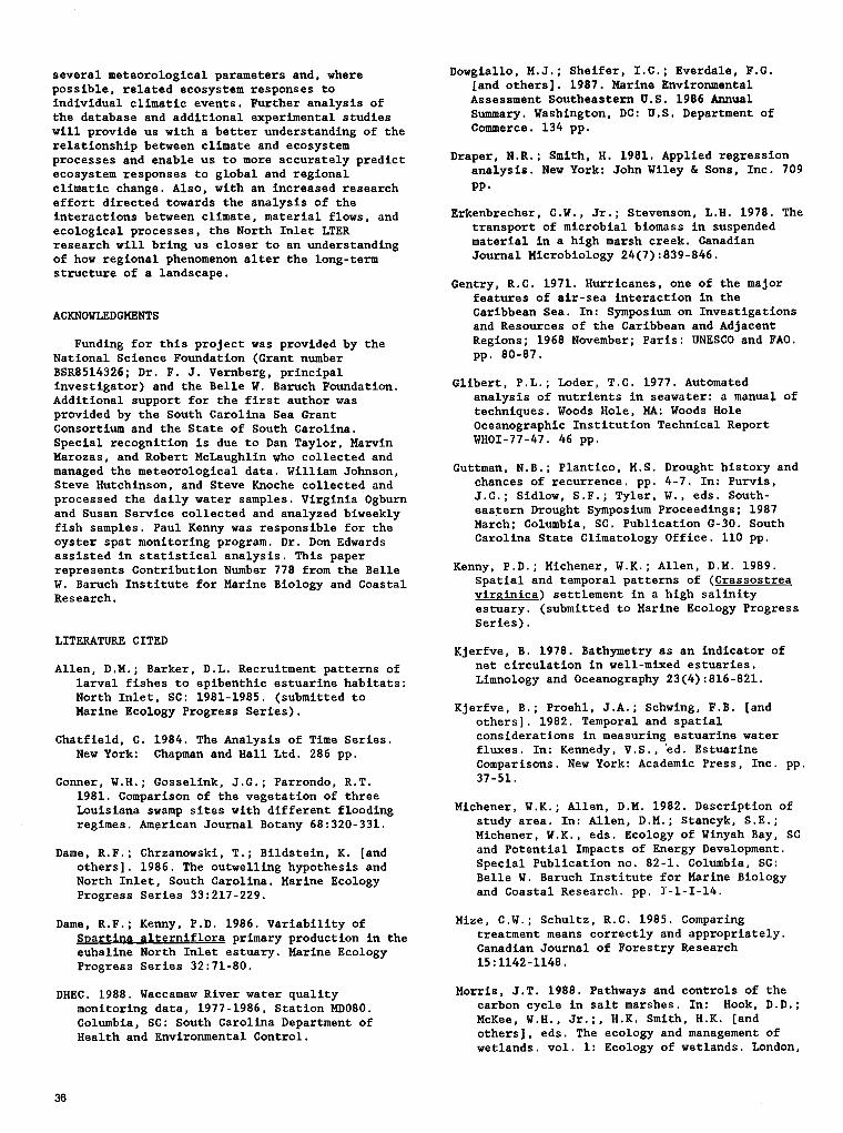
several meteorological parameters and, where possible, related ecosystem responses to individual climatic events. Further analysis of the database and additional experimental studies will provide us with a better understanding of the relationship between climate and ecosystem processes and enable us to more accurately predict ecosystem responses to global and regional climatic change. Also, with an increased research effort directed towards the analysis of the interactions between climate, material flows, and ecological processes, the North Inlet LTER research will bring us closer to an understanding of how regional phenomenon alter the long-term structure of a landscape.

ACKNOWLEDGMENTS

Funding for this project was provided by the National Science Foundation (Grant number BSR8514326; Dr. F. J. Vernberg, principal investigator) and the Belle W. Baruch Foundation. Additional support for the first author was provided by the South Carolina Sea Grant Consortium and the State of South Carolina. Special recognition is due to Dan Taylor, Marvin Marozas, and Robert McLaughlin who collected and managed the meteorological data. William Johnson, Steve Hutchinson, and Steve Knoche collected and processed the daily water samples. Virginia Ogburn and Susan Service collected and analyzed biweekly fish samples. Paul Kenny was responsible for the oyster spat monitoring program. Dr. Don Edwards assisted in statistical analysis. This paper represents Contribution Number 778 from the Belle W. Baruch Institute for Marine Biology and Coastal Research.

LITERATURE CITED

Allen, D.M.; Barker, D.L. Recruitment patterns of larval fishes to epibenthic estuarine habitats: North Inlet, SC: 1981-1985. (submitted to Marine Ecology Progress Series).

Chatfield, C. 1984. The Analysis of Time Series. New York: Chapman and Hall Ltd. 286 pp.

Conner, W.H.; Gosselink, J.G.; Parrondo, R.T. 1981. Comparison of the vegetation of three Louisiana swamp sites with different flooding regimes. American Journal Botany 68:320-331.

Dame, R.F.; Chrzanowski, T.; Bildstein, K. [and others]. 1986. The outwelling hypothesis and North Inlet, South Carolina. Marine Ecology Progress Series 33:217-229.

Dame, R.F.; Kenny, P.D. 1986. Variability of Spartina alterniflora primary production in the euhaline North Inlet estuary. Marine Ecology Pr.ogress Series 32:71-80.

DHEC. 1988. Waccamaw River water quality monitoring data, 1977-1986, Station MD080. Columbia, SC: South Carolina Department of Health and Environmental Control.

36

Dowgiallo, M.J.; Sheifer, I.e.; Everdale, F.G. [and others]. 1987. Marine Environmental Assessment Southeastern U.S. 1986 Annual Summary. Washington, DC: U.S. Department of Commerce. 134 pp.

Draper, N.R.; Smith, H. 1981. Applied regression analysis. New York: John Wiley & Sons, Inc. 709 pp.

Erkenbrecher, C.W., Jr.; Stevenson, L.H. 1978. The transport of microbial biomass in suspended material in a high marsh creek. Canadian Journal Microbiology 24(7):839-846.

Gentry, R.C. 1971. Hurricanes, one of the major features of air-sea interaction in the Caribbean Sea. In: Symposium on Investigations and Resources of the Caribbean and Adjacent Regions; 1968 November; Paris: UNESCO and FAO. pp. 80-87.

Glibert, P.L.; Loder, T.C. 1977. Automated analysis of nutrients in seawater: a manual of techniques. Woods Hole, MA: Woods Hole Oceanographic Institution Technical Report WHOI-77-47. 46 pp.

Guttman, N.B.; Plantico, M.S. Drought history and chances of recurrence. pp. 4-7. In: Purvis, J.C.; Sidlow, S.F.; Tyler, W., eds. South­eastern Drought Symposium Proceedings; 1987 March; Columbia, SC. Publication G-30. South Carolina State Climatology Office. 110 pp.

Kenny, P.D.; Michener, W.K.; Allen, D.M. 1989. Spatial and temporal patterns of (Crassostrea virginica) settlement in a high salinity estuary. (submitted to Marine Ecology Progress Series).

Kjerfve, B. 1978. Bathymetry as an indicator of net circulation in well-mixed estuaries. Limnology and Oceanography 23(4):816-821.

Kjerfve, B.; Proehl, J.A.; Schwing, F.B. [and others]. 1982. Temporal and spatial considerations in measuring estuarine water fluxes. In: Kennedy, V. S. , 'ed. Estuarine Comparisons. New York: Academic Press, Inc. pp. 37-51.

Michener, W.K.; Allen, D.M. 1982. Description of study area. In: Allen, D.M.; Stancyk, S.E.; Michener, W.K., eds. Ecology of Winyah Bay, SC and Potential Impacts of Energy Development. Special Publication no. 82-1. Columbia, SC: Belle W. Baruch Institute for Marine Biology and Coastal Research. pp. I-1-I-14.

Mize, C.W.; Schultz, R.C. 1985. Comparing treatment means correctly and appropriately. Canadian Journal of Forestry Research 15: 1142-1148 .

Morris, J.T. 1988. Pathways and controls of the carbon cycle in salt marshes. In: Hook, D.D.; McKee, W.H., Jr.;, H.K. Smith, H.K. [and others], eds. The ecology and management of wetlands. vol. 1: Ecology of wetlands. London,

UK: Croom Helm and Portland, OR:, Timber Press. pp. 497-510.

Morris, J.T.; Haskin, B. Relationships among stem size, turnover, and net aerial production in the salt marsh grass Spartina alterniflora: A four year record of primary production. (submitted to Ecology).

Myers, V.A. 1975. Storm tide frequencies on the S. c. coast. NOAA Technical Memorandum ERL WMP-3. Silver Spring, MD: U. S. Department of Commerce, National Weather Service. 79 pp. [cited in Purvis and McNab, 1985].

NOAA, 1985. Local Climatological Data for Georgetown, SC. (30 Year Summary, 1951-1980). Asheville, NC: U. S. Department of Commerce, National Climatic Data Center.

Odum, E.P.; Finn, J.T.; Frang, E.H. 1979. Perturbation theory and the subsidy-stress gradient. Bioscience 29:349-352.

Purvis, J.C.; McNab, A., Jr. 1985. Hurricane vulnerability for Georgetown County. Columbia, SC: South Carolina Water Resources Commission. 17 pp.

Purvis, J.C.; Tyler, W.; Sidlow, S. 1986. Hurricanes affecting South Carolina. Columbia, SC: South Carolina State Climatology Office. 19 pp.

Robert, R.; His, E.; Dinet, A. 1988. Combined effects of temperature and salinity on fed and starved larvae of the European flat oyster Ostrea edulis. Marine Biology 97:95-100.

SAS Institute, Inc. 1985a. SAS User's Guide: Statistics, Version 5 Edition. Cary, NC: SAS Institute, Inc. 956 pp.

SAS Institute, Inc. 1985b. SAS User's Guide: Basics, Version 5 Edition. Cary, NC: SAS Institute, Inc. 1290 pp.

Schwing, F.B.; Kjerfve, B. 1980. Longitudinal characterization of a tidal marsh creek separating two hydrographically distinct estuaries. Estuaries 3:236-241.

Sokal, R.R.; Rohlf, F.J. 1981. Biometry. San Francisco: W.H. Freeman and Co. 859 pp.

Thornthwaite, C.W.; Mather, J.R. 1955. The water balance. Centerton, NJ: Drexel Institute Tech., Laboratory of Climatology. Climatology 8(1):1-86.

Thornthwaite, C.W.; Mather, J.R. 1957. Instructions and tables for computing potential evapotranspiration and the water balance. Publications in Climatology 10(3):185-311.

37

LAKES AS INDICATORS OF AND RESPONDERS TO CLIMATE CHANGE!/

Dale M. Robertso~/

Abstract--Lakes integrate short-term fluctuations in the atmospheric climate. Interannual changes in the response of thermal features, namely, epilimnion and hypolimnion temperatures, thermocline depth, duration of ice cover and freeze and break up dates, can therefore be used to detect and quantify past changes in the climate which are· often obscured by short-term variability and secular changes in meteorological measurements. Given future climatic scenarios and the quantitative relationship with air temperatures, future lake conditions can be estimated. Extensive ice cover and water temperature data for Lake Mendota, Wisconsin, beginning in 1856, are used to demonstrate the utility of historical lake records to detect past changes in mean air temperature. Future lake conditions are forecast in response to projected "greenhouse" warming scenarios.

Keywords: Air temperature, water temperature, historical lake records, "greenhouse" warming

INTRODUCTION

"Climate" is defined as the collective state of the earth's atmosphere for a given place for a specified interval of time (Landsberg, 1960). Therefore, when one describes climatic changes, the time frame and meteorological parameters must be specified. Here, climate and climatic change will primarily refer to air temperature and changes in mean air temperature, respectively. Climatic changes have been occurring since the earth formed and will continue to occur in the future. Time scales of climatic change range from changes over millions' of years to changes over days. To detect historical and future climatic changes,·the climate or weather conditions must have been recorded in a manner allowing a rigorous comparison of climatic conditions through time. Many indicators have been used to detect past climatic changes; however, most only detect changes over specific time scales (Heicht and others, 1979). Indicators used to detect changes over time scales from 10's to 100's years include meteorological (Budyko, 1977; Wahl and Lawson, 1970), phenological (Novitzkie and Deyaul, 1978),

!; Presented at the LTER Workshop on Climate Variability, Niwot Ridge Green Lakes Valley LTER Site, CO, August 21-23, 1988.

~/ Post Doctoral Fellow, Northern Lakes LTER Site, Center for Limnology, University of Wisconsin-Madison, WI. Present address: Centre for Water Research, University of Western Australia, Nedlands, WA, 6009 Australia.

38

tree ring (Fritts and others, 1971; Meko and others, 1985), and lake sediment data (Webb and Bryson, 1972; Bernabe, 1981; Swain, 1978). In addition to these, ice cover and water temperature records of lakes also serve as climatic indicators (McFadden, 1965; Tramoni, 1985; Palecki and Barry, 1986; Strub and others, 1985; Robertson, 1989) .

Recently, major questions dealing with climate change have focused on anthropogenic effects, such as: ·Have human disturbances to the atmosphere and land affected historical climates and will they affect future climates? Will increasing concentrations of atmospheric co2 and other "greenhouse" gases cause surface temperatures of the earth to increase? If air temperature increases, how will this affect the various ecosystems on the earth, specifically aquatic ecosystems? In this paper, I demonstrate how lake ice cover and water temperature records for a specific lake, Lake Mendota, WI, can be used to detect and:quantify past local changes in mean air temperature that otherwise be undetectable using past meteorological records, Future mean conditions of the lake are forecast using projected climatic warming scenarios and the calibrated response of the lake parameters.

Changes in mean air temperature over time scales ranging from 10's to 100's of years are often difficult to discern using biological indicators because the effects of air temperature are usually integrated with effects of other meteorological conditions, primarily precipitation and humidity (Swain, 1978) .

Biological indicators also have variable response times dependent on the life span or growth rate of the organism. Air temperature records themselves often have secular changes or systematic biases incorporated i_nto the records which may be larger than subtle climatic changes. These systematic biase·s can be caused by changes in the equipment, station location, station design, and time of observation (Schaal and Da7e, 1977; Karl and Williams, 1987). Some systemat~c biases can be removed using coinciding data from nearby stations (Karl and Williams, 1987) or using theoretically based corrections to adjust for some known changes in observational techniques. However, changes in early observational techniques, which are usually not documented, can be almost impossible to remove resulting in early air temperature records being of questionable quality and often very misleading.

Ice cover (freeze and break up dates, and total days of ice cover) and water temperature records for a lake represent an integration of local weather conditions. These parameters often integrate daily fluctuations in weather conditions, primarily air temperature, in a manner less subject to secular biases than other climatic indicators including direct meteorological measurements. Ice cover and water temperature data are not internally recorded; each has to be observed and documented by an observer. Therefore, lake records, as well as any parameter documented by observers such as meteorological data, may have systematic biases incorporated into the records caused by changes in observational techniques or criteria. However, for some lakes, such as _Lake Mendota, the transition to and from complete ice cover are very rapid and can often be resolved to one or two days. For the ice cover records of such lakes, variability introduced by observer subjectivity is small compared to the variability of the system.

Annual differences in ice cover and water temperature for small to medium sized lakes are primarily driven by changes in air temperature for specific seasons (McFadden, 1965; Palecki and Barry, 1986; Robertson, 1989). Freeze dates represent an integration of fall air temperatures; break up dates represent the period between freezing and break up (winter and early spring) and total ice duration represents the entire fall, winter, and early spring period. The length of the integration period represented by the ice records depend on lake depth, with deeper lakes integrating a longer time period (McFadden, 1965). Water temperatures represent an integration of weather conditions from the spring, summer, and fall periods.

Lake records have had limited use as climatic indicators because long-term continuous ice cover and water temperature measurements are extremely rare. Few lakes have water temperature records that extend more than 20 years or exist prior to 1920. Possibly the most extensive water temperature records available exist for Lake

Mendota, WI, which begin in 1894 and continue intermittently to present. Long-term ice records are a little more common, and a few exist from as early as 1840 in North America (Tramoni, 1985). The longest continuous records available for any lake in North America begin in 1855, also for Lake Mendota (Tramoni, 1985).

LAKE MENDOTA

Lake Mendota is a dimictic, eutrophic lake located in Madison in south-central Wisconsin (43°4'N, 89°24'W). The lake has a surface area of 3,940 ha, a maximum depth of 26m, a mean depth of 12.4 m, and a maximum fetch of 9.8 km (Wisconsin Department of Natural Resources, 1961) .

DETECTING CLIMATIC CHANGES

Detecting prior climatic changes from lake records or other climatic indicators is generally approached by examining a time series for statistically significant changes in mean conditions. Ice records of Lake Mendota are used to demonstrate how lake indicators can be used to detect climatic change. In Figure 1, mean ice duration (as demonstrated by the seven year moving average) of Lake Mendota has significantly changed since 1856. In fact, most of the climatic change appears to have been rather abrupt around 1890. Since 1980, there appears to possibly be another transition to shorter ice cover.

Climatic changes are generally thought to occur over several years. To determine whether a significant change has occurred in the indicator, the data are tested to determine whether there is a significant slope or change through time. Often the indicator time series has significant

DURATION (DAYS)

LAKE MEN DOT A ICE DURATION

180.-------------------------------.

160

140

120

100

80

60 7 YEAR MOVING AVERAGE

40+---~----.-----~---.----~--~ 1850 1900 1950 2000

YEAR

Figure 1. Total days of winter ice cover (ice duration) for Lake Mendota. The seven year moving average, plotted in year four, is superimposed on the observed data as an estimate of mean ice durations.

39

autocorrelation; therefore, ARIMA analyses are used to remove the autocorrelation, prior to testing for significant changes. There is a significant downward slope or change to shorter ice durations for Lake Mendota since 1856 (a~ o·. 05). However, when examining the time series of the indicator, often the change appears to occur rather abruptly rather than gradually. One technique which has been used to test whether a rather abrupt change better describes the change in the indicator is ARIMA intervention analyses (Box and Tiao, 1975) . This technique tests for significant slopes or changes before and after a possible abrupt change. This technique can be used with or without significant autocorrelation in the dataset. The timing of the change is defined by the user. The "best" model is often selected by comparing t-ratios of consecutive yearly interventions. The "best" model describing the change in the mean ice duration of Lake Mendota had a constant mean of 118 days from 1856 to 1888 (Figure 2A) . In 1888 a rather abrupt change occurred, modeled as a step change followed by a stationary mean of 103 days. The decrease in ice duration of 15 days is indicative of higher mean air temperatures after 1888. Whether the change occurred precisely in 1888 or over several years only slightly modifies estimated changes in mean conditions.

Often when examining a time series, a period of unusual years appears present. For example, the ice duration from 1980 to 1988 appear to be shorter than that prior to 1980 (Figure 1). The seven year moving average ice duration, from 1982 to 1988, is the shortest on record, even if the record short ice duration of 1983 was replaced by the mean ice duration from 1889 to 1979. one technique to test whether the mean of a specific period is significantly different from that of another is a Student t test (Burr, 1974). The period from 1980 to 1988 had significantly shorter ice duration, by 12 days, than the prior period (a~ 0.05). Therefore, the "best" description of the mean ice duration of Lake Mendota is demonstrated in Figure 2A.

Similar procedures to describe mean freeze and breakup dates were used and the results are demonstrated in Figure 2B, C, respectively. A change in mean freeze date occurred in about 1888, but no significant change was observed in recent years. From the freeze date data, it was unable to be determined whether the first, cooler, period ended abruptly or whether it was a gradual transition period. For the purpose of further analyses, it was assumed the first period ended abruptly in 1888. This gave a change in mean freeze date from Julian day 348 to 356, a change of 8 days based on mean freeze dates. Three climatic periods, similar to those found with ice duration records, were found from break up dates. The first period lasted from the beginning of record to 1888, when mean break up date changed rather abruptly from Julian day 101 to 94, a 7 day change. The second period lasted from 1889 to approximately 1979. The later mean break up date of the first period indicated a

40

cooler climate prior to 1888. No significant trends occurred in the first or second periods. Since 1980, mean break up date appears to be in transition to earlier dates. Presently, the moving seven year average, from 1982 to 1988, has obtained the earliest on record at Julian day 85. The mean break up date from 1980 to 1988 was Julian day 86, an 8 day earlier mean break up date than that of the second period, indicative of a warmer period.

LAKE MENDOTA ICE DURATION

160

ICE 140

DURATION 120

(DAYS) 100

80

60

1900 1950 2000

A. FREEZE DATE

400~------------------------------~

FREEZE DATE

380

360 (DAY NUMBER)

340

320+-----~----,------------r----~----~

B.

BREAK UP DATE

1850

120

100 (DAY NUMBER)

90

80

70

1900 1950 2000

BREAK UP DATE

so+-----~--~----~-----r----~--~ 1850 1900 1950 2000

c. YEAR

Figure 2. Observed annual ice cover records for Lake Mendota with the "best" estimate of how the mean for each parameter has changed. The idealized means were determined from several ARIMA intervention models fit to the observed data. (A) Ice Duration. (B) Freeze Date. (C) Break Up Date.

QUANTIFYING CLIMATIC CHANGES

To quantify these changes in terms of specific meteorological parameters, we must determine what that change means in terms of air temperatures. This is done by determining how the indicator has responded to changes in that meteorological parameter, i.e., calibrate the indicator. The calibration can often be very complex because of the integrating nature of the indicators.

Two approaches have been used to determine how climatic indicators respond to changes in a specific meteorological parameter: the dynamic, or mechanistic approach, and the empirical or statistical approach (Wright, 1980) . Since the calibration techniques are much different for ice cover and water temperature, both are described below.

In the dynamical approach, mathematical models are developed to simulate the response of specific indicators to weather or climatic conditions, based on equations simulating the physical processes occurring in the system. All important parameters must be included in the model to properly simulate the system. The models are calibrated using concurrent historical records for the climatic indicator and measured meteorological data. The response of the indicator to a specific meteorological parameter, such as air temperature, is then determined by running the model for various simulations with only the specified meteorological parameter altered. The change in response of the indicator in these simulations is then used to determine the relationship between the indicator and the specified meteorologicai parameter. This approach is more commonly used than the empirical approach because only a few years of measured data are required.

In the empirical approach, we exploit the fact that nature has been performing experiments with the climatic system for a long time; the results of those experiments are our observational records (Wright, 1980) . These records are used to develop statistical relationships between the important meteorological parameters, including air temperature, and the climatic indicator. If statistically significant relationships involving air temperature are found, the equation(s) are then used to determine the pattern and response of the indicator to changes in air temperature.

Whenever possible, dynamic models should be used in concert with empirical models to determine if the results agree. A similar quantitative response using two independent approaches adds more confidence to the results than results found only using one technique.

Ice Cover

Freeze and break up dates were analyzed separately to quantitatively determine the magnitude and seasonal timing of the climatic

changes rather than calibrating ice duration as a total winter indicator. Two techniques have been used to develop lake ice cover records into temperature indices: fixed period regression analyses (Rannie, 1983; Tramoni and others, 1985; Palecki and Barry, 1986; Robertson, 1989) and variable length air temperature integration (McFadden, 1965; Robertson, 1989) .

Regression analyses have been used to calibrate ice records of specific lakes by regressing specific air temperature summary parameters, such as a monthly or bi-monthly average air temperature, with observed freeze or break up dates. To calibrate the freeze date for Lake Mendota, annual freeze dates from 1884 to 1988 were regressed against several combinations of monthly mean air temperatures. The earlier years in the record were not included because of secular biases in meteorological records prior to 1884. Average November to December air temperatures were most strongly correlated with observed freeze dates, R2 = 0.61 (Figure 3A).

REGRESSION MODEL 400.----------------------------------,

FREEZE DATE

390

380

370 (DAY NUMBER)

360

350

340

Y = 355.9 + 4.32 • X R2 = 0.61

• 4 • 2 0 2 4 G

A. NOV I DEC AVE. AIR TEMPERATURE (C)

INTEGRATED "FREEZE" MODEL 400.--------------------------------,

FREEZE DATE

390

380

370 (DAY NUMBER)

360

350

340

Y = 356.8 + 4.83 • X R2

= 0.99

330+-~--~-----r----~-----..-----4 • 4 • 2 2 4 G

B. il MEAN DAILY AIR TEMPERATURE (C)

Figure 3. Calibration of mean freeze date into an index of fall and early winter air temperatures. (A) Fixed period analysis. Observed freeze dates from 1884 to 1988 versus the deviation from the long-term average November to December air temperature (1884 to 1988). (B) Moving integrated air temperature analysis ("Freeze" model) .

41

The slope of the regression suggests mean freeze date changes 4.32 days (± 0.6 days, 95% C.I.) per 1.0°c change in average November to December air temperature. Deviation from the average November to December air temperature, from 1884 to 1988, was used as the x-axis to simplify comparison of model results. Interpolation of the regression slope suggests the 8 day earlier freeze date before 1888 corresponds to average November to December air temperatures which were 1.7°C lower than those after 1888.

The second technique to calibrate ice records involves using a moving index which accumulates through time, such as a moving mean air temperature (McFadden, 1965) or integrated air temperature (Robertson, 1989) . When the moving index reaches a specified threshold value, the specific event such as freezing or break up is estimated to occur. When calculating simple moving average air temperatures, days early in the period of the moving average are weighted similar to days just prior to freezing or break up; whereas, integrated air temperatures can weight the more recent air temperatures more heavily. Therefore, integrated air temperatures were used. Integrated moving air temperatures were used to predict daily water temperatures and ultimately when the surface temperature became 0°C and the lake froze. This was done by weighting the prior day's predicted water temperature by a specific value and adding to this the change estimated for that day, which is dependent on the difference in air and water temperatures (Eq. 1). Therefore, the most recent days are more influential to the present daily water temperature value. Eq. 1 can be adjusted to add the effects of daily synoptic conditions such as strong winds which could cause the lake to freeze later or break up earlier than expected without modifying the estimated day's water temperature.

or

WT = a + b * AT_1 + c * WT_1

where:

WT = Water temperature on Day T

(1)

(2)

Water temperature on Day T - 1

Air temperature (°C) on Day T - 1

a, b, c, and K are Empirical Constants:

a = 0.056; b 0.946; c 0.326

Initially, WT-1 = 28.70 on 1 October

Integrated moving air temperatures were developed into a "Freeze" model (Eq. 2) by calibrating the coefficients such that the estimated surface water temperature (WT), calculated starting on 1 October of each year, became ~ 0°C very near to the day the lake was observed to freeze. The "best" coefficients for estimating annual freeze dates for Lake Mendota

42

were determined by iteratively calculating the coefficients which minimized the sum of square errors for a 40 year reference period, 1948 to 1987. This minimization process was done using the Nelder-Mead simplex procedure (O'Neill, 1971). Additional terms were added to Eq. 2 in an attempt to adjust for synoptic conditions. These terms had the effect of raising or lowering the threshold criteria but did not affect future predictions of WT, i.e., these terms did not alter the following WT_1 . Therefore, with a strong wind lower water temperatures may be required for the lake to freeze. Additional terms, however, did not significantly improve the model.

For annual models, such as the "Freeze" model or a similar "Break up" model, the estimated effects of changes in mean air temperature are made by comparing average estimated freeze or break up dates of a reference period, a 30 year period from 1948 to 1977 was used here, with average predicted dates obtained from the models after the daily air temperatures for those years are raised or lowered by the simulated change in air temperature. Daily air temperatures for all 30 years were lowered 1, 2, and 3°C and raised 1, 2, 3, 4, and 5°C. The average freeze dates estimated by the "Freeze" model were then regressed on the simulated change in air temperature (Figure 3B) . The slope of the regression suggests a change in freeze date of 4.83 days per 1.0°C change in air temperature, very similar to the 4.32 days per 1°C change estimated using the fixed period analysis. Interpolation of the regression slope suggests the 8 day earlier freeze date before 1888 corresponds to average November to December air temperatures which were 1.5°C lower than those after 1888. This approach to estimate the effects of changes in air temperature assumed that the daily variability in weather conditions for the simulated changes in air temperature was and would be similar to that of the reference period.

A similar analysis for break up dates suggests a change of approximately 6 days per 1°C change in mid winter to early spring, January to April, air temperatures. Therefore, the changes in mean break up dates (Figure 2C) suggest the period prior to 1889 was 1.1°C lower than the second period and the period after 1979 was 1.2°C higher than the second period.

Water Temperatures

The DYnamical REservior Simulation Model (DYRESM) (Imberger and Patterson, 1981) was used to simulate the physical processes and ultimately water temperatures in Lake Mendota responding to the forcing meteorological conditions. DYRESM is a one-dimensional numerical model used to predict water temperature and salinity profiles of small to medium sized lakes and reservoirs given initial temperature and salinity profiles, lake morphometry, meteorological conditions, and inflow and outf1ow information. For each simulation DYRESM was started on the day after ice break up when the lake has been shown to be

very near 3°C (Neese and Bunge, 19S6; Robertson, 1989) . DYRESM was calibrated for Lake Mendota using two years of daily weather data and approximately biweekly measured water temperature profiles from shortly after ice break up until a few weeks prior to freeze up for 19S8 and 1966 (Robertson, 1989). These years were selected because the thermal structures varied considerably between years. The "best" values for the empirical coefficients used in DYRESM were determined by iteratively calculating the values which minimize the overall average of the mean daily absolute errors for both years (Eq. 3). The minimization process was done using the Nelder-Mead simplex procedure (O'Neill, 1971). The calibrated model simulation for 19S8 is compared with observed data in Figure 4. DYRESM simulated the daily temperature progression very well, with the possible exception during late fall.

MDAE

Where:

N

I:: I Tobserved - Tmodell i=l

N

MDAE = Mean Daily Absolute Error

(3)

N Total Number of depths with observed water temperatures (Tobservedl

Tmodel

0

5

DEPTH 1 0

1 5

20

25

DYRESM simulated water temperature

610 1418 2226

Figure 4. DYRESM model verification for Lake Mendota in 19SB. Computed vertical temperature profiles (solid connected dots) and observed (open squares) temperatures. Profiles were

measured and compared approximately biweekly from

To determine how changes in air temperature influence the thermal structure of the lake, DYRESM was run for 11 years for each of 6 air temperature regimes. Eleven years of daily meteorological data (19S8-63, 1966-67, 1971-73) were used as the base or reference air temperature regime. Five other air temperature regimes were obtained by adding -3, -1, +1, +3, and +S°C to each daily average air temperature for all 11 years. Since annual ice break up dates or the date at which the simulation began should change with air temperature, forecasted ice out dates were determined for each year based on the "Break Up" model, using daily adjusted air temperatures as input for the model.

For each annual simulation, morphometrically weighted monthly mean epilimnion or shallow layer temperature (0 to 7m), hypolimnion or deep layer temperature (lS to 18m), and average monthly thermocline depth were computed. Average monthly values for these three parameters were computed for each air temperature regime and subtracted from that for the the reference regime. Differences from the means of reference period represent the average effect caused solely by the change in air temperature.

Changes in average monthly epilimnion temperatures were related directly to changes in air temperature, with water temperatures increasing with air temperature increases and decreasing with air temperature decreases (Figure SA) . However, the changes were smaller than the air temperature change and varied seasonally, with the largest response occurring in spring. The response of epilimnion temperatures varied from approximately 6S% of the change in air temperature in May to approximately 40% for most summer months.

61014182226 D D D D D 0 0 0 0 0 0 0 0 0 0 0

0 0 0 0 0 0 0 0 0 0

0

0 0 0 0 0 0 0 0 0 0 0 0 0 0 0 0 0

0 0 0 0

Julian day number 129 (B May) to 32S (20 November) and are in order of day number from left to right. Each date is offset by 6°C. Each date has the same relative x scale, indicated by the scales on the top of the figure for the 1st and 8th profiles.

43

Changes in average monthly hypolimnion temperatures were also related directly to changes in air temperature, with mean water temperatures increasing in response to air temperature increases and decreasing in response to air temperature decreases (Figure SB ). The response was again smaller than the change in air temperature and varied seasonally from approximately 4S% of the change in air temperature in May to 2S to 30% for most of the summer.

Simulated thermocline depths displayed little response to changes in air temperature (Figure SC) . There was a slight indication of shallower thermoclines from August to October with increasing air temperature; however, these changes were not statistically significant.

PROJECTED RESPONSE TO FUTURE CLIMATIC CHANGE

The future response of the thermal structure and ice phenology of Lake Mendota can be made based on climatic warming scenarios estimated from various General Circulation Models (Hansen and others, 1984; Manabe and Wetherald, 1986; Schlesinger and Zhao, 1988) in response to increased atmospheric co2 and other "greenhouse" gases in concert with the quantitative relationships found above. If all other non-air temperature parameters remain unchanged, a uniform monthly increase in air temperature of 1°C should cause the responses listed in Table 1 for Lake Mendota. With further increases in air temperature these responses should be approximately additive, i.e., a 2°C increase should cause the responses to double, etc. However, with a 4 and S°C increase in air temperatures, results suggest the lake will often freeze and break up more than one time per winter which in turn will further shorten total ice duration (Figure 6) . The frequency of refreezing should increase with continued warming. With a s0 c increase, expected to occur around 20SO to

Table 1. Seasonal response of Lake Mendota to a 1 oc increase in air

temperature, all other meteorological parameters were assumed

to remain unchanged.

Response

Spring - Entire water column temperatures higher by 0.650C.

Early Summer - Higher eplllmnlon temperatures by 0.5 to o.soc.

- Earlier stratification.

- Higher hypolimnion temperatures by 0.30C.

Mid - Late - Higher epilimnion temperatures by 0.4 to 0.5oc.

Summer - Little change in thermocline depths.

- Higher hypolimnion temperatures by 0.3oc.

Fall - Higher epilimnion temperatures by 0.4 to o.soc.

- Longer stratification.

- Higher hypolimnion temperatures by 0.4 to 0.5oc.

Early Winter - Mean freeze date delayed by 5 days.

Late Winter - Mean break up date earlier by 6 days.

- Mean total ice duration shorter by 11 days.

44

CHANGE IN MEAN EPILIMNION TEMPERATURE (C) 6~---------------------------------,

I:!. 0 TO 7 M 4

TEMPERATURE +5

(c) 2 +3~: : :::=: +1

0 0 - 1

-2 -3

A. -4~.----.--~----.----r---.----~ APR MAY JUN JUL AUG SEP OCT

CHANGE IN MEAN HYPOLIMNION TEMP. (C) 4~--------------------------------~

3 I:!. 15 TO 18M TEMPERATURE 2 +5

(C) +3

+1

0 0 - 1

-1 -3

-2

B. -3L-.----,---.----.---~-------.~ APR MAY JUN JUL AUG SEP OCT

CHANGE IN MEAN THERMOCLINE DEPTH

7

I:!. THERMOCLINE

c.

DEPTH 5

( M) 3

-1

-3

+5 +3 -3 +1

-~±:3l~~~e~~~

-5~.----.---.----.---,--------~

APR MAY JUN JUL AUG SEP OCT

Figure S. Estimated changes in the thermal structure of Lake Mendota in response to changes in air temperature. The simulated change in air temperature is labelled on each curve. All changes are differences from the mean monthly or seasonal values. All monthly and seasonal changes have the 9S% confidence limits. (A) Change in mean epilimnion temperture. (B) Change in mean hypolimnion temperature. (C) Change in mean thermocline depth. Mean epilimnion and hypolimnion temperatures are defined as the morphometrically weighted mean water temperature from 0 to 7m and lS to 18m, respectively. Thermocline depth is defined as the depth of the maximum temperature gradient.

ICE DURATION

160

ICE 140 DURATION

120 (DAYS)

100

80

60

40+---~--~----~--.---~----.---~--~

1850 1900 1950 2000 2050

YEAR

Figure 6. Expected future response of mean ice cover to climatic warming as projected by the Transient General Circulation Model from the Goddard Institute of Space Studies (Hansen and others, 1984). Projections were made using the "Freeze" and "Break up" models. Historical annual records and the best description of historical means are included (similar to Figure 2).

2060, mean ice duration should be reduced by 6S days and results of the "Freeze" model suggest the lake should remain ice free all winter with a frequency of 1 out of 30 years. With increasing air temperatures the possibility of the lake not freezing in a particular winter will increase further.

CONCLUSIONS

Changes in the response of the thermal features of lakes, namely, epilimnion and hypolimnion temperatures, thermocline depth, freeze and break up dates, and total ice duration, are good quantitative indicators of past changes in air temperature. These parameters integrate the daily fluctuations in weather conditions, primarily air temperature, in a manner less subject to secular biases than other climatic indicators including

meteorological measurements. Ice cover records are especially good climatic indicators because each ice parameter has a large response to small changes in air temperature.

Other studies have estimated future climatic warming in response to increased levels of atmospheric co2 and other "greenhouse" gases using General Circulation Models. Higher air temperatures should cause the changes in water temperature and ice cover described for a 1.0°C increase to be multiplied by a factor equal to the increase in air temperature. With an increase of 4 to S0 c, winters in which the lake freezes and breaks up more than once should become more common and further shorten ice duration. With an increase of S0 c, mean ice duration should be shortened by 6S days and the lake should remain ice free with a frequency of about 1 in 30 years.

Because lake ice cover has a large response to changes in air temperature and because lake ice cover integrates air temperature over the seasons when climatic warming is projected to be largest (winter and spring), a lake's ice cover may be one of the best early indicators of climatic warming induced by the "Greenhouse Effect."

LITERATURE CITED

Bernabo, J.C. 1981. Quantitative estimates of temperature changes over the last 2700 years in Michigan based on pollen data. Quate'rnary Research 1S:143-1S9.

Box, G; Tiao, G. 197S. Intervention analysis with application to economic and environmental problems. Journal of American Statistical Association 70:70-79.

Budyko, M.I. 1977. On present-day climatic change. Tellus 29:193-204.

Burr, I.W. 1974. Applied Statistical Methods. London: Academic Press, Inc. 479 pp.

Fritts, H.C.; Blasing, T.J.; Mayden, B.P.; Kutzbach, J.E. 1971. Multivariate techniques for specifying tree growth and climate relationships and for reconstructing anomalies in paleoclimate. Journal of Applied Meteorology 10:84S-864.

Hansen, J.; Lacis, A.; Rind, D.; Russell, G.; Stone, P.; Fund, I.; Ruedy, R.; Lerner, J. 1984. Climate sensitivity: analysis of feedback mechanisms. In: Hansen, J.E.; Takahashi, T., eds. Climate Processes and Climate Sensitivity. Geophysical Monograph Series 29, Washington D.C.: American Geophysical Union: pp. 130-163.

Heicht, A.D., Fritts, H.; Imbrie, J.; and others. 1979. Paleoclimatic research: Status and opportunities. Quaternary Research 12:6-17.

Imberger, J.; Patterson, J.C. 1981. A dynamic reservoir simulation model-DYRESM:S. 310-361. In: Fischer, H., ed. Transport Models For Inland and Coastal Waters. Proceedings of a Symposium on Predictive Models. New York: Academic Press, Inc. 542 pp.

Karl, T.R.; Williams, C.N. 1987. An approach to adjusting climatological time series for discontinuous inhomogeneities. Journal of Climate and Applied Meteorology 26:1744-1763.

Landsberg, H. 1960. Physical Climatology. Dubois, PA: Gray Printing Co. pp.

Manabe, S.; Wetherald, R.T. 1986. Reduction in summersoil wetness induced by an increase in atmospheric carbon dioxide. Science 232:626-628.

McFadden, J.D. 196S. The interrelationship of lake ice and climate in central Canada. Technical Report Number 20, Department of

Meteorology, University of Wisconsin­Madison, llS pp.

Meko, D.M.; Stockton, C.W.; Blasing, T.J. 198S. Periodicity in tree rings from the corn belt. Science 229:381-384.

45

Neese, J. C.; Bunge Jr., W.W. 1956. An unpublished manuscript of E.A. Birge on the temperature of Lake Mendota: Part I. Transactions of the Wisconsin Academy of Sciences, Arts, and Letters 45:193-238.

Novitzkie, R.P.; Devaul, R.W. 1978. Wisconsin Water Levels: Their Ups and Downs. United States Department of the Interior Geological Survey and University of Wisconsin-Extension Geological and Natural History Survey. 12 pp.

O'Neill, R. 1971. Algorithm 47. Function minimization using a simplex procedure. Applied Statistics 20:338-345.

Palecki, M.A.; Barry, R.G. 1986. Freeze-up and break-up of lakes as an index of temperature changes during the transition seasons: A case study for Finland. Journal of Climate and Applied Meteorology 25:893-902.

Rannie, W.F. 1983. Breakup and freezeup of the Red River at Winnepeg, Manitoba Canada in the 19th century and some climatic implications. Climatic Change 5:283-296.

Robertson, D.M. 1989. The use of lake water temperature and ice cover as climatic indicators. Ph.D. dissertation, Limnology and Oceanography Graduate Program, University of Wisconsin-Madison.

Schaal, L.A.; Dale, R.F. 1977. Time of

46

, observation temperature bias and "climate change." Journal of Applied Meteorology 16:215-222.

Schlesinger, M.E.; Zhao, Z.C. 1988. Seasonal climate changes induced by doubled C02 as simulated by the osu atmospheric GCM/Mixed­Layer Ocean Model. Climate Research Institute Report, Oregon State University, Corvallis, Oregon. 84 pp.

Strub, P.T.; Powell, T.; Goldman, C.R. 1985. Climate forcing: effects of El Nino on a small temperate lake. Science 227:55-57.

Swain, A.M. 1978. Environmental changes during the past 2000 years in North-Central wisconsin: analysis of pollen, charcoal, and seeds from varved lake sediments. Quaternary Research 10:55-68.

Tramoni, F. 1985. Lake ice occurrence as a climatic indicator in studies of carbon dioxide induced warming: a Canadian case study. M.A. thesis. Department. of Geography, University of Colorado-Boulder.

Wahl, E.W.; Lawson, T.L. 1970. The climate of the midnineteenth century United States compared to current normals. Monthly Weather Review 98:259-265.

Webb, T.; Bryson, R.A. 1972. Late- and Postglacial climatic change in the northern Midwest, USA: quantitative estimates derived from fossil pollen spectra by multivariate statistical analysis. Quaternary Research, 2:70-115.

Wisconsin Department of Natural Resources. 1981. Hydrographic map of the Madison Area Lakes.

Wright, P.B. 1980. An approach to modeling climate based on feedback relationships. Climate Change 2:283-298.

AVAIIABILl'l'Y AND (JJALl'IY OF EARLY WEMHER Jllta2\, AND IMPLICATICR; FCR CLIMATE ~ ASSER.I.'IQIS-

'IHE II.l..Jl«)IS EXHn'.LE

Wayne M. Wendlandll

At:stract.-Farly weather omervations from Illinois are examined for quality. Discontinuous records are COiliiiDn, as are changes in time of ol:Eervation, exposure and method of calculating means. Quality control of current data continues to be a problem.

Keywords: quality clilnate data, early weather omervations, Illinois

INI'RODUCriON

'!he first formal and systematic meteorol­ogical omervations (as opposed to occasional records in diaries etc. ) in the United states were made along the eastern seaboard in the late 1700s. only several decades later did such omervations begin in the central United states.

'!he first systematic omervations were made by conuni tted individuals, like 'Ihomas Jefferson, Benjamin Franklin on the east coast, and Increase A. LaP1am in Wisconsin (Witnah 1961). 'Ihe latter's omervations begin in 1827. LaP1am was particularly interested in beginning a network of ol:serving sites, and played a promin­ent role in the establishment of a national weather service.

Networks of systematic ol:servations began operation under the direction of several or­ganizations. 'Ihe u.s. Arrrrj began a network during the War of 1812. 'Ihe network was aug­mented by private individuals, and by state­supported observers in Illinois, Indiana, Iowa, Kansas 1 Michigan, Missouri, Nebraska, Nevada, New Jersey and Ohio (Witnah 1961).

-----·----,--11 state Clilnatologist, Illinois state Water Survey I Champaign n.. 61820 I and Prof • Of Geography, University of Illinois-Urbana.

Between the 1870s and 1900, funding to the Signal service (which directed the meteorological effort) increased ten-fold, and there were nore than 3, 900 reporting weather stations in the U. s. by 1904. Table 1 shows the number of current station records continuous to the 1840s in Illinois by decade. Individual station opera­tions may have begun earlier, however no record persists.

'Ihe srni thsonian Institution began to distribute raingages to individuals by 1853 (smithsonian Institution 1855). Meteorological data were published by several 1 and sometimes, multiple sources during the mid-1800s, including the Smithsonian, and/or some state agency (e.g., the IllinoiS state Weather service 1 ChicagO around the turn of the century), and/or privately published sources, g_,_g_,, Blodget (1857). Multi­ple publishing was comrron.

Table 1.--Number of Illinois weather station records beginning by decade.

1840s 1850s 1860s 1870s 1880s 1890s

1 7 7 9 93 57

47

FARLY OBSERVERS AND OBSERVATIONS m ILLINOIS

'!he aCCOlU'lts of Andrew Ellicott, of cairo IL, refer to the severity of the 1796-1797 winter claiming a minilmJm temperature of -17. 2?c on 22 Dec 1796.

Table 2.--Early weather obsel:vers in Illinois after Smithsonian Institution ( 1855) •

lOCATION BEGmNING DATE OBSERVER

Alton Athens Augusta Chicago§/

Elgin§/ Highland

May 1849 Jan 1843 Aug 1833 Jul 1832

Jan 1824 Jan 1841

Jacksonville§/ Apr 1849 Joliet9/ Oct 1843 Monroe 1849 Upper Alton§/ 1849 warsaw May 1840 waukegan§/ 1849

Johnson Prof. J. Hall Dr. S. B. Mead Surgeon General s. Meacham, s. Brooks, I. I. Langguth Assistant Surgeon Dr. Ryhiner, A. G. Bandelier T. Dudley & COffin Dr. M. K. Brownson Main James Ben Whitaker Joslyn

9/ otservations continue through the time of this writing (though, perhaps discontinuous)

Many of the earliest obsel:vations cont­inued only for 1 or 2 years, probably ceasing because of lack of continued interest on the part of the observer, or because the settlement disbanded. Six of the cities in Illinois which began obsel:vations in the 1870s are no longer cities (see Table 2). Clear lake (Putnam CO.) became ~abb in 1900; Prairieville (lee co.) is now a rural deli very route of Dixon; Irishtown (Clinton co.) remains only as a township name today; Brush Hill (Tazewell co.) is now only the name of a rural schex>l near Pekin IL; Jordon's Grove (Randolph co.) disbanded during the 1880s; and 'Ihree Mile (Perry co.), whose population in 1880 was 27, now only remains as the name of a prairie occupying large portions of 2 townships.

'!he earliest otservations in Illinois are from Albion (1856), Alton (1843), Marengo (1855), ottawa ( 1852) I Pekin ( 1855) I White Hall ( 1854) I and WOOdstock ( 1857) • Two of these, Pekin and WOOdstock, no longer function as active weather stations.

Published mean and extreme data from Illinois first appeared in the 1850s. Blodget ( 1857) published mean temperatures for 7 Illinois sites, <lti.cago (Ft. Dearborn), data beginning in 1832, Ft. Annstrong (Moline), ottawa, Augusta,

48

Athens, Ft. Des Moines, and Ft. Dodge in 1854. '!he means were composed of 2 to 12 year's daily data, as opposed to the current use of 30-year means. Incidently, there is substantial evidence (e.g., see COurt 1967-68, Lamb & Changnon 1981) that means of shorter periods are mre appropri­ate when the means are to be specifically used for estimating the likely parameter value for the next year. Because of these discrepancies, it is suggested that the tenn "nonnal" not be inter­changeably used with mean.

'!he Smithsonian Institution was first to prom:>te and sponsor systematic meteorological otservations in the U. S, interestingly, some decades before the efforts of the Mannheim Meteorological Society in Europe during the 1890s. '!he latter made great strides distribut­ing instruments and encouraging routine otserva­tions at sites aroWld the world. In 1873, the Smithsonian published (Smithsonian Institution 1873) mean mnthly precipitation values for 40 Illinois sites, based on 2 to 20 year's data. In 1876, mean temperature values for 93 Illinois sites, the data covering the same general time as those for precipitation (Smithsonian Institution 1876) appeared. In 1885, mean lOOnthly precipi­tation data from 78 sites in Illinois (Smith­sonian Institution 1885) were published.

Fifty-six Illinois weather stations began a continuous period of otservation prior to 1900 and continue to the present (listed in Table 3) • '!he earliest of these daily records from Illinois is from ottawa.

Note that the earliest sites (1860s) tend to be foWld in northeastern Illinois, and in the southeast along the Wabash River, with another score or so beginning operation in the southwest part of the state in the 1880s.

ESTABLISHMEN!' OF A NATIONAL OBSERVING NEimRK

The occasional ol:servations made by individuals in Illinois and elsewhere prior to about 1850 evolved into routine, systematic otservations first made Wlder the auspices of the u.s. Deparbnent of war, when calhoun was Secreta­ry, the program being Wlder control of the Surgeon General (Maury 1857) . '!he directing agency then became the u.s. Deparbnent of Agricu­lture, and finally the u.s. Deparbnent of Com-merce.

one of the first to tout systematic otservations taken at a. COlTD!Dn time was Lt. Matthew Fontain Maury (USN) • In a 1855 letter to the Ekiitor of the Alterican Farmer, Maury urged farmers to join in systematic weather ol:Eerving, as he had successfully urged sailors earlier (Maury 1857). His connnents are JOOSt perceptive, namely, ''We want not only corresponding otserva­tions as to the time, but we want them made with instnnnents that are alike, or that can be com­pared; with them we may expect to find out

Table 3.-Illinois weather observing sites for ~ch ~ti~ ~ available before 1900 and continue to the present, l.IlCludi.ng the begl.J1IW'Ig year of continuous data.

---------------------------------------Sl'ATION NAME BEX;INNING DATE

OITAWA MARENGO FLORA AURORA HAVANA ROCKFORD SYCAMJRE GRIGGSVTILE MASCXX1I'AH MC LFANSOORO PALESI'INE WHITEHALL FAIRFIElD BELLE.VILLE CASEY DUQUOIN GREENVILLE HENNEPIN HOOPES'ION JACKSONVTILE KANKAKEE MI'. CARMEL OINE'i VIRDEN SPARI'A WHEA'ION URBANA RUSHVILLE CARLINVTI..oLE

OF CX>NI'INtXXJS DATA

1852 1855 1869 1870 1870 1872 1881 1882 1882 1882 1882 1884 1885 1887 1887 1887 1887 1887 1887 1887 1887 1887 1887 1887 1887 1887 1888 1889 1991

srATION NAME BEX;INNING DATE

CAROONDALE PARIS WAI.NUI' BUx:MINGION GALVA JOLIEI' ANNA DOCA'IUR MJNrOJIH 'IUSOOIA WATSEKA HILlSBORO KASKASKIA lAHARPE MINONK MJRRISON MI'. CARROLL MI'. VERNON PEORIA RAtmXJL TISKilWA CHARLESIDN DIXON HARRISBURG PANA ALEIX)

VANDALIA

OF CXJNI'INOOUS DATA

1892 1892 1892 1893 1893 1893 1894 1894 1894 1894 1894 1895 1895 1895 1895 1895 1895 1895 1895 1895 1895 1896 1896 1898 1898 1899 1899

--------------------------------------------

something certain and valuable concerning the movements of this grand and beautiful machine, called the abrosP,.ere." (op. cit., p. 488). Not only. did he recognize the importance of standard exposures, rut also the importance of a C01l111Dn time of observation.

CHANGES IN OBSERVING TACriCS WI'IH TIME

Prior to the mid 1800s, observations from official sites were usually made at two or more of the following times: 0500, 0600, 0700, 1400, 1700, 1800, and 2100 local time. Mean and extreme daily temperatures could therefore be calculated by a variety of methods. standard methods for calculating the daily mean included:

[T (morning) + T (evening)] I 2 [T7 + T14 + T211 I 3, or [T7 + T14 + T21 + T21J I 4

Because of the numerous ways used to calculate daily means, the homogeneity of temper­ature records reaching back into the 1800s are suspect until verified. Even if daily means were

obtained from maximum/minimum thermometers throughout the time of record, changes in the time of observation must be known to aCCOll1l'lDdate the time of observation bias (Karl and others 1986) since these biases can be as much as 2-3°C.

Aside from station relocations and changes in the time of observation, mean monthly tempera­ture data from prior to about the turn of the century to after are likely not homogeneous. 'Iherefore the use of means to determine change or trend over time may be improper. . In addition, only after the mid-1880s in the United states was inst.nunent exposure enq:ilasized. At this time Hazen and Aitken strongly argued for proper ther­liDilleter exposures, including a radiation screen with ventilation. Prior to that time, ther­liDilleters were generally located in an unheated, north-facing room, or hung outside in a (hope­fully) shaded location.

OBSERVATIONS AT URBANA

Beginning in 1873, maximum and minbnum temperature, 24-hour precipitation, snowfall, wind direction, cloud amount, and "intensity" of

49

stonos were recorded by Prof. Burrill~/, Director of the Unive:i:sity of Illinois Experiment station. Perusal of these C>t:emva.tions shows that January and February of 1875 were very cold indeed, e.g., January's mean temperature was 14.0~ (current mean: 24. ~), a value only exceeded 3 tiJnes since 1888 (1918, 1977 and 1979) •. Similarly the February 1875 mean temperature was 15. ~ (cur­rent mean: 29.3~), coldest of any February of record. ·

Regular, systematic ot:E!mva.tions on the University of Illinois campus began primarily because of 2 significant occurrences, ( 1) passage of the Hatch Act in March 1887 (which authorized federal support to establish agricultural experi­ment stations, and ( 2) the foresight of the University Trustees, who 6 days after law pas­sage, decided that the University should es­tablish a weather station.

Cllangnon and Boyd (1963) report that the Urbana site was first located near the southeast comer of the current Lincoln Hall. In June 1897 the observing site was :rroved about 200m to the 'south southeast, adjacent to Morrow Plots. '!he site was :rroved twice mre at the Plat:s, ~ never l!Dre than 20m from the second location ( m April, 1904 and again in June 1948) .

'!he initial raingage was essentially the same as one still used today, i.e., a 20.3 em (8 inch) diameter can. 'Ihe maxjmin thenoornete:s were l!Dunted in a lotNered wood.en shelter. S01.l temperature was nvaasured by thenoorneters placed in glass tubes which penetrated the sod to the appropriate depth.

station operation was initially under the direction of the Agricultural Experiment sta?-on at the University of Illinois-Urbana. With tl.rne, Agronomy Department personnel became interested in the operation of the site, as well as other faculty in the University, notably from the oepts. of Soils, and Geogra]:ily. In August 1902 the Urbana station became a U.S. Weather Bureau Cooperative station, a status which continues to today. ~ing the 1930s, interest in the. Morrow Plots weather station relaxed somewhat, In ~ because a the University South Fanus were growmg in use. Indeed, a second observing s~te ~ in­stalled at the South Fanus under the direction of the Agroilorny Dept., the operation of which also continues until today.

'!he Illinois state Water SUrvey has supervised the operation of the (now) National Weather service Cooperative station since May 1948. '!he site remained at the Morrow Plots until the summer of 1985, when it was :rroved to the Water SUrvey Research Center, located abo';lt 5 km south southwest of the Morrow Plots Sl.te. Recording instruments continue to be main~ined at the Morrow Plots, and temperature compansons

~/Burrill rn.s., University of Illinois Libr.ary.

50

between the 2 sites will be made after several years of mutual data have been collected.

MEMlRABLE 19'IH CENIURY WE'A'IHER EVENl'S IN ILLINOIS

Records of early tornadoes in Illinois are sparse. After the Monnan carnmunity left Nauvoo, a French communal group ( Icarians) settled to restore the Monnan temple. 'Ihe temple was totally destroyed by a tornado 27 May 1850 (I.ud.l\.Dil 1970).

On 13 June 1857, Pana experienced a tornado which destroyed 25 houses, and essential­ly ruined the remaining b.J.ildings in the town from the effects of wind and hail. In another occurrence, nineteen persons were killed, and 50 injured in the Ellison (Warren eo., population: 500) tornado, 31 May 1858.

Ludl\.Dil ( 1968) reports several severe winters and winter stonos in Illinois. At times, it is difficult to determine whether the stonos were l!Dre severe or l!Dre frequent than today, or whether the early settlers were simply inex­perienced with the severity of Midwestern winte­rs. Regardless, the winter of 1830-31 was intense and is now generally known as the Winter of the Deep Snow in Illinois. Records from Ft. Anostrong (Moline) and Ft. Dearborn (aricago), and those of Dr. Samuel Mead of Augusta IL, a quality omerver serving under the direction of the Smithsonian, all indicated cold temperatures for the winter as a whole, and heavy snowfalls of 2 to 3 feet occurring at the end of December. '!his severe winter with a resulting poor com harvest in northern Illinois, compelled northern Illinoisans to seek grain in southern Illinois, who had largely escaped the extreme conditions of the north. '!he furnishing of grain by the south was reminiscent of the Biblical account, leading to the use of the term "Little Egypt" still given to southern Illinois.

'!he winter of 1836-37 is known as the Winter of Starving Time in Illinois (I.ud.l\.Dil, 1968) • In December a strong cold front passed through northern and central Illinois dropping temperatures by l!Dre than 22°C in less than 24 hrs. A temperature change of that intensity in Novembers, today, has a recurrence frequency of about once each 4 years (Wendland 1987). A man riding a horse from Chatham to Springfield to procure a marriage license began the trip in rain and arrived in Springfield in snow with ~tures falling rapidly through oOc. Upon arrival, his great coat was frozen solid, and he was so firmly frozen to the saddle, that he and the saddle were carried into a house and thawed next to the fire. Ft. Dearborn reported a mean December temperature (method of calculation unknown) of -6. 70c ( 4. 2 below the 1951-80 mean) , that of January was -5.1 Oc ( +0. 8) , that of February was -5.60c (-2.2), and that of March was -2.00c (-4.1).

'!he winters of 1855-56 and 1856-57 were also menorable in Illinois. During the former, temperatures at Dl.ll1lque IA were less than o0 c for all observations from 21 December through 15 February I 57 days • From 22 December through 11 January, the maxiim.Dn temperature at Sandwich TI.o ( 60 mi west of ati.cago) never exceeded -17. 2°C. '!he winter of 1856-57 was very cold in the Upper Midwest, with Ft. Ripley MN reporting -45.5°C on 10 February 1857.

'!HE srATE OF aJRRENI' C!I.JWI.'IOIOOICAL DATA m n.LINOIS

'!he Morrow Plots site continues to be m:mitored for temperature and precipitation, however a full component of pararreters is ncM

continuously measured at the Water Survey Resea­rch Center.

somewhat rore than 110 NWS Cooperative stations daily record temperature, precipitation, sncMfall and sncM on the ground today. 'Ihese data are quality-cOntrolled and published by the National Climatic Data Center (NCDC) , Asheville NC. Copies of the original fonns are on file at the ISWS, as is the published information from the NCDC.

, A conunent is appropriate concerning changes in quality-control exercised on climate data through the years. Funding declines require declining services, and often, such cuts are made in "hidden" components, as in quality-control. Witnah (1961) gives several examples where weather service oJ::servations and services were cut during the mid-1800s for this reason.

In addition to the Coop stations referred to above, NWS supports 5 first order stations in the state: O'Hare, Rockford, Moline, Peoria and Springfield. 'Ihese sites operate 24 hours a day, ronitoring virtually all components of the near surface atll'Osphere; strongly focused on flight operations. Because (1) these site are all located in the northern half of the state, ( 2) because of the increasing interest in alternative energy sources, and ( 3) because of the water survey's commi:bnent to ronitor the whole water envirorunent of the state, about 5 years ago the ISWS, supported by the Illinois Dept. of Energy and Natural Resources, installed 17 automatic, recording weather stations in the state, each monitoring temperature, precipitation, wind, solar, soil temperature and soil roisture. one need only recall the Water survey's timely assessments of the 1988 drought to reali?e only one of the benefits of such a network.

'!he water survey was a pioneer in es­tablishing a means for the dissemination of near real-time climate data to the user public by es­tablishing the Climate Assistance service ( CIA'3S) several years ago (Changnon and others 1987). '!his computer-based system of data and informa­tion has been widely used by private citizens and agencies to assess the current state of climate

and water resources. CIA'3S provided a foundation for a regional data and information system currently operated for the 9-state region by the Midwest Climate Center.

'!he Water Survey represents the largest 0011111lWlity of meteorologists and climatologists in one location in Illinois, indeed, in ll'OSt states. It's data, services and research have added lTll.lCh to the understanding of the atm:Jsphere. We are connni tted to maintain that posture.

REFERENCES

Blodget, L. 1857: Climatology of the United states. Lippincott and Co. , Philadelphia. 536 pp.

Changnon, S. A., Jr. & Boyd, G. R. 1963: History of Urbana weather station, 1888-1963. Circular 88. Cha!rpiign: Illinois state Water Survey. 37pp.

__ , Wendland, W. M. & Vogel, J. L. 1987. Usage of near real-time climate information. Journal Clim. & Appl. Meteor. 26:1072-1079. ·

Court, A. 1967-68. Climatic nonnals as predic­tors: Part I-V. Contr. AF19(628)-5176). science Report. [N!'IS AJ:r657 358 1 AJ:r686 163

1 AJ:r672

103, Alr687 137, Alr687 138]. Air Force Cambri­dge Research Laboratory, Bedford MA.

Karl, T. R., Williams, Jr., c. N., Young, P. J. & Wendland,. W. M. 1986: A ll'Odel to estimate the time of ol::servation bias associated with ronthly mean maxill!um, m:iniJm.un, and mean temperatures for the United states. Journal of Climatology & Applied Meteorology. 23:145-160.

Iamb, P. J. & Changnon, Jr. I s. A. 1981: on the "best" temperature and precipitation normals: 'Ihe Illinois situation. Journal of Applied Meteorology. 20:1383-1390.

Ludlum, D. M. 1968: Farly American winters II, 1821-1870. Amer. Meteor. Soc., Boston. 257pp.

___ 1970: Early American tornadoes, 1586-1870. Amer. Meteor. Soc., Boston. 219pp.

Maury, M. F. 1857: Meteorology for the farmers. Illinois state llgricultural Society, Transac­tions. 2:487-491

Smithsonian Institution 1855: Smithsonian Contril::utions to Knowledge. Vol. 7. Smithsonian Institution, Washington, DC.

1873: Smithsonian Contril::utions to Knowle­dge. Vol. 18. Smithsonian Institution, Washing­ton, DC.

1876: Smithsonian Contril:utions to Knowle­dge. VoL 21. Smithsonian Institution, Washing­ton, DC.

51

1885: smithsonian contribltions to Knowle­dge. Vol. 24. smithsonian Institution, Washing­ton, oc.

Wendland, w. M. 1987: Prominent November coldwa­ves in the North central United states since 1901. Bulletin, American Meteorological society. 68:616-619.

Witnah, D. R. 1961: states Weather Bureau. Illinois Press. 267pp.

52

A history of the United Urbana: University of

INTRODUCTION

LONG-TERM CLIMATE TRENDS AND AGRICULTURAL

PRODUCTIVITY IN SOUTHWEST MICHIGAN1

James R. Crum2

G. Philip Robertson Fred Nurnberger

Long-term meteorological data (1888-1988) were obtained for the Kalamazoo weather station to describe the precipitation and temperature patterns for the last 100 years in the area surrounding the W.K. Kellogg Biological Station's Long Term Ecological Research site. Also, corn (~ ~) yield data were obtained from the Michigan Department of Agriculture to examine relationships between the amount and timing of precipitation and harvested corn yield for the period 1945-1985 for Kalamazoo County, Michigan.

Long-term temperature trends for Kalamazoo County, Michigan show a 0.5-1.0 °C increase in mean annual temperature since 1930. Nonurban records of less duration from a nearby rural site do not show this increase in temperature; possibly indicating this increase may be due to urban heat load from the City of Kalamazoo. Annual precipitation patterns show little change over the 1888-1988 period other than a greater frequency of above-normal amounts for years post 1930, and the strongest correlation between precipitation and yield occurred for the June-July precipitation period.

Keywords: climate, corn, soils, variability agricultural productivity, Michigan

Agricultural ecosystems differ from most natural systems in their disturbance regimes, in the restricted diversity of both plant species and plant life history patterns, in the levels of inputs (e.g. water, fertilizers, pesticides) added to the systems, and in their degree of

·human management. Agricultural ecosystems are managed to produce a crop that will return an economic profit. In all systems production is

dependent to one degree or another on the amount and timing of rainfall to satisfy crop demands for water, even where supplemental irrigation is used. In Southwest Michigan, annual field crops (mainly corn and soybeans) are planted in late April and May and harvested in October or November. Rainfall before and within this period is critical to crop success. Too much precipitation in the spring delays planting, decreasing the length of the growing season and grain yield. Too little precipitation delays crop emergence and makes the maturing crop susceptible to late season drought or frost. Midseason rainfall, during pollination and grain-fill periods, is equally critical: too little precipitation from late July to early September drastically reduces yield under rain­fed conditions and too much precipitation delays harvest and losses occur from stock lodging and grain spoilage.

1Presented at the 1988 LTER Climate Variability Workshop, University of Colorado, Mountain Research Station, Boulder, Colorado, August 1988.

2Associate Professor of Soil Science, Michigan State University, East Lansing, MI; Assistant Professor of Soil Ecology, Kellogg Biological Station, Michigan State University, Hickory Corners, MI; and State Climatologist, Michigan State University, East Lansing, MI.

Between rainfall events all ecosystems depend on water storage in soil. Soils vary greatly in their ability to store water and buffer the effects of prolonged dry conditions. Thus the timing of rainfall events is especially critical in well-drained soils

53

such as those typical of SW Michigan. In this paper we 1) describe precipitation

and temperature patterns for the last 100 years in the area surrounding the W.K. Kellogg Biological Station's Long Term Ecological Research (LTER) site in agricultural ecology, and 2) examine relationships between the amount and timing of precipitation and harvested corn yield since 1945 for the county in which the LTER site is located.

SITE DESCRIPTION AND METHODS

Soils and Agriculture of Southwest Michigan

Fourteen thousand years ago Michigan's Lower Peninsula was covered by glacial ice advancing from three basins: (1) the Lake Erie basin to the southeast; (2) the Saginaw-Huron basin to the due east; and (3) the Lake Michigan basin to the west. Upon retreat of the glacial lobes, some 12,000 years BP, glacial outwash (mainly sand and gravel) was deposited over much of Southwest Michigan, including the area around the Kellogg Biological Station (KBS). A variety of soils have formed on this sandy-textured parent material: Mollisols in areas of flat topography that supported prairie vegetation and Alfisols in areas with more rolling terrain. At KBS, principal soils are Alfisols of the Kalamazoo series (Fine-loamy, mixed, mesic Typic Hapludalfs) and Oshtemo series (Coarse-loamy, mixed, mesic Typic Hapludalfs). These two soils are quite similar, differing mainly in the thickness of the clay loam textured upper argillic horizon. The Kalamazoo has a thicker upper Bt horizon than the Oshtemo and therefore has a greater water holding capacity.

Agriculture in southwest Michigan is as varied as the soils of the region. Major agricultural commodities include grain and forage crops (corn, soybeans, wheat, oats, hay) fruit crops (apples, cherries, peaches, grapes, pears, plums, blueberries) vegetables (asparagus, carrots, cauliflower, celery, cucumbers, tomatoes, lettuce, onions) flowers (bedding plants, potted plants, cut flowers) and animals (beef and dairy cattle, hogs, poultry). Michigan ranks among the top five states for many of the above crops (particularly fruits and vegetables) and among the top 10 for most. Major reasons for this agricultural

diversity are 1) the moderating climatic effect of Lake Michigan, 2) inherent soil fertility, and 3) proximity to several large population centers.

General Climate of SW Michigan

KBS is about 65 km north of the Indiana border and 95 km east of Lake Michigan. It is east of Michigan's fruit belt and th~ snow belt that extends north-south along Lake Michigan's eastern shore. The climate is primarily continental in character but the marine influence of Lake Michigan is sometimes expressed (Strommen 1971). The most noticeable lake effect, the result of prevailing westerly winds, is increased cloudiness and milder temperatures during the fall and winter months.

~ong-term Meteorological Data

The long-term meteorological data (1888-1988) on which much of our results are based were obtained from the Kalamazoo, Michigan weather station located approximately 15 km southwest of the KBS LTER site. The station was opened in June of 1867 on the grounds of the State Regional Psychiatric Hospital (85 °, 36 ' W; 42 °, 17 1 N; elevation 288m). It has been in continuous operation since opening. The Hospital is located on one of the highest topographic positions in Kalamazoo (population 85,000); effects of urban heat load on the temperature patterns are unknown.

RESULTS AND DISCUSSION

Long-term Trends

Because day-to-day weather in SW Michigan is controlled largely by the movement of pressure systems across the continent, KBS seldom experiences prolonged periods of either hot, humid weather in the summer or extreme cold during the winter (Table 1). The 30-year (1951-1980) mean annual temperature is 9.2 °C and the mean annual precipitation is 86.2 em (Table 1), Figures 1 and 2 show the mean annual (MA) temperatures and total precipitation for the years 1888-1988. The deviation from the calculated 30 year normal (1951-1980) is quite large for both MA temperature and precipitation,

Table 1. Temperature and Precipitation Normals for the Kellogg Biological Station, 1951-1980.

Jan Feb Mar Apr May Jun Jul Aug Sep Oct Nov Dec Ann

TemE(C) max -0.9 1.0 6.6 14.9 21.6 26.6 28.8 27.9 24.0 17.4 8.7 1.8 14.9 min -9.6 -8.9 -4.0 2.3 8.1 13.4 15.7 14.9 11.1 5.4 -0.2 -6.1 3.5 mean -5.2 -3.9 1.3 8.6 14.8 20.0 22.3 21.4 17.6 11.4 4.3 -2.2 9.2

PreciE(mm) mean 45 36 51 89 80 106 86 89 75 73 68 57 855

54

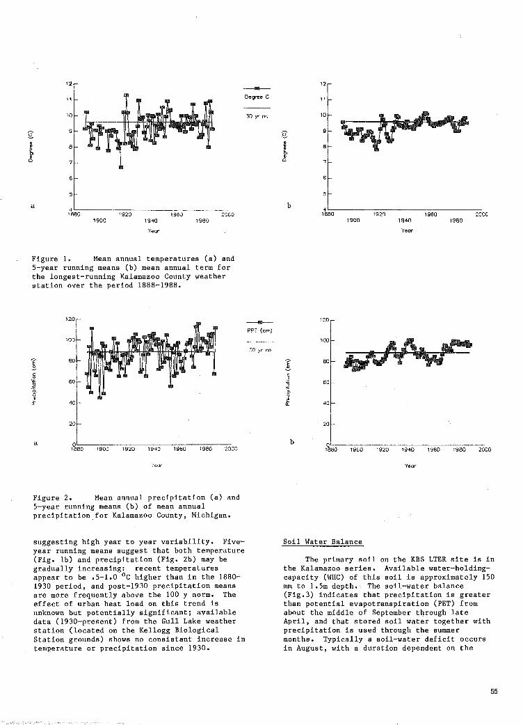
12

11 --­De9f1'e C

6

5

a 4~-----------------------------------1 eao 1920 196D :ceo

1900 1940 1980

Year

Figure 1. Mean annual temperatures (a) and 5-year running means (b) mean annual term for the longest-running Kalamazoo County weather station over the period 1888-1988.

120

a OL------------------------------------1880 1900 1920 19+0 1960 1980 2000

'taor

Figure 2. Mean annual precipitation (a) and 5-year running means (b) of mean annual precipitation for Kalamazoo County, Michigan.

suggesting high year to year variability. Five­year running means suggest that both temperature (Fig. 1b) and precipitation (Fig. 2b) may be gradually increasing: recent temperatures appear to be .5-1.0 °C higher than in the 1880-1930 period, and post-1930 precipitation means are more frequently above the 100 y norm. The effect of urban heat load on this trend is unknown but potentially significant; available data (1930-present) from the Gull Lake weather station (located on the Kellogg Biological Station grounds) shows no consistant increase in temperature or precipitation since 1930.

30 yr no

--­PPT (em)

12

11

10

9

8

7

6

b 1~~80~---------19~2-0 __________ 19_6_0 ___________ 2CCC

1900 1940 1960

Year

120r-

100

b 0~--~~--~----~----~--~----~ 1880 19GO 1920 1940 1960 1980 2000

Year

Soil Water Balance

The primary soil on the KBS LTER site is in the Kalamazoo series. Available water-holding­capacity (WHC) of this soil is approximately 150 mm to 1.5m depth.· The soil-water balance (Fig.3) indicates that precipitation is greater than potential evapotranspiration (PET) from about the middle of September through late April, and that stored soil water together with precipitation is used through the summer months. Typically a soil-water deficit occurs in August, with a duration dependent on the

55

timing of summer rainfall. For example in 1988 KBS received below normal precipitation from May through mid-July and then above normal for the remainder of the year. A soil water deficit occurred early and strongly affected crop yields, though soil-water recharge occurred the remainder of the year. Despite the growing­season drought, soils were at or near field­capacity at the beginning of the 1989 crop year.

oL-J~M~~~~~~~~~~~J~ut--~s~.~P--,~~v~--F""'b ltpr Jurt Au9 Oct De~

!-'kmth

-­Preclp -­PET

Figure 3. Monthly precipitation means and annual soil water balance for a Kalamazoo Soil, 150mm water-holding-capacity. Precipitation and PET based on 30-year (1951-1980) means.

Yield vs. precipitation.

We used Michigan Agriculture Statistics for Field Crops (Borum et al., 1950, 1960; Fedewa et al., 1983, 1986; Hines et al., 1970, 1976, 1980) for the years 1945 through 1985 for Kalamazoo County corn yields together with Kalamazoo weather data to test the hypothesis that annual amounts of precipitation are not as important as precipitation that occurs during the crop growing season, when PET is greater than precipitation (Fig. 3).

Corn yields have increased remarkably in Kalamazoo County since 1945 (Fig. 4). This increase is due mainly to increased fertilizer use, improved crop varieties, and the use of herbicides and pesticides. In order to relate yields to precipitation patterns, we attempted to remove such changes in management as a factor by expressing Kalamazoo yields as a ratio of Kalamazoo yields to yields from Lenawee County. Lenawee County, located in SE Michigan near Lake Erie, is the most productive (greatest yield per area) county for corn in Michigan because the soils generally have a higher water­holding capacity which better buffers against short-term drought. Our hypothesis predicts that changes in the Kalamazoo:Lenawee production ratio are due strictly to climatic factors. Management factors are presumed to be equivalent for the two counties. Monthly weather data for Lenawee were accumulated from the Adrian Station, located in the geographic center of the

56

140 -­Leoowee 120 --­V.atomozo 100

8Q

60

40

zo

0 1940 t;;o 1~50

r~ar

Figure 4. Corn yields 1945-1985 in Kalamazoo and Lenawee counties.

county. To remove differences due to total annual precipitation we have also expressed precipitation as a ratio of Kalamazoo vs. Lenawee counties.

We found very weak correlations between rainfall and corn yields for both annual (Fig. 5) and key-month (Fig. 6a-d) periods. Nevertheless, correlation was stronger (r=0.36, n=41, p<.025) for the July-August period (July­August precipitation ratios vs. annual yield ratios) than for either annual precipitation (r=.22, n=41, p).5) or precipitation in any other 2-month period (r<.06). This suggests that annual yields are indeed most sensitive to precipitation deficits in the July-August period, as predicted above based on our knowledge of the soil water balance (Fig. 3). Earlier in the growing season precipitation is not as important a predictor because stored soil-water is generally available and the plant's water demand is not as great.

1.2

II

Ill IIIII ... Ill II II Ill

0.8 II ..... .... Ill Ill 1111

Ill Ill Ill ........ .. 1111

Ill "' o.~ 1111

Ill Ill

0.4

0.2

0 0.7 o.s o.~ 1.1 1.2 1.3 1.4

Precipitation Rollo

Figure 5. Ratios of corn yield (Kalamazoo: Lenawee counties) vs. annual precipitation (Kalamazoo:Lenawee) for the period 1945-1985.

1.5

1.2

1111

o.e 1111 Ill

Q.~ 1111

1111 1111

0.4

0.2

a 0.4 o.e 0.8 1.2 1.4 I.e 1.6

Apr-Moy Precipitation Rotio

1.2

11!1

1111111111111111.: 1111

o.s 111111!1 c 1011 1111

1111 Ill Ill

Ill ·;· .. 1111 .: lllil 1111 o.e 11!1 1111 Ill

1111 1111

0.4

0.2

b

Hoy-June Precipitation Ratio

Figure 6. Ratios of corn yield (Kalamazoo: Lenawee counties) vs. precipitation for the periods of a) April-May, b) May-June, c) June­July, and d) July-August, 1945-1985.

That our correlations are not stronger could be due to a number of factors. First, precipitation data are from a single county station while yield estimates are from the entire county. Summer precipitation is mainly in the form of afternoon showers and thunderstorms (Strommen 1971) with relatively small impact areas. A single weather station may thus only roughly represent county-wide means. A second source of error is county-wide differences in water holding capacities among soils under corn cultivation. Small differences in WHC will significantly affect a crop's ability to weather short-term, midseason drought, and thus have a significant effect on the relationship of midseason precipitation to county-wide yields. Finally, bimonthly (e.g. June-July) means may not sufficiently resolve precipitation patterns that affect corn growth. Corn is most susceptible to drought stress during tasseling, silking and early ear growth.

c

0 'g

"' il >'

d 2.2

1.2

1!111

•••• 1111. Ill 1111 -~~~~~· ......

11111111 Ill 1111111 1111' II • • ,..

1!11 ~ IIIII

0.6 1111

1111 o.e 101

0.4

0.2

0o~----~o~.5------~----~~~.5~----~----~2~.5~--~3

June-.,luly Precipitation Ratio

1.2

1111

.1111 .... 1111 1111

Ill

0.8 1111 1111 ·.:-1111 1111 ..,.. •• II IIIII

1111 IIIII Q,Q 1!1!1

1111 • 1111

Iii IIIII

0.4

0.2

0 0.6 1.2 1.<; 2.4 2.8 0.+

0.6 1.• 1.6 00 :?:.6 3

July-August Precipltotlon Ratio

CONCLUSIONS

1. Long-term temperature trends (1888-1988) for Kalamazoo County, Michigan show a 0.5-1.0 °C increase in mean annual temperatures since 1930. Some portion of this increase is likely due simply to urban heat load at the weather station site. Nonurban records of shorter duration (Gull Lake, 1930-1988) do not show consistantly increasing temperature for the post-1930 period.

2. Annual precipitation patterns show little change over the 1888-1988 period other than a greater frequency of above-normal precipitation years post-1930.

3. County-wide corn yields and single-station precipitation patterns were weakly correlated. The strongest correlation between precipitation and yield occurred for the June-July precipitation period. The soil water deficit is also highest for this period.

57

Acknowledgment: The authors thank John Gorentz for help with weather data compilations and J, T. Ritchie and 0. B. Hesterman for comments on an earlier draft of this manuscript. This work is made possible with funding from NSF grant BSR87-02332 and the Michigan Agricultural Experiment Station.

REFERENCES

Borum, C.J.; Norman, R.V.; Garrett, J.R. 1950. Michigan Crop Reports 1945-1949. Lansing, MI: Michigan Department of Agriculture. 450 PP•

Borum, C.J.; Norman, R.V.; Garrett, J,R, 1960. Michigan agricultural statistics 1950-1959. Lansing, MI: Michigan Department of Agriculture. 431 pp.

Fedewa, D.J.; Pscodna, S.J. 1983. Michigan agricultural statistics 1980-1982. Lansing, MI: Michigan Department of Agriculture. 240 PP•

58

Fedewa, D.J.; Pscodna, S,J, 1986. Michigan agricultural statistics 1983-1985. Lansing, MI: Michigan Department of Agriculture. 256 PP•

Hines, C.A.; Pscodna, S,J, 1980. Michigan agricultural statistics 1976-1979. Lansing, MI: Michigan Department of Agriculture. 246 PP•

Hines, C.A.; Swanson, G.A. 1970. Michigan agricultural statistics 1960-1969. Lansing, MI: Michigan Department of Agriculture. 399 PP•

Hines, C.A.; Swanson, G,A, 1976. Michigan agricultural statistics 1970-1975. Lansing, MI: Michigan Department of Agriculture. 453 PP•

Strommen, N.D. 1971, Climate of Michigan by Stations. East Lansing, MI: Michigan Department of Agriculture. 257 PP•

GLIMATE VARIABILITY AT NIWOT RIDGE IN THE TWENTIETH CENTURY l

David Greenland 2

Abstract.--The climate of Niwot Ridge di~plays abnormally low temperatures in the early 1980's and an overall downward trend in temperature. Some cyclicity appears in the data series of annual values of both temperature and precipitation. Silver Lake annual precipitation data show only a slight downward trend when the extremely high value for the year of 1921 is excluded. Implications of these changes for the alpine tundra ecosystem are briefly discussed.

Keywords: Climate Change, Climate Analysis, LTER, Ecosystem Response.

INTRODUCTION

The climate of Niwot Ridge, Colorado is espec­ially important because of the large amount of re­search in physical geography and ecology which is performed there. It has been the site of research in the International Biological Programme, the Man and the Biosphere Program, and, more recently, the Long-Term Ecological Research Program (LTER). It is over 16 years since Barry (1972, 1973) pro­vided a much quoted analysis of the climatic ob­servations at the site. Since that time meteoro­logical observations have continued to be made and it is fitting that a new analysis of the record be undertaken, not only because of the increasing frequency of LTER-related and other studies at the site but also because of the current general interest in climatic variability and global change.

This paper focuses on monthly mean and annual values of temperature and precipitation for the Cl and Dl stations on Niwot Ridge and on other nearby stations. The establishment of the Niwot Ridge stations is described by Greenland (1987). Data associated with the Niwot Ridge stations are presented for 1952-1987 and additional precipita­tion data from Silver Lake, 1 km. southwest of Cl, are analyzed from 1915. The Ridge, along with the nearby Green Lakes valley to the south, is the locus of research operations in the LTER

1/ Presented at the LTER Workshop on Climate Variability, Niwot Ridge Green Lakes Valley LTER Site, CO, August 21-23, 1988.

2/ Professor of Geography, Department of Geog­raphy, Campus Box 260, University of Colorado, Boulder, CO 80309.

program. The site and its synoptic climate is described briefly. Most attention in the climate analysis is given to the years 1951-80, the time selected by the LTER Intersite Climate Committee for cross site comparison. Considerable effort was given to estimating early and missing values in the Niwot Ridge data using values from the nearby Allenspark observation site, The resulting data series are analyzed to give a climatic de­scription of the site including information on the long-term average water balance and temporal variation. Station data are:

Station Latitude Longitude Elevation Degrees N. Degrees W. Meters

Como~

Cl 40 02' 105 32' 3048 Niwot Ridge, Dl 40 03' lOS 37' 3749 Boulder 40 02' 105 16' 1638 Allenspark 40 12' 105 32' 2591 Silver Lake 40 02' 105 35' 3109

Readers who are interested in climatic variables and values other than monthly mean and annual temperature and precipitation should refer to other sources listed in the Front Range alpine and subalpine bibliography compiled by Halfpenny et al. (1986). A more comprehensive version of this paper has been presented elsewhere (Greenland, 1989).

THE SITE AND ITS SYNOPTIC CLIMATOLOGY

The Niwot Ridge site is in an alpine tundra ecosystem. The Ridge stretches eastwards from the Continental Divide and the area of most studies is found between the Cl station at 3048 m

59

and the Dl station at 3750 m with the treeline being found at approximately between 3350 and 3500 m. On the ridge and in the Green Lakes valley to the south, there are many distinct topoclimates associated with such factors as saddles and knolls, moraines and other glacial and periglacial features, semipermanent snow banks, and permanent ice and lakes.

The synoptic scale climate of the area is controlled by the mid-latitude, continental lo­cation and by the elevational and topographical situation. The high elevation causes low air temperatures at all times of the year. Air temperatures are effectively further depressed by the high velocities of the wind which gives rise to low wind chill values. The mid-conti­nental location leads to a large temperature range between summer and winter but this large range is more marked at the lower elevations. Precipitation-carrying storms are brought over the site in the winter and spring by the upper westerly flow. In these seasons, snow is brought from the west at higher elevations. Snow is also brought from the east, at the lower elevations, by cyclonic easterly, upslope flow developing to the east of the Continental Divide.

Table 1

SUMMARY STATISTICS Dl

TEMPERATURE Deg. c.

Jan Feb Mar Apri I May Man Mean -13.15 -12.77 -II. 23 -7.01 -0.86

An Mean -3.71 St Dev 6.06

Mean M>< T -10.09 -9.61 -7.60 -3.32 2.68 Mean Mi T -16.21 -15.94 -14.86 -10.70 -4.40

Mean Temp Harmest Month 8.23 St Dev 0.88 ~1ean Temp Coldest Month -13.15 St Dev I. 35

Annual Range of ~1onthly Mean Temps 21.38

Num months with mean temp >0 4

Num months with mean temp >15 0

Highest monthly mean in record per 10.48 Lo"•est monthly mean in record per -17.58

PREC I P !TAT ION mm

Jan Feb Mar April May Man mean 102.5 80.1 127.8 100.1 87.5

Mean annual total 930.0

Het.test year in period 1427 Driest year in period 541

Monthly totals during wettest year in period Jan Feb Mar April ~1ay 209 121 235 220 45

Monthly totals during driest year in period Jan Feb Mar April May

22 20 54 52 71

Total precip in months with temp >0 221

60

These storms are responsible for the spring maximum of precipitation. In the summer, rain­fall is produced from localized convectional storms. Fall is the driest season.

METHODS OF DATA PROCESSING AND ANALYSIS

Missing and Biased Data

There are two principal problems in creating monthly and annual summaries for the Cl and Dl stations. First, there are occasional data gaps when data were simply not collected. Second, until November 1964 there was no wind shield around the precipitation gauge at the Dl site. This gave rise to significant under-catch in pre­cipitation, particularly in the winter.

Estimates of the missing values caused by the above problems were given by standard climato­logical techniques of using regression analysis or by ratios with observed values from a nearby station (Brooks and Carruthers, 1953). The most suitable station for use in this analysis is that of Allenspark located 28 km almost due north of the Cl station. It is the nearest station that has a long enough climate record and is in the

Jui"\E' July Aug Sept Oct Nov Dec 4.60 8.23 7.06 3.39 -2. 13 -8.94 -11.77

8.74 12.43 11.00 7.35 I. 34 -5.39 -8.46 0.46 4.03 3. II -0.57 -5.59 -12.50 -15.07

June July Aug Sept Oct Nov Dec 59.5 50.5 62.1 49.1 40.3 80.3 90.1

Year 1974 June July Aug Sept Oct Nov Dec

100 96 12 49 104 79 157

Year 1954 June July Aug Sept Oct Nov Dec

16 61 48 64 35 55 43

same climatic regime as the Niwot stations with its high latitude, east of the Continental Divide location. The Allenspark data and their treat­ment are described by Greenland (1987). During the analysis of the Niwot data it was determined that any slight discrepancies in values quoted by Marr (1961) and Barry (1972, 1973) are due to variations in the ways in which missing values for individual days are treated. Estimated values of monthly precipitation for the Dl station for the years 1951-1964 are used in the data pre­sented in Table 1. A new study comparing precipi­tation values from unshielded and shielded rain gauges for a limited time during the 1951-1964 period suggests that the synthetic values are quite reasonable (Clark and Halfpenny, pers. comm. 1989).

Water Budget Computations

Water budget computations were made based on the Thornthwaite technique (Thornthwaite and Mather, 1957) and using an adaptation of a program by Willmott and Rowe (1985), which was based on and is more fully described by Willmott (1977). The technique is not fully applicable for this area owing to its neglect of such factors as windspeed, humidity conditions, and a direct net radiation input. It is useful, however, to give a relative comparison between the Dl and Cl sites and also between other LTER sites. The latest version of the program, which incorporates snow­pack water equivalent and snowmelt, gives a vivid impression of the importance of snowmelt in the Niwot Ridge area.

Time Series Analysis

The data were preprocessed as follows. Month­ly data values in Lotus worksheet files were con­verted to ASCII files. The ASCII files were up­loaded onto the University of Colorado VAX 8550 cluster. SAS data sets were created for time series modeling and ASCII data sets of annual data values were created for spectral analysis.

The prepared data sets were plotted as time series and examined. Trends were investigated by fitting quadratic regressions. Exploratory modeling of the annual data values took the form of identifying the best fitting Autoregressive (AR) and Autoregressive Integrated Moving Average (ARIMA) models using an iterative process. Autocorrelation functions (ACF) and Partial Autocorrelation functions (PACF) were used to guide initial estimates of parameters.

In order to perform the spectral analysis first the time series were smoothed and detrended. Next the ACF of the detrended series was checked for Markov persistence using the first three values of the ACF. Confidence intervals for which Markov persistence did not exist were dismissed. The spectral peaks in frequency cycles per year were translated into periods. The Nyquist fre­quency prevents the detection of periods of less than 2 years. Host of the present analyses show a sharp rise at the two year period perhaps due to the 1-year autoregressive component evident in most of the time series.

Annual precipitation values for Silver Lake were prepared for time series analysis in the following manner. Unpublished microfiche data for 1910 to 1985 and published NWS data for 1910 to 1950 were combined to form what was believed to be the most accurate data set. Data from Allenspark for 1945 to 1985 and from Cl from 1951 to 1987 were assembled for regression analyses to help simulate missine data values. There were too many missing values between 1910 and 1913 so the final modified data set which was analyzed consisted of the 74 data points between 1914 and 1987. The analysis was then performed in the same manner as for the Cl and Dl data as previous­ly described.

DISCUSSION OF RESULTS

Climate Description

Summary statistics for Dl and Cl for the years 1951-80 are presented in Tables 1 and 2. These clearly show the severity of the climate at Dl on the tundra. Important characteristics include (1) the existence of only four months with temper­ature above freezing, (2) the large annual range of monthly mean temperatures, (3) the relatively large variability in intra-annual precipitation, (4) the winter and spring precipitation maximum, and (5) the small amount of precipitation arriving in a "growing season" defined as one having monthly mean temperatures above 0°C. Cl station, below the treeline, shows (1) an extended grow­ing season, (2) an almost equally large range of monthly mean temperatures, and (3) a more clearly defined spring precipitation maximum. The rela­tively small amount of precipitation arriving in the "growing season" is misleading in this case because of the importance of snowpack. Whereas much of the snowfall arriving at Dl is blown away and never becomes available to the plants, at Cl winter snowfall largely resides as a snowpack on the ground between the trees and becomes avail­able to the vegetation during the spring melt.

Water Budget

Water budget analysis suggests that about half of the precipitation at Cl is lost by evapo­transpiration while the rest is lost by surface runoff of percolation into the soil. At Dl, in contrast, only about a third of the precipitation is lost by evapotranspiration, while the rest of the greater amount of precipitation is lost as runoff or, more realistically, percolation into the soil. The importance of the spring thaw is seen at both sites.

Temporal Variation

Some of the most interesting findings of the present study are associated with the time series analysis of the data. Although analyses were performed for both the Cl and the Dl stations only diagrams for the latter are described here in de­tail. Pertinent points relating to the Cl ana­lyses are summarized but in general the same over­all characteristics appearing in the Dl data are also seen in the Cl data.

61

Table 2

SUNMARY STATISTICS C1

TE~IPERATURE Deg. c.

Jan Feb Mar t1on Mean -7.49 -6.70 -5.51

An ~lean 1. 30 St Dev 0.60

Mean Mx T -3.09 -1.49 -0.21 ~lean Mi T -11.90 -11.91 -10.80

Mean Temp Warmest Month 11.91 Nean Temp Coldest Month -7.49

Annual RangE' of Monthly ME> an Temps

Num months with mean temp >0

Num months with mean temp >15

Highest monthly mE>an in rE>cord per LowE>st monthly mean in rE>cord pE>r

PRECIPITATION mm

Jan Feb Man 1nean 50.3 45.2

ME>an annual total 6Sl2.0

Wettest year in pE>riod Driest yE>ar in period

~lonthly totals dut·ing Jan

65

wettest Feb

46

Mar 67,2

949 395

yE>ar· Mar

52

in

~lonthly totals during driest yE>ar ih Jan Feb Mar

13 10 33

Total precip in months with temp >0

April Nay -1.24 3.75

4.06 9.39 -6.55 -1.89

St Dev 0.96 St Dev 1. 58

19.40

6

0

13.75 -11.34

Apri 1 May 85.4 85.3

period April ~lay

199 185

period Apri 1 t·lay

20 47

352

Annual temperatures at Dl (Figure 1) are note­worthy for their year to year variability from 1951 to 1980 with a standard deviation of 0.64 °C around a mean of -3.71 °C and for the relative­ly low temperatures in the early 1980s. A quad­ratic regression curve fit to the data series indicates a general decreasing trend with the steepness of the descent being greater in the second part of the series. There is a linear trend over the data period of -0.00l3°C per year for the first part of the period from 195.1 to 1980. Although Barry (1973) did not find a signi­ficant trend for the Dl data, he did find a down­ward trend of -0.07°C per year for the Cl data. The linear trend for the whole data set including the low temperature values of the early 1980s yields a downward rat(;' of - 0.05 °C per year. Five year running means of this data series emphasize low temperatures of the early 1980s. There also is a suggestion of a decreasing trend from 1953 to the mid-1960s and a slight increase from here to the beginning of the 1980s.

It is important to consider whether the period of low temperatures in the early 1980s, which might be called the Niwot Minimum, is real or not. Since the Minimum appears at both Dl and Cl, it

62

June July Aug Sept Oct Nov Dec -6.02 8.63 11.91 10.95 7.40 3.16 -3.26

15.47 19.18 17.91 14.13 9.28 1. 78 -1.41 -10.62 1. 78 4.64 3.99 0.67 -2.96 -8.30

YE>ar

Year

JunE> July Aug Sept Oct Nov Dec

54.8 65.3 59 .. 3 50.2 37.0 46. '3 45.0

1957 June July Aug Sept Oct t·lov D.ec

84 89 76 43 62 29 19

1954 June July Aug Sept Oct Nov Dec

3 78 42 71 28 32 18

is unlikely that the feature is due to some charac­teristic of one of the sites. The observing personnel did change in 1980, but calibration. pro­cedures and instrument did not and the new ob­server is not aware of any instrumental or pro­cedural reason for the appearance of the Minimum. The likelihood of observational or instrumental error would be decreased if similar changes were seen in nearby, independent systems. Unfortunate­ly there are many missing data for the Allenspark station between 1979 and 1983 and in 1984 its location was changed from a ridge site to a valley site 46 m lower and 2.4 km to the north. Thus, temperatures at Allenspark for 1984 and 1985 that are significantly lower than the 1951-1980 mean, although being consistent with the Niwot Minimum, may· reflect the site change. Annual mean temperatures at Nederland (8.5 km south southwest of Cl) for 1982-85 are about 1.5°C lower than in 1980 and 1981, but are higher than in the previous decade. Annual mean temperatures at Boulder during the Niwot Minimum are lower than in the previous three decades. Other pieces of information that support the reality of the Minimum exist. First, there were positive mass balances of ice in many of the glaciers near Niwot Ridge in the years of the early 1980s

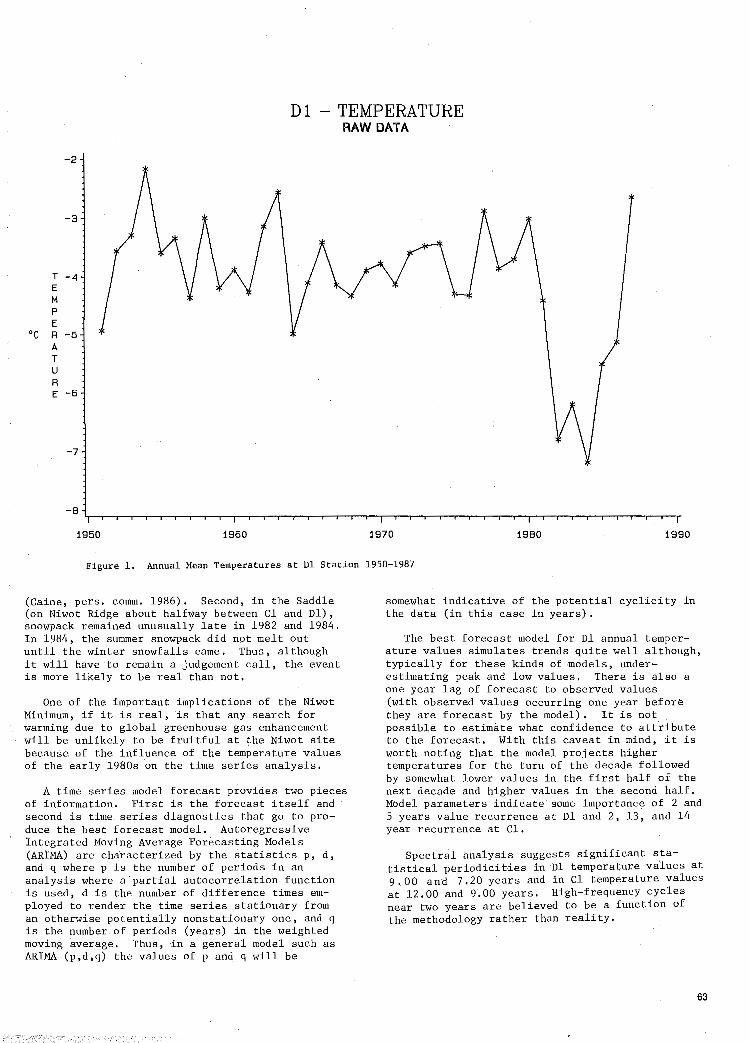
D1 -TEMPERATURE RAW DATA

-2

-3

T -4 E M p E

oc R -5 A T u R E -6

-7

-8

1950 1960 1970 1980 1990

Figure 1. Annual Mean Temperatures at Dl Station 1950-1987

(Caine, pers. cornrn. 1986). Second, in the Saddle (on Niwot Ridge about halh7ay between Cl and Dl), snowpack remained unusually late in 1982 and 1984. In 1984, the summer snowpack did not melt out until the winter snowfalls carne. Thus, although it 1vill have to remain a judgement call, the event is more likely to be real than not.

One of the important implications of the Niwot Minimum, if it is real, is that any search for warming due to global greenhouse gas enhancement will be unlikely to be fruitful at the Niwot site because of the influence of the temperature values of the early 1980s on the time series analysis.

A time series model forecast provides two pieces of information. First is the forecast itself and second is time series diagnostics that go to pro­duce the best forecast model. Autoregressive lntegrated Moving Av:erage Forecasting Models (ARIMA) are characterized by the statistics p, d, and q where p is the number of periods in an analysis where a'partial autocorrelation function is used, d is the number of difference times em­ployed to render the time series stationary from an otherwise potentially nonstationary one, and q is the number of periods (years) in the weighted moving average. Thus, in a general model such as ARIMA (p,d,q) the values of p and q will be

somewhat indicative of the potential cyclicity in the data (in this case in years).

The best forecast model for Dl annual temper­ature values simulates trends quite well although, typically for these kinds of models, under­estimating peak and low values. There is also a one year lag of forecast to observed values (with observed values occurring one year before they are forecast by the model). It is not possible to estimate what confidence to attribute to the forecast. With this caveat in mind, it is worth noting that the model projects higher temperatures for the turn of the decade followed by somewhat lower values in the first half of the next decade and higher values in the second half. Model parameters indicate some importance of 2 and 5 years value recurrence at Dl and 2, 13, and 14 year recurrence at Cl.

Spectral analysis suggests significant sta­tistical periodicities in Dl temperature values at 9. 00 and 7. 20 years and in Cl temperature values at 12.00 and 9.00 years. High-frequency cycles near two years are believed to be a function of th&methodology rather than reality.

63

Annual precipitation values at Dl demonstrate high inter-annual variability. The 1983 value, which occurred during the first five years of LTER studies at the site, was the highest in the 37-year record. The summer (JJA) precipitation for 1984 was also the highest of all comparable values in this record. There is a small upward trend in the record when fitted with a quadratic regression curve. Although when scaled to emphasize trend the 5-year running mean does suggest an upward trend with dry years in the mid 1950s, around 1970 and in the late 1970s. The best ARIMA fore­case model does well in simulating high and low values, but shows a lag of one year between fore­cast and observed values, It does not project any large changes into the next century. Spectral analysis of the Dl annual precipitation record manifests significant peaks at 7.19 and 9.00 years.

The Silver Lake annual values of precipitation again show high year to year variability but are important in that they are able to place some of the Niwot Ridge values into a better temporal per­spective. For example, 1983 is shown here to have only the second highest precipitation value in the years back to 1951. More importantly an idea of the largest possible precipitation for the area is shown by high values in 1921 about which more will be said later. A linear regression of these data shows only a small downward trend but the 5-year running means suggest that this may be due to the 1921 value and that the upward trend previously seen in the Dl data might be continuous from the dry period of the mid-1920s. The best ARIMA model forecast does less well in simulating amplitude and suggests only a continuation of the small up­ward trend through to the end of the century. No highly significant low frequency periodicities are shown by the spectral analysis although in­teresting high spectral values significant at the 80% confidence level are found at 14.71 and 12.35 years. The last of these parallel the 12.05 year periodicity found in Dl precipitation at the same confidence level.

The year 1921 is identified as an extraordinary high precipitation year at Silver Lake and pre­sumably in the Niwot Ridge area. Monthly values (Table 3) indicate winter, spring, and the month of June had high values. Potential snow equiva­lents at 1/10 and 1/15 ratios for the winter months are also provided. If all precipitation fell as snow in April and none melted or blew away and the higher conversion ratio is used the 15.8 m (51.84 ft) falling on the previous snow­pack would certainly have buried much of the vegetation.

Implications for the Ecosystem

It is difficult to say exactly how the climate changes described above would affect the eco­system, if at all.

Some preliminary points are in order. First, it is not necessarily annual values of temperature and precipitation that have the most marked effect

64

on the alpine ecosystem. In many cases, the snow­pack development in the spring, and the growing season conditions are the most important. To the extent that annual values are indicative of these, then the annual values might have greater utility. With respect to this it has been shown that the summer temperature values play a large role in affecting the annual temperatures for Cl and Dl (Greenland, 1987). Second, it is hard to deter­mine the effect of runs or patterns of years with similar values as opposed to individual years of high or low values. Greenland et al. (1985a) showed that the 1983 and 1984 years show­ed only small differences in above - ground net primary productivity despite quite large differ­ences in summer soil moisture. The fact that the majority of the alpine tundra biomass is below ground will create a buffer to inter-a~nual and shorter climate variations. Greenland (1984) further demonstrated that values of the surface summer energy budget in the alpine tundra could vary more in one year between the moist and dry surfaces at the Saddle than between a dry year and a wet year over the same surface. It is quite likely that it is the early growing season snow­melt and rainfall which is important for plant growth and survival, Snowpack distribution and ablation rates are critical in the phenology of the vegetation communities at the Saddle.

The above points go some way to explaining the fact that there is at present no evidence for dramatic changes, such as species disappearance, in the vegetation of Niwot Ridge over the last 40 years or so. Neither the long term trends in the annual temperature and precipitation data, nor the cyclicities, nor the periods of several or individual years with high or low values of these variables appear to be related to any ob­vious changes in the vegetation. This testifies to the resilience of the flora and how it is fair­ly well adjusted to the normal year to year variability of the present day climate. This is not to say, however, that there have been no changes in the vegetation asso_ciated with some of the climate changes described here. The vegeta­tional changes, if they exist, may be quite subtle and concerned with variations in the re­lative proportions of different species existing at any one time at a locality on the Ridge. Some scientists who have been working on the Ridge in the last decade believe they have noticed such changes (Halfpenny, pers. comm., 1988). Current­ly, a very detailed Geographic Information System is being constructed which should have the ability to detect such changes if they occur.

There are certainly many questions to answer. Are the correct climatic variables being measured? The answer to this lies in what ecological questions require resolution. Annual values of

3 Greenland, D.E. 1984. Energy budgets over a

moisture gradient in alpine tundra. Paper delivered at Association of American Geographers Meeting. Washington, D.C.

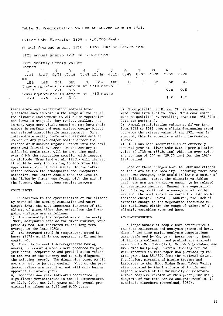
Table 3. Precipitation Values at Silver Lake in 1921.

Silver Lake Elevation 3109 m (10,200 feet)

Annual Average precip 1910 - 1930 847 mm (33.35 ins)

1921 annual precip 1735 mm (68.30 ins)

1921 Monthly Precip Values Inches

J F M A M J 7.31 6.63 8.31 15.16 3.09 12.36

mm 1E16 168 211 385 78 314

J 4. 1::'j

105 Snow equivalent in

1.9 1.7 2.1 Snow equivalent in

meters .at 1110 ratio

2.8 ,, c:· L. • .... J

-:o· ~-.

•..:•uL

3.9 mf?t<.~rs

5.B at 1/l~i r-atiD

temperature and precipitation address broad questions such as what is the range of values of the climatic environment to which the vegetation and fauna is adapted. Day to day, smaller, but in many ways more vital, questions may have their answer in surface and near surface energy budget and related microclimatic measurements. On an intermediate scale, there are questions such as do wet or dry years and/or months effect the release of Dissolved Organic Carbon into the soil water and fluvial systems? On the century to millenia! scale there will be some time scale over which the vegetation zonation with respect to altitude (Greenland et al, 1985b) will change. It would be very interesting tv determine the approximate size of this scale. In the inter­action between the atmospheric and biospheric scientist, the latter should take the lead in the dialog by first specifying, with the aid of the former, what questions require answers.

CONCLUSIONS

In addition to the specification of the climate by means of the summary statistics and water budget data, the most important features 0f the climate of Niwot Ridge that arise from the fore­going analysis are as follows: 1) The unusually low temperatures of the early 1980s, designated here as the Niwot Minimum, were probably real but recovered to the long term average in the late 1980s. 2) The downward trend in temperature noted by Barry (1973) at Cl is now apparent at Dl and has continued. 3) Potentially useful Autoregressive Moving Average forecasting models were produced to pro­ject annual temperature and precipitation values to the end of the century and to help diagnose the existing record. The diagnosive function did not turn out to be very useful. Whether the pro­jected values are useful or not will only become apparent in future years. 4) Spectral analysis indicated statistically significant periodicities in annual temperatures at 12.0, 9.00, and 7.20 years and in annual pre­cipitation values at 7.19 and 9.00 years.

A ::_\.42

B7

s 0.07

,., L

0 2.05

-=~> ,_,..::.

N

' C" (:J,.J

0.6

1.0

D 3.20

8J.

0. EJ

L2

5) Precipitation at Dl and Cl has shown an up­ward trend from 1951 to 1987. This conclusion must be qualified by recalling that the 1951-64 Dl data are estimated. 6) Annual precipitation values at Silver Lake from 1913 to 1987 show a slight decreasing trend but. when the extreme value of the 1921 year is removed, this is actually a slight increasing trend. 7) 1921 has been identified as an extremely unusual year at Silver Lake with a precipitation value of 1735 mm (68.30 ins) which is over twice the average of 755 mm (29.75 ins) for the 1914-1987 period.

None of these changes have had obvious effects on the flora of the locality. Assuming there have been some changes, this would indicate a number of possibilities. First, the climatic variables used here are not sensitive enough to be related to vegetation changes. Second, the vegetation is not being monitored in enough detail or by means of the most sensitive variables that would indicate change. Overall, however, the lack of dramatic change in the vegetation testifies to its resilience within the range of values of the climatic variables reported here.

ACKNOWLEDGEMENTS

A large number of people have contributed to the data collection and analysis presented here. Much of the time series analysis computations were performed by Ms. Terri Bettancourt. Much of the data collection and preliminary analysis was done by Mr. John Clark, Mr. Mark Losleben, and Dr. James Halfpenny. Partial funding for the work reported in this paper was provided by the LTER grant BSR 8514329 from the National Science Fourtdation, Division of Biotic Systems and Resources to the Niwot Ridge Green Lakes Valley site operated by the Institute of Arctic and Alpine Research at the University of Colorado. A more complete version of this paper, including diagrams of the time series analysis results, is available elsewhere (Greenland, 1989).

65

LITERATURE CITED

Barry, R.G. 1972. Climatic environment of the east slope of the Colorado Front Range. Occasional Paper 3. Boulder: Institute of Arcttc and Alpine Research, University of Colorado. 206 pp.

Barry, R.G. 1973. A climatological transect on on the east slope of the Front Range, Colorado. Arctic and Alpine Research~ 5(2):89-110.

Brooks, C.E.P.; Carruthers, N. 1953. Handbook of statistical methods in meteorology. London: Her Majesty's Stationary Office.

Greenland, D.E. 1987. The climate of Niwot Ridge. University of Colorado long-term ecological research data report, 87/7. 57 pp.

Greenland, D.E.; Caine, N.; Pollak, 0. 1985a. The summer water budget of alpine tundra in Colorado and its ecological importance. Physical Geography. 5(3):221-239.

Greenland, D.E.; Burbank, J.; Key, J.; [and others]· 1985b. The bioclimates of the Color­ado Front Range. Mountain Research and Devel­opment, 5(3): 251-262.

Greenland, D.E. 1989. The climate of Niwot Ridge, Colorado front range USA. Arctic and Alpine Research, in press.

Halfpenny, J.C.; Ingraham, K.P.; Mattysse, J.; [and others] 1986. Bibliography of alpine areas of the Front Range, Colorado. Univer­sity of Colorado, Institute of Arctic and Alpine Research. Occasional Paper 43: 114 pp.

Marr, J.W. 1961. Ecosystems of the eastern slope of the front range in Colorado. Studies, in Biology. No. 8. Boulder: University of Colorado. 124 pp.

Thornthwaite, C.W.; Mather, J .R. 1957. Instruc­tions and tables for computing potential eva­potranspiration and the water balance. Publications in climatology. Sea Brook, N.J.: Laboratory of Climatoloty. Vol. 10(3). 126 pp.

Willmott, C.J. 1977. WATBUG: A FORTRAN IV Algorithm for calculating the climatic water budget. Publications in Climatology. Sea Brook Farms, N.J.: Laboratory of Climatology. Vol. 30(2): 55 pp.

Willmott, C.J.; Rowe, C.M. 1985. Computer aided instruction in the climatic water budget. Abstracts of annual meeting of Association of American Geographers, Session 55; 1985 April; Detroit.

66

CLIMATE VARIABILITY IN THE SHORTGRASS STEPPE1

Timothy G.F. Kittel2

Abstract.- Climatic variability at the Central Plains Experimen­tal Range LTER in northeastern Colorado was evaluated from annual, decadal, and century perspectives. Spectral analysis separated climatic variation into 2-7 y and >10 y scales. The record is dominated by cold-wet and warm-dry years. El Nino years had on average higher annual precipitation than years with cold water anomalies in the equatorial Pacific. At the decadal level, variations in temperature and precipitation parallel those for the Central U.S. and broader regions. The temperature record has a significant 75-y trend of +2°C. Such variations in climate have impacts on the structure and function of the short­grass ecosystem.

Keywords: Colorado, Central Plains Experimental Range, Long­Term Ecological Research, scale, El Nino/Southern Oscillation, ecological response to climate variability, Vegetation Index.

I INTRODUCTION

Ecosystems are responsive to climate variability at a range of temporal scales. Temperature, precipitation, and other climate variables (e.g., humidity, cloud cover) vary year-to-year and decade-to-decade in ways that are likely to influence ecosystem composition and function.

I present an analysis of variability in temperature and precipitation at a range of temporal scales (annual, decadal, century) for the shortgrass steppe region in the vicinity of the Central Plains Experimental Range (CPER) in northeastern Colorado. Questions I address are whether there are characteristic scales of variation in temperature and precipitation, whether these scales are the same for the two variables (e.g., are dry periods characteristically warm or cold?); and whether there are long-term trends in the record. These are important questions because they seek to characterize periodic and unidirectional changes in the external forcing on ecosystems. Such understanding provides a basis for the study of between-year and long-term changes in ecosystem dynamics.

1Presented at the Long-Term Ecological Research (LTER) Workshop on Climate Variability and Ecosys­tem Response, Nederland, CO, August 21-23, 1988.

2Research Associate, Natural Resource Ecology Laboratory and Cooperative Institute for Research in the Atmosphere, Colorado State University, Ft. Collins, co 80523

In the context of interannual variability, I examine possible long-distance links (teleconnections) between the climate of the steppe region and a source of global climate variability, El Nino and the Southern Oscilla­tion (ENSO); ENSO consists of quasi-periodic (general­ly 3-7 y) oscillations in ocean-climate dynamics of the tropical Pacific Basin (Philander and Rasmusson 1985). As part of these oscillations, El Nino is a strong warming of surface ocean waters in the central and eastern equatorial Pacific. ENSO teleconnections play a role in the climate dynamics of the extratropics (Yarnal 1985); impacts on ecological dynamics have been suggested for sites in the United States (e.g., Strub et al. 1985, Gosz 1988).

Finally, I discuss observational and modeling studies on the impacts of climate variability on the steppe ecosystem.

METHODS

Site Description

The CPER (40°49' N, 104°46'W, 1650 m above sea level) is operated by the USDA Agricultural Research Service (ARS) and is an NSF Long-Term Ecological Research (LTER) site. The vegetation at the CPER is shortgrass steppe dominated by perennial grasses Bouteloua gracilis and Buchloi! dactyloides, with important succulent (Opuntia oolyacantha) and sub­shrub components (Moir and Trlica 1976). Much of the surrounding region is grazed native grassland and cropland.

67

The climate of the shortgrass steppe is characteris­tic of mid-latitude, continental semi-arid regions; it is classified as BSk (cold, steppe climate) in the Klippen­Geiger system (Muller 1982). The mean climate and water budget is described by Parton and Greenland (1987) based on the period 1951-1980. Monthly mean temperature peaks in July (21.6°C) and is lowest in January (-3.1°), Mean annual precipitation is 309 rom, with maximum monthly precipitation usually occurring in May and June. Winter precipitation is associated with mid-latitude cyclonic storms and summer rainfall with cumulus convective storms that often initiate along the Rocky Mountain Front Range to the west and intensify as they progress eastward. Mean month­ly precipitation does not exceed monthly actual evapo­transpiration year-round (Parton and Greenland 1987).

Climate Data

The CPER

I used temperature and precipitation data from two climate stations on the CPER, one operated by ARS and the other by LTER. The ARS station is at an elevation of 1645 m above sea level (asl); the LTER station is at 1643 m asl. The stations are -5 km apart. ARS data are for the period 1940-1973 (tem­perature data start in 1948, precipitation data are continuous from April 1947). LTER data used here are from July 1970 to May 1988. The records of these stations were concatenated, with the LTER data replac­ing ARS data in October 1970; this was considered appropriate because the stations are in close proximity and have strongly correlated traces for the period of overlap (monthly temperature r 2=0.99, monthly precipi­tation r2=0.74; Parton and Greenland 1987). Monthly mean temperatures were calculated as an average of monthly mean minimum and maximum temperatures.

Grover

To analyze long-term behavior in regional climate, I used data from a National Weather Service cooperative station approximately 16 km west of Grover. This station, officially named Grover10W, has a 58-y record (1911-1969). It is roughly 25 km east-northeast from and 100 m asl below the LTER station. The station was moved several times during its history. For most of its operation (1929-1962), it was at 40°52' N, 104°25'W, and 1547 m asl. A significant move occurred in 1962 and is reflected in the temperature record (Fig. 1a).

Neither temperature nor precipitation monthly records for Grover are without gaps. To create a continuous record, gaps of usually one month (occasion­ally up to three months) were filled with corresponding long-term monthly means for 13 years in the tempera­ture record and two years in the precipitation record. An advantage of this substitution is to retain years with nearly complete monthly data, although it reduces interannual variability and trends and blurs spectral signals.

Analysis

For analysis of interannual variability, blocking the data into 12-month periods is often arbitrary (e.g.,

68

calendar years). In this study, I used water year (October to following September) to associate fall and winter precipitation with the following growing season. Consequently, this annual period includes the approxi­mate integrating period over which an important climate-ecosystem interaction, soil water recharge, operates. Water years are identified by the year the period ends: e.g., water year 1982 is October 1981-September 1982. Five-year running means of these data were constructed to investigate decadal and longer-term behavior.

Spectral analysis was used to identify characteristic scales of variation in the yearly data. This analysis characterizes periodic behavior in a time series and identifies frequencies at which there is high covariance between two time series (i.e., high coherence). This analysis was accomplished using time series analysis software (BMDP/P1 T; Thrall and Engelman 1985). Statistical software (SPSSIPC+; SPSS and NoruAis 1986) was used to test for linear trends in the data. The time series analyses were run on detrended data and used a wide band width. A wider band width strengthens the statistical stability of the analyses, although it reduces the spectral resolution.

Spatial Variability

Spatial variability may give rise to problems in interpreting these station data in a regional and ecological context. Point measurements of precipitation may not represent the 6280 ha CPER because winter­time winds redistribute snow across the landscape and summer convective precipitation events are often patchy in their occurrence. For example, growing season precipitation varied across the site by as much as 96 rom in 1988, an amount greater than the standard deviation of annual precipitation (Hazlett 1990). These effects can be ecologically important, influencing local soil water recharge (Burke et al. 1989) and contribut­ing to spatial variability in biomass accumulation (Lauenroth and Milchunas, unpublished data) and community structure.

Southern Oscillation Index

To evaluate possible teleconnections with El Nino episodes and the Southern Oscillation (ENSO), I compared CPER data to a Southern Oscillation index (SST80) based on central and eastern equatorial Pacific sea surface temperature anomalies developed by Wright (1984). The sign of this index is opposite to that of SO indices based on sea level pressure: SST80 is positive during El Nino episodes and negative during cold water ("anti-El Nino" or "La Nina") episodes. Wright's (1984) record for this index is for 1950-1983. Water year averages of SST80 were included in correlation arid spectral analyses.

RESULTS AND DISCUSSION

Water Year Time Series

Station Comparison

During the period of record overlap (1948-1969), there is a high cmTelation between CPER and Grover water year precipitation totals (r=+0.67, p<0.001;

Table 1, Fig. 1b). However, precipitation during the overlap period differs between the two sites (p<0.05, t­test, Table 1). Greater precipitation at Grover likely reflects a regional gradient in precipitation (Cowie and McKee 1986): northeast of CPER, Grover is less in the rain shadow of the Front Range.

There is also a difference in temperature means between sites during the overlap period (p<0.01, t-test; Table 1, Fig. 1a). This is primarily due to a diver­gence in temperature series after 1962 that reflects the change in Grover's location. For the period of overlap up to this station change, annual temperature means are not significantly different (p>0.5, t-test) and are highly correlated (r=+0.71, p<0.005; Table 1, Fig. 1a). The difference in temperature means calculated for each station's record (L'1TcPER-GR=+0.5°C, Table 1) may be due to climatic trends and is discussed later.

Power Spectra

Both high and low frequency variability is evident in the temperature and precipitation time series (Fig. 1). The temperature power spectrum for Grover (Fig. 2a) shows peaks in variance for oscillations at periods around 2¥.!-4 y and greater than -20 y. The spectrum for precipitation (Fig. 2b) is broader with less well defined peaks at -2 and 2¥.!-5 y, as well as at >10 y. This reveals a natural break in temporal dynamics between annual and decadal scales. Dye (1983) found comparable breaks in the precipitation spectra for stations throughout Colorado.

a -GROVER

14 ---- CPER

6

1911 1931

b -G~OVER

---- CPER

500

1951 YEAR

Tann

I, ,, ,, ,'\ f l 1 I I 1

,, J v \...// ___ _ly ___________ .

t\1 11\/\ f1 1/111 1. 1\ I

' \ /\ ,'\ ,l v '" y

1971 1991

101~\;-11---'--"'---~"19""3"1 ~~-~1,:95071~-~~"19..;-71.----~~~"19;;191 YEAR

Figure 1.- (a) Water year mean temperature, oc, and (b) precipitation, mm/y, for CPER (- - - -) and Grover10W (--). Horizontal lines are record means for each station.

Table 1.- Summary of CPER and Grover10W (GR) climate data for record and for period of overlap (1949-69 for T ••• , 1948-69 for ppt. •• ). Numerical subscripts indicate other periods (e.g., 12-62 = 1912-62). Years are water years. Trends over station record (and also over 1912-62 for Grover) and corresponding significance levels (two-tailed t-test) are given. Station comparison over the full overlap period and over the overlap until 1962 are shown based on correlation analysis (r) and paired two-tailed t-test for difference of means (t). Level of significance for trends, r, and t are: * = p<0.05 and ** = p<O.Ol. T ••• = water year mean temperature (°C); ppt ••• = water year precipitation (mm!y). Elevations (m asl) are approximate because of station location changes. sd = standard deviation. n/a = not applicable.

Elevation

Record:

T ••• dates mean sd trend trend12.62

ppt ••• dates mean sd trend trend13.62

Overlap:

T ••• mean sd mean4u.s2

pptnnn mean sd mean4s.62

CPER

1643

1949-87 9.0 1.3

+2.4** n/a

1948-87 317

88 +52 n/a

8.2 0.9 8.6

315 102 300

GR

1547

1912-69 8.5 1.0

+2.1 ** +1.7**

1913-69 347

95 -15

+1

9.0 0.7 8.6

356 93

373

d(CPER-GR) r

+96

+0.5 +0.3

-30 -7

-0.8 +0.2

0.0

+0.14

+0.71**

t

3.2**

0.5

-41 +0.67** 2.4* +9

-73 +0. 77** 4.5**

Coherence (h2) is analogous to the squared correla­tion between two variables within a given spectral band. A high coherence identifies a frequency at which variables strongly co-vary. There are peaks in the coherence between Grover temperature and precipita­tion series (Fig. 3a) in the short-period region (2¥-l-7¥-l y, h2>0.3) and in the long-period region (>20 y, h2>0.4). Analysis for CPER reveals a similar pattern with strong coherence at 3-3¥-l y (h2=0.5) and at 20 y (h2=0.4). The phase of these spectral correlations (Fig. 3b) is such that temperature leads precipitation by -Vl cycle across all frequencies; i.e., annual mean tempera­ture and annual precipitation fluctuations are out of phase. Significance of the coherence and phase is discussed below in the context of annual and decadal variability.

69

a T

0.2

0

::;: ::;) (1: t;·0.2

~ Cll Cl -0.4 g

-o.6

-o.8

60 20 10 6 5 4 2.5 PERIOD (YR)

b ppt

4.2

::;: 4.0 ::;) (1:

t; w 3.8 0.. Ul

Cl 0 --' 3.6

3.4

60 20 10 6 5 4 2.5 2 PERIOD (YR) 1

Figure 2.- Power spectra for Grover water year (a) temperature and (b) precipitation. Band width = 0.1167 y·1

•

Interannual Variability

Comparison of temperature and precipitation time series (Figs. 1a and b) suggests that peaks in annual temperature often coincide with low precipitation years and vice versa (Table 2). Indeed, annual temperature and precipitation are negatively correlated (r=-0.41, p<0.02). This is in accordance with the phase shift of 1h cycle found in the coherence results (Fig. 3b). The alternation of warm dry years with cold wet years implies control by oscillations in position and intensity of the mid-latitude polar jet and subtropical high pressure centers: e.g., cold wet years occur when the jet is farther south than average, warm dry years

Table 2.- Contingency table of cold vs. warm and wet vs. dry yeats for Grover. Years are blocked based on water year mean temperature and precipitation greater vs. less than corresponding local (5-y running) mean to adjust for decadal trends. (X2=5.175, df=1, p<0.025).

T<T6y

ppt<ppt 6y 11

ppt>ppt 6y 17

70

17

8

a 1.0 T 81 ppt

O.B

w ~ 0.6 w (1: w J: 0 0.4 l)

0.2

6 5 4 PERIOD (YR)

b 180'

ppt- T

90'

w Ul <( 0 J: 0..

-90'

-180'

60 20 10 6 5 4 2.5 2 PERIOD (YR)

Figure 3.- Cross spectral (a) coherence, h2, and (b)

phase for Grover water year temperature and precipita­tion.

when farther north. While the predominance of cold­wet and warm-dry years is significant (p<0.025, Table 2), the alternative combinations of temperature and precipitation anomalies are present in the record (Table 2). Because controls over summer versus winter precipitation-generating mechanisms are relatively independent, control over variation in annual statistics is probably complex. Analysis of seasonal statistics may more readily reveal continental-scale controls over regional climate variability.

Complexity in climate variability at the regional level is illustrated by decoupled variation in climate at CPER and Niwot Ridge, -100 km to the southwest (Greenland 1990, this volume). The difference in behavior is likely because the climate of Niwot Ridge (3000-3750 m asl) is more strongly dominated by westerly flow across the continental divide.

El Niii.o Teleconnection?

Spectral analysis revealed peaks in temperature and precipitation spectra and their coherence at periods of 21h-71h y (Figs. 1 and 2a). This range of periods is similar to that recognized for the Southern Oscillation (2-10 y, Rasmusson and Carpenter 1982) and so hints at a possible link to El Niii.o episodes.

There is a positive correlation between the annual Southern Oscillation SST Index (SST80) and CPER

annual precipitation (r=+0.30, p=O.ll), such that precipitation tends to be higher during El Nino years. There is no significant correlation with annual tem­perature. However, at periods of 3-4 y there is spectral coherence between SSTso and CPER tempera­ture (h2=0.5), as well as between SSTso and CPER precipitation (h2=0.3). The ratio of annual precipitation during years with a strongly positive SSTso (El Nino years) to those with highly negative SSTso is 1.13 (Table 3), although only 5 of 9 El Nino years between 1951 and 1983 had greater than average precipitation. Sheaffer (personal communication) found that the corresponding El Nino to "anti-El Nino" ratio for summer precipitation in northeastern Colorado is on the order of 1.33. By comparison, the Sevilleta LTER region (central New Mexico) is more strongly influenced by tropical Pacific climate dynamics: the El Nino to "anti-El Nino" ratio is 1.59 for annual precipitation and 2.45 for winter-spring precipitation (MoUes and Dahm, in Gosz 1988).

Observational and modeling studies of ENSO indicate that strongest teleconnections should be in winter, associated with the polar jet. For northern central North America inclusive of the shortgrass region, these teleconnections include increases in winter temperature and surface pressure (van Loon and Madden 1981, van Loon and Rogers 1981, Rasmusson and Wallace 1983). This is in accordance with greater annual temperatures observed at the CPER during El Nino years (Table 3). Increases in winter surface pressure suggest that El Nino years should have drier winters (Yarnal 1985). Sheaffer (personal communica­tion) found this to be the case for NE Colorado: winter precipitation El Nino to "anti-El Nino" ratio is <0.75. However, depressed winter precipitation has only a small impact on total annual precipitation, during El Nino years since most precipitation at the CPER comes during summer.

Table 3.- Comparison of CPER water year mean temperature (T.""' °C) and precipitation (ppt.""' mm/y) for years with high vs. low eastern and central equatorial Pacific sea surface temperatures (SST). High SST years correspond to El Nino episodes and were selected as those years with annual SSTso exceeding the mean + 1h its standard deviation (s.d.). SSTso falls below the mean- 1h s.d. in low years and within the region prescribed by the mean ± 1h s.d. in 'Near Mean' years. Analysis is for water years 1951-1983. n = number of years. n/a = not applicable.

SST pptann

High 343 Near Mean 313 Low 303

High:Low 1.13 L!.(High-Low) +40

Mean5!-sa 318

Tann

9.3 8.7 8.7

n/a +0.7

8.9

n

9 14 10

33

While a clear ENSO teleconnection is weak for the CPER, difficulty in finding such a signal in the climate of the steppe is expected. Four factors contribute to the problem. (1) Teleconnections are partly a function of mid-latitude circulation patterns prior to ENSO episodes (Y arnal 1985). Consequently, the character' of extratropical teleconnections shifts over decades with shifts in hemispheric circulation (Carleton 1987, Sheaffer and Reiter 1985). (2) Southern Oscillation indices can fail to catch the timing or intensity of an ENSO episode because of variations in the location of equatorial SST and/or atmospheric anomalies (Y arnal 1985). This is because such indices are empirical and do not adequately reflect ocean-climate dynamics.· (3) Large-scale studies show that ENSO-linked variation in climate for northern and central North America is less consistent in nature than for other parts of the continent (van Loon and Madden 1981, Blackmon et al. 1979). (4) ENSO teleconnections account for only a small portion of extratropical climate variability (Wallace and Blackmon 1983).

Decadal Variability and Long-Term Trends

Annual Temperature

A warming trend (8T=+3°) through the late 1930's and subsequent cooling trend until 1950 (L!.T=-1.5°) are observed in 5-y running means of the Grover data (Fig. 4a). A -3.5° warming in the 1970's is shown in the CPER data. These patterns agree with the general behavior of Northern Hemispheric temperatures reported by Hansen and Lebedeff (1987) and with that for eastern Colorado (Doesken et al. 1989) and the Midwest United States (Diaz and Karl 1988). The amplitude of the 1920's to 1950 oscillation in the Grover record is magnified from that for the Northern Hemisphere (+0.4° warming; ~.15° cooling) and the Midwest (+1.5°, -1.0°), reflecting the steppe's continen­tality. While a regional trend in the 1950's and 1960's is not clear due to the Grover station location change in 1962 (Fig. 4a), the trend in CPER data clearly follows that for other stations in eastern Colorado (Doesken et al. 1989) and the central United States (Diaz and Karl 1988): a slight warming in the early 1950's followed by cooling into the late 1960's.

The long-term linear trend in the Grover tempera­ture record (until the 1962 station move, 1912-1962 water years) is +1.7°C; that for the 1949-1987 CPER record is +2.4° (Table 1). The accumulative 75-y trend is 2.1 o, not adjusted for station differences. The slopes of the CPER. and Grover trends are significantly different from zero (p<0.01, t-test), in spite of high year-to-year variability. This contrasts with Diaz and Karl's (1988) conclusion that there has been no century-scale change in temperatures across the United States. Doesken et al. (1989) showed that trends in mean annual temperature in eastern Colorado are dominated by increases in winter temperatures.

The result of a significant trend must be viewed cautiously before concluding that a regional. change in climate has taken place. These results are only for two stations, each of which has a poor history with respect to location changes and data gaps. Other possible station changes such as in instruments, environs (e.g., buildings, vegetation), and time of day of

71

a 14 -GROVER

---CPER

6

1911 1931

b -GROVER --- CPER

/,. __ \ /" c.

--~~----l----------· c::7 ~ . .._ I

1951 YEAR

'',,-,~--')

1971

ppl5y

f·- ... ! \ ,' \

' ! ---~------7'"------

\ ,-' ' ' "' ' \~l

1991

IOj§!rrll---'--~~"19""3"1 ~~-~"'19T-51~-~~,.19>'>7>1 ~~-........ 199~1 YEAR

Figure 4.- As Figure 1, but for five-year running means.

observation could potentially play a role in changing station means.

Annual Precipitation

The five-year running means of annual precipitation show significant decadal variation (Fig. 4b), such as the 1930's drought. Again there is considerable disagree­ment between Grover and CPER during the period of overlap. However, the CPER record agrees with the independent analysis of United States precipitation by Bradley et al. (1987) and shows the wide-spread 1950's drought.

Linear trends in Grover and CPER precipitation series are not significant (p>0.25, t-test; Table 1). This is in accordance with Bradley et al. (1987) who found no trend in annual precipitation for the United States since the 1850's.

Covariance

There is a general pattern of temperatures increas­ing from the 1910's until the mid-1930's, followed by a decrease into the late sixties and an increase since then (Fig. 4a). Superimposed on this apparent 50-y wave in temperature, recognized by Wigley and Raper (1987) for Northern Hemispheric temperatures, is a more rapid oscillation (15-20 y period) in precipitation (Fig. 4b). As a consequence, changes in the 5-y running means of temperature and precipitation follow the same pattern during some decades and opposite in

72

others. However, there is spectral coherence of temperature and precipitation at periods of 20 y or greater with a 1h cycle phase shift (h2>0,4, Fig. 3). This suggests that, as at the annual scale, multi­decadal variation in temperature and precipitation tends to be negatively correlated. This is supported by the pattern of droughts in the 1930's and 1950's being warmer than average and the wet 1910's and 1960's being colder.

Some of the observed decadal or longer-term changes may be linked to continental-scale shifts in circulation patterns that are in response to hemispheric or global changes in atmosphere-ocean climate dynam­ics (Balling and Lawson 1982, Sheaffer and Reiter 1985). Such shifts involve changes in the seasonal variation in intensity and position of the mid-latitude jet and the subtropical highs. Such changes signifi­cantly affect important abiotic controls over population, community, and ecosystem processes, such as the magnitude and timing of frosts and early growing season precipitation.

ECOLOGICAL SIGNIFICANCE

Identification of ecological responses to observed climatic variations is generally limited by a paucity of long-term biological data. However, some conclusions can be drawn based on available observations and modeling studies.

Interannual Variability

Net primary production of the shortgrass grasslands is strongly influenced by interannual fluctuations in precipitation (Lauenroth 1979), Lauenroth et al. (in preparation) compared field estimates of annual aboveground biomass production and annual precipita­tion at the CPER from 1941 to 1987. These data show that an extremely dry year reduces production for that and several years following. This suggests that dry episodes result in a reduction in the number of aboveground active meristems, constraining above­ground production in subsequent years, and cause belowground dieback, reducing the plants' ability to acquire water also in ensuing years (Webb et al. 1978).

Interannual variation in biomass development in the steppe is also influenced by the timing and amount of precipitation within the growing season. Seasonal dynamics of aboveground photosynthetically-active biomass can be inferred from satellite-based observa­tions, such as the normalized-difference vegetation index (NDVI) (Goward et al. 1985, Justice et al. 1985). NDVI is derived from data from the Advanced Very High Resolution Radiometer (AVHRR) on NOAA series polar-orbiting satellites. Comparison of seasonal variation in NDVI and precipitation (Fig. 5) suggests that in 1983 and 1984 high March-May precipitation resulted in a strong June peak in green biomass. In contrast, in 1982, high mid- through late growing season precipitation corresponds to only a slight increase in late season biomass. These results suggest that early growing season precipitation is more crucial for the development of aboveground biomass than late season rainfall.

The frequency and timing of climatic events can also be critical for population and community level processes. For example, Lauenroth et al. (1987) showed that interannual variability in the occurrence of a combination of spring temperatures and precipitation events results in marked year-to-year variation in seedling establishment of blue grama (Bouteloua gracilis), with long-term consequences for community structure (Coffin and Lauenroth 1990).

These results demonstrate that to assess the impact of interannual climate variability on shortgrass ecosystems, between-year differences in climate need to be evaluated at seasonal and event levels as well as the annual level. While the resolution of an analysis must be tailored to response times of ecological processes of interest, the sensitivity of a particular process may not be limited to climate variability at a single scale because of interactions with biological processes operating at finer and coarser scales (Allen and Starr 1982, O'Neill et al. 1988). Such interactions generate time lags in the response of ecosystems to abiotic forcing.

Decadal and Long-Term Trends

Decadal and long-term climatic trends are expected to impact ecosystem dynamics through climatic. controls

a 0.5

0.4

0.3

0.2

0.1

0

0.5

0,4

> 0,3

0 :z 0.2

0.1

0

0.5

0.4

0.3

0.2

0.1

0

VEGETATION INDEX

1982

--------~-1983

1984

FMAMJJASOND

MONTH

on rates of net primary production (NPP) and decom­position. Using a grassland ecosystem model (CENTURY, Parton et al. 1987), Kittel et al. (1990) tested the sensitivity of a Colorado shortgrass ecosystem to directional climatic change. In the model experiment, annual temperature was increased by 4.9°C (roughly twice the 1949-1987 trend observed at CPER) and annual precipitation increased by 46 mm, based on a C02-doubling climate change scenario (Hansen et al. 1984). Mter 50 years, simulated aboveground NPP increased by 40 percent. This response was driven by increased precipitation and increased availability of nitrogen that was released as soil organic matter decreased. The net loss of soil organic matter was due primarily to increased decomposition driven by the increase in temperature. These results illustrate the potential importance of climatic shifts to the shortgrass steppe and the role of system dynamics in determining the response to such change (Schimel et al. 1990).

Long-term climatic trends are also likely to influ­ence grassland community structure by changing species establishment rates and shifting interspecific competitive interactions. Such structural changes would influence the impact of climate change on ecosystem processes.

b WEEKLY PRECIPITATION

1982 15

10

5

,.., 'C

' E .§ w 1983

~ 15

:z 0 10

~ c a.. i5

lrl 0::: a.. :z ~ :::!: 1984

15

10

5

D

Figure 5.- (a) Envelope of weekly-composited normalized difference vegetation index, NDVI, for a 50x50 km region centered on the CPER in 1982, 1983, and 1984. (b) Weekly averages of CPER daily precipitation rate, mm/dy, for the same years. Dashed lines in (a) show a minimal threshold of 0.07 below which NDVI values are assumed to indicate no green biomass.

73

CONCLUSIONS

Climatic variability of the shortgrass steppe exhibits important characteristics that form a basis for evaluat­ing its impacts on the grassland's ecological dynamics. These are:

(1) There is a natural break in the temporal dynamics of the steppe climate between annual and decadal+ scales. At both scales, variation in tempera­ture and precipitation is generally 1h cycle out of phase.

(2) At the annual scale, the phase relationship results in a predominance of cold-wet and warm-dry years, perhaps controlled by shifts in the position of the mid-latitude jet and subtropical highs.

(3) There is a positive correlation between annual precipitation and ENSO episodes. However, there are limits to the empirical detection of an ENSO signal because teleconnections are dynamic and may be inconsistent in this region.

(4) 20-50 y scale variations in the steppe tempera­tures match those in hemispheric and United States records and are of greater magnitude because of the region's continentality. There is shorter period variability in precipitation at the decadal scale, such that in some decades temperature and precipitation change in the same direction and in other decades in an opposite fashion.

(5) There is a statistically significant 75-y trend in temperature (-+2°C), but known and unknown problems in station histories warrant caution in attaching importance to this trend. No significant trend was found for annual precipitation.

Ecological studies indicate that interannual and longer-term climate variability have significant conse­quences for ecosystem, community, and population dynamics in the shortgrass steppe. Climate-induced interannual variability in ecological processes can be complex, exhibiting significant year-to-year lags and sensitivity to climatic variation at within-season and event levels.

Acknowledgements: This work benefitted from discus­sions with N. Doesken, J. Sheaffer, W. Lauenroth, W. Parton, D. Greenland, and participants in the 1988 LTER Climate Committee Workshop. Thanks go to Diana Deutch for her invaluable assistance in data analysis. R. Scott and T. Kirchner also provided support for the analysis. Nolan Doesken and the Colorado Climate Center provided the GroverlOW data. John Sheaffer (Dept. of Atmospheric Science, Colorado State University) kindly made his analyses on western United States-El Nifio teleconnections available. D. Jepsen, M. Nelson, and J. Sorbie-Dunn assisted with manuscript and figure preparation. Thanks to W. Lauenroth, I. Burke, N. Doesken, D. Greenland, and D. Schimel for their comments on the paper. This work was supported by NSF through CPER LTER (BSR-8612105) and LTER Coordinating Committee (BSR-8805390) grants and by a Cooperative Institute for Research in the Atmosphere (Colorado State University) fellowship.

74

LITERATURE CITED

Allen, T.F.H.; Starr, T.B. 1982. Hierarchy: perspectives for ecological complexity. Chicago: University of Chicago Press.

Balling, R.C., Jr.; Lawson; M.P. 1982. Twentieth century changes in winter climatic regions. Climatic Change 4:57-69.

Blackmon, M.L.; Madden, R.A.; Wallace, J.M.; Gutsier, D.S. 1979. Geographical variations in the vertical structure of geopotential height fluctuations. Journal of Atmospheric Science 36:2450-2466.

Bradley, R.S.; Diaz, H.F.; Eischeid, J.K.; Jones, P.D.; Kelley, P.M.; Goodess, C.M. 1987. Precipitation fluctuations over northern hemisphere land areas in the mid-19th century. Science 237:171-175.

Burke, I.C.; Reiners, W.A.; Olson, R.K. 1989. Topogra­phic control of vegetation in a mountain big sagebrush steppe. Vegetatio 84:77-86.

Carleton, A.M. 1987. Summer circulation climate of the American Southwest, 1945-1984. Annals of the Association of American Geographers 77:619-634.

Coffin, D.P.; Lauenroth, W.K. 1990. A gap dynamiCs simulation model of succession in a semiarid grassland. Ecological Modelling 49:229-266.

Cowie, J.R.; McKee, T.B. 1986. Colorado precipitation event and variability analysis. Atmospheric Science Paper No. 400. Ft. Collins, CO: Dept. of Atmos­pheric Science, Colorado State University. 102 pp.

Diaz, H.F.; Karl, T.R. 1988. Temperature trends and urban effects in the contiguous United States. In: Pielke, R.A.; Kittel, T.G.F., eds. Monitoring climate for the effects of increasing greenhouse gas concen­trations. Ft. Collins, CO: Cooperative Inst. for Research in the Atmosphere, Colorado State Univ. pp. 73-90.

Doesken, N.J.; Kleist, J.; McKee, T.B. 1989. Colorado temperatures with degree day and growing season data. Climatology Report 89-2. Ft. Collins, CO: Dept. of Atmospheric Science, Colorado State University. 45 pp. + tables.

Dye, A.F. 1983. An analysis of periodicity in Colorado precipitation. Ft. Collins, CO: Colorado State University. 97 pp. Thesis.

Gosz, J.R. 1988. Long-term ecological research on climatic and ecological gradients: Sevilleta National Wildlife Refuge. NSF proposal. Albuquerque, NM: University of New Mexico. 54 pp.

Goward, S.N.; Tucker, C.J.; Dye, D.G. 1985. North American vegetation patterns observed with the NOAA-7 advanced very high resolution radiometer. Vegetatio 64:3-14.

Greenland, D. 1990. The climate of Niwot Ridge. In: Climate variability and ecosystem response. D. Greenland and L. Swift, eds. U.S. Forest Service.

Hansen, J.; Lacis, A; Rind, D.; Russell, G.; Stone, P.; Fung, 1.; Ruedy, R.; Lerner, J. 1984. Climate sensitivity: Analysis of feedback mechanisms. In: Hansen, J.E.; Takahashi, T., eds. Climate processes and climate sensitivity. American Geophysical Union, Washington, DC. pp. 130-163.

Hansen, J.; Lebedeff, S. 1987. Global trends of measured surface air temperature. Journal of Geophysical Research 92:13345-13372.

Hazlett, D. 1990. Leaf area development of four plant communities in the Colorado steppe. Journal of Applied Ecology, submitted.

Justice, C.O.; Townshend, J.R.G.; Holben, B.N.; Tucker, C.J. 1985. Analysis of the phenology of global vegetation using meteorological satellite data. International Journal of Remote Sensing 6:1271-1318.

Kittel, T.G.F.; Schimel, D.S.; Parton, W.J. 1990. Sensitivity of North American Central Grassland ecosystems to climatic change. Submitted.

Lauenroth, W.K 1979. Grassland primary production: North American grasslands in perspective. In: French, N.R., ed. Perspectives in grassland ecology. Ecological Studies, Vol. 32. Springer-Verlag. pp. 3-24.

Lauenroth, W.K; Sala, O.E.; Kirchner, T. 1987. Soil water dynamics and the establishment of seedlings of Bouteloua gracilis in the shortgrass steppe: a simulation analysis. In: Abstracts of the 40th annual meeting of the Society of Range Manage­ment, Boise, ID.

Moir, W.H.; Trlica, M.J. 1976. Plant communities and vegetation patterns as affected by various treat­ments in shortgrass prairies of northeastern Colorado. Southwestern Naturalist 21: 359-371.

MUller, M.J. 1982. Selected climatic data for a global set of standard stations for vegetation science. The Hague: W. Junk Publ. 306 pp.

O'Neill, R.V.; DeAngelis, D.L.; Waide, J.B.; Allen, T.F.H. 1986. A hierarchical concept of ecosystems. Princeton, NJ: Princeton University Press. 253 pp.

Parton, W.; Greenland, D. 1987. Central plains experimental range, Colorado. In: Greenland, D., ed. The climates of the long-term ecological research sites. Occasional Paper No. 44. Boulder, CO: Institute of Arctic and Alpine Research, Univ. of Colorado. pp. 23-27.

Parton, W. J.; Schimel, D.S.; Cole, C.V.; Ojima, D.S. 1987. Analysis of factors controlling soil organic matter levels in Great Plains grasslands. Soil Science Society of America Journal 51:1173-1179.

Philander, S.G.; Rasmusson, E.M. 1985. The southern oscillation and El Nino. Advances in Geophysics 28A: 197-215.

Rasmusson, E.M.; Carpenter, T.H. 1982. Variations in tropical sea surface temperature and surface wind fields associated with the Southern Oscillation/El Nino. Monthly Weather Review 110:354-384.

Rasmusson, E.M.; Wallace, J.M. 1983. Meteorological aspects of the El Nino/Southern Oscillation. Science 22:1195-1202.

Schimel, D.S.; Parton, W.J.; Kittel, T.G.F.; Ojima, D.S.; Cole, C.V. 1990. Grassland biogeochemistry: links to atmospheric processes. Climatic Change, in press.

Sheaffer, J.D.; Reiter, E.R. 1985. Influence of Pacific sea surface temperatures on seasonal precipitation over the western plateau of the United States. Archives for Meteorology, Geophysics, and Bioclima­tology, Series A 34:111-130.

SPSS Inc.; Nor~is, M.J. 1986. SPSSIPC+ for the IBM PCIXT/AT. Chicago: SPSS Inc. 630 pp.

Strub, P.T.; Powell, T.; Goldman, C.R. 1985. Climatic forcing: effects of El Nino on a small, temperate lake. Science 227:55-57.

Thrall, T.; Engelman, L. 1985. P1T. Univariate and bivariate spectral analysis. In: BMDP statistical software. 1985 edition. Berkeley, CA: University of California Press. pp. 604-638.

van Loon, H.; Madden, R.A 1981. The Southern Oscillation. Part 1: Global associations with pressure and temperature in the northern winter. Monthly Weather Review 109:1150-1162.

van Loon, H.; Rogers, J.C. 1981. The Southern Oscilla­tion. Part II: Association with changes in the middle troposphere in the northern winter. Monthly Weather Review 109:1163-1168.

Wallace, J.M.; Blackmon, M.L. 1983. Observations of low-frequency atmospheric variability. In: Hoskins, B.; Pearce, R., eds. Large-scale dynamical processes in the atmosphere. London: Academic Press. pp. 55-94.

Webb, W.; Szarek, S.; Lauenroth, W.; Kinerson, R.; Smith, M. 1978. Primary production and water use in native forest, grassland, and desert ecosystems. Ecology 59:1239-1247.

Wigley, T.M.L.; Raper, S.C.B. 1987. Thermal expansion of sea water associated with global warming. Nature 330:127-131.

Wright, P.B. 1984. Relationships between indices of the Southern Oscillation. Monthly Weather Review 112:1913-1919.

Yamal, B. 1985. Extratropical teleconnections with El Nino/Southern Oscillation (ENSO) events. Progress in Physical Geography 9:315-352.

75

INTRODUCTION

CLIMATE CHANGE AND ECOSYSTEM DYNAMICS AT THE VIRGINIA COAST RESERVE

18,000 B.P. AND DURING THE LAST CENTURY1

Bruce P. Hayden2

-----------------------Abstract. -- The forest cover of the Virginia Coast Reserve was studied using a Boreal FORET model parameterized using periglacial conditions derived independently of the pollen record of the site. Modern conditions of the landscape dynamics were studied using historical aerial photography and t he meteorological record of coastal storms.

Keywords: Barrier islands, FORET model, climate change, island morphology, shorezone dynamics.

---------------------------

The Virginia Coast Reserve (VCR) includes a string of barrier islands on the coastal plain of the trailing margin of the North American Plate. It extends 100 km along the seaward margin of the Delmarva Peninsula. It encompasses 13 barrier islands (14, 170 ha), broad intervening inlets and extensive back barrier islands and shallow bays (Figure 1 ). Distinct communities include sandy intertidal, open beach, grassland, shrub thicket, pine forest, mud flat, salt marsh and estuarine lagoon. Terrestrial vegetation is conspicuously shore parallel in general structure, with sharp transitions or ecotones betweeen communities.

Ecosystem dynamics of the VCR are closely tied to climate dynamics. Coastal storms are the dominant agents of landscape change in this coastal system. Storm waves and storm surges hydraulically work and rework the sediments of

11 Presented at the LTER Climate Workshop on Climate and Ecosystem Dynamics, Niwot Ridge, CO August 1988.

.

t.·\y '·.· ATEAOUE .

VIRGINIA IIARRIER ISLANDS

10 10

SCALI. IU.f

2} Professor, Department of Environmental Sciences, University of Virginia, Charlottesville, VA. 22901

Figure 1. -- The Virginia Barrier Islands on the Eastern Shore of Virginia.

76

DUNE GRASS GRASSES 8

SCATTERED SHRUBS SHRUB

/CLUSTERS

MARSH

OFFSHORE WINOS

DUNE GRASS

SHRUB THICKETS TREES

STORM SURGE ONSHORE WINDS SALT SPRAY

Figure 2. -- Cross-section of a barrier island showing the dominant morphological and vegetation zonation with the arrows indicating the extent of various marine processes a low dune case (top) and high dune case (bottom).

this sandy coast and are responsible for the overall shore parallel zonation of the coastal landforms and communities on the barrier islands. The general form of the island zonation is shown in Figure 2. Woody species are restricted in their proximity to the sea by the presence of aeolian sea salts. Wind pruning of the vegetation by easterly sea breezes and northeasterly storm winds results in a direction oriented canopy morphology. The presence of shore parallel coastal dunes and wind roll vorticies contribute to the zonation of communities on the islands (Clarman 1977). The transition between the beach zone and the sandy grassland immediately inland is forced landward (eroded) by storms but aggressive growth by grasses encroach seaward during the growing season. Over the past four decades this ecotone over the entire VCR has been moving landward at about 5 m/yr (S.D. = 8 m/yr).

OFFSHORE WINDS

Had the VCR existed 18,000 years ago, its seaward margin would have been 100 kilometers east of its current position and part of the boreal forest biome (Emery and others 1967, Bonan and Hayden 1989). Peat deposits found at this distance offshore contain freshwater sphagnum peat and a decidedly boreal forest pollen assemblage (Emery and others 1967). With the post glacial sea level rise, the barrier islands "migrated" westward by the process known as roll-over. Beach sands from the shoreface are driven across the island during storm surges and deposited on the back side of the island. Thus erosion on the seaward side and accretion on the landward side of the island has the net effect of "moving" the island landward.

At several places along the VCR tree stumps of forests once found on the back side of the barrier island now emerge from the beach face. In other locations lagoonside salt marsh peats outcrop on the beach. 18,000 years ago a boreal forest extended seaward 100 km. We have used a FORET model to simulate the structdure of this forest using climatic conditions at the

77

end of the last ice age and have . evaluated the output using fossil pollen assemblags from the area. Fossil pollen was not used to "tune" the FORET model as a totally independent test of the model was desired. By 5000 BP sea level rise had slowed and the islands were just a few kilometers seaward of their current position. Currently the rate of movement or trangression is about 5 m/yr. This rate is only exceeded on the sand starved barrier islands fronting the Mississippi Delta. If the charging of our atmosphere with C02 gives rise to a global warmiQ.g and an increased sea level rise, then the rate of transgression of the Virginia Barrie1 Islands will also increase.

The model ISLAND is designed to connect climate, geomorphology, hydrology and vegetation cover in a stochastic-dynamic structure. The test site for ISLAND model development, parameterization and calibaration is Hog Island. Hog Island is the .main research site for the Virginia Coast Reserve L TER. The southern end of this island is eroding rapidly and the northern end is accreting. At the northern end of the island, new landscapes are evolving while at the southern end old landscapes are being truncated. The history of shoreline erosion is shown in map form in Figure 3.

In 1920 there was a tqwn, Broadwater, Virginia, on the south end of Hog Island. There were about 100 buildings a coast guard station and a lighthouse. The former location of Broadwater is now hundreds of meters offshore. The rapid rate of landscape change on the Virginia Coast Reserve means that large changes can easily be monitored at the time scale of L TER research programs. The dominant driving forces for change on the Virginia Coast REserve are decidedly climatological.

The landscape dynamics of the VCR is driven by astronomical and wind tides, winds, aeolian sea salts, storm waves and surges, fair weather swell, overwashed sands and saline water and the catchemnt of fresh rain water. Nutrients for the higher elevation fresh water elements of the landscape are by means of atmospheric deposition.

78

..._1871

Figure 3. -- Shorelines of Hog Island from 1852 to 1980. The site of the 19th century town of Broadwater at the southern end of the island was seaward of the current shoreline.

THE VCR FORET MODEL: 18,000 B. P.

The record of fresh water peats with arboreal pollen 80 km offshore dating to 18,000 B.P. offers an opportunity to test the climate driving functions of FORET type forest models against pollent data. The version of the FORET model we used in our studies was that of Bonan (1988) which is adapted from Shugart ( 1986). the basic components of Bonan's model are schematically illustrated in Figure 4. Bonan's gap model was designed to simulate the modern northern boreal forest and has been tested at four North American locations under a variety of local site conditions. The model was found to correctly simulate existing forest composition and dynamics.

MORTALITY ,. .............. , ENVtRONIIIEIUAL 8 llfooa 0

COIIIITRAtMTI : .... I 1 tnoocto 1 • •

tg~::!::~ I ·•· • ..................

GROWTH r-------------, ENVtRONioiUH Al I avollol>to light 8 8 ooll oooooturo 8] CONIITRAtNT8 I aile quality I 8 8fOWIAfiJ d8QfG&-dOWI 8 i doptl> ol aa .. out lha• :

• POlENIIAL I I GROWTH 8 dlamolat, age, hoeahl 8

·----~---------·

Figure 4. -- Schematic of a stand element used in Bonan's FORET model of the boreal forest.

In order to apply the Bonan model to the Virginia coast 18,000 years ago, climate and site conditions for the VCR were estimated indepnedent of the pollen record which was reserved for model validation. Climate and site parameters needed to run the VCR FORET model are listed in Table 1. Periglacial climatic conditions at the southern margin of the Laurentide ice sheet 18,000 years ago were taken from Moran (1972) and adjusted to take into account the distance between the edge of the ice cap and the VCR.

Model Temperatures Mean monthly air temperatures from the modern record and those for 18,000 B.P. are shown in Figure 5. Monthly standard deviations of temperature for the modern period were used for the period 18,000 B.P. Summer time temperatures were about 100 C cooler than modern and winter temperatures were about like modern. This latter condition arises because of the adiabatic warming of air moving southward and down over the ice sheet and thus the preculding of extremely cold temperatures. One significant effect of this moderate glacial winter thermal climate is the absence of permafrost on the VCR.

fNVtRONt.IEIH AL COIIIITRAtNlll

POTENIIAL

REI'AODUC liON

30

,---------------.......... llgM 8011 M018hU8 ........... ., •••••na ctagraa-ctawo tlapth ot aeaaonal thaw 888d Iliad C8fUIUIOA8

108d AVAIIablhiV

............. ....... ,.lit 1.-------------..a

25 - MODERN

u --· 18,000 YR B.P.

0

20 UJ a:: ::J ........ -_ t- ~ <( 15 ,. ,. a:: ,. UJ I Q. I ~ I UJ I t- 10 I

I a:: I

< I I ,

5 I I ,

0 M A M

MONTH

-... ... ... ... \

\ \

\

' \ \

\ \

\ \

\

A s 0 N D

Figure 5. -- Monthly mean temperatures. for the modern and 18,000 B.P. conditions at the Virginia Coast Reserve.

Model Precipitation Precipitation estimates for the end of the last ice age were modern values except for the hurricane season. Wendland (1977) reported a very low frequency of Atlantic hurricnaces at the end of the last ice age. Modern summer/fall rainfall averages for the years with no

79

AGE MAX DDHMAX HTMAX G LITE SMOIST

Sprouting N DBHMIN DBHMAX

KTOL NUTR IPFR IMO IBW ALC GDDMIN GDDMAX SWTCH

TABLE I

Maximum age of species (years) Maximum diameter at breast height (em) Maximum height (m) Growth parameter Shade tolerance classification (1, tolerant; 2, intermediate; 3, intolerant) The maximum percentage of the growing season that the species can tolerate soil

moisture below the wilting point

The tendency for stump sprouting The minimum diameter at breast height for sprouting (em) The maximum diameter at breast height for sprouting (em) Fire tolerance (1, tolerant; 2, intermediate; 3, intolerant) Nutrient stress toleran«: class (1, tolerant; 2, intermediate; 3, intolerant) Ability to grow on permafrost (1, good; 2, poor) Ability to reproduce on moss-organic layer (I, tolerant; 2, intermediate; 3, intoleranl) Vulnerability to spruce budwonn outbreaks (1, high; 2,1ow) Light level at which reproduction is inhibited Minimum growing degree-days in the species' range Maximum growing degree-days in the species' range Reproduction switches [SWTCH(I) is true if the species has serotinous cones.

SWTCH(2) is true if the species has copious, light, wind dispersed seeds. SWTCH(3) is true if the species can reproduce by layering].

hurricanes were used. In September, the month of highest hurricane frequency, more than 40% of the modern rainfall on the VCR is the result of passing hurricanes and tropical storms. The percentage is less in adjacent months. Aggregated over the year a 250 mm shortfall relative to modern rainfall totals results from the adjustment made. Summertime rainfall standard deviations were reduced to reflect the reduction in rainfall variance associated with a hurricane free climate. Monthly precipitation for the modern versus that of 18,000 B.P. are shown in Figure 6 along with potential evapotranspiration (PET).

Potential Evaporation (PET) Using calculated mean monthly radiation and temperature, elevation, and saturation vapor pressures. Mean monthly potential evapo­transpiration (PET) was estimated by the method of Jensen and Haise (1963). Figure 6 contrasts the monthly mean water balance for the modern period and for 18,000 B.P. the PET deficit for 18,000 B.P. summer season is much lower than is typical for the modern conditons (note the scale difference in the two charts in Figure 6).

Cloudiness and Radiation Cloudiness estimates in tenths sky cover used in the model were arrived at by using modern values except in the summer. Summer values used were the average of the October through April values. The rational for this was that the termal contrst of winter and summer was little different across the seasons and the location of storm tracks in the middle latitudes was also seasonally stalbe.

80

MONTHLY WATER BALANCE: MODERN

17.5 ~-------------,

15.0

::; ~ 12.5

.J

~ 10.0 0 >->- 7.5 .J J: t- 5.0 z 0 ::; 2. 5 ' '

' ' ' '

0 . 0 +---.---.---.--.--.-r-.---.---.--,----j JFMAMJJASOND

MONTH

::; 0

.J

"' >-0 >->­.J J: >­z 0 ::;

MONTHLY WATER BALANCE: 18,000 YR B.P.

10

' ' ' ,'

'

' ' ' '

\

-PPT --·PET

\ \

\ \

\ \

\ \

\ \

JFMAMJJASOND

MONTH

Figure 6. -- Water balance for the Virginia Coast Reserve for the modern and 18,000 B.P. conditions.

Monthly total, diffuse and direct solar radiation fwere calculated for the latitude of the VCR using the method of Liu and Jordan (1963) and adjusted for cloudiness. Modern Observed versus calcualted 18,000 B.P. mean monthly solar radiation for the VCR is given in Figure 7. Mean monthly radiation was not adjusted for the Milankovitch or orbital variations.

MODEL RESULTS The results of the Bonan FORET model presented here are the average of 30 model runs. Biomass and % composition of the forest stand are calculated annually and the length of the model run is 500 years. Figure 8 shows biomass model output statistics for the average of 30 plots (runs) using a fire cycle of 200 years. The model seems to achieve an equilibrium structure after about 250 years. In this run the "boreal forst" simulated was a white pine dominatd forest with more typically boreal species as co-equal subdominates in terms of biomass. More will be said about this white pine boreal forest later. Table II summarizes

~ 600-r----------.-------,

~ ' ~ ~ 500

~ 0 ~ "' 400 :5 0

"' ~ i: 300 :z: 0 ::E

z ~

I I

I I

I I

I

I I

I

I

I I

I I

I I

I

I I

,_ I

LEGEND

-MODERN

-- · 18,000 BP

' ' ' ' ' ' I

I I

I I

I I

'

::E 200 +---.--.-,--,---,---,-,...----,---.-1.4 A 1.4 0

MONTH

Figure 7. -- Radiation at the Virginia Coast Reserve for the modern and 18,000 B.P. conditions.

the model output statistics in % composition for the average forest stand simulated. Output statistics for fire cycles of 200 years and 50 years are compared with pollen percentages from Emery and others (1967). It is clear from the table that at the general level the model simulation is rather similar to the observed pollen assemblage. Both model and pollen record s indicate a pine dominate forest with subdominates of spruce, birch and fir. The model output perhaps underestimates spruce percent composition.

too.------------------,

-BAlSAM rtR

,.., ,., '

80 - - Y£llOW BIRCH I \ .... A[O SPftVC[ I \

V\ V\

"' ::> 40 0 iD

- JACK PIH[ I ...... I' - W»>H PIH[ I \ ""''\,-.,., \

I \,..\ I I \1

(\ I,

f '-f '-\ ______ ', .... . r/' "'. \ " ..... -, ....... ....._.( .. ~ ... -; .. ..

20 1 \, , ... ... - - .... .... .. , I ~--· .. ,.-/ ·-\.

-~·-··············· ---./ 0

0 100 200 300 500

YEARS

Figure 8. -- Average biomass per species for 30 model runs of 500 years each with a fire cycle of 200 years for climate conditions at 18,000 B.P.

TABLE n Firecyde

Nutrient rich Nutritnt poor Dry site

100 )'T 200 )'T 100 yr 200 ,, 30 ,, 100 yr

Balsam fir 11.6% 10.8% 19.7% 17.9% 10.5% 12.3% Birch 19.8 14.1 10.7 l.4 23.7 20.6

YeUow birch 19.8 14.1 10.6 , .. 23.0 20.4 White birch 0.0 0.0 0.1 o.o 0.7 0.2

Red spruce 11.3 20.3 10.2 19.5 l.2 H.2

Red oak 0.9 0.3 0.7 O.l J,l 0.9

Pi<>< l<>.l ..... 58.6 l<>.l 51.5 51.9 Jack pine 20.4 8.l 17.6 1.9 35.3 20.5 Red piM 0.2 0.1 0.4 0.2 1.4 0.6

White pine )5.9 45.8 40.6 .... 20.8 36.8

Previous investigatiors of Delmarva Peninsula pollen record have interpreted the record as evidence of a "classical" boreal forst and assumed that climatic conditions for the region were typical of conditions in the presen5t day boreal forest. It should be noted that we did not derive our climate data inut from inference from pollen records. if white pine. is not an available species in the model a forst of equal % compositon of pine, spruce, birch and fir results. This outcome is not consistent with the pollen record.

We used a typical lapse rate for the atmosphere and adjusted our 18,000 B.P. VCR thermal climate to 1000 meters altitude so that we could simulate the forest of the Blue Ridge Moutains 150 km west. Other climate data (modern values) were taken from the climate station Big Meadows. The simulation gave a typical spruce dominated boreal forest with both black and red spruce as the dominant spruces. Comparative pollen records for the crest of the Blue Ridge are not available. our model runs indicate that the boral forest of the mid-Atlantic region, from the Blue Ridge Mountians to the now-continental shelf area had a clinal shift from a spruce dominated boreal forest to a white pine dominated boreal forest. While pine pollen in published records do not go below the genera level, Harrison and others ( 1965) indicats that the pine pollen present at the end of the last ice age was large-grained and therefore probably white pine. In addition, white pine pollen is indicatd at Hack Pond, Virginia (Craig 1969). These records indicate perhaps a more general conclusion is in order: temperate latitude boreal forests in glacial times are white pine and spruce forests with spruce dominant in the higher altitudes and close to the glacial margin and white pine dominant at lower altitudes. This conclusion should stand as a working hypothesis awaiting further work. Two questions are important: at what elevation did the shift from a white pine to a spruce dominated forest occur; and at what latitude along the east coast did the white pine boreal forest replace the spruce dominated boreal forest. In subsequent runs of Bonan's Boreal FORET model for the VCR and using 30C warmer growing season temperatures consistent with GCM model runs for the end of the last ice age, white pine was replaced by Jack Pine as the pine of the VCR boreal forest.

81

ISLAND

ISLAND is a stochastically forced two dimensional dynamic model of a barrier island. The prototype version of the model was written at the University of Virginia (Rastetter 1989) and the ongoing island vegetion cover L TER monitoring is in part designed to provide critical parameterization for the model. In the prototype version of the model the following dynamics are included: shoreline erosion, movement of the beach/grassland ecotone, width of the active sand zone, coastal storm frequency, sea level change, dune construciton and erosion, island hydrology and island vegetation cover changes.

The dynamics of the topographic dynamics of the barrier island are driven by aeolina and hydraulic sand transports. Of the two, hydraulic sand transport is by far the most important and this is driven by storm waves and storm surges. The maximum elevation that sand can be hydraulically delvated is around 4 meters above mean sea level. A small fraction of this sand can be elevated still higher by aeolian processees to form dunes. On the Virignia Barrier Islands dunes are rarely more than 2 meters higher than the base of hydraulically transported sands.

Horizontal changes in island topography' are for the most part on the seaward side of the island. Storm waves and surges result in an offshore and across the island transport of snad. At present the net change in the isalnds is the transport of sand from the beach face across the islands. SAnd deposition on the subaerial portion of the island results in the general elevation of the island. This general elefvation of the island has to keep pace with the current rate of sea le.vel rise (about 2 mm/yr). Sea level rise is an importna variable inour model ISLAND.

Erosion

Erosion of the seaward margin of the Virginia BArrier Island today averages nearly 5 m/year (Dolan and others 1979). We have records of this rate of change each 50 meters along the 100 km VCR coast as well as the standard deviation of this rate of change (Figure 9) The model we are deveoping is a transect model and we plan to rund the model at each 50 meter location along the coast in order to arive at a three dimensional landscape model.

82

-3;~-----------.-----.-----.----~ O SOUTH 2 4 6

KILOMETERS 6 NORTH IO

Figure 9. -- Historical erosion of shoreline of Hog Island over the last 5 decades.

Topographic, hydrologic and vegetation transect data is being collected to parameterize the three-dimensional version of ISLAND.

The rate of shoreline erosion is highly correlated with the frequency of storms offshore and our record of storminess off the VCR dates from 1885 (Figure 10). The correlation between shoreline eroision rate and storm frequency has been tabulated for each trasect for the period 1938-1989. While storminess off most of the U.S. Atlantic coast shows similar variation, shoreface dynamcis is most highly correlated with storms 100 to 200 km offshore. Storm frequency recoreds for this location will be used to dynamically drive ISLAND landforms, hydrology and ecosystems.

During storms, waves and surge penetrate inland as an overwash of oceanic wates and beach sands. The zone subjected to this overwash is scoured (cut) and then new sands are deposited (fill). In the growing season following the storm vegetation encroaches seaward and revegetates the overwash scar. An equilibrium between climate forces moving the active beach zone inland and the seaward encroachment of grasses seaward results. Because the shoreline is not constant in position, the boundary between the active sand zone and the edge of encroaching grasses also changes. The width of the active beach zone, the distance between the shoreline and the encroaching grassland, varies along the caost. Along the southern end of Hog Island the active beach zone is around 220 m wide. Along the central section of the island the active sand zone is only 120 m wide. At the northern end there is a rapid shoreline accretion and new land is being

8

4

1!UIO 19110 2000

Figure 10. -- Frontal storm frequency off the Virginia Coast for the period 1885-1987.

deposited. here the active beach zone is around 520 m wide.

ISLAND Dunes

A dune erosion model has been constructed (DeKimpe 1987) which manages the demise of dunes as a function of the progress of the shoreline erosion and a model for the development of incipient dunes on the backshore is under construction. Woody shrub development on the ialnd is very much dependent on the protection against salt spray afforded by the presence of dunes. Studies on Assateague Island (Clarman 1977) indicate that the radial rate of growth and the elongation of shrub canopies are dependent on the direction of the sea breeze, onshore storm winds, and the presece of dunes.

ISLAND Hydrology

Barrier islands are typified by a shallow freshwater aquifer atop saline ground water (Bolyard, T. and others1979). The elevation of the water table surface of the fresh water aquifer is a function of the elevation of the sand surface, island width and precipitation input. Water table elevation in the model is driven by sand elevation and thus indrectly by sea level variations and by the frequency of coastal storms. Barrier Island vegetation is in genera111y sensitive to ground water salinity (Schneider 1984 ). Vegetation along each transect is in part be governed by local model salinity.

ISLAND Results

Studies of barrier island vegetation dynamics (Clarman 1977, Elmer 1975, Schneider 1984, and Schroeder 1977) in addition to new vegetation transects are used to parameterize ISLAND. Detailed vegetation surveys in the early 1970s and an on going resurvey effort using photos and ground surveys are also used in the parameterization. Figure 11 shows schematically output from ISLAND for an eroding coastal unit. Island profiles, water table and vegetation cover are shown. Figure 11 shows model output after 30 years following a simulated extinction of the grasses. The model is sensitive to grasses in that aeolian sand transport and deposition is involved in dune development which in turn alters the island's water table and thus the success of salinity sensitive vegetation.

TOPOGRAPHY & SEALEVEL

•ag

AOUNOANCE ·~j.._ ____ __.~~~~~~~~;~~:.::..l....l~ - PERENNIAL ~ANNUAL ~MARSH GRASS

Figure 11. ISLAND output for experimental extinction of the grasses on island. The results shown are abundances perennial and annual terrestrial plants and marsh grasses.

CONCLUSIONS

an the for for

Research at the Virginia Coast Reserve L TER has three foci: investigation of environmental processes, monitoring landform and ecosystem change, and modeling ecosystem dynamics. Climate and climate dynamicas are importnat part of each of these efforts. Sea level change and storm climate change are important in landscape evolution and thuis ecosystem evolution while chagnes in weather elements (temperature, rainfall, cloudiness, etc.) over the time period of decades to centuiries have direct effects on the vegetation cover of the VCR.

83

Because the chnages on this sandy coast have been and continue to be very rapid, the VCR LTER is in an ideal position ot make substantial progress in the study of long term ecological processes within the contex of L TER funding cycles.

LITERATURE CITED

Bolyard, T.; Hornberger, G. M.; Dolan, R. ; Hayden B. P. 1979. Fresh-water reserves of mid­Atlantic coast Barrier Islands. Environmental Geology 3:1-11.

Bonan, G. 1988. Environmental processes and vegetation patterns in boreal forests. Charlottesville: University of Virginia. 286 pp. Dissertation.

Bonan, G.; Hayden, B. P. 1990. Using a forest stand simulation model to examine the ecological and climatic significance of the late­Quaternary pine-spruce pollen zone in eastern Virginia, U.S.A. Quaternary Research in press.

Clarman, R. 1977. Shrub growth patterns on Assateague Island: effects of dune stabilization. Charlottesville: University of Virginia. 38 pp. Thesis.

Craig, A. J. 1969. Vegetational history of the Shenandoah Valley, Virginia. Geological Society of America Special paper 123:283-296.

De Kimpe, N. M. 1987. Dune erosion on the Outer Banks. Charlottesville: University of Virginia. 79 pp. Thesis.

Dolan, R.; Hayden, B. P.; Jones, C. 1979. Barrier island configuration. Science 204(4391):401-403.

Elmer, D. A. 1975. Bayside shoreline dynamics along natural and stabilized barrier dune sections of Assateague Island, Maryland. Charlottesville: University of Virginia. 87 pp. Thesis.

Emery, K. 0.; Wigley, R. L.; Bartlett, A.S. and others. 1967. Freshwater peat on the continental shelf. Science 158(3806):1301-1307.

84

Harrison, W. D.; Malloy, R. J.; Rusnak, G. A.; Terasmae, J. 1965. Possible late Pleistocene uplift Chesapeake Bay entrance. Journal of Geology 73(2):201-229.

Jensen, M. E.; Raise, H. R. 1963. Estimating evapotranspiration from solar radiation. Journal of Irrigation and Drainage Division, American Society of Civil Engineering 89:15-41.

Moran, J. 1972. An analysis of periglacial climatic indicators of late glacial time in North America. Madison: University of Wisconsin, 160 pp. Dissertation.

Rastetter, E. 1989. A spatially explicit model of vegetation-habitat interactions on barrier islands. in Quantitative Methods in landscape Ecology. in press. Springer Verlag.

Schneider, R. L. 1984. The relationship of infrequent oceanic flooding to groundwater salinity, topography and coastal vegetation. Charlottesville: University of Virginia. 78 pp. Thesis.

Schroeder, P. M. 1977. Vegetation changes on Assateague Island following the Ash Wednesday Storm of March 1962. Charlottesville: University of Virginia. 31 pp. Thesis.

Shugart, H. H., Jr. 1984. A theory of forest Dynamics. Springer Verlag, New York.

Wendland, W. M. 1977. Tropical storm frequencies related to sea surface temperatures. Journal of Applied Meteorology 16:477-481.

OVERVIEW OF CLIMATE VARIABILITY AND ECOSYSTEM RESPONSE1

David Greenland and Lloyd W. Swift, Jr. 2

Abstract.-- Unusual ecosystem responses are frequently driven by meteorological events. The frequency and magnitude of these events and responses can be characterized through Long-Term Ecological Research. The LTER Climate Committee identifies four issues to be considered in future investigations: (1) the need to clarify terms and definitions used in discussing climate variability, (2) the importance'of recognizing the various time and space scales of climate variability and ecosystem response, (3) the need to expand data beyond dependence on traditional summaries of temperature and precipitation, and (4) the value of insights gained from examining similarities and dissimilarities among climate episodes and ecosystem responses across LTER sites.

Keywords: LTER, scale, climate change, air mass.

INTRODUCTION

An important contribution of long-term ecological research is the ability to place unusual ecological events in perspective. In a study of 380 ecology papers, Weatherhead (1986) concludes that "the danger of short-term studies may be that they experience too many unusual events. The reason for this unexpected conclusion may be that we tend to overestimate the importance of some unusual events when we lack the perspective provided by a longer study." He also notes that abiotic atmospheric factors, particularly precipitation and/or temperature, cause the great majority of unusual ecosystem events. In their report on long-term research, Strayer and others (1986) find that long-term studies are necessary to explore four major classes of ecological phenomena. They identify these phenomena as (1) slow processes, (2) rare events, (3) subtle changes in systems, and (4) complex processes requiring long-term multivariate studies to detect change. Note that the static or no change situation was not listed as an

1 Developed from a discussion of the LTER Climate Committee held at the Workshop on Climate Variability and Ecosystem Response, August 21-24, 1988 at Niwot Ridge-Green Lakes LTER Site, CO.

2 Professor of Geography, University of Colorado, Boulder, CO, and Research Meteorologist, Coweeta Hydrologic Laboratory, Forest Service, U.S. Department of Agriculture, Otto, NC.

ecological phenomenon. The first three of these classes of change may be closely correlated with climate data while climate data may be a significant variant in the fourth. Furthermore, according to Strayer and others, the measurement variables eventually selected in long-term research could be classified either as structural variables, such as species composition, or as functional variables such as primary productivity. Climate might be classified best as a set of functional variables, even though some of the functional relationships are not yet known.

Following presentation of the papers in this volume, the LTER Climate Committee discussed the application of long-term studies to research on climate variability and ecosystem response. We focused on four main areas: (1) clarifying our terminology, (2) recognizing the importance of time and space scale in all aspects of such work, (3) developing and promoting climatic indices, other than standard expressions of temperature and precipitation, that may be useful in ecosystem studies, and (4) utilizing the similarities and dissimilarities between sites.

TERMINOLOGY

Even before the Workshop began, Committee members began debating the meaning of the term "climatic variability". The view was that the term, as used in the Workshop title, implies abnormality whereas climate variability (or any other kind of ecosystem variability) is the normal condition. Climate variability was described as consisting of a pattern of "episodes" and "events". The time scale of the episode or event

85

is significant. The following points led·the group into the concept.of episodes versus events as it applies to Long-Term Ecological Research (LTER).

We defined weather as a real-time event, whereas climate is a synthesis or time integration of weather element values or weather systems. Climate has the component of expectation that a characteristic will occur.

Clear terminology is necessary because weather events and climatic episodes have political ramifications when reported to the public by popular media. Reports must clearly state whether a particular heat wave or drought is a significant event or part of the variability that is an integral part of routine weather. Unfortunately, terms such as "climatic normal" and "normal climate" detract from the reality that variability is the normal characteristic of a climate system.

Because of their long-term emphasis and extensive spread over diverse ecosystems, LTER sites are key elements in the national effort to detect changes in the climate system. Without data, the detection of change is strongly molded by human bias toward a time scale which corresponds to the human lifespan. Extreme weather events are ranked in severity against those events within the observer's memory. The "Great Southeastern Drought of 1986-88" is most significant to those who cannot recall the drought of the mid-1920's. A mature forest or natural grassland may be described as unchanging until someone obtains measurements of its characteristics over a period long enough to detect change. Investigators must be able to evaluate the state variables of an ecosystem before they can begin to relate change to climate variation. Consistently collected, long-term climatic data is a most valuable and necessary tool to categorize weather events and climate episodes. The LTER network provides opportunities to test for climate change and to relate it to ecosystem response without an anthropocentric time scale bias. This bias limits the ability to detect real changes between one episode and another. A corollary question might be, what other biases do we impose on the LTER ecosystems we study? For example, how do the sizes or sampling intensities of the LTER sites affect understanding of spatial scales?

Both the cyclic nature of and rapid changes in climatic values have been noted in earlier chapters of this volume. Examples include data from Hubbard Brook (accumulated daily precipitation and temperature records), Northern Lakes (dates of lake freezing), and Niwot Ridge (recent annual temperature values). Step functions might be more common than smooth trends or cycles, even on an intra-annual scale and for all elements. On a seasonal scale, phenological changes may force step-function shifts in microclimate values. Albedo, light transmission, and litter temperature, for example, change rapidly with leaf development or leaf fall. Other discontinuities in time series of climate variables are common at many LTER sites. These

86

discontinuities may be more important than regular trends because they "reset" the ecosystem. For example, every storm establishes a new state for soils, vegetation, and associated drainage systems. Rapid change is a prime characteristic of the interval (event) between episodes.

For research on climatic cycles or step functions, members of the Committee cautioned against using methodology such as spectral analysis which looks for cyclic forms irrespective of the realities of the ecosystem. Such techniques should simply be used to search for an explanation of variance. Spectral analysis was applied to the Niwot-Green Lakes system and limited power was found to explain actual ecosystem operation. Other, more appropriate, methodologies may be available for investigating value discontinuities in ecosystem and abiotic variables. An example is the work of Walsh and Richman (1981) on the rotation of orthogonal principal components. By examining the sizes of anomaly fields, they were able to identify sister stations in both time and space and define discontinuities in the record. This technique could be very useful for extrapolating out from LTER sites.

As a result of the above considerations, the Committee found that LTER scientists, and others working in the field of climatic variability, should be more specific than the term "climatic change" allows. For clarity, we should apply a distinction between "episodes" and "events". An "event" was defined as a single occurrence, such as a large rainstorm, often embedded in the functioning of the synoptic climatic scale. An "episode" was taken as a string of events and its duration is probably related to the time constant of the system. Some events and most episodes reset the time clock of the system. They result in a large change in the ecosystem at the time of occurrence followed by a long tail of less obvious adjustments.

The Committee recognized at least three versions of climate episode. First, climate episodes are.defined by the data of the climatic time series bounded by their indications of changes of state. Second, the perceived climatic episode is often described by means of climatic data but is actually bounded by a time scale of human memory lasting between 40 and 80 years. Third, a climate episode may be best defined by responses of the components of the ecosystem. All are especially dependent on spatial scale and the latter is specifically apropos for Long-Term Ecological Research.

SCALE

In discussion, the Committee continually returned to questions about time and space scales in which episodes occur. Scale is an important consideration because it determines what kinds of questions can be asked about the operation of the ecosystem. Researchers must relate the scales on which climate systems operate to those scales on which the biotic parts of the ecosystems operate.

Actually, some of the difficulty in defining "climate" and "climatic variability" arose because of difficulty in defining the time scale of climate. The 30-year period over which "climatic normals" are calculated is an artificial human construct championed by the National Weather Service (NWS) of the United States and may have little relevance to ecosystem realities. Other averaging periods for climate data might be more meaningful (Kunkel and Court 1990). The averaging period will have a very large role in defining an "episode" and its importance.

The definition of climate, as perceived by an individual component of the ecosystem, is directly related to scale. A soil micro-organism might regard an individual rainstorm as a significant climatic event whereas a tree at the Andrews site in Oregon would be acclimated to a climate range far exceeding that found in any 30-year climatic normal of the NWS. Each ecosystem responder defines its own climate scale. Each organism has a condition where it is most successful and a band of tolerance where it can exist. Species with narrow tolerances may become endangered by a new episode.

Partly because scale has been ignored, we do not have a good understanding of many ecosystems. Ecosystems are often described as complex, and may appear unnecessarily so because we have not considered the various time scales ·relating the functioning of systems to their elements. Thus, complexity may be a function of the way we study the system and not necessarily a characteristic of the ecosystem itself.

Definition of appropriate time and space scales can be a major contribution of the LTER network. LTER scientists, and especially the climatologists, are well positioned to attack this problem. Sites should equip themselves with the tools to put events such as droughts and storms into perspective. An example of such tools is the Z-T methodology applied at the Coweeta site. The importance of developing such tools is demonstrated by the Midwest drought of 1988. Even in retrospect it is difficult to specify a tool to answer the question: when did the drought begin? Agroclimatic indices like the Palmer index suggested that this drought started in April. But the media only began asking questions about the drought in June - at least two months later. Part of the function of LTER is to answer questions from the public. Thus, we could adopt a goal of developing procedures that relate climate to the ecosystem and yet are understood by the public and the media. A major challenge would be to foster public understanding of research results at LTER sites where plant succession is a long time-scale process, such as Cedar Creek MN and Bonanza Creek AK. Another important LTER project might be to develop an index of drought (or any other abiotic variable) that would detect and define the short­term phenomenon that is superimposed and acting on a longer term process.

We may not have been characterizing the most relevant and comparable time and space scales between ecosystems and climatic events.

Discussion suggested that hierarchy theory can be helpful, and that the functional factors of ecosystems should be used to select those climatic events that may be most important. The reverse. process was also recognized. Ecologists are now asked to estimate ecosystem responses for the multitude of climate projections. In some cases, the rate of the projected climatic or environmental change exceeds the capacity of an ecosystem to respond gradually. What is that limit, and what alternate response can be predicted from research?

Various examples of environmental change exceeding the response capacity of the ecosystem are available in the LTER Network. A short-time­scale example is the inability of root growth in the Midwest to keep up with lowering water table during the 1988 drought. On a longer time scale, marsh growth on the Virginia Barrier Islands was unable to keep up with a relatively high rate of rise in sea level.

Our current climatic data impose several time­and space-scale limitations. The time limitation is that the length of the reliable observed climatic record in most parts of the U.S. is on the order of a hundred years. This affects the results in several papers in this volume. A scale limitation is that most modeling studies based on current General Circulation Models (GCMs) employed to investigate potential effects of increase in greenhouse gasses are on a scale so large that a State the size of Colorado might contain only one grid point.

Furthermore, each ecosystem has a significant spatial scale, yet each LTER site can study only a portion of its ecosystem. Tansley's (1935) original definition recognized scale as an element of the ecosystem. He said (p. 299), "These ecosystems, as we may call them, are of the most various kinds and sizes." Ecosystems are perceived and identified because they have a degree of resilience and resistance to episodic change and thus are able to transcend smaller time- and space-scale changes.

If we recognize that varying time- and space­scales are important in the structure of ecosystems, then how should this fact be included in research plans? One approach, based on hierarchy theory as noted above, can use elements of the ecosystem to identify important scales. A second method is to identify important scales in descriptive data,

Such an identification has been attempted elsewhere, and the Committee suggested that climatologists and ecologists refer to earlier attempts by Clark (1985), Delcourt and others (1983), Di Castri (1988), and Mason (1970). For example, Delcourt used log-log axes in diagrams that related ecosystem events to time scales and/or ecosystem events to space scales. Thus, we would display at one end of the scale the activities of soil microbes and, further up the scale, plants and trees in a successional system.

87

In making these time and space distinctions, we will be addressing the problems of complexity in the same sense as in the concepts of hierarchy theory. Those concepts were applied to ecology by such seminal works as Allen and Starr (1982) and O'Neill and others (1986). In organizing our ideas around specific time and space scales we will be dealing with an organized complexity instead of disorganized complexity. We will find that all parts of the system do not interact at the same time because of the very existence of different time and space scales. For instance, microbial respiration rates are more related to individual rain events than to gap/phase succession events in forests that have been subject to long-lasting droughts. This approach for simplifying organized complexity will enable us to structure our view of systems, but we may need to upgrade our key skills for sampling our systems. In all of these considerations, the functional ecosystem variables assume greater importance than the structural variables. Therefore, the climate variables that relate to ecosystem function rather than to structure should be emphasized.

Thus, we conclude that understanding climate variability and ecosystem response demands that we pay particular attention to space and time scales. We must beware of arbitrarily imposed, human­derived scales and concentrate on those scales that emerge from the functioning of the ecosystem and climate systems. Research should specifically identify those functions and processes of the ecosystem that cannot keep up with potential rates of abiotic change such as postulated global warming rates.

INDICES FOR INTERSITE COMPARISON

The LTER Climate Committee recognized a continuing need for consistency in obtaining and handling data across the Network. A set of time series analyses across all sites would be useful. Also useful would be new indices, not directly dependent on monthly and annual mean temperature and precipitation values, to extend the information base beyond our earlier work (Greenland 1987). One such index, the date of lake freezing, is ably demonstrated in this volume for the Northern Lakes site. However, this and another index related to storm surge data are specific for the LTER sites and ecosystems they represent.

Other data sets exist that could provide useful and general climatic indices. For example, the Department of Environmental Sciences at the University of Virginia has records of cyclone frequencies since 1885 and 500 to 1000 mb thickness levels for all LTER sites.

An index that seemed to have wide application for intersite comparisons emanated from air mass climatology. Climate at a place is dependent on exposure to a characteristic pattern of air mass types which integrate many climatic elements such as temperature, precipitation, and humidity. Wendland and Bryson (1981) refined the concept of

frequency of air mass climatology by using streamline analysis to map airstream regions. The regions are defined by the boundaries between airstreams from different global source areas. Wendland and Bryson traced the source of these air streams by mapping monthly surface level streamlines (i.e., lines of resultant winds along which air actually flows at any given moment). Every LTER site experiences periods during the year when there is a shift between being in the region of one airstream and being under the influence of air from another. An index for comparing LTER sites might be the number of months duration in different airstream regions. The time pattern of airstream regions could also explain the seasonal distribution of precipitation and strong site contrasts such as the extreme between Jornada and Andrews. Variation might increase with distance of a site from the source of the airstream.

Wendland, who pioneered this work, has since examined air mass frequency data for all LTER sites (Table 1). These frequencies can be refined to ensure that the boundaries for the air mass regions are based on data representative for each LTER site. For example, the elevated Niwot site is not expected to be in the same air mass as the Plains site, both based here on Denver data. Table 1 indicates the duration of each air mass from various source regions and suggests the climate for the 1948-1963 period. In another time period, the air mass frequencies might change, especially at sites near the confluences of airstreams. Thus, this. data form may provide evidence of moves from one climatic episode to another.

The Committee thus recommends that sites, singly and as a network, investigate new and non­standard climatic indices to supplement the information obtained from standard climatic observations and summaries. Our goal is to define and refine relationships between climatic variation and ecosystem response.

SIMILARITY AND DISSIMILARITY

Outwardly, LTER sites appear so different that useful comparisons are either obvious or else impossible. A benefit of having LTER sites in very different biomes is that broad-scale comparisons, not often available to ecologists, can be made which should give valuable insights into ecosystem function and processes. This was demonstrated during the Workshop when similarities and dissimilarities between sites were examined.

Many sites have not yet identified clear or obvious ecosystem responses to slow climate trends or even to events of mid-scale severity. But most sites have experienced major responses to a severe weather event. The Hubbard Brook ecosystem, for example, was not markedly disturbed by the droughts of the 1960s but still shows the effect of a single hurricane in 1938. This may be yet another example of our inability to perceive long­term changes. Tree blowdown has been a repeated catastrophic wind event at several LTER sites and,

Table 1.--Mean number of months per year of domination by five air mass types for LTER sites, 1948-1963.

Site

Andrews, OR

Sevilleta, NH

Konza Prairie, KS

Hubbard Brook, NH

Bonanza Creek, AK

Jornada, NH

Virginia Coast, VA

Niwot Ridge, CO

Central Plains, CO

Okefenokee, GA

North Inlet, SC

Coweeta Lab, NC

Luquillo For., PR

Cedar Creek, HN

Illinois Rivers, IL

Northern Lakes, WI

Kellogg Sta., HI

Harvard For., HA

Arctic Tundra, AK

North North Ohio Arctic Paci fie Atlantic Valley

and Gulf

12

11

5 5 2

2 3

8 3

2

3 5

12

3 2

2

8

High Plains

2

2

2

since the Workshop, hurricane damage has significantly altered both the North Inlet and Luquillo sites. Many ecological responses are due to secondary effects of atmospheric events, such as flooding or landslides. For example, the redistribution of sediment by an intense rainstorm on the otherwise dry Jornada site has marked consequences on the biota either by burying them or by providing new microhabitats.

Several sites reported possible time coincidence for deviations in climate variables. The years of climatic change suggested by shifts in freezing dates of Lake Mendota, WI, in 1880, 1940, and possibly 1980, were noted as times of change at some other sites and also in general climate data. LTER sites may benefit from examining their own records for common break points in data sets. Data at most sites, as well demonstrated by the Central Plains Experimental Range, follow hemispheric, or at least regional,

trends in temperature and precipitation. This augurs well for the extrapolation of results from the LTER network to larger areas. Yet, unique or isolated sites such as Niwot will not display the same spatial and temporal trends as adjacent dissimilar areas.

At first the Kellogg Biological site was believed to be functionally different from other sites because of its emphasis on monoculture of agricultural crops and the attention given to short time-scale investigations emphasizing specific times of the year. These seasonal studies include winter impact on the life cycle of insect pests, spring weather affecting germination, and climatic influences on pollination and seed set. The lesson is that weather events are marked by phenological events, a phenomenon equally true at other LTER sites. The fact that the Kellogg ecosystem defines shorter time scales is another demonstration of the importance of recognizing all time scales as was discussed earlier.

Discussion revealed that many LTER sites had considerably more data than simply monthly means and totals of temperature and precipitation values. In many cases, high-quality data for climate and ecosystem variables coexist. Opportunities were recognized for episodic studies on daily and other time scales in intersite LTER studies.

In sUDDDary, seve.ral fertile areas for further research can capitalize on the similarities and dissimilarities of climate variability and ecosystem response across LTER sites. These include an investigation of (1) the importance of catastrophic events in relation to slower trends and cycles, (2) the time coincidence of certain major climatic breakpoints which appear to exist at several sites and the effects on ecosystems as they shift from one episode to another, (3) the relationship of climate to phenological studies across the LTER network.

CONCLUSION

Climatic variability and ecosystem response is clearly a topic having all the intricacies of a Gordian knot. Deliberations of the LTER Climate Committee have indicated some important starting points at which the knot may be unravelled. First, we must be very conscious of our terminology. Loose usage of terms may well hinder our conceptualization of reality. Second, we must put considerations of scale at the beginning of our investigations instead of making a priori assumptions about them. There is a tendency, of which we must be cautious, to impose human­oriented concepts of scale on our real systems instead of letting the functions of the ecosystems themselves define our scale for us. Third, we have identified some exciting ways by which we can go beyond the use of simple temperature and precipitation values to relate to ecosystem functions or define breakpoints between climatic episodes. Finally, insights gained by comparing similarity and dissimilarity between the LTER

89

sites will improve understanding of on-site ecosystems as well as explain intersite variation.

None of these ideas are new; but within the context of climate variability and ecosystem response at LTRR sites, they take on a new significance. The highly disparate nature of LTRR sites allows the Committee to search for indices like air mass frequency that go beyond information restrained to local observations alone. This opportunity can lead to a broader search for new concepts and techniques in ecosystem science as a whole. The LTRR Climate Committee Workshop generated ideas and concepts that should facilitate notable progress in understanding climate variability and ecosystem response.

REFERENCES

Allen, T.F.H.; Starr, T.B. 1982. Hierarchy: perspectives for ecological complexity. Chicago: University of Chicago Press. 291 pp.

Clark, W.C. 1985. Scales of climate impacts. Climatic Change. 7:5-27.

Delcourt, H.R.; Delcourt, P.A.; Webb, T. 1983. Dynamic plant ecology: The spectrum of vegetation change in space and time. Quaternary Science Reviews. 1:153-175.

Di Castri, F. 1988. Enhancing the credibility of ecology: Interacting along and across hierarchical scales. GeoJournal 17(1):5-35.

Greenland, D., ed. 1987. The climates of the Long­Term Ecological Research sites. Occasional Paper 44. Boulder, CO: Institute of Arctic and Alpine Research. 81 pp.

Kunkel, Kenneth E.; Court, Arnold. 1990. Climatic means and normals -- A statement of the American Association of State Climatologists (AASC). Bulletin American Meteorological Society. 71(2):201-204.

Mason, B.J. 1970. Future developments in meteorology; an outlook to the year 2,000. Quarterly Journal of the Royal Meteorological Society. 96:349-368.

O'Neill, R.V.; DeAngelis, D.L; Waide, J.B.; Allen, T.F.H. 1986. A hierarchical concept of the ecosystem. Princeton, NJ: Princeton University Press. 253 pp.

Strayer, D.; Glitzenstein, J.S.; Jones, C.G. [and others]. 1986. Long-term ecological studies: An illustrated account of their design, operation, and importance to ecology. Occasional Publication 2. Millbrook, NY: Institute of Ecosystem Studies. 38 pp.

Tansley, A.G. 1935. The use and abuse of vegetational concepts and terms. Ecology. 16:284-307.

Walsh, J.E.; Richman, M.B. 1981. Seasonality in the associations between surface temperature

90

over the United States and the North Pacific Ocean. Monthly Weather Review. 109:767-783.

Weatherhead, P.J. 1986. How unusual are unusual events? American Naturalist. 128(1)150-154.

Wendland, W.M.; Bryson, R.A. 1981. Northern Hemisphere airstream regions. Monthly Weather Review. 109:255-270.

rl - ~e::nd~a:; Swift, Lloyd W., Jr., :d~. 1~~ ~:ate vari~b:ty :d--- -1 ecosystem response: Proceedings of a long-term ecological research workshop; ~

1 1988 August 21-23; Boulder, CO. Gen. Tech. Rep. SE-65. Asheville, NC: U.S. I j Department of Agriculture, Forest Service, Southeastern Forest Experiment I I Station. 90 pp. 1 I I I Nine papers describe studies of climate variability and ecosystem response. 1

I I I I I I I I

The studies were conducted at LTER (Long-Term Ecological Research) sites representing forest, agricultural, and aquatic ecosystems and systems in which extreme climates limit vegetational cover. An overview paper prepared by the LTER Climate Committee stresses the importance of (1) clear definitions of terms, (2) use of appropriate temporal and spatial scales, (3) development of new and more useful indices of climate, and ( 4) opportunities to take scientific advantage of differences and similarities among LTER sites.

Keywords: Climate, climatic variability, Long-Term Ecological Research. L _____ _

-----------------~ Greenland, David; Swift, Lloyd W., Jr., eds. 1990. Climate variability and ecosystem response: Proceedings of a long-term ecological research workshop; 1988 August 21-23; Boulder, CO. Gen. Tech. Rep. SE-65. Asheville, NC: U.S. Department of Agriculture, Forest Service, Southeastern Forest Experiment Station. 90 pp.

Nine papers describe studies of climate variability and ecosystem response. The studies were conducted at LTER (Long-Term Ecological Research) sites representing forest, agricultural, and aquatic ecosystems and systems in which extreme climates limit vegetational cover. An overview paper prepared by the LTER Climate Committee stresses the importance of (1) clear definitions of terms, (2) use of appropriate temporal and spatial scales, (3) development of new and more useful indices of climate, and (4) opportunities to take scientific advantage of differences and similarities among LTER sites.

L~rds:~~'::. cllinatic~~ab~~-T:m ~~~~~:-~ch. -- _J