ARTICLE

Climate change effects on paddy field thermal environmentand evapotranspiration

Satyanto K. Saptomo • Budi Indra Setiawan •

Kozue Yuge

Received: 4 May 2009 / Accepted: 24 September 2009

� Springer-Verlag 2009

Abstract The effect of air temperature increase from

meteorological data on thermal microenvironment of irri-

gated paddy field is simulated using energy balance model.

Statistical test was used to determine the existence of the

trend in temperature change of data from meteorological

stations in Indonesia. The temperature was tested to have

positive trend, and it was used to generate future and past

increase of temperature for the simulation. According to

the simulation, the change in energy balance occurs fol-

lowing additional heat contributed by the increase of air

temperature. The results show that irrigated paddy field

seems to have function of decreasing effect of temperature

increase whereas, evapotranspiration increases. However,

increasing air temperature also increases temperature in

paddy system, but seems to be more moderate than in

nonpaddy field.

Keywords Paddy fields � Energy balance �Evapotranspiration

Introduction

Global climate has been known to fluctuate, driven by

many of the natural events, for example, fluctuations of

solar radiation or periodic eruption of volcanoes that cause

rise and fall of temperatures in million years of the earth

existence. What probably has not happened in the past is

the contribution of human activities in the present and in

the future changes, e.g., the increases of greenhouse gases

from fossil fuel combustions, while unmanaged deforesta-

tions also occur.

Meteorological data show that increase of air tempera-

ture and change in rainfall pattern in many places occur

around the globe. Temperature rise may not seem very

great, but it can affect the yield of rice field, increase

evapotranspiration, and interact with many other influences

of climate change such as causing the drought even more

severe.

Paddy field being one of the most important food pro-

duction fields, more or less will also be affected by the

global climate change. Some rice cultivars have a natural

adaptive capacity that enables them to avoid the damaging

effects of higher temperatures. This kind of adaptation to

temperature change has to be studied more, and the

quantification of temperature change influences to paddy

thermal environment must also be conducted. This article

aims to present the effect of temperature change on paddy

thermal environment and evapotranspiration.

Air temperature

Temperature increase influence to rice yields

Although this article is intended to present the effect of the

temperature change on paddy field environment as a part of

climate change, it is also important to cite some results of

the studies describing the effect of temperature change on

crop productivity or yield. Temperature increase is reported

to have influences to crop growth and productivity.

S. K. Saptomo (&) � B. I. Setiawan

Department of Civil and Environmental Engineering, Bogor

Agricultural University, FATETA Kampus IPB Darmaga,

PO Box 220, Bogor 16002, Indonesia

e-mail: saptomo@ipb.ac.id

K. Yuge

Faculty of Agriculture, Kyushu University, 6-10-1 Hakozaki,

Higashi-ku, Fukuoka-shi, 812-8581 Fukuoka, Japan

123

Paddy Water Environ

DOI 10.1007/s10333-009-0184-8

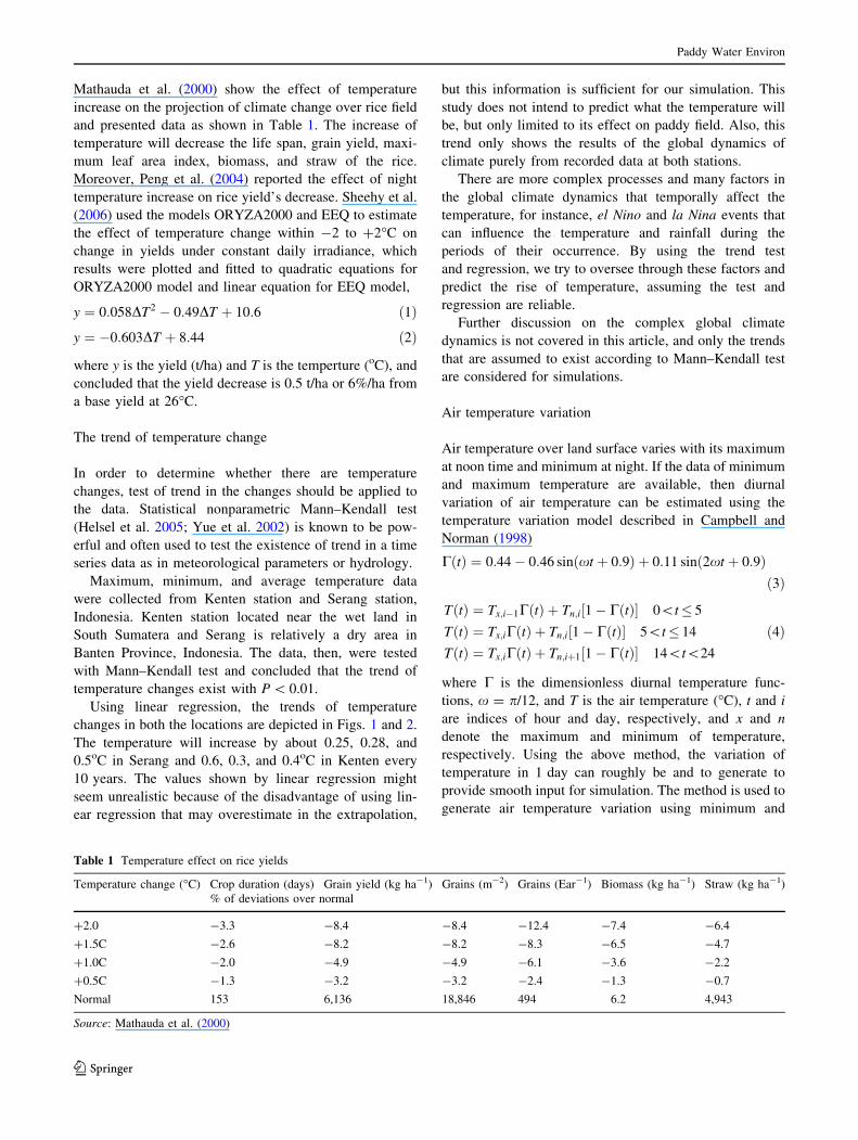
Mathauda et al. (2000) show the effect of temperature

increase on the projection of climate change over rice field

and presented data as shown in Table 1. The increase of

temperature will decrease the life span, grain yield, maxi-

mum leaf area index, biomass, and straw of the rice.

Moreover, Peng et al. (2004) reported the effect of night

temperature increase on rice yield’s decrease. Sheehy et al.

(2006) used the models ORYZA2000 and EEQ to estimate

the effect of temperature change within -2 to ?2�C on

change in yields under constant daily irradiance, which

results were plotted and fitted to quadratic equations for

ORYZA2000 model and linear equation for EEQ model,

y ¼ 0:058DT2 � 0:49DT þ 10:6 ð1Þy ¼ �0:603DT þ 8:44 ð2Þ

where y is the yield (t/ha) and T is the temperture (oC), and

concluded that the yield decrease is 0.5 t/ha or 6%/ha from

a base yield at 26�C.

The trend of temperature change

In order to determine whether there are temperature

changes, test of trend in the changes should be applied to

the data. Statistical nonparametric Mann–Kendall test

(Helsel et al. 2005; Yue et al. 2002) is known to be pow-

erful and often used to test the existence of trend in a time

series data as in meteorological parameters or hydrology.

Maximum, minimum, and average temperature data

were collected from Kenten station and Serang station,

Indonesia. Kenten station located near the wet land in

South Sumatera and Serang is relatively a dry area in

Banten Province, Indonesia. The data, then, were tested

with Mann–Kendall test and concluded that the trend of

temperature changes exist with P \ 0.01.

Using linear regression, the trends of temperature

changes in both the locations are depicted in Figs. 1 and 2.

The temperature will increase by about 0.25, 0.28, and

0.5oC in Serang and 0.6, 0.3, and 0.4oC in Kenten every

10 years. The values shown by linear regression might

seem unrealistic because of the disadvantage of using lin-

ear regression that may overestimate in the extrapolation,

but this information is sufficient for our simulation. This

study does not intend to predict what the temperature will

be, but only limited to its effect on paddy field. Also, this

trend only shows the results of the global dynamics of

climate purely from recorded data at both stations.

There are more complex processes and many factors in

the global climate dynamics that temporally affect the

temperature, for instance, el Nino and la Nina events that

can influence the temperature and rainfall during the

periods of their occurrence. By using the trend test

and regression, we try to oversee through these factors and

predict the rise of temperature, assuming the test and

regression are reliable.

Further discussion on the complex global climate

dynamics is not covered in this article, and only the trends

that are assumed to exist according to Mann–Kendall test

are considered for simulations.

Air temperature variation

Air temperature over land surface varies with its maximum

at noon time and minimum at night. If the data of minimum

and maximum temperature are available, then diurnal

variation of air temperature can be estimated using the

temperature variation model described in Campbell and

Norman (1998)

C tð Þ ¼ 0:44� 0:46 sin xt þ 0:9ð Þ þ 0:11 sin 2xt þ 0:9ð Þð3Þ

T tð Þ ¼ Tx;i�1C tð Þ þ Tn;i 1� C tð Þ½ � 0\t� 5

T tð Þ ¼ Tx;iC tð Þ þ Tn;i 1� C tð Þ½ � 5\t� 14

T tð Þ ¼ Tx;iC tð Þ þ Tn;iþ1 1� C tð Þ½ � 14\t\24

ð4Þ

where C is the dimensionless diurnal temperature func-

tions, x = p/12, and T is the air temperature (�C), t and i

are indices of hour and day, respectively, and x and n

denote the maximum and minimum of temperature,

respectively. Using the above method, the variation of

temperature in 1 day can roughly be and to generate to

provide smooth input for simulation. The method is used to

generate air temperature variation using minimum and

Table 1 Temperature effect on rice yields

Temperature change (�C) Crop duration (days) Grain yield (kg ha-1) Grains (m-2) Grains (Ear-1) Biomass (kg ha-1) Straw (kg ha-1)

% of deviations over normal

?2.0 -3.3 -8.4 -8.4 -12.4 -7.4 -6.4

?1.5C -2.6 -8.2 -8.2 -8.3 -6.5 -4.7

?1.0C -2.0 -4.9 -4.9 -6.1 -3.6 -2.2

?0.5C -1.3 -3.2 -3.2 -2.4 -1.3 -0.7

Normal 153 6,136 18,846 494 6.2 4,943

Source: Mathauda et al. (2000)

Paddy Water Environ

123

maximum temperature at the surface atmosphere. The

variations of temperatures are estimated using this

approach for each year presented in this article. The min-

imum and maximum temperatures were estimated, using

trends of minimum and maximum temperature, which were

assumed to exist, based on the trend test and linear

regression.

The needed parameter for the simulation is actually the

temperature at its upper boundary at a certain height from the

surface, which is 100 m in this case. Within the closest

atmosphere layer the Earth’s surface (troposphere) air tem-

perature normally decreases with height above the surface

because the primary source of heating for the air is the Earth.

The rate of change in temperature with altitude is called the

environmental lapse rate of temperature (ELR) which

temporally and spatially varies, and the average value of the

normal lapse rate of temperature is 0.65�C/100 m. This

approach is used to estimate the temperature needed for

boundary condition of the model.

Simulation model

Various studies on global climate change and its influences

have been reported, where many of those focussed on

global or regional climate model. The models were used to

project the effect on, for example, evapotranspiration over

paddy fields (Yu et al. 2002) or temperature changes and

afterward rice production (Iizumi et al. 2007). Instead of

using a similar model, in this simulation, a detailed model

of paddy microenvironment is used, based on the model of

irrigated paddy field proposed by Saptomo et al.(2004).

The influence of temperature increase is studied using

the combination of atmosphere boundary layer variations

in wind, humidity and temperature, soil heat transport, and

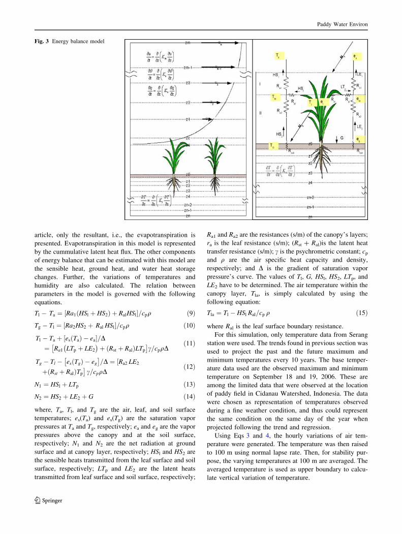
two-layered surface energy balance for irrigated paddy.

The schematic of the model is shown in Fig. 3. In general,

this model calculates the variations in the air boundary

layer, the energy balance, and flux analyses on the vege-

tated surface layer, and heat transport in the soil layer.

Variations in the air boundary layer are analyzed based

on wind, humidity, and temperature variation equation in

turbulence layer. Heat transport in the soil is analyzed

based on soil heat transport equation, assuming the soil has

uniform physical and thermal properties. The governing

equations for these calculations are as follows:

ou

ot¼ o

ozKm

ou

oz

� �ð5Þ

ohot¼ o

ozKh

ohoz

� �ð6Þ

oq

ot¼ o

ozKv

oq

oz

� �ð7Þ

oT

ot¼ o

ozKs

oT

oz

� �ð8Þ

where Km, Kh, and Kv are the turbulent diffusivities

(m2 s-1) of momentum, thermal, and vapor, respectively,

in which Km = Kh = Kv = Kd(z), z is the height (m), T is

the soil temperature (�C), and Ks is the thermal diffusivity

(m2 s-1).

Equations 5, 6, and 7 then were arranged by means of

finite-difference scheme and used to simulate heat, wind,

and humidity transports in the atmospheric boundary layer.

The energy balance analysis in the vegetated surface

layer is approached following resistance model. Thermal

and vapor fluxes in heat energy terms are assumed to flow

accross a network of wires through resistances (Fig. 3),

which are the aerodynamic resistance and plant physical

resistance. The physical parameters of the plant, such as

LAI and heights, are needed for this calculation. The

source energy for the process is the net radiation. Energy

balances are then analyzed on each layer which is below

the leaf and from the leaf above.

The model can be used to estimate separately evapora-

tion and transpiration, since it analyzes the energy balance

of two stratified layers; each layer deals with the energy

balance components belonging to it. However, in this

Serang

y = 0.025x - 26.35

y = 0.028x - 29.444

y = 0.05x - 71

202122232425262728293031

1986 1991 1996 2001 2006

Year

Tem

pera

ture

(°C

)

Average

Min

Max

Fig. 1 Air temperature changes trend in Kenten

Kenten

Min

Max

Average

y = 0.0432x - 51.191

y = 0.0344x - 36.771

y = 0.06x - 93.33

20

22

24

26

28

30

32

34

36

38

1984 1989 1994 1999 2004

Year

Tem

pera

ture

(°C

)

Fig. 2 Air temperature changes trend in Serang

Paddy Water Environ

123

article, only the resultant, i.e., the evapotranspiration is

presented. Evapotranspiration in this model is represented

by the cummulative latent heat flux. The other components

of energy balance that can be estimated with this model are

the sensible heat, ground heat, and water heat storage

changes. Further, the variations of temperatures and

humidity are also calculated. The relation between

parameters in the model is governed with the following

equations.

Tl � Ta ¼ Ra1 HSl þ HS2ð Þ þ RalHSl½ �=cpq ð9Þ

Tg � Tl ¼ Ra2HS2 þ Ral HSl½ �=cpq ð10Þ

Tl � Ta þ es Tað Þ � ea½ �=D¼ Ra1 LTp þ LE2

� �þ Rst þ Ralð ÞLTp

� �c=cpqD

ð11Þ

Tg � Tl � esðTgÞ � eg

� �=D ¼ Ra2 LE2½

þ Rst þ Ralð ÞTp

�c=cpqD

ð12Þ

N1 ¼ HSl þ LTp ð13Þ

N2 ¼ HS2 þ LE2 þ G ð14Þ

where, Ta, Tl, and Tg are the air, leaf, and soil surface

temperatures; es(Ta) and es(Tg) are the saturation vapor

pressures at Ta and Tg, respectively; ea and eg are the vapor

pressures above the canopy and at the soil surface,

respectively; N1 and N2 are the net radiation at ground

surface and at canopy layer, respectively; HSl and HS2 are

the sensible heats transmitted from the leaf surface and soil

surface, respectively; LTp and LE2 are the latent heats

transmitted from leaf surface and soil surface, respectively;

Ra1 and Ra2 are the resistances (s/m) of the canopy’s layers;

ra is the leaf resistance (s/m); (Rst ? Ral)is the latent heat

transfer resistance (s/m); c is the psychrometric constant; cp

and q are the air specific heat capacity and density,

respectively; and D is the gradient of saturation vapor

pressure’s curve. The values of Tl, G, HSl, HS2, LTp, and

LE2 have to be determined. The air temperature within the

canopy layer, Tla, is simply calculated by using the

following equation:

Tla ¼ Tl � HSl Ral=cp q ð15Þ

where Ral is the leaf surface boundary resistance.

For this simulation, only temperature data from Serang

station were used. The trends found in previous section was

used to project the past and the future maximum and

minimum temperatures every 10 years. The base temper-

ature data used are the observed maximum and minimum

temperature on September 18 and 19, 2006. These are

among the limited data that were observed at the location

of paddy field in Cidanau Watershed, Indonesia. The data

were chosen as representation of temperatures observed

during a fine weather condition, and thus could represent

the same condition on the same day of the year when

projected following the trend and regression.

Using Eqs 3 and 4, the hourly variations of air tem-

perature were generated. The temperature was then raised

to 100 m using normal lapse rate. Then, for stability pur-

pose, the varying temperatures at 100 m are averaged. The

averaged temperature is used as upper boundary to calcu-

late vertical variation of temperature.

Fig. 3 Energy balance model

Paddy Water Environ

123

The boundary temperatures used for the simulations for

the years 1986, 1996, 2006, 2016, and 2026 are 28.05,

28.41, 28.77, 29.78, and 29.49�C, respectively. These

values were also used as initial condition of air temperature

that is assumed vertically uniform at the beginning of the

simulation. The other boundary conditions of wind speed,

soil temperature and specific humidity are fixed at 6 km/s,

27�C, and 0.014. The other input needed for the simulation

is the solar radiation that was generated from extra ter-

restrial radiation according to the geographic location of

Serang and day of the year. The paddy field was assumed to

be irrigated with 5-cm depth of water on its soil surface.

Here, only air temperature is considered to be different

due to climate change. The other parameters in the model as

well as the factors that are known to have influence to paddy

such as carbon dioxide status are assumed to be the same.

Paddy fields thermal environment

Variation in heat and evapotranspiration

Simulation was conducted using the model described in the

previous section of this article. The parameters used for the

model are those taken from Saptomo et al. (2004). Varia-

tions in heat fluxes resulting from the simulation are

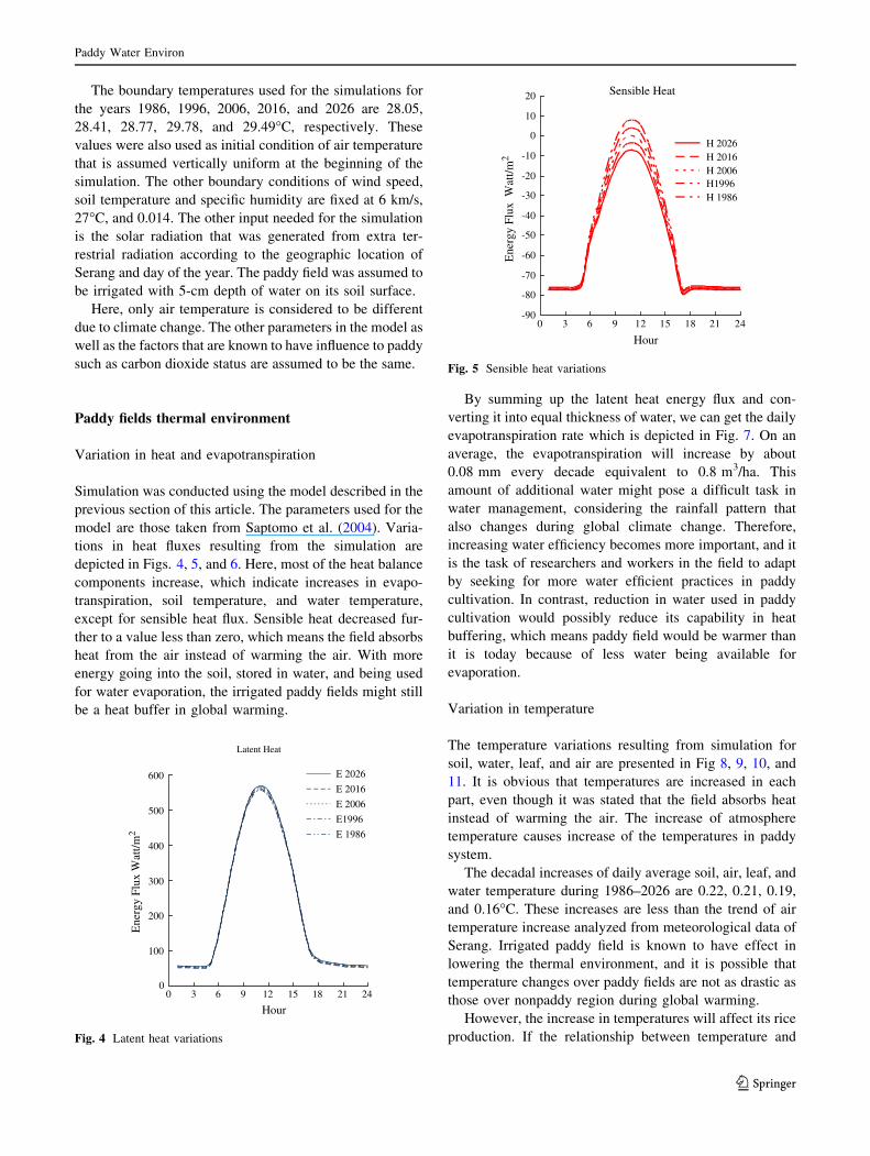
depicted in Figs. 4, 5, and 6. Here, most of the heat balance

components increase, which indicate increases in evapo-

transpiration, soil temperature, and water temperature,

except for sensible heat flux. Sensible heat decreased fur-

ther to a value less than zero, which means the field absorbs

heat from the air instead of warming the air. With more

energy going into the soil, stored in water, and being used

for water evaporation, the irrigated paddy fields might still

be a heat buffer in global warming.

By summing up the latent heat energy flux and con-

verting it into equal thickness of water, we can get the daily

evapotranspiration rate which is depicted in Fig. 7. On an

average, the evapotranspiration will increase by about

0.08 mm every decade equivalent to 0.8 m3/ha. This

amount of additional water might pose a difficult task in

water management, considering the rainfall pattern that

also changes during global climate change. Therefore,

increasing water efficiency becomes more important, and it

is the task of researchers and workers in the field to adapt

by seeking for more water efficient practices in paddy

cultivation. In contrast, reduction in water used in paddy

cultivation would possibly reduce its capability in heat

buffering, which means paddy field would be warmer than

it is today because of less water being available for

evaporation.

Variation in temperature

The temperature variations resulting from simulation for

soil, water, leaf, and air are presented in Fig 8, 9, 10, and

11. It is obvious that temperatures are increased in each

part, even though it was stated that the field absorbs heat

instead of warming the air. The increase of atmosphere

temperature causes increase of the temperatures in paddy

system.

The decadal increases of daily average soil, air, leaf, and

water temperature during 1986–2026 are 0.22, 0.21, 0.19,

and 0.16�C. These increases are less than the trend of air

temperature increase analyzed from meteorological data of

Serang. Irrigated paddy field is known to have effect in

lowering the thermal environment, and it is possible that

temperature changes over paddy fields are not as drastic as

those over nonpaddy region during global warming.

However, the increase in temperatures will affect its rice

production. If the relationship between temperature and

Latent Heat

0

100

200

300

400

500

600

0 3 6 9 12 15 18 21 24

Hour

Ene

rgy

Flux

Wat

t/m2

E 2026

E 2016

E 2006

E1996

E 1986

Fig. 4 Latent heat variations

Sensible Heat

-90

-80

-70

-60

-50

-40

-30

-20

-10

0

10

20

0 3 6 9 12 15 18 21 24

Hour

Ene

rgy

Flux

Wat

t/m2

H 2026H 2016H 2006H1996H 1986

Fig. 5 Sensible heat variations

Paddy Water Environ

123

yield are assumed same as those refered early in this arti-

cle, the effect on rice yields can be presented (Table 2).

It is clear that the increase of the air temperature at the

upper boundary will contribute extra heat energy to the

surface, which will, in turn, contribute the changing of

surface energy balance as presented in this article. In irri-

gatted field, there is enough water to absorb the heat which

causes more evaporation and further evapotranspiration.

The effect of the increasing temperature on evapotranspi-

ration is also easy to understand when we look into the

equations for calculating evapotranspiration, e.g., like in

Allen et al. (1998), in which all the approaches directly

take into account the air temperature. The results presented

in this article are site specific to the place from where

measured data inputs were taken.

Concluding remarks

The effect of climate change in the form of temperature

increase on irrigated paddy thermal environment has been

studied using two-layered energy balance model. The

simulation uses the predicted past and future temperature

Ground Heat

-80

-60

-40

-20

0

20

40

60

80

0 3 6 9 12 15 18 21 24

Hour

Ene

rgy

Flux

Wat

t/m2

Ene

rgy

Flux

Wat

t/m2

G 2026G 2016G 2006G 1996G 1986

-100

-50

0

50

100

150

0 3 6 9 12 15 18 21 24

Hour

dSw 2026

dSw 2016

dSw 2006

dSw 1996

dSw 1986

Fig. 6 Ground heat and water

heat storage changes

7.100

7.200

7.300

7.400

7.500

7.600

1986 1996 2006 2016 2026

Year

ET

(m

m/d

ay)

Fig. 7 Evapotranspiration rate

Water Temperature

20

22

24

26

28

30

0 3 6 9 12 15 18 21 24

Hour

Tem

pera

ture

(°C

)

Water 1986

Water 1996

Water 2006

Water 2016

Water 2026

Fig. 8 Water temperature variations

Soil Temperature

20

22

24

26

28

30

0 3 6 9 12 15 18 21 24

Hour

Tem

pera

ture

(°C

)

Soil 1986

Soil 1996

Soil 2006

Soil 1996

Soil 2026

Fig. 9 Soil temperature variations

Paddy Water Environ

123

changes, trends of which were found using Mann–Kendall

tests to obtain time series temperature data. Simulation

results show that irrigated paddy field seems to be able to

lower the effect of the increase of air temperature in global

warming. In contrast, evapotranspiration increases and may

become a problem in water management as the rainfall

pattern also changes. Although paddy field has a function

as thermal buffer, its temperature still increases affected by

the global warming, thus affecting the rice production.

References

Allen RG, Pereira LS, Raes D, Smith M (1998) Crop evapotranspi-

ration: guidance for computing crop water requirements, FAO

irrigation and drainage paper, vol 56

Campbell GS, Norman JM (1998) An introduction to environmental

biophysics. Springer, New York

Helsel DR, Mueller DK, Slack JR (2005) Computer program for the

Kendall family of trend tests scientific investigations report

2005–5275. US Geological Survey

Iizumi T, Hayashi Y, Kimura F (2007) Influence on rice production in

Japan from cool and hot summers after global warming. J Agric

Meteorol 63(1):11–23

Peng S, Jianliang H, Sheehy JE, Laza RC, Visperas RM, Xuhua Z,

Centeno HGS, Khush GS, and KG (2004) Rice yields decline

with higher night temperature from global warming. Proc Natl

Acad Sci USA 101:9971–9975

Mathauda SS, Mavi HS, Bhangoo BS, Dhaliwal BK (2000) Impact of

projected climate change on rice production in Punjab (India).

Trop Ecol 41(1):95–98

Saptomo SK, Nakano Y, Yuge K, Haraguchi T (2004) Observation

and simulation of thermal environment in a paddy field. Paddy

Water Environ 2004(2):73–82

Sheehy JE, Mitchell PL, Ferrer AB (2006) Decline in rice grain yields

with temperature: models and correlations can give different

estimates. Field Crops Res 98:151–156

Yu PS, Yang TC, Chou CC (2002) Effects of climate change on

evapotranspiration from paddy fields in southern Taiwan. Clim

Change 54:165–179

Yue S, Pilon P, Cavadias G (2002) Power of the Mann-Kendall and

Spearman’s rho tests for detecting monotonic trends in hydro-

logical series. J Hydrol 259:254–271

Air Temperature

20

22

24

26

28

30

0 3 6 9 12 15 18 21 24

Hour

Tem

pera

ture

(°C

)

Air 1986

Air 1996

Air 2006

Air 2016

Air 2026

Fig. 10 Air temperature variations

Leaf Temperature

20

22

24

26

28

30

0 3 6 9 12 15 18 21 24

Hour

Tem

pera

ture

(°C

)

Leaf 1986

Leaf 1996

Leaf 2006

Leaf 2016

Leaf 2026

Fig. 11 Leaf temperature variations

Table 2 Estimated rice yield’s decrease

Year 1996 2006 2016 2026

Total temperature increase (oC) 0.22 0.40 0.60 0.79

Yield decrease (% of normal)a (Mathauda

et al. (2000))

0.6 1.0 1.6 2.1

Yield decrease (t/ha) (Sheehy et al. (2006)) 0.1 0.2 0.4 0.5

a Normal yield at 6,136 kg/ha (Table 1)

Paddy Water Environ

123