I

The Department of International Environment and Development Studies, Noragric, is the

international gateway for the Norwegian University of Life Sciences (UMB). Eight

departments, associated research institutions and the Norwegian College of Veterinary

Medicine in Oslo. Established in 1986, Noragric’s contribution to international development

lies in the interface between research, education (Bachelor, Master and PhD programmes) and

assignments.

The Noragric Master thesis are the final theses submitted by students in order to fulfil the

requirements under the Noragric Master programme “International Environmental Studies”,

“Development Studies” and other Master programmes.

The findings in this thesis do not necessarily reflect the views of Noragric. Extracts from this

publication may only be reproduced after prior consultation with the author and on condition

that the source is indicated. For rights of reproduction or translation contact Noragric.

© Monika Salmivalli, May 2013

monika.salmivalli@gmail.com

Noragric

Department of International Environment and Development Studies

P.O. Box 5003

N-1432 Ås

Norway

Tel.: +47 64 96 52 00

Fax: +47 64 96 52 01

Internet: http://www.umb.no/noragric

II

Declaration

I, Monika Salmivalli, declare that this thesis is a result of my research investigations and

findings. Sources of information other than my own have been acknowledged and a reference

list has been appended. This work has not been previously submitted to any other university

for award of any type of academic degree.

Signature………………………………..

Date…………………………………………

III

Acknowledgements

I wish to thank many people for helping me with this thesis. First, I wish to thank my main

supervisor, Siri Aas Rustad. Thank you Siri for believing in my capacity to take upon this

challenge, for inspiring, encouraging and motivating me, for all the help you have given me

and for being such a nice person.

Next, I wish to thank Stig Jarle Hansen, my supervisor and program coordinator at UMB, for

helpful advice; Jonas Nordkvelle and Andreas Forø Tollefsen at PRIO for great help with

PRIO-GRID and for good ideas on how to improve the study; Tor Arve Benjaminsen at

UMB, Jens Aune at UMB, Ole Magnus Theisen at PRIO/NTNU and Halvard Buhaug at

PRIO/NTNU for helpful ideas, discussions and advice; and all the participants to a brown bag

lunch on March 18th

2013 at PRIO for advice.

Katharina Koschnick, my classmate, deserves big thanks for being good company the past

five months and for making the thesis writing time much nicer. Duba Jarso, my classmate,

also deserves big thanks for reading through drafts of the thesis, for giving helpful advice and

for long discussions on the topic and methods of the thesis. I also wish to thank my other

classmates for good times during the master’s degree. Moreover, I wish to thank my good

friends Maj Sundberg and Mariya Simon for always being there for me, and Mariya also for

reading through a draft of the thesis.

I wish to deeply thank my family, who are always there for me and who have supported me

and my choices throughout. Moreover, I wish to thank the Fleischer family for helping me to

a good start in Norway and for being good friends ever since.

Finally, the greatest thank you goes to my dear boyfriend Erik Østreng. Your support has been

invaluable. Thank you for inspiring and encouraging me to write a quantitative thesis, for

insightful discussions all the way, for crucial help with practical issues, and for always

making me laugh about my own mistakes. Thank you for being there for me at all times.

Monika Salmivalli May 14th

2013 Oslo, Norway

IV

Abstract

Does climate change lead to violent conflicts? This question worries world leaders, but

research has not yet reached consensus on the topic. Inspired by theories of the Environmental

Security School, many studies have been conducted on climate change and conflicts, in

particular civil wars. However, this thesis argues that if climate change should lead to

conflicts, a more likely outcome may be communal conflicts, on which there are only a few

studies. To help fill this knowledge gap, this thesis investigates the relationship between

climate change and communal conflicts in Sub-Saharan African in 1989-2008. It employs

quantitative method and a disaggregated approach, using grid cells of 0.05˚ x 0.05˚ as units of

analysis. Additionally to a regular large-N analysis, this thesis also analyzes climate change

and communal conflict in a most likely scenario. Arguably, if climate change and conflicts are

related, a relationship should be found where the circumstances for communal conflict, the

most likely type of conflict to occur, are most favorable. Yet, this thesis finds no relationship

between climate change and communal conflicts. Measured as changes in temperatures and

rainfall, climate is not found to explain communal conflict events, not even in the most likely

scenario. These results run contradictory to the few other studies which have been conducted

on climate change and communal conflicts in Africa.

V

Table of contents

1 Introduction ........................................................................................................................ 1

1.1 Definitions ................................................................................................................... 4

1.1.1 Environmental vs. climate change ....................................................................... 4

1.1.2 Environmental scarcity vs. resource scarcity ....................................................... 5

1.1.3 Civil war, non-state conflict and communal conflict ........................................... 5

2 Literature review ................................................................................................................ 7

2.1 The history of environment and conflict research ....................................................... 7

2.2 The key debates ........................................................................................................... 8

2.3 Climate change and civil war .................................................................................... 10

2.4 Climate change and non-state conflicts ..................................................................... 11

2.4.1 Continent-wide and regional quantitative studies of Africa ............................... 11

2.4.2 Local quantitative studies ................................................................................... 14

2.4.3 Qualitative case studies ...................................................................................... 15

2.4.4 Overview of quantitative studies ........................................................................ 16

3 Theory .............................................................................................................................. 19

3.1 Impact on livelihoods in Sub-Saharan Africa ............................................................ 20

3.2 Violent conflict .......................................................................................................... 22

3.2.1 Sources of scarcity ............................................................................................. 22

3.2.2 Consequences of scarcity ................................................................................... 23

3.2.3 Communal conflict vs. civil war ........................................................................ 25

3.2.4 Hypotheses ......................................................................................................... 29

3.3 Most likely scenario ................................................................................................... 30

3.3.1 Marginalized groups ........................................................................................... 31

3.3.2 Poverty ............................................................................................................... 31

3.3.3 Rural areas .......................................................................................................... 32

3.3.4 Hypotheses for the most likely scenario ............................................................ 33

VI

3.4 Summary of hypotheses ............................................................................................. 33

4 Methods ............................................................................................................................ 35

4.1 Introduction ............................................................................................................... 35

4.2 Quantitative vs. qualitative method ........................................................................... 36

4.3 Disaggregation using a grid cells structure ................................................................ 37

4.3.1 Benefits of disaggregation .................................................................................. 37

4.3.2 Benefits of grid cells .......................................................................................... 38

4.4 Data structure ............................................................................................................. 40

4.5 Sampling .................................................................................................................... 41

4.6 Variables and their operationalizations ..................................................................... 42

4.6.1 Dependent variable ............................................................................................. 42

4.6.2 Independent variables ......................................................................................... 44

4.6.3 Control variables ................................................................................................ 45

4.7 Logistic regression ..................................................................................................... 50

4.8 Methodological challenges ........................................................................................ 53

4.8.1 Multicollinearity ................................................................................................. 53

4.8.2 Omitted variable bias ......................................................................................... 53

4.8.3 Outliers ............................................................................................................... 53

4.8.4 Rare events ......................................................................................................... 54

4.8.5 Time dependency and spatial dependency ......................................................... 55

4.8.6 Missing data and selection bias .......................................................................... 55

4.9 Limitations ................................................................................................................. 56

5 Results .............................................................................................................................. 59

5.1 Large-model analyses ................................................................................................ 59

5.1.1 Descriptive statistics ........................................................................................... 59

5.1.2 Baseline model for the multivariate analyses ..................................................... 60

5.1.3 Multivariate analyses with climatic variables .................................................... 64

VII

5.2 Most likely scenario ................................................................................................... 71

5.2.1 Descriptive statistics ........................................................................................... 72

5.2.2 Multivariate analyses .......................................................................................... 73

5.3 Summary of all results ............................................................................................... 80

5.4 Statistical tests ........................................................................................................... 80

5.4.1 Multicollinearity ................................................................................................. 81

5.4.2 Extreme and influential observations ................................................................. 81

6 Discussion ........................................................................................................................ 83

7 Conclusion ........................................................................................................................ 87

8 References ........................................................................................................................ 89

Appendix A Countries in Sub-Saharan Africa ......................................................................... 95

Appendix B Countries in the EPR dataset ............................................................................... 96

Appendix C Baseline model ..................................................................................................... 97

Appendix D Bivariate results ................................................................................................... 99

Appendix E Robustness tests for the baseline model ............................................................. 101

Appendix F Robustness tests .................................................................................................. 103

VIII

Figure S- 1 presents the results of a Pregibon’s leverage test on the baseline model. Mean

leverage value: 0.0014. Number of observations with leverage value >(0.0014 x 3): 395. ... 101

Figure S- 2 presents the results of Pregibon’s delta-beta test on the baseline model. Number of

observations: 7411. Number of observations with a delta-beta value <1: 7411. ................... 102

Figure S- 3 presents the results of Pregibon’s delta-beta test on the variables included in the

multivariate models testing hypotheses 1a and 2a. Number of observations: 7113. Number of

observations with delta-beta values<1: 7113. ........................................................................ 103

Figure S- 4 presents the results of Pregibon’s leverage test on the variables included in the

multivariate models testing hypotheses 1a and 2a. Mean of leverage values: 0.0019. Number

of observations with leverage values >(0.0019 x 3): 390. ..................................................... 104

Figure S- 5 presents results of Pregibon’s delta-beta test on the variables included in the

multivariate models testing hypotheses 3a and 4a. Number of observations: 1179. Number of

observations with delta-beta<1: 1176. ................................................................................... 108

Figure S- 6 presents results of Pregibon’s leverage test on the variables included in the

multivariate models testing hypotheses 3a and 4a. Mean of leverage values: 0.0036. Number

of observations with leverage-values >(00.36 x 3): 62. ......................................................... 108

Table 1 Overview of quantitative non-state conflict results. ................................................... 17

Table 2 Descriptive statistics for the larger models ................................................................. 60

Table 3 The baseline model ..................................................................................................... 62

Table 4 Results for hypotheses 1a and 2a ................................................................................ 65

Table 5 Results for hypotheses 1b and 2b ................................................................................ 68

Table 6 Results for larger models á la Fjelde and Uexkull (2012) .......................................... 70

Table 7 Descriptive statistics for the most likely scenario ....................................................... 72

Table 8 Results for hypotheses 3a and 4a ................................................................................ 74

Table 9 Results for hypotheses 3b and 4b ................................................................................ 77

Table 10 Results for most likely scenario models á la Fjelde and Uexkull (2012) .................. 79

Table S- 1 Development of the baseline model ....................................................................... 98

Table S-2 Bivariate results for hypotheses 1a and 2a .............................................................. 99

Table S-3 Bivariate results for hypotheses 1b and 2b .............................................................. 99

Table S-4 Bivariate results for hypotheses 3a and 4a ............................................................ 100

Table S-5 Bivariate results for hypotheses 3b and 4b ............................................................ 100

IX

Table S-6 VIF-tests for variables included in hypotheses 1a and 2a. .................................... 104

Table S-7 Correlation matrix for variables included in hypotheses 1a and 2a....................... 105

Table S- 8 VIF-tests for variables included in hypotheses 1b and 2b. ................................... 106

Table S- 9 Correlation matrix for variables included in hypotheses 1b and 2b. .................... 107

Table S-10 VIF-tests for variables included in hypotheses 3a and 4a. .................................. 109

Table S- 11 Correlation matrix for variables included in hypotheses 3a and 4a.................... 110

Table S- 12 VIF-test for variables included in hypotheses 3b and 4b. .................................. 111

Table S- 13 Correlation matrix for variables included in hypotheses 3b and 4b. .................. 112

X

1

1 Introduction

World leaders worry that climate change has been the cause of violent conflict. Amongst

others the US President Barack Obama (Obama 2009:1) and the Secretary-General of the

United Nations Ban Ki-Moon (Ban 2007) have expressed a clear concern for this. Further, the

Norwegian Nobel Committee awarded the Nobel Peace Prize in 2007 to the IPCC and Al

Gore for their efforts to collect knowledge of climate change and communicate the severity of

it to people worldwide. In the announcement speech, the Chairman of the Committee, Ole

Danbolt Mjøs, said:

“Unfortunately we can already establish that global warming not only has negative

consequences for ‘human security’, but can also fuel violence and conflict within and

between states. (…) The consequences are most obvious, however, among the poorest

of the poor, in Darfur and in large sectors of the Sahel belt, where we have already

had the first ‘climate war’.” (Mjøs 2007:1)

Within International Relations, the Environmental Security School (e.g. Ullman (1983);

Homer-Dixon (1999)) argues that resource scarcity, which may be caused by climate change,

can worsen livelihoods of people in developing countries and as a consequence, lead to

conflicts. However, contrary to these theories and to the worries of world leaders, research has

not yet reached consensus on whether climate change and conflicts are correlated or not.

Gleditsch (2012:7) summarizes, in a special issue of the Journal of Peace Research, that “on

the whole […] it seems fair to say that so far there is not yet much evidence for climate

change as an important driver of conflict.” The same has been stated in recent reviews by

Salehyan (2008) and Bernauer et al. (2012).

However, research on the climate change – conflict relationship has so far focused mainly on

studying civil wars. This thesis proposes (as have e.g. Theisen (2008), Hendrix and Salehyan

(2012) and Fjelde and Uexkull (2012)) that if climate change and conflicts are associated, an

association should be found between climate change and non-state conflicts, in particular

communal conflicts, rather than between climate change and civil wars. The threshold for

groups to challenge the state (causing a civil war) is arguably much higher than for groups to

engage in a violent conflict with each other (defined as a non-state conflict). Furthermore,

2

communal conflict is more likely to be related to climate change than other types of non-state

conflicts, as will be argued for in this study.

Some studies have already addressed the relationship between climate change and communal

conflicts (e.g. Fjelde and Uexkull (2012) and Raleigh and Kniveton (2012)), and between

climate change and non-state conflicts (e.g. Hendrix and Salehyan (2012) and O’Loughlin et

al. (2012)). Yet, there are great variations in the results of these studies, possibly because the

studies also vary regarding the geographical area studied, the unit of analysis used, the exact

definition of conflict used and the conflict data used. Therefore, a lot remains to uncover.

This study will follow the path of focusing on conflicts short of civil war. It will investigate

the relationship between climate change and communal conflicts in Sub-Saharan Africa in the

years 1989-2008. Its primary contributions to the literature will be to show how the use of

both temperature and precipitation as measures of climate change, and the use of grid-cells as

disaggregated units of analysis, affects the analysis of climate change and communal conflict.

So far, only few climate-conflict studies have looked at temperature as a measure for climate

change. These are O’Loughlin et al. (2012) and Theisen (2012), which study non-state

conflicts, and Burke et al. (2009), Buhaug (2010a) and Wischnath and Buhaug (2013)), which

focus on climate change and civil wars.

Moreover, the level of analysis chosen may have important consequences on the analysis of

climate change and conflicts, as is argued by for instance Buhaug and Lujala (2005) and as

will be discussed in this thesis. The analyses in this thesis are conducted on a disaggregated

level using grid cells as units of analysis. O’Loughlin et al. (2012) and Theisen (2012) have,

similarly to this thesis, used grid cells as units of analysis to study climate change and non-

state conflict. However, as O’Loughlin et al. (2012) studies East Africa and Theisen (2012)

studies Kenya, this thesis will be the first one to undertake an analysis of climate change and

(any type of) non-state conflict in Sub-Saharan Africa using grid cells as units of analysis.

This thesis can thus provide a great opportunity to see whether the use of grid cells affects the

results compared to using other disaggregated units. In this sense, the most interesting study

to compare to is the study by Fjelde and Uexkull (2012), which uses first-order administrative

3

units to study the same area, Sub-Saharan Africa, and the same type of conflicts, namely

communal conflicts, with the same conflict data, the UCDP GED (Melander and Sundberg

2011) and UCDP non-state conflict dataset (Sundberg et al. 2012).

Interestingly, the results of this study indicate that there is no relationship between climate

change and communal conflicts: none of the models in which the variables for temperature

and rainfall were included were able to better explain communal conflict events than a model

where only control variables were included. These results thus contradict the theoretical

expectations in this thesis about a relationship between climate change and communal

conflicts.

Moreover, this thesis also analyzes climate change and communal conflicts in a most likely

scenario. The reason to analyze a most likely scenario is that if climatic changes have the

potential to cause conflicts, arguably this will most likely happen in the circumstances

described in this scenario. In this study, the most likely scenario is argued to occur in rural

areas in Sub-Saharan Africa, characterized by political marginalization and poverty. The most

likely scenario is presented in section 3.3.

However, changes in temperature and rainfall proved equally bad at explaining communal

conflict events in the most likely scenario. As in the larger models, none of the climatic

coefficients helped to explain communal conflict events, compared to models where only

control variables were included.

Furthermore, attempt was also made to analyze rainfall and communal conflicts with models

as similar as possible to the models used by Fjelde and Uexkull (2012), who have found

drought to increase the likelihood of communal conflicts, and whose study differs from this

thesis mainly by using first-order administrative units rather than grid cells as disaggregated

units of analysis. Still, this thesis did not find any relationship between rainfall and communal

conflicts.

Consequently, the results of this thesis run contrary to most other studies on climate change

and communal conflicts or non-state conflicts, for instance Fjelde and Uexkull (2012),

Raleigh and Kniveton (2012), Hendrix and Salehyan (2012) and O’Loughlin et al. (2012).

Especially regarding the difference in results compared to Fjelde and Uexkull (2012), the

4

results of this thesis raise questions about the methodologies applied in studies of climate

change and communal conflicts. In particular, the results raise questions about whether grid

cells and first-order administrative units capture the relationship between climate change and

communal conflicts differently.

This thesis is built up in the following way. In chapter 2, the relevant literature on climate

change and conflict will be presented and discussed. In chapter 0, the theoretical arguments

underlying and motivating this study are elaborated on. In chapter 4, focus is given on

methodological choices and the data used in this study. In chapter 5, the results of this study

are presented. In chapter 6, the results are discussed and some ideas for future research are

given. Finally, chapter 7 concludes.

1.1 Definitions

1.1.1 Environmental vs. climate change

This thesis studies the relationship between climate change and communal conflicts. Climate

change is defined as

“change in the state of the climate that can be identified (e.g. using statistical tests) by

changes in the mean and/or the variability of its properties, and that persists for an

extended period, typically decades or longer” (IPCC 2007:30).1

Although climate change is the focus of this thesis, a part of the theoretical arguments in this

thesis are based on literature on diverse environmental changes and conflict (e.g. Homer-

Dixon (1994), Homer-Dixon (1999)). Consequently, the term environmental change is often

used in this thesis when referring to relevant literature on environmental changes and conflict.

This should, however, not be confused with the aim of this thesis, namely to study climate

change and conflict. The reason why theoretical arguments on environmental changes are

1 According to the IPCC (2007:30) “this usage differs from that in the United Nations Framework Convention on

Climate Change (UNFCCC), where climate change refers to a change of climate that is attributed directly or

indirectly to human activity that alters the composition of the global atmosphere and that is in addition to natural

climate variability observed over comparable time periods”. Notwithstanding this, the motivation to study the

relationship between climate change and conflict is in this study the accelerating tempo in which human-induced

climate change is becoming a reality.

5

used in this study is that climate change2 is a sub-category of the term environmental changes

(Homer-Dixon 1991:88).

1.1.2 Environmental scarcity vs. resource scarcity

The term environmental scarcity is often used in the literature on environment and conflict.

Homer-Dixon (1999:14-15) defined environmental scarcity as the combination of supply-

induced, demand-induced and structural scarcity. Supply-induced scarcity occurs when the

availability of necessary renewable resources like land, water or fish decreases. Demand-

induced scarcity occurs for example through population growth, when there are more people

who need to share the same amount of resources. Structural scarcity on the other hand is a

social and political phenomenon: when the access to resources is divided unequally, some

groups will face resource scarcity although there might be enough resources for the whole

population on a national basis. (Homer-Dixon 1999:14-16)

Several scholars have criticized the term environmental scarcity as being too vague (Gleditsch

(1998:388) or to include too many diverse phenomena (Benjaminsen (2009:154). In this

study, the term environmental scarcity is used where the literature talks about environmental

scarcity. Yet, the theoretical arguments underlying this study are based on the more specific

term scarcity of renewable resources such as food and water, originating in supply-induced

scarcity. Moreover, scarcity of renewable resource is in this thesis often shortened to resource

scarcity to make the text more easily readable.

1.1.3 Civil war, non-state conflict and communal conflict

The key difference between a civil war and a non-state conflict is that a civil war occurs

between the authorities of a state and between an organized rebel group (Gleditsch et al.

2002:619), while a non-state conflict does not involve the authorities of a state but only more

or less organized groups (Sundberg et al. 2012:352-353). Moreover, a communal conflict is a

form of non-state conflict and occurs between groups whose members “share a common

identification along ethnic, clan, religious, national or tribal lines” (Pettersson 2012:4).

2 Homer-Dixon (1991) uses the terms green-house warming and climate change interchangeably.

6

7

2 Literature review

This chapter will present the literature on climate change and conflict which is relevant for

this study. First, a quick overview of the history of environment and conflict research is given

(section 2.1), before the key debates in the literature are presented (section 2.2). Thereafter, a

brief review is given over the literature on climate change and civil war (section 2.3), before a

more extensive review is given over literature on climate change and non-state conflict

(section 2.4).

2.1 The history of environment and conflict research

The relationship between environment and conflict has been studied for a few decades.

Rønnfeldt (1997) identifies three generations of environmental conflict research. According to

Rønnfeldt (1997:473-474), the first generation appeared in the 1980s and argued for taking

environmental factors into account in discussions of security (see for instance Ullman (1983),

Myers (1989) and Renner (1996)). The first and second generations are often called the

“environmental security school”. The second generation took the initiative to start empirical

studies on the relationship between environmental factors and conflict. It also formalized the

hypothesis that environmental scarcity would lead to conflict, discussed already by the first

generation. Researchers of the second generation conducted mostly case studies, and through

them tried to map exactly how environmental scarcity could lead to conflict (Rønnfeldt

1997:473, 475). Researchers of the second generation include amongst others Homer-Dixon

(1991; 1994) and Baechler (1998). The second generation will also be discussed in section

2.2, which outlines the key debates in the literature.

The third generation identified by Rønnfeldt (1997) has criticized a number of the second

generations’ methodological choices, including failing to study non-conflict cases. This

criticism will be elaborated in section 2.2 on key debates in the literature. In addition, the third

generation has broadened empirical research on environment and conflict by introducing more

environmental variables and more social variables in the research and, according to Rønnfeldt

(1997:473,476-477), consequently also connected environment-conflict research to general

peace and conflict-research. Although not explicitly mentioned by Rønnfeldt, the third

generation also introduced quantitative research on the environment and conflict. Research of

the third generation explicitly mentioned by Rønnfeldt (1997) include Gleditsch (1996) and

Hauge and Ellingsen (1996), but later the number of researchers affiliated with the third

8

generation’s research has increased dramatically (see for instance Nordås and Gleditsch

(2007), Raleigh and Urdal (2007), Salehyan (2008), Theisen (2008), Burke et al. (2009),

Buhaug (2010a), Bernauer et al. (2012), Hendrix and Salehyan (2012), O’Loughlin et al.

(2012) and Fjelde and Uexkull (2012)), as illustrated in the sections on climate change and

civil war (2.3) and climate change and non-state conflicts (2.4).

2.2 The key debates

The second generation’s concrete hypotheses and empirical studies have arguably been

among the most important motivators and sources of disagreement in empirical environment-

conflict studies. The second generation’s perhaps most prominent scholar has been Thomas

Homer-Dixon3. Homer-Dixon hypothesized different causal pathways between environmental

scarcity and conflict and laid out a plan for empirical research in 1991 (Homer-Dixon 1991).

According to him, environmental scarcity might lead to conflict when combined with conflict-

risk increasing social, political and economic factors, as discussed in section 3.2.2. Based on

empirical case studies conducted by his research group, Homer-Dixon (1994:6) argued in

1994 that many of his hypotheses had proved to be true and that environmental scarcities were

already partly responsible for several conflicts in developing countries.

However, these conclusions have later been contested by a number of researchers working

with different methods, including researchers affiliated with the third generation. Quantitative

researchers have criticized the Environmental Security School amongst other things for

selection bias (Gleditsch 1998) and for concluding prematurely that a climate-conflict link

exists (e.g. Theisen (2008), Salehyan (2008), Gleditsch (1998)). The selection bias critique

concerns that environmental security scholars, including Homer-Dixon (1994), have only

studied cases of conflict and have not included in their research cases where environmental

problems occur but conflict does not (Gleditsch 1998:391). The consequence of selection bias

may be that false conclusions are presented:

3 In his section on the second generation, Rønnfeldt (1997) discusses only Homer-Dixon and Homer-Dixon’s

Toronto Group’s research due to space constrains. Rønnfeldt explains choosing Homer-Dixon “because of the

great frequency by which this group is cited in the literature on this topic” (Rønnfeldt 1997:475). However, as

Rønnfeldt notes in note 4 (Rønnfeldt 1997:480), also a number of other researchers are affiliated with the second

generation.

9

“In examining only cases of conflict, one is likely to find at least partial confirmation

of whatever one is looking for […] No society is completely free of environmental

degradation, nor is any society completely free of ethnic fragmentation, religious

differences, economic inequalities, or problems of governance. From a set of armed

conflicts, one may variously conclude that they are all environmental conflicts, ethnic

conflicts […]” (Gleditsch 1998:392)

Furthermore, Gleditsch (1998:392) points out that Homer-Dixon’s (1994:6) conclusion about

environmental scarcities leading to conflict is not correct. This is according to Gleditsch

because Homer-Dixon draws general conclusions based on case-studies. Generalizing results

of case studies is violating an important principle in social science research (see for instance

Bryman (2008:391)). In addition, Homer-Dixon’s conclusions are seen as premature as a

number of quantitative large-N studies have failed to find a relationship between

environmental factors, including climate change, and conflict (see reviews by Theisen (2008),

Salehyan (2008) and Gleditsch (2012)).

Also political ecologists have criticized the environmental security school. Political ecologists

have argued the environmental security school does not take enough into account neither

context specific factors nor factors of political and economic power, which according to

political ecologists are crucial for understanding violent conflicts (see for instance Peluso and

Watts (2001), Turner (2004) and Benjaminsen et al. (2009)). To illustrate this, case studies

conducted by political ecologists have found underlying social and political explanations to

conflicts which on the surface have seemed to be related to environmental degradation. These

explanations include political marginalization, corruption and long-term strategies to affect

the politics of resource distribution (see Benjaminsen (2008), Benjaminsen et al. (2009) and

Turner (2004)).

Moreover, a frequently cited counter-argument to the resource scarcity – conflict thesis is the

cornucopian argument. The cornucopians4 can be characterized as development optimists,

because they reject the notion that resource scarcity will necessarily have negative

consequences. Instead, they reason that humans are inventive and adaptive, and will therefore

find ways to cope with or solve resource scarcity (see for instance Boserup (1965), Simon

4 Homer-Dixon (1999) talks about economic optimists, which is another term for cornucopians.

10

(1981) and Ruttan and Hayami (1984)). Although the cornucopian argument dates back to the

1960s-1980s, i.e. to a time before theories on climate change and conflict, the argument’s

basic idea may be argued to still be relevant today: resource scarcity (be it caused by

population growth, climate change or another reason) will not necessarily lead to starvation

and social turmoil, because people are adaptive and inventive.

2.3 Climate change and civil war

This section will provide a brief overview of the most important conclusions and dilemmas so

far in the quantitative climate change and civil war literature. It will thus not go as much into

detail on the different studies as the review on climate change and non-state conflict literature

will (section 2.4), as the relationship between climate change and civil war is not the main

focus of this study. Nevertheless, the studies of climate change and civil war provide an

important background on which the quantitative non-state conflict studies build.

A number of quantitative studies have been conducted on climate change and civil war, but

the results have been remain contradictory (see reviews by Gleditsch (2012), Bernauer et al.

(2012) and Salehyan (2008)). Changes in rainfall are the most often used proxy for climate

change. Studies using it are according to Gleditsch (2012:7) many enough to allow a

conclusion: drought and civil war do not seem to be correlated in general. Studies that have

not found changes in precipitation and civil wars to be related include Theisen (2008), Koubi

et al. (2012) and Theisen et al. (2011).

Gleditsch (2012:7) furthermore points out that studies which use other proxies than changes in

rainfall are still too few to allow conclusions. This point applies also to studies on temperature

changes and civil war, which are only a few. Of these, the study by Burke et al. (2009)

demonstrates a link between temperature increase and civil wars in Africa. However, it has

been criticized by Buhaug (2010a) who showed that the findings by Burke et al. (2009)

cannot be replicated when some key variables, such as civil war, are operationalized in a

theoretically more justifiable way. In sum, the evidence for an overall climate change – civil

war link is still highly contradictory and highly contested.

11

2.4 Climate change and non-state conflicts

In recent years, the focus of quantitative climate-conflict research has started to shift

somewhat from studying civil war towards studying different types of conflicts, including

non-state conflicts in general and communal conflicts in particular. This section will have its

main focus on research on climate change and different types of non-state conflicts, although

it also includes results for studies which have not separated between different types of

conflicts and thus study for instance civil war and non-state conflicts together.

Research on climate change and non-state conflicts includes global, regional and national

quantitative studies as well as qualitative case studies. So far, many of the quantitative studies

have found some kind of an association between climate change and non-state conflicts.

However, the directions of these associations are not consistent across different studies.

Importantly, the number of studies is still too small to draw any conclusions, and more

research is needed. The following sections will give an overview of the results of climate

change and non-state conflict studies, and Table 1 will provide a summary of them.

2.4.1 Continent-wide and regional quantitative studies of Africa

Studying Sub-Saharan Africa, Fjelde and Uexkull (2012) have found that exceptionally dry

years are positively correlated with communal conflicts. This finding supports the

environmental scarcity –thesis, which predicts that droughts may lead to resource scarcity,

which in turn may lead to conflict (see section 3.2.2). In addition, Fjelde and Uexkull (2012)

find some evidence to support their hypothesis that areas characterized by political and

economic marginalization see a higher risk for communal violence than other areas in

exceptionally dry years. This finding is interesting regarding the most likely scenario tested in

this study (see section 3.3). The most likely scenario expects climate-related conflict to have a

bigger chance to occur in rural areas characterized by political marginalization and poverty.

However, interestingly Fjelde and Uexkull (2012) do not find a higher likelihood for

communal conflict in areas characterized by poverty. They speculate that this might be due to

their measures of poverty5, which might not be sufficiently fine-grained to capture the effects

of poverty (Fjelde and Uexkull 2012:452). Notably, Fjelde and Uexkull (2012) use conflict

data from the Uppsala Conflict Data Program’s Geo-referenced Event Dataset (UCDP GED)

5 based on income per capita in the first-order administrative unit and belonging in the poorer half of the

population in Sub-Saharan Africa (Fjelde and Uexkull 2012:452)

12

(Melander and Sundberg 2011) i.e. the same data which is used in this study. The UCDP GED

contains geo-referenced data on events of state-based, non-state and one-sided violence. In

addition, Fjelde and Uexkull (2012) have supplemented the UCDP GED data with data from

the UCDP non-state conflict dataset (Sundberg et al. 2012) in order to separate between

different types of non-state conflicts and have only included communal conflicts in their

study, as is also done in this thesis.

Contrary to Fjelde and Uexkull (2012), Hendrix and Salehyan (2012) find that social conflict

in Africa including civil war, smaller episodes of violence and non-violent protests are all

related to changes in the climate, although in different ways. They find that all types of social

conflict (both violent and non-violent) are more likely to occur in years with extreme

deviations from average rainfall, i.e. in abnormally dry and wet years. Moreover, they also

find that violent events including civil wars, communal violence and riots are most likely in

abnormally wet years, while non-violent conflicts like protests and strikes are most likely in

abnormally dry years (Hendrix and Salehyan 2012:45-46).

Hendrix and Salehyan (2012) operationalize conflict in six different ways, namely civil

conflict onset, total events, non-violent events, violent events, government-targeted events,

and non-government targeted events. Notably, none of these categories correspond directly to

either communal conflict or non-state conflict in general according to the definitions in this

thesis. The conflict data which Hendrix and Salehyan (2012) use is derived from the Social

Conflict in Africa Database (SCAD) (Salehyan et al. 2012), which contains geo-referenced

data on events of violent and non-violent social and political unrest in Africa. Yet, while the

SCAD data is geo-referenced, Hendrix and Salehyan (2012) use countries as their units of

analysis.

Studying East Africa, O’Loughlin et al. (2012) find that abnormally wet years are more

peaceful than years with average rainfall, whereas abnormally dry years are not related to

conflict. These results stands in contrast to the continent-wide studies by both Hendrix and

Salehyan (2012) and Fjelde and Uexkull (2012). Notably, O’Loughlin et al. (2012) do not

differentiate between civil wars, non-state violence and one-sided violence, but include all

types of violent conflict under “conflict”. Moreover, they also use temperature as a climatic

variable, and find that warm years see more violence than years with average temperature.

13

Abnormally cold years are not related to conflict. However, O’Loughlin et al. (2012) note that

although these findings are significant, the effect of the climatic variables on conflict is

modest compared to effects of political, economic and physical geographic factors.

O’Loughlin et al. use conflict data from the Armed Conflict Location and Event Dataset

(ACLED) (Raleigh et al. 2010), which contains geo-referenced data on both violent and non-

violent conflict events. ACLED also assigns each conflict event to specific conflict parties.

Contrary to O’Loughlin et al. (2012), Raleigh and Kniveton (2012) find that violent events

connected to civil wars and communal conflict in East Africa are more frequent both in times

of drought and in times of excessive rain. Yet, civil war events are most likely during

droughts whereas communal conflict events are most likely in times of abundant rainfall

(Raleigh and Kniveton 2012:62). This difference between the findings of O’Loughlin et al.

(2012) and Raleigh and Kniveton (2012) is puzzling, as both use conflict data from ACLED.

In other words, Raleigh and Kniveton (2012) and O’Loughlin et al. (2012) use the same

conflict data to study the same region, but get different results. A possible explanation might

be that O’Loughlin et al. (2012) analyze civil war, non-state conflict and one-sided violence

together without differentiating between the conflict types, whereas Raleigh and Kniveton

(2012) run separate analyses for civil war and communal violence. Another possible

explanation is that the time periods studied do not overlap entirely: O’Loughlin et al. (2012)

use conflict data for 1990-2009, while Raleigh and Kniveton (2012) only use data for 1997-

2009. Thirdly, while O’Loughlin et al. (2012) use grid cells as their units of analysis, Raleigh

and Kniveton (2012) use conflict locations, which also might affect the results.

Furthermore, the results which Raleigh and Kniveton (2012) get are also interesting compared

to Hendrix and Salehyan (2012) and Fjelde and Uexkull (2012). While Hendrix & Salehyan

find both government-targeted (e.g. civil war) and non-government targeted (e.g. non-state

conflict) events to be most likely in wet years, Raleigh and Kniveton (2012) find civil war

events to be most likely in dry years and communal violence most likely in wet years.

Contrary to both of them, Fjelde and Uexkull (2012) find communal violence to be most

likely in dry years.

There are several possible explanations for these different findings. For instance, an

explanation may lie in the study area: Hendrix and Salehyan (2012) study Africa and Fjelde

14

and Uexkull (2012) study Sub-Saharan Africa, while O’Loughlin et al. (2012) and Raleigh

and Kniveton (2012) study East Africa. Moreover, an explanation may lie in the lack of

conflict specification. Namely, Hendrix and Salehyan (2012) and O’Loughlin et al. (2012) do

not show separate results for communal conflicts or even non-state conflicts in general,

making it hard to directly compare their results to the communal conflict results by Fjelde and

Uexkull (2012) and Raleigh and Kniveton (2012)).

Another possible explanation may lie in the conflict data used by the different studies: Fjelde

and Uexkull (2012) have used data from UCDP GED (Melander and Sundberg 2011),

Hendrix and Salehyan (2012) have used data from SCAD (Salehyan et al. 2012), and

O’Loughlin et al. (2012) and Raleigh and Kniveton (2012) have used data from ACLED

(Raleigh et al. 2010). Concerning the data, there are a few points that are worth discussing.

Firstly, different datasets are likely to contain partly different data even when trying to capture

the same phenomena, if they are based on different sources and compiled by different coders.

In this case, the different datasets have used different combinations of sources, although all

have relied at least partly on media sources (see Salehyan et al. (2012:505), Raleigh et al.

(2010:656), Sundberg et al. (2012:353-354)). Secondly, ACLED has been criticized for poor

coding quality compared to UCDP GED. According to Eck (2012:131-132), there are many

errors in the ACLED data including errors in coding of conflict locations. Eck also argues that

ACLED is very likely to give a false impression of how secure its data on event locations is.

While UCDP GED reports being very confident on 29% of the event locations it reports,

ACLED reports being very confident in 77% of the event locations. Yet, conflict locations

ought to be equally difficult for coders behind ACLED and UCDP GED to identify (Eck

2012:133-134). These problems with the ACLED data may in the worst case lead to

researchers using ACLED, such as O’Loughlin et al. (2012) and Raleigh and Kniveton

(2012), to get misleading results.

2.4.2 Local quantitative studies

Studying drylands of Northern Kenya, Witsenburg and Adano (2009) have found there to be

more violent incidents related to so called cattle raiding, i.e. pastoralists stealing cattle from

other pastoralists, in Northern Kenya during times of abundant rainfall. They note that the

environment in years with abundant rainfall makes raiding easier, for instance as there is

better access for water during raiding trips (Witsenburg and Adano 2009:529,531). On the

15

contrary, in times of scarce rainfall and consequently scarce resources the pastoralists do not

have resources to spend on raiding (Witsenburg and Adano 2009:531).

Looking at different types of violent conflicts short of civil war in Kenya, Theisen (2012)

finds that dry years and especially years following dry years see less conflicts compared to

years with average or abundant rainfall. This finding matches the finding of Witsenburg and

Adano (2009), as most of the conflicts that occurred in the time period and area of Theisen’s

study are pastoral conflicts (Theisen 2012:93).

Meier et al. (2007) study whether cattle raiding in the Horn of Africa is linked to

precipitation, vegetation and forestry. They do not get a significant result for precipitation and

forestry, but find a positive relationship between vegetation and cattle raiding. They argue this

positive relation to be fairly logical, as high grass allows raiders to hide more easily both

before and after raids (Meier et al. 2007:731).

2.4.3 Qualitative case studies

Qualitative case studies give varying results. Turner (2004) finds some pastoral conflicts in

the Sahel to be related to herders’ access to resources, but he shows that these conflicts are not

spontaneous actions driven by herders’ sudden scarcity of resources during hard times.

Rather, these conflicts are part of herder groups’ long-term strategies to gain access to

resources. Thus Turner’s study does not lend support to the resource scarcity-hypothesis.

Benjaminsen (2009) studies a conflict between herders and farmers in Tanzania, but he finds

the political marginalization of pastoralists and the effects of corruption to be the most

important explanations for the conflict. In contrast, scarcity of resources is not seen to have

much explanatory power.

Eaton (2008) studies cattle raiding in Kenya and similarly to Witsenburg and Adano (2009)

and Theisen (2012), finds cattle raiding to be more frequent in wet than dry periods (Eaton

2008:100-101). He also clearly contests the notion that cattle raiding would be a consequence

of poverty, since raiders many times make fortunes through raiding (Eaton 2008:101-102). If

raiding is not a consequence of poverty, it logically follows that it cannot occur as a survival

strategy when facing acute resource scarcity.

16

2.4.4 Overview of quantitative studies

Table 1 below will give an overview of the quantitative climate change and non-state conflict

studies, which were presented above, and their key differences.

17

Table 1 Overview of quantitative non-state conflict results.

Study

Area Proxy for

climate

change

Type of conflict Unit of

analysis6

Onset or

event

Result Important control results?

Fjelde &

Uexkull

(2012)

Sub-

Saharan

Africa

Rainfall

deviations

Communal violence Disggregated:

First order

administrative

units within

countries

Events Dry years see more communal

violence

Marginalization possibly

related to conflict; poverty

not

Hendrix &

Salehyan

(2012)

Africa Rainfall

deviations

Social conflict

including civil war,

communal conflict,

non-violent protests

etc.

Aggregated:

Countries

Events Wet years see more violent conflict,

dry years see more non-violent

conflict

O’Loughlin

et al. (2012)

East

Africa

Rainfall and

temperature

deviations

Violent conflict

including civil wars,

non-state conflict and

one-sided violence

Disaggregated:

Grid cells

Events Wet years see less conflicts, warm

years see more conflict. Dry and

cold years are not correlated to

conflict.

Political, economic and

physical geographic factors

have a stronger relationship

to conflict than climate

Raleigh &

Kniveton7

(2012)

East

Africa

Rainfall

deviations

Civil war and

communal violence

Disaggregated:

Conflict

location

Events Wet and dry years see more of both

types of conflict than average

years, but civil war is most likely in

dry years and communal violence

in wet years

Witsenburg

and Adano

(2009)

Northern

Kenya

Rainfall

deviations

Cattle raiding

between pastoralist

groups

Regional: One

district

Events and

intensity

Wet years see more cattle raiding

Theisen

(2012)

Kenya Rainfall and

temperature

deviations

Conflicts short of

civil war, mostly

pastoral conflicts

Disaggregated:

grid cells

Occurrence

and events

Dry years and years following dry

years see less conflict

Meier et al.

(2007)

Horn of

Africa

Rainfall,

forestry and

vegetation

Cattle raiding

between pastoralist

groups

Disaggregation:

first order

administrative

units

Events Vegetation increases risk of conflict Vegetation result: the effect

is stronger when coupled

with disturbing behavior

and lack of peace efforts

6 The units of analysis are discussed more in-depth in section 4.3.

7 Uses months instead of years as units.

18

19

3 Theory

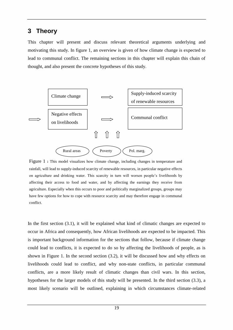
This chapter will present and discuss relevant theoretical arguments underlying and

motivating this study. In figure 1, an overview is given of how climate change is expected to

lead to communal conflict. The remaining sections in this chapter will explain this chain of

thought, and also present the concrete hypotheses of this study.

In the first section (3.1), it will be explained what kind of climatic changes are expected to

occur in Africa and consequently, how African livelihoods are expected to be impacted. This

is important background information for the sections that follow, because if climate change

could lead to conflicts, it is expected to do so by affecting the livelihoods of people, as is

shown in Figure 1. In the second section (3.2), it will be discussed how and why effects on

livelihoods could lead to conflict, and why non-state conflicts, in particular communal

conflicts, are a more likely result of climatic changes than civil wars. In this section,

hypotheses for the larger models of this study will be presented. In the third section (3.3), a

most likely scenario will be outlined, explaining in which circumstances climate-related

Poverty Pol. marg. Rural areas

Climate change Supply-induced scarcity

of renewable resources

Negative effects

on livelihoods Communal conflict

Figure 1 : This model visualizes how climate change, including changes in temperature and

rainfall, will lead to supply-induced scarcity of renewable resources, in particular negative effects

on agriculture and drinking water. This scarcity in turn will worsen people’s livelihoods by

affecting their access to food and water, and by affecting the earnings they receive from

agriculture. Especially when this occurs to poor and politically marginalized groups, groups may

have few options for how to cope with resource scarcity and may therefore engage in communal

conflict.

20

conflict is most likely to occur. Hypotheses for the most likely scenario are also presented.

Finally, in the fourth section (3.4), all the hypotheses tested in this study will be summarized.

3.1 Impact on livelihoods in Sub-Saharan Africa

Climate change is found to impact Africa in a variety of ways. According to the Fourth

Assessment Report of the Intergovernmental Panel on Climate Change (IPCC), Africa will

likely experience higher temperatures, less rain in some regions, more rain in other regions,

more extreme events (such as storms, sustained droughts and floods) as well as ecosystem

changes (such as increasing of arid- and semiarid lands and sea level rise) (Boko et al. 2007).

These effects are, in their turn, likely to impact livelihoods of people.

As temperature and rainfall are used as proxies of climate change in this study, a brief

overview will now be given of how the changes in temperature and rainfall will differ across

different regions in Africa. All across Africa, in all seasons, temperatures are very likely to

increase between 3˚C-4˚C during the next century (Christensen et al. 2007:867). These rises

are higher than the global average of approximately 2˚C (ibid). Dry subtropical regions, in

particular the western part of the Sahara, will see the highest increases (around 4˚C), while

coastal areas and moister tropics such as equatorial areas will see increases of approximately

3˚C (Christensen et al. 2007:866-867). Compared to temperature, changes in rainfall will vary

more across different regions in Africa. North Africa including Northern Sahara will see

considerably less rainfall (Christensen et al. 2007:868). Also the extreme southwest of Africa

is very likely to see less rainfall in winter (Christensen et al. 2007:868). On the other hand,

East Africa is likely to see increased rainfall (Christensen et al. 2007:869). Notably, changes

in rainfall in the Sahel, Southern Sahara and the Guinean cost are still unknown (Christensen

et al. 2007:850, 869-871).

The Fourth Assessment Report lists examples of how the livelihoods of people may be

impacted. For instance, droughts and higher temperatures may in many cases decrease

agricultural productivity (Boko et al. 2007:439, 447-448), which in turn means less food and

earnings for farmers and herders. However, in some regions agricultural production may also

increase as a consequence of higher temperatures (Boko et al. 2007:447-448). The effects on

agricultural production are important as the portion of GDP that agriculture contributes with

21

varies between 10-70% across African countries (Boko et al. 2007:439). Higher temperatures,

together with other effects of climate change such as changes in freshwater flows, may also

decrease fish stocks, although this is likely to depend on human management of the water

resources (Boko et al. 2007:448). If fish stocks decrease, it will mean less food and earnings

for fishers. Furthermore, climate change is likely to increase water stress in Northern and

Southern Africa, while East and West Africa may see increased water availability (Boko et al.

2007:444-445). On the other hand, extreme weather events may cause shocks for populations

across the continent for instance by damaging infrastructure (Boko et al. 2007:439-440, 450).

Ecosystem changes like sea level rise may amongst other things decrease fish stocks (Boko et

al. 2007:449-450), meaning less food and earnings for fishers. Sea level rise may also threaten

populations living in coastal cities in Africa, most notably poor populations (Boko et al.

2007:450). Finally, all the effects on livelihoods may lead to migration (Boko et al.

2007:450). In sum, climate change will mostly impact livelihoods through water availability

and food production, and maybe also some through effects on infrastructure and migration.

It is important to note, however, that there are also a number of uncertainties related to both

the predicted effects of climate change and the predicted effects on African livelihoods. For

instance, temperature predictions vary between different estimations (Boko et al. 2007:443),

precipitation predictions are relatively uncertain for the whole of Africa (Boko et al.

2007:443), and the development of agricultural production is hard to predict even without

climate change (Boko et al. 2007:448). Despite these uncertainties in magnitude, Africa is

very likely to see climatic changes (see summary by Christensen et al. (2007:4)) and there is a

good possibility that African livelihoods will be impacted by these changes (Boko et al.

2007:450).

Furthermore, Africa is also considered especially vulnerable to climate change because of a

range of social, political and economic factors that affect the livelihoods and adaptation

capacities of the African societies (Boko et al. 2007:454). For example poverty can limit

people’s coping strategies, such as their possibilities to change income source as a response to

environmental stress (Adger and Kelly 1999:258-260). Consequently in Africa, due to

widespread poverty, many poor farmers whose crops are not resilient to climate change may

not have the capacity to change the crops they grow to more heat or drought tolerant crops, or

to seek employment in other sectors outside agriculture. Moreover, herders, whose cattle may

22

suffer from decreasing amounts of grazing land and drinking water, may also be likely to have

few options to seek alternative employment.

3.2 Violent conflict

In this section, it will be discussed how changes in livelihoods caused by climate change,

especially resource scarcity, may lead to conflict, and what type of conflict is most likely to

occur. This discussion firstly looks at the sources of scarcity (section 3.2.1) and thereafter on

the consequences of scarcity (section 3.2.2). Next, section 3.2.3 argues for why communal

conflict is the most likely type of conflict to occur as a consequence of resource scarcity.

Finally, section 3.2.4 presents hypotheses for this study.

3.2.1 Sources of scarcity

Ullman (1983) was one of the first scholars to address the issue of resource scarcity leading to

increased insecurity, and was thus one of the key scholars behind the term “environmental

security”. He argued that especially population growth would lead to resource scarcity, which

again would constitute a security threat. Ullman also discussed scarcity in the supply of

resources, which originated amongst other things from the overuse of certain resources like

forests, fish, and seed crops (Ullman 1983:143-145).

Moreover, Thomas Homer-Dixon and his research group at the University of Toronto were

among the first to study environmental security empirically (see literature review in Chapter

2). Homer-Dixon defined three sources of environmental scarcity: supply-induced scarcity,

demand-induced scarcity and structural scarcity (Homer-Dixon 1999:14-16). These terms

were explained in section 1.1.2. For the framework of this study, supply-induced scarcity is of

core interest. Many of the effects of climatic changes on African livelihoods, including

negative effects on agricultural production and water supplies, diminish the supply of critical

renewable resources. However, demand-induced and structural scarcities are also taken into

account in this study through trying to control for their effects by using control variables such

as population and politically and economically marginalized groups.

It is also important to note, that Homer-Dixon (1994:7-8) argued primarily for environmental

changes such as “degradation and depletion of agricultural land, forests, water and fish” to be

related to conflict, and stated that climate change was not among the phenomena most likely

23

to cause conflict. This statement was based on the argument that the effects of climate change

would not be felt for decades, and its effects would “most likely operate not as individual

environmental stresses, but in interaction with other, long-present resource, demographic,

and economic pressures that have gradually eroded the buffering capacity of some

societies” (Homer-Dixon 1994:7-8).

However, the study presented in this thesis is based on the logic that by studying climatic

changes in the past it will be possible to understand climatic changes’ potential to cause

conflict also in the future, when the effects of anthropogenic climate change will become most

clearly visible8. Furthermore, it is argued that effects of climate change, such as temperature

and precipitation changes, may indeed act as “individual environmental stresses” through

their effects on livelihoods, at least to the same degree that Homer-Dixon argues that

scarcities of agricultural land, forests, water and fish act (see section 3.2.2). Thus Homer-

Dixon’s theoretical arguments are seen to speak in favor of also climatic changes leading to

conflict.

3.2.2 Consequences of scarcity

On way scarcity of renewable resources may lead to conflict, is if groups start fighting over

scarce resources, or access to scarce resources. Several conflicts in developing countries,

including conflicts between pastoralists and between pastoralists and farmers, have been

described as conflicts over scarce resources such as land and water (see for instance Homer-

Dixon (1994), Bächler (1998), Kahl (2006), Suliman (1999)). For instance, Suliman

(1999:34) argues that the conflicts in Darfur in western Sudan can be explained as a result of

resource competition between farmers and herders. He notes that the droughts in 1983-1984

led herders to use the land of farmers to a much higher extent than before, and this eventually

led to conflict between the groups. Moreover, Kahl (1998) argues that the ethnic violence in

Kenya in 1991-1993 was possible due to scarcity of crop land. According to Kahl, the ethnic

clashes were arranged by President Moi and his allies, who felt threatened by an ethnically

united opposition which demanded increased democratization. To arrange the clashes, the

authorities played on the lack of good-quality crop land and old grievances relating to the

division of crop land.

8 See section 4.9 for a discussion on this logic.

24

Another way scarcity of renewable resources may lead to conflict is that groups may also

wish to change national or local laws and regulations in order to get a better long term access

to resources. In that case, groups would arguably need to direct their demands towards local

or national authorities. Homer-Dixon (1994:24) notes, that frustration over lack of resources

may breed willingness among groups to challenge the state. Therefore, if non-violent means

of trying to impact laws and regulations regarding for instance land ownership prove

ineffective, groups may arguably rebel. However, challenging the state is very costly, and in

section 3.2.3 it will be discussed more in detail under which circumstances rebellion against

the state would be possible, and why groups suffering from resource scarcity are more likely

to challenge other groups than to challenge the state.

Furthermore, negative economic effects due to degradation of the environment can lead to

increased poverty. These negative effects can occur for instance when increases in

temperature or decreases in rainfall decrease agricultural productivity, as explained in section

3.1, and thus also decrease the income and nutrition that households gain from farming.

Facing increased poverty may in turn increase the willingness of a group to fight the state.

Poverty, measured by low per capita income and low economic growth rates, has been found

to be robustly correlated to the onset of civil war (Hegre and Sambanis 2006). However, it can

be argued that increased poverty may also increase a group’s willingness to fight other

groups, if other groups have better access to resources and fewer restraints on food

production. It has been noted, namely, that in addition to absolute scarcity, i.e. lacking

resources that one needs, also relative scarcity may increase the risk of conflict (see Fjelde

and Uexkull (2012:446-447) and Raleigh (2010:79)).

Both absolute and relative scarcity can be classified as grievance-based potential reasons for

conflict. The question of whether greed or grievance causes conflict is extensively researched

in relation to civil war (see for instance (Gurr 1970), (Collier and Hoeffler 2004) and (Regan

and Norton 2005)). Yet, the discussion is arguably equally relevant when studying non-state

conflicts, such as communal conflicts. Notably, the arguments presented in this chapter are

supportive of grievance, rather than greed, explaining climate change –induced conflict.

25

Resource scarcity has also been argued to lead to conflict through migration. As the

renewable resources which are necessary for maintaining a livelihood, including water and

yields from agriculture, get too scarce, people will migrate into areas with more resources.

According to Homer-Dixon (1994:20), when groups, who suffer from environmental scarcity,

migrate to new areas to get better access to resources, this migration can result in conflicts

between the migrating group and groups who already live in the new area. However, in this

thesis, the issue of scarcity-caused migration leading to conflict is not addressed explicitly.

Doing so would require analyzing quantitative data which already follows a potential causal

path from resource scarcity to migration and further to conflict, and this kind of an analysis

was beyond the capacity of this study9.

Furthermore, it is important to note, that environmental factors are never likely to be the only

explanatory factors for conflict, as emphasized by Homer-Dixon. Rather, environmental

scarcity combined with a range of social, political and economic factors could lead to conflict

(Homer-Dixon 1999:16). Despite the importance of social, political and economic factors,

Homer-Dixon still saw that environmental factors can be independent triggers of conflict. To

find out whether environmental factors can be seen as independent triggers of conflict, as

Homer-Dixon argues, this study will test whether climatic changes correlate with communal

conflict when several social, political and economic variables are controlled for. All of the

control variables will be presented and discussed in chapter 4.

3.2.3 Communal conflict vs. civil war

There are good reasons to expect that if a link between climate change and conflict exists, it is

to be found between climate change and communal conflicts rather than between climate

change and civil wars. In section 3.2.2 different climate change –induced reasons for

engaging in violent conflict were discussed, and these included gaining access to scarce

resources which another group holds, and changes in national or local laws and regulations in

order to improve a group’s access to scarce resources. Thus this section will concentrate on

discussing firstly, why civil wars are a less likely consequence of climate change than non-

state conflicts (section 3.2.3.1) and secondly, why communal conflict is the most likely type

of non-state conflict to occur (section 3.2.3.2).

9 Reuveny (2007) has done a qualitative variant of this kind of study by studying cases of environmental

migration and whether they led to conflict in the migrant-receiving area.

26

3.2.3.1 Non-state conflict vs. civil war

As Hendrix and Salehyan (2012:37) argue, referring to Maxwell and Reuveny (2000), civil

war does not lead to an increase in the absolute amount of resources a state has. Therefore,

what a civil war can affect is the distribution of resources. Hendrix and Salehyan continue by

arguing that this means that engaging in war against the government is not logical for a group

suffering from resource scarcity. They write that “often times, groups will find neighboring

communities, rather than the government, the most appropriate target for making demands;

this is especially true if the state is known to be unwilling or unable to redistribute resources

in a society” (Hendrix and Salehyan 2012:37). This can be seen as a feasible argument if the

state is unable to redistribute resources. However, the state’s unwillingness to distribute

resources is something that a suffering group in theory could try to affect, even through war if

negotiations or other peaceful means prove insufficient. Next it will be discussed a bit deeper

why the state’s unwillingness to distribute resources nevertheless unlikely would lead to civil

war.

As Raleigh and Kniveton (2012:53) point out, groups that engage in civil war want to

overthrow the current regime. Groups that suffer from resource scarcity, on the other hand,

will not necessarily want to overthrow the regime, but only improve their own livelihoods.

Simultaneously, one can imagine that overthrowing the government and taking power of the

whole state would enable scarcity affected groups to change laws and regulations for their

own benefit. Thus engaging in civil war could be a viable option. However, this is where the

conditions for a conflict become important and help explaining why scarcity-affected groups

are more likely to fight other groups, i.e. engage in non-state conflict, than to engage in civil

war.

First off, it is very costly for any group to engage in a civil war because the government is

likely to have a relatively strong military force (Hendrix and Salehyan 2012:37). Thus only

strong groups have the possibility to start a civil war, and not the weak groups that are the

most likely to suffer from resource scarcity (see for instance Raleigh (2010)). Also, it is not

just the strength of the government’s forces that is important in determining the cost of

engaging in civil war. Militias fighting the state also need to be able to provide protection to

the individuals and groups who participate in the insurgency (Regan and Norton 2005:324). In

addition, they also need to afford to pay the warriors participating in the insurgency.

27

According to Regan and Norton (2005:324), common people are highly unlikely to participate

in civil war only out of a moral conviction for the cause. This point reflects the emerging

consensus in the literature on causes of civil wars that grievances alone cannot explain civil

wars (Hendrix and Salehyan 2012:37). The costs for people to participate are so high (e.g.

threats from government forces) that they will need to be paid well by the militias in order to

keep them fighting (Regan and Norton 2005:323). Thus only relatively wealthy groups can

have the capability to engage in civil wars.

On the other hand, for less strong groups suffering from resource scarcity, smaller forms of

conflict may be an option. The cost of fighting another group of people (e.g. a pastoralist

group fighting farmers over access to land and water) is arguably lower. According to Regan

and Norton (2005:324), when the costs are lower, experienced grievances (e.g. a

discrimination in division of resources) may be a sufficient reason for starting a conflict.

However, Regan and Norton talk about nonviolent forms of protest as conflicts with low costs

and civil wars as conflicts with high costs. Thus it is unsure where non-state conflicts would

be placed on Regan and Norton’s threshold for greed/grievance motivated conflicts, i.e.

whether they believe grievances would be enough to cause non-state conflicts.

Yet, reflecting on points made earlier in this section, good arguments can be presented for

why grievances could be enough to cause non-state violence. Firstly, the costs for individuals

engaging in non-state violence are likely to be lower than when participating in civil war, as

the counterpart (the group that one fights against) most often will be much less strong than

government forces. Thus the individuals are not likely to feel a similar need for protection as

when participating in civil war. Secondly, when the individuals do not feel a similar need for

protection, the leaders of a fighting group do not have the same need to get access to

resources, e.g. diamonds, to finance their soldiers. Thus the economic threshold for starting a

conflict is lower for non-state conflicts than for civil wars.

It is time to return to the question over who groups will fight if they find violence necessary to

ease their resource scarcity. Looking at the purpose of a conflict, groups could gain from both

fighting the state and fighting other groups. However, looking at the conditions for a conflict,

fighting other groups is likely to be the only executable option. As the discussion above has

shown, “for most aggrieved actors, most of the time, rebellion is not a viable option” (Hendrix

28

and Salehyan 2012:37). Therefore, if climate change –caused resource scarcity will lead to

violent conflicts, these conflicts are more likely to be non-state conflicts than civil wars.

3.2.3.2 Communal conflict vs. other types of non-state conflicts

Non-state conflicts can occur between very different types of groups and for different reasons,

including resource scarcity. This thesis argues that communal conflict is the most likely type

of non-state conflict to occur as a result of climate change –induced resource scarcity. This is

because other types of non-state conflicts are probably better explained by other factors, as

also argued by Fjelde and Uexkull (2012:447).

The UCDP non-state conflict database which is used in this study to separate between

different types of non-state conflicts has separated between three types according to the

conflicting parties levels of organization. The first type of non-state conflict is conflict

between “highly organized rebel groups” (Pettersson 2012:4). The second type is between

“groups composed of supporters and affiliates to political parties and candidates”, and

“captures fighting between political parties/candidates and lethal electoral violence”

(Pettersson 2012:4). The third type, which is referred to as communal conflict, is conflict

between “groups that share a common identification along ethnic, clan, religious, national or

tribal lines” (Pettersson 2012:4).

Violence between rebel groups is argued to occur as a way for the groups to become more

powerful in their struggle against the government (Fjelde and Nilsson 2012). Moreover,

having a highly organized rebel organization requires large resources, as was argued for in the

previous section (3.2.3.1). Poor and marginalized groups, who are argued in this thesis

(section 3.3) to be most likely to suffer from resource scarcity, often do not have such

resources. Therefore, they are unlikely to be represented by highly organized rebel groups and

consequently unlikely to engage in fighting with another rebel group in order to ease their

resource scarcity.

Electoral violence, in turn, may occur either because groups are against elections in general,

because groups are against the electoral system which is applied, or because groups wish to

affect the results of the elections (Höglund 2009:415-416). In relation to resource scarcity,

electoral violence could occur because groups wish to affect results of elections, e.g. to

29

change the parties in power into parties that promise changes in distribution of necessary

renewable resources. However, those groups which this thesis proposes to be most likely to

suffer highest from resource scarcity are politically marginalized and therefore least likely to

be able to affect national politics. Therefore, those groups do not have a purpose to use

resources for trying to affect the outcome of national elections. Thus electoral violence is not

seen as the most likely type of violent conflict to occur as a consequence of resource scarcity.

Instead, communal conflicts may occur between groups who are marginalized and poor, as

none of the groups participating in communal conflicts will by definition10

have highly

organized fighting organizations, and because groups may see a realistic chance to improve

their situation regarding scarce resources by fighting another group. Therefore, the arguments

presented in this thesis for how climate change could lead to conflict, fit best for communal

conflict.

3.2.4 Hypotheses

Based on the discussions above, four hypotheses will be tested. The first hypothesis is based

on the notion that higher temperatures may lead to negative consequences for agriculture, as

noted in section 3.1, which again can lead to conflict, as discussed in section 3.2.2:

H1a: Higher temperatures in one year will increase the likelihood of communal

conflict events in the same year

However, the negative consequences of higher temperatures on agricultural production will

not be felt immediately. It takes some months for agricultural crops to grow and produce

yield, and thus farmers need to store food from one yield to the next. Following this logic, the

following hypothesis is added:

H1b: Higher temperatures in one year will increase the likelihood of communal

conflict events in the following year

10

The following is noted in Pettersson (2012:4) about groups participating in communal conflicts: “These are

not groups that are permanently organized for combat, but who at times organize themselves along said lines to

engage in fighting”.

30

Yet, bearing this logic in mind, what might make a conflict start in the same year that scarcity

occurs, is people’s awareness of the coming resource scarcity. Thus it is meaningful to

statistically analyze the effects of climatic changes both on communal conflicts in the same

year and in the next year, as reflected in the hypotheses above. This logic also applies to the

hypotheses below.

Moreover, also too little rainfall may have negative effects for agriculture and for livestock

keeping, as noted in section 3.1. These negative effects can again lead to conflict, as discussed

in section 3.2.2. Consequently, the following hypothesis is developed:

H2a: Lower rainfall will increase the likelihood of communal conflict events in the

same year

However, neither negative consequences of low rainfall on agriculture will be felt

immediately, for the same reasons as explained regarding temperature changes. Thus the

following hypothesis is added:

H2b: Lower rainfall will increase the likelihood of communal conflict events in the

following year

3.3 Most likely scenario

In this section, a most likely scenario for a climate change induced communal conflict will be

described. The idea behind designing a most likely case is that if climatic changes have the

potential to cause conflicts, this will most likely happen in the circumstances described in this

scenario. These circumstances are when people belong to social or ethnic groups, which are

politically marginalized, when poverty is widespread, and when people live in rural areas.

The basis for this most likely scenario resembles the arguments by Fjelde and Uexkull (2012),

who study rainfall and communal conflict in Sub-Saharan Africa. Fjelde and Uexkull expect

the possibility of communal conflict to increase with the presence of marginalized groups and

poverty. However, what makes the study of this thesis different is that instead of only

controlling for marginalized groups and poverty, as Fjelde and Uexkull, the most likely

31

scenario in this study is designed so that only grid cells, where a marginalized group and

poverty are present, and which are considered to be in rural areas, are included in the analysis.

This way the effects of climatic changes on communal conflict should, if they exist, not be

overshadowed by grid cells where climate change –induced communal conflict is highly

unlikely. These include grid cells over urban areas and grid cells over desert and other non-

populated areas.

3.3.1 Marginalized groups

According to Raleigh (2010:70), politically and economically marginalized groups facing

resource scarcity may have few other options to improve their situation than to fight against

other groups to get more resources. On the other hand, groups who have more influence over

politics or are seen by the government as more important, get more help from the government

when facing resource scarcity than marginalized groups (Raleigh 2010:70) and will thus

likely not consider violence an option to cope with resource scarcity. Thus, following this

logic, it is not resource scarcity per se that may make people fight, but their lack of other

options to cope with scarcity.

In addition, marginalized people often live in areas which are poor and have few public

services and where living environments are challenging, for example arid- and semi-arid lands

(Raleigh 2010:73,77). These areas are also expected to be hardest hit by climate change and

disasters (Raleigh 2010:73). These facts can make marginalized groups under increased

conflict risk, as it is widely noted in the literature that groups suffering from a combination of

physical and social vulnerability are more prone to conflict (Raleigh 2010:71).

3.3.2 Poverty

Poverty is found to robustly increase the risk of civil war (Hegre and Sambanis 2006). Yet, it

may also be likely to increase the risk of communal conflicts, as discussed in section 3.2.2.

The poor are also likely to be hardest hit by climatic changes (Raleigh 2010:72) and they

often also have the lowest capacity to adapt to the changes (Adger and Kelly 1999).

Furthermore, the poor are argued to have least to lose by engaging in violent conflict, making

violent conflict more likely where there is poverty (Fjelde and Uexkull (2012)). In addition,

Fjelde and Østby (2012) have found that economic inequality increases the risk of non-state

32

conflicts. However, it is important not to mix poverty with economic inequality, as poverty

refers to poverty in absolute terms, i.e. living under a certain poverty limit or lacking

necessary resources, while economic inequality means that some groups are poor compared to

other groups. Thus the finding by Fjelde and Østby (2012) does not illuminate whether poor

groups, who live in an area where other groups are relatively poor as well, are any more likely

to engage in non-state conflict than richer people are. However, for reasons outlined above, it

is reasonable to expect that they are.

3.3.3 Rural areas

Climate change –induced conflict is also more likely in rural than urban areas. According to

Raleigh (2010:76), government’s are more likely to react to urban trouble than rural, such as

food shortages, because urban populations are often seen as politically more relevant than

rural populations. Rural populations are easier to ignore than urban population, because riots

or violence in urban areas are seen to be more threatening to the elites than rural unrest

(Raleigh 2010:76). Consequently, being ignored by the state, rural groups are often

marginalized and, facing resource scarcity, may have few other options than to engage in

violent conflict in order to improve their situation, in the same way as marginalized groups, as

pointed out in section 3.3.1.

Secondly, rural populations in Sub-Saharan Africa are often highly dependent on income from

agriculture (Chauvin et al. 2012). As urban populations have different and more varied

income sources, lower agricultural productivity and water shortages are arguably likely to

impact rural populations harder and earlier than urban populations. Urban populations may

also suffer as a consequence of declining agricultural production when food prices increase

(Hendrix and Salehyan 2012:38), but they are still likely to be effected later than rural people

and, as noted above, to be protected better by the state than rural people (Raleigh 2010:76).

33

3.3.4 Hypotheses for the most likely scenario

Based on the discussion above, the following hypotheses are added:

H3a: Higher temperatures in one year will increase the likelihood of communal conflict

events in the same year in rural grid cells hosting marginalized groups where the level of

poverty is high

H3b: Higher temperatures in one year will increase the likelihood of communal conflict

events in the next year in rural grid cells hosting marginalized groups where the level of

poverty is high

H4a: Lower precipitation in one year will increase the likelihood of communal conflict

events in the same year in rural grid cells hosting marginalized groups where the level of

poverty is high

H4b: Lower precipitation in one year will increase the likelihood of communal conflict

events in the next year in rural grid cells hosting marginalized groups where the level of

poverty is high

3.4 Summary of hypotheses

Larger models:

H1a: Higher temperatures in one year will increase the likelihood of communal conflict

events in the same year

H1b: Higher temperatures in one year will increase the likelihood of communal conflict

events in the following year

H2a: Lower precipitation will increase the likelihood of communal conflict events in the same

year

34

H2b: Lower precipitation will increase the likelihood of communal conflict events in the

following year

Most likely scenario:

H3a: Higher temperatures in one year will increase the likelihood of conflicts in the same

year in rural grid cells hosting marginalized groups where the level of poverty is high

H3b: Higher temperatures in one year will increase the likelihood of conflicts in the next year

in rural grid cells hosting marginalized groups where the level of poverty is high

H4a: Lower precipitation in one year will increase the likelihood of conflicts in the same year

in rural grid cells hosting marginalized groups where the level of poverty is high

H4b: Lower precipitation in one year will increase the likelihood of conflicts in the next year

in rural grid cells hosting marginalized groups where the level of poverty is high

35

4 Methods

4.1 Introduction

This chapter will present and discuss the methodological choices of this study.

Methodological choices are important because they determine what kind of information it is

possible to retrieve from a study. For example, the use of qualitative method allows the

researcher to study details of a phenomenon deeply and try to understand the views of the

people he/she studies. On the other hand, quantitative method, which is utilized in this study,

allows the researcher to study for example the opinions of thousands of people and to

generalize from the results. (Bryman 2008)

More specific methodological choice, such as which statistical methods to use, which control

variables to use and how to measure the dependent and independent variable are also very

important. They determine whether a researcher succeeds in measuring exactly what he/she

aims to measure, and whether he/she has taken relevant alternative explanations into account.

For example, in quantitative climate change and conflict studies, discussions of

methodological choices have revealed premature conclusions. This is illustrated by the debate

between Homer-Dixon (1994) and Gleditsch (1998), and between Burke et al. (2009); (2010)

and Buhaug (2010a); (2010b) (both debates are discussed in chapter 2). Discussions of

methodological choices have also helped to bring studies on climate change and conflict

forward, for instance by introducing disaggregation of the unit of analysis, which is discussed

in section 4.3 in this chapter.

This chapter will proceed in the following way. First it will discuss why quantitative method

is used instead of qualitative in this study (section 4.2). Next, it will discuss why the analyses

are disaggregated, and why a grid cells structure is used (section 4.3). Thereafter, it will

present the data structure which is used (section 4.4) and the sampling which is conducted

(section 4.5) before presenting which variables are chosen and how they are operationalized

(section 4.6). Furthermore, it will explain why logistic regression is chosen as the specific tool

for conducting the analyses (section 4.7), and also which methodological challenges the study

faces (section 4.8). Finally, it will discuss a few limitations related to the study (section 4.9).

36

4.2 Quantitative vs. qualitative method

US President Barack Obama has said that “more frequent droughts and crop failures breed

hunger and conflict” (Obama 2009:1). His statement illustrates a popular narrative11

according to which climate change causes conflicts. Scientific research, however, has not yet

found enough robust evidence to back this claim (see Gleditsch (2012:7), Salehyan (2008)

and Bernauer et al. (2012)). For studying the claim scientifically, it is meaningful to start with

looking at whether climate change and conflicts are associated on a wider scale. This study

aims to contribute to the knowledge on whether there is a general association between climate

change and conflict in Sub-Saharan Africa, and therefore quantitative research method is the

appropriate choice.

Quantitative method has the advantage of enabling the study of phenomena in a highly

consistent manner. More precisely, it allows researchers to make sure they measure and

analyze phenomena in the same way across studies conducted by different researchers and in

different points in time (Bryman 2008:144). This consistency is arguably important in order to

compare results of different studies and to draw conclusions based on them. In addition,

quantitative method enables researchers to detect “fine differences” (Bryman 2008:144). For

instance, in conflict research quantitative studies can compare the intensity of conflicts by

measuring the amount of battle-related deaths between conflicts. Furthermore, quantitative

method also enables researchers to make “more precise estimates of the degree of relationship

between concepts” (Bryman 2008:144). In climate change and conflict studies this means that

it is possible to conduct statistical analyses on data about climate and conflicts and to see

whether and to what degree changes in climate and conflict are related. Notably, it is also

possible to check whether a possible correlation between climate variables and conflict is

caused or affected by a third variable, i.e. a spurious effect.

Finally, quantitative method allows researchers to generalize conclusions from a sample,

given that proper sampling criteria have been followed (Bryman 2008:156). This means that it

is not necessary to gather data on for instance all of the African population on the variables of

interest to say something about the whole of Africa. Instead, it is sufficient to gather

information on a representative sample of the African population and to generalize the results

from the sample to the whole population. In this study, random sampling was done when a

11

See for example Benjaminsen (2009) for an overview

37

subset of grid cells without communal conflict events was chosen, as will be explained in

section 4.5.

Qualitative method has also been useful in studying the climate-conflict relationship, but it

cannot illuminate the issue on an equally large scale since a qualitative study often cannot be

generalized beyond the particular case studied (see Bryman (2008:391-392)). So far,

qualitative case studies have been successfully used to give indications on whether and how

climate and conflict may be related in certain places, and what other factors affect the climate-

conflict relationship (examples of case studies are presented in sections 2.4.3 and 3.2.2).

Despite varying results, case studies have informed quantitative studies for instance by

inspiring hypotheses (e.g. Homer-Dixon (1994)) and giving ideas for control variables, in

addition to providing thorough analyses on the particular cases studied. Yet, as this study

looks for a general pattern between climate change and conflict, qualitative method including

case study is not the appropriate choice.

4.3 Disaggregation using a grid cells structure

In this study, the relationship between climate change and communal conflicts will be studied

on a disaggregated level, i.e. on a lower geographical level than the nation state. This section

will discuss the role of disaggregation in the conflict literature, the benefits of disaggregation

and the benefits of using grid cells as a tool for disaggregation.

4.3.1 Benefits of disaggregation

In the study of conflicts, the focus has in recent years moved from using whole countries to

using smaller geographical areas as the units of analysis (Tollefsen et al. 2012:363-364).

Studies have used several different types of units including first order administrative entities

within countries, i.e. provinces and districts (e.g. Fjelde and Uexkull (2012), Østby et al.

(2009), Rustad et al. (2011), Urdal (2008)), conflict zones (e.g. Buhaug and Gates (2002)),

social groups (e.g. Buhaug et al. (2008)), and grid-cells (e.g. Buhaug and Rød (2006), Raleigh

and Urdal (2007), and Theisen (2012)).

Disaggregation has at least two important benefits over country-level analysis. Firstly,

disaggregation allows studies to focus on those geographical areas where conflicts actually

are fought. “Fighting rarely spans entire countries”, as noted by Buhaug and Lujala

38

(2005:403) regarding civil wars. Furthermore, it is typical for civil conflicts to be fought in

remote rural areas, close to borders with other countries (Rustad et al. 2011:19). Secondly,

conflict areas seldom have the same characteristics as the country on average. Thus, if one

tries to find out which social, political, economic, demographic or geographic factors are

related to a conflict that is limited in geographic scope, but one studies the national averages

of these factors, the results are likely to be misleading (Buhaug and Lujala 2005:404). Instead,

using disaggregated data on both conflicts and different explanatory and control variables

makes it possible to better capture the variables that correlate with conflict.

These arguments can be illustrated with an example provided by Buhaug and Lujala

(2005:404). They write that none of the conflicts that India has seen since 1990 have taken

place on more than 5% of the country’s total area. Using country-level variables (i.e. national

averages of the level of economic development, geographical terrain, changes in temperature

etc.) do not make it possible to understand differences between these conflicts. Consequently,

a study of these Indian conflicts and possible explanatory variables needs to occur on a lower

geographical level than the entire nation state to provide some explanations. These arguments

are equally relevant, if not even more relevant when studying communal conflicts, as

communal conflicts are likely to be fairly local phenomena. Many countries have also

experienced several communal conflicts (see Sundberg et al. (2012)).

However, counter-arguments have also been presented. Hendrix and Salehyan (2012:38)

argue for the benefits of country-level analysis, rather than disaggregation, in studies of

climate change and conflict, because “many of the most significant effects are likely to be felt

across the country”. Examples of such effects are droughts that cause people to migrate from

rural areas to the cities. Notwithstanding these remarks, disaggregation is in this study judged

to have most arguments in favor when studying communal conflicts.

4.3.2 Benefits of grid cells

Using grid cells also has several benefits compared to other types of disaggregation. Grid cells

are artificially constructed units (section 4.4 will describe this more in detail). They are all of

equal sizes, they are apolitical and they are not determined by any specific social,

demographic, or geographic characteristic (Tollefsen et al. 2012:365). Thus they may be used

without taking any of the above mentioned characteristics into account (Rustad et al.

39

2011:25). This implies that the units of analysis are fully independent on any characteristics,

such as demography, that one may wish to use as independent variables (Tollefsen et al.

2012:365). In addition, their sizes can be changed depending on the researcher’s needs

(Tollefsen et al. 2012). Furthermore, as Theisen (2012:87) points out, it is easier to “model

dependence between observations” when the cells are of identical sizes.

Other ways of disaggregation are less beneficial for this study for reasons presented below.

First-order administrative units, such as provinces and districts, vary in form and political

function between countries and between different points in time. Thus it may be hard for the

researcher to stay on track of all of these differences (Tollefsen et al. 2012:365). It may also

be hard to get information on how the administrative units have changed over time (Rustad et

al. 2011:25). Moreover, first-order administrative units are can be of highly varying sizes. As

a consequence, the analysis of for instance climate and conflict within these units will be

disaggregated to different degrees: in administrative units that encompass a small surface area

the spatial resolution for variables will be high, whereas in administrative units with a large

surface area the spatial resolution will be much lower.

Furthermore, using conflict zones as units of analysis was not possible in this study, because

using conflict zones as the unit of analysis means that no areas without conflict are included

in the analysis. In studies where one is interested for instance to study the duration of conflicts

on a disaggregated level, it may be beneficial to use conflict zones as units of analysis (see for

instance Rustad et al. (2008)). However, this was not the case for this study and therefore

conflict zones were not an option.

Using social groups as units of analysis firstly suffers from the lack of disaggregated data on

other types of groups than ethnic groups (Rustad et al. 2011:25). Secondly, using social

groups would mean concentrating the analysis on previously known groups (such as ethnic

and religious groups). This would in turn imply that one would effectively rule out the

possibility to grasp correlations between climatic changes and communal violence between

new forms of groups, for example groups with mixed ethnic and religious characteristics.

Buhaug et al. (2008) use ethnic groups as their units of analysis, but in their study it makes

sense because they expect ethnic group characteristics to largely explain the occurrence of

civil conflict, and ethnic groups are consequently also chosen as their independent variable.

40

However, in this study the independent variables are changes in climatic effects such as

precipitation and temperature. Therefore using social groups as units of analysis might limit

the validity of the analysis for the reasons mentioned above.

Using grid cells have also been noted to suffer from some limitations. Since the grid cells are

apolitical and independent from all other kinds of social factors, they ignore “important

societal cleavages that follow sub-national boundaries” which might be a problem for

grasping conflict dynamics in some cases (Rustad et al. 2011:25). However, this limitation is

in this study attempted to be overcome by using different group characteristics and cleavages

as control variables, such as income level and marginalized groups. Moreover, despite their

limitations, grid cells are still viewed to be the best of the options available based on the

discussion above.

4.4 Data structure

In order to analyze variables on a disaggregated level using grid cells, this study utilizes the

PRIO-GRID unified spatial data structure (Tollefsen et al. 2012)12

. The PRIO-GRID divides

the world into grid cells based on longitudes and latitudes, and there are several cells within

each country. The cells are sized 0.05˚ x 0.05˚ degrees, corresponding to 55km x 55km at the

equator. Furthermore, the cells give information on specific variables (e.g. whether a conflict

occurred or not) for one year at the time. Thus the structure of PRIO-GRID is a year – grid

cell structure. (Tollefsen et al. 2012)

Moreover, the PRIO-GRID contains data on many variables, such as temperature and rainfall

values (the independent variables of this study) and several variables which are used as

control variables in this study. The data for these variables is given per grid cell. However, as

PRIO-GRID does not contain data on all the variables used in this study, a new dataset was

created by expanding the PRIO-GRID with data on communal conflict events (the dependent

variable of this study) and several control variables. Some of these variables have data on a

disaggregated level, while data for other variables was only available on a country level. More

information on this will be given when the specific variables are discussed (see section 4.6).

Furthermore, the new dataset has excluded grid cells outside Sub-Saharan Africa and years

12

http://www.prio.no/Data/PRIO-GRID/

41

before 1989, because the data on communal conflict events that is used in this study is

available only from 1989. To see which countries are counted as part of Sub-Saharan Africa,

see Appendix A.

4.5 Sampling

In this study, sampling was conducted for grid cells in which there were no communal

conflict events. The sample was taken from the full dataset which includes all grid cells in

Sub-Saharan Africa. A sample was taken from the full dataset in order to deal with the

problem of spatial correlation and to reduce the number of observations (grid cells) without

communal conflict events.

Spatial correlation occurs when units of analysis (here grid cells) which are close to each

other contain information on different variables which is not entirely independent from

information of the same variables in neighboring units. If uncorrected, spatial correlation may

cause “underestimated standard errors and inefficient coefficient estimates” (Buhaug et al.

2011:825). A way to reduces the problem with spatial correlation between units is to use only

a subset of units for the analyses (see for instance Buhaug et al. (2011); Wischnath and

Buhaug (2013)). In this study, the subset is constituted of the sample of grid cells without

conflict events and all grid cells with conflict events. When using a subset, the likelihood of

units being geographically close to each other and thus potentially being spatially correlated,

becomes quite small.

Secondly, reducing the amount of grid cells without conflict events increases the percentage

of grid cells with conflict events in the total amount of observations. In the dataset used in this

study, the amount of grid cells is very high, approximately 160000, and only 368 (0.2%) of

these contain communal conflict events. Using all grid cells, the effects of different variables

on conflict events could easily drown in the huge amount of grid cells without conflict events.

Therefore, using only a subset of grid cells makes the effects of different variables on conflict

events become more visible. Using a subset of units is one of the solutions that King and Zeng

(2001) provide to a rare events problem.

42

In this thesis, a subset of grid cells is chosen by letting STATA choose a random sample of

5% of all grid cells without conflict events. In addition, all grid cells with communal conflict

events are included into the subset. In total the subset includes 8001 grid cells without conflict

events, and 368 grid cells with communal conflict events. Consequently, the percentage of

grid cells with communal conflict events is 4.4 % of all grid cells in the subset.

Moreover, because the grid cells without communal conflict events are chosen by random

sampling, the results of the analysis can be generalized on all grid cells in Sub-Saharan Africa

(King and Zeng 2001:139,142). Therefore using a subset of grid cells instead of all grid cells

does not limit the amount of observations on which the results of the analyses are applied on.

Instead, it only makes a possible correlation between temperature and rainfall on communal

conflict events more clearly visible than the correlation would be if all grid cells were

included in the analysis.

4.6 Variables and their operationalizations

4.6.1 Dependent variable

The dependent variable is in this study “communal conflict event”, indicating whether or not

there has been a communal conflict event in a particular grid cell in a particular year. The

dependent variable is operationalized as a dummy variable, taking the value 1 for every

calendar year a grid-cell has seen a communal conflict event and 0 otherwise.

The data for communal conflict events is derived from a combination of two datasets. The

UCDP Geo-referenced Event Dataset (GED) (Melander and Sundberg 2011; Sundberg et al.

2010) contains information on non-state conflict events in grid cells. A non-state conflict

event is defined in the UCDP GED as

“The incidence of the use of armed force by an organized actor against another

organized actor, or against civilians, resulting in at least 1 direct death in either

the best, low or high estimate categories at a specific location and for a specific

temporal duration.” (Sundberg et al. 2010:4)

43

However, the UCDP GED does not provide information on what type of non-state conflicts

the events are part of. Therefore the UCDP GED is in this study supplied with information

from the UCDP non-state conflict dataset (Sundberg et al. 2012), which provides information

on what type of non-state conflicts the conflicts are. The UCDP non-state conflict dataset has

categorized non-state conflicts into three types: conflicts between highly organized rebel

groups; conflicts between supporters of political parties or candidates; and communal

conflicts, which occur between

“Groups that share a common identification along ethnic, clan, religious, national or

tribal lines. These are not groups that are permanently organized for combat, but who

at times organize themselves along said lines to engage in fighting. This level of

organization captures aspects of what is commonly referred to as ‘communal

conflicts’, in that conflict stands along lines of communal identity.” (Pettersson

2012:4)

Non-state conflicts of the two first types are not included in this study for reasons explained in

section 3.2.3.2. The UCDP GED and UCDP non-state conflict dataset were combined using a

few variables they have in common, namely year, conflict ID, side A ID and side B ID, to

obtain information on which grid cells have seen communal conflict events. The information

from the two UCDP datasets were further included in the PRIO-GRID based dataset used in

this study by converting the excel files into STATA files and thereafter using the merge-

command in STATA.

In principle, no sampling lies behind the data on communal conflict events, as both the UCDP

GED and the UCDP non-state conflict dataset have attempted to collect information on all

non-state conflicts, including communal conflicts, for the study period and area of this study,

namely Sub-Saharan Africa in 1989-2008. However, it is vital to note that the UCDP non-

state conflict dataset does not contain information on all non-state conflict events which are

included in the UCDP GED. This became visible when combining the two datasets, as only

740 of the total 1130 non-state conflict events in UCDP GED received information on the

type of non-state conflict. When this was investigated further, it was found that several

conflict IDs which were included in the UCDP GED were not found in the UCDP non-state

conflict dataset. As a consequence, not all communal conflict events in Sub-Saharan African

44

in 1989-2008 which are included in the UCDP GED are included in this study. It was a trade-

off between the number of non-state conflict events and the ability to identify which type of

non-state conflict the conflict events were part of. The theoretical arguments of this study

support mainly the idea of events of communal conflict (rather than all three types of non-

state conflict) being related to climate change. Therefore, a smaller but more precisely defined

amount of observations was chosen over a larger but less precisely defined amount. In other

words, 368 observations on communal conflicts were chosen over 1130 observations of non-

state conflicts.

Moreover, it is good to bear in mind that although datasets like the UCDP GED and the

UCDP non-state conflict dataset attempt to contain information on all observations of conflict,

it is not certain that they succeed in their task. These two datasets, as many other datasets on

conflicts, rely on both media and expert sources (Sundberg et al. 2012:353-354). However,

there is always a possibility that some conflict events go unnoticed by the media or even by

experts, especially if they occur in peripheral, difficultly accessible places.

4.6.2 Independent variables

The independent variables are two effects of climate change, namely temperature and rainfall.

Temperature is operationalized as deviation from the average temperature for the time period

1989-2008 for each grid cell. Rainfall is operationalized through two different variables:

precipitation and drought. Like temperature, precipitation is operationalized as deviation from

the average precipitation for the time period 1989-2008 for each grid cell. This

operationalization is done following the example of Hendrix and Salehyan (2012:41), who

argue that measuring deviations from the long-term average better captures the actual climatic

realities for farmers and herders than measuring deviations from the previous year, as is done

in many climate-conflict studies (e.g. Hendrix and Glaser (2007); Miguel et al. (2004)). This

is because a high rise in for instance precipitation from the previous year does not necessarily

imply a wet year, if the previous year was exceptionally dry (Hendrix and Salehyan 2012:41).

Furthermore, the yearly means for temperature and precipitation are based on monthly

statistics.

Drought, on the other hand, is operationalized as four categories indicating different degrees

of drought within a year: These categories are “no drought”, which has the value 0 and which

45

means that a grid cell did not see any drought events within a year; “moderate drought”,

which has the value 1 and which means that a grid cell had three or more consecutive months

with moderate drought; “severe drought”, which has the value 1.5 and which means that a

grid cell had at least two consecutive months with severe drought; and “extreme drought”,

which has the value 2.5 and which means that a grid cell fits in both the category “moderate

drought” and “severe drought” (Tollefsen 2012:10). These values are based on the

Standardized Precipitation Index (Rudolf et al. 2010), which gives standardized measures for

deviations from normal rainfall patterns compared to the long-term averages in the preceding

six months, based on monthly data. These values are coded as annual values by the authors of

PRIO-GRID.

Data for temperature and rainfall changes are incorporated into the original version of PRIO-

GRID, and are thus already given for each grid cell. The data for temperature and

precipitation are derived from the University of Delaware (NOOA 2011), while the data for

drought are derived from the Global Precipitation Climatology Center (Rudolf et al. 2010).

4.6.3 Control variables

Control variables are used to check whether other factors than the independent variables

influence the dependent variable. In this study, control variables are used to develop a

baseline model, i.e. a model consisting of variables which are known to best explain conflict,

and climatic variables are thereafter added to this model to test the explanatory power of the

climatic variables. See a presentation and discussion of the baseline model in section 5.1.2.

Although this procedure differs from how control variables are used in many other studies, the

role of control variables remains the same, i.e. to check whether and in which way they affect

the relationship between the dependent and independent variables.

In this section, the control variables are presented which are used in the baseline model,

namely population per grid cell; gross cell product per capita; infant mortality rate per grid

cell; regime type; spatial lag of conflict; and time lag of conflict. In addition is also those

control variables are presented which are used to define the most likely scenario, namely (in

addition to infant mortality rate) distance from nearest city of 50000 inhabitants and

politically marginalized groups. When the baseline model was developed all the control

variables mentioned above were tested, in addition to distance from capital. However, as the

46

distance from capital -variable was not included in either the baseline model or to define the

most likely scenario, it is presented briefly in Appendix C, which also presents the

development of the baseline model.

4.6.3.1 Population per grid cell

High population is argued to be positively linked to conflict (Fearon and Laitin 2003), and

population is a standard control variable in the literature (Fjelde and Uexkull 2012:449). In

this study, population is operationalized as population per grid cell. The data for population

was incorporated into the original version of PRIO-GRID, and is derived from Gridded

Population of the World, version 3 (CIESIN Center for International Earth Science

Information Network Columbia University 2005). As the data for population was available

only for the years 1990, 1995, 2000 and 2005, population for the years in between has been

interpolated from those years for which there was data, and extrapolated for the years before

and after years for which there was data. Also, the values for the population variable are not

used as such, but rather the natural logarithm of the variable is used. This is because the

relationship between population and communal conflicts is expected to be logarithmic rather

than linear. Moreover, as population is found in the literature to be related to conflict, high

population is in this study expected to increase the risk of communal conflicts. Furthermore,

the variable population is included in the baseline model.

4.6.3.2 Poverty

Poverty is found to be one of the key factors to explain and predict civil conflict (see Fearon

and Laitin (2003); Hegre and Sambanis (2006)). There are also many arguments for why poor

regions are more likely to see communal conflicts induced by climate change, as is discussed

in section 3.3.2. In this study, poverty is operationalized as two different variables: gross cell

product per capita (GDP PC) and infant mortality rate per grid cell (IMR). Gross domestic

product per capita is a standard control variable in the literature (see e.g. Hegre and Sambanis

(2006)), but it has been criticized frequently for not necessarily reflecting the real level of

development and human well-being in a society, for instance if there are great economic

cleavages within the society (Fleurbaey 2009). It is nevertheless included in this study, partly

because it is a standard control variable and partly because it was available on a disaggregated

level (GCP PC), which may increase its representativeness. However, like GDP PC, also GCP

47

PC may be unable to reflect the real level of development in a grid cell, if there are great

economic cleavages within the grid cell. Another indicator for poverty is infant mortality rate

(IMR), which may better capture the level of development and human well-being than GCP

PC. IMR is found to reflect the health of entire populations, which again is related to the

general level of development and human well-being (Reidpath and Allotey 2003).

The data for both GCP PC and IMR were incorporated into the original version of PRIO-

GRID. The data for GCP PC is derived from the G-Econ dataset (Nordhaus 2006), which has

released the data at a lower resolution than the PRIO-GRID, namely at 0.1˚ x 0.1˚. Thus the

GCP PC data is not on an equally disaggregated level as the units of analysis in this study.

The GCP PC data is also only available for the years 1990, 1995, 2000 and 2005, so the data

has been interpolated for the years in between and extrapolated for the years before and after

those years for which there is data. On the other hand, the data for IMR is derived from raster

data in the SEDAC Global Poverty Mapping project (Storeygard et al. 2008), and the values

of IMR mean the number of children who die before the age of one year. The data for IMR

are only available for the year 2000, and therefore the value for year 2000 is given for each

year in the dataset. Moreover, the values for GCP PC and IMR are not used as such in the

baseline model, but rather the natural logarithm of the variables is used. This is because the

relationship between GCP PC and IMR respectively and communal conflicts is expected to be

logarithmic rather than linear. However, when defining the most likely scenario, IMR is used

as such rather than the natural logarithm of IMR. Furthermore, low values on GCP PC and

high values on IMR are in this study expected to increase the risk of communal conflicts for

the reasons mentioned above. GCP PC and IMR are included in the baseline model, and IMR

is also used to define the most likely scenario.

4.6.3.3 Regime type

A country’s regime type is good to control for since there is found to be a difference in the

level of unrest in countries depending on the regime type: highly democratic and highly

authoritarian countries are found to be most stable, whereas countries in between see most

unrest (e.g. Hegre et al. (2001)). Operationalization of regime type uses the ‘polityII’ variable,

where the scale of regime type ranges from -10 to 10 (full autocracies – full democracies).

The polityII –variable data are derived from the Polity IV project at the Center for Systemic

Peace (Marshall 2011). It is important to note that the polityII -variable is a country-level

48

variable, and thus every grid cell within a country has the same value for regime type. The

polityII -variable was incorporated to the dataset used in this study by using the variables year

and gwno, which are used in both the PRIO-GRID (Tollefsen et al. 2012) and the Polity IV

dataset (Marshall 2011). The gwno-variable is a country code assigned by Gleditsch and

Ward (1999), and the year variable identifies the calendar year in question. The regime type

variable is used in the baseline model to ease comparison with regime type squared, which is

presented next.

4.6.3.4 Regime type squared

The relationship between regime type and conflict is found to have an inverted u-shape

(Hegre et al. 2001), as was described above. The regime type variable was in this study

squared in order to achieve two things: firstly, to create a regime type variable that has a

linear relationship with conflict, and secondly, to give both observations of full autocracies

and observations of full democracies low values on the regime type variable, and observations

with a regime type halfway between full democracy and full autocracy high values on the

regime type variable. The regime type squared variable is used in the baseline model, and low

values on the variable are expected to increase the likelihood of communal conflict events.

4.6.3.5 Politically marginalized groups

Politically marginalized groups are potentially more likely to engage in communal violence

than less marginal groups, as Raleigh (2010) has thoroughly argued for and as is discussed in

the theory chapter of this thesis. Thus politically marginalized groups are controlled for in this

study. The variable for politically marginalized groups is a dummy variable which indicates

whether or not at least one politically marginalized group lives in a grid cell. The variable

takes the value 1 if at least one politically marginalized group lives in a grid cell, and 0

otherwise. The data for politically marginalized groups is derived from the Ethnic Power

Relations Dataset (EPR) v.1.1 (Cederman et al. (2009-05-01); Wimmer et al. (2009)). The

exclusion-variable from the EPR was merged with a PRIO-GRID file containing information

from the Geo-referenced Ethnic Power Relations Dataset (Geo-EPR) (Wucherpfennig et al.

(2010-02-12); Wucherpfennig et al. (2011)), which the PRIO-GRID had already given grid

cell identifications. In this way a dummy variable containing information on politically

marginalized groups in grid cells was created.

49

However, it is important to note that the EPR dataset only contains data for the political status

of groups in countries with surface area of minimum 500000 square kilometers and a

population of minimum one million as of year 2005 (Wimmer et al. 2009:325, footnote 11).

This leads the variable for politically marginalized groups to suffer from a form of selection

bias, which will be discussed in section 4.8.6. Moreover, the variable political marginalization

was in this thesis tested for the baseline model, but as it did not contribute significantly to it, it

was not included. However, the variable is used to define the most likely scenario.

4.6.3.6 City distance

City distance is included to control for how urban/rural a grid cell is. Controlling for whether

an area is urban or rural is interesting since urban and rural areas can be expected to see

different types of conflict. While for instance food riots may be more likely in urban areas, in

this study communal conflicts motivated by resource scarcity are expected to most likely

occur in rural areas (see 3.3.3). Moreover, while communal conflicts for other reasons may

occur also in urban societies, the risk for communal conflicts in urban areas might decrease

since governments can be expected to act faster to stop urban unrest, which is seen as

constituting a greater threat towards the government than rural unrest (Raleigh 2010:76). Thus

communal conflict is in this study expected to occur more frequently in rural areas.

The variable city distance is operationalized as the within grid cell-average distance to the

nearest city of 50 000 inhabitants, in minutes by land transportation. The data were

incorporated in the PRIO-GRID and are derived from a high-resolution raster map of

accessibility by Nelson (2008). Higher city distance is in this thesis expected to increase the

risk of communal conflicts. Moreover, the values for city distance were not used as such when

the variable was tested for the baseline model, but rather the natural logarithm of the variable

was used. This is because the relationship between city distance and communal conflicts is

expected to be logarithmic rather than linear. However, because the variable did not

contribute to the baseline model, it is not included in the baseline model. However, when

defining the most likely scenario, city distance is used as such rather than the natural

logarithm of the city distance.

50

4.6.3.7 Spatial and temporal lag of conflict

Spatial lag of conflict is important to control for, since conflicts may spread to neighboring

countries or areas (see e.g. Hegre and Sambanis (2006); Buhaug and Gleditsch (2008)).

Furthermore, a conflict may be the continuation of another conflict instead of actually

connected to a new exogenous event like climate. Therefore, time lag of conflict is also

controlled for. Consequently, it is expected in this study that spatial and time lag of conflict

will increase the risk of communal conflict events. The spatial lag of conflict -variable checks

whether there is a communal conflict event in a neighboring grid cell, and gives a grid cell the

value 1 if there is a communal conflict event in a neighboring grid cell in the same year, and 0

otherwise. Notably, this variable only checks the grid cells directly above and below and

directly to the left and right of a grid cell. Thus it does not check for those grid cells which are

diagonal neighbors to a grid cell, because this was technically too difficult to do with the

statistical software used in this study, namely STATA 9. As a consequence, the diagonally

neighboring cells are left unchecked for conflict, which may be a limitation for this study. On

the other hand, the time lag for conflict –variable checks whether there was a communal

conflict event in a grid cell in the previous year and takes the value 1 if there was, and 0

otherwise.

4.7 Logistic regression

Out of several quantitative methods, logistic regression has been chosen to analyze all data in

this study. This is because the dependent variable (whether there is a communal conflict event

or not) is a dichotomous variable, and logistic regression is a good analysis tool when

working with dichotomous variables. Using linear regression, e.g. ordinary least squares

regression, requires that the relationship between the variables is expected to be linear.

However, with a dichotomous variable, one cannot get a linear relationship, and therefore one

of the central assumptions of linear regression, linearity, cannot be fulfilled (Field 2009:265-

267). In comparison, logistic regression deals with this problem by converting the non-linear

relationships, which one gets when using dichotomous variables, to linear relationships (Field

2009:265-267).

Technically, this is done by converting shares into logits (Skog 2010:355). Firstly, the odds

are calculated:

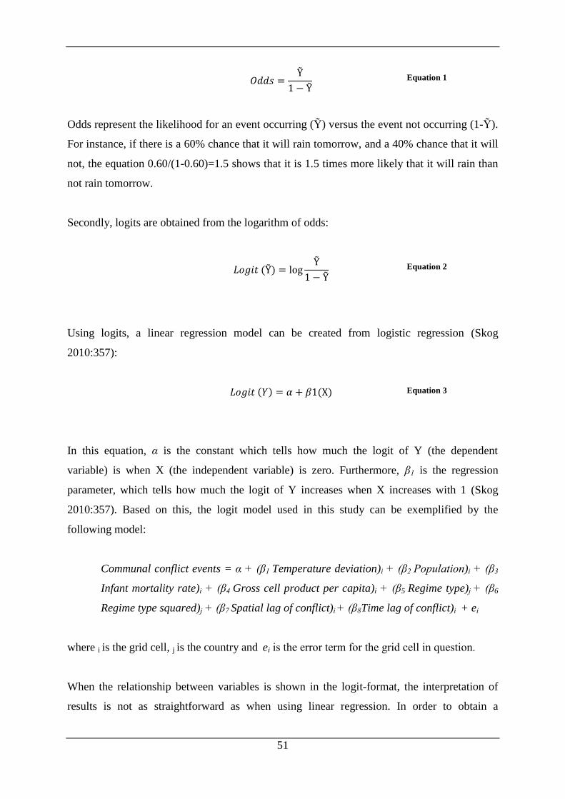
51

Equation 1

Odds represent the likelihood for an event occurring (Ỹ) versus the event not occurring (1-Ỹ).

For instance, if there is a 60% chance that it will rain tomorrow, and a 40% chance that it will

not, the equation 0.60/(1-0.60)=1.5 shows that it is 1.5 times more likely that it will rain than

not rain tomorrow.

Secondly, logits are obtained from the logarithm of odds:

Equation 2

Using logits, a linear regression model can be created from logistic regression (Skog

2010:357):

Equation 3

In this equation, α is the constant which tells how much the logit of Y (the dependent

variable) is when X (the independent variable) is zero. Furthermore, β1 is the regression

parameter, which tells how much the logit of Y increases when X increases with 1 (Skog

2010:357). Based on this, the logit model used in this study can be exemplified by the

following model:

Communal conflict events = α + (β1 Temperature deviation)i + (β2 Population)i + (β3

Infant mortality rate)i + (β4 Gross cell product per capita)i + (β5 Regime type)j + (β6

Regime type squared)j + (β7 Spatial lag of conflict)i + (β8Time lag of conflict)i + ei

where i is the grid cell, j is the country and ei is the error term for the grid cell in question.

When the relationship between variables is shown in the logit-format, the interpretation of

results is not as straightforward as when using linear regression. In order to obtain a

52

substantial interpretation, i.e. to say for instance how many percentages the risk for a conflict

event increases with a specific increase in the independent variable, one needs to calculate the

odds and oddsratios (Skog 2010:361-363). However, in this thesis odds and oddsratios are not

used. Instead, interpretations of the results are given only based on the output of logit.

Therefore, the interpretations given in this thesis are technical in nature. It means that the

significance and direction of the coefficients are commented on, as well as the different

models’ fit to the data.

A model’s fit to the data is in this study analyzed by comparing the log likelihoods of the

different models. Log likelihood is the result of estimation done by the maximum likelihood –

method (Skog 2010:375). Lower log likelihood indicates a better fit of the model to the data

(Skog 2010:368). However, as log likelihoods almost automatically decrease for each variable

which is added to the dataset, one cannot compare the log likelihoods of two models simply

by looking at which model has smaller log likelihood. Therefore likelihood ratio (LR) tests

are conducted to see whether a difference between the log likelihoods of two models is

statistically significant, controlling for the difference in the number of variables in a model

(Skog 2010:375). A statistically significant difference is found by looking at whether the

difference in log likelihoods receives the following result from the LR test: the result needs to

be more than the chi-square value for the amount of degrees of freedom which is equal to the

difference in the amount of variables in the model (Skog 2010:375-376). In other words, if

model A has 6 variables and model B has 5 variables, the degrees of freedom between the

models is 1. Therefore a significant difference in the log likelihoods of the two models needs

to be at least the chi-square value for 1 degrees of freedom.

In this study, the statistical software STATA 9.0 is used to conduct the analyses. With the

command “logit”, STATA reports amongst other things the regression parameters (β1), the

constant (α), the standard errors and the p-values for the variables in question. STATA also

reports the log likelihoods for each model.

53

4.8 Methodological challenges

4.8.1 Multicollinearity

In statistics, multicollinearity may be a problem. Multicollinearity means that two or more

independent variables correlate to a high degree, and it may lead to negative consequences for

both the estimated coefficients and their standard errors (Chen et al. 2003). It is possible to

check whether a model suffers from multicollinearity in several ways. In this thesis, pairwise

correlations between the variable were conducted, and these correlations are shown in

correlation matrices. In addition, variance inflation factor (VIF) -tests were conducted.

4.8.2 Omitted variable bias

It is also possible that the relationship between the dependent and independent variable is

explained by a third variable, which affects them both. This third variable, if not controlled

for, could cause a spurious relationship between the dependent and independent variable. The

chance to see a spurious relationship is reduced by adding those variables to a model which

can be expected to influence both the dependent and independent variable. These are so called

control variables, and they are used also in this study. Furthermore, there is always a chance

that a relevant control variable has not been included into the model. In this case, the analyses

suffer from omitted variable bias. To minimize the chance for omitted variable bias, control

variables should be chosen through carefully reviewing the literature. (Skog 2010:41-45) This

was done also in this thesis.

4.8.3 Outliers

Observations, which have values that deviate a lot from the average values, are called outliers

and may influence the regression results. There are several ways of dealing with outliers. In

this study, two tests are used to check the effects of outliers in the models. The first one is

Pregibon’s (1981) delta-beta test, which identifies the effect that the removal of one

observation has on the whole model, including on all coefficients. The delta-beta test

resembles the Cook’s D in ordinary least squares regression, and like with Cook’s D,

observations which have a delta-beta -value higher than 1 should be investigated further

(Chen et al. (2013); Field (2000:124)). The second test is Pregibon’s (1981) leverage test,

which identifies the leverage, or effect, of a specific observation on the predicted outcome of

54

the model. If any observations have leverage values which are higher than two or three times

the average leverage values, these observations should be investigated further (Field

2000:124-125). The results of these tests are commented on in section 5.4.2.

4.8.4 Rare events

Only 0.2% of all grid cells in Sub-Saharan African in 1989-2008 have seen a communal

conflict event. This makes the occurrence of a communal conflict event a very rare

phenomenon, which in turn may cause problems for the analysis of them. The effects of rare

events may namely be underestimated by regular logit analysis (King and Zeng 2001).

In this study, the problem of rare events was attempted to be overcome by running the

analyses on a subset of observations, i.e. on grid cells with communal conflict events and on a

random sample of 5% of all grid cells without conflict events (see section 4.5 for a description

of the subset). Consequently, the number of grid cells with communal conflict events rose to

4.4 % of the total amount of grid cells studied. However, King and Zeng (2001), who suggest

to use this method, also argue that it should be used with “appropriate statistical corrections”

(King and Zeng 2001:143). Unfortunately, due to time constraints, this was not done in this

thesis. In principle, this may cause the results to be misleading, as the results are not corrected

for the actual ratio between observations with and without communal conflict events in the

full dataset. However, this may in practice not be of great concern for the results of this study,

as this study found no significant results. Thus the results should not suffer from the fact that

the effect from communal conflict events in the results could be higher than it would be if

corrected for the true ratio between observations with and without conflict.

Moreover, King and Zeng (2001) suggest a limit for when it is appropriate to use the rare

events logit method for conducting analyses. They argue that the advantages of using rare

events logit are highest when the sample size is less than “a few thousand” and when there are

less than “5% or so” events in the total sample (King and Zeng 2001:157). In this study, the

sample size (size of the subset) is in total 8369 observations, being a little higher than the

sample size which would benefit most of rare events logit, and the number of events is 4.4%,

which is only a little less than the 5% limit which King and Zeng suggest. Therefore, rare

events logit was not chosen as the primary type of regression to be used in this study. It would

have been interesting, however, to compare the results of this study to the same analyses

55

conducted with rare events logit. Unfortunately, due to time constraints this was not possible

to do in this thesis.

4.8.5 Time dependency and spatial dependency

Spatial and time dependencies of conflicts are likely to cause problems in quantitative conflict

research: as discussed in section 4.6.3.7, earlier and nearby incidences of conflict are strong

predictors of conflict. In this study, spatial and time dependency are tried to control for by the

time lag of communal conflict and spatial lag of communal conflict variables. However, as

discussed in section 4.6.3.7, these variables are not able to capture all incidents of earlier and

nearby communal conflicts. Therefore, some time and spatial dependencies of conflict might

remain unseen in this study.

4.8.6 Missing data and selection bias

Missing data may be a problem in quantitative studies. In this study, many variables lack data

on some observations, because these data points do not exist in the available datasets. The

variables population, infant mortality rate and gross cell product per capita did not have data

for all years, and the available data were therefore interpolated/extrapolated to those years

which lacked data, as described in section 4.6.3. A consequence of this is that the data for

these three variables do not necessarily reflect the real values for all years. However, this is

seen as a better option than lacking data for many years.

When the interpolated and extrapolated values are included in the dataset, the total number of

observations with missing data is small13

for most variables. A notable exception is the

variable political marginalization, for which one-third of all grid cells in the dataset lack

information. This has some consequences especially for the most likely scenario analyses

(which among other things only include grid cells in which politically marginalized groups

live). Notably, 76 out of 169 grid cells with communal conflict events in the most likely

scenario lack information on marginalized groups. Consequently, this lack of data further

limits the number of grid cells with communal conflict events and marginalized groups in the

most likely scenario.

13

4.5% at the highest.

56

One reason for the lack of data on marginalized groups is that the EPR dataset (Wimmer et al.

2009), from which the information on the political status of groups is derived, only includes

data on groups which live in countries with an area of minimum 500,000 square kilometers

and with a population of minimum 1 million as of year 2005 (Wimmer et al. 2009:325,

footnote 11). Thus only those 19 countries14

in Sub-Saharan Africa which fulfill these criteria

have information about marginalized groups in the dataset used in this study. Consequently,

the most likely scenario used in this study suffers from a selection bias, which is that only

observations from relatively big countries are included. Yet, as this is the only data available,

not much could be done to correct this selection bias.

However, there are also grid cells within these 19 countries that lack data on marginalized

groups15

. The reason for this is unknown. If there is a systematic pattern in which grid cells

have information on marginalized groups and which do not, the data on marginalized groups

may suffer from another selection bias.

Furthermore, the most important problem with missing data in this thesis is arguably the fact

that not all communal conflict events in Sub-Saharan Africa in the study period could be

included in this study, for the reasons explained in section 4.6.1. This may also lead to a

selection bias for the dependent variable, if there is a systematic pattern in which communal

conflicts were included and which were not. However, the author of this thesis is not aware of

any such pattern.

4.9 Limitations

In addition to the methodological challenges discussed in section 4.8, there are a few

limitations to the research conducted in this thesis. The first is that the data which is used is

data on past events, while, as is generally known, effects of anthropogenic climate change are

not expected to occur until a little into the future. However, it is reasonable to look at how the

effects of climatic changes (e.g. temperature rise) have correlated with conflict in the past.

Although temperature rise would be natural in the time period studied in this thesis, a

temperature rise of for instance two degrees is still likely to affect (or not affect) societies and

14

A list of which countries this includes is available in Appendix B. 15

The dataset used in this study includes in total 133428 grid cells which are part of those 19 countries included

in the EPR dataset, and 52161 of those grid cells lack information on the variable political marginalization.

57

livelihoods in the same ways regardless of whether it is caused by anthropogenic climate

change or not.

Secondly, the time period of this study is relatively short. This study will look at temperature

and rainfall changes over 20 years (1989-2008), but it could be that this is a too short period

to reveal changes that are comparable to changes caused by anthropogenic climate change.

However, this is the time period for which the UCDP GED (Melander and Sundberg 2011)

and the UCDP non-state conflict database (Sundberg et al. 2012) provide data on communal

conflict events. In addition, the time period used in this study might still reveal if small

changes in temperature or rainfall correlate with communal conflict events.

58

59

5 Results

In this chapter, the results of the study are presented. First, the results for the larger models

are presented (section 5.1). This presentation includes some descriptive statistics, a

presentation of the baseline model and finally the multivariate analyses. Thereafter, the results

for the most likely scenario are presented (section 5.2). This presentation includes the same

elements as the presentation of the larger models. Section 5.3 gives a summary of all the

results. Finally, section 5.4 presents the results of relevant statistical tests.

Based on the discussion in section 4.5, all analyses in this thesis are based on a subset of grid

cells, i.e. only grid cells with communal conflict events and a random sample of 5% of grid

cells without conflict events. Moreover, all analyses are conducted using logistic regression,

because the dependent variable is a dichotomous variable, taking the value 1 if a communal

conflict event has occurred and 0 if not. For a presentation and discussion on methodological

choices in this study, see chapter 4.

Furthermore, bivariate analyses were also conducted for all hypotheses. Although the results

of bivariate analyses provide a good start, they need to be controlled for a number of other

possible explanatory factors, so called control variables. Moreover, analyses including control

variables, so called multivariate analyses, are seen in this study to be of higher importance

than bivariate analyses. Because of this, and due to space constraints, the results of the

bivariate analyses are reported in Appendix D.

5.1 Large-model analyses

In this section, analyses for the large models are presented. First, some descriptive statistics

are provided (section 5.1.1). Thereafter, the baseline model for the large-model analyses is

presented (section 5.1.2), before the multivariate analyses are reported and the hypotheses 1

and 2 are discussed based on the multivariate results (section 5.1.3).

5.1.1 Descriptive statistics

Table 2 presents some descriptive statistics for the variables used in this study. These results

are based on the subset of grid cells.

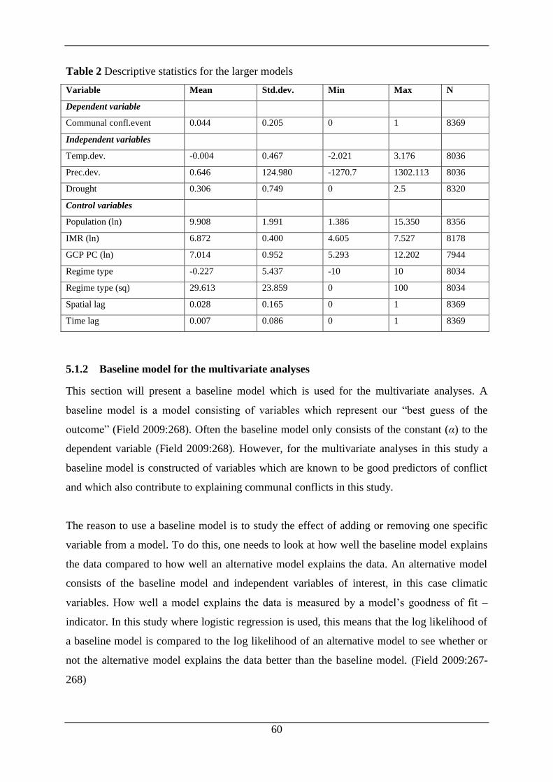
60

Table 2 Descriptive statistics for the larger models

Variable Mean Std.dev. Min Max N

Dependent variable

Communal confl.event 0.044 0.205 0 1 8369

Independent variables

Temp.dev. -0.004 0.467 -2.021 3.176 8036

Prec.dev. 0.646 124.980 -1270.7 1302.113 8036

Drought 0.306 0.749 0 2.5 8320

Control variables

Population (ln) 9.908 1.991 1.386 15.350 8356

IMR (ln) 6.872 0.400 4.605 7.527 8178

GCP PC (ln) 7.014 0.952 5.293 12.202 7944

Regime type -0.227 5.437 -10 10 8034

Regime type (sq) 29.613 23.859 0 100 8034

Spatial lag 0.028 0.165 0 1 8369

Time lag 0.007 0.086 0 1 8369

5.1.2 Baseline model for the multivariate analyses

This section will present a baseline model which is used for the multivariate analyses. A

baseline model is a model consisting of variables which represent our “best guess of the

outcome” (Field 2009:268). Often the baseline model only consists of the constant (α) to the

dependent variable (Field 2009:268). However, for the multivariate analyses in this study a

baseline model is constructed of variables which are known to be good predictors of conflict

and which also contribute to explaining communal conflicts in this study.

The reason to use a baseline model is to study the effect of adding or removing one specific

variable from a model. To do this, one needs to look at how well the baseline model explains

the data compared to how well an alternative model explains the data. An alternative model

consists of the baseline model and independent variables of interest, in this case climatic

variables. How well a model explains the data is measured by a model’s goodness of fit –

indicator. In this study where logistic regression is used, this means that the log likelihood of

a baseline model is compared to the log likelihood of an alternative model to see whether or

not the alternative model explains the data better than the baseline model. (Field 2009:267-

268)

61

The following variables were tested when the baseline model was developed: spatial lag of

communal conflict; time lag of communal conflict; population per grid cell; infant mortality

rate per grid cell; gross cell product per capita; regime type of the country; regime type of the

country, squared; political marginalization; distance to capital; and distance to nearest city of

50000 inhabitants. The baseline model was developed by adding all the variables to one

model, and then comparing the log likelihood of that model to alternative models where one

variable at the time were removed. When a variable was removed and the log likelihood of the

alternative model became significantly worse compared to the full model, the variable in

question was included in the baseline model. To see the results of the development of the

baseline model, see Appendix C.

The baseline model which was chosen for the multivariate analyses in this study consists of

the following variables: spatial lag of communal conflict, time lag of communal conflict,

population per grid cell, infant mortality rate per grid cell, gross cell product per capita,

regime type of the country and regime type of the country, squared. The baseline model is

presented in Table 3.

62

Table 3 The baseline model

(Baseline model)

VARIABLES Confl.events

Population (ln) 0.517***

(0.059)

IMR (ln) -1.571***

(0.244)

GCP PC (ln) -0.537***

(0.131)

Regime type -0.006

(0.019)

Regime type (sq) -0.014***

(0.004)

Spatial lag 4.519***

(0.236)

Time lag 5.123***

(0.775)

Constant 5.037**

(2.277)

Degrees of freedom 7

LR chi2(x) 960.51

Log likelihood -565.414

Observations 7,411

Standard errors in parentheses

*** p<0.01, ** p<0.05, * p<0.1

In Table 3, the values which are given for the variables are the regression coefficients, and

stars indicate their significance levels. Below the coefficients, in parentheses, are the

coefficients’ standard errors. Moreover, the log likelihood, likelihood ratio test score

(abbreviated as LRchi2(x)) and the degrees of freedom compared to the baseline model (in

this case compared to a model where only the constant is included) are given in the bottom of

the table. Log likelihood is a goodness-of-fit indicator, and was discussed in section 4.7, and

LR tests and degrees of freedom are explained below.

In Table 3, the total amount of observations for the baseline model is 7411. Looking at the

different variables, it is visible firstly that the coefficient for population is positive. This result

means that for every one unit increase in population (ln), the risk of communal conflict events

increases with 0.517 on the logit scale. In order to interpret for instance the percentages that

63

0.517 on the logit scale indicates, one would need to calculate the odds and odds ratio for the

value. However, as noted in section 4.7, odds and odds ratios are not calculated in this study,

and therefore no substantial interpretations will be given. Instead, technical interpretations are

given16

. Regarding the coefficient for population in the baseline model, it can therefore be

interpreted here as showing that higher population increases the risk of communal conflict

events. This result was as expected (see a discussion on control variables and expectations to

them in section 4.6.3). Moreover, the coefficient for population is statistically significant on a

0.01 level. This means that there is a 99% chance that the coefficient for temperature actually

is 0.517 according to the data, and that it is not 0.517 only by coincidence.

Table 3 further shows that the regression coefficients for the variables in the baseline model

are all significant on a 0.01 level, except for regime type, which is included only to ease

comparison with regime type squared. Moreover, grid cells with lower infant mortality rates

significantly increase the risk of communal conflict events, according to the result of the

baseline model. This result is surprising and runs contrary to what was expected. On the other

hand, lower gross cell product per capita significantly increases conflict risk. This result is as

expected, but it is contradictory to the result of IMR, as high IMR and low GCP PC are

expected to indicate poverty. Furthermore, the coefficient for regime type is negative,

indicating that low levels of democracy are related to communal conflict. However, this result

is insignificant and therefore cannot be trusted with minimum 90% certainty (corresponding

to significance on a 0.1 level). On the other hand, a low value on the regime type squared –

variable increases the likelihood of communal conflict events, meaning that countries with a

regime type which is somewhere halfway between full democracy and full dictatorship run

the highest risk of witnessing communal conflict events. This result is significant and was as

expected. Finally, spatial lag of conflict, i.e. that a communal conflict event has occurred in a

neighboring cell, as well as time lag of conflict, i.e. that a communal conflict event has

occurred in the same cell in the previous year, significantly increase the risk of a communal

conflict events. These results are as expected.

16

The software CLARIFY could also have been used to ease the substantial interpretation of coefficients.

However, as none of climatic coefficients in the multivariate results in this thesis helped to explain communal

conflict events, the use of CLARIFY was not seen as giving the interpretations any additional value.

64

Moreover, the baseline model does significantly better at explaining communal conflict

events than a model where only the constant is included17

. This is visible from the likelihood

ratio (LR) test. The LR test shows whether there is a statistically significant difference

between the log likelihoods of two models (Skog 2010:375). Log likelihood here tells how

well a model explains communal conflict events. The difference between two log likelihoods

is statistically significant when the score of the LR test is similar or higher than the chi-square

distributed value for that amount of degrees of freedom which corresponds to the difference in

the number of variables between the models (Skog 2010:375-376). The chi-square distributed

values are obtained from a chi-square table18

. Regarding the baseline model which is

presented in Table 3, the LR test for the difference between the log likelihood of the baseline

model, compared to a model where only the constant is included, is higher than the chi-square

distributed value for 1 degree of freedom. Thus it may be concluded that the log likelihood of

the baseline model is significantly better than the log likelihood of a model where only the

constant is included.

5.1.3 Multivariate analyses with climatic variables

In this section, the hypotheses 1 and 2 are tested by adding climatic variables to the baseline

model. These climatic variables are deviation from yearly average temperature, deviation

from yearly average precipitation, and the degree of drought. As temperature can also be

affected by rainfall, temperature is also tested together with precipitation and drought.

Precipitation and drought are, however, not included in the same model, as they measure the

same phenomena, namely rainfall, although with different techniques (see section 4.6 for a

presentation of the variables).

5.1.3.1 Hypotheses 1a and 2a

Firstly, hypotheses 1a and 2a are tested. These hypotheses expect higher temperatures and

lower rainfall respectively to increase the risk of communal conflict in the same year. The

results for the analysis are presented in Table 4.

17

Often a model, where only the constant is included, is called a baseline model, as was explained in section

5.1.2. However, in this thesis the term ”baseline model” refers to the model presented in Table 3. 18

See for instance Skog (2010:193)

65

Table 4 Results for hypotheses 1a and 2a

(Baseline model) (10) (11) (12) (13) (14)

VARIABLES Confl.events Confl.events Confl.events Confl.events Confl.events Confl.events

Temp.dev.

0.185

0.194 0.181

(0.212)

(0.214) (0.212)

Prec.dev.

0.000

0.000

(0.000)

(0.000)

Drought

0.094

0.067

(0.109)

(0.112)

Population (ln) 0.517*** 0.504*** 0.504*** 0.519*** 0.504*** 0.506***

(0.059) (0.059) (0.059) (0.059) (0.059) (0.059)

IMR (ln) -1.571*** -1.782*** -1.772*** -1.565*** -1.777*** -1.776***

(0.244) (0.253) (0.255) (0.244) (0.254) (0.254)

GCP PC (ln) -0.537*** -0.547*** -0.551*** -0.528*** -0.545*** -0.542***

(0.131) (0.133) (0.133) (0.131) (0.133) (0.133)

Regime type -0.006 0.002 -0.001 -0.005 0.002 0.003

(0.019) (0.020) (0.019) (0.019) (0.020) (0.020)

Regime type (sq) -0.014*** -0.015*** -0.014*** -0.014*** -0.015*** -0.014***

(0.004) (0.004) (0.004) (0.004) (0.004) (0.004)

Spatial lag 4.519*** 4.568*** 4.551*** 4.522*** 4.571*** 4.570***

(0.236) (0.240) (0.239) (0.236) (0.241) (0.240)

Time lag 5.123*** 5.099*** 5.092*** 5.062*** 5.091*** 5.057***

(0.775) (0.777) (0.778) (0.777) (0.778) (0.780)

Constant 5.037** 6.727*** 6.665*** 4.885** 6.673*** 6.596***

(2.277) (2.304) (2.312) (2.291) (2.310) (2.321)

Degrees of freedom

1 1 1 2 2

LR chi2(x)

0.75 0.05 0.73 0.87 1.11

Log likelihood -565.414 -549.340 -549.694 -564.492 -549.284 -548.972

Observations 7,411 7,120 7,120 7,374 7,120 7,113

Standard errors in parentheses

*** p<0.01, ** p<0.05, * p<0.1

In Table 4, the baseline model from Table 3 is included in order to ease comparison between

the models. In Model 10, temperature was added to the baseline model to test the effect of

temperature on the model’s explanatory power over communal conflict events. As Table 4

shows, the coefficient for temperature is positive but not statistically significant. Therefore the

analysis points to higher temperature increasing the risk of communal conflict events, but it

cannot tell with a high enough certainty if this really is a true result or if it is just based on

coincidence. Moreover, the log likelihood of Model 10 was compared to the log likelihood of

the baseline model by conducting a likelihood ratio (LR) test. As the LR between the models

is less than the chi-square value with one degree of freedom, the difference between the log

likelihoods of the baseline model and Model 10 is not statistically significant. This means that

66

adding temperature to the baseline model does not improve the model’s capacity to explain

the data.

Model 11 tests the effect of adding precipitation to the model. The coefficient for precipitation

is zero, meaning that higher or lower precipitation does not affect the risk of communal

conflict events. However, as the coefficient is insignificant, the result cannot be guaranteed

with at least 90% certainty to not be caused by chance. Thus it is not possible to say with high

enough certainty how precipitation affects communal conflict events. Furthermore, the LR

test between Model 11 and the baseline model revealed that there is no significant difference

in how well the two models explain the data. Consequently, precipitation does not seem to

help explain communal conflict events.

Model 12 uses another indicator for rainfall, namely drought. The coefficient for drought is

positive but not significant, thus pointing to lower rainfall increasing conflict risk but with

less than 90% certainty. Furthermore, the LR test between Model 12 and the baseline model

also proved that adding drought does not improve the model’s capacity to explain the

communal conflict events.

In Model 13, temperature and precipitation were tested together. This is done in order to see

whether the coefficients for temperature and precipitation change when tested together, as

precipitation may affect temperature. However, neither of the coefficients has become

significant, and they have approximately the same size and direction as in Models 10 and 11

where temperature and precipitation respectively were tested alone. Moreover, due to the

coefficients’ lack of significance these results are less than 90% certain. A LR test further

reveals that adding both temperature and precipitation to the model does not improve the

models explanatory power compared to the baseline model.

In Model 14, temperature and drought are tested together. Neither of them is significant, and

they have the same directions as in Models 10 and 12 when they were tested alone. The

coefficient for temperature has also approximately the same size as in Model 10, but the

coefficient for drought has decreased some in size compared to Model 12, suggesting that part

of the effect of drought is explained by temperature, although due to insignificance this cannot

be verified by minimum 90% certainty. Furthermore, like the previous models, a LR test

67

reveals that Model 14 does no better in explaining communal conflict events than the baseline

model.

Based on the results for Models 10-14, hypotheses 1a and 2a are rejected in this study.

Hypothesis 1a expects higher temperature to increase the risk of communal conflict events,

while hypothesis 2a expects lower levels of rainfall to increase conflict risk. The coefficient

for temperature pointed in the same direction as was anticipated by hypothesis 1a, suggesting

that hypothesis 1a could be correct. Simultaneously, the coefficient for drought also pointed to

the same direction as anticipated by hypothesis 2a, while the coefficient for precipitation was

zero, pointing to no relationship between rainfall and conflict. The results for drought and

precipitation are therefore somewhat contradictory. However, none of the three coefficients

were statistically significant, and therefore none of the results for the climatic variables can be

trusted with minimum 90% certainty. In addition, and most importantly, none of models with

climatic variables contributed significantly to explain the data, compared to the baseline

model. Thus climatic variables, controlled for the variables in the baseline model, did not help

to explain communal conflict events in this study. Hypotheses 1a and 2a are thus discarded in

this study.

5.1.3.2 Hypotheses 1b and 2b

The hypotheses 1b and 2b expect changes in temperature and rainfall respectively in one year

to increase communal conflict risk the following year. These hypotheses are tested by

changing the Models 10-12 by including values for the climatic variables for the previous

year relative to the values for all the other variables. This change is reflected in Models 15-17.

The results for the analyses are presented in Table 5.

68

Table 5 Results for hypotheses 1b and 2b

(Baseline model) (15) (16) (17)

VARIABLES Confl.events Confl.events Confl.events Confl.events

Temp.dev. t-1

-0.382*

(0.216)

Prec.dev. t-1

0.000

(0.000)

Drought

-0.091

(0.115)

Population (ln) 0.517*** 0.509*** 0.506*** 0.519***

(0.059) (0.061) (0.061) (0.060)

IMR (ln) -1.571*** -1.688*** -1.688*** -1.493***

(0.244) (0.264) (0.262) (0.250)

GCP PC (ln) -0.537*** -0.510*** -0.497*** -0.485***

(0.131) (0.134) (0.134) (0.132)

Regime type -0.006 -0.007 0.001 -0.001

(0.019) (0.020) (0.020) (0.020)

Regime type (sq) -0.014*** -0.013*** -0.015*** -0.014***

(0.004) (0.004) (0.004) (0.004)

Spatial lag 4.519*** 4.530*** 4.551*** 4.521***

(0.236) (0.239) (0.240) (0.237)

Time lag 5.123*** 5.158*** 5.125*** 5.128***

(0.775) (0.777) (0.779) (0.775)

Constant 5.037** 5.729** 5.719** 4.200*

(2.277) (2.368) (2.364) (2.328)

Degrees of freedom

1 1 1

LR chi2(x)

3.12 0.32 0.65

Log likelihood -565.414 -530.498 -531.901 -546.528

Observations 7,411 6,757 6,757 6,998

Standard errors in parentheses

*** p<0.01, ** p<0.05, * p<0.1

In Table 5, the baseline model is again included to ease the comparison. In Model 15,

temperature for the previous year is added to the baseline model. The coefficient for

temperature is negative, meaning that lower temperatures increasing the risk of conflict, and

significant on a 0.1 level. However, a LR test shows that Model 15 does not have a

significantly better log likelihood than the baseline model. Thus, despite a significant

coefficient, adding temperature for the previous year to the baseline model does not improve

the model’s capacity to explain communal conflict events.

Model 16 tests the effect of precipitation in the previous year on communal conflict events in

a current year. The coefficient is zero, indicating that changes in precipitation are not related

69

to increases the risk of communal conflict events. However, the coefficient is not significant,

meaning that the results of Model 16 cannot be trusted with minimum 90% certainty.

Moreover, a LR test between the log likelihoods of Model 16 and the baseline model shows

that the log likelihoods are not significantly different. Consequently Model 16, where

precipitation for the previous year is tested, is not able to explain communal conflict events

any better than the baseline model is.

In Model 17, the effect of drought in the previous year is tested on communal conflict events

in the current year. The coefficient for drought is negative, indicating that lower levels of

drought increase the risk of communal conflict events. However, the coefficient is not

significant, and thus the results cannot be trusted with minimum 90% certainty. Furthermore,

the difference in the explanatory power of Model 17 is not significantly different from the

baseline model, meaning that drought in the previous year cannot help to explain communal

conflict events any better than the baseline model.

In the same way as in models 13-14 in Table 4, temperature for the previous year was also

analyzed together with the coefficients for precipitation and drought in the previous year.

However, as the results of these analyses did not differ significantly from the results of

Models 15-17, the results for them are not reported.

Consequently, the results for Models 15-17 show that both hypothesis 1b and 2b are rejected

in this study. Hypothesis 1b expects higher temperatures in one year to increase the risk of

communal conflicts in the following year, while hypothesis 2b expects lower levels of rainfall

in one year to increase the risk of communal conflicts in the following year. Firstly, all the

climatic coefficients pointed in different directions than what was anticipated by the

hypotheses. Secondly, only the coefficient for temperature was statistically significant.

Thirdly, and most importantly, none of the models, not even Model 15 with the significant

coefficient for temperature, had significantly higher log likelihood than the baseline model.

This means that none of the climatic coefficients improved the baseline model’s capacity to

explain communal conflict events. As a result, hypotheses 1b and 2b are rejected in this study.

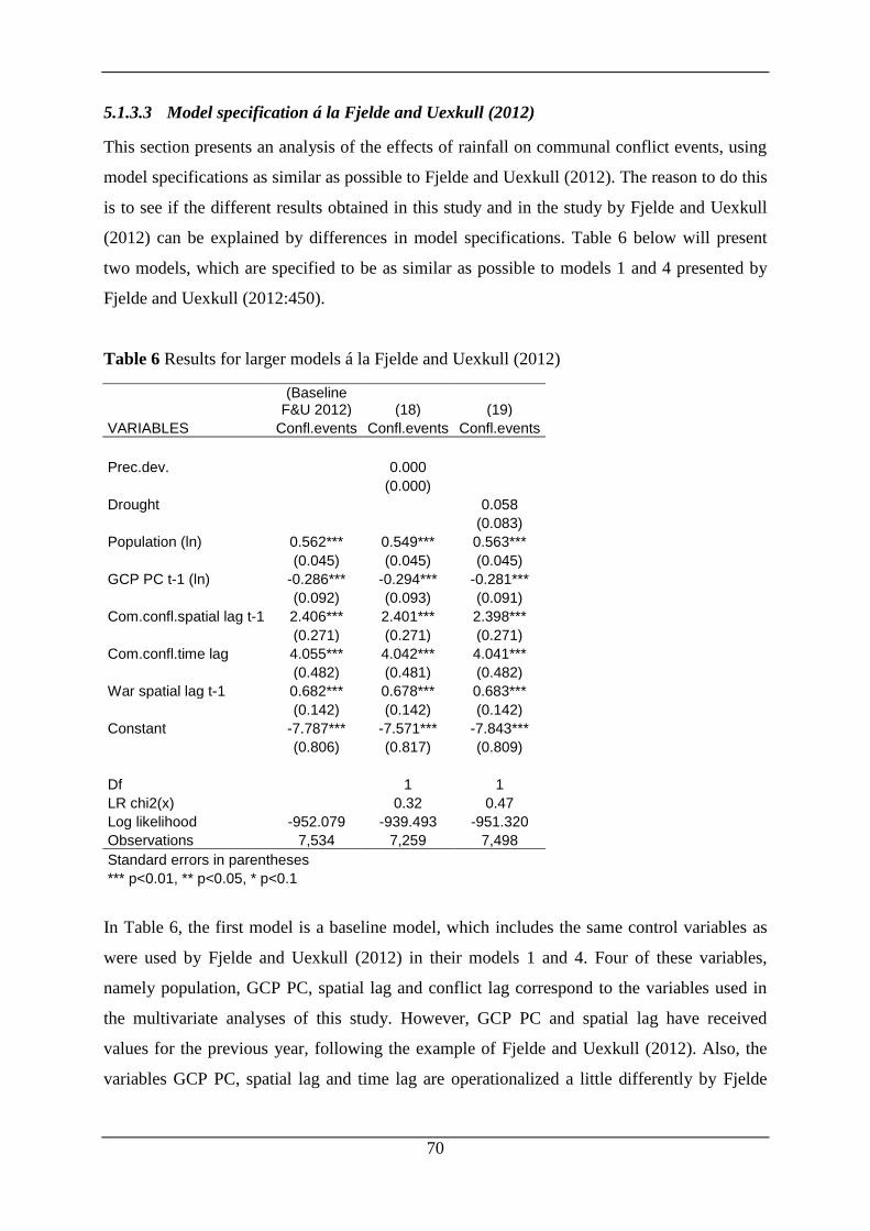
70

5.1.3.3 Model specification á la Fjelde and Uexkull (2012)

This section presents an analysis of the effects of rainfall on communal conflict events, using

model specifications as similar as possible to Fjelde and Uexkull (2012). The reason to do this

is to see if the different results obtained in this study and in the study by Fjelde and Uexkull

(2012) can be explained by differences in model specifications. Table 6 below will present

two models, which are specified to be as similar as possible to models 1 and 4 presented by

Fjelde and Uexkull (2012:450).

Table 6 Results for larger models á la Fjelde and Uexkull (2012)

(Baseline

F&U 2012) (18) (19)

VARIABLES Confl.events Confl.events Confl.events

Prec.dev.

0.000

(0.000)

Drought

0.058

(0.083)

Population (ln) 0.562*** 0.549*** 0.563***

(0.045) (0.045) (0.045)

GCP PC t-1 (ln) -0.286*** -0.294*** -0.281***

(0.092) (0.093) (0.091)

Com.confl.spatial lag t-1 2.406*** 2.401*** 2.398***

(0.271) (0.271) (0.271)

Com.confl.time lag 4.055*** 4.042*** 4.041***

(0.482) (0.481) (0.482)

War spatial lag t-1 0.682*** 0.678*** 0.683***

(0.142) (0.142) (0.142)

Constant -7.787*** -7.571*** -7.843***

(0.806) (0.817) (0.809)

Df

1 1

LR chi2(x)

0.32 0.47

Log likelihood -952.079 -939.493 -951.320

Observations 7,534 7,259 7,498

Standard errors in parentheses *** p<0.01, ** p<0.05, * p<0.1

In Table 6, the first model is a baseline model, which includes the same control variables as

were used by Fjelde and Uexkull (2012) in their models 1 and 4. Four of these variables,

namely population, GCP PC, spatial lag and conflict lag correspond to the variables used in

the multivariate analyses of this study. However, GCP PC and spatial lag have received

values for the previous year, following the example of Fjelde and Uexkull (2012). Also, the

variables GCP PC, spatial lag and time lag are operationalized a little differently by Fjelde

71

and Uexkull (2012) than they are in the models in Table 6 and in this thesis in general.

Nevertheless, these variables, including population, are based on the same data in this thesis

and in Fjelde and Uexkull (2012). The variable war spatial lag for the previous year, on the

other hand, is not used in other analyses in this thesis, and it measures the spatial lag of civil

war (corresponding to conflict types 3 and 4 in UCDP/PRIO Armed Conflict Dataset

(Themnér and Wallensteen 2012)). In this thesis, it is operationalized in the same way as

spatial lag of conflict, while it is operationalized a little differently in Fjelde and Uexkull

(2012). Furthermore, of the independent variables drought is based on the same data and

operationalized in the same way in both studies, while precipitation is in this thesis based on

data derived from a different source than in Fjelde and Uexkull (2012), but it is

operationalized in a similar way.

The results of the models in Table 6 show that the coefficient for precipitation in Model 18 is

zero and the coefficient for drought in Model 19 is positive, just like in models 10 and 12 in

this thesis. Moreover, none of the coefficients are significant, and none of the models have

significantly higher log likelihood than the baseline model. Consequently, also these models

reject hypothesis 2a, which expects lower rainfall to increase the risk of communal conflict

events. Thus the results of this study remain contradictory to the results of Fjelde and Uexkull

(2012), even when the models are specified to be as similar as possible. Chapter 6 will discuss

possible reasons for this.

5.2 Most likely scenario

The results presented in this section are based on analyses in a most likely scenario for

resource scarcity –induced conflict. The argument for using a most likely scenario is that if

resource scarcity caused by climate change is related to conflict, this relationship should as a

minimum be found where the conditions for climate change induced conflict are most

favorable. Moreover, no other study to date has analyzed communal conflict or non-state

conflicts of any kind in a similar way (however, Wischnath and Buhaug (2013) have used a

most likely scenario to study climate and civil wars in Asia). The most likely scenario is

argued in this thesis to be a rural area, where politically marginalized groups live and where

the level of poverty is relatively high. For a presentation and discussion of the scenario, see

section 3.3.

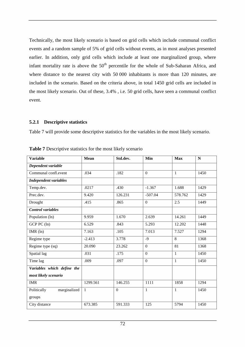
72

Technically, the most likely scenario is based on grid cells which include communal conflict

events and a random sample of 5% of grid cells without events, as in most analyses presented

earlier. In addition, only grid cells which include at least one marginalized group, where

infant mortality rate is above the 50th

percentile for the whole of Sub-Saharan Africa, and

where distance to the nearest city with 50 000 inhabitants is more than 120 minutes, are

included in the scenario. Based on the criteria above, in total 1450 grid cells are included in

the most likely scenario. Out of these, 3.4% , i.e. 50 grid cells, have seen a communal conflict

event.

5.2.1 Descriptive statistics

Table 7 will provide some descriptive statistics for the variables in the most likely scenario.

Table 7 Descriptive statistics for the most likely scenario

Variable Mean Std.dev. Min Max N

Dependent variable

Communal confl.event .034 .182 0 1 1450

Independent variables

Temp.dev. .0217 .430 -1.367 1.688 1429

Prec.dev. 9.420 126.231 -507.04 578.762 1429

Drought .415 .865 0 2.5 1449

Control variables

Population (ln) 9.959 1.670 2.639 14.261 1449

GCP PC (ln) 6.529 .843 5.293 12.202 1448

IMR (ln) 7.163 .105 7.013 7.527 1294

Regime type -2.413 3.778 -9 8 1368

Regime type (sq) 20.090 23.262 0 81 1368

Spatial lag .031 .175 0 1 1450

Time lag .009 .097 0 1 1450

Variables which define the

most likely scenario

IMR 1299.561 146.255 1111 1858 1294

Politically marginalized

groups

1 0 1 1 1450

City distance 673.385 591.333 125 5794 1450

73

5.2.2 Multivariate analyses

The following section will report the results for the multivariate analyses in the most likely

scenario. However, one thing needs to be noted first concerning the baseline model. The

baseline model, which was developed for the larger models, is also used as a baseline model

for the most likely scenario. A baseline model was also developed separately for the most

likely scenario, testing which variables improved the model’s explanatory power under the

conditions defined for the most likely scenario. However, only three variables contributed to

explain communal conflict events. These variables were population, time lag of conflict and

spatial lag of conflict, of which STATA dropped time lag of conflict due to its capacity to

predict observations perfectly. Based on these results, a baseline model for the communal

conflict would have included only two variables. This was seen as a quite thin baseline model,

and therefore it was chosen that the baseline model which was developed for the larger

models should also be used for the most likely scenario analyses.

5.2.2.1 Hypotheses 3a and 4a

Hypotheses 3a and 4a expect higher temperatures and less rainfall respectively to increase the

risk of communal conflict events. The results for the analyses are presented in Table 8.

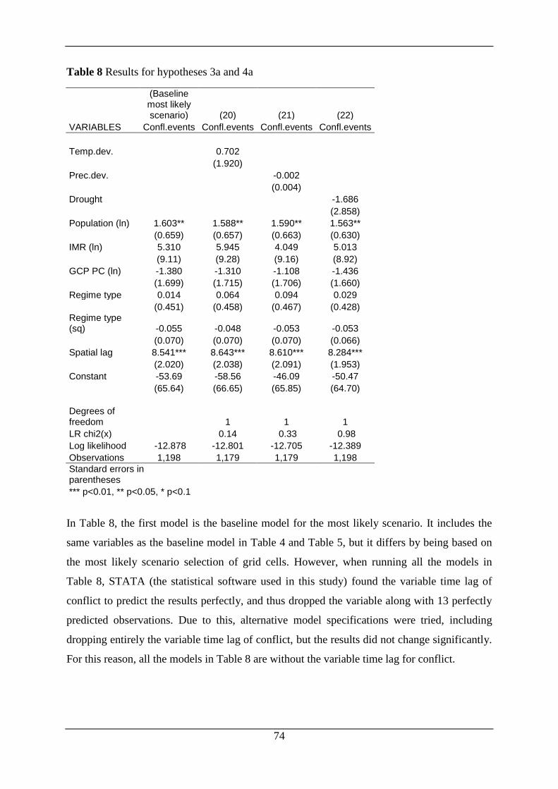
74

Table 8 Results for hypotheses 3a and 4a

(Baseline most likely scenario) (20) (21) (22)

VARIABLES Confl.events Confl.events Confl.events Confl.events

Temp.dev.

0.702

(1.920)

Prec.dev.

-0.002

(0.004)

Drought

-1.686

(2.858)

Population (ln) 1.603** 1.588** 1.590** 1.563**

(0.659) (0.657) (0.663) (0.630)

IMR (ln) 5.310 5.945 4.049 5.013

(9.11) (9.28) (9.16) (8.92)

GCP PC (ln) -1.380 -1.310 -1.108 -1.436

(1.699) (1.715) (1.706) (1.660)

Regime type 0.014 0.064 0.094 0.029

(0.451) (0.458) (0.467) (0.428)

Regime type (sq) -0.055 -0.048 -0.053 -0.053

(0.070) (0.070) (0.070) (0.066)

Spatial lag 8.541*** 8.643*** 8.610*** 8.284***

(2.020) (2.038) (2.091) (1.953)

Constant -53.69 -58.56 -46.09 -50.47

(65.64) (66.65) (65.85) (64.70)

Degrees of freedom

1 1 1

LR chi2(x)

0.14 0.33 0.98

Log likelihood -12.878 -12.801 -12.705 -12.389

Observations 1,198 1,179 1,179 1,198

Standard errors in parentheses

*** p<0.01, ** p<0.05, * p<0.1

In Table 8, the first model is the baseline model for the most likely scenario. It includes the

same variables as the baseline model in Table 4 and Table 5, but it differs by being based on

the most likely scenario selection of grid cells. However, when running all the models in

Table 8, STATA (the statistical software used in this study) found the variable time lag of

conflict to predict the results perfectly, and thus dropped the variable along with 13 perfectly

predicted observations. Due to this, alternative model specifications were tried, including

dropping entirely the variable time lag of conflict, but the results did not change significantly.

For this reason, all the models in Table 8 are without the variable time lag for conflict.

75

Furthermore, the results for the variables in the baseline model have changed some compared

to the large-N analyses, and are therefore worth commenting on. The coefficient for

population has increased in size, but is significant only on 0.05 level compared to 0.01 in the

larger models. Moreover, the coefficient for IMR has seized to be significant. Interestingly,

the coefficient for IMR has shifted from being negative in the larger models to become

positive in the most likely scenario models. As a consequence, IMR now reflects the

theoretical expectations for it, which were presented in section 4.6.3.2. GCP PC has also

seized to be significant, but has increased in size and remained negative. Furthermore, regime

type is still insignificant, but is positive in all models in Table 8, while it varied between

positive and negative in the larger models. Regime type squared, on the other hand, has seized

to be significant but remained negative as in the large-N models. Finally, the coefficient for

spatial lag of conflict has increased in size, and remains significant on a 0.01 level. These

changes for the control variables are reflected in all models in Table 8.

In Model 20, temperature is added to the most likely scenario baseline model and the

coefficient for temperature is positive. This result suggests that studying a most likely

scenario for climate change –induced communal conflict, higher temperature may increase the

risk of communal conflicts. It is moreover visible in Model 21 that lower precipitation seems

to increase the risk of communal conflicts, as the coefficient for precipitation is negative,

while the coefficient for drought in Model 22 is also negative, suggesting that lower levels of

drought increase the risk of communal conflict. The results for precipitation and drought are

therefore contradictory. However, none of the coefficients for climatic variables are

statistically significant, making it impossible to accept them as true with minimum 90%

certainty. Furthermore, none of the models which include climatic variables are able to

explain communal conflict events better than the baseline model, as is reflected in the LR

tests.

Temperature was also tested together with precipitation and drought in a most likely scenario,

but the results did not differ significantly from the results presented in Table 8. Therefore they

are not reported.

Based on these results, hypotheses 3a and 4a are both rejected in this study. Hypothesis 3a

expects higher temperatures to increase the risk of communal conflicts in a most likely

76

scenario. Although the coefficient for temperature points in the same direction as is

anticipated by the hypothesis, the coefficient is not statistically significant, and most

importantly, Model 20 which includes temperature is not able to explain communal conflict

events in a most likely scenario any better than the baseline model. Hypothesis 4a, on the

other hand, expects lower levels of rainfall to increase the risk of communal conflicts in a

most likely scenario. The results for precipitation and drought point in opposite directions,

and none of the coefficients are significant in any models. Most importantly, neither Model 21

nor Model 22, which include precipitation and drought respectively, help to explain

communal conflict events, compared to the baseline model.

5.2.2.2 Hypotheses 3b and 4b

Hypotheses 3b and 4b expect higher temperatures and lower rainfall respectively in the

previous year to increase the risk of communal conflict events in a current year. The results

for the analyses are presented in Table 9.

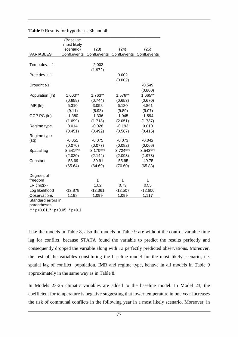
77

Table 9 Results for hypotheses 3b and 4b

(Baseline most likely scenario) (23) (24) (25)

VARIABLES Confl.events Confl.events Confl.events Confl.events

Temp.dev. t-1

-2.003

(1.972)

Prec.dev. t-1

0.002

(0.002)

Drought t-1

-0.549

(0.800)

Population (ln) 1.603** 1.763** 1.576** 1.665**

(0.659) (0.744) (0.653) (0.670)

IMR (ln) 5.310 3.098 6.120 4.861

(9.11) (8.98) (9.89) (9.07)

GCP PC (ln) -1.380 -1.336 -1.945 -1.594

(1.699) (1.713) (2.051) (1.737)

Regime type 0.014 -0.028 -0.193 0.010

(0.451) (0.492) (0.587) (0.415)

Regime type (sq) -0.055 -0.075 -0.073 -0.042

(0.070) (0.077) (0.082) (0.066)

Spatial lag 8.541*** 8.170*** 8.724*** 8.543***

(2.020) (2.144) (2.093) (1.973)

Constant -53.69 -39.91 -55.95 -49.75

(65.64) (64.69) (70.60) (65.83)

Degrees of freedom

1 1 1

LR chi2(x)

1.02 0.73 0.55

Log likelihood -12.878 -12.361 -12.507 -12.600

Observations 1,198 1,099 1,099 1,117

Standard errors in parentheses

*** p<0.01, ** p<0.05, * p<0.1

Like the models in Table 8, also the models in Table 9 are without the control variable time

lag for conflict, because STATA found the variable to predict the results perfectly and

consequently dropped the variable along with 13 perfectly predicted observations. Moreover,

the rest of the variables constituting the baseline model for the most likely scenario, i.e.

spatial lag of conflict, population, IMR and regime type, behave in all models in Table 9

approximately in the same way as in Table 8.

In Models 23-25 climatic variables are added to the baseline model. In Model 23, the

coefficient for temperature is negative suggesting that lower temperature in one year increases

the risk of communal conflicts in the following year in a most likely scenario. Moreover, in

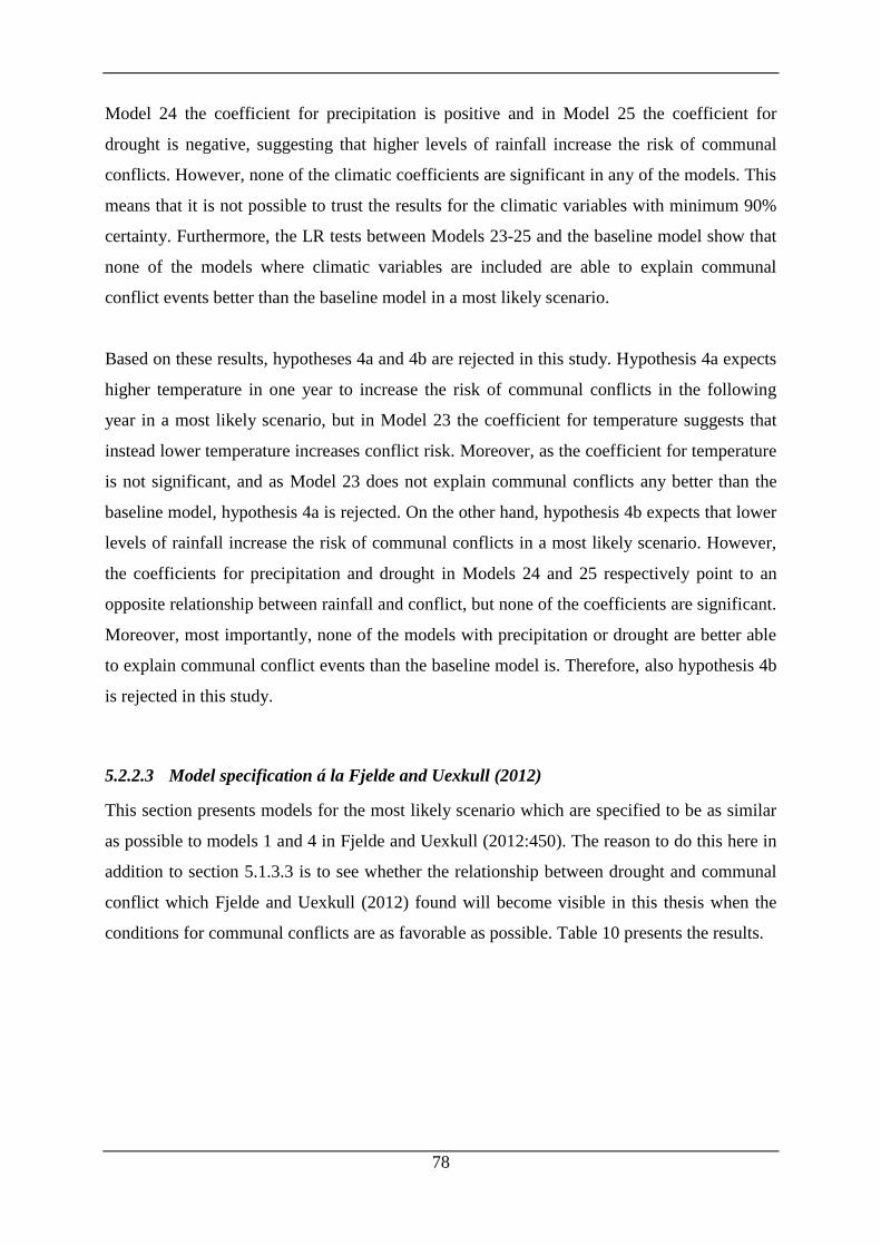
78

Model 24 the coefficient for precipitation is positive and in Model 25 the coefficient for

drought is negative, suggesting that higher levels of rainfall increase the risk of communal

conflicts. However, none of the climatic coefficients are significant in any of the models. This

means that it is not possible to trust the results for the climatic variables with minimum 90%

certainty. Furthermore, the LR tests between Models 23-25 and the baseline model show that

none of the models where climatic variables are included are able to explain communal

conflict events better than the baseline model in a most likely scenario.

Based on these results, hypotheses 4a and 4b are rejected in this study. Hypothesis 4a expects

higher temperature in one year to increase the risk of communal conflicts in the following

year in a most likely scenario, but in Model 23 the coefficient for temperature suggests that

instead lower temperature increases conflict risk. Moreover, as the coefficient for temperature

is not significant, and as Model 23 does not explain communal conflicts any better than the

baseline model, hypothesis 4a is rejected. On the other hand, hypothesis 4b expects that lower

levels of rainfall increase the risk of communal conflicts in a most likely scenario. However,

the coefficients for precipitation and drought in Models 24 and 25 respectively point to an

opposite relationship between rainfall and conflict, but none of the coefficients are significant.

Moreover, most importantly, none of the models with precipitation or drought are better able

to explain communal conflict events than the baseline model is. Therefore, also hypothesis 4b

is rejected in this study.

5.2.2.3 Model specification á la Fjelde and Uexkull (2012)

This section presents models for the most likely scenario which are specified to be as similar

as possible to models 1 and 4 in Fjelde and Uexkull (2012:450). The reason to do this here in

addition to section 5.1.3.3 is to see whether the relationship between drought and communal

conflict which Fjelde and Uexkull (2012) found will become visible in this thesis when the

conditions for communal conflicts are as favorable as possible. Table 10 presents the results.

79

Table 10 Results for most likely scenario models á la Fjelde and Uexkull (2012)

(Baseline

F&U 2012) (25) (26)

VARIABLES Confl.events Confl.events Confl.events

Prec.dev.

-0.000

(0.001)

Drought

-0.923**

(0.425)

Population (ln) 0.966*** 0.966*** 0.958***

(0.148) (0.148) (0.148)

GCP PC t-1 (ln) -0.954*** -0.934*** -1.008***

(0.356) (0.357) (0.369)

Com.confl.spatial lag t-1 2.478*** 2.487*** 2.487***

(0.628) (0.631) (0.644)

Com.confl.time lag 2.571* 2.542* 2.653**

(1.369) (1.376) (1.337)

War spatial lag t-1 0.913** 0.895** 0.832**

(0.401) (0.404) (0.407)

Constant -8.965*** -9.063*** -8.286***

(2.685) (2.694) (2.755)

Df

1 1

LR chi2(x)

0.08 7.95

Log likelihood -118.110 -117.914 -114.136

Observations 1,358 1,340 1,358

Standard errors in parentheses *** p<0.01, ** p<0.05, * p<0.1

In the model 25 in Table 10, precipitation is zero and insignificant, just like in earlier models.

Moreover, the log likelihood of model 25 is not significantly different from the log likelihood

of the baseline model, meaning that precipitation does not help to explain communal conflict

events. On the other hand, the coefficient for drought has become significant in model 26, and

it is negative, indicating that lower levels of drought (i.e. higher levels of rainfall) are related

to communal conflicts. A LR test further shows that model 26 is able to explain communal

conflict events significantly better than the baseline model. It is therefore visible that rainfall,

measured as precipitation, cannot help explain communal conflict events in a most likely

scenario, while rainfall measured as drought can contribute to explaining communal conflict

events in the scenario. However, this relationship runs contrary to what was expected by

hypothesis 4a, which expected lower levels of rainfall to increase the risk of communal

conflict events in a most likely scenario. Consequently, also when analyzing the relationship

80

between rainfall and communal conflict events in a most likely scenario, even when the

models are specified as similarly as possible to the models by Fjelde and Uexkull (2012), this

study finds different results than their study.

5.3 Summary of all results

In this study, the effects of temperature, precipitation and drought were tested on communal

conflict events. In the bivariate analyses (reported in Appendix D), temperature was

significant and improved the model’s log likelihood in all the bivariate large-N analyses,

while precipitation and drought were insignificant and did not contribute significantly to the

model’s log likelihood in the same analyses. In the bivariate analyses for the most likely

scenario, temperature was significant in all models and improved the model’s log likelihood

in most models, while precipitation and drought were significant in most models and

improved the model’s log likelihood in some models.

However, when control variables are added to the models in the multivariate section, the

majority of the climatic coefficients become insignificant. Only temperature for the previous

year is significant in Model 15. Moreover, and most importantly, none of the multivariate

models where climatic coefficients are included have a better log likelihood than the baseline

model. This means that the climatic variables which were tested in this study do not help to

explain communal conflict events in Sub-Saharan Africa in 1989-2008, not even when tested

in a most likely scenario for climate change induced conflict. An attempt was further made to

specify the models as similarly as possible to Fjelde and Uexkull (2012), who found drought

to increase the risk of communal conflict events using first-order administrative units as units

of analysis. However, the results remained approximately the same. Consequently, all the

hypotheses of this study are rejected.

5.4 Statistical tests

In this study, some statistical tests have been conducted in order to control for possible

methodological challenges, which were described in section 4.8.

81

5.4.1 Multicollinearity

The multivariate models presented in this study were tested for multicollinearity by

conducting pairwise correlations and VIF-tests. The results show that the models do not suffer

from multicollinearity between independent variables. Only spatial lag of communal conflict

vs. communal conflict events gets a correlation value which is above 0.7, but this is not a

multicollinearity problem since communal conflict events is the dependent variable. Instead,

the result only shows that spatial lag of communal conflict is highly correlated with

communal conflict, as was theoretically expected and as is visible from the regression

coefficients for spatial lag of communal conflict in the multivariate analyses in this study.

5.4.2 Extreme and influential observations

The multivariate models were also tested for extreme and influential observations by

conducting Pregibon’s leverage and delta-beta tests. The results of these tests show a few

things. Firstly, the delta-beta tests of the larger models show that there are no observations

which exercise a high influence on the larger models. Secondly, the delta-beta tests show that

there are three observations which affect the most likely scenario-models considerably. The

most likely scenario models were ran without these three observations, but this resulted in

STATA not conducting the regression because the variable spatial lag of conflict predicted the

remaining observations perfectly. An attempt was further made at removing spatial lag of

conflict from the analysis (time lag of conflict was removed by STATA automatically for the

same reason, as explained in section 5.2). Thus results were obtained for a model without the

variables spatial lag of conflict and time lag of conflict (the models are not reported here). In

these models, some climatic variables became significant, and some models with climatic

variables received a better log likelihood than the baseline model. Yet, these results are

arguably of little substantial interest, as they suffer from omitted variable bias after the

removal of the spatial and time lag of conflict –variables. What the consequences of the delta-

beta test on the most likely scenario models show, on the other hand, is that the study of

climate change and communal conflict should perhaps study communal conflict onsets instead

of communal conflict events, in order to avoid spatial and time lag of conflict events to

explain such a big part of the conflict observations and to get a better possibility to see which

independent variables actually explain communal conflict onsets.

82

The results for the leverage tests for both the large-N models and the most likely scenario

models show that all models have a high number of observations which affect the outcome of

the model to a much higher degree than the average observation. In statistics, observations

like these are seen as outliers and therefore as problematic observations, which should be

investigated. However, this was difficult to do in this study, as the number of observations

with high leverage values was so high (390 observations in the larger models, and around 62

observations in the most likely scenario models).

83

6 Discussion

This chapter discusses all the results of this study in relation to the literature. As was

presented in chapter 5, the results from both the analyses of the larger models and the most

likely scenario –models reject all the hypotheses of this study. These results run contrary to

most results of the quantitative studies on climate change and non-state conflicts presented in

section 2.4. Where for instance Fjelde and Uexkull (2012) find that communal conflict is

more frequent in dry years; Raleigh and Kniveton (2012) that communal conflict occurs more

often in wet years; and Hendrix and Salehyan (2012) that violent conflict in general is more

likely in wet years; this study finds no relationship between rainfall and communal conflicts,

not even when analyzing a most likely scenario. The results of this study are more in line with

O’Loughlin et al. (2012), who do not find dry years to be correlated to conflict. However,

O’Loughlin et al. (2012) instead find that wet years decrease the risk of conflict compared to

years with normal levels of rainfall. In contrast, the results of this study do not find any such

effect.

Moreover, where O’Loughlin et al. (2012) find warmer than average years to increase the risk

of conflicts, including non-state conflict, this study does not find any significant effect of

temperature on communal conflict events. Although the coefficient for temperature was

significant in one model, the coefficient was negative, indicating that colder than average

years are related to conflict. Also, the model did not explain communal conflict events any

better than a model with the same control variables but without the coefficient for

temperature, i.e. the baseline model.

What is especially interesting about the findings in this thesis is that climatic coefficients were

not found to affect the risk of communal conflict events even in a most likely scenario. The

most likely scenario was argued in this thesis to be rural areas where politically marginalized

groups live and where the level of poverty is high. Theory suggests that these are the

circumstances were climate change induced conflict is most likely to occur. Yet, neither

changes in temperature nor rainfall were found to increase the risk of communal conflict

events in these circumstances.

There are many possible reasons for the different results between this study and other studies

on climate change and non-state conflicts, including communal conflicts. As was discussed in

84

section 2.5, the climate change – non-state conflict studies (including this study) differ in

terms of how they define conflict, which area and time period they study, which conflict data

they use and what they use as their units of analysis. In addition, the specific models which

are used in the different studies also differ.

In order to explain these differences, systematic comparisons may be in order. Firstly, more

studies are needed on climate change and communal conflicts. There are only a few studies to

date which explicitly look at communal conflicts and climate change, although communal

conflicts are arguably the most likely form of climate change -induced conflict. Moreover,

some of the current studies which use non-state conflicts in general have combined non-state

conflicts into a variable ‘conflict’ or ‘violent conflict’, which also includes civil war and one-

sided violence. In these cases, the effects of climate on non-state conflicts may be

overshadowed by the effects, or lack of effects, of climate on the other types of violence,

which are not as likely to be related to climate as non-state conflicts are. Hence, this thesis

argues that the most useful conflicts to study related to climate change are communal

conflicts. However, already separating non-state conflicts in general from civil war and one-

sided violence could help researchers get closer to analyzing the most likely type of conflict to

potentially occur as a result of climate change.

Moreover, it would be useful to compare whether different datasets on non-state or communal

conflict events give different results. In order to compare them systematically, researchers

would need to use a concise definition of conflict, preferably communal conflict, and they

would need to study the same areas and time periods. Preferably these areas and time periods

would be as large and long as possible. In order to reduce the risk of studying too many

irrelevant places, one possible approach is to narrow down the amount of observations by

conducting analyses on a subset of disaggregated units, as was done in this study.

Furthermore, in order to eliminate the possibility of small differences in model specifications

causing differences in results, the same models should be tried on the different datasets.

Methodologically, the most interesting finding of this study is that using grid cells as units of

analysis (as is done in this study) yields different results than using first-order administrative

units as units of analysis, as is done in the study by Fjelde and Uexkull (2012). Both this study

and the study by Fjelde and Uexkull (2012) analyze the relationship between climate change

85

and communal conflicts in Sub-Saharan African in 1989-2008, i.e. the two studies analyze the

same type of conflicts in the same area and in the same time period, and use the same data on

communal conflicts, namely UCDP GED (Melander and Sundberg (2011); Sundberg et al.

(2010)). An attempt was even made in this study to analyze models which were specified as

similarly as possible to the models by Fjelde and Uexkull (2012) (see sections 5.1.3.3 and

5.2.2.3). Yet, the results differ.

Therefore, it is possible that grid cells and first-order administrative units differ in how they

capture relationships between for instance rainfall and communal conflict. However, it is not

possible to state definitively that the difference in results is caused by the difference in the

unit of analysis, as the attempt to analyze similarly specified models in this thesis was not an

exact replication of the study by Fjelde and Uexkull (2012). Thus it may be that very small

differences in the operationalizations of some variables are the reasons for the differences.

However, this does not seem very likely, as the remaining differences are quite small. Finding

out whether this is the case is important not only for research on climate change and

communal conflicts, but also for other disaggregated studies of conflict.

Also more generally, more studies are needed on climate change and communal conflicts in

order to establish whether communal conflicts can occur as a consequence of climate change.

Future studies could make use of comparing different regions within Africa to see whether the

likelihood of climate change –induced communal conflicts differs between the regions. For

instance, no study to date has looked at climate change and communal conflicts in West

Africa, while a few studied different regions in East Africa. Moreover, future studies could

also do wisely in trying to study communal conflict onset rather than events of communal

conflicts. This could improve the possibility to see whether climate change acts as a trigger

for communal conflicts. Studying conflict onset could namely help to overcome the problem

of communal conflict events being perfectly predicted by conflict events which have occurred

nearby or in the previous year, as partly happened in the most likely scenario of this thesis (as

discussed in section 5.4.2). In this way, studying communal conflict onsets could illuminate

which factors make a communal conflict start. However, for this to be possible, geo-coded

data on communal conflict onsets is needed.

86

87

7 Conclusion

Theories of the Environmental Security School have inspired a number of studies on climate

change and violent conflict. However, no consensus has yet been reached on whether climate

change affects violent conflict. Simultaneously, only a few studies have been conducted on

climate change and communal conflicts, which is arguably the most likely type of conflict to

occur as a result of climate change. This thesis has contributed to fill this gap by studying the

relationship between climate change and communal conflicts in Sub-Saharan Africa in the

years 1989-2008. It has studied this relationship using quantitative method, more specifically

logistic regression, and by using grid cells of 0.05˚ x 0.05˚ as disaggregated units of analysis.

Both temperature and precipitation have been used as measures of climate change. This thesis

has also studied climate change and communal conflict in a most likely scenario, arguing that

if climate change and communal conflicts are related, a relationship should be found in this

scenario. This scenario is argued to be rural areas, where politically marginalized groups live

and where the level of poverty is high.

Yet, this thesis finds no relationship between climate change and communal conflicts. Neither

temperature nor rainfall contributed to explain communal conflicts in any of the models used

in this study, and therefore all the hypotheses of this study are rejected. A relationship

between climate change and communal conflicts was thus not found even where the

circumstances for climate change –induced communal conflict were most favorable, i.e. in the

most likely scenario.

These results differ from the results of other studies on climate change and communal

conflicts (e.g. Fjelde and Uexkull (2012) and Raleigh and Kniveton (2012)), and climate

change and non-state conflicts (e.g. Hendrix and Salehyan (2012) and O’Loughlin et al.

(2012)). Most interestingly, the results of this thesis differ from the results of Fjelde and

Uexkull (2012), who found drought to increase the likelihood of communal conflicts. The

study by Fjelde and Uexkull (2012) is very similar to this thesis, except regarding the choice

of disaggregated units of analysis: while this thesis uses grid cells, Fjelde and Uexkull (2012)

use first-order administrative units. As the results in this thesis differed from Fjelde and

Uexkull (2012) even when models were specified as similarly as possible, there is a

possibility that the unit of analysis used affects the results.

88

89

8 References

Adger, W. N. & Kelly, P. M. (1999). Social Vulnerability to Climate Change and the

Architecture of Entitlements. Mitigation and Adaptation Strategies for Global

Change, 4 (3-4): 253-266.

Baechler, G. (1998). Why Environmental Transformation Causes Violence: A Synthesis.

Environmental Change and Security Project Report (4): 24-44.

Ban, K.-m. (2007). A Climate Culprit in Darfur. The Washington Post, 16th of June.

Benjaminsen, T. A. (2008). Does Supply-Induced Scarcity Drive Violent Conflicts in the

African Sahel? The Case of the Tuareg Rebellion in Northern Mali. Journal of Peace

Research, 45 (6): 819-836.

Benjaminsen, T. A. (2009). Klima og konflikter i Sahel - eller politikk og vitenskap ved

klimaets nullpunkt [Climate and conflicts in the Sahel – or politics and science at the

climate’s ground zero] Internasjonal Politikk, 67 (2): 151-172.

Benjaminsen, T. A., Maganga, F. P. & Abdallah, J. M. (2009). The Kilosa Killings: Political

Ecology of a Farmer–Herder Conflict in Tanzania. Development and Change, 40 (3):

423-445.

Bernauer, T., Böhmelt, T. & Koubi, V. (2012). Environmental changes and violent conflict.

Environmental research letters, 7 (1): 015601.

Boko, M., Niang, I., Nyong, A., Vogel, C., Getheko, A., Medany, M., Osman-Elasha, B.,

Tabo, R. & Yanda, P. (2007). Africa. In Parry, M., Canziani, O., Palutikof, J., van der

Linden, P. & CE Hanson, C. (eds) Climate Change 2007: Impacts, Adaptation, and

Vulnerability. Contribution of Working Group II to the Fourth Assessment Report of

the Intergovernmental Panel on Climate Change., pp. 433-467. Cambridge:

Cambridge University Press.

Boserup, E. (1965). The conditions of agricultural growth: the economics of agrarian change

under population pressure. Chicago: Aldine.

Bryman, A. (2008). Social Research Methods. 3rd ed. New York: Oxford University Press

Inc.

Buhaug, H. & Gates, S. (2002). The Geography of Civil War. Journal of Peace Research, 39

(4): 417-433.

Buhaug, H. & Lujala, P. (2005). Accounting for scale: Measuring geography in quantitative

studies of civil war. Political Geography, 24 (4): 399-418.

Buhaug, H. & Rød, J. K. (2006). Local determinants of African civil wars, 1970–2001.

Political Geography, 25 (3): 315-335.

Buhaug, H., Cederman, L.-E. & Rød, J. K. (2008). Disaggregating Ethno-Nationalist Civil

Wars: A Dyadic Test of Exclusion Theory. International Organization, 62 (3): 531-

551.

Buhaug, H. & Gleditsch, K. S. (2008). Contagion or Confusion? Why Conflicts Cluster in

Space. International Studies Quarterly, 52 (2): 215-233.

Buhaug, H. (2010a). Climate not to blame for African civil wars. Proceedings of the National

Academy of Sciences of the United States of America, 107 (38): 16477-16482.

Buhaug, H. (2010b). Reply to Burke et al: Bias and climate war research. Letter. Proceedings

of the National Academy of Sciences of the United States of America, 107 (51): E186-

187.

Buhaug, H., Gleditsch, K. S., Holtermann, H., Østby, G. & Tollefsen, A. F. (2011). It’s the

Local Economy, Stupid! Geographic Wealth Dispersion and Conflict Outbreak

Location. Journal of Conflict Resolution, 55 (5): 814-840.

90

Burke, M. B., Miguel, E., Satyanath, S., Dykema, J. A. & Lobell, D. B. (2009). Warming

increases the risk of civil war in Africa. Proceedings of the National Academy of

Sciences of the United States of America, 106 (49): 20670-20674.

Burke, M. B., Dykema, J. A., Lobell, D. B., Miguel, E. & Satyanath, S. (2010). Climate and

civil war: Is the relationship robust? National Bureau of Economic Research (Working

paper 16440).

Bächler, G. (1998). Violence through environmental discrimination: Causes, Rwanda arena

and conflict model. Dordrecht: Kluwer Academic.

Cederman, L.-E., Min, B. & Wimmer, A. (2009-05-01). Ethnic Power Relations dataset

http://hdl.handle.net/1902.1/11796 UNF:5:k4xxXC2ASI204QZ4jqvUrQ== V1.

Chauvin, N. D., Mulangu, F. & Porto, G. (2012). Food Production and Consumption Trends

in Sub-Saharan Africa: Prospects for the Transformation of the Agricultural Sector.

Working Paper. UNDP Regional Bureau for Africa, WP 2012-011: February 2012.

Chen, X., Ender, P. B., Mitchell, M. & Wells, C. (2003). Regression diagnostics, in:

Regression with Stata. Available at:

http://www.ats.ucla.edu/stat/stata/webbooks/reg/chapter2/statareg2.htm (accessed:

12.05.2013).

Chen, X., Ender, P., Mitchell, M. & Wells, C. (2013). Logistic regression diagnostics, in:

Logistic regression with Stata. Available at:

http://www.ats.ucla.edu/stat/stata/webbooks/logistic/chapter3/statalog3.htm (accessed:

08.05.2013).

Christensen, J. H., Hewitson, B., Busuioc, A., Chen, A., Gao, X., Held, I., Jones, R., Kolli, R.

K., Kwon, W.-T., Laprise, R., et al. (2007). Regional Climate Projections. In Solomon,

S., Qin, D., Manning, M., Chen, Z., Marquis, M., Averyt, K. B., Tignor, M. & Miller,

H. L. (eds) Climate Change 2007: The Physical Science Basis. Contribution of

Working Group I to the Fourth Assessment Report of the Intergovernmental Panel on

Climate Change. Cambridge, United Kingdom and New York, NY, USA: Cambridge

University Press.

CIESIN Center for International Earth Science Information Network Columbia University.

(2005). Gridded Population of the World Version 3 (GPWv3): Population Grids.

Palisades, NY: Socioeconomic Data and Applications Center (SEDAC), Columbia

University (http://sedac.ciesin.columbia.edu/gpw/). .

Collier, P. & Hoeffler, A. (2004). Greed and grievance in civil war. Oxford Economic Papers,

56 (4): 563-595.

Eaton, D. (2008). The Business of Peace: Raiding and Peace Work Along the Kenya–Uganda

Border (Part I). African Affairs, 107 (426): 89-110.

Eck, K. (2012). In data we trust? A comparison of UCDP GED and ACLED conflict events

datasets. Cooperation and Conflict, 47 (1): 124-141.

Fearon, J. D. & Laitin, D. D. (2003). Ethnicity, Insurgency, and Civil War. The American

Political Science Review, 97 (1): 75-90.

Field, A. (2000). Discovering statistics using SPSS for Windows. London: SAGE

Publications.

Field, A. (2009). Discovering statistics using SPSS. 3rd ed. London: SAGE Publications.

Fjelde, H. & Nilsson, D. (2012). Rebels against Rebels Explaining Violence between Rebel

Groups. The Journal of Conflict Resolution, 56 (4): 604.

Fjelde, H. & Uexkull, N. v. (2012). Climate triggers: Rainfall anomalies, vulnerability and

communal conflict in sub-Saharan Africa. Political Geography, 31 (7): 444.

Fjelde, H. & Østby, G. (2012). Economic inequality and inter-group violence. Paper

presented at the Democracy as Idea and Practice conference, Oslo, January 12-13,

2012.

91

Fleurbaey, M. (2009). Beyond GDP: The Quest for a Measure of Social Welfare. Journal of

Economic Literature, 47 (4): 1029-1075.

Gleditsch, K. S. & Ward, M. D. (1999). A revised list of independent states since the congress

of Vienna. International Interactions, 25 (4): 393-413.

Gleditsch, N. P. (1996). The environment, politics and armed conflict - a critique and

research proposal. Paper presented at 'Conflict and the Environment', NATO

Advanced Research Workshop, Bolkesjo, 12-16 June.

Gleditsch, N. P. (1998). Armed Conflict and the Environment: A Critique of the Literature.

Journal of Peace Research, 35 (3): 381-400.

Gleditsch, N. P., Wallensteen, P., Eriksson, M., Sollenberg, M. & Strand, H. (2002). Armed

Conflict 1946-2001: A New Dataset. Journal of Peace Research, 39 (5): 615-637.

Gleditsch, N. P. (2012). Whither the Weather? Climate Change and Conflict. Journal of

Peace Research, 49 (1): 3-9.

Gurr, T. (1970). Why men rebel. Princeton, NJ: Princeton University Press.

Hauge, W. & Ellingsen, T. (1996). Environmental Change and Civil War: A Multivariate

Approach. Paper presented at 'Conflict and the Environment', NATO Advanced

Research Workshop, Bolkesjo, 12-16 June.

Hegre, H., Ellingsen, T., Gates, S. & Gleditsch, N. P. (2001). Toward a Democratic Civil

Peace? Democracy, Political Change, and Civil War, 1816-1992. The American

Political Science Review, 95 (1): 33-48.

Hegre, H. & Sambanis, N. (2006). Sensitivity Analysis of Empirical Results on Civil War

Onset. The Journal of conflict resolution, 50 (4): 508-535.

Hendrix, C. S. & Glaser, S. M. (2007). Trends and triggers: Climate, climate change and civil

conflict in Sub-Saharan Africa. Political Geography, 26 (6): 695-715.

Hendrix, C. S. & Salehyan, I. (2012). Climate change, rainfall, and social conflict in Africa.

Journal of Peace Research, 49 (1): 35-50.

Homer-Dixon, T. (1991). On the threshold: Environmental changes as causes of acute

conflict. International Security, 16 (2): 76-116.

Homer-Dixon, T. (1994). Environmental Scarcities and Violent Conflict: Evidence from

Cases. International Security, 19 (1): 5-40.

Homer-Dixon, T. (1999). Environment, Scarcity and Violence. New Jersey: Princeton

University Press.

Höglund, K. (2009). Electoral Violence in Conflict-Ridden Societies: Concepts, Causes, and

Consequences. Terrorism and Political Violence, 21 (3): 412-427.

IPCC. (2007). Climate Change 2007: Synthesis Report.

Kahl, C. (2006). States, scarcity and civil strife in the developing world. Princeton, NJ:

Princeton University Press.

Kahl, C. H. (1998). Population Growth, Environmental Degradation, and State-Sponsored

Violence: The Case of Kenya, 1991-93. International Security, 23 (2): 80-119.

King, G. & Zeng, L. (2001). Logistic Regression in Rare Events Data. Political Analysis, 9

(2): 137-163.

Koubi, V., Bernauer, T., Kalbhenn, A. & Spilker, G. (2012). Climate variability, economic

growth, and civil conflict. Journal of Peace Research, 49 (1): 113-127.

Marshall, M. G. (2011). Polity IV Project: Dataset User's Manual. version 2010 ed. Center

for Systemic Peace at www.systemicpeace.org.

Maxwell, J. W. & Reuveny, R. (2000). Resource Scarcity and Conflict in Developing

Countries. Journal of Peace Research, 37 (3): 301-322.

Meier, P., Bond, D. & Bond, J. (2007). Environmental influences on pastoral conflict in the

Horn of Africa. Political Geography, 26 (6): 716-735.

92

Melander, E. & Sundberg, R. (2011). Climate Change, Environmental Stress, and Violent

Conflict – Test Introducing the UCDP Georeferenced Event Dataset. Paper presented

at the International Studies Association, March 16-19, Montreal, Canada.

Miguel, E., Satyanath, S. & Sergenti, E. (2004). Economic Shocks and Civil Conflict: An

Instrumental Variables Approach. Journal of Political Economy, 112 (4): 725-753.

Mjøs, O. D. (2007). Presentation speech. Available at:

http://nobelpeaceprize.org/en_GB/laureates/laureates-2007/presentation-2007/

(accessed: 17.1.).

Myers, N. (1989). Environment and Security. Foreign Policy (74): 23-41.

Nelson, A. (2008). Global travel time to major cities: A global map of Accessibility.

Environment Monitoring Unit - Joint Research Centre of the European Commission,

Ispra Italy. Available at: http://gem.jrc.ec.europa.eu/ (accessed: 28.4.2013).

NOOA. (2011). Delaware climate data provided by the NOAA/OAR/ESRL PSD. National

Oceanic and Atmospheric Administration (NOOA), Boulder, Colorado, USA,

http://www.esrl.noaa.gov/psd/.

Nordhaus, W. D. (2006). Geography and macroeconomics: New data and new findings.

Proceedings of the National Academy of Sciences of the United States of America, 103

(10): 3510-3517.

Nordås, R. & Gleditsch, N. P. (2007). Climate change and conflict. Political Geography, 26

(6): 627-638.

O’Loughlin, J., Witmer, F. D. W., Linke, A. M., Laing, A., Gettelman, A. & Dudhia, J.

(2012). Climate variability and conflict risk in East Africa, 1990–2009. Proceedings of

the National Academy of Sciences, 109 (45): 18344-18349.

Obama, B. H. (2009). Remarks by the President at the United Nations Secretary General Ban

Ki-moon's Climate Change Summit 22 september. United Nations Headquarters, New

York. Available at: http://www.whitehouse.gov/the_press_office/Remarks-by-the-

President-at-UN-Secretary-General-Ban-Ki-moons-Climate-Change-Summit/

(accessed: 11.04.2012).

Peluso, N. L. & Watts, M. e. (2001). Violent environments. Ithaca: Cornell University Press.

Pettersson, T. (2012). UCDP Non-State Conflict Codebook, version 2.4-2012. Available at:

http://www.pcr.uu.se/research/ucdp/datasets/ucdp_non-state_conflict_dataset_/

(accessed: 22.01.2013).

Pregibon, D. (1981). Logistic Regression Diagnostics. Annals of Statistics, 9: 705-724.

Raleigh, C. & Urdal, H. (2007). Climate change, environmental degradation and armed

conflict. Political Geography, 26 (6): 674-694.

Raleigh, C. (2010). Political Marginalization, Climate Change, and Conflict in African Sahel

States. International Studies Review, 12 (1): 69-86.

Raleigh, C., Linke, A., Hegre, H. & Karlsen, J. (2010). Introducing ACLED: An Armed

Conflict Location and Event Dataset: Special Data Feature. Journal of Peace

Research, 47 (5): 651-660.

Raleigh, C. & Kniveton, D. (2012). Come rain or shine: An analysis of conflict and climate

variability in East Africa. Journal of Peace Research, 49 (1): 51-64.

Regan, P. M. & Norton, D. (2005). Greed, grievance, and mobilization in civil wars. Journal

of Conflict Resolution, 49 (3): 319-336.

Reidpath, D. D. & Allotey, P. (2003). Infant Mortality Rate as an Indicator of Population

Health. Journal of Epidemiology and Community Health (1979-), 57 (5): 344-346.

Renner, M. (1996). Fighting for survival - environmental decline, social conflict and the new

age of insecurity. New York and London: Norton.

Reuveny, R. (2007). Climate change-induced migration and violent conflict. Political

Geography, 26: 656-673.

93

Rudolf, B., Becker, A., Schneider, U., Meyer-Christoffer, A. & Ziese, M. (2010). GPCC

Status Report, December 2010. Global Precipitation Climatology Centre,

http://gpcc.dwd.de. .

Rustad, S. C. A., Rød, J. K., Larsen, W. & Gleditsch, N. P. (2008). Foliage and fighting:

Forest resources and the onset, duration, and location of civil war. Political

Geography, 27 (7): 761-782.

Rustad, S. C. A., Buhaug, H., Falch, A. & Gates, S. (2011). All Conflict is Local. Modeling

Sub-National Variation in Civil Conflict Risk. Conflict Management and Peace

Science, 28 (1): 15-40.

Ruttan, V. & Hayami, Y. (1984). Toward a theory of induced institutional innovation. Journal

of Development Studies, 20 (4): 203-223.

Rønnfeldt, C. F. (1997). Three Generations of Environment and Security Research. Journal of

Peace Research, 34 (4): 473-482.

Salehyan, I. (2008). From climate change to conflict? No consensus yet. Journal of Peace

Research, 45 (3): 315-326.

Salehyan, I., Hendrix, C. S., Hamner, J., Case, C., Linebarger, C., Stull, E. & Williams, J.

(2012). Social Conflict in Africa: A New Database. International Interactions, 38 (4):

503-511.

Simon, J. (1981). The Ultimate Resource. Princeton, N.J.: Princeton University Press.

Skog, O.-J. (2010). Å forklare sosiale fenomener. En regresjonsbasert tilnærming. 2nd ed.

Oslo: Gyldendal Akademisk.

Storeygard, A., Balk, D., Levy, M. & Deane, G. (2008). The global distribution of infant

mortality: A subnational spatial view. Population, Space and Place, 14 (3): 209-229

Suliman, M. (1999). The rationality and irrationality of violence in Sub-Saharan Africa. In

Suliman, M. (ed.) Ecology, politics and violent conflict, pp. 25-44. London and New

York: Zed Books.

Sundberg, R., Lindgren, M. & Padskocimaite, A. (2010). UCDP GED Codebook version 1.0-

2011: Department of Peace and Conflict Research, Uppsala University

Sundberg, R., Eck, K. & Kreutz, J. (2012). Introducing the UCDP Non-State Conflict Dataset.

Journal of Peace Research, 49 (2): 351-362.

Theisen, O. M. (2008). Blood and Soil? Resource Scarcity and Internal Armed Conflict

Revisited. Journal of Peace Research, 45 (6): 801-818.

Theisen, O. M., Holtermann, H. & Buhaug, H. (2011). Climate Wars? Assessing the Claim

That Drought Breeds Conflict. International Security, 36 (3): 79-106.

Theisen, O. M. (2012). Climate clashes? Weather variability, land pressure, and organized

violence in Kenya, 1989–2004. Journal of Peace Research, 49 (1): 81-96.

Themnér, L. & Wallensteen, P. (2012). Armed Conflicts, 1946–2011. Journal of Peace

Research, 49 (4): 565-575.

Tollefsen, A. F. (2012). PRIO-GRID Codebook. Available at:

http://www.prio.no/Global/upload/CSCW/Data/PRIO-GRID_codebook_v1_01.pdf

(accessed: 09.05.2013).

Tollefsen, A. F., Strand, H. & Buhaug, H. (2012). PRIO-GRID: A unified spatial data

structure. Journal of Peace Research, 49 (2): 363-374.

Turner, M. D. (2004). Political ecology and the moral dimensions of ‘‘resource conflicts’’: the

case of farmer–herder conflicts in the Sahel. Political Geography, 23 (7): 863-889.

Ullman, R. H. (1983). Redefining Security. International Security, 8 (1): 129-153.

UN, S. d. (2013). Composition of macro geographical (continental) regions, geographical

sub-regions, and selected economic and other groupings. Available at:

http://unstats.un.org/unsd/methods/m49/m49regin.htm (accessed: 12.05.2013).

94

Urdal, H. (2008). Population, Resources, and Political Violence: A Subnational Study of

India, 1956-2002. The Journal of conflict resolution, 52 (4): 590-617.

Weidmann, N. B., Kuse, D. & Gleditsch, K. S. (2008). The geography of the international

system: The CShapes Dataset. International Interactions: Empirical and Theoretical

Research in International Relations, 36 (1): 86-106.

Wimmer, A., Cederman, L.-E. & Min, B. (2009). Ethnic Politics and Armed Conflict: A

Configurational Analysis of a New Global Data Set. American Sociological Review,

74 (2): 316-337.

Wischnath, G. & Buhaug, H. (2013). On Climate Variability and Civil War in Asia. Climatic

Change, under review.

Witsenburg, K. M. & Adano, W. R. (2009). Of Rain and Raids: Violent Livestock Raiding in

Northern Kenya. Civil Wars, 11 (4): 514-538.

Wucherpfennig, J., Weidmann, N. B., Cederman, L.-E., Girardin, L., Duhart, P., Brown, G.,

Flora, J. & Wimmer, A. (2010-02-12). GeoEPR dataset,

http://hdl.handle.net/1902.1/14206 V2 [Version].

Wucherpfennig, J., Weidmann, N. B., Girardin, L., Cederman, L.-E. & Wimmer, A. (2011).

Politically Relevant Ethnic Groups across Space and Time: Introducing the GeoEPR

Dataset. Conflict Management and Peace Science, 28 (5): 423-437.

Østby, G., Nordås, R. & Rød, J. K. (2009). Regional Inequalities and Civil Conflict in Sub-

Saharan Africa1. International Studies Quarterly, 53 (2): 301-324.

95

Appendix A Countries in Sub-Saharan Africa

Countries counted as belonging to Sub-Saharan Africa in this thesis:

Angola, Benin, Botswana, Burkina Faso, Burundi, Cameroon, Cape Verde, Central African

Republic, Chad, Comoros, Republic of Congo (Brazzaville), Democratic Republic of Congo

(Kinshasa), Cote D’Ivoire, Djibouti, Equatorial Guinea, Eritrea, Ethiopia, Gabon, Gambia,

Ghana, Guinea, Guinea Bissau, Kenya, Lesotho, Liberia, Madagascar, Malawi, Mali,

Mauritania, Mauritius, Mozambique, Namibia, Niger, Nigeria, Rwanda, Senegal, Sierra

Leone, Somalia, South Africa, The Sudan, Swaziland, Tanzania, Togo, Uganda, Zambia,

Zimbabwe.

This list of countries is based on the listing by UN (2013), where Sub-Saharan Africa is said

to include all countries in Africa expect for countries which are part of Northern Africa.

However, the Sudan, which is also part of Northern Africa, is also counted as Sub-Saharan

Africa. Moreover, in this thesis two Sub-Saharan countries are excluded from the study.

These are Seychelles and Sao Tome & Principe, and they are excluded because they have not

been given a gwno-number in Gleditsch and Ward (1999), which was in this thesis necessary

for countries to have in order to combine data for the countries on different variables.

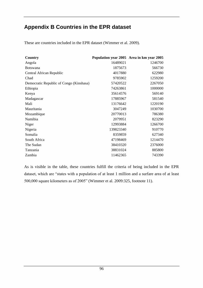
96

Appendix B Countries in the EPR dataset

These are countries included in the EPR dataset (Wimmer et al. 2009).

Country Population year 2005 Area in km year 2005

Angola 16489021 1246700

Botswana 1875673 566730

Central African Republic 4017880 622980

Chad 9785902 1259200

Democratic Republic of Congo (Kinshasa) 57420522 2267050

Ethiopia 74263861 1000000

Kenya 35614576 569140

Madagascar 17885967 581540

Mali 13176642 1220190

Mauritania 3047249 1030700

Mozambique 20770013 786380

Namibia 2079951 823290

Niger 12993884 1266700

Nigeria 139823340 910770

Somalia 8359859 627340

South Africa 47198469 1214470

The Sudan 38410320 2376000

Tanzania 38831024 885800

Zambia 11462365 743390

As is visible in the table, these countries fulfill the criteria of being included in the EPR

dataset, which are “states with a population of at least 1 million and a surfare area of at least

500,000 square kilometers as of 2005” (Wimmer et al. 2009:325, footnote 11).

97

Appendix C Baseline model

Table S- 1 presents the results of the development of the baseline model. In Table S- 1, it is

visible that models 2-4, 6, and 10-11 are have a significantly worse log likelihood compared

to model 1. This means that the variables, which were omitted from the model these models

did contribute significantly to the models log likelihood, i.e. the models explanatory power.

Therefore these variables qualify to be included in the baseline model.

Capital distance

The variable capital distance is presented here, as it was tested for the baseline model but was

not included in it. Distance from capital is included to control for how politically peripheral a

grid cell is expected to be. Distance from capital is operationalized as distance in kilometers

from the center of a grid cell to the national capital. The data were incorporated into the

original version of PRIO-GRID, and have been calculated based on geographical coordinates

for national capitals derived from the cShapes dataset (Weidmann et al. 2008). In this study,

distance from capital is also log transformed. High distance from capital is furthermore

expected to increase the risk of communal conflicts.

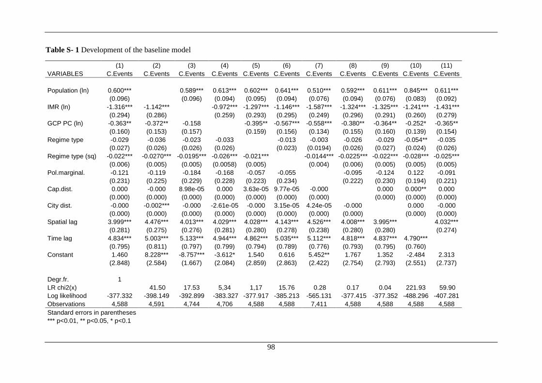
98

Table S- 1 Development of the baseline model

(1) (2) (3) (4) (5) (6) (7) (8) (9) (10) (11)

VARIABLES C.Events C.Events C.Events C.Events C.Events C.Events C.Events C.Events C.Events C.Events C.Events

Population (ln) 0.600***

0.589*** 0.613*** 0.602*** 0.641*** 0.510*** 0.592*** 0.611*** 0.845*** 0.611***

(0.096)

(0.096) (0.094) (0.095) (0.094) (0.076) (0.094) (0.076) (0.083) (0.092)

IMR (ln) -1.316*** -1.142***

-0.972*** -1.297*** -1.146*** -1.587*** -1.324*** -1.325*** -1.241*** -1.431***

(0.294) (0.286)

(0.259) (0.293) (0.295) (0.249) (0.296) (0.291) (0.260) (0.279)

GCP PC (ln) -0.363** -0.372** -0.158

-0.395** -0.567*** -0.558*** -0.380** -0.364** -0.252* -0.365**

(0.160) (0.153) (0.157)

(0.159) (0.156) (0.134) (0.155) (0.160) (0.139) (0.154)

Regime type -0.029 -0.036 -0.023 -0.033

-0.013 -0.003 -0.026 -0.029 -0.054** -0.035

(0.027) (0.026) (0.026) (0.026)

(0.023) (0.0194) (0.026) (0.027) (0.024) (0.026)

Regime type (sq) -0.022*** -0.0270*** -0.0195*** -0.026*** -0.021***

-0.0144*** -0.0225*** -0.022*** -0.028*** -0.025***

(0.006) (0.005) (0.005) (0.0058) (0.005)

(0.004) (0.006) (0.005) (0.005) (0.005)

Pol.marginal. -0.121 -0.119 -0.184 -0.168 -0.057 -0.055

-0.095 -0.124 0.122 -0.091

(0.231) (0.225) (0.229) (0.228) (0.223) (0.234)

(0.222) (0.230) (0.194) (0.221)

Cap.dist. 0.000 -0.000 8.98e-05 0.000 3.63e-05 9.77e-05 -0.000

0.000 0.000** 0.000

(0.000) (0.000) (0.000) (0.000) (0.000) (0.000) (0.000)

(0.000) (0.000) (0.000)

City dist. -0.000 -0.002*** -0.000 -2.61e-05 -0.000 3.15e-05 4.24e-05 -0.000

0.000 -0.000

(0.000) (0.000) (0.000) (0.000) (0.000) (0.000) (0.000) (0.000)

(0.000) (0.000)

Spatial lag 3.999*** 4.476*** 4.013*** 4.029*** 4.028*** 4.143*** 4.526*** 4.008*** 3.995***

4.032***

(0.281) (0.275) (0.276) (0.281) (0.280) (0.278) (0.238) (0.280) (0.280)

(0.274)

Time lag 4.834*** 5.003*** 5.133*** 4.944*** 4.862*** 5.035*** 5.112*** 4.818*** 4.837*** 4.790***

(0.795) (0.811) (0.797) (0.799) (0.794) (0.789) (0.776) (0.793) (0.795) (0.760)

Constant 1.460 8.228*** -8.757*** -3.612* 1.540 0.616 5.452** 1.767 1.352 -2.484 2.313

(2.848) (2.584) (1.667) (2.084) (2.859) (2.863) (2.422) (2.754) (2.793) (2.551) (2.737)

Degr.fr. 1 LR chi2(x)

41.50 17.53 5,34 1,17 15.76 0.28 0.17 0.04 221.93 59.90

Log likelihood -377.332 -398.149 -392.899 -383.327 -377.917 -385.213 -565.131 -377.415 -377.352 -488.296 -407.281

Observations 4,588 4,591 4,744 4,706 4,588 4,588 7,411 4,588 4,588 4,588 4,588

Standard errors in parentheses *** p<0.01, ** p<0.05, * p<0.1

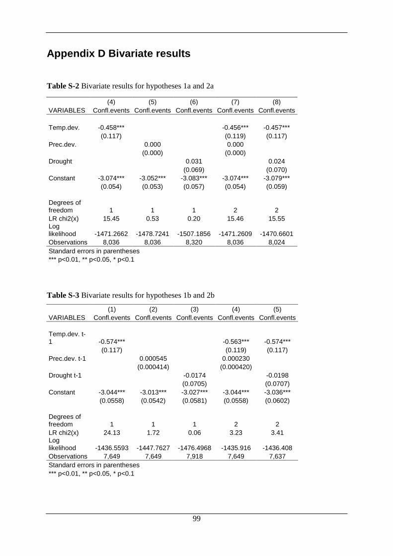
99

Appendix D Bivariate results

Table S-2 Bivariate results for hypotheses 1a and 2a

(4) (5) (6) (7) (8)

VARIABLES Confl.events Confl.events Confl.events Confl.events Confl.events

Temp.dev. -0.458***

-0.456*** -0.457***

(0.117)

(0.119) (0.117)

Prec.dev.

0.000

0.000

(0.000)

(0.000)

Drought

0.031

0.024

(0.069)

(0.070)

Constant -3.074*** -3.052*** -3.083*** -3.074*** -3.079***

(0.054) (0.053) (0.057) (0.054) (0.059)

Degrees of freedom 1 1 1 2 2

LR chi2(x) 15.45 0.53 0.20 15.46 15.55 Log likelihood -1471.2662 -1478.7241 -1507.1856 -1471.2609 -1470.6601

Observations 8,036 8,036 8,320 8,036 8,024

Standard errors in parentheses *** p<0.01, ** p<0.05, * p<0.1

Table S-3 Bivariate results for hypotheses 1b and 2b

(1) (2) (3) (4) (5)

VARIABLES Confl.events Confl.events Confl.events Confl.events Confl.events

Temp.dev. t-1 -0.574***

-0.563*** -0.574***

(0.117)

(0.119) (0.117)

Prec.dev. t-1

0.000545

0.000230

(0.000414)

(0.000420)

Drought t-1

-0.0174

-0.0198

(0.0705)

(0.0707)

Constant -3.044*** -3.013*** -3.027*** -3.044*** -3.036***

(0.0558) (0.0542) (0.0581) (0.0558) (0.0602)

Degrees of freedom 1 1 1 2 2

LR chi2(x) 24.13 1.72 0.06 3.23 3.41 Log likelihood -1436.5593 -1447.7627 -1476.4968 -1435.916 -1436.408

Observations 7,649 7,649 7,918 7,649 7,637

Standard errors in parentheses *** p<0.01, ** p<0.05, * p<0.1

100

Table S-4 Bivariate results for hypotheses 3a and 4a

(1) (2) (3) (4) (5)

VARIABLES Confl.events Confl.events Confl.events Confl.events Confl.events

Temp.dev. -0.580*

-0.753** -0.580*

(0.332)

(0.350) (0.325)

Prec.dev.

-0.002*

-0.002**

(0.001)

(0.001)

Drought

-0.731**

-0.738**

(0.317)

(0.317)

Constant -3.334*** -3.328*** -3.160*** -3.353*** -3.159***

(0.146) (0.146) (0.149) (0.150) (0.151)

Degrees of freedom 1 1 1 2 2

LR chi2(x) 3.04 3.08 8.85 7.72 12.08 Log likelihood -215.23136 -215.21124 -213.03471 -212.88833 -210.70861

Observations 1,429 1,429 1,449 1,429 1,429

Standard errors in parentheses *** p<0.01, ** p<0.05, * p<0.1

Table S-5 Bivariate results for hypotheses 3b and 4b

(1) (2) (3) (4) (5)

VARIABLES Confl.events Confl.events Confl.events Confl.events Confl.events

Temp.dev. t-1 -1.299***

-1.468*** -1.304***

(0.374)

(0.389) (0.373)

Prec.dev. t-1

-0.001

-0.002**

(0.001)

(0.001)

Drought t-1

-0.180

-0.198

(0.181)

(0.181)

Constant -3.309*** -3.266*** -3.192*** -3.344*** -3.229***

(0.154) (0.147) (0.157) (0.159) (0.166)

Degrees of freedom 1 1 1 2 2

LR chi2(x) 12.58 2.67 1.09 17.68 13.91 Log likelihood -207.18779 -212.13814 -213.64671 -204.63774 -206.52108

Observations 1,340 1,340 1,359 1,340 1,340

Standard errors in parentheses *** p<0.01, ** p<0.05, * p<0.1

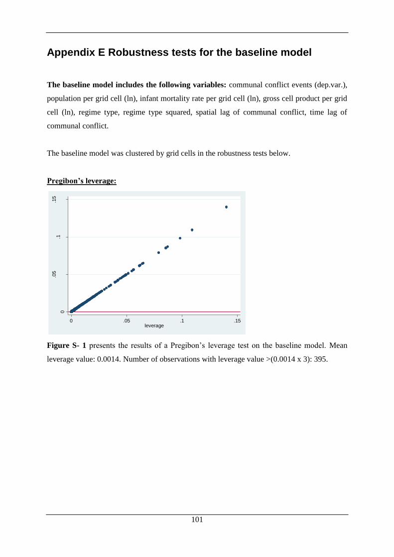
101

Appendix E Robustness tests for the baseline model

The baseline model includes the following variables: communal conflict events (dep.var.),

population per grid cell (ln), infant mortality rate per grid cell (ln), gross cell product per grid

cell (ln), regime type, regime type squared, spatial lag of communal conflict, time lag of

communal conflict.

The baseline model was clustered by grid cells in the robustness tests below.

Pregibon’s leverage:

Figure S- 1 presents the results of a Pregibon’s leverage test on the baseline model. Mean

leverage value: 0.0014. Number of observations with leverage value >(0.0014 x 3): 395.

0

.05

.1.1

5

leve

rag

e

0 .05 .1 .15leverage

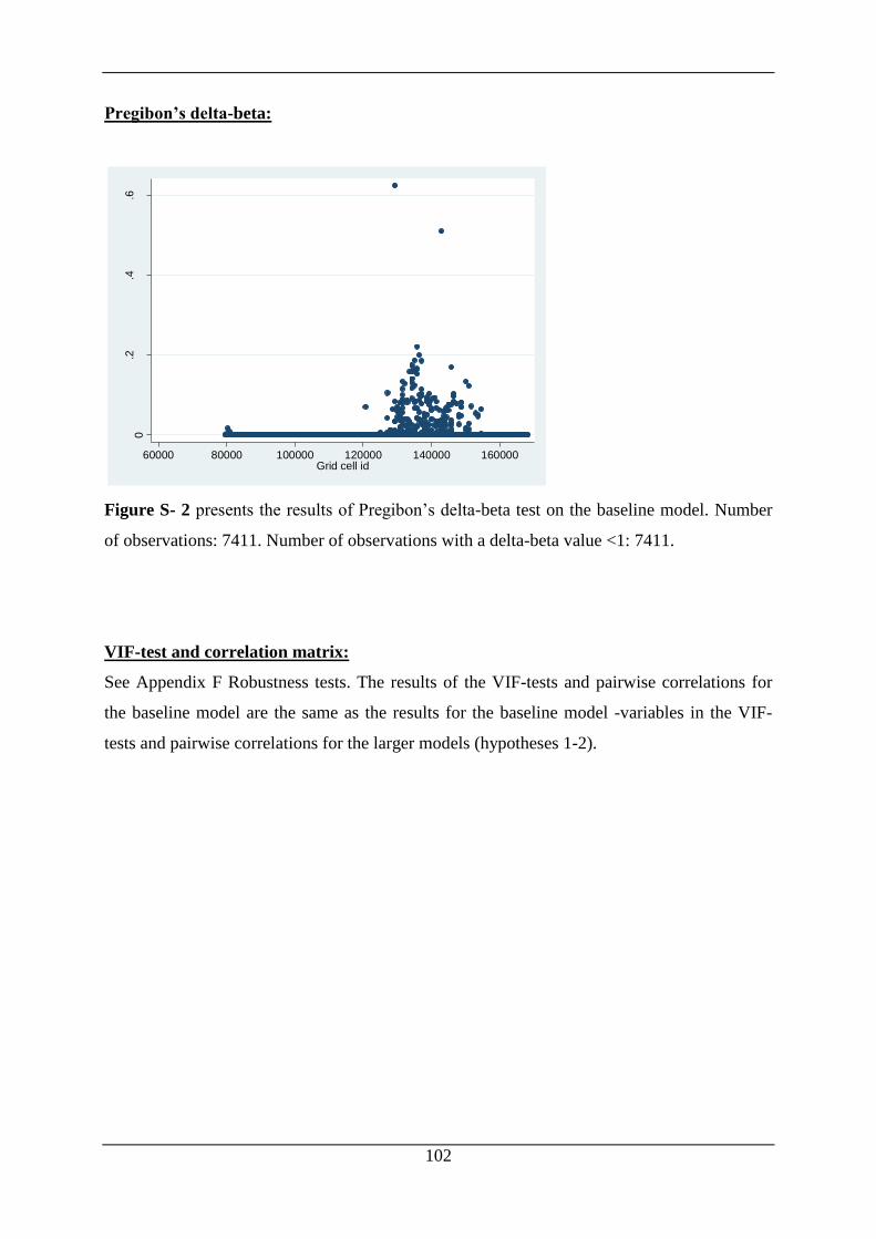
102

Pregibon’s delta-beta:

Figure S- 2 presents the results of Pregibon’s delta-beta test on the baseline model. Number

of observations: 7411. Number of observations with a delta-beta value <1: 7411.

VIF-test and correlation matrix:

See Appendix F Robustness tests. The results of the VIF-tests and pairwise correlations for

the baseline model are the same as the results for the baseline model -variables in the VIF-

tests and pairwise correlations for the larger models (hypotheses 1-2).

0.2

.4.6

Pre

gib

on's

db

eta

60000 80000 100000 120000 140000 160000Grid cell id

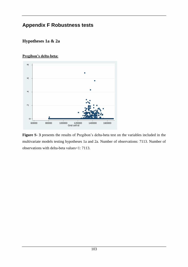
103

Appendix F Robustness tests

Hypotheses 1a & 2a

Pregibon’s delta-beta:

Figure S- 3 presents the results of Pregibon’s delta-beta test on the variables included in the

multivariate models testing hypotheses 1a and 2a. Number of observations: 7113. Number of

observations with delta-beta values<1: 7113.

0.2

.4.6

.8

Pre

gib

on's

db

eta

60000 80000 100000 120000 140000 160000Grid cell id

104

Pregibon’s leverage:

Figure S- 4 presents the results of Pregibon’s leverage test on the variables included in the

multivariate models testing hypotheses 1a and 2a. Mean of leverage values: 0.0019. Number

of observations with leverage values >(0.0019 x 3): 390.

VIF-tests:

Table S-6 VIF-tests for variables included in hypotheses 1a and 2a.

Variable VIF 1/VIF

Population (ln) 1.96 0.511066

City distance 1.90 0.525263

GCP PC (ln) 1.64 0.611556

IMR (ln) 1.61 0.620244

Regime type (sq) 1.33 0.751549

Regime type 1.26 0.794885

Temp.deviation 1.10 0.908025

Prec.deviation 1.08 0.929023

Political marginalization 1.07 0.932326

Drought 1.05 0.950560

Mean VIF 1.40

0

.05

.1.1

5

leve

rag

e

0 .05 .1 .15leverage

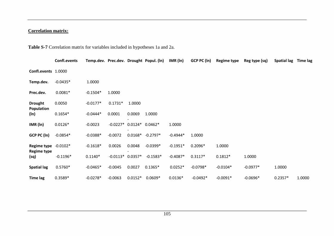
105

Correlation matrix:

Table S-7 Correlation matrix for variables included in hypotheses 1a and 2a.

Confl.events Temp.dev. Prec.dev. Drought Popul. (ln) IMR (ln) GCP PC (ln) Regime type Reg type (sq) Spatial lag Time lag

Confl.events 1.0000

Temp.dev. -0.0435* 1.0000

Prec.dev. 0.0081* -0.1504* 1.0000

Drought 0.0050 -0.0177* 0.1731* 1.0000 Population

(ln) 0.1654* -0.0444* 0.0001 0.0069 1.0000

IMR (ln) 0.0126* -0.0023 -0.0227* -0.0124* 0.0462* 1.0000

GCP PC (ln) -0.0854* -0.0388* -0.0072

-0.0168* -0.2797* -0.4944* 1.0000

Regime type -0.0102* -0.1618* 0.0026 0.0048 -0.0399* -0.1951* 0.2096* 1.0000

Regime type (sq) -0.1196* 0.1140* -0.0113*

-0.0357* -0.1583* -0.4087* 0.3117* 0.1812* 1.0000

Spatial lag 0.5760* -0.0465* -0.0045 0.0027 0.1365* 0.0252* -0.0798* -0.0104* -0.0977* 1.0000

Time lag 0.3589* -0.0278* -0.0063 0.0152* 0.0609* 0.0136* -0.0492* -0.0091* -0.0696* 0.2357* 1.0000

106

Hypotheses 1b & 2b

Pregibon’s delta-beta: No result, because delta-beta tests cannot be conducted on time series

operators (here temperature, precipitation and drought in the previous year).

Pregibon’s leverage: No result, because leverage tests cannot be conducted on time series

operators (here temperature, precipitation and drought in the previous year).

VIF-tests:

Table S- 8 VIF-tests for variables included in hypotheses 1b and 2b.

Variable VIF 1/VIF

Population (ln) 1.96 0.509604

City distance 1.91 0.523005

GCP PC (ln) 1.66 0.603330

IMR (ln) 1.64 0.608907

Regime type (sq) 1.47 0.678745

Regime type 1.24 0.804607

Political marginalization 1.09 0.920957

Temp.deviation (t-1) 1.08 0.923696

Prec.deviation (t-1) 1.06 0.942792

Drought (t-1) 1.05 0.950929

Mean VIF 1.42

107

Correlation matrix:

Table S- 9 Correlation matrix for variables included in hypotheses 1b and 2b.

Confl events Temp.dev. (t-1)

Prec.dev. (t-1)

Drought (t-1)

Popul. (ln)

IMR (ln) GCP PC (ln)

Regime type

Reg type (sq)

Spatial lag Time lag

Confl.events 1.0000 Temp.dev.

(t-1) -0.0558* 1.0000 Prec.dev. (t-

1) 0.0150* -0.1455* 1.0000 Drought (t-1) -0.0028 -0.0193* 0.1728* 1.0000

Population (ln) 0.1654* -0.0361* -0.0016 0.0376* 1.0000

IMR (ln) 0.0126* -0.0319* 0.0101* -0.0177* 0.0462* 1.0000 GCP PC (ln) -0.0854* -0.0313* -0.0146* -0.0212* -0.2797* -0.4944* 1.0000

Regime type -0.0102* -0.1543* 0.0136* 0.0273* -0.0399* -0.1951* 0.2096* 1.0000 Regime type

(sq) -0.1196* 0.1136* 0.0003 -0.0256* -0.1583* -0.4087* 0.3117* 0.1812* 1.0000 Spatial lag 0.5760* -0.0494* 0.0201* 0.0037 0.1365* 0.0252* -0.0798* -0.0104* -0.0977* 1.0000

Time lag 0.3589* -0.0269* 0.0016 0.0053 0.0609* 0.0136* -0.0492* -0.0091* -0.0696* 0.2357* 1.0000

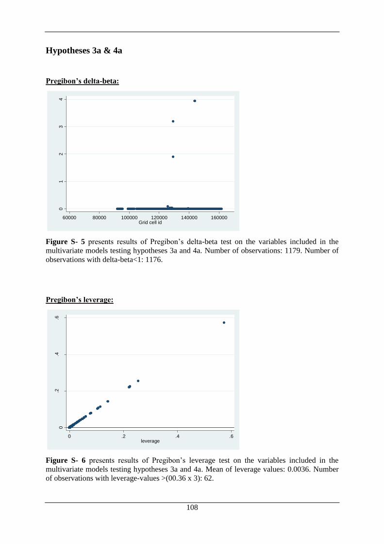
108

Hypotheses 3a & 4a

Pregibon’s delta-beta:

Figure S- 5 presents results of Pregibon’s delta-beta test on the variables included in the

multivariate models testing hypotheses 3a and 4a. Number of observations: 1179. Number of

observations with delta-beta<1: 1176.

Pregibon’s leverage:

Figure S- 6 presents results of Pregibon’s leverage test on the variables included in the

multivariate models testing hypotheses 3a and 4a. Mean of leverage values: 0.0036. Number

of observations with leverage-values >(00.36 x 3): 62.

01

23

4

Pre

gib

on's

db

eta

60000 80000 100000 120000 140000 160000Grid cell id

0.2

.4.6

leve

rag

e

0 .2 .4 .6leverage

109

VIF-tests:

Table S-10 VIF-tests for variables included in hypotheses 3a and 4a.

Variable VIF 1/VIF

Spatial lag 1.89 0.529035

Time lag 1.80 0.556428

Regime type 1.47 0.681994

Regime type (sq) 1.45 0.688544

GCP PC (ln) 1.41 0.710792

IMR (ln) 1.28 0.781744

Population (ln) 1.17 0.856374

Temperature deviation 1.12 0.889859

Precipitation deviation 1.09 0.920454

Drought 1.06 0.943502

Mean VIF 1.37

|

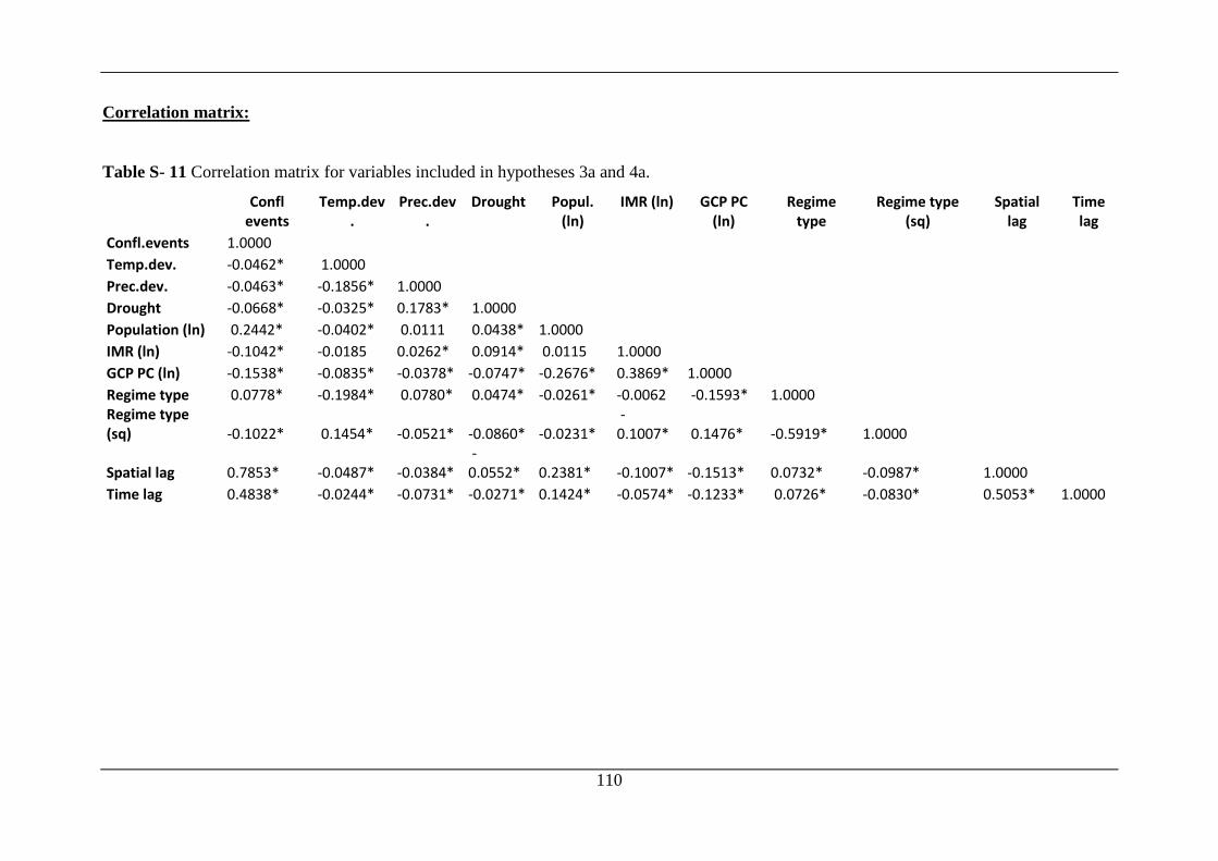
110

Correlation matrix:

Table S- 11 Correlation matrix for variables included in hypotheses 3a and 4a.

Confl events

Temp.dev.

Prec.dev.

Drought Popul. (ln)

IMR (ln) GCP PC (ln)

Regime type

Regime type (sq)

Spatial lag

Time lag

Confl.events 1.0000 Temp.dev. -0.0462* 1.0000

Prec.dev. -0.0463* -0.1856* 1.0000 Drought -0.0668* -0.0325* 0.1783* 1.0000

Population (ln) 0.2442* -0.0402* 0.0111 0.0438* 1.0000 IMR (ln) -0.1042* -0.0185 0.0262* 0.0914* 0.0115 1.0000

GCP PC (ln) -0.1538* -0.0835* -0.0378* -0.0747* -0.2676* 0.3869* 1.0000 Regime type 0.0778* -0.1984* 0.0780* 0.0474* -0.0261* -0.0062 -0.1593* 1.0000

Regime type (sq) -0.1022* 0.1454* -0.0521* -0.0860* -0.0231*

-0.1007* 0.1476* -0.5919* 1.0000

Spatial lag 0.7853* -0.0487* -0.0384*

-0.0552* 0.2381* -0.1007* -0.1513* 0.0732* -0.0987* 1.0000

Time lag 0.4838* -0.0244* -0.0731* -0.0271* 0.1424* -0.0574* -0.1233* 0.0726* -0.0830* 0.5053* 1.0000

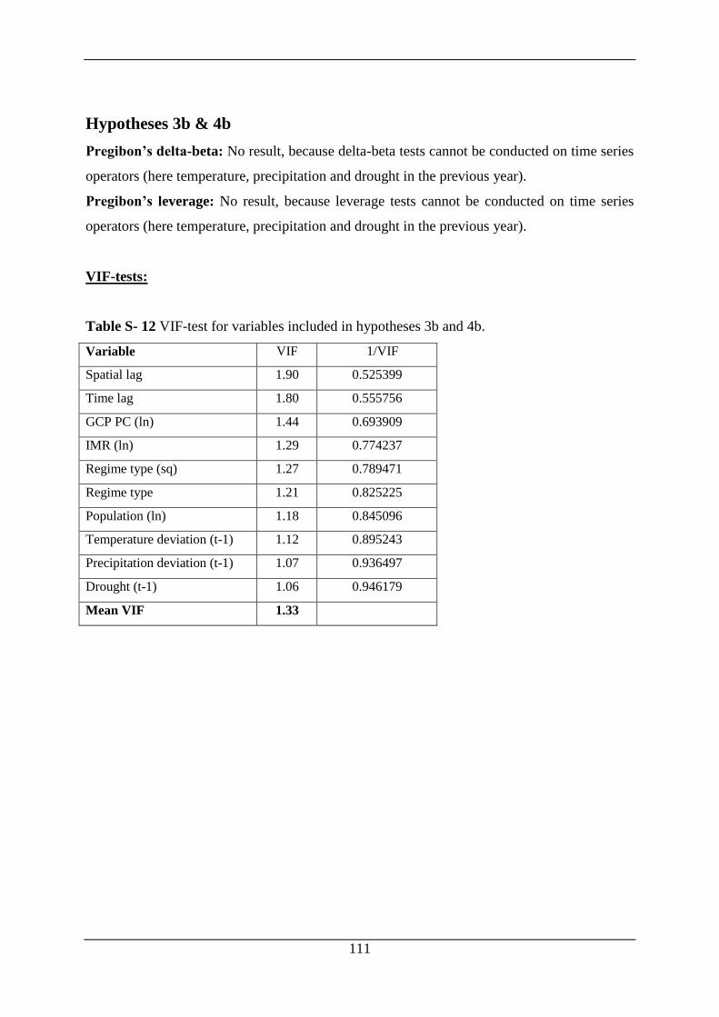
111

Hypotheses 3b & 4b

Pregibon’s delta-beta: No result, because delta-beta tests cannot be conducted on time series

operators (here temperature, precipitation and drought in the previous year).

Pregibon’s leverage: No result, because leverage tests cannot be conducted on time series

operators (here temperature, precipitation and drought in the previous year).

VIF-tests:

Table S- 12 VIF-test for variables included in hypotheses 3b and 4b.

Variable VIF 1/VIF

Spatial lag 1.90 0.525399

Time lag 1.80 0.555756

GCP PC (ln) 1.44 0.693909

IMR (ln) 1.29 0.774237

Regime type (sq) 1.27 0.789471

Regime type 1.21 0.825225

Population (ln) 1.18 0.845096

Temperature deviation (t-1) 1.12 0.895243

Precipitation deviation (t-1) 1.07 0.936497

Drought (t-1) 1.06 0.946179

Mean VIF 1.33

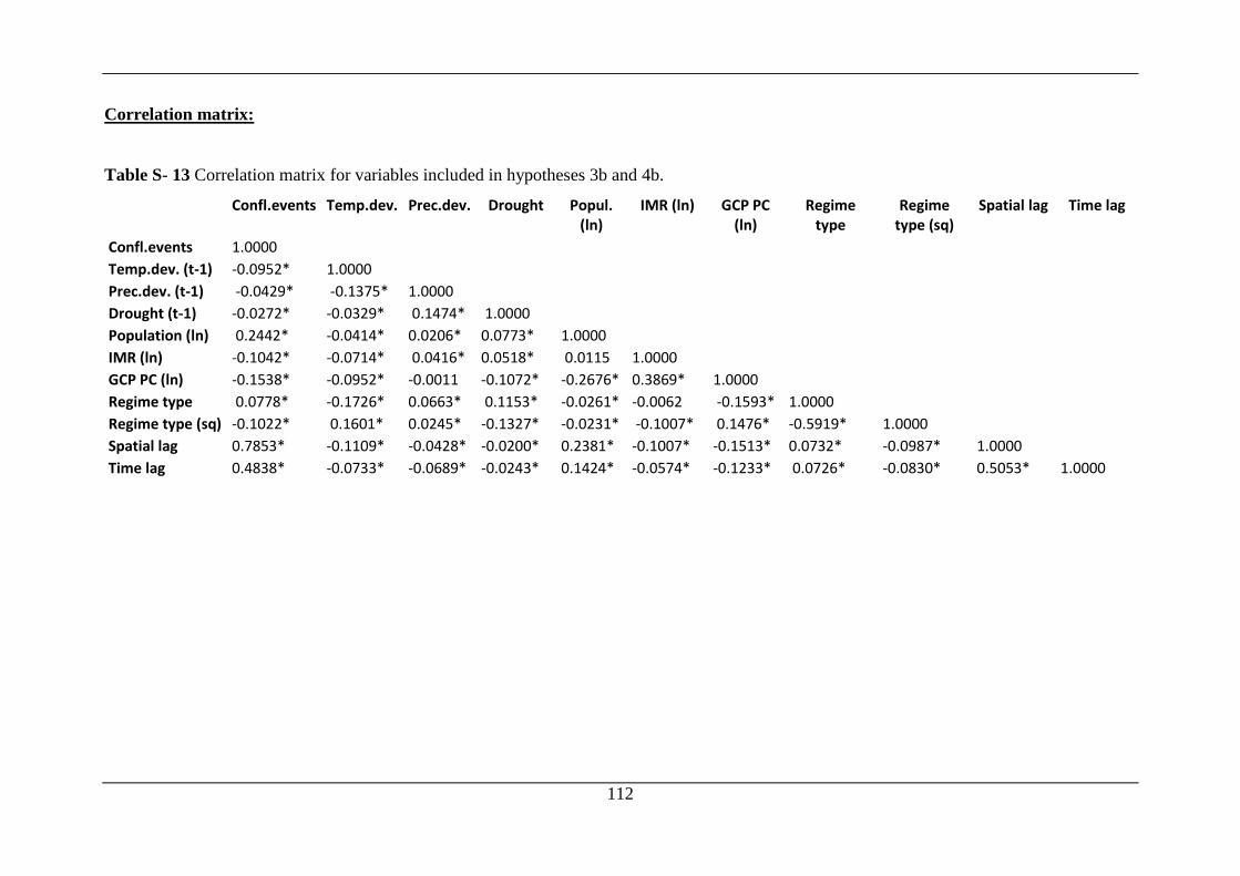
112

Correlation matrix:

Table S- 13 Correlation matrix for variables included in hypotheses 3b and 4b.

Confl.events Temp.dev. Prec.dev. Drought Popul. (ln)

IMR (ln) GCP PC (ln)

Regime type

Regime type (sq)

Spatial lag Time lag

Confl.events 1.0000 Temp.dev. (t-1) -0.0952* 1.0000

Prec.dev. (t-1) -0.0429* -0.1375* 1.0000 Drought (t-1) -0.0272* -0.0329* 0.1474* 1.0000

Population (ln) 0.2442* -0.0414* 0.0206* 0.0773* 1.0000 IMR (ln) -0.1042* -0.0714* 0.0416* 0.0518* 0.0115 1.0000

GCP PC (ln) -0.1538* -0.0952* -0.0011 -0.1072* -0.2676* 0.3869* 1.0000 Regime type 0.0778* -0.1726* 0.0663* 0.1153* -0.0261* -0.0062 -0.1593* 1.0000

Regime type (sq) -0.1022* 0.1601* 0.0245* -0.1327* -0.0231* -0.1007* 0.1476* -0.5919* 1.0000 Spatial lag 0.7853* -0.1109* -0.0428* -0.0200* 0.2381* -0.1007* -0.1513* 0.0732* -0.0987* 1.0000

Time lag 0.4838* -0.0733* -0.0689* -0.0243* 0.1424* -0.0574* -0.1233* 0.0726* -0.0830* 0.5053* 1.0000

113