ORIGINAL PAPER

Climate-based model of spatial pattern of the speciesrichness of ants in Georgia

Giorgi Chaladze

Received: 4 July 2011 / Accepted: 23 January 2012

� Springer Science+Business Media B.V. 2012

Abstract For optimal planning of conservation and

monitoring measures, it is important to know the spatial

pattern of species richness and especially areas with high

species richness. A spatial pattern of the species richness of

ants in Georgia (Caucasus) was modeled, areas with the

highest number of ant’s species were inferred, and climatic

factors that influence the pattern of ant diversity were

identified. A database was created by accumulating

occurrences for 63 ant species, including 256 localities and

2,018 species/occurrences. Species richness was positively

correlated with variables associated with temperature and

negatively correlated with variables associated with pre-

cipitation. Species richness reaches a maximum at the

elevations 800–1,200 m a.s.l. and declines at both lower

and higher altitudes. The role of climatic variables and

geography of the study area in determining the observed

pattern of species richness is discussed.

Keywords Biodiversity �Climatic variables � Formicidae �Spatial pattern � Altitudinal gradient � Ground moisture

Introduction

For optimal planning of conservation and ecological

monitoring, it is important to know geographic areas with

particularly high species richness (Ceballos and Brown

1995; Garcia 2006; Myers et al. 2000; Newbold et al.

2009). However, development of biodiversity inventories is

a very time and effort consuming process, especially for

highly diverse species groups such as insects, because it

requires intensive sampling and taxonomic expertise

(Agosti et al. 2000). An alternative is to develop spatial

models based on the limited occurrence data which are

already compiled in literature and online databases (Garcia

2006; Newbold et al. 2009).

Understanding spatial pattern of species richness in

Georgia is important at the global scale as the whole ter-

ritory of Georgia is part of the Caucasus biodiversity hot-

spot, which is one of 25 global biodiversity hotspots. These

global biodiversity hotspots comprise only 1.4% of the land

surface of the Earth and contain as many as 44% of vas-

cular plant species and more than 30% of vertebrate species

(Myers et al. 2000).

Knowing the dependence of species richness on environ-

mental variables is important for understanding the formation

of modern species richness distribution and for the prediction

of how species richness would be affected by climate change

(Kerr 2001; Kienasta et al. 1998; Iverson and Prasad 2001).

Dunn et al. (2009) showed that ant species richness is posi-

tively correlated with temperature, and negatively correlated

with precipitation at a global scale. The use of ants as bio-

indicators is also growing in Australia (Andersen and Majer

2004), tropical location (e.g. Bestelmeyer and Wiens 2001;

Van Hamburg et al. 2004) and temperate areas (Kaspari and

Majer 2000; Sauberer et al. 2004).

Taxonomic studies of ants in Georgia started in the late

nineteenth century (Gratiashvili and Barjadze 2008). The

studies collected much data on the occurrences of ant

species (Gratiashvili and Barjadze 2008) but did not

identify spatial patterns of the species richness.

Recent algorithms and statistical methods have helped to

develop spatial models describing biodiversity including

those developed for the prediction of species distributions

(Fitzpatrick et al. 2007; Munoz et al. 2009; Ortega-Huerta

G. Chaladze (&)

Institute of Ecology, Ilia State University, 3/5 Cholokashvili

Ave., 0162 Tbilisi, Georgia

e-mail: Giorgi.chaladze@gmail.com

123

J Insect Conserv

DOI 10.1007/s10841-012-9464-5

and Peterson 2008; Soberon and Peterson 2005; Stockwell

1999; Stockwell and Peters 1999). In order to identify the

spatial pattern of species richness, distribution models for

single species are developed and then those models are

summed (Garcia 2006; Newbold et al. 2009). An alterna-

tive method is recording species richness at individual

localities and modeling richness patterns directly. Newbold

et al. (2009) compared the two approaches while modeling

the butterfly and mammal fauna of Egypt. They showed

that using the former approach (summing individual

models) produces more accurate output. Summing indi-

vidual models is a good approach only when the available

distribution data are sufficient to create individual species

distribution models.

In this study, spatial patterns of the species richness of

ants in Georgia were modeled and the factors of spatial and

altitudinal variation of species richness were inferred.

Methods

Study area

The study area included the entire territory of Georgia

(Fig. 1). The elevation within the area varies between -1

and 4,550 m. a.s.l., mean annual temperature between -9.7

and 15�C, and annual precipitation between 439 and

2,376 mm (Hijmans et al. 2005). The country has a broad

variety of landscapes, from temperate mountain rainforests

to semi-deserts and alpine tundra, including agricultural

and alpine landscapes covering nearly half of the country

(Tarkhnishvili et al. 2010).

Modeling

A database was created by compiling data on the locations

of Georgian ant species (Gratiashvili and Barjadze 2008).

Geographic coordinates of individual locations were scored

from the GeoNames database (http://www.geonames.org/).

In total, 2,018 species/locations were analyzed, providing

data on 72 ant species and 258 unique localities (Fig. 1).

The modeling of species distribution was performed

using openModeller (Munoz et al. 2009). This software

helps to model suitable habitats for individual species and

then overlay them in order to estimate summed model of

species richness (Munoz et al. 2009). The GARP algorithm

(ecological niche model) was used in order to infer the ant

diversity hotspots (Stockwell 1999; Stockwell and Peters

1999).

In total, 19 variables were taken from the WorldClim

version 1.4 dataset at a resolution of 30 arcsec (c. 1 km)

(Hijmans et al. 2005).These were: (1) annual mean tem-

perature, (2) mean diurnal range, (3) isothermality, (4)

temperature seasonality, (5) maximum temperature of

warmest month, (6) minimum temperature of coldest

month, (7) temperature annual range, (8) mean temperature

of wettest quarter, (9) mean temperature of driest quarter,

(10) mean temperature of warmest quarter, (11) mean

temperature of coldest quarter, (12) annual precipitation,

(13) precipitation of wettest month, (14) precipitation of

driest month, (15) precipitation seasonality, (16) precipi-

tation of wettest quarter, (17) precipitation of driest quarter,

(18) precipitation of warmest quarter, and (19) precipita-

tion of coldest quarter.

Range models were developed for each species with at

least five records (Garcia 2006). In total, 72 species met

this criteria. Seventy five percent of occurrence locations

were used for training the models and 25% was used for

validation. Occurrences were divided into test and training

points randomly. The accuracy of each model was assessed

using the area under the receiver operator (ROC) curve

(AUC); the calculations were performed in openModeller

with supply of test and training occurrences independently.

Following the recommendations made by Swets (1986),

Fig. 1 Study area and

localities of ant species

J Insect Conserv

123

nine species with the AUC scores of \0.7 were excluded

from the further analysis.

The individual binary models of species ranges pre-

dicted by the GARP system were overlaid and summed for

producing map of species richness.

Statistical analysis

Thousand random points were generated using Arcview

3.1, covering whole study area. The following variables

were scored for each random point: inferred species rich-

ness index, the 19 bioclimatic variables listed above, ele-

vation and Annual Potential Ground Moisture (PGM). Data

was extracted from GIS layers using Grid Pig tools

extension of ArcView 3.1.

Annual PGM was calculated as: Annual PGM = MP -

PET; Where MP = Monthly precipitation, PET = Poten-

tial Evapotranspiration; PET = Monthly temperature mean

above 0�C 9 4.910833333, otherwise = 0 (Thornthwaite

1948; Thornthwaite and Mather 1957).

The regression tree analysis with CHAID (Chi-squared

Automatic Interaction Detector, Kass 1980) method was

used in order to determine the interaction between species

richness and the environmental variables. CHAID analysis

is a non-parametric procedure and no assumptions about

the data distribution need to be made (Van Diepen and

Franses 2006).

SPSS software (SPSS v.16) was used to carry out the

analysis. A significance level of 5% was used in the F test,

the maximum number of levels was established as three,

and the minimum number of cases in a node for being a

child node was established at 50. Analysis was performed

(1) for each variable separately and (2) including all

variables.

Results

From 72 species included in the analysis 63 passed cross

validation test (AUC [0.7). Average AUC value of

validated models was 0.87 and average prediction accuracy

80%. Inferred species richness varied from 2 to 63 with an

average value of 36. Inferred Species richness was not

uniform within the study area (Fig. 2).

Species richness in this study showed non linear corre-

lation with elevation, with a well expressed mid-elevation

(*800 m) peak (Fig. 3). The lowest richness was pre-

dicted for high elevation ([2,500 m) and low species

richness was predicted for the Colchis lowland and Black

Sea Coast. The highest richness was predicted for the

elevation between 500 and 1,500 m.

Species richness was positively correlated with variables

associated with temperature and negatively with variables

associated with precipitation (Table 1; Fig. 4); only a few

variables had no significant correlation with species rich-

ness (Table 1).

The regression tree analysis for each variable separately

is given in Table 1. Most of the variables were useful for

discrimination of species richness except: Precipitation of

Coldest Quarter, Precipitation of Driest Quarter and

Fig. 2 Ant species richness

generated by summing

individual predictions of the

distributions of species. Lightertones indicate high predicted

species richness and darkertones indicate lower species

richness

Fig. 3 Distribution of ant species richness along altitudinal gradient

with line of best fit

J Insect Conserv

123

Precipitation of Driest Month. In General Variables asso-

ciated with precipitation were less useful for discrimination

of species richness using single factor. Variables associated

with temperature were more predictive for species richness

(Table 1).

The regression tree including 21 environmental factors

revealed four important discriminators for species richness:

Elevation, Precipitation of driest quarter, Precipitation of

coldest quarter and Annual precipitation (R2 = 0.827,

SEE = 3.006). Figure 5 provides an overall picture of

the relative importance of the variables. The first most

important discriminator is elevation (P \ 0.001). The

second splitter is precipitation, however different season

precipitations are important at different elevations: (1) for

Table 1 Summary table of

regression tree analysis using

CHAID algorithm for single

variables and correlation of

species richness with those

variables

Significant correlations

(P \ 0.005) are marked with

asterisk (*)

Variables Correlation coefficient Regression tree analysis

using CHAID algorithm

R2 SEE

Mean temperature of driest quarter 0.311* 0.673 6.36

Mean temperature of wettest quarter 0.435* 0.389 7.123

Temperature annual range 0.221* 0.295 9.304

Min temperature of coldest month 0.409* 0.685 5.649

Max temperature of warmest month 0.562* 0.659 5.194

Temperature seasonality 0.391* 0.337 8.045

Isothermality -0.272* 0.252 9.372

Mean diurnal range -0.022

Precipitation of coldest quarter 0.008

Precipitation of warmest quarter -0.309* 0.243 9.31

Precipitation of driest quarter 0.004

Precipitation of wettest quarter -0.260* 0.256 8.635

Precipitation seasonality -0.219* 0.17 9.578

Precipitation of driest month 0.013

Precipitation of wettest month -0.232* 0.245 8.573

Mean temperature of coldest quarter 0.436* 0.724 5.539

Mean temperature of warmest quarter 0.548* 0.694 4.71

Annual precipitation -0.144* 0.225 9.696

Mean annual temperature 0.510* 0.777 3.491

Elevation -0.538* 0.777 3.86

Annual potential ground moisture -0.417* 0.445 7.715

Fig. 4 Correlation of inferred species richness with precipitation of warmest month and mean temperature of warmest quarter

J Insect Conserv

123

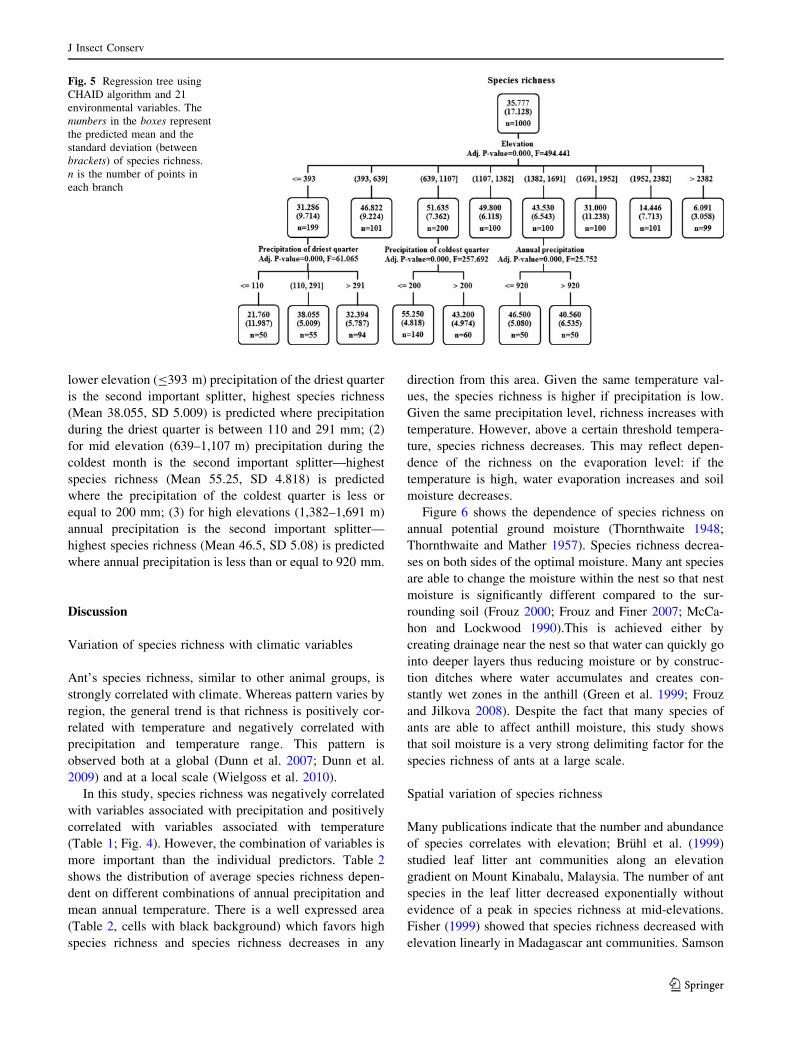
lower elevation (B393 m) precipitation of the driest quarter

is the second important splitter, highest species richness

(Mean 38.055, SD 5.009) is predicted where precipitation

during the driest quarter is between 110 and 291 mm; (2)

for mid elevation (639–1,107 m) precipitation during the

coldest month is the second important splitter—highest

species richness (Mean 55.25, SD 4.818) is predicted

where the precipitation of the coldest quarter is less or

equal to 200 mm; (3) for high elevations (1,382–1,691 m)

annual precipitation is the second important splitter—

highest species richness (Mean 46.5, SD 5.08) is predicted

where annual precipitation is less than or equal to 920 mm.

Discussion

Variation of species richness with climatic variables

Ant’s species richness, similar to other animal groups, is

strongly correlated with climate. Whereas pattern varies by

region, the general trend is that richness is positively cor-

related with temperature and negatively correlated with

precipitation and temperature range. This pattern is

observed both at a global (Dunn et al. 2007; Dunn et al.

2009) and at a local scale (Wielgoss et al. 2010).

In this study, species richness was negatively correlated

with variables associated with precipitation and positively

correlated with variables associated with temperature

(Table 1; Fig. 4). However, the combination of variables is

more important than the individual predictors. Table 2

shows the distribution of average species richness depen-

dent on different combinations of annual precipitation and

mean annual temperature. There is a well expressed area

(Table 2, cells with black background) which favors high

species richness and species richness decreases in any

direction from this area. Given the same temperature val-

ues, the species richness is higher if precipitation is low.

Given the same precipitation level, richness increases with

temperature. However, above a certain threshold tempera-

ture, species richness decreases. This may reflect depen-

dence of the richness on the evaporation level: if the

temperature is high, water evaporation increases and soil

moisture decreases.

Figure 6 shows the dependence of species richness on

annual potential ground moisture (Thornthwaite 1948;

Thornthwaite and Mather 1957). Species richness decrea-

ses on both sides of the optimal moisture. Many ant species

are able to change the moisture within the nest so that nest

moisture is significantly different compared to the sur-

rounding soil (Frouz 2000; Frouz and Finer 2007; McCa-

hon and Lockwood 1990).This is achieved either by

creating drainage near the nest so that water can quickly go

into deeper layers thus reducing moisture or by construc-

tion ditches where water accumulates and creates con-

stantly wet zones in the anthill (Green et al. 1999; Frouz

and Jilkova 2008). Despite the fact that many species of

ants are able to affect anthill moisture, this study shows

that soil moisture is a very strong delimiting factor for the

species richness of ants at a large scale.

Spatial variation of species richness

Many publications indicate that the number and abundance

of species correlates with elevation; Bruhl et al. (1999)

studied leaf litter ant communities along an elevation

gradient on Mount Kinabalu, Malaysia. The number of ant

species in the leaf litter decreased exponentially without

evidence of a peak in species richness at mid-elevations.

Fisher (1999) showed that species richness decreased with

elevation linearly in Madagascar ant communities. Samson

Fig. 5 Regression tree using

CHAID algorithm and 21

environmental variables. The

numbers in the boxes represent

the predicted mean and the

standard deviation (between

brackets) of species richness.

n is the number of points in

each branch

J Insect Conserv

123

et al. (1997) surveyed how species richness and abundance

in ant communities changes along an elevation gradient in

Philippines. Measures of species richness and relative

abundances peaked at mid-elevations and declined sharply

with increasing elevation. Ants were extremely rare above

1,500 m. Similar patterns were observed in a number of

other studies (Olson 1994; Sanders et al. 2003; Sabu et al.

2008). Sanders et al. (2003) surveyed species richness in

three canyons in Spring Mountains, Southern Nevada. Ant

species richness increased linearly with elevation along

two transects and peaked at mid-elevation along a third

transect.

Several explanations have been suggested to explain the

dependence of species richness on the altitudinal gradient:

direct effect of climate (Krebs 2001); indirect effect of

climate through net primary productivity—a high net pri-

mary production permits consumers to maintain high

population densities, thereby reducing the probability of

Table 2 Mean annual precipitation (mm), Annual temperature (�C) and Average species richness

Annual

Mean

Temperature -2 -1 0 1 2 3 4 5 6 7 8 9 10 11 12 13 14 15

Annual

Precipitation

400 4 1

500 43 33 35 29 21 4

600 8 12 22 39 40 38 44 40 43 43 35 18 14

700 4 7 11 25 34 41 44 47 46 45 42 38 30

800 2 2 3 13 17 32 37 43 44 44 42 39 37 37

900 3 3 3 3 14 13 33 33 40 41 41 40 39

1000 3 3 3 4 7 15 23 32 39 39 41 37 35 36 37

1100 5 5 8 19 36 34 33 39 37 36 36

1200 8 16 34 27 34 33 33 34 36 38

1300 33 34 34 27 37 35

1400 32 28 28 30 29

1500 30 30 27 23

1600 30 26 26 25

1700 25 24 24 27

1800 27 30 28

1900 25 26 25

2000 22 24

2100 23

2200 21

2300 10

2400 17

Average Elevation

29832811264424652262204818341681145012921096953814724571397175 53(m)

Darker tones indicate highest species richness; lighter tones indicate lowest species richness. The numbers in the cells indicate the average

number of species at a combination of precipitation and temperature

J Insect Conserv

123

local extinction (Janzen 1973; Siemann 1998; Srivastava

and Lawton 1998; Kaspari and Majer 2000); human impact

(Sanders et al. 2003).

Species richness in this study showed a mid-elevation

peak (800–1,200 m). The drop of species richness at high

elevations was expected in this study because temperature

decreases with increase of elevation and after a certain

value it would directly limit development of ants. How-

ever, ant species richness as also declines at lower eleva-

tions, where the temperature is high and when it is known

that ants species richness is positively correlated with

temperature. Explanation of why species richness is low at

lower elevations (\500 m) derives from the geographic

conditions of Georgia. Figure 7 illustrates changes in mean

annual temperature and annual precipitation with elevation

within the study area.

Annual mean temperature linearly decreases with

increase of elevation. Annual precipitation at lower eleva-

tions (\700 m) has two basic trends: it either increases or

decrease with with a decrease of altitude. This means that

low elevation areas in Georgia are either too wet or too dry.

After 700 m precipitation varies across mean (900 mm).

Figure 8 shows exponentiated elevation with an optimal

value 1,000 m as the mean. Those locations that show

decreasing precipitation with elevation (\500) correspond

to the Colchis lowland (Fig. 8 area 1). Locations below

600 m and with low annual precipitation are basically arid

or semi-arid sites in the south-eastern part of Georgia

(Fig. 7, area 3). Generally then, sites below 500 meters in

Georgia are out of the optimal humidity levels for ants.

The white color in Fig. 8 shows the optimal altitudinal

range for ants in space. Even it is not the only factor

affecting the spatial pattern of species richness—some

basic trends can be observed. The highest species richness

(Fig. 8, area 6, marked with quadratic pattern) is concen-

trated at the biggest and central patch of optimal space But

theoptimal spaces which are remote and enclosed by

below-optimal space have a lower species richness (Fig. 8,

areas 4, 5, 7, 8).

Ant species are very strongly bound within the high

elevation mountain ranges of the Great Caucasus from the

north and the Lesser Caucasus and arid places in Armenia

from the south. Most probably, species turnover within

Georgia will be higher than from adjacent territories.

Species turnover within Georgia might be limited by the

Likhi Range (Fig. 8, area 2) which connects the Great and

Lesser Caucasus ranges. This will increase re-colonization

times in the western part of optimal space, resulting in

lower species richness.

Usage of spatial model of species richness

for conservation

Spatial distribution of species richness might be different

for other taxa, but many studies have shown that that

species numbers of different taxa in the same area correlate

with each other (Toranza and Arim 2010; Newbold et al.

2009, Garcia 2006). Therefore, it is logical to expect that

species in other groups will show similar spatial distribu-

tions to that of ants in Georgia. The area which was shown

in this study to have the highest number of ants might be

the core area for Georgian biodiversity. Unfortunately,

there are no studies on spatial distribution of species

Fig. 6 Dependence of species richness on annual potential ground moisture

J Insect Conserv

123

richness conducted for other groups in Georgia to test this

hypothesis. But, if this turns out to be true, it will be an

important outcome for practical conservational. Georgia is

still undergoing a process of creation of National Parks.

Information about spatial pattern of species richness would

be helpful for such planning. Single taxa may not be suf-

ficient for usage as indicators of biodiversity (Oliver et al.

1998) or for detection of overall biodiversity change

(Lawton et al. 1998). However, data on species occurrences

is accumulated in the literature and in online which can be

used for determining important sites for conservation.

Distribution data for more than 10 thousand species is

available for Georgia (Eliava et al. 2007, Tarkhnishvili

et al. 2010), and this study is a first attempt to understand

the primary drivers of the spatial pattern of species richness

in Georgia. The methods here, can be applied to other taxa

and can be used to assist in the decision making processes

surrounding where conservation efforts needs to be

focused.

Acknowledgments I thank Lexo Gavashelishvili and David

Tarkhnishvili for providing valuable suggestions during the statistical

analysis and for their comments on manuscript. I also express my

gratitude to two anonymous reviewers whose comments significantly

improved manuscript.

References

Agosti D, Majer JD, Alonso LE, Schultz TR (2000) Ants: standard

methods for measuring and monitoring biological diversity.

Smithsonian Institution Press, Washington, DC

Andersen AN, Majer JD (2004) Ants show the way down-under:

invertebrates as bioindicators in land management. Front Ecol

Environ 2:218–291

Bestelmeyer BT, Wiens JA (2001) Ant biodiversity in semi-arid

landscape mosaics: the consequences of grazing vs. natural

heterogeneity. Ecol Appl 11:1123–1140

Bruhl CA, Mohamed M, Linsenmair KE (1999) Altitudinal distribu-

tion of leaf litter ants along a transect in primary forests on

Mount Kinabalu, Sabah, Malaysia. J Trop Ecol 15:265–277

Fig. 7 Distribution of mean

annual temperature (oC 9 10)

and annual precipitation (mm)

across altitudinal gradient in

Georgia. Data collected from

1,000 randomly generated

points across study area

Fig. 8 Exponentieted elevation.

Lighter tones show areas near to

the mean elevation (800 m) of

highest predicted species

richness and darker tones show

deviation from mean elevation.

1, 3 Unfavorable climatic

conditions; 2 Likhi range; 4, 5,

7, 8 suitable climatic conditions,

enclosed with unfavorable

areas; 6 central patch of suitable

climatic conditions, quadratic

pattern shows highest species

richness

J Insect Conserv

123

Ceballos G, Brown JH (1995) Global patterns of mammalian

diversity, endemism, and endangerment. Conserv Biol 9:559–

568

Dunn RR, Sanders NJ, Fitzpatrick MC, Laurent E, Lessard J-P, Agosti

D, Andersen AN, Bruhl C, Cerda X, Ellison AM, Fisher BL,

Gibb H, Gotelli NJ, Gove A, Guenard B, Janda M, Kaspari M,

Longino JT, Majer J, Mcglynn TP, Menke SB, Parr CL, Philpott

SM, Pfeiffer M, Retana J, Suarez AV, Vasconcelos HL (2007)

Global ant (Hymenoptera: Formicidae) biodiversity and bioge-

ography—a new database and its possibilities. Myrmecological

News 10:77–83

Dunn RR, Sanders NJ, Menke SB, Weiser MD, Fitzpatrick MC,

Laurent E, Lessard J-P, Agosti D, Andersen A, Bruhl C, Cerda

X, Ellison A, Fisher B, Gibb H, Gotelli H, Gove A, Guenard B,

Janda M, Kaspari M, Longino JT, Majer J, McGlynn TP, Menke

SB, Parr C, Philpott S, Pfeiffer M, Retana J, Suarez A,

Vasconcelos H (2009) Climatic drivers of hemispheric asym-

metry in global patterns of ant species richness. Ecol Lett

12:324–333

Eliava I, Cholokava A, Kvavadze E, Bakhtadze G, Bukhnikashvili A

(2007) New data on animal biodiversity of Georgia. Bulletin of

the Georgian National Academy of Sciences 175(2):115–119

Fisher BL (1999) Ant diversity patterns along an elevational gradient

in the resreve Naturalle Integraled’Andohalela, Madagascar.

Fieldiana Zool 94:129–147

Fitzpatrick MC, Weltzin JF, Sanders NJ, Dunn RR (2007) The

biogeography of prediction error: why does the introduced range

of the fire ant over-predict its native range? Glob Ecol Biogeogr

16(1):24

Frouz J (2000) The effect of nest moisture on daily temperature

regime in the nest of Formica polyctena wood ants. Insect Soc

47:229–235

Frouz J, Finer L (2007) Diurnal and seasonal flucatuations in wood

ant (Formica polyctena) nest temperature in two geographically

distant populations along a south - north gradient. Insect Soci

54:251–259

Frouz J, Jilkova V (2008) The effect of ants on soil properties and

processes (Hymenoptera: Formicidae). Myrmecol News

11:191–199

Garcia A (2006) Using ecological niche modelling to identify

diversity hotspots for the herpetofauna of Pacific lowlands and

adjacent interior valleys of Mexico. Biol Conserv 130:25–46

Gratiashvili N, Barjadze Sh (2008) Checklist of the ants (FORMICI-

DAE LATREILLE, 1809) of Georgia. Proc Instit Zool

23:130–146

Green WP, Pettry DE, Switzer RE (1999) Structure and hydrology of

mounds of the imported fire ants in the south-eastern United

States. Geoderma 93:1–17

Hijmans RJ, Cameron SE, Parra JL, Jones PG, Jarvis A (2005) Very

high resolution interpolated climate surfaces for global land

areas. Int J Climogy 25:1965–1978

Iverson LR, Prasad MA (2001) Potential changes in tree species

richness and forest community types following climate change.

Ecosystems 4:186–199

Janzen DH (1973) Sweep samples of tropical foliage insects: effects

of seasons, vegetation types, elevation, time of day, and

insularity. Ecology 54:687-708

Kaspari M, Majer JD (2000) Using ants to monitor environmental

change. In: Agosti D, Majer JD, Alonso LE, Schultz TR (eds)

Ants: standard methods for measuring and monitoring biodiver-

sity. Smithsonian Institution Press, Washington, pp 89–98

Kass G (1980) An exploratory technique for investigating large

quantities of categorical data. Appl Stat 29:119–127

Kerr JT (2001) Butterfly species richness patterns in Canada: energy,

heterogeneity, and the potential consequences of climate change.

Conserv Ecol 5(1):10. [Online] URL: http://www.consecol.org/

vol5/iss1/art10/

Kienasta F, Wildia O, Brzezieckib B (1998) Potential impacts of

climate change on species richness in mountain forests—an

ecological risk assessment. Bioll Conserv 83:291–305

Krebs CJ (2001) Ecology: the experimental analysis of distribution

and abundance. Benjamin Cummings, San Francisco

Lawton JH, Bifnell DE, Bolton B, Blowmers GF, Eggleton P,

Hammond PM, Hodda M, Holt RD, Larsen TB, Mawdsley NA,

Stork NE, Srivastava DS, Watt AD (1998) Biodiversity inven-

tories, indicator taxa and effects of habitat modification in

tropical forest. Nature 391:72–76

McCahon TJ, Lockwood JA (1990) Nest architecture and pedotur-

bation of Formica obscuripes FOREL (Hymenoptera, Formici-

dae). Pan-Pac Entomol 66:147–156

Munoz MES, Giovanni R, Siqueira MF, Sutton T, Brewer P, Pereira

RS, Canhos DAL, Canhos VP (2009) openModeller: a generic

approach to species’ potential distribution modelling. GeoIn-

formatica 15:111–135

Myers N, Mittermier RA, Mittermier CG, da Fonseca GAB, Kent J

(2000) Biodiversity hotspots for conservation priorities. Nature

403:853–858

Newbold T, Gilbert F, Zalat S, El-Gabbas A, Reader T (2009)

Climate-based models of spatial patterns of species richness in

Egypt’s butterfly and mammal fauna. J Biogeog 36:2085–2095

Oliver I, Beattie AJ, York A (1998) Spatial fidelity of plants,

vertebrate and invertebrate assemblages in multiple-use forest in

Eastern Australia. Conserv Biol 12:822–835

Olson DM (1994) The distribution of leaf litter invertebrates along a

neotropical altitudinal gradient. J Trop Ecol 10:129–150

Ortega-Huerta MA, Peterson AT (2008) Modeling ecological niches

and predicting geographic distributions - a test of six presence-

only methods. Rev Mex Biodivers 79:205–216

Sabu TK, Vineesh PJ, Vinod KV (2008) Diversity of forest litter-

inhabiting ants along elevations in the Wayanad region of the

Western Ghats. J Insect Sci 8:69. Available online: insect-

science.org/8.69

Samson DA, Rickart EA, Gonzales PC (1997) Ant diversity and

abundance along an elevational gradient in the Philippines.

Biotropica 29(3):349–363

Sanders NJ, Moss J, Wagner D (2003) Patterns of ant species richness

along elevational gradients in an arid ecosystem. Global Ecol

Biogeog 12:93–102

Sauberer N, Zulka KP, Abensperg-Traun M, Berg HM, Bieringer

G, Milasowszy N, Moser D, Storch C, Trostl R, Zechmeister

H, Grabherr G (2004) Surrogate taxa for biodiversity in

agricultural landscapes of eastern Austria. Biol Conser 117:

181–190

Siemann E (1998) Experimental tests of effects of plant productivity

and diversity on grassland Arthropod diversity. Ecology 79:2057-

2070

Soberon J, Peterson AT (2005) Interpretation of models of funda-

mental ecological niches and species’ distributional areas.

Biodivers Inform 2:1–10

Srivastava DS, Lawton JH (1998) Why more productive sites have

more species: an experimental test of theory using tree-hole

communities. Am Nat 152:510–529

Stockwell DRB (1999) Genetic algorithms II. In: Fielding AH (ed)

Machine learning methods for ecological applications. Kluwer

Academic Publishers, Boston, pp 123–144

Stockwell DRB, Peters DP (1999) The GARP modeling system:

problems and solutions to automated spatial prediction. Int J

Geogr Infn Syst 13:143–158

Swets JA (1986) Indexes of discrimination or diagnostic accuracy—

their ROCs and implied models. Psychol Bull 99:100–117

J Insect Conserv

123

Tarkhnishvili D, Chaladze G, Gavashelishvili L, Javakhishvili Z,

Mumladze L (2010) Georgian biodiversity database. Internet:

http://www.biodiversity-georgia.net/. Accessed 12 Feb 2011

Thornthwaite CW (1948) An approach toward a rational classification

of climate. Geogr Rev 38:55–94

Thornthwaite CW, Mather JR (1957) Instructions and tables for

computing potential evapotranspiration and the water balance.

Publ Climatol 10:311

Toranza C, Arim M (2010) Cross-taxon congruence and environ-

mental conditions. Ecology 10:18

Van Diepen MV, Franses HP (2006) Evaluating Chi-squared

automatic interaction detection. Inf Syst 31:814–831

Van Hamburg H, Andersen AN, Meyer WJ, Robertson HG (2004)

Ant commun ity development on rehabilitated ash dams in South

African Highveld. Restor Ecol 12:552–558

Wielgoss A, Tscharntke T, Buchori D, Fiala B, Clough Y (2010)

Temperature and a dominant dolichoderine ant species affect ant

diversity in Indonesian cacao plantations. Agr Ecosyst Environ

135:253–259

J Insect Conserv

123