Climate and demographic change in Arctic Alaska

NORDREGIO WORKING PAPER 2013:6

Proceedings from the First International Conference on Urbanisation in the ArcticConference 28-30 August 2012

and Ryan Weber (editors)

147NORDREGIO WORKING PAPER 2013:6

Introduction!e impacts of future climate change present an im-portant frontier of research, currently under study through a wide range of methods (Parry et al. 2007). In the Arctic, where climate changes already have been visible and rapid, residents are experiencing challenges to ecosystems, infrastructure, transportation, territo-rial claims, and both economic and subsistence activi-ties. Pressures from environmental change are expect-ed to have social e"ects up to the scale of community viability and people’s commitment to stay. Net migra-tion, a volatile #ow shaping Arctic community demo-graphics (Hamilton and Mitiguy 2009; Hamilton 2010), provides one sensitive but general indicator that could be monitored for possible impacts from climate or other changes (Hamilton, Bjerregaard and Poppel 2010).

!e most imminent climate-related threats facing several Alaska communities involve erosion, which might be accelerated by increased runo", thawing per-mafrost, and/or reduced sea ice giving less protection from waves and storms. !is paper focuses on some of those threatened communities, comparing them with similar places that are not imminently threatened. !e association between erosion-threatened status and net migration is examined by a statistical method, mixed-e"ects modeling, that could have broad applications in assessing climate impacts. In general terms the method involves community-level time series of social indica-tors, integrated with relevant climate indicators and dynamically modeled. !e demonstration model in this paper employs a crude climate indicator, and re-

sults are not meant to be de$nitive. Rather, they test the practicality of a general approach that can be re$ned in future research. !e results include a statistically sig-ni$cant e"ect from the climate indicator (“threatened” status) on net outmigration, across 43 towns and vil-lages over a period of 22 years (1990–2011). !e $nding encourages future research that will test more sophis-ticated climate indicators and models, applied to more extensive data.

!e following sections discuss general Arctic cli-mate and demographic trends, including increased urbanization that has made communities more vul-nerable to erosion problems. !e place/year database framework, use of net migration as a key indicator, and mixed-e"ects modeling are introduced as extensions to previous research. !ese elements come together in a formal model, followed by graphical interpretation and diagnostic tests.

Arctic climate trendsWhile global average temperature rose over the past century, Arctic warming has been more pronounced. !e “Arctic ampli$cation” predicted by global climate models (Solomon et al. 2007; Richardson et al. 2009) is clearly visible in Figure 1, a graph of global and Arctic mean annual temperature anomalies from 1880 to 2011 (data from NASA 2012). !e year 1975 marks a take-o" point for many indexes of global warming. Since 1975, Arctic surface temperatures warmed at an average rate of 0.53 °C per decade, three times faster than the global average (0.17 °C per decade).

148 NORDREGIO WORKING PAPER 2013:6

Figure 1: Arctic and global annual temperature anomalies from 1880 through 2011.

-2-1

0+

1+

2T

em

pe

ratu

re a

no

ma

ly,

°C

1880 1900 1920 1940 1960 1980 2000

Arctic +.53°C/decade

Global +.17°C/decade

Since 1975

data: NASA GISS

Arctic and global temperature 1880–2011

Surface and deeper ocean temperatures have warmed in many parts of the Arctic as well, in#uenced not only by air temperatures and albedo feedback (less ice al-lows more solar warming) but by the intrusion of warmer Atlantic waters (Spielhagen et al. 2011). Arctic sea ice cover has declined in all seasons, but most dra-matically in late summer. Figure 2 graphs mean Sep-tember sea ice extent from 1972 through 2012, when it reached a new historical low point. Sea ice data from

1979 to 2012 come from NSIDC (2012); I calculated values for earlier years by linear rescaling of data from Cavalieri et al. (2003). Lowess regression, a smoothing technique that makes no assumptions about shape of the curve (Hamilton 2013:217), depicts a steepening downward trend in Figure 2. If this trend continues, virtually ice-free summer conditions could occur with-in a few decades or less.

Figure 2: September mean Arctic sea ice extent 1972–2012, with lowess regression trend.

01

23

45

67

8Ic

e e

xte

nt,

millio

n k

m!

197219761980 1984 1988 19921996 20002004 2008 2012

Observed

lowess trend

data: NSIDC 1979-2012; rescaled based on Cavalieri (2003) 1972-1978

September mean Arctic sea ice extent 1972–2012


Less ice cover has consequences for global to local-

scale climate, for Arctic ecosystems, and for people

who travel or live near the sea. One consequence

felt by some Alaska communities has been increased

shoreline erosion as sea ice forms later in the fall,

leaving the shore exposed to waves from fall storms.

Infrastructure and some entire communities (such

as Kivalina and Shishmaref) are threatened by such

erosion. Erosion and infrastructure problems also

are exacerbated by warming temperatures that thaw

permafrost. Figure 3 graphs annual temperature trends

in records from Barrow and Kotzebue 1950–2011,

showing uneven but unmistakable warming (station

data from NASA 2012).

Figure 3: Mean annual temperature in Kotzebue and Barrow 1950–2011, Alaska, with lowess regression trends.

-8-7

-6-5

-4-3

1950 1960 1970 1980 1990 2000 2010

Kotzebue

-14

-13

-12

-11

-10

-9

1950 1960 1970 1980 1990 2000 2010

Barrow

Te

mp

era

ture

, °C

data: GISS surface temperature analysis

Arctic Alaska mean annual temperature 1950–2011

Figures 1–3 depict some physical changes a"ecting the Arctic, including communities of Arctic Alaska. !e following section turns to demographic changes that also are a"ecting those communities.

Arctic Alaska population trendsHistorical anthropologist Ernest Burch Jr., writing

about the Iñupiaq of Northwest Alaska, gives a population estimate of about 7,300 people in 1800 at the start of the contact era (Burch 2006). !is aboriginal population, loosely organized into 13 social groups or nations, spread over a Northwest Alaska landscape of some 107,000 square kilometers. Individual nations ranged from about 300 to 1300 people, as graphed at le% in Figure 4.

Northwest Alaskaregion in 1800:

population 7,315area 107,406 km

2

05

00

1,0

00

1,5

00

2,0

00

2,5

00

3,0

00

Buc

klan

d R

iver

Cen

tral K

obuk

Goo

dhop

e

Kiv

alin

aK

obuk

Del

ta

Kot

zebu

eLo

wer

Noa

tak

Low

er S

elaw

ik

Poi

nt H

ope

Shi

smar

efU

pper

Noa

tak

Upp

er S

elaw

ik Wal

es

Northwest ArcticBorough in 2011:population 7,651area 105,573 km

2

05

00

1,0

00

1,5

00

2,0

00

2,5

00

3,0

00

Am

bler

city

Buc

klan

d ci

ty

Dee

ring

city

Kia

na c

ity

Kiv

alin

a ci

ty

Kob

uk c

ityK

otze

bue

city

Noa

tak

CD

P

Noo

rvik

city

Sel

awik

city

Shu

ngna

k ci

ty

Po

pu

latio

n

data: Burch (2006); Alaska Dept Labor and Workforce Development

Northwest Alaska population in 1800 and 2011

Figure 4: The population of Northwest Alaska today is similar to that two centuries earlier, but much more urbanized or concentrated today.


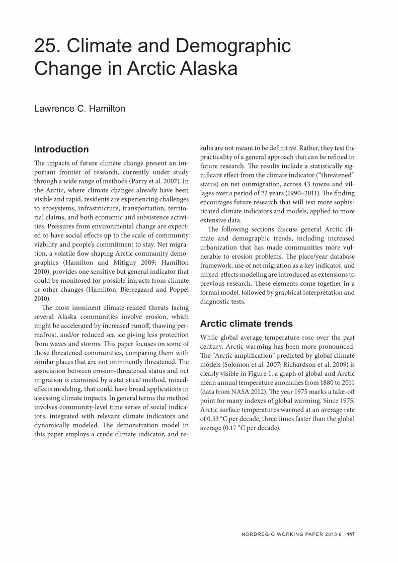
Burch’s Northwest Alaska region roughly corresponds to the modern Northwest Arctic Borough, an adminis-trative area of 106,000 km2 with 7,700 people in 2011. !e right-hand chart in Figure 4 depicts the population of the Northwest Arctic Borough in 2011. Although the modern borough is not identical to Burch’s Northwest Alaska region, they substantially overlap and have sim-ilar size: the borough covers 106,000 square kilometers, compared with 107,000 for Burch’s region. !e bor-ough’s 2011 population (7,700) likewise resembles that of the region in 1800 (7,300). Comparing the le% and right panels of Figure 4, however, one great di"erence stands out: the 2011 population is far more concentrat-ed, with about half living in the hub town of Kotzebue.

!is trend toward urbanization is even more pro-nounced than it appears because the 11 modern towns and villages each are spatially compact, unlike the 13 nations of 1800. Contemporary housing and the need for electricity and water, as well as education and jobs, pull people closely together — a pattern unsuited for

the old hunting-gathering way of life. !e concentra-tion and infrastructure investments, however, make modern communities vulnerable to environmental changes like erosion. Relocating houses, schools, wa-ter systems and other infrastructure as a shoreline erodes incurs economic costs far beyond the resources of small communities, and daunting even to the much larger state government.

!e geographical scope of this paper encompass-es the 11 contemporary towns and villages of the Northwest Arctic Borough, along with 8 in the North Slope Borough, 16 in the Nome Census Area, 5 in the Dillingham Census Area, and s3 in the Bethel Census Area. !is set of 43 predominantly Native communi-ties has been the focus of previous analysis in Ham-ilton and Mitiguy (2009) and Hamilton et al. (2011). Figure 5 maps the town and village locations, and also of the larger regions (Northwest Arctic Borough, etc.) to which they belong.

Figure 5: Forty-three selected Arctic Alaska towns and villages (larger map), and 27 county-equivalent entities (boroughs, census areas or municipalities) comprising all Alaska (inset). From Hamilton and Mitiguy (2009).


Although Northwest Alaska Native populations in 1800 and 2011 have similar size, this coincidence does not imply demographic stability. Like other indigenous peoples of the Americas, Alaska Natives experienced terrible mortality with exposure to European disease. Recovery from that disaster, the Northwest Arctic pop-ulation as recently as 1971 was little more than half its

current level. Natural increase, with periods of positive net migration, drove the overall growth seen in Figure 6. Internal migration within regions drove the local ur-banization seen earlier in Figure 5. !e next section looks more closely at how the balance between net mi-gration and natural increase a"ects variation in popu-lation of individual Arctic communities.

4,0

00

5,0

00

6,0

00

7,0

00

8,0

00

Popula

tion

1970 1980 1990 2000 2010

data: Alaska Dept Labor and Workforce Development

Northwest Arctic Borough 1971–2011

Figure 6: Although modern populations may resemble pre-contact levels, contact was followed by high mortality from disease. Modern populations have rebuilt from historically low levels.

Net migration and Arctic populationsPopulation change re#ects the sum of four #ows: births, deaths, in-migration and outmigration. Figure 7 em-ploys a graphical style developed by Hamilton and Mi-tiguy (2009) to visualize population change and its components. !is example describes recent changes in Kivalina, a coastal village in the Northwest Arctic Bor-ough. Bars along the lower part of the graph indicate the number of deaths (dark bars) and births (lighter bars) for each year from 1990 to 2011. !ese data are

from the Alaska Bureau of Vital Statistics. We show births from July 1 2010 through June 30 2011 as “2011” and so forth, for consistency with the state’s midsum-mer population estimates. !e number of deaths per year ranged from 0 to 8, and there were 5 to 18 children born to Kivalina residents each year. (!e seemingly exact counts of births, deaths and population indicated by such graphs are of course subject to some errors.) On average, about 9.5 more births than deaths oc-curred each year.

Vertical lines showestimated net

migration effects

-20

02

0B

irth

s a

nd

de

ath

s

30

03

20

34

03

60

38

04

00

Po

pu

latio

n

1990 1994 1998 2002 2006 2010

data: Hamilton and Mitiguy (2009)

Kivalina, Northwest Arctic Borough, Alaska

Figure 7: Population dynamics (total, births, deaths and net migration) of Kivalina, Alaska, 1990–2011.


Without migration, the population of this village would have continually increased. Due to outmigra-tion, it has not actually done so. !e scale for births and deaths appears at lower right in this graph. At upper le% is a comparable vertical scale for population. !e graph’s main curve tracks total population, as estimat-ed for most years by the Alaska Department of Labor and Workforce Development. For non-Census years (all but 1990, 2000 and 2010), the state provides esti-mates based on administrative data, notably Perma-nent Fund Dividend applications — a unique data re-source that permits relatively accurate yearly estimates.

Short line segments that extend above the main curve in Figure 7 indicate net outmigration, inferred from a population estimate that is lower than would be expected due to natural increase alone. For exam-ple, Kivalina’s estimated population for July 1, 2005 was 363. By June 30 the following year there had been 15 births and 8 deaths, resulting in a 2006 projection of 363 + 15 – 8 = 370 people. !e actual population estimate for 2006 is 365, leading to an estimated net migration of 365 – 370 = –5, or $ve people leaving.

Consequently, the line segment extends down from 370 to the main population curve at 265. A line seg-ment extending up to the main curve would indicate net in-migration, or population growth exceeding that expected from natural increase. Although a few years, such as 1992, experienced net in-migration, in most of these years, more people le% than arrived. !e average was a loss of about 6 people per year, largely o"setting natural increase.

Figure 8 displays similar graphs for four other Arc-tic Alaska communities. Net migration can be seen to have strong e"ects on the total population of each. !e Health and Population chapter of the Arctic Social Indicators report (Hamilton, Bjerregaard and Poppel 2010) identi$es net migration as an important indica-tor that integrates push and pull forces acting on Arctic communities. Net migration can change rapidly in re-sponse to a changing balance of forces including bet-ter or worse conditions in the community, and more or less attractive options elsewhere. Especially in small places, net migration can rapidly alter not both the size and composition of a population.

Vertical lines show

estimated net

migration effects

-100

100 Birth

s and

dea

ths

3400

3700

4000

4300

4600

4900

Pop

ulatio

n

1990 1994 1998 2002 2006 2010

Barrow, North Slope Borough

Vertical lines show

estimated net

migration effects

-50

5Bi

rths a

nd d

eath

s

110

120

130

140

150

160

Pop

ulatio

n

1990 1994 1998 2002 2006 2010

Deering, Northwest Arctic Borough

Vertical lines show

estimated net

migration effects

-50

050

Birth

s and

dea

ths

2000

2100

2200

2300

2400

2500

Pop

ulatio

n

1990 1994 1998 2002 2006 2010

Dillingham, Dillingham Census Area

Vertical lines show

estimated net

migration effects

-20

020

Birth

s and

dea

ths

460

480

500

520

540

560

580

600

Pop

ulatio

n

1990 1994 1998 2002 2006 2010

Shishmaref, Nome Census Area

data: Hamilton and Mitiguy (2009)

Figure 8: Population dynamics of four Arctic Alaska communities, 1990–2011.


Many Arctic Alaska communities today $nd them-selves on the front lines of global change. Kivalina and Shishmaref, for example, are built along shorelines where the later formation of sea ice has reduced their protection from erosion by fall storms. Since 2003, 31 Alaska Native towns and villages — including those in Figures 7 and 8 — have been identi$ed as facing “im-minent threats” from #ooding and erosion (GAO 2009). At least 12 are considering full or partial reloca-tion. !e problems o%en are climate-related, whether from changes in sea ice, permafrost, or intensi$cation of Arctic hydrological cycles. Such changes are hap-pening now, with potentially severe consequences for the communities a"ected.

!e impacts of resource and economic changes are o%en re#ected in net migration to or from northern places, as well documented in the case of $sheries-de-pendent communities (Hamilton et al. 2004a, 2004b, 2004c). Might climate change likewise have measur-able e"ects on net migration? !e next section takes an exploratory look at this question.

Modeling environmental effects on migrationRecent advances in mixed-e"ects modeling provide statistical tools for analyzing relationships among mul-tiple time series, such as the Arctic community demo-graphics in Figures 7 and 8. Mixed-e"ect models are regression models containing both $xed and random e"ects. Fixed e"ects resemble coe&cients in an ordi-nary multiple regression: they characterize relation-ships for the data as a whole. Random e"ects can vary across clusters or subsets of the data. !e inclusion of random e"ects o"ers advantages for representing clus-tered or panel data such as multiple years for each com-

munity (Rabe-Hesketh and Skrondal 2012; Hamilton 2013). Hamilton et al. (2012) adapt this approach to modeling annual electricity use by Arctic Alaska com-munities as a function of population, price, trend and weather.

!e following example employs a crude indicator of environmental stress: whether a particular commu-nity has been classed as “imminently threatened” due to #ooding or erosion, as described in the GAO (2009) report. Although crude, this indicator permits a practi-cal trial of the modeling approach for detecting e"ects of environmental stress on net migration from small places. !e analysis employs data on 43 Arctic Alaska towns and villages over the years 1990 through 2011, or more than 900 place-years.

Table 1 shows results from a mixed-e"ects model for net migration to or from the ith community in year t (netmigit), predicted from a nonlinear time trend, pop-ulation and an indicator coded as 1 for “imminently threatened” places a%er 2003, and 0 otherwise. Tests of alternative speci$cations support a simple model with the form

!e $ parameters in equation [1] represent $xed e"ects, common across all communities. !e :i parameter rep-resents random variations in the time trends exhibited by di"erent communities. D in equation [2] is a $rst-order autoregression parameter, describing the correla-tion between error terms for successive years within communities. !e uit in equation [2] are assumed (and later con$rmed by testing) to be white noise.


Fixed e"ects Coef. SE p(z)t (calendar year minus 2003) –.075 .248 .763t 2 (t squared) .093 .035 .008pop (community population) –.007 .001 .000threat (1 since 2003 if “threatened”) –8.586 4.110 .037intercept –5.113 1.937 .008AR(1) D .135 .036 .000

Community-level random e"ect Std. dev. SEt 2 .032 .074

Residual standard deviation = 30.99LR test vs. linear regression, p = .0002Portmanteau Q tests of residuals (lag 5): 40 of 43 p > .05 (and 31 of 43 p > .20)

Table 1: Net migration to or from 43 Arctic Alaska communities over 1990–2011, as a function of “imminently threatened” status,

Tests of alternative speci$cations including higher-or-der autoregressive or moving-average processes, and additional random e"ects, complicated the model without signi$cantly improving the overall $t.

!e maximum restricted likelihood (REML) esti-mates in Table 1 are based on 43 parallel time series: the years 1990 through 2011 in each of 43 communi-ties. Substituting the estimated coe&cients from Table 1 into equations [1] and [2] yields equation [3]:

Figure 9 shows some examples of the $t between

model and data. Yearly migration from these small places is erratic and di&cult to predict. !e model achieves only limited success, explaining about 10 % of the variance in net migration. Nonlinear time trend, population and threat status all have statistically sig-ni$cant coe&cients, however. Moreover, the e"ect of threat status is negative as expected. Controlling for population and community-speci$c time trend, threat status increases predicted net outmigration by 8 or 9 people per year ($4 = –8.586).


Figure 9:

0

1990 2000 2010

Barrow

0

1990 2000 2010

Kotzebue

0

1990 2000 2010

Nome0

1990 2000 2010

Bethel

0

1990 2000 2010

Atqasuk

0

1990 2000 2010

Kivalina

0

1990 2000 2010

Shishmaref

0

1990 2000 2010

Togiak

0

1990 2000 2010

Dillingham Ne

t m

igra

tio

n

(sq

ua

re

s)

Ne

t m

ig p

re

dic

ted

(d

ash

ed

cu

rve

s)

In their paper on electricity use, Hamilton et al. (2012) employ more detailed climatic data: monthly tempera-ture and precipitation estimates from the University of Delaware Center for Climatic Research (Matsuura & Willmott 2009a, 2009b), projected to 25 km H 25 km grid cells within which each community is located. Similarly detailed climate variables, and better general indicators, are worth developing in future research. Despite the limitations of the Table 1analysis, its $nd-ing of signi$cant and plausible e"ects in the hypothe-sized direction provides encouragement for taking the next steps.

Conclusion!is paper presented the general research context and tried out a new statistical modeling approach that could prove broadly useful in testing for impacts from climate or any other change. For the $rst time, availa-ble data are becoming extensive enough to support such multivariate modeling, as the time series grow longer each year. As a next step, more sophisticated cli-mate indicators, based on observational, reanalysis or modeled climate and hydrological information should

be developed.Mixed modeling holds promise for studying impacts

from non-climate forces too, such as changes in subsi-dies, resource development or the price of fuel. In prin-ciple, this method could help to untangle the in#uence of multiple factors that all a"ect migration (or are re-#ected in other social indicators) from Arctic commu-nities. Statistical analysis cannot match the nuanced detail of ethnographic or community case-study work, but it complements such work with a broader step-back view that takes in several decades of change across dozens of di"erent places. !e regional to global scale of environmental changes being felt now in the Arc-tic, and also of the scienti$c research on such change, makes a broad perspective on social change important as well.

Acknowledgement!e research described here continues work begun un-der two projects (H3L and AON – SI) supported by grants from the Arctic Social Sciences and Arctic Sys-tem Science programs at the U.S. National Science Foundation (OPP-0638413 and OPP-0531354).


References

-

-

Islands.” Society and Natural Resources 17(5):443–453.

25(3):195–215.

-

62(4):393–398.

123.

-

-

-

-

--

-

-

-

450–453.

Climate and demographic change in Arctic Alaska

Documents

Transcript of Climate and demographic change in Arctic Alaska