Classification of Sextics of Torus Type

arX

iv:m

ath/

0201

035v

1 [

mat

h.A

G]

7 J

an 2

002

CLASSIFICATION OF SEXTICS OF TORUS TYPE

MUTSUO OKA AND DUC TAI PHO

Dedicated to Professor Tatsuo Suwa on his 60th birthday

Abstract. In [7], the second author classified configurations of the singularities on tame

sextics of torus type. In this paper, we give a complete classification of the singularities on

irreducible sextics of torus type, without assuming the tameness of the sextics. We show that

there exists 121 configurations and there are 5 pairs and a triple of configurations for which

the corresponding moduli spaces coincide, ignoring the respective torus decomposition.

1. Introduction

We consider an irreducible sextics of torus type C defined by

C : {(X,Y,Z) ∈ P2;F2(X,Y,Z)3 + F3(X,Y,Z)2 = 0}(1)

where Fi(X,Y,Z) is a homogeneous polynomial of degree i, for i = 2, 3. We consider the

conic C2 = {F2(X,Y,Z) = 0} and the cubic C3 = {F3(X,Y,Z) = 0}. Let Σ(C) be the set

of singular points of C. A singular point P ∈ Σ(C) is called inner (respectively outer) with

respect to the given torus decomposition (1) if P ∈ C2 (resp. P /∈ C2). We say that C is

tame if Σ(C) ⊂ C2 ∩ C3. For tame sextics of torus type, there are 25 local singularity types

among which 20 appear on irreducible sextics of torus type by [7]. As global singularities,

there are 43 configurations of singularities on irreducible tame torus curves. The result in [7]

is valid for non-tame sextics of torus type as the sub-configurations of the inner singularities

on sextics of torus type. We call them the inner configuration. In this paper, we complete the

classification of configurations of the singularities on irreducible sextics of torus type.

This paper is composed as follows. In §2, we give the list of topological types for outer

singularities and explain basic degenerations among singularities. In §3, we study possible

outer configurations of singularities. We start from a given inner configuration, and we de-

termine the possible singularities which can be inserted outside of the conic C2. We prove

that there exist 121 configurations of singularities of non-tame sextics among which there

exist 21 maximal configurations (Theorem 4, Corollary 6). In §4, we introduce the notions

of a distinguished configuration moduli space and a reduced configuration moduli space and a

minimal moduli slice. Minimal moduli slices are very convenient for the topological study of

plane curves. We prove that the dimension of a minimal slice is equal to the expected minimal

dimension (Theorem 11). In §5, we give normal forms for the maximal configurations. In this

process, we show that the moduli spaces of certain configurations are not irreducible but their

2000 Mathematics Subject Classification. 14H10,14H45, 32S05.

Key words and phrases. Torus type, maximal curves, dual curves.

1

http://arXiv.org/abs/math/0201035v1

https://www.researchgate.net/publication/38324839_Classification_of_singularities_on_torus_curves_of_type_23?el=1_x_8&enrichId=rgreq-d1d800c4-a001-46a4-9d82-0c37d60a4454&enrichSource=Y292ZXJQYWdlOzIxMDEwMTg7QVM6MTAyMjkzMzA3Mzk2MDk3QDE0MDE0MDAwMzMxMjA=


2 M. OKA AND D.T. PHO

minimal slices have dimension zero and they have normal forms which are mutually inter-

changeable by a Galois action. However it is not clear if they are isomorphic in the classical

topology. See Proposition 17 and Proposition 19. We also prove that there exist 5 pairs and

a triple of configurations for which the moduli spaces are identical if we ignore the distinction

of inner and outer singularities (Theorem 20).

For reduced non-irreducible sextics of torus type, we will study their configurations in [4].

2. Inner and outer singularities

2.1. Inner and outer singularities. Let C be an irreducible sextics defined by f(x, y) = 0

where f = f32 + f2

3 and fi(x, y) is a polynomial of degree i for i = 2, 3. Here (x, y) is the affine

coordinates x = X/Z, y = Y/Z. Let C2, C3 be the conic and the cubic defined by f2 = 0 and

f3 = 0 respectively. We assume that the line at infinity is not a component of any of C2, C3

and C. Let P be a singular point of C. A singular point P of C is called an inner singularity

(respectively an outer singularity) if P is on the intersection C2∩C3 (resp. P /∈ C2∩C3) with

respect to the torus decomposition (1). We will see later that the notion of inner or outer

singularity depends on the choice of a torus expression. In [7], second author classified inner

singularities. Simple singularities which appear as singularities on sextics of torus type are

A2, A5, A8, A11, A14, A17, E6,D4,D5. We use the following normal forms.

An : y2 + xn+1 = 0, E6 : y3 + x4 = 0, Dk : y2x+ xk−1

Non-simple inner singularities on irreducible sextics of torus type are the following ([6]):

B3,2j , j = 3, 4, 5, B4,6, C3,k, k = 7, 8, 9, 12, 15, C6,6, C6,9, C9,9 and Sp1 where

Bp,q : yp + xq = 0 (Brieskorn-Pham type)

Cp,q : yp + xq + x2y2 = 0, 2p + 2

q < 1

Sp1 : (y2 − x3)2 + (xy)3 = 0

Note that B3,3 = D4. For outer singularities, a direct computation gives the following.

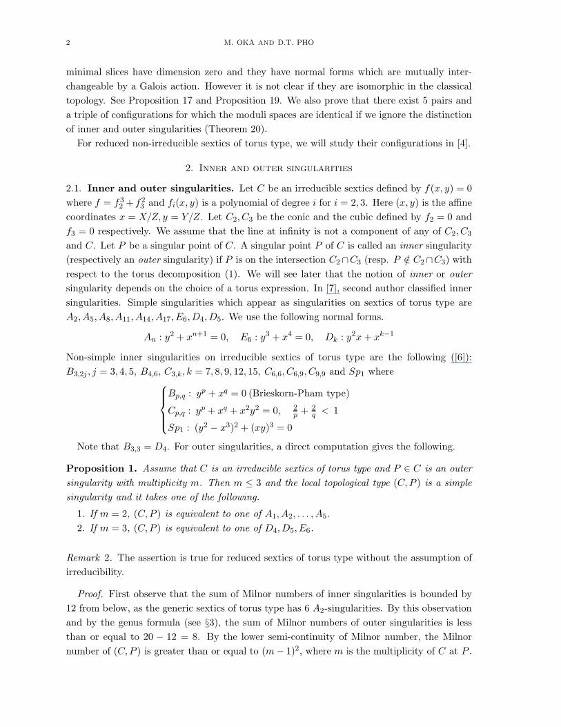
Proposition 1. Assume that C is an irreducible sextics of torus type and P ∈ C is an outer

singularity with multiplicity m. Then m ≤ 3 and the local topological type (C,P ) is a simple

singularity and it takes one of the following.

1. If m = 2, (C,P ) is equivalent to one of A1, A2, . . . , A5.

2. If m = 3, (C,P ) is equivalent to one of D4,D5, E6.

Remark 2. The assertion is true for reduced sextics of torus type without the assumption of

irreducibility.

Proof. First observe that the sum of Milnor numbers of inner singularities is bounded by

12 from below, as the generic sextics of torus type has 6 A2-singularities. By this observation

and by the genus formula (see §3), the sum of Milnor numbers of outer singularities is less

than or equal to 20 − 12 = 8. By the lower semi-continuity of Milnor number, the Milnor

number of (C,P ) is greater than or equal to (m− 1)2, where m is the multiplicity of C at P .

https://www.researchgate.net/publication/2097100_Fundamental_group_of_sextics_of_torus_type?el=1_x_8&enrichId=rgreq-d1d800c4-a001-46a4-9d82-0c37d60a4454&enrichSource=Y292ZXJQYWdlOzIxMDEwMTg7QVM6MTAyMjkzMzA3Mzk2MDk3QDE0MDE0MDAwMzMxMjA=


CLASSIFICATION OF SEXTICS OF TORUS TYPE 3

Thus we get m ≤ 3. The rest of the assertion is proved by an easy computation. We may

assume that P = O, where O is the origin. The generic form of f2, f3 are given as

f2 (x, y) := a02 y2 + (a11 x+ a01 ) y + a20 x

2 + a10 x+ a00

f3 (x, y) := b03 y3 + (b12 x+ b02 ) y2 +

(

b21 x2 + b11 x+ b01

)

y

+b30 x3 + b20 x

2 + b10 x+ b00

(2)

The condition P ∈ C and P /∈ C2 says that a00 = −t2, b00 = −t3 for some t ∈ C∗. Using the

condition fx(O) = fy(O) = 0 where fx, fy are partial derivatives in x and y respectively, we

eliminate coefficients b01 and b10 as

b01 :=3

2t0 a01 , b10 :=

3

2t0 a10

We denote the Newton principal part of f by NPP (f, x, y). Assume that m = 2. Then

(C,O) = A1 generically. By the action of GL(3,C), we can assume that the tangent direction

of (C,O) is given by y = 0. The degeneration A1 → A2 is given by putting fxx(O) = fxy(O) =

0. A direct computation shows that the equivalent class (C,O) can be Ak for k ≤ 5. For

example, to make the degeneration A2 → A3, we put the coefficient of x3 in NPP (f, x, y) to

be zero. Then NPP (f, x, y) takes the form c2y2 + c1yx

2 + c0x4 with c2 6= 0 as m = 2. The

degeneration A3 → A4 takes place when the discriminant of the above polynomial vanishes.

Then we take a new coordinate system (x, y1) so that c2y2 + c1yx

2 + c0x4 = c2y

21 . Then we

repeat a similar argument. We can see that A5 → A6 makes f to be divisible by y2 by an

easy computation.

Assume that m = 3. Generically this gives (C,O) ∼= D4. Assume that the 3-jet is degenerated.

We may assume (by a linear change of coordinates) that the tangent cone is defined by y2x or

y3 corresponding either the number of the components in the tangent cone is 2 or 1. Assume

that it is given by y2x = 0. Thus the Newton principal part of f is given by

− 3

64

(

a012 + 4 a02 t0

2)2y4

t0 2 −1/8(

16 t03b12 + 12 t0

2a11 a01 + 12 t02a02 a10 + 3 a01

2a10

)

xy2

− 3

64

(

4 a20 t02 + a10

2)2x4

t0 2

Thus (C,O) ∼= D5. Further we observe by a direct computation that a210 + 4t20a20 = 0 makes

f reducible. Thus no Dk (k ≥ 6) appears. If the tangent cone is given by y3 = 0, a similar

argument shows that the only possible singularity (C,O) is E6.

2.2. Degenerations on sextics of torus type. We consider the basic degenerations among

singularities. First, the possibility of the degeneration of outer singularities under fixing the

inner singularities is as usual: A1 → A2 → A3 → A4 → A5 → E6 and D4 → D5 → E6. Of

course, some of the above singularities does not exist when the inner configuration is very

restrictive (i.e., far from the generic one = [6A2]).

The degenerations of inner singularities are studied in [7]: A2 → A5 → A8 → A11 →A14 → A17 and A5 → E6. The degeneration of an outer singularity into an inner singularity

is described by the following.



Proposition 3. 1. An outer A1 and two inner A2’s degenerate into an E6.

2. An outer A2 and three inner A2’s degenerate into a B3,6.

3. An outer A3 and three inner A2’s degenerate into a C3,7.



There are no other degenerations.

Proof. The proof is computational. We show the first two degenerations in detail and leave

the other cases to the reader. We start from the normal form f = f32 + f2

3 where f2, f3 are

given as in (2). We assume that C has a node at O which is not on the conic C2. Putting

f2(0, 0) = −t20 and f3(0, 0) = −t30 for some t0 ∈ C∗, we get the normal form:

f2 (x, y) = a02 y2 + (a11 x+ a01 ) y + a20 x

2 + a10 x− t02

f3 (x, y) = b03 y3 + (b12 x+ b02 ) y2 +

(

b21 x2 + b11 x+ 3/2 t0 a01

)

y

+b30 x3 + b20 x

2 + 3/2 t0 a10 x− t03

We can put t0 → 0 in this form to see that two inner A2 singularities are used to create a

E6 singularity: 2A2 + A1 → E6. Note that as f(O) = −t20, t0 → 0 implies the conic C2

approaches to O so that O becomes an inner singularity for t0 = 0. To check the degeneration

of inner A2 singularities, we can look at the resultant R(f2, f3, y) of f2 and f3 and find that

x = 0 has a multiplicity two in R = 0.

Next we consider that the case (C,O) = A2. We may assume that the tangent cone at O

is given by y = 0. The corresponding normal form is given by

f2 (x, y) = a02 y2 + (a11 x+ a01 ) y + a20 x

2 + A10 t0 x− t02

f3 (x, y) = b03 y3 + (b12 x+ b02 ) y2 +

(

b21 x2 + (−3/4 a01 A10 + 3/2 a11 t0 ) x

)

y

+3/2 t0 a01 y + b30 x3 − 3/8 t0

(

A102 − 4 a20

)

x2 + 3/2 t02A10 x− t0

3

Here we have substituted a10 = A10t0 so that we can easily see the limit limt0→0 fi(x, y). We

can see easily (C,O) → B3,6. We observe also that the cubic C3 has a node at O as the limit

t0 = 0 and the intersection multiplicity of C2 and C3 at O is 3. See [7] for the degeneration

B3,6 → C3,7 → C3,8 → C3,9.

For (C,O) = A3, the normal form is given as follows and the assertion is easily checked by

putting t0 = 0.

f2 (x, y) = a02 y2 + (a11 x+ a01 ) y + a20 x

2 + A10 t0 x− t02

f3 (x, y) = b03 y3 + (b12 x+ b02 ) y2 +

(

b21 x2 + (−3/4 a01 A10 + 3/2 a11 t0 )x

)

y

+ 3/2 t0 a01 y− 1/16A10

(

A102 + 12 a20

)

x3 − 3/8 t0(

A102 − 4 a20

)

x2 + 3/2 t02A10 x− t0

3

The other cases is similar.



2.3. List of configurations of inner singularities. For the classification of non-tame

configurations, we start from the classification of the configurations of singularities on tame

sextics of torus type [7]. The list of configurations in [7] is valid as the sub-configuration defined

by the inner singularities for a sextics which may have outer singularities. Let C2 ∩ C3 =

{P1, . . . , Pk}. The i-vector is by definition the k-tuple of integers given by the intersection

numbers I(C2, C3;Pi), i = 1, . . . , k. There exist 43 possible configurations as follows, assuming

C is irreducible. Put v := i-vector(C)

1. v = [1, 1, 1, 1, 1, 1] : t1 = [6A2].

2. v = [1, 1, 1, 1, 2] : t2 = [4A2, A5], t3 = [4A2, E6].

3. v = [1, 1, 2, 2] : t4 = [2A2, 2A5], t5 = [2A2, A5, E6], t6 = [2A2, 2E6].

4. v = [1, 1, 1, 3] : t7 = [3A2, A8], t8 = [3A2, B3, 6], t9 = [3A2, C3, 7], t10 = [3A2, C3, 8],

t11 = [3A2, C3, 9]

5. v = [2, 2, 2] : t12 = [3A5], t13 = [2A5, E6], t14 = [A5, 2E6], t15 = [3E6].

6. v = [1, 2, 3] : t16 = [A2, A5, A8], t17 = [A2, A5, B3, 6], t18 = [A2, A5, C3, 7], t19 =

[A2, E6, A8], t20 = [A2, E6, B3, 6], t21 = [A2, E6, C3, 7],

7. v = [1, 1, 4] : t22 = [2A2, A11], t23 = [2A2, C♮3, 9], t24 = [2A2, B3, 8], t25 = [2A2, C6,6],

t26 = [2A2, B4,6].

8. v = [3, 3] : t27 = [2A8], t28 = [A8, B3, 6], t29 = [A8, C3, 7],

9. v = [2, 4] : t30 = [A5, A11], t31 = [A5, C♮3, 9], t32 = [A5, B3, 8], t33 = [E6, A11],

t34 = [E6, C♮3, 9], t35 = [E6, B3, 8]

10. v = [1, 5] : t36 = [A2, A14], t37 = [A2, C3, 12], t38 = [A2, B3, 10], t39 = [A2, C6, 9],

t40 = [A2, Sp1].

11. v = [6] : t41 = [A17], t42 = [C3,15], t43 = [C9,9].

3. Configurations of non-tame sextics

3.1. Genus admissible configurations. For the classification, we consider two inequalities

by the positivity of the genus formula:

g(C) =(d− 1)(d − 2)

2−

∑

P∈Σ(C)

δ(C,P ) ≥ 0(3)

and by the positivity of the class number n∗(C):

n∗(C) = d(d− 1) −∑

P∈Σ(C)

(µ(C,P ) +m(C,P ) − 1) ≥ 0(4)

Here d = degree(C), Σ(C) is the set of singular points of C and δ(C,P ) is the δ-genus of

C at P which is equal to 12 (µ(C,P ) + r(C,P ) − 1) with r(C,P ) being the number of local

irreducible components at P (see Milnor [2]). The class number n∗(C) of C is defined by the

degree of the dual curve C∗ where m(C,P ) is the multiplicity of C at P . See [3, 5] for the

class number formula (4).

A configuration Σ is called a genus-admissible if the genus and the class number given by

the above formulae (3), (4) are non-negative.


https://www.researchgate.net/publication/38387899_On_deformations_of_quintic_surfaces?el=1_x_8&enrichId=rgreq-d1d800c4-a001-46a4-9d82-0c37d60a4454&enrichSource=Y292ZXJQYWdlOzIxMDEwMTg7QVM6MTAyMjkzMzA3Mzk2MDk3QDE0MDE0MDAwMzMxMjA=






https://www.researchgate.net/publication/239059820_Singular_Points_of_Complex_Hypersurfaces?el=1_x_8&enrichId=rgreq-d1d800c4-a001-46a4-9d82-0c37d60a4454&enrichSource=Y292ZXJQYWdlOzIxMDEwMTg7QVM6MTAyMjkzMzA3Mzk2MDk3QDE0MDE0MDAwMzMxMjA=




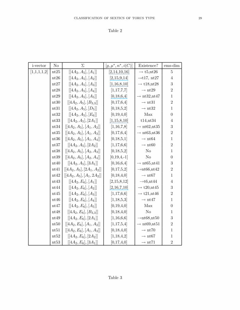
There exist 145 configurations which satisfy those inequalities. See Table 1 ∼ 5 in the end of

this paper. In the list, the first bracket shows the configuration of the inner singularities and

the second is that of the outer singularities. For example, [[6A2], [3A1]] shows that C has 6 A2

as inner singularities and 3 A1 as outer singularities. The vector (g(C), µ∗(C), n∗(C), i(C))

denotes the invariants of C, where g(C) is the genus of the normalization, µ∗(C) is the

sum of Milnor numbers at singular points, n∗(C) is the class number and i(C) is defined by

3d(d − 2) − ∑

P δ(P ) which is the number of flex points on C. For the calculation of δ(P ),

we refer Oka [5]. (In Corollary 12 of [5], there is a trivial mistake. The correct formula is

δ(A2p−1) = 6p for any p which follows from Theorem 10, [5].)

3.2. Existing configurations. The main problem is how to know those configurations which

do exist and which do not exist in the list of Table 1 ∼ 5 in subsection 6.1.

Theorem 4. The possible configurations of singularities of irreducible sextics of torus type

with at least one outer singularity are given by Table1 ∼ Table 5 in the last subsection 6.1.

There are 24 configurations in the table which do not exist (they are marked ‘No’) and the

other 121 configurations exist.

Combining the list of the configuration of tame sextics of torus type, there exist 164 config-

urations on irreducible sextics of torus type.

The column of the table “Existence ?” provides the informations about existence and non-

existence and typical degenerations. “No” implies the corresponding configuration does not

exist. “Max” implies that the configuration is maximal among irreducible sextics of torus

type. The arrow shows a possible degeneration. The last column gives the expected minimal

moduli slice dimension, which is defined in §3.

Corollary 5. The fundamental group π1(P2 − C) of the complement of a sextics C with a

configuration corresponding to one of the following is isomorphic to Z2 ∗ Z3 by [6].

nt j, j = 1, 2, 3, 4, 5, 19, 25, 26, 27, 33, 43, 44, 45, 54, 61, 68, 72, 73, 74, 90, 92

Corollary 6. There exist 21 maximal configurations on non-tame sextics of torus type:

nt23 = [[6A2], [3A2]], nt32 = [[4A2, A5], [E6]], nt47 = [[4A2, E6], [A5]]

nt64 = [[2A2, A5, E6], [A4]], nt67 = [[2A2, A5, E6], [2A2]], nt70 = [[2A2, 2E6], [A3]]

nt78 = [[3A2, A8], [D5]], nt83 = [[3A2, A8], [A1, A4]], nt91 = [[3A2, B3,6], [A2]]

nt99 = [[A5, 2E6], [A2]], nt100 = [[3E6], [A1]], nt104 = [[A2, A5, A8], [A4]]

nt110 = [[A2, E6, A8], [A3]], nt113 = [[A2, E6, A8], [A1, A2]], nt118 = [[2A2, A11], [A4]]

nt123 = [[2A2, C♮3,9], [A2]], nt128 = [[2A8], [A3]], nt136 = [[E6, A11], [A2]]

nt139 = [[A2, A14], [A3]], nt142 = [[A2, A14], [A1, A2]], nt145 = [[A17], [A2]]

In the table, C3,9 and C♮3,9 are topologically isomorphic but they are distinguished by ι = 3

and 4 respectively. See Pho [7].



3.3. Proof of the non-existence of 24 configurations. In this subsection, we prove the

non-existence of the configurations nt j, j =14,16, 17, 18, 38, 39, 48, 76, 79, 84, 85, 86, 89, 93,

107, 111, 114, 121, 125, 129, 131, 132, 140, 143 in Table 1 ∼ 5. It is well-known that the total

sum of the Milnor numbers µ∗ on sextics is bounded by 19 if the singularities are all simple

([1],[8]). Thus the configurations nt79, nt86, nt111, nt114, nt129, nt132, nt140, nt143 do not

exist.

Another powerful tool is to consider the dual curves. We know that the dual singularities

of Ak, k ≥ 3, C3,p, p ≥ 7 and B3,q, q ≥ 6 are generically isomorphic to themselves [5]. If the

singularity is not generic, the dual singularity has a bigger Milnor number. The singularity

B3,3 corresponds to a tri-tangent line in the dual curve C∗. By Bezout theorem, a tri-tangent

line does not exist for curves of degree ≤ 5. Thus the existence of B3,3 implies n∗(C) ≥ 6.

The non-existence of the configurations nt14, nt16, nt17, nt18, nt38, nt39, nt48, nt89, nt93,

and nt125 can be proved by taking the dual curve information into consideration. For example,

consider the configuration nt14 = [[6A2], [A1, B3,3]]. If such a curve C exists, the dual curve

C∗ has degree 4, which is impossible. Next we show that the configurations nt16 ∼ nt18 do

not exist. Assume a curve C with the configuration nt16= [[6A2], [A2, A3]] for example. Then

the dual curve C∗ has degree 5 and C∗ has A3, 4A2 as singularities. By the class formula, the

dual curve C∗∗ = (C∗)∗ have degree 4 which is absurd. The other two can be eliminated in

the same discussion.

For nt93, we use the fact that the dual singularity of C3,7 is again C3,7 ( [6]). Assume that

there exists a sextics C with configuration nt93. Then the dual curve C∗ is a quintic with

C3,7 and A2. Then by the Plucker formula, this is ridiculous as δ(C3,7) = 6. Suppose that

a sextics with the configuration nt125 exists. Then the dual curve have degree 5 and B3,8

as a singularity. However the total sum of the Milnor numbers on an irreducible quintic is

bounded by 12, a contradiction. The other configurations are treated in a similar way.

The configurations nt76, nt85, nt107, nt121 and nt131 do not exist as they are not in the list

of Yang table [10]. The non-existence of these configurations can be also checked by a direct

maple computation. The non-existence of nt84 has to be checked by a direct computation.

Remark 7. We remark here that a configuration in the list of Yang does not necessarily exist

as a configuration of a sextics of torus type. There are also a certain configurations with only

simple singularities which is not a sublattice of a lattice of maximal rank in Yang’s list.

4. Moduli spaces

4.1. Distinguished configuration moduli and reduced configuration moduli. Let

Σ1,Σ2 be configurations of singularities. In this paper, a configuration is a finite set of

topological equivalent classes of germs of isolated curve singularities. We say that Σ := [Σ1,Σ2]

be a distinguished configuration on a sextics of torus type if Σ1 is the configuration of inner

singularities and Σ2 is the configuration of outer singularities. We put Σred := Σ1 ∪ Σ2

and we call Σred a reduced configuration. We now introduce several moduli spaces which we

consider in this paper. First, recall that spaces of conics and cubics are 6 and 10 dimensional



https://www.researchgate.net/publication/38368768_Sextic_curves_with_simple_singularities?el=1_x_8&enrichId=rgreq-d1d800c4-a001-46a4-9d82-0c37d60a4454&enrichSource=Y292ZXJQYWdlOzIxMDEwMTg7QVM6MTAyMjkzMzA3Mzk2MDk3QDE0MDE0MDAwMzMxMjA=


respectively. Let T be the vector space of dimension 16 which is defined by

T := {f = (f2, f3); degree f2 = 2, degree f3 = 3}

There is a canonical GL(3,C)-action on T . The center of GL(3,C) is identified with C∗.

It defines a canonical weighted homogeneous action on T and we introduce an equivalence

relation ∼ by (f2, f3) ∼ (f ′2, f′3) ⇐⇒ f ′2 = f2 t

2, f ′3 = f3 t3 for some t ∈ C∗. In particular,

(f2, f3) ∼ (f2 ωj,± f3) for j = 1, 2 where ω = (

√3I− 1)/2). ( We use the notation I =

√−1.)

Let T be the weighted projective space by the C∗-action and let π : T → T be the quotient

map. Then PGL(3,C) = GL(3,C)/C∗ acts on T . Each equivalence class (f) defines a sextics

of torus type C(f) defined by f2(x, y)3 + f3(x, y)

2 = 0. We put

Σ(f)in := {(C(f), Pi); f2(Pi) = 0}, Σ(f)out := {(C(f), Pi); f2(Pi) 6= 0}

where {P1, . . . , Pk} are the singular points of C(f) and (C(f), Pi) is the topological equivalent

class of the germ at Pi. Let Σ = [Σ1,Σ2] be a distinguished configuration. The distinguished

configuration moduli M(Σ) ⊂ T is defined by the quotient M(Σ)/C∗

M(Σ) := {f = (f2, f3) ∈ T ; Σ(f)in = Σ1, Σ(f)out = Σ2}

The space of sextics, denoted by S, is a vector space of dimension 28 and its quotient by

the homogeneous C∗-action is denoted by S. There exist a canonical GL(3,C)-equivariant

mapping ψred : T → S which is defined by ψred(f2, f3) = f32 + f2

3 and it induces a canonical

PGL(3,C)-equivariant mapping ψred : T → S. Let Σ0 be a reduced configuration. The

reduced configuration moduli Mred(Σ0) is defined by Mred(Σ0)/C∗ where C∗-action is the

the scalar multiplication and

Mred(Σ0) = {f ∈ S;∃Σ = [Σ1,Σ2], Σ0 = Σ1 ∪ Σ2, ∃f ∈ M(Σ), ψred(f) = f}

The map ψred : M(Σ) → Mred(Σred) is not necessarily injective (see Observation 14).

Remark 8. Let f = (f2, f3) ∈ M([Σ1,Σ2]) and assume that f32 +f2

3 = 0 is an irreducible sextics

and assume that Σ2 is not empty. Consider the family of sextics Ct : t f32 (x, y)+f3(x, y)

2 = 0.

By Bertini theorem, for a generic t 6= 0, Ct has only inner singularities and Σ(Ct) = Σ′1, where

simple singularities in Σ1 are unchanged in Σ′1 and non-simple singularities are replaced by

the first generic singularities fixing the singularities of the conic f2 = 0 and the cubic f3 = 0

and their local intersection numbers in Table A′ of [7]. For example, inner singularities with

a nodal cubic and a smooth conic, with the intersection number 3, any singularity in the

series B3,6 → C3,7 → C3,8 → C3,9 is replaced by B3,6. This is the reason why we need the

information of defining polynomials f2, f3, not only the geometry of C2 and C3.

4.2. Moduli slice and irreducibility. A subspace A ⊂ M(Σ) is called a moduli slice of

M(Σ) if its GL(3,C)-orbit covers the whole moduli space M(Σ) and A is an algebraic variety.

A moduli slice is called minimal if the dimension is minimum. As we are mainly interested

in the topology of the pair (P2, C) where C is a sextics defined by f32 + f2

3 = 0, the important

point is the connectedness of the moduli. Thus we are interested, not in the algebraic structure

of the moduli spaces but in the explicit form of a minimal moduli slice, which we call a normal



form. Note that the moduli space M(Σ) might be irreducible even if a minimal slice A is not

irreducible.

Points P1, P2, . . . , Pk in P2 are called generic if any three of them are not on a line. Let

P1, P2, P3 are generic points and let Li be lines through Pi, for i = 1, 2. We say Li is a generic

line through Pi with respect to {P1, P2, P3} if Li does not pass through any of other two

points {Pj ; j 6= i}. Observe that two set of generic four points, or of generic three points and

two generic lines through two of them are transformed each other by PGL(3,C)-action. Note

that the dimension of the isotropy group of a point (respectively a point and a line through

it) is codimension 2 (resp. 3). As dim PGL(3,C) = 8, we can fix, using the above principle

either

(a) location of four singularities at generic positions or

(b) three singularities at generic positions and two generic tangent cones.

This technique is quite useful to compute various normal forms.

4.3. Virtual dimension and transversality. In general, the dimension of the moduli space

of a given configuration of singularities is difficult to be computed. However in the space of

sextics of torus type, the situation is quite simple. Suppose that we are given a sextics defined

by (2). Take a point P = (α, β) ∈ C2 and consider the condition for P to be a singular point

of C. For simplicity we assume that P = (0, 0).

(I) First assume that P to be an inner singularity. Let σ be a class of (C,P ). We define the

integer i-codim(σ) by (the number of independent conditions on the coefficients) −2. Here 2

is the freedom to choose P . For example, the condition for P to be an inner A2 singularity

is simply f2(P ) = f3(P ) = 0. So i-codim(A2) = 0. Assume that (C,P ) ∼= A5. Then the

corresponding condition is f2(P ) = f3(P ) = 0 and the intersection multiplicity of C2 and C3

at P is 2. This condition is equivalent to (f2xf3y − f2yf3x)(P ) = 0. Thus i-codim(A5) = 1.

Similarly the condition (C,P ) ∼= E6 is given by f2(P ) = f3(P ) = 0 and the partial derivatives

f3x and f3y vanishes at P . See Pho [7] for the characterization of inner singularities. Thus

we have i-codim(E6) = 2.

Let ι = I(C2, C3;P ) be the intersection number of C2 and C3 at P . Similar discussion

proves that

Proposition 9. For the inner singularities on sextics of torus type, i-codim is given as fol-

lows.i-codim 1 2 3 4

singularity A5 E6, A8 A11, B3,6 A14, C♮3,9

C3,7, C6,6

i-codim 5 6 7 8

singularity A17, C3,12B3,8, C3,8C6,9, B4,6

C3,15, B3,10C3,9, Sp1C9,9, C6,12D4,7

B3,12, Sp2 B6,6

The proof is immediate from the above consideration and the existence of the degeneration

series where each step is codimension one ([7]). The vertical degenerations keep the intersec-

tion number ι and it is observed to have codimension one for each arrow in [7]. The first and



the second horizontal sequence are induced by increasing ι by one for each arrow. Thus each

arrow has codimension one. Recall that P is C6,6 singularity if both of C2 and C3 has a node

at P . Thus we can easily see that i-codim(C6,6) = 4. The degenerations C6,6 → C6,9 → C9,9

or C6,9 → C6,12 has also codimension one for each arrow ([7]). So the rest of assertion follows

immediately from the above consideration.

A5 → A8 → A11 → A14 → A17

y

y

y

y

y

E6 → B3,6 → C♮3,9 → C3,12 → C3,15

y

y

y

y

C3,7 → B3,8 → B3,10 → B3,12

y

C3,8 C6,6 → C6,9 →→ C9,9C6,12

y

y

y

C3,9 B4,6 → Sp1 → Sp2

y

D4,7

(II) Now we assume that P is an outer singularity. This means f2(P ) 6= 0. Let σ be

the topological equivalent class of (C,P ). We define the integer o-codim(P ) by the number

of conditions on the space of coefficients of f minus 2. By the argument in the proof of

Proposition 1, we can easily see that

Proposition 10. For an outer singularity on sextics of torus type, we have o-codim(Ai) =

i, i = 1, . . . , 5 and o-codim(Di) = i, i = 4, 5 and o-codim(E6) = 6. Thus in all cases,

o-codim(σ) is equal to the Milnor number.

Proof. For A1, we need three condition f(P ) = fx(P ) = fy(P ) = 0. Here fx, fy are partial

derivatives. Thus o-codim(A1) = 3 − 2 = 1. The other assertion follows from the basic

degeneration series of codimension one:

A1 → A2 → A3 → A4 → A5, B3,3 = D4 → D5 → E6

Note that B3,3 singularity is defined by 6 equations, f(P ) = fx(P ) = fy(P ) = fx,x(P ) =

fxy(P ) = fyy(P ) = 0. Thus we have o-codim(B3,3) = 4 and other assertion follows from the

above degeneration sequence.

For a given configuration Σ = [Σ1,Σ2] on sextics of torus type, we define the expected

minimal moduli slice dimension, denoted by ems-dim(Σ) by the integer

ems-dim(Σ) := 16 −∑

σ∈Σ1

i-codim(σ) −∑

σ∈Σ2

o-codim(σ) − 9

Here 16 is the dimension of sextics of torus type and 9 is the dimension of GL(3,C). On the

other hand, we denote the dimension of minimal moduli slice of the decomposition moduli


M(Σ) by ms-dim(Σ). By the above definition, it is obvious that

ms-dim(Σ) ≥ ems-dim(Σ)

if it is not empty. We say that Σ has a transverse moduli slice or the moduli M(Σ) is

transversal if ms-dim(Σ) = ems-dim(Σ).

Theorem 11. For any configuration Σ of sextics of torus type, there exists a component M0

of M(Σ) whic is transvesal.

It is probably true that M(Σ) is transverse for any Σ but we do not want to check this

assertion for 121 cases. The proof of the above weaker assertion is reduced to the assertion

on maximal configurations (see the next section) and to the following proposition.

Lemma 12. Assume that Σ degenerates into a maximal configuration Σ′ which has a trans-

verse moduli slice. Then the moduli M(Σ) has also a component which is transversal.

Proof. By the definition, a minimal moduli slice for M(Σ′) can be obtained by adding ν

equations on the space of coefficients where ν := ems-dim(Σ) − ems-dim(Σ′). Thus we have

ms-dim(Σ′) ≥ ms-dim(Σ) − (ems-dim(Σ) − ems-dim(Σ′))

≥ ms-dim(Σ′) + (ms-dim(Σ) − ems-dim(Σ)) ≥ ms-dim(Σ′)

which implies the assertion.

5. Minimal moduli slices for maximal configurations

In this section, we give normal forms of minimal moduli slices for the maximal configura-

tions. Using the degeneration argument and Lemma 12, this guarantees the existence of any

other non-maximal configurations in Table 1 ∼ 5 in the subsection 6.1. We also show that

they have transverse minimal moduli slices.

nt23. We consider the minimal moduli slice of M(Σ23) with Σ23 = [[6A2], [3A2]] by the

following minimal slice condition:

(⋆) three outer A2’s are at P0 := (0, 0) and P1 := (1, 1) and P3 := (1,−1). The (reduced)

tangent cones of C at (1,±1) are given by y = ±1 respectively.

The calculation is easy. We start from the normal form f = f32 + f2

3 where f2, f3 are given

as in (2). Necessary conditions are

f2(Pi) = −t2i , f3(Pi) = −t3i , fx(Pi) = fy(Pi) = 0, i = 0, 1, 2.

The assumption on the tangential cones gives fxy(Pi) = fxx(Pi) = 0, i = 1, 2. Solving

these equations, we get the following normal form with one free parameter t := t0. As

ems-dim(Σ23) = 1, it has a transverse minimal moduli slice.


f2(x, y) = y2 − 9x2 t2 − 3x2 + 6 t2 x+ 2x− t2

f3(x, y) =1

2(−9 y2 t2 x− 3 y2 x+ 3 y2 t2 + 3 y2 + 3x3 + 27x3 t2 + 54x3 t4 − 3x2 − 27x2 t2

− 54 t4 x2 + 18x t4 + 6 t2 x− 2 t4)/t

As is well-known, the corresponding sextics are the dual of smooth cubics.

nt32. We consider the moduli space M(Σ32) with Σ32 = [[4A2, A5], [E6]]. The irreducibility

is easily observed using the slice condition:

(⋆) an inner A5 is at (0, 0) and an outer E6 is at (0, 1) with respective tangent cones defined

by y = 0 and y = 1.

We usually use the C∗-action to normalize the coefficient of y2 in f2 to be 1. The normal

forms are given by

f2(x, y) = y2 + (−1 − t12) y + a02 x

2

f3(x, y) =1

8t1(t1

4 + 6 t12 − 3) y3 +

1

8t1(6 − 6 t1

4) y2

+1

8t1(−6 a02 x

2 − 6 t12 + 6 t1

2 a02 x2 − 3 t1

4 − 3) y +1

8t1(6 t1

2 a02 x2 + 6 a02 x

2)

Observe that M(Σ32) is irreducible by this expression. We have used 6 dimension of

PGL(3,C) for the above slice. To get a minimal slice, we have two more dimension to use,

so we can fix a location of an inner A2. Here, we have two choice: either (a) to choose a

location which is on Q2 or (b) to choose a simple normal form. The case (a) give as a little

complicated normal form. So we choose (b). We choose t1 = a02 = 1. This can be done by

taking an inner A2-singularity at (α, β) where

α = −1

2

√

6 − 2I√

3, β = (3 + I√

3)/2.

Note that α is not well-defined but α2 is well-defined. This is enough as f2(x, y), f3(x, y) are

even in x in the above normal form and the condition implies also (−α, β) is another inner

A2. The corresponding minimal slice has dimension 0, and consists of two points and as the

moduli is irreducible, we can take the normal form

f2(x, y) = y2 − 2 y + x2, f3(x, y) = (y3 − 3 y + 3x2)/2

f(x, y) = (y2 − 2 y + x2)3 + (y3 − 3 y + 3x2)2/4(5)

Let f(32)(x, y) be the corresponding sextics.

nt47. The moduli space M(Σ47) is irreducible and ems-dim(Σ47) = 0 where Σ47 := [[4A2, E6], [A5]].

This can be checked easily using the slice as in nt32:

(⋆) an outer A5 is at (0, 0) and an inner E6 is at (0, 1) with respective tangent cones given

by y = 0 and y = 1.


The corresponding normal form is given as

f2(x, y) = y2 + (−1 + t02) y − t0

2 + a02 x2

f3(x, y) = (−3

2t0 − 1

2t0

3) y3 + 3 y2 t0 + y

(

3

2t0 (−1 + t0

2) +3

2 t0a02 x

2

)

− t03 +

3

2t0 a02 x

2

Thus the irreducibility follows from this expression. Observe also that f2, f3 are even in

x. Now we compute the minimal moduli slice with an additional condition, an inner A2 at

(α, β) where α, β are as in nt32. As a minimal slice, we can take

f2(x, y) = y2 − 5

2y +

3

2+

1

2x2

f3(x, y) =√

6 I

(

−3

8y3 +

3

2y2 +

1

6(−45

4− 3

2x2) y +

1

6(9

2+

9

4x2)

)

Let f(47)(x, y) be the corresponding sextics. The above normal form proves ms-dim(Σ47) =

ems-dim(Σ47) = 0. It is easy to observe that 8 f(32)(x, y) = f(47)(x, y) by a direct computation.

nt67. The moduli space M(Σ67) with Σ67 = [[2A2, A5, E6], [2A2]] is not irreducible. First

we observe that ems-dim(Σ67) = 0 as before. We consider the minimal moduli slice with the

slice condition:

(⋆) two outer A2’s are at (0,±1), an inner E6 is at (1, 0) and an inner A5 at (−1, 0).

The corresponding slice reduces to two points defined by fa = (f2a, f3a) and fb = (f2b, f3b)

where

fa :

f2a = y2 + 12 − 1

2 x2 + 1

2 I x2√

3 − 12 I

√3

f3a = 14

√

18 − 6 I√

3 (1 − x+ I√

3 y2 − x2 + x3 + x y2)

fb :

f2b = y2 + 12 − 1

2 x2 − 1

2 I x2√

3 + 12 I

√3

f3b = 14

√

18 + 6 I√

3 (1 − x− I√

3 y2 − x2 + x3 + x y2)

Observation 13. They are not in the same orbit of PGL(3,C) in M(Σ67).

Proof. For a matrix A ∈ GL(3,C), we define as usual φA : P2 → P2 by the multiplication

from the left. Assume that there is a matrix A ∈ GL(3,C) such that fAa := φ∗A(fa) = (fb),

it must keep the singular points (−1, 0), (1, 0). Moreover we observe that f2a, f3a, f2b, f3b are

even in y variable. Thus the involution (x, y) → (x,−y) keep the above polynomials. As the

image of outer singularities must be outer singularities, we may assume that (0, 1), (0,−1) are

also invariant by φA. This implies that A = Id in PGL(3,C). This is ridiculous.

Observation 14. Each of ψred(fa), ψred(fb) has two different torus decompositions in M(Σ67).

Proof. We will show the assertion for fa. First , two inner A2 are located at

P1 := (−1

3I√

3,1

3

√3 + I), P2 := (

−1

3I√

3, −1

3

√3 − I)


We choose a conic h2(x, y) = 0 which passes through four A2 singularities (−1, 0), (1, 0), P1 , P2,

and cut x-axis vertically at (1, 0). Then another decomposition is given by ψred(fa) = h32 +h2

3

where h2(x, y) := y2 − 1 + x2 and

h3(x, y) :=1

4(x3 − x2 − I y2 x

√3 − x+ 1 − y2)

√

18 − 6 I√

3

Observation 15. h = (h2, h3) and fb = (f2b, f3b) are in the same GL(3,C)-orbit in M(Σ67).

In particular, ψred(fa) and ψred(fb) are PGL(3,C)-equivalent.

In fact, a direct computation shows that φ∗B(h2, h3) = (f2b, f3b) where

B =

34 0 −1

4 I√

3

0 14

√3 + 3

4 I 0

−14 I

√3 0 3

4

Proposition 16. The images of the moduli spaces M([[4A2, A5], [E6]]), M([[4A2, E6], [A5]])

and M([[2A2, A5, E6], [2A2]]) by the morphism ψred into M([4A2, A5, E6]) are the same.

The first equality ψred(M([[4A2, A5], [E6]])) = ψred(M([[4A2, E6], [A5]])) is already ob-

served by the above normal forms. Observation 15 proves that M([[2A2, A5, E6], [2A2]]) is

irreducible. Thus it is enough to show that ψred(fa) ∈ ψred(M([[4A2, A5], [E6]]). In fact, we

have ψred(fa) = ψred(g) where g = (g2, g3) ∈ ψred(M([[4A2, A5], [E6]]) and g2, g3 are given by

g2(x, y) = y2 − 1 + (1 + 2 I√

3)x2 + 2 I√

3x

g3(x, y) =1

28(7x y2 + 2 y2 + I

√3 y2 + 4x3 + 9 I x3

√3 − 2x2 + 13 I x2

√3 − 8x

+ 3 I x√

3 − 2 − I√

3)

√

−54 − 78 I√

3

nt64. We consider the distinguished configuration moduliM(Σ64) with Σ64 = [[2A2, A5, E6], [A4]].

We have ems-dim(Σ64) = 0. We consider the minimal slice with respect to:

(⋆) an inner A5 is at (0,1), an inner E6 is at (1,−1) with tangent cone x = 1 and an outer

A4 is at (0, 0) with tangent cone y = 0.

The minimal slice consists of two points fa = (f2a, f3a) and fb = (f2b, f3b):

f2a(x, y) =1

5(5 y2

√5 − 10 + 5 y x+ 4x

√5 + 16x− y

√5 + 5 y + 5x2

√5 − x2

− 4√

5 + 11 y x√

5 + 5 y2)/(1 +√

5)

f3a =1

125

√

50 + 30√

5(250 + 110x3√

5 + 88x3 − 420 y x+ 110√

5 − 192 y2√

5

− 210x√

5 − 15 y√

5 − 48x2√

5 + 155 y3 + 366 y x2 + 348 y2 x√

5 + 336 y x2√

5

+ 97 y3√

5 − 510x − 75 y + 498 y2 x− 300 y x√

5 + 30x2 − 330 y2)/

(1 +√

5)3


f2b(x, y) =1

5(11 y x

√5 − 5 y x− y

√5 + 10 + 5 y2

√5 + x2 + 5x2

√5 − 5 y − 16x

+4x√

5 − 4√

5 − 5 y2)/(−1 +√

5)

f3b(x, y) =1

125I

√

−50 + 30√

5(−250 + 110x3√

5 − 88x3 + 420 y x+ 110√

5

− 192 y2√

5 − 210x√

5 − 15 y√

5 − 48x2√

5 − 155 y3 − 366 y x2 + 348 y2 x√

5

+ 336 y x2√

5 + 97 y3√

5 + 510x + 75 y − 498 y2 x− 300 y x√

5 − 30x2 + 330 y2)/

(−1 +√

5)3

Note that the stabilizer in PGL(3,C) of three points (0, 0), (1,−1), (0, 1) and two lines x = 1

and y = 0 is trivial. Thus fa and fb are not in the same orbit even in the reduced moduli

space Mred([2A2, A5, E6, A4]). Thus the reduced moduli has two irreducible components.

Proposition 17. Two sextics fa := f32a + f2

3a and fb := f32b + f2

3b are defined over Q(√

5).

Let ι : Q(√

5) → Q(√

5) be the involution induced by the Galois automorphism defined by

ι(√

5) = −√

5. Then ι(fa) = fb.

We do not know if there exists an explicit homeomorphism of the complements of the sextics

fa = 0 and fb = 0 in P2.

nt70. The moduli space M(Σ70) with Σ70 = [[2A2, 2E6], [A3]]. The distinguished configu-

ration moduli is irreducible and transversal and ems-dim(Σ70) = ms-dim(Σ70) = 0. For the

computation of a minimal slice, we use the slice condition:

(⋆) an outer A3 is at the origin with tangent cone x = 0 and two inner E6’s are at (1,±1).

The tangent cone at (1, 1) is given by y = 1.

The normal form is given by

f2(x, y) = 13(3y2 + (6x− 6)y − 2x2 − 2x+ 1)

f3(x, y) = I√

39 (x− 1)(18y2 + (9x− 9)y − 17x2 − 2x+ 1)

nt78. We consider the moduli slice of M(Σ78) where Σ78 = [[3A2, A8], [D5]]. We have

ems-dim(Σ78) = 0. However the computation of minimal slice turns out to be messy. So we

consider the slice A under the condition:

(⋆) an outer D5 is at O = (0, 0) with y = 0 as the tangent cone of multiplicity 1, and an

inner A8 is at (1, 1) with y = 1 as the tangent cone.

The normal form f = (f2, f3) is given by

f2(x, y) =1

8t1 2 (8 t14 y − 8 t1

4 + 8 y2 t12 + 8 a10 x t1

2 − 8 y a10 x t12 − 8 y t1

2 + 2 y a102 x

− y a102 − a10

2 x2)


f3(x, y) =1

512(−24 y3 a10

2 t14 + 48 a10

2 t12 y2 + 192 y2 t1

4 + 288 t14 x2 a10

2 + 512 t18

− 48 y2 a102 x t1

2 − 16 a103 x3 t1

2 + 24 y a103 x2 t1

2 + 1152 y a10 x t16

− 192 y a102 x t1

4 − 48 y a103 x t1

2 + 3 y a104 x2 − 768 y t1

8 + 24 y a102 x2 t1

2

− 264 y t14 x2 a10

2 + 384 y2 a10 x t14 + 48 y2 a10

3 x t12 − 384 y2 a10 x t1

6

+ 144 y2 a102 x t1

4 − 48 a102 y2 t1

4 − 192 y3 t14 + 384 t1

6 y3 − 768 a10 x t16

+ 64 y3 t18 − 1152 t1

6 y2 + 768 y t16 + 3 a10

4 y2 − 8 y3 t12 a10

3 − 24 y3 t12 a10

2

− 384 y a10 x t14 + 192 t1

8 y2 − 6 y2 a104 x+ 96 y t1

4 a102)/t1

5

From this normal form, we see that A is irreducible and we can fix one special point fa =

(f2a, f3a), substituting t1 = 1, a10 = −1, where

f2a(x, y) = −1

8y − 1 + y2 − x+

5

4x y − 1

8x2

f3a := 1 − 57

32x y − 261

512x2 y +

21

256x y2 +

1

32x3 − 765

512y2 +

27

64y3 +

3

16y +

3

2x+

9

16x2

The isotropy subgroup fixing (0, 0), (1, 1) and two lines y = 0 and y = 1 is generated by

A =

a1 a2 0

0 a1 + a2 0

0 a1 + a2 − a9 a9

We can easily see that the orbit of fa by this isotropy group is the whole slice A. Thus M(Σ78)

has also a transversal minimal moduli slice which is given by one point fa. In fact, we can see

that fAa = f where A is defined by

a1 = −a10

t1, a2 =

1

25

8 t14 + a10

2 + 17 a10 t12 + 8 t1

2

t1 3 , a9 = t1

nt83. The moduli space M(Σ83) with Σ83 = [[3A2, A8], [A1, A4]] is irreducible. Here we

compute the minimal slice S with the following slice condition:

(⋆) an outer A4 is at the origin, an outer A1 is at (1,−1) and an inner A8 is at (1, 1). The

tangent cones at the origin and at (1, 1) are given by x = 0 and y = 1 respectively.

Then ems-dim(Σ83) = 0 and it has a transverse minimal slice which consists of a single

point {(f2, f3)} where

f2(x, y) = 1565 (565 y2 + 126 y x− 176 y + 405x2 − 936x + 16)

f3(x, y) = 1319225 I

√565(13321 y3 + 28215 y2 x− 6294 y2 + 16767 y x2 − 31644 y x

+ 1056 y + 18225x3 − 45198x2 + 5616x − 64)

nt91. We consider the moduli space M(Σ91) with Σ91 = [[3A2, B3,6], [A2]]. The distinguished

configuration moduli is irreducible and transversal and ems-dim(Σ83) = ms-dim(Σ83) = 2. For

the computation of a minimal slice, we use the slice condition:

(⋆) an outer A2 is at O = (0, 0) with the tangent cone x = 0, an inner B3,6 is at (1, 1) with

the tangent cone y = 1 and an inner A2 is at (1,−1)


The normal form are given by the following polynomials with two-parameters t1, t2 (t1 6= 0,

t2 6= 0):

f2(x, y) = y2 − (t2x− t2)y + (1 + t2 − t21)x2 + (2t21 − t2 − 2)x− t21

f3(x, y) = 18t1

(6t2y3 + ((−6t2 + 12t21 − 3t22)x− 12t21 + 3t22)y

2 + ((6t2 + 6t22 − 12t2t21)x

2

+ (−6t22 + 24t2t21 − 12t2)x− 12t2t

21)y + (−8t41 + 12t21 − 6t2 − 3t22 + 12t2t

21)x

3

+ (3t22 + 24t41 − 24t2t21 + 12t2 − 36t21)x

2 + (24t21 − 24t41 + 12t2t21)x+ 8t41)

nt99. The moduli space M(Σ99) with Σ99 = [[A5, 2E6], [A2]] is not irreducible. First we

observe that ems-dim(Σ99) = 0 as before. We consider the minimal moduli slice with the slice

condition:

(⋆) an outer A2 is at (−1, 0), two inner E6’s are at (0,±1) and an inner A5 is at (1, 0).

The corresponding slice reduces to two points fa = (f2a, f3a) and fb = (f2b, f3b) where

f2a(x, y) = − 123 (5 + 4

√3) (5 y2 − 5 + 23x2 − 18x− 4x

√3 − 4 y2

√3 + 4

√3)

f3a(x, y) = 2√

3 + 2√

3 (1 +√

3) (√

3 + 3x2 − x√

3 − 3x− y2√

3)x

f2b(x, y) = 123 (−5 + 4

√3) (5 y2 − 5 + 23x2 − 18x+ 4x

√3 + 4 y2

√3 − 4

√3)

f3b(x, y) = −2√

3 − 2√

3 (−1 +√

3) (−√

3 + 3x2 + x√

3 − 3x+ y2√

3)x

The isotropy subgroup fixing the configuration of singularity, except possibly exchanging two

E6 is generated by the involution ι(x, y) → (x,−y). However the defining conics and cubics

are even in y. Thus fa, fb are invariant under this involution. Thus the moduli spaces M(Σ99)

and Mred((Σ99)red) has two irreducible components, like the case nt64. Also we have a similar

assertion:

Proposition 18. Both sextics ψred(fa) = f32a+f

23a = 0 and ψred(fb) = f3

2b+f23b = 0 are defined

over Q(√

3). Let ι : Q(√

3) → Q(√

3) be the involution induced by the Galois automorphism

defined by ι(√

3) = −√

3. Then ι(ψred(fa)) = ψred(fb).

nt100. Let us consider the moduli space M(Σ100) with Σ100 = [[3E6], [A1]]. The distinguished

configuration moduli is irreducible and transversal and ems-dim(Σ100) = ms-dim(Σ100) = 0.

For the computation of a minimal slice, we use the slice condition:

(⋆) an outer A1 is at (−1, 0) and three inner E6’s are at (0,±1), and (1, 0).

The normal forms are given by

f2(x, y) = y2 − 5x2 + 6x− 1, f3(x, y) = 6√

3x(x+ y − 1)(x− y − 1)

This curve has been studied in our previous paper [6].

nt104. The moduli space M(Σ104) with Σ104 = [[A2, A5, A8], [A4]] is not irreducible. First

we observe that ems-dim(Σ104) = 0 as before. We consider the minimal moduli slice with the

slice condition:


(⋆) an outer A4 is at (0, 0) with the tangent cone x = 0, an inner A8 is at (1, 1) with the

tangent cone y = 1 and an inner A5 is at (1,−1).

The corresponding slice reduces to two points fa = (f2a, f3a) and fb = (f2b, f3b) where

f2a(x, y) = y2 + 115 y x− 11

5 y − 16 x

2 − 2815 x+ 31

30 + I (−25 y x+ 2

5 y − 16 x

2 + 1115 x− 17

30)

f3a(x, y) = 1443682000

√−537594690 − 620415330 I (−14148 y3 + 7532 − 25008x

+ 3925x3 − 41895 y2 x− 21546 y x2 + 72522 y x− 36828 y + 12849x2 + 42597 y2

+ I(−24093x2 − 18324 + 25497 y x2 − 29529 y2 − 74754 y x+ 42696 y + 43956x

+ 6561 y3 + 27990 y2 x))

f2b(x, y) = y2 + 115 y x− 11

5 y − 16 x

2 − 2815 x+ 31

30 − I (−25 y x+ 2

5 y − 16 x

2 + 1115 x− 17

30)

f3b(x, y) = 1443682000

√−537594690 + 620415330 I (−14148 y3 + 7532 − 25008x

+ 3925x3 − 41895 y2 x− 21546 y x2 + 72522 y x− 36828 y + 12849x2 + 42597 y2

− I(−24093x2 − 18324 + 25497 y x2 − 29529 y2 − 74754 y x+ 42696 y + 43956x

+ 6561 y3 + 27990 y2 x))

Proposition 19. Let fa := f32a + f2

3a and fb := f32b + f2

3b and we consider the sextics Ca :=

{fa = 0} and Cb := {fb = 0}. Let ϕ : C[x, y] → C[x, y] be the Galois involution defined by the

complex conjugation on the coefficients. We first observe that fb = ϕ(fa). Let ξ : P2 → P2 be

the homeomorphism defined by the complex conjugation ξ((X,Y,Z) = (X, Y , Z), or, ξ(x, y) =

(x, y) in the affine coordinate. The above observation gives the homeomorphism of the pairs

of spaces ξ : (P2, Ca) → (P2, Cb). In particular, their complements P2 −Ca and P2 − Cb are

homeomorphic.

nt110. We consider the moduli space M(Σ110) with Σ110 = [[A2, E6, A8], [A3]]. The distin-

guished configuration moduli is irreducible and transversal and ems-dim(Σ110) = ms-dim(Σ110) =

0. For the computation of a minimal slice, we use the slice condition:

(⋆) an outer A3 is at (0, 0) with the tangent cone x = 0, an inner A8 is at (1, 1) with the

tangent cone y = 1 and an inner E6 is at (1,−1).

The defining polynomials are given by

f2(x, y) = 115 (15 y2 + 12 y x− 12 y + 5x2 − 22x+ 2)

f3(x, y) =I√

30

450(81 y3 + 180 y2 x− 99 y2 + 117 y x2 − 234 y x+ 36 y + 40x3

− 183x2 + 66x− 4)

nt113. We consider the moduli space M(Σ113) with Σ113 = [[A2, E6, A8], [A1, A2]]. First we

observe that ems-dim(Σ113) = 0. We first compute the minimal slice of M([[2A2, E6, A5], [A1, A1]])

with respect to:

(⋆) an outer A1 is at P := (0,−1), an outer A1 is at O := (0, 0), an inner E6 is at

Q := (−1,−1) and an inner A5 is at R := (−1, 1).

The corresponding normal form is given by


f2(x, y) = −(−y2 t a01 + t3 y2 + y2 + y2 a01 − y2 t − t2 y2 − x t a01 y + y x a01

− a01 y t + a01 y + x2 t3 + 5x2 t2 − 2x2 t a01 − 4x2 a01 − 6x2 − 3x t a01

− 3 a01 x− 6x+ 4x t2 + 2x t3 + t − 1)/

(t − 1)

f3(x, y) = −12(−2 + 2 t + 12 y x t2 + 6 y2 + 4 y3 − 20x2 − 3 a01 y t − 9x t a01

− 15x2 t a01 − 9 y2 t a01 + 9x2 t a01 y − 8 y x t3 + 16 y x t − 9x2 t2 a01

− 4 y x t4 − 6 y x a01 + 6 t2 y2 + 2 t3 y3 − 16 y x+ 4x2 t4 + 20x2 t3 + 6x2 t2

− 20 y x2 + 2 t4 x3 + 16 t3 x3 − 2 y2 x t3 − 2 y2 x t + 2 y2 x t4 + 26 y x2 t

− 2 y x2 t4 − 10 y x2 t3 + 6 y x2 t2 − 18 t x3 + 2 y2 x− 10x2 t − 2 t4 y3

+ 6 t2 y3 − 12 t a01 x3 − 12x2 a01 y + 3 a01 y − 9 a01 x− 6 y3 t a01

+ 3 y3 t2 a01 + 3 y2 t2 a01 + 3 y2 a01 x− 12 y2 t + 6 y2 a01 + 6x t3 + 12x t2

− 12x2 a01 + 3 y3 a01 − 10 y3 t + 3 y x2 t2 a01 − 18x− 3 y2 t a01 x

− 6x3 a01 t2 + 6 y x t2 a01 )/

(t − 1)

Now the conditions for R (respectively O) to be A8 (resp. A2) singularities are given by

A8 :

g1 = 2 a01 − 2 a01 s − a01 s2 + 4 − 4 s − 5 s2 + 3 s3 = 0 or

g2 = 16 − 7 a012 + 12 a01 + 59 s5 − 49 s4 − 23 s6 + 3 s7 + 85 a01 s2 + 2 s3

− 40 s2 + 8 a01 s + 56 s − 118 a01 s3 + 44 a01 s4 − 2 a01 s5 − a01 s6

+ 23 a012 s − 3 a01

2 s2 − 7 a012 s3 + 2 a01

2 s4 = 0

A2 : H1 = −20 s6 + 120 s5 + 12 a01 s5 − 12 a01 s4 − 144 s4 − 24 a012 s3 − 448 s3

− 240 a01 s3 + 768 a01 s2 + 1344 s2 + 108 a012 s2 − 768 a01 s − 1152 s

− 144 a012 s + 192 a01 + 48 a01

2 + 256 = 0

where we put t = s− 1. It turns out that g1 = H1 = 0 gives three points, defined by

f2(x, y) = ((x2 − 1 − 5 y x+ x− 5 y + y2) s2 + (−2 − 7x− 4 y x− 17

2y2 − 4 y +

7

2x2) s

+ 2 +11

2y2 − 2x2 +

11

2y +

11

2y x+

11

2x)/(−2 + 2 s + s2)

f3(x, y) = ((6 y x2 − 15 y + 19x3 − 2 − 36 y2 x− 33 y2 + 3 y3 − 6 y x+ 3x+ 21x2) s2

+ (−21x+ 9 y2 x− 33

2y2 − 51

2y3 − 12 y − 33

2x2 − 4 − 25x3 − 21 y x+

33

2y x2) s

+ 4 +33

2y3 + 30 y2 + 3x2 − 12 y x2 +

33

2x+ 7x3 +

27

2y2 x+ 21 y x+

33

2y)/(

− 4 + 4 s + 2 s2)


where −1 + 2 s3 = 0. The other pair g2 = H1 = 0 is equivalent to g2 = 0 and 2 s24 − 13 s23 +

27 s22 − 19 s2 + 5 = 0. As g2 has degree 2 in a01, this gives 8 points. Anyway we have that

ms-dim(Σ113) = 0.

nt118. We consider the moduli slice of M(Σ118) where Σ118 = [[2A2, A11], [A4]]. We have

ems-dim(Σ118) = 0. However the computation of minimal slice turns out to be complicated.

So we consider the slice A under the condition:

(⋆) an inner A11 is at O = (0, 0) with the tangent cone x = 0 and an outer A4 is at (1, 0)

with x = 1 as the tangent cone.


f2(x, y) = −864125

a112 y2

a104 + a11 x y + (−a10 − 25

576 a104)x2 + a10 x

f3(x, y) = 18640000 (−155271168 y3 a11

3 + 59719680 y2 a10 a112 x

+ 34214400 y2 a104 x a11

2 − 59719680 y2 a10 a112 − 31104000 a10

5 x2 y a11

− 2700000 y a108 x2 a11 + 31104000 a10

5 x y a11 + 2700000 a109 x3

+ 8640000 a106 x3 + 78125 a10

12 x3 − 2700000 a109 x2 − 17280000x2 a10

6

+ 8640000 a106 x)/a10

6

We can easily see that A is irreducible and we can fix one special point fa = (f2a, f3a),

substituting a11 = a10 = 1, where

f2a(x, y) = −864125 y

2 + y x− 601576 x

2 + x

f3a(x, y) = −11232625 y3 + 1359

125 y2 x− 864

125 y2 − 313

80 y x2 + 18

5 y x+ 1826913824 x

3 − 3716 x

2 + x

The isotropy subgroup G0 fixing (0, 0), (1, 0) and two lines x = 0 and x = 1 is given by

G0 =

u 0 0

0 w 0

u− v 0 v

∈ PGL(3,C) ; u, v,w ∈ C∗

We can also show that the orbit of fa by this isotropy group is the whole slice A. Thus

M(Σ118) has also a transversal minimal moduli slice which is given by one point fa.

nt123. For the normal forms of M(Σ123) with Σ123 = [[2A2, C♮3,9], [A2]], see the next section.

nt128. Now we consider the moduli space M(Σ128) with Σ128 = [[2A8], [A3]]. The distin-

guished configuration moduli is irreducible and transversal and ems-dim(Σ128) = 0. For the

computation of a minimal slice, we use the slice condition:

(⋆) an outer A3 is at (−1, 0) with the tangent cone x = −1, an inner A8 is at (0, 1) with

the tangent cone y = 1 and another inner A8 is at (0,−1).

The defining polynomials are given by

f2(x, y) = −3y2 − 6xy − x2 + 6x+ 3

f3(x, y) = 116(81y3 + 252y2x+ 207x2y − 162xy − 81y + 38x3 − 180x2 − 90x)


nt136. We consider the moduli space M(Σ136) with Σ136 = [[E6, A11], [A2]]. The distin-

guished configuration moduli is irreducible and transversal and ems-dim(Σ136) = ms-dim(Σ136) =

0. For the computation of a minimal slice, we use the slice condition:

(⋆) an inner A11 at (0, 0) with the tangent cone x = 0, an outer A2 at (1, 1) with the

tangent cone y + x = 2 and an inner E6 at (1,−1).


f2(x, y) = y2 +4

3x y − 11

3x2 + 4x

f3(x, y) =1

36I (14 y3 + 18 y2 x+ 12 y2 − 54x2 y + 72x y − 10x3 − 36x2 + 48x)

√6

nt139. We consider the moduli slice of M(Σ139) where Σ139 = [[A2, A14], [A3]]. We have

ems-dim(Σ139) = 0. We consider the slice A under the condition:

(⋆) an inner A14 is at O = (0, 0) with the tangent cone x = 0 and an outer A3 at (1, 0) with

x = 1 as the tangent cone, and an inner A2 at (−1,−1).

The corresponding slice is reduced to a single point and we can take the normal form as

follows.

f2(x, y) = y2 − 10

3x y +

41

18x2 − 1

18x

f3(x, y) = − 7

16I√

5 y3 +433

192I y2

√5x− 1

192I y2

√5 − 27

8I y

√5x2 +

1

24I y

√5x

+1771

1152I√

5x3 − 97

1728I√

5x2 +1

3456I√

5x

nt142. We consider the moduli slice of M(Σ142) where Σ142 = [[A2, A14], [A1, A2]]. We have

ems-dim(Σ142) = 0. The minimal slice under the condition:

(⋆) an inner A14 is at O = (0, 0) with the tangent cone x = 0, an outer A2 is at (1, 0) with

the tangent cone x = 1 and an outer A1 at (−1, 1).

The normal form is given by one point described by

f2(x, y) = y2 +16

3x y +

106

45x2 − 2x

f3 =41

27I y3

√5 +

403

45I y2 x

√5 − 5

9I y2

√5 +

122

15I y x2

√5 − 6 I y x

√5 +

1354

675I x3

√5

− 136

45I x2

√5 +

10

9I√

5x

nt145. We consider the moduli slice of M(Σ145) where Σ145 = [[A17], [A2]]. We have

ems-dim(Σ145) = 0. However the computation of minimal slice turns out to be complicated.

So we consider the slice A under the condition:

(⋆) A17 is at O = (0, 0) with the tangent cone x = 0 and A2 is at (1, 0).

We note that the tangent cone at A2 can not be generic. In fact, we see, by computation,

that the tangent cone at A2 must pass through A17. The normal form is given by three

dimensional family:


f2(x, y) = a10 b02 y2 + 1

2 a10 b11 x y + (−a10 − 964 a10

4)x2 + a10 x

f3(x, y) = 12 b02 b11 y

3 − 2764 y

2 x a103b02 − b02 y

2 x+ 14 y

2 x b112 + b02 y

2

− 932 b11 x

2 y a103 − b11 x

2 y + b11 x y + x3 + 916 x

3 a103 + 27

512 x3 a10

6

− 916 x

2 a103 − 2x2 + x

We can easily see that A is irreducible and we can fix one special point fa = (f2a, f3a),

substituting b11 = 0 and a10 = b02 = 1, where

f2a(x, y) = y2 − 73

64x2 + x, f3a(x, y) = −91

64x y2 + y2 +

827

512x3 − 41

16x2 + x

The isotropy subgroup J fixing (0, 0), (1, 0) and one lines x = 0 is 3-dimensional and it is

given by

J =

M =

v + s 0 0

0 u 0

v w s

∈ PGL(3,C); u, s 6= 0, v 6= −1

We can also show that the orbit of fa by this isotropy group is the whole slice A. Thus

M(Σ145) has also a transversal minimal moduli slice which is given by one point fa.

6. Coincidence of some moduli spaces

We have seen that there exist 121(= 145 − 24) different distinguished configurations. On

the other hand, we assert

Theorem 20. For the following six reduced configurations, the corresponding distinguished

configurations are not unique: [6A2, A5], [6A2, E6], [6A2, A1, A5], [4A2, 2A5], [4A2, A5, E6], [3A2, C3,9].

More precisely, we have

1. ψred([[6A2], [A5]]) = ψred([[4A2, A5], [2A2]]) ( nt5 and nt37).

2. ψred([[6A2], [E6]]) = ψred([[4A2, E6], [2A2]]) (nt8, nt52).

3. ψred([[6A2], A1, A5]) = ψred([[4A2, A5], A1, 2A2]) (nt 13, nt42).

4. ψred([[4A2, A5], [A5]]) = ψred([[2A2, 2A5], 2A2]) (nt29, nt60).

5. ψred([[4A2, A5], E5]) = ψred([[4A2, E6], [A5]]) = ψred([[2A2, A5, E6], [2A2]]) (nt32, nt47,

nt67).

6. ψred([[2A2, C♮3,9], [A2]]) = ψred([3A2, C3,9]) ( nt123 and t11 ).

Proof. We prove the assertion by giving explicit torus decompositions for a given f ∈Mred(Σ) using minimal moduli slices.

I. We will show that the respective images of M(Σ5) and M(Σ37) into the reduced moduli

space Mred([6A2, A5]) coincide, where Σ5 = [[6A2], [A5]]) and Σ37 = [[4A2, A5], [2A2]]). As

their minimal slice dimensions are both equal to two, this case requires a heavy computation.

So we need a special device for the computation. We first compute the normal form of the

minimal moduli slice of M(Σ5), with the slice conditions:

(⋆1): an outer A5 is at O := (0, 0) with the tangent cone x = 0.


(⋆2) Two inner A2 are at P := (1, 1) and Q := (1,−1). The tangent cone at P is given by

y = 1.

First, we can easily observe that M(Σ5) is irreducible, by looking at the slice with respect

to (⋆1). Then we compute the minimal slice with respect to (⋆1 + ⋆2). There are several

components but we can use the following component A by the irreducibility of M(Σ5).

f2(x, y) = y2 + (−1 − a10 + t02)x2 + a10 x− t0

2

f3(x, y) = −1

2(−3 y2 x t0

2 + 3 y2 a10 x+ 6 y2 x− 3 t02 y2 + 4x3 t0

4 − 9x3 t02

−3x3 a10 t02 + 3x3 a10 + 6x3 − 6x2 t0

4 + 15x2 t02 + 6x2 a10 t0

2 − 6x2 a10

−12x2 − 3 a10 t02 x+ 2 t0

4)/t0

(6)

Note that t0 = f3(0, 0)/f2(0, 0). We observe that f2(x, y), f3(x, y) are even in y-variable and

t0 is even in f2(x, y) and in t0 f3(x, y). Thus the sextics f32 +f2

3 = 0 is symmetric with respect

to x-axis and the change t0 → −t0 does not change the class of (f2, f3) in M(Σ5). In fact,

this is the reason we consider the above slice condition. For the computation of the minimal

slice M(Σ37), we consider the slice B with the condition:

(⋆3) Two outer A2 at P,Q and an inner A5 at O. The tangent cone at O and P are given

by x = 0 and y = 1.

The normal form is given by g(x, y) = g2(x, y)3 + g3(x, y)

2 where

g2(x, y) = y2 + a20 x2 + (−1 − a20 − t1

2)x

g3(x, y) = −1

8(−6x t1

2 + 6 a20 x− 6 a20 + 6 − 6x− 6 t12) y2/t1

−1

8(6x2 t1

2 − 6 a20 x2 + 3x t1

4 + 6x t12 + 6 a20 x− 9x− 3x3 + 3x3 a20

2

−6x3 a20 t12 − x3 t1

4 + 6x2 t14 + 12x2 − 6x2 a20

2 + 3x a202 + 6x a20 t1

2)/t1

(7)

Here t1 = f3(P )/f2(P ). We observe that g2, g3 are also even in y-variable, while t1 is even in

f2 and in t1 f3. The assertion follows from

Proposition 21. There are canonical bijective morphisms ξ1 : A → B and ξ2 : B → A so

that ξ1 ◦ ξ2 and ξ2 ◦ ξ1 induce the identity maps on the images π(A) and π(B).

Proof. First we construct ξ1. Take a fa = (f2, f3) in A written as (6). First we show the

existence of a conic g2(x, y) = 0 which contains 4 A2 singularities of f32 + f2

3 = 0 other than

P,Q and A5 with the tangent line y = 0 at O. Four A2 are symmetric with respect to x-axis

and their x-coordinates are the solutions of

R1 = 3x2t02 + 6 b12 x

2t0 + 4x2b122 + 3xt0

2 + 6 b12 xt0 + 3 t02 = 0

We do not need to solve these solutions explicitly. We start from the form h2(x, y) = y2 +

ax2 + b x+ c. First we put the condition h2(0, 0) = 0. Then we compute the resultant S(x)

of h2 and f3 in y. Then by the above symmetry condition, S can be written as S(x) = S1(x)2

where S1 is a polynomial of degree 3. Then S1 must be divisible by R1. This condition is


enough to solve the coefficient of h2 up to a multiplication of a constant, and we have

h2(x, y) = (4 t04 x+ 8x2 t0

4 − 19x2 t02 − 2 a10 t0

2 x+ t02 y2 − 10x2 a10 t0

2 − 6 t02 x

+ 12x2 a10 + 12x2 + 3 a102 x2)/t0

2

Now we have to find the partner cubic polynomial g3(x, y) such that f(x, y) = h2(x, y)3 t +

h3(x, y)2 for some polynomial h3(x, y). The argument by Tokunaga [9] can not be used as we

have A5. Instead of using that, we introduce a systematic computational method. For that

purpose, we consider the family of polynomial ft(x, y) := f(x, y) − h2(x, y)3 t. Assuming the

existence of such h3, this family of sextics ft = 0 has 4 A2 at the same location as f = 0 and

A5 at the origin. (Note that the tangent line of the conic h2 = 0 at O is the same with that

of f3 = 0.) If there is a τ0 such that fτ0 is a square of a cubic polynomial, fτ0(x, y) = 0 has

an non-isolated singularity at O. So we look for a special value for which the singularity at

O is bigger than A5. In fact such a τ0 is given by τ0 = 1 and then we see that fτ0 is a square

of a polynomial of degree 3. This technique is quite useful to find the partner cubic for other

cases and hereafter we refer this technique as degeneration method. The corresponding cubic

form is given by

h3(x, y) =−1

2I(t0

4 y2 − 4 t04 x+ 2 t0

6 x− 6 y2 x t02 + 5 y2 x t0

4 + 36x2 t02 − 53x2 t0

4

+ 20x2 t06 − 48x3 + 114x3 t0

2 − 93x3 t04 + 26x3 t0

6 − t04 x a10 − 3 y2 a10 t0

2 x

+ 30x2 a10 t02 − 22x2 t0

4 a10 − 72x3 a10 + 117x3 a10 t02 − 49x3 t0

4 a10

+ 6x2 t02 a10

2 − 36x3 a102 + 30x3 a10

2 t02 − 6 a10

3 x3)√

3/t03

Thus we define ξ1(f2, f3) = (h2, h3). In terms of the parameters, ξ1 is defined by ξ1(a10, t0) =

(a20, t1) where

a20 =3 a10

2 − 10 a10 t02 + 12 a10 − 19 t0

2 + 8 t04 + 12

t0 2 , t1 =I√

3 (a10 − 2 t02 + 2)

t0

Now the construction of the morphism ξ2 : B → A is done in exact same way. Take

g = (g2, g3) ∈ B as in (7). First find a conic which pass through 6A2 of g(x, y) = 0, and then

find the partner cubic by degeneration method. In term of parameters, we define ξ2(a20, t1) =

(a10, t0) where

a10 = −1

2

3 a202 + 5 a20 t1

2 − 6 a20 − t12 + 3 + 2 t1

4

t1 2 , t0 =−1

2

I√

3 (−1 + t12 + a20 )

t1

We can easily check that ξ1 ◦ ξ2(g2, g3) = (g2,−g3) and ξ2 ◦ ξ1(f2, f3) = (f2,−f3) which

implies the assertion. (Recall that (f2, f3) ∼ (f2,−f3).)

Remark 22. We remark that the generic element of A is contained in the moduli space M(Σ5).

However for non-generic element (f2, f3) ∈ A, the slice condition (⋆1 +⋆2) guarantee only that

f32 + f2

3 = 0 has an outer A5 at O and two inner A2 at P,Q. As Σ13 or Σ29 has an outer A5

and 4 inner A2, their slices with respect to the slice condition (⋆1 + ⋆2) are subvarieties of

A. Here Σj is the configuration corresponding to nt-j in the table at the end. Similarly the


slices of M(Σ42), M(Σ60) with respect to the slice condition (⋆3) are subvarieties of B. This

observation will be used in the next two pairs.

II. The equalities ψred(M(Σ13)) = ψred(M(Σ42)) and ψred(M(Σ29)) = ψred(M(Σ60)) follow

from the above argument ( Proposition 21), where Σ13 = [[6A2], [A1, A5]], Σ42 =

[[4A2, A5], [A1, 2A2]], Σ29 = [[4A2, A5], [A5]] and Σ60 = [[2A2, 2A5], [2A2]]. First we consider

the equality ψred(M(Σ13)) = ψred(M(Σ42)). In fact, we may consider the slice A′,B′ of

M(Σ13) or M(Σ42) subject to the slice condition (⋆1+⋆2) or (⋆3). Then we have the canonical

inclusions A′ ⊂ A, B′ ⊂ B. For example, A′ consist of (f2, f3) ∈ A such that f32 +f2

3 = 0 has

also an outer A1. As f2, f3 are symmetric with respect to x-axis, A1 must be on y = 0. Thus

the condition for (f2, f3) to be in A′ is given by the vanishing of the discriminant polynomial

of f(x, 0)/x2 in x, which is

(−8 + 12 t02 + 3 a10 t0

2 − 6 t04)(3 a10

4 − 24 a103 t0

2 + 30 a103

+ 72 t04 a10

2 − 180 t02 a10

2 + 120 a102 − 96 t0

6 a10 + 360 t04 a10 − 474 a10 t0

2

+ 216 a10 + 48 t08 − 240 t0

6 + 469 t04 − 420 t0

2 + 144) = 0

Similarly B′ is described in B by the equation

(27 − 45 a20 + 9 a202 + 9 a20

3 + 19 t12 + 18 t1

2 a20 + 27 t12 a20

2 + 9 t14 + 27 t1

4 a20

+ 9 t16)(t1

4 a202 + 3 a20

2 − 6 a20 − 6 t12 a20 + 2 t1

6 a20 + 2 t14 a20 + 6 t1

2 + t18

+ 4 t14 + 3 + 2 t1

6) = 0

One can check that the generic sextics in A′ is contained in M(Σ13), putting explicit values

to parameters. It is obvious that ξ1(A′) ⊂ B′ and ξ2(B′) ⊂ A′. Thus the assertion follows.

Next we consider the equality ψred(M(Σ29)) = ψred(M(Σ60)) with Σ29 = [[4A2, A5], [A5]]

and Σ60 = [[2A2, 2A5], [2A2]]. Consider the slice A′′,B′′ of M(Σ29) and M(Σ60) subject to the

slice condition (⋆1+⋆2) or (⋆3). Then we have the canonical inclusions A′′ ⊂ A, B′′ ⊂ B. The

slices A′′,B′′ are at the “boundary” of A,B respectively. For example, consider (f2, f3) ∈ A.

Then if the sextics f32 + f2

3 = 0 has one inner A5, it must be on x-axis. Thus this is the case

if and only if the resultant S(y) of f2(x, y) and f3(x, y) in x, which is an even polynomial in

y, has y = 0 as a solution. This condition is described as

− 96 t06 a10 − 180 a10

2 t02 − 24 a10

3 t02 + 72 t0

4 a102 − 240 t0

6 + 469 t04 + 360 a10 t0

4

+ 3 a104 − 420 t0

2 + 216 a10 + 48 t08 + 144 + 30 a10

3 + 120 a102 − 474 a10 t0

2 = 0

Now we consider B′′. Take (g2, g3) ∈ B and let S(y) be the resultant of g2 and g3 in x-

variable. As it has an inner A5 at O, S(y) is divisible by y2. The condition that the sextics

g32 + g2

3 = 0 has two inner A5 is equivalent to S(y) is divisible by y4. Thus the slice B′′ consist

of (g2, g3) ∈ B which satisfy

t18 + 2 a20 t1

6 + 2 t16 + a20

2 t14 + 4 t1

4 + 2 a20 t14 − 6 t1

2 a20 + 6 t12 + 3 a20

2 − 6 a20

+ 3 = 0


Then after checking that a generic sextics of A′′,B′′ have the prescribed singularities, the

assertion follows from ξ1(A′′) ⊂ B′′, ξ2(B′′) ⊂ A′′.

III. We show that the coincidence of moduli spaces ψred(M(Σ8)) = ψred(M(Σ52)) where Σ8 =

[[6A2], [E6]] and Σ52 = [[4A2, E6], [2A2]]. First we observe that ems-dim(Σ6) = ems-dim(Σ52) =

1. In fact, it is easy to see that both moduli spaces are irreducible and have transverse slice.

We consider the minimal slices S52 of M(Σ52) (respectively S8 of M(Σ8)) with respect to the

slice condition:

(⋆) : two outer (resp. inner) A2 are at P = (1, 1) and Q = (1,−1) and an inner (resp.

outer) E6 is at O = (0, 0). The tangent cones at P and O are given by y = 1 and x = 0

respectively.

The normal forms of the slice S52 and S8 can be given as follows.

S52 :

f2(x, y) = y2 + (−3 − t12)x2 + 2x

f3(x, y) = −1

2

−6 y2 x− 3 y2 x t12 + 6 y2 + 6x3 + 9x3 t1

2 + 2x3 t14 − 6x2 t1

2 − 6x2

t1

S8 :

g2 := y2 + (3 − t02)x2 + (−4 + 2 t0

2)x− t02

g3 :=1

2(6 y2 x− 3 y2 x t0

2 + 3 y2 t02 + 6x3 − 9x3 t0

2 + 2x3 t04 − 12x2 + 21x2 t0

2

− 6x2 t04 − 12x t0

2 + 6x t04 − 2 t0

4)/t0

We can see that f32 + f2

3 = g32 + g2

3 under the correspondence t0 = 2 I√

3/t1.

IV. We have already seen the coincidence of the images of three moduli spaces M([[4A2, A5], [E6]]),

M([[4A2, E6], [A5]]) and M([[2A2, A5, E6], [2A2]]) in the previous section (Proposition 16 ).

V. We show that ψred(M(Σ123)) = ψred(M(Σt11)) where Σ123 = [[2A2, C♮3,9], [A2]] and Σt11 =

[3A2, C3,9]. By Maple computation, we can show that both moduli spaces are irreducible and

the dimensions of minimal moduli slices are 1. First, we consider the minimal moduli slices

A of M(Σ123) and B of M(Σt11) with three singularities are specialized as follows.

(⋆1) for A: C3,9-singularity is at (0, 0) with y = 0 as the tangent line, P := (0, 1) is an outer

A2-singularity with x = 0 as the tangent line and Q := (1,−1) is an inner A2-singularity.

(⋆2) for B: C3,9-singularity is at (0, 0) with y = 0 as the tangent line, P := (0, 1) is an inner

A2-singularity with x = 0 as the tangent line and Q := (1,−1) is an inner A2-singularity.

The normal form of A is given by

f2(x, y) = y2 − y − y t02 − y x t0

2 +1

3I y x t0

2√

3 − 2x2 t02 − 2x2 +

1

3I x2 t0

2√

3

f3(x, y) =1

4(2 y3 t0

2 + 3 I x3 t02√

3 − 13 y x2 t02 − 6 y2 t0

2 − 5x3 t02 + I y x t0

2√

3

+ I y2 x t02√

3 + 3 I y x2 t02√

3 − 3 y x t02 − 3 y2 x t0

2 + 6 y3 − 6x3 − 6 y2

− I y2 x√

3 − 3 y x+ I y x√

3 + 3 y2 x+ 2 I x3√

3 − 12 y x2)t0

We observe that f3(x, y) = 0 has a node at O and the intersection number I(C2, C3; fgO) = 4.

See also [7]. Now we look for another torus decomposition f(x, y) = g2(x, y)3 + g3(x, y)

2 so

that I(g2, g3;O) = 3 and thus the conic g2(x, y) = 0 passes through three A2 singularities and


C3,9-singularity. By an easy computation, we find g2 is given by

g2(x, y) = −1

6(−6 y2 − 6 y2 t0

2 + 6 y + 6 y t02 − 3 y x t0

2 + I y x t02√

3

+ I x2 t02√

3 + 9x2 t02 + 12x2)/(1 + t0

2)

To look for a partner cubic form g3, we apply the degeneration method to the family gt :=

f − t g23. We can take t = (1 + t20)

3 and the partner cubic form is given by

g3(x, y) =1

8(10x3 t0

2 + 4 y x2 t02 + 2 I y x2 t0

2√

3 − 6 y2 x t02 + 6 y x t0

2 − 3 y3 t02

− I√

3 y3 t02 + 3 y2 t0

2 + I y2 t02√

3 + 12x3 + 6 y x2 + 2 I y x2√

3 − 6 y2 x+ 6 y x

− 3 y3 − I√

3 y3 + 3 y2 + I y2√

3)

√

−2 + 2 I√

3 t0

where t0 = f3(0, 1)/f2(0, 1). This gives an isomorphism φ : A → B which completes the proof.


6.1. Configuration table.

Table 1

i-vector No Σ [g, µ∗, n∗, i(C)] Existence? ems-dim

[1,1,1,1,1,1] nt1 [[6A2], [A1]] [3,13,10,18] → t3,nt2 6

nt2 [[6A2], [A2]] [3,14,9,16] → t8,nt3 5

nt3 [[6A2], [A3]] [2,15,8,12] → t9,nt4 4

nt4 [[6A2], [A4]] [2,16,7,9] → t10,nt5 3

nt5 [[6A2], [A5]] [1,17,6,6] → t11,nt29 2

nt6 [[6A2], [B3,3]] [1,16,6,6] → nt30,nt7 3

nt7 [[6A2], [D5]] [1,17,5,4] → nt31,nt8 2

nt8 [[6A2], [E6]] [1,18,4,2] → nt32 1

nt9 [[6A2], [2A1]] [2,14,8,12] → nt43,nt10 5

nt10 [[6A2], [A1, A2]] [2,15,7,10] → nt44,nt11 4

nt11 [[6A2], [A1, A3]] [1,16,6,6] →nt45,nt12 3

nt12 [[6A2], [A1, A4]] [1,17,5,3] → nt46,nt13 2

nt13 [[6A2], [A1, A5]] [0,18,4,0] → nt47 1

nt14 [[6A2], [A1, B3,3]] [0,17,4,0] No 2

nt15 [[6A2], [2A2]] [2,16,6,8] → nt23 3

nt16 [[6A2], [A2, A3]] [1,17,5,4] No 2

nt17 [[6A2], [A2, A4]] [1,18,4,1] No 1

nt18 [[6A2], [2A3]] [0,18,4,0] No 1

nt19 [[6A2], [3A1]] [1,15,6,6] → t15,nt20 4

nt20 [[6A2], [2A1, A2]] [1,16,5,4] → nt69,nt21 3

nt21 [[6A2], [2A1, A3]] [0,17,4,0] → nt70 2

nt22 [[6A2], [A1, 2A2]] [1,17,4,2] → nt52,nt23 2

nt23 [[6A2], [3A2]] [1,18,3,0] Max 1

nt24 [[6A2], [4A1]] [0,16,4,0] → nt100 3




















https://www.researchgate.net/publication/43794777_23_torus_sextics_and_the_Albanese_images_of_6-fold_cyclic_multiple_planes?el=1_x_8&enrichId=rgreq-d1d800c4-a001-46a4-9d82-0c37d60a4454&enrichSource=Y292ZXJQYWdlOzIxMDEwMTg7QVM6MTAyMjkzMzA3Mzk2MDk3QDE0MDE0MDAwMzMxMjA=



Table 2


[1,1,1,1,2] nt25 [[4A2, A5], [A1]] [2,14,10,16] → t5,nt26 5

nt26 [[4A2, A5], [A2]] [2,15,9,14] →t17, nt27 4

nt27 [[4A2, A5], [A3]] [1,16,8,10] → t18,nt28 3

nt28 [[4A2, A5], [A4]] [1,17,7,7] → nt29 2

nt29 [[4A2, A5], [A5]] [0,18,6,4] → nt32,nt47 1

nt30 [[4A2, A5], [B3,3]] [0,17,6,4] → nt31 2

nt31 [[4A2, A5], [D5]] [0,18,5,2] → nt32 1

nt32 [[4A2, A5], [E6]] [0,19,4,0] Max 0

nt33 [[4A2, A5], [2A1]] [1,15,8,10] t14,nt34 4

nt34 [[4A2, A5], [A1, A2]] [1,16,7,8] → nt62,nt35 3

nt35 [[4A2, A5], [A1, A3]] [0,17,6,4] → nt63,nt36 2

nt36 [[4A2, A5], [A1, A4]] [0,18,5,1] → nt64 1

nt37 [[4A2, A5], [2A2]] [1,17,6,6] → nt60 2

nt38 [[4A2, A5], [A2, A3]] [0,18,5,2] No 1

nt39 [[4A2, A5], [A2, A4]] [0,19,4,-1] No 0

nt40 [[4A2, A5], [3A1]] [0,16,6,4] → nt65,nt41 3

nt41 [[4A2, A5], [2A1, A2]] [0,17,5,2] →nt66,nt42 2

nt42 [[4A2, A5], [A1, 2A2]] [0,18,4,0] → nt67 1

nt43 [[4A2, E6], [A1]] [2,15,8,12] →t6,nt44 4

nt44 [[4A2, E6], [A2]] [2,16,7,10] → t20,nt45 3

nt45 [[4A2, E6], [A3]] [1,17,6,6] → t21,nt46 2

nt46 [[4A2, E6], [A4]] [1,18,5,3] → nt47 1

nt47 [[4A2, E6], [A5]] [0,19,4,0] Max 0

nt48 [[4A2, E6], [B3,3]] [0,18,4,0] No 1

nt49 [[4A2, E6], [2A1]] [1,16,6,6] →nt68,nt50 3

nt50 [[4A2, E6], [A1, A2]] [1,17,5,4] → nt69,nt51 2

nt51 [[4A2, E6], [A1, A3]] [0,18,4,0] → nt70 1

nt52 [[4A2, E6], [2A2]] [1,18,4,2] → nt67 1

nt53 [[4A2, E6], [3A1]] [0,17,4,0] → nt71 2

Table 3









[1,1,2,2] nt54 [[2A2, 2A5], [A1]] [1,15,10,14] → t13 4

nt55 [[2A2, 2A5], [A2]] [1,16,9,12] → nt56 3

nt56 [[2A2, 2A5], [A3]] [0,17,8,8] → nt57 2

nt57 [[2A2, 2A5], [A4]] [0,18,7,5] → nt64 1

nt58 [[2A2, 2A5], [2A1]] [0,16,8,8] → nt96, nt59 3

nt59 [[2A2, 2A5], [A1, A2]] [0,17,7,6] → nt97,nt60 2

nt60 [[2A2, 2A5], [2A2]] [0,18,6,4] → nt67 1

nt61 [[2A2, A5, E6], [A1]] [1,16,8,10] → t14,nt62 3

nt62 [[2A2, A5, E6], [A2]] [1,17,7,8] → nt63 2

nt63 [[2A2, A5, E6], [A3]] [0,18,6,4] → nt64 1

nt64 [[2A2, A5, E6], [A4]] [0,19,5,1] Max 0

nt65 [[2A2, A5, E6], [2A1]] [0,17,6,4] →nt98,nt66 2

nt66 [[2A2, A5, E6], [A1, A2]] [0,18,5,2] → nt67 1

nt67 [[2A2, A5, E6], [2A2]] [0,19,4,0] Max 0

nt68 [[2A2, 2E6], [A1]] [1,17,6,6] →t15,nt69 2

nt69 [[2A2, 2E6], [A2]] [1,18,5,4] → nt70 1

nt70 [[2A2, 2E6], [A3]] [0,19,4,0] Max 0

nt71 [[2A2, 2E6], [2A1]] [0,18,4,0] → nt100 1

[1,1,1,3] nt72 [[3A2, A8], [A1]] [2,15,10,15] → t19,nt73 4

nt73 [[3A2, A8], [A2]] [2,16,9,13] → t28,nt74 3

nt74 [[3A2, A8], [A3]] [1,17,8,9] → t29,nt75 2

nt75 [[3A2, A8], [A4]] [1,18,7,6] → nt78 1

nt76 [[3A2, A8], [A5]] [0,19,6,3] No 0

nt77 [[3A2, A8], [B3,3]] [0,18,6,3] → nt78 1

nt78 [[3A2, A8], [D5]] [0,19,5,1] Max 0

nt79 [[3A2, A8], [E6]] [0,20,4,-1] No -1

nt80 [[3A2, A8], [2A1]] [1,16,8,9] → nt108,nt81 3

nt81 [[3A2, A8], [A1, A2]] [1,17,7,7] → nt82 2

nt82 [[3A2, A8], [A1, A3]] [0,18,6,3] → nt83 1

nt83 [[3A2, A8], [A1, A4]] [0,19,5,0] Max 0

nt84 [[3A2, A8], [2A2]] [1,18,6,5] No 1

nt85 [[3A2, A8], [A2, A3]] [0,19,5,1] No 0

nt86 [[3A2, A8], [A2, A4]] [0,20,4,-2] No -1

nt87 [[3A2, A8], [3A1]] [0,17,6,3] → nt112,nt88 2

nt88 [[3A2, A8], [2A1, A2]] [0,18,5,1] → nt113 1

nt89 [[3A2, A8], [A1, 2A2]] [0,19,4,-1] No 0

nt90 [[3A2, B3,6], [A1]] [0,17,7,6] → t20,nt91 3

nt91 [[3A2, B3,6], [A2]] [0,18,6,4] Max 2

nt92 [[3A2, C3,7], [A1]] [0,18,6,3] → t21 2

nt93 [[3A2, C3,7], [A2]] [0,19,5,1] No 1









Table 4


[2,2,2] nt94 [[3A5], [A1]] [0,16,10,12] → nt95,nt100 3

nt95 [[3A5], [A2]] [0,17,9,10] → nt97 2

nt96 [[2A5, E6], [A1]] [0,17,8,8] → nt97,nt98 2

nt97 [[2A5, E6], [A2]] [0,18,7,6] → nt99 1

nt98 [[A5, 2E6], [A1]] [0,18,6,4] → nt99,nt100 1

nt99 [[A5, 2E6], [A2]] [0,19,5,2] Max 0

nt100 [[3E6], [A1]] [0,19,4,0] Max 0

[1,2,3] nt101 [[A2, A5, A8], [A1]] [1,16,10,13] → nt102 3

nt102 [[A2, A5, A8], [A2]] [1,17,9,11] → nt103 2

nt103 [[A2, A5, A8], [A3]] [0,18,8,7] → nt104 1

nt104 [[A2, A5, A8], [A4]] [0,19,7,4] Max 0

nt105 [[A2, A5, A8], [2A1]] [0,17,8,7] → nt106 2

nt106 [[A2, A5, A8], [A1, A2]] [0,18,7,5] → nt113 1

nt107 [[A2, A5, A8], [2A2]] [0,19,6,3] No 0

nt108 [[A2, E6, A8], [A1]] [1,17,8,9] → nt109 2

nt109 [[A2, E6, A8], [A2]] [1,18,7,7] → nt110 1

nt110 [[A2, E6, A8], [A3]] [0,19,6,3] Max 0

nt111 [[A2, E6, A8], [A4]] [0,20,5,0] No -1

nt112 [[A2, E6, A8], [2A1]] [0,18,6,3] → nt113 1

nt113 [[A2, E6, A8], [A1, A2]] [0,19,5,1] Max 0

nt114 [[A2, E6, A8], [2A2]] [0,20,4,-1] No -1

[1,1,4] nt115 [[2A2, A11], [A1]] [1,16,10,14] → t33, nt116 3

nt116 [[2A2, A11], [A2]] [1,17,9,12] → nt117 2

nt117 [[2A2, A11], [A3]] [0,18,8,8] → nt118 1

nt118 [[2A2, A11], [A4]] [0,19,7,5] Max 0

nt119 [[2A2, A11], [2A1]] [0,17,8,8] → nt135, nt120 2

nt120 [[2A2, A11], [A1, A2]] [0,18,7,6] → nt136 1

nt121 [[2A2, A11], [2A2]] [0,19,6,4] No 0

nt122 [[2A2, C♮3,9], [A1]] [0,18,7,5] → t34,nt123 2

nt123 [[2A2, C♮3,9], [A2]] [0,19,6,3] Max 1

nt124 [[2A2, B3,8], [A1]] [0,19,6,2] → t35 1

nt125 [[2A2, B3,8], [A2]] [0,20,5,0] No 0





Table 5


[3,3] nt126 [[2A8], [A1]] [1,17,10,12] → nt127 2

nt127 [[2A8], [A2]] [1,18,9,10] → nt128 1

nt128 [[2A8], [A3]] [0,19,8,6] Max 0

nt129 [[2A8], [A4]] [0,20,7,3] No -1

nt130 [[2A8], [2A1]] [0,18,8,6] → nt128 1

nt131 [[2A8], [A1, A2]] [0,19,7,4] No 0

nt132 [[2A8], [2A2]] [0,20,6,2] No -1

[2,4] nt133 [[A5, A11], [A1]] [0,17,10,12] → nt134 2

nt134 [[A5, A11], [A2]] [0,18,9,10] → nt136 1

nt135 [[E6, A11], [A1]] [0,18,8,8] → nt136 1

nt136 [[E6, A11], [A2]] [0,19,7,6] Max 0

[1,5] nt137 [[A2, A14], [A1]] [1,17,10,13] → nt138 2

nt138 [[A2, A14], [A2]] [1,18,9,11] → nt139 1

nt139 [[A2, A14], [A3]] [0,19,8,7] Max 0

nt140 [[A2, A14], [A4]] [0,20,7,4] No -1

nt141 [[A2, A14], [2A1]] [0,18,8,7] → nt142 1

nt142 [[A2, A14], [A1, A2]] [0,19,7,5] Max 0

nt143 [[A2, A14], [2A2]] [0,20,6,3] No -1

[6] nt144 [[A17], [A1]] [0,18,10,12] → nt145 1

nt145 [[A17], [A2]] [0,19,9,10] Max 0

References

[1] E. Horikawa. On deformations of quintic surfaces. Invent. Math., 31:43–85, 1975.

[2] J. Milnor. Singular Points of Complex Hypersurface, volume 61 of Annals Math. Studies. Princeton Univ.

Press, 1968.

[3] M. Namba. Geometry of projective algebraic curves. Decker, New York, 1984.

[4] M. Oka. Geometry of reduced sextics of torus type, preprint in preparation.

[5] M. Oka. Geometry of cuspidal sextics and their dual curves. In Singularities—Sapporo 1998, pages 245–277.

Kinokuniya, Tokyo, 2000.

[6] M. Oka and D. T. Pho. Fundamental group of sextic of torus type. In Trends in Singularities, pages

151–180. Birkhauser, Basel, 2002.

[7] D. T. Pho. Classification of singularities on torus curves of type (2, 3). Kodai Math. J., 24(2):259–284,

2001.

[8] T. Shioda and H. Inose. On singular K3 surfaces. In Complex analysis and algebraic geometry, pages

119–136. Iwanami Shoten, Tokyo, 1977.

[9] H.-o. Tokunaga. (2,3) torus sextics and the Albanese images of 6-fold cyclic multiple planes. Kodai Math.

J., 22(2):222–242, 1999.

[10] J.-G. Yang. Sextic curves with simple singularities. Tohoku Math. J., 48(2):203–227, 1996.


Mutsuo Oka

Department of Mathematics

Tokyo Metropolitan University

1-1 Mimami-Ohsawa, Hachioji-shi

Tokyo 192-0397

E-mail:[email protected]

Duc Tai Pho

Dept. of Math. and Computer Sci.

Bar-Ilan University

52900 Ramat-Gan, Israel

[email protected]

Classification of Sextics of Torus Type

Documents

Transcript of Classification of Sextics of Torus Type