Overview of results from the National Spherical Torus Experiment (NSTX
Upload
khangminh22Category
view
4download
0
Numerical relativity simulations oftilted black hole-torus systems
Vassilios Mewes
Departament d’Astronomia i AstrofísicaUniversitat de València
TESIS DOCTORAL
Directores:José Antonio Font RodaPedro J. Montero Muriel
2016


JOSÉ ANTONIO FONT RODA, Profesor Titular de Astronomía y Astrofísicade la Universitat de València
y
PEDRO J. MONTERO MURIEL, Investigador Postdoctoral del Max-Planck-Institut für Astrophysik (Garching, Alemania)
CERTIFICAN:
Que la presente memoria, titulada Numerical relativity simulations of tiltedblack hole–torus systems, ha sido realizada en el Departamento de Astronomía yAstrofísica de la Universitat de València por Vassilios Mewes bajo su dirección yconstituye su Tesis Doctoral para optar al grado de Doctor en Ciencias Físicas.
Valencia, 26 de Mayo de 2016
Fdo: José Antonio Font Roda Fdo: Pedro J. Montero Muriel


Für Evelyn.


Acknowledgements
This project would have never come to an end (or even started) had it not beenfor all the people who helped and guided me along the way.
First and foremost, I would like to thank my thesis supervisors, Prof. ToniFont and Dr. Pedro Montero, for all their help, encouragement and guidancethroughout my doctoral studies, for suggesting the very interesting topics wehave worked on together and for giving me the freedom to explore my own ideas.
I would like to thank the thesis committee and the external examiners foragreeing to review my thesis and for providing me with their valuable commentsand corrections to the thesis manuscript.
I would like to thank Prof. Ewald Müller and the Max Planck Institute forAstrophysics for their hospitality during two extended research visits I enjoyedin Garching.
I thank my collaborators Prof. Nikolaos Stergioulas and Dr. Filippo Galeazzi,who have collaborated on the majority of the work presented in this thesis.Filippo has been invaluably supportive during the entire duration of the projectand I would have been much more overwhelmed during the early stages of thethesis without his help.
I would like to thank the developers and maintainers of the Einstein Toolkit,for providing the community with their public toolkit for numerical relativisticastrophysics and for their superb support regarding all questions concerning thethe toolkit I had during the years.
I thank the Department of Astronomy and Astrophysics at the Universityof Valencia for its hospitality and excellent work atmosphere, and especiallythe secretaries Feli and Manel for always helping me with paperwork and themysterious ways of Spanish bureaucracy. I thank the professors in the departmentand the postdocs in the group for their help and insightful discussions duringmy time here.
I thank my office mates and the other PhD students in our group for interest-ing discussions on the subtleties of Spanish life and grammar, and lunches filled

vi
with laughter, with special thanks going out to Juan Antonio Chistoso. Thanksto my Colombian roommates Alejandro, Andrés, Celso, Diego, and William, Ihave learnt to speak proper spanish during my time here in Valencia.
My time in Cambridge, which laid the academic foundation my doctoralstudies have built upon, would have been much duller had it not been for countlessdiscussions with Audrunas and Enno, which have fortunately continued to thisday.
A big hug to my friends Daniel E., Daniel W., Heike, Jonas, Julian, Lisa,Philipp, Robin, Sarah, Sergej, Sven, and Tabea who were always there for meand have visited me here in Valencia on such numerous occasions.
I thank my family, and especially my parents, for always believing in me andsupporting me in all my endeavours and choices I have made. I would not behere if it was not for them.
Finally, I would like to thank you, Evelyn, for all you have done for me! Wordsfall truly short to express my gratitude for your endless endurance, support andlove.
My doctoral studies have been funded by the Spanish Ministry of Science and Innovation(through the FPI-MICINN program). The research has also been funded by the SpanishMinistry of Economy and Competitiveness (MINECO) through grant AYA2013-40979-P, andby the Generalitat Valenciana (PROMETEOII-2014-069).
Abstract
Mergers of compact objects are among the most interesting events of relativisticastrophysics, being, in particular, the prime target for gravitational wave astron-omy. In this thesis, we investigate the possible end-states of black hole-neutronstar and binary neutron star mergers: thick accretion tori around spinningKerr black holes. These black hole-torus systems are believed to be the en-gines of the brightest events in the Universe, so-called gamma-ray bursts. Ourunderstanding of the evolution and stability of these systems relies cruciallyon accurate numerical relativity simulations of their dynamics, evolving bothspacetime and matter fields. The main work in this thesis are such numericalrelativity simulations of black hole–torus systems. We use equilibrium models ofself-gravitating discs around black holes as initial data, which represent idealised(yet relevant) models of the actual post-merger discs found in self-consistentnumerical relativity merger simulations. Traditionally, numerical simulations ofthese systems have been carried out under the assumption that the black holespin and disc angular momentum are aligned. There are arguments, however,that many black hole-torus systems should be tilted instead, which means thatthe equatorial plane of the disc is no longer parallel to that of the black hole.These tilted black hole-torus systems form indeed self-consistently in numericalrelativity simulations of misaligned black hole-neutron star mergers. In thesetilted systems, the dynamics of the torus and black hole change completely ascompared to the untilted case due to general relativistic effects arising from thestructure of the Kerr spacetime. Specifically, due to differential Lense-Thirringprecession, the disc may become twisted and warped. To capture the correctdynamical response of these effects on the disc evolution, it is therefore necessaryto evolve the systems in general relativistic hydrodynamics simulations. Pio-neering work in this field has been carried out by Fragile and collaborators, whoperformed the first relativistic simulations of tilted black hole-torus systems inthe test-fluid approximation, which means that the spacetime was held fixed intime and the self-gravity of the disc ignored. Building on this seminal work, we

viii
have performed in this thesis the first systematic study of tilted black hole-torussystems with a fully evolved spacetime. We observe many of the disc morpholog-ical features described in the test-fluid simulations of Fragile and collaborators.Additionally, we observe significant black hole precession and nutation as a resultof the tilted disc evolution for all disc-to-black hole mass ratios considered inthis thesis. The black hole spin direction is measured using a standard methodin numerical relativity, which, as we show in this thesis, can be derived fromWeinberg’s pseudotensor. The black hole precession is seen to arise from thetorque the disc exerts as it starts to precess due to the Lense-Thirring torque ofthe central black hole. When considering a non-rotating black hole, some of ourinitial models were known to be prone to develop the global, non-axisymmetrichydrodynamic Papaloizou-Pringle instability. We study these models in thetilted case in order to gauge the effect the black hole tilt has on the developmentof the instability. Our results show that the instability is a very robust featureof this physical system in the sense that it indeed develops for all initial blackhole spin magnitudes and tilt angles we investigate. The contrary is also true,namely that a stable initial model remains so for the entire parameter space ofthe study. We investigate the precise mechanism of the instability and show thatit manifests itself in a spiral density wave of constant pattern speed travelingthrough the differentially rotating disc. The density wave facilitates the outwardtransport of angular momentum from the inner region of the torus, where it hasnegative angular momentum with respect to the fluid, as it couples to the fluidvia dissipation when its amplitude becomes non-linear and mild shocks develop.Our three-dimensional simulations show the presence of quasi-periodic oscilla-tions in the instantaneous accretion rate, with frequencies in a range compatiblewith those observed in low mass X-ray binaries with either a black hole or aneutron star component. The frequency ratio of the dominant low frequencypeak and the first overtone is o1/f ∼ 1.9, a frequency ratio not attainable whenmodelling the quasi-periodic oscillations as p-mode oscillations in axisymmetrictori.

Resumen
Las fusiones de objetos compactos se encuentran entre los eventos más intere-santes de la astrofísica relativista, siendo, en particular, el principal objetivo dela astronomía de ondas gravitatorias. En esta tesis investigamos los posiblesestados finales de la fusión de sistemas binarios formados por agujero negro-estrella de neutrones o por dos estrellas de neutrones: discos gruesos (o toros)de acrecimiento alrededor de agujeros negros en rotación tipo Kerr. Estos sis-temas agujero negro-toro se cree que constituyen el motor central de los eventosmás luminosos del Universo: los llamados estallidos de rayos gamma. Nuestroconocimiento sobre la evolución y la estabilidad de estos sistemas depende cru-cialmente de la realización de simulaciones numéricas precisas de su dinámica,en el contexto de la relatividad numérica, es decir, tanto el espacio-tiempo comola materia. El principal trabajo de esta tesis es llevar a cabo tales simulacionesen relatividad numérica de sistemas agujero negro-toro. Para ello utilizamosmodelos de equilibrio de discos auto-gravitantes alrededor de agujeros negroscomo datos iniciales, los cuales representan modelos idealizados (aunque apropi-ados) de los discos post-fusión reales obtenidos de manera auto-consistente ensimulaciones de fusión de binarias compactas en relatividad numérica. Tradi-cionalmente, la simulación numérica de estos sistemas se ha realizado bajo lahipótesis de que el espín del agujero negro y el momento angular del disco estánalineados. Sin embargo, existen razones para creer que muchos de estos sistemasdeberían estar inclinados, lo cual significa que el plano ecuatorial del disco yano es paralelo al del agujero negro. Ciertamente, sistemas agujero negro-toroinclinados se han obtenido auto-consistentemente en simulaciones de relatividadnumérica de la fusión de un agujero negro y una estrella de neutrones con losmomentos angulares no alineados. En tales sistemas inclinados, la dinámica delsistema agujero negro-toro cambia completamente con respecto al caso alineado,debido a los efectos de relatividad general que surgen de la estructura del espaciotiempo de la métrica de Kerr. Especialmente, debido a la precesión diferencialde Lense-Thirring, el disco puede l legar a estar trenzado y combado. Para

x
capturar la respuesta dinámica correcta de estos efectos en la evolución del discoes necesario evolucionar los sistemas mediante simulaciones hidrodinámicas enrelatividad general. El trabajo pionero en este campo fue llevado a cabo porFragile y colaboradores, quienes realizaron las primeras simulaciones relativistasde sistemas agujero negro-toro inclinados en la aproximación fluido de prueba,es decir, asumiendo que el espacio-tiempo se mantiene inalterado en el tiempo eignorando la auto-gravedad del disco. Basándonos en este influyente trabajo,hemos realizado en esta tesis el primer estudio numérico sistemático de sistemasagujero negro-toro inclinados en un espacio-tiempo totalmente evolucionado.Nuestro trabajo confirma la mayoría de las características morfológicas del discodescritas en las simulaciones con fluidos prueba de Fragile y colaboradores.Además, nuestros resultados muestran precesión y nutación significativas enel agujero negro como consecuencia de la evolución del disco inclinado paratodas las proporciones entre las masas del disco y del agujero negro consideradasen esta tesis. La dirección del espín del agujero negro se mide utilizando unmétodo estándar en relatividad numérica que, como se demuestra en la tesis,puede ser derivado a partir del pseudotensor de Weinberg. Hemos visto que laprecesión del agujero negro surge del par de fuerzas que el disco ejerce cuando seinicia su movimiento de precesión debida al par de fuerzas tipo Lense-Thirringdel agujero negro central. Por otro lado, simulaciones previas han mostradoque modelos iniciales que involucran agujeros negros sin rotación y sistemasalineados son propensos a desarrollar la inestabilidad global hidrodinámica noaxisimétrica de Papaloizou-Pringle. En este trabajo estudiamos estos modelosen el caso inclinado para estimar el efecto que la inclinación del agujero negrotiene sobre el desarrollo de tal inestabilidad. Nuestros resultados muestranque la inestabilidad de Papaloizou-Pringle es una característica muy robustade nuestro sistema físico puesto que, de hecho, se desarrolla para todas lasmagnitudes de espín y ángulos de inclinación iniciales investigados. Lo contrariotambién es cierto, es decir, un modelo inicialmente estable permanece establepara todo el espacio de parámetros considerados en nuestro estudio. En esta tesisinvestigamos en detalle el mecanismo de la inestabilidad y mostramos que éstase manifiesta en la forma de una onda de densidad espiral, con una velocidad depatrón constante, que viaja a través del disco que gira con rotación diferencial.Esta onda de densidad facilita el transporte de momento angular hacia afueradesde las regiones internas del toro, donde tiene momento angular negativo conrespeto al fluido, acoplándose al fluido mediante disipación una vez su amplitudse vuelve no-lineal y desarrollando choques moderados. Nuestras simulacionestridimensionales muestran la presencia de oscilaciones cuasi-periódicas en la

xi
tasa de acreción instantánea, con frecuencias en un rango compatible con lasobservadas en binarias de rayos X de baja masa con la componente compactasiendo o bien una estrella de neutrones o bien un agujero negro. La razón defrecuencias entre el pico de baja frecuencia dominante y el primer armónicoes o1/f ∼ 1.9, una razón no reproducible cuando se modelan las oscilacionescuasi-periódicas como modos p de oscilación de toros axisimétricos.

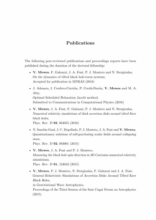
Publications
The following peer-reviewed publications and proceedings reports have beenpublished during the duration of the doctoral fellowship:
• V. Mewes, F. Galeazzi, J. A. Font, P. J. Montero and N. Stergioulas,On the dynamics of tilted black hole-torus systems,Accepted for publication in MNRAS (2016)
• J. Adsuara, I. Cordero-Carrión, P. Cerdá-Durán, V. Mewes and M. A.Aloy,Optimal Scheduled Relaxation Jacobi method,Submitted to Communications in Computational Physics (2016)
• V. Mewes, J. A. Font, F. Galeazzi, P. J. Montero and N. Stergioulas,Numerical relativity simulations of thick accretion disks around tilted Kerrblack holes,Phys. Rev. D 93, 064055 (2016)
• N. Sanchis-Gual, J. C. Degollado, P. J. Montero, J. A. Font and V. Mewes,Quasistationary solutions of self-gravitating scalar fields around collapsingstars,Phys. Rev. D 92, 083001 (2015)
• V. Mewes, J. A. Font and P. J. Montero,Measuring the black hole spin direction in 3D Cartesian numerical relativitysimulations,Phys. Rev. D 91, 124043 (2015)
• V. Mewes, P. J. Montero, N. Stergioulas, F. Galeazzi and J. A. Font,General Relativistic Simulations of Accretion Disks Around Tilted KerrBlack Holes,in Gravitational Wave Astrophysics,Proceedings of the Third Session of the Sant Cugat Forum on Astrophysics(2015)


Contents
List of Figures xix
List of Tables xxi
Nomenclature xxiii
I Introduction 1
1 Astrophysical background 31.1 The detection of gravitational waves: a new window to the universe 31.2 Mergers of compact objects and BH–torus systems . . . . . . . . 41.3 Dynamics of tilted BH–torus systems . . . . . . . . . . . . . . . . 71.4 Stability of accretion discs . . . . . . . . . . . . . . . . . . . . . . 91.5 Organisation of the thesis . . . . . . . . . . . . . . . . . . . . . . 131.6 Conventions . . . . . . . . . . . . . . . . . . . . . . . . . . . . . . 13
II Numerical relativity 15
2 Spacetime Evolution 192.1 The 3 + 1 formalism of GR . . . . . . . . . . . . . . . . . . . . . 222.2 The BSSN equations . . . . . . . . . . . . . . . . . . . . . . . . . 292.3 Choosing the gauge . . . . . . . . . . . . . . . . . . . . . . . . . . 312.4 The moving puncture . . . . . . . . . . . . . . . . . . . . . . . . 332.5 GW extraction . . . . . . . . . . . . . . . . . . . . . . . . . . . . 342.6 BH mass and spin . . . . . . . . . . . . . . . . . . . . . . . . . . 372.7 Total energy of the system . . . . . . . . . . . . . . . . . . . . . . 39

xvi Contents
3 General relativistic hydrodynamics 413.1 The general relativistic Euler equations in the 3 + 1 formalism . 433.2 High-resolution shock-capturing methods . . . . . . . . . . . . . 44
4 Computational framework 494.1 McLachlan . . . . . . . . . . . . . . . . . . . . . . . . . . . . . . 504.2 GRHydro . . . . . . . . . . . . . . . . . . . . . . . . . . . . . . . 524.3 Diagnostics . . . . . . . . . . . . . . . . . . . . . . . . . . . . . . 544.4 The disc analysis thorn . . . . . . . . . . . . . . . . . . . . . . . 55
4.4.1 Twist and tilt . . . . . . . . . . . . . . . . . . . . . . . . . 564.5 Fluid tracer particles . . . . . . . . . . . . . . . . . . . . . . . . . 59
III Results 61
5 Measuring the BH spin direction in 3D Cartesian NR simula-tions 635.1 Angular momentum with Weinberg’s pseudotensor . . . . . . . . 645.2 The angular momentum pseudotensor integral in Gaussian coor-
dinates . . . . . . . . . . . . . . . . . . . . . . . . . . . . . . . . . 665.3 Measuring the angular momentum in NR simulations . . . . . . . 69
6 NR simulations of tilted BH–torus systems 716.1 Initial data and setup . . . . . . . . . . . . . . . . . . . . . . . . 71
6.1.1 Self-gravitating accretion discs . . . . . . . . . . . . . . . 726.1.2 Tilted Kerr spacetime in improved quasi-isotropic coordi-
nates . . . . . . . . . . . . . . . . . . . . . . . . . . . . . . 746.1.3 Numerical setup . . . . . . . . . . . . . . . . . . . . . . . 796.1.4 Accuracy and convergence . . . . . . . . . . . . . . . . . . 80
6.2 Results . . . . . . . . . . . . . . . . . . . . . . . . . . . . . . . . . 846.2.1 Surface plots . . . . . . . . . . . . . . . . . . . . . . . . . 846.2.2 Maximum rest-mass density evolution . . . . . . . . . . . 906.2.3 Evolution of the accretion rate . . . . . . . . . . . . . . . 926.2.4 PPI growth in the disc and BH motion . . . . . . . . . . . 956.2.5 PPI saturation and BH kick . . . . . . . . . . . . . . . . . 1036.2.6 BH precession and nutation . . . . . . . . . . . . . . . . . 1036.2.7 Disc twist and tilt . . . . . . . . . . . . . . . . . . . . . . 1106.2.8 Angular momentum transport . . . . . . . . . . . . . . . . 1166.2.9 Gravitational waves . . . . . . . . . . . . . . . . . . . . . 120

Contents xvii
7 Analysing the tilted BH–torus dynamics with fluid tracers 1297.1 Initial data and setup . . . . . . . . . . . . . . . . . . . . . . . . 1297.2 BH precession from Lense-Thirring torque . . . . . . . . . . . . . 1307.3 m = 1 non-axisymmetric instability . . . . . . . . . . . . . . . . . 132
7.3.1 Spiral density wave . . . . . . . . . . . . . . . . . . . . . . 1327.3.2 Gravitational torque and motion of the central BH . . . . 1357.3.3 Disc alignment . . . . . . . . . . . . . . . . . . . . . . . . 139
7.4 QPOs in the accretion rate . . . . . . . . . . . . . . . . . . . . . 141
IV Discussion and outlook 145
8 Discussion 1478.1 Measuring the BH spin direction in 3D Cartesian NR simulations 1478.2 NR simulations of tilted BH–torus systems . . . . . . . . . . . . 1498.3 Analysing the tilted BH–torus dynamics with fluid tracers . . . . 152
9 Outlook 155
V Appendices 159
A Hyperbolic partial differential equations 161A.1 Characterising hyperbolic PDEs . . . . . . . . . . . . . . . . . . 162A.2 The hyperbolicity of the 3 + 1 evolution equations . . . . . . . . 164A.3 Conservation laws . . . . . . . . . . . . . . . . . . . . . . . . . . 165
B Implementation details of the disc analysis thorn 167


List of Figures
2.1 Diagram showing the 3+1 splitting of spacetime . . . . . . . . . 22
4.1 Disc analysis diagram . . . . . . . . . . . . . . . . . . . . . . . . 57
6.1 Innermost region of the initial rest-mass density profile along thex-axis for model C1Ba0b0 . . . . . . . . . . . . . . . . . . . . . . 72
6.2 Contour plot in the xz plane of the initial rest-mass density profilein the disc for model C1Ba0b0 . . . . . . . . . . . . . . . . . . . . 78
6.3 Convergence properties of BH–torus simulations . . . . . . . . . 806.4 Dependence of the irreducible mass of the BH on grid resolution
for model C1Ba01b30 plotted for the first 4 orbits. . . . . . . . . 816.5 Evolution of the fractional error in the irreducible mass . . . . . 826.6 Initial radial profile of the Hamiltonian constraint for a vacuum
Kerr BH and for model C1Ba03b30 . . . . . . . . . . . . . . . . . 836.7 Surface plots of the logarithm of the rest-mass density for model
C1Ba01b30 . . . . . . . . . . . . . . . . . . . . . . . . . . . . . . . 856.8 Surface plots of the (normalised) rest-mass density at the final
time of the evolution for the lower spin models . . . . . . . . . . 866.9 Surface plots of the (normalised) rest-mass density at the final
time of the evolution for the higher spin models . . . . . . . . . . 876.10 Density isocontours plots for lower spin models . . . . . . . . . . 886.11 Density isocontours plots for higher spin models . . . . . . . . . . 896.12 Evolution of the maximum rest-mass density . . . . . . . . . . . 916.13 Evolution of the accretion rate . . . . . . . . . . . . . . . . . . . 936.14 Evolution of the first four non-axisymmetric (PPI) modes . . . . 966.15 Evolution of the non-axisymmetric m = 1 mode . . . . . . . . . . 996.16 Trajectories of BH centre on the xy plane . . . . . . . . . . . . . 1006.17 Full 3D trajectory of the BH for model C1Ba01b30 . . . . . . . . 102

xx List of Figures
6.18 Radiated linear momentum for models C1Ba01 . . . . . . . . . . 1046.19 Evolution of the precession rate of the BH spin about the z-axis 1056.20 Total precession of the BH spin about the z-axis . . . . . . . . . 1066.21 Evolution of the nutation rate of the BH spin about the z-axis . 1076.22 Evolution of the tilt angle of the BH spin w.r.t. the z-axis . . . . 1096.23 Evolution of the disc tilt angle νDisc . . . . . . . . . . . . . . . . 1116.24 Evolution of the total precession of the total disc angular momen-
tum JDisc . . . . . . . . . . . . . . . . . . . . . . . . . . . . . . . 1136.25 Spacetime t− r diagrams of the radial disc tilt profile ν(r) . . . . 1146.26 Spacetime t− r diagrams of the radial disc twist profile σ(r) . . 1156.27 Spacetime t− r diagram showing the time evolution of the radial
profile of the angular momentum magnitude ∥J(r)∥ . . . . . . . . 1186.28 Time evolution of the l = m = 2 mode of the real part of the
Weyl scalar Ψ4 . . . . . . . . . . . . . . . . . . . . . . . . . . . . 1216.29 Spectrum of the effective strain for models C1B . . . . . . . . . . 1226.30 Spectrum of the effective strain for models NC1 . . . . . . . . . . 1246.31 Spectrum of the effective strain for models D2 . . . . . . . . . . . 1266.32 Detectability of peak GW amplitudes . . . . . . . . . . . . . . . 127
7.1 Evolution of the x and y components of the BH spin S . . . . . . 1307.2 Evolution of the x and y components of the BH spin S and total
disc angular momentum Jdisc. . . . . . . . . . . . . . . . . . . . 1317.3 Fractional change in the rest mass density ∆ρ/ρ . . . . . . . . . 1337.4 Fractional change in the fluid entropy s . . . . . . . . . . . . . . 1347.5 Time derivative of the components of the BH orbital angular
momentum vector LBH . . . . . . . . . . . . . . . . . . . . . . . 1367.6 Evolution of the m = 1 mode . . . . . . . . . . . . . . . . . . . . 1377.7 Spacetime diagram of the radial profile of the tilt angle ν(r) . . . 1387.8 Time evolution of the tilt angle of the disc . . . . . . . . . . . . . 1397.9 Evolution of the sum of disc eccentricity e1 and disc ellipticity e2
and the rest mass accretion rate M . . . . . . . . . . . . . . . . . 1407.10 Power spectrum density of e, M , and vr
BH . . . . . . . . . . . . . 1417.11 Trajectory of BH projected onto xy-plane . . . . . . . . . . . . . 142

List of Tables
6.1 Main characteristics of our initial models . . . . . . . . . . . . . . 756.2 Main characteristics of our initial models, continued . . . . . . . 76


Nomenclature
List of Symbols
Γγαβ Christoffel symbols
xµ coordinates
Gµν Einstein tensor
gµν spacetime metric
ηµν Minkowski metric
M spacetime manifold
Rµν Ricci tensor
R 3-dimensional Ricci scalar
R(4) 4-dimensional Ricci scalar
Rαβγδ Riemann tensor
Tµν stress-energy tensor
Cαβγδ Weyl tensor
α lapse function
βi shift vector
γij spatial metric
Kij extrinsic curvature
Σt spacelike hypersurface
Aij conformally related traceless part of extrinsic curvature

xxiv Nomenclature
ϕ conformal factor
γij conformal spatial metric
Γi conformal connection functions
E matter energy density
h specific enthalpy
ϵ specific internal energy
l specific angular momentum
W Lorentz factor
P pressure
ρ rest-mass density
D conserved rest-mass density
s entropy
Si matter momentum density
Sij matter stress tensor
vi three-velocity
uµ four-velocity
Acronyms / Abbreviations
ADM Arnowitt-Deser-Misner
AH apparent horizon
BH black hole
BBH binary black hole
BHNS black hole–neutron star
BNS binary neutron star
BSSN Baumgarte-Shapiro-Shibata-Nakamura
EH event horizon

Nomenclature xxv
EOS equation of state
ET Einstein Toolkit
GRB gamma ray burst
GR General Relativity
GRHD general relativistic hydrodynamics
GRMHD general relativistic magnetohydrodynamics
GW gravitational wave
HRSC high-resolution shock-capturing
IVP initial value problem
LIGO Laser Interferometer Gravitational-Wave Observatory
LT Lense–Thirring
MoL method of lines
MRI magneto-rotational instability
NR numerical relativity
NS neutron star
PDE partial differential equations
PPI Papaloizou-Pringle instability
PPM piecewise parabolic method
QPO quasi-periodic oscillation
RI runaway instability


Part I
Introduction


Chapter 1
Astrophysical background
1.1 The detection of gravitational waves: a newwindow to the universe
On September 14, 2015 at 09:50:45 UTC, the two advanced Laser InterferometerGravitational-Wave Observatories (LIGO) detected a transient gravitationalwave (GW) signal produced by the merger of two black holes (BHs) [Abbott et al.2016]. The event was named GW150914. This landmark detection confirmedthe existence of GW by their direct observation for the first time. GWs hadbeen predicted by Einstein [1918] as a direct consequence of his theory of generalrelativity (GR) [Einstein 1915, Einstein 1916]. Previous to the event GW150914,there was only an indirect confirmation of the existence of GWs by the discoveryof the binary pulsar PSR B1913+16 [Hulse and Taylor 1975] and its energy lossvia GW [Taylor and Weisberg 1982]. While the detection has confirmed yetanother prediction of GR, it has also, even more importantly, opened a newwindow to the observation of the universe, allowing us to study cosmological andastrophysical systems via the GW they emit. Contrary to the electromagneticmessengers that have let us observe the universe so far, there is no opacityfor GWs, as they propagate as perturbations of spacetime itself. Among theastrophysical systems to be observed by means of GW are binary BH (BBH)mergers such as the observed event GW150914, as well as BH-neutron star(BHNS) mergers, binary neutron star (BNS) mergers, accretion tori around BHand NS, and core-collapse supernovae, to name but a few.

4 Astrophysical background
To estimate parameters from detected signals, it is necessary to model theastrophysical sources and their emission of GW as accurately as possible inorder to build large catalogs of waveforms for wide ranges of system parameters.For instance, the dynamics of a BBH coalescence can be divided in threedistinct phases: the early inspiral, the actual merger phase and the subsequentringdown of the remnant to a Kerr BH [Flanagan and Hughes 1998]. While thegravitational waveforms of the inspiral and ringdown can be accurately modelledusing the Post-Newtonian formalism and BH perturbation theory, respectively, itis necessary to solve the nonlinear field equations of GR numerically to producethe waveforms of the actual merger phase [Berti, Cardoso, and Will 2006]. Inmatter spacetimes, such as BNS or BHNS mergers, the calculation of waveformsfurthermore depends crucially on the physics used to model the matter.
1.2 Mergers of compact objects and BH–torussystems
Shortly after the first numerical relativity (NR) simulations of a complete BBHorbit presented in Brügmann, Tichy, and Jansen [2004], the first successfulmultiple orbit NR simulations of the actual merger of a BBH system wereachieved in Pretorius [2005a], Campanelli et al. [2006], and Baker et al. [2006].Since then, ever-growing computational resources and advances in the numericalmethods used to simulate these systems have made the exploration of the vastinitial parameter space possible (see e.g. Hinder [2010] and references therein fora recent overview of the status of BBH simulations). The initial parameters ofBBH simulations are the BH mass ratio and the six components of their initialspin vectors. The investigation of these initial parameters has led to significantdiscoveries, as the occurrence of the orbital hang-up [Campanelli, Lousto, andZlochower 2006] and the presence of the so-called super-kicks, where the final BHis displaced from the orbital plane after its formation with a higher speed thanpredicted by Post-Newtonian estimates. This happens for initial configurationswith anti-aligned BH spins that lie in the orbital plane (see Brügmann et al.[2008] and references therein).
Stellar mass BH–torus systems are believed to be the end states of BNS orBHNS mergers, as well as of the rotational gravitational collapse of massivestars1. BNS mergers can also form an intermediate, transient structure known
1We note that there are more types of mergers that might lead to the formation of post-merger accretion tori, such as BH–white dwarf, NS–white dwarf, and binary white dwarfmergers (see, for instance Fryer et al. [1999], Paschalidis et al. [2011], and Raskin et al. [2012]).

1.2 Mergers of compact objects and BH–torus systems 5
as a hypermassive NS after the merger, whose large differential rotation leadsto a delayed collapse to a BH (see, e.g. Shibata et al. [2006]), or to a magnetar(a NS with a extremely strong magnetic field) surrounded by an accretion disc(see, e.g. Giacomazzo and Perna [2013]. Our theoretical understanding of theformation of BH–torus systems and their evolution relies strongly on numericalwork. The first BNS mergers in full GR (albeit for simplified matter models) wereperformed by Shibata and Uryu [2000], and following the BBH breakthrough in2005, Shibata and Uryu [2006] performed the first NR BHNS mergers. If the NSdoes not plunge into the BH during the final merger phase of a BHNS binary, butis rather tidally disrupted by the BH, a thick accretion torus can form aroundthe remnant Kerr BH (see Shibata and Taniguchi [2011] and references therein).Thick accretion tori also form in unequal mass BNS mergers (see Faber andRasio [2012] and references therein). The formation of a thick, massive accretiontorus in these systems is of particular interest as the remnant BH–torus system isbelieved to be a possible gamma-ray burst (GRB) engine [Woosley 1993, Jankaet al. 1999, Aloy, Janka, and Müller 2005]. In particular, the BH–torus systemsresulting from BNS and BHNS mergers are believed to be the birthplaces ofshort GRBs (SGRB), as the expected lifetime of the accretion torus is of theorder of the duration of SGRBs, while long GRBs are more likely to be producedby “failed” Type Ib supernovae [Woosley 1993]. BH–torus systems emit GWs,which may eventually provide the direct means to study their actual formationand evolution. Observing these GWs will help to prove whether the hypothesisthat these systems form the central engine of GRBs is correct, as due to theirintrinsic high density and temperature electromagnetic observations are out ofreach. Furthermore, once observed, the detected gravitational waveforms ofthe actual inspiral and coalescence in BNS and BHNS mergers will enhanceour understanding of the actual equation of state (EOS) of NS [Read et al.2009], thus providing valuable insights about the behaviour of matter at nucleardensities. For an overview of the event rate estimates of BNS and BHNS mergersthat are observable with initial and advanced LIGO see e.g. Abadie et al. [2010],Dominik et al. [2013], and Dominik et al. [2015].
In recent years a significant number of NR simulations have shown the feasi-bility of the formation of such systems from generic initial data (see e.g. Rezzollaet al. [2010], Kyutoku et al. [2011], Hotokezaka et al. [2013b], Hotokezaka et al.[2013a], and Kastaun and Galeazzi [2015] for recent progress). In particular,the 3D simulations of Rezzolla et al. [2010] (see also references therein) haveshown that unequal-mass BNS mergers lead to the self-consistent formation ofmassive accretion tori (or thick discs) around spinning BHs, thus meeting the

6 Astrophysical background
necessary requirements of the GRB’s central engine hypothesis. However, ifthe energy released in a SGRB comes from the accretion torus, the BH–torussystem has to survive for up to a few seconds [Rees and Meszaros 1994]. Anyinstability which might disrupt the system on shorter timescales, such as therunaway instability [Abramowicz, Calvani, and Nobili 1983] or the Papaloizou-Pringle instability (PPI) [Papaloizou and Pringle 1984], could pose a severeproblem for the prevailing GRB models. Additionally, post-merger discs shouldbe highly magnetised, due to efficient magnetic field amplification mechanismsactive in BNS mergers [Kiuchi et al. 2015a]. Large accretion rates facilitatedby the magneto-rotational instability (MRI), which might be active in accre-tion discs [Balbus and Hawley 1991], could further shorten the lifetime of theaccretion torus.
The majority of compact merger simulations to date have led to the produc-tion of BH–torus systems in which the central BH spin and the torus angularmomentum vector are aligned. This is the expected outcome for BNS mergers,where the direction of the remnant BH spin is perpendicular to the originalorbital plane of the binary. For BHNS mergers, an aligned BH–torus system isproduced if the BH has zero spin initially or if the BH spin is initially alignedwith the orbital plane of the binary system. However, if the BH spin is initiallymisaligned with the orbital plane of the binary, tilted BH–torus systems havebeen shown to form self-consistently in full NR simulations [Foucart et al. 2011,Foucart et al. 2013, Kawaguchi et al. 2015]. Another possible scenario for theformation of tilted BH–torus systems is by means of asymmetric supernovaexplosions in binary systems [Fragos et al. 2010]. In fact, it is believed that mostBH–torus systems should be tilted (see Fragile, Mathews, and Wilson [2001],Maccarone [2002], and Fragile et al. [2007] for arguments).
As shown in Foucart [2012], the disc mass in BHNS mergers increases witha larger initial BH spin and decreases with a larger initial BH mass. This isdue to the size of the innermost circular stable orbit (ISCO) of the BH in themerger. The ISCO grows with BH mass and decreases with the spin magnitudeof the BH. If the ISCO is large enough, the NS will be “swallowed” entirelyby the BH before being tidally disrupted, leaving no accretion torus behind.Another factor in determining the tidal disruption of the NS is its compactness(the ratio of the NS mass and its radius). As seen in Foucart [2012], the largerthe NS, the more favoured are massive post-merger discs. In order to estimatedisc masses resulting from BHNS mergers, one needs thus an estimate for theinitial BH masses in these system. One such method, via population synthesisconsiderations, favour larger BH masses [Belczynski et al. 2008, Belczynski et al.

1.3 Dynamics of tilted BH–torus systems 7
2010, Fryer et al. 2012], with a peak around 8 M⊙ and a mass gap betweenthe lightest expected BHs and NS masses. This means that these massive BHswould need very large initial spins in order to be able to form massive remnantdiscs after the BHNS merger. However, the prediction of accurate remnant BHmasses via population synthesis is difficult, as the BH mass crucially dependson the detailed supernova explosion mechanism [Kreidberg et al. 2012] which inturn is very model dependent on the actual presupernova evolution of rotatingmassive stars [Heger, Langer, and Woosley 2000].
1.3 Dynamics of tilted BH–torus systems
In a tilted BH–torus system, the dynamics of the system is fundamentally differentfrom the aligned case due to general relativistic effects affecting inclined particleorbits in the Kerr spacetime, such as the Lense–Thirring (LT) effect [Lense andThirring 1918]. The torque caused by the LT effect has a strong radial (r−3)dependence and causes the disc to start precessing differentially, as a result ofwhich it might become twisted and warped, affecting its dynamical behaviour(see Nelson and Papaloizou [2000] or Section 4.4.1 below for a definition of twistand warp). The inner regions of a thin disc might also be forced to move into theequatorial plane of the BH due to viscosity, via the so-called Bardeen-Pettersoneffect [Bardeen and Petterson 1975].
As the driving force of the tilted disc evolution are GR effects, one is guaran-teed to include all relevant effects by evolving these systems in GR. Both generalrelativistic hydrodynamics (GRHD) and general relativistic magnetohydrody-namic (GRMHD) simulations of tilted thick accretion discs around Kerr BHshave been performed by Fragile and collaborators within the so-called Cowling(fixed spacetime, test–fluid) approximation (see e.g. Fragile and Anninos [2005]and Fragile et al. [2007]). In those seminal works, the authors carried outsimulations to study both the dynamics and observational signatures of thickaccretion tori around tilted Kerr BHs.
In thick, tilted discs around Kerr BHs, the evolution and propagation ofwarps can be described by bending waves rather than diffusion [Lubow, Ogilvie,and Pringle 2002] (see also the model of Foucart and Lai [2014] describing thelinear warp evolution in tilted discs). In particular, in these systems the tilt angledoes not approach zero in the vicinity of the central BH, as one would expectif the viscous Bardeen-Petterson effect would be at play [Ivanov and Illarionov1997, Demianski and Ivanov 1997, Lubow, Ogilvie, and Pringle 2002]. Thisbehaviour of the radial tilt profile in the inner region of thick, tilted accretion

8 Astrophysical background
discs has been observed in the inviscid GRHD simulations of Fragile and Anninos[2005]. Incorporating GR effects in the simulations of these systems is crucial toobtain correct disc evolutions; see for instance, the simulations of Nealon et al.[2016], where omitting or accounting for general relativistic apsidal precessioncompletely changes the evolution of the tilt angle in the vicinity of the centralBH. The response of the disc to the differential torque depends on the sizeand properties of the disc. Notably, if the sound crossing time in the disc issmall compared to the timescale of the LT precession, which is the case forgeometrically thick and radially slender discs, the response of the disc to the LTtorque of the central BH is solid body precession [Fragile and Anninos 2005].The precessing disc is exerting an equal and opposite torque on the central KerrBH [King et al. 2005], which should therefore start to precess as well, at leastin those systems in which the disc mass is not negligible and the spacetimetherefore cannot be assumed to be a fixed background. As described in Kinget al. [2005], the LT torque alone does not act in a direction that results indisc alignment. However, there have been early arguments that the central BHshould eventually align with the disc angular momentum [Rees 1978, Scheuerand Feiler 1996]. In particular, King et al. [2005] argued that the total torquecannot have a component in the direction of the BH spin, but can be brokendown to a contribution that induces precession and a second, dissipative torquethat tends to align the BH and the accretion disc.
The response of the BH to the torque exerted by the precessing disc canonly be self-consistently analysed in GRHD simulations with a fully dynamicalspacetime evolution. For discs with negligible mass compared to the centralBH, the fixed-spacetime approximation in the seminal simulations of Fragile andcollaborators is perfectly justified. However, for BHNS mergers with an initiallylow mass BH, the post-merger accretion disc can have a non-negligible masscompared to the remnant central BH, making the inclusion of the disc self-gravitynecessary. To investigate these systems, and to extend the earlier works intothe fully dynamical spacetime regime, we present here the first comprehensivestudy of tilted BH–torus systems with a fully evolved spacetime via 3D GRHDsimulations. All simulations reported in the thesis have been carried out usingthe publicly available Einstein Toolkit (ET). In order to be able to monitorthe disc evolution during our simulations, we have implemented a module forthe ET performing the usual measure of the twist and tilt in the disc.
In order to quantify the response of the BH to the torque exerted by thedisc, we need an accurate measure of the direction of the BH spin. One of thestandard methods in NR to measure the magnitude of the angular momentum

1.4 Stability of accretion discs 9
of the BH horizon is described in Dreyer et al. [2003]. This method is basedon the so-called isolated horizon formalism [Ashtekar, Beetle, and Fairhurst1999] and its generalisation to dynamical horizons [Ashtekar and Krishnan 2003].This method does not, however, give the direction of the BH spin in the 3DCartesian reference frame of the computational grid of a NR simulation. Oneof the ways to measure the BH spin direction is via the so-called flat spacerotational Killing vector method presented in Campanelli et al. [2007], wherethe authors showed that the method (while being coordinate based) reproducesthe spin magnitude and direction on initial slices very well. The authors remark,however, that the method is not guaranteed to yield an accurate evaluationfor generic gauges (such as the ones attained during NR simulations). For thesimulations presented in this thesis we are in the need for an accurate measureof the BH spin direction for many orbits of the disc evolution in order to havean accurate description of the BH response to the disc torque. To achieve thisgoal we present below results showing that the method can be derived fromWeinberg’s pseudotensor [Weinberg 1972] and is equal, for an axisymmetrichorizon, to computing the Komar angular momentum [Komar 1959], when thelatter is expressed in a foliation adapted to axisymmetry.
1.4 Stability of accretion discs
Using perturbation theory, Papaloizou and Pringle [1984] found that tori withconstant specific angular momentum (l) are unstable to non-axisymmetric globalmodes. Such modes have a co-rotation radius within the torus, located in anarrow region where waves cannot propagate. Waves can still tunnel through theco-rotation zone and interact with waves outside that region. The transmittedmodes are amplified by reflections at the boundaries at the inner and outer edgesof the torus.
In early simulations of the PPI in the non-linear regime, Hawley [1987]showed the formation of m counterrotating over-density lumps, where m isthe azimuthal mode number. These over-density lumps were dubbed “plan-ets”. Goodman, Narayan, and Goldreich [1987] elucidated the precise mechanismof the instability and showed that the planets found in Hawley [1987] could be anew equilibrium configuration of the fluid after the saturation of the instability.The counterrotating over-density lumps manifest themselves as trailing spiraldensity waves of constant pattern speed. In a differentially rotating disc, thismeans that there is a region, namely at the co-rotation radius, where the spiraldensity wave is traveling with the same angular velocity as the fluid. Inside
10 Astrophysical background
the co-rotation radius, the wave travels slower, which means that it has nega-tive angular momentum with respect to the fluid in that region. In the linearregime, the wave does not interact with the fluid, but once the wave amplitudebecomes non-linear, mild shocks are formed and the wave can couple to thefluid of the disc via dissipation [Papaloizou and Lin 1995, Goodman and Rafikov2001, Heinemann and Papaloizou 2012]. As it couples to the fluid, it removesangular momentum from the fluid in the region within the co-rotation radiusand transports it outwards, thereby facilitating accretion.
Non-axisymmetric modes with an azimuthal mode number of m = 1 arespecial, as their appearance causes the centre of mass of the disc to no longercoincide with the centre of mass of the system. This results in a perturbedgravitational potential that causes a drift of the central compact object awayfrom the centre of mass of the system [Adams, Ruden, and Shu 1989, Heemskerk,Papaloizou, and Savonije 1992]. The induced movement of the central mass canalso enhance the strength of the m = 1 mode significantly [Adams, Ruden, andShu 1989, Christodoulou and Narayan 1992]. This enhanced mode growth whenthe central BH is allowed to move provides another reason why simulations ofBH–torus systems have to be evolved in fully dynamical spacetimes when thedisc mass is not negligible, as the central BH remains fixed by definition in theCowling approximation.
Korobkin et al. [2011] have studied non-axisymmetric instabilities in self-gravitating discs around BHs using three-dimensional hydrodynamical simula-tions in full GR. Their models incorporate both moderately slender and slenderdiscs with disc-to-BH mass ratios ranging from 0.11 to 0.24. They observed thegrowth of unstable non-axisymmetric modes and also observed the movement ofthe central BH as a result of the growth of a m = 1 non-axisymmetric mode. Alsoemploying NR simulations of both constant and non-constant l discs, Kiuchi et al.[2011] showed that the m = 1 mode survives for a long time after saturation innon-constant l discs, making the BH–torus system an emitter of large-amplitude,quasi-periodic GW that are potentially observable. In our comprehensive studyof tilted accretion discs presented in this thesis, some of our initial disc modelshave been specifically chosen because they were known to be PP-unstable whenthe central BH was non-spinning. This allowed us to investigate what kind ofeffect the disc surrounding tilted Kerr BH will have on its stability.
BH–torus systems are characterised by the presence of a cusp-like inner discedge where mass transfer driven by the radial pressure gradient is possible. Ifthe cusp moves deeper inside the disc due to accretion, the mass transfer speedsup leading to a runaway process that destroys the disc on a dynamical timescale

1.4 Stability of accretion discs 11
(see Font and Daigne [2002] and Daigne and Font [2004] for test-fluid simulationsin general relativity of the occurrence of this instability and Montero, Font, andShibata [2010] for axisymmetric simulations where the self-gravity of the discwas first taken into account). In most recent NR simulations [Rezzolla et al.2010, Hotokezaka et al. 2013b, Neilsen et al. 2014, Kastaun and Galeazzi 2015]the BH–torus systems under consideration did not manifest signs of runawayinstabilities on dynamical timescales, because the non-constant l profiles of themassive discs that form self-consistently in the simulations seem to make themstable against the development of the runaway instability. This is because thedisc is stabilised against the runaway instability when l is not constant [Daigneand Mochkovitch 1997], which was also observed numerically in Daigne and Font[2004]. Recently Korobkin et al. [2013] observed that by a suitable choice ofmodel parameters, namely constant angular momentum tori exactly filling orslightly overflowing their Roche lobe, a rapid mass accretion episode with thecharacteristics of a runaway instability sets in. The astrophysical significanceof such fine-tuned models is uncertain as they do not seem to be favouredas the end-product of self-consistent NR simulations of binary neutron starmergers [Rezzolla et al. 2010, Hotokezaka et al. 2013b, Kastaun and Galeazzi2015, Sekiguchi et al. 2015].
In a follow up paper to their seminal work in 1984, Papaloizou and Pringle[1985] showed that the dynamical instabilities of constant l profile tori werestill present in tori with non-constant l profiles, which, as indicated above,are more realistic outcomes of BNS and BHNS mergers. Furthermore, Zurekand Benz [1986] observed that discs with a larger exponent in the power-lawdistribution of l, l ∼ lq than the critical value given in Papaloizou and Pringle[1985], q > qPP = 2 −
√3, were still unstable, although angular momentum
transport was slower in those cases. This means that global non-axisymmetricmodes can indeed affect the disc evolution of post-merger BH–torus systems.For instance, in the recent GRHD simulations of Kawaguchi et al. [2015], theauthors observe significant BH–disc alignment in one of the tilted post-mergerBH–torus system they studied. These authors assume that angular momentumtransport facilitated by a non-axisymmetric shock wave in the disc could providethe dissipation needed for the BH–disc alignment. Another example for theimportance of non-axisymmetric instabilities is provided by the recent GRHDsimulations of Paschalidis et al. [2015], where the authors observe the formationof a one-armed (m = 1) spiral arm instability in the hypermassive NS formedfollowing a BNS merger.

12 Astrophysical background
Due to the importance of global non-axisymmetric modes in BH–torussystems, we investigate in this thesis the effects of the disc self-gravity aroundtilted BHs. Some of the initial models we have built were known to be unstableagainst the PPI in the untilted case [Korobkin et al. 2011]. Therefore, weinvestigate in particular the effects the BH tilt has on the development of theseinstabilities in the torus.
We end this introduction with a word on the initial disc models (see Section 6.1below for full details). All the simulations reported in this thesis are performedusing initial data constructed as equilibrium models of thick accretion discsaround a Schwarzschild BH, using a construction described in Stergioulas [2011].In order to obtain initial data that model a tilted BH–torus system, we replace thespacetime consisting of the non-rotating BH and self-gravitating disc spacetimeby a Kerr spacetime with its symmetry axis tilted with respect to the disc angularmomentum. We note that there is currently no known method of constructingtilted self-gravitating discs around Kerr BH, as such a tilted BH–torus system isnot stationary by definition. Currently, the only way of self-consistently arrivingat self-gravitating tilted BH–torus initial data is therefore via NR simulationsof tilted BHNS mergers, such as the ones reported in Foucart et al. [2011],Foucart et al. [2013], and Kawaguchi et al. [2015]. While performing the mergersand investigating the subsequent post-merger disc evolution would have beenpossible using the ET, it would have rendered the study prohibitively expensivecomputationally and was therefore out of the scope of this work. We are notaware of publicly available tilted BH–torus data from self-consistent NR mergersimulations either that we could have used as initial data.

1.5 Organisation of the thesis 13
1.5 Organisation of the thesisThe rest of the thesis is organised in three parts:
In Part II, we give a brief introduction to the field of NR, describing thespacetime evolution formalism in Chapter 2, GRHD in Chapter 3, and finallygiving an overview of the computational framework in Chapter 4. This chapterbriefly describes the ET, the numerical code which we use for all simulationspresented in this thesis.
We present our results in three chapters in Part III. In Chapter 5, we presentresults regarding the measurement of BH spin direction in NR simulations. Ourcomprehensive parameter study of different accretion disc models around tiltedKerr BHs is presented in Chapter 6. In the final Chapter 7 of Part III, weanalyse one of the models of Chapter 6 in more detail, using fluid tracer particlesas a new means of analysing the disc evolution.
The discussion of the results and our outlook are presented in Part IV.Finally, Part V contains two appendices. Appendix A contains a brief
overview of hyperbolic partial differential equations (PDEs) and in Appendix Bwe give details on the actual implementation of the disc analysis thorn we havewritten.
1.6 ConventionsWhere physical quantities are given without explicit units, we use units in whichc = G = M⊙ = 1 throughout the thesis, where c, G and M⊙ are the speed oflight, the gravitational constant and the solar mass, respectively. Specifically,this means that units of length and time are given by [L] = M⊙ ∼ 1.477 km and[T] = M⊙ ∼ 4.92673×10⁻⁶ s. A notable exception are frequencies, which we willgive in units of Hz. We adopt a spacelike signature of the metric (−,+,+,+).Lower case Latin indices run from 1 to 3, Greek indices run from 0 to 3 andupper case Latin indices indicate the number of equations in a hyperbolic system.We adopt the standard Einstein summation convention for the summation ofrepeated indices. Vector and tensor variables are indicated in boldface. Indicesof objects living in three-dimensional hypersurfaces are raised and lowered withthe spatial three-metric of the respective hypersurface.

Part II
Numerical relativity


17
One hundred years have passed since Albert Einstein formulated GR [Einstein1915, Einstein 1916], deriving the equations of motion of the gravitational field.The field equations are a set of non-linear partial differential equations (PDEs)for the spacetime metric. The non-linearity is a consequence of the fact thatthe gravitational field itself carries energy and momentum. Obtaining exactsolutions to the field equations is notoriously difficult. The most famous are thevacuum solutions of Schwarzschild [1916] and Kerr [1963]. The Schwarzschildsolution is a spherically symmetric, static spacetime, describing the vacuumgravitational field around a non-rotating, uncharged mass. The Kerr spacetimeis an axisymmetric, stationary solution, giving the vacuum gravitational fieldaround a rotating mass. For an excellent introduction to the Kerr spacetime,see Visser [2007]. For an overview of exact solutions to the Einstein equations,see Kramer and Schmutzer [1980].
As noted in the introduction, ground based GW detectors have opened anew window to the observation of the universe. While the investigation ofexact solutions to the field equations is an important field in itself, most exactsolutions are stationary/static and as such do not emit GWs. It is thereforenecessary to numerically solve the full non-linear field equations in order tomodel gravitational waveforms emitted in dynamical scenarios. This chaptergives an introduction to the methods and techniques developed in order tonumerically integrate the field equations of GR.
The field of NR has come a long way from the first reformulation of theEinstein equations in a 3 + 1 split by Darmois [1927] to the groundbreakingvacuum BBH simulations of Pretorius [2005a], Campanelli et al. [2006], and Bakeret al. [2006]. For matter spacetimes, the first BNS mergers by Shibata and Uryu[2000] and BHNS mergers by Shibata and Uryu [2006] were equally importantbreakthroughs. As we can only give an overview of the field and the necessarytechniques to solve the Einstein equations numerically, we refer the reader tothe lectures notes of Gourgoulhon [2012] and the books by Alcubierre [2008]and Baumgarte and Shapiro [2010] for a general introduction to NR, as well as theLiving Review articles on numerical hydrodynamics and magnetohydrodynamicsin general relativity by Font [2008], on BNS mergers by Faber and Rasio [2012],as well as on BHNS mergers by Shibata and Taniguchi [2011].
This part of the manuscript is split in chapters describing the spacetimeevolution, the evolution of GRHD and the computational framework that is usedfor the numerical simulations presented in this work.


Chapter 2
Spacetime Evolution
GR abandons the notion of a global flat space and a universal time in which thedynamics of matter take place, as is the case in Newtonian dynamics. Instead,the dynamics take place in a 4-dimensional spacetime consisting of events, whichare 4-dimensional labels of 3 spatial and one temporal coordinate. Notably,space and time are brought on an equal footing. The mathematical structure ofspacetime is that of a 4 dimensional pseudo-Riemannian manifold M equippedwith a bilinear, symmetric form, the spacetime metric g, together forming theset (M, g).
The equation of motion for the gravitational field is the following tensorialequation:
G = 8π T , (2.1)
where G is the Einstein tensor and T the stress-energy tensor of the mattercontained in the spacetime. A guiding principle in the development of the theoryhas been general covariance, as the laws of physics should not depend on thecoordinates used in calculations. This is reflected in the fact that the equation ofmotion of the gravitational field is a tensorial equation. The Einstein equationsdetermine the curvature of the manifold M for a given matter distributiondescribed by the stress-energy tensor T , while the curvature in turn determinesthe gravitational field felt by the matter distribution. This, as Zeidler [2011]remarks, can be formulated as a guiding principle of modern theoretical physics,namely as the realisation that force equals curvature.
Introducing the coordinates xµ in M, the line element (which measuresdistances and times between points in the manifold) is given in terms of the

20 Spacetime Evolution
spacetime metric as:ds2 = gµνdx
µdxν . (2.2)
The Christoffel symbols of the Levi-Civita connection, which is torsion-free, aredefined as
Γγαβ := 1
2(∂αgβµ + ∂βgαµ − ∂µgαβ)gµγ , (2.3)
where we have introduced the shorthand notation ∂α := ∂∂xα and gµν is the
inverse of the spacetime metric gµν in the sense that
gανgνβ = δβ
α, (2.4)
with δβα being the Kronecker delta. As usual, indices are raised and lowered
with the spacetime metric gµν . The curvature of M is completely determinedby the Riemann tensor Rδ
αβγ given by
Rδαβγ := ∂α Γδ
βγ − ∂β Γδαγ + Γδ
αµΓµβγ − Γδ
βµΓµαγ . (2.5)
From the Riemann tensor, we can construct the Ricci tensor Rαβ of the spacetime,which is obtained by contracting the Riemann tensor once
Rαβ := Rδαδβ , (2.6)
and contracting the Ricci tensor once more gives the Ricci scalar or scalarcurvature
R(4) := gαβRαβ . (2.7)
As the Ricci scalar does not carry indices by definition, we use the notation R(4)
to indicate that it is a four-dimensional object of the manifold M, distinguishingit from the 3-dimensional Ricci scalar R. Using the Ricci tensor and scalarcurvature, we can express the Einstein tensor in the coordinates xµ as follows
Gµν := Rµν − 12gµν R(4) , (2.8)
which gives the Einstein equations in coordinates
Rµν − 12gµν R(4) = 8π Tµν . (2.9)
Contracting Eq. (2.9) with gµν leads to
R(4) = −8π Tλλ (2.10)
which means that the scalar curvature of the spacetime is directly related to theenergy-momentum of the matter via the trace of Tµν . Substituting Eq. (2.10)back into Eq. (2.9), we are led to the following equivalent form of the Einstein

21
equations:Rµν = 8π (Tµν − 1
2gµνTλ
λ). (2.11)
From this form of the Einstein equations, we see immediately that a vacuumspacetime (Tµν = 0) has a vanishing Ricci tensor.
The symmetric Einstein tensor Gµν has ten independent components, so thatEq. (2.9) is a set of 10 algebraically independent equations. However, as a resultof the Bianchi identities (see, e.g. Weinberg [1972]), the components of Gµν arerelated by four differential identities,
Gµν;µ = 0, (2.12)
where ;µ denotes the covariant derivative with respect to the metric gµν . We aretherefore left with 10 − 6 independent equations for the spacetime metric, whichmeans there are 4 degrees of freedom. These represent the gauge invariance ofthe theory, namely the diffeomorphisms of the 4 dimensional spacetime.
We note that by virtue of the Einstein equation (2.9), the local conservationof the Einstein tensor, Eq. (2.12), directly implies that the stress-energy tensoris locally conserved as well:
Tµν;µ = 0. (2.13)
The fact that time and space are combined into events in GR, as well as the4 dimensional gauge invariance make the numerical integration of the equationsof motion of the gravitational field a daunting task. For dynamical vacuumspacetimes, we do not know the future end states of the system in order to beable to properly formulate boundary conditions. Furthermore, the presence ofmatter complicates the evolution of the system further, as the matter mightbe subject to the other forces of nature (the electromagnetic, electroweak andstrong force) as well. Additionally, we know that there is an arrow of time, givenby the second law of thermodynamics, namely that the entropy of an isolatedsystem cannot decrease in time. We would therefore like to rewrite the fieldequations (2.9) in a way that enables us to integrate them forward in time, aswe are required to integrate the internal evolution of the matter forward in timeas well. We are thus led to consider if we can solve the Einstein equations as aCauchy initial value problem (IVP):
Given the metric gµν and its “velocity” ∂0gµν at a single point in time x0 = t0
everywhere in space, can we integrate the field equations coupled to the matterevolution equations forward along x0?

22 Spacetime Evolution
Σt
Σt+δt
xi = constn ∂t
β
αn
Figure 2.1 Diagram showing the 3+1 splitting of spacetime in a foliation adapted to thecoordinates xi of the spacelike hypersurface Σt. See main text for details.
2.1 The 3 + 1 formalism of GR
By slicing the 4 dimensional spacetime as a family of non-intersecting 3-dimensionalspacelike hypersurfaces Σt, one can reformulate finding the solution to the Ein-stein equations as the Cauchy IVP sought above. This is based on the worksof Darmois [1927], Lichnerowicz [1944] and Choquet-Bruhat [1952]. In thedescription of the 3 + 1 formalism below, we largely follow the derivations givenin Gourgoulhon [2012], to which we refer the reader for full details.
In the 3 + 1 formalism, the 4 dimensional spacetime manifold M is foliatedby a set of non-intersecting spacelike hypersurfaces Σt, where t is a parameterindicating the elapsed time between neighbouring hypersurfaces. In the followingwe choose to foliate M in a manner that is adapted to the coordinates xµ,expressing the tensorial equations in those coordinates, as we are ultimatelyinterested in rewriting the field equations as PDEs in order to numericallyintegrate them. We denote the normal vector to the hypersurface as n, andthe tangent vector to the coordinate lines of xi = const as ∂t (called thetime vector [Gourgoulhon 2012]). The three central quantities in expressingthe spacetime metric gµν in the 3 + 1 formalism are then: The spatial 3-metric γij , which determines the intrinsic geometry of Σt, the lapse functionα, which is a measure of the temporal distance along the normal n betweenΣt and the neighbouring Σt+δt, and the shift vector βi, which measures the

2.1 The 3 + 1 formalism of GR 23
shift of the coordinates between the normal n and the time vector ∂t. Fig. 2.1displays a diagram illustrating the resulting foliation. Indices of objects livingon the hypersurface Σt are raised and lowered with the spatial metric γij . Thenormal vector nµ and the covariant normal vector nµ are given by the followingexpressions in the coordinates xµ
nµ =(
1α,−βi
α
), (2.14)
nµ = (−α, 0), (2.15)
while the time vector is given by
∂t = αn + β. (2.16)
From this, we see that the normal vector n is given by:
n = 1α
(∂t − β). (2.17)
In this 3+1 split, the 4 dimensional spacetime metric takes the following form:
gµν =(
−α2 + βiβi γijβ
j
γijβj γij
), (2.18)
and its inverse is given by
gµν =(
−α−2 βiα−2
βjα−2 γij − βiβjα−2
), (2.19)
where γij is the inverse of 3-metric γij . While the spatial metric γij defines theintrinsic geometry of Σt, it gives no information on how Σt is embedded in thefour dimensional manifold M. This information is provided by the extrinsiccurvature Kij , which measures the evolution of the spatial metric betweenneighbouring hypersurfaces. The extrinsic curvature is a spatial tensor of Σt
and is given by the Lie derivative of the spatial metric γij along the direction ofthe normal n:
K = − 12α (L∂t − Lβ) γ, (2.20)
where L∂tγ and Lβ γ are expressed in coordinates as follows:
L∂t γ = ∂t γij , (2.21)Lβ γ = Diβj +Djβi, (2.22)
where Di is the covariant derivative associated with the spatial metric γij . Incomponent notation, the extrinsic curvature is therefore given by:
Kij = − 12α (∂t γij −Diβj +Djβi), (2.23)

24 Spacetime Evolution
showing that the extrinsic curvature is closely related to the time derivative ofthe spatial metric. In fact, this gives us an evolution equation for γij stemmingpurely from the geometry of the foliation. Having defined the spacetime metricgµν in terms of the set α, βi, γij, the embedding of Σt in M with the help ofthe extrinsic curvature Kij has therefore given us the first evolution equation ofthe 3 + 1 field equations:
(∂t − Lβ) γij = −2αKij . (2.24)
To proceed, we need to define how to project the four dimensional tensors livingin M onto the hypersurface Σt in order to be able to project the field equationsonto the hypersurface. We can project four dimensional tensors in various ways;namely projecting along the tangents of the hypersurface using the orthogonalprojector γα
β :γα
β = δαβ + nαnβ , (2.25)
or a projection along the normal to Σt using nµ, or as a mix of the two projections.We first project the stress-energy tensor Tµν onto the hypersurface, which givesrise to the following quantities related to the matter content of the spacetime:
E ≡ nµ nν Tµν = 1α2
(T00 − 2βaT0a + βaβbTab
), (2.26)
Si ≡ −γµi n
ν Tµν = − 1α
(T0i − Tiaβa), (2.27)
Sij ≡ γµi γ
νj Tµν = Tij , (2.28)
S ≡ γij Sij . (2.29)
These quantities are respectively, the matter energy density E, the mattermomentum density Si, the matter stress tensor Sij , and the trace of the matterstress tensor S. Contracting the Einstein equations in the form of Eq. (2.11)twice with the orthogonal projector leads to
(∂t −Lβ)Kij = −DiDjα+α (Rij +KKij − 2KiaKa
j + 4π((S − E)γij − 2Sij))(2.30)
Projecting Eq. (2.11) twice with the normal to the hypersurface results in:
R+K2 −KijKij = 16πE, (2.31)
which is the so-called Hamiltonian constraint. Finally, performing a mixedprojection of Eq. (2.11) leads to the following equation:
DjKj
i −DiK = 8πSi, (2.32)

2.1 The 3 + 1 formalism of GR 25
which is the so-called momentum constraint. To arrive to these equations,one needs to make use of the Gauss, Codazzi, and Ricci equations. We refer thereader to Gourgoulhon [2012] for the full details of the derivation.
Eqs. (2.24) and (2.30) constitute the evolution equations of the 3+1 formalism,while Eqs. (2.31) and (2.32) are constraint equations that need to be fulfilled atevery spatial hypersurface Σt. These four equations, written in the 3+1 formalismare equivalent to the original four dimensional Einstein equations (2.11).
For completeness (see Gourgoulhon [2012]), we explicitly give the variousterms in the above equations by expressing the covariant derivative Di associatedwith the spatial metric γij in terms of partial derivatives using the Christoffelsymbols associated with the connection of γij , Γa
bc:
Γaij = 1
2γab(∂iγbj + ∂jγib − ∂bγij). (2.33)
Then
DiDjα = ∂i∂jα− Γaij ∂a α, (2.34)
DaKa
i = ∂aKa
i + Γaab K
bi − Γb
ai Ka
b, (2.35)DiK = ∂iK. (2.36)
Furthermore, the Lie derivatives with respect to the shift vector, Lβ, are givenby
Lβ γij = ∂jβi + ∂iβj − 2Γaij βa, (2.37)
Lβ Kij = βa ∂aKij +Kaj ∂iβa +Kia ∂jβ
a. (2.38)
The Ricci tensor Rij and the spatial scalar curvature R are given by
Rij = ∂aΓaij − ∂jΓa
ia + Γaij Γb
ab − Γbia Γa
bj , (2.39)R = γij Rij . (2.40)
The evolution and constraint equations constitute a set of second-order non-linear PDEs for the set of variables γij ,Kij , α, β
i, E, Si, Sij. We note thatthere are no time derivatives in the Hamiltonian and Momentum constraintequations. They are rather restrictions on the initial data on the initial spacelikehypersurface Σt=0. Loosely speaking, this means that the initial data needs to bea solution to the field equations in order to be able to obtain a meaningful timeevolution. Due to the Bianchi identities, we are guaranteed that the constraintsare identically fulfilled during the time evolution. However, this is only truein the continuum limit, while numerical systems tend to drift away from theconstraint surface due to the accumulation of truncation errors.

26 Spacetime Evolution
In order to gain some insight into the meaning of the constraints, and inparticular into the role played by the lapse and the shift, we will now brieflydescribe a Hamiltonian formulation of GR. Utilising the 3 + 1 split, Dirac[1949] and Arnowitt, Deser and Misner (ADM) [1961] (republished in Arnowitt,Deser, and Misner [2008]), derived a Hamiltonian formulation of GR, where,in close analogy to quantum mechanics, the generator of time evolution is theHamiltonian of the system. The starting point is the Hilbert action of GR
SGR[gµν ] = 116π
∫M
R(4) √−g d4x, (2.41)
where g is the determinant of gµν . The action is a functional of the metric.In the 3 + 1 formalism, we want to express the action SGR[gµν ] in terms ofthe set γij , α, β
i. The spatial metric γij will play the role of the generalisedcoordinates q, and we denote by pij the canonically conjugate momentum toγij . We restrict ourselves to the vacuum case below, but the inclusion of matterproceeds analogously. The action in terms of the set γij , α, β
i is then givenby:
S3+1[γij , α, βi] = 1
16π
∫R
(∫Σt
pij γij d3x−Hα −Hβi
)dt, (2.42)
whereHα andHβi are obtained by “smearing” the gravitational super-Hamiltonian
H = 1√γ
(pijpij − p2
2 ) − √γR, (2.43)
where γ ≡ det(γij), and super-momentum
Hi = −2Dipj
i, (2.44)
with the Lagrangian multipliers lapse
Hα =∫
Σt
αH d3x, (2.45)
and shift [Kucha and Torre 1991]
Hβi =∫
Σt
βi Hi d3x. (2.46)
As the variations of the action with respect to the lapse and shift need to vanishin order for the action to be extremal, and no term in the action explicitlydepends on either α or βi, apart from their use as Lagrangian multipliers, Hα
and Hβi must be identically zero:
δS3+1
δα= 0 =⇒ H = 1
√γ
(pijp
ij − p2
2
)− √
γR = 0, (2.47)

2.1 The 3 + 1 formalism of GR 27
andδS3+1
δβi= 0 =⇒ Hi = −2Djp
ji = 0. (2.48)
These are precisely the Hamiltonian and momentum constraints. The varia-tion of the action with respect to γij and pij leads to the Hamiltonian equationsof motion for the spatial metric and the conjugate momentum in terms of thefollowing Poisson brackets:
γij = γij , Hα +Hβi, (2.49)pij = pij , Hα +Hβi. (2.50)
As Kucha and Torre [1991] remark, the Einstein equations remain valid whenintroducing coordinate conditions after the variation, which the ADM reformu-lation allows us to do. The coordinate conditions only prescribe the passagefrom one hypersurface Σt to another Σt+δt. For reference, we give the relationbetween the extrinsic curvature Kij and the canonically conjugate momentumpij :
pij = √γ(K γij −Kij). (2.51)
After having obtained the Einstein equations as PDEs in coordinates adaptedto the coordinates introduced in the 3 + 1 split of the spacetime, we could inprinciple go ahead and numerically integrate them, after having specified a set ofinitial data γij ,Kij , E, Si, Sij that satisfies the constraints. As we have seen,the lapse and shift are Lagrangian multipliers of the Hamiltonian reformulationand therefore not dynamic variables, the freedom to choose them freely reflectsthe original diffeomorphism invariance of the 4 dimensional theory. There are,however, various caveats:
Firstly, although we should in principle be able to freely choose the gauge infree evolution schemes, choosing the correct gauge for the numerical integrationis crucial for the long-term stability of simulations. We will return to this issuein section 2.3 below.
Secondly, although the Bianchi identities guarantee that the constraints arefulfilled during the entire evolution, this is only strictly true in the continuumlimit, and performing the numerical integration of the field equations with finiteresolution will in general not preserve the constraints. When the constraints arenot satisfied, we are no longer solving the Einstein equations. There exist there-fore two different approaches to the numerical integration of the field equations:the so-called free evolution schemes, in which the level of constraint violationsis only monitored during the evolution, and the so-called constrained evolutionschemes, where the constraints are actively enforced during the evolution. Both

28 Spacetime Evolution
approaches have advantages and disadvantages. In free evolution schemes, theresulting nonlinear PDEs are hyperbolic, and therefore much easier and compu-tationally cheaper to solve than the nonlinear mixed elliptic-hyperbolic PDEsarising in constraint evolution schemes. However, as said above, the constraintsare only fulfilled in the continuum limit and numerical errors result in solutionsthat are not true solutions of the Einstein equations as the simulation proceeds.We use a free evolution scheme in this work, and will therefore not describeconstrained evolution schemes further. For examples of constrained schemes forthe numerical integration of the Einstein equations see Bonazzola et al. [2004]and Cordero-Carrión et al. [2009] and references therein.
Finally, when performing a free evolution using the discretised 3+1 evolutionequations (2.24) and (2.30) directly, the evolution is not stable. The reason isthat the equations are only weakly hyperbolic and as such mathematically notwell posed. The root of the problem is the appearance of the spatial Ricci tensorin these equations [Friedrich 1996], due to the fact that it contains mixed partialderivatives of the spatial metric. We will discuss this further in Appendix A,where we define the notion of hyperbolicity for first order systems of PDEs andprovide a heuristic argument showing how indeed the mixed partial derivativesof the Ricci tensor influence the hyperbolicity of the 3 + 1 evolution equations.
One way to eliminate these mixed derivatives is the conformal-tracelessreformulation of the 3 + 1 evolution equations, first presented by Nakamura,Oohara, and Kojima [1987]. The introduction of auxiliary variables removes thetroublesome mixed partial derivatives in the Ricci tensor, and additionally, thetrace of the extrinsic curvature, K, is evolved separately. One of the resulting,and arguably most widely used, free evolution scheme based on the conformal-traceless reformulation of the 3 + 1 evolution equations is the so-called BSSNformulation [Baumgarte and Shapiro 1999, Shibata and Nakamura 1995]1. As weexclusively use the BSSN formulation for all simulations in this work, we restrictourselves to its description only, which we present in the following section.
As a final remark, we note that there exist other formulations of the Einsteinequations not based on the 3 + 1 formalism, such as the characteristic initialvalue problem (for a review see Winicour [2012]) or the generalised harmonicdecomposition by Pretorius [2005b].
1Note that it is sometimes called BSSNOK, because it is based on the strategy of Nakamura,Oohara, and Kojima [1987] to simplify the spatial Ricci tensor.

2.2 The BSSN equations 29
2.2 The BSSN equations
The starting point of the conformal-traceless reformulation is a conformal de-composition of the spatial metric γij , an idea dating back to Lichnerowicz [1944],by introducing a conformal factor ϕ and the conformal spatial metric
γij = e−4ϕ γij , (2.52)
in a way that the determinant of the conformal metric, γ, is unity and theconformal factor is given by ϕ = ln(γ)/12. Defining the traceless part of theextrinsic curvature as
Aij = Kij − 13γijK, (2.53)
the conformally related traceless part of the extrinsic curvature is given by
Aij = e−4ϕ Aij . (2.54)
By taking the trace of the 3 + 1 evolution equation for the spatial metric (2.24)one obtains an evolution equation for the trace of γij :
∂tln(γii) = −2αK + 2Diβ
i. (2.55)
The evolution of the conformal factor ϕ is given by
∂tϕ = −16αK + βi∂iϕ+ 1
6∂iβi. (2.56)
In a similar fashion, by taking the trace of the evolution equation (2.30) of theextrinsic curvature and combining it with the Hamiltonian constraint (2.31),one obtains an evolution equation for the trace of the extrinsic curvature:
∂tK = −γij Dj Di α+ α
(AijA
ij + K2
3
)+ 4πα(E + S) + βi∂iK. (2.57)
Finally, combining the evolution equations for the trace of the extrinsic cur-vature (2.56) and the conformal factor (2.57) with the 3 + 1 evolution equa-tions (2.24) and (2.30), one arrives at the evolution equations for the conformalmetric and the conformally related traceless extrinsic curvature:
∂tγij = −2αAij + βa∂aγij + γia∂jβa + γaj∂iβ
a − 23γij∂aβ
a, (2.58)
∂tAij = e−4ϕ [α(Rij − 13γij R) − 8π α (Sij − 1
3γijS)
− (DiDjα− 13γijD
aDaα)] + α (K Aij − 2AiaAa
j)
+ βa∂aAij + Aia∂jβa + Aaj∂iβ
a − 23 Aij∂aβ
a. (2.59)

30 Spacetime Evolution
Note that the Ricci tensor still appears unaltered in the above equation for thetime evolution of Aij , and specifically, the mixed derivatives of the metric havenot yet been eliminated. To do so, one proceeds by splitting the Ricci tensorinto two parts:
Rij = Rϕij + Rij , (2.60)
where Rϕij is given by
Rϕij = −2DiDjϕ− 2γijD
aDaϕ+ 4DiϕDjϕ− 4γijDaϕDaϕ, (2.61)
and Di is the covariant derivative associated with the conformal metric. Intro-ducing the conformal connection functions Γi [Baumgarte and Shapiro 1999],defined as
Γi ≡ γab Γiab = −∂aγ
ia, (2.62)
where the Γiab are Christoffel symbols of the connection associated with the
conformal metric γij , the conformal Ricci tensor Rij can be expressed as:
Rij = 12 γ
ab∂abγij + γa(j∂j)Γa + ΓaΓ(ij)a + γab(2 Γca(iΓj)cb + Γc
ibΓcaj). (2.63)
The only second derivatives of the metric left in the definition of Rij is theLaplace operator γab∂abγij . The rest of the second derivatives have been recastin terms of the conformal connection functions Γi, which was the aim of thereformulation of the original 3+1 evolution equations. The conformal connectionfunctions are now considered as independent variables and need to be evolved.The evolution equation is obtained by performing a permutation of space andtime derivatives in the definition (2.62):
∂tΓi = − 2Aia∂aα+ 2α (ΓiabA
ab − 23 γ
ia∂aK − 8π γiaSa + 6Aia∂aϕ)
+ βa∂aΓi − Γa∂aβi + 2
3Γi∂aβa + 1
3 γbi∂abβ
a + γba∂baβi. (2.64)
Thus, in the BSSN reformulation of the 3 + 1 evolution equations, the evolutionvariables are now the set:
ϕ, γij ,K, Aij , Γi. (2.65)
The aim of the reformulation of the original 3 + 1 equations was to obtaina mathematically well-posed system. To this end, the removal of the mixedderivatives in the Ricci tensor has been achieved with a conformal-tracelessreformulation and the introduction of new auxiliary evolution variables. Weshould therefore be able to numerically integrate constraint-satisfying initialdata forward in time using the BSSN equations. However, we have not yet

2.3 Choosing the gauge 31
specified the gauge. As we show next, our choice of gauge is based on bothphysical and numerical reasons.
2.3 Choosing the gauge
The search for a suitable gauge has been guided by the following requirements:On physical grounds, the coordinate evolution should be singularity avoiding,while numerically, the BSSN system supplemented with evolution equations forthe lapse and shift should be strongly hyperbolic. Choosing a suitable foliationas well as suitable evolution of the spatial coordinates will be equally importantto guarantee long-term stable simulations. For a geometric interpretation of thelapse and shift, see for instance Fischer and Marsden [1972].
Let us start by analysing the gauge freedom with the simplest choice, theso-called Gaussian coordinates, which are defined by choosing the followingconstant lapse and shift: α = 1, βi = 0. Foliations with α = 1 are alsoknown as geodesic slicing. In this gauge, the lines xi = const are orthogonal tothe hypersurface (see Fig.2.1), and the time elapsed between hypersurfaces isthe proper time measured by Eulerian observers. In this gauge, the geodesicsemanating from a hypersurface Σt are orthogonal to the hypersurface, andfurthermore irrotational [Senovilla 1998]. While the 3 + 1 evolution equationssimplify tremendously when using Gaussian coordinates, they are not useful inthe numerical integration, as they are not singularity avoiding when the initialdata contains singularities, as is the case for BHs (see Smarr and York [1978]).But even in spacetimes initially not containing singularities, the solution to thefield equations necessarily develops coordinate singularities in finite time [Komar1956] when using Gaussian coordinates.
There have been several attempts to remedy the inability of geodesic slicingto avoid singularities, such as maximal slicing, which amounts to choosing alapse that corresponds to a vanishing trace of the extrinsic curvature (K = 0).This leads to an elliptic equation for the lapse (DiD
iα = αKijKij in vacuum).
An alternative is the harmonic slicing condition [Choquet-Bruhat and Ruggeri1983], corresponding to the following evolution equation for the lapse:
(∂t − Lβ)α = −K α2. (2.66)
A generalisation of the harmonic slicing condition (2.66) was given in Bona et al.[1995]:
(∂t − Lβ)α = −K α2 f(α), (2.67)

32 Spacetime Evolution
where f(α) is an arbitrary function. Note that f(α) = 1 recovers the originalharmonic slicing condition. Choosing f(α) = 2/α leads to
(∂t − Lβ)α = −2K α, (2.68)
which admits the following solution (for βi = 0):
α = 1 + ln(γ). (2.69)
This slicing is therefore known as 1+log slicing. It is singularity avoiding [Bonaet al. 1995] and has become (with various variations) one of the standard choicesfor NR simulations. Notably, two of the three breakthrough BBH simulations,the ones of Campanelli et al. [2006] and Baker et al. [2006], have used variationsof the 1+log slicing.
The role of the shift is more elusive, and in early works it has been routinelyset to zero. When dealing with spacetimes containing BHs, however, this hasthe unwanted effect of producing large stretching of the coordinates near theBH, with the coordinates falling into the BH as the simulation proceeds, causingthe horizon to continuously grow. In axisymmetric spacetimes of rotating BHs,there is further complication since a vanishing shift produces large shears closeto the BH due to frame dragging [Alcubierre 2008].
One successful cure to the fall-in of the spatial coordinates has been theso-called Γ-freezing of Alcubierre and Brügmann [2001], which amounts to ’freeze’the evolution of the conformal connection functions Γ in the sense that theirtime derivative is vanishing, i.e. ∂tΓ = 0. This prescription leads to an ellipticevolution equation for the shift. To avoid solving a computationally expensiveelliptic equation, Alcubierre et al. [2003] introduced the so-called hyperbolicΓ-driver condition:
∂2t β
i = k ∂tΓ − (η − ∂tln(k)) ∂tβi, (2.70)
where k and η are positive functions, the latter playing the role of a damping term.This results in a hyperbolic evolution equation for the shift. By introducingthe auxiliary variable Bi, one can write the Γ-driver as a set of two first-orderevolution equations:
∂tβi = k Bi, (2.71)
∂tBi = ∂tΓi − η Bi. (2.72)
The damping parameter η is a free parameter (see van Meter et al. [2006] forresults using different values of η). In practice, when using mesh-refinement, theη parameter introduces a step size limit for the time step, as noted in Schnetter

2.4 The moving puncture 33
[2010], where damping η as a function of the coordinate radius r is presented asa simple and effective solution to this problem.
We have therefore almost reached the goal of having rewritten the 3 + 1evolution equations in a form that is well-posed, as well as having found suitablegauge conditions that allow the long-term evolution of constraint-satisfying initialdata. There is one last missing ingredient, however: If we start with a spacetimecontaining a true singularity, such as the centre of a BH, or a spacetime that willdevelop a true singularity, for instance through the gravitational collapse of aNS, we need a prescription to deal with the singular geometry at the location ofthe singularity. One way is to excise a certain volume containing the singularity.Specifically, one can “remove” the entire volume enclosed by the surface of theBH from the computational domain, which was first performed in Seidel andSuen [1992]. This method effectively cured the problems of numerically evolvingspacetimes containing singularities, but has two apparent deficits: First, whenusing Cartesian grids, one needs to construct a so-called “Lego-sphere” [Cooket al. 1993] which only approximates the axisymmetric EH, and second, one needsto find appropriate boundary conditions for moving excision regions [Szilágyiet al. 2007] when the BHs are moving in the computational grid.
The alternative to singularity excision is the so-called moving puncturemethod, which is the standard choice for most groups.
2.4 The moving punctureIn Brandt and Brügmann [1997], the authors described a novel construction ofmultiple BH initial data where the spatial metric γij on the initial hypersurfaceis defined as
γij = (ψ)4 δij , (2.73)
where the conformal factor ψ is split in two parts, ψ = ΨBL + u. ΨBL is theBrill-Lindquist conformal factor [Brill and Lindquist 1963] and u is an everywhereregular function that represents the non-singular part of the solution at thecentre of the BHs, the “punctures”, namely
ψ = ΨBL + u, ΨBL =N∑
i=1
mi
2|r − ri|, (2.74)
where mi is the mass of the i-th puncture and N is the total number of BHs onthe grid. Using this split, one can solve for u (using the Hamiltonian constraint)without imposing special boundary conditions at the punctures. In this approach,the punctures remain fixed on the computational grid. This means that for

34 Spacetime Evolution
BBHs in orbital motion, the punctures are fixed in a co-rotating frame, so thatthe coordinates themselves need to evolve in such a way as to represent theorbital motion of the BHs. In Campanelli et al. [2006] and Baker et al. [2006]the authors discovered a way of evolving the puncture initial data without theneed for keeping the punctures fixed, but allowing them to move freely on thegrid. The singular part of the conformal factor can be evolved together with theregular part, using the following modification of the Γ-driver condition whichamounts to adding a shift advection term [Baker et al. 2006]:
∂tβi = 3
4 αBi, (2.75)
∂tBi = ∂tΓi − βi∂aΓa − η Bi. (2.76)
The geometry and regularity of moving punctures was analysed by Hannamet al. [2007] and their equivalence to moving BHs established in Thornburg et al.[2007].
With these ingredients, namely the conformal-traceless reformulation ofthe 3+1 evolution system, the 1+log slicing, the Γ-driver coordinate evolution(for the well-posedness of the BSSN system with a dynamical evolution of thelapse and shift see Beyer and Sarbach [2004] and Gundlach and Martín-García[2006]) and the moving puncture method, it is possible to long-term evolveconstraint-satisfying initial data.
2.5 GW extraction
One of the most important outcomes of NR simulations is the calculation ofgravitational waveforms. Indeed, the estimates for the initial BH masses ofthe recently discovered BBH merger GW150914, as well as the estimate of thefinal BH mass and its spin have been possible by comparing the measured GWsignal with a large catalog of GW signals obtained from GR [Abbott et al.2016]. While the early inspiral phase is very accurately described in the post-Newtonian formalism (see, for instance Blanchet et al. [1996]), and the predictedwaveforms agree well with the results from NR up until about the last orbit ofthe merger [Baker et al. 2007], the use of NR simulations is indispensable for anaccurate modelling of the GW signal produced by the actual merger of compactobjects.
Einstein [1918] predicted the existence of GW by obtaining wave-like solutionsto the linearised field equations in the weak-field regime. We can split the

2.5 GW extraction 35
spacetime metric gµν as Minkowski space ηµν plus a non-flat metric hµν :
gµν = ηµν + hµν . (2.77)
In the weak-field limit, we assume that |hµν | ≪ 1. We adopt the conventionthat indices are raised and lowered with ηµν when working to first-order inhµν [Weinberg 1972]
ηµσ hσν ≡ hµν . (2.78)
The first-order Ricci tensor R(1)µν then becomes
R(1)µν ≡ 1
2(hµν − ∂λ∂µh
λν − ∂λ∂νh
λµ + ∂µ∂νh
λλ
), (2.79)
where is the d’Alembert operator. The Einstein field equations then read
hµν − ∂λ∂µhλ
ν − ∂λ∂νhλ
µ + ∂µ∂νhλ
σ = 16π (Tµν − 12 ηµνT
λλ). (2.80)
Choosing a harmonic coordinate system, which is defined as
gκλ Γµκλ = 0, (2.81)
we have to first order∂λh
λν = 1
2 ∂µhλ
λ, (2.82)
which reduces the field equation to
hµν = −16π (Tµν − 12 ηµνT
λλ), (2.83)
which is precisely a wave equation for the weak-field perturbation hµν . Onesolution is given by the retarded potential
hµν(t,x) = 4∫d3y
Sµν(t− |x − y|,y)|x − y|
, (2.84)
whereSµν ≡ (Tµν − 1
2 ηµνTλ
λ). (2.85)
As seen from the wave equation for hµν (2.83) and also from the form of thetime argument in Sµν(t− |x − y|,y), GWs travel with a speed equal to 1, i.e.the speed of light.
We now turn to the extraction of GWs from numerical simulations. Thereare three main approaches to the extraction of gravitational waveforms fromnumerical data: Using gauge invariant perturbations of the Schwarzschild metric,also called the Moncrief [1974] formalism (for a review, see Nagar and Rezzolla[2005]), the Newman-Penrose formalism [Newman and Penrose 1962] and theCauchy-characteristic extraction [Babiuc et al. 2005] (for an implementationsee Reisswig et al. [2009]).

36 Spacetime Evolution
We will restrict ourselves to the description of the Newman-Penrose formalism,as this is the method we use to extract GWs in our simulations. In this formalismthe extraction is performed using one of the so called Newman-Penrose scalarsor Weyl scalars, Ψ4. The Weyl scalars are the 10 independent components ofthe four dimensional Weyl tensor C
(4)αβµν , which is defined as follows:
C(4)αβµν ≡ R(4)
αβµν −(gα[µ R(4)
ν]β − gβ[µ R(4)ν]α
)+ 1
3 gα[µgν]β R(4) , (2.86)
where square brackets around indices refer to the antisymmetric part of thetensor. The Weyl tensor has the same symmetries as the Riemann tensor, andin addition it is traceless, C(4)
αβαν = 0. The Weyl tensor of a conformal metricgµν = ψ gµν is equal to the Weyl tensor of the original metric gµν . In particular,this means that a conformally flat spacetime has a vanishing Weyl tensor.
The Weyl scalars are formed by contracting the Weyl tensor of the spacetimewith a complex null tetrad. This means choosing a tetrad of four vectorslµ, kµ,mµ, mµ such that:
lµlµ = kµkµ = mµmµ = mµmµ = 0. (2.87)
If one further imposes that −lµkµ = 1 = mµmµ, one has constructed a so-calledNewman-Penrose null tetrad. One way to construct such a null tetrad is bychoosing lµ and kµ to be two real vectors that are radially outgoing and ingoingnull vectors, respectively. We then construct two complex spatial vectors, mµ
and mµ that are orthogonal to lµ and kµ. Using the null tetrad, we can thencontract it with the Weyl tensor to obtain the Weyl scalars. As noted above,for the extraction of GWs we are interested in the Weyl scalar Ψ4 only, asone can show that it corresponds to outgoing gravitational radiation (see forinstance Baumgarte and Shapiro [2010]). In terms of the Weyl tensor and theconstructed null tetrad, Ψ4 is given by
Ψ4 = C(4)αβµν k
α mβ kµ mν . (2.88)
In particular, the gravitational strain is related to Ψ4 via:
Ψ4 = h+ − i h×, (2.89)
where h+ and h× are the plus and cross polarisation of the GW, respectively,and the double dot symbol indicates the second time derivative. In order tocalculate the Weyl scalar Ψ4 from the 3 + 1 numerical data of a simulation oneneeds to express C(4)
αβµν in terms of the 3+1 variables and construct a suitabletetrad. We first note that the Weyl tensor is equal to the Riemann tensor invacuum, so both tensors can be interchanged in vacuum. This means we can use

2.6 BH mass and spin 37
the Gauss, Codazzi and Ricci equations to express the four-dimensional Riemanntensor R(4)
αβµν in terms of the 3 + 1 variables. Following Baker, Campanelli,and Lousto [2002], the relevant components are given by:
R(4)ijkl = Rijkl + 2Ki[kKl]j , (2.90)
R(4)0jkl = 2 ∂[kKl]j + 2Ka[kΓa
l]j , (2.91)R(4)
0j0l = Rjl −KjaKa
l +KKjl. (2.92)
Finally, to construct a suitable null tetrad, one may proceed as described in Baker,Campanelli, and Lousto [2002].
2.6 BH mass and spinBH belong to the most interesting objects in the universe, yet they are char-acterised by just one or two parameters, for Schwarzschild and Kerr BHs,respectively. The defining property of a Schwarzschild BH is its mass M , whilea Kerr BH is completely defined by its mass M and angular momentum J , withthe Kerr parameter a being a = J/M . When monitoring BHs in numericalsimulations, one would therefore like to measure these quantities with greataccuracy. In the case of a single vacuum BH, we could just measure the totalmass of the spacetime in order to infer the BH mass, but as soon as we havemultiple BHs in our computational domain, or BHs surrounded by matter, weneed to measure the mass and angular momentum of the BH using its intrinsicproperties. One such possibility would be the calculation of the mass and angularmomentum using the surface of the BH, the so called event horizon (EH). Thedefining property of the EH is that it causally disconnects the interior of the BHfrom the outside, as no light rays emitted from within the EH can reach infinitybut rather fall back to the singularity, while light rays emitted from the outsidecan reach infinity [Hawking and Ellis 1975]. In this sense, the EH is a globalproperty of the 4 dimensional space, and one needs the entire time evolution ofthe spacetime to locate it. While it is possible to use the numerical data of asimulation to integrate geodesics backward in time to obtain the EH [Anninoset al. 1995, Libson et al. 1996], it would be desirable to obtain information aboutthe mass and angular momentum that can be calculated on every spacelikehypersurface as the simulation proceeds.
There is an additional way to define a horizon for a BH, the so-calledapparent horizon (AH). The AH can be computed locally in time, that is on eachhypersurface Σt. (See Thornburg [2007] and references therein for definitionsand implementations of EH and AH finders.) To define the AH, one begins
38 Spacetime Evolution
with the definition of a marginally trapped surface (MTS), which may be definedas a closed spacelike 2-surface in Σt with the property that its future-pointingoutgoing null geodesics have zero expansion Θ. In terms of the 3 + 1 variables,the expansion is defined as [York 1989]:
Θ ≡ Dini +Kij n
i nj −K = 0, (2.93)
where ni is the unit normal to the surface. The AH is then defined as theoutermost MTS in Σt. Given a spacetime containing an AH, Hawking and Ellis[1975] have shown that its existence necessarily implies the existence of an EH,and therefore the existence of a BH. Finding an AH during a simulation thereforemeans that the spacetime contains a BH. Note, however, that the converse is nottrue: The existence of an EH does not guarantee the existence of an AH, thiscan be seen from the absence of an AH in certain slicings of the Schwarzschildspacetime [Wald and Iyer 1991]. When found, the AH is also always containedwithin the EH, and coincides with the latter for a stationary spacetime.
Once we have located an AH, we want to obtain its quasi-local mass andangular momentum. The precise definitions are provided in the so-called isolatedand dynamical horizon formalism [Ashtekar, Beetle, and Fairhurst 1999, Ashtekarand Krishnan 2003] (see Ashtekar and Krishnan [2004] for a review of theformalisms, and for the application of the isolated and dynamical horizonformalism to NR see Dreyer et al. [2003] and Schnetter, Krishnan, and Beyer[2006]).
The BH spin is calculated by performing the following surface integral onthe AH of the BH
JAH = 18π
∫S
(ψaRbKab
)dS, (2.94)
where ψa is an approximate rotational Killing vector on the horizon that has tobe determined numerically (see Dreyer et al. [2003]), Rb is the outward pointingunit vector normal to the horizon, Kab is the extrinsic curvature on the horizonsurface and dS is the surface element.
Once the spin is known, we can calculate the horizon mass MAH:
MAH = 12RAH
√R4
AH + 4 J2AH, (2.95)
where RAH = (AAH/(4π))1/2 is the areal radius of the AH. In the case of a Kerrspacetime, the mass of the AH coincides with the Christodoulou mass [Christodoulou1970, Smarr 1973]. Moreover, the irreducible mass of the horizon is
Mirr =√AAH
16π . (2.96)

2.7 Total energy of the system 39
As the area of the AH cannot decrease, the conservation of the irreduciblemass provides a very good check for the accuracy of the simulation.
2.7 Total energy of the systemAfter having discussed the quasi-local mass of individual BHs in the previoussection, we now turn to a definition of the total mass or energy contained in ahypersurface Σt. If the spacetime is asymptotically flat (for details see Jaramilloand Gourgoulhon [2011]), one can define the total energy contained in thehypersurface Σt as the following surface integral, called the ADM energy:
EADM = 116π lim
r→∞
∫∫S
(∂jγij − ∂iγjj)nidS, (2.97)
where ni is the outward normal to the surface and the integration has to becarried out in Cartesian-like coordinates. Numerically, especially when usinglarge domains and mesh refinement, calculating the ADM energy using (2.97)using a large surface might not be very accurate, as the resolution is reduced nearthe outer boundaries of the domain. It would therefore be preferable to evaluatethe ADM energy as a volume integral. Following the derivation in Ó Murchadhaand York [1974], we can also calculate the total energy in Σt as the followingvolume integral:
EADM = 116π
∫Σt
∂l
(α
√γγijγkl(γik,j − γij,k)
)d3x. (2.98)
In Yo, Baumgarte, and Shapiro [2002], the authors derive an equivalent volumeintegral for the total energy using the BSSN variables.


Chapter 3
General relativistichydrodynamics
After having discussed the evolution of the spacetime, whose curvature representsthe gravitational force felt by the matter fields, we now turn to the descriptionof the intrinsic matter evolution. Most matter fields in astrophysical scenarioscan be modelled as a fluid, including stars, neutron stars, and accretion discs.Therefore, we need a GRHD formalism describing the matter evolution whichwill be coupled to the evolution of the spacetime via the Einstein field equations.We incorporate all non-gravitational interactions of the matter fields in the stress-energy tensor Tµν when coupling the matter to the evolution of the gravitationalfield. In this work, we have restricted those non-gravitational interactions to bethose of the evolution of the fluid only, neglecting other possible contributionssuch as electromagnetic fields or radiation transport. Neglecting these is a highlyidealised assumption, as we know that accretion tori are likely to be highlymagnetised (as already indicated in the Introduction) and that neutrino coolingwill play a significant role in the thermal properties of the torus due to the veryhigh densities and temperatures found in these systems (see Foucart et al. [2014]for BHNS merger simulations with neutrino cooling).
In ordinary fluid dynamics, the fluid evolution is described by the Navier-Stokes equations. We will model the matter as a perfect fluid, which correspondsto the assumption that the fluid has no viscosity, and that there is no heat conduc-tion in the fluid. Under these assumptions, the Navier-Stokes equations reduce

42 General relativistic hydrodynamics
to the so-called Euler equations. We first describe the classical Euler equationsand then proceed to the general relativistic form of the Euler equations1.
In classical fluid dynamics, a perfect fluid is subject to the following threeconservation laws: The conservation of mass, given by the continuity equation:
∂tρ+ ∂a(ρ va) = 0, (3.1)
where ρ is the fluid density, and vi its velocity, the conservation of momentum,expressed in the momentum (Euler) equation:
∂t(ρ vi) + ∂a(ρ vi va + p δa
i) = 0, (3.2)
where p is the fluid pressure, and the conservation of the total energy:
∂tE + ∂a(va(E + p)) = 0, (3.3)
where E is the total energy of the fluid, which can be written as:
E = 12ρ va v
a + ρ ϵ, (3.4)
where ϵ is the specific internal energy of the fluid. The conservation of the totalenergy therefore reads
∂t
(12ρ va v
a + ρ ϵ
)+ ∂a
(va
(12ρ va v
a + ρ ϵ+ p
))= 0. (3.5)
We define the 5 dimensional state vector w as
w =
ρ
ρ vi( 12ρ va v
a + ρ ϵ) , (3.6)
and similarly define the 5 × 3 flux matrix F , which is a function of (w), as
F (w) =
ρ va δ1A
(ρ vi va + p δa
i) δiA
( 12ρ va v
a + ρ ϵ+ p) va δ5A
, (3.7)
where we adopt the convention that upper case Latin indices run from 1 ton, where n is the dimension of w. The δA
B therefore selects the rows of theflux matrix, which correspond to the equations of the system. Using the statevector and flux matrix as defined above, the classical Euler equations can thenbe written as the following system of first-order hyperbolic PDEs
∂twA + ∂aFa
A(w) = 0. (3.8)
1In magnetised discs, the MRI is likely to provide an effective viscosity [Balbus and Hawley1991]. Foucart et al. [2014] estimate the viscous timescale in their post-merger accretion torito be ∼ 0.1s, which is significantly longer than the simulations presented in this thesis.

3.1 The general relativistic Euler equations in the 3 + 1 formalism 43
A set of PDEs written in the above form is called a system of conservation laws.In the next section, we describe how the Euler equations (3.8) can be rewrittenin a general relativistic manner in the 3 + 1 formalism. We follow the derivationlaid out in Banyuls et al. [1997] (for further details and information on additionalapproaches see Font [2008]).
3.1 The general relativistic Euler equations inthe 3 + 1 formalism
The starting point of the derivation of the general relativistic Euler equations are,analogously to their Newtonian version, the conservation of rest-mass density(the continuity equation) and the conservation of the fluid energy-momentum.A general relativistic perfect fluid has a rest-mass current Jµ and stress-energytensor Tµν given by
Jµ = ρ uµ, (3.9)Tµν = ρ huµ uν + p gµν , (3.10)
where ρ is the fluid rest-mass density, uµ the fluid four-velocity, P the fluidpressure and h the fluid enthalpy
h = 1 + ϵ+ p
ρ. (3.11)
The general relativistic continuity equation and the conservation of energy-momentum are then given by
Jµ;µ = 0, (3.12)
Tµν;µ = 0. (3.13)
As the system is underdetermined, we need to close it with an equation ofstate (EOS) that relates the fluid rest-mass density, pressure and internal energy,p = p(ρ, ϵ).
The three-velocity of the fluid as measured by observers at rest in the spatialhypersurface Σt (so-called Eulerian observers) is
vi = ui
αu0 + βi
α, (3.14)
and the corresponding Lorentz factor of the fluid, W , is defined as
W ≡ αu0 = 1√1 − γijvivj
. (3.15)

44 General relativistic hydrodynamics
The set of variables ρ, vi, ϵ describing the fluid is called the set of primitivevariables. This set does not correspond to the fluid properties as measuredby Eulerian observers in Σt, which are described by the so-called conservedvariables: the conserved baryon number D, the conserved momentum density inthe i-th direction Si and the total energy E. In terms of the primitive variables,these are given by the following definitions:
D = ρW, (3.16)Si = ρ hW 2 vi, (3.17)E = ρ hW 2 − P. (3.18)
Defining the state vector U(w) as
U(w) =
DSi
τ
, (3.19)
the 5 × 3 flux matrix F (w) and source vector S(w) are given by
F (w) =
D vi δ1A
(Sj vi + P δi
j) δjA
(τ vi + P vi) δ5A
, (3.20)
S(w) =
0Tµν(∂µgνi − Γλ
µνgλi)α(Tµ0∂µ(lnα) − TµνΓ0
µν)
, (3.21)
where τ ≡ E − D and vi ≡ vi − βi/α. Therefore, it is possible to writethe conservation laws of energy-momentum and the continuity equation as aconservation law by means of the conserved variables, resulting in the followingfirst-order, flux-conservative hyperbolic system of equations [Banyuls et al. 1997]:
1√−g[∂0(√γ UA) + ∂i(
√−g F i
A)]
= SA, (3.22)
where g ≡ det(gµν) = α√γ. This constitutes the general relativistic version of
the Euler equations in the 3 + 1 formalism, which is known as the so-calledValencia formulation.
3.2 High-resolution shock-capturing methods
Systems of nonlinear hyperbolic PDEs such as the Euler equations or the GRHDequations (3.22) are characterised by the fact that smooth initial data can develop

3.2 High-resolution shock-capturing methods 45
discontinuities in the variables in finite time2. The reason the GRHD equationsin the Valencia formulation were written in conservative form is that, in sucha form, a numerical scheme that converges guarantees the correct Rankine-Hugoniot conditions across discontinuities, which is called the shock-capturingproperty. This property is at the heart of high-resolution shock-capturing (HRSC)methods that guarantee that the physics of the flow will be correctly modelledby the numerical scheme in the presence of discontinuities in the fluid variables.Moreover, finite difference schemes written in conservation form guarantee thatthe convergence of the solution (if it exists) will be to one of the weak solutions ofthe system of PDEs [Lax and Wendroff 1960]. Weak solutions are characterisedby being solutions to the integral form of the conservation system. The setof all weak solutions is too large to be of practical use, as many (numerically)admissible weak solutions will not represent physically relevant solutions. Thusthere is need for an additional (thermodynamic) condition, the so-called entropycondition (namely that the entropy of a fluid element must increase when crossinga discontinuity) to guarantee that the numerical scheme will converge to thephysical solution. The convergence of the numerical scheme is closely relatedto its stability, and one useful measure is the total-variation (TV) stability (seee.g. LeVeque [1992] for a detailed discussion).
Additionally, numerical schemes written in conservation form guarantee thatthe conserved quantities of the system are numerically conserved in the absenceof sources or sinks. This means that the change of the state vector UA in time ina domain V that does not contain sources or sinks will be given by the fluxes F i
A
through the boundaries of the domain ∂V, a three dimensional surface which isdefined as the standard-oriented hyper-parallelepiped consisting of two spacelikesurfaces Σx0 ,Σx0+∆x0 and the timelike surfaces Σxi ,Σxi+∆xi joining thetwo temporal slices together. System (3.22) is thus expressed in integral form∫
V
1√−g
∂0(√γ UA) dV +∫
V
1√−g
∂i(√
−g F iA) dV =
∫VSA dV, (3.23)
2While it is known that physical shocks (discontinuities in the spacetime) do not exist inGR, there is nevertheless the possibility of the formation of gauge shocks when the kinematicalvariables (lapse and shift) are evolved as hyperbolic equations, such as the 1 + log slicing (2.67)and the Γ-driver (2.70) described in Section 2.3 above. Alcubierre [2003] has investigated theformation of shocks for the family of 1 + log slicing conditions and found a member that isshock avoiding. Additionally, it appears as if the formation of shocks in the evolution of thelapse is suppressed due to under-resolution caused by the shift in the puncture method in 3Dsimulations [Garfinkle, Gundlach, and Hilditch 2008]. When performing the shift evolution viathe Γ-driver, it seems that Γ acts as an effective “shock-absorber” [van Meter et al. 2006], asthis shift evolution equation have proven to be very stable.

46 General relativistic hydrodynamics
where dV = √−g d4x. This is the starting point to devise HRSC schemes to
solve it. Specifically, the flux integrals in (3.23) are given by∫V
1√−g
∂i(√
−g F iA) dV =
∫Σx1+∆x1
√−g F 1
A dx2 dx3 −
∫Σx1
√−g F 1
A dx2 dx3,
+∫
Σx2+∆x2
√−g F 2
A dx1 dx3 −
∫Σx2
√−g F 2
A dx1 dx3,
+∫
Σx3+∆x3
√−g F 3
A dx1 dx2 −
∫Σx3
√−g F 3
A dx1 dx2.
(3.24)
This means that the time integration of the conserved variables is given by theinterface fluxes of matter and energy-momentum of the fluid, as well as the(cell-centred) sources. One can therefore approximate those numerical fluxes(which depend on the solution at the cell interfaces) as the time-averaged fluxesacross cell interfaces during a timestep as
(F iA)i+ 1
2≈ 1
∆t
∫ tn+1
tn
F iA(UA(xi+ 1
2 , x0)). (3.25)
In general, the approximation to the real solution on a grid with finite resolutionwill be a piecewise continuous function, which means that the fluxes can beobtained by solving local Riemann problems at cell interfaces, an idea firstdescribed in Godunov [1959].
Riemann problems are IVPs with discontinuities in the solution. Duringthe evolution, a discontinuity in the fluid variables decays into shock waves,rarefaction waves and contact discontinuities. Shock waves move from thehigher to lower density regions, while rarefaction waves move in the oppositedirection. Contact discontinuities are characterised by a discontinuity in thedensity, while both pressure and velocity are constant across them. In order tosolve the Riemann problem, we need to obtain the spectrum (eigenvalues andeigenvectors) of the first-order system. As explained in Appendix A, we need tobring system (3.22) into the following quasi-linear form
∂tUA +maBA(U) ∂aUB + SA(U) = 0, (3.26)
in order to compute the spectrum and eigenvectors of the matrix maBA(U). Once
obtained, the Riemann problem is solved analytically to obtain the numericalfluxes. In order to rewrite the system in quasi-linear form, one obtains theJacobian of the system by taking partial derivatives of the flux matrix withrespect to the state vector. The resulting three (one for each spatial dimension)

3.2 High-resolution shock-capturing methods 47
5 × 5 Jacobian matrices are then combined into the block matrix maBA(U)
miBA(U) = α∂UA
F iB(U), (3.27)
which has real (but degenerate) eigenvalues and a complete set of eigenvec-tors [Banyuls et al. 1997] (the Jacobian miB
A(U) is therefore diagonizable andsystem (3.22) is therefore strongly hyperbolic). The features of the solutiontravel at characteristic speeds given by the eigenvalues of the Jacobian miB
A(U).Specifically, for a fluid moving in the x-direction, the eigenvalues are given
by
λ0 = αvx − βx (triple), (3.28)
λ± = α
1 − v2c2s
(vx(1 − c2
s) ± cs
√(1 − v2)[γxx(1 − v2c2
s) − vxvx(1 − c2s)])
− βx, (3.29)
where v2 = γabvavb and cs is the sound speed in the fluid, whose square is given
by
c2s = ∂p
∂E
∣∣∣∣s
= 1h
(∂p
∂ρ
∣∣∣∣ϵ
+ p
ρ2∂p
∂ϵ
∣∣∣∣ρ
). (3.30)
Note that the Newtonian limit of the eigenvalues (in which α → 1, βi → 0, vx ≪1) is correctly recovered (λ0 = vx, λ± = vx ± cs).
In practice, obtaining the numerical fluxes using the analytical solution ofthe Riemann problem is often not feasible, in particular in multidimensionalsimulations. One avoids finding the exact solution and uses linearised (approxi-mate) Riemann solvers instead, which still make use of the spectrum and theeigenvectors of the first-order system. Examples of approximate Riemann solversare the Harten-Lax-van Leer-Einfeldt (HLLE) solver [Harten, Lax, and Leer1983, Einfeldt 1988], the approximate solver of Roe [1981] and the Marquinaflux formula [Donat and Marquina 1996, Aloy et al. 1999].
The fluid data at the cell interfaces needed to obtain the numerical fluxesvia the solution of local Riemann problems could simply be obtained as theaverage of the data at neighbouring cell centres (which only yields overall first-order methods). A wide variety of higher order cell-reconstruction methodsare available in the literature (see e.g. Toro [2013]). Examples of higher orderreconstruction schemes are the piecewise-parabolic method (PPM) [Colella andWoodward 1984] and essentially non-oscillatory (ENO) methods [Harten et al.1987]. Regardless of their spatial order for smooth solutions, these reconstructiontechniques always reduce to first-order in the presence of physical shocks and localextrema of the fluid variables (such as the central density of a NS, for instance).

48 General relativistic hydrodynamics
While the choice of variables is crucial to obtain the GRHD evolution equationsin conservative form, it is usually the primitive variables that are reconstructedat the cell interfaces. To do this, one needs a conservative-to-primitive schemewhich inverts Eqs. (3.16)-(3.18), involving numerical root-finding. Once we haveobtained the numerical fluxes via the solution of local Riemann problems, weupdate the solution of the conserved variables by one timestep with the numericalfluxes and the sources. This is usually done employing high-order, conservativeRunge-Kutta schemes [Shu and Osher 1988].
We finish this chapter with a summary of the steps necessary to advance thesolution by a timestep in a numerical GRHD scheme coupled to the spacetimeevolution:
• Advance spacetime evolution in time
• Calculate the source vector SA(U) at all grid points
• Reconstruct primitive variables at cell interfaces using high-order recon-struction methods
• Set up local Riemann problems using the reconstructed primitive variablesat cell interfaces as initial data
• Calculate the numerical fluxes at cell interfaces by solving the local Rie-mann problems using approximate Riemann solvers
• Advance the solution of the conserved variables in time by using theobtained numerical fluxes and sources
• Recover primitive variables
• Update the stress energy-tensor Tµν with the new matter field configuration
• Update spacetime variables in time using the new matter field configurationas source

Chapter 4
Computational framework
The simulations reported in this thesis are performed using the publicly avail-able [Einstein Toolkit n.d.] code (described in detail in Löffler et al. [2012],to which we refer the reader for a complete overview of the components of theET). In the following, we provide a brief summary of the main components ofthe toolkit we use in our simulations.
The ET is a code for relativistic astrophysics simulations, which is based onthe modular [Cactus Computational Toolkit n.d.] [Goodale et al. 2003, Allenet al. 2011]. Cactus provides a very small core of base functionalities (the so-called “flesh”) coupled to general modules commonly called “thorns”. Simulationsof astrophysical systems often span a very wide range of distance scales, makinglarge domains with high resolutions necessary. In the BH–torus systems we areinvestigating in this thesis, we need very high resolution to capture the correctdynamics of the system, while GW extraction needs to be performed in the“wave zone”, that is, far away from the sources of the gravitational field. In 3Dsimulations, large domains with high resolution quickly become prohibitivelyexpensive in terms of both memory and computational power requirements.We are therefore in need of mesh refinement, where the resolution is graduallydecreased away from the origin. Adaptive mesh refinement (AMR) in the ETis provided by the [Carpet n.d.] driver [Schnetter, Hawley, and Hawke 2004,Schnetter et al. 2006], which employs the Berger-Oliger algorithm [Berger andOliger 1984] with subcycling in time. Using AMR is crucial when the resolutionin the domain needs to be dynamically adapted to the system (for instanceto add finer mesh refinement levels during the late stages of a NS collapse orto follow the BHs with the finest meshes in a BBH simulations as they movethrough the computational domain). In our simulations, we need to follow the

50 Computational framework
central BH of the BH–torus system as it starts moving due to the developmentof the PPI in the disc.
The ET provides numerical solvers that use the infrastructure of Cactus andCarpet to numerically evolve the Einstein equations (2.9). The main ingredientsare methods to evolve the Einstein equations based on the 3 + 1 formalismdescribed in Chapter 2 coupled to methods to solve the GRHD equations in theValencia formulation described in Chapter 3. These tasks are performed by theMcLachlan and GRHydro codes, respectively. In addition, there are numerousthorns performing diagnostics during simulations. We will describe these thornsbelow and describe in detail a new thorn for the ET that was written as partof this thesis with the aim of analysing the disc evolution of the simulationsreported in this thesis. We follow the description of the disc analysis thorn bya short introduction to the fluid tracer particles that we have employed in thesimulations of Chapter 7.
4.1 McLachlan
The left hand side of the Einstein field equations (2.9) is evolved using theMcLachlan code [Brown et al. 2009, Reisswig et al. 2011], solving the BSSNequations. The McLachlan code is generated automatically from tensorial equa-tions using the Kranc code [Husa, Hinder, and Lechner 2006].
Using McLachlan, we evolve the BSSN evolution equations using a fourth-order accurate, centred finite-differencing operator, while the advection termsfor the shift vector are evolved with a fourth-order upwind stencil. We applyfifth-order Kreiss-Oliger dissipation to all spacetime variables to achieve overallfourth-order accuracy for the spacetime evolution. Using the BSSN evolutionsystem together with the 1 + log and Γ-driver gauge evolution conditions, theMcLachlan code can evolve stably a single puncture for several light crossingtimes, see e.g. Löffler et al. [2012].
The specific evolution equations used in McLachlan are the following:
∂0α = −α2 f(α, ϕ, xµ)(K −K0(xµ)) , (4.1)
∂0K = −γijDi Dj α+ α(Aij Aij + 13K
2) + 4π(E + γij Sij) , (4.2)
∂0βi = α2 G(α, ϕ, xµ)Bi , (4.3)
∂0Bi = e−4 ϕ H(α, ϕ, xµ) ∂0Γi − ηi(Bi, α, xµ) , (4.4)
∂0ϕ = −16(αK − ∂kβ
k), (4.5)

4.1 McLachlan 51
∂0γij = −2α Aij + 2 γk(i∂j)βk − 2
3 γij ∂kβk , (4.6)
∂0Aij = e−4 ϕ(α Rij + αRϕ
ij − DiDjα)TF
+ αK Aij − 2α Aik Akj + 2 Ak(i∂j)β
k
− 23 Aij ∂kβ
k − 8π αe−4 ϕ STFij , (4.7)
∂0Γi = −2 Aij ∂jα
+ 2α(
Γikl A
kl + 6 Aij ∂jϕ− 23 γ
ij K,j
)− Γj ∂jβ
i + 23 Γi ∂jβ
j + 13 γ
ik βj,jk + γjk βi
,jk
− 16π α γik Sk , (4.8)
where f,K0, G,H and ηi are functions controlling the gauge evolution, the TF
superscript denotes the trace-free part of an expression and we have used thefollowing shorthand notation, ∂0 = ∂t − βj ∂j . The coupling to the stress-energytensor Tµν is done via the projections (2.26)-(2.29). This system constitutes theso-called ϕ-variant of the BSSN formulation (see Pollney et al. [2011] for otherpossible variations).
The 1+log slicing (2.67) for the evolution of the lapse corresponds to thefollowing choice of f and K0
f(α, ϕ, xµ) ≡ 2α, (4.9)
K0(xµ) ≡ 0 , (4.10)
and the Γ-driver shift condition (2.70) for the evolution of the shift is achievedby choosing
G(α, ϕ, xµ) ≡ 34α2 , (4.11)
H(α, ϕ, xµ) ≡ e−4 ϕ , (4.12)ηi(Bi, α, xµ) ≡ η Bi q(r) , (4.13)
where q(r) is a function that attenuates the Γ-driver depending on the ra-dius [Schnetter 2010] and η is a damping parameter. The strong hyperbolicity ofthe BSSN system implemented in MacLachlan has been discussed in Brown et al.[2009]. For the simulations reported in Chapter 6 we use a dynamically evolveddamping parameter η using the formulation of Alic et al. [2010], adapted to asingle puncture. The simulations of Chapter 7, however, are performed usingthe standard Γ-driver evolution of the shift, with a fixed and radially damped η.

52 Computational framework
The change in the gauge evolution is motivated by greater compatibility withthe standard McLachlan code and also serves as an important check to quantifythe influence of the gauge evolution on the physics of the BH–torus system.
We apply Sommerfeld outgoing boundary conditions for all BSSN evolutionvariables with an extrapolation to include the part of the boundary conditionsthat does not behave like a simple outgoing wave [Alcubierre et al. 2000],implemented in the NewRad thorn. The boundary condition assumes a radialoutgoing wave with wave speed v0, so that any tensor component of the evolutionvariables A can be modelled as
A = A0 + u(r − v0t)r
, (4.14)
where A0 is the value at infinity and u a spherically symmetric perturbation.The value at infinity and wave speed depend on each variable and have to bespecified (for example, α0 = 1 and βi
0 = 0). Assuming this behaviour of thefields implies the following differential equation:
∂tA = −v0xi
rA− v0
A−A0
r. (4.15)
To account for contributions to the boundary that do not behave as pure waves,it is necessary to incorporate extra parts decaying with a certain power of theradius, defining a corrected source term (∂tA)∗ as follows:
(∂tA)∗ = (∂tA) +(
r
r − ni∂ir
)p
ni∂i(∂tA), (4.16)
where ni is the unit normal to the respective boundary face. As stated in Löffleret al. [2012], using p = 2 usually works well in practice, which is the value weuse for all simulations reported in this thesis. This type of boundary conditiongives stable evolutions if applied far enough from the sources of the gravitationalfield. The outer boundaries produce errors traveling inwards, hence the needto place the outer boundaries sufficiently far away to causally disconnect themfrom the central regions of the domain.
4.2 GRHydro
The evolution of the hydrodynamics is performed by GRHydro [Baiotti et al. 2005,Löffler et al. 2012, Mösta et al. 2014], a code that solves the GRHD equationsin flux-conservative form, in the so-called Valencia formulation [Banyuls et al.1997, Font 2008], using HRSC methods.

4.2 GRHydro 53
We use the PPM [Colella and Woodward 1984] to reconstruct the primitivevariables at the cell interfaces and Marquina’s flux formula [Donat and Marquina1996, Aloy et al. 1999] to compute the numerical fluxes. Differently from theoriginal implementation [Baiotti, Hawke, and Rezzolla 2007], we reconstructthe quantities Wvi instead of the three-velocities vi. This guarantees that thevelocities reconstructed at the cell boundaries remain subluminal even underextreme conditions like those encountered near the AH of the BH [Galeazziet al. 2013]. We have found this measure to be crucial in guaranteeing long-termstable evolutions of the fluid near the AH.
The corresponding first-order flux-conservative hyperbolic evolution systemevolved in GRHydro is:
∂U
∂t+ ∂F i
∂xi= S , (4.17)
with the vector of conserved quantities
U = [D,Si, τ ] , (4.18)
and the vector of fluxes
F i =[D vi, Sj v
i + δij p, τ v
i + p vi], (4.19)
with vi = αvi − βi. In GRHydro, the components of the vector of sources arecalculated using the extrinsic curvature in order to remove all time derivativesthat are present in (3.21), resulting in
S =
0α2S
kl∂iγkl + Sk∂iβk − (τ +D) ∂iα
αSklKkl − Sj∂jα
. (4.20)
As necessary in GRHD computations, the primitive variables are calculated fromthe conserved quantities at each time step of the evolution using a root-findingprocedure (see Mösta et al. [2014] and references therein for details).
In our simulations the torus is initially described by a polytropic EOS
p = KρΓ , (4.21)
where K is the polytropic constant and Γ the adiabatic exponent. The polytropicEOS describes a cold, degenerate gas of (noninteracting) fermions in both thenon-relativistic and ultra-relativistic limit [Shapiro and Teukolsky 1986] and thepolytropic EOS can be used to model NS as non-ideal Fermi gases [Alcubierre2008]. While this EOS is only a poor approximation to the real EOS describingmatter at near nuclear densities, there are still large theoretical uncertaintiesconcerning the real EOS of NS and very dense matter as encountered in our

54 Computational framework
discs. NS are therefore still often modelled by polytropic EOS (see, e.g. Faberand Rasio [2012]) and the initial data have been built with these considerationsin mind as well. During the evolution we allow for non-isotropic changes in thefluid flow such as shocks and for this reason we use an ideal gas EOS,
p = (Γ − 1)ρϵ , (4.22)
where Γ is the same adiabatic index as in (4.21). As indicated in Tables 6.1and 6.2, we use Γ = 4/3 for the evolution of all our models. A Gamma-law EOSwith Γ = 4/3 is commonly adopted to describe a single-component perfect gas inthe relativistic regime. Our work focuses in particular on the comparison withprevious work on tilted accretion discs by Fragile and Anninos [2005], as well asthe works of Korobkin et al. [2011] and Kiuchi et al. [2011] where this value of Γwas also adopted.
As a grid-based code GRHydro cannot evolve regions without matter contentas the determinant of the Jacobian (3.27) becomes zero in those regions. Asis customary, a low density atmosphere (typically several orders of magnitudebelow the maximum density of the initial data) fills those grid points that shouldbelong to vacuum regions. In all our simulations we set the density of theatmosphere to 10−8 times the initial maximum rest-mass density in the torus.Although fully evolved, the dynamical effects of the atmosphere regions can beneglected.
The set of complex time-dependent PDEs of the GRHD evolution coupled tothe BSSN equations is integrated using the method of lines (MoL) [Hyman 1976]using a 4 : 2 multi-rate Runge-Kutta (RK) algorithm that evolves the spacetimeusing a fourth-order RK and the fluid using a second-order RK.
4.3 Diagnostics
We measure the BH mass during the evolution using the AHFinderDirectthorn which implements the AH finder described in Thornburg [2003]. TheBH spin magnitude and direction are measured using the QuasiLocalMeasuresthorn [Dreyer et al. 2003, Schnetter, Krishnan, and Beyer 2006] (see also thereview of quasi-local methods in Szabados [2009]). We measure the spin directionusing the so-called flat-space rotational Killing vector method of Campanelliet al. [2007], which can be derived using Weinberg’s pseudotensor in Gaussiancoordinates and is equal to the Komar angular momentum integral when thelatter is expressed in a foliation adapted to the axisymmetry of spacetime [Mewes,Font, and Montero 2015], see Chapter 5. To track the time-dependent location

4.4 The disc analysis thorn 55
of the puncture during the evolution, we use the PunctureTracker thorn. GWsare extracted using a multipole expansion of the Weyl scalar Ψ4 at different, userspecified radii. The thorns Multipole and WeylScal4 compute the respectivequantities. The accuracy of the WeylScal4 thorn is described in Hinder, Wardell,and Bentivegna [2011], recovering correctly the radial fall-off rates for the Weylscalars predicted by the peeling theorem. We calculate the mass accretion rateM as the instantaneous flow of matter through the AH, using the Outflow thorn.We monitor the error in our simulations using the Hamiltonian and momentumconstraint, calculated in the thorn ML_ADMConstraints. The two constraintsare calculated directly from Eqs. (2.31) and (2.32) using finite-differencing.
It is difficult to judge how large the constraint violations may become during asimulation before one can no longer trust the results. In some works, normalisedHamiltonian and momentum constraints are used to monitor the error evolution(see, e.g. Etienne et al. [2008]) where the Hamiltonian and momentum constraintare divided by the Euclidean norm of all terms entering their calculation. Wenote that when using mesh refinement levels and large computational domains,this normalisation is not useful, as some terms in Eqs. (2.31) and (2.32) arebeing calculated directly using finite differences of γij or Kii. These quantitiesare therefore computed with a different accuracy in different mesh refinementdomains while the rest of the terms is simply being read off the grid. As a result,normalising the constraints by the Euclidean norm of all the terms includedin the computation causes them to approach one away from the origin, asthe resolution becomes coarser with each refinement level. In practice, one istherefore concerned with the growth of constraint violations rather than theirabsolute values, which, for the reasons indicated above, are not a useful measure.Rapidly growing constraint violations usually indicate that a crash is soon tohappen in the simulation.
4.4 The disc analysis thorn
One of the main tasks of this work has been the development of a thorn forthe ET to analyse the disc evolution during the simulations we performed. Thethorn and its capacities have grown during the duration of this work and wewill therefore describe its latest version.
The following global quantities are calculated: The total disc rest mass M0,the total disc gravitational mass M , the total disc angular momentum JDisc, thetotal rotational kinetic energy T of the disc, and the total internal energy of thedisc Eint. These quantities are defined as follows (see, for instanceBaumgarte

56 Computational framework
and Shapiro [2010]):
M0 =∫
D√γ d3x , (4.23)
M =∫
(−2T 00 + Tµ
µ)α√γ d3x , (4.24)
JDisc =∫
T 0ϕ α
√γ d3x , (4.25)
T =∫ 1
2uϕ
u0 T0
ϕ α√γ d3x , (4.26)
Eint =∫
ϵD√γ d3x . (4.27)
To quantify the growth of non-axisymmetric modes in the disc, we compute3D Fourier integrals of the density, as described in Baiotti et al. [2007]. Theamplitude of the m-th mode is given by:
Dm =∫
ρ e−i m ϕ √γ d3x . (4.28)
The mode calculation in Eq. (4.28) implicitly assumes the total disc angularmomentum to be aligned with the z-axis. For arbitrary orientations of the disc,this leads to wrong results in the calculation of the modes. We therefore alsocalculate the amplitude of the non-axisymmetric modes using the total discangular momentum vector as our reference axis.
When using computational domains that are very large, the total massof the atmosphere can be a non-negligible fraction of the total rest-mass ofthe torus. We therefore have to ignore cells corresponding to the atmospherewhen integrating the global quantities above and in the calculations of thenon-axisymmetric modes in the disc.
4.4.1 Twist and tilt
In order to keep track of the response of the tilted accretion disc and to check forLT precession and the occurrence of the Bardeen-Patterson effect, we measuretwo angles, the twist (precession) and tilt (inclination) of the disc [Nelson andPapaloizou 2000]. We closely follow the description of the angles given by Fragileand Anninos [2005], with a modification in the calculation of the twist, andfurthermore adapt the way they are calculated.
The main idea is to split the disc up into a series of annuli and calculate theangular momentum vector of the matter, JDisc(r), for each individual annulus.

4.4 The disc analysis thorn 57
SBH
JDisk(r)
ν(r)
SBH× Sxy−90
P(JDisk(r),SBH)
σ(r)
Sxy
Sxy−90
Figure 4.1 The figure visualises the various vectors and projections we use to calculate thetwist and tilt in the disc. Note that all vectors in the figure have been scaled to unity forbetter visualisation.
Using this vector, we define two angles, the twist σ(r)
σ(r) = ∠(SBH × Sxy−90,P(JDisc(r),SBH)) , (4.29)
and the tilt ν(r)ν(r) = ∠(SBH,JDisc(r)) , (4.30)
whereP(a,n) = a − a · n
|n|2n , (4.31)
is the projection of vector a onto the plane with normal n.The vector SBH × Sxy−90 is constructed in the following way: We project the
BH spin SBH onto the xy-plane, Sxy = P(SBH, z) and then rotate the resultingvector Sxy by π/2 about the z-axis. The cross product of SBH and Sxy−90 thenlies in the equatorial plane of the BH (the plane orthogonal to the BH spin)and the twist σ(r) at t = 0 is 0 throughout the disc. A sketch showing theconstruction of these vectors and twist and tilt angles is provided in Fig. 4.1.The reference coordinate system for the actual calculations is centred about theBH origin.
The twist σ(r) is then a measure of how much the angular momentum vectorof each annulus has precessed in the (dynamically changing) equatorial plane ofthe BH, while the tilt ν(r) gives the angle between the BH spin and the angularmomentum vectors for each annulus. The disc is said to be twisted if the twist

58 Computational framework
becomes a function of radius, σ = σ(r), and is said to be warped if the tiltbecomes a function of radius, ν = ν(r).
The angular momentum vector for each annulus is calculated following theprocedure outlined in the section on spin in [Weinberg 1972] (pages 46f.). Wecalculate JDisc(r) from the anti-symmetric angular momentum tensor
Lµν =∫d3x(xµT ν0 − xνTµ0) (4.32)
in the following way:
Jx = L23, Jy = L31 and Jz = L12 . (4.33)
The relevant components of the stress-energy tensor Tµν are
T i0 = ρ h
(W 2
αvi − W
αβi
)+ P
βi
α2 . (4.34)
We note that our procedure differs slightly from that given in Fragile andAnninos [2005], where the components of the disc shell angular momentumvectors were computed using the intrinsic spin as follows:
Sα = 12 ϵαβγδ J
βγ Uδ , (4.35)
where ϵαβγδ is the 4-dimensional Levi-Civita symbol and Uδ = pδ/(−pβpβ) 1
2 isthe total 4-velocity of the system, with pα being the 4-momentum.
Using the intrinsic spin, the contribution to the total angular momentumstemming from choosing a reference point is accounted for in the linear mo-mentum of the centre of mass of the system. We choose to use the angularmomentum tensor Lµν , calculated about the centre of the BH instead, usingEq. (4.32) in the calculation of σ(r) and ν(r). We therefore pick a referenceframe centred on the BH, as it is moving around the grid and we are interestedin the total angular momentum of the disc shell about the BH centre. We notethat the calculation of the twist and tilt angles is in fact gauge dependent. Wehave checked the impact of the gauge choice on the twist and tilt angles bymeasuring the angles for the initial data with different lapse and shift profilesto find that the angles are calculated correctly (as the initial tilt and twistprofiles are parameters of our initial data), which also serves as an importantconsistency check for the correct measure of the initial angles. We also computethe instantaneous precession and nutation rates for both the BH spin vectorS and the total disc angular momentum vector JDisc (which we calculate bysumming the components of all shells). For the BH, we compute its precessionand nutation about the z-axis, while the total precession and nutation of thedisc angular momentum vector JDisc is calculated about the BH spin axis.
4.5 Fluid tracer particles 59
We refer the reader to Appendix B for details on the actual implementationof the disc analysis thorn.
4.5 Fluid tracer particles
In the simulations reported in Chapter 7, we use fluid tracers particles placedin the disc at the beginning of the simulation that are advected with the flow.Employing tracers provides an additional valuable means to analyse the discevolution. In order to compute the evolution of the tracer particles in our systemwe adopt a simple test particle approximation to convert from the Eulerianrepresentation of the fluid flow, in which the hydrodynamics variables are evolvedon the computational grid, into the the Lagrangian one needed to compute thevelocity of the particles. This method is often use in the context of core-collapsesupernovae simulation to describe the evolution of the unbound material subjectto r-process nucleosynthesis (see Travaglio et al. [2004] and Nakamura et al.[2015]). These passively advected particles allow us to record their velocity,internal energy and pressure by interpolating the corresponding quantities fromthe underlying grid. We adopt a linear interpolation to project the physicalquantities computed on the grid onto the tracer particles.
Using the local 3-velocity of the fluid, v, lapse α, and shift vector β we canevolve the position of the particle by simply integrating
dx
dt= v(x) , (4.36)
where v ≡ αv −β is the advection speed with respect to the coordinates [Foucartet al. 2014]. For the time evolution of the tracers, we use a second-order accuratein time Adams-Bashforth explicit integrator which requires two previous timesteps, tn−1 and tn, to compute the position vector, x, of the particles at tn+1.As a result, we can express the evolution equation for the position as
xn+1 = xn + 32∆t
(vn − vn−1)
), (4.37)
where ∆t represent the time step relative to the finest mesh refinement wherethe tracer particle is located.
Using this prescription, the tracers are then advected with the fluid flowduring the evolution of the disc. The tracers are output in hdf5 snapshots atuser-specified time intervals during the evolution, which allows one to performthe disc analysis as a post-processing step rather than during the simulation. Theanalysis of the disc via the tracer particles performs very well in the bulk regionsof the disc and accurately reflect the total mass, energy and angular momentum

60 Computational framework
of the disc during the evolution. For the analysis of complicated flow detailsin low density regions (such as the accretion streams observed in Fragile andAnninos [2005] and Chapter 6), however, the disc analysis thorn of Section 4.4performs much more accurate as it analyses the disc morphology using the full3D data during the evolution. Due to the much larger output files resulting fromthe output of the 3D spacetime and hydrodynamics variables, the disc analysishas to be performed during the simulation rather than as a post-processingstep. Depending on the number of tracers, it might be computationally cheaperto advect the tracer particles with the flow and later analyse them ratherthan performing the complicated disc analysis during the simulation. Thismight significantly reduce the runtime of the evolution simulations. Due to themanageable file sizes of the tracer output, the tracers are furthermore a verypowerful tool for the visualisation of the disc evolution.

Part III
Results


Chapter 5
Measuring the BH spindirection in 3D CartesianNR simulations
The results of this chapter have been originally published in:V. Mewes, J. A. Font and P. J. MonteroPhys. Rev. D 91, 124043 (2015).
The direction of the BH spin in NR is commonly measured by the approachsuggested by Campanelli et al. [2007]. In this approach the BH spin direction issimply defined as the Euclidean unit vector tangent to the coordinate line joiningthe two poles on the horizon (i.e. the two points where the axially symmetricvector ψa given in Eq. (2.94) vanishes). The approximate Killing vector fieldψa on the horizon is obtained numerically using spherical-polar coordinates andthe accuracy in the spin direction is typically about a few angular grid zones.This definition of the spin vector reproduces the Bowen-York spin parameteron the initial slice and gives satisfactory results as long as the BH horizon doesnot become too distorted. Moreover, Campanelli et al. [2007] present anothermethod for finding the spin magnitude and direction, using flat-space coordinaterotational Killing vectors to calculate the Cartesian components of the BHspin and its magnitude from the Euclidean norm of the resulting vector. Theflat-space Killing vector method has the practical advantage that the vector ψa
used in the surface integral (2.94) is given analytically and is constant, thereforeit does not have to be found numerically on each timeslice.
64 Measuring the BH spin direction in 3D Cartesian NR simulations
We show below how the flat-space Killing vector method can be derivedby performing a surface integral of Weinberg’s energy-momentum pseudoten-sor [Weinberg 1972]1. By using the 3+1 split of spacetime and Gaussian coordi-nates, it is possible to express the angular momentum of a given volume usingWeinberg’s energy-momentum pseudotensor in a simple form that allows for astraightforward calculation of the spin vector of the BH horizon. Weinberg’senergy-momentum pseudotensor is a symmetric pseudotensor derived by writingEinstein’s equations using a coordinate system that is quasi-Minkowskian, whichmeans that the four-dimensional metric gµν is approaching the Minkowski metricηµν at infinity. Although it is not generally covariant, the pseudotensor is Lorentzcovariant, and with the appropriate choice of coordinates it provides a measureof the total angular momentum of the system.
5.1 Angular momentum with Weinberg’s pseu-dotensor
Weinberg’s energy-momentum pseudotensor is obtained by writing the Einsteinequations in a coordinate system that is quasi-Minkowskian in Cartesian co-ordinates, so that the metric gµν approaches the Cartesian Minkowski metricηµν = diag(−1, 1, 1, 1) at infinity as follows
gµν = ηµν + hµν , (5.1)
where hµν does not necessarily have to be small everywhere. By writing theEinstein equations in parts linear in hµν (one is usually interested in evaluatingintegrals containing the pseudotensor as surface integrals far from the sources ofthe gravitational field), one arrives at an energy-momentum pseudotensor τµν ,which is the total energy-momentum “tensor” of the matter fields, Tλκ, and ofthe gravitational field, tλκ,
τµν = ηµληνκ [Tλκ + tλκ] = 18π
∂
∂xσQσµν , (5.2)
where Qσµν is the superpotential given by
Qσµν = 12
(∂hλ
λ
∂xµησν − ∂hλ
λ
∂xσηµν − ∂hλµ
∂xλησν
1In GR, pseudotensors are objects akin to the stress-energy tensor T µν which containthe energy-momentum contribution of the gravitational field itself. They are therefore non-covariant objects, as the gravitational field can be made to vanish at any point in space bychoosing a freely falling reference frame.

5.1 Angular momentum with Weinberg’s pseudotensor 65
+ ∂hλσ
∂xληµν + ∂hµν
∂xσ− ∂hσν
∂xµ
), (5.3)
and indices of linearised quantities are raised and lowered with ηµν .
Using the pseudotensor, the volume integrals giving the total four-momentum(of matter sources and gravitational field) of the volume V are given by
Pµ =∫
V
τ0µd3x = − 18π
∫V
(∂Qi0µ
∂xi
)d3x. (5.4)
Furthermore, the pseudotensor τµν defined by Eq. (5.2) is symmetric, whichallows one to use it to calculate the total angular momentum in a volume Vusing the following volume integral:
Jµν =∫
V
(xµτ0ν − xντ0µ
)d3x
= − 18π
∫V
(xµ ∂Q
i0ν
∂xi− xν ∂Q
i0µ
∂xi
)d3x. (5.5)
As Weinberg remarks, the physically interesting Cartesian components ofthe angular momentum contained in the volume are
Jx ≡ J23, Jy ≡ J31, Jz ≡ J12. (5.6)
Using the divergence theorem, the volume integral can be transformed tothe following surface integral over the bounding surface:
J ij = − 116π
∫∫S
(− xi
∂h0j
∂xk+ xj
∂h0i
∂xk+ xi
∂hjk
∂t
− xj∂hik
∂t+ h0jδki − h0iδkj
)nkdS, (5.7)
where ni is the unit normal to the surface of integration and dS the surfaceelement.
The convergence of the four-momentum volume integrals (5.4) involvingthe pseudotensor τµν critically depends on the rate at which the metric gµν
approaches the Minkowski reference metric at large distances. Given the followingbehaviour of hµν as r → ∞,
hµν = O(r−1), (5.8)∂hµν
∂xσ= O(r−2), (5.9)
∂2hµν
∂xσ∂xρ= O(r−3), (5.10)

66 Measuring the BH spin direction in 3D Cartesian NR simulations
where r = (x2 + y2 + z2) 12 , it can be shown that the energy-momentum “tensor”
of the gravitational field, tµν , behaves at large distances as
tµν = O(r−4), (5.11)
which in turn shows that the four-momentum volume integral (5.4) converges.The convergence of the total angular momentum volume integral (5.5) and of thecorresponding surface integral (5.7) is more problematic, due to the appearanceof xµ in the volume integral. This is also observed in the convergence propertiesof the integrals of the ADM quantities [Arnowitt, Deser, and Misner 2008],where the surface integrals for the ADM mass and linear momentum convergewhen imposing fall-off conditions like those of Eq. (5.8), while the calculationof the ADM angular momentum generally requires stronger asymptotic fall-offconditions autociteJaramillo2011. We shall return to the issue of the convergenceof Eq. (5.7) after we have expressed it in terms of the 3+1 variables and inGaussian normal coordinates in the next section.
5.2 The angular momentum pseudotensor inte-gral in Gaussian coordinates
We can express the total angular momentum given by Eq. (5.7) in Gaussiannormal coordinates (also called synchronous coordinates), which represent free-falling observers. By using the 3+1 decomposition of the four-dimensionalmetric gµν in Eq. (2.18) and from the requirement that the metric gµν approachesCartesian Minkowski space at infinity (5.1), we see that in the 3+1 decompositionhµν is given by
hµν =(
−α2 + βiβi + 1 γijβ
j
γijβj γij − δij
). (5.12)
If we now express the angular momentum surface integral, Eq. (5.7), in terms ofthe 3+1 variables we find that J ij can be written as
J ij = − 116π
∫∫S
(− xi
∂(γjmβm)
∂xk+ xj
∂(γimβm)
∂xk
+ xi∂(γjk − δjk)
∂t− xj
∂(γik − δik)∂t
+ γjmβmδki − γimβ
mδkj
)nkdS. (5.13)
Moreover, using the definition of Gaussian coordinates in terms of the 3+1variables, we see that in these coordinates h00 = h0i = hi0 = 0. In this gauge,

5.2 The angular momentum pseudotensor integral in Gaussian coordinates 67
Eq. (5.13) considerably simplifies to
J ij = − 116π
∫∫S
(xi∂γjk
∂t− xj
∂γik
∂t
)nkdS. (5.14)
We can now use the definition of the extrinsic curvature Kij ,
Kij = − 12α
(∂γij
∂t− Lβγij
), (5.15)
where Lβ is the Lie derivative with respect to the shift vector βi, to see that thetime derivative of the spatial metric ∂γij/∂t in Gaussian coordinates is simply
∂γij
∂t= −2Kij . (5.16)
Substituting Eq. (5.16) in Eq. (5.14), we find that
J ij = 18π
∫∫S
(xiKjk − xjKik)nkdS. (5.17)
Finally, using Eq. (5.6), the three components of the Cartesian angular momen-tum vector of a volume are given by
Jx = J23 = 18π
∫∫S
(yK3k − zK2k)nkdS , (5.18)
Jy = J31 = 18π
∫∫S
(zK1k − xK3k)nkdS , (5.19)
Jz = J12 = 18π
∫∫S
(xK2k − yK1k)nkdS . (5.20)
Introducing the components of the three Cartesian Killing vectors of the rota-tional symmetry of Minkowski space
ξx = (0,−z, y) (5.21)ξy = (z, 0,−x) (5.22)ξz = (−y, x, 0) (5.23)
we can rewrite the surface integrals of the three Cartesian components of theangular momentum in the following way:
Ji = 18π
∫∫S
Kjk(ξi)jnkdS . (5.24)
Thus, Weinberg’s identification of the (2,3), (3,1) and (1,2) components as beingthe physically interesting ones is now clearly seen from Eq. (5.24), as it is therotational Killing vectors of Minkowski space that enter in the calculation of theCartesian components of the total angular momentum of the volume.

68 Measuring the BH spin direction in 3D Cartesian NR simulations
Note that this form of the angular momentum is remarkably similar to thatof the ADM angular momentum [Jaramillo and Gourgoulhon 2011]:
Ji = 18π lim
r→∞
∫∫S
(Kjk −Kγjk) (ξi)jnkdS . (5.25)
If the integration is done over a sphere, the components of the surface normalnk are given by
ni =(xr,y
r,z
r
), (5.26)
so that (ξi)j and nk are orthogonal vectors,
γjk(ξi)jnk = (ξi)knk = 0 ∀ i. (5.27)
Therefore, the part of the integral containing the trace of Kij in Eq. (5.25)vanishes for spherical surfaces and therefore equations (5.24) and (5.25) areidentical. We have thus shown that by using Weinberg’s pseudotensor in Gaussiancoordinates we obtain the total ADM angular momentum evaluated at spatialinfinity, when the integration surface is a sphere. We might still need toimpose a stricter asymptotic behaviour than the asymptotic Euclidean flatnessdescribed in Jaramillo and Gourgoulhon [2011] (for instance the quasi-isotropicor asymptotic maximal gauge), but as Gourgoulhon [2012] noted, the Kjk(ξi)jnk
part of Eq. (5.25) converges in practice. We are, however, interested in evaluatingEq. (5.24) quasi-locally, that is, associated with finite 2-surfaces (in our actualapplications, these will be apparent horizons of black holes [Mewes et al. 2016]).
For an axisymmetric spacetime, the angular momentum can be calculatedvia the so-called Komar angular momentum [Komar 1959], which is definedas (following again the notation of Jaramillo and Gourgoulhon [2011] andGourgoulhon [2012]):
JK = 116π
∫∫S
∇µϕνdSµν , (5.28)
where ϕν is the axial Killing vector. Note the extra factor of 2 in the denominator,known as Komar’s anomalous factor [Katz 1985]. The Komar angular momentumintegral does not have to be evaluated at spatial infinity, but is valid for everysurface. In Jaramillo and Gourgoulhon [2011] and Gourgoulhon [2012] it is shownthat using a slicing adapted to the axisymmetry of the spacetime, and expressingEq. (5.28) in terms of the 3+1 variables, the Komar angular momentum becomes
JK = 18π
∫∫S
KijϕinkdS. (5.29)
In Gourgoulhon [2012] the above integral is evaluated for a Kerr BH in spher-ical Boyer-Lindquist coordinates, and the angular momentum is found to be

5.3 Measuring the angular momentum in NR simulations 69
JK = Ma, as expected, where M and a are the BH mass and spin parameter,respectively. As the two integrals (5.24) and (5.29) have exactly the same struc-ture, and the latter is coordinate (but not foliation) invariant, we arrive at theconclusion that the introduction of Gaussian coordinates has led to a coordi-nate invariant expression for the angular momentum derived from Weinberg’spseudotensor, namely the Komar angular momentum2. Note the absence of theanomalous factor of 2 in our final expression (5.24). It therefore seems that it ispossible to relax the restriction of using Cartesian coordinates in calculationsinvolving Weinberg’s pseudotensor.
5.3 Measuring the angular momentum in NRsimulations
It is easy to check that not only the choice of Gaussian coordinates simplifies thecalculation of the total angular momentum via Weinberg’s pseudotensor, but alsothat it makes straightforward the implementation of the above expressions in aNR 3D Cartesian code based on the 3+1 decomposition. For instance, if using thewidely adopted BSSN formulation [Nakamura, Oohara, and Kojima 1987, Shibataand Nakamura 1995, Baumgarte and Shapiro 1999], the extrinsic curvature Kij
of the spatial slices is closely related to one of the evolved variables, namely thetraceless part of the conformally related extrinsic curvature. We note that inpresent-day NR simulations one does not typically use Gaussian coordinates forthe actual numerical evolutions. This has to do with the fact that Gaussiancoordinates can only be used in the close vicinity of a spatial hypersurface, asthe geodesics emanating from the hypersurfaces will eventually cross and formcaustics in a finite time [Gourgoulhon 2012]. Furthermore the foliation is notsingularity-avoiding, which means Gaussian coordinates are unsuitable for thenumerical evolution of spacetimes containing curvature singularities. Instead,the gauge conditions most commonly employed today in NR belong to the familyof the so-called moving puncture gauges, which consist of the “1+log” conditionfor the lapse function [Bona et al. 1995] and the Gamma driver condition for theshift vector [Alcubierre et al. 2003]. However, one can use the numerical solution
2Integrals over all space containing the pseudotensor have to be evaluated in Cartesian-likecoordinates in order to give finite results. Specifically, when using spherical coordinates, theintegrals (5.4) and (5.5) might diverge. See the discussion on the integration of the Ricci scalarR in Gourgoulhon and Bonazzola [1994] for a detailed discussion of this issue and strategies toallow the use of non-Cartesian coordinates in these type of integrals.

70 Measuring the BH spin direction in 3D Cartesian NR simulations
for the extrinsic curvature Kij in Eq. (5.24) due to the freedom to choose anygauge for calculations done on each timeslice.
In addition, Eq. (5.24) is actually equivalent to the method proposed by Cam-panelli et al. [2007] for the calculation of the angular momentum of a volumeusing flat-space coordinate rotational Killing vectors (cf. Eq. (5.21)). To seethis, consider the definition of the Killing vectors in Cartesian coordinates givenin Campanelli et al. [2007]:
ψax = [0,−(z − zc), (y − yc)], (5.30)
ψay = [(z − zc), 0,−(x− xc)], (5.31)
ψaz = [−(y − yc), (x− xc), 0], (5.32)
where (xc, yc, zc) is the coordinate centroid of the AH, which has to be subtractedto avoid including contributions from a possible orbital angular momentum ofthe BH about the centre of the computational grid in the calculation of itsspin. Upon substituting their flat-space coordinate rotational Killing vectorsinto Eq. (2.94), we find that
Jx = 18π
∫∫S
(yK3b − zK2b)nbdS , (5.33)
Jy = 18π
∫∫S
(zK1b − xK3b)nbdS , (5.34)
Jz = 18π
∫∫S
(xK2b − yK1b)nbdS , (5.35)
where we have set xc = yc = zc = 0 for simplicity. We see that the two sets ofexpressions for the Cartesian components of the angular momentum vector ofthe AH, those from Weinberg’s pseudotensor evaluated in Gaussian coordinatesand those from the flat space rotational Killing vector method, are equivalentand equal to the Komar angular momentum in an axisymmetric spacetime.

Chapter 6
NR simulations of tiltedBH–torus systems
The results of this chapter have been originally published in:V. Mewes, J. A. Font, F. Galeazzi, P. J. Montero and N. StergioulasPhys. Rev. D 93, 064055 (2016).
6.1 Initial data and setup
The initial setup for the simulations presented in this chapter is a thick, self-gravitating axisymmetric accretion disc in equilibrium around a rotating BH.Such a system is built following the approach laid out in Stergioulas [2011] thatwe briefly describe below. The solver to build the initial data (ID) first computesmodels of self-gravitating, massive tori around non-rotating BHs. For BH–torusinitial data, the accuracy is usually evaluated by the deviations of the constraintsrather than some Virial-like expressions as the ones derived in Gourgoulhon andBonazzola [1994] and Bonazzola and Gourgoulhon [1994], though it might beinteresting to derive explicit forms of the GR Virial theorem for the BH–torusinitial data in the future. For our simulations of tilted discs around rotatingBHs we retain the hydrodynamical content of a model and replace the spacetimeby a tilted Kerr spacetime in quasi-isotropic coordinates. The generated IDis then interpolated onto Cartesian coordinates and evolved with the ET. Weare not aware of a method to generate self-consistent data for self-gravitating

72 NR simulations of tilted BH–torus systems
−4 −2 0 2 4
x
10−13
10−12
10−11
10−10
10−9
10−8
10−7
10−6
10−5
10−4
ρ(x
)
Figure 6.1 Innermost region of the initial rest-mass density profile along the x-axis for modelC1Ba0b0. The disc ends at 3.03 and the AH is initially located at x = 0.46.
tilted discs around Kerr BHs and therefore resort to this method1. In order tokeep the constraint violations as low as possible, we use disc models with restmasses of only a few percent of the BH mass and with small to moderate BHspins. When replacing the original spacetime of the ID with the tilted Kerrspacetime in the computational domain, both the torus rest-mass M0 and thetorus gravitational mass MT will change somewhat, due to the fact that thevolume element of the spacetime, as well as the lapse, have changed. In orderto assess the difference in M0 and MT due to the replacement of the spacetimewe calculate both quantities using Eqs. (4.23) and (4.24). We find the largestdifference in M0 and MT in model C1Ba03b30 (see a list of models in Table 6.1below), where we obtain the following fractional differences: ∆M0 ≈ −3% and∆MT ≈ −3%.
6.1.1 Self-gravitating accretion discs
Our ID are self-gravitating discs around a Schwarzschild BH in quasi-isotropic(QI) coordinates [Stergioulas 2011]. The ID is fully described by the four metricpotentials λ(r, θ), B(r, θ), α(r, θ) and ω(r, θ) that characterise the metric of astationary, axisymmetric spacetime in spherical polar QI coordinates,
ds2 = −e2νdt2 + e2α(dr2 + r2dϕ2) + B2
e2νr2sin2θ(dϕ− ωdt)2 , (6.1)
1A possible attempt to construct these initial models might be to solve the constraintequations with a matter source representing a warped disc in steady-state.

6.1 Initial data and setup 73
where the isotropic radius r is given in terms of the areal radius r by
r = 12
(r −M +
√r2 − 2Mr
), (6.2)
where M is the mass of the BH. The ID also provides the pressure p and orbitalangular velocity Ω = uϕ/ut, measured by an observer at infinity at rest. Theevolution time is measured in terms of the initial orbital period at the radius ofthe initial maximum of the rest-mass density, ρc. These two quantities, togetherwith the EOS, are sufficient to obtain the remaining hydrodynamical quantities.The ID is constructed using the polytropic EOS given by (4.21). The valueof the constant K (see Table 6.1) in the polytropic EOS essentially fixes thecentral density in the construction of our ID, leading to values expected inpost-merger accretion tori (see, e.g. the values reported in Rezzolla et al. [2010]).The components of the 3-velocity in Cartesian coordinates are given by
vi =(y
(ω − Ωα
),−x
(ω − Ωα
), 0)
(6.3)
where α is the lapse function. The Lorentz factor is calculated directly from the3-velocity
W = 1√1 − vivi
= 1√1 − (ω − Ω)2 B2
e4ν (x2 + y2). (6.4)
The matter content of the ID only fills the computational domain up to theevent horizon of the BH. In our simulations we do not excise the BH but rathertreat it as a puncture. We noticed that when evolving the BH as a puncturewith matter content without excision, the simulations were not long-term stableand failed at early stages of the evolution due to errors in the matter evolutionat the location of the puncture. The reason is a very rapid pile up of matter atthis location, which leads to non-physical values of the hydrodynamical variablesat the puncture. These lead to failures in the GRHydro evolution code duringthe conversion from conserved to primitive variables. In Faber et al. [2007] asuccessful method to evolve hydrodynamics in the presence of punctures waspresented. This method checks for unphysical values of the hydrodynamicalvariables at the immediate vicinity of the puncture and resets them to physicalvalues. In practice it checks for the positivity of the conserved energy (τ ≥ 0)and an upper bound for |S|2:
γijSiSj ≤ τ(τ + 2ρ). (6.5)
In our simulations, we use a similar treatment inside the BH horizon, namelywe specify a fraction of the volume of the AH in which we reset the matterfields to atmosphere values and the stress-energy tensor Tµν to zero, which is

74 NR simulations of tilted BH–torus systems
essentially the same technique as described in Reisswig et al. [2013]. In this way,we avoid using a moving excision boundary for the hydrodynamical variables asin Löffler, Rezzolla, and Ansorg [2006]. From the point of view of the evolutionit is safe to do this, as the evolution of the hydrodynamics inside the horizoncannot influence the evolution outside the horizon. In fact, we checked that thefraction of the AH in which we apply such atmosphere resetting has no effect onthe evolution, as expected. We checked this by applying the atmosphere resetfor different fractions of the AH. In all cases, the evolution outside the AH wasunaffected, confirming that the region inside the AH is causally disconnected.This has been employed for instance in the so-called “turduckening” of initialBH data [Brown et al. 2009]. For the practical implementation of this approachwe use a spherical surface that contains the shape of the AH and apply theatmosphere method in a fraction of the minimum radius of that surface. Ourprocedure is illustrated in Fig. 6.1 where we plot the initial density profile alongthe x-axis for model C1Ba0b0 of our sample (see Tables 6.1 and 6.2). The AHis initially located at x = 0.46 and there exists a smooth density profile acrossthe horizon. The remaining hydrodynamical quantities are treated in the sameway. By using this approach we are able to evolve matter fields in the presenceof punctures for very long times without the need for moving hydrodynamicalexcision zones.
6.1.2 Tilted Kerr spacetime in improved quasi-isotropiccoordinates
We set up a Kerr BH tilted about the x-axis by an angle β0 in the improvedquasi-isotropic coordinates proposed by Liu, Etienne, and Shapiro [2009]. Inthose coordinates, the radius of the horizon does not shrink to zero in the extremeKerr limit, but approaches r = M/4 > 0. The initial mass M of the Kerr BH ischosen to be equal to the value used in the ID calculation of the self-gravitatingtorus. The spin parameter a varies for different runs. The list of 21 models weuse in our investigation is summarised in Tables 6.1 and 6.2.
We perform the rotation of the BH about the x-axis in the following way:we first rotate by an angle β0 the coordinates x, y, z to the tilted coordinates,
x = R x =⇒
xyz
=
1 0 00 cosβ0 − sin β0
0 sin β0 cosβ0
xyz
. (6.6)
We then calculate the spatial metric γij and extrinsic curvatureKij by performingcoordinate transformations of the respective expressions given in Liu, Etienne,

6.1 Initial data and setup 75
Table 6.1 Main characteristics of our initial models. From left to right the columns indicatethe name of the model, the BH mass MBH, the disc-to-BH mass ratio q, defined as the ratioof the total gravitational mass of the torus of the original ID and the irreducible mass of theSchwarzschild BH, the inner and outer disc radii rin and rout, the maximum rest-mass densityρc and the polytropic constant of the EOS K. All models are evolved with a Γ-law idealfluid EOS with Γ = 4/3. Models indicated with a * were simulated using half the canonicalresolution of ∆x = 0.02. See main text for details.
Name MBH q rin rout ρc K(×10−5)
D2a01b0 1.0002 0.044 3.42 30.1 1.05 0.323D2a01b5 1.0002 0.044 3.42 30.1 1.05 0.323D2a01b15 1.0002 0.044 3.42 30.1 1.05 0.323D2a01b30 1.0002 0.044 3.42 30.1 1.05 0.323D2a05b5 1.0002 0.044 3.42 30.1 1.05 0.323D2a05b15 1.0002 0.044 3.42 30.1 1.05 0.323D2a05b30 1.0002 0.044 3.42 30.1 1.05 0.323C1Ba0b0 0.9569 0.160 3.03 22.7 5.91 0.180C1Ba01b5 0.9569 0.160 3.03 22.7 5.91 0.180C1Ba01b15 0.9569 0.160 3.03 22.7 5.91 0.180C1Ba01b30 0.9569 0.160 3.03 22.7 5.91 0.180C1Ba03b5* 0.9569 0.160 3.03 22.7 5.91 0.180C1Ba03b15* 0.9569 0.160 3.03 22.7 5.91 0.180C1Ba03b30* 0.9569 0.160 3.03 22.7 5.91 0.180NC1a0b0* 0.9775 0.110 3.60 33.5 1.69 0.170NC1a01b5* 0.9775 0.110 3.60 33.5 1.69 0.170NC1a01b15* 0.9775 0.110 3.60 33.5 1.69 0.170NC1a01b30* 0.9775 0.110 3.60 33.5 1.69 0.170NC1a03b5* 0.9775 0.110 3.60 33.5 1.69 0.170NC1a03b15* 0.9775 0.110 3.60 33.5 1.69 0.170NC1a03b30* 0.9775 0.110 3.60 33.5 1.69 0.170
and Shapiro [2009] (in spherical polar coordinates) to our tilted Cartesiancoordinates xi. We set the initial shift βi to 0 and choose the following initiallapse profile:
α = 21 + (1 + M
2r )4 . (6.7)
We find that this initial lapse profile greatly helps with the conservation ofirreducible mass and spin during the initial gauge transition the system undergoes.The bigger the difference between the initially chosen lapse profile and the profilethe system attains after the transition to the puncture coordinates, the largerthe errors in irreducible mass and spin. As all quantities have been set up in thetilted coordinates xi, we also need to apply rotations to vectors and tensors, in

76 NR simulations of tilted BH–torus systems
Table 6.2 Main characteristics of our initial models (continued). From left to right the columnsindicate the name of the model, the orbital period Porb in code units and (milliseconds) andorbital frequency forb at the radius of the initial ρc, the specific angular momentum profile inthe equatorial plane of the disc l ≡ −uϕ/u0 (in terms of the Schwarzschild radial coordinateR), the BH spin parameter a, and the initial tilt angle β0. All models are evolved with aΓ-law ideal fluid EOS with Γ = 4/3. Models indicated with a * were simulated using half thecanonical resolution of ∆x = 0.02. See main text for details.
Name Porb forb l-profile a β0(Hz) (deg)
D2a01b0 150 (0.74) 1360 3.75 (const) 0.1 0D2a01b5 150 (0.74) 1360 3.75 (const) 0.1 5D2a01b15 150 (0.74) 1360 3.75 (const) 0.1 15D2a01b30 150 (0.74) 1360 3.75 (const) 0.1 30D2a05b5 150 (0.74) 1360 3.75 (const) 0.5 5D2a05b15 150 (0.74) 1360 3.75 (const) 0.5 15D2a05b30 150 (0.74) 1360 3.75 (const) 0.5 30C1Ba0b0 157 (0.77) 1300 3.67 (const) 0.0 0C1Ba01b5 157 (0.77) 1300 3.67 (const) 0.1 5C1Ba01b15 157 (0.77) 1300 3.67 (const) 0.1 15C1Ba01b30 157 (0.77) 1300 3.67 (const) 0.1 30C1Ba03b5* 157 (0.77) 1300 3.67 (const) 0.3 5C1Ba03b15* 157 (0.77) 1300 3.67 (const) 0.3 15C1Ba03b30* 157 (0.77) 1300 3.67 (const) 0.3 30NC1a0b0* 242 (1.19) 843 3.04 R0.11 0.0 0NC1a01b5* 242 (1.19) 843 3.04 R0.11 0.1 5NC1a01b15* 242 (1.19) 843 3.04 R0.11 0.1 15NC1a01b30* 242 (1.19) 843 3.04 R0.11 0.1 30NC1a03b5* 242 (1.19) 843 3.04 R0.11 0.3 5NC1a03b15* 242 (1.19) 843 3.04 R0.11 0.3 15NC1a03b30* 242 (1.19) 843 3.04 R0.11 0.3 30
order to obtain the correct components of the shift, spatial metric and extrinsiccurvature in the original xi coordinate system that is going to be used in thesimulations. We obtain the components of the shift vector with
β = R β , (6.8)
and the components of the spatial metric and extrinsic curvature with
γ = R γ RT , (6.9)K = R K RT , (6.10)
where R is the rotation matrix from xi to xi.

6.1 Initial data and setup 77
Our choice of the initial BH spin magnitude is currently limited by ourcomputational method and is therefore somewhat smaller than spins expectedin certain astrophysical scenarios. For example, as the simulations of misalignedBHNS mergers of Foucart et al. [2011], Foucart et al. [2013], and Kawaguchiet al. [2015] have shown, accretion discs form in these systems only for relativelyhigh (> 0.7) initial BH spins; see also Foucart [2012] for disc mass predictionsfrom BHNS mergers. These initial spins in astrophysical merger scenarios arelarger than the spins investigated in our study a ∈ [0, 0.5]. However, the smallerthe BH mass, the smaller the BH spins that are necessary to tidally disrupt theNS during the BHNS merger. The BHs in our study have all masses close to thesolar mass. The reasons for our choice of smaller spins are the very demandingresolution requirements when evolving highly spinning BHs (see, e.g. Loustoet al. [2012]). Furthermore, spin conservation seems to be affected non-linearlywith higher spin magnitude [Marronetti et al. 2008], which we have also observedin Mewes et al. [2015]. The choice of astrophysically more realistic BH spinmagnitudes would have been prohibitively expensive (see, e.g. Lousto et al. [2012]for details) and is beyond the scope of our study of self-gravitating accretiondiscs around tilted Kerr BHs. Nevertheless, our results with dimensionless spinvalues of 0.5 should provide a first qualitative understanding of what may happenat dimensionless spin values of 0.7.
It is believed that there is a mass gap between the heaviest remnant NS andlightest remnant BH in supernova explosions (see, for instance, the recent super-novae simulations spanning a large parameter space of progenitors in Uglianoet al. [2012] and Ertl et al. [2016]). Specifically, the mass gap found in Uglianoet al. [2012] is between ∼ 1.8M⊙ and ∼ 6.5M⊙. However, we note that theexistence of this mass gap in BH masses has been questioned in Kreidberg et al.[2012]. While the peak of BH masses in these considerations is still around8 M⊙, very small BH masses in mergers are at least not ruled out as in previousstudies. Furthermore, the BH mass predictions population synthesis modelsare based on assumptions about the exact details of the supernova explosionmechanism (see for instance Belczynski et al. [2012], where no mass gap is foundusing a delayed supernova explosion model assuming a 100-150 ms instabilitygrowth time). As we explained in the introduction, the smaller the BH mass,the smaller the BH spin needs to be in order to tidally disrupt the NS duringthe merger in order to leave a thick accretion torus around the BH. It thereforeseems that some of the combination of BH spins and mass-ratios studied in thiswork (while having been primarily motivated on computational grounds) area possible (although maybe not the most likely) outcome from BHNS mergers.

78 NR simulations of tilted BH–torus systems
Figure 6.2 Contour plot in the xz plane of the initial rest-mass density profile in the disc formodel C1Ba0b0. The innermost contour (blue line) corresponds to a density of 2.1 × 10⁻⁵
while the outermost contour (red line) corresponds to 5.9 × 10⁻¹⁰ (code units). The AMRgrid structure, showing the 6 innermost mesh refinement levels (out of 13), is shown as wellin the figure. The box is 46 units of length across. See main text for details on the actualresolution of the different grids.
Based on these considerations, model D2, the lightest in our study, is the mostastrophysically relevant model of the three models studied.
We remark that our models are idealised approximations to the BH–torussystems formed in BHNS and BNS mergers. The biggest differences are thefinal BH mass resulting from BHNS mergers and the rotation profile of theaccretion disc formed in these mergers. Two of our discs have constant specificangular momentum profiles, which are unlikely to be found in real astrophysicaldiscs. See for instance the evolution of the specific angular momentum profilesin the post-merger torus NR simulations of BNS in Rezzolla et al. [2010], wherenon-axisymmetric structures redistribute angular momentum in the very earlystages of the torus evolution (see also Section 6.2.8 below). The chosen massratios in our ID are attainable for BNS post-merger discs, but, as explainedabove, probably not viable models for tilted BH–torus systems.
We choose the initial tilt angle β0 ∈ [5, 30]. In the simulations of tiltedBHNS mergers of Foucart et al. [2011], the authors found that for initial inclina-tions < 40, the mass of the resulting accretion disc would be around 10 − 15%

6.1 Initial data and setup 79
of the initial NS mass, whereas higher initial inclinations produced a sharp dropin the mass of the resulting disc. For those pre-merger inclinations < 40, theresulting tilt of the post-merger disc was around 10. In the recent simulations oftilted BHNS mergers of Kawaguchi et al. [2015], the authors report a post-mergerdisc with a tilt ≈ 20 − 30, for an initial tilt of ≈ 60. These findings seem tobe in accordance with the probability distributions of post-merger tilt angles forBH-NS mergers obtained in Stone, Loeb, and Berger [2013], which show a sharpcut-off in the probability distribution for post-merger tilt angles > 50.
The two initial disc models D2 and NC1 are inside the Roche lobe, while modelC1B overfills the Roche lobe slightly initially. We have not seen any indicationfor the occurrence of the runaway instability in any of the simulations presentedin this work.
6.1.3 Numerical setup
The use of mesh-refinement techniques is of fundamental importance in oursimulations where different physical scales need to be accurately resolved. Forthis reason, we use the Carpet driver that implements a vertex-centred AMRscheme adopting nested grids [Schnetter, Hawley, and Hawke 2004]. Figure 6.2shows isocontours of the initial rest-mass density profile for a representative discmodel (C1Ba0b0) in a vertical cut (xz-plane) together with the initial innermostAMR grid structure. In our simulations, we use 13 levels of mesh refinement, withthe outer boundary placed at 4096. In computational grids that are not radiallycompactified and are therefore of finite size, the location of the outer boundarydetermines the maximum time of evolution before the system might be affectedby possible junk radiation propagating inwards from the outer boundary. Fordisc models C1B and D2, our computational domain is large enough to causallydisconnect the outer boundary from the BH–torus system. For model NC1, whichhas a larger orbital period at the pressure maximum, the simulation time islarger than the light-crossing time of the domain. However, we have checked thatthere is no growth of the constraints associated with the arrival of junk radiationfrom the outer boundary. We perform a comprehensive series of simulationsusing two different resolutions, high resolution runs with a highest resolutionof ∆x = 0.02 and simulations with half this resolution, see Tables 6.1 and 6.2.Every refinement level except the innermost one is half the size of the precedinglevel. The innermost refinement level, as can be seen in Fig. 6.2, is more thanhalf the size of the next refinement level. All simulations have been performedusing a CFL factor of 0.25. In the outermost 6 refinement levels, we use the

80 NR simulations of tilted BH–torus systems
0.0 0.5 1.0 1.5 2.0 2.5 3.0 3.5 4.0
t/torb
10−7
10−6
‖H‖ 2
∆x = 0.02
∆x = 0.04
∆x = 0.08
0.0 0.5 1.0 1.5 2.0 2.5 3.0 3.5 4.0
t/torb
0.5
1.0
1.5
2.0
2.5
3.0
3.5
converg
ence
ord
erq
‖H‖2
Figure 6.3 Convergence properties: Top panel: dependence on grid resolution for the L2-normof the Hamiltonian constraint. Bottom panel: corresponding order of convergence. ModelC1Ba01b30 has been used for this figure.
same time step as in level 7, in order to prevent instabilities in the spatiallyvarying damping parameter η. Using the same (smaller) time step in the outerlevels is necessary, even though the spatially varying η parameter of Alic et al.[2010] takes into account the time step limitation of the η parameter describedin Schnetter [2010]. In the following section, we provide details of the accuracyand convergence properties of our simulations using this numerical setup.
6.1.4 Accuracy and convergence
In Fig. 6.3 we plot the time evolution of the L2-norm of the Hamiltonianconstraint (top panel) and the convergence order of this quantity (bottom panel)for the first four orbits of model C1Ba01b30. The plot shows the results obtainedby using both the canonical (finest grid resolution ∆x = 0.02) and two lower(∆x = 0.04 and ∆x = 0.08) resolutions. We follow Galeazzi et al. [2013] and

6.1 Initial data and setup 81
0.0 0.5 1.0 1.5 2.0 2.5 3.0 3.5 4.0
t/torb
−0.08
−0.07
−0.06
−0.05
−0.04
−0.03
−0.02
−0.01
0.00
∆M
irr
Mir
r
∆x = 0.02
∆x = 0.04
∆x = 0.08
Figure 6.4 Dependence of the irreducible mass of the BH on grid resolution for model C1Ba01b30plotted for the first 4 orbits.
define the convergence order q as
q = 1log(f) log
(∥∥H∥low
2 − ∥H∥med2 ∥
∥∥H∥med2 − ∥H∥high
2 ∥
), (6.11)
where f is the refinement factor f = ∆xlow/∆xmed = ∆xmed/∆xhigh = 2. FromFig. 6.3 we see that the order of convergence shows some variability between aminimum of ∼ 1 and a maximum of about 3. The spacetime evolution is fourthorder, while the evolution of the hydrodynamics is only second order accurateand reduces to first order in the presence of shocks. We observe higher thansecond order convergence in the L2-norm of the Hamiltonian constraint. Thiscould be ascribed to the spacetime evolution which, due to the small disc-to-BHmass ratio and to the inconsistent ID setup, could dominate the error budget inour simulations. Furthermore, it is difficult to assess the order of convergenceof our simulations at later times once the PPI sets in, since the truncationerror of the different resolutions could excite the exponential growth of thenon-axisymmetric modes at different times causing the study of convergence tobe difficult, as one would compare different physical systems.
The fractional change in the irreducible mass of the BH for model C1Ba01b30is plotted in Fig. 6.4. The most striking feature of this figure is the absence of aninitial drop of the irreducible mass due to the inconsistent choice of ID, contraryto the behaviour found in the simulations of Korobkin et al. [2011]. The initialdrop found by Korobkin et al. [2011] (which is about 8-10%) happened in the firstorbit and was due to their metric blending technique in the ID setup. After thatsignificant initial drop, the irreducible mass in Korobkin et al. [2011] increases

82 NR simulations of tilted BH–torus systems
0 5 10 15 20
t/torb
−0.0004
−0.0003
−0.0002
−0.0001
0.0000
0.0001
0.0002
∆M
irr
Mir
r
∆x = 0.04
∆x = 0.08
Figure 6.5 Evolution of the fractional error in the irreducible mass of a vacuum Kerr BH withthe same mass as that of model C1B and a Kerr parameter of a = 0.3. Results are shown fortwo different resolutions.
again to remain at around 97.5% of its initial value during the evolution. Sucha precise control of the irreducible mass conservation may be related to the useof a (quasi) spherical grid. In contrast, in our setup without AH excision, thereis no oscillatory behaviour in the evolution of the irreducible mass at the earlystages of the evolution, as the ID in quasi-isotropic coordinates dynamicallyadapts to the puncture gauge2. Nevertheless, the irreducible mass is seen tostart decreasing in a smooth fashion from 0.5torb onwards. By the total timeof 4 orbital periods shown in Fig. 6.4, the irreducible mass has decreased toa minimum of about 92% of its initial value, to subsequently increase as thesimulation proceeds as matter and angular momentum accrete onto the BH.Moreover, Fig. 6.4 shows that this (unphysical) drop in the irreducible massdoes not converge away with resolution.
In order to investigate this issue, we have performed two additional vacuum(Tµν = 0) simulations of a BH with the same mass as of that of the C1Bmodels and with an initial Kerr parameter of a = 0.3. In Fig. 6.5 we plotthe corresponding fractional error in the irreducible mass for two (finest grid)resolutions, ∆x = 0.04 and 0.08, for a total time of 20 orbits. Similar to ourresults for the BH–torus setup, we observe no convergence in the unphysicaldrop of the irreducible mass during the first ≈ 10 orbits, while the irreduciblemass decreases slower for the higher resolution run in the later stages of theevolution, as expected. We note, however, that the magnitude of the fractional
2In order to avoid the initial gauge transition, one could try to use the trumpet slices for aKerr BH described in Dennison, Baumgarte, and Montero [2014] as initial data.
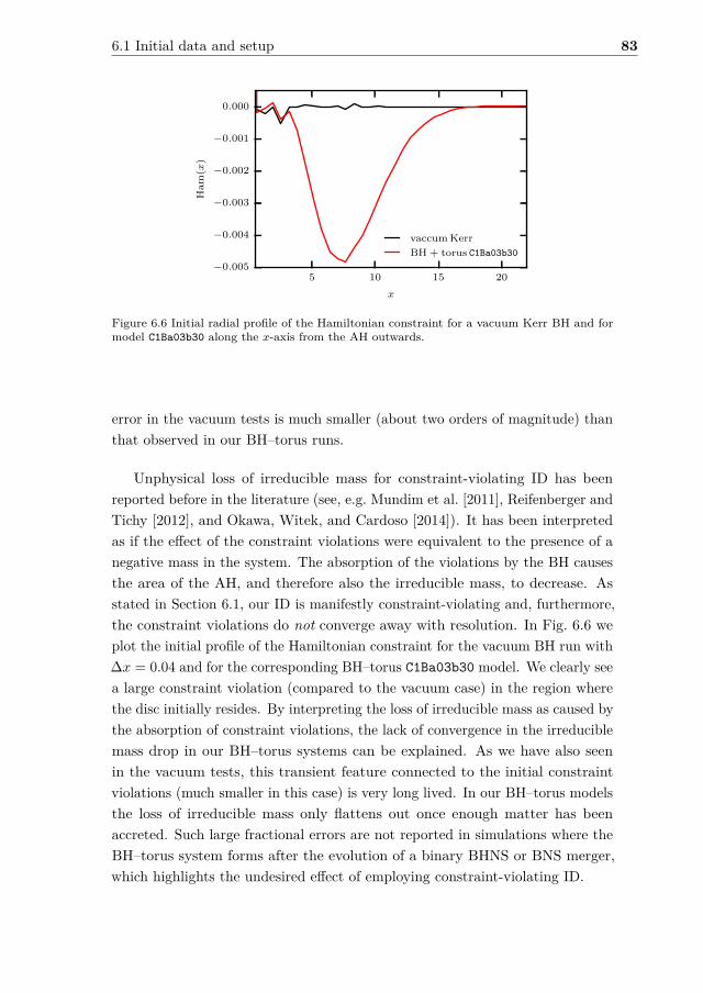
6.1 Initial data and setup 83
5 10 15 20
x
−0.005
−0.004
−0.003
−0.002
−0.001
0.000
Ham
(x)
vaccum Kerr
BH + torus C1Ba03b30
Figure 6.6 Initial radial profile of the Hamiltonian constraint for a vacuum Kerr BH and formodel C1Ba03b30 along the x-axis from the AH outwards.
error in the vacuum tests is much smaller (about two orders of magnitude) thanthat observed in our BH–torus runs.
Unphysical loss of irreducible mass for constraint-violating ID has beenreported before in the literature (see, e.g. Mundim et al. [2011], Reifenberger andTichy [2012], and Okawa, Witek, and Cardoso [2014]). It has been interpretedas if the effect of the constraint violations were equivalent to the presence of anegative mass in the system. The absorption of the violations by the BH causesthe area of the AH, and therefore also the irreducible mass, to decrease. Asstated in Section 6.1, our ID is manifestly constraint-violating and, furthermore,the constraint violations do not converge away with resolution. In Fig. 6.6 weplot the initial profile of the Hamiltonian constraint for the vacuum BH run with∆x = 0.04 and for the corresponding BH–torus C1Ba03b30 model. We clearly seea large constraint violation (compared to the vacuum case) in the region wherethe disc initially resides. By interpreting the loss of irreducible mass as caused bythe absorption of constraint violations, the lack of convergence in the irreduciblemass drop in our BH–torus systems can be explained. As we have also seenin the vacuum tests, this transient feature connected to the initial constraintviolations (much smaller in this case) is very long lived. In our BH–torus modelsthe loss of irreducible mass only flattens out once enough matter has beenaccreted. Such large fractional errors are not reported in simulations where theBH–torus system forms after the evolution of a binary BHNS or BNS merger,which highlights the undesired effect of employing constraint-violating ID.

84 NR simulations of tilted BH–torus systems
6.2 Results
6.2.1 Surface plots
We start describing the morphology and dynamics of a representative model ofour sample. The evolution of model C1Ba01b30 is shown in Fig. 6.7. This figuredisplays surface plots of the logarithm of the rest-mass density at six differentstages of the evolution. The final panel shows the morphology of the systemafter the disc has completed 20 orbits around the BH. The interpolation of theID from QI spherical polar coordinates to Cartesian coordinates, along withthe inclusion of a moderate BH spin in the originally non-rotating BH, resultsin a significant perturbation of the equilibrium model that triggers a phase ofoscillations of the torus around its equilibrium. These oscillations are presentthroughout the simulation and, as the disc is initially filling its Roche lobe, theyinduce a small accretion process of matter through the cusp towards the BH.This does not reduce significantly the total rest-mass of the torus as we showbelow. The oscillations are damped due to numerical viscosity and also by theformation of shocks developing in density waves that propagate inside the discand convert kinetic energy into thermal energy. These oscillations therefore onlytrigger nonphysical accretion during the very early times of the simulation. Theoutward-propagating shocks, also found in the simulations of Korobkin et al.[2011], are produced by in-falling material along the funnel walls which reachesinner high-density regions and bounces back. One such shock wave can be clearlyseen on the right portion of the disc in the 12 orbits panel of Fig. 6.7. The initialtilt of the BH spin (β0 = 30) twists and warps the innermost parts of the disccloser to the BH. This gradual effect becomes evident on the time series shownin Fig. 6.7 and by the final 20 orbits the disc is significantly misaligned with the(horizontal) y-axis.
In Fig. 6.8 we show surface plots of the rest-mass density for the modelsC1B, NC1 and D2 for the lower spin simulations (a = 0.1) at the final time of theevolution t/torb = 20. The effects of the initial BH tilt on the morphology ofthe disc at the final time are more clearly pronounced for the heavier modelsC1B (top row) and NC1 (middle row). Although the spin of the BH is verysmall and the spacetime is therefore nearly spherically symmetric, the initialtilt angle nevertheless causes a different evolution. In contrast, the significantlylighter model D2 is seen to be hardly affected by the initial tilt by the end of theevolution for these low spin simulations.
Similarly, in Fig. 6.9, we plot the same rest-mass density surface plots as inFig. 6.8 for all our models with higher initial spin. Comparing the evolution of

6.2 Results 85
Figure 6.7 Surface plots of the logarithm of the rest-mass density for model C1Ba01b30 atsix different snapshots of the evolution, t/torb = 0, 4, 8, 12, 16 and 20. The domain shown inall panels is 60 across the y-axis and 45 across the z-axis, which also indicates the upwarddirection in the plots. The surface of the disc is set at a density of 10−4ρc and half the discis removed for visualisation purposes. The BH lies at the cutting plane of each panel. Theevolution shows the development of two accretion streams on to the BH as the disc inclinationincreases during the evolution with respect to the initial equatorial plane.
the disc morphology with the lower initial spin figure, we see that there are nowsignificant changes in the morphology when increasing the initial tilt angle β0
for all models. The effects of evolving the disc in the tilted Kerr spacetime arenow more pronounced, as the higher spin causes a significant deviation fromspherical symmetry in the spacetime. In particular, the disc model D2 is now alsoclearly affected by the BH spin. As it represents the lightest disc in our study,its evolution is most similar to the evolutions observed in Fragile and Anninos[2005], which were performed using BHs of significantly higher spins than in the

86 NR simulations of tilted BH–torus systems
β = 5 β = 15 β = 30
C1Ba01
NC1a01
D2a01
Figure 6.8 Surface plots of the (normalised) rest-mass density at the final time of the evolutiont/torb = 20 for models C1B with a = 0.1 (top row), NC1 with a = 0.1 (middle row), and D2with a = 0.1 (bottom row). From left to right the columns correspond to initial tilt anglesβ0 = 5, 15, and 30, respectively. The domain shown in all panels is 20 across the y-axisand 15 across the z-axis, which also indicates the upward direction in the plots. The colorpalette and corresponding normalised density used are the same as in Fig. 6.7.
simulations presented here. Low mass discs therefore do exhibit twisting andwarping, but not at very low spins. The growth of non-axisymmetric modesassociated with the PPI (see below) in the two more massive models C1B andNC1 causes an alignment of the overall disc angular momentum vector with theBH spin. This interesting effect will be discussed in Section 6.2.6 below, wherewe comment on the BH precession and nutation properties.
In Figures 6.10 and 6.11 we plot linearly spaced isocontours and the loga-rithm of the rest-mass density in the plane perpendicular to the total angularmomentum vector of the disc. This kind of “equatorial” plots allows for a bettervisualisation of the possible growth of non-axisymmetric structures in the disc.We note that due to the twisting and warping of the disc as a result of theinitial BH tilt, the choice of the plane on to which project the isocontours for anadequate visualisation is not straightforward and careless choices (as e.g. thesimple choice of the equatorial xy-plane) may hide important pieces of informa-tion on the dynamics and morphology. The top row of Fig. 6.10 corresponds

6.2 Results 87
β = 5 β = 15 β = 30
C1Ba03
NC1a03
D2a05
Figure 6.9 Surface plots of the (normalised) rest-mass density at the final time of the evolutiont/torb = 20 for models C1B with a = 0.3 (top row), NC1 with a = 0.3 (middle row), and D2with a = 0.5 (bottom row). From left to right the columns correspond to initial tilt anglesβ0 = 5, 15, and 30, respectively. The domain shown in all panels is 20 across the y-axisand 15 across the z-axis, which also indicates the upward direction in the plots. The colorpalette and corresponding normalised density used are the same as in Fig. 6.7.
to models C1Ba01b5 (left), C1Ba01b15 (middle), and C1Ba01b30 (right), and allof them are displayed at the time at which the growth of the fastest growingnon-axisymmetric structure in the disc saturates (see Fig. 6.15 in Section 6.2.4below where we discuss the mode growth of the PPI for the different modelsof our sample). The middle row of Fig. 6.10 corresponds to models NC1a01b5(left), NC1a01b15 (middle), and NC1a01b30 (right), also shown at the time thefastest growing mode has maximum amplitude, while the bottom row showsmodels D2a01b5 (left), D2a01b15 (middle), and D2a01b30 (right), which aredisplayed at the final time of the evolution (t = 20torb) when the amplitudes ofthe corresponding PPI modes (if present) are largest. Correspondingly Fig. 6.11shows the same type of isocontour plots as Fig. 6.10 but for the models withhigher initial spin. The top row of Fig. 6.11 corresponds to models C1Ba03b5(left), C1Ba03b15 (middle), and C1Ba03b30 (right), the middle row of Fig. 6.10corresponds to models NC1a03b5 (left), NC1a03b15 (middle), and NC1a03b30(right) and the bottom row shows models D2a05b5 (left), D2a05b15 (middle),

88 NR simulations of tilted BH–torus systems
β = 5 β = 15 β = 30
C1Ba01
NC1a01
D2a01
Figure 6.10 Linearly spaced isocontours in plots showing the logarithm of the rest-mass densityin the plane perpendicular to the total angular momentum vector of the disc. From left toright the rows show models C1Ba01b5, C1Ba01b15 and C1Ba01b30 (top), NC1a01b5, NC1a01b15and NC1a01b30 (middle), and D2a01b5, D2a01b15, and D2a01b30 (bottom). The color paletteand corresponding normalised density used are the same as in Fig. 6.7. The morphologicalstructures shown in the different panels reflect the dominant PPI mode at the time of maximumnon-axisymmetric mode amplitude. See main text for further details.
and D2a05b30 (right). As in Fig. 6.10, the times shown are at either saturationof the fastest growing non-axisymmetric structure or when the maximum modeamplitudes are largest.
The inspection of the different panels displayed in Figs. 6.10 and 6.11 showsnoticeable differences in the flow morphology. On the one hand all six modelsC1B (top rows in both figures), corresponding to initial BH spins of a = 0.1 anda = 0.3, respectively, exhibit a very prominent spiral density wave once thestationary accretion phase is reached. This structure, which is visible for allthree tilt angles considered, β = 5, 15 and 30, is associated with the growth ofthe m = 1 non-axisymmetric PPI mode, which is the fastest-growing mode and

6.2 Results 89
β = 5 β = 15 β = 30
C1Ba03
NC1a03
D2a05
Figure 6.11 Linearly spaced isocontours in plots showing the logarithm of the rest-mass densityin the plane perpendicular to the total angular momentum vector of the disc. From left toright the rows show models C1Ba03b5, C1Ba03b15 and C1Ba03b30 (top), NC1a03b5, NC1a03b15and NC1a03b30 (middle), and D2a05b5, D2a05b15, and D2a05b30 (bottom). The color paletteand corresponding normalised density used are the same as in Fig. 6.7. The morphologicalstructures shown in the different panels reflect the dominant PPI mode at the time of maximumnon-axisymmetric mode amplitude. See main text for further details.
has the largest amplitude (see also Fig. 6.14). The middle rows, correspondingto the six models NC1, show the development of a spiral arm as well, however notas clearly pronounced as in the case of C1B. On the other hand the isodensitycontours of all three models D2 displayed in the bottom row of Fig. 6.10 fora BH spin a = 0.1 barely show any morphological deviation from the initialaxisymmetry. Only the innermost regions closest to the BH show some slightnon-axisymmetric structure, particularly for the model with the largest tilt angle(β = 30) shown on the right panel. The disc of model D2 is considerable lighterthan that of model C1B, and model NC1 has an initial non-constant specificangular momentum profile and according to Kiuchi et al. [2011] more massive
90 NR simulations of tilted BH–torus systems
tori with l = const profiles favour the appearance of the PPI with respect toless massive tori (see in particular Figs. 2 and 3(a) of Kiuchi et al. [2011] fortheir model C1 which has very similar properties regarding size and BH-to-discmass ratio to our model C1B). Our results seem to only partially confirm thoseprevious findings as there seems to be some weak dependence of a moderatem = 2 PPI growth with increasing tilt angles. A possible origin of the m = 2mode growth in these models might be connected to our Cartesian grid. However,the dependence of the growth on initial tilt angle seems to indicate that this isa physical effect. To gauge the effect of the Cartesian grid, one would have tocompare the disc evolutions of our models with new simulations performed inspherical grids.
The dependence on the BH spin seems however to be more significant forthe light model D2, as shown in the panels at the bottom row of Figures 6.10and 6.11. For the higher spin runs shown in Fig. 6.11, all three panels shownon-axisymmetric morphological features. All three snapshots correspond tothe same final time of the evolution (t = 20torb) and the dynamical differencesbetween the three models are only due to the initial BH tilt angle. For β = 5
(left panel) the m = 1 spiral structure is visible and dominant but, at the sametime, the m = 2 mode seems to have reached an almost similar amplitude (seethe bottom panel of Fig. 6.14). Such m = 2 feature becomes clearly dominantthe larger the BH inclination becomes, as depicted in the central regions of themiddle and right panels.
6.2.2 Maximum rest-mass density evolution
We next show the evolution of the maximum rest-mass density in the discs inFig. 6.12, normalised to the corresponding initial central density of each model(see Tables 6.1 and 6.2). For model D2 (bottom panel), the effect of tilting theBH has very little effect on the evolution of ρmax for a BH spin of a = 0.1.However, for a = 0.5, the evolution of ρmax differs for the different initial tiltangles. Model D2a05b5 exhibits an upward drift from 10 orbits onwards tobring ρmax to the level of the lower spin runs towards the end of the simulation.This might be connected to the growth of the m=1 non-axisymmetric modein this model, as discussed in the previous section. In the initial stages of theevolution, ρmax is higher for larger tilt angles, a dependence that is also observedin the accretion rate (see Section 6.2.3). The maximum rest-mass density staysbelow its initial value for almost the entire evolution for both models D2 andNC1 (middle panel). This is very different in model C1B (top panel) where the
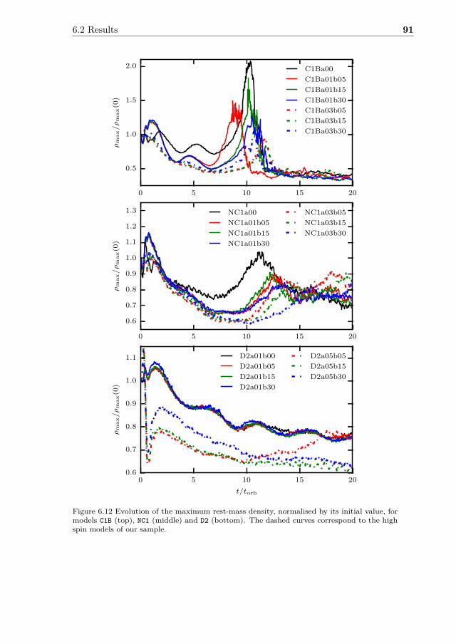
6.2 Results 91
0 5 10 15 20
t/torb
0.5
1.0
1.5
2.0
ρm
ax/ρ
max(0
)
C1Ba00
C1Ba01b05
C1Ba01b15
C1Ba01b30
C1Ba03b05
C1Ba03b15
C1Ba03b30
0 5 10 15 20
t/torb
0.6
0.7
0.8
0.9
1.0
1.1
1.2
1.3
ρm
ax/ρ
max(0
)
NC1a00
NC1a01b05
NC1a01b15
NC1a01b30
NC1a03b05
NC1a03b15
NC1a03b30
0 5 10 15 20
t/torb
0.6
0.7
0.8
0.9
1.0
1.1
ρm
ax/ρ
max(0
)
D2a01b00
D2a01b05
D2a01b15
D2a01b30
D2a05b05
D2a05b15
D2a05b30
Figure 6.12 Evolution of the maximum rest-mass density, normalised by its initial value, formodels C1B (top), NC1 (middle) and D2 (bottom). The dashed curves correspond to the highspin models of our sample.

92 NR simulations of tilted BH–torus systems
occurrence and saturation of the PPI has a drastic effect on the evolution ofρmax. When the PPI starts growing, a situation which is accompanied by anexponential growth of the accretion rate, ρmax grows to up to twice its initialvalue, reaching the highest value for the untilted model C1Ba00. It subsequentlysettles to a value that is very similar for all initial spins and tilt angles, butthe time of growth and the shape of the “lump” in the density evolution aredifferent for the different spins and initial tilt angles. Model NC1 shows featuresfrom both models D2 and C1B described above. Similarly to model D2, ρmax
stays below its initial value for almost the entire evolution, with model NC1a00being an exception where it grows above the initial value briefly. There is, as inmodels C1B, a rapid growth in the central density, albeit somewhat smaller forthe non-constant angular momentum discs, associated with the growth of thePPI in all the models. The magnitudes at which the mode growth saturates aresimilar, while the time at which the growth sets in depends on the initial spinand tilt angle.
6.2.3 Evolution of the accretion rate
Fig. 6.13 shows the time evolution of the mass accretion rate for all models ofour sample, in units of M⊙/s. The colours used for the different models as wellas the line style follow the same convention as in the rest-mass density evolutionfigure (Fig. 6.12). The top panel displays the mass flux for models C1B, themiddle panel for models NC1, and the bottom panel for models D2. The massflux is computed as the instantaneous flux of matter across the AH surface whichis parameterised in spherical coordinates by the polar angle θ and azimuthalangle ϕ and is given by:
M = 2πr2∫ 2π
0
∫ π
0Dvr sin θ dϕ dθ , (6.12)
where r is the radius of the AH and vr is the radial velocity of the fluid crossingthe sphere. In the actual implementation in the Outflow thorn, the relevantquantities are interpolated onto the respective spherical surface (the AH in ourcase) and the integration is performed as a two dimensional surface integral inspherical coordinates (see the thorn documentation at the Einstein Toolkit[n.d.] website for details). All three panels of Fig. 6.13 show that after a transientinitial phase the mass accretion rate is seen to tend asymptotically to a fairlyconstant value.
In the previous fixed spacetime simulations of Fragile and Anninos [2005] itwas found that the tilt and the twist of the discs are not strongly responsive to M .

6.2 Results 93
0 5 10 15 20
t/torb
10−4
10−3
10−2
10−1
100
101
102
M[M/s]
C1Ba00
C1Ba01b05
C1Ba01b15
C1Ba01b30
C1Ba03b05
C1Ba03b15
C1Ba03b30
0 5 10 15 20
t/torb
10−4
10−3
10−2
10−1
100
101
M[M/s]
NC1a00
NC1a01b05
NC1a01b15
NC1a01b30
NC1a03b05
NC1a03b15
NC1a03b30
0 5 10 15 20
t/torb
10−4
10−3
10−2
10−1
100
M[M/s]
D2a01b00
D2a01b05
D2a01b15
D2a01b30
D2a05b05
D2a05b15
D2a05b30
Figure 6.13 Evolution of the accretion rate in M⊙/s for models C1B (top), NC1 (middle) andD2 (bottom).
Our results for a dynamical spacetime validate those earlier findings, as the finaldispersion found in M once this quantity reaches steady-state values is relatively

94 NR simulations of tilted BH–torus systems
small irrespective of the BH spin and inclination angles (M [M⊙/s] ∈ [0.2, 1.5]for models C1B and NC1, and [0.06, 0.2] for model D2). However, the transitionto the steady-state does seem to show a clear dependence on the BH spin. Wefind that the initial M values are consistently smaller the larger the BH spin,about 2 orders of magnitude for models D2 after ∼1 orbit and about half thatvalue for the more massive discs C1B and NC1. Another trend, which is mostclearly seen in model D2, is the initial dependence of the accretion rate on thetilt angle as well. We find that the higher the initial tilt angle, the higher theaccretion rate in the early stages of the evolution. This is because the innermoststable circular orbit (ISCO) of a rotating Kerr BH has an ellipsoidal shape,attaining the smallest size at the equatorial plane of the BH. For progradeorbits such as those considered in our work, the specific angular momentum atthe ISCO decreases with higher BH spin. Matter is accreted when its specificangular momentum is lower than that at the ISCO, which means that higherBH spins present larger centrifugal barriers for the matter to be accreted. Forinclined orbits, the specific angular momentum at the respective ISCO for agiven inclination angle increases with larger inclination (up to its maximumvalue at the pole of the BH) and the accretion rate becomes therefore higher forlarger inclinations. While the transition stage is physically not relevant (as realpost-merger discs would not show such an episode) it is nevertheless reassuringthat we observe the correct physics during the transition.
A common feature present in the mass-flux plots of the simulations of Fragileand Anninos [2005] was a late-time “bump” which the authors attributed tothe reflection of an outgoing wave within the disc at the outer edge. Thatfeature does not seem to be so apparent in our models apart from maybe modelC1B which shows a bump around t ∼ 10torb somewhat similar to that reportedby Fragile and Anninos [2005]. However, in our interpretation, the phase ofrapid growth in M in less than about 5 orbits seems to have a different origin.This conclusion is reached by comparing the time at which the growth of thePPI saturates (discussed in Figs. 6.14 and 6.15 in the following section) with thesaturation time of the accretion rate for model C1B, which yields a significantclose agreement. We note that this peak in the accretion rate is the highestof all our models, ∼ 30M⊙/s, lasting for less than about 1 ms. Therefore, weidentify the exponential growth and subsequent saturation of the mass accretionrate with the growth and saturation of the PPI in our models.
The total rest mass accreted during the evolution ranges within Macc ∈[0.022, 0.033], [0.005, 0.013] and [0.0006, 0.002] for models C1B, NC1 and D2,respectively. The accretion is facilitated by the outward transport of angular

6.2 Results 95
momentum, which we describe in section 6.2.8 below. The growth of the PPI, towhich we attribute the high peak accretion rates, is very effective in transportingangular momentum outwards. While we have performed our study withoutconsidering magnetic fields, it is known that magnetic fields are very effective attransporting angular momentum in accretion discs [Balbus and Hawley 1991],via the development of the MRI [Velikhov 1959, Chandrasekhar 1960]. Nottaking into account the effects of magnetic fields in accretion discs seems tounderestimate the accretion rate [Gold et al. 2014], see also recent GRMHDsimulations of BHNS mergers in Paschalidis, Ruiz, and Shapiro [2015] and Kiuchiet al. [2015b] and the accretion rates reported therein. The accretion rates weobserve are well above the Eddington limit and in a range compatible with thatneeded to power GRBs [Popham, Woosley, and Fryer 1999].
6.2.4 PPI growth in the disc and BH motion
In their seminal paper on the PPI, Papaloizou and Pringle [1984] showed thatvertically thick, radially slender tori with constant specific angular momentumprofiles are unstable against the development of global non-axisymmetric modes.Two of our models, C1B and D2, have constant specific angular momentum profiles,while model NC1 has a radial dependence of l ∼ Rq, where q = 0.11. Zurek andBenz [1986] showed that tori with non-constant angular momentum profilesmight become PP-unstable as well. In order to check for the onset and thegrowth of non-axisymmetric instabilities, we monitor the mode amplitudescomputed using Eq. (4.28), which is basically a Fourier decomposition of theazimuthal distribution of the density in the disc [Zurek and Benz 1986]. Insimulations of accretion tori susceptible to the development of the PPI performedon spherical grids, it is customary to induce the instability with small initialnon-axisymmetric density or velocity perturbations. Any non-axisymmetricperturbation will trigger the growth of the instability provided the torus is notstable against it. We do not actively seed the PPI in any of our models. Instead,there are two main sources of perturbations in our simulations, both connected tothe fact that we evolve the BH-disc system in a Cartesian grid. First, the exactaxisymmetry of the ID is lost when we interpolate the ID onto the Cartesiangrid of the evolution, introducing small, non-axisymmetric perturbations inall interpolated quantities. This is due to the fact that in Cartesian gridsneighbouring cells lie on concentric shells only in the limit of infinite resolution.The second source of perturbation is the so-called junk-radiation leaving theBH while the gauge evolves from the values specified by the ID to the puncture

96 NR simulations of tilted BH–torus systems
0 5 10 15 20
t/torb
10−9
10−8
10−7
10−6
10−5
10−4
10−3
10−2
10−1
100
Dm/D
0
m = 1
m = 2
m = 3
m = 40 5 10 15 20
10−5
10−4
10−3
10−2
10−1
100
ρBH
m = 1
0 5 10 15 20
t/torb
10−9
10−8
10−7
10−6
10−5
10−4
10−3
10−2
10−1
100
Dm/D
0
m = 1
m = 2
m = 3
m = 40 5 10 15 20
10−5
10−4
10−3
10−2
10−1
100
ρBH
m = 1
0 5 10 15 20
t/torb
10−9
10−8
10−7
10−6
10−5
10−4
10−3
10−2
10−1
Dm/D
0
m = 1
m = 2
m = 3
m = 40 5 10 15 20
10−5
10−4
10−3
10−2
10−1
100
ρBH
m = 1
Figure 6.14 Evolution of the first four non-axisymmetric (PPI) modes scaled by the total rest-mass density (D0) for models C1Ba01b30 (top), NC1a01b30 (middle) and D2a01b30 (bottom).The inset shows the evolution of the m = 1 mode and the polar distance of the centre of theBH from the origin, both having been rescaled with their respective maximum values attainedduring the evolution.

6.2 Results 97
gauge attained during the evolution. Here, we need to distinguish betweenmodels evolved around Schwarzschild BHs and the models evolved around tiltedKerr BHs. For the former, the junk-radiation leaving the BH initially should beaxisymmetric. Indeed, when analysing this initial burst of radiation with theWeyl scalar Ψ4, we find that the amplitudes of the Ψl,0
4 multipoles (which areaxisymmetric) are the largest. Nevertheless, the initial junk-radiation has alsonon-vanishing amplitudes in the other Ψl,m
4 multipoles. Again, the reason forthe presence of these non-axisymmetric Ψl,m
4 multipoles seems to be connectedto the evolution in the Cartesian grid, and specifically to the existence of meshrefinement boundaries, which are not axisymmetric even in the continuum limit(see Zlochower, Ponce, and Lousto [2012] for interference patterns producedby the radiation crossing mesh refinement boundaries). Finally, in the case ofthe disc being around a tilted Kerr BH, the junk-radiation reaching the disc isnow truly non-axisymmetric even without taking into account the effects of theCartesian grid and the mesh refinement boundaries, as the axis of rotation istilted with respect to the z = 0 plane.
We show in Fig. 6.14 the evolution of the amplitude of the first four non-axisymmetric modes Dm (m = 1 − 4) in the disc for models C1Ba01b30 (top),NC1a01b30 (middle) and D2a01b30 (bottom). Those amplitudes are computedusing Eq. (4.28). In addition, in the inset of all three plots we also show as ablack solid curve the evolution of the polar distance of the centre of the BHfrom the origin of the computational grid, which we label ρBH. We note thatthe m = 4 mode is dominant in the very early stages of the evolution for allmodels. This is due to the Cartesian grid. At the later stages, the (physical)m = 1 and m = 2 (for models D2) become dominant, as expected.
Model C1Ba01b30 is the one that most clearly is found to develop the PPI,as signalled by the exponential growth of the m = 1 mode. Modes m = 2 − 4also show a phase of exponential growth lasting for about 2 orbital periods(between t ∼ 8 − 10 torb) but the saturation amplitudes reached are 1 to 2 ordersof magnitude smaller than for m = 1. As mentioned in the previous section,the growth of the PPI is accompanied by an exponential growth of the massaccretion rate (see Fig. 6.13). For this model the PPI clearly saturates at aroundt ∼ 10 torb, when the amplitude of the m = 1 mode quickly drops by an order ofmagnitude. After that, the amplitude of all the modes we have analysed remainsrather constant. The strength of the m = 2 − 4 modes becomes similar at latetimes while the m = 1 mode still retains a significantly larger amplitude.
The polar distance of the BH from the origin for model C1Ba01b30 closelyfollows the behaviour of the m = 1 fastest growing PPI mode. This distance is

98 NR simulations of tilted BH–torus systems
found to grow at the same actual rate as the m = 1 mode, because the circularmotion of the m = 1 over-density hump (well visible in the top-rightmost panelof Fig. 6.10) causes the BH to start moving in a spiral trajectory. After modesaturation the polar distance of the BH from the origin remains almost constant,reflecting a similar trend in the m = 1 evolution. This spiral motion of theBH as a result of the development of the PPI has also been observed in thesimulations of Korobkin et al. [2011].
For the non-constant angular momentum model NC1a01b30 (middle panel)the growth rate of the m = 1 mode is smaller, although it is still the dominantmode, as in model C1Ba01b30. The growth of the mode saturates somewhatlater at around t ∼ 12.5 torb but, contrary to the evolution of C1Ba01b30, itdoes not drop significantly after saturation, remaining fairly constant thereafter.Furthermore, it remains the dominant mode at late times while the threeremaining modes attain similar amplitudes. The evolution of the polar distanceof the BH from the origin shows a small secular drift after the saturation of thePPI.
On the other hand, model D2a01b30 (bottom panel) shows a very distinctbehaviour. The amplitude of all four modes and the polar distance of the BHremain below the values attained in models C1Ba01b30 and NC1a01b30, typicallyin the range between 1 to 2 orders of magnitude. Furthermore, the m = 1 andm = 2 modes grow at approximately the same rate and to similar final valuesduring the evolution. The growth rate of ρBH is very similar to the growth rateof the modes m = 1 and m = 2. We also note that at early times the m = 4mode shows the largest amplitude (purple line; not so clearly noticeable in theprevious two models), perhaps an artefact of the Cartesian grid we use in oursimulations. Nevertheless, the amplitude of this mode at late times is sufficientlysmaller than the dominant amplitudes (mostly that of the m = 1 mode) tosafely consider its effect on the dynamics negligible. From the mode analysis,we can therefore say that model D2 is essentially PP-stable. We will return tothis point in section 6.2.8, where we analyse the angular momentum transportin the models.
The results we have just described connect the exponential growth andsaturation of the mass accretion rate with the growth and saturation of the PPIin the models where it has unambiguously taken place. To further justify this,we plot in Fig. 6.15 the evolution of the m = 1 mode for all models consideredin our sample. Focusing on the evolution of the models C1B displayed in thisfigure (top panel) we can clearly see that the temporal order of the saturationof the mode growth closely coincides with the various peaks present in the mass

6.2 Results 99
0 5 10 15 20
t/torb
10−6
10−5
10−4
10−3
10−2
10−1
100
D1/m
ax(D
1)C
1B
a00
C1Ba00
C1Ba01b05
C1Ba01b15
C1Ba01b30
C1Ba03b05
C1Ba03b15
C1Ba03b30
0 5 10 15 20
t/torb
10−6
10−5
10−4
10−3
10−2
10−1
100
D1/m
ax(D
1)N
C1a00
NC1a00
NC1a01b05
NC1a01b15
NC1a01b30
NC1a03b05
NC1a03b15
NC1a03b30
0 5 10 15 20
t/torb
10−5
10−4
10−3
10−2
10−1
100
101
D1/m
ax(D
1)D
2a01b00
D2a01b00
D2a01b05
D2a01b15
D2a01b30
D2a05b05
D2a05b15
D2a05b30
Figure 6.15 Evolution of the non-axisymmetric m = 1 mode for all models, namely C1B (top),NC1 (middle) and D2 (bottom), rescaled to the maximum amplitude of the D1 mode of therespective untilted models.
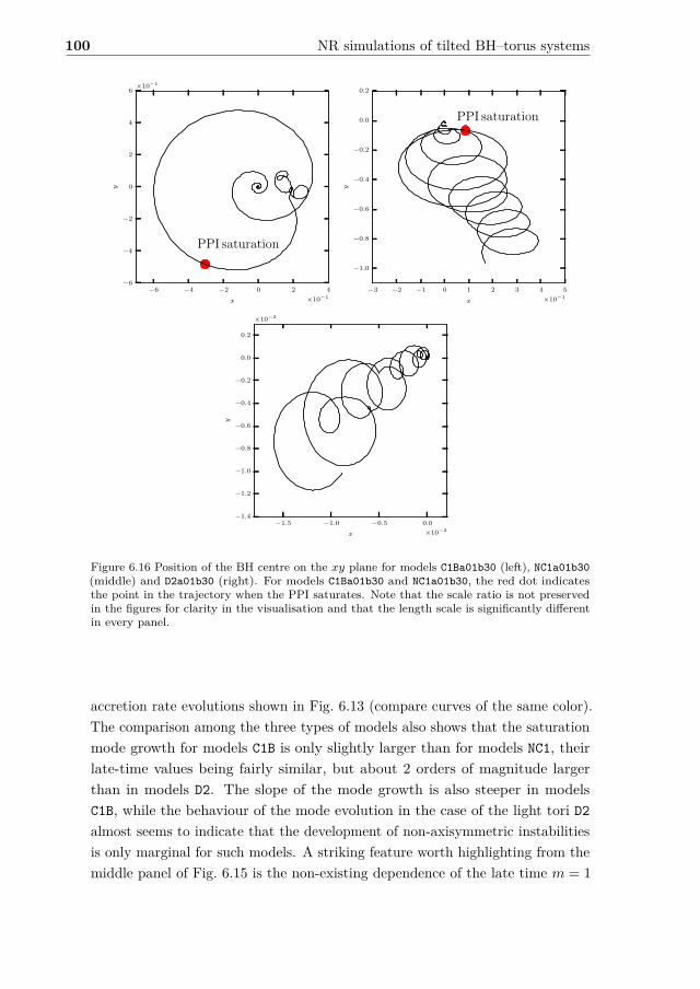
100 NR simulations of tilted BH–torus systems
−6 −4 −2 0 2 4
x ×10−1
−6
−4
−2
0
2
4
6
y
×10−1
PPI saturation
−3 −2 −1 0 1 2 3 4 5
x ×10−1
−1.0
−0.8
−0.6
−0.4
−0.2
0.0
0.2
y
PPI saturation
−1.5 −1.0 −0.5 0.0
x ×10−2
−1.4
−1.2
−1.0
−0.8
−0.6
−0.4
−0.2
0.0
0.2
y
×10−2
Figure 6.16 Position of the BH centre on the xy plane for models C1Ba01b30 (left), NC1a01b30(middle) and D2a01b30 (right). For models C1Ba01b30 and NC1a01b30, the red dot indicatesthe point in the trajectory when the PPI saturates. Note that the scale ratio is not preservedin the figures for clarity in the visualisation and that the length scale is significantly differentin every panel.
accretion rate evolutions shown in Fig. 6.13 (compare curves of the same color).The comparison among the three types of models also shows that the saturationmode growth for models C1B is only slightly larger than for models NC1, theirlate-time values being fairly similar, but about 2 orders of magnitude largerthan in models D2. The slope of the mode growth is also steeper in modelsC1B, while the behaviour of the mode evolution in the case of the light tori D2almost seems to indicate that the development of non-axisymmetric instabilitiesis only marginal for such models. A striking feature worth highlighting from themiddle panel of Fig. 6.15 is the non-existing dependence of the late time m = 1

6.2 Results 101
mode amplitude on the BH spin and tilt angle for the non-constant angularmomentum tori NC1.
To demonstrate the connection between the growth of non-axisymmetricmodes in the disc with the motion of the BH, we plot in Fig. 6.16 the position ofthe BH centre on the xy plane for models C1Ba01b30 (top), NC1a01b30 (middle)and D2a01b30 (bottom). This figure shows several interesting features connectedto the growth of the modes in the tori. The motion of the BH is caused by theformation of a “quasi-binary system” between the BH and the m = 1 over-densitylump, which was also observed in Korobkin et al. [2011]. Note that the motion ofthe BH is well within the initial inner disc radius (see Table 6.1). It is the binarymotion that causes the long-term emission of GWs reported in Kiuchi et al. [2011].We will return to this in the discussion of the GW emission connected to the PPIin section 6.2.9. For model C1Ba01b30, the development of the dominant m = 1structure in the disc exerts a small kick in the BH. As a result the BH startsmoving in a spiral trajectory until the PPI saturates and the mode amplitudedrops, at which point the BH is roughly located at (x, y) = (−0.3,−0.5). Aftersaturation, the xy position of the BH is a combination of linear and circularmotion. In model NC1a01b30, the linear motion is stronger from the beginning,causing a linear shift in the growing spiral motion. Upon saturation of thePPI, the circular motion continues with a smaller radius, in accordance to theevolution of the m = 1 mode which remains at a rather f value after saturationand up until the end of the evolution. Finally, for model D2a01b30 we havea superposition of circular and linear motion again, as the modes m = 1 andm = 2 are of almost equal magnitude during the evolution. Here, the overalldistance covered by the BH is significantly smaller than for the heavier modelsC1Ba01b30 and NC1a01b30, as the mode amplitudes are much smaller for D2and the disc is also lighter. From our simulations, we see that more massivediscs favour the development of the PPI. This might be in connection withthe enhanced m = 1 mode strength due to the motion of the BH describedabove. We will investigate the effect of the BH motion on the mode growthrate and maximum amplitude in more detail in Chapter 7. The strength ofthe m = 1 mode growth will affect almost every diagnostic that we investigatein the subsequent sections. The growth of the PPI has therefore far reachingconsequences on the disc evolutions.
We argue that the non-axisymmetric instability we observe in our modelsis indeed the PPI based on the azimuthal mode evolution in the disc and thedevelopment of the m = 1 over-density lump. However, we do not claim tohave presented a direct, undeniable proof that the instability observed in our

102 NR simulations of tilted BH–torus systems
Figure 6.17 Full 3D trajectory of the BH along with its spin vectors for model C1Ba01b30. Thecurved arrow indicates the direction of the BH’s motion. The magnitude of the spin vectorshas been rescaled with a constant factor for visualisation purposes.
simulations is the analytical PPI studied in Papaloizou and Pringle [1984].To do so, we should have compared the predicted growth rates of the PPIfor our models in the linear regime to those observed in our simulations, andshould have checked for the occurrence of the so-called non-axisymmetric I-modes(see Christodoulou and Narayan [1992] and Korobkin et al. [2011]) during the discevolution. We also note that there exist other instabilities in self-gravitating discswhich display spiral arm formation in the disc or even disc fragmentation, such asthe axisymmetric local Toomre instability (a gravitational instability) [Toomre1964]. Although Christodoulou and Narayan [1992] have shown that the Toomreinstability is unlikely to affect radially slender accretion tori such as the onesconsidered in our study, we will analyse the gravitational stability of our discsin the following. A disc will be gravitationally unstable if the so-called Toomreparameter Q becomes less that unity, where Q is defined as
Q ≡ κcs
πΣ , (6.13)
where κ is the epicyclic frequency, cs the local sound speed in the disc, and Σthe surface density of the disc. For thick accretion tori, this measure of thedisc stability against its self-gravity might not be adequate. Hachisu, Tohline,and Eriguchi [1987] derived a different criterion for gravitational stability, validfor both thick and thin discs, κ2/(πρ) < 1. As outlined in Christodoulouand Narayan [1992], we should choose Ω0 (the orbital velocity at the pressuremaximum) as the epicyclic frequency κ, and not the usual definition (κ2 ≡(1/r3)dl2/dr), as we are interested in the development of non-axisymmetric

6.2 Results 103
modes. Defining the Jeans (gravitational) angular velocity at the pressuremaximum as Ω2
J ≡ 4πρ, Christodoulou and Narayan [1992] showed that the discis gravitationally stable if ΩJ/Ω0 ≲ 2.4. Using Ω0 as the epicyclic frequency,the stability criterion of Hachisu, Tohline, and Eriguchi [1987] corresponds toΩJ/Ω0 < 2. Evaluating ΩJ/Ω0 for our initial models, we find the following values:ΩJ/Ω0 = 0.274, 0.681, and 0.561 for disc models D2, C1B and NC1, respectively.We therefore conclude that out initial models are stable against their self-gravity.The discs remain gravitationally stable during the duration of the simulations,as we have not seen any evidence for gravitational fragmentation.
6.2.5 PPI saturation and BH kick
The complete 3D trajectory of the BH and its spin vector is plotted for modelC1Ba01b30 in Fig. 6.17. In this plot each small sphere with an attached arrowcorresponds to the position of the BH and the magnitude (scaled for bettervisualisation) and direction of its spin vector. The positions are plotted at equaltime intervals, so we see that the BH is moving much faster during the finalstages of the PPI than before its occurrence or after its saturation. We can alsosee that there is a motion in the vertical direction, which is caused by the factthat the “binary” motion of the BH and m = 1 over-density lump does not lie inthe equatorial plane anymore due to the initial tilt. While the PPI is growing,the BH–torus system therefore moves up and down in an oscillatory fashion.As we have seen in the m = 1 mode plots for models C1B (see the top panel ofFig. 6.15), the saturation of the PPI is very fast. The rapid saturation of the PPI(and the corresponding destruction of the m = 1 over-density lump) result in amild vertical kick of the BH+torus system. To see that this is indeed connectedto the saturation of the PPI, we plot in Fig. 6.18 the linear momentum radiatedaway by gravitational waves in the z-direction for models C1Ba01. From theplot, we can clearly see that the time of maximum emission of linear momentumcorresponds exactly to the time the PPI saturates for each model. The radiatedlinear momentum has been calculated with the pyGWAnalysis package of theET [Reisswig and Pollney 2011].
6.2.6 BH precession and nutation
Contrary to the test-fluid simulations of Fragile and Anninos [2005] and Fragileet al. [2007], as we are evolving the full spacetime, we can monitor the responseof the BH to the evolution of the disc in the initially tilted configuration. Inparticular we can measure the total precession of the BH spin about the z-axis

104 NR simulations of tilted BH–torus systems
2 4 6 8 10 12 14 16
(t− rdet)/torb
−6
−5
−4
−3
−2
−1
0
1
2
Pz
×10−20
C1Ba01b05
C1Ba01b15
C1Ba01b30
Figure 6.18 Radiated linear momentum in the z-direction for models C1Ba01.
(σBH = ∠(y − axis,Sxy)) and its rate, as well as the inclination of the spin withrespect to the z-axis νBH = ∠(z − axis,SBH) and the corresponding nutation.
In Fig. 6.19 we plot the evolution of the precession rate σBH of the BHabout the z-axis for models C1B (top), NC1 (middle) and D2 (bottom panel)in radians per orbital period. The first thing to mention is that the constantangular momentum discs D2 and C1B show a clear dependence of the precessionrate with the initial BH spin magnitude. Namely, for models D2 and C1B, thelarger the spin the smaller the precession rate. However, for the non-constantangular momentum torus NC1 the precession rate is very similar irrespective ofthe spin magnitude, particularly at the early stages (t < 10 torb). In modelsD2 the evolution of σBH is very smooth, and changes sign for the higher spinruns after about 17 orbits, whereas it remains fairly constant for the lower spinsimulations.
A fact worth emphasising is that there is essentially no dependence of theprecession rate on the tilt angle for constant angular momentum tori. This isparticularly true for models D2 but also models C1B show this lack of dependenceup until the growth of the PPI. In all models C1B we observe a prominentmodulation of the precession rate when the PPI enters the final stages of itsgrowth and then saturates, as well as the change in sign for the higher spin runs.The magnitude of the precession rate is about an order of magnitude highercompared to models D2, which we attribute to the higher disc-to-BH mass ratiomodels C1B possess. The evolution of the BH precession rate for models NC1seems to fit in between the two other models. The magnitude of the precessionrate is similar for the two BH spins considered in models NC1. We also note from

6.2 Results 105
5 10 15 20
t/torb
−0.2
−0.1
0.0
0.1
0.2
0.3
σB
H[r
adia
ns/t o
rb]
C1Ba01b05
C1Ba01b15
C1Ba01b30
C1Ba03b05
C1Ba03b15
C1Ba03b30
5 10 15 20
t/torb
0.03
0.04
0.05
0.06
0.07
0.08
0.09
0.10
0.11
0.12
σB
H[r
adia
ns/t o
rb]
NC1a01b05
NC1a01b15
NC1a01b30
NC1a03b05
NC1a03b15
NC1a03b30
5 10 15 20
t/torb
−0.02
−0.01
0.00
0.01
0.02
0.03
0.04
0.05
0.06
σB
H[r
adia
ns/t o
rb]
D2a01b05
D2a01b15
D2a01b30
D2a05b05
D2a05b15
D2a05b30
Figure 6.19 Evolution of the precession rate of the BH spin about the z-axis for models C1B(top), NC1 (middle) and D2 (bottom) in units of radians/torb.
Fig. 6.19 that models C1Ba01 and D2a01 attain a fairly constant precession rateby the end of our simulations, namely ∼ 20 Hz and ∼ 6 Hz for models C1Ba01

106 NR simulations of tilted BH–torus systems
5 10 15 20
t/torb
0.0
0.5
1.0
1.5
2.0
σB
H[r
adia
ns]
C1Ba01b05
C1Ba01b15
C1Ba01b30
C1Ba03b05
C1Ba03b15
C1Ba03b30
5 10 15 20
t/torb
0.0
0.2
0.4
0.6
0.8
1.0
1.2
σB
H[r
adia
ns]
NC1a01b05
NC1a01b15
NC1a01b30
NC1a03b05
NC1a03b15
NC1a03b30
5 10 15 20
t/torb
0.0
0.1
0.2
0.3
0.4
0.5
0.6
σB
H[r
adia
ns]
D2a01b05
D2a01b15
D2a01b30
D2a05b05
D2a05b15
D2a05b30
Figure 6.20 Total precession of the BH spin about the z-axis for models C1B (top), NC1 (middle)and D2 (bottom) in units of radians.
and D2a01, respectively. These are the frequencies for the BH masses indicatedin Table 6.1.

6.2 Results 107
5 10 15 20
t/torb
−0.10
−0.05
0.00
0.05
νB
H[r
adia
ns/t o
rb]
C1Ba01b05
C1Ba01b15
C1Ba01b30
C1Ba03b05
C1Ba03b15
C1Ba03b30
5 10 15 20
t/torb
−0.030
−0.025
−0.020
−0.015
−0.010
−0.005
0.000
0.005
0.010
0.015
νB
H[r
adia
ns/t o
rb]
NC1a01b05
NC1a01b15
NC1a01b30
NC1a03b05
NC1a03b15
NC1a03b30
5 10 15 20
t/torb
−0.010
−0.005
0.000
0.005
0.010
νB
H[r
adia
ns/t o
rb]
D2a01b05
D2a01b15
D2a01b30
D2a05b05
D2a05b15
D2a05b30
Figure 6.21 Evolution of the nutation rate of the BH spin about the z-axis for models C1B(top), NC1 (middle) and D2 (bottom) in units of radians/torb.
The total precession of the BH spin about the z-axis is shown in Fig. 6.20.The lower spin models C1Ba01, that show the highest BH precession rate, have

108 NR simulations of tilted BH–torus systems
completed a quarter of a full precession cycle by the end of our simulations att = 20torb. Given that the precession rate for those models appears to settle toa rather constant value (see Fig. 6.19) we would need a prohibitively expensiveevolution of about 80 orbital periods for a full precession cycle of the BH forthose models. If we assume that the precessing Kerr BH radiates GW as a freelyprecessing rigid body, it will radiate at σBH and 2 σBH in the l = 2, m = 1, 2multipole modes [Zimmermann and Szedenits 1979]. This means we would haveto evolve the BH–torus system for at least one full BH precession cycle in orderto see the slow modulation of the GW signal caused by the BH precession. Itremains an interesting open issue to see if the upcoming advanced GW detectorswill be able to measure these GWs in the low tens of Hz.
The imprint of the growth of non-axisymmetric instabilities in the disc onthe BH response can be seen even clearer in Fig. 6.21. This figure shows theevolution of the nutation rate for all models, that is, the evolution of the temporalvariation of the tilt angle of the BH with the z-axis, νBH. For models C1B (toppanel) there is a clear period of alignment of the BH spin with the z-axis aroundthe time when the PPI starts to grow. This is signalled by the rapid fall and riseof the nutation rate around the 10 torb mark for the slow spin (a = 0.1) BHs, butit is also (less) visible in the more rapidly rotating BHs (dashed lines). Uponsaturation of the instability the nutation rate becomes almost constant andfairly close to being again zero for the a = 0.1 BH models (see solid lines). Thisbehaviour is consistent with the evolution of the BH tilt angle itself displayed inFig. 6.22, which, for the case of models C1B with small spins, shows two distinctzones of constant spin inclination, particularly for models with β0 = 5 and 15
(model with β0 = 30 still shows a negative slope at late times). The transitionto zero nutation rate in the a = 0.3 C1B models after PPI saturation seems totake a longer time than that displayed in Fig. 6.21.
In addition Fig. 6.21 also shows that the maximum nutation rate attainedincreases with increasing initial tilt angle. This is very clearly seen in models C1Bbut it is also visible in most of the models D2 and NC1. In particular the evolutionof νBH for the non-constant angular momentum models NC1 with a = 0.3 (dashedcurves) does not seem to reach a local maximum, at least during the timescaleswe can afford to simulate. This is despite these models are also affected by thePPI. This might be explained by the fact that the non-axisymmetric m = 1mode does not drop as sharply after the saturation of the PPI in the modelsNC1 as it does in the C1B models (see Fig. 6.15). The growth of the mode in thedisc seems to cause an alignment of the BH spin with the z-axis. Furthermore,the nutation rate is much larger for the C1B models. Finally, in the absence of

6.2 Results 109
5 10 15 20
t/torb
0.0
0.1
0.2
0.3
0.4
0.5
0.6
0.7
νB
H[r
adia
ns]
C1Ba01b05
C1Ba01b15
C1Ba01b30
C1Ba03b05
C1Ba03b15
C1Ba03b30
5 10 15 20
t/torb
0.0
0.1
0.2
0.3
0.4
0.5
0.6
0.7
0.8
νB
H[r
adia
ns]
NC1a01b05
NC1a01b15
NC1a01b30
NC1a03b05
NC1a03b15
NC1a03b30
0 5 10 15 20
t/torb
0.0
0.1
0.2
0.3
0.4
0.5
0.6
0.7
νB
H[r
adia
ns]
D2a01b05
D2a01b15
D2a01b30
D2a05b05
D2a05b15
D2a05b30
Figure 6.22 Evolution of the tilt angle of the BH spin with respect to the z-axis for modelsC1B (top), NC1 (middle) and D2 (bottom) in units of radians.
any strong growth of PPI modes, models D2 do not show strong modulation of

110 NR simulations of tilted BH–torus systems
the nutation rate, which is therefore closely connected to the existence of m = 1non-axisymmetric modes in the disc.
The corresponding evolution of the inclination of the BH spin away from thez-axis is seen in Fig. 6.22. The panels show that a significant realignment ofthe BH spin with the z-axis takes place by the end of the simulations in modelsC1B, i.e. in those models that develop the PPI most significantly. For all modelswe see that the final inclination is smaller the bigger the initial tilt angle is, forequal spin magnitudes. This trend also seems to be more pronounced the higherthe initial spin magnitude is.
6.2.7 Disc twist and tilt
We turn now to describe in this section the response of the discs as they evolvein the tilted spacetime, using the diagnostics we have introduced in Section 4.4.In Figures 6.23 and 6.24, we plot the evolution of the tilt and precession of thetotal angular momentum vector of the disc JDisc. This vector is the sum of theangular momentum vectors of each shell, as described in Section 4.4. We willrefer to these as the global disc tilt and global disc precession around the BHspin, in order to distinguish them from the twist σ(r) and tilt ν(r) angles in theindividual disc shells.
The evolution of the global disc tilt, shown in Fig. 6.23, shows resemblanceswith the evolution of the tilt of the BH spin (see Fig. 6.22). For models C1B(top panel) we see that the development of the PPI not only causes a partialrealignment of the BH spin with the z-axis, but also a realignment of the BHspin and disc angular momentum. This alignment seems to become constanttowards the end of the simulation than the alignment of BH spin and the z-axis.We also note that the amount of realignment is reversed for the global disc tiltfor models C1B. Here the higher initial spin magnitude leads to less alignment,in contrast with the evolution of the BH tilt. On the other hand, the alignmentbetween BH spin and total disc angular momentum for models NC1 (middlepanel) is less pronounced as the realignment of the BH spin with the z-axis.As in the case of models C1B, the trend of more alignment with higher spin forthe BH tilt is inverted for the evolution of the global disc tilt. There are alsooscillations in the evolution of the global disc tilt for models NC1, which are notvisible in the other two set of models. These oscillations seem to be caused bythe persistent m = 1 non-axisymmetric mode in models NC1. Finally, for modelsD2 (bottom panel), neither the initial spin magnitude nor the initial tilt angleseem to affect the evolution of the global disc tilt, which is furthermore hardly

6.2 Results 111
0 5 10 15 20
t/torb
0.0
0.1
0.2
0.3
0.4
0.5
0.6
0.7
0.8
νD
isc
[radia
ns]
C1Ba01b05
C1Ba01b15
C1Ba01b30
C1Ba03b05
C1Ba03b15
C1Ba03b30
5 10 15 20
t/torb
0.0
0.1
0.2
0.3
0.4
0.5
0.6
0.7
0.8
νD
isc
[radia
ns]
NC1a01b05
NC1a01b15
NC1a01b30
NC1a03b05
NC1a03b15
NC1a03b30
5 10 15 20
t/torb
0.0
0.1
0.2
0.3
0.4
0.5
0.6
0.7
0.8
νD
isc
[radia
ns]
D2a01b05
D2a01b15
D2a01b30
D2a05b05
D2a05b15
D2a05b30
Figure 6.23 Evolution of the tilt angle νDisc between then BH spin and the total disc angularmomentum JDisc for models C1B (top), NC1 (middle) and D2 (bottom) in units of radians.
changed during the entire evolution for all initial spins. The development of thePPI therefore seems to cause an alignment of the BH spin with the total disc

112 NR simulations of tilted BH–torus systems
angular momentum, which is larger for smaller initial spins. We will analyse therole played by the PPI in the BH-disc alignment more carefully in Chapter 7. Asboth νBH and νDisc decrease during the growth of the PPI, it is clear that boththe BH spin and disc angular momentum are modulated during the alignmentperiod.
In Fig. 6.24 we plot the global precession of the total disc angular momentumvector about the BH spin axis for models C1B (top), NC1 (middle) and D2 (bottompanel). For all models, the higher the spin (dashed curves), the larger the globalprecession, as expected. The initial tilt angle does not seem to influence stronglythe evolution for models C1B and D2, while the evolution for NC1 shows oscillationstowards the end of the evolution. Note that these oscillations are superimposedon the slow growth of the precession, which is always growing, as expected. Theoscillations are caused by the wobbling and smaller precession cycles about thedirection of the global vector. These oscillations are then visible in the projectionof the disc angular momentum vector onto the equatorial plane of the BH. Theamplitude of the oscillations is larger the smaller the initial tilt angle. Thenon-axisymmetric modes that survive much longer in the case of models NC1could be causing these oscillations in the global disc tilt and precession.
In Fig. 6.25 we show spacetime (t− r) diagrams of the radial disc tilt profilefor the entire time evolution for all tilted models in order to see whether andwhich disc models become warped during their evolution. The initial radial tiltprofile is flat and the panels cover the initial radial extent of each model. Formodels C1B (top two rows) we see that by the end of the simulations the radialtilt for larger radii is significantly lowered compared to the initial tilt angle.Furthermore, there is a clear distinction in the radial tilt profile before and afterthe saturation of the PPI for the lower spin models (a = 0.1), in accordance withwhat we have observed for the global disc angular momentum tilt (see Fig. 6.23).For the higher spin models (a = 0.3) the tilt profile evolution is broken up intotwo regions as well. In these cases, the peak close to the origin reemerges afterthe saturation of the PPI. Likewise, models NC1 (two middle rows) also showa peak close to the origin, but contrary to the previous set of models, the latetime tilt profiles are oscillating in the regions closest to the BH. The oscillationsare stronger for both, radii closer to the origin and smaller initial BH spin. Asdescribed before, we believe that these oscillations are a consequence of thelong-lasting non-axisymmetric m = 1 mode in the disc.
The oscillations of the tilt angle close to the origin in models NC1 will beinvestigated in detail in Chapter 7. To complete the analysis of Fig. 6.25, wenote that models D2 (two bottom rows) become clearly warped, with all models

6.2 Results 113
0 5 10 15 20
t/torb
0.0
0.5
1.0
1.5
2.0
σD
isc
[radia
ns]
C1Ba01b05
C1Ba01b15
C1Ba01b30
C1Ba03b05
C1Ba03b15
C1Ba03b30
5 10 15 20
t/torb
0.0
0.2
0.4
0.6
0.8
1.0
1.2
σD
isc
[radia
ns]
NC1a01b05
NC1a01b15
NC1a01b30
NC1a03b05
NC1a03b15
NC1a03b30
5 10 15 20
t/torb
0.0
0.5
1.0
1.5
2.0
σD
isc
[radia
ns]
D2a01b05
D2a01b15
D2a01b30
D2a05b05
D2a05b15
D2a05b30
Figure 6.24 Evolution of the total precession of the total disc angular momentum JDisc aroundthe BH spin for models C1B (top), NC1 (middle) and D2 (bottom) in units of radians.
showing a peak near the origin. The profiles of the low spin models D2a01are very similar in shape for the three initial tilt angles. The peak in models
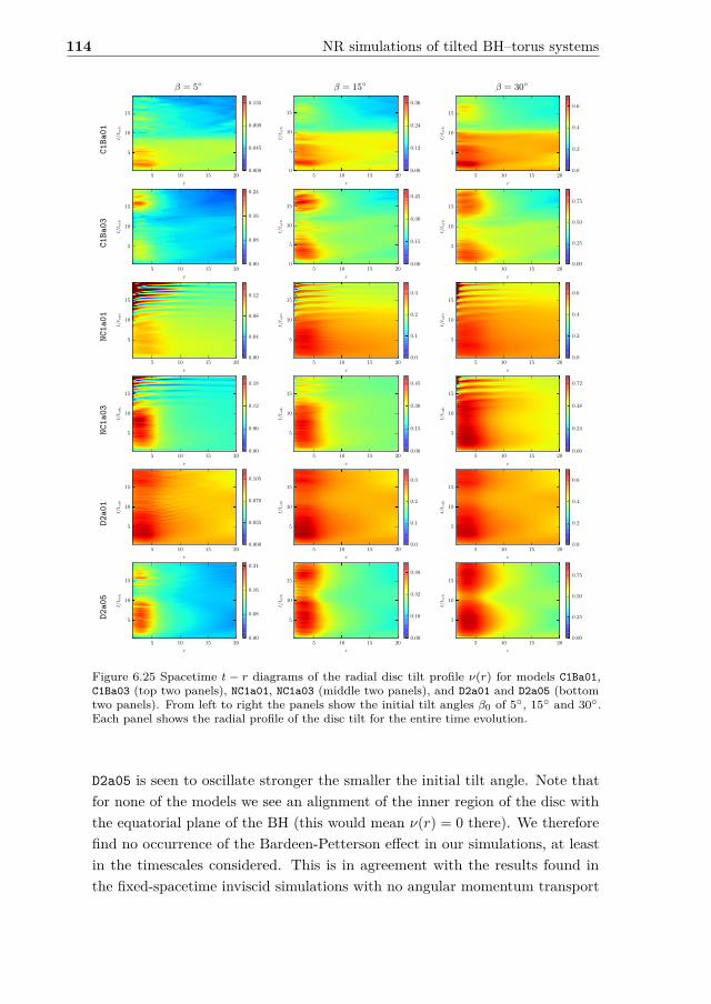
114 NR simulations of tilted BH–torus systems
β = 5 β = 15 β = 30
C1Ba01
5 10 15 20
r
5
10
15t/
t orb
0.000
0.045
0.090
0.135
5 10 15 20
r
0
5
10
15
t/t o
rb
0.00
0.12
0.24
0.36
5 10 15 20
r
5
10
15
t/t o
rb
0.0
0.2
0.4
0.6C1Ba03
5 10 15 20
r
5
10
15
t/t o
rb
0.00
0.08
0.16
0.24
5 10 15 20
r
0
5
10
15
t/t o
rb
0.00
0.15
0.30
0.45
5 10 15 20
r
5
10
15
t/t o
rb
0.00
0.25
0.50
0.75
NC1a01
5 10 15 20
r
5
10
15
t/t o
rb
0.00
0.04
0.08
0.12
5 10 15 20
r
5
10
15
t/t o
rb
0.0
0.1
0.2
0.3
5 10 15 20
r
5
10
15
t/t o
rb
0.0
0.2
0.4
0.6
NC1a03
5 10 15 20
r
5
10
15
t/t o
rb
0.00
0.06
0.12
0.18
5 10 15 20
r
5
10
15
t/t o
rb
0.00
0.15
0.30
0.45
5 10 15 20
r
5
10
15
t/t o
rb
0.00
0.24
0.48
0.72
D2a01
5 10 15 20
r
5
10
15
t/t o
rb
0.000
0.035
0.070
0.105
5 10 15 20
r
5
10
15
t/t o
rb
0.0
0.1
0.2
0.3
5 10 15 20
r
5
10
15
t/t o
rb
0.0
0.2
0.4
0.6
D2a05
5 10 15 20
r
5
10
15
t/t o
rb
0.00
0.08
0.16
0.24
5 10 15 20
r
5
10
15
t/t o
rb
0.00
0.16
0.32
0.48
5 10 15 20
r
5
10
15
t/t o
rb
0.00
0.25
0.50
0.75
Figure 6.25 Spacetime t − r diagrams of the radial disc tilt profile ν(r) for models C1Ba01,C1Ba03 (top two panels), NC1a01, NC1a03 (middle two panels), and D2a01 and D2a05 (bottomtwo panels). From left to right the panels show the initial tilt angles β0 of 5, 15 and 30.Each panel shows the radial profile of the disc tilt for the entire time evolution.
D2a05 is seen to oscillate stronger the smaller the initial tilt angle. Note thatfor none of the models we see an alignment of the inner region of the disc withthe equatorial plane of the BH (this would mean ν(r) = 0 there). We thereforefind no occurrence of the Bardeen-Petterson effect in our simulations, at leastin the timescales considered. This is in agreement with the results found inthe fixed-spacetime inviscid simulations with no angular momentum transport

6.2 Results 115
β = 5 β = 15 β = 30
C1Ba01
2 4 6 8 10 12 14
r
4
6
8
10
12
14
16
18
t/t o
rb
0.0
0.6
1.2
1.8
2 4 6 8 10 12 14
r
4
6
8
10
12
14
16
18
t/t o
rb
0.0
0.6
1.2
1.8
2 4 6 8 10 12 14
r
4
6
8
10
12
14
16
18
t/t o
rb
0.0
0.6
1.2
1.8
C1Ba03
2 4 6 8 10 12 14
r
4
6
8
10
12
14
16
18
t/t o
rb
0.0
1.2
2.4
3.6
2 4 6 8 10 12 14
r
4
6
8
10
12
14
16
18
t/t o
rb
0.0
1.2
2.4
3.6
2 4 6 8 10 12 14
r
4
6
8
10
12
14
16
18
t/t o
rb
0.0
1.2
2.4
3.6
NC1a01
2 4 6 8 10 12 14
r
4
6
8
10
12
t/t o
rb
0.0
0.3
0.6
0.9
2 4 6 8 10 12 14
r
4
6
8
10
12
t/t o
rb
0.0
0.3
0.6
0.9
2 4 6 8 10 12 14
r
4
6
8
10
12
t/t o
rb
0.0
0.3
0.6
0.9
NC1a03
2 4 6 8 10 12 14
r
4
6
8
10
12
t/t o
rb
0.0
0.6
1.2
1.8
2 4 6 8 10 12 14
r
4
6
8
10
12
t/t o
rb
0.0
0.6
1.2
1.8
2 4 6 8 10 12 14
r
4
6
8
10
12
t/t o
rb
0.0
0.6
1.2
1.8
D2a01
2 4 6 8 10 12 14
r
4
6
8
10
12
14
16
18
t/t o
rb
0.0
0.3
0.6
0.9
2 4 6 8 10 12 14
r
4
6
8
10
12
14
16
18
t/t o
rb
0.00
0.24
0.48
0.72
2 4 6 8 10 12 14
r
4
6
8
10
12
14
16
18
t/t o
rb
0.00
0.24
0.48
0.72
D2a05
2 4 6 8 10 12 14
r
4
6
8
10
12
14
16
18
t/t o
rb
0
1
2
3
2 4 6 8 10 12 14
r
4
6
8
10
12
14
16
18
t/t o
rb
0
1
2
3
2 4 6 8 10 12 14
r
4
6
8
10
12
14
16
18
t/t o
rb
0
1
2
3
Figure 6.26 Spacetime t − r diagrams of the radial disc twist profile σ(r) for models C1Ba01,C1Ba03 (top two panels), NC1a01, NC1a03 (middle two panels), and D2a01 and D2a05 (bottomtwo panels). From left to right the panels show the initial tilt angles β0 of 5, 15 and 30.Each panel shows the radial profile of the inner region disc twist from 3 orbits onwards.
of Fragile and Anninos [2005] and also with the GRMHD simulations of Fragileet al. [2007] that included angular momentum transport driven by the MRI.The observed profile and evolution of the disc warp seems to be in qualitativeagreement with the analytic work on warp propagation as bending-waves in tiltedthick accretion discs (see, for instance, the analytic tilt profiles in Ivanov andIllarionov [1997], Demianski and Ivanov [1997], and Lubow, Ogilvie, and Pringle[2002], the analytic model of linear warp evolution of Foucart and Lai [2014]
116 NR simulations of tilted BH–torus systems
and the application of the linear warp evolution model in Franchini, Lodato,and Facchini [2016]). In these models, the tilt profile is non-zero near the BHwith a hilltop profile. Our discs are in the bending-wave regime as they arethick and we do not take the fluid viscosity into account. We note that whilethe Bardeen-Petterson effect is not manifest in our models, we neverthelessdo observe a global partial realignment of the BH spin with the disc angularmomentum, caused by the growth of the PPI. This alignment of the disc angularmomentum with the BH spin has also been observed in the post-merger evolutionof a tilted accretion disc in Kawaguchi et al. [2015]. The authors conclude thatthe transport of angular momentum by non-axisymmetric shock waves in thedisc might be responsible for such a Bardeen-Petterson-like effect. We will comeback to this issue in Chapter 7 below. Finally, to check for Lense-Thirringprecession, we plot the evolution of the inner region disc twist σ(r) from t = 3orbits onwards for all our tilted models in Fig. 6.26. We see that all modelsbecome twisted (as σ(r) varies with r) in the regions for radii up to 5. Theplots further indicate solid precession of the discs, as the radial profile of σ(r)is increasing smoothly in time almost independently of the radius in the outerregions of the disc and does not remain 0 for large radii. This is consistent withthe solid-body precession found in the fixed spacetime simulations of Fragile andAnninos [2005]. Models D2 actually show a slightly growing twist for larger radii.In this trend, the higher initial spin models show flatter profiles, while there issome radial modulation of the profiles for the lower spin simulations. A strikingfeature of the plots is the smaller difference in accumulated twist for large radiibetween different initial spin magnitude for models NC1. In models C1B and D2the higher spin models show a much higher twist at large radii than their lowspin counterparts (see also Fig. 6.24, where this is seen in the evolution of globaltwist of the disc angular momentum vector as well). As the long survival ofthe m = 1 mode in the NC1 models seems to have an effect on the evolution ofthe twist, we plot this evolution only up to the saturation of the PPI for thesemodels in order to properly visualise the solid body precession of the disc.
6.2.8 Angular momentum transport
In this section we investigate the transport of angular momentum in the discs.To illustrate the transport of angular momentum during the evolution of ourmodels, we plot spacetime t− r diagrams showing the magnitude of the angularmomentum in radial shells, computed using Eq. (4.33). Such diagrams aredisplayed in Fig. 6.27. The magnitude of the angular momentum in each shell,

6.2 Results 117
∥J(r)∥, has been rescaled to the global maximum value attained in any shellduring the evolution. Fig. 6.27 shows the evolution of ∥J(r)∥ for the threeuntilted models C1Ba0b0 (top panel), NC1a0b0 (middle panel) and D2a01b0(bottom panel). This figure reveals that compared to the latter two models,model C1Ba0b0 shows a radical redistribution of angular momentum in theradial direction. This drastic difference is due to the development of the PPI inmodel C1Ba0b0. Following the initial perturbation we see that the contours of∥J(r)∥ start growing in a wave-like manner, transporting angular momentumoutwards. This happens up until the saturation of the PPI at about 10 orbitalperiods. As noted by Balbus [2003] during the growth phase the PPI is thoughtto be an effective mechanism for angular momentum transport in thick accretiondiscs, where a right combination of rotation and pressure at the boundariesof the disc allows the growing non-axisymmetric modes to transport angularmomentum outwards. Zurek and Benz [1986] showed as well that the developmentof non-axisymmetric instabilities is closely connected to the transport of angularmomentum. After saturation, the new distribution of angular momentum seemsPP-stable and does not exhibit drastic changes for the rest of the evolution.
We can compare the evolution of ∥J(r)∥ to the development of the m = 1non-axisymmetric mode in the disc, which drops to a value of around 1% ofits maximum value after saturation (see top panel of Fig. 6.15). As describedin Balbus [2003], the development of the PPI crucially relies on the propertiesof both the inner and outer boundaries of the disc. Blaes [1987] showed thata small amount of accretion (which modifies the inner boundary of the disc)was sufficient to saturate the growing PPI. Furthermore, wider tori are knownto be less violently unstable than slender tori [Hawley 1991]. In subsections6.2.3 and 6.2.4 we already showed that the accretion rate and the growth of them = 1 non-axisymmetric mode saturate at the same time, but the t− r diagramof Fig. 6.27 also shows that the angular momentum isocontours in the outerregions of the disc are being pushed outwards with growing amplitude as well.It therefore seems that both mechanisms are saturating the PPI simultaneouslyin model C1Ba00.
Model NC1a0b0, displayed in the middle panel of Fig. 6.27, has a non-constantspecific angular momentum distribution, and shows a very different evolutionof ∥J(r)∥. The inner region of the disc shows a gentle reduction of angularmomentum during the entire evolution and no sudden and drastic redistributionis found as the one that occurred in model C1Ba0b0. The outer contour growsto encompass the entire outer domain shown in the plot. Another differenceis the almost complete absence of variability of the inner region of the disc,

118 NR simulations of tilted BH–torus systems
5 10 15 20 25 30 35 40
r
0
5
10
15
20
t/t o
rb
0.00
0.15
0.30
0.45
0.60
0.75
0.90
5 10 15 20 25 30 35 40
r
0
5
10
15
20
t/t o
rb
0.00
0.15
0.30
0.45
0.60
0.75
0.90
5 10 15 20 25 30 35 40
r
0
5
10
15
20
t/t o
rb
0.00
0.15
0.30
0.45
0.60
0.75
0.90
Figure 6.27 Spacetime t − r diagram showing the time evolution of the radial profile ofthe angular momentum magnitude ∥J(r)∥ for untilted models C1Ba0b0 (top panel), NC1a0b0(middle panel) and D2a01b0 (bottom panel).

6.2 Results 119
which is in contrast to model C1Ba0b0, where oscillatory behaviour is seen inthe inner boundary of the disc too. The specific angular momentum profileof model NC1a0b0 is between constant and Keplerian, with Keplerian discsbeing essentially PP-stable. Model NC1a0b0 still develops the PPI, albeit in amilder manner than model C1Ba0b0, with the torus of model NC1a0b0 beinginitially wider. Finally, model D2a01b0 (bottom panel), the lightest of ourmodels, is PP-stable as already shown in subsection 6.2.4. The correspondingspacetime diagram of ∥J(r)∥ shows no pronounced outward transport of angularmomentum as the evolution proceeds, the profile remaining very similar to itsinitial configuration. The inner region with a high angular momentum magnitudeis thinned out slightly, and the profile spreads a bit overall, but the changes arenowhere nearly as pronounced as for models C1Ba0b0 and NC1a0b0. As we haveseen in the analysis of the modes, the amplitude of the m = 1 mode drops sharplyupon the saturation of the PPI in the C1Ba00 model. The subsequent evolutionof the angular momentum profile remains constant, similar to what we observefor the entire evolution of the PP-stable model D2a01b0. There is a clear splitbetween the stages of the evolution: the first during which the PPI develops andsaturates, and the subsequent evolution of an essentially PP-stable torus. ModelNC1a00, on the other hand, shows a very different behaviour: as already seen inthe mode analysis, the m = 1 mode amplitude remains roughly at its saturationvalue for the rest of the evolution, which is lower than the values attainedby models C1B. The persistent m = 1 mode is seen to continuously transportangular momentum outwards till the end of the simulation. The restructuringof the disc by the transport of angular momentum is more long-lived, comparedto the drastic change the saturation of the PPI brings about in model C1Ba00.These findings seem to confirm those found in Zurek and Benz [1986]. Using thesame kind of spacetime diagrams we have also checked the dependence of theangular momentum transport on the BH spin a and on the initial tilt angle β0
for all models of our sample. We find that the angular momentum transportshows weak dependence with the tilt angle (the higher the tilt angle the slowestthe transport) and shows essentially no dependence with the spin, at least forthe moderate values of the BH spin we could afford in our study. This is aremarkable result, as it demonstrates that models C1B and NC1 are PP-unstablefor a wide range of initial BH spin magnitudes and tilt angles.
We note that our GRHD simulations are underestimating the real angularmomentum transport likely to occur in astrophysical accretion discs due toour lack of accounting for viscosity (for instance via the MRI). The sources ofviscosity in our discs are due to the developing non-axisymmetric modes and

120 NR simulations of tilted BH–torus systems
numerical viscosity. The latter seems to play only a minor role, as can be seenfrom the accretion rates reported for models C1Ba00, NC1a00 and D1a01b00,which is about an order of magnitude lower for the PP-stable model D1a01b00than for the other two. The timescale at which the viscosity provided by the MRIoperates is difficult to estimate. In Foucart et al. [2014], the authors estimatea viscous timescale of ∼ 0.1 s in their BHNS post-merger torus. This wouldcorrespond to about 130 torb for disc model C1B. We should take the evolutionof magnetic fields into account for longer simulations in our discs (to complete afull BH spin precession cycle, for instance).
6.2.9 Gravitational waves
In this section, we explicitly report frequencies and times in SI units. Note thatthe results presented here have been obtained using the BH masses listed inTable 6.1. None of the results have been rescaled for different BH masses.
The recent numerical simulations of Kiuchi et al. [2011] have shown thatthe growth and saturation of the PPI makes BH–torus systems emitters oflarge amplitude, quasi-periodic GW, potentially detectable by forthcomingground-based and spacecraft detectors. It was found in particular that them = 1 non-axisymmetric structure survives with an appreciable amplitudeafter saturation of the PPI, which leads to the emission of quasi-periodic GWswith a large amplitude3. In this section we turn our attention to analyse theimplications of the PPI in our tilted BH–torus systems regarding the emissionof GWs, namely the dependence of the resulting gravitational waveforms andspectra on the BH spin magnitude and initial tilt angle.
In Fig. 6.28 we plot the real part of the (l,m) = (2, 2) mode of the outgoingpart of the complex Weyl scalar Ψ4 for models C1Ba01 and NC1a01 and for allinitial tilt angles β0. This quantity has been computed at an extraction radiusr = 640 (945 km). Fig. 6.28 shows that, in agreement with Kiuchi et al. [2011],all models display strong emission of gravitational waves and that the emissionpersists for many dynamical timescales well after the saturation of the PPI. Thepeak amplitude for models C1Ba01 is about an order of magnitude higher thanfor models NC1a01.
We recall that model C1B has a slightly higher initial disc-to-BH mass ratiothan model NC1 (q = 0.16 and 0.11, respectively) and that the development of the
3First estimates through full GRHD simulations of the GW detectability by the PPIinstability in self-gravitating BH–torus systems were obtained in Korobkin et al. [2011] wherethe nonlinear saturation phase was almost reached. See also van Putten [2001] for earlierproposals and alternative estimates of the gravitational waves emitted by non-axisymmetricinstabilities in such systems.

6.2 Results 121
0 2 4 6 8 10 12 14 16
(t− rdet)/torb
−0.8
−0.6
−0.4
−0.2
0.0
0.2
0.4
0.6
0.8
rΨ
2,2
4
×10−5
C1Ba01b05
C1Ba01b15
C1Ba01b30
0 2 4 6 8 10 12 14 16 18
(t− rdet)/torb
−1.0
−0.8
−0.6
−0.4
−0.2
0.0
0.2
0.4
0.6
0.8
rΨ
2,2
4
×10−6
NC1a01b05
NC1a01b15
NC1a01b30
Figure 6.28 Time evolution of the l = m = 2 mode of the real part of the Weyl scalar Ψ4multiplied by the extraction radius (r = 640). The top panel shows models C1Ba01 and thebottom panel models NC1a01.
PPI in models C1B is more pronounced than in the non-constant specific angularmomentum models NC1 (see Fig. 6.10). These two features are responsible forthe difference in the peak amplitudes between the two initial models. We alsonote that the peak amplitude in the C1Ba01 models, reached at PPI saturation,is much higher than the amplitude of the remaining signal, whereas in modelsNC1a01 the variations are not so pronounced. As we showed in Fig. 6.15, uponPPI saturation the dominant m = 1 PPI mode drops to about 1% of its peakvalue in models C1B, while it remains at a similar strength for models NC1.
Fig. 6.28 also shows that the GW signal depends weakly on the initial tiltangle, particularly for the non-constant specific angular momentum models NC1.The smallest peak amplitudes are attained for the most tilted BH spacetime

122 NR simulations of tilted BH–torus systems
0 1 2 3 4 5
f [kHz]
10−27
10−26
10−25
10−24
10−23
10−22
10−21
heff/M
pc
a00
a01b05
a01b15
a01b30
a03b05
a03b15
a03b30
0 1 2 3 4 5
f [kHz]
10−27
10−26
10−25
10−24
10−23
10−22
10−21
heff/M
pc
a00
a01b05
a01b15
a01b30
a03b05
a03b15
a03b30
Figure 6.29 Spectrum of the effective strain for models C1B, showing the l = 2, m = 1 modes(top) and l = m = 2 modes (bottom) for the source located at 1 Mpc.
(β0 = 30). In any event, the differences found in the values spanned by thepeak amplitudes with regard to β0 are not too significant.
We use the fixed frequency integration (FFI) described in Reisswig andPollney [2011] in the integration of the Ψ4 data to obtain the GW strain. InFigs. 6.29-6.31 we plot the effective strain heff/Mpc as a function of frequencyfor all models, placing the sources at 1 Mpc, in order to see any possible imprintof the initial spin magnitude and tilt angle on the GW spectrum. As describedabove, we use the same timestep for the time integration of the spacetime andGRHD evolution equations in the 7 outermost refinement levels (which meansthat in those outer refinement levels ∆t = 1.58 × 10⁻⁶ s and 3.16 × 10⁻⁶ s forhigher and lower resolution runs, respectively). At our extraction radius, thetimestep in the respective mesh refinement level is therefore sufficiently small to

6.2 Results 123
sample the GW multipole signal with a δt of 6.32×10⁻⁶ s (1.26×10⁻⁵ s) for thehigher (lower) resolution runs, respectively, where δt is the output timestep ofthe GW data from the simulation. Due to the Nyquist criterion, we can thereforeresolve the GW spectra up to ≈ 80 (40) kHz4. The top panels of Figs. 6.29and 6.30 correspond to the (l,m) = (2, 1) mode and the bottom panels to the(l,m) = (2, 2) mode. The highest power is usually found at a frequency of about1kHz. For the effective strain of the (l,m) = (2, 1) mode for models C1B shownin the top panel of Fig. 6.29, we can clearly identify two trends. On the onehand there is a difference at high frequencies between the models with eitherno or low (a = 0.1) initial BH spin (models C1Ba00 and C1Ba01) and the highspin models (a = 0.3). The spectra for these two groups show a different slopefrom f ∼ 2kHz onwards. On the other hand, for models C1Ba00 and C1Ba01, anincrease in the initial tilt angle leads to an increase in the power for frequenciesf > 2kHz. This also seems to be present at lower frequencies although it issomewhat less clear. Correspondingly, the power spectra of the (l,m) = (2, 2)mode shown in the bottom panel of Fig. 6.29 neatly splits the models into threegroups, according to the initial spin magnitude of the BH. We find that theslope of the spectra becomes steeper from f ∼ 2kHz onwards the higher theBH spin. In all cases, the slope of the effective strain with the frequency showsessentially no dependence with the initial tilt angle for the various groups ofmodels characterised by the same BH spin. The power in model C1Ba00 is atleast an order of magnitude larger for all frequencies than that of the tiltedmodels. This is because the spiralling motion in the equatorial plane of boththe BH and the m = 1 over-density PPI “planet” emits GWs predominantlyin the l = m = 2 mode which is emitted in the direction perpendicular to theequatorial plane. This is an optimal situation for the model with aligned BHand disc spins, as the coordinate system in which we perform the multipoleexpansion of the GW is aligned with the z-axis. However for the tilted modelsthe “orbit” of the BH and of the over-density lump in the disc is not confined to
4We note that this analysis serves to establish that we would be able to resolve the GWspectra up to ≈ 80 (40) kHz using the timestep at the extraction radius. Physically, there isno reason to expect such high frequencies in the spectra of the GW signals of our BH–torussystems. To analyse the maximum expected frequencies, we assume the maximum fluid orbitalfrequency in our systems to be the orbital frequency at the ISCO, νISCO, which, for theBH masses indicated in Table 6.1, is between νISCO ∼ 2.2 kHz for a non-spinning BH andνISCO ∼ 16 kHz for a maximally spinning Kerr BH [Remillard and McClintock 2006]. Forour initial models with a maximum initial Kerr parameter of a = 0.5, we therefore expectthe maximum orbital frequency to be ∼ 4 kHz. The emitted GW will have a frequency twiceas large, so we would thus expect to obtain GW frequencies of up to 8 kHz. In order toconcentrate on the lower-frequency properties of the spectrum (namely the radiation at theorbital frequency at the initial pressure maximum and the frequency of the PPI pattern speed),we plot the GW spectra for frequencies up to 5 kHz.

124 NR simulations of tilted BH–torus systems
0 1 2 3 4 5
f [kHz]
10−28
10−27
10−26
10−25
10−24
10−23
10−22
heff/M
pc
a00
a01b05
a01b15
a01b30
a03b05
a03b15
a03b30
0 1 2 3 4 5
f [kHz]
10−28
10−27
10−26
10−25
10−24
10−23
10−22
heff/M
pc
a00
a01b05
a01b15
a01b30
a03b05
a03b15
a03b30
Figure 6.30 Spectrum of the effective strain for models NC1, showing the l = 2, m = 1 modes(top) and l = m = 2 modes (bottom) for the source located at 1 Mpc.
the equatorial plane anymore because of the reaction of the disc to the tiltedBH spin. This results in a decrease in the GW power. In order to have a faircomparison of the GW power emitted in the untilted and tilted systems, onewould need to extract the waves in a (time-changing) coordinate system adaptedwith its z-axis aligned with the total angular momentum of the system.
The spectra of the non-constant specific angular momentum models NC1displayed in Fig. 6.30 are markedly different to those of constant specific angularmomentum tori. Namely, their dependence on the frequency is similar for allmodes (same slope) irrespective of the initial tilt angle and of the BH spin. Nosplit in two or three families is found according to the BH spin. The effectivestrain of the (l,m) = (2, 1) mode for models NC1 shows a plateau in the lowfrequency part (up to ∼ 0.5kHz) for models NC1a03b15 and NC1a03b30. The

6.2 Results 125
spectra show a prominent peak around 0.6kHz for all models but these two. Theheight of the peak drops with growing initial spin and initial inclination angle,which might as well be an artefact due the multipole expansion in the untiltedcoordinate system. For the l = m = 2 mode we find that the curve for theuntilted model NC1a00 lies more than an order of magnitude above the curvescorresponding to the initially tilted discs, as seen also for the C1Ba00 model inthe previous figure.
Finally, in Fig. 6.31 we show the effective strains of the (l,m) = (2, 1) mode(top panel), (2,2) mode (middle panel) and (3,1) mode (bottom panel) for modelsD2. In the spectra of the (l,m) = (2, 1) mode there is a clear variation with theinitial tilt and BH spin magnitude, with both increasing the power of the modefor all frequencies shown. The fact that the power increases with growing tiltangle seems to indicate that this behaviour is really a physical consequence ofthe tilted disc evolution. Contrary to model C1B and similar to model NC1, wefind now that model D2 does not show the grouping of models depending on theBH spin, and the associated frequency dependence (i.e. steeper slopes for higherspins). As this model is PP-stable and has an initially constant distributionof specific angular momentum, its dynamics is somewhat between that of theother two models. The spectra of the l = m = 2 mode (middle panel) show inparticular a very different behaviour to those shown for models C1B and NC1,namely that the model with zero initial inclination does not show significantlylarger power than the models with a = 0.1 and a = 0.5. Since models D2 do notdevelop the PPI, there is no strong emission of GW in the l = m = 2 mode dueto the absence of the spiral motion of both BH and over-density ‘planet’ that ispresent for the other two initial models.
Therefore, the power spectrum of the untilted model D2a01b0 does not exceedthat of the rest of the other tilted D2 models. The two models D2a05b15 andD2a05b30 both show two peaks in the low frequency part of the spectrum.
The absence of the PPI in the D2 models results in a GW emission where thel = m = 2 mode is not the dominant mode. To show this, we plot the effectivestrain of the (l,m) = (3, 1) mode in the bottom panel of Fig. 6.31. The poweris comparable with that of the (l,m) = (2, 1) and l = m = 2 modes, which isnot the case for models C1B and NC1 that both develop the PPI. The plot of theeffective strain of the (l,m) = (3, 1) mode shows that same trend as that of the(l,m) = (2, 1) mode, i.e. the power density increases with spin magnitude andinitial tilt angle. Furthermore, we can see clear quasi-periodic oscillations in thelow frequency part of the spectrum for models D2a05. These oscillations mightbe the result of two non-axisymmetric modes being present in disc models D2, as

126 NR simulations of tilted BH–torus systems
0 1 2 3 4 5
f [kHz]
10−28
10−27
10−26
10−25
10−24
10−23
heff/M
pc
a01b00
a01b05
a01b15
a01b30
a05b05
a05b15
a05b30
0 1 2 3 4 5
f [kHz]
10−28
10−27
10−26
10−25
10−24
10−23
heff/M
pc
a01b00
a01b05
a01b15
a01b30
a05b05
a05b15
a05b30
0 1 2 3 4 5
f [kHz]
10−28
10−27
10−26
10−25
10−24
10−23
heff/M
pc
a01b00
a01b05
a01b15
a01b30
a05b05
a05b15
a05b30
Figure 6.31 Spectrum of the effective strain for models D2, showing the l = 2, m = 1 modes(top panel) and l = m = 2 modes (middle panel) and l = 3, m = 1 modes (bottom panel) forthe source located at 1 Mpc.

6.2 Results 127
101 102 103
f [Hz]
10−25
10−24
10−23
10−22
10−21
10−20
10−19
heff
Sensitivity aLIGO
C1Ba00
NC1a00
D2a05b05
Figure 6.32 Plot showing the peak amplitudes of the effective strain, inferred from the accretiontimescale, for the three different initial models. The sensitivity curve for advanced LIGO withzero-detuning and high-power configuration is shown in black. The small bump at ∼ 500Hz in the sensitivity curve is the fundamental vibrational mode of the test mass suspensionfibres [LIGO Scientific Collaboration et al. 2015].
the m = 1 and m = 2 mode are of roughly equal strength (see Fig. 6.14). Thespectra of all models shown are not very smooth and show small peaks. To checkif these are due to numerical effects or actual imprints of the fluid evolutionwould probably require much higher resolution simulations than those presentedin this work.
In order to estimate the detectability of the GWs emitted by these systems,we follow the analysis in Kiuchi et al. [2011]. We assume that the BH–torussystem of models NC1 will radiate GWs for the entire accretion timescale tacc
(which is the time needed for the entire disc to accrete). This is because inthese models, the m = 1 over-density lump and the BH form a long-lastingquasi-binary system. Assuming that the accretion rate will remain at the levelit attained by the end of the simulations (see Fig. 6.13), a lower limit for theaccretion timescale for models NC1 is tacc ≈ 0.1 s. Note that this is only aboutfour times longer than the duration of the simulations reported here. It alsocoincides with the viscous timescale reported in Foucart et al. [2014], whichmeans that additional physics such as the MRI are likely to shorten this timescalein real accretion discs.
From the timescale, we can estimate the number of GW oscillations at thepeak frequency, which yields ≈ 100 cycles5 as a lower limit for models NC1.
5The peak frequency for models NC1 is around 1 kHz, which means that the source shouldemit ∼ 100 wave cycles at the peak frequency during the accretion timescale.

128 NR simulations of tilted BH–torus systems
The peak amplitude of the GW strain will then be amplified by√Ncycles ≈ 10,
while we assume no such amplification neither for models C1B (where the PPI israpidly damped after saturation) nor for models D2 (which are PP-stable). Wenote that these estimates are in very good agreement with the correspondingfindings reported in Kiuchi et al. [2011]. The corresponding peak amplitudesfor the BH–torus systems located at a distance of 50 Mpc, together with theadvanced LIGO (aLIGO) sensitivity curve, are plotted in Fig. 6.32, showingthat the GWs emitted by models NC1 could be detectable due to the long-lastingemission of GWs due to the persistent m = 1 mode. We also note that theplanned factor-of-3 upgrade of aLIGO [Hild 2012, Adhikari 2014, Miller et al.2015] will further improve the detectability in the future.
To put the occurrence of BH–torus systems resulting from BHNS mergersinto perspective, we note that the current, realistic merger rate of BHNS upto a distance of 50 Mpc is about 3.75 × 10⁻³ yr−1 (see Abadie et al. [2010]and references therein). The actual number of BHNS mergers that result inBH–torus systems is likely to be lower than this, as not all BHs in these mergerswill have sufficiently low masses and/or sufficiently high spins to tidally disruptthe NS during inspiral, therefore leaving no torus behind.

Chapter 7
Analysing the tiltedBH–torus dynamics withfluid tracers
The results of this chapter have been originally published in:V. Mewes, F. Galeazzi, J. A. Font, P. J. Montero and N. StergioulasAccepted for publication in MNRAS
In this chapter, we investigate the dynamics of one titled BH–torus model ofChapter 6 (NC1a03b05) in more detail using fluid tracer particles as an additionalmeans to analyse the disc evolution.
7.1 Initial data and setupModel NC1a03b05 has a non-constant l-profile and was shown to exhibit thedevelopment of a long-lasting non-axisymmetric m = 1 mode in Chapter 6. Theparameters of this model are given in Tables 6.1 and 6.2. In the simulationspresented in this chapter, we evolve the model for up to 32 orbital periods(significantly longer than we did in the simulations reported in Chapter 6) intwo different ways to gauge the influence of the self-gravity of the fluid in theevolution of this model. The first evolution takes into account the solutionof the coupled system of Einstein equations and GRHD equations, and thuscorresponds to a fully dynamical spacetime evolution. For the second evolutionwe assume the test-fluid (Cowling) approximation in which the spacetime is

130 Analysing the tilted BH–torus dynamics with fluid tracers
0 5 10 15 20 25 30
t/torb
−0.04
−0.03
−0.02
−0.01
0.00
0.01
0.02
Sx
Sy
Sx from TLT
Sy from TLT
Figure 7.1 Evolution of the x and y components of the BH spin S and the evolution of thespin components resulting from the LT torque exerted by the disc.
fixed and only the GRHD equations are solved. As initial data for this secondsimulation we use the data of the fully evolved spacetime run that has beencheckpointed at t = 1.5torb. This is to ensure that we are evolving the samesystem once the gauge perturbations have left the region where the torus resides,and in particular to provide the same perturbation that triggers the growth ofthe non-axisymmetric instability in both runs.
Initially we place 250000 tracers at random locations in the accretion disc,where the probability distribution is weighted according to the underlying rest-mass density distribution. This results in all tracer particles being of equal mass(3.97 × 10⁻⁷) initially and during the evolution. The bulk motion of the tracersis able to capture accurately the motion of the underlying fluid flow especiallywhen it is not turbulent and strong shocks are not present.
7.2 BH precession from Lense-Thirring torque
The main driver of the tilted disc evolution is the LT precession. At the lowestpost-Newtonian order of spin-orbit interactions, a particle in an inclined orbitaround a central Kerr BH will be subject to the following torque [Kidder 1995,Merritt and Vasiliev 2012]:
T LT = 2S × J
r3 , (7.1)
where S is the BH spin, J is the angular momentum vector of the particle, and ris the distance of the particle from the BH centre. This is the LT torque exerted

7.2 BH precession from Lense-Thirring torque 131
0 5 10 15 20 25 30
t/torb
−1.5
−1.0
−0.5
0.0
0.5
1.0
1.5
2.0×10⁻²
Sx
Jx
0 5 10 15 20 25 30
t/torb
−3.0
−2.5
−2.0
−1.5
−1.0
−0.5
0.0×10⁻²
Sy
Jy
Figure 7.2 Evolution of the x and y components of the BH spin S and total disc angularmomentum Jdisc.
by the central BH on the particle. As a result of this torque, the orbital angularmomentum of the particle will start to precess around the BH spin. As there isa strong radial dependence on the magnitude of the torque, the inner regions ofa tilted accretion disc will become twisted, i.e. they will differentially precessaround the central BH. However, as shown in the results of Fragile and Anninos[2005] and in Chapter 6, the sound crossing time in the disc is shorter than theLT timescale, which results in a global disc response to the LT torque producedby the Kerr BH, leading to solid body precession of the disc. By Newton’s thirdlaw, the disc exerts a torque of equal magnitude and opposite direction on theBH, causing it to precess as well.
To check whether the precession of the BH we observe in our simulations hasa physical origin, we compare the time evolution of the x and y components of

132 Analysing the tilted BH–torus dynamics with fluid tracers
the BH spin, Sx, Sy, with the evolution of the BH spin that would have resultedfrom summing up the cumulative spin change resulting from the LT torque ofthe disc at each timestep:
SLT(t) = S(0) +∫ t
0T LTdt. (7.2)
As the disc is approximately precessing as a solid body, we calculate thetorque coming from the disc total angular momentum vector, Jdisc, and choosethe radius in Eq. (7.1) to be that of the location of the initial density maximum,r = 10.2. The results are shown in Figure 7.1. This figure shows that thetime evolution of the BH spin components agree well with the torque exertedon the BH by the disc. In Fig. 7.2 we show the time evolution of the x andy components of S and Jdisc. Clearly, the sum of the spin components anddisc angular momentum components along the two directions is seen to beapproximately constant for the evolution, in agreement with the fact that theLT torque is the main driver for both disc and BH precession.
7.3 m = 1 non-axisymmetric instability
7.3.1 Spiral density wave
Two of the three models we studied in Chapter 6 were found to develop a globalnon-axisymmetric instability with m = 1 being the dominant azimuthal mode.One such instability is the instability of tori with constant specific angularmomentum profiles, the Papaloizou-Pringle instability [Papaloizou and Pringle1984]. Early numerical investigations of Hawley [1987] showed that the non-linear regime of the PPI resulted in the formation of counterrotating over-densitylumps. The precise mechanism of the instability was elucidated in Goodman,Narayan, and Goldreich [1987], where the authors showed that the planets foundin Hawley [1987] might be a new equilibrium configuration of the fluid. Theinstability was subsequently investigated numerically by Hawley [1991] as wellas in the recent, fully general relativistic simulations of Kiuchi et al. [2011],Korobkin et al. [2011], and Mewes et al. [2016].
In this section we show that the growth of the m = 1 mode in the disc resultsin the formation of a spiral density wave with a constant global pattern speedΩP . As the disc is differentially rotating this means that there is a location inthe disc, the so-called corotation radius rco, where the spiral density wave hasthe same orbital velocity as the fluid in the disc. Inside rco the wave travelsslower than the fluid, which means that it has negative angular momentum with

7.3 m = 1 non-axisymmetric instability 133
Figure 7.3 Fractional change in the rest mass density ∆ρ/ρ between two timesteps, shown at 9different snapshots of the evolution, t/torb = 1, 4, 8, 12, 16, 20, 24, 28, and 32 (from the top-leftpanel). The domain shown in all panels is 100 across both x-axis and y-axis. The grey circlesshow the tracers at the location of the corotation radius rco. The formation of a spiral densitywave from the growth of the m = 1 mode is noticeable.
respect to the fluid. While the wave amplitude is linear, it does not interact withthe fluid, but once non-linear amplitude effects come into play, the spiral densitywave can couple to the fluid via dissipation [Papaloizou and Lin 1995, Goodmanand Rafikov 2001, Heinemann and Papaloizou 2012]. When this happens, thewave begins to transport angular momentum outwards as the fluid loses angularmomentum to the wave inside the corotation radius. The development andpersistence of the spiral density wave is shown in Figure 7.3. The figure showsthe fractional change in density between two successive snapshots of the tracerparticles ∆ρ/ρ at 9 different times of the disc evolution, as well as the tracerparticles that are located at rco (grey circles). The location of the corotationradius is defined as the radius where the m = 1 pattern speed and the fluidorbital velocity are equal. As usual, the non-axisymmetric modes in the disc areanalysed by means of an azimuthal Fourier transform of the rest-mass density

134 Analysing the tilted BH–torus dynamics with fluid tracers
Figure 7.4 Fractional change in the fluid entropy s between two timesteps, for tracers with∆ρ/ρ > 0.1, shown at t/torb = 32.
ρ [Zurek and Benz 1986, Heemskerk, Papaloizou, and Savonije 1992]:
Dm =∫
α√γ ρ e−i m ϕ d3x , (7.3)
Similarly, the mode analysis performed using the tracers is performed by meansof the following sum
Dm =N∑j
mj e−i m ϕ, (7.4)
where mj is the mass of each tracer particle. From the mode amplitudes, thepattern speed of an azimuthal mode with mode number m is defined as (see, forinstance Heemskerk, Papaloizou, and Savonije [1992])
ΩP = 1m
dϕm
dt, (7.5)
where the phase angle ϕm is given by
ϕm = tan−1(
Im(−Dm)Re(Dm)
). (7.6)
For our simulation, we obtain an orbital period of the m = 1 pattern of PP ∼ 1.96ms, which is slightly shorter than twice the initial orbital period of the disc at thelocation of the density maximum (see Table 6.2). We note that we have chosen

7.3 m = 1 non-axisymmetric instability 135
the same range of the fractional change in the rest-mass density in all snapshotsshown, which corresponds to the interval [−0.1, 0.1]. At these wave amplitudes,non-linear effects are negligible compared to the linear effects [Masset and Tagger1997]. This plot range has however been chosen for visualisation purposes andthe wave amplitudes are actually much larger than 0.1 after the saturation of them = 1 growth, reaching almost unity. At these wave amplitudes non-linear effectsare important and the spiral density wave can couple to the fluid via dissipation.To show the development of weak shocks, we plot the fractional change in theentropy s = p/ρΓ for tracers with ∆ρ/ρ > 0.1 in Figure 7.4. From this plot,we clearly see an increase in the fluid entropy in the inner and outer regions ofthe spiral density wave. We note that the mesh refinement boundaries of ourcomputational grid also produce entropy changes due to dissipation. However,these changes are about an order of magnitude smaller than the physical increaseof entropy due to the development of shocks in the spiral density wave.
7.3.2 Gravitational torque and motion of the central BH
We next turn to the interaction of the non-axisymmetric m = 1 mode andthe central BH. The moving over-density planet in the disc represents a time-changing non-axisymmetric gravitational potential. Following Roedig et al.[2012], we estimate the total gravitational torque on the BH exerted by thetracer particles in the following way:
T G =N∑i
MBHmirBH × (ri − rBH)
|ri − rBH|3, (7.7)
where the sum runs over all tracer particles.
The resulting components of the gravitational torque T G and the timederivative of the components of the BH orbital angular momentum LBH, areshown in Figure 7.5. This figure clearly shows that the orbital angular momentumof the BH is caused by the gravitational torque of the non-axisymmetric matterdistribution in the disc. The orbital angular momentum components of theBH are calculated using the flat space coordinate rotational Killing vectors onthe AH [Campanelli et al. 2007] (which gives the Komar angular momentumin axisymmetry [Mewes, Font, and Montero 2015]) without the subtraction ofthe position of the BH centre and the subsequent subtraction of the intrinsicspin of the AH. While this is by no means a gauge invariant measure of theorbital angular momentum of the BH, it agrees very well with the Newtonian

136 Analysing the tilted BH–torus dynamics with fluid tracers
10 15 20 25 30
t/torb
−4
−2
0
2
4
LB
H
×10−5
Lx
Tx
10 15 20 25 30
t/torb
−4
−2
0
2
4
LB
H
×10−5
Ly
Ty
10 15 20 25 30
t/torb
−2
−1
0
1
2
LB
H
×10−5
Lz
Tz
Figure 7.5 Time derivative of the components of the BH orbital angular momentum vectorLBH and the components of the gravitational torque computed from the non-axisymmetricmatter distribution T G.

7.3 m = 1 non-axisymmetric instability 137
0 5 10 15 20 25 30
t/torb
0.00
0.02
0.04
0.06
0.08
0.10
0.12
|D1|/D
0
dynamical spacetime
fixed spacetime
Figure 7.6 Evolution of the m = 1 mode for the dynamical spacetime simulation (black line)and the fixed spacetime simulation (red curve), calculated with the tracer particles. We notethat we are using a linear scale for the vertical axis in this plot, contrary to the mode plotsshown in Chapter 6.
calculation of the BH orbital angular momentum as
LBH = MBH rBH × vBH. (7.8)
The disc acquires some bulk orbital angular momentum (equal and oppositeto that of the BH) as a result of the growth and the longevity of the m = 1mode as well. During the later stages of the evolution, after the saturationof the m = 1 mode growth, this bulk orbital angular momentum of the discbecomes comparable to the fluid angular momentum in the x and y direction.We note that it is precisely the evolution of the bulk orbital angular momentumthat we mistakenly identified as tilt and twist oscillations in Mewes et al. [2016].This was due to an error in the reading of the location of the BH centre in thedisc analysis code described in Section 4.4, which ultimately resulted in thecalculation of the disc angular momentum about the origin rather than aboutthe BH centre.
As a result of this error in the disc analysis used for the results presentedin Mewes et al. [2016], we speculated that the observed global oscillations in thetilt and twist might be due to the development of the Kozai-Lidov (KL) [Kozai1962, Lidov 1962] effect. This effect results in the periodic exchange of theinclination and eccentricity of a particle orbit around a central mass that isitself in an orbit with a third mass (called the perturber). The effect is adirect consequence of the conservation of the total angular momentum of thesystem. As the KL effect has recently been observed to operate in inclined

138 Analysing the tilted BH–torus dynamics with fluid tracers
4 6 8 10 12 14 16 18 20
r
5
10
15
20
25
30
t/t o
rb
0
4
8
Figure 7.7 Spacetime diagram of the radial profile of the tilt angle ν(r). The tilt angle isshown in degrees.
hydrodynamical discs around a central mass which is in a binary with anothermass [Martin et al. 2014], we assumed in Mewes et al. [2016] that the KL effectmight also be in operation in our discs as the long-lasting m = 1 mode forcesthe central BH to move in a quasi-binary orbit with the over-density planetin the disc. To demonstrate the operation of the KL effect and to explain theoscillations in more detail has been one of the main motivations for carrying outnew simulations and employing the tracer particles as a new tool for the analysisof the disc. As explained above, we have clarified the origin of the global tiltand twist oscillations as being connected to the bulk orbital angular momentumthe disc acquires when forming the quasi-binary system with the BH. The KLeffect is therefore not seen to be in operation in our discs.
The effect of the motion of the central BH on the strength of the m = 1 modeis shown in Figure 7.6. This figure displays the time evolution of the normalisedmagnitude of the D1 mode for our two simulations. While growth rates of them = 1 mode strength are very similar for the two runs, the maximum modeamplitude is about two times higher in the fully dynamical spacetime simulation(where the BH is allowed to move). We note that the growth rate and maximumm = 1 mode amplitude in the simulation presented here is smaller than theone reported in Chapter 6 for the same model. The difference arises from theuse of a constant damping parameter in the standard Γ-driver shift condition,which is known to be less accurate than dynamical damping parameters for largemass-ratio BBH simulations (see for instance Gold and Brügmann [2013]). Thedynamics of the high mass-ratio quasi-binary system composed of the central BH

7.3 m = 1 non-axisymmetric instability 139
0 5 10 15 20 25 30
t/torb
3.8
4.0
4.2
4.4
4.6
4.8
5.0
5.2νdisc
Figure 7.8 Time evolution of the tilt angle of the disc, νdisc, shown in degrees.
and the moving over-density planet in the disc should therefore be described withbetter accuracy using the dynamical damping parameter employed in Chapter 6.It seems that the fixed damping parameter restricts the BH motion, resultingin a smaller mode power. We note, however, that the actual development ofthe instability and the overall properties of the disc after its saturation remainunaffected by the choice of gauge, as they should.
7.3.3 Disc alignment
As shown in King et al. [2005], the direction of the torque responsible for disc(and therefore also BH) precession does not act in the direction to align the discangular momentum with the central BH. The alignment torque ultimately resultsfrom the inclusion of the effects of viscosity or dissipation, and its magnitudedepends, as King et al. [2005] remark, on the actual disc properties. As our fluidevolution does not explicitly account for viscosity, viscous and dissipative effectsmight therefore only arise due to numerical viscosity and dissipation in shocks.As we have seen in Section 7.3.1, the spiral density wave that results from thedevelopment of the m = 1 mode provides dissipation that is stronger than theone arising from the numerics. Another factor working towards alignment ofthe BH spin and the disc is the accretion of angular momentum, which is anegligible effect in our simulations due to the very low amount of total massaccreted during the evolution.
In Figure 7.7, we plot a spacetime diagram showing the evolution of thetilt angle profile ν(r) obtained from the tracers. Similar to the disc analysis

140 Analysing the tilted BH–torus dynamics with fluid tracers
0 5 10 15 20 25 30
t/torb
0.0
0.1
0.2
0.3
0.4
0.5
e
0.00
0.05
0.10
0.15
0.20
0.25
M/s
e
M
Figure 7.9 Evolution of the sum of disc eccentricity e1 and disc ellipticity e2 and the rest massaccretion rate M in units of M⊙/s. The accretion rate has been shifted by 0.65 torb in timefor a better visualisation of the correlation between its modulation and e.
explained in Nelson and Papaloizou [2000] and Fragile and Anninos [2005] andemployed in Chapter 6, we split the domain in radial shells and calculate thecomponents of the total angular momentum of all tracers within a given shell toobtain the tilt profile. We clearly see the expected, non-zero oscillating tilt profilepredicted by the warp propagation as bending waves during the early stagesof the simulation. The tilt amplitude close to the central BH is significantlyreduced from about 15torb onwards. This could be connected to the time whenthe developing spiral density wave becomes non-linear for the first time, couplingto the fluid inside the corotation radius and lowering the tilt amplitude. Wedo not see a complete global alignment as observed in Kawaguchi et al. [2015]during the time of the evolution. However, as Figure 7.8 shows, there is a clearmonotonic drop in the global tilt angle νdisc from t = 2 torb onwards, whichis when the m = 1 non-axisymmetric mode starts growing. Kawaguchi et al.[2015] noted that the alignment timescale was comparable or shorter than theprecession timescale of the disc. We note that our disc is precessing slower thanthe ones studied in Kawaguchi et al. [2015], as our initial BH spin is much smallerthan that of the central BH they obtain in their BHNS merger simulations. Inour dynamical spacetime simulation, both the disc angular momentum andBH spin have completed half a precession cycle within 32 torb, while the globaltilt angle νdisc has not dropped by half within the same period. A differencebetween our disc evolution and the ones described in Kawaguchi et al. [2015]is the accretion timescale, which in their case is comparable to the precession

7.4 QPOs in the accretion rate 141
200 400 600 800 1000 1200 1400 1600
f [Hz]
0.000
0.005
0.010
0.015
0.020
0.025
0.030
0.035
PSD e
PSD MPSD vrBH
Figure 7.10 Power spectrum density of e, the rest mass accretion rate M and the radial BHvelocity vr
BH.
timescale and, therefore, to the alignment timescale. We do not observe thisbehaviour in our simulations, as the total rest mass accreted during the evolution(2.6 × 10⁻³) is very small compared to the initial disc rest mass (1.02 × 10⁻¹).Assuming that the accretion rate remains constant for the lifetime of the disc,the accretion timescale would be ≈ 10 times larger than the precession timescaleof the disc.
7.4 QPOs in the accretion rate
As already observed in Chapter 6, the growth of the m = 1 non-axisymmetricmode in the disc strongly influences the instantaneous accretion rate. As theaccretion rate can be assumed to be a measure of X-ray luminosity (see, forinstance van Paradijs, Penninx, and Lewin [1988] and Méndez et al. [1999]),finding QPOs in the accretion rate and correlating them with the disc evolutionmight serve as a model to explain the QPOs observed in LMXBs (see e.g. vander Klis [2006] and references therein). The origin of these QPOs is still not fullyunderstood, and there are various models trying to explain the observed X-rayvariability in these sources (see Lai and Tsang [2009] for a detailed summary ofthe proposed models, Belloni and Stella [2014] for a recent review of QPOs inLMXBs and Mishra et al. [2015] and Mazur et al. [2016] for recent models). Asmatter accretion implies the development of a radial flow, we follow MacFadyenand Milosavljević [2008] and calculate the eccentricity e1 and ellipticity e2 of

142 Analysing the tilted BH–torus dynamics with fluid tracers
-0.2
-0.1
0
0.1
0.2
0.3
0.4
0.5
-0.1 0 0.1 0.2 0.3 0.4 0.5 0.6
y
x
0
5
10
15
20
25
30
35
Figure 7.11 Trajectory of BH projected onto xy-plane. The colorbar indicates the time in torbalong the trajectory.
the tracer particles as
en =|∑N
j mjvreinϕ|∑N
j mjvϕ, (7.9)
where vr and vϕ are the radial and azimuthal components of the 3-velocity,respectively. We denote the sum of disc eccentricity and ellipticity by
e ≡ e1 + e2. (7.10)
The evolution of e together with the mass accretion rate M is plotted inFigure 7.9. As in Chapter 6, we calculate the accretion rate as the followingsurface integral at the AH:
M = 2πr2∫ 2π
0
∫ π
0Dvr sin θ dϕ dθ . (7.11)
The mass accretion rate in Fig. 7.9 has been shifted by 0.65torb to better illustratethat the accretion rate is clearly modulated by e and shows distinct QPOs. Asexpected, the applied shift is backwards in time, as the evolution of M trailsthe evolution of e. The power spectral densities (PSD) of e, M and the radialvelocity of the BH are shown in Figure 7.10. The PSD show a clear dominantpeak at ∼ 260 Hz with a first overtone at ∼ 490 Hz for e and M . The frequencyratio of the dominant low frequency peak and the overtone is o1/f ∼ 1.9. Thedouble peak in the PSD arises from the modulation of the strength of the m = 1mode (see Fig. 7.6). The modulation causes changes in the eccentricity of theorbital motion of the BH as well, which is displayed in Fig. 7.11.

7.4 QPOs in the accretion rate 143
Periodicity in the accretion rate due to the inner region of a circumbinaryaccretion disc becoming eccentric has also been observed in Farris et al. [2014],as well as in the MHD simulations of Machida and Matsumoto [2008], wherethe authors attribute the QPOs in the accretion rate to the development of am = 1 non-axisymmetric mode. We note that the QPO frequencies extractedfrom our simulation are for a fiducial model with a central BH mass of ∼ 1M⊙
(see Table 6.1). The observed frequencies in these systems usually scale as M−1,where M is the mass of the central compact object, as in the p-mode torusoscillation model of Rezzolla et al. [2003]. Assuming the M−1 frequency scalingto be universal (see for instance Abramowicz et al. [2004] and Zhou et al. [2015]for arguments and observational support), this would mean that the QPOs weobserve in the accretion rate would be at ∼ 26 Hz and ∼ 49 Hz if we rescaleour results for a 10M⊙ BH. These frequencies are compatible with the resultsof Machida and Matsumoto [2008], who found 10 Hz QPOs for a 10M⊙ BH.Therefore, the QPOs we observe resulting from the modulation of the m = 1mode strength could help explain the low-frequency QPO sector of the fast X-rayvariability seen in LMXBs.
On the other hand, if we assume the accretor to be a NS, after rescalingour results for typical NS masses, the QPOs in the accretion rate would alsohave frequency peaks in a range compatible with those observed in LMXBs.Note that models based on the p-mode oscillations of axisymmetric tori cannotexplain the observed twin QPOs in LMXBs with a NS as an accretor, witha fundamental frequency smaller than 500 Hz, since the fundamental modefrequency decreases as the size of the disc increases or as the distribution ofthe disc specific angular momentum approaches the Keplerian profile [Monteroand Zanotti 2012]. Therefore, the o1/f frequency ratio in axisymmetric modelsshows a tendency to concentrate towards the 3 : 2 ratio line as the fundamentalmode frequency tends to zero. However, deviations from axisymmetry may relaxthis constraint, and there exist several works where the idea that the QPOsin accretion discs might be connected to non-axisymmetric modes has beenput forward (see for instance Li, Goodman, and Narayan [2003], Tagger andVarnière [2006], Machida and Matsumoto [2008], Lai and Tsang [2009], andHenisey, Blaes, and Fragile [2012]). By rescaling our results for a 1.4 M⊙ NS,the fundamental mode would lie at ∼ 185 Hz while the first overtone would beat ∼ 350 Hz. Such values, extracted from the modulation in the accretion ratetriggered by the development of a non-axisymmetric m = 1 instability, lie thuswithin the range needed to explain, for instance, the observed QPOs in sourceslike Cir X-1 or XTE J1807-294.


Part IV
Discussion and outlook


Chapter 8
Discussion
In the sections below, we provide a detailed, individual discussion of our resultspresented in the three chapters of Part III.
8.1 Measuring the BH spin direction in 3D Carte-sian NR simulations
As we have shown in Chapter 5, the flat-space rotational Killing vector methodof Campanelli et al. [2007] can be derived from Weinberg’s pseudotensor whenusing Gaussian coordinates. These coordinates have two interesting propertiesthat make them particularly useful for the evaluation of the angular momentumpseudotensor integral, Eq. (5.7). First, the complicated integral (5.7) reducesto the much simpler expressions given by Eq. (5.24) and this final expression isequal to the Komar angular momentum integral in a foliation adapted to theaxisymmetry of the system. As a result, one does not need the knowledge of theshift vector and of its spatial derivatives on the surface of integration, which inpractice would involve more quantities that one would need to interpolate ontothe horizon surface for the calculation of the spin, thus also avoiding the numericalerror associated with the computation of the finite difference approximationto those spatial derivatives. Second, Gaussian coordinates trivially satisfy thenecessary falloff conditions for the lapse and shift. Moreover, by using Gaussiancoordinates we recover the ADM angular momentum evaluated at spatial infinity,provided we use a spherical surface of integration.
It is generally known that the various energy-momentum pseudotensors pro-posed in the literature are not covariant and care has to be taken when evaluating

148 Discussion
them in different coordinate systems and gauges (see Szabados [2009] for a reviewon quasi-local mass and angular momentum in GR, where the problems arisingwhen using pseudotensors for the calculation of mass and angular momentumare also discussed). The derivation of Weinberg’s pseudotensor relies cruciallyon the reference space being Cartesian Minkowski. In his textbook, Weinberg[1972] states that a spherical polar coordinate system would lead to a gravi-tational energy density concentrated at infinity. This is ultimately due to thenon-covariance of the pseudotensor. Additionally, the choice of gauge is alsocrucial to obtain meaningful results. Gaussian coordinates guarantee the correctasymptotic behaviour of the lapse and shift, irrespective of the asymptoticbehaviour the numerically evolved lapse and shift may posses, which are, aspreviously stated, not explicitly used in the calculation of the AH spin on therespective timeslice. Furthermore, we have shown that Gaussian coordinatestransform the pseudotensor angular momentum surface integral (5.13) to theKomar angular momentum integral (5.29) which is coordinate independent. Theuse of Gaussian coordinates (as an explicit gauge-fixing) seems to thereforeremove the coordinate restrictions of the pseudotensor.
When Campanelli et al. [2007] introduced the flat-space rotational Killingvectors for the calculation of the BH spin direction, the authors stated thatthey could not guarantee the correct results for all times because the method isnot gauge invariant. However, as we have shown in Chapter 5, the method canactually be derived from the integration of Weinberg’s total angular momentumpseudotensor over the AH surface when using Gaussian normal coordinatesin the integration. As a result, the method does not depend on the evolvinglapse and shift, as the gauge is fixed to the Gaussian normal coordinates onthe respective timeslice. We stress that the evolution of the lapse and shiftduring the free evolution of the spacetime does not enter the calculation, giventhe coordinates evolve in such a way that an AH is found at all times duringthe evolution, which is usually the case in puncture evolutions with the BSSNsystem. There is a dependence on the gauge evolution via the extrinsic curvatureKij that is interpolated onto the AH for the calculation of the spin direction,but the same is true for the expression of the spin magnitude in Eq. (2.94).
Schnetter, Krishnan, and Beyer [2006] showed that Eq. (2.94) gives thespin magnitude provided an approximate Killing vector can be found on thehorizon and is gauge independent on the respective time-slice if the approximateKilling vector field ψa is divergence-free. In Chapter 5 we have shown that bothmethods (i.e. either via Weinberg’s pseudotensor in Gaussian coordinates or viaflat-space rotational Killing vectors) yield the Komar angular momentum when

8.2 NR simulations of tilted BH–torus systems 149
the latter is expressed in a foliation adapted to the axisymmetry. We note thatthe restriction to axisymmetry turns out in practice not to be a major weakness,as NR simulations have repeatedly shown that the remnants of BBH mergersand perturbed Kerr BHs typically settle down to the axisymmetric Kerr solutionquickly [Schnetter, Krishnan, and Beyer 2006, Owen 2009]. Moreover, bothmethods provide a measure of the BH spin magnitude and direction that is notexplicitly dependent on the lapse and the shift on the respective time-slice. Asboth methods use the fixed rotational Killing vectors of Minkowski space, theymeasure the spin contribution from the axisymmetry of the AH, which is theonly meaningful way to measure its angular momentum as it is not clear hownon-axisymmetric perturbations of the AH influence the actual spin value.
8.2 NR simulations of tilted BH–torus systems
In Chapter 6 we have presented the results of an extended set of NR simulationsof massive accretion discs around tilted Kerr BHs. We considered three differentthick accretion discs of varying mass and specific angular momentum magnitudeand distribution, along with different BH configurations with two spin magnitudesa and four initial tilt angles β0. On the one hand, the motivation for this work hasbeen to extend the investigations of Fragile and Anninos [2005] and Fragile et al.[2007] performed in the test-fluid approximation to full GR, thereby analysingthe influence of the self-gravity of the disc on the BH–torus dynamics. On theother hand, our work has also served to enlarge the parameter space of theexisting NR simulations of thick accretion tori around BHs [Korobkin et al. 2011,Kiuchi et al. 2011] by accounting for tilted BH–torus systems for the first time.
For the models with disc-to-BH mass ratios of 0.044 − 0.16 we studied, wefind that the assumption of using a fixed background spacetime is not justified.We observed significant precession and nutation of the tilted BH, which meansthat the tilted BH–torus evolution cannot be accounted for in fixed spacetimesimulations. For some of our models the precession rate attained a fairly constantvalue by the end of the simulation. The BH nutation rate was also seen to bestrongly modulated for those models that develop the PPI, showing that thedevelopment of non-axisymmetric modes in the disc exerts a torque on the BH.
Our simulations revealed that the development of the PPI is universal forthe range of initial spin magnitudes and tilt angles investigated. Models C1Band NC1, both PP-unstable when the central BH is non-rotating or untilted,remained PP-unstable when the BH was rotating or tilted, for all initial spinmagnitudes and tilt angles investigated. The reverse also seems to be true:

150 Discussion
model D2, which is PP-stable for an untilted, non-rotating central BH remainedPP-stable for the entire parameter space of initial spins and tilt angles consideredin our study. As we mentioned before, model D2, having the smallest mass ratioin our study, is the most likely outcome of BHNS mergers based on astrophysicalconsiderations. Thus, our findings are relevant to gauge the importance of thePPI in thick post-merger accretion discs around black holes. In agreement withthe NR simulations of Kiuchi et al. [2011], the growth of the m = 1 PPI modemanifested itself in the formation of a counter-rotating over-density lump thatformed a “quasi-binary” with the BH during its existence. This caused the BHto move in a spiral trajectory for as long as the “planet” existed. For models C1B,the “planet” dispersed quickly upon the saturation of the PPI, while in modelsNC1 the over-density structure persisted much longer, with the m = 1 modeamplitude remaining at its level of saturation till the end of the simulations.When the PPI develops around a tilted Kerr BH, the binary motion of BH and“planet” is not restricted to the xy-plane but also shows some vertical motion.For models C1B in particular, the rapid destruction of the non-axisymmetricstructure caused a mild kick to the BH–torus system in the vertical directionwhich was also imprinted in the time evolution of the linear momentum radiatedaway by gravitational waves in the opposite direction.
The evolution of the disc around the tilted BH can cause a significant twisting(differential precession) and warping (spatially varying tilt) in the disc. Wemonitored the evolution of the twist σ(r) and tilt ν(r) of radial shells duringthe simulations, using an analysis thorn we developed for the ET. For modelsC1B (NC1) we found a phase of rapid (mild) realignment of the total angularmomentum vector of the disc, JDisc, and the BH spin, JBH, during the growthof the PPI. We attribute this alignment to the development of the m = 1structure in the disc. In their recent NR simulations of tilted BHNS mergersand the corresponding post-merger disc evolution, Kawaguchi et al. [2015] alsoobserved significant alignment of the tilted accretion disc and the central BH, ina timescale comparable to the accretion timescale of the system. While therewas no mode analysis presented, the authors argued that angular momentumtransport caused by a non-axisymmetric shock wave in the disc should workin favour of disc–BH alignment. Our simulations also confirmed the presenceof significant differential disc twisting due to LT precession. For all models,the cumulative twist is higher for higher initial BH spins, as expected, and theouter regions of the discs precess as a solid body. This solid body precessionwas also observed in Fragile and Anninos [2005] and is a consequence of thesound crossing time in the disc being small compared to the timescale of the

8.2 NR simulations of tilted BH–torus systems 151
LT precession, which is the case for the geometrically thick and radially slenderdiscs we studied in this thesis. The evolution of the tilt profiles of models D2 wassimilar to what Fragile and Anninos [2005] observed, with the development of apeak in the innermost region of the disc. This behaviour is in agreement withthe evolution and propagation of warps being described by bending waves ratherthan diffusion [Lubow, Ogilvie, and Pringle 2002]. For models C1B, the PPIcaused a drastic change in the tilt profile upon saturation. We did not observethe Bardeen-Petterson effect in any of our models, as the tilt angle ν(r) = 0in the inner region of the discs, in agreement with the model of Ivanov andIllarionov [1997], Demianski and Ivanov [1997], and Lubow, Ogilvie, and Pringle[2002].
The PPI is thought to activate the outward transport of angular momentum.This is indeed the case in our simulations, as the evolution of the angularmomentum profiles shows. For model C1Ba0b0, angular momentum profilecontour lines in the the outer parts of the disc were seen to start movingoutwards in a wave-like manner up until the sudden saturation of the PPI.After saturation there was no more transport of angular momentum and theevolution resembled that of the PP-stable model D2a01b0. For model NC1a0b0the persistence of the m = 1 structure in the disc caused a continuous transportof angular momentum outwards for the entire simulation of the disc.
As Kiuchi et al. [2011] showed, the development of the PPI and the corre-sponding over-density m = 1 lump in the disc cause the long-term radiation ofGWs, predominantly in the l = m = 2 multipole mode, as expected from theradiation emitted by a binary system. Our simulations confirmed these results,showing that models C1B and NC1 do indeed radiate mainly in that particularmode. The rapid destruction of the m = 1 structure in models C1B caused theamplitude of the emitted GW signal to drop significantly after the PPI saturated,while the peak amplitude was closely correlated with the time of saturation.Models NC1 on the other hand, continued to emit at an amplitude similar tothat attained at saturation, as the m = 1 structure survived until the end of thesimulations. We also calculated the effective strains of the GW signals. Whilemodels C1B showed different spectra for different initial spin magnitudes and tiltangles, there seemed to be no such trend for models NC1. For those two set ofmodels, the GW emission was predominantly in the l = m = 2 mode while inmodels D2 we also found also significant power in the l = 3, m = 1 mode. Inaddition, the strain spectra of models D2 showed a clear trend to higher valueswith increasing initial spin and tilt angle. We follow the analysis of Kiuchi et al.[2011] and assume that if the m = 1 structure survives for the entire accretion

152 Discussion
timescale, the peak strain of the GW signal will be amplified by the square rootof the number of GW cycles emitted at the peak frequency. The GWs emittedby models NC1 could currently be detectable for BH–torus systems located atdistances up to 50 Mpc. Finally, we briefly touched on the issue of the possiblemodulation of the GW signal caused by the BH precession. For the fastestprecessing models of our sample, models C1Ba01, we showed that in order tosee such an effect, we would need to perform a simulation lasting for about 80orbits to obtain a complete BH precession cycle, assuming the precession rateremains constant beyond the 20 orbit mark we could afford in our simulations.
8.3 Analysing the tilted BH–torus dynamics withfluid tracers
In Chapter 7 we have investigated in detail the BH–torus dynamics of modelNC1a03b05. We employed fluid tracer particles as a powerful new tool to analysethe disc dynamics. The tracers provide a complementary tool to the existingdisc analysis thorn described in Section 4.4.
Using the tracers, which accurately describe the bulk morphology of the fluidin the disc, we showed that the BH precession we reported in Chapter 6 wasindeed caused by a torque resulting from the disc precessing as a solid body,which in turn resulted from the LT torque the BH exerts on the disc. Thisis expected, as the disc should exert an equal and opposite torque on the BH.For sufficiently high disc-to-BH mass ratios, tilted BH–torus systems shouldtherefore contain precessing central BHs, and the BHs should precess for at leastthe accretion timescale of the disc.
The main characteristic of model NC1 is its non-constant l profile. As alreadyobserved in the NR simulations of Kiuchi et al. [2011] and also in Chapter 6these models form a long-lived over-density “planet” as the result of the growthof the PPI. Using the tracers, we showed that the growth of the m = 1 non-axisymmetric instability manifests itself as a spiral density wave of constantpattern speed in the differentially rotating disc. The pattern period was shownto be slightly smaller than the initial fluid period at the location of the maximumrest-mass density of the disc. While the spiral wave remains of small amplitude, ittravels through the fluid without interaction. Once the wave amplitude becomeslarge enough for non-linear effects to become important (in some regions thefractional change in rest-mass density became as high as 0.9), the wave couplesto the fluid via the formation of mild shocks, which can be seen clearly as an

8.3 Analysing the tilted BH–torus dynamics with fluid tracers 153
increase in the fluid entropy. As the disc is differentially rotating, the spiraldensity wave has negative angular momentum w.r.t. the fluid inside the regionthat is smaller than the so-called co-rotation radius; therefore the wave cantransport fluid angular momentum outwards and becomes the main driver foraccretion.
The density wave also represents a time-changing non-axisymmetric grav-itational potential. As observed in Korobkin et al. [2011] and Chapter 6 thisgravitational potential causes the BH to move along a spiral trajectory. Usingthe tracers, we calculated the total gravitational pull exerted by the disc on theBH and showed that the resulting torque agrees very well with the observedmotion of the BH. This is an important confirmation that the BH movement is ofphysical origin, and not caused by numerical effects or the evolution of the gaugevariables lapse and shift. BH–disc alignment within the accretion timescale wasobserved in the NR simulations of tilted post-merger discs in Kawaguchi et al.[2015]. Correspondingly, in the simulations reported in Chapters 6 and 7 wealso saw partial realignment of the BH–torus system. In all cases, there wasno explicit viscosity in the fluid evolution. As the torque acting to align theBH spin with the disc must be of dissipative nature, the only way to achieveBH–torus alignment is via numerical dissipation or dissipation via shocks in thefluid. The spiral density wave that results from the growth of the m = 1 modeprovides such a channel, and Kawaguchi et al. [2015] speculated that shocks innon-axisymmetric waves might be responsible for the observed alignment of theBH–torus system in their simulations. This is a strong argument to carefullycheck for non-axisymmetric structures in post-merger disks, as they seem toinfluence the evolution of the system profoundly.
Our simulations also revealed the presence of distinct QPOs in the evolution ofthe accretion rate, in a frequency range compatible with that of X-ray luminosityQPOs in LMXBs. When rescaling the frequency of the observed QPOs inour simulation for a 10M⊙ BH, the extracted frequencies are compatible withthe range of low-frequency QPOs in those systems. Furthermore, the samerescaling for typical NS masses also gives QPOs with frequencies compatiblewith those observed in sources like Cir X-1 or XTE J1807-294. The frequencyratio of the dominant low frequency peak and the first overtone found in ourthree-dimensional simulations was o1/f ∼ 1.9, a frequency ratio not attainablewhen modelling the QPOs as p-mode oscillations in axisymmetric tori. As theflow needs to develop a non-zero radial velocity component in order to accrete,we have also analysed the sum of disc eccentricity and ellipticity using the tracersand showed that its evolution exhibits the same QPO structure at exactly the

154 Discussion
same frequencies. While the origin of the variability of the eccentricity (whichwas also exhibited in the radial motion of the BH) is still unclear, the fact thatthe accretion rate is so clearly modulated could be the starting point to devise anew model to explain the observed QPOs in LMXBs.

Chapter 9
Outlook
There are numerous direct extensions to the work presented in this thesis onNR simulations of tilted BH–torus systems. We plan on performing long-termsimulations in the future in order to, firstly, obtain the complex GW signalfrom the kind of precessing BH–torus systems we have started to explore here(namely, the imprint of BH precession on the waveform), and, secondly, toobtain clearer PSD of the accretion rate, which might help to shed some lightonto the origin of HFQPOs in LMXRBs. As explained in the manuscript, wehave restricted ourselves in this study to modelling the matter in the torususing GRHD and the ideal fluid EOS. For thick discs formed following BNSor BHNS mergers, this EOS is a poor approximation. We are planning onextending our work to more realistic EOSs (including the effects of compositionand pressure from trapped neutrinos) such as the one described in Paschalidiset al. [2011]. Furthermore, it is most likely that post-merger discs should behighly magnetised, as there are efficient magnetic flied amplification mechanismsin BNS mergers [Kiuchi et al. 2015a]. In this regard, Fragile et al. [2007] havealready performed GRMHD simulations of tilted, magnetised BH–torus systemsin the Cowling approximation. Moving into the regime of GRMHD simulationswith a fully dynamical spacetime will be interesting especially in connectionwith precessing jets that might naturally emerge from these systems.
The role played by magnetic fields in connection with non-axisymmetrichydrodynamical instabilities such as the PPI is also not yet fully understood.The interest in the PPI quickly diminished after the discovery that the MRIis active in accretion discs [Balbus and Hawley 1991]. However, Fu and Lai[2011] suggest that highly magnetised tori might still be unstable to globalhydrodynamic instabilities even if they are stable against the development of

156 Outlook
the MRI. Elucidating these global non-axisymmetric instabilities through NRsimulations of hot, magnetised accretion tori around BHs is one of the directand obvious extensions of the work presented in this thesis.
For these future simulations, we want to improve our ID and/or experimentwith spacetime evolution schemes that offer constraint damping, such as theZ4 [Bona et al. 2003, Bona and Palenzuela 2004], CCZ4 [Alic et al. 2012] or fCCZ4systems [Sanchis-Gual et al. 2014]. Another possibility could be moving excisionsimulations using the constrained evolution scheme described in Bonazzola et al.[2004] and Cordero-Carrión et al. [2009]. This is due to our observation thatthe constraint violations of our initial tilted BH–torus data (which act as atype of negative mass) are absorbed by the BH during the evolution, causingan unphysical loss of irreducible mass. Constraint damping schemes might helpin radiating away the constraint violations. Constructing tilted BH–torus datais however a daunting task on the other hand, as the system is not stationary.For small mass-ratios, it might therefore be sufficient to resolve the constraintsof the ID. A possible idea is to write a new, general purpose elliptic solver inthe ET, building on the scheduled relaxation Jacobi (SRJ) method of Yang andMittal [2014]. The SRJ method solves elliptic equations by using a scheduledsequence of relaxation weights in the Jacobi iterative method. The method iseasy to implement and trivially parallelised. In Adsuara et al. [2016] we haveanalytically derived the optimal set of weights for a given grid structure anddesired tolerance using Chebyshev polynomials. Of course, the ultimate goalis to obtain tilted BH–torus ID that has been self-consistently formed via NRsimulations of tilted (magnetised) BHNS mergers (especially with small massratios) and to use the tools developed in this thesis to analyse the subsequentpost-merger disc evolutions.
Obtaining better ID is the most pressing issue in this future program, asany extension (such as GRMHD or improved microphysics described above) toour simulations will be plagued with the same problems we encountered in thiswork, related to the initial constraint violations. Even if constraint transportingschemes could cure our problems, the need for accurate initial BH–torus datawill remain in order to perform comprehensive parameter space studies of thesesystems without having to perform the actual merger beforehand. This is,however, a very ambitious and time-consuming project which would require newtechniques (general purpose constraint solvers, steady-state tilted and warpedaccretion disc hydro ID) and is aimed at the long run.
There is one more area in which we can improve our future simulations.All simulations in this thesis have been performed on Cartesian grids, which

157
are known for being notoriously substandard when used in the evolution ofazimuthal flows, such as the ones encountered in accretion discs. Spherical polarcoordinates are be much better suited for the GRHD evolution of accretion discsas they are adapted to the topology and symmetries of the flow. Baumgarteet al. [2013] have recently developed an implementation of the BSSN equationsin spherical polar coordinates without any symmetry assumptions, which haslater been extended to a fully covariant and conformal formulation of the Z4system by Sanchis-Gual et al. [2014]. For the simulations of self-gravitatingscalar fields around collapsing stars reported in Sanchis-Gual et al. [2015], Ihave developed a new radial coordinate composed of two patches, a geometricalprogression in the interior and a hyperbolic cosine outside, allowing to push theouter boundary much further out without the use of prohibitively many radialgrid points to achieve a sufficiently high resolution near the origin. We havealso experimented with the 3D version of the Nada code, having implementedthe spacetime variables boundary condition described in Section 4.1 as well asdifferent GW extraction routines via the Weyl scalar Ψ4. We plan on comparingthe spherical Nada code and the ET in the future, focusing in particular onobtaining gravitational waveforms of the gravitational collapse of a rapidlyrotating NS using both codes. This comparison is a short term goal, as thecodes are in place and the problem is well defined.
Last but not least, we want to add more functionality to the disc analysisthorn (implementing some of the measures for which we have used the tracers)and, subject to interest from the community, work on making the thorn publicto the ET.

Part V
Appendices


Appendix A
Hyperbolic partialdifferential equations
In this appendix we provide a brief introduction to hyperbolic PDEs, as theyare central to our numerical integration of the Einstein field equations coupledto the matter evolution via GRHD. We refer the reader to [Courant and Hilbert1962, Toro 2013, LeVeque 1992] for a detailed analysis of the topic.
We start by classifying second-order PDEs. Consider a general second-orderpartial differential operator L, acting on the dependent variable u(x1, x2, .., xn)of n independent variables xn:
L[u] = 0. (A.1)
We can rewrite this as the double sum of the second-order partial differentialsplus terms of lower order partial derivatives:
L[u] = mAB∂A∂Bu+ terms of lower order = 0, (A.2)
where uppercase latin indices run from 1 to n. mAB∂A∂Bu denotes the principalpart of the PDE where mAB are the components of the principal part matrixM . In the case that the coefficients mAB are constant and real-valued, we canclassify the PDE (A.2) depending on the properties of the eigenvalues of thematrix M (see, for instance Courant and Hilbert [1962]):
1. The equation (A.1) is elliptic if the eigenvalues of M are real and allpositive, or all negative.

162 Hyperbolic partial differential equations
2. The equation (A.1) is parabolic if the eigenvalues of M are real and allpositive, or all negative except one that is 0.
3. The equation (A.1) is hyperbolic if M has real eigenvalues with eitherone positive eigenvalue and the rest are negative, or one negative eigenvalueand the rest are positive.
The classification of the PDE in the general case when mAB are differentiablefunctions of the independent variables xn is also described in Courant and Hilbert[1962].
As an example, consider the following PDE in 2 dimensions:
∂t∂tu(x, y, t) − ∂x∂xu(x, y, t) − ∂y∂yu(x, y, t) = 0, (A.3)
from which we see immediately that M = diag(1,−1,−1) with eigenvaluesλn = −1,−1, 1. The PDE (A.3), called the wave equation, is thereforehyperbolic. Hyperbolic PDEs have a finite speed of information propagation,which means that disturbances will travel away from the source with finite speedand are not immediately felt everywhere. This is in contrast to elliptic equations,where the propagation of information is instantaneous.
A.1 Characterising hyperbolic PDEs
As we have seen in section 2.1 of this thesis, the 3+1 split has essentially allowedus to reformulate the 4 dimensional Einstein field equations as a first-order quasi-linear hyperbolic system and to treat the time evolution of the gravitationalfield as a Cauchy initial value problem. We have also seen that the numericalintegration of the original 3 + 1 system is not stable, which is attributed tothe appearance of the Ricci tensor Rij in the evolution equation (2.30) of theextrinsic curvature Kij . To gain some insight and understand why the evolutionequations in their original 3 + 1 form are not stable, we need a criterion for thehyperbolicity of the evolution system.
In the following, we categorise the hyperbolicity of PDEs, following theclassification of the hyperbolicity outlined in Shinkai and Yoneda [2002].
Consider the following system of n first-order, (quasi-) linear PDEs:
∂tuA +maBA(u)∂auB + SA(u) = 0, (A.4)
where, as above, uppercase latin indices run from 1 to n, and maBA is a n× n
matrix for a fixed a, where the indices a run over the spatial dimensions of

A.1 Characterising hyperbolic PDEs 163
the system (1 to 3 in our case). The vector SA(u) is a vector of sources. Thematrices maB
A can be understood as block matrices along the diagonal of alarger 3n× 3n matrix M :
M =
m1BA 0 0
0 m2BA 0
0 0 m3BA
(A.5)
The classification of the hyperbolicity depends on the spectrum of the charac-teristic matrix M in the following way:
1. The system (A.4) is weakly hyperbolic if all eigenvalues of M are real.
2. The system (A.4) is strongly hyperbolic if the matrix M is diagonizable(M has 3n linearly independent eigenvectors).
3. The system (A.4) is symmetric hyperbolic if the matrix M is Hermitian.
Let us analyse the hyperbolicity of the wave equation (A.3). We first needto rewrite the PDE as a system of first-order PDEs. To do this, we introducethe following state vector:
U =
∂xu
∂yu
∂tu
, (A.6)
so that
∂tU = ∂t
∂xu
∂yu
∂tu
=
∂t∂xu
∂t∂yu
∂x∂xu+ ∂y∂yu
, (A.7)
allowing us to write the first-order system of the form:
∂t
∂xu
∂yu
∂tu
=
0 0 10 0 01 0 0
∂x
∂xu
∂yu
∂tu
+
0 0 00 0 10 1 0
∂y
∂xu
∂yu
∂tu
, (A.8)
which means that the characteristic matrix of M is given by:
M =
0 0 1 0 0 00 0 0 0 0 01 0 0 0 0 00 0 0 0 0 00 0 0 0 0 10 0 0 0 1 0
, (A.9)

164 Hyperbolic partial differential equations
which has 6 linearly independent eigenvectors and is therefore diagonizable.Furthermore, since M = M †, where M † is the conjugate transpose of M , thematrix is Hermitian and system (A.8) is therefore symmetric hyperbolic.
A.2 The hyperbolicity of the 3+1 evolution equa-tions
To analyse the hyperbolicity of the original 3 + 1 evolution equations (2.24)and (2.30), we follow the discussion in Gourgoulhon [2012] and express themfirst in Gaussian coordinates, for which, as stated earlier, the lapse and shifttake the following form: α = 1, βi = 0. In this gauge, Eqs. (2.24) and (2.30)reduce to:
∂tγij = −2Kij , (A.10)
and∂tKij = Rij +KKij − 2KiaK
aj , (A.11)
respectively, where we have assumed a vacuum spacetime (Tµν = 0) for simplicity.We can therefore substitute the extrinsic curvature in Eq. (A.11) with − 1
2 γij toarrive at the following equation:
γij + 2Rij + 12γ
ab γab γij − 2γab γia γbj = 0. (A.12)
Remember that the Ricci tensor Rij is essentially a second-order partial differen-tial operator acting on the metric γij (which can be seen from its definition (2.39)),thus Eq. (A.12) is basically a wave equation for the metric γij , with the addi-tional appearance of mixed partial derivatives of the metric due to the presenceof Rij . We will not analyse the hyperbolicity of equation (A.12) directly, butmake an heuristic argument based on the investigation of the hyperbolicity ofthe simple 2 dimensional wave equation (A.3) written as a first-order systemwhen adding a single mixed partial derivative.
To do this, we consider the following PDE where we have added a mixedpartial derivative (∂x∂yu(x, y, t)) to Eq. (A.3):
∂t∂tu(x, y, t) − ∂x∂xu(x, y, t) − ∂y∂yu(x, y, t) − ∂x∂yu(x, y, t) = 0. (A.13)
As above, we define the state vector U and rewrite (A.13) as a first-order system:
∂tU = ∂t
∂xu
∂yu
∂tu
=
∂t∂xu
∂t∂yu
∂x∂xu+ ∂y∂yu+ ∂x∂yu
, (A.14)

A.3 Conservation laws 165
so that
∂t
∂xu
∂yu
∂tu
=
0 0 10 0 01 0 0
∂x
∂xu
∂yu
∂tu
+
0 0 00 0 10 1 0
∂y
∂xu
∂yu
∂tu
+
0 0 00 0 01 0 0
∂y
∂xu
∂yu
∂tu
(A.15)
The 9 × 9 characteristic matrix M of the system is:
M =
0 0 1 0 0 0 0 0 00 0 0 0 0 0 0 0 01 0 0 0 0 0 0 0 00 0 0 0 0 0 0 0 00 0 0 0 0 1 0 0 00 0 0 0 1 0 0 0 00 0 0 0 0 0 0 0 00 0 0 0 0 0 0 0 00 0 0 0 0 0 1 0 0
. (A.16)
This matrix has the following set of eigenvalues: λn−1,−1, 1, 1, 0, 0, 0, 0, 0,which are all real. The characteristic matrix, has not, however, a set of 9independent eigenvectors and therefore cannot be diagonalised. The first-ordersystem (A.15) is therefore only weakly hyperbolic. This shows that thesimple addition of a mixed partial derivative to the wave equation (A.3) rendersthe resulting equation weakly hyperbolic. The appearance of mixed partialderivatives of γij in (A.12) due to the presence of Rij therefore lies at the heartof the problem that the original 3 + 1 evolution equations are not stronglyhyperbolic. Investigating the type of hyperbolicity is important, as the Cauchyproblem for a weakly hyperbolic equation is not well-posed [Kreiss and Lorenz1989].
A.3 Conservation laws
There is a very important class of hyperbolic PDEs, called system of conservationlaws. We call a system of n hyperbolic PDEs a system of conservation laws if itcan written in the following form:
∂twA + ∂aFaB
A(w) = 0, (A.17)

166 Hyperbolic partial differential equations
where wA are the components of the state vector w of conserved variables andF aB
A(w) the components of the matrix F (w) of fluxes, and uppercase latinindices run from 1 to n. The hyperbolicity of the system (A.17) can be analysedby investigating the spectrum of the characteristic matrix M , whose componentsmaB
A are defined as follows:
∂twA +maBA(w)∂awB + SA(w) = 0, (A.18)
which means we need to bring the system (A.17) in a form that resembles (A.18).This is achieved by using the chain rule for partial derivatives, allowing us towrite (A.17) as:
∂twA + ∂wAF aB(w)∂awB = 0, (A.19)
where ∂wAF aB(w) is the Jacobian for the system, a (in three dimensions) 3n×3n
block diagonal matrix with three n×n matrices along the diagonal. For instance,∂wA
F 1B(w) is given by:
∂wAF 1B(w) =
∂F 11
∂w1· · · ∂F 11
∂wn......
...∂F 1n
∂w1· · · ∂F 1n
∂wn
, (A.20)
and the full characteristic matrix of the system (A.17) is given by:
M =
∂wAF 1B(w) 0 0
0 ∂wAF 2B(w) 0
0 0 ∂wAF 3B(w)
(A.21)

Appendix B
Implementation details ofthe disc analysis thorn
The values of the twist σ(r) and the tilt ν(r) are computed for radial shellsspecified by the user in the .par file of the simulation. The integrals areperformed by summing the values of the integrand for all grid points that fulfilthe following inequality:shell_radius[i-1]<r[i,j,k]<shell_radius[i], where shell_radius[i] isthe radius of current shell.
In practice, we setup the three components of the angular momentum vectorof each computational cell Jx, Jy and Jz as grid functions, and calculate theirvalue at every point on the grid across the processors of the simulation. If a gridpoint does not fulfil the equality above, the values of the angular momentumvector components are set to 0. The location of the BH is taken into account usinginformation from the PunctureTracker thorn, in the sense that the coordinatesin Eq. (4.32) are actually given by:
x = x - pt_loc_x and similarly for y and z.This processor-local routine is scheduled nradii times, where nradii is thetotal number of shells. The total angular momentum vector for each shell issubsequently calculated using a global reduction across all processors. Thepseudocode of the computation is shown in the algorithm diagram 1. Note thatwhile the pseudocode in diagram 1 displays the calculation of the fluid angularmomentum in each shell as a single procedure, the actual implementation is splitin various functions due to the scheduling involved.
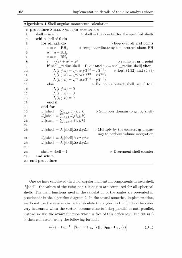
168 Implementation details of the disc analysis thorn
Algorithm 1 Shell angular momentum calculation1: procedure Shell angular momentum2: shell = nradii ▷ shell is the counter for the specified shells3: while shell = 0 do4: for all i,j,k do ▷ loop over all grid points5: x = x− BHx ▷ setup coordinate system centred about BH6: y = y − BHy
7: z = z − BHz
8: r =√x2 + y2 + z2 ▷ radius at grid point
9: if shell_radius[shell − 1] < r and r <= shell_radius[shell] then10: Jx(i, j, k) = √
γ α(y T 30 − z T 20) ▷ Eqs. (4.32) and (4.33)11: Jy(i, j, k) = √
γ α(z T 10 − xT 30)12: Jz(i, j, k) = √
γ α(xT 20 − y T 10)13: else ▷ For points outside shell, set Ji to 014: Jx(i, j, k) = 015: Jy(i, j, k) = 016: Jz(i, j, k) = 017: end if18: end for19: Jx[shell] =
∑i,j,k Jx(i, j, k) ▷ Sum over domain to get Ji(shell)
20: Jy[shell] =∑
i,j,k Jy(i, j, k)21: Jz[shell] =
∑i,j,k Jz(i, j, k)
22:23: Jx[shell] = Jx[shell]∆x∆y∆z ▷ Multiply by the coarsest grid spac-
ings to perform volume integration24: Jx[shell] = Jx[shell]∆x∆y∆z25: Jx[shell] = Jx[shell]∆x∆y∆z26:27: shell = shell − 1 ▷ Decrement shell counter28: end while29: end procedure
One we have calculated the fluid angular momentum components in each shell,Ji[shell], the values of the twist and tilt angles are computed for all sphericalshells. The main functions used in the calculation of the angles are presented inpseudocode in the algorithm diagram 2. In the actual numerical implementation,we do not use the inverse cosine to calculate the angles, as the function becomesvery inaccurate when the vectors become close to being parallel or anti-parallel,instead we use the atan2 function which is free of this deficiency. The tilt ν(r)is then calculated using the following formula:
ν(r) = tan−1[
|SBH × JDisc(r)| , SBH · JDisc(r)]
(B.1)
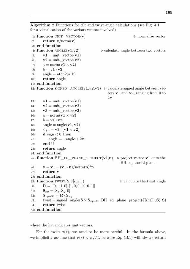
169
Algorithm 2 Functions for tilt and twist angle calculations (see Fig. 4.1for a visualisation of the various vectors involved)
1: function unit_vector(v) ▷ normalise vector2: return v/norm(v)3: end function4: function angle(v1,v2) ▷ calculate angle between two vectors5: v1 = unit_vector(v1)6: v2 = unit_vector(v2)7: a = norm(v1 × v2)8: b = v1 · v29: angle = atan2(a,b)
10: return angle11: end function12: function signed_angle(v1,v2,v3) ▷ calculate signed angle between vec-
tors v1 and v2, ranging from 0 to2π
13: v1 = unit_vector(v1)14: v2 = unit_vector(v2)15: v3 = unit_vector(v3)16: a = norm(v1 × v2)17: b = v1 · v218: angle = angle(v1,v2)19: sign = v3 · (v1 × v2)20: if sign < 0 then21: angle = −angle + 2π22: end if23: return angle24: end function25: function BH_eq_plane_project(v1,n) ▷ project vector v1 onto the
BH equatorial plane26: v = v1 − (v1 · n)/norm(n)2n27: return v28: end function29: function twist(S,J[shell]) ▷ calculate the twist angle30: R = [[0,−1, 0], [1, 0, 0], [0, 0, 1]]31: Sxy = [Sx,Sy, 0]32: Sxy−90 = R · Sxy
33: twist = signed_angle(S × Sxy−90,BH_eq_plane_project(J[shell],S),S)34: return twist35: end function
where the hat indicates unit vectors.For the twist σ(r), we need to be more careful. In the formula above,
we implicitly assume that ν(r) < π , ∀ t, because Eq. (B.1) will always return

170 Implementation details of the disc analysis thorn
angles ≤ π. Although it does not generally make much sense to consider angles≥ π between two 3D vectors, because there is an up and down direction, weare nevertheless interested in directional (signed) angles ≥ π for the twist σ.The reason is that we want to be able to track cumulative twists larger thanπ. In order to calculate the directional angle σ(r) from the reference vectorSBH × Sxy−90 to the target vector P(JDisc(r),SBH) in a fixed sense of rotation,we need a third reference vector that always lies above the plane spanned by thetwo original vectors. As the plane in which both vectors live is constructed to bethe equatorial plane of the BH, we can therefore choose this vector to be SBH.This information allows us (because the cross product contains this informationin the sign it returns) to calculate twist angles in the range [0, 2π].

Bibliography
[1] J. Abadie, B. P. Abbott, R. Abbott, M. Abernathy, T. Accadia, F. Ac-ernese, C. Adams, R. Adhikari, P. Ajith, B. Allen, and et al. “TopicalReview: Predictions for the rates of compact binary coalescences observ-able by ground-based gravitational-wave detectors.” In: Class. QuantumGrav. 27.17 (Sept. 2010), p. 173001.
[2] B. P. Abbott, R. Abbott, T. D. Abbott, M. R. Abernathy, F. Acernese,K. Ackley, C. Adams, T. Adams, P. Addesso, R. X. Adhikari, and et al.“Observation of Gravitational Waves from a Binary Black Hole Merger.”In: Physical Review Letters 116.6, 061102 (Feb. 2016), p. 061102. arXiv:1602.03837 [gr-qc].
[3] M. A. Abramowicz, M. Calvani, and L. Nobili. “Runaway instability inaccretion disks orbiting black holes.” In: Nature 302 (Apr. 1983), pp. 597–599.
[4] M. A. Abramowicz, W. Kluźniak, J. E. McClintock, and R. A. Remillard.“The Importance of Discovering a 3:2 Twin-Peak Quasi-periodic Oscilla-tion in an Ultraluminous X-Ray Source, or How to Solve the Puzzle ofIntermediate-Mass Black Holes.” In: Astrophys. J. Lett. 609 (July 2004),pp. L63–L65. eprint: astro-ph/0402012.
[5] F. C. Adams, S. P. Ruden, and F. H. Shu. “Eccentric gravitationalinstabilities in nearly Keplerian disks.” In: Astrophys. J. 347 (Dec. 1989),pp. 959–976.
[6] R. X. Adhikari. “Gravitational radiation detection with laser interferom-etry.” In: Reviews of Modern Physics 86 (Jan. 2014), pp. 121–151. arXiv:1305.5188 [gr-qc].
[7] J. Adsuara, I. Cordero-Carrión, P. Cerdá-Durán, V. Mewes, and M. Á.Aloy. “Optimal Scheduled Relaxation Jacobi method.” In: Submitted toCommunications in Computational Physics (2016).
[8] M. Alcubierre. “Hyperbolic slicings of spacetime: singularity avoidanceand gauge shocks.” In: Classical and Quantum Gravity 20 (Feb. 2003),pp. 607–623. eprint: gr-qc/0210050.
[9] M. Alcubierre. Introduction to 3+1 Numerical Relativity. Oxford Univer-sity Press, 2008.
[10] M. Alcubierre and B. Brügmann. “Simple excision of a black hole in3+1 numerical relativity.” In: Phys. Rev. D 63.10, 104006 (May 2001),p. 104006. eprint: gr-qc/0008067.

172 Bibliography
[11] M. Alcubierre, B. Brügmann, P. Diener, M. Koppitz, D. Pollney, E. Seidel,and R. Takahashi. “Gauge conditions for long-term numerical black holeevolutions without excision.” In: Phys. Rev. D 67.8, 084023 (Apr. 2003),p. 084023. eprint: gr-qc/0206072.
[12] M. Alcubierre, B. Brügmann, T. Dramlitsch, J. A. Font, P. Papadopoulos,E. Seidel, N. Stergioulas, and R. Takahashi. “Towards a stable numericalevolution of strongly gravitating systems in general relativity: The con-formal treatments.” In: Phys. Rev. D 62.4, 044034 (Aug. 2000), p. 044034.eprint: gr-qc/0003071.
[13] D. Alic, C. Bona-Casas, C. Bona, L. Rezzolla, and C. Palenzuela. “Confor-mal and covariant formulation of the Z4 system with constraint-violationdamping.” In: Phys. Rev. D 85.6, 064040 (Mar. 2012), p. 064040. arXiv:1106.2254 [gr-qc].
[14] D. Alic, L. Rezzolla, I. Hinder, and P. Mösta. “Dynamical damping termsfor symmetry-seeking shift conditions.” In: Classical and Quantum Gravity27.24, 245023 (Dec. 2010), p. 245023. arXiv: 1008.2212 [gr-qc].
[15] M. A. Aloy, J. M. Ibáñez, J. M. Martı/, and E. Müller. “GENESIS: A High-Resolution Code for Three-dimensional Relativistic Hydrodynamics.” In:Astrophys. J. Suppl. Ser. 122 (May 1999), pp. 151–166. eprint: astro-ph/9903352.
[16] M. A. Aloy, H.-T. Janka, and E. Müller. “Relativistic outflows fromremnants of compact object mergers and their viability for short gamma-ray bursts.” In: Astron. Astrophys. 436 (June 2005), pp. 273–311. eprint:astro-ph/0408291.
[17] P. Anninos, D. Bernstein, S. Brandt, J. Libson, J. Massó, E. Seidel, L.Smarr, W.-M. Suen, and P. Walker. “Dynamics of Apparent and EventHorizons.” In: Physical Review Letters 74 (Jan. 1995), pp. 630–633. eprint:gr-qc/9403011.
[18] R. Arnowitt, S. Deser, and C. W. Misner. “Republication of: The dynamicsof general relativity.” In: General Relativity and Gravitation 40 (Sept.2008), pp. 1997–2027. eprint: gr-qc/0405109.
[19] A. Ashtekar, C. Beetle, and S. Fairhurst. “Isolated horizons: a general-ization of black hole mechanics.” In: Classical and Quantum Gravity 16(Feb. 1999), pp. L1–L7. eprint: gr-qc/9812065.
[20] A. Ashtekar and B. Krishnan. “Dynamical horizons and their properties.”In: Phys. Rev. D 68.10, 104030 (Nov. 2003), p. 104030. eprint: gr-qc/0308033.
[21] A. Ashtekar and B. Krishnan. “Isolated and Dynamical Horizons andTheir Applications.” In: Living Reviews in Relativity 7 (Dec. 2004). eprint:gr-qc/0407042.
[22] M. Babiuc, B. Szilágyi, I. Hawke, and Y. Zlochower. “Gravitational waveextraction based on Cauchy characteristic extraction and characteristicevolution.” In: Classical and Quantum Gravity 22 (Dec. 2005), pp. 5089–5107. eprint: gr-qc/0501008.

Bibliography 173
[23] L. Baiotti, R. de Pietri, G. M. Manca, and L. Rezzolla. “Accurate simu-lations of the dynamical bar-mode instability in full general relativity.”In: Phys. Rev. D 75.4, 044023 (Feb. 2007), p. 044023. eprint: astro -ph/0609473.
[24] L. Baiotti, I. Hawke, P. J. Montero, F. Löffler, L. Rezzolla, N. Stergioulas,J. A. Font, and E. Seidel. “Three-dimensional relativistic simulations ofrotating neutron-star collapse to a Kerr black hole.” In: Phys. Rev. D71.2, 024035 (Jan. 2005), p. 024035. eprint: gr-qc/0403029.
[25] L. Baiotti, I. Hawke, and L. Rezzolla. “On the gravitational radiationfrom the collapse of neutron stars to rotating black holes.” In: Classicaland Quantum Gravity 24 (June 2007), S187–S206. eprint: gr-qc/0701043.
[26] J. G. Baker, J. Centrella, D.-I. Choi, M. Koppitz, and J. van Meter.“Gravitational-Wave Extraction from an Inspiraling Configuration ofMerging Black Holes.” In: Physical Review Letters 96.11, 111102 (Mar.2006), p. 111102. eprint: gr-qc/0511103.
[27] J. G. Baker, J. R. van Meter, S. T. McWilliams, J. Centrella, and B. J.Kelly. “Consistency of Post-Newtonian Waveforms with Numerical Rela-tivity.” In: Physical Review Letters 99.18, 181101 (Nov. 2007), p. 181101.eprint: gr-qc/0612024.
[28] J. Baker, M. Campanelli, and C. O. Lousto. “The Lazarus project: Apragmatic approach to binary black hole evolutions.” In: Phys. Rev. D65.4, 044001 (Feb. 2002), p. 044001. eprint: gr-qc/0104063.
[29] S. A. Balbus. “Enhanced Angular Momentum Transport in AccretionDisks.” In: Annu. Rev. Astron. Astrophys. 41 (2003), pp. 555–597. eprint:astro-ph/0306208.
[30] S. A. Balbus and J. F. Hawley. “A powerful local shear instability inweakly magnetized disks. I - Linear analysis. II - Nonlinear evolution.”In: Astrophys. J. 376 (July 1991), pp. 214–233.
[31] F. Banyuls, J. A. Font, J. M. Ibáñez, J. M. Martí, and J. A. Miralles.“Numerical 3 + 1 General Relativistic Hydrodynamics: A Local Char-acteristic Approach.” In: Astrophys. J. 476 (Feb. 1997), pp. 221–231.
[32] J. M. Bardeen and J. A. Petterson. “The Lense-Thirring Effect andAccretion Disks around Kerr Black Holes.” In: Astrophys. J. Lett. 195(Jan. 1975), p. L65.
[33] T. W. Baumgarte, P. J. Montero, I. Cordero-Carrión, and E. Müller.“Numerical relativity in spherical polar coordinates: Evolution calculationswith the BSSN formulation.” In: Phys. Rev. D 87.4, 044026 (Feb. 2013),p. 044026. arXiv: 1211.6632 [gr-qc].
[34] T. W. Baumgarte and S. L. Shapiro. “Numerical integration of Einstein’sfield equations.” In: Phys. Rev. D 59.2, 024007 (Jan. 1999), p. 024007.eprint: gr-qc/9810065.
[35] T. W. Baumgarte and S. L. Shapiro. Numerical Relativity: Solving Ein-stein’s Equations on the Computer. June 2010.
[36] K. Belczynski, M. Dominik, T. Bulik, R. O’Shaughnessy, C. Fryer, andD. E. Holz. “The Effect of Metallicity on the Detection Prospects forGravitational Waves.” In: Astrophys. J. Lett. 715 (June 2010), pp. L138–L141. arXiv: 1004.0386 [astro-ph.HE].

174 Bibliography
[37] K. Belczynski, R. E. Taam, E. Rantsiou, and M. van der Sluys. “BlackHole Spin Evolution: Implications for Short-Hard Gamma-Ray Burstsand Gravitational Wave Detection.” In: Astrophys. J. 682, 474-486 (July2008), pp. 474–486. eprint: astro-ph/0703131.
[38] K. Belczynski, G. Wiktorowicz, C. L. Fryer, D. E. Holz, and V. Kalogera.“Missing Black Holes Unveil the Supernova Explosion Mechanism.” In:Astrophys. J. 757, 91 (Sept. 2012), p. 91. arXiv: 1110.1635.
[39] T. M. Belloni and L. Stella. “Fast Variability from Black-Hole Binaries.”In: Space Science Reviews 183.1 (2014), pp. 43–60. issn: 1572-9672.
[40] M. J. Berger and J. Oliger. “Adaptive Mesh Refinement for HyperbolicPartial Differential Equations.” In: Journal of Computational Physics 53(Mar. 1984), pp. 484–512.
[41] E. Berti, V. Cardoso, and C. M. Will. “Gravitational-wave spectroscopyof massive black holes with the space interferometer LISA.” In: Phys. Rev.D 73.6, 064030 (Mar. 2006), p. 064030. eprint: gr-qc/0512160.
[42] H. Beyer and O. Sarbach. “Well-posedness of the Baumgarte-Shapiro-Shibata-Nakamura formulation of Einstein’s field equations.” In: Phys.Rev. D 70.10, 104004 (Nov. 2004), p. 104004. eprint: gr-qc/0406003.
[43] O. M. Blaes. “Stabilization of non-axisymmetric instabilities in a rotatingflow by accretion on to a central black hole.” In: Mon. Not. R. Astron.Soc. 227 (Aug. 1987), pp. 975–992.
[44] L. Blanchet, B. R. Iyer, C. M. Will, and A. G. Wiseman. “Gravitationalwaveforms from inspiralling compact binaries to second-post-Newtonianorder.” In: Classical and Quantum Gravity 13 (Apr. 1996), pp. 575–584.eprint: gr-qc/9602024.
[45] C. Bona, T. Ledvinka, C. Palenzuela, and M. Žáček. “General-covariantevolution formalism for numerical relativity.” In: Phys. Rev. D 67.10,104005 (May 2003), p. 104005. eprint: gr-qc/0302083.
[46] C. Bona, J. Massó, E. Seidel, and J. Stela. “New Formalism for NumericalRelativity.” In: Physical Review Letters 75 (July 1995), pp. 600–603.eprint: gr-qc/9412071.
[47] C. Bona and C. Palenzuela. “Dynamical shift conditions for the Z4 andBSSN formalisms.” In: Phys. Rev. D 69.10, 104003 (May 2004), p. 104003.eprint: gr-qc/0401019.
[48] S. Bonazzola and E. Gourgoulhon. “A virial identity applied to relativis-tic stellar models.” In: Classical and Quantum Gravity 11 (July 1994),pp. 1775–1784.
[49] S. Bonazzola, E. Gourgoulhon, P. Grandclément, and J. Novak. “Con-strained scheme for the Einstein equations based on the Dirac gaugeand spherical coordinates.” In: Phys. Rev. D 70.10, 104007 (Nov. 2004),p. 104007. eprint: gr-qc/0307082.
[50] S. Brandt and B. Brügmann. “A Simple Construction of Initial Datafor Multiple Black Holes.” In: Physical Review Letters 78 (May 1997),pp. 3606–3609. eprint: gr-qc/9703066.
[51] D. R. Brill and R. W. Lindquist. “Interaction Energy in Geometrostatics.”In: Physical Review 131 (July 1963), pp. 471–476.

Bibliography 175
[52] D. Brown, P. Diener, O. Sarbach, E. Schnetter, and M. Tiglio. “Turduck-ening black holes: An analytical and computational study.” In: Phys. Rev.D 79.4, 044023 (Feb. 2009), p. 044023. arXiv: 0809.3533 [gr-qc].
[53] B. Brügmann, J. A. González, M. Hannam, S. Husa, and U. Sperhake.“Exploring black hole superkicks.” In: Phys. Rev. D 77.12, 124047 (June2008), p. 124047. arXiv: 0707.0135 [gr-qc].
[54] B. Brügmann, W. Tichy, and N. Jansen. “Numerical Simulation of Orbit-ing Black Holes.” In: Physical Review Letters 92.21, 211101 (May 2004),p. 211101. eprint: gr-qc/0312112.
[55] Cactus Computational Toolkit. http://www.cactuscode.org/.[56] G. Allen, T. Goodale, G. Lanfermann, T. Radke, D. Rideout, and J.
Thornburg. Cactus Users’ Guide. 2011. url: http://www.cactuscode.org/Guides/Stable/UsersGuide/UsersGuideStable.pdf.
[57] M. Campanelli, C. O. Lousto, P. Marronetti, and Y. Zlochower. “AccurateEvolutions of Orbiting Black-Hole Binaries without Excision.” In: PhysicalReview Letters 96.11, 111101 (Mar. 2006), p. 111101. eprint: gr - qc/0511048.
[58] M. Campanelli, C. O. Lousto, and Y. Zlochower. “Spinning-black-holebinaries: The orbital hang-up.” In: Phys. Rev. D 74.4, 041501 (Aug. 2006),p. 041501. eprint: gr-qc/0604012.
[59] M. Campanelli, C. O. Lousto, Y. Zlochower, B. Krishnan, and D. Merritt.“Spin flips and precession in black-hole-binary mergers.” In: Phys. Rev. D75.6, 064030 (Mar. 2007), p. 064030. eprint: gr-qc/0612076.
[60] Carpet. http://carpetcode.org.[61] S. Chandrasekhar. “The Stability of Non-Dissipative Couette Flow in
Hydromagnetics.” In: Proceedings of the National Academy of Science 46(Feb. 1960), pp. 253–257.
[62] Y. Choquet-Bruhat. “Théorème d’existence pour certains systèmes d’équationsaux dérivées partielles non linéaires.” In: Acta Mathematica, Volume 88,Issue 1, pp 141-225 88 (1952).
[63] Y. Choquet-Bruhat and T. Ruggeri. “Hyperbolicity of the 3+1 systemof Einstein equations.” In: Communications in Mathematical Physics 89(June 1983), pp. 269–275.
[64] D. Christodoulou. “Reversible and Irreversible Transformations in Black-Hole Physics.” In: Physical Review Letters 25 (Nov. 1970), pp. 1596–1597.
[65] D. M. Christodoulou and R. Narayan. “The stability of accretion tori.IV - Fission and fragmentation of slender, self-gravitating annuli.” In:Astrophys. J. 388 (Apr. 1992), pp. 451–466.
[66] P. Colella and P. R. Woodward. “The Piecewise Parabolic Method (PPM)for Gas-Dynamical Simulations.” In: Journal of Computational Physics54 (Sept. 1984), pp. 174–201.
[67] G. B. Cook, M. W. Choptuik, M. R. Dubal, S. Klasky, R. A. Matzner,and S. R. Oliveira. “Three-dimensional initial data for the collision oftwo black holes.” In: Phys. Rev. D 47 (Feb. 1993), pp. 1471–1490.

176 Bibliography
[68] I. Cordero-Carrión, P. Cerdá-Durán, H. Dimmelmeier, J. L. Jaramillo,J. Novak, and E. Gourgoulhon. “Improved constrained scheme for theEinstein equations: An approach to the uniqueness issue.” In: Phys. Rev.D 79.2, 024017 (Jan. 2009), p. 024017. arXiv: 0809.2325 [gr-qc].
[69] R. Courant and D. Hilbert. Methods of mathematical physics. Vol. II:Partial differential equations.(Vol. II by R. Courant.) 1962.
[70] F. Daigne and J. A. Font. “The runaway instability of thick discs aroundblack holes - II. Non-constant angular momentum discs.” In: Mon. Not.R. Astron. Soc. 349 (Apr. 2004), pp. 841–868. eprint: astro-ph/0311618.
[71] F. Daigne and R. Mochkovitch. “Gamma-ray bursts and the runawayinstability of thick discs around black holes.” In: Mon. Not. R. Astron.Soc. 285 (Mar. 1997), pp. L15–L19.
[72] G. Darmois. “Les équations de la gravitation einsteinienne.” In: Mémorialdes sciences mathématiques 25 (1927), pp. 1–48.
[73] M. Demianski and P. B. Ivanov. “The dynamics of twisted accretiondisc around a Kerr black hole.” In: Astron. Astrophys. 324 (Aug. 1997),pp. 829–834.
[74] K. A. Dennison, T. W. Baumgarte, and P. J. Montero. “Trumpet Slicesin Kerr Spacetimes.” In: Physical Review Letters 113.26, 261101 (Dec.2014), p. 261101. arXiv: 1409.1887 [gr-qc].
[75] P. A. M. Dirac. “Forms of Relativistic Dynamics.” In: Rev. Mod. Phys.21.3 (July 1949), pp. 392–399.
[76] M. Dominik, K. Belczynski, C. Fryer, D. E. Holz, E. Berti, T. Bulik,I. Mandel, and R. O’Shaughnessy. “Double Compact Objects. II. Cosmo-logical Merger Rates.” In: Astrophys. J. 779, 72 (Dec. 2013), p. 72.
[77] M. Dominik, E. Berti, R. O’Shaughnessy, I. Mandel, K. Belczynski, C.Fryer, D. E. Holz, T. Bulik, and F. Pannarale. “Double Compact ObjectsIII: Gravitational-wave Detection Rates.” In: Astrophys. J. 806, 263 (June2015), p. 263. arXiv: 1405.7016 [astro-ph.HE].
[78] R. Donat and A. Marquina. “Capturing Shock Reflections: An ImprovedFlux Formula.” In: J. Comp. Phys. 125 (Apr. 1996), pp. 42–58.
[79] O. Dreyer, B. Krishnan, D. Shoemaker, and E. Schnetter. “Introductionto isolated horizons in numerical relativity.” In: Phys. Rev. D 67.2, 024018(Jan. 2003), p. 024018. eprint: gr-qc/0206008.
[80] B. Einfeldt. “On Godunov-type methods for gas dynamics.” In: SIAMJournal on Numerical Analysis 25.2 (1988), pp. 294–318.
[81] Einstein Toolkit. http://einsteintoolkit.org/.[82] A. Einstein. “Die Feldgleichungen der Gravitation.” In: Sitzungsberichte
der Königlich Preußischen Akademie der Wissenschaften (Berlin), Seite844-847. (1915).
[83] A. Einstein. “Die Grundlage der allgemeinen Relativitätstheorie.” In:Annalen der Physik 354 (1916), pp. 769–822.
[84] A. Einstein. “Über Gravitationswellen.” In: Sitzungsberichte der KöniglichPreußischen Akademie der Wissenschaften (Berlin), Seite 154-167. (1918).

Bibliography 177
[85] T. Ertl, H.-T. Janka, S. E. Woosley, T. Sukhbold, and M. Ugliano. “ATwo-parameter Criterion for Classifying the Explodability of MassiveStars by the Neutrino-driven Mechanism.” In: Astrophys. J. 818, 124 (Feb.2016), p. 124. arXiv: 1503.07522 [astro-ph.SR].
[86] Z. B. Etienne, J. A. Faber, Y. T. Liu, S. L. Shapiro, K. Taniguchi,and T. W. Baumgarte. “Fully general relativistic simulations of blackhole-neutron star mergers.” In: Phys. Rev. D 77.8, 084002 (Apr. 2008),p. 084002. arXiv: 0712.2460.
[87] J. A. Faber, T. W. Baumgarte, Z. B. Etienne, S. L. Shapiro, and K.Taniguchi. “Relativistic hydrodynamics in the presence of puncture blackholes.” In: Phys. Rev. D 76.10, 104021 (Nov. 2007), p. 104021. arXiv:0708.2436 [gr-qc].
[88] J. A. Faber and F. A. Rasio. “Binary Neutron Star Mergers.” In: LivingReviews in Relativity 15 (July 2012). arXiv: 1204.3858 [gr-qc].
[89] B. D. Farris, P. Duffell, A. I. MacFadyen, and Z. Haiman. “Binary BlackHole Accretion from a Circumbinary Disk: Gas Dynamics inside theCentral Cavity.” In: Astrophys. J. 783, 134 (Mar. 2014), p. 134. arXiv:1310.0492 [astro-ph.HE].
[90] A. E. Fischer and J. E. Marsden. “The Einstein Equations of Evolution-AGeometric Approach.” In: J. Math. Phys. 13 (Apr. 1972), pp. 546–568.
[91] É. É. Flanagan and S. A. Hughes. “Measuring gravitational waves frombinary black hole coalescences. I. Signal to noise for inspiral, merger,and ringdown.” In: Phys. Rev. D 57 (Apr. 1998), pp. 4535–4565. eprint:gr-qc/9701039.
[92] J. A. Font. “Numerical Hydrodynamics and Magnetohydrodynamics inGeneral Relativity.” In: Living Reviews in Relativity 11 (Sept. 2008).
[93] J. A. Font and F. Daigne. “The runaway instability of thick discs aroundblack holes - I. The constant angular momentum case.” In: Mon. Not. R.Astron. Soc. 334 (Aug. 2002), pp. 383–400. eprint: astro-ph/0203403.
[94] F. Foucart. “Black-hole-neutron-star mergers: Disk mass predictions.”In: Phys. Rev. D 86.12, 124007 (Dec. 2012), p. 124007. arXiv: 1207.6304[astro-ph.HE].
[95] F. Foucart, M. B. Deaton, M. D. Duez, L. E. Kidder, I. MacDonald,C. D. Ott, H. P. Pfeiffer, M. A. Scheel, B. Szilagyi, and S. A. Teukolsky.“Black-hole-neutron-star mergers at realistic mass ratios: Equation ofstate and spin orientation effects.” In: Phys. Rev. D 87.8, 084006 (Apr.2013), p. 084006. arXiv: 1212.4810 [gr-qc].
[96] F. Foucart, M. B. Deaton, M. D. Duez, E. O’Connor, C. D. Ott, R. Haas,L. E. Kidder, H. P. Pfeiffer, M. A. Scheel, and B. Szilagyi. “Neutronstar-black hole mergers with a nuclear equation of state and neutrinocooling: Dependence in the binary parameters.” In: Phys. Rev. D 90.2,024026 (July 2014), p. 024026. arXiv: 1405.1121 [astro-ph.HE].
[97] F. Foucart, M. D. Duez, L. E. Kidder, and S. A. Teukolsky. “Black hole-neutron star mergers: Effects of the orientation of the black hole spin.”In: Phys. Rev. D 83.2, 024005 (Jan. 2011), p. 024005. arXiv: 1007.4203[astro-ph.HE].

178 Bibliography
[98] F. Foucart and D. Lai. “Evolution of linear warps in accretion discs andapplications to protoplanetary discs in binaries.” In: Mon. Not. R. Astron.Soc. 445 (Dec. 2014), pp. 1731–1744. arXiv: 1406.3331 [astro-ph.EP].
[99] P. C. Fragile and P. Anninos. “Hydrodynamic Simulations of TiltedThick-Disk Accretion onto a Kerr Black Hole.” In: Astrophys. J. 623 (Apr.2005), pp. 347–361. eprint: astro-ph/0403356.
[100] P. C. Fragile, O. M. Blaes, P. Anninos, and J. D. Salmonson. “GlobalGeneral Relativistic Magnetohydrodynamic Simulation of a Tilted BlackHole Accretion Disk.” In: Astrophys. J. 668 (Oct. 2007), pp. 417–429.arXiv: 0706.4303.
[101] P. C. Fragile, G. J. Mathews, and J. R. Wilson. “Bardeen-Petterson Effectand Quasi-periodic Oscillations in X-Ray Binaries.” In: Astrophys. J. 553(June 2001), pp. 955–959. eprint: astro-ph/0007478.
[102] T. Fragos, M. Tremmel, E. Rantsiou, and K. Belczynski. “Black HoleSpin-Orbit Misalignment in Galactic X-ray Binaries.” In: Astrophys. J.Lett. 719 (Aug. 2010), pp. L79–L83. arXiv: 1001.1107 [astro-ph.HE].
[103] A. Franchini, G. Lodato, and S. Facchini. “Lense-Thirring precessionaround supermassive black holes during tidal disruption events.” In: Mon.Not. R. Astron. Soc. 455 (Jan. 2016), pp. 1946–1956. arXiv: 1510.04879[astro-ph.HE].
[104] H. Friedrich. “Hyperbolic reductions for Einstein’s equations.” In: Classicaland Quantum Gravity 13 (June 1996), pp. 1451–1469.
[105] C. L. Fryer, K. Belczynski, G. Wiktorowicz, M. Dominik, V. Kalogera,and D. E. Holz. “Compact Remnant Mass Function: Dependence on theExplosion Mechanism and Metallicity.” In: Astrophys. J. 749, 91 (Apr.2012), p. 91. arXiv: 1110.1726 [astro-ph.SR].
[106] C. L. Fryer, S. E. Woosley, M. Herant, and M. B. Davies. “Merging WhiteDwarf/Black Hole Binaries and Gamma-Ray Bursts.” In: Astrophys. J.520 (Aug. 1999), pp. 650–660. eprint: astro-ph/9808094.
[107] W. Fu and D. Lai. “Papaloizou-Pringle instability of magnetized accretiontori.” In: Mon. Not. R. Astron. Soc. 410 (Jan. 2011), pp. 1617–1630. arXiv:1006.3824 [astro-ph.HE].
[108] F. Galeazzi, W. Kastaun, L. Rezzolla, and J. A. Font. “Implementation ofa simplified approach to radiative transfer in general relativity.” In: Phys.Rev. D 88.6, 064009 (Sept. 2013), p. 064009. arXiv: 1306.4953 [gr-qc].
[109] D. Garfinkle, C. Gundlach, and D. Hilditch. “Comments on Bona Massó-type slicing conditions in long-term black hole evolutions.” In: Classicaland Quantum Gravity 25.7, 075007 (Apr. 2008), p. 075007. arXiv: 0707.0726 [gr-qc].
[110] B. Giacomazzo and R. Perna. “Formation of Stable Magnetars fromBinary Neutron Star Mergers.” In: Astrophys. J. Lett. 771, L26 (July2013), p. L26. arXiv: 1306.1608 [astro-ph.HE].
[111] S. K. Godunov. “A difference method for numerical calculation of discon-tinuous solutions of the equations of hydrodynamics.” In: Mat. Sb. 89.3(1959), pp. 271–306.

Bibliography 179
[112] R. Gold and B. Brügmann. “Eccentric black hole mergers and zoom-whirlbehavior from elliptic inspirals to hyperbolic encounters.” In: Phys. Rev.D 88.6, 064051 (Sept. 2013), p. 064051. arXiv: 1209.4085 [gr-qc].
[113] R. Gold, V. Paschalidis, Z. B. Etienne, S. L. Shapiro, and H. P. Pfeiffer.“Accretion disks around binary black holes of unequal mass: General rela-tivistic magnetohydrodynamic simulations near decoupling.” In: Phys. Rev.D 89.6, 064060 (Mar. 2014), p. 064060. arXiv: 1312.0600 [astro-ph.HE].
[114] T. Goodale, G. Allen, G. Lanfermann, J. Massó, T. Radke, E. Seidel,and J. Shalf. “High Performance Computing for Computational Science
— VECPAR 2002: 5th International Conference Porto, Portugal, June26–28, 2002 Selected Papers and Invited Talks.” In: ed. by J. M. L. M.Palma, A. A. Sousa, J. Dongarra, and V. Hernández. Berlin, Heidelberg:Springer Berlin Heidelberg, 2003. Chap. The Cactus Framework andToolkit: Design and Applications, pp. 197–227. isbn: 978-3-540-36569-3.
[115] J. Goodman, R. Narayan, and P. Goldreich. “The stability of accretiontori. II - Non-linear evolution to discrete planets.” In: Mon. Not. R. Astron.Soc. 225 (Apr. 1987), pp. 695–711.
[116] J. Goodman and R. R. Rafikov. “Planetary Torques as the Viscosity ofProtoplanetary Disks.” In: Astrophys. J. 552 (May 2001), pp. 793–802.eprint: astro-ph/0010576.
[117] E. Gourgoulhon, ed. 3+1 Formalism in General Relativity. Vol. 846.Lecture Notes in Physics, Springer. 2012.
[118] E. Gourgoulhon and S. Bonazzola. “A formulation of the virial theoremin general relativity.” In: Classical and Quantum Gravity 11 (Feb. 1994),pp. 443–452.
[119] C. Gundlach and J. M. Martín-García. “Well-posedness of formulationsof the Einstein equations with dynamical lapse and shift conditions.” In:Phys. Rev. D 74.2, 024016 (July 2006), p. 024016. eprint: gr-qc/0604035.
[120] I. Hachisu, J. E. Tohline, and Y. Eriguchi. “Fragmentation of rapidlyrotating gas clouds. I - A universal criterion for fragmentation.” In:Astrophys. J. 323 (Dec. 1987), pp. 592–613.
[121] M. Hannam, S. Husa, D. Pollney, B. Brügmann, and N. Ó. Murchadha.“Geometry and Regularity of Moving Punctures.” In: Physical ReviewLetters 99.24, 241102 (Dec. 2007), p. 241102. eprint: gr-qc/0606099.
[122] A. Harten, B. Engquist, S. Osher, and S. R. Chakravarthy. “Uniformlyhigh order accurate essentially non-oscillatory schemes, III.” In: Upwindand High-Resolution Schemes. Springer, 1987, pp. 218–290.
[123] A. Harten, P. D. Lax, and B. v. Leer. “On upstream differencing andGodunov-type schemes for hyperbolic conservation laws.” In: SIAM review25.1 (1983), pp. 35–61.
[124] S. W. Hawking and G. F. R. Ellis. The Large Scale Structure of Space-Time. 1975.
[125] J. F. Hawley. “Non-linear evolution of a non-axisymmetric disc instability.”In: Mon. Not. R. Astron. Soc. 225 (Apr. 1987), pp. 677–694.
[126] J. F. Hawley. “Three-dimensional simulations of black hole tori.” In:Astrophys. J. 381 (Nov. 1991), pp. 496–507.

180 Bibliography
[127] M. H. M. Heemskerk, J. C. Papaloizou, and G. J. Savonije. “Non-lineardevelopment of M = 1 instabilities in a self-gravitating gaseous disc.” In:Astron. Astrophys. 260 (July 1992), pp. 161–174.
[128] A. Heger, N. Langer, and S. E. Woosley. “Presupernova Evolution of Ro-tating Massive Stars. I. Numerical Method and Evolution of the InternalStellar Structure.” In: Astrophys. J. 528 (Jan. 2000), pp. 368–396. eprint:astro-ph/9904132.
[129] T. Heinemann and J. C. B. Papaloizou. “A weakly non-linear theoryfor spiral density waves excited by accretion disc turbulence.” In: Mon.Not. R. Astron. Soc. 419 (Jan. 2012), pp. 1085–1096. arXiv: 1109.2907[astro-ph.EP].
[130] K. B. Henisey, O. M. Blaes, and P. C. Fragile. “Variability from Non-axisymmetric Fluctuations Interacting with Standing Shocks in TiltedBlack Hole Accretion Disks.” In: Astrophys. J. 761, 18 (Dec. 2012), p. 18.arXiv: 1211.2273 [astro-ph.HE].
[131] S. Hild. “Beyond the second generation of laser-interferometric gravi-tational wave observatories.” In: Classical and Quantum Gravity 29.12,124006 (June 2012), p. 124006. arXiv: 1111.6277 [gr-qc].
[132] I. Hinder. “The current status of binary black hole simulations in numeri-cal relativity.” In: Classical and Quantum Gravity 27.11, 114004 (June2010), p. 114004. arXiv: 1001.5161 [gr-qc].
[133] I. Hinder, B. Wardell, and E. Bentivegna. “Falloff of the Weyl scalars inbinary black hole spacetimes.” In: Phys. Rev. D 84.2, 024036 (July 2011),p. 024036. arXiv: 1105.0781 [gr-qc].
[134] K. Hotokezaka, K. Kiuchi, K. Kyutoku, T. Muranushi, Y.-i. Sekiguchi,M. Shibata, and K. Taniguchi. “Remnant massive neutron stars of binaryneutron star mergers: Evolution process and gravitational waveform.”In: Phys. Rev. D 88.4, 044026 (Aug. 2013), p. 044026. arXiv: 1307.5888[astro-ph.HE].
[135] K. Hotokezaka, K. Kiuchi, K. Kyutoku, H. Okawa, Y.-i. Sekiguchi, M.Shibata, and K. Taniguchi. “Mass ejection from the merger of binaryneutron stars.” In: Phys. Rev. D 87.2, 024001 (Jan. 2013), p. 024001.arXiv: 1212.0905 [astro-ph.HE].
[136] R. A. Hulse and J. H. Taylor. “Discovery of a pulsar in a binary system.”In: Astrophys. J. Lett. 195 (Jan. 1975), pp. L51–L53.
[137] S. Husa, I. Hinder, and C. Lechner. “Kranc: a Mathematica package togenerate numerical codes for tensorial evolution equations.” In: ComputerPhysics Communications 174 (June 2006), pp. 983–1004. eprint: gr -qc/0404023.
[138] J. M. Hyman. “Method of lines solution of partial differential equations.”In: (1976).
[139] P. B. Ivanov and A. F. Illarionov. “The oscillatory shape of the stationarytwisted disc around a Kerr black hole.” In: Mon. Not. R. Astron. Soc.285 (Feb. 1997), pp. 394–402.
[140] H.-T. Janka, T. Eberl, M. Ruffert, and C. L. Fryer. “Black Hole-NeutronStar Mergers as Central Engines of Gamma-Ray Bursts.” In: Astrophys.J. Lett. 527 (Dec. 1999), pp. L39–L42. eprint: astro-ph/9908290.
Bibliography 181
[141] J. L. Jaramillo and E. Gourgoulhon. “Mass and Angular Momentum inGeneral Relativity.” In: Mass and Motion in General Relativity. Ed. byL. Blanchet, A. Spallicci, and B. Whiting. 2011, pp. 87–124.
[142] W. Kastaun and F. Galeazzi. “Properties of hypermassive neutron starsformed in mergers of spinning binaries.” In: Phys. Rev. D 91.6, 064027(Mar. 2015), p. 064027. arXiv: 1411.7975 [gr-qc].
[143] J. Katz. “A note on Komar’s anomalous factor.” In: Classical and QuantumGravity 2 (May 1985), pp. 423–425.
[144] K. Kawaguchi, K. Kyutoku, H. Nakano, H. Okawa, M. Shibata, andK. Taniguchi. “Black hole-neutron star binary merger: Dependence onblack hole spin orientation and equation of state.” In: Phys. Rev. D 92.2,024014 (July 2015), p. 024014. arXiv: 1506.05473 [astro-ph.HE].
[145] R. P. Kerr. “Gravitational Field of a Spinning Mass as an Example ofAlgebraically Special Metrics.” In: Physical Review Letters 11 (Sept. 1963),pp. 237–238.
[146] L. E. Kidder. “Coalescing binary systems of compact objects to (post)5/2-Newtonian order. V. Spin effects.” In: Phys. Rev. D 52 (July 1995),pp. 821–847. eprint: gr-qc/9506022.
[147] A. R. King, S. H. Lubow, G. I. Ogilvie, and J. E. Pringle. “Aligningspinning black holes and accretion discs.” In: Mon. Not. R. Astron. Soc.363 (Oct. 2005), pp. 49–56. eprint: astro-ph/0507098.
[148] K. Kiuchi, P. Cerdá-Durán, K. Kyutoku, Y. Sekiguchi, and M. Shibata.“Efficient magnetic-field amplification due to the Kelvin-Helmholtz insta-bility in binary neutron star mergers.” In: Phys. Rev. D 92.12, 124034(Dec. 2015), p. 124034. arXiv: 1509.09205 [astro-ph.HE].
[149] K. Kiuchi, Y. Sekiguchi, K. Kyutoku, M. Shibata, K. Taniguchi, andT. Wada. “High resolution magnetohydrodynamic simulation of blackhole-neutron star merger: Mass ejection and short gamma ray bursts.”In: Phys. Rev. D 92.6, 064034 (Sept. 2015), p. 064034. arXiv: 1506.06811[astro-ph.HE].
[150] K. Kiuchi, M. Shibata, P. J. Montero, and J. A. Font. “GravitationalWaves from the Papaloizou-Pringle Instability in Black-Hole-Torus Sys-tems.” In: Physical Review Letters 106.25, 251102 (June 2011), p. 251102.arXiv: 1105.5035 [astro-ph.HE].
[151] A. Komar. “Covariant Conservation Laws in General Relativity.” In:Physical Review 113 (Feb. 1959), pp. 934–936.
[152] A. Komar. “Necessity of Singularities in the Solution of the Field Equa-tions of General Relativity.” In: Physical Review 104 (Oct. 1956), pp. 544–546.
[153] O. Korobkin, E. B. Abdikamalov, E. Schnetter, N. Stergioulas, and B.Zink. “Stability of general-relativistic accretion disks.” In: Phys. Rev. D83.4, 043007 (Feb. 2011), p. 043007. arXiv: 1011.3010 [astro-ph.HE].
[154] O. Korobkin, E. Abdikamalov, N. Stergioulas, E. Schnetter, B. Zink, S.Rosswog, and C. D. Ott. “The runaway instability in general relativisticaccretion discs.” In: Mon. Not. R. Astron. Soc. 431 (May 2013), pp. 349–354. arXiv: 1210.1214 [astro-ph.HE].

182 Bibliography
[155] Y. Kozai. “Secular perturbations of asteroids with high inclination andeccentricity.” In: Astrophys. J. 67 (Nov. 1962), p. 591.
[156] D. Kramer and E. Schmutzer. Exact solutions of Einstein’s field equations.1980.
[157] L. Kreidberg, C. D. Bailyn, W. M. Farr, and V. Kalogera. “Mass Mea-surements of Black Holes in X-Ray Transients: Is There a Mass Gap?” In:Astrophys. J. 757, 36 (Sept. 2012), p. 36. arXiv: 1205.1805 [astro-ph.HE].
[158] H.-O. Kreiss and J. Lorenz. Initial-boundary value problems and theNavier-Stokes equations. Vol. 47. Siam, 1989.
[159] K. V. Kucha and C. G. Torre. “Gaussian reference fluid and interpretationof quantum geometrodynamics.” In: Phys. Rev. D 43 (Jan. 1991), pp. 419–441.
[160] K. Kyutoku, H. Okawa, M. Shibata, and K. Taniguchi. “Gravitationalwaves from spinning black hole-neutron star binaries: dependence onblack hole spins and on neutron star equations of state.” In: Phys. Rev. D84.6, 064018 (Sept. 2011), p. 064018. arXiv: 1108.1189 [astro-ph.HE].
[161] D. Lai and D. Tsang. “Corotational instability of inertial-acoustic modesin black hole accretion discs and quasi-periodic oscillations.” In: Mon.Not. R. Astron. Soc. 393 (Mar. 2009), pp. 979–991. arXiv: 0810.0203.
[162] P. Lax and B. Wendroff. “Systems of conservation laws.” In: Commun.Pure Appl. Math. 13.2 (1960), pp. 217–237.
[163] J. Lense and H. Thirring. “Über den Einfluß der Eigenrotation derZentralkörper auf die Bewegung der Planeten und Monde nach der Ein-steinschen Gravitationstheorie.” In: Physikalische Zeitschrift 19 (1918).
[164] R. J. LeVeque. Numerical methods for conservation laws. Vol. 132. Springer,1992.
[165] L.-X. Li, J. Goodman, and R. Narayan. “Nonaxisymmetric g-Mode and p-Mode Instability in a Hydrodynamic Thin Accretion Disk.” In: Astrophys.J. 593 (Aug. 2003), pp. 980–991. eprint: astro-ph/0210455.
[166] J. Libson, J. Massó, E. Seidel, W.-M. Suen, and P. Walker. “Eventhorizons in numerical relativity: Methods and tests.” In: Phys. Rev. D 53(Apr. 1996), pp. 4335–4350. eprint: gr-qc/9412068.
[167] A. Lichnerowicz. “L’intégration des équations de la gravitation relativisteet le probleme des n corps.” In: J. Math. Pures Appl 23.37 (1944), p. 4.
[168] M. L. Lidov. “The evolution of orbits of artificial satellites of planetsunder the action of gravitational perturbations of external bodies.” In:Planet. Space Sci. 9 (Oct. 1962), pp. 719–759.
[169] LIGO Scientific Collaboration, J. Aasi, B. P. Abbott, R. Abbott, T.Abbott, M. R. Abernathy, K. Ackley, C. Adams, T. Adams, P. Addesso,and et al. “Advanced LIGO.” In: Classical and Quantum Gravity 32.7,074001 (Apr. 2015), p. 074001. arXiv: 1411.4547 [gr-qc].
[170] Y. T. Liu, Z. B. Etienne, and S. L. Shapiro. “Evolution of near-extremal-spin black holes using the moving puncture technique.” In: Phys. Rev. D80.12, 121503 (Dec. 2009), p. 121503. arXiv: 1001.4077 [gr-qc].

Bibliography 183
[171] F. Löffler, J. Faber, E. Bentivegna, T. Bode, P. Diener, R. Haas, I. Hinder,B. C. Mundim, C. D. Ott, E. Schnetter, G. Allen, M. Campanelli, and P.Laguna. “The Einstein Toolkit: a community computational infrastructurefor relativistic astrophysics.” In: Classical and Quantum Gravity 29.11,115001 (June 2012), p. 115001. arXiv: 1111.3344 [gr-qc].
[172] F. Löffler, L. Rezzolla, and M. Ansorg. “Numerical evolutions of a blackhole-neutron star system in full general relativity: Head-on collision.” In:Phys. Rev. D 74.10, 104018 (Nov. 2006), p. 104018. eprint: gr-qc/0606104.
[173] C. O. Lousto, H. Nakano, Y. Zlochower, B. C. Mundim, and M. Cam-panelli. “Study of conformally flat initial data for highly spinning blackholes and their early evolutions.” In: Phys. Rev. D 85.12, 124013 (June2012), p. 124013. arXiv: 1203.3223 [gr-qc].
[174] S. H. Lubow, G. I. Ogilvie, and J. E. Pringle. “The evolution of a warpeddisc around a Kerr black hole.” In: Mon. Not. R. Astron. Soc. 337 (Dec.2002), pp. 706–712. eprint: astro-ph/0208206.
[175] T. J. Maccarone. “On the misalignment of jets in microquasars.” In:Mon. Not. R. Astron. Soc. 336 (Nov. 2002), pp. 1371–1376. eprint: astro-ph/0209105.
[176] A. I. MacFadyen and M. Milosavljević. “An Eccentric CircumbinaryAccretion Disk and the Detection of Binary Massive Black Holes.” In:Astrophys. J. 672, 83-93 (Jan. 2008), pp. 83–93. eprint: astro-ph/0607467.
[177] M. Machida and R. Matsumoto. “Excitation of Low-Frequency QPOs inBlack-Hole Accretion Flows.” In: Publ. Astron. Soc. Jpn 60 (June 2008),pp. 613–626. arXiv: 0802.3779.
[178] P. Marronetti, W. Tichy, B. Brügmann, J. González, and U. Sperhake.“High-spin binary black hole mergers.” In: Phys. Rev. D 77.6, 064010(Mar. 2008), p. 064010. arXiv: 0709.2160 [gr-qc].
[179] R. G. Martin, C. Nixon, S. H. Lubow, P. J. Armitage, D. J. Price, S.Doğan, and A. King. “The Kozai-Lidov Mechanism in HydrodynamicalDisks.” In: Astrophys. J. Lett. 792, L33 (Sept. 2014), p. L33. arXiv:1409.1226 [astro-ph.EP].
[180] F. Masset and M. Tagger. “Non-linear coupling of spiral waves in diskgalaxies: a numerical study.” In: Astron. Astrophys. 322 (June 1997),pp. 442–454. eprint: astro-ph/9902125.
[181] G. P. Mazur, O. Zanotti, A. Sądowski, B. Mishra, and W. Kluźniak.“Oscillations of radiation pressure supported tori near black holes.” In:Mon. Not. R. Astron. Soc. 456 (Mar. 2016), pp. 3245–3252. arXiv: 1510.08810 [astro-ph.HE].
[182] M. Méndez, M. van der Klis, E. C. Ford, R. Wijnands, and J. vanParadijs. “Dependence of the Frequency of the Kilohertz Quasi-periodicOscillationson X-Ray Count Rate and Colors in 4U 1608-52.” In: Astrophys.J. Lett. 511 (Jan. 1999), pp. L49–L52. eprint: astro-ph/9811261.
[183] D. Merritt and E. Vasiliev. “Spin evolution of supermassive black holesand galactic nuclei.” In: Phys. Rev. D 86.10, 102002 (Nov. 2012), p. 102002.arXiv: 1208.6274 [astro-ph.GA].

184 Bibliography
[184] V. Mewes, J. A. Font, and P. J. Montero. “Measuring the black hole spindirection in 3D Cartesian numerical relativity simulations.” In: Phys. Rev.D 91.12, 124043 (June 2015), p. 124043. arXiv: 1505.07225 [gr-qc].
[185] V. Mewes, P. J. Montero, N. Stergioulas, F. Galeazzi, and J. A. Font.“General Relativistic Simulations of Accretion Disks Around Tilted KerrBlack Holes.” In: Astrophys. Space Sci. Proc. 40 (2015). Springer Interna-tional Publishing Cham, pp. 121–127.
[186] V. Mewes, J. A. Font, F. Galeazzi, P. J. Montero, and N. Stergioulas.“Numerical relativity simulations of thick accretion disks around tiltedKerr black holes.” In: Phys. Rev. D 93 (6 Mar. 2016), p. 064055.
[187] J. Miller, L. Barsotti, S. Vitale, P. Fritschel, M. Evans, and D. Sigg.“Prospects for doubling the range of Advanced LIGO.” In: Phys. Rev. D91.6, 062005 (Mar. 2015), p. 062005. arXiv: 1410.5882 [gr-qc].
[188] B. Mishra, F. H. Vincent, A. Manousakis, P. C. Fragile, T. Paumard,and W. Kluźniak. “Quasi-periodic oscillations from relativistic hydrody-namical slender tori.” In: ArXiv e-prints (Oct. 2015). arXiv: 1510.07414[astro-ph.HE].
[189] V. Moncrief. “Gravitational perturbations of spherically symmetric sys-tems. I. The exterior problem.” In: Annals of Physics 88 (Dec. 1974),pp. 323–342.
[190] P. J. Montero, J. A. Font, and M. Shibata. “Influence of Self-Gravityon the Runaway Instability of Black-Hole-Torus Systems.” In: PhysicalReview Letters 104.19, 191101 (May 2010), p. 191101. arXiv: 1004.3102[gr-qc].
[191] P. J. Montero and O. Zanotti. “Oscillations of relativistic axisymmetrictori and implications for modelling kHz-QPOs in neutron star X-raybinaries.” In: Mon. Not. R. Astron. Soc. 419 (Jan. 2012), pp. 1507–1514.arXiv: 1107.2546 [astro-ph.SR].
[192] P. Mösta, B. C. Mundim, J. A. Faber, R. Haas, S. C. Noble, T. Bode, F.Löffler, C. D. Ott, C. Reisswig, and E. Schnetter. “GRHydro: a new open-source general-relativistic magnetohydrodynamics code for the Einsteintoolkit.” In: Classical and Quantum Gravity 31.1, 015005 (Jan. 2014),p. 015005. arXiv: 1304.5544 [gr-qc].
[193] B. C. Mundim, B. J. Kelly, Y. Zlochower, H. Nakano, and M. Campanelli.“Hybrid black-hole binary initial data.” In: Classical and Quantum Gravity28.13, 134003 (July 2011), p. 134003. arXiv: 1012.0886 [gr-qc].
[194] A. Nagar and L. Rezzolla. “Gauge-invariant non-spherical metric per-turbations of Schwarzschild black-hole spacetimes.” In: Classical andQuantum Gravity 22 (Aug. 2005), R167–R192. eprint: gr-qc/0502064.
[195] K. Nakamura, T. Kajino, G. J. Mathews, S. Sato, and S. Harikae. “r-process nucleosynthesis in the MHD+neutrino-heated collapsar jet.” In:Astron. Astrophys. 582, A34 (Oct. 2015), A34.
[196] T. Nakamura, K. Oohara, and Y. Kojima. “General Relativistic Collapseto Black Holes and Gravitational Waves from Black Holes.” In: Progressof Theoretical Physics Supplement 90 (1987), pp. 1–218.

Bibliography 185
[197] R. Nealon, C. Nixon, D. J. Price, and A. King. “Apsidal precession, discbreaking and viscosity in warped discs.” In: Mon. Not. R. Astron. Soc.455 (Jan. 2016), pp. L62–L66. arXiv: 1510.02525 [astro-ph.HE].
[198] D. Neilsen, S. L. Liebling, M. Anderson, L. Lehner, E. O’Connor, andC. Palenzuela. “Magnetized neutron stars with realistic equations ofstate and neutrino cooling.” In: Phys. Rev. D 89.10, 104029 (May 2014),p. 104029.
[199] R. P. Nelson and J. C. B. Papaloizou. “Hydrodynamic simulations of theBardeen-Petterson effect.” In: Mon. Not. R. Astron. Soc. 315 (July 2000),pp. 570–586. eprint: astro-ph/0001439.
[200] E. Newman and R. Penrose. “An Approach to Gravitational Radiationby a Method of Spin Coefficients.” In: Journal of Mathematical Physics 3(May 1962), pp. 566–578.
[201] N. Ó Murchadha and J. W. York. “Gravitational energy.” In: Phys. Rev.D 10 (Oct. 1974), pp. 2345–2357.
[202] H. Okawa, H. Witek, and V. Cardoso. “Black holes and fundamentalfields in numerical relativity: Initial data construction and evolution ofbound states.” In: Phys. Rev. D 89.10, 104032 (May 2014), p. 104032.arXiv: 1401.1548 [gr-qc].
[203] R. Owen. “Final remnant of binary black hole mergers: Multipolar analy-sis.” In: Phys. Rev. D 80.8, 084012 (Oct. 2009), p. 084012. arXiv: 0907.0280[gr-qc].
[204] J. C. B. Papaloizou and D. N. C. Lin. “Theory Of Accretion DisksI: Angular Momentum Transport Processes.” In: Annu. Rev. Astron.Astrophys. 33 (1995), pp. 505–540.
[205] J. C. B. Papaloizou and J. E. Pringle. “The dynamical stability of differ-entially rotating discs. II.” In: Mon. Not. R. Astron. Soc. 213 (Apr. 1985),pp. 799–820.
[206] J. C. B. Papaloizou and J. E. Pringle. “The dynamical stability of dif-ferentially rotating discs with constant specific angular momentum.” In:Mon. Not. R. Astron. Soc. 208 (June 1984), pp. 721–750.
[207] V. Paschalidis, W. E. East, F. Pretorius, and S. L. Shapiro. “One-armspiral instability in hypermassive neutron stars formed by dynamical-capture binary neutron star mergers.” In: Phys. Rev. D 92.12, 121502(Dec. 2015), p. 121502. arXiv: 1510.03432 [astro-ph.HE].
[208] V. Paschalidis, Y. T. Liu, Z. Etienne, and S. L. Shapiro. “Merger ofbinary white dwarf-neutron stars: Simulations in full general relativity.”In: Phys. Rev. D 84.10, 104032 (Nov. 2011), p. 104032. arXiv: 1109.5177[astro-ph.HE].
[209] V. Paschalidis, M. Ruiz, and S. L. Shapiro. “Relativistic Simulations ofBlack Hole-Neutron Star Coalescence: The Jet Emerges.” In: Astrophys.J. Lett. 806, L14 (June 2015), p. L14. arXiv: 1410.7392 [astro-ph.HE].
[210] D. Pollney, C. Reisswig, E. Schnetter, N. Dorband, and P. Diener. “Highaccuracy binary black hole simulations with an extended wave zone.”In: Phys. Rev. D 83.4, 044045 (Feb. 2011), p. 044045. arXiv: 0910.3803[gr-qc].
186 Bibliography
[211] R. Popham, S. E. Woosley, and C. Fryer. “Hyperaccreting Black Holesand Gamma-Ray Bursts.” In: Astrophys. J. 518 (June 1999), pp. 356–374.eprint: astro-ph/9807028.
[212] F. Pretorius. “Evolution of Binary Black-Hole Spacetimes.” In: PhysicalReview Letters 95.12, 121101 (Sept. 2005), p. 121101. eprint: gr - qc/0507014.
[213] F. Pretorius. “Numerical relativity using a generalized harmonic decom-position.” In: Classical and Quantum Gravity 22 (Jan. 2005), pp. 425–451.eprint: gr-qc/0407110.
[214] C. Raskin, E. Scannapieco, C. Fryer, G. Rockefeller, and F. X. Timmes.“Remnants of Binary White Dwarf Mergers.” In: Astrophys. J. 746, 62(Feb. 2012), p. 62. arXiv: 1112.1420 [astro-ph.HE].
[215] J. S. Read, C. Markakis, M. Shibata, K. Uryu, J. D. E. Creighton, andJ. L. Friedman. “Measuring the neutron star equation of state withgravitational wave observations.” In: Phys. Rev. D 79.12, 124033 (June2009), p. 124033. arXiv: 0901.3258 [gr-qc].
[216] M. J. Rees. “Relativistic jets and beams in radio galaxies.” In: Nature275 (Oct. 1978), p. 516.
[217] M. J. Rees and P. Meszaros. “Unsteady outflow models for cosmologicalgamma-ray bursts.” In: Astrophys. J. Lett. 430 (Aug. 1994), pp. L93–L96.eprint: astro-ph/9404038.
[218] G. Reifenberger and W. Tichy. “Alternatives to standard puncture initialdata for binary black hole evolution.” In: Phys. Rev. D 86.6, 064003 (Sept.2012), p. 064003. arXiv: 1205.5502 [gr-qc].
[219] C. Reisswig, N. T. Bishop, D. Pollney, and B. Szilágyi. “UnambiguousDetermination of Gravitational Waveforms from Binary Black Hole Merg-ers.” In: Physical Review Letters 103.22, 221101 (Nov. 2009), p. 221101.arXiv: 0907.2637 [gr-qc].
[220] C. Reisswig, R. Haas, C. D. Ott, E. Abdikamalov, P. Mösta, D. Pollney,and E. Schnetter. “Three-dimensional general-relativistic hydrodynamicsimulations of binary neutron star coalescence and stellar collapse withmultipatch grids.” In: Phys. Rev. D 87.6, 064023 (Mar. 2013), p. 064023.arXiv: 1212.1191 [astro-ph.HE].
[221] C. Reisswig, C. D. Ott, U. Sperhake, and E. Schnetter. “Gravitationalwave extraction in simulations of rotating stellar core collapse.” In: Phys.Rev. D 83.6, 064008 (Mar. 2011), p. 064008. arXiv: 1012.0595 [gr-qc].
[222] C. Reisswig and D. Pollney. “Notes on the integration of numericalrelativity waveforms.” In: Classical and Quantum Gravity 28.19, 195015(Oct. 2011), p. 195015. arXiv: 1006.1632 [gr-qc].
[223] R. A. Remillard and J. E. McClintock. “X-Ray Properties of Black-HoleBinaries.” In: Annu. Rev. Astron. Astrophys. 44 (Sept. 2006), pp. 49–92.eprint: astro-ph/0606352.
[224] L. Rezzolla, L. Baiotti, B. Giacomazzo, D. Link, and J. A. Font. “Accurateevolutions of unequal-mass neutron-star binaries: properties of the torusand short GRB engines.” In: Classical and Quantum Gravity 27.11, 114105(June 2010), p. 114105. arXiv: 1001.3074 [gr-qc].

Bibliography 187
[225] L. Rezzolla, S. Yoshida, T. J. Maccarone, and O. Zanotti. “A new simplemodel for high-frequency quasi-periodic oscillations in black hole can-didates.” In: Mon. Not. R. Astron. Soc. 344 (Sept. 2003), pp. L37–L41.eprint: astro-ph/0307487.
[226] P. L. Roe. “Approximate Riemann solvers, parameter vectors, and differ-ence schemes.” In: J. Comp. Phys. 43.2 (1981), pp. 357–372.
[227] C. Roedig, A. Sesana, M. Dotti, J. Cuadra, P. Amaro-Seoane, and F.Haardt. “Evolution of binary black holes in self gravitating discs. Dissect-ing the torques.” In: Astron. Astrophys. 545, A127 (Sept. 2012), A127.arXiv: 1202.6063 [astro-ph.CO].
[228] N. Sanchis-Gual, J. C. Degollado, P. J. Montero, J. A. Font, and V.Mewes. “Quasistationary solutions of self-gravitating scalar fields aroundcollapsing stars.” In: Phys. Rev. D 92.8, 083001 (Oct. 2015), p. 083001.arXiv: 1507.08437 [gr-qc].
[229] N. Sanchis-Gual, P. J. Montero, J. A. Font, E. Müller, and T. W. Baum-garte. “Fully covariant and conformal formulation of the Z4 system ina reference-metric approach: Comparison with the BSSN formulationin spherical symmetry.” In: Phys. Rev. D 89.10, 104033 (May 2014),p. 104033. arXiv: 1403.3653 [gr-qc].
[230] P. A. G. Scheuer and R. Feiler. “The realignment of a black hole misalignedwith its accretion disc.” In: Mon. Not. R. Astron. Soc. 282 (Sept. 1996),p. 291.
[231] E. Schnetter. “Time step size limitation introduced by the BSSN GammaDriver.” In: Classical and Quantum Gravity 27.16, 167001 (Aug. 2010),p. 167001. arXiv: 1003.0859 [gr-qc].
[232] E. Schnetter, P. Diener, E. N. Dorband, and M. Tiglio. “A multi-blockinfrastructure for three-dimensional time-dependent numerical relativity.”In: Classical and Quantum Gravity 23 (Aug. 2006), S553–S578. eprint:gr-qc/0602104.
[233] E. Schnetter, S. H. Hawley, and I. Hawke. “Evolutions in 3D numericalrelativity using fixed mesh refinement.” In: Classical and Quantum Gravity21 (Mar. 2004), pp. 1465–1488. eprint: gr-qc/0310042.
[234] E. Schnetter, B. Krishnan, and F. Beyer. “Introduction to dynamicalhorizons in numerical relativity.” In: Phys. Rev. D 74.2, 024028 (July2006), p. 024028. eprint: gr-qc/0604015.
[235] K. Schwarzschild. “Über das Gravitationsfeld eines Massenpunktes nachder Einsteinschen Theorie.” In: Sitzungsberichte der Königlich PreußischenAkad. der Wissenschaften (1916).
[236] E. Seidel and W.-M. Suen. “Towards a singularity-proof scheme in numer-ical relativity.” In: Physical Review Letters 69 (Sept. 1992), pp. 1845–1848.eprint: gr-qc/9210016.
[237] Y. Sekiguchi, K. Kiuchi, K. Kyutoku, and M. Shibata. “Dynamical massejection from binary neutron star mergers: Radiation-hydrodynamicsstudy in general relativity.” In: Phys. Rev. D 91.6, 064059 (Mar. 2015),p. 064059.

188 Bibliography
[238] J. M. M. Senovilla. “Singularity Theorems and Their Consequences.” In:General Relativity and Gravitation 30 (May 1998), pp. 701–848.
[239] S. L. Shapiro and S. A. Teukolsky. Black Holes, White Dwarfs andNeutron Stars: The Physics of Compact Objects. June 1986, p. 672.
[240] M. Shibata, M. D. Duez, Y. T. Liu, S. L. Shapiro, and B. C. Stephens.“Magnetized Hypermassive Neutron-Star Collapse: A Central Engine forShort Gamma-Ray Bursts.” In: Physical Review Letters 96.3, 031102 (Jan.2006), p. 031102. eprint: astro-ph/0511142.
[241] M. Shibata and T. Nakamura. “Evolution of three-dimensional gravita-tional waves: Harmonic slicing case.” In: Phys. Rev. D 52 (Nov. 1995),pp. 5428–5444.
[242] M. Shibata and K. Taniguchi. “Coalescence of Black Hole-Neutron StarBinaries.” In: Living Reviews in Relativity 14 (Aug. 2011).
[243] M. Shibata and K. Uryu. “Merger of black hole-neutron star binaries:Nonspinning black hole case.” In: Phys. Rev. D 74.12, 121503 (Dec. 2006),p. 121503. eprint: gr-qc/0612142.
[244] M. Shibata and K. Uryu. “Simulation of merging binary neutron starsin full general relativity: Γ=2 case.” In: Phys. Rev. D 61.6, 064001 (Mar.2000), p. 064001. eprint: gr-qc/9911058.
[245] H.-a. Shinkai and G. Yoneda. “Re-formulating the Einstein equationsfor stable numerical simulations: Formulation Problem in NumericalRelativity.” In: ArXiv General Relativity and Quantum Cosmology e-prints (Sept. 2002). eprint: gr-qc/0209111.
[246] C.-W. Shu and S. Osher. “Efficient Implementation of Essentially Non-oscillatory Shock-Capturing Schemes.” In: Journal of ComputationalPhysics 77 (Aug. 1988), pp. 439–471.
[247] L. Smarr. “Mass Formula for Kerr Black Holes.” In: Physical ReviewLetters 30 (Mar. 1973), pp. 521–521.
[248] L. Smarr and J. W. York Jr. “Kinematical conditions in the constructionof spacetime.” In: Phys. Rev. D 17 (May 1978), pp. 2529–2551.
[249] N. Stergioulas. “Black hole spacetimes with self-gravitating, massiveaccretion tori.” In: Journal of Physics Conference Series 283.1, 012036(Feb. 2011), p. 012036.
[250] N. Stone, A. Loeb, and E. Berger. “Pulsations in short gamma ray burstsfrom black hole-neutron star mergers.” In: Phys. Rev. D 87.8, 084053(Apr. 2013), p. 084053. arXiv: 1209.4097 [astro-ph.HE].
[251] L. B. Szabados. “Quasi-Local Energy-Momentum and Angular Momen-tum in General Relativity.” In: Living Reviews in Relativity 12 (June2009).
[252] B. Szilágyi, D. Pollney, L. Rezzolla, J. Thornburg, and J. Winicour.“An explicit harmonic code for black-hole evolution using excision.” In:Classical and Quantum Gravity 24 (June 2007), S275–S293. eprint: gr-qc/0612150.

Bibliography 189
[253] M. Tagger and P. Varnière. “Accretion-Ejection Instability, MHD RossbyWave Instability, Diskoseismology, and the High-Frequency QPOs ofMicroquasars.” In: Astrophys. J. 652 (Dec. 2006), pp. 1457–1465. eprint:astro-ph/0608123.
[254] J. H. Taylor and J. M. Weisberg. “A new test of general relativity - Grav-itational radiation and the binary pulsar PSR 1913+16.” In: Astrophys.J. 253 (Feb. 1982), pp. 908–920.
[255] J. Thornburg. “A Fast Apparent-Horizon Finder for 3-Dimensional Carte-sian Grids in Numerical Relativity.” In: The Astrophysics of GravitationalWave Sources. Ed. by J. M. Centrella. Vol. 686. American Institute ofPhysics Conference Series. Oct. 2003, pp. 247–252.
[256] J. Thornburg. “Event and Apparent Horizon Finders for 3+1 NumericalRelativity.” In: Living Reviews in Relativity 10 (June 2007).
[257] J. Thornburg, P. Diener, D. Pollney, L. Rezzolla, E. Schnetter, E. Seidel,and R. Takahashi. “Are moving punctures equivalent to moving blackholes?” In: Classical and Quantum Gravity 24 (Aug. 2007), pp. 3911–3918.eprint: gr-qc/0701038.
[258] A. Toomre. “On the gravitational stability of a disk of stars.” In: Astrophys.J. 139 (May 1964), pp. 1217–1238.
[259] E. F. Toro. Riemann solvers and numerical methods for fluid dynamics:a practical introduction. Springer Science & Business Media, 2013.
[260] C. Travaglio, W. Hillebrandt, M. Reinecke, and F.-K. Thielemann. “Nucle-osynthesis in multi-dimensional SN Ia explosions.” In: Astron. Astrophys.425 (Oct. 2004), pp. 1029–1040. eprint: astro-ph/0406281.
[261] M. Ugliano, H.-T. Janka, A. Marek, and A. Arcones. “Progenitor-explosionConnection and Remnant Birth Masses for Neutrino-driven Supernovaeof Iron-core Progenitors.” In: Astrophys. J. 757, 69 (Sept. 2012), p. 69.arXiv: 1205.3657 [astro-ph.SR].
[262] M. van der Klis. “Rapid X-ray Variability.” In: Compact stellar X-raysources. Ed. by W. H. G. Lewin and M. van der Klis. Apr. 2006, pp. 39–112.
[263] J. R. van Meter, J. G. Baker, M. Koppitz, and D.-I. Choi. “How tomove a black hole without excision: Gauge conditions for the numericalevolution of a moving puncture.” In: Phys. Rev. D 73.12, 124011 (June2006), p. 124011. eprint: gr-qc/0605030.
[264] J. van Paradijs, W. Penninx, and W. H. G. Lewin. “On the relationbetween X-ray burst properties and the persistent X-ray luminosity.” In:Mon. Not. R. Astron. Soc. 233 (July 1988), pp. 437–450.
[265] M. H. van Putten. “Proposed Source of Gravitational Radiation froma Torus around a Black Hole.” In: Physical Review Letters 87.9, 091101(Aug. 2001), p. 091101. eprint: astro-ph/0107007.
[266] E. Velikhov. “Stability of an ideally conducting liquid flowing betweenrotating cylinders in a magnetic field.” In: Zhur. Eksptl’. i Teoret. Fiz. 36(1959).
[267] M. Visser. “The Kerr spacetime: A brief introduction.” In: (June 2007).arXiv: 0706.0622.

190 Bibliography
[268] R. M. Wald and V. Iyer. “Trapped surfaces in the Schwarzschild geometryand cosmic censorship.” In: Phys. Rev. D 44 (Dec. 1991), R3719–R3722.
[269] S. Weinberg. Gravitation and cosmology: principles and applications ofthe general theory of relativity. Vol. 1. Wiley New York, 1972.
[270] J. Winicour. “Characteristic Evolution and Matching.” In: Living Reviewsin Relativity 15 (Jan. 2012).
[271] L. Witten. “Gravitation: An introduction to current research.” In: (1961).[272] S. E. Woosley. “Gamma-ray bursts from stellar mass accretion disks
around black holes.” In: Astrophys. J. 405 (Mar. 1993), pp. 273–277.[273] X. I. Yang and R. Mittal. “Acceleration of the Jacobi iterative method
by factors exceeding 100 using scheduled relaxation.” In: Journal ofComputational Physics 274 (2014), pp. 695–708.
[274] H.-J. Yo, T. W. Baumgarte, and S. L. Shapiro. “Improved numericalstability of stationary black hole evolution calculations.” In: Phys. Rev.D 66.8, 084026 (Oct. 2002), p. 084026. eprint: gr-qc/0209066.
[275] J. W. York Jr. “Initial data for collisions of black holes and other gravi-tational miscellany.” In: Frontiers in Numerical Relativity. Ed. by C. R.Evans, L. S. Finn, and D. W. Hobill. 1989, pp. 89–109.
[276] E. Zeidler. Quantum Field Theory III: Gauge Theory: A Bridge betweenMathematicians and Physicists. Springer Science & Business Media, 2011.
[277] X.-L. Zhou, W. Yuan, H.-W. Pan, and Z. Liu. “Universal Scaling of the3:2 Twin-peak Quasi-periodic Oscillation Frequencies With Black HoleMass and Spin Revisited.” In: Astrophys. J. Lett. 798, L5 (Jan. 2015),p. L5. arXiv: 1411.7731 [astro-ph.HE].
[278] M. Zimmermann and E. Szedenits Jr. “Gravitational waves from rotatingand precessing rigid bodies - Simple models and applications to pulsars.”In: Phys. Rev. D 20 (July 1979), pp. 351–355.
[279] Y. Zlochower, M. Ponce, and C. O. Lousto. “Accuracy issues for numericalwaveforms.” In: Phys. Rev. D 86.10, 104056 (Nov. 2012), p. 104056. arXiv:1208.5494 [gr-qc].
[280] W. H. Zurek and W. Benz. “Redistribution of angular momentum bynonaxisymmetric instabilities in a thick accretion disk.” In: Astrophys. J.308 (Sept. 1986), pp. 123–133.
Copyright © 2022 FDOKUMEN