cjes-2016-0112.pdf - TSpace

Draft

Using a Multiple Variogram Approach to Improve the

Accuracy of Subsurface Geological Models

Journal: Canadian Journal of Earth Sciences

Manuscript ID cjes-2016-0112.R3

Manuscript Type: Article

Date Submitted by the Author: 30-Apr-2017

Complete List of Authors: MacCormack, Kelsey; Alberta Geological Survey, Arnaud, Emmanuelle; University of Guelph, Parker, Beth; University of Guelph, School of Engineering; University of Guelph, G360 Institute for Groundwater Research

Is the invited manuscript for consideration in a Special

Issue? :

Quaternary Geology of Southern Ontario and Applications to

Keyword: Variogram, Three-dimensional, Quaternary Geology, Paris Moraine, Geologic Model

https://mc06.manuscriptcentral.com/cjes-pubs

Canadian Journal of Earth Sciences

Draft

1

Using a Multiple Variogram Approach to Improve the Accuracy of 1

Subsurface Geological Models 2

3

4

5

6

7

8

Kelsey MacCormack1,3, *,4

, Emmanuelle Arnaud1,3, Beth L. Parker

2,3 9

1 School of Environmental Sciences, University of Guelph, Guelph, Ontario, N1G 2W1, Canada 10

2 School of Engineering, University of Guelph, Guelph, Ontario, N1G 2W1, Canada 11

3 G360 Institute for Groundwater Research, University of Guelph, 360 College Avenue, Guelph, Ontario 12

N1G 2W1, Canada 13

14

*Corresponding author: [email protected]; 1-780-644-5502

15

4 Present Address: Alberta Geological Survey; Alberta Energy Regulator, 4999-98 Avenue, Edmonton

AB, T6B 2X3

Page 1 of 52



Draft

2

ABSTRACT 16

Subsurface geological models are often used to visualize and analyze the nature, geometry, and 17

variability of geologic and hydrogeologic units in the context of groundwater resource studies. The 18

development of three-dimensional (3D) subsurface geological models covering increasingly larger 19

model domains has steadily increased in recent years, in step with the rapid development of computing 20

technology and software, and the increasing need to understand and manage groundwater resources at 21

the regional scale. The models are then used by decision makers to guide activities and policies related 22

to source water protection, well field development, and industrial or agricultural water use. It is 23

important to ensure that the modelling techniques and procedures are able to accurately delineate and 24

characterize the heterogeneity of the various geological environments included within the regional 25

model domain. The purpose of this study is to examine if 3D stratigraphic models covering complex 26

Quaternary deposits can be improved by splitting the regional model into multiple sub-models based on 27

the degree of variability observed between surrounding data points and informed by expert geological 28

knowledge of the geological/depositional framework. This is demonstrated using subsurface data from 29

the Paris Moraine area near Guelph in southern Ontario. The variogram models produced for each sub-30

model region were able to better characterize the data variability resulting in a more geologically 31

realistic interpolation of the entire model domain as demonstrated by the comparison of the model 32

output with pre-existing maps of surficial geology and bedrock topography as well as depositional 33

models for these complex glacial environments. Importantly, comparison between model outputs reveal 34

significant differences in the resulting subsurface stratigraphy, complexity and variability, which would 35

in turn impact groundwater flow model predictions. 36

Key Words: Three-dimensional, 3D, Paris Moraine, Geologic Model, variogram, Quaternary Geology 37

38

Page 2 of 52



Draft

3

INTRODUCTION 39

Many three-dimensional (3D) subsurface geological models were created for various regions in 40

Southern Ontario following the Walkerton Inquiry (O’Connor 2002) and the consequent source water 41

protection initiatives. Such models have been used in Ontario and elsewhere for a number of 42

environmental management applications including risk assessments of municipal or hazardous waste 43

and the management and protection of groundwater resources (e.g. Artimo et al. 2004; Bajc et al. 2011; 44

Thomason and Keefer 2011; Atkinson and Glombick 2015). In other cases, 3D geological models have 45

been used in the context of the delineation and remediation of contaminants, and the exploration and 46

extraction of aggregate and mineral resources (Houlding 2000; Kauffman and Martin 2008). The 47

overall aim of these models is to characterize the nature and distribution of subsurface materials, which 48

typically necessitate modelling near-surface glacial deposits, in order to constrain the modelling of the 49

groundwater flow system, contaminant migration pathways, transport rate of contaminants and risk to 50

receptors, or to optimize natural resource extraction (Wycisk et al. 2009; Babak et al. 2014; Dunkle et al. 51

2016). Accurately characterizing glacial deposits can be particularly difficult, as subsurface stratigraphy 52

in glacial settings typically have short length scales, abrupt facies transitions, and erosionally truncated 53

relationships as a result of the dynamic nature of these depositional environments and multiple and 54

spatially variable erosional and depositional events associated with repeated ice advances and retreats. 55

The scale of 3D subsurface geological models developed in the context of groundwater resource 56

management have been rapidly increasing over the past decade to cover larger model domains (Bajc and 57

Newton 2005; Logan et al. 2005; Kessler et al 2007; Arihood 2008; Gunnink et al. 2013; McLaughlin et 58

al. 2015). With increasing size, regional models (100’s of km2 or more) are likely to encompass a 59

variety of depositional environments resulting in multiple heterogeneous zones within a 60

Page 3 of 52



Draft

4

stratigraphic/hydrostratigraphic model (Weissmann et al. 1999; Babak et al. 2014; Dunkle et al. 2016). 61

Modelling heterogeneity across regional study areas can lead to erroneous interpretations when models 62

are constructed using geostatistical interpolators that attempt to incorporate this variability without 63

acknowledgment of these sub-domains (de Marsily et al. 2005). 64

The most commonly applied geostatistical interpolation algorithm is ordinary kriging (Kravchenko 65

and Bullock 1999; Johnston et al. 2001; Jones et al. 2003; Kravchenko 2003; Mueller et al. 2004). 66

Ordinary kriging is a distance weighted estimation algorithm that uses a variogram to characterize the 67

variability between individual data points across a study area to optimize the weights assigned to the 68

data points during the estimation of each grid node (Issaks and Srivastava 1989; Krajewski and Gibbs 69

1996). If there is a large amount of spatial variability within the dataset, it may not be possible to fit a 70

reliable variogram, which will result in poor estimates with large associated errors (Weber and Englund 71

1994; Gringarten and Deutsch 2001). The problem with interpolating subsurface units across regional 72

models containing zones of both high and low variability (the current standard procedure), is that the 73

resulting variogram must characterize the variability within the entire model area, and as a result, 74

produces a blended estimate with unknown bias of the actual variability (Houlding 2000). This problem 75

is compounded by the fact that geostatistical interpolators are often utilized as a ‘black box’ tool by 76

users who do not fully understand how the predictions were calculated or if they are realistic in their 77

geologic context. Together, these factors may severely compromise the accuracy of the model outputs 78

(Goodchild and Haining 2004). Unfortunately, little attention (if any at all) is paid to variogram analysis, 79

which lies at the center of all geostatistical analysis and estimation for assessing how similar the existing 80

and interpolated data are to one another (Gringarten and Deutsch 2001; Chiles and Delfiner 2012). 81

Page 4 of 52



Draft

5

The objective of this study is to determine if a model can be improved by splitting the regional 82

model into multiple sub-models based on the degree of variability observed between surrounding data 83

points and our understanding of the depositional environment. This modelling approach will aim to 84

incorporate the existing geologic framework (‘hard’ data, eg. topography, geomorphic features, geologic 85

logs) with ‘soft’ qualitative data (e.g. geological knowledge of specific depositional environments) to 86

define the sub-model domains, thus optimizing the measured data values as input to the geostatistical 87

model. The hypothesis is that by separating the regional model domain into sub-models based on the 88

data variability and our understanding of the geologic context, a variogram can be produced for each 89

sub-model region that is more representative of the true variability within the data for each area, thus 90

resulting in a more geologically realistic interpolation and model results for both the sub-domains and 91

entire model domain (Weissmann et al. 1999; de Marsily et al. 2005). 92

The regional model domain for this study encompasses a 165 km2 area that includes a section of the 93

Paris Moraine near Guelph, Ontario (Figure 1). This was an ideal dataset to use for this study because 94

the model area contains several geological environments and has been identified by the province of 95

Ontario as an area requiring a water budget evaluation and development of a source water protection 96

policy (Ontario Ministry of the Environment 2009). Developing methods to more accurately delineate 97

the form and geometry of the subsurface sedimentary deposits as presented here can be used to help 98

quantify the impact of the Paris Moraine on groundwater recharge and flow variability as well as inform 99

our understanding of potential contaminant pathways and receptors–both important aspects of current 100

water resource management in the region (Russell et al. 2009; Ontario Ministry of the Environment 101

2009). The method developed here can also be used elsewhere, in other glaciated regions where a 102

Page 5 of 52



Draft

6

variety of depositional environments are expected to create significant heterogeneity across a modeling 103

domain. 104

BACKGROUND GEOLOGY 105

The Guelph area was glaciated multiple times during the Quaternary period resulting in a 106

complex interfingering of glacial deposits overlying Paleozoic bedrock and multiple glacial landforms at 107

surface (Karrow 1963, 1968, 1987; Chapman and Putnam 1984; Barnett 1992). Drift thickness over 108

bedrock ranges from 10-15 m in the outwash and till plains and up to 40 m along the Paris Moraine. 109

The oldest glacial deposits in the region are defined as Early to Mid-Wisconsinan in age and are either 110

till (Canning Till) or stratified sediments, though these are only documented in a few places. Overlying 111

these older deposits is a relatively continuous regional basal till (Catfish Creek Till) deposited during the 112

major ice advance of the Nissouri Phase (Late Wisconsinan; Table 1) has been described by Karrow 113

(1968, 1987). The Catfish Creek Till unit is overlain by kame and outwash deposits of the subsequent 114

Erie glacial retreat phase. The Port Stanley Till is found at surface in the NW section of the study area 115

and is thought to be associated with the younger Port Bruce ice advance, whereas the Wentworth Till at 116

surface in the SE sector records an ice readvance during the overall retreat of the Erie-Ontario lobe 117

(Mackinaw Phase) (Table 1; Karrow 1987; Barnett 1992; Karrow et al. 2000). In some areas, Karrow 118

(1968, 1987) described an additional till between the Catfish Creek Till and the tills at surface, which he 119

interpreted as Port Bruce in age (Maryhill/Middle Till), although the similarities between Maryhill and 120

Port Stanley Tills in this area, and the limited stratigraphic control and radiometric data do not always 121

allow differentiation of tills at depth. Lastly, laterally discontinuous kame and outwash deposits occur at 122

surface throughout the study area and record glaciofluvial processes associated with ice retreat from the 123

region. 124

Page 6 of 52



Draft

7

The most prominent landform at surface is the Paris Moraine, a NE-SW trending topographic 125

high that cuts across the study area (Sadura et al. 2006) and records stagnation or minor readvance 126

during the Mackinaw Phase (Karrow 1968). It is defined by a core belt of hummocky topography and is 127

composed of silty sandy diamict (Wentworth Till), as well as coarse-grained outwash, kame and ablation 128

deposits. The surrounding landscape consists primarily of outwash plains on either side of the moraine, 129

as well as a drumlinized till plain with Port Stanley Till at surface on its NW side (Karrow 1968; 130

Chapman and Putnam 1984). The Paris Moraine is thought to be an important hydrogeologic feature for 131

enhanced recharge to the underlying bedrock aquifer and provides spatially distributed baseflow to 132

adjacent creeks (Blackport et al. 2009; Russell et al. 2009). The Paris Moraine is also considered to be 133

an important aggregate resource (Ontario Ministry of the Environment 2009). Delineating the 3D 134

spatial geometry of the Paris Moraine and associated deposits is important for accurately assessing its 135

economic and hydrogeologic value and potential, which in turn, can be used to inform source water 136

protection and groundwater resource management decisions. 137

METHODS 138

Data Compilation 139

A total of 1508 data points recording depth and occurrence of 7 different stratigraphic units were 140

integrated to produce this 165 km2 model. 263 of these data points came from moderate to high 141

resolution geologic logs from academic studies (8), and geotechnical reports (255), whereas the 142

remaining 1245 boreholes were obtained from the Ontario Ministry of the Environment water well 143

database (Figure 1). This resulted in a data density of 9.1 data points/km2 for the entire study area. 144

When using lithology data to interpolate stratigraphic models, it is best to use only (or primarily) high 145

quality and reliable data. However, in this and many other cases, the use of low quality data from more 146

Page 7 of 52



Draft

8

regionally extensive databases is necessary to improve the distribution of data across the study area as 147

there were very few high-quality data points, and many of the moderate quality data were typically very 148

shallow (7 m or less) and clustered around local construction sites. As a result, the more regionally 149

extensive water well database (lower quality data) was used to provide information about the subsurface 150

lithology where high quality data were not available (MacCormack and Eyles 2010). To help reduce the 151

number of inaccurate water well data included within the model, only data with a location accuracy of 152

less than 100m, and elevation accuracies of approximately 3 meters or less were included. This 153

methodology of filtering water well data has been applied in other studies forced to rely heavily on 154

water well data (Gao et al. 2006; Puckering 2011). Removing inaccurate water well data prior to model 155

interpolation has been done in previous studies such as Logan et al. (2006). 156

Lithologic and Stratigraphic Coding 157

The sediment description data provided for each borehole record were reduced from 108 unique 158

descriptions to 22 textural categories. Combining similar sediment descriptions, such as (sand, fine 159

sand, sandy, silty sand, medium sand, etc.) into categories is necessary in order to gain a better sense of 160

the significant textural variability across a study area (MacCormack et al. 2005; Dumedah and 161

Schuurman 2008; Dunkle et al, 2016). In this study, 22 textural categories were then grouped into 162

assemblages representing 7 stratigraphic units: Bedrock, Undifferentiated tills, Port Stanley Till, 163

Ablation deposits, Wentworth Till, Kame deposits, and Outwash deposits. This was done by comparing 164

the descriptions within the boreholes to the regional stratigraphic framework and assigning stratigraphic 165

units depending on the thickness and sequence of sediment descriptions within each borehole (Figure 2; 166

Table 1). Bedrock was assigned to the base of boreholes that indicated bedrock or solid rock had been 167

encountered and was drilled for at least 1m. The Undifferentiated tills unit was used where till or 168

diamict identified in the borehole records did not fit stratigraphically or lithologically with the other till 169

Page 8 of 52



Draft

9

units. Karrow (1968, 1974) suggests that finding till deposits older than the Port Stanley or Wentworth 170

Tills within the Paris Moraine is likely. However, the water well data typically do not contain 171

sufficiently detailed sediment description to accurately identify and differentiate these older till/diamict 172

units within the existing regional till stratigraphic framework (Table 1). The Port Stanley Till is 173

identified where the borehole records identified a silty sandy till, or similar description at surface or at a 174

relatively shallow depth below surface and in the NW sector of the study area (Table 1; Karrow 1968; 175

Russell 2009). Ablation deposits were identified as stratified sand and gravel typically found in a 176

stratigraphically similar position as the Port Stanley Till (Table 1). The Wentworth Till is a sandy to 177

silty till unit and is typically found in the SE sector of the study area (Table 1; Karrow 1968; Russell 178

2009). Above the Wentworth Till and primarily along the moraine and back slope in the SE sector are 179

numerous isolated and discontinuous packages of sand and gravel that have been identified as kame 180

deposits (Table 1; Cowan 1975; Karrow 1987). The uppermost stratigraphic unit is a more extensive 181

package of stratified sand and gravel identified throughout the study area as outwash deposits associated 182

with the stagnation and final retreat of the Laurentide Ice Sheet from this region (Table 1; Karrow 1987; 183

Russell et al. 2009). All borehole data were coded with picks identifying the elevation of the top contact 184

for each stratigraphic unit (Figure 2). If a stratigraphic unit was determined to be missing within a 185

borehole, the unit’s top and base elevations were assigned the top elevation of the underlying horizon 186

resulting in a zero thickness, except if the missing unit(s) occurred at the bottom of the well, in which 187

case they were not recorded. 188

Kriging and the Use of Variography 189

Borehole data were interpolated using the kriging algorithm in RockWorks15 (a geological 190

modelling software package; www.rockware.com) to predict the vertical and horizontal distribution and 191

overall geometry of each stratigraphic unit. Due to the substantial differences in the spatial extent of the 192

Page 9 of 52



Draft

10

stratigraphic units, it was necessary to produce modelled surfaces for the top and base of each unit. For 193

example, the kame deposit is often laterally discontinuous so that its top surface cannot always be used 194

to define the base of the overlying outwash deposit. 195

Kriging is the most common algorithm used to interpolate geologic data (Kravchenko and Bullock 196

1999; Johnston et al., 2001; Jones et al. 2003; Kravchenko 2003; Mueller et al., 2004). This 197

geostatistical algorithm is capable of considering the spatial proximity of the observed data values (i.e. 198

depth and occurrence of the 7 stratigraphic units) as well as incorporate statistical properties of the 199

measured observations into the calculations of the predicted value (Isaaks and Srivastava 1989). This is 200

achieved by utilizing a variogram to provide additional information on the spatial autocorrelation of the 201

observed stratigraphic units with respect to the model grid nodes (Johnston 2001; Isaaks and Srivastava 202

1989). This provides an effective method of quantifying the similarity (or dissimilarity) between data 203

points with respect to distance (Cressie 1993; Logan et al. 2006, Chiles and Delfiner 2012). 204

The variogram is defined by the following equation; 205

206

The basic function of a variogram is to illustrate the semi-variance between two data points (X at 207

locations { ��} and {��}) over varying lag distances (ℎ) (Houlding 2000). This equation calculates the 208

sum of the squared differences between pairs of points separated by distance. The number of points 209

used in the comparison is , therefore − ℎ represents the number of comparisons (Davis 2002). 210

Variogram components that provide information about the spatial autocorrelation and continuity 211

of the data (such as nugget, major range, direction of major range, sill, type of variogram model, and 212

Page 10 of 52



Draft

11

correlation coefficient) were analyzed to assess the impact of subdividing the regional model on the 213

interpolation of each stratigraphic unit within each sub-model. 214

Subdividing the Model 215

Interpolating and modelling complex geological environments within a single model is often 216

very difficult, as such deposits typically include a substantial amount of natural (real) variability that 217

modeling algorithms are unable to account for (Keefer 2007; Logan et al. 2006). Conventional 218

geostatistical algorithms, such as kriging, require the assumption that the data being interpolated is 219

stationary, such that the variance and mean are the same throughout the model domain (Weissmann and 220

Fogg 1999; Davis 2002). When interpolating data across a glaciated region, it is unlikely that the 221

assumption of stationarity will remain valid considering the dynamic nature of these depositional 222

environments that result in both variable sediments at surface and a complex subsurface stratigraphy 223

(Weissmann and Fogg 1999; Babak et al. 2014). Thus, to improve the results of the regional model 224

interpolation, the study area was subdivided into regions of high and low complexity (variability) that 225

were analyzed independently. The regional model area was divided into sub-models (representing zones 226

of local stationarity) by assessing the data variability and geological complexity within the context of the 227

regional conceptual model. The Original Regional Model domain was subdivided into 3 sub-model 228

zones (Figure 1) by comparing changes in the lateral facies variability at depth in the borehole data set 229

(Figure 2) with stratigraphic and physiographic information from previous scientific publications (Table 230

1; Karrow 1968; Sadura et al. 2006; Russell et al. 2009). These publications typically include details on 231

the spatial extent of these different environments at surface as well as typical stratigraphic units 232

associated with each environment based on surficial mapping, borehole records and ground penetrating 233

radar datasets. 234

Page 11 of 52



Draft

12

Subsurface sediments in Zone 1 are composed of a series of diamict units overlain in many areas 235

by channelized fans of outwash sand and gravel. Zone 1, which encompasses outwash and till plain 236

physiographic elements at surface was identified as a sub-model because the stratigraphic layers in this 237

region tend to be more continuous and laterally extensive in comparison to the neighbouring hummocky 238

deposits of the moraine. Zone 2 is typically very hummocky at surface with a complex internal 239

stratigraphy of Wentworth Till at surface, older till(s) at depth, as well as isolated outwash, kame, and 240

ablation deposits. Zone 2 broadly corresponds to the elongated form and geometry of the Paris Moraine 241

and will likely result in data from the stratigraphic units being correlated in a direction along the length 242

of the moraine and not in the direction of ice movement as expected for the outwash and till plain 243

sediments (Figure 1). Zone 3 encompasses the area to the southeast of the Paris Moraine. These 244

deposits are distinct from the main moraine body and modeled independently due to the highly variable 245

and complex nature of the subsurface sediments and stratigraphic units in this area. The complexity of 246

the Zone 3 deposits (Figure 1) within this region are the result of sediment reworking by gravity and 247

glaciofluvial processes and drainage water ponding between the topographic highs of the Paris Moraine 248

and nearby Galt Moraine. 249

Once the sub model domains were identified, polygon filters were created to subdivide the data 250

based on the defined sub model areas (Figure 1). The individual sub-models were interpolated using the 251

same process as the Original Regional Model. The ordinary kriging algorithm was used to interpolate 252

each model and the variogram results were analyzed to see how the nugget, distance of major range 253

(herein referred to as range), direction of range, sill, type of variogram model, and correlation coefficient 254

varied for each sub-model. A grid spacing of 100 m x 100 m in the X and Y directions respectively was 255

used for each model. This grid node spacing was chosen to ensure that our models were able to capture 256

Page 12 of 52



Draft

13

the smaller-scale structures of the kame and outwash deposits, while not being too computationally 257

intensive. This produced a total of 615,600 grid nodes covering the 165 km2 study area, which offered 258

good resolution for defining the spatial extent of each stratigraphic unit. 259

Re-Combining the Sub-Models 260

Once all the sub-models were interpolated, the upper and lower grid surfaces of each 261

stratigraphic unit were joined together using the Grid Editor in Rockworks15. The stratigraphic units 262

were joined with the respective stratigraphic units in neighbouring sub-model domains to form 263

continuous layers over the entire Original Regional Model domain. There were generally sufficient data 264

points along the common boundaries between the sub-models to permit adjacent models to be 265

seamlessly recombined. Where stratigraphic unit grids did not align across sub-model boundaries, a 266

local grid filter (4 grid cells x 4 grid cells) was applied to smooth the transition between the grids. Once 267

the grid surfaces from neighboring sub-model areas were joined together, the regional model was rebuilt 268

using the new grids for each stratigraphic unit (Figure 3). 269

Comparing the Model Output Results 270

To assess the impact that subdividing the regional model had on the model results, six variogram 271

parameters were evaluated for the regional model and each of the sub-models:1) Distance of range, 2) 272

Nugget, 3) Sill, 4) Type of variogram model, 5) Direction of range, and 6) Correlation coefficient of the 273

variogram model. By subdividing the regional model into smaller zones within which the data are more 274

similar, it is expected that the variogram produced will be more characteristic of the data and better able 275

to model the geological features within each submodel. This is in turn should be reflected in changes in 276

variogram parameters as discussed below. The scale of the grids used to model the regional and sub-277

model are the same, and the density of data for each zone are quite similar (10.8 data points/km2, 7.8 278

Page 13 of 52



Draft

14

data points/km2, and 8.5 data points/km

2 for Zones 1, 2, and 3 respectively). Therefore the change in the 279

size of the modelled area in and of itself, is not expected to affect the variogram parameters. 280

Root Mean Square Error (RMSE) was used to compare the model output results from the 281

standard Original Regional Model and the proposed sub-models to the original observed/measured data 282

points. RMSE is a good comparative statistic for assessing model output as it provides a global 283

indication of how similar the interpolated values are to the observed/measured data point values 284

(MacCormack et al. 2013). When analyzing the RMSE statistics, a small RMSE value indicates that the 285

interpolated values for the output model are more similar to the observed data point values, whereas a 286

large RMSE value suggests that the interpolated model values are less similar to the observed data 287

points. Thus, RMSE values are used here to determine how well the model fits the observed data 288

values, with low RMSE values indicting a high degree of model accuracy (Zimmerman et al. 1999; 289

Davis 2002; Dille et al. 2003; Jones et al. 2003; Mueller et al. 2004). 290

� �� = �∑ �� ) − ��)��

Where �� ) is the interpolated value at the point ��), and ��) is the observed (true) value from the 291

original dataset at that same location, and is the number of points within the input dataset. 292

RESULTS AND DISCUSSION 293

The goal of this study was to investigate if by subdividing the regional model domain, based on the 294

data variability and our understanding of the geological framework and depositional environment, the 295

variogram produced for each sub-model would be more representative of the variability within the data 296

for each area, thus resulting in a more geologically realistic interpolation of the entire model domain. 297

Page 14 of 52



Draft

15

The regional 3D stratigraphic reconstructions were modelled using the same algorithm for both the 298

standard approach of modelling the entire regional domain at one time (Original Regional Model), and 299

the proposed methodology of combining sub-models of the regional domain (Subdivided Regional 300

Model); these reconstructions were then compared to one another (Figure 3). The kriging algorithm 301

used to interpolate data in each of the models is highly sensitive to the variogram model parameters 302

(Myers 1997). Therefore, the variogram parameters (distance of major range, nugget, sill, type of 303

variogram model, direction of major range, and correlation coefficient) from the Original Regional 304

Model and each of the sub-models are compared to provide additional insight into the difference in 305

model output. 306

307

Comparing the Nature and Geometry of Stratigraphic Units 308

Visually, there are substantial differences between the two models. The Subdivided Regional Model 309

was able to characterize additional complexity and variability both at surface (Figure 3) and at depth 310

(Figures 4, 5). The surficial outwash deposits of the Subdivided Regional Model are much less 311

extensive, and constrained to the NW and SE corner of the model domain, which is more consistent with 312

published surficial geology maps of the area (Figure 3C; Ontario Geological Survey 2003). The fence 313

diagram shows that other stratigraphic units at depth are also less extensive across the domain, resulting 314

in more complex geometry of units that pinch out or thicken in specific areas and at specific depths 315

within the domain (e.g NW and EW panels on Figure 4); this more complex geometry is thought to be 316

more geologically realistic than the simpler ‘layer-cake’ model of the Original Regional Model, 317

considering the sediment heterogeneity encountered in glacial deposits in general (Stephenson et al. 318

1988) and in this area in particular (Blackport et al. 2009; Russell et al. 2013; Arnaud et al. this volume). 319

Page 15 of 52



Draft

16

The variable geometry of these units is an important consideration in the context of both local and 320

regional hydrogeological investigations where different unit geometry (with distinct lithology 321

characteristics) can affect overall recharge rates of groundwater, travel time and distribution of 322

contaminants. Improving model predictions of the form and geometry of highly heterogeneous areas 323

like this may help to identify where windows in aquitard materials exist, which may compromise the 324

integrity of the aquitard and water quality in the underlying aquifer. 325

Notably, there are also significant differences in the geometry of the sediment-bedrock interface 326

between the Original Regional Model and the Subdivided Regional Model outputs (Figure 4, 5), with 327

significantly more relief on the bedrock surface and better constrained buried bedrock valleys in the 328

Subdivided Regional Model compared to the Original Regional Model. This variable sediment bedrock 329

interface is consistent with the variable bedrock surface topography and the relatively deep and well-330

defined buried bedrock valleys documented previously (Karrow 1968, 1987; Gao et al. 2006; Cole et al. 331

2009) and observed in recently drilled boreholes within the study area (Steelman et al. this volume). 332

Relief on the bedrock topography surface is important in both local and regional groundwater 333

applications, as it has an impact on the distribution of recharge to underlying bedrock aquifers. 334

Modeling the geometry and distribution of the glacial deposits infilling the incised bedrock valleys with 335

respect to their hydrogeologic properties allows the user to better understand groundwater migration 336

pathways and the potential for increased groundwater recharge of bedrock aquifers. 337

Although the Paris Moraine (Zone 2) in the Subdivided Regional Model is dominated by till units, 338

specific units of coarse-grained materials (outwash, kame or ablation deposits) within the moraine tend 339

to be thicker and more spatially constrained compared to that in the Original Regional Model (Figure 5). 340

This is indeed more consistent with the subsurface stratigraphy of the moraine identified as 341

Page 16 of 52



Draft

17

heterogeneous and variable in regional studies based on water well records and geotechnical reports as 342

well as more local studies based on both water well records and recovered sediment core (Blackport et 343

al. 2009; Russell et al. 2013; Arnaud et al. this volume). Sediment composition in water well records of 344

the Paris Moraine in the area surrounding Guelph for example suggests there is approximately 30% 345

gravel, with relatively less sand (~10%) and mud (<10-15%) that make up the Paris Moraine subsurface 346

stratigraphy (Russell et al. 2013). Cores recovered in the moraine together with cross section through the 347

moraine in the Guelph area also have laterally restricted sequences of coarse grained materials adjacent 348

(within 100’s of m) to boreholes dominated by diamict (Arnaud et al. this volume). The lateral 349

continuity of units within Zones 1 and 3 appear to have been more impacted by sub-dividing the model 350

domain than those within the Paris Moraine. Generally, the geologic units within the Subdivided 351

Regional Models are more laterally discontinuous, and have greater variability in unit thicknesses 352

(Figure 5), which is also consistent with previous findings based on standard geological cross sections 353

through the area (Blackport et al. 2009; McGill 2012; Arnaud et al. this volume), where subsurface 354

heterogeneity, lateral discontinuity of geologic units and/or the relief on the underlying bedrock surface 355

leads to rapid changes in unit thicknesses. For example, the basal diamict that underlies the outwash 356

plain is not always preserved (McGill 2012), and the regional Catfish Creek Till thickens considerably 357

from < 5m to over 25 m as it infills a topographic low in the underlying bedrock surface (Steelman et al. 358

this volume). 359

360

Comparing Range Values 361

It is typically assumed that a longer range is better because it indicates that the data values were 362

similar to one another over greater distances. However, in areas where the data are more variable over 363

shorter distances, a variogram with a shorter range of correlation would likely produce a more realistic 364

Page 17 of 52



Draft

18

model result. The variogram ranges for the Original Regional Model varied between 1818.9 m 365

(Outwash base grid) and 2496 m (Ablation base grid) with an average range of 2210.8 m for the entire 366

model (Table 2). The ranges for the subdivided models tended to be shorter than those of the Original 367

Regional Model (Tables 2, 3, 4, and 5). The range values in the Zone 1 sub-model varied between 368

1197.1 m for the Outwash base grid and 1712.9 m for the Undifferentiated tills top grid with an average 369

range of 1585.9 m for the entire sub-model (Table 3). The Zone 2 sub-model ranges varied between 370

1599.3 m for the Wentworth Till base grid and 2182.2 m for the Undifferentiated till base grid, with an 371

average range of 1973.8 m for the entire model (Table 4). The range values for the stratigraphic units 372

within the Zone 3 sub-model varied between 1284.9 m for the Wentworth Till base grid and 1809.9 m 373

for the Kame base grid, with an average range of 1531.4 m for all of the stratigraphic units within this 374

sub-model (Table 5). 375

Glacial ice margin advances and retreats over the study area have led to a complex interfingering 376

of glacial deposits of variable texture. Regionally, the subsurface stratigraphy has been characterized as 377

consisting of alternating diamict and stratified sediment such as sand, gravel and mud; the former 378

representing ice advances, whereas the latter records ice margin retreat and glaciofluvial and 379

glaciolacustrine processes in ice proximal to ice marginal settings. However, local studies of the 380

subsurface stratigraphy to date have demonstrated that the subsurface stratigraphy is more variable with 381

laterally discontinuous stratigraphic units (Blackport et al. 2009, Russell et al. 2013; Arnaud et al. this 382

volume). This heterogeneity is attributed to the dynamic interplay of glacial processes over time, 383

namely glaciofluvial and glacial erosion and variable preservation of previously deposited glacial 384

sediments, as well as the spatially and temporally varied distribution of glaciofluvial networks and 385

Page 18 of 52



Draft

19

glaciolacustrine ponding that would have occurred in different places over time as the ice margin melted 386

and glaciofluvial and ice marginal processes modified the pre-existing deposits. 387

Considering the highly variable nature of the deposits described by various geological studies of 388

the Paris Moraine (Karrow 1968; Barnett 1996; Sadura et al. 2006; Russell et al. 2009; Blackport et al. 389

2009; Arnaud et al. this volume), variograms with a shorter range are probably geologically more 390

realistic, characterizing the true variability within the subsurface. By subdividing the study area prior to 391

interpolation, the average range lengths for the stratigraphic units were decreased between 11% and 31% 392

compared to the original regional model where all data were lumped rather than subdivided (Tables 2, 3, 393

4 and 5). A lower range value does not suggest that one model is necessarily better than another, but 394

rather that the variability has been constrained to the local sub-model areas, and ensuring the 395

stratigraphic variability characteristic to each sub-model zone was preserved. 396

Comparing Nugget Values 397

The variogram nugget represents the amount of very short range (zero distance) variability that 398

cannot be accounted for in the variogram model and is associated with unexplained errors in the data or 399

sampling procedures (Krajewski and Gibbs 1996). The nugget is often the result of sampling errors or 400

geological variability that is occurring on a smaller scale than the data point spacing and is measured in 401

units squared (Davis 2002). Although it would be ideal to have a variogram without any nugget effect, 402

this is typically uncommon in geological investigations (Krajewski and Gibbs 1996; Davis 2002). The 403

nugget for the Original Regional Model ranged from 0 to 25.3 m2 for the 7 stratigraphic units, with an 404

average nugget of 14.9 m2 for all units (Table 2). The Zone 1 sub-model had nugget values that ranged 405

from 0 to 15 m2, with an average nugget of 6.9 m

2 (Table 3). The Zone 2 sub-model had nugget values 406

that ranged from 0 to 15.6 m2, and an average nugget of 7.5 m

2 (Table 4). The Zone 3 sub-model 407

Page 19 of 52



Draft

20

produced variograms with nuggets ranging from 0 to 9.9 m2, and an average nugget of 4.7 m

2 (Table 5). 408

Subdividing the regional model resulted in lower nugget values for each of the sub-models as average 409

nugget values were reduced by 54%, 50%, and 68% for the Zone 1, 2, and 3 sub-models, respectively. 410

These results suggest that the variograms were able to better characterize more of the data (resulting in 411

less unexplained variability) when the subdivided models were interpolated separately. Essentially, 412

the sub-models are better at capturing smaller scale variability that is likely related to the depositional 413

conditions of each zone, thus resulting in less unexplained variability. The lower nugget values indicate 414

that by subdividing the regional model based on data variability and geologic knowledge, the amount of 415

unexplained variability within the models was reduced for each sub-model. 416

Comparing Sill Values 417

The sill represents the amount of variability observed between the data points at the variogram 418

range. Theoretically, if the distance between the sample points is zero, the value at each data point will 419

be compared with itself and therefore the variance would also be zero. As the distance between points 420

get slightly larger, so too would the difference in values. At some distance, the points are so far apart 421

that they are no longer spatially related. At this point, the variance (gamma), which is measured in units 422

squared, between successive data points no longer increases and it is referred to as the sill. If the sill is 423

reached at a low gamma value, this indicates that there tends to be less variability between data point 424

values. In contrast, if the sill is reached at a high gamma value, then there is generally more variability 425

between data point values. Statistically, it is better to have a variogram with a low sill value, which 426

indicates that there is lower variability between the data points even up to the distance at which the 427

points are no longer statistically similar to one another (Krajewski and Gibbs 1996). However, 428

geologically, a low or high sill value allows the level of variability within the stratigraphic dataset to be 429

Page 20 of 52



Draft

21

established, which in turn provides information on the subsurface variability within each of the sub 430

model zones. 431

The Original Regional Model variogram produce d sills ranging from 36.4 – 144.2 m2, with an 432

average sill of 103.5 m2 (Table 2). The Zone 1 sub-model variograms produced sills ranging from 10.6 433

– 90.2 m2, and an average sill of 57.2 m

2 (Table 3). The Zone 2 variogram sill values ranged from 20.6 434

– 98.8 m2, with an average sill of 66.7 m

2 (Table 4). The Zone 3 sub-model variogram sill values ranged 435

from 19.2 – 83.1 m2, with an average sill value of 45.2 m

2 (Table 5). The sub-model variograms had 436

lower average sill values than the Original Regional Model (103.5 m2; Table 2). A lower sill value does 437

not suggest that one model is better than another, but rather that there is less variability within the data 438

used to model the variogram. The results of this study indicate that there is less variability between the 439

data points within the sub-model variograms than in the Original Regional Model variogram 440

representing the entire model domain. The lower sill values are consistent with our current 441

understanding of the local geology: Zone 1 and Zone 3 are characterized by the drumlinized till plain 442

and outwash plain, and have relatively consistent subsurface stratigraphy dominated by till and stratified 443

sediments respectively, whereas the slightly larger sill value observed for Zone 2 is representative of the 444

more heterogeneous deposits of the Paris Moraine (Arnaud et al. this volume). By subdividing the 445

regional model into sub-models of similar data variability, the respective variograms were able to better 446

characterize the site variability and are more likely to produce a more realistic representation of the 447

volumes for each geologic unit. 448

Correlation Coefficients 449

The correlation coefficient is used to assess how well the variogram model matches the data, 450

which provides some information on the predictive capabilities of the interpolation parameters. The 451

Page 21 of 52



Draft

22

correlation coefficient is a measure between -1 and +1, indicating that there is a perfect negative 452

correlation (-1), no correlation (0), or a perfect positive correlation (+1) between the data points and the 453

variogram model. A correlation coefficient close to 1 indicates that the variogram was able to 454

accurately define the spatial relationship of the data points and that there is a good fit between the 455

observed data points and the variogram model that will be used to predict the grid surfaces; both of 456

which are extremely important in order to achieve an accurate interpolation result. The correlation 457

coefficient is therefore a useful statistic to help analyze how well the variogram model is able to match 458

the observed data, which provides some information on the predictive capabilities of the interpolation 459

parameters. In this study, we are interpolating the elevation of specific stratigraphic units, therefore the 460

correlation coefficient was used to assess how well the variogram model was able to predict the 461

elevation of the stratigraphic units at observed (borehole) locations. 462

The Original Regional Model produced correlation coefficients between 0.89 and 0.99, with an 463

average of 0.96 for all grids (Table 2). The Zone 1 sub-model produced variogram models with better 464

correlation coefficients ranging from 0.98 – 1.0, with an average of 0.98 (Table 3). The Zone 2 sub-465

model correlation coefficients ranged between 0.97 and 1.0, with an average of 0.99 (Table 4). The 466

Zone 3 sub-model values ranged between 0.88 and 0.99, with an average of 0.95 (Table 5). The Zone 1 467

and 2 sub-models both performed better than the Original Regional Model, whereas the Zone 3 sub-468

model performed equally as well as the Original Regional Model. 469

It is apparent that there is higher variability amongst the data of the Zone 3 sub-model due to the 470

lower average correlation coefficient. This may be due to the complex depositional conditions that 471

would have existed in this area during ice retreat and that include slumping of sediments along the Paris 472

Moraine back slope as the buttressing ice retreated from the area, as well as glaciofluvial reworking and 473

Page 22 of 52



Draft

23

ponding that would have occurred as the ice retreated to the position of the Galt Moraine to the SE. In 474

addition, some of the lower correlation coefficients observed in Zone 3 may be related to the difficulty 475

of identifying those units at depth (e.g. Port Stanley and Undifferentiated tills; Table 5). This may be 476

due to several factors including: i) the possibility that these lower tills were partially eroded and 477

therefore more randomly distributed, ii) the predominance of low quality data point in Zone 3, which 478

makes it difficult to distinguish between the various tills at depth, and iii) the relatively sparse coverage 479

of data points within portions of Zone 3. 480

It is likely that the lower correlation coefficient observed within the Zone 3 sub-model is causing 481

the lower correlation coefficient observed within the Original Regional Model, as both the Zone 1 and 2 482

sub-models produced variograms with better (higher) correlation coefficients (0.99 and 0.98 483

respectively; Tables 3 and 4) than the Original Regional Model (0.96; Table 2). Therefore, by 484

subdividing the regional model into sub-model areas, it was possible to limit the amount of influence 485

between the regions of increased variability observed within the Zone 3 sub-model, and the less variable 486

model areas of Zones 1 and 2. Developing a geologic model that more realistically characterizes the 487

stratigraphy and subsurface heterogeneity will ultimately provide a more robust framework for assigning 488

hydrogeologic parameters in groundwater flow models used in regional resource management or 489

contaminated site remediation applications (de Marsily et al. 2005). 490

Optimal Variogram Model 491

For the variogram to be used in the interpolation process, a variogram model must be fit to the 492

data to provide a prediction of the unknown values at specific locations. The Variogram model is 493

essentially a generalized mathematical equation that provides the best fit to the observed data (Isaaks 494

and Srivastava 1989; Gringarten and Deutsch 2001; Chiles and Delfiner 2012). There are a variety of 495

Page 23 of 52



Draft

24

variogram models (ie. spherical, exponential, linear, gaussian, nugget, hole-effect, and drift) that can be 496

applied to data depending on how quickly the data variability increases as the distance between data 497

points increases. Many software packages will automatically assign a spherical model when fitting a 498

variogram unless otherwise specified. For this study, variograms were fit using each type of variogram 499

model to determine which variogram model produced the best fit with the observed data points, had a 500

high correlation coefficient, and corresponded with our understanding of the spatial variability for each 501

specific stratigraphic unit (Gringarten and Deutsch 2001). A complete list of variogram models and 502

their implications to model output can be found in Isaaks and Srivastava (1989), Krajewski and Gibbs 503

(1996), Gringarten and Deutsch (2001), and Johnson (2001). 504

The Exponential variogram model most often provided the best fit for the stratigraphic unit 505

datasets in this study. Exponential variogram models typically provide the best fit for datasets where the 506

variance increases quickly at short-distances and then gradually tapers off for data points that are further 507

apart (Gringarten and Deutsch 2001). This seems appropriate considering many stratigraphic units in 508

this study area are quite variable at short distances, however because these units are often dispersed 509

throughout the study area, the data tends to fit best with models with positive correlations that persist 510

below the sill for large horizontal distances, and often do not reach the expected sill variance. All of the 511

grid surfaces for the Original Regional Model were modelled using an Exponential variogram either 512

with or without a nugget (Table 2). Only three surfaces in the Zone 1 and 2 sub-models (outwash 513

deposit top in zones 1 and 2 and base in zone 1) were modelled with a Gaussian variogram model both 514

with and without a nugget (Tables 3 and 4). Gaussian variogram models typically provide the best fit 515

for datasets whose variance initially increases gradually, then begins to increase more rapidly as the 516

distance between points increases, which is likely considering the outwash deposits have a patchy 517

Page 24 of 52



Draft

25

distribution at the surface (Figure 3C; Krajewski and Gibbs 1996). The only other grid that used a 518

variogram model other than Exponential was the Ablation base grid in the Zone 3 sub-model, which 519

used a spherical model (Table 5). Spherical variogram models are characteristic of datasets where 520

variance initially increases linearly with increasing distance up to a well-defined sill, and are also 521

typically used for modelling properties with higher levels of short-range variability (Krajewski and 522

Gibbs 1996). In general, there was very little change in variogram type between the Original Regional 523

Model and the individual sub-models, and therefore, subdividing the regional model domain for this 524

study area was minimally impacted by the type of variogram selected. 525

Variation in the Direction of Longest Variogram Range 526

In order to determine the direction for which the variogram range is the longest and produces the 527

greatest correlation over the greatest distance, variograms were evaluated in multiple directions to test 528

the data for anisotropy. The direction of longest variogram range provides a sense of the direction in 529

which sediment types are most consistent from one data point to the next. This parameter may change 530

when the regional model is subdivided, if dominant processes change from one area of the regional 531

model to the next. The direction of longest variogram range is also expected to be more closely aligned 532

for the top and base of geological units in a sub-model zone, as that zone will have been subjected to 533

specific depositional conditions and be associated with specific geological features that are directionally 534

more consistent, compared to the wide range of depositional conditions and anisotropy captured in a 535

regional model. Lower correlation between the top and base of thicker or more extensive units is 536

expected where the basal contact and the overlying sediment result from different processes (e.g. 537

glaciolacustrine sediments blanketing an irregular topography associated with the underlying 538

depositional regime). 539

Page 25 of 52



Draft

26

The results from the anisotropic variograms revealed that the direction of longest range changed 540

for some stratigraphic units when the regional model was subdivided into sub-models based on data 541

variability and geological context. For example, the top and bottom grid surfaces of the Kame deposit 542

for the Original Regional Model produced the longest ranges at N 135 and N 141 respectively. When 543

the variograms were produced for the subdivided models, the top and bottom grid surfaces of the Kame 544

deposits for the Zone 2 sub-model produced the longest ranges at N 7 and N 9 respectively, which 545

represents a 130 degree shift (Table 2 and 4). Kames can have a wide variety of ranges considering that 546

they are deposits that represent the internal drainage that was occurring on and within the ice (Benn and 547

Evans, 2010). The change in the direction of longest range between the Original Regional Model and 548

the Zone 2 sub-model highlights the variation of the kame deposits between the sub-model zones while 549

maintaining consistency within each sub-model zone. 550

The consistency of the range direction did indeed increase for 2 of the 3 sub-model regions when 551

the Regional Model domain was subdivided. The direction of longest range within the Original 552

Regional model varied between N 3.9 – N 169 (degrees from North; Figure 6A; Table 2) for the seven 553

stratigraphic units. The direction of greatest correlation range for the sub-models were much more 554

consistent within the Zone 1 and 2 sub-models. The major axis for stratigraphic units within Zone 1 555

ranged from N 121 to N 149, which is a difference of only 28 degrees, and coincides with the orientation 556

of drumlins, the direction of ice flow and melt-water run-off in this study area (Karrow 1968, 1987; 557

Barnett 1992; Figure 6B; Table 3). There was also much greater consistency between the top and base 558

grids for each stratigraphic unit within Zone 2 (average difference of only 12.6 degrees; Figure 6C; 559

Table 4). Although the range direction for the Zone 2 sub-model stratigraphic units varied between N 7 560

and N 176 (a 169 degree difference), the rose diagram for the Zone 2 sub-model (Figure 6C) shows that 561

Page 26 of 52



Draft

27

the direction of longest range for the majority of stratigraphic units were aligned in the direction of ice 562

movement and meltwater runoff to the NW. In contrast, the kame deposits and uppermost outwash 563

deposits of Zone 2 were aligned nearly N-S (Figure 6C, Table 4), which in some places is aligned with 564

the front edge of the Paris Moraine (Figure 1) and explains the 169 degree difference in range directions 565

for the different stratigraphic units of Zone 2. It is perhaps not surprising that kames are not consistent 566

with the rest of the data considering their deposition is related to glacial hydrology controlled by 567

localized ice configuration and drainage networks. In contrast, the Zone 3 sub-model showed 568

considerable variation in the direction of the unit variogram long axis. The directions ranged from N 8.6 569

to N 177, which is a difference of 168.4 degrees (Figure 6D; Table 5). This is consistent with the 570

palaeoenvironmental model for this area that suggests initial deposition and deformation by ice in the 571

SE-NW direction, further deposition by debris flows as the ice retreated and support of the moraine 572

sediment was removed, and lastly glaciofluvial and glaciolacustrine reworking of sediments along the 573

back slope of the Paris Moraine in the NE-SW direction as water drained between the Paris Moraine and 574

the adjacent Galt Moraine. The difference in direction between the top and base grid surfaces for each 575

unit was also significantly lower with an average difference of 54.4 degrees (Figure 6D; Table 5). 576

Visually, the 3D stratigraphic models of the Original Regional Model and the Subdivided 577

Regional Model appear quite different from one another (Figures 3, 4, 5). The most substantial 578

difference is in the Outwash deposit, which appears much less extensive in the Subdivided Model, and is 579

limited to two broad swaths; one in Zone 1 and one in the SE corner of the study area in Zone 3 (Figure 580

3). Zone 2 of the subdivided model is characterized by more extensive tracts of Wentworth Till, kames 581

and minor outwash (Figure 3B), which are consistent with the distribution of Wentworth Till and gravel 582

identified in the surficial geology map (Figure 3C). The variation in the range direction between the top 583

Page 27 of 52



Draft

28

and bottom of the Outwash stratigraphic unit in the Original Regional Model was 40 degrees (Figure 584

6A; Table 2). However, when the Outwash unit was interpolated in the sub-model sections, the 585

variation between the top and bottom grids was a maximum of 20 degrees (Tables 2, 3, 4 and 5). The 586

reduced variation in range likely occurred because there was greater correlation between the direction of 587

longest range between the top and bottom grids of the stratigraphic units, which resulted in a more 588

localized and streamlined model representation of the Outwash deposits (Figure 3). In constrast, the 589

deposits within Zone 3 had much more directional variability than those of Zone 2 or 1 (Figure 6D). It 590

is likely that the greater directional variability of the stratigraphic units within Zone 3 significantly 591

affected the Original Regional Model variograms, resulting in more directional variation and greater 592

inconsistencies between top and bottom of each unit, therefore biasing the form and geometry of the 593

Outwash unit. By subdividing the regional model, it was possible to produce variograms that better 594

characterize the individual stratigraphic units within each zone, thus revealing the different degrees of 595

variability associated with each zone, reflective of depositional environments and spatial data. 596

In geological terms, the subdivided model variograms were able to capture the variability in flow 597

direction associated with each zone and thus better infer the resulting distribution of the Outwash 598

stratigraphic unit in those different meltwater drainage networks. In Zone 1, the direction of longest 599

variogram range is consistent with meltwater flow directions away from the ice margin and the Paris 600

Moraine and influenced by the NW-SE drumlin orientations of the pre-existing till plain. In Zone 2, the 601

direction of longest variogram range for the top and base of the outwash deposit varies by 20 degrees, 602

consistent with the likely more variable drainage patterns influenced by the chaotic hummocky 603

topography of the moraine. Lastly in zone 3, the direction of longest variogram shifts to a NNW-SSE 604

direction, which is perhaps capturing some of the predominant NW-SE drainage as well as some 605

Page 28 of 52



Draft

29

deflection of that flow towards the south as meltwater was routed between the Paris and adjacent Galt 606

moraines. 607

RMSE Results 608

Root mean square error results have been used in many studies as an effective method of 609

assessing the accuracy (i.e. how closely the model matches the observed points) of interpolated results 610

(Zimmerman et al. 1999; Davis 2002; Dille et al. 2003; Mueller et al. 2004). RMSE results were used in 611

this study to compare the model accuracy of the regional model interpolated using all the available data 612

(Original Regional Model) and the regional model produced by subdividing and interpolating sub-613

models based on data complexity/variability (Subdivided Regional Model; Figure 3). The Subdivided 614

Regional Model produced a lower RMSE value (0.57) than the Original Regional Model (0.86). 615

Therefore, subdividing the regional model domain into sub-models produced a more accurate spatial 616

interpolation of the regional data. 617

Ideally, only data from high quality and reliable data sources would have been used. However, as is 618

often the case in regional geological models, it was necessary to include variable quality data from 619

regional databases due the size of the regional model domain, and the fact that the available moderate 620

quality data were often clustered and did not penetrate very deep in the subsurface. It is likely that as 621

additional high quality data becomes available for the model domain, the performance of the subdivided 622

model variograms will improve further, thus having an even greater impact on the 3D stratigraphic 623

model accuracy and an improved basis for informing hydrogeologic parameter variability. Stochastic 624

modelling approaches could also be applied within sub-model zones to visualize and assess multiple 625

model realizations and capture the variability in the model predictions (Kearsey et al. 2015). The next 626

step is to integrate this improved representation of the geologic spatial variability with hydrologic 627

Page 29 of 52



Draft

30

parameters to assess the effects on flow system conditions where water balance and hydraulic head 628

distributions from field and model outputs can be evaluated. This improved delineation of the 629

subsurface deposits within the Paris Moraine will in turn be useful for the management of groundwater 630

resources as source water protection policies are implemented in coming years. 631

632

CONCLUSIONS 633

The objective of this study was to determine if subsurface geological model accuracy could be 634

improved by splitting the regional model into multiple sub-models based on the degree of variability 635

observed between surrounding data points and our knowledge of the geological/depositional framework 636

from previous studies. The hypothesis is that by separating the regional model domain into sub-models 637

based on the data variability and our understanding of the geological context, a variogram can be 638

produced for each sub-model region that is more representative of variability within each area, thus 639

resulting in a more geostatistically appropriate and geologically realistic (cf. Karrow 1968) model 640

interpolation for the entire study area that can be used to better inform aggregate and groundwater 641

resource characterization studies (Weissmann et al. 1999; de Marsily et al. 2005). 642

The results showed that by interpolating the regional stratigraphic units within sub-models based on 643

the spatial variability within the data, the kriging algorithm was able to produce a more representative 644

variogram of the data. The Zone 1 and 2 sub-models produced variograms with lower ranges, more 645

consistent major axis directions, higher correlation coefficients, and lower sill and nugget values. This 646

is to be expected considering the stratigraphic units in Zones 1 and 2 are typically elongate and laterally 647

continuous deposits in the SE-NW direction for the outwash and drumlinized till plain deposits (Zone 1), 648

Page 30 of 52



Draft

31

recording the dominant meltwater and ice flow directions, and in the NE-SW direction along the Paris 649

Moraine (Zone 2). Thus, the variogram models for these sub-models were more constrained and able to 650

better characterize the observation data then when the data for the entire model domain was considered 651

as a whole. The Zone 3 sub-models produced variograms with the shortest ranges, lots of variability in 652

the major axis direction, and produced lower correlation coefficients. The Zone 3 sub-model data were 653

evidently more difficult for the variogram to characterize, suggesting that this area contains the most 654

variable and complex stratigraphy within the model domain. This variability is attributed to sediment 655

reworking by gravity and glaciofluvial processes, and drainage water ponding between the topographic 656

highs of the Paris Moraine and nearby Galt Moraine. Zone 3 likely requires additional high resolution 657

field data to help characterize this complexity or further subdivision to improve variogram parameters 658

and model outputs. 659

The results of this study reveal that when all of the data were modelled together as one large regional 660

model, the resulting variograms produced blended estimates of the variogram parameters. However, 661

when the Zone 3 sub-model data were modelled independently of the Zone 1 and 2 sub-models, the 662

variograms were better able to capture the subsurface characteristics of each zone. The increased 663

variability within Zone 3 attributed to the complex sediment reworking and variable glaciofluvial, 664

glaciolacustrine and ice marginal processes associated with ice margin retreat to the adjacent Galt 665

moraine was confined to Zone 3and did not impact the sub-models of the neighbouring zones. 666

Conversely, the data characteristics of the more laterally extensive and directionally consistent 667

stratigraphic units within the outwash and till plain of Zone 1 as well as the elongate form and geometry 668

of the stratigraphic units within the Paris moraine (Zone 2) sub-models were confined to those areas and 669

did not reduce the variability observed within the Zone 3 sub-model area. 670

Page 31 of 52



Draft

32

The proposed sub-model approach produces a more geologically realistic model of the study area 671

when compared with the regional model approach as evidenced by comparing the model results against 672

the regional surficial geology map (Ontario Geological Survey 2003) and previous subsurface studies in 673

this area (Karrow 1968, 1987; Blackport 2009; Arnaud et al. this volume). In the sub-model outputs, 674

various stratigraphic units, are laterally more constrained and their bounding surfaces, including that of 675

the underlying bedrock, exhibit more significant relief. This is consistent with subsurface observations 676

in the study area where tills are laterally discontinuous, stratified sediments are found in close proximity 677

to diamict within the moraine and the underlying bedrock surface is dissected by various well-defined 678

buried bedrock valleys. The sub-model results are also more consistent with what is generally known of 679

sediment landform associations in terrestrial glaciated landsystems, namely the relative lateral continuity 680

of facies in till and outwash plains and the relative variability of facies found in ice marginal or ice 681

contact sediments (Stephenson et al. 1988; Benn and Evans 2010). The integration of sub-models 682

provides a means to highlight the heterogeneity across the regional domain and avoids blending areas of 683

differing variability together, resulting in a more realistic characterization of the nature, geometry and 684

extent of geological and hydrogeological units within this complex depositional environment. This is 685

turn can improve the geological framework used in various groundwater flow modelling efforts, both in 686

site specific contaminant transport investigations or in regional susceptibility or groundwater supply 687

studies carried out in previously glaciated regions like Southern Ontario. 688

ACKNOWLEDGMENTS 689

We would like to thank Ontario Research Fund-Research Excellence (BLP, principal investigator 690

and EA, co-investigator) and the Natural Sciences and Engineering Research Council (Discovery Grant 691

to EA; Industrial Research Chair to BLP) for funding this research; Gregg Zwiers and the Grand River 692

Page 32 of 52



Draft

33

Conservation Authority for providing additional sources of data; Colin Gutcher, Kyle Press, Erica 693

Gilbeaut-Ryan, Katy Nesbitt and Ramita Kedia for careful data entry; and Mike McGill, Steve Sadura, 694

and Anna Best for their assistance in collecting field data. We would also like to thank the reviewers, 695

and Hazen Russell, guest editor, whose helpful suggestions and comments certainly improved the paper. 696

697

REFERENCES 698

Arihood, L.D. 2008. Processing, Analysis, and General Evaluation of Well-Driller Logs for Estimating 699

Hydrogeologic Parameters of the Glacial Sediments in a Ground-Water Flow Model of the Lake 700

Michigan Basin. Scientific Investigations Report, 2008-5184. 701

Arnaud, E., McGill, M., Trapp, A., Smith, J. E. 2017. Subsurface heterogeneity in the geological and 702

hydraulic properties of Quaternary glacial deposits, Guelph, Ontario. Canadian Journal of Earth 703

Sciences. Doi: 10.1139/cjes-2016-0161 704

Artimo, A., Sarapera, S., and Ylander, I. 2004. Utilization of 3-D Geologic Modelling for a Large-scale 705

Water Supply project in Southwestern Finland. Illinois State Geological Survey (IGSG) Open-706

File Series 2004-8. 707

Atkinson, L.A. and Glombick, P.M. 2015. Three-Dimensional Hydrostratigraphic Modelling of the 708

Sylvan Lake Sub-Basin in the Edmonton-Calgary Corridor, Central Alberta. Alberta Geological 709

Survey Open File Report 2014-10. 710

Babak, O., Bergey, P., & Deutsch, C. V. 2014. Facies trend modeling for SAGD application at Surmont. 711

Journal of Petroleum Science and Engineering, 119: 85-103. 712

Page 33 of 52



Draft

34

Bajc, A. F. & Newton, M. J. 2005. 3D Modelling of Quaternary Deposits in Waterloo Region, Ontario: 713

A Case Study Using Datamine Studio Software. Three-Dimensional Geologic Modelling for 714

Groundwater Applications. Workshop Extended Abstracts, Geological Survey of Canada Open 715

File 5048. 716

Bajc, A.F., Burt, A.K., and Rainsford, D.R.B. 2011. Approaching a Decade of Three-Dimensional 717

Mapping of Quaternary sediments in Southern Ontario; A Progress Report from the Ontario 718

Geological Survey, Three-dimensional Geological Mapping for Groundwater Applications. 719

Workshop Extended Abstracts, Geological Survey of Canada Open-File Report 6998. 720

Barnett, P.J. 1992. Quaternary Geology of Ontario: in Thurston, P.C., Williams, H.R., Sutcliffe, R.H. 721

and Stott, M.T., eds., Geology of Ontario: Ontario Geological Survey Special, 4 Part 2:. 1011-722

1090. 723

Benn, D. I. and Evans, D.J.A. 2010. Glaciers and glaciation. 2nd edition. Hodder Education, London. 724

Blackport Hydrogeology Inc., Blackport and Associates Ltd., and AquaResource Inc., 2009. Review of 725

the State of Knowledge for the Waterloo and Paris/Galt Moraines. Report prepared for the 726

Ontario Ministry of the Environment. 727

Chapman, L.J. and Putnam, D.F. 1984. The physiography of southern Ontario; Ontario Geological 728

Survey, Special Volume 2. 729

Chiles, J.P., and Delfiner, P. 2012. Geostatistics: Modeling Spatial Uncertainty. 2nd Ed. Wiley Series in 730

Probability and Statistics. John Wiley and Sons Ltd. 731

Page 34 of 52



Draft

35

Cole, J., Coniglio, M., and Gautrey, S. 2009. The role of buried bedrock valleys on the development of 732

karstic aquifers in flat-lying carbonate bedrock: insights from Guelph, Ontario, Canada. 733

Hydrogeology Journal, 17: 1411-1425. 734

Cowan, W.R. 1975. Quaternary geology of the Woodstock area, southern Ontario. Ontario Geological 735

Survey, Geological Report 119. 736

Cressie, N.A.C. 1993. Statistics for Spatial Data Revised Edition. New York: John Wiley & Sons, Inc. 737

Davis, J. C. 2002. Statistics and data analysis and geology. John Wiley and Sons. 738

de Marsily, G., Delay, F., Goncalves, J., Renard, P., Teles, V., & Violette, S. 2005. Dealing with spatial 739

heterogeneity. Hydrogeology Journal, 13: 161-183. 740

Dille, J. A., Milner, M., Groeteke, J. J., Mortensen, D. A., & Williams, M. M. 2003. How good is your 741

weed map? A comparison of spatial interpolators. BioOne, 51: 44-55. 742

Dumedah, G. & Schuurman, N. 2008. Minimizing the effects of inaccurate sediment description in 743

borehole data using rough sets and transition probability. Journal of Geographical Systems, : 744

291-315. 745

Dunkle, K. M., Anderson, M. P. and Hart, D. 2016. New Ways of Using Well Construction Reports for 746

Hydrostratigraphic Analyses. Groundwater, 54: 126–130. 747

Gao, C., Shirota, J., Kelly, R.I., Brunton, F.R., and Van Haaften, S. 2006. Bedrock Topography and 748

Overburden Thickness Mapping, Southern Ontario. Ontario Geological Survey, Miscellaneous 749

Release–Data 207. 750

Page 35 of 52



Draft

36

Goodchild, M. F. & Haining, R. P. 2004. GIS and spatial data analysis: converging perspectives. Papers 751

in Regional Science, : 363-385. 752

Gringarten, E. & Deutsch, C. 2001. Teacher’s aide to variogram interpretation and modeling. 753

Mathematical Geology, 4: 507–534. 754

Gunnink, J., Stafleu, J., Maljers, D., Hummelman, J. 2013. Hydraulic Parameterization of 3D 755

Subsurface Models: From Measurement-Scale to Model-Scale: Three-dimensional Geological 756

Mapping, Workshop Extended Abstracts, Minnesota Geological Survey Open File Report 757

OFR-13-2. 758

Houlding, S. W. 2000. Practical Geostatistics: Modeling and Spatial Analysis. Germany: Springer-759

Verlag. 760

Isaaks, E. H. & Srivastava, R. M. 1989. An Introduction to Applied Geostatistics. New York: Oxford 761

University Press. 762

Johnston, K., Ver Hoef, J. M., Krivoruchko, K., & Lucas, N. 2001. Using ArcGIS Geostatistical 763

Analyst. USA. 764

Jones, N. L., Davis, R. J., & Sabbah, W. 2003. A comparison of Three-dimensional interpolation 765

techniques for plume characterization. Groundwater, 41: 411-419. 766

Karrow, P. F. 1963. Pleistocene Geology of the Hamilton - Galt Area (Rep. No. 16). Ontario 767

Department of Mines. 768

Karrow, P.F. 1968. Pleistocene geology of Guelph area. Ontario Department of Mines, Geological 769

Report 61. 770

Page 36 of 52



Draft

37

Karrow, P.F. 1974, Till Stratigraphies in parts of southwestern Ontario: Geological Society of America 771

Bulletin, 85: 761–768. 772

Karrow, P.F. 1987. Quaternary Geology of the Hamilton-Cambridge Area, Southern Ontario. Ontario 773

Geological Survey, Mine and Minerals Division, Report 255. 774

Karrow, P.F., Dreimanis, A., Barnett, P. 2000. A Proposed Diachronic Revision of Late Quaternary 775

Time-Stratigraphic Classification in the Eastern and Northern Great Lakes Area. Quaternary 776

Research, 54:1–12. 777

Kearsey T, Williams J, Finlayson A, Williamson P, Dobbs M, Marchant B, Kingdon A, Campbell D. 778

2015. Testing the application and limitation of stochastic simulations to predict the lithology of 779

glacial and fluvial deposits in Central Glasgow, UK. Engineering Geology, 17:98-112. 780

Keefer, D. A. 2007. A framework and methods for characterizing uncertainty in geologic maps. Three 781

Dimensional Geologic mapping for Groundwater Applications, Minnesota Geological Survey 782

Open File Report 07-4. 783

Kessler, H., Lelliott, M., Bridge, D., Ford, F., Sibusch, H. G., Mathers, S. 2005. 3D geosciences models 784

and their delivery to customers. Three-dimensional Geologic Mapping for Groundwater 785

Applications.Geological Survey of Canada, Open File 5048. 786

Krajewski, S.A., Gibbs, B. L. 1996. Understanding Contouring: A practical guide to estimation and 787

contouring using a computer and Basics of using variograms: Gibbs Associates, Industrial 788

Ergonomics, Inc. 789

Page 37 of 52



Draft

38

Kravchenko, A.N., and Bullock, D.G. 1999. A comparative study of interpolation methods for mapping 790

soil properties, Agron Journal, 91: 393 – 400. 791

Kravchenko, A. N. 2003. Influence of spatial structure on accuracy of interpolation methods. Soil 792

Science Society of America Journal, 67: 1564-1571. 793

Logan, C., Russel, H. A. J., Sharpe D.R., Kenny, F. M. 2006. The role of GIS and expert knowledge in 794

3-D modelling, Oak Ridges Moraine, southern Ontario. in J.R.Harris (Ed.), GAC Special Paper 795

44: GIS for the Earth Sciences. St. John's: Geological Association of Canada, p. 519-542. 796

MacCormack, K.E., MacLachlan, J.C., and Eyles, C.H. 2005. Viewing the Subsurface in Three-797

dimensions: Initial Results of Modelling the Quaternary Sedimentary Infill of the Dundas Valley, 798

Hamilton, Ontario. Geosphere, 1: 23-31. 799

MacCormack, K. E. and Eyles, C. H. 2010. Enhancing the Reliability of 3D Subsurface Models through 800

Differential Weighting and Mathematical Recombination of Variable Quality Data. Transactions 801

in GIS, 14: 401–420. 802

MacCormack, K.E., Brodeur, J.J., Eyles, C.H. 2013. Evaluating the impact of data quantity, distribution, 803

and algorithms selection on the accuracy of 3D subsurface models using synthetic grid models of 804

varying complexity, Journal of Geographical Systems, 15: 71-88. 805

McGill, M. 2012. A sedimentological and geomorphological investigation of the Paris Moraine in the 806

Guelph area, Ontario, Canada. Unpublished M.Sc. thesis, School of Environmental Sciences, 807

University of Guelph, Guelph, ON. Available at: http://hdl.handle.net/10214/3865. 808

Page 38 of 52



Draft

39

McLaughlin P.P., Tomlinson, J.L., Lawson, A.K. 2015. Attributing Groundwater Withdrawals to 809

Aquifers Using 3-D Geological Maps in Delaware, USA, Three-dimensional Geological 810

Mapping: Workshop Extended Abstracts, Alberta Energy Regulator/Alberta Geological Survey 811

Special Report 101. 812

Myers, J.C. 1997. Geostatistical Error Management. New York: Van Nostrand Reinhold. 813

Mueller, T. G., Pusuluri, P. B., Mathias, K. K., Cornelius, P. L., Barnhisel, R. I., Shearer, S. A. 2004. 814

Map quality for ordinary kriging and inverse distance weighted interpolation. Soil Science 815

Society of America Journal, : 2042-2047. 816

O’Connor, D.R. 2002. Report of the Walkerton Inquiry: Part 1 – The Events of May 2000 and Related 817

Issues. Toronto, Canada. 818

Ontario Geological Survey. 2003. Surficial geology of southern Ontario [GIS data]. Ontario Geological 819

Survey, Miscellaneous Release – Data 128 – Revised. 820

Ontario Ministry of the Environment. 2009. EBR Review Response: Paris and Galt Moraines. Queen’s 821

Printer of Ontario, Canada. 822

Rockworks 15, Rockware. Software for visualizing subsurface data with popular tools such as maps, 823

logs, cross sections, fence diagrams, solid models and volumetrics. [https://www.rockware.com] 824

Russell, H.A., Cummings, D.I., Sharpe, D.R. 2009. Sedimentology of the Paris and Galt Moraines and 825

Hydrogeological Implications. Fieldtrip for the 2009 Joint Assembly. Geological Association of 826

Canada. 827

Page 39 of 52



Draft

40

Russell, H. A. J., Bajc, A., Sharpe, D. R., and Cummings, D. I. 2013. Paris and Galt Moraines, southern 828

Ontario: depositional elements, paleoglacial implications, and hydrogeological applications; 829

Geological Survey of Canada, Open File 7153; 1 sheet, doi:10.4095/292705 830

Sadura, S., Martini, I.P., Endres, A.L., Wolf, K. 2006. Morphology and GPR stratigraphic of a frontal 831

part of an end Moraine of the Laurentide Ice Sheet: Paris Moraine near Guelph, ON, Canada. 832

Geomorphology, 75: 212-225. 833

Steelman, C.M., Arnaud, E., Pehme, P. and Parker, B.L. 2017. Geophysical, geological and 834

hydrogeological characterization of a tributary buried bedrock valley in southern Ontario, 835

Canadian Journal of Earth Sciences. doi: 10.1139/cjes-2016-0120 836

Stephenson, D., Fleming, A., Mickleson, D. 1988. Glacial deposits. In Back, W., Roshenshein, J. S., and 837

Seaber, P. R., (eds.), Hydrogeology; Boulder, Colorado, Geological Society of America, The 838

Geology of North America, 301-314. 839

Thomason, J.F., and Keefer, D.A. 2011. Geologic Framework Modeling for groundwater Applications 840

in Northeast Illinois. Three-dimensional Geological Mapping for Groundwater Applications: 841

Workshop Extended Abstracts, Geological Survey of Canada Open-File Report 6998. 842

Weber, D., Englund, E. J. 1994. Evaluation and comparison of spatial interpolators II. Mathematical 843

Geology, 26: 589-603. 844

Weissmann, G. S., & Fogg, G. E. 1999. Multi-scale alluvial fan heterogeneity modeled with transition 845

probability geostatistics in a sequence stratigraphic framework. Journal of Hydrology, 226: 48-846

65. 847

Page 40 of 52



Draft

41

Weissmann, G. S., Carle, S. F., & Fogg, G. E. 1999. ThreeVdimensional hydrofacies modeling based on 848

soil surveys and transition probability geostatistics. Water Resources Research, 35: 1761-1770. 849

Wycisk, P., Hubert, T., Gossel, W., & Neumann, C. 2009. High-resolution 3D spatial modelling of 850

complex geological structures for an environmental risk assessment of abundant mining and 851

industrial megasites. Computers & Geosciences, 35: 165-182. 852

Zimmerman, D., Pavlik, C., Ruggles, A., Armstrong, M. P. 1999. An experimental comparison of 853

Ordinary and Universal Kriging and inverse distance weighting. Mathematical Geology, 31: 375-854

390. 855

856

Page 41 of 52



Draft

42

Table 1: Generalized Stratigraphy as Described by Previous Studies in this

Region

Karrow 1968 Karrow 1987-NW sector Karrow 1987-SE sector

Wentworth Till Kame/ outwash Kame/ outwash

ablation deposits Port Stanley Wentworth Till

Middle till

Kame/outwash/Maryhill

Till

Kame/outwash/Maryhill

Till

Catfish Creek Till Catfish Creek Till Catfish Creek Till

Canning Till or

older Canning Till or older Canning Till or older

Bedrock Bedrock Bedrock

*Note: A major unconformity surface exists between the Silurian bedrock and overlying Quaternary 857

deposits 858

Page 42 of 52



Draft

43

Table 2: Variogram parameters for the Original Regional Model

Unit Direction Range (m) Sill (m2)

Nugget

(m2) Type

Cor.

Coef.

Outwash Deposit top 169 2000.3 36.4 0 Exponential No nugget 0.98

Outwash Deposit base 129 1818.9 70.7 10.9 Exponential w/ nugget 0.97

Kame Deposit top 141 2121.5 91.8 14.5 Exponential w/ nugget 0.94

Kame Deposit base 135 2109.5 95.4 15.1 Exponential w/ nugget 0.95

Wentworth Till top 3.9 2253.5 65.6 0 Exponential No nugget 0.99

Wentworth Till base 125 1957.1 78.2 12.3 Exponential w/ nugget 0.97

Abblation top 138 2448.1 124.1 20.1 Exponential w/ nugget 0.93

Abblation base 148 2496 130.1 22.2 Exponential w/ nugget 0.89

Port Stanley top 9.5 2344.7 138.7 25.3 Exponential w/ nugget 0.94

Port Stanley base 161 2343.3 137.3 23.5 Exponential w/ nugget 0.97

Undifferentiated Till top 160 2357 139.3 23.9 Exponential w/ nugget 0.98

Undifferentiated Till base 162 2380.9 144.2 25.2 Exponential w/ nugget 0.99

Bedrock top 126 2109.2 93.5 0 Linear No nugget 0.98

Average 123.65 2210.77 103.48 14.85 0.96

Table 3: Variogram parameters for the Zone 1 sub-model

Unit Direction Range (m) Sill (m2) Nugget (m2) Type Cor. Coef.

Outwash Deposit top 125 1329.8 10.6 1.4 Gaussian w/ nugget 1

Outwash Deposit base 132 1197.1 74.8 0 Gaussian No nugget 0.98

Kame Deposit top 149 1634.5 88.3 14.7 Exponential w/ nugget 0.98

Kame Deposit base 148 1639.6 90.2 15 Exponential w/ nugget 0.98

Wentworth Till top 154 1535.4 25.2 4.2 Exponential w/ nugget 0.99



Abblation base 142 1688.1 108.3 17.7 Exponential w/ nugget 0.98

Port Stanley top 145 1701 107.7 16.8 Exponential w/ nugget 0.98

Port Stanley base 144 1702 101.8 16.6 Exponential w/ nugget 0.98

Undifferentiated Till top 144 1712.9 103.2 17 Exponential w/ nugget 0.98


Bedrock top 121 1588 43.4 6.4 Exponential w/ nugget 0.99

Average 140.00 1585.88 76.62 11.47 0.98

Page 43 of 52



Draft

44



Outwash Deposit top 156 1837.1 20.6 0 Gaussian No nugget 0.99

Outwash Deposit base 176 2010.7 34.8 0 Exponential No nugget 0.98

Kame Deposit top 7 2085.3 47.6 0 Exponential No nugget 0.99

Kame Deposit base 9 2102.7 53.7 0 Exponential No nugget 0.99

Wentworth Till top 163 1692.7 28 0 Exponential No nugget 0.97



Abblation base 126 1951.7 85.8 10.5 Exponential w/ nugget 1

Port Stanley top 121 2028.3 83.5 12.1 Exponential w/ nugget 1

Port Stanley base 123 2033.6 84 12.3 Exponential w/ nugget 1

Undifferentiated Till top 126 2142 88.3 13.2 Exponential w/ nugget 1


Bedrock top 123 2040.4 94.9 15.2 Exponential w/ nugget 0.99

Average 114.85 1973.75 66.73 7.48 0.99



Outwash Deposit top 146 1410.8 19.2 2.6 Exponential w/ nugget 0.99

Outwash Deposit base 156 1522.4 39.3 6.4 Exponential w/ nugget 0.98

Kame Deposit top 8.6 1809.4 54.5 0 Exponential No nugget 0.99

Kame Deposit base 177 1809.9 83.1 0 Exponential No nugget 0.98

Wentworth Till top 39 1772.1 60.1 0 Exponential No nugget 0.99



Abblation base 121 1504.4 41.5 0 Spherical No nugget 0.94

Port Stanley top 124 1553.6 40.8 6.4 Exponential w/ nugget 0.93

Port Stanley base 83 1417.1 36.1 7.6 Exponential w/ nugget 0.9

Undifferentiated Till top 95 1415.6 35.3 7.2 Exponential w/ nugget 0.88


Bedrock top 107 1515.7 52.4 7.8 Exponential w/ nugget 0.97

Averages 105.58 1531.38 45.22 4.68 0.95

Page 44 of 52



Draft

45

List of Figures 711

Figure 1. Map of the Regional Model Domain, data point locations and locations of cross sections (A-712

A1, B-B

1, and C-C

1). There are 1245 lower quality data points (red dots) from the water well database, 713

263 moderate quality data points (yellow dots) from more reliable sources such as cored boreholes and 714

geotechnical reports and 6 high quality data points (green dots) from related research of the co-authors. 715

The three sub-model regions are delineated with white lines and identified as Zone 1, Zone 2, and Zone 716

3. Note that Zone 2 broadly coincides with the Paris Moraine. Coordinates are in UTM zone 17N, 717

Datum: NAD83. 718

Figure 2. Three-dimensional borehole representation of the data distribution and regional stratigraphy. 719

The vertical exaggeration of this model is 20x. 720

Figure 3. Three-dimensional geological models of A) the Original Regional Model for which all the 721

data was interpolated, and B) the Subdivided Regional Model for which the 3 sub-models were 722

interpolated independently and then recombined. Models have a vertical exaggeration of 10x. C) 723

Surficial geology map of the study area for comparison with model outputs, note the improved 724

correlation between the surficial geology map and the Subdivided Regional Model. Note that orange 725

and yellow in A) and B) represent the sand and gravel (undifferentiated) of the outwash and kame 726

stratigraphic units, whereas orange and yellow in C) represent gravel and sand respectively. Map in C) 727

created using ESRI ArcMap 10.1 and data from Ontario Geological Survey (2003); white lines represent 728

the sub-model boundaries defined in Figure 1; black hatched lines represent the location of the cross-729

sections in Figure 4. 730

Page 45 of 52



Draft

46

Figure 4. Fence diagram through A) the Original Regional Model, and B) the Subdivided Regional 731

Model. Both fence diagrams have a vertical exaggeration of 20x. 732

Figure 5. Cross sections through the model domain highlighting the difference in output based on a 733

single (original model) versus a multiple (subdivided model) variogram. See Figure 1 for location of 734

transects. Cross section distances: A-A1=18.5 km; B-B

1= 12.5 km; C-C

1= 11.1 km. All cross sections 735

have a vertical exaggeration of 20x. 736

Figure 6. Rose diagrams indicating the direction of longest variogram range correlation from Tables 2-737

5, with red line representing the average: A) the Original Model, B) Zone 1 sub-model, C) Zone 2 sub-738

model, and D) Zone 3 sub-model. 739

740

741

List of Tables 742

Table 1: Generalized stratigraphy as described by previous studies in the region. A major unconformity 743

surface exists between the Silurian bedrock and overlying quaternary deposits. 744

Table 2: Variogram Parameters for the Original Regional Model. 745

Table 3: Variogram Parameters for the Zone 1 Sub-model. 746



Page 46 of 52



Draft

Map of the Regional Model Domain, data point locations and locations of cross sections (A-A1, B-B1, and C-C1). There are 1245 lower quality data points (red dots) from the water well database, 263 moderate quality data points (yellow dots) from more reliable sources such as cored boreholes and geotechnical

reports and 6 high quality data points (green dots) from related research of the co-authors. The three sub-model regions are delineated with white lines and identified as Zone 1, Zone 2, and Zone 3. Note that Zone

2 broadly coincides with the Paris Moraine. Coordinates are in UTM zone 17N, Datum: NAD83.

279x361mm (300 x 300 DPI)

Page 47 of 52



Draft

0.0 m

100

200

300

400

15.2 km13.9 kmN

Figure 2, MacCormack et al., PDF

Page 48 of 52



Draft

Three-dimensional geological models of A) the Original Regional Model for which all the data was interpolated, and B) the Subdivided Regional Model for which the 3 sub-models were interpolated

independently and then recombined. Models have a vertical exaggeration of 10x. C) Surficial geology map

of the study area for comparison with model outputs, note the improved correlation between the surficial geology map and the Subdivided Regional Model. Note that orange and yellow in A) and B) represent the sand and gravel (undifferentiated) of the outwash and kame stratigraphic units, whereas orange and yellow in C) represent gravel and sand respectively. Map in C) created using ESRI ArcMap 10.1 and data from

Ontario Geological Survey (2003); white lines represent the sub-model boundaries defined in Figure 1; black hatched lines represent the location of the cross-sections in Figure 4.

215x279mm (300 x 300 DPI)

Page 49 of 52



DraftN N


15.2 km

13.9

km

15.2 km

13.9

km138 m 138 m

A) B)

Page 50 of 52



Draft

Single Variogram

Multiple Variogram

Single Variogram

Multiple Variogram

B

B

B1

B1

A

A

A1

A1

Multiple Variogram

Single Variogram

C

CC1

C1

Figure 5 MacCormack et al. PDF

Zone 1

Zone 2

Zone 3

18.5 km

18.5 km

12.5 km

12.5 km

11.1 km

11.1 km

0 m

120 m100 m80 m60 m40 m20 m

0 m

80 m

60 m

40 m

20 m

0 m

80 m

60 m

40 m

20 m

140 m

0 m

120 m100 m80 m60 m40 m20 m

140 m

0 m

80 m

60 m

40 m

20 m

0 m

80 m

60 m

40 m

20 m

Page 51 of 52



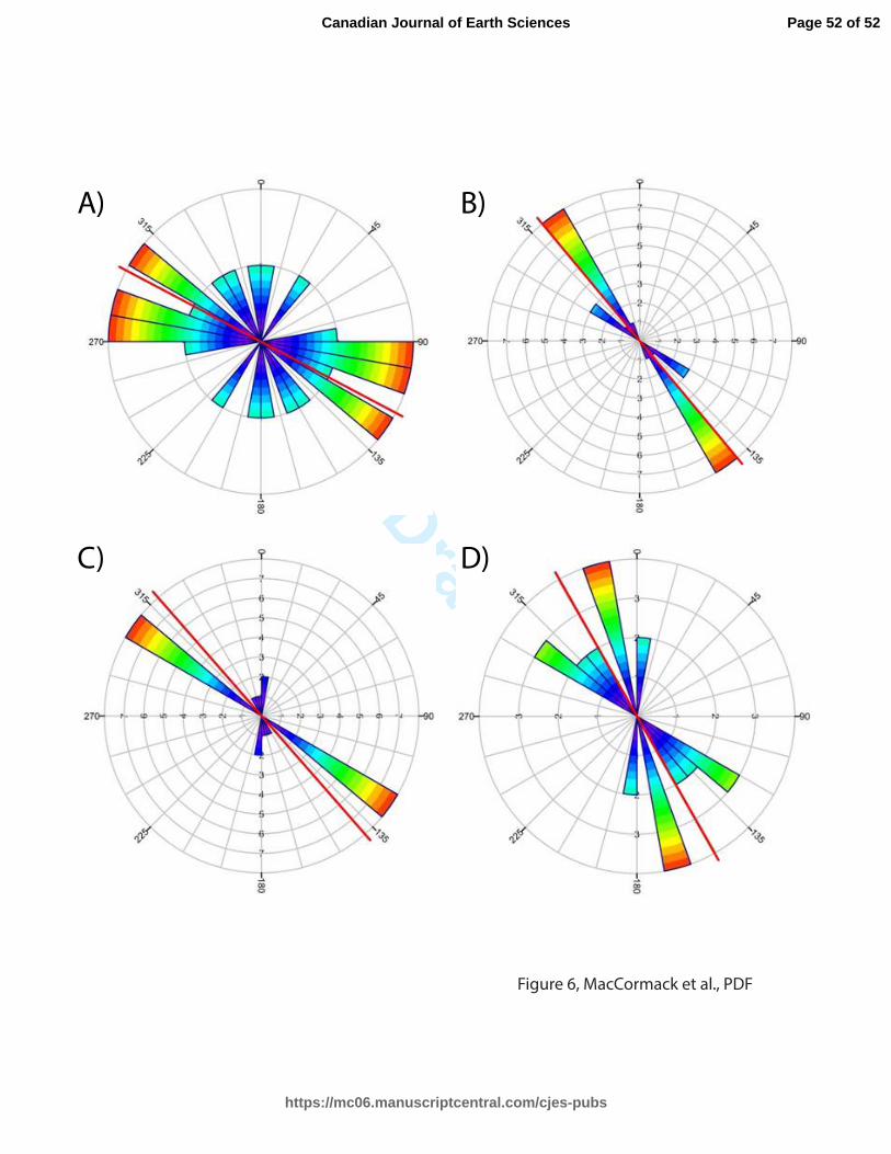
Draft

A)

D)C)

B)


Page 52 of 52



cjes-2016-0112.pdf - TSpace

Documents

Transcript of cjes-2016-0112.pdf - TSpace