MODELING OF SEASONAL VARIATION OF GROUNDWATER LEVELS USING ARTIFICIAL NEURAL NETWORK – A CASE STUDY (APO/GUDU)

METROPOLIS, ABUJA

CHUKWUEMEKA WILLIAMS ATUMA

BU/18A/3000/ENG

Department of Civil Engineering

Baze University

Abuja, Nigeria

July 2021

II

Appendix II

DECLARATION

BAZE UNIVERSITY

DEPARTMENT OF CIVIL ENGINEERING

I, Chukwuemeka Williams Atuma, confirm that this report and the work presented in it are my own achievement.

I have read and do understand the penalties associated with plagiarism.

Signed: .......................................................

Date: ...........................................................

III

CERTIFICATION

This is to certify that this thesis is fully adequate in scope and quality as an undergraduate project work for the award of degree of Bachelor of Engineering in Civil Engineering.

----------------------------------------------------- ------------------ Name and Signature of First Supervisor Date

----------------------------------------------------- ------------------

Name and Signature of Second Supervisor (if applicable) Date

This is to certify that this thesis satisfies the requirements as a graduation project for the award of degree of Bachelor of Engineering in ------------------- Engineering.

----------------------------------------------------- ------------------ Name and Signature of H.O.D, Date Department of -----------------

Engineering

Endorsement of External Examiner:

This is to confirm that this thesis satisfies the requirements as a graduation project for the award of degree of Bachelor of Engineering in -------------------- Engineering.

----------------------------------------------------- ------------------ Name and Signature of External Examiner Date

Approval of the Faculty of Engineering:

----------------------------------------------------- ------------------ Name and Signature of Dean, Date Faculty of Engineering

IV

Dedication

I dedicate this project to God Almighty my creator, my stronghold, alpha, and omega. He has been

my guidance and my source of strength, wisdom, and understanding. Without him, I would not be

able to carry this project out. I would also like to dedicate the thesis to my Family. Without their

unconditional love and guidance over me, I would not have been able to complete my studies and see

this project through.

V

Acknowledgment

I want to thank my family and companions who helped me a great deal in concluding this venture

during the restricted period.

To my father who has been the stronghold of the family, thank you for seeing me through these years,

your guidance and faith in me made me who I am today.

To my mother who never lets me go astray and reminds me where I come from, thank you for all the

love and advice given unto me.

To Victoria and Joshua thank you for being there for me and make living at home pleasant and

enjoyable to live in.

To my friends our countless study sessions will never go in vain, thank you for being such kind souls

to me and helping me when times get rough, we always found a way.

I want to send my extraordinary thanks of appreciation to my instructor Dr. Sani Isah Abba and also

the head of the department Dr. Rotimi who offered me the brilliant chance to do this great undertaking

on the subject Modeling of Seasonal Variation of Groundwater Levels Using Artificial Neural

Network – A Case Study (Apo/Gudu) Metropolis, Abuja, which likewise assisted me with lotting of

Research and I came to think about such countless new things I am truly grateful to them.

Thank you all. My love for you all can never be quantified. God bless you all.

VI

ABSTRACT

Artificial Neural Networks (ANNs) have been successfully used for predicting and modeling

groundwater levels for a good period. In this paper, I use Artificial Neural Network (ANN) and Multi-

Linear Regression (MLR) to model groundwater levels in Abuja, Nigeria using Apo-Gudu as a case

study. After setting the models with the various parameters that affect groundwater level in Abuja, the

developed ANN and MLR should be able to produce near accurate predictions of the groundwater

level variations using just the input variables that have been identified as maximum and minimum

temperature, rainfall, relative humidity, and wind speed. To accomplish this, the models are first

aligned on a preparation dataset to perform as they should as neural networks to forecasts future

groundwater levels utilizing past noticed groundwater levels and outside inputs. Reproductions are

then delivered on another informational index by iteratively taking care of back the anticipated

ground-water levels, alongside genuine outer information. The outcomes show that the created ANN

and MLR can precisely imitate groundwater levels and accurately model them. With the results

obtained a comparison will be made of which neural network is more accurate. The examination

proposes that such tools can be utilized as a suitable option in contrast to physical-based models to

recreate the reactions of the seasons under conceivable future situations or to remake extensive

stretches of missing perceptions gave past information to the impacting factors is accessible.

VII

Table of Contents CHAPTER ONE ......................................................................................................................................................1

INTRODUCTION ...................................................................................................................................................1

1.1 Background of the Study .....................................................................................................................1

1.2 Statement of the Problem ...................................................................................................................3

1.3 Objectives of the Study .......................................................................................................................4

1.4 Research Questions .............................................................................................................................4

1.5 Significance of the Study .....................................................................................................................4

1.6 Scope of the Study ...............................................................................................................................5

1.7 Limitations of the study .......................................................................................................................5

1.8 Definition of Terms ..............................................................................................................................6

CHAPTER TWO .....................................................................................................................................................7

LITERATURE REVIEW ...........................................................................................................................................7

2.1 Introduction .........................................................................................................................................7

2.2 CONCEPTUAL FRAMEWORK ................................................................................................................7

2.3 Concept of Aquifers ...................................................................................................................................9

2.3.1 Type of aquifers ......................................................................................................................................9

2.3.2 Aquifers Chemical characteristics of groundwater ............................................................................. 10

2.4 Spatial and Seasonal Variation in Groundwater Quality .................................................................. 11

2.5 Application of Artificial Neural Network in GWL .................................................................................... 12

CHAPTER 3 ........................................................................................................................................................ 15

REVIEW OF ARTIFICIAL NEURAL NETWORK AND MULTILINEAR REGRESSION ANALYSIS ................................ 15

3.1 Artificial Neural Network (ANN) ............................................................................................................. 15

3.2 Network Training of ANN ....................................................................................................................... 16

3.3 Process of Learning................................................................................................................................. 17

3.4 Standard of Learning .............................................................................................................................. 17

3.5 Training algorithm .................................................................................................................................. 18

3.6 Learning algorithm ................................................................................................................................. 19

3.7 The Design of neural network ................................................................................................................ 20

3.8 Properties of Neural Networks ............................................................................................................... 23

3.8.1 Input layer ....................................................................................................................................... 23

3.8.2 Output layer .................................................................................................................................... 23

3.8.3 Hidden layer .................................................................................................................................... 23

VIII

3.9 Model development ......................................................................................................................... 24

3.9.1 Data standardization ................................................................................................................ 24

3.9.2 Performance criteria of the model ........................................................................................... 25

3.10 Multi Linear Regression Analysis (MLR) ............................................................................................... 26

CHAPTER FOUR ................................................................................................................................................. 29

RESULTS AND DISCUSSION ............................................................................................................................... 29

4.0 Data Processing and Pre-analysis ........................................................................................................... 29

4.1 Results of ANN, and MLR models ........................................................................................................... 32

CHAPTER FIVE ................................................................................................................................................... 49

SUMMARY, CONCLUSION AND RECOMMENDATIONS .................................................................................... 49

5.1 SUMMARY OF FINDINGS .................................................................................................................. 49

5.2 CONCLUSION .................................................................................................................................... 49

5.3 RECOMMENDATION ......................................................................................................................... 50

References ........................................................................................................................................................ 51

1

CHAPTER ONE

INTRODUCTION 1.1 Background of the Study

Water is a universal solvent and natural resource tapped by man, animals, and plants to meet their

need on the earth, either in vapor, liquid, or solid form. Water is one of the essential compounds for

all forms of plants and animals, thus its pollution is generally considered more important than soil.

Studies show that about 80% of communicable diseases are either water-borne or water-related. Water

is an indispensable resource for the existence of man, animals, and plants. Demand for groundwater

has been on the increase due to rapid growth in population as well as the accelerated pace of

industrialization and urbanization in the last few decades especially in developing countries like

Nigeria (Abimbola, A. P. and Odukoya, Abiodun M. and Olatunji, 2012). The inadequate supply of

pipe-borne water and the paucity of surface water has led to an increase in demand for groundwater

in Abuja. People around the world have used groundwater as a source of drinking water and even

today more than half the world’s population depends on groundwater for survival.

Groundwater has long been considered as one of the purest forms of water available in nature and

meets the overall demand for rural and semi-rural people (Amadi et al., 2012). The increase in

groundwater demand for various human activities has placed great importance on water science and

management practice worldwide. (UNESCO, 2003) estimates that globally, groundwater provides

about 50% of current potable water supplies, 40% of the demand of the self-supplied industry, and

20% of water use in irrigated agriculture. Over much of Africa, groundwater is the most realistic water

supply option for meeting water demand.

However, increasing demand and withdrawal, significant changes in land-use patterns, vast industrial

and agricultural effluents entering the hydrological cycle as well as seasonal variation, affect the

quality and quantity of groundwater (O. M. Idoko, 2010). The determination of groundwater quality

for human consumption is important for the wellbeing of the ever-increasing population. Groundwater

quality depends, to some extent, on its chemical composition (Al-Ariqi & Ghaleb, 2010; M. Idoko &

2

Oklo, 2012) which may be affected by natural and anthropogenic factors. Changes in groundwater

recharge, due to seasonal variation, also affect the concentration of the water parameters. Rapid

urbanization, especially in developing countries like Nigeria, has affected the availability and quality

of groundwater due to waste and effluent disposal practices, especially in urban areas. Once

groundwater is contaminated, its quality cannot be restored by just stopping the pollutants from the

source, this is because groundwater contamination may continue years after the waste source is in

place (Ramakrishnaiah et al., 2009; Water & For, 2012).

As groundwater has a huge potential to ensure the supply of future demand for water, it is important

that human activities on the surface do not negatively affect the precious resource. Agricultural

activities, especially abattoir operations, produce a characteristic highly organic waste with relatively

high levels of suspended solid, liquid, and fat. The improper disposal of these wastes onto lands and

into water bodies leads to the contamination of the environment, one of which is the impairment of

water quality (Abdul-Gafar, 2016). There is a high possibility that the effluents from the abattoir will

percolate into the ground and pollute the groundwater. This study, therefore, seeks to determine the

extent of pollution of the groundwater from the abattoir effluents through the qualitative analysis of

groundwater samples taken from different existing wells at various distances from the abattoir. It also

evaluates the influence of seasonal variation on the concentrations of the parameters.

The groundwater level is a key parameter for evaluating spatial and temporal changes in groundwater

environments (Iwasaki et al., 2013). The groundwater level is governed by various factors. Climate

change, as reflected in precipitation and evaporation rates, influences the groundwater level

fluctuation. (Z. Chen et al., 2002). (Z. Chen et al., 2004) also found that climate trends have high

correlations with groundwater level variations in southern Manitoba (Z. Chen et al., 2004). In plain

areas, precipitation infiltration and evapotranspiration in the vertical direction are the major recharge

and discharge processes of the water cycle. In the study area, most of the rainfall falls between July

and October. Seasonal variation in climate is obvious. So, the focus is on the influence of short-term

seasonal variation in climate on groundwater level in this place. The impact of climate variability on

groundwater levels can be investigated by analyzing the relationship between climate records and

groundwater level fluctuations. Hence, the study aims to investigate the modeling of seasonal

variation of groundwater levels using artificial neural networks across Abuja using Apo and Gudu

District of Abuja metropolis as a case study.

3

1.2 Statement of the Problem

Abuja is underlain by crystalline basement rocks with rocks that include different textures

of granites, coarse to fine, consisting essentially of biotite, feldspars, and quartz. In most cases, the

rock has weathered into reddish micaceous sandy clay to clay materials capped by laterites. Generally,

only a small amount of water can be obtained in the freshly un-weathered bedrock below the

weathered layers. Groundwater is found mainly in the variable weathered/transition zone and in

fractures, joints, and cracks of the crystalline basement. Fissure systems in Nigeria rarely extend

beyond 50m, as evidenced by the available drilling data. The local water table depth is controlled by

textural and compositional changes within the regolith vertical profile and the bedrock topography.

However, the poor management of waste arising from industrialization and urbanization has led to

contamination of groundwater hence the need for the present study. It, therefore, becomes imperative

to evaluate the quality of groundwater from shallow aquifers in Abuja, to prevent the occurrence of

water-borne diseases such as typhoid, cholera, diarrhea, and dysentery as well as cancer-related

diseases due to contamination by heavy metals.

Figure 1.1: Aerial map of the specified location.

4

1.3 Objectives of the Study

The main objective of this study is to examine the high-resolution spatial modeling of seasonal

variation of groundwater levels across Abuja using the Apo-Gudu metropolis as a case study.

The specific objectives include;

i. To perform the sensitivity analysis to determine the most dominant GW parameters.

ii. To determine the performance of ANN and MLR model in modeling GWL

iii. To develop an independent model for the prediction of GWL at APO/GUDU

iv. To detect the dynamic of GWL in both wet and dry season

v. To compare the performance linear model (MLR) and Nonlinear model (ANN) for the

simulation of GWL

1.4 Research Questions

i. What are the dynamics of groundwater level and salinity in the wet and dry seasons?

ii. Is there any relationship between the groundwater level, maximum and minimum

temperature, rainfall, relative humidity, wind speed in the Apo and Gudu metropolis in

Abuja?

iii. What is the relationship between the geophysical survey on Apo-Gudu metropolis and its

results with drilling data for better resistivity interpretations for productive and effective

borehole construction?

1.5 Significance of the Study

This study will benefit the management of groundwater level companies in Nigeria, especially in the

Abuja metropolis to understand the importance of using artificial intelligence such as artificial neural

networks in modeling seasonal variation of groundwater levels in Nigeria.

This study will be of immense benefit to other researchers who intend to know more about this study

and can also be used by non-researchers to build more on their research work. This study contributes

to knowledge and could serve as a guide for another study.

5

1.6 Scope of the Study This study is on the modeling of seasonal variation of groundwater levels using an artificial neural

network across Abuja using Apo and Gudu metropolis as a case study.

Gudu is an established district in phase 2 of Abuja city. It is also sometimes known as Apo-Gudu. The

district occupies a strategic location just outside Abuja’s city center. Gudu is residential but has quite

an extensive commercial part to it. Although well-populated it is not as dense or as busy as

neighboring areas like Garki. Gudu sits close to Garki in the north, Guzape in the northeast, Apo

Dutse in the southeast, Gaduwa in the southwest, and Durumi to the west.

Being a developed neighborhood, the infrastructure is good. The road network is extensive, giving

easy access to most parts of the Abuja metropolis. The main roads are Oladipo Diya Street, Ahmadu

Bello Way, and the Nnamdi Azikiwe Expressway. An excellent location (away from the hustle and

bustle of the inner city) and a high level of development have attracted many people to the

neighborhood. Residents include civil servants, politicians, traders, and other middle-class citizens.

The research study will cover the Apo/Gudu metropolises in Abuja.

1.7 Limitations of the study The demanding schedule of respondents at work made it very difficult to get the respondents to

participate in the survey. As a result, retrieving copies of a questionnaire in a timely fashion was very

challenging. Also, the researcher is a student and therefore has limited time as well as resources in

covering extensive literature available in conducting this research.

Financial constraint: Insufficient fund tends to impede the efficiency of the researcher in sourcing

for the relevant materials, literature, or information and in the process of data collection (internet,

questionnaire, and interview).

Time constraint: The researcher will simultaneously engage in this study with other academic work.

This consequently will cut down on the time devoted to the research work.

Information provided by the researcher may not hold true for all businesses or organizations but is

restricted to the selected organization used as a study in this research especially in the locality where

this study is being conducted. Finally, the researcher is restricted only to the evidence provided by the

participants in the research and therefore cannot determine the reliability and accuracy of the

information provided.

6

1.8 Definition of Terms

Artificial Neural Network: An artificial neural network (ANN) is the piece of a figuring framework

intended to mimic the manner in which the human mind investigates and

measures data. It is the establishment of man-made reasoning (AI) and tackles

issues that would demonstrate outlandish or troublesome by human or factual

guidelines.

Modeling: Modeling involves making a representation of something.

Seasonal Variation: Seasonal variation is variation in a time series within one year that is repeated

more or less regularly. The seasonal variation may be caused by the

temperature, rainfall, public holidays, cycles of seasons, or holidays.

Groundwater: Groundwater is water that exists underground in saturated zones beneath the

land surface. The upper surface of the saturated zone is called the water table.

It fills the pores and fractures in underground materials such as sand, gravel,

and other rock, much the same way that water fills a sponge.

Metropolis: An urban area that has a name, defined boundaries, and local government, and

that is larger than a village and generally smaller than a city.

7

CHAPTER TWO

LITERATURE REVIEW 2.1 Introduction This chapter tries to present a brief continuation of research findings related to the modeling of

seasonal variation of groundwater levels using artificial neural networks across Abuja, Apo-Gudu

metropolis. In the present context, the interest of the researcher is to review the findings of past

research. The previous research helps the researchers to theorize and assume occurrence and do critical

appraisal which may contribute regarding design appropriate methodology. Keeping in mind these

objectives, the researcher reviewed the literature to obtain information and the status of work being

done in this area. Therefore, literature from various sources was extensively reviewed in the light of

the present investigation.

2.2 CONCEPTUAL FRAMEWORK

Groundwater accounts for about 98% of the world’s fresh water and it is fairly well distributed

throughout the world (Bouwer, 2002). The exploration and exploitation of groundwater as a major

resource to meet the growing population in some urban cities in Nigeria located on basement complex

rocks has been a subject of discussion (Woakes, M, Rahaman, M.A. and Ajibade, 2013). Those works

involved a combination of hydrogeological and geoelectrical parameters to delineate aquifer

characteristics in the Nigerian crystalline basement rocks in Akure, Gusa, and Lokoja. However, this

work is concerned with the exploration and exploitation of groundwater resources in the basement

complex terrain in parts of Abuja, northcentral, Nigeria. Abuja, the Federal Capital Territory of

Nigeria, has witnessed exponential growth in physical infrastructures and human development. The

major surface water scheme in use within the city has been the ‘Lower Usman Dam’. A smaller dam

8

built at the Apo-Gudu metropolis serves its immediate community also within the territory. Another

dam, the ‘Gurara Dam’, constructed from a distance of about 56 km from the metropolis has been

reticulated to serve the city. In the meantime, government, private establishments, and individuals

have had to drill boreholes to supplement discharge from the dam for both domestic and industrial

uses.

Groundwater may be defined as the subsurface water in soils and rocks that are fully saturated. Due

to precipitation surplus, part of the infiltrated rainwater flows through the soil and reaches the

saturated zone, where it becomes groundwater (Ward R.C. & Robinson M., 2012). The increasing

demands for freshwater, on the one hand, and the decrease in availability, on the other, have become

matters of serious concern. In general, fresh groundwater flows in the direction of the lowest

groundwater heads, usually the lower elements in the landscape, where it finally exfiltrates as surface

water. The flow speed depends on the gradient (slope) in the groundwater table and the permeability

of the soil.

Groundwater is the water present beneath Earth's surface in soil pore spaces and in

the fractures of rock formations. A unit of rock or an unconsolidated deposit is called an aquifer when

it can yield a usable quantity of water. The depth at which soil pore spaces or fractures and voids in

rock become completely saturated with water is called the water table. Groundwater is recharged from

the surface; it may discharge from the surface naturally at aquifers and seeps and can

form oases or wetlands. Groundwater is also often withdrawn for agricultural, municipal,

and industrial use by constructing and operating extraction wells. The study of the distribution and

movement of groundwater is hydrogeology, also called groundwater hydrology.

Typically, groundwater is thought of like water flowing through shallow aquifers, but, in the technical

sense, it can also contain soil moisture, permafrost (frozen soil), immobile water in very low

permeability bedrock, and deep geothermal or oil formation water. Groundwater is hypothesized to

provide lubrication that can possibly influence the movement of faults. It is likely that much of Earth's

subsurface contains some water, which may be mixed with other fluids in some instances.

Groundwater may not be confined only to Earth. The formation of some of the landforms observed

on Mars may have been influenced by groundwater. There is also evidence that liquid water may also

exist in the subsurface of Jupiter's moon Europa Richard Greenburg ( 2015).

Groundwater is often cheaper, more convenient, and less vulnerable to pollution than surface water.

Therefore, it is commonly used for public water supplies. For example, groundwater provides the

9

largest source of usable water storage in the United States, and California annually withdraws the

largest amount of groundwater of all the states (Geographic, 2013). Underground reservoirs contain

far more water than the capacity of all surface reservoirs and lakes in the US, including the Great

Lakes. Many municipal water supplies are derived solely from groundwater (National Geographic,

2015).

The use of groundwater has related environmental issues. For example, polluted groundwater is less

visible and more difficult to clean up than pollution in rivers and lakes. Groundwater pollution most

often results from improper disposal of wastes on land. Major sources include industrial and

household chemicals and garbage landfills, excessive fertilizers and pesticides used in agriculture,

industrial waste lagoons, tailings and process wastewater from mines, industrial fracking, oil field

brine pits, leaking underground oil storage tanks and pipelines, sewage sludge, and septic systems.

Additionally, groundwater is susceptible to saltwater intrusion in coastal areas and can cause land

subsidence when extracted unsustainably, leading to sinking cities (like Bangkok)) and loss in

elevation (such as the multiple meters lost in the Central Valley of California). These issues are made

more complicated by sea-level rise and other changes caused by climate changes which will change

precipitation and water scarcity globally.

2.3 Concept of Aquifers

An aquifer is an assortment of permeable stone or residue filled with groundwater. Groundwater enters

the aquifer as precipitation leaks through the earth’s surface. It can travel through the aquifer and

reemerge through aquifers and wells.

2.3.1 Type of aquifers

There are two general sorts of aquifers: confined and unconfined. Confined aquifers have a layer of

impervious stone or earth above them, while unconfined aquifers lie under a porous layer of soil. A

typical confusion about aquifers is that they are underground waterways or lakes. While groundwater

can saturate or out of aquifers because of its permeable nature, it cannot move adequately quickly to

stream like a waterway. The rate at which groundwater travels through an aquifer fluctuates relying

upon the rocks' porousness. A large part of the water we use for homegrown, modern, or agrarian

intentions is groundwater. Most groundwater, including a lot of our drinking water, comes from

10

aquifers. To get to this water, a well should be made by boring an opening that arrives at the spring.

While wells are synthetic purposes of release for aquifers, they additionally release normally at

aquifers and in wetlands.

Aquifers normally channel groundwater by constraining it to go through little pores and between silt,

which assists with eliminating substances from the water. This characteristic filtration measure, in any

case, may not be sufficient to eliminate the entirety of the impurities.

2.3.2 Aquifers Chemical characteristics of groundwater

Since groundwater often occurs in association with geological materials containing soluble minerals,

higher concentrations of dissolved salts are normally expected in groundwater relative to surface

water. The type and concentration of salts depend on the geological environment and the source and

movement of the water. A simple hydro-chemical classification divides groundwater into meteoric,

connate, and juvenile. Meteoric groundwater, easily the most important, is derived from rainfall and

infiltration within the normal hydrological cycle and is subjected to the type of hydro-chemical

evolution. Groundwater originating as seawater that has been entrapped in the pores of marine

sediments since their time of deposition is generally referred to as connate water. The term has usually

been applied to saline water encountered at great depths in old sedimentary formations. It is now

accepted that meteoric groundwater can eventually become equally saline, and that entrapped

seawater can become modified and moved from its original place of entrapment. It is doubtful whether

groundwater exists that meets the original definition of connate water, and the non-generic term

formation water is preferred by many authors. Connate Water is, perhaps, useful to describe

groundwater that has been removed from atmospheric circulation for a significant period of geological

time. Formation waters are not usually developed for water supplies because of their high salinity.

However, they may become involved in the assessment of saline intrusions caused by the over-

pumping of overlying aquifers.

11

Figure 2.1

Generalized distribution of hydrocarbon phases down a groundwater gradient following a surface

spillage.

Juvenile groundwater describes the relatively small amounts of water which have not previously been

involved in the circulating system of the hydrological cycle but are derived from igneous processes

within the earth. However, juvenile groundwater often cannot be distinguished geochemically from

meteoric groundwater that has circulated to great depths and becomes involved in igneous processes.

True juvenile waters unmixed with meteoric water are rare and of a very localized extent and are not

normally associated with the development and assessment of fresh groundwater resources.

2.4 Spatial and Seasonal Variation in Groundwater Quality

Knowledge of hydrological processes (change of groundwater level, groundwater quality, and tidal

level) in coastal aquifers is important because approximately 50 percent of the world population live

12

in coastal zones, particularly in low-lying deltaic areas within 60 km of the shoreline (Nickson et al.,

2005).

An understanding of the spatial variation and processes affecting water quality is essential in

sustaining usable water supplies under changing climate and local environmental pressures. Temporal

changes of recharged water composition, hydrologic and human factors, may cause periodic changes

in groundwater quality (Vasanthavigar et al., 2010). The quality of alluvial groundwater in rural areas

is sensitive to contaminants originating from agricultural chemicals, such as fertilizers, pesticides, and

lime (Kelly, 1997). The use of nitrogen fertilizers frequently leads to extremely high nitrate

concentrations in groundwater and may cause serious health problems. In such circumstances, the

knowledge of temporal and spatial trends of water quality should help in the decision-making process,

particularly in developing countries, where there are insufficient data.

2.5 Application of Artificial Neural Network in GWL

Trichakis et al. (2011) tested a proposed ANN to measure data from Edward’s aquifer in Texas USA

by simulating the hydraulic head change at an observation well in the area (Trichakis et al., 2011). All

the input factors are directly or indirectly connected to the aquatic equilibrium and the ANN will be

regarded as a sophisticated analog to empirical models of the past. Nourani et al. (2011) used a hybrid,

the artificial neural network-geostatistics study is offered for spatiotemporal prediction for

groundwater level (Nourani et al., 2011). The proposal contains two separate stages for the prediction

of GWL and is applied in the Shabetar plain. Taormina et al. (2012) employed the ANN model using

FFNN to predict the GWL in a coastal unconfined aquifer sited in the Lagoon of Venice, Italy

(Taormina et al., 2012). the study used different input variables combinations, and the obtained results

showed that ANN with FFNN algorithms can produce reliable simulation outcomes. Reza and

Mohammad (2012) employed four different neural networks for GWL predictions in the Shiraz plane

(Reza & Mohammad, 2012). The results were put up against each other by means of statistical

measures of mean square error and square of a correlation coefficient. They found out the best overall

performance was attained by the feed-forward neural network, which was seconded by Elman neural

network. Sahoo and Jha (2013) compared multiple linear regression (MLR)and artificial neural

network (ANN) techniques in predicting GWL (Sahoo & Jha, 2013). The modeling was carried out

in 17 different sites in Japan and they considered all influential factors such as rainfall, temperature,

13

etc. Their results were that ANN is better than MLR. Mohanty et al. (2013) appraised the execution

of finite difference-based numerical model MODFLOW and ANN model developed in this research

in simulating GWL in an alluvial aquifer system (Mohanty et al., 2013). Groundwater levels were

observed at 18 different wells and were simulated in a specific period. ANN was made to predict the

GWL of those 18 wells. The results of the MODFLOW and ANN were compared, and ANN is of a

higher caliber than MODFLOW. Emamgholizadeh and Moslemi (2014) researched the potential of

the intelligent models named Artificial Neural Network (ANN) and Adaptive Neuro-Fuzzy Inference

System (ANFIS) in predicting GWL in the Bastam Plain, Iran (Emamgholizadeh & Moslemi, 2014).

The result showed that both ANN and ANFIS predict GWL accurately. Taylor et al. (2014) used ANN

to predict the hydraulic head in well locations (Taylor et al., 2014). In the present work, the particle

swarm optimization algorithm was used to train a feed-forward multi-layer ANN for the simulation

of hydraulic head change at an observation well in the region of Agia, Chania, Greece. ANN was

ultimately used for midterm prediction of the hydraulic head, as well as for the research of three

climate change scenarios. Data time series were created using a stochastic weather generator, and the

scenarios were examined for a period of ten years (2010-2020). Juan et al. (2015) developed two ANN

models, one with three input variables and another with two input variables, were developed to

simulate and predict the site-specific suprapermafrost groundwater level on the slope scale (Juan et

al., 2015). The results indicate that the three-input variable ANN model has superior real-time site-

specific prediction capability and produces excellent accuracy performance in the simulation and

forecasting of the variation in the suprapermafrost groundwater level. Manouchehr Chitsazan (2015)

used the feed-forward back propagation neural network (FNN) to predict the groundwater level of the

Aghili plain in Iran (MANOUCHEHR CHITSAZAN, 2015). The achieved results of ANN model was

different to the results of finite difference model and showed a very high accuracy of artificial neural

network in calculating groundwater level. Yoon et al. (2016) Utilized a weighted error approach to

enhance the output of ANN and SVM using recursive prediction models for long-term prediction of

GWL in relation to rainfall. The results shows in comparison that the SVM was better than ANN

(Yoon et al., 2016). Okeechobee (2015) Carried out a research to test authenticity of three nonlinear

time-series intelligence models, artificial neural networks (ANN), support vector machines (SVM)

and adaptive neuro fuzzy inference system (ANFIS) in the prediction of the GWL when taking the

interaction between surface water and groundwater into consideration (Okeechobee, 2015). The

attained results from this study would be valuable to the water resources management, it proved to be

14

necessary and effective, considering the surface water-ground water. Ostad-ali-askari et al. (2017)

investigated and represented nitrate pollution in groundwater of marginal area of Zayandeh-rood

River, Isfahan, Iran using water quality and ANN (Ostad-ali-askari et al., 2017). The results were

successful and determined that ANN models can be used in investigating water quality parameters. S.

Sahoo and Jha (2013) developed a new modeling outline using spectral analysis, machine learning,

and uncertainty analysis, as a second choice to complex and computationally expensive physical

models(Sahoo & Jha, 2013). It was concluded that the modeling outline can serve as an alternative

approach to simulating groundwater level change and water availability, especially in regions where

subsurface properties are not available. Ngoie et al. (2018) studied a review process in the field of

GWL, water management, and hydrology using ANN application (Ngoie et al., 2018). Kaya et al.

(2018) researched GWL by using methods such as ANN and M5T in the Reyhanl region in Turkey

(Kaya et al., 2018). The study was carried out efficiently and the result demonstrated that ANN and

M5T models were close to one another. Rajaee et al. (2019) reviewed the special issue on artificial

intelligence approaches for GWL modeling and predictions (Rajaee et al., 2019). This study also

provides a short but effective overview of the most popular AI methods. Many of the results were

attained by reviewing various papers in this area. Roshni et al. (2019) developed the Feedforward

Artificial Neural Network (FFANN) and the hybrid WANN model and later put with Gamma and M-

tests (GT) method for predicting Spatio-temporal groundwater fluctuations in a complex alluvial

aquifer system (Roshni et al., 2019). From the research, the results are that the GTWANN method can

be an effective predictive tool for modeling Spatio-temporal fluctuations of groundwater levels. Y.

Chen et al. (2020) conducted an extensive investigation and analysis on ANN-based water quality

prediction from three aspects, namely feedforward, recurrent, and hybrid architectures (Y. Chen et al.,

2020). The results of many of the review articles are useful to researchers in prediction and similar

fields. Several new architectures shown in the study like recurrent and hybrid structures, can improve

the modeling quality of any development in the future. Khaledian and Pham (2020) used this research

to estimate the water level of Caspian sea using support vector machine and artificial neural network

(Khaledian & Pham, 2020). The results show that the SVM simulated better than ANN.

15

CHAPTER 3

REVIEW OF ARTIFICIAL NEURAL NETWORK AND MULTILINEAR REGRESSION ANALYSIS

3.1 Artificial Neural Network (ANN)

Artificial Neural Network (ANN) as an artificial intelligence model, is a numerical model expected

to deal with non-linear relationships of information yield dataset. ANN has been used effectively,

over the previous decade, in the field of design, drafting, and science. Additionally, ANN has shown

to be efficient in handling complex functions in different fields. Some of which include design

acknowledgment, prediction, arrangement, forecasting, and simulation of control energy.(S &

Jayalekshmi, 2015). Notwithstanding, ANN can be ordered in terms of various capacities, among

the groupings, Levenberg Marquart (LM), Scaled Conjugate Gradient (SCG), and Conjugate

Gradient with Powell/Beale Restarts (CGB) are the most normal and generally utilized strategies

in different written works (Leung et al., 2006). In LM, each input training data is intended to stream

by means of the framework and therefore go through the yield layer by including it in the cycle.

The error is arrived at which is alluded to as a training error. This error is then proliferated back to

the underlying interaction until the ideal yield of the reaction is reached. Meanwhile, the layer

consists of interconnected neurons by weight and enactment work (Isa & Elkiran, 2018). The

organic neuron related with computational neuron is introduced in Fig. 3.1

Figure 3.1: A portrayal of the likeness between a human and an artificial neuron(Can et al., 2004)

16

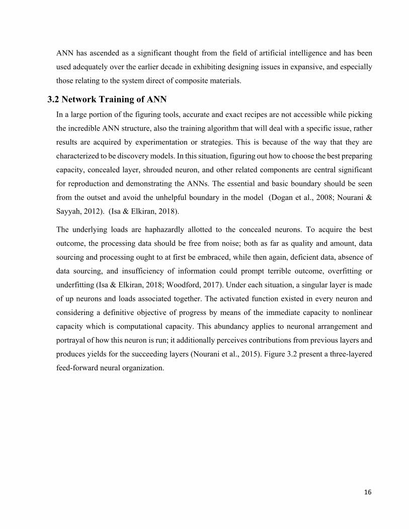
ANN has ascended as a significant thought from the field of artificial intelligence and has been

used adequately over the earlier decade in exhibiting designing issues in expansive, and especially

those relating to the system direct of composite materials.

3.2 Network Training of ANN In a large portion of the figuring tools, accurate and exact recipes are not accessible while picking

the incredible ANN structure, also the training algorithm that will deal with a specific issue, rather

results are acquired by experimentation or strategies. This is because of the way that they are

characterized to be discovery models. In this situation, figuring out how to choose the best preparing

capacity, concealed layer, shrouded neuron, and other related components are central significant

for reproduction and demonstrating the ANNs. The essential and basic boundary should be seen

from the outset and avoid the unhelpful boundary in the model (Dogan et al., 2008; Nourani &

Sayyah, 2012). (Isa & Elkiran, 2018).

The underlying loads are haphazardly allotted to the concealed neurons. To acquire the best

outcome, the processing data should be free from noise; both as far as quality and amount, data

sourcing and processing ought to at first be embraced, while then again, deficient data, absence of

data sourcing, and insufficiency of information could prompt terrible outcome, overfitting or

underfitting (Isa & Elkiran, 2018; Woodford, 2017). Under each situation, a singular layer is made

of up neurons and loads associated together. The activated function existed in every neuron and

considering a definitive objective of progress by means of the immediate capacity to nonlinear

capacity which is computational capacity. This abundancy applies to neuronal arrangement and

portrayal of how this neuron is run; it additionally perceives contributions from previous layers and

produces yields for the succeeding layers (Nourani et al., 2015). Figure 3.2 present a three-layered

feed-forward neural organization.

17

Figure 3.2: Three-layer feed-forward neural network (Nourani et al., 2015)

3.3 Process of Learning Learning is characterized as the limit of the neural organization to gain from its current

circumstance and to improve its presentation through learning (Mendel & Mclaren, 1970). Adapting

in a general sense suggests obtaining/getting data and rules from a circumstance. The Neural

Network is mimicking/copying the human model, moreover acquiring from an intelligent network

of changing its synaptic loads and predisposition stages notwithstanding upgrading following

progressive cycle according to suggested measures (Haykin, 1999, 2001)

3.4 Standard of Learning There are five essential standards of learning, which are as follows;

• Error-Correction Learning

At the point when data is inputted into the framework in the midst of training and goes through the

framework creating a set of characteristics on the output units, then, the noticed yield is

differentiated while the anticipated yield and a match are figured. In case the yield shifts from the

evenhanded, a change should be made to the amendments. One of the instances of error correction

is the Least Mean Square analytical process (Belciug & Gorunescu, 2016).

18

• Memory-Based Learning

A memory-based learning network is an extended memory organization network that different the

data space into sub-areas either statically or progressively to store and recuperate practical

information. The guideline theory techniques utilized by memory-based learning networks are the

nearest neighbor search, space decay methodology, and clustering (Haykin, 1999).

• Hebbian Learning

It is an unaided learning algorithm that is fit for getting sorted out itself to arranging contributions

to a completely new way it has not been instructed. In Hebb's words, Hebbian learning is when two

associated neurons are initiated all the while, the association fortifies, which makes them bound to

be enacted together later. This interaction assumed a critical part in the learning cycle and

arrangement of living creatures, including people (Guo et al., 2015; Morris, 1999)

• Competitive Learning

This can also be illustrated as an unaided neural organization. The point of emphasis here is to

decrease error while increasing entropy. It changes the organization loads to oblige a new set in

another example that will influence the centroid of the set (Haykin, 1999).

• Boltzmann Learning

Boltzmann learning resembles error-correction learning and is applied in the midst of regulated

learning. In this estimation, the state of each and every neuron and yield are thought of. In such a

manner, the mistake remedy learning is quicker than Boltzmann learning. It is likewise used to

prepare the organization for each emphasis. Notwithstanding, rather than examination between the

anticipated value and the noticed worth, the distinction is between the odds of the conveyance of

the organization (Haykin, 1999).

3.5 Training algorithm There are a few algorithms of training received while preparing an organization in neural networks.

Be that as it may, in this examination Levenberg–Marquardt backpropagation (trainlm) and scale

form angle (trainscg) work are utilized.

19

Backpropagation is the name given to the algorithm used for this. Subsequent to giving the

organization information, it will deliver a yield, the following stage is to show the organization

what ought to have been the right yield for that input (the ideal yield). The organization will take

this ideal yield and begin changing the loads to deliver a more precise yield sometime later,

beginning from the yield layer and going in reverse until arriving at the information layer. So next

time a similar it will show that equivalent contribution to the organization, it will give a yield nearer

to that ideal one that was prepared. This cycle is rehashed for some emphasis until we consider the

mistake between the ideal yield and the one yield by the network or organization to be adequately

little.

This training work finds the base of a multivariate potential that can be conveyed as the total of

squares of non-straight originally-regarded limits. It is an iterative method that works such that the

presentation limit will be diminished in each algorithm cycle. Trainlm is the fastest training

algorithm as a result of it having this component (Khademi et al., 2017).

• Scaled conjugate gradient (trainscg)

This is a second-order algorithm that is faster than any other second-order algorithms. The trainscg

work needs more iteration to assemble than the other conjugate gradient algorithms, however, the

number of calculations in each iteration is significantly less because no line search is carried out.

Conjugate gradient backpropagation (Ascione et al., 2017).

More iteration is required for the training function to amass than the other form of gradient

algorithms, in any case, the quantity of figuring in every cycle is altogether less on the grounds that

no line search is done. Form angle backpropagation (Ascione et al., 2017).

3.6 Learning algorithm Artificial neural networks are equipped for gaining from the exhibition of tests, which shows the

conduct of the framework. Along these lines, ensuing to the framework to gain proficiency with

the relationship among information sources and yields, in which the framework organization could

make an objective yield that, is nearer to the foreseen consequence of predefined input factors.

Accordingly, the preparation phases of neural organizations incorporate the presentation of

utilizing a few stages of changing the neurons and loads so that the neural total will deliver the

yield (Haykin, 1999; Wilson, 1993).

20

The framework is observed to be reacting until the existing varieties in the synaptic weight are

exhausted and when this is achieved, the framework is thought to have stopped learning and is to

suggest as organization consolidating (Kasabov, 1996).

Two algorithms of learning are inspected hereunder;

a. Supervised Learning System

In the learning framework, the required information and target yield are organized and fed into

the organization accordingly and the weight and inclination are refreshed forward which is

called the feed-forward cycle while it goes through the training with engendered error till the

objective worth is reach. This learning cycle happens with the predefined information and yield

values by the software engineer (Haykin, 2001).

b. Unsupervised or solo Learning System

The interaction of the solo learning framework happens when just the required inputs factors are

set and inputted into the organizations for the training purpose. The neurotransmitter is

consequently changed once the factors are inputted, this cycle is called learning with no

developer and has the ability to get sorted out the data with the least mistake values. It is a self-

assenting method where just info information is used. This calculation uses no data of the

potential yields and is otherwise called learning without educator (Haykin, 1999). This algorithm

uses no data of the potential yields to grasp its assignment by identifying the information data

(Becker & Plumbley, 1996).

3.7 The Design of neural network Artificial neural networks principle designs, the dissemination of nodes, layers course, and

interconnections are briefly analyzed underneath:

• Single-layered feedforward network

Is a kind of artificial neural network that includes just one layer referred to as the input layer and

the next layer called the output or yield layer of the network.

21

Figure 3.3: Single-layered feedforward neural network (Haykin, 1999)

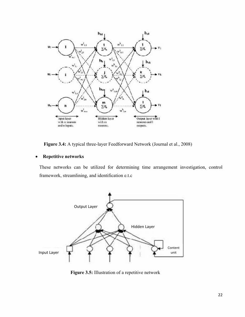
• Multi-layered feedforward neural network

These are networks that incorporate three layers to be specific: input, hidden,

and output layer.

22

Figure 3.4: A typical three-layer Feedforward Network (Journal et al., 2008)

• Repetitive networks

These networks can be utilized for determining time arrangement investigation, control

framework, streamlining, and identification e.t.c

Figure 3.5: Illustration of a repetitive network

Input Layer Content

unit

Hidden Layer

Output Layer

23

• Mesh networks

This organization considers the spatial underlying of modes and plan utilized for design

acknowledgment and expulsion purposes. This organization is most and broadly applied in a

few fields of streamlining, grouping, neural organization design acknowledgment, etc.

Figure 3.6: Structure of a mesh network

3.8 Properties of Neural Networks 3.8.1 Input layer

This is the accepting layer, where data like images, unprocessed data, signals, and so on from any

acknowledged source are inputted into the organization for training purposes. These data sources

are typically standardized inside the breaking point values in order to scale the data.

3.8.2 Output layer Following the input layer in the organization is the output layer where the information is gotten to

deliver the last and wanted objective. The layer interacts with the inputs introduced by the input

layer with weight and predisposition.

3.8.3 Hidden layer

The hidden layers contain nodes that are in control of taking out patterns related to the technique

that is assessed. This layer executes the most extreme inward interactions from an organization

(Haykin, 1999)

24

3.9 Model development Model advancement is viewed as a proficient examination strategy. It helps the researcher in

depicting, foreseeing, testing, or understanding troublesome frameworks. Subsequently, models

typically present a structure for directing an examination and can comprise of synopses like

drawings, conditions, or figures for the investigation of a framework. It incorporates

fundamental outlines of what is the issue here. A few phrases and steps which were undergone

during model development are shown in Fig. 3.7. for both the ANN and MLR models.

Figure 3.7: Model development process (Khademi et al., 2017)

3.9.1 Data standardization The training algorithm is very sensitive in scaling data, Thus, the input and output values of the

data set should be standardized. For the most part, input and output data was set up to the scale

scopes of either (– 1, 1), (0.1, 0.9), or (0, 1) (Khademi et al., 2016).

Standardization is the method of figuring out and laying out a data model capable of storing data

in a data set. The eventual outcome is that inconsequential data is eliminated, and just data

Identify inputs & Data collection

&

Conduct descriptive data &

Model Design

Select computer development

Determine network architecture

Train the designed

Find the optimal set of

Model Testing Evaluate performance

Model Execution

Run the model for future

Model Training

25

applicable to the attributes are placed in a table. Unimportant data waste circle space and make

maintenance issues. In the event that the data that exists much of the time should have fluctuated,

the data should be varied similarly in all areas. The condition underneath was embraced for the

standardization (Nourani et al., 2015):

𝑆𝑆𝑇𝑇 = 𝑆𝑆𝑖𝑖−𝑆𝑆𝑚𝑚𝑆𝑆𝑀𝑀−𝑆𝑆𝑚𝑚

(3.1)

Where;

SM = maximum

Si = actual values to be used.

ST = normalized

Sm = minimum

3.9.2 Performance criteria of the model Distinctive statistical parameters, like the mean square error (MSE) and correlation coefficient (R)

are adopted when exploring the presentation of the ANN model. Conditions (3.2) and (3.3) show

the R and the MSE separately.

𝑹𝑹 = 𝟏𝟏 − ∑ (𝑺𝑺𝒊𝒊−𝑺𝑺𝒊𝒊′)𝑵𝑵

𝒊𝒊=𝟏𝟏∑ (𝑺𝑺𝒊𝒊−𝑵𝑵𝒊𝒊=𝟐𝟐 𝑺𝑺�)𝟐𝟐

(3.2)

𝑴𝑴𝑺𝑺𝑴𝑴 = �∑ (𝑺𝑺𝒊𝒊−𝑵𝑵𝒊𝒊=𝟏𝟏 𝑺𝑺𝒊𝒊

′)𝟐𝟐

𝑵𝑵 (3.3)

Where;

26

N = number of data used

Si = Observed value

Si’= model computed value

𝑆𝑆̅= average observed data

The conditions applied to obtain the effectiveness and functioning of the model development are

dependent upon particular difficulties, and the statistical performance assessment applied to arrive

at the correlation coefficient (R) and the mean square error (MSE). Both MSE and R show the

variation between the two instances, i.e. measured and calculated values. To obtain the excellent

model, the higher the R and MSE values in the training and validation the better, and the higher the

R-value, the lesser the MSE value under normal circumstances (Nourani & Sayyah, 2012).

The standard MSE strategy is employed to value the productivity and adequacy of the model and

its capacity to acquire a precise expectation and decision, also to give out the best match among

estimated and determined qualities when MSE is zero way of its qualities. Spanning from zero to

best gauge, indicate that the contrasts among expected and estimated values are progressively more

noteworthy.

3.10 Multi Linear Regression Analysis (MLR) A few designing issues comprise of a decision for the connection between at least two variables.

Regression analysis is a valuable statistical tool for researchers in this field of study. Considering

a linear Regression model, that is explicit to this sort of regression model, linear prediction abilities

will be utilized for information demonstrating, and the objective boundaries of the information are

assessed. It is important to note that, in numerous employments of regression examination, more

than one information factor is viewed as that would bring about a "multi-linear regression". For

this situation, MLR assesses the connection between at least two input factors, by introducing a

linear equation to control the processed data (Khademi et al., 2016; Sadrmomtazi et al., 2013).

The role played by regression analysis is of utmost importance to researchers in the field. Generally,

regression analysis can be considered as the route toward fitting models to data. In a linear

regression model which is a specific sort of regression model, the linear indicator limits would be

utilized to show the data, and target boundaries are assessed from the data (Akbari & Jamal, 2015;

27

Khademi et al., 2017). It justifies indicating that in various usages of regression analysis, more than

one input factor is incorporated which would trigger the "multilinear regression" work. The goal of

MLR is to find a condition that can anticipate the dependent variable as a part of a couple of

independent variables. Various linear regressions incorporate instructions data and furthermore

investigating the association between factors (Sobhani et al., 2010). The MLR condition is given

by:

𝒚𝒚 = 𝒃𝒃𝒄𝒄 + 𝒃𝒃𝟏𝟏𝒙𝒙𝟏𝟏 + 𝒃𝒃𝟐𝟐𝒙𝒙𝟐𝟐 + ⋯𝒃𝒃𝒊𝒊𝒙𝒙𝒊𝒊 (3.4)

Where;

x1 is the ith predictor value

bc is the constant of regression

bi is the ith predictor coefficient

28

Figure 3.8: Overall Proposed Methodology Diagram

29

CHAPTER FOUR

RESULTS AND DISCUSSION

4.0 Data Processing and Pre-analysis

Data pre-processing and pre-analysis are very important prior to the modeling procedure. Data

mining is the process of turning the raw data into appropriate and meaningful information, for the

purpose of this work, the available daily data were obtained from two different places including

NASA, and NHA. The estimation of the chosen parameters was based on a different set of inputs and

outputs variables as shown in statistical Table 4.1. Every data analysis concerning AI base models

relies normally on historical data. Therefore, the mathematical and data modeling of the input-output

is important as it describes the nature and strength of the relationship between inputs and outputs. To

efficiently train AI base model, these data need to be clean and filtered properly, because the raw data

is often comprised of missing records, outliers, noise, discrepancies of codes and names, or was

infected by all kinds of error including human and instrumental. The descriptive statistical analysis

used to explain the data trend series are smoothing and normalization, the former was carried out by

fitting the data into regression function to eliminate the noise from the data and the latter was to ensure

the uniformity of the input-output value (scaling to fall within a small, specified range). At the initial

phase, all input and output data were standardized within the range between 0 and 1 prior to model

training. Normalization is performed to reduce data redundancy and improve data credibility. The

descriptive statistic of the selected parameter can be presented in Table 4., as stated above.

30

Table 4.1: Descriptive statistic between the parameters

Parameters T.MAX T.MIN R (mm) RH (%) WS (m/s) GWL Mean 0.4812 0.4678 0.2591 0.6501 0.3827 0.4139 Median 0.5319 0.4474 0.2035 0.7542 0.4143 0.4148 Standard Deviation 0.2843 0.2309 0.2758 0.3043 0.2253 0.1054 Sample Variance 0.0808 0.0533 0.0761 0.0926 0.0508 0.0111 Kurtosis -1.1411 -0.4694 -0.1592 -0.8364 0.0581 -1.1857 Skewness 0.1231 -0.0808 0.7845 -0.7276 0.2075 -0.1882 Minimum 0.0000 0.0000 0.0000 0.0000 0.0000 0.2214 Maximum 1.0000 1.0000 1.0000 1.0000 1.0000 0.5797

In this research work, descriptive statistical analysis and correlation matrix was applied to explore the

degree, type, and extent of the relation between the input-output parameters. The correlation

coefficient (R) was evaluated to measure the extent of linear interaction between the two variables.

The concept of R is to classified a variable using a linear function that acts as a tentative indicator of

a possible correlation between the set of variables. As presented in Table 4.2 the R-value with bold

marked is stationary and significant variables with probability less than 0.05 (P<0.05) that indicates

high strength of linear correlations. Also, the negatives R-values indicate an inverse interaction

between the two variables. Therefore, the weakness observed by R-value showed that the use of

conventional approaches in modeling complex interactions is insignificant and it is crucial to

implement a more robustness method. The major importance of this correlation is to determine the

linear input variable selection as indicated in the objective sections. As mentioned above, three

different models based on dominant factors were generated to classify the GWL. This could be better

understood by considering the newly adopted visualized correlation matrix between the parameter as

indicated in Fig. 4.1.

31

Table 4.2: Correlation analysis between the input and output variables

Parameters T.MAX T.MIN R (mm) RH (%) WS

(mtrs./s) GWL T.MAX 1 T.MIN 0.373604 1 R(mm) -0.71785 0.04151 1 RH (%) -0.69133 0.25756 0.773566 1 WS (m./s) 0.233262 0.386059 0.11881 0.040017 1 GWL 0.725675 0.022414 -0.61478 -0.75147 -0.1119 1

Fig. 4.1: Visualized correlation matrix between the parameters

Correlation Matrix

0.2 0.4 0.6

GWL1 0 0.5 1

WS 0 0.5 1 1.5

RH 0 0.5 1

R 0 0.5 1

TMIN10 0.5 1

TMAX1

0.2

0.4

0.6

GW

L1

0

0.5

1

WS

0

0.5

1

1.5

RH

0

0.5

1

R

0

0.5

1

TMIN

1

0

0.5

1

TMAX

1

0.37 -0.72 -0.69 0.23 0.73

0.37 0.04 0.26 0.39 0.02

-0.72 0.04 0.77 0.12 -0.61

-0.69 0.26 0.77 0.04 -0.75

0.23 0.39 0.12 0.04 -0.11

0.73 0.02 -0.61 -0.75 -0.11

32

From Fig. 4.1, the Spearman Pearson Correlation demonstrates how effectively a linear function

can be used to explain the relationship between the GWL variables. The direction or the sign does not

affect the strength of the correlation. In other words, a positive correlation implies that an increase in

the first parameter is proportional to an increase in the second parameter, whereas a negative

coefficient implies an inverse relationship, in which as one parameter increases, the second parameter

decreases(S. I. Abba et al., 2020; Eisinga et al., 2013; Ghali et al., 2020; Selin & Abba, 2020; USMAN

et al., 2020).

4.1 Results of ANN, and MLR models

As stated above the ANN, and MLR models were used in this study for the prediction of GWL using

different input parameters.

For ANN the optimum model architecture was optimized and selected using the trial-and-error

technique based on hyper-turning parameters, such as hidden neurons, activation function, learning

algorithms, etc. A qualified model is one that fits the requirements of most statistical evaluation

criteria, according to the literature (Abdullahi et al., 2020; Pham et al., 2019; USMAN et al., 2020).

In both calibration and verification, the model simulation was assessed using the most commonly used

performance metrics, such as R2, MSE, RMSE, and R. Table 2 shows the simulated outcomes in terms

of evaluation assessment based on model combinations (M1-M5) for ANN models. It is worth

mentioning that, for all the model development the simulation was done in MATLAB 9.3 (R2020a).

meanwhile, the MLR models were carried out in excel software based on the above model

combination (M1-M5).

33

Table 2: Modeling Results of ANN models

Training Phase Testing Phase R2 R MSE RMSE R2 R MSE RMSE ANN-M1 0.6120 0.7823 0.0038 0.0614 0.6241 0.7900 0.0045 0.0668 ANN-M2 0.5286 0.7271 0.0046 0.0677 0.5723 0.7565 0.0051 0.0712 ANN-M3 0.6414 0.8008 0.0035 0.0590 0.5552 0.7451 0.0053 0.0726 ANN-M4 0.7134 0.8446 0.0028 0.0528 0.8700 0.9327 0.0015 0.0393 ANN-M5 0.6624 0.8139 0.0033 0.0573 0.9170 0.9576 0.0010 0.0314

From the results in Table 2, the level of precision of all the models in terms of statistical criteria

was attained within the range of marginal to good (M4) by almost all the combinations. According to

the obtained results, these algorithms are known to be capable of handling models with multiple free

parameters, reducing the error function, solving data fitting problems, and have become a standard

approach for highly chaotic non-linear problems. Besides, the overall single ANN results

demonstrated that ANN-M4 served as the best simulation in terms of R2, MSE, RMSE, and R.

Although it is difficult to rank the models in accordance with the achieved accuracies, nevertheless

the ANN-M4 approach relatively showed the best predictions. However, the accuracy of both the three

models (ANN-M1, ANN-M2, and ANN-M3) attained more than 60% in terms of R. However, the

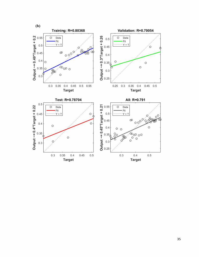
comparative visualization of the three-model combination is presented in scatter plots (see, Fig. 4.2

(a-e)). A scatter plot shows the level of agreement between the observed and predicted load for the

overall goodness-of-fit. It is obvious from the scatter plot that the ANN-M4 model shows higher

accuracy in comparison to the others models.

34

(a)

35

(b)

36

(c)

37

(d)

38

Fig. 4.2 Scatter Plots for (a) ANN-M1, (b) ANN-M2 (c) ANN-M3, (c), ANN-M4, and (e) ANN-M5

(e)

39

(a)

(b)

40

(c)

(d)

41

Fig. 4.2: Performance and training stage plots for (a) ANN-M1, (b) ANN-M2 (c) ANN-M3, (c), ANN-M4, and (e) ANN-M5

Regardless of the nonlinear relationship between predictors (inputs variables), and their associated

target objectives, the overall accuracy of single models was good and reported substantial certainty in

terms of error for both MLR and ANN. Essentially, it should be noted that the positive, and promising

estimations occurred during the verification phase, which is generally used to correctly calibrate

models using known input variables and goals. The testing process, on the other hand, is critical in

evaluating a model's performance since it checks the model's accuracy based on unknown goal values.

This benefit does not apply to the calibration phase alone. The section of MLR and ANN models have

generally depicted promising also ability with regards to the single model. This is not surprising as

can be seen in many pieces of literature (S. I. Abba et al., 2020, 2021; S. Abba & Lee, 2014; Alas et

al., 2020; Elkiran et al., 2018; Isa & Elkiran, 2018; Sammen et al., 2021; Sani & Abba, n.d.). The

radar diagram also known as spider chart was introduced in the research to determine the overall

comparison of the single models, and this justified the goodness-of-fit (see, Fig. 4.4).

(e)

42

Table 4.3: Modeling Results of MLR models

Training Phase Testing Phase R2 R MSE RMSE R2 R MSE RMSE MLR-M1 0.625125 0.790648 0.003642 0.06035 0.655661 0.809729 0.004085 0.063914 MLR-M2 0.619209 0.786899 0.0037 0.060825 0.671561 0.819488 0.003896 0.062421 MLR-M3 0.625125 0.790648 0.003642 0.06035 0.674244 0.821124 0.003865 0.062166 MLR-M4 0.651325 0.807047 0.003388 0.058203 0.783258 0.885019 0.002571 0.050708 MLR-M5 0.652627 0.807854 0.003375 0.058094 0.783022 0.884885 0.002574 0.050736

43

Fig. 4.3: Radar Plots for ANN, and MLR Models

0.7

0.75

0.8

0.85

0.9MLR-M1

MLR-M2

MLR-M3MLR-M4

MLR-M5

MLR MODEL

R-Training R-Testing

0

0.2

0.4

0.6

0.8MLR-M1

MLR-M2

MLR-M3MLR-M4

MLR-M5

MLR MODEL

R2-Training R2-Testing

0.00000.20000.40000.60000.80001.0000

ANN-M1

ANN-M2

ANN-M3ANN-M4

ANN-M5

ANN MODEL

R-Training R-Testing

00.20.40.60.8

1ANN-M1

ANN-M2

ANN-M3ANN-M4

ANN-M5

ANN MODEL

R2-Training R2-Testing

44

Fig. 4.4: Error Plots in terms of MSE, and RMSE

0.0000 0.0200 0.0400 0.0600 0.0800

ANN-M1

ANN-M2

ANN-M3

ANN-M4

ANN-M5

RMSE-Testing RMSE-Training

0 0.001 0.002 0.003 0.004 0.005 0.006

ANN-M1

ANN-M2

ANN-M3

ANN-M4

ANN-M5

MSE-Testing MSE-Training

0 0.001 0.002 0.003 0.004 0.005

MLR-M1

MLR-M2

MLR-M3

MLR-M4

MLR-M5

MSE-Testing MSE-Training

0 0.01 0.02 0.03 0.04 0.05 0.06 0.07

MLR-M1

MLR-M2

MLR-M3

MLR-M4

MLR-M5

RMSE-Training RMSE-Training

45

0

0.2

0.4

0.6

0.8

1 3 5 7 9 11 13 15 17 19 21 23 25 27 29 31 33 35 37 39 41 43 45 47PRED

ICTE

D AN

N M

ODE

L 1

TIME SERIES

ANN MODEL 1

GWL ANN-M1

0

0.2

0.4

0.6

0.8

1 3 5 7 9 11 13 15 17 19 21 23 25 27 29 31 33 35 37 39 41 43 45 47

PRED

ICTE

D AN

N M

ODE

L 3

TIME SERIES

ANN MODEL 3

GWL ANN-M3

0

0.2

0.4

0.6

0.8

1 3 5 7 9 11 13 15 17 19 21 23 25 27 29 31 33 35 37 39 41 43 45 47PRED

ICTE

D AN

N M

ODE

L 2

TIME SERIES

ANN MODEL 2

GWL ANN-M2

46

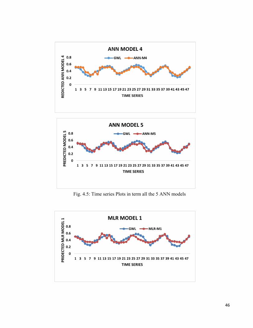
Fig. 4.5: Time series Plots in term all the 5 ANN models

0

0.2

0.4

0.6

0.8

1 3 5 7 9 11 13 15 17 19 21 23 25 27 29 31 33 35 37 39 41 43 45 47PRED

ICTE

D M

ODE

L 5

TIME SERIES

ANN MODEL 5GWL ANN-M5

0

0.2

0.4

0.6

0.8

1 3 5 7 9 11 13 15 17 19 21 23 25 27 29 31 33 35 37 39 41 43 45 47

PRID

ECTE

D M

LR M

ODE

L 1

TIME SERIES

MLR MODEL 1

GWL MLR-M1

47

48

Fig. 4.5: Time series Plots in terms of all the 5 MLR models

49

CHAPTER FIVE

SUMMARY, CONCLUSION, AND RECOMMENDATIONS

5.1 SUMMARY OF FINDINGS

The purpose of this study was to assess the modeling of seasonal variation of groundwater levels using

an artificial neural network across Abuja using Apo-Gudu metropolis as a case. Two hypotheses were

formulated (generated) to guide the researcher. The first was meant to find out there is a relationship

between the minimum and maximum temperature, rainfall, relative humidity, and wind speed of the

Apo-Gudu metropolis in Abuja.

The objectives of the study were to;

i. To perform the sensitivity analysis to determine the most dominant GW parameters.

ii. To determine the performance of ANN and MLR model in modeling GWL

iii. To develop an independent model for the prediction of GWL at APO/GUDU

iv. To detect the dynamic of GWL in both wet and dry season

v. To compare the performance linear model (MLR) and Nonlinear model (ANN) for the simulation of

GWL

5.2 CONCLUSION

This study has gone a long way to establish the fact that some parts of the Federal Capital Territory

contain a reasonable amount of groundwater which if well tapped will go a long way to alleviate the

water problem in the city. There is a need for a proper understanding of the groundwater condition of

the area, the foundation of which has been laid through this study. This could be achieved by carrying

out comprehensive predrilling hydrogeological studies for the entire area and all boreholes should be

properly designed and properly developed and pump tested. The knowledge of this will reduce

borehole failures and low yield currently experienced in some parts of the project area.

This study assessed the potentials of groundwater using artificial neural networks and multi-linear

regression in basement complex terrain of Apo-Gudu area of Abuja metropolis for the supply of

50

potable water for domestic uses. Results show that ANN model 4 was the best model for groundwater

resources available in both the weathered overburden and fractured zones of the basement complex

rocks in the area. Subsurface fractures in the study area were at depths ranging from 7.0 m to 36.00 m

and they served as good reservoirs for water. Generally, drilling penetrated both the overburden and

the competent basement complex rocks until fractures were encountered.

5.3 RECOMMENDATION

In view of the findings revealed by this study, it is recommended that there is the need for artificial

intelligence in the treatment of the abattoir effluents into a non-toxic state before they are discharged

into the environment.

Efforts should also be made by the regulatory agencies such as National Environmental Standards and

Regulation Enforcement Agency (NESREA) and Abuja Environmental Protection Board (AEPB) to

meet and enforce the international standards and recommendations for the location of abattoirs.

51

References Abba, S. I., Elkiran, G., & Nourani, V. (2021). Improving novel extreme learning machine using PCA

algorithms for multi-parametric modeling of the municipal wastewater treatment plant.

215(October 2019), 414–426. https://doi.org/10.5004/dwt.2021.26903

Abba, S. I., Pham, Q. B., Usman, A. G., Linh, N. T. T., Aliyu, D. S., Nguyen, Q., & Bach, Q. V.

(2020). Emerging evolutionary algorithm integrated with kernel principal component analysis

for modeling the performance of a water treatment plant. Journal of Water Process Engineering,

33(September 2019), 101081. https://doi.org/10.1016/j.jwpe.2019.101081

Abba, S., & Lee, J. (2014). Microprocessors and Microsystems A parametric-based performance

evaluation and design trade-offs for interconnect architectures using FPGAs for networks-on-

chip. MICROPROCESSORS AND MICROSYSTEMS, May.

https://doi.org/10.1016/j.micpro.2014.04.011

Abdul-Gafar, H. B. (2016). Analysis of Surface and Groundwater Pollution from Abattoir astes: Case

Study of Minna Abattoir. Unpublished B. Eng. Project. Department of Agricultural Engineering

Federal University of Technology, Minna, Nigeria.

Abdullahi, H. U., Usman, A. G., & Abba, S. I. (2020). Modelling the Absorbance of a Bioactive

Compound in HPLC Method using Artificial Neural Network and Multilinear Regression

Methods. 6(2), 362–371.

Abimbola, A. P. and Odukoya, Abiodun M. and Olatunji, A. S. (2012). Influence of Bedrock on the

Hydrogeochemical Characteristics of Groundwater in Northern Part of Ibadan Metropolis,SW

Nigeria. Journal Of the Nigerian Association Of Hydrogeologists, 22.

http://eprints.covenantuniversity.edu.ng/id/eprint/9439

Akbari, M., & Jamal, S. M. (2015). Prediction of Compressive Strength of Concrete by Data-Driven

Models RESEARCH PAPERS PREDICTION OF COMPRESSIVE STRENGTH OF CONCRETE

BY DATA-DRIVEN MODELS. May.

Al-Ariqi, W. S. T., & Ghaleb, A. A. D. S. (2010). Assessment of hydrochemical quality of ground

water under some urban areas within sana’a secreteriat. Ecletica Quimica, 35(1), 77–84.

52

https://doi.org/10.1590/S0100-46702010000100009

Alas, M., Ismael, S., Ali, A., Ph, D., Asce, A. M., Abdulhadi, Y., Abba, S. I., & Ph, D. (2020).

Experimental Evaluation and Modeling of Polymer Nanocomposite Modified Asphalt Binder

Using ANN and ANFIS. 32(10), 1–11. https://doi.org/10.1061/(ASCE)MT.1943-5533.0003404

Amadi, A. N., Yisa, J., Ogbonnaya, I. C., Dan-Hassan, M. A., Jacob, J. O., & Alkali, Y. B. (2012).

Quality Evaluation of River Chanchaga Using Metal Pollution Index and Principal Component

Analysis. Journal of Geography and Geology, 4(2), 13–21. https://doi.org/10.5539/jgg.v4n2p13

Ascione, F., Bianco, N., Masi, R. F. De, Stasio, C. De, & Mauro, G. M. (2017). Artificial Neural

Networks for Predicting the Energy Behavior of a Building Category : A Powerful Tool for Cost-

Optimal Analysis. In Cost-Effective Energy Efficient Building Retrofitting. Elsevier Ltd.

https://doi.org/10.1016/B978-0-08-101128-7.00011-3

Becker, S. U. Z. A. N. N. A., & Plumbley, M. (1996). Unsupervised Neural Network Learning

Procedures for Feature Extraction and Classification *. 203, 185–203.

Belciug, S., & Gorunescu, F. (2016). IMPROVING PERFORMANCE IN NEURAL NETWORKS

USING FEATURE SELECTION BASED ON RANDOM FORESTS : APPLICATION TO

AUTOMATED MEDICAL DIAGNOSIS Smaranda Belciug , Florin Gorunescu. 10(1), 33–46.

Bouwer, H. (2002). Artificial recharge of groundwater: Hydrogeology and engineering. Hydrogeology

Journal, 10(1), 121–142. https://doi.org/10.1007/s10040-001-0182-4

Can, B. S., Submitted, D., Fulfillment, P., Science, M., Major, E., & Science, M. (2004). Artificial

Neural Networks and Fuzzy Logic Applications in Modeling the Compressive Strength of Major :

Materials Science and Engineering. 1–65.

Chen, Y., Song, L., Liu, Y., Yang, L., & Li, D. (2020). Applied sciences A Review of the Artificial

Neural Network Models for Water Quality Prediction.

Chen, Z., Grasby, S. E., & Osadetz, K. G. (2002). Predicting average annual groundwater levels from

climatic variables: An empirical model. Journal of Hydrology, 260(1–4), 102–117.

https://doi.org/10.1016/S0022-1694(01)00606-0

Chen, Z., Grasby, S. E., & Osadetz, K. G. (2004). Relation between climate variability and

53

groundwater levels in the upper carbonate aquifer, southern Manitoba, Canada. Journal of

Hydrology, 290(1–2), 43–62. https://doi.org/10.1016/j.jhydrol.2003.11.029

Dogan, E., Ates, A., & Yilmaz, C. (2008). Application of Artificial Neural Networks to Estimate

Wastewater Treatment Plant Inlet Biochemical Oxygen Demand. 27(4), 439–446.

https://doi.org/10.1002/ep

Eisinga, R., Grotenhuis, M. Te, & Pelzer, B. (2013). The reliability of a two-item scale: Pearson,

Cronbach, or Spearman-Brown? International Journal of Public Health, 58(4), 637–642.

https://doi.org/10.1007/s00038-012-0416-3

Elkiran, G., Nourani, V., Abba, S. I., & Abdullahi, J. (2018). Artificial intelligence-based approaches

for multi-station modelling of dissolve oxygen in river Artificial intelligence-based approaches

for multi-station modelling of dissolve oxygen in river. September.

https://doi.org/10.22034/gjesm.2018.04.005

Emamgholizadeh, S., & Moslemi, K. (2014). Prediction the Groundwater Level of Bastam Plain (

Iran ) by Artificial Neural Network ( ANN ) and Adaptive Neuro-Fuzzy Inference System ( ANFIS

). https://doi.org/10.1007/s11269-014-0810-0

Geographic, N. N. (2013). Almanac of Geography.

Ghali, U. M., Usman, A. G., Chellube, Z. M., Degm, M. A. A., Hoti, K., Umar, H., & Abba, S. I.

(2020). Advanced chromatographic technique for performance simulation of anti-Alzheimer

agent: an ensemble machine learning approach. SN Applied Sciences, 2(11).

https://doi.org/10.1007/s42452-020-03690-2

Guo, Y., Bennamoun, M., Sohel, F., Lu, M., Wan, J., & Ming, N. (2015). A Comprehensive

Performance Evaluation of 3D Local Feature Descriptors. International Journal of Computer

Vision. https://doi.org/10.1007/s11263-015-0824-y

Haykin, S. (1999). Neural Networks - A Comprehensive Foundation (p. 823).

Haykin, S. (2001). NEURAL NETWORKS KALMAN FILTERING AND Edited by (Vol. 5).

Idoko, M., & Oklo, A. (2012). Seasonal variation in physico-chemical characteristics of rural

groundwater of Benue State, Nigeria. Journal of Asian Scientific Research, 2(10), 574–586.

54

Idoko, O. M. (2010). Seasonal variation in iron in rural groundwater of Benue state, middle belt,

Nigeria. Pakistan Journal of Nutrition, 9(9), 892–895. https://doi.org/10.3923/pjn.2010.892.895

Isa, S., & Elkiran, G. (2018). ScienceDirect ScienceDirect Effluent prediction of chemical oxygen

demand from the astewater treatment plant using artificial neural network application. Procedia

Computer Science, 120, 156–163. https://doi.org/10.1016/j.procs.2017.11.223

Iwasaki, Y., Ozaki, M., Nakamura, K., Horino, H., & Kawashima, S. (2013). Relationship between

increment of groundwater level at the beginning of irrigation period and paddy filed area in the

Tedori River Alluvial Fan Area, Japan. Paddy and Water Environment, 11(1–4), 551–558.

https://doi.org/10.1007/s10333-012-0348-9

Journal, B., Hanini, S., Derriche, R., Bouhedda, M., & Bouzidi, A. (2008). PREDICTION OF HIGH-

PRESSURE VAPOR LIQUID EQUILIBRIUM OF SIX BINARY SYSTEMS , CARBON DIOXIDE

WITH SIX ESTERS , USING AN ARTIFICIAL NEURAL NETWORK MODEL. 25(01), 183–199.

Juan, C., Genxu, W., & Tianxu, M. (2015). Simulation and prediction of suprapermafrost groundwater

level variation in response to climate change using a neural network model. JOURNAL OF

HYDROLOGY, 529, 1211–1220. https://doi.org/10.1016/j.jhydrol.2015.09.038

Kasabov, N. K. (1996). Foundations of Neural Networks , Fuzzy Systems , and Knowledge

Engineering.

Kaya, Y. Z., Üne, F. Ş., Demirci, M., Ar, B. T. A. Ş., & Varç, H. İ. N. (2018). GROUNDWATER

LEVEL PREDICTION USING ARTIFICIAL NEURAL NETWORK AND M5 TREE MODELS.

195–201.

Kelly, W. R. (1997). Heterogeneities in ground-water geochemistry in a sand aquifer beneath an

irrigated field. Journal of Hydrology, 198(1–4), 154–176. https://doi.org/10.1016/S0022-

1694(96)03316-1

Khademi, F., Akbari, M., Mohammadmehdi, S., & Nikoo, M. (2017). Multiple linear regression , arti

fi cial neural network , and fuzzy logic prediction of 28 days compressive strength of concrete.

11(1), 90–99. https://doi.org/10.1007/s11709-016-0363-9

Khademi, F., Mohammadmehdi, S., & Deshpande, N. (2016). Predicting strength of recycled

aggregate concrete using Artificial Neural Network , Adaptive Neuro-Fuzzy Inference System

55

and Multiple Linear Regression. International Journal of Sustainable Built Environment.

https://doi.org/10.1016/j.ijsbe.2016.09.003

Khaledian, M. R., & Pham, M. I. S. M. B. Q. B. (2020). Simulating Caspian Sea surface water level

by artificial neural network and support vector machine models. Acta Geophysica, 0123456789.

https://doi.org/10.1007/s11600-020-00419-y

Leung, C. K. Y., Asce, M., Ng, M. Y. M., & Luk, H. C. Y. (2006). Empirical Approach for

Determining Ultimate FRP Strain in FRP-Strengthened Concrete Beams. 10(2), 125–138.

MANOUCHEHR CHITSAZAN, G. R. and A. N. (2015). Forecasting Groundwater Level by

Artificial Neural Networks as an Alternative Approach to Groundwater Modeling. 85(2001), 98–

106.

Mendel, J. M., & Mclaren, R. W. (1970). 8. Mathematics in Science and Engineering, 66, 287–318.

https://doi.org/10.1016/S0076-5392(08)60497-X

Mohanty, S., Jha, M. K., Kumar, A., & Panda, D. K. (2013). Comparative evaluation of numerical

model and artificial neural network for simulating groundwater flow in Kathajodi – Surua Inter-

basin of Odisha , India. Journal of Hydrology, 495, 38–51.

https://doi.org/10.1016/j.jhydrol.2013.04.041

Morris, R. G. M. (1999). D . O . Hebb : The Organization of Behavior , Wiley : New York ; 1949.

50(99), 9230.

National Geographic. (2015). Almanac of Geography.

Ngoie, S., Lunda, J., Mbuyu, A., & Makenda, G. (2018). Overview of Artificial Neural Networks

Applications in Groundwater Studies. 3768–3773.

Nickson, R. T., McArthur, J. M., Shrestha, B., Kyaw-Myint, T. O., & Lowry, D. (2005). Arsenic and

other drinking water quality issues, Muzaffargarh District, Pakistan. Applied Geochemistry,

20(1), 55–68. https://doi.org/10.1016/j.apgeochem.2004.06.004

Nourani, V., Alami, M. T., & Vousoughi, F. D. (2015). Wavelet-entropy data pre-processing approach

for ANN-based groundwater level modeling. JOURNAL OF HYDROLOGY, 524, 255–269.

https://doi.org/10.1016/j.jhydrol.2015.02.048

56

Nourani, V., Ejlali, R. G., & Alami, M. T. (2011). Spatiotemporal Groundwater Level Forecasting in

Coastal Aquifers by Hybrid Artificial Neural Network-Geostatistics Model: A Case Study. 28(3).

https://doi.org/10.1089/ees.2010.0174

Nourani, V., & Sayyah, M. (2012). Advances in Engineering Software Sensitivity analysis of the

artificial neural network outputs in simulation of the evaporation process at different climatologic

regimes. Advances in Engineering Software, 47(1), 127–146.

https://doi.org/10.1016/j.advengsoft.2011.12.014

Okeechobee, L. (2015). A Comparative Study of Artificial Neural Networks , Support Vector

Machines and Adaptive Neuro Fuzzy Inference System for Forecasting Groundwater Levels.

https://doi.org/10.1007/s11269-015-1167-8

Ostad-ali-askari, K., Shayannejad, M., & Ghorbanizadeh-kharazi, H. (2017). Artificial Neural

Network for Modeling Nitrate Pollution of Groundwater in Marginal Area of Zayandeh-rood

River , Isfahan , Iran. 21, 134–140. https://doi.org/10.1007/s12205-016-0572-8

Pham, Q. B., Abba, S. I., Usman, A. G., Linh, N. T. T., Gupta, V., Malik, A., Costache, R., Vo, N. D.,

& Tri, D. Q. (2019). Potential of Hybrid Data-Intelligence Algorithms for Multi-Station

Modelling of Rainfall. Water Resources Management, 33(15), 5067–5087.

https://doi.org/10.1007/s11269-019-02408-3

Rajaee, T., Ebrahimi, H., & Nourani, V. (2019). Review papers A review of the arti fi cial intelligence

methods in groundwater level modeling. Journal of Hydrology, 572(May 2018), 336–351.

https://doi.org/10.1016/j.jhydrol.2018.12.037

Ramakrishnaiah, C. R., Sadashivaiah, C., & Ranganna, G. (2009). Assessment of water quality index

for the groundwater in Tumkur taluk, Karnataka state, India. E-Journal of Chemistry, 6(2), 523–

530. https://doi.org/10.1155/2009/757424

Reza, G., & Mohammad, R. (2012). R E S E A R C H A RT I C L E - C I V I L E N G I N E E R I N G

Forecasting Groundwater Level in Shiraz Plain. 1871–1883. https://doi.org/10.1007/s13369-

012-0291-5

Richard Greenburg. (2015). The Ocean Moon: Search for an Alien Biosphere.

Roshni, T., Jha, M. K., Deo, R. C., & Vandana, A. (2019). Development and Evaluation of Hybrid

57

Artificial Neural Network Architectures for Modeling Spatio-Temporal Groundwater

Fluctuations in a Complex Aquifer System.

S, S. J. J., & Jayalekshmi, S. (2015). A Review on Artificial Neural Network Concepts in Structural

Engineering Applications. 1(4), 6–11.

Sadrmomtazi, A., Sobhani, J., & Mirgozar, M. A. (2013). Modeling compressive strength of EPS

lightweight concrete using regression , neural network and ANFIS. Construction and Building

Materials, 42, 205–216. https://doi.org/10.1016/j.conbuildmat.2013.01.016

Sahoo, S., & Jha, M. K. (2013). Groundwater-level prediction using multiple linear regression and

arti fi cial neural network techniques : a comparative assessment. 1865–1887.

https://doi.org/10.1007/s10040-013-1029-5

Sammen, S. S., Ehteram, M., Abba, S. I., Abdulkadir, R. A., Ahmed, A. N., & El-Shafie, A. (2021).

A new soft computing model for daily streamflow forecasting. Stochastic Environmental

Research and Risk Assessment, 1. https://doi.org/10.1007/s00477-021-02012-1

Sani, M. G., & Abba, S. I. (n.d.). Estimation of water quality index using artificial intelligence

approaches and multi-linear regression Related papers.

https://doi.org/10.11591/ijai.v9.i1.pp126-134

Selin, A. G. U., & Abba, I. S. I. (2020). A Novel Multi ‑ model Data ‑ Driven Ensemble Technique

for the Prediction of Retention Factor in HPLC Method Development. Chromatographia,

0123456789. https://doi.org/10.1007/s10337-020-03912-0

Sobhani, J., Najimi, M., Pourkhorshidi, A. R., & Parhizkar, T. (2010). Prediction of the compressive

strength of no-slump concrete : A comparative study of regression , neural network and ANFIS

models. Construction and Building Materials, 24(5), 709–718.

https://doi.org/10.1016/j.conbuildmat.2009.10.037

Taormina, R., Chau, K., & Sethi, R. (2012). Engineering Applications of Artificial Intelligence

Artificial neural network simulation of hourly groundwater levels in a coastal aquifer system of

the Venice lagoon. Engineering Applications of Artificial Intelligence, 25(8), 1670–1676.

https://doi.org/10.1016/j.engappai.2012.02.009

Taylor, P., Tapoglou, E., Trichakis, I. C., Dokou, Z., Nikolos, I. K., & George, P. (2014).

58

Groundwater-level forecasting under climate change scenarios using an artificial neural

network trained with particle swarm optimization Groundwater-level forecasting under climate

change scenarios using an artificial neural network trained with particle. June 2014, 37–41.

https://doi.org/10.1080/02626667.2013.838005

Trichakis, I. C., Nikolos, I. K., & Karatzas, G. P. (2011). Artificial Neural Network ( ANN ) Based

Modeling for Karstic Groundwater Level Simulation. 1143–1152.

https://doi.org/10.1007/s11269-010-9628-6

UNESCO. (2003). duplicateWater for People, Water for Life. The World Water Development Report,

36.

USMAN, A. G., IŞIK, S., ABBA, S. I., & MERİÇLİ, F. (2020). Artificial intelligence–based models

for the qualitative and quantitative prediction of a phytochemical compound using HPLC

method. Turkish Journal of Chemistry, 44(5), 1339–1351. https://doi.org/10.3906/kim-2003-6

Vasanthavigar, M., Srinivasamoorthy, K., Vijayaragavan, K., Rajiv Ganthi, R., Chidambaram, S.,

Anandhan, P., Manivannan, R., & Vasudevan, S. (2010). Application of water quality index for

groundwater quality assessment: Thirumanimuttar sub-basin, Tamilnadu, India. Environmental

Monitoring and Assessment, 171(1–4), 595–609. https://doi.org/10.1007/s10661-009-1302-1

Ward R.C. & Robinson M. (2012). Principles of Hydrology, McGraw Hill, 3rd Edition.

Water, A., & For, Q. (2012). ASSESSING WATER QUALITY FOR HUMAN CONSUMPTION

WITHIN THE VICINITY OF KARU AiiATTOIR , ABUJA FCT , NIGERIA BY.

Wilson, W. J. (1993). A Multi-Layered Learning Model.

Woakes, M, Rahaman, M.A. and Ajibade, A. D. I. A. K. . (2013). Geology of Nigeria. 2nd Revised

Edition. In Geology of Nigeria. 2nd Revised Edition.

Woodford, C. (2017). How Neural Network Works. https://www.explainthatstuff.com/introduction-

to-neural-networks.html

Yoon, H., Hyun, Y., Ha, K., Lee, K., & Kim, G. (2016). Author ’ s Accepted Manuscript. Computers

and Geosciences. https://doi.org/10.1016/j.cageo.2016.03.002