Choice under Uncertainty with the Best and Worstin Mind: Neo-additive Capacities¤.

Alain Chateauneuf Jürgen EichbergerCERMSEM Wirtschaftstheorie I

Université Paris I Universität Heidelberg

Simon GrantDepartment of Economics

Rice University

September, 2002

This Version: November 13, 2002

AbstractThe concept of a non-extreme-outcome-additive capacity (neo-additive capacity ) is intro-duced. Neo-additive capacities model optimistic and pessimistic attitudes towards uncer-tainty as observed in many experimental studies. Moreover, neo-additive capacities canbe applied easily in economic problems, as we demonstrate by examples. This paper pro-vides an axiomatisation of Choquet expected utility with neo-capacities in a frameworkof purely subjective uncertainty.

JEL Classification: D81

Keywords: optimism, pessimism, Choquet expected utility, portfolio choice.

* We would like to thank Michele Cohen, Peter Hartley, Jean-Yves Jaffray, Mark Machina, MatthewRyan, Jean-Marc Tallon, and Jean-Christophe Vergnaud for extremely stimulating and helpful discussions.

‘‘That the chance of gain is naturally over-valued we maylearn from the universal success of lotteries. [...] The vainhope of gaining some of the great prizes is the sole cause ofthis demand. The soberest people scarce look upon it as afolly to pay a small sum for the chance of gaining ten or twen-ty thousand pounds.’’

Adam Smith (1776)‘‘The Wealth of Nations’’ (p.210).

“Overconfidence, however generated, appears to be a funda-mental factor promoting the high volume of trade we observein speculative markets. Without such confidence, one wouldthink that there would be little trading in financial markets.

Robert Shiller (2001)“Irrational Exuberance” (p.144/5).

1. Introduction

Optimism and pessimism are important features of a person’s attitude towards uncertainty.

On an aggregate level, business cycles and stock market fluctuations have been attributed

to “irrational” optimism and pessimism. Economic theory, however, finds it difficult to

see in such moods a major factor determining economic behavior. With large amounts of

money and wealth at stake, as in the investment behavior of traders in financial markets,

one hesitates to attribute major influence on decisions to vague notions of belief.

Faced with uncertainty economists like to think of investors as cool analysts, carefully

weighing likelihoods of events relevant for their decisions. Yet, many observers of in-

vestment behavior in financial markets, from Keynes (1921) to Robert Shiller

(2001), could not escape the conclusion that psychological effects seem to interact with

probabilistic information in shaping investors’ behavior.

Embracing Ramsey’s (1926) and de Finetti’s (1937) personalistic view of proba-

bility, Savage (1954) provided a set of behavioral postulates showing that it is possible

to view decision makers’ behavior in the face of uncertainty as guided by a consistent

system of probabilistic beliefs. His axioms gave researchers an opportunity to put these

postulates to direct tests. Allais (1953) and Ellsberg (1962) were the most promi-

2

nent articles reportingchoice behavior of people which contradicts Savage’s postulates. In

particular, the Sure-Thing-Principle which allows one to decompose a decision problem,

omitting ‘‘equivalent parts’’ and focussing choice on the remaining parts, was quickly

identified as especially problematic.

There are behavioral regularities which inf luence individuals’ betting behavior. People

distinguish categorically between situations which they consider as certain, just possible,

or strictly impossible. These consistently observed certainty and impossibility effects

cannot be modeled by a transition from zero probability of an event to a positive proba-

bility, or from a positive probability to the probability of one.

A typical lottery with a high prize on a very unlikely event can turn the certainty of low

wealth for a poor person into the possibility of great riches, providing a reason for ac-

cepting an unfair gamble. Conversely, rich people may find the possibility of loosing

substantial amounts of wealth so dangerous that high expected returns are necessary to

induce them to an investment.

Bell (1985) interprets these psychological biases as disappointment aversion or elation-

seeking behavior. He studies situations where these biases determine the behavior, such

as the process of releasing information, behavior in auctions and the Ellsberg paradox.

Based on these observations he argues for an inverse-S shaped pattern of decision weights

as an adequate representation of individual attitudes towards uncertainty.

Optimistic behavior overestimates the likelihood of good outcomes while pessimistic at-

titudes exaggerate the likelihood of bad outcomes. Based upon mounting experimental

evidence for certainty and impossibility effects, Wakker (2001) extends these no-

tions to arbitrary events with rank-ordered outcomes and characterizes optimistic and

pessimistic attitudes. In the context of the Choquet expected utility (CEU) model, con-

cave capacities ref lect optimistic attitudes towards uncertainty, while convex capacities

model pessimism.

1.1 Experimental evidence

Camerer (1995) reviews numerous studies refuting the validity of the expected utility

3

approach as a description of individual behavior. More recently, however, experiments

find evidence for typical patterns of deviation from the expected utility model. In par-

ticular, one often observes subjects willing to bet on high outcomes with low probability

while refusing to accept even small risks. For subjects choosing between lotteries, one can

explain such behavior by a function w(p) weighting the probability p of events. Experi-

mental studies by Gonzalez & Wu (1999), Abdellaoui (2000), Bleichrodt

& Pinto (2000) and others show a pattern of probability weights as in Figure 1.

.............................................

p0

.........................................

1

1

w(p)

Figure 1: Probability weighting function

The decision weight of an event E , w(p(E)), measured by the willingness to bet on this

event, differs usually from the probability of the event p(E): Figure 1 shows an inverse-S

shaped weighting function, overweighting probabilities close to zero and underweight-

ing probabilities close to one as. Tversky & Wakker (1995) study the relationship

between decision weights and attitudes towards risk and characterize the possibility and

certainty effects. Wakker (2001) defines optimism and pessimism in terms of decision

weights. This article contains also a brief survey of the relevant experimental literature.

Kilka & Weber (2001) demonstrate how decision weights and subjective probabilis-

tic beliefs can be distinguished in experiments.

4

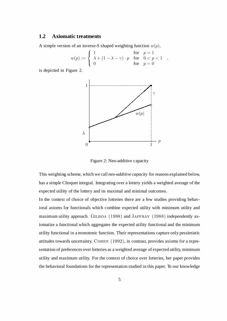
1.2 Axiomatic treatments

A simple version of an inverse-S shaped weighting function w(p);

w(p) :=

8<:

1 for p = 1¸+ (1 ¡¸ ¡ °) ¢ p for 0 < p < 10 for p = 0

;

is depicted in Figure 2.

p0

......................................................................................

1

1

s

s

c

c

°

¸

w(p)

Figure 2: Neo-additive capacity

This weighting scheme, which we call neo-additive capacity for reasons explained below,

has a simple Choquet integral. Integrating over a lottery yields a weighted average of the

expected utility of the lottery and its maximal and minimal outcomes.

In the context of choice of objective lotteries there are a few studies providing behav-

ioral axioms for functionals which combine expected utility with minimum utility and

maximum utility approach. Gilboa (1988) and Jaffray (1988) independently ax-

iomatize a functional which aggregates the expected utility functional and the minimum

utility functional in a monotonic function. Their representations capture only pessimistic

attitudes towards uncertainty. Cohen (1992), in contrast, provides axioms for a repre-

sentation of preferences over lotteries as a weighted average of expected utility, minimum

utility and maximum utility. For the context of choice over lotteries, her paper provides

the behavioral foundations for the representation studied in this paper. To our knowledge

5

there is no axiomatization for choice over acts in either the Anscombe-Aumann or the

Savage framework.

The neo-additive weighting scheme provides an easy way to model the certainty and

the impossibility effects. Combined with a probability function Pr (:) over ranges of

monetary outcomes, this weighting scheme models an individual who overweights the

likelihood of a monetary outcome x exceeding x;

w(Pr(x > x)) = ¸+ (1¡ ¸ ¡ °) ¢ Pr(x > x)

> Pr(x > x);

whenever Pr(x > x) < ¸= (¸+ °) : In contrast, outcomes below x occurring with low

probability Pr(x · x) obtain a weight,

w(Pr(x · x)) ´ 1 ¡ w(1 ¡ Pr(x > x))

= (1 ¡¸)¡ (1 ¡¸ ¡ °) (Pr(x · x))

> Pr(x · x);

whenever Pr(x · x) < °= (¸ + °).In the next section, we introduce some notation and concepts necessary for our analysis.

Section 3 studies the neo-additive weighting scheme in the context of the CEU model.

This parameterized CEU model can be easily applied to economic models in order to

analyse the implications of the certainty and impossibility effect. Section 4 illustrates the

potential of the neo-additive CEU representation for economic applications in the context

of a portfolio choice model. Section 5 provides an axiomatic treatment of neo-additive

capacities in a framework of purely subjective uncertainty. Proofs are collected in an

appendix.

2. Capacities and the Choquet integral

We assume that the uncertainty a decision maker faces can be described by a non-empty

set of states, denoted by S. This set may be finite or infinite. Associated with the set

of states is the set of events, taken to be a sigma-algebra of subsets of S , denoted by E :

6

We assume that for each s in S , fsg is in E . Capacities are real-valued functions defined

on E , that generalize the notion of probability distributions. Formally, a capacity is a

normalized monotone set function.

Definition 2.1 A capacity is a function º : E ! R which assigns real numbers to

events, such that(i) E;F 2 E ; E µ F implies º(E) 6 º(F ); monotonicity

(ii) º(;) = 0 and º(S) = 1: normalization

A capacity º is called convex if º(E [F ) ¸ º(E)+º(F )¡º(E \F ) holds for arbitrary

eventsE;F 2 E : If the reverse inequality holds then the capacity is called concave. Prob-

ability distributions are special cases of capacities which are both concave and convex.

For each capacity º there is a dual or conjugate capacity º defined by º (E) = 1 ¡º (S ¡ E) for allE 2 E : If the dual capacity º is convex, then the capacityº is concave.

The most common way to integrate functions with respect to a capacity is the Choquet

integral. Let f : S ! R be a E-measurable real-valued function. We consider finite

outcome acts and suppose that f has finite range, that is, the set f(S) is finite. We call

a function f with these properties a simple function. The Choquet integral can therefore

be written in the following intuitive form.

Definition 2.2 For any simple function f the Choquet integral with respect to the ca-

pacity º is defined as

V (fjº) = Pu2f(S)

u ¢ [º (fsj f (s) ¸ ug) ¡ º (fsj f(s) > ug)] :

Each element in the range has a decision weight equal to the difference between the capac-

ity of the states yielding an element better or equal than the one under consideration and

the capacity of the states yielding a strictly better outcome. The Choquet integral is inter-

preted as the expected value of the function f with respect to the capacity º: The decision

weights used in the computation of the Choquet integral will overweight high outcomes

if the capacity is concave and will overweight low outcomes if the capacity is convex. It

is therefore well-suited to model such responses to ambiguity as optimism or pessimism.

7

Sarin & Wakker (1998) provide a detailed discussion of decision weights.

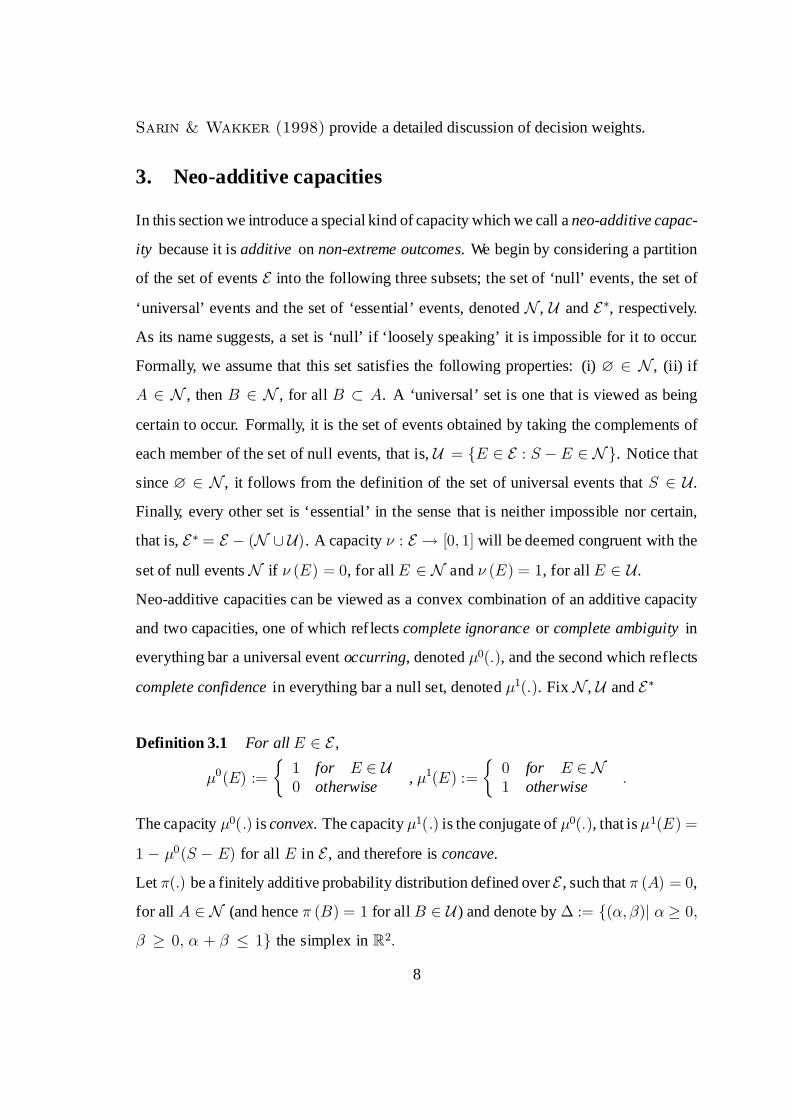
3. Neo-additive capacities

In this section we introduce a special kind of capacity which we call a neo-additive capac-

ity because it is additive on non-extreme outcomes. We begin by considering a partition

of the set of events E into the following three subsets; the set of ‘null’ events, the set of

‘universal’ events and the set of ‘essential’ events, denoted N , U and E¤, respectively.

As its name suggests, a set is ‘null’ if ‘loosely speaking’ it is impossible for it to occur.

Formally, we assume that this set satisfies the following properties: (i) ? 2 N , (ii) if

A 2 N , then B 2 N , for all B ½ A. A ‘universal’ set is one that is viewed as being

certain to occur. Formally, it is the set of events obtained by taking the complements of

each member of the set of null events, that is, U = fE 2 E : S ¡ E 2 N g. Notice that

since ? 2 N , it follows from the definition of the set of universal events that S 2 U.

Finally, every other set is ‘essential’ in the sense that is neither impossible nor certain,

that is, E¤ = E ¡ (N [ U). A capacity º : E ! [0; 1] will be deemed congruent with the

set of null events N if º (E) = 0, for all E 2 N and º (E) = 1, for all E 2 U.

Neo-additive capacities can be viewed as a convex combination of an additive capacity

and two capacities, one of which ref lects complete ignorance or complete ambiguity in

everything bar a universal event occurring, denoted ¹0(:), and the second which reflects

complete confidence in everything bar a null set, denoted ¹1(:). Fix N , U and E¤

Definition 3.1 For all E 2 E ,

¹0(E) :=½

1 for E 2 U0 otherwise , ¹1(E) :=

½0 for E 2 N1 otherwise :

The capacity ¹0(:) is convex. The capacity ¹1(:) is the conjugate of ¹0(:), that is¹1(E) =

1 ¡ ¹0(S ¡ E) for all E in E , and therefore is concave.

Let ¼(:) be a finitely additive probability distribution defined over E , such that ¼ (A) = 0,

for all A 2 N (and hence ¼ (B) = 1 for allB 2 U ) and denote by ¢ := f(®; ¯)j ® ¸ 0;

¯ ¸ 0; ® + ¯ · 1g the simplex in R2:

8

Definition 3.2 For a given finitely additive probability distribution ¼ on (S; E), and a

pair of numbers (°; ¸) 2 ¢, a neo-additive capacity º(¢j¼; °; ¸) is defined as

º(Ej¼; °; ¸) := ° ¢ ¹0(E) + ¸ ¢ ¹1(E) + (1¡ ° ¡ ¸) ¢ ¼(E)

for all E in E.

It is straightforward to derive the Choquet integral of a simple function f with respect to

a neo-additive capacity in terms a weighted sum of the infimum, the supremum and the

expectation with respect to ¼ of the act. We say z = inf (f) if f¡1 (x : x ¸ z) 2 U and for

every y > z, f¡1 (x : x > y) =2 U . Similarly, we say z = sup (f) if f¡1 (x : x > z) 2 Nand for every y < z, f¡1 (x : x ¸ y) =2 N .

Lemma 3.1 The Choquet expected value of a simple function f : S ! R with respect

to the neo-additive capacity º(Ej¼; °; ¸) is given by:

V (fjº(¢j¼; °; ¸)) := ° ¢ inf (f) + ¸ ¢ sup (f) + (1 ¡ ° ¡ ¸) ¢ E¼ [f] : (1)

Proof. To see this note that V (f j¹0(¢)) = inf (f ) ; V (f j¹1(¢)) = sup(f ) and V (f j¼) =E¼ [f] : The result then follows from the linearity of the Choquet integral with respect to

the capacity (Denneberg (2000), Properties (ix) and (x) on page 49).

Notice that we have do not require that ¼ (E) = 0 implies E 2 N . Indeed nothing in

the discussion and definitions above, prevent N consisting only of the empty set, ? (and

hence U contains only the element S). In this case, even if for some event E , ¼ (E) = 0,

the capacities º (E) = ¸ and 1¡ º (S ¡ E) = ° are still both positive. That is, an event

E may receive a zero decision weight in the evaluation of the Choquet expected value

for any act with neither its infimum nor its supremum on E, but for an act, for which the

infimum (respectively, supremum) results in a state of E the decision weight on E is °

(respectively, ¸). For further illustration of this point, consider the following example.

Example 3.1 Suppose S is the unit interval, [0; 1], E is power set of [0; 1] and N is the

set of singleton states and pairs of states. That is, E 2 N if E is an event consisting of

no more than two states. Suppose further that ¼ is a finitely additive probability measure

9

for which ¼ (s) = 0 for all s in [0; 1]. From the finite additivity of ¼, it follows that

¼ (f0; 1g) = ¼ (f0; 0:5; 1g) = 0 but only f0; 1g is in N . In particular, º (f0; 1g) = 0

and º (f0; 0:5; 1g) = ¸. Furthermore, although ¼ (S ¡ f0; 1g) = ¼ (S ¡ f0; 0:5; 1g) =1, only S ¡ f0; 1g is in U, and hence º (S ¡ f0; 1g) = 1 > º (S ¡f0; 0:5; 1g) = 1¡ °.

Several well-known decision criteria can be viewed as special cases of the Choquet in-

tegral of a neo-additive capacity:(i) ° = ¸ = 0 expected utility,(ii) 1 ¸ ° > 0; ¸ = 0 pure pessimism,(iii) ° = 0; 1 ¸ ¸ > 0 pure optimism,(iv) ° + ¸ = 1 Hurwitz criterion.

Neo-additive capacities satisfy three conditions:

² They are additive for pairs of events which are not null and do not form a partition ofa universal event.

² They exhibit uncertainty aversion for some events.² They exhibit uncertainty preference for some other events.

Indeed, as the following proposition shows, these conditions characterize neo-additive

capacities completely.

Proposition 3.1 Let º be a capacity on (S; E);where E¤ contains at least three elements

E1, E2 and E3 which are pairwise disjoint (that is, Ei \Ej = ? for all i 6= j). Then the

following statements are equivalent:

(i) º is a neo-additive capacity,

(ii) the capacity º satisfies the following properties:

(a) for any three events (E;F;G) 2 E¤ £ E¤ £ E¤ such that E \ F = ; = E \ G;E [ F =2 U , and E [G =2 U;

º(E [ F ) ¡ º(F ) = º(E [G) ¡ º(G);

(b) for some (E;F ) 2 E¤ £ E¤ such that E \ F = ; and E [ F =2 U;

º(E [ F ) · º(E) + º(F );

10

(c) for some (E;F ) 2 E¤ £ E¤ such that E \ F = ; and E [ F =2 U;

º(E [ F ) · º(E) + º(F ):

Proof. Appendix.

Note that for a neo-additive capacity º on (S; E);whereE¤ contains at least three elements,

as assumed throughout the paper, uniqueness of the pessimism and optimism coefficients

and of the underlying probability measure ¼ is guaranteed. This is proved in a lemma

preceding the proof of Proposition 3.1 in the appendix.

Property (iia) establishes additivity of the neo-additive capacity for events that yield non-

extreme outcomes. According to property (iib), the capacity overweights the event in

which the most preferred prize is obtained, hence ¸ ¸ 0: Property (iic) says the capacity

overweights also the event with the least preferred prize. It implies ° ¸ 0:

3.1 Optimism and pessimism

In this section we will provide two arguments why one may be justified to interpret the

overweighting of the extreme outcomes with the notions of optimism and pessimism. The

first argument shows that neo-additivecapacities are a special caseof the behavioural con-

cept of optimism and pessimism advanced in Wakker (2001). The second argument

appeals to the intuitive notion of optimism and pessimism suggested by the context of the

multiple prior approach.

3.1.1 The behavioural approach of Wakker (2001)

Inspired by the Allais and Ellsberg paradox ,Wakker (2001) suggests a notion of op-

timism and pessimism based on choice behaviour over acts. This approach derives its

appeal from its immediate testability in experiments and its natural representation by

properties of capacities.

Properties (iib) and (iic) of Proposition 3.1 imply the neo-additive capacity to be concave

on some events, which corresponds to the notion of optimism suggested in Wakker

(2001), and convex on some others, hence pessimistic in the sense ofWakker (2001).

To see this, consider the following four acts f1; f2; f3; f4 defined on a partition of the state

space (B;A; I; L) with lottery outcomes M  m  0.

11

B A I Lf1 M m m 0f2 M M 0 0f3 m m m mf4 m M 0 m

(*)

Assume that m is chosen such that V (f1) = V (f2):Wakker (2001) calls a decision

maker pessimistic if V (f3) > V (f4) and optimistic if V (f3) < V (f4): Of course, an

expected utility maximiser must be indifferent between f3 and f4:

If the decision maker is indifferent between acts f1 and f2; thenmmeasures the willing-

ness to pay for the gamble M on A and 0 on I conditional on the gamble M on B and

0 on L: If f3 is preferred to f4; then the gamble M on A and 0 on I is worth less than

m because there is no chance of losing in event L: This special attention given to bad

outcomes is associated with pessimism. In contrast, an optimist, will be willing to pay

more for the gambleM on A and 0 on I if there is no chance of winning in event B:

Consider a neo-additive capacity º(¢j¼; °; ¸): Since neo-additive capacities exhibit pes-

simism for some acts and optimism for others, we have to distinguish two cases.

Case (i): pessimism

Assume B 2 N . From V (f1jº(¢j¼; °; ¸)) = V (f2jº(¢j¼; °; ¸)), we conclude that

[¸ + (1¡ ¸ ¡ °) ¢ ¼(A [ I)] ¢m = [¸ + (1¡ ¸ ¡ °) ¢ ¼(A)] ¢M:

Hence,

V (f4jº(¢j¼; °; ¸))

= [¸ + (1¡ ¸ ¡ °) ¢ ¼(A)] ¢M + (1 ¡ ¸¡ °) ¢ ¼(L) ¢m

= [¸ + (1¡ ¸ ¡ °) ¢ ¼(A [ I [ L)] ¢m

= (1 ¡ °) ¢m < m = V (f3jº(¢j¼; °; ¸)):

Case (ii): optimism

Assume L 2 N . From V (f1jº(¢j¼; °; ¸)) = V (f2jº(¢j¼; °; ¸)), we conclude now

[° + (1 ¡ ¸¡ °) ¢ ¼(A [ I)] ¢m = (1 ¡ ¸¡ °) ¢ ¼(A) ¢M:

12

Therefore,

V (f4jº(¢j¼; °; ¸))

= ¸ ¢M + (1¡ ¸ ¡ °) ¢ ¼(A) ¢M + (1 ¡¸ ¡ °) ¢ ¼(B) ¢m

= ¸ ¢M + [° + (1 ¡ ¸¡ °) ¢ ¼(A [ I [ B)] ¢m

= ¸ ¢M + (1¡ ¸) ¢m > m = V (f3jº(¢j¼; °; ¸)):

It is easy to check that condition B 2 N . is necessary for pure pessimism, and L 2 Nfor pure optimism. If none of the four elements of the partition are elements of N , then

V (f1jº(¢jS; ¼; °; ¸)) = V (f2jº(¢jS; ¼; °; ¸)) does not imply an unambiguous ranking of

V (f3jº(¢jS; ¼; °; ¸)) and V (f4jº(¢jS; ¼; °; ¸)). Neo-additive capacities show both opti-

mism and pessimism as they relate to the certainty and the impossibility effect1.

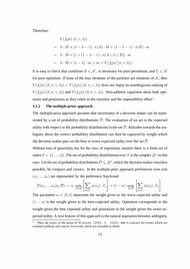
3.1.2 The multiple-prior approach

The multiple-prior approach assumes that uncertainty of a decision maker can be repre-

sented by a set of probability distributions D: The evaluation of an act is the expected

utility with respect to the probability distributions in the set D: Attitudes towards the am-

biguity about the correct probability distribution can then be captured by weight which

the decision maker puts on the best or worst expected utility over the set D:Without loss of generality, but for the ease of exposition, assume there is a finite set of

statesS = f1; :::; ng: The set of probability distributions over S is the simplex ¢n in this

case. Let the set of probability distributions D µ ¢n;which the decision maker considers

possible, be compact and convex. In the multiple-prior approach preferences over acts

(x1; :::; xn) are represented by the preference functional

V(x1; :::; xnj®;D) := ®¢ mine¼2D

"X

s2Su(xs) ¢ e¼s

#+ (1 ¡ ®)¢ max

e¼2D

"X

s2Su(xs) ¢ e¼s

#:

The parameter ® 2 [0; 1] represents the weight given to the worst expected utility and

(1 ¡ ®) is the weight given to the best expected utility. Optimism corresponds to the

weight given the best expected utility and pessimism to the weight given the worst ex-

pected utility. A nice feature of this approach is the natural separation between ambiguity,1 They are cavex in the sense of Wakker (2001, p. 1049), that is concave for events which arerevealed unlikely and convex for events which are revealed as likely.

13

reflected by the set D; and attitudes towards ambiguity, ref lected by the degrees of pes-

simism ® and optimism (1 ¡ ®):The Choquet expected utility of a neo-additive capacity defined in Equation 1 can be

viewed as a multiple-prior expected utility. Applied to the case of a finite state space, it

is not difficult to verify the following equality:

V (x1; :::; xnjº(¢j¼; °; ¸)) :=

°¢ mins2S

u(xs) + ¸¢ maxs2S

u(xs) + (1¡ ° ¡ ¸) ¢"X

s2Su(xs) ¢ ¼s

#

= °° + ¸

¢ mine¼2D

"X

s2Su(xs) ¢ e¼s

#+ ¸° + ¸

¢ maxe¼2D

"X

s2Su(xs) ¢ e¼s

#

= : V(x1; :::; xnj°° + ¸

;D);

with

D := fe¼ 2 ¢nj e¼s ¸ (1¡ ° ¡ ¸) ¢ ¼s; s 2 Sg :Note that the set of probabilities D is convex and compact. Moreover, it has a nice geo-

metric structure as Figure 3 illustrates for the case of n = 3: For a neo-additive capacity

q

qq~¼1 = 1 ~¼2 = 1

~¼3 = 1

s¼

Figure 3: Multiple priors

14

º(¢j¼; °; ¸) the set of possible probability distributions D is centered around the proba-

bility distribution ¼ and has a size determined by ° + ¸: Hence, ° + ¸ can be viewed

as the degree of ambiguity about the additive probability distribution ¼: The degree of

pessimism °°+¸ and the degree of optimism ¸

°+¸ measure the decision maker’s attitude

towards this ambiguity. Thus, neo-additive capacities have also a natural interpretation

in the context of the multiple-prior approach.

It is worth noting that it is well-known that the Choquet expected utility approach is equiv-

alent to the multiple prior approach if capacities are convex. It is worth noting that, in

general, neo-additive capacities are neither convex nor concave.

4. Economic Applications

The ups and downs of economic activity during the business cycle which are usually

accompanied by swings in investors’ sentiments, ranging from bull to bear spirits in fi-

nancial markets, provide numerous examples of the impact of uncertainty on economic

behavior.

Neo-additive capacities provide a natural way for modelling optimism and pessimism

influencing economic activities. The parameters of a neo-additive capacity can be inter-

preted as measuring confidence in beliefs and degrees of optimism and pessimism. A

neo-additive capacity º(E j¼; °; ¸) is based on an additive probability distribution ¼ re-

f lecting the subjective beliefs of the decision maker. It represents an assessment of the

likelihood of events consistent with the individual’s belief. The weight (1¡ ° ¡¸) given

to ¼ is a measure of the degree of confidence which the individual holds in this belief. The

core belief of a neo-additive capacity represented by the additive probability distribution

¼ can be determined endogenously in equilibrium2 . Thus, standard equilibrium analysis

is always the special case of full confidence, ° = ¸ = 0:

Positive parameters ° and ¸ represent the impact of pessimism and optimism respec-

tively. Neo-additive capacities can therefore model psychological phenomena such as

2 Eichberger & Kelsey (2000) provide a thorough analysis of strategic games when beliefs aremodelled as non-additive capacities.

15

excessive optimism and pessimism which have been put forward as explanations for eco-

nomic behavior in depressions or bubbles and which have been confirmed in laboratory

experiments.

In this section we show by example that optimism and pessimism can explain behavior

inconsistent with expected utility maximization. In theses cases, optimism and pessimism

can help to explain well-known economic puzzles. We will reconsider the paradox of

people buying insurance and gambling, and we will review portfolio choice behavior

where one observes unreasonably high risk premia (the equity premium puzzle ) and a

willingness to invest in high-risk stock of unknown start-up companies (the small stock

puzzle ).

4.1 Insurance and gambling

The same individual is often observed to buy both insurance against risk and lottery tick-

ets. As our introductory quotation of Adam Smith illustrates, such behavior is ubiquitous

but hard to reconcile with rational decision making based on probabilistic calculus. For

expected utility maximizers with a von Neumann-Morgenstern utility function such be-

havior is hard to explain.3 Buying insurance suggests a preference for reduced risk, while

paying for a lottery implies preference for a risky gamble, often at very unfair odds.

To see how both types of behavior can be accommodated by a neo-additive capacity,

consider an individual endowed with wealth x, whose preferences over lotteries can be

represented by the Choquet expected utility of a neo-additive capacity, with parameters

° > ¸ ¸ 0 for the neo-additive capacity and utility index u (taken to be concave). This

individual faces a (small) probability ¼L of incurring a loss of size L. Insurance coverage

is available at a premium q. Also available at a price p is a lottery ticket that ‘wins’ with

(a very small ) probability ¼W and pays out the single prize of size W and otherwise

pays out nothing. Suppose that the individual views the event in which he incurs the loss

and the event in which he wins the lottery (should he purchase a ticket) are independent.

3 Friedman & Savage (1948) suggest an S-shaped von Neumann-Morgenstern utility function.This approach to reconcile such behaviour has been critisised by Markowitz (1952). See Hirsh-leifer & Riley (1992) for a discussion of the Friedman-Savage approach (pp. 26-28).

16

Further suppose that [° + (1 ¡ ° ¡ ¸) ¢ ¼L] ¢ L > q ¸ ¼L ¢ L: The weak inequality is a

feasibility condition for the insurance premium to cover at least the expected loss (and if

strict it means that the insurance coverage is actuarially unfair). The strict inequality is

satisfied if the individual has a positive degree of pessimism ° and if the potential loss

L is sufficiently large.

The difference in the Choquet expected utilities between buying and not buying the in-

surance is

u (x¡ q)¡ ([¸+ (1¡ ° ¡ ¸) ¢ (1¡ ¼L)] ¢ u (x) + [° + (1¡ ° ¡ ¸) ¢ ¼L] ¢ u (x¡ L))

¸ u (x¡ q)¡ u ([¸ + (1¡ ° ¡ ¸) ¢ (1 ¡¼L)] ¢ x + [° + (1¡ ° ¡ ¸) ¢ ¼L] ¢ (x¡ L))

= u (x¡ q)¡ u (x¡ [° + (1¡ ° ¡ ¸)¼L]L) > 0

The first inequality follows from Jensen’s inequality applied to the convex function ¡u,

and the second inequality follows from monotonicity of u. Figure 4 illustrates the desir-

ability of purchase of full coverage at the unfair premium for the case where u is affine.

slope: ¡ °+(1¡°¡ )̧¼L¸+(1¡°¡¸)(1¡¼L)

0

purchase of insuranceno accident

accident

............................................

s

s.......................

......................

x¡ L x¡ q

x¡ q

x

slope: ¡ ¼L1¡¼L¡

¡¡ª

¢¢¢®

slope: ¡ ¸+(1¡°¡¸)¼L°+(1¡°¡ )̧(1¡¼L)

¾

Figure 4: Insurance

Having purchased the insurance, the difference in Choquet expected utilities between

17

buying the lottery ticket and not may now be expressed as

[¸ + (1 ¡ ° ¡ ¸) ¢ ¼W ] ¢ u (x+W ¡ p¡ q)

+[° + (1¡ ° ¡ ¸) ¢ (1 ¡ ¼W )] ¢ u (x¡ p¡ q)¡ u (x¡ q)

> ¸ ¢ u (x+W ¡ p ¡ q) + (1 ¡ ¸) ¢ u (x¡ p ¡ q) ¡ u (x ¡ q)

¸ ¸ ¢ [u (x +W ¡ p¡ q) ¡ u (x¡ q)]¡ p ¢ u0 (x¡ q) :

The last inequality follows from the concavity of u: For ¸ > 0 and u strictly increasing,

there is a lottery (W;¼W ; p)withW highenough and¼W small enoughsuch that¼W ¢W <p and

¸ ¢ [u (x +W ¡ p¡ q) ¡ u (x¡ q)]p

> u0 (x¡ q) :

Notice that this is true for any degree of concavity of u: Optimism makes lotteries with

high prizes and low probabilities of winning attractive even for individuals who are averse

to accepting actuarially fair fifty-fifty gambles. Figure 5 illustrates the desirability of the

purchase of an unfair lottery ticket for the case where u is affine.

4.2 Portfolio choice

There are numerous puzzles in portfolio choice theory. Thaler (2000) provides a

stimulating exposition of some well-known irregularities. These puzzles highlight incon-

sistencies between standard economic theories and empirical regularities. Naturally, not

all can be related to optimism or pessimism. The following two puzzles however can be

explained easily by a small degree of optimism and pessimism.

The equity premium puzzle refers to the large difference between the average return on a

stock portfolio and the return of a fixed interest bearing bond which was first noted by

Mehra & Prescott (1985). The implied risk premium appears to be too big to be

explained by risk aversion as modelled by a concave von Neumann-Morgenstern utility

function. The conservative behavior in the face of uncertainty suggested by such a high

risk premium stands in stark contrast to the observation that small firms with high-risk

stocks seem to attract investors’ interest more than is warranted by their average returns.

18

purchase of a lottery ticketlose lottery

ss

.........

.........

x¡ q

x¡ q

x¡ q ¡ px +W ¡ q ¡ p

slope: ¡ ¸+(1¡°¡¸)¼W°+(1¡°¡ )̧(1¡¼W )

slope: ¡ ¼W1¡¼W

slope: ¡ °+(1¡°¡¸)¼W¸+(1¡°¡ )̧(1¡¼W )¡

¡¡ª

¡¡ª

CCCCCCO

win lottery

Figure 5: Gambling

To invest in stock of young ‘‘promising’’ companies appears to be extraordinarily risky.

Yet such uncertainty did not deter investors who otherwise requested a surprisingly high

risk premium.

We study a simple financial market system with a representative investor, one risky and

one riskless asset and an exogenous supply of assets. This framework suffices to illustrate

the impact of optimism and pessimism on portfolio choice. With well-known modifica-

tions these results carry over to more general models of financial markets.

Consider an investor with initial wealth W0 who can invest in two assets, a stock with

uncertain returns and a bond with a certain payoff. The following table summarizes the

notation of the assets.asset quantity price payoff in state s 2 Sstock a q rsbond b 1 r

Preferences of the investor are represented by a Choquet expected utility V (W1; :::;WS)

19

of end-of-period wealth,Ws = rs ¢ a + r ¢ b; with respect to a neo–additive capacityV (W1; :::;WS):= ° ¢ minfu(W1); :::; u(WS)g + ¸ ¢ maxfu(W1); :::; u(WS)g+(1¡ ° ¡ ¸)¢ P

s2S¼s ¢ u(Ws):

Using the budget constraint, W0 = q ¢ a + b; to substitute for the bond, one gets wealth

as a function of stock transactions a,

Ws = r ¢W0 + [rs¡ q ¢ r] ¢ a:

Denoting by r = maxfr1; :::; rSg and r = minfr1; :::; rSg the maximal and minimal

returns of the risky stock, one can write the Choquet expected utility from a stock invest-

ment a > 0 asV (a) := ° ¢ u(r ¢W0 + [r ¡ q ¢ r] ¢ a)

+¸ ¢ u(r ¢W0 + [r ¡ q ¢ r] ¢ a)+(1¡ ° ¡ ¸)¢ P

s2S¼s ¢ u(r ¢W0 + [rs¡ q ¢ r] ¢ a):

For a stock market equilibrium price q¤ with an aggregate endowment of equity A > 0

and bonds B = 0 where the single investor maximizes Choquet expected utility V (a);V 0(A) = ° ¢ u0(r ¢W0 + [r ¡ q¤ ¢ r] ¢ A) ¢ [r ¡ q¤ ¢ r]

+¸ ¢ u0(r ¢W0+ [r ¡ q¤ ¢ r] ¢ A) ¢ [r ¡ q¤ ¢ r]+(1¡ ° ¡ ¸)¢ P

s2S¼s ¢ u0(r ¢W0 + [rs ¡ q¤ ¢ r] ¢ A) ¢ [rs¡ q¤ ¢ r] = 0

must hold in equilibrium. Substituting for the initial wealthW0 = q¤ ¢A; this equilibrium

condition can be solved explicitly for the equilibrium stock price q¤;

q¤ =° ¢ u0(r ¢ A) ¢ r + ¸ ¢ u0(r ¢ A) ¢ r + (1¡ ° ¡ ¸)¢ P

s2S¼s ¢ u0(rs ¢ A) ¢ rs

r ¢·° ¢ u0(r ¢ A) + ¸ ¢ u0(r ¢ A) + (1 ¡ ° ¡ ¸)¢ P

s2S¼s ¢ u0(rs ¢ A)

¸ : (*)

The case of subjective expected utility, ° = ¸ = 0; is the reference situation against

which we can assess the impact of optimism or pessimism. Denote by q¤0 the equity price

in this case,

q¤0 =

Ps2S¼s ¢ u0(rs ¢ A) ¢ rs

r¢ Ps2S¼s ¢ u0(rs ¢ A) :

The equity premium is defined as the ratio

®(q¤) :=

Ps2S¼s ¢ rsq¤ ¢ r :

20

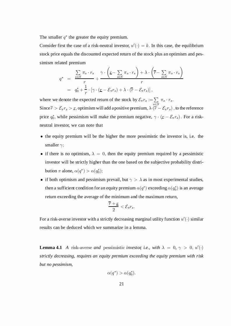
The smaller q¤ the greater the equity premium.

Consider first the case of a risk-neutral investor, u0(¢) = k: In this case, the equilibrium

stock price equals the discounted expected return of the stock plus an optimism and pes-

simism related premium

q¤ =

Ps2S¼s ¢ rsr

+° ¢

µr¡ P

s2S¼s ¢ rs

¶+ ¸ ¢

µr¡ P

s2S¼s ¢ rs

¶

r

= q¤0 +1r ¢ [° ¢ (r ¡ E¼rs) + ¸ ¢ (r ¡ E¼rs)] ;

where we denote the expected return of the stock by E¼rs :=Ps2S¼s ¢ rs:

Sincer > E¼rs > r; optimism will add apositive premium, ¸¢(r ¡ E¼rs) ; to the reference

price q¤0; while pessimism will make the premium negative, ° ¢ (r ¡ E¼rs) : For a risk-

neutral investor, we can note that

² the equity premium will be the higher the more pessimistic the investor is, i.e. the

smaller °;

² if there is no optimism, ¸ = 0; then the equity premium required by a pessimistic

investor will be strictly higher than the one based on the subjective probability distri-

bution ¼ alone, ®(q¤) > ®(q¤0);

² if both optimism and pessimism prevail, but ° > ¸ as in most experimental studies,

then a sufficient condition for an equity premium ®(q¤) exceeding ®(q¤0) is an average

return exceeding the average of the minimum and the maximum return,r + r2< E¼rs:

For a risk-averse investor with a strictly decreasing marginal utility function u0(¢) similar

results can be deduced which we summarize in a lemma.

Lemma 4.1 A risk-averse and pessimistic investor, i.e., with ¸ = 0, ° > 0; u0(¢)strictly decreasing, requires an equity premium exceeding the equity premium with risk

but no pessimism,

®(q¤) > ®(q¤0):

21

Proof. Appendix.

In recent years ‘‘new stock markets’’ have emerged in many developed countries where

stock of start-up firms is traded. These markets were opened in order to provide ven-

ture capital for new high-risk enterprises with great potential. In the light of the rather

conservative behavior reflected in the equity premium puzzle it is even more surprising

that investors were willing to bet substantial amounts of wealth on firms with no record

of earnings.

Optimism and pessimism as modelled with a neo-additive capacity enables us to explain

such behavior. In fact, we can show that for an arbitrary small degree of optimism there

are maximal returns of a firm high enough to induce a positive stock price for high-risk

firms with potentially high returns. Reconsider the stock market equilibrium price of

Equation (*) and assume, without loss of generality, that the firm’s stock pays off a return

R only in state 1. Hence, r = r1 = R and r = rs = 0 for all s 6= 1: Suppose the expected

return of the firm is bounded away from zero, ¼1 ¢ R ¸ · > 0: Then the equilibrium

price satisfies

q¤ =1r

¢ ¸ ¢ u0(R ¢ A) ¢R + (1¡ ° ¡ ¸) ¢ ¼1 ¢ u0(R ¢ A) ¢R

° ¢ u0(0) + ¸ ¢ u0(R ¢ A) + (1 ¡ ° ¡ ¸) ¢"¼1 ¢ u0(R ¢ A)+ P

s6=1¼s ¢ u0(0)

#

=Rr

¢ u0(R ¢ A) ¢ [¸ + (1¡ ° ¡¸) ¢ ¼1]u0(R ¢ A) ¢ [¸ + (1¡ ° ¡ ¸) ¢ ¼1] + u0(0) ¢ [° ¢ +(1 ¡ ° ¡ ¸) ¢ (1¡ ¼1)]

¸ Rr

¢ [¸ + (1¡ ° ¡ ¸) ¢ ¼1]

>Rr

¢ ¸;

where the first inequality follows from u0(0) ¸ u0(R ¢A) and the second strict inequality

from the positive expected return.

It is clear that with some optimism, ¸ > 0; even a vanishing probability of success ¼1

will not deter investors provided the return rises sufficiently,R ¸ ·=¼1:The stock market

price will not collapse. There is no contradiction if investors buy high-risk stock because

of optimism, ¸ > 0; and require an “excessive” equity premium. Adam Smith’s observa-

22

tion that even “sober people” do play lotteries and Robert Shiller’s observed “exuberance”

in the stock market can be reconciled with rational decision making under uncertainty, if

one allows for optimism and pessimism as modelled by neo-additive capacities.

5. Behavioral axioms

We present our theory in the context of a variant of Savage’s (1954) purely subjective

uncertainty framework employed by Ghirardato & Marinacci (2001) and Ghi-

rardato, Maccherioni, Marinacci & Siniscalchi (2002) (hereafter, GMMS).

The state space S is taken to be the same as was defined in section 2 above. Let X, the

set of outcomes, be a connected and separable topological space. An act is a function

(measurable with respect to E) f : S ! X with finite range, F denotes the set of such

acts and is endowed with the product topology induced by the topology on X. We shall

identify each x 2 X with the constant act, f(s) = x for all s 2 S. For any pair of acts f; g

in F and any event E 2 E , fEg will denote the acth 2 F , formed from the concatenation

of the two acts f and g, in which h (s) equals f (s) if s 2 E , and equals g (s) if s =2 E .

Let % denote the individual’s preference relation on F : For any f 2 F , the certainty

equivalent of f , denoted by m (f ), is the set of constant acts that are indifferent to f .

That is, x 2 m(f), if x » f . Although many constant acts may be equivalent, when there

is no risk of confusion, we shall writem (f) to indicate an arbitrary member of the set.

We say f and g are comonotonic if for every pair of states s and s0 in S , f (s) Â f (s0)implies g (s) % g (s0). We say an event E 2 E is null if fEg » g for all f; g 2 F . Let

N denote the set of null events. An event E is universal, if its complement is null, that

is, S ¡ E 2 N . We shall denote by E¤, the set of events that are neither impossible nor

certain, that is the set E ¡ (N [ U).For ease of exposition and without any essential loss of generality we assume there exist

outcomes 0 and M in X, that are, respectively, the “best ” and “worst ” outcomes in X,

in the sense that M Â 0 andM % x % 0 for all x 2 X.

Neo-additive capacities are a special case of the Choquet expected utility theory. In order

23

to obtain a behavioral characterization, we seek to modify the axioms of GMMS appro-

priately. Their key innovation is to define a behavioral definition of ‘subjective mixtures’

of acts which allows them to define in a Savage framework of purely subjective uncer-

tainty, analogs to axioms based on probability mixtures that play such a key role in the

Anscombe-Aumann framework.

The first is the standard ordering axiom.

Axiom 1 (Ordering )

The preference relation % on F is complete, reflexive and transitive.

The neo-additive expectedutility representation allows for the ‘discontinuous over-weighting’

of events on which extreme, i.e. either best or the worst, outcomes obtain. Hence, stan-

dard continuity with respect to the product topology cannot be expected to hold for the

whole preference relation. Following Ghirardato & Marinacci (2001) we only

require a weaker notion of pointwise convergence, where in this product topology, we

say a net ff®g®2D µ F converges pointwise to f 2 F , if and only if f® (s) ! f (s)

for all s 2 S .

Axiom 2 (Continuity ).

Let ff®g®2D µ F be a net that converges pointwise to f and such that all f®s and f are

measurable with respect to the same finite partition.. If f® % g (respectively, g % f®) for

all ® 2 D, then f % g (respectively, g % f).

We also adopt the monotonicity axiom of Chew & Karni (1994) which combines

statewise dominance with a weakening of Savage’s axiom P3.

Axiom 3 (Eventwise Monotonicity ).

For any pair of acts, f; g 2 F , if f (s) % g (s) for all s 2 S , then f % g. In addition, for

any triple of outcomes x; y; z 2 X, and any event E =2 N

(a) if x % z, y % z then x  y) xEz  yEz;(b) if z % x, z % y then x  y) xEz  yEz.

The next axiom due to Ghirardato & Marinacci (2001) builds on the idea of

24

Nakamura (1990) and Gul (1992) of a ‘subjective mixture’ of two acts f and g.

Fix some event E , and then construct state by state an act which yields at each state s, the

certainty equivalent of the bet f (s)E g (s). Formally, the statewise (event) E-mixture of

f and g, denoted as fEg, is taken to be the act

fEg (s) =m (f (s)E g (s)) .

Adopting the shorthand fx; yg % z for x % z and y % z, and z %fx; yg for z % x and

z % x, the next axiom may be stated as follows.

Axiom 4 (Binary Comonotonic Act Independence )

For any event A 2 E¤ (that is, neither A nor S ¡ A is null), any event B 2 E , and for all

f; g; h 2 F , such that f = xAy, g = x0Ay 0, h = x00Ay00. If f; g; h are pairwise comonotonic,

and fx; x0g % x00 and fy; y0g % y00 (or x00 % fx; x0g and y00 % fy; y0g), then

f % g) fBh % gBh.

As its names suggests, Binary Comontonic Act Independence, means that the preference

relation restricted to acts that are measurable with respect to two-element partitions, con-

forms to the theory of Choquet Expected Utility. With these four axioms, Ghirardato

& Marinacci (2001) were able to prove that the preference relation admits what they

dubbed a (canonical) biseparable representation, namely, a Choquet Expected Utility rep-

resentation defined on this restricted set of acts.

Proposition 5.1 (Ghirardato and Marinacci [2001], Theorem 11) LetX bea connected

and separable topological space and let % be a binary relation on F for which there exist

outcomes 0 and M in X, such that M Â 0 and M % x % 0 for all x 2 X. Then the

following are equivalent:

(i) % satisfies Axioms 1-4 and there exists an event A such that A and S ¡ A are both

non-null.

(ii) There exist a unique continuous utility index u : X ! [0; 1], with u (0) = 0 and

u (M ) = 1, and a unique capacity º : E ! [0; 1] such that for all x; y; x0; y0, such that

25

x % y and x0 % y 0 and all E;E0 2 E

xEy % x0E0y0 (2)

, º (E) u (x) + (1 ¡ º (E))u (y) ¸ º (E0) u (x0) + (1 ¡ º (E 0)) u (y0)

It remains to impose an appropriate version of an independence-type axiom that extends

the biseparable CEU representation obtained in Proposition 5.1 to the whole domain Fand moreover entails that the capacity in that representation is neo-additive. To do this,

we first need to define GMMS’s notion of a ‘subjective mixture’ of two acts. We begin

with their definition of a ‘preference average’ of two consequences..

Definition 5.1 Fix x; y 2 X, such that x  y . We say that a consequence z 2 X is a

preference average of x and y (given E) if x % z % y and

xEy »m (xEz)E m (zEy)

The reason for their nomenclature becomes apparent if we consider for a preference re-

lation that satisfies Axioms 1-4, the preference average of x and y given an event E that

is not null and whose complement is also not null. From Proposition (5:1) we obtain the

equality

º (E) u (x) + (1¡ º (E)) u (y)

= º (E) u (m (xEz)) + (1¡ º (E)) u (m (zEy))

= [º (E)]2 u (x) + 2º (E) (1 ¡ º (E))u (z) + (1 ¡ º (E))2u (y) .

Notice that if neither the event E nor its complement is null then 0 < º (E) < 1, and

so solving for u (z) yields

u (z) =12u (x) +

12u (y) ,

which is independent of E. We shall therefore denote by (1=2) x©(1=2)y the preference

average of the outcomes x and y. To deliver weighted averages of x and y, we follow

the line of argument detailed in GMMS. That is, by using iterated averages (for example,

(1=2) x © ((1=2) x© (1=2)y) corresponds to a (3=4; 1=4)¡weighted average of x and

y) and appealing to standard continuity arguments, it is possible to identify, for any ® in

26

[0;1] and every x and y in X, the weighted preference averages characterized by

u (z) = ®u (x) + (1¡ ®) u (y) . (3)

With slight abuse of notation, we shall let ®x © (1¡ ®) y (or, equivalently, (1¡ ®) y ©®x) denote an arbitrary element of the indifferent set of outcomes for such preference

averages. We are now in a position to define subjective mixtures of acts.

Definition 5.2 Fix f; g 2 F and ® 2 [0; 1]. A subjective mixture of f and g with

weight ® is any act h 2 F such that h (s) » ®f (s)© (1 ¡ ®)g (s) for each s 2 S .

As GMMS note, all subjective mixtures of f and g with weight ® are state-wise in-

different, and hence by Axiom 3 (i), indifferent. So we follow them and denote by

®f © (1¡ ®) g any one of them.

Our final axiom is key to characterizing the decision maker’s attitudes towards events that

yield extreme outcomes. We first need, however, to define for each act which events the

decision maker views as yielding the extreme outcomes. We begin with preference-based

definitions for the infimum and the supremum of an act.

Definition 5.3 Fix f 2 F . An outcome z 2 X is said to be in the indifference set of the

infimum of f , z 2 infº(f), if for A := f¡1(x : z  x), zAf » f and if for every y  zand B := f¡1(x : y º x), yBf  f . Similarly, an outcome z 2 X is said to be in the

indifference set of the supremum of f , z 2 supº(f) if for A := f¡1(x : x  z), zAf » fand if for every y such that z  y and B := f¡1(x : x º y), f  yBf .

Although infº(f) and supº(f ) are defined to be indifference sets of outcomes, when

there is no risk of confusion, we shall write infº(f ) and supº(f ) to indicate arbitrary

members of these respective sets.

From the definition of a subjective mixture and equation (3) it follows that for every f; g

2 F , ® 2 [0; 1] and s 2 S

u (®f (s) © (1¡ ®) g (s)) = ®u (f (s)) + (1¡ ®) u (g (s)) .

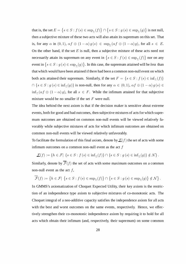
Hence, if there is a non-null event on which both acts f and g attain their supremum,

27

that is, the set E =©s 2 S : f (s) 2 supº(f)

ª\

©s 2 S : g (s) 2 supº(g)

ªis not null,

then a subjective mixture of these two acts will also attain its supremum on this set. That

is, for any ® in (0; 1), ®f © (1¡ ®) g (s) 2 supº(®f © (1 ¡ ®)g), for all s 2 E.

On the other hand, if the set E is null, then a subjective mixture of these acts need not

necessarily attain its supremum on any event in©s 2 S : f (s) 2 supº(f)

ªnor on any

event in©s 2 S : g (s) 2 supº(g)

ª. In this case, the supremum attained will be less than

that which would have been attained if there had been a common non-null event on which

both acts attained their supremum. Similarly, if the set F = fs 2 S : f (s) 2 infº(f)g\ fs 2 S : g (s) 2 infº(g)g is non-null, then for any ® 2 (0; 1), ®f © (1 ¡ ®) g (s) 2infº(®f © (1¡ ®) g), for all s 2 F . While the infimum attained for that subjective

mixture would be no smaller if the set F were null.

The idea behind the next axiom is that if the decision maker is sensitive about extreme

events, both for good and bad outcomes, then subjective mixtures of acts for which supre-

mum outcomes are obtained on common non-null events will be viewed relatively fa-

vorably while subjective mixtures of acts for which infimum outcomes are obtained on

common non-null events will be viewed relatively unfavorably.

To facilitate the formulation of this final axiom, denote by F(f ) the set of acts with some

infimum outcomes on a common non-null event as the act f

F(f) := fh 2 Fj fs 2 S : f (s) 2 infº(f )g \ fs 2 S : g (s) 2 infº(g)g =2 Ng :

Similarly, denote by F(f) the set of acts with some maximum outcomes on a common

non-null event as the act f ,

F(f) :=©h 2 Fj

©s 2 S : f (s) 2 supº(f)

ª\

©s 2 S : g (s) 2 supº(g)

ª=2 N

ª:

In GMMS’s axiomatization of Choquet Expected Utility, their key axiom is the restric-

tion of an independence type axiom to subjective mixtures of co-monotonic acts. The

Choquet integral of a neo-additive capacity satisfies the independence axiom for all acts

with the best and worst outcomes on the same events, respectively. Hence, we effec-

tively strengthen their co-monotonic independence axiom by requiring it to hold for all

acts which obtain their infimum (and, respectively, their supremum) on some common

28

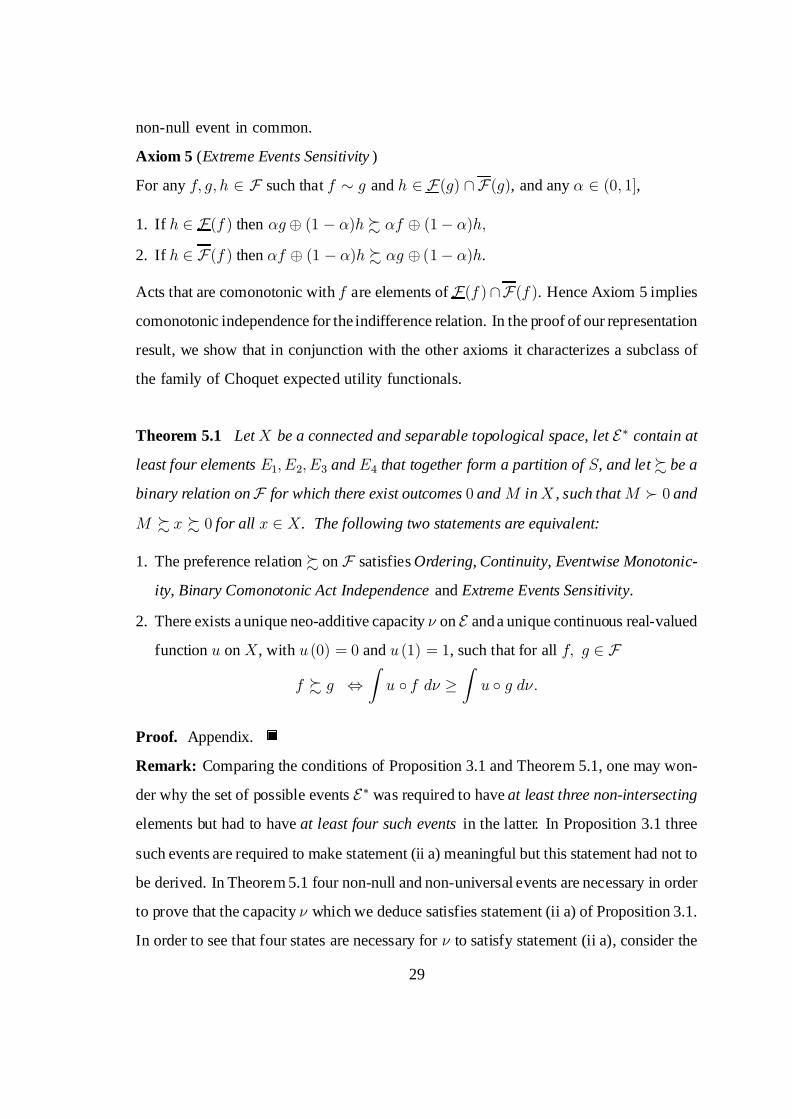
non-null event in common.

Axiom 5 (Extreme Events Sensitivity )

For any f; g; h 2 F such that f » g and h 2 F(g) \ F(g), and any ® 2 (0; 1],

1. If h 2 F(f ) then ®g© (1 ¡ ®)h % ®f © (1¡ ®)h;2. If h 2 F(f ) then ®f © (1 ¡ ®)h % ®g © (1¡ ®)h.

Acts that are comonotonic with f are elements of F(f )\F(f ). Hence Axiom 5 implies

comonotonic independence for the indifference relation. In the proof of our representation

result, we show that in conjunction with the other axioms it characterizes a subclass of

the family of Choquet expected utility functionals.

Theorem 5.1 LetX be a connected and separable topological space, let E¤ contain at

least four elements E1; E2; E3 and E4 that together form a partition of S, and let % be a

binary relation on F for which there exist outcomes 0 andM inX , such thatM Â 0 and

M % x % 0 for all x 2 X. The following two statements are equivalent:

1. The preference relation % on F satisfies Ordering, Continuity, Eventwise Monotonic-

ity, Binary Comonotonic Act Independence and Extreme Events Sensitivity.

2. There exists aunique neo-additive capacity º on E anda unique continuous real-valued

function u on X, with u (0) = 0 and u (1) = 1, such that for all f; g 2 F

f % g ,Zu ± f dº ¸

Zu ± g dº:

Proof. Appendix.

Remark: Comparing the conditions of Proposition 3.1 and Theorem 5.1, one may won-

der why the set of possible events E¤ was required to have at least three non-intersecting

elements but had to have at least four such events in the latter. In Proposition 3.1 three

such events are required to make statement (ii a) meaningful but this statement had not to

be derived. In Theorem 5.1 four non-null and non-universal events are necessary in order

to prove that the capacity º which we deduce satisfies statement (ii a) of Proposition 3.1.

In order to see that four states are necessary for º to satisfy statement (ii a), consider the

29

following counterexample. The capacity º on S = fs1; s2; s3g defined by

º(s1) = 12 ; º(s2) = 1

3 ; º(s3) = 14 ;

º(fs1; s2g) = º(fs1; s3g) = º(fs2; s3g) = 12

satisfies statements (ii b) and (ii c) but not (ii a) of Proposition 3.1 Hence, it is not neo-

additive.

6. Concluding remarks

Optimism and pessimism have long been recognized as important determinants of eco-

nomic behavior. Subjective expected utility theory assumes that the impact of uncertainty

can be reduced to the statistical properties of a probability distribution. This reduction

extends economic analysis to situations under uncertainty where one could rightfully ne-

glect psychological aspects relating to the focal attraction of the best and worst outcome

of economic choices.

In this paper we have introduced a special case of capacity and its Choquet integral which

captures aspects of optimism and pessimism without abandoning the subjectively proba-

bilistic approach all together. In particular, subjective expected utility is always contained

as a special parametric case in this approach. Moreover, as inEichberger & Kelsey

(2000), the additive part of a neo-additive capacity can be determined endogenously in

equilibrium.

Most importantly neo-additive capacities open new avenues of research. It appears nat-

ural to view the degree of confidence which a decision maker holds in a probabilistic

assessment of an uncertain situation as dependent on past experience and subject to inf lu-

ence from other people’s beliefs. Optimism and pessimism may spread in a population.

Attitudes towards uncertain outcomes may be contagious leading to general swings in

optimism and pessimism. So ‘‘irrational exuberance’’ as observed by Shiller (2001)

may become amenable to formal economic analysis after all.

30

Appendix A

The following preliminary lemma establishes uniqueness of °; ¸; and ¼:

Lemma: Let º be a capacity on (S; E); where E contains at least three elements E1, E2,

and E3, such that Ei \ Ej = ?, for all i 6= j, and º (Ei) > 0, for all i. Then (°; ¸; ¼)

is unique.

Proof. Let (°; ¸; ¼) be a given vector of parameters of º: Denote by ± := 1 ¡ ° ¡ ¸ and

e¼(E) := ± ¢ ¼(E) for all E 2 E :For any E 2 E¤ and F 2 E¤ such that E \ F = ; and E [ F =2 U, e¼(E) is uniquely

defined by e¼(E) := º(E [ F ) ¡ º(F ):Assume now that E 2 E¤, then there exists (E1; E2) 2 E¤ £ E¤ such that E1 \ E2 = ;and E1 [E2 = E: Hence, e¼(E) is uniquely defined by e¼(E) = e¼(E1) + e¼(E2):

This implies that e¼(E) is uniquely defined for all E 2 E¤ and that ¸ is uniquely defined

by ¸ := º(E) ¡ e¼(E) for all E 2 E¤:Let fEi 2 E¤j i = 1; ::; 3g be a partition of S: Then ® is uniquely defined by ® :=

3Pi=1

e¼(Ei): Hence, ° is unique. For, either ® = 0 and there is no ¼ in the expression of º; or

® > 0 and ¼ is uniquely defined for any E 2 E¤ by ¼(E) := e¼(E)® :

A.1 Proof of Proposition 3.1

(i) =) (ii). This follows from the definition of a neo-additive capacity.

(ii) =) (i).

(a) First we define a non-negative simple additive measure e¼ on E¤:Case 1: E 2 eE := fE 2 E¤j 9 F 2 E¤; E \ F = ;; E [ F =2 Ug:Define e¼(E) := º(E [ F ) ¡ º(F ) for all F 2 E¤ such that E \ F = ;; E [ F =2 U.

Property (a) implies that e¼(E) is well-defined.

Case 2: E 2 E¤¡eE :HenceF = S¡E =2 E¤ is a singleton and there exists a finite partition

31

of E , fEi 2 eEj i = 1; :::; ng: Define e¼(E) :=nPi=1

e¼(Ei): It is well defined because

nX

i=1

e¼(Ei) = [º(E1 [ ::: [En) ¡ º(E2 [ ::: [En)]

+::::+ [º(En¡1 [En) ¡ º(En)] + e¼(En)

= º(E) ¡ º(En) + e¼(En)

= º(E) ¡ º(F ) + e¼(F ):

Monotonicity of º implies that e¼(E) ¸ 0 for all E 2 E¤:Let us check now:

e¼(E [ F ) = e¼(E) + e¼(F )

for all E;F 2 E¤ such that E \ F = ;; E [ F =2 U.

If E [ F 2 E¤ ¡ eE then this follows directly from Case 2.

If E [ F 2 eE then, for G 2 E¤ such that G \ (E [ F ) = ; and G [ (E [ F ) =2 Uone obtains

e¼(E [ F ) = º(E [ F [ G) ¡ º(G)

= [º(E [ F [G) ¡ º(F [ G)] + [º(F [ G) ¡ º(G)]

= e¼(E) + e¼(F ):

(b) Next we extend e¼ on all of E to a non-negative simple additive measure.

Clearly, defining e¼(E) = 0 for all E 2 N is consistent with the restricted additivity of

e¼; i.e. e¼(E [ F ) = e¼(E) + e¼(F ) for all E;F 2 E such that E \ F = ;; E [ F =2 U :Consider a finite partition of S; fEi 2 E¤j i = 1; :::; ng; and define e¼(S) :=

nPi=1

e¼(Ei):To check that e¼(S) is well-defined, let fFj 2 E¤j j = 1; :::;mg be another finite partition

of S; then one obtains

e¼(S) : =nX

i=1

e¼(Ei) =nX

i=1

"mX

j=1

e¼(Ei \ Fj)#

=mX

j=1

"nX

i=1

e¼(Ei \ Fj)#=mX

j=1

e¼(Fj):

32

Let ® := e¼(S): Clearly, ® ¸ 0:

It remains to prove that e¼(E [F ) = e¼(E)+e¼(F ) for all E;F 2 E¤ such that E\F = ;;E [ F =2 U : Since E¤ contains at least three elements, one can assume, without loss

of generality, that E = E1 [ E2 with E1; E2 2 E¤; E1 \ E2 = ;. Hence, e¼(E) =

e¼(E1) + e¼(E2) and, from the definition of e¼(S); the desired result follows.

(c)We prove that there exists ¸ 2 R+ such that º(E) = ¸+ e¼(E) for all E 2 E¤:If E 2 E¤ ¡ eE then, from Case 2, there exists A 2 E¤ such that

º(E) = e¼(E) + º(A) ¡ e¼(A):

IfE 2 eE then there existsF 2 E¤ and B 2 E¤ such thatE[F [G = S: Hence, one has

e¼(E [ F ) = º(E [ F ) + º(B) ¡ e¼(B);

and, therefore,

e¼(E) + e¼(F ) = º(E [ F ) ¡ º(E) + º(E) + e¼(B) ¡ º(B);

which gives

º(E) = e¼(E) + º(B) ¡ e¼(B):

Hence,

º(A)¡ e¼(Ag) = º(B)¡ e¼(B)for all A;B 2 E¤:It remains to check that the common value ¸ := º(A) ¡ e¼(A) is non-negative. Let

E;F 2 E¤ satisfy Property (b) and consider A ½ E and B ½ F: Applying Property (a)

twice gives

0 · º(E) + º(F ) ¡ º(E [ F ) = º(A) + º(B) ¡ º(A [B)

= º(A) ¡ e¼(A) = ¸:

(d)We prove that ® + ¸ · 1.

33

By Property (c), there is E;F 2 E¤ such that

0 · º(E) + º(F )¡ º(E [ F )

= 1¡ º(S ¡ E)¡ º(S ¡ F ) + º(S ¡ (E [ F ))

= 1¡ (¸ + e¼(S ¡ E))¡ (¸ + e¼(S ¡ F )) + (¸ + e¼(S ¡ (E [ F )))

= 1¡ ¸ ¡ ®:

(e) Setting ° := 1 ¡ ¸ ¡ ®; we finally obtain: º(E) = ° ¢ ¹0(E) + ¸ ¢ ¹1(E) + (1 ¡° ¡ ¸) ¢ ¼(E) for all E 2 E where, for 1¡ ° ¡ ¸ > 0; the probability measure ¼(E) is

defined by ¼(E) := 11¡°¡¸ ¢ e¼(E):

A.2 Proof of Lemma 4.1

Proof. From Equation (*), we get

q¤ =° ¢ u0(r ¢ A) ¢ r + (1 ¡ °)¢ P

s2S¼s ¢ u0(rs ¢ A) ¢ rs

r ¢·° ¢ u0(r ¢ A) + (1 ¡ °)¢ P

s2S¼s ¢ u0(rs ¢ A)

¸

=° ¢ u0(r ¢ A) ¢ r + (1 ¡ °) ¢

·r ¢ q¤0¢

Ps2S¼s ¢u0(rs ¢ A)

¸

r ¢·° ¢ u0(r ¢ A) + (1¡ °)¢ P

s2S¼s ¢ u0(rs ¢ A)

¸

<° ¢ u0(r ¢ A) ¢ r ¢ q¤0 + (1 ¡ °) ¢

·r ¢ q¤0¢

Ps2S¼s ¢ u0(rs ¢ A)

¸

r ¢·° ¢ u0(r ¢ A) + (1 ¡ °)¢ P

s2S¼s ¢ u0(rs ¢ A)

¸

= q¤0:

The inequality follows because

r ¢ q¤0 =

Ps2S¼s ¢ u0(rs ¢ A) ¢ rs

Ps2S¼s ¢ u0(rs ¢ A) < r:

A.3 Proof of Theorem 5.1

We begin with an observation and a couple of preliminary results. The observation is that

34

any act f 2 F may be expressed as [x1 on E1; : : : ; xn on En], where fE1; : : : ; Eng is the

coarsest finite %-ordered partition of S with respect to which f measurable. By that we

mean for any pair of states s; t 2 S, if both s and t are in some E 2 fE1; : : : ; Engthen f (s) = f (t), otherwise f (s) 6= f (t). Furthermore for any s 2 Ei and t 2Ej , i < j implies f (s) % f (t). Throughout this proof, if an act is expressed in the

form [x1 on E1; : : : ; xn on En] then it should be taken as given that xi % xi+1, for

i = 1; : : : ; i ¡ 1. We also note that Axiom 5 (Extreme Events Sensitivity) and Axiom

1 (Ordering) imply that if the preference relation expresses indifference between two co-

monotonic acts then indifference is preserved when those two acts are each mixed with a

third act that is pairwise co-monotonic with both.

Lemma: (Comonotonic Independence of Indifference) Axiom 5 implies that % satisfies

the following independence property for pairwise comonotonic acts. For any ® 2 [0; 1]

and any three acts f; g; h 2 F , that are pairwise comonotonic, if f » g then ®f ©(1 ¡ ®)h » ®g © (1 ¡ ®) h.

Proof : From the pairwise co-monotonicity of h with both f and g, it follows that h 2F(g) \ F(g) and h 2 F(f) \ F(f). Hence Axiom 5 implies that ®f © (1¡ ®) h %®g © (1¡ ®) h and ®g © (1¡ ®) h % ®f © (1¡ ®) h, as required. ¤

Finally we report GMMS’s result (2002, Proposition 6) that the triple (X;»;©) consti-

tutes a mixture set. That is, for allx; y 2 X and all®; ¯ in [0; 1], (M0)®x©(1¡ ®) y ½ X,

(M1) x 2 (1x © 0y), (M2) ®x © (1¡ ®) y = (1¡ ®) y © ®x (commutative law), and

(M3) ¯ (®x© (1¡ ®) y) © (1¡ ¯)y = ®¯x © (1¡ ®¯)y (distributive law). Applying

this result state by state, to Definition 5.2 (the definition of a subjective mixture of f and

g with weight ® in [0; 1]) it readily follows that the triple (F ;»;©) is also a mixture set

and hence exhibits the analogous properties.

Proof of Theorem 5.1-

1. Sufficiency

We first show that % has a CEU representation, Part (i), and then that the capacity is

35

neo-additive, Part (ii).

Part (i) . % admits a CEU-representation. Let u (:) and º (:) be the continuous utility

index and capacity of the canonical biseperable representation that from Proposition (5:1)

we know % admits. Recall that u (:) represents % restricted to the constant acts, and that

V ([x1 on E ; x2 on S ¡ E]) = º (E) u (x1) + (1 ¡ º (E))u (x2) represents % restricted

to the set of acts that are measurable with respect to a two-element partition of S.

Fix, f = [x1 on E1; : : : ; xn on En]. For each i = 1; : : : ; n, it follows from the definition

of © and the connectedness of X, that there exists a unique ¸i 2 [0; 1] for which xi 2¸iM © (1¡ ¸i) 0 and a unique ºi for which

[M on E1 [ : : : [ Ei; 0 on Ei+1 [ : : : [ En] » ºiM © (1 ¡ º i)0.

Equation (3) implies that 1 ¸ ¸1 ¸ : : : ¸ ¸n ¸ 0 and 0 · º1 · : : : · ºn¡1 · 1.

Hence we have, by construction and the mixture set properties of (F ;»;©) that

f =

24x1 on E1...

...xn on En

35 =

24¸1M © (1 ¡¸1) 0 on E1

......

¸nM © (1 ¡¸n) 0 on En

35

= (1¡ ¸1)

26666664

0 on E10 on E20 on E3...

...0 on En¡10 on En

37777775©(¸1 ¡ ¸2)

26666664

M on E10 on E20 on E3...

...0 on En¡10 on En

37777775

©(¸2 ¡ ¸3)

26666664

M on E1M on E20 on E3...

...0 on En¡10 on En

37777775

© ¢ ¢ ¢ © (¸n¡1 ¡ ¸n)

26666664

M on E1M on E2M on E3...

...M on En¡10 on En

37777775

© ¸n

26666664

M on E1M on E2M on E3...

...M on En¡1M on En

37777775

By applying the comonotonic independence of indifference property of Lemma 6.3 n¡1

times and utilizing the distributive law of (F ;»;©), we obtain

f » (1¡ ¸1) 0© (¸1 ¡ ¸2) [º1M © (1¡ º1) 0] © (¸2 ¡ ¸3) [º2M © (1¡ º2) 0]

© : : :© (¸n¡1 ¡ ¸n) [ºn¡1M © (1¡ ºn¡1)0] © ¸nM

=

"n¡1X

i=1

(¸i ¡ ¸i+1)º i + ¸n#M ©

"1¡ ¸n ¡

n¡1X

i=1

(¸i ¡ ¸i+1) º i

#±0.

36

Hence it follows from equation (3) that for any pair of acts

f =

24x1 on E1...

...xn on En

35 and f 0 =

24x01 onE 01...

...x0n0 on E 0n0

35

applying the above methods we have

f % f 0 if and only if"n¡1X

i=1

(¸i ¡ ¸i+1)º i + ¸n#

¸"n0¡1X

j=1

¡¸0j ¡ ¸0j+1

¢º0i + ¸

0n

#

By construction, u (0) = 0, u (M) = 1, u (xi) = ¸i, º (;) := 0, º (S) := 1 and

º¡[ij=1Ei

¢= º i. Thus we have established that % can be represented by the Choquet

expected utility functional

CEU

0@

24x1 on E1...

...xn on En

351A =

n¡1X

i=1

(u (xi) ¡ u (xi+1)) º¡[ij=1Ej

¢+ u (xn)

as required.

2. Necessity.

º satisfies conditions (ii) of Proposition 3.1.

(a) We prove that for any three events (E;F;G) 2 E¤ £E¤ £ E¤ such that E \ F = ; =

E \ G, E [ F =2 U, E [ G =2 U .

º(E [ F ) ¡ º(F ) = º(E [G) ¡ º(G);

Since there are at least four pairwise disjoint events in E¤; we can assume that there are

E;F;G 2 E¤ £ E¤ £ E¤ such that E \ F = E \ G = F \ G = ; and E [ F [G =2 U.

The following lemma contains the key argument.

Lemma: If there are E¤ £ E¤ £ E¤ such that E \ F = E \ G = F \ G = ; and

E [ F [ G =2 U. Then

º(E [ F [G) ¡ º(F [G) = º(E [ F ) ¡ º(F ): (*)

Proof: Assume, without loss of generality, º(E [ F ) · º(F [ G) and let ¯ 2 [0; 1] be

37

such that º(E [ F ) = ¯ ¢ º(F [ G): Consider

f : =·M on E [ F0 on S ¡ (E [ F )

¸;

g : =·¯ ¢M © (1¡ ¯) ¢ 0 on F [G0 on S ¡ (F [G)

¸;

h : =·M on F [G0 on S ¡ (F [G)

¸:

Clearly, f » g; h 2 F(f) \ F(f) and h 2 F(g) \ F(g): By Axiom 5, Extreme Event

Sensitivity, we have12

¢ g © 12

¢ h » 12

¢ f © 12

¢ h:

Hence,12

¢ [º(E [ F [G) + º(F )] = 12

¢ (1 + ¯) ¢ º(F [ G)

=12

¢ (º(F [G) + º(E [ F )) :

Thus, weconclude º(E[F[G)¡º(F[G) = º(E[F )¡º(F ): ¤

Let us now show that (E;F;G) 2 E¤ £ E¤ £ E¤ such that E \ F = ; = E \ G;E [ F =2 U, E [ G =2 U implies

º(E [ F ) ¡ º(F ) = º(E [G) ¡ º(G):

Several cases have to be considered when F 6= G:Case 1.1 : F ½ G: Using Equation (*), we get

º(E [ G)¡ º(G) = º(E [ F [ (G¡ F )) ¡ º(F [ (G¡ F ))

= º(E [ F )¡ º(F ):

Case 1.2 : G ½ F: Similar to Case 1.1.

Case 2.1 : F ¡G 6= ; 6= G¡ F and F \G 6= ; Using Equation (*), we get

º(E [ F )¡ º(F ) = º(E [ (F \G) [ (F ¡G)) ¡ º((F \G) [ (F ¡G))

= º(E [ (F \G)) ¡ º(F \G)

= º(E [ (F \G) [ (G¡ F )) ¡ º((F \G) [ (G¡ F ))

= º(E [G) ¡ º(G):

38

Case 2.2 : F ¡ G 6= ; 6= G ¡ F and F \ G = ; If E [ F [ G =2 U , then the result

follows immediately from Equation (*).

Suppose E [ F [G 2 U . Since E¤ contains at least four elements we may assume that

one of the eventsE;F orG can be partitioned into two events. Without loss of generality,

suppose E can be partitioned into E1 and E2. Then Equation (*) implies

º(E [ F ) ¡ º(F ) = º(E1 [E2 [ F )¡ º(F )

= [º(E1 [E2 [ F ) ¡ º(E1 [ F )] + [º(E1 [ F )¡ º(F )]

= [º(E2 [ F ) ¡ º(F )] + [º(E1 [ F )¡ º(F )]

= [º(E2 [G)¡ º(G)] + [º(E1 [ G)¡ º(G)]

= [º(E1 [E2 [G) ¡ º(E1 [G)] + [º(E1 [ G) ¡ º(G)]

= º(E [ G)¡ º(G):

(b) We prove that for some (E;F ) 2 E¤£ E¤ such that E \ F = ; and E [ F =2 U,

º(E [ F ) · º(E) + º(F ):

Consider (E;F ) 2 E¤ £ E¤ such that E \ F = ; and E [ F =2 U. Assume, without loss

of generality, that º(E) = ¯ ¢ º(F ) for some ¯ 2 [0; 1]: Let

f : =·M on E0 on S ¡ E

¸;

g : =·¯ ¢M © (1¡ ¯) ¢ 0 on F0 on S ¡ F

¸;

h : =·M on F0 on S ¡ F

¸:

Clearly, f » g; h 2 F(f ) and h 2 F(g) \ F(g): By Axiom 5(1), Extreme Event

Sensitivity, we have12

¢ g+ 12

¢ h º 12

¢ f + 12

¢ h:

Hence,12

¢ º(E [ F ) · 12

¢ (1 + ¯) ¢ º(F )

=12

¢ (º(F ) + º(E)) :

39

Thus, we conclude º(E [ F ) · º(E) + º(F ):

(c) We prove that for some (E;F ) 2 E¤ £ E¤ such that E \ F = ; and E [ F =2 U ,

º(E [ F ) · º(E) + º(F ):

Consider (E;F ) 2 E¤ £ E¤ such that E \ F = ; and E [ F =2 U. Assume, without loss

of generality, that º(S ¡ E) = ¯ ¢ º(S ¡ F ) for some ¯ 2 [0; 1]: Let

f : =·M on S ¡ E0 on E

¸;

g : =·¯ ¢M © (1¡ ¯) ¢ 0 on S ¡ F0 on F

¸;

h : =·M on S ¡ F0 on F

¸:

Clearly, f » g; h 2 F(f ) and h 2 F(g) \ F(g): By Axiom 5(2), Extreme Event

Sensitivity, we have12

¢ f + 12

¢ h º 12

¢ g + 12

¢ h:

Hence,12+

12

¢ º((S ¡ E) [ (S ¡ F )) ¸ 12

¢ (1 + ¯) ¢ º(S ¡ F )

= 12

¢ (º(S ¡ F ) + º(S ¡ E))

or12 ¢ [(1¡ º(S ¡ F )) + (1 ¡ º(S ¡ E))] ¸ 1

2 ¢ [1¡ º((S ¡ E) [ (S ¡ F ))] :

Thus, we conclude º(E [ F ) · º(E) + º(F ):

The necessity of the representation follows straightforwardly from the definition of the

neo-additive representation and so the proof is omitted.

40

References

Allais, M. (1953). ‘‘Le comportement de l’homme rationnel devant le risque: Critiquedes postulats et axioms de l’école Americaine’’. Econometrica 21, 503-546.

Abdellaoui, M. (2000). ‘‘Parameter-Free Elicitation ofUtility andProbability Weight-ing Functions’’. Management Science 46, 1497-1512.

Anscombe, F.J. & Aumann, R.J. (1963). ‘‘A Definition of Subjective Probabili-ty’’. Annals of Mathematical Statistics 34, 199-205.

Bell, D.E. (1985). ‘‘Disappointment in Decision Making under Uncertainty’’. Oper-ations Research 33, 1-27.

Bleichrodt, H., & Pinto, J.L. (2000). ‘‘A parameter-Free Elicitation of the Prob-abaility Weighting Function in Medical Decision Analysis’’. Management Science 46,1485-1496.

Chew, Soo Hong and Edi Karni (1994). ‘‘Choquet expected utility with a finitestate space: commutativityandact-independence’’, Journal of Economic Theory, 62, 469-479.

Cohen, M. (1992). ‘‘Security Level, Potential Level, Expected Utility: A Three-Criteria Decision Model under Risk’’. Theory and Decision 33, 101-134.

De Finetti, B. (1937). ‘‘La prevision: ses lois logiques, ses sources subjectives’’.Annales de l’Institut Henri Poincaré 7, 1-68. (English translation in Kyburg, H.E.Jr. & Smokler, H.E., Studies in Subjective Probability. New York: John Wiley andSons, 1964).

Denneberg, D. (2000). ‘‘Non-additive Measure and Integral, Basic Concepts andTheir Role for Applications’’. In Grabisch, M., Murofushi, T. & Sugeno, M.(eds.), Fuzzy Measures and Integrals. Theory and Applications. Heidelberg, New York:Physica Verlag.

Eichberger, J. & Kelsey, D. (2000). ‘‘Non-Additive Beliefs and Strategic Equi-libria’’. Games and Economic Behaviour 30, 182-215.

Eichberger, J. & Kelsey, D. (1999). ‘‘E-Capacities and the Ellsberg Paradox’’.Theory and Decision 46, 107-140.

Ellsberg, D. (1961). ‘‘Risk, Ambiguity and the Savage Axioms’’. Quarterly Journalof Economics 75, 643-669.

Fishburn, P.C. (1970). Utility Theory for Decision Making. Reprinted Edition 1979.New York: Robert Krieger Publishing Company.

Friedman, M. & Savage, L.J. (1948). ‘‘The Utility Analysis of Choices InvolvingRisk’’. Journal of Political Economy 56, 279-304.

41

Ghirardato, Paulo & Massimo Marinacci (2001). ‘‘Risk, Ambiguity, and theSeparation of Utility and Beliefs’’, Mathematics of Operations Research 26, 864–890.

Ghirardato, Paulo, Fabio Maccheroni, Massimo Marinacci & Mar-ciano Siniscalchi, (2001). ‘‘A Subjective Spin on Roulette Wheels’’, Calfornia In-stitute of Technology Social Science Working Paper 1127R.

Gilboa, I. (1988). ‘‘A Combination of Expected Utility and Maxmin Decision Crite-ria’’. Journal of Mathematical Psychology 32, 405-420.

Gonzalez, R. & Wu, G. (1999). ‘‘On the Shape of the Probability Weighting Func-tion’’. Cognitive Psychology 38, 129-166.

Gul, Faruk (1992). ‘‘Savage’s Theorem with a Finite Number of States’’, Journal ofEconomic Theory 57, 99-110.

Hirshleifer, J. & Riley, J.C. (1992). The Analytics of Uncertainty and Informa-tion. Cambridge, UK: Cambridge University Press.

Jaffray, J.-Y. (1988). ’’Choice under Risk and the Security Factor: An AxiomaticModel’’. Theory and Decision 24, .

Keynes, J.M. (1921). A Treatise on Probability. London: Macmillan.

Kilka, M. & Weber, M. (1998). ‘‘What Determines the Shape of the ProbabilityWeighting Function under Uncertainty?’’ Management Science 47, 1712-1726..

Machina, M. & Schmeidler, D. (1992). ‘‘A More Robust Definition of SubjectiveProbability’’. Econometrica 60, 745-780.

Markowitz, H. (1952). ‘‘The Utility of Wealth’’. Journal of Political Economy 60,151-158.

Mehra, R. & Prescott, E. (1985). ‘‘The Equity Premium: A Puzzle’’. Journal ofMonetary Economics 15, 145-161.

Nakamura, Yutaka (1990). ‘‘Subjective Expected Utility with Non-additive Prob-abilities on Finite State Spaces’’, Journal of Economic Theory 51, 346-366.

Ramsey, F.P. (1926). ‘‘Truth and Probability’’. In: The Foundations of Mathematicsand Other Logical Essays. New York: Harcourt,Brace and Co., 1931.

Sarin, R. & Wakker, P. (1998). ‘‘Revealed Likelihood and Knightian Uncertain-ty’’. Journal of Risk and Uncertainty 16, 223-250.

Savage, L.J. (1954). The Foundations of Statistics. New York: Dover Publications1972.

Schmeidler, D. (1989). ‘‘Subjective Probability and Expected utility without Addi-tivity’’. Econometrica 57, 571-587.

Shiller, R.J. (2001). Irrational Exuberance. Paperback edition. New York: Broad-way Books.

42

Smith, Adam (1776). The Wealthof Nations. Editedby Andrew Skinner.Harmondsworth:Pelican Classics, 1976.

Thaler, R.H. (1994). The Winnwer’s Curse. Paradoxes and anomalies of EconomicLife. Princeton, N.J.: Princeton University Press.

Tversky, A., & Wakker, P. (1995). ‘‘Risk Attitudes and Decision Weights’’.Econometrica 63, 1255-1280.

Wakker, P. (2001). ‘‘Testing and Characterizing Properties of Nonadditive Measuresthrough Violations of the Sure-Thing Principle’’. Econometrica 69, 1039-1059.

43