MPRAMunich Personal RePEc Archive

Child Labour and Schooling Responsesto Access to Microcredit in RuralBangladesh

Asadul Islam and Chongwoo Choe

Department of Economics, Monash University

2009

Online at http://mpra.ub.uni-muenchen.de/16842/MPRA Paper No. 16842, posted 18. August 2009 18:37 UTC

Child Labour and Schooling Responses to Access to

Microcredit in Rural Bangladesh*

Asadul Islam†

Department of Economics, Monash University, Australia

and

Bangladesh Institute of Development Studies (BIDS)

Email: Asadul.Islam@buseco.monash.edu.au

Chongwoo Choe

Department of Economics, Monash University, Australia

Email: Chongwoo.Choe@buseco.monash.edu.au

January 24, 2009

Abstract

Microcredit has been shown to be effective in reducing poverty in many developing countries.

However, less is known about its effect on human capital formation. In this paper, we develop a model

examining the relation between microcredit and child labour. We then empirically examine the impact

of access to microcredit on children‘s education and child labour using a new and large data set from

rural Bangladesh. We address the selection bias using the instrumental variable method where the

instrument relies on an exogenous variation in treatment intensity among households in different

villages. The results show that household participation in a microcredit program may increase child

labour and reduce school enrolment. The adverse effects are more pronounced for girls than boys.

Younger children are more adversely affected than their older siblings and the children of poorer and

less educated households are affected most adversely. Our findings remain robust to different

specifications and methods, and when corrected for various sources of selection bias.

JEL: H43, I21, J13, J24, L30, O12

Keywords: Microcredit, child labour, school enrolment, instrumental variable, treatment effect.

* We are thankful to Dietrich Fausten, Guang-Zhen Sun, Michael Keane, Glenn Harrison, Bruce Weinberg, Mark

Harris, Pushkar Maitra, Chikako Yamauchi, Gigi Foster, Frank Vella, participants at the Managing Selection

Workshop at the University of South Australia, the 4th Australasian Development Workshop at the Australian

National University, seminar participants at Monash University and Bangladesh Institute of Development Studies

(BIDS) for very helpful comments and suggestions. The usual disclaimer applies. † The corresponding author. Department of Economics, Monash University, PO Box 197, Caulfield East, Victoria

3145, Australia; Tel: +61 3 99032783; Fax: +61 3 99031128

1

1. Introduction

Microcredit programs have expanded rapidly in recent decades in the developing world. It has

reached more than 20 million borrowers in Bangladesh, which accounts for about 60 percent

of the country‘s poor rural households (World Bank 2006). The United Nations (UN) declared

2005 as the International Year of Microcredit, and urged multilateral donor agencies and

developed countries to support the microfinance movement to achieve its Millennium

Development Goal of halving poverty by 2015. International donors, lending agencies,

national governments are now allocating tens of millions of dollars for microcredit programs

each year. There has been renewed pledge from policy makers and practitioners to expand

such programs and to increase their outreach to reduce poverty. The success and popularity of

microcredit over the past decades are evidenced by the fact that there are more than 7000

microfinance institutions today, serving millions of poor people, and that microcredit has

proved to be an important instrument in helping ―large population groups find ways in which

to break out of poverty‖ (The Norwegian Nobel Committee‘s press release in awarding the

Nobel Peace Prize for 2006 to Grameen Bank and its founder Muhammad Yunus.).

If access to microcredit helps reduce poverty, then one might surmise that it could also

improve investment in children‘s education. This is because underdeveloped credit markets

coupled with low household income (Ranjan 1999; Baland and Robinson 2000; Doepke and

Zilibotti 2005) or lack of access to credit are often considered major factors responsible for

inadequate education for children in developing countries (Jacoby and Skoufias 1997; Ranjan

2001; Dehejia and Gatti 2005; Edmonds 2006). Access to credit can have a positive effect on

children‘s education through a number of channels. First, to the extent that credit may

increase the borrower‘s income, the income effect may positively affect the demand for

children‘s schooling (Behrman and Knowles 1999). Second, the vulnerability of rural

households to adverse exogenous shocks may force them to pull their children out of school in

times of need, hampering sustained school enrolment for their children. Loans from

microcredit organizations (MOs) can assist consumption smoothing (Pitt and Khandker 1998;

Khandker 2005; Islam 2007), thereby reducing the likelihood that children are withdrawn

from school in response to adverse shocks. Third, several studies have demonstrated that

women have stronger preferences than men for their children‘s education (Pitt and Khandker

1998; Behrman and Rosenzweig 2002). Since women are the dominant group of borrowers

from MOs, microcredit may positively affect children‘s schooling through empowering

2

women. These preferences toward schooling may also be influenced by mandatory adult

training programs conducted by MOs. Though MOs in general do not have any direct declared

objective of improving children‘s education, they do educate members about the potential

benefits of sending children to school. For example, Grameen Bank members need to

memorize sixteen decisions, one of which is, ‗we shall educate our children‘.

On the other hand, microcredit may also have unintended consequences on children‘s

education for several reasons. First, microcredit loans often require establishment of

household enterprise, which requires extra labour to work in it. For example, if a household

uses microcredit loans to purchase livestock, it will require labour to take care of the animals,

which can increase the demand for child labour. Second, the amount of loan is not large

enough to hire external labour, which may compel the household to resort to child labour.1

Third, the loan repayment period is short and interest rate is high, making the household

myopic, which may induce parents to heavily discount the future return on their children‘s

education.2 In order to service the loan, it may be necessary to supplement household income,

at least temporarily, with the proceeds from child labour. Therefore, the additional activities

made possible by access to microcredit and the factors related to servicing the terms of

microcredit loan may adversely affect children‘s education. Children may need to be

employed directly in the newly created or expanded household enterprises, or as carer for their

siblings, or in farm and livestock duties and other household chores.

While various empirical studies have found that microcredit can increase the household‘s

income and consumption (Pitt and Khandker 1998; Kaboski and Townsend 2005; Islam 2007;

Karlan and Zinman 2008a), there is less evidence on the impact of microcredit on human

capital formation, and the limited evidence that exists is far less conclusive than the effect of

microcredit on alleviating poverty. One strand of empirical studies reports that access to

credit can help reduce child labour and increase schooling in developing countries.3 For

example, Jacoby (1994) finds that unequal access to credit is an important source of inequality

1 Loan size varies but is typically between US$40 to $150. However, members may take larger loans after repaying

their first loan. Loans are made for any profitable and socially acceptable income generating activities such as

poultry, livestock, sericulture, fisheries, rural trading, rural transport, paddy husking, food processing, small shops

and restaurants. 2 Typical interest rates on microcredit loan are above 30% on a reducing-balance basis and most MOs require that

households start repaying the loans four weeks after obtaining credit. The effective interest rates are even higher

because of commissions and fees charged by microcredit organizations. The frequency of repayments, and the

systems adopted to collect repayments also raise the effective interest rates. 3 See Belly and Lochner (2007) for the empirical literature on borrowing constraints and schooling in the context of

developed countries.

3

in schooling investment in Peru. Dehejia and Gatti (2005) find a negative association between

child labour and access to credit across various countries. Jacoby and Skoufias (1997) observe

that, in India, the incidence of child labour increases as access to credit becomes more

difficult.4 The second strand of literature finds ambiguous results. Wydick (1999) reports that

the relation between access to microcredit and children‘s schooling is not unambiguously

positive in the case of Guatemala. He finds that a child is more likely to work in a household

enterprise when the household borrowing is used for capital equipment instead of working

capital. A similar conclusion is drawn in Maldonaldo and Gonzalez-Vega (2008), who find

that households demand more child labour if they cultivate land and operate labour-intensive

microenterprises. Based on microcredit programs in Bangladesh, Pitt and Khandker (1998)

find that girls‘ schooling is positively affected when women borrow from Grameen but not so

when they borrow from other microcredit programs. Finally, Yamauchi (2007) finds that

investment in household enterprise may not necessarily eliminate child labour or promote

children‘s education in rural Indonesia while Hazarika and Sarangi (2008) report that, in rural

Malawi, children tend to work more in households that have access to microcredit.

Given the limited and conflicting evidence summarized above, the purpose of this paper is to

examine the impact of household participation in microcredit programs on both children‘s

schooling and child labour using a new, large, nationally representative and unique data set

constructed from various microcredit programs in Bangladesh. Our results show that

participation in microcredit programs adversely affects children‘s schooling and exacerbates

the problem of child labour. The results overwhelmingly indicate that girls are more likely to

be affected adversely, although the effect on boys is ambiguous. It is also shown that younger

children, who are more exposed to the program, are more likely to be put to work and less

likely to attend school as their parents take out microcredit.

We also estimate the treatment effect by gender of participants, by household income proxied

by the level of education obtained by parents, and by household land ownership. Although

the adverse effect does not differ much whether credit is obtained by women or men, we find

some evidence for gender preferences: the adverse effect on girls‘ schooling tends to be

smaller when credit is obtained by mother than when it is obtained by father. The adverse

effect decreases in household income and asset ownership, implying that children of poorer

households are more likely to be caught in a vicious poverty cycle. Our empirical findings

4 Similar results are reported in Beglee, Dehejia and Gatti (2005) for Tanzania, and in Edmonds (2006) for South

Africa.

4

remain robust to different specifications and methods, and when corrected for various sources

of selection bias.

The adverse effect of microcredit on children‘s schooling and child labour is likely to be due

to several specific aspects of microcredit loans discussed earlier. Indeed we also find evidence

showing that participation in microcredit programs increases the likelihood that children are

taken out of school to work for their parents in household enterprises set up with microcredit.

Overall our results suggest that care needs to be taken in assessing the effectiveness of

microcredit programs. On one hand, successful microcredit programs can alleviate poverty

and contribute to rural economy. On the other hand, they can alter parents‘ incentives in a

way that adversely affects children‘s schooling, which could exacerbate poverty in the longer

term. In addition, the adverse effect that falls unequally on girls would reduce the

effectiveness of policies to promote gender equality in education in developing countries. In

sum, microcredit programs need to be complemented by other policies to tackle the multiple

goals of poverty reduction, human capital formation, and social development.

The rest of the paper is organized as follows. Section 2 provides a simple theoretical model

examining the relation between microcredit and child labour and shows that access to

microcredit can result in increased child labour if the credit cannot be used to hire external

labour and the required returns on investment are high. Section 3 describes our data and

presents descriptive statistics. Section 4 discusses issues related to our empirical methodology

while Section 5 reports the main empirical findings. Section 6 provides the results from

additional robustness check. Section 7 concludes the paper.

2. A Model of Microcredit and Child Labour

Child labour contributes to the household‘s current consumption at the cost of reduced

consumption for children in the future. Therefore, if the household‘s current consumption is

too low (and marginal utility too high) relative to discounted marginal utility of children‘s

future consumption and the household is unable to borrow against future earnings to increase

its current consumption, then the household would resort to child labour to increase current

consumption. The corollary is that children‘s education will benefit if the household can

increase its current consumption without resorting to child labour. In this section, we present

a simple model to understand whether microcredit offers such opportunities.

5

Our basic model follows Baland and Robinson (2000). A household consists of parents and a

child. Parents live for two periods indexed by 2,1t . In each period, parents have a unit of

time endowment, which can be supplied inelastically to market activities or used in the

household enterprise. Parents‘ time endowment is worth 1e efficiency units of labour. At

,1t the child also has a unit of time endowment. Parents decide how to allocate the child‘s

time between child labour and human capital accumulation. If cl is the fraction of child‘s time

that is allocated to work, then cl1 is the fraction allocated to schooling, and the child‘s

human capital at 2t measured in efficiency units of labour is )1( clh where h is twice-

differentiable, strictly increasing, and strictly concave with 1)0( h . The labour market is

assumed competitive in each period, and wage per efficiency unit of labour is normalized to

one. Parental utility function takes the form

),()()())(,,( 2121 cc cwcucucwccU (1)

where tc is the household‘s consumption at 2,1t , cc is child‘s consumption at 2t , and

both u and w are twice-differentiable, strictly increasing, and strictly concave. In the above,

)1,0( is a discount factor for the household‘s second-period consumption and )1,0(

is a parameter measuring the extent to which parents are altruistic to their child.5 Unlike

Baland and Robinson, we do not consider the possibility of parents‘ savings or bequests since

the low level of current consumption is the main reason for child labour.

We first look at the case where the household does not have access to microcredit and is

unable to establish a household enterprise. In this case, parents‘ entire time endowment and

5 In Baland and Robinson (2000), the parental utility function has the same form in both periods and there is no

discounting. Because child labour contributes to parents‘ income only in the first period, parents‘ first-period

consumption is larger than their second-period consumption if bequests are non-negative and savings are zero.

Since the parental utility function is strictly increasing and concave, this implies that, with zero savings, the

marginal utility from the first-period consumption is less than the marginal utility from the second-period

consumption. Thus it follows that zero savings can never be optimal for parents: if savings are set equal to zero for

some reason (although it cannot be optimal as argued above), then the marginal utility from the first-period

consumption is less than that from the second-period consumption so that the laissez-faire level of child labour is

actually below the efficient level, contrary to Baland and Robinson‘s Proposition 3 (p. 670). A simple way to

rectify the problem is either to assign different parental utility functions in the two periods or to introduce

discounting. We choose the second option.

6

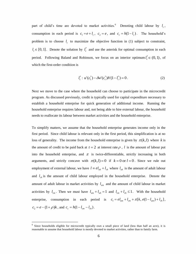
part of child‘s time are devoted to market activities.6 Denoting child labour by cl ,

consumption in each period is clec 1 , ec 2 , and )1( cc lhc . The household‘s

problem is to choose cl to maximize the objective function in (1) subject to constraint,

]1,0[cl . Denote the solution by *

cl and use the asterisk for optimal consumption in each

period. Following Baland and Robinson, we focus on an interior optimum )1,0(*cl , of

which the first-order condition is

0)1(')(')(': ***

1

* ccc lhcwcul . (2)

Next we move to the case where the household can choose to participate in the microcredit

program. As discussed previously, credit is typically used for capital expenditure necessary to

establish a household enterprise for quick generation of additional income. Running the

household enterprise requires labour and, not being able to hire external labour, the household

needs to reallocate its labour between market activities and the household enterprise.

To simplify matters, we assume that the household enterprise generates income only in the

first period. Since child labour is relevant only in the first period, this simplification is at no

loss of generality. The income from the household enterprise is given by ),( lk where k is

the amount of credit to be paid back at 2t at interest rate , l is the amount of labour put

into the household enterprise, and is twice-differentiable, strictly increasing in both

arguments, and strictly concave with 0),( lk if 0or0 lk . Since we rule out

employment of external labour, we have chah lell where ahl is the amount of adult labour

and chl is the amount of child labour employed in the household enterprise. Denote the

amount of adult labour in market activities by aml and the amount of child labour in market

activities by cml . Then we must have 1 aham ll and 1 chcm ll . With the household

enterprise, consumption in each period is ])1(,[1 chamcmam lleklelc ,

kec )1(2 , and )1( chcmc llhc .

6 Since households eligible for microcredit typically own a small piece of land (less than half an acre), it is

reasonable to assume that household labour is mostly devoted to market activities, rather than to family farm.

7

The household‘s problem is now to choose ),,,( klll chcmam to maximize the objective

function in (1) subject to constraints, ],1,0[aml ,0,0 chcm ll ,1 chcm ll 0k . To

make the comparison with the case without household enterprise meaningful, we focus on the

interior optimum for child labour, which will be true if, for example, is not too small. Thus

the constraint 1 chcm ll is slack. Denoting the solution by )ˆ,ˆ,ˆ,ˆ( klll chcmam and the second

partial derivative of evaluated at the solution by l , the first-order conditions with respect

to labour variables are given by

,1ˆif0

),1,0(ˆif0

,0ˆif0

)ˆ(')1(:ˆ1

am

am

am

lam

l

l

l

cuel (3)

),1,0(ˆif0

,0ˆif0)ˆˆ1(')ˆ(')ˆ(':ˆ

1

cm

cmchcmccm

l

lllhcwcul (4)

).1,0(ˆif0

,0ˆif0)ˆˆ1(')ˆ(')ˆ(':ˆ

1

ch

chchcmclch

l

lllhcwcul (5)

Needless to say, participation in the microcredit program should be individually rational for

the household. That is, the household should be better off with microcredit than without it if it

decided to participate in the program. It is then easy to see that a necessary condition for

beneficial microcredit is 1l , or the marginal return on labour from the household

enterprise should be larger than that from market activities. To see this, suppose 1l .

Then from (3), we have 1ˆ aml , or entire adult labour should be in market activities. Also

from (4) and (5), we have chcm lUlU // . Thus if optimal child labour in market

activities is positive, then child labour in the household enterprise should be zero. In sum,

if 1l , then the solution to the household‘s problem is the same as the one in the absence of

microcredit. Thus in what follows, we focus on the case 1l . In this case, we have

0ˆ aml and, from (4) and (5) again, child labour should necessarily be employed only in the

household enterprise. At the interior solution, the first-order condition (5) holds with equality:

8

0)ˆ1(')ˆ(')ˆ(')ˆˆ1(')ˆ(')ˆ(':ˆ11 chclchcmclch lhcwcullhcwcul . (6)

We now turn to our main question of how microcredit affects the extent of child labour. Let

us first observe that if the household decides to participate in the microcredit program, its

utility should be at least as large as when it does not participate. Since participation in

microcredit reduces the household‘s second-period consumption, it should necessarily be that

either the first-period consumption increases or the child‘s second-period consumption

increases, the latter being equivalent to reduced child labour. Otherwise, the household can

always return to the situation without microcredit. Rearranging (2) and (6) leads us to

).(')ˆ(')]1('')ˆ1(''[ *

11

* cuculhwlhw lcch (7)

Since w and h are strictly concave, it follows from (7) that *ˆcch ll or child labour increases

with microcredit if and only if )ˆ('/)(' 1

*

1 cucul . Note also that )ˆ('/)(' 1

*

1 cucul is

consistent with 1l , a necessary condition for beneficial microcredit. This is because, when

child labour increases, the only way the household can benefit from microcredit is to increase

the first-period consumption (*

11̂ cc ), from which 1)ˆ('/)(' 1

*

1 cucu follows since u is

strictly concave. The above condition has a ready interpretation: beneficial microcredit

increases child labour if the marginal return on labour from the household enterprise is

sufficiently large. In this case, parents divert more child labour to the household enterprise

than when they did not have access to microcredit. Needless to say, child labour need not

increase in this case if parents can hire external labour at market wage of one. On the other

hand, if )ˆ('/)('1 1

*

1 cucul , then microcredit can actually reduce child labour. As this

case shows, inability to hire external labour alone is not sufficient for an increase in child

labour; if the return on child labour from the household enterprise is not sufficiently large

relative to the return on schooling, then parents would continue to send their children to

school. However, since repayment of the loan typically requires high returns on investment,

one could argue that the case of )ˆ('/)(' 1

*

1 cucul is more likely. In sum, access to

microcredit can result in increased child labour if the credit cannot be used to hire external

labour and the required returns on investment are high.

9

3. The Program, Data and Descriptive Statistics

3.1. Background: Schooling and Child Labour in Bangladesh

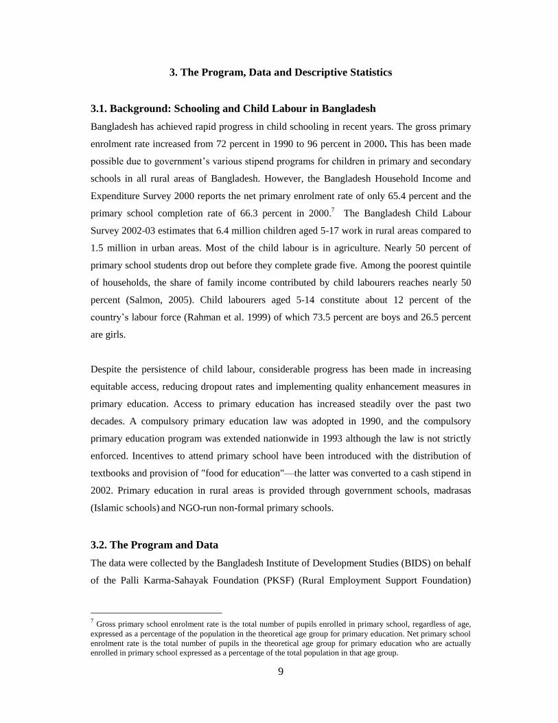
Bangladesh has achieved rapid progress in child schooling in recent years. The gross primary

enrolment rate increased from 72 percent in 1990 to 96 percent in 2000. This has been made

possible due to government‘s various stipend programs for children in primary and secondary

schools in all rural areas of Bangladesh. However, the Bangladesh Household Income and

Expenditure Survey 2000 reports the net primary enrolment rate of only 65.4 percent and the

primary school completion rate of 66.3 percent in 2000.7 The Bangladesh Child Labour

Survey 2002-03 estimates that 6.4 million children aged 5-17 work in rural areas compared to

1.5 million in urban areas. Most of the child labour is in agriculture. Nearly 50 percent of

primary school students drop out before they complete grade five. Among the poorest quintile

of households, the share of family income contributed by child labourers reaches nearly 50

percent (Salmon, 2005). Child labourers aged 5-14 constitute about 12 percent of the

country‘s labour force (Rahman et al. 1999) of which 73.5 percent are boys and 26.5 percent

are girls.

Despite the persistence of child labour, considerable progress has been made in increasing

equitable access, reducing dropout rates and implementing quality enhancement measures in

primary education. Access to primary education has increased steadily over the past two

decades. A compulsory primary education law was adopted in 1990, and the compulsory

primary education program was extended nationwide in 1993 although the law is not strictly

enforced. Incentives to attend primary school have been introduced with the distribution of

textbooks and provision of "food for education"—the latter was converted to a cash stipend in

2002. Primary education in rural areas is provided through government schools, madrasas

(Islamic schools)

and NGO-run non-formal primary schools.

3.2. The Program and Data

The data were collected by the Bangladesh Institute of Development Studies (BIDS) on behalf

of the Palli Karma-Sahayak Foundation (PKSF) (Rural Employment Support Foundation)

7 Gross primary school enrolment rate is the total number of pupils enrolled in primary school, regardless of age,

expressed as a percentage of the population in the theoretical age group for primary education. Net primary school

enrolment rate is the total number of pupils in the theoretical age group for primary education who are actually

enrolled in primary school expressed as a percentage of the total population in that age group.

10

with support from the World Bank.8 This survey is the largest and the most comprehensive of

the existing microcredit programs in Bangladesh. Its geographic coverage is spread evenly

across Bangladesh, and the sub-district (thana) level comparisons reveal that selected sub-

districts are not different from the average (Zohir et al. 2001). The data cover 13 MOs of

different sizes in terms of operations and membership. These MOs were selected to constitute

a nationally representative data set for the entire microcredit program in Bangladesh. The

most notable MOs studied in this paper are ASA and Proshikha, the third and fourth largest

MOs, respectively, in Bangladesh. All 13 MOs follow the Grameen Bank-style lending

procedure and typically give access to microcredit to households owning less than a half-acre

of land.

The survey includes 13 districts covering 91 villages spread over 23 sub-districts in

Bangladesh. A census of all households in the 91 villages was conducted before the survey

was administered in early 1998. The actual targeting of survey households involves two

stages: (1) the selection of the villages where MOs operate; (2) the selection of treated

households within the selected villages. The non-participants from the program villages who

are observationally similar were also selected as the control group. Participation in a credit

program was defined in terms of current membership reported during the census. From the

village census lists of households, 34 households were drawn from each program and non-

program village. Because the census found a large number of ineligible households in

program villages, the sample was drawn to maintain the proportion of eligible and ineligible

households of about 12:5. The sample size within program and control villages was also

determined accordingly.

3.3. Descriptive Statistics

The original survey consists of 3026 households. In this paper, we consider the subset of 2034

households who have at least one child aged 7-16 at the time of the survey. This represents a

total of 4277 children of which 2658 belong to treatment households and the remainder to the

control group. Our sample contains both male and female borrowers but the former account

for only 12 percent of all borrowers (and 133 households) representing 281 children. Among

all children, 54.2 percent are boys.

8 The PKSF is the apex organization for microfinance. The microlending community regards it as a regulatory

agency, and it exercises authority over the MOs.

11

The household level questionnaire includes primary and secondary activity of each child. We

define ―child labourer‖ as anyone aged 7-16 who performs any economic activity (i.e., if a

parent answers ‗employed‘, ‗household work‘, or ‗employed but not working‘). A child is

considered to be in school if he/she is currently enrolled in school and attended school in the

last month of the survey period. By this definition 77.4 percent of girls aged 7-16 in the

sample were classified as being in school and 10.4 percent in work. The corresponding figures

for boys are 71.3 percent and 15.7 percent, respectively. Other children are reported to be

neither working nor in school, and possibly many of them are helping parents with household

work. So there may well be under-reporting of child labour.9 The results by participation

status are reported in Table 1. School enrolment is lower and child labour higher among

children of the treatment group. We find a statistically significant difference in school

enrolment and child labour between boys of treated and untreated households, but no such

difference exists for girls. However, the difference in school enrolment between girls and boys

is larger in the treatment group.

--- Table 1 goes about here. ---

Figure 1 plots school enrolment of children by age for both sex groups. Children at high-

school age (12-16 years old) are less likely to be enrolled in school because of drop-outs. At

primary-school age, the proportion of children aged 7-8 enrolled in school is lower than their

older counterpart (9-11 years old), indicating that there are a considerable number of children

who start schooling at a later age. The difference between treatment and control groups in

school enrolment is larger for boys. Girls aged 7-11 have a similar rate of enrolment in both

treatment and control groups, but after age 13, girls in the control group tend to have a lower

enrolment rate. On average, children at primary-school age have a higher enrolment rate

compared to their older siblings, the latter more likely to drop out from school and go to work.

Overall, a higher proportion of children from treated households are in work (Figure 2).

--- Figures 1 and 2 go about here. ---

Table 1 also provides other descriptive statistics for child and household demographics and

village characteristics. It shows that the average age of children is 11.5 years for both groups

9 In our sample, only one percent of children are reported to be both in school and in work, so we ignore these

cases. It is usual in rural areas of Bangladesh that parents arrange a modest amount of part-time work for their

children while still keeping them at school (see, for example, Ravallion and Woodon 2000).

12

of households. There is no difference between treatment and control groups in the gender

composition of children. The treated group has slightly more members in the household than

the non-treated group. For each household in the survey, there is an average of four children

below 18 years of age. Non-treated households tend to be better educated, a little older but

smaller in household size. Descriptive statistics not reported in Table 1 shows that a total of

about one quarter of mothers did not go to school at all. More than a quarter of our sample has

a secondary school in their locality, and primary schools exist in most of the villages.

Compared to program villages, control villages are more likely to have primary and secondary

schools, telephone office and local government (UP) offices. On the other hand, program

villages have superior health facilities and are located relatively closer to the nearest sub-

district. However, most of these differences are not statistically significant at the conventional

level. Thus we do not think that the differences between the program and control villages

render the possibility of non-random program placement an issue of concern. Nonetheless,

we control these characteristics plus a wide variety of village-level variables in our regression

to take into account of possibility of non-random program placement at the village level.

4. Empirical Methodology

In estimating the impact of microcredit on children‘s school enrolment and child labour, we

follow a standard methodology (Wydick 1999; Ravallion and Wodon 2000; Edmonds 2006).

Let Si be a binary variable that denotes whether child i (i) works (Si =1) or not (Si =0) and (ii)

attends school (Si =1) or not (Si=0). We estimate the impact of participation in microcredit

programs on children‘s schooling/work with the following equation:

(8) 3210 ijkljklklijkllijkl εCreditβZβXβ S

where the subscripts index child (i), household (j), village (k), and district (l). X is a vector of

child- and household-specific covariates, and Z is a vector of village-specific covariates. β0l

captures fixed effects. ‗Credit‘ is a continuous treatment variable defined by the amount of

microcredit borrowed by the household. It is equal to zero if a household did not participate in

a microcredit program. The error term εijkl is assumed to be i.i.d. Using equation (8) we can

13

use the probit model to estimate the probabilities of child labour or school enrolment

attributable to participation in microcredit programs.10

Estimating equation (8) directly is problematic, however. First, programs may be placed in

specific villages and hence program placement may not be random. Selection for placement

could be influenced by biases in favour of high-income villages – because they may have

higher participation rates – or by official bias in favour of poorer villages. However, given

that programs are placed by central decision and that there are hundreds of MOs, it is

reasonable to assume that village level program placement is a problem of ―selection-on-

observables‖. The survey covers a wide range of village level variables. So we can account for

the non-random program placement by a set of control variables at the village level, which are

included in the vector Z. We also use district level fixed effects to remove any unobserved

heterogeneity across different geographical areas. Since we have 13 MOs, each from a

different district, this fixed effect also captures the differences between the MOs. Thus, we

tackle the potential problem of non-random program placement using both geographical and

MO-level fixed effects and village-level observed covariates.11

It is to be noted that we adopt

an estimation strategy different from that used by Pitt and Khandker (1998). We do not use

village fixed effects. Rather we use village-level pre-program characteristics to control non-

random program placement. Village fixed effects could give us biased results if the programs

are placed based on certain shocks (e.g, floods) at the village level. We control any

unobserved heterogeneity using geographical (district level) and MO-level fixed effects.12

Second, households self-select into the program but not all of them are able to obtain

microcredit. Generally only eligible poor households receive microcredit, the eligibility being

typically determined based on the amount of land-holding. However, other factors that

influence whether a household has access to microcredit could also affect outcomes for

10 It is possible to use a bivariate probit model to estimate child labour and schooling simultaneously. However, the

number of children who are both in school and in work or who do neither is very small in our sample. Thus the

work versus schooling is nearly a dichotomous decision and therefore we do not adopt a bivariate probit model. 11 Probit estimates with fixed effects give rise to inconsistent coefficients of the fixed effects. However, when the

number of observations per fixed effect is at least 8, we can consistently estimate the fixed effects (Heckman

1981). We have at least 250 observations per district and so the model is consistently estimated. For the same

reason, we do not estimate parental fixed effects which can eliminate unobserved time-invariant household-level

variables or permanent heterogeneity. Instead we consider clustering at the household level. 12 Fixed effects would eliminate village-level omitted characteristics, but differences in initial conditions also

matter for program placement. See Keane and Wolpin (2002) for a similar analogy for problems using state-level

fixed effects to estimate the welfare impacts in the US, and the resulting bias in the estimates. See also Morduch

(1999) for pitfalls using village fixed effects in Pitt and Khandker (1998). However, our qualitative conclusion is

not affected even if we use village fixed effects or separate fixed effects for target and non-target populations in

each village. Using different fixed effects only changes the size, not the sign, of the coefficient estimates.

14

children of that household. One such factor could be household income or wealth. For

example, MOs may be more willing to provide credit to households that operate non-farm

enterprises because the use of credit is less fungible in such households. Microcredit loans

often require that family enterprises be established because they provide less opportunity for

misuse of the loan. Poor households that operate an enterprise are also more likely to employ

their children in that enterprise, and thus less likely to send them to school. Such negative

correlation between credit access and schooling introduces a conservative bias in the

coefficients. Thus we need to consider the endogeneity of participation in microcredit

programs at the household level. The endogeneity problem implies that selection into

treatment is on the basis of unobserved characteristics εijkl in equation (8). This implies

potential non-zero correlation between εijkl and Creditjk. Consequently, impact estimates that

use a simple probit/linear probability model (LPM) may not reflect the program‘s causal

effect on children‘s school enrolment or child labour.

To account for self-selection into the program, we consider a source of exogenous variation.

The MOs set the eligibility criteria for participating in the program. A household is eligible if

it does not own more than a half-acre of land. The land ownership criterion is mainly used as a

targeting mechanism to identify the poor. Since poverty does not exclusively depend on land

ownership, however, the administrator, local loan officer or branch manager sometimes take

into account other socio-economic conditions of a household. Consequently there are some

ineligible households that receive microcredit. Although these households are a distinct

minority (70 percent of the treatment group in our sample is eligible), the participation in the

program based on eligibility is probabilistic since the program eligibility criterion is not

strictly followed. Thus our approach in estimating the treatment effect is similar to the use of

fuzzy regression discontinuity design (see Van der Klaauw 2002), which we implement using

an IV approach.

It is clear that a household is more likely to receive microcredit when a microcredit program is

already available in a village. Therefore as an instrument for the actual receipt of microcredit,

we may consider the eligibility status interacted with an indicator for presence of program in a

given village.13

Instead of using this instrument directly, however, we utilize an unexploited

13 Pitt and Khandker (1998) and Islam (2007) use this instrument for participation in a credit program in

Bangladesh, and discuss the plausibility of this instrument in detail. Morduch (1998) questions the validity of

using this instrument, but in response to Morduch‘s critique, Pitt (1999) argues at length that the eligibility criterion

satisfies the conditional exogeneity and exclusion restriction.

15

exogenous source of variation in the treatment intensity based on a household‘s exposure to

the program in different villages. As shown in Figure 3, treated households in different

villages appear to borrow different amounts. Intensity of treatment varies widely in different

villages, depending on how long a microcredit program has been available in the village. In

our sample, the earliest a program was made available in a village was 1980 and the latest a

program became available in another village was 1997. As shown in Figure 3, the amount of

credit a household borrows largely depends on how long the program has been available in the

village. So we use the instrument, I = Mk × Ej × Nk where Mk is a binary variable that equals

1 if village k has a microcredit program, Ej is a binary variable that equals 1 if household j is

eligible (i.e., owns less than half-acre of land), and Nk is the number of years a microcredit

program has been available in village k.14

With controls for village and fixed effects,

identification requires that there be no contemporaneous village-level unobservables that are

correlated with program placement and child labour/schooling. The equation for the demand

for credit then assumes the form:

(9) 2210 ξZαXα)NE(MαCredit jklkjkkjkjkljkl

where X now includes only household-specific covariates since participation in microcredit

programs is determined at the household level.

--- Figure 3 goes about here. ---

The probit estimates are obtained using the two-stage procedure where the second-stage

regression uses the value of credit from the first-stage credit demand equation (9), which is

estimated by a standard Tobit model. The use of estimated variable (instrumented credit) in a

non-linear specification may lead to bias but this bias is of second order and thus very small

(Train et al. 1987). We also estimate the second stage using ordinary least squares (OLS)

estimations of LPM. Additionally, because of the non-random nature of our sample we use

inverse-propensity score weights in the standard fashion for all the estimators (Hirano, Imbens

and Rider 2003). This involves attaching an estimated weight to each observation in one

sample that corresponds to the probability of observing a similar observation in the other

14

We also used Mk × Ej only as an instrument and obtained qualitatively similar results. We also experimented

with instruments that include separate dummies for year of microfinance placement in villages. Again the results

turn out to be similar.

16

sample. With normalization, we attach a weight of one to each treated household, and to each

comparison group member a weight of p/(1-p), where p is the estimated propensity score.15

A potential problem with interpreting these results when using credit as the treatment variable

is that the reported amount of credit is subject to misreporting or other types of measurement

error since households may forget or not report the amount correctly.16

This measurement

error is likely to impart attenuation bias to the estimated coefficients. However, we do not

think the problem of measurement error is serious in our case since we are using instrumented

credit variable as the treatment variable. Nonetheless, we also use a binary treatment indicator,

i.e., whether or not a household is currently a member of a microcredit program or not, which

is unlikely to be measured or reported with error. It can also serve as a robustness check of our

main results. It should be noted, however, that the use of binary treatment indicator raises

another issue as dummy endogenous regressors with limited dependent variables raise some

econometric problems. Angrist (2001) advocates using simple IV estimators as an alternative

because they require weaker assumptions and are often sufficient to answer questions of

interest in empirical studies. We therefore estimate the treatment effect also by using a LPM

in the second stage of the IV regression.17

To adjust for clustering at the village level we first use the cluster-correlated Huber-White

covariance matrix estimator. Donald and Lang (2007) have pointed out that asymptotic

justification of this estimator requires a large number of aggregate units. Monte Carlo

simulations (Bertrand, Duflo and Mullainathan 2004) suggest that, when the number of

primary sampling units (PSUs) is less than 50, this estimator performs poorly, leading to

excessive rejection of the null hypothesis of no effect. Fortunately, with 91 PSUs in our

sample we can potentially overcome the problem by using cluster-consistent standard errors.

The cluster-adjustment works well for binary outcomes and nonlinear models such as logit

and probit models, provided that the number of clusters is large (Angrist and Lavy 2002).18

15 The estimated difference in covariate after adjusting propensity scores is lower than the unadjusted difference

between treatment and control groups. However, our qualitative conclusion remains unchanged with or without

weighting. 16 See, for example, Karlan and Zinman (2008b) for problems with self-reported credit data. 17

When all independent variables are discrete (as is the case with most of our variables), the LPM is fairly general,

and fitted probabilities lie within the interval. In addition, the LPM has also the advantage of allowing

straightforward interpretation of the regression coefficients. Moreover, we compute Huber-White standard error to

take into account the heteroscedastic error term of LPM. 18 Alternatives to cluster-adjusted standard errors include the hierarchical linear modelling, two-step procedure by

Donald and Lang (2007) and the Bell and McCaffrey‘s (2002) biased reduced linearization estimator for micro

data.

17

Secondly, children of the same household are likely to be similar in a wide variety of

characteristics. It follows that there may be large intra-household correlations. Moreover, the

data were collected by using households as the survey unit. Therefore we also estimate

standard errors clustering at the household level as there is usually more than one school age

child within a household.

Checking the Validity of the Instrument:

Before presenting our main findings, we discuss if our chosen instrument is a suitable one.

The first-stage regression of equation (9) using a standard Tobit model shows that the

instrument is highly statistically significant with t-statistic of 8.5. The coefficient estimate is

positive and also economically significant, implying that our instrument is significantly

related to the demand for credit. We also estimate the participation decision equation by

regressing a binary indicator for participation on an indicator of interaction between eligibility

and program village dummies (plus all controls). The results are stronger with t-statistic of 12.

The regression using basic controls and no controls results in stronger coefficient estimates.

Since we have a single instrument for the credit variable, we cannot test the exogeneity of the

instrument as in an over-identified model. The remaining concern is whether the instrument

satisfies the exclusion restriction, i.e., whether eligibility affects child labour or school

enrolment only through participation in the credit program or the amount of credit borrowed.

Although the exclusion restriction is not directly testable, we address this concern in a number

of ways. First, we estimate a reduced form regression to examine the effect of loan eligibility

on school enrolment/child labour. The results indicate that that there is no effect of eligibility

or program placement on school enrolment and child labour. We also estimate an equation in

which credit is instrumented but instrument eligibility enters the second-stage regression

directly (and naturally in the first stage regression). By definition of IV, the instrument should

be uncorrelated with the outcomes of interest through any channels other than their effects via

the endogenous regressors. Therefore, once the credit is instrumented, eligibility itself should

have no effect on schooling or child labour when both instrumented credit and eligibility

status are entered as controls for child labour/school enrolment equation. The results do not

indicate any significant effect of eligibility in any of the specifications.19

Finally we stress that

our identification strategy does not depend exclusively on the eligibility rule since we also

exploit the variation in credit demand among households in different villages based on the

availability of program in different villages.

19 The detailed results of the first-stage regression are available upon request.

18

5. Empirical Findings

This section reports our empirical findings where the estimated value of credit from the first-

stage regression (equation (9)) is used as the regressor in the second-stage estimation

(equation (8)). We estimate the impacts of credit extended to women and men separately.20

This is to see how the gender of participants in the microcredit program affects schooling and

work decision for their children. As mentioned earlier, Pitt and Khandker (1998) and

Behrman and Rosenzweig (2002) report that women tend to show a stronger preference than

men for educating their children. Pitt, Khandker and Cartwright (2006) also find that

women's participation in microcredit programs helps to improve women's empowerment. If

microcredit empowers women, then it may also increase the relative chance of girls‘

schooling. If parents have differential preferences for the education of their daughters and

sons, then education outcomes could be different for boys and girls, which could be

determined by a household production function (Rosenzweig and Schultz 1982). We thus

estimate the results separately for boys and girls by credit given to both women and men using

three sets of control variables: ―no controls‖ (excluding the X and Z variables), ―basic

controls‖ (some household and child demographic variables, and village controls), and ―full

controls‖ (the full set X and Z variables). The list of the full controls is chosen from a larger

set of controls by selecting those that were most significant. In identifying the set of control

variables we first consider the variables (e.g., household and village characteristics) that the

MOs use to select a household and that are likely to determine household demand for credit.

We then include a number of regressors to take into account the number of siblings, family

composition that can potentially determine the children‘s schooling or work status. The final

set of covariates included in X and Z is listed in the Appendix.

Table 2 reports the estimates of the second-stage regression using the LPM and probit models

under different covariate specifications. Columns (1) and (4) represent the treatment effects

without any controls. The estimates in column (1) can be considered the Wald estimates,

representing the difference in the probability of child labour between children of microcredit

participants and non-participants divided by the amount of credit borrowed by the

participating households. The Wald estimates in Table 2 show that credit is associated with

20 Though credit is given to both women and men in different villages, credit groups are never mixed by gender.

Households do not have choice over which gender is to participate since MOs select one or the other gender, but

not both.

19

higher probabilities of child labour for girls but lower probabilities of child labour for boys,

regardless of whether credit is obtained by men or women. However, the coefficients are not

statistically significant. Moreover the Wald estimates are likely to suffer from the omitted

variable bias since parental decisions on schooling and child labour are likely to be influenced

by household demographic and socio-economic characteristics.

To address the above issues, we consider two sets of control variables, basic control and full

control variables, as discussed in Section 4. In Table 2, the results from the LPM model are

reported in columns (2) and (3) and those from the probit model are reported in columns (5)

and (6). In columns (3) and (6), the full set of controls is included, which is our preferred

specification. All coefficients are estimated as marginal effects calculated at the mean. The

results in columns (3) and (6) portray a clear picture. Microcredit significantly increases the

probability of child labour for girls. For boys, there is some indication that microcredit

reduces the probability of child labour especially when credit is obtained by women. Overall,

the impact of microcredit on child labour is positive and significant. The qualitative results

are independent of whether credit is obtained by men or women. For example, microcredit

increases the probability of child labour for girls by 7.9% according to the probit model and

13.7% according to the LPM model. The probability increases by 8.4% and 14.3%

respectively when women are borrowers. For boys, women‘s credit has a marginal negative

effect on child labour. Table 2 also shows that girls are affected more adversely, and boys

more favourably, when credit is obtained by men than by women, although these estimates are

not statistically significant. A Hausman-like test does not support the difference in treatment

effect between men and women borrowers. Finally the magnitude of the estimated coefficients

increases as we move from basic controls to full controls. The overall finding is that

microcredit clearly increases the likelihood of child labour for girls while the impact on boys

is less clear.

--- Table 2 goes about here. ---

Table 3 reports the effect of microcredit on school enrolment. The results overwhelmingly

indicate that access to microcredit negatively affects children‘s school enrolment. This is true

across all regression models and regardless of whether credit is obtained by men or women.

The negative effect is especially pronounced for girls although, for boys, it is statistically

insignificant. For example, microcredit decreases the probability of school enrolment for girls

20

by 22.6% according to the LPM model and 19.2% according to the probit model. We also

find that the negative effect on girls‘ school enrolment is larger when microcredit is obtained

by men than by women: in the probit model, the probability changes from 19.4% to 22.8%.

The negative effect on boys‘ school enrolment, while statistically insignificant, is larger when

women are borrowers. One might surmise that this could be an indication of gender

preference by parents. However, Hausman-type tests do not reject the equality of the

coefficients between the sexes of the borrower. Once again, the magnitude of the estimated

coefficients increases as we move from basic controls to full controls, suggesting that a fuller

picture requires the analysis of how a household‘s socio-economic characteristics affect child

labour and school enrolment. We turn to this below.

--- Table 3 goes about here. ---

Table 4 shows how the probabilities of children‘s school enrolment and child labour are

associated with other control variables. The results are mostly consistent with previous

studies. For controls at the household level, children‘s school enrolment is positively

associated with education attained by any adult member of the household, the household

head‘s education level, and the male head of the household, while it is negatively associated

with the number of younger siblings and the age of the household head. Presence of a mother

in the household has a positive but statistically insignificant effect on schooling. For controls

at village level and beyond, children‘s school enrolment is positively related to presence of

secondary school or college, and infrastructure such as health facility and brick-built road.

Interestingly, presence of grocery market and bus stand has a negative effect on children‘s

schooling. A primary school in the village does not have any statistically significant effect on

school enrolment or child labour. This may reflect the fact that almost all villages have a

primary school. Similarly rice prices do not have any effect on either school enrolment or

child labour possibly because the geographical variation in rice prices is very small. The sign

of the adult male wage coefficient in the child labour equation is positive but statistically and

economically insignificant, suggesting that adult male and child labour are imperfect

substitutes.21

--- Table 4 goes about here. ---

21 According to Basu and Van (1998), if children and adults are substitutes in production (the "substitution

axiom"), the prevalence of child labour depresses adult wages —a condition under which a ban on child labour

may be desirable. Our results indirectly suggest that this might not be the case. Moreover, when we regress adult

male wages on child labour, we find a positive coefficient (t-ratio=1.53), indicating that the substitution axiom does

not hold in our case.

21

The results reported in Tables 2 and 3 do not change qualitatively if we change the treatment

variable. Table 5 shows the treatment-on-treated effect using a binary participation indicator

as the treatment variable. The estimated effect using two-stage least squares (2SLS) is

identical to the indirect least squares estimate obtained from taking the ratio of the reduced-

form coefficients, because we are estimating a just identified equation. The results are

qualitatively similar to the previous estimates which used credit as participation variable.

Girls‘ education continues to be affected adversely by parental participation in microcredit

programs whether credit is obtained by men or women. In probit results, for example, we find

that women‘s microcredit borrowing increases the probability of girls‘ child labour by 13.7%

and decreases the probability their school enrolment by 44.4%. The magnitude of the impact

estimates is similar in case the borrower is a man. The corresponding coefficient estimates for

child labour for boys are not statistically significant and have mixed signs. Overall, binary

participation measures generate considerably larger coefficient estimates for girls. However,

these results are only indicative as they do not take into account the variation of treatment

intensity, and treat the program effect to be the same for all children in the treatment group.

--- Table 5 goes about here. ---

The standard errors reported in the above tables are corrected for clustering at the village level

and weighted by the propensity score to take into account the choice-based sampling. The

standard errors in square brackets take into account intra-sibling correlations within a

household. Both standard errors are typically of similar magnitude. Since they do not differ

much, we report below the regression results only with the clustered standard error at the

village level. We also experimented with the two-step procedure discussed by Donald and

Lang (2007). In our case this amounts to estimating village fixed effects (household fixed

effects when considering intra-sibling correlation) in an equation like (8), and then regressing

the estimated fixed effects on instrumented credit and other village covariates (household

covariates). Since the estimation results are similar, they are not reported for the sake of

brevity. In what follows, we report the results of impact estimates separately by various

control variables.

5.1. Impact Estimates by Children’s School Age

Table 6 reports the impact estimates for children aged 7-12 (primary school age) and 12-16

(secondary school age: up to grade 10). As before, we use the binary treatment status

22

indicator as the participation variable. The results show that the adverse effect of microcredit

on children at the primary school age is mostly significant regardless of the gender of

borrowers and children. Girls at the primary school age are especially adversely affected than

boys, and more so when credit is obtained by men. For example, the probability of their

school enrolment decreases by 33% when credit is obtained by women and by 41% when

credit is obtained by men. For children at the secondary school age, microcredit has a mixed

effect. Women‘s credit has a statistically significant negative impact on girls‘ schooling while

men‘s credit also has a negative but statistically insignificant effect, possibly due to smaller

sample size of male participants. For boys at the secondary school age, microcredit increases

their likelihood of school enrolment although coefficient estimates are not statistically

significant. Overall, microcredit adversely affects younger children more than their older

siblings, and girls more than boys, irrespective of the gender of the borrower.

--- Table 6 goes about here. ---

5.2. Impact Estimates by Household Income

Household income plays an important role in determining child labour and school enrolment

(Basu and Van 1998; Edmonds 2005; Bhalotra 2007; Belly and Lochner 2007). Poorer

families are more likely to take their children out of school in times of need. Poverty is

associated with increased level of parental stress, depression and poor health — conditions

which might adversely affect parents‘ ability to nurture their children. Impact estimates by

household income also allow us to examine the hypothesis implicit in Basu and Van‘s (1998)

‗luxury axiom‘ that parents send their children to work and keep them from school only if

household income falls below a certain (subsistence) level. However, we cannot treat income

as exogenous. Income is endogenous because the amount of credit borrowed by the

household directly affects household income. If the participation in microcredit programs has

a positive effect on household income, then including income as an explanatory variable

would underestimate the actual effect of the program. Moreover, children‘s contribution to

household income also makes the income variable endogenous. Since children working on the

family farm are not paid a wage, their contribution cannot be deducted from total income.

Even if we could observe income from child labour, the endogeneity problem would not be

resolved by simply subtracting it from the total household income if the labour supply of

different household members is jointly determined. Income is endogenous for another reason:

children living in poorer families may have adverse home environment or face other

23

problems. Such omitted variables may continue to affect their schooling or child labour even

if family income may increase.

There are mainly two approaches in dealing with the endogeneity issue: fixed effects

estimation (Blau 1999) and instrumental variable technique. While the fixed effects estimation

should eliminate any bias from permanent differences in family or children, it may exacerbate

bias due to unobserved temporary family shocks (Dahl and Lochner 2005). In the absence of

appropriate instruments for income in our context, we use parental education as a proxy for

permanent income. If education has a positive return, families with more educated parents are

expected to have more income. Clearly parental education is not affected by program

participation or child labour supply. We use three categories of parental education: Low refers

to those households where the highest level of education obtained by parents is primary (0-4

years of schooling) or less; Middle refers to households where the highest level of education

obtained by parents is more than primary but less than a high school degree (5-10 years of

schooling), and High includes households where one of the parents obtained at least a high

school degree (11 or more years of schooling). We adopt the following functional form:

ν)(δ

)(δ)(δδδδ

5

43210

ijkljkjk

jkjkjkjkkijlijkl

HighCredit

MiddleCreditLowCreditZXY

(10)

where we incorporate the household‘s permanent income by interacting the three categories of

parental education with the amount of credit borrowed. These interaction terms capture the

differences in slope across different levels of education within the treatment group.

Equation (10) is unidentified since the number of endogenous regressors exceeds the number

of instruments. Therefore, we need additional instruments that are correlated with the

interaction terms between credit and different education categories. Since credit is interacted

with education dummies all the predicted values will be closely correlated. In the absence of

suitable identifying instruments, we use estimated credit from the first-stage and interact the

education dummy variables with the estimated credit variable. Our equation thus becomes:

11 )ˆ()ˆ()ˆ( 543210 ijkljkjkjkjkjkjkkijlijkl HighDMiddleDLowDZXY

where D̂ is the credit demand estimated from equation (9).

24

Figure 4 shows how children‘s school enrolment and child labour vary as the level of parental

education changes. The graphs show that there is a positive relationship between children‘s

school enrolment and parental education and a negative relationship between child labour and

parental education. Households in the control group tend to have a higher level of children‘s

school enrolment and lower incidence of child labour.

--- Figure 4 goes about here. ---

Table 7 reports the impact estimates based on different levels of parental education. A clear

picture emerges. Households with the lowest parental education are those with the largest and

significant adverse effect of microcredit on children‘s schooling. For example, the probit

estimates imply that the probability of children‘s school enrolment decreases by 29.3% in

these households while that of child labour increases by 9.7%. For households with medium

to high levels of parental education, the impact is largely insignificant, although there is some

indication that girls are adversely affected by microcredit in households with medium level of

parental education. Given our interpretation of parental education as a proxy for household

income, these results indicate that microcredit to the poorest of the poor households neither

alleviates the problem of child labour nor improves children‘s schooling. These households

engage their children more in work in order to generate immediate returns from their

microenterprise projects. An additional observation is that, while statistically insignificant,

the likelihood of children‘s school enrolment is positive in households with high education.

Figure 4 also shows that children are more likely to be sent to school as household income

proxied by parental education increases. Taken together, these results indirectly support Basu

and Van‘s (1998) ‗luxury axiom‘.

--- Table 7 goes about here. ---

5.3. Microcredit, Household Income and Child Schooling

The results in the previous section have shown that children‘s schooling is less likely to be

adversely affected if they come from relatively less poor or more educated family. Microcredit

given to high income households actually reduces the probability of child labour and improves

children‘s schooling. To the extent that microcredit can increase household income, one

might argue that it could help poor households to graduate out of poverty, thereby improving

25

children‘s education in the long term. Conversely, if escape from poverty proceeds only very

slowly, then microcredit may intensify the problem of child labour and worsen human capital

formation. We examine this issue below based on the regression coefficients in Table 7.

Consider the difference between the coefficients for the low and middle income groups in

Table 7. Since the coefficient estimates measure the difference in probabilities between

treated and untreated households in different income groups, the difference in estimated

coefficients between two treated groups can be interpreted as the difference-in-difference

estimate of the impact of household income. Then the first column in Table 7 suggests that a

10 percent increase in credit given to middle-income households reduces the probability of

children‘s schooling by about 2.6 percent less than if it had been given to low-income

households. A similar calculation for child labour indicates that a 10 percent increase in credit

given to middle-income households increases the probability of child labour by 0.6 percent

less than if it had been given to low-income households. While the adverse effect of

microcredit is reduced when household income increases from low to middle, the adverse

effect remains nonetheless. Microcredit can improve children‘s schooling and reduce child

labour only for high-income households: a 10 percent increase in credit given to high-income

households improves children‘s schooling by 0.8 percent and reduces child labour by 0.4

percent than if it had been given to middle-income households. Given the modest increase in

income due to participation in microcredit programs,22

however, it seems reasonable to

conclude that child labour remains an issue to be tackled by MOs and policy makers rather

than by letting the households graduate out of poverty. With microcredit alone, it would

require a substantial amount of time for households to break out of poverty.

5.4. Impact Estimates by Land Ownership

In many rural areas in developing countries, land is often the most significant asset the

household owns. If land can be used as collateral for general-purpose loans, then land

ownership may have a positive effect on children‘s schooling. In this case, more land implies

more household wealth, and the possible positive relationship between land ownership and

children‘s schooling can be considered a confirmation of the positive relationship between

household wealth and children‘s schooling. However, microcredit is mainly to be used to set

up a household enterprise and the purchase of external labour is not often possible. Moreover

households in the treated group have microcredit as the main source of loans. Therefore we do

22

See, for example, Islam (2007) and references therein.

26

not expect a positive relationship between land ownership and children‘s schooling. Rather

we may expect land ownership to have a negative effect since adult labour may need to be

shifted from family farms to the household enterprise, increasing the need for child labour in

family farms.

To examine this, we divide households into two groups: those with less than a half acre of

land (poorer households) and those with more than a half acre of land (less poor

households).23

Although land ownership of less than a half acre of land is the eligibility

criterion for microcredit, there were some households with larger land who still obtained

microcredit. Table 8 reports the impact estimates by land ownership. The results show that

microcredit has different effects in the two groups of households. In poorer households, it

decreases the likelihood of school enrolment for girls while decreasing the likelihood of child

labour for boys. In less poor households, the result is reversed. Although it is not clear why

less poor households tend to keep boys at work when they obtain microcredit, we surmise that

less poor households engage boys more in agriculture activity, while households with

marginal landholding engage girls more in the household enterprise.

--- Table 8 goes about here. ---

Many of the results are statistically insignificant possibly because of relatively small sample

size. However, overall results also show that our earlier findings were not driven by pre-

existing differences in the characteristics between treatment and control groups. It is to be

noted that poorer treated households have observed characteristics that are very similar to

their non-treated counterparts.24

Once again, our results show that poor households tend to put

girls to work and keep them away from school when they obtain microcredit.

6. Additional Robustness Check

6.1. Potential Identification Issue: Causal Effect or Selection Bias?

23 Household land ownership is less likely to be affected by microcredit. There is not enough evidence in the data

that shows a different pattern of buying and selling land after becoming a member of a MO. Since microcredit is

mainly provided for non-agricultural purposes, households are not entitled to buy land using the credit. Also, there

is no evidence that households sell land to become eligible for microcredit. 24

Descriptive statistics for this sub-group is not reported here, but similar results are available in Islam (2007).

27

Section 5 has reported on how microcredit affects children‘s schooling and child labour under

the assumption that the differences in schooling and child labour between the treatment and

control groups are not due to underlying differences in household characteristics. It could be

argued, however, that households from program villages that are less likely to send their

children to school are more likely to participate in microcredit programs. If this is the case,

then our estimates would be picking up effects that are attributable to pre-existing differences

in household characteristics between the treatment and control groups, and not to the

participation in microcredit programs. In addressing the issue of possible selection bias, we

first note from Table 1 that many of the household characteristics are not statistically different

between the treatment and control groups. Any remaining differences have been accounted

for by using propensity score weights, which also significantly reduce the differences between

the two groups. Possible selection bias resulting from unobservable variables has been further

addressed using the IV strategy. Nonetheless there may still remain some potential

confounders that would violate the exclusion restriction. Given our efforts to control for

confounders, the risk of such distortions does not seem large.

In order to substantiate the above claim, we conduct additional robustness checks using

alternative approaches. We first use regression-adjusted years of education for older siblings:

children who are 16-20 years old. This group of children is less likely to be affected by their

parents‘ microcredit since they would have completed secondary school or dropped out before

their parents obtained microcredit. We find no statistically significant difference between the

children of treatment and control groups (t-ratio = 0.7). This result is also consistent with our

finding that older children are less adversely affected by microcredit, presumably because

their schooling period is less exposed to microcredit and younger children can work in the

household enterprise instead of their older siblings. Furthermore, the opportunity cost of using

child labour in the household enterprise increases with children‘s age. If they are at the

advanced stage in school, much of the investment in schooling that has already been made

would be forfeited or, if they are engaged in market work, their higher wage earnings would

need to be sacrificed.

Next, we also control selection bias using an alternative method. We consider corrections for

endogeneity using reduced form residuals that lead to a control function method of accounting

28

for both selection and endogeneity.25

This is also important if the impact of microcredit varies

across households. In that case, IV/2SLS may not estimate the average treatment effect of

credit. There are, however, different approaches to estimate control functions, and not all

these procedures produce consistent estimates of the treatment effect. We adopt the procedure

suggested by Vella (1993), which correctly identifies the treatment effect parameter in our

context.26

We first obtain generalized residuals using either Tobit (for credit as the treatment

variable) or probit (for binary treatment indicator) for the reduced form first-stage equation,

and then use the estimated residuals as an additional regressor in the second stage.27

The

results, available upon request from the authors, are similar to those reported before.

6.2. Alternative Measures of Children’s Educational Attainment

In this sub-section, we consider the impact of microcredit participation on various alternative

measures of children‘s educational attainment. While the previous measure of school

enrolment has the advantage of capturing the current status of school age children, it does not

measure the achievement of those who are not in school at the time of the survey. Two

alternative measures are the number of years of schooling completed and the ‗education gap‘.

In Bangladesh, the age at which children are expected to start school does not vary cross the

country. The age at which a child is legally supposed to go to school is also the same.

Therefore, we can construct a variable ‗education gap‘ to measure the achievement in terms of

grade completion for a given age. The education gap can be defined as:

Education Gap = max{0, Expected education – Actual Education}, where

16age7 if 6age

6age if 0Education Expected

For example, if a child successfully stayed in school as expected, the gap is zero. If a child

encountered problems such as late entry, failed grades, or drop-outs, then the gap is a positive

number. If a child never attended school, then the gap is the level of expected education at that

age. Finally, following Patrinos and Psacharopoulos (1997), educational attainment is

25

The control function approach estimates the average treatment effect by controlling directly for the correlation

between the error term and the outcome of equations with the treatment variable. It treats selection bias as an

omitted variable problem and augments the outcome equation by a term to control for this omission. The traditional

example is the Heckman‘s sample selection model that augments the outcome equation by an estimate of the Mills

ratio. 26 Garen (1984) suggests a linear control function estimator to correct for endogeneity. However, Garen‘s approach

is appropriate when the dependent variable in the first stage can take a value over a continuous range and it should

be uncensored. Similarly the two-stage conditional maximum likelihood approach of Rivers and Vuong (1988) is

not applicable as the approach also requires that the credit variable be continuous (see Vella 1993, Ravallion and

Wodon 2000). 27 This model is identified even without the exclusion restrictions because of the non-linearity of the residuals.

29

obtained by defining a grade-for-age dependent variable as 100*[Education Grade/Expected

Education], where education Grade is the number of years a child successfully completed in

school.

The control function estimates using the above educational achievement measures are

reported in Table 9. The results are based on OLS regressions in the second stage for each of

these measures.28

The negative coefficients for grade completion and grade-for-age, and the

positive coefficient for education gap all imply that participation in microcredit program

adversely affects children‘s grade achievement. Once more, girls are more adversely affected

than boys: coefficient estimates for girls are larger than for boys and statistically significant at

the 1 percent level. Women‘s participation in microcredit reduces girls‘ education by about 3

years of schooling while the corresponding decrease for boys‘ education is about 0.2 years of

schooling. Men‘s participation has a larger negative impact on girls‘ grade completion—a

reduction of 3.8 years in schooling compared to the girls from the control group. The effects

on boys‘ school achievement are not statistically significant in general. The results from all

three measures of educational achievement are similar, which is not particularly surprising

since the three measures are likely to be highly correlated.29

--- Table 9 goes about here. ---

6.3 Are Children Really Working in Household Enterprises?

A possible explanation for the adverse effect of microcredit on children‘s schooling is that

microcredit increases demand for labour in household enterprises set up with microcredit,

which may cause children‘s time to be diverted away from school into household enterprises.

We examine this issue below. We classify a child‘s current status into five different categories

based on the detailed occupational information collected during the survey. They are (i) self-

employment activity (in household enterprise), (ii) agricultural activity, (iii) day labour, (iv)

service-related activity, and (v) student (enrolled in school). We run a multinomial logit model

where the parameter of interest is the coefficient corresponding to the instrumented credit

28 We use OLS instead of conventional Tobit, because in the first stage we estimate credit demand using Tobit.

Using Tobit in the second stage then creates further difficulty in consistently estimating coefficients unless the first

stage is exactly correctly specified (Angrist 2001). This is not the case if we use OLS. 29 The coefficient of the residual from the first stage provides an exogeneity test and most of the results reject the

exogeneity of credit. Adding squared or higher-order terms of the control function does not change the sign of the

coefficient, and the magnitude of the coefficients becomes stable. The higher order terms are not statistically

significant either.

30

variable obtained from equation (9). Table 10 reports the odds-ratios and corresponding

marginal effects of the treatment variable.30

The results show that, for children from treated

households, the odds of being in self-employment activities instead of being in school are

more than doubled. The corresponding marginal effect indicates that children from treated

households are 26.6 percent more likely to work in self-employment activities than those from

non-treated households. The odds-ratio is higher and negative for agricultural activity.

However, the corresponding marginal effect is economically insignificant. The rest of the

coefficient estimates (day labour and service-related activities) are not statistically significant.

Finally, the marginal effect for the student status implies that children from treated households

have a 26.6 percent lower chance of being enrolled in school than those from non-treated

households. Overall, these results support the explanation that children from treated

households are more likely to work in household enterprises set up with microcredit.

--- Table 10 goes about here. ---

7. Summary and Conclusion

This paper has studied the impact of access to microcredit on children‘s education and child

labour using a new, large and nationally representative data set from various microcredit

programs in Bangladesh. The results overwhelmingly indicate that household participation in

microcredit programs has adverse effects on children‘s schooling, which are especially

pronounced for girls. Younger children are more adversely affected than their older siblings

and the children of poorer and less educated households are affected most adversely. It

appears that children taken out from school are more likely to work in household enterprises

that are set up with microcredit than in other types of work. Overall our results suggest that

care needs to be taken in assessing the effectiveness of microcredit programs. While

microcredit programs can alleviate poverty and contribute to rural economy in the short term,

they can also result in unintended consequences of adversely affecting children‘s schooling,

which could exacerbate poverty in the longer term. An additional concern relates to the

gender-asymmetric impact of access to microcredit. Government policies aimed at rectifying

30 We conducted a Hausman-like test to examine whether the maintained assumption of independence of irrelevant

alternatives (IIA) is appropriate in our case. The results do not reject the null hypothesis that IIA holds, hence the

multinomial logit model is suitable for the data.

31

gender imbalance in education may turn out to be less effective in the presence many active

microcredit programs.

A number of policies can be adopted to mitigate the adverse effect on child labour and

schooling so that microcredit can benefit both current and future generations (Wydick 1999).

At the level of microcredit organizations, the gestation period between actual loan

disbursement and the start of repayment can be extended. This allows many households to

invest in suitable investment projects where they may find a greater balance between

employing children at household enterprises and sending them to school. Reduced interest

rates and longer repayment periods can also help households to become less myopic. In

addition, increases in the size of credit allowing employment of external labour can take the

burden off from households to resort to child labour. The latter suggests that microcredit

organizations may eventually need to look further and consider financing rural enterprises at

the village level rather than at the household level. These measures that are directed at

microcredit organizations alone are by no means sufficient in reducing child labour and

improving child schooling. They need to be complemented by policies that directly target

children‘s education, of which the essence is to increase the return on education perceived by

parents. In sum, microcredit programs need to be complemented by other policies to tackle

the multiple goals of poverty reduction, human capital formation, and social development.

32

Appendix

Control Variables Included in the Regression:

Basic Control:

Child characteristics: Age, age squared, sex*

Household characteristics: landholding (less than one acre, one acre to 2 acres, 2 acres to less

than 5 acres, more than 5 acres), mother‘s education, maximum education attained by any

member of the household, age of father, sex of household head.

Village characteristics: Presence of primary school, secondary school.

*Sex is included when combined regression is run.

Full Control: Basic Control plus

Child characteristics: Sex*age, first-born, second-born, third-born, fourth-born, fifth or higher

born, number of younger siblings, number of elder sisters.

Household characteristics: Number of children aged 0-6, 7-15, education of father (low (0-4

years), middle (5-10 years), high (11 and above)), age of mother, presence of mother.

Village characteristics: religious school, distance to the nearest school, child wage, adult

wage, presence of brick-built road, presence of hospital, post office, grocery market, bus

stand, distance to the nearest sub-districts, price of rice.

33

References

Angrist, J. (2001). "Estimation of Limited Dependent Variable Models with Dummy

Endogenous Regressors: Simple Strategies for Empirical Practice", Journal of

Business & Economic Statistics, 19(1): 2-16.

Angrist, J. and V. Lavy (2002). "The Effect of High School Matriculation Awards: Evidence

from Randomized Trials", NBER Working Paper, 9389

Basu, K. and P. Van (1998). "The Economics of Child Labour", American Economic Review

88(3): 412-427.

Baland J.-M. and J. A. Robinson (2000), ―Is Child Labor Inefficient?‖, Journal of Political

Economy 108(4): 663-679.

Becker, G. (1993). Human Capital, 3rd edition. Chicago: University of Chicago Press.

Becker, G. (1991). A Treatise on the Family (Enlarged Edition), Cambridge, MA: Harvard

University Press.

Beegle, K., R. Dehejia, R. Gatti, (2006). "Child Labour and Agricultural Shocks", Journal of

Development Economics, 81(1): 80-96.

Behrman, J. and J. Knowles (1999). "Household Income and Child Schooling in Vietnam",

World Bank Economic Review, 13(2): 211-256.

Behrman, J. and M. Rosenzweig (2002). "Does Increasing Women's Schooling Raise the

Schooling of the Next Generation?", American Economic Review, 92(1): 323-334.

Bell, R., and D. McCaffrey(2002). "Bias Reduction in Standard Errors for Linear Regression

with Multi-stage Samples‖, Survey Methodology, 28:169-179

Belley, P. and L. Lochner (2007). "The Changing Role of Family Income and Ability in

Determining Educational Achievement", Journal of Human Capital, 1(1): 37-89.

Bertrand, M., E. Duflo, S. Mullainathan (2004). "How Much Should We Trust Differences-in-

Differences Estimates?", Quarterly Journal of Economics, 119(1): 249-275.

Bhalotra, S. (2007) ―Is Child Labour Necessary?‖, Oxford Bulletin of Economics and

Statistics, 69(1): 29-56, 2007.

Blau, D. (1999). "The Effect of Income on Child Development‖, Review of Economics and

Statistics, 81(2):261-276.

Dahl, G., L. Lochner (2005). "The Impact of Family Income on Child Achievement", NBER

Working Paper, 11279.

Dehejia, R. and R. Gatti (2005). "Child Labour: The Role of Income Variability and Access to

Credit across Countries", Economic Development and Cultural Change, 53(4): 913-

932.

Doepke M. and F. Zilibotti (2005), ―The Macroeconomics of Child Labor Regulation‖,

American Economic Review 95(5): 1492-1524.

Donald, S. and K. Lang (2007). ―Inference with Difference-in-Differences and Other Panel

Data‖, Review of Economics and Statistics, 89 (2): 221-233.

Edmonds, E. (2007). "Child Labour", in T. P. Schultz and J. Strauss, eds., Handbook of

Development Economics, Volume 4 (Elsevier Science, Amsterdam, North-Holland).

Edmonds, E. (2006). "Child Labour and Schooling Responses to Anticipated Income in South

Africa", Journal of Development Economics, 81(2): 386-414.

Edmonds, E. (2005). ―Does Child Labour Decline with Improving Economic Status?‖,

Journal of Human Resources, 40(1): 77-99.

Garen, J. (1984). "The Returns to Schooling: A Selectivity Bias Approach with a Continuous

Choice Variable", Econometrica, 52(5): 1199-1218.

Hazarika, G. and S. Sarangi (2008). "Household Access to Microcredit and Child labour in

Rural Malawi", World Development, 36(5):843-59.

Heckman, J. (1981) ―The Incidental Parameters Problem and the Problem of Initial Conditions

in Estimating a Discrete Time-Discrete Data Stochastic Process‖, in Charles Manski

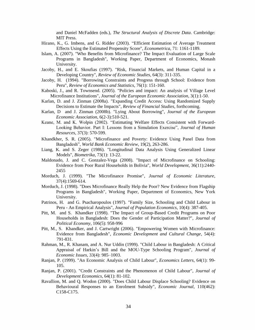
34

and Daniel McFadden (eds.), The Structural Analysis of Discrete Data. Cambridge:

MIT Press.

Hirano, K., G. Imbens, and G. Ridder (2003). ―Efficient Estimation of Average Treatment

Effects Using the Estimated Propensity Score", Econometrica, 71: 1161-1189.

Islam, A. (2007). "Who Benefits from Microfinance? The Impact Evaluation of Large Scale

Programs in Bangladesh", Working Paper, Department of Economics, Monash

University.

Jacoby, H., and E. Skoufias (1997). "Risk, Financial Markets, and Human Capital in a

Developing Country", Review of Economic Studies, 64(3): 311-335.

Jacoby, H. (1994). "Borrowing Constraints and Progress through School: Evidence from

Peru", Review of Economics and Statistics, 76(1): 151-160.

Kaboski, J., and R. Townsend. (2005). "Policies and impact: An analysis of Village Level

Microfinance Institutions", Journal of the European Economic Association, 3(1):1-50.

Karlan, D. and J. Zinman (2008a). "Expanding Credit Access: Using Randomized Supply

Decisions to Estimate the Impacts", Review of Financial Studies, forthcoming.

Karlan, D and J. Zinman (2008b). "Lying About Borrowing", Journal of the European

Economic Association, 6(2-3):510-521.

Keane, M. and K. Wolpin (2002). ―Estimating Welfare Effects Consistent with Forward-

Looking Behavior. Part I: Lessons from a Simulation Exercise‖, Journal of Human

Resources, 37(3): 570-599.

Khandkher, S. R. (2005). "Microfinance and Poverty: Evidence Using Panel Data from

Bangladesh‖, World Bank Economic Review, 19(2), 263-286.

Liang, K. and S. Zeger (1986). "Longitudinal Data Analysis Using Generalized Linear

Models", Biometrika, 73(1): 13-22.

Maldonado, J. and C. Gonzalez-Vega (2008). "Impact of Microfinance on Schooling:

Evidence from Poor Rural Households in Bolivia", World Development, 36(11):2440-

2455

Morduch, J. (1999). "The Microfinance Promise", Journal of Economic Literature,

37(4):1569-614.

Morduch, J. (1998). "Does Microfinance Really Help the Poor? New Evidence from Flagship

Programs in Bangladesh", Working Paper, Department of Economics, New York

University.

Patrinos, H. and G. Psacharopoulos (1997). "Family Size, Schooling and Child Labour in

Peru - An Empirical Analysis", Journal of Population Economics, 10(4): 387-405.

Pitt, M. and S. Khandker (1998). "The Impact of Group-Based Credit Programs on Poor

Households in Bangladesh: Does the Gender of Participation Matter?", Journal of

Political Economy, 106(5): 958-996

Pitt, M., S. Khandker, and J. Cartwright (2006). "Empowering Women with Microfinance:

Evidence from Bangladesh", Economic Development and Cultural Change, 54(4):

791-831.

Rahman, M., R. Khanam, and A. Nur Uddin (1999). "Child Labour in Bangladesh: A Critical

Appraisal of Harkin‘s Bill and the MOU-Type Schooling Program", Journal of

Economic Issues, 33(4): 985–1003.

Ranjan, P. (1999). "An Economic Analysis of Child Labour", Economics Letters, 64(1): 99-

105.

Ranjan, P. (2001). "Credit Constraints and the Phenomenon of Child Labour", Journal of

Development Economics, 64(1): 81-102.

Ravallion, M. and Q. Wodon (2000). "Does Child Labour Displace Schooling? Evidence on

Behavioural Responses to an Enrolment Subsidy", Economic Journal, 110(462):

C158-C175.

35

Rivers, D. and Q. Vuong (1988). "Limited Information Estimators and Exogeneity Tests for

Simultaneous Probit Models", Journal of Econometrics, 39(3): 347-366.

Rosenzweig, M. and T. Schultz (1982). "Market Opportunities, Genetic Endowments, and

Intrafamily Resource Distribution: Child Survival in Rural India", American

Economic Review, 72(4): 803-815.

Salmon, C. (2005). "Child Labour in Bangladesh: Are Children the Last Economic Resource

of the Household?", Journal of Developing Societies, 21: 33-54.

Train, K., D. McFadden, and M. Ben-Akiva (1987). "The Demand for Local Telephone

Service: A Fully Discrete Model of Residential Calling Patterns and Service

Choices", RAND Journal of Economics, 18(1): 109-123.

Vella, F. (1993). "A Simple Estimator for Simultaneous Models with Censored Endogenous

Regressors", International Economic Review, 34(2): 441-457.

Van der Klaauw, W. (2002). "Estimating the Effect of Financial Aid Offers on College

Enrolment: A Regression-Discontinuity Approach", International Economic Review,

43(4): 1249-1287.

Wydick, B. (1999). "The Effect of Microenterprise Lending on Child Schooling in

Guatemala", Economic Development and Cultural Change, 47(4): 853-869.

World Bank (2006). ―Microfinance in South Asia: Towards a Financial Inclusion for the

Poor‖ The World Bank, Washington, D.C.

Yamauchi, C. (2007). "Can Investment in Household Enterprises Advance Children‘s

Schooling Attendance?: Consequences of Poverty Alleviation Program in Indonesia",

Working paper, RSSS, Australian National University.

Zohir, S., S. Mahmud, B. Sen. and M. Asaduzzaman. (2001). "Monitoring and Evaluation of

Microfinance Institutions", Bangladesh Institute of Development Studies, Dhaka,

http://www.pksf-bd.org/bids_report.html.

36

Table 1: Descriptive Statistics

Variables

Treatment

(I)

Control

(II)

Difference

III=(I-II)

Child Characteristics (7-16 years old)

Child in work (in percentage)

Boys 16.9 13.8 3.0

Girls 11.0 9.3 1.7

Child in school (in percentage)

Boys 69.3 74.7 -5.5

Girls 76.6 78.9 -2.3

Age of child (in years) 11.497 11.494 0.003

Sex of child (percentage of girls) 55.7 55.6 0.1

Household Characteristics

Mother age (in years) 37.66 38.14 -0.48

Mother schooling (years of education) 1.09 1.54 -0.45

Father age (in years) 45.85 46.80 -0.95

Father schooling (years of education) 2.64 3.20 -0.56

Household size 6.56 6.48 -0.08

Number of children

0-6 years 0.81 0.79 0.02

6-16 years 2.79 2.66 0.13

Maximum education by any household member

Male borrower (years of education) 4.78 5.29 -0.50

Female borrower (years of education) 4.17 4.57 -0.40

Amount of land (in decimals) 64.7 91.2 -26.6

Village Characteristics

Program

village (I)

Control

village (II)

Difference

III=(I-II)

Primary school (%) 86.25 90.91 -4.66

Secondary school (%) 27.27 31.25 -3.98

Union health centre (%) 17.5 10 7.5

Distance to nearest sub-district (km) 7.14 11.91 -4.77

Presence of r grocery market (%) 22.5 18.2 4.3

Presence of bus stand (%) 15 9.1 5.9

Presence of post office (%) 20 18.2 1.8

Presence of telephone office (%) 6.3 9.1 -2.8

Presence of UP office (%) 13.8 18.2 -4.4

Notes: The third column presents the difference between columns (1) and (2). Differences that are statistically

significant at less than five percent are marked bold.

37

Table 2: Impact Estimates of the Participation in Microcredit Program

on Child Labour

LPM Probit

No

Control

Basic

Control

Full

Control

No

Control

Basic

Control

Full

Control

(1) (2) (3) (4) (5) (6)

Women and Men’s credit

All -0.0146 0.0252 0.0801 -0.0144 0.0192 0.0541

(0.0291) (0.0290) (0.0441)+ (0.0287) (0.0219) (0.0023)+

[0.0228] [0.0276] [0.0418]+ [0.0225] [0.0203] [0.0304]+

Boys -0.0433 -0.0121 0.0034 -0.043 -0.0136 -0.0106

(0.0357) (0.0383) (0.0583) (0.0354) (0.0297) (0.0418

[0.0320] [0.0370] [0.0526] [0.0316] [0.0280] [0.0383

Girls 0.0161 0.0502 0.1367 0.0158 0.0372 0.0794

(0.0373) (0.0394) (0.0594)** (0.0363) (0.0241) (0.0336)**

[0.0309] [0.0395] [0.0609]** [0.0301] [0.0239] [0.0351]**

Women's Credit

All -0.0134 0.0335 0.087 -0.0133 0.0276 0.0558

(0.0285) (0.0289) (0.0456)+ (0.0281) (0.0213) (0.0302)+

[0.0231] [0.0284] [0.0426]** [0.0228] [0.0203] [0.0302]+

Boys -0.042 -0.0029 0.0129 -0.0417 -0.0018 -0.0093

(0.0353) (0.0369) (0.0590) (0.0349) (0.0261) (0.0377)

[0.0325] [0.0377] [0.0861] [0.0320] [0.0257] [0.0258]+

Girls 0.0172 0.0611 0.1426 0.0168 0.0442 0.0835

(0.0370) (0.0400) (0.0610)** (0.0361) (0.0241)+ (0.0348)**

[0.0312] [0.0409] [0.0626]** [0.0304] [0.0245]+ [0.0363]**

Men's Credit

All -0.0187 0.0252 0.0774 -0.0184 0.0199 0.064

(0.0426) (0.0503) (0.0746) (0.0420) (0.0323) (0.0378)+

[0.0363] [0.0452] [0.0681] [0.0358] [0.0293] [0.0373]+

Boys -0.0671 -0.0285 -0.0239 -0.0664 -0.0233 -0.0112

(0.0550) (0.0643) (0.0912) (0.0542) (0.0435) (0.0456)

[0.0506] [0.0603] [0.0841] [0.0497] [0.0405] [0.0426]

Girls 0.0345 0.0685 0.1507 0.0339 0.0416 0.1008

(0.0570) (0.0690) (0.1094) (0.0556) (0.0285) (0.0421)**

[0.0497] [0.0654] [0.1040] [0.0483] [0.0273] [0.0439]** Notes: All the results are the marginal effects of instrumented credit variable using IV regressions. The

regressions include child, household, village characteristics and district fixed effects (except the first and fourth

columns). ‗Basic control‘ is the subset of ‗full control‘ and includes some household and child demographic

variables. Standard errors presented in parentheses are corrected for clustering at the village level using the

formulas in Liang and Zeger (1986), while those in brackets are corrected for clustering at the household level.

The coefficients and the standard errors are multiplied by the average credit borrowed by the respective group of

households. All the estimates are also weighted propensity scores. Coefficients with + are significant at the 10%,

those with ** at the 5%, and those with * at the 1%.

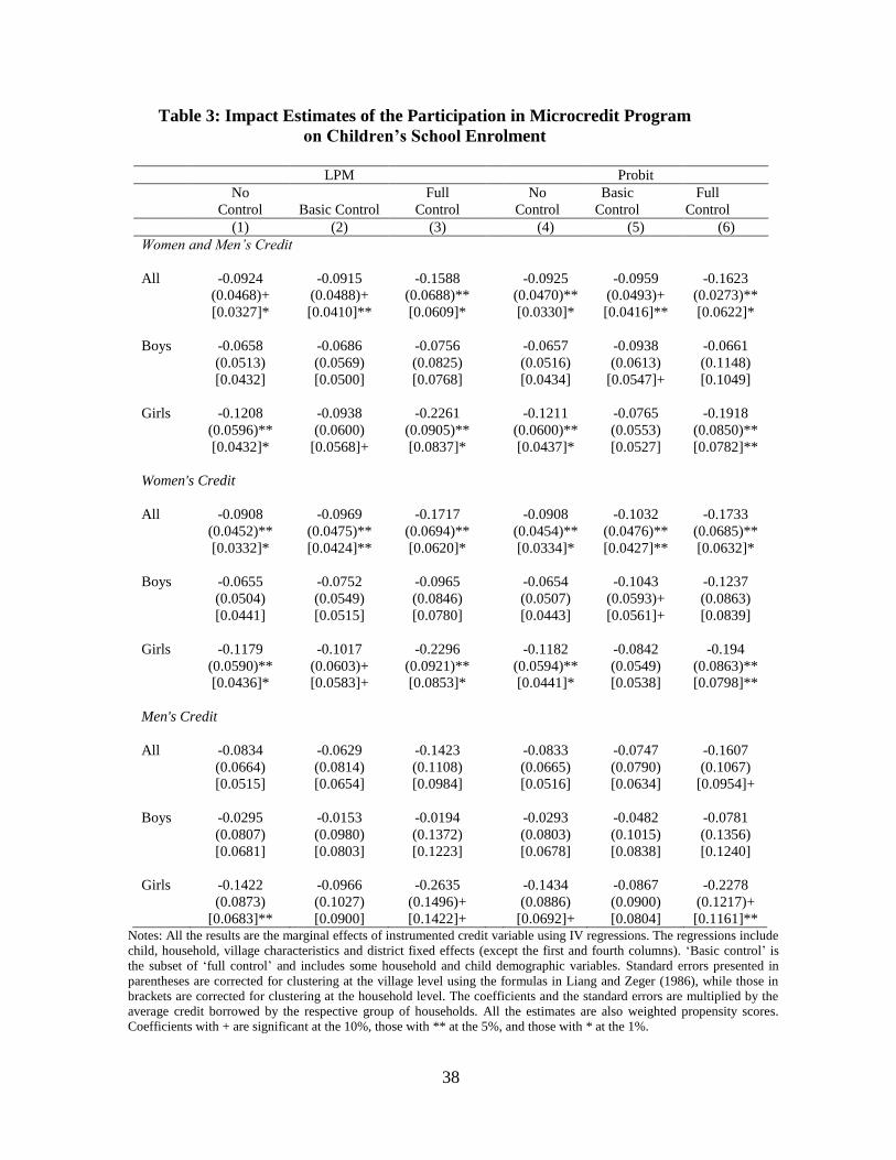
38

Table 3: Impact Estimates of the Participation in Microcredit Program

on Children’s School Enrolment

LPM Probit

No

Control Basic Control

Full

Control

No

Control

Basic

Control

Full

Control

(1) (2) (3) (4) (5) (6)

Women and Men’s Credit

All -0.0924 -0.0915 -0.1588 -0.0925 -0.0959 -0.1623

(0.0468)+ (0.0488)+ (0.0688)** (0.0470)** (0.0493)+ (0.0273)**

[0.0327]* [0.0410]** [0.0609]* [0.0330]* [0.0416]** [0.0622]*

Boys -0.0658 -0.0686 -0.0756 -0.0657 -0.0938 -0.0661

(0.0513) (0.0569) (0.0825) (0.0516) (0.0613) (0.1148)

[0.0432] [0.0500] [0.0768] [0.0434] [0.0547]+ [0.1049]

Girls -0.1208 -0.0938 -0.2261 -0.1211 -0.0765 -0.1918

(0.0596)** (0.0600) (0.0905)** (0.0600)** (0.0553) (0.0850)**

[0.0432]* [0.0568]+ [0.0837]* [0.0437]* [0.0527] [0.0782]**

Women's Credit

All -0.0908 -0.0969 -0.1717 -0.0908 -0.1032 -0.1733

(0.0452)** (0.0475)** (0.0694)** (0.0454)** (0.0476)** (0.0685)**

[0.0332]* [0.0424]** [0.0620]* [0.0334]* [0.0427]** [0.0632]*

Boys -0.0655 -0.0752 -0.0965 -0.0654 -0.1043 -0.1237

(0.0504) (0.0549) (0.0846) (0.0507) (0.0593)+ (0.0863)

[0.0441] [0.0515] [0.0780] [0.0443] [0.0561]+ [0.0839]

Girls -0.1179 -0.1017 -0.2296 -0.1182 -0.0842 -0.194

(0.0590)** (0.0603)+ (0.0921)** (0.0594)** (0.0549) (0.0863)**

[0.0436]* [0.0583]+ [0.0853]* [0.0441]* [0.0538] [0.0798]**

Men's Credit

All -0.0834 -0.0629 -0.1423 -0.0833 -0.0747 -0.1607

(0.0664) (0.0814) (0.1108) (0.0665) (0.0790) (0.1067)

[0.0515] [0.0654] [0.0984] [0.0516] [0.0634] [0.0954]+

Boys -0.0295 -0.0153 -0.0194 -0.0293 -0.0482 -0.0781

(0.0807) (0.0980) (0.1372) (0.0803) (0.1015) (0.1356)

[0.0681] [0.0803] [0.1223] [0.0678] [0.0838] [0.1240]

Girls -0.1422 -0.0966 -0.2635 -0.1434 -0.0867 -0.2278

(0.0873) (0.1027) (0.1496)+ (0.0886) (0.0900) (0.1217)+

[0.0683]** [0.0900] [0.1422]+ [0.0692]+ [0.0804] [0.1161]** Notes: All the results are the marginal effects of instrumented credit variable using IV regressions. The regressions include

child, household, village characteristics and district fixed effects (except the first and fourth columns). ‗Basic control‘ is

the subset of ‗full control‘ and includes some household and child demographic variables. Standard errors presented in

parentheses are corrected for clustering at the village level using the formulas in Liang and Zeger (1986), while those in

brackets are corrected for clustering at the household level. The coefficients and the standard errors are multiplied by the

average credit borrowed by the respective group of households. All the estimates are also weighted propensity scores.

Coefficients with + are significant at the 10%, those with ** at the 5%, and those with * at the 1%.

39

Table 4: Effects of Control Variables on School Enrolment and Child Labour

Control Variables

School Enrolment Child Labour

LPM Probit LPM Probit

(1) (2) (3) (4)

Age of child 0.257 0.271 -0.096 -0.005

(0.023)* (0.022)* (0.018)* (0.014)

Age of child squared -0.012 -0.013 0.006 0.001

(0.001)* (0.001)* (0.001)* (0.001)**

Number of younger siblings -0.015 -0.015 0.023 0.014

(0.008)+ (0.009)+ (0.006)* (0.003)*

Number of older sister 0.016 0.018 -0.011 -0.01

(0.006)* (0.007)* (0.004)* (0.004)*

Sex of household head 0.128 0.119 -0.103 -0.071

(0.054)** (0.067)+ (0.032)* (0.032)**

Whether mother is present in the family 0.039 0.019 -0.051 -0.026

(0.051) (0.060) (0.042) (0.034)

Highest education of any member 0.038 0.039 -0.02 -0.013

(0.003)* (0.004)* (0.002)* (0.002)*

Age of household head -0.004 -0.004 0.004 0.002

(0.001)* (0.001)* (0.001)* (0.001)*

Education of household head

(0-4 years of schooling) 0.064 0.033 -0.051 -0.017

(0.031)** (0.049) (0.025)** (0.030)

(5-9 years of schooling) 0.044 0.004 -0.016 0.008

(0.024)+ (0.042) (0.017) (0.025)

Years of mother‘s schooling -0.002 0.004 0 -0.004

(0.003) (0.006) (0.003) (0.003)

Village Characteristics:

Presence of primary school -0.02 -0.024 0.008 0.007

(0.032) (0.029) (0.025) (0.014)

Presence of secondary school or college 0.052 0.058 -0.011 -0.011

(0.019)* (0.018)* (0.014) (0.009)

Presence of religious school 0.026 0.022 -0.008 -0.002

(0.034) (0.034) (0.028) (0.018)

Presence of health facility 0.041 0.04 -0.017 -0.01

(0.020)** (0.023)+ (0.018) (0.013)

Presence of brick-built road 0.066 0.065 -0.048 -0.031

(0.027)** (0.027)** (0.017)* (0.011)*

Presence of grocery market -0.082 -0.09 0.033 0.026

(0.021)* (0.025)* (0.012)* (0.010)*

Presence of bus stand -0.072 -0.072 0.058 0.043

(0.031)** (0.042)+ (0.020)* (0.022)+

Distance to nearest sub-district (in km) -0.002 -0.001 0.001 0.001

(0.002) (0.002) (0.001) (0.001)

Adult male wage -0.001 -0.001 0.001 0.001

(0.001) (0.001) (0.001) (0.001)

Rice price 0 0.001 0.006 0.003

(0.011) (0.011) (0.008) (0.005)

Number of observations 4277 4277 4277 4277

R-squared 0.22 0.23 Notes: Regressions also include dummies for birth-order, dummies for land-holding, presence of post-office and

instrumented credit variable. All the coefficient estimates are the marginal effects. Standard errors presented in

parentheses are corrected for clustering at the village level using the formulas in Liang and Zeger (1986) and using

the propensity score weighting scheme. Coefficients with + are significant at the 10%, those with ** at the 5%,

and those with * at the 1%.

40

Table 5: Impact Estimates Based on Binary Participation Measure

on School Enrolment and Child Labour

Child is in school Child is in work

LPM Probit LPM Probit

Women's Credit

Boys -0.1690 -0.1878 0.0193 -0.0120

(0.1374) (0.1463) (0.0956) (0.0590)

[0.1240] [0.1353] [0.0879] [0.0567]

Girls -0.4782 -0.4438 0.2569 0.1369

(0.1359)* (0.1322)* (0.0946)* (0.05376)**

[0.1309]* [0.1281]* [0.0944]* [0.05375]**

Men's Credit

Boys -0.1190 -0.1634 0.0097 -0.0325

(0.1744) (0.1769) (0.1175) (0.0663)

[0.1636] [0.1702] [0.1176] [0.0679]

Girls -0.5828 -0.5153 0.3019 0.0842

(0.1782)* (0.1521)* (0.1357)** (0.04224)**

[0.1800]* [0.1571]* [0.1313]** [0.03974]**

Notes: All the results are the marginal effects of instrumented binary treatment indicator variable

using IV regressions. The regressions include full control using child, household, village

characteristics and district fixed effects. Standard errors presented in parentheses are corrected for

clustering at the village level using the formulas in Liang and Zeger (1986) and using the propensity

score weighting scheme. Coefficients with ** are significant at the 5%, and those with * at the 1%.

41

Table 6: Impact Estimates Based on Children’s Age Group

Child is in school Child is in work

Age 7-12 Age 12-16 Age 7-12 Age 12-16

Women's credit

Boys -0.3274 0.1978 0.0491 -0.1784

(0.1557)** (0.2952) (0.0413) (0.2156)

Girls -0.3295 -0.5991 0.0785 0.2818

(0.1507)** (0.2224)* (0.0401)+ (0.1416)**

Men's credit

Boys -0.2329 0.0491 0.0051 -0.1673

(0.1612) (0.3816) (0.0312) (0.2666)

Girls -0.4131 -0.6178 0.0382 0.1077

(0.1877)** (0.7428) (0.0398) (0.2457)

Notes: All the results are the probit marginal effects of instrumented binary treatment indicator variable using

IV regressions. The regressions include full control using child, household, village characteristics and district

fixed effects. Standard errors presented in parentheses are corrected for clustering at the village level using the

formulas in Liang and Zeger (1986) and using the propensity score weighting scheme. Coefficients with + are

significant at the 10%, those with ** at the 5%, and those with * at the 1%.

42

Table 7: Impact Estimates Based on Parental Education

Education of

Household Head

Child is in school Child is in work

All

children Boys Girls

All

children Boys Girls

Probit

Low -0.2931 -0.2235 -0.3477 0.0966 0.0220 0.1373

(0.0705)* (0.0839)* (0.0878)* (0.0317)* (0.0410) (0.0346)*

Middle -0.0333 0.0415 -0.0920 0.0319 -0.0783 0.1019

(0.0736) (0.0911) (0.1009) (-0.0338) (-0.0546) (0.0367)*

High 0.0472 0.0887 0.0322 -0.0080 -0.1087 0.0649

(0.1115) (0.1446) (0.1220) (0.0470) (0.0730) (0.0472)

LPM

Low -0.2756 -0.1938 -0.3479 0.1302 0.0471 0.1972

(0.0670)* (0.0797)** (0.0854)* (0.0424)* (0.0526) (0.0524)*

Middle -0.0452 0.0420 -0.1191 0.0617 -0.0653 0.1574

(0.0652) (0.0797) (0.0894) (0.0400) (0.0585) (0.0510)*

High 0.0046 0.0668 -0.0454 0.0082 -0.0925 0.1011

(0.0914) (0.1223) (0.0936) (0.0530) (0.0769) (0.0635)

Notes: Low refers to households where the highest level of education obtained by parents is primary (0-4 years of

schooling) or less; Middle refers to households where the highest level of education obtained by parents is more than

primary but less than a high school degree (5-10 years of schooling), and High refers households where one of the parents

obtained at least a high school degree (11 or more years of schooling). All the results are the marginal effects of

instrumented credit interacted with education dummies using IV regressions. The regressions include full control using

child, household, village characteristics and district fixed effects. Standard errors in parentheses are corrected for

clustering at the village level using the formulas in Liang and Zeger (1986) and using propensity score weighting scheme.

Coefficients with ** are significant at the 5%, and those with * at the 1%.

43

Table 8: Impact Estimates Based on Land Ownership

Child is in school Child is in work

LPM Probit LPM Probit

Poorer Households

Boys 0.136 0.115 -0.085 -0.078

(0.119) (0.139) (0.073) (0.044)+

Girls -0.231 -0.238 0.098 0.089

(0.123)+ (0.128)+ (0.098) (0.070)

Less Poor Households

Boys -0.331 -0.328 0.260 0.451

(0.844) (0.848) (0.696) (0.476)

Girls 0.017 0.073 -0.007 0.019

(0.824) (0.591) (0.568) (0.057)

Notes: Poorer household are those who own less than a half acre of land and less poor households own more

than a half acre of land. The regressions include full control using child, household, village characteristics and

district fixed effects. The coefficients and the standard errors are multiplied by the average credit borrowed by

the respective group of households. Standard errors presented in parentheses are corrected for clustering at the

village level using the formulas in Liang and Zeger (1986) and using propensity score weighting scheme.

Coefficients with + are significant at the 10%, those with ** at the 5%, and those with * at the 1%.

44

Table 9: Impact of the Microcredit Program on Children’s School Achievement

Boys Girls

Female

Borrower

Grade

Completion

Education

Gap

Grade-

for-age

Grade

Completion

Education

Gap

Grade-

for-age

Treatment effect -0.196 -0.092 -21.647 -2.953 2.752 -48.393

(0.617) (0.611) (12.912)+ (0.738)* (0.696)* (16.089)*

Control function 0.158 0.143 22.286 2.963 -2.755 49.405

(0.624) (0.617) (13.283)+ (0.745)* (0.705)* (16.256)*

Male Borrower

Treatment effect -0.423 0.043 -23.727 -3.773 3.39 -72.497

(0.846) (0.817) (17.603) (0.961)* (0.923)* (21.299)*

Control function 0.327 0.047 25.084 3.537 -3.199 69.099

(0.787) (0.765) (16.855) (0.958)* (0.921)* (21.373)*

Notes: All the results are estimated using the control function method. The regressions include full control using

child, household, village characteristics and district fixed effects. The coefficients and the standard errors of

treatment effects are multiplied by the average credit borrowed by male and female borrowers. Standard errors

presented in parentheses are corrected for clustering at the village level using the formulas in Liang and Zeger

(1986) and using propensity score weighting scheme. Coefficients with + are significant at the 10%, and those

with * at the 1%.

45

Table 10: Multinomial Logit Model for Children’s Work/School Status

Child Occupation Coefficient Marginal Effect

Self-employment activity 2.03 0.266

(0.71)* (0.095)*

Agriculture -6.48 0.000

(1.73)* (0.0000)*

Day labourer 1.33 0.0000

(1.07) (0.001)

Service-related activity 2.42 0.0000

(4.50) (0.0000)

Enrolled in school -0.266

(0.096)*

Notes: The regressions include full control using child, household, village

characteristics and district fixed effects. Standard errors presented in

parentheses are corrected for clustering at the village level using the

formulas in Liang and Zeger (1986). Coefficients with * are significant at

the 1%.

46

Figure 1: Proportion of Children in School

.4.5

.6.7

.8.9

Pro

po

rtio

n a

tten

din

g S

ch

oo

l

7 8 9 10 11 12 13 14 15 16Age Year

Children of Treatment Group Children of Control Group

Figure 1a: Proportion of Boys in School

.4.5

.6.7

.8.9

Pro

po

rtio

n a

tten

din

g S

ch

oo

l

7 8 9 10 11 12 13 14 15 16

Age Year

Children of Treatment Group Children of Control Group

Figure 1b: Proportion of Girls in School

47

Figure 2: Proportion of Children in Work

.05

.15

.25

.35

.45

Pro

po

rtio

n w

ork

ing

7 8 9 10 11 12 13 14 15 16Age Year

Children of Treatment Group Children of Control Group

Figure 2a: Proportion of Boys in Work

.05

.15

.25

.35

.45

Pro

po

rtio

n w

ork

ing

7 8 9 10 11 12 13 14 15 16

Age Year

Children of Treatment Group Children of Control group

Figure 2b: Proportion of Girls in Work

48

Figure 3: Yeas of Microfinance Program in a Village and the Amount of Credit

Borrowed by Households

2000

4000

6000

8000

Ave

rag

e cr

edit

per

hou

seho

ld in

a v

illag

e

2 6 10 14 18Number of years a MO is avilable in a village

Notes: Average credit per household in a village is the amount of credit borrowed (in taka) by all

households divided by the number of participating households in the program village. Number of years

a MO is available in a village is the period from which microcredit has been first avilable in the

program village.

49

Figure 4: School Enrolment and Child Labour at Different Levels of Parental

Education

Note: Low-edu refers to those households where the highest level of education obtained by parents is primary

(0-4 years of schooling) or less; Mid-edu refers to households where the highest level of education obtained

by parents is more than primary but less than a high school degree (5-10 years of schooling), and High-edu

includes households where one of the parents obtained at least a high school degree (11 or more years of

schooling).