arX

iv:0

807.

4301

v2 [

phys

ics.

optic

s] 1

9 A

ug 2

008

Cherenkov radiation has nothing to do with X-shaped LocalizedWaves (Comments on “Cherenkov-Vavilov Formulation of

X-Waves”) (†)

Michel Zamboni-Rached,

Universidade Federal do ABC, Centro de Ciencias Naturais e Humanas, Santo Andre, SP, Brazil.

and

Erasmo Recami

Facolta di Ingegneria, Universita statale di Bergamo, Bergamo, Italy;

and INFN—Sezione di Milano, Milan, Italy.

Abstract — The Localized Waves (LW) are nondiffracting (“soliton-like”) solutions to

the wave equations, and are known to exist with subluminal, luminal and superluminal

peak-velocities V . For mathematical, and experimental, reasons, the ones that called

more attention are the “X-shaped” superluminal waves. Such waves are associated with

a cone, so that some authors –let us confine ourselves to electromagnetism– have been

tempted to look for links between them and the Cherenkov radiation: A good example of

such attempts is represented by the article by Walker and Kuperman recently appeared

in PRL 99, no.244802, of Dec.2007. However, the X-shaped waves belong to a very

different realm: For instance, they exist even in the vacuum, independently of any media,

as localized non-diffracting pulses propagating rigidly with a peak-velocity V > c, as

verified in a number of papers [cf., e.g., the refs. in the book Localized Waves (J.Wiley;

Jan.2008)]. We deem it necessary to clarify the whole question on the basis of a

rigorous formalism, in part original, and of clear physical considerations. In particular

we clarify, by explicit calculations based on Maxwell equations only, that, at variance with

what assumed by some authors: (i) the “X-waves” exist in all space, and in particular

inside both the front and the rear part of their double cone (that has nothing to do with

Cherenkov’s); (ii) they have not been found heuristically, via ad hoc assumptions, but by

(†) Work partially supported by FAPESP and CNPq (Brazil), and by INFN, MIUR(Italy). E-mail addresses for contacts: recami@mi.infn.it [ER]; mzamboni@ufabc.edu.br, mzam-boni@dmo.fee.unicamp.br [MZR]

1

use of strict mathematical (or experimental) procedures; (iii) the ideal X-waves (as well

as plane waves) are actually endowed with infinite energy, but finite-energy X-waves can

be easily constructed (even without space-time truncations): And at the end of this Ms.,

by following an original technique, we construct exact finite-energy solutions (totally free

from backward-traveling waves); (iv) the large majority of the researchers working in this

area do not aim at using the X-waves for “superluminal transmission of information”,

but are interested in the circumstance that they are localized waves, endowed with a

self-reconstruction property, and in their important practical applications (in part already

realized, since 1992); (v) an actual attempt at comparing Cherenkov radiation and

X-waves would lead one to consider the very different situation of the (X-shaped, too)

field generated by a superluminal point-charge, a question actually exploited in previous

papers, appeared e.g. in 2004 in Phys.Rev.E [Recami, Zamboni-Rached & Dartora, PRE

69, no.027602]: We show here explicitly that in this case the point-charge would not lose

energy in the vacuum, and that the field generated by it would not need to be continuously

feeded by incoming side-waves (as it is indeed the case for an ideal, ordinary X-wave).

PACS nos.: 41.60.Bq; 03.50.De; 03.30.+p; 41.20;Jb; 04.30.Db; 42.25.-p; 42.25.Fx;

47.35.Rs.

Keywords: Cherenkov radiation; Localized waves; X-shaped waves; Superluminal pulses;

Maxwell equations; Special Relativity; Lorentz transformations; Superluminal point-

charge; Wave equations; Bessel beams.

The Localized Waves (LW) are nondiffracting (“soliton-like”) solutions to the wave equa-

tions, and are known to exist with subluminal, luminal and superluminal peak-velocities

V . For mathematical, and experimental, reasons, the ones that called more attention

are the “X-shaped” superluminal waves. Such waves are associated with a cone, so that

some authors —let us confine ourselves to electromagnetism— have been tempted to look

for links between them and the Cherenkov radiation: A good example of such attempts

is represented by the article by Walker and Kuperman, recently appeared[1]. However,

the X-shaped waves belong to a very different realm: For instance, they exist even in

the vacuum, independently of any media, as localized non-diffracting pulses propagating

2

rigidly with a peak-velocity V > c, as verified in a number of papers (cf., e.g., the refs.

in the book Localized Waves [2]). We deem it necessary to clarify all the question on the

basis of a rigorous formalism, in part original, and of clear physical considerations. In

particular we clarify, by explicit calculations based on Maxwell equations only, that, at

variance with what assumed by some authors: (i) the “X-waves” exist in all space, and in

particular inside both the front and the rear part of their double cone (that has nothing to

do with Cherenkov’s); (ii) they have not been found heuristically, via ad hoc assumptions,

but by use of strict mathematical (or experimental) procedures; (iii) the ideal X-waves

(as well as plane waves) are actually endowed with infinite energy, but finite-energy X-

waves can be easily constructed (even without space-time truncations): And at the end

of this work, by following an original technique, we construct exact finite-energy solutions

(totally free from backward-traveling waves); (iv) the large majority of the researchers

working in this area do not aim at using the X-waves for “superluminal transmission of in-

formation”, but are interested in the circumstance that they are localized waves, endowed

with a self-reconstruction property, and in their important practical applications (in part

already realized, since 1992); (v) an actual attempt at comparing Cherenkov radiation

and X-waves would lead one to consider the very different situation of the (X-shaped, too)

field generated by a superluminal point-charge, a question actually exploited in previous

papers, appeared e.g. in 2004 in Phys.Rev.E [3]: We show here explicitly that in this case

the point-charge would not lose energy in the vacuum, and that the field generated by it

would not need to be continuously feeded by incoming side-waves (as it is indeed the case

for an ideal, ordinary X-wave).

As already said, we wish to reply to attempts, like the one in Ref.[1], at setting forth

“Cherenkov-Vavilov formulations of the X-shaped Localized Waves” (in the following we

shall write only “Cherenkov” for brevity’s sake). The classical problem of the Cherenkov

radiation[4] from a point-charge traveling in a medium with speed v such that cn < v < c,

where cn and c are the speed of light in the medium and in the vacuum, respectively, is

normally investigated in correct terms. Also in [1] it is presented in a mathematically

correct way; sometimes, however, the language used in such a context is ambiguous: For

example, in [1] the speed cn in the medium is just called c; furthermore, the point-charge

associated with the Cherenkov radiation is called “superluminal”, despite the fact that

its speed is smaller than the light-speed in the vacuum. In the existing theoretical and

experimental literature on Localized Waves (see again, e.g., Ref.[2]) and in particular on

X-shaped waves[5, 6], the word superluminal is reserved to group-speeds actually larger

than the speed of light in the vacuum. These ambiguities create difficulties, especially

3

whenever a comparison is made of the Cherenkov radiation with X-shaped waves. Let

us repeat that, in reality, the latter belong to a very different realm; and exist even in

vacuum as localized non-diffracting pulses, propagating rigidly with superluminal (in our

language) peak-velocities, V > c, independently of any media. Let us try to clarify the

whole subject, and several unjustified implications in papers like [1], by using a rigorous

formalism and clear physical considerations.

Our specific considerations and comments are as follows:

1) — As already mentioned, the papers addressing the Cherenkov effect do incorporate

sometimes[1] an ambiguous terminology (see above), about which the readers must be

warned. Except for the ambiguous notation, the analysis of the ordinary scalar-valued

Cherenkov radiation in normally correct —cf., e.g., the first part of [1]— as it can be

explicitly checked; anyway, the relevant results are well-known[4]. Except for the am-

biguous notation, the analysis of the ordinary scalar-valued Cherenkov radiation in the

first part of [1] is correct, as it can be explicitly checked; however, the relevant results

seem to be already known[4]. It can be pointed out, incidentally, that even the vector-

valued electromagnetic fields generated by a really superluminal point-charge, endowed

with speed V > c, have already been considered and published in [3] using a procedure

totally different, of course, from the one followed e.g. in [1].

2) — The main equivocal aspect of works like [1] is that such authors attempt at

using the ordinary Cherenkov radiation to draw conclusions about superluminal Localized

Waves (LW) known as X-shaped waves (or simply X-waves). The latter, as we said,

are nondiffractive solutions to the homogeneous wave equations and propagate rigidly

with superluminal peak-velocities. They have been predicted long ago[7, 8], have been

mathematically constructed[5], and finite-energy versions of these wave-packets have been

experimentally produced[6] in the vacuum, independently of any media. We are going to

show the drawbacks of the path followed in articles as [1] by using explicit calculations.

To be clear and self-contained, we initially address the (simpler) scalar case, in which

a field ψ is governed by the inhomogeneous wave equation

(∇2 −

1

c2n

∂2

∂t2

)ψ(r, t) = −

4π

cnj(r, t) (1)

with j = qv δ(ρ) δ(z− vt)/(2πρ). Here cn is the speed of light in the considered medium

4

and j(r, t) is the generating source, assumed to be pointlike and moving along the positive

z-axis with subluminal speed cn < v < c, while ρ denotes the cylindrical radial coordinate.

A Green’s function for Eq.(1) is given explicitly as

G(r, t, r ′, t′) = l G+(r, t, r ′, t′) + (1 − l) G−(r, t, r ′, t′) (2)

where

G±(r, t, r ′, t′) =δ (t′ − (t∓ R/cn))

cnR(3)

and R ≡√

(z − z′)2 + ρ2 + ρ′2 − 2ρρ′ cos(θ − θ′).

Quantities G+ and G− are the retarded and advanced Green’s functions, respectively.

When considering only the retarded Green’s function (l = 1), the solution to the wave

equation can be expressed as

ψ(r, t) =∫

dx′3∫

dt′G+(r, t, r ′, t′) j(r ′, t′) . (4)

We can use the expression for G+ given in Eq.(3) for a direct calculation of the wave

function ψ(r, t). However, for reasons that will be made clear in the sequel, we shall

follow the procedure adopted in papers like [1]. Specifically, we shall determine the Fourier

transform of G+ in the variables z and t, and subsequently the transform of ψ in the same

variables. For cn < v < c, we obtain:

ψ(ρ, ζ) =1

2πcn

[(∫ 0

−∞dω(−iπ)qH2

0 (ργ−1n |ω|/v)eiωζ/v

)+(∫ ∞

0dω(iπ)qH1

0(ργ−1n ω/v)eiωζ/v

)]

where ζ ≡ z − vt, and H1,20 are the zero-order Hankel functions of first and second kind.

Using, next, the relation H20 (x) = −H1

0 (−x) for x ≥ 0, the last equation is reduced to

Eq.(7) of Ref.[1], viz.,

ψ(ρ, ζ) =1

2cn

∫ ∞

−∞dωiqH1

0 (ργ−1n ω/V )eiωζ/V (5)

from which one determines the well-known expression for the Cherenkov radiation

ψ(ρ, z, t) =

2qβn√ζ2 − γ−2

n ρ2for ζ < −γ−1

n ρ

0 elsewhere ,

(6)

5

where it should be noted that βn ≡ v/cn and γn ≡ 1/√v2/c2n − 1. The radiation exists

only inside the rear part ζ = −γ−1n ρ of the Cherenkov cone.

As to the vectorial case, physically more significant, let us only mention that is can

be constructed by adopting the Lorentz gauge, and by considering the vector potential

A = Azez, with Az ≡ ψ and the current density j = jzez, with jz ≡ j.

2a) – Some authors, as the ones of Ref.[1], have been induced at looking for a

connection between the Cherenkov emission and X-shaped waves. The simple X-waves to

which many authors refer to are solutions to the homogeneous scalar wave equation: They

are wave functions of the type X(ρ, z, t) = X(ρ, ζ), with ζ ≡ z−V t and cn < V <∞, and

can be obtained by suitable superpositions of axially symmetric Bessel beams, propagating

in the positive z-direction with the same phase-velocity (cf., e.g., Refs.[5]); precisely,

ψX(ρ, ζ) =∫ ∞

0dωS(ω)J0(ρ

ω

V

√V 2/c2 − 1)eiω/V ζ (7)

where J0(.) is an ordinary zero-order Bessel function and S(ω) is the temporal frequency

spectrum. Incidentally, let us stress that Eq.(7) represents a particular case of the

superluminal waves, which in their turn are just a particular case of the (subluminal,

luminal or superluminal) Localized Waves. For the specific spectrum S(ω) = exp[−aω],

with a a positive constant, one obtains the zero-order (classic) X-wave:

X ≡ X(ρ, ζ) =V√

(aV − iζ)2 + (V 2/c2 − 1)ρ2. (8)

Authors like the ones in Ref.[1] are led to attempt a comparison between the Cherenkov

effect and the zero-order X-wave by the apparent mathematical similarity of equations (5)

and (7) [which correspond, for instance, to equations (7) and (13) of Ref.[1].] To be more

specific: (i) we have seen that for the inhomogeneous wave-equation (1), a Cherenkov

solution of the type given in Eq.(6) exists only inside the cone rear part ζ = −γ−1ρ. To

obtain a solution existing only inside the cone forward part ζ = γ−1ρ, one should make

use of the advanced Green’s function G−: This —to go on with our example— induced

the authors in [1] to state that the forward part of the X-wave is non-causal; (ii) Another

point that misled Walker and Kuperman[1] is that, if one puts S(ω) = i into the ψX-wave

(7), that is, if one sets a = 0 in Eq.(8) and multiplies it by i, one obtains

X(ρ, ζ) =V√

ζ2 − (V 2/c2 − 1)ρ2, (9)

6

which is mathematically identical, apart from a constant, to the Cherenkov solution in

Eq.(6]), with a real part existing this time inside both the rear cone ζ = −γ−1ρ and

the forward cone ζ = γ−1ρ. The statement in papers like [1] that the advanced part of

the zero-order X-wave [cf. Eq.(8)] is non-causal is due to an illicit extrapolation. Being

a solutions to the homogeneous wave equation, the X-wave cannot admit singularities.

In contrast, the solution given in Eq.(9), which was obtained from the Bessel beam su-

perposition (7) using a constant spectrum S(ω), does have singularities and cannot be

considered a solution to the homogeneous wave equation. Actually, the real part of the

solution (9) can be an acceptable solution for the inhomogeneous case only: Indeed, we

shall show later on that it represents the field of a point-charge traveling with speed V > c

when using as a Green’s function the expression G = G+/2 + G−/2, half retarded and

half advanced (which means, again, that it refers to an inhomogeneous problem).

It should be pointed out that the Bessel beam synthesis in Eq.(7) is a particular case of

more general spectral representations leading not only to infinite but also to finite energy

superluminal LWs[2, 5]. Not less important, even a finite-energy close replica of the the

classic X-wave (8) (endowed, incidentally, also with a finite field-depth) can be generated

in a causal manner by means of a “dynamic” finite aperture (antennas, holographic or

optical elements, etc.). For instance, it is enough an array of circular elements excited

according to the function X(ρ, z = 0, t), given by equations (7) or (8) on the aperture

plane located at z = 0. The emitted finite-energy X-wave can be calculated by means of

the Rayleigh-Sommerfeld (II) formula [9]

ψRS(II) (ρ, z, t) =∫ 2π

0dφ′

∫ D/2

0dρ′ρ′

1

2πR

{[X]

(z − z′)

R2+ [∂cnt′X]

(z − z′)

R

}. (10)

The quantities inside the square brackets are evaluated at the retarded time cnt′ = cnt−R.

The distance R =√

(z − z′)2 + ρ2 + ρ′2 − 2ρρ′ cos (φ− φ′) is now the separation between

source and observation points, and the aperture diameter is denoted by D. The depth

of field of the particular solution given in Eq.(10) is known[10] to be Z = Rγn.

What stated above has been theoretically (even via numerical simulations...) and

experimentally verified, as published in a large number of well-known papers: see, for

example, Refs.[5, 6, 11, 10, 12, 13, 2].

2b) – We agree with authors as Walker and Kuperman[1] that the superluminal

spot of any X-wave is fed by the waves coming from the elements of the aperture, and

that these waves carry energy with at most luminal (V = cn) speed. In such cases, the

7

X-wave intensity peaks at two different locations are not causally correlated. But such a

correct claim, contained also in [1], is well known and firmly accepted since the nineties

by practically all the scholars working in the area of LWs (cf., e.g., the references in

[14] and [13], as well as Refs.[2, 5, 10, 11]): The claim in [1] that efforts in the area of

X-waves are aimed at transmitting information superluminally is not correct. The large

majority of the experts in such a subject are interested in X-waves due to their spatio-

temporal localization, unidirectionality, “soliton-like”, and self-reconstruction properties

in the near-to-far zone. Such properties bear interesting consequences, from theoretical

and experimental points of view in all sectors of physics in which a role is played by

a wave equation (including —mutatis mutandis— elementary particle physics, and even

gravitation).

3) — The statement, contained in papers like [1], that the (ideal) zero-order X-wave in

Eq.(7) has infinite energy (as well as the plane-waves) does not convey new information.

The fact that such a solution needs to be fed for an infinite time has been known since the

start of LW theory. In any case, as mentioned earlier, such a problem can be overcome

either by using (cf. Eq.(10)) apertures finite in space and time, i.e., by truncating the

X-wave, or by constructing exact, analytical finite-energy solutions[12, 11]. For reasons

of space, we shall show only briefly, but in an original rigorous way, how closed-form

solutions of the latter type can be actually constructed, without any recourse to the

backward-traveling waves that trouble the ordinary approaches: See point 5) below.

Here, for the moment, let us recall that X-waves endowed by themselves with finite

energy even without truncation have been easily constructed in the past by use of diffrac-

tion integrals: See, for instance, the approximate solution in Eqs.(2.31),(2.32) of Ref.[15],

that is, the “SMPS pulse”, which is depicted in Figs.1. A finite-energy X-wave gets de-

formed while propagating: and Fig.1(b) shows the pulse in Fig.1(a) after it has travelled

50 km.

Let us emphasize, as well, that the formulations leading to LWs, and to X-waves, are

not chosen ad hoc, as believed in papers as [1], but are to be based on proper choices

of the spectra (which imply a specific space-time coupling[12, 11, 16]) and of the Bessel

functions (in order to avoid singularities both at ρ = 0 and at ρ = ∞): In contrast,

the choice suggested, e.g., in Eq.(15) of [1] presents singularities. To be clearer, let us

observe that a general solution to the scalar homogeneous wave-equation in free space can

be written [when eliminating evanescent waves] in the form

8

Figure 1: Example of an X-type LW endowed with finite energy (even without truncation),and that consequently gets deformed while propagating: (b) represents the pulse depictedin (a) after it has traveled 50 km. See Ref.[15], and the text.

ψ(ρ, φ, z, t) =∞∑

ν=−∞

∫ ∞

0dω

∫ ω/c

−ω/cdkzAν(kz, ω)Jν

ρ

√ω2

c2− k2

z

eikzze−iωteiνφ

(11)

by considering positive angular frequencies ω only. For obtaining ideal LWs propagating

along the positive z-direction with peak-velocity V (that can assume a priori any value

0 ≤ V ≤ ∞), the spectra Aν must have the form:[12, 2, 16]

Aν(kz, ω) =∞∑

µ=−∞

Sνµ(ω) δ[ω − (V kz + bµ)] (12)

where bµ = 2πµV/∆z0, and it can be easily shown[12, 16] that solution (11) possesses

the important property ψ(ρ, φ, z, t) = ψ(ρ, φ, z+∆z0, t+∆z0/V ), where ∆z0 is a chosen

space-interval along z. The last two equations already show that LWs are not to be

found by “ad hoc” assumptions: Equation (12) does explicitly show that —as mentioned

above— the ideal LWs exist only in correspondence with linear relations between ω and

kz, that is, with specific space-time couplings. By assuming in particular A0(kz, ω) ≡

Aν(kz, ω) = δν0 S(ω) Θ(kz) δ[ω − (V kz + α0)], where the Heaviside function Θ does

eliminate, as desired, any backward components, and α0 is a constant, we can construct

an infinite number of subluminal, luminal, or superluminal Localized Solutions, with axial

symmetry, and in closed form. For instance, the X-shaped waves represented in Eq.(7),

and used for the sake of comparison also in Ref.[1], correspond to the particular value

9

α0 = 0. [To get finite-energy solutions one has to abandon the strict request of a linear

relation between ω and kz, and impose instead that the spectral functions A(kz, ω) possess

non negligible values only in the vicinity of a straight line of the mentioned type[12]: This

is briefly exploited under point 5) below].

4) — We have already established that the analogy attempted in works like [1] between

the Cherenkov radiation and the X-wave solution is not justified even in material media.

In the case of vacuum, the aforementioned analogy should have rather led one to consider

the field generated by a really superluminal point-charge: A problem that was investigated

in [3], and refs. therein. In such a situation, the point-charge superluminally traveling in

the vacuum is not expected to radiate due to physical reasons published long ago[17, 8, 18].

Such a charge does not radiate in its rest-frame[8, 18] and, consequently, does not radiate

also according to observers for whom it is superluminal[17]. We shall establish this result

below, by explicit calculations based on Maxwell equations only.

Let us consider the wave equation (1) in vacuum (cn → c) with a superluminally

moving (v → V > c) point charge source. Use of the Green’s function G = (G+ +G−)/2

(cf., e.g., Refs.[19, 20]) yields the following integral representation for the solution:

ψ(ρ, ζ, t) =q

c

∫ ∞

0dω N0(ρ

ω

Vγ−1) cos(

ω

Vζ) , (13)

where N0 is the zero-order Neumann function, and, now, βn and γn have been replaced

with β ≡ V/c and γ−1 ≡√V 2/c2 − 1. The integration can be carried out explicitly, and

yields, for the field generated by a point-charge traveling superluminally in the vacuum,

the expression

ψ(ρ, z, t) =

qβ[ζ2 − ρ2γ−2

]−1/2when 0 < ργ−1 < |ζ |

0 elsewhere .

(14)

This solution is different from zero inside the rear and front parts of the unlimited double

cone[3, 14] generated by the rotation around the z-axis of the straight lines ρ = ±γζ , in

agreement with the predictions of the “extended” (or, rather, “non-restricted”) theory of

Special Relativity[8, 18]. The expression in Eq.(14) is precisely equivalent to the solution

given by Eq.(8) in our Ref.[3]; except for a constant that was wrong therein.

Going on to the (physically more suited) vectorial formalism, adopting the Lorentz

gauge, and choosing a current density j = jzez; jz ≡ j, a scalar electric potential

10

φ = cψ/V and a vector magnetic potential A ≡ ψez (cf. Fig.2 in Ref.[3], which refers to

a negative point-charge), one obtains, in analogy to [3], the electric and magnetic fields

E(ρ, ζ) = −qγ−2Y (ρ eρ + ζ ez) ; B = −qβγ−2Y ρ eθ , (15)

in Gaussian units; where

Y ≡[ζ2 − ρ2γ−2

]−3/2

inside the double cone (i.e., for 0 < ργ−1 < |ζ |), while Y = 0 outside it (that is, E and

B are zero outside it). The corresponding Poynting vector is given by

S =c

4πq2βγ−4Y 2ρ (ρ ez − ζ eρ) . (16)

The total flux, through any closed surface containing the point-charge at the considered

instant of time, is equal to zero. Thus, a point-charge traveling at a constant superluminal

speed in vacuum does not radiate energy. This fact is depicted and explained in an

intuitive way in Fig.4 of Ref.[3], which originally appeared in Refs.[7, 8] and, for clarity,

is reproduced in this article as Fig.2.

We wish to emphasize that in the present case the field needs not be fed, at variance

with the case of the ordinary X-waves. Once more, one can see that the analogy exploited

in papers like [1] between the Cherenkov effect and the X-waves completely breaks down

in the case of the vacuum.

Eventually, most authors do not address many of the other interesting physical points.

For example, no mention appears in [1] of the fact that a superluminal charge is expected

to behave as a magnetic pole, in the sense fully clarified in Refs.[21, 7, 8]. One can see

even from Eqs.(15) that E → 0, and one is left with a pure magnetic field, in the limit

V → ∞.

5) — At last, as anticipated in point 3) above, finite-energy solutions can be obtained in

closed form without any recourse to the backward-traveling waves that trouble the usual

approaches (even if the intervention of such components has been already minimized

in Refs.[12, 11], at the cost —however— of going on to frequency spectra with a very

large bandwidth). In fact, when confining ourselves to superluminal LWs with axial

symmetry, let us put in Eq.(11) Aν(kz, ω) = δν0A(kz, ω), and adopt the “unidirectional

decomposition”

11

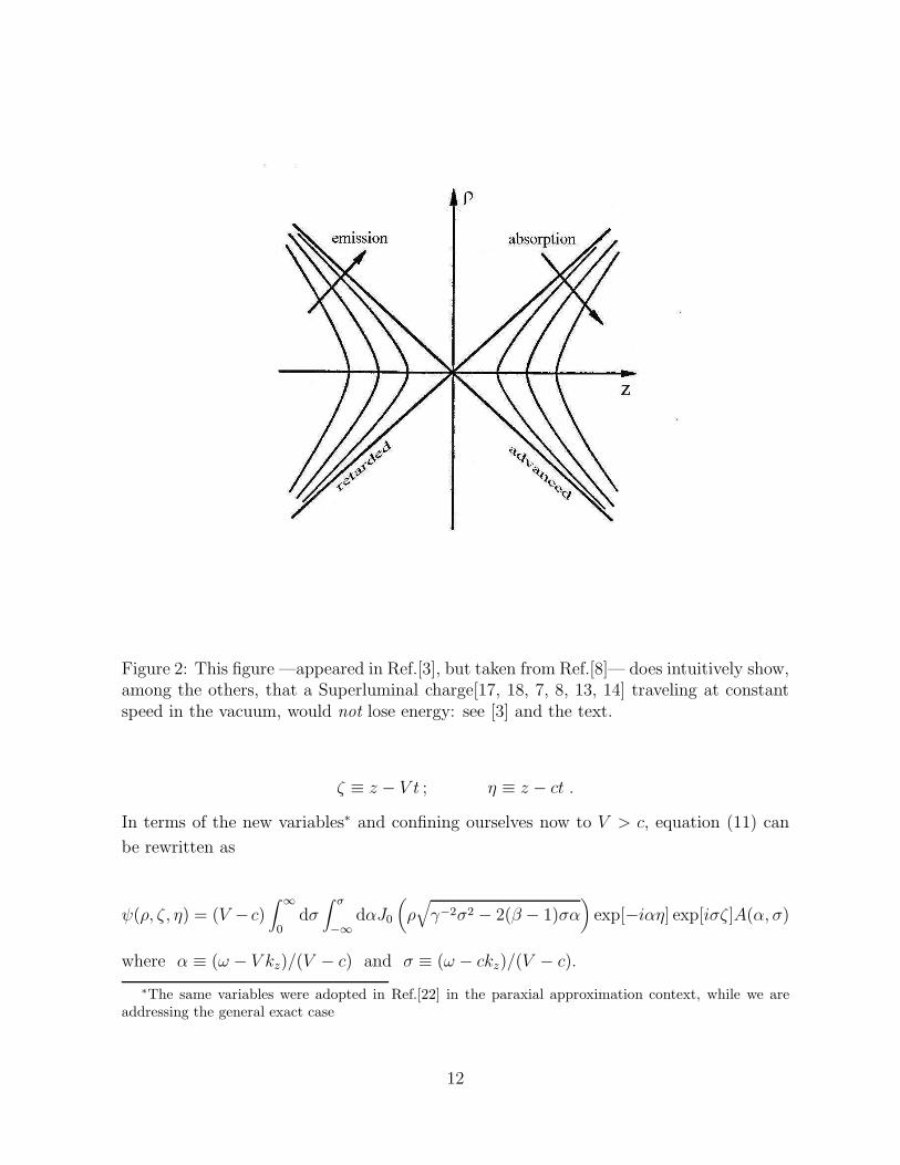
Figure 2: This figure —appeared in Ref.[3], but taken from Ref.[8]— does intuitively show,among the others, that a Superluminal charge[17, 18, 7, 8, 13, 14] traveling at constantspeed in the vacuum, would not lose energy: see [3] and the text.

ζ ≡ z − V t ; η ≡ z − ct .

In terms of the new variables∗ and confining ourselves now to V > c, equation (11) can

be rewritten as

ψ(ρ, ζ, η) = (V −c)∫ ∞

0dσ∫ σ

−∞dαJ0

(ρ√γ−2σ2 − 2(β − 1)σα

)exp[−iαη] exp[iσζ ]A(α, σ)

where α ≡ (ω − V kz)/(V − c) and σ ≡ (ω − ckz)/(V − c).

∗The same variables were adopted in Ref.[22] in the paraxial approximation context, while we areaddressing the general exact case

12

Figure 3: Example of a finite-energy X-type LW, corresponding to an exact, analyticsolution of Eq.18, totally free from backward-components. This figure represents the realpart of the field, normalized at ρ = z = 0 for t = 0, with the choices a = 3.99 × 10−6 m,d = 20 m, V = 1.005 c, and α0 = 1.26×107 m−1. In this case the frequency spectrum startsat ω ≡ ωmin ≈ 3.77 × 1015 Hz and afterwards decays exponentially with the bandwidth∆ω ≈ 7.54 × 1013 Hz. The value ωmin can be regarded as the pulse central frequency;since ∆ω/ωmin << 1, it exists a well-defined carrier wave, which does clearly show up inthe plots. Any finite-energy LW gets deformed while propagating, and (b) represents thepulse depicted in (a) after it has traveled 2.78 km.

As mentioned above, ideal (infinite energy) superluminal LWs are got by imposing

the linear constraint A(α, σ) = B(σ) δ(α+ α0). By contrast, finite-energy superluminal

LWs are obtained by concentrating the spectrum A(α, σ) in the vicinity of the straight

line α = −α0. By choosing for example

A(α, σ) =Θ(−α− α0)

V − cedα e−aσ , (17)

we get the finite-energy exact solutions (free from any backward-components):

ψ(ρ, ζ, η) =X

V Ze−α0Z , (18)

where X is defined in eq.(8), quantities a, d and α0 are positive constants, and

Z ≡ (d− iη) −c

V + c(a− iζ − V X−1) .

13

In Figs.3 we show one of such finite-energy Superluminal LWs, corresponding to an

exact, analytic solution totally free from backward-travelling components. As we know,

any finite-energy X-wave gets deformed while propagating: and Fig.3(b) shows the pulse

in Fig.3(a) after it has travelled 2.78 km.

6) Acknowledgements — The authors are greatly indebted to I.M.Besieris for having

called their attention to Ref.[1] and for a very careful, extensive and painstaking revision of

this work; and to I.M.Besieris, P.Saari, and C.A.Dartora for many stimulating discussions.

References

[1] S.C.Walker and W.A.Kuperman: “Cherenkov-Vavilov formulation of X waves”, Phys.

Rev. Lett. 99 (2007) 244802.

[2] Localized Waves: Theory and Applications, ed. by H.E.Hernandez-Figueroa,

M.Zamboni-Rached, and E.Recami (J.Wiley; New York, Jan.2008), book, 369 pages.

[3] E.Recami, M.Zamboni-Rached and C.A.Dartora: “Localized X-shaped field gener-

ated by a superluminal charge”, Phys. Rev. E69 (2004) 027602.

[4] F.V.Hartmann: High-Field Electrodynamics (CRC Press; London, 2002); I.Ye.Tamm

and I.M.Frank: Dokl. Akad. Nauk SSSR 14 (1937) 107.

[5] J.-y. Lu and J.F.Greenleaf: IEEE Transactions in Ultrasonics Ferroelectricity and

Frequency Control 39 (1992) 19-31; I.M.Besieris, A.M.Shaarawi and R.W.Ziolkowski:

J. Math. Phys. 30 (1989) 1254-1269; E.Recami: Physica A252 (1998) 586-610 and

refs. therein.

[6] J.-y. Lu and J.F.Greenleaf: IEEE Transactions in Ultrasonics Ferroelectricity and

Frequency Control 39 (1992) 441-446; P.Saari and K.Reivelt: Phys. Rev. Lett. 79

(1997) 4135-4138.

[7] A.O.Barut, G.D.Maccarrone and E.Recami: Nuovo Cimento A71 (1982) 509.

[8] See pp.1-178 in issue 6 of E.Recami: Rivista Nuovo Cim. 9(6) (1986) 1, and refs.

therein.

14

[9] J.W.Goodman: Introduction to Fourier Optics (McGraw Hill College; San Francisco,

1968).

[10] M.Zamboni-Rached: J. Opt. Soc. Am. A23 (2006) 2166-2176; R.W.Ziolkowski,

I.M.Besieris and A.M.Shaarawi: J. Opt. Soc. Am. A10 (1993) 75-87. See also

A.Chatzipetros, A.M.Shaarawi, I.M.Besieris and M.Abdel-Rahman: J. Acoust. Soc.

Am. 103 (1998) 2289-2295.

[11] S.He and J.-y.Lu: J. Acoust. Soc. Am. 107 (2000) 3556; J.-y.Lu, H.-h.Zou and

J.F.Greenleaf: Ultrasound in Medicine and Biology 20 (1994) 403-428; I.M.Besieris,

A.M.Shaarawi, M.Abdel-Rahman, and A.Chatzipetros: Prog. Electromagn. Res.

19 (1998) 1-48; J. Acoust. Soc. Am. 103 (1998) 2287-2295; I.M.Besieris and

A.M.Shaarawi: Jour. Phys. A: Math. and Gen. 33 (2000) 7227-7254; A.M.Shaarawi,

I.M.Besieris and T.M.Said: J. Opt. Soc. Am. A20 (2003) 1658-1665; M.Zamboni-

Rached, A.M.Shaarawi, E.Recami: J. Opt. Soc. Am. A21 (2004) 1564-1574.

[12] M.Zamboni-Rached, E.Recami and H.E.Hernandez-Figueroa: European Physical

Journal D21 (2002) 217-228.

[13] E.Recami, M.Zamboni-Rached, K.Z.Nobrega, C.A.Dartora and H.E.Hernandez-

Figueroa: IEEE Journal of Selected Topics in Quantum Electronics 9 (2003) 59-73.

[14] E.Recami, M.Zamboni-Rached and H.E.Hernandez-Figueroa: “Localized Waves: A

historical and scientific introduction”, in Ref.[2].

[15] M.Zamboni-Rached, E.Recami and H.E.Hernandez-Figueroa: “Structure of non-

diffracting waves, and some interesting applications”, in Ref.[2].

[16] M.Zamboni-Rached: “Localized solutions: Structure and Applications”, M.Sc.

thesis (Phys. Dept., Campinas State University, 1999); and M.Zamboni-

Rached, “Localized waves in diffractive/dispersive media”, PhD thesis

(DMO/FEEC, Campinas State University, Aug.2004) [can be download at

http://libdigi.unicamp.br/document/?code=vtls000337794], and refs. therein.

[17] R.Mignani and E.Recami: Lett. Nuovo Cim. 7 (1973) 388-390. Cf. also R.Folman

and E.Recami: Found. Phys. Lett. 8 (1995) 127-134.

[18] E.Recami and R.Mignani: Rivista Nuovo Cim. 4 (1974) 209-290, E398.

15

[19] A.Sommerfeld: K. Ned. Akad. Wet. 8 (1904) 346; Nachr. Ges. Wiss. Gottingen

(Feb.25, 2005) 201-236; E.C.G.Sudarshan: private communications (1971). See also

J.J.Thomson: Philos. Mag. 28 (1889) 13.

[20] P.Saari: “Superluminal localized waves of electromagnetic field in vacuo”, in Time

Arrows, Quantum Measurement and Superluminal Behaviour”, ed. by D.Mugnai et

al. (CNR; Rome, 2001), p.37. In this paper it is used, however, G+(r, t, r ′, t′) −

G−(r, t, r ′, t′), instead of G+(r, t, r ′, t′)/2 +G−(r, t, r ′, t′)/2: a choice that does not

apply to a non-homogeneous problem as ours, in which we deal with a (superluminal)

charge.

[21] E.Recami and R.Mignani: Phys. Lett. B62 (1976) 41-43; R.Mignani and E.Recami:

Nuovo Cimento A30 (1975) 533-540.

[22] I.M.Besieris and A.M.Shaarawi: Opt. Exp. 12 (2004) 3848-3864.

16