CHEMICAL ENGINEERING DEPARTMENT
127
Budhijanto, Teknik Kimia UGM, 2012 Page 1 CHEMICAL ENGINEERING DEPARTMENT GADJAH MADA UNIVERSITY TKK 2105 ENGINEERING ECONOMICS (2 SKS) INSTRUCTOR: Budhijanto REFERENCES: a. Sullivan, W.G., Wicks, E.M., and Luxhoj, J.T., 2003, “Engineering Economy”, 12 ed., Pearson Education, Inc., New Jersey. b. Garrett, D.E, 1989, “Chemical Engineering Economics”, Van Nostrand Reinhold, New York. c. Peters, M.S. and Timmerhaus, K.D., 2003, “Plant Design and Economics for Chemical Engineers”, 5 ed., McGraw-Hill, Inc., New York. d. Turton, R., Bailie, R.C., Whiting, W.B., and Shaeiwitz, 2003, Analysis, Synthesis, and Design of Chemical Processes, 2 ed, Pearson Education, Inc. Publishing as Prentice Hall PTR.
Transcript of CHEMICAL ENGINEERING DEPARTMENT
Budhijanto, Teknik Kimia UGM, 2012 Page 1
CHEMICAL ENGINEERING DEPARTMENT GADJAH MADA UNIVERSITY
TKK 2105
ENGINEERING ECONOMICS (2 SKS)
INSTRUCTOR: Budhijanto REFERENCES: a. Sullivan, W.G., Wicks, E.M., and Luxhoj,
J.T., 2003, “Engineering Economy”, 12 ed., Pearson Education, Inc., New Jersey.
b. Garrett, D.E, 1989, “Chemical Engineering Economics”, Van Nostrand Reinhold, New York.
c. Peters, M.S. and Timmerhaus, K.D., 2003, “Plant Design and Economics for Chemical Engineers”, 5 ed., McGraw-Hill, Inc., New York.
d. Turton, R., Bailie, R.C., Whiting, W.B., and Shaeiwitz, 2003, Analysis, Synthesis, and Design of Chemical Processes, 2 ed, Pearson Education, Inc. Publishing as Prentice Hall PTR.
Budhijanto, Teknik Kimia UGM, 2012 Page 2
e. Aries, R.S. and Newton, R.D., 1955, Chemical Engineering Cost Estimation, McGraw-Hill Book Company, New York.
Goal: Students are able to do calculation based on the time value of money, to analyze profit and profitability, and to choose among several investment alternatives. Topics: a. Introduction to Engineering Economics b. Cost Concepts c. Time Value of Money Concept d. Applications of the Time Value of Money
Concept e. Comparing Alternatives f. Depreciation and Profit Analysis g. Cost Estimation Techniques h. Uncertainty Grade: Midterm Exam 45 % Final Exam 45 % Homeworks/Projects 10 %

Budhijanto, Teknik Kimia UGM, 2012 Page 3
A ≥ 75 60 > C ≥ 45 30 > E 75 > B ≥ 60 45 > D ≥ 30 Policy: Closed book exams No exam remedy Questions regarding exam/homework/project grades/scores must be submitted in a week after students received their grades/scores No late-homework A minimum of 75% class attendance to get a final grade
Budhijanto, Teknik Kimia UGM, 2012 Page 4
I. Introduction to Engineering Economics What will we learn? Systematic evaluation of the economic merits of proposed solutions to engineering problems. To be economicaly acceptable, the solutions must demonstrate a positive balance of long term benefits over a long term costs, and also fulfils other criteria, such as safety, reliability, etc. Fundamental question: Does the income exceed all the costs? Why do we learn Engineering Economics? Chemical Engineering Profession is the profession in which knowledge of mathematics, chemistry, and other natural science gained by study, experience, and practice is applied with judgment to develop economic ways of using materials and energy for the benefit of mankind. (Turton et al., 2003 p. 729) Point: Chemical Engineers develop ”economic ways”.
Budhijanto, Teknik Kimia UGM, 2012 Page 5
More economic way: less cost → higher profit. Profit: the excess of income over expenditure
Engineering (regardless of the engineering discipline), without economy, makes no sense
at all. Example (Barir Kurniawan`s Final Project): Methyl mercaptan (CH3SH): • Gas industry: leakage detector in gas
pipelines • Polymer industry: terminator to control
molecular weight • Feed industry: raw material in methionin
synthesis • etc.
Methods: 1. OHSHCHHSCO 2322 24 +→++
(250 – 400oC, 30 − 70 atm) 2. SHSHCHHCS 2322 3 +→+
(catalytic, 150 – 350oC, 10 − 50 atm) 3. 2324 HSHCHSHCH +→+
(new process)
Budhijanto, Teknik Kimia UGM, 2012 Page 6
4. OHSHCHSHOHCH 2323 +→+ (catalytic, 200 – 500oC, 1 − 25 atm)
All these methods are different one from the others in:
1. Raw Materials 2. Side products 3. Process equipments 4. Energy consumption 5. New/old process 6. etc.
Which one? → the most economical one. How? → economic evaluation. Engineering Economics : a tool to assist in decision making → a. Is an investment plan economically
attractive? b. Among several investment alternatives,
which one is the most economically attractive?
Economics is one of the Chemical Engineering Tools. Chemical Engineering Tools:
1. Mass balance
Budhijanto, Teknik Kimia UGM, 2012 Page 7
2. Energy balance 3. Equilibria 4. Rate processes 5. Economics 6. Humanity
Is economy the only aspect to be considered in a feasibility study of an investment plan? NO. Other aspects such as ethics, professionalism, welfare, safety, and environment. Principles of Engineering Economics Principle 1: Develop the alternatives. ”Doing nothing” is one of the possible alternatives. Principle 2: Focus on the differences. Consider relevant differences only. Principle 3: Use a consistent viewpoint. Viewpoints: the firm owner interest, employee satisfaction, customer satisfaction, etc. Principle 4: Use a Common Unit of Measurement. Purpose: direct comparison among all the prospective outcomes.
Budhijanto, Teknik Kimia UGM, 2012 Page 8
The common measurement unit: monetary unit. Principle 5: Consider all relevant criteria. Decision making should consider all the criteria. Example of a criterion: alternative that gives the most attractive interest. Principle 6: Make uncertainty explicit. Outcome estimation of an alternative always contains uncertainty. Principle 7: Revisit your decision. The real outcome is different from what was predicted. The difference is the base for the necessary revision on the decision. Engineering Economic Analysis Procedure 1. Problem recognition, definition, and
evaluation. 2. Development of the feasible alternatives. 3. Development of the outcomes and cash flows
for each alternative. 4. Selection of a criterion (or criteria) 5. Analysis and comparison of the alternatives. 6. Selection of the preferred alternative. 7. Performance monitoring and post-evaluation
of results.
Budhijanto, Teknik Kimia UGM, 2012 Page 9
II. Cost Concepts Costs related to the implementation of an investment plan need to be estimated. The purposes include: 1. To provide information used in settling a
selling price for quoting, bidding, or evaluating contracts.
2. To determine whether a proposed product is profitable.
3. To evaluate how much capital needed for the process changes or other improvements, and
4. To establish benchmarks for productivity improvement programs
Two fundamental aproaches in cost estimation: a. ”Top-down” approach: use historical data
from similar engineering projects b. ”Bottom-up” approach: break down a project
into small, manageable units and estimate their economic consequences
HOMEWORK # 1: Explain the following cost terminologies (References : 1. Sullivan, et. al. (2003); 2. Aries and Newton (1955)). Compare your
Budhijanto, Teknik Kimia UGM, 2012 Page 10
answers based on reference #1 to those based on reference #2. 1. a. Fixed costs.
b. Variable costs. c. Incremental cost (or incremental revenue).
2. a. Recurring costs. b. Nonrecurring costs.
3. a. Direct costs. b. Indirect costs. c. Overhead. d. Standard cost.
4. a. Cash costs. b. Noncash costs (= book cost).
5. Sunk costs. 6. Opportunity costs. 7. a.Life-Cycle cost.
b. Investment cost (=capital investment). c. Working capital. d. Operation and maintenance cost. e. Disposal cost.
General economic concepts 1. Consumer and Producer Goods and Services.
Budhijanto, Teknik Kimia UGM, 2012 Page 11
Consumer goods and services: products or services that are directly used by people to satisfy their wants. Example: food, entertainment. Producer goods and services: products or services that are used to produce consumer goods and services or other producer goods. Example: machine tools, factory buildings. 2. Measures of Economic Worth Why are goods and services produced and desired? Because they have utility. Utility : the power to satisfy human wants and needs → expressed as the price that must be paid to obtain the goods or services. Utility (value) of materials and products could be increased by changing their form or location. Example: Iron ore → stainless steel → razor blades 3. Necessities, Luxuries, and Price Demand Goods and services may be categorized into: necessities and luxuries → relative to the users. Example:
Budhijanto, Teknik Kimia UGM, 2012 Page 12
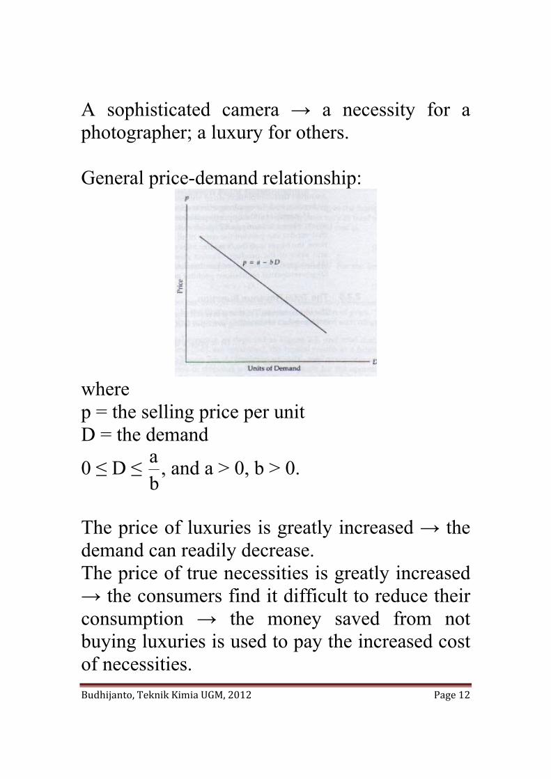
A sophisticated camera → a necessity for a photographer; a luxury for others. General price-demand relationship:
where p = the selling price per unit D = the demand
0 ≤ D ≤ ba , and a > 0, b > 0.
The price of luxuries is greatly increased → the demand can readily decrease. The price of true necessities is greatly increased → the consumers find it difficult to reduce their consumption → the money saved from not buying luxuries is used to pay the increased cost of necessities.
Budhijanto, Teknik Kimia UGM, 2012 Page 13
4. Competition Perfect competition : a situation in which any given product is supplied by a large number of vendors and there is no restriction on additional suppliers entering the market → there is assurance of complete freedom on the part of buyer and seller. Perfect monopoly : a unique product or service is available from only a single supplier and the vendor can prevent the entry of all others into the market. The buyer is at the complete mercy of the supplier in terms of the availability and price of the product. Perfect monopolies rarely occur in practice, because: (i) any product can usually be substituted by other products with satisfactory performance; (ii) governmental regulations prohibit monopolies. 5. Total Revenue (TR) Function Total revenue = TR = (selling price per unit) · (the number of units sold) = p·D If: p = a − bD, then:
Budhijanto, Teknik Kimia UGM, 2012 Page 14
TR = (a − bD)D = aD − bD2 for 0 ≤ D ≤ ba , and
a > 0, b > 0.
0Db2adD
dTR=−=
) →
b2aD =
) where:
D)
= the demand that will produce maximum TR. 6. Cost, Volume, and Breakeven Point
Relationships Assuming linear relationship between variable cost and demand, total cost is:
DcCCCC VFVFT ⋅+=+= where: CT = total cost CF = fixed cost CV = variable cost cV = variable cost per unit Profit/loss = TR − CT At breakeven point, TR = CT. Scenario 1: p = a – bD Profit/loss = (aD − bD2) − (CF + cV · D) = −bD2 + (a – cV)D – CF
Budhijanto, Teknik Kimia UGM, 2012 Page 15
for 0 ≤ D ≤ ba , dan a > 0, b > 0.
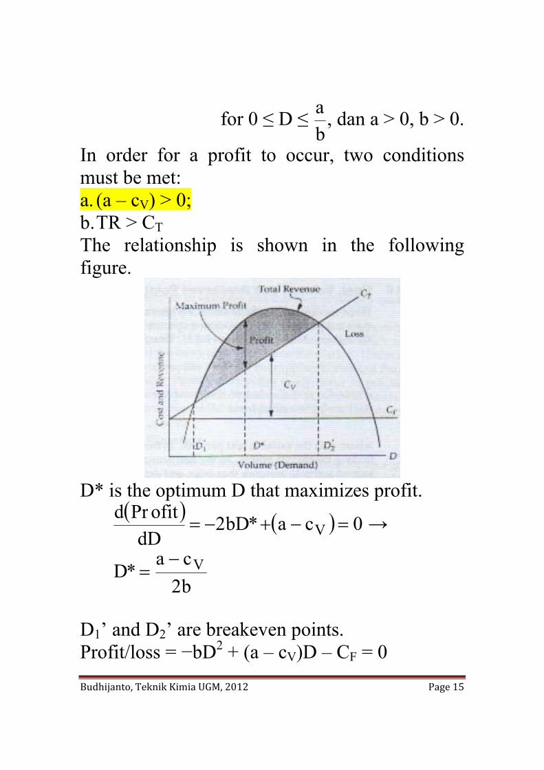
In order for a profit to occur, two conditions must be met: a. (a – cV) > 0; b. TR > CT The relationship is shown in the following figure.
D* is the optimum D that maximizes profit.
( ) ( ) 0ca*bD2dD
ofitPrdV =−+−= →
b2ca
*D V−=
D1’ and D2’ are breakeven points. Profit/loss = −bD2 + (a – cV)D – CF = 0
Budhijanto, Teknik Kimia UGM, 2012 Page 16
( ) ( ) ( )( )[ ]( )b2
Cb4cacaD,D
21F
2VV'
2'1 −
−−−−±−−=
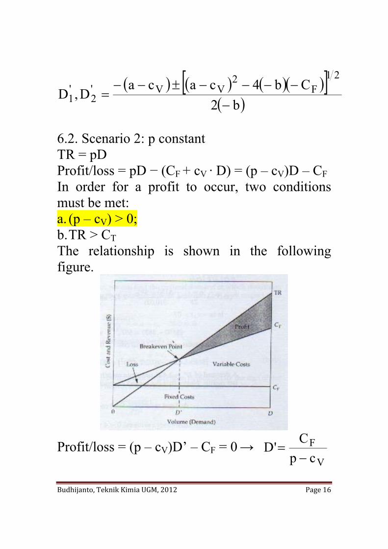
6.2. Scenario 2: p constant TR = pD Profit/loss = pD − (CF + cV · D) = (p – cV)D – CF In order for a profit to occur, two conditions must be met: a. (p – cV) > 0; b. TR > CT The relationship is shown in the following figure.
Profit/loss = (p – cV)D’ – CF = 0 →
V
Fcp
C'D−
=

Budhijanto, Teknik Kimia UGM, 2012 Page 17
Case study: Data of an engineering consulting firm: Variable cost (cV) = $62 per standard service hour; Charge-out rate (p) = $85.56 per hour; Maximum output of the firm = 160,000 hours per year; Fixed cost (CF) = $2,024,000 per year. Calculate: a) Breakeven point (BEP) b) Sensitivity analysis by calculating the
percentage reduction of BEP if CF is reduced 10%; if cV is reduced 10%; if CF and cV are reduced 10% each; and if p is increased 10%.
Answer: a) At breakeven point: Total revenue = total cost →
'DcC'pD VF += → V
Fcp
C'D−
=
yearperhours908,8562$56.85$
000,024,2$'D =−
=
537,0000,160908,85'D == or 53,7% of maximum
capacity. ( ) 288,350,7$908,8556,85$'D ==
Budhijanto, Teknik Kimia UGM, 2012 Page 18
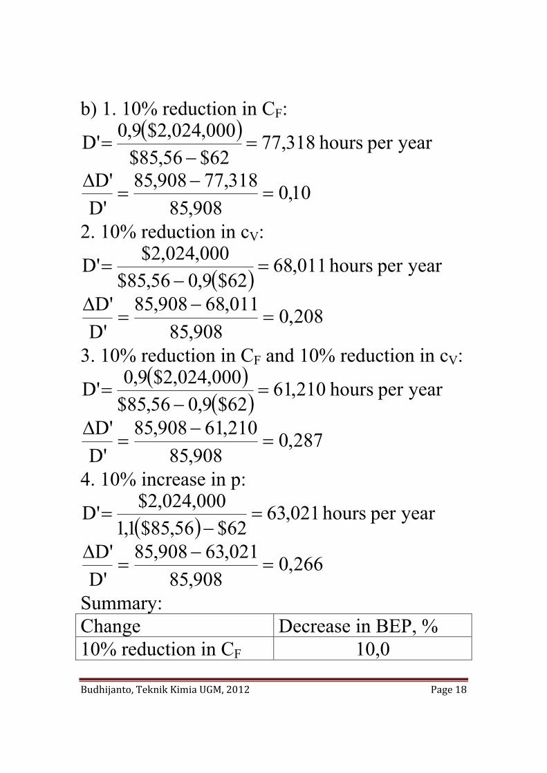
b) 1. 10% reduction in CF: ( ) yearperhours318,77
62$56,85$000,024,2$9,0'D =
−=
10,0908,85
318,77908,85'D'D
=−
=Δ
2. 10% reduction in cV:
( ) yearperhours011,6862$9,056,85$
000,024,2$'D =−
=
208,0908,85
011,68908,85'D'D
=−
=Δ
3. 10% reduction in CF and 10% reduction in cV: ( )
( ) yearperhours210,6162$9,056,85$
000,024,2$9,0'D =−
=
287,0908,85
210,61908,85'D'D
=−
=Δ
4. 10% increase in p:
( ) yearperhours021,6362$56,85$1,1
000,024,2$'D =−
=
266,0908,85
021,63908,85'D'D
=−
=Δ
Summary: Change Decrease in BEP, % 10% reduction in CF 10,0
Budhijanto, Teknik Kimia UGM, 2012 Page 19
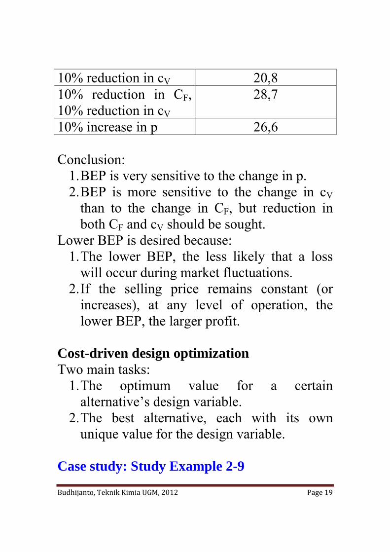
10% reduction in cV 20,8 10% reduction in CF, 10% reduction in cV
28,7
10% increase in p 26,6 Conclusion:
1. BEP is very sensitive to the change in p. 2. BEP is more sensitive to the change in cV
than to the change in CF, but reduction in both CF and cV should be sought.
Lower BEP is desired because: 1. The lower BEP, the less likely that a loss
will occur during market fluctuations. 2. If the selling price remains constant (or
increases), at any level of operation, the lower BEP, the larger profit.
Cost-driven design optimization Two main tasks:
1. The optimum value for a certain alternative’s design variable.
2. The best alternative, each with its own unique value for the design variable.
Case study: Study Example 2-9
Budhijanto, Teknik Kimia UGM, 2012 Page 20
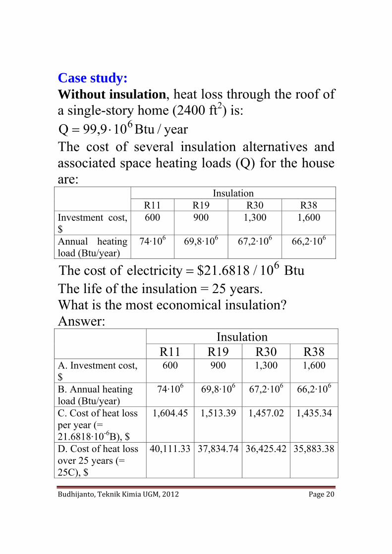
Case study: Without insulation, heat loss through the roof of a single-story home (2400 ft2) is:
year/Btu109,99Q 6⋅= The cost of several insulation alternatives and associated space heating loads (Q) for the house are: Insulation
R11 R19 R30 R38 Investment cost, $
600 900 1,300 1,600
Annual heating load (Btu/year)
74·106 69,8·106 67,2·106 66,2·106
Btu10/6818.21$yelectricitoftcosThe 6= The life of the insulation = 25 years. What is the most economical insulation? Answer: Insulation
R11 R19 R30 R38 A. Investment cost, $
600 900 1,300 1,600
B. Annual heating load (Btu/year)
74·106 69,8·106 67,2·106 66,2·106
C. Cost of heat loss per year (= 21.6818·10-6B), $
1,604.45 1,513.39 1,457.02 1,435.34
D. Cost of heat loss over 25 years (= 25C), $
40,111.33 37,834.74 36,425.42 35,883.38
Budhijanto, Teknik Kimia UGM, 2012 Page 21
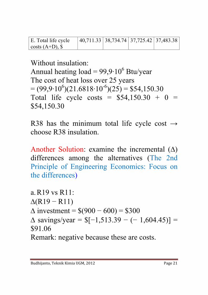
E. Total life cycle costs (A+D), $
40,711.33 38,734.74 37,725.42 37,483.38
Without insulation: Annual heating load = 99,9·106 Btu/year The cost of heat loss over 25 years = (99,9·106)(21.6818·10-6)(25) = $54,150.30 Total life cycle costs = $54,150.30 + 0 = $54,150.30 R38 has the minimum total life cycle cost → choose R38 insulation. Another Solution: examine the incremental (∆) differences among the alternatives (The 2nd Principle of Engineering Economics: Focus on the differences) a. R19 vs R11: Δ(R19 − R11) Δ investment = $(900 − 600) = $300 Δ savings/year = $[−1,513.39 − (− 1,604.45)] = $91.06 Remark: negative because these are costs.
Budhijanto, Teknik Kimia UGM, 2012 Page 22
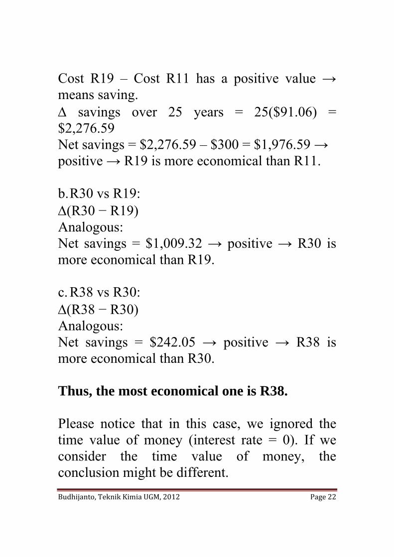
Cost R19 – Cost R11 has a positive value → means saving. Δ savings over 25 years = 25($91.06) = $2,276.59 Net savings = $2,276.59 – $300 = $1,976.59 → positive → R19 is more economical than R11. b. R30 vs R19: Δ(R30 − R19) Analogous: Net savings = $1,009.32 → positive → R30 is more economical than R19. c. R38 vs R30: Δ(R38 − R30) Analogous: Net savings = $242.05 → positive → R38 is more economical than R30. Thus, the most economical one is R38. Please notice that in this case, we ignored the time value of money (interest rate = 0). If we consider the time value of money, the conclusion might be different.
Budhijanto, Teknik Kimia UGM, 2012 Page 23
Present Economy Studies. → engineering economic analyses when alternatives for accomplishing a specific task are being compared over one year or less and the influence of time on money can be ignored. Rule 1: When revenues and other economic benefits are present and vary among alternatives, choose the alternative that maximizes overall profitability based on the number of defect-free units of a product or service produced. Rule 2: When revenues and other economic benefits are not present or are constant among all alternatives, consider only the costs and select the alternative that minimizes total cost per defect-free unit of product or service output. Case study: Two machines are being considered for the production of a part. The capital investment associated with the machines is about the same. The important differences between the machines are their: 1) production capacity (= production
Budhijanto, Teknik Kimia UGM, 2012 Page 24
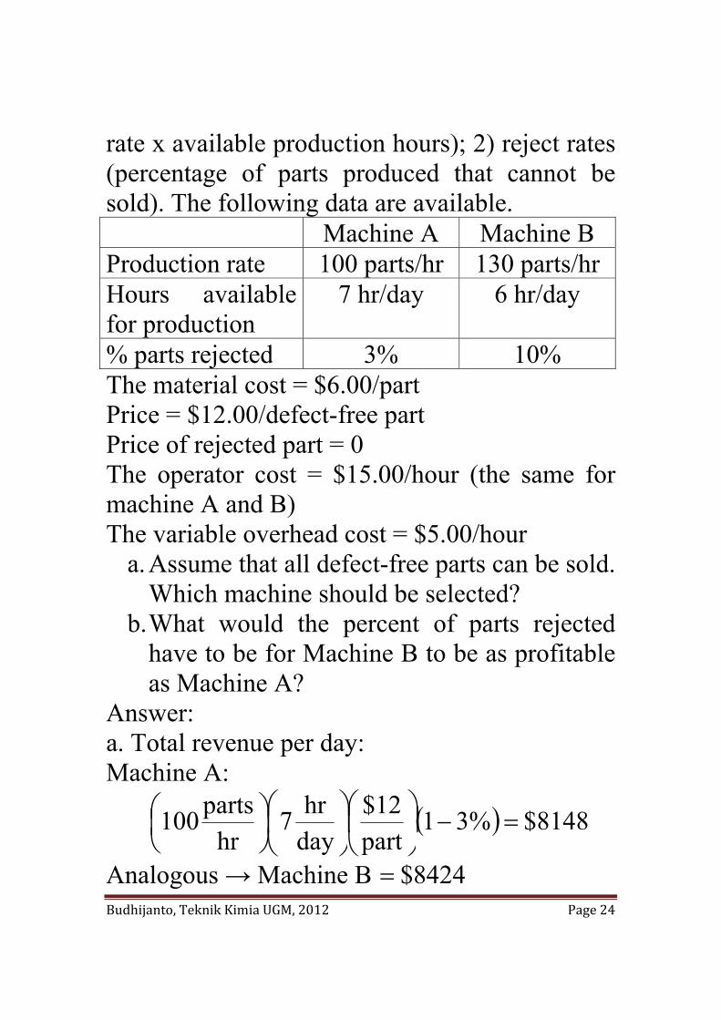
rate x available production hours); 2) reject rates (percentage of parts produced that cannot be sold). The following data are available.
Machine A Machine B Production rate 100 parts/hr 130 parts/hr Hours available for production
7 hr/day 6 hr/day
% parts rejected 3% 10% The material cost = $6.00/part Price = $12.00/defect-free part Price of rejected part = 0 The operator cost = $15.00/hour (the same for machine A and B) The variable overhead cost = $5.00/hour
a. Assume that all defect-free parts can be sold. Which machine should be selected?
b. What would the percent of parts rejected have to be for Machine B to be as profitable as Machine A?
Answer: a. Total revenue per day: Machine A:
( ) 8148$%31part
12$dayhr7
hrparts100 =−⎟
⎠
⎞⎜⎝
⎛⎟⎠
⎞⎜⎝
⎛⎟⎠⎞
⎜⎝⎛
Analogous → Machine B 8424$=
Budhijanto, Teknik Kimia UGM, 2012 Page 25
There is difference in revenue → use Rule 1. • Total cost per day: Machine A:
4340$day
hours7hour
00.5$hour
00.15$part
00.6$hourparts100
=
⎟⎠
⎞⎜⎝
⎛⎥⎦
⎤⎢⎣
⎡++⎟
⎠
⎞⎜⎝
⎛⎟⎠⎞
⎜⎝⎛
Analogous → Machine B 4800$= • Profit per day Machine A: $8148 − $4340 = $3808 Machine B: $8424 − $4800 = $3624 • Select machine A. b. Let X = % parts rejected for machine B. Profitability machine B = machine A. Thus:
( )
3808$
4800$X1part
12$day
hours6hourparts130
=
−−⎟⎠
⎞⎜⎝
⎛⎟⎠
⎞⎜⎝
⎛⎟⎠⎞
⎜⎝⎛
( )( )( )( )
08.0126130
480038081X =+
−=
Thus, percent of parts rejected for Machine B can be no higher than 8%. Homework: Study Sullivan et. al, 2003, pp. 56 – 61.
Budhijanto, Teknik Kimia UGM, 2012 Page 26
Time Value of Money Investment: an agreement between two parties, whereby, one party, the investor, provides money, P, to a second party, the producer, with the expectation that the producer will return money, F, to the investor at some future specified date, where F>P. P : Principal/Present Value F : Future Value n : Years between F and P The amount of money earned from the investment = E = F – P. In general:
( )i,nfPF=
where i = interest rate For example:
( )ni1PF
s+=
Budhijanto, Teknik Kimia UGM, 2012 Page 27
The yearly earnings rate = simple interest rate =
PnPF
PnEis
−==
Capital: wealth in the form of money or property that can be used to produce more wealth. The time value of money concept:
Money today is worth more than money in the future.
How: Invest the money to earn more money. The time value of money is different from inflation. Two basic categories of capital:
a. Equity capital: capital that is owned by individuals who have invested their money or property in a business project or venture in the hope of receiving a profit. The owners of equity capital are also the owners of the project and fully participate in the risks of the project. Example: stockholders.
b. Debt capital (= borrowed capital): capital that is obtained from lenders, and the lenders earn interest as the incentive for their
Budhijanto, Teknik Kimia UGM, 2012 Page 28
investment on the project. The owner of debt capital are not owners of the project and do not participate as fully as the owners in the risks of the project. Interest and repayment of the debt capital are assured by the owners of the project. Example: bonds holder.
If capital is invested in a project, investors would expect, as a minimum, to receive a return at least equal to the amount they have sacrificed by not using it in some other available opportunity of comparable risk. This interest or profit available from an alternative investment is the opportunity cost of using capital in the proposed undertaking. Of course if the alternative investment has lower risk than the proposed project, the project must produce much more profit than the alternative investment to be attractive for the investors. Profitability of a project can be evaluated from the future value of the capital invested on the project → the concept of interest → Interest: compensation paid for debt capital.
Budhijanto, Teknik Kimia UGM, 2012 Page 29
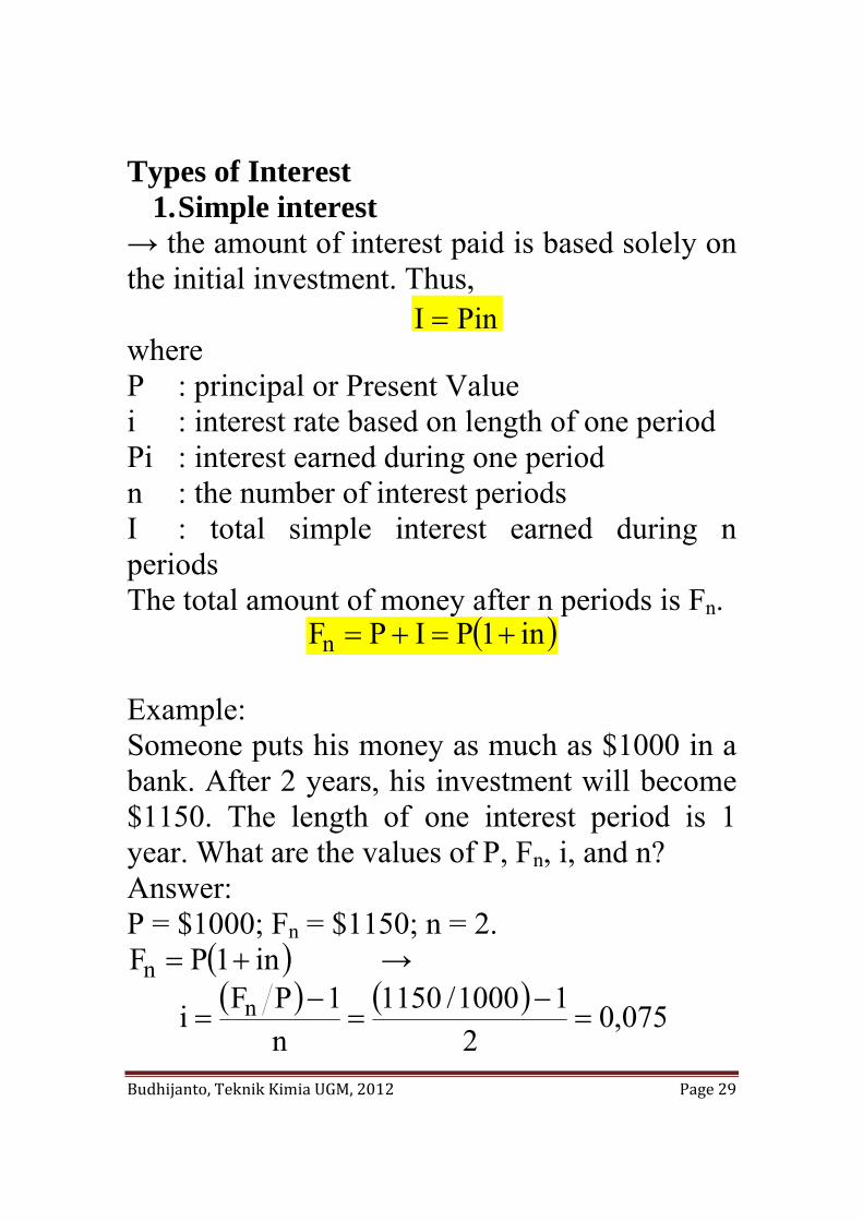
Types of Interest 1. Simple interest
→ the amount of interest paid is based solely on the initial investment. Thus,
PinI = where P : principal or Present Value i : interest rate based on length of one period Pi : interest earned during one period n : the number of interest periods I : total simple interest earned during n periods The total amount of money after n periods is Fn.
( )in1PIPFn +=+= Example: Someone puts his money as much as $1000 in a bank. After 2 years, his investment will become $1150. The length of one interest period is 1 year. What are the values of P, Fn, i, and n? Answer: P = $1000; Fn = $1150; n = 2.
( )in1PFn += →
( ) ( ) 075,02
11000/1150n
1PFi n =−
=−
=
Budhijanto, Teknik Kimia UGM, 2012 Page 30
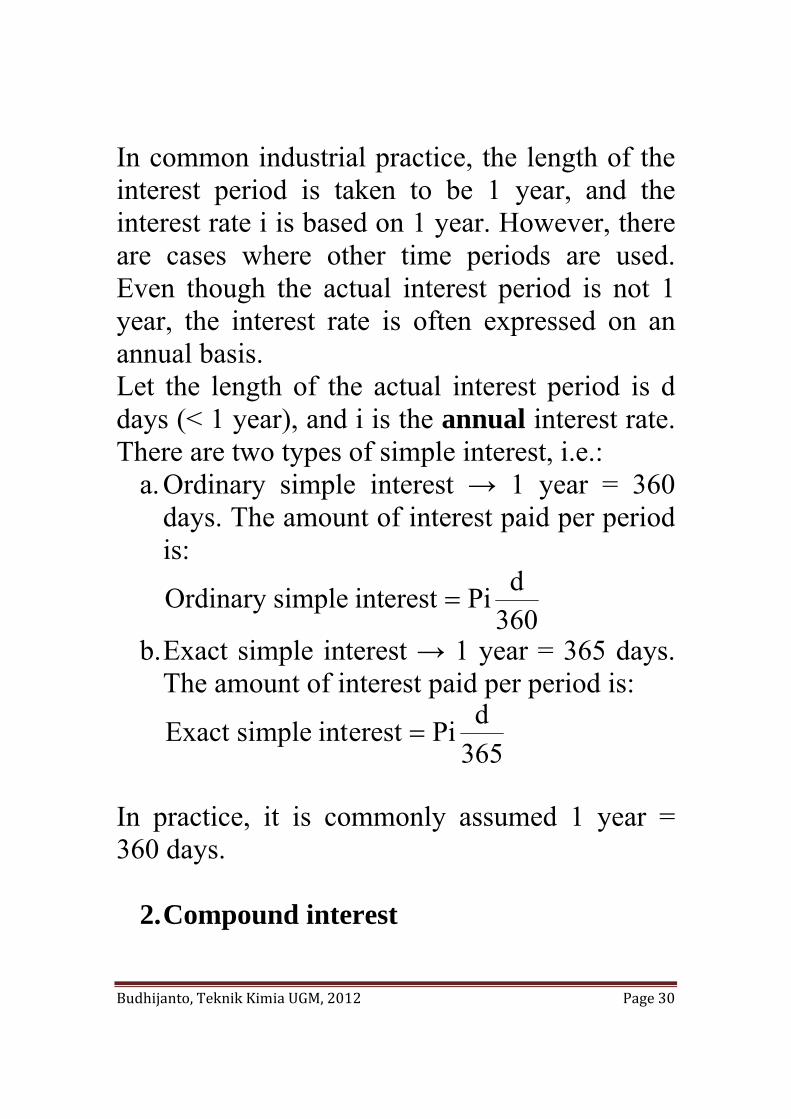
In common industrial practice, the length of the interest period is taken to be 1 year, and the interest rate i is based on 1 year. However, there are cases where other time periods are used. Even though the actual interest period is not 1 year, the interest rate is often expressed on an annual basis. Let the length of the actual interest period is d days (< 1 year), and i is the annual interest rate. There are two types of simple interest, i.e.:
a. Ordinary simple interest → 1 year = 360 days. The amount of interest paid per period is:
360dPierestintsimpleOrdinary =
b. Exact simple interest → 1 year = 365 days. The amount of interest paid per period is:
365dPierestintsimpleExact =
In practice, it is commonly assumed 1 year = 360 days.
2. Compound interest
Budhijanto, Teknik Kimia UGM, 2012 Page 31
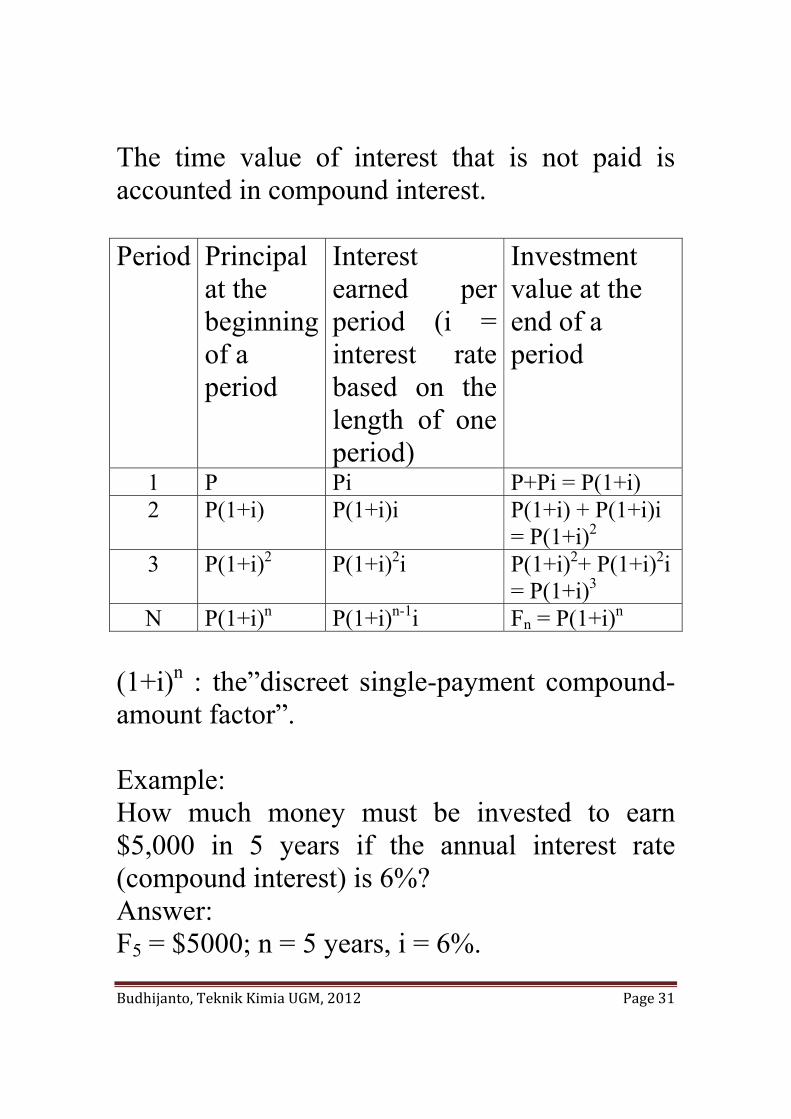
The time value of interest that is not paid is accounted in compound interest. Period Principal
at the beginning of a period
Interest earned per period (i = interest rate based on the length of one period)
Investment value at the end of a period
1 P Pi P+Pi = P(1+i) 2 P(1+i) P(1+i)i P(1+i) + P(1+i)i
= P(1+i)2
3 P(1+i)2 P(1+i)2i P(1+i)2+ P(1+i)2i = P(1+i)3
N P(1+i)n P(1+i)n-1i Fn = P(1+i)n
(1+i)n : the”discreet single-payment compound-amount factor”. Example: How much money must be invested to earn $5,000 in 5 years if the annual interest rate (compound interest) is 6%? Answer: F5 = $5000; n = 5 years, i = 6%.
Budhijanto, Teknik Kimia UGM, 2012 Page 32
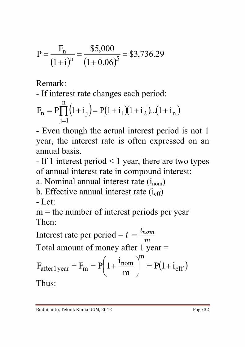
( ) ( )29.736,3$
06.01000,5$
i1FP 5n
n =+
=+
=
Remark: - If interest rate changes each period:
( ) ( )( ) ( )n2n
1j1jn i1...i1i1Pi1PF +++=+= ∏
=
- Even though the actual interest period is not 1 year, the interest rate is often expressed on an annual basis. - If 1 interest period < 1 year, there are two types of annual interest rate in compound interest: a. Nominal annual interest rate (inom) b. Effective annual interest rate (ieff) - Let: m = the number of interest periods per year Then: Interest rate per period = Total amount of money after 1 year =
( )eff
mnom
myear1after i1Pm
i1PFF +=⎟⎠⎞
⎜⎝⎛ +==
Thus:
Budhijanto, Teknik Kimia UGM, 2012 Page 33
1m
i1im
nomeff −⎟
⎠⎞
⎜⎝⎛ +=
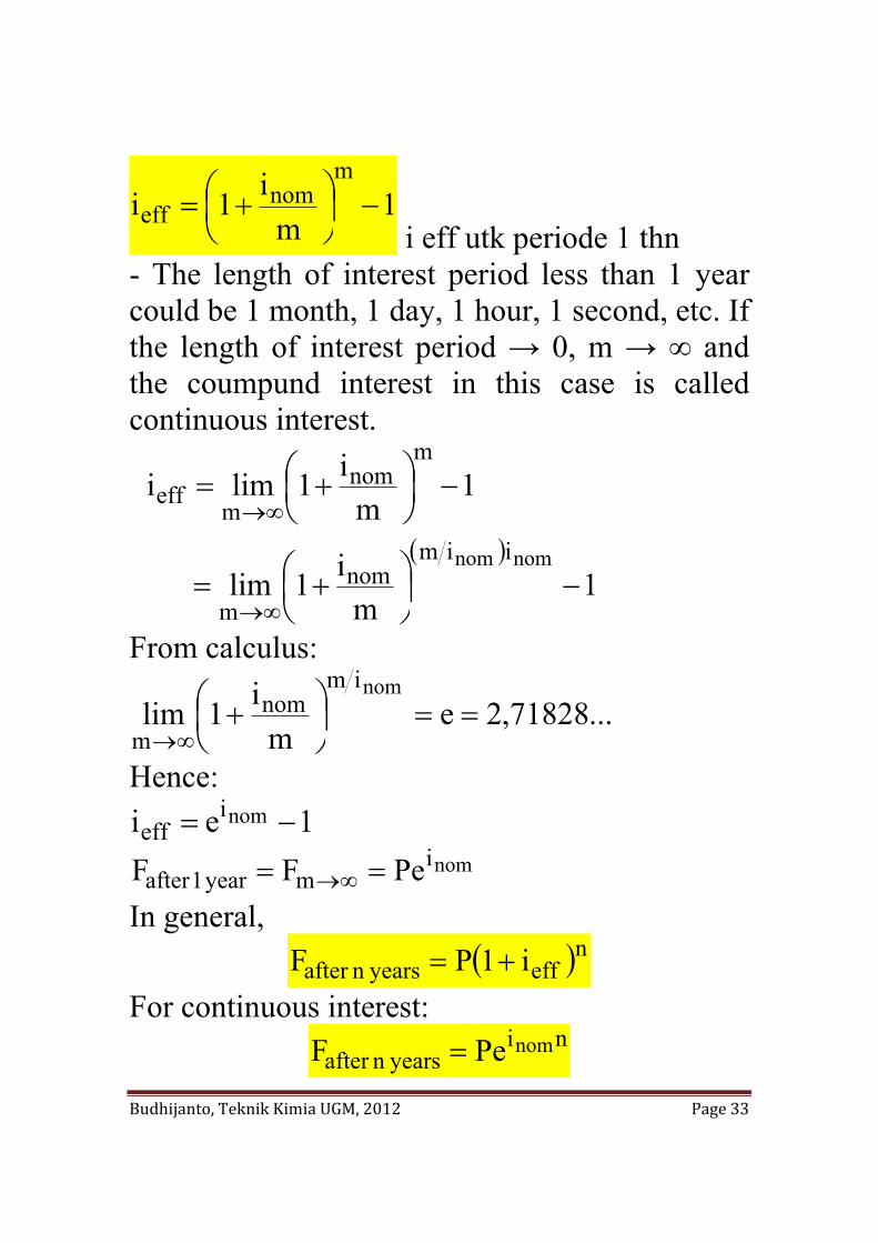
i eff utk periode 1 thn
- The length of interest period less than 1 year could be 1 month, 1 day, 1 hour, 1 second, etc. If the length of interest period → 0, m → ∞ and the coumpund interest in this case is called continuous interest.
( )
1m
i1lim
1m
i1limi
nomnom iimnom
m
mnom
meff
−⎟⎠⎞
⎜⎝⎛ +=
−⎟⎠⎞
⎜⎝⎛ +=
∞→
∞→
From calculus:
...71828,2em
i1limnomim
nomm
==⎟⎠⎞
⎜⎝⎛ +
∞→
Hence: 1ei nomi
eff −= nomi
myear1after PeFF == ∞→ In general,
( )neffyearsnafter i1PF += For continuous interest:
niyearsnafter
nomPeF =
Budhijanto, Teknik Kimia UGM, 2012 Page 34
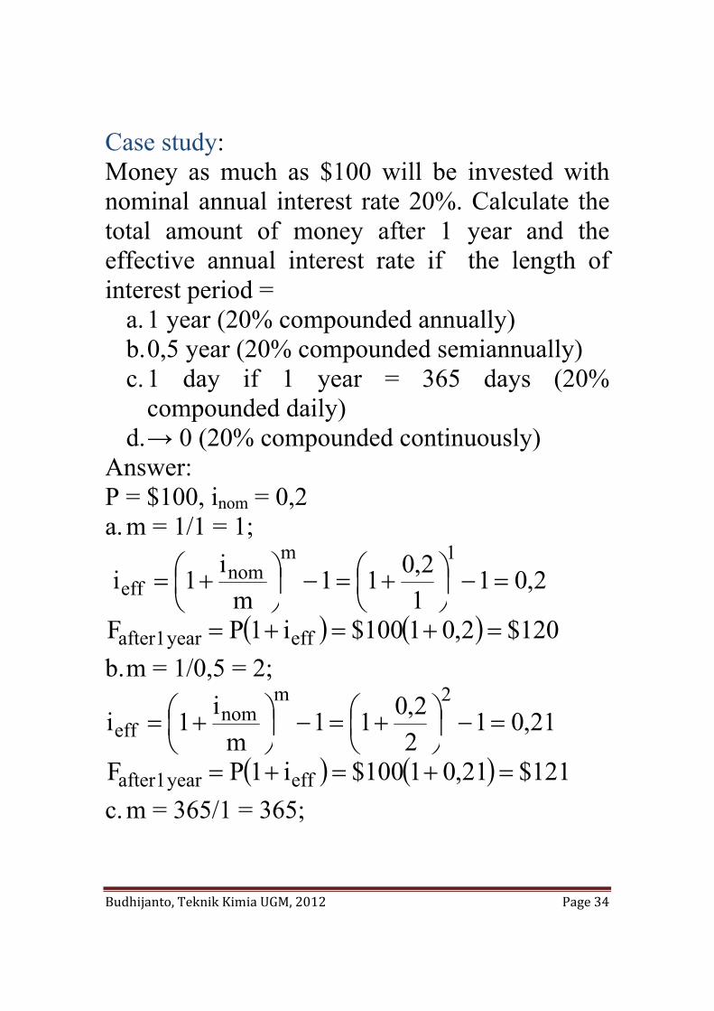
Case study: Money as much as $100 will be invested with nominal annual interest rate 20%. Calculate the total amount of money after 1 year and the effective annual interest rate if the length of interest period =
a. 1 year (20% compounded annually) b. 0,5 year (20% compounded semiannually) c. 1 day if 1 year = 365 days (20%
compounded daily) d. → 0 (20% compounded continuously)
Answer: P = $100, inom = 0,2 a. m = 1/1 = 1;
2,0112,011
mi1i
1mnom
eff =−⎟⎠⎞
⎜⎝⎛ +=−⎟
⎠⎞
⎜⎝⎛ +=
( ) ( ) 120$2,01100$i1PF effyear1after =+=+= b. m = 1/0,5 = 2;
21,0122,011
mi1i
2mnom
eff =−⎟⎠⎞
⎜⎝⎛ +=−⎟
⎠⎞
⎜⎝⎛ +=
( ) ( ) 121$21,01100$i1PF effyear1after =+=+= c. m = 365/1 = 365;
Budhijanto, Teknik Kimia UGM, 2012 Page 35
2213,01365
2,011m
i1i365m
nomeff =−⎟
⎠⎞
⎜⎝⎛ +=−⎟
⎠⎞
⎜⎝⎛ +=
( ) ( ) 13.122$2213,01100$i1PF effyear1after =+=+=
d. m →∞; 2214,01e1ei 2,0ieff
nom =−=−= ( ) ( ) 14.122$2214,01100$i1PF effyear1after =+=+=
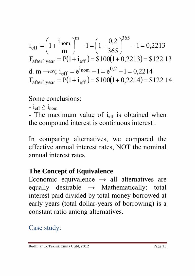
Some conclusions: - ieff ≥ inom - The maximum value of ieff is obtained when the compound interest is continuous interest . In comparing alternatives, we compared the effective annual interest rates, NOT the nominal annual interest rates. The Concept of Equivalence Economic equivalence → all alternatives are equally desirable → Mathematically: total interest paid divided by total money borrowed at early years (total dollar-years of borrowing) is a constant ratio among alternatives. Case study:
Budhijanto, Teknik Kimia UGM, 2012 Page 36
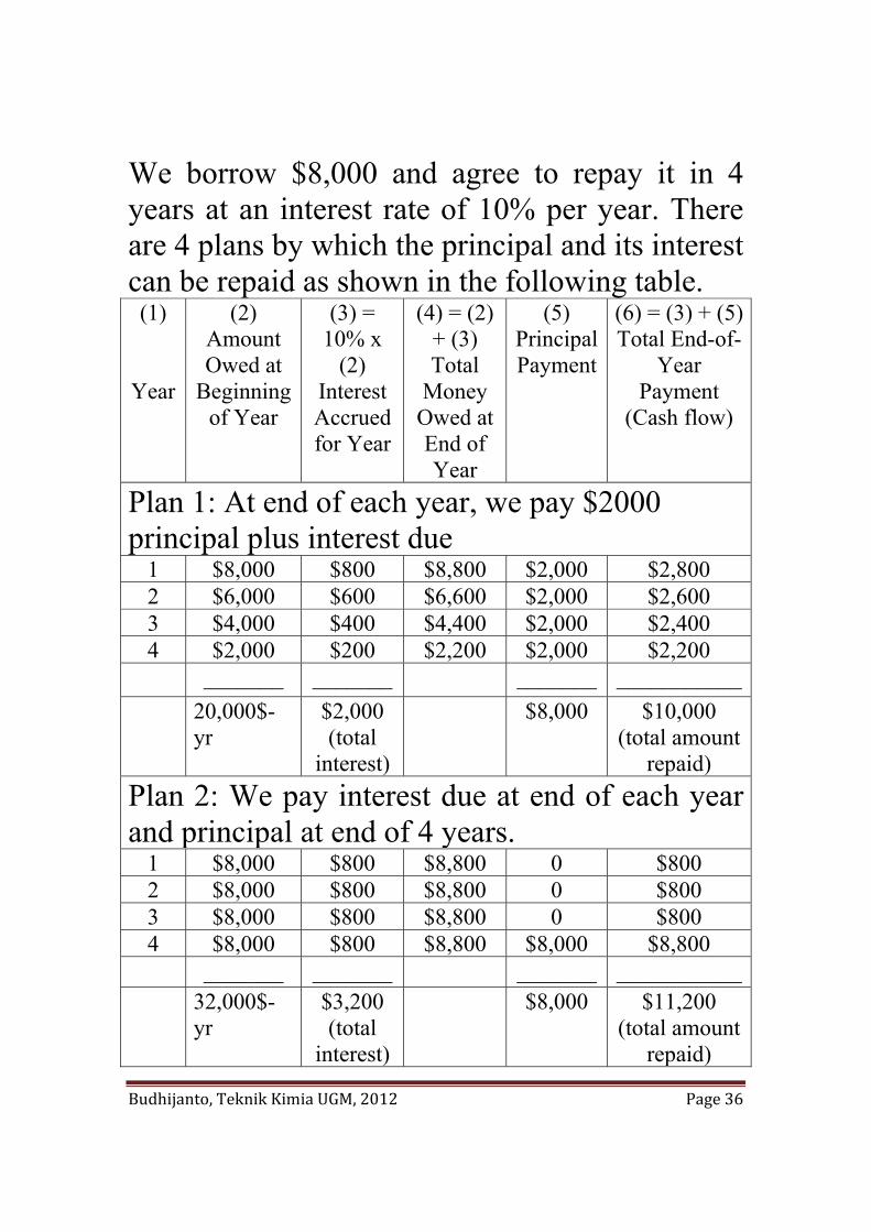
We borrow $8,000 and agree to repay it in 4 years at an interest rate of 10% per year. There are 4 plans by which the principal and its interest can be repaid as shown in the following table.
(1)
Year
(2) Amount Owed at
Beginning of Year
(3) = 10% x
(2) Interest Accrued for Year
(4) = (2) + (3) Total
Money Owed at End of Year
(5) Principal Payment
(6) = (3) + (5)Total End-of-
Year Payment
(Cash flow)
Plan 1: At end of each year, we pay $2000 principal plus interest due
1 $8,000 $800 $8,800 $2,000 $2,800 2 $6,000 $600 $6,600 $2,000 $2,600 3 $4,000 $400 $4,400 $2,000 $2,400 4 $2,000 $200 $2,200 $2,000 $2,200 _______ _______ _______ ___________ 20,000$-
yr $2,000 (total
interest)
$8,000 $10,000 (total amount
repaid) Plan 2: We pay interest due at end of each year and principal at end of 4 years.
1 $8,000 $800 $8,800 0 $800 2 $8,000 $800 $8,800 0 $800 3 $8,000 $800 $8,800 0 $800 4 $8,000 $800 $8,800 $8,000 $8,800 _______ _______ _______ ___________ 32,000$-
yr $3,200 (total
interest)
$8,000 $11,200 (total amount
repaid)
Budhijanto, Teknik Kimia UGM, 2012 Page 37
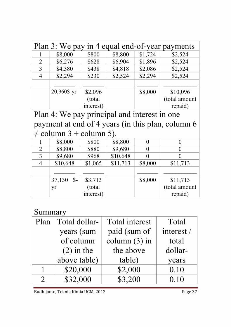
Plan 3: We pay in 4 equal end-of-year payments 1 $8,000 $800 $8,800 $1,724 $2,524 2 $6,276 $628 $6,904 $1,896 $2,524 3 $4,380 $438 $4,818 $2,086 $2,524 4 $2,294 $230 $2,524 $2,294 $2,524 _______ _______ _______ ___________ 20,960$-yr $2,096
(total interest)
$8,000 $10,096 (total amount
repaid) Plan 4: We pay principal and interest in one payment at end of 4 years (in this plan, column 6 ≠ column 3 + column 5).
1 $8,000 $800 $8,800 0 0 2 $8,800 $880 $9,680 0 0 3 $9,680 $968 $10,648 0 0 4 $10,648 $1,065 $11,713 $8,000 $11,713 _______ _______ _______ ___________ 37,130 $-
yr $3,713 (total
interest)
$8,000 $11,713 (total amount
repaid) Summary Plan Total dollar-
years (sum of column (2) in the
above table)
Total interest paid (sum of column (3) in
the above table)
Total interest /
total dollar- years
1 $20,000 $2,000 0.10 2 $32,000 $3,200 0.10
Budhijanto, Teknik Kimia UGM, 2012 Page 38
3 $20,960 $2,096 0.10 4 $37,130 $3,713 0.10
Because the ratio is constant at 0,10 for all plans, all the 4 repayment methods are equivalent. Cash-Flow Diagrams and Tables Cash flow diagrams:
1. The horizontal line is a time scale. 2. The arrows show cash flows and are placed
at the end of the periods. Downward arrows represent expenses (negative cash flow or cash outflows); Upward arrows represent receipts (positive cash flow or cash inflows).
3. The cash-flow diagram is dependent on the point of view. Cash inflows for the lender is cash outflows for the borrower.
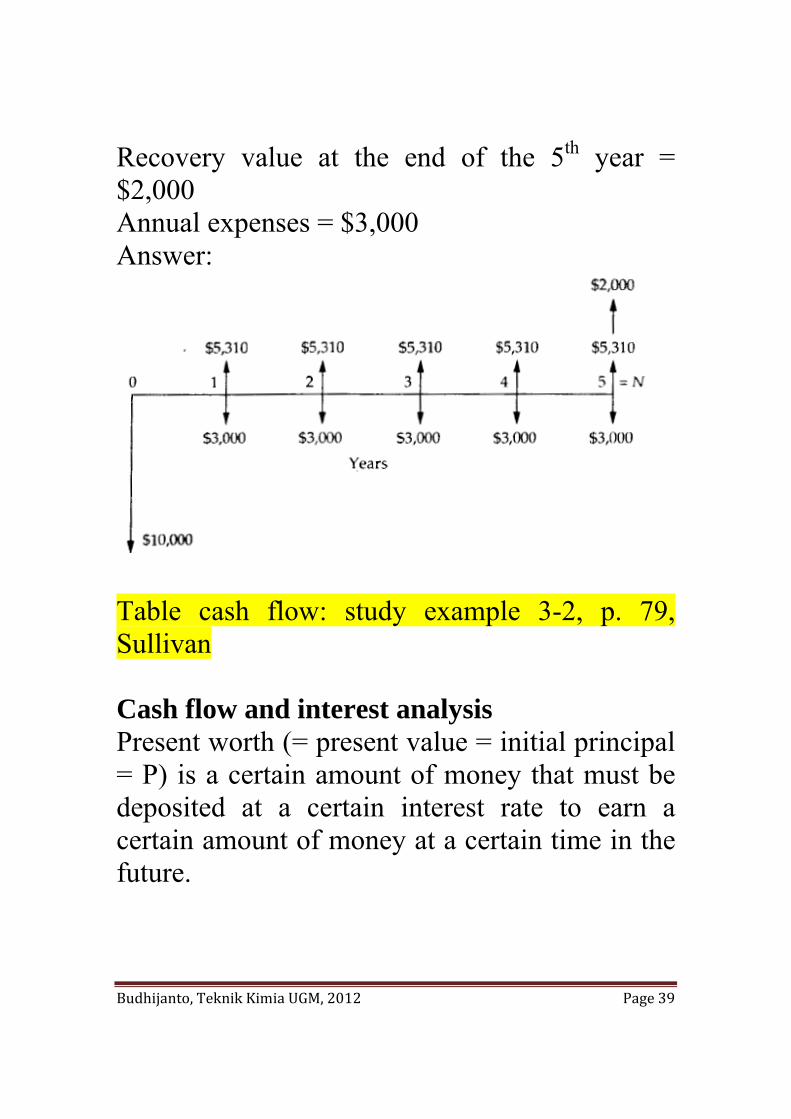
Cash flow tables basically have the same usage as cash flow diagrams. Example: Draw a cash flow diagram from the corporation’s viewpoint. Investment = $10,000 Annual revenue = $5,310 for 5 years
Budhijanto, Teknik Kimia UGM, 2012 Page 39
Recovery value at the end of the 5th year = $2,000 Annual expenses = $3,000 Answer:
Table cash flow: study example 3-2, p. 79, Sullivan Cash flow and interest analysis Present worth (= present value = initial principal = P) is a certain amount of money that must be deposited at a certain interest rate to earn a certain amount of money at a certain time in the future.
Budhijanto, Teknik Kimia UGM, 2012 Page 40
The amount of money at a certain time in the future is called the future value (= future worth = F) of the initial principal. Discount = F – P For discrete compound interest:
( )ni11FP+
= ;
( )ni11+
is called discrete single-payment present-
worth factor (= P/F,i,n). (1+i)n is called single-payment compound-amount factor (= F/P,i,n). For continuous interest:
ninome1FP =
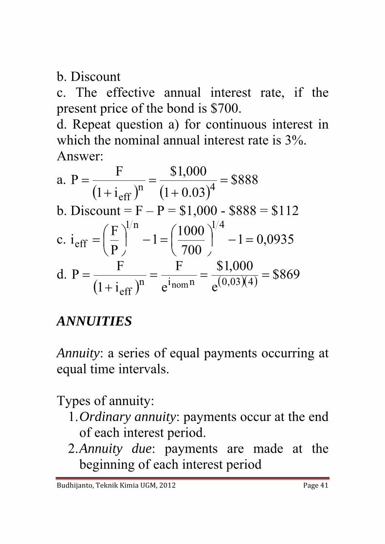
Case Study: Maturity value of a bond is $ 1,000 with the effective annual interest rate 3%. Determine: a. Present worth at 4 years before the bond reaches its maturity value
Budhijanto, Teknik Kimia UGM, 2012 Page 41
b. Discount c. The effective annual interest rate, if the present price of the bond is $700. d. Repeat question a) for continuous interest in which the nominal annual interest rate is 3%. Answer:
a. ( ) ( )
888$03.01
000,1$i1FP 4neff
=+
=+
=
b. Discount = F – P = $1,000 - $888 = $112
c. 0935,01700
10001PFi
41n1
eff =−⎟⎠⎞
⎜⎝⎛=−⎟
⎠⎞
⎜⎝⎛=
d. ( ) ( )( ) 869$
e000,1$
eF
i1FP 403,0nineff
nom===
+=
ANNUITIES
Annuity: a series of equal payments occurring at equal time intervals. Types of annuity:
1. Ordinary annuity: payments occur at the end of each interest period.
2. Annuity due: payments are made at the beginning of each interest period
Budhijanto, Teknik Kimia UGM, 2012 Page 42
3. Deferred annuity: the first payment is due after a definite number of years.
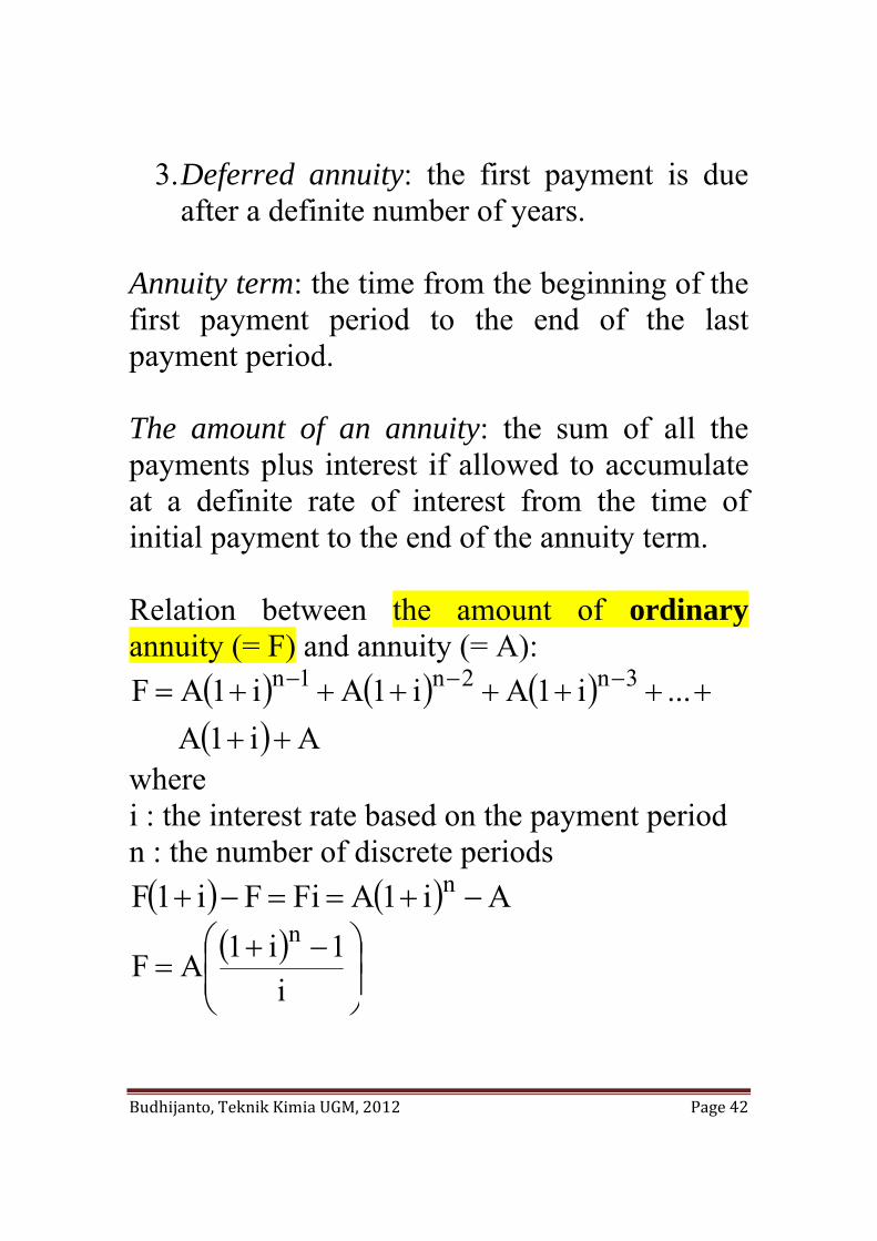
Annuity term: the time from the beginning of the first payment period to the end of the last payment period. The amount of an annuity: the sum of all the payments plus interest if allowed to accumulate at a definite rate of interest from the time of initial payment to the end of the annuity term. Relation between the amount of ordinary annuity (= F) and annuity (= A):
( ) ( ) ( )( ) Ai1A
...i1Ai1Ai1AF 3n2n1n
+++++++++= −−−
where i : the interest rate based on the payment period n : the number of discrete periods ( ) ( ) Ai1AFiFi1F n −+==−+
( )⎟⎟⎠
⎞⎜⎜⎝
⎛ −+=
i1i1AF
n
Budhijanto, Teknik Kimia UGM, 2012 Page 43
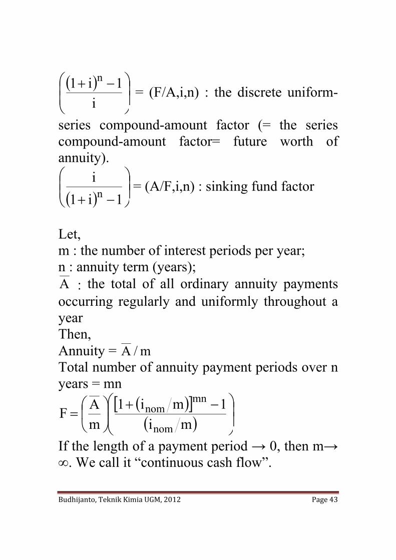
( )⎟⎟⎠
⎞⎜⎜⎝
⎛ −+i
1i1 n = (F/A,i,n) : the discrete uniform-
series compound-amount factor (= the series compound-amount factor= future worth of annuity).
( ) ⎟⎟⎠
⎞⎜⎜⎝
⎛
−+ 1i1in = (A/F,i,n) : sinking fund factor
Let, m : the number of interest periods per year; n : annuity term (years); A : the total of all ordinary annuity payments occurring regularly and uniformly throughout a year Then, Annuity = m/A Total number of annuity payment periods over n years = mn
( )[ ]( ) ⎟
⎟⎠
⎞⎜⎜⎝
⎛ −+⎟⎠
⎞⎜⎝
⎛=
mi1mi1
mAF
nom
mnnom
If the length of a payment period → 0, then m→ ∞. We call it “continuous cash flow”.
Budhijanto, Teknik Kimia UGM, 2012 Page 44
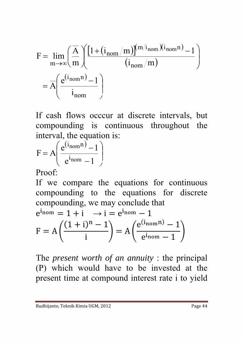
( )[ ]( )( )
( )( )
⎟⎟⎠
⎞⎜⎜⎝
⎛ −=
⎟⎟⎠
⎞⎜⎜⎝
⎛ −+⎟⎠
⎞⎜⎝
⎛=∞→
nom
ni
nom
niimnom
m
i1eA
mi1mi1
mAlimF
nom
nomnom
If cash flows occcur at discrete intervals, but compounding is continuous throughout the interval, the equation is:
( )
⎟⎟⎠
⎞⎜⎜⎝
⎛
−
−=
1e1eAF
nom
nom
i
ni
Proof: If we compare the equations for continuous compounding to the equations for discrete compounding, we may conclude that e 1 i → i e 1
F A1 i 1
i Ae 1e 1
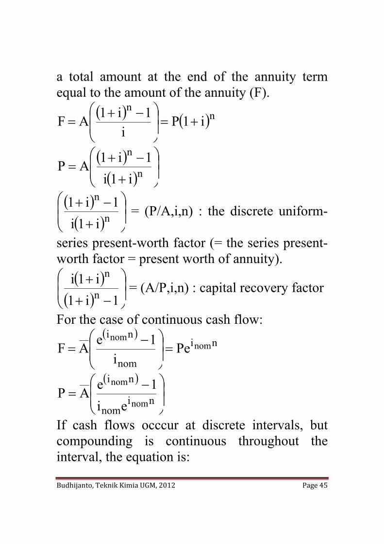
The present worth of an annuity : the principal (P) which would have to be invested at the present time at compound interest rate i to yield
Budhijanto, Teknik Kimia UGM, 2012 Page 45
a total amount at the end of the annuity term equal to the amount of the annuity (F).
( ) ( )nn
i1Pi
1i1AF +=⎟⎟⎠
⎞⎜⎜⎝
⎛ −+=
( )( ) ⎟
⎟⎠
⎞⎜⎜⎝
⎛
+
−+= n
n
i1i1i1AP
( )( ) ⎟
⎟⎠
⎞⎜⎜⎝
⎛
+
−+n
n
i1i1i1 = (P/A,i,n) : the discrete uniform-
series present-worth factor (= the series present-worth factor = present worth of annuity).
( )( ) ⎟
⎟⎠
⎞⎜⎜⎝
⎛
−+
+
1i1i1in
n = (A/P,i,n) : capital recovery factor
For the case of continuous cash flow: ( )
ni
nom
ninom
nomPe
i1eAF =⎟⎟⎠
⎞⎜⎜⎝
⎛ −=
( )
⎟⎟⎠
⎞⎜⎜⎝
⎛ −= ni
nom
ni
nom
nom
ei1eAP
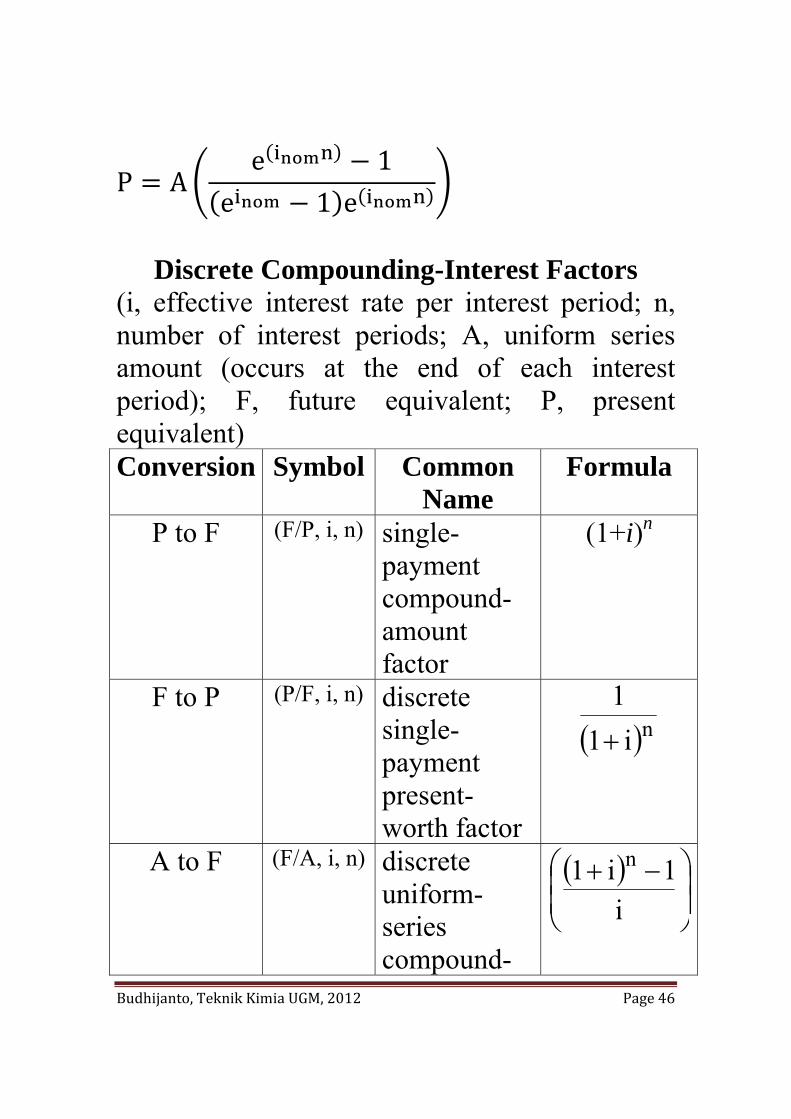
If cash flows occcur at discrete intervals, but compounding is continuous throughout the interval, the equation is:
Budhijanto, Teknik Kimia UGM, 2012 Page 46
P Ae 1
e 1 e
Discrete Compounding-Interest Factors
(i, effective interest rate per interest period; n, number of interest periods; A, uniform series amount (occurs at the end of each interest period); F, future equivalent; P, present equivalent) Conversion Symbol Common
Name Formula
P to F (F/P, i, n) single-payment compound-amount factor
(1+i)n
F to P (P/F, i, n) discrete single-payment present-worth factor
( )ni11+
A to F (F/A, i, n) discrete uniform-series compound-
( )⎟⎟⎠
⎞⎜⎜⎝
⎛ −+i
1i1 n
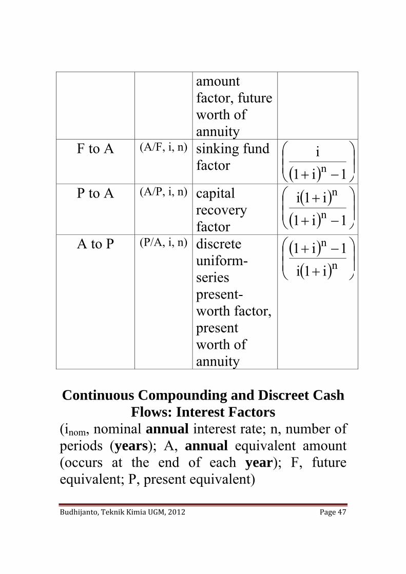
Budhijanto, Teknik Kimia UGM, 2012 Page 47
amount factor, future worth of annuity
F to A (A/F, i, n) sinking fund factor ( ) ⎟⎟
⎠
⎞⎜⎜⎝
⎛
−+ 1i1in
P to A (A/P, i, n) capital recovery factor
( )( ) ⎟
⎟⎠
⎞⎜⎜⎝
⎛
−+
+
1i1i1in
n
A to P (P/A, i, n) discrete uniform-series present-worth factor, present worth of annuity
( )( ) ⎟
⎟⎠
⎞⎜⎜⎝
⎛
+
−+n
n
i1i1i1
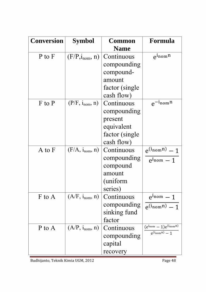
Continuous Compounding and Discreet Cash
Flows: Interest Factors (inom, nominal annual interest rate; n, number of periods (years); A, annual equivalent amount (occurs at the end of each year); F, future equivalent; P, present equivalent)
Budhijanto, Teknik Kimia UGM, 2012 Page 48
Conversion Symbol Common Name
Formula
P to F (F/P,inom, n) Continuous compounding compound-amount factor (single cash flow)
e
F to P (P/F, inom, n) Continuous compounding present equivalent factor (single cash flow)
e
A to F (F/A, inom, n) Continuous compounding compound amount (uniform series)
e 1e 1
F to A (A/F, inom, n) Continuous compounding sinking fund factor
e 1e 1
P to A (A/P, inom, n) Continuous compounding capital recovery
e 1 ee 1
Budhijanto, Teknik Kimia UGM, 2012 Page 49
factor A to P (P/A, inom, n) Continuous
compounding present equivalent (uniform series)
e 1e 1 e
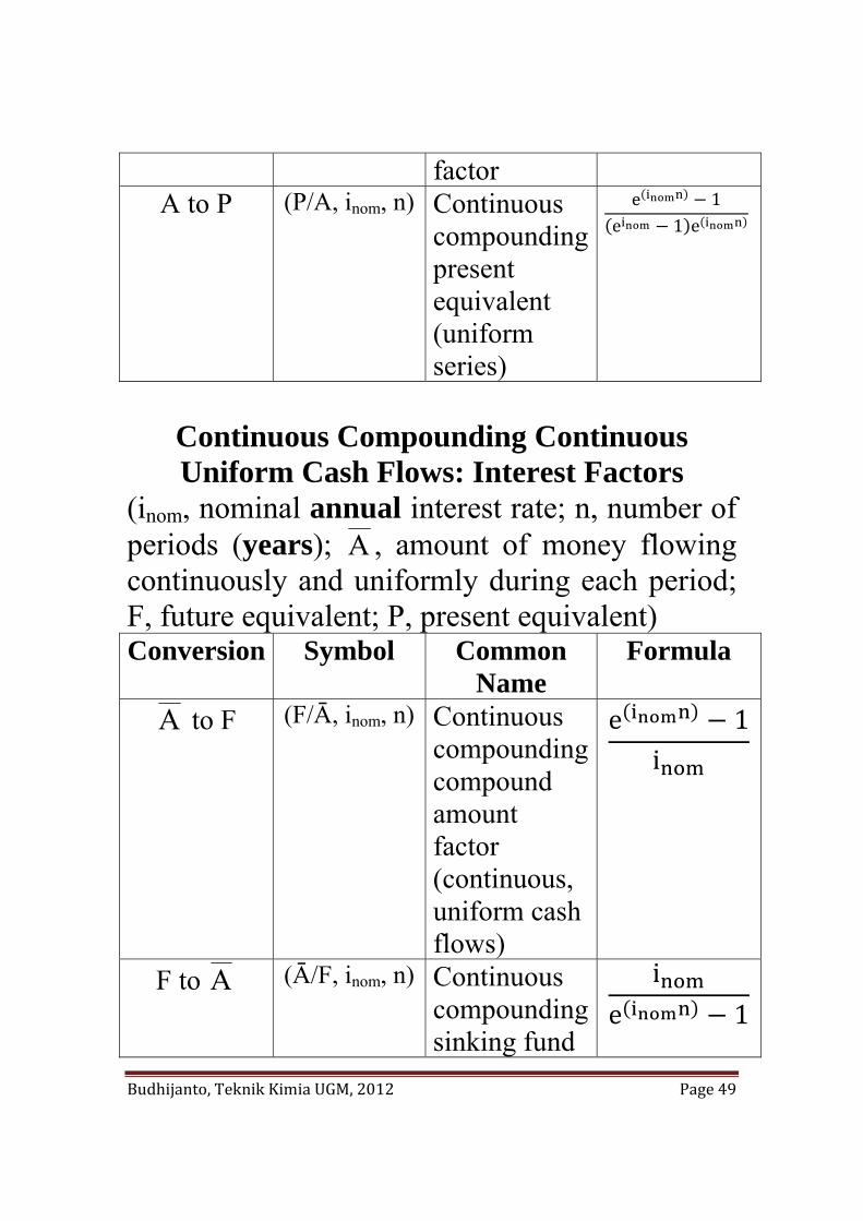
Continuous Compounding Continuous Uniform Cash Flows: Interest Factors
(inom, nominal annual interest rate; n, number of periods (years); A , amount of money flowing continuously and uniformly during each period; F, future equivalent; P, present equivalent) Conversion Symbol Common
Name Formula
A to F (F/Ā, inom, n) Continuous compounding compound amount factor (continuous, uniform cash flows)
e 1i
F to A (Ā/F, inom, n) Continuous compounding sinking fund
ie 1
Budhijanto, Teknik Kimia UGM, 2012 Page 50
factor (continuous, uniform cash flows)
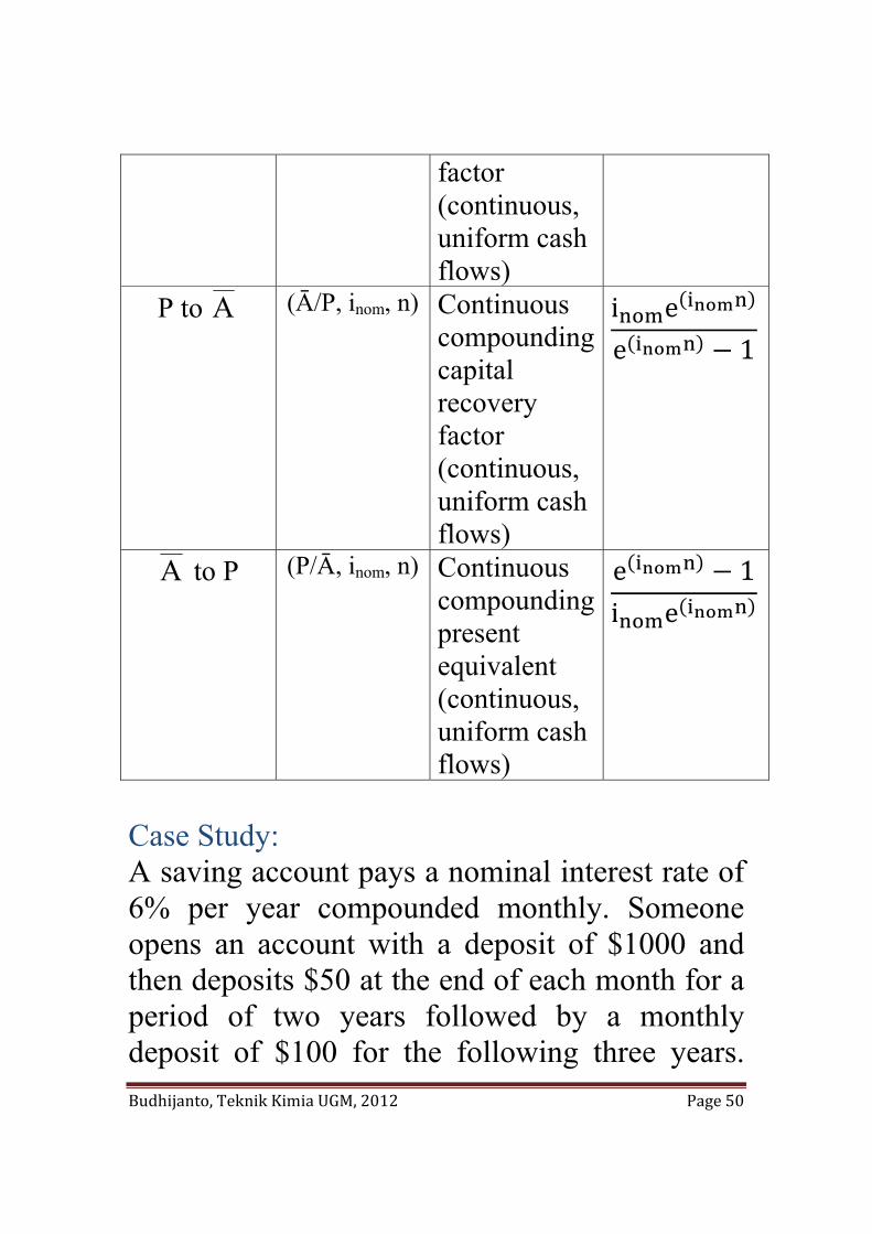
P to A (Ā/P, inom, n) Continuous compounding capital recovery factor (continuous, uniform cash flows)
i ee 1
A to P (P/Ā, inom, n) Continuous compounding present equivalent (continuous, uniform cash flows)
e 1i e
Case Study: A saving account pays a nominal interest rate of 6% per year compounded monthly. Someone opens an account with a deposit of $1000 and then deposits $50 at the end of each month for a period of two years followed by a monthly deposit of $100 for the following three years.
Budhijanto, Teknik Kimia UGM, 2012 Page 51
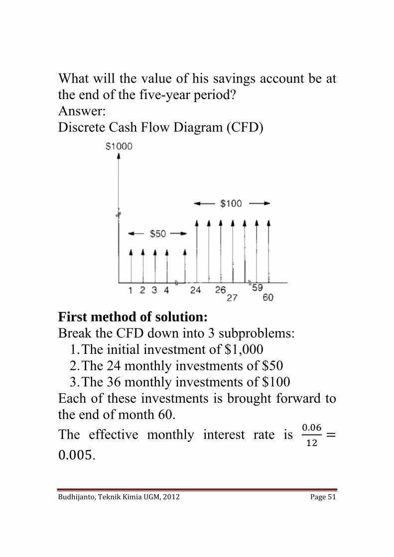
What will the value of his savings account be at the end of the five-year period? Answer: Discrete Cash Flow Diagram (CFD)
First method of solution: Break the CFD down into 3 subproblems:
1. The initial investment of $1,000 2. The 24 monthly investments of $50 3. The 36 monthly investments of $100
Each of these investments is brought forward to the end of month 60. The effective monthly interest rate is .
0.005.
Budhijanto, Teknik Kimia UGM, 2012 Page 52
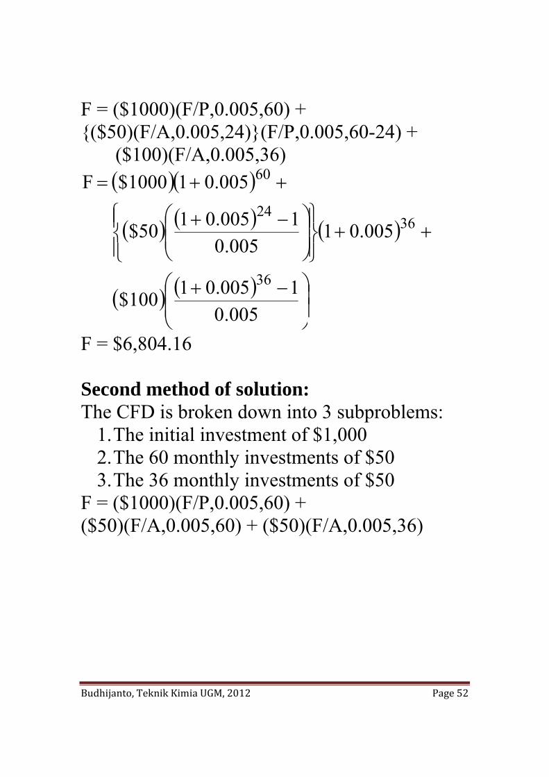
F = ($1000)(F/P,0.005,60) + {($50)(F/A,0.005,24)}(F/P,0.005,60-24) + ($100)(F/A,0.005,36)
( )( )
( ) ( ) ( )
( ) ( )⎟⎟⎠
⎞⎜⎜⎝
⎛ −+
++⎪⎭
⎪⎬⎫
⎪⎩
⎪⎨⎧
⎟⎟⎠
⎞⎜⎜⎝
⎛ −+
++=
005.01005.01100$
005.01005.0
1005.0150$
005.011000$F
36
3624
60
F = $6,804.16 Second method of solution: The CFD is broken down into 3 subproblems:
1. The initial investment of $1,000 2. The 60 monthly investments of $50 3. The 36 monthly investments of $50
F = ($1000)(F/P,0.005,60) + ($50)(F/A,0.005,60) + ($50)(F/A,0.005,36)
Budhijanto, Teknik Kimia UGM, 2012 Page 53
( )( )
( ) ( )
( ) ( ) 16.804,6$005.0
1005.0150$
005.01005.0150$
005.011000$F
36
60
60
=⎟⎟⎠
⎞⎜⎜⎝
⎛ −+
+⎟⎟⎠
⎞⎜⎜⎝
⎛ −+
++=
PERPETUITIS AND CAPITALIZED COST Perpetuity: an annuity in which the periodic payments continue indefinitely. This type of annuity is of particular interest, for example in a case where it is desired to determine a total cost for a piece of equipment or other asset under conditions which permit the asset to be replaced perpetually without considering inflation or deflation.
( )ni1PF += Here, n is the number of interest periods during service-life of the asset.
Budhijanto, Teknik Kimia UGM, 2012 Page 54
If perpetuation to occur, F minus the cost for the replacement must equal P. Let CR represent the replacement cost. Therefore, F – CR = P Combining the two equations, we get
( )nR i1PCP +=+
( ) 1i1CP n
R
−+=
Capitalized cost is defined as the original cost of the equipment plus the present value of the renewable perpetuity. Let, K = capitalized cost, and CV = the original cost of the equipment. Then,
( ) 1i1CCK n
Rv
−++=
Case Study: A new piece of completely installed equipment costs $12,000, and will have a scrap value of $2,000 at the end of its useful life. If the useful-life period is 10 years and the interest is compounded at 6% per year, what is the capitalized cost of the equipment?
Budhijanto, Teknik Kimia UGM, 2012 Page 55
Answer: CV = $12,000; SV = $2,000 Assuming no inflation or deflation, the replacement cost of the equipment at the end of its useful life is CR = CV – SV = $12,000 - $2,000 = $10,000 Other data, i = 0.06 n = 10 Then,
( )650,24$
650,12$000,12$106.01
000,10$000,12$K 10
=
+=−+
+=
Hence, if the equipment is to perpetuate itself, the amount of total capital necessary at the start would be $24,650, which consists of $12,000 for the equipment plus $12,650 for the replacement fund. After 10 years, the $12,650 replacement fund becomes $12,650(1.06)10 = $22,650. The scrap value of the equipment is $2,000. Thus, the total amount of money available at the end of the 10th year is $24,650 (= K, capitalized cost).
Budhijanto, Teknik Kimia UGM, 2012 Page 56
Alternative derivation of the capitalized cost equation:
SVRCK R ++= where R is residual. The purpose of this residual is to earn sufficient interest during the service life of the asset to pay for its replacement. Hence, the relation between CR and R is:
( ) ( )[ ]1i1RRi1RC nnR −+=−+=
Combining the two equations:
( )SV
1i11CCK nRR +
−++=
( )( )
factortcosdcapitalize1i1
i1C
SVKn
n
R=
−+
+=
−
Interest Formulas Relating a Uniform Gradient of Cash Flows (an Arithmetic Sequence of Cash Flows)
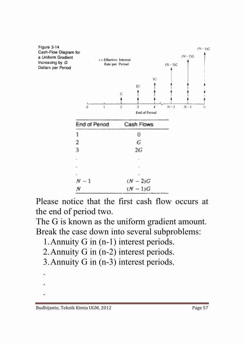
Budhijanto, Teknik Kimia UGM, 2012 Page 57
Please notice that the first cash flow occurs at the end of period two. The G is known as the uniform gradient amount. Break the case down into several subproblems:
1. Annuity G in (n-1) interest periods. 2. Annuity G in (n-2) interest periods. 3. Annuity G in (n-3) interest periods. . . .
Budhijanto, Teknik Kimia UGM, 2012 Page 58
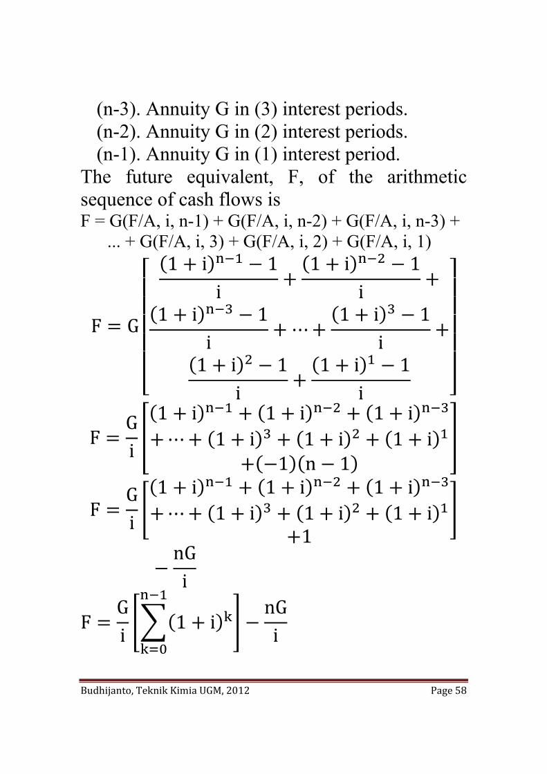
(n-3). Annuity G in (3) interest periods. (n-2). Annuity G in (2) interest periods. (n-1). Annuity G in (1) interest period.
The future equivalent, F, of the arithmetic sequence of cash flows is F = G(F/A, i, n-1) + G(F/A, i, n-2) + G(F/A, i, n-3) + ... + G(F/A, i, 3) + G(F/A, i, 2) + G(F/A, i, 1)
F G
1 i 1i
1 i 1i
1 i 1i
1 i 1i
1 i 1i
1 i 1i
FGi
1 i 1 i 1 i1 i 1 i 1 i
1 n 1
FGi
1 i 1 i 1 i1 i 1 i 1 i
1nGi
FGi 1 i
nGi
Budhijanto, Teknik Kimia UGM, 2012 Page 59
1 i 1 i 1 i
1 i 1
1 i1 i 1
i F A⁄ , i, n
FGiF A⁄ , i, n
nGi
The ordinary annuity, A, equivalent to the arithmetic sequence of cash flows is A F A F⁄ , i, n G
i F ⁄ A, i, nnGi A F⁄ , i, n
G nGi A F⁄ , i, n G
inGi
i1 i n 1
A G1i
n1 i n 1 G A G⁄ , i, n
A G⁄ , i, n Gradient to uniform series conversion factor. The present equivalent, P, of the arithmetic sequence of cash flows is P F P F⁄ , i, n
Budhijanto, Teknik Kimia UGM, 2012 Page 60
Gi F ⁄ A, i, n
nGi
11 i n
PG
i 1 i1 i n 1
i n G P G⁄ , i, n
P G⁄ , i, n 1i 1 i n
n Gradient to present equivalent conversion factor.
P G⁄ , i, n1i
1 i 1i 1 i n n
11 i n
P G⁄ , i, n1i
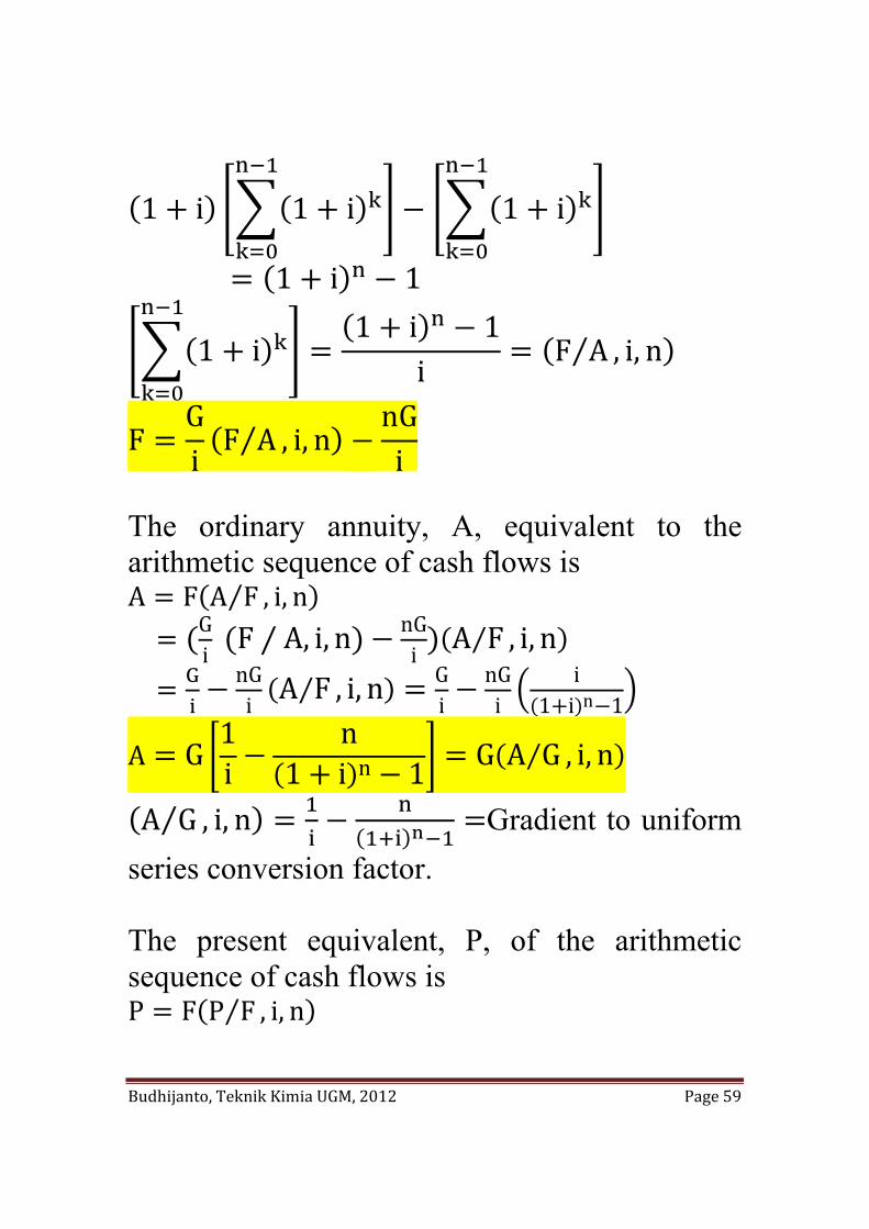
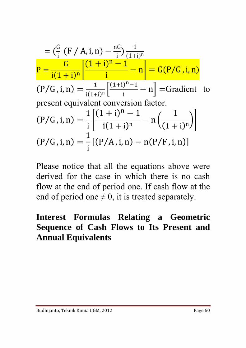
P A⁄ , i, n n P F⁄ , i, n Please notice that all the equations above were derived for the case in which there is no cash flow at the end of period one. If cash flow at the end of period one ≠ 0, it is treated separately. Interest Formulas Relating a Geometric Sequence of Cash Flows to Its Present and Annual Equivalents
Budhijanto, Teknik Kimia UGM, 2012 Page 61
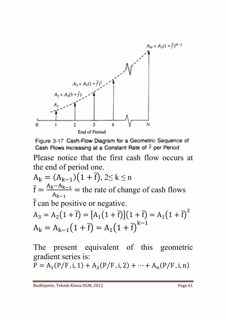
Please notice that the first cash flow occurs at the end of period one. A A 1 f , 2≤ k ≤ n f A A
A the rate of change of cash flows
f can be positive or negative. A A 1 f A 1 f 1 f A 1 f
A A 1 f A 1 f The present equivalent of this geometric gradient series is: P A P F⁄ , i, 1 A P F⁄ , i, 2 A P F⁄ , i, n
Budhijanto, Teknik Kimia UGM, 2012 Page 62
P A P F⁄ , i, kA
1 i
PA 1 f
1 iA1 f
1 f1 i
Let:
i R1 i1 f
11 i 1 f
1 fi f1 f
= convenience rate 1 i1 f
i R 1
Thus,
PA1 f
11 i R
1
1 i R1
11 i R
11 i R
11 i R
i R
1 i R
11 i R
1 1 i R
1 i R
11 i R
1 i R 1i R 1 i R
Budhijanto, Teknik Kimia UGM, 2012 Page 63
When f , i R 0, this equation is valid only when n is finite.
PA1 f
11 i R
A1 f
1 i R 1i R 1 i R
PA1 f
P A⁄ , i R, n
We know that
P F,⁄ i R, k1
1 i R
PA1 f
P F⁄ , i R, k
Special case: When i f, i R 0
PA1 f
11 0
nA1 f
The end-of-period uniform annual equivalent, A, of this geometric gradient series is: A P A P⁄ , i, n Let’s define
Budhijanto, Teknik Kimia UGM, 2012 Page 64
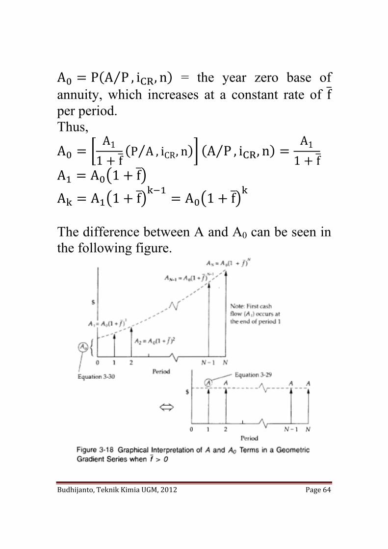
A P A P⁄ , i R, n = the year zero base of annuity, which increases at a constant rate of f per period. Thus,
AA11 f
P A⁄ , iCR, n A P⁄ , i R, nA11 f
A A 1 f
A A 1 f A 1 f The difference between A and A0 can be seen in the following figure.
Budhijanto, Teknik Kimia UGM, 2012 Page 65
The future equivalent of this geometric gradient series is: F P F P⁄ , i, n HOMEWORK: Study examples in Chapter 3, Sullivan. Applications of the Time Value of Money Concept Minimum Attractive Rate of Return (MARR) = hurdle rate MARR is determined by the top management of an organization. MARR determination involves numerious considerations, such as:
1. The amount of money available for investments, and the source and cost of these funds.
2. The number of good alternatives for the investments and their purpose.
3. The amount of perceived risk associated with investment alternatives and their estimated costs.
4. The type of organization involved.
Budhijanto, Teknik Kimia UGM, 2012 Page 66
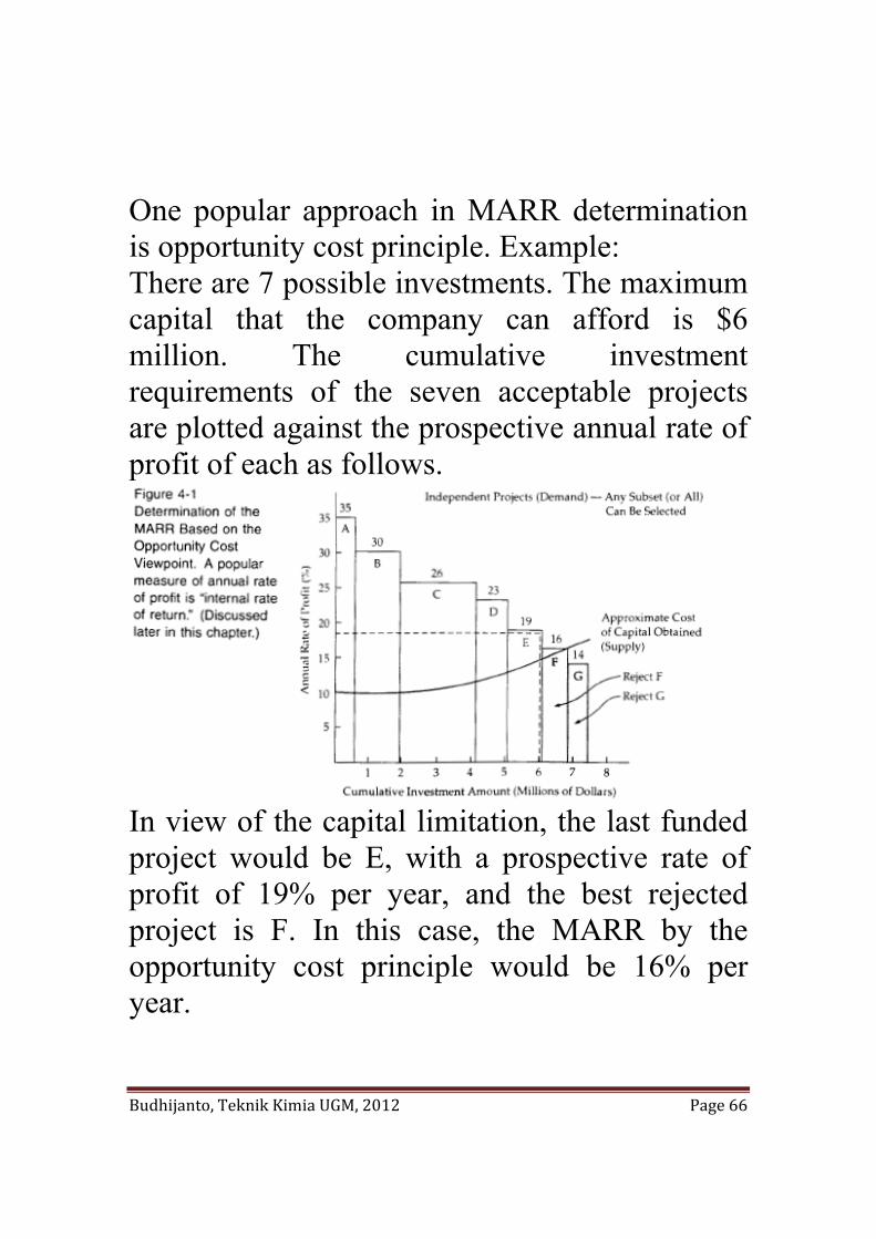
One popular approach in MARR determination is opportunity cost principle. Example: There are 7 possible investments. The maximum capital that the company can afford is $6 million. The cumulative investment requirements of the seven acceptable projects are plotted against the prospective annual rate of profit of each as follows.
In view of the capital limitation, the last funded project would be E, with a prospective rate of profit of 19% per year, and the best rejected project is F. In this case, the MARR by the opportunity cost principle would be 16% per year.
Budhijanto, Teknik Kimia UGM, 2012 Page 67
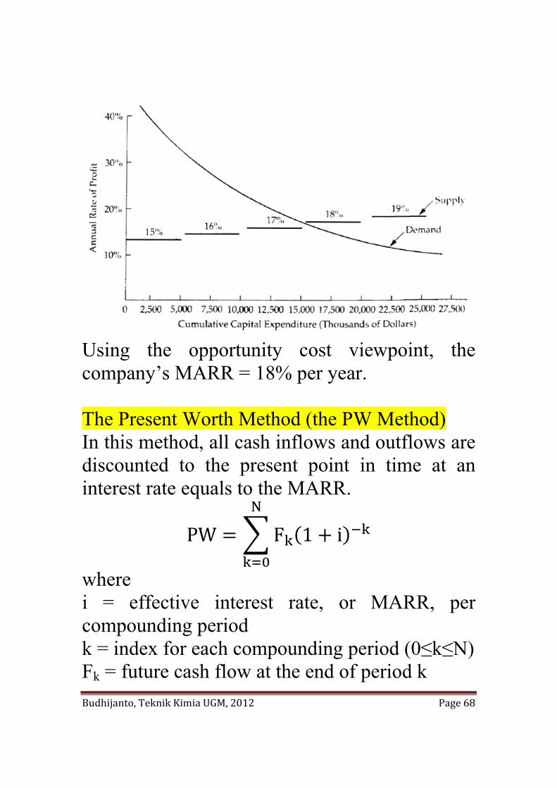
Figure 4 also shows the approximate cost of obtaining the $6 million. The project E is acceptable only as long as its annual rate of profit exceeds the cost of raising the last $1 million (capital investment of E). Example 4.1: The following table shows prospective annual rates of profit for a company’s portfolio of capital investment projects. Expected Annual Rate of Profit
Investment Requirements (Thousands of Dollars)
Cumulative Investment
40% and over $2,200 $2,20030-39.9% 3,400 5,60020-29.9% 6,800 12,40010-19.9% 14,200 26,600Below 10% 22,800 49,400Note: All projects with a rate of profit of 10% or greater are acceptable The supply of capital obtained from internal and external sources has a cost of 15% per year for the first $5,000,000 invested and then increases 1% for every $5,000,000 thereafter. What is the company’s MARR? Answer:
Budhijanto, Teknik Kimia UGM, 2012 Page 68
Using the opportunity cost viewpoint, the company’s MARR = 18% per year. The Present Worth Method (the PW Method) In this method, all cash inflows and outflows are discounted to the present point in time at an interest rate equals to the MARR.
PW F 1 iN
where i = effective interest rate, or MARR, per compounding period k = index for each compounding period (0≤k≤N) Fk = future cash flow at the end of period k
Budhijanto, Teknik Kimia UGM, 2012 Page 69
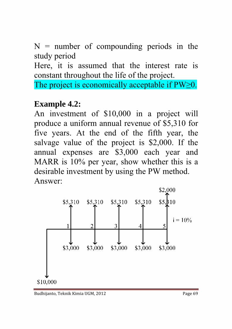
N = number of compounding periods in the study period Here, it is assumed that the interest rate is constant throughout the life of the project. The project is economically acceptable if PW≥0. Example 4.2: An investment of $10,000 in a project will produce a uniform annual revenue of $5,310 for five years. At the end of the fifth year, the salvage value of the project is $2,000. If the annual expenses are $3,000 each year and MARR is 10% per year, show whether this is a desirable investment by using the PW method. Answer:
Budhijanto, Teknik Kimia UGM, 2012 Page 70
PW 10,000 5,310 3,000 P A⁄ , 0.1,52,000 P F⁄ , 0.1,5
PW 10,000 2,3101.1 10.1 1.1
2,0001.1 0
Thus, the project is marginally acceptable. The Future Worth Method (The FW Method) This method is based on the equivalent worth of all cash inflows and outflows at the end of study period at an interest rate equals to the MARR.
FW P 1 i NN
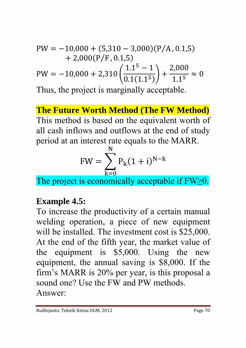
The project is economically acceptable if FW≥0. Example 4.5: To increase the productivity of a certain manual welding operation, a piece of new equipment will be installed. The investment cost is $25,000. At the end of the fifth year, the market value of the equipment is $5,000. Using the new equipment, the annual saving is $8,000. If the firm’s MARR is 20% per year, is this proposal a sound one? Use the FW and PW methods. Answer:
Budhijanto, Teknik Kimia UGM, 2012 Page 71
$25,000
$8,000 $8,000 $8,000 $8,000 $8,000$5,000
i = 20% per year1 2 3 4 5
Using the FW method:
The investment is economically justified. Using the PW method:
The investment is economically justified. The Annual-Worth Method (The AW Method)
Budhijanto, Teknik Kimia UGM, 2012 Page 72
The Annual Worth (AW) of a project is an equal annual series of dollar amounts, for a stated study period that is equivalent to the cash inflows and outflows at an interest rate equals to the MARR. AW = R – E – CR where R is annual equivalent revenues or savings. E is annual equivalent expenses. CR is annual equivalent Capital Recovery amount, which is defined as
where I = initial investment for the project S = salvage (market) value at the end of the study period N = project study period
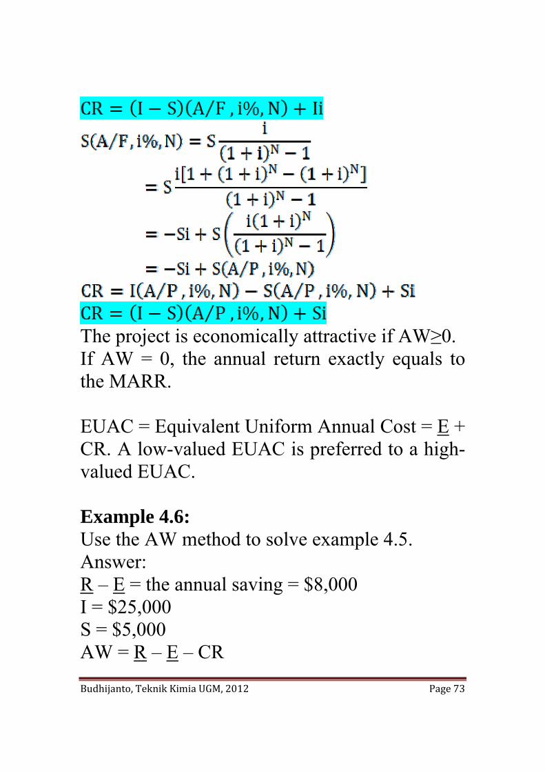
Budhijanto, Teknik Kimia UGM, 2012 Page 73
The project is economically attractive if AW≥0. If AW = 0, the annual return exactly equals to the MARR. EUAC = Equivalent Uniform Annual Cost = E + CR. A low-valued EUAC is preferred to a high-valued EUAC. Example 4.6: Use the AW method to solve example 4.5. Answer: R – E = the annual saving = $8,000 I = $25,000 S = $5,000 AW = R – E – CR
Budhijanto, Teknik Kimia UGM, 2012 Page 74
The investment is economically attractive The Internal Rate of Return Method (The IRR Method) The IRR method = the investor’s method = the discounted cash flow method = the profitability index. For a single alternative, from the lender’s viewpoint, the IRR is not positive unless (1) both receipts and expenses are present in the cash flow pattern and (2) the sum of receipts exceeds the sum of all cash outflows. Using a PW formulation:
where Rk = net revenues or savings for the kth year Ek = net expenditures including any investment costs for the kth year N = project life (or study period) i'% = the IRR
Budhijanto, Teknik Kimia UGM, 2012 Page 75
Alternatively, using a FW formulation:
Thus, in this method, we calculate the IRR (i’%). The alternative is acceptable if i’≥MARR. Example 4.7: A capital investment of $10,000 in a project will produce a uniform annual revenue of $5,310 for five years. The salvage value of the project is $2,000. Annual expenses will be $3,000. The company is willing to accept any project that will earn at least 10% per year on all invested capital. Determine using the IRR method whether it is acceptable. Answer: Check: The sum of cash inflows = 5($5,310) + $2,000 = $28,550 > the sum of cash outflows = 5($3,000) + $10,000 = $25,000. Thus, i’% is positive.
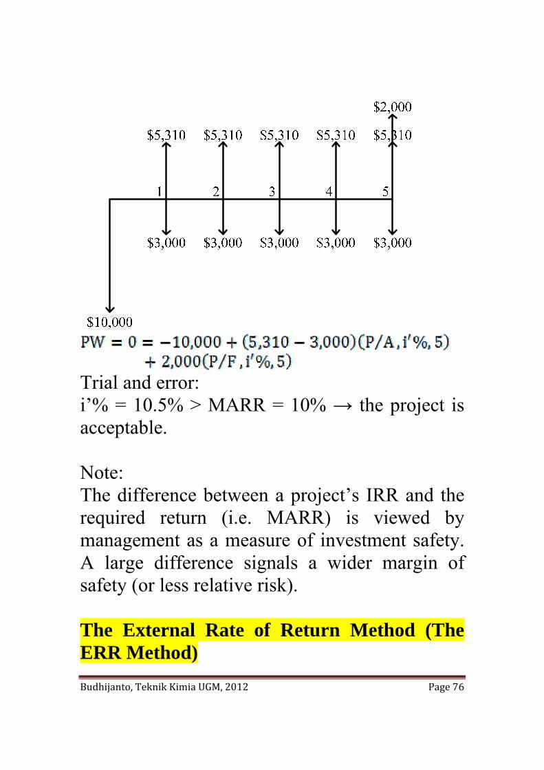
Budhijanto, Teknik Kimia UGM, 2012 Page 76
Trial and error: i’% = 10.5% > MARR = 10% → the project is acceptable. Note: The difference between a project’s IRR and the required return (i.e. MARR) is viewed by management as a measure of investment safety. A large difference signals a wider margin of safety (or less relative risk). The External Rate of Return Method (The ERR Method)
Budhijanto, Teknik Kimia UGM, 2012 Page 77
In the IRR method, it is assumed that net cash proceeds are reinvested at interest rate = IRR. In practice, this assumption may not be valid. For example, if a firm’s MARR is 20% per year and the IRR of a project is 42.4%, it may not be possible for the firm to reinvest the net cash proceeds from the project at much more than 20% → the ERR method can remedy this weakness. The ERR method takes into account the interest rate ( ) external to a project at which net cash flows generated (or required) by the project over its life can be reinvested (or borrowed). Steps of calculation: 1. All net cash outflows are discounted to time 0
(the present) at per compounding period. 2. All net cash inflows are compounded to period
N at . 3. The interest rate that establishes equivalence
between the two quantities (the external rate of return) is determined.
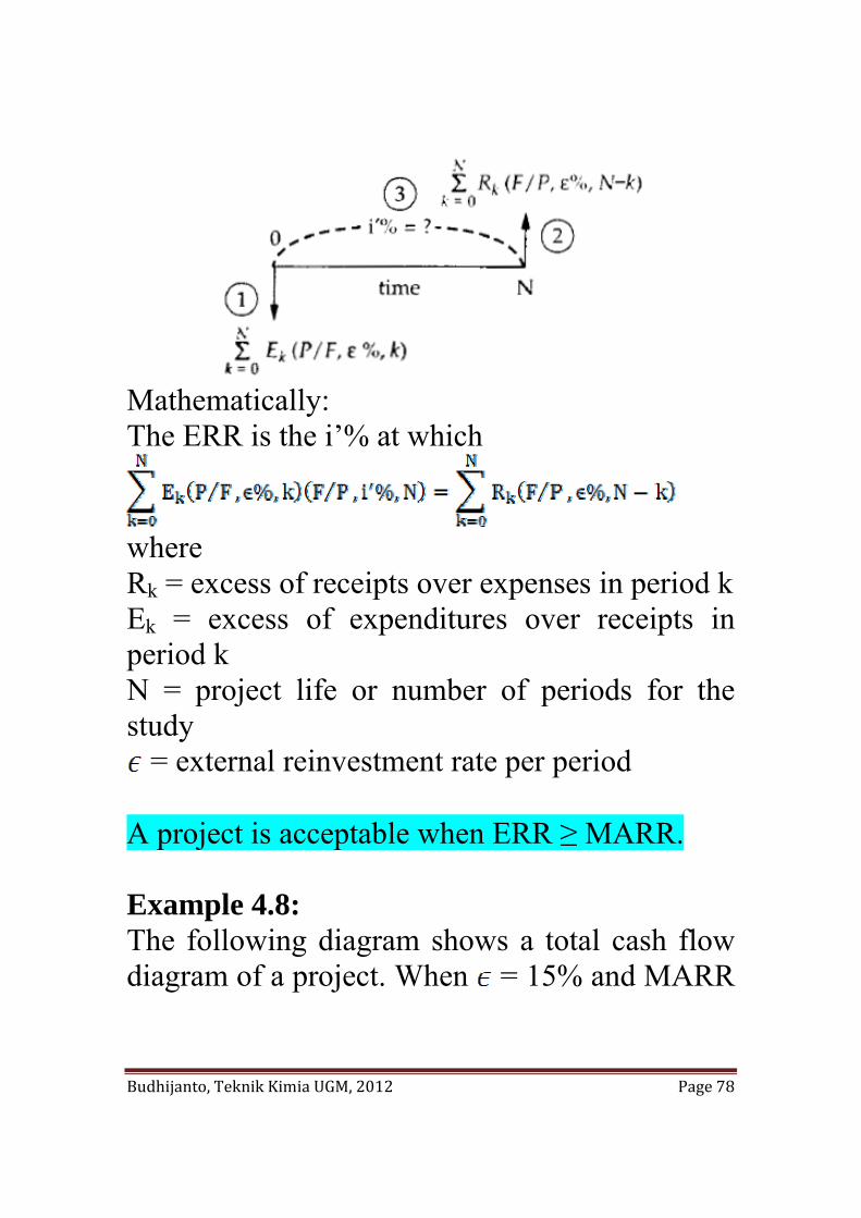
Graphically:
Budhijanto, Teknik Kimia UGM, 2012 Page 78
Mathematically: The ERR is the i’% at which
where Rk = excess of receipts over expenses in period k Ek = excess of expenditures over receipts in period k N = project life or number of periods for the study
= external reinvestment rate per period A project is acceptable when ERR ≥ MARR. Example 4.8: The following diagram shows a total cash flow diagram of a project. When = 15% and MARR
Budhijanto, Teknik Kimia UGM, 2012 Page 79
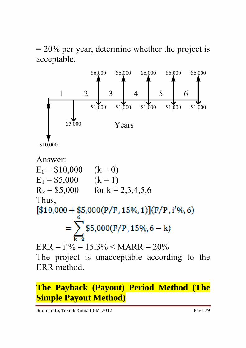
= 20% per year, determine whether the project is acceptable.
$1,000
$6,000
$10,000
$6,000$6,000$6,000$6,000
$1,000 $1,000 $1,000 $1,000
$5,000
Answer: E0 = $10,000 (k = 0) E1 = $5,000 (k = 1) Rk = $5,000 for k = 2,3,4,5,6 Thus,
ERR = i’% = 15,3% < MARR = 20% The project is unacceptable according to the ERR method. The Payback (Payout) Period Method (The Simple Payout Method)
Budhijanto, Teknik Kimia UGM, 2012 Page 80
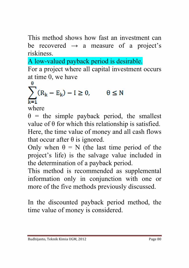
This method shows how fast an investment can be recovered → a measure of a project’s riskiness. A low-valued payback period is desirable. For a project where all capital investment occurs at time 0, we have
where θ = the simple payback period, the smallest value of θ for which this relationship is satisfied. Here, the time value of money and all cash flows that occur after θ is ignored. Only when θ = N (the last time period of the project’s life) is the salvage value included in the determination of a payback period. This method is recommended as supplemental information only in conjunction with one or more of the five methods previously discussed. In the discounted payback period method, the time value of money is considered.
Budhijanto, Teknik Kimia UGM, 2012 Page 81
where i% = MARR I = the capital investment made at the present time (k = 0) θ' = the discounted payback period, the smallest value of θ’ for which this relationship is satisfied. Payback periods of three years or less are often desired in U.S. industry. Using the payback period methods to make investment decisions should be generally be avoided except as a measure of how quickly invested capital will be recovered, which is an indicator of project risk. Example 4.9: = Example 4.5 Cash flow diagram:
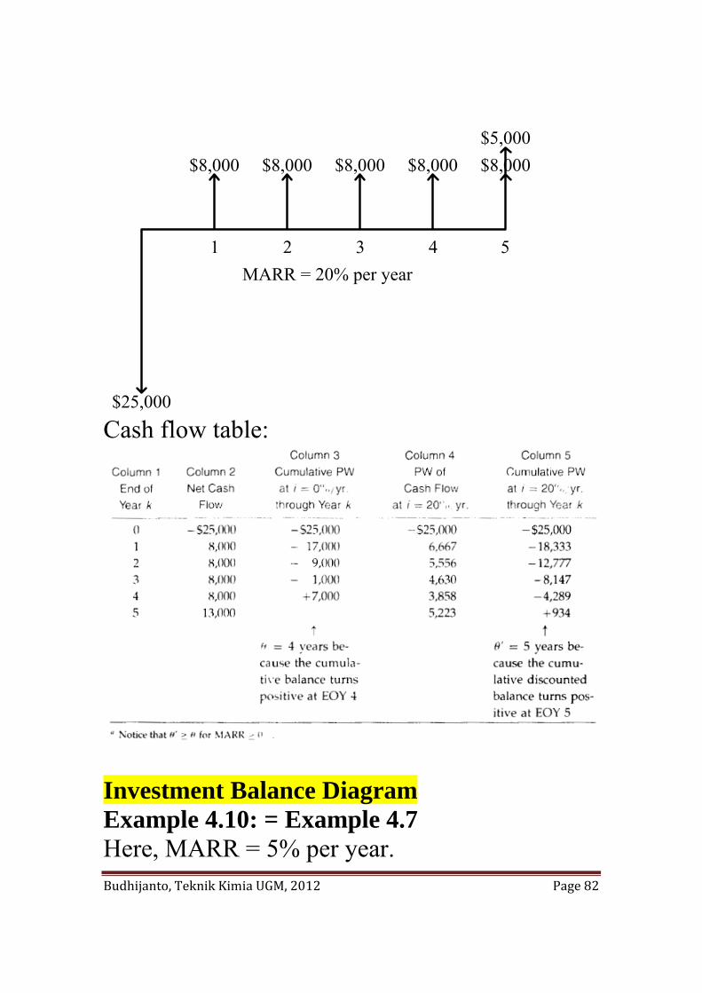
Budhijanto, Teknik Kimia UGM, 2012 Page 82
$25,000
$8,000 $8,000 $8,000 $8,000 $8,000$5,000
MARR = 20% per year1 2 3 4 5
Cash flow table:
Investment Balance Diagram Example 4.10: = Example 4.7 Here, MARR = 5% per year.
Budhijanto, Teknik Kimia UGM, 2012 Page 83
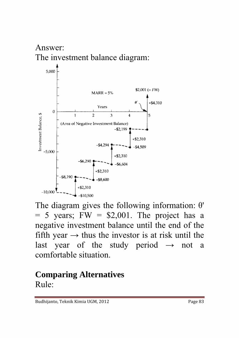
Answer: The investment balance diagram:
The diagram gives the following information: θ' = 5 years; FW = $2,001. The project has a negative investment balance until the end of the fifth year → thus the investor is at risk until the last year of the study period → not a comfortable situation. Comparing Alternatives Rule:
Budhijanto, Teknik Kimia UGM, 2012 Page 84
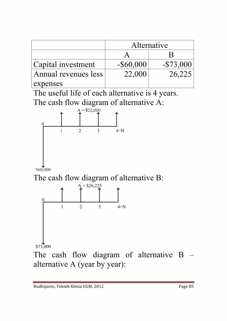
The alternative that requires the minimum investment of capital and produces satisfactory functional results will be chosen unless the incremental capital associated with an alternative having a larger investment can be justified with respect to its incremental benefits. The base alternative: the acceptable alternative that requires the least investment of capital. This rule will keep as much capital as possible invested at a rate of return equal to or greater than the MARR. Case study: Alternatives A and B are two mutually exclusive investment alternatives. (Two or more alternatives are mutually exclusive when the selection of one of these alternatives excludes the choice of any of the others. Investment alternatives are those with initial (or front-end) capital investment(s) that produce positive cash flows from increased revenue, savings through reduced costs, or both.) The estimated net cash flows of the alternatives are as follows.
Budhijanto, Teknik Kimia UGM, 2012 Page 85
Alternative A B Capital investment -$60,000 -$73,000Annual revenues less expenses
22,000 26,225
The useful life of each alternative is 4 years. The cash flow diagram of alternative A:
The cash flow diagram of alternative B:
$73,000
A = $26,225
1 2 3 4=N0
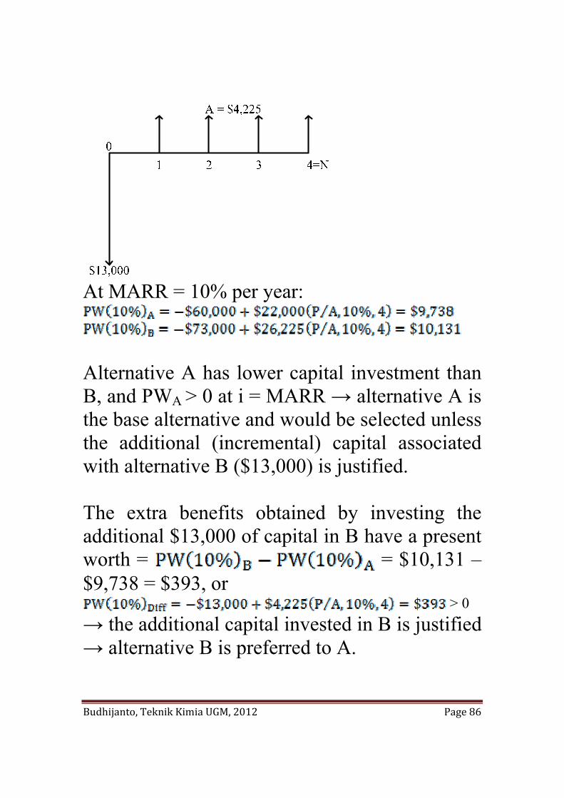
The cash flow diagram of alternative B – alternative A (year by year):
Budhijanto, Teknik Kimia UGM, 2012 Page 86
At MARR = 10% per year:
Alternative A has lower capital investment than B, and PWA > 0 at i = MARR → alternative A is the base alternative and would be selected unless the additional (incremental) capital associated with alternative B ($13,000) is justified. The extra benefits obtained by investing the additional $13,000 of capital in B have a present worth = = $10,131 – $9,738 = $393, or
> 0 → the additional capital invested in B is justified → alternative B is preferred to A.
Budhijanto, Teknik Kimia UGM, 2012 Page 87
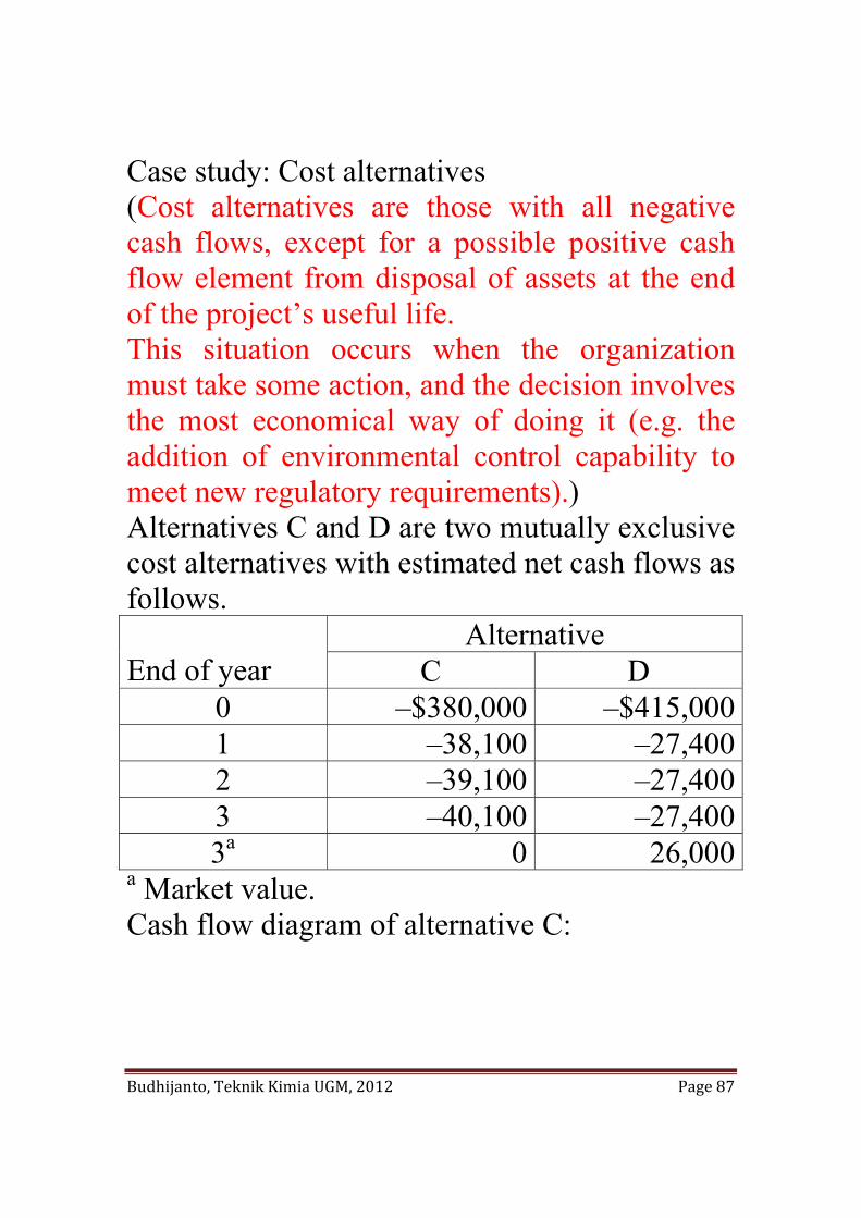
Case study: Cost alternatives (Cost alternatives are those with all negative cash flows, except for a possible positive cash flow element from disposal of assets at the end of the project’s useful life. This situation occurs when the organization must take some action, and the decision involves the most economical way of doing it (e.g. the addition of environmental control capability to meet new regulatory requirements).) Alternatives C and D are two mutually exclusive cost alternatives with estimated net cash flows as follows. End of year
AlternativeC D
0 –$380,000 –$415,0001 –38,100 –27,4002 –39,100 –27,4003 –40,100 –27,4003a 0 26,000
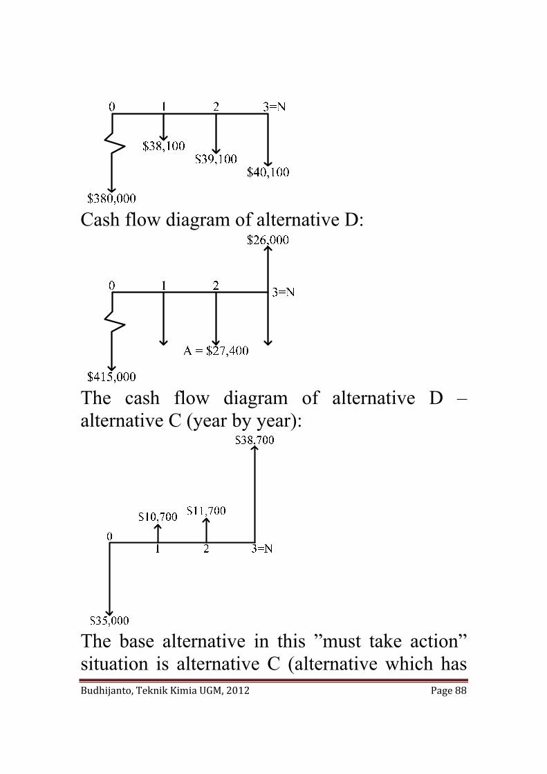
a Market value. Cash flow diagram of alternative C:
Budhijanto, Teknik Kimia UGM, 2012 Page 88
Cash flow diagram of alternative D:
The cash flow diagram of alternative D – alternative C (year by year):
The base alternative in this ”must take action” situation is alternative C (alternative which has
Budhijanto, Teknik Kimia UGM, 2012 Page 89
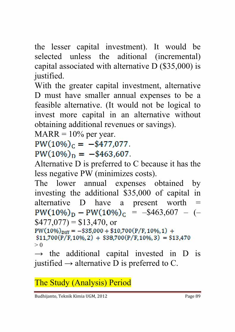
the lesser capital investment). It would be selected unless the aditional (incremental) capital associated with alternative D ($35,000) is justified. With the greater capital investment, alternative D must have smaller annual expenses to be a feasible alternative. (It would not be logical to invest more capital in an alternative without obtaining additional revenues or savings). MARR = 10% per year.
. .
Alternative D is preferred to C because it has the less negative PW (minimizes costs). The lower annual expenses obtained by investing the additional $35,000 of capital in alternative D have a present worth =
= –$463,607 – (– $477,077) = $13,470, or
> 0 → the additional capital invested in D is justified → alternative D is preferred to C. The Study (Analysis) Period
Budhijanto, Teknik Kimia UGM, 2012 Page 90
The study (analysis) period = the planning horizon = the selected time period over which mutually exclusive alternatives are compared. Factors that may influence the determination of the study period are the service period required, the useful lives of the alternatives, company policy, and so on. The useful life of an asset is the period during which it is kept in productive use in a trade or business. Case 1: Useful lives are the same for all alternatives and equal to the study period 1.1. Equivalent Worth Methods. There are 3 methods in this category that we have learned, i.e. the PW, AW, and FW methods. When these 3 methods are used, the conclusion will be the same. Thus, if and only if PW(i%)A < PW(i%)B, then AW(i%)A < AW(i%)B and FW(i%)A < FW(i%)B. Proof: a. PW(i%)A < PW(i%)B PW(i%)A < PW(i%)B
AW(i%)A < AW(i%)B b. PW(i%)A < PW(i%)B
Budhijanto, Teknik Kimia UGM, 2012 Page 91
PW(i%)A < PW(i%)B FW(i%)A < FW(i%)B
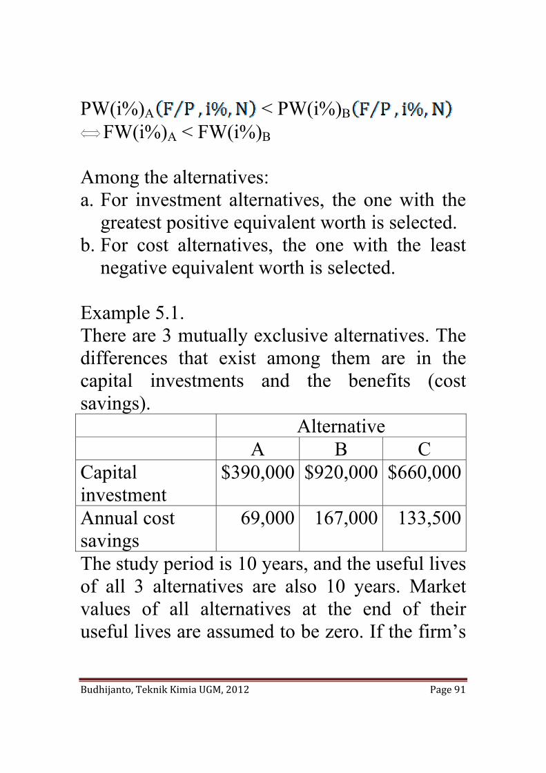
Among the alternatives: a. For investment alternatives, the one with the
greatest positive equivalent worth is selected. b. For cost alternatives, the one with the least
negative equivalent worth is selected. Example 5.1. There are 3 mutually exclusive alternatives. The differences that exist among them are in the capital investments and the benefits (cost savings). Alternative A B C Capital investment
$390,000 $920,000 $660,000
Annual cost savings
69,000 167,000 133,500
The study period is 10 years, and the useful lives of all 3 alternatives are also 10 years. Market values of all alternatives at the end of their useful lives are assumed to be zero. If the firm’s
Budhijanto, Teknik Kimia UGM, 2012 Page 92
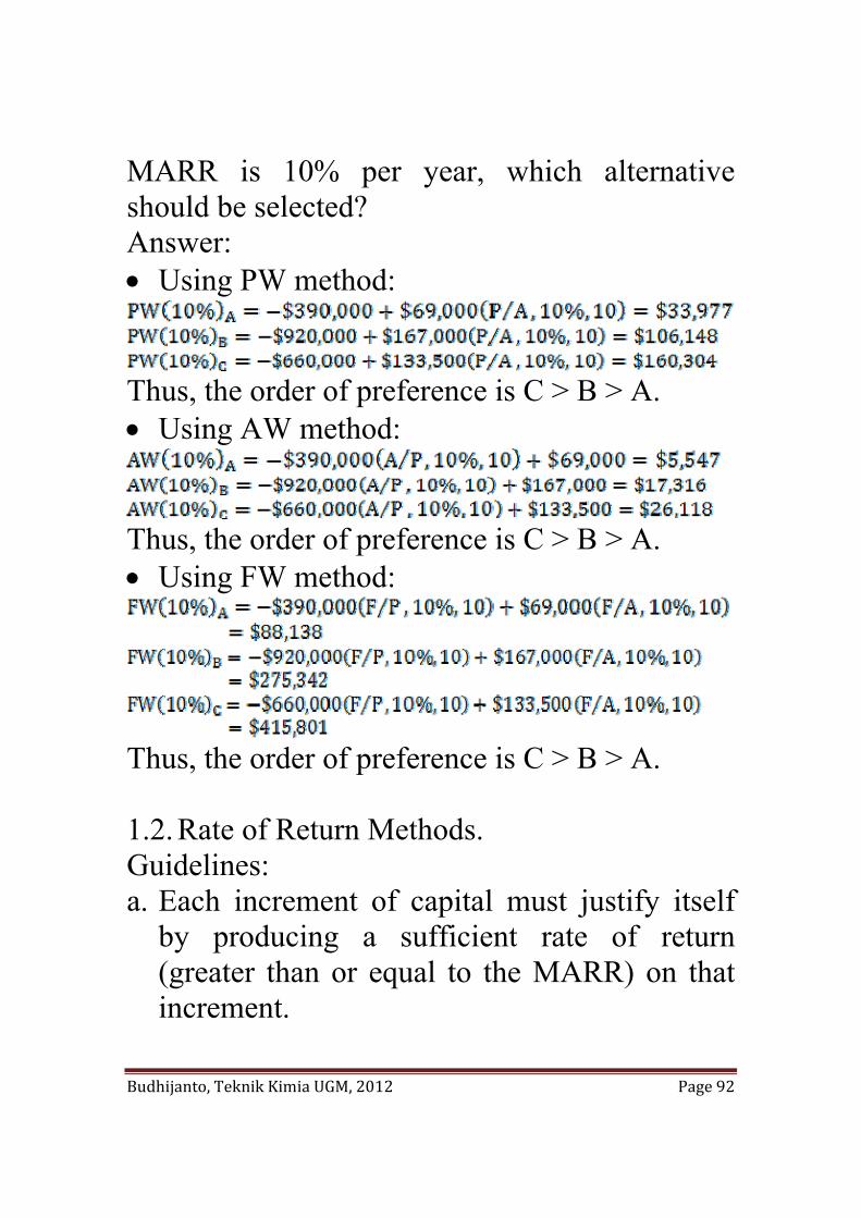
MARR is 10% per year, which alternative should be selected? Answer: • Using PW method:
Thus, the order of preference is C > B > A. • Using AW method:
Thus, the order of preference is C > B > A. • Using FW method:
Thus, the order of preference is C > B > A. 1.2. Rate of Return Methods. Guidelines: a. Each increment of capital must justify itself
by producing a sufficient rate of return (greater than or equal to the MARR) on that increment.
Budhijanto, Teknik Kimia UGM, 2012 Page 93
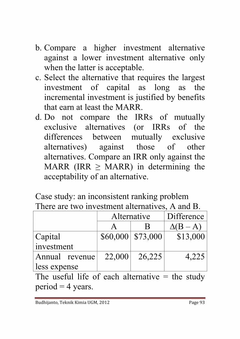
b. Compare a higher investment alternative against a lower investment alternative only when the latter is acceptable.
c. Select the alternative that requires the largest investment of capital as long as the incremental investment is justified by benefits that earn at least the MARR.
d. Do not compare the IRRs of mutually exclusive alternatives (or IRRs of the differences between mutually exclusive alternatives) against those of other alternatives. Compare an IRR only against the MARR (IRR ≥ MARR) in determining the acceptability of an alternative.
Case study: an inconsistent ranking problem There are two investment alternatives, A and B. Alternative Difference
A B ∆(B – A) Capital investment
$60,000 $73,000 $13,000
Annual revenue less expense
22,000 26,225 4,225
The useful life of each alternative = the study period = 4 years.
Budhijanto, Teknik Kimia UGM, 2012 Page 94
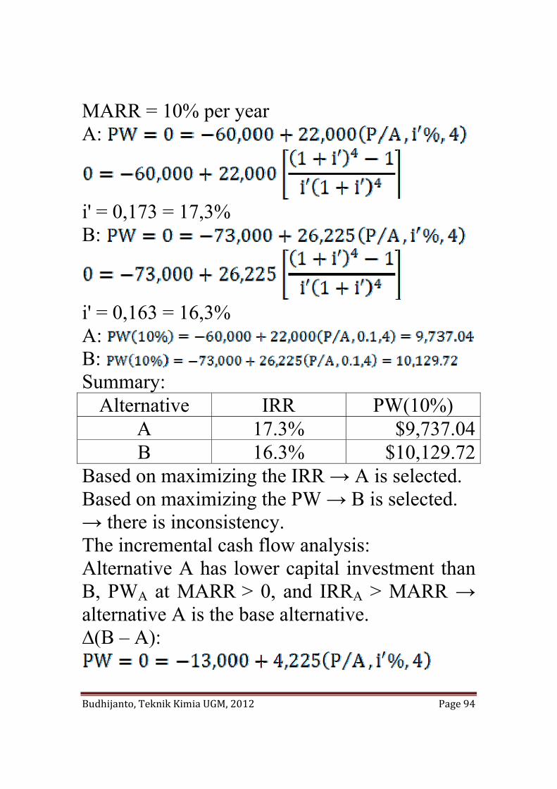
MARR = 10% per year A:
i' = 0,173 = 17,3% B:
i' = 0,163 = 16,3% A: B: Summary:
Alternative IRR PW(10%) A 17.3% $9,737.04B 16.3% $10,129.72
Based on maximizing the IRR → A is selected. Based on maximizing the PW → B is selected. → there is inconsistency. The incremental cash flow analysis: Alternative A has lower capital investment than B, PWA at MARR > 0, and IRRA > MARR → alternative A is the base alternative. ∆(B – A):
Budhijanto, Teknik Kimia UGM, 2012 Page 95
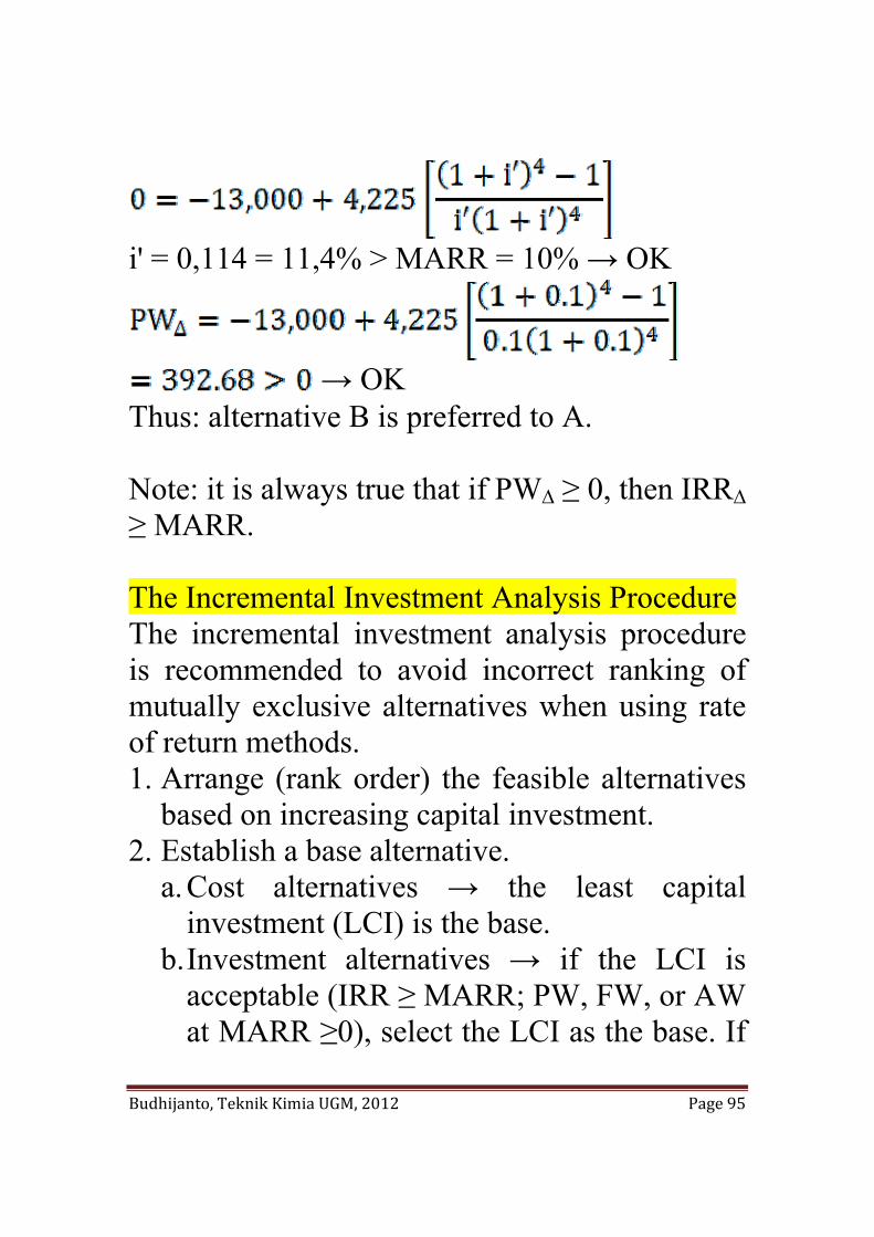
i' = 0,114 = 11,4% > MARR = 10% → OK
→ OK
Thus: alternative B is preferred to A. Note: it is always true that if PW∆ ≥ 0, then IRR∆ ≥ MARR. The Incremental Investment Analysis Procedure The incremental investment analysis procedure is recommended to avoid incorrect ranking of mutually exclusive alternatives when using rate of return methods. 1. Arrange (rank order) the feasible alternatives
based on increasing capital investment. 2. Establish a base alternative.
a. Cost alternatives → the least capital investment (LCI) is the base.
b. Investment alternatives → if the LCI is acceptable (IRR ≥ MARR; PW, FW, or AW at MARR ≥0), select the LCI as the base. If
Budhijanto, Teknik Kimia UGM, 2012 Page 96
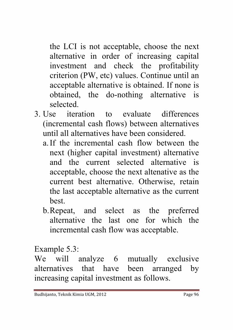
the LCI is not acceptable, choose the next alternative in order of increasing capital investment and check the profitability criterion (PW, etc) values. Continue until an acceptable alternative is obtained. If none is obtained, the do-nothing alternative is selected.
3. Use iteration to evaluate differences (incremental cash flows) between alternatives until all alternatives have been considered. a. If the incremental cash flow between the
next (higher capital investment) alternative and the current selected alternative is acceptable, choose the next altenative as the current best alternative. Otherwise, retain the last acceptable alternative as the current best.
b. Repeat, and select as the preferred alternative the last one for which the incremental cash flow was acceptable.
Example 5.3: We will analyze 6 mutually exclusive alternatives that have been arranged by increasing capital investment as follows.
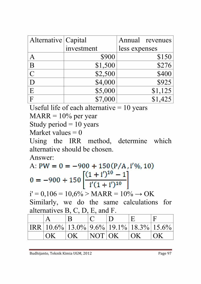
Budhijanto, Teknik Kimia UGM, 2012 Page 97
Alternative Capital investment
Annual revenues less expenses
A $900 $150B $1,500 $276C $2,500 $400D $4,000 $925E $5,000 $1,125F $7,000 $1,425Useful life of each alternative = 10 years MARR = 10% per year Study period = 10 years Market values = 0 Using the IRR method, determine which alternative should be chosen. Answer: A:
i' = 0,106 = 10,6% > MARR = 10% → OK Similarly, we do the same calculations for alternatives B, C, D, E, and F. A B C D E F IRR 10.6% 13.0% 9.6% 19.1% 18.3% 15.6% OK OK NOT OK OK OK
Budhijanto, Teknik Kimia UGM, 2012 Page 98
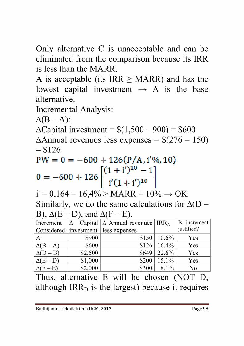
Only alternative C is unacceptable and can be eliminated from the comparison because its IRR is less than the MARR. A is acceptable (its IRR ≥ MARR) and has the lowest capital investment → A is the base alternative. Incremental Analysis: ∆(B – A): ∆Capital investment = $(1,500 – 900) = $600 ∆Annual revenues less expenses = $(276 – 150) = $126
i' = 0,164 = 16,4% > MARR = 10% → OK Similarly, we do the same calculations for ∆(D – B), ∆(E – D), and ∆(F – E). Increment Considered
∆ Capital investment
∆ Annual revenues less expenses
IRR∆ Is increment justified?
A $900 $150 10.6% Yes ∆(B – A) $600 $126 16.4% Yes ∆(D – B) $2,500 $649 22.6% Yes ∆(E – D) $1,000 $200 15.1% Yes ∆(F – E) $2,000 $300 8.1% No Thus, alternative E will be chosen (NOT D, although IRRD is the largest) because it requires
Budhijanto, Teknik Kimia UGM, 2012 Page 99
the largest investment for which the last increment of capital investment is justified. Case 2: Useful lives are different among the alternatives and at least one does not match the study period The principle: ”Compare the mutually exclusive alternatives being considered in a decision situation over the same study period.” There are two types of assumptions used in the comparisons. a. The repeatability assumption This assumption involves two main conditions: a.1. The study period over which the alternatives are being compared is either indefinitely long or equal to a common multiple of the lives of the alternatives. a.2. The economic consequences that are estimated to happen in an alternative’s initial useful life span will also happen in all succeeding life spans (replacements). b. The coterminated assumption
Budhijanto, Teknik Kimia UGM, 2012 Page 100
This assumption uses a finite and identical study period for all alternatives → needs appropriate adjustments to the estimated cash flows. The guidelines: b.1. (Useful life) < (study period) b.1.1. Cost alternatives: Because each cost alternative has to provide the same level of service over the study period, contracting for the service or leasing the needed equipment for the remaining years may be appropriate. Another potential course of action is to repeat part of the useful life of the original alternative, and then use an estimated market value to truncate it at the end of the study period. b.1.2. Investment alternatives: The first asumption is that all cash flows will be reinvested in other opportunities available to the firm at the MARR to the end of the study period. A second assumption involves replacing the initial investment with another asset having possibly different cash flows over the remaining life. b.2. (Useful life) > (study period) The most common technique is to truncate the alternative at the end of the study period using
Budhijanto, Teknik Kimia UGM, 2012 Page 101
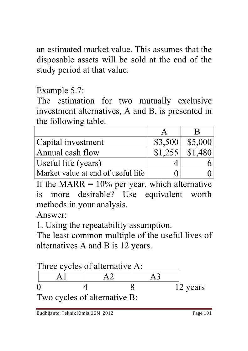
an estimated market value. This assumes that the disposable assets will be sold at the end of the study period at that value. Example 5.7: The estimation for two mutually exclusive investment alternatives, A and B, is presented in the following table. A B Capital investment $3,500 $5,000Annual cash flow $1,255 $1,480Useful life (years) 4 6Market value at end of useful life 0 0If the MARR = 10% per year, which alternative is more desirable? Use equivalent worth methods in your analysis. Answer: 1. Using the repeatability assumption. The least common multiple of the useful lives of alternatives A and B is 12 years. Three cycles of alternative A:
A1 A2 A3 0 4 8 12 years Two cycles of alternative B:
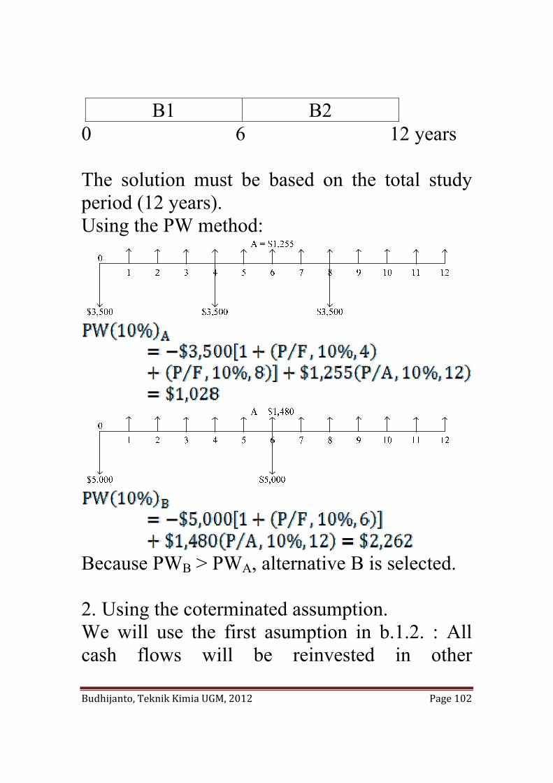
Budhijanto, Teknik Kimia UGM, 2012 Page 102
B1 B2 0 6 12 years The solution must be based on the total study period (12 years). Using the PW method:
Because PWB > PWA, alternative B is selected. 2. Using the coterminated assumption. We will use the first asumption in b.1.2. : All cash flows will be reinvested in other
Budhijanto, Teknik Kimia UGM, 2012 Page 103
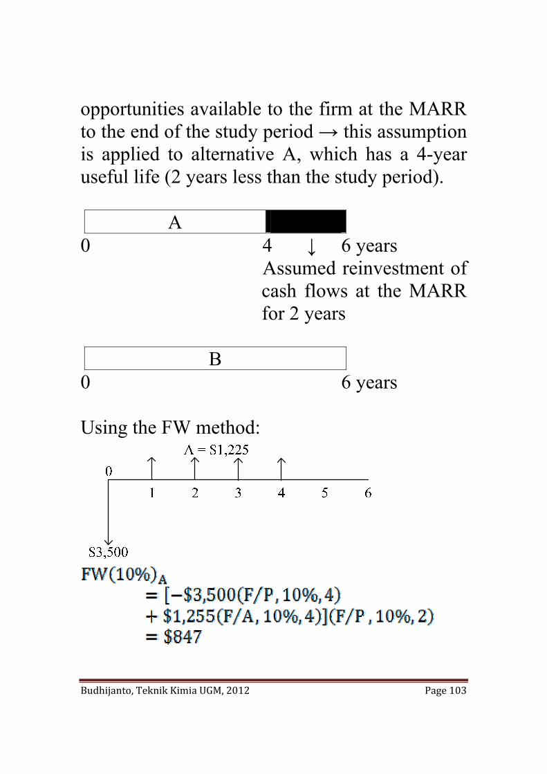
opportunities available to the firm at the MARR to the end of the study period → this assumption is applied to alternative A, which has a 4-year useful life (2 years less than the study period).
A 0 4 ↓ 6 years Assumed reinvestment of
cash flows at the MARR for 2 years
B
0 6 years Using the FW method:
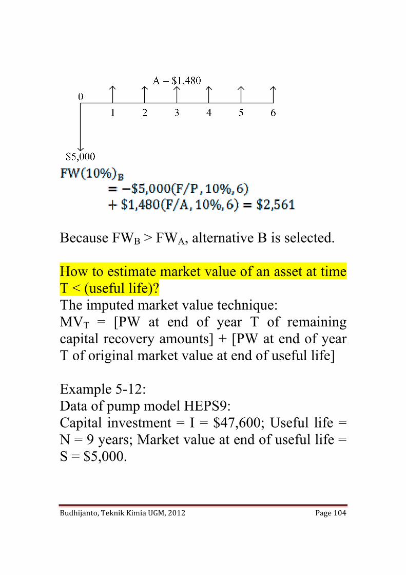
Budhijanto, Teknik Kimia UGM, 2012 Page 104
Because FWB > FWA, alternative B is selected. How to estimate market value of an asset at time T < (useful life)? The imputed market value technique: MVT = [PW at end of year T of remaining capital recovery amounts] + [PW at end of year T of original market value at end of useful life] Example 5-12: Data of pump model HEPS9: Capital investment = I = $47,600; Useful life = N = 9 years; Market value at end of useful life = S = $5,000.
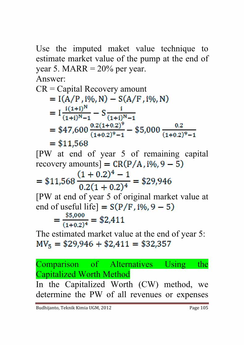
Budhijanto, Teknik Kimia UGM, 2012 Page 105
Use the imputed maket value technique to estimate market value of the pump at the end of year 5. MARR = 20% per year. Answer: CR = Capital Recovery amount
[PW at end of year 5 of remaining capital recovery amounts]
[PW at end of year 5 of original market value at end of useful life] The estimated market value at the end of year 5:
Comparison of Alternatives Using the Capitalized Worth Method In the Capitalized Worth (CW) method, we determine the PW of all revenues or expenses
Budhijanto, Teknik Kimia UGM, 2012 Page 106
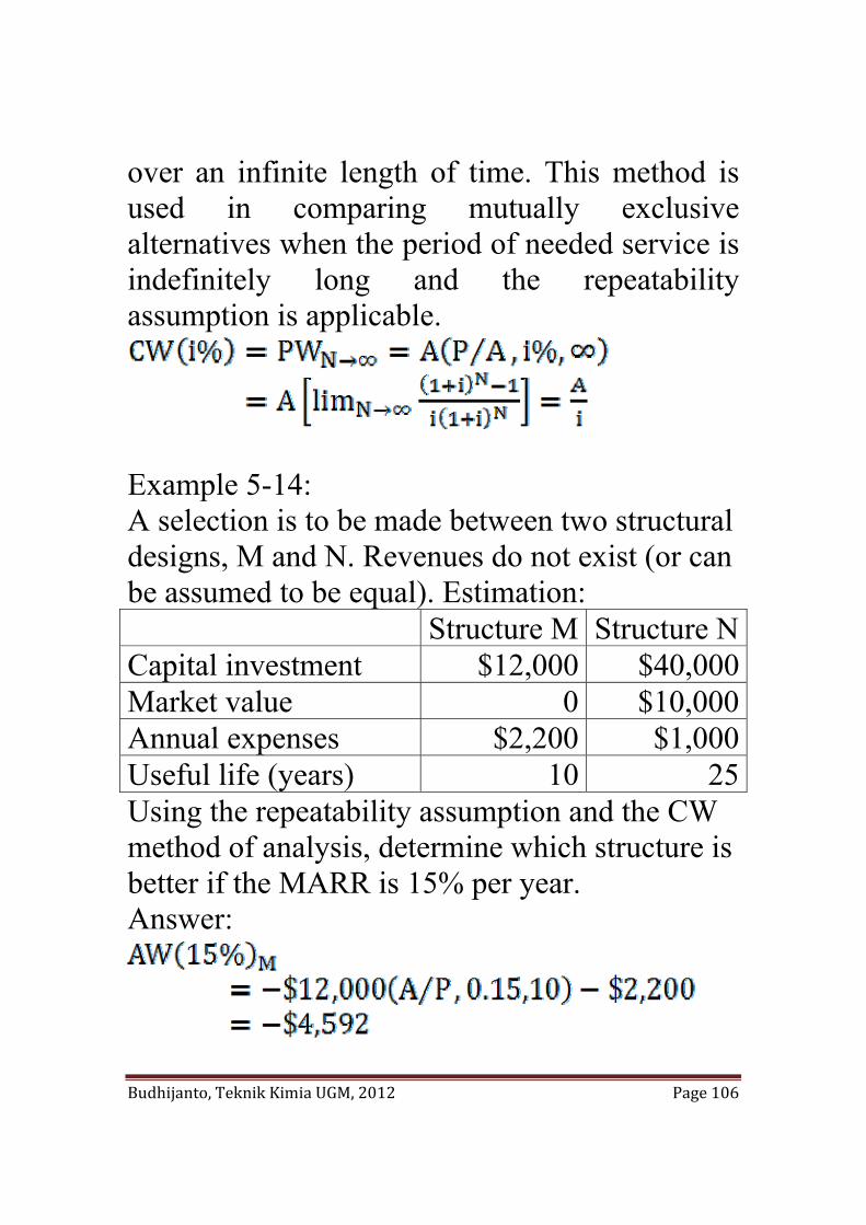
over an infinite length of time. This method is used in comparing mutually exclusive alternatives when the period of needed service is indefinitely long and the repeatability assumption is applicable.
Example 5-14: A selection is to be made between two structural designs, M and N. Revenues do not exist (or can be assumed to be equal). Estimation: Structure M Structure NCapital investment $12,000 $40,000Market value 0 $10,000Annual expenses $2,200 $1,000Useful life (years) 10 25Using the repeatability assumption and the CW method of analysis, determine which structure is better if the MARR is 15% per year. Answer:
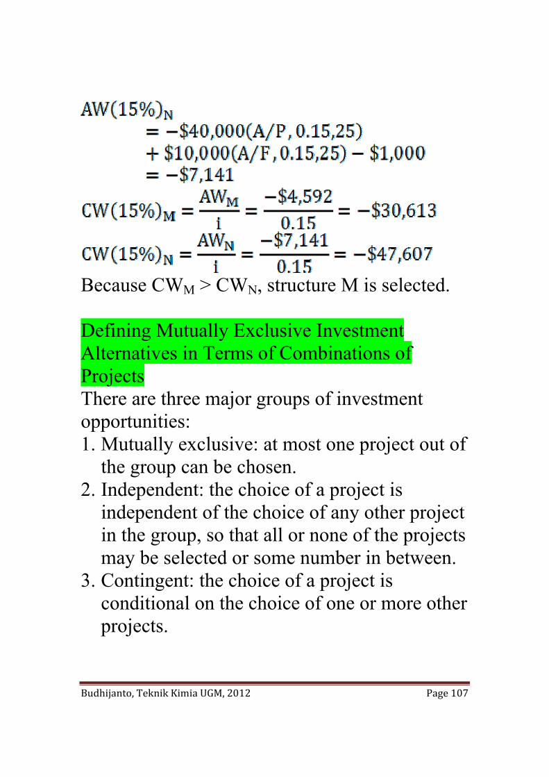
Budhijanto, Teknik Kimia UGM, 2012 Page 107
Because CWM > CWN, structure M is selected. Defining Mutually Exclusive Investment Alternatives in Terms of Combinations of Projects There are three major groups of investment opportunities: 1. Mutually exclusive: at most one project out of
the group can be chosen. 2. Independent: the choice of a project is
independent of the choice of any other project in the group, so that all or none of the projects may be selected or some number in between.
3. Contingent: the choice of a project is conditional on the choice of one or more other projects.
Budhijanto, Teknik Kimia UGM, 2012 Page 108
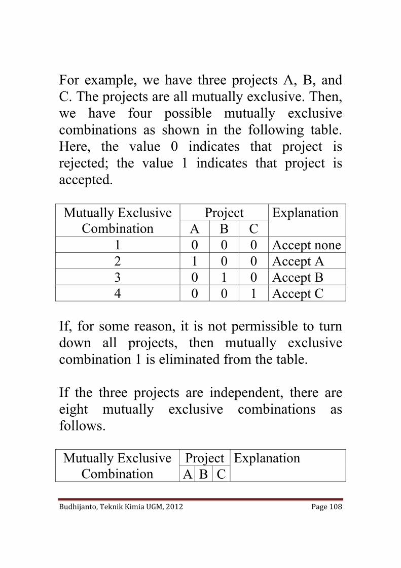
For example, we have three projects A, B, and C. The projects are all mutually exclusive. Then, we have four possible mutually exclusive combinations as shown in the following table. Here, the value 0 indicates that project is rejected; the value 1 indicates that project is accepted. Mutually Exclusive
Combination Project Explanation
A B C 1 0 0 0 Accept none2 1 0 0 Accept A 3 0 1 0 Accept B 4 0 0 1 Accept C
If, for some reason, it is not permissible to turn down all projects, then mutually exclusive combination 1 is eliminated from the table. If the three projects are independent, there are eight mutually exclusive combinations as follows. Mutually Exclusive
Combination Project Explanation A B C
Budhijanto, Teknik Kimia UGM, 2012 Page 109
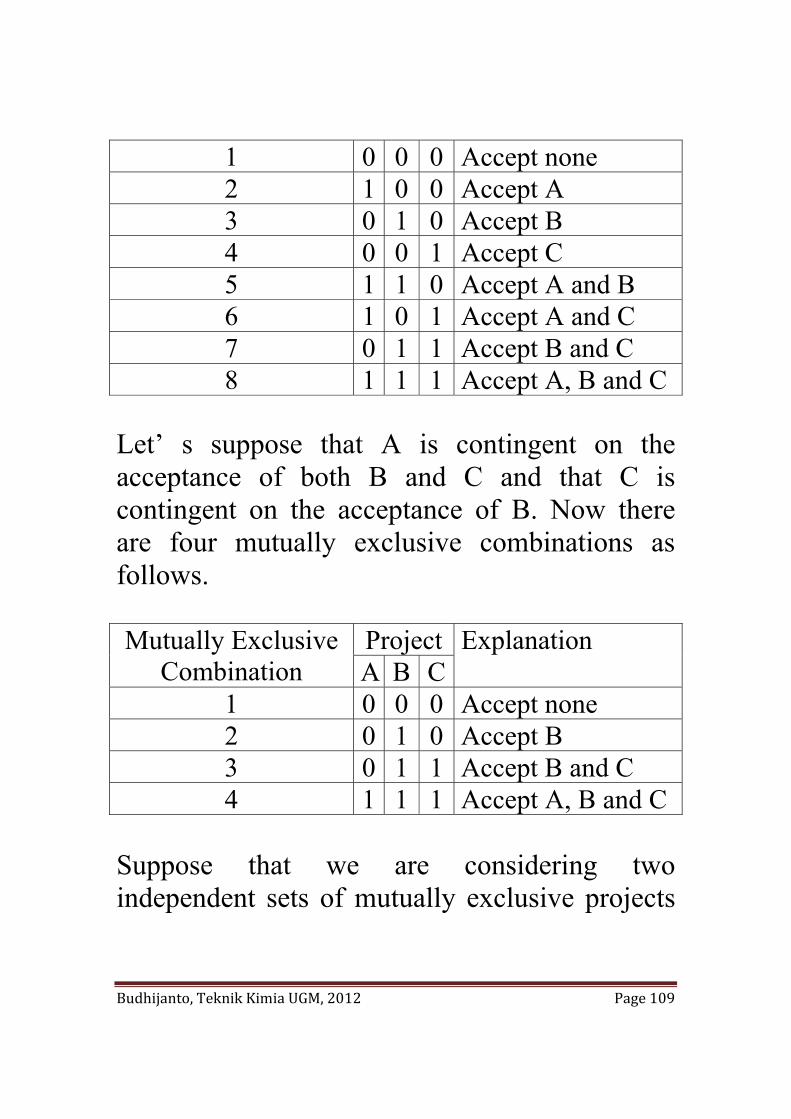
1 0 0 0 Accept none 2 1 0 0 Accept A 3 0 1 0 Accept B 4 0 0 1 Accept C 5 1 1 0 Accept A and B 6 1 0 1 Accept A and C 7 0 1 1 Accept B and C 8 1 1 1 Accept A, B and C
Let’ s suppose that A is contingent on the acceptance of both B and C and that C is contingent on the acceptance of B. Now there are four mutually exclusive combinations as follows. Mutually Exclusive
Combination Project Explanation A B C
1 0 0 0 Accept none 2 0 1 0 Accept B 3 0 1 1 Accept B and C 4 1 1 1 Accept A, B and C
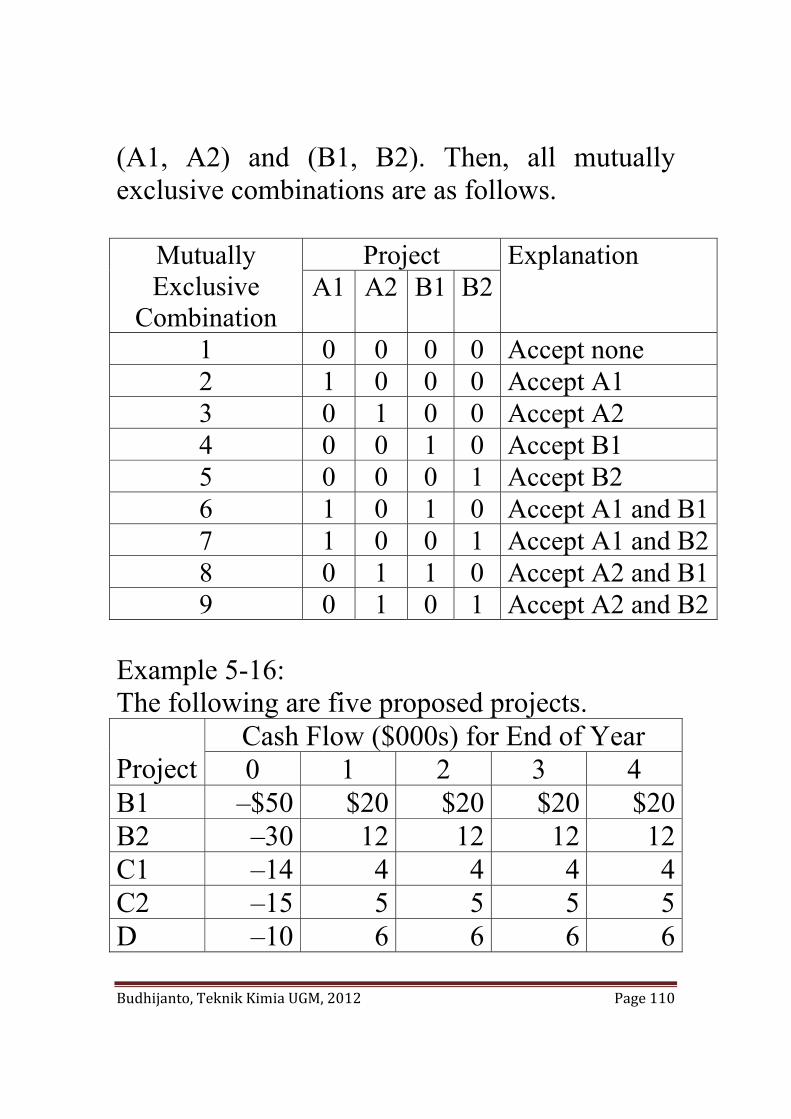
Suppose that we are considering two independent sets of mutually exclusive projects
Budhijanto, Teknik Kimia UGM, 2012 Page 110
(A1, A2) and (B1, B2). Then, all mutually exclusive combinations are as follows.
Mutually Exclusive
Combination
Project Explanation A1 A2 B1 B2
1 0 0 0 0 Accept none 2 1 0 0 0 Accept A1 3 0 1 0 0 Accept A2 4 0 0 1 0 Accept B1 5 0 0 0 1 Accept B2 6 1 0 1 0 Accept A1 and B17 1 0 0 1 Accept A1 and B28 0 1 1 0 Accept A2 and B19 0 1 0 1 Accept A2 and B2
Example 5-16: The following are five proposed projects. Project
Cash Flow ($000s) for End of Year 0 1 2 3 4
B1 –$50 $20 $20 $20 $20B2 –30 12 12 12 12C1 –14 4 4 4 4C2 –15 5 5 5 5D –10 6 6 6 6
Budhijanto, Teknik Kimia UGM, 2012 Page 111
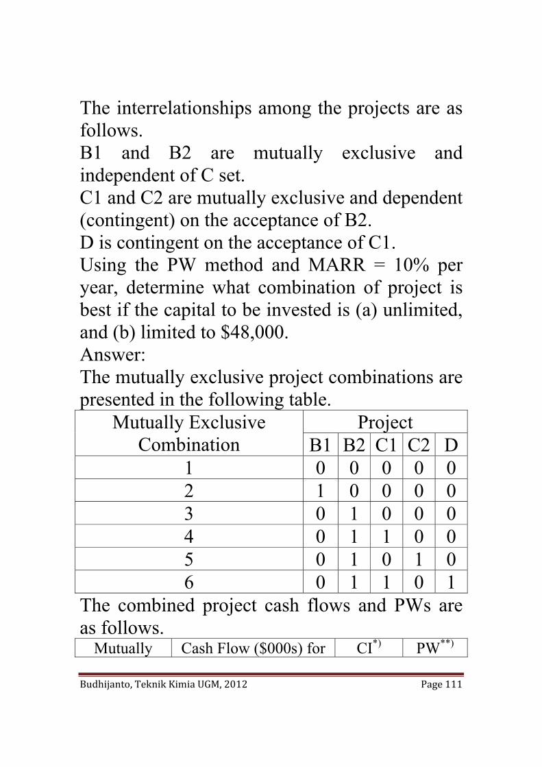
The interrelationships among the projects are as follows. B1 and B2 are mutually exclusive and independent of C set. C1 and C2 are mutually exclusive and dependent (contingent) on the acceptance of B2. D is contingent on the acceptance of C1. Using the PW method and MARR = 10% per year, determine what combination of project is best if the capital to be invested is (a) unlimited, and (b) limited to $48,000. Answer: The mutually exclusive project combinations are presented in the following table.
Mutually Exclusive Combination
Project B1 B2 C1 C2 D
1 0 0 0 0 0 2 1 0 0 0 0 3 0 1 0 0 0 4 0 1 1 0 0 5 0 1 0 1 0 6 0 1 1 0 1
The combined project cash flows and PWs are as follows.
Mutually Cash Flow ($000s) for CI*) PW**)
Budhijanto, Teknik Kimia UGM, 2012 Page 112
Exclusive Combination
End of Year ($000s) ($000s)0 1 2 3 4
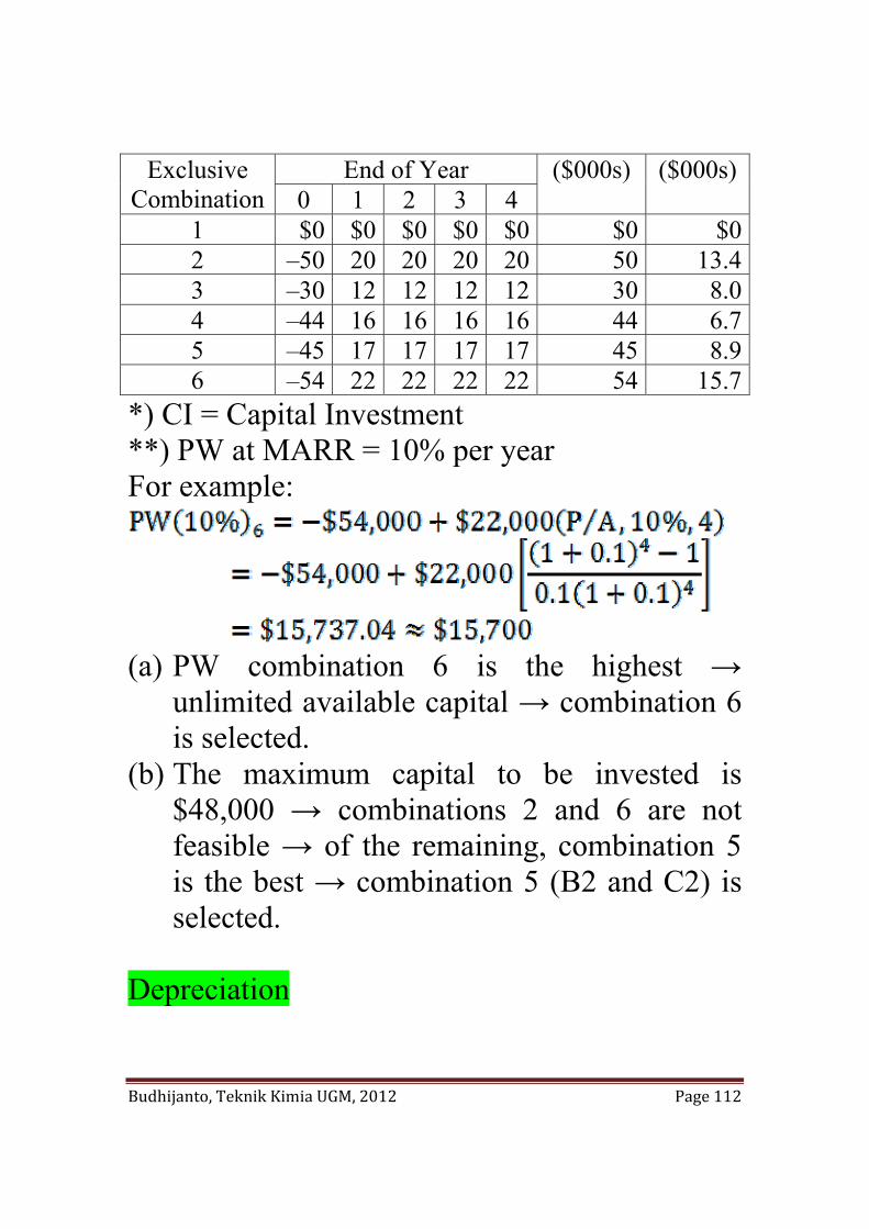
1 $0 $0 $0 $0 $0 $0 $02 –50 20 20 20 20 50 13.43 –30 12 12 12 12 30 8.04 –44 16 16 16 16 44 6.75 –45 17 17 17 17 45 8.96 –54 22 22 22 22 54 15.7
*) CI = Capital Investment **) PW at MARR = 10% per year For example:
(a) PW combination 6 is the highest →
unlimited available capital → combination 6 is selected.
(b) The maximum capital to be invested is $48,000 → combinations 2 and 6 are not feasible → of the remaining, combination 5 is the best → combination 5 (B2 and C2) is selected.
Depreciation
Budhijanto, Teknik Kimia UGM, 2012 Page 113
Depreciation is the decrease in value of physical properties with the passage of time and use. More specifically, depreciation is an annual deduction against before-tax income such that the effect of time and use on an asset’s value can be reflected in a firm’s financial statement. Depreciation is a noncash cost that affects income taxes. In general property is depreciable if: 1. It must be used in business or held to produce
income. 2. It must have a determinable useful life, and
the life must be longer than one year. 3. It must be something that wears out, decays,
gets used up, becomes obsolete, or loses value from natural causes.
4. It is not inventory, stock in trade, or investment property.
Examples of depreciable properties: machinery, vehicles, equipment, furniture, buildings, copyright, patent, franchise, etc. Depreciation Methods a. Straight-Line (SL) Method Let:
Budhijanto, Teknik Kimia UGM, 2012 Page 114
N = depreciable life of the asset in years = estimated period that a property will be used in a trade or business to produce income. It is not how long the property will last, but how long the owner expects to productively use it. B = cost basis, including allowable adjustments. Cost basis = the initial cost of acquiring an asset (purchase price plus any sales taxes), including transportation expenses and other normal costs of making the asset serviceable for its intended use. Example of allowable adjustments: cost of any improvement to a capital asset with a useful life greater than one year increases the original cost basis. dk = annual depreciation deduction in year k (1≤ k ≤ N) BVk = book value at end of year k = adjusted cost basis minus total depreciation deduction until end of year k. SVN = estimated salvage value at end of year N.
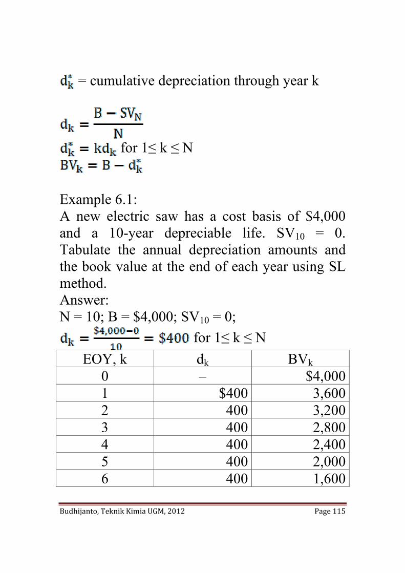
Budhijanto, Teknik Kimia UGM, 2012 Page 115
= cumulative depreciation through year k
for 1≤ k ≤ N
Example 6.1: A new electric saw has a cost basis of $4,000 and a 10-year depreciable life. SV10 = 0. Tabulate the annual depreciation amounts and the book value at the end of each year using SL method. Answer: N = 10; B = $4,000; SV10 = 0;
for 1≤ k ≤ N EOY, k dk BVk
0 – $4,0001 $400 3,6002 400 3,2003 400 2,8004 400 2,4005 400 2,0006 400 1,600
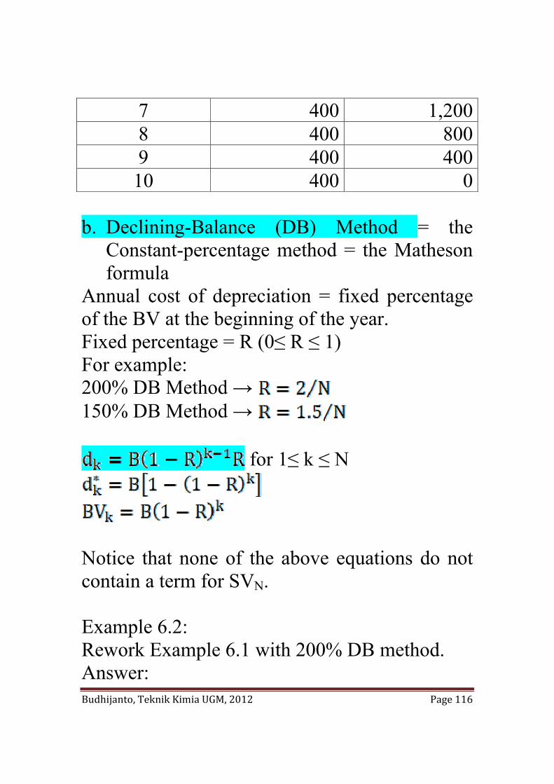
Budhijanto, Teknik Kimia UGM, 2012 Page 116
7 400 1,2008 400 8009 400 400
10 400 0 b. Declining-Balance (DB) Method = the
Constant-percentage method = the Matheson formula
Annual cost of depreciation = fixed percentage of the BV at the beginning of the year. Fixed percentage = R (0≤ R ≤ 1) For example: 200% DB Method → 150% DB Method →
for 1≤ k ≤ N
Notice that none of the above equations do not contain a term for SVN. Example 6.2: Rework Example 6.1 with 200% DB method. Answer:
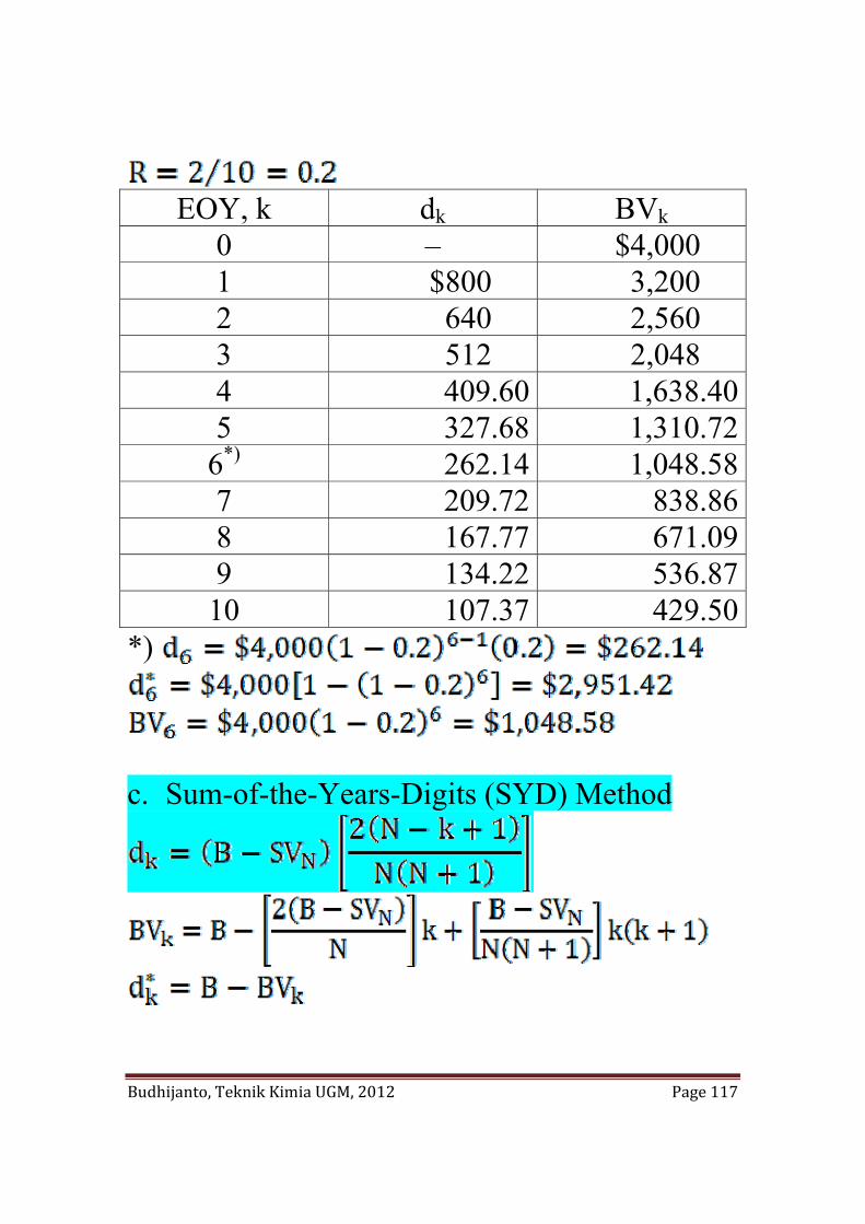
Budhijanto, Teknik Kimia UGM, 2012 Page 117
EOY, k dk BVk
0 – $4,000 1 $800 3,200 2 640 2,560 3 512 2,048 4 409.60 1,638.405 327.68 1,310.72
6*) 262.14 1,048.587 209.72 838.868 167.77 671.099 134.22 536.87
10 107.37 429.50*)
c. Sum-of-the-Years-Digits (SYD) Method
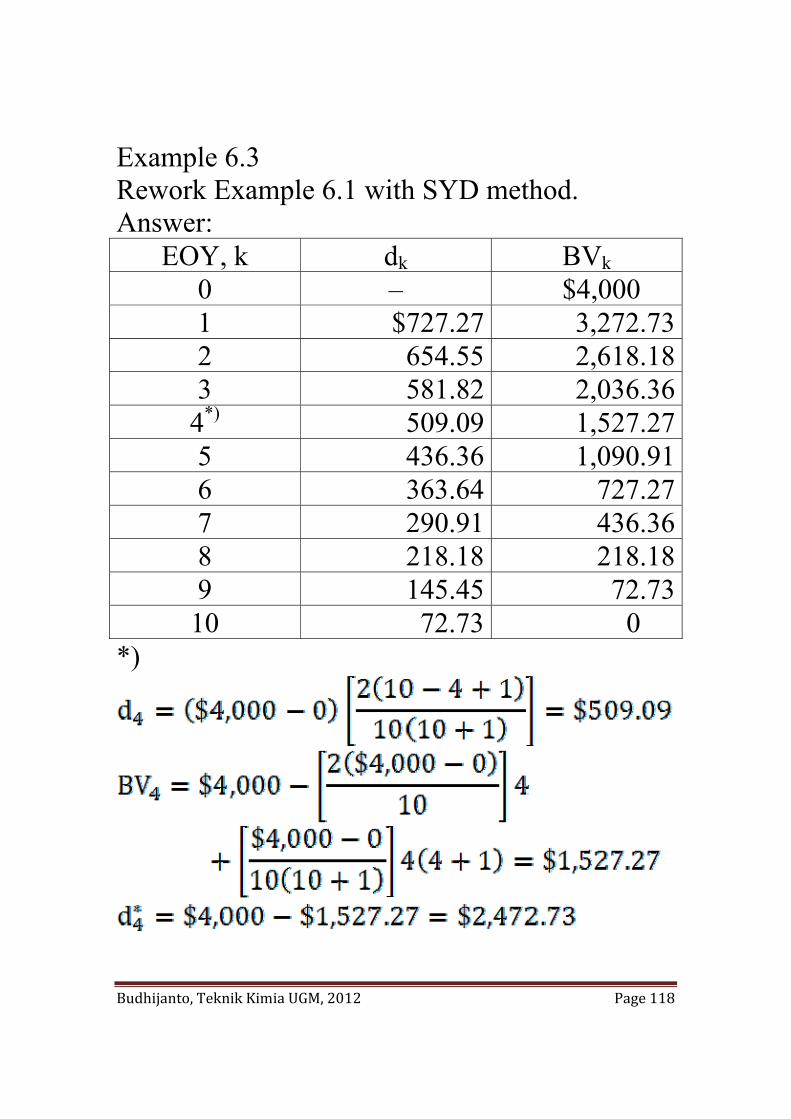
Budhijanto, Teknik Kimia UGM, 2012 Page 118
Example 6.3 Rework Example 6.1 with SYD method. Answer:
EOY, k dk BVk 0 – $4,000 1 $727.27 3,272.732 654.55 2,618.183 581.82 2,036.36
4*) 509.09 1,527.275 436.36 1,090.916 363.64 727.277 290.91 436.368 218.18 218.189 145.45 72.73
10 72.73 0 *)
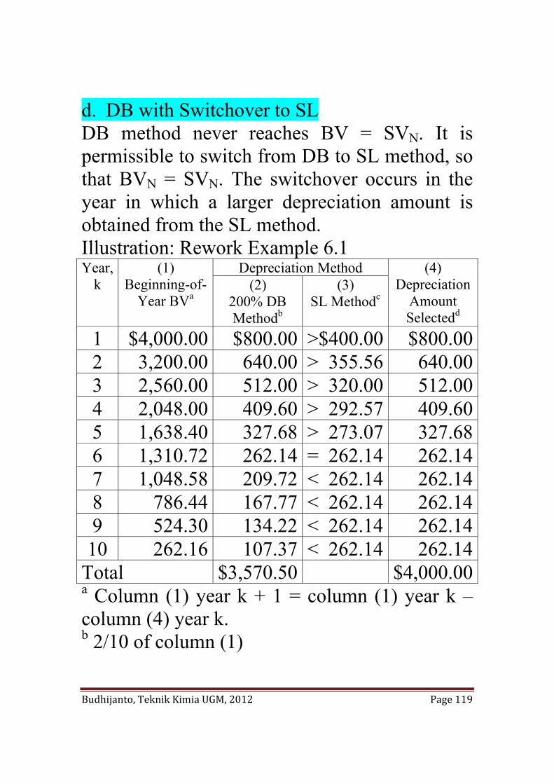
Budhijanto, Teknik Kimia UGM, 2012 Page 119
d. DB with Switchover to SL DB method never reaches BV = SVN. It is permissible to switch from DB to SL method, so that BVN = SVN. The switchover occurs in the year in which a larger depreciation amount is obtained from the SL method. Illustration: Rework Example 6.1 Year,
k (1)
Beginning-of-Year BVa
Depreciation Method (4) Depreciation
Amount Selectedd
(2) 200% DB Methodb
(3) SL Methodc
1 $4,000.00 $800.00 >$400.00 $800.002 3,200.00 640.00 > 355.56 640.003 2,560.00 512.00 > 320.00 512.004 2,048.00 409.60 > 292.57 409.605 1,638.40 327.68 > 273.07 327.686 1,310.72 262.14 = 262.14 262.147 1,048.58 209.72 < 262.14 262.148 786.44 167.77 < 262.14 262.149 524.30 134.22 < 262.14 262.1410 262.16 107.37 < 262.14 262.14
Total $3,570.50 $4,000.00a Column (1) year k + 1 = column (1) year k –column (4) year k. b 2/10 of column (1)
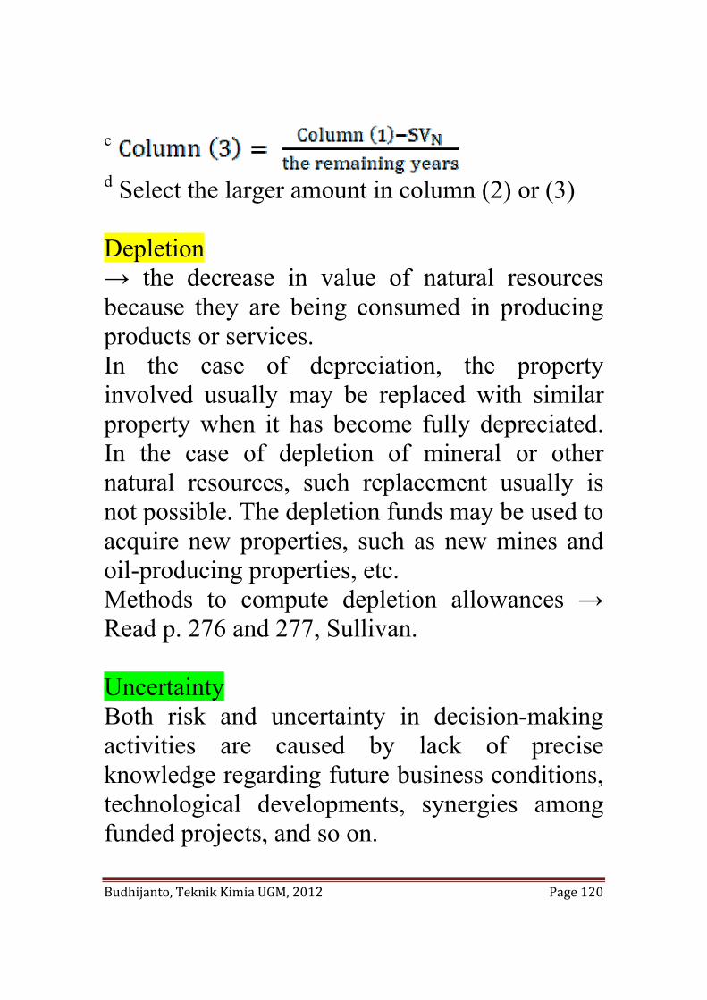
Budhijanto, Teknik Kimia UGM, 2012 Page 120
c d Select the larger amount in column (2) or (3) Depletion → the decrease in value of natural resources because they are being consumed in producing products or services. In the case of depreciation, the property involved usually may be replaced with similar property when it has become fully depreciated. In the case of depletion of mineral or other natural resources, such replacement usually is not possible. The depletion funds may be used to acquire new properties, such as new mines and oil-producing properties, etc. Methods to compute depletion allowances → Read p. 276 and 277, Sullivan. Uncertainty Both risk and uncertainty in decision-making activities are caused by lack of precise knowledge regarding future business conditions, technological developments, synergies among funded projects, and so on.
Budhijanto, Teknik Kimia UGM, 2012 Page 121
Decisions under risk: decisions in which the analyst models the decision problem in terms of assumed possible future outcomes, or scenarios, whose probabilities of occurrence can be estimated. Decisions under uncertainty: decision problems characterized by several unknown futures for which probabilities of occurrence can not be estimated. In dealing with risk/uncertainty, we do sensitivity analysis to determine how sensitive the situation is to the several factors of concern so that proper consideration may be given to them in the decision process. Techniques used in the sensitivity analysis: 1. Break-even analysis → used when the selection among project alternatives or the economic acceptability of an engineering project is heavily dependent upon a single factor, which is uncertain. Example 10-1: There are two alternative electric motors that provide 100-hp output. Alpha motor Beta motor
Budhijanto, Teknik Kimia UGM, 2012 Page 122
Capital Investment, $ 12,500 16,000 Efficiency, % 74 92 Useful life, years 10 10 Maintenance expense, $/year
500 250
Taxes and insurance expenses, % of the investment
1.5 1.5
Electricity cost, $/kWh 0.05 0.05 Market Value, $ 0 0 Assume that revenues are equal for both motors. MARR = 15% per year. If the best estimate of hours of operation per year is 600 hours, which motor is preferred? Answer: Let: X = number of hours of operation per year The equivalent annual worth of Alpha motor ( = the equivalent uniform annual cost
Budhijanto, Teknik Kimia UGM, 2012 Page 123
( )
Beta motor:
At the break-even point,
hours/year
Plot:
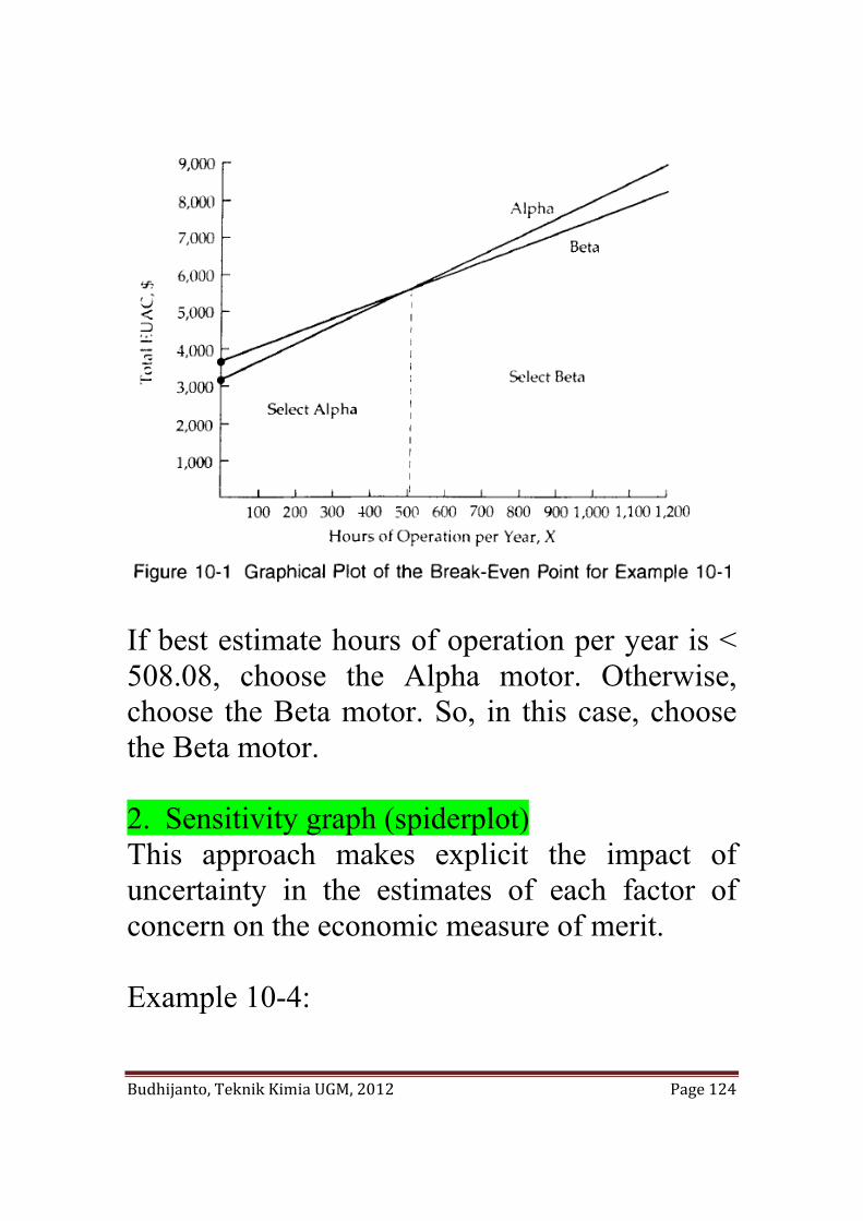
Budhijanto, Teknik Kimia UGM, 2012 Page 124
If best estimate hours of operation per year is < 508.08, choose the Alpha motor. Otherwise, choose the Beta motor. So, in this case, choose the Beta motor. 2. Sensitivity graph (spiderplot) This approach makes explicit the impact of uncertainty in the estimates of each factor of concern on the economic measure of merit. Example 10-4:
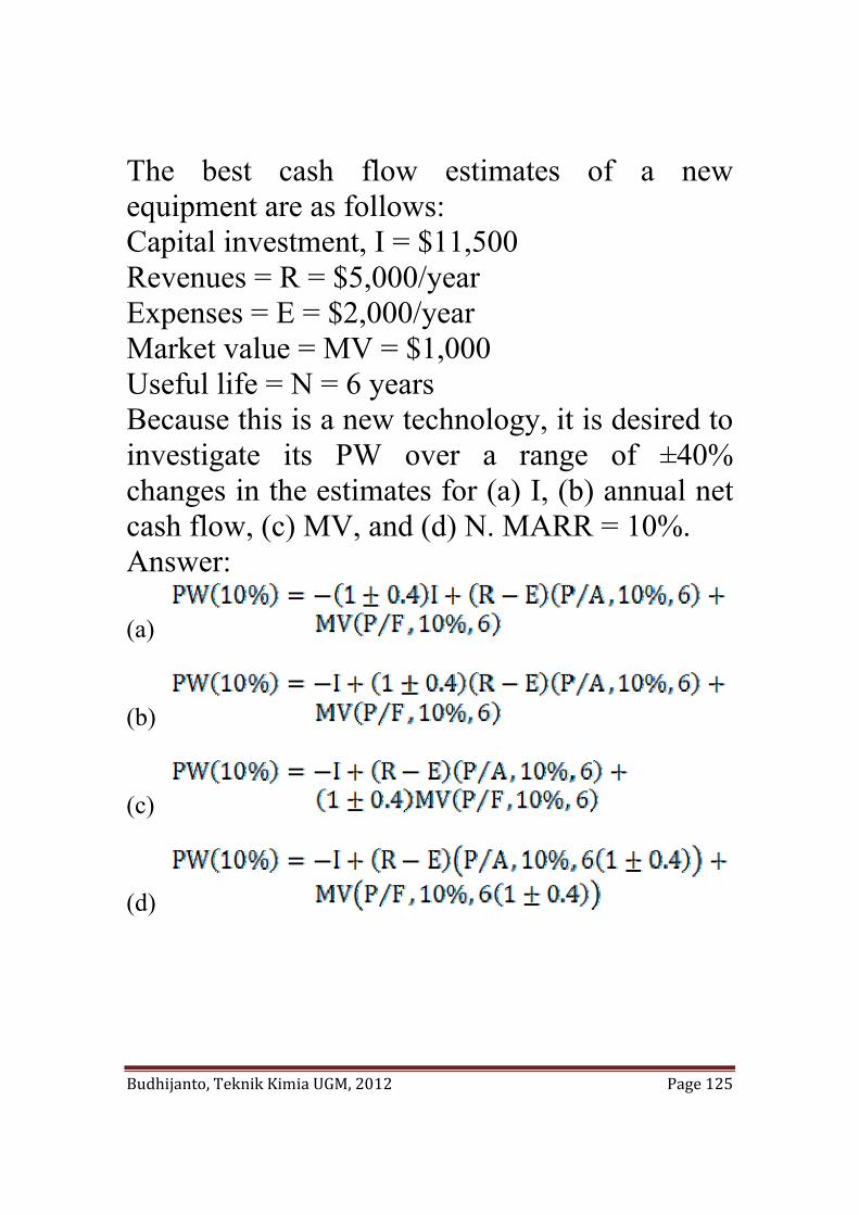
Budhijanto, Teknik Kimia UGM, 2012 Page 125
The best cash flow estimates of a new equipment are as follows: Capital investment, I = $11,500 Revenues = R = $5,000/year Expenses = E = $2,000/year Market value = MV = $1,000 Useful life = N = 6 years Because this is a new technology, it is desired to investigate its PW over a range of ±40% changes in the estimates for (a) I, (b) annual net cash flow, (c) MV, and (d) N. MARR = 10%. Answer:
(a)
(b)
(c)
(d)
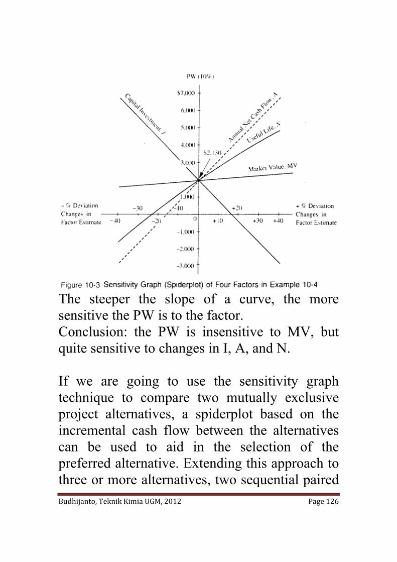
Budhijanto, Teknik Kimia UGM, 2012 Page 126
The steeper the slope of a curve, the more sensitive the PW is to the factor. Conclusion: the PW is insensitive to MV, but quite sensitive to changes in I, A, and N. If we are going to use the sensitivity graph technique to compare two mutually exclusive project alternatives, a spiderplot based on the incremental cash flow between the alternatives can be used to aid in the selection of the preferred alternative. Extending this approach to three or more alternatives, two sequential paired
Budhijanto, Teknik Kimia UGM, 2012 Page 127
comparisons can be used. Another approach is to plot in the same figure a sensitivity graph for each alternative. 3. Combination of factors → concerned about the combined effects of uncertainty in two or more project factors on the economic of merit. Read Sullivan p. 459-465. Cost Estimation Techniques Read Chapter 7 Sullivan Read Peters and Timmerhaus. Read Aries, R.S. and Newton, R.D., 1955, Chemical Engineering Cost Estimation, McGraw-Hill Book Company, New York.