Chawla_Composite_Materials_ir... - IIS Windows Server - Iran ...

هب انم خدا

Composite Materials

www.Iran-mavad.com مرجع دانشجويان و مهندسين مواد

Krishan K. Chawla

Composite Materials

Science and Engineering

Third Edition

With 278 Illustrations


Krishan K. ChawlaDepartment of Materials Science and EngineeringUniversity of Alabama at BirminghamBirmingham, AL 35294, [email protected]

ISBN 978-0-387-74364-6 ISBN 978-0-387-74365-3 (eBook)DOI 10.1007/978-0-387-74365-3Springer New York Heidelberg Dordrecht London

Library of Congress Control Number: 2012940847

This work is subject to copyright. All rights are reserved by the Publisher, whether the whole or part ofthe material is concerned, specifically the rights of translation, reprinting, reuse of illustrations,recitation, broadcasting, reproduction on microfilms or in any other physical way, and transmission orinformation storage and retrieval, electronic adaptation, computer software, or by similar or dissimilarmethodology now known or hereafter developed. Exempted from this legal reservation are brief excerptsin connection with reviews or scholarly analysis or material supplied specifically for the purpose of beingentered and executed on a computer system, for exclusive use by the purchaser of the work. Duplicationof this publication or parts thereof is permitted only under the provisions of the Copyright Law of thePublisher’s location, in its current version, and permission for use must always be obtained fromSpringer. Permissions for use may be obtained through RightsLink at the Copyright Clearance Center.Violations are liable to prosecution under the respective Copyright Law.The use of general descriptive names, registered names, trademarks, service marks, etc. in thispublication does not imply, even in the absence of a specific statement, that such names are exemptfrom the relevant protective laws and regulations and therefore free for general use.While the advice and information in this book are believed to be true and accurate at the date ofpublication, neither the authors nor the editors nor the publisher can accept any legal responsibility forany errors or omissions that may be made. The publisher makes no warranty, express or implied, withrespect to the material contained herein.

Cover illustration: Fan blades made of carbon fiber/epoxy composite in the GEnx jet engine. [Courtesyof General Electric.]

Printed on acid-free paper

Springer is part of Springer Science+Business Media (www.springer.com)

pringer Science+Business Media New York 2012, rrected t rinting 13 Co a 2 p 20nd© S


�A no bhadr�ah˙kratavo yantu visvatah

˙Let noble thoughts come to us from every sideRigveda 1-89-i

Dedicated affectionately to A, K3, and N3


Preface to the Third Edition

Since the publication of the second edition of this book, there has been a spate of

activity in the field of composites, in the academia as well as in the industry.

The industrial activity, in particular, has been led by the large-scale use of

composites by aerospace companies, mainly Boeing and Airbus. It would not be

far off the mark to say that the extensive use of carbon fiber/epoxy resin composites

in Boeing 787 aircraft and a fairly large use of composites in Airbus’s A 380 aircraft

represent a paradigm shift. Boeing 787 has composites in the fuselage, windows,

wings, tails, stabilizers, etc., resulting in 50% in composites by weight. Neverthe-

less, it should be pointed out that in reality, the extensive use of composites in

aircraft is a culmination of a series of earlier steps over the decades since mid-1960s.

Besides the large-scale applications in the aerospace industry, there have been

impressive developments in other fields such as automotive, sporting goods, super-

conductivity, etc.

All of this activity has led to a substantial addition of new material in this edition.

Among these are the following: Carbon/carbon brakes, nanocomposites, biocom-

posites, self-healing composites, self-reinforced composites, fiber/metal laminate

composites, composites for civilian aircraft, composites for aircraft jet engine,

second-generation high-temperature superconducting composites, WC/metal par-

ticulate composites, new solved examples, and new problems. In addition, I have

added a new chapter called nonconventional composites. This chapter deals with

some nonconventional composites such as nanocomposites (polymer, metal, and

ceramic matrix), self-healing composites, self-reinforced composites, biocom-

posites, and laminates made of bidimensional layers.

Once again, I plead guilty to the charge that the material contained in this edition

is more than can be covered in a normal, semester-long course. The instructor of

course can cut the content to his/her requirements. I have always had the broader

aim of providing a text that is suitable as a source of reference for the practicing

researcher, scientist, and engineer.

Finally, there is the pleasant task of acknowledgments. I am grateful to National

Science Foundation, Office of Naval Research, Federal Transit Administration,

Los Alamos National Laboratory Sandia national Laboratory, Oak Ridge National

vii


Laboratory, Smith International Inc., and Trelleborg, Inc. for supporting my

research work over the years, some of which is included in this text. Among the

people with whom I have had the privilege of collaborating over the years and

who have enriched my life, professional and otherwise, I would like to mention,

in alphabetical order, C.H. Barham, A.R. Boccaccini, K. Carlisle, K. Chawla,

N. Chawla, X. Deng, Z. Fang, M.E. Fine, S.G. Fishman, G. Gladysz, A. Goel,

N. Gupta, the late B. Ilschner, M. Koopman, R.R. Kulkarni, B.A. MacDonald,

A. Mortensen, B. Patel, B.R. Patterson, P.D. Portella, J.M. Rigsbee, P. Rohatgi,

H. Schneider, N.S. Stoloff, Y.-L. Shen, S. Suresh, Z.R. Xu, U. Vaidya, and

A.K. Vasudevan. Thanks are due to Kanika Chawla and S. Patel for help with the

figures in this edition. I owe a special debt of gratitude to my wife, Nivi, for being

there all the time. Last but not least, I am ever grateful to my parents, the late

Manohar L. and Sumitra Chawla, for their guidance and support.

Birmingham, AL, USA Krishan K. Chawla

March, 2011

Supplementary Instructional Resources

viii Preface to the Third Edition

exercises and PowerPoint Slides of figures suitable for use in lectures are available

to instructors who adopt the book for classroom use. Please visit the bookWeb page

at www.springer.com for the password-protected material.

An Instructor’s Solutions Manual containing answers to the end-of-the-chapter


Preface to the Second Edition

The first edition of this book came out in 1987, offering an integrated coverage of

the field of composite materials. I am gratified at the reception it received at the

hands of the students and faculty. The second edition follows the same format as

the first one, namely, a well-balanced treatment of materials and mechanics aspects

of composites, with due recognition of the importance of the processing.

The second edition is a fully revised, updated, and enlarged edition of this widely

used text. There are some new chapters, and others have been brought up-to-date in

light of the extensive work done in the decade since publication of the first edition.

Many people who used the first edition as a classroom text urged me to include

some solved examples. In deference to their wishes I have done so. I am sorry that it

took me such a long time to prepare the second edition. Things are happening at a

very fast pace in the field of composites, and there is no question that a lot of very

interesting and important work has been done in the past decade or so. Out of

necessity, one must limit the amount of material to be included in a textbook.

In spite of this view, it took me much more time than I anticipated. In this second

edition, I have resisted the temptation to cover the whole waterfront. So the reader

will find here an up-to-date treatment of the fundamental aspects. Even so, I do

recognize that the material contained in this second edition is more than what can be

covered in the classroom in a semester. I consider that to be a positive aspect of the

book. The reader (student, researcher, practicing scientist/engineer) can profitably

use this as a reference text. For the person interested in digging deeper into a

particular aspect, I provide an extensive and updated list of references and

suggested reading.

There remains the pleasant task of thanking people who have been very helpful and

a constant source of encouragement to me over the years: M.E. Fine, S.G. Fishman,

J.C. Hurt, B. Ilschner, B.A. MacDonald, A. Mortensen, J.M. Rigsbee, P. Rohatgi,

S. Suresh, H. Schneider, N.S. Stoloff, and A.K. Vasudevan. Among my students and

post-docs, I would like to acknowledge G. Gladysz, H. Liu, and Z.R. Xu. I am

immensely grateful to my family members, Nivi, Nikhil, and Kanika. They were

ix


patient and understanding throughout. Without Kanika’s help in word processing and

fixing things, this work would still be unfinished. Once again I wish to record my

gratitude to my parents, Manohar L. Chawla and the late Sumitra Chawla for all they

have done for me!

Birmingham, AL, USA Krishan K. Chawla

February, 1998

x Preface to the Second Edition


Preface to the First Edition

The subject of composite materials is truly an inter- and multidisciplinary one.

People working in fields such as metallurgy and materials science and engineering,

chemistry and chemical engineering, solid mechanics, and fracture mechanics have

made important contributions to the field of composite materials. It would be an

impossible task to cover the subject from all these viewpoints. Instead, we shall

restrict ourselves in this book to the objective of obtaining an understanding of

composite properties (e.g., mechanical, physical, and thermal) as controlled by their

structure at micro- and macro-levels. This involves a knowledge of the properties of

the individual constituents that form the composite system, the role of interface

between the components, the consequences of joining together, say, a fiber and

matrix material to form a unit composite ply, and the consequences of joining

together these unit composites or plies to form a macrocomposite, a macroscopic

engineering component as per some optimum engineering specifications. Time and

again, we shall be emphasizing this main theme, that is structure–property

correlations at various levels that help us to understand the behavior of composites.

In Part I, after an introduction (Chap. 1), fabrication and properties of the various

types of reinforcement are described with a special emphasis on microstructure–

property correlations (Chap. 2). This is followed by a chapter (Chap. 3) on the three

main types of matrix materials, namely, polymers, metals, and ceramics. It is

becoming increasingly evident that the role of the matrix is not just that of a binding

medium for the fibers but it can contribute decisively toward the composite

performance. This is followed by a general description of the interface in

composites (Chap. 4). In Part II a detailed description is given of some of the

important types of composites (Chap. 5), metal matrix composites (Chap. 6),

ceramic composites (Chap. 7), carbon fiber composites (Chap. 8), and multifilam-

entary superconducting composites (Chap. 9). The last two are described separately

because they are the most advanced fiber composite systems of the 1960s and

1970s. Specific characteristics and applications of these composite systems are

brought out in these chapters. Finally, in Part III, the micromechanics (Chap. 10)

and macromechanics (Chap. 11) of composites are described in detail, again

emphasizing the theme of how structure (micro and macro) controls the properties.

xi


This is followed by a description of strength and fracture modes in composites

(Chap. 12). This chapter also describes some salient points of difference, in regard

to design, between conventional and fiber composite materials. This is indeed of

fundamental importance in view of the fact that composite materials are not just any

other new material. They represent a total departure from the way we are used to

handling conventional monolithic materials, and, consequently, they require uncon-

ventional approaches to designing with them.

Throughout this book examples are given from practical applications of

composites in various fields. There has been a tremendous increase in applications

of composites in sophisticated engineering items. Modern aircraft industry readily

comes to mind as an ideal example. Boeing Company, for example, has made

widespread use of structural components made of “advanced” composites in 757

and 767 planes. Yet another striking example is that of the Beechcraft Company’s

Starship 1 aircraft. This small aircraft (eight to ten passengers plus crew) is

primarily made of carbon and other high-performance fibers in epoxy matrix. The

use of composite materials results in 19% weight reduction compared to an

identical aluminum airframe. Besides this weight reduction, the use of composites

made a new wing design configuration possible, namely, a variable-geometry

forward wing that sweeps forward during takeoff and landing to give stability and

sweeps back 30� in level flight to reduce drag. As a bonus, the smooth structure of

composite wings helps to maintain laminar air flow. Readers will get an idea of the

tremendous advances made in the composites field if they would just remind

themselves that until about 1975 these materials were being produced mostly on

a laboratory scale. Besides the aerospace industry, chemical, electrical, automobile,

and sports industries are the other big users, in one form or another, of composite

materials.

This book has grown out of lectures given over a period of more than a decade to

audiences comprised of senior year undergraduate and graduate students, as well as

practicing engineers from industry. The idea of this book was conceived at Instituto

Militar de Engenharia, Rio de Janeiro. I am grateful to my former colleagues there,

in particular, J.R.C. Guimaraes, W.P. Longo, J.C.M. Suarez, and A.J.P. Haiad, for

their stimulating companionship. The book’s major gestation period was at the

University of Illinois at Urbana-Champaign, where C.A. Wert and J.M. Rigsbee

helped me to complete the manuscript. The book is now seeing the light of the day

at the New Mexico Institute of Mining and Technology. I would like to thank my

colleagues there, in particular, O.T. Inal, P. Lessing, M.A. Meyers, A. Miller,

C.J. Popp, and G.R. Purcell, for their cooperation in many ways, tangible and

intangible. An immense debt of gratitude is owed to N.J. Grant of MIT, a true

gentleman and scholar, for his encouragement, corrections, and suggestions

as he read the manuscript. Thanks are also due to R. Signorelli, J. Cornie, and

P.K. Rohatgi for reading portions of the manuscript and for their very constructive

suggestions. I would be remiss in not mentioning the students who took my courses

on composite materials at New Mexico Tech and gave very constructive feedback.

A special mention should be made of C.K. Chang, C.S. Lee, and N. Pehlivanturk

for their relentless queries and discussions. Thanks are also due to my wife,

xii Preface to the First Edition


Nivedita Chawla, and Elizabeth Fraissinet for their diligent word processing; my

son, Nikhilesh Chawla, helped in the index preparation. I would like to express my

gratitude to my parents, Manohar L. and Sumitra Chawla, for their ever-constant

encouragement and inspiration.

Socorro, NM, USA Krishan K. Chawla

June, 1987

Preface to the First Edition xiii


About the Author

Professor Krishan K. Chawla received his B.S. degree fromBanaras HinduUniversity

and his M.S. and Ph.D. degrees from the University of Illinois atUrbana-Champaign.

He has taught and/or done research work at Instituto Militar de Engenharia, Brazil;

University of Illinois at Urbana-Champaign; Northwestern University; Universite

Laval, Canada; Ecole Polytechnique Federale de Lausanne, Switzerland; the New

Mexico Institute of Mining and Technology (NMIMT); Arizona State University;

German Aerospace Research Institute (DLR), Cologne, Germany; Los Alamos

National Laboratory; Federal Institute for Materials Research and Testing (BAM)

Berlin, Germany; and the University of Alabama at Birmingham. Among the honors

he has received are the following: Eshbach Distinguished Scholar at Northwestern

University, U.S. Department of Energy Faculty Fellow at Oak Ridge National Labo-

ratory, Distinguished Researcher Award at NMIMT, Distinguished Alumnus Award

from Banaras Hindu University, President’s Award for Excellence in Teaching at the

University of Alabama at Birmingham, and Educator Award from The Minerals,

Metals and Materials Society (TMS). In 1989–1990, he served as a program director

xv


for Metals and Ceramics at the U.S. National Science Foundation (NSF). He is a

Fellow of ASM International.

Professor Chawla is editor of the journal International Materials Reviews.

Among his other books are the following: Ceramic Matrix Composites, Fibrous

Materials, Mechanical Metallurgy (coauthor), Metalurgia Mecanica (coauthor),

Mechanical Behavior of Materials (coauthor), Metal Matrix Composites

(coauthor), and Voids in Materials (coauthor).

xvi About the Author


Contents

Preface to the Third Edition . . . . . . . . . . . . . . . . . . . . . . . . . . . . . . . . . . . . . . . . . . . . . . . . . . . . vii

Preface to the Second Edition . . . . . . . . . . . . . . . . . . . . . . . . . . . . . . . . . . . . . . . . . . . . . . . . . . . ix

Preface to the First Edition . . . . . . . . . . . . . . . . . . . . . . . . . . . . . . . . . . . . . . . . . . . . . . . . . . . . . . xi

Part I

1 Introduction . . . . . . . . . . . . . . . . . . . . . . . . . . . . . . . . . . . . . . . . . . . . . . . . . . . . . . . . . . . . . . . . . . . 3

References . . . . . . . . . . . . . . . . . . . . . . . . . . . . . . . . . . . . . . . . . . . . . . . . . . . . . . . . . . . . . . . . . . . . . . 5

2 Reinforcements . . . . . . . . . . . . . . . . . . . . . . . . . . . . . . . . . . . . . . . . . . . . . . . . . . . . . . . . . . . . . . . 7

2.1 Introduction . . . . . . . . . . . . . . . . . . . . . . . . . . . . . . . . . . . . . . . . . . . . . . . . . . . . . . . . . . . . . 7

2.1.1 Flexibility . . . . . . . . . . . . . . . . . . . . . . . . . . . . . . . . . . . . . . . . . . . . . . . . . . . . . . 8

2.1.2 Fiber Spinning Processes . . . . . . . . . . . . . . . . . . . . . . . . . . . . . . . . . . . . . 10

2.1.3 Stretching and Orientation . . . . . . . . . . . . . . . . . . . . . . . . . . . . . . . . . . . . 11

2.2 Glass Fibers . . . . . . . . . . . . . . . . . . . . . . . . . . . . . . . . . . . . . . . . . . . . . . . . . . . . . . . . . . . . 11

2.2.1 Fabrication . . . . . . . . . . . . . . . . . . . . . . . . . . . . . . . . . . . . . . . . . . . . . . . . . . . . . 12

2.2.2 Structure . . . . . . . . . . . . . . . . . . . . . . . . . . . . . . . . . . . . . . . . . . . . . . . . . . . . . . . . 14

2.2.3 Properties and Applications . . . . . . . . . . . . . . . . . . . . . . . . . . . . . . . . . . 15

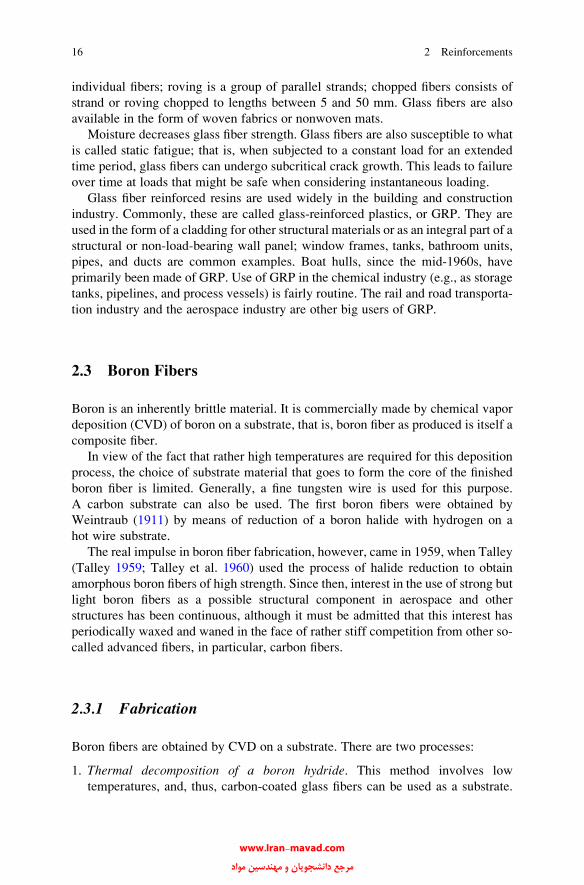
2.3 Boron Fibers . . . . . . . . . . . . . . . . . . . . . . . . . . . . . . . . . . . . . . . . . . . . . . . . . . . . . . . . . . . . 16

2.3.1 Fabrication . . . . . . . . . . . . . . . . . . . . . . . . . . . . . . . . . . . . . . . . . . . . . . . . . . . . . 16

2.3.2 Structure and Morphology . . . . . . . . . . . . . . . . . . . . . . . . . . . . . . . . . . . . 19

2.3.3 Residual Stresses . . . . . . . . . . . . . . . . . . . . . . . . . . . . . . . . . . . . . . . . . . . . . . 21

2.3.4 Fracture Characteristics . . . . . . . . . . . . . . . . . . . . . . . . . . . . . . . . . . . . . . . 22

2.3.5 Properties and Applications of Boron Fibers . . . . . . . . . . . . . . . 22

2.4 Carbon Fibers . . . . . . . . . . . . . . . . . . . . . . . . . . . . . . . . . . . . . . . . . . . . . . . . . . . . . . . . . . 24

2.4.1 Processing . . . . . . . . . . . . . . . . . . . . . . . . . . . . . . . . . . . . . . . . . . . . . . . . . . . . . . 26

2.4.2 Structural Changes Occurring During Processing . . . . . . . . . . 31

2.4.3 Properties and Applications . . . . . . . . . . . . . . . . . . . . . . . . . . . . . . . . . . 32

2.5 Organic Fibers . . . . . . . . . . . . . . . . . . . . . . . . . . . . . . . . . . . . . . . . . . . . . . . . . . . . . . . . . . 36

2.5.1 Oriented Polyethylene Fibers . . . . . . . . . . . . . . . . . . . . . . . . . . . . . . . . 38

2.5.2 Aramid Fibers . . . . . . . . . . . . . . . . . . . . . . . . . . . . . . . . . . . . . . . . . . . . . . . . . 40

xvii


2.6 Ceramic Fibers . . . . . . . . . . . . . . . . . . . . . . . . . . . . . . . . . . . . . . . . . . . . . . . . . . . . . . . . . 50

2.6.1 Oxide Fibers . . . . . . . . . . . . . . . . . . . . . . . . . . . . . . . . . . . . . . . . . . . . . . . . . . . 51

2.6.2 Nonoxide Fibers . . . . . . . . . . . . . . . . . . . . . . . . . . . . . . . . . . . . . . . . . . . . . . . 55

2.7 Whiskers . . . . . . . . . . . . . . . . . . . . . . . . . . . . . . . . . . . . . . . . . . . . . . . . . . . . . . . . . . . . . . . . 62

2.8 Other Nonoxide Reinforcements . . . . . . . . . . . . . . . . . . . . . . . . . . . . . . . . . . . . . 64

2.8.1 Silicon Carbide in a Particulate Form . . . . . . . . . . . . . . . . . . . . . . . 65

2.8.2 Tungsten Carbide Particles . . . . . . . . . . . . . . . . . . . . . . . . . . . . . . . . . . . 65

2.9 Effect of High-Temperature Exposure on the Strength

of Ceramic Fibers . . . . . . . . . . . . . . . . . . . . . . . . . . . . . . . . . . . . . . . . . . . . . . . . . . . . . . 66

2.10 Comparison of Fibers . . . . . . . . . . . . . . . . . . . . . . . . . . . . . . . . . . . . . . . . . . . . . . . . . . 67

References . . . . . . . . . . . . . . . . . . . . . . . . . . . . . . . . . . . . . . . . . . . . . . . . . . . . . . . . . . . . . . . . . . . . . . 68

3 Matrix Materials . . . . . . . . . . . . . . . . . . . . . . . . . . . . . . . . . . . . . . . . . . . . . . . . . . . . . . . . . . . . . 73

3.1 Polymers . . . . . . . . . . . . . . . . . . . . . . . . . . . . . . . . . . . . . . . . . . . . . . . . . . . . . . . . . . . . . . . . . 73

3.1.1 Glass Transition Temperature . . . . . . . . . . . . . . . . . . . . . . . . . . . . . . . . . 74

3.1.2 Thermoplastics and Thermosets . . . . . . . . . . . . . . . . . . . . . . . . . . . . . . . 76

3.1.3 Copolymers . . . . . . . . . . . . . . . . . . . . . . . . . . . . . . . . . . . . . . . . . . . . . . . . . . . . . . 77

3.1.4 Molecular Weight . . . . . . . . . . . . . . . . . . . . . . . . . . . . . . . . . . . . . . . . . . . . . . . 77

3.1.5 Degree of Crystallinity . . . . . . . . . . . . . . . . . . . . . . . . . . . . . . . . . . . . . . . . . 78

3.1.6 Stress–Strain Behavior . . . . . . . . . . . . . . . . . . . . . . . . . . . . . . . . . . . . . . . . . 78

3.1.7 Thermal Expansion . . . . . . . . . . . . . . . . . . . . . . . . . . . . . . . . . . . . . . . . . . . . . 80

3.1.8 Fire Resistance or Flammability . . . . . . . . . . . . . . . . . . . . . . . . . . . . . . 80

3.1.9 Common Polymeric Matrix Materials . . . . . . . . . . . . . . . . . . . . . . . . 80

3.2 Metals . . . . . . . . . . . . . . . . . . . . . . . . . . . . . . . . . . . . . . . . . . . . . . . . . . . . . . . . . . . . . . . . . . . . 91

3.2.1 Structure . . . . . . . . . . . . . . . . . . . . . . . . . . . . . . . . . . . . . . . . . . . . . . . . . . . . . . . . . 91

3.2.2 Conventional Strengthening Methods . . . . . . . . . . . . . . . . . . . . . . . . 93

3.2.3 Properties of Metals . . . . . . . . . . . . . . . . . . . . . . . . . . . . . . . . . . . . . . . . . . . . 95

3.2.4 Why Reinforcement of Metals? . . . . . . . . . . . . . . . . . . . . . . . . . . . . . . . 96

3.3 Ceramic Matrix Materials . . . . . . . . . . . . . . . . . . . . . . . . . . . . . . . . . . . . . . . . . . . . . . 98

3.3.1 Bonding and Structure . . . . . . . . . . . . . . . . . . . . . . . . . . . . . . . . . . . . . . . . . . 98

3.3.2 Effect of Flaws on Strength . . . . . . . . . . . . . . . . . . . . . . . . . . . . . . . . . . . . 100

3.3.3 Common Ceramic Matrix Materials . . . . . . . . . . . . . . . . . . . . . . . . . . 101

References . . . . . . . . . . . . . . . . . . . . . . . . . . . . . . . . . . . . . . . . . . . . . . . . . . . . . . . . . . . . . . . . . . . . . . 101

4 Interfaces . . . . . . . . . . . . . . . . . . . . . . . . . . . . . . . . . . . . . . . . . . . . . . . . . . . . . . . . . . . . . . . . . . . . . . 105

4.1 Wettability . . . . . . . . . . . . . . . . . . . . . . . . . . . . . . . . . . . . . . . . . . . . . . . . . . . . . . . . . . . . . . . 106

4.1.1 Effect of Surface Roughness . . . . . . . . . . . . . . . . . . . . . . . . . . . . . . . . . . . 109

4.2 Crystallographic Nature of Interface . . . . . . . . . . . . . . . . . . . . . . . . . . . . . . . . . . 110

4.3 Interactions at the Interface . . . . . . . . . . . . . . . . . . . . . . . . . . . . . . . . . . . . . . . . . . . . 111

4.4 Types of Bonding at the Interface . . . . . . . . . . . . . . . . . . . . . . . . . . . . . . . . . . . . . 113

4.4.1 Mechanical Bonding . . . . . . . . . . . . . . . . . . . . . . . . . . . . . . . . . . . . . . . . . . . . 114

4.4.2 Physical Bonding . . . . . . . . . . . . . . . . . . . . . . . . . . . . . . . . . . . . . . . . . . . . . . . 116

4.4.3 Chemical Bonding . . . . . . . . . . . . . . . . . . . . . . . . . . . . . . . . . . . . . . . . . . . . . . 116

4.5 Optimum Interfacial Bond Strength . . . . . . . . . . . . . . . . . . . . . . . . . . . . . . . . . . . 117

xviii Contents


4.5.1 Very Weak Interface or Fiber Bundle

(No Matrix) . . . . . . . . . . . . . . . . . . . . . . . . . . . . . . . . . . . . . . . . . . . . . . . . . . . . . . 118

4.5.2 Very Strong Interface . . . . . . . . . . . . . . . . . . . . . . . . . . . . . . . . . . . . . . . . . . 118

4.5.3 Optimum Interfacial Bond Strength . . . . . . . . . . . . . . . . . . . . . . . . . . . 119

4.6 Tests for Measuring Interfacial Strength . . . . . . . . . . . . . . . . . . . . . . . . . . . . . . 119

4.6.1 Flexural Tests . . . . . . . . . . . . . . . . . . . . . . . . . . . . . . . . . . . . . . . . . . . . . . . . . . . 119

4.6.2 Single Fiber Pullout Tests . . . . . . . . . . . . . . . . . . . . . . . . . . . . . . . . . . . . . . 122

4.6.3 Curved Neck Specimen Test . . . . . . . . . . . . . . . . . . . . . . . . . . . . . . . . . . 125

4.6.4 Instrumented Indentation Tests . . . . . . . . . . . . . . . . . . . . . . . . . . . . . . . . 126

4.6.5 Fragmentation Test . . . . . . . . . . . . . . . . . . . . . . . . . . . . . . . . . . . . . . . . . . . . . 129

4.6.6 Laser Spallation Technique . . . . . . . . . . . . . . . . . . . . . . . . . . . . . . . . . . . . 130

References . . . . . . . . . . . . . . . . . . . . . . . . . . . . . . . . . . . . . . . . . . . . . . . . . . . . . . . . . . . . . . . . . . . . . . 131

Part II

5 Polymer Matrix Composites . . . . . . . . . . . . . . . . . . . . . . . . . . . . . . . . . . . . . . . . . . . . . . . . 137

5.1 Processing of PMCs . . . . . . . . . . . . . . . . . . . . . . . . . . . . . . . . . . . . . . . . . . . . . . . . . . . . . 137

5.1.1 Processing of Thermoset Matrix Composites . . . . . . . . . . . . . . . . 138

5.1.2 Thermoplastic Matrix Composites . . . . . . . . . . . . . . . . . . . . . . . . . . . . 148

5.1.3 Sheet Molding Compound . . . . . . . . . . . . . . . . . . . . . . . . . . . . . . . . . . . . . 153

5.1.4 Carbon Fiber Reinforced Polymer Composites . . . . . . . . . . . . . . 154

5.2 Interface in PMCs . . . . . . . . . . . . . . . . . . . . . . . . . . . . . . . . . . . . . . . . . . . . . . . . . . . . . . . 155

5.2.1 Glass Fiber/Polymer . . . . . . . . . . . . . . . . . . . . . . . . . . . . . . . . . . . . . . . . . . . . 155

5.2.2 Carbon Fiber/Polymer Interface . . . . . . . . . . . . . . . . . . . . . . . . . . . . . . . 158

5.2.3 Polyethylene Fiber/Polymer Interface . . . . . . . . . . . . . . . . . . . . . . . . 163

5.3 Structure and Properties of PMCs . . . . . . . . . . . . . . . . . . . . . . . . . . . . . . . . . . . . . 164

5.3.1 Structural Defects in PMCs . . . . . . . . . . . . . . . . . . . . . . . . . . . . . . . . . . . . 164

5.3.2 Mechanical Properties . . . . . . . . . . . . . . . . . . . . . . . . . . . . . . . . . . . . . . . . . . 164

5.4 Applications . . . . . . . . . . . . . . . . . . . . . . . . . . . . . . . . . . . . . . . . . . . . . . . . . . . . . . . . . . . . . . 176

5.4.1 Pressure Vessels . . . . . . . . . . . . . . . . . . . . . . . . . . . . . . . . . . . . . . . . . . . . . . . . 178

5.5 Recycling of PMCs . . . . . . . . . . . . . . . . . . . . . . . . . . . . . . . . . . . . . . . . . . . . . . . . . . . . . 192

References . . . . . . . . . . . . . . . . . . . . . . . . . . . . . . . . . . . . . . . . . . . . . . . . . . . . . . . . . . . . . . . . . . . . . . 194

6 Metal Matrix Composites . . . . . . . . . . . . . . . . . . . . . . . . . . . . . . . . . . . . . . . . . . . . . . . . . . . 197

6.1 Types of Metal Matrix Composites . . . . . . . . . . . . . . . . . . . . . . . . . . . . . . . . . . . . 197

6.2 Important Metallic Matrices . . . . . . . . . . . . . . . . . . . . . . . . . . . . . . . . . . . . . . . . . . . . 198

6.2.1 Aluminum Alloys . . . . . . . . . . . . . . . . . . . . . . . . . . . . . . . . . . . . . . . . . . . . . . . 198

6.2.2 Titanium Alloys . . . . . . . . . . . . . . . . . . . . . . . . . . . . . . . . . . . . . . . . . . . . . . . . . 199

6.2.3 Magnesium Alloys . . . . . . . . . . . . . . . . . . . . . . . . . . . . . . . . . . . . . . . . . . . . . . 200

6.2.4 Copper . . . . . . . . . . . . . . . . . . . . . . . . . . . . . . . . . . . . . . . . . . . . . . . . . . . . . . . . . . . 200

6.2.5 Intermetallic Compounds . . . . . . . . . . . . . . . . . . . . . . . . . . . . . . . . . . . . . . 200

Contents xix


6.3 Processing . . . . . . . . . . . . . . . . . . . . . . . . . . . . . . . . . . . . . . . . . . . . . . . . . . . . . . . . . . . . . . . . 201

6.3.1 Liquid-State Processes . . . . . . . . . . . . . . . . . . . . . . . . . . . . . . . . . . . . . . . . . 201

6.3.2 Solid State Processes . . . . . . . . . . . . . . . . . . . . . . . . . . . . . . . . . . . . . . . . . . . 209

6.3.3 In Situ Processes . . . . . . . . . . . . . . . . . . . . . . . . . . . . . . . . . . . . . . . . . . . . . . . . 211

6.4 Interfaces in Metal Matrix Composites . . . . . . . . . . . . . . . . . . . . . . . . . . . . . . . 212

6.4.1 Major Discontinuities at Interfaces in MMCs .. . . . . . . . . . . . . . . 214

6.4.2 Interfacial Bonding in Metal Matrix Composites . . . . . . . . . . . . 214

6.5 Properties . . . . . . . . . . . . . . . . . . . . . . . . . . . . . . . . . . . . . . . . . . . . . . . . . . . . . . . . . . . . . . . . . 223

6.5.1 Modulus . . . . . . . . . . . . . . . . . . . . . . . . . . . . . . . . . . . . . . . . . . . . . . . . . . . . . . . . 225

6.5.2 Strength . . . . . . . . . . . . . . . . . . . . . . . . . . . . . . . . . . . . . . . . . . . . . . . . . . . . . . . . 227

6.5.3 Thermal Characteristics . . . . . . . . . . . . . . . . . . . . . . . . . . . . . . . . . . . . . . . 235

6.5.4 High Temperature Properties, Creep, and Fatigue . . . . . . . . . 236

6.6 Applications . . . . . . . . . . . . . . . . . . . . . . . . . . . . . . . . . . . . . . . . . . . . . . . . . . . . . . . . . . . . . . 239

6.6.1 Electronic-Grade MMCs . . . . . . . . . . . . . . . . . . . . . . . . . . . . . . . . . . . . . . 241

6.6.2 Recycling of Metal Matrix Composites . . . . . . . . . . . . . . . . . . . . . 243

References . . . . . . . . . . . . . . . . . . . . . . . . . . . . . . . . . . . . . . . . . . . . . . . . . . . . . . . . . . . . . . . . . . . . . . 245

7 Ceramic Matrix Composites . . . . . . . . . . . . . . . . . . . . . . . . . . . . . . . . . . . . . . . . . . . . . . . . 249

7.1 Processing of CMCs . . . . . . . . . . . . . . . . . . . . . . . . . . . . . . . . . . . . . . . . . . . . . . . . . . . . 250

7.1.1 Cold Pressing and Sintering . . . . . . . . . . . . . . . . . . . . . . . . . . . . . . . . . . 250

7.1.2 Hot Pressing . . . . . . . . . . . . . . . . . . . . . . . . . . . . . . . . . . . . . . . . . . . . . . . . . . . 250

7.1.3 Reaction Bonding Processes . . . . . . . . . . . . . . . . . . . . . . . . . . . . . . . . . 253

7.1.4 Infiltration . . . . . . . . . . . . . . . . . . . . . . . . . . . . . . . . . . . . . . . . . . . . . . . . . . . . . . 254

7.1.5 Directed Oxidation or the Lanxide™ Process . . . . . . . . . . . . . . 256

7.1.6 In Situ Chemical Reaction Techniques . . . . . . . . . . . . . . . . . . . . . . 259

7.1.7 Sol–Gel . . . . . . . . . . . . . . . . . . . . . . . . . . . . . . . . . . . . . . . . . . . . . . . . . . . . . . . . . 262

7.1.8 Polymer Infiltration and Pyrolysis . . . . . . . . . . . . . . . . . . . . . . . . . . . 263

7.1.9 Electrophoretic Deposition . . . . . . . . . . . . . . . . . . . . . . . . . . . . . . . . . . . 267

7.1.10 Self-Propagating High-Temperature Synthesis . . . . . . . . . . . . . 267

7.2 Interface in CMCs . . . . . . . . . . . . . . . . . . . . . . . . . . . . . . . . . . . . . . . . . . . . . . . . . . . . . . . 269

7.3 Properties of CMCs . . . . . . . . . . . . . . . . . . . . . . . . . . . . . . . . . . . . . . . . . . . . . . . . . . . . . 272

7.4 Toughness of CMCs . . . . . . . . . . . . . . . . . . . . . . . . . . . . . . . . . . . . . . . . . . . . . . . . . . . . 275

7.4.1 Crack Deflection at the Interface in a CMC . . . . . . . . . . . . . . . . 282

7.5 Thermal Shock Resistance . . . . . . . . . . . . . . . . . . . . . . . . . . . . . . . . . . . . . . . . . . . . . 286

7.6 Applications of CMCs . . . . . . . . . . . . . . . . . . . . . . . . . . . . . . . . . . . . . . . . . . . . . . . . . . 286

7.6.1 Cutting Tool Inserts . . . . . . . . . . . . . . . . . . . . . . . . . . . . . . . . . . . . . . . . . . . 287

7.6.2 Ceramic Composite Filters . . . . . . . . . . . . . . . . . . . . . . . . . . . . . . . . . . . 287

7.6.3 Other Applications of CMCs . . . . . . . . . . . . . . . . . . . . . . . . . . . . . . . . . 289

References . . . . . . . . . . . . . . . . . . . . . . . . . . . . . . . . . . . . . . . . . . . . . . . . . . . . . . . . . . . . . . . . . . . . . . 290

8 Carbon Fiber/Carbon Matrix Composites . . . . . . . . . . . . . . . . . . . . . . . . . . . . . . . 293

8.1 Processing of Carbon/Carbon Composites . . . . . . . . . . . . . . . . . . . . . . . . . . . . 294

8.1.1 High Pressure Processing . . . . . . . . . . . . . . . . . . . . . . . . . . . . . . . . . . . . . 296

8.2 Oxidation Protection of Carbon/Carbon Composites . . . . . . . . . . . . . . . . 297

8.3 Properties of Carbon/Carbon Composites . . . . . . . . . . . . . . . . . . . . . . . . . . . . . 298

xx Contents


8.3.1 Thermal Properties . . . . . . . . . . . . . . . . . . . . . . . . . . . . . . . . . . . . . . . . . . . . . 300

8.3.2 Frictional Properties of the Composites . . . . . . . . . . . . . . . . . . . . . . 301

8.3.3 Ablative Properties . . . . . . . . . . . . . . . . . . . . . . . . . . . . . . . . . . . . . . . . . . . . . 301

8.4 Applications of Carbon/Carbon Composites . . . . . . . . . . . . . . . . . . . . . . . . . . 302

8.4.1 Carbon/Carbon Composite Brakes . . . . . . . . . . . . . . . . . . . . . . . . . . . . 303

8.4.2 Other Applications of Carbon/Carbon Composites . . . . . . . . . . 305

8.4.3 Carbon/SiC Brake Disks . . . . . . . . . . . . . . . . . . . . . . . . . . . . . . . . . . . . . . . 306

References . . . . . . . . . . . . . . . . . . . . . . . . . . . . . . . . . . . . . . . . . . . . . . . . . . . . . . . . . . . . . . . . . . . . . . 306

9 Multifilamentary Superconducting Composites . . . . . . . . . . . . . . . . . . . . . . . . 309

9.1 The Problem of Flux Pinning . . . . . . . . . . . . . . . . . . . . . . . . . . . . . . . . . . . . . . . . . 311

9.2 Types of Superconductor . . . . . . . . . . . . . . . . . . . . . . . . . . . . . . . . . . . . . . . . . . . . . . 313

9.3 Processing and Structure of Multifilamentary

Superconductors . . . . . . . . . . . . . . . . . . . . . . . . . . . . . . . . . . . . . . . . . . . . . . . . . . . . . . . . 314

9.3.1 Niobium–Titanium Alloys . . . . . . . . . . . . . . . . . . . . . . . . . . . . . . . . . . . . 314

9.3.2 A15 Superconductors . . . . . . . . . . . . . . . . . . . . . . . . . . . . . . . . . . . . . . . . . . 317

9.3.3 Ceramic Superconductors . . . . . . . . . . . . . . . . . . . . . . . . . . . . . . . . . . . . . 321

9.4 Applications . . . . . . . . . . . . . . . . . . . . . . . . . . . . . . . . . . . . . . . . . . . . . . . . . . . . . . . . . . . . 329

9.4.1 Magnetic Resonance Imaging . . . . . . . . . . . . . . . . . . . . . . . . . . . . . . . . 331

References . . . . . . . . . . . . . . . . . . . . . . . . . . . . . . . . . . . . . . . . . . . . . . . . . . . . . . . . . . . . . . . . . . . . . 332

Part III

10 Micromechanics of Composites . . . . . . . . . . . . . . . . . . . . . . . . . . . . . . . . . . . . . . . . . . . 337

10.1 Density . . . . . . . . . . . . . . . . . . . . . . . . . . . . . . . . . . . . . . . . . . . . . . . . . . . . . . . . . . . . . . . . . 337

10.2 Mechanical Properties . . . . . . . . . . . . . . . . . . . . . . . . . . . . . . . . . . . . . . . . . . . . . . . . 339

10.2.1 Prediction of Elastic Constants . . . . . . . . . . . . . . . . . . . . . . . . . . . . 339

10.2.2 Micromechanical Approaches . . . . . . . . . . . . . . . . . . . . . . . . . . . . . 342

10.2.3 Halpin-Tsai Equations . . . . . . . . . . . . . . . . . . . . . . . . . . . . . . . . . . . . . . 346

10.2.4 Transverse Stresses . . . . . . . . . . . . . . . . . . . . . . . . . . . . . . . . . . . . . . . . . 348

10.3 Thermal Properties . . . . . . . . . . . . . . . . . . . . . . . . . . . . . . . . . . . . . . . . . . . . . . . . . . . 352

10.3.1 Expressions for Coefficients of Thermal

Expansion of Composites . . . . . . . . . . . . . . . . . . . . . . . . . . . . . . . . . . 354

10.3.2 Expressions for Thermal Conductivity

of Composites . . . . . . . . . . . . . . . . . . . . . . . . . . . . . . . . . . . . . . . . . . . . . . . 358

10.3.3 Electrical Conductivity . . . . . . . . . . . . . . . . . . . . . . . . . . . . . . . . . . . . . 361

10.3.4 Hygral and Thermal Stresses . . . . . . . . . . . . . . . . . . . . . . . . . . . . . . 362

10.3.5 Thermal Stresses in Fiber Reinforced Composites . . . . . . 364

10.3.6 Thermal Stresses in Particulate Composites . . . . . . . . . . . . . 367

10.4 Mechanics of Load Transfer from Matrix to Fiber . . . . . . . . . . . . . . . . 371

10.4.1 Fiber Elastic–Matrix Elastic . . . . . . . . . . . . . . . . . . . . . . . . . . . . . . . 372

10.4.2 Fiber Elastic–Matrix Plastic . . . . . . . . . . . . . . . . . . . . . . . . . . . . . . . 379

10.5 Load Transfer in Particulate Composites . . . . . . . . . . . . . . . . . . . . . . . . . . . 381

References . . . . . . . . . . . . . . . . . . . . . . . . . . . . . . . . . . . . . . . . . . . . . . . . . . . . . . . . . . . . . . . . . . . . . 382

Contents xxi


11 Macromechanics of Composites . . . . . . . . . . . . . . . . . . . . . . . . . . . . . . . . . . . . . . . . . . . 387

11.1 Elastic Constants of an Isotropic Material . . . . . . . . . . . . . . . . . . . . . . . . . . 388

11.2 Elastic Constants of a Lamina . . . . . . . . . . . . . . . . . . . . . . . . . . . . . . . . . . . . . . . 391

11.3 Relationships Between Engineering Constants

and Reduced Stiffnesses and Compliances . . . . . . . . . . . . . . . . . . . . . . . . . 396

11.4 Variation of Lamina Properties with Orientation . . . . . . . . . . . . . . . . . . 398

11.5 Analysis of Laminated Composites . . . . . . . . . . . . . . . . . . . . . . . . . . . . . . . . . 400

11.5.1 Basic Assumptions . . . . . . . . . . . . . . . . . . . . . . . . . . . . . . . . . . . . . . . . . . 402

11.5.2 Constitutive Relationships

for Laminated Composites . . . . . . . . . . . . . . . . . . . . . . . . . . . . . . . . . 404

11.6 Stresses and Strains in Laminate Composites . . . . . . . . . . . . . . . . . . . . . . 413

11.7 Interlaminar Stresses and Edge Effects . . . . . . . . . . . . . . . . . . . . . . . . . . . . . 415

References . . . . . . . . . . . . . . . . . . . . . . . . . . . . . . . . . . . . . . . . . . . . . . . . . . . . . . . . . . . . . . . . . . . . . 417

12 Monotonic Strength and Fracture . . . . . . . . . . . . . . . . . . . . . . . . . . . . . . . . . . . . . . . . 421

12.1 Tensile Strength of Unidirectional Fiber Composites . . . . . . . . . . . . . 421

12.2 Compressive Strength of Unidirectional Fiber Composites . . . . . . 422

12.3 Fracture Modes in Composites . . . . . . . . . . . . . . . . . . . . . . . . . . . . . . . . . . . . . . 425

12.3.1 Single and Multiple Fracture . . . . . . . . . . . . . . . . . . . . . . . . . . . . . . 425

12.3.2 Debonding, Fiber Pullout,

and Delamination Fracture . . . . . . . . . . . . . . . . . . . . . . . . . . . . . . . . . 427

12.4 Effect of Variability of Fiber Strength . . . . . . . . . . . . . . . . . . . . . . . . . . . . . . 432

12.5 Strength of an Orthotropic Lamina . . . . . . . . . . . . . . . . . . . . . . . . . . . . . . . . . 440

12.5.1 Maximum Stress Theory . . . . . . . . . . . . . . . . . . . . . . . . . . . . . . . . . . . 441

12.5.2 Maximum Strain Criterion . . . . . . . . . . . . . . . . . . . . . . . . . . . . . . . . . 443

12.5.3 Maximum Work (or the Tsai–Hill) Criterion . . . . . . . . . . . . 443

12.5.4 Quadratic Interaction Criterion . . . . . . . . . . . . . . . . . . . . . . . . . . . . 444

References . . . . . . . . . . . . . . . . . . . . . . . . . . . . . . . . . . . . . . . . . . . . . . . . . . . . . . . . . . . . . . . . . . . . . 447

13 Fatigue and Creep . . . . . . . . . . . . . . . . . . . . . . . . . . . . . . . . . . . . . . . . . . . . . . . . . . . . . . . . . . . 451

13.1 Fatigue . . . . . . . . . . . . . . . . . . . . . . . . . . . . . . . . . . . . . . . . . . . . . . . . . . . . . . . . . . . . . . . . . 451

13.1.1 S–N Curves . . . . . . . . . . . . . . . . . . . . . . . . . . . . . . . . . . . . . . . . . . . . . . . . . . 453

13.1.2 Fatigue Crack Propagation . . . . . . . . . . . . . . . . . . . . . . . . . . . . . . . . . 458

13.1.3 Damage Mechanics of Fatigue . . . . . . . . . . . . . . . . . . . . . . . . . . . . 464

13.1.4 Thermal Fatigue . . . . . . . . . . . . . . . . . . . . . . . . . . . . . . . . . . . . . . . . . . . . 471

13.2 Creep . . . . . . . . . . . . . . . . . . . . . . . . . . . . . . . . . . . . . . . . . . . . . . . . . . . . . . . . . . . . . . . . . . . 474

13.3 Closure . . . . . . . . . . . . . . . . . . . . . . . . . . . . . . . . . . . . . . . . . . . . . . . . . . . . . . . . . . . . . . . . . 479

References . . . . . . . . . . . . . . . . . . . . . . . . . . . . . . . . . . . . . . . . . . . . . . . . . . . . . . . . . . . . . . . . . . . . . 479

14 Designing with Composites . . . . . . . . . . . . . . . . . . . . . . . . . . . . . . . . . . . . . . . . . . . . . . . . 485

14.1 General Philosophy . . . . . . . . . . . . . . . . . . . . . . . . . . . . . . . . . . . . . . . . . . . . . . . . . . . 485

14.2 Advantages of Composites in Structural Design . . . . . . . . . . . . . . . . . . . 486

14.2.1 Flexibility . . . . . . . . . . . . . . . . . . . . . . . . . . . . . . . . . . . . . . . . . . . . . . . . . . . . 486

14.2.2 Simplicity . . . . . . . . . . . . . . . . . . . . . . . . . . . . . . . . . . . . . . . . . . . . . . . . . . . . 486

14.2.3 Efficiency . . . . . . . . . . . . . . . . . . . . . . . . . . . . . . . . . . . . . . . . . . . . . . . . . . . . 486

14.2.4 Longevity . . . . . . . . . . . . . . . . . . . . . . . . . . . . . . . . . . . . . . . . . . . . . . . . . . . . 486

xxii Contents


14.3 Some Fundamental Characteristics

of Fiber Reinforced Composites . . . . . . . . . . . . . . . . . . . . . . . . . . . . . . . . . . . . . 487

14.4 Design Procedures with Composites . . . . . . . . . . . . . . . . . . . . . . . . . . . . . . . . 487

14.5 Hybrid Composite Systems . . . . . . . . . . . . . . . . . . . . . . . . . . . . . . . . . . . . . . . . . . 493

References . . . . . . . . . . . . . . . . . . . . . . . . . . . . . . . . . . . . . . . . . . . . . . . . . . . . . . . . . . . . . . . . . . . . . 495

15 Nonconventional Composites . . . . . . . . . . . . . . . . . . . . . . . . . . . . . . . . . . . . . . . . . . . . . . 497

15.1 Nanocomposites . . . . . . . . . . . . . . . . . . . . . . . . . . . . . . . . . . . . . . . . . . . . . . . . . . . . . . . 497

15.1.1 Polymer Clay Nanocomposites . . . . . . . . . . . . . . . . . . . . . . . . . . . . 497

15.2 Self-Healing Composites . . . . . . . . . . . . . . . . . . . . . . . . . . . . . . . . . . . . . . . . . . . . . 499

15.3 Self-Reinforced Composites . . . . . . . . . . . . . . . . . . . . . . . . . . . . . . . . . . . . . . . . . 501

15.4 Biocomposites . . . . . . . . . . . . . . . . . . . . . . . . . . . . . . . . . . . . . . . . . . . . . . . . . . . . . . . . . 503

15.5 Laminates . . . . . . . . . . . . . . . . . . . . . . . . . . . . . . . . . . . . . . . . . . . . . . . . . . . . . . . . . . . . . . 503

15.5.1 Ceramic Laminates . . . . . . . . . . . . . . . . . . . . . . . . . . . . . . . . . . . . . . . . . 506

15.5.2 Hybrid Composites . . . . . . . . . . . . . . . . . . . . . . . . . . . . . . . . . . . . . . . . . 506

References . . . . . . . . . . . . . . . . . . . . . . . . . . . . . . . . . . . . . . . . . . . . . . . . . . . . . . . . . . . . . . . . . . . . . 509

Appendix A Matrices . . . . . . . . . . . . . . . . . . . . . . . . . . . . . . . . . . . . . . . . . . . . . . . . . . . . . . . . . . 511

Appendix B Fiber Packing in Unidirectional Composites . . . . . . . . . . . . . . . . 519

Appendix C Some Important Units and Conversion Factors . . . . . . . . . . . . 521

Author Index . . . . . . . . . . . . . . . . . . . . . . . . . . . . . . . . . . . . . . . . . . . . . . . . . . . . . . . . . . . . . . . . . . . . . . 523

Subject Index . . . . . . . . . . . . . . . . . . . . . . . . . . . . . . . . . . . . . . . . . . . . . . . . . . . . . . . . . . . . . . . . . . . . . . 533

Contents xxiii


Part I


Chapter 1

Introduction

It is a truism that technological development depends on advances in the field of

materials. One does not have to be an expert to realize that the most advanced

turbine or aircraft design is of no use if adequate materials to bear the service loads

and conditions are not available. Whatever the field may be, the final limitation on

advancement depends on materials. Composite materials in this regard represent

nothing but a giant step in the ever-constant endeavor of optimization in materials.

Strictly speaking, the idea of composite materials is not a new or recent one.

Nature is full of examples wherein the idea of composite materials is used.

The coconut palm leaf, for example, is essentially a cantilever using the concept

of fiber reinforcement. Wood is a fibrous composite: cellulose fibers in a lignin

matrix. The cellulose fibers have high tensile strength but are very flexible (i.e., low

stiffness), while the lignin matrix joins the fibers and furnishes the stiffness. Bone is

yet another example of a natural composite that supports the weight of various

members of the body. It consists of short and soft collagen fibers embedded in a

mineral matrix called apatite. Weiner andWagner (1998) give a good description of

structure and properties of bone. For descriptions of the structure–function

relationships in the plant and animal kingdoms, the reader is referred to Elices

(2000) and Wainwright et al. (1982). In addition to these naturally occurring

composites, there are many other engineering materials that are composites in a

very general way and that have been in use for a very long time. The carbon black in

rubber, Portland cement or asphalt mixed with sand, and glass fibers in resin are

common examples. Thus, we see that the idea of composite materials is not that

recent. Nevertheless, one can safely mark the origin of the distinct discipline of

composite materials as the beginning of the 1960s. It would not be too much off the

mark to say that a concerted research and development effort in composite materials

began in 1965. Since the early 1960s, there has been an increasing demand for

materials that are stiffer and stronger yet lighter in fields as diverse as aerospace,

energy, and civil construction. The demands made on materials for better overall

performance are so great and diverse that no one material can satisfy them.

This naturally led to a resurgence of the ancient concept of combining different

materials in an integral-composite material to satisfy the user requirements.

K.K. Chawla, Composite Materials: Science and Engineering,DOI 10.1007/978-0-387-74365-3_1, # Springer Science+Business Media New York 2012

3


Such composite material systems result in a performance unattainable by the

individual constituents, and they offer the great advantage of a flexible design;

that is, one can, in principle, tailor-make the material as per specifications of an

optimum design. This is a muchmore powerful statement than it might appear at first

sight. It implies that, given the most efficient design of, say, an aerospace structure,

an automobile, a boat, or an electric motor, we can make a composite material that

meets the need. Schier and Juergens (1983) surveyed the design impact of

composites on fighter aircraft. According to these authors, “composites have

introduced an extraordinary fluidity to design engineering, in effect forcing the

designer-analyst to create a different material for each application as he pursues

savings in weight and cost.”

Yet another conspicuous development has been the integration of the materials

science and engineering input with the manufacturing and design inputs at all

levels, from conception to commissioning of an item, through the inspection during

the lifetime, as well as failure analysis. More down-to-earth, however, is the fact

that our society has become very energy conscious. This has led to an increasing

demand for lightweight yet strong and stiff structures in all walks of life. And

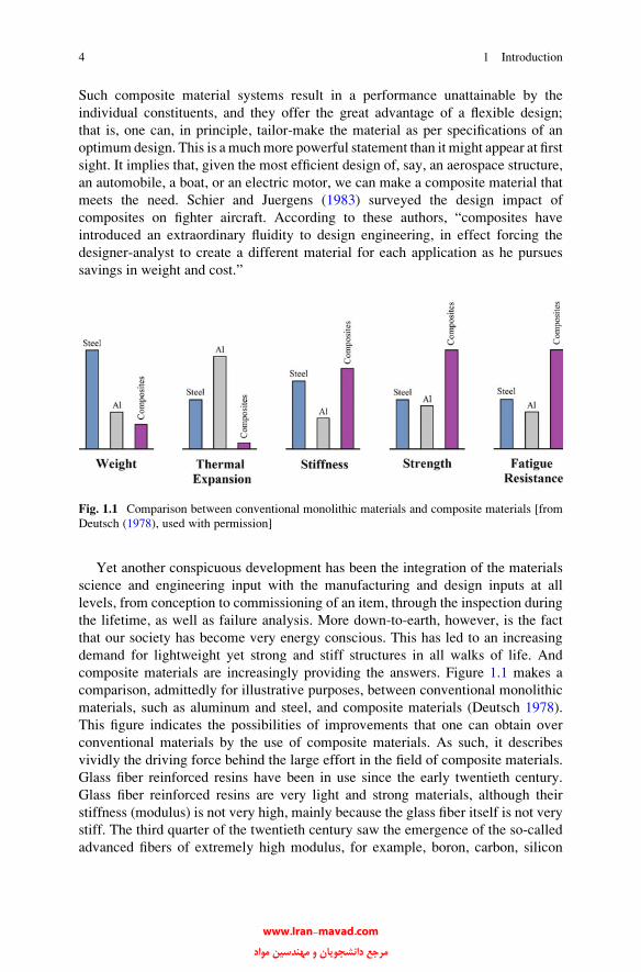
composite materials are increasingly providing the answers. Figure 1.1 makes a

comparison, admittedly for illustrative purposes, between conventional monolithic

materials, such as aluminum and steel, and composite materials (Deutsch 1978).

This figure indicates the possibilities of improvements that one can obtain over

conventional materials by the use of composite materials. As such, it describes

vividly the driving force behind the large effort in the field of composite materials.

Glass fiber reinforced resins have been in use since the early twentieth century.

Glass fiber reinforced resins are very light and strong materials, although their

stiffness (modulus) is not very high, mainly because the glass fiber itself is not very

stiff. The third quarter of the twentieth century saw the emergence of the so-called

advanced fibers of extremely high modulus, for example, boron, carbon, silicon

Fig. 1.1 Comparison between conventional monolithic materials and composite materials [from

Deutsch (1978), used with permission]

4 1 Introduction


carbide, and alumina (Chawla 1998, 2005). These fibers have been used for

reinforcement of resin, metal, and ceramic matrices. Fiber reinforced composites

have been more prominent than other types of composites for the simple reason that

most materials are stronger and stiffer in the fibrous form than in any other form.

By the same token, it must be recognized that a fibrous form results in reinforcement

mainly in fiber direction. Transverse to the fiber direction, there is little or no

reinforcement. Of course, one can arrange fibers in two-dimensional or even three-

dimensional arrays, but this still does not gainsay the fact that one is not getting the

full reinforcement effect in directions other than the fiber axis. Thus, if a less

anisotropic behavior is the objective, then perhaps laminate or sandwich composites

made of, say, two different materials would be more effective. A particle reinforced

composite will also be reasonably isotropic. There may also be specific nonmechan-

ical objectives for making a fibrous composite. For example, an abrasion- or

corrosion-resistant surface would require the use of a laminate (sandwich) form,

while in superconductors the problem of flux-pinning requires the use of extremely

fine filaments embedded in a conductive matrix. In what follows, we discuss the

various aspects of composites, mostly fiber reinforced composites, in greater detail,

but first let us agree on an acceptable definition of a composite material. Practically

everything in this world is a composite material. Thus, a common piece of metal is a

composite (polycrystal) of many grains (or single crystals). Such a definition would

make things quite unwieldy. Therefore, we must agree on an operational definition

of composite material for our purposes in this text. We shall call a material that

satisfies the following conditions a composite material:

1. It is manufactured (i.e., naturally occurring composites, such as wood, are

excluded).

2. It consists of two or more physically and/or chemically distinct, suitably

arranged or distributed phases with an interface separating them.

3. It has characteristics that are not depicted by any of the components in isolation.

References

Chawla KK (1998) Fibrous materials. Cambridge University Press, Cambridge

Chawla KK (Feb., 2005) J Miner, Metals Mater Soc 57:46

Deutsch S (May, 1978). 23rd National SAMPE Symposium, p 34

Elices M (ed) (2000) Structural biological materials. Pergamon Press, Amsterdam

Schier JF, Juergens RJ (Sept., 1983) Astronautics Aeronautics 21:44

Wainwright SA, Biggs WD, Currey JD, Gosline JM (1982) Mechanical design in organisms.

Princeton University Press, Princeton, NJ

Weiner S, Wagner HD (1998) Annu Rev Mater 28:271

References 5


Problems

1.1. Describe the structure and properties of some fiber reinforced composites that

occur in nature.

1.2. Many ceramic-based composite materials are used in the electronics industry.

Describe some of these electroceramic composites.

1.3. Describe the use of composite materials in the Voyager airplane that circled

the globe for the first time without refueling in flight.

1.4. Nail is a fibrous composite. Describe its components, microstructure, and

properties.

1.5. Discuss the use of composite materials in civilian aircraft, with special atten-

tion to Boeing 787 and Airbus A380 aircraft.

6 1 Introduction


Chapter 2

Reinforcements

2.1 Introduction

Reinforcements need not necessarily be in the form of long fibers. One can have

them in the form of particles, flakes, whiskers, short fibers, continuous fibers, or

sheets. It turns out that most reinforcements used in composites have a fibrous form

because materials are stronger and stiffer in the fibrous form than in any other form.

Specifically, in this category, we are most interested in the so-called advanced

fibers, which possess very high strength and very high stiffness coupled with a very

low density. The reader should realize that many naturally occurring fibers can be

and are used in situations involving not very high stresses (Chawla 1976; Chawla

and Bastos 1979). The great advantage in this case, of course, is its low cost.

The vegetable kingdom is, in fact, the largest source of fibrous materials. Cellulosic

fibers in the form of cotton, flax, jute, hemp, sisal, and ramie, for example, have

been used in the textile industry, while wood and straw have been used in the paper

industry. Other natural fibers, such as hair, wool, and silk, consist of different forms

of protein. Silk fibers produced by a variety of spiders, in particular, appear to be

very attractive because of their high work of fracture. Any discussion of such fibers

is beyond the scope of this book. The interested reader is directed to some books

that cover the vast field of fibers used as reinforcements (Chawla 1998; Warner

1995). In this chapter, we confine ourselves to a variety of man-made

reinforcements. Glass fiber, in its various forms, has been the most common

reinforcement for polymer matrices. Aramid fiber, launched in the 1960s, is much

stiffer and lighter than glass fiber. Kevlar is Du Pont’s trade name for aramid fiber

while Twaron is the trade name of aramid fiber made by Teijin Aramid. Gel-spun

polyethylene fiber, which has a stiffness comparable to that of aramid fiber, was

commercialized in the 1980s. Other high-performance fibers that combine high

strength with high stiffness are boron, silicon carbide, carbon, and alumina. These

were all developed in the second part of the twentieth century. In particular, some

ceramic fibers were developed in the last quarter of the twentieth century by


7


some very novel processing techniques, namely, sol-gel processing and controlled

pyrolysis of organic precursors.

The use of fibers as high-performance engineering materials is based on three

important characteristics (Dresher 1969):

1. A small diameter with respect to its grain size or other microstructural unit. This

allows a higher fraction of the theoretical strength to be attained than is possible

in a bulk form. This is a direct result of the so-called size effect; the smaller the

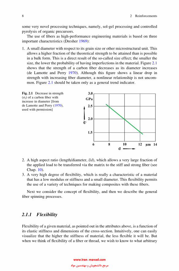
size, the lower the probability of having imperfections in the material. Figure 2.1

shows that the strength of a carbon fiber decreases as its diameter increases

(de Lamotte and Perry 1970). Although this figure shows a linear drop in

strength with increasing fiber diameter, a nonlinear relationship is not uncom-

mon. Figure 2.1 should be taken only as a general trend indicator.

2. A high aspect ratio (length/diameter, l/d), which allows a very large fraction of

the applied load to be transferred via the matrix to the stiff and strong fiber (see

Chap. 10).

3. A very high degree of flexibility, which is really a characteristic of a material

that has a low modulus or stiffness and a small diameter. This flexibility permits

the use of a variety of techniques for making composites with these fibers.

Next we consider the concept of flexibility, and then we describe the general

fiber spinning processes.

2.1.1 Flexibility

Flexibility of a given material, as pointed out in the attributes above, is a function of

its elastic stiffness and dimensions of the cross-section. Intuitively, one can easily

visualize that the higher the stiffness of material, the less flexible it will be. But

when we think of flexibility of a fiber or thread, we wish to know to what arbitrary

Fig. 2.1 Decrease in strength

(sf) of a carbon fiber with

increase in diameter [from

de Lamotte and Perry (1970),

used with permission]

8 2 Reinforcements


http://dx.doi.org/10.1007/978-0-387-74365-3_10

radius we can bend it before it fails. We can treat our single fiber to be an elongated

elastic beam. Let us subject this fiber of Young’s modulus, E and diameter, d to a

bending moment,M, which will bend it to a radius, R. For such an elastic bending ofa beam, we define flexural rigidity as MR. From elementary strength of materials,

we have the following relationship for a beam bent to a radius R:

M

I¼ E

R;

or,

MR ¼ EI ;

where E is the Young’s modulus of the material and I is the second moment of area

or moment of inertia of its cross-section. For a beam or a fiber of diameter, d, thesecond moment of area about an axis through the centroid of the beam is given by

I ¼ pd4/64. Now, we can define flexibility of the fiber (i.e., the elastic beam under

consideration) as the inverse of flexural rigidity. In other words, flexibility of a fiber

is an inverse function of its elastic modulus, E, and the second moment of area or

moment of inertia of its cross-section, I. The elastic modulus of a material is

generally independent of its form or size and is generally a material constant for

a given chemical composition (assuming a fully dense material). Thus, for a given

composition and density, the flexibility of a material is determined by its shape, or

more precisely by its diameter. Substituting for I ¼ pd4/64 in the above expression,we get,

MR ¼ EI ¼ Ep d4

64;

or, the flexibility, being equal to 1/MR, is

Flexibility ¼ 1

MR¼ 64

Epd4; (2.1)

where d is the equivalent diameter and I is the moment of inertia of the beam (fiber).

Equation (2.1) indicates that flexibility, 1/MR, is a very sensitive function of

diameter, d. We can summarize the important implications of Eq. (2.1) as follows:

• Flexibility of a fiber is a very sensitive inverse function of its diameter, d.• Given a sufficiently small diameter, it is possible to produce, in principle, a fiber

as flexible as any from a polymer, a metal, or a ceramic.

• One can make very flexible fibers out of inherently brittle materials such as

glass, silicon carbide, alumina, etc., provided one can shape these brittle

materials into a fine diameter fiber. Producing a fine diameter ceramic fiber,

however, is a daunting problem in processing.

2.1 Introduction 9


To illustrate this concept of flexibility, we plot the diameter of various materials in

fibrous formwith flexibility (1/MR) equal to that of highly flexible filament, namely, a

25-mm-diameter nylon fiber as function of the elastic modulus, E. Note that given a

sufficiently small diameter, it is possible for a metal or ceramic to have the same

degree of flexibility as that of a 25-mm-diameter nylon fiber; it is, however, another

matter that obtaining such a small diameter in practice can be prohibitively expensive.

2.1.2 Fiber Spinning Processes

Fiber spinning is the process of extruding a liquid through small holes in a spinneret

to form solid filaments. In nature, silkworms and spiders produce continuous

filaments by this process. There exists a variety of different fiber spinning

techniques; some of the important ones are:

Wet spinning. A solution is extruded into a coagulating bath. The jets of liquid

freeze or harden in the coagulating bath as a result of chemical or physical

changes.

Dry spinning. A solution consisting of a fiber-forming material and a solvent is

extruded through a spinneret. A stream of hot air impinges on the jets of solution

emerging from the spinneret, the solvent evaporates, and solid filaments are left

behind.

Fig. 2.2 Fiber diameter of different materials with flexibility equal to that of a nylon fiber of

diameter equal to 25 mm. Note that one can make very flexible fibers out of brittle materials such as

glass, silicon carbide, alumina, etc., provided one can process them into a small diameter

10 2 Reinforcements


Melt spinning. The fiber-forming material is heated above its melting point and the

molten material is extruded through a spinneret. The liquid jets harden into solid

filaments in air on emerging from the spinneret holes.

Dry jet–wet spinning. This is a special process devised for spinning of aramid fibers.

In this process, an appropriate polymer liquid crystal solution is extruded

through spinneret holes, passes through an air gap before entering a coagulation

bath, and then goes on a spool for winding. We describe this process in detail in

Sect. 2.5.2.

2.1.3 Stretching and Orientation

The process of extrusion through a spinneret results in some chain orientation in the

filament. Generally, the molecules in the surface region undergo more orientation

than the ones in the interior because the edges of the spinneret hole affect the near-

surface molecules more. This is known as the skin effect, and it can affect many other

properties of the fiber, such as the adhesion with a polymeric matrix or the ability to

be dyed. Generally, the as-spun fiber is subjected to some stretching, causing further

chain orientation along the fiber axis and consequently better tensile properties, such

as stiffness and strength, along the fiber axis. The amount of stretch is generally

given in terms of a draw ratio, which is the ratio of the initial diameter to the final

diameter. For example, nylon fibers are typically subjected to a draw ratio of 5 after

spinning. A high draw ratio results in a high elastic modulus. Increased alignment of

chains means a higher degree of crystallinity in a fiber. This also affects the ability of

a fiber to absorb moisture. The higher the degree of crystallinity, the lower the

moisture absorption. In general, the higher degree of crystallinity translates into a

higher resistance to penetration by foreign molecules, i.e., a greater chemical

stability. The stretching treatment serves to orient the molecular structure along

the fiber axis. It does not, generally, result in complete elimination of molecular

branching; that is, one gets molecular orientation but not extension. Such stretching

treatments do result in somewhat more efficient packing than in the unstretched

polymer, but there is a limit to the amount of stretch that can be given to a polymer

because the phenomenon of necking can intervene and cause rupture of the fiber.

2.2 Glass Fibers

Glass fiber is a generic name like carbon fiber or steel or aluminum. Just as different

compositions of steel or aluminum alloys are available, there are many of different

chemical compositions of glass fibers that are commercially available. Common

glass fibers are silica based (~50–60 % SiO2) and contain a host of other oxides of

calcium, boron, sodium, aluminum, and iron, for example. Table 2.1 gives the

compositions of some commonly used glass fibers. The designation E stands for

2.2 Glass Fibers 11


electrical because E glass is a good electrical insulator in addition to having good

strength and a reasonable Young’s modulus; C stands for corrosion and C glass has

a better resistance to chemical corrosion than other glasses; S stands for the high

silica content that makes S glass withstand higher temperatures than other glasses.

It should be pointed out that most of the continuous glass fiber produced is of the E

glass type but, notwithstanding the designation E, electrical uses of E glass fiber are

only a small fraction of the total market.

2.2.1 Fabrication

Figure 2.3 shows schematically the conventional fabrication procedure for glass

fibers (specifically, the E glass fibers that constitute the workhorse of the resin

reinforcement industry) (Loewenstein 1983; Parkyn 1970; Lowrie 1967). The raw

materials are melted in a hopper and the molten glass is fed into the electrically

Fig. 2.3 Schematic of glass fiber manufacture

Table 2.1 Approximate chemical compositions of some glass fibers (wt.%)

Composition E glass C glass S glass

SiO2 55.2 65.0 65.0

Al2O3 8.0 4.0 25.0

CaO 18.7 14.0 –

MgO 4.6 3.0 10.0

Na2O 0.3 8.5 0.3

K2O 0.2 – –

B2O3 7.3 5.0 –

12 2 Reinforcements


Fig. 2.4 Glass fiber is available in a variety of forms: (a) chopped strand, (b) continuous yarn,

(c) roving, (d) fabric [courtesy of Morrison Molded Fiber Glass Company]

Fig. 2.5 Continuous glass fibers (cut from a spool) obtained by the sol–gel technique [from Sakka

(1985), used with permission]


heated platinum bushings or crucibles; each bushing contains about 200 holes at its

base. The molten glass flows by gravity through these holes, forming fine continu-

ous filaments; these are gathered together into a strand and a size is applied before itis a wound on a drum. The final fiber diameter is a function of the bushing orifice

diameter; viscosity, which is a function of composition and temperature; and the

head of glass in the hopper. In many old industrial plants the glass fibers are not

produced directly from fresh molten glass. Instead, molten glass is first turned into

marbles, which after inspection are melted in the bushings. Modern plants do

produce glass fibers by direct drawing. Figure 2.4 shows some forms in which

glass fiber is commercially available.

The conventional methods of making glass or ceramic fibers involve drawing

from high-temperature melts of appropriate compositions. This route has many

practical difficulties such as the high processing temperature required, the immis-

cibility of components in the liquid state, and the easy crystallization during

cooling. Several techniques have been developed for preparing glass and ceramic

fibers (Chawla 1998). An important technique is called the sol–gel technique

(Brinker and Scherer 1990; Jones 1989). We shall come back to this sol–gel

technique at various places in this book. Here we just provide a brief description.

A sol is a colloidal suspension in which the individual particles are so small

(generally in the nm range) that they show no sedimentation. A gel, on the other

hand, is a suspension in which the liquid medium has become viscous enough to

behave more or less like a solid. The sol–gel process of making a fiber involves a

conversion of fibrous gels, drawn from a solution at a low temperature, into glass

or ceramic fibers at several hundred degrees Celsius. The maximum heating

temperature in this process is much lower than that in conventional glass fiber

manufacture. The sol–gel method using metal alkoxides consists of preparing an

appropriate homogeneous solution, changing the solution to a sol, gelling the sol,

and converting the gel to glass by heating. The sol–gel technique is a very

powerful technique for making glass and ceramic fibers. The 3M Company

produces a series of alumina and silica-alumina fibers, called the Nextel fibers,

from metal alkoxide solutions (see Sect. 2.6). Figure 2.5 shows an example of

drawn silica fibers (cut from a continuous fiber spool) obtained by the sol–gel

technique (Sakka 1985).

Glass filaments are easily damaged by the introduction of surface defects.

To minimize this and to make handling of these fibers easy, a sizing treatment is

given. The size, or coating, protects and binds the filaments into a strand.

2.2.2 Structure

Inorganic, silica-based glasses are analogous to organic glassy polymers in that they

are amorphous, i.e., devoid of any long-range order that is characteristic of a

crystalline material. Pure, crystalline silica melts at 1,800 �C. However, by adding

some metal oxides, we can break the Si–O bonds and obtain a series of amorphous

14 2 Reinforcements


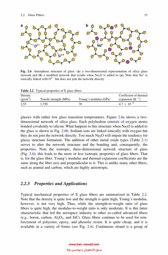
glasses with rather low glass transition temperatures. Figure 2.6a shows a two-

dimensional network of silica glass. Each polyhedron consists of oxygen atoms

bonded covalently to silicon. What happens to this structure when Na2O is added to

the glass is shown in Fig. 2.6b. Sodium ions are linked ionically with oxygen but

they do not join the network directly. Too much Na2O will impair the tendency for

glassy structure formation. The addition of other metal oxide types (Table 2.1)

serves to alter the network structure and the bonding and, consequently, the

properties. Note the isotropic, three-dimensional network structure of glass

(Fig. 2.6); this leads to the more or less isotropic properties of glass fibers. That

is, for the glass fiber, Young’s modulus and thermal expansion coefficients are the

same along the fiber axis and perpendicular to it. This is unlike many other fibers,

such as aramid and carbon, which are highly anisotropic.

2.2.3 Properties and Applications

Typical mechanical properties of E glass fibers are summarized in Table 2.2.

Note that the density is quite low and the strength is quite high; Young’s modulus,

however, is not very high. Thus, while the strength-to-weight ratio of glass

fibers is quite high, the modulus-to-weight ratio is only moderate. It is this latter

characteristic that led the aerospace industry to other so-called advanced fibers

(e.g., boron, carbon, Al2O3, and SiC). Glass fibers continue to be used for rein-

forcement of polyester, epoxy, and phenolic resins. It is quite cheap, and it is

available in a variety of forms (see Fig. 2.4). Continuous strand is a group of

Table 2.2 Typical properties of E glass fibers

Density

(g/cm3) Tensile strength (MPa) Young’s modulus (GPa)

Coefficient of thermal

expansion (K�1)

2.55 1,750 70 4.7 � 10�6

Fig. 2.6 Amorphous structure of glass: (a) a two-dimensional representation of silica glass

network and (b) a modified network that results when Na2O is added to (a). Note that Na+ is

ionically linked with O2� but does not join the network directly

2.2 Glass Fibers 15


individual fibers; roving is a group of parallel strands; chopped fibers consists of

strand or roving chopped to lengths between 5 and 50 mm. Glass fibers are also

available in the form of woven fabrics or nonwoven mats.

Moisture decreases glass fiber strength. Glass fibers are also susceptible to what

is called static fatigue; that is, when subjected to a constant load for an extended

time period, glass fibers can undergo subcritical crack growth. This leads to failure

over time at loads that might be safe when considering instantaneous loading.

Glass fiber reinforced resins are used widely in the building and construction

industry. Commonly, these are called glass-reinforced plastics, or GRP. They are

used in the form of a cladding for other structural materials or as an integral part of a

structural or non-load-bearing wall panel; window frames, tanks, bathroom units,

pipes, and ducts are common examples. Boat hulls, since the mid-1960s, have

primarily been made of GRP. Use of GRP in the chemical industry (e.g., as storage

tanks, pipelines, and process vessels) is fairly routine. The rail and road transporta-

tion industry and the aerospace industry are other big users of GRP.

2.3 Boron Fibers

Boron is an inherently brittle material. It is commercially made by chemical vapor

deposition (CVD) of boron on a substrate, that is, boron fiber as produced is itself a

composite fiber.

In view of the fact that rather high temperatures are required for this deposition

process, the choice of substrate material that goes to form the core of the finished

boron fiber is limited. Generally, a fine tungsten wire is used for this purpose.

A carbon substrate can also be used. The first boron fibers were obtained by

Weintraub (1911) by means of reduction of a boron halide with hydrogen on a

hot wire substrate.

The real impulse in boron fiber fabrication, however, came in 1959, when Talley

(Talley 1959; Talley et al. 1960) used the process of halide reduction to obtain

amorphous boron fibers of high strength. Since then, interest in the use of strong but

light boron fibers as a possible structural component in aerospace and other

structures has been continuous, although it must be admitted that this interest has

periodically waxed and waned in the face of rather stiff competition from other so-

called advanced fibers, in particular, carbon fibers.

2.3.1 Fabrication

Boron fibers are obtained by CVD on a substrate. There are two processes:

1. Thermal decomposition of a boron hydride. This method involves low

temperatures, and, thus, carbon-coated glass fibers can be used as a substrate.

16 2 Reinforcements


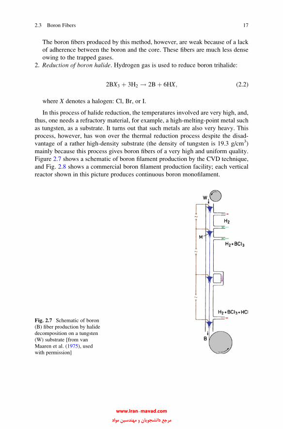
The boron fibers produced by this method, however, are weak because of a lack

of adherence between the boron and the core. These fibers are much less dense

owing to the trapped gases.

2. Reduction of boron halide. Hydrogen gas is used to reduce boron trihalide:

2BX3 þ 3H2 ! 2Bþ 6HX; (2.2)

where X denotes a halogen: Cl, Br, or I.

In this process of halide reduction, the temperatures involved are very high, and,

thus, one needs a refractory material, for example, a high-melting-point metal such

as tungsten, as a substrate. It turns out that such metals are also very heavy. This

process, however, has won over the thermal reduction process despite the disad-

vantage of a rather high-density substrate (the density of tungsten is 19.3 g/cm3)

mainly because this process gives boron fibers of a very high and uniform quality.

Figure 2.7 shows a schematic of boron filament production by the CVD technique,

and Fig. 2.8 shows a commercial boron filament production facility; each vertical

reactor shown in this picture produces continuous boron monofilament.

Fig. 2.7 Schematic of boron

(B) fiber production by halide

decomposition on a tungsten

(W) substrate [from van

Maaren et al. (1975), used

with permission]

2.3 Boron Fibers 17


In the process of BCl3 reduction, a very fine tungsten wire (10–12 mm diameter)

is pulled into a reaction chamber at one end through a mercury seal and out at the

other end through another mercury seal. The mercury seals act as electrical contacts

for resistance heating of the substrate wire when gases (BCl3 + H2) pass through

the reaction chamber, where they react on the incandescent wire substrate. The

reactor can be a one- or multistage, vertical or horizontal, reactor. BCl3 is an

expensive chemical, and only about 10 % of it is converted into boron in this

reaction. Thus, an efficient recovery of the unused BCl3 can result in a considerable

lowering of the boron filament cost.

There is a critical temperature for obtaining a boron fiber with optimum

properties and structure (van Maaren et al. 1975). The desirable amorphous form

of boron occurs below this critical temperature while above this temperature

crystalline forms of boron also occur that are undesirable from a mechanical

properties viewpoint, as we shall see in Sect. 2.3.2. With the substrate wire

Fig. 2.8 A boron filament

production facility

(courtesy of AVCO

Specialty Materials Co.)

18 2 Reinforcements


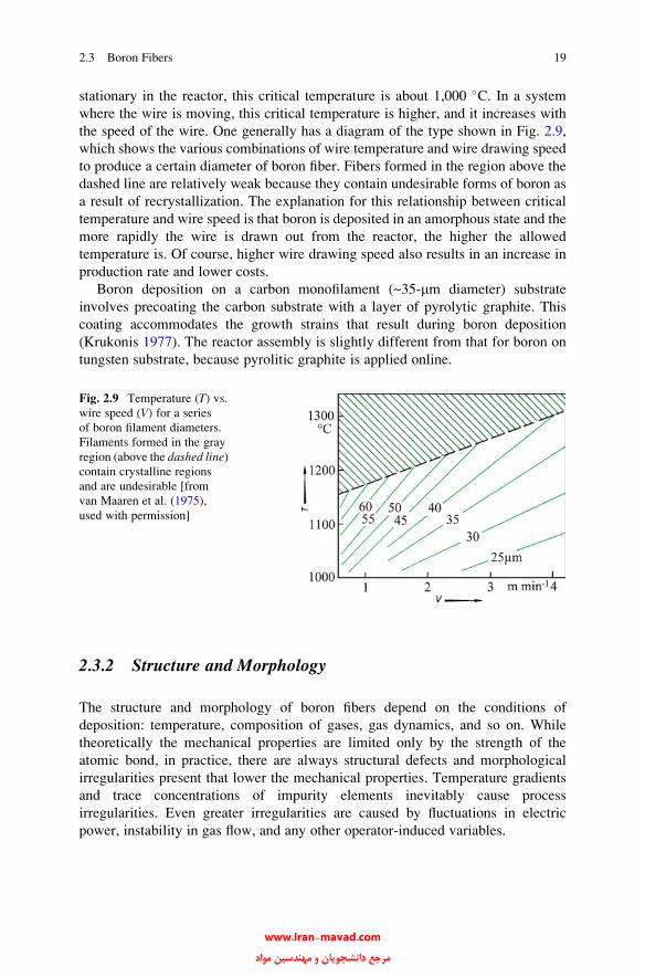
stationary in the reactor, this critical temperature is about 1,000 �C. In a system

where the wire is moving, this critical temperature is higher, and it increases with

the speed of the wire. One generally has a diagram of the type shown in Fig. 2.9,

which shows the various combinations of wire temperature and wire drawing speed

to produce a certain diameter of boron fiber. Fibers formed in the region above the

dashed line are relatively weak because they contain undesirable forms of boron as

a result of recrystallization. The explanation for this relationship between critical

temperature and wire speed is that boron is deposited in an amorphous state and the

more rapidly the wire is drawn out from the reactor, the higher the allowed

temperature is. Of course, higher wire drawing speed also results in an increase in

production rate and lower costs.

Boron deposition on a carbon monofilament (~35-mm diameter) substrate

involves precoating the carbon substrate with a layer of pyrolytic graphite. This

coating accommodates the growth strains that result during boron deposition

(Krukonis 1977). The reactor assembly is slightly different from that for boron on

tungsten substrate, because pyrolitic graphite is applied online.

2.3.2 Structure and Morphology

The structure and morphology of boron fibers depend on the conditions of

deposition: temperature, composition of gases, gas dynamics, and so on. While

theoretically the mechanical properties are limited only by the strength of the

atomic bond, in practice, there are always structural defects and morphological

irregularities present that lower the mechanical properties. Temperature gradients

and trace concentrations of impurity elements inevitably cause process

irregularities. Even greater irregularities are caused by fluctuations in electric

power, instability in gas flow, and any other operator-induced variables.

Fig. 2.9 Temperature (T) vs.wire speed (V) for a seriesof boron filament diameters.

Filaments formed in the gray

region (above the dashed line)contain crystalline regions

and are undesirable [from

van Maaren et al. (1975),


2.3 Boron Fibers 19


2.3.2.1 Structure

Depending on the conditions of deposition, the elemental boron can exist in various

crystalline polymorphs. The form produced by crystallization from the melt or CVD

above 1,300 �C is b-rhombohedral. At temperatures lower than this, if crystalline

boron is produced, the most commonly observed structure is a-rhombohedral.

Boron fibers produced by theCVDmethod described earlier have amicrocrystalline

structure that is generally called amorphous. This designation is based on the charac-teristic X-ray diffraction pattern produced by the filament in the Debye-Scherrer

method, that is, large and diffuse halos with d spacings of 0.44, 0.25, 0.17, 1.4, 1.1,

and 0.091 nm, typical of amorphous material (Vega-Boggio and Vingsbo 1978).

Electron diffraction studies, however, lead one to conclude that this “amorphous”

boron is really a nanocrystalline phase with a grain diameter of the order of 2 nm

(Krukonis 1977).

Based on X-ray and electron diffraction studies, one can conclude that amorphous

boron is really nanocrystalline b-rhombohedral. In practice, the presence of micro-

crystalline phases (crystals or groups of crystals observable in the electron

microscope) constitutes an imperfection in the fiber that should be avoided. Larger

and more serious imperfections generally result from surpassing the critical temper-

ature of deposition (see Sect. 2.3.1) or the presence of impurities in the gases.

When boron fiber is made by deposition on a tungsten substrate, as is generally

the case, then depending on the temperature conditions during deposition, the core

may consist of, in addition to tungsten, a series of compounds, such as W2B, WB,

W2B5, andWB4 (Galasso et al. 1967). A boron fiber cross-section (100 mmdiameter)

is shown in Fig. 2.10a, while Fig. 2.10b shows schematically the various subparts of

the cross-section. The various tungsten boride phases are formed by diffusion

of boron into tungsten. Generally, the fiber core consists only of WB4 and W2B5.

On prolonged heating, the core may be completely converted into WB4. As boron

diffuses into the tungsten substrate to form borides, the core expands from its

Fig. 2.10 (a) Cross-section of a 100-mm-diameter boron fiber. (b) Schematic of the cross-section

of a boron fiber with SiC barrier layer

20 2 Reinforcements


original 12.5 mm (original tungsten wire diameter) to 17.5 mm. The SiC coating

shown in Fig. 2.10b is a barrier coating used to prevent any adverse reaction between

B and the matrix, such as Al, at high temperatures. The SiC barrier layer is vapor

deposited onto boron using a mixture of hydrogen and methyldichlorosilane.

2.3.2.2 Morphology

The boron fiber surface shows a “corn-cob” structure consisting of nodules

separated by boundaries (Fig. 2.11). The nodule size varies during the course of

fabrication. In a very general way, the nodules start as individual nuclei on the

substrate and then grow outward in a conical form until a filament diameter of

80–90 mm is reached, above which the nodules seem to decrease in size. Occasion-

ally, new cones may nucleate in the material, but they always originate at an

interface with a foreign particle or inclusion.

2.3.3 Residual Stresses

Boron fibers have inherent residual stresses that have their origin in the process of

chemical vapor deposition. Growth stresses in the nodules of boron, stresses

induced by the diffusion of boron into the tungsten core, and stresses generated

by the difference in the coefficient of expansion of deposited boron and tungsten

boride core, all contribute to the residual stresses and thus can have a considerable

influence on the fiber mechanical properties. The residual stress pattern across the

transverse section of a boron fiber is shown in Fig. 2.12 (Vega-Boggio and Vingsbo

1978). The compressive stresses on the fiber surface are due to the quenching action

involved in pulling the fiber out from the chamber (Vega-Boggio and Vingsbo

1978). Morphologically, the most conspicuous aspect of these internal stresses is

the frequently observed radial crack in the transverse section of these fibers. The

crack runs from within the core to just inside the external surface. Some workers,

however, doubt the preexistence of this radial crack (Krukonis 1977). They think

that the crack appears during the process of boron fiber fracture.

Fig. 2.11 Characteristic corncob structure of boron fiber [from van Maaren et al. (1975), used

with permission]. The fiber diameter is 142 mm

2.3 Boron Fibers 21


2.3.4 Fracture Characteristics

It is well known that brittle materials show a distribution of strengths rather than a

single value. Imperfections in these materials lead to stress concentrations much

higher than the applied stress levels. Because the brittle material is not capable of

deforming plastically in response to these stress concentrations, fracture ensues at

one or more such sites. Boron fiber is indeed a very brittle material, and cracks

originate at preexisting defects located at either the boron-core interface or the

surface. Figure 2.13 shows the characteristic brittle fracture of a boron fiber and

the radical crack. It is worth pointing out here that the radial crack does not extend

all the way to surface of the fiber. This is because the surface layer of boron fiber is

in compression; see Fig. 2.12. The surface defects in boron fiber stem from the

nodular surface that results from the growth of boron cones. In particular, when a

nodule coarsens due to an exaggerated growth around a contaminating particle,

a crack can result from this large nodule and weaken the fiber.

2.3.5 Properties and Applications of Boron Fibers

Many researchers have investigated the mechanical properties of boron fibers

(Krukonis 1977; Vega-Boggio and Vingsbo 1978; Galasso et al. 1967; Galasso

and Paton 1966; DeBolt 1982; Wawner 1967; DiCarlo 1985). Due to the com-

posite nature of the boron fiber, complex internal stresses and defects such as

voids and structural discontinuities result from the presence of a core and the

deposition process. Thus, one would not expect boron fiber to show the intrinsic

Fig. 2.12 Schematic

of residual stress pattern

across the transverse section

of a boron fiber [from

Vega-Boggio and Vingsbo


22 2 Reinforcements


strength of boron. The average tensile strength of boron fiber is 3–4 GPa, while

its Young’s modulus is between 380 and 400 GPa.

An idea of the intrinsic strength of boron can be obtained in a flexure test

(Wawner 1967). In flexure, assuming the core and interface to be near the neutral

axis, critical tensile stresses would not develop at the core or interface. Flexure tests

on boron fibers lightly etched to remove any surface defects gave a strength of

14 GPa. Without etching, the strength was half this value. Table 2.3 provides a

summary of the characteristics of boron fiber (DiCarlo 1985). Commercially

produced 142-mm-diameter boron fiber shows average tensile strength of

3.8 GPa. The tensile strength and fracture energy values of the as-received and

some limited-production-run larger-diameter fibers showed improvement after

chemical polishing, as shown in Table 2.3. Fibers showing strengths greater than

4 GPa had their fracture controlled by a tungsten boride core, while fibers with

strengths of 4 GPa or less were controlled by fiber surface flaws. The high-

temperature treatment, indicated in Table 2.3, improved the fiber properties by

putting a permanent axial compressive strain in the sheath.

Boron has a density of 2.34 g/cm3 (about 15 % less than that of aluminum).

Boron fiber with a tungsten core has a density of 2.6 g/cm3 for a fiber with 100 mmdiameter. Its melting point is 2,040 �C, and it has a thermal expansion coefficient of

8.3 � 10�6 �C�1 up to 315 �C.Boron fiber composites are in use in a number of US military aircraft, notably the

F-14 and F-15, and in the US space shuttle. They are also used for stiffening golf

shafts, tennis rackets, bicycle frames, and in making repair patches for PMCs. A big

advantage of boron fiber over other high performance fibers is their relatively better

properties in compression. This stems from their larger diameter. A commercial

product called Hy-Bor uses a mix of carbon and boron fibers in an epoxy matrix,

Fig. 2.13 Fracture surface

of a boron fiber showing

a characteristically brittle

fracture and a radial crack

2.3 Boron Fibers 23


wherein improved properties in compression result because of the boron fibers. One

big obstacle to the widespread use of boron fiber is its high cost compared to that of

other fibers.

2.4 Carbon Fibers

Carbon is a very light element with a density equal to 2.268 g/cm3. Carbon can exist

in a variety of crystalline forms. Our interest here is in the so-called graphitic

structure wherein the carbon atoms are arranged in the form of hexagonal layers.

The other well-known form of carbon is the covalent diamond structure wherein the

carbon atoms are arranged in a three-dimensional configuration with little structural

flexibility. Another form of carbon is Buckminster Fullerene (or Bucky ball), with a

molecular composition of C60 or C70. One can also have carbon nanotubes, which

are nothing but drawn out version of Buckyballs. Carbon in the graphitic form is

highly anisotropic, with a theoretical Young’s modulus in the layer plane being

equal to about 1,000 GPa, while that along the c-axis is equal to about 35 GPa.

The graphite structure (Fig. 2.14a) has a very dense packing in the layer planes.

The lattice structure is shown more clearly with only lattice planes in Fig. 2.14b.

As we know, the bond strength determines the modulus of a material. Thus, the

high-strength bond between carbon atoms in the layer plane results in an extremely

high modulus while the weak van der Waals-type bond between the neighboring

layers results in a lower modulus in that direction. Consequently, almost all

processing techniques of carbon fiber have the goal of obtaining a very high degree

of preferred orientation of hexagonal planes along the fiber axis.

Carbon fibers of extremely high modulus can be made by carbonization of

organic precursor fibers followed by graphitization at high temperatures.

The organic precursor fiber, that is, the raw material for carbon fiber, is generally a

special textile polymeric fiber that can be carbonized without melting. The precursor

fiber, like any polymeric fiber, consists of long-chain molecules (0.1–1 mm when

Table 2.3 Strength properties of improved large-diameter boron fibers

Diameter (mm) Treatment

Strength Relative fracture

energyAveragea (GPa) COVb (%)

142 As-produced 3.8 10 1.0

406 As-produced 2.1 14 0.3

382 Chemical polish 4.6 4 1.4

382 Heat treatment plus polish 5.7 4 2.2a Gauge length ¼ 25 mmbCoefficient of variation ¼ standard deviation/average value

Source: Reprinted with permission from J Metals 37, No. 6, 1985, a publication of The Metallur-

gical Society, Warrendale PA

24 2 Reinforcements


fully stretched) arranged in a random manner. Such polymeric fibers generally have

poor mechanical properties and typically show rather large deformations at low

stresses mainly because the polymeric chains are not ordered. A commonly used

precursor fiber is polyacrylonitrile (PAN). Other precursor fibers include rayon and

the ones obtained from pitches, polyvinyl alcohol, polyimides, and phenolics.

Carbon fiber is a generic term representing a family of fibers (Chawla 1981).

As pointed out earlier, unlike the rigid diamond structure, graphitic carbon has a

lamellar structure. Thus, depending on the size of the lamellar packets, their

stacking heights, and the resulting crystalline orientations, one can obtain a range

of properties. Most of the carbon fiber fabrication processes involve the following

essential steps:

1. A fiberization procedure to make a precursor fiber. This generally involves wet-,

dry-, or melt-spinning followed by some drawing or stretching.

2. A stabilization treatment that prevents the fiber from melting in the subsequent

high-temperature treatments.

3. A thermal treatment called carbonization that removes most noncarbon

elements.

4. An optional thermal treatment called graphitization that improves the properties

of carbon fiber obtained in step 3.

It should be clear to the reader by now that in order to make a high-modulus

fiber, one must improve the orientation of graphitic crystals or lamellas. This is

achieved by various kinds of thermal and stretching treatments involving rather

rigorous controls. If a constant stress were applied for a long time, for example, it

would result in excessive fiber elongation and the accompanying reduction in area

may lead to fiber fracture.

Fig. 2.14 (a) Graphitic layer structure. The layers are shown not in contact for visual ease. (b) The

hexagonal lattice structure of graphite

2.4 Carbon Fibers 25


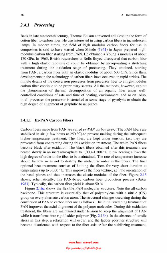
2.4.1 Processing

Back in late nineteenth century, Thomas Edison converted cellulose in the form of

cotton fiber to carbon fiber. He was interested in using carbon fibers in incandescent

lamps. In modern times, the field of high modulus carbon fibers for use in

composites is said to have started when Shindo (1961) in Japan prepared high-

modulus carbon fiber starting from PAN. He obtained a Young’s modulus of about

170 GPa. In 1963, British researchers at Rolls Royce discovered that carbon fiber

with a high elastic modulus of could be obtained by incorporating a stretching

treatment during the oxidation stage of processing. They obtained, starting

from PAN, a carbon fiber with an elastic modulus of about 600 GPa. Since then,

developments in the technology of carbon fibers have occurred in rapid strides. The

minute details of the conversion processes from precursor fiber to a high-modulus

carbon fiber continue to be proprietary secrets. All the methods, however, exploit

the phenomenon of thermal decomposition of an organic fiber under well-

controlled conditions of rate and time of heating, environment, and so on. Also,

in all processes the precursor is stretched at some stage of pyrolysis to obtain the

high degree of alignment of graphitic basal planes.

2.4.1.1 Ex-PAN Carbon Fibers

Carbon fibers made from PAN are called ex-PAN carbon fibers. The PAN fibers are

stabilized in air (a few hours at 250 �C) to prevent melting during the subsequent

higher-temperature treatment. The fibers are kept under tension, i.e., they are

prevented from contracting during this oxidation treatment. The white PAN fibers

become black after oxidation. The black fibers obtained after this treatment are

heated slowly in an inert atmosphere to 1,000–1,500 �C. Slow heating allows the

high degree of order in the fiber to be maintained. The rate of temperature increase

should be low so as not to destroy the molecular order in the fibers. The final

optional heat treatment consists of holding the fibers for very short duration at

temperatures up to 3,000 �C. This improves the fiber texture, i.e., the orientation of

the basal planes and thus increases the elastic modulus of the fiber. Figure 2.15

shows, schematically, this PAN-based carbon fiber production process (Baker

1983). Typically, the carbon fiber yield is about 50 %.

Figure 2.16a shows the flexible PAN molecular structure. Note the all-carbon

backbone. This structure is essentially that of polyethylene with a nitrile (CN)

group on every alternate carbon atom. The structural changes occurring during the

conversion of PAN to carbon fiber are as follows. The initial stretching treatment of

PAN improves the axial alignment of the polymer molecules. During this oxidation

treatment, the fibers are maintained under tension to keep the alignment of PAN

while it transforms into rigid ladder polymer (Fig. 2.16b). In the absence of tensile

stress in this step, a relaxation will occur, and the ladder polymer structure will

become disoriented with respect to the fiber axis. After the stabilizing treatment,

26 2 Reinforcements


the resulting ladder-type structure (also called oriented cyclic structure) has a highglass transition temperature so that there is no need to stretch the fiber during the next

stage, which is carbonization. There are still considerable quantities of nitrogen and

hydrogen present, which are eliminated as gaseous waste products during carboni-

zation, that is, heating to 1,000–1,500 �C (Fig. 2.15). The carbon atoms remaining

after this treatment are mainly in the form of a network of extended hexagonal

ribbons, which has been called turbostratic graphite structure in the literature.

Although these strips tend to align parallel to the fiber axis, the degree of order of

Fig. 2.15 Schematic of PAN-based carbon fiber production [reprinted with permission from

Baker (1983)]

Fig. 2.16 (a) Flexible polyacrylonitrile molecule. (b) Rigid ladder (or oriented cyclic) molecule



one ribbon with respect to another is relatively low. This can be improved further by

heat treatment at still higher temperatures (up to 3,000 �C). This is the graphitizationtreatment (Fig. 2.15). The mechanical properties of the resultant carbon fiber may

vary over a large range depending mainly on the temperature of the final heat

treatment (Fig. 2.17) (Watt 1970). Hot stretching above 2,000 �C results in plastic

deformation of carbon fibers, leading to an improvement in elastic modulus.

2.4.1.2 Ex-Cellulose Carbon Fibers

Cellulose is a natural polymer that is frequently found in a fibrous form. In fact,

cotton fiber, which is cellulosic, was one of the first to be carbonized. As mentioned

above, Thomas Edison did that to obtain carbon filament for incandescent lamp.

Cotton has the desirable property of decomposing before melting. It is not very

suitable, however, for high-modulus carbon fiber manufacture because it has a

rather low degree of orientation along the fiber axis, although it is highly crystalline.

It is also not available as a tow of continuous filaments and is quite expensive.

These difficulties have been overcome in the case of rayon fiber, which is made

from wood pulp, a cheap source. The cellulose is extracted from wood pulp, and

continuous filament tows are produced by wet spinning.

Rayon is a thermosetting polymer. The process used for the conversion of

rayon into carbon fiber involves the same stages: fiberization, stabilization in a

reactive atmosphere (air or oxygen, <400 �C), carbonization (<1,500 �C), andgraphitization (>2,500 �C). Various reactions occur during the first stage, causing

Fig. 2.17 Strength and elastic modulus of carbon fiber as a function of final heat treatment

temperature [after Watt (1970), used with permission]

28 2 Reinforcements


extensive decomposition and evolution of H2O, CO, CO2, and tar. The stabilization

is carried out in a reactive atmosphere to inhibit tar formation and improve yield

(Bacon 1973). Chain fragmentation or depolymerization occurs in this stage.

Because of this depolymerization, stabilizing under tension, as in the case of

PAN precursor, does not work (Bacon 1973). The carbonization treatment involves

heating to about 1,000 �C in nitrogen. Graphitization is carried out at 2,800 �Cunder stress. This orienting stress at high temperature results in plastic deformation

via multiple-slip system operation and diffusion. Figure 2.18 shows the process

schematically. The carbon fiber yield from rayon is between 15 and 30 % by weight,

compared to a yield of about 50 % in the case of PAN precursors.

2.4.1.3 Ex-Pitch Carbon Fibers

There are various sources of pitch, but the three commonly used sources are

polyvinyl chloride (PVC), petroleum asphalt, and coal tar. Pitch-based carbon fibers

are attractive because of the cheap raw material, high yield of carbon fiber, and a

highly oriented carbon fiber that can be obtained from mesophase pitch precursor

fiber.

The same sequence of oxidation, carbonization, and graphitization is required

for making carbon fibers from a pitch precursor. Orientation in this case is obtained

by spinning. An isotropic but aromatic pitch is subjected to melt spinning at very

high strain rates and quenched to give a highly oriented, pitch precursor fiber. This

thermoplastic fiber is then oxidized to form a cross-linked structure that makes the

fiber nonmelting. This is followed by carbonization and graphitization.

Fig. 2.18 Schematic of

rayon-based carbon fiber

production [after Diefendorf

and Tokarsky (1975), used

with permission]



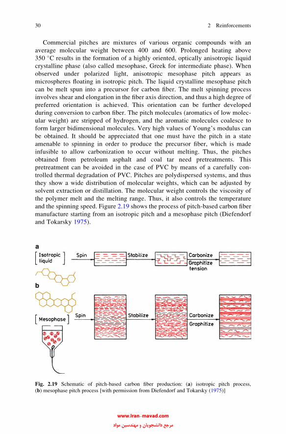
Commercial pitches are mixtures of various organic compounds with an

average molecular weight between 400 and 600. Prolonged heating above

350 �C results in the formation of a highly oriented, optically anisotropic liquid

crystalline phase (also called mesophase, Greek for intermediate phase). When

observed under polarized light, anisotropic mesophase pitch appears as

microspheres floating in isotropic pitch. The liquid crystalline mesophase pitch

can be melt spun into a precursor for carbon fiber. The melt spinning process

involves shear and elongation in the fiber axis direction, and thus a high degree of

preferred orientation is achieved. This orientation can be further developed

during conversion to carbon fiber. The pitch molecules (aromatics of low molec-

ular weight) are stripped of hydrogen, and the aromatic molecules coalesce to

form larger bidimensional molecules. Very high values of Young’s modulus can

be obtained. It should be appreciated that one must have the pitch in a state

amenable to spinning in order to produce the precursor fiber, which is made

infusible to allow carbonization to occur without melting. Thus, the pitches

obtained from petroleum asphalt and coal tar need pretreatments. This

pretreatment can be avoided in the case of PVC by means of a carefully con-

trolled thermal degradation of PVC. Pitches are polydispersed systems, and thus

they show a wide distribution of molecular weights, which can be adjusted by

solvent extraction or distillation. The molecular weight controls the viscosity of

the polymer melt and the melting range. Thus, it also controls the temperature

and the spinning speed. Figure 2.19 shows the process of pitch-based carbon fiber

manufacture starting from an isotropic pitch and a mesophase pitch (Diefendorf

and Tokarsky 1975).

Fig. 2.19 Schematic of pitch-based carbon fiber production: (a) isotropic pitch process,

(b) mesophase pitch process [with permission from Diefendorf and Tokarsky (1975)]

30 2 Reinforcements


2.4.2 Structural Changes Occurring During Processing

The thermal treatments for all precursor fibers serve to remove noncarbon elements in

the form of gases. For this, the precursor fibers are stabilized to ensure that they

decompose rather than melt. Generally, they become black after this treatment.

Carbon fibers obtained after carbonization contain many “grown-in” defects because

the thermal energy supplied at these low temperatures is not enough to break the

already-formed carbon–carbon bonds. That is why these carbon fibers are very stable

up to 2,500–3,000 �C when they change to graphite. The decomposition of the

precursor fiber invariably results in a weight loss and a decrease in fiber diameter.

The weight loss can be considerable–from 40 to 90 %, depending on the precursor

and treatment (Ezekiel and Spain 1967). The external morphology of the fiber,

however, is generally maintained. Thus, precursor fibers with transverse sections in

the form of a kidney bean, dog bone, or circle maintain their form after conversion to

carbon fiber. Figure 2.20 shows a scanning electron micrograph of a PAN-based

carbon fiber. Note the surface markings that appear during the fiber drawing process.

At the microscopic level, carbon fibers possess a rather heterogeneous

microstructure. Not surprisingly, many workers (Diefendorf and Tokarsky

1975; Watt and Johnson 1969; Johnson and Tyson 1969; Perret and Ruland

1970; Bennett and Johnson 1978, 1979; Inal et al. 1980) have attempted to

characterize the structure of carbon fibers, and one can find a number of models

in the literature. There is a better understanding of the structure of PAN-based

carbon fibers. Essentially, a carbon fiber consists of many graphitic lamellar

ribbons oriented roughly parallel to the fiber axis with a complex interlinking of

Fig. 2.20 Scanning electron micrograph of PAN-based carbon fiber (fiber diameter is 8 mm). Note

the surface markings that stem from the fiber drawing process



layer planes both longitudinally and laterally. Based on high-resolution lattice

fringe images of longitudinal and transverse sections in TEM, a schematic two-

dimensional representation is given in Fig. 2.21 (Bennett and Johnson 1979),

while a three-dimensional model is shown in Fig. 2.22 (Bennett and Johnson

1978). The structure is typically defined in terms of crystallite dimensions, La andLc in directions a and c, respectively, as shown in Fig. 2.23. The degree of

alignment and the parameters La and Lc vary with the graphitization temperature.

Both La and Lc increase with increasing heat treatment temperature.

2.4.3 Properties and Applications

The density of the carbon fiber varies with the precursor and the thermal treatment

given. It is generally in the range of 1.6–2.0 g/cm3. Note that the density of the

carbon fiber is more than that of the precursor fiber; the density of the precursor is

generally between 1.14 and 1.19 g/cm3 (Bennett et al. 1983). There are always flaws

of various kinds present, which may arise from impurities in the precursors or may

simply be the misoriented layer planes. A mechanism of tensile failure of carbon

fiber based on the presence of misoriented crystallites is shown in Fig. 2.23 (Bennett

et al. 1983). Figure 2.23a shows a misoriented crystallite linking two crystallites

parallel to the fiber axis. Under the action of applied stress, basal plane rupture

occurs in the misoriented crystallite in the Lc direction, followed by crack develop-

ment along La and Lc (Fig. 2.23b). Continued stressing causes complete failure of

the misoriented crystallite (Fig. 2.23c). If the crack size is greater than the critical

size in the La and Lc directions, catastrophic failure results.

Fig. 2.21 Two-dimensional

representation of PAN-based

carbon fiber [after Bennett

and Johnson (1979), used

with permission]

32 2 Reinforcements


Fig. 2.23 Model for tensile failure of carbon fiber: (a) a misoriented crystallite linking two

crystallites parallel to the fiber axis, (b) basal plane rupture under the action of applied stress,

(c) complete failure of the misoriented crystallite [from Bennett et al. (1983), used with

permission]

Fig. 2.22 Three-dimensional representation of PAN-based carbon fiber [from Bennett and John-

son (1978), used with permission]



As mentioned earlier, the degree of order, and consequently the modulus in the

fiber axis direction, increases with increasing graphitization temperature. Fourdeux

et al. (1971) measured the preferred orientation of various carbon fibers and plotted

the Young’s modulus of the carbon fibers obtained by different precursors against

an orientation parameter, q (Fig. 2.24). The absolute value of this parameter, |q| hasa value of 1 for perfect orientation and zero for the isotropic case. In Fig. 2.24 we

have plotted the absolute value of q. Note also that the modulus has been corrected

for porosity. The theoretical curve fits the experimental data very well.

Even among the PAN carbon fibers, we can have a series of carbon fibers: for

example, high tensile strength but medium Young’s modulus (HT) fiber

(200–300 GPa); high Young’s modulus (HM) fiber (400 GPa); extra- or superhigh

tensile strength (SHT); and superhigh modulus type (SHM) carbon fibers. The

mesophase pitch-based carbon fibers show rather high modulus but low strength

levels (2 GPa). Not unexpectedly, the HT-type carbon fibers show a much higher

strain-to-failure value than the HM type. The mesophase pitch-based carbon fibers

are used for reinforcement, while the isotropic pitch-based carbon fibers (very low

modulus) are more frequently used as insulation and fillers. Table 2.4 compares the

properties of some common carbon fibers and graphite monocrystal (Singer 1979).

For high-temperature applications involving carbon fibers, it is important to take

into account the variation of inherent oxidation resistance of carbon fibers with

modulus. Figure 2.25 shows that the oxidation resistance of carbon fiber increases

with the modulus value (Riggs 1985). The modulus, as we know, increases with the

final heat treatment temperature during processing.

We note from Table 2.4 that the carbon fibers produced from various precursor

materials are fairly good electrical conductors. Although this led to some work toward

a potential use of carbon fibers as current carriers for electrical power transmission

Fig. 2.24 Variation of

longitudinal Young’s

modulus for various carbon

fibers with the degree

of preferred orientation.

The value of the orientation

parameter, q, is 1 for perfect

orientation and zero for the

isotropic case [from Fourdeux

et al. (1971), used with

permission]

34 2 Reinforcements


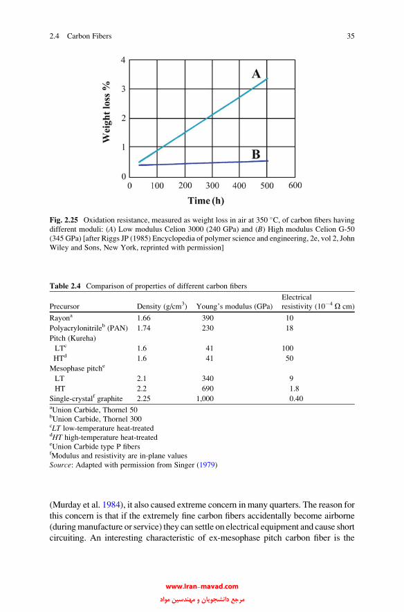
(Murday et al. 1984), it also caused extreme concern in many quarters. The reason for

this concern is that if the extremely fine carbon fibers accidentally become airborne

(duringmanufacture or service) they can settle on electrical equipment and cause short

circuiting. An interesting characteristic of ex-mesophase pitch carbon fiber is the

Table 2.4 Comparison of properties of different carbon fibers

Precursor Density (g/cm3) Young’s modulus (GPa)

Electrical

resistivity (10�4 O cm)

Rayona 1.66 390 10

Polyacrylonitrileb (PAN) 1.74 230 18

Pitch (Kureha)

LTc 1.6 41 100

HTd 1.6 41 50

Mesophase pitche

LT 2.1 340 9

HT 2.2 690 1.8

Single-crystalf graphite 2.25 1,000 0.40aUnion Carbide, Thornel 50bUnion Carbide, Thornel 300cLT low-temperature heat-treateddHT high-temperature heat-treatedeUnion Carbide type P fibersfModulus and resistivity are in-plane values

Source: Adapted with permission from Singer (1979)

Fig. 2.25 Oxidation resistance, measured as weight loss in air at 350 �C, of carbon fibers having

different moduli: (A) Low modulus Celion 3000 (240 GPa) and (B) High modulus Celion G-50

(345 GPa) [after Riggs JP (1985) Encyclopedia of polymer science and engineering, 2e, vol 2, John

Wiley and Sons, New York, reprinted with permission]



extremely high thermal conductivity it can have. Ex-pitch carbon fibers with a suitably

oriented microstructure can have thermal conductivity as high as 1,100 W/mK. The

figure for an ex-PAN carbon fiber is generally less than 50W/mK.

Anisotropic as the carbon fibers are, they have two principal coefficients of

thermal expansion, namely, longitudinal or parallel to the fiber axis, al and trans-

verse or perpendicular to the fiber axis, at. Typical values of the expansion

coefficients are

al � 5.5 to 8.4 � 10–6 K–1,

at � –0.5 to –1.3 � 10–6 K–1.

Compressive strength of carbon fibers is about half their tensile strength! Still,

they are an order of magnitude better than aramid-type fibers (see Sect. 2.5).

Carbon fibers are used in a variety of applications in the aerospace and sporting

goods industries. Cargo bay doors and booster rocket casings in the US space

shuttle are made of carbon fiber reinforced epoxy composites. Modern commercial

aircraft such as Boeing 787 (Dreamliner) has fuselage and wings made of carbon

fiber/epoxy composites. With the ever decreasing price of carbon fibers,

applications of carbon fibers in other areas have also increased, for example,

various machinery items such as turbine, compressor, and windmill blades and

flywheels; in the field of medicine the applications include both equipment and

implant materials (e.g., ligament replacement in knees and hip joint replacement).

We discuss these in more detail in Chap. 5.

2.5 Organic Fibers

In general, polymeric chains assume a random coil configuration, i.e., they have the

so-called cooked-spaghetti structure (see Chap. 3). In this random coil structure, the

macromolecular chains are neither aligned in one direction nor stretched out. Thus,

they have predominantly weak van der Waals interactions rather than strong

covalent interactions, resulting in a low strength and stiffness. Because the covalent

carbon–carbon bond is very strong, one would expect that linear chain polymers,

such as polyethylene, would be potentially very strong and stiff. Conventional

polymers show a Young’s modulus, E, of about 10 GPa or less. Highly drawn

polymers with a Young’s modulus of about 70 GPa can be obtained easily.

However, if one wants strong and stiff organic fibers, one must obtain not only

oriented molecular chains but oriented and fully extended chains. Thus, in order to

obtain high-stiffness and high-strength polymers, we must extend these polymer

chains and pack them in a parallel array. The orientation of these polymer chains

with respect to the fiber axis and the manner in which they fit together (i.e., order or

crystallinity) are controlled by their chemical nature and the processing route. The

case of molecular chain orientation without high molecular extension is shown in

Fig. 2.26a while chain orientation with high molecular extension is depicted

36 2 Reinforcements


http://dx.doi.org/10.1007/978-0-387-74365-3_5

http://dx.doi.org/10.1007/978-0-387-74365-3_3

in Fig. 2.26b. It is the chain structure shown in Fig. 2.26b, i.e., molecular chain

orientation coupled with molecular chain extension, which is needed for high

stiffness and high strength. To get a Young’s modulus value greater than 70 GPa,

one needs rather high draw ratios, i.e., a very high degree of elongation must be

carried out under such conditions that macroscopic elongation results in a

corresponding elongation at a molecular level. It turns out that the Young’s

modulus, E, of a polymeric fiber increases linearly with the deformation ratio

(draw ratio in tensile drawing or die drawing and extrusion ratio in hydrostatic

extrusion). The drawing behavior of a polymer is a sensitive function of (1) its

molecular weight and molecular weight distribution and (2) deformation conditions

(temperature and strain rate). Too low a drawing temperature produces voids, while

too high a drawing temperature results in flow drawing, i.e., the macroscopic

elongation of the material does not result in a molecular alignment, and conse-

quently, no stiffness enhancement results. An oriented and extended macromolec-

ular chain structure, however, is not easy to achieve in practice.

Nevertheless, considerable progress in this area wasmade during the last quarter of

the twentieth century. Organic fibers, such as aramid and polyethylene, possessing

high strength and modulus are the fruits of this realization. Two very different

approaches have been taken to make high-modulus organic fibers. These are:

1. Process the conventional flexible-chain polymers in such a way that the internal

structure takes a highly oriented and extended-chain arrangement. Structural

modification of “conventional” polymers such as high-modulus polyethylene

was developed by choosing appropriate molecular weight distributions,

followed by drawing at suitable temperatures to convert the original folded-

chain structure into an oriented, extended chain structure.

2. The second, radically different, approach involves synthesis, followed by extrusion

of a new class of polymers, called liquid crystal polymers. These have a rigid-rod

molecular chain structure. The liquid crystalline state, as we shall see, has played a

very significant role in providing highly ordered, extended chain fibers.

These two approaches have resulted in two commercialized high-strength and

high-stiffness fibers, polyethylene and aramid. Next, we describe the processing,

structure, and properties of these two fibers.

Fig. 2.26 Two types of molecular orientation: (a) oriented without high molecular extension and

(b) oriented with high molecular extension [from Barham and Keller (1985), used with permission]

2.5 Organic Fibers 37


2.5.1 Oriented Polyethylene Fibers

The ultrahigh-molecular-weight polyethylene (UHMWPE) fiber is a highly crystal-

line fiber with very high stiffness and strength. This results from some innovative

processing and control of the structure of polyethylene.

2.5.1.1 Processing of Polyethylene Fibers

Drawing of melt crystallized polyethylene (molecular mass between 104 and 105) to

very high draw ratios can result in moduli of up to 70 GPa. Tensile drawing, die

drawing, or hydrostatic extrusion can be used to obtain the high permanent or plastic

strains required to obtain a high modulus. It turns out that modulus is dependent on

the draw ratio but independent of how the draw ratio is obtained (Capaccio et al.

1979). In all these drawing processes, the polymer chains become merely oriented

without undergoing molecular extension, and we obtain the kind of structure shown

in Fig. 2.26a. Later developments led to solution and gel spinning of very high

molecular weight polyethylene (>106) with moduli as high as 200 GPa. The gel

spinning method of making polyethylene fibers has become technologically and

commercially most successful. Pennings and coworkers (Kalb and Pennings 1980;

Smook and Pennings 1984) made high-modulus polyethylene fiber by solution

spinning. Their work was preceded by Smith and Lemstra (1976), who made

polyethylene fiber by gel spinning. The gel spinning process of making polyethylene

was industrialized in the 1980s. Gels are swollen networks in which crystalline

regions form the network junctions. An appropriate polymer solution is converted

into gel, which is drawn to give the fiber. At least three commercial firms produce

oriented polyethylene fiber using similar techniques; Dyneema, Spectra, Tekmilonare the trade names of these UHMWPE fibers. Next, we describe the gel spinning

process of making the high-stiffness polyethylene fiber.

2.5.1.2 Gel Spinning of Polyethylene Fiber

Polyethylene (PE) is a particularly simple, linear macromolecule, with the follow-

ing chemical formula

�CH2 � CH2 � CH2 � CH2 � CH2 � CH2 � CH2 � CH2�½ �nThus, compared to other polymers, it is easier to obtain an extended and oriented

chain structure in polyethylene. High-density polyethylene (HDPE) is preferred to

other types of polyethylene because HDPE has fewer branch points along its

backbone and a high degree of crystallinity. The characteristics of linearity and

crystallinity are important from the point of getting a high degree of orientational

order and obtaining an extended chain structure in the final fiber.

38 2 Reinforcements


Figure 2.27 provides a flow diagram of the gel spinning process for making the

high-modulus polyethylene fiber. Different companies use different solvents, such

as decalin, paraffin oil, and paraffin wax, to make a dilute (5–10 %) solution of

polymer in the appropriate solvent at about 150 �C. A dilute solution is important in

that it allows for a lesser chain entanglement, which makes it easier for the final

fiber to be highly oriented. A polyethylene gel is produced when the solution

coming out of the spinneret is quenched by air. The as-spun gelled fiber enters

a cooling bath. At this stage, the fiber is thought to have a structure consisting

of folded chain lamellae with solvent between them and a swollen network

of entanglements. These entanglements allow the as-spun fiber to be drawn to

very high draw ratios, which can be as high as 200. The maximum draw ratio is

related to the average distance between the entanglements, i.e., the solution con-

centration. The gelled fibers are drawn at 120 �C. One problem with this gel route is

the rather low spinning rates of 1.5 m/min. At higher rates, the properties obtained

are not very good (Kalb and Pennings 1980; Smook and Pennings 1984).

2.5.1.3 Structure and Properties of Polyethylene Fiber

The unit cell of a single crystal (orthorhombic) of polyethylene has the dimensions

of 0.741, 0.494, and 0.255 nm. There are four carbon and eight hydrogen atoms per

Fig. 2.27 Gel spinning process for making the high-modulus polyethylene fiber concentration

Table 2.5 Properties

of polyethylene fibersaProperty Spectra 900 Spectra 1000

Density (g/cm3) 0.97 0.97

Diameter (mm) 38 27

Tensile strength (GPa) 2.7 3.0

Tensile modulus (GPa) 119 175

Tensile strain to fracture (%) 3.5 2.7aManufacturer’s data; indicative values



unit cell. One can compute the theoretical density of polyethylene, assuming a

100 % single-crystal polyethylene. If one does that, the theoretical density of

polyethylene comes out to be 0.9979 g/cm3; of course, in practice, one can only

tend toward this theoretical value. As it turns out, the highly crystalline, oriented

and extended chain UHMWPE fiber has a density of 0.97 g/cm3, which is very near

the theoretical value. Thus, polyethylene fiber is very light; in fact, it is lighter than

water and thus floats on water. Properties of some commercially available polyeth-

ylene fibers are summarized in Table 2.5.

Its strength and modulus are slightly lower than those of aramid fibers but on a

per-unit-weight basis, i.e., specific property values are about 30–40 % higher than

those of aramid. As is true of most organic fibers, both polyethylene and aramid

fibers must be limited to low-temperature (lower than 150 �C) applications.Another effect of the high degree of chain alignment in these fibers is their super

smooth surface. This is manifested when they are put in a polymeric matrix to form

a fiber reinforced composite. High-modulus polyethylene fibers, such as Spectra or

Dyneema, are hard to bond with any polymeric matrix. Some kind of surface

treatment must be given to the polyethylene fiber to bond with resins such as

epoxy and PMMA. By far, the most successful surface treatment involves a cold

gas (such as air, ammonia, or argon) plasma (Kaplan et al. 1988). A plasma consists

of gas molecules in an excited state, i.e., highly reactive, dissociated molecules.

When the polyethylene, or any other fiber, is treated with a plasma, surface

modification occurs by the removal of any surface contaminants and highly ori-

ented surface layers, the addition of polar and functional groups on the surface, and

the introduction of surface roughness; all these factors contribute to an enhanced

fiber/matrix interfacial strength (Biro et al. 1992; Brown et al. 1992; Hild and

Schwartz 1992a, b; Kaplan et al. 1988; Li et al. 1992). Exposure to the plasma for

just a few minutes is enough.

Polyethylene fiber (the gel spun UHMWPE variety) is 90–95 % crystalline and

has a density of 0.97 g/cm3. There is a linear relationship between density and

crystallinity for polyethylene. A 100 % crystalline polyethylene will have a theo-

retical density, based on an orthorhombic unit cell, of about 1 g/cm3. A totally

amorphous polyethylene (0 % crystallinity) will have a density of about 0.85 g/cm3.

Raman spectroscopy has been used to study the deformation behavior of polyeth-

ylene fiber. Creep properties of these fibers are not very good, Spectra 1000 has

better creep properties than Spectra 900. It should be mentioned that although

plasma treatment, in general, improves the interfacial adhesion between the fiber

and the matrix, it does result in some deterioration of the mechanical properties of

the fiber.

2.5.2 Aramid Fibers

Aramid fiber is a generic term for a class of synthetic organic fibers called aromatic

polyamide fibers. The US Federal Trade Commission gives a good definition of an

40 2 Reinforcements


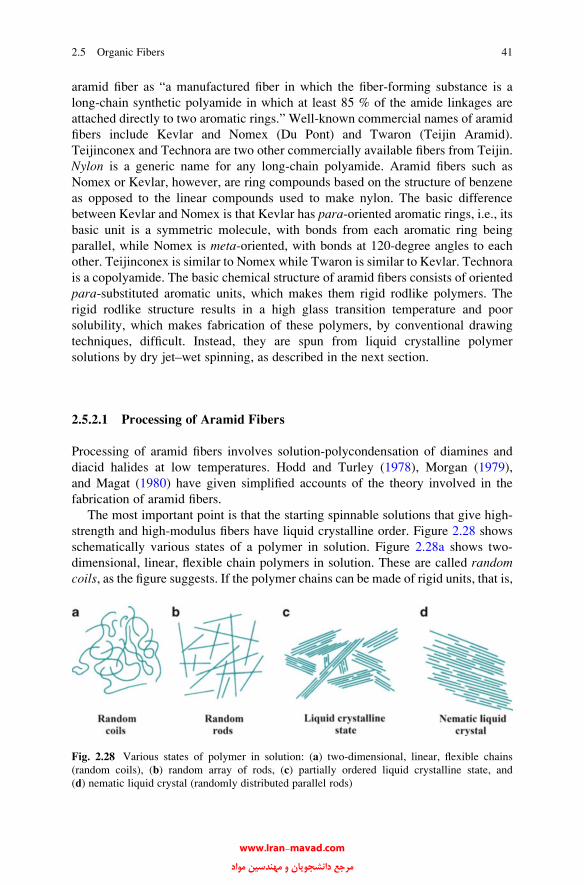
aramid fiber as “a manufactured fiber in which the fiber-forming substance is a

long-chain synthetic polyamide in which at least 85 % of the amide linkages are

attached directly to two aromatic rings.” Well-known commercial names of aramid

fibers include Kevlar and Nomex (Du Pont) and Twaron (Teijin Aramid).

Teijinconex and Technora are two other commercially available fibers from Teijin.

Nylon is a generic name for any long-chain polyamide. Aramid fibers such as

Nomex or Kevlar, however, are ring compounds based on the structure of benzene

as opposed to the linear compounds used to make nylon. The basic difference

between Kevlar and Nomex is that Kevlar has para-oriented aromatic rings, i.e., its

basic unit is a symmetric molecule, with bonds from each aromatic ring being

parallel, while Nomex is meta-oriented, with bonds at 120-degree angles to each

other. Teijinconex is similar to Nomex while Twaron is similar to Kevlar. Technora

is a copolyamide. The basic chemical structure of aramid fibers consists of oriented

para-substituted aromatic units, which makes them rigid rodlike polymers. The

rigid rodlike structure results in a high glass transition temperature and poor

solubility, which makes fabrication of these polymers, by conventional drawing

techniques, difficult. Instead, they are spun from liquid crystalline polymer

solutions by dry jet–wet spinning, as described in the next section.

2.5.2.1 Processing of Aramid Fibers

Processing of aramid fibers involves solution-polycondensation of diamines and

diacid halides at low temperatures. Hodd and Turley (1978), Morgan (1979),

and Magat (1980) have given simplified accounts of the theory involved in the

fabrication of aramid fibers.

The most important point is that the starting spinnable solutions that give high-

strength and high-modulus fibers have liquid crystalline order. Figure 2.28 shows

schematically various states of a polymer in solution. Figure 2.28a shows two-

dimensional, linear, flexible chain polymers in solution. These are called randomcoils, as the figure suggests. If the polymer chains can be made of rigid units, that is,

Fig. 2.28 Various states of polymer in solution: (a) two-dimensional, linear, flexible chains

(random coils), (b) random array of rods, (c) partially ordered liquid crystalline state, and

(d) nematic liquid crystal (randomly distributed parallel rods)



rodlike, we can represent them as a random array of rods (Fig. 2.28b). Any

associated solvent may contribute to the rigidity and to the volume occupied

by each polymer molecule. It is easy to see that with increasing concentration of

rodlike molecules, one can dissolve more polymer by forming regions of partial

order, that is, regions in which the chains form a parallel array. This partially ordered

state is called a liquid crystalline state (Fig. 2.28c). When the rodlike chains become

approximately arranged parallel to their long axes, but their centers remain unorga-

nized or randomly distributed, we have what is called a nematic liquid crystal

(Fig. 2.28d). It is this kind of order that is found in the extended-chain polyamides.

Liquid crystal solutions, because of the presence of the ordered domains, are

optically anisotropic, that is, they show the phenomenon of birefringence. Birefrin-gence, also known as double refraction, is the phenomenon of splitting of a ray of

light into two rays when it passes through certain types of material, depending on

the polarization of the light. Figure 2.29 shows the anisotropic Kevlar aramid and

sulfuric acid solution at rest between crossed polarizers. Note the parallel arrays of

ordered polymer chains in the liquid crystalline state, which become even more

ordered when these solutions are subjected to shear as, for example, in extruding

through a spinneret hole. It is this inherent property of liquid crystal solutions that is

exploited in the manufacture of aramid fibers. This alignment of polymer

crystallites along the fiber axis results in the characteristic fibrillar structure of

aramid fibers. Para-oriented aromatic polyamides form liquid crystal solutions

under certain conditions of concentration, temperature, solvent, and molecular

weight. This can be represented in the form of a phase diagram. As an example,

Fig. 2.30a shows a phase diagram of the system poly-p-benzamide in

tetramethylurea-LiCl solutions (Magat 1980). The region marked anisotropic

represents the liquid crystalline state. Only under certain conditions do we get

this desirable anisotropic state. There also occurs an anomalous relationship

between viscosity and polymer concentration in liquid crystal solutions. Initially,

an increase in viscosity occurs as the concentration of polymer in solution

increases, as it would in any ordinary polymer solution. At a critical point where

it starts assuming an anisotropic liquid crystalline shape, a sharp drop in the

viscosity occurs; see Fig. 2.30b. This drop in viscosity of liquid crystal polymers

at a critical concentration was predicted by Flory (1956). The drop in viscosity

occurs due to the formation of a lyotropic nematic structure. The liquid crystalline

regions act like dispersed particles and contribute very little to viscosity of the

solution. With increasing polymer concentration, the amount of liquid crystalline

phase increases up to a point after which the viscosity tends to rise again. There are

other requirements for forming a liquid crystalline solution from aromatic

polyamides. The molecular weight must be greater than some minimum value

and the solubility must exceed the critical concentration required for liquid crystal-

linity. Thus, starting from liquid crystalline spinning solutions containing highly

ordered arrays of extended polymer chains, we can spin fibers directly into an

extremely oriented, chain-extended form. These as-spun fibers are quite strong and,

because the chains are highly extended and oriented, the use of conventional

drawing techniques becomes optional.

42 2 Reinforcements


Para-oriented rigid diamines and dibasic acids give polyamides that yield, under

appropriate conditions of solvent, polymer concentration, and polymer molecular

weight, the desired nematic liquid crystal structure. One would like to have, for any

solution spinning process, a highmolecular weight in order to have improved mechan-

ical properties, a low viscosity to easily spin the fiber, and a high polymer concentration

for high yield. For para-aramid, poly-p-phenylene terephthalamide (PPTA), the

nematic liquid crystalline state is obtained in 100 % sulfuric acid solvent at a polymer

concentration of about 20 %. That is, to dissolve PPTA we need concentrated sulfuric

acid as the solvent. In industry, this solution is often referred to as the dope.For aramid fibers, the dry jet–wet spinning method is used. The process is

illustrated in Fig. 2.31. Solution-polycondensation of diamines and diacid halides

at low temperatures (near 0 �C) gives the aramid forming polyamides. Low

temperatures are used to inhibit any by-product generation and promote linear

polyamide formation. The resulting polymer is pulverized, washed, and dried;

mixed with concentrated H2SO4; and extruded through a spinneret at about

100 �C. The jets from the orifices pass through about 1 cm of air layer before

entering a cold water (0–4 �C) bath. The fiber solidifies in the air gap, and the acid isremoved in the coagulation bath. The spinneret capillary and air gap cause rotation

and alignment of the domains, resulting in highly crystalline and oriented as-spun

fibers. The air gap also allows the dope to be at a higher temperature than is possible

without the air gap. The higher temperature allows a more concentrated spinning

solution to be used, and higher spinning rates are possible. Spinning rates of several

hundred meters per minute are not unusual. Figure 2.32 compares the dry jet–wet

spinning method used with nematic liquid crystals and the spinning of a conven-

tional polymer. The oriented chain structure, together with molecular extension, is

achieved with dry jet–wet spinning. The conventional wet or dry spinning gives

Fig. 2.29 Anisotropic Kevlar aramid and sulfuric acid solution at rest between crossed polarizers

[courtesy of Du Pont Co.]



Fig. 2.30 (a) Phase diagram of poly-p-benzamide in tetramethylurea–LiCl solutions. Note that

the anisotropic state is obtained under certain conditions [with permission from Magat (1980)]

(b) Viscosity vs. polymer concentration in solution. A sharp drop in viscosity occurs when the

solution starts becoming anisotropic liquid crystal [after Kwolek and Yang (1993)]

44 2 Reinforcements


Fig. 2.31 The dry jet–wet

spinning process of producing

aramid fibers

Fig. 2.32 Comparison of dry jet–wet spinning of nematic liquid crystalline solution and conven-

tional spinning of a polymer [reprinted from Jaffe and Jones (1985), p 349, courtesy of Marcel

Dekker, Inc.]


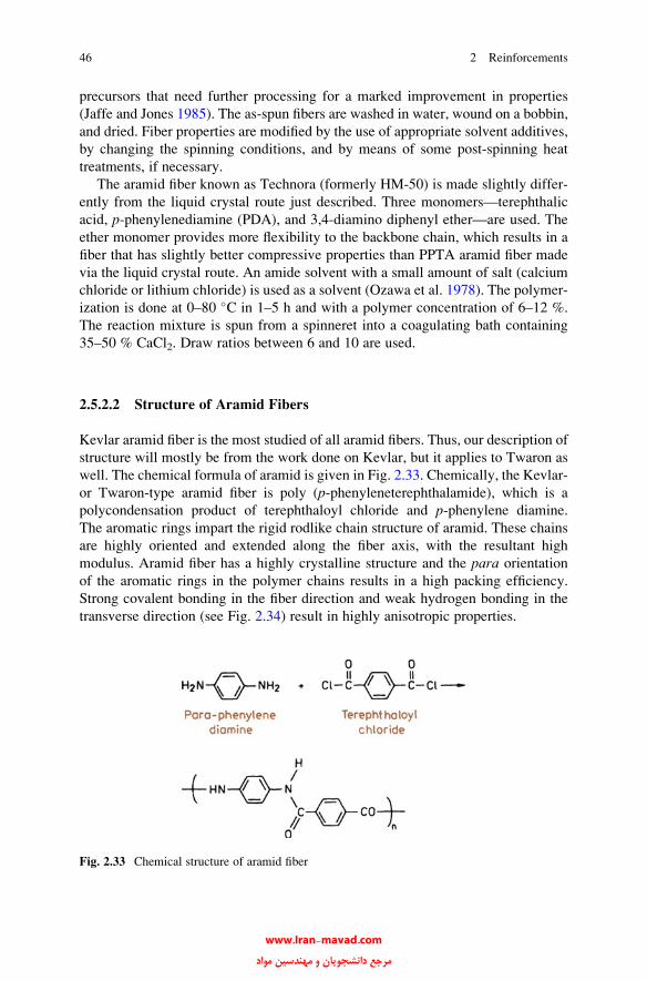
precursors that need further processing for a marked improvement in properties

(Jaffe and Jones 1985). The as-spun fibers are washed in water, wound on a bobbin,

and dried. Fiber properties are modified by the use of appropriate solvent additives,

by changing the spinning conditions, and by means of some post-spinning heat

treatments, if necessary.

The aramid fiber known as Technora (formerly HM-50) is made slightly differ-

ently from the liquid crystal route just described. Three monomers—terephthalic

acid, p-phenylenediamine (PDA), and 3,4-diamino diphenyl ether—are used. The

ether monomer provides more flexibility to the backbone chain, which results in a

fiber that has slightly better compressive properties than PPTA aramid fiber made

via the liquid crystal route. An amide solvent with a small amount of salt (calcium

chloride or lithium chloride) is used as a solvent (Ozawa et al. 1978). The polymer-

ization is done at 0–80 �C in 1–5 h and with a polymer concentration of 6–12 %.

The reaction mixture is spun from a spinneret into a coagulating bath containing

35–50 % CaCl2. Draw ratios between 6 and 10 are used.

2.5.2.2 Structure of Aramid Fibers

Kevlar aramid fiber is the most studied of all aramid fibers. Thus, our description of

structure will mostly be from the work done on Kevlar, but it applies to Twaron as

well. The chemical formula of aramid is given in Fig. 2.33. Chemically, the Kevlar-

or Twaron-type aramid fiber is poly (p-phenyleneterephthalamide), which is a

polycondensation product of terephthaloyl chloride and p-phenylene diamine.

The aromatic rings impart the rigid rodlike chain structure of aramid. These chains

are highly oriented and extended along the fiber axis, with the resultant high

modulus. Aramid fiber has a highly crystalline structure and the para orientation

of the aromatic rings in the polymer chains results in a high packing efficiency.

Strong covalent bonding in the fiber direction and weak hydrogen bonding in the

transverse direction (see Fig. 2.34) result in highly anisotropic properties.

Fig. 2.33 Chemical structure of aramid fiber

46 2 Reinforcements


The structure of Kevlar aramid fiber has been investigated by electron micro-

scopy and diffraction. A schematic representation of the supramolecular structure

of Kevlar 49 is shown in Fig. 2.35 (Dobb et al. 1980). It shows radially arranged,

axially pleated crystalline supramolecular sheets. The molecules form a planar

array with interchain hydrogen bonding. The stacked sheets form a crystalline

Fig. 2.34 Strong covalent

bonding in the fiber direction

and weak hydrogen bonding

(indicated by H) in the

transverse direction

Fig. 2.35 Schematic

representation of the

supramolecular structure

of aramid fiber, Kevlar 49.

The structure consists of

radially arranged, axially

pleated crystalline sheets

[from Dobb et al. (1980),




array, but between the sheets the bonding is rather weak. Each pleat is about 500 nm

long, and the pleats are separated by transitional bands. The adjacent components of

a pleat make an angle of 170�. Such a structure is consistent with the experimentally

observed rather low-longitudinal shear modulus and poor properties in compression

and transverse to the Kevlar fiber axis. A correlation between good compressive

characteristics and a high glass transition temperature (or melting point) has been

suggested (Northolt 1981). Thus, since the glass transition temperature of organic

fibers is lower than that of inorganic fibers, the former would be expected to show

poorer properties in compression. For aramid- and polyethylene-type high stiffness

fibers, compression results in the formation of kink bands leading to an eventual

ductile failure. Yielding is observed at about 0.5 % strain; this is thought to

correspond to a molecular rotation of the amide carbon–nitrogen bond shown in

Fig. 2.33 from the normal, extended, trans configuration to a kinked, cis configura-tion (Tanner et al. 1986). In the chemical literature, this is referred to as cis–transisomerism. It describes the orientation of functional groups in a molecule.

In aromatic structures, the rotation of bonds is greatly restricted. Cis in Latin

means “on the same side” while trans means “on the other side” or “across.” This

trans to cis rotation in the aramid fiber causes a 45� bend in the chain. This bend

propagates across the unit cell, the microfibrils, and a kink band results in the fiber.

This anisotropic behavior of aramid fiber is revealed in a vivid manner in the SEM

micrograph of knotted fiber shown in Fig. 2.36. Note the buckling or kink marks on

the compressive side of a knotted Kevlar aramid fiber. Note also the absence of such

markings on the tensile side. Such markings on the aramid fiber surface have also

been reported by, among others, DeTeresa et al. (1984) when the aramid fiber is

subjected to uniform compression or torsion.

Fig. 2.36 Knotted Kevlar aramid fiber showing buckling marks on the compressive side. The

tensile side is smooth [courtesy of Fabric Research Corp.]

48 2 Reinforcements


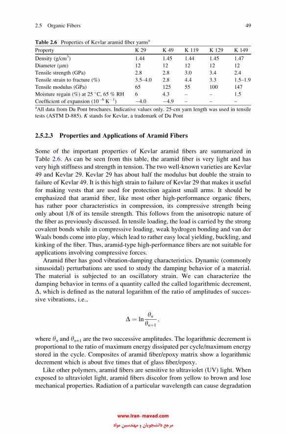
2.5.2.3 Properties and Applications of Aramid Fibers

Some of the important properties of Kevlar aramid fibers are summarized in

Table 2.6. As can be seen from this table, the aramid fiber is very light and has

very high stiffness and strength in tension. The two well-known varieties are Kevlar

49 and Kevlar 29. Kevlar 29 has about half the modulus but double the strain to

failure of Kevlar 49. It is this high strain to failure of Kevlar 29 that makes it useful

for making vests that are used for protection against small arms. It should be

emphasized that aramid fiber, like most other high-performance organic fibers,

has rather poor characteristics in compression, its compressive strength being

only about 1/8 of its tensile strength. This follows from the anisotropic nature of

the fiber as previously discussed. In tensile loading, the load is carried by the strong

covalent bonds while in compressive loading, weak hydrogen bonding and van der

Waals bonds come into play, which lead to rather easy local yielding, buckling, and

kinking of the fiber. Thus, aramid-type high-performance fibers are not suitable for

applications involving compressive forces.

Aramid fiber has good vibration-damping characteristics. Dynamic (commonly

sinusoidal) perturbations are used to study the damping behavior of a material.

The material is subjected to an oscillatory strain. We can characterize the

damping behavior in terms of a quantity called the called logarithmic decrement,

D, which is defined as the natural logarithm of the ratio of amplitudes of succes-

sive vibrations, i.e.,

D ¼ lnynynþ1

;

where yn and yn+1 are the two successive amplitudes. The logarithmic decrement is

proportional to the ratio of maximum energy dissipated per cycle/maximum energy

stored in the cycle. Composites of aramid fiber/epoxy matrix show a logarithmic

decrement which is about five times that of glass fiber/epoxy.

Like other polymers, aramid fibers are sensitive to ultraviolet (UV) light. When

exposed to ultraviolet light, aramid fibers discolor from yellow to brown and lose

mechanical properties. Radiation of a particular wavelength can cause degradation

Table 2.6 Properties of Kevlar aramid fiber yarnsa

Property K 29 K 49 K 119 K 129 K 149

Density (g/cm3) 1.44 1.45 1.44 1.45 1.47

Diameter (mm) 12 12 12 12 12

Tensile strength (GPa) 2.8 2.8 3.0 3.4 2.4

Tensile strain to fracture (%) 3.5–4.0 2.8 4.4 3.3 1.5–1.9

Tensile modulus (GPa) 65 125 55 100 147

Moisture regain (%) at 25 �C, 65 % RH 6 4.3 – – 1.5

Coefficient of expansion (10�6 K�1) �4.0 �4.9 – – –aAll data from Du Pont brochures. Indicative values only. 25-cm yarn length was used in tensile

tests (ASTM D-885). K stands for Kevlar, a trademark of Du Pont



because of absorption by the polymer and breakage of chemical bonds. Near-UV

and part of the visible spectrum should be avoided for outdoor applications involv-

ing use of unprotected aramid fibers. A small amount of such light emanates from

incandescent and fluorescent lamps or sunlight filtered by window glass. Du Pont

Co. recommends that Kevlar aramid yarn should not be stored within 1 ft (0.3 m) of

fluorescent lamps or near windows.

The Technora fiber of Teijin shows properties that are a compromise between

conventional fibers and rigid-rod fibers; Table 2.7 provides a summary of these. In

terms of its stress–strain behavior, it can be said that Technora fiber lies between

Kevlar 49 and Kevlar 29.

Different types of Kevlar aramid fibers provide an impressive set of properties,

see Table 2.6. The three important types of Kevlar aramid fibers are used for

specific applications (Magat 1980):

1. Kevlar. This is meant mainly for use as rubber reinforcement for tires (belts or

radial tires for cars and carcasses of radial tires for trucks) and, in general, for

mechanical rubber goods.

2. Kevlar 29. This is used for ropes, cables, coated fabrics for inflatables, architec-

tural fabrics, and ballistic protection fabrics. Vests made of Kevlar 29 have been

used by law-enforcement agencies in many countries.

3. Kevlar 49. This is meant for reinforcement of epoxy, polyester, and other resins

for use in the aerospace, marine, automotive, and sports industries.

2.6 Ceramic Fibers

Continuous ceramic fibers present an attractive package of properties. They com-

bine high strength and elastic modulus with high-temperature capability and a

general freedom from environmental attack. These characteristics make them

attractive as reinforcements in high-temperature structural materials.

There are three methods to fabricate ceramic fibers: chemical vapor deposition,

polymer pyrolysis, and sol–gel techniques. The latter two involve rather novel

techniques of obtaining ceramics from organometallic polymers. The sol–gel tech-

nique was mentioned in Sect. 2.2 in regard to the manufacture of silica-based glass

fibers. The sol–gel technique is also used to produce a variety of alumina-based

oxide fibers commercially. Another breakthrough in the ceramic fiber area is the

concept of pyrolyzing; under controlled conditions, polymers containing silicon

Table 2.7 Properties of Technora fibera

Density

(g/cm3) Diameter (mm) Tensile strength (GPa) Tensile modulus (GPa)

Tensile strain

to fracture (%)

1.39 12 3.1 71 4.4aManufacturer’s data; indicative values only

50 2 Reinforcements


and carbon or nitrogen can be converted to high-temperature ceramic fibers. This

idea is nothing but an extension of the polymer pyrolysis route to produce a variety

of carbon fibers wherein a suitable carbon-based polymer (e.g., PAN or pitch) is

subjected to controlled heating to produce carbon fibers (see Sect. 2.4). The

pyrolysis route of producing ceramic fibers has been used with polymers containing

silicon, carbon, nitrogen, and boron, with the end products being SiC, Si3N4, B4C,

and BN in fiber form, foam, or coating. We describe some important ceramic fibers.

2.6.1 Oxide Fibers

Many alumina-type oxide fibers are available commercially. Alumina has many

allotropic forms: g, d, Z, and a. Of these, a-alumina is the most stable form.

A variety of alumina-based continuous fibers made by sol–gel processing are

available commercially. The sol–gel process of making fibers involves the follow-

ing steps, common to all fibers:

1. Formulate sol.

2. Concentrate to form a viscous gel.

3. Spin the precursor fiber.

4. Calcine to obtain the oxide fiber.

3M Co. produces a series of ceramic fibers called the Nextel fibers. They are

mainly Al2O3 + SiO2 and some B2O3. The composition and properties of some

Nextel fibers are given in Table 2.8. Figure 2.37 shows an optical micrograph of

Nextel 312 fibers. The sol–gel manufacturing process used by 3M Co. has metal

Fig. 2.37 Optical micrograph of Nextel 312 (Al2O3 + B2O3 + SiO2) fiber

2.6 Ceramic Fibers 51


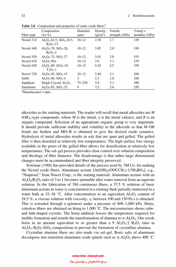
alkoxides as the starting materials. The reader will recall that metal alkoxides areM(OR)n-type compounds, where M is the metal, n is the metal valence, and R is an

organic compound. Selection of an appropriate organic group is very important.

It should provide sufficient stability and volatility to the alkoxide so that M–ORbonds are broken and MO–R is obtained to give the desired oxide ceramics.

Hydrolysis of metal alkoxides results in sols that are spun and gelled. The gelled

fiber is then densified at relatively low temperatures. The high surface free energy

available in the pores of the gelled fiber allows for densification at relatively low

temperatures. The sol–gel process provides close control over solution composition

and rheology of fiber diameter. The disadvantage is that rather large dimensional

changes must be accommodated and fiber integrity preserved.

Sowman (1988) has provided details of the process used by 3M Co. for making

the Nextel oxide fibers. Aluminum acetate [Al(OH)2(OOCCH3)·1/3H3BO3], e.g.,

“Niaproof,” from Niacet Corp., is the starting material. Aluminum acetate with an

Al2O3/B2O3 ratio of 3 to 1 becomes spinnable after water removal from an aqueous

solution. In the fabrication of 3M continuous fibers, a 37.5 % solution of basic

aluminum acetate in water is concentrated in a rotating flask partially immersed in a

water bath at 32–36 �C. After concentration to an equivalent Al2O3 content of

28.5 %, a viscous solution with viscosity, �, between 100 and 150 Pa s is obtained.

This is extruded through a spinneret under a pressure of 800–1,000 kPa. Shiny,

colorless fibers are obtained on firing to 1,000 �C. The microstructure shows cube-

and lath-shaped crystals. The boria addition lowers the temperature required for

mullite formation and retards the transformation of alumina to a-Al2O3. One needs

boria in an amount equivalent to or greater than a 9 Al2O3:2 B2O3 ratio in

Al2O3–B2O3-SiO2 compositions to prevent the formation of crystalline alumina.

Crystaline alumina fibers are also made via sol–gel. Boric salts of aluminum

decompose into transition aluminum oxide spinels such as Z-Al2O3 above 400�C.

Table 2.8 Composition and properties of some oxide fibersa

Fiber type

Composition

(wt.%)

Diameter

(mm)

Density,

(g/cm3)

Tensile

strength (GPa)

Young’s

modulus (GPa)

Nextel 312 Al2O3-62.5, SiO2-24.5,

B2O3-13

10–12 2.70 1.7 150

Nextel 440 Al2O3-70, SiO2-28,

B2O3-2

10–12 3.05 2.0 190

Nextel 550 Al2O3-73, SiO2-27 10–12 3.03 2.0 193

Nextel 610 Al2O3-99+ 10–12 3.9 3.1 370

Nextel 650 Al2O3-89, ZrO2-10,

Y2O3-1

10–12 4.10 2.5 358

Nextel 720 Al2O3-85, SiO2-15 10–12 3.40 2.1 260

Saffil Al2O3-96, SiO2-4 3 2.3 1.0 100

Saphikon Single Crystal Al2O3 75–250 3.8 3.1 380

Sumitomo Al2O3-85, SiO2-15 9 3.2 2.6 250aManufacturer’s data

52 2 Reinforcements


These transition cubic spinels convert to hexagonal a-Al2O3 on heating to between

1,000 and 1,200 �C. The problem is that the nucleation rate of pure a-Al2O3 is too

low and results in rather large grains. Also, during the transformation to a phase, a

large shrinkage results in a rather large porosity. The a-Al2O3 fiber, 3 M Co.’s

tradename Nextel 610, is obtained by seeding the high-temperature a-alumina with

a very fine hydrous colloidal iron oxide. The fine iron oxide improves the nucleation

rate of a-Al2O3, resulting in a high-density, ultrafine, homogeneous a-Al2O3 fiber

(Wilson 1990). a-Fe2O3 is isostructural with a-Al2O3 (5.5 % lattice mismatch).

3M’s hydrous colloidal iron oxide sol appears to be an efficient nucleating agent.

Without the seeding with iron oxide, the Z-alumina-to-a-alumina transformation

occurred at about 1,100 �C. With 1 % Fe2O3, the transformation temperature was

decreased to 1,010 �C, while with 4 % Fe2O3, the transformation temperature came

down to 977 �C. Concomitantly, the grain size was refined. In addition to Fe2O3,

about 0.5 wt.% SiO2 is added to reduce the final grain size of Nextel 610 fiber,

although SiO2 inhibits the transformation to the a phase. The SiO2 addition also

reduces grain growth during soaking at 1,400 �C.Many other alumina- or alumina–silica-type fibers are available. Most of these

are also made by the sol–gel process. Sumitomo Chemical Co. produces a fiber that

is a mixture of alumina and silica. The flow diagram of this process is shown in

Fig. 2.38. Starting from an organoaluminum (polyaluminoxanes or a mixture of

polyaluminoxanes and one or more kinds of Si-containing compounds), a precursor

fiber is obtained by dry spinning. This precursor fiber is calcined to produce the final

fiber. The fiber structure consists of fine crystallites of spinel. SiO2 serves to stabilize

the spinel structure and prevents it from transforming to a-Al2O3. Yet another

variety of alumina fiber available commercially is a d-Al2O3, a staple fiber

(tradename Saffil). This fiber has about 4 % SiO2 and a very fine diameter (3 mm).

The starting material for Saffil is an aqueous phase containing an oxide sol and an

organic polymer: Aluminum oxychloride [Al2(OH)5Cl] is mixed with a medium-

molecular-weight polymer such as 2 wt.% polyvinyl alcohol. The sol is extruded as

filaments into a coagulating (or precipitating) bath in which the extruded shape gels.

The gelled fiber is then dried and calcined to produce the final oxide fiber. This

solution is slowly evaporated in a rotary evaporator until a viscosity of about 80 Pa s

(800 P) is attained. This solution is extruded through a spinneret, the fibers are

wound on a drum, and fired to about 800 �C. The organic material is burned away,

and a fine-grain alumina fiber with 5–10 % porosity and a diameter of 3–5 mm is

obtained. The fibers as produced at this stage are suitable for filtering purposes

because of their high porosity. By heating them to 1,400–1,500 �C, which causes

3–4 % of linear shrinkage, one obtains a refractory alumina fiber suitable for

reinforcement purposes. Care is taken to produce fibers with diameter greater than

1 mm (to avoid biological hazards) but less than 6 mm (to avoid skin irritation).

A technique called edge-defined film-fed growth (EFG) has been used to make

continuous, monocrystalline sapphire (Al2O3) fiber (LaBelle and Mlavsky 1967;

LaBelle 1971; Pollack 1972; Hurley and Pollack 1972). LaBelle and Mlavsky

(1967) grew sapphire (Al2O3) single-crystal fibers using a modified Czochralski

puller and radio frequency heating. The process is called the edge-defined film-fed



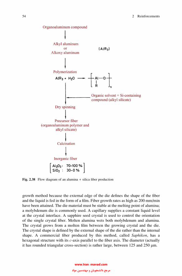
growth method because the external edge of the die defines the shape of the fiber

and the liquid is fed in the form of a film. Fiber growth rates as high as 200 mm/min

have been attained. The die material must be stable at the melting point of alumina;

a molybdenum die is commonly used. A capillary supplies a constant liquid level

at the crystal interface. A sapphire seed crystal is used to control the orientation

of the single crystal fiber. Molten alumina wets both molybdenum and alumina.

The crystal grows from a molten film between the growing crystal and the die.

The crystal shape is defined by the external shape of the die rather than the internal

shape. A commercial fiber produced by this method, called Saphikon, has a

hexagonal structure with its c-axis parallel to the fiber axis. The diameter (actually

it has rounded triangular cross-section) is rather large, between 125 and 250 mm.

Fig. 2.38 Flow diagram of an alumina + silica fiber production

54 2 Reinforcements


A laser-heated floating zone method has been devised to make a variety of

ceramic fibers. Gasson and Cockayne (1970) used laser heating for crystal growth

of Al2O3, Y2O3, MgAl2O4, and Na2O3. Haggerty (1972) used a four-beam laser-

heated float zone method to grow single-crystal fibers of Al2O3, Y2O3, TiC, and

TiB2. A CO2 laser is focused on the molten zone. A source rod is brought into the

focused laser beam. A seed crystal, dipped into the molten zone, is used to control

the orientation. Crystal growth starts by moving the source and seed rods simulta-

neously. Mass conservation dictates that the diameter be reduced as the square root

of the feed rate/pull rate ratio. It is easy to see that, in this process, the fiber purity is

determined by the purity of the starting material.

2.6.2 Nonoxide Fibers

Nonoxides such as silicon carbide and silicon nitride have very attractive

properties. Silicon carbide, in particular, is commercially available in a fibrous

form. In this section, we describe some of these nonoxide fibers.

2.6.2.1 Silicon Carbide Fibers by CVD

Silicon carbide fiber must be regarded as a major development in the field of

ceramic reinforcements during the last quarter of the twentieth century. In particu-

lar, a process developed by the late Professor Yajima in Japan, involving controlled

pyrolysis of a polycarbosilane (PCS) precursor to yield a small diameter, flexible

fiber, must be considered to be the harbinger of the manufacture of ceramic fibers

from polymeric precursors. In this section, we describe the processing, microstruc-

ture, and properties of the silicon carbide fibers in some detail.

We can easily classify the fabrication methods for SiC as conventional or

nonconventional. The conventional category would include CVDwhile the noncon-

ventional would include controlled pyrolysis of polymeric precursors. There is yet

another important type of SiC available for reinforcement purposes: SiC whiskers.

Silicon carbide fiber can be made by CVD on a substrate heated to approxi-

mately 1,300 �C. The substrate can be tungsten or carbon. The reactive gaseous

mixture contains hydrogen and alkyl silanes. Typically, a gaseous mixture

consisting of 70 % hydrogen and 30 % silanes is introduced at the reactor top

(Fig. 2.39), where the tungsten substrate (~13 mm diameter) also enters the reactor.

Mercury seals are used at both ends as contact electrodes for the filament. The

substrate is heated by combined direct current (250 mA) and very high frequency

(VHF ~60 MHz) to obtain an optimum temperature profile. To obtain a 100-mm SiC

monofilament, it generally takes about 20 s in the reactor. The filament is wound on

a spool at the bottom of the reactor. The exhaust gases (95 % of the original

mixture + HCl) are passed around a condenser to recover the unused silanes.



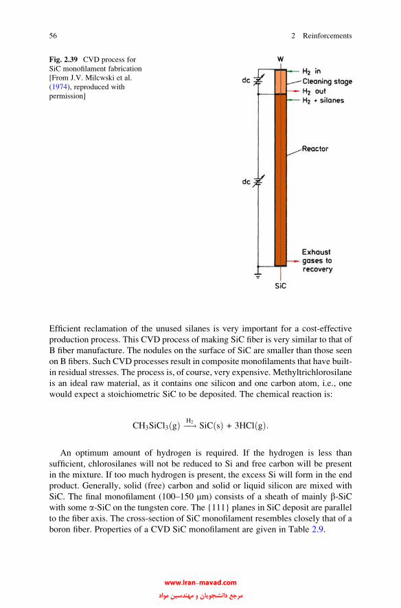
Efficient reclamation of the unused silanes is very important for a cost-effective

production process. This CVD process of making SiC fiber is very similar to that of

B fiber manufacture. The nodules on the surface of SiC are smaller than those seen

on B fibers. Such CVD processes result in composite monofilaments that have built-

in residual stresses. The process is, of course, very expensive. Methyltrichlorosilane

is an ideal raw material, as it contains one silicon and one carbon atom, i.e., one

would expect a stoichiometric SiC to be deposited. The chemical reaction is:

CH3SiCl3 gð Þ �!H2SiC sð Þ + 3HCl gð Þ:

An optimum amount of hydrogen is required. If the hydrogen is less than

sufficient, chlorosilanes will not be reduced to Si and free carbon will be present

in the mixture. If too much hydrogen is present, the excess Si will form in the end

product. Generally, solid (free) carbon and solid or liquid silicon are mixed with

SiC. The final monofilament (100–150 mm) consists of a sheath of mainly b-SiCwith some a-SiC on the tungsten core. The {111} planes in SiC deposit are parallel

to the fiber axis. The cross-section of SiC monofilament resembles closely that of a

boron fiber. Properties of a CVD SiC monofilament are given in Table 2.9.

Fig. 2.39 CVD process for

SiC monofilament fabrication

[From J.V. Milcwski et al.

(1974), reproduced with

permission]

56 2 Reinforcements


Commercially, a series of surface-modified silicon carbide fibers, called SCS

fibers is available. These special fibers have a complex through the thickness

gradient structure. SCS-6, for example, is a thick fiber (diameter ¼ 142 mm) that

is produced by CVD of silicon- and carbon-containing compounds onto a pyrolytic

graphite-coated carbon fiber core. The pyrolytic graphite coating is applied to a

carbon monofilament to give a substrate of 37 mm. This is then coated with SiC by

CVD to give a final monofilament of 142 mm diameter. Figure 2.40 shows

schematically the SCS-6 silicon carbide fiber and its characteristic surface compo-

sitional gradient. The surface modification of the SCS-6 fibers consists of the

following. The bulk of the 1-mm-thick surface coating consists of C-doped Si.

Zone I at and near the surface is a carbon-rich zone. In zone II, Si content decreases.

This is followed by zone III in which the Si content increases back to the stoichio-

metric SiC composition. Thus, the SCS-6 silicon carbide fiber has a carbon rich

surface and back to stoichiometric SiC a few micrometer from the surface.

Another CVD-type silicon carbide fiber is called sigma fiber. Sigma fiber is a

continuous silicon carbide monofilament by CVD on a tungsten substrate.

Table 2.9 Properties of CVD SiC monofilament

Composition Diameter (mm) Density (g/cm3) Tensile strength (MPa)

Young’s

modulus (GPa)

b-SiC 140 3.3 3,500 430

Fig. 2.40 Schematic of SCS-6 silicon carbide fiber and its surface compositional gradient

(courtesy of Textron Specialty Materials Co.)



2.6.2.2 Nonoxide Fibers via Polymers

As pointed out earlier, the SiC fiber obtained via CVD is very thick and not very

flexible. Work on alternate routes of obtaining fine, continuous, and flexible fiber

had been ongoing, when in the mid-1970s the late Professor Yajima and his

colleagues (1976, 1980) in Japan developed a process of making such a fiber by

controlled pyrolysis of a polymeric precursor. This method of using silicon-based

polymers to produce a family of ceramic fibers with good mechanical properties,

good thermal stability, and oxidation resistance has enormous potential. The vari-

ous steps involved in this polymer route, shown in Fig. 2.41 (Wax 1985), are:

1. Synthesis and characterization of polymer (yield, molecular weight, purity, and

so on).

2. Melt spin polymer into a precursor fiber.

3. Cure the precursor fiber to cross-link the molecular chains, making it infusible

during the final stage of pyrolysis.

Specifically, the Yajima process of making SiC involves the following steps and

is shown schematically in Fig. 2.42. PCS, a high-molecular-weight polymer

containing Si and C, is synthesized. The starting material is commercially available

dimethylchlorosilane. Solid polydimethylsilane (PDMS) is obtained by dechlorina-

tion of dimethylchlorosilane by reacting it with sodium. PCS is obtained by thermal

decomposition and polymerization of PDMS. This is carried out under high pres-

sure in an autoclave at 470 �C in an argon atmosphere for 8–14 h. A vacuum

distillation treatment at up to 280 �C follows. The average molecular weight of the

resulting polymer is about 1,500. This is melt spun from a 500-hole spinneret at

Fig. 2.41 Schematic of ceramic fiber production starting from silicon-based polymers [adapted

from Wax (1985), used with permission]

58 2 Reinforcements


about 350 �C in nitrogenous atmosphere to obtain the preceramic continuous,

precursor fiber. The precursor fiber is quite weak (tensile strength ~ 10 MPa).

This is converted to inorganic SiC by curing in air, heating to about 1,000 �C in

N2 gas, followed by heating to 1,300 �C in N2 under stretch. This is basically the

Nippon Carbon Co. manufacture process for Nicalon (the commercial name of fine

diameter silicon carbide fiber) fibers (Andersson and Warren 1984; Simon and

Bunsell 1984). During the pyrolysis, the first stage of conversion occurs at approxi-

mately 550 �C when cross-linking of polymer chains occurs. Above this tempera-

ture, the side chains containing hydrogen and methyl groups decompose. Fiber

density and mechanical properties improve sharply. The conversion to SiC takes

place above about 850 �C.There are different grades of Nicalon (nominally SiC) available commercially.

The properties of the first generation of Nicalon fiber were less than desirable, they

would start degrading above about 600 �C because of the thermodynamic instability

of composition and microstructure. A ceramic-grade Nicalon fiber, called NLP-202,

having low oxygen content is also available and shows better high-temperature

properties. Yet another version of multifilament silicon carbide fiber is Tyranno.

This is made by pyrolysis of poly (titano carbosilane), and it contains between 1.5

and 4 wt.% titanium.

Fine-diameter, polymer-derived silicon carbide fibers, such as Nicalon, gener-

ally have high oxygen content. This results from the curing of the precursor fibers in

an oxidizing atmosphere to introduce cross-linking. Cross-linking is required to

make the precursor fiber infusible during the subsequent pyrolysis step. One way

around this is to use electron beam curing. Other techniques involve dry spinning of

high-molecular-weight PCS polymers (Sacks et al. 1995). In this case, the as-spun

fiber does not require a curing step because of the high-molecular-weight PCS

polymer used, i.e., it does not melt during pyrolysis without requiring curing. Sacks

et al. (1995) used dopants to produce low-oxygen, near-stoichiometric, small-

diameter (10–15 mm) SiC fibers. They reported an average tensile strength for

these fibers of about 2.8 GPa. Their fiber had a C-rich and near stoichiometric

SiC and low oxygen content (Sacks et al. 1995; Toreki et al. 1994). They started

with PDMS, which has an Si–Si backbone. This is subjected to pressure pyrolysis to

obtain PCS, which has an Si–C backbone. The key point in their process is to have a

molecular weight of PCS between 5,000 and 20,000. This is a high molecular

weight compared to that used in other processes. The spinning dope was obtained

by adding suitable spinning aids and a solvent. This dope was dry spun to produce

green fibers, which were heated under controlled conditions to produce SiC fiber.

Laine and coworkers (1993, 1995) and Zhang et al. (1994) have used a

polymethylsilane (PMS) ([CH3SiH]x) as the precursor polymer for making a fine-

diameter, silicon carbide fiber. Spinning aids were used to stabilize the polymer

solution and the precursor fiber was extruded from a 140-mm orifice extruder into an

argon atmosphere. The precursor fiber was pyrolyzed at 1,800 �C in Ar. Boron,

added as a sintering aid, helped to obtain a dense product.



Fig. 2.42 Schematic of SiC

(Nicalon) production

[adapted from Andersson

and Warren (1984), used

with permission]

60 2 Reinforcements


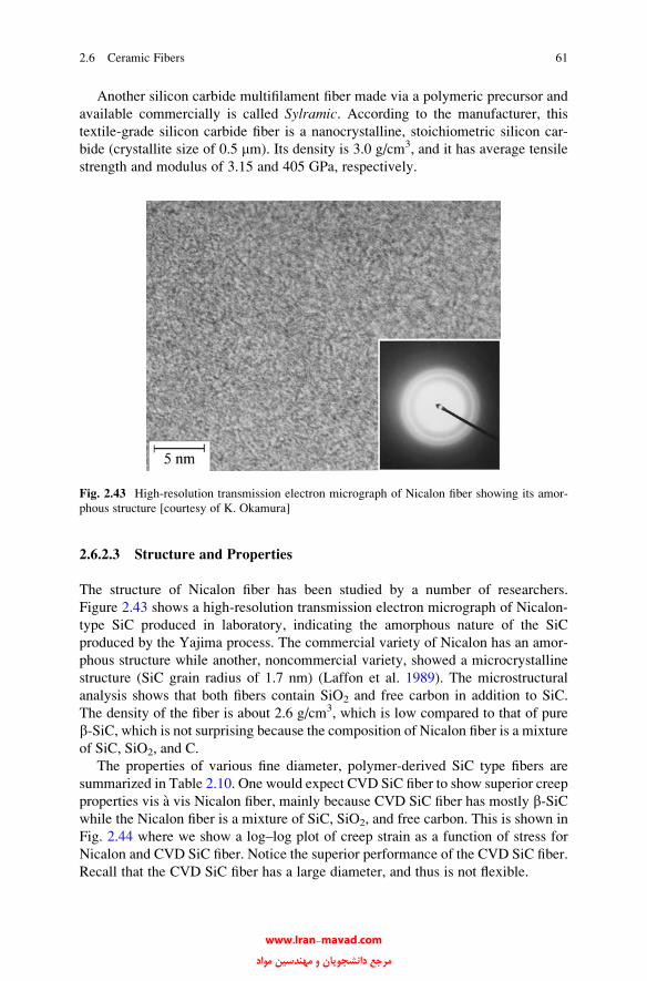
Another silicon carbide multifilament fiber made via a polymeric precursor and

available commercially is called Sylramic. According to the manufacturer, this

textile-grade silicon carbide fiber is a nanocrystalline, stoichiometric silicon car-

bide (crystallite size of 0.5 mm). Its density is 3.0 g/cm3, and it has average tensile

strength and modulus of 3.15 and 405 GPa, respectively.

2.6.2.3 Structure and Properties

The structure of Nicalon fiber has been studied by a number of researchers.

Figure 2.43 shows a high-resolution transmission electron micrograph of Nicalon-

type SiC produced in laboratory, indicating the amorphous nature of the SiC

produced by the Yajima process. The commercial variety of Nicalon has an amor-

phous structure while another, noncommercial variety, showed a microcrystalline

structure (SiC grain radius of 1.7 nm) (Laffon et al. 1989). The microstructural

analysis shows that both fibers contain SiO2 and free carbon in addition to SiC.

The density of the fiber is about 2.6 g/cm3, which is low compared to that of pure

b-SiC, which is not surprising because the composition of Nicalon fiber is a mixture

of SiC, SiO2, and C.

The properties of various fine diameter, polymer-derived SiC type fibers are

summarized in Table 2.10. One would expect CVD SiC fiber to show superior creep

properties vis a vis Nicalon fiber, mainly because CVD SiC fiber has mostly b-SiCwhile the Nicalon fiber is a mixture of SiC, SiO2, and free carbon. This is shown in

Fig. 2.44 where we show a log–log plot of creep strain as a function of stress for

Nicalon and CVD SiC fiber. Notice the superior performance of the CVD SiC fiber.

Recall that the CVD SiC fiber has a large diameter, and thus is not flexible.

Fig. 2.43 High-resolution transmission electron micrograph of Nicalon fiber showing its amor-

phous structure [courtesy of K. Okamura]



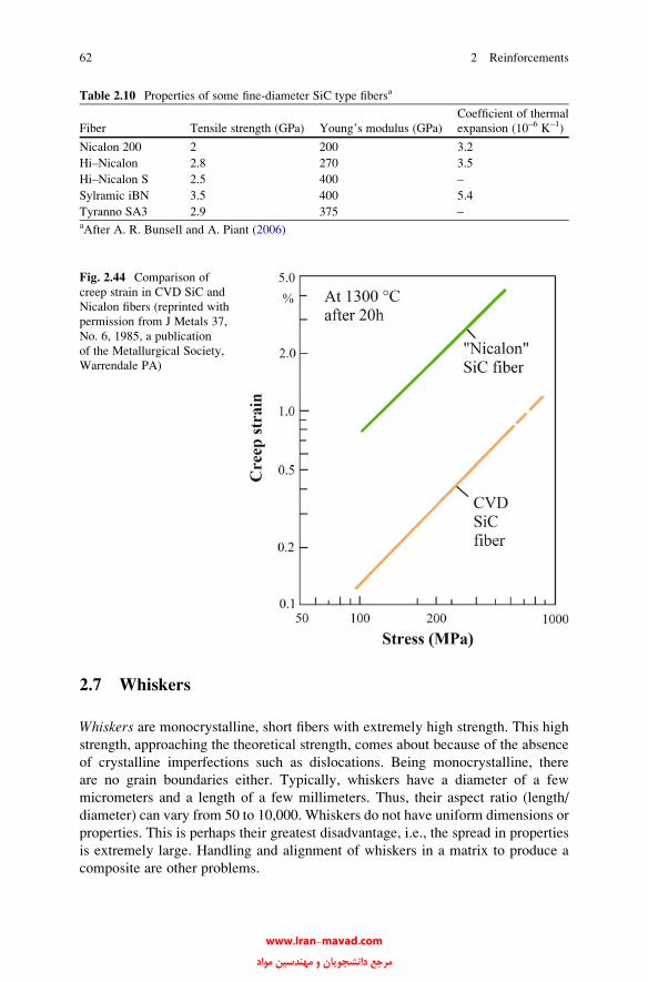
2.7 Whiskers

Whiskers are monocrystalline, short fibers with extremely high strength. This high

strength, approaching the theoretical strength, comes about because of the absence

of crystalline imperfections such as dislocations. Being monocrystalline, there

are no grain boundaries either. Typically, whiskers have a diameter of a few

micrometers and a length of a few millimeters. Thus, their aspect ratio (length/

diameter) can vary from 50 to 10,000. Whiskers do not have uniform dimensions or

properties. This is perhaps their greatest disadvantage, i.e., the spread in properties

is extremely large. Handling and alignment of whiskers in a matrix to produce a

composite are other problems.

Fig. 2.44 Comparison of

creep strain in CVD SiC and

Nicalon fibers (reprinted with

permission from J Metals 37,

No. 6, 1985, a publication

of the Metallurgical Society,

Warrendale PA)

Table 2.10 Properties of some fine-diameter SiC type fibersa

Fiber Tensile strength (GPa) Young’s modulus (GPa)


expansion (10–6 K–1)

Nicalon 200 2 200 3.2

Hi–Nicalon 2.8 270 3.5

Hi–Nicalon S 2.5 400 –

Sylramic iBN 3.5 400 5.4

Tyranno SA3 2.9 375 –aAfter A. R. Bunsell and A. Piant (2006)

62 2 Reinforcements


Whiskers are normally obtained by vapor phase growth. Back in the 1970s, a

new process was developed that used rice hulls as the starting material to produce

SiC particles and whiskers (Lee and Cutler 1975; Milewski et al. 1974). The SiC

particles produced by this process are of a fine size. Rice hulls are a waste by-

product of rice milling. For each 100 kg of rice milled, about 20 kg of rice hull is

produced. Rice hulls contain cellulose, silica, and other organic and inorganic

materials. Silica from soil is dissolved and transported in the plant as monosilicic

acid. This is deposited in the cellulosic structure by liquid evaporation. It turns out

that most of the silica ends up in hull. It is the intimate mixture of silica within the

cellulose that gives the near-ideal amounts of silica and carbon for silicon carbide

production. Raw rice hulls are heated in the absence of oxygen at about 700 �C to

drive out the volatile compounds. This process is called coking. Coked rice hulls,

containing about equal amounts of SiO2 and free C, are heated in inert or reducing

atmosphere (flowing N2 or NH3 gas) at a temperature between 1,500 and 1,600 �Cfor about 1 h to form silicon carbide as per the following reaction:

3Cþ SiO2 ! SiCþ 2CO:

Figure 2.45 shows the schematic of the process. When the reaction is over, the

residue is heated to 800 �C to remove any free C. Generally, both particles and

whiskers are produced, together with some excess free carbon. A wet process is

used to separate the particles and the whiskers. Typically, the average aspect ratio

of the as-produced whiskers is 75.

Exceptionally strong and stiff silicon carbidewhiskers have beenwere grown using

the so-called VLS process (Milewski et al. 1985; Petrovic et al. 1985). The average

tensile strength and modulus were 8.4 and 581 GPa, respectively. The acronym VLSstands for vapor feed gases, liquid catalyst, and solid crystalline whiskers. In this

process, the catalyst forms a liquid solution interface with the growing crystalline

phase,while elements are fed from the vapor phase through the liquid–vapor interface.

Whisker growth takes place by precipitation from the supersaturated liquid at the

solid–liquid interface. The catalyst must take in solution the atomic species of the

whisker to be grown. For SiC whiskers, transition metals and iron alloys meet this

requirement. Figure 2.46 illustrates the process for SiCwhisker growth. Steel particles

(~30 mm) are used as the catalyst. At 1,400 �C, the solid steel catalyst particle melts

and forms a liquid catalyst ball. From the vapor feed of SiC, H2, and CH4, the liquid

catalyst extracts C and Si atoms and forms a supersaturated solution. The gaseous

silicon monoxide is generated as per the following reaction:

SiO2 gð Þ þ C sð Þ ! SiO gð Þ þ CO gð Þ:

The supersaturated solution of C and Si in the liquid catalyst precipitates out

solid SiC whisker on the substrate. As the precipitation continues, the whisker

grows (Fig. 2.46). Generally, the process results in a range of whisker

morphologies. The tensile strength values vary a lot, they ranged from 1.7 to

23.7 GPa in 40 tests. Whisker lengths were about 10 mm; the equivalent circular

diameter averaged 5.9 mm.

2.7 Whiskers 63


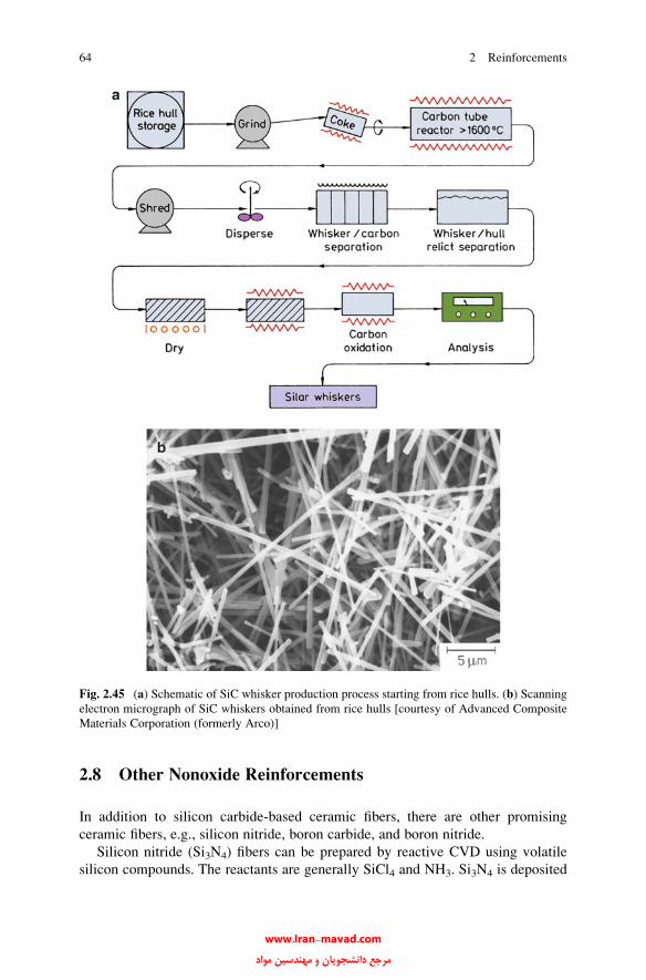
2.8 Other Nonoxide Reinforcements

In addition to silicon carbide-based ceramic fibers, there are other promising

ceramic fibers, e.g., silicon nitride, boron carbide, and boron nitride.

Silicon nitride (Si3N4) fibers can be prepared by reactive CVD using volatile

silicon compounds. The reactants are generally SiCl4 and NH3. Si3N4 is deposited

Fig. 2.45 (a) Schematic of SiC whisker production process starting from rice hulls. (b) Scanning

electron micrograph of SiC whiskers obtained from rice hulls [courtesy of Advanced Composite

Materials Corporation (formerly Arco)]

64 2 Reinforcements


on a carbon or tungsten substrate. Again, as in other CVD processes, the resultant

fiber has good properties, but the diameter is very large and it is expensive. In the

polymer route, organosilazane polymers with methyl groups on Si and N have been

used as silicon nitride precursors. Such carbon-containing, silicon–nitrogen

precursors, on pyrolysis, give silicon carbide as well as silicon nitride, i.e., the

resulting fiber is not an SiC-free silicon nitride fiber. Wills et al. (1983) have

discussed the mechanisms involved in the conversion of various organometallic

compounds into ceramics.

2.8.1 Silicon Carbide in a Particulate Form

SiC in particulate form has been available quite cheaply and abundantly for

abrasive, refractories, and chemical uses. In this conventional process, silica in

the form of sand and carbon in the form of coke are made to react at 2,400 �C in an

electric furnace. The SiC produced in the form of large granules is subsequently

comminuted to the desired size.

2.8.2 Tungsten Carbide Particles

Tungsten carbide is made by carburization of tungsten metal, which in turn, is

prepared by hydrogen reduction of tungsten oxide. A mixture of tungsten powder

and carbon black in the appropriate particle size and distribution is obtained by ball

milling. The addition of carbon black helps control particle size and size distribu-

tion. The objective is to produce stoichiometric tungsten carbide with a small

excess of free carbon, which prevents the formation of the highly undesirable eta-phase. Carburization is done in the presence of hydrogen at temperatures between

Fig. 2.46 The VLS process for SiC whisker growth [after Milewski et al. (1985), used with

permission]

2.8 Other Nonoxide Reinforcements 65


1,400 and 2,650 �C. The hydrogen reacts with the carbon black to form gaseous

hydrocarbons, which react with tungsten to form tungsten carbide per the following

reaction:

Wþ CH4 ! WCþ 2H2:

Commonly, after carburization, WC particles are deagglomerated by milling.

The final particle size can range from 0.5 to 30 mm. The particles are generally quite

angular.

2.9 Effect of High-Temperature Exposure

on the Strength of Ceramic Fibers

Carbon fiber is excellent at high temperatures in an inert atmosphere. In air, at

temperatures above 400–450 �C, it starts oxidizing. SiC and SixNy show reasonable

oxidation resistance for controlled composition fibers. SiC starts oxidizing above

1,300–1,400 �C in air. The high-temperature strength of the SiC-type fibers is

limited by oxidation and internal void formation, while in the case of oxide fibers

any intergranular glassy phase leads to softening. Mah et al. (1984) studied the

degradation of Nicalon fiber after heat treatment in different environments.

The strength degradation of this fiber at temperatures greater than 1,200 �C was

because of CO evaporation from the fiber as well as b-SiC grain growth. Ceramic

fibers made via pyrolysis of polymeric precursors, especially with compositions

Si–C–O and Si–N–C–O, have lower densities than the theoretical values (Lipowitz

et al. 1990). The theoretical density, rt, can be calculated using the relationship

rt ¼ riVi;

where r is the density, V is the volume fraction, the subscript i indicates the ithphase, and summation over all the phases present is implied (see also chap. 10).

X-ray scattering techniques were used to show that porosity present in such fibers

was in the form of globular pores of nm size and that the pore fractions ranged from

5 to 25% (Lipowitz et al. 1990). Channels of nm size diameter form during the early

stages of pyrolysis, when rather large volumes of gases are given out. In the later

stages of pyrolysis, smaller volumes of gases are given out. In the later stages of

pyrolysis, i.e., during densification, these nano-channels suffer a viscous collapse

and nanopores are formed. The volume fraction of nanopores decreases with

increasing pyrolysis temperature. The reader should note that a higher density

and the consequent lower void fraction will result higher elastic modulus and

strength of these ceramic fibers.

66 2 Reinforcements


http://dx.doi.org/10.1007/978-0-387-74365-3_10

2.10 Comparison of Fibers

A comparison of some important characteristics of reinforcements discussed indi-

vidually in Sects. 2.2–2.7 is made in Table 2.11, and a plot of strength vs. modulus

is shown in Fig. 2.47. We compare and contrast some salient points of these fibers.

First of all, we note that all these high-performance fibers have low density

values. If we take the general low density of these fibers as a given, the best of these

fibers group together in the top right-hand corner of Fig. 2.47. The reader will also

recognize that the elements comprising these fibers pertain to the first two rows of

the periodic table. Also to be noted is the fact that, irrespective of whether in

compound or elemental form, they are mostly covalently bonded, which is the

strongest bond. Generally, such light, strong, and stiff materials are very desirable

in most applications, but particularly in aerospace, land transportation, energy-

related industry, housing and civil construction, and so on.

Fiber flexibility is associated with the Young’s modulus and the diameter (see

Sect. 2.1). In the general area of high-modulus (i.e., high-E) fibers, the diameter

becomes the dominant parameter controlling the flexibility. For a given E, thesmaller the diameter the more flexible it is. Fiber flexibility is a very desirable

characteristic if one wants to bend, wind, and weave a fiber in order to make a

complex-shaped final product.

Some of these fibers have quite anisotropic characteristics. Consider the situa-

tion in regard to thermal properties; in particular, the thermal expansion coefficient

of carbon is quite different in the radial and longitudinal directions. This would also

be true of any single-crystal fiber or whisker, e.g., alumina single-crystal fiber,

which has a hexagonal structure. Polycrystalline fibers such as SiC or Al2O3 are

isotropic. Carbon, aramid, and polyethylene are anisotropic because the high degree

Fig. 2.47 Comparison of different fibers

2.10 Comparison of Fibers 67


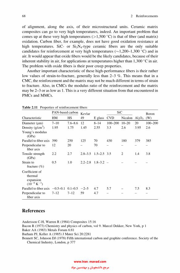
of alignment, along the axis, of their microstructural units. Ceramic matrix

composites can go to very high temperatures, indeed. An important problem that

comes up at these very high temperatures (>1,500 �C) is that of fiber (and matrix)

oxidation. Carbon fiber, for example, does not have good oxidation resistance at

high temperatures. SiC- or Si3N4-type ceramic fibers are the only suitable

candidates for reinforcement at very high temperatures (�1,200–1,300 �C) and in

air. It would appear that oxide fibers would be the likely candidates, because of their

inherent stability in air, for applications at temperatures higher than 1,300 �C in air.

The problem with oxide fibers is their poor creep properties.

Another important characteristic of these high-performance fibers is their rather

low values of strain-to-fracture, generally less than 2–3 %. This means that in a

CMC, the reinforcement and the matrix may not be much different in terms of strain

to fracture. Also, in CMCs the modulus ratio of the reinforcement and the matrix

may be 2–3 or as low as 1. This is a very different situation from that encountered in

PMCs and MMCs.

References

Andersson C-H, Warren R (1984) Composites 15:16

Bacon R (1973) Chemistry and physics of carbon, vol 9. Marcel Dekker, New York, p 1

Baker AA (1983) Metals Forum 6:81

Barham PJ, Keller A (1985) J Mater Sci 20:2281

Bennett SC, Johnson DJ (1978) Fifth international carbon and graphite conference. Society of the

Chemical Industry, London, p 377

Table 2.11 Properties of reinforcement fibers

Characteristic

PAN-based carbon Kevlar

49 E glass

SiC

Al2O3

Boron

(W)HM HS CVD Nicalon

Diameter (mm) 7–10 7.6–8.6 12 8–14 100–200 10–20 20 100–200

Density (g/cm3) 1.95 1.75 1.45 2.55 3.3 2.6 3.95 2.6

Young’s modulus

(GPa)

Parallel to fiber axis 390 250 125 70 430 180 379 385

Perpendicular to

fiber axis

12 20 – 70 – – – –

Tensile strength

(GPa)

2.2 2.7 2.8–3.5 1.5–2.5 3.5 2 1.4 3.8

Strain to

fracture (%)

0.5 1.0 2.2–2.8 1.8–3.2 – – – –

Coefficient of

thermal

expansion

(10�6 K�1)

Parallel to fiber axis �0.5–0.1 0.1–0.5 �2–5 4.7 5.7 – 7.5 8.3

Perpendicular to

fiber axis

7–12 7–12 59 4.7 – – – –

68 2 Reinforcements


Bennett SC, Johnson DJ (1979) Carbon 17:25

Bennett SC, Johnson DJ, Johnson W (1983) J Mater Sci 18:3337

Biro DA, Pleizier G, Deslandes Y (1992) J Mater Sci Lett 11:698

Brinker CJ, Scherer G (1990) The sol-gel science. Academic, New York

Brown JR, Chappell PJC, Mathys Z (1992) J Mater Sci 27:3167

Bunsell AR, Piant A (2006) J Mater Sci 40:823

Capaccio G, Gibson AG, Ward IM (1979) Ultra-high modulus polymers. Applied Science

Publishers, London, p 1

Chawla KK (1976) Proceedings of the international conference on the mechanical behavior of

materials II. ASM, Metals Park, OH, p 1920

Chawla KK (1981) Mater Sci Eng 48:137

Chawla KK (1998a) Fibrous materials. Cambridge University Press, Cambridge

Chawla KK, Bastos AC (1979) Proceedings of the international conference on the mechanical

behavior of materials III. Pergamon, Oxford, p 191

de Lamotte E, Perry AJ (1970) Fibre Sci Technol 3:157

DeBolt HE (1982) Handbook of composites. Van Nostrand Reinhold, New York, p 171

DeTeresa SJ, Allen SR, Farris RJ, Porter RS (1984) J Mater Sci 19:57

DiCarlo JA (1985) J Metals 37:44

Diefendorf RJ, Tokarsky E (1975) Polym Eng Sci 15:150

Dobb MG, Johnson DJ, Saville BP (1980) Philos Trans R Soc Lond A294:483

Dresher WH (1969) J Metals 21:17

Ezekiel HN, Spain RG (1967) J Polym Sci C 19:271

Flory PJ (1956) Proc R Soc Lond 234A:73

Fourdeux A, Perret R, Ruland W (1971) Carbon fibres: their composites and applications. The

Plastics Institute, London, p 57

Galasso F, Paton A (1966) Trans Met Soc AIME 236:1751

Galasso F, Knebl D, Tice W (1967) J Appl Phys 38:414

Gasson DG, Cockayne B (1970) J Mater Sci 5:100

Haggerty JS (1972) NASA-CR-120948. NASA Lewis Res Center, Cleveland, OH

Hild DN, Schwartz P (1992a) J Adhes Sci Technol 6:879

Hild DN, Schwartz P (1992b) J Adhes Sci Technol 6:897

Hodd KA, Turley DC (1978) Chem Br 14:545

Hurley GF, Pollack JTA (1972) Met Trans 7:397

Inal OT, Leca N, Keller L (1980) Phys Status Solidi 62:681

Jaffe M, Jones RS (1985) Handbook of fiber science & technology, vol 111, High technology

fibers. Part A. Marcel Dekker, NewYork, p 349

Johnson J, Tyson CN (1969) Br J Appl Phys 2:787

Jones RW (1989) Fundamental principles of sol-gel technology. The Institute of Metals, London

Kalb B, Pennings AJ (1980) J Mater Sci 15:2584

Kaplan SL, Rose PW, Nguyen HX, Chang HW (1988) SAMPE Quart 19:55

Kikuchi T (1982) Surface 20:270

Krukonis V (1977) Boron and refractory borides. Springer-Verlag, Berlin, p 517

Kwolek SL, Morgan PW, Schaefgen JR, Gultich LW (1977) Macromolecules 10:1390

Kwolek SL, Yang HH (1993) Manmade fibers: their origin and development. Elsevier App. Sci,

London, p 315

LaBelle HE (1971) Mater Res Bull 6:581

LaBelle HE, Mlavsky AI (1967) Nature 216:574

Laffon C, Flank AM, Lagarde P, Laridjani M, Hagege R, Olry P, Cotteret J, Dixmier J, Niquel JL,

Hommel H, Legrand AP (1989) J Mater Sci 24:1503

Laine RM, Babonneau F (1993) Chem Mater 5:260

Laine RM, Zhang Z-F, Chew KW, Kannisto M, Scotto C (1995) Ceramic processing science and

technology. Am. Ceram. Soc, Westerville, OH, p 179

Lee J-G, Cutler IB (1975) Am Ceram Soc Bull 54:195

References 69


Li ZF, Netravali AN, Sachse W (1992) J Mater Sci 27:4625

Lipowitz J, Rabe JA, Frevel LK (1990) J Mater Sci 25:2118

Loewenstein KL (1983) The manufacturing technology of continuous glass fibers, 2nd edn.

Elsevier, New York

Lowrie RE (1967) In: Modern composite materials. Addison-Wesley, Reading, MA, p 270

Magat EE (1980) Philos Trans R Soc Lond A296:463

Mah T, Hecht NL, McCullum DE, Hoenigman JR, Kim HM, Katz AP, Lipsitt HA (1984) J Mater

Sci 19:1191

Milcwski JV, Sandstrom JL, BrownWS (1974) Silicon carbide 1973. University of South Carolina

Press, Columbia, p 634

Milewski JV, Gac FD, Petrovic JJ, Skaggs SR (1985) J Mater Sci 20:1160

Morgan PW (1979) Plast Rubber Mater Appl 4:1

Murday JS, Dominguez DD, Moran LA, Lee WD, Eaton R (1984) Synth Met 9:397

Northolt MG (1981) J Mater Sci 16:2025

Ozawa S, Nakagawa Y, Matsuda K, Nishihara T, Yunoki H (1978). US patent 4,075,172

Parkyn B (ed) (1970) Glass reinforced plastics. Butterworth, London

Perret R, Ruland W (1970) J Appl Crystallogr 3:525

Petrovic JJ, Milewski JV, Rohr DL, Gac FD (1985) J Mater Sci 20:1167

Pollack JTA (1972) J Mater Sci 7:787

Riggs JP (1985) Encyclopedia of polymer science & engineering, 2nd edn, vol 2. Wiley, New

York, p 640

Sacks MD, Scheiffele GW, Saleem M, Staab GA, Morrone AA, Williams TJ (1995) Ceramic

matrix composites: advanced high-temperature structural materials. MRS, Pittsburgh, PA, p 3

Sakka S (1985) Am Ceram Soc Bull 64:1463

Simon G, Bunsell AR (1984) J Mater Sci 19:3649

Singer LS (1979) Ultra-high modulus polymers. Applied Science Publishers, Essex, p 251

Shindo A (1961). Rep Osaka Ind Res Inst. No. 317

Smith P, Lemstra PJ (1976) Colloid Polym Sci 15:258

Smith WD (1977) Boron and refractory borides. Springer-Verlag, Berlin, p 541

Smook J, Pennings AJ (1984) J Mater Sci 19:31

Sowman HG (1988). In sol-gel technology. Klein LJ (ed) Noyes Pub., Park Ridge, NJ, p 162

Talley CP (1959) J Appl Phys 30:1114

Talley CP, Line L, Overman O (1960) Boron: synthesis, structure, and properties. Plenum, New

York, p 94

Tanner D, Dhingra AK, Pigliacampi JJ (1986) J Metals 38:21

Toreki W, Batich CD, Sacks MD, Saleem M, Choi GJ, Morrone AA (1994) Compos Sci Technol

51:145

van Maaren AC, Schob O, Westerveld W (1975) Philips Tech Rev 35:125

Vega-Boggio J, Vingsbo O (1978) In: 1978 International conference on composite materials,

ICCM/2. TMS-AIME, New York, p 909

Warner SB (1995) Fiber science. Prentice Hall, Englewood Cliffs, NJ

Warren R, Andersson C-H (1984) Composites 15:101

Watt W (1970) Proc R Soc A319:5

Watt W, Johnson W (1969) Appl Polym Symp 9:215

Wawner FW (1967) In: Modern composite materials. Addison-Wesley, Reading, MA, p 244

Wax SG (1985) Am Ceram Soc Bull 64:1096

Weintraub E (1911) J Ind Eng Chem 3:299

Wills RR, Mankle RA, Mukherjee SP (1983) Am Ceram Soc Bull 62:904

Wilson DM (1990) In: Proceedings of the 14th conference on metal matrix, carbon, and ceramic

matrix composites, Cocoa Beach, FL, 17–19 January 1990, NASA Conference Publication

3097, Part 1, p 105

Wynne KJ, Rice RW (1984) Annu Rev Mater Sci 15:297

Yajima S (1980) Philos Trans R Soc Lond A294:419

70 2 Reinforcements


Yajima S, Okamura K, Hayashi J, Omori M (1976) J Am Ceram Soc 59:324

Zhang Z-F, Scotto S, Laine RM (1994) Ceram Eng Sci Proc 15:152

Further Reading

Bunsell AR (ed) (1988) Fibre reinforcements for composite materials. Elsevier, Amsterdam

Bunsell AR, Berger M (eds) (1999) Fine ceramic fibers. Marcel Dekker, New York

Chawla KK (1998b) Fibrous materials. Cambridge University Press, Cambridge

Donnet J-B, Wang TK, Peng JCM, Rebouillat S (eds) (1998) Carbon fibers, vol 3. Marcel Dekker,

New York

Fitzer E (1985) Carbon fibres and their composites. Springer-Verlag, Berlin

Peebles LH (1995) Carbon fibers. CRC, Boca Raton, FL

Watt W, Perov BV (eds) (1985) Strong fibres, vol 1 in the handbook of composites series. North-

Holland, Amsterdam

Yang HH (1993) Kevlar aramid fiber. Wiley, Chichester

Problems

2.1. Nonwoven fibrous mats can be formed through entanglement and/or fibers

bonded in the form of webs or yarns by chemical or mechanical means. What

are the advantages and disadvantages of such nonwovens over similar woven

mats?

2.2. Glass fibers are complex mixtures of silicates and borosilicates containing

mixed sodium, potassium, calcium, magnesium, and other oxides. Such a glass

fiber can be regarded as an inorganic polymeric fiber. Do you think you can

provide the chemical structure of such a inorganic fiber chain?

2.3. A special kind of glass fiber is used as a medium for the transmission of light

signals. Discuss the specific requirements for such an optical fiber.

2.4. The compressive strength of aramid fiber is about one-eighth of its tensile

stress. Estimate the smallest diameter of a rod on which the aramid fiber can be

wound without causing kinks, etc., on its compression side.

2.5. Several types of Kevlar aramid fibers are available commercially. Draw

schematically the stress–strain curves of Kevlar 49 and Kevlar 29. Describe

how much of the strain is elastic (linear or nonlinear). What microstructural

processes occur during their deformation?

2.6. Aramid fiber, when fractured in tension, shows characteristically longitudinal

splitting, i.e., microfibrillation is observed. Explain why.

2.7. Describe the structural differences between Kevlar and Nomex (both aramids)

that are responsible for their different mechanical characteristics.

2.8. What is asbestos fiber and why is it considered to be a health hazard?

2.9. Describe the problems involved in mechanical testing of short fibers such as

whiskers.

Problems 71


Chapter 3

Matrix Materials

A brief description of the various matrix materials, polymers, metals, and ceramics,

is given in this chapter. We emphasize the characteristics that are relevant to

composites. The reader should consult the references listed under Further Reading

for greater details regarding any particular aspect of these materials.

3.1 Polymers

Polymers are structurally much more complex than metals or ceramics. They are

cheap and can be easily processed. On the other hand, polymers have lower strength

and modulus and lower use temperature limits. Prolonged exposure to ultraviolet

light and some solvents can cause the degradation of polymer properties. Because

of predominantly covalent bonding, polymers are generally poor conductors of heat

and electricity. Polymers, however, are generally more resistant to chemicals than

are metals. Structurally, polymers are giant chainlike molecules (hence the name

macromolecules) with covalently bonded carbon atoms forming the backbone of

the chain. The process of forming large molecules from small ones is called

polymerization; that is, polymerization is the process of joining many monomers,

the basic building blocks, together to form polymers. There are two important

classes of polymerization:

1. Condensation polymerization. In this process a stepwise reaction of molecules

occurs and in each step a molecule of a simple compound, generally water, forms

as a by-product.

2. Addition polymerization. In this process monomers join to form a polymer

without producing any by-product. Addition polymerization is generally carried

out in the presence of catalysts. The linear addition of ethylene molecules (CH2)

results in polyethylene (a chain of ethylene molecules), with the final mass of

polymer being the sum of monomer masses.


73


Based on their behavior, there are two major classes of polymers, produced by

either condensation or addition polymerization, i.e., thermosetting and thermoplas-

tic polymers. Thermosets undergo a curing reaction that involves cross-linking of

polymeric chains. They harden on curing, hence the term thermoset. The curing

reaction can be initiated by appropriate chemical agents or by application of heat

and pressure, or by exposing the monomer to an electron beam. Thermoplastics are

polymers that flow under the application of heat and pressure, i.e., they soften or

become plastic on heating. Cooling to room temperature hardens thermoplastics.

Their different behavior, however, stems from their molecular structure and shape,

molecular size or mass, and the amount and type of bond (covalent or van der

Waals). We first describe the basic molecular structure in terms of the

configurations of chain molecules. Figure 3.1 shows the different chain configura-

tion types.

1. Linear polymers. As the name suggests, this type of polymer consists of a long

chain of atoms with attached side groups. Examples include polyethylene,

polyvinyl chloride, and polymethyl methacrylate (PMMA). Figure 3.1a shows

the configuration of linear polymers; note the coiling and bending of chains.

2. Branched polymers. Polymer branching can occur with linear, cross-linked, or

any other type of polymer; see Fig. 3.1b.

3. Cross-linked polymers. In this case, molecules of one chain are bonded with

those of another; see Fig. 3.1c. Cross-linking of molecular chains results in a

three-dimensional network. Cross-linking makes sliding of molecules past one

another difficult; thus such polymers are strong and rigid.

4. Ladder polymers. If we have two linear polymers linked in a regular manner

(Fig. 3.1d) we get a ladder polymer. Not unexpectedly, ladder polymers are more

rigid than linear polymers.

3.1.1 Glass Transition Temperature

Pure crystalline materials have well-defined melting temperatures. The melting

point is the temperature at which crystalline order is completely destroyed on

heating. Polymers, however, show a range of temperatures over which crystallinity

vanishes. Figure 3.2 shows specific volume (volume/unit mass) vs. temperature

curves for amorphous and semicrystalline polymers. When a polymer liquid is

cooled, it contracts. The contraction occurs because of a decrease in the thermal

vibration of molecules and a reduction in the free space; that is, the molecules

occupy the space less loosely. At certain temperature, called the melting point, Tm,

74 3 Matrix Materials


there occurs a thermodynamic phase transformation and the material assumes an

orderly crystalline structure. In the case a semicrystalline polymer consists of a

crystalline and an amorphous phase, the crystalline part undergoes this transforma-

tion. In the case of amorphous polymers, there is no fixed melting point, Tm. Thepolymer liquid continues to contract, below what would be the melting point for the

crystalline phase. It does so down to a less well-defined temperature called the glass

transition temperature, Tg. Below Tg, it becomes a supercooled liquid polymer that

is quite rigid and solidlike because of very high viscosity. Unlike the crystalline

phase, the structure of a glassy or amorphous material below Tg is essentially that ofa liquid (highly disordered), albeit a very viscous one. Such a phenomenon is

commonly observed in silica-based inorganic glasses. In the case of amorphous

polymers, we are dealing with a glassy structure made of organic molecules.

Fig. 3.2 Specific volume vs.

temperature for an amorphous

and a semicrystalline polymer

Fig. 3.1 Different molecular chain configurations: (a) linear, (b) branched, (c) cross-linked,

(d) ladder

3.1 Polymers 75


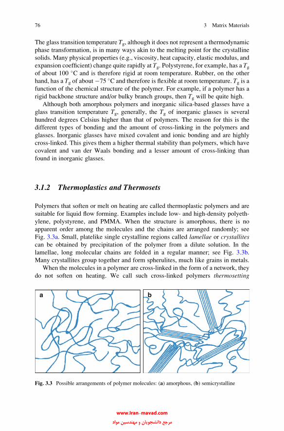
The glass transition temperature Tg, although it does not represent a thermodynamic

phase transformation, is in many ways akin to the melting point for the crystalline

solids. Many physical properties (e.g., viscosity, heat capacity, elastic modulus, and

expansion coefficient) change quite rapidly at Tg. Polystyrene, for example, has a Tgof about 100 �C and is therefore rigid at room temperature. Rubber, on the other

hand, has a Tg of about�75 �C and therefore is flexible at room temperature. Tg is afunction of the chemical structure of the polymer. For example, if a polymer has a

rigid backbone structure and/or bulky branch groups, then Tg will be quite high.Although both amorphous polymers and inorganic silica-based glasses have a

glass transition temperature Tg, generally, the Tg of inorganic glasses is several

hundred degrees Celsius higher than that of polymers. The reason for this is the

different types of bonding and the amount of cross-linking in the polymers and

glasses. Inorganic glasses have mixed covalent and ionic bonding and are highly

cross-linked. This gives them a higher thermal stability than polymers, which have

covalent and van der Waals bonding and a lesser amount of cross-linking than

found in inorganic glasses.

3.1.2 Thermoplastics and Thermosets

Polymers that soften or melt on heating are called thermoplastic polymers and are

suitable for liquid flow forming. Examples include low- and high-density polyeth-

ylene, polystyrene, and PMMA. When the structure is amorphous, there is no

apparent order among the molecules and the chains are arranged randomly; see

Fig. 3.3a. Small, platelike single crystalline regions called lamellae or crystallitescan be obtained by precipitation of the polymer from a dilute solution. In the

lamellae, long molecular chains are folded in a regular manner; see Fig. 3.3b.

Many crystallites group together and form spherulites, much like grains in metals.

When the molecules in a polymer are cross-linked in the form of a network, they

do not soften on heating. We call such cross-linked polymers thermosetting

Fig. 3.3 Possible arrangements of polymer molecules: (a) amorphous, (b) semicrystalline



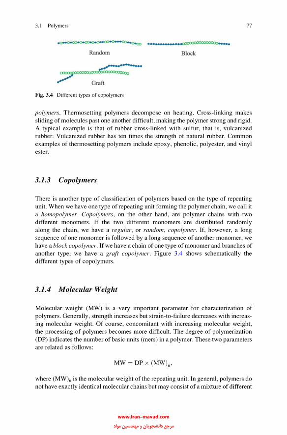
polymers. Thermosetting polymers decompose on heating. Cross-linking makes

sliding of molecules past one another difficult, making the polymer strong and rigid.

A typical example is that of rubber cross-linked with sulfur, that is, vulcanized

rubber. Vulcanized rubber has ten times the strength of natural rubber. Common

examples of thermosetting polymers include epoxy, phenolic, polyester, and vinyl

ester.

3.1.3 Copolymers

There is another type of classification of polymers based on the type of repeating

unit. When we have one type of repeating unit forming the polymer chain, we call it

a homopolymer. Copolymers, on the other hand, are polymer chains with two

different monomers. If the two different monomers are distributed randomly

along the chain, we have a regular, or random, copolymer. If, however, a long

sequence of one monomer is followed by a long sequence of another monomer, we

have a block copolymer. If we have a chain of one type of monomer and branches of

another type, we have a graft copolymer. Figure 3.4 shows schematically the

different types of copolymers.

3.1.4 Molecular Weight

Molecular weight (MW) is a very important parameter for characterization of

polymers. Generally, strength increases but strain-to-failure decreases with increas-

ing molecular weight. Of course, concomitant with increasing molecular weight,

the processing of polymers becomes more difficult. The degree of polymerization

(DP) indicates the number of basic units (mers) in a polymer. These two parameters

are related as follows:

MW ¼ DP� MWð Þu;

where (MW)u is the molecular weight of the repeating unit. In general, polymers do

not have exactly identical molecular chains but may consist of a mixture of different

Fig. 3.4 Different types of copolymers

3.1 Polymers 77


species, each of which has a different molecular weight or DP. Thus, the molecular

weight of the polymer is characterized by a distribution function. Clearly, the

narrower this distribution function is, the more homogeneous the polymer is. That

is why one speaks of an average molecular weight or degree of polymerization.

It is instructive to compare the molecular weights of some common polymeric

materials vis a vis monomeric materials. A molecule of water, H2O, has a molecular

weight of 18. Benzene, a low-molecular-weight organic solvent, has a molecular

weight of 78. Compared to these, natural rubber can have a molecular weight of

about 106. Polyethylene, a common synthetic polymer, can have molecular weights

greater than 105. The molecular size of these high-molecular-weight solids is also

very large. The molecular diameter of water, for example, is 40 nm, while that of

polyethylene can be as large as 6,400 nm (Mandelkern 1983).

3.1.5 Degree of Crystallinity

Polymers can be amorphous or partially crystalline; see Fig. 3.3. A 100 % crystal-

line polymer is difficult to obtain. In practice, depending on the polymer type,

molecular weight, and crystallization temperature, the amount of crystallinity in a

polymer can vary from 30 to 90 %. The inability to attain a fully crystalline

structure is mainly due to the long chain structure of polymers. Some twisted and

entangled segments of chains that get trapped between crystalline regions never

undergo the conformational reorganization necessary to achieve a fully crystalline

state. Molecular architecture also has an important bearing on the polymer crystal-

lization behavior. Linear molecules with small or no side groups crystallize easily.

Branched chain molecules with bulky side groups do not crystallize as easily. For

example, linear high-density polyethylene can be crystallized to 90 %, while

branched polyethylene can be crystallized to only about 65 %. Generally, the

stiffness and strength of a polymer increase with the degree of crystallinity. It

should be mentioned that deformation processes such as slip and twinning, as well

as phase transformations that take place in monomeric crystalline solids, can also

occur in polymeric crystals.

3.1.6 Stress–Strain Behavior

Characteristic stress–strain curves of an amorphous polymer and of an elastomer

(a rubbery polymer) are shown in Fig. 3.5a, b, respectively. Note that the elasto-

mer does not show a Hookean behavior; its behavior is characterized as nonlinear

elastic. The characteristically large elastic range shown by elastomers

results from an easy reorganization of the tangled chains under the action of an

applied stress.



Yet another point in which polymers differ from metals and ceramics is the

extreme temperature dependence of their elastic moduli. Figure 3.6 shows

schematically the variation of the elastic modulus of an amorphous polymer with

temperature. In the temperature range below Tg, the polymer is hard and a typical

value of elastic modulus would be about 5 GPa. Above Tg, the modulus value drops

significantly and the polymer shows a rubbery behavior. Above Tf (the temperature

at which the polymer becomes fluid), the modulus drops abruptly. It is in this region

of temperatures above Tf that polymers are subjected to various processing

operations.

Fig. 3.5 (a) Hookean elastic behavior of a glassy polymer. (b) Nonlinear elastic behavior of an

elastomer

Fig. 3.6 Variation of elastic modulus of an amorphous polymer with temperature (schematic)

3.1 Polymers 79


3.1.7 Thermal Expansion

Polymers generally have higher thermal expansivities than metals and ceramics.

Furthermore, their thermal expansion coefficients are not truly constants; that is, the

polymers expand markedly in a nonlinear way with temperature. Epoxy resins have

coefficient of linear expansion values between 50 � 10�6 and 100 � 10�6 K�1

while polyesters show values between 100 � 10�6 and 200 � 10�6 K�1. Small

compositional changes can have a marked influence on the polymer expansion

characteristics.

3.1.8 Fire Resistance or Flammability

Fire performance of any polymer depends on a number of variables, such as surface

spreading of flame, fuel penetration, and oxygen index. The limiting oxygen index

(LOI) is the minimum amount of oxygen that will support combustion.

The degree of flammability of a polymer or a PMC is a function of the following

parameters:

• Matrix type and amount (dominant!)

• Quantity of fire-retardant additives

• Type and amount of reinforcement (if any)

The order of increasing fire resistance of common polymer matrix materials is as

follows: polyester, vinyl ester, epoxy, phenolic. Phenolic has very low smoke

emission and gives out no toxic by-products. An added advantage of phenolic is

that when it burns, it leaves behind char which is a good thermal insulator. In the

case of thermosets, such as polyester, it is common practice to add fire-retardant

additives. Addition of large amount of glass fiber also helps.

3.1.9 Common Polymeric Matrix Materials

Thermosets and thermoplastic polymers are common matrix materials. A brief

description of important polymer matrix materials is provided here.

3.1.9.1 Common Thermoset Matrix Materials

Among the common polymer matrices used with continuous fibers are polyester

and epoxy resins. We provide a summary of thermosetting resins commonly used as

matrix materials.



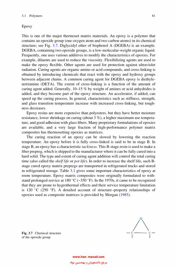
Epoxy

This is one of the major thermoset matrix materials. An epoxy is a polymer that

contains an epoxide group (one oxygen atom and two carbon atoms) in its chemical

structure; see Fig. 3.7. Diglycidyl ether of bisphenol A (DGEBA) is an example.

DGEBA, containing two epoxide groups, is a low-molecular-weight organic liquid.

Frequently, one uses various additives to modify the characteristics of epoxies. For

example, diluents are used to reduce the viscosity. Flexibilizing agents are used to

make the epoxy flexible. Other agents are used for protection against ultraviolet

radiation. Curing agents are organic amino or acid compounds, and cross-linking is

obtained by introducing chemicals that react with the epoxy and hydroxy groups

between adjacent chains. A common curing agent for DGEBA epoxy is diethyle-

netriamine (DETA). The extent of cross-linking is a function of the amount of

curing agent added. Generally, 10–15 % by weight of amines or acid anhydrides is

added, and they become part of the epoxy structure. An accelerator, if added, can

speed up the curing process. In general, characteristics such as stiffness, strength,

and glass transition temperature increase with increased cross-linking, but tough-

ness decreases.

Epoxy resins are more expensive than polyesters, but they have better moisture

resistance, lower shrinkage on curing (about 3 %), a higher maximum use tempera-

ture, and good adhesion with glass fibers. Many proprietary formulations of epoxies

are available, and a very large fraction of high-performance polymer matrix

composites has thermosetting epoxies as matrices.

The curing reaction of an epoxy can be slowed by lowering the reaction

temperature. An epoxy before it is fully cross-linked is said to be in stage B. In

stage B, an epoxy has a characteristic tackiness. This B-stage resin is used to make a

fiber prepreg, which is shipped to the manufacturer where it can be fully cured into a

hard solid. The type and extent of curing agent addition will control the total curing

time (also called the shelf life or pot life). In order to increase the shelf life, such B-stage cured epoxy matrix prepregs are transported in refrigerated trucks and stored

in refrigerated storage. Table 3.1 gives some important characteristics of epoxy at

room temperature. Epoxy matrix composites were originally formulated to with-

stand prolonged service at 180 �C (~350 �F). In the 1970s, it came to be recognized

that they are prone to hygrothermal effects and their service temperature limitation

is 120 �C (250 �F). A detailed account of structure–property relationships of

epoxies used as composite matrices is provided by Morgan (1985).

Fig. 3.7 Chemical structure

of the epoxide group

3.1 Polymers 81


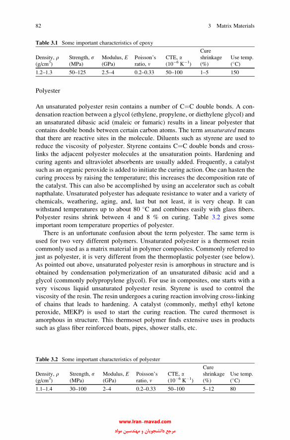
Polyester

An unsaturated polyester resin contains a number of C¼C double bonds. A con-

densation reaction between a glycol (ethylene, propylene, or diethylene glycol) and

an unsaturated dibasic acid (maleic or fumaric) results in a linear polyester that

contains double bonds between certain carbon atoms. The term unsaturated means

that there are reactive sites in the molecule. Diluents such as styrene are used to

reduce the viscosity of polyester. Styrene contains C¼C double bonds and cross-

links the adjacent polyester molecules at the unsaturation points. Hardening and

curing agents and ultraviolet absorbents are usually added. Frequently, a catalyst

such as an organic peroxide is added to initiate the curing action. One can hasten the

curing process by raising the temperature; this increases the decomposition rate of

the catalyst. This can also be accomplished by using an accelerator such as cobalt

napthalate. Unsaturated polyester has adequate resistance to water and a variety of

chemicals, weathering, aging, and, last but not least, it is very cheap. It can

withstand temperatures up to about 80 �C and combines easily with glass fibers.

Polyester resins shrink between 4 and 8 % on curing. Table 3.2 gives some

important room temperature properties of polyester.

There is an unfortunate confusion about the term polyester. The same term is

used for two very different polymers. Unsaturated polyester is a thermoset resin

commonly used as a matrix material in polymer composites. Commonly referred to

just as polyester, it is very different from the thermoplastic polyester (see below).

As pointed out above, unsaturated polyester resin is amorphous in structure and is

obtained by condensation polymerization of an unsaturated dibasic acid and a

glycol (commonly polypropylene glycol). For use in composites, one starts with a

very viscous liquid unsaturated polyester resin. Styrene is used to control the

viscosity of the resin. The resin undergoes a curing reaction involving cross-linking

of chains that leads to hardening. A catalyst (commonly, methyl ethyl ketone

peroxide, MEKP) is used to start the curing reaction. The cured thermoset is

amorphous in structure. This thermoset polymer finds extensive uses in products

such as glass fiber reinforced boats, pipes, shower stalls, etc.

Table 3.1 Some important characteristics of epoxy

Density, r(g/cm3)

Strength, s(MPa)

Modulus, E(GPa)

Poisson’s

ratio, nCTE, a(10�6 K�1)

Cure

shrinkage

(%)

Use temp.

(�C)1.2–1.3 50–125 2.5–4 0.2–0.33 50–100 1–5 150

Table 3.2 Some important characteristics of polyester

Density, r(g/cm3)

Strength, s(MPa)

Modulus, E(GPa)

Poisson’s

ratio, nCTE, a(10�6 K�1)

Cure

shrinkage

(%)

Use temp.

(�C)1.1–1.4 30–100 2–4 0.2–0.33 50–100 5–12 80



There is another resin which is also commonly referred to as polyester, but it is

very different from the unsaturated polyester described above. The full name of this

thermoplastic polyester is polyethylene terephthalate or PET (sometimes PETE). It

is one of the three major commodity thermoplastics—PE, PP, and PET. PET is

made by an esterification reaction between terephthalic acid and ethylene glycol to

produce the monomer PET, with water as a by-product. The PET monomer is

subjected to polymerization via a polycondensation reaction of monomers. Inter-

estingly, ethylene glycol is a by-product of this reaction, which is of course

recycled. PET, or polyester as it is commonly called, is used extensively to make

fibers, films, and bottles for water and soda pop. The bottle variety has a higher

molecular weight. PET is a semicrystalline material. PET-based fibers form about

60 % of the market while bottles make up 30 %. Common trade names of PET-

based fibers include Tergal, Terylene, and Dacron fibers.

Other Thermosets

Polyimides are thermosetting polymers that have a relatively high service tempera-

ture range, 250–300 �C. However, like other thermosetting resins, they are brittle.

Their fracture energies are in the 15–70 J/m2 range. A major problem with

polyimides is the elimination of water of condensation and solvents during

processing. There is a considerable interest in developing polymeric materials

that can withstand high temperatures. Polyimides represent a class of resins that

can have a higher service temperature than epoxies. PMR resins are based on

aromatic dianhydride ester acid and aromatic diamine. They are polymerized via

solvent-addition. The acronym PMR stands for polymerized monomeric reactant.

PMR-15 and PMR-II-50 are two trade names. Their service temperature can be

around 250 �C. Their use has been limited, mainly because PMR resins contain a

toxic compound methylene dianiline (MDA) and emit volatile organic compounds

(VOCs) during processing. A polyimide developed by NASA is called DMBZ-15,

wherein MDA is replaced with a noncoplanar diamine, 2,20-dimethylbenzidine

(DMBZ). The DMBZ-15 composition has a glass transition temperature of

414 �C, an increase in use temperature of 55 �C over PMR-15 composites. Carbon

fiber reinforced DMBZ-15 has an operational temperature range up to 335 �C and

good thermo-oxidative stability in aircraft engine or missile environments.

Some newer resins can extend the use temperature range to 300 �C. An example

is phenylethynyl-terminated imide (PETI) oligomers. PET 15, PETI-298, PETI-

330, and PETI-365 are the designations with the numbers indicating the glass

transition temperature in �C. In particular, PETI-330 is a high-temperature resin

(PETI resins were developed at NASA) that is suitable for infusion and resin-

transfer molding (RTM) processes. This resin has high-temperature mechanical

properties coupled with low melt viscosity (<10 Pa s at 288 �C) and melt stability

which allow it to be processed by relatively low-cost RTM. The resin has a high

glass transition temperature of 330 �C, and it can be processed without the use of

solvents, i.e., no VOCs are generated during processing.

3.1 Polymers 83


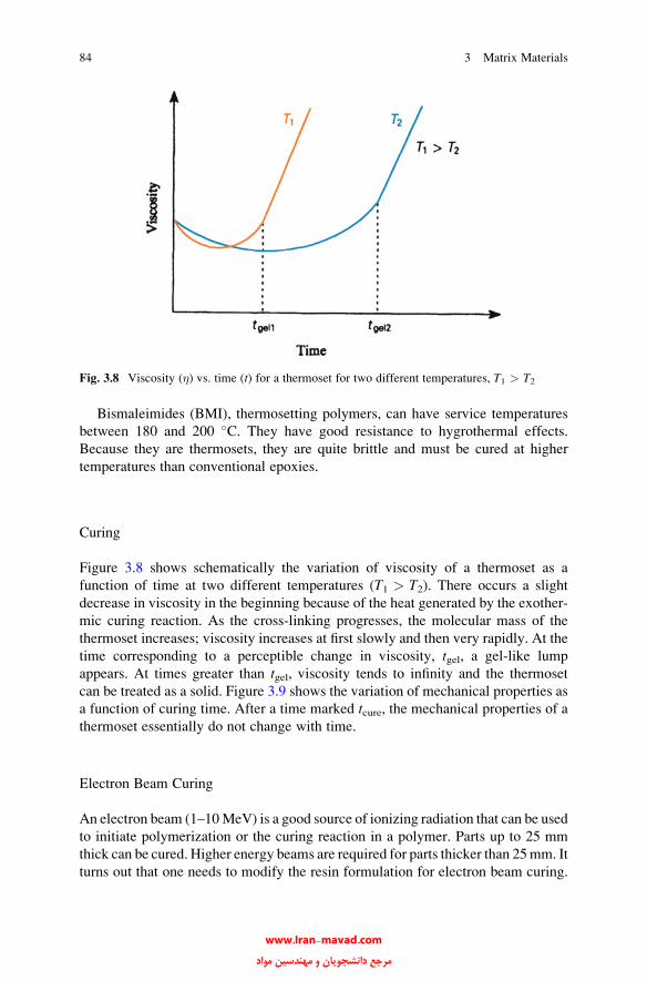
Bismaleimides (BMI), thermosetting polymers, can have service temperatures

between 180 and 200 �C. They have good resistance to hygrothermal effects.

Because they are thermosets, they are quite brittle and must be cured at higher

temperatures than conventional epoxies.

Curing

Figure 3.8 shows schematically the variation of viscosity of a thermoset as a

function of time at two different temperatures (T1 > T2). There occurs a slight

decrease in viscosity in the beginning because of the heat generated by the exother-

mic curing reaction. As the cross-linking progresses, the molecular mass of the

thermoset increases; viscosity increases at first slowly and then very rapidly. At the

time corresponding to a perceptible change in viscosity, tgel, a gel-like lump

appears. At times greater than tgel, viscosity tends to infinity and the thermoset

can be treated as a solid. Figure 3.9 shows the variation of mechanical properties as

a function of curing time. After a time marked tcure, the mechanical properties of a

thermoset essentially do not change with time.

Electron Beam Curing

An electron beam (1–10MeV) is a good source of ionizing radiation that can be used

to initiate polymerization or the curing reaction in a polymer. Parts up to 25 mm

thick can be cured. Higher energy beams are required for parts thicker than 25mm. It

turns out that one needs to modify the resin formulation for electron beam curing.

Fig. 3.8 Viscosity (�) vs. time (t) for a thermoset for two different temperatures, T1 > T2



Addition of 1–3 parts per hundred of a cationic photo-initiator can do the job. No

hardener is required. However, other conventional additives, such as toughening

agents or diluents, can be used to improve the processability of the resin. Among the

advantages of electron beam curing, one may list the following:

• Shorter cure times (minutes rather than the hours required by conventional

thermal processes).

• Curing can be accomplished at a selected temperature (room temperature or near

the service temperature).

• Lower energy consumption than in thermal curing.

• Removal of hardener means elimination of the undesirable VOCs. It also allows

the use of thermoset resins with unlimited shelf life.

Among the limitations, one may list the following:

• Only a few electron beam curing facilities are available, especially for large and

complex structures. This is especially so in the 5–15 MeV range.

• Shipping parts to outside accelerator facilities can be problematic.

• Long-term testing and experience in the field are missing; that is, customer

confidence needs to be built.

3.1.9.2 Common Thermoplastic Matrix Materials

Thermoplastics are characterized by linear chain molecules and can be repeatedly

melted or reprocessed. It is important to note that in this regard the cool-down time

affects the degree of crystallinity of the thermoplastic. This is because the polymer

chains need time to get organized in the orderly pattern of the crystalline state; too

quick a cooling rate will not allow crystallization to occur. Although repeated

melting and processing are possible with thermoplastics, it should be recognized


mechanical properties with

curing time

3.1 Polymers 85


that thermal exposure (too high a temperature or too long a dwell time at a given

temperature) can degrade the polymer properties such as, especially, impact

properties.

Linear molecules in a thermoplastic result in higher strain-to-failure values

compared to those of thermosets, i.e., thermoplastics are tougher than the cross-

linked thermosets. Thermoplastic matrix materials can have failure strains ranging

from 30 to 100 %, while the thermosets typically range from 1 to 3 %. The large

range of failure strains in thermoplastics stems from the rather large variations in

the amount of crystallinity.

Common thermoplastic resins used as matrix materials in composites include

some conventional thermoplastics such as polypropylene, nylon, thermoplastic

polyesters (PET, PBT), and polycarbonates. Some of the new thermoplastic

matrix materials include polyamide imide, polyphenylene sulfide (PPS),

polyarylsulfone, and polyetherether ketone (PEEK). Figure 3.10 shows the chem-

ical structure of some of these thermoplastics. PEEK is an attractive matrix

material because of its toughness and impact properties, which are a function of

its crystalline content and morphology. It should be pointed out that crystalliza-

tion kinetics of a thermoplastic matrix can vary substantially because of the

presence of fibers (Waddon et al. 1987). In order to make a thermoplastic matrix

flow, heating must be done to a temperature above the melting point of the matrix.

In the case of PEEK, the melting point of the crystalline component is 343 �C. Ingeneral, most thermoplastics are harder to flow vis a vis thermosets such as epoxy!

Their viscosity decreases with increasing temperature, but at higher temperatures

the danger is decomposition of resin.

Fig. 3.10 Chemical structure

of (a) PPS, (b) polyaryl

sulfone, and

(c) polyetherether

ketone (PEEK)



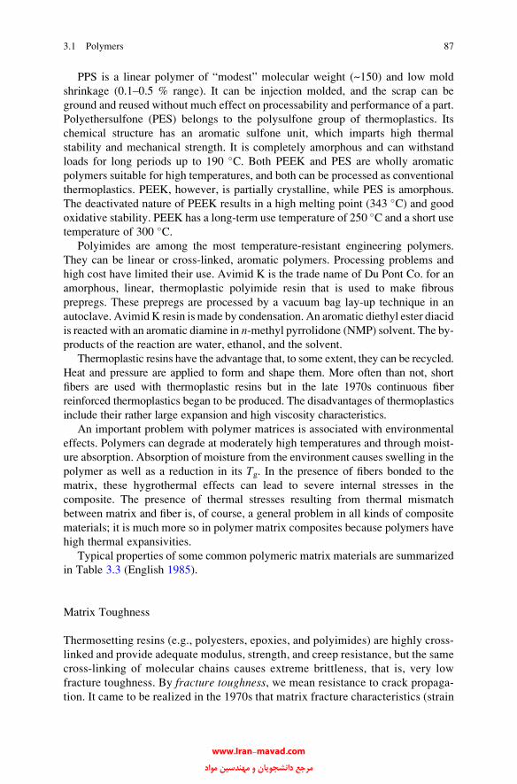
PPS is a linear polymer of “modest” molecular weight (~150) and low mold

shrinkage (0.1–0.5 % range). It can be injection molded, and the scrap can be

ground and reused without much effect on processability and performance of a part.

Polyethersulfone (PES) belongs to the polysulfone group of thermoplastics. Its

chemical structure has an aromatic sulfone unit, which imparts high thermal

stability and mechanical strength. It is completely amorphous and can withstand

loads for long periods up to 190 �C. Both PEEK and PES are wholly aromatic

polymers suitable for high temperatures, and both can be processed as conventional

thermoplastics. PEEK, however, is partially crystalline, while PES is amorphous.

The deactivated nature of PEEK results in a high melting point (343 �C) and good

oxidative stability. PEEK has a long-term use temperature of 250 �C and a short use

temperature of 300 �C.Polyimides are among the most temperature-resistant engineering polymers.

They can be linear or cross-linked, aromatic polymers. Processing problems and

high cost have limited their use. Avimid K is the trade name of Du Pont Co. for an

amorphous, linear, thermoplastic polyimide resin that is used to make fibrous

prepregs. These prepregs are processed by a vacuum bag lay-up technique in an

autoclave. Avimid K resin is made by condensation. An aromatic diethyl ester diacid

is reacted with an aromatic diamine in n-methyl pyrrolidone (NMP) solvent. The by-

products of the reaction are water, ethanol, and the solvent.

Thermoplastic resins have the advantage that, to some extent, they can be recycled.

Heat and pressure are applied to form and shape them. More often than not, short

fibers are used with thermoplastic resins but in the late 1970s continuous fiber

reinforced thermoplastics began to be produced. The disadvantages of thermoplastics

include their rather large expansion and high viscosity characteristics.

An important problem with polymer matrices is associated with environmental

effects. Polymers can degrade at moderately high temperatures and through moist-

ure absorption. Absorption of moisture from the environment causes swelling in the

polymer as well as a reduction in its Tg. In the presence of fibers bonded to the

matrix, these hygrothermal effects can lead to severe internal stresses in the

composite. The presence of thermal stresses resulting from thermal mismatch

between matrix and fiber is, of course, a general problem in all kinds of composite

materials; it is much more so in polymer matrix composites because polymers have

high thermal expansivities.

Typical properties of some common polymeric matrix materials are summarized

in Table 3.3 (English 1985).

Matrix Toughness

Thermosetting resins (e.g., polyesters, epoxies, and polyimides) are highly cross-

linked and provide adequate modulus, strength, and creep resistance, but the same

cross-linking of molecular chains causes extreme brittleness, that is, very low

fracture toughness. By fracture toughness, we mean resistance to crack propaga-

tion. It came to be realized in the 1970s that matrix fracture characteristics (strain

3.1 Polymers 87


Table

3.3

Representativeproperties

ofsomepolymeric

matrixmaterials

Property

Epoxy

Polyim

ide

PEEK

Polyam

ideimide

Polyetherim

ide

Polysulfone

Polyphenylene

sulfide

Phenolics

Tensile

strength

(MPa)

35–85

120

92

95

105

75

70

50–55

Flexuralmodulus(G

Pa)

15–35

35

40

50

35

28

40

–

Density

(g/cm

3)

1.38

1.46

1.30

1.38

–1.25

1.32

1.30

Continuous-servicetemperature

(�C)

25–85

260–425

310

–170

175–190

260

150–175

Coefficientofthermalexpansion(10�5� C

�1)

8–11

9–

6.3

5.6

9.4–10

9.9

4.5–11

Water

absorption(24h%)

0.1

0.3

0.1

0.3

0.25

0.2

0.2

0.1–0.2

Source:

Adaptedwithpermissionfrom

English

(1985)



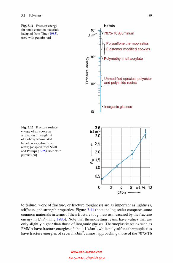
to failure, work of fracture, or fracture toughness) are as important as lightness,

stiffness, and strength properties. Figure 3.11 (note the log scale) compares some

common materials in terms of their fracture toughness as measured by the fracture

energy in J/m2 (Ting 1983). Note that thermosetting resins have values that are

only slightly higher than those of inorganic glasses. Thermoplastic resins such as

PMMA have fracture energies of about 1 kJ/m2, while polysulfone thermoplastics

have fracture energies of several kJ/m2, almost approaching those of the 7075-T6

Fig. 3.11 Fracture energy

for some common materials

[adapted from Ting (1983),



energy of an epoxy as

a function of weight %

of carboxyl-terminated

butadiene-acrylo-nitrile

(ctbn) [adapted from Scott

and Phillips (1975), used with

permission]

3.1 Polymers 89


aluminum alloy. Amorphous thermoplastic polymers show higher fracture energy

values because they have a large free volume available that absorbs the energy

associated with crack propagation. Among the well known modified

thermoplastics are the acrylonitrile-butadiene-styrene (ABS) copolymer and

high-impact polystyrene (HIPS). One class of thermosetting resins that comes

close to polysulfones is the elastomer-modified epoxies. Elastomer-modified or

rubber-modified thermosetting epoxies form multiphase systems, a kind of com-

posite in their own right. Small (a few micrometers or less), soft, rubbery

inclusions distributed in a hard, brittle epoxy matrix enhance its toughness by

several orders of magnitude (Sultan and McGarry 1973; Riew et al. 1976; Bascom

and Cottington 1976; St. Clair and St. Clair 1981; Scott and Phillips 1975).

Epoxy and polyester resins are commonly modified by introducing carboxyl-

terminated butadiene-acrylonitrile copolymers (ctbn). The methods of manufacture

can be simple mechanical blending of the soft, rubbery particles and the resin or

copolymerization of a mixture of the two. Figure 3.12 shows the increase in fracture

surface energy of an epoxy as a function of weight % of ctbn elastomer (Scott and

Phillips 1975).

Toughening of glassy polymers by elastomeric additions involves different

mechanisms for different polymers. Among the mechanisms proposed for

explaining this enhanced toughness are triaxial dilation of rubber particles at the

crack tip, particle elongation, and plastic flow of the epoxy. Ting (1983) studied

such a rubber-modified epoxy containing glass or carbon fibers. He observed that

the mechanical properties of rubber-modified composite improved more in flexure

than in tension. Scott and Phillips (1975) obtained a large increase in matrix

toughness by adding ctbn in unreinforced epoxy. But this large increase in tough-

ness could be translated into only a modest increase in carbon fiber reinforced

modified epoxy matrix composite. Introduction of a tough elastomeric phase, for

example, a silicone rubber with good thermal resistance in a polyimide resin,

produced a tough matrix material: a three- to fivefold gain in toughness,GIc without

a reduction in Tg (St. Clair and St. Clair 1981).

Continuous fiber reinforced thermoplastics show superior toughness values

owing to superior matrix toughness. PEEK is a semicrystalline aromatic thermo-

plastic (Hartness 1983; Cogswell 1983; Blundell et al. 1985) that is quite tough.

PEEK can have 20–40 % crystalline phase. At 35 % crystallinity, the spherulite size

is about 2 mm (Cogswell 1983). Its glass transition temperature Tg is about 150�C,

and the crystalline phase melts at about 350 �C. It has an elastic modulus of about

4 GPa, a yield stress of 100 MPa, and a relatively high fracture energy of about

500 J/m2. In addition to PEEK, other tough thermoplastic resins are available, for

example, thermoplastic polyimides and PPS, which is a semicrystalline aromatic

sulfide. PPS is the simplest member of a family of polyarylene sulfides (O’Connor

et al. 1986). PPS (trade name Ryton), a semicrystalline polymer, has been

reinforced by chopped carbon fibers and prepregged with continuous carbon fibers

(O’Connor et al. 1986).



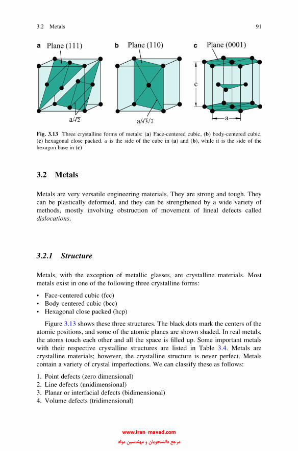
3.2 Metals

Metals are very versatile engineering materials. They are strong and tough. They

can be plastically deformed, and they can be strengthened by a wide variety of

methods, mostly involving obstruction of movement of lineal defects called

dislocations.

3.2.1 Structure

Metals, with the exception of metallic glasses, are crystalline materials. Most

metals exist in one of the following three crystalline forms:

• Face-centered cubic (fcc)

• Body-centered cubic (bcc)

• Hexagonal close packed (hcp)

Figure 3.13 shows these three structures. The black dots mark the centers of the

atomic positions, and some of the atomic planes are shown shaded. In real metals,

the atoms touch each other and all the space is filled up. Some important metals

with their respective crystalline structures are listed in Table 3.4. Metals are

crystalline materials; however, the crystalline structure is never perfect. Metals

contain a variety of crystal imperfections. We can classify these as follows:

1. Point defects (zero dimensional)

2. Line defects (unidimensional)

3. Planar or interfacial defects (bidimensional)

4. Volume defects (tridimensional)

Fig. 3.13 Three crystalline forms of metals: (a) Face-centered cubic, (b) body-centered cubic,

(c) hexagonal close packed. a is the side of the cube in (a) and (b), while it is the side of the

hexagon base in (c)

3.2 Metals 91


Point defects can be of three types. A vacancy is created when an atomic position

in the crystal lattice is vacant. An interstitial is produced when an atom of material

or a foreign atom occupies an interstitial or nonlattice position. A substitutionalpoint defect comes into being when a regular atomic position is occupied by a

foreign atom. Intrinsic point defects (vacancies and self-interstitials) in metals exist

at a given temperature in equilibrium concentrations. Increased concentrations of

these defects can be produced by quenching from high temperatures, bombarding

with energetic particles such as neutrons, and plastic deformation. Point defects can

have a marked effect on the mechanical properties.

Line imperfections, called dislocations, represent a critically important structural

imperfection that plays a very important role in the area of physical and mechanical

metallurgy, diffusion, and corrosion. A dislocation is defined by two vectors: a

dislocation line vector, t, (tangent to the line) and its Burgers vector, b, which gives

the magnitude and direction of atomic displacement associated with the dislocation.

There are two types of dislocations: in an edge dislocation b and t vectors are

perpendicular to each other, while in a screw dislocation, b and t are parallel. The

dislocation has a kind of lever effect because its movement allows one part of metal to

be sheared over the otherwithout the need for simultaneousmovement of atoms across

a plane. It is the presenceof these line imperfections thatmakes it easy todeformmetals

plastically. Under normal circumstances then, the plastic deformation of metals is

accomplished by the movement of these dislocations. Figure 3.14a shows an edge

dislocation. The two vectors, defining the dislocation line and the Burgers vector, are

designatedas t (not shown) and b, respectively (seeFig. 3.14a). Thedislocation permits

shear in metals at stresses much below those required for simultaneous shear across a

plane. Figure 3.14b shows this in an analogy. A carpet, of course, can be moved by

pushing or pulling. However, a much lower force is required to move the carpet by a

distance b if a defect (a bump in the carpet) is introduced into it and made to move the

whole extension of the carpet. Figure 3.15 shows dislocations as seen by transmission

electron microscopy in a thin foil of steel. This is a dark field electron micrograph;

dislocation lines appear aswhite lines.Dislocations become visible in the transmission

electron microscope because of the distortion of the atomic planes owing to the

presence of dislocations. Also visible in this micrograph are equiaxial precipitate

particles pinning the dislocations at various points.

Table 3.4 Crystal structure of some important metals

fcc bcc hcp

Iron (910–1,390 �C) Iron (T < 910 �C and T > 1,390 �C) Titaniuma

Nickel Beryllium (T > 1,250 �C) Beryllium (T < 1,250 �C)Copper Cobalt (T > 427 �C) Cobalt (T < 427 �C)Aluminum Tungsten Cerium (�150 �C < T < �10 �C)Gold Molybdenum Zinc

Lead Chromium Magnesium

Platinum Vanadium Zirconiuma

Silver Niobium Hafniuma (T < 1,950 �C)aUndergoes bcc $ hcp transformation at different temperatures



The interfacial or planar defects occupy an area or surface of the crystal, for

example, grain boundaries, twin boundaries, domain or antiphase boundaries.

Grain boundaries are, by far, the most important of these planar defects from the

mechanical behavior point of view. Among the volumetric or tridimensional

defects we can include large inclusions and porosity and preexisting cracks.

3.2.2 Conventional Strengthening Methods

Experimental results show that work hardening (or strain hardening), which is the

ability of a metal to become more resistant to deformation as it is deformed, is

Fig. 3.14 (a) Edge dislocation, (b) dislocation in a carpet

Fig. 3.15 Dislocations (white lines) in a steel sample: dark field transmission electron micro-

graph. Also visible are equiaxial precipitate particles

3.2 Metals 93


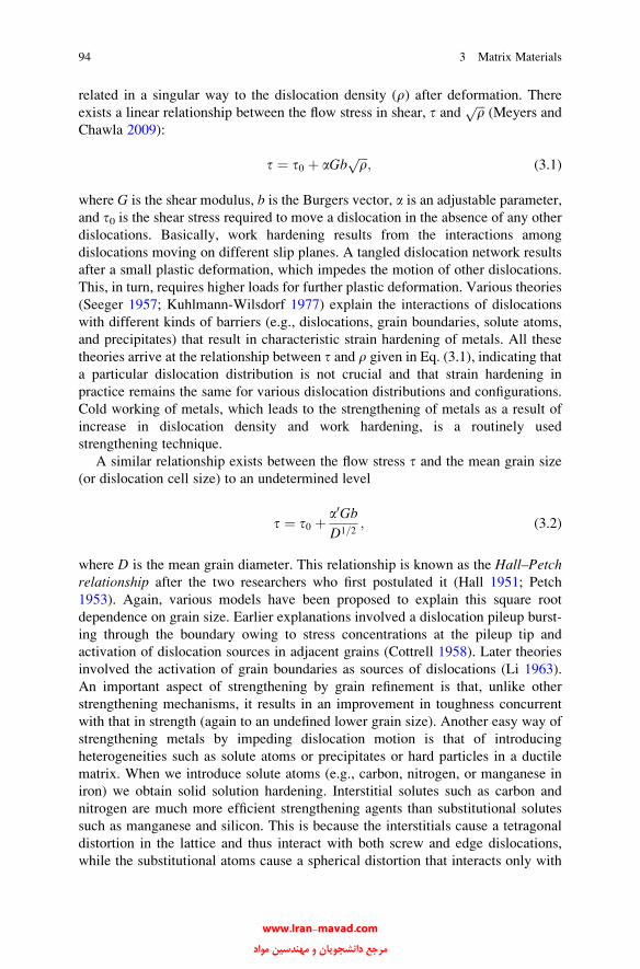
related in a singular way to the dislocation density (r) after deformation. There

exists a linear relationship between the flow stress in shear, t andffiffiffir

p(Meyers and

Chawla 2009):

t ¼ t0 þ aGbffiffiffir

p; (3.1)

where G is the shear modulus, b is the Burgers vector, a is an adjustable parameter,

and t0 is the shear stress required to move a dislocation in the absence of any other

dislocations. Basically, work hardening results from the interactions among

dislocations moving on different slip planes. A tangled dislocation network results

after a small plastic deformation, which impedes the motion of other dislocations.

This, in turn, requires higher loads for further plastic deformation. Various theories

(Seeger 1957; Kuhlmann-Wilsdorf 1977) explain the interactions of dislocations

with different kinds of barriers (e.g., dislocations, grain boundaries, solute atoms,

and precipitates) that result in characteristic strain hardening of metals. All these

theories arrive at the relationship between t and r given in Eq. (3.1), indicating that

a particular dislocation distribution is not crucial and that strain hardening in

practice remains the same for various dislocation distributions and configurations.

Cold working of metals, which leads to the strengthening of metals as a result of

increase in dislocation density and work hardening, is a routinely used

strengthening technique.

A similar relationship exists between the flow stress t and the mean grain size

(or dislocation cell size) to an undetermined level

t ¼ t0 þ a0GbD1=2

; (3.2)

where D is the mean grain diameter. This relationship is known as the Hall–Petchrelationship after the two researchers who first postulated it (Hall 1951; Petch

1953). Again, various models have been proposed to explain this square root

dependence on grain size. Earlier explanations involved a dislocation pileup burst-

ing through the boundary owing to stress concentrations at the pileup tip and

activation of dislocation sources in adjacent grains (Cottrell 1958). Later theories

involved the activation of grain boundaries as sources of dislocations (Li 1963).

An important aspect of strengthening by grain refinement is that, unlike other

strengthening mechanisms, it results in an improvement in toughness concurrent

with that in strength (again to an undefined lower grain size). Another easy way of

strengthening metals by impeding dislocation motion is that of introducing

heterogeneities such as solute atoms or precipitates or hard particles in a ductile

matrix. When we introduce solute atoms (e.g., carbon, nitrogen, or manganese in

iron) we obtain solid solution hardening. Interstitial solutes such as carbon and

nitrogen are much more efficient strengthening agents than substitutional solutes

such as manganese and silicon. This is because the interstitials cause a tetragonal

distortion in the lattice and thus interact with both screw and edge dislocations,

while the substitutional atoms cause a spherical distortion that interacts only with



edge dislocations, because the screw dislocations have a pure shear stress field and

no hydrostatic component. Precipitation hardening of a metal is obtained by

decomposing a supersaturated solid solution to form a finely distributed second

phase. Classical examples of precipitation strengthening alloys are Al–Cu and

Al–Zn–Mg alloys, which are used in the aircraft industry (Fine 1964). Oxide

dispersion strengthening involves artificially dispersing rather small volume

fractions (0.5–3 vol.%) of strong and inert oxide particles (e.g., Al2O3, Y2O3, and

ThO2) in a ductile matrix by internal oxidation or powder metallurgy blending

techniques (Ansell 1968). Both the second-phase precipitates and dispersoids act as

barriers to dislocation motion in the ductile matrix, thus making the matrix more

deformation resistant. Dispersion hardened systems (e.g., Al + Al2O3) show high

strength levels at elevated temperatures while precipitates (say, CuAl2 in alumi-

num) tend to dissolve at those temperatures. Precipitation hardening systems,

however, have the advantage of enabling one to process the alloy in a soft condition

and give the precipitation treatment to the finished part. The precipitation process

carried out for long periods of time can also lead to overaging and solution; a

weakening effect.

Quenching a steel to produce a martensitic phase has been a time-honored

strengthening mechanism for steels. The strength of the martensite phase in steel

depends on a variety of factors, the most important being the amount of carbon. The

chemical composition of martensite is the same as that of the parent austenite phase

from which it formed, but it is supersaturated with carbon (Roberts and Owen

1968). Carbon saturation and the lattice distortion that accompanies the transfor-

mation lead to the high hardness and strength of martensite.

Another approach to obtaining enhanced mechanical performance is rapid solid-

ification processing (Grant 1985). By cooling metals at high rates, 104 to 109 K/s, it

is possible to produce unique microstructures. Very fine powders or ribbons of

rapidly solidified materials are processed into bulk materials by hot pressing, hot

isostatic pressing, or hot extrusion. The rapidly solidified materials can be amor-

phous (noncrystalline), nanocrystalline (grain size in the nm range), or

microdendritic solid solutions containing solute concentrations vastly superior to

those of conventionally processed materials. Effectively, massive second-phase

particles are eliminated. These unique microstructures lead to very favorable

mechanical properties.

3.2.3 Properties of Metals

Typical values of elastic modulus, yield strength, and ultimate strength in tension

and fracture toughness of some common metals and their alloys are listed in

Table 3.5, while typical engineering stress–strain curves in tension are shown in

Fig. 3.16. Note the large plastic strain range.

3.2 Metals 95


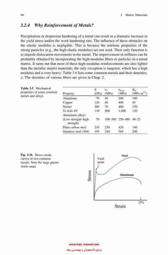
3.2.4 Why Reinforcement of Metals?

Precipitation or dispersion hardening of a metal can result in a dramatic increase in

the yield stress and/or the work hardening rate. The influence of these obstacles on

the elastic modulus is negligible. This is because the intrinsic properties of the

strong particles (e.g., the high elastic modulus) are not used. Their only function is

to impede dislocation movements in the metal. The improvement in stiffness can be

profitably obtained by incorporating the high-modulus fibers or particles in a metal

matrix. It turns out that most of these high-modulus reinforcements are also lighter

than the metallic matrix materials; the only exception is tungsten, which has a high

modulus and is very heavy. Table 3.6 lists some common metals and their densities,

r. The densities of various fibers are given in Chap. 2.

Table 3.5 Mechanical

properties of some common

metals and alloysProperty

E(GPa)

sy(MPa)

smax

(MPa)

KIc

(MPa m1/2)

Aluminum 70 40 200 100

Copper 120 60 400 65

Nickel 200 70 400 350

Ti–6Al–4V 110 900 1,000 120

Aluminum alloys

(Low strength–high

strength)

70 100–380 250–480 40–23

Plain carbon steel 210 250 420 140

Stainless steel (304) 195 240 365 200

Fig. 3.16 Stress–strain

curves of two common

metals. Note the large plastic

strain range



http://dx.doi.org/10.1007/978-0-387-74365-3_2

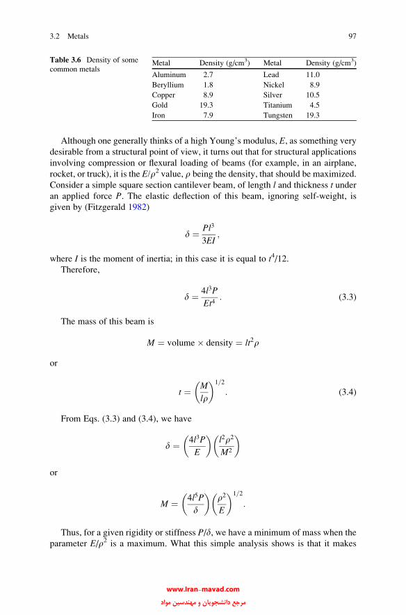
Although one generally thinks of a high Young’s modulus, E, as something very

desirable from a structural point of view, it turns out that for structural applications

involving compression or flexural loading of beams (for example, in an airplane,

rocket, or truck), it is the E/r2 value, r being the density, that should be maximized.

Consider a simple square section cantilever beam, of length l and thickness t underan applied force P. The elastic deflection of this beam, ignoring self-weight, is

given by (Fitzgerald 1982)

d ¼ Pl3

3EI;

where I is the moment of inertia; in this case it is equal to t4/12.Therefore,

d ¼ 4l3P

Et4: (3.3)

The mass of this beam is

M ¼ volume� density ¼ lt2r

or

t ¼ M

lr

� �1=2

: (3.4)

From Eqs. (3.3) and (3.4), we have

d ¼ 4l3P

E

� �l2r2

M2

� �

or

M ¼ 4l5P

d

� �r2

E

� �1=2

:

Thus, for a given rigidity or stiffness P/d, we have a minimum of mass when the

parameter E/r2 is a maximum. What this simple analysis shows is that it makes

Table 3.6 Density of some

common metalsMetal Density (g/cm3) Metal Density (g/cm3)

Aluminum 2.7 Lead 11.0

Beryllium 1.8 Nickel 8.9

Copper 8.9 Silver 10.5

Gold 19.3 Titanium 4.5

Iron 7.9 Tungsten 19.3

3.2 Metals 97


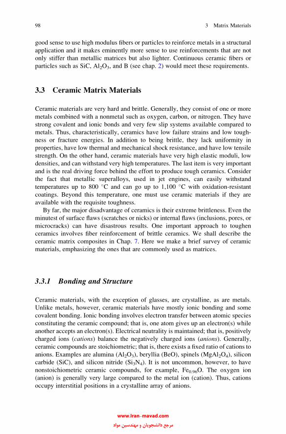
good sense to use high modulus fibers or particles to reinforce metals in a structural

application and it makes eminently more sense to use reinforcements that are not

only stiffer than metallic matrices but also lighter. Continuous ceramic fibers or

particles such as SiC, Al2O3, and B (see chap. 2) would meet these requirements.

3.3 Ceramic Matrix Materials

Ceramic materials are very hard and brittle. Generally, they consist of one or more

metals combined with a nonmetal such as oxygen, carbon, or nitrogen. They have

strong covalent and ionic bonds and very few slip systems available compared to

metals. Thus, characteristically, ceramics have low failure strains and low tough-

ness or fracture energies. In addition to being brittle, they lack uniformity in

properties, have low thermal and mechanical shock resistance, and have low tensile

strength. On the other hand, ceramic materials have very high elastic moduli, low

densities, and can withstand very high temperatures. The last item is very important

and is the real driving force behind the effort to produce tough ceramics. Consider

the fact that metallic superalloys, used in jet engines, can easily withstand

temperatures up to 800 �C and can go up to 1,100 �C with oxidation-resistant

coatings. Beyond this temperature, one must use ceramic materials if they are

available with the requisite toughness.

By far, the major disadvantage of ceramics is their extreme brittleness. Even the

minutest of surface flaws (scratches or nicks) or internal flaws (inclusions, pores, or

microcracks) can have disastrous results. One important approach to toughen

ceramics involves fiber reinforcement of brittle ceramics. We shall describe the

ceramic matrix composites in Chap. 7. Here we make a brief survey of ceramic

materials, emphasizing the ones that are commonly used as matrices.

3.3.1 Bonding and Structure

Ceramic materials, with the exception of glasses, are crystalline, as are metals.

Unlike metals, however, ceramic materials have mostly ionic bonding and some

covalent bonding. Ionic bonding involves electron transfer between atomic species

constituting the ceramic compound; that is, one atom gives up an electron(s) while

another accepts an electron(s). Electrical neutrality is maintained; that is, positively

charged ions (cations) balance the negatively charged ions (anions). Generally,ceramic compounds are stoichiometric; that is, there exists a fixed ratio of cations to

anions. Examples are alumina (Al2O3), beryllia (BeO), spinels (MgAl2O4), silicon

carbide (SiC), and silicon nitride (Si3N4). It is not uncommon, however, to have

nonstoichiometric ceramic compounds, for example, Fe0.96O. The oxygen ion

(anion) is generally very large compared to the metal ion (cation). Thus, cations

occupy interstitial positions in a crystalline array of anions.



http://dx.doi.org/10.1007/978-0-387-74365-3_2

http://dx.doi.org/10.1007/978-0-387-74365-3_7

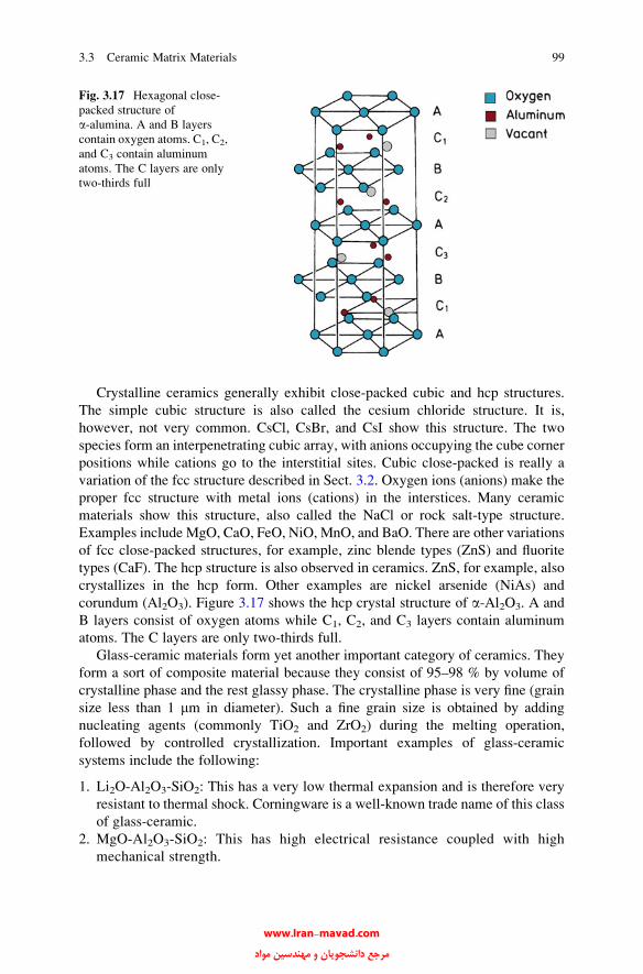
Crystalline ceramics generally exhibit close-packed cubic and hcp structures.

The simple cubic structure is also called the cesium chloride structure. It is,

however, not very common. CsCl, CsBr, and CsI show this structure. The two

species form an interpenetrating cubic array, with anions occupying the cube corner

positions while cations go to the interstitial sites. Cubic close-packed is really a

variation of the fcc structure described in Sect. 3.2. Oxygen ions (anions) make the

proper fcc structure with metal ions (cations) in the interstices. Many ceramic

materials show this structure, also called the NaCl or rock salt-type structure.

Examples include MgO, CaO, FeO, NiO, MnO, and BaO. There are other variations

of fcc close-packed structures, for example, zinc blende types (ZnS) and fluorite

types (CaF). The hcp structure is also observed in ceramics. ZnS, for example, also

crystallizes in the hcp form. Other examples are nickel arsenide (NiAs) and

corundum (Al2O3). Figure 3.17 shows the hcp crystal structure of a-Al2O3. A and

B layers consist of oxygen atoms while C1, C2, and C3 layers contain aluminum

atoms. The C layers are only two-thirds full.

Glass-ceramic materials form yet another important category of ceramics. They

form a sort of composite material because they consist of 95–98 % by volume of

crystalline phase and the rest glassy phase. The crystalline phase is very fine (grain

size less than 1 mm in diameter). Such a fine grain size is obtained by adding

nucleating agents (commonly TiO2 and ZrO2) during the melting operation,

followed by controlled crystallization. Important examples of glass-ceramic

systems include the following:

1. Li2O-Al2O3-SiO2: This has a very low thermal expansion and is therefore very

resistant to thermal shock. Corningware is a well-known trade name of this class

of glass-ceramic.

2. MgO-Al2O3-SiO2: This has high electrical resistance coupled with high

mechanical strength.

Fig. 3.17 Hexagonal close-

packed structure of

a-alumina. A and B layers

contain oxygen atoms. C1, C2,

and C3 contain aluminum

atoms. The C layers are only

two-thirds full

3.3 Ceramic Matrix Materials 99


Ceramicmaterials can also formsolid solutions.Unlikemetals, however, interstitial

solid solutions are less likely in ceramics because the normal interstitial sites are

already filled. Introduction of solute ions disrupts the charge neutrality. Vacancies

accommodate the unbalanced charge. For example, FeO has a NaCl-type structure

with an equal number of Fe2+ and O2� ions. If, however, two Fe3+ ions were to replace

three Fe2+ ions we would have a vacancy where an iron ion would form.

Glasses, the traditional silicate ceramic materials, are inorganic solidlike

materials that do not crystallize when cooled from the liquid state. Their structure

(see Fig. 2.6) is not crystalline but that of a supercooled liquid. In this case we have

a specific volume vs. temperature curve similar to the one for polymers (Fig. 3.2)

and a characteristic glass transition temperature Tg. Under certain conditions,

crystallization of glass can occur with an accompanying abrupt decrease in volume

at the melting point because the atoms take up ordered positions.

3.3.2 Effect of Flaws on Strength

As in metals, imperfections in crystal packing of ceramics do exist and reduce their

strength. The difference is that important defects in ceramic materials are surface

flaws and vacancies. Dislocations do exist but are relatively immobile. Grain

boundaries and free surfaces are important planar defects. As in metals, small

grain size improves the mechanical properties of ceramics at low to medium

temperatures.

Surface flaws and internal pores (Griffith flaws) are particularly dangerous for

strength and fracture toughness of ceramics. Fracture stress for an elastic material

having an internal crack of length 2a is given by the Griffith relationship:

sf ¼ 2Ega

� �1=2

;

whereE is theYoung’smodulus and g is the surface energy of the crack surface. Linearelastic fracturemechanics treats this problem of brittle fracture in terms of a parameter

called the stress intensity factor, K. The stresses at a radius, r from the crack tip are

given by

sij ¼ K

ð2prÞ1=2" #

fijðyÞ;

where fij(y) is a geometric function. Fracture occurs when K attains a critical value

KIc. Yet another approach is based on the energy viewpoint, a modification of the

Griffith idea. Fracture occurs, according to this approach, when the crack extension

force G reaches a critical value GIc. For ceramic materials, GIc ¼ 2g. It can also be

shown that K2 ¼ EG for opening failure mode and plane stress; that is, the stress

intensity factor and the energy approaches are equivalent.



http://dx.doi.org/10.1007/978-0-387-74365-3_2#Fig5_2

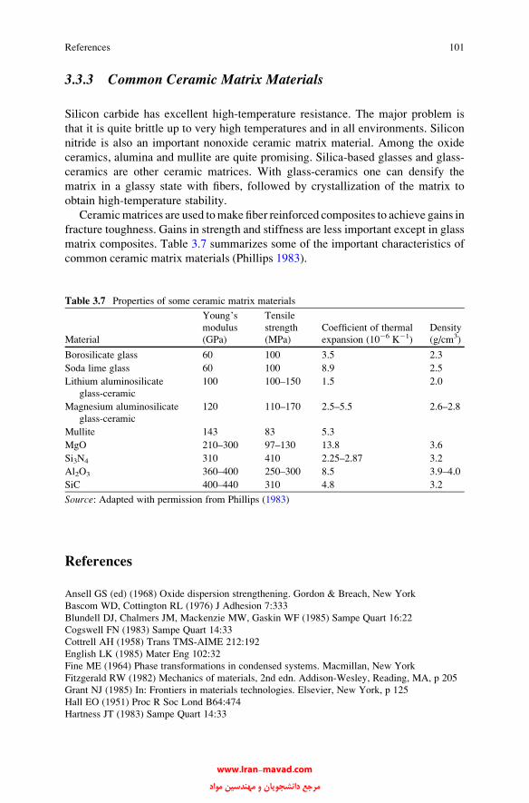
3.3.3 Common Ceramic Matrix Materials

Silicon carbide has excellent high-temperature resistance. The major problem is

that it is quite brittle up to very high temperatures and in all environments. Silicon

nitride is also an important nonoxide ceramic matrix material. Among the oxide

ceramics, alumina and mullite are quite promising. Silica-based glasses and glass-

ceramics are other ceramic matrices. With glass-ceramics one can densify the

matrix in a glassy state with fibers, followed by crystallization of the matrix to

obtain high-temperature stability.

Ceramicmatrices are used tomake fiber reinforced composites to achieve gains in

fracture toughness. Gains in strength and stiffness are less important except in glass

matrix composites. Table 3.7 summarizes some of the important characteristics of

common ceramic matrix materials (Phillips 1983).

References

Ansell GS (ed) (1968) Oxide dispersion strengthening. Gordon & Breach, New York

Bascom WD, Cottington RL (1976) J Adhesion 7:333

Blundell DJ, Chalmers JM, Mackenzie MW, Gaskin WF (1985) Sampe Quart 16:22

Cogswell FN (1983) Sampe Quart 14:33

Cottrell AH (1958) Trans TMS-AIME 212:192

English LK (1985) Mater Eng 102:32

Fine ME (1964) Phase transformations in condensed systems. Macmillan, New York

Fitzgerald RW (1982) Mechanics of materials, 2nd edn. Addison-Wesley, Reading, MA, p 205

Grant NJ (1985) In: Frontiers in materials technologies. Elsevier, New York, p 125

Hall EO (1951) Proc R Soc Lond B64:474

Hartness JT (1983) Sampe Quart 14:33

Table 3.7 Properties of some ceramic matrix materials

Material

Young’s

modulus

(GPa)

Tensile

strength

(MPa)


expansion (10�6 K�1)

Density

(g/cm3)

Borosilicate glass 60 100 3.5 2.3

Soda lime glass 60 100 8.9 2.5

Lithium aluminosilicate

glass-ceramic

100 100–150 1.5 2.0

Magnesium aluminosilicate

glass-ceramic

120 110–170 2.5–5.5 2.6–2.8

Mullite 143 83 5.3

MgO 210–300 97–130 13.8 3.6

Si3N4 310 410 2.25–2.87 3.2

Al2O3 360–400 250–300 8.5 3.9–4.0

SiC 400–440 310 4.8 3.2

Source: Adapted with permission from Phillips (1983)

References 101


Kuhlmann-Wilsdorf D (1977) In: Work hardening in tension and fatigue. TMS-AIME,

New York, p 1

Li JCM (1963) Trans TMS-AIME 227:239

Mandelkern L (1983a) An introduction to macromolecules, 2nd edn. Springer, New York, p 1

Meyers MA, Chawla KK (2009a) Mechanical behavior of materials, 2nd edn. Cambridge University

Press, Cambridge

Morgan RJ (1985) Epoxy resins and composites. Springer, Berlin, p 1

O’Connor JE, Beever WR, Geibel JF (1986) Proc Sampe Mater Symp 31:1313

Petch NJ (1953) J Iron Steel Inst 174:25

Phillips DC (1983) Fabrication of composites. North-Holland, Amsterdam, p 373

Riew CK, Rowe EH, Siehert AR (1976)Toughness and brittleness of plastics, vol 154. American

Chemical Society, Advances in Chemistry series, p 326

Roberts MJ, Owen WS (1968) J Iron Steel Inst 206:375

Scott JM, Phillips DC (1975) J Mater Sci 10:551

Seeger A (1957) In: Dislocations and mechanical properties of crystals. Wiley, New York, p 23

St. Clair AK, St. Clair TL (1981) J Adhesion Adhesives 1:249

Sultan JN, McGarry FJ (1973) Polym Eng Sci 13:29

Ting RY (1983) The role of polymeric matrix in the processing and structural properties of

composite materials. Plenum, New York, p 171

Waddon AJ, Hill MJ, Keller A, Blundell DJ (1987) J Mater Sci 22:1773

Further Reading

Barrett CS, Massalski TB (1980) Structure of metals, 3rd edn. Pergamon, Oxford

Carter CB, Norton MG (2007) Ceramic materials. Springer, New York

Dusek K (ed) (1985) Epoxy resins and composites I (advances in polymer science 72). Springer,

Berlin

Roesler J, Harders H, Baeker M (2007) Mechanical behaviour of engineering materials. Springer,

Berlin

Kingery WD, Bowen HK, Uhlmann DR (1976) Introduction to ceramics, 2nd edn. Wiley, New

York

Mandelkern L (1983b) An introduction to macromolecules, 2nd edn. Springer, New York

Meyers MA, Chawla KK (1984) Mechanical metallurgy: principles and applications. Prentice-Hall,

Englewood Cliffs, NJ

MeyersMA, Chawla KK (2009b) Mechanical behavior of materials, 2nd edn. Cambridge University

Press, Cambridge

Wachtman JB (1996) Mechanical properties of ceramics. Wiley, New York

Problems

3.1. Ductility, the ability to deform plastically in response to stresses, is more of a

characteristic of metals than it is of ceramics or polymers. Why?

3.2. Ceramic materials generally have some residual porosity. How does the

presence of porosity affect the elastic constants of ceramic materials? How

does it affect the fracture energy of ceramics?



3.3. Explain why it is difficult to compare the stress–strain behavior of polymers

(particularly thermoplastics) with that of metals.

3.4. The mechanical behavior of a polymer can be represented by an elastic spring

and a dashpot in parallel (Voigt model). For such a model we can write for

stress

s ¼ sel þ svisc ¼ Ee þ � de=dt;

where E is the Young’s modulus, e is the strain, � is the viscosity, and t is thetime. Show that

e ¼ s=E 1� expð�E=�Þt½ �:

3.5. What is the effect of the degree of crystallinity on fatigue resistance of

polymers?

3.6. Discuss the importance of thermal effects (hysteretic heating) on fatigue of

polymers.

3.7. Glass-ceramics combine the generally superior mechanical properties of crys-

talline ceramics with the processing ease of glasses. Give a typical thermal

cycle involving the various stages for producing a glass-ceramic.

3.8. Silica-based glasses and many polymers have amorphous structure. An amor-

phous structure is characterized by a glass transition temperature. Explain why

silica-based glasses have a much higher glass transition temperature than

polymers.

Problems 103


Chapter 4

Interfaces

We can define an interface between a reinforcement and a matrix as the bounding

surface between the two, across which a discontinuity in some parameter occurs.

The discontinuity across the interface may be sharp or gradual. Mathematically,

interface is a bidimensional region. In practice, we have an interfacial region with a

finite thickness. In any event, an interface is the region through which material

parameters, such as concentration of an element, crystal structure, atomic registry,

elastic modulus, density, coefficient of thermal expansion, etc., change from one

side to another. Clearly, a given interface may involve one or more of these items.

The behavior of a composite material is a result of the combined behavior of the

following three entities:

• Fiber or the reinforcing element

• Matrix

• Fiber/matrix interface

The reason the interface in a composite is of great importance is that the internal

surface area occupied by the interface is quite extensive. It can easily go as high as

3,000 cm2/cm3 in a composite containing a reasonable fiber volume fraction.

We can demonstrate this very easily for a cylindrical fiber in a matrix. The fiber

surface area is essentially the same as the interfacial area. Ignoring the fiber ends,

one can write the surface-to-volume ratio (S/V) of the fiber as

S=V ¼ 2prl=pr2l ¼ 2=r; (4.1)

where r and l are the fiber radius and length of the fiber, respectively. Thus, the

surface area of a fiber or the interfacial area per unit volume increases as rdecreases. Clearly, it is important that the fibers not be weakened by flaws because

of an adverse interfacial reaction. Also, the applied load should be effectively

transferred from the matrix to the fibers via the interface. Thus, it becomes

extremely important to understand the nature of the interface region of any

given composite system under a given set of conditions. Specifically, in the case


105


of a fiber reinforced composite material, the interface, or more precisely the

interfacial zone, consists of near-surface layers of fiber and matrix and any layer

(s) of material existing between these surfaces. Wettability of the fiber by the matrix

and the type of bonding between the two components constitute the primary

considerations. Additionally, one should determine the characteristics of the inter-

face and how they are affected by temperature, diffusion, residual stresses, and so

on. We discuss some of the interfacial characteristics and the associated problems

in composites in a general way. The details regarding interfaces in polymer matrix,

metal matrix, and ceramic matrix composites are given in specific chapters devoted

to those composite types.

4.1 Wettability

Various mechanisms can assist or impede adhesion (Baier et al. 1968). A key

concept in this regard is that of wettability. Wettability tells us about the ability

of a liquid to spread on a solid surface. We can measure the wettability of a given

solid by a liquid by considering the equilibrium of forces in a system consisting of a

drop of liquid resting on a plane solid surface in the appropriate atmosphere.

Figure 4.1 shows the situation schematically. The liquid drop will spread and wet

the surface only if this results in a net reduction of free energy of the system. Note

that a portion of the solid/vapor interface is substituted by the solid/liquid interface.

Contact angle, y, of a liquid on the solid surface fiber is a convenient and important

parameter to characterize wettability. Commonly, the contact angle is measured by

putting a sessile drop of the liquid on the flat surface of a solid substrate. The

contact angle is obtained from the tangents along three interfaces: solid/liquid,

liquid/vapor, and solid/vapor. The contact angle, y can be measured directly by a

goniometer or calculated by using simple trigonometric relationships involving

drop dimensions. In theory, one can use the following expression, called Young’s

equation, obtained by resolving forces horizontally

gSV ¼ gLS þ gLV cos y; (4.2)

where g is the specific surface energy, and the subscripts SV, LS, and LV represent

solid/vapor, liquid/solid, and liquid/vapor interfaces, respectively. If this process of

substitution of the solid/vapor interface involves an increase in the free energy of

the system, then complete spontaneous wetting will not result. Under such

conditions, the liquid will spread until a balance of forces acting on the surface is

attained; that is, we shall have partial wetting. A small y implies good wetting. The

extreme cases are: y ¼ 0�, corresponding to perfect wetting and y ¼ 180�,corresponding to no wetting. In practice, it is rarely possible to obtain a unique

equilibrium value of y. Also, there exists a range of contact angles between the

maximum or advancing angle, ya, and the minimum or receding angle, yr. Thisphenomenon, called the contact-angle hysteresis, is generally observed in

106 4 Interfaces


polymeric systems. Among the sources of this hysteresis are: chemical attack,

dissolution, inhomogeneity of chemical composition of solid surface, surface

roughness, and local adsorption.

It is important to realize that wettability and bonding are not synonymous terms.

Wettability describes the extent of intimate contact between a liquid and a solid; it

does not necessarily mean a strong bond at the interface. One can have excellent

wettability and a weak van der Waals-type low-energy bond. A low contact angle,

meaning good wettability, is a necessary but not sufficient condition for strong

bonding. Consider again a liquid droplet lying on a solid surface. In such a case,

Young’s equation, Eq. (4.1), is commonly used to express the equilibrium among

surface tensions in the horizontal directions. What is normally neglected in such an

analysis is that there is also a vertical force gLV sin y, which must be balanced by

Fig. 4.1 Three different conditions of wetting: complete wetting, no wetting, and partial wetting

4.1 Wettability 107


a stress in the solid acting perpendicular to the interface. This was first pointed out

by Bikerman and Zisman in their discussion of the proof of Young’s equation

by Johnson (1959). The effect of internal stress in the solid for this configuration

was discussed by Cahn et al. (1964; 1979). In general, Young’s equation has been

applied to void formation in solids without regard to the precise state of internal

stress. Fine et al. (1993) analyzed the conditions for occurrence of these internal

stresses and their effect on determining work of adhesion in particle reinforced

composites.

Wettability is very important in PMCs because in the PMC manufacturing

the liquid matrix must penetrate and wet fiber tows. Among polymeric resins that

are commonly used as matrix materials, thermoset resins have a viscosity in the

1–10 Pas range. The melt viscosities of thermoplastics are two to three orders of

magnitude higher than those of thermosets and they show, comparatively, poorer

fiber wetting characteristics. Although the contact angle is a measure of wettability,

the reader should realize that its magnitude will depend on the following important

variables: time and temperature of contact; interfacial reactions; stoichiometry,

surface roughness and geometry; heat of formation; and electronic configuration.

Example 4.1 Consider a laminated composite made by laminating sheets of two

materials (1 and 2), each of volume, v, in an alternating sequence. Let the

thickness of the laminae of the two materials be t1 and t2, and the number of

sheets of each be N1 and N2, respectively. For a given volume fraction

of component 1, V1 (remember that V1 + V2 ¼ 1), derive an expression for the

interfacial area as a function of t1 and t2.

Solution Let the area of cross section of the laminate beA. Let v,V,N, and t representthe volume, volume fraction, number, and thickness of the laminae, respectively, and

let subscripts 1 and 2 denote the two components. Then, we can write

V1 ¼ volume of component 1/total volume ¼ AN1t1=v

V2 ¼ volume of component 2/total volume ¼ AN2t2=v

V1 þ V2 ¼ 1

AðN1t1=vþ N2t2=vÞ ¼ 1

or

A=v ¼ 1=ðN1t1 þ N2t2Þ (4.3)

Total number of interfaces ¼ ðN1 þ N2 � 1Þ

Total interfacial area per unit volume, Ia ¼ ðN1 þ N2 � 1ÞA=v: (4.4)

From Eqs. (4.3) and (4.4), we have

Ia ¼ ðN1 þ N2 � 1Þ=ðN1t1 þ N2t2Þ:

108 4 Interfaces


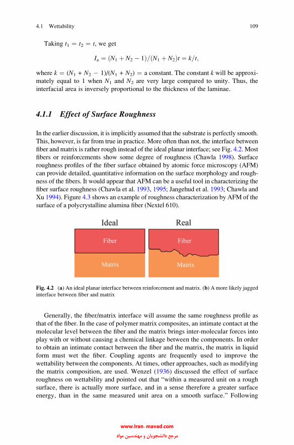
Taking t1 ¼ t2 ¼ t, we get

Ia ¼ ðN1 þ N2 � 1Þ=ðN1 þ N2Þt ¼ k=t;

where k ¼ (N1 + N2 � 1)/(N1 + N2) ¼ a constant. The constant k will be approxi-mately equal to 1 when N1 and N2 are very large compared to unity. Thus, the

interfacial area is inversely proportional to the thickness of the laminae.

4.1.1 Effect of Surface Roughness

In the earlier discussion, it is implicitly assumed that the substrate is perfectly smooth.

This, however, is far from true in practice. More often than not, the interface between

fiber and matrix is rather rough instead of the ideal planar interface; see Fig. 4.2. Most

fibers or reinforcements show some degree of roughness (Chawla 1998). Surface

roughness profiles of the fiber surface obtained by atomic force microscopy (AFM)

can provide detailed, quantitative information on the surface morphology and rough-

ness of the fibers. It would appear that AFM can be a useful tool in characterizing the

fiber surface roughness (Chawla et al. 1993, 1995; Jangehud et al. 1993; Chawla and

Xu 1994). Figure 4.3 shows an example of roughness characterization by AFM of the

surface of a polycrystalline alumina fiber (Nextel 610).

Generally, the fiber/matrix interface will assume the same roughness profile as

that of the fiber. In the case of polymer matrix composites, an intimate contact at the

molecular level between the fiber and the matrix brings inter-molecular forces into

play with or without causing a chemical linkage between the components. In order

to obtain an intimate contact between the fiber and the matrix, the matrix in liquid

form must wet the fiber. Coupling agents are frequently used to improve the

wettability between the components. At times, other approaches, such as modifying

the matrix composition, are used. Wenzel (1936) discussed the effect of surface

roughness on wettability and pointed out that “within a measured unit on a rough

surface, there is actually more surface, and in a sense therefore a greater surface

energy, than in the same measured unit area on a smooth surface.” Following

Fig. 4.2 (a) An ideal planar interface between reinforcement and matrix. (b) A more likely jagged

interface between fiber and matrix

4.1 Wettability 109


Wenzel, the effect of surface roughness on wettability can be described in terms of

r, the ratio of real area, Areal, to projected area, Aproj, of the interface. Thus,

cos y0 ¼ rgSV � gLS

gLV; (4.5)

where r ¼ Areal/Aproj.

If y0 < 90�, wettability is enhanced by roughness, and if y0 > 90�, wettability isreduced by roughness. If wetting is poor (y0 > 90�), surface roughness can reduce

bonded area and lead to void formation and possible stress concentrations.

4.2 Crystallographic Nature of Interface

Most of the physical, chemical, and mechanical discontinuities at the interface

mentioned previously are self-explanatory. The concept of atomic registry or the

crystallographic nature of an interface needs some elaboration. In terms of the types

Fig. 4.3 Characterization of surface roughness of a polycrystalline alumina fiber (Nextel 610) by

atomic force microscopy. The three profiles on the left-hand side correspond to the two horizontaland one vertical lines on the right-hand side figure. The bottom figure shows a three-dimensional

perspective view of surface

110 4 Interfaces


of atomic registry, we can have a coherent, semicoherent, or incoherent interface.

A coherent interface is one where atoms at the interface form part of both the crystal

lattices; that is, there exists a one-to-one correspondence between lattice planes on

the two sides of the interface. A coherent interface thus has some coherency strains

associated with it because of the straining of the lattice planes in the two phases to

provide the continuity at the interface to atomic sites on the two sides of the interface.

In general, a perfect atomic registry does not occur between unconstrained crystals.

Rather, coherency at the interface invariably involves an elastic deformation of the

crystals. A coherent interface, however, has a lower energy than an incoherent one.

A classic example of a coherent interface is the interface between Guinier–Preston

(G-P) zones and the aluminum matrix. These G-P zones are precursors to the

precipitates in aluminum matrix. With increasing size of the crystals, the elastic

strain energy becomes more than the interfacial energy, leading to a lowering of the

free energy of the system by introducing dislocations at the interface. Such an

interface, containing dislocations to accommodate the large interfacial strains and

thus having only a partial atomic registry, is called a semicoherent interface. Thus, asemicoherent interface is one that does not have a very large lattice mismatch

between the phases, and the small mismatch is accommodated by the introduction

of dislocations at the interface. As examples, we cite interfaces between a precipitate

and a matrix as well as interfaces in some eutectic composites such as NiAl–Cr

system (Walter et al. 1969), which has semicoherent interfaces between phases.

With still further increases in crystal sizes, the dislocation density at the interface

increases, and eventually the dislocations lose their distinct identity; that is, it is no

longer possible to specify individual atomic positions at the interface. Such an

interface is called an incoherent interface. An incoherent interface consists of

such severe atomic disorder that no matching of lattice planes occurs across the

boundary, i.e., no continuity of lattice planes is maintained across the interface. This

eliminates coherency strains, but the energy associated with the boundary increases

because of severe atomic disorder at the grain boundary. The atoms located at such an

interface do not correspond to the structure of either of the two crystals or grains.

Crystallographically, most of the interfaces that one encounters in fiber, whisker,

or particle reinforced composites are incoherent.

4.3 Interactions at the Interface

We mentioned earlier that interfaces are bidimensional regions. An initially planar

interface, however, can become an interfacial zone with, possibly, multiple

interfaces resulting from the formation of different intermetallic compounds, inter-

diffusion, and so on. In such a case, in addition to the compositional parameter, we

need other parameters to characterize the interfacial zone: for example, geometry

and dimensions; microstructure and morphology; and mechanical, physical, chem-

ical, and thermal characteristics of different phases present in the interfacial zone.

It commonly occurs that initially the components of a composite system are chosen

4.3 Interactions at the Interface 111


on the basis of their mechanical and physical characteristics in isolation. It is

important to remember, however, that when one puts together two components to

make a composite, the composite will rarely be a system in thermodynamic

equilibrium. More often than not, there will be a driving force for some kind of

interfacial reaction(s) between the two components, leading to a state of thermody-

namic equilibrium for the composite system. Of course, thermodynamic informa-

tion, such as phase diagrams, can help predict the final equilibrium state of the

composite. For example, data regarding reaction kinetics, diffusivities of

one constituent in another, etc. can provide information about the rate at which

the system would tend to attain the equilibrium state. In the absence of thermody-

namic and kinetic data, experimental studies would have to be done to determine

the compatibility of the components. Quite frequently, the very process of fabrica-

tion of a composite can involve interfacial interactions that can cause changes in the

constituent properties and/or interface structure. For example, if the fabrication

process involves cooling from high temperatures to ambient temperature, the

difference in the expansion coefficients of the two components can give rise to

thermal stresses of such a magnitude that the softer component (generally the

matrix) will deform plastically. Chawla and Metzger (1972) showed in a tungsten

fiber/single crystal copper matrix (nonreacting components) that liquid copper

infiltration of tungsten fibers at about 1,100 �C followed by cooling to room

temperature resulted in a dislocation density in the copper matrix that was much

higher in the vicinity of the interface than away from the interface. The high

dislocation density in the matrix near the interface occurred because of plastic

deformation of the matrix caused by high thermal stresses near the interface.

Arsenault and coworkers (Arsenault and Fisher 1983; Vogelsang et al. 1986)

found similar results in SiC whisker/aluminum matrix composite. Many other

researchers have observed dislocation generation in the vicinity of reinforcement/

matrix interface due to the thermal mismatch between the reinforcement and metal

matrix. In PMCs and CMCs, the matrix is unlikely to deform plastically in response

to the thermal stresses. It is more likely to relieve those stresses by matrix

microcracking. In powder processing techniques, the nature of the powder surface

will influence the interfacial interactions. For example, an oxide film, which is

invariably present on the surface of powder particles, will affect the chemical nature

of the powder. Topographic characteristics of the components can also affect the

degree of atomic contact that can be obtained between the components. This can

result in geometrical irregularities (e.g., asperities and voids) at the interface, which

can be a source of stress concentrations.

Example 4.2 Distinguish between the terms surface energy and surface tension.

Answer Surfaces in solids and liquids have special characteristics because

surfaces represent the termination of the phase. Consider an atom or a molecule

in the interior of an infinite solid. It will be bonded in all directions, and this

balanced bonding results in a reduced potential energy of the system. At a free

surface, atoms or molecules are not surrounded by other atoms or molecules on all

sides; they have bonds or neighbors on only one side. Thus there exists an

112 4 Interfaces


imbalance of forces at the surface (it is true at any interface, really) that results in a

rearrangement of atoms or molecules at the surface. We say that a surface has an

extra energy called surface energy, i.e., surface energy is the excess energy per unitarea associated with the surface because of the unsatisfied bonds at the surface.

The units of surface energy are J m2. We can also define it as the energy needed to

create a unit surface area. Surface energy depends on the crystallographic orienta-

tion. For example, if we hold a single crystal at high temperature, it will assume a

shape bounded by low-energy crystallographic planes of minimum surface energy.

Surface tension is the tendency to minimize the total surface energy by minimizing

the surface area. Surface energy and surface tension are numerically equal for

isotropic materials. Surface tension is generally given in units of N/m, which is

the same as J m2. This is not true for anisotropic solids. Consider a surface of area Awith a surface energy of g. If we increase the surface area by a small amount, the

work done per unit increase of area can be written as

d Agð Þ=dA ¼ gþ @g=@A:

The term ∂g/∂A is zero for liquids because of atomic or molecular mobility in

the liquid state. The structure of a liquid surface is unchanged when we increase its

surface area. Actually, for any material that is incapable of withstanding shear,

∂g/∂A ¼ 0. In general, such materials include liquids and solids at high

temperatures. Thus, for a liquid, the surface tension and surface energy are equal.

Because, thermodynamically, the most stable state is the one with a minimum of

free energy, isotropic liquids tend toward a minimum area/unit volume, i.e., a

sphere. Such equality does not hold for solids that can withstand shear. If we stretch

the surface of a solid, the atoms or molecules at the surface are pulled apart, gdecreases, and the quantity ∂g/∂A becomes negative. Thus, for solids, the surface

tension is not equal to surface energy. That is why a piece of solid metal does not

assume a spherical shape when left to stand at room temperature. In fact, the surface

energy of a crystal varies with crystallographic orientation. Generally, the more

densely packed planes have a lower surface energy, and they end up forming the

stable planes on the surface.

Typically, polymers have surface energies <100 mJ m2; oxides have between

100 and 2,000 mJ m2, while metals, carbides, nitrides have >1,000 mJ m2.

4.4 Types of Bonding at the Interface

It is important to be able to control the degree of bonding between the matrix and

the reinforcement. To do so, it is necessary to understand all the different possible

bonding types, one or more of which may be acting at any given instant. We can

conveniently classify the important types of interfacial bonding as follows:

• Mechanical bonding

• Physical bonding

• Chemical bonding

4.4 Types of Bonding at the Interface 113


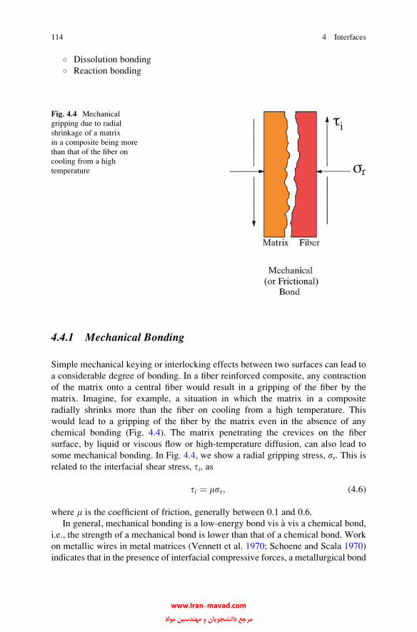
○ Dissolution bonding○ Reaction bonding

4.4.1 Mechanical Bonding

Simple mechanical keying or interlocking effects between two surfaces can lead to

a considerable degree of bonding. In a fiber reinforced composite, any contraction

of the matrix onto a central fiber would result in a gripping of the fiber by the

matrix. Imagine, for example, a situation in which the matrix in a composite

radially shrinks more than the fiber on cooling from a high temperature. This

would lead to a gripping of the fiber by the matrix even in the absence of any

chemical bonding (Fig. 4.4). The matrix penetrating the crevices on the fiber

surface, by liquid or viscous flow or high-temperature diffusion, can also lead to

some mechanical bonding. In Fig. 4.4, we show a radial gripping stress, sr. This isrelated to the interfacial shear stress, ti, as

ti ¼ msr; (4.6)

where m is the coefficient of friction, generally between 0.1 and 0.6.

In general, mechanical bonding is a low-energy bond vis a vis a chemical bond,

i.e., the strength of a mechanical bond is lower than that of a chemical bond. Work

on metallic wires in metal matrices (Vennett et al. 1970; Schoene and Scala 1970)

indicates that in the presence of interfacial compressive forces, a metallurgical bond

Fig. 4.4 Mechanical

gripping due to radial

shrinkage of a matrix

in a composite being more

than that of the fiber on

cooling from a high

temperature

114 4 Interfaces


is not quite necessary because the mechanical gripping of the fibers by the matrix is

sufficient to cause an effective reinforcement, as indicated by the occurrence of

multiple necking in fibers when the composite is pulled in tension. Hill et al. (1969)

confirmed the mechanical bonding effects in tungsten filament/aluminum matrix

composites. Chawla and Metzger (1978) studied bonding between an aluminum

substrate and anodized alumina (Al2O3) films and found that with a rough interface

a more efficient load transfer from the aluminum matrix to the alumina occurred.

There is only mechanical bond between Al2O3 and Al. Pure mechanical bonding

alone is not enough in most cases. However, mechanical bonding could add, in the

presence of reaction bonding, to the overall bonding. Also, mechanical bonding is

efficient in load transfer when the applied force is parallel to the interface. In the

case of mechanical bonding, the matrix must fill the hills and valleys on the surface

of the reinforcement. Rugosity, or surface roughness, can contribute to bond

strength only if the liquid matrix can wet the reinforcement surface. A good

example of excellent wetting (contact angle, y ¼ 0�) is between WC and cobalt

liquid. If, on the other hand, the matrix, liquid polymer or molten metal, is unable to

penetrate the asperities on the fiber surface, then the matrix will solidify and leave

interfacial voids, as shown in Fig. 4.5. Examples of surface roughness contributing

to interfacial strength include:

1. Surface treatments of carbon fibers, e.g., nitric acid oxidation of carbon fibers,

which increase specific surface area and lead to good wetting in PMCs, conse-

quently an improved interlaminar shear strength (ILSS) of the composite (see

Chap. 8).

2. Most metal matrix composites will have some roughness-induced mechanical

bonding between the ceramic reinforcement and the metal matrix (see Chap. 6).

3. Most CMC systems also show a mechanical gripping between the fiber and the

matrix (see Chap. 7).

Fig. 4.5 (a) Good mechanical bond. (b) Lack of wettability can make a liquid polymer or metal

unable to penetrate the asperities on the fiber surface, leading to interfacial voids

4.4 Types of Bonding at the Interface 115


http://dx.doi.org/10.1007/978-0-387-74365-3_8

http://dx.doi.org/10.1007/978-0-387-74365-3_6

http://dx.doi.org/10.1007/978-0-387-74365-3_7

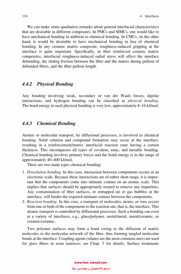
We can make some qualitative remarks about general interfacial characteristics

that are desirable in different composites. In PMCs and MMCs, one would like to

have mechanical bonding in addition to chemical bonding. In CMCs, on the other

hand, it would be desirable to have mechanical bonding in lieu of chemical

bonding. In any ceramic matrix composite, roughness-induced gripping at the

interface is quite important. Specifically, in fiber reinforced ceramic matrix

composites, interfacial roughness-induced radial stress will affect the interface

debonding, the sliding friction between the fiber and the matrix during pullout of

debonded fibers, and the fiber pullout length.

4.4.2 Physical Bonding

Any bonding involving weak, secondary or van der Waals forces, dipolar

interactions, and hydrogen bonding can be classified as physical bonding.The bond energy in such physical bonding is very low, approximately 8–16 kJ/mol.

4.4.3 Chemical Bonding

Atomic or molecular transport, by diffusional processes, is involved in chemical

bonding. Solid solution and compound formation may occur at the interface,

resulting in a reinforcement/matrix interfacial reaction zone having a certain

thickness. This encompasses all types of covalent, ionic, and metallic bonding.

Chemical bonding involves primary forces and the bond energy is in the range of

approximately 40–400 kJ/mol.

There are two main types chemical bonding:

1. Dissolution bonding. In this case, interaction between components occurs at an

electronic scale. Because these interactions are of rather short range, it is impor-

tant that the components come into intimate contact on an atomic scale. This

implies that surfaces should be appropriately treated to remove any impurities.

Any contamination of fiber surfaces, or entrapped air or gas bubbles at the

interface, will hinder the required intimate contact between the components.

2. Reaction bonding. In this case, a transport of molecules, atoms, or ions occurs

from one or both of the components to the reaction site, that is, the interface. This

atomic transport is controlled by diffusional processes. Such a bonding can exist

at a variety of interfaces, e.g., glass/polymer, metal/metal, metal/ceramic, or

ceramic/ceramic.

Two polymer surfaces may form a bond owing to the diffusion of matrix

molecules to the molecular network of the fiber, thus forming tangled molecular

bonds at the interface. Coupling agents (silanes are the most common ones) are used

for glass fibers in resin matrices; see Chap. 5 for details. Surface treatments

116 4 Interfaces


http://dx.doi.org/10.1007/978-0-387-74365-3_5

(oxidative or nonoxidative) are given to carbon fibers to be used in polymeric

materials; we describe these in Chap. 5. In metallic systems, solid solution and

intermetallic compound formation can occur at the interface. A schematic of the

diffusion phenomenon between a fiber and a matrix resulting in solid solution as

well as a layer of an intermetallic compound,MxFy is shown in Fig. 4.6. The plateau

region of the interfacial zone, which has a constant proportion of the two atomic

species, is the region of intermetallic compound formation. The reaction products

and the reaction rates can vary, depending on the matrix composition, reaction time,

and temperature. Generally, one tries to fit such data to an expression of the form

x2 � Dt; (4.7)

where x is the thickness of the reaction zone, D is the diffusivity, and t is the time.

This expression follows from the theory of diffusion in solids. The diffusivity, D,depends on the temperature in an exponential manner

D ¼ A expð�DQ=kTÞ; (4.8)

where A is a preexponential constant, DQ is the activation energy for the rate-

controlling process, k is Boltzmann’s constant, and T is the temperature in kelvin.

This relationship follows from the diffusion-controlled growth in an infinite diffu-

sion couple with planar interface. For a composite containing cylindrical fibers of a

small diameter, the diffusion distance is very small, i.e., the condition of an infinite

diffusion couple with planar interface is not likely to be valid. However, to a first

approximation, we can write

x2 � ct; (4.9)

where c is a pseudodiffusivity and has the dimensions of diffusivity (m2/s). The

reader should bear in mind that this approximate relationship can be expected to

work for composites in which the reaction thickness is small compared to the

interfiber spacing. Under these conditions, one can use an Arrhenius-type relation-

ship, c ¼ B exp(�DQ/kT), where B is a preexponential constant. A plot of ln c vs.1/T can be used to obtain the activation energy, DQ, for a fiber/matrix reaction in a

given temperature range. The preexponential constant, the constant B, depends onthe matrix composition, fiber, and the environment.

4.5 Optimum Interfacial Bond Strength

Two general ways of obtaining an optimum interfacial bond involve treatments of

fiber or reinforcement surface or modification of matrix composition. It should

be emphasized that maximizing the bond strength is not always the goal. In brittle

4.5 Optimum Interfacial Bond Strength 117


http://dx.doi.org/10.1007/978-0-387-74365-3_5

matrix composites, too strong a bond would cause embrittlement. We can illustrate

the situation by examining the following three cases.

4.5.1 Very Weak Interface or Fiber Bundle (No Matrix)

This extreme situation will prevail when we have no matrix and the composite

consists of only a fiber bundle. The bond strength in such a composite will only

be due to interfiber friction. A statistical treatment of fiber bundle strength (see

Chap. 12) shows that the fiber bundle strength is about 70–80 % of average single-

fiber strength.

4.5.2 Very Strong Interface

The other extreme in interfacial strength is when the interface is as strong or

stronger than the higher-strength component of the composite, generally the

reinforcement. In this case, of the three components—reinforcement, matrix,

and interface—the interface will have the lowest strain-to-failure. The composite

will fail when any cracking occurs at a weak spot along the brittle interface.

Typically, in such a case, a catastrophic failure will occur, and we will have

a composite with very low toughness.

Fig. 4.6 Interface zone in

a metal matrix composite

showing solid solution

and intermetallic compound

formation

118 4 Interfaces


http://dx.doi.org/10.1007/978-0-387-74365-3_12

4.5.3 Optimum Interfacial Bond Strength

An interface with an optimum interfacial bond strength will result in a composite

with an enhanced toughness, but without a severe penalty on the strength

parameters. Such a composite will have multiple failure sites, most likely spread

over the interfacial area, which will result in a diffused or global spread of damage,

rather than a very local damage.

4.6 Tests for Measuring Interfacial Strength

Numerous tests have been devised to characterize the fiber/matrix interface

strength. We briefly describe some of these.

4.6.1 Flexural Tests

Flexural or bend tests are very easy to do and can be used to get a semiqualitative

idea of the fiber/matrix interfacial strength of a composite. There are two basic

governing equations for a simple beam elastically stressed in bending:

M

I¼ E

R(4.10)

and

M

I¼ s

y; (4.11)

whereM is the applied bending moment, I is the second moment of area of the beam

section about the neutral plane, E is the Young’s modulus of elasticity of the

material, R is the radius of curvature of the bent beam, and s is the tensile or

compressive stress on a plane distance y from the neutral plane. For a uniform,

circular section beam

I ¼ pd4

64; (4.12)

where d is the diameter of the circular section beam. For a beam of a uniform,

rectangular section, we have

I ¼ bh3

12; (4.13)

4.6 Tests for Measuring Interfacial Strength 119


where b is the beam width and h is the height of the beam. Bending takes place in

the direction of the depth, i.e., h and y are measured in the same direction. Also, for

a beam with symmetrical section with respect to the neutral plane, replacing y in

Eq. (4.11) by h/2 gives the stress at the beam surface. When an elastic beam is bent,

the stress and strain vary linearly with thickness, y across the section, with the

neutral plane representing the zero level. The material on the outside or above

the neutral plane of the bent beam is stressed in tension while that on the inside or

below the neutral plane is stressed in compression. In the elastic regime, the stress

and strain are related by

s ¼ Ee: (4.14)

From Eqs. (4.10), (4.11), and (4.14) we can obtain the following simple relation

valid in the elastic regime:

e ¼ y

R: (4.15)

Thus, the strain e in a beam bent to a radius of curvature R varies linearly with

distance y from the neutral plane across the beam thickness. We describe some

variants of flexural tests.

4.6.1.1 Three-Point Bending

The bending moment in three-point bending is given by

M ¼ P

2� S

2¼ PS

4; (4.16)

where P is the load and S is the span. The important point to note is that the bending

moment in a three-point bend test increases from the two extremities of the beam to

a maximum value at the midpoint, i.e., the maximum stress is reached along a line

at the center of the beam. From Eqs. (4.11), (4.13), and (4.16), and taking y ¼ h/2,we get the following expression for the maximum stress for a rectangular beam in

three-point bending:

s ¼ 6PS

4bh2¼ 3PS

2bh2; (4.17)

where b and h are breadth and height of the beam, respectively. We can have the

fibers running parallel or perpendicular to the specimen length. When the fibers are

running perpendicular to the specimen length, we obtain a measure of transverse

strength of the fiber/matrix interface.

120 4 Interfaces


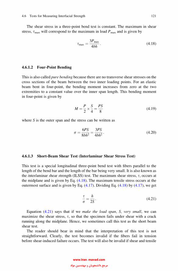
The shear stress in a three-point bend test is constant. The maximum in shear

stress, tmax will correspond to the maximum in load Pmax and is given by

tmax ¼ 3Pmax

4bh: (4.18)

4.6.1.2 Four-Point Bending

This is also called pure bending because there are no transverse shear stresses on thecross sections of the beam between the two inner loading points. For an elastic

beam bent in four-point, the bending moment increases from zero at the two

extremities to a constant value over the inner span length. This bending moment

in four-point is given by

M ¼ P

2� S

4¼ PS

8(4.19)

where S is the outer span and the stress can be written as

s ¼ 6PS

8bh2¼ 3PS

4bh2: (4.20)

4.6.1.3 Short-Beam Shear Test (Interlaminar Shear Stress Test)

This test is a special longitudinal three-point bend test with fibers parallel to the

length of the bend bar and the length of the bar being very small. It is also known as

the interlaminar shear strength (ILSS) test. The maximum shear stress, t, occurs atthe midplane and is given by Eq. (4.18). The maximum tensile stress occurs at the

outermost surface and is given by Eq. (4.17). Dividing Eq. (4.18) by (4.17), we get

ts¼ h

2S: (4.21)

Equation (4.21) says that if we make the load span, S, very small, we can

maximize the shear stress, t, so that the specimen fails under shear with a crack

running along the midplane. Hence, we sometimes call this test as the short beam

shear test.

The reader should bear in mind that the interpretation of this test is not

straightforward. Clearly, the test becomes invalid if the fibers fail in tension

before shear-induced failure occurs. The test will also be invalid if shear and tensile



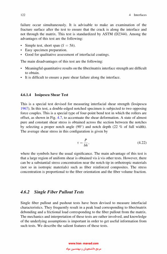
failure occur simultaneously. It is advisable to make an examination of the

fracture surface after the test to ensure that the crack is along the interface and

not through the matrix. This test is standardized by ASTM (D2344). Among the

advantages of this test are the following:

• Simple test, short span (S ¼ 5h).• Easy specimen preparation.

• Good for qualitative assessment of interfacial coatings.

The main disadvantages of this test are the following:

• Meaningful quantitative results on the fiber/matrix interface strength are difficult

to obtain.

• It is difficult to ensure a pure shear failure along the interface.

4.6.1.4 Iosipescu Shear Test

This is a special test devised for measuring interfacial shear strength (Iosipescu

1967). In this test, a double-edged notched specimen is subjected to two opposing

force couples. This is a special type of four-point bend test in which the rollers are

offset, as shown in Fig. 4.7, to accentuate the shear deformation. A state of almost

pure and constant shear stress is obtained across the section between the notches

by selecting a proper notch angle (90�) and notch depth (22 % of full width).

The average shear stress in this configuration is given by

t ¼ P

bh; (4.22)

where the symbols have the usual significance. The main advantage of this test is

that a large region of uniform shear is obtained vis a vis other tests. However, there

can be a substantial stress concentration near the notch tip in orthotropic materials

(not so in isotropic materials) such as fiber reinforced composites. The stress

concentration is proportional to the fiber orientation and the fiber volume fraction.

4.6.2 Single Fiber Pullout Tests

Single fiber pullout and pushout tests have been devised to measure interfacial

characteristics. They frequently result in a peak load corresponding to fiber/matrix

debonding and a frictional load corresponding to the fiber pullout from the matrix.

The mechanics and interpretation of these tests are rather involved, and knowledge

of the underlying assumptions is important in order to get useful information from

such tests. We describe the salient features of these tests.

122 4 Interfaces


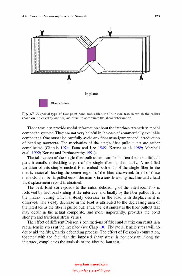
These tests can provide useful information about the interface strength in model

composite systems. They are not very helpful in the case of commercially available

composites. One must also carefully avoid any fiber misalignment and introduction

of bending moments. The mechanics of the single fiber pullout test are rather

complicated (Chamis 1974; Penn and Lee 1989; Kerans et al. 1989; Marshall

et al. 1992; Kerans and Parthasarathy 1991).

The fabrication of the single fiber pullout test sample is often the most difficult

part; it entails embedding a part of the single fiber in the matrix. A modified

variation of this simple method is to embed both ends of the single fiber in the

matrix material, leaving the center region of the fiber uncovered. In all of these

methods, the fiber is pulled out of the matrix in a tensile testing machine and a load

vs. displacement record is obtained.

The peak load corresponds to the initial debonding of the interface. This is

followed by frictional sliding at the interface, and finally by the fiber pullout from

the matrix, during which a steady decrease in the load with displacement is

observed. The steady decrease in the load is attributed to the decreasing area of

the interface as the fiber is pulled out. Thus, the test simulates the fiber pullout that

may occur in the actual composite, and more importantly, provides the bond

strength and frictional stress values.

The effect of different Poisson’s contractions of fiber and matrix can result in a

radial tensile stress at the interface (see Chap. 10). The radial tensile stress will no

doubt aid the fiber/matrix debonding process. The effect of Poisson’s contraction,

together with the fact that the imposed shear stress is not constant along the

interface, complicates the analysis of the fiber pullout test.

Fig. 4.7 A special type of four-point bend test, called the Iosipescu test, in which the rollers

(position indicated by arrows) are offset to accentuate the shear deformation



http://dx.doi.org/10.1007/978-0-387-74365-3_10

These tests, however, can provide useful quantitative information about the

interface strength in model composite systems. One must also carefully avoid any

fiber misalignment and introduction of bending moments. Figure 4.8a shows the

experimental setup for such a test. A portion of fiber, length l, is embedded in a

matrix and a pulling tensile force is applied as shown. If we measure the stress

required to pull the fiber out of the matrix as a function of the embedded fiber

length, we get the plot shown in Fig. 4.8b. The stress required to pull the fiber out,

without breaking it, increases linearly with the embedded fiber length, up to a

critical length, lc. At embedded fiber lengths greater than or equal to lc, the fiber willfracture under the action of the tensile stress, s, acting on the fiber. Consider

Fig. 4.8a again. The tensile stress, s, acting on the fiber results in a shear stress,

t, at the fiber/matrix interface. A simple force balance along the fiber length gives

spr2 ¼ t2prl:

For l < lc, the fiber is pulled out and the interfacial shear strength is given by

t ¼ sr2l

: (4.23)

Fig. 4.8 (a) An experimental setup for a single fiber pullout test. A portion of fiber, length l, isembedded in a matrix and a pulling tensile force is applied as shown. (b) The stress required to pull

the fiber out of the matrix as a function of the embedded fiber length

124 4 Interfaces


At l > lc, fiber failure rather than pullout occurs. One measures the load required

to debond as a function of the embedded fiber length. Then we can write

P ¼ 2prlt (4.24)

and the interfacial shear strength, t, can be calculated from the slope of the P vs. l.There is an implicit assumption in this analysis, viz., the shear stress acting along the

fiber/matrix interface is a constant. In a single fiber embedded test, one obtains the

average the load value over the entire interfacial surface area to get the interfacial

debond strength and/or frictional strength. Analytical and finite element analyses show

that the shear stress is a maximum close to the surface ends and falls rapidly within a

distance of a few fiber diameters. Thus, one would expect the interface debonding to

start near the surface and progressively propagate along the embedded length.

The interfacial shear strength is a function of the coefficient of friction, m, and anynormal compressive stress at the interface, sr. The source of radial compressive

stress is the shrinkage of the matrix during cooling from the processing temperature.

4.6.3 Curved Neck Specimen Test

This technique was devised for PMCs. A special mold is used to prepare a curved

neck specimen of the composite containing a single fiber along its central axis. The

specimen is compressed and the fiber/matrix debonding is observed visually.

The curved neck shape of the specimen enhances the transverse tensile stress at

the fiber/matrix interface. The transverse tensile stress leading to interface

debonding results from the fact that the matrix and the fiber have different Poisson’s

ratios. If the matrix Poisson ratio, nm, is greater than that of the fiber, vf, then on

compression, there will result a transverse tensile stress at the center of the neck and

perpendicular to the interface whose magnitude is given by (Broutman 1969):

si ¼ s nm � vfð ÞEf

1þ nmð ÞEf þ 1� nf � 2n2f� �

Em

� � ; (4.25)

where s is the net section compressive stress (i.e., load/minimum area), E is the

Young’s modulus, n is the Poisson’s ratio, and the subscripts f and m denote fiber

and matrix, respectively. Note the expression in (4.29) gives the magnitude of

tensile stress developed perpendicular to the interface when the sample is subjected

to a compressive load.

One canmeasure the net section stress, s, corresponding to interface debonding andcompute the interfacial tensile strength from (4.25). There are some important

points that should be taken into account before using this test. One needs a special

mold to prepare the specimen, anda veryprecise alignment of thefiber along the central

axis is a must. Finally, a visual examination is required to determine the interface

debonding point. This would limit the technique to transparent matrix materials.

Acoustic emission detection techniques may be used to avoid visual examination.



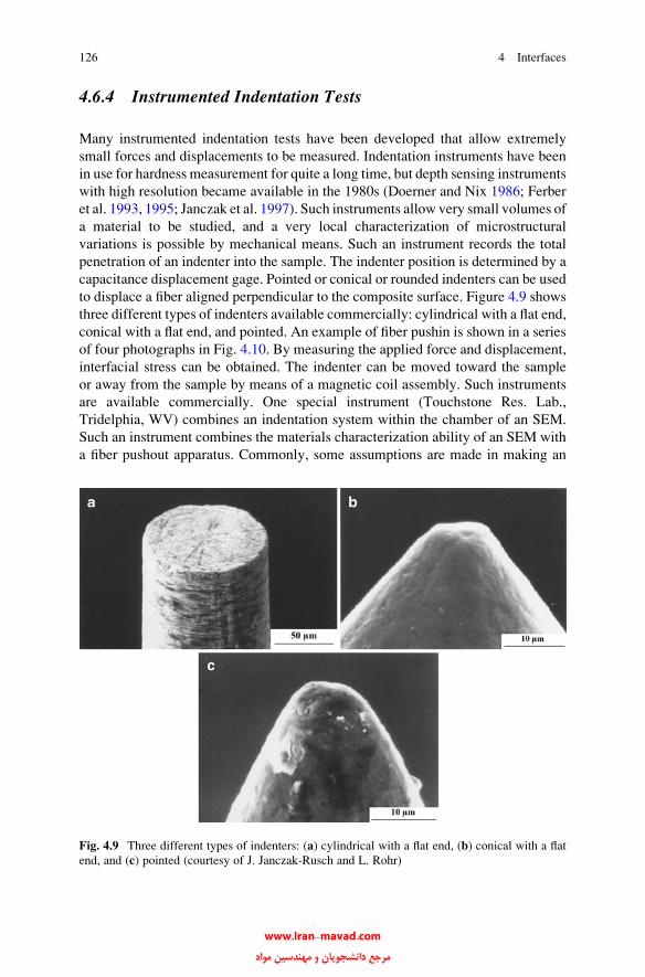
4.6.4 Instrumented Indentation Tests

Many instrumented indentation tests have been developed that allow extremely

small forces and displacements to be measured. Indentation instruments have been

in use for hardness measurement for quite a long time, but depth sensing instruments

with high resolution became available in the 1980s (Doerner and Nix 1986; Ferber

et al. 1993, 1995; Janczak et al. 1997). Such instruments allow very small volumes of

a material to be studied, and a very local characterization of microstructural

variations is possible by mechanical means. Such an instrument records the total

penetration of an indenter into the sample. The indenter position is determined by a

capacitance displacement gage. Pointed or conical or rounded indenters can be used

to displace a fiber aligned perpendicular to the composite surface. Figure 4.9 shows

three different types of indenters available commercially: cylindrical with a flat end,

conical with a flat end, and pointed. An example of fiber pushin is shown in a series

of four photographs in Fig. 4.10. By measuring the applied force and displacement,

interfacial stress can be obtained. The indenter can be moved toward the sample

or away from the sample by means of a magnetic coil assembly. Such instruments

are available commercially. One special instrument (Touchstone Res. Lab.,

Tridelphia, WV) combines an indentation system within the chamber of an SEM.

Such an instrument combines the materials characterization ability of an SEM with

a fiber pushout apparatus. Commonly, some assumptions are made in making an

Fig. 4.9 Three different types of indenters: (a) cylindrical with a flat end, (b) conical with a flat

end, and (c) pointed (courtesy of J. Janczak-Rusch and L. Rohr)

126 4 Interfaces


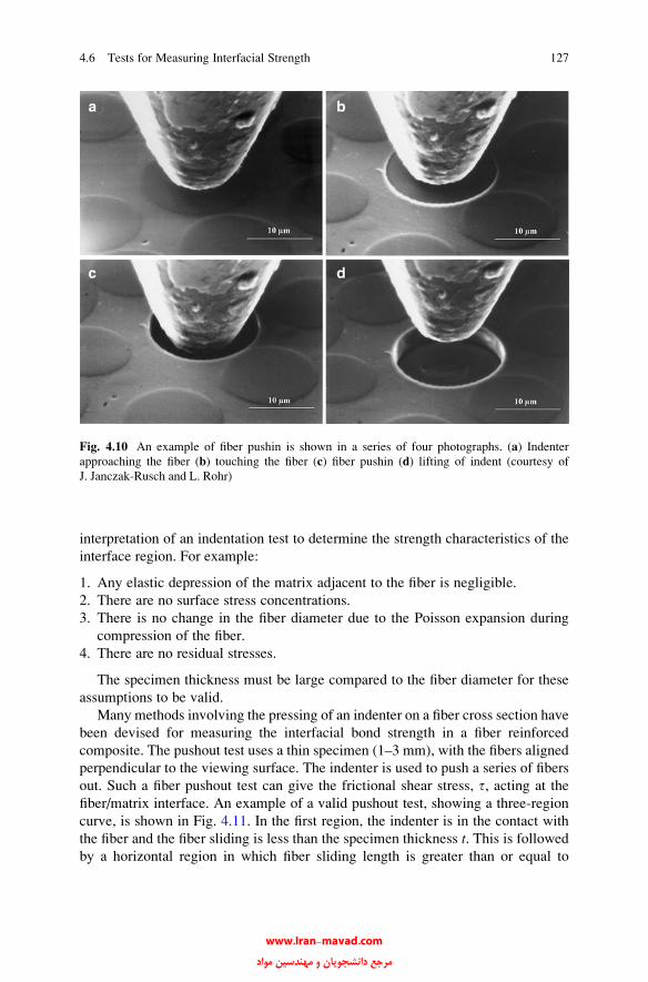
interpretation of an indentation test to determine the strength characteristics of the

interface region. For example:

1. Any elastic depression of the matrix adjacent to the fiber is negligible.

2. There are no surface stress concentrations.

3. There is no change in the fiber diameter due to the Poisson expansion during

compression of the fiber.

4. There are no residual stresses.

The specimen thickness must be large compared to the fiber diameter for these

assumptions to be valid.

Many methods involving the pressing of an indenter on a fiber cross section have

been devised for measuring the interfacial bond strength in a fiber reinforced

composite. The pushout test uses a thin specimen (1–3 mm), with the fibers aligned

perpendicular to the viewing surface. The indenter is used to push a series of fibers

out. Such a fiber pushout test can give the frictional shear stress, t, acting at the

fiber/matrix interface. An example of a valid pushout test, showing a three-region

curve, is shown in Fig. 4.11. In the first region, the indenter is in the contact with

the fiber and the fiber sliding is less than the specimen thickness t. This is followedby a horizontal region in which fiber sliding length is greater than or equal to

Fig. 4.10 An example of fiber pushin is shown in a series of four photographs. (a) Indenter

approaching the fiber (b) touching the fiber (c) fiber pushin (d) lifting of indent (courtesy of

J. Janczak-Rusch and L. Rohr)



the sample thickness. In the third region, the indenter comes in contact with the

matrix. In the horizontal region, the interfacial shear stress is given by:

ti ¼ P

2prt;

where P is the applied load, r is the fiber radius, and t is the specimen thickness.

The specimen thickness should be much greater that the fiber diameter for this

relationship to be valid. In the third region of Fig. 4.11 the value of the interfacial

shear stress cannot be determined because the indenter comes in contact with the

matrix, i.e., the test is no more valid.

In such indentation tests, after interfacial debonding, the fiber will slide along

the interface over a distance that is dependent on the load applied by the indenter.

The fiber is elastically compressed by the indenter load over the debonded length,

which is assumed to be dependent on the interfacial friction. The axial load on the

indenter is assumed to be balanced by the frictional stress at the interface, and

the effect of radial expansion during indentation is neglected. There are two

analytical models due to Kerans and Parthasarathy (1991) and Hsueh (1992) that

take into account progressive debonding and sliding during fiber pushin and

pushout. Radial and axial stresses are taken into account in both models and

Coulombic friction is assumed at the fiber/matrix interface. Lara-Curzio and Ferber

(1994) found that the two models gave almost identical results in Nicalon fiber/

calcium aluminosilicate matrix composites.

Fig. 4.11 Stress vs. displacement obtained in fiber pushout test (Chawla et al. 2001)

128 4 Interfaces


An instrumented indentation test to be used at high temperature was developed

by Eldridge (1995). Such a test is very useful for CMCs. Such a test is also useful to

analyze the effect of residual stresses.

4.6.5 Fragmentation Test

In this test, a single fiber is embedded in a dog-bone-type tensile sample of matrix.

When a tensile load is applied to such a sample, the load is transferred to the fiber

via shear strains and stresses produced on planes parallel to the fiber/matrix

interface. We discuss the subject of load transfer in fiber reinforced composites in

Chap. 10. When the tensile stress in the fiber reaches its ultimate strength, it

fragments into two parts. If we continue loading, this process of fiber fragmentation

continues, i.e., the single fiber continues to fragment into even smaller pieces until

the fiber fragment length becomes too small to enable loading it to fracture. This

fiber length is called the critical length, lc. This is shown schematically in Fig. 4.12.

From a consideration of equilibrium of forces over an element dx of the fiber (seeChap. 10 also), we can write

pr2 ds ¼ 2pr dxt

ds=dx ¼ 2t=r: (4.26)

where s is the tensile stress, t is the shear stress, and p is the fiber radius.

From Eq. (4.26), we obtain the critical length as follows. For simplicity, we

consider that the matrix is perfectly plastic, i.e., we ignore any strain hardening

effects and that the matrix yields in shear at shear stress of ty. We also assume that

the shear stress along the fiber/matrix interface is constant over the length of the

fiber fragment, lc. Integrating Eq. (4.30), we get

ðsmax

0

ds ¼ðlc=20

2t dx=r

smax ¼ tlc=r (4.27)

or

t ¼ smaxr=lc ¼ smaxd=2lc: (4.28)

The fiber fragmentation technique is a simple technique that gives us a quanti-

tative measure of the fiber/matrix interfacial strength. Drzal et al. (1983, 1994, 1997)

and others have used this technique extensively to characterize carbon fiber

reinforced polymer matrix composites. Clearly, a transparent matrix is required.

The technique will work only if the fiber failure strain is less than that of the matrix,



http://dx.doi.org/10.1007/978-0-387-74365-3_10

http://dx.doi.org/10.1007/978-0-387-74365-3_10

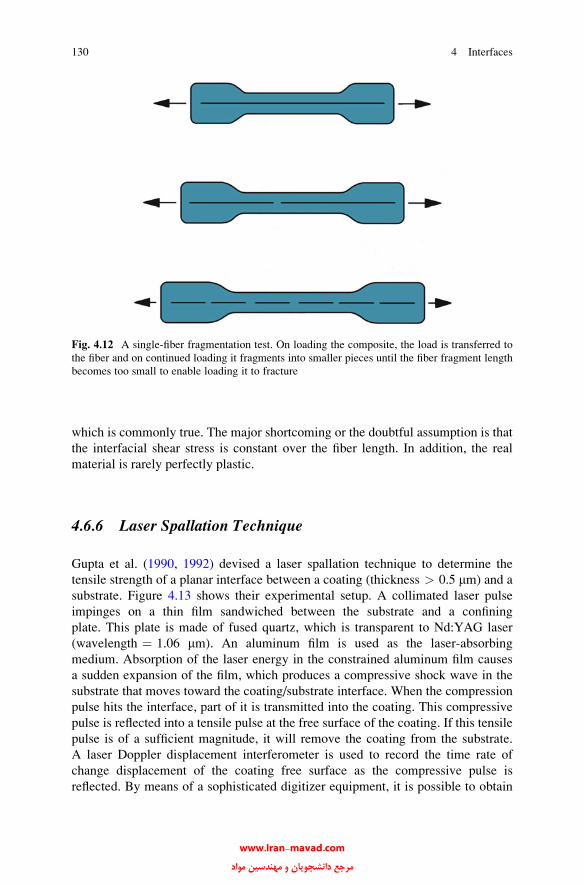
which is commonly true. The major shortcoming or the doubtful assumption is that

the interfacial shear stress is constant over the fiber length. In addition, the real

material is rarely perfectly plastic.

4.6.6 Laser Spallation Technique

Gupta et al. (1990, 1992) devised a laser spallation technique to determine the

tensile strength of a planar interface between a coating (thickness > 0.5 mm) and a

substrate. Figure 4.13 shows their experimental setup. A collimated laser pulse

impinges on a thin film sandwiched between the substrate and a confining

plate. This plate is made of fused quartz, which is transparent to Nd:YAG laser

(wavelength ¼ 1.06 mm). An aluminum film is used as the laser-absorbing

medium. Absorption of the laser energy in the constrained aluminum film causes

a sudden expansion of the film, which produces a compressive shock wave in the

substrate that moves toward the coating/substrate interface. When the compression

pulse hits the interface, part of it is transmitted into the coating. This compressive

pulse is reflected into a tensile pulse at the free surface of the coating. If this tensile

pulse is of a sufficient magnitude, it will remove the coating from the substrate.

A laser Doppler displacement interferometer is used to record the time rate of

change displacement of the coating free surface as the compressive pulse is

reflected. By means of a sophisticated digitizer equipment, it is possible to obtain

Fig. 4.12 A single-fiber fragmentation test. On loading the composite, the load is transferred to

the fiber and on continued loading it fragments into smaller pieces until the fiber fragment length

becomes too small to enable loading it to fracture

130 4 Interfaces


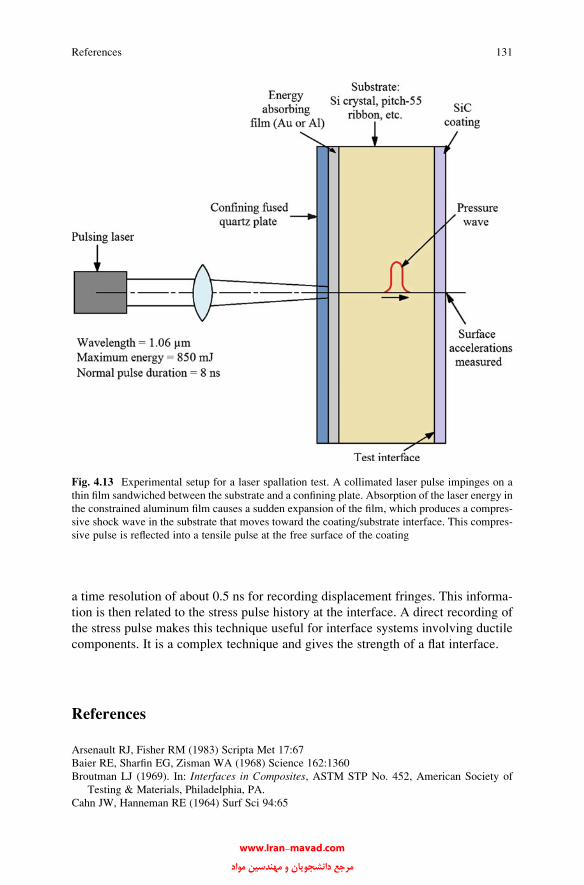
a time resolution of about 0.5 ns for recording displacement fringes. This informa-

tion is then related to the stress pulse history at the interface. A direct recording of

the stress pulse makes this technique useful for interface systems involving ductile

components. It is a complex technique and gives the strength of a flat interface.

References

Arsenault RJ, Fisher RM (1983) Scripta Met 17:67

Baier RE, Sharfin EG, Zisman WA (1968) Science 162:1360

Broutman LJ (1969). In: Interfaces in Composites, ASTM STP No. 452, American Society of

Testing & Materials, Philadelphia, PA.

Cahn JW, Hanneman RE (1964) Surf Sci 94:65

Fig. 4.13 Experimental setup for a laser spallation test. A collimated laser pulse impinges on a

thin film sandwiched between the substrate and a confining plate. Absorption of the laser energy in

the constrained aluminum film causes a sudden expansion of the film, which produces a compres-

sive shock wave in the substrate that moves toward the coating/substrate interface. This compres-

sive pulse is reflected into a tensile pulse at the free surface of the coating

References 131


Cahn JW (1979) In: Interfacial segregation. ASM, Metals Park, OH, p 3

Chamis CC (1974) In: Composite materials, vol 6. Academic, New York, p 32

Chawla KK (1997) Compos Interf 4:287

Chawla KK, Metzger M (1972) J Mater Sci 7:34

Chawla KK, Metzger M (1978) In: Advances in research on strength and fracture of materials, vol

3. Pergamon, New York, p 1039

Chawla KK, Xu ZR (1994) In: High performance composites: commonalty of phenomena. TMS,

Warrendale, PA, p 207

Chawla KK, Xu ZR, Ha J-S, Lara-Curzio E, Ferber MK, Russ S (1995) Advances in ceramic

matrix composites II. American Ceramic Society, Westerville, OH, p 779

Chawla KK, Xu ZR, Hlinak A, Chung Y-W (1993) In: Advances in ceramic-matrix composites.

American Ceramic Society, Westerville, OH, p 725

Chawla N, Chawla KK, Koopman M, Patel B, Coffin C, Eldridge J (2001) Compos Sci Tech

61:1923

Doerner MF, Nix WD (1986) J Mater Res 1:601

Drzal LT, Madhukar M, Waterbury M (1994) Compos Sci Tech 27:65–71

Drzal LT, Rich MJ, Lloyd PF (1983) J Adhesion 16:1–30

Drzal LT, Sugiura N, Hook D (1997) Compos Interf 4:337

Eldridge JI (1995). Mat. Res. Soc. Symp. Proc., vol 365, Materials Research Society, p 283

Ferber MK, Wereszczak AA, Riester L, Lowden RA, Chawla KK (1993) In: Ceramic Sci. & Eng.

Proc., Amer. Ceram. Soc., Westerville, OH

Ferber MK, Lara-Curzio E, Russ S, Chawla KK (1995) In: Ceramic matrix composites—advanced

high-temperature structural materials. Materials Research Society, Pittsburgh, PA, p 277

Fine ME, Mitra R, Chawla KK (1993) Scripta Met Mater 29:221

Gupta V, Argon AS, Cornie JA, Parks DM (1990) Mater Sci Eng A126:105

Gupta V, Argon AS, Cornie JA, Parks DM (1992) J Mech Phys Solids 4:141

Hill RG, Nelson RP, Hellerich CL (1969) In: Proceedings of the refractory working group

meeting, Seattle, WA, Oct

Hsueh C-H (1992) J Am Ceram Soc 76:3041

Iosipescu N (1967) J Mater 2:537

Janczak J, B€urki G, Rohr L (1997) Key Eng Mater 127:623

Jangehud I, Serrano AM, Eby RK, Meador MA (1993) In: Proc. 21st Biennial Conf. on Carbon,

Buffalo, NY, June 13–18

Johnson RE (1959) J Phys Chem 63:1655

Kerans RJ, Hays RS, Pagano NJ, Parthasarathy TA (1991) Am Ceram Soc Bull 68:429

Kerans RJ, Parthasarathy TA (1991) J Am Ceram Soc 74:1585

Lara-Curzio E, Ferber MK (1994) J Mater Sci 29:6158

Marshall DB, Shaw MC, Morris WL (1992) Acta Met Mater 40:443

Penn LS, Lee SM (1989) J Comp Tech & Res 11:23

Schoene C, Scala E (1970) Met Trans 1:3466

Vennett RM, Wolf SM, Levitt AP (1970) Met Trans 1:1569

Vogelsang M, Arsenault RJ, Fisher RM (1986) Met Trans A 17:379

Walter JL, Cline HE, Koch E (1969) Trans AIME 245:2073

Weihs TP, Nix WD (1991) J Am Ceram Soc 74:524

Wenzel RN (1936) Ind Eng Chem 28:987

Further Reading

Adams DF, Carlsson LA, Pipes RB (1998) Experimental characterization of advanced composite

materials, 3rd edn. CRC, Boca Raton, FL

Faber KT (1997) Annu Rev Mater Sci 27:499

132 4 Interfaces


Kim J-K, Mai Y-W (1998) Engineered interfaces in fiber reinforced composites. Elsevier,

New York

Plueddemann EP (ed) (1974) Interfaces in polymer matrix composites (vol 6 of the series

Composite Materials), Academic, New York

Stokes RJ, Evans DF (1997) Fundmentals of interfacial engineering. Wiley-VCH, New York

Wagner HD, Marom G (eds) (1997) Composite interfaces (special issue—selected papers from the

sixth international conference on composite interfaces (ICCI-6), Israel). VSP, Zeist, The

Netherlands

Problems

4.1. Describe some techniques for measuring interfacial energies in different

composite systems.

4.2. In order to study the interfacial reactions between the fiber and matrix,

oftentimes one uses very high temperatures in order to reduce the time

necessary for the experiment. What are the objections to such accelerated

tests?

4.3. What are the objections to the use of short beam shear test to measure the

interlaminar shear strength (ILSS)?

4.4. Diffusion along free surface is faster than in the bulk of a material. Similarly,

diffusion along a grain boundary is faster than in the lattice. Taking these

factors into account, write an expression for diffusion coefficients in order of

descent for diffusion along lattice, dislocation, grain boundary, reinforcement/

matrix interface, and surface. Explain the reason behind your answer.

4.5. Discuss the importance of moisture diffusion in fiber reinforced polymer

matrix composites. Recall that moisture absorption in PMCs is largely due to

the permeability of the polymer matrix. Suggest some possible effects of

moisture absorption in fiber reinforced PMCs in terms of effects on different

moduli (along the fiber and perpendicular to the fiber) and ILSS.

Problems 133


Part II


Chapter 5

Polymer Matrix Composites

Polymer matrix composites (PMCs) have established themselves as engineering

structural materials, not just as laboratory curiosities or cheap stuff for making

chairs and tables. This came about not only because of the introduction of high-

performance fibers such as carbon, boron, and aramid but also because of some new

and improved matrix materials (see Chap. 3). Nevertheless, glass fiber reinforced

polymers represent the largest class of PMCs. Carbon fiber reinforced PMCs are

perhaps the most important structural composites; especially in the aerospace field.

In this chapter, we discuss polymer composite systems containing glass, aramid,

polyethylene, boron, and carbon fibers.

5.1 Processing of PMCs

Many techniques, originally developed for making glass fiber reinforced polymer

matrix composites can also be used with other fibers. Glass fiber reinforced polymer

composites represent the largest class of PMCs. As we saw in Chap. 3, polymeric

matrix materials can be conveniently classified as thermosets and thermoplastics.

Recall that thermosets harden on curing. Curing or cross-linking occurs in

thermosets by appropriate chemical agents and/or application of heat and pressure.

Conventionally, thermal energy (heating to 200 �C or above) is provided for this

purpose. This process, however, brings in the problems of thermal gradients,

residual stresses, and long curing times. Residual stresses can cause serious

problems in nonsymmetric or very thick PMC laminates, where they may be

relieved by warping of the laminate, fiber waviness, matrix microcracking, and

ply delamination. We mentioned electron beam curing in Chap. 3. Electron beam

curing offers an alternative that avoids these problems. It is a nonthermal curing

process that requires much shorter cure time cycles. Curing by electron beam

occurs by electron-initiated reactions at a selectable cure temperature. We describe

different methods of fabrication of polymer matrix composites—first thermoset-

based composites and then thermoplastic-based composites.


137


http://dx.doi.org/10.1007/978-0-387-74365-3_3

http://dx.doi.org/10.1007/978-0-387-74365-3_3

http://dx.doi.org/10.1007/978-0-387-74365-3_3

5.1.1 Processing of Thermoset Matrix Composites

There are many processing methods for composites with thermoset matrix materials

including epoxy, unsaturated polyester, and vinyl ester.

5.1.1.1 Hand Layup and Spray Techniques

Hand layup and spray techniques are perhaps the simplest polymer processing

techniques. Fibers can be laid onto a mold by hand and the resin (unsaturated

polyester is one of the most common) is sprayed or brushed on. Frequently, resin

and fibers (chopped) are sprayed together onto the mold surface. In both cases, the

deposited layers are densified with rollers. Figure 5.1 shows schematics of these

processes. Accelerators and catalysts are frequently used. Curing may be done at

room temperature or at a moderately high temperature in an oven.

5.1.1.2 Filament Winding

Filament winding (Shibley 1982; Tarnopol’skii and Bail’ 1983) is another very

versatile technique in which a continuous tow or roving is passed through a resin

impregnation bath and wound over a rotating or stationary mandrel. A roving

consists of thousands of individual filaments. Figure 5.2a shows a schematic of

this process, while Fig. 5.2b shows a pressure vessel made by filament winding.

The winding of roving can be polar (hoop) or helical. In polar winding, the

fiber tows do not cross over, while in the helical they do. The fibers are, of course,

laid on the mandrel in a helical fashion in helical windings; the helix angle

depends on the shape of the object to be made. Successive layers are laid on at

a constant or varying angle until the desired thickness is attained. Curing of the

thermosetting resin is done at an elevated temperature and the mandrel is

removed. Very large cylindrical (e.g., pipes) and spherical (e.g., for chemical

storage) vessels are built by filament winding. Glass, carbon, and aramid fibers are

routinely used with epoxy, polyester, and vinyl ester resins for producing filament

wound shapes.

There are two types of filament winding processes: wet winding and prepreg

winding. In wet winding, low-viscosity resin is applied to the filaments during the

winding process. Polyesters and epoxies with viscosity less than 2 Pa s (2,000 cP)

are used in wet winding. In prepreg winding, a hot-melt or solvent-dip process is

138 5 Polymer Matrix Composites


used to preimpregnate the fibers. Rigid amines, novolacs, polyimides, and higher-

viscosity epoxies are generally used for this process. In filament winding, the most

probable void sites are roving crossovers and regions between layers with different

fiber orientations.

Fig. 5.1 (a) In hand layup, fibers are laid onto a mold by hand, and the resin is sprayed or brushed

on. (b) In spray-up, resin and fibers (chopped) are sprayed together onto the mold surface

5.1 Processing of PMCs 139


5.1.1.3 Pultrusion

In this process continuous sections of polymer matrix composites with fibers

oriented mainly axially are produced. Figure 5.3a shows a schematic of this

process. Continuous fiber tows come from various creels. Mat or biaxial fabric

may be added to these to provide some transverse strength. These are passed

through a resin bath containing a catalyst. After this, the resin-impregnated fibers

pass through a series of wipers to remove any excess polymer and then through a

collimator before entering the heated die. A thorough wet-out of the rovings is very

important. Stripped excess resin is recirculated to the resin bath. The heated die has

the shape of the finished component to be produced. The resin is cured in the die and

the composite is pulled out. At the end of the line the part is cut by a flying saw to a

fixed length. Typically, the process can produce continuously at a rate of

10–200 cm/min. The exact speed depends on the resin type and the cross-sectional

thickness of the part being produced. Pultruded profiles as wide as 1.25 m with

more than 60 % fiber volume fraction can be made routinely. An example of a

product obtained by pultrusion is shown in Fig. 5.3b. The hollow trapezoidal-

shaped product shown is a helicopter windshield post made of carbon fiber mat

and tows in a high-temperature vinyl ester resin matrix.

Fig. 5.2 (a) Schematic of filament winding process. (b) Schematic of a filament wound pressure

vessel with a liner; helical and hoop winding are shown



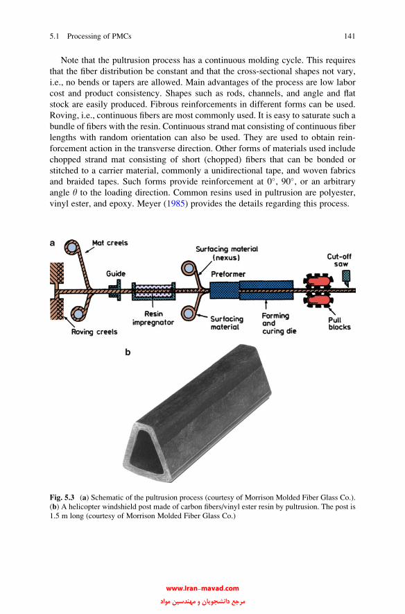
Note that the pultrusion process has a continuous molding cycle. This requires

that the fiber distribution be constant and that the cross-sectional shapes not vary,

i.e., no bends or tapers are allowed. Main advantages of the process are low labor

cost and product consistency. Shapes such as rods, channels, and angle and flat

stock are easily produced. Fibrous reinforcements in different forms can be used.

Roving, i.e., continuous fibers are most commonly used. It is easy to saturate such a

bundle of fibers with the resin. Continuous strand mat consisting of continuous fiber

lengths with random orientation can also be used. They are used to obtain rein-

forcement action in the transverse direction. Other forms of materials used include

chopped strand mat consisting of short (chopped) fibers that can be bonded or

stitched to a carrier material, commonly a unidirectional tape, and woven fabrics

and braided tapes. Such forms provide reinforcement at 0�, 90�, or an arbitrary

angle y to the loading direction. Common resins used in pultrusion are polyester,

vinyl ester, and epoxy. Meyer (1985) provides the details regarding this process.

Fig. 5.3 (a) Schematic of the pultrusion process (courtesy of Morrison Molded Fiber Glass Co.).

(b) A helicopter windshield post made of carbon fibers/vinyl ester resin by pultrusion. The post is

1.5 m long (courtesy of Morrison Molded Fiber Glass Co.)



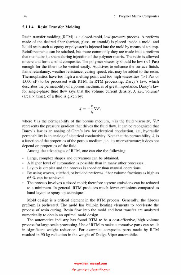
5.1.1.4 Resin Transfer Molding

Resin transfer molding (RTM) is a closed-mold, low-pressure process. A preform

made of the desired fiber (carbon, glass, or aramid) is placed inside a mold, and

liquid resin such as epoxy or polyester is injected into the mold by means of a pump.

Reinforcements can be stitched, but more commonly they are made into a preform

that maintains its shape during injection of the polymer matrix. The resin is allowed

to cure and form a solid composite. The polymer viscosity should be low (<1 Pas)

enough for the fibers to be wetted easily. Additives to enhance the surface finish,

flame retardancy, weather resistance, curing speed, etc. may be added to the resin.

Thermoplastics have too high a melting point and too high viscosities (>1 Pas or

1,000 cP) to be processed with RTM. In RTM processing, Darcy’s law, which

describes the permeability of a porous medium, is of great importance. Darcy’s law

for single-phase fluid flow says that the volume current density, J, i.e., volume/

(area � time), of a fluid is given by:

J ¼ � k

�rP;

where k is the permeability of the porous medium, � is the fluid viscosity, rPrepresents the pressure gradient that drives the fluid flow. It can be recognized that

Darcy’s law is an analog of Ohm’s law for electrical conduction, i.e., hydraulic

permeability is an analog of electrical conductivity. Note that the permeability, k, isa function of the properties of the porous medium, i.e., its microstructure; it does not

depend on properties of the fluid.

Among the advantages of RTM, one can cite the following:

• Large, complex shapes and curvatures can be obtained.

• A higher level of automation is possible than in many other processes.

• Layup is simpler and the process is speedier than manual operations.

• By using woven, stitched, or braided preforms, fiber volume fractions as high as

65 % can be achieved.

• The process involves a closed mold; therefore styrene emissions can be reduced

to a minimum. In general, RTM produces much fewer emissions compared to

hand layup or spray-up techniques.

Mold design is a critical element in the RTM process. Generally, the fibrous

preform is preheated. The mold has built-in heating elements to accelerate the

process of resin curing. Resin flow into the mold and heat transfer are analyzed

numerically to obtain an optimal mold design.

The automotive industry has found RTM to be a cost-effective, high volume

process for large scale processing. Use of RTM to make automotive parts can result

in significant weight reduction. For example, composite parts made by RTM

resulted in 90 kg reduction in the weight of Dodge Viper automobile.



5.1.1.5 Automated Tape Placement and Automated Fiber Placement

In general, automation in most any field results in productivity gains. For example,

a completely automated process, i.e., no human being is required, has a great

attraction for use in radioactive or clean environments. In the area of fabrication

of composites, it has led to two very important techniques: automatic tape place-

ment (ATL) and automatic fiber placement (AFP). Another significant advantage is

that rather large structures can be made by this process. The hand layup process is

limited by the extent of a worker’s reach. Clearly, such a restriction would be absent

in any automatic process. Most automated machines are large, sophisticated and

represent a major capital investment. Resin choices for tapes can be grouped by

processing characteristics. These are commonly thermoset resins such as epoxies;

they are cured to B-stage, i.e., tacky, and later fully cured. The second group

comprises of nontacky solid resins that melt and flow prior to curing to a thermoset

polymer, e.g., bismaleimides and nontacky thermoplastic resins processed entirely

by melting and freezing, e.g., polyether ether ketone, (PEEK), and polyphenylene

sulfide, (PPS).

Capital expenditures for computer-controlled, automated equipment can be

significant, however. Understandably, such equipment initially found applications

in defense related applications, e.g., the wing skin panels of F-22 Raptor fighter jet.With Boeing 787 and Airbus A380 and other advanced aircrafts, automated

processing techniques have moved into civilian aircraft construction as well.

Automated Tape Placement

In this technique, resin preimpregnated high performance reinforcement fibers in

the form of a tape are placed in specific directions. It is easy to see that part weight

will be minimized by placing fibers only along the directions needed. Automated

tape placement (ATP) has gained wide acceptance for part fabrication in the

aerospace industry; examples include aircraft wings, body skins, and control

surfaces. In ATP, prepregged tape, rather than single fiber tows, is laid down

continuously to form parts. It is often used for parts with highly complex contours

or angles. Tape layup is versatile; it allows breaks in the process and easy changes

in direction. Although, the process is commonly used with thermosets, it can be

adapted for thermoplastic materials as well.

In principle, the ATL works as follows. The customer’s computer aided design

(CAD) is the starting point. Using the CAD system, the product or component to be

manufactured, say a curved part, is developed mathematically onto a flat surface.

This is further broken down into layers to be fabricated by laying strips of tape side

by side. Sophisticated software is used to translate strips in each layer via a series of

numerical control steps to develop the final product shape. A spool of tape

(consisting of, say, carbon fiber preimpregnated with a thermosetting resin, com-

monly epoxy), covered with a protective paper on the top and protective film



underneath, is unwound; the film and the paper are peeled off, and the tape

suspended in mid air is cut to correct shape by cutting blades. The cutting blades

are very fast; they can make 6,000 cuts per minute. A laser beam in the tape laying

head is used to accurately lay the tape on the mold.

Automated tape laying machines (ATL) are used to make aircraft parts such as

wing stringers, spars, skins and elevators, tail skins and horizontal planes, engine

cowls, fuselage skins and belly fairings. These automated tape laying machines are

capable of laying preimpregnated tapes of 75-, 150- or 300-mm width at any

orientation and can build up the product consisting of any number of plies. Modern

ATL machines have heads that integrate ultrasonic cutting of the laminate, cutter

depth-setting, and dockable inkjet marking. Low-rail gantry platforms are available

in medium and large size ranges that can be matched to customer part size and floor

space requirements. The machines feature tape-deposit speeds of up to 50 m/min

and a high degree of placement accuracies on complex contours.

Automated Fiber Placement

Automated fiber placement (AFP) involves the use of individual fiber tows. Multi-

ple resin preimpregnated fiber tows are placed onto a mandrel at high speed, using a

numerically controlled placement head to dispense, clamp, cut and restart each tow

during placement. Minimum cut length (the shortest tow length a machine can lay

down) is the essential ply-shape determinant. The fiber placement heads can be

attached to a 5-axis gantry or retrofitted to a filament winder. Machines are

available with dual mandrel stations to increase productivity. Advantages of fiber

placement fabrication include speed, reduced material scrap and labor costs, part

consolidation and improved part-to-part uniformity. The process is employed when

producing large thermoset parts with complex shapes.

The fiber tows, preimpregnated with the resin, from spools are fed into the fiber

placement head where they are collimated into a single band and laminated onto the

work surface. Typically, each tow is about 3 mm wide strand of continuous fibers.

A strand, in its turn, may consist of 12,000 individual filaments impregnated with an

epoxy resin.

Different fiber tows can be delivered at different speeds, thus conforming to a

complex structural shape. For example, when a curved surface is to be laminated,

the outer tows of the band pull more strand length than the inner tows. It is possible

to cut individual tows and restart without stopping the motion of the head. This

allows in-process control of the band width, avoiding excess resin build-up and to

fill in any gaps. A compaction roller or shoe consolidates the tape pressing it onto

the work surface. This pressing action serve to removes any trapped air and any

minor gaps between individual tows. Figure 5.4 shows a schematic of the automatic

fiber placement process.



High speed, automatic processing has become very popular with the coming of

large-sized civilian aircraft. As an example of a commercially produced AFP

machine, we mention VIPER made by MAG Cincinnati (Hebron, Ky.). Such

machines are used for automated fabrication of composite fuselage panels for the

commercial aircraft. The VIPER 6000 series AFP machines can produce fuselage

panels up to 6.3 m in diameter. The VIPERs will produce 92 % of the fuselage for

the A350 XWB. According to MAG Cincinnati, the company that manufactures

the VIPER machines, such machines enable independent control over feed, clamp,

cut and start for up to 32 individual tows or slit tape. Multistrands of carbon fiber/

epoxy can be placed around a mandrel to make a single finished part without seams

and rivets.

5.1.1.6 Autoclave-Based Methods

Autoclave-based methods or bag molding processes (Slobodzinsky 1982) are used

to make large parts. Before we describe this important process, we should digress

and describe an important term, although we have used it earlier, viz., prepreg.

The term prepreg is a short form of preimpregnated fibers. Generally, a prepreg is

in the form of a thin sheet or lamina of unidirectional (or occasionally woven) fiber/

polymer composite protected on both sides with easily removable separators.

Figure 5.5a shows schematic of a prepreg. Prepregs thus represent an intermediate

stage in the fabrication of a polymeric composite component. The prepreg generally

has the resin in a partially cured state with a moderately self-adhesive tack. This can

easily be obtained with epoxies whose cure can be separated into two stages (see

Chap. 3). Some composite systems have thermoset matrix materials that do not go

through a two-stage cure, such as polyesters and polyimides; in such systems,

Fig. 5.4 Schematic of automatic fiber placement process



http://dx.doi.org/10.1007/978-0-387-74365-3_3

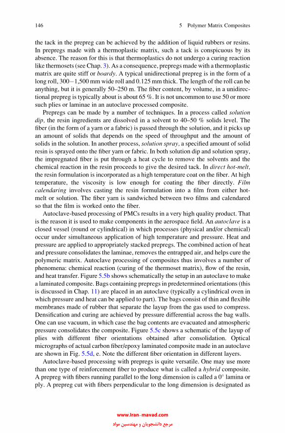
the tack in the prepreg can be achieved by the addition of liquid rubbers or resins.

In prepregs made with a thermoplastic matrix, such a tack is conspicuous by its

absence. The reason for this is that thermoplastics do not undergo a curing reaction

like thermosets (see Chap. 3). As a consequence, prepregsmadewith a thermoplastic

matrix are quite stiff or boardy. A typical unidirectional prepreg is in the form of a

long roll, 300�1,500 mmwide roll and 0.125mm thick. The length of the roll can be

anything, but it is generally 50–250 m. The fiber content, by volume, in a unidirec-

tional prepreg is typically about is about 65 %. It is not uncommon to use 50 or more

such plies or laminae in an autoclave processed composite.

Prepregs can be made by a number of techniques. In a process called solutiondip, the resin ingredients are dissolved in a solvent to 40–50 % solids level. The

fiber (in the form of a yarn or a fabric) is passed through the solution, and it picks up

an amount of solids that depends on the speed of throughput and the amount of

solids in the solution. In another process, solution spray, a specified amount of solid

resin is sprayed onto the fiber yarn or fabric. In both solution dip and solution spray,

the impregnated fiber is put through a heat cycle to remove the solvents and the

chemical reaction in the resin proceeds to give the desired tack. In direct hot-melt,the resin formulation is incorporated as a high temperature coat on the fiber. At high

temperature, the viscosity is low enough for coating the fiber directly. Filmcalendaring involves casting the resin formulation into a film from either hot-

melt or solution. The fiber yarn is sandwiched between two films and calendared

so that the film is worked onto the fiber.

Autoclave-based processing of PMCs results in a very high quality product. That

is the reason it is used to make components in the aerospace field. An autoclave is aclosed vessel (round or cylindrical) in which processes (physical and/or chemical)

occur under simultaneous application of high temperature and pressure. Heat and

pressure are applied to appropriately stacked prepregs. The combined action of heat

and pressure consolidates the laminae, removes the entrapped air, and helps cure the

polymeric matrix. Autoclave processing of composites thus involves a number of

phenomena: chemical reaction (curing of the thermoset matrix), flow of the resin,

and heat transfer. Figure 5.5b shows schematically the setup in an autoclave to make

a laminated composite. Bags containing prepregs in predetermined orientations (this

is discussed in Chap. 11) are placed in an autoclave (typically a cylindrical oven in

which pressure and heat can be applied to part). The bags consist of thin and flexible

membranes made of rubber that separate the layup from the gas used to compress.

Densification and curing are achieved by pressure differential across the bag walls.

One can use vacuum, in which case the bag contents are evacuated and atmospheric

pressure consolidates the composite. Figure 5.5c shows a schematic of the layup of

plies with different fiber orientations obtained after consolidation. Optical

micrographs of actual carbon fiber/epoxy laminated composite made in an autoclave

are shown in Fig. 5.5d, e. Note the different fiber orientation in different layers.

Autoclave-based processing with prepregs is quite versatile. One may use more

than one type of reinforcement fiber to produce what is called a hybrid composite.

A prepreg with fibers running parallel to the long dimension is called a 0� lamina or

ply. A prepreg cut with fibers perpendicular to the long dimension is designated as



http://dx.doi.org/10.1007/978-0-387-74365-3_3

http://dx.doi.org/10.1007/978-0-387-74365-3_11

Fig. 5.5 (a) Schematic of a prepreg. (b) Setup in an autoclave to make a laminated composite.

(c) Layup of plies with different fiber orientations. (d) Micrograph of carbon fiber/epoxy laminated

composite made in an autoclave. (e) A higher magnification picture of (e). Note the different fiber

orientation in different layers


a 90� lamina, while a prepreg with fibers running at an intermediate angle y is

designated a y-ply. The exact orientation sequence of plies in the laminate

is determined from theory of elasticity (see Chap. 11) to obtained appropriate

magnitudes and directions of stress and to avoid unwanted twisting and/or torsion.

Such laminate construction, mostly done by hand, can result in high fiber volume

fractions (60–65 %). A nice example of an autoclave, one the largest in the world

which is used to make the wings of the Boeing 787 plane is shown in Fig. 5.6.

An idea of the physical dimensions can be had from the man standing in the

cylindrical body of the autoclave. One of the end pieces is shown on the left hand

side in the picture.

5.1.2 Thermoplastic Matrix Composites

Thermoplastic matrix composites have several advantages and disadvantages over

thermoset matrix composites. We first list these and then we will describe some of

the important processes used to form thermoplastic matrix composites.

The advantages of thermoplastic matrix composites include:

• Refrigeration is not necessary with a thermoplastic matrix.

• Parts can be made and joined by heating.

• Parts can be remolded, and any scrap can be recycled.

Fig. 5.6 A large autoclave that is used to make the wings of Boeing 787. An idea of the size of the

autoclave can be had from the height of the person standing inside the autoclave (courtesy of ASC

Process Systems Inc., Sylmar, California)



http://dx.doi.org/10.1007/978-0-387-74365-3_11

• Thermoplastics have better toughness and impact resistance than thermosets.

This can generally also be translated into thermoplastic matrix composites.

The disadvantages include:

• The processing temperatures are generally higher than those with thermosets.

• Thermoplastics are stiff and boardy, i.e., they lack the tackiness of the partially

cured epoxies.

A good quality laminate must be void-free. This implies that there must be

sufficient flow of the thermoplastic matrix between layers as well as within individ-

ual tows. Generally, a pressure of 6–12 MPa, a temperature between 275 and

350 �C, and dwell times of up to 30 min are appropriate for thermoplastics such

as polysulfones and polyetheretherketone (PEEK). Because no time is needed for

any curing reaction, the time length of the molding cycle with a thermoplastic

matrix is less than that with a thermoset matrix.

A brief description of processing methods for thermoplastic matrix composites

follows.

5.1.2.1 Film Stacking

Laminae of thermoplastic matrix containing fibers with very low resin content (~15

w/o) are used in this process. Low resin content is used because these are very

boardy materials. The laminae are stacked alternately with thin films of pure

polymer matrix material. This stack of laminae consists of fibers impregnated

with insufficient matrix and polymer films of complementary weight to give the

desired fiber volume fraction in the end product. These are then consolidated by

simultaneous application of heat and pressure.

The impregnation of thermoplastic matrix takes place under the simultaneous

application of heat and pressure; the magnitude of pressure and temperature must be

sufficient to force the polymeric melt to flow into and through the reinforcement

preform. The rate of penetration of a fluid into the fibrous preform structure is

described by Darcy’s law (see Sect. 5.1.1.4). Darcy’s law says that flow rate is

directly proportional to the applied pressure and inversely proportional to the

viscosity. Thus, increasing the applied pressure and decreasing the viscosity of the

molten polymer (i.e., increasing the temperature) helps in the processing.

5.1.2.2 Diaphragm Forming

This process involves the sandwiching of freely floating thermoplastic prepreg

layers between two diaphragms (Cogswell 1992). The air between the diaphragms

is evacuated and thermoplastic laminate is heated above the melting point of the

matrix. Pressure is applied to one side, which deforms the diaphragms and makes

them take the shape of the mold. The laminate layers are freely floating and very



flexible above the melting point of the matrix, thus they readily conform to the mold

shape. After the completion of the forming process, the mold is cooled, the

diaphragms are stripped off, and the composite is obtained. One of the advantages

of this technique is that components with double curvatures can be formed. The

diaphragms are the key to the forming process, and their stiffness is a very critical

parameter. Compliant diaphragms do the job for simple components. For very

complex shapes requiring high molding pressures, stiff diaphragms are needed.

At high pressures, a significant transverse squeezing flow can result, and this can

produce undesirable thickness variations in the final composite.

5.1.2.3 Thermoplastic Tape Laying

Thermoplastic tape laying machines are also available, although they are not as

common as the thermosetting tape laying machines. Figure 5.7 shows the schematic

of one such machine. A controllable tape head has the tape dispensing and shim

dispensing/take-up reels and heating shoes. The hot head dispenses thermoplastic

tape from a supply reel. There are three heating and two cooling/compaction shoes.

The hot shoes heat the tape to molten state. The cold shoes cool the tape instantly to

a solid state.

5.1.2.4 Commingled Fibers

The thermoplastic matrix can be provided in the form of a fiber. The matrix fiber

and the reinforcement fiber are commingled to produce a yarn that is a blend of the

thermoplastic matrix and reinforcement yarn. Such a commingled yarn can be

Fig. 5.7 Schematic of a thermoplastic tape laying machine (courtesy of Cincinnati Milacron)



woven, knit, or filament wound. The yarn formed into the appropriate shape is then

subjected to heat and pressure to melt the thermoplastic matrix component, wet out

the reinforcement fibers, and obtain a composite.

There are many commingled fibers available commercially for processing into a

composite. As examples, we cite the following. Vectran is the trade name of a liquid

crystal thermoplastic aromatic polyester fiber. The multifilament yarn is produced

by melt spinning. It has a low melting point, and thus when commingled with a

reinforcement fiber, it can provide the matrix component in the composite. It is

available in the form of multifilament yarn that can be commingled with glass or

other reinforcement fibers. Twintex is another commercial name that involves

commingled polypropylene fibers and glass fibers.

5.1.2.5 Thermoforming and Injection Molding

As pointed out earlier, thermoplastics soften on heating, and therefore melt flow

techniques of forming can be used. Such techniques include injection molding,

extrusion, and thermoforming. Thermoforming involves the production of a sheet,

which is heated and stamped, followed by vacuum or pressure forming. Generally,

discontinuous fibrous (principally glass) reinforcement is used, which results in an

increase of melt viscosity. Short fiber reinforced thermoplastic resin composites can

also be produced by a method called reinforced reaction injection molding (RRIM)

(Lockwood and Alberino 1981). RRIM is actually an extension of the reactioninjection molding (RIM) of polymers. In RIM, two liquid components are pumped

at high speeds and pressures into a mixing head and then into a mold where the two

components react to polymerize rapidly. An important example is a urethane RIM

polymer. In RRIM, short fibers (or fillers) are added to one or both of the

components. The equipment for RRIM must be able to handle rather abrasive

slurries. The fiber lengths that can be handled are generally short, owing to viscosity

limitations. Because a certain minimum length of fiber, called the critical length

(see Chap. 10), is required for effective fiber reinforcement, more often than not

RRIM additives are fillers rather than reinforcements. Most RIM and RRIM

applications are in the automotive industry.

5.1.2.6 Long Fiber Thermoplastic Compression Molding

The most common way of making thermoplastic composites involves mixing of

short length of fibers (about 2–3 mm or less) with a thermoplastic matrix and

injection molding the composite (see above). The properties of these short fiber

reinforced composites are better than those of the unreinforced matrix material, but

the full potential of the reinforcing fiber is not achieved. We treat the important

subject of critical length of fiber for load transfer in Chap. 10. Suffice it here to state

that increasing the length of fibers to greater than 10 mm would result in

improvements in a variety of properties of the composites. In the literature the



http://dx.doi.org/10.1007/978-0-387-74365-3_10

http://dx.doi.org/10.1007/978-0-387-74365-3_11

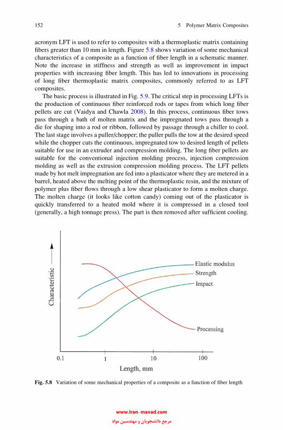
acronym LFT is used to refer to composites with a thermoplastic matrix containing

fibers greater than 10 mm in length. Figure 5.8 shows variation of some mechanical

characteristics of a composite as a function of fiber length in a schematic manner.

Note the increase in stiffness and strength as well as improvement in impact

properties with increasing fiber length. This has led to innovations in processing

of long fiber thermoplastic matrix composites, commonly referred to as LFT

composites.

The basic process is illustrated in Fig. 5.9. The critical step in processing LFTs is

the production of continuous fiber reinforced rods or tapes from which long fiber

pellets are cut (Vaidya and Chawla 2008). In this process, continuous fiber tows

pass through a bath of molten matrix and the impregnated tows pass through a

die for shaping into a rod or ribbon, followed by passage through a chiller to cool.

The last stage involves a puller/chopper; the puller pulls the tow at the desired speed

while the chopper cuts the continuous, impregnated tow to desired length of pellets

suitable for use in an extruder and compression molding. The long fiber pellets are

suitable for the conventional injection molding process, injection compression

molding as well as the extrusion compression molding process. The LFT pellets

made by hot melt impregnation are fed into a plasticator where they are metered in a

barrel, heated above the melting point of the thermoplastic resin, and the mixture of

polymer plus fiber flows through a low shear plasticator to form a molten charge.

The molten charge (it looks like cotton candy) coming out of the plasticator is

quickly transferred to a heated mold where it is compressed in a closed tool

(generally, a high tonnage press). The part is then removed after sufficient cooling.

Fig. 5.8 Variation of some mechanical properties of a composite as a function of fiber length



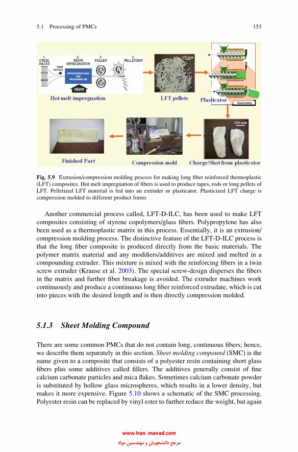
Another commercial process called, LFT-D-ILC, has been used to make LFT

composites consisting of styrene copolymers/glass fibers. Polypropylene has also

been used as a thermoplastic matrix in this process. Essentially, it is an extrusion/

compression molding process. The distinctive feature of the LFT-D-ILC process is

that the long fiber composite is produced directly from the basic materials. The

polymer matrix material and any modifiers/additives are mixed and melted in a

compounding extruder. This mixture is mixed with the reinforcing fibers in a twin

screw extruder (Krause et al. 2003). The special screw-design disperses the fibers

in the matrix and further fiber breakage is avoided. The extruder machines work

continuously and produce a continuous long fiber reinforced extrudate, which is cut

into pieces with the desired length and is then directly compression molded.

5.1.3 Sheet Molding Compound

There are some common PMCs that do not contain long, continuous fibers; hence,

we describe them separately in this section. Sheet molding compound (SMC) is the

name given to a composite that consists of a polyester resin containing short glass

fibers plus some additives called fillers. The additives generally consist of fine

calcium carbonate particles and mica flakes. Sometimes calcium carbonate powder

is substituted by hollow glass microspheres, which results in a lower density, but

makes it more expensive. Figure 5.10 shows a schematic of the SMC processing.

Polyester resin can be replaced by vinyl ester to further reduce the weight, but again

Fig. 5.9 Extrusion/compression molding process for making long fiber reinforced thermoplastic

(LFT) composites. Hot melt impregnation of fibers is used to produce tapes, rods or long pellets of

LFT. Pelletized LFT material is fed into an extruder or plasticator. Plasticized LFT charge is

compression molded to different product forms



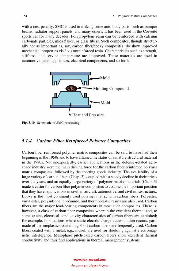
with a cost penalty. SMC is used in making some auto body parts, such as bumper

beams, radiator support panels, and many others. It has been used in the Corvette

sports car for many decades. Polypropylene resin can be reinforced with calcium

carbonate particles, mica flakes, or glass fibers. Such composites, though structur-

ally not as important as, say, carbon fiber/epoxy composites, do show improved

mechanical properties vis a vis unreinforced resin. Characteristics such as strength,

stiffness, and service temperature are improved. These materials are used in

automotive parts, appliances, electrical components, and so forth.

5.1.4 Carbon Fiber Reinforced Polymer Composites

Carbon fiber reinforced polymer matrix composites can be said to have had their

beginning in the 1950s and to have attained the status of a mature structural material

in the 1980s. Not unexpectedly, earlier applications in the defense-related aero-

space industry were the main driving force for the carbon fiber reinforced polymer

matrix composites, followed by the sporting goods industry. The availability of a

large variety of carbon fibers (Chap. 2), coupled with a steady decline in their prices

over the years, and an equally large variety of polymer matrix materials (Chap. 3)

made it easier for carbon fiber polymer composites to assume the important position

that they have: applications in civilian aircraft, automotive, and civil infrastructure..

Epoxy is the most commonly used polymer matrix with carbon fibers. Polyester,

vinyl ester, polysulfone, polyimide, and thermoplastic resins are also used. Carbon

fibers are the major load-bearing components in most such composites. There is,

however, a class of carbon fiber composites wherein the excellent thermal and, to

some extent, electrical conductivity characteristics of carbon fibers are exploited;

for example, in situations where static electric charge accumulation occurs, parts

made of thermoplastics containing short carbon fibers are frequently used. Carbon

fibers coated with a metal, e.g., nickel, are used for shielding against electromag-

netic interference. Mesophase pitch-based carbon fibers show excellent thermal

conductivity and thus find applications in thermal management systems.

Fig. 5.10 Schematic of SMC processing



http://dx.doi.org/10.1007/978-0-387-74365-3_2

http://dx.doi.org/10.1007/978-0-387-74365-3_3

5.2 Interface in PMCs

We provide below a summary of some important features of the interface region in

PMCs with glass, carbon, aramid, and polyethylene fibers.

5.2.1 Glass Fiber/Polymer

The reader would recall from the description given in Chaps. 2 and 3 that inorganic,

silica-based glasses are analogous to many organic polymers in that they are

amorphous. Recall also that pure, crystalline silica melts at 1,800 �C and can be

worked in the range of 1,600–1,800 �C. However, by adding some metal oxides,

one can break the Si–O bonds and obtain a series of amorphous glasses with low

glass transition temperatures so that they can be processed at much lower

temperatures than pure silica. In general, the atomic or molecular arrangement in

any material is different at the surface than in the interior. In particular, in the case

of silica-based glasses containing a variety of oxides, a complex hydroxyl layer is

formed rather easily. Nonhygroscopic oxides absorb water as hydroxyl groups

while hygroscopic oxides become hydrated. The activity of a glass surface is thus

a function of the hydroxyl content and the cations just below the surface. That is, the

surface activity of E-glass will be different from that of fused silica. Invariably,

glass fibers are surface treated by applying a size on the freshly drawn glass fibers toprotect them from the environment, for handling ease, and to avoid introducing

surface defects. Common sizes are starch gum, hydrogenated vegetable oil, gelatin,

polyvinyl alcohol (PVA), and a variety of nonionic emulsifiers. The size is gener-

ally incompatible with the matrix resin and is therefore removed before putting the

glass fibers in a resin matrix by heat cleaning at ~350 �C for 15–20 h in air, followed

by washing with detergent or solvent and drying. After cleaning, organometallic or

organosilane coupling agents are applied; an aqueous solution of silane is com-

monly used for this purpose. The organosilane compounds have the chemical

formula

R� Si� X3;

where R is a resin-compatible group and X represents groups capable of interacting

with hydroxylated silanols on the glass surface. Typically, a silane coupling agent

will have the following general chemical structure:

X3Si CH2ð ÞnY;

where n can have a value between 0 and 3, X is a hydrolyzable group on silicon, and

Y is an organofunctional group that is resin-compatible. Silane coupling agents are

generally applied to glass from an aqueous solution. Hydrolyzable groups are

5.2 Interface in PMCs 155


http://dx.doi.org/10.1007/978-0-387-74365-3_2

http://dx.doi.org/10.1007/978-0-387-74365-3_3

essential for generating intermediate silanols. Examples of coupling agents

commonly used are organometallic or organosilane complexes. It is thought by

some researchers (Knox 1982) that the coupling agents create a chemical bridge

between the glass surface and the resin matrix. Other researchers (Kardos 1985) do

not subscribe to this view.

The chemical bridge theory goes as follows. Silane molecules, as mentioned

earlier, are multifunctional groups with a general chemical formula of R–SiX3,

where X stands for hydrolyzable groups bonded to Si. For example, X can be an

ethoxy group—OC2H5—and R is a resin-compatible group. They are hydrolyzed in

aqueous size solutions to give trihydroxy silanols (Fig. 5.11a). These trihydroxy

silanols get attached to hydroxyl groups at the glass surface by means of hydrogen

bonding (Fig. 5.11b). During the drying of sized glass fibers, water is removed and a

condensation reaction occurs between silanol and the glass surface and between

adjacent silanol molecules on the glass surface, leading to a polysiloxane layer

bonded to the glass surface (Fig. 5.11c). Now we can see that the silane coating is

anchored at one end, through the R group, to the uncured epoxy or polyester matrix,

and at the other end to the glass fiber through the hydrolyzed silanol groups.

On curing, the functional groups R either react with the resin or join the resin

molecular network (Fig. 5.11d).

Appealing though this chemical bridge model of silane coupling is, there are

certain shortcomings. The interface model shown in Fig. 5.11d will result in such a

Fig. 5.11 Chemical bridge theory of a silane coupling agent: (a) hydrolysis of silane to silanol; (b)

hydrogen bonding between hydroxy groups of silanol and a glass surface; (c) polysiloxane bonded

to a glass surface; and (d) resin-compatible functional groups R form part of the polymer matrix

[from Hull (1981), reprinted with permission]



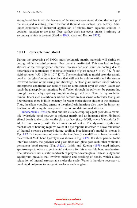
strong bond that it will fail because of the strains encountered during the curing of

the resin and resulting from differential thermal contraction (see below). Also,

under conditions of industrial application of silanes from aqueous solution, a

covalent reaction to the glass fiber surface does not occur unless a primary or

secondary amine is present (Kardos 1985; Kaas and Kardos 1971).

5.2.1.1 Reversible Bond Model

During the processing of PMCs, most polymeric matrix materials will shrink on

curing, while the reinforcement fiber remains unaffected. This can lead to large

stresses at the fiber/polymer interface. Stresses can also result on cooling due to

differences in coefficients of thermal expansion of glass (about 5 � 10�6 K�1) and

rigid polymer (~50–100 � 10�6 K�1). The chemical bridge model provides a rigid

bond at the glass/polymer interface that will not be able to withstand the strains

involved because of the curing and shrinkage. A clean glass surface under ordinary

atmospheric conditions can readily pick up a molecular layer of water. Water can

reach the glass/polymer interface by diffusion through the polymer, by penetrating

through cracks or by capillary migration along the fibers. Note that hydrophobic

mineral fibers such as carbon or silicon carbide are less sensitive to water than glass

fiber because there is little tendency for water molecules to cluster at the interface.

Thus, the silane coupling agents at the glass/resin interface also have the important

function of allowing the composite to accommodate internal stresses.

Plueddemann (1974) pointed out that a silane coupling agent provides a revers-

ible hydrolytic bond between a polymer matrix and an inorganic fiber. Hydrated

silanol bonds to the oxides on the glass surface, (i.e., –MOH, whereM stands for Si,

Al, Fe, and so on), with the elimination of water. The dynamic equilibrium

mechanism of bonding requires water at a hydrophilic interface to allow relaxation

of thermal stresses generated during cooling. Plueddemann’s model is shown in

Fig. 5.12. In the presence of water at the interface (it can diffuse in from the resin),

the covalent M–O bond hydrolyzes as shown in Fig. 5.12a. If a shear parallel to the

interface occurs, the polymer and glass fiber can glide past each other without a

permanent bond rupture (Fig. 5.12b). Ishida and Koenig (1978) used infrared

spectroscopy to obtain experimental evidence for this reversible bond mechanism.

The interface is not a static sandwich of polymer–water–glass. Instead, a dynamic

equilibrium prevails that involves making and breaking of bonds, which allows

relaxation of internal stresses at a molecular scale. Water is therefore necessary to

bond rigid polymers to inorganic surfaces such as glass.



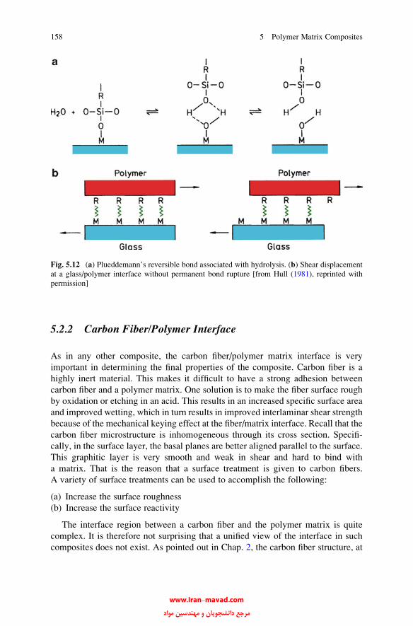
5.2.2 Carbon Fiber/Polymer Interface

As in any other composite, the carbon fiber/polymer matrix interface is very

important in determining the final properties of the composite. Carbon fiber is a

highly inert material. This makes it difficult to have a strong adhesion between

carbon fiber and a polymer matrix. One solution is to make the fiber surface rough

by oxidation or etching in an acid. This results in an increased specific surface area

and improved wetting, which in turn results in improved interlaminar shear strength

because of the mechanical keying effect at the fiber/matrix interface. Recall that the

carbon fiber microstructure is inhomogeneous through its cross section. Specifi-

cally, in the surface layer, the basal planes are better aligned parallel to the surface.

This graphitic layer is very smooth and weak in shear and hard to bind with

a matrix. That is the reason that a surface treatment is given to carbon fibers.

A variety of surface treatments can be used to accomplish the following:

(a) Increase the surface roughness

(b) Increase the surface reactivity

The interface region between a carbon fiber and the polymer matrix is quite

complex. It is therefore not surprising that a unified view of the interface in such

composites does not exist. As pointed out in Chap. 2, the carbon fiber structure, at

Fig. 5.12 (a) Plueddemann’s reversible bond associated with hydrolysis. (b) Shear displacement

at a glass/polymer interface without permanent bond rupture [from Hull (1981), reprinted with

permission]



http://dx.doi.org/10.1007/978-0-387-74365-3_2

submicrometer level, is not homogeneous through its cross section. The orientation

of the basal planes depends on the precursor fiber and processing conditions.

In particular, the so-called onion-skin structure is frequently observed in PAN-

based fibers, wherein basal planes in a thin surface layer are aligned parallel to the

surface while the basal planes in the core are less well-aligned. Figure 5.13 shows

the structure of a carbon fiber/epoxy composite (Diefendorf 1985). The onion-skin

zone (C in Fig. 5.13) has a very graphitic structure and is quite weak in shear. Thus,

failure is likely to occur in this thin zone. Additionally, the skin can be hard to bind

with a polymeric matrix because of the high degree of preferred orientation of the

basal planes, thus, facilitating interfacial failure (zone D). The matrix properties in

zone E (close to the interface) may be different from those of the bulk epoxy (zone

B). Carbon fibers meant for polymer reinforcement invariably receive some form of

surface treatment from the manufacturer to improve their compatibility with the

polymer matrix and their handleability. Organic sizes are commonly applied by

passing the fibers through a sizing bath. Common sizes include polyvinyl alcohol,

epoxy, polyimide, and titanate coupling agents.

Carbon fibers, especially high-modulus carbon fibers that have undergone a

high-temperature graphitization, are quite smooth. They have a rather low specific

area, varying from 0.1 to 2 m2/g. Invariably, there is a microscopic scale of

roughness; mostly as longitudinal striations (see Fig. 2.20). Carbon fibers are also

generally chemically inert; that is, interfacial interactions in carbon fiber-based

composites would be rather weak. Generally, a short beam bending test

is conducted to measure what is called interlaminar shear strength, ILSS (see

Chap. 4). Admittedly, such a test is not entirely satisfactory, but for lack of any

better, quicker, or more convenient test, the ILSS test value is taken as a measure of

bond strength.

Fig. 5.13 Schematic structure of a carbon fiber/epoxy composite showing carbon fiber, interface,

and epoxy matrix [from Diefendorf (1985), used with permission]




http://dx.doi.org/10.1007/978-0-387-74365-3_4

Ehrburger and Donnet (1980) point out that there are two principal ways of

improving interfacial bonding in carbon fiber composites: increase the fiber surface

roughness, and thus the interfacial area, and increase the surface reactivity. Many

surface treatments have been developed to obtain improved interfacial bonding

between carbon fibers and the polymer matrix (Donnet and Bansal 1984; McKee

and Mimeault 1973). A brief description of these follows.

5.2.2.1 Chemical Vapor Deposition

Silicon carbide and pyrocarbon have been deposited on carbon fibers by chemical

vapor deposition (CVD). Growing whiskers (~2 mm in diameter) on the carbon fiber

surface, called whiskerization in the literature, can result in a two- to threefold

increase of ILSS. The improvement in ILSS is mainly due to the increase in surface

area. Whiskerization involving the growth of single-crystal SiC whiskers perpen-

dicular to the fiber results in an efficient mechanical keying effect with the polymer

matrix. The CVD method of doing this is expensive, and handling of whiskerized

fibers is difficult. Although this treatment results in an increase in ILSS, there also

occurs a weakening of the fibers. Ehlert et al. (2010) have developed a solution-

based technique of growing ZnO nanorods perpendicular to the carbon fiber which

seems to be quite promising inasmuch as it is claimed not to result in a decrease in

strength while improving the interfacial strength by mechanical interlocking.

5.2.2.2 Oxidative Etching

Treating carbon fibers with several surface-oxidation agents leads to significant

increases in the ILSS of composites. This is because the oxidation treatment

increases the fiber surface area and the number of surface groups (Ehrburger

and Donnet 1980). Figure 5.14 shows a linear relationship between the fiber

surface roughness as measured by AFM and interlaminar shear strength in a series

of carbon fiber/epoxy composites (Jangehud et al. 1993). Yet another reason for

increased ILSS may be the removal of surface defects, such as pores, weakly

bonded carbon debris, and impurities (Donnet and Bansal 1984). Oxidation

treatments can be carried out by a gaseous or a liquid phase. Gas phase oxidation

can be done with air or oxygen diluted with an inert gas (Clark et al. 1974). Gas

flow rates and the temperature are the important parameters in this process.

Oxidation results in an increase in the fiber surface roughness by pitting and

increased longitudinal striations (Donnet and Bansal 1984). Too high an oxidation

rate will result in nonuniform etching of the carbon fibers and a loss of fiber tensile

strength. Since oxidation results in a weight loss, we can conveniently take the

amount of weight loss as an indication of the degree of oxidation. Figure 5.15

shows ILSS vs. weight loss for high-strength and high-modulus carbon fiber



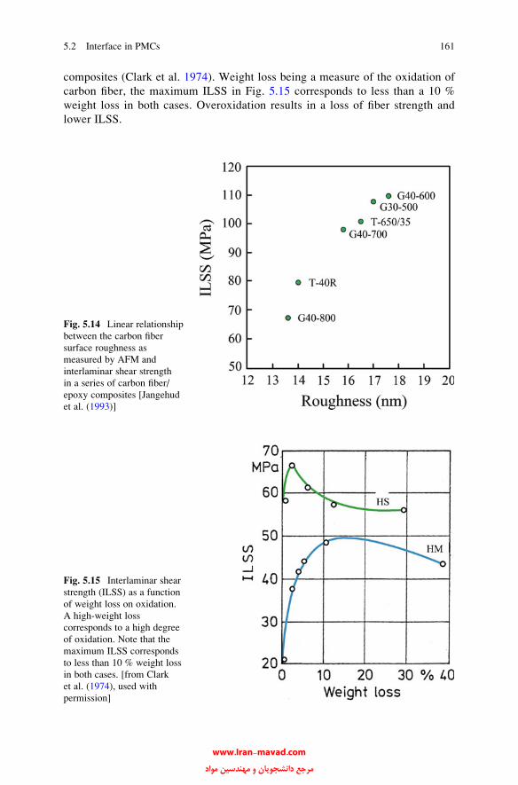
composites (Clark et al. 1974). Weight loss being a measure of the oxidation of

carbon fiber, the maximum ILSS in Fig. 5.15 corresponds to less than a 10 %

weight loss in both cases. Overoxidation results in a loss of fiber strength and

lower ILSS.

Fig. 5.14 Linear relationship

between the carbon fiber

surface roughness as

measured by AFM and

interlaminar shear strength

in a series of carbon fiber/

epoxy composites [Jangehud

et al. (1993)]

Fig. 5.15 Interlaminar shear

strength (ILSS) as a function

of weight loss on oxidation.

A high-weight loss

corresponds to a high degree

of oxidation. Note that the

maximum ILSS corresponds

to less than 10 % weight loss

in both cases. [from Clark


permission]



5.2.2.3 Liquid Phase Oxidation

Liquid phase oxidation involves treatments in nitric acid, sodium hypochlorite,

potassium permanganate, and anodic etching (Donnet and Bansal 1984). Liquid

phase oxidation by nitric acid and sodium hypochlorite results in an increase in the

interfacial area and formation of oxygenated surface groups due to fiber etching.

Wetting of the carbon fibers by the polymer is enhanced by these changes.

Graphitic oxides are lamellar compounds having large amounts of hydroxylic

and carboxylic groups. The formation of a graphitic oxide layer increases the

number of acidic groups on the carbon fibers.

Anodic etching or electrochemical oxidation using dilute nitric acid or dilute

sodium hydroxide solutions results in no significant decrease in tensile strength of

the carbon fibers, according to Ehrburger and Donnet (1980). The fiber weight loss

is less than 2 % and no great change in surface area or fiber roughness occurs, the

major change being an increase in the acidic surface groups. Oxidative treatments

produce functional groups (e.g., –CO2H, –C–OH, and –C¼O) on carbon fiber

surfaces. They form at the edges of basal planes and at defects. These functional

groups form chemical bonds with unsaturated resins.

According to Drzal et al. (1983a, b) various carbon fiber surface treatments

promote adhesion to epoxy materials through a two-pronged mechanism: (a) the

surface treatment removes a weak outer layer that is present initially on the fiber

and (b) chemical groups are added to the surface which increase interaction with the

matrix. When a fiber finish is applied, according to Drzal and coworkers, the effect

is to produce a brittle but high modulus interphase layer between the fiber and the

matrix. As amine content is reduced, the modulus of epoxy goes up accompanied by

lower fracture strength and strain. That is, the interphase being created between the

fiber and the matrix has high modulus but low toughness. This promotes matrix

fracture as opposed to interfacial fracture.

5.2.2.4 Aramid Fiber/Polymer Interface

Most polymers show rather poor adhesion to aramid fibers. This is evidenced by the

generally poor interlaminar shear strength and transverse tensile strength values

obtained with aramid reinforced PMCs. Typically, aramid/epoxy interfacial

strengths are about half of the interfacial strengths of glass/epoxy or carbon/

epoxy composites. A highly oriented chain microstructure and skin/core hetero-

geneity are responsible for this low, poor interfacial strength. This may not be a

disadvantage in aramid/polymer composites used to make impact-resistant items

such as helmets or body armor, where ease of delamination may be an advantage

from a toughness point of view. However, in high-strength and high-stiffness

composites, poor interfacial adhesion can be a disadvantage. Various fiber surface

treatments have been tried to alleviate this problem. Among these are the following:

• Bromine water treatment. This also results in reduced fiber strength.



• Silane coupling agents developed for glass fibers.

• Isocyanate-linked polymer.

• Treatment with reactive chemicals such as acetic acid anhydride, methacrylol

chloride, sulfuric acid, among others. Such treatments, however, result in a

decrease in the tensile strength of aramid fiber and that of aramid/polyester

composites attributable to etching of the aramid fiber.

• Acid (HCl, H2SO4) or base (NaOH) hydrolysis of aramid fiber yields reactive

terminal amino groups to which diepoxide molecules could attach.

• Plasma treatment in vacuum, ammonia, or argon. Plasma treatment in ammonia

increases the amine concentration on the fiber surface, which is thought to lead

to covalent bonding at the interface. An increase in nitrogen content in the form

of amine groups is accompanied by a decrease in oxygen content with increasing

exposure time.

5.2.3 Polyethylene Fiber/Polymer Interface

Ultrahigh-molecular-weight polyethylene (UHMWPE) fiber is another chemically

very inert fiber, and therefore it does not adhere very well to polymeric matrix

materials. High-modulus polyethylene fibers such as Spectra or Dyneema are hard

to bond with any polymeric matrix. Some kind of surface treatment must be given

to the polyethylene fiber to bond with resins such as epoxy, PMMA. By far the most

successful surface treatment involves a cold gas (such as air, ammonia, or argon)

plasma (Kaplan et al. 1988). A plasma consists of gas molecules in an excited state,

i.e., highly reactive, dissociated molecules. When the polyethylene, or any other

fiber, is treated with a plasma, surface modification occurs by removal of any

surface contaminants and highly oriented surface layers, addition of polar and

functional groups on the surface, and introduction of surface roughness, all these

factors contribute to an enhanced fiber/matrix interfacial strength (Biro et al. 1992;

Brown et al. 1992; Hild and Schwartz 1992a, b; Kaplan et al. 1988; Li et al. 1992).

An exposure of just a few minutes to the plasma is sufficient to do the job.

In a UHMWPE fiber/epoxy composite, a plasma treatment of fiber resulted in an

increase in fiber surface roughness and an increased bonding area and interfacial

shear strength (Kaplan et al. 1988; Biro et al. 1992). In another work (Brown et al.

1992), it was shown that chemical etching of UHMWPE fibers resulted in more

than a sixfold increase in interfacial shear strength of UHMWPE/epoxy composites.

Chemical treatment with chromic acid and plasma etching in the presence of

oxygen are two treatments that are commonly used to modify the surface

characteristics of polyethylene fiber with a view to improve their adhesion to

polymeric matrix materials.



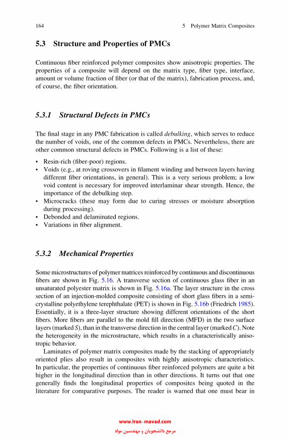
5.3 Structure and Properties of PMCs

Continuous fiber reinforced polymer composites show anisotropic properties. The

properties of a composite will depend on the matrix type, fiber type, interface,

amount or volume fraction of fiber (or that of the matrix), fabrication process, and,

of course, the fiber orientation.

5.3.1 Structural Defects in PMCs

The final stage in any PMC fabrication is called debulking, which serves to reduce

the number of voids, one of the common defects in PMCs. Nevertheless, there are

other common structural defects in PMCs. Following is a list of these:

• Resin-rich (fiber-poor) regions.

• Voids (e.g., at roving crossovers in filament winding and between layers having

different fiber orientations, in general). This is a very serious problem; a low

void content is necessary for improved interlaminar shear strength. Hence, the

importance of the debulking step.

• Microcracks (these may form due to curing stresses or moisture absorption

during processing).

• Debonded and delaminated regions.

• Variations in fiber alignment.

5.3.2 Mechanical Properties

Somemicrostructures of polymermatrices reinforced by continuous and discontinuous

fibers are shown in Fig. 5.16. A transverse section of continuous glass fiber in an

unsaturated polyester matrix is shown in Fig. 5.16a. The layer structure in the cross

section of an injection-molded composite consisting of short glass fibers in a semi-

crystalline polyethylene terephthalate (PET) is shown in Fig. 5.16b (Friedrich 1985).

Essentially, it is a three-layer structure showing different orientations of the short

fibers. More fibers are parallel to the mold fill direction (MFD) in the two surface

layers (marked S), than in the transverse direction in the central layer (markedC). Notethe heterogeneity in the microstructure, which results in a characteristically aniso-

tropic behavior.

Laminates of polymer matrix composites made by the stacking of appropriately

oriented plies also result in composites with highly anisotropic characteristics.

In particular, the properties of continuous fiber reinforced polymers are quite a bit

higher in the longitudinal direction than in other directions. It turns out that one

generally finds the longitudinal properties of composites being quoted in the

literature for comparative purposes. The reader is warned that one must bear in



Fig. 5.16 (a) Continuous glass fibers in a polyester matrix showing resin-rich regions.

(b) Discontinuous glass fibers in a semicrystalline polyethylene terephthalate thermoplastic matrix

showing anisotropic distribution of fibers. MFD denotes the mold fill direction. S and C denote the

surface and central layers, respectively [from Friedrich (1985), used with permission]

5.3 Structure and Properties of PMCs 165


mind this discrepancy when comparing such data of highly anisotropic materials

with the data of isotropic materials such as common polycrystalline materials.

Besides, composites containing aramid and polyethylene fibers will not have such

attractive properties in compression in the longitudinal direction. A summary of

some important characteristics of PMCs is presented in Tables 5.1 and 5.2.

Most thermoset matrix composites show essentially elastic behavior right up to

fracture, i.e., there is no yield point or plasticity. The strain-to-failure values are

rather low, typically, less than 0.5 %. Consequently, the work done during fracture

is also small. This has some very practical implications for the design engineer, viz.,

he or she cannot bank on any local yielding in such composites to take care of stress

concentrations.

In general, the continuous fiber reinforced composites will be stiff and strong

along the fiber axis, but off-angle these properties fall rather sharply. Typically, in a

unidirectional PMC, the fiber volume fraction can be 65 %. In composites having

fibers aligned bidirectionally, this value can fall to 50 %, while in a composite

containing in-plane random distribution of fibers, the volume fraction will rarely be

more than 30 %. As a general rule-of-thumb, we can take the Young’s modulus of

the composite in the longitudinal direction to be given by the following rule-of-

mixtures relationship

Ecl ¼ EfVf þ EmVm;

where E and V denote the Young’s modulus and the volume fraction of a compo-

nent and the subscripts c, f, m, and l indicate composite, fiber, matrix, and

the longitudinal direction, respectively. From the data provided in Chap. 2 on the

mechanical properties of fibers, the reader can easily verify that glass fiber/polymer

will only give a modest increase in modulus. However, aramid, polyethylene, and

carbon fiber reinforced polymer composites will show a significant increase in

modulus. Aramid fiber/polymer composites are likely to show higher creep rate

than glass/polymer composites. Aramid fiber has superior impact characteristics,

therefore, aramid fiber-based polymer composites will show good ballistic resis-

tance, and impact resistance in general. Similar observations can be made regarding

strength characteristics of the other polymer matrix composites. As should be clear

to the reader, these properties are highly dependent on the fiber properties.

5.3.2.1 Damping Characteristics

Damping in material has to do with dissipation of vibrations. High damping or the

ability to reduce vibrations can be very important in many applications; for exam-

ple, in mechanical equipment that is subject to variable speeds, resonance problems

lead to unacceptable levels of noise. Also, in sporting goods such as tennis rackets,

fishing rods, and golf clubs, it is desirable to have high damping. In a composite,

damping will depend on relative proportion of fiber and matrix, orientation of



http://dx.doi.org/10.1007/978-0-387-74365-3_2

Table

5.1

Representativeproperties

ofsomePMCsa

Materials

Density

(g/cm

3)

Tensile

modulus

Shear

modulus

(GPa)

Tensile

strength

Compressive

strength

longitudinal

(MPa)

Flexural

modulus

(GPa)

Flexural

strength

(MPa)

ILSSb

(MPa)

Longitudinal

coefficientof

thermal

expansion

(10�6K�1)

Longitudinal

(GPa)

Transverse

(GPa)

Longitudinal

(MPa)

Transverse

(MPa)

Unidirectional

Eglass

60v/o

240

10

4.5

780

28

480

35

840

40

4.5

Bidirectional

Eglass

cloth

35v/o

1.7

16.5

16.5

3280

280

100

15

220

60

11

Chopped

strandmat

Eglass

20v/o

1.4

77

2.8

100

100

120

7140

69

30

Boron60v/o

2.1

215

24.2

6.9

1,400

63

1,760

––

84

4.5

Kevlar29

60v/o

1.38

50

53

1,350

–238

51.7

535

44

–

Kevlar49

60v/o

1.38

76

5.6

2.8

1,380

30

276

70

621

60

�2.3

aThevalues

areonly

indicativeandarebased

onepoxymatrixat

room

temperatures

bILSSisinterlam

inar

shearstrength

Sou

rce:

Adaptedwithpermissionfrom

Hancox(1983)



reinforcement with respect to the axis of loading, viscoelastic characteristics of the

matrix and the reinforcement, any slipping at the interface between the matrix and

the reinforcement, and last but not least, any source of damage such as cracks or

environmental attack. In general, aramid fiber/polymer composites provide good

damping characteristics. This, of course, stems from the superior damping of

aramid fiber (see Chap. 2).

5.3.2.2 Moisture Effects in Polymer Matrix Composites

Environmental moisture can penetrate organic materials by diffusion. Typically,

moisture works as a plasticizer for a polymer, i.e., properties such as stiffness,

strength, and glass transition temperature decrease with the ingress of moisture in a

polymer. It is now well recognized that the problem of moisture absorption in

polymer matrix composites is a very important one. The maximum moisture

content under saturated condition, Mm as a function of relative humidity, is given

by the following relationship:

Mm ¼ A % relative humidityð ÞB;

where A and B are constants. The moisture content in a composite, M, can be

written as

M ¼ Mi þ G Mm �Mið Þ;

whereMi is the initial moisture content (¼ 0 for a completely dry material) and G is

a dimensionless, time-dependent parameter related to the diffusion coefficient.

Generally, one assumes that Fickian diffusion prevails, i.e., Fick’s law of diffusion

is applicable. Under conditions of Fickian diffusion, water diffuses into the

Table 5.2 Typical mechanical properties of some carbon fiber/epoxy compositesa

Property AS HMS Celion 6000 GY 70

Tensile strength (MPa) 1,850 1,150 1,650 780

Tensile modulus (GPa) 145 210 150 290–325

Tensile strain-to-fracture (%) 1.2 0.5 1.1 0.2

Compressive strength (MPa) 1,800 380 1,470 620–700

Compressive modulus (GPa) 140 110 140 310

Compressive strain-to-fracture (%) – 0.4 1.7 –

Flexural strength (4-point) (MPa) 1,800 950 1,750 790

Flexural modulus (GPa) 120 170 135 255

Interlaminar shear strength (MPa) 125 55 125 60aValues given are indicative only and are for a unidirectional composite (62 % Vf) in the

longitudinal direction

Source: Adapted with permission from Riggs et al. (1982)



http://dx.doi.org/10.1007/978-0-387-74365-3_2

laminate from the two surfaces that are in equilibrium with their surroundings, and

the parameter G is given by (Chen and Springer 1976)

G � 1� 8=p2� �

exp �p2Dt=S2� �

;

where D is the diffusion coefficient (m2/s) in the direction normal to the laminate

surface; t ¼ time (s); S ¼ h (the laminate thickness), if exposed on both sides, and

S ¼ 2 h, if exposed on one side.

A dried specimen, usually in the form of a thin sheet, is placed in a humid

environment at a constant temperature, and the mass gained is measured as a

function of time. If we plot the mass gained (say, as percentage moisture absorbed)

as a function of the square root of time, at a given temperature, we obtain a curve

with the following characteristics. After an initial linear portion (i.e.,M / ffiffit

p), the

curve assumes a plateau form in an asymptotic manner as shown in Fig. 5.17. The

slope of the linear portion can be used to determine the diffusion coefficient as

follows:

Slope ¼ M2 �M1ffiffiffiffit2

p � ffiffiffiffit1

p ¼ 4Mm

ffiffiffiffiD

p

hffiffiffip

p ;

Fig. 5.17 Schematic curve of fractional moisture absorbed as a function of the square root of time,

at a given temperature



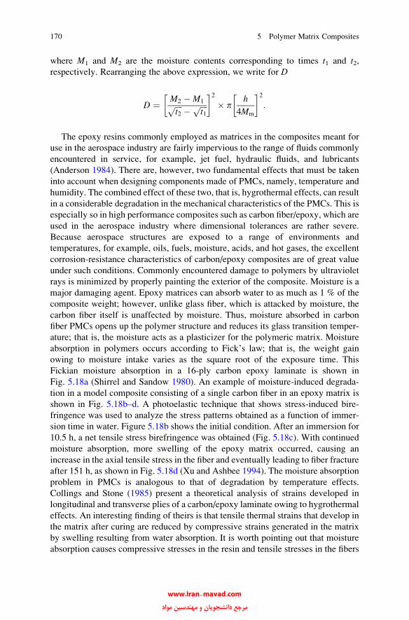
where M1 and M2 are the moisture contents corresponding to times t1 and t2,respectively. Rearranging the above expression, we write for D

D ¼ M2 �M1ffiffiffiffit2

p � ffiffiffiffit1

p� �2

� ph

4Mm

� �2:

The epoxy resins commonly employed as matrices in the composites meant for

use in the aerospace industry are fairly impervious to the range of fluids commonly

encountered in service, for example, jet fuel, hydraulic fluids, and lubricants

(Anderson 1984). There are, however, two fundamental effects that must be taken

into account when designing components made of PMCs, namely, temperature and

humidity. The combined effect of these two, that is, hygrothermal effects, can result

in a considerable degradation in the mechanical characteristics of the PMCs. This is

especially so in high performance composites such as carbon fiber/epoxy, which are

used in the aerospace industry where dimensional tolerances are rather severe.

Because aerospace structures are exposed to a range of environments and

temperatures, for example, oils, fuels, moisture, acids, and hot gases, the excellent

corrosion-resistance characteristics of carbon/epoxy composites are of great value

under such conditions. Commonly encountered damage to polymers by ultraviolet

rays is minimized by properly painting the exterior of the composite. Moisture is a

major damaging agent. Epoxy matrices can absorb water to as much as 1 % of the

composite weight; however, unlike glass fiber, which is attacked by moisture, the

carbon fiber itself is unaffected by moisture. Thus, moisture absorbed in carbon

fiber PMCs opens up the polymer structure and reduces its glass transition temper-

ature; that is, the moisture acts as a plasticizer for the polymeric matrix. Moisture

absorption in polymers occurs according to Fick’s law; that is, the weight gain

owing to moisture intake varies as the square root of the exposure time. This

Fickian moisture absorption in a 16-ply carbon epoxy laminate is shown in

Fig. 5.18a (Shirrel and Sandow 1980). An example of moisture-induced degrada-

tion in a model composite consisting of a single carbon fiber in an epoxy matrix is

shown in Fig. 5.18b–d. A photoelastic technique that shows stress-induced bire-

fringence was used to analyze the stress patterns obtained as a function of immer-

sion time in water. Figure 5.18b shows the initial condition. After an immersion for

10.5 h, a net tensile stress birefringence was obtained (Fig. 5.18c). With continued

moisture absorption, more swelling of the epoxy matrix occurred, causing an

increase in the axial tensile stress in the fiber and eventually leading to fiber fracture

after 151 h, as shown in Fig. 5.18d (Xu and Ashbee 1994). The moisture absorption

problem in PMCs is analogous to that of degradation by temperature effects.

Collings and Stone (1985) present a theoretical analysis of strains developed in

longitudinal and transverse plies of a carbon/epoxy laminate owing to hygrothermal

effects. An interesting finding of theirs is that tensile thermal strains that develop in

the matrix after curing are reduced by compressive strains generated in the matrix

by swelling resulting from water absorption. It is worth pointing out that moisture

absorption causes compressive stresses in the resin and tensile stresses in the fibers



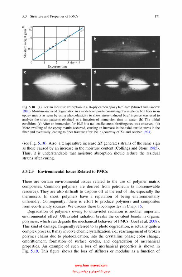
(see Fig. 5.18). Also, a temperature increase DT generates strains of the same sign

as those caused by an increase in the moisture content (Collings and Stone 1985).

Thus, it is understandable that moisture absorption should reduce the residual

strains after curing.

5.3.2.3 Environmental Issues Related to PMCs

There are certain environmental issues related to the use of polymer matrix

composites. Common polymers are derived from petroleum (a nonrenewable

resource). They are also difficult to dispose off at the end of life, especially the

thermosets. In short, polymers have a reputation of being environmentally

unfriendly. Consequently, there is effort to produce polymers and composites

from eco-friendly sources. We discuss these biocomposites in Chap. 15.

Degradation of polymers owing to ultraviolet radiation is another important

environmental effect. Ultraviolet radiation breaks the covalent bonds in organic

polymers, which can degrade the mechanical behavior of PMCs (Goel et al. 2008).

This kind of damage, frequently referred to as photo degradation, is actually quite a

complex process. It may involve chemicrystallization, i.e., rearrangement of broken

polymer chains due to photooxidation, into the crystalline phase; color change,

embrittlement, formation of surface cracks, and degradation of mechanical

properties. An example of such a loss of mechanical properties is shown in

Fig. 5.19. This figure shows the loss of stiffness or modulus as a function of

Fig. 5.18 (a) Fickian moisture absorption in a 16-ply carbon epoxy laminate (Shirrel and Sandow

1980). Moisture-induced degradation in a model composite consisting of a single carbon fiber in an

epoxy matrix as seen by using photoelasticity to show stress-induced birefringence was used to

analyze the stress patterns obtained as a function of immersion time in water. (b) The initial

condition. (c) After an immersion for 10.5 h, a net tensile stress birefringence was observed. (d)

More swelling of the epoxy matrix occurred, causing an increase in the axial tensile stress in the

fiber and eventually leading to fiber fracture after 151 h (courtesy of Xu and Ashbee 1994)



http://dx.doi.org/10.1007/978-0-387-74365-3_15

exposure to ultraviolet radiation for glass fiber reinforced polypropylene

composites. Crystallinity of PP increases with rate of oxidation (chemicrystal-

lization). Sometimes a prolonged exposure of epoxy laminates to ultraviolet radia-

tion results in a slight increase in strength, attributed to postcuring of the resin,

followed by a gradual loss of strength as a result of laminate surface degradation

(Bergmann 1984).

Hazardous air pollutants (HAPs) are generated during the curing of thermoset

polymers. These include volatile organic compounds (VOCs) and nitrogenous

oxides (commonly denoted by NOx). Certain VOCs are thought to interact

photochemically in the atmosphere and form ozone. HAPs may have long-term

adverse health effects. Sources of these during processing of PMCs include solvents

used to reduce viscosity, gases evolved, and disposal of scrap material. Commonly,

styrene is the main culprit. The government regulatory agencies such as the US

EPA have set certain regulatory limits on the emission of VOCs and HAPs.

Among the ways to reduce VOC emissions are (Sands et al. 2001): use closed

processing, accelerated curing to react or trap VOCs in the curing media, and e-

beam curing. Autoclave processing is thought to be a major source of such HAPs,

especially NOx. Nonautoclave processing would help in this regard. Substitution ofthermosets with thermoplastic is another possibility. E-beam curing of resins is

done at room temperature without any solvent; the amount of VOCs is reduced.

Fig. 5.19 Loss of stiffness or modulus as a function of exposure to ultraviolet radiation for glass

fiber reinforced polypropylene composites [from Goel et al. 2008]



5.3.2.4 Mechanical Behavior

Fracture in PMCs, as in other composites, is associated with the characteristics of

the three entities: fibers, matrix, and interface. Specifically, fiber/matrix debonding,

fiber pullout, fiber fracture, polymer crazing, and fracture of the matrix are the

energy-absorbing phenomena that can contribute to the failure process of the

composite. Of course, the debonding and pullout processes depend on the type of

interface. At low temperatures, the fracture of a PMC involves a brittle failure of the

polymeric matrix accompanied by pullout of the fibers transverse to the crack plane.

Figure 5.20a shows this kind of fracture at �80 �C in the case of a short glass fiber/

PET composite. Note the brittle fracture in the matrix. At room temperature, the

same polymeric matrix (PET) deformed locally in a plastic manner, showing

crazing (Friedrich 1985). Generally, stiffness and strength of a PMC increase

Fig. 5.20 (a) Brittle matrix fracture and fiber pullout in a short glass fiber reinforced polyethylene

terephthalate (PET) composite fractured at �80 �C [from Friedrich (1985), used with permission]

(b) Creep strains at ambient temperature for a �45� and for a 0�/90�/�45� carbon/epoxy laminate

[from Sturgeon (1978), used with permission]



with the amount of stiff and strong fibers introduced in a polymer matrix. The same

cannot be said unequivocally for the fracture toughness. The toughness of the

matrix and several microstructural factors related to the fibers and the fiber/matrix

interface have a strong influence on the fracture toughness of the composite.

Friedrich (1985) describes the fracture toughness of short fiber reinforced thermo-

plastic matrix composite in an empirical manner by a relationship of the form

Kcc ¼ MKcm

where Kcm is the fracture toughness of the matrix and M is a microstructural

efficiency factor. M can be larger than 1 and depends on fiber amount, fiber

orientation, and the fiber orientation distribution over the fracture plane, as well

as the deformation behavior of the matrix and the relative effectiveness of all the

energy-absorbing mechanisms.

Carbon fiber/epoxy composites exhibit superior properties in creep compared to

aramid/epoxy. This is because aramid fibers, similar to other polymeric fibers, creep

significantly even at quite low stresses (Eriksen 1976). Additionally, in a laminated

composite made by stacking prepregs of different fiber orientations, the ply

stacking sequence can affect the composite properties. Figure 5.20b shows tensile

creep strain at ambient temperature as a function of time for two different stacking

sequences (Sturgeon 1978). The laminate with carbon fibers at �45� shows more

creep strain than one containing plies at 0�/90�/�45�. The reason for this is that in

the �45� sequence, the epoxy matrix undergoes creep strain by tension in the

loading direction, shear in the �45� directions, and rotation of the plies in a

scissor-like action. As we shall see in Chap. 11, 0� and 90� plies do not show this

scissor-like rotation, which is a characteristic of the 45� plies. Thus, the addition of0� and 90� plies reduces the matrix shear deformation. Consequently, the creep

resistance of 0�/90�/�45� sequence is better than that of the �45� sequence.Carbon fiber reinforced PMCs generally show excellent fatigue strength.

Depending on the ply stacking arrangement, their fatigue strength (tension–tension)

may vary from 60 to 80 % of the ultimate tensile strength for lives over 107 cycles

(Baker 1983). The higher fatigue strength levels pertain to composites having more

than 50 % of the fibers in the longitudinal direction (0�), which leads to high

longitudinal stiffness and low strains. Pipes and Pagano (1970) showed that certain

stacking sequences can result in tensile stresses at the free edges, which can lead to

early local delamination effects in fatigue and consequently to lower fatigue lives.

Further discussion of these topics can be found in Chaps. 11–14.

A considerable amount of work has been done to toughen the carbon fiber

reinforced PMCs. This has involved modifying epoxies and using polymeric matrix

materials other than epoxies. Among the latter are modified bismaleimides and

some new thermoplastic materials (see also Chap. 3). The latter category includes

poly (phenylene sulfide) (PPS), polysulfones (PS), and polyetherether ketone

(PEEK), among others. PEEK, a semicrystalline polyether, combines excellent

toughness with chemical inertness. Typically, PEEK-based carbon fiber composites



http://dx.doi.org/10.1007/978-0-387-74365-3_11

http://dx.doi.org/10.1007/978-0-387-74365-3_11

http://dx.doi.org/10.1007/978-0-387-74365-3_14

http://dx.doi.org/10.1007/978-0-387-74365-3_3

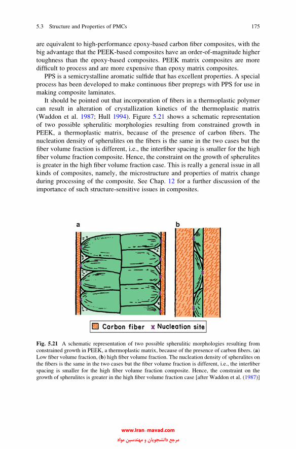
are equivalent to high-performance epoxy-based carbon fiber composites, with the

big advantage that the PEEK-based composites have an order-of-magnitude higher

toughness than the epoxy-based composites. PEEK matrix composites are more

difficult to process and are more expensive than epoxy matrix composites.

PPS is a semicrystalline aromatic sulfide that has excellent properties. A special

process has been developed to make continuous fiber prepregs with PPS for use in

making composite laminates.

It should be pointed out that incorporation of fibers in a thermoplastic polymer

can result in alteration of crystallization kinetics of the thermoplastic matrix

(Waddon et al. 1987; Hull 1994). Figure 5.21 shows a schematic representation

of two possible spherulitic morphologies resulting from constrained growth in

PEEK, a thermoplastic matrix, because of the presence of carbon fibers. The

nucleation density of spherulites on the fibers is the same in the two cases but the

fiber volume fraction is different, i.e., the interfiber spacing is smaller for the high

fiber volume fraction composite. Hence, the constraint on the growth of spherulites

is greater in the high fiber volume fraction case. This is really a general issue in all

kinds of composites, namely, the microstructure and properties of matrix change

during processing of the composite. See Chap. 12 for a further discussion of the

importance of such structure-sensitive issues in composites.

Fig. 5.21 A schematic representation of two possible spherulitic morphologies resulting from

constrained growth in PEEK, a thermoplastic matrix, because of the presence of carbon fibers. (a)

Low fiber volume fraction, (b) high fiber volume fraction. The nucleation density of spherulites on

the fibers is the same in the two cases but the fiber volume fraction is different, i.e., the interfiber

spacing is smaller for the high fiber volume fraction composite. Hence, the constraint on the

growth of spherulites is greater in the high fiber volume fraction case [after Waddon et al. (1987)]



http://dx.doi.org/10.1007/978-0-387-74365-3_12

5.4 Applications

Glass fiber reinforced polymers are used in a wide variety of industries: from

sporting goods to civil construction to aerospace. Tanks and vessels (pressure and

nonpressure) in the chemical process industry, as well as process and effluent

pipelines, are routinely made of glass fiber reinforced polyester resin. Figure 5.22

shows a wide variety of fiberglass/resin matrix structural shapes made by the

pultrusion technique. S-2 glass fibers and aramid fibers are used in the storage

bins and floorings of civilian aircraft. Other aircraft applications include doors,

fairings, and radomes. Aramid fiber is also used in light load-bearing components in

helicopters and small planes. In most applications involving glass fiber reinforced

polymers, aramid fibers can be substituted for glass without much difficulty. Racing

yachts and private boats are examples of aramid fiber making inroads into the glass

fiber fields where performance is more important than cost. Drumsticks made with a

pultruded core containing Kevlar aramid fibers and a thermoplastic injection-

molded cover are shown in Fig. 5.23. These drumsticks last longer than the wooden

ones, are lightweight, do not warp, and are more consistent than wooden sticks.

Military applications vary from ordinary helmets to rocket engine cases. One has to

guard against using aramid reinforcement in situations involving compressive,

shear, or transverse tensile loading paths.

Fig. 5.22 A large variety of fiberglass/resin structural shapes made by pultrusion are available

(courtesy of Morrison Molded Fiber Glass Co.)



Fig. 5.24 A filament wound pipe (diameter ¼ 2 m) made for irrigation purposes in Ecuador.

(courtesy of Odebrecht Co.)

Fig. 5.23 Drumsticks made with a pultruded Kevlar core and a thermoplastic injection-molded

cover (courtesy of Morrison Molded Fiber Glass Co.)

5.4 Applications 177


5.4.1 Pressure Vessels

A very important application of PMCs is in the use of natural gas for transporta-

tion. Use of natural gas as a fuel results in lower emissions (NOx, CO2) vis a vis

gasoline fuel. It may also be a cheaper fuel in certain locations. The use of

compressed natural gas as a vehicle fuel requires on-board storage of gas at

high pressure (~200 kPa). Steel cylinders were used as pressure vessels. These

metallic gas cylinders are quite heavy and thus result in a reduced payload. Much

lighter, filament-wound PMC cylinders were developed to replace the steel

cylinders. Examples of these include steel or aluminum cylinders hoop-wrapped

with glass fiber/polyester and hoop- and polar-wound glass or carbon fiber

reinforced polymer cylinders with a thermoplastic liner. Other common

applications involve pipes for transportation of water or petroleum. Figure 5.24

shows a large diameter (2 m) glass fiber reinforced filament-wound cylinder made

for water transport for irrigation purposes in Ecuador.

5.4.1.1 Ballistic Protection

Woven fabrics made of fibers than can deform under impact make an essential

constituent of modern ballistic protection systems. Fabrics are commonly used in

layers to make what is called concealable body armor, which are used for

protection against low- and medium-energy handgun rounds. Ballistic fabrics

are made of aramid fiber (Kevlar or Twaron) or polyethylene (Spectra or

Dyneema) by many manufacturers in a variety of styles. Typically, concealable

body armor is constructed of multiple layers of ballistic fabric, assembled into the

“ballistic panel.” The ballistic panel is then inserted into the “carrier,” which is

constructed of conventional garment fabrics such as nylon or cotton. The ballistic

panel may be permanently sewn into the carrier or may be removable. Ballistic

fabric is available from a number of manufacturers in various styles. Body armor

intended for routine use is commonly worn under the normal clothing. Although

the overall finished product looks relatively simple in construction, the ballistic

panel is very complex.

Kevlar 29, Kevlar 129, and a new line called Kevlar Protera are DuPont aramid

fibers meant for this purpose. Spectra fiber of Honeywell is used with resin a

product called Spectra Shield composite, which is used to make helmets, hard

armor for vehicles, and soft body armor. The helmet manufacture involves a special

version of Spectra Shield, a special shell design, and a three-way adjustable liner of

shock-absorbing foam padding.



5.4.1.2 Applications of Composites in Aerospace

It can be said without any exaggeration that Boeing 787 aircraft represents a

watershed event in the use of composites in the civilian aerospace industry. This

aircraft has major structural components such as fuselage, wings, floor beams, etc.

made of composite materials. In fact the composites represent 50% by weight. This

did not happen overnight though. It should be recognized that Boeing 777 has 9%

composites by weight. Most of the larger components in 787 are carbon fiber

reinforced epoxy; with smaller parts made of short fibers in a variety matrix

materials, including thermoplastic matrix materials. Besides the obvious weight

savings resulting from the use of composites, allowing fuel savings and extended

range of flying, there are other fundamental design and processing changes made

possible by the use of composites.

Modern large airplanes, flying at high altitudes, have pressurized cabins. The

limit of pressurization depends on the strength of the fuselage material. In Boeing

787, the fuselage is made of carbon fiber/epoxy composites, which have a higher

strength and stiffness than the conventional aluminum. This allows the fuselage to

be pressurized to higher stress levels. The use of high strength composites, in turn,

allows larger size viewing windows, higher humidity levels in the cabin, etc. than in

conventional aircraft. Recall that the cabin of an aircraft undergoes pressurization

cycles many thousands of times over its lifetime. A fuselage made of high strength

composites can withstand higher pressure (corresponding to 1,800 m altitude) than

one made of aluminum (corresponding to 2,400 m). Recall that it is easier to breathe

at an altitude of 1,800 m than at 2,400 m. In addition, composites are more resistant

to moisture than aluminum which means the level of humidity in the cabin can be

increased (more comfortable for the passengers) and bigger windows (better view-

ing for the passengers) can be used.

Processing and tooling for composites are other areas which saw a tremendous

change because of the large size of composite components needed for Boeing 787.

An iron-nickel alloy called Invar is used to make tooling for large composites.

Boeing uses the tape laying process wherein strips of carbon fiber/epoxy (<30 mm

wide) are laid by multiple robotic tape laying heads on a spinning mandrel. The

mandrel is made of this special alloy called Invar, which has a constant coefficient

of thermal expansion. The mandrel is actually made of six interlocking pieces of

Invar. It is etched to provide a mirror image of the plane interior. It has lengthwise

grooves which allow composite stringers to be incorporated. Layer upon layer of

prepreg strips are laid on the spinning mandrel until desired shape and thickness is

obtained. This is followed by curing for about 2 h in an autoclave at around 250 �C.Figure 5.26 shows a specially built huge autoclave for this purpose. The hat shaped

longitudinal stringers are cocured with fuselage skin. The strips of composites are

laid into etched grooves for structural support. Finally, windows and doors are cut

out by abrasive water jets into fuselage after curing.

All of the carbon/epoxy composites for Boeing 787 are supplied be Toray

Industries, the world’s largest producer of carbon fibers. The demand for ex-PAN



carbon fiber has grown tremendously with the advent of Boeing 787. Boeing 787

represented very large scale application of composites, not seen heretofore. Toray’s

3900-Z prepreg, consisting of intermediate modulus T800 carbon fiber and a

toughened epoxy matrix (cured at 175 �C) is a major material component. T800

carbon fiber has a tensile strength of 5.49 GPa and tensile modulus of 300 GPa.

Toray’s T700 carbon fiber (4.9 MPa tensile strength, 235 GPa tensile modulus) and

glass fiber are also used.

Nanoparticles are added to polymers for use in the cabin interior to improve

flammability. In some areas, Boeing has used resin film infusion (RFI) for horizon-

tal cross-beams that span the fuselage. Tape-laying and fiber-placement machines

allowed high speed production of parts. These machines allowed formation of

complex geometric shapes using software tools that translate information from

CAD and laminate data.

Composite materials enable 787 to have a high aspect ratio than in a conven-

tional aluminum aircraft. In aerodynamics, the aspect ratio of a wing is defined as

the square of the wing span divided by the area of the wing:

Aspect ratio; AR ¼ b2=A;

where b is the span of the wing and A it the area of the wing. A high aspect ratio

indicates long, narrowwings, whereas a low aspect ratio implies short, stubbywings.

Composites allow a high aspect ratio, which together with raked wing tips make it

possible for 787 to cruise at 0.85Mach and consume less fuel than a conventional

aircraft of a comparable size. The reason for this is that carbon/epoxy composites

have high strength and stiffness and low density, which make it feasible to design

long, slender (high AR) wings that would not be possible with conventional alu-

minum. It is worth pointing out that most birds have wings with a high aspect ratio.

The V-formation commonly observed in flights ofmigratory birds has been regarded

as akin to a single swept wing with a very high aspect ratio. It is thought that such a

formation confers a high efficiency compared to a single bird in flight.

Composites deliver other benefits besides weight reduction. The structural com-

posite can integrate an acoustic damping system, thermal transfer characteristics,

and electrical functions. The use of composites also allowed a large reduction in the

numbers of fasteners used. Boeing also claims that there is extended lamellar flow

where the inlet of the nacelle meets with the structure of nacelle. The enhanced

lamellar flow results in large fuel savings.

The main wing boxes are made by Mitsubishi Heavy Industries, Tokyo, Japan.

Cured, solid laminate wing skins are cut to shape by abrasive waterjet cutters (Flow

International Corp, Kent, WA). These waterjet cutters can cut through thick

(25 mm) laminates very quickly and without overheating. Thick sections can be

cut at 0.67 m/min. Thinner (6 mm) laminates can be cut at 3 m/min.

PMCs such as carbon/epoxy do not undergo corrosion like metals. They do bring

in other problems though, such as photooxidation. This requires painting and use of

intermediate barrier coatings. The thermal and electrical characteristics of PMCs



are much inferior from those of aluminum. Electrical shortening is not a problem

with aluminum because of its high electrical conductivity. Similarly, metals like

aluminum are better against lightening strikes.

5.4.1.3 Use of Composites in Jet Engines: GEnx

Composites have been used in the outer parts of a modern jet engine. These include

nacelles, fan exit guide vanes, ducts, etc. Attempts to introduce composite materials

inside the engine have been made since mid-twentieth century. Rolls Royce tried

compressor fan blades made of PMCs; most noteworthy effort being the blades of

the RB-211 engine, made of carbon fiber/epoxy. These blades had severe problems

in the area of foreign-object damage (FOD) and reproducible properties. These

problems, unfortunately, led to bankruptcy of the company in 1973. Nevertheless,

RB-211 did represent important advance of composites into the cold sections of the

engines. It had a new, wide-chord design, which allowed a smaller number of

blades to be used, which reduced the noise. But the FOD or bird strike problem

proved to be fatal one for the company.

General Electric has also been involved in this effort to introduce PMCs into the

jet engine. It launched the GE 90-768 engine which had fan blades made of polymer

matrix composite. This engine was selected for Boeing B777. These fan blades were

wide-chord shape. In particular, we wish to describe the GEnx engine which is used

in Boeing 787 and 747. A picture of this engine showing the fanblades made of

PMCs is on the cover of the book you are holding in your hands; also in Fig. 5.25.

Engine fan cases on GEnx jet engine are made by resin infusion process by GKN

Aerospace at its Alabama plant. Among the special features GEnx are the following:

• Advanced dual rotor, axial flow, high by-pass turbofan engine (used in Boeing

787 and 747).

• Represents an advance over GE90 turbofan, especially the use of PMCs to make

fan blades and case fan.

• Is designed to produce a thrust between 240 and 330 kN.

• It is a quieter and a more efficient engine compared to the earlier versions.

• Use of composite blades leads to higher by-pass ratio.

Following are the dimensions of GEnx:

• Fan diameter. 2.8 m for 787 and 2.7 m for 747

• Fanblades. Carbon fiber/epoxy with titanium leading edges

• Fan case. Carbon fiber/epoxy (braided fabric with optimized braid orientations)

The new fan case, made of composites, results in weight savings of about 150 kg/

engine. The composite fan case can also survive a blade detachment without

requiring an aramid fabric wrapping which is done on conventional aluminum

casings. GEnx has only 18 fan blades compared to 36 in CF6. The shape optimiza-

tion of blades results in this benefit, which leads to a quieter engine.



5.4.1.4 Other Aerospace Applications

The helicopter industry in particular has long been an enthusiastic user of carbon

fiber PMCs. It is claimed that composite helicopter rotor blades have lower direct

operating costs than aluminum blades (Mayer 1974), and this is without taking into

account the intangibles such as longer fatigue life, reduced maintenance, and lower

manufacturing costs. Boeing Vertol, Bell Aircraft, and Sikorsky, among others, use

composite rotor blades in their helicopters. Cargo bay doors, maneuvering engine

pods, arm booms, and booster rocket casings in the US Space Shuttle Orbiter are

made of carbon fiber/epoxy composites. Figure 5.26 shows the primary tower

structure and several antennas made of carbon fiber/epoxy for use in Intelsat 5.

The main attractions for their use are lightness and dimensional stability.

5.4.1.5 Applications in Leisure Industry

The leisure and sporting goods industry is another big market for PMCs. Golf clubs,

archery bows, fishing rods, tennis rackets, cricket bats, and skis are commonplace

items in which carbon fiber PMCs are used. Figure 5.27a shows a tennis racket, a

pair of skis, and a fishing rod while Fig. 5.27b shows a bicycle frame made of

carbon fiber/epoxy. Note the sleek lines that have become a hallmark of composite

construction. In addition to attractive mechanical characteristics, carbon fiber

reinforced thermoplastic composites have excellent electrical properties. This

is exploited in situations where a static charge builds up easily, for example, in

high-speed computer parts and in musical instruments where rubbing, sliding, or

separation of an insulating material results in electrostatic voltages. In parts made of

insulating polymeric resins, this charge stays localized until the polymer comes in

contact with a body at a different potential and the electrostatic voltage discharges

via an arc or spark. Voltages as high as 30–40 kV can build up. This electrostatic

charge can be painful to a human being or even fatal in extreme circumstances.

Some very sensitive microelectronic parts can be damaged by an electrostatic

discharge of a mere 20 V. Thus, it is not surprising that carbon fibers dispersed in

thermoplastic resins find applications where dissipation of a static charge is impor-

tant. Of course, conductive fillers of other than carbon fiber can be used to

overcome the problem of static electricity, but carbon fibers also serve to reinforce

mechanically in situations requiring high strength and wear resistance. Figure 5.28a,

b show a microphone and head shell, the unit that holds the stylus at the end of the

turntable arm. Carbon fibers dissipate the static directly, thus eliminating the need

for copper conductors. This is coupled with a high stiffness-to-weight ratio of these

composites, which allows a weight reduction of the part as well. We should also

mention that quite a few companies are making musical instruments such as guitars,

violins, and violas as well as bows out of carbon fiber reinforced composites.



Fig. 5.26 Intelsat 5 has a primary structure and several antennas made of carbon fiber PMCs

(courtesy of Fiberite Co.)

Fig. 5.25 Blades of GEnx engine are made of carbon fiber/epoxy composites (courtesy of General

Electric Co.)



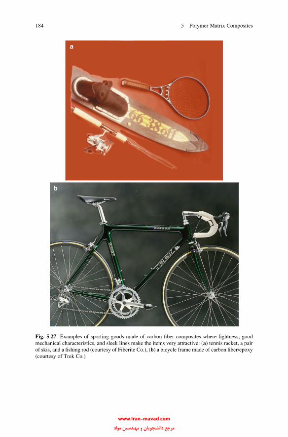
Fig. 5.27 Examples of sporting goods made of carbon fiber composites where lightness, good

mechanical characteristics, and sleek lines make the items very attractive: (a) tennis racket, a pair

of skis, and a fishing rod (courtesy of Fiberite Co.), (b) a bicycle frame made of carbon fiber/epoxy

(courtesy of Trek Co.)



Fig. 5.28 Use of carbon fiber/thermoplastic matrix composites in situations involving

static charge: (a) microphone, (b) a head shell unit of a turntable arm (courtesy of LNP

Corporation)



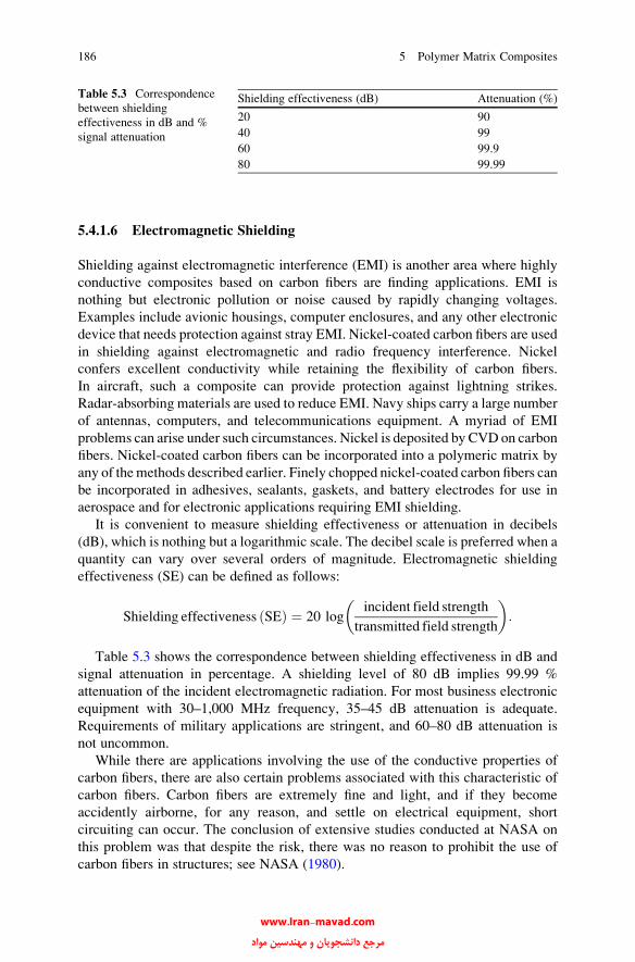
5.4.1.6 Electromagnetic Shielding

Shielding against electromagnetic interference (EMI) is another area where highly

conductive composites based on carbon fibers are finding applications. EMI is

nothing but electronic pollution or noise caused by rapidly changing voltages.

Examples include avionic housings, computer enclosures, and any other electronic

device that needs protection against stray EMI. Nickel-coated carbon fibers are used

in shielding against electromagnetic and radio frequency interference. Nickel

confers excellent conductivity while retaining the flexibility of carbon fibers.

In aircraft, such a composite can provide protection against lightning strikes.

Radar-absorbing materials are used to reduce EMI. Navy ships carry a large number

of antennas, computers, and telecommunications equipment. A myriad of EMI

problems can arise under such circumstances. Nickel is deposited by CVD on carbon

fibers. Nickel-coated carbon fibers can be incorporated into a polymeric matrix by

any of themethods described earlier. Finely chopped nickel-coated carbon fibers can

be incorporated in adhesives, sealants, gaskets, and battery electrodes for use in

aerospace and for electronic applications requiring EMI shielding.

It is convenient to measure shielding effectiveness or attenuation in decibels

(dB), which is nothing but a logarithmic scale. The decibel scale is preferred when a

quantity can vary over several orders of magnitude. Electromagnetic shielding

effectiveness (SE) can be defined as follows:

Shielding effectiveness SEð Þ ¼ 20 logincident field strength

transmitted field strength

� �:

Table 5.3 shows the correspondence between shielding effectiveness in dB and

signal attenuation in percentage. A shielding level of 80 dB implies 99.99 %

attenuation of the incident electromagnetic radiation. For most business electronic

equipment with 30–1,000 MHz frequency, 35–45 dB attenuation is adequate.

Requirements of military applications are stringent, and 60–80 dB attenuation is

not uncommon.

While there are applications involving the use of the conductive properties of

carbon fibers, there are also certain problems associated with this characteristic of

carbon fibers. Carbon fibers are extremely fine and light, and if they become

accidently airborne, for any reason, and settle on electrical equipment, short

circuiting can occur. The conclusion of extensive studies conducted at NASA on

this problem was that despite the risk, there was no reason to prohibit the use of

carbon fibers in structures; see NASA (1980).

Table 5.3 Correspondence

between shielding

effectiveness in dB and %

signal attenuation

Shielding effectiveness (dB) Attenuation (%)

20 90

40 99

60 99.9

80 99.99



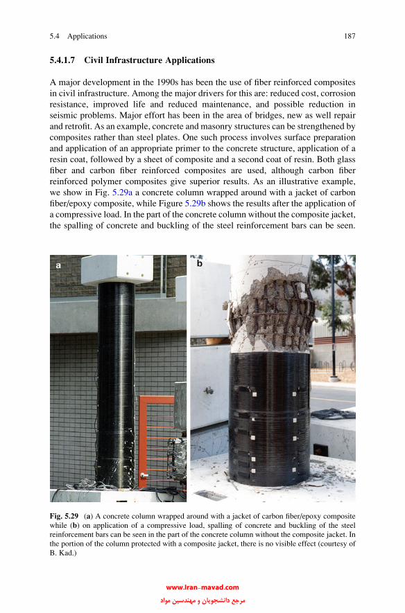
5.4.1.7 Civil Infrastructure Applications

A major development in the 1990s has been the use of fiber reinforced composites

in civil infrastructure. Among the major drivers for this are: reduced cost, corrosion

resistance, improved life and reduced maintenance, and possible reduction in

seismic problems. Major effort has been in the area of bridges, new as well repair

and retrofit. As an example, concrete and masonry structures can be strengthened by

composites rather than steel plates. One such process involves surface preparation

and application of an appropriate primer to the concrete structure, application of a

resin coat, followed by a sheet of composite and a second coat of resin. Both glass

fiber and carbon fiber reinforced composites are used, although carbon fiber

reinforced polymer composites give superior results. As an illustrative example,

we show in Fig. 5.29a a concrete column wrapped around with a jacket of carbon

fiber/epoxy composite, while Figure 5.29b shows the results after the application of

a compressive load. In the part of the concrete column without the composite jacket,

the spalling of concrete and buckling of the steel reinforcement bars can be seen.

Fig. 5.29 (a) A concrete column wrapped around with a jacket of carbon fiber/epoxy composite

while (b) on application of a compressive load, spalling of concrete and buckling of the steel

reinforcement bars can be seen in the part of the concrete column without the composite jacket. In

the portion of the column protected with a composite jacket, there is no visible effect (courtesy of

B. Kad.)



In the portion of the column protected with a composite jacket, there is no visible

effect. Potentially, composite wrapping of structural columns for seismic reinforce-

ment would appear to be a huge market. The reader should not get the impression

that everything is perfect in this area of use of composites in the civil infrastructure.

There are many problems, such as durability, moisture absorption by the polymer

matrix and other environmental effects. In addition, there is a lack of design

guidelines and database of material specifications, which makes it difficult for

civil engineers to accept the composites.

Carbon fiber is also used to reinforce cement. The resultant brittle composite

shows an improved tensile and flexural strength, high impact strength, dimensional

stability, and a high resistance to wear. Another application of carbon fiber PMCs in

civil infrastructure has to do with the ability of bridges and other structures to

withstand earthquakes. Earthquake-proofing of bridge columns is done by wrapping

columns with carbon fiber reinforced composites as described above.

Reinforced concrete is a common building construction material. Since

reinforced concrete has high compressive strength but low tensile strength, we

use reinforcing bars, often referred to as rebar, on the tensile side of concrete

structures. Conventional rebar is made of steel; which is quite an effective and

cost-efficient reinforcement material for concrete. The main problem with steel

rebar is that it is subject to corrosion by chloride ions. Chloride ions are present in

coastal areas, locations where salt is used for deicing, and sites where aggressive

chemicals and ground conditions provide chloride ions. It turns out that the

products of corrosion of rebar have a larger volume (2–5 times) than the original

metal that is consumed in the corrosion process. This change in volume leads to

tensile loading of the concrete, followed by cracking and spalling. One way out of

this problem has been to use epoxy coated steel rebar. Of course, stainless steel

would solve the corrosion problem, but it would be highly uneconomical. A glass

fiber reinforced polymer composite rebar can be used as non-prestressed reinforce-

ment in concrete These composite rebars are resistant to chloride ion attack, have a

tensile strength of 1½ to 2 times that of steel, and weigh only 25 % of the weight of

equivalent size steel rebar. The elastic modulus of glass fiber polymer is about

50 GPa, much less than that of steel, about 210 GPa. This lower stiffness causes

greater deflection in the structure which can lead to cracking. Other reinforcements

such as carbon fiber, aramid fiber or S-glass fiber can be used instead of E-glass

fiber, but all these fibers are very expensive, so these options are generally not cost

effective compared to steel. Yet another point that needs to be taken into account is

the higher ductility of steel compared to that of composite rebar.

5.4.1.8 Composites in Wind Energy

Wind energy is an important renewable energy resource. Here, we briefly describe

the basic concept of a wind turbine and how and why polymer matrix composites

play a vital role in this field.



Windmills of one sort or another have been around for quite a while. Electrical

power is produced by the spinning blades of awind turbine. The basic principle behind

the windmill is very simple. Large, multiple airfoil blades move under the action of

wind.When thewind blows, it creates positive pressure on the front side of the blade it

and negative pressure behind it, i.e., the blade moves because of differential air

pressure on the airfoil, which makes the rotor turn. The blade movement produces

mechanical energy which is converted into electrical energy by a generator.

In the past, windmill blades were made of wood. A typical windmill consists of a

rotor with aerodynamically shaped blades (commonly, a set of three) placed on a

tower. The rotor blade has the shape of an aerofoil like the wing of an airplane. The

material for the skins of the aerofoil needs to be strong, stiff, but light. These

requirements lead to wood and fiber reinforced polymer composites as the optimum

materials. Wood does not measure up to the composites mainly because of a very

large variability in properties and likely environmental damage. Since the 1990s,

fiber reinforced composites have been increasingly used to make the blades of a

windmill. Most common composites used are glass fibers reinforced epoxy

composites; carbon fiber/epoxy forms a distant second. Glass fiber composites are

cheaper than carbon fiber composites. However, longer blades (60 m) can be made

by a judicial mix of glass and carbon fibers to lower the mass of the blade.

The longer blades improve the efficiency of turbine (see below).The most common

resin matrixes are bisphenol-A epoxy or polyester or vinyl ester. Three blades are

commonly used on a windmill turbine. It should be pointed out the skins of

the turbine blades fiber are made of fiber reinforced polymers as facings with the

core being made of suitable foam.

Figure 5.30 shows an offshore windmill farm. The rotors of such windmills are

typically made of glass fiber reinforced epoxy. The rotor blade corresponds to an

elastic beam. For such a beam we can define a figure of merit (Brøndsted et al.

2005)

Mb ¼ E0:5=r;

where E is the young’s modulus or tensile stiffness and r is the density of the

material. One can have a figure of merit based on fracture toughness as well.

The blades spin at 25 rpm under forces that are equivalent to forces encountered

by a widebody jet at takeoff. Some blades are comparable in size to the wing of a

Boeing 747 aircraft. In a windmill, a turbine converts the kinetic energy of wind

into electrical energy with the power, P, given by (Brøndsted et al. 2005)

P ¼ arAv3;

where a is a constant based on aerodynamic efficiency, r is the density of air, A is

the area of the rotor-plane, and v is the wind velocity. We note from the above



expression that the power obtained in a windmill is proportional to the square of the

radius, r of the windmill and to the cube of wind velocity, v, i.e.,

P / r2v3:

So, for a given wind velocity, it makes sense to increase the radius of the

windmill. In the 1990s, wind turbines commonly had 15 m long blades and could

produce 50 kW of power. In 2008, blades of length 60 m were being used, while the

largest wind turbines could produce 5 MW of power.

5.4.1.9 Processing of Rotor Blades

Rotor blades can be made manually (e.g., wet layup), but manual processes are

restricted to small blades. Manual processes are cheap but quality control is

questionable. Variability if the resin content can be a serious problem in wet

layup. Use of prepregs helps avoid this problem, but one must apply heat and

pressure for consolidation, which adds to the cost. Large blades can be made by

filament winding or automatic tape placement. Blade skins made by manual

processes are made as two half-shells and cured. The skins are then bonded by

adhesives.

Automation of the layup process of fiber in the blade mold can lead to economies

of processing large blades. In an automatic process based upon automatic tape

laying or automatic fiber placement, the blade geometry is programmed into control

system. Commonly the molds themselves are made of composite materials.

5.4.1.10 Loading of Rotor Blades in a Wind Mill

The rotor blades of a wind turbine, made of fiber reinforced polymer composites,

experience gravity, centrifugal forces because of the rotation of the rotor, and cyclic

fatigue loading. The blades are commonly designed for a lifetime of about 20 years

which translates to 108 to 109 cycles (Brøndsted et al. 2005). Fatigue loading of the

turbine blade and the gearbox can be a serious problem. One should point out a

major difference between the fatigue loading of the wing of an aircraft and the blade

of a wind turbine; the loading conditions in a windmill are more strenuous.

An aircraft at its cruising speed at high altitudes is not subjected to the same forces

as a wind turbine blade on earth. It is important to realize that if, during high speed

spinning of the rotor blades, one of the blades came loose and smashed into the

central tower, it could cause the whole structure to collapse. Such incidents have

been captured on video.



5.4.1.11 Static Testing

Static loading is carried out in a traction rig attached to the blade by steel wires.

The blade is loaded in tension to maximum load. According to the practice used at

LMGlasfiber, a large manufacturer of wind mills, the rotor blade must stay under

load for at least 10 seconds without breaking. The tensile test is repeated twice

flapwise and then the extreme load is tested in all directions: leading edge, trailing

edge, suction side and pressure side. It can take about a week to do the static testing,

and the test is repeated after the blade has been subjected to the dynamic test (see

the description of the dynamic test below). This is done to make sure that the

dynamic or fatigue loading of the blade has not introduced a subcritical damage.

5.4.1.12 Dynamic Testing

Dynamic testing of the rotor blades is very important because they must be able to

sustain fatigue loads corresponding to 20 years of life. Every materials has a natural

frequency of oscillation, f, given by

f ¼ 1

2p

ffiffiffiffik

m

r

where k is the stiffness (N/m) and m is the mass. The blade sets into oscillation

corresponding to its natural frequency. The larger or more massive the blade, the

lower the natural frequency. It is not uncommon to subject the blade to five million

oscillations edgewise followed by five million oscillations flapwise. A 60 m long

blade could easily be fatigue tested for a year. During fatigue testing, nondestruc-

tive techniques are use to detect any damage in the blades, e.g., an infrared camera

may be used to detect cracks in the laminate. Concurrently, many strain gages,

attached to the surface of the blade, are used to track the deformation and

deflections.

5.4.1.13 Protection Against Lightning

As is well known, lightning strikes the highest point in a given area. This makes

wind turbines a very likely target, because of their height and elevated location.

Lightning strikes involve currents of very large amperage (can be up to 200 kA) and

they release very large amount of energy in a very short time period (milliseconds).

Besides the obvious electrical and magnetic properties, lightning strikes involve

X-rays, thunder which is nothing but an acoustic shock wave, and intense heat.

Thus, a lightning strike can easily destroy a blade, if it is not protected. Windmills

in offshore locations are particularly vulnerable to lightning strikes. Commonly,

lightning protection involves several external copper air termination disks called



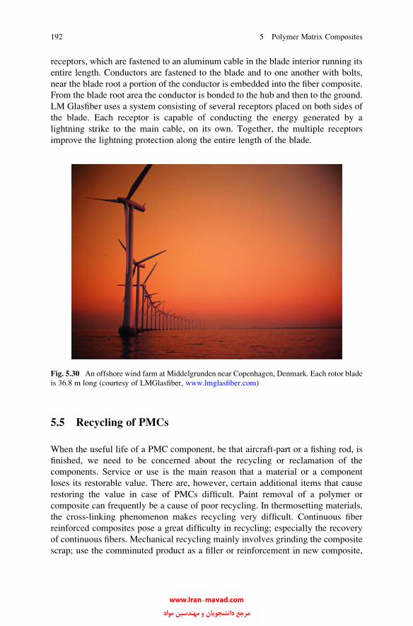
receptors, which are fastened to an aluminum cable in the blade interior running its

entire length. Conductors are fastened to the blade and to one another with bolts,

near the blade root a portion of the conductor is embedded into the fiber composite.

From the blade root area the conductor is bonded to the hub and then to the ground.

LM Glasfiber uses a system consisting of several receptors placed on both sides of

the blade. Each receptor is capable of conducting the energy generated by a

lightning strike to the main cable, on its own. Together, the multiple receptors

improve the lightning protection along the entire length of the blade.

5.5 Recycling of PMCs

When the useful life of a PMC component, be that aircraft-part or a fishing rod, is

finished, we need to be concerned about the recycling or reclamation of the

components. Service or use is the main reason that a material or a component

loses its restorable value. There are, however, certain additional items that cause

restoring the value in case of PMCs difficult. Paint removal of a polymer or

composite can frequently be a cause of poor recycling. In thermosetting materials,

the cross-linking phenomenon makes recycling very difficult. Continuous fiber

reinforced composites pose a great difficulty in recycling; especially the recovery

of continuous fibers. Mechanical recycling mainly involves grinding the composite

scrap; use the comminuted product as a filler or reinforcement in new composite,

Fig. 5.30 An offshore wind farm at Middelgrunden near Copenhagen, Denmark. Each rotor blade

is 36.8 m long (courtesy of LMGlasfiber, www.lmglasfiber.com)



http://www.lmglasfiber.com

5.5 Recycling of PMCs 193

generally meant for less-demanding applications than the virgin material (Pickering

2006). There is the option of using a variety of thermal techniques that breakdown

the composite scrap. SMC is a polymer matrix composite containing particles/short

fibers. Such a material can easily be ground into a fine powder and reused as filler.

Such a technique would not work with continuous fiber reinforced thermoset matrix

PMCs. As we know, thermosets are the most common matrix materials in PMCs,

and they are not amenable to recycling in a manner similar to metals and

thermoplastics. Tertiary recycling, i.e., recovery of the monomer, is one possible

way. Tertiary or chemical recycling involving conversion of polymer fractions into

a gaseous mixture of low molecular weight hydrocarbons with a low temperature

(200 �C) catalytic process has been tried (M nson 1994; Allred et al. 1997). Such

chemical recycling breaks polymeric waste into reusable hydrocarbon fractions for

use as monomers, chemicals, or fuel. The thermoset polymer matrix is separated

into low molecular weight chemicals and the reclaimed fibers and fillers can be

reused. It has been claimed that although the reclaimed carbon fibers are not

continuous, their structural and mechanical characteristics are not altered by the

chemical recycling (Allred et al. 1997). Analysis of the reclaimed carbon fibers by

SEM, XPS, and single fiber tensile tests showed them to have surface texture,

chemistry and strength close to the virgin fibers. The epoxy was converted to

hydrocarbon fractions. It is important to recognize that these recycling procedures

result in a material that is suitable for use in applications less demanding than the

original application because of a considerably reduced intrinsic value of the mate-

rial after each step. Figure 5.31 shows schematically the change in value of the

constituents with increasing life cycle (M nson 1994).

Fig. 5.31 Change in value of the constituents with increasing life cycle [after M nson (1994)]

å

å

å


References

Allred RE, Newmeister GC, Doak TJ, Cochran RC, Coons AB (1997). In: Composites ’97

Manufacturing and Tooling, Paper #EM97-110, Society of Manufacturing Engineering.

Dearborn, MI

Anderson BW (1984) In: Advances in fracture research, ICF4, vol 1, New Delhi, Pergamon Press,

Oxford, p 607

Baker A (1983) Met Forum 6:81

Bergmann HW (1984) In: Advances in fracture research, ICF4, vol 1, New Delhi, Pergamon Press,

Oxford, p 569

Biro DA, Pleizier G, Deslandes Y (1992) J Mater Sci Lett 11:698

Brøndsted P, Lilholt H, Lystrup A (2005) Annu Rev Mater Res 35:505

Brown JR, Chappell PJC, Mathys Z (1992) J Mater Sci 27:3167

Chen CH, Springer GS (1976) J Composite Mater 10:2

Clark D, Wadsworth NJ, Watt W (1974) In: Carbon fibres, their place in modern technology. The

Plastics Institute, London, p 44

Cogswell FN (1992) Thermoplastic aromatic polymer composites. Butterworth-Heinemann,

Oxford, p 136

Collings TA, Stone DEW (1985) Composites 16:307

Diefendorf RJ (1985) In: Tough composite materials. Noyes Publishing, Park Ridge, NJ, p 191

Donnet J-B, Bansal RC (1984) Carbon fibers. Marcel Dekker, New York, p 109

Drzal LT, Rich MJ, Lloyd PF (1983a) J Adhes 16:1

Drzal LT, Rich MJ, Koenig MF, Lloyd PF (1983b) J Adhes 16:133

Ehlert GJ, Lin Y, Galan U, Sodano HA (2010) J Solid Mech Mater Eng 4:1687

Ehrburger P, Donnet JB (1980a) Philos Trans R Soc Lond A294:495

Eriksen RH (1976) Composites 7:189

Friedrich K (1985) Compos Sci Technol 22:43

Goel A, Chawla KK, Vaidya UK, Koopman M (2008) J Mater Sci 43:4423

Hancox NL (1983) In: Fabrication of composite materials. North-Holland, Amsterdam, p 1

Hild DN, Schwartz P (1992a) J Adhes Sci Technol 6:879

Hild DN, Schwartz P (1992b) J Adhes Sci Technol 6:897

Hull D (1981) An introduction to composite materials. Cambridge University Press, Cambridge, p 42

Hull D (1994) Mater Sci Eng A184:173

Ishida H, Koenig JL (1978) J Colloid Interface Sci 64:555

Jangehud I, Serrano AM, Eby RK, Meador MA (1993) In: Proc. 21st biennial conference on

carbon, Buffalo, NY, June 13–18

Kaas RL, Kardos JL (1971) Polym Eng Sci 11:11

Kaplan SL, Rose PW, Nguyen HX, Chang HW (1988) SAMPE Quart 19:55

Kardos JL (1985) In: Molecular characterization of composite interfaces. Plenum, New York, p 1

Knox CE (1982) In: Handbook of composite materials. Van Nostrand Reinhold, New York, p 136

Krause W, Henning F, Troster S, Geiger O, Eyerer P (2003) J Thermoplastic Compos Mater

16:292

Li ZF, Netravali AN, Sachse W (1992) J Mater Sci 27:4625

Lockwood RJ, Alberino LM (1981) In: Advances in urethane science and technology. Technomic,

Westport, CT

J.A. Manson (1994). In: High performance composite: commonalty of phenomena, Chawla KK,

Liaw PK, and Fishman SG (eds) The Minerals, Metals & Materials Society, Warrendale, PA,

p 1

Mayer NJ (1974) Engineering applications of composites. Academic, New York, p 24

McKee D, Mimeault V (1973) In: Chemistry and physics of carbon, vol 8. Marcel Dekker, New

York, p 151

Meyer RW (1985) Handbook of pultrusion technology. Chapman & Hall, New York

NASA (1980) Risk to the public from carbon fibers released in civil aircraft accidents, SP-448.

NASA, Washington, DC



Pickering SJ (2006) Compos A Appl Sci Manuf 37:1206

Pipes RB, Pagano NJ (1970) J Compos Mater 1:538

Plueddemann EP (1974a) In: Interfaces in polymer matrix composites. Academic, New York,

p 174

Riggs DM, Shuford RJ, Lewis RW (1982) Handbook of composites. Van Nostrand Reinhold,

New York, p 196

Sands JM, Fink BK, McKnight SH, Newton CH, Gillespie JW Jr, Palmese GR (2001) Clean Prod

Process 2:228

Shibley AM (1982) Handbook of composite materials. Van Nostrand Reinhold, New York, p 448

Shirrel CD, Sandow FA (1980) Fibrous composites in structural design. Plenum, New York, p 795

Slobodzinsky A (1982) Handbook of composite materials. Van Nostrand Reinhold, New York,

p 368

Sturgeon JB (1978) In: Creep of engineering materials. A Journal of Strain Analysis Monograph,

p 175

Tarnopol’skii YM, Bail’ AI (1983) In: Fabrication of composites. North-Holland, Amsterdam, p 45

Vaidya UK, Chawla KK (2008) Int Mater Rev 53:185

Waddon AJ, Hill MJ, Keller A, Blundell DJ (1987) J Mater Sci 27:1773

Xu ZR, Ashbee KHG (1994) J Mater Sci 29:394

Further Reading

Advani SG (ed) (1994) Flow and rheology in polymer composites manufacturing. Elsevier,

Amsterdam

Ehrburger P, Donnet JB (1980b) Interface in composite materials. Philos Trans R Soc Lond

A294:495

Kelly A, Mileiko ST (eds) (1983) Fabrication of composites. North-Holland, Amsterdam

Plueddemann EP (ed) (1974b) Interfaces in polymer matrix composites. Academic, New York

Vaidya U (2011) Composites for automotive, truck and mass transit. DEStech Pub, Lancaster, PA

Problems

5.1. Why are prepregs so important in polymer matrix composites? What are their

advantages? Describe the different types of prepregs.

5.2. Randomly distributed short fibers should result in more or less isotropic

properties in an injection molded composite. But this is generally not true.

Why? What are the other limitations of injection molding process?

5.3. In a thermally cured PMC, the fiber surface treatments have been well

established for certain systems. For example, silanes are used on glass fiber

in an epoxy matrix while an oxidizing treatment to carbon fiber for use in an

epoxy matrix. What would be the effect of electron beam curing on the

interface development in a PMC?

5.4. Describe the major differences in the processing of composites having a

thermoset matrix and those having a thermoplastic matrix.

5.5. What are the important factors in regard to fire resistance of PMCs?

Problems 195


Chapter 6

Metal Matrix Composites

Metal matrix composites consist of a metal or an alloy as the continuous matrix and

a reinforcement that can be particle, short fiber or whisker, or continuous fiber.

In this chapter, we first describe important techniques to process metal matrix

composites, then we describe the interface region and its characteristics, properties

of different metal matrix composites, and finally, we summarize different

applications of metal matrix composites.

6.1 Types of Metal Matrix Composites

There are three kinds of metal matrix composites (MMCs):

• Particle reinforced MMCs

• Short fiber or whisker reinforced MMCs

• Continuous fiber or sheet reinforced MMCs

Table 6.1 provides examples of some important reinforcements used in metal

matrix composites and their aspect (length/diameter) ratios and diameters. Parti-

cle or discontinuously reinforced MMCs have become very important because

they are inexpensive vis a vis continuous fiber reinforced composites and they

have relatively isotropic properties compared to fiber reinforced composites.

Figure 6.1a, b show typical microstructures of continuous alumina fiber/magne-

sium alloy and silicon carbide particle/aluminum alloy composites, respectively.

Use of nanometer-sized fullerenes as a reinforcement has been tried. In addition to

being very small, fullerenes (of which C60 is the most common) are light

and hollow. The important question in this regard is whether they remain stable

during processing and service. For the interested reader, we cite work by Barrera

et al. (1994), who used powder metallurgy, RF sputtering of a composite


197


(multifullerene) target, and thin film codeposition methods to make fullerene/

metal composites. Copper–fullerene composites were processed by sputtering

copper during fullerene sublimation in an argon atmosphere. Fullerenes were

found to withstand the processing. However, in the case of aluminum matrix,

brittle Al4C3 was observed to form at high temperatures.

6.2 Important Metallic Matrices

A variety of metals and their alloys can be used as matrix materials. We describe

briefly the important characteristics of some of the more common ones.

6.2.1 Aluminum Alloys

Aluminum alloys, because of their low density and excellent strength, toughness,

and resistance to corrosion, find important applications in the aerospace field.

Of special mention in this regard are the Al–Cu–Mg and Al–Zn–Mg–Cu

alloys, very important precipitation-hardenable alloys. Aluminum-lithium alloys

form one of the most important precipitation-hardenable aluminum alloys. Lith-

ium, when added to aluminum as a primary alloying element, has the unique

characteristic of increasing the elastic modulus and decreasing the density of the

alloy. Understandably, the aerospace industry has been the major target of this

development. Al–Li alloys are precipitation hardenable, much like the Al–Cu–Mg

and Al–Zn–Mg–Cu alloys. The precipitation hardening sequence in Al–Li

alloys is, however, much more complex than that observed in conventional

precipitation-hardenable aluminum alloys. Generally, these alloys contain,

besides lithium, some copper, zirconium, and magnesium. Vasudevan and

Doherty (1989) provide an account of the heat treatments and structure/property

aspects of various aluminum alloys.

Table 6.1 Typical reinforcements used in metal matrix composites

Type Aspect ratio

Diameter

(mm) Examples

Particle ~1–4 1–25 SiC, Al2O3, WC, TiC, BN, B4C

Short fiber or

whisker

~10–1,000 0.1–25 SiC, Al2O3, Al2O3 + SiO2, C

Continuous fiber >1,000 3–150 SiC, Al2O3, Al2O3 + SiO2, C, B, W, NbTi,

Nb3Sn

198 6 Metal Matrix Composites


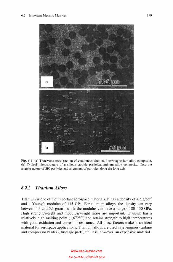
6.2.2 Titanium Alloys

Titanium is one of the important aerospace materials. It has a density of 4.5 g/cm3

and a Young’s modulus of 115 GPa. For titanium alloys, the density can vary

between 4.3 and 5.1 g/cm3, while the modulus can have a range of 80–130 GPa.

High strength/weight and modulus/weight ratios are important. Titanium has a

relatively high melting point (1,672�C) and retains strength to high temperatures

with good oxidation and corrosion resistance. All these factors make it an ideal

material for aerospace applications. Titanium alloys are used in jet engines (turbine

and compressor blades), fuselage parts, etc. It is, however, an expensive material.

Fig. 6.1 (a) Transverse cross-section of continuous alumina fiber/magnesium alloy composite.

(b) Typical microstructure of a silicon carbide particle/aluminum alloy composite. Note the

angular nature of SiC particles and alignment of particles along the long axis

6.2 Important Metallic Matrices 199


At supersonic speeds, the skin of an airplane heats up so much that aluminum

alloys are no good; titanium alloys must be used at such high temperatures.

At speeds greater than Mach 2, the temperatures will be even higher than what

titanium alloys can withstand. Titanium aluminides are one of the candidate

materials in this case.

Titanium has two polymorphs: alpha (a) titanium has a hexagonal close-packed

(hcp) structure and is stable below 885�C and beta (b) titanium has a bcc structure

and is stable above 885�C. Aluminum raises the a!b transformation temperature,

i.e., aluminum is an alpha stabilizer. Most other alloying elements (Fe, Mn, Cr, Mo,

V, No, Ta) lower the a!b transformation temperature, i.e., they stabilize the

b phase. Thus, three general alloy types can be produced, viz., a, a + b, and btitanium alloys. The Ti-6%Al-4% V, called the workhorse Ti alloy of the aerospaceindustry, belongs to the a + b group. Most titanium alloys are not used in a

quenched and tempered condition. Generally, hot working in the a + b region is

carried out to break the structure and distribute the a phase in an extremely fine form.

Titanium has a great affinity for oxygen, nitrogen, and hydrogen. Parts per

million of such interstitials in titanium can change mechanical properties drasti-

cally; particularly embrittlement can set in. That is why welding of titanium by any

technique requires protection from the atmosphere. Electron beam techniques, in a

vacuum, are frequently used.

6.2.3 Magnesium Alloys

Magnesium and its alloys form another group of very light materials. Magnesium is

one of the lightest metals; its density is 1.74 g/cm3. Magnesium alloys, especially

castings, are used in aircraft gearbox housings, chain saw housings, electronic equip-

ment, etc.Magnesium, being a hexagonal close-packedmetal, is difficult to coldwork.

6.2.4 Copper

Copper has a face centered cubic structure. Its use as an electrical conductor is quite

ubiquitous. It has good thermal conductivity. It can be cast and worked easily. One

of the major applications of copper in a composite as a matrix material is in

niobium-based superconductors.

6.2.5 Intermetallic Compounds

Intermetallic compounds can be ordered or disordered. The structure of ordered

intermetallic alloys is characterized by long-range ordering, i.e., different atoms

occupy specific positions in the lattice. Because of their ordered structure, the motion



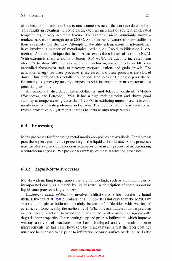
of dislocations in intermetallics is much more restricted than in disordered alloys.

This results in retention (in some cases, even an increase) of strength at elevated

temperatures, a very desirable feature. For example, nickel aluminide shows a

marked increase in strength up to 800�C. An undesirable feature of intermetallics is

their extremely low ductility. Attempts at ductility enhancement in intermetallics

have involved a number of metallurgical techniques. Rapid solidification is one

method. Another technique that has met success is the addition of boron to Ni3Al.

With extremely small amounts of boron (0.06 wt.%), the ductility increases from

about 2% to about 50%. Long-range order also has significant effects on diffusion-

controlled phenomena such as recovery, recrystallization, and grain growth. The

activation energy for these processes is increased, and these processes are slowed

down. Thus, ordered intermetallic compounds tend to exhibit high creep resistance.

Enhancing toughness by making composites with intermetallic matrix materials is a

potential possibility.

An important disordered intermetallic is molybdenum disilicide (MoSi2)

(Vasudevan and Petrovic, 1992). It has a high melting point and shows good

stability at temperatures greater than 1,200�C in oxidizing atmosphere. It is com-

monly used as a heating element in furnaces. The high oxidation resistance comes

from a protective SiO2 film that it tends to form at high temperatures.

6.3 Processing

Many processes for fabricating metal matrix composites are available. For the most

part, these processes involve processing in the liquid and solid state. Some processes

may involve a variety of deposition techniques or an in situ process of incorporating

a reinforcement phase. We provide a summary of these fabrication processes.

6.3.1 Liquid-State Processes

Metals with melting temperatures that are not too high, such as aluminum, can be

incorporated easily as a matrix by liquid route. A description of some important

liquid-state processes is given here.

Casting, or liquid infiltration, involves infiltration of a fiber bundle by liquid

metal (Divecha et al. 1981; Rohatgi et al. 1986). It is not easy to make MMCs by

simple liquid-phase infiltration, mainly because of difficulties with wetting of

ceramic reinforcement by the molten metal. When the infiltration of a fiber preform

occurs readily, reactions between the fiber and the molten metal can significantly

degrade fiber properties. Fiber coatings applied prior to infiltration, which improve

wetting and control reactions, have been developed and can result in some

improvements. In this case, however, the disadvantage is that the fiber coatings

must not be exposed to air prior to infiltration because surface oxidation will alter

6.3 Processing 201


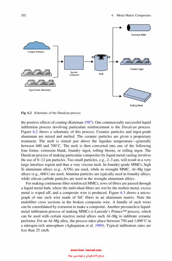
the positive effects of coating (Katzman 1987). One commercially successful liquid

infiltration process involving particulate reinforcement is the Duralcan process.

Figure 6.2 shows a schematic of this process. Ceramic particles and ingot-grade

aluminum are mixed and melted. The ceramic particles are given a proprietary

treatment. The melt is stirred just above the liquidus temperature—generally

between 600 and 700�C. The melt is then converted into one of the following

four forms: extrusion blank, foundry ingot, rolling bloom, or rolling ingot. The

Duralcan process of making particulate composites by liquid metal casting involves

the use of 8–12 mm particles. Too small particles, e.g., 2–3 mm, will result in a very

large interface region and thus a very viscous melt. In foundry-grade MMCs, high

Si aluminum alloys (e.g., A356) are used, while in wrought MMC, Al–Mg type

alloys (e.g., 6061) are used. Alumina particles are typically used in foundry alloys,

while silicon carbide particles are used in the wrought aluminum alloys.

For making continuous fiber reinforced MMCs, tows of fibers are passed through

a liquid metal bath, where the individual fibers are wet by the molten metal, excess

metal is wiped off, and a composite wire is produced. Figure 6.3 shows a micro-

graph of one such wire made of SiC fibers in an aluminum matrix. Note the

multifiber cross sections in the broken composite wire. A bundle of such wires

can be consolidated by extrusion to make a composite. Another pressureless liquid-

metal infiltration process of making MMCs is Lanxide’s Primex™ process, which

can be used with certain reactive metal alloys such Al–Mg to infiltrate ceramic

preforms. For an Al–Mg alloy, the process takes place between 750 and 1,000�C in

a nitrogen-rich atmosphere (Aghajanian et al. 1989). Typical infiltration rates are

less than 25 cm/h.

Fig. 6.2 Schematic of the Duralcan process



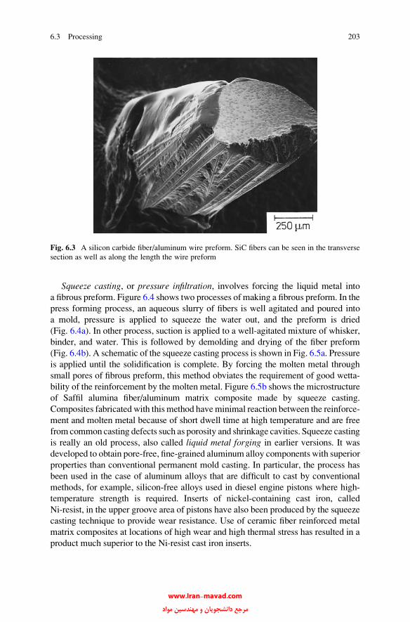
Squeeze casting, or pressure infiltration, involves forcing the liquid metal into

a fibrous preform. Figure 6.4 shows two processes of making a fibrous preform. In the

press forming process, an aqueous slurry of fibers is well agitated and poured into

a mold, pressure is applied to squeeze the water out, and the preform is dried

(Fig. 6.4a). In other process, suction is applied to a well-agitated mixture of whisker,

binder, and water. This is followed by demolding and drying of the fiber preform

(Fig. 6.4b). A schematic of the squeeze casting process is shown in Fig. 6.5a. Pressure

is applied until the solidification is complete. By forcing the molten metal through

small pores of fibrous preform, this method obviates the requirement of good wetta-

bility of the reinforcement by the molten metal. Figure 6.5b shows the microstructure

of Saffil alumina fiber/aluminum matrix composite made by squeeze casting.

Composites fabricated with this method haveminimal reaction between the reinforce-

ment and molten metal because of short dwell time at high temperature and are free

from common casting defects such as porosity and shrinkage cavities. Squeeze casting

is really an old process, also called liquid metal forging in earlier versions. It was

developed to obtain pore-free, fine-grained aluminum alloy components with superior

properties than conventional permanent mold casting. In particular, the process has

been used in the case of aluminum alloys that are difficult to cast by conventional

methods, for example, silicon-free alloys used in diesel engine pistons where high-

temperature strength is required. Inserts of nickel-containing cast iron, called

Ni-resist, in the upper groove area of pistons have also been produced by the squeeze

casting technique to provide wear resistance. Use of ceramic fiber reinforced metal

matrix composites at locations of high wear and high thermal stress has resulted in a

product much superior to the Ni-resist cast iron inserts.

Fig. 6.3 A silicon carbide fiber/aluminum wire preform. SiC fibers can be seen in the transverse

section as well as along the length the wire preform

6.3 Processing 203


The squeeze casting technique, shown in Fig. 6.5a, has been quite popular in

making composites with selective reinforcement. A porous fiber preform (generally

of discontinuous Saffil-type Al2O3 fibers) is inserted into the die. Molten metal

(aluminum) is poured into the preheated die located on the bed of a hydraulic press.

The applied pressure (70–100 MPa) makes the molten aluminum penetrate the fiber

preform and bond the fibers. Infiltration of a fibrous preform bymeans of a pressurized

inert gas is another variant of liquid metal infiltration technique. The process is

conducted in the controlled environment of a pressure vessel and rather high fiber

volume fractions; complex-shaped structures are obtainable (Mortensen et al. 1988;

Cook andWarner 1991). Although commonly, aluminummatrix composites aremade

by this technique, alumina fiber reinforced intermetallicmatrix composites (e.g., TiAl,

Ni3Al, and Fe3Al matrix materials) have been prepared by pressure casting

(Nourbakhsh et al. 1990). The technique involves melting the matrix alloy in a

crucible in vacuum, while the fibrous preform is heated separately. The molten matrix

Fig. 6.4 (a) Press forming of a preform. (b) Suction forming of a preform



material (at about 100�C above the Tm) is poured onto the fibers, and argon gas is

introduced simultaneously. Argon gas pressure forces the melt to infiltrate the pre-

form. The melt generally contains additives to aid in wetting the fibers.

6.3.1.1 Special Issues in Casting of MMCs

Casting of metal matrix composites consisting of a metal containing particulate or

fibrous reinforcement may appear to be superficially similar to casting of metals.

Metals can be cast into near net-shape product forms because of their relatively low

melt viscosities. In particular, when a metal is heated above its melting point (or in

the case of an alloy above its liquidus temperature), we get a low-viscosity liquid

that has nice fluid flow characteristics such that it can be used to infiltrate a fibrous

or particulate preform (Michaud 1993; Cornie et al. 1986). Darcy’s law describes

the phenomenon of permeability of porous medium by a fluid. Specifically, in the

case of MMCs, we can write for the permeability of a porous medium, k, in terms of

Darcy’s Law for single-phase fluid flow:

J ¼ � k

�rP;

Fig. 6.5 (a) Squeeze casting technique of making a metal matrix composite. (b) The microstruc-

ture of Saffil alumina fiber/aluminum matrix composite made by squeeze casting. [Courtesy of

G. Eggeler]

6.3 Processing 205


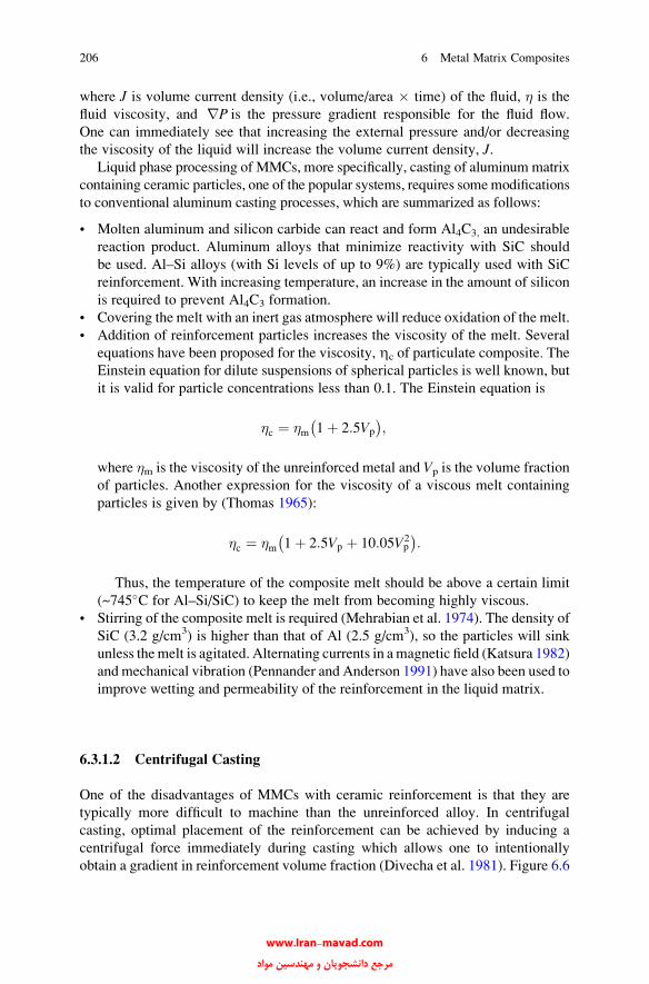
where J is volume current density (i.e., volume/area � time) of the fluid, � is the

fluid viscosity, and rP is the pressure gradient responsible for the fluid flow.

One can immediately see that increasing the external pressure and/or decreasing

the viscosity of the liquid will increase the volume current density, J.Liquid phase processing of MMCs, more specifically, casting of aluminum matrix

containing ceramic particles, one of the popular systems, requires somemodifications

to conventional aluminum casting processes, which are summarized as follows:

• Molten aluminum and silicon carbide can react and form Al4C3, an undesirable

reaction product. Aluminum alloys that minimize reactivity with SiC should

be used. Al–Si alloys (with Si levels of up to 9%) are typically used with SiC

reinforcement. With increasing temperature, an increase in the amount of silicon

is required to prevent Al4C3 formation.

• Covering the melt with an inert gas atmosphere will reduce oxidation of the melt.

• Addition of reinforcement particles increases the viscosity of the melt. Several

equations have been proposed for the viscosity, Zc of particulate composite. TheEinstein equation for dilute suspensions of spherical particles is well known, but

it is valid for particle concentrations less than 0.1. The Einstein equation is

�c ¼ �m 1þ 2:5Vp

� �;

where �m is the viscosity of the unreinforced metal and Vp is the volume fraction

of particles. Another expression for the viscosity of a viscous melt containing

particles is given by (Thomas 1965):

�c ¼ �m 1þ 2:5Vp þ 10:05Vp2

� �:

Thus, the temperature of the composite melt should be above a certain limit

(~745�C for Al–Si/SiC) to keep the melt from becoming highly viscous.

• Stirring of the composite melt is required (Mehrabian et al. 1974). The density of

SiC (3.2 g/cm3) is higher than that of Al (2.5 g/cm3), so the particles will sink

unless themelt is agitated. Alternating currents in amagnetic field (Katsura 1982)

and mechanical vibration (Pennander and Anderson 1991) have also been used to

improve wetting and permeability of the reinforcement in the liquid matrix.

6.3.1.2 Centrifugal Casting

One of the disadvantages of MMCs with ceramic reinforcement is that they are

typically more difficult to machine than the unreinforced alloy. In centrifugal

casting, optimal placement of the reinforcement can be achieved by inducing a

centrifugal force immediately during casting which allows one to intentionally

obtain a gradient in reinforcement volume fraction (Divecha et al. 1981). Figure 6.6



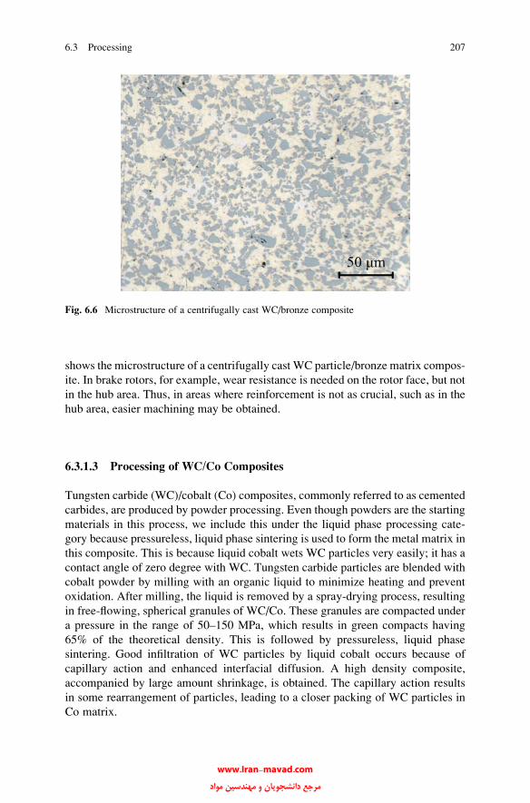
shows the microstructure of a centrifugally cast WC particle/bronze matrix compos-

ite. In brake rotors, for example, wear resistance is needed on the rotor face, but not

in the hub area. Thus, in areas where reinforcement is not as crucial, such as in the

hub area, easier machining may be obtained.

6.3.1.3 Processing of WC/Co Composites

Tungsten carbide (WC)/cobalt (Co) composites, commonly referred to as cemented

carbides, are produced by powder processing. Even though powders are the starting

materials in this process, we include this under the liquid phase processing cate-

gory because pressureless, liquid phase sintering is used to form the metal matrix in

this composite. This is because liquid cobalt wets WC particles very easily; it has a

contact angle of zero degree with WC. Tungsten carbide particles are blended with

cobalt powder by milling with an organic liquid to minimize heating and prevent

oxidation. After milling, the liquid is removed by a spray-drying process, resulting

in free-flowing, spherical granules of WC/Co. These granules are compacted under

a pressure in the range of 50–150 MPa, which results in green compacts having

65% of the theoretical density. This is followed by pressureless, liquid phase

sintering. Good infiltration of WC particles by liquid cobalt occurs because of

capillary action and enhanced interfacial diffusion. A high density composite,

accompanied by large amount shrinkage, is obtained. The capillary action results

in some rearrangement of particles, leading to a closer packing of WC particles in

Co matrix.

Fig. 6.6 Microstructure of a centrifugally cast WC/bronze composite

6.3 Processing 207


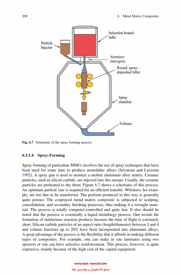
6.3.1.4 Spray-Forming

Spray-forming of particulate MMCs involves the use of spray techniques that have

been used for some time to produce monolithic alloys (Srivatsan and Lavernia

1992). A spray gun is used to atomize a molten aluminum alloy matrix. Ceramic

particles, such as silicon carbide, are injected into this stream. Usually, the ceramic

particles are preheated to dry them. Figure 6.7 shows a schematic of this process.

An optimum particle size is required for an efficient transfer. Whiskers, for exam-

ple, are too fine to be transferred. The preform produced in this way is generally

quite porous. The cosprayed metal matrix composite is subjected to scalping,

consolidation, and secondary finishing processes, thus making it a wrought mate-

rial. The process is totally computer-controlled and quite fast. It also should be

noted that the process is essentially a liquid metallurgy process. One avoids the

formation of deleterious reaction products because the time of flight is extremely

short. Silicon carbide particles of an aspect ratio (length/diameter) between 3 and 4

and volume fractions up to 20% have been incorporated into aluminum alloys.

A great advantage of the process is the flexibility that it affords in making different

types of composites. For example, one can make in situ laminates using two

sprayers or one can have selective reinforcement. This process, however, is quite

expensive, mainly because of the high cost of the capital equipment.

Fig. 6.7 Schematic of the spray forming process



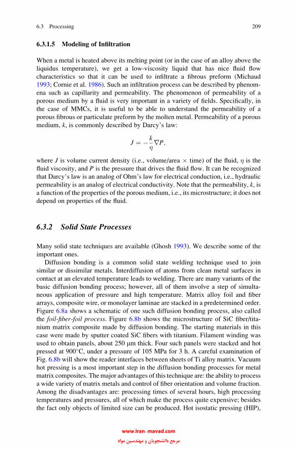
6.3.1.5 Modeling of Infiltration

When a metal is heated above its melting point (or in the case of an alloy above the

liquidus temperature), we get a low-viscosity liquid that has nice fluid flow

characteristics so that it can be used to infiltrate a fibrous preform (Michaud

1993; Cornie et al. 1986). Such an infiltration process can be described by phenom-

ena such as capillarity and permeability. The phenomenon of permeability of a

porous medium by a fluid is very important in a variety of fields. Specifically, in

the case of MMCs, it is useful to be able to understand the permeability of a

porous fibrous or particulate preform by the molten metal. Permeability of a porous

medium, k, is commonly described by Darcy’s law:

J ¼ � k

�rP;

where J is volume current density (i.e., volume/area � time) of the fluid, � is the

fluid viscosity, and P is the pressure that drives the fluid flow. It can be recognized

that Darcy’s law is an analog of Ohm’s law for electrical conduction, i.e., hydraulic

permeability is an analog of electrical conductivity. Note that the permeability, k, isa function of the properties of the porous medium, i.e., its microstructure; it does not

depend on properties of the fluid.

6.3.2 Solid State Processes

Many solid state techniques are available (Ghosh 1993). We describe some of the

important ones.

Diffusion bonding is a common solid state welding technique used to join

similar or dissimilar metals. Interdiffusion of atoms from clean metal surfaces in

contact at an elevated temperature leads to welding. There are many variants of the

basic diffusion bonding process; however, all of them involve a step of simulta-

neous application of pressure and high temperature. Matrix alloy foil and fiber

arrays, composite wire, or monolayer laminae are stacked in a predetermined order.

Figure 6.8a shows a schematic of one such diffusion bonding process, also called

the foil-fiber-foil process. Figure 6.8b shows the microstructure of SiC fiber/tita-

nium matrix composite made by diffusion bonding. The starting materials in this

case were made by sputter coated SiC fibers with titanium. Filament winding was

used to obtain panels, about 250 mm thick. Four such panels were stacked and hot

pressed at 900�C, under a pressure of 105 MPa for 3 h. A careful examination of

Fig. 6.8b will show the reader interfaces between sheets of Ti alloy matrix. Vacuum

hot pressing is a most important step in the diffusion bonding processes for metal

matrix composites. Themajor advantages of this technique are: the ability to process

a wide variety of matrix metals and control of fiber orientation and volume fraction.

Among the disadvantages are: processing times of several hours, high processing

temperatures and pressures, all of which make the process quite expensive; besides

the fact only objects of limited size can be produced. Hot isostatic pressing (HIP),

6.3 Processing 209


instead of uniaxial pressing, can also be used. In HIP, gas pressure against a can

consolidates the composite piece contained inside the can. With HIP, it is relatively

easy to apply high pressures at elevated temperatures over variable geometries.

Deformation processing of metal/metal composites involves mechanical

processing (swaging, extrusion, drawing, or rolling) of a ductile two-phase mate-

rial. The two phases codeform, causing the minor phase to elongate and become

fibrous in nature within the matrix. These materials are sometimes referred to as insitu composites. The properties of a deformation-processed composite depend

largely on the characteristics of the starting material, which is usually a billet of

Fig. 6.8 (a) Schematic of diffusion bonding process. (b) The microstructure of SiC fiber/titanium

matrix composite made by diffusion. Each fiber is 142 mm in diameter. [Courtesy of J. Baughman]



two-phase alloy that has been prepared by casting or powder metallurgy methods.

Roll bonding is a common technique used to produce a laminated composite

consisting of different metals in the sheet form (Chawla and Collares 1978;

Sherby et al. 1985). Such composites are called sheet laminated metal matrix

composites. Other examples of deformation-processed metal matrix composites

are the niobium-based conventional filamentary superconductors and the high-Tcsuperconductors (see Chap. 9).

Deposition techniques for metal matrix composite fabrication involve coating

individual fibers in a tow with the matrix material needed to form the composite

followed by diffusion bonding to form a consolidated composite plate or structural

shape. The main disadvantage of using deposition techniques is that they are very

time consuming. However, there are several advantages:

• The degree of interfacial bonding is easily controllable; interfacial diffusion

barriers and compliant coatings can be formed on the fiber prior to matrix

deposition or graded interfaces can be formed.

• Thin, monolayer tapes can be produced by filament winding; these are easier to

handle and mold into structural shapes than other precursor forms—unidirec-

tional or angle-plied composites can be easily fabricated in this way.

Several deposition techniques are available: immersion plating, electroplating,

spray deposition, chemical vapor deposition (CVD), and physical vapor deposition

(PVD) (Partridge and Ward-Close 1993). Dipping or immersion plating is similar to

infiltration casting except that fiber tows are continuously passed through baths of

molten metal, slurry, sol, or organometallic precursors. Electroplating produces a

coating from a solution containing the ion of the desired material in the presence of

an electric current. Fibers are wound on a mandrel, which serves as the cathode, and

placed into the platingbathwith ananodeof the desiredmatrixmaterial. The advantage

of thismethod is that the temperatures involved aremoderate and no damage is done to

the fibers. Problems with electroplating involve void formation between fibers and

between fiber layers, adhesion of the deposit to the fibers may be poor, and there are

limited numbers of alloy matrices available for this processing. A spray deposition

operation, typically, consists of winding fibers onto a foil-coated drum and spraying

molten metal onto them to form a monotape. The source of molten metal may be

powder or wire feedstock, which is melted in a flame, arc, or plasma torch. The

advantages of spray deposition are easy control of fiber alignment and rapid solidifica-

tion of the molten matrix. In a CVD process, a vaporized component decomposes or

reacts with another vaporized chemical on the substrate to form a coating on that

substrate. The processing is generally carried out at elevated temperatures.

6.3.3 In Situ Processes

In in situ techniques, one forms the reinforcement phase in situ. The composite

material is produced in one step from an appropriate starting alloy, thus avoiding

the difficulties inherent in combining the separate components as in a typical

6.3 Processing 211


http://dx.doi.org/10.1007/978-0-387-74365-3_9

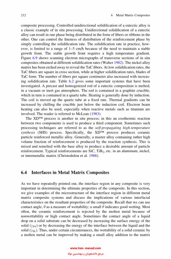
composite processing. Controlled unidirectional solidification of a eutectic alloy is

a classic example of in situ processing. Unidirectional solidification of a eutectic

alloy can result in one phase being distributed in the form of fibers or ribbons in the

other. One can control the fineness of distribution of the reinforcement phase by

simply controlling the solidification rate. The solidification rate in practice, how-

ever, is limited to a range of 1–5 cm/h because of the need to maintain a stable

growth front. The stable growth front requires a high temperature gradient.

Figure 6.9 shows scanning electron micrographs of transverse sections of in situ

composites obtained at different solidification rates (Walter 1982). The nickel alloy

matrix has been etched away to reveal the TaC fibers. At low solidification rates, the

TaC fibers are square in cross section, while at higher solidification rates, blades of

TaC form. The number of fibers per square centimeter also increased with increas-

ing solidification rate. Table 6.2 gives some important systems that have been

investigated. A precast and homogenized rod of a eutectic composition is melted,

in a vacuum or inert gas atmosphere. The rod is contained in a graphite crucible,

which in turn is contained in a quartz tube. Heating is generally done by induction.

The coil is moved up the quartz tube at a fixed rate. Thermal gradients can be

increased by chilling the crucible just below the induction coil. Electron beam

heating can also be used, especially when reactive metals such as titanium are

involved. The reader is referred to McLean (1983).

The XD™ process is another in situ process; in this an exothermic reaction

between two components is used to produce a third component. Sometimes such

processing techniques are referred to as the self-propagating high-temperaturesynthesis (SHS) process. Specifically, the XD™ process produces ceramic

particle reinforced metallic alloy. Generally, a master alloy containing rather high

volume fraction of reinforcement is produced by the reaction synthesis. This is

mixed and remelted with the base alloy to produce a desirable amount of particle

reinforcement. Typical reinforcements are SiC, TiB2, etc. in an aluminum, nickel,

or intermetallic matrix (Christodolou et al. 1988).

6.4 Interfaces in Metal Matrix Composites

As we have repeatedly pointed out, the interface region in any composite is very

important in determining the ultimate properties of the composite. In this section,

we give examples of the microstructure of the interface region in different metal

matrix composite systems and discuss the implications of various interfacial

characteristics on the resultant properties of the composite. Recall that we can use

contact angle, y as a measure of wettability; a small y indicates good wetting. Most

often, the ceramic reinforcement is rejected by the molten metal because of

nonwettability or high contact angle. Sometimes the contact angle of a liquid

drop on a solid substrate can be decreased by increasing the surface energy of the

solid (gSV) or by decreasing the energy of the interface between the liquid and the

solid (gSL). Thus, under certain circumstances, the wettability of a solid ceramic by

a molten metal can be improved by making a small alloy addition to the matrix



Fig. 6.9 Transverse sections of in situ composites obtained from a eutectic at different solidifica-

tion rates indicated in left-hand top corners (cm/h). The nickel alloy matrix has been etched away

to reveal the TaC fibers. [From Walter (1982), used with permission]

6.4 Interfaces in Metal Matrix Composites 213


composition. An example of this is the addition of lithium to aluminum to improve

the wettability in the alumina fiber/aluminum composite (Champion et al. 1978;

Chawla 1989). However, in addition to wettability, there are other important factors

such as chemical, mechanical, thermal, and structural ones that affect the nature of

bonding between reinforcement and matrix. As it happens, these factors frequently

overlap, and it may not always be possible to isolate these effects.

6.4.1 Major Discontinuities at Interfaces in MMCs

As we said earlier, at the interface a variety of discontinuities can occur.

The important parameters that can show discontinuities in MMCs at a ceramic

reinforcement/metal matrix interface are as follows:

• Bonding. A ceramic reinforcement will have an ionic or a mixed ionic/covalent

bonding, while the metal matrix will have a metallic bonding.

• Crystallography. The crystal structure and the lattice parameter of the matrix

and the reinforcement will be different.

• Moduli. In general, the elastic moduli of the matrix and the reinforcement will be

different.

• Chemical potential. The matrix and the reinforcement will not be in thermody-

namic equilibrium at the interface, i.e., there will be a driving force for a

chemical reaction.

• Coefficient of thermal expansion (CTE). The matrix and the reinforcement will,

in general, have different CTEs.

6.4.2 Interfacial Bonding in Metal Matrix Composites

Here we provide a summary of salient features of the interfacial region in some of

the most important metal matrix composites.

6.4.2.1 Crystallographic Nature

In crystallographic terms, ceramic/metal interfaces in composites are, generally,

incoherent, high-energy interfaces. Accordingly, they can act as very efficient

Table 6.2 Some important

in situ composite systemsSystem Carbide (vol. %) TE

a (�C)Co–NbC 12 1,365

Co–TiC 16 1,360

Co–TaC 10 1,402

Ni–HfC 15–28 1,260

Ni–NbC 11 1,330

Ni–TiC 7.5 1,307a TE is the eutectic temperature



vacancy sinks, provide rapid diffusion paths, segregation sites, sites of heteroge-

neous precipitation, and sites for precipitate free zones. Among the possible

exceptions to this are the eutectic composites (Cline et al. 1971) and the XD™-

type particulate composites (Mitra et al. 1993). In eutectic composites, X-ray and

electron diffraction studies show preferred crystallographic growth directions, pre-

ferred orientation relationships between the phases, and low-index habit planes.

Boundaries between in situ components are usually semicoherent, and the lattice

mismatch across the interfaces can be accommodated by interface dislocations.

Figure 6.10 shows a network of dislocations between the NiAl matrix and a

chromium rod in a unidirectionally solidified NiAl–Cr eutectic (Cline et al. 1971).

6.4.2.2 Mechanical Bonding

Some bonding must exist between the ceramic reinforcement and the metal matrix

for load transfer to occur from matrix to fiber. Two main categories of bonding are

mechanical and chemical. Mechanical keying between two surfaces can lead to

bonding. Hill et al. (1969) confirmed this experimentally for tungsten filaments in

an aluminum matrix, while Chawla and Metzger (1978) observed mechanical

Fig. 6.10 A network of dislocations between the NiAl matrix and a chromium rod in a unidirec-

tionally solidified NiAl–Cr eutectic. [Reprinted with permission from Acta Mater, 19, H.E. Cline

et al. 1971, Pergamon Press Ltd.]



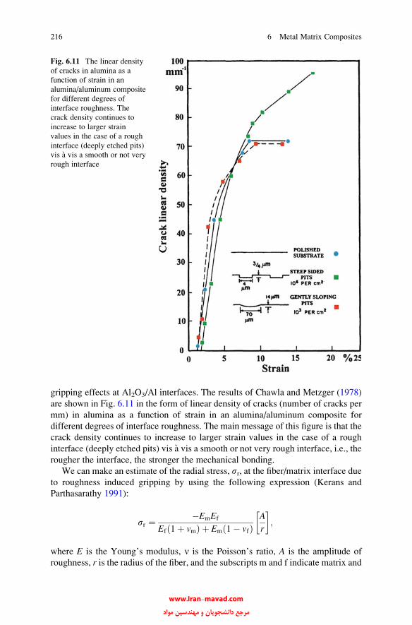
gripping effects at Al2O3/Al interfaces. The results of Chawla and Metzger (1978)

are shown in Fig. 6.11 in the form of linear density of cracks (number of cracks per

mm) in alumina as a function of strain in an alumina/aluminum composite for

different degrees of interface roughness. The main message of this figure is that the

crack density continues to increase to larger strain values in the case of a rough

interface (deeply etched pits) vis a vis a smooth or not very rough interface, i.e., the

rougher the interface, the stronger the mechanical bonding.

We can make an estimate of the radial stress, sr, at the fiber/matrix interface due

to roughness induced gripping by using the following expression (Kerans and

Parthasarathy 1991):

sr ¼ �EmEf

Ef 1þ vmð Þ þ Em 1� vfð ÞA

r

� �;

where E is the Young’s modulus, n is the Poisson’s ratio, A is the amplitude of

roughness, r is the radius of the fiber, and the subscripts m and f indicate matrix and

Fig. 6.11 The linear density

of cracks in alumina as a

function of strain in an

alumina/aluminum composite

for different degrees of

interface roughness. The

crack density continues to

increase to larger strain

values in the case of a rough

interface (deeply etched pits)

vis a vis a smooth or not very

rough interface



fiber, respectively. For a given composite, the compressive radial stress increases

with the roughness amplitude and decreases with the fiber radius. An important

example of such an MMC, i.e., nonreacting components with purely a mechanical

bond at the interface, is the filamentary superconducting composite consisting of

niobium–titanium alloy filaments in a copper matrix.

6.4.2.3 Chemical Bonding

Ceramic/metal interfaces are generally formed at high temperatures. Diffusion and

chemical reaction kinetics are faster at elevated temperatures. One needs to have

knowledge of the chemical reaction products and, if possible, their properties. Molten

iron, nickel, titanium, low alloy steels, austenitic and ferritic stainless steels, and

nickel-based superalloys react with silicon-containing ceramics to form eutectics,

with the reaction products being mainly metal silicides and carbides. It is thus

imperative to understand the thermodynamics and kinetics of reactions in order to

control processing and obtain optimum properties. We provide some examples.

Most metal matrix composite systems are nonequilibrium systems in the

thermodynamic sense; that is, there exists a chemical potential gradient across

the fiber/matrix interface. This means that given favorable kinetic conditions

(which in practice means a high enough temperature or long enough time), diffu-

sion and/or chemical reactions will occur between the components (see Fig. 4.4 in

Chap. 4). Two common morphologies of reaction products at an interface

in common metal matrix composites are as follows: (a) a reaction layer that covers

the ceramic reinforcement more or less uniformly and (b) a discrete precipitation,

particle or needle shaped, around the reinforcement. Type (a) reaction is controlled

by diffusion of elements in the reaction layer. Typically, such a diffusional growth

of the reaction layer scales as x2 ’ Dt, where x is the reaction layer thickness, t isthe time, and D is the diffusion coefficient. Examples of systems showing such

interfacial reactions include B/Al and SiC/Ti. Fujiwara et al. (1995) observed such a

parabolic growth of the reaction zone in SCS-6 silicon carbide fiber/Ti-4.5Al-3V-

2Fe-2Mo (wt.%) composites at three different temperatures. Figure 6.12 shows the

reaction zone thickness squared (x2) as a function of reaction time for three different

Fig. 6.12 Reaction zone

thickness squared (x2) as afunction of reaction time for

three different B/Ti

composites. A B4C carbide

coating on the boron is most

effective for the B/Ti system.

[From Naslain et al. (1976),




http://dx.doi.org/10.1007/978-0-387-74365-3_4#Fig.�4_4

http://dx.doi.org/10.1007/978-0-387-74365-3_4

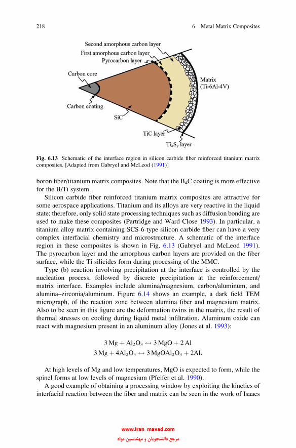
boron fiber/titanium matrix composites. Note that the B4C coating is more effective

for the B/Ti system.

Silicon carbide fiber reinforced titanium matrix composites are attractive for

some aerospace applications. Titanium and its alloys are very reactive in the liquid

state; therefore, only solid state processing techniques such as diffusion bonding are

used to make these composites (Partridge and Ward-Close 1993). In particular, a

titanium alloy matrix containing SCS-6-type silicon carbide fiber can have a very

complex interfacial chemistry and microstructure. A schematic of the interface

region in these composites is shown in Fig. 6.13 (Gabryel and McLeod 1991).

The pyrocarbon layer and the amorphous carbon layers are provided on the fiber

surface, while the Ti silicides form during processing of the MMC.

Type (b) reaction involving precipitation at the interface is controlled by the

nucleation process, followed by discrete precipitation at the reinforcement/

matrix interface. Examples include alumina/magnesium, carbon/aluminum, and

alumina–zirconia/aluminum. Figure 6.14 shows an example, a dark field TEM

micrograph, of the reaction zone between alumina fiber and magnesium matrix.

Also to be seen in this figure are the deformation twins in the matrix, the result of

thermal stresses on cooling during liquid metal infiltration. Aluminum oxide can

react with magnesium present in an aluminum alloy (Jones et al. 1993):

3Mgþ Al2O3 $ 3MgOþ 2Al

3Mgþ 4Al2O3 $ 3MgOAl2O3 þ 2Al:

At high levels of Mg and low temperatures, MgO is expected to form, while the

spinel forms at low levels of magnesium (Pfeifer et al. 1990).

A good example of obtaining a processing window by exploiting the kinetics of

interfacial reaction between the fiber and matrix can be seen in the work of Isaacs

Fig. 6.13 Schematic of the interface region in silicon carbide fiber reinforced titanium matrix

composites. [Adapted from Gabryel and McLeod (1991)]



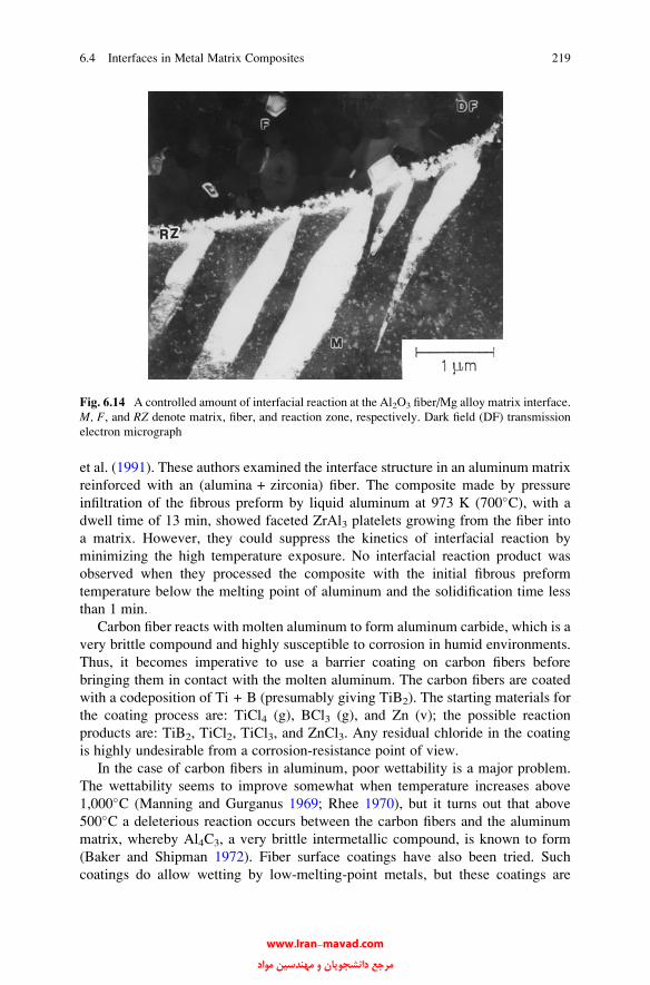
et al. (1991). These authors examined the interface structure in an aluminum matrix

reinforced with an (alumina + zirconia) fiber. The composite made by pressure

infiltration of the fibrous preform by liquid aluminum at 973 K (700�C), with a

dwell time of 13 min, showed faceted ZrAl3 platelets growing from the fiber into

a matrix. However, they could suppress the kinetics of interfacial reaction by

minimizing the high temperature exposure. No interfacial reaction product was

observed when they processed the composite with the initial fibrous preform

temperature below the melting point of aluminum and the solidification time less

than 1 min.

Carbon fiber reacts with molten aluminum to form aluminum carbide, which is a

very brittle compound and highly susceptible to corrosion in humid environments.

Thus, it becomes imperative to use a barrier coating on carbon fibers before

bringing them in contact with the molten aluminum. The carbon fibers are coated

with a codeposition of Ti + B (presumably giving TiB2). The starting materials for

the coating process are: TiCl4 (g), BCl3 (g), and Zn (v); the possible reaction

products are: TiB2, TiCl2, TiCl3, and ZnCl3. Any residual chloride in the coating

is highly undesirable from a corrosion-resistance point of view.

In the case of carbon fibers in aluminum, poor wettability is a major problem.

The wettability seems to improve somewhat when temperature increases above

1,000�C (Manning and Gurganus 1969; Rhee 1970), but it turns out that above

500�C a deleterious reaction occurs between the carbon fibers and the aluminum

matrix, whereby Al4C3, a very brittle intermetallic compound, is known to form

(Baker and Shipman 1972). Fiber surface coatings have also been tried. Such

coatings do allow wetting by low-melting-point metals, but these coatings are

Fig. 6.14 A controlled amount of interfacial reaction at the Al2O3 fiber/Mg alloy matrix interface.

M, F, and RZ denote matrix, fiber, and reaction zone, respectively. Dark field (DF) transmission

electron micrograph



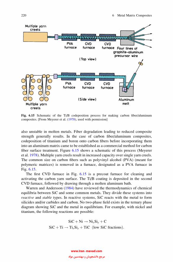
also unstable in molten metals. Fiber degradation leading to reduced composite

strength generally results. In the case of carbon fiber/aluminum composites,

codeposition of titanium and boron onto carbon fibers before incorporating them

into an aluminum matrix came to be established as a commercial method for carbon

fiber surface treatment. Figure 6.15 shows a schematic of this process (Meyerer

et al. 1978). Multiple yarn creels result in increased capacity over single yarn creels.

The common size on carbon fibers such as polyvinyl alcohol (PVA) (meant for

polymeric matrices) is removed in a furnace, designated as a PVA furnace in

Fig. 6.15.

The first CVD furnace in Fig. 6.15 is a precoat furnace for cleaning and

activating the carbon yarn surface. The Ti/B coating is deposited in the second

CVD furnace, followed by drawing through a molten aluminum bath.

Warren and Andersson (1984) have reviewed the thermodynamics of chemical

equilibria between SiC and some common metals. They divide these systems into

reactive and stable types. In reactive systems, SiC reacts with the metal to form

silicides and/or carbides and carbon. No two-phase field exists in the ternary phase

diagram showing SiC and the metal in equilibrium. For example, with nickel and

titanium, the following reactions are possible:

SiCþ Ni ! NixSiy þ C

SiCþ Ti ! TixSiy þ TiC low SiC fractionsð Þ:

Fig. 6.15 Schematic of the Ti/B codeposition process for making carbon fiber/aluminum

composites. [From Meyerer et al. (1978), used with permission]



Such reactions are thermodynamically possible between SiC and nickel or

titanium, but in practice, reaction kinetics determine the usefulness of the compos-

ite. In stable systems, SiC and a metallic matrix alloy can coexist thermodynami-

cally, that is, a two-phase field exists. Examples are SiC fibers in alloys of

aluminum, gold, silver, copper, magnesium, lead, tin, and zinc. This does not

imply that SiC will not be attacked. In fact, a fraction of SiC fibers in contact

with molten aluminum can dissolve and react to give Al4C3:

SiCþ Al ! SiCþ Sið Þ þ Al4C3:

This reaction can happen because the section SiC-Al lies in a three-phase field.

Such reactions can be avoided by prior alloying of aluminum with silicon.

The interface product(s) formed because of a reaction will generally have

characteristics different from those of either component. It should be pointed out,

however, that at times, some controlled amount of reaction at the interface, such as

that shown in Fig. 6.14, may be desirable for obtaining strong bonding between

the fiber and the matrix, but, too thick an interaction zone will adversely affect the

composite properties.

Silicon carbide particle reinforced aluminum composites have been investigated

extensively. An important processing technique for these MMCs involves liquid

metal infiltration of a particulate preform. In a silicon-free aluminum alloy matrix,

silicon carbide and molten aluminum can react as follows:

4AlðlÞ þ 3SiCðsÞ $ Al4C3ðsÞ þ 3SiðsÞ:

The forward reaction will add silicon to the matrix. As the silicon level increases

in the molten matrix, the melting point of the alloy decreases with time. The

reaction can be made to go leftward by using high silicon alloys. This, of course,

restricts the choice of Al alloys for liquid route processing. Table 6.3 gives a

summary of interfacial reactions in some important MMCs.

In general, ceramic reinforcements (fibers, whiskers, or particles) have a coefficient

of thermal expansion smaller than that of most metallic matrices. This means

that when the composite is subjected to a temperature change, thermal stresses

Table 6.3 Interfacial

reaction products in some

important MMCs

Reinforcement Matrix Reaction product(s)

SiC Ti alloy TiC, Ti5Si3Al alloy Al4C3

Al2O3 Mg alloy MgO, MgAl2O4 (spinel)

C Al alloy Al4C3

B Al alloy AlB2

Al2O3 + ZrOz Al alloy ZrAl3W Cu None

C Cu None

Al2O3 Al None



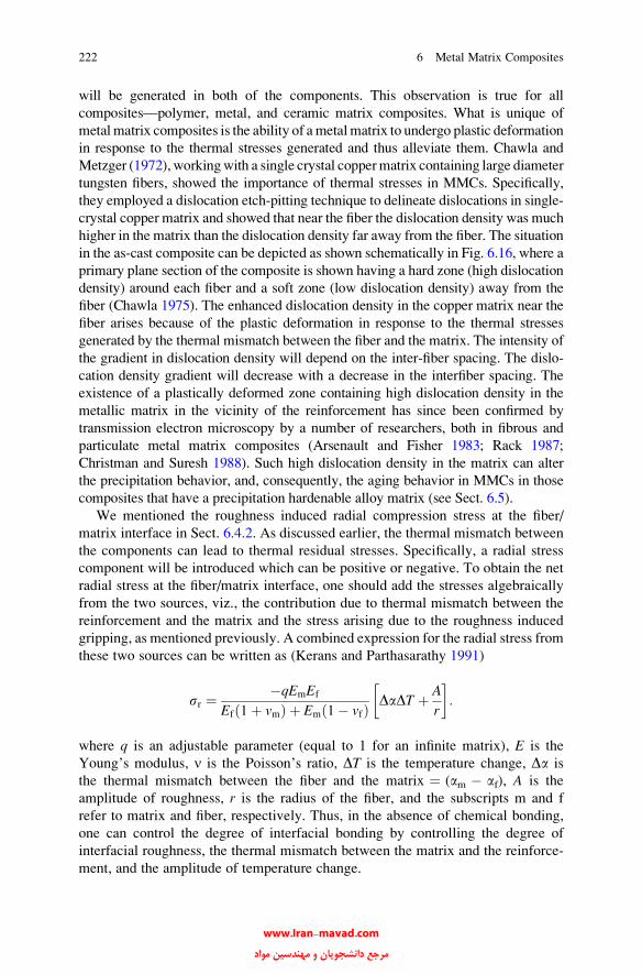
will be generated in both of the components. This observation is true for all

composites—polymer, metal, and ceramic matrix composites. What is unique of

metal matrix composites is the ability of ametalmatrix to undergo plastic deformation

in response to the thermal stresses generated and thus alleviate them. Chawla and

Metzger (1972), workingwith a single crystal coppermatrix containing large diameter

tungsten fibers, showed the importance of thermal stresses in MMCs. Specifically,

they employed a dislocation etch-pitting technique to delineate dislocations in single-

crystal copper matrix and showed that near the fiber the dislocation density was much

higher in the matrix than the dislocation density far away from the fiber. The situation

in the as-cast composite can be depicted as shown schematically in Fig. 6.16, where a

primary plane section of the composite is shown having a hard zone (high dislocation

density) around each fiber and a soft zone (low dislocation density) away from the

fiber (Chawla 1975). The enhanced dislocation density in the copper matrix near the

fiber arises because of the plastic deformation in response to the thermal stresses

generated by the thermal mismatch between the fiber and the matrix. The intensity of

the gradient in dislocation density will depend on the inter-fiber spacing. The dislo-

cation density gradient will decrease with a decrease in the interfiber spacing. The

existence of a plastically deformed zone containing high dislocation density in the

metallic matrix in the vicinity of the reinforcement has since been confirmed by

transmission electron microscopy by a number of researchers, both in fibrous and

particulate metal matrix composites (Arsenault and Fisher 1983; Rack 1987;

Christman and Suresh 1988). Such high dislocation density in the matrix can alter

the precipitation behavior, and, consequently, the aging behavior in MMCs in those

composites that have a precipitation hardenable alloy matrix (see Sect. 6.5).

We mentioned the roughness induced radial compression stress at the fiber/

matrix interface in Sect. 6.4.2. As discussed earlier, the thermal mismatch between

the components can lead to thermal residual stresses. Specifically, a radial stress

component will be introduced which can be positive or negative. To obtain the net

radial stress at the fiber/matrix interface, one should add the stresses algebraically

from the two sources, viz., the contribution due to thermal mismatch between the

reinforcement and the matrix and the stress arising due to the roughness induced

gripping, as mentioned previously. A combined expression for the radial stress from

these two sources can be written as (Kerans and Parthasarathy 1991)

sr ¼ �qEmEf

Ef 1þ vmð Þ þ Em 1� vfð Þ DaDT þ A

r

� �:

where q is an adjustable parameter (equal to 1 for an infinite matrix), E is the

Young’s modulus, n is the Poisson’s ratio, DT is the temperature change, Da is

the thermal mismatch between the fiber and the matrix ¼ (am � af), A is the

amplitude of roughness, r is the radius of the fiber, and the subscripts m and f

refer to matrix and fiber, respectively. Thus, in the absence of chemical bonding,

one can control the degree of interfacial bonding by controlling the degree of

interfacial roughness, the thermal mismatch between the matrix and the reinforce-

ment, and the amplitude of temperature change.



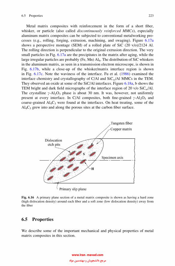
Metal matrix composites with reinforcement in the form of a short fiber,

whisker, or particle (also called discontinuously reinforced MMCs), especiallyaluminum matrix composites can be subjected to conventional metalworking pro-

cesses (e.g., rolling, forging, extrusion, machining, and swaging). Figure 6.17a

shows a perspective montage (SEM) of a rolled plate of SiC (20 v/o)/2124 Al.

The rolling direction is perpendicular to the original extrusion direction. The very

small particles in Fig. 6.17a are the precipitates in the matrix after aging, while the

large irregular particles are probably (Fe, Mn) Al6. The distribution of SiC whiskers

in the aluminum matrix, as seen in a transmission electron microscope, is shown in

Fig. 6.17b, while a close-up of the whisker/matrix interface region is shown

in Fig. 6.17c. Note the waviness of the interface. Fu et al. (1986) examined the

interface chemistry and crystallography of C/Al and SiCw/Al MMCs in the TEM.

They observed an oxide at some of the SiC/Al interfaces. Figure 6.18a, b shows the

TEM bright and dark field micrographs of the interface region of 20 v/o SiCw/Al.

The crystalline g-Al2O3 phase is about 30 nm. It was, however, not uniformly

present at every interface. In C/Al composites, both fine-grained g-Al2O3 and

coarse-grained Al4C3 were found at the interfaces. On heat treating, some of the

Al4C3 grew into and along the porous sites at the carbon fiber surface.

6.5 Properties

We describe some of the important mechanical and physical properties of metal

matrix composites in this section.

Fig. 6.16 A primary plane section of a metal matrix composite is shown as having a hard zone

(high dislocation density) around each fiber and a soft zone (low dislocation density) away from

the fiber

6.5 Properties 223


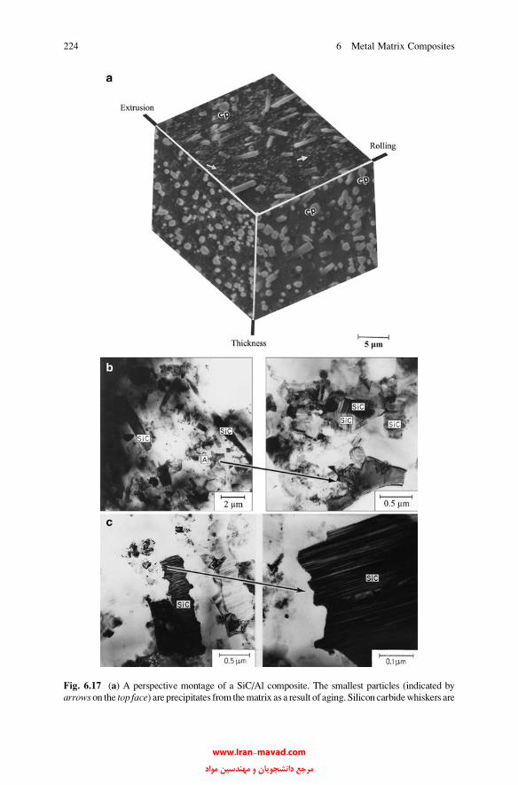
Fig. 6.17 (a) A perspective montage of a SiC/Al composite. The smallest particles (indicated by

arrows on the top face) are precipitates from thematrix as a result of aging. Silicon carbidewhiskers are



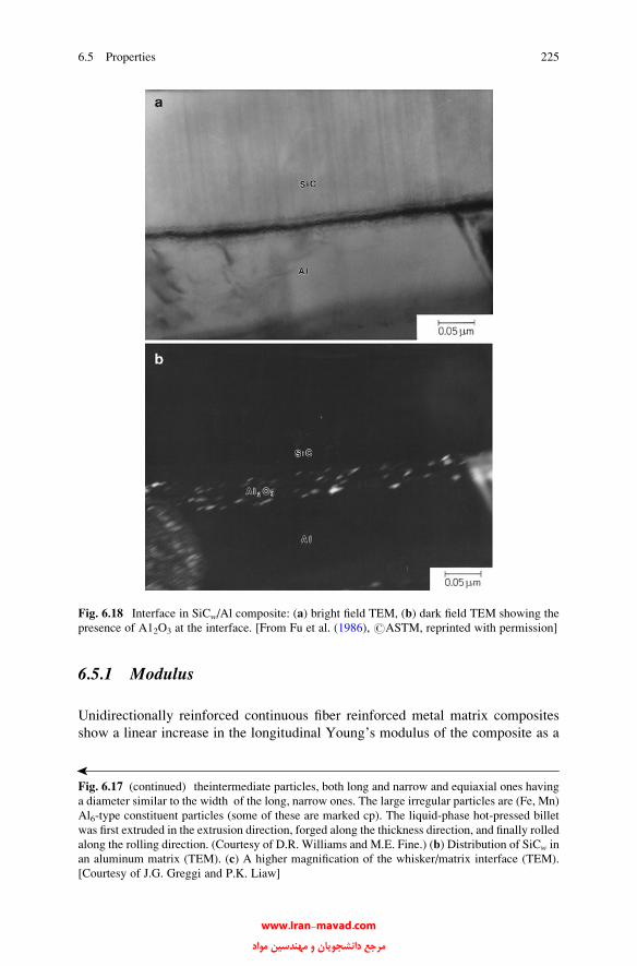
6.5.1 Modulus

Unidirectionally reinforced continuous fiber reinforced metal matrix composites

show a linear increase in the longitudinal Young’s modulus of the composite as a

�

Fig. 6.17 (continued) theintermediate particles, both long and narrow and equiaxial ones having

a diameter similar to the width of the long, narrow ones. The large irregular particles are (Fe, Mn)

Al6-type constituent particles (some of these are marked cp). The liquid-phase hot-pressed billet

was first extruded in the extrusion direction, forged along the thickness direction, and finally rolled

along the rolling direction. (Courtesy of D.R. Williams and M.E. Fine.) (b) Distribution of SiCw in

an aluminum matrix (TEM). (c) A higher magnification of the whisker/matrix interface (TEM).

[Courtesy of J.G. Greggi and P.K. Liaw]

Fig. 6.18 Interface in SiCw/Al composite: (a) bright field TEM, (b) dark field TEM showing the

presence of A12O3 at the interface. [From Fu et al. (1986), #ASTM, reprinted with permission]

6.5 Properties 225


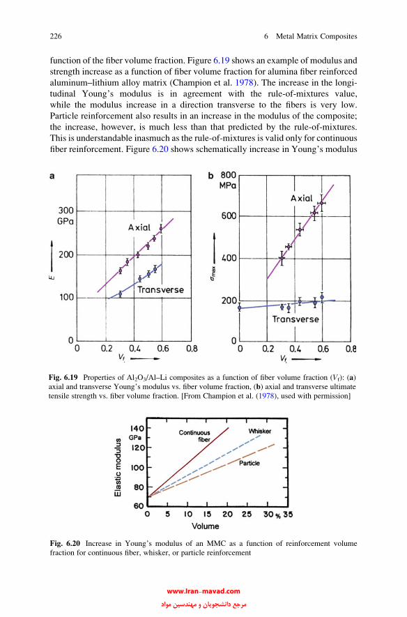
function of the fiber volume fraction. Figure 6.19 shows an example of modulus and

strength increase as a function of fiber volume fraction for alumina fiber reinforced

aluminum–lithium alloy matrix (Champion et al. 1978). The increase in the longi-

tudinal Young’s modulus is in agreement with the rule-of-mixtures value,

while the modulus increase in a direction transverse to the fibers is very low.

Particle reinforcement also results in an increase in the modulus of the composite;

the increase, however, is much less than that predicted by the rule-of-mixtures.

This is understandable inasmuch as the rule-of-mixtures is valid only for continuous

fiber reinforcement. Figure 6.20 shows schematically increase in Young’s modulus

Fig. 6.19 Properties of Al2O3/Al–Li composites as a function of fiber volume fraction (Vf): (a)

axial and transverse Young’s modulus vs. fiber volume fraction, (b) axial and transverse ultimate

tensile strength vs. fiber volume fraction. [From Champion et al. (1978), used with permission]

Fig. 6.20 Increase in Young’s modulus of an MMC as a function of reinforcement volume

fraction for continuous fiber, whisker, or particle reinforcement



of an MMC as a function of reinforcement volume fraction for different forms

of reinforcement viz., continuous fiber, whisker, or particle. Note the loss of

reinforcement efficiency as one goes from continuous fiber to particle. Metal

matrix particulate composites, such as SiC particle reinforced aluminum can

offer a 50–100% increase in modulus over that of unreinforced aluminum, i.e., a

modulus equivalent to that of titanium but density about 33% less. Also, unlike

the fiber reinforced composites, the stiffness enhancement in particulate

composites is reasonably isotropic.

6.5.2 Strength

Prediction of strength of an MMC is more complicated than the prediction of

modulus. This is so because there can be direct and indirect strengthening. The

direct strengthening considers the contribution of fiber and the metal matrix without

taking into account and strength contribution stemming from any microstructural

changes in the metal matrix. The direct strengthening is described as follows.

Consider an aligned fiber reinforced metal matrix composite under a load Pc in

the direction of the fibers. This load is distributed between the fiber and the matrix.

Thus,

Pc ¼ PmVm þ PfVf ;

where Pm and Pf are the loads on the matrix and the fiber, and Vm and Vf are the

volume fractions of the matrix and the fiber, respectively. This equation can be

converted to the following rule-of-mixtures (we discuss this in more detail in Chap.

10) relationship under conditions of isostrain (i.e., the strain in the fiber, matrix, and

composite is the same):

sc ¼ sfVf þ smVm;

where s is the stress, V is the volume fraction, and the subscripts c, f, and m denote

the composite, fiber, and matrix, respectively. This equation, commonly referred to

as the Rule-of-Mixtures, says that the strength of the composite is a volume-

weighted average of the strengths of the fiber and the matrix.

On the face of it, there is nothing wrong with rule-of-mixtures as written above

for strength. The problem is that one needs the in situ values of sf and sm. If thefiber remains essentially elastic up to the point of fracture, then sf, the fiber strengthin the composite, is the same as that determined in an isolated test of the fiber. This

is particularly true of ceramic fibers. The same, however, cannot be said for the

metallic matrix. The matrix strength in the composite (the in situ strength) will, in

6.5 Properties 227


http://dx.doi.org/10.1007/978-0-387-74365-3_10

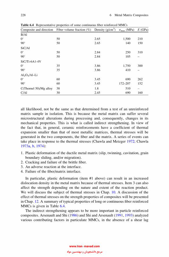
all likelihood, not be the same as that determined from a test of an unreinforced

matrix sample in isolation. This is because the metal matrix can suffer several

microstructural alterations during processing and, consequently, changes in its

mechanical properties. This is what is called indirect strengthening. In view of

the fact that, in general, ceramic reinforcements have a coefficient of thermal

expansion smaller than that of most metallic matrices, thermal stresses will be

generated in the two components, the fiber and the matrix. A series of events can

take place in response to the thermal stresses (Chawla and Metzger 1972; Chawla

1973a, b, 1974):

1. Plastic deformation of the ductile metal matrix (slip, twinning, cavitation, grain

boundary sliding, and/or migration).

2. Cracking and failure of the brittle fiber.

3. An adverse reaction at the interface.

4. Failure of the fiber/matrix interface.

In particular, plastic deformation (item #1 above) can result in an increased

dislocation density in the metal matrix because of thermal stresses. Item 3 can also

affect the strength depending on the nature and extent of the reaction product.

We will discuss the subject of thermal stresses in Chap. 10. A discussion of the

effect of thermal stresses on the strength properties of composites will be presented

in Chap. 12. A summary of typical properties of long or continuous fiber reinforced

MMCs is given in Table 6.4.

The indirect strengthening appears to be more important in particle reinforced

composites. Arsenault and Shi (1986) and Shi and Arsenault (1991, 1993) analyzed

various contributing factors in particulate MMCs, in the absence of a shear lag

Table 6.4 Representative properties of some continuous fiber reinforced MMCs

Composite and direction Fiber volume fraction (%) Density (g/cm3) smax (MPa) E (GPa)

B/Al

0� 50 2.65 1,500 210

90� 50 2.65 140 150

SiC/Al

0� 50 2.84 250 310

90� 50 2.84 105 –

SiC/Ti-6A1-4V

0� 35 3.86 1,750 300

90� 35 3.86 410 –

Al2O3/Al–Li

0� 60 3.45 690 262

90� 60 3.45 172–207 152

C(Thornel 50)/Mg alloy 38 1.8 510 –

C/Al 30 2.45 690 160



http://dx.doi.org/10.1007/978-0-387-74365-3_10

http://dx.doi.org/10.1007/978-0-387-74365-3_12

strengthening mechanism, which would be more effective in the case of long

fibrous reinforcement. They enumerated the following indirect strengthening

mechanisms in particulate MMCs:

• Orowan strengthening, which is given by Gb/l, where G is the shear modulus of

the matrix, b is the Burgers vector of the matrix, and l is the particle spacing.• Grain and substructure strengthening in the metal matrix, following a Hall–Petch-

typerelationship, i.e., strength varying as d�1/2, where d is the grain or subgrain size

in thematrix. TheHall–Petch slope k forAl is in the range of 0.1–0.15MPa√m2, i.e., it

is very low, while for steels, k is very high. Thus, a grain diameter d < 10 mmwill

give significant strengthening, while d < 1 mmcan give very good strengthening.

• Quench strengthening with thermal strain in the matrix given by em ¼ DaDT.According to the model of Arsenault and Shi (1986), dislocation punching

occurs in the matrix due to thermal mismatch. The dislocation density resulting

from the coefficient of thermal expansion mismatch is

rCTE ¼ AeVp

� �=b 1� Vp

� �d;

where A is a geometric constant, e is the thermal misfit strain, A is the particle

area, b is the Burgers vector, and Vp is the particle volume fraction.

The corresponding stress is given by

sq ¼ aGb rCTEð Þ1=2;

where a is a constant. This contribution to strength can be significant.

• Work hardening of the matrix. Particles affect the matrix work hardening rate.

In powder metallurgy processed composites, fine oxide from the SiC particle’s

surface can enter the matrix. The contribution of grain boundary strengthening is

given by

sgb ¼ kd�1=2:

Grain boundary strengthening can be high in spray cast and powder metallurgy

processed composites.

It is thus complicated to predict the strength of a particulate MMC. An analysis

(Nardone and Prewo 1986) that takes into account tensile loading at the particle

ends gives the following expression for the yield strength of a particulate composite

syc ¼ sym 1þ Lþ tð Þ=4L½ �Vp þ sym 1� Vp

� �;

where sym is the yield stress of the unreinforced matrix, Vp is the particle volume

fraction, L is the length of the particle perpendicular to the applied load and t is thelength of the particle parallel to the loading direction (see also Chap. 10).

6.5 Properties 229


http://dx.doi.org/10.1007/978-0-387-74365-3_10

6.5.2.1 Effect of Thermal Stresses

It is important to realize is that the matrix in composites is not merely a kind of glue

or cement to hold the reinforcement in place [Chawla 1985]. The characteristics of

the matrix, as modified by the introduction of fibers, must be evaluated and exploited

to obtain an optimum set of properties of the composite. The nature of the fibers or

particles, fiber or particle diameter, and distribution, as well as conventional solidi-

fication parameters, all influence the final matrix microstructure. Porosity is one of

themajor defects in castMMCs, owing to the shrinkage of themetallic matrix during

solidification. At high fiber volume fractions, the flow of interdendritic liquid

becomes difficult, and large scale movement of semisolid metal may not be

possible. More importantly, the microstructure of the metallic matrix in a fiber

composite can differ significantly from that of the unreinforced metal. Mention has

been made of higher dislocation density in the metal matrix because of plastic

deformation originating in thermal stresses (Chawla and Metzger 1972).

Mortensen et al. (1986) showed that the presence of fibers influences the solidifi-

cation of the matrix alloy. Figure 6.21a shows a cross section of an SCS-2 silicon

carbide fiber/Al-4.5% Cu matrix. Note the normal dendritic cast structure in the

unreinforced region, whereas in the reinforced region the dendritic morphology is

controlled by the fiber distribution. Figure 6.21b shows the same system at a higher

magnification. The second phase (y) appears preferentially at the fiber/matrix

interface or in the narrow interfiber spaces. Kohyama et al. (1985) observed that

shrinkage cavities present in the matrix in SiC/Al composites were the predomi-

nant crack-initiation sites. They also observed a wavy interface structure between

SiC and the aluminum matrix, indicating some mechanical bonding in addition to

any chemical and physical bonding. In the system SiC/Mg (AZ19C), they observed

a magnesium-rich interfacial layer that acted as the fracture-initiating site.

Frequently the metal matrix alloy used in an MMC has precipitation hardening

Mortensen 1991a, b; Dutta et al. 1988; Dutta and Bourell 1988; 1990; Chawla et al.

1991; Nieh and Karlak 1984; Parrini and Schaler 1994) that the microstructure of the

metallic matrix is modified by the presence of ceramic reinforcement and conse-

quently the standard aging treatment for, say, an unreinforced aluminum alloy will not

be valid (see Suresh and Chawla (1993) for a review of this topic). The reinforcements

(fiber or particle), such as SiC, B4C, Al2O3, are unaffected by the aging process. These

reinforcements, however, can affect the precipitation behavior of the matrix quite

significantly. In particular, as we pointed out earlier, a higher dislocation density in

the matrix metal or alloy than that in the unreinforced metal or alloy is produced.

The higher dislocation density in the matrix has its origin in the thermal mismatch

(Da) between the reinforcement and the metallic matrix. This thermal mismatch can

be quite large, for example, in the case of SiC and aluminum, it has a high value of

21 � 10�6/K. The precipitate-hardenable aluminum alloy matrix has a more impor-

tant role to play in these composites than a nonhardenable matrix material. A consid-

erable strength increment results due to the age-hardening treatments. One would


characteristics, i.e., such an alloy can be hardened by a suitable heat treatment,

called aging treatment. It has been shown by many researchers (Dunand and


expect that the high dislocation density will also affect the precipitation kinetics in a

precipitation-hardenable matrix such as 2XXX series aluminum alloy. Indeed, faster

precipitation kinetics have been observed in the matrix than in the bulk unreinforced

alloy. This has very important practical implications. One may not use the standard

heat treatments commonly available in various handbooks, say, for monolithic alumi-

num alloys for the same alloy used as a matrix in an MMC.

Fig. 6.21 Transverse section of an SCS-2 SiC fiber in an Al-4.5 % Cu matrix. (a) Note the

difference in the dendritic structure of the unreinforced and the fiber-rich regions of the matrix.

(b) the second phase appears preferentially at the fiber/matrix interface or in the narrow interfiber

region. The fiber diameter is 142 mm in both (a) and (b). [Reprinted with permission from J Metals

37(6):45, 47, and 48, a publication of the Metallurgical Society, Warrendale, Pennsylvania]

6.5 Properties 231


6.5.2.2 Properties of In Situ Composites

We mentioned earlier the class of MMCs called in situ composites. An important

example of such a system is a composite made by directional solidification of a

eutectic alloy. The strength, s, of such an in situ metal matrix composite is given by

a relationship similar to the Hall–Petch relationship used for grain boundary

strengthening of metals (Meyers and Chawla 1984):

s ¼ so þ kl�1=2;

where so is a friction stress term, k is a material constant, and l is the spacing

between rods or lamellae. It turns out that one can vary the interfiber spacing, l,rather easily by controlling the solidification rate, R, because

l2R ¼ constant:

van Suchtelen (1972) has classified eutectic or in situ composites into two broad

categories from an electronic property viewpoint:

1. Combination-type properties. This can be further subdivided into (a) sum type

and (b) product type. In sum type, properties of the constituent phases contributeproportionately to their amount. Examples are heat conduction, density, and

elastic modulus. In the product type, the physical output of one phase serves asinput for the other phase: for example, conversion of a magnetic signal into an

electrical signal in a eutectic composite consisting of a magnetostrictive phase

and a piezoelectric phase.

2. Morphology-dependent properties. In this case, the properties depend on

the periodicity and anisotropy of the microstructure, the shape and size of the

phases, and the amount of interface area between the phases. A good example is

InSb–NiSb, which is a quasibinary system with a eutectic at 1.8% NiSb. Unidi-

rectional solidification of a eutectic melt at a growth rate of 2 cm/h results in an

aligned composite consisting of an InSb semiconducting matrix containing long

hexagonal fibers of the NiSb phase. The magnetoresistance of the InSb–NiSb

composite becomes extremely large if the directions of the metallic fibers, the

electric current, and the magnetic field are mutually perpendicular. This charac-

teristic has been exploited in making contactless control devices; a practical

example is described in Sect. 6.6.

6.5.2.3 Properties of Particulate Composites

Tensile stress–strain curves of SiCp/Al composites are shown in Fig. 6.22 (Chawla

et al. 1998). Figure 6.22a shows the true stress–true strain curves for one particle

size (6 mm) but different volume fractions of the SiC particles. As the particle

volume fraction increases, the strength of the composite increases but the ductility



decreases. Figure 6.22b shows the true stress–true strain curves for different particle

sizes but for a fixed volume fraction (20% by volume). The strength increases as the

particle size decreases.

Fig. 6.22 (a) True stress–true strain curves for different volume fractions of the SiC particles in

aluminum matrix (6 mm). As the particle volume fraction increases, the strength of the composite

increases but the ductility decreases. (b) True stress–true strain curves for different particle sizes

but for a fixed volume fraction (20 % by volume). The strength increases as the particle size

decreases. [Courtesy of N. Chawla]

6.5 Properties 233


Toughness can be regarded as a measure of energy absorbed in the process of

fracture, or more specifically as the resistance to crack propagation, KIc. The

toughness of MMCs depends on the following factors:

• matrix alloy composition and microstructure

• reinforcement type, size, and orientation

• processing, insofar as it affects microstructural variables (e.g., distribution of

reinforcement, porosity, segregation, and so on)

For a given Vf, the larger the diameter of the fiber, the tougher the composite.

This is because the larger the fiber diameter, for a given fiber volume fraction, the

larger the amount of tough, metallic matrix in the interfiber region that can undergo

plastic deformation and thus contribute to the toughness.

Unidirectional fiber reinforcement can lead to easy crack initiation and easy

propagation vis a vis the unreinforced alloy matrix. Braiding of fibers can make

the crack propagation toughness increase tremendously due to extensive matrix

deformation, fiber bundle debonding, and pullout (Majidi and Chou 1987). The

general range of KIc values for particle reinforced aluminum-type MMCs is

between 15 and 30 MPa m1/2, while short fiber- or whisker-reinforced MMCs

have ’5–10 MPa m1/2.

The fracture toughness of particle reinforced MMCs is controlled by: (a)

volume fraction of reinforcement, (b) interparticle spacing and strength of

Fig. 6.23 Toughness in several particulate composite systems as a function of reinforcement

volume fraction. All the composites show a decrease in toughness with increasing volume fraction

of reinforcement [after Manoharan et al. 1993; Hunt et al. 1993, and Beck Tan et al. 1994]



particles, (c) spatial distribution of particles (i.e., particle clustering), and (d)

matrix microstructure (as controlled by heat-treatment in age-hardenable

alloys). Figure 6.23 shows toughness in several particulate composite systems

as a function of reinforcement volume fraction. All the composites show a

decrease in toughness with increasing volume fraction of reinforcement. The

toughness appears to reach a “plateau” at volume fraction of 20% and above.

The decrease in toughness is attributed to an increase in stress triaxiality with

increasing volume fraction of particles.

Among the explanations for low toughness values of the composites are the

following variables: the type of intermetallic particles, inhomogeneous internal

stress, and particle or whisker distribution. Improvements in fracture toughness of

SiCw/Al composites and KIc values levels equivalent to those of 7075 A1(T6) have

been obtaind by using a cleaner matrix powder, better mixing, and increased

mechanical working during fabrication (McDanels 1985). McDanels’ work also

reinforces the idea that the metallic matrix is not merely a medium to hold the fibers

together. The type of aluminum matrix used in 20 v/o SiCw/Al composites was the

most important factor affecting yield strength and ultimate tensile strength of these

composites (McDanels 1985). Higher-strength aluminum alloys showed higher

strengths but lower ductilities. Composites with 6061 Al matrix showed good

strength and higher fracture strain.

6.5.3 Thermal Characteristics

In general, ceramic reinforcements (fibers, whiskers, or particles) have a coefficient

of thermal expansion smaller than that of most metallic matrices. This means that

when the composite is subjected to a temperature change (deliberate or inadver-

tent), thermal stresses will be generated in both the components because of the

constraint imposed by the interfacial bonding.

Chawla and Metzger (1972), working with a single crystal copper matrix

containing large-diameter tungsten fibers, showed the importance of thermal

stresses in MMCs. Specifically, they employed a dislocation etch-pitting technique

to delineate dislocations in a single crystal copper matrix. This system has the

advantage of showing pure fiber reinforcement, i.e., no interfacial reaction, no grain

boundaries in the matrix, etc. They showed that, in their low fiber volume fraction

composites, near the fiber the dislocation density was much higher in the matrix

than the dislocation density far away from the fiber. The situation in the as-cast

composite can be depicted as was shown schematically in Fig. 6.15, where a

primary plane section of the composite is shown having a hard zone (high disloca-

tion density) around each fiber and a soft zone (low dislocation density) away from

the fiber. The enhanced dislocation density in the copper matrix near the fiber arises

because of the plastic deformation in response to the thermal stresses generated by

the thermal mismatch between the fiber and the matrix. The intensity of the gradient

6.5 Properties 235


in dislocation density will depend on the interfiber spacing. The dislocation density

gradient will decrease with a decrease in the interfiber spacing. The existence of a

plastically deformed zone containing high dislocation density in the metallic matrix

near the reinforcement has also been confirmed by transmission electron micros-

copy by a number of researchers, both in fibrous and particulate metal matrix

composites.

Thermal mismatch is indeed something that is difficult to avoid in any composite.

By the same token, however, one can control the overall thermal expansion

characteristics of a composite by controlling the proportion of reinforcement and

matrix and the distribution of the reinforcement in the matrix. Many researchers

have proposed models to predict the coefficients of thermal expansion of

composites, determined experimentally these coefficients, and analyzed the gen-

eral thermal expansion characteristics of metal matrix composites; we describe

some of these in Chap. 10. It would be appropriate to point out here some special

aspects of thermal characteristics of MMCs, especially particulate MMCs. This is

because of their applications in electronic packaging, where their superior thermal

characteristics play an important role; this makes it very important to understand

the effects of thermal stresses and thermal cycling in MMCs. Prediction of CTE is

complicated because of the structure of the composite (particles, whiskers, or

fibers), interface, and the matrix plastic deformation due to internal thermal

stresses. Expansion characteristics of isotropic composites are a function of Vp

or Vf, size, and morphology of the reinforcement. Phenomena such as hysteretic

deformation during thermal cycling, microcracking, and fiber intrusion on the

surface lead to surface roughness. Rezai-Aria et al. (1993) observed surface

roughness when they subjected Saffill fiber reinforced aluminum to thermal

cycling. It is important to realize that the CTE of a material is not an absolute

physical constant, but that it varies with temperature. This is especially so with

MMCs, where the matrix can undergo plastic deformation as a result of thermal

stresses (Vaidya and Chawla 1994). In addition, there are many microstructural

factors that come into play. For example, a micromechanical analysis of the

thermal expansion of two-dimensional SiCp/Al composites showed the importance

of reinforcement continuity (Shen et al. 1994). Balch et al. (1996) investigated the

role of reinforcement continuity on the thermal expansion of SiC/Al and the effect

of the presence of voids on CTE. Their analysis showed that a high matrix yield

strength, a high interfacial strength, and a convex reinforcement shape would

minimize variations in CTE of a SiCp/Al type composite during any thermal

excursion. In foam-reinforced composites, a weak interface could be exploited to

produce void and thus minimize the average CTE of the composite, but hysteretic

thermal expansion would be observed.

6.5.4 High Temperature Properties, Creep, and Fatigue

Superior high-temperature properties of MMCs have been demonstrated in a

number of systems. For example, silicon carbide whiskers (SiCw) improve the



http://dx.doi.org/10.1007/978-0-387-74365-3_10

high-temperature properties of aluminum considerably. Figure 6.22 compares

the elastic modulus, yield stress, and ultimate tensile strength of SiCw (21% Vf)/

2024 Al composites to those of the unreinforced aluminum alloy (Phillips 1978).

Figure 6.25 shows the fracture surface after tensile testing of a Nicalon fiber/

aluminum composite at two temperatures. Note the more or less planar fracture

with no fiber pullout at room temperature (Fig. 6.25a). At 500�C, a loss of adhesionbetween the fiber and the matrix occurs with the accompanying fiber/matrix separa-

tion and fiber pullout. The fiber pullout has left a hole in the center; see Fig. 6.25b.

High-modulus carbon fiber/aluminum composites combine a very high stiffness

with a very low thermal expansion due mainly to the almost zero longitudinal

Fig. 6.24 Comparison of high-temperature properties of SiCw/Al composites and aluminum:

(a) elastic modulus, (b) yield stress, (c) ultimate tensile strength. [From Phillips (1978), used

with permission]

6.5 Properties 237


expansion coefficient of carbon fibers. Carbon/aluminum composites, however, are

susceptible to galvanic corrosion between carbon and aluminum. Carbon is

cathodic in nature, while aluminum is anodic. Thus, galvanic corrosion can be a

serious problem in joining aluminum to a carbon fiber composite. A common

solution is to have an insulating layer of glass between the aluminum and the

carbon composite. Any welding or joining involving localized heating could also

Fig. 6.25 Tensile fracture in Nicalon fiber/aluminum: (a) at room temperature showing a planar

fracture, (b) at 500 �C showing fiber/matrix separation and fiber pullout leaving a hole. [Courtesy

of K. Okamura]

Fig. 6.26 Dislocation distribution in the aluminum matrix of a SiCw/Al composite: (a) inhomo-

geneous dislocation distribution before testing, (b) uniform dislocation distribution after fatigue

testing. [From Williams and Fine (1985a), used with permission]



be a potential source of problems because aluminum carbide may form as a result of

overheating, which will be detrimental to the mechanical and corrosion properties.

The phenomenon of creep refers to time-dependent deformation. In practice, at

least for most metals and ceramics, the creep behavior becomes important at high

temperatures and, thus, sets a limit on the maximum application temperature.

In general, this limit increases with the melting point of a material. We describe

the creep behavior of MMCs along with that of other composites in Chap. 12.

Fatigue is the phenomenon of mechanical property degradation leading to failure

of a material or a component under cyclic loading. Many high-volume applications

of composite materials involve cyclic loading situations, e.g., automobile

components. For a general discussion of fatigue behavior of composites, see

Chap. 12. We mention here but one example of the importance of matrix micro-

structure on the fatigue behavior of MMCs. Williams and Fine (1985a) investigated

the fatigue behavior of SiC whisker-reinforced 2124 Al alloy composites. Cyclic

loading results in a uniform distribution of dislocations in the metal matrix.

Figure 6.26 shows the dislocation distribution in an aluminum matrix before and

after fatigue testing of a SiCw/Al composite (Williams and Fine 1985a). Note the

uniform dislocation distribution after fatigue testing. They found that unbonded

SiCp and non-SiC intermetallics were the fatigue crack-initiation sites. The

unbonded SiC particles occur when clusters of SiC are present. Thus, not unexpect-

edly, reducing the clustering of SiC and the number and size of the intermetallics

resulted in increased fatigue life.

6.6 Applications

It is convenient to divide the applications of metal matrix composites into aerospace

and nonaerospace categories. In the category of aerospace applications, low density

and other desirable features such as a tailored thermal expansion and conductivity

and high stiffness and strength are the main drivers. Performance rather than cost is

the important item. Inasmuch as continuous fiber reinforced MMCs deliver superior

performance than particle reinforced composites, the former are frequently used in

aerospace applications. In the nonaerospace applications, cost and performance are

important, i.e., an optimum combination of these items is required. It is thus

understandable that particle reinforced MMCs find more structural and nonstruc-

tural applications in nonaerospace fields. By far, the largest commercial application

of MMCs is in the form of filamentary superconducting composites. We devote a

whole chapter to such composites (Chap. 9) because of their commercial impor-

tance. Here, we provide a brief description of various other applications of MMCs.

Reduction in the weight of a component is a major driving force for any

application in the aerospace field. For example, in the Hubble telescope, pitch-

based continuous carbon fiber reinforced aluminum was used for waveguide booms

because this composite is very light, has a high elastic modulus, E, and has a low

coefficient of thermal expansion, a. Other aerospace applications of MMCs involve



http://dx.doi.org/10.1007/978-0-387-74365-3_12

http://dx.doi.org/10.1007/978-0-387-74365-3_12

http://dx.doi.org/10.1007/978-0-387-74365-3_9

replacement of light but toxic beryllium. For example, in the US Trident missile,

beryllium has been replaced by SiCp/Al composite.

One of the important applications of MMCs in the automotive area is in diesel

piston crowns (Donomoto et al. 1983). This application involves incorporation of

short fibers of alumina or alumina + silica in the crown of the piston. The conven-

tional diesel engine piston has an Al–Si casting alloy with crown made of a nickel

cast iron. The replacement of the nickel cast iron by aluminum matrix composite

resulted in a lighter, more abrasion-resistant, and cheaper product. Figure 6.27

shows a picture of such a piston; the arrow indicates the piston crown that is

made of short fiber reinforced aluminum composite. Another application in the

automotive sector involves the use of carbon fiber and alumina fibers in an

aluminum alloy matrix for use as cylinder liners in the Prelude model of Honda

Motor Co. Figure 6.28 shows the microstructure of the cylinder liner showing the

unreinforced and fiber reinforced portions.

Continuous alumina fiber (Nextel 610)-reinforced Al composites are used to

make power transmission cables. The cable consists of a composite core, consisting

of Al2O3/Al composite wrapped with Al–Zr wires. The composite core bearsmost of

the load as it has much higher stiffness and strength. Several tests were conducted on

the actual conductor, including sag–tension behavior, vibration fatigue, thermal

expansion, lightning resistance, and electrical resistance. Figure 6.29a shows these

cables, while Fig. 6.29b shows the advantage in reducing the sag by using the 3M’s

Aluminum Conductor Composite Reinforced (ACCR) instead of the conventional

aluminum-steel reinforced conductor (ACSR).

An important potential commercial application of particle reinforced aluminum

composite is to make automotive driveshafts. In the design of a driveshaft, one

needs to consider the speed at which it becomes dynamically unstable. It turns out

that in terms of geometric parameters, a shorter shaft length and larger diameter will

give a higher critical speed, Nc, while in terms of material parameters, the higher

Fig. 6.27 A cutout of a squeeze cast piston with MMC inserts indicated by dotted lines. [Courtesyof Toyota Motor Co.]



the specific stiffness (E/r), the higher Nc will be. One can make changes in the

driveshaft geometry (increase the length or reduce the diameter) while maintaining

a constant critical speed. A decrease in the driveshaft diameter can be important

because of under-chassis space limitations.

Particulate metal matrix composites, especially with light metal matrix composites

such as aluminum and magnesium, also find applications in automotive and sporting

goods. In this regard, the price per kilogram becomes the driving force for application.

An excellent example involves the use of Duralcan particulate MMCs to make

mountain bicycles. A company, Specialized Bicycle in the United States, sells these

bicycles with frames made from extruded tubes of 6061 aluminum containing about

10% alumina particles. The major advantage is the gain in stiffness.

An interesting example of a sheet laminate composite is a nonvibration sheet

steel, made by Kawasaki Steel under the trade name Nonvibra™. A thin film of resin

is sandwiched between two metal sheets. A chromate coating is applied on the inner

surface of the skin metal. The chromate coating is conducive to cementing the bond

between the resin and the outer skin metal. Such a laminated composite muffles

noise over a broad range of frequencies, and it can be used in the temperature range

of 0–100�C. Examples of applications include oil pans, locker covers, dashboard

panels, floor panels, electrical machinery and appliances, and office equipment.

6.6.1 Electronic-Grade MMCs

Metal matrix composites can be tailored to have optimal thermal and physical

properties to meet the requirements of electronic packaging systems (e.g., cores,

substrates, carriers, and housings). Continuous boron fiber reinforced aluminum

composites made by diffusion bonding have been used as heat sinks in chip carrier

multilayer boards.

Fig. 6.28 Microstructure of the cylinder liner showing the unreinforced Al alloy (bottom) andfiber (alumina + carbon)-reinforced (top) portions



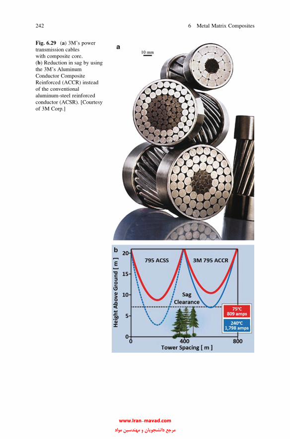
Fig. 6.29 (a) 3M’s power

transmission cables

with composite core.

(b) Reduction in sag by using

the 3M’s Aluminum

Conductor Composite

Reinforced (ACCR) instead

of the conventional

aluminum-steel reinforced

conductor (ACSR). [Courtesy

of 3M Corp.]



Unidirectionally aligned, pitch-based carbon fibers in an aluminum matrix can

have very high thermal conductivity along the fiber direction. The conductivity

transverse to the fibers is about two-thirds that of aluminum. Such a C/Al composite

can find applications in heat transfer applications where weight reduction is an

important consideration, for example, in high-density, high-speed integrated-circuit

packages for computers and in base plates for electronic equipment. Can the reader

think of a potential application in the disk drive of a computer?

Example Discuss the use of carbonfiber/coppermatrix as a high-thermal-conductivity

metalmatrix composite for applications that require high thermal conductivity andhigh

strength.

Answer Pitch-based carbon fibers can have very high thermal conductivity along

the fiber axis, higher than even copper. Putting such fibers in a copper matrix will

result in a high-strength, high-thermal-conductivity metal matrix composite.

The problem with carbon fibers and metallic matrixes is that the surface energy

considerations preclude wetting of the carbon fibers by the molten metals.

The surface energy of carbon fiber is about 100 mJ/m2, while most molten metals

have surface energy of about 1,000 mJ/m2. Recall from Chap. 2 that wetting occurs

when the surface energy of the substrate (fiber) is higher than that of the molten

metal. Thus, one does not expect the wetting of carbon fibers by molten copper.

Two possible routes around this difficulty are as follows:

• Fiber surface modification

• Matrix modification

It would appear that modification of carbon fiber surface bymaking it rough could

result in a reasonable mechanical bond between carbon fiber and copper matrix.

6.6.2 Recycling of Metal Matrix Composites

Particle reinforced metal matrix composites such as SiCp/Al or Al2O3/Al are more

cost-effective than continuous fiber reinforced MMCs such the ones reinforced with

C, SiC, or Al2O3 fibers. There are two main reasons for this: the cost of continuous

fiber and the cost of processing the composite. Also, secondary fabrication (extru-

sion, forging, rolling, etc.) is very difficult with continuous fiber reinforced

composites MMCs. One of the problems of recycling of composites made of

alumina or silicon carbide particles in an aluminum matrix is that a mass of

unreinforced aluminum is indistinguishable from a mass of reinforced aluminum.

The ultimate objective is always to obtain a part or component that performs a

function in a cost-effective manner.

There are two aspects of recycling MMCs (Schuster et al. 1993; Lloyd 1994;

Nishida 2001):

• Recycling of MMCs as MMCs, i.e., without separating the reinforcement from

the matrix. This can be quite economical where it is possible to use. One should



http://dx.doi.org/10.1007/978-0-387-74365-3_2

be mindful of certain steps in such a reuse of MMCs. One should avoid excessive

use of treatments involving thermal excursions or lengthy thermal exposures,

because they can cause adverse chemical interactions at the interface. Some

aluminum metal matrix composites can be recycled and reused, especially if the

Si content is sufficient to retard formation of aluminum carbide, which is highly

deleterious to mechanical properties. Addition of virgin metal to the reinforced

material to obtain a composite with a desired particle volume fraction may be

required.

• Recovery or reclamation of the original components by separating them via the

use of fluxing materials that have lower surface energies with the ceramic

reinforcement than with the metal matrix is a viable option. This is similar to

tertiary recycling of PMCs (see Chap. 5), i.e., one attempts to recover the

original components. There are two ways to do this: mechanical or chemical.

Various mechanical methods of separating the metal and ceramic particles, such

as crushing, shredding, and gravity separation, can be used. Chemical techniques

involve the use of fluxing materials. These fluxing materials should have lower

surface energies with the ceramic reinforcement than with the metal matrix.

Al can be reclaimed from scrap by melting at 700�C, and by adding salt and

bubbling argon through the melt to form froth that concentrates alumina and SiC

particles dewetted by the salt. Figure 6.30 show this process of chemical

separation via fluxing. Using combined argon and salt fluxes, silicon carbide

particles can be removed from the melt and 85–90% of the aluminum can be

reclaimed (Lloyd 1994).

Fig. 6.30 Chemical action of

fluxing materials to separate

the metal matrix from fiber or

particle [after Nishida 2001]



http://dx.doi.org/10.1007/978-0-387-74365-3_5

References

Aghajanian MK, Burke JT, White DR, Nagelberg AS (1989) SAMPE Quart 34:817–823

Arsenault RJ, Fisher RM (1983) Scr Mater 17:67

Arsenault RJ, Shi N (1986) Mater Sci Eng 81:175

Baker AA, Shipman C (1972) Fibre Sci Technol 5:282

Balch DK, Fitzgerald TJ, Michaud VJ, Mortensen A, Shen Y-L, Suresh S (1996) Metall Mater

Trans A 27A:3700

Barrera EV, Sims J, Callahan DL, Provenzano VJ, Milliken J, Holtz RL (1994) J Mater Res 9:2662

Beck Tan NC, Aikiri, Jr. RM, Briber RM (1994) Met Mater Trans 25A:2461

Champion AR, Krueger WH, Hartman HS, Dhingra AK (1978). In: Proceedings of International

Conference on Composite Materials (ICCM/2). TMS-AIME, New York, p 883

Chawla KK (1973a) Metallography 6:155

Chawla KK (1973b) Philos Mag 28:401

Chawla KK (1974) In: Grain boundaries in engineering materials. Claitor’s, Baton Rouge, p 435

Chawla KK (1975) Fibre Sci Technol 8:49

Chawla KK (Dec., 1985) J Metals 37:25

Chawla KK (1989) In: Precious and rare metal technologies. Elsevier, Amsterdam, p 639

Chawla KK, Collares CE (1978). In: Proceedings of the 1978 International Conference on

Composite Materials (ICCM/2), TMS-AIME, New York, p 1237


Chawla KK, Metzger M (1978) In: Fracture 1977. In: Proceedings of the 4th international

conference on fracture, vol 3, Pergamon Press, p 1039

Chawla KK, Esmaeili AH, Datye AK, Vasudevan AK (1991) Scr Mater et Mater 25:1315

Chawla N, Andres C, Jones JW, Allison JE (1998) Metall Mater Trans 29A:2843

Christman T, Suresh S (1988) Mater Sci Eng A102:211

Christodolou L, Parrish PA, Crowe CR (1988) In: Mater Res Soc Symp Proc 120:29–34

Cline HE, Walter JL, Koch EF, Osika LM (1971) Acta Mater 19:405

Cook AJ, Warner PS (1991) Mater Sci Eng A144:189

Cornie JA, Chiang Y-M, Uhlmann DR, Mortensen AS, Collins JM (1986) Ceram Bull 65:293

Divecha AP, Fishman SG, Karmarkar SD (Sept., 1981) J Metals 9:12

Donomoto T, Miura N, Funatani K, and Miyake N (1983). SAE Techical Paper No. 83052,

Detroit, MI

Dunand DC, Mortensen A (1991a) Acta Metall Mater 39:127

Dunand DC, Mortensen A (1991b) Acta Metall Mater 39:1405

Dutta I, Bourell DL (1988) Mater Sci Eng A112:67

Dutta I, Bourell DL (1990) Acta Metall 38:2041

Dutta I, Bourell DL, Latimer D (1988) J Compos Mater 22:829

Fu L-J, Schmerling M, Marcus HL (1986) In: Composite materials: fatigue and fracture, ASTM

STP 907. ASTM, Philadelphia, 51

Fujiwara C, Yoshida M, Matsuhama M, Ohama S (1995). In: Proceedings of International

Conference on Composite Materials (ICCM-10), p II–687.

Gabryel CM, McLeod AD (1991) Metall Trans 23A:1279

Ghosh AK (1993) In: Metal matrix composites. Butterworth-Heinemann, Boston, p 119

Hill RG, Nelson RP, Hellerich CL (1969). In: Proceedings of the 16th refractory working group

meeting, Seattle, WA

Isaacs JA, Taricco F, Michaud VJ, Mortensen A (1991) Metall Trans 22A:2855

Jones C, Kiely CJ, Wang SS (1993) J Mater Res 4:327

Katzman HA (1987) J Mater Sci 22:144

Kerans RJ, Parthasarathy TA (1991) J Am Ceram Soc 74:1585

References 245

Hunt WH, Osman TM, Lewandowski JJ (January, 1993) JOM 45:30


Kohyama A, Igata N, Imai Y, Teranishi H, Ishikawa T (1985). In: Proceedings of the fifth

International Conference on Composite Materials (ICCM/V), TMS-AIME, Warrendale, PA,

p 609

Lloyd DJ (1994) Int Mater Rev 39:1

Majidi AP, Chou TW (1987) Proc Int Conf Compos Mater VI 2:422

Manning C, Gurganus T (1969) J Am Ceram Soc 52:115

Manoharan M, Lewandowski JJ, Hunt WH (1993) Mater Sci Eng A17:63

McDanels DL (1985) Metall Trans 16A:1105

McLean M (1983) Directionally solidified materials for high temperature service. The Metals Soc,

London

Mehrabian R, Riek RG, Flemings MC (1974) Metall Trans 5:1899

Meyerer W, Kizer D, Paprocki S, Paul H (1978). In: Proceedings of the 1978 International

Conference on Composite Materials (ICCM/2), TMS-AIME, New York, p 141

Meyers MA, Chawla KK (1984) Mechanical metallurgy. Prentice-Hall, Englewood Cliffs, 494

Michaud VJ (1993) Metal matrix composites. Butterworth-Heinemann, Boston, p 3

Mitra R, Chiou WA, Fine ME, Weertman JR (1993) J Mater Res 8:2300

Nardone VC, Prewo KM (1986) Scr Mater 20:43

Naslain R, Thebault J, Pailler R (1976). In: Proceedings of the 1975 International Conference on

Composite Materials, vol 1, TMS-AIME, New York, p 116

Nieh TG, Karlak RF (1984) Scr Mater 17:67

Nishida Y (2001) Adv Eng Mater 3:315

Nourbakhsh S, Liang FL, Margolin H (1990) Metall Trans A 21A:213

Parrini L, Schaler R (1994) J Alloy Comp 211:402

Partridge PG, Ward-Close CM (1993) Int Mater Rev 38:1

Pennander L, Anderson C-H (1991) In: Hansen N et al. (eds) Metal matrix composites –

Processing, microstructure and properties. 12th Risø international symposium on materials

science, p 575

Pfeifer M, Rigsbee JM, Chawla KK (1990) J Mater Sci 25:1563

Phillips WL (1978). In: Proceedings of the 1978 International Conference on Composite Materials

(ICCM/2), TMS-AIME, New York, p 567

Rack HJ (1987). In: Sixth International Conference on Composite Materials, Elsevier Applied

Science, New York, p 382

Rezai-Aria F, Liechti T, Gagnon G (1993) Scr Metall Mater 28:587

Rhee S (1970) J Am Ceram Soc 53:386

Rohatgi PK, Asthana R, Das S (1986) Int Met Rev 31:115

Schuster DM, Skibo MD, Bruski RS (1993) J Miner Met Mater Soc 45(5):26

Shen Y-L, Needleman A, Suresh S (1994) Metall Mater Trans A 25A:839

Sherby O, Lee S, Koch R, Sumi T, Wolfenstine J (1985) Mater Manuf Process 5:363

Shi N, Arsenault RJ (1991) J Compos Technol Res 13:211

Shi N, Arsenault RJ (1993) Metall Trans 24A:1879

Srivatsan TS, Lavernia EJ (1992) J Mater Sci 27:5965

Suresh S, Chawla KK (1993) In: Metal matrix composites. Butterworth-Heinemann, Boston, p 119

Thomas DG (1965) J Colloid Sci 20:267

Vaidya RU, Chawla KK (1994) Compos Sci Technol 50:13

van Suchtelan J (1972) Philips Res Rep 27:28

van Suchtelen J (1972) Philips Res Rep 27:28

Vasudevan AK, Doherty RD (eds) (1989) Aluminum alloys – Contemporary research and

applications. Academic, Boston

Vasudevan AK, Petrovic JJ (eds) (1992) High temperature structural silicides, Elsevier,

Amsterdam

Walter JL (1982) In situ composites IV. Elsevier, New York, p 85


Mortensen A, Gungor MN, Cornie JA, Flemings MC (March, 1986) J Metals 38:30

Mortensen A, Cornie JA, Flemings MC (February, 1988) J Metals 40:12


Warren R, Andersson C-H (1984) Composites 15:101

Williams DR, Fine ME (1985a). In: Proceedings of the 5th International Conference on Composite

Materials (ICCM/V), TMS, Warrendale, PA, p 275

Williams DR, Fine ME (1985b). In: Proceedings of the Fifth International Conference on Com-

posite Materials (ICCM/V), TMS-AIME, Warrendale, PA, p 369

Further Reading

Chawla N, Chawla KK (2006) Metal matrix composites. Springer, New York

Clyne TW, Withers PJ (1993) An introduction to metal matrix composites. Cambridge University

Press, Cambridge

Mortensen A, Llorca J (2010) Annu Rev Mater Res 40:243

Suresh S, Needleman A, Mortensen A (eds) (1993) Metal matrix composites. Butterworth-

Heinemann, Boston

Taya M, Arsenault RJ (1990) Metal matrix composites. Pergamon, Oxford

Problems

6.1. Pressure casting is frequently used to prepare metal matrix composite.

Explain why.

6.2. Describe some of the advantages of metal matrix composites over monolithic

metals.

6.3. Discuss the advantages of metal matrix composites vis a vis polymer matrix

composite.

6.4. Discuss the advantages and disadvantages of liquid metal processing vis a vis

other methods of fabricating metal matrix composites.

6.5. Silicon carbide (0.1 mm thick) coated boron fiber was used to reinforce a

metallic matrix. The SiC coating serves as a diffusion barrier coating. Esti-

mate the time for dissolution of this coating at 700 K if the diffusion

coefficient at 700 K is 10�16 m2/s.

6.6. The metallic matrix will generally undergo constrained plastic flow in the

presence of a moderately high volume fraction of high modulus fibers. Draw

schematically the stress–strain curves of a constrained metal matrix (i.e., in

situ behavior) and an unconstrained metal (i.e., 100% matrix metal). Explain

the difference.

6.7. Aluminum and magnesium are two common metal matrix materials. What is

the viscosity of molten aluminum and magnesium?

Problems 247


6.8. What is the effect on viscosity of adding ceramic particles to a molten metal

such as aluminum or magnesium? Discuss its implications in the processing

of MMCs with respect to features such as particle size, volume fraction, etc.

6.9. Discuss the problem of thermal stability of unidirectionally solidified eutectic

(in situ) metallic composites.

6.10. Discuss the use of silicon carbide particle reinforced aluminum composites in

braking applications.



Chapter 7

Ceramic Matrix Composites

Ceramic materials in general have a very attractive package of properties: high

strength and high stiffness at very high temperatures, chemical inertness, low

density, and so on. This attractive package is marred by one deadly flaw, namely,

an utter lack of toughness. They are prone to catastrophic failures in the presence of

flaws (surface or internal). They are extremely susceptible to thermal shock and are

easily damaged during fabrication and/or service. It is therefore understandable that

an overriding consideration in ceramic matrix composites (CMCs) is to toughen the

ceramics by incorporating fibers in them and thus exploit the attractive high-

temperature strength and environmental resistance of ceramic materials without

risking a catastrophic failure. It is worth pointing out at the very outset that there are

certain basic differences between CMCs and other composites. The general philos-

ophy in nonceramic matrix composites is to have the fiber bear a greater proportion

of the applied load. This load partitioning depends on the ratio of fiber and matrix

elastic moduli, Ef/Em. In nonceramic matrix composites, this ratio can be very high,

while in CMCs, it is rather low and can be as low as unity; think of alumina fiber

reinforced alumina matrix composite. Another distinctive point regarding CMCs is

that because of limited matrix ductility and generally high fabrication temperature,

thermal mismatch between components has a very important bearing on CMC

performance. The problem of chemical compatibility between components in

CMCs has ramifications similar to those in, say, MMCs. We first describe some

of the processing techniques for CMCs, followed by a description of some salient

characteristics of CMCs regarding interface and mechanical properties and, in

particular, the various possible toughness mechanisms, and finally a description

of some applications of CMCs.


249


7.1 Processing of CMCs

Ceramic matrix composites (CMCs) can be processed either by conventional

powder processing techniques used for making polycrystalline ceramics or by

some new techniques developed specifically for making CMCs. We describe

below some of the important processing techniques for CMCs.

7.1.1 Cold Pressing and Sintering

Cold pressing of the matrix powder and fiber followed by sintering is a carryover

from conventional processing of ceramics. Generally, in the sintering step, the

matrix shrinks considerably and the resulting composite has many cracks. In

addition to this general problem of shrinkage associated with sintering of any

ceramic, certain other problems arise when we put high-aspect ratio (length/diame-

ter) reinforcements in a glass or ceramic matrix material and try to sinter. Fibers and

whiskers can form a network that may inhibit the sintering process. Depending on

the difference in thermal expansion coefficients of the reinforcement and matrix, a

hydrostatic tensile stress may develop in the matrix on cooling, which will counter

the driving force (surface energy minimization) for sintering (Raj and Bordia 1989;

Kellett and Lange 1989). Thus, the densification rate of the matrix will, in general,

be retarded in the presence of reinforcements (Bordia and Raj 1988; De Jonghe

et al. 1986; Sacks et al. 1987; Rahaman and De Jonghe 1987; Prewo 1986).

Whiskers or fibers may also give rise to the phenomenon of bridging, which is a

function of the orientation and aspect ratio of the reinforcement.

7.1.2 Hot Pressing

Some form of hot pressing is frequently resorted to in the consolidation stage of

CMCs. This is because a simultaneous application of pressure and high temperature

can accelerate the rate of densification and a pore-free and fine-grained compact can

be obtained. A common variant, called the slurry infiltration process, is one of the

most important technique used to produce continuous fiber reinforced glass and

glass–ceramic composites (Sambell et al. 1974; Phillips 1983; Cornie et al. 1986;

Prewo and Brennan 1980; Brennan and Prewo 1982; Chawla et al. 1993a, b).

The slurry infiltration process involves two stages:

1. Incorporation of a reinforcing phase into an unconsolidated matrix.

2. Consolidation of matrix by hot pressing.

Figure 7.1 shows a schematic of this process. In addition to incorporation of the

reinforcing phase, the first stage involves some kind of fiber alignment. A fiber tow

250 7 Ceramic Matrix Composites


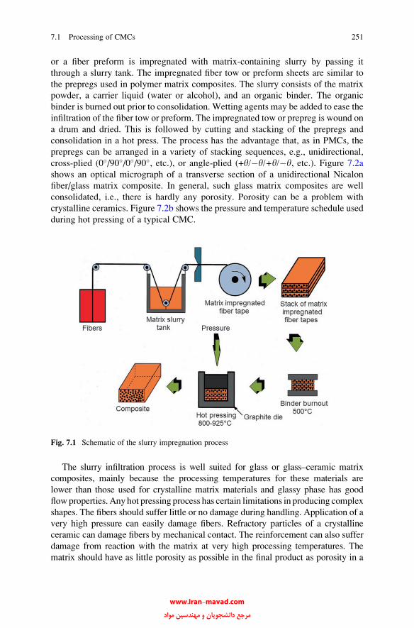
or a fiber preform is impregnated with matrix-containing slurry by passing it

through a slurry tank. The impregnated fiber tow or preform sheets are similar to

the prepregs used in polymer matrix composites. The slurry consists of the matrix

powder, a carrier liquid (water or alcohol), and an organic binder. The organic

binder is burned out prior to consolidation. Wetting agents may be added to ease the

infiltration of the fiber tow or preform. The impregnated tow or prepreg is wound on

a drum and dried. This is followed by cutting and stacking of the prepregs and

consolidation in a hot press. The process has the advantage that, as in PMCs, the

prepregs can be arranged in a variety of stacking sequences, e.g., unidirectional,

cross-plied (0�/90�/0�/90�, etc.), or angle-plied (+y/�y/+y/�y, etc.). Figure 7.2a

shows an optical micrograph of a transverse section of a unidirectional Nicalon

fiber/glass matrix composite. In general, such glass matrix composites are well

consolidated, i.e., there is hardly any porosity. Porosity can be a problem with

crystalline ceramics. Figure 7.2b shows the pressure and temperature schedule used

during hot pressing of a typical CMC.

The slurry infiltration process is well suited for glass or glass–ceramic matrix

composites, mainly because the processing temperatures for these materials are

lower than those used for crystalline matrix materials and glassy phase has good

flowproperties. Any hot pressing process has certain limitations in producing complex

shapes. The fibers should suffer little or no damage during handling. Application of a

very high pressure can easily damage fibers. Refractory particles of a crystalline

ceramic can damage fibers by mechanical contact. The reinforcement can also suffer

damage from reaction with the matrix at very high processing temperatures. The

matrix should have as little porosity as possible in the final product as porosity in a

Fig. 7.1 Schematic of the slurry impregnation process

7.1 Processing of CMCs 251


structural ceramic material is highly undesirable. To this end, it is important to

completely remove the fugitive binder and use a matrix powder particle smaller

than the fiber diameter. The hot pressing operational parameters are also important.

Precise control within a narrow working temperature range, minimization of the

processing time, and utilization of a pressure low enough to avoid fiber damage are

important factors in this final consolidation part of the process. Fiber damage and any

fiber/matrix interfacial reaction, along with its detrimental effect on the bond strength,

are unavoidable attributes of the hot pressing operation.

Fig. 7.2 (a) An optical micrograph of a transverse section of a unidirectional Nicalon fiber/glass

matrix composite. (b) Pressure and temperature schedule used during hot pressing of a typical

composite



In summary, the slurry infiltration process generally results in a fairly uniform

fiber distribution; low porosity and high strength values can be obtained. The main

disadvantage of this process is that one is restricted to relatively low melting or low

softening point matrix materials.

Whisker reinforced CMCs are generally made by mixing the whiskers with a

ceramic powder slurry, followed by drying and hot-pressing. Sometimes hot iso-

static pressing (HIPing) rather than uniaxial hot pressing is used. Whisker agglom-

eration in a green body is a major problem. Mechanical stirring and adjustment of

pH level of the suspension (matrix powder + whiskers in water) can be of help in

this regard. Addition of whiskers to slurry can result in very high viscosity. Also,

whiskers with large aspect ratios (>50) tend to form bundles and clumps (Liu et al.

1991). Obtaining well-separated and deagglomerated whiskers is of great impor-

tance for reasonably high-density composites. Use of organic dispersants (Barclay

et al. 1987), techniques such as agitation mixing assisted by an ultrasonic probe, and

deflocculation by a proper pH control (Yang and Stevens 1990) can be usefully

employed. Most whisker reinforced composites are made at temperatures in the

1,500–1,900�C range and pressures in the 20–40 MPa range (Homeny et al. 1987;

Shalek et al. 1986).

7.1.3 Reaction Bonding Processes

Reaction bonding processes similar to the ones used for monolithic ceramics can be

used to make ceramic matrix composites. Reaction bonding process has the follow-

ing advantages:

• Problems with matrix shrinkage during densification can be avoided.

• Rather large volume fractions of whiskers or fiber can be used.

• Multidirectional, continuous fiber preforms can be used.

• The reaction bonding temperatures for most systems are generally lower than the

sintering temperatures so that fiber degradation can be avoided.

One great disadvantage of this process is that high porosity is difficult to avoid.

A hybrid process involving a combination of hot pressing and reaction bonding

technique can also be used (Bhatt 1986; Bhatt 1990). A silicon cloth is prepared by

attrition milling a mixture of silicon powder, a polymer binder, and an organic

solvent to obtain a dough of proper consistency. This dough is then rolled to make a

silicon cloth of desired thickness. Fiber mats are made by filament winding of

silicon carbide with a fugitive binder. The fiber mats and silicon cloth are stacked in

an alternate sequence, debinderized (the step of binder removal), and hot pressed in

a molybdenum die in a nitrogen or vacuum environment. The temperature and

pressure are adjusted to produce a handleable preform. At this stage, the silicon

matrix is converted to silicon nitride by transferring the composite to a nitriding

furnace between 1,100 and 1,400�C. Typically, the silicon nitride matrix has about

30% porosity, which is not unexpected in reaction bonded silicon nitride.



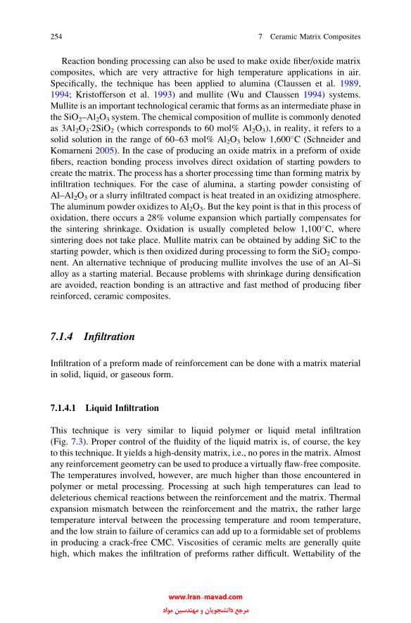
Reaction bonding processing can also be used to make oxide fiber/oxide matrix

composites, which are very attractive for high temperature applications in air.

Specifically, the technique has been applied to alumina (Claussen et al. 1989,

1994; Kristofferson et al. 1993) and mullite (Wu and Claussen 1994) systems.

Mullite is an important technological ceramic that forms as an intermediate phase in

the SiO2–Al2O3 system. The chemical composition of mullite is commonly denoted

as 3Al2O3·2SiO2 (which corresponds to 60 mol% Al2O3), in reality, it refers to a

solid solution in the range of 60–63 mol% Al2O3 below 1,600�C (Schneider and

Komarneni 2005). In the case of producing an oxide matrix in a preform of oxide

fibers, reaction bonding process involves direct oxidation of starting powders to

create the matrix. The process has a shorter processing time than forming matrix by

infiltration techniques. For the case of alumina, a starting powder consisting of

Al–Al2O3 or a slurry infiltrated compact is heat treated in an oxidizing atmosphere.

The aluminum powder oxidizes to Al2O3. But the key point is that in this process of

oxidation, there occurs a 28% volume expansion which partially compensates for

the sintering shrinkage. Oxidation is usually completed below 1,100�C, wheresintering does not take place. Mullite matrix can be obtained by adding SiC to the

starting powder, which is then oxidized during processing to form the SiO2 compo-

nent. An alternative technique of producing mullite involves the use of an Al–Si

alloy as a starting material. Because problems with shrinkage during densification

are avoided, reaction bonding is an attractive and fast method of producing fiber

reinforced, ceramic composites.

7.1.4 Infiltration

Infiltration of a preform made of reinforcement can be done with a matrix material

in solid, liquid, or gaseous form.

7.1.4.1 Liquid Infiltration

This technique is very similar to liquid polymer or liquid metal infiltration

(Fig. 7.3). Proper control of the fluidity of the liquid matrix is, of course, the key

to this technique. It yields a high-density matrix, i.e., no pores in the matrix. Almost

any reinforcement geometry can be used to produce a virtually flaw-free composite.

The temperatures involved, however, are much higher than those encountered in

polymer or metal processing. Processing at such high temperatures can lead to

deleterious chemical reactions between the reinforcement and the matrix. Thermal

expansion mismatch between the reinforcement and the matrix, the rather large

temperature interval between the processing temperature and room temperature,

and the low strain to failure of ceramics can add up to a formidable set of problems

in producing a crack-free CMC. Viscosities of ceramic melts are generally quite

high, which makes the infiltration of preforms rather difficult. Wettability of the



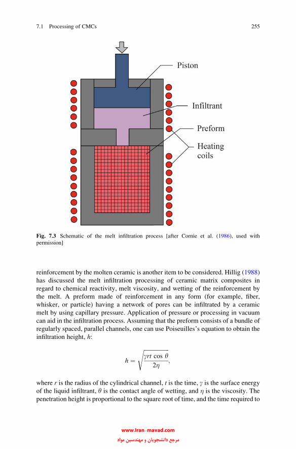
reinforcement by the molten ceramic is another item to be considered. Hillig (1988)

has discussed the melt infiltration processing of ceramic matrix composites in

regard to chemical reactivity, melt viscosity, and wetting of the reinforcement by

the melt. A preform made of reinforcement in any form (for example, fiber,

whisker, or particle) having a network of pores can be infiltrated by a ceramic

melt by using capillary pressure. Application of pressure or processing in vacuum

can aid in the infiltration process. Assuming that the preform consists of a bundle of

regularly spaced, parallel channels, one can use Poiseuilles’s equation to obtain the

infiltration height, h:

h ¼ffiffiffiffiffiffiffiffiffiffiffiffiffiffiffiffiffiffigrt cos y

2�

s;

where r is the radius of the cylindrical channel, t is the time, g is the surface energyof the liquid infiltrant, y is the contact angle of wetting, and � is the viscosity. The

penetration height is proportional to the square root of time, and the time required to

Fig. 7.3 Schematic of the melt infiltration process [after Cornie et al. (1986), used with

permission]



penetrate a given height is inversely proportional to the viscosity of the melt.

Penetration will also be easier if the contact angle is low (i.e., better wettability),

and the surface energy, g, and the pore radius, r, are large. If the radius, r, of thechannel is made too large, the capillarity effect will be lost.

Infiltration of a fibrous preform by a molten intermetallic matrix material under

pressure has been successfully done (Nourbakhsh and Margolin 1990). Alumina

fiber reinforced intermetallic matrix composites (e.g., TiAl, Ni3Al, and Fe3Al

matrix materials) have been prepared by pressure casting, also called squeezecasting (Nourbakhsh and Margolin 1990; Nourbakhsh et al. 1990). The matrix

alloy is melted in a crucible in a vacuum while the fibrous preform is heated

separately. The molten matrix material (at about 100�C above the melting temper-

ature, Tm) is poured onto the fibers and argon gas is introduced simultaneously.

Argon gas pressure forces the melt to infiltrate the preform. The melt generally

contains additives to aid wetting of the fibers.

We may summarize the advantages and disadvantages of different melt infiltra-

tion techniques as follows. The advantages are as follows:

• The matrix is formed in a single processing step.

• A homogeneous matrix can be obtained.

The disadvantages of infiltration techniques are as follows:

• High melting points of ceramics mean a greater likelihood of reaction between

the melt and the reinforcement.

• Ceramics have higher melt viscosities than metals; therefore, infiltration of

preforms is relatively difficult.

• The matrix is likely to crack because of the differential shrinkage between the

matrix and the reinforcement on solidification. This can be minimized by

choosing components with nearly equal coefficients of thermal expansion.

7.1.5 Directed Oxidation or the Lanxide™ Process

Yet another version of liquid infiltration is the directed oxidation process, or the

Lanxide™ process, developed by erstwhile Lanxide Corp. (Urquhart 1991). One of

the Lanxide processes is called DIMOX™, which stands for directed metal oxida-

tion process. A schematic of the directed metal oxidation process is shown in

Fig. 7.4. The first step in this process is to make a preform, which in the case of a

particulate composite can be a ceramic green body. In the case of a fibrous

composite, filament winding or a fabric lay-up may be used to make a preform.

A barrier to stop growth of the matrix material is placed on the preform surfaces. In

this method, a molten metal is subjected to directed oxidation, i.e., the desired

reaction product forms on the surface of the molten metal and grows outward. The

metal is supplied continuously to the reaction front by a wicking action through

channels in the oxidation product. For example, molten aluminum in air will get



oxidized to aluminum oxide. If one wants to form aluminum nitride, then molten

aluminum is reacted with nitrogen. The reaction can be represented as follows:

Alþ air ! Al2O3;Alþ nitrogen ! AlN:

The end product in this process is a three-dimensional, interconnected network of

a ceramic material plus about 5–30% of unreacted metal. When filler particles are

placed next to the molten metal surface, the ceramic network forms around these

particles. As we said earlier, a fabric made of a continuous fiber can also be used. The

fabric is coated with a proprietary coating to protect the fiber from highly reducing

aluminum and to provide a weak interface, which is desirable for enhanced tough-

ness in CMCs. Some aluminum (6–7 wt.%) remains at the end of the process. This

must be removed if the composite is to be used at temperatures above the melting

point of aluminum (660�C). On the other hand, the presence of a residual metal can

be exploited to provide some fracture toughness in these composites.

Proper control of the reaction kinetics is of great importance in this process. The

process is potentially a low-cost process because near-net shapes are possible. Also,

good mechanical properties (such as strength and toughness) have been reported

(Urquhart 1991). Figure 7.5 shows some fiber reinforced ceramic components made

Fig. 7.4 Schematic of the directed metal oxidation process of Lanxide Corp. (Courtesy of

Lanxide Corp.)



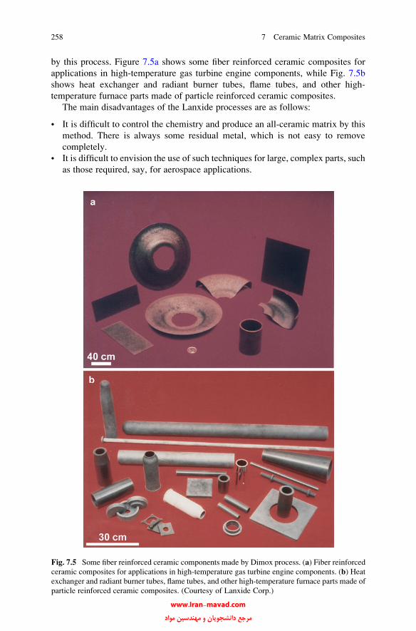
by this process. Figure 7.5a shows some fiber reinforced ceramic composites for

applications in high-temperature gas turbine engine components, while Fig. 7.5b

shows heat exchanger and radiant burner tubes, flame tubes, and other high-

temperature furnace parts made of particle reinforced ceramic composites.

The main disadvantages of the Lanxide processes are as follows:

• It is difficult to control the chemistry and produce an all-ceramic matrix by this

method. There is always some residual metal, which is not easy to remove

completely.

• It is difficult to envision the use of such techniques for large, complex parts, such

as those required, say, for aerospace applications.

Fig. 7.5 Some fiber reinforced ceramic components made by Dimox process. (a) Fiber reinforced

ceramic composites for applications in high-temperature gas turbine engine components. (b) Heat

exchanger and radiant burner tubes, flame tubes, and other high-temperature furnace parts made of

particle reinforced ceramic composites. (Courtesy of Lanxide Corp.)



7.1.6 In Situ Chemical Reaction Techniques

In situ chemical reaction techniques to produce CMCs are extensions of those used

to produce monolithic ceramic bodies. We describe below some of the more

important techniques, viz., chemical vapor deposition (CVD) and chemical vapor

infiltration (CVI) and different types of reaction bonding techniques.

7.1.6.1 Chemical Vapor Deposition and Chemical Vapor Impregnation

When the chemical vapor deposition (CVD) technique is used to impregnate rather

large amounts of matrix material in fibrous preforms, it is called chemical vaporimpregnation (CVI). Common ceramic matrix materials used are SiC, Si3N4, and

HfC. The CVI method has been used successfully by several researchers to impreg-

nate fibrous preforms (Fitzer and Hegen 1979; Fitzer and Schlichting 1980; Fitzer

and Gadow 1986; Stinton et al. 1986; Burkland et al. 1988). The preforms can

consist of yarns, woven fabrics, or three-dimensional shapes.

In very simple terms, in the CVI process a solid material is deposited from

gaseous reactants onto a heated substrate. A typical CVD or CVI process would

require a reactor with the following parts:

1. A vapor feed system.

2. A CVD reactor in which the substrate is heated and gaseous reactants are fed.

3. An effluent system where exhaust gases are handled.

The chemistry for making ceramic fibers by CVD was given in Chap. 2. The

basic chemistry to make a bulk ceramic matrix in and around fibers in a preform

remains the same. One can synthesize a variety of ceramic matrixes such as oxides,

glasses, ceramics, and intermetallics by CVD. Commonly, the process involves an

isothermal decomposition of a chemical compound in the vapor form to yield the

Fig. 7.6 Schematic of an

isothermal chemical vapor

infiltration process



http://dx.doi.org/10.1007/978-0-387-74365-3_2

desired ceramic matrix on and in between the fibers in a preform. Figure 7.6 shows

a schematic of such an isothermal process. For example, methyltrichlorosilane

(CH3SiCl3), the starting material to obtain SiC, is decomposed at a temperature

between 1,200 and 1,400 K:

CH3Cl3Si gð Þ ! SiC sð Þ þ 3HCl gð Þ:

Fig. 7.7 An example of the microstructure of a Nicalon fiber/SiC matrix composite obtained by

CVI. (Courtesy of R.H. Jones). Note the growth interfaces within the matrix indicated by arrows

Fig. 7.8 Schematic of a chemical vapor infiltration process with pressure and temperature

gradients [after Stinton et al. (1986)]



The vapors of SiC deposit as solid phase on and in between the fibers in a

free-standing preform to make the matrix. An example of the microstructure of a

SiC/SiC composite obtained by CVI is shown in Figure 7.7. The CVI process is

very slow because it involves diffusion of the reactant species to the fibrous

substrate, followed by outflow of the gaseous reactant products. The CVI process

of making a ceramic matrix is, indeed, a kind of low-stress and low-temperature

CVD process, and thus avoids some of the problems associated with high-

temperature ceramic processing. However, when the CVI process is carried out

isothermally, near surface pores tend to close first, restricting the gas flow to the

interior of the preform. This necessitates multiple cycles of impregnation, surface

machining, and reinfiltration to obtain an adequate density. One can avoid some

of these problems to some extent by using a forced gas flow and a temperature

gradient. A schematic of one version of this process is shown in Fig. 7.8 (Stinton

et al. 1986). A graphite holder in contact with a water-cooled metallic gas

distributor holds the fibrous preform. The bottom and side surfaces thus stay

cool while the top of the fibrous preform is exposed to the hot zone, creating a

steep thermal gradient. The reactant gaseous mixture passes unreacted through the

fibrous preform because of the low temperature. When these gases reach the hot

zone, they decompose and deposit on and between the fibers to form the matrix.

As the matrix material gets deposited in the hot portion of the preform, the

preform density and thermal conductivity increase and the hot zone moves

progressively from the top of the preform toward the bottom. When the composite

is formed completely at the top and is no longer permeable, the gases flow radially

through the preform, exiting from the vented retaining ring.

This variant of CVI, which combines forced gas flow and temperature gradient,

avoids some of the problems mentioned earlier. Under these modified conditions,

70–90% dense SiC and Si3N4 matrices can be impregnated in SiC and Si3N4 fibrous

preforms in less than a day. Under conditions of plain CVI, it would take several

weeks to achieve such densities, i.e., one can reduce the processing time from

several days to less than 24 h. One can also avoid using binders in this process with

their attendant problems of incomplete removal. The use of a graphite holder

simplifies the fabrication of the preform, and the application of a moderate pressure

to the preform can result in a higher-than-normal fiber volume fraction in the final

product. The final obtainable density in a ceramic body is limited by the fact that

closed porosity starts at about 93–94% of theoretical density. It is difficult to

impregnate past this point.

Advantages of a CVI technique or any variant thereof include:

• Good mechanical properties at high temperatures.

• Large, complex shapes can be produced in a near-net shape.

• Considerable flexibility in the fibers and matrices that can be employed (oxide

and nonoxide).

Among the disadvantages, one should mention that the process is slow and

expensive.



7.1.6.2 Reactive Consolidation or Liquid-Phase Sintering

Siliconized silicon carbide is the name give to a composite of SiC grains in a silicon

matrix. Molten silicon reacts with carbon fibers to form SiC. The original geometry

of the carbon fibers is retained. Carbon fiber in the form of cloth, tow, felt, or matte

is used as a precursor. A preform is made of carbon fiber and infiltrated with liquid

silicon. Silicon reacts with carbon fibers to form SiC fibers in a Si matrix. Typical

composition of the resultant composite is Si (30–50%) + SiC fiber. The silicon

matrix limits the use temperature to about 1,400�C. A big advantage of SiC/Si

composites is that the constituents are in chemical equilibrium and they have

closely matched thermal expansion coefficients.

In another version of this process, a liquid phase forms as a result of an

exothermic reaction between elemental powders. A good example is that from the

field of intermetallics, e.g., nickel aluminides. The following steps are involved:

1. Mix nickel and aluminum in stoichiometric proportions.

2. Cold isostatic press to 70% theoretical density to obtain a green body.

3. Vacuum encapsulate the green body in a 304 stainless steel can.

4. Subject the canned material to reactive hot isostatic pressing.

7.1.7 Sol–Gel

Sol–gel techniques, which have been used to make conventional ceramic materials,

can also be used to make ceramic matrix materials in the interstices of a fibrous

preform. We described the sol–gel technique in Chap. 2. To recapitulate, a solution

containing metal compounds, e.g., a metal alkoxide, acetate, or halide, is reacted to

form a sol. The sol is converted to a gel, which in turn is subjected to controlled

heating to produce the desired end product: a glass, a glass–ceramic, or a ceramic.

Characteristically, the gel-to-ceramic conversion temperature is much lower than

that required in a conventional melting or sintering process. Some of the advantages

of these techniques for making composites are the same as the ones for monolithic

ceramics, viz., lower processing temperatures, greater compositional homogeneity

in single-phase matrices, and potential for producing unique multiphase matrix

materials, etc. Specifically, in regard to composite material fabrication, the sol–gel

technique allows processing via liquids of low viscosity such as the ones derived

from alkoxides. Among the disadvantages of sol–gel are high shrinkage and low

yield compared to slurry techniques. The fiber network provides a very high surface

area to the matrix gel. Consequently, the shrinkage during the drying step, fre-

quently, results in a large density of cracks in the matrix. Generally, repeated

impregnations are required to produce a substantially dense matrix.

It is easy to see that many of the polymer handling and processing techniques can

be used for sol–gel as well. Impregnation of fibrous preforms in vacuum and

filament winding are two important techniques. In filament winding, fiber tows or



http://dx.doi.org/10.1007/978-0-387-74365-3_2

rovings are passed through a tank containing the sol, and the impregnated tow is

wound on a mandrel to a desired shape and thickness. The sol is converted to gel

and the structure is removed from the mandrel. A final heat treatment then converts

the gel to a ceramic or glass matrix.

The sol–gel technique can also be used to prepare prepregs by the slurry

infiltration method. The sol in the slurry acts as a binder and coats fibers and

glass particles. The binder burnout step is thus eliminated because the binder,

being of the same composition as the matrix, becomes part of the glass matrix.

An advantage of this sol–gel-based slurry method is that consolidation can be done

at lower temperatures. Among the problems, one should mention that the coating

layer on the fiber is porous, frequently carbon-rich, and nonuniform.

7.1.8 Polymer Infiltration and Pyrolysis

Just as polymeric precursors can be used to make ceramic fibers (see Chap. 2), we

can use polymeric precursors to form a ceramic matrix in a composite. This

technique is called polymer infiltration and pyrolysis (PIP). It is an attractive

processing route because of its relatively low cost, small amounts of residual

porosity and minimal degradation of the fibers. Moreover, this approach allows

near net-shape molding and fabrication technology that is able to produce nearly

fully dense composites. In PIP, the fibers are infiltrated with an organic polymer,

which is heated to fairly high temperatures and pyrolyzed to form a ceramic matrix.

Due to the relatively low yield of polymer to ceramic, multiple infiltrations are used

to densify the composite.

Polymeric precursors for ceramic matrices allow one to use conventional poly-

mer composite fabrication technology that is readily available, and take advantage

of processes used to make polymer matrix composites (French 1996; Hurwitz et al.

1989). These include complex shape forming and fabrication. Furthermore, by

processing and pyrolyzing at lower temperatures (compared to sintering and hot-

pressing, for example) one can avoid fiber degradation and the formation of

unwanted reaction products at the fiber/matrix interface.

Among the desirable characteristics of a preceramic polymer are (more ofwish list):

• High ceramic yield from polymer precursor.

• Precursor that yields a ceramic with low free carbon content (which will oxidize

at high temperatures).

• Controllable molecular weight, which allows for solvent solubility and control

over viscosity for fabrication purposes.

• Low temperature crosslinking of the polymer, which allows resin to harden and

maintain its dimensions during the pyrolysis process.

• Low cost and toxicity.



http://dx.doi.org/10.1007/978-0-387-74365-3_2

Most preceramic polymer precursors are formed from chloroorganosilicon

compounds to form poly(silanes), poly(carbosilanes), poly(silazanes), poly

(borosilanes), poly(silsesquioxanes), and poly(carbosiloxanes). The synthesis reaction

involves the dechlorination of the chlorinated silane monomers. Since a lot of the

chlorosilane monomers are formed as byproducts in the silicone industry, they are

inexpensive and readily available. The monomers can be further controlled by an

appropriate amount of branching which controls important properties such as the

viscosity of the precursor as well as the amount of ceramic yield. All silicon based

polymer precursors lead to an amorphous ceramic matrix, where silicon atoms are

tetrahedrally arrangedwith nonsilicon atoms. This arrangement is similar to that found

in amorphous silica. High temperature treatments typically lead to crystallization and

slight densification of thematrix, which results in shrinkage. At high temperatures, the

amorphous ceramic begins to form small domains of crystalline phase,which aremore

thermodynamically stable. Si–C matrices derived from polycarbosilane begin to

crystallize at 1,100–1,200�C, while Si–C–O (polysiloxanes) and Si–N–C

(polysilazanes) remain amorphous to 1,300–1,400�C.Typically the range of the molecular weight of the polymer is tailored, followed

by shaping of the product. The polymer is then crosslinked and finally pyrolyzed in

an inert or reactive atmosphere (e.g., NH3) at temperatures between 1,000 and

1,400�C. The pyrolysis step can be further subdivided into three steps. In the first

step, between 550 and 880�C, an amorphous hydrogenated compound of the type Si

(CaObNcBd) is formed. The second step involves nucleation of crystalline

precipitates such as SiC, Si3N4, and SiO2 at temperatures between 1,200 and

1,600�C. Grain coarsening may also result from consumption of any residual

amorphous phase and reduction of the amount of oxygen due to vaporization of

SiO and CO. Porosity is typically on the order of 5–20 vol.% with pore sizes of the

order of 1–50 nm. It should be noted that the average pore size and volume fraction

of pores decrease with increasing pyrolysis temperature, since the amount of

densification (and shrinkage) becomes irreversible at temperatures above the maxi-

mum pyrolysis temperature

Among the disadvantages of PIP, we can list:

• Low yield accompanies the polymer-to-ceramic transformation.

• Large shrinkage, which typically causes cracking in the matrix during fabrica-

tion. Due to shrinkage and weight loss during pyrolysis, residual porosity after a

single impregnation is on the order of 20–30%.

• To reduce the amount of residual porosity, multiple impregnations are needed.

Reimpregnation is typically conducted with a very low viscosity prepolymer so

that the slurry may wet and infiltrate the small micropores that exist in the

preform. Usually, reimpregnation is done by immersing the part in the liquid

polymer in a vacuum bag, while higher viscosity polymers require pressure

impregnation. Typically, the amount of porosity will reduce from 35% to less

than 10% after about five impregnations.



Significant gas evolution also occurs during pyrolysis (French 1996). Thus, it is

advisable to allow these volatile gases to slowly diffuse out of the matrix, especially

for thicker parts. Typically, pyrolysis cycles ramp to somewhere between 800 and

1,400�C over periods of 1–2 days, to avoid delamination. Recall that pyrolysis must

be done at a temperature below the crystallization temperature of the matrix (or

large volume changes will occur) and below the degradation temperature of the

reinforcing fibers. The pyrolysis atmosphere is most commonly argon or nitrogen,

although in ammonia, we obtain a pure amorphous silicon nitride with low amounts

of free carbon. Fitzer and Gadow (1986) used repeated infiltration and in situ

thermal decomposition of porous reaction-bonded ceramics to process Si3N4/SiC

composites. The following steps are taken in processing the composites:

(i) Prepare a porous SiC or Si3N4 fibrous preform with some binder phase.

(ii) Fibrous preform is evacuated in an autoclave.

(iii) Samples are infiltrated with molten precursors, silazanes or polycarbosilanes,

at high temperature (780 K) and the argon or nitrogen pressure is slowly

increased from 2 to 40 MPa. The high temperature results in a transformation

of the oligomer silane to polycarbosilane and simultaneous polymerization at

high pressures.

(iv) Infiltrated samples are cooled and treated with solvents.

(v) Samples are placed in an autoclave and the organosilicon polymer matrix is

thermally decomposed in an inert atmosphere at a high pressure and at

temperature in the 800-1,300 K range.

(vi) Steps (ii) through (v) are repeated to attain an adequate density. To produce

an optimum matrix crystal structure, the material is annealed in the 1,300-

1,800 K range.

Polymer-derived ceramic matrix composites, similar to carbon/carbon

composites (see Chap. 8), typically have a cracked matrix from processing as

well as a number of small pores. The large amount of shrinkage and cracking in

the matrix can be contained, to some extent, by the additions of particulate fillers to

the matrix, which, when added to the polymer reduce shrinkage and stiffen the

matrix material in the composite. Figure 7.9 shows schematically the role of fillers

in reducing the porosity and cracking in the final product. Particulate or whisker

ceramics used as fillers in the polymeric matrix can serve a variety of purposes:

• Reduce and disrupt the formation of matrix cracks that form during shrinkage of

the polymer.

• Enhance ceramic yield by forming reaction products during pyrolysis.

• Strengthen and toughen the weak amorphous matrix and increase the interlami-

nar shear strength of the composite.

The filler must be submicrometer in size in order to penetrate the tow bundle and

the filler’s coefficient of thermal expansion must match that of the polymeric

matrix. The filler must not be used in very high fractions and the slurry should

not be forced into the reinforcing fibers since abrasion of the fiber fabric may

take place. This is especially true with hard, angular fillers or ceramic whiskers.



http://dx.doi.org/10.1007/978-0-387-74365-3_8

Typically, the volume fraction of filler is 15–25% of the matrix volume fraction.

High filler loading may result in an increase in interply spacing and lower volume

fraction of fibers.

When an “active” filler phase is added to the polymer, the following generic

reaction can take place to form new carbide phase (Greil 1995):

Pðs; lÞ þ TðsÞ ! CðsÞ þMðsÞ þ GðgÞ;

where P is the polymer, T is the active filler, C is the ceramic, and G is the gaseous

by-product, and M is the carbide phase formed. By controlling the amount of filler,

the degree of shrinkage can be controlled.

Fiber architecture may have an impact in regard to polymer infiltration and

pyrolysis (PIP). One of the key factors is wetting of the fiber bundles. During

pyrolysis, the precursor shrinks around the fibers, so cracks are introduced. For

example, two dimensional woven fabrics seem to have less propensity in develop-

ing interlaminar cracks than do cross-ply or unidirectional architectures. Satin

weaves are preferred over plain weaves because more uniform cracking is achieved

and large cracks between weave crossover points are avoided (Hurwitz 1992). Due

to the looser nature of the satin weave (it is more drapeable), better wetting and

densification may take place, although the loose nature of the weave also makes it

more difficult to handle.

Fig. 7.9 The role of fillers in reducing the porosity and cracking in the final CMC product



7.1.9 Electrophoretic Deposition

The phenomenon of electrophoresis has been known since the beginning of the

nineteenth century, but its applications in processing of ceramics and ceramic

composites are relatively recent. Electrophoretic deposition (EPD) should not be

confused with electroplating. In electroplating, ions are the moving species and they

undergo ion reduction on deposition. In EPD, on the other hand, solid particlesmigrate

with no charge reduction on deposition. Also, the deposition rate in EPD is �1 mm/

min while in electroplating it�0.1 mm/min. Electrophoretic deposition is a relatively

simple and inexpensive technique, which can be profitably exploited for infiltration of

tightly woven preforms made of fibers (Illston et al. 1993). EPD makes use of

nanoscale ceramic particles in a stable nonagglomerated form (such as in a sol or

colloidal suspension) and exploits their net surface electrostatic charge characteristics

while in suspension. On application of an electric field such surface charge carrying

particles will migrate toward and deposit on an electrode. If the deposition electrode is

replaced by a conducting fibrous preform, the suspended particleswill be attracted into

and deposited within it, providing an appropriate means of effectively infiltrating

densely packed fibrous bundles. A schematic of the basic EPD cell is shown in

Fig. 7.10a while an example of the microstructure of Nextel 720 fiber reinforced

mullite matrix composite is shown in Fig. 7.10b. The movement of ceramic sol

particles in an aqueous suspension within an electric field is governed by the field

strength, and the pH, ionic strength and viscosity of the solution (Illston et al. 1993).

The electrophoretic mobility of charged particles in a suspension is given by the

following equation called the Smoluchowski equation:

electrophoretic mobility ¼ U

E¼ ez

4p�;

where U is the velocity, E is the field strength, e is the dielectric constant, z is thezeta potential, and � is the viscosity. The zeta potential is a parameter that

characterizes a suspension. It can be determined by measuring particle velocity in

an electric field. According to the above equation, a suitable suspension for EPD

should have the following characteristics: a high particle surface charge, a high

dielectric constant of the liquid phase, and a low viscosity. In addition, a low

conductivity of the suspending medium to minimize solvent transport would be

desirable (Kaya et al. 2000, 2009).

7.1.10 Self-Propagating High-Temperature Synthesis

The self-propagating high-temperature synthesis (SHS) technique involves synthesis

of compounds without an external source of energy. One exploits exothermic

reactions to synthesize ceramic compounds, which are difficult to fabricate by



conventional techniques. For example, one can mix titanium powder and carbon

black, cold press themixture, and ignite the compact at the top in a cold-walled vessel.

A combustion wave will pass through the compact, giving titanium carbide.

Among the salient features of SHS are:

• High combustion temperature (up to 4,000�C).• Simple, low-cost equipment.

• Good control of chemical composition.

• Different shapes and forms can be obtained.

This technique can be used to produce a variety of refractory materials. The main

disadvantage is that SHS products are very porous, because of the fairly large

Fig. 7.10 (a) Schematic of the basic electrophoretic deposition (EPD) cell. (b) Microstructure of

Nicalon 720 fiber/mullite composite made by electrophoretic deposition (from Kaya et al. 2009)



porosity in the original mix of reactants and because of the large volume change

that results when the reactants transform to the products. Any adsorbed gases at the

elevated temperatures used during this process can also add to the porosity of the

final product. Synthesis concomitant with densification can improve the situation to

some extent. This involves application of high pressure during the combustion or

immediately after the completion of the combustion reaction, when the product

temperature is still quite high. Hot pressing, rolling, and shock waves are some of

the techniques used to apply the necessary pressure.

Many ceramics, such as borides, carbides, nitrides, silicides, and sialons, and

composites, such as SiCw + Al2O3, have been synthesized by means of SHS. The

SHS process gives a weakly bonded compact. Therefore, the process is generally

followed by breaking the compact, milling, and consolidation by some technique

such as HIPing. Explosive or dynamic compaction can result in a relatively dense

product. A good example of an SHS process to make composites is the XD™process, wherein exothermic reactions are used to produce multiphase alloy

powders. These are hot pressed at ~1,450�C to full density. Reinforcement in the

form of particles, whiskers, and platelets can be added to the master alloy to make a

composite. A good example is that of TiB2 particles, about 1 mm in diameter,

distributed in intermetallic matrices such as TiAl, TiAl + Ti3Al, and NiAl.

7.2 Interface in CMCs

In general, for CMCs one must satisfy the following compatibility requirements:

thermal expansion compatibility and chemical compatibility. Ceramics have a limited

ductility, and in the fabrication of CMCs one uses high temperatures. Thus, thermal

mismatch on cooling from high temperatures can cause cracking in matrix (or fiber).

Thermal strain in composites is proportional to DaDT, where Da ¼ af � am, af andam being the linear expansion coefficients of the fiber andmatrix, respectively, andDTis the temperature interval. There is, of course, another complication, namely, fiber

expansion coefficients are also sometimes not equal in the axial and radial directions.

Carbon fiber in particular has the following axial and radial coefficients:

aa � 0;

ar � 8� 10�6 K�1:

If Da is positive, i.e., af > am, the matrix is compressed on cooling, which is

beneficial because it leads to an increase in the tensile stress at which matrix

cracking will occur. Conversely, if Da is negative, i.e., af < am, the matrix

experiences tension, which, if DT is sufficiently large, can cause matrix cracking.

In the radial direction, if Da, is positive, the fibers tend to shrink away from the

matrix on cooling, which results in a reduced interfacial bond strength. If, however,

Da is negative, the fiber matrix bond strength can even be improved.

7.2 Interface in CMCs 269


Matrix cracking resulting from thermal mismatch is, comparatively speaking, a

more serious problem in short fiber composites than in continuous fiber composites.

The reason is that in a ceramic matrix containing aligned continuous fibers,

transverse microcracks appear in the matrix, but fibers continue to hold the various

matrix blocks together and the composite can still display a reasonable amount of

strength. In a randomly oriented short fiber composite, owing to increased stress at

the fiber ends, matrix cracking occurs in all directions and the composite is very

weak. We can define a thermal expansion mismatch parameter for axial and radial

directions in an aligned fiber composite as (Sambell et al. 1972):

fa;fr ¼ DaDT Em=smð Þ:

Table 7.1 makes a comparison of damage resulting from thermal expansion

mismatch in some carbon fiber reinforced ceramic matrix composites. Note that

only glass and glass–ceramic matrices (low modulus materials) show no damage.

Chemical compatibility between the ceramic matrix and the fiber involves the

same thermodynamic and kinetic considerations as with other composite types.

Quite frequently, the bond between fiber and ceramic matrix is simple mechanical

interlocking. During fabrication (by hot pressing) or during subsequent heat

treatments, the fiber/matrix bond could be affected by the high temperatures

attained because of any chemical reaction between the fiber and matrix or because

of any phase changes in either one of the components. Sambell et al. (1972) studied

the zirconia reinforced magnesia composite system in which there occurs a chemi-

cal reaction at 1,600�C. At temperatures less than 1,600�C, the composites showed

a weak fiber/matrix interface and fiber pullout occurred during mechanical

polishing. Upon heat treating at 1,600�C, however, because of the interfacial

reaction and the resultant improved bonding, no damage was observed upon

mechanical polishing. Heat treatment at 1,700�C resulted in the complete destruc-

tion of the zirconia fibers and the distribution of zirconia to grain boundaries in

magnesia. Thus, as we noted in the case of MMCs (Chap. 6), it is important to be

Table 7.1 A comparison of damage resulting from the thermal expansion mismatch in some

carbon fiber reinforced systemsa

Matrix

amb

(10�6 �C�1) Tcc (�C) E (GPa)

smud

(MPa) fae fr

e Damage

MgO 13.6 1,200 300 200 25 10 Severe cracking

Al2O3 (80 % dense) 8.3 1,400 230 300 9 0.3 Severe cracking

Soda-lime glass 8.9 480 60 100 2.6 0.3 Localized cracks

Borosilicate glass 3.5 520 60 100 1.1 �1.4 Uncracked

Glass–ceramic 1.5 1,000 100 100 1.5 �6.5 UncrackedaType I carbon fibers aa � 0, ar � 8 � 10�6 K�1

bam is the matrix thermal expansion coefficientcTc is the temperature below which little stress relaxation can occurdsmu is the matrix strength.efa and fr are the thermal expansion mismatch parameters

Source: Adapted with permission from Phillips (1983)



http://dx.doi.org/10.1007/978-0-387-74365-3_6

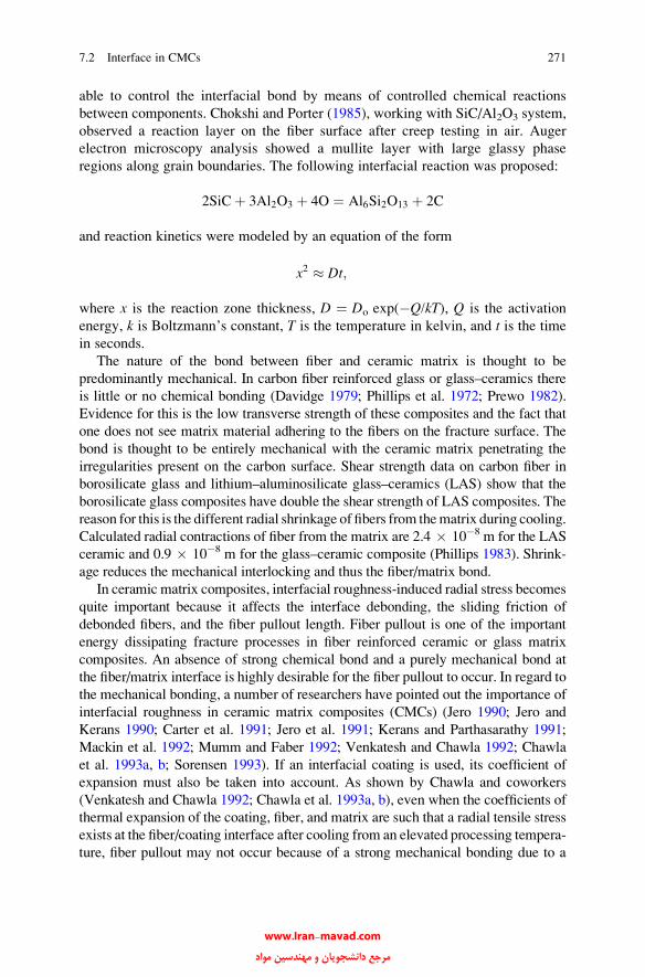
able to control the interfacial bond by means of controlled chemical reactions

between components. Chokshi and Porter (1985), working with SiC/Al2O3 system,

observed a reaction layer on the fiber surface after creep testing in air. Auger

electron microscopy analysis showed a mullite layer with large glassy phase

regions along grain boundaries. The following interfacial reaction was proposed:

2SiCþ 3Al2O3 þ 4O ¼ Al6Si2O13 þ 2C

and reaction kinetics were modeled by an equation of the form

x2 � Dt;

where x is the reaction zone thickness, D ¼ Do exp(�Q/kT), Q is the activation

energy, k is Boltzmann’s constant, T is the temperature in kelvin, and t is the time

in seconds.

The nature of the bond between fiber and ceramic matrix is thought to be

predominantly mechanical. In carbon fiber reinforced glass or glass–ceramics there

is little or no chemical bonding (Davidge 1979; Phillips et al. 1972; Prewo 1982).

Evidence for this is the low transverse strength of these composites and the fact that

one does not see matrix material adhering to the fibers on the fracture surface. The

bond is thought to be entirely mechanical with the ceramic matrix penetrating the

irregularities present on the carbon surface. Shear strength data on carbon fiber in

borosilicate glass and lithium–aluminosilicate glass–ceramics (LAS) show that the

borosilicate glass composites have double the shear strength of LAS composites. The

reason for this is the different radial shrinkage of fibers from thematrix during cooling.

Calculated radial contractions of fiber from the matrix are 2.4 � 10�8 m for the LAS

ceramic and 0.9 � 10�8 m for the glass–ceramic composite (Phillips 1983). Shrink-

age reduces the mechanical interlocking and thus the fiber/matrix bond.

In ceramic matrix composites, interfacial roughness-induced radial stress becomes

quite important because it affects the interface debonding, the sliding friction of

debonded fibers, and the fiber pullout length. Fiber pullout is one of the important

energy dissipating fracture processes in fiber reinforced ceramic or glass matrix

composites. An absence of strong chemical bond and a purely mechanical bond at

the fiber/matrix interface is highly desirable for the fiber pullout to occur. In regard to

the mechanical bonding, a number of researchers have pointed out the importance of

interfacial roughness in ceramic matrix composites (CMCs) (Jero 1990; Jero and

Kerans 1990; Carter et al. 1991; Jero et al. 1991; Kerans and Parthasarathy 1991;

Mackin et al. 1992; Mumm and Faber 1992; Venkatesh and Chawla 1992; Chawla

et al. 1993a, b; Sorensen 1993). If an interfacial coating is used, its coefficient of

expansion must also be taken into account. As shown by Chawla and coworkers

(Venkatesh and Chawla 1992; Chawla et al. 1993a, b), even when the coefficients of

thermal expansion of the coating, fiber, and matrix are such that a radial tensile stress

exists at the fiber/coating interface after cooling from an elevated processing tempera-

ture, fiber pullout may not occur because of a strong mechanical bonding due to a

7.2 Interface in CMCs 271


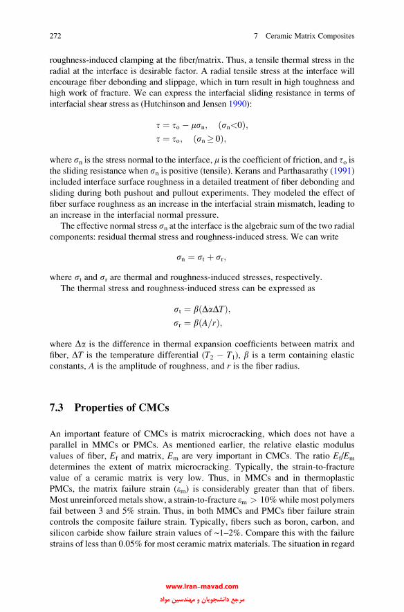
roughness-induced clamping at the fiber/matrix. Thus, a tensile thermal stress in the

radial at the interface is desirable factor. A radial tensile stress at the interface will

encourage fiber debonding and slippage, which in turn result in high toughness and

high work of fracture. We can express the interfacial sliding resistance in terms of

interfacial shear stress as (Hutchinson and Jensen 1990):

t ¼ to � msn; ðsn<0Þ;t ¼ to; ðsn � 0Þ;

where sn is the stress normal to the interface, m is the coefficient of friction, and to isthe sliding resistance when sn is positive (tensile). Kerans and Parthasarathy (1991)included interface surface roughness in a detailed treatment of fiber debonding and

sliding during both pushout and pullout experiments. They modeled the effect of

fiber surface roughness as an increase in the interfacial strain mismatch, leading to

an increase in the interfacial normal pressure.

The effective normal stress sn at the interface is the algebraic sum of the two radial

components: residual thermal stress and roughness-induced stress. We can write

sn ¼ st þ sr;

where st and sr are thermal and roughness-induced stresses, respectively.

The thermal stress and roughness-induced stress can be expressed as

st ¼ b DaDTð Þ;sr ¼ b A=rð Þ;

where Da is the difference in thermal expansion coefficients between matrix and

fiber, DT is the temperature differential (T2 � T1), b is a term containing elastic

constants, A is the amplitude of roughness, and r is the fiber radius.

7.3 Properties of CMCs

An important feature of CMCs is matrix microcracking, which does not have a

parallel in MMCs or PMCs. As mentioned earlier, the relative elastic modulus

values of fiber, Ef and matrix, Em are very important in CMCs. The ratio Ef/Em

determines the extent of matrix microcracking. Typically, the strain-to-fracture

value of a ceramic matrix is very low. Thus, in MMCs and in thermoplastic

PMCs, the matrix failure strain (em) is considerably greater than that of fibers.

Most unreinforced metals show, a strain-to-fracture em > 10%while most polymers

fail between 3 and 5% strain. Thus, in both MMCs and PMCs fiber failure strain

controls the composite failure strain. Typically, fibers such as boron, carbon, and

silicon carbide show failure strain values of ~1–2%. Compare this with the failure

strains of less than 0.05% for most ceramic matrix materials. The situation in regard



to fiber and/or matrix failure is shown in a simplified manner in Fig. 7.11. The crack-

free original situation is shown in Fig. 7.11a. In the case of MMCs and PMCs, fibers

fail first at various weak points distributed along their lengths; see Fig. 7.11b. The

final failure of the composite will occur along a section that has the most fiber

fractures. In a strongly bonded CMC, fiber and matrix would fail simultaneously at

matrix failure strain and a situation similar to that shown in Fig. 7.11c will prevail. In

a weakly bonded CMC, however, the matrix will start cracking first and the fibers

will be bridging the matrix blocks, Fig. 7.11d shows an idealized situation. Thus,

from a toughness point of view, in general, we do not want too strong a bond in a

CMC because it would make a crack run through the specimen. A weak interface,

however, would lead to fiber-bridging of matrix microcracks.

A CMC with even a microcracked ceramic matrix can retain some reasonable

strength (sc ’ sfVf) and there are applications, such as bushings, where such a

damage-tolerant characteristic would be very valuable because in the absence of

fibers bridging the cracks, the monolithic matrix would simply disintegrate. The

disadvantage, of course, is that matrix microcracking provides an easy path for

environmental attack of the fibers and the fiber/matrix interface. Let us consider an

idealized situation of a fiber reinforced, unidirectionally aligned, CMC, loaded in the

longitudinal direction. Assume that the CMC has proper interface, i.e., it is damage-

tolerant. At a stress s0, the stress–strain curve will show a dip, indicating the

incidence of periodic matrix cracking, see Fig. 7.12. Because the fibers have enough

strength to support the load in the presence of a damaged matrix (a very desirable

feature indeed), the stress–strain curve will continue to rise until, at a stress marked

su, the fiber bundle fails. At this point, the phenomenon of fiber pullout starts. The

extent of this fiber pullout region depends critically on the interfacial frictional

resistance. The fiber/matrix interface has a lot to do with the form of the stress–strain

curve. If the bonding is too strong, matrix cracking will be accompanied by a small

amount of fiber pullout, which is an undesirable characteristic from the toughness

Fig. 7.11 (a) Original crack-free situation. (b) In the case of MMCs and PMCs, fibers fail first at

various weak points distributed along their lengths. The composite will fail along a section that has

the maximum number of fiber fractures. (c) In a strongly bonded CMC, fiber and matrix would fail

simultaneously at matrix failure strain. (d) In a weakly bonded CMC, however, the matrix will

start cracking first and the fibers will be bridging the matrix blocks

7.3 Properties of CMCs 273


viewpoint, aswe shall see in Sect. 7.4. Increased stiffness and strengthwere observed

in a unidirectionally aligned composite consisting of continuous carbon fibers (50%

Vf) in a glass matrix compared to the unreinforced glass matrix (Davidge 1979). But

more importantly, a large increase in the work of fracture occurred. The increased

work of fracture is a result of the controlled fracture behavior of the composite, while

the unreinforced matrix failed in a catastrophic manner.

Fiber length, or more precisely, the fiber aspect ratio (length/diameter), fiber

orientation, relative strengths and moduli of fiber and matrix, thermal expansion

mismatch, matrix porosity, and fiber flaws are the important variables that control

the performance of CMCs. Sambell et al. (1974) showed that, for ceramic matrix

materials containing short, randomly distributed carbon fibers, a weakening effect

occurred rather than a strengthening effect. This was attributed to the stress concen-

tration effect at the extremities of randomly distributed short fibers and thermal

expansion mismatch. Aligned continuous fibers do lead to a real fiber reinforcement

effect. The stress concentration at fiber ends is minimized and higher fiber volume

fractions can be obtained. At very high fiber volume fractions, however, it becomes

difficult to eliminate the porosity in the ceramic matrix. Figure 7.12 shows that the

strength increases in a linear fashion for carbon fiber/glass matrix composites, for up

to ~55% Vf (Phillips et al. 1972). Beyond 55% Vf, the high matrix porosity led to a

drop in the strength. The Young’s modulus also increased linear with Vf, as shown in

Fig. 7.13; at higher Vf it deviated from linearity owing to matrix porosity and

possible fiber misalignment (Phillips et al. 1972).

Creep resistance of a ceramic such as alumina can be improved by adding fibers

or whiskers. Silicon carbide SiC whisker reinforced alumina showed superior creep-

resistance than polycrystalline alumina (Chokshi and Porter 1985); see Figure 7.14.

This figures shows, on a log–log plot, the creep strain rate as a function of stress at a

constant temperature. Note that the composite has a higher-stress exponent than the

unreinforced matrix. The higher-stress exponent indicates a change in the operating

creep mechanism. The exponent for polycrystalline alumina is about 2, and this is

rationalized in terms of some kind of diffusion creep being the controlling mecha-

nism. A stress exponent of about 5, which was observed for the composite, is

indicative of a dislocation creep mechanism being in operation. Observation of the

specimens deformed in creep in transmission electron microscope showed disloca-

tion activity.

Fig. 7.12 Stress-strain curve

of an aligned CMC in the

longitudinal direction

showing a damage-tolerant

behavior



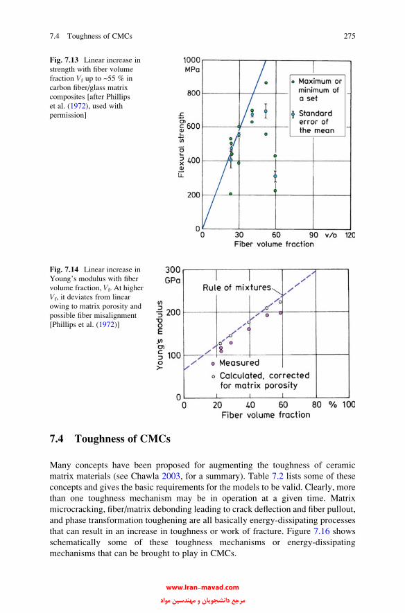
7.4 Toughness of CMCs

Many concepts have been proposed for augmenting the toughness of ceramic

matrix materials (see Chawla 2003, for a summary). Table 7.2 lists some of these

concepts and gives the basic requirements for the models to be valid. Clearly, more

than one toughness mechanism may be in operation at a given time. Matrix

microcracking, fiber/matrix debonding leading to crack deflection and fiber pullout,

and phase transformation toughening are all basically energy-dissipating processes

that can result in an increase in toughness or work of fracture. Figure 7.16 shows

schematically some of these toughness mechanisms or energy-dissipating

mechanisms that can be brought to play in CMCs.

Fig. 7.13 Linear increase in

strength with fiber volume

fraction Vf up to ~55 % in

carbon fiber/glass matrix

composites [after Phillips


permission]

Fig. 7.14 Linear increase in

Young’s modulus with fiber

volume fraction, Vf. At higher

Vf, it deviates from linear

owing to matrix porosity and

possible fiber misalignment

[Phillips et al. (1972)]

7.4 Toughness of CMCs 275


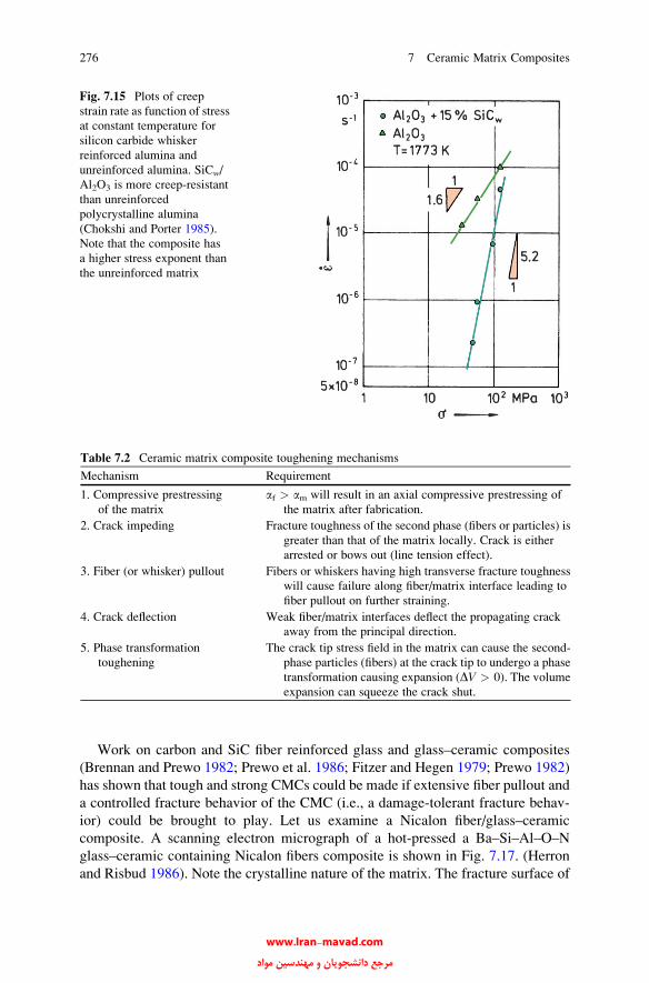
Work on carbon and SiC fiber reinforced glass and glass–ceramic composites

(Brennan and Prewo 1982; Prewo et al. 1986; Fitzer and Hegen 1979; Prewo 1982)

has shown that tough and strong CMCs could be made if extensive fiber pullout and

a controlled fracture behavior of the CMC (i.e., a damage-tolerant fracture behav-

ior) could be brought to play. Let us examine a Nicalon fiber/glass–ceramic

composite. A scanning electron micrograph of a hot-pressed a Ba–Si–Al–O–N

glass–ceramic containing Nicalon fibers composite is shown in Fig. 7.17. (Herron

and Risbud 1986). Note the crystalline nature of the matrix. The fracture surface of

Fig. 7.15 Plots of creep

strain rate as function of stress

at constant temperature for

silicon carbide whisker

reinforced alumina and

unreinforced alumina. SiCw/

Al2O3 is more creep-resistant

than unreinforced

polycrystalline alumina

(Chokshi and Porter 1985).

Note that the composite has

a higher stress exponent than

the unreinforced matrix

Table 7.2 Ceramic matrix composite toughening mechanisms

Mechanism Requirement

1. Compressive prestressing

of the matrix

af > am will result in an axial compressive prestressing of

the matrix after fabrication.

2. Crack impeding Fracture toughness of the second phase (fibers or particles) is

greater than that of the matrix locally. Crack is either

arrested or bows out (line tension effect).

3. Fiber (or whisker) pullout Fibers or whiskers having high transverse fracture toughness

will cause failure along fiber/matrix interface leading to

fiber pullout on further straining.

4. Crack deflection Weak fiber/matrix interfaces deflect the propagating crack

away from the principal direction.

5. Phase transformation

toughening

The crack tip stress field in the matrix can cause the second-

phase particles (fibers) at the crack tip to undergo a phase

transformation causing expansion (DV > 0). The volume

expansion can squeeze the crack shut.



this composite (Fig. 7.18) showed the phenomenon of fiber pullout, indicating a

weak fiber/matrix bond. The fibers were bonded to the matrix by an amorphous

layer whose characteristics changed with heat treatment; a carbon-rich layer was

also observed on the fiber surface (Herron and Risbud 1986). Remnants of the

interfacial amorphous layer adhering to the Nicalon fibers can be seen in Fig. 7.18.

One can accentuate the propensity of fiber pullout by applying a suitable coating on

the fiber, which would control the interfacial characteristics. This was observed in

the composite system Nicalon/pyrolitic carbon coating/SiC, as shown in Fig. 7.19

wherein we see Nicalon fibers pulled out of the matrix (Chawla et al. 1994). Among

oxide ceramic matrix materials, alumina and mullite are quite important. In partic-

ular, SiC whisker reinforced alumina composites (20–30% by volume of SiC

Fig. 7.16 Schematic of some toughness or energy-dissipating mechanisms that can be brought to

play in CMCs



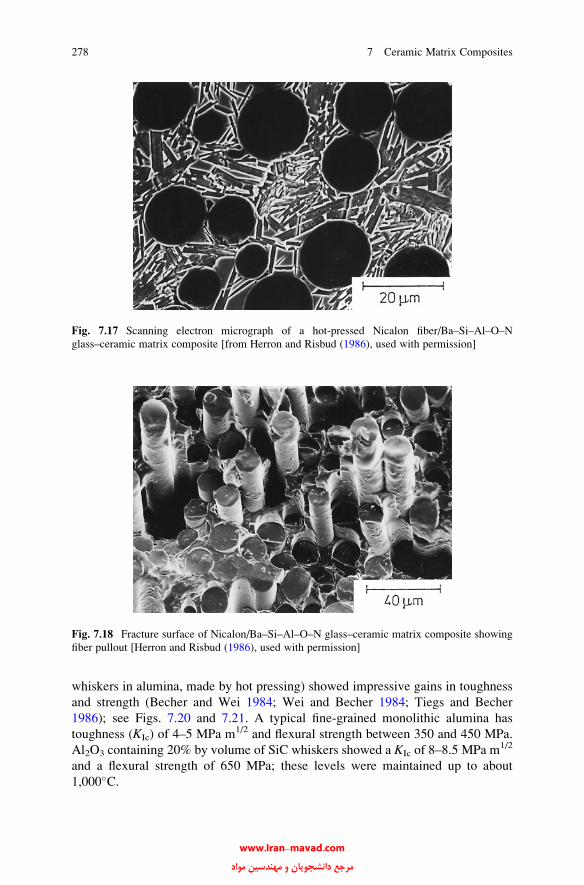
whiskers in alumina, made by hot pressing) showed impressive gains in toughness

and strength (Becher and Wei 1984; Wei and Becher 1984; Tiegs and Becher

1986); see Figs. 7.20 and 7.21. A typical fine-grained monolithic alumina has

toughness (KIc) of 4–5 MPa m1/2 and flexural strength between 350 and 450 MPa.

Al2O3 containing 20% by volume of SiC whiskers showed a KIc of 8–8.5 MPa m1/2

and a flexural strength of 650 MPa; these levels were maintained up to about

1,000�C.

Fig. 7.17 Scanning electron micrograph of a hot-pressed Nicalon fiber/Ba–Si–Al–O–N

glass–ceramic matrix composite [from Herron and Risbud (1986), used with permission]

Fig. 7.18 Fracture surface of Nicalon/Ba–Si–Al–O–N glass–ceramic matrix composite showing

fiber pullout [Herron and Risbud (1986), used with permission]



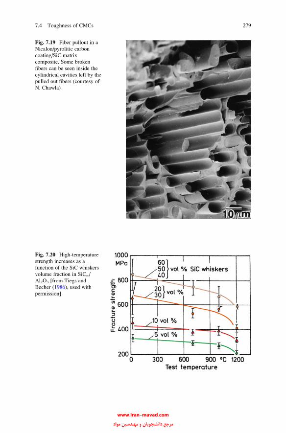
Fig. 7.19 Fiber pullout in a

Nicalon/pyrolitic carbon

coating/SiC matrix

composite. Some broken

fibers can be seen inside the

cylindrical cavities left by the

pulled out fibers (courtesy of

N. Chawla)

Fig. 7.20 High-temperature

strength increases as a

function of the SiC whiskers

volume fraction in SiCw/

Al2O3 [from Tiegs and

Becher (1986), used with

permission]



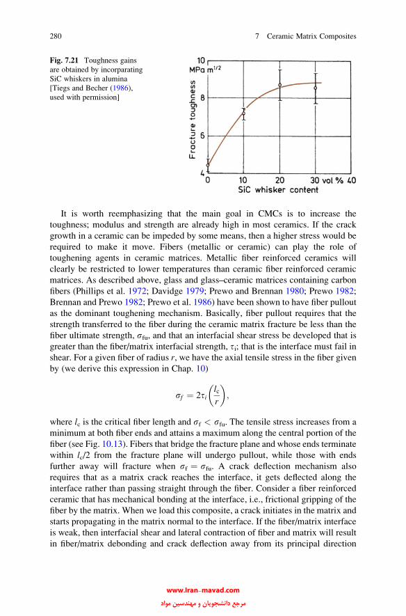
It is worth reemphasizing that the main goal in CMCs is to increase the

toughness; modulus and strength are already high in most ceramics. If the crack

growth in a ceramic can be impeded by some means, then a higher stress would be

required to make it move. Fibers (metallic or ceramic) can play the role of

toughening agents in ceramic matrices. Metallic fiber reinforced ceramics will

clearly be restricted to lower temperatures than ceramic fiber reinforced ceramic

matrices. As described above, glass and glass–ceramic matrices containing carbon

fibers (Phillips et al. 1972; Davidge 1979; Prewo and Brennan 1980; Prewo 1982;

Brennan and Prewo 1982; Prewo et al. 1986) have been shown to have fiber pullout

as the dominant toughening mechanism. Basically, fiber pullout requires that the

strength transferred to the fiber during the ceramic matrix fracture be less than the

fiber ultimate strength, sfu, and that an interfacial shear stress be developed that is

greater than the fiber/matrix interfacial strength, ti; that is the interface must fail in

shear. For a given fiber of radius r, we have the axial tensile stress in the fiber givenby (we derive this expression in Chap. 10)

sf ¼ 2tilcr

� �;

where lc is the critical fiber length and sf < sfu. The tensile stress increases from a

minimum at both fiber ends and attains a maximum along the central portion of the

fiber (see Fig. 10.13). Fibers that bridge the fracture plane and whose ends terminate

within lc/2 from the fracture plane will undergo pullout, while those with ends

further away will fracture when sf ¼ sfu. A crack deflection mechanism also

requires that as a matrix crack reaches the interface, it gets deflected along the

interface rather than passing straight through the fiber. Consider a fiber reinforced

ceramic that has mechanical bonding at the interface, i.e., frictional gripping of the

fiber by the matrix. When we load this composite, a crack initiates in the matrix and

starts propagating in the matrix normal to the interface. If the fiber/matrix interface

is weak, then interfacial shear and lateral contraction of fiber and matrix will result

in fiber/matrix debonding and crack deflection away from its principal direction

Fig. 7.21 Toughness gains

are obtained by incorparating

SiC whiskers in alumina

[Tiegs and Becher (1986),




http://dx.doi.org/10.1007/978-0-387-74365-3_10


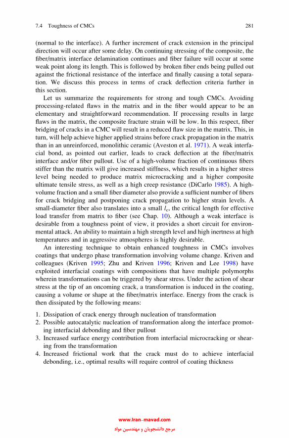
(normal to the interface). A further increment of crack extension in the principal

direction will occur after some delay. On continuing stressing of the composite, the

fiber/matrix interface delamination continues and fiber failure will occur at some

weak point along its length. This is followed by broken fiber ends being pulled out

against the frictional resistance of the interface and finally causing a total separa-

tion. We discuss this process in terms of crack deflection criteria further in

this section.

Let us summarize the requirements for strong and tough CMCs. Avoiding

processing-related flaws in the matrix and in the fiber would appear to be an

elementary and straightforward recommendation. If processing results in large

flaws in the matrix, the composite fracture strain will be low. In this respect, fiber

bridging of cracks in a CMC will result in a reduced flaw size in the matrix. This, in

turn, will help achieve higher applied strains before crack propagation in the matrix

than in an unreinforced, monolithic ceramic (Aveston et al. 1971). A weak interfa-

cial bond, as pointed out earlier, leads to crack deflection at the fiber/matrix

interface and/or fiber pullout. Use of a high-volume fraction of continuous fibers

stiffer than the matrix will give increased stiffness, which results in a higher stress

level being needed to produce matrix microcracking and a higher composite

ultimate tensile stress, as well as a high creep resistance (DiCarlo 1985). A high-

volume fraction and a small fiber diameter also provide a sufficient number of fibers

for crack bridging and postponing crack propagation to higher strain levels. A

small-diameter fiber also translates into a small lc, the critical length for effective

load transfer from matrix to fiber (see Chap. 10). Although a weak interface is

desirable from a toughness point of view, it provides a short circuit for environ-

mental attack. An ability to maintain a high strength level and high inertness at high

temperatures and in aggressive atmospheres is highly desirable.

An interesting technique to obtain enhanced toughness in CMCs involves

coatings that undergo phase transformation involving volume change. Kriven and

colleagues (Kriven 1995; Zhu and Kriven 1996; Kriven and Lee 1998) have

exploited interfacial coatings with compositions that have multiple polymorphs

wherein transformations can be triggered by shear stress. Under the action of shear

stress at the tip of an oncoming crack, a transformation is induced in the coating,

causing a volume or shape at the fiber/matrix interface. Energy from the crack is

then dissipated by the following means:

1. Dissipation of crack energy through nucleation of transformation

2. Possible autocatalytic nucleation of transformation along the interface promot-

ing interfacial debonding and fiber pullout

3. Increased surface energy contribution from interfacial microcracking or shear-

ing from the transformation

4. Increased frictional work that the crack must do to achieve interfacial

debonding, i.e., optimal results will require control of coating thickness



http://dx.doi.org/10.1007/978-0-387-74365-3_10

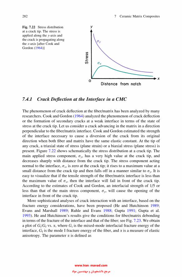
7.4.1 Crack Deflection at the Interface in a CMC

The phenomenon of crack deflection at the fiber/matrix has been analyzed by many

researchers. Cook and Gordon (1964) analyzed the phenomenon of crack deflection

or the formation of secondary cracks at a weak interface in terms of the state of

stress at the crack tip. Let us consider a crack advancing in the matrix in a direction

perpendicular to the fiber/matrix interface. Cook and Gordon estimated the strength

of the interface necessary to cause a diversion of the crack from its original

direction when both fiber and matrix have the same elastic constant. At the tip of

any crack, a triaxial state of stress (plane strain) or a biaxial stress (plane stress) is

present. Figure 7.22 shows schematically the stress distribution at a crack tip. The

main applied stress component, sy, has a very high value at the crack tip, and

decreases sharply with distance from the crack tip. The stress component acting

normal to the interface, sx, is zero at the crack tip; it rises to a maximum value at a

small distance from the crack tip and then falls off in a manner similar to sy. It iseasy to visualize that if the tensile strength of the fiber/matrix interface is less than

the maximum value of sx, then the interface will fail in front of the crack tip.

According to the estimates of Cook and Gordon, an interfacial strength of 1/5 or

less than that of the main stress component, sy, will cause the opening of the

interface in front of the crack tip.

More sophisticated analyses of crack interaction with an interface, based on the

fracture energy considerations, have been proposed (He and Hutchinson 1989;

Evans and Marshall 1989; Ruhle and Evans 1988; Gupta 1991; Gupta et al.

1993). He and Hutchinson’s results give the conditions for fiber/matrix debonding

in terms of the fracture of the interface and that of the fiber; see Fig. 7.23. We obtain

a plot of Gi/Gf vs. a, where Gi is the mixed-mode interfacial fracture energy of the

interface, Gf is the mode I fracture energy of the fiber, and a is a measure of elastic

anisotropy. The parameter a is defined as

Fig. 7.22 Stress distribution

at a crack tip. The stress is

applied along the y-axis andthe crack is propagating along

the x-axis [after Cook and

Gordon (1964)]



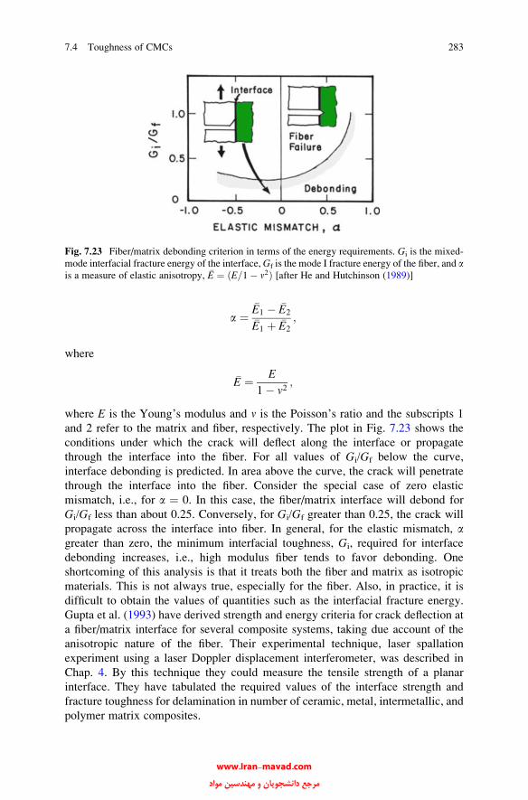
a ¼�E1 � �E2

�E1 þ �E2

;

where

�E ¼ E

1� v2;

where E is the Young’s modulus and n is the Poisson’s ratio and the subscripts 1

and 2 refer to the matrix and fiber, respectively. The plot in Fig. 7.23 shows the

conditions under which the crack will deflect along the interface or propagate

through the interface into the fiber. For all values of Gi/Gf below the curve,

interface debonding is predicted. In area above the curve, the crack will penetrate

through the interface into the fiber. Consider the special case of zero elastic

mismatch, i.e., for a ¼ 0. In this case, the fiber/matrix interface will debond for

Gi/Gf less than about 0.25. Conversely, for Gi/Gf greater than 0.25, the crack will

propagate across the interface into fiber. In general, for the elastic mismatch, agreater than zero, the minimum interfacial toughness, Gi, required for interface

debonding increases, i.e., high modulus fiber tends to favor debonding. One

shortcoming of this analysis is that it treats both the fiber and matrix as isotropic

materials. This is not always true, especially for the fiber. Also, in practice, it is

difficult to obtain the values of quantities such as the interfacial fracture energy.

Gupta et al. (1993) have derived strength and energy criteria for crack deflection at

a fiber/matrix interface for several composite systems, taking due account of the

anisotropic nature of the fiber. Their experimental technique, laser spallation

experiment using a laser Doppler displacement interferometer, was described in

Chap. 4. By this technique they could measure the tensile strength of a planar

interface. They have tabulated the required values of the interface strength and

fracture toughness for delamination in number of ceramic, metal, intermetallic, and

polymer matrix composites.

Fig. 7.23 Fiber/matrix debonding criterion in terms of the energy requirements. Gi is the mixed-

mode interfacial fracture energy of the interface, Gf is the mode I fracture energy of the fiber, and ais a measure of elastic anisotropy, �E ¼ ðE=1� n2Þ [after He and Hutchinson (1989)]



http://dx.doi.org/10.1007/978-0-387-74365-3_4

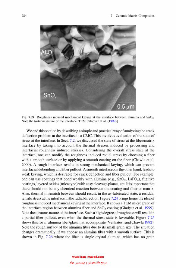
Weend this section by describing a simple andpracticalway of analyzing the crack

deflection problem at the interface in a CMC. This involves evaluation of the state of

stress at the interface. In Sect. 7.2, we discussed the state of stress at the fiber/matrix

interface by taking into account the thermal stresses induced by processing and

interfacial roughness induced stresses. Considering the overall stress state at the

interface, one can modify the roughness induced radial stress by choosing a fiber

with a smooth surface or by applying a smooth coating on the fiber (Chawla et al.

2000). A rough interface results in strong mechanical keying, which can prevent

interfacial debonding andfiber pullout. A smooth interface, on the other hand, leads to

weak keying, which is desirable for crack deflection and fiber pullout. For example,

one can use coatings that bond weakly with alumina (e.g., SnO2, LaPO4), fugitive

coatings, layered oxides (mica type)with easy cleavage planes, etc. It is important that

there should not be any chemical reaction between the coating and fiber or matrix.

Also, thermal mismatch between should result, in the as-fabricated state, a residual

tensile stress at the interface in the radial direction. Figure 7.24 brings home the idea of

roughness inducedmechanical keying at the interface. It shows a TEMmicrograph of

the interface region between alumina fiber and SnO2 coating (Gladysz et al. 1999).

Note the tortuous nature of the interface. Such a high degree of roughnesswill result in

a partial fiber pullout, even when the thermal stress state is favorable. Figure 7.25

shows this for an alumina fiber/glassmatrix composite (Venkatesh andChawla 1992).

Note the rough surface of the alumina fiber due to its small grain size. The situation

changes dramatically, if we choose an alumina fiber with a smooth surface. This is

shown in Fig. 7.26 where the fiber is single crystal alumina, which has no grain

Fig. 7.24 Roughness induced mechanical keying at the interface between alumina and SnO2.

Note the tortuous nature of the interface. TEM [Gladysz et al. (1999)]



Fig. 7.25 Fracture surface of

alumina fiber/SnO2

coating–glass matrix

composite showing partial

fiber pullout. Note the rough

surface of the alumina fiber

due to its small grain size


single crystal alumina fiber/

SnO2/glass composite

showing fiber pullout. This

fiber is single crystal alumina,

which has no grain

boundaries and is, therefore,

very smooth. Crack deflection

at the interface leads to fiber

pullout



boundaries and is, therefore, very smooth (Venkatesh and Chawla 1992). Crack

deflection at the interface leads to fiber pullout etc., which contribute to toughness

(see also Chap. 10). For detailed analysis of this important topic of interface engineer-

ing for toughness, the reader is referred to a review by Chawla et al. (2000).

7.5 Thermal Shock Resistance

Thermal shock resistance is a very important characteristic for ceramics and

ceramic composites that are meant to be used at high temperatures and must

undergo thermal cycling. We define a thermal shock resistance (TSR) parameter as

Thermal shock resistance ¼ skEa

;

where s is the fracture strength, k is the thermal conductivity, E is the Young’s

modulus, and a is the coefficient of thermal expansion. Most ceramics have low

thermal conductivity which is one problem. But high a coefficient of thermal

expansion, a, will aggravate the situation further. Thus, common soda-lime glass

and alumina have a high a, about 9 � 10�6 K�1. This makes them very poor in TSR.

If we reduce CaO and Na2O in the common glass, and add B2O3 to form a borosili-

cate, we get a special glass that has an a ¼ 3 � 10�6 K�1. Such a glass will show

superior TSR and is commercially available under the trade names, Pyrex or Duran

glass. Glass–ceramics such as lithium aluminosilicates (LAS) have an a close to zeroand thus excellent TSR. LAS are used to make the Corningware which can be taken

directly from the freezer to the cooking range or oven without causing it to shatter!

Boccaccini et al. (1997a, b) studied the cyclic thermal shock behavior of Nicalon

fiber reinforced Duran glass matrix composites. The thermal mismatch between the

fiber and the matrix in this system is almost zero. A decrease in Young’s modulus

and a simultaneous increase in internal friction as a function of thermal cycles were

observed. The magnitude of internal friction was more sensitive to microstructural

damage than Young’s modulus. An interesting finding of theirs involved the phe-

nomenon of crack healing when the glass matrix composite was cycled above the

glass transition temperature of the matrix. We discuss this topic further in Chap. 13.

7.6 Applications of CMCs

Ceramic matrix composites find applications in many areas. A convenient classifica-

tion of the applications of CMCs is aerospace and nonaerospace. Materials-related

drivers for applications of CMCs in the aerospace field are:



http://dx.doi.org/10.1007/978-0-387-74365-3_10

http://dx.doi.org/10.1007/978-0-387-74365-3_13

• High specific stiffness and strength leading to a weight reduction, and, conse-

quently, decreased fuel consumption.

• Reduction in fabrication and maintenance cost.

• Higher operating temperatures leading to a greater thermal efficiency.

• Longer service life.

• Signature reduction, which is valuable in stealth technology (reduce the distance

at which a vehicle can be detected).

CMCs can lead to improvements in aerospace vehicles including aircraft,

helicopters, missiles, and reentry vehicles. Projected skin temperatures in future

hypersonic aircraft are higher than 1,600�C. Other parts, such as radomes, nose tips,

leading edges, and control surfaces, will experience only slightly lower

temperatures. Currently, one uses sacrificial, nonload-bearing thermal-protection

materials on load-bearing components.

Next we give a description of some nonaerospace applications of CMCs.

7.6.1 Cutting Tool Inserts

An important area of CMC applications is that of cutting tool inserts. Silicon

carbide whisker reinforced alumina (SiCw/Al2O3) composites are used as cutting

tool inserts for high-speed cutting of superalloys. For example, in the cutting of

Inconel 718, SiCw/Al2O3 composite tools show performance that is three times

better than conventional ceramic tools, and eight times better than cemented

carbides. Among the characteristics that make CMCs good candidates for cutting

tool inserts are the following:

• Abrasion resistance

• Thermal shock resistance

• Strength

• Fracture toughness

• Thermal conductivity

Commonly, the volume fraction of SiCw is 30–45%, and they are made by hot

pressing. Figure 7.27 shows the microstructure of such a composite.

7.6.2 Ceramic Composite Filters

Candle-type filters consisting of Nextel™ 312 ceramic fibers in a silicon carbide

matrix (see Fig. 7.28) can be used to remove particulate matter from high-temperature

gas streams up to 1,000�C. The collected particles are removed by reverse pulse jet

cleaning. The high-temperature capability of such filters can eliminate the need to cool

the gas stream prior to filtration, which may increase process efficiency and eliminate

the cost and complexity of gas dilution, air scrubbers, or heat exchangers. The ceramic

7.6 Applications of CMCs 287


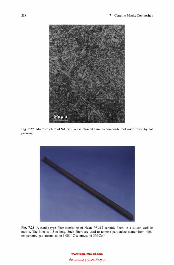
Fig. 7.27 Microstructure of SiC whisker reinforced alumina composite tool insert made by hot

pressing

Fig. 7.28 A candle-type filter consisting of Nextel™ 312 ceramic fibers in a silicon carbide

matrix. The filter is 1.3 m long. Such filters are used to remove particulate matter from high-

temperature gas streams up to 1,000 �C (courtesy of 3M Co.)



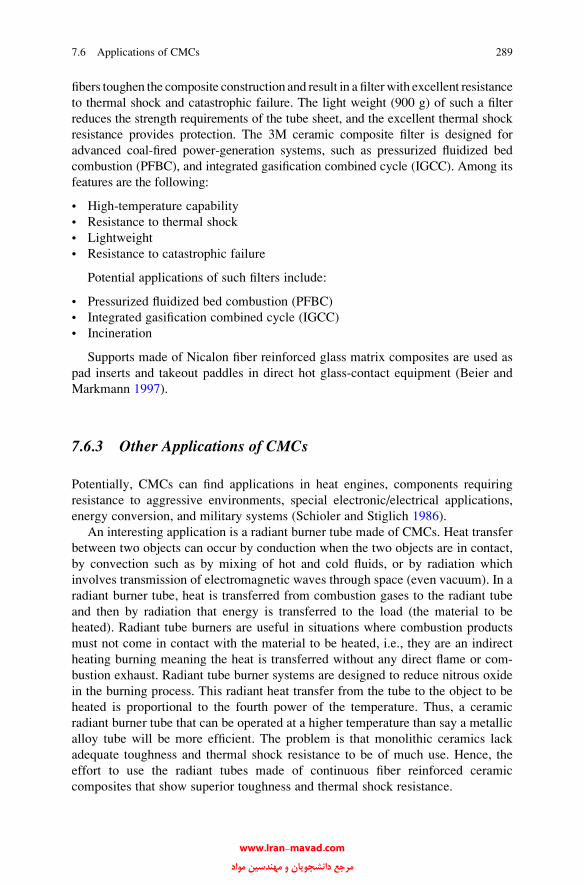
fibers toughen the composite construction and result in a filterwith excellent resistance

to thermal shock and catastrophic failure. The light weight (900 g) of such a filter

reduces the strength requirements of the tube sheet, and the excellent thermal shock

resistance provides protection. The 3M ceramic composite filter is designed for

advanced coal-fired power-generation systems, such as pressurized fluidized bed

combustion (PFBC), and integrated gasification combined cycle (IGCC). Among its

features are the following:

• High-temperature capability

• Resistance to thermal shock

• Lightweight

• Resistance to catastrophic failure

Potential applications of such filters include:

• Pressurized fluidized bed combustion (PFBC)

• Integrated gasification combined cycle (IGCC)

• Incineration

Supports made of Nicalon fiber reinforced glass matrix composites are used as

pad inserts and takeout paddles in direct hot glass-contact equipment (Beier and

Markmann 1997).

7.6.3 Other Applications of CMCs

Potentially, CMCs can find applications in heat engines, components requiring

resistance to aggressive environments, special electronic/electrical applications,

energy conversion, and military systems (Schioler and Stiglich 1986).

An interesting application is a radiant burner tube made of CMCs. Heat transfer

between two objects can occur by conduction when the two objects are in contact,

by convection such as by mixing of hot and cold fluids, or by radiation which

involves transmission of electromagnetic waves through space (even vacuum). In a

radiant burner tube, heat is transferred from combustion gases to the radiant tube

and then by radiation that energy is transferred to the load (the material to be

heated). Radiant tube burners are useful in situations where combustion products

must not come in contact with the material to be heated, i.e., they are an indirect

heating burning meaning the heat is transferred without any direct flame or com-

bustion exhaust. Radiant tube burner systems are designed to reduce nitrous oxide

in the burning process. This radiant heat transfer from the tube to the object to be

heated is proportional to the fourth power of the temperature. Thus, a ceramic

radiant burner tube that can be operated at a higher temperature than say a metallic

alloy tube will be more efficient. The problem is that monolithic ceramics lack

adequate toughness and thermal shock resistance to be of much use. Hence, the

effort to use the radiant tubes made of continuous fiber reinforced ceramic

composites that show superior toughness and thermal shock resistance.

7.6 Applications of CMCs 289


Among the barriers that need to be overcome for large-scale applications of

CMCs are the high production costs, accepted design philosophy, and the lack of

models for strength and toughness. Complicated shapes are difficult to make

economically by hot pressing. Sintering or sintering followed by hot isostatic

pressing (HIP) are the alternate routes for nonglassy matrices.

References

Aveston J, Cooper GA, Kelly A (1971) In: The properties of fibre composites. IPC Science &

Technology, Guildford, p 15

Barclay SJ, Fox JR, Bowen HK (1987) J Mater Sci 22:4403

Becher PF, Wei GC (1984) Commun Am Ceram Soc 67:259

Beier W, Markmann S (1997) Adv Mater Processes 152:37

Bhatt RT (1986) NASA TN-88814

Bhatt RT (1990) J Mater Sci 25:3401

Boccaccini AR, Pearce DH, Janczak J, Beier W, Ponton CB (1997a) Mater Sci Technol 13:852

Boccaccini AR, Ponton CB, Chawla KK (1997b) Mater Sci Eng A241:142

Bordia RK, Raj R (1988) J Am Ceram Soc 71:302

Brennan JJ, Prewo KM (1982) J Mater Sci 17:2371

Burkland CV, Bustamante WE, Klacka R, Yang J-M (1988) In: Whisker- and fiber-toughened

ceramics. ASM Intl, Materials Park, OH, p 225

Carter WC, Butler EP, Fuller ER Jr (1991) Scripta Metall Mater 25:579–584

Chawla KK (2003) Ceramic matrix composites, 2nd edn. Kluwer Acad. Pub, Boston, MA

Chawla KK, Ferber MK, Xu ZR, Venkatesh R (1993a) Mater Sci Eng A162:35–44

Chawla KK, Xu ZR, Hlinak A, Chung Y-W (1993b) In: Advances in ceramic-matrix composites.

Am. Ceram. Soc, Westerville, OH, pp 725–736

Chokshi AH, Porter JR (1985) J Am Ceram Soc 68:c144

Claussen N, Le T, Wu S (1989) J Eur Ceram Soc 5:29

Claussen N, Wu S, Holtz D (1994) J Eur Ceram Soc 14:209

Cook J, Gordon JE (1964) Proc R Soc Lond A228:508

Cornie JA, Chiang Y-M, Uhlmann DR, Mortensen A, Collins JM (1986) Am Ceram Soc Bull

65:293

Davidge RW (1979) Mechanical behavior of ceramics. Cambridge University Press, Cambridge,

p 116

De Jonghe LC, Rahaman MN, Hseuh CH (1986) Acta Metall 39:1467

DiCarlo JA (1985) J Met 37:44

Evans AG (1985) Mater Sci Eng 71:3

Evans AG, Marshall DB (1989) Acta Metall 37:2567

Fitzer E, Gadow R (1986) Am Ceram Soc Bull 65:326

Fitzer E, Hegen D (1979) Angew Chem 91:316

Fitzer E, Schlichting J (1980) Z Werkstofftech 11:330

French JE (1996) In: Handbook of continuous fiber ceramic composites. Amer. Ceramic Soc,

Westerville, OH, p 269

Greil P (1995) J Am Ceram Soc 78:835

Gupta V (1991) MRS Bull XVI-4:39

Gupta V, Yuan J, Martinez D (1993) J Am Ceram Soc 76:305


Chawla N, Liaw PK, Lara-Curzio E, Lowden RA, Ferber MK (1994) In: High performance

composites: commonalty of phenomena. The Minerals, Metals & Materials Society,


Chawla KK, Coffin C, Xu ZR (2000) Intl Mater Rev 45:165


Gladysz GM, Chawla KK (2001) Composities A 32:173

Gladysz GM, Schm€ucker M, Chawla KK, Schneider H, Joslin DL, Ferber MK (1999) Journal of

Mater Sci 34:4351

He MY, Hutchinson JW (1989) J Appl Mech 56:270

Herron M, Risbud SH (1986) Am Ceram Soc Bull 65:342

Hillig WB (1988) J Am Ceram Soc 71:C-96

Homeny J, Vaughn WL, Ferber MK (1987) Am Ceram Soc Bull 67:333

Hurwitz FI (1992) NASA Tech Memo, 105754

Hurwitz FI, Gyekenyesi JZ, Conroy PJ (1989) Ceram Eng Sci Proc 10:750

Hutchinson JW, Jensen HM (1990) Mech Mater 9:139–163

Illston TJ, Ponton CB, Marquis PM, Butler EG (1993) Manufacture of doped glasses using

electrophoretic deposition. In: Duran P, Fernandez JF (eds) Third euroceramics, vol 1. Faenza

Editirice Iberica, Madrid, p 419

Jero PD (1990) Am Ceram Soc Bull 69:484

Jero PD, Kerans RJ (1990) Scripta Metall 24:2315–2318

Jero PD, Kerans RJ, Parthasarathy TA (1991) J Am Ceram Soc 74:2793–2801

Kaya C, Boccaccini AR, Chawla KK (2000) J Am Ceram Soc 83:1885

Kaya C, Kaya F, Butler EG, Boccaccini AR, Chawla KK (2009) J Eur Ceram Soc 29:1631

Kellett B, Lange FF (1989) J Am Ceram Soc 67:369

Kerans RJ, Parthasarathy TA (1991) J Am Ceram Soc 74:1585–1596

Kristofferson A, Warren A, Brandt J, Lundberg R (1993) In: Naslain R et al (eds) Proc. Int. Conf.

HTCMC-1. Woodhead Pub., Cambridge, p 151

Kriven WM (1995) J Phys (France) 5:C8–C101

Kriven WM, Lee SJ (1998) Ceram Eng Sci Proc 19:305

Liu HY, Claussen N, Hoffmann MJ, Petzow G (1991) J Eur Ceram Soc 7:41

Mackin TJ, Warren PD, Evans AG (1992) Acta Metall Mater 40:1251–1257

Mumm DR, Faber KT (1992) Ceram Eng Sci Proc 7–8:70–77

Nourbakhsh S, Liang FL, Margolin H (1990) Metall Trans A 21A:213

Nourbakhsh S, Margolin H (1990) Metall Trans A 20A:2159

Phillips DC (1983a) Fabrication of composites. North-Holland, Amsterdam, p 373

Phillips DC, Sambell RAJ, Bowen DH (1972) J Mater Sci 7:1454

Prewo KM (1982) J Mater Sci 17:3549

Prewo KM (1986) Tailoring multiphase and composite ceramics, vol 20, Materials science

research. Plenum, New York, p 529

Prewo KM, Brennan JJ (1980) J Mater Sci 15:463

Prewo KM, Brennan JJ, Layden GK (1986) Am Ceram Soc Bull 65:305

Rahaman MN, De Jonghe LC (1987) J Am Ceram Soc 70:C-348

Raj R, Bordia RK (1989) Acta Metall 32:1003

Ruhle M, Evans AG (1988) Mater Sci Eng A107:187

Sacks MD, Lee HW, Rojas OE (1987) J Am Ceram Soc 70:C-348

Sambell RAJ, Bowen DH, Phillips DC (1972) J Mater Sci 7:773

Sambell RAJ, Phillips DC, Bowen DH (1974) Carbon fibres: their place in modern technology.

The Plastics Institute, London, p 16/9

Schioler LJ, Stiglich JJ (1986) Am Ceram Soc Bull 65:289

Schneider H, Komarneni S (2005) Mullite. Wiley-VCH, New York, 509 pp

Shalek PD, Petrovic JJ, Hurley GF, Gac FD (1986) Am Ceram Soc Bull 65:351

Sorensen BF (1993) Scripta Metall Mater 28:435–439

Stinton DP, Caputo AJ, Lowden RA (1986) Am Ceram Soc Bull 65:347

Tiegs TN, Becher PF (1986) Tailoring multiphase and composite ceramics. Plenum, New York,

p 639

Urquhart AW (1991) Mater Sci Eng A144:75

Venkatesh R, Chawla KK (1992) J Mater Sci Lett 11:650–652

Wei GC, Becher PF (1984) Am Ceram Soc Bull 64:298

References 291


Wu S, Claussen N (1994) J Am Ceram Soc 77:2898

Yang M, Stevens R (1990) J Mater Sci 25:4658

Zhu D, Kriven WM (1996) Ceram Eng Sci Proc 17:383

Further Reading

Chawla KK (1998) Ceramic matrix composites, 2nd edn. Kluwer, Boston

Colombo P, Riedel R, Soraru GD, Kleebe H-J (eds) (2009) Polymer derived ceramics. Destech,

Lancaster, PA

Faber KT (1997) Annu Rev Mater Res 27:499

Krenkel W (ed) (2008) Ceramic matrix composite. Wiley-VCH, Weinheim

Phillips DC (1983b) Fiber reinforced ceramics. In: Kelly A, Mileiko ST (eds) Fabrication of

ceramics, vol 4 of Handbook of composites. North-Holland, Amsterdam, p 373

Warren R (ed) (1991) Ceramic matrix composites. Blackie & Sons, Glasgow

Problems

7.1. What are the sources of fiber degradation during processing of ceramic matrix

composites?

7.2. Describe the advantages of using sol–gel and polymer pyrolysis techniques to

process the ceramic matrix in CMCs.

7.3. Explain how a carbon fiber reinforced glass–ceramic composite can be

obtained with an almost zero in-plane coefficient of thermal expansion.

7.4. Chemically, what is an alkoxide? Describe some of the alkoxides that can be

used to obtain different ceramic matrixes in CMC.

7.5. Distinguish between interphase and interface.

7.6. Why is thermal shock resistance more of a problem in CMCs than in MMCs?



Chapter 8

Carbon Fiber/Carbon Matrix Composites

We devote this chapter to a very special kind of composite that consists of carbon

fibers embedded in a carbonaceous matrix. The carbon fiber in these composites can

be continuous or short. We described the processing of carbon fibers in Chap. 2.

Carbon is a very versatile material. It can exist in a variety of forms; amorphous,

graphite, diamond, fullerenes, graphene, nanotubes, etc. Below we summarize the

salient features of some important forms of carbon.

Diamond. Carbon in the diamond form has an FCC structure; it is also called

diamond cubic. Each C atom is covalently bonded to four carbon atoms at the

vertices of a tetrahedron and the interatomic distance ¼ 0.154 nm. Carbon in

the diamond form has isotropic properties. It is one of the hardest materials.

Graphite. Graphitic form of carbon has a hexagonal structure. Carbon atoms are

arranged in layers. The bonding between atoms in the plane of the layer is covalent

but the bonding between layers is weak, van der Waals type. This difference in the

bonding in a and c directions makes graphite is highly anisotropic. Young’s

modulus in the basal plane (a direction) is ~1,000 GPa, while in a direction

perpendicular to the basal plane (c direction) it is ~35 GPa. Tensile strength,

thermal expansion, and thermal conduction are also anisotropic in a similar manner.

Pyrolytic graphite. Pyrolytic graphite is produced from a gaseous phase via pyro-

lysis of hydrocarbons. The pyrolysis of hydrocarbons results in carbon, which is

deposited on a hot substrate. Pyrolytic graphite has a highly oriented structure and

therefore is highly anisotropic.

Carbon black. A generic term for carbon powder of extremely fine size (nm range)

and very high surface area. It is essentially elemental carbon (>97 %), electrically

conductive, and finds extensive use as a reinforcement in tires and other rubber

products as well as in printing inks and paints.

Carbon nanotubes. These are hollow, cylindrical tubes of carbon atoms with

diameter in the range of 5–20 nm. They are frequently referred to as CNTs.


293


http://dx.doi.org/10.1007/978-0-387-74365-3_2

CNTs can have very large aspect ratios. They show some very unusual properties,

such as extremely high stiffness and strength.

Carbon is an excellent high temperature material when used in an inert or

nonoxidizing atmosphere. Potential high temperature applications call for 10 h to

a few 1,000 h at greater than 1,000 �C and at times approaching 2,200 �C. The major

drawback of carbon is that it reacts with oxygen, forming gaseous oxides of carbon.

Unlike other nonoxide ceramics, carbon powder cannot be sintered. Thus, the

carbon matrix in a carbon fiber/carbon matrix composite is generally obtained by

chemical vapor deposition (CVD) of carbon or thermal decomposition of a source

of carbon such as pitch or phenolic resin. Generally, many pores form during this

conversion of a hydrocarbon to carbon. Thus, a dense and strong pore-free carbon/

carbon composite is not easy to fabricate. A very wide range of characteristics,

however, can be obtained in these composites, the principal characteristic being the

high temperature capability of these composites in inert environments. Being very

light, carbon/carbon composites show superior specific strength at high

temperatures in inert atmospheres.

Although, carbon/carbon composites were originally developed for the space

program, they have now become high performance engineering materials, with

special high temperature applications. More specifically, these high temperature

applications involve brakes for aircraft and automobiles, dies for use in hot-

pressing, high temperature fasteners, heating elements in furnaces, liners and

protection tubes, etc. Carbon/carbon composites are expensive mainly because of

the long processing times involved. Essentially, we take a carbon fiber reinforced

polymer matrix composite and convert the polymer matrix by pyrolysis to carbon or

we deposit carbon from gaseous reactants into interstices of a woven carbon fiber

preform. The process can take days, making the final product very expensive.

In what follows we describe the processing techniques, properties, and major

applications of carbon/carbon (C/C) composites.

8.1 Processing of Carbon/Carbon Composites

Three methods are commonly used to fabricate carbon/carbon composites:

1. A woven preform of carbon fiber is impregnated, under heat and pressure, with

thermoplastic pitch, followed by pyrolysis of pitch into carbon. Generally the

cycle is repeated to obtain the desired density. A special version of this technique

is called high pressure impregnation carbonization or HIPIC (see below). Pitches

are mixtures of hydrocarbons of different molecular weights. Yield of carbon

from the pitch precursor increases with increasing average molecular weight of

the pitch but high molecular weight means high viscosity which makes penetra-

tion of the fibrous preform difficult.

2. A carbon fiber/polymer matrix composite is made by one of the conventional PMC

fabrication techniques (see Chap. 5), followed by conversion of the resin, generally

a thermoset, to carbon by pyrolysis. Again, reimpregnation and repyrolysis are

294 8 Carbon Fiber/Carbon Matrix Composites


http://dx.doi.org/10.1007/978-0-387-74365-3_5

used to attain the desired density of the composite. Phenolics are one of

the common resins used because of the comparatively high carbon yield.

3. CVD of carbon is made from a gaseous phase onto and in between the carbon

fibers in a preform. Hydrocarbon gases become unstable with respect to carbon

at high temperatures (>550 �C).

Fig. 8.1 Processing of carbon/carbon composites by pyrolysis of carbon fiber/polymer composites

Fig. 8.2 Processing of carbon/carbon composites by chemical vapor deposition (CVD) process

8.1 Processing of Carbon/Carbon Composites 295


Methane, a common precursor for CVD, decomposes as per the following

reaction:

CH4 gð Þ ! C sð Þ þ 2H2 gð Þ:

Low pressure (or addition of inert diluent gases such as H2, N2, or Ar to the

gaseous stream) is used to improve diffusion because it increases the mean free path

of the gaseous molecules.

Figure 8.1 shows the process corresponding to the pyrolysis of a PMC, while

Fig. 8.2 shows the CVD process. In both processes, multiple impregnation cycles are

required to increase the density of the composites, i.e., reduce the amount of porosity

in the composite to an acceptable level. Invariably, in all the processes, there occurs

a large weight loss (between 10 and 60 %) during the pyrolysis step, which results in

a large amount of shrinkage porosity. In addition, there is the complexity of the

anisotropic nature of the carbon fiber (properties are different in the axial and radial

directions). The carbon matrix, obtained by pyrolysis, is essentially isotropic. This

leads to generation of thermal stresses in each cycle, because of thermal mismatch

between the fiber and the matrix, which leads to the formation of microcracks in the

C/C composites after multiple cycles of impregnation and pyrolysis.

8.1.1 High Pressure Processing

Application of isostatic pressure in an autoclave during carbonization of pitch can

increase the yield of carbon from 50 % at atmospheric pressure to over 90 % at

100 MPa. This high pressure processing is also called high pressure impregnation

carbonization or HIPIC. Commonly, partially impregnated preform and excess

pitch are placed in a sealed metal can, which in turn is placed in the pressure

vessel. The temperature is increased to 550–650 �C and pressure in the range of

5–100 MPa is applied. The thin metal can acts like a rubber bag in the processing of

PMCs in an autoclave. The process can take as much as 24 h. After HIPIC, the

metal container is stripped off and the impregnated composite is generally

subjected to a graphitization treatment at temperatures above 2,300 �C.Properties of C/C composites depend a great deal on the volume fraction of

porosity present. Essentially, the pores present are of open-cell type. An easy

parameter to follow the evolution of porosity in C/C composites is the density of

the composite. One generally starts with a carbon fiber preform of density of 1 g/cm3.

After about four cycles of impregnation, we attain a density of 1.4 g/cm3. However,

under conditions of HIPIC, it is possible to reach a density of 1.8 g/cm3 after four or

five cycles, see Fig. 8.3. It is possible to reach a density of 1.8 g/cm3 after four or five

cycles, see Fig 8.3. It is worth pointing out here that the theoretical density of carbon

is 2.25 g/cm3. Carbon fiber itself can have density between 1.6 and 2.2 g/cm3.

A value of 2.2 g/cm3 for carbon fiber is very uncommon; only mesophase pitch-

based carbon fiber can show such a value after high temperature graphitization



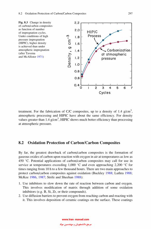
treatment. For the fabrication of C/C composites, up to a density of 1.4 g/cm3,

atmospheric processing and HIPIC have about the same efficiency. For density

values greater than 1.4 g/cm3, HIPIC shows much better efficiency than processing

at atmospheric pressure.

8.2 Oxidation Protection of Carbon/Carbon Composites

By far, the greatest drawback of carbon/carbon composites is the formation of

gaseous oxides of carbon upon reaction with oxygen in air at temperatures as low as

450 �C. Potential applications of carbon/carbon composites may call for use in

service at temperatures exceeding 1,000 �C and even approaching 2,200 �C for

times ranging from 10 h to a few thousand hours. There are two main approaches to

protect carbon/carbon composites against oxidation (Buckley 1988; Luthra 1988;

McKee 1986, 1987; Strife and Sheehan 1988):

1. Use inhibitors to slow down the rate of reaction between carbon and oxygen.

This involves modification of matrix through addition of some oxidation

inhibitors (e.g. B, Si, Zr, or their compounds).

2. Use diffusion barriers to prevent oxygen from reaching carbon and reacting with

it. This involves deposition of ceramic coatings on the surface. These coatings

Fig. 8.3 Change in density

of carbon/carbon composites

as function of number

of impregnation cycles.

Under conditions of high

pressure impregnation

(HIPIC), higher density

is achieved than under

atmospheric impregnation

(after Taverna

and McAllister 1971)

8.2 Oxidation Protection of Carbon/Carbon Composites 297


are generally multilayer coatings of functionally gradied materials of carbides,

nitrides and oxides of Si, Zr, Ta, Al, etc.

The diffusion barrier coating should have the following characteristics:

• Oxidation resistance

• Low oxygen permeability and volatility

• Good adhesion to carbon

• Chemical compatibility with carbon

• Thermal expansion match with carbon

Figure 8.4a shows the critical factors that should be considered in an oxidation

protection system for carbon/carbon composites (Strife and Sheehan 1988), while

Fig. 8.4b shows, schematically, a typical multilayer oxidation protection system on

a C/C substrate.

The two approaches involving the use of inhibitors and diffusion barriers are

frequently combined: use diffusion barriers and internal glass forming inhibitors

and sealants. Silicon-based ceramics, such as SiC and Si3N4, are commonly used as

the primary oxygen barrier coatings. Sealants have the added advantage that they

also seal thermal stress cracks originating because of the thermal mismatch between

C/C composite and silicon carbide coating. Tetraethylorthosilicate (TEOS) is

commonly used to impregnate such cracks (McKee 1986; 1987). TEOS leaves

oxidation resistant silica in the cracks. Addition of boria B2O3 can inhibit the

oxidation (Ehrburger et al. 1986; McKee 1986).

Extended oxidation protection of carbon/carbon composites can be obtained by

using boria containing dense Si3N4 or SiC coatings and boron-rich inner coating.

Borate glasses act as sealants and fill up the cracks that form in the outer coatings

because of thermal expansion mismatch. An oxidation protection system used for

extended protection under thermal cycling conditions, with peak temperatures

reaching 1,400 �C, is shown in Fig. 8.4a (Strife and Sheehan 1988).Moisture sensitiv-

ity of borate glasses, corrosion of outer coatings by glasses, glass volatilization, and

unacceptably high oxygen permeability are some of the negative factors. Alvey and

George (1991)usedmultilayerZr/Pt coating that formedZrPt3 onannealing oncarbon/

carbon composites. Their results showed that this coating protected carbon and a

carbon fiber/phenolic resin composite from a 2,800 �C flame. They attributed this

performance to the oxidation resistance of ZrPt3 and to the reflectivity of the coating,

which reduced the thermal flux on the substrate to a short time.

8.3 Properties of Carbon/Carbon Composites

Properties of carbon/carbon composites depend on the type of carbon fiber used

(high-modulus or high-strength type), fiber volume fraction, the fiber distribution,

and the amount of porosity. One-, two-, and three-dimensionally woven carbon

fibers may be used. Carbon fiber can be woven in a variety of weaves for



reinforcement in two or more dimensions. Two main types of weave are plain and

satin. A plain weave has one warp yarn running over and under one fill yarn and is

the simplest weave. Satin-type weaves are more flexible; that is, they can conform

to complicated shapes easily. Figure 8.5 shows a two-dimensional (2D) plain weave

and a five-harness satin weave (McAllister and Lachman 1983). Modifications

of the basic three-dimensional (3D) orthogonal weave involving different fiber

Fig. 8.4 (a) Critical factors that should be taken into account for an oxidation protection system

for carbon/carbon composites (after Strife and Sheehan 1988). (b) Schematic of a typical multi-

layer oxidation protection system on a C/C substrate

8.3 Properties of Carbon/Carbon Composites 299


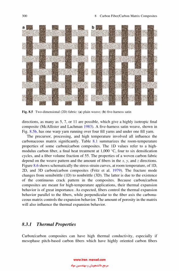
directions, as many as 5, 7, or 11 are possible, which give a highly isotropic final

composite (McAllister and Lachman 1983). A five-harness satin weave, shown in

Fig. 8.5b, has one warp yarn running over four fill yarns and under one fill yarn.

The precursor, processing, and high temperature involved all influence the

carbonaceous matrix significantly. Table 8.1 summarizes the room-temperature

properties of some carbon/carbon composites. The 1D values refer to a high-

modulus carbon fiber, a final heat treatment at 1,000 �C, four to six densification

cycles, and a fiber volume fraction of 55. The properties of a woven carbon fabric

depend on the weave pattern and the amount of fibers in the x, y, and z directions.Figure 8.6 shows schematically the stress-strain curves, at room temperature, of 1D,

2D, and 3D carbon/carbon composites (Fritz et al. 1979). The fracture mode

changes from semibrittle (1D) to nonbrittle (3D). The latter is due to the existence

of the continuous crack pattern in the composites. Because carbon/carbon

composites are meant for high-temperature applications, their thermal expansion

behavior is of great importance. As expected, fibers control the thermal expansion

behavior parallel to the fibers, while perpendicular to the fiber axis the carbona-

ceous matrix controls the expansion behavior. The amount of porosity in the matrix

will also influence the thermal expansion behavior.

8.3.1 Thermal Properties

Carbon/carbon composites can have high thermal conductivity, especially if

mesophase pitch-based carbon fibers which have highly oriented carbon fibers

Fig. 8.5 Two-dimensional (2D) fabric: (a) plain weave; (b) five-harness satin



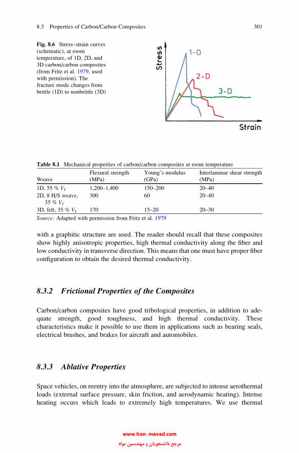
with a graphitic structure are used. The reader should recall that these composites

show highly anisotropic properties, high thermal conductivity along the fiber and

low conductivity in transverse direction. This means that one must have proper fiber

configuration to obtain the desired thermal conductivity.

8.3.2 Frictional Properties of the Composites

Carbon/carbon composites have good tribological properties, in addition to ade-

quate strength, good toughness, and high thermal conductivity. These

characteristics make it possible to use them in applications such as bearing seals,

electrical brushes, and brakes for aircraft and automobiles.

8.3.3 Ablative Properties

Space vehicles, on reentry into the atmosphere, are subjected to intense aerothermal

loads (external surface pressure, skin friction, and aerodynamic heating). Intense

heating occurs which leads to extremely high temperatures. We use thermal

Fig. 8.6 Stress–strain curves

(schematic), at room

temperature, of 1D, 2D, and

3D carbon/carbon composites

(from Fritz et al. 1979, used

with permission). The

fracture mode changes from

brittle (1D) to nonbrittle (3D)

Table 8.1 Mechanical properties of carbon/carbon composites at room temperature

Weave

Flexural strength

(MPa)

Young’s modulus

(GPa)

Interlaminar shear strength

(MPa)

1D, 55 % Vf 1,200–1,400 150–200 20–40

2D, 8 H/S weave,

35 % Vf

300 60 20–40

3D, felt, 35 % Vf 170 15–20 20–30

Source: Adapted with permission from Fritz et al. 1979

8.3 Properties of Carbon/Carbon Composites 301


protection systems (TPS) made of suitable materials in order to keep space vehicle

and occupants and equipments safe. Ablative TPS is commonly used because it is

quite effective in expending thermal energy. In an ablative TPS, we sacrifice the

material and thus absorb the thermal energy. There is a variety of ablative materials

available. The one of interest to us here is the high temperature ablative material of

which C/C composites are a prime example. They are used in manned space

vehicles, hypersonic vehicles, and missiles.

Please see problem 8.6 at the end of this chapter about the Columbia shuttle

disaster which involved C/C composites.

8.4 Applications of Carbon/Carbon Composites

Major applications of carbon/carbon composites involve uses at high temperatures,

for example, as heat shields for reentry vehicles, aircraft brakes, hot-pressing dies,

and high-temperature parts such as nozzles. Figure 8.7 shows a fully processed 3D

carbon/carbon frustum. Hot-pressing dies made of carbon/carbon composites are

commercially available, while brake disks are used in conventional aircraft,

although their first use in civilian aircraft occurred in the Concorde supersonic

aircraft. Brakes for racing cars and some high end luxury cars are the latest entry.

Heat shields and nozzles are made of multidirectionally reinforced carbon/carbon

composites. As pointed out, carbon/carbon composites can withstand high

temperatures in an inert atmosphere. Lack of oxidation resistance is a major

problem, and a great deal of effort has been put into the development of

Fig. 8.7 A three-dimensional

carbon/carbon frustum

(courtesy of Fiber

Materials Inc.)



oxidation-resistant coatings for carbon fibers, with SiC coating being the primary

coating material.

Other applications of carbon/carbon composites include their use as implants

and internal repair of bone fractures because of their excellent biocompatibility.

They are also used to make molds for hot pressing. Carbon/carbon molds can

withstand higher pressures and offer a longer use life than polycrystalline graphite.

8.4.1 Carbon/Carbon Composite Brakes

Brakes of any kind use friction between contact surfaces to stop a moving compo-

nent. In the process, the kinetic energy of a moving object is converted into heat,

which needs to be absorbed by the brake materials. Most commonly, the essential

components of a braking system are: a rotating part (such as a wheel, axle, disk, or

brake drum) and a stationary part that is pressed against the rotating part to slow or

stop the moving object. The transmission of kinetic energy from the moving vehicle

to heat in the brake pads generates high temperatures in the friction pad material and

brake components. Efficient brake systems must be able to withstand the thermal

shock, dissipate heat quickly (i.e., high thermal conductivity or more appropriately

high thermal diffusivity) and maintain consistent braking performance. Any brake

design must consider the following items (Awasthi and Wood 1988):

• Friction members must generate stopping torque (over a range of environmental

conditions: rain, snow, dust storms, etc.).

• Heat sinks must absorb the kinetic energy of the aircraft.

• Structural elements should be able to transfer torque to the tires.

Brakes are one of the major applications of carbon/carbon composites. An

example of a carbon/carbon brake assembly used on a Boeing 767 plane is shown

in Fig. 8.8. Brakes, aircraft or automobile, have the following general requisites

(Awasthi and Wood 1988):

(a) Oxidation resistance

(b) High thermal capacity

(c) Good strength, impact resistance, strain to failure

(d) Adequate and consistent friction characteristics

(e) High thermal conductivity

When the brakes are applied, multiple-disk brakes with alternating rotors and

stators are forced against adjacent members by hydraulic pressure. Friction between

rotating and stationary disks causes them to heat up to 1,500 �C (surface temperature

can be as high as 3,000 �C) over a short time period, i.e., one needs excellent thermal

shock resistance. In commercial processing of carbon/carbon brakes, a fabric made

of woven carbon fibers with fiber tows inserted in the thickness (or z-direction)direction is used.

8.4 Applications of Carbon/Carbon Composites 303


In view of the requisites listed above, any braking material must be a good

structural material, an efficient heat sink, and must have excellent abrasion resis-

tance. Let us consider an example from the aircraft field which will help illustrate

the formidable demands made on a braking material. Many civilian aircraft use

carbon/carbon composite brakes. Let us take Boeing 767 as an example to help

illustrate the formidable demands made on a braking material. In the event of an

aborted takeoff, an extremely large amount of kinetic energy must be dissipated in

about 30 s by the eight brakes on the aircraft (see the example below for an estimate

of the temperature rise in an RTO). A rejected takeoff (RTO) is, indeed, the worst

case scenario but then the braking material must be able to meet such requirements.

It is estimated that about 3,000 RTOs occur every year in the USA.

The weight savings that result from replacement of conventional brakes by

carbon/carbon brakes helps one understand why the aircraft industry has taken up

the C/C brakes (Awasthi and Wood 1988). In a large aircraft, a conventional

multiple stator and rotor arrangement (a sintered high friction material sliding

against a high temperature steel) weighs about 1,100 kg. Carbon/carbon brakes

(both the stator and the rotor being made of carbon/carbon composite) weigh about

700 kg, resulting in a weight savings of 400 kg. Also, as a braking material, carbon/

carbon composites are superior to high strength bulk graphite. Carbon/carbon

composites have much higher strength at the same density.

The Formula 1 racing cars usually use a new set of brake linings for each race.

Aircraft brakes, on the other hand, are required to survive 2,000–4,000 landings.

Fig. 8.8 A carbon/carbon brake assembly that is used on a Boeing 767 airplane (courtesy of

Alied-Signal Corp.)



An Airbus A380 has 16 sets of brakes; each brake costs something between US$

35,000 and 45,000. However, use of carbon/carbon composite brakes results in

weight savings relative to the conventional steel brakes; 250 kg on a Boeing 737.

This allows more payload and/or or fuel savings.

Example One of the functions of the brake system is to absorb the heat energy

developed during braking. Consider the Boeing 777 plane. Find out its mass and

takeoff speed from the Web. Compute the kinetic energy of the plane when it is

about to takeoff. Assume that the plane has carbon/carbon brakes. The pilot is asked

to abort the takeoff for some reason. Under these conditions, assuming that all of the

kinetic energy is converted to thermal energy, compute the temperature rise in this

aborted takeoff.

Answer From the website of Boeing, we find that the maximum takeoff weight of a

Boeing777plane is 247,000kg.The takeoff speed can range from270 to345km/h.Let

us take a speed of 78.6 m/s. Putting these values in to the equation for kinetic energy

K:E: ¼ 1

2mv2;

wherem is the mass of the plane and v is its velocity. Substituting the values of mass

and velocity in the above expression, we get the kinetic energy to be 763 MJ.

This is the kinetic energy that is converted into heat and must be absorbed in

the plane during a rejected take off. To find the change in temperature, we use the

following relationship

Q ¼ DTCpm;

whereQ is the kinetic energy converted to heat, DT is the change in temperature, m is

themass of the brakes, and Cp is the specific heat of the carbon brakes. Themass of the

brakes is 700 kg. The specific heat of the carbon brakes is 1:6ðkJ=kg� KÞ: Putting allthese values in the above expression, we get a change in temperature of 954 �C.

8.4.2 Other Applications of Carbon/Carbon Composites

Among other aerospace applications of carbon/carbon composites, one may cite

their use in rocket propulsion components and reentry thermal protection of a

spacecraft. Figure 8.7 shows the frustum of a cone of a rocket made of a 3D

carbon/carbon composite. A 3D composite has fibers in x, y, and z directions. Thetop layer in contact with the high temperature environment gets eventually

sacrificed. Among nonaerospace applications, there are examples of use of carbon/

carbon composites as implants as well as internal fixation of bone fractures because

of their excellent biocompatibility. They are also used for making molds for hot

pressing. Carbon/carbonmolds canwithstand higher pressures and offer a longer life

8.4 Applications of Carbon/Carbon Composites 305


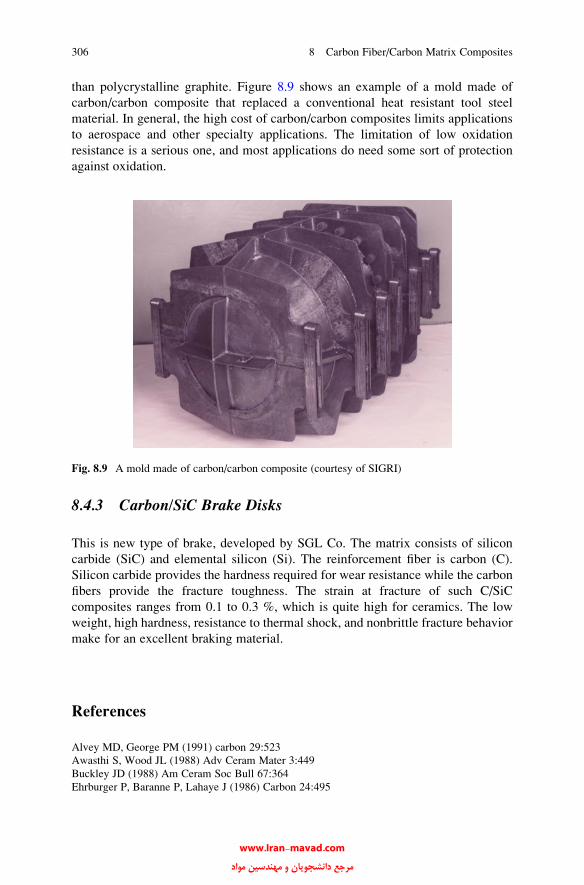
than polycrystalline graphite. Figure 8.9 shows an example of a mold made of

carbon/carbon composite that replaced a conventional heat resistant tool steel

material. In general, the high cost of carbon/carbon composites limits applications

to aerospace and other specialty applications. The limitation of low oxidation

resistance is a serious one, and most applications do need some sort of protection

against oxidation.

8.4.3 Carbon/SiC Brake Disks

This is new type of brake, developed by SGL Co. The matrix consists of silicon

carbide (SiC) and elemental silicon (Si). The reinforcement fiber is carbon (C).

Silicon carbide provides the hardness required for wear resistance while the carbon

fibers provide the fracture toughness. The strain at fracture of such C/SiC

composites ranges from 0.1 to 0.3 %, which is quite high for ceramics. The low

weight, high hardness, resistance to thermal shock, and nonbrittle fracture behavior

make for an excellent braking material.

References

Alvey MD, George PM (1991) carbon 29:523

Awasthi S, Wood JL (1988) Adv Ceram Mater 3:449

Buckley JD (1988) Am Ceram Soc Bull 67:364

Ehrburger P, Baranne P, Lahaye J (1986) Carbon 24:495

Fig. 8.9 A mold made of carbon/carbon composite (courtesy of SIGRI)



Fritz W, H€uttner W, Hartwig G (1979) Nonmetallic materials and composites at low temperatures.

Plenum, New York, p 245

Luthra KL (1988) Carbon 26:217

McAllister LE, Lachman WL (1983) Fabrication of composites. North-Holland, Amsterdam,

p 109

McKee DW (1986) Carbon 24:737

McKee DW (1987) Carbon 25:551

Strife JR, Sheehan JE (1988) Am Ceram Soc Bull 67:369

Taverna AR, McAllister LE (1971) Adv. materials: composites and carbon. Amer. Ceram. Soc,

Columbus, OH, p 199

Further Reading

Chawla KK (2003) Ceramic matrix composites, 2nd edn. Kluwer, Boston, MA

Donnet J-B, Bansal RC (1984) Carbon fibers, 2nd edn. Marcel Dekker, New York

Fitzer E (1985) Carbon fibres and their composites. Springer, Berlin

Savage G (1992) Carbon–carbon composites. Chapman & Hall, London

Thomas CR (ed) (1993) Essentials of carbon–carbon composites. Royal Society of Chemistry,

Cambridge

Problems

8.1. The terms voids and cracks are frequently used interchangeably but in reality

they are not synonymous. Specifically, in regard to C/C composites, distin-

guish between voids and microcracks in terms of their form and origin.

8.2. TEOS is often used as a glass forming sealant to heal the microcracks in C/C

composites. However, there are some limitations on efficiency. Explain what

the limitations are and why.

8.3. Invariably C/C composites will need to be joined to other conventional

materials. Describe the different joining approaches that can be used to

accomplish this; give the pros and cons of each technique.

8.4. C/C composites are frequently made of carbon fibers woven in more than three

directions. What effect does this have on crack propagation, fracture surface

appearance, and toughness of C/C composite?

8.5. Glass-forming sealants help close the crack-like defects in C/C composites.

Are there any deleterious effects of such sealants?

8.6. Describe the NASA’s Columbia shuttle disaster in which all seven astronauts

lost their lives in 2003. Highlight the role of carbon/carbon composites in this

disaster. How and why did the disaster occur? Describe the modifications

instituted by NASA to prevent such a disaster in the future.

Problems 307


Chapter 9

Multifilamentary Superconducting Composites

Certain materials lose all resistance to the flow of electricity when cooled to within

a few degrees of absolute zero. The phenomenon is called superconductivity, andthe materials exhibiting this phenomenon are called superconductors. Super-

conductors can carry a high current density without any electrical resistance;

thus, they can generate the very high magnetic fields that are desirable in many

applications: magnetic resonance imaging, high-energy physics, and fusion energy

programs. Other fields of application include magnetic levitation vehicles, magneto

hydrodynamic generators, rotating machines, and magnets in general. Kamerlingh

Onnes discovered the phenomenon of superconductivity in mercury in 1911. Since

then, some 27 elements and hundreds of solid solutions or compounds have been

discovered that show this phenomenon of total disappearance of electrical resis-

tance below a critical temperature, Tc. Figure 9.1 shows the variation of electrical

resistivity with temperature of a normal metal and that of a superconducting

material, Nb3Sn. The critical temperature is a characteristic constant of each

material. Kunzler et al. (1961) discovered the high critical field capability of

Nb3Sn and thus opened up the field of practical, high-field superconducting

magnets. It turns out that most of the superconductors came into the realm of

economic viability when techniques were developed to put the superconducting

species in the form of ultrathin filaments in a copper matrix as described below.

A similar development route is used for the newer oxide superconductors.

Multifilamentary composite superconductors started becoming available in the

1970s. These are niobium-based (Nb–Ti and Nb3Sn) superconductors, also referred

to as conventional superconductors. The erstwhile record of critical temperature

at which a conventional material became a superconductor was 23 K and was set

in 1974. These conventional superconductors require liquid helium as a coolant,

which is expensive. In 1986, there began a new era in the field of superconductivity,

called high-temperature superconductivity (HTS), which started with the now well-

known work of Bednorz and Muller. They reported of superconductivity at 30 K


309


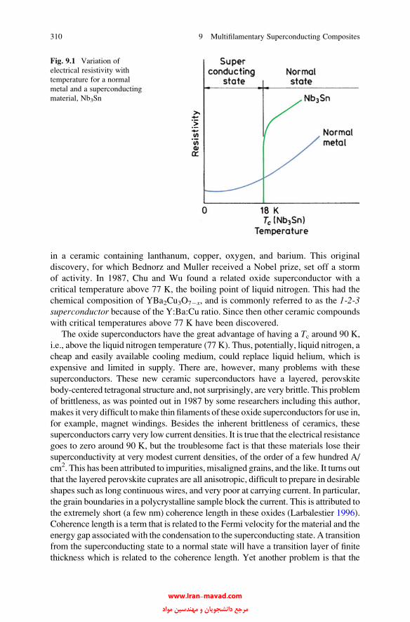
in a ceramic containing lanthanum, copper, oxygen, and barium. This original

discovery, for which Bednorz and Muller received a Nobel prize, set off a storm

of activity. In 1987, Chu and Wu found a related oxide superconductor with a

critical temperature above 77 K, the boiling point of liquid nitrogen. This had the

chemical composition of YBa2Cu3O7�x, and is commonly referred to as the 1-2-3superconductor because of the Y:Ba:Cu ratio. Since then other ceramic compounds

with critical temperatures above 77 K have been discovered.

The oxide superconductors have the great advantage of having a Tc around 90 K,

i.e., above the liquid nitrogen temperature (77 K). Thus, potentially, liquid nitrogen, a

cheap and easily available cooling medium, could replace liquid helium, which is

expensive and limited in supply. There are, however, many problems with these

superconductors. These new ceramic superconductors have a layered, perovskite

body-centered tetragonal structure and, not surprisingly, are very brittle. This problem

of brittleness, as was pointed out in 1987 by some researchers including this author,

makes it very difficult tomake thin filaments of these oxide superconductors for use in,

for example, magnet windings. Besides the inherent brittleness of ceramics, these

superconductors carry very low current densities. It is true that the electrical resistance

goes to zero around 90 K, but the troublesome fact is that these materials lose their

superconductivity at very modest current densities, of the order of a few hundred A/

cm2. This has been attributed to impurities, misaligned grains, and the like. It turns out

that the layered perovskite cuprates are all anisotropic, difficult to prepare in desirable

shapes such as long continuous wires, and very poor at carrying current. In particular,

the grain boundaries in a polycrystalline sample block the current. This is attributed to

the extremely short (a few nm) coherence length in these oxides (Larbalestier 1996).

Coherence length is a term that is related to the Fermi velocity for the material and the

energy gap associatedwith the condensation to the superconducting state. A transition

from the superconducting state to a normal state will have a transition layer of finite

thickness which is related to the coherence length. Yet another problem is that the


electrical resistivity with

temperature for a normal

metal and a superconducting

material, Nb3Sn

310 9 Multifilamentary Superconducting Composites


performance of these oxide superconductors deteriorates drastically as the applied

magnetic field increases. At a magnetic field of 1 T, the critical current density, Jc, isabout 1–10A/cm2. For any reasonable commercial application, one needs a Jc of about105 A/cm2. The critical current density, Jc, is a function of the processing and,

consequently, of the microstructure of the superconductor. This is where some

innovative processing can be of great value. Heine et al. (1989) took just such a step

when they partially melted Bi–Sr–Ca–Cu–O (BSCCO) in a silver sheath and observed

that the resultant superconductor showed high Jc in the grains. There remains a large

gap to be bridged between producing a small sample for testing in the laboratory and

making a viable commercial product. We need superconductors (Larbalestier 1996)

that “. . . must be electrically continuous, otherwise there can be no applications.”

They must also be strong and tough, amenable to being economically made into long

lengths, and possess high overall Jc values. The term overall implies that all of the

space required to make the superconductor must be taken into account when critical

current density is computed (Larbalestier 1996). It should be pointed out that the

Nb–Ti system took 15–20 years between its discovery and commercial availability.

The new high-temperature oxide superconductors hold great promise, and it would

appear that eventually some kind of composite superconductors will be used commer-

cially as are theNb-based conventional superconductors. Thus, it is quite instructive to

review the composite material aspects of niobium-based superconductors, which we

do first in this chapter. We describe the processing, structure, and properties of the

conventional and high-Tc superconductors. Both are truly multifilamentary metal

matrix composites. But first let us describe why we need these superconductors in

the form of multifilamentary metal matrix composites.

9.1 The Problem of Flux Pinning

For a variety of applications, we need long-length superconductors of uniform

properties, for example, large solenoids and coils for rotating machinery and magnets

for plasma confinement in a fusion reactor. In conventional superconductors, ultrathin

superconducting filaments are incorporated in a copper matrix to form a filamentary

fibrous composite. In the high-Tc superconductors, we have ceramic superconducting

material in the form of thin filaments in a metal matrix. Small diameter, continuous,

superconducting filaments distributed in a high conductivity (electrical and thermal)

matrix constitute nothing but a superconducting metal matrix composite (MMC). The

main reason for using superconductors in the form of filamentary composites is that

flux jumps can be avoided if the diameter of superconducting filaments is below a

certain value (Irie 1994). It is important to realize that stable, superconductingmagnets

need flexible and continuous wires that can be wound; this became possible only after

wires and cables were made of such MMC composites.

Superconducting filaments have a micrometer-size diameter that helps to reduce

the risk of flux jump in any given filament. If a superconductor is perturbed, say, by

motion or a change in the applied field, it leads to a rearrangement of magnetic flux

9.1 The Problem of Flux Pinning 311


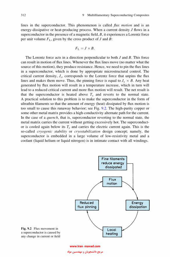
lines in the superconductor. This phenomenon is called flux motion and is an

energy-dissipative or heat-producing process. When a current density J flows in a

superconductor in the presence of a magnetic field, B, it experiences a Lorentz forceper unit volume FL, given by the cross product of J and B:

FL ¼ J � B:

The Lorentz force acts in a direction perpendicular to both J and B. This forcecan result in motion of flux lines. Whenever the flux lines move (no matter what the

source of this motion), they produce resistance. Hence, we need to pin the flux lines

in a superconductor, which is done by appropriate microstructural control. The

critical current density, Jc, corresponds to the Lorentz force that unpins the flux

lines and makes them move. Thus, the pinning force is equal to Jc � B. Any heat

generated by flux motion will result in a temperature increase, which in turn will

lead to a reduced critical current and more flux motion will result. The net result is

that the superconductor is heated above Tc and reverts to the normal state.

A practical solution to this problem is to make the superconductor in the form of

ultrathin filaments so that the amount of energy (heat) dissipated by flux motion is

too small to cause this runaway behavior; see Fig. 9.2. The high-purity copper or

some other metal matrix provides a high-conductivity alternate path for the current.

In the case of a quench, that is, superconductor reverting to the normal state, the

metal matrix carries the current without getting excessively hot. The superconduct-

or is cooled again below its Tc and carries the electric current again. This is the

so-called cryogenic stability or cryostabilization design concept; namely, the

superconductor is embedded in a large volume of low-resistivity metal and a

coolant (liquid helium or liquid nitrogen) is in intimate contact with all windings.

Fig. 9.2 Flux movement in

a superconductor is caused by

any change in current or field



9.2 Types of Superconductor

The technologically most important property of a superconductor is its capacity to

carry an electric current without normal I2R losses up to a critical current density,

Jc. I2R losses are known as Joule heating, with I and R representing the electric

current and resistance, respectively. The critical current density, Jc, is a function

of the applied field and temperature. The commercially available superconductors

in the 1980s could demonstrate critical current densities of Jc > 106 A/cm2 at

4.2 K, the liquid helium temperature, and an applied field of 5 T.

There are three parameters that limit the properties of a superconductor, namely,

the critical temperature (Tc), the critical electrical current density (Jc), and the

critical magnetic field (Hc); see Fig. 9.3. As long as the material stays below

the shaded area indicated in Fig. 9.3, it will behave as a superconductor.

There are two types of superconductor:

Type I: These are characterized by low Tc values, and they lose their superconduc-

tivity abruptly at Hc.

Type II: These behave as diamagnetic materials up to a field Hc1. Above this field,

the magnetic field penetrates gradually into the material, and concomitantly the

superconductivity is gradually lost, until at the critical magnetic field Hc2 the

material reverts to the normal state.

All major applications of superconductivity involve the use of these type

II superconductors. The magnetic field penetrates a type II superconductor in the

Fig. 9.3 The state of

superconductivity in a

material is described by three

critical parameters: magnetic

field (H ), temperature (T ),and current density (J ). Thematerial will remain in a

superconducting state as long

as it is below the shaded

portion

9.2 Types of Superconductor 313


form of thin filaments called magnetic vortices, which are fixed by what are called

pinning centers. When an electric current is applied, the Lorentz force exerted by

current tends to move these vortices. If there is no pinning or if the pinning is weak

such that the Lorentz force moves the vortices, then the motion of these vortices

generates voltage and the resultant heat will destroy the superconducting state.

An interesting demonstration of such a dynamic interaction of vortices with pinning

centers was done by Matsuda et al. (1996) by means of a technique called Lorentzmicroscopy. They studied a niobium film sample in which they had made a square

lattice of defects by ion irradiation. The sample was placed in a low-temperature

specimen stage of a 300 kV field emission transmission electron microscope. The

objective lens of TEM was replaced by an intermediate lens to make an out-of-

focus image (i.e., a Lorentz micrograph) in which vortices appear as dark spots.

One needs microstructural pinning of these flux lines in a filamentary superconduct-

or embedded in a metal matrix.

In the following sections, we describe processing, microstructure, and properties

of some important superconducting composite systems. Finally, we provide a

summary of their applications.

9.3 Processing and Structure of Multifilamentary

Superconductors

There are three main categories of multifilamentary superconductors: Nb–Ti-based

ductile alloy superconductors, Nb3Sn-type brittle superconductors, and ceramic

oxide brittle superconductors.

9.3.1 Niobium–Titanium Alloys

Niobium–titanium alloys provide a good combination of superconducting and

mechanical properties. A range of compositions is available commercially:

Nb–44 % Ti, Nb–46.5 % Ti, and Nb–50 % Ti (all atomic percents).

In all these alloys, a Jc > 106 A/cm2 at 4.2 K and an applied field of 7 T can be

obtained by a suitable combination of mechanical working and annealing

treatments. Strong flux pinning and therefore high Jc are obtained in these alloys

by means of dislocation of cell walls and precipitates. The flux pinning by

precipitates becomes important in high-Ti alloys because the Nb–Ti phase diagram

indicates precipitation of a-Ti in these alloys; see Fig. 9.4. As pointed out earlier,

the condition of stability against flux motion requires that the superconductor be

manufactured in the form of a composite system: extremely fine superconducting

filaments embedded in a copper matrix provide flux stability and reduced losses

caused by varying magnetic fields. Fortunately, Nb–Ti and copper are compatible,



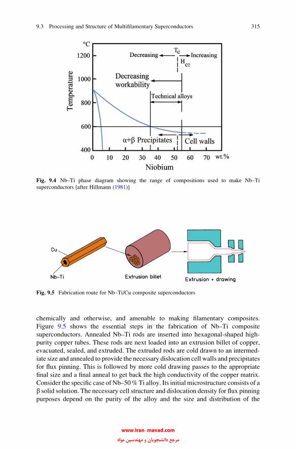
chemically and otherwise, and amenable to making filamentary composites.

Figure 9.5 shows the essential steps in the fabrication of Nb–Ti composite

superconductors. Annealed Nb–Ti rods are inserted into hexagonal-shaped high-

purity copper tubes. These rods are next loaded into an extrusion billet of copper,

evacuated, sealed, and extruded. The extruded rods are cold drawn to an intermed-

iate size and annealed to provide the necessary dislocation cell walls and precipitates

for flux pinning. This is followed by more cold drawing passes to the appropriate

final size and a final anneal to get back the high conductivity of the copper matrix.

Consider the specific case of Nb–50%Ti alloy. Its initial microstructure consists of a

b solid solution. The necessary cell structure and dislocation density for flux pinningpurposes depend on the purity of the alloy and the size and distribution of the

Fig. 9.4 Nb–Ti phase diagram showing the range of compositions used to make Nb–Ti

superconductors [after Hillmann (1981)]

Fig. 9.5 Fabrication route for Nb–Ti/Cu composite superconductors

9.3 Processing and Structure of Multifilamentary Superconductors 315


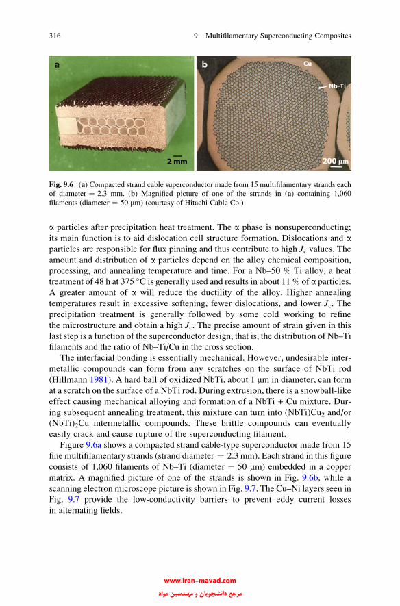
a particles after precipitation heat treatment. The a phase is nonsuperconducting;

its main function is to aid dislocation cell structure formation. Dislocations and aparticles are responsible for flux pinning and thus contribute to high Jc values. Theamount and distribution of a particles depend on the alloy chemical composition,

processing, and annealing temperature and time. For a Nb–50 % Ti alloy, a heat

treatment of 48 h at 375 �C is generally used and results in about 11 % of a particles.

A greater amount of a will reduce the ductility of the alloy. Higher annealing

temperatures result in excessive softening, fewer dislocations, and lower Jc. Theprecipitation treatment is generally followed by some cold working to refine

the microstructure and obtain a high Jc. The precise amount of strain given in this

last step is a function of the superconductor design, that is, the distribution of Nb–Ti

filaments and the ratio of Nb–Ti/Cu in the cross section.

The interfacial bonding is essentially mechanical. However, undesirable inter-

metallic compounds can form from any scratches on the surface of NbTi rod

(Hillmann 1981). A hard ball of oxidized NbTi, about 1 mm in diameter, can form

at a scratch on the surface of a NbTi rod. During extrusion, there is a snowball-like

effect causing mechanical alloying and formation of a NbTi + Cu mixture. Dur-

ing subsequent annealing treatment, this mixture can turn into (NbTi)Cu2 and/or

(NbTi)2Cu intermetallic compounds. These brittle compounds can eventually

easily crack and cause rupture of the superconducting filament.

Figure 9.6a shows a compacted strand cable-type superconductor made from 15

fine multifilamentary strands (strand diameter ¼ 2.3 mm). Each strand in this figure

consists of 1,060 filaments of Nb–Ti (diameter ¼ 50 mm) embedded in a copper

matrix. A magnified picture of one of the strands is shown in Fig. 9.6b, while a

scanning electron microscope picture is shown in Fig. 9.7. The Cu–Ni layers seen in

Fig. 9.7 provide the low-conductivity barriers to prevent eddy current losses

in alternating fields.

Fig. 9.6 (a) Compacted strand cable superconductor made from 15 multifilamentary strands each

of diameter ¼ 2.3 mm. (b) Magnified picture of one of the strands in (a) containing 1,060

filaments (diameter ¼ 50 mm) (courtesy of Hitachi Cable Co.)



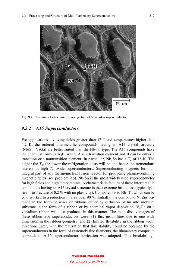
9.3.2 A15 Superconductors

For applications involving fields greater than 12 T and temperatures higher than

4.2 K, the ordered intermetallic compounds having an A15 crystal structure

(Nb3Sn, V3Ga) are better suited than the Nb–Ti type. The A15 compounds have

the chemical formula A3B, where A is a transition element and B can be either a

transition or a nontransition element. In particular, Nb3Sn has a Tc of 18 K. The

higher the Tc, the lower the refrigeration costs will be and hence the tremendous

interest in high Tc oxide superconductors. Superconducting magnets form an

integral part of any thermonuclear fusion reactor for producing plasma-confining

magnetic fields (see problem 9.6). Nb3Sn is the most widely used superconductor

for high fields and high temperatures. A characteristic feature of these intermetallic

compounds having an A15 crystal structure is their extreme brittleness (typically, a

strain-to-fracture of 0.2 % with no plasticity). Compare this to Nb–Ti, which can be

cold worked to a reduction in area over 90 %. Initially, the compound Nb3Sn was

made in the form of wires or ribbons either by diffusion of tin into niobium

substrate in the form of a ribbon or by chemical vapor deposition. V3Ga on a

vanadium ribbon was also produced in this manner. The main disadvantages of

these ribbon-type superconductors were: (1) flux instabilities due to one wide

dimension in the ribbon geometry, and (2) limited flexibility in the ribbon width

direction. Later, with the realization that flux stability could be obtained by the

superconductors in the form of extremely fine filaments, the filamentary composite

approach to A-15 superconductor fabrication was adopted. This breakthrough

Fig. 9.7 Scanning electron microscope picture of Nb–Ti/Cu superconductor



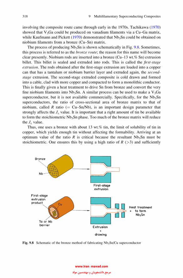
involving the composite route came through early in the 1970s. Tachikawa (1970)

showed that V3Ga could be produced on vanadium filaments via a Cu–Ga matrix,

while Kaufmann and Pickett (1970) demonstrated that Nb3Sn could be obtained on

niobium filaments from a bronze (Cu–Sn) matrix.

The process of producing Nb3Sn is shown schematically in Fig. 9.8. Sometimes,

this process is referred to as the bronze route; the reason for this name will become

clear presently. Niobium rods are inserted into a bronze (Cu–13 wt.% Sn) extrusion

billet. This billet is sealed and extruded into rods. This is called the first-stageextrusion. The rods obtained after the first-stage extrusion are loaded into a copper

can that has a tantalum or niobium barrier layer and extruded again, the second-stage extrusion. The second-stage extruded composite is cold drawn and formed

into a cable, clad with more copper and compacted to form a monolithic conductor.

This is finally given a heat treatment to drive Sn from bronze and convert the very

fine niobium filaments into Nb3Sn. A similar process can be used to make a V3Ga

superconductor, but it is not available commercially. Specifically, for the Nb3Sn

superconductors, the ratio of cross-sectional area of bronze matrix to that of

niobium, called R ratio (¼ Cu–Sn/Nb), is an important design parameter that

strongly affects the Jc value. It is important that a right amount of tin be available

to form the stoichiometric Nb3Sn phase. Too much of the bronze matrix will reduce

the Jc value.Thus, one uses a bronze with about 13 wt.% tin, the limit of solubility of tin in

copper, which yields enough tin without affecting the formability. Arriving at an

optimum value of the ratio R is critical because the resultant Nb3Sn must be

stoichiometric. One ensures this by using a high ratio of R (>3) and sufficiently

Fig. 9.8 Schematic of the bronze method of fabricating Nb3Sn/Cu superconductor



long diffusion times. An example of an Nb3Sn monolithic superconductor used in

high-field magnets is shown in Fig. 9.9. Each little dot in this photograph (Fig. 9.9a)

is a 4-mm Nb3Sn filament. Wide strips in the hexagonal form are niobium; they

serve as barriers to tin diffusion from the bronze into the copper. Tantalum is also

used as a diffusion barrier. Figure 9.9b shows a scanning electron micrograph of a

niobium/bronze composite before heat treatment to form Nb3Sn. The good flux

pinning and the consequent high critical currents in these superconductors are

due to the grain boundaries (Scanlan et al. 1975; Nembach and Tachikawa 1979).

At a heat treatment temperature of about 650–700 �C, the Nb3Sn forms and consists

of very fine grains, less than 80 nm (0.08 mm) in diameter. The critical current

density for Nb3Sn under these conditions is more than 2 � 105 A/cm2 at 10 T

and 4.2 K.

The problem of thermal mismatch, i.e., the differential expansion or contrac-

tion between the components of a composite (Chawla 1973a, b), something very

much inherent to composites, also exists in superconductors. In the case of A15-

type composite superconductors, their brittle nature makes this thermal mismatch

problem of great importance. It turns out that in this case, when cooled from the

reaction temperature (~1,000 K) to 4.2 K, the different coefficients of thermal

expansion of copper and Nb3Sn lead to rather large compressive strains in the

brittle Nb3Sn filament. Luhman and Suenaga (1976) showed that the Tc of Nb3Snvaried with the strain applied to the Nb3Sn filament by the copper matrix. Later,

measurements of critical currents as a function of applied strain confirmed these

results, and one could explain the strain-critical current behavior in terms of the

effects of strain on Tc and Hc2. This understanding of strain-critical current

behavior is used to good effect in the design of Nb3Sn superconducting magnets.

As pointed out, Nb3Sn filaments fail at a tensile strain of about 0.2 %. Thus, if the

superconductor is designed so that the Nb3Sn filaments in the bronze matrix

experience compression between 0.4 and 0.6 %, then one can expect these

composites to withstand applied strains of between 0.6 and 0.8 % before fracture

ensues in the Nb3Sn filaments.

Although the bronze route of manufacturing the superconductor is a commercial

process now, there are some disadvantages involved. One must have frequent

interruptions for annealing the work-hardened bronze matrix. To shorten this

process of fabrication, a number of in situ and powder metallurgy techniques

have been tried (Roberge and Foner 1980). These in situ techniques involve melting

of copper-rich Cu–Nb mixtures (~1,800–1,850 �C), homogenization, and casting.

Niobium is practically insoluble in copper at ambient temperature. Thus, the casting

has a microstructure consisting of niobium precipitates in a copper matrix. When

this is cold drawn into wire, niobium is converted into fine filaments in the copper

matrix. Tin is then plated onto the wire and diffused to form Nb3Sn. The different

melting and cooling techniques used include chill casting, continuous casting,

levitation melting, and consumable electrode arc melting. The powder metallurgy

techniques involve mixing of copper and niobium powder, pressing, hot or cold

extrusion, and drawing to a fine wire that is coated or reacted with tin. The

contamination of niobium with oxygen causes embrittlement and prevents its



conversion into fine filaments. This has led to the addition of a third element (Al, Zr,

Mg, or Ca) to the Cu–Nb mixture. This third element preferentially binds oxygen

and leaves the niobium ductile.

A summary of characteristics of Nb/Ti and Nb3Sn multifilamentary composites

is provided in Table 9.1.

Fig. 9.9 (a) An Nb3Sn/Cu composite superconductor used in high-field magnets. Each little dot in

this picture is a 4-mm diameter Nb3Sn filament. Hexagonal strips are niobium diffusion barriers for

tin (courtesy of Hitachi Cable Co.). (b) Scanning electron micrograph of a niobium/bronze

composite before the heat treatment to form Nb3Sn



9.3.3 Ceramic Superconductors

The ceramic oxide superconductors with a transition temperature higher than the

conventional superconductors were discovered in late 1986 and early 1987. Since

then many oxide superconductors have been discovered, and they have a range of

critical transition temperatures. There are two classes of high temperature

superconductors (HTS): First Generation (1G) and Second Generation (2G). Also

there is a rather complex notation that is commonly used in the ceramic oxide

superconductor literature. For example, the oxides used in 1G HTS are bismuth-

based, the one-layer compound Bi2Sr2Cu1Oy is denoted by (2210), the two-layer

compound Bi2Sr2Ca1Cu2Oy is designated by (BSCCO) or (2212), and the three-

layer compound Bi2�xPbxSr2Ca2Cu3Oy is denoted by (Pb) (2223). 2G HTS are

yttrium based, specifically YBa2Cu3O (referred to as YBCO). In fact, YBCO was

one of the earlier oxide superconductors; interest in it waned when it was discov-

ered that bismuth-based superconductors could carry more current in the presence

of low magnetic fields. Oxide superconductors with a transition temperature around

90 K are available. The reader will recall that such high transition temperatures

enable the use of liquid nitrogen (boiling point 77 K), a cheap and easily available

coolant. With conventional superconductors, one must use liquid helium as a

coolant. There are still many problems with these high-Tc superconductors; oneof the major ones is that they carry very low current densities, especially in the

presence of magnetic fields. The electrical resistance goes to zero at a Tc of 90 K,

Table 9.1 A summary of characteristics of Nb–Ti and Nb3Sn-type multifilamentary composites

(after Hillmann 1981)

Characteristic Nb–Ti Nb3Sn

Tc �9 K 18.1 K

Bc2 �14.5 K 24.5 K

Stabilization Simple, coextrusion with

high-purity Cu matrix

Complex, coprocessing with bronze

matrix, followed by heat treatment

to obtain Nb3Sn in a Cu matrix

Insulation Conventional; varnish, cotton, and

polymeric tape can be used

Complex, in prereaction insulated

conductors, high thermal stability

of insulation is needed; in post-

reaction insulated conductors, careful

mechanical handling is required

Advantages Fabrication process is cheap;

insensitive to mechanical handing,

simple magnet technology

Applications to high magnetic fields

and high temperatures

Disadvantages Applications limited to 8 T at 4.2 K Brittleness of the Nb3Sn, restricted

mechanical handling, large number

of very fine filaments (diameter

�5 mm) is required, complicated

magnet winding



but the supercurrents have difficulty going from one grain to another. Various

explanations, such as impurities and misaligned grains, have been put forth to

explain this behavior. The performance of these new superconductors deteriorates

with increasing magnetic field. At a magnetic field of 1 T, the critical current

density, Jc, is between 1 and 10 A/cm2. The conventional superconductors, on the

other hand, can carry as much as 105 A/cm2.

Understandably, a large amount of research and development effort has been

focused on wire and system development. HTS wire must be flexible and strong and

capable of carrying large currents in the presence of a magnetic field. The key

parameters in making a HTS wire system commercially successful are critical

current density, operating temperature (related to but less than the critical tempera-

ture), magnetic field, and last but not least, cost. Critical current is the amount of

current a given wire can carry without losing superconductivity. It would be

desirable to have a Jc value between 103 and 105 A/cm2. HTS wires must be able

to carry current at relatively high temperatures to decrease the difficulties associated

with cooling. The anticipated range for HTS operating temperature (depending on

the application) is 4.2–77 K. Superconducting devices also require tolerance to

surrounding magnetic fields and should be able to operate in the presence of

magnetic fields. The goal for a cost-effective HTS wire is $0.01/Am.

We alluded earlier to the extreme brittleness of the ceramic superconductors.

Very powerful tensile and shear forces develop in dipole magnets due to the

phenomenon of Lorentz force, enough to literally explode the ceramic oxides.

This also means that processing of such superconductors into long lengths is

much more difficult than is the case with a ductile Nb–Ti system. Since the

discovery of HTS, many techniques have been tried to make HTS in the form of

flexible, long conductor wires. One method called the oxide-powder-in-tube (OPIT)method (Sandhage et al. 1991) involved the use of oxide powder of appropriate

composition (stoichiometry, phase content, purity, etc.) packed in silver tube

(4–7 mm inside diameter and 6–11 mm outside diameter). The silver tube is sealed

after packing and degassed. The deformation processing techniques commonly

used are swaging and drawing for wires and rolling is used for tapes. Heat

treatments, intermediate and/or subsequent to deformation, are given to form the

correct phase, to promote grain interconnectivity and crystallographic alignment of

the oxide, and to obtain proper oxygenation (Sandhage et al. 1991). Figure 9.10

shows a schematic of this process. What we need is a high degree of crystallo-

graphic alignment of the superconducting oxide grains. It is known that the critical

current density in HTS is increased with the alignment of oxide grains (Osamura

et al. 1990; Uno et al. 1991). A major obstacle in the manufacture of long lengths of

YBCO wire is the existence of weak links, such as a grain boundary. Also, the use

of silver as the matrix makes it very expensive.

In a manner similar to the so-called bronze route of making conventional

superconductors, where the superconductor is a very brittle intermetallic, Nb3Sn,

one must avoid the synthesis of the brittle ceramic until the very end. The sintering

step should be carried after the formation of the desired shape. This technique,



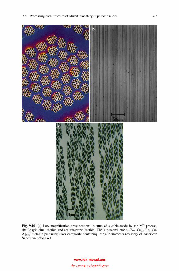
Fig. 9.10 (a) Low-magnification cross-sectional picture of a cable made by the MP process.

(b) Longitudinal section and (c) transverse section. The superconductor is Y0.9 Ca0.1 Ba2 Cu4Ag0.65 metallic precursor/silver composite containing 962,407 filaments (courtesy of American

Superconductor Co.)



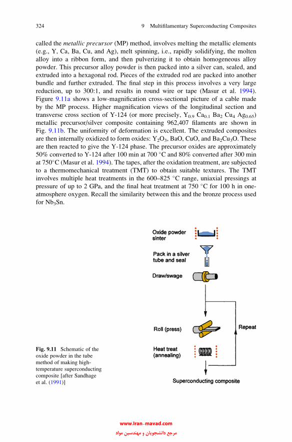
called the metallic precursor (MP) method, involves melting the metallic elements

(e.g., Y, Ca, Ba, Cu, and Ag), melt spinning, i.e., rapidly solidifying, the molten

alloy into a ribbon form, and then pulverizing it to obtain homogeneous alloy

powder. This precursor alloy powder is then packed into a silver can, sealed, and

extruded into a hexagonal rod. Pieces of the extruded rod are packed into another

bundle and further extruded. The final step in this process involves a very large

reduction, up to 300:1, and results in round wire or tape (Masur et al. 1994).

Figure 9.11a shows a low-magnification cross-sectional picture of a cable made

by the MP process. Higher magnification views of the longitudinal section and

transverse cross section of Y-124 (or more precisely, Y0.9 Ca0.1 Ba2 Cu4 Ag0.65)

metallic precursor/silver composite containing 962,407 filaments are shown in

Fig. 9.11b. The uniformity of deformation is excellent. The extruded composites

are then internally oxidized to form oxides: Y2O3, BaO, CuO, and Ba2Cu3O. These

are then reacted to give the Y-124 phase. The precursor oxides are approximately

50% converted to Y-124 after 100 min at 700 �C and 80% converted after 300 min

at 750�C (Masur et al. 1994). The tapes, after the oxidation treatment, are subjected

to a thermomechanical treatment (TMT) to obtain suitable textures. The TMT

involves multiple heat treatments in the 600–825 �C range, uniaxial pressings at

pressure of up to 2 GPa, and the final heat treatment at 750 �C for 100 h in one-

atmosphere oxygen. Recall the similarity between this and the bronze process used

for Nb3Sn.

Fig. 9.11 Schematic of the

oxide powder in the tube

method of making high-

temperature superconducting

composite [after Sandhage

et al. (1991)]



One of the key developments in regard to HTS was the demonstration that

crystallographic texture could be introduced into metal by rolling and annealing

the metal into a thin tape, and this texture could be transferred to a superconducting

oxide coating through buffer layers deposited on the metallic template. The buffer

layers also serve to prevent any unwanted coating-substrate chemical reactions. The

result was a superconducting oxide, such as yttrium–barium–copper oxide

(YBCO), with oriented crystals. Such a tape can conduct large electrical currents

without resistance at liquid nitrogen temperature (77 K). Although American

Superconductor’s first-generation, or 1G, HTS wires are in commercial use,

second-generation (2G) wires are expected to be a formed-fit replacement for 1G

wire. Eliminating silver in the manufacturing process will make the 2G wire less

expensive. Also, 2G wire will work better than 1G wire in the presence of a strong

magnetic field in a motor, generator, or transformer.

We now briefly describe two important processes of obtaining aligned grains of

oxide superconductors. The first one, called ion beam assisted deposition technique

(IBAD), starts with a randomly oriented sheet of Hastelloy (a nickel alloy) on which

a yttrium-stabilized zirconia (YSZ) layer is deposited as a buffer. The ion beam

selectively removes the YSZ atoms that are not aligned at certain orientations

biaxially. YBCO film is then deposited on this template. This process is based

on some earlier Japanese work and the work done at the Los Alamos National

Laboratory in the USA. The second process, developed at the Oak Ridge

National Laboratory, is called “rolling assisted biaxially textured substrates,” or

RABiTS (Goyal et al. 1999; Bhattacharjee et al. 2007). This results in a biaxial

texture in a range of metals. On this textured metallic substrate, oxide

superconductors are deposited epitaxially. These textured substrates serve as struct-

ural templates for the final superconductor layer, which has substantially fewer

weak links. In the RABiTS process, silver is replaced by nickel or nickel

alloys, eliminating the expensive silver. The RABiTS process consists of the

following steps:

1. Thermomechanical processing (rolling, heat treatments, and annealing) is used

to obtain flexible, biaxially oriented Ni or Ni alloy substrates. The substrate

serves as a structural template for the superconducting YBCO layer, which has

substantially fewer weak links than the substrate. This is shown in Fig. 9.12.

The circles show the pole figures showing the specific type of grain texture

obtained.

2. Deposit a series of buffer layers on the substrate. YBCO superconductors are

then deposited epitaxially on the buffer layer. The buffer layers transfer the

texture of the metal substrate to the superconductor and prevent any reaction

between the substrate and the superconductor. The final composite

superconducting tape is shown schematically in Fig. 9.13.



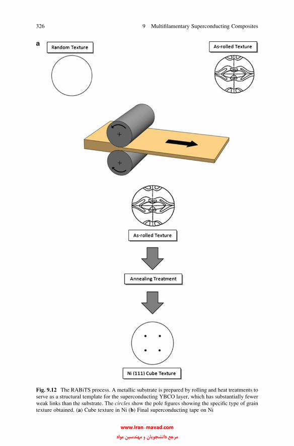
Fig. 9.12 The RABiTS process. A metallic substrate is prepared by rolling and heat treatments to

serve as a structural template for the superconducting YBCO layer, which has substantially fewer

weak links than the substrate. The circles show the pole figures showing the specific type of grain

texture obtained. (a) Cube texture in Ni (b) Final superconducting tape on Ni



Fig. 9.12 (continued)



American Superconductor Co. makes HTS wires that are high-performance,

long-length, RABiTS-based, nickel–tungsten substrate coated with very thin buffer

layers. The company produces wide ribbons of material that are slit into 100-m-

long, 4-mm-wide wires. Figure 9.14 shows such a superconducting cable, trade

name Amperium. An impressive array of different materials is used to make the

superconducting cable.

Fig. 9.14 A schematic of a 2G superconducting cable, trade name Amperium. Note the number of

different materials used (courtesy of American Superconductor Co.)

Fig. 9.13 A schematic of final composite superconducting tape obtained by the RABiTS process.

The series of buffer layers and the YBCO superconductor are deposited epitaxially on the

substrate. The buffer layers transfer the texture of the metal substrate to the superconductor and

prevent any reaction between the substrate and the superconductor



9.4 Applications

Filamentary superconducting composites have some very important applications.

Examples of applications of metal matrix composite superconducting coils include

(Cyrot and Pavuna 1992):

• High-field magnets for research in high energy and in condensed matter physics.

• Magnetic resonance imaging (MRI), which requires extremely uniform mag-

netic fields of ~1–2 T.

• Coils for windings in motors and generators.

• Magnetic levitating (MAGLEV) coils for high-speed trains.

• Magnetohydrodynamic and electromagnetic thrust systems for propulsion in

ships and submarines.

Since the discovery of HTS, much emphasis has been placed on the high Tc ofthese superconductors. It is good to remember a rule-of-thumb for most supercond-

uctor applications, which says that critical temperature Tc of a technological

superconductor should be about twice the use temperature (Cyrot and Pavuna

1992), i.e.,

Tuse � Tc=2:

This implies that superconductors that are used with liquid helium (4.2 K) as a

coolant should have a Tc > 8 K. In fact, due to the heating of the magnet, the actual

operational temperature is closer to ~7 K, so one needs a Tc ~ 15 K. Thus, to use the

oxide high-temperature superconductors (HTS) in applications at 77 K one needs a

superconductor with a Tc ~ 150 K. Such a material has not yet been synthesized;

the thallium-compound with Tc ~ 125 K would appear to be the best candidate for

the “true” technological material at liquid nitrogen temperature. For most

electronic-type applications, the rule of thumb is less stringent, and we can write:

Tuse � 2=3 Tc:

Nb3Sn/Cu superconducting composites are used for magnetic fields greater than

12 T. Such high fields are encountered in thermonuclear fusion reactors, and

superconducting composite magnets would represent a sizable fraction of the

capital cost of such a fusion power plant. Table 9.2 shows the requirements for

critical current density in a given magnetic field for several applications of

superconductors. The performance of superconducting magnets will affect the

plasma as well as the plasma density—and hence the importance of materials

research aimed at improving the performance limits of these superconducting

magnets. The main difference between the magnets used in a fusion reactor and

in power transmission is that the former use superconductors at very high magnetic

fields while the latter use them at low fields.



A large scale potential application of Nb–Ti/Cu superconducting magnets is in

magnetically levitated trains. Japan National Railways has tested such trains over

a small stretch at speeds over 500 km/h. Nb–Ti/Cu superconductor composites are

also employed in pulsed magnets for particle accelerators in high-energy physics.

Other applications of these superconductors include the fields of magnetohydro-

dynamics and power. Superconducting electric generators for utility applications

allow two times or more kilovoltamperes of electricity to be produced than by a

conventional generator of a comparable size. The field windings can be made

from a Nb–Ti/Cu composite or HTS composites. By using superconducting

materials, the designers could make a generator that developed a much stronger

magnetic field than a conventional generator, permitting a significant reduction in

the size of the generator for the same power output. Superconducting magnets do

require cryogenic temperatures to operate, but the cost of this refrigeration is

more than compensated by the energy savings. One has only to remember that, in

a superconducting machine working with almost zero resistance, the normal

losses associated with the flow of electricity in rotor windings of a conventional

machine are absent, resulting in a higher efficiency and reduced operating costs.

A major problem in this development of superconducting generators is to prevent

the movement of rotor windings under the intense centrifugal and magnetic forces

exerted on them. The rotor spins at a speed of 360 rpm. Thus, even an infinitesi-

mally small movement of these components would generate enough heat by

friction to quench the superconductors. One solution used by the GE researchers

involved a special vacuum epoxy-impregnation process to bond the Nb–Ti

superconductors into rock solid modules and strong aluminum supports to hold

the windings rigidly.

An electrical transformer, built by ABB, using 1G HTS wires has been in use in

Geneva, Switzerland since 1997. This transformer used the flexible HTS wires

made by American Superconductor. The process involves packing of the raw

material into hollow silver tubes, drawing into fine filaments, grouping the

multifilaments in another metal jacket, further drawing and heat treating to convert

the raw material into the oxide superconductor (see Sect. 9.3.3). The wire is then

flattened into a ribbon (2.5 � 0.25 mm) that is used to make the transformer coils.

The transformer contains 6 km of HTS wires wound into coils, immersed in liquid

nitrogen. According to ABB this transformer loses only about one fifth of the ac

power losses of the conventional ones. Because HTS wires can carry a higher

current density, this new transformer is more compact and lighter than a

Table 9.2 Critical current

density in a given magnetic

field for several applications

of superconductors (after

Cyrot and Pavuna 1992)

Application B (T) Jc (A/cm2)

Interconnects 0.1 5 � 106

AC transmission lines 0.2 105

DC transmission lines 0.2 2 � 104

SQUIDs 0.1 2 � 102

Motors and generators ~ 4 ~104

Fault current limiters >5 >105



conventional transformer. It should also be mentioned that liquid nitrogen used as a

coolant in the HTS transformer is safer than oils used as insulators in conventional

transformers.

Finally, we describe a very important application of Nb-based superconducting

composites.

9.4.1 Magnetic Resonance Imaging

The phenomenon of nuclear magnetic resonance (NMR) is exploited in the technique

of magnetic resonance imaging (MRI). This technique has a major advantage over

X-ray radiography in that it is a noninvasive diagnostic technique, and thus the human

body is not exposed to an ionizing radiation. It would be useful to briefly explain the

principle behind this important technique. Use is made of the electromagnetic

characteristics of the nuclei of elements such as hydrogen, carbon, and phosphorus

that are present in the human body. The nuclei of these elements act as bar magnets

when placed in a strong magnetic field. The patient is placed in the center of a very

powerful magnet. When the magnetic field is turned on, the nuclei of the elements in

the patient’s body part under examination realign along the magnetic field direction.

If we apply a radiofrequency field, the nuclei will reorient. And if we repeat this

process over and over again, the nuclei will resonate. The resonance frequency is

picked up by a sensitive antenna, amplified, and processed by a computer into an

image. The MRI images, obtained from the resonance patterns are more detailed and

have a higher resolution than traditional techniques of visualization of soft tissues.

And best of all, these images are obtained without exposing the patient to a radiation

or performing biopsy.

MRI became a major diagnostic tool after solenoids made of metal matrix

composites consisting of continuous fiber (Nb–Ti) in copper matrix became

commercially available. Of course, MRI techniques do not have to use

superconducting magnets, i.e., other magnets can be used. There are, however,

certain advantages with superconductors: better homogeneity and resolution of

magnetic fields and higher field strengths than are available with conventional

magnets. The disadvantage is that higher fields with superconductors lead to

greater shielding problems. The superconducting solenoid, made from Nb–Ti/

Cu composite wire, is immersed in a liquid helium cryogenic dewar. The liquid

helium is consumed at about 4 ml/h, and each refill of the dewar lasts about

3 months. Commercially manufactured NMR (nuclear magnetic resonance) spec-

trometer systems, also called magnetic resonance imaging systems, for medical

diagnostics became available in the 1980s; Fig. 9.15 shows one such system.

It should be pointed out no ferromagnetic articles should be brought in the vicinity

of an MRI superconductor.



References

Bhattacharjee PK, Ray RK, Upadhyaya A (2007) J Mater Sci 42:1984



Cyrot M, Pavuna D (1992) Introduction to superconductivity and high Tc materials. World

Scientific, Singapore, p 202

Goyal A, Ren SX, Specht ED, Kroeger DM, Feenstra R, Norton D, Paranthaman M, Lee DF,

Christen DK (1999) Micron 30:463

Heine K, Tenbrink N, Thoerer M (1989) App Phys Lett 55:2441

Hillmann H (1981) Superconductor materials science. Plenum, New York, p 275

Irie F (1994) In: Osamura K (ed) Composite superconductors. Marcel Dekker, New York. p 7

Kaufmann AR, Pickett JJ (1970) Bull Am Phys Soc 15:833

Kunzler JE, Bachler E, Hsu FSL, Wernick JE (1961) Phys Rev Lett 6:89

Larbalestier D (1996) Science 274:736

Luhman T, Suenaga M (1976) Appl Phys Lett 29:1

Masur LJ, Podtburg ER, Craven CA, Otto A, Wang ZL, Kroeger DM (1994) J Miner Met Mater

Soc 46:28

Matsuda T, Harada K, Kasai H, Kamimura O, Tonomura A (1996) Science 271:1393

Nembach E, Tachikawa K (1979) J Less Common Met 19:1962

Osamura K, Oh SS, Ochiai S (1990) Superconductor Sci Technol 3:143

Roberge R, Foner S (1980) Filamentary A15 superconductors. Plenum, New York, p 241

Sandhage RH, Riley GN Jr, Carter WL (1991) J Miner Met Mater Soc 21:25

Scanlan RM, Fietz WA, Koch EF (1975) J Appl Phys 46:2244

Tachikawa K (1970) In: Proceedings of the third ICEC, Illife Science and Technology Publishing,

Surrey, UK

Uno N, Enomoto N, Kikuchi H, Matsumoto K, Mimura M, Nakajima M (1991) Adv Supercond

2:341

Fig. 9.15 A magnetic resonance imaging system for clinical diagnostics, under preparation

(courtesy of Oxford-Airco)



Further Reading

Osamura K (ed) (1994) Composite superconductors. Marcel Dekker, New York

Problems

9.1. There are many known superconducting A15 compounds. Of these Nb3Al,

Nb3Ga, and Nb3Ge have higher values of Tc and Hc2 than do Nb3Sn and V3Ga.

How then does one explain the fact that only Nb3Sn and to a lesser extent V3Ga

are available commercially?

9.2. It is believed that grain boundaries are the imperfections responsible for the

flux-pinning in high-Jc materials like Nb3Sn and V3Ga. How does Jc vary withgrain size?

9.3. What is the effect of any excess unreacted bronze leftover in the manufacture

of Nb3Sn superconductor composite via the bronze route?

9.4. Examine the Nb–Sn phase diagram. At what temperature does the A15

compound (Nb3Sn) become unstable? Nb3Sn is formed by solid state diffusion

in Nb/Cu–Sn composites at 700 �C or below. Is this in accord with information

from the phase diagram? Explain.

9.5. Do you think it is important to study the effect of irradiation on super-

conducting materials? Why?

9.6. In the high magnetic field coils of large dimensions, rather large tensile and

compressive loads can be encountered during energizing and deenergizing.

Discuss the effects of cyclic stress on the superconducting coil materials.

9.7. Superconducting composites in large magnets can be subjected to high

mechanical loads. Describe the sources of such loadings.

Problems 333


Part III


Chapter 10

Micromechanics of Composites

In this chapter we consider the results of incorporating a reinforcement (fibers,

whiskers, particles, etc.) in a matrix to make a composite. It is of great importance

to be able to predict the properties of a composite, given the properties of the

components and the geometric arrangement of the components in the composite.

We examine various micromechanical aspects of composites. A particularly simple

case is the rule-of-mixtures, a rough tool that considers the composite properties as

volume-weighted averages of the component properties. It is important to realize

that the rule-of-mixtures works in only certain simple situations. Composite density

is an example where the rule-of-mixtures is applied readily. In the case of mechani-

cal properties, there are certain restrictions to its applicability. When more precise

information is desired, it is better to use more sophisticated approaches based on the

theory of elasticity.

10.1 Density

Consider a composite of mass mc and volume vc. The total mass of the composite is

the sum total of the masses of fiber and matrix, that is,

mc ¼ mf þ mm: (10.1)

The subscripts c, f, and m indicate composite, fiber, and matrix, respectively.

Note that Eq. (10.1) is valid even in the presence of any voids in the composite. The

volume of the composite, however, must include the volume of voids, vv. Thus,

vc ¼ vf þ vm þ vv: (10.2)


337


Dividing Eq. (10.1) by mc and Eq. (10.2) by vc and denoting the mass and

volume fractions by Mf, Mm and Vf, Vm, Vv, respectively, we can write

Mf þMm ¼ 1 (10.3)

and

Vf þ Vm þ Vv ¼ 1: (10.4)

The composite density rc (¼ mc/vc) is given by

rc ¼mc

vc¼ mf þ mm

vc¼ rf vf þ rmvm

vc

or

rc ¼ rf Vf þ rmVm: (10.5)

We can also derive an expression for rc in terms of mass fractions. Thus,

rc ¼mc

vc¼ mc

vf þ vm þ vv¼ mc

mf =rf þ mm=rm þ vv

¼ 1

Mf =rf þMm=rm þ vv=mc

¼ 1

Mf =rf þMm=rm þ vv=rcvc

¼ 1

Mf =rf þMm=rm þ Vv=rc: (10.6)

We can use Eq. (10.6) to indirectly measure the volume fraction of voids in a

composite. Rewriting Eq. (10.6), we obtain

rc ¼rc

rc Mf =rf þMm=rmh i

þ Vv

or

Vv ¼ 1� rcMf

rfþMm

rm

!: (10.7)

Example 10.1 A thermoplastic matrix contains 40 wt.% glass fiber. If the density of

the matrix, rm, is 1.1 g/cm3 while that of glass fiber, rf, is 2.5 g/cm3, what is the

density of the composite? Assume that no voids are present.

338 10 Micromechanics of Composites


Solution Consider 100 g of the composite:

Amount of glass fiber,mf ¼ 40 g

Amount of matrix, mm ¼ 60 g:

Volume of the composite, vc is the sum of the volumes of fiber, vf and matrix, vm

vc ¼ vm þ vf

¼ mm=rmð Þ þ mf =rf� �

¼ 60=1:1þ 40=2:5ð Þcm3

¼ 54:5þ 16 ¼ 70:5 cm3:

The density of the composite, is

rc ¼ 100 g/70:5 cm3 ¼ 1:42 g/cm3:

10.2 Mechanical Properties

In this section, we first describe some of the methods for predicting elastic

constants, thermal properties, and transverse stresses in fibrous composites and

then we treat the mechanics of load transfer.

10.2.1 Prediction of Elastic Constants

Consider a unidirectional composite such as the one shown in Fig. 10.1. Assume

that plane sections of this composite remain plane after deformation. Let us apply a

force Pc in the fiber direction. Now, if the two components adhere perfectly and if

they have the same Poisson’s ratio, then each component will undergo the same

longitudinal elongation, Dl. Thus, we can write for the strain in each component

ef ¼ em ¼ ecl ¼ Dll; (10.8)

where ecl is the strain in the composite in the longitudinal direction. This is called

the isostrain or action-in-parallel situation. It was first treated by Voigt (1910). If

both fiber and matrix are elastic, we can relate the longitudinal stress s in the two

components to the longitudinal strain el by Young’s modulus E. Thus,

sf ¼ Ef ecl and sm ¼ Emecl:

10.2 Mechanical Properties 339


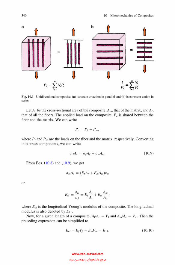
Let Ac be the cross-sectional area of the composite, Am, that of the matrix, and Af,

that of all the fibers. The applied load on the composite, Pc is shared between the

fiber and the matrix. We can write

Pc ¼ Pf þ Pm;

where Pf and Pm are the loads on the fiber and the matrix, respectively. Converting

into stress components, we can write

sclAc ¼ sf Af þ smAm: (10.9)

From Eqs. (10.8) and (10.9), we get

sclAc ¼ EfAf þ EmAm

� �ecl

or

Ecl ¼ sclecl

¼ EfAf

Acþ Em

Am

Ac;

where Ecl is the longitudinal Young’s modulus of the composite. The longitudinal

modulus is also denoted by E11.

Now, for a given length of a composite, Af/Ac ¼ Vf and Am/Ac ¼ Vm. Then the

preceding expression can be simplified to

Ecl ¼ EfVf þ EmVm ¼ E11: (10.10)

Fig. 10.1 Unidirectional composite: (a) isostrain or action in parallel and (b) isostress or action in

series



Equation (10.10) is called the rule-of-mixtures for Young’s modulus in the fiber

direction.

A similar expression can be obtained for the composite longitudinal strength

from (10.9), namely,

scl ¼ sf Vf þ smVm: (10.11)

For properties in the transverse direction, we can represent the simple unidirect-

ional composite by what is called the action-in-series or isostress situation; see

Fig. 10.1b. In this case, we group the fibers together as a continuous phase normal to

the stress. Thus, we have equal stresses in the two components and the model is

equivalent to that treated by Reuss (1929). For loading transverse to the fiber

direction, we have for isostress

sct ¼ sf ¼ sm

while the total displacement of the composite in the thickness direction, Dtc, is thesum of displacements of the matrix and fiber, that is,

Dtc ¼ Dtm þ Dtf :

Dividing throughout by tc, the gage length of the composite, we obtain

Dtctc

¼ Dtmtc

þ Dtftc

:

Now Dtc/tc ¼ ect, strain in the composite in the transverse direction, while Dtmand Dtf equal the strains in the matrix and fiber times their respective gage lengths;

that is, Dtm ¼ emtm and Dtf ¼ eftf. Then

ect ¼ Dtctc

¼ Dtmtm

tmtcþ Dtf

tf

tftc

or

ect ¼ emtmtcþ ef

tftc: (10.12)

For a given cross-sectional area of the composite under the applied load, the

volume fractions of fiber and matrix can be written as

Vm ¼ tmtc

and Vf ¼ tftc:

This simplifies Eq. (10.12) to

ect ¼ em Vm þ ef Vf : (10.13)



Considering both components to be elastic and remembering that sct ¼ sf ¼ smin this case, we can write (10.13) as

sctEct

¼ sctEm

Vm þ sctEf

Vf

or

1

Ect¼ Vm

Emþ Vf

Ef¼ 1

E22

: (10.14)

The relationships given by Eqs. (10.5), (10.10), (10.11), (10.13), and (10.14) are

commonly referred to as rules-of-mixtures (volume weighted averages). Figure 10.2

shows the plots of Eqs. (10.10) and (10.14). The reader should appreciate that these

relationships and their variants are but rules-of-thumb obtained from a simple,

strength of materials approach. More comprehensive micromechanical models,

based on the theory of elasticity, can and should be used to obtain the elastic constants

of fibrous composites. We describe below, albeit very briefly, some of these.

10.2.2 Micromechanical Approaches

The states of stress and strain can each be described by six components.

An anisotropic body with no symmetry elements present requires 21 independent

elastic constants to relate stress and strain (Nye 1985). This is the most general case

of elastic anisotropy. An elastically isotropic body, on the other hand, is the simplest

case; it needs only two independent elastic constants. In such a body, when a tensile


longitudinal modulus (E11)

and transverse modulus (E22)

with fiber volume fraction

(Vf)



stress sz is applied in the z direction, a tensile strain ez results in that direction. In

addition to this tensile strain, there are two equal compressive strains (ex ¼ ey) in thex and y directions. In a generally anisotropic body, the two transverse strain

components are not equal. In fact, as we shall see in Chap. 11, in such a body, tensile

loading can result in tensile and shear strains. The large number of independent

elastic constants (21 in the most general case, i.e., no symmetry elements) represents

the degree of elastic complexity in a given system. Any symmetry elements present

will reduce the number of independent elastic constants (Nye 1985).

A composite containing uniaxially aligned fibers will have a plane of symmetry

perpendicular to the fiber direction (i.e., material on one side of the plane will be the

mirror image of the material on the other side). Figure 10.3 shows square, hexagonal,

and random fiber arrays in a matrix. A square array of fibers, for example, will have

symmetry planes parallel to the fibers aswell as perpendicular to them. Such amaterial

is an orthotropic material (three mutually perpendicular planes of symmetry) and

possesses nine independent elastic constants (Nye 1985). Hexagonal and random

arrays of aligned fibers are transversely isotropic and have five independent elastic

constants. These five constants as well as the stress–strain relationships, as derived by

Hashin and Rosen (1964) and Rosen (1973), are given in Table 10.1. There are two

Poisson’s ratios: one gives the transverse strain caused by an axially applied stress, and

the other gives the axial strain caused by a transversely applied stress. The two are not

independent but are related (see Sect. 11.3). Thus, the number of independent elastic

constants for a transversely isotropic composite is five. Note that the total number of

independent elastic constants in Table 10.1 is five (count the number of Cs).More accurate results can be obtained if we take into account the inevitable scatter

in the distribution of fibers, i.e., in reality, they never have an idealized distribution in

the matrix. A summary of the elastic constants for a transversely isotropic composite

(see Fig. 10.4) in terms of the elastic constants of the two components is given in

Table 10.2 (Chamis 1983). Note the use of√Vf in these expressions. Because the plane

2–3 is isotropic in Fig. 10.4, the properties in directions 2 and 3 are identical. The

matrix is treated as an isotropic material while the fiber is treated as an anisotropic

material. Thus, Em and vm are the two constants required for the matrix while five

constants (Ef1, Ef2, Gf12, Gf23, and vf12) are required for the fiber. The expressions forthe five independent constants (E11, E22, G12, G23, and v12) are given in Table 10.2.

The two Poisson’s ratios are not independent (see Chap. 11).

Frequently, composite structures are fabricated by stacking thin sheets of

unidirectional composites called plies in an appropriate orientation sequence

Fig. 10.3 Various fiber arrays in a matrix: (a) square, (b) hexagonal, and (c) random



http://dx.doi.org/10.1007/978-0-387-74365-3_11

http://dx.doi.org/10.1007/978-0-387-74365-3_11#Sec3_11

http://dx.doi.org/10.1007/978-0-387-74365-3_11

dictated by elasticity theory (see Chap. 11). It is of interest to know properties, such

as the elastic constants and the strength characteristics of a ply. In particular, it is

very valuable if we are able to predict the lamina characteristics starting from the

characteristics of the individual components. Later in the macro-mechanical analy-

sis (Chap. 11), we treat a ply as a homogeneous but thin orthotropic material.

Elastic constants in the thickness direction can be ignored in such a ply, leaving four

independent elastic constants, namely, E11, E22, v12, and G12, i.e., one less than the

number of constants required for a thick but transversely isotropic material. The

missing constant is G23, the transverse shear modulus in the 2–3 plane, normal to

the fiber axis. A brief description of the various micromechanical techniques used

to predict the elastic constants follows and then we give an account of a set of

empirical equations, called Halpin-Tsai equations, that can be used under certain

conditions to predict the elastic constants of a fiber composite.

In the so-called self-consistent field methods (Chamis and Sendecky 1968),

approximations of phase geometries are made and a simple representation of the

Table 10.1 Elastic moduli of a transversely isotropic fibrous composite

E ¼ C11 � 2C212

C22 þ C23

K23 ¼ 1

2C22 þ C23ð Þ

G ¼ G12 ¼ G13 ¼ G44 G23 ¼ 1

2C22 � C23ð Þ

n ¼ n13 ¼ n31 ¼ 1

2

C11 � E

K23

� �1=2

v23 ¼ K23 � fG23

K23 þ fG23

E2 ¼ E3 ¼ 4G23K23

K23 þ fG23

f ¼ 1þ 4K23n2

E

Stress–strain relationships

e11 ¼ 1

E1

s11 � n s22 þ s33ð Þ½ � e22 ¼ e33 ¼ 1

E2

s22 � ns33ð Þ � nEs11

g12 ¼ g13 ¼1

Gs12 g23 ¼

2 1þ n23ð ÞE2

s23

Source: Adapted with permission from Hashin and Rosen (1964)

Table 10.2 Elastic constants of a transversely isotropic composite in terms of component

constants (matrix isotropic, fiber anisotropic)

Longitudinal modulus E11 ¼ Ef 1Vf þ EmVm

Transverse modulus E22 ¼ E33 ¼ Em

1� ffiffiffiffiffiVf

p1� Em=Ef2ð Þ

Shear modulus G12 ¼ G13 ¼ Gm


p1� Gm=Gf12ð Þ

Shear modulus G23 ¼ Gm


p1� Gm=Gf23ð Þ

Poisson’s ratio n12 ¼ n13 ¼ vf12Vf þ vmVm

Poisson’s ratio n23 ¼ E22

2G23

� 1

Source: Adapted with permission from Chamis (1983)



http://dx.doi.org/10.1007/978-0-387-74365-3_11

http://dx.doi.org/10.1007/978-0-387-74365-3_11

response field is obtained. The phase geometry is represented by one single fiber

embedded in a matrix cylinder. This outer cylinder is embedded in an unbounded

homogeneous material whose properties are taken to be equivalent to those of

average composite properties. The matrix under a uniform load at infinity

introduces a uniform strain field in the fiber. Elastic constants are obtained from

this strain field. The results obtained are independent of fiber arrangements in the

matrix and are reliable at low-fiber-volume fractions (Vf), reasonable at intermedi-

ate Vf, and unreliable at high Vf (Hill 1964). Exact methods deal with specific

geometries, for example, fibers arranged in a hexagonal, square, or rectangular

array in a matrix. The elasticity problem is then solved by a series development, a

complex variable technique, or a numerical solution. The approach of Eshelby

(1957, 1959) considers an infinite matrix containing an ellipsoidal inclusion.

Modifications of the Eshelby method have been made by Mori and Tanaka (1973).

The variational or bounding methods focus on the upper and lower bounds on

elastic constants. When the upper and lower bounds coincide, the property is

determined exactly. Frequently, the upper and lower bounds are well separated.

When these bounds are close enough, we can safely use them as indicators of the

material behavior. It turns out that this is the case for longitudinal properties of a

unidirectional lamina. Hill (1965) derived bounds for the ply elastic constants that

are analogous to those derived by Hashin and Rosen (1964) and Rosen (1973).

In particular, Hill put rigorous bounds on the longitudinal Young’s modulus, E11, in

terms of the bulk modulus in plane strain (kp), Poisson’s ratio (n), and the shear

modulus (G) of the two phases. No restrictions were made on the fiber form or

packing geometry. The term kp is the modulus for lateral dilation with zero

longitudinal strain and is given by

kp ¼ E

2 1� 2nð Þ 1þ nð Þ :

Fig. 10.4 A transversely isotropic fiber composite: plane transverse to fibers (2–3 plane) is isotropic



The bounds on the longitudinal modulus, E11, are

4VfVm vf � vm� �2

Vf =kpm� �þ Vm=kpf

� �þ 1=Gm

� E11 � Ef Vf � EmVm

� 4VfVm vf � vm� �2

Vf =kpm� �þ Vm=kpf

� �þ 1=Gf

(10.15)

Equation (10.15) shows that the deviations from the rule-of-mixtures (10.10) are

quite small (<2 %). We may verify this by substituting some values of practical

composites such as carbon or boron fibers in an epoxy matrix or a metal matrix

composite such as tungsten in a copper matrix. Note that the deviation from the

rule-of-mixtures value comes from the (vm � vf)2 factor. For vf ¼ vm, we have E11

given exactly by the rule-of-mixtures.

Hill (1965) also showed that for a unidirectionally aligned fiber composite

n12 >< vf Vf þ vmVm accordingly as ðvf � vmÞðkpf � kpmÞ >

< 0 (10.16)

Generally, vf < vm and Ef >> Em. Then, v12 will be less than that predicted by

the rule-of-mixtures (¼ vfVf + vmVm). It is easy to see that the bounds on v12 are notas close as the ones on E11. This is because vf � vm appears in the case of n12(10.16) while (vf � vm)

2 appears in the case of E11 (10.15). In the case where

vf � vm is very small, the bounds are close enough to allow us to write

n12 � vf Vf þ vmVm: (10.17)

10.2.3 Halpin-Tsai Equations

Halpin, Tsai, and Kardos (Halpin and Tsai 1967; Halpin and Kardos 1976; Kardos

1971) empirically developed some generalized equations that readily give satisfac-

tory results compared to the complicated expressions. They are also useful in

determining the properties of composites that contain discontinuous or short fibers

oriented in the loading direction. One writes a single equation of the form

p

pm¼ 1þ x�Vf

1� �Vf; (10.18)

� ¼ pf =pm � 1

pf =pm þ x; (10.19)



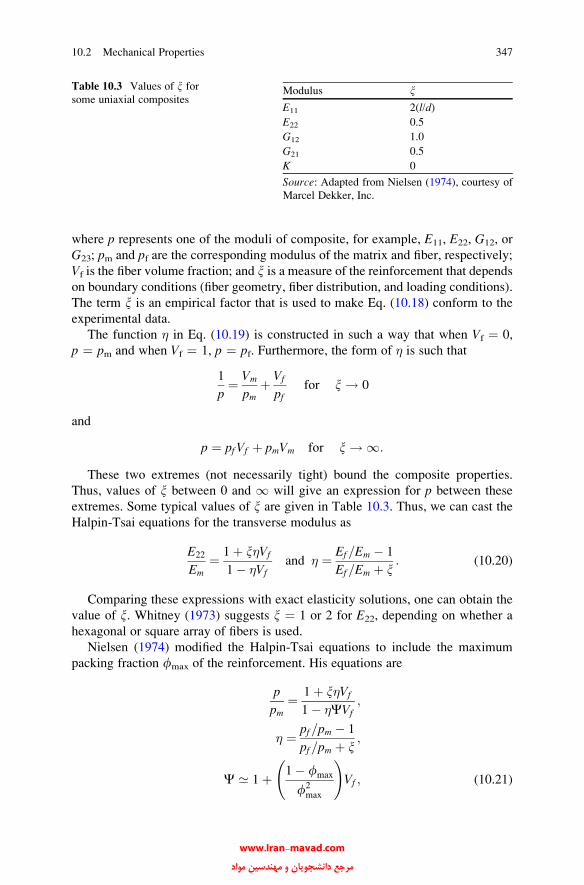
where p represents one of the moduli of composite, for example, E11, E22, G12, or

G23; pm and pf are the corresponding modulus of the matrix and fiber, respectively;

Vf is the fiber volume fraction; and x is a measure of the reinforcement that depends

on boundary conditions (fiber geometry, fiber distribution, and loading conditions).

The term x is an empirical factor that is used to make Eq. (10.18) conform to the

experimental data.

The function � in Eq. (10.19) is constructed in such a way that when Vf ¼ 0,

p ¼ pm and when Vf ¼ 1, p ¼ pf. Furthermore, the form of � is such that

1

p¼ Vm

pmþ Vf

pffor x ! 0

and

p ¼ pf Vf þ pmVm for x ! 1:

These two extremes (not necessarily tight) bound the composite properties.

Thus, values of x between 0 and 1 will give an expression for p between these

extremes. Some typical values of x are given in Table 10.3. Thus, we can cast the

Halpin-Tsai equations for the transverse modulus as

E22

Em¼ 1þ x�Vf

1� �Vfand � ¼ Ef =Em � 1

Ef =Em þ x: (10.20)

Comparing these expressions with exact elasticity solutions, one can obtain the

value of x. Whitney (1973) suggests x ¼ 1 or 2 for E22, depending on whether a

hexagonal or square array of fibers is used.

Nielsen (1974) modified the Halpin-Tsai equations to include the maximum

packing fraction fmax of the reinforcement. His equations are

p

pm¼ 1þ x�Vf

1� �CVf;

� ¼ pf =pm � 1

pf =pm þ x;

C ’ 1þ 1� fmax

f2max

!Vf ; (10.21)

Table 10.3 Values of x for

some uniaxial compositesModulus x

E11 2(l/d)

E22 0.5

G12 1.0

G21 0.5

K 0

Source: Adapted from Nielsen (1974), courtesy of

Marcel Dekker, Inc.



where fmax is the maximum packing factor. It allows one to take into account the

maximum packing fraction. For a square array of fibers, fmax ¼ 0.785, while for a

hexagonal arrangement of fibers, fmax ¼ 0.907. In general, fmax is between these

two extremes and near the random packing, fmax ¼ 0.82.

Example 10.2 Consider a unidirectionally reinforced glass fiber/epoxy composite.

The fibers are continuous and 60 % by volume. The tensile strength of glass fibers is

1 GPa and the Young’s modulus is 70 GPa. The tensile strength of the epoxy matrix

is 60MPa and its Young’s modulus is 3 GPa. Compute the Young’s modulus and the

tensile strength of the composite in the longitudinal direction.

Solution Young’s modulus of the composite in the longitudinal direction is

given by

Ecl ¼ 70� 0:6þ 3� 0:4 ¼ 42þ 1:2 ¼ 43:2 GPa:

To calculate the tensile strength of the composite in the longitudinal direction,

we need to determine which component, fiber or matrix, has the lower failure strain.

The failure strain of the fiber is

ef ¼ sf =Ef ¼ 1=70 ¼ 0:014

while that of the matrix is

em ¼ 60� 10�3� �

=3 ¼ 0:020:

Thus, ef < em, i.e., fibers fail first. At that strain, assuming a linear stress–strain

curve for the epoxy matrix, the matrix strength is s0m ¼ Emef ¼ 3� 0:014 ¼ 0:042GPa. Then, we get the composite tensile strength as

sc ¼ 0:6� 1þ 0:4� 0:042

¼ 0:6þ 0:0168 ¼ 617 MPa:

10.2.4 Transverse Stresses

When a fibrous composite consisting of components with different elastic moduli is

uniaxially loaded, stresses in transverse directions arise because of the difference in

Poisson’s ratio of the matrix and the fiber, that is, because the two components have

different contractile tendencies. Here we follow Kelly’s (1970) treatment of this

important but, unfortunately, not well-appreciated subject. This problem in



elasticity is also useful in computing thermal stresses in composites; in which case

the two components have different thermal expansion coefficients.

Consider a unit fiber reinforced composite consisting of a single fiber (radius a)surrounded by its shell of matrix (outer radius b) as shown in Fig. 10.5. The

composite as a whole is thought to be built of an assembly of such unit composites,

a reasonably valid assumption at moderate fiber volume fractions. We axially load

the composite in direction z. Owing to the obvious cylindrical symmetry, we treat

the problem in polar coordinates, r, y, and z. It follows from the axial symmetry that

the stress and strain are independent of angle y and are functions only of r, whichsimplifies the problem. We can write Hooke’s law for this situation as

er 0 0

0 ey 0

0 0 ez

24

35 ¼ 1þ n

E

sr 0 0

0 sy 0

0 0 sz

24

35� n

Esr þ sy þ szð Þ

1 0 0

0 1 0

0 0 1

24

35 (10.22)

where e is the strain, s is the stress, n is the Poisson’s ratio, E is Young’s modulus in

the longitudinal direction, and the subscripts r, y, and z refer to the radial, circum-

ferential, and axial directions, respectively. The only equilibrium equation for this

problem is

dsrdr

þ sr � syr

¼ 0: (10.23)

Fig. 10.5 A single fiber surrounded by its matrix shell



Also, for the plane strain condition, we can write for the strain components, in

terms of displacements,

er ¼ durdr

; ey ¼ urr; ez ¼ const (10.24)

where ur is the radial displacement.

From Eq. (10.22) we have, after some algebraic manipulation,

syK

¼ 1� nð Þey þ n er þ ezð Þ;srK

¼ 1� nð Þer þ n ey þ ezð Þ;(10.25)

where

K ¼ E

1þ nð Þ 1� 2nð Þ :

From Eqs. (10.24) and (10.25), we get

syK

¼ ndurdr

þ 1� nð Þ urrþ nez;

srK

¼ 1� nð Þ durdr

þ nurrþ nez:

(10.26)

Substituting Eq. (10.26) in Eq. (10.23), we obtain the following differential

equation in terms of the radial displacement ur:

d2urdr2

þ 1

r

durdr

� urr2

¼ 0: (10.27)

Equation (10.27) is a common differential equation in elasticity problems with

rotational symmetry (Love 1952), and its solution is

ur ¼ Cr þ C0

r(10.28)

where C and C0 are constants of integration to be determined by using boundary

conditions. Now, Eq. (10.28) is valid for displacements in both components, that is,

fiber andmatrix. Let us designate the central component by subscript 1 and the sleeve

by subscript 2. Thus, we can write the displacements in the two components as

ur1 ¼ C1r þ C2

r;

ur2 ¼ C3r þ C4

r:

(10.29)



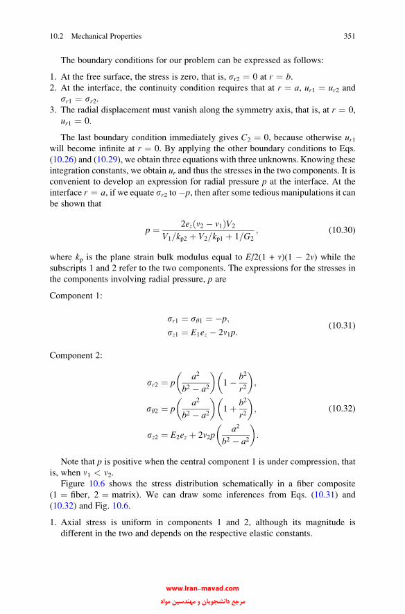
The boundary conditions for our problem can be expressed as follows:

1. At the free surface, the stress is zero, that is, sr2 ¼ 0 at r ¼ b.2. At the interface, the continuity condition requires that at r ¼ a, ur1 ¼ ur2 and

sr1 ¼ sr2.3. The radial displacement must vanish along the symmetry axis, that is, at r ¼ 0,

ur1 ¼ 0.

The last boundary condition immediately gives C2 ¼ 0, because otherwise ur1will become infinite at r ¼ 0. By applying the other boundary conditions to Eqs.

(10.26) and (10.29), we obtain three equations with three unknowns. Knowing these

integration constants, we obtain ur and thus the stresses in the two components. It is

convenient to develop an expression for radial pressure p at the interface. At the

interface r ¼ a, if we equate sr2 to�p, then after some tedious manipulations it can

be shown that

p ¼ 2ez n2 � n1ð ÞV2

V1=kp2 þ V2=kp1 þ 1=G2

; (10.30)

where kp is the plane strain bulk modulus equal to E/2(1 + n)(1 � 2n) while the

subscripts 1 and 2 refer to the two components. The expressions for the stresses in

the components involving radial pressure, p are

Component 1:

sr1 ¼ sy1 ¼ �p;

sz1 ¼ E1ez � 2n1p:(10.31)

Component 2:

sr2 ¼ pa2

b2 � a2

� �1� b2

r2

� �;

sy2 ¼ pa2

b2 � a2

� �1þ b2

r2

� �;

sz2 ¼ E2ez þ 2n2pa2

b2 � a2

� �:

(10.32)

Note that p is positive when the central component 1 is under compression, that

is, when n1 < n2.Figure 10.6 shows the stress distribution schematically in a fiber composite

(1 ¼ fiber, 2 ¼ matrix). We can draw some inferences from Eqs. (10.31) and

(10.32) and Fig. 10.6.

1. Axial stress is uniform in components 1 and 2, although its magnitude is

different in the two and depends on the respective elastic constants.



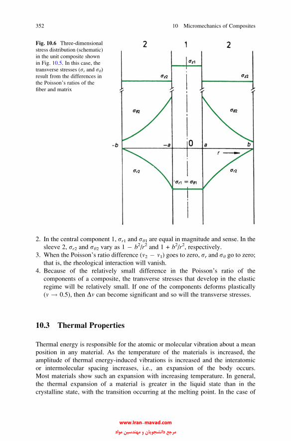
2. In the central component 1, sr1 and sy1 are equal in magnitude and sense. In the

sleeve 2, sr2 and sy2 vary as 1 � b2/r2 and 1 + b2/r2, respectively.3. When the Poisson’s ratio difference (n2 � n1) goes to zero, sr and sy go to zero;

that is, the rheological interaction will vanish.

4. Because of the relatively small difference in the Poisson’s ratio of the

components of a composite, the transverse stresses that develop in the elastic

regime will be relatively small. If one of the components deforms plastically

(n ! 0.5), then Dn can become significant and so will the transverse stresses.

10.3 Thermal Properties

Thermal energy is responsible for the atomic or molecular vibration about a mean

position in any material. As the temperature of the materials is increased, the

amplitude of thermal energy-induced vibrations is increased and the interatomic

or intermolecular spacing increases, i.e., an expansion of the body occurs.

Most materials show such an expansion with increasing temperature. In general,

the thermal expansion of a material is greater in the liquid state than in the

crystalline state, with the transition occurring at the melting point. In the case of

Fig. 10.6 Three-dimensional

stress distribution (schematic)

in the unit composite shown

in Fig. 10.5. In this case, the

transverse stresses (sr and sy)result from the differences in

the Poisson’s ratios of the

fiber and matrix



a glassy material, such a transition occurs at the glass transition temperature,

although it is not as well defined as the one at the melting point. Over a certain

range of temperature, one can relate the temperature interval and thermal strain by a

coefficient, called the coefficient of thermal expansion. In the case of a linear strain,the linear thermal expansion coefficient, a, is a second-rank symmetric tensor, and

is related to the strain tensor, e, by the following relationship:

eij ¼ aijDT; (10.33)

where DT is the temperature change. The two indexes indicate the second-rank

tensor. The thermal expansion coefficient, a, generally does not have a constant

value over a very large range of temperature. Thus, we can define aij in a more

general way by taking into account this variation with temperature as follows:

aij ¼ deij=dT:

If we consider a volumetric strain, the volumetric coefficient of thermal expan-

sion, b, is given by

bij ¼1

V

dVdT

� �;

where V is the volume and T is the temperature. For small strains, it can be easily

shown that

bij ¼ 3aij:

Recall that the sum of the diagonal terms of the strain tensor is equal to volume

change. Hence, the volumetric expansion coefficient, b, is equal to the sum of the

diagonal terms of the strain tensor, i.e.,

b ¼ e11 þ e22 þ e33 ¼ 3a (10.34a)

or

a ¼ 1

3e11 þ e22 þ e33½ �: (10.34b)

As we said earlier, only over some specified range of temperature can the coeffi-

cient of thermal expansion (CTE) be treated as a constant. Consider a temperature

range DT over which a is a constant. We can write Eq. (10.33) in an extended form as

e11 e12 e13e22 e23

e33

¼

a11 a12 a13a22 a23

a23

DT: (10.35a)

10.3 Thermal Properties 353


Or, using the contracted notation (see Sect. 11.1), we can write

e1e2e3e4e5e6

¼

a1a2a3a4a5a6

DT (10.35b)

If an arbitrary direction [hkl] has direction cosines n1, n2, and n3, then we can

write for the linear thermal expansion coefficient, ahkl, in that direction

ahkl ¼ n21a1 þ n22a2 þ n23a3: (10.36)

In a transversely isotropic fibrous composite (i.e., hexagonal symmetry), we

have a1 ¼ a2 ¼ a⊥, perpendicular to the fiber axis and a3 ¼ a||, parallel to the fiberaxis. Then, remembering that n21 þ n22 þ n23 ¼ 1, Eq. (10.36) becomes

ahkl ¼ n21 þ n22� �

a1 þ n23a3;

ahkl ¼ a?sin2yþ ajjcos2y; (10.37a)

ahkl ¼ a? þ ajj � a?� �

cos2y; (10.37b)

where y is the angle between direction [hkl] and the fiber axis.

10.3.1 Expressions for Coefficientsof Thermal Expansion of Composites

Various expressions have been proposed that give the thermal expansion coefficients

of a composite, knowing the material constants of the components and their geo-

metric arrangements. Different expressions predict very different values of expan-

sion coefficients for a given composite. Almost all expressions, however, predict

expansion coefficient values that are different from those given by a simple rule-of-

mixtures (¼ afVf + amVm). This is because these expressions take into account the

important fact that the presence of a reinforcement, with an expansion coefficient

less than that of the matrix, introduces a mechanical constraint on the expansion of

the matrix. A fiber will cause a greater constraint on the matrix than a particle. Let us

consider the expansion coefficients of particulate and fibrous composites.

One can regard a particulate composite as a homogeneous material in a statistical

sense, i.e., we assume a uniform distribution of the particles in the matrix. Let us

denote the volume fractions of the two phases making a particulate composite by V1




and V2 (¼1 � V1). Various researchers have derived bounds and given expressions

for the expansion coefficients and other transport properties such as thermal con-

ductivity. Kerner (1956) developed the following expression for the volumetric

expansion coefficient, bc, of a composite consisting of spherical particles dispersed

in a matrix:

bc ¼ bmVm þ bpVp � bm � bp� �

Vp

1=Km � 1=Kp

Vm=Kp þ Vp=Km þ 0:75Gm

�;

where subscripts c, m, and p denote the composite, matrix, and particle, respec-

tively; b is the volumetric expansion coefficient, and K denotes the bulk modulus.

Kerner’s expression does not differ significantly from the rule-of-mixtures because

the particle reinforcement constrains the matrix much less than fibers. The coeffi-

cient of linear thermal expansion according to Turner (1946) is given by:

ac ¼ amVmKm þ apVpKp

VpKp þ VmKm;

where the symbols have the significance given earlier. Turner’s expression, gener-

ally, gives an expansion coefficient much lower than the rule-of-mixtures value.

Unidirectionally aligned fibrous composites have two (or sometimes three)

thermal expansion coefficients: acl in the longitudinal direction and act in the

transverse direction. Fibers generally have a lower expansion coefficient than that

of the matrix, and thus the fibers mechanically constrain the matrix. The constraint

is more along the length of the fiber than in the radial direction. This results in the

longitudinal coefficient of expansion of the composite, acl being smaller than

the transverse coefficient, act for the composite. At low fiber volume fractions, it

is not unusual to find the transverse expansion of a fibrous composite, act, greaterthan that of the matrix in isolation. The reason for this is as follows. The long, stiff,

low CTE fibers prevent the matrix from expanding in the longitudinal direction, and

as a result the matrix is forced to expand more than normal in the transverse

direction. It should be pointed out that in the case of some CMCs, this situation

can be reversed. For example, in the case of alumina fibers (a ¼ 8 � 10�6 K�1) in

a low-expansion glass or ceramic matrix, it is the matrix that will constrain the

fibers, i.e., the situation in this case is the reverse of the one commonly encountered.

We give below some expressions for the CTE of unidirectionally reinforced fiber

composites. All of these analyses involve the following assumptions:

1. The bonding between the fiber and matrix is perfect and mechanical in nature,

i.e., no chemical interaction is allowed.

2. The fibers are continuous and perfectly aligned.

3. The properties of the constituents do not change with temperature.

Schapery (1969) used energy methods to derive the following expressions for

expansion coefficient of a fibrous composite, assuming Poisson’s ratios of the



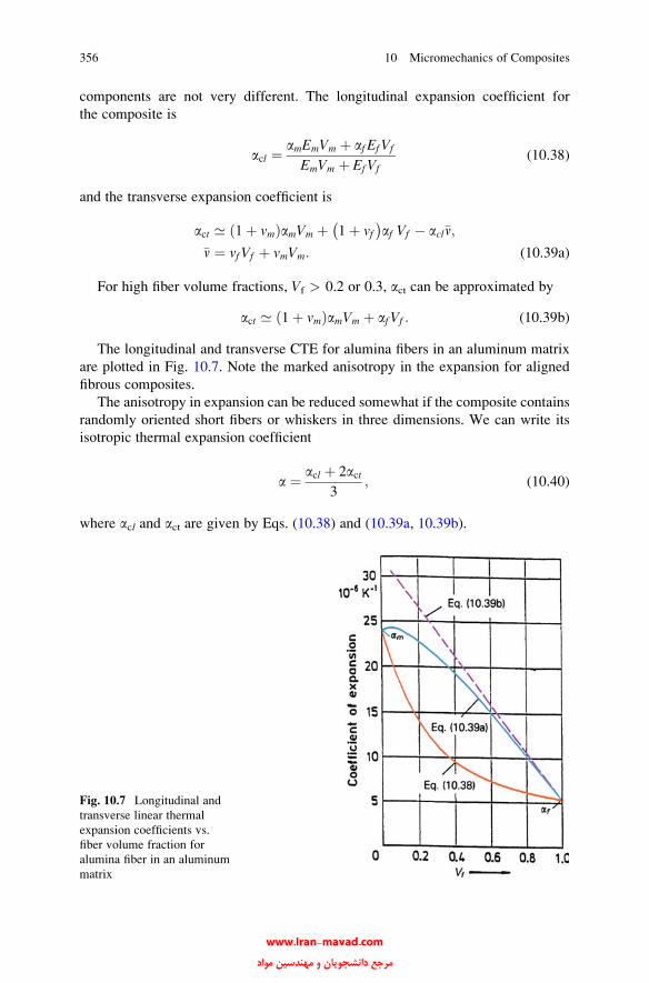
components are not very different. The longitudinal expansion coefficient for

the composite is

acl ¼ amEmVm þ af Ef Vf

EmVm þ EfVf(10.38)

and the transverse expansion coefficient is

act ’ 1þ vmð ÞamVm þ 1þ vf� �

af Vf � acl�n;

�n ¼ vf Vf þ vmVm: (10.39a)

For high fiber volume fractions, Vf > 0.2 or 0.3, act can be approximated by

act ’ 1þ vmð ÞamVm þ af Vf : (10.39b)

The longitudinal and transverse CTE for alumina fibers in an aluminum matrix

are plotted in Fig. 10.7. Note the marked anisotropy in the expansion for aligned

fibrous composites.

The anisotropy in expansion can be reduced somewhat if the composite contains

randomly oriented short fibers or whiskers in three dimensions. We can write its

isotropic thermal expansion coefficient

a ¼ acl þ 2act3

; (10.40)

where acl and act are given by Eqs. (10.38) and (10.39a, 10.39b).

Fig. 10.7 Longitudinal and

transverse linear thermal

expansion coefficients vs.

fiber volume fraction for

alumina fiber in an aluminum

matrix



It should be pointed out the length of fiber as well as fiber orientation has an

effect on the CTEs (Marom and Weinberg 1975; Vaidya et al. 1994). It would

appear that the fiber length has a more sensitive effect on the expansion

characteristics because the constraint on the matrix is highest when the fibers are

continuous. An extreme case of a low constraint is one of a matrix containing

spherical particles, i.e., aspect ratio ¼ 1. Continuous fibers with an aspect ratio of

infinity represent the other extreme in constraint.

The effect of the fiber length on the thermal expansion can be incorporated into

Schapery’s equation as (Marom and Weinberg 1975; Vaidya and Chawla 1994)

a11 ¼ kaf Vf Ef þ amVmEm þ aiViEi

kVf Ef þ VmEm þ ViEi

;

where the value of k is given by

k ¼ llc

l<lc; 0< k<0:5ð Þ;

k ¼ 1� lc=2l l>lc; 0<k<1ð Þ;

where l is the length and lc is the critical length of the fiber (see Sect. 10.4).

Chamis (1983) used a simple force balance to arrive at the following expressions

for a1 and a2:

a1 ¼ Ef1af1Vf þ EmamVm

Ef1Vf þ EmVm

� ;

a2 ¼ af2ffiffiffiffiffiVf

p þ 1� ffiffiffiffiffiVf

p� �1þ Vf vm

Ef1

Ec

� �am:

Rosen and Hashin (1970) used a plane strain model to derive expressions for a1and a2:

a1 ¼ �aþ af � am1=Kf � 1=Km

�3ð1� 2vcÞ

Ec� 1

Kc

�;

a2 ¼ �aþ af � am1=Kf � 1=Km

� 3

2kc� 3ð1� 2vcÞvc

Ec� 1

Kc

� ;

where �a ¼ af Vf þ amVm; Kc is the composite bulk modulus, Ec is the composite

Young’s modulus, and kc is the composite transverse bulk modulus.

Many applications of composites require controlled thermal expansion

characteristics. All the expressions given above predict thermal expansion

coefficients of composites based on continuum mechanics. That is, no account is

taken of the effect of fiber or particle size on the CTE. Xu et al. (1994) examined the



effect of particle size on the CTE of TiC/Al XD™ composite, with two TiC particle

sizes, 0.7 and 4 mm. The results of this work showed the effect of particle size on the

thermal expansion coefficient of particle reinforced aluminum composites in terms

of the degree of constraint on the matrix expansion. Careful TEM work showed

lattice distortion at the interfacial zone. The effect of particle size on the CTE of

composite was related to the volume fraction of interfacial zone through which the

constraint occurs. A phenomenological approach that takes into account the differ-

ent degree of constraint on the matrix expansion based on the TEM work allows us

to compute the CTE of this composite with different particle sizes.

10.3.2 Expressions for Thermal Conductivity of Composites

Thermal conductivity is an important physical property. The heat flow in a material

is proportional to the temperature gradient, and the constant of proportionality is

called the thermal conductivity. Thus, in the most general form, using indicial

notation, we can write

qi ¼ �kij dT=dxj;

where qi is the heat flux along the xi axis, dT/dxj is the temperature gradient across a

surface perpendicular to the xj axis, and kij is the thermal conductivity. As should be

evident from the two indexes, thermal conductivity is also a second-rank tensor.

Although kij is not a symmetric tensor in the most general case, it is a symmetric

tensor for most crystal systems. For an isotropic and a cubic material, kij reduces toa scalar number, k. For an orthotropic material, we have three constants along the

three principal axes, viz., k11, k22, and k33. For a transversely isotropic material such

as a unidirectionally reinforced fibrous composite, there will be two constants:

thermal conductivity in the axial direction, kcl, and that in the transverse direction,

kct. The thermal conductivity in the axial direction, kcl, can be predicted by a rule-

of-mixtures type expression (Behrens 1968)

k1 ¼ kcl ¼ kf1Vf þ kmVm; (10.41)

where kf1 is the thermal conductivity of the fiber in the axial direction, km is that of

the isotropic matrix, and Vf and Vm are the volume fractions of the fiber and matrix,

respectively.

In a transverse direction, the thermal conductivity of a unidirectionally aligned

fiber composite (i.e., transversely isotropic) can be approximated by the action-in-

series model discussed earlier. This would give

kct ¼ k2 ¼ kf2km= kf2Vf þ kmVm

� �:



More complicated expressions have been derived for the transverse thermal

conductivity. These expressions implicitly assume perfect contact between the

fiber and the matrix. In real composites, it is likely that the thermal contact at the

fiber/matrix interface will be less than perfect because of any microvoids, thermal

mismatch, etc. An expression for the transverse thermal conductivity that takes into

account the fact that the interface region may have a different thermal conductance

than the matrix or the fiber is as follows (Hasselman and Johnson 1987):

kct ¼ k2 ¼ km kf =km � 1� kf =ahi� �

Vf

�þ 1þ kf =km þ kf ahi� ��

1� kf km þ kf =ahi��

Vf

��þ 1þ kf km þ kf

�ahi=

� �;

(10.42)

where km is the matrix thermal conductivity, kf is the transverse thermal conductivity

of the fibers, Vf is the fiber volume fraction, a is the fiber radius, and hi is the thermal

conductance of the interface region. Note that the units of thermal conductivity are

W/mK while for thermal conductance the units are W/K. The effect of interfacial

conductivity is governed by the magnitude of nondimensional parameter, kf/ahi. hiwill have a value of infinity for perfect thermal contact and it will be equal to zero for

a pore. Bhatt et al. (1992) studied the important role of interface in controlling the

effective thermal conductivity of composites. In particular, one can use the mea-

surement of thermal conductivity as a nondestructive tool to determine the integrity

of the fiber/matrix interface.

We can also use Halpin-Tsai-Kardos equations to obtain the following express-

ion for the transverse thermal conductivity of a composite containing unidirection-

ally aligned fibers:

kc2 ¼ kc3 ¼ kct ¼ 1þ �Vf

� �1� �Vf

� �km

�and

� ¼ kf2=kmð Þ � 1½ � kf2 km=ð Þ þ 1½ �= ;

where we have taken z equal to 1 in the Halpin-Tsai-Kardos equation.

Similar to the description of the coefficient of thermal expansion, we can find

thermal conductivity of a unidirectionally reinforced fiber composite in any arbi-

trary direction if we know the thermal conductivity in directions 1 (longitudinal)

and 2 (transverse). The thermal conductivity kx and ky in any arbitrary directions, xand y, respectively, are given by the following equations:

kx ¼ k1cos2yþ k2sin

2y;

ky ¼ k1sin2yþ k2cos

2y;

kxy ¼ k2 � k1ð Þ sin y cos y;



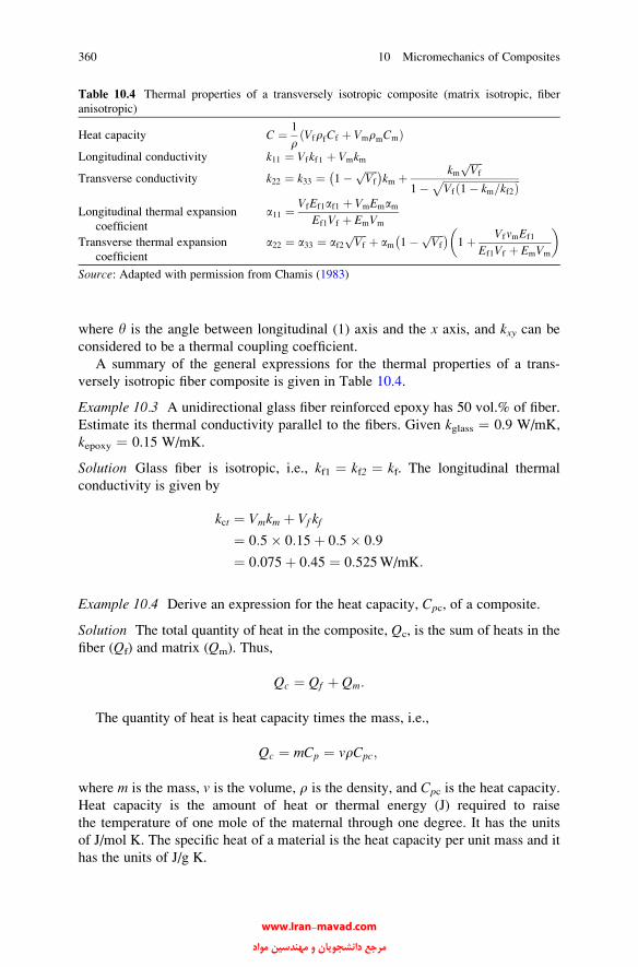
where y is the angle between longitudinal (1) axis and the x axis, and kxy can be

considered to be a thermal coupling coefficient.

A summary of the general expressions for the thermal properties of a trans-

versely isotropic fiber composite is given in Table 10.4.

Example 10.3 A unidirectional glass fiber reinforced epoxy has 50 vol.% of fiber.

Estimate its thermal conductivity parallel to the fibers. Given kglass ¼ 0.9 W/mK,

kepoxy ¼ 0.15 W/mK.

Solution Glass fiber is isotropic, i.e., kf1 ¼ kf2 ¼ kf. The longitudinal thermal

conductivity is given by

kct ¼ Vmkm þ Vf kf

¼ 0:5� 0:15þ 0:5� 0:9

¼ 0:075þ 0:45 ¼ 0:525W/mK:

Example 10.4 Derive an expression for the heat capacity, Cpc, of a composite.

Solution The total quantity of heat in the composite, Qc, is the sum of heats in the

fiber (Qf) and matrix (Qm). Thus,

Qc ¼ Qf þ Qm:

The quantity of heat is heat capacity times the mass, i.e.,

Qc ¼ mCp ¼ vrCpc;

where m is the mass, v is the volume, r is the density, and Cpc is the heat capacity.

Heat capacity is the amount of heat or thermal energy (J) required to raise

the temperature of one mole of the maternal through one degree. It has the units

of J/mol K. The specific heat of a material is the heat capacity per unit mass and it

has the units of J/g K.

Table 10.4 Thermal properties of a transversely isotropic composite (matrix isotropic, fiber

anisotropic)

Heat capacity C ¼ 1

rVfrfCf þ VmrmCmð Þ

Longitudinal conductivity k11 ¼ Vfkf 1 þ Vmkm

Transverse conductivity k22 ¼ k33 ¼ 1� ffiffiffiffiffiVf

p� �km þ km

ffiffiffiffiffiVf

p

1� ffiffiffiffiffiffiffiffiffiffiffiffiffiffiffiffiffiffiffiffiffiffiffiffiffiffiffiffiffiffiVf 1� km kf2=ð Þp

Longitudinal thermal expansion

coefficient

a11 ¼ VfEf1af1 þ VmEmamEf1Vf þ EmVm

Transverse thermal expansion

coefficient

a22 ¼ a33 ¼ af2ffiffiffiffiffiVf

p þ am 1� ffiffiffiffiffiVf

p� �1þ VfvmEf1

Ef1Vf þ EmVm

� �

Source: Adapted with permission from Chamis (1983)



Using the subscripts c, f, and m for composite, fiber, and matrix, respectively, we

can write

vcrcCpc ¼ vfrf Cpf þ vmrmCpm:

Remembering that vf/vc ¼ Vf, the fiber volume fraction, and vm/vc ¼ Vm, the

matrix volume fraction, we can write

rcCpc ¼ Vfrf Cpf þ VmrmCpm

or

Cpc ¼ 1

rc½Vfrf Cpf þ VmrmCpm�:

10.3.3 Electrical Conductivity

Electrical conductivity or its inverse electrical resistivity is another important

physical property. In terms of electrical conductivity, composites represent a

mixed bag. PMCs and CMCs are generally poor electrical conductors. The electri-

cal conductivity of polymers can be increased by the addition of carbon fibers,

carbon black, and graphite. Such composites can be used for situations involving

electromagnetic and radio-frequency interference (EMI/RFI) shielding for elec-

tronic devices and for dissipation of static charge (Clingerman et al. 2002). Most

metal matrix composites are mixtures of good electrical conductors (e.g., Cu, Al,

etc.) and insulators (e.g., B, SiC, Al2O3, etc.), with W/Cu composite being a notable

exception. We can write for the resistivity of a fiber reinforced composite in the

axial direction a simple rule-of-mixtures type expression

rc‘ ¼ r1V1 þ r2V2;

where r is the electrical resistivity, V is volume fraction, and the subscripts c‘, 1,and 2 designate the composite in the longitudinal direction and the two components

of the composite, respectively. Or in terms of electrical conductivity in the axial

direction, s, we can write

sc‘ ¼ s1V1 þ s2V2:

In the transverse direction, we have

1

sct¼ V1

s1þ V2

s2;



where the symbols have the usual significance.

There is a logarithmic expression also

log sc ¼ V1 log s1 þ V2 log s2:

Of course, one can generalize these expressions to more than two components in

the composite, should that be the case.

Self-consistent models can also be used to get expressions for the electrical

conductivity of a composite (Hale 1976).

The electrical resistivity (and therefore electrical conductivity) of the metal

matrix in a composite is likely to be different from that of the unreinforced metal

because of possible plastic deformation during processing which will introduce

dislocations due to thermal mismatch between the matrix and the reinforcement; the

dislocations in turn will increase the resistivity of the matrix. It should be pointed

out that unlike the unreinforced metal, one cannot recover electrical conductivity by

resorting to an annealing treatment. Physical properties such as thermal and elec-

trical conductivity of composites depend on the properties of the matrix and

reinforcement, their volume fractions, characteristics of the interface region,

shape of the reinforcement, and the connectivity of the phases (Weber et al.

2003a, b; Weber 2005). The conductivity (thermal or electrical) of a composite

will depend on conductivity characteristics of the matrix, reinforcement, volume

fraction, and aspect ratio of the reinforcement, and, of course, the interfacial

characteristics. In particular, interfacial resistance will vary with the form and

size of reinforcement.

10.3.4 Hygral and Thermal Stresses

Hygroscopy, the ability of a substance to absorb water absorption, can be a problemwith polymeric resins and natural fibers because it can lead to swelling. Swelling

can lead to stresses if, as is likely in a composite, the material is not allowed to

expand freely because of the presence of the matrix. Such stresses resulting from

moisture absorption or hygroscopy are called hygral stresses. Thermal stresses will

result in a material when the material is not allowed to expand or contract freely

because of a constraint. When both hygral and thermal stresses are present, we call

them hygrothermal stresses. Mathematically, these two types of internal stresses

are quite similar, and we can treat them together.

Consider the passage of a composite from a reference state, where the body is

stress-free and relaxed at a temperature T, concentration of moisture C ¼ 0, and

external stress s ¼ 0, to a final state where the body has hygrothermal as well as

external stresses. We can consider that the final state of the composite with

hygrothermal stresses and external loading is attained via two intermediate stages

shown in Fig. 10.8. The final strain in the body can then be written as the sum of



nonmechanical (thermal strain, eTi and hygral strain, eHi ) and mechanical strains. The

mechanical strain is given by the Hooke’s law (compliance times the stress). Thus,

et ¼ eTi þ eHi|fflfflfflffl{zfflfflfflffl}nonmechanical strains

þ Sijsj|{z}mechanical strain

; (10.43)

where Sij is the compliance. If we regard the composite as transversely isotropic, we

can immediately write the following relationships for the strain components

eTxy ¼ eHxy ¼ 0;

eTy ¼ eTz and eHy ¼ eHz ;

eTi ¼ ai T � T0ð Þ;eHi ¼ biC;

(10.44)

where the ai are thermal expansion coefficients (K�1), the bi are nondimensional

swelling coefficients, T is the temperature, T0 is the equilibrium temperature, C is

the concentration of water vapor, and the superscripts H and T indicate hygral and

thermal strain components, respectively.

Total volumetric hygrothermal strain can be expressed as the sum of the dia-

gonal terms of the strain matrix. It is important to note that the thermal and hygral

effects are dilational only, i.e., they cause only expansion or contraction but do not

affect the shear components. Thus,

DVV

¼ eTx þ eTy þ eTz þ eHx þ eHy þ eHz

¼ eTx þ 2eTy þ eHx þ 2eHy : (10.45)

Fig. 10.8 (a) Strain-free reference state; (b) thermal strain (eT); (c) hygral (eH) and thermal (eT)strains; and (d) final state: hygral (eH), thermal (eT), and mechanical strain



Hygrothermal stresses are very important in polymer matrix composites (see

also Chaps. 3 and 5).

We first consider the constitutive equations for an isotropic material and then for

an anisotropic material. Consider an isotropic material, in plane stress, subjected to

a temperature change, DT, and a change in moisture content, DC. We can write the

constitutive equations for this case as follows

e1 ¼ s1=E� vs2=Eþ bDCþ aDT;

e2 ¼ vs1=E� s2=Eþ bDCþ aDT;

e6 ¼ s6=G:

Note that, as pointed out earlier, DC and DT do not produce shear strains. For a

specially orthotropic, unidirectionally reinforced fiber lamina (i.e., one in which

material and geometric axes coincide, see also Chap. 11), we can write

e1e2e6

24

35 ¼

S11 S12 0

S22 0

S66

24

35 s1

s2s6

24

35þ

a1a20

24

35DCþ

b1b20

24

35DT:

In this expression the subscript 6 indicate inplane shear. We explain this notation

in Chap. 11. In a PMC, the matrix is likely to absorb more moisture than the fiber,

which will lead to b2 > b1. In an off-axis, generally orthotropic, unidirectionally

reinforced fiber lamina, the material and geometric axes do not coincide, and the

strain components take the following form

exeyes

24

35 ¼

S11 S12 S16S22 S26

S66

24

35 sx

syss

24

35þ

axayas

24

35DCþ

bxbybs

24

35DT;

where �Sij designate the compliance matrix for the generally orthotropic lamina.

10.3.5 Thermal Stresses in Fiber Reinforced Composites

During curing or solidification of the matrix around reinforcement fibers or

particles, a large magnitude of shrinkage stresses can result. The interfacial pressure

developed during curing is akin to that obtained upon embedding a cylinder

(sphere) of radius r + dr in a cylindrical (spherical) hole of radius r. The thermal

stresses generated depend on the reinforcement volume fraction, reinforcement

geometry, thermal mismatch (Da), and the modulus ratio, Er/Em where E is the

Young’s modulus and the subscripts r and m refer to the reinforcement and matrix,

respectively. Generally, am > af; that is, on cooling from T0 to T (T0 > T), thematrix would tend to contract more than the fibers, causing the fibers to experience

axial compression. In extreme cases, fiber buckling can also lead to the generation

of interfacial shear stresses. This problem of thermal stresses in composite materials

is a most serious and important problem. It is worth repeating that thermal stresses



http://dx.doi.org/10.1007/978-0-387-74365-3_3

http://dx.doi.org/10.1007/978-0-387-74365-3_4

http://dx.doi.org/10.1007/978-0-387-74365-3_11

http://dx.doi.org/10.1007/978-0-387-74365-3_11

are internal stresses that arise whenever there is a constraint on the free dimensional

change of a body (Chawla 1973a). In the absence of this constraint, the body can

experience free thermal strains without any accompanying thermal stresses. The

constraint can have its origin in (1) a temperature gradient, (2) crystal structure

anisotropy (e.g., a noncubic structure), (3) phase transformations resulting in a

volume change, and (4) a composite material made of dissimilar materials (i.e.,

materials having different CTEs). The thermal gradient problem is a serious one in

ceramic materials in general. A thermal gradient DT is inversely related to the

thermal diffusivity, a, of a material. Thus,

DT ¼ f1

a

� �¼ f

Cpp

k

� �; (10.46)

where Cp is the specific heat, r is the density, and k is the thermal conductivity.

Metals generally have high thermal diffusivity and any thermal gradients that might

develop are dissipated rather quickly. It should be emphasized that in composite

materials even a uniform temperature change (i.e., no temperature gradient) will

result in thermal stresses owing to the ever-present thermal mismatch (Chawla

1973a). Thermal stresses resulting from a thermal mismatch will generally have an

expression of the form

s ¼ f EDaDTð Þ: (10.47)

We describe below first the three-dimensional thermal stress state in a composite

consisting of a central fiber surrounded by its shell of matrix; see Fig. 10.5. After

this, we derive the three-dimensional stress state for a particulate composite.

The elasticity problem is basically the same as the one discussed for transverse

stresses (see Sect. 10.2.4). We use polar coordinates; r, y, and z (see Fig. 10.5).

Axial symmetry makes shear stresses go to zero and the principal stresses are

independent of y. At low volume fractions, the outer cylinder is the matrix and

the inner cylinder is the fiber. The expressions for strain in the generalized Hooke’s

law contain an aDT term. Thus, for component 2,

er2 ¼ sr2E2

� v2E2

sy2 þ sz2ð Þ þ a2DT

ey2 ¼ sy2E2

� v2E2

sr2 þ sz2ð Þ þ a2DT

ez2 ¼ sz2E2

� v2E2

sr2 þ sy2ð Þ þ a2DT

The resultant stresses in 1 and 2 will have the form (see Sect. 10.2.4)

Component 1 Component 2

sr1 ¼ A1 sr2 ¼ A2 � B2

r2

sy1 ¼ A1 sy2 ¼ A2 þ B2

r2

sz1 ¼ C1 sz2 ¼ C2

: (10.48)



The following boundary conditions exist for our problem:

1. At the interface r ¼ a, sr1 ¼ sr2 for stress continuity.2. At the free surface r ¼ b, sr2 ¼ 0.

3. The resultant of axial stress sz on a section z ¼ constant is zero.

4. Radial displacements in the two components are equal at the interface; that is, at

r ¼ a, ur1 ¼ ur2.5. The radial displacement in component 1 must vanish at the symmetry axis; that

is, at r ¼ 0, ur1 ¼ 0.

Using these boundary conditions, it is possible to determine the constants given

in Eq. (10.48). The final equations for the matrix sleeve are given here (Poritsky

1934; Chawla 1973b):

sr ¼ A 1� b2

r2

� �; sy ¼ A 1þ b2

r2

� �; sz ¼ B; (10.49)

where

A ¼ � Em am � af� �

DT a=bð Þ2

1þ a=bð Þ2 1� 2vð Þ b=að Þ2 � 1h i

Em=Ef

24

35;

B ¼ A

a=bð Þ2

� 2va

b

� �2þ1þ a=bð Þ2 1� 2vð Þ þ a=bð Þ2 1� 2vð Þ b=að Þ2 � 1

h iEm=Ef

1þ b=að Þ2 � 1h i

Em=Ef

24

35:

vm ¼ vf ¼ v

A plot of sr, sy, and sz against r/a, where r is the distance in the radial directionand a is the fiber radius, is shown in Fig. 10.9 for the system W/Cu for two fiber

volume fractions (Chawla and Metzger 1972). Note the change in stress level of szwith Vf. This thermoelastic solution can provide information about the magnitude

of the elastic stresses involved. A comparison with the yield or fracture strength of

the matrix can inform us whether or not plastic deformation or fracture of matrix

will occur. Also, if the matrix deforms plastically in response to these thermal

stresses, the plots of thermal stress distribution can tell where the plastic deforma-

tion will begin. Chawla and Metzger (1972) and Chawla (1973a, b, 1974, 1976a, b),

in a series of studies with metal matrix composites, showed that the magnitude of the

thermal stresses generated is large enough to deform the soft metallic matrix

plastically. Depending on the temperatures involved, the plastic deformation of

the metal matrix could involve slip, cavitation, grain boundary sliding, and/or

migration. They measured the dislocation densities in the copper matrix of tungsten

filament/copper single-crystal composites by the etch-pitting technique and showed



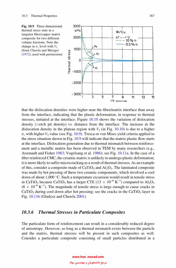
that the dislocation densities were higher near the fiber/matrix interface than away

from the interface, indicating that the plastic deformation, in response to thermal

stresses, initiated at the interface. Figure 10.10 shows the variation of dislocation

density (’etch pit density) vs. distance from the interface. The increase in the

dislocation density in the plateau region with Vf (in Fig. 10.10) is due to a higher

sz with higher Vf value (see Fig. 10.9). Tresca or von Mises yield criteria applied to

the stress situation shown in Fig. 10.9 will indicate that the matrix plastic flow starts

at the interface. Dislocation generation due to thermal mismatch between reinforce-

ment and a metallic matrix has been observed in TEM by many researchers (e.g.,

Arsenault and Fisher 1983; Vogelsang et al. 1986); see Fig. 10.11a. In the case of a

fiber reinforced CMC, the ceramicmatrix is unlikely to undergo plastic deformation;

it is more likely to suffer microcracking as a result of thermal stresses. As an example

of this, consider a composite made of CaTiO3 and Al2O3. The laminated composite

was made by hot pressing of these two ceramic components, which involved a cool

down of about 1,000 �C. Such a temperature excursion would result in tensile stress

in CaTiO3 because CaTiO3 has a larger CTE (13 � 10–6 K–1) compared to Al2O3

(8 � 10–6 K–1). The magnitude of tensile stress is large enough to cause cracks in

CaTiO3 during cool down after hot pressing; see the cracks in the CaTiO3 layer in

Fig. 10.11b (Gladysz and Chawla 2001).

10.3.6 Thermal Stresses in Particulate Composites

The particulate form of reinforcement can result in a considerably reduced degree

of anisotropy. However, so long as a thermal mismatch exists between the particle

and the matrix, thermal stresses will be present in such composites as well.

Consider a particulate composite consisting of small particles distributed in a

Fig. 10.9 Three-dimensional

thermal stress state in a

tungsten fiber/copper matrix

composite for two different

volume fractions. Note the

change in sz level with Vf

[from Chawla and Metzger




matrix. If we regard this composite as an assembly of elastic spheres of uniform size

embedded in an infinite elastic continuum, then it can be shown from the theory of

elasticity (see, for example, Timoshenko and Goodier 1951) that an axially sym-

metrical stress distribution will result around each particle. Figure 10.12 shows a

schematic of such a particle reinforced composite. The particle radius is a while the

Fig. 10.10 Variation of dislocation density (’pit density) with distance from the interface. The

higher dislocation density in the plateau region with high Vf is due to a higher sz with higher Vf

(Fig. 10.9) [from Chawla and Metzger (1972), used with permission]

Fig. 10.11 (a) Dislocations generated at SiC whiskers in an aluminum matrix in an in situ thermal

cycling experiment done in a high-voltage electron microscope [from Vogelsang et al. (1986),

used with permission]. (b) Cracking in the CaTiO3 layer in a CaTiO3/Al2O3 composite due to

thermal stresses generated during cool down from the processing temperature (from Gladysz and

Chawla 2001)



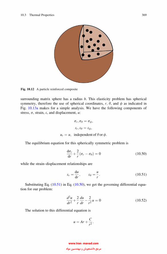
surrounding matrix sphere has a radius b. This elasticity problem has spherical

symmetry, therefore the use of spherical coordinates, r, y, and f as indicated in

Fig. 10.13a makes for a simple analysis. We have the following components of

stress, s, strain, e, and displacement, u:

sr; sy ¼ sf;

er; ey ¼ ef;

ur ¼ u; independent of y orf:

The equilibrium equation for this spherically symmetric problem is

dsrdr

þ 2

rsr � syð Þ ¼ 0 (10.50)

while the strain–displacement relationships are

er ¼ du

dr; ey ¼ u

r: (10.51)

Substituting Eq. (10.51) in Eq. (10.50), we get the governing differential equa-

tion for our problem:

d2u

dr2þ 2

r

du

dr� 2

r2u ¼ 0 (10.52)

The solution to this differential equation is

u ¼ Ar þ C

r2:

Fig. 10.12 A particle reinforced composite



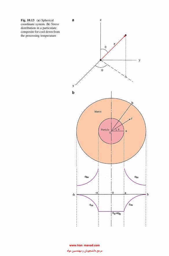
Fig. 10.13 (a) Spherical

coordinate system. (b) Stress

distribution in a particulate

composite for cool down from

the processing temperature


We apply the following boundary conditions:

1. Stress vanishes at the free surface (i.e., at r ¼ b).2. The radial stress at the interface (r ¼ a) is the interfacial pressure, P, i.e.,

srðaÞ ¼ �P

The particle has a hydrostatic state of stress with the stress components

srp ¼ �P ¼ constant ¼ syp (10.53)

while the stresses in the matrix are

srm ¼ P

1� Vp

a3

r3� Vp

�; (10.54)

sym ¼ � P

1� Vp

1

2

a3

r3þ Vp

�; (10.55)

P ¼ am � ap� �

DT

0:5 1þ vmð Þ þ 1� 2vmð ÞVp

Em 1� Vp

� � þ 1� 2vpEp

" # ; (10.56)

Vp ¼ a

b

� �3;

where Vp is the particle volume fraction, a is the particle radius, b is the matrix

radius, and other symbols have the significance given earlier. Figure 10.13b shows

the stress distribution in a particulate composite when cooled down from the

processing temperature and for am > ap. Note the different stress distribution in a

particulate composite from that in a fibrous composite. The particle is under a

uniform pressure, P, while the matrix has different radial and tangential stress

components. The radial and tangential components in the matrix vary with distance,

as shown in Fig. 10.13b. The radial component goes to zero at the free surface,

r ¼ b, as per our boundary conditions. The tangential component has a nonzero

value at the free surface.

10.4 Mechanics of Load Transfer from Matrix to Fiber

The topic of load transfer from the matrix to the fiber has been treated by a number

of researchers (Cox 1952; Dow 1963; Schuster and Scala 1964; Kelly 1973). The

matrix holds the fibers together and transmits the applied load to the fibers, the real

load-bearing component in most cases. Let us focus our attention on a high-

10.4 Mechanics of Load Transfer from Matrix to Fiber 371


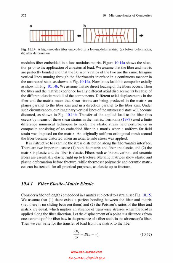
modulus fiber embedded in a low-modulus matrix. Figure 10.14a shows the situa-

tion prior to the application of an external load. We assume that the fiber and matrix

are perfectly bonded and that the Poisson’s ratios of the two are the same. Imagine

vertical lines running through the fiber/matrix interface in a continuous manner in

the unstressed state, as shown in Fig. 10.14a. Now let us load this composite axially

as shown in Fig. 10.14b. We assume that no direct loading of the fibers occurs. Then

the fiber and the matrix experience locally different axial displacements because of

the different elastic moduli of the components. Different axial displacements in the

fiber and the matrix mean that shear strains are being produced in the matrix on

planes parallel to the fiber axis and in a direction parallel to the fiber axis. Under

such circumstances, our imaginary vertical lines of the unstressed state will become

distorted, as shown in Fig. 10.14b. Transfer of the applied load to the fiber thus

occurs by means of these shear strains in the matrix. Termonia (1987) used a finite

difference numerical technique to model the elastic strain field perturbance in

composite consisting of an embedded fiber in a matrix when a uniform far field

strain was imposed on the matrix. An originally uniform orthogonal mesh around

the fiber became distorted when an axial tensile stress was applied.

It is instructive to examine the stress distribution along the fiber/matrix interface.

There are two important cases: (1) both the matrix and fiber are elastic, and (2) the

matrix is plastic and the fiber is elastic. Fibers such as boron, carbon, and ceramic

fibers are essentially elastic right up to fracture. Metallic matrices show elastic and

plastic deformation before fracture, while thermoset polymeric and ceramic matri-

ces can be treated, for all practical purposes, as elastic up to fracture.

10.4.1 Fiber Elastic–Matrix Elastic

Consider a fiber of length l embedded in amatrix subjected to a strain; see Fig. 10.15.

We assume that (1) there exists a perfect bonding between the fiber and matrix

(i.e., there is no sliding between them) and (2) the Poisson’s ratios of the fiber and

matrix are equal, which implies an absence of transverse stresses when the load is

applied along the fiber direction. Let the displacement of a point at a distance x fromone extremity of the fiber be u in the presence of a fiber and v in the absence of a fiber.Then we can write for the transfer of load from the matrix to the fiber

dPf

dx¼ B u� vð Þ; (10.57)

Fig. 10.14 A high-modulus fiber embedded in a low-modulus matrix: (a) before deformation,

(b) after deformation



where Pf is the load on the fiber and B is a constant that depends on the geometric

arrangement of fibers, the matrix type, and moduli of the fiber and matrix.

Differentiating Eq. (10.57), we get

d2Pf

dx2¼ B

du

dx� dv

dx

� �: (10.58)

We have

du

dx¼ strain in fiber =

Pf

Ef Af;

dv

dx¼ strain in thematrix away from the fiber

= imposed strain, e:

Thus, Eq. (10.58) can be rewritten as

d2Pf

dx2¼ B

Pf

Af Ef� e

� �: (10.59)

Fig. 10.15 Load transfer in a fiber/matrix composite and variation of tensile stress (sf) in the fiberand interfacial shear stress (t) with distance along the interface



A solution of this differential equation is

Pf ¼ EfAf eþ S sinh bxþ T cosh bx; (10.60)

where S and T are constants of integration and

b ¼ B

AfEf

� �1=2: (10.61)

We use the following boundary condition to evaluate the constants S and T:

Pf ¼ 0 at x ¼ 0 and x ¼ l:

Putting in these values and using the half-angle trigonometric formulas, we get

the following result:

Pf ¼ EfAf e 1� cosh b l=2� xð Þcosh bl=2ð Þ

�for 0<x<l=2 (10.62)

or

sf ¼ Pf

Af¼ Ef e 1� cosh b l=2� xð Þ

cosh bl=2ð Þ �

for 0<x<l=2: (10.63)

The maximum possible value of strain in the fiber is the imposed strain e, andthus the maximum stress is Efe. Therefore, if we have a long enough fiber, the stressin the fiber will increase from the two ends to a maximum value, sfu ¼ Efe. It canbe shown readily that the average stress in the fiber is

sf ¼ Ef e

l

ðl0

1� cosh b l=2� xð Þcosh bl=2ð Þ

�dx ¼ Ef e 1� tanh bl=2ð Þ

bl=2

�: (10.64)

We can obtain the variation of shear stress t along the fiber/matrix interface by

considering the equilibrium of forces acting over an element of fiber (radius rf).Thus, from Fig. 10.15 we can write

dPf

dxdx ¼ 2prf dx t: (10.65)

Now Pf, the tensile load on the fiber, is equal to pr2f sf . Substituting this in

Eq. (10.65), we get

t ¼ 1

2prf

dPf

dx¼ rf

2

dsfdx

: (10.66)



From Eqs. (10.63) and (10.66), we obtain

t ¼ Ef rf eb2

sinh b l=2� xð Þcosh bl=2ð Þ : (10.67)

Figure 10.15 shows the variation of t and sf with distance x. The maximum shear

stress, in Eq. (10.67), will be the smaller of the following two shear strength values:

(1) the shear yield strength of the matrix or (2) the shear strength of the fiber/matrix

interface. Whichever of these two shear strength values is attained first will control

the load transfer phenomenon and should be used in Eq. (10.67).

Now we can determine the constant B. The value of B depends on the fiber

packing geometry. Consider Fig. 10.15 again and let the fiber length l be much

greater than the fiber radius rf. Let 2R be the average fiber spacing (center to center).

Let us also denote the shear stress in the fiber direction at a distance r from the axis

by t(r). Then, at the fiber surface (r ¼ rf), we can write

dPf

dx¼ �2prf t rf

� � ¼ B u� vð Þ:

Thus,

B ¼ � 2prf t rf� �

u� v: (10.68)

Let w be the real displacement in the matrix. Then at the fiber/matrix interface,

no sliding being permitted, w ¼ u. At a distance R from the center of a fiber, the

matrix displacement is unaffected by the fiber presence and w ¼ v. From the

equilibrium of forces acting on the matrix volume between rf and R, we can write

2prtðrÞ ¼ constant = 2prf tðrf Þ;

or

tðrÞ ¼ t rf� �

rf

r: (10.69)

The shear strain g in the matrix is given by t(r) ¼ Gmg, where Gm is the matrix

shear modulus. Then

g ¼ dw

dr¼ tðrÞ

Gm¼ tðrf Þrf

Gmr: (10.70)

Integrating from rf to R, we obtain



ðRrf

dw ¼ Dw ¼ t rf� �

rf

Gm

ðRrf

1

rdr ¼ t rf

� �rf

Gmln

R

rf

� �: (10.71)

But, by definition,

Dw ¼ u� u ¼ � u� vð Þ: (10.72)

From (10.71) and (10.72), we get

t rf� �

rf

u� v¼ � Gm

ln R=rf� � : (10.73)

From Eqs. (10.68) and (10.73), one obtains

B ¼ 2pGm

ln R=rf� � (10.74)

and from Eq. (10.61), one can obtain an expression for the load transfer parameter b:

b ¼ B

EfAf

� �1=2¼ 2pGm

Ef Af ln R=rf� �

" #1=2: (10.75)

The value of R/rf is a function of fiber packing. For a square array of fibers,

we have ln R=rf� � ¼ 1

2ln p=Vf

� �. For a hexagonal packing of fibers, we have

ln R=rf� � ¼ 1

2ln 2p=

ffiffiffi3

pVf

� �. We can define ln R=rf

� � ¼ 12ln fmax=Vf

� �; , where

fmax is the maximum packing factor. Substituting this in Eq. (10.75), we get

b ¼ 4pGm

EfAf ln fmax=Vf

� �" #1=2

:

Note that the greater the value of the ratio Gm/Ef, the greater the value of b and

the more rapid the stress increase in the fiber from either end.

More rigorous analyses give results similar to the one above and differ only in

the value of b. In all analyses, b is proportional to (Gm/Ef)1/2, and differences occur

only in the term involving fiber volume fraction, ln(R/rf), in the preceding equation.Termonia (1987) used the finite difference method to show the high shear

strains in the matrix near the fiber extremeties. Micro-Raman spectroscopy has

been used to study the deformation behavior of organic and inorganic fiber

reinforced composites (Galiotis et al. 1985; Day et al. 1987, 1989; Schadler and

Galiotis 1995; Yang et al. 1992; Young et al. 1990). Characteristic Raman spectra

can be obtained from these fibers in the undeformed and the deformed states. Under

tension, the peaks of the Raman bands shift to lower frequencies. The magnitude of



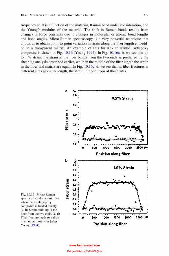
frequency shift is a function of the material, Raman band under consideration, and

the Young’s modulus of the material. The shift in Raman bands results from

changes in force constants due to changes in molecular or atomic bond lengths

and bond angles. Micro-Raman spectroscopy is a very powerful technique that

allows us to obtain point-to-point variation in strain along the fiber length embedd-

ed in a transparent matrix. An example of this for Kevlar aramid 149/epoxy

composite is shown in Fig. 10.16 (Young 1994). In Fig. 10.16a, b, we see that up

to 1 % strain, the strain in the fiber builds from the two ends as predicted by the

shear lag analysis described earlier, while in the middle of the fiber length the strain

in the fiber and matrix are equal. In Fig. 10.16c, d, we see that as fiber fractures at

different sites along its length, the strain in fiber drops at those sites.

Fig. 10.16 Micro-Raman

spectra of Kevlar aramid 149

when the Kevlar/epoxy

composite is loaded axially.

(a, b) Strain build up in the

fiber from the two ends. (c, d)

Fiber fracture leads to a drop

in strain at those sites [after

Young (1994)]



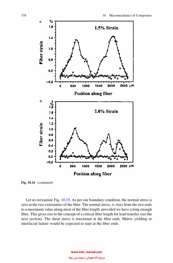
Let us reexamine Fig. 10.15. As per our boundary condition, the normal stress is

zero at the two extremities of the fiber. The normal stress, s, rises from the two ends

to a maximum value along most of the fiber length, provided we have a long enough

fiber. This gives rise to the concept of a critical fiber length for load transfer (see the

next section). The shear stress is maximum at the fiber ends. Matrix yielding or

interfacial failure would be expected to start at the fiber ends.

Fig. 10.16 (continued)



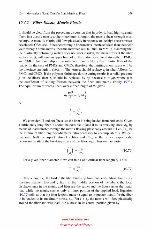
10.4.2 Fiber Elastic–Matrix Plastic

It should be clear from the preceding discussion that in order to load high-strength

fibers in a ductile matrix to their maximum strength, the matrix shear strength must

be large. A metallic matrix will flow plastically in response to the high shear stresses

developed. Of course, if the shear strength fiber/matrix interface is less than the shear

yield strength of the matrix, then the interface will fail first. InMMCs, assuming that

the plastically deforming matrix does not work-harden, the shear stress at the fiber

surface, t(rf), will have an upper limit of ty, the matrix shear yield strength. In PMCs

and CMCs, frictional slip at the interface is more likely than plastic flow of the

matrix. In the case of PMCs and CMCs, therefore, the limiting shear stress will be

the interface strength in shear, ti. The term ti should replace ty in what follows for

PMCs and CMCs. If the polymer shrinkage during curing results in a radial pressure

p on the fibers, then ty should be replaced by mp because ti ¼ mp, where m is

the coefficient of sliding friction between the fiber and matrix (Kelly 1973).

The equilibrium of forces, then, over a fiber length of l/2 gives

sfpd2

4¼ typd

l

2

or

l

d¼ sf

2ty:

We consider l/2 and not l because the fiber is being loaded from both ends. Given

a sufficiently long fiber, it should be possible to load it to its breaking stress sfu bymeans of load transfer through the matrix flowing plastically around it. Let (l/d)c bethe minimum fiber length-to-diameter ratio necessary to accomplish this. We call

this ratio (l/d) the aspect ratio of a fiber and (l/d)c is the critical aspect ratio

necessary to attain the breaking stress of the fiber, sfu. Then we can write

l

d

� �c

¼ sfu2ty

: (10.76)

For a given fiber diameter d, we can think of a critical fiber length lc. Thus,

lcd¼ sfu

2ty: (10.77)

Over a length lc, the load in the fiber builds up from both ends. Strain builds in a

likewise manner. Beyond lc (i.e., in the middle portion of the fiber), the local

displacements in the matrix and fiber are the same, and the fiber carries the major

load while the matrix carries only a minor portion of the applied load. Equation

(10.77) tells us that the fiber length l must be equal to or greater than lc for the fiberto be loaded to its maximum stress, sfu. For l < lc, the matrix will flow plastically

around the fiber and will load it to a stress in its central portion given by



sf ¼ 2tl

d<sfu (10.78)

This is shown in Fig. 10.17. An examination of this figure shows that even for

l/d > (l/d)c the average stress in the fiber will be less than the maximum stress to

which it is loaded in its central region. In fact, one can write for the average fiber stress

sf ¼ 1

l

ðl0

sf dx ¼ 1

lsf l� lcð Þ þ bsf lc� � ¼ 1

lsf l� lc sf � bsf

� ��

or

sf ¼ sf 1� 1� b1=lc

� �; (10.79)

where bsf is the average stress in the fiber over a portion lc/2 of its length at both

ends. One can thus regard b as a load transfer function. Its value will be precisely

0.5 for an ideally plastic material; that is, the increase in stress in the fiber over the

portion lc/2 will be linear. The longitudinal strength of a composite containing short

but well aligned fibers will always be less than that of a composite containing

unidirectionally aligned continuous fibers. For the strength of short fiber composite,

per rule-of-mixtures, we can write:

sc ¼ sf Vf þ s0mVm

sc ¼ sf Vf 1� 1� b1=lc

� �þ s0m 1� Vf

� �:

(10.80)

If b ¼ 0.5,

Fig. 10.17 Schematic of variation of tensile stress in a fiber (sf) and interface shear stress (t) withdifferent fiber aspect ratios (l/d)



sc ¼ sf Vf 1� lc2l

� �þ s0m 1� Vf

� �;

wheres0m is the in situ matrix stress at the strain under consideration. Suppose that in

a whisker or short fiber reinforced metal the whiskers have an l/lc ¼ 10; then it can

easily be shown that the strength of such a composite containing discontinuous but

aligned fibers will be 95 % of that of a composite containing continuous fibers.

Thus, as long as the fibers are reasonably long compared to the load transfer length,

there is not much loss of strength owing to their discontinuous nature. The stress

concentration effect at the ends of the discontinuous fibers has been neglected in

this simple analysis.

10.5 Load Transfer in Particulate Composites

The shear lag model described in the previous section is suitable for explaining the

load transfer from the matrix to a high aspect ratio reinforcement via shear along the

interface parallel to the loading direction. No direct tensile loading of the reinforce-

ment occurs. Such a model will not be expected to work for a particulate composite.

A modified shear lag model (Fukuda and Chou 1981; Nardone and Prewo 1986)

takes into account tensile loading at the particle ends. According to this modified

shear lag model, the yield strength of a particulate composite is given by

syc ¼ sym 1þ Lþ tð Þ=4L½ �Vp þ sym 1� Vp

� �;

where sym is the yield stress of the unreinforced matrix, Vp is the particle volume

fraction, L is the length of the particle perpendicular to the applied load and t is thelength of the particle parallel to the loading direction.

For the case of a composite with equiaxed particles (aspect ratio ¼ 1), the above

expression reduces to

syc ¼ sym 1þ 0:5Vp

� �:

Note that this expression predicts a linear but modest increase in the strength of

the composite with particle volume fraction. However, no account is taken of the

particle size or other microstructural parameters.

Models involving the modified shear lag model, Eshelby’s equivalent inclusion

approach, and Weibull statistics have been proposed (Lewis and Withers 1995;

Song et al. 2010). Incorporation of Weibull statistics (see Chap. 12) makes sense

because the brittle, ceramic particles in a metallic matrix can debond and/or crack

during deformation. The yield strength of the particulate MMC increases as the

volume fraction and aspect ratio of the particles increase, while it decreases as

the size of the SiC particles increases.

10.5 Load Transfer in Particulate Composites 381


http://dx.doi.org/10.1007/978-0-387-74365-3_12

References

Arsenault RJ, Fisher RM (1983) Scripta Met 17:67

Behrens E (1968) J Composite Mater 2:2

Bhatt H, Donaldson KY, Hasselman DPH, Bhatt RT (1992) J Mater Sci 27:6653

Chamis CC (1983) NASA Tech. Memo. 83320, presented at the 38th annual conference of the

Society of Plastics Industry (SPI), Houston, TX

Chamis CC, Sendecky GP (1968) J Compos Mater 2:332



Chawla KK (1974) In: Grain boundaries in engineering materials. Claitor’s Publishing Division,

Baton Rouge, LA, p 435

Chawla KK (1976a) J Mater Sci 11:1567

Chawla KK (1976b) In: Proceedings of the international conference on composite materials/1975,

TMS-AIME, New York. p 535


Clingerman ML, King JA, Schulz KH, Meyers JD (2002) J Appl Polym Sci 83:1341

Cox HL (1952) Brit J Appl Phys 3:122

Day RJ, Robinson IM, Zakikhani M, Young RJ (1987) Polymer 28:1833

Day RJ, Piddock V, Taylor R, Young RJ, Zakikhani M (1989) J Mater Sci 24:2898

Dow NF (1963) General Electric Report No. R63-SD-61Eshelby JD (1957) Proc R Soc A241:376

Eshelby JD (1959) Proc R Soc A252:561

Fukuda H, Chou TW (1981) J Compos Mater 15:79

Galiotis C, Robinson IM, Young RJ, Smith BJE, Batchelder DN (1985) Polym Commun 26:354

Gladysz GM, Chawla KK (2001) Composites A 32:173

Hale DK (1976) J Mater Sci 11:2105

Halpin JC, Kardos JL (1976) Polym Eng Sci 16:344

Halpin JC, Tsai SW (1967) Environmental factors estimation in composite materials design.

AFML TR 67-423

Hashin Z, Rosen BW (1964) J Appl Mech 31:233

Hasselman DPH, Johnson LF (1987) J Compos Mater 27:508

Hill R (1964) J Mech Phys Solids 12:199

Hill R (1965) J Mech Phys Solids 13:189

Kardos JL (1971) CRC Crit Rev Solid State Sci 3:419

Kelly A (1970) Chemical and mechanical behavior of inorganic materials. Wiley-Interscience,

New York, p 523

Kelly A (1973a) Strong solids, 2nd edn. Clarendon, Oxford, p 157

Kerner EH (1956) Proc Phys Soc Lond B69:808

Lewis CA, Withers PJ (1995) Acta Metall Mater 43:3685

Love AEH (1952) A treatise on the mathematical theory of elasticity, 4th edn. Dover, New York,

p 144

Marom GD, Weinberg A (1975) J Mater Sci 10:1005

Mori T, Tanaka K (1973) Acta Metall 21:571

Nardone VC, Prewo KM (1986) Scripta Met 20:43

Nielsen LE (1974) Mechanical properties of polymers and composites, vol 2. Marcel Dekker,

New York

Nye JF (1985) Physical properties of crystals. Oxford University Press, London, p 131

Poritsky H (1934) Physics 5:406

Reuss A (1929) Z Angew Math Mech 9:49

Rosen BW (1973) Composites 4:16

Rosen BW, Hashin Z (1970) Int J Eng Sci 8:157

Schadler LS, Galiotis C (1995) Int Mater Rev 40:116



Schapery RA (1969) J Compos Mater 2:311

Schuster DM, Scala E (1964) Trans Met Soc-AIME 230:1635

Song M, He Y, Fang S (2010) J Mater Sci 45:4097

Termonia Y (1987) J Mater Sci 22:504

Timoshenko S, Goodier JN (1951) Theory of elasticity. McGraw-Hill, New York, p 416

Turner PS (1946) J Res Natl Bur Stand 37:239

Vaidya RU, Chawla KK (1994) Compos Sci Technol 50:13

Vaidya RU, Venkatesh R, Chawla KK (1994) Composites 25:308

Vogelsang M, Arsenault RJ, Fisher RM (1986) Metall Trans A 7A:379

Voigt W (1910) Lehrbuch der Kristallphysik. Teubner, Leipzig

Weber L (2005) Acta Mater 53:1945

Weber L, Dorn J, Mortensen A (2003a) Acta Mater 51:3199

Weber L, Fischer C, Mortensen A (2003b) Acta Mater 51:495

J.M. Whitney (1973). J. Struct. Div., 113.

Xu ZR, Chawla KK, Mitra R, Fine ME (1994) Scripta Met Mater 31:1525

Yang X, Hu X, Day RJ, Young RJ (1992) J Mater Sci 27:1409

Young RJ, Day RJ, Zakikhani M (1990) J Mater Sci 25:127

Young RJ (1994) In: Chawla KK, Liaw PK, Fishman SG (eds) High-performance composites:

commonalty of phenomena. TMS, Warrendale, PA. p 263

Further Reading

Herakovich CT (1998) Mechanics of fibrous composites. Wiley, New York

Kelly A (1973b) Strong solids, 2nd edn. Clarendon, Oxford

Nemat-Nasser S, Hori M (1993) Micromechanics: overall properties of heterogenous materials.

North-Holland, Amsterdam

Tewary VK (1978) Mechanics of fibre composites. Halsted, New York

Problems

10.1. Describe some experimental methods of measuring void content in

composites. Give the limitations of each method.

10.2. Consider a 40 % Vf SiC whisker-reinforced aluminum composite. Ef ¼ 400

GPa, Em ¼ 70 GPa, and (l/d) ¼ 20. Compute the longitudinal elastic mod-

ulus of this composite if all the whiskers are aligned in the longitudinal

direction. Use Halpin-Tsai-Kardos equations. Take x ¼ 2(l/d).10.3. A composite has 40 % Vf of a 150 mm diameter fiber. The fiber strength is

2 GPa, the matrix strength is 75 MPa, while the fiber/matrix interfacial

strength is 50MPa. Assuming a linear build up of stress from the two ends of

a fiber, estimate the composite strength for (a) 200 mm long fibers and (b)

3 mm long fibers.

10.4. Derive the load transfer expression Eq. (10.62) using the boundary conditions.

Show that average tensile stress in the fiber is given by Eq. (10.63).

Problems 383


10.5. Consider a fiber reinforced composite system in which the fiber has an

aspect ratio of 1,000. Estimate the minimum interfacial shear strength ti,as a percentage of the tensile stress in fiber, sf, which is necessary to avoid

interface failure in the composite.

10.6. Show that as x ! 0, the Halpin-Tsai equations reduce to

l=p ¼ Vm=pm þ Vf =pf

while as x ! 1; they reduce to

p ¼ Vmpm þ Vf pf :

10.7. Consider an alumina fiber reinforced magnesium composite. Calculate the

composite stress at the matrix yield strain. The matrix yield stress 180 MPa,

Em ¼ 70 GPa, and n ¼ 0.3. Take Vf ¼ 50 %.

10.8. Estimate the aspect ratio and the critical aspect ratio for aligned SiC

whiskers (5 mm diameter and 2 mm long) in an aluminum alloy matrix.

Assume that the matrix alloy does not show much work hardening.

10.9. Alumina whiskers (density ¼ 3.8 g/cm3) are incorporated in a resin matrix

(density ¼ 1.3 g/cm3). What is the density of the composite? Take

Vf ¼ 0.35. What is the relative mass of the whiskers?

10.10. Consider a composite made of aligned, continuous boron fibers in an

aluminum matrix. Compute the elastic moduli, parallel, and transverse to

the fibers. Take Vf ¼ 0.50.

10.11. Fractographic observations on a fiber composite showed that the average

fiber pullout length was 0.5 mm. If Vfu ¼ 1 GPa and the fiber diameter is

100 mm, calculate the strength of the interface in shear.

10.12. Consider a tungsten/copper composite with following characteristics: fiber

fracture strength ¼ 3 GPa, fiber diameter ¼ 200 mm, and the matrix shear

yield strength ¼ 80 MPa. Estimate the critical fiber length which will make

it possible that the maximum load bearing capacity of the fiber is utilized.

10.13. Carbon fibers (Vf ¼ 50 %) and polyimide matrix have the following

parameters:

Ef ¼ 280GPa Em ¼ 276MPa

vf ¼ 0:2 vm ¼ 0:3

(a) Compute the elastic modulus in the fiber direction, E11, and transverse

to the fiber direction, E22.

(b) Compute the Poisson ratios, n12 and n21.

10.14. Copper or aluminum wires with steel cores are used for electrical power

transmission. Consider a Cu/steel composite wire having the following data:

inner diameter ¼ 1 mm

outer diameter ¼ 2 mm



ECu ¼ 150 GPa aCu ¼ 16� 10�6 K�1

Esteel ¼ 210 GPa asteel ¼ 11� 10�6 K�1

syCu ¼ 100 MPa vCu ¼ vsteel ¼ 0:3systeel ¼ 200 MPa

(a) The composite wire is loaded in tension. Which of the two components

will yield plastically first? Why?

(b) Compute the tensile load that the wire will support before any plastic

strain occurs.

(c) Compute the Young’s modulus and CTE of the composite wire.

10.15. A composite is made of unidirectionally aligned carbon fibers in a

glass-ceramic matrix. The following data are available:

Ef1 ¼ 280 GPa, Ef2 ¼ 40 GPa, Em ¼ 70 GPa

nf1 ¼ 0:2 nm ¼ 0:3

Gf12 ¼ 18 GPa

(a) Compute the elastic modulus in the longitudinal and transverse

directions.

(b) Compute the two Poisson’s ratios.

(c) Compute the principal shear modulus, G12.

Problems 385


Chapter 11

Macromechanics of Composites

Laminated fibrous composites are made by bonding together two or more laminae.

These composites, frequently referred to as laminates, are different from sheet

laminates made by bonding flat sheets of materials. In a laminated fibrous composite,

the individual unidirectional laminae or plies are oriented in such a manner that the

resulting structural component has the desired mechanical and/or physical

characteristics in different directions. Thus, one exploits the inherent anisotropy of

fibrous composites to design a composite material with appropriate properties.

In Chap. 10 we treated the micromechanics of fibrous composites, that is, how to

obtain the composite properties when the properties of the matrix and the fiber and

their geometric arrangements are known. While micromechanics is very useful in

analyzing the composite behavior, we use the information obtained from a

micromechanical analysis of a thin unidirectional lamina (or in the case of a lack

of such analytical information, we must determine experimentally the properties of

a lamina) as input for a macromechanical analysis of a laminated composite.

Figure 11.1 shows this concept schematically (McCullough 1971). Once we have

determined, analytically or otherwise, the characteristics of a fibrous lamina, we

ignore its detailed microstructural nature and simply treat it as a homogeneous,

orthotropic sheet. A laminated fibrous composite is made by stacking a number of

such orthotropic fiber reinforced plies or sheets at specific orientations to get

composite laminate with the desired characteristics. We then use the well-

established theory of laminated plates or shells to analyze macromechanically

such laminated composites.

To appreciate the significance of such a macromechanical analysis, we first

review the basic ideas of the elastic constants of a bulk isotropic material and a

lamina, a lamina as an orthotropic sheet, and finally the use of classical laminated

plate theory to analyze macromechanically the laminated composites. The reader is

referred to some standard texts on elasticity (Love 1952; Timoshenko and Goodier

1951; Nye 1985) for a detailed review of elasticity.


387


http://dx.doi.org/10.1007/978-0-387-74365-3_10

11.1 Elastic Constants of an Isotropic Material

Stress is defined as force per unit area of a body. We can represent the stress acting

at a point in a solid by the stress components acting on the surfaces of an elemental

cube at that point. There are nine stress components (three normal and six shear)

acting on the front faces of an elemental cube. The component sij represents theforce per unit area in the i direction on a face whose normal is the j direction.Rotational equilibrium requires that sij ¼ sji. Thus, we are left with six stress

components; i ¼ j gives the normal stresses while i 6¼ j gives three shear stresses.The displacement of a point in a deformed body with respect to its original

position in the undeformed state can be represented by a vector u with components

u1, u2, and u3; these components are the projections of u on the x1, x2, and x3 axes.Strain is defined as the ratio of change in length to original length. We can define

the strain components in terms of the first derivatives of the displacement

components as follows:

eij ¼ 1

2

@ui@xj

þ @uj@xi

� �:

Similar to stress components, when the subscripts i ¼ j, we have normal strains

while i 6¼ j gives shear strains. It should be noted, however, that eij for i 6¼ j giveshalf of the engineering shear strain, gij; that is,

gij ¼ 2eij ¼ @ui@xj

þ @uj@xi

:

The relationship between stress and strain in linear elasticity is described by

Hooke’s law. Hooke’s law states that, for small strains, stress is linearly proportional

Fig. 11.1 Macromechanical analysis of laminate composites. A unidirectional ply is treated as a

homogeneous, orthotropic material. Many such plies are stacked in an appropriate order (following

laminated plate or shell theory) to make the composite [reprinted from McCullough (1971),

courtesy of Marcel Dekker, Inc.]

388 11 Macromechanics of Composites


to strain. For the simple case of a uniaxial stress applied to an isotropic solid, we can

write Hooke’s law as

s ¼ Ee; (11.1)

where s is the uniaxial stress, e is the strain in the applied stress direction, and E is

Young’s modulus. We have omitted the indices in this simple unidirectional case.

In its most generalized form, Hooke’s law can be written in the indicial or

tensorial notation as

sij ¼ Cijklekl; (11.2)

where Cijkl are the elastic constants or stiffnesses. Equation (11.2), when written out

in an expanded form, will have 81 elastic constants. It is general practice to use a

contracted matrix notation for writing stresses, strains, and elastic constants.

The contracted notation is especially useful for matrix algebra operations.

We use Cmn for Cijkl, sm for sij, and en for ekl as per the following scheme:

ij or kl 11 22 33 23 31 12

m or n 1 2 3 4 5 6

Then Eq. (11.2) can be rewritten as

sm ¼ Cmnen: (11.3)

It can be shown from symmetry considerations that Cmn ¼ Cnm.

Conversely, we can write

em ¼ Smnsn; (11.4)

where Smn, the compliance matrix, is the inverse of the stiffness matrix Cmn.

In the expanded form, we have

s1

s2

s3

s4

s5

s6

266666666666666664

377777777777777775

¼

C11 C12 C13 C14 C15 C16

nC22 C23 C24 C25 C26

nC33 C34 C35 C36

nC44 C45 C46

nC55 C56

nC66

266666666666666664

377777777777777775

e1

e2

e3

e4

e5

e6

266666666666666664

377777777777777775

: (11.5)

11.1 Elastic Constants of an Isotropic Material 389


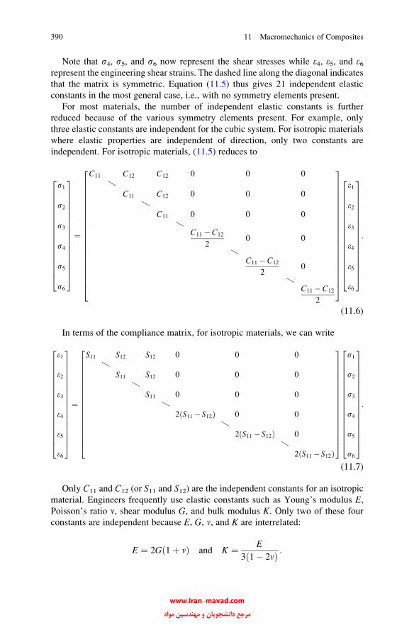
Note that s4, s5, and s6 now represent the shear stresses while e4, e5, and e6represent the engineering shear strains. The dashed line along the diagonal indicates

that the matrix is symmetric. Equation (11.5) thus gives 21 independent elastic

constants in the most general case, i.e., with no symmetry elements present.

For most materials, the number of independent elastic constants is further

reduced because of the various symmetry elements present. For example, only

three elastic constants are independent for the cubic system. For isotropic materials

where elastic properties are independent of direction, only two constants are

independent. For isotropic materials, (11.5) reduces to

s1

s2

s3

s4

s5

s6

266666666666666664

377777777777777775

¼

C11 C12 C12 0 0 0

nC11 C12 0 0 0

nC11 0 0 0

nC11 �C12

20 0

nC11 �C12

20

nC11 �C12

2

2666666666666666666664

3777777777777777777775

e1

e2

e3

e4

e5

e6

266666666666666664

377777777777777775

:

(11.6)

In terms of the compliance matrix, for isotropic materials, we can write

e1

e2

e3

e4

e5

e6

266666666666666664

377777777777777775

¼

S11 S12 S12 0 0 0

nS11 S12 0 0 0

nS11 0 0 0

n2 S11�S12ð Þ 0 0

n2 S11�S12ð Þ 0

n2 S11� S12ð Þ

266666666666666664

377777777777777775

s1

s2

s3

s4

s5

s6

266666666666666664

377777777777777775

:

(11.7)

Only C11 and C12 (or S11 and S12) are the independent constants for an isotropic

material. Engineers frequently use elastic constants such as Young’s modulus E,Poisson’s ratio n, shear modulus G, and bulk modulus K. Only two of these four

constants are independent because E, G, n, and K are interrelated:

E ¼ 2Gð1þ nÞ and K ¼ E

3ð1� 2nÞ :



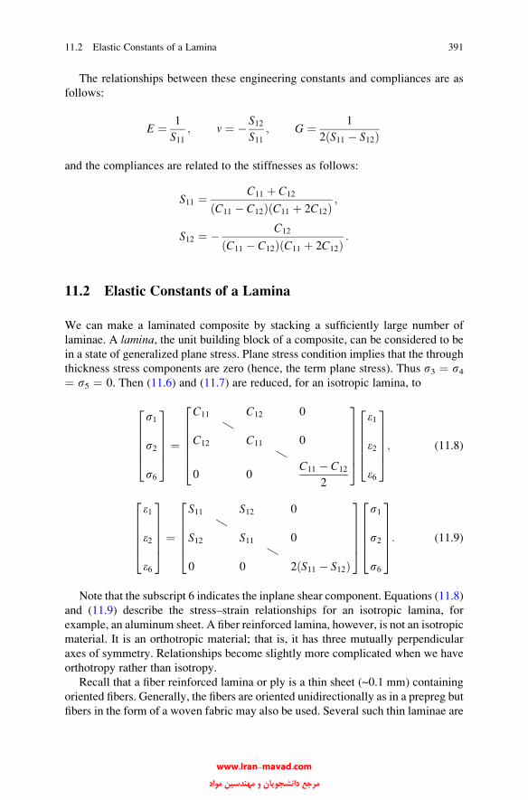
The relationships between these engineering constants and compliances are as

follows:

E ¼ 1

S11; n ¼ � S12

S11; G ¼ 1

2ðS11 � S12Þ

and the compliances are related to the stiffnesses as follows:

S11 ¼ C11 þ C12

ðC11 � C12ÞðC11 þ 2C12Þ;

S12 ¼ � C12

ðC11 � C12ÞðC11 þ 2C12Þ:

11.2 Elastic Constants of a Lamina

We can make a laminated composite by stacking a sufficiently large number of

laminae. A lamina, the unit building block of a composite, can be considered to be

in a state of generalized plane stress. Plane stress condition implies that the through

thickness stress components are zero (hence, the term plane stress). Thus s3 ¼ s4¼ s5 ¼ 0. Then (11.6) and (11.7) are reduced, for an isotropic lamina, to

s1

s2

s6

266664

377775 ¼

C11 C12 0

nC12 C11 0

n0 0

C11 � C12

2

2666664

3777775

e1

e2

e6

266664

377775; (11.8)

e1

e2

e6

266664

377775 ¼

S11 S12 0

nS12 S11 0

n0 0 2 S11 � S12ð Þ

266664

377775

s1

s2

s6

266664

377775: (11.9)

Note that the subscript 6 indicates the inplane shear component. Equations (11.8)

and (11.9) describe the stress–strain relationships for an isotropic lamina, for

example, an aluminum sheet. A fiber reinforced lamina, however, is not an isotropic

material. It is an orthotropic material; that is, it has three mutually perpendicular

axes of symmetry. Relationships become slightly more complicated when we have

orthotropy rather than isotropy.

Recall that a fiber reinforced lamina or ply is a thin sheet (~0.1 mm) containing

oriented fibers. Generally, the fibers are oriented unidirectionally as in a prepreg but

fibers in the form of a woven fabric may also be used. Several such thin laminae are

11.2 Elastic Constants of a Lamina 391


stacked in a specific order of fiber orientation, cured, and bonded into a laminated

composite. Because the behavior of a laminated composite depends on the

characteristics of individual laminae, and with due regard to their directionality,

we now discuss the elastic behavior of an orthotropic lamina.

For the case of an orthotropic material with the coordinate axes parallel to the

symmetry axes of the material, the array of elastic constants is given by

Stj� � ¼

S11 S12 S13 0 0 0

nS22 S23 0 0 0

nS33 0 0 0

nS44 0 0

nS55 0

nS66

266666666666666664

377777777777777775

: (11.10)

A similar expression can be written for Cij. We now take into account the fact

that a lamina is a thin orthotropic material, that is, through thickness components

are zero. We can obtain the compliance matrix for an orthotropic lamina by simply

eliminating the terms involving the z axis:

Sij� � ¼

S11 S12 0

nS22 0

nS66

266664

377775: (11.11)

We can rewrite in full form Hooke’s law for a thin orthotropic lamina, with

natural and geometric axes coinciding, as follows:

e1e2e6

24

35 ¼

S11 S12 0

S12 S22 0

0 0 S66

24

35 s1

s2s6

24

35: (11.12)

Conversely,

s1s2s6

24

35 ¼

Q11 Q12 0

Q12 Q22 0

0 0 Q66

24

35 e1

e2e6

24

35: (11.13)



It is customary to use the symbol Qij rather than Cij for thin material. The Qij are

called reduced stiffnesses. The relationships betweenQij and Sij can easily be shownto be

Q11 ¼ S22S11S22 � S222

;

Q12 ¼ � S12S11S22 � S212

;

Q22 ¼ S11S11S22 � S212

;

Q66 ¼ 1

S66:

(11.14)

Also,

Qij ¼ Cij � Ci3Cj3

C33

ði; j ¼ 1; 2; 6Þ:

Note that three-dimensional orthotropy requires nine independent elastic

constants [Eq. (11.10)], while bidimensional orthotropy requires only four [Eq.

(11.11) or (11.14)]. For an isotropic material (two- or three-dimensional), one just

needs two independent elastic constants [Eqs. (11.6) through (11.9)].

It is worth emphasizing that Eqs. (11.12) and (11.13), showing terms with

indices 16 and 26 to be zero, represent a special case of orthotropy when the

principal material axes of symmetry (the fiber direction [1] and the direction

transverse to it [2]) coincide with the geometric directions. If this is not so, that

is, if the material symmetry axes and the geometric axes do not coincide, then we

have the more general case of orthotropy. In the case of two-dimensional general

orthotropy, we shall have a fully populated elastic constant matrix and the

stress–strain relationships become

sxsyss

24

35 ¼

�Q11�Q12

�Q16�Q12

�Q22�Q26

�Q16�Q26

�Q66

24

35 ex

eyes

24

35; (11.15)

where the �Qij matrix is called the transformed reduced stiffness matrix because it is

obtained by transforming Qij (specially orthotropic) to �Qij (generally orthotropic),

the subscripts x and y represent the geometric axes x and y, and the subscript s refersto inplane shear components. We can perform the transformation of axes as will be

shown presently and obtain �Qij from Qij.

Figure 11.2 shows the situation for a unidirectional composite lamina where the

two sets of axes do not coincide. The properties in the 1–2 or material system of

axes are known, and we wish to determine them in the x–y or geometric system or



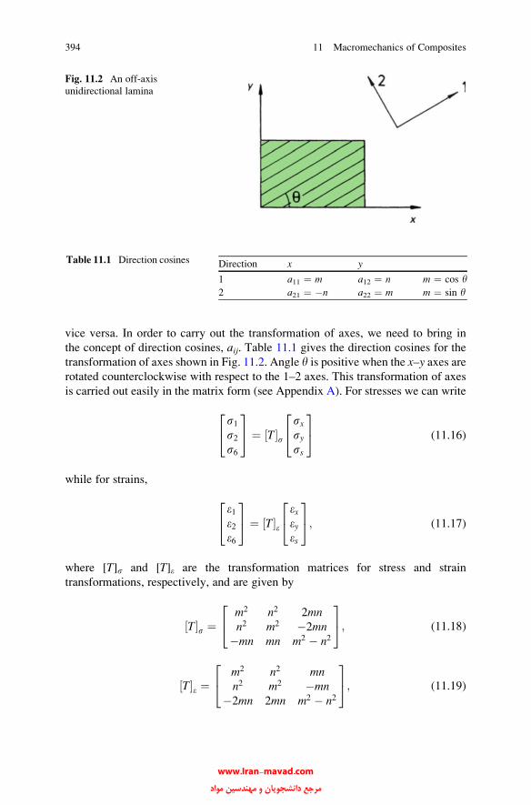
vice versa. In order to carry out the transformation of axes, we need to bring in

the concept of direction cosines, aij. Table 11.1 gives the direction cosines for the

transformation of axes shown in Fig. 11.2. Angle y is positive when the x–y axes arerotated counterclockwise with respect to the 1–2 axes. This transformation of axes

is carried out easily in the matrix form (see Appendix A). For stresses we can write

s1s2s6

24

35 ¼ ½T�s

sxsyss

24

35 (11.16)

while for strains,

e1e2e6

24

35 ¼ ½T�e

exeyes

24

35; (11.17)

where [T]s and [T]e are the transformation matrices for stress and strain

transformations, respectively, and are given by

½T�s ¼m2 n2 2mnn2 m2 �2mn

�mn mn m2 � n2

24

35; (11.18)

½T�e ¼m2 n2 mnn2 m2 �mn

�2mn 2mn m2 � n2

24

35; (11.19)

Fig. 11.2 An off-axis

unidirectional lamina

Table 11.1 Direction cosines Direction x y

1 a11 ¼ m a12 ¼ n m ¼ cos y2 a21 ¼ �n a22 ¼ m m ¼ sin y



http://dx.doi.org/10.1007/978-0-387-74365-3_BM1#Sec1_BM1

where m ¼ cos y and n ¼ sin y. This method of using different transformation

matrices for stress and stain transformations avoids the need of putting the factor

1/2 before the engineering shear strains to convert them to tensorial strain

components suitable for transformation. Multiplying both sides of Eq. (11.16) by

½T��1s and remembering that ½T�s½T��1

s ¼ ½I�, the identity matrix, we get

sxsyss

24

35 ¼ ½T��1

s

s1s2s6

24

35: (11.20)

½T��1s can be obtained from [T]s by simply substituting �y for y. Appendix A gives

the procedure for obtaining the inverse of a given matrix. In this particular case,

substituting �y for y in Eq. (11.18) results in

½T��1s ¼

m2 n2 �2mnn2 m2 2mnmn �mn m2 � n2

24

35; (11.21)

where m ¼ cos y and n ¼ sin y. Substituting Eq. (11.13) in Eq. (11.20), we obtain

sxsyss

24

35 ¼ ½T��1

s ½Q�e1e2e6

24

35: (11.22)

If we now substitute Eq. (11.17) in Eq. (11.22), we arrive at

sxsyss

24

35 ¼ ½T��1

s ½Q�½T�eexeyes

24

35 ¼ �Q

�� exeyes

24

35; (11.23)

where

�Q� � ¼ ½T��1

s ½Q�½T�e: (11.24)

[ �Q] is the stiffness matrix for a generally orthotropic lamina whose components in

expanded form are written as follows (m ¼ cos y, n ¼ sin y):

�Q11 ¼ Q11m4 þ 2ðQ12 þ 2Q66Þm2n2 þ Q22n

4

�Q12 ¼ ðQ11 þ Q22 � 4Q66Þm2n2 þ Q12ðm4 þ n4Þ�Q22 ¼ Q11n

4 þ 2ðQ12 þ 2Q66Þm2n2 þ Q22m4

�Q16 ¼ ðQ11 � Q12 � 2Q66Þm3nþ ðQ12 � Q22 þ 2Q66Þmn3�Q26 ¼ ðQ11 � Q12 � 2Q66Þmn3 þ ðQ12 � Q22 þ 2Q66Þm3n�Q66 ¼ ðQ11 þ Q22 � 2Q12 � 2Q66Þm2n2 þ Q66ðm4 þ n4Þ

: (11.25)



http://dx.doi.org/10.1007/978-0-387-74365-3_BM1#Sec1_BM1

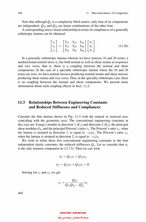
Note that although �Qij is a completely filled matrix, only four of its components

are independent: �Q16 and �Q26 are linear combinations of the other four.

A corresponding stress–strain relationship in terms of compliances of a generally

orthotropic lamina can be obtained:

exeyes

24

35 ¼

S11 S12 S16S12 S22 S26S16 S26 S66

24

35 sx

syss

24

35: (11.26)

In a generally orthotropic lamina wherein we have nonzero 16 and 26 terms, a

unidirectional normal stress sx has both normal as well as shear strains as responses

and vice versa; that is, there is a coupling between the normal and shear

components. In the case of a specially orthotropic lamina where the 16 and 26

terms are zero, we have normal stresses producing normal strains and shear stresses

producing shear strains and vice versa. Thus, in the specially orthotropic case, there

is no coupling between the normal and shear components. We present more

information about such coupling effects in Sect. 11.5.

11.3 Relationships Between Engineering Constants

and Reduced Stiffnesses and Compliances

Consider the thin lamina shown in Fig. 11.3 with the natural or material axes

coinciding with the geometric axes. The conventional engineering constants in

this case are Young’s moduli in direction 1 (E1) and direction 2 (E2), the principal

shear modulus G6, and the principal Poisson’s ratio n1. The Poisson’s ratio n1, whenthe lamina is strained in direction 1, is equal to �e2/e1. The Poisson’s ratio n2,when the lamina is strained in direction 2, is equal to �e1/e2.

We wish to relate these five conventional engineering constants to the four

independent elastic constants, the reduced stiffnesses Qij. Let us consider that s1is the only nonzero component in (11.13). Then we can write

s1 ¼ Q11e1 þ Q12e2;

s2 ¼ Q12e1 þ Q22e2 ¼ 0:

Solving for e1 and e2, we get

e1 ¼ Q22

Q11Q22 � Q212

s1

and



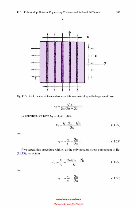
e2 ¼ Q12

Q11Q22 � Q212

s1:

By definition, we have E1 ¼ s1/e1. Thus,

E1 ¼ Q11Q22 � Q212

Q22

(11.27)

and

n1 ¼ � e2e1

¼ Q12

Q22

: (11.28)

If we repeat this procedure with s2 as the only nonzero stress component in Eq.

(11.13), we obtain

E2 ¼ s2e2

¼ Q11Q22 � Q212

Q11

(11.29)

and

n2 ¼ � e1e2

¼ Q12

Q11

: (11.30)

Fig. 11.3 A thin lamina with natural (or material) axes coinciding with the geometric axes

11.3 Relationships Between Engineering Constants and Reduced Stiffnesses. . . 397


If we consider that s6 is the only nonzero component, we can get

G6 ¼ s6e6

¼ Q66: (11.31)

Note that only four of the five constants are independent because

n1E2 ¼ n2E1 (11.32)

or

E1

E2

¼ n1n2

: (11.33)

We can solve Eqs. (11.27)–(11.30) for the Qij to give

Q11 ¼ E1

1� n1n2Q22 ¼ E2

1� n1n2Q12 ¼ n1E2

1� n1n2¼ n2E1

1� n1n2

and Q66 ¼ G6 is given by Eq. (11.31). Similarly, we can show that the relationships

between compliances and engineering constants are as follows:

S11 ¼ 1

E1

S22 ¼ 1

E2

S12 ¼ � n1E1

¼ � n2E2

S66 ¼ 1

G6

:

11.4 Variation of Lamina Properties with Orientation

In Sect. 11.2 we obtained the relationships between Qij and �Qij. It is of interest to

obtain similar relationships for conventional engineering constants referred to

geometric axes x–y (Ex, Ey, Gs, and nx) in terms of engineering constants referred

to material symmetry axes 1–2 (E1, E2, G6, and n1). Consider Eqs. (11.16) and(11.18) and let sx be the only nonzero stress component. Then

s1 ¼ sxm2; (11.34a)

s2 ¼ sxn2; (11.34b)

s6 ¼ �sxmn: (11.34c)

By Hooke’s law, we can write for the strains in a lamina

e1 ¼ 1

E1

ðs1 � n1s2Þ; (11.35a)



e2 ¼ 1

E2

ðs2 � n2s2Þ; (11.35b)

e6 ¼ s6G6

: (11.35c)

From Eqs. (11.34a–11.34c) and (11.35a–11.35c), we get

e1 ¼ sxm2

E1

� n1n2

E1

� �¼ sx

m2

E1

� n2E2

n2� �

; (11.36a)

e2 ¼ sxn2

E2

� n2m2

E2

� �¼ sx

n2

E2

� n1E1

m2

� �; (11.36b)

e6 ¼ � sxmnG6

: (11.36c)

Because we have the strain transformation given by Eq. (11.17), we can write the

inverse of Eq. (11.17) as

exeyes

24

35 ¼ ½T��1

e

e1e2e6

24

35;

where ½T��1e can be obtained by substituting�y for y in Eq. (11.19). In the expanded

form, we can write the above expression as

ex ¼ m2e1 þ n2e2 � mne6; (11.37a)

ey ¼ n2e1 þ m2e2 þ mne6; (11.37b)

es ¼ 2ðe1 � e2Þmnþ e6ðm2 � n2Þ: (11.37c)

Substituting Eqs. (11.36a–11.36c) in (11.37a–11.37c), we obtain

ex ¼ sxm4

E1

þ n4

E2

þ 1

G6

� 2n1E1

� �m2n2

� �; (11.38a)

ey ¼ �sxn1E1

� 1

E1

þ 2n1E1

þ 1

E2

� 1

G6

� �m2n2

� �; (11.38b)

es ¼ �sxð2mnÞ n1E1

þ 1

E2

� 1

2G6

� m2 1

E1

þ 2n1E1

þ 1

E2

� 1

G6

� �� : (11.38c)

11.4 Variation of Lamina Properties with Orientation 399


Now, by definitions, Ex ¼ sx/Ex. Combining this with Eq. (11.38a), we obtain

1

Ex¼ m4

E1

þ n4

E2

þ 1

G6

� 2n1E1

� �m2n2: (11.39)

Ey can be obtained from Ex by substituting y + 90� for y in Eq. (11.39):

1

Ey¼ n4

E1

þ m4

E2

þ 1

G6

� 2n1E1

� �m2n2: (11.40)

Now, nx ¼ �ey/ex when sx is the applied stress. Then, from Eqs. (11.38b) and

(11.39), we obtain

nxEx

¼ � eyExex

¼ � eysx

¼ n1E1

� 1

E1

þ 2n1E1

þ 1

E2

� 1

G6

� �m2n2

or

nx ¼ Exn1E1

� 1

E1

þ 2n1E1

þ 1

E2

� 1

G6

� �m2n2

� �: (11.41)

Similarly, it can be shown that

ny ¼ Eyn2E2

� 1

E1

þ 1

E2

þ 2n1E1

� 1

G6

� �m2n2

� �: (11.42)

Taking ss to be the only nonzero stress component, noting that es ¼ ss/Gs, and

applying Hooke’s law, we can obtain

1

Gs¼ 1

G6

þ 4m2n21þ n1E1

þ 1þ n2E2

� 1

G6

� �: (11.43)

Equations (11.39)–(11.43) give the expressions for the variations of elastic

constants of a unidirectional composite with fiber orientation. These are very useful

expressions. Figure 11.4 shows the variations of Ex, Ey, Gs, nx, and ny with fiber

orientation y for a 50 % Vf carbon/epoxy composite. The other relevant data used in

Fig. 11.4 are E1 ¼ 240 GPa, E2 ¼ 8 GPa, G6 ¼ 6 GPa, and n1 ¼ 0.26.

11.5 Analysis of Laminated Composites

Now that we have discussed the analysis of an individual lamina, we proceed to

discuss the macroscopic analysis of laminated composites (Jones 1975;

Christensen 1979; Tsai and Hahn 1980; Halpin 1984; Daniel and Ishai 1994).



In this analysis, the individual identities of fiber and matrix are ignored. Each

individual, fiber reinforced lamina (also called ply) is treated as a homogeneous,

orthotropic sheet, and the laminated composite is analyzed using the classical

theory of laminated plates.

It would be in order at this point to describe how a multidirectional laminate

can be defined by using a code to designate the stacking sequence of laminae.

Figure 11.5 shows an example of a stacking sequence. The stacking sequence

shown in Fig. 11.5 can be described by the following code:

½02=902=� 453=453�s:

This code says that starting from the bottom of the laminate, that is, at z ¼ �h/2,we have two plies at 0� orientation; then two plies at 90� orientation; followed by agroup of three plies at �45� orientation; and lastly, a group of three plies at +45�

orientation. The subscript s indicates that the laminate is symmetric with respect to

the midplane (z ¼ 0); that is, the top half of the laminate is a mirror image of the

bottom half. It is not necessary that a laminate composite be symmetrical. If the top

Fig. 11.4 Variation of elastic constants with fiber orientation angle for a 50 v/o carbon/epoxy

composite: (a) longitudinal and transverse Young’s moduli (Ex and Ey), (b) shear modulus (Gxy),

and (c) Poisson’s ratio (nx and ny)

11.5 Analysis of Laminated Composites 401


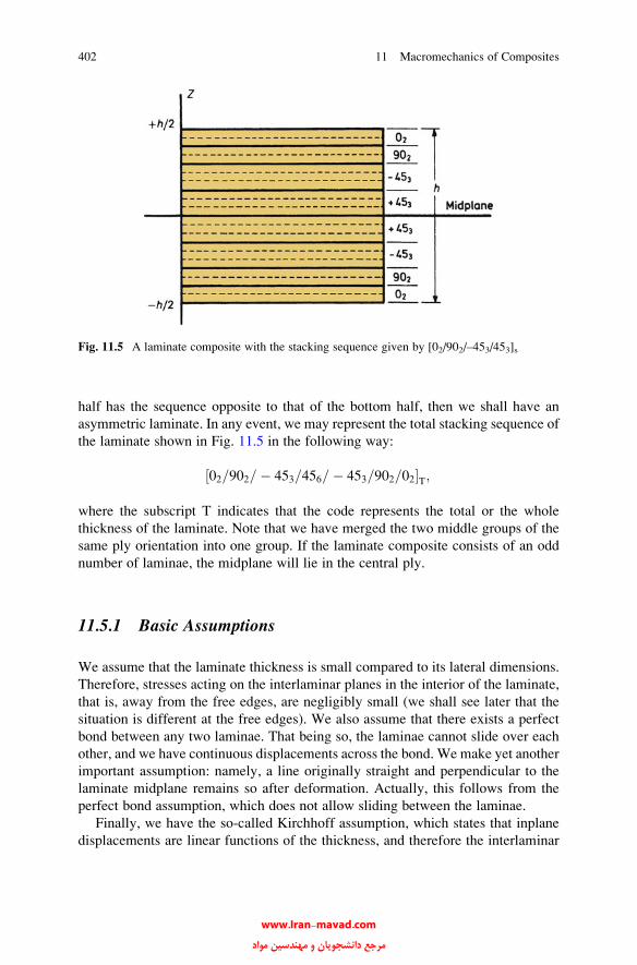
half has the sequence opposite to that of the bottom half, then we shall have an

asymmetric laminate. In any event, we may represent the total stacking sequence of

the laminate shown in Fig. 11.5 in the following way:

½02=902=� 453=456=� 453=902=02�T;

where the subscript T indicates that the code represents the total or the whole

thickness of the laminate. Note that we have merged the two middle groups of the

same ply orientation into one group. If the laminate composite consists of an odd

number of laminae, the midplane will lie in the central ply.

11.5.1 Basic Assumptions

We assume that the laminate thickness is small compared to its lateral dimensions.

Therefore, stresses acting on the interlaminar planes in the interior of the laminate,

that is, away from the free edges, are negligibly small (we shall see later that the

situation is different at the free edges). We also assume that there exists a perfect

bond between any two laminae. That being so, the laminae cannot slide over each

other, and we have continuous displacements across the bond. We make yet another

important assumption: namely, a line originally straight and perpendicular to the

laminate midplane remains so after deformation. Actually, this follows from the

perfect bond assumption, which does not allow sliding between the laminae.

Finally, we have the so-called Kirchhoff assumption, which states that inplane

displacements are linear functions of the thickness, and therefore the interlaminar

Fig. 11.5 A laminate composite with the stacking sequence given by [02/902/–453/453]s



shear strains, exz and eyz, are negligible. With these assumptions we can reduce the

laminate behavior to a two-dimensional analysis of the laminate midplane.

We have the following strain–displacement relationships:

ex ¼ @u

@xexy ¼ @u

@yþ @v

@x

ey ¼ @v

@yexz ¼ @u

@zþ @w

@x

ez ¼ @w

@zeyz ¼ @v

@zþ @w

@y

: (11.44)

Here, u, v, and w are the displacements in the x, y, and z directions, respectively. Fori 6¼ j, the eij represent engineering shear strain components equal to twice the tensorial

shear components. As per Kirchhoff’s assumption, the inplane displacements are

linear functions of the thickness coordinate, z. Then

u ¼ u0ðx; yÞ þ zF1ðx; yÞ; v ¼ v0ðx; yÞ þ zF2ðx; yÞ; (11.45)

where u0 and v0 are displacements of the midplane and F1 and F2 are functions to be

determined; see below. It also follows fromKirchhoff’s assumptions that interlaminar

shear strains exz and eyz are zero. Therefore, from Eqs. (11.44) and (11.45) we obtain

exz ¼ F1 x; yð Þ þ @w

@x¼ 0

eyz ¼ F2 x; yð Þ þ @w

@y¼ 0

:

It therefore follows that

F1ðx; yÞ ¼ � @w

@xand F2ðx; yÞ ¼ � @w

@y: (11.46)

The normal strain in the thickness direction, ez, is negligible: thus we can write

w ¼ wðx; yÞ:

That is, the vertical displacement of any point does not change in the thickness

direction.

Substituting Eq. (11.46) in Eq. (11.45), we obtain

ex ¼ @u

@x¼ @u0

@x� z

@2w

@x2¼ e0x þ zKx; (11.47a)



ey ¼ @v

@y¼ @v0

@y� z

@2w

@y2¼ e0y þ zKy; (11.47b)

exy ¼ @u

@yþ @v

@x¼ @u0

@yþ @v0

@x� 2z

@2w

@x@y¼ e0xy þ zKxy: (11.47c)

Denoting exy by es and Kxy by Ks, as per our notation, we can rewrite the

expression for exy as

es ¼ e0s þ zKs: (11.47d)

Here, e0x , e0y , and e0s are the midplane strains, while Kx, Ky, and Ks are the plate

curvatures. We can represent these quantities in a compact form as follows:

e0xe0y

e0s

264

375 ¼

@u0=@x

@v0=@y

@u0=@yþ @v0=@x

264

375 (11.48)

and

Kx

Ky

Ks

264

375 ¼ �

@2w=@x2

@2w=@y2

2@2w=@x@y

264

375: (11.49)

Equation (11.47a–11.47d) can be put into the following form:

exeyes

264

375 ¼

e0xe0y

e0s

264

375þ z

Kx

Ky

Ks

264

375: (11.50)

11.5.2 Constitutive Relationships for Laminated Composites

Consider a composite made of n stacked layers or plies; see Fig. 11.6a. Let h be thethickness of the laminated composite. Then we can write, for the kth layer, the

following constitutive relationship:

½s�k ¼ �Q� �

k½e�k: (11.51)



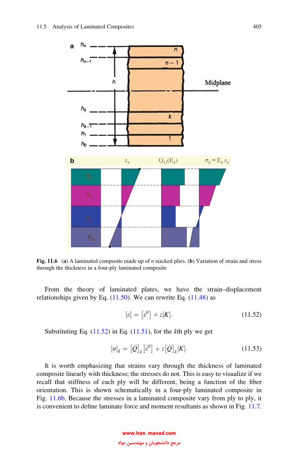
From the theory of laminated plates, we have the strain–displacement

relationships given by Eq. (11.50). We can rewrite Eq. (11.48) as

½e� ¼ e0� �þ z½K�: (11.52)

Substituting Eq. (11.52) in Eq. (11.51), for the kth ply we get

½s�k ¼ �Q� �

ke0� �þ z �Q

� �k½K�: (11.53)

It is worth emphasizing that strains vary through the thickness of laminated

composite linearly with thickness; the stresses do not. This is easy to visualize if we

recall that stiffness of each ply will be different, being a function of the fiber

orientation. This is shown schematically in a four-ply laminated composite in

Fig. 11.6b. Because the stresses in a laminated composite vary from ply to ply, it

is convenient to define laminate force and moment resultants as shown in Fig. 11.7.

Fig. 11.6 (a) A laminated composite made up of n stacked plies. (b) Variation of strain and stressthrough the thickness in a four-ply laminated composite



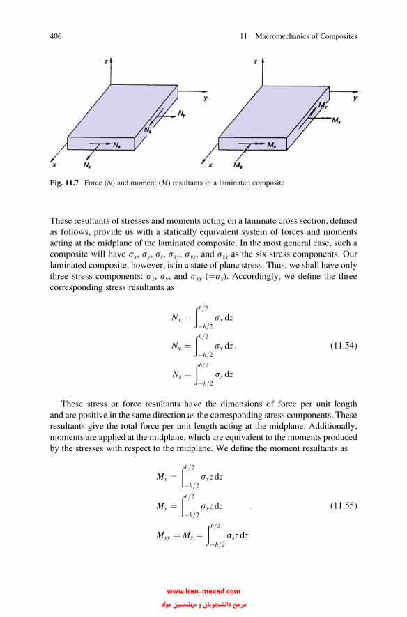
These resultants of stresses and moments acting on a laminate cross section, defined

as follows, provide us with a statically equivalent system of forces and moments

acting at the midplane of the laminated composite. In the most general case, such a

composite will have sx, sy, sz, sxy, syz, and szx as the six stress components. Our

laminated composite, however, is in a state of plane stress. Thus, we shall have only

three stress components: sx, sy, and sxy (¼ss). Accordingly, we define the three

corresponding stress resultants as

Nx ¼ðh=2�h=2

sx dz

Ny ¼ðh=2�h=2

sy dz

Ns ¼ðh=2�h=2

ss dz

: (11.54)

These stress or force resultants have the dimensions of force per unit length

and are positive in the same direction as the corresponding stress components. These

resultants give the total force per unit length acting at the midplane. Additionally,

moments are applied at the midplane, which are equivalent to the moments produced

by the stresses with respect to the midplane. We define the moment resultants as

Mx ¼ðh=2�h=2

sxz dz

My ¼ðh=2�h=2

syz dz

Mxy ¼ Ms ¼ðh=2�h=2

ssz dz

: (11.55)

Fig. 11.7 Force (N) and moment (M) resultants in a laminated composite



This system of three stress resultants Eq. (11.54) and three moment resultants

Eq. (11.55) is statically equivalent to actual stress distribution through the thickness

of the composite laminate.

From Eqs. (11.52) and (11.53), we can write for the stress resultants a summa-

tion over the n plies:

Nx

Ny

Ns

264

375¼ Xn

k¼1

ðhkhk�1

sxsyss

264

375 dz

¼Xnk¼1

ðhkhk�1

�Q11�Q12

�Q16

�Q12�Q22

�Q26

�Q16�Q26

�Q66

264

375

0B@

e0xe0ye0s

264

375 dz

þðhkhk�1

�Q11�Q12

�Q16

�Q12�Q22

�Q26

�Q16�Q26

�Q66

264

375

Kx

Ky

Kx

264

375z dz

1CA (11.56)

Note that [e0] and [K] are not functions of z and in a given ply [ �Q ] is not a

function of z. Thus, we can simplify the preceding expression to

Nx

Ny

Ns

264

375 ¼

Xnk¼1

�Q11�Q12

�Q16

�Q12�Q22

�Q26

�Q16�Q26

�Q66

264

375

0B@

e0xe0ye0s

264

375ðhk

hk�1

dz

þ�Q11

�Q12�Q16

�Q12�Q22

�Q26

�Q16�Q26

�Q66

264

375

Kx

Ky

Kx

264

375ðhk

hk�1

z dz

1CA

: (11.57)

We can rewrite Eq. (11.57) as

Nx

Ny

Ns

264

375 ¼

A11 A12 A16

A12 A22 A26

A16 A26 A66

264

375

e0xe0ye0s

264

375þ

B11 B12 B16

B12 B22 B26

B16 B26 B66

264

375

Kx

Ky

Ks

264

375 (11.58)

or

½N� ¼ ½A� e0� �þ ½B�½K�; (11.59)

where

Aij ¼Xnk¼1

�Qij

kðhk � hk�1Þ (11.60)



and

Bij ¼ 1

2

Xnk¼1

�Qij

kðhk2 � h2k�1Þ: (11.61)

Similarly, from Eqs. (11.52) and (11.55), we can write for the moment resultants

Mx

My

Ms

264

375 ¼

B11 B12 B16

B12 B22 B26

B16 B26 B66

264

375

e0xe0ye0s

264

375þ

D11 D12 D16

D12 D22 D26

D16 D26 D66

264

375

Kx

Ky

Kz

264

375 (11.62)

or

½M� ¼ ½B� e0� �þ ½D�½K�; (11.63)

where

Dij ¼ 1

3

Xnk¼1

�Qij

kðh3k � h3k�1Þ (11.64)

and the Bij are given by (11.61).

We may combine Eqs. (11.59) and (11.63) and write the constitutive equations

for the laminate composite in a more compact form. Thus,

N

M

� �¼ A B

B D

� �e0

K

� �: (11.65)

To appreciate the significance of the preceding expressions, let us examine the

expression for Nx:

Nx ¼ A11e0x þ A12e0y þ A16e0s þ B11Kx þ B12Ky þ B16Ks:

We note that the stress resultant is a function of the midplane tensile strains

(e0x and e0y), the midplane shear strain e0s

, the bending curvatures (Kx and Ky),

and the twisting (Ks). This is a much more complex situation than that

observed in a homogeneous plate where tensile loads result in only tensile

strains. In a laminated plate we have coupling between tensile and shear,

tensile and bending, and tensile and twisting effects. Specifically, the terms

A16 and A26 bring in the tension–shear coupling, while the terms B16 and B26



represent the tension–twisting coupling. The D16 and D26 terms in a similar

expression for Mx represent flexure–twisting coupling.

Under certain conditions, the stress and moment resultants become uncoupled.

It is instructive to examine the conditions under which some of these simplifications

can result. The Aij terms are the sum of ply �Qij times the ply thickness, Eq. (11.60).

Thus, the Aij will be zero if the positive contributions of some laminae are nullified

by the negative contributions of others. Now the Qij terms of a ply are derived from

orthotropic stiffnesses and, because of the form of transformation equations

(11.25), �Q11 , �Q12 , �Q22 , and �Q66 are always positive. This means that A11, A12,

A22, and A66 are always positive. �Q16 and �Q26 , however, are zero for 0� and 90�

orientations and can be positive or negative for y between 0� and 90�. In fact, �Q16

and �Q26 are odd functions of y; that is, for equal positive and negative orientations,

they will be equal in magnitude but opposite in sign. In particular, �Q16 and �Q26 for a

+y orientation are equal to but opposite in sign to �Q16 and �Q26 values for a �yorientation. Thus, if for each +y ply, we have another identical ply of the samethickness at �y, then we shall have what is called a specially orthotropic laminatewith respect to in-plane stresses and strains; that is, A16 ¼ A26 ¼ 0. The relativeposition of such plies in the stacking sequence does not matter.

The Bij terms are sums of terms involving �Qij and differences of the square of zterms for the top (hk) and bottom (hk�1) of each ply. Thus, the Bij terms are even

functions of hk, which means that they are zero if the laminate composite is

symmetric with respect to thickness. In other words, the Bij are zero if we havefor each ply above the midplane a ply identical in properties and orientation and atan equal distance below the midplane. Such a laminate is called a symmetriclaminate and will have Bij identically zero. This simplifies the constitutive

equations, and symmetric laminates are considerably easier to analyze. Additionally,

because of the absence of bending–stretching coupling in symmetric laminates, they

do not have the problem of warping encountered in nonsymmetric laminates and

caused by in-plane forces induced by thermal contractions occurring during the

curing of the resin matrix. Symmetric laminates will only experience tensile strains

at the midplane but no flexure. The reader should realize that the origin of the [B]matrix lies not in the intrinsic orthotropy of the laminae, but in the heterogeneous

(nonsymmetric) stacking sequence of the plies. Thus, a two-ply composite consisting

of isotropic materials such as aluminum and steel will show a nonzero [B].The terms in the Dij matrix are defined in terms of �Qij and the difference between

h3k and h3k�1. The geometrical contribution h3k � h3k�1

is always positive. Thus, as

explained above for Aij, D11, D12, D22, and D66 are always positive. Recall that �Q16

and �Q26 are odd functions of y.D16 andD26 are zero for all plies oriented at 0� or 90�

because these plies have �Q16 ¼ �Q26 ¼ 0. D16 and D26 can also be made zero if, for

each ply oriented at +y and at a given distance above the midplane, we have an

identical ply at an equal distance below the midplane but oriented at �y. Thisfollows from the property of the odd function of y that is, �Q16ðþyÞ ¼ � �Q16ð�yÞ,and �Q26ðþyÞ ¼ � �Q26ð�yÞ , while ðh3k � h3k�1Þ is the same for both plies.

Note, however, that such a laminated composite does not have a midplane of



symmetry; that is, Bij 6¼ 0. In fact, D16 and D26 are not zero for any midplane

symmetric laminate except for unidirectional laminates (0� or 90�) and crossplied

laminates (0�/90�). We can makeD16 andD26 arbitrarily small, however, by using a

large enough number of plies stacked at �y. This is because the contributions of +yplies to D16 and D26 are opposite in sign to those of �y plies, and although their

locations are different distances from the midplane, given large enough number of

plies, they will practically cancel each other.

Yet another simple stacking sequence is the quasi-isotropic sequence. Such a

laminated composite can be made by having plies of identical properties oriented in

such a way that the angle between any two adjacent layers is 2p/n, where n is the

number of plies. Such a laminate has [A] independent of orientation in the plane. We

call such a stacking sequence quasi-isotropic, because [B] and [D] are not necessarilyisotropic.We provide a summary of some of these special laminates that we discussed

above in Fig. 11.8. Note the coupling coefficients that go to zero for each case.

The important results of this section can be summarized as follows:

½s�k ¼ �Q� �

k½e�k;

where 1 � k � n and i, j ¼ 1, 2, 6.

ei¼ e0i þ zKi

Ni¼ðh=2�h=2

si dz

Mi¼ðh=2�h=2

sidz

Ni¼ Aije0j þ BijKj

Mi¼ Bije0j þ DijKj

Aij¼Xnk¼1

�Qij

kðhk � hk�1Þ

Bij¼ 1

2

Xnk¼1

�Qij

kðh2k � h2k�1Þ

Dij¼ 1

3

Xnk¼1

�Qij

kðh3k � h3k�1Þ

:

Symmetric laminates

�QðzÞ ¼ �Qð�zÞ:

Antisymmetric laminates

�QðzÞ ¼ � �Qð�zÞ:



Example 11.1A laminate is made up by stacking 0� and 45� plies as shown below:

3 mm45°

3 mm0°

3 mm0°

3 mm45°

h0

h1

h2

h3

h4

Fig. 11.8 Some special laminates



The [Qij]0� and [ �Qij]45� matrices are

Qij

� �0�¼

140 5 0

5 0

5

264

375GPa

�Qij

� �45�¼

50 35 30

50 30

35

264

375GPa

:

Compute the [A], [B], and [D] matrices for this laminate.

Solution

�Qij

45�¼

50 35 30

50 30

35

24

35

�Qij

0�¼ Qij

0� ¼

140 5 0

5 0

5

24

35:

Let us now compute the submatrices, [A], [B], and [D].

Aij ¼X4k¼1

�Qij

khk � hk�1ð Þ

¼ �Qij

1h1 � h0ð Þ þ �Qij

2h2 � h1ð Þ þ �Qij

3h3 � h2ð Þ

þ �Qij

4h4 � h3ð Þ

Aij ¼ �Qij

1

�3ð Þ � �6ð Þ½ � þ �Qij

20� �3ð Þ½ � þ �Qij

33� 0½ �

þ �Qij

46� 3½ �

¼ 3 �Qij

1þ �Qij

2þ �Qij

3þ �Qij

4

h i

�Qij

1¼ �Qij

4¼ �Qij

45�

�Qij

2¼ �Qij

3¼ �Qij

0�

A ¼ 6 �Qij

45� þ �Qij

0�

h i

¼ 6

50 35 30

50 30

35

264

375þ

140 5 0

5 0

5

264

375

8><>:

9>=>;

¼1140 240 180

330 180

240

264

375� 106 N/m

:



We have a symmetric laminate, therefore

B½ � ¼ 0½ �

3D¼X4k¼1

�Qij

kh3k � h3k�1

¼ �Qij

1h31 � h30 þ �Qij

2h32 � h31 þ �Qij

3h33 � h32

þ �Qij

4h34 � h33

¼ �Qij

1

�3ð Þ3 � �6ð Þ3h i

þ �Qij

0� �3ð Þ3h i

þ �Qij

33 � 0� �

þ �Qij

463 � 33� �

¼ �Qij

1�27þ 216ð Þ þ �Qij

20þ 27ð Þ þ �Qij

327� 0ð Þ

þ �Qij

4216� 27ð Þ

3D ¼ 189 �Qij

1þ 27 �Qij

2þ 27 �Qij

3þ 189 �Qij

4

�Qij

1¼ �Qij

4¼ �Qij

45�

�Qij

2¼ �Qij

3¼ �Qij

0�

D ¼ 126 �Qij

45� þ 18 �Qij

0�

D ¼ 126

50 35 30

50 30

35

264

375þ 18

140 5 0

5 0

5

264

375

8><>:

9>=>;� 109

N

m2� 10�9m3

D ¼8820 4500 3780

6390 3780

4500

264

375N �m:

11.6 Stresses and Strains in Laminate Composites

We saw in Sect. 11.5 that strains produced in a lamina under load depend on the

midplane strains, plate curvatures, and distances from the midplane. Midplane

strains and plate curvatures can be expressed as functions of an applied load system,

that is, in terms of stress and moment resultants. We derived the general constitutive

equation (11.65) for laminate composites. We can invert Eq. (11.65) partially or

fully and obtain explicit expressions for [e0] and [K]. We use (11.59) and (11.63) for

this purpose. Solving (11.59) for midplane strains, we obtain

e0� � ¼ ½A��1½N� � ½A��1½B�½K�: (11.66)

Substituting Eq. (11.66) in Eq. (11.63), we obtain

½M� ¼ ½B�½A��1½N� � ð½B�½A��1½B� � ½D�Þ½K�: (11.67)

11.6 Stresses and Strains in Laminate Composites 413


Combining Eqs. (11.66) and (11.67), we obtain a partially inverted form of the

constitutive equation:

e0

M

� �¼ A B

C D

� �N

K

� �; (11.68)

where

A½ � ¼ ½A��1

B½ � ¼ �½A��1½B�C½ � ¼ ½B�½A��1 ¼ � B½ �TD½ � ¼ ½D� � ½B�½A��1½B�

: (11.69)

From Eqs. (11.66) and (11.69), we can write

e0� � ¼ A½ �½N� þ B½ �½K�; (11.70)

M½ � ¼ C½ �½N� þ D½ �½K�: (11.71)

From Eq. (11.71), we solve for [K] and obtain

½K� ¼ D½ ��1½M� � D½ ��1 C½ �½N�: (11.72)

Substituting this value of [K] [Eq. (11.72)] in Eq. (11.70), we obtain

e0½ � ¼ A½ �½N� þ B½ � D½ ��1½M� � D½ ��1 C½ �½N��

¼ A½ � � B½ � D½ ��1 C½ ��

½N� þ B½ � D½ ��1½M�: (11.73)

We can combine Eqs. (11.72) and (11.70) to obtain the fully inverted form:

e0

K

� �¼ A0 B0

B0 D0

� �N

M

� �¼ A0 B0

C0 D0

� �N

M

� �; (11.74)

where

A0½ � ¼ A½ � � B½ � D½ ��1 C½ � ¼ A½ � þ B½ � D½ ��1 B½ �T; C½ � ¼ � B½ �T� �

B0½ � ¼ B½ � D½ ��1

C0½ � ¼ � D½ ��1 C½ � ¼ D½ ��1 B½ �T ¼ B0½ �T ¼ B0½ �D0½ � ¼ D½ ��1

:

Equations (11.65), (11.68), and (11.74) are useful forms of the laminate consti-

tutive relationships. We note that each form involves using the elastic properties

of the lamina (from the �Qij values for each lamina) and the ply stacking sequence

(z coordinate).



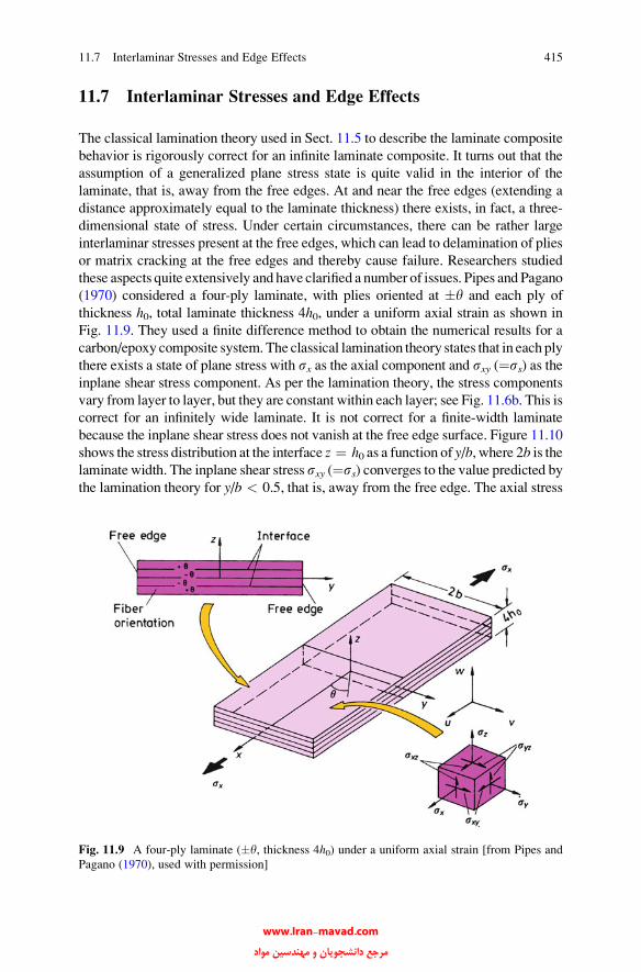
11.7 Interlaminar Stresses and Edge Effects

The classical lamination theory used in Sect. 11.5 to describe the laminate composite

behavior is rigorously correct for an infinite laminate composite. It turns out that the

assumption of a generalized plane stress state is quite valid in the interior of the

laminate, that is, away from the free edges. At and near the free edges (extending a

distance approximately equal to the laminate thickness) there exists, in fact, a three-

dimensional state of stress. Under certain circumstances, there can be rather large

interlaminar stresses present at the free edges, which can lead to delamination of plies

or matrix cracking at the free edges and thereby cause failure. Researchers studied

these aspects quite extensively and have clarified a number of issues. Pipes and Pagano

(1970) considered a four-ply laminate, with plies oriented at �y and each ply of

thickness h0, total laminate thickness 4h0, under a uniform axial strain as shown in

Fig. 11.9. They used a finite difference method to obtain the numerical results for a

carbon/epoxy composite system. The classical lamination theory states that in each ply

there exists a state of plane stress with sx as the axial component and sxy (¼ss) as theinplane shear stress component. As per the lamination theory, the stress components

vary from layer to layer, but they are constant within each layer; see Fig. 11.6b. This is

correct for an infinitely wide laminate. It is not correct for a finite-width laminate

because the inplane shear stress does not vanish at the free edge surface. Figure 11.10

shows the stress distribution at the interface z ¼ h0 as a function of y/b, where 2b is thelaminate width. The inplane shear stress sxy (¼ss) converges to the value predicted bythe lamination theory for y/b < 0.5, that is, away from the free edge. The axial stress

Fig. 11.9 A four-ply laminate (�y, thickness 4h0) under a uniform axial strain [from Pipes and

Pagano (1970), used with permission]

11.7 Interlaminar Stresses and Edge Effects 415


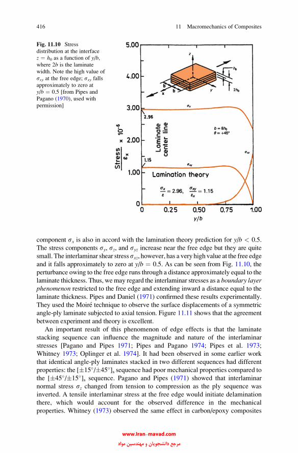
component sx is also in accord with the lamination theory prediction for y/b < 0.5.

The stress components sy, sz, and syz increase near the free edge but they are quite

small. The interlaminar shear stresssxz, however, has a very high value at the free edgeand it falls approximately to zero at y/b ¼ 0.5. As can be seen from Fig. 11.10, the

perturbance owing to the free edge runs through a distance approximately equal to the

laminate thickness. Thus, wemay regard the interlaminar stresses as a boundary layerphenomenon restricted to the free edge and extending inward a distance equal to the

laminate thickness. Pipes and Daniel (1971) confirmed these results experimentally.

They used the Moire technique to observe the surface displacements of a symmetric

angle-ply laminate subjected to axial tension. Figure 11.11 shows that the agreement

between experiment and theory is excellent.

An important result of this phenomenon of edge effects is that the laminate

stacking sequence can influence the magnitude and nature of the interlaminar

stresses [Pagano and Pipes 1971; Pipes and Pagano 1974; Pipes et al. 1973;

Whitney 1973; Oplinger et al. 1974]. It had been observed in some earlier work

that identical angle-ply laminates stacked in two different sequences had different

properties: the [�15�/�45�]s sequence had poor mechanical properties compared to

the [�45�/�15�]s sequence. Pagano and Pipes (1971) showed that interlaminar

normal stress sz changed from tension to compression as the ply sequence was

inverted. A tensile interlaminar stress at the free edge would initiate delamination

there, which would account for the observed difference in the mechanical

properties. Whitney (1973) observed the same effect in carbon/epoxy composites

Fig. 11.10 Stress

distribution at the interface

z ¼ h0 as a function of y/b,where 2b is the laminate

width. Note the high value of

sxy at the free edge; sxy fallsapproximately to zero at

y/b ¼ 0.5 [from Pipes and

Pagano (1970), used with

permission]



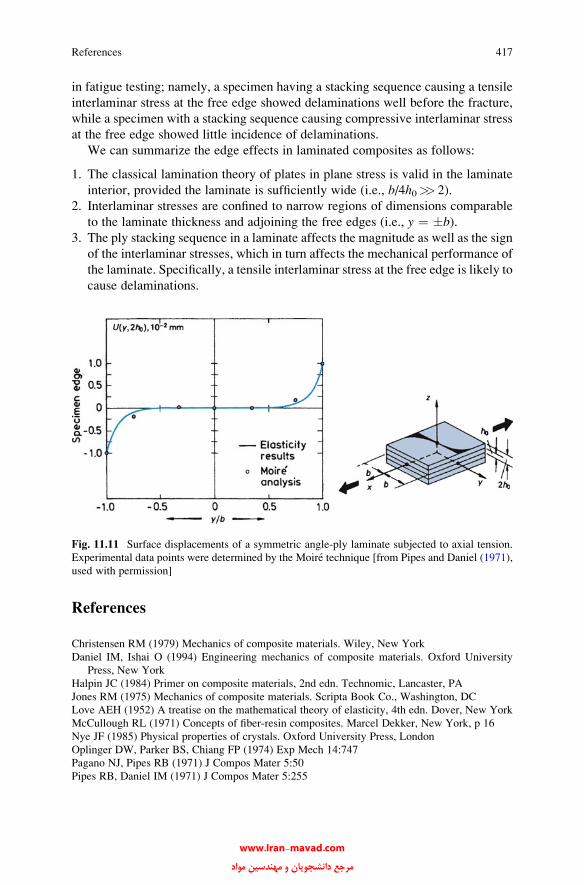
in fatigue testing; namely, a specimen having a stacking sequence causing a tensile

interlaminar stress at the free edge showed delaminations well before the fracture,

while a specimen with a stacking sequence causing compressive interlaminar stress

at the free edge showed little incidence of delaminations.

We can summarize the edge effects in laminated composites as follows:

1. The classical lamination theory of plates in plane stress is valid in the laminate

interior, provided the laminate is sufficiently wide (i.e., b/4h0>> 2).

2. Interlaminar stresses are confined to narrow regions of dimensions comparable

to the laminate thickness and adjoining the free edges (i.e., y ¼ �b).3. The ply stacking sequence in a laminate affects the magnitude as well as the sign

of the interlaminar stresses, which in turn affects the mechanical performance of

the laminate. Specifically, a tensile interlaminar stress at the free edge is likely to

cause delaminations.

References

Christensen RM (1979) Mechanics of composite materials. Wiley, New York

Daniel IM, Ishai O (1994) Engineering mechanics of composite materials. Oxford University

Press, New York

Halpin JC (1984) Primer on composite materials, 2nd edn. Technomic, Lancaster, PA

Jones RM (1975) Mechanics of composite materials. Scripta Book Co., Washington, DC

Love AEH (1952) A treatise on the mathematical theory of elasticity, 4th edn. Dover, New York

McCullough RL (1971) Concepts of fiber-resin composites. Marcel Dekker, New York, p 16

Nye JF (1985) Physical properties of crystals. Oxford University Press, London

Oplinger DW, Parker BS, Chiang FP (1974) Exp Mech 14:747

Pagano NJ, Pipes RB (1971) J Compos Mater 5:50

Pipes RB, Daniel IM (1971) J Compos Mater 5:255

Fig. 11.11 Surface displacements of a symmetric angle-ply laminate subjected to axial tension.

Experimental data points were determined by the Moire technique [from Pipes and Daniel (1971),


References 417


Pipes RB, Kaminski BE, Pagano NJ (1973) Analysis of the test methods for high modulus fibers

and composites, ASTM STP 521. ASTM, Philadelphia, PA, p 218

Pipes RB, Pagano NJ (1970) J Compos Mater 4:538

Pipes RB, Pagano NJ (1974) J Appl Mech 41:668

Timoshenko S, Goodier JN (1951) Theory of elasticity. McGraw-Hill, New York

Tsai SW, Hahn HT (1980a) Introduction to composite materials. Technomic, Westport, CT

Whitney JM (1973) Analysis of the test methods for high modulus fibers and composites, ASTM

STP 521. ASTM, Philadelphia, PA, p 167

Further Reading

Bunsell AR, Renard J (2005) Fundamentals of fibre reinforced composites. Institute of Physics

Pub, Bristol

Calcote LR (1969) Analysis of laminated composite structures. Van Nostrand Reinhold, New York

Daniel IM, Ishai O (2006) Engineering mechanics of composite materials, 2nd edn. Oxford

University Press, New York

Herakovich CT (1998) Mechanics of fibrous composites. Wiley, New York

Hyer MW (1997) Stress analysis of fiber reinforced composite materials. McGraw-Hill, New York

Jones RM (1999) Mechanics of composite materials, 2nd edn. Taylor & Francis, Philadelphia, PA

Tsai SW, Hahn HT (1980b) Introduction to composite materials. Technomic, Westport, CT

Problems

11.1. An isotropic material is subjected to a uniaxial stress. Is the stain state also

uniaxial? Write the stress and strain in matrix form.

11.2. For a symmetric laminated composite, we have, �QijðþzÞ ¼ �Qijð�zÞ, i.e., themoduli are even functions of thickness z. Starting from this definition, split

the integral and show that Bij is identically zero for a symmetric laminate.

11.3. An orthotropic lamina has the following characteristics: E11 ¼ 210 GPa,

E22 ¼ 8 GPa, G12 ¼ 5 GPa, and n12 ¼ 0.3. Consider a three-ply laminate

made of such laminae arranged at y ¼ �60�. Compute the submatrices [A],[B], and [D]. Take the ply thickness to be 1 mm.

11.4. Enumerate the various phenomena which can cause microcracking in a fiber

composite.

11.5. A thin lamina of a composite with fibers aligned at 45� to the lamina major

axis is subjected to the following stress system along its geometric axes:

½si� ¼sxsyss

24

35 ¼

10

2

3

24

35MPa:

Compute the stress components along the material axes (i.e., s1, s2, and s6).



11.6. A two-ply laminate composite has the top and bottom ply orientations of 45

and 0� and thicknesses of 2 and 4 mm, respectively. The stiffness matrix for

the 0� ply is

½Qij� ¼20 1 0

1 3 0

0 0 1

24

35GPa:

Find �Qij

� �45

and then compute the matrices [A], [B], and [D] for this

laminate.

11.7. A two-ply laminate composite is made of polycrystalline, isotropic aluminum

and steel sheets, each 1 mm thick. The constitutive equations for the two

sheets are

Al :

s1s2s6

264

375 ¼

70 26 0

26 70 0

0 0 26

264

375

e1e2e6

264

375MPa

Steel:

s1s2s6

264

375 ¼

210 60 0

60 210 0

0 0 78

264

375

e1e1e6

264

375MPa

:

Compute the matrices [A], [B], and [D] for this laminate composite. Point

out any salient features of this laminate.

Problems 419


Chapter 12

Monotonic Strength and Fracture

In this chapter we describe the monotonic strength and fracture behavior of fiber

reinforced composites at ambient temperatures. The term monotonic behaviormeans behavior under an applied stress that increases in one direction, i.e., not a

cyclic loading condition. We discuss the behavior of composites under fatigue

or cyclic loading as well as under conditions of creep in Chap. 13.

12.1 Tensile Strength of Unidirectional Fiber Composites

In Chap. 10 we discussed the prediction of elastic and thermal properties when the

properties of the components are known. A particularly simple but crude form of

this is the rule-of-mixtures, which works reasonably well for predicting the longi-

tudinal elastic constants. Unfortunately, the same cannot be said for the strength of

a fiber reinforced composite. It is instructive to examine why the rule-of-mixtures

approach does not always work for strength properties of a composite. For a

composite containing continuous fibers, unidirectionally aligned and loaded in the

fiber direction (isostrain condition), we can write for the stress in the composite

sc ¼ sfVf þ sm 1� Vfð Þ; (12.1)

where s is the axial stress, Vf is the volume fraction, and the subscripts c, f, and m

refer to composite, fiber, and matrix, respectively. The important question here is:

What is the value of the matrix stress, sm? Ideally, it should be the in situ value of

the stress on the matrix at a given strain. The main reason that the rule-of-mixtures

does not always work for predicting the strength of a composite, while it works

reasonably well for Young’s modulus in the longitudinal direction, is that the elastic

modulus is a relatively microstructure-insensitive property, while strength is a

highly microstructure-sensitive property. For example, the grain size of a polycrys-

talline material affects its strength but not its modulus. Thus, the response of a

composite for elastic modulus is nothing but the volume-weighted average of the


421


http://dx.doi.org/10.1007/978-0-387-74365-3_13

http://dx.doi.org/10.1007/978-0-387-74365-3_10

individual responses of the isolated components. Because the strength is an

extremely structure-sensitive property, synergism can occur in regard to composite

strength. Consider the various factors that may influence the composite strength

properties. First, matrix or fiber structure may be altered during fabrication. Second,

composite materials consist of two components whose thermomechanical

properties are generally quite different and thus may have residual stresses and/or

undergo structure alterations owing to these internal stresses. We discussed at

length in Chap. 10 the effects of differential contraction during cooling from the

fabrication temperature to ambient temperature, which leads to thermal stresses

large enough to deform the matrix plastically, which leads to high dislocation

density and work-hardening of the matrix (Chawla and Metzger 1972; Chawla

1973a, b; Arsenault and Fisher 1983; and Vogelsang et al. 1986).

Yet another source of microstructural modification of a component is a phase

transformation induced by the fabrication process. In a metallic laminate composite

made by roll-bonding aluminum and austenitic stainless steel (type 304), it was

observed that the fabrication procedure work-hardened the steel and partially

transformed the austenite to martensite (Chawla et al. 1986).

The matrix stress state may also be influenced by rheological interaction

between the components during straining (Ebert and Gadd 1965; Kelly and Lilholt

1969). The plastic constraint on the matrix owing to the large differences in the

Poisson’s ratios of the matrix and the fiber, especially in the stage wherein the fiber

deforms elastically while the matrix deforms plastically, can considerably alter the

stress state in the composite. Thus, microstructural changes in one or both of the

components, or rheological interaction between the components during straining

can lead to the phenomenon of synergism in the strength properties. In view of this,

the rule-of-mixtures should be regarded, in the best of circumstances, as an order of

magnitude indicator of the strength of a composite.

12.2 Compressive Strength of Unidirectional Fiber Composites

Fiber reinforced composites under compressive loading can be regarded, as a first

approximation, as elastic columns under compression. Thus, themain failuremodes in

the failure of a composite are the ones that occur in the buckling of columns. Buckling

occurs when a slender column under axial compression becomes unstable against

lateral movement of the central portion. The critical stress corresponding to failure by

buckling of a column with ends-pinned is given by the Euler bucking formula:

sc ¼ p2E16

d

l

� �2

; (12.2)

where E is the elastic modulus, d is the diameter, and l is the length of the column. It is

easy to see that a high aspect ratio (l/d) will result in a low sc. Of course, in a fiber

422 12 Monotonic Strength and Fracture


http://dx.doi.org/10.1007/978-0-387-74365-3_10

reinforced composite we do not load a fiber directly and the conditions of ends-

pinned do not prevail. The main effect of different end conditions of the column is

that the length of the column should be replaced with an effective length. In a

composite, the matrix provides some stability in the lateral direction. Rosen

(1965a) showed by means of photoelasticity that fiber reinforced composites fail by

periodic buckling of the fibers, with the buckling wavelength being proportional to

the fiber diameter. This is not surprising in view of the fact that in the analysis of a

column on an elastic foundation, it is observed that the buckling wavelength depends

on the column diameter. Figure 12.1 shows schematically the three situations: an

unbuckled fiber composite, in-phase buckling, and out-of-phase buckling. The in-

phase buckling of fibers involves shear deformation of the matrix. In such a case the

composite strength in compression is proportional to the matrix shear modulus Gm;

that is, sc ¼ Gm/Vm, where Vm is the matrix volume fraction. For an isotropic matrix

we have Gm ¼ Em/2(1 + nm), where Em and nm are the matrix Young’s modulus and

Poisson’s ratio, respectively. Thus,

sc ¼ Em

2 1þ nmð ÞVm

: (12.3)

Out-of-phase buckling of fibers involves transverse compressive and tensile

strains. The compressive strength in such a case is proportional to the geometric

mean of the fiber and matrix Young’s moduli (Rosen 1965a):

sc ¼ 2Vf

VfEmEf

3Vm

� �1=2

; (12.4)

where V and E denote the volume fraction and Young’s modulus, respectively, and

the subscripts f and m denote fiber and matrix, respectively.

From Eqs. (12.3) and (12.4), we can see that the two failure modes in compres-

sion have a different dependence on the moduli of the components, that is,

sc / EmEfð Þ1=2 out - of - phase

sc / Gm in - phase: (12.5)

Thus, if we were to put the same fiber in two different matrices (i.e., with

different matrix moduli), we should be able to distinguish between these two

compressive failure modes. Lager and June (1969) did just that with boron fibers

in two different polymer matrices. An out-of-phase buckling mode predominated at

low fiber volume fractions. At high fiber volume fractions, fibers exerted more

influence on each other and a coupled or in-phase buckling mode prevailed. The

approximate nature of Eqs. (12.7) and (12.8) is easy to see. Both imply that as

Vm ! 0 (or Vf ! 1), sc ! 1, that is, the fibers are infinitely strong. Of course, no

fibers are infinitely strong. Fiber/matrix adhesion (Hancox 1975) and matrix yield-

ing (Piggott and Harris 1980) also affect the compressive strength of fiber

composites. Narayanan and Schadler (1999) observed that the kink bands initiated

12.2 Compressive Strength of Unidirectional Fiber Composites 423


from a damage zone comprising crushed and broken fibers. When the damage zone

reached a critical size, the unsupported column of matrix caused a local matrix

shear instability (or microbuckling). This local instability propagated as a kink

band. The damage zone angle was found to depend on the interface properties, and

it affected the strain to form kink bands. In the case of a laminated composite, poor

interlaminar bonding can result in easy buckling of fibers (Piggott 1984).

Kyriakides et al. (1995) investigated the failure in compression of unidirectionally

reinforced AS4 carbon fiber/PEEK matrix composites. The failure load of the

composite depended on geometric imperfections such as fiber waviness, and failure

occurred via formation of kink bands. They modeled the composite as a two-

dimensional solid with alternating fiber and matrix layers and investigated numeri-

cally the response in compression with different imperfections of various spatial

distributions. The calculated responses were characterized by an initially elastic

regime that ended at a limit load instability (the instability or limit load is the peak

point on the system’s load deflection curve), following which the deformation

localized into inclined bands. As the localization process progressed, the fiber

bending stresses at the ends of these bands grew to values comparable to those of

the fiber strength. Heat and moisture as well as the ply stacking sequence can also

affect the compressive strength. Budiansky and Fleck (1993) proposed a fiber

microbuckling model which predicts a kinking stress as a function of the shear

modulus of the composite, shear yield strain, and the strain hardening exponent.

Gupta and coworkers (Gupta et al. 1994; Anand et al. 1994; Grape and Gupta

1995a, b) examined the behavior under uniaxial and biaxial compression of

laminated carbon/carbon and carbon/polyimide composites. Carbon/carbon

Fig. 12.1 (a) Unbuckled fiber composite, (b) in-phase buckling of fibers, and (c) out-of-phase

buckling of fibers



laminates under uniaxial stress showed the formation of a diagonal shear fault,

which consisted of a mixture of fiber bundle kinks and interply delaminations.

Carbon/polyimide composites under inplane biaxial loading showed a new failure

mechanism where the shear in the off-axis plies led to axial interply delaminations

which were very similar to wing cracks observed in deformation of brittle materials

under compression. Compressive strength of MMCs is generally higher than that of

PMCs. Deve (1997) observed a compressive strength �4 GPa for aluminum alloy

matrix containing high fiber volume fraction (55–65 %) Nextel 610 alumina fibers.

Fiber microbuckling was the observed failure mode. For a review of various models

and experimental techniques related to compressive failure of fiber reinforced

composites, see Schultheisz and Waas (1996) and Waas and Schultheisz (1996).

12.3 Fracture Modes in Composites

A large variety of deformation modes can lead to failure of the composite. The

operative failure mode depends, among other things, on loading conditions and

the microstructure of a particular composite system. By microstructure, we mean

fiber diameter, fiber volume fraction, fiber distribution, and damage resulting from

thermal stresses that may develop during fabrication and/or in service. In view of

the fact that many factors can and do contribute to the fracture process in

composites, it is not surprising that a multiplicity of failure modes is observed in

a given composite system.

12.3.1 Single and Multiple Fracture

In general, the fiber and matrix will have different values of strain at fracture. When

the component that has the smaller breaking strain fractures, for example, a brittle

fiber or a brittle ceramic matrix, the load carried by this component is thrown onto

the other one. If the component with a higher strain of fracture can bear this

additional load, the composite will show multiple fracture of the brittle component.

A manifestation of this phenomenon is fiber bridging of the ceramic matrix (see

Chap. 7). Eventually, a particular transverse section of the composite becomes so

weak that the composite is unable to carry the load any further and it fails.

Consider the case of a fiber reinforced composite in which the fiber fracture

strain is less than that of the matrix, for example, a ceramic fiber in a metallic

matrix. The composite will then show a single fracture (Hancox 1975) when

sfuVf > smuVm � s0mVm; (12.6)

12.3 Fracture Modes in Composites 425


http://dx.doi.org/10.1007/978-0-387-74365-3_7

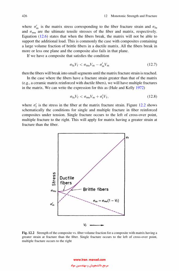
where s0m is the matrix stress corresponding to the fiber fracture strain and sfuand smu are the ultimate tensile stresses of the fiber and matrix, respectively.

Equation (12.6) states that when the fibers break, the matrix will not be able to

support the additional load. This is commonly the case with composites containing

a large volume fraction of brittle fibers in a ductile matrix. All the fibers break in

more or less one plane and the composite also fails in that plane.

If we have a composite that satisfies the condition

sfuVf < smuVm � s0mVm (12.7)

then the fiberswill break into small segments until thematrix fracture strain is reached.

In the case where the fibers have a fracture strain greater than that of the matrix

(e.g., a ceramic matrix reinforced with ductile fibers), we will have multiple fractures

in the matrix. We can write the expression for this as (Hale and Kelly 1972)

sfuVf < smuVm þ s0fVf ; (12.8)

where s0f is the stress in the fiber at the matrix fracture strain. Figure 12.2 shows

schematically the conditions for single and multiple fracture in fiber reinforced

composites under tension. Single fracture occurs to the left of cross-over point,

multiple fracture to the right. This will apply for matrix having a greater strain at

fracture than the fiber.

Fig. 12.2 Strength of the composite vs. fiber volume fraction for a composite with matrix having a

greater strain at fracture than the fiber. Single fracture occurs to the left of cross-over point,

multiple fracture occurs to the right



12.3.2 Debonding, Fiber Pullout, and Delamination Fracture

Debonding of the fiber/matrix interface, fiber pullout, and delamination fracture are

some of the features that are commonly observed in fiber reinforced composites;

these modes of fractue are not observed in conventional, monolithic materials.

Consider the situation wherein a crack originates in the matrix and approaches the

fiber/matrix interface. In a short fiber composite with a critical length lc, fibers withextremities within a distance lc/2 from the plane of the crack will debond and pull

out of the matrix (see Fig. 10.7). These fibers will not break. In fact, the fraction of

fibers pulling out will be lc/l. Continuous fibers (l > lc) invariably have flaws

distributed along their length. Thus, some of them may fracture in the plane of

the crack, while others may fracture away from the crack plane. This is treated in

some detail later in this section.

The final fracture of the composite will generally involve some fiber pullout.

Consider a model composite consisting of a fiber of length l embedded in a matrix;

see Fig. 12.3. If this fiber is pulled out, the bonding between the matrix and the fiber

will produce a shear stress t parallel to the fiber surface. The shear force acting on

the fiber as a result of this stress is given by 2prftl, where rf is the fiber radius. Let tibe the maximum shear stress that the interface can support and let sfu be the fiberfracture stress in tension. The maximum force caused by this normal stress on the

fiber is pr2f sfu. For maximum fiber strengthening, we would like the fiber to break

rather than get pulled out of the matrix. From a toughness point of view, however,

fiber pullout may be more desirable. We can then write from the balance of forces

the following condition for the fiber to be fractured under tension:

pr2f sfu < 2prftil

or

sfu4ti

<l

2rf¼ l

d; (12.9)

where d is the fiber diameter and the ratio l/d is the aspect ratio of the fiber.

Fig. 12.3 A fiber of length l, embedded in a matrix, being pulled out




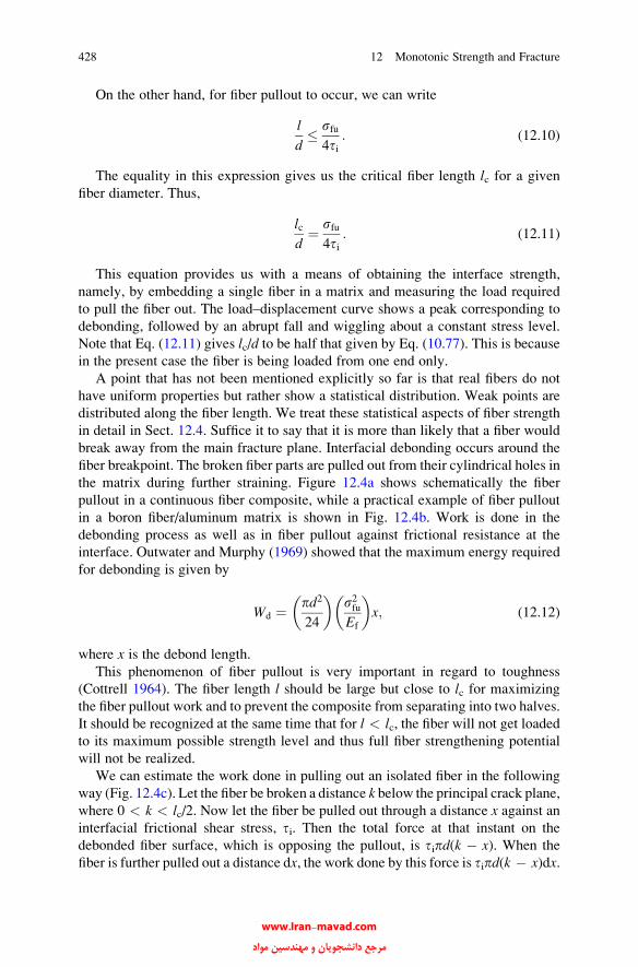
On the other hand, for fiber pullout to occur, we can write

l

d� sfu

4ti: (12.10)

The equality in this expression gives us the critical fiber length lc for a given

fiber diameter. Thus,

lcd¼ sfu

4ti: (12.11)

This equation provides us with a means of obtaining the interface strength,

namely, by embedding a single fiber in a matrix and measuring the load required

to pull the fiber out. The load–displacement curve shows a peak corresponding to

debonding, followed by an abrupt fall and wiggling about a constant stress level.

Note that Eq. (12.11) gives lc/d to be half that given by Eq. (10.77). This is becausein the present case the fiber is being loaded from one end only.

A point that has not been mentioned explicitly so far is that real fibers do not

have uniform properties but rather show a statistical distribution. Weak points are

distributed along the fiber length. We treat these statistical aspects of fiber strength

in detail in Sect. 12.4. Suffice it to say that it is more than likely that a fiber would

break away from the main fracture plane. Interfacial debonding occurs around the

fiber breakpoint. The broken fiber parts are pulled out from their cylindrical holes in

the matrix during further straining. Figure 12.4a shows schematically the fiber

pullout in a continuous fiber composite, while a practical example of fiber pullout

in a boron fiber/aluminum matrix is shown in Fig. 12.4b. Work is done in the

debonding process as well as in fiber pullout against frictional resistance at the

interface. Outwater and Murphy (1969) showed that the maximum energy required

for debonding is given by

Wd ¼ pd2

24

� �s2fuEf

� �x; (12.12)

where x is the debond length.

This phenomenon of fiber pullout is very important in regard to toughness

(Cottrell 1964). The fiber length l should be large but close to lc for maximizing

the fiber pullout work and to prevent the composite from separating into two halves.

It should be recognized at the same time that for l < lc, the fiber will not get loadedto its maximum possible strength level and thus full fiber strengthening potential

will not be realized.

We can estimate the work done in pulling out an isolated fiber in the following

way (Fig. 12.4c). Let the fiber be broken a distance k below the principal crack plane,

where 0 < k < lc/2. Now let the fiber be pulled out through a distance x against aninterfacial frictional shear stress, ti. Then the total force at that instant on the

debonded fiber surface, which is opposing the pullout, is tipd(k � x). When the

fiber is further pulled out a distance dx, the work done by this force is tipd(k � x)dx.



http://dx.doi.org/10.1007/978-0-387-74365-3_10#Equ69_10

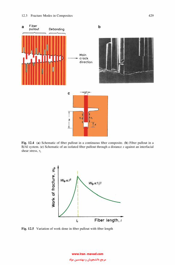
Fig. 12.4 (a) Schematic of fiber pullout in a continuous fiber composite. (b) Fiber pullout in a

B/Al system. (c) Schematic of an isolated fiber pullout through a distance x against an interfacial

shear stress, ti

Fig. 12.5 Variation of work done in fiber pullout with fiber length



We can obtain the total work done in pulling out the fiber over the distance k by

integrating. Thus,

Work of fiber pullout ¼ðk0

tipd k � xð Þdx ¼ tipdk2

2: (12.13)

The reader should be careful with our use of d as a symbol for the fiber

diameter and differentiation. Now the pullout length of the fiber can vary between

a minimum of 0 and a maximum of lc/2. The average work of pullout per fiber

is then

Wfp ¼ 1

lc=2

ðlc=20

tipdk2

2dk ¼ tipdlc2

24:

This analysis assumes that all fibers are pulled out. In a discontinuous fiber

composite, it has been observed experimentally (Kelly 1970) that only the fibers

with ends within a distance lc/2 of the main fracture plane and that cross this

fracture plane undergo pullout. Thus, it is more likely that a fraction (lc/l) of fiberswill pull out. The above expression for average work done per fiber can then be

modified as

Wfp ¼ lcl

� �pdtil2c24

: (12.14)

In general, fiber pullout provides a more significant contribution to composite

fracture toughness than fiber/matrix debonding. The reader should appreciate

the fact that debonding must precede pullout. Figure 12.5 shows schematically

the variation of work of fracture with fiber length. For l < lc, Wfp increases as l2

(substitute l for k in Eq. (12.14)). Physically, this makes sense because as the fiber

length increases, an increasing fiber length will be pulled out. For l > lc, as pointedout earlier, some fibers will fracture in the plane of fracture of the composite and

thus their contribution to Wfp will be nought. Those fibers whose ends are within a

distance of lc/2 from the fracture plane, they will undergo the process of fiber

pullout. In this case, the average work of fracture is given by Eq. (12.14), i.e., Wfp

varies as 1/l because with increasing fiber length, fiber breaks intervene and the

fiber pullout decreases. The work of fracture, Wfp peaks at l ¼ lc. The reader can

easily show that for l ¼ lc, the average stress in the fiber will only be half that in aninfinitely long fiber.

One measure of fracture toughness can loosely be defined as resistance to crack

propagation. Consider a fiber reinforced composite containing a crack transverse to

the fibers. In such a situation, we can increase the crack propagation resistance by

one of the following means, each of which involves additional work:

1. Plastic deformation of the matrix (applicable in a metal matrix).

2. Presence of weak interfaces, fiber/matrix separation, and deflection of the crack.

3. Fiber pullout.



For a metal matrix composite the work of fracture is mostly the work done

during plastic deformation of the matrix. The work of fracture is proportional to d(Vm/Vf)

2 (Cooper and Kelly 1967), where d is the fiber diameter and Vm and Vf are

the matrix and fiber volume fractions, respectively. This is understandable

inasmuch as in the case of large-diameter fibers, for a given Vf, the advancing

crack will result in a greater amount of plastically deformed matrix, which will

result in a larger work of fracture.

Crack deflection along an interface frequently follows separation of the fiber/

matrix interface. This provides us with a potent mechanism of increasing the crack

propagation resistance in composites; we discussed this topic in Chap. 7. This

improvement in fracture toughness owing to the presence of weak interfaces has

been confirmed experimentally. This crack deflection mechanism can be a major

source of toughness in ceramic matrix composites (Chawla 2003). Yet another

related failure mode in laminated composites is the delamination failure associated

with the plies and the fiber/matrix interface. This fracture mode is of importance in

structural applications involving long-term use, for example, under fatigue

conditions and where environmental effects are important. Highly oriented fibers

such as aramid can also contribute to the work of fracture. Figure 12.6 shows a

delamination-type fracture in a Kevlar aramid/epoxy composite (Saghizadeh and

Dharan 1985) and the characteristic fibrillation of the Kevlar fiber, which stems

Fig. 12.6 A delamination-

type fracture of Kevlar/epoxy

composite. Note the

characteristic fibrils in the

fiber [from Saghizadeh and

Dharan (1985), used with

permission]



http://dx.doi.org/10.1007/978-0-387-74365-3_7

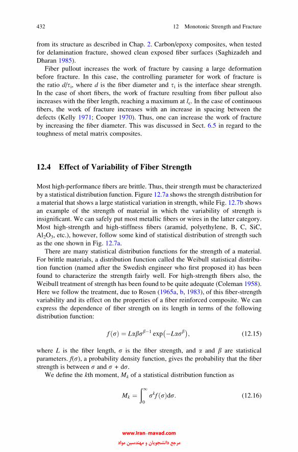
from its structure as described in Chap. 2. Carbon/epoxy composites, when tested

for delamination fracture, showed clean exposed fiber surfaces (Saghizadeh and

Dharan 1985).

Fiber pullout increases the work of fracture by causing a large deformation

before fracture. In this case, the controlling parameter for work of fracture is

the ratio d/ti, where d is the fiber diameter and ti is the interface shear strength.

In the case of short fibers, the work of fracture resulting from fiber pullout also

increases with the fiber length, reaching a maximum at lc. In the case of continuousfibers, the work of fracture increases with an increase in spacing between the

defects (Kelly 1971; Cooper 1970). Thus, one can increase the work of fracture

by increasing the fiber diameter. This was discussed in Sect. 6.5 in regard to the

toughness of metal matrix composites.

12.4 Effect of Variability of Fiber Strength

Most high-performance fibers are brittle. Thus, their strength must be characterized

by a statistical distribution function. Figure 12.7a shows the strength distribution for

a material that shows a large statistical variation in strength, while Fig. 12.7b shows

an example of the strength of material in which the variability of strength is

insignificant. We can safely put most metallic fibers or wires in the latter category.

Most high-strength and high-stiffness fibers (aramid, polyethylene, B, C, SiC,

Al2O3, etc.), however, follow some kind of statistical distribution of strength such

as the one shown in Fig. 12.7a.

There are many statistical distribution functions for the strength of a material.

For brittle materials, a distribution function called the Weibull statistical distribu-

tion function (named after the Swedish engineer who first proposed it) has been

found to characterize the strength fairly well. For high-strength fibers also, the

Weibull treatment of strength has been found to be quite adequate (Coleman 1958).

Here we follow the treatment, due to Rosen (1965a, b, 1983), of this fiber-strength

variability and its effect on the properties of a fiber reinforced composite. We can

express the dependence of fiber strength on its length in terms of the following

distribution function:

f sð Þ ¼ Labsb�1 exp �Lasb� �

; (12.15)

where L is the fiber length, s is the fiber strength, and a and b are statistical

parameters. f(s), a probability density function, gives the probability that the fiber

strength is between s and s + ds.We define the kth moment, Mk of a statistical distribution function as

Mk ¼ð10

skf sð Þds: (12.16)



http://dx.doi.org/10.1007/978-0-387-74365-3_2


Knowing that the mean strength of the fiber is given by �s ¼ R10

sf ðsÞds ,we can write

s ¼ M1 (12.17)

and the standard deviation s can be expressed as

s ¼ M2 �M21

� �1=2: (12.18)

From the Weibull distribution Eq. (12.15) and Eqs. (12.17) and (12.18), we

obtain

s ¼ aLð Þ�1=bG 1� 1

b

� �(12.19)

and

s ¼ aLð Þ�1=b G 1þ 2

b

� �� G2 1þ 1

b

� �� 1=2; (12.20)

where G(n) is the gamma function given byR10

expð�xÞxn�1 dx. Note that x in thisintegral is a general, mathematical variable. The reader should not confuse x with

the fiber length, x in Fig. 12.4. The coefficient of variation m for this distribution

then follows from the expression given below

m ¼ s

s¼ G 1þ 2=bð Þ � G2 1þ 1=bð Þ� 1=2

G 1þ 1=bð Þ : (12.21)

Fig. 12.7 (a) Strength distribution for a brittle material. (b) Strength distribution for material with

insignificant variability of strength

12.4 Effect of Variability of Fiber Strength 433


We note that m is a function only of the parameter b. Rosen showed that for

0.05 � m � 0.5, m � b�0.92 or m � 1/b. In other words, parameter b is an inverse

measure of the coefficient of variation m. For fibers that are characterized by the

Weibull distribution (12.15), b > 1. For glass fibers, m can be about 0.1, which

would correspond to b ¼ 11. For boron and SiC fibers, m can be between 0.2 and

0.4 and b will be between 2.7 and 5.8.

Let us consider (12.19). We can write for a unit length of fiber

s1 ¼ ka�1=b; (12.22)

where

k ¼ G 1þ 1

b

� �: (12.23)

For b > 1, we have 0.88 � k � 1.0. Thus, we can regard the quantity a�1/b as

the reference strength level. We can plot Eq. (12.19) in the form of curves of s=a�l=b (a normalized mean strength) against fiber length L for different b values,

see Fig. 12.8. In Fig. 12.8, b ¼ 1 corresponds to a spike distribution function such

as the one shown in Fig. 12.7b. In such a case, all the fibers have identical strength

and there is no fiber length dependence. For b ¼ 10, which corresponds to a

m � 12 %, an order-of-magnitude increase in fiber length produces a 20 % fall in

average strength. For b ¼ 4, the corresponding fall in strength is about 50 %.

We can obtain the statistical mode s*, which is the most probable strength value

by differentiating Eq. (12.15) and equating it to zero. Thus,

s� � b� 1

b

� �1=b

aLð Þ�1=b: (12.24)

For large b,

s� � aLð Þ�1=b: (12.25)

(aL)�1/b, as mentioned earlier, is a reference stress level. The values of a and bcan be obtained from experimental s and m values.

If we use Weibull statistics to characterize ceramic fibers, we can answer the

following important question: For making tough, strong fiber reinforced ceramic

matrix composites, would we want fibers with small or large Weibull modulus?

Lara-Curzio et al. at Oak Ridge National Laboratory have examined this problem.

Figure 12.9 shows their results in the form of fiber bundle strength vs. strain in a

CMC for different Weibull modulus values. The take away message of this figure is

their properties), the more graceful failure of the CMC. It is understandable if we

recall that a low Weibull modulus fiber will fracture in the composite at different

strain values and thus spread the damage, which would lead to a final

noncatastrophic failure of the CMC.


that the lower the Weibull modulus of ceramic fibers, (i.e., the less uniformity in


There is yet another important statistical point with regard to this variability of

fiber strength. This has to do with the fact that in a unidirectionally aligned fiber

composite, the fibers act in a bundle in parallel. It turns out that the strength of a

bundle of fibers whose elements do not possess a uniform strength is not the average

strength of the fibers. Coleman (1958) investigated this nontrivial problem, which

we describe below.

In the simplest case, we assume that all fibers have the same cross section and the

same stress–strain curve but with different strain-to-fracture values. Let the strength

distribution function for the fiber be given by the Weibull function f(s), Eq. (12.15),then the probability that a fiber will break before a certain value s is attained is

given by the cumulative strength distribution function F(s). We can write

F sð Þ ¼ðs0

f sð Þds: (12.26)

Fig. 12.8 Normalized mean fiber strength vs. fiber length L

Fig. 12.9 Fiber bundle strength vs. strain in a CMC for different Weibull modulus values

(courtesy of E. Lara-Curzio)



One makes a large number of measurements of strength of individual packets or

bundles of fibers. Each bundle has the same large number of fibers of identical cross

section and they are loaded from their extremities. From such tests we can obtain the

mean fiber strength in the bundle. Daniels (1945) showed that, for a very large number

of fibers in the bundle, the distribution of the mean fiber strength at bundle failure

attains a normal distribution, with the expectation or mean value being given by

sB ¼ sfu 1� F sfuð Þ½ �; (12.27)

where sfu is the maximum fiber strength, i.e., sfu corresponds to the condition

where the bundle supports the maximum load. Thus, we can obtain sfu by taking the

derivative and equating it to zero,

d

dss 1� F sð Þ½ �f gs¼sfu ¼ 0: (12.28)

The fiber bundle strength, sB values are characterized by the following density

function for normal distribution function:

o sBð Þ ¼ 1

CB

ffiffiffiffiffiffi2p

p exp � 1

2

sB � sBCB

� �2" #

; (12.29)

where CB is the standard deviation given by

CB ¼ sfu F sfuð Þ 1� F sfuð Þ½ �f g1=2N�1=2; (12.30)

where N is the number of fibers in the bundle.

As N becomes very large, not unexpectedly, the standard variation CB becomes

small. That is, the larger the number of fibers in the bundle, the more reproducible is

the bundle strength. For bundles characterized by Eq. (12.29), we can define a

cumulative distribution function O(sB). Thus,

O sBð Þ ¼ðsB0

o sBð ÞdsB: (12.31)

Consider the Weibull distribution, Eq. (12.15), then we have [from Eq. (12.28)]

sfu ¼ Labð Þ�1=b: (12.32)

Substituting this in Eq. (12.27), we get the following expression (left as an

exercise for the reader to do) for the mean fiber bundle strength

sB ¼ Labeð Þ�1=b: (12.33)



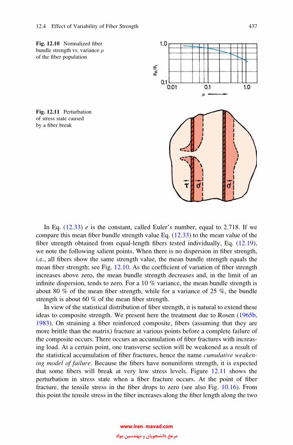
In Eq. (12.33) e is the constant, called Euler’s number, equal to 2.718. If we

compare this mean fiber bundle strength value Eq. (12.33) to the mean value of the

fiber strength obtained from equal-length fibers tested individually, Eq. (12.19),

we note the following salient points. When there is no dispersion in fiber strength,

i.e., all fibers show the same strength value, the mean bundle strength equals the

mean fiber strength; see Fig. 12.10. As the coefficient of variation of fiber strength

increases above zero, the mean bundle strength decreases and, in the limit of an

infinite dispersion, tends to zero. For a 10 % variance, the mean bundle strength is

about 80 % of the mean fiber strength, while for a variance of 25 %, the bundle

strength is about 60 % of the mean fiber strength.

In view of the statistical distribution of fiber strength, it is natural to extend these

ideas to composite strength. We present here the treatment due to Rosen (1965b,

1983). On straining a fiber reinforced composite, fibers (assuming that they are

more brittle than the matrix) fracture at various points before a complete failure of

the composite occurs. There occurs an accumulation of fiber fractures with increas-

ing load. At a certain point, one transverse section will be weakened as a result of

the statistical accumulation of fiber fractures, hence the name cumulative weaken-ing model of failure. Because the fibers have nonuniform strength, it is expected

that some fibers will break at very low stress levels. Figure 12.11 shows the

perturbation in stress state when a fiber fracture occurs. At the point of fiber

fracture, the tensile stress in the fiber drops to zero (see also Fig. 10.16). From

this point the tensile stress in the fiber increases along the fiber length along the two

Fig. 12.11 Perturbation

of stress state caused

by a fiber break

Fig. 12.10 Normalized fiber

bundle strength vs. variance mof the fiber population




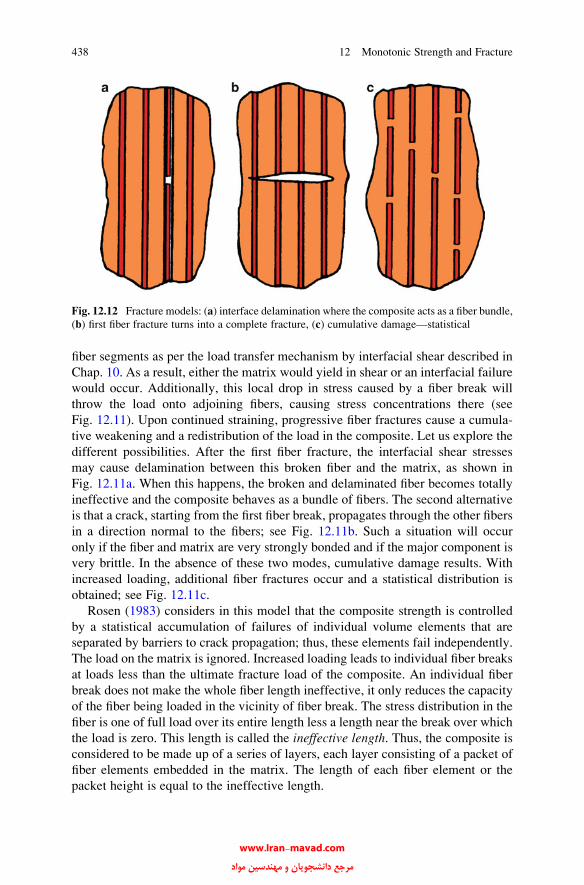
fiber segments as per the load transfer mechanism by interfacial shear described in

Chap. 10. As a result, either the matrix would yield in shear or an interfacial failure

would occur. Additionally, this local drop in stress caused by a fiber break will

throw the load onto adjoining fibers, causing stress concentrations there (see

Fig. 12.11). Upon continued straining, progressive fiber fractures cause a cumula-

tive weakening and a redistribution of the load in the composite. Let us explore the

different possibilities. After the first fiber fracture, the interfacial shear stresses

may cause delamination between this broken fiber and the matrix, as shown in

Fig. 12.11a. When this happens, the broken and delaminated fiber becomes totally

ineffective and the composite behaves as a bundle of fibers. The second alternative

is that a crack, starting from the first fiber break, propagates through the other fibers

in a direction normal to the fibers; see Fig. 12.11b. Such a situation will occur

only if the fiber and matrix are very strongly bonded and if the major component is

very brittle. In the absence of these two modes, cumulative damage results. With

increased loading, additional fiber fractures occur and a statistical distribution is

obtained; see Fig. 12.11c.

Rosen (1983) considers in this model that the composite strength is controlled

by a statistical accumulation of failures of individual volume elements that are

separated by barriers to crack propagation; thus, these elements fail independently.

The load on the matrix is ignored. Increased loading leads to individual fiber breaks

at loads less than the ultimate fracture load of the composite. An individual fiber

break does not make the whole fiber length ineffective, it only reduces the capacity

of the fiber being loaded in the vicinity of fiber break. The stress distribution in the

fiber is one of full load over its entire length less a length near the break over which

the load is zero. This length is called the ineffective length. Thus, the composite is

considered to be made up of a series of layers, each layer consisting of a packet of

fiber elements embedded in the matrix. The length of each fiber element or the

packet height is equal to the ineffective length.

Fig. 12.12 Fracture models: (a) interface delamination where the composite acts as a fiber bundle,

(b) first fiber fracture turns into a complete fracture, (c) cumulative damage—statistical



http://dx.doi.org/10.1007/978-0-387-74365-3_10

As the load is increased, fiber breaks accumulate until at a critical load a packet

of elements is unable to transmit the applied load and the composite fails. Thus,

composite failure occurs because of this weakened section. A characteristic length dcorresponding to the packet height must be chosen. The term d is defined as the lengthover which the stress attains a certain fraction f of the unperturbed stress in the fiber.

Rosen took f equal to that length over which the stress increases elastically from

0 (at a fiber end) to 90 % of the unperturbed level. One then derives the stress

distribution in the fiber elements and packets. The theory of the weakest link is then

applied to obtain the composite strength. In the case of fibers characterized by the

Weibull distribution, the stress distribution in the fiber elements is

w sð Þ ¼ dabsb�1 exp �dasb� �

; (12.34)

where d is the fiber element length (i.e., the ineffective length).

The composite is now a chain, the strength of whose elements is given by a

normal distribution function w(sB). The strength of a chain having m links (do not

confuse with the Weibull modulus) of this population is characterized by a

distribution function l(sc):

l scð Þ ¼ mw scð Þ 1� O scð Þ½ �m�1; (12.35)

where

O scð Þ ¼ðsc0

w scð Þds: (12.36)

Suppose now that the number of elements N (i.e., the number of fibers in the

bundle) in a composite is so large that the standard deviation of the packet tends to

zero. Then the statistical mode of composite strength is equal to sB Eq. (12.27).

In the case of a Weibull distribution, it follows from Eq. (12.33) that

s�c ¼ dabeð Þ�1=b(12.37)

and the statistical mode of the tensile strength of the composite is

s� ¼ Vf dabeð Þ�1=b; (12.38)

where Vf is the fiber volume fraction and e ¼ 2.718.

It should be pointed out that d will be of the order of 10–100 fiber diameters and

thus much smaller than the gage length used for individual tests.

If we compare the (cumulative) average strength of a group of fibers of length Lwith the expected fiber strength from Eqs. (12.21) and (12.37), we get



s�csL

¼ L

dbe

� �1=b1

G 1þ 1=bð Þ : (12.39)

For b ¼ 5 and L/d ¼ 100, we have s�c=sL ¼ 1:62; that is, the composite will be

much stronger than what we expect from individual fiber tests. We can plot the

composite strength s�c , normalized with respect to the average strength sL , ofindividual fibers of length L against m, the variance of individual fiber strengths; seeFig. 12.13. The curves shown are for different values of the ratio L/d. For L/d ¼ 1,

that is, the fiber length is equal to the ineffective length, the statistical mode of

composite strength is less than the average fiber strength. This difference between

the two increases with an increase in m of the fibers. For a more realistic ratio, for

example, L/d > 10, we note that the composite strength is higher than the average

fiber strength.

A modification of this cumulative weakening model has been proposed by

Zweben and Rosen (1970), which takes into account the redistribution of stress

that results at each fiber break; that is, there is greater probability that fracture will

occur in immediately adjacent fibers because of a stress magnification effect.

12.5 Strength of an Orthotropic Lamina

We saw in Chaps. 10 and 11 that fiber reinforced composites are anisotropic in

elastic properties. This results from the fact that the fibers are aligned in the matrix.

Additionally, the fibers are, generally, a lot stiffer and stronger than the matrix.

Therefore, not unexpectedly, fiber reinforced composites also show anisotropy in

strength properties. Quite frequently, the strength in the longitudinal direction is

Fig. 12.13 Normalized composite strength s�c=�sL vs. variance m (from Fiber composite materials,

ASM, 1965, pp 39, 38, used with permission)



http://dx.doi.org/10.1007/978-0-387-74365-3_10

http://dx.doi.org/10.1007/978-0-387-74365-3_11

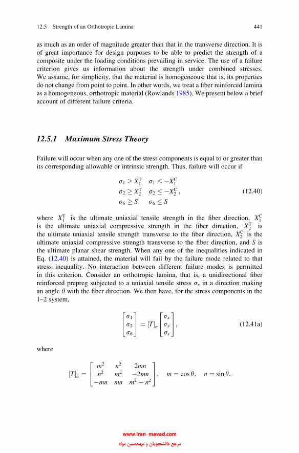
as much as an order of magnitude greater than that in the transverse direction. It is

of great importance for design purposes to be able to predict the strength of a

composite under the loading conditions prevailing in service. The use of a failure

criterion gives us information about the strength under combined stresses.

We assume, for simplicity, that the material is homogeneous; that is, its properties

do not change from point to point. In other words, we treat a fiber reinforced lamina

as a homogeneous, orthotropic material (Rowlands 1985). We present below a brief

account of different failure criteria.

12.5.1 Maximum Stress Theory

Failure will occur when any one of the stress components is equal to or greater than

its corresponding allowable or intrinsic strength. Thus, failure will occur if

s1 � XT1 s1 � �XC

1

s2 � XT2 s2 � �XC

2

s6 � S s6 � S

; (12.40)

where XT1 is the ultimate uniaxial tensile strength in the fiber direction, XC

1

is the ultimate uniaxial compressive strength in the fiber direction, XT2 is

the ultimate uniaxial tensile strength transverse to the fiber direction, XC2 is the

ultimate uniaxial compressive strength transverse to the fiber direction, and S is

the ultimate planar shear strength. When any one of the inequalities indicated in

Eq. (12.40) is attained, the material will fail by the failure mode related to that

stress inequality. No interaction between different failure modes is permitted

in this criterion. Consider an orthotropic lamina, that is, a unidirectional fiber

reinforced prepreg subjected to a uniaxial tensile stress sx in a direction making

an angle y with the fiber direction. We then have, for the stress components in the

1–2 system,

s1s2s6

24

35 ¼ T½ �s

sxsyss

24

35; (12.41a)

where

T½ �s ¼m2 n2 2mnn2 m2 �2mn

�mn mn m2 � n2

24

35; m ¼ cos y; n ¼ sin y:

12.5 Strength of an Orthotropic Lamina 441


Using the fact that only sx is nonzero, we obtain

s1 ¼ sxm2

s2 ¼ sxn2

s6 ¼ �sxmn: (12.41b)

Using these expressions forsx in conjunction with Eq. (12.40), we get, according

to the maximum stress criterion, the following three independent failure modes:

sx ¼ XT1

m2longitudinal tensileð Þ

sx ¼ XT2

n2transverse tensileð Þ

sx ¼ S

mnplanar shearð Þ

; (12.42)

Here we are disregarding the sign of the shear stress, S. Figure 12.14 shows the failurestress with changing fiber orientation, y. Note the failure mode changes

from longitudinal tension to planar shear to transverse tension, as shown by the dashed

lines. The agreement with experiment is poor, particularly around y ¼ p/4. Thisindicates that at intermediate angles, interactions between failure modes do occur.

Fig. 12.14 Variation of strength with fiber orientation for boron/epoxy. Quadratic interaction

criterion (solid curve) shows better agreement with experimental data than the maximum stress

criterion (dashed curve) [after Pipes and Cole (1973)]



12.5.2 Maximum Strain Criterion

This criterion is analogous to the maximum stress criterion. Failure occurs when

any one of the strain components is equal to or greater than its corresponding

allowable strain. Thus,

e1 � eT1 e1 � �eC1

e2 � eT2 e2 � �eC2

e6 � e6 e6 � e6

; (12.43)

where eT1 is the ultimate tensile strain in the fiber direction, eC1 is the ultimate

compressive strain in the fiber direction, eT2 is the ultimate tensile strain in the

transverse direction,eC2 is the ultimate compressive strain in the transverse direction,

and e6 is the ultimate planar shear strain. This criterion is also not very satisfactory

for the same reason as the maximum stress criterion, namely, absence of any

interaction of failure modes.

12.5.3 Maximum Work (or the Tsai–Hill) Criterion

This criterion, originally proposed by Hill, is based on a modification of the

distortion energy criterion for ductile metals. Hill’s modification worked for aniso-

tropic ductile metals such as metals that have undergone rolling etc. The Tsai–Hill

criterion adopted Hill’s modification to orthotropic fiber reinforced composites.

According to the Tsai–Hill criterion, failure of an orthotropic lamina will occur

under a general two-dimensional stress state when the following expression holds:

s21X21

� s1s2X21

þ s22X22

þ s26S2

� 1; (12.44)

where X1, X2, and S are the longitudinal tensile failure strength, the transverse

tensile failure strength, and the inplane shear failure strength, respectively.

If compressive stresses are involved, then the corresponding compressive failure

strengths should be used.

Consider again a uniaxial stress sx applied to an orthotropic lamina. Then,

following Eq. (12.41), we can write

s1 ¼ sxm2

s2 ¼ sxn2

s6 ¼ �sxmn

; (12.45)



where m ¼ cos y and n ¼ sin y. Substituting these values in Eq. (12.44), we have

m4

X21

þ n4

X22

þ m2n21

S2� 1

X21

� �<

1

s2x¼ 1

s2y: (12.46)

This expression gives us the off-axis strength of composite lamina as function of

fiber orientation. We can use this to verify the validity of the criterion. This criterion

does take into account the interaction between the failure modes. However, it does

not make any direct distinction between tensile and compressive stresses.

12.5.4 Quadratic Interaction Criterion

As the name indicates, this criterion takes into account the stress interactions.

Tsai and Wu (1971) proposed this modification of the Hill theory for a lamina by

adding some additional terms. Tsai and Hahn (1980) provide a good account of

this criterion. According to this theory, the failure surface in stress space can be

described by a function of the form

f sð Þ ¼ Fisi þ Fijsisj ¼ 1 i; j ¼ 1; 2; 6; (12.47)

where Fi and Fij are the strength parameters. For the case of plane stress, i, j ¼ 1,

2, 6. We can expand Eq. (12.47) as follows:

F1s1 þ F2s2 þ F6s6 þ F11s21 þ F22s22 þ F66s26 þ 2F12s1s2þ 2F16s1s6 þ 2F26s2s6 ¼ 1:

(12.48)

For the orthotropic lamina, sign reversal for normal stresses, whether tensile

or compressive, is important. The linear stress terms provide for this difference.

For the shear stress component, the sign reversal should be immaterial. Thus, terms

containing the first-degree shear stress must vanish. These terms are F16s1s6,F26s2s6, and F6s6. The stress components in general are not zero. Therefore, for

these three terms to vanish, we must have

F16 ¼ F26 ¼ F6 ¼ 0:

Equation (12.48) is now simplified to

F1s1 þ F2s2 þ F11s21 þ F22s22 þ F66s26 þ 2F12s1s2 ¼ 1: (12.49)

There are six strength parameters in Eq. (12.49). We can measure five of these by

the following simple tests.



12.5.4.1 Longitudinal (Tensile and Compressive) Tests

If s1 ¼ XT1 ; then F11 XT

1

� �2 þ F1XT1 ¼ 1:

If s1 ¼ �XC1 ; then F11 XC

1

� �2 þ F1XC1 ¼ 1:

From these we get

F11 ¼ 1

XT1X

C1

(12.50)

and

F1 ¼ 1

XT1

� 1

XC1

: (12.51)

12.5.4.2 Transverse (Tensile and Compressive) Tests

If XT2 and XC

2 are the transverse tensile and compressive strengths, respectively,

then proceeding as earlier, we get

F22 ¼ 1

XT2X

C2

(12.52)

and

F2 ¼ 1

XT2

� 1

XC2

: (12.53)

12.5.4.3 Longitudinal Shear Test

If S is the shear strength, we have

F66 ¼ 1

S2: (12.54)

Thus, we can express all the failure constants except F12 in terms of the ultimate

intrinsic strength properties. F12 is the only remaining parameter and it must be

evaluated by means of a biaxial test, which can be quite complicated to do. Many

workers (Hoffman 1967; Cowin 1979) have proposed variations of the Tsai–Wu

criterion involving F12 explicitly in terms of uniaxial strengths. Tsai and Hahn (1980)

suggest that, in the absence of other data, we should use F12 ¼ �0:5ffiffiffiffiffiffiffiffiffiffiffiffiffiffiF11F22

p.

Figure 12.13 shows the variation of strength with orientation assuming F12 ¼ 0 for



the boron/epoxy system (Pipes and Cole 1973). The intrinsic properties of this boron

fiber/epoxy system used to obtain the curve in Fig. 12.13 are as follows:

XT1 ¼ 27:3MPa XT

2 ¼ 1:3MPa S ¼ 1:4MPa

XC1 ¼ 52:4MPa XC

2 ¼ 6:5MPa:

Note the excellent agreement between the computed curve using the quadratic

interaction criterion and the experimental values. The agreement with the maxi-

mum stress criterion (dashed curve) is poor.

12.5.4.4 Comparison of Failure Theories

Important attributes of the four main failure theories, namely, maximum stress,

maximum strain, maximum work, and quadratic interaction are compared in

Table 12.1. The applicability of a given theory depends on material properties and

the failure modes (Daniel and Ishai 1994). As expected, the maximum stress and

maximum strain criteria are generally valid with brittle materials. They do require

three subcriteria but are conceptually quite simple and experimental determination

of parameters is also quite simple and straightforward. The two interactive theories,

maximum work and quadratic interaction, are more suitable for computational

purposes. In particular, the quadratic interaction criterion is quite general and compre-

hensive. Both require more complicated experimental characterization. According

to Daniel and Ishai (1994), when material behavior and failure modes are not known

and when a conservative approach is required, all four criteria should be evaluated

Table 12.1 Comparison of failure theories [after Daniel and Ishai (1994)]

Criterion Physical basis Computational aspects

Experimental

characterization

Maximum

stress

Tensile behavior of brittle

material, no stress

interaction

Inconvenient Simple

Maximum

strain

Tensile behavior of brittle

material, no stress

interaction

Inconvenient Simple

Maximum

work

Valid for ductile

anisotropic materials,

curve fitting

for heterogeneous

brittle composites

Can be programmed,

different functions

required for tensile and

compressive strengths

Biaxial testing needed

Quadratic

interaction

Mathematically consistent,

reliable curve fitting

Simple, comprehensive Complicated, numerous

parameters needed



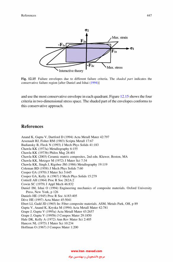
and use the most conservative envelope in each quadrant. Figure 12.15 shows the four

criteria in two-dimensional stress space. The shaded part of the envelopes conforms to

this conservative approach.

References

Anand K, Gupta V, Dartford D (1994) Acta Metall Mater 42:797

Arsenault RJ, Fisher RM (1983) Scripta Metall 17:67

Budiansky B, Fleck N (1993) J Mech Phys Solids 41:183



Chawla KK (2003) Ceramic matrix composites, 2nd edn. Kluwer, Boston, MA


Chawla KK, Singh J, Rigsbee JM (1986) Metallography 19:119

Coleman BD (1958) J Mech Phys Solids 7:60

Cooper GA (1970) J Mater Sci 5:645

Cooper GA, Kelly A (1967) J Mech Phys Solids 15:279

Cottrell AH (1964) Proc R Soc 282A:2

Cowin SC (1979) J Appl Mech 46:832

Daniel IM, Ishai O (1994) Engineering mechanics of composite materials. Oxford University

Press, New York, p 126

Daniels HE (1945) Proc R Soc A183:405

Deve HE (1997) Acta Mater 45:5041

Ebert LI, Gadd JD (1965) In: Fiber composite materials. ASM, Metals Park, OH, p 89

Gupta V, Anand K, Kryska M (1994) Acta Metall Mater 42:781

Grape J, Gupta V (1995a) Acta Metall Mater 43:2657

Grape J, Gupta V (1995b) J Compos Mater 29:1850

Hale DK, Kelly A (1972) Ann Rev Mater Sci 2:405

Hancox NL (1975) J Mater Sci 10:234

Hoffman O (1967) J Compos Mater 1:200

Fig. 12.15 Failure envelopes due to different failure criteria. The shaded part indicates the

conservative failure region [after Daniel and Ishai (1994)]

References 447


Kelly A (1970) Proc R Soc London A319:95

Kelly A (1971) In: The properties of fibre composites. IPS Science & Technology, Guildford, p 5

Kelly A, Lilholt H (1969) Philos Mag 20:311

Kyriakides S, Arseculeratne R, Perry EJ, Liechti KM (1995) Int J Solids Struct 32:689

Lager JR, June RR (1969) J Compos Mater 3:48

Narayanan S, Schadler LS (1999) Compos Sci Technol 59:2201

Outwater JO, Murphy MC (1969) In: Proceedings of the 24th SPI/RP conference, paper 11–6,

Society of Plastics Industry, New York

Piggott MR (1984) In: Developments in reinforced plastics, 4th edn. Elsevier Applied Science

Publishers, London, p 131

Piggott MR, Harris B (1980) J Mater Sci 15:2523

Pipes RB, Cole BW (1973) J Compos Mater 7:246

Rosen BW (1965a) In: Fiber composite materials. American Society for Metals, Metals Park, OH,

p 58

Rosen BW (1965b) In: Fiber composite materials. American Society for Metals, Metals Park, OH,

p 37

Rosen BW (1983) In: Mechanics of composite materials: recent advances. Pergamon, Oxford,

p 105

Rowlands RE (1985) Failure mechanics of composites, vol 3 of the series handbook of composites.

North-Holland, Amsterdam, p 71

Saghizadeh H, Dharan CKH (1985) American Society of Mechanical Engineering. Paper #85WA/

Mats-15, presented at the Winter Annual Meeting, Miami Beach, FL

Schultheisz CR, Waas AM (1996) Prog Aerospace Sci 32:1

Tsai SW, Hahn HT (1980) Introduction to composite materials. Technomic, Westport, CT

Tsai SW, Wu EM (1971) J Compos Mater 5:58

Vogelsang M, Arsenault RJ, Fisher RM (1986) Metall Trans A 17A:379

Waas AM, Schultheisz CR (1996) Prog Aerospace Sci 32:43

Zweben C, Rosen BW (1970) J Mech Phys Solids 18:189

Further Reading



Nahas MN (1986) J Comp Technol Res 8:138

Problems

12.1. For a ceramic fiber with m ¼ 12 %, show that b � 10. Show also that if the

fiber length is changed by an order of magnitude, the corresponding drop in

the average strength is about 20 %.

12.2. In a series of tests on boron fibers, it was found that m ¼ 10 %. Compute

the ratio sB=s, where sB is the average strength of the fiber bundle and sis the average strength of fibers tested individually.



12.3. Estimate the work of fiber pullout in a 40 % carbon fiber/epoxy composite.

Given sfu ¼ 0.2 GPa, d ¼ 8 mm, and ti ¼ 2 MPa.

12.4. How would you go about testing a single fine-diameter fiber (recall that

carbon fiber has a diameter of about 7 mm)? Do discuss the effect of

variability in diameter of the fiber along its length in computing the strength

of the fiber.

Problems 449


Chapter 13

Fatigue and Creep

In Chap. 12 we described the monotonic behavior of a composite under ambient

temperature conditions of loading. There are many applications of composites

where cyclic fatigue and high-temperature, i.e., creep conditions prevail. Accord-

ingly, in this chapter we go further in complexity and describe the fatigue and creep

behavior of composites. Fatigue is the phenomenon of mechanical property degra-

dation leading to failure of a material or a component under cyclic loading.

The operative word in this definition is cyclic. This definition thus excludes the

so-called phenomenon of static fatigue, which is sometimes used to describe stress

corrosion cracking in glasses and ceramics in the presence of moisture. Creep refers

to time-dependent deformation in a material, which becomes important at relatively

high temperatures (T > 0.4Tm, where Tm is the melting point in kelvin). We first

describe fatigue and then creep of composites.

13.1 Fatigue

Degradation of mechanical properties of a material or a component under cyclic

loading is called fatigue. Understanding the fatigue behavior of composites of all

kinds is of vital importance, because without such an understanding it would be

virtually impossible to gain acceptance of the design engineers. Many high volume

applications of composite materials involve cyclic loading situations, e.g.,

components used in automobile, truck, and mass transit. It would be a fair admission

that this understanding of the fatigue behavior of composites has lagged that of other

aspects such as the elastic stiffness or strength. The major difficulty in this regard is

that the application of conventional approaches to fatigue of composites, for exam-

ple, the stress vs. cycles (S–N) curves or the application of linear elastic fracture

mechanics (LEFM), is not straightforward. Themain reasons for this are the inherent

heterogeneity and anisotropic nature of the composites. These characteristics result

in damage mechanisms in composites being very different from those encountered

in conventional, homogeneous, or monolithic materials. The fracture behavior of


451


http://dx.doi.org/10.1007/978-0-387-74365-3_12

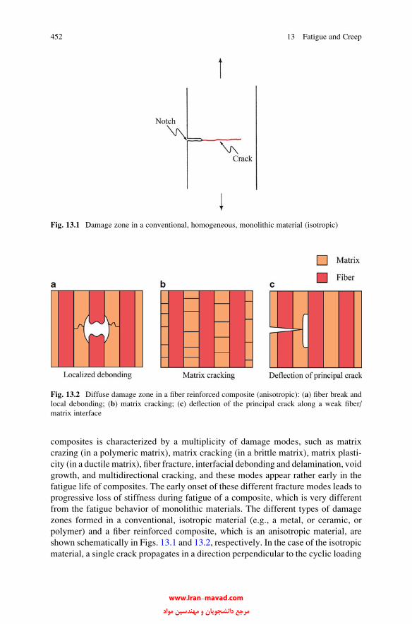
composites is characterized by a multiplicity of damage modes, such as matrix

crazing (in a polymeric matrix), matrix cracking (in a brittle matrix), matrix plasti-

city (in a ductile matrix), fiber fracture, interfacial debonding and delamination, void

growth, and multidirectional cracking, and these modes appear rather early in the

fatigue life of composites. The early onset of these different fracture modes leads to

progressive loss of stiffness during fatigue of a composite, which is very different

from the fatigue behavior of monolithic materials. The different types of damage

zones formed in a conventional, isotropic material (e.g., a metal, or ceramic, or

polymer) and a fiber reinforced composite, which is an anisotropic material, are

shown schematically in Figs. 13.1 and 13.2, respectively. In the case of the isotropic

material, a single crack propagates in a direction perpendicular to the cyclic loading

Fig. 13.1 Damage zone in a conventional, homogeneous, monolithic material (isotropic)

Fig. 13.2 Diffuse damage zone in a fiber reinforced composite (anisotropic): (a) fiber break and

local debonding; (b) matrix cracking; (c) deflection of the principal crack along a weak fiber/

matrix interface

452 13 Fatigue and Creep


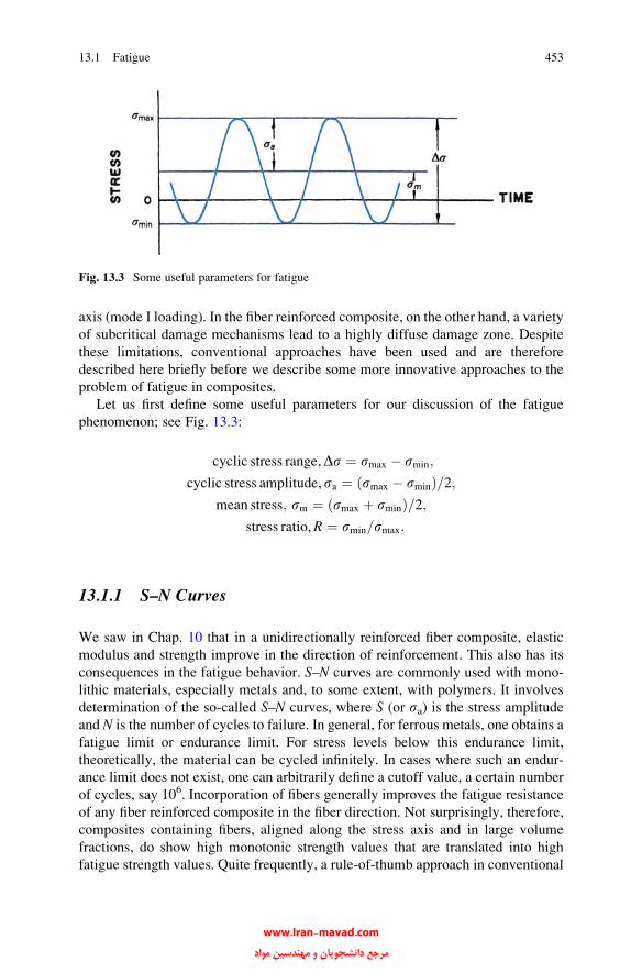
axis (mode I loading). In the fiber reinforced composite, on the other hand, a variety

of subcritical damage mechanisms lead to a highly diffuse damage zone. Despite

these limitations, conventional approaches have been used and are therefore

described here briefly before we describe some more innovative approaches to the

problem of fatigue in composites.

Let us first define some useful parameters for our discussion of the fatigue

phenomenon; see Fig. 13.3:

cyclic stress range,Ds ¼ smax � smin;

cyclic stress amplitude, sa ¼ smax � sminð Þ=2;mean stress; sm ¼ smax þ sminð Þ=2;

stress ratio,R ¼ smin=smax:

13.1.1 S–N Curves

We saw in Chap. 10 that in a unidirectionally reinforced fiber composite, elastic

modulus and strength improve in the direction of reinforcement. This also has its

consequences in the fatigue behavior. S–N curves are commonly used with mono-

lithic materials, especially metals and, to some extent, with polymers. It involves

determination of the so-called S–N curves, where S (or sa) is the stress amplitude

and N is the number of cycles to failure. In general, for ferrous metals, one obtains a

fatigue limit or endurance limit. For stress levels below this endurance limit,

theoretically, the material can be cycled infinitely. In cases where such an endur-

ance limit does not exist, one can arbitrarily define a cutoff value, a certain number

of cycles, say 106. Incorporation of fibers generally improves the fatigue resistance

of any fiber reinforced composite in the fiber direction. Not surprisingly, therefore,

composites containing fibers, aligned along the stress axis and in large volume

fractions, do show high monotonic strength values that are translated into high

fatigue strength values. Quite frequently, a rule-of-thumb approach in conventional

Fig. 13.3 Some useful parameters for fatigue

13.1 Fatigue 453


http://dx.doi.org/10.1007/978-0-387-74365-3_10

materials is to increase its monotonic strength, which concomitantly results in an

increase in its cyclic strength. This rule-of-thumb assumes that the ratio of fatigue

strength/tensile strength is about constant. It should also be noted that the maximum

efficiency in terms of stiffness and strength gains in fiber reinforced composites

occurs when the fibers are continuous, uniaxially aligned and the properties are

measured parallel to the fiber direction. As we go off-angle, the strength and

stiffness drop sharply. Also, at off-angles, the role of the matrix becomes more

important in the deformation and failure processes. One major drawback of this

S–N approach to fatigue behavior of a material is that no distinction can be made

between the crack initiation phase and the crack propagation phase.

The variety of operating mechanisms and the inadequacy of the S–N curve

approach have been documented by many researchers. Owen et al. (1967, 1969),

for example, studied the fatigue behavior of chopped strand mat glass/polyester

composite and observed the following sequence of events in the fatigue failure

process: (1) debonding, generally at fibers oriented transverse to the stress axis, (2)

cracking in the matrix, and (3) final separation or fracture. The debonding and

cracking phenomena set in quite early in the fatigue life. Lavengood and

Gulbransen (1969) investigated the importance of fiber aspect ratio and the role

of matrix in the fatigue performance of composites. They studied the effect of

cyclic loading on short boron fibers (50–55 % volume fraction) in an epoxy matrix.

They used a low frequency (3 Hz) to minimize the hysteretic heating effects and

measured the number of cycles required to produce a 20 % decrease in the

composite elastic modulus, i.e., this was their arbitrary definition of fatigue life.

The fatigue life increased with aspect ratio up to about 200, beyond which there was

little effect. In all cases, the failure consisted of a combination of interfacial fracture

and brittle failure of matrix at 45� to the fiber axis. Incorporation of fibers certainly

improves the fatigue resistance of the fiber reinforced polymeric matrix composites

in the fiber direction. Not surprisingly, therefore, composites containing these

fibers, aligned along the stress axis and in large volume fractions, will show high

monotonic strength values, which are translated into high fatigue strength values.

An example of S–N curves of unreinforced polysulfone (PSF) and composites with

a PSF matrix and different amount of short fibers (glass and carbon) is shown in

Fig. 13.4a. These results were obtained from tests done at room temperature,

cycling frequency between 5 and 20 Hz, and at R ¼ 0.1 (Mandell et al. 1983).

Izuka et al. (1986) studied the fatigue behavior of two different types of carbon

fibers (T800 and T300 carbon fiber) in an epoxy matrix. Both had 60 % fiber

volume fraction (Vf) but T800 carbon fiber has a maximum strength of 4.5 GPa and

a Young’s modulus of 230 GPa while T300 carbon fiber has 3.5 and 210 GPa,

respectively. As expected, the higher monotonic strength of T800 carbon fiber

resulted in a superior S–N curve for the composite.

The polymeric matrices, however, show a viscoelastic behavior and are, generally,

poor conductors of heat. Owing to the viscoelastic nature of the polymer matrix, there

will be a phase lag between the stress and the strain, i.e., the strain lags the stress or vice

versa, and that energy is stored in the material in the form of heat in each cycle.

Because of the low thermal conductivity of the polymeric matrix, the heat generated is



not dissipated quickly. This can cause a temperature difference between the interior

and the surface of a PMC, and the fatigue behavior of PMCs becomes even more

complex due to such internal heating. The internal heating phenomenon, of course,

depends on the cycling frequency. For a given stress level, this temperature difference

Fig. 13.4 (a) S–N curves of unreinforced polysulfone (PSF) and composites with a PSFmatrix and

different amount of short fibers (glass and carbon) [after Mandell et al. (1983)]. (b) Temperature

rise under fatigue for glass fiber/polypropylene composites (Goel et al. 2009). At a given stress

amplitude, temperature rises more quickly at higher frequency and leads to premature failure of the

composite

13.1 Fatigue 455


increases with increasing frequency. Figure 13.4b shows this for glass fiber/polypro-

pylene composites (Goel et al. 2009). At a given stress amplitude, temperature rises

more quickly at higher frequency and leads to premature failure of the composite.

Typically, the carbon fibers are much more effective in improving the fatigue

behavior of a given polymeric matrix than glass fibers. The reasons for this are the

high stiffness and high thermal conductivity of carbon fibers vis-a-vis glass fibers.

The higher thermal conductivity of carbon fibers will contribute to a lower hyster-

etic heating of the matrix at a given frequency.

Examples of S–N curves for fiber reinforced MMCs are shown in Fig. 13.5a,

which shows the S–N curves in tension–tension for unidirectionally reinforced

Fig. 13.5 (a) S–N curves for MMCs in tension–tension for unidirectionally reinforced boron fiber

(40 % v/o)/A16061, alumina fiber (50 % v/o)/Al, and alumina fiber (50 % v/o)/Mg composites

[after Champion et al. (1978)]. (b) S–N curves for silicon carbide particle reinforced aluminum

matrix composites [courtesy of N. Chawla]



boron (40 % v/o)/A16061, alumina (50 % v/o)/Al, and alumina (50 % v/o)/Mg

composites (Champion et al. 1978). The cyclic stress is normalized with respect to

the monotonic ultimate tensile stress. Note the rather flat S–N curves in all the cases

and the fact that the unidirectional composites show better fatigue properties than

the matrix when loaded parallel to the fibers. For example, at 107 cycles, the

fatigue-to-tensile strength ratio of the composite is about 0.77, almost double that

of the matrix. S–N curves for silicon carbide particle reinforced aluminum matrix

composites are shown in Fig. 13.5b. Increase in volume fraction of SiCp results in

an increase in fatigue life (Chawla et al. 1998a, b).

Gouda et al. (1981) observed crack initiation early in the fatigue life at

defects in boron fibers in unidirectionally reinforced B/Al composites. These

cracks then grew along the fiber/matrix interface and accounted for a major

portion of the fatigue life, as would be the case in a composite with a high fiber-

to-matrix strength ratio. In composites with low fiber-to-matrix strength ratios,

crack propagation may take up a major portion of fatigue life, but the crack

would be expected to grow across the fibers and a poor fatigue resistance will

result. This simply confirms the observation that in unidirectional composites

the fatigue resistance will be maximum along the fiber direction and the greatest

efficiency will be achieved if the fibers have uniform properties, as much as

possible defect-free, and much stronger than the matrix. Similar results have

been obtained by other researchers. For example, McGuire and Harris (1974)

studied the fatigue behavior of tungsten fiber reinforced aluminum–4 % copper

alloy under tension–compression cycling R ¼ smin=smax ¼ �1ð Þ . They found

that increasing the fiber volume fraction from 0 to 24 % resulted in increased

fatigue resistance. This was a direct result of increased monotonic strength of

the composite as a function of the fiber volume fraction. The reader should note

that due to the highly anisotropic nature of the fiber reinforced composites in

general, the fatigue strength of any off-axis fibrous composite will be expected

to decrease with increasing angle between the fiber axis and the stress axis. This

has been confirmed by studies involving S–N behavior of alumina fiber

reinforced magnesium composites (Hack et al. 1987; Page et al. 1987) It was

found that the S–N behavior followed the tensile behavior. Increased fiber

volume fractions resulted in enhanced fatigue life times in the axial direction

but little or no improvement was observed in the off-axis directions. Fatigue

crack initiation and propagation occurred primarily through the magnesium

matrix. Thus, alloy additions to increase the strength of the matrix and fiber/

matrix interface were tried. The alloy additions did improve the off-axis

properties but decreased the axial properties. The reason for this was that

while the alloy additions resulted in the matrix and interface strengthening,

they decreased the fiber strength. Similar effect of fiber orientation on fatigue

properties exists in PMCs. As an example, Goel et al. (2009) observed better

fatigue performance in the longitudinal direction than in the transverse direction

in glass fiber/polypropylene composites.

13.1 Fatigue 457


13.1.2 Fatigue Crack Propagation

Fatigue crack propagation tests are generally conducted in an electro-hydraulic

closed-loop testing machine on notched samples. The results are presented as log

da/dN (crack growth per cycle) vs. log DK (cyclic stress intensity factor). Crack

growth rate, da/dN, is related to the cyclic stress intensity factor range, DK,according to the power law relationship formulated by Paris and Erdogan (1963):

da=dN ¼ A DKð Þm; (13.1)

where A and m are constants that depend on the material and test conditions. The

applied cyclic stress intensity range is given by

DK ¼ YDsffiffiffiffiffiffipa

p;

where Y is a geometric factor, Ds is the cyclic stress range, and a is the crack length.The major problem in this kind of test is to make sure that there is one and only

one dominant crack that is propagating. This is called the self-similar crack growth,i.e., the crack propagates in the same plane and direction as the initial crack. Fatigue

crack propagation studies, under conditions of self-similar crack propagation, have

been made on metallic sheet laminates (McCartney et al. 1967; Taylor and Ryder

1976; Pfeiffer and Alic 1978; Chawla and Liaw 1979; Godefroid and Chawla 1988)

and unidirectionally aligned fiber reinforced MMCs (Saff et al. 1988). For the crack

arrest geometry, if the interface is weak, then the crack on reaching the interface

bifurcates and changes its direction and thus the failure of the composite is delayed.

The improved fatigue crack propagation resistance in crack divider geometry has

been attributed either to interfacial separation, which relieves the triaxial state of

stress, or to an interfacial holding back of crack in the faster crack-propagating

component by the slower crack-propagating component. Generally, a relationship

of the form of Eq. (13.1) describes the fatigue crack propagation behavior.

In general, the fibers provide a crack-impeding effect but the nature of the fiber

(morphology, rigidity, and fracture strain), the fiber/interface, and/or any reaction

zone phases that might form at the interface can have great influence.

Fatigue crack propagation studies have also been done on aligned eutectic or in

situ composites. Because many of these in situ composites are meant for high-

temperature applications such as in turbines, their fatigue behavior has been studied

at temperatures ranging from room temperature to 1,100 �C. The general consensusis that the mechanical behavior of in situ composites, static and cyclic strengths, is

superior to that of the conventional cast superalloys (Stoloff 1987).

It should be emphasized that only fatigue crack propagation rate data obtained

under conditions of self-similar propagation can be used for comparative purposes.

In a composite consisting of plies with different fiber orientation, in general, the self

similar mode of crack propagation will not be obtained.



13.1.2.1 Fatigue of Composites under Compression

Fiber reinforced composites generally show lower fatigue resistance in compression

than in tension. This may be due to the cooperative buckling of adjacent fibers and

the accompanying matrix shear. In monotonic compression of unidirectionally

reinforced fiber composites, a fiber kinking mechanism leads to failure. The failure

in this case initiates at a weak spot, e.g., at a point where the fiber/matrix bonding is

weak. This initial failure will, in turn, destabilize the neighboring fibers, causing

more kink failure. Eventually, various kink failure sites can coalesce and lead to

transverse tensile loading of the composite and longitudinal splitting. Pruitt and

Suresh (1992) showed that in addition to kink band formation, in unidirectional

carbon fiber/epoxy composites under cyclic compression, a single mode I crack can

start and grow perpendicular to the fiber axis. This compression fatigue phenomenon

is thought to be macroscopically similar to that observed in metals, polymers, and

ceramics. The origin of amode I crack ahead of a stress concentration is the presence

of residual tensile stresses which can result from a variety of permanent damage

modes involving matrix, fiber, interface, etc.

One can also introduce defects to simulate a delamination in fiber reinforced

laminated composites and then study its propagation under conditions of fatigue.

Such defects may be introduced in a laminate by one of the following means:

1. Insert circular inserts of different diameters at different interfaces

2. Insert a hole in the laminate

3. Produce defects in a laminate by controlled, low-velocity impacts

Delamination growth under cyclic compression fatigue in a 38-ply T300 carbon/

5208 epoxy composite laminate was studied by O’Brien (1984). The maximum

strain decreased with cycling. The impacted laminates suffered the most severe

degradation on compressive cycling, while the laminates with a single implanted

delamination suffered the least damage.

13.1.2.2 Fatigue Behavior of CMCs

We describe the fatigue behavior of CMCs under a separate subheading because of

new discoveries. Conventional wisdom had it that cyclic fatigue was unimportant

so far as ceramics were concerned. However, in actuality the subject of cyclic

fatigue in ceramics and ceramic matrix composites is an important one. Engineers

and researchers began to appreciate the importance of cyclic fatigue in ceramics

and ceramic matrix composites only in the 1970s. The fracture resistance of CMCs

under cyclic conditions needs to be evaluated for design in a variety of potential

structural applications. For example, it is not unusual to have a design requirement

for a ceramic component in an automotive gas turbine to withstand more than

30,000 cycles of fatigue (low-cycle fatigue) (Helms and Haley 1989). In the case of

13.1 Fatigue 459


carbon fiber reinforced glass composites, no significant loss of strength was

observed on cyclic loading (Phillips 1983). However, the density and penetration

of matrix cracks was more under cyclic loading than under static loading

conditions. Also, under static loading this CMC showed higher work of fracture

than under cyclic loading. Prewo et al. (1986) studied the tensile fatigue behavior of

Nicalon-type silicon carbide fiber reinforced lithium aluminosilicate (LAS)

glass–ceramic composite. They used two different types of LAS as the matrix

material: one showed a linear tensile stress–strain curve to failure (LAS I) while

the other showed a markedly nonlinear behavior due to extensive matrix cracking

prior to ultimate failure (LAS II). It was observed that the level of tensile stress at

which the inelastic behavior (proportional limit) of the composite began had an

important bearing on the fatigue behavior of the CMC. The residual tensile strength

and elastic modulus of the LAS I composite after fatigue was the same as that of as-

fabricated composite. In the LAS II composite, cycling below the proportional limit

produced the same result. However, on cycling to stress levels higher than the

proportional limit, a second linear stress–strain region having a modulus less than

the initial modulus was observed. Presumably, this change in behavior was due to

matrix microcracking at stresses above the proportional limit.

It was generally thought that the phenomenon of cyclic fatigue was unimpor-

tant in ceramics. Work by Suresh and coworkers (Suresh et al. 1988; Suresh 1991;

Han and Suresh 1989) on fatigue crack growth in a variety of brittle solids in

compression, tension, and tension-compression fatigue shows that mechanical

fatigue effects, i.e., due to cyclic loading, occur at room temperature in brittle

solids as well. A variety of mechanisms such as microcracking, dislocation

plasticity, stress- or strain-induced phase transformations, interfacial slip, and

creep cavitation can promote an inelastic constitutive response in brittle solids of

all kinds under compressive cycling. Particularly, in CMCs, the mechanisms of

crack-tip deformation differ significantly under static and cyclic loading. They

demonstrated that under pulsating compression, nucleation and growth of stable

fatigue cracks occurred even at room temperature. Suresh et al. showed conclu-

sively that cyclic compressive loading caused mode I fatigue crack growth in SiC

whiskers/Si3N4 matrix composites. They also observed whisker pullout and

breakage after fatigue cycling. Such behavior is generally not observed under

monotonic loading. This mode I fatigue crack growth under far-field cyclic

compression occurs because a residual zone of tensile stress is generated at the

crack tip on unloading. Wang et al. (1991) investigated the behavior of a [0/90]

carbon fiber reinforced silicon carbide composite under cyclic loading. They

used tension–tension loading of smooth and notched samples and compression–-

compression loading. Damage in pulsating tension consisted of cumulative

microcracking and spalling. In this regard, it worth pointing out that investigation

of cyclic behavior of polycrystalline continuous alumina fiber showed a definite

cyclic fatigue effect, i.e., cyclic fatigue of alumina fibers showed more damage

than static fatigue (Chawla et al. 2005).

An important problem in high-temperature behavior of polycrystalline ceramics

is the presence of intergranular glassy phases. Sintering and other processing aids



can form glassy phases at the boundaries, which can result in rather conspicuous

subcritical crack growth. Such subcritical crack growth can become very important

in ceramic matrix composites because fibers such as silicon carbide can undergo

oxidation. Han and Suresh (1989) examined the tensile cyclic fatigue crack growth

in a silicon carbide whisker (33 vol.%)/alumina composite at 1,400 �C.The composite showed subcritical fatigue crack growth at stress intensity values

far below the fracture toughness. The fatigue behavior was characterized by the

cyclic stress intensity factor, stress ratio, and frequency. They examined the crack

tip region by optical and transmission electron microscopy and found that the

nucleation and growth of flaws at the interface was the main damage mechanism.

Diffuse microcracking in the wake of the crack and crack deflection/branching were

observed. An increase in the test temperature (or the cyclic stress intensity or a

reduction in the loading rate) can cause a rather significant increase in the size of the

damage zone at the crack tip. Han and Suresh observed oxidation of silicon carbide

whiskers to a silica-type glassy phase in the crack tip region at 1,400 �C, in air.

The alumina matrix can react with the main oxidation product, viz., SiO2, to form

aluminosilicates, SiC-rich or stoichiometric mullite, and the like. Viscous flow of

glass can result in interfacial debonding, followed by the nucleation, growth,

and coalescence of cavities. The important thing to note is that there is a difference

in deformation and failure mechanisms under static and cyclic loadings, even

in CMCs.

In a manner analogous to PMCs, there can be a hysteretic heating in CMCs under

cyclic loading conditions due to interfacial friction (Holmes 1991). Sørensen and

Holmes (1995) observed that a lubricating layer may be beneficial in improving

fatigue life of CMCs. A thicker coating, which would be expected to provide

greater protection to the fiber against abrasion damage, resulted in less frictional

heating because of less wear of the fibers during fatigue of a chemical vapor

infiltrated (CVI) Nicalon/C/SiC composite (Chawla 1997 and Chawla et al.

1998a, b). The composite with a thinner coating exhibited much higher frictional

heating. At higher frequencies, more heating was observed since the energy

dissipated per unit time also increased. Substantial damage in terms of loss of

stiffness was observed in fatigue of Nicalon/C/SiC, with most of the damage

occurring during the first cycle. At a constant stress, the level of damage was not

significantly dependent on frequency. At a given frequency, however, higher

stresses induced more damage in both composites. In the case of the fiber in the

form of a plain-weave fabric, a recovery in modulus of these woven composites was

observed due to stretching and alignment of the fabric during fatigue, creating a

stiffer reinforcing architecture.

The laminate stacking sequence can affect the high-frequency fatigue behavior

of CMCs. In SCS-6/Si3N4 composites, frictional heating in angle-ply laminates

[�45] was substantially higher than that in cross-ply laminates [0/90] (Chawla

1997). Because the angle ply had a lower stiffness, matrix microcracking in this

composite was more predominant. Temperature rise in the specimens correlated

very well with stiffness loss as a function of fatigue cycles in the composites

(see Sect. 13.1.3).

13.1 Fatigue 461


13.1.2.3 Fatigue of Particle and Whisker Reinforced Composite

Ceramic particle reinforced metal matrix composites, such as silicon carbide or

alumina particle reinforced aluminum alloy composites can have improved fatigue

properties vis-a-vis unreinforced aluminum alloys, which can make these

composites useful in applications where aluminum alloys would not be considered

(Allison and Jones 1993). Such systems have been studied by some researchers

(Chawla et al. 1998a, b; Crowe and Hasson 1982; Williams and Fine 1985, 1987;

Logsdon and Liaw 1986; Shang et al. 1988; Davidson 1989; Kumai et al. 1990;

Bonnen et al. 1990; Christman and Suresh 1988a, b). In general, in terms of S–Ncurve behavior, the composite shows an improved fatigue behavior vis-a-vis the

unreinforced alloy. Such an improvement in stress-controlled cyclic loading or high

cycle cyclic fatigue is attributed to the higher stiffness of the composite. However,

the fatigue behavior of the composite, evaluated in terms of strain amplitude vs.

cycles or low-cycle fatigue, was inferior to that of the unreinforced alloy (Bonnen

et al. 1990). This was attributed to the generally lower ductility of the composite

compared to the unreinforced alloy.

Particle or short fibers can provide easy crack initiation sites. The detailed

behavior can vary depending on the volume fraction of the reinforcement,

shape, size, and most importantly on the reinforcement/matrix bond strength.

For example, Williams and Fine (1987) observed fatigue crack initiation at the

poles of SiC whiskers in 2124 aluminum. They also observed arrest of short

cracks at the whisker/Al interfaces. Frequently in aluminum matrix composites,

especially those made by casting, there are particles, called constituent particles

in aluminum literature, other than SiC, such as CuAl2, (Fe,Mn)3·SiAl12, and

Cu2Mg5Si6Al5 (Kumai and Knott 1991). During liquid metal processing of

particle reinforced MMCs, there occurs the phenomenon of particle pushing

ahead of the solidification front (Rohatgi et al. 1994). This results in SiC particles

and the constituent particles decorating the cell boundaries in the aluminum alloy

matrix.

Some possible interactions between the ceramic particle reinforcement and the

crack tip in the matrix are shown schematically in Fig. 13.6a. When the ceramic

particles are large, they can be loaded to the point of fracture and the fatigue crack

runs though the particles. When we have fine particles, the crack goes around the

particles. Examples of such behavior can be found in practical composites (SiCp/Al

alloy) (Chawla and Ganesh 2010). Figure 13.7 shows schematic representations of

crack growth vs. cyclic intensity factor for a monolithic alloy and a particulate

composite. Levin et al. (1989) observed superior resistance to fatigue crack growth

in 15 vol.% SiC particle/Al 6061 composite vis-a-vis Al 6061 alloy, which was

attributed to a slower crack growth rate in the composite due to crack deflection

caused by the SiC particles. Computer simulation of crack growth behavior in

particle reinforced MMCs starting with actual microstructures rather than

simplified models has become quite important. Ceramic particle shape, size



distribution, spatial distribution, etc. are very important during deformation of these

materials, particularly during crack growth.

It would appear that choosing the optimum particle size and volume fractions,

together with a clean matrix alloy, will result in a composite with improved

fatigue characteristics. Shang et al. (1988) examined the effect of particle size

on fatigue crack propagation as a function of cyclic stress intensity in a silicon

carbide particle reinforced aluminum. They observed that for fine particle size,

the threshold stress intensity, DKth, for the composite was less than that for the

unreinforced alloy, i.e., initial fatigue crack growth resistance of the composite

was less than that of the unreinforced alloy. For coarse particles, the threshold

intensity values were about the same for the two, while at very high values of the

cyclic stress intensity, the fatigue crack growth of the composite was less than that

of the unreinforced alloy.

Fig. 13.6 Some possible

particle reinforcement and

crack tip interactions

13.1 Fatigue 463


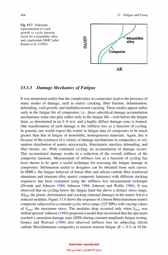
13.1.3 Damage Mechanics of Fatigue

It was mentioned earlier that the complexities in composites lead to the presence of

many modes of damage, such as matrix cracking, fiber fracture, delamination,

debonding, void growth, and multidirectional cracking. These modes appear rather

early in the fatigue life of composites, i.e., these subcritical damage accumulation

mechanisms come into play rather early in the fatigue life—well before the fatigue

limit, as determined in an S–N test, and a highly diffuse damage zone is formed.

One manifestation of such damage is the stiffness loss as a function of cycling.

In general, one would expect the scatter in fatigue data of composites to be much

greater than that in fatigue of monolithic, homogeneous materials. Again, this is

because of the existence of a variety of damage mechanisms in composites, to wit,

random distribution of matrix microcracks, fiber/matrix interface debonding, and

fiber breaks, etc. With continued cycling, an accumulation of damage occurs.

This accumulated damage results in a reduction of the overall stiffness of the

composite laminate. Measurement of stiffness loss as a function of cycling has

been shown to be quite a useful technique for assessing the fatigue damage in

composites. Information useful to designers can be obtained from such curves.

In MMCs, the fatigue behavior of boron fiber and silicon carbide fiber reinforced

aluminum and titanium alloy matrix composite laminates with different stacking

sequences has been examined using the stiffness loss measurement technique

(Dvorak and Johnson 1980; Johnson 1988; Johnson and Wallis 1986). It was

observed that on cycling below the fatigue limit but above a distinct stress range,

DSSD, the plastic deformation and cracking (internal damage) in the matrix led to a

reduced modulus. Figure 13.8 shows the response of a boron fiber/aluminum matrix

composite subjected to a constant cyclic stress range (225 MPa) with varying values

of Smax, the maximum stress. The modulus drop occurred only when Smax was

shifted upward. Johnson (1988) proposed a model that envisioned that the specimen

reached a saturation damage state (SDS) during constant-amplitude fatigue testing.

Gomez and Wawner (1988) also observed stiffness loss on subjecting silicon

carbide fiber/aluminum composites to tension–tension fatigue (R ¼ 0.1) at 10 Hz.

Fig. 13.7 Schematic

representation of crack

growth vs. cyclic intensity

factor for a monolithic alloy

and a particulate MMC [after

Kumai et al. (1990)]



Fig. 13.8 Response of a boron fiber/aluminum matrix composite subjected to a constant cyclic

stress range (225 MPa) with varying values of Smax, the maximum stress [after Johnson (1988)]

Fig. 13.9 Typical modulus loss curve for unidirectional silicon carbide/aluminum composites. EN

is the modulus after N cycles and E0 is the modulus in the uncycled state [after Gomez andWawner

(1988)]

13.1 Fatigue 465


Periodically, the cycling was stopped and the elastic modulus was measured.

Figure 13.9 shows a typical modulus loss curve for unidirectional silicon carbide

fiber/aluminum composites. Modulus at N cycles, EN, normalized with respect

to the original modulus, E0, is plotted against the log (number of cycles, N).These authors used a special type of silicon carbide fiber, called the SCS-8 silicon

carbide fiber, which is a silicon carbide fiber with a modified surface to give a strong

bond between the fiber and the aluminum matrix. The SCS coating broke off at high

cycles and the fracture surface showed the coating clinging to the matrix. Stiffness

loss as a function of number of cycles was also observed for Nicalon fiber/

borocilicate glass-ceramic matrix composites (Ramakrishnan and Jayaraman

1993). In CMCs, the matrix can have a lower strain-to-failure than the fibers. In

such a case, the matrix starts cracking first. Thereafter, we have two possible routes.

In the case of a weak interface, we observe fiber/matrix debonding followed by fiber

pullout, etc. In the case of a strong interface, matrix cracking leads to failure and a

brittle failure of the composite. Karandikar and Chou (1992) used the approach of

stiffness loss as a function of stress cycles with unidirectionally reinforced Nicalon

fiber/calcium aluminosilicate (CAS) composites and obtained correlations between

crack density and stiffness reduction.

Let us now focus our attention on the fatigue behavior of fiber reinforced

laminated composites that are made by consolidating prepregs. Figure 13.10a

shows schematically a comparison of damage accumulation as a function of fatigue

cycles in a laminated composite made by appropriately stacking differently ori-

ented plies and a monolithic, homogeneous material under constant stress ampli-

tude fatigue (Hahn and Lorenzo 1984). We plot damage ratio against cycle ratio.

The damage ratio is the current damage normalized with respect to the damage at

final failure. The cycle ratio, similarly, is the number of cycles at a given instant

divided by the number of cycles to failure. In a conventional, homogeneous

material, the term damage simply represents the crack length, and not surprisingly

it increases monotonically with cycling. In the case of a laminate, we do not have a

simple and unambiguous manifestation of damage, such as a crack length. Instead,

damage is diffuse and involves a variety of cracks; so damage, in principle, would

mean the crack density. Note that, unlike in homogeneous materials, the damage

(i.e., crack density) in laminates accelerates at first and then decelerates with

cycling. This distinctive behavior is very important. Such a multiplicity of fracture

modes is common to all composites. As an example, Figure 13.10b shows the

fracture surface of B(W)/A1 6061 composite made by diffusion bonding. Note the

ductile fracture in aluminum, brittle fracture in boron, fiber pullout (see the missing

fiber in top-left-hand corner), and sheet delamination.

As was pointed out earlier, the fiber reinforced laminates can sustain a variety of

subcritical damage (crazing and cracking of matrix, fiber/matrix decohesion, fiber

fracture and pullout, ply cracking, delamination, and so on). For example, the

cracking of a ply will result in a relaxation of stress in that ply, and with continued

cycling no further cracking occurs in that ply. Ply cracking generally involves

cracking in the matrix and along the fiber/matrix interface but rarely any fiber

fracture. Other damage-accumulating mechanisms include the growth of existing



cracks into interfaces leading to ply delamination. The subcritical damage can

accumulate rather rapidly on cycling.

The various types of subcritical damage mentioned above result in a reduction of

the load-carrying capacity of the composite, which in turn manifests itself as a

reduction in stiffness and strength of the composite. Many researchers have experi-

mentally related the stiffness changes in the laminated composites to the

accumulated damage under fatigue (Hahn and Kim 1976; Highsmith and Reifsnider

1982; Talreja 1985; Ogin et al. 1985). Work with polymer– and metal–matrix

composites shows that this change in stiffness values is a good indicator of the

extent of damage in these composites. The various types of subcritical damage

mentioned above result in a reduction of the load-carrying capacity of the laminate

composite, which in turn manifests itself as a reduction of laminate stiffness and

strength (Hahn and Kim 1976; Highsmith and Reifsnider 1982; Talreja 1985;

O’Brien and Reifsnider 1981; Ogin et al. 1985). Figure 13.11 depicts schematically

the changes in crack density, delamination, and modulus in a composite laminate

under fatigue (Hahn and Lorenzo 1984). Reifsnider et al. (1981) modeled the

fatigue development in laminate composites as occurring in two stages. In the

first stage, homogeneous, noninteractive cracks appear in individual plies. In the

second stage, the damage gets localized in zones of increasing crack interaction.

The transition from stage one to stage two occurs at what has been called the

characteristic damage state (CDS), which consists of a well-defined crack pattern

characterizing saturation of the noninteractive cracking. Talreja (1985) used this

model to determine the probability distribution of the number of cycles required to

attain the CDS.

Fig. 13.10 (a) Comparison of damage accumulation as a function of fatigue cycles in a laminated

composite (made by appropriately stacking differently oriented plies) and a monolithic, homoge-

neous material under constant stress amplitude fatigue [after Hahn and Lorenzo (1984)]. (b)

Fracture surface of B(W)/A1 6061 composite made by diffusion bonding. Note the different

modes of damage: ductile fracture in aluminum, brittle fracture in boron, fiber pullout (see the

missing fiber in top-left-hand corner), and sheet delamination

13.1 Fatigue 467


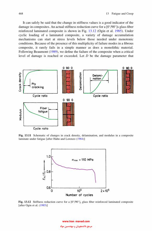
It can safely be said that the change in stiffness values is a good indicator of the

damage in composites. An actual stiffness reduction curve for a [0�/90�]s glass fiberreinforced laminated composite is shown in Fig. 13.12 (Ogin et al. 1985). Under

cyclic loading of a laminated composite, a variety of damage accumulation

mechanisms can start at stress levels below those needed under monotonic

conditions. Because of the presence of this multiplicity of failure modes in a fibrous

composite, it rarely fails in a simple manner as does a monolithic material.

Following Beaumont (1989), we define the failure of the composite when a critical

level of damage is reached or exceeded. Let D be the damage parameter that

Fig. 13.12 Stiffness reduction curve for a [0�/90�]s glass fiber reinforced laminated composite

[after Ogin et al. (1985)]

Fig. 13.11 Schematic of changes in crack density, delamination, and modulus in a composite

laminate under fatigue [after Hahn and Lorenzo (1984)]



increases as a function of number of cycles, N. Then, dD/dN will be the damage

growth rate. We can write for the damage growth rate

dD=dN ¼ f Ds;R;Dð Þ; (13.2)

where Ds is the cyclic stress range, R is the stress ratio, and D is the current value of

damage. Let Nf be the number of cycles to failure, i.e., the fatigue life

corresponding to a critical level of damage. Then integrating Eq. (13.2) between

limits of initial damage, Di and final damage, Df, we can write for the number of

cycles to failure as

Nf ¼ðDf

Di

dD=f Ds;R;Dð Þ: (13.3)

The main problem is that the function f is not known. One measure of damage is

the instantaneous load-bearing capacity or the stiffness, E. We can write

E ¼ E0gðDÞ; (13.4)

where E0 is the stiffness of the undamaged material and g(D) is a function of

damage, D.Rewriting Eq. (13.4) as E/E0 ¼ g(D) and differentiating, we get

1=E0ð ÞdE=dN ¼ dgðDÞ=dN: (13.5)

Also,

D ¼ g�1 E=E0ð Þ;

where g�1 is the inverse of g. This allows us to rewrite Eq. (13.5) as

1=E0ð ÞdE=dN ¼ g0 g�1 E=E0ð Þ� �f Ds;R;Dð Þ:

The function g(D) can be obtained experimentally by obtaining data in terms of

E/E0 vs. N. We can then evaluate the function f as:

f Ds;R;Dð Þ ¼ 1=g0 g�1 E=E0ð Þ� �� 1=E0ð ÞdE=dN:

We can evaluate the right-hand side of this expression for a range of Ds,maintaining constant E/E0, R, etc. If 2S is the average crack spacing, then crack

density or damage ¼ 1/2S. The following relationship was found experimentally

for crack growth as a function of cycles, da/dN (Ogin et al. 1985):

da=dN / smax22S

� �n:

13.1 Fatigue 469


Total crack length a is proportional to damage or crack density, D, i.e.,

dD=dN / smax2=D

� �n:

Modulus of the damaged material E is given by

E ¼ E0 1� cDð Þ; (13.6)

where c is a material constant.

For a given value of E/E0, we can write the modulus or stiffness reduction rate as

ð�1=E0ÞdE=dN ¼ A smax2=E0

2 1� E=E0ð Þ� �n; (13.7)

where A and n are constants. The left-hand side of this expression can be deter-

mined experimentally. Note that both sides are dimensionless quantities. The

modulus reduction rate (�1/E0)dE/dN, at a given value of E/E0, is the tangent to

the curve shown in Fig. 13.12. This rate of Young’s modulus reduction was well

described over the range of peak fatigue stress between 110 and 225 MPa for the

glass fiber/epoxy composite by Eq. (13.7); see Fig. 13.13. We can integrate Eq.

(13.7) to obtain a diagram relating stiffness reduction to number of cycles for

different stress levels, as shown in Fig. 13.14. Such a diagram can be a very useful

design aid: It gives us the number of cycles it will take, when the composite is

cycled at a certain fraction of the monotonic ultimate strength, to attain a specific

amount of stiffness reduction (i.e., a specific amount of damage that the component

or the structure can withstand.)

Fig. 13.13 Modulus

reduction rate vs. a parameter

involving the peak stress

[after Ogin et al. (1985)]



13.1.4 Thermal Fatigue

There exists a very fundamental physical incompatibility between the reinforcement

(be that fiber, whisker, or particle) and the matrix, to wit, the difference in their

thermal expansion (or contraction) coefficients. This problem of thermal expansion

mismatch between the components of a composite is a very important one. Thermal

stresses arise in composite materials due to the generally large differences in the

thermal expansion coefficients (a) of the fiber and the matrix. It should be

emphasized that thermal stresses in composites cannot be alleviated by slow cooling

or some kind of annealing treatment, techniques that might work in conventional

material. The reason for this is that the thermal mismatch will be there even if the

temperature change is uniform throughout the volume of the composite. Thermal

stresses can be introduced in composites during cooling from high temperature of

fabrication, annealing, or curing temperatures or during any temperature excursions

(inadvertent or by design) during service. Turbine blades, for example, are very

much susceptible to thermal fatigue. The magnitude of thermal stresses in

composites is proportional to DaDT, where Da is the difference in the expansion

coefficients of the two components and DT is the amplitude of the thermal cycle

(see Chap. 10).

In PMCs and MMCs, the matrix generally has a much higher coefficient of

thermal expansion than the fiber. In CMCs, the thermal coefficients of the

components may not be that much different but the ceramic materials have very

low strain-to-failure values, i.e., very low ductility. In general, the matrix has a

much higher coefficient of thermal expansion than the fiber. Rather large internal

stresses can result when fiber reinforced composites are heated or cooled through

a temperature range. When this happens in a repeated manner, we have the

phenomenon of thermal fatigue, because the cyclic stress is thermal in origin.

Fig. 13.14 Number of cycles

required to attain a given

stiffness reduction after

cycling at different fractions

of the ultimate tensile

strength sUTS [after Oginet al. (1985)]

13.1 Fatigue 471


http://dx.doi.org/10.1007/978-0-387-74365-3_10

Thermal fatigue can cause cracking in the brittle polymeric matrix or plastic

deformation in a ductile metallic matrix (Chawla 1973a, b, 1975a, b). Cavitation

in the matrix and fiber/matrix debonding are other forms of damage observed due

to thermal fatigue in composites (Chawla 1973a, b, 1975b; Lee and Chawla 1987;

Lee et al. 1988). Xu et al. (1995) studied the damage evolution as a function of

thermal cycles in terms of three metal matrix systems: Al2O3f/Mg alloy, B4Cp/

6061 A1 alloy, and SiCp/8090 A1 alloy. The samples were thermally cycled

between room temperature (22 �C) and 300 �C. The incidence of void formation

at the fiber/matrix interface increased with the number of cycles. They observed

that loss in stiffness and density could be used as damage parameters. The damage

in density and elastic modulus caused by thermal cycling was more severe in the

fiber reinforced composite than in the particle reinforced composites.

There has been some work involving the use of X-ray tomography to charac-

terize the internal damage in the form of cavitation in particle reinforced MMCs.

This is a very impressive tool, although it must be recognized that such equipment

is not a common item, i.e., one has to go to some large scale facility, but it would

appear that the effort is worth it. Figure 13.15a show the surface of SiCp/Al

composite after thermal cycling. No damage is visible. However, when examined

by X-ray tomography, we observe the damage in the interior of the same sample;

see Fig. 13.15b.

In view of the fact that CMCs are likely to find major applications at

high temperatures, it is of interest to study their behavior under conditions of

isothermal exposure as well as under conditions of thermal cycling. Wetherhold

and Zawada (1991) studied the behavior of ceramic-grade Nicalon fiber in an

aluminosilicate glass matrix under isothermal and thermal cycling conditions.

At 650–700 �C, isothermally exposed and thermally cycled samples showed rapid

oxidation and loss in strength. Oxidation behavior overshadowed any thermal

cycling effect for these test conditions. The embrittlement was attributed to oxygen

infiltration from the surface, which destroyed the weak carbon-rich interface in this

composite. At 800 �C, however, less embrittlement was observed and the fiber

toughening effect remained. This decreased embrittlement at higher temperatures

was attributed to smoothening of the sample surface by glass flow and slow oxygen

infiltration. Boccaccini et al. (1997, 1998) studied the cyclic thermal shock behav-

ior of Nicalon fiber reinforced glass matrix composites. The thermal mismatch

between the fiber and the matrix in this system was almost nil. A decrease in

Young’s modulus and a simultaneous increase in internal friction as a function of

thermal cycles were observed. The magnitude of internal friction was more sensi-

tive to microstructural damage than Young’s modulus. An interesting finding of

theirs involved the phenomenon of crack healing when the glass matrix composite

was cycled to a temperature above the glass transition temperature of the matrix

where the glass flowed and caused crack healing.

It is possible to obtain a measure of the internal stresses generated on subjecting

a composite to thermal cycling. Kwei and Chawla (1992) used a computer-

controlled servohydraulic thermal fatigue system to perform tests on an alumina

fiber/AlLi alloy composite. Thermal fatigue testing in this case involved subjecting



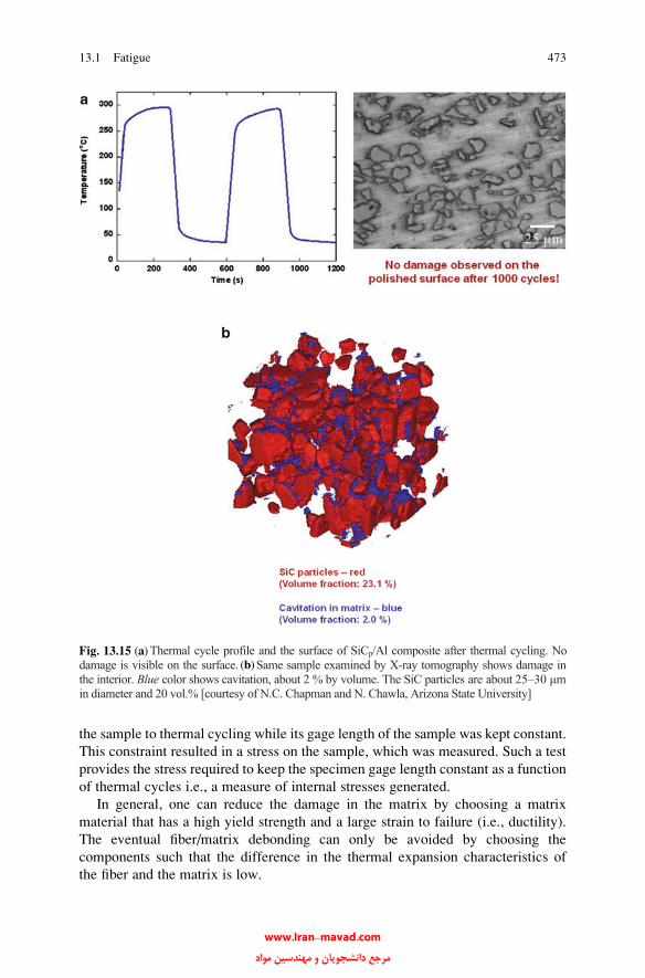
the sample to thermal cycling while its gage length of the sample was kept constant.

This constraint resulted in a stress on the sample, which was measured. Such a test

provides the stress required to keep the specimen gage length constant as a function

of thermal cycles i.e., a measure of internal stresses generated.

In general, one can reduce the damage in the matrix by choosing a matrix

material that has a high yield strength and a large strain to failure (i.e., ductility).

The eventual fiber/matrix debonding can only be avoided by choosing the

components such that the difference in the thermal expansion characteristics of

the fiber and the matrix is low.

13.1 Fatigue 473

Fig. 13.15 (a)(b)

Thermal cycle profile and the surface of SiCp/Al composite after thermal cycling. No damage is visible on the surface. Same sample examined by X-ray tomography shows damage in the interior. Blue color shows cavitation, about 2 % by volume. The SiC particles are about in diameter and 20 vol.% [courtesy of N.C. Chapman and N. Chawla, Arizona State University]

25–30 μm


13.2 Creep

Creep is defined as the time-dependent deformation in a material. It becomes

important at relatively high temperatures, especially at temperatures greater than

0.4–0.5TH, where TH is the homologous temperature equal to T/Tm, T is the temper-

ature of interest in kelvin, and Tm is the melting point of the material in kelvin.

The phenomenon of creep can cause small deformations under a sustained load over

a long period of time. In a variety of situations or equipments (e.g., a pressure vessel

or a rotating component), such slow deformations can lead to dimensional problems

or even failure. Creep sets a limit on the maximum service temperature. In general,

this limit increases with the melting point of a material. Without going into the

theoretical andmodeling details, suffice it to say that the basic governing equation of

creep can be written in the following form:

_e ¼ A s=Gð Þn exp �DQ=kTð Þ;

where _e is the creep strain rate, s is the applied stress, n is an exponent, G is the

shear modulus, DQ is the activation energy for creep, k is the Boltzmann’s constant,

and T is the temperature in kelvin. The stress exponent, n, typically varies between

3 and 7 in the dislocation climb regime and between 1 and 2 when diffusional

mechanisms are operating. Pure dislocation creep, grain boundary sliding, vacancy

motion in grains and in the grain boundaries can cause creep. The applied stress,

grain size, porosity, and impurity content are important variables.

In polymers and PMCs such as Kevlar 49 aramid fiber/epoxy, one can observe

creep even at room temperature (Eriksen 1976). At a given temperature, cross-

linked thermosets show less creep than thermoplastics. Creep in polymers is the

same as defined above, viz., we apply a constant stress and observe the strain as a

function of time. There is a related phenomenon called stress relaxation, which is

also important in polymers. In stress relaxation, we impose a constant strain on the

specimen and observe the drop in stress as a function of time. If we substitute a

polymeric fiber such as aramid with a more creep-resistant fiber—say alumina, SiC,

or even glass—we can make the composite more creep-resistant.

In very simple terms, creep in a PMC or MMC is likely to be dominated by the

creep behavior of the matrix. As the matrix deforms in creep, the applied load is

transferred to the load-bearing component, viz., fiber. Eventually, the fibers will

carry all the load. McLean (1983, 1985) showed that for a composite containing a

matrix that follows a power-law creep _e ¼ Asnð Þ, the creep rate in the composite is

given by:

_ec ¼Asn 1� _e

_e1

� �n

1þ VfEf

VmEm

� �Vnm

;



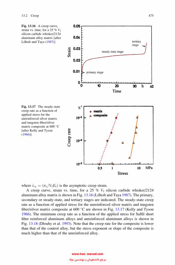
where _e1 ¼ sc=VfEfð Þ is the asymptotic creep strain.

A creep curve, strain vs. time, for a 25 % Vf silicon carbide whisker/2124

aluminum alloy matrix is shown in Fig. 13.16 (Lilholt and Taya 1987). The primary,

secondary or steady-state, and tertiary stages are indicated. The steady-state creep

rate as a function of applied stress for the unreinforced silver matrix and tungsten

fiber/silver matrix composite at 600 �C are shown in Fig. 13.17 (Kelly and Tyson

1966). The minimum creep rate as a function of the applied stress for Saffil short

fiber reinforced aluminum alloys and unreinforced aluminum alloys is shown in

Fig. 13.18 (Dlouhy et al. 1993). Note that the creep rate for the composite is lower

than that of the control alloy, but the stress exponent or slope of the composite is

much higher than that of the unreinforced alloy.

Fig. 13.16 A creep curve,

strain vs. time, for a 25 % Vf

silicon carbide whisker/2124

aluminum alloy matrix [after

Lilholt and Taya (1987)]

Fig. 13.17 The steady-state

creep rate as a function of

applied stress for the

unreinforced silver matrix

and tungsten fiber/silver

matrix composite at 600 �C[after Kelly and Tyson

(1966)]

13.2 Creep 475


The anomalously high values of the stress exponent, n, and activation energy, Q,have been explained by using the concept of a threshold stress (Webster 1982; Nieh

1984; Nardone and Strife 1987). Nardone and Strife (1987) used the concept of a

threshold stress sR, for creep deformation in composites. This theory was originally

used to explain the high values for Q and n in dispersion-strengthened alloys

(Davies et al. 1973; Parker and Wilshire 1975; Nardone and Tien 1986; Kerr and

Chawla 2004). By introducing the threshold stress, the general steady-state creep

rate is modified to:

_ess ¼ As� sR

E

nexp

�Q

RT

� �;

where A is a constant, E is the elastic modulus of the composite, and Q is the

activation energy. The threshold stress in the discontinuously reinforced composite

system can be attributed to a variety of sources (Dunand and Derby 1993; Pandey

et al. 1992): (1) Orowan bowing between particles, (2) back-stress associated with

dislocation climb, (3) attractive force between dislocations and particles, resulting

from relaxation of the strain field of dislocations at the particle/matrix interface

(Artz and Wilkinson 1986).

A threshold stress approach cannot always be used to explain the higher stress

exponents observed in MMCs, when compared to the unreinforced alloy. Load

transfer to the reinforcement, despite the lower aspect ratios of particles and

whiskers, is significant, as the applied load is carried by the high stiffness reinforce-

ment. With increasing load transfer to the reinforcement, the resolved shear stress

Fig. 13.18 The minimum creep rate as a function of the applied stress for Saffil short fiber

reinforced aluminum alloys and unreinforced aluminum alloys. Note that the creep rate for the

composite is lower than that of the control alloy, but the stress exponent or slope of the composite

is much higher than that of the unreinforced alloy [after Dlouhy et al. 1993]



on dislocations in the matrix may be lowered significantly below that required for

Orowan bowing. Dragone and Nix (1992) studied the creep behavior of Al2O3 short

fiber reinforced Al–5 % Mg alloy between 200 and 400 �C. They also observed

anomalously high values of stress exponent (n ~ 12–15) in the composites, while

the unreinforced alloy exhibited much lower, typical values (n ~ 3). The measured

activation energy (225 kJ/mol) for the composites was also anomalously high.

A threshold stress analysis showed that the contribution from Orowan bowing

was very small. Using a model consisting of randomly oriented short fibers in the

Al alloy matrix, and considering the progressive damage to the fibers during creep,

they were able to predict the experimentally observed high values of stress expo-

nent and activation energy. Dragone and Nix (1992) also noted that the arrangement

of fibers has a significant effect on the degree of matrix constraint. A decrease in

effective stress (increase in matrix constraint) was observed with increasing volume

fraction, fiber aspect ratio, and degree of overlap between fibers. The normal and

shear stresses at the fiber/matrix interface were also quite large, indicating that void

growth or debonding might take place during the creep process.

In some cases, creep behavior of MMCs shows a close correlation between the

properties of the matrix and those of the composite (Kelly and Tyson 1966; Kelly

and Street 1972a, b; Dragone et al. 1991). In other cases, this is not observed. Creep

experiments on an aluminum matrix containing ceramic particles or short fibers

show a very high value of stress exponent, n ~ 20 and an activation energy for

creep, Q ~ 225–400 kJ/mol. This is in contrast to the activation energy for self-

diffusion in aluminum matrix, Q ~ 150 kJ/mol (Nieh 1984; Nardone and Strife

1987; Morimoto et al. 1988; Pandey et al. 1992; Dragone and Nix 1992; Dlouhy

et al. 1993; Eggeler and Dlouhy 1994). Various models have been proposed to

rationalize these discrepancies. For a review of these models, the reader is referred

to a review article by Dunand and Derby (1993).

In CMCs too, the incorporation of fibers or whiskers can result in improved

creep resistance. The creep rate, in four-point bending, of silicon carbide whisker

(20 v/o)-reinforced alumina was significantly reduced compared to that of the

unreinforced alumina (Lin and Becher 1990). For the creep tests done at 1,200

and 1,300 �C, the stress exponent, n in the expression _e ¼ AðsÞn , was 2 for the

composite, not much different from the value of 2.3 for the unreinforced alumina,

indicating that the creep rate controlling process was similar in these two materials

at these two temperatures. This improvement was attributed to a retardation of grain

boundary sliding by SiC whiskers present at the grain boundaries. The creep curve

at 1,400 �C for the composites showed a marked change in the n value at a stress

level of about 125 MPa indicating a change in the rate controlling process. A stress

exponent value of about 2 is generally thought to be due to grain boundary sliding.

The higher stress exponent and the higher creep rate at 1,400 �C was attributed by

the authors to extensive cavitation. There are, however, some differences in the

creep behavior of CMCs vis-a-vis MMCs. Wiederhorn and Hockey (1991) have

analyzed the creep behavior of CMCs, both particle and whisker reinforced. In two-

phase ceramics, creep rate in tension was faster than in compression for identical

stress and temperature conditions. At first sight, this might appear to be due to the

ease of cavitation and microcracking during tension rather than in compression

13.2 Creep 477


because tensile stresses assist cavitation while compressive stresses tend to close

the cavities and micro-cracks. This is not so because Wiederhorn et al. (1988)

observed the asymmetry in creep behavior in CMCs even under conditions where

cavitation was absent.

Although continuous ceramic fibers can lead to substantial toughening of

ceramics at room temperature, most of these fibers are not sufficiently creep-

resistant. In fact, creep rates of many fibers are much higher than those of the

corresponding monolithic ceramics (Lin and Becher 1990; Routbort et al. 1990;

Bender et al. 1991; Pysher et al. 1989). In the case of creep of ceramic matrix

composites, one needs to consider the intrinsic creep resistance of the fiber, matrix,

and interface region. Oxide fibers are fine-grained and generally contain some

glassy phase. Nonoxide fibers are also fine-grained, multiphasic (with some glassy

phase), and susceptible to oxidation (Bender et al. 1991). Nonoxide fiber/nonoxide

matrix composites, such as SiC/SiC and SiC/Si3N4, generally show good

low-temperature strength, but their poor oxidation resistance is a major limitation.

Mah et al. (1984) observed that the strength of Nicalon-type SiC fiber was very

sensitive to temperature above 1,200 �C and its environment. Nonoxide fiber/oxide

matrix composites or oxide fiber/nonoxide matrix composites, such as carbon/

glass, SiC/glass, SiC/alumina, and Al2O3/SiC, generally do not possess high

oxidation resistance because the permeability constant for the diffusion of oxygen

is high, resulting in rapid oxygen permeation through the oxide matrix. Prewo et al.

(1986) found that the glass matrix did not prevent the degradation of carbon fiber

caused by oxidation. Holmes (1991) observed the formation of a complex glass

layer (SiO2–Y2O3–MgO) on the surface of hot-pressed SCS-6/Si3N4 subjected to

creep. The glass layer forms by oxidation of silicon nitride and sintering aids.

He also observed that the extent of fiber pullout decreased as the applied stress

increased in a creep test. Rather pronounced separation along the fiber/matrix

interface was observed after low stress (70 MPa) creep.

Creep behavior of laminated ceramic composites has also been studied. The

steady-state creep rate of monolithic silicon nitride matrix, [0] and [0/90] cross-

plied SCS-6/Si3N4 composites as a function of applied stress at 1,200 �C showed that

the creep resistance of the composite was superior to that of the monolithic silicon

nitride, while the creep resistance of the unidirectional composite was superior to

that of the cross-plied composite because the fibers in the 90� direction contribute

less to creep resistance than the fibers in the 0� direction (Yang and Chen 1992).

From the preceding discussion of high-temperature behavior of nonoxide

composites (even when one component is a nonoxide), it would appear that in

situations where stability in air at high temperatures is a prime objective, oxide

fiber/oxide matrix composites should be most promising because of their inherent

stability in air. Some such systems have been investigated (Chawla et al. 1996a, b).

Among the oxide fibers, alumina-based and mullite fibers are the most widely used,

while glass, glass–ceramics, alumina, and mullite are the most widely used oxide

matrices. One can have two categories of oxide/oxide composites: oxide matrix

reinforced with uncoated oxide fibers and oxide matrix reinforced with coated

oxide fibers. In the first category of oxide/oxide composites, strength and modulus



of the composite are generally better than the unreinforced oxide. The toughness

characteristics of these composites are not substantially changed because of the

strong chemical bonding at the fiber/matrix interface. Interface tailoring via fiber

coating (the second category) is employed extensively in order to achieve the

desired properties of the composites.

13.3 Closure

Let us summarize the important points of this chapter. In general, the fatigue

resistance of a given material can be enhanced by reinforcing it with continuous

fibers or by bonding two different metals judiciously selected to give the desired

characteristics. Not unexpectedly, the improvement is greatest when the fibers are

aligned parallel to the stress direction. While conventional approaches such as

stress vs. cycles (S–N) curves or fatigue crack propagation tests under conditions

of self-similar crack propagation can be useful for comparative purposes and for

obtaining information on the operative failure mechanisms, they do not provide

information useful to designers. Fatigue crack propagation under mixed-mode

cracking conditions should be analyzed analytically and experimentally. Novel

approaches such as that epitomized by the measurement of stiffness reduction of

the composite as a function of cycles seem to be quite promising. Because many

applications of composites do involve temperature changes, it is important that

thermal fatigue characteristics of these composites be evaluated in addition to their

mechanical fatigue characteristics.

In regard to creep behavior of composites, introduction of creep-resistant rein-

forcement, especially fibers in a matrix that undergoes substantial creep, can result

in a composite that is more creep-resistant than the unreinforced matrix. Experi-

mental observations show that the stress exponent for the composite in the creep

rate vs. stress curve is frequently much higher than that for the unreinforced alloy.

References

Allison JE, Jones JW (1993) In: Suresh S, Mortensen A, Needleman A (eds) Fundamentals of

metal matrix composites. Butterworth-Heinemann, Boston, MA, p 269

Artz E, Wilkinson DS (1986) Acta Metall 34:1893

Beaumont PWR (1989) In: Phillips LN (ed) Design with advanced composite materials. Springer,

Berlin, p 303

Bender BA, Wallace JS, Schrodt DJ (1991) J Mater Sci 12:970

Boccaccini AR, Pearce DH, Janczak J, Beier W, Ponton CB (1997) Mater Sci Technol 13:852

Boccaccini AR, Ponton CB, Chawla KK (1998) Mater Sci Eng A241:142

Bonnen JJ, You CP, Allison JE, Jones JW (1990) Proc Int Conf Fatigue. Pergamon, New York,

p 887

Champion AR, Krueger WH, Hartman HS, Dhingra AK (1978) Proc:1978 Intl Conf Compos

Mater (ICCM/2). TMS-AIME, New York, p 883

References 479




Chawla KK (1975a) Fibre Sci Technol 8:49

Chawla KK (1975b) In: Grain boundaries in eng. materials, Proc. 4th Bolton landing conf.

Claitor’s Pub. Div., Baton Rouge, LA, p 435

Chawla KK, Liaw PK (1979) J Mater Sci 14:2143

Chawla KK, Schneider H, Xu ZR, Schm€ucker M (1996) In: High temperature materials: design &

processing considerations, Engineering foundation conference, Davos, Switzerland, TMS,

Warrendale, PA, 19–24 May. p 235

Chawla N (1997) Met Mater Trans 28A:2423

Chawla N, Holmes JW, Lowden RA (1996b) Scripta Mater 35:1411

Chawla N, Andres C, Jones JW, Allison JE (1998a) Metall Mater Trans 29:2843

Chawla N, Tur YK, Holmes JW, Barber JR, Szweda A (1998b) J Am Ceram Soc 81:1221

Chawla N, Kerr M, Chawla KK (2005) J Am Ceram Soc 88:101

Chawla N, Ganesh VV (2010) Int J Fatigue 32:856

Christman T, Suresh S (1988a) Acta Metall 36:1691

Christman T, Suresh S (1988b) Mater Sci Eng 102A:211

Crowe CR, Hasson DF (1982) In: Proc. 6th Int Conf. on the strength of metals and alloys.

Pergamon, Oxford, p 859

Davidson DL (1989) Eng Fract Mech 33:965

Davies PW, Nelmes G, Williams KR, Wilshire B (1973) Metal Sci J 7:87

Dlouhy A, Merk N, Eggeler G (1993) Acta Metall Mater 41:3245

Dragone TL, Nix WD (1992) Acta Metall Mater 40:2781

Dragone TL, Schlautmann JJ, Nix WD (1991) Metall Trans 22A:1029

Dunand DC, Derby B (1993) In: Suresh S, Mortensen A, Needleman A (eds) Fundamentals of

metal matrix composites. Butterworth-Heinemann, Boston, MA, p 191

Dvorak GJ, Johnson WS (1980) Int J Fracture 16:585

Eggeler G, Dlouhy A (1994) In: Chawla KK, Liaw PK, Fishman SG (eds) High performance

composites: commonalty of phenomena. TMS, Warrendale, PA, p 477

Eriksen RH (1976) Composites 7:189

Godefroid LB, Chawla KK (1988) In: 3rd Latin American colloquium on fatigue and fracture of

materials, Rio de Janeiro, Brazil

Goel A, Chawla KK, Vaidya UK, Chawla N, Koopman M (2009) Mater Charact 60:537

Gomez JP, Wawner FW (1988) Personal communication

Gouda M, Prewo KM, McEvily AJ (1981) In: Fatigue of fibrous composite materials, ASTM STP

723. American Society of Testing and Materials, Philadelphia, PA, p 101

Hack JE, Page RA, Leverant GR (1987) Met Trans A 15A:1389

Hahn HT, Kim RY (1976) J Compos Mater 10:156

HahnHT, LorenzoL (1984) In:Advances in fracture research, ICF6,Vol. 1. Pergamon,Oxford, p 549

Han LX, Suresh S (1989) J Am Ceram Soc 72:1233

Helms HE, Haley PJ (1989) In: Tennery VJ (ed) Ceramic materials and components for engines.

Amer. Ceram. Soc, Westerville, OH, p 1347

Highsmith AL, Reifsnider KL (1982) In: Damage in composite materials, ASTM STP 775. Amer.

Soc. of Testing and Mater, Philadelphia, PA, p 103

Holmes JW (1991) J Mater Sci 26:1808

Izuka Y, Norita T, Nishimura T, Fujisawa K (1986) In: Carbon fibers. Noyes Pub, Park Ridge, NJ,

p 14

Johnson WS (1988) In: Mechanical and Physical Behavior of Metallic and Ceramic Composites,9th Risø Intl. Symp. on Metallurgy and Materials Science, Riso Nat. Lab., Roskilde, Denmark,

p 403

Johnson WS, Wallis RR (1986) Composite materials: fatigue and fracture, ASTM STP 907.

ASTM, Philadelphia, PA, p 161

Karandikar PG, Chou T-W (1992) Ceram Eng Sci Proc 13:882



Kelly A, Street KN (1972a) Proc R Soc Lond A 328:267

Kelly A, Street KN (1972b) Proc R Soc Lond A 328:283

Kelly A, Tyson WR (1966) J Mech Phys Solids 14:177

Kerr M, Chawla N (2004) Acta Mater 52:4527

Kumai S, Knott JF (1991) Mater Sci Eng A146:317

Kumai S, King JE, Knott JF (1990) Fatigue Fract Eng Mater Struct 13:511

Kwei LK, Chawla KK (1992) J Mater Sci 27:1101

Lavengood RE, Gulbransen LE (1969) Polym Eng Sci 9:365

Lee CS, Chawla KK (1987) In: Proc.: Industry-University Adv. Mater. Conf. TMS-AIME,


Lee CS, Chawla KK, Rigsbee JM, Pfeifer M (1988) In: Cast reinforced metal composites. ASM

Int, Metals Park, OH, p 301

Levin M, Karlsson B, Wasen J (1989) In: Fundamental relationships between microstructures and

mechanical properties of metal matrix composites. TMS, Warrendale, PA, p 421

Lilholt H, Taya M (1987) Proc: ICCM/6. Elsevier, Barking, pp 2.234–2.244

Lin H-T, Becher PF (1990) J Am Ceram Soc 73:1378

Logsdon WA, Liaw PK (1986) Eng Fract Mech 24:737

Mah T, Hecht NL, McCullum DE, Hoenigman JR, Kim HM, Katz AP, Lipsitt HA (1984) J Mater

Sci 19:1191

Mandell JF, Mcgarry FJ, Huang DD, Li CG (1983) Polym Compos 4:32

McCartney RF, Richard RC, Trozzo PS (1967) Trans ASM 60:384

McGuire MA, Harris B (1974) J Phys D Appl Phys 7:1788

McLean M (1983) Directionally solidified materials for high temperature service. The Metals Soc,

London

McLean M (1985) Proc.: 5th Intl. Conf. on Composite Materials (ICCM/V). TMS-AIME,


Morimoto T, Yamaoka T, Lilholt H, Taya M (1988) J Eng Mater Tech Trans ASME 110:70

Nardone VC, Strife JR (1987) Metall Trans 18A:109

Nardone VC, Tien JK (1986) Scripta Mater 20:797

Nieh TG (1984) Metall Trans 15A:139

O’Brien TK (1984) Interlaminar fracture of composites. NASA TM 85768

O’Brien TK, Reifsnider KL (1981) J Compos Mater 15:55

Ogin SL, Smith PA, Beaumont PWR (1985) Compos Sci Technol 22:23

Owens MJ, Dukes R (1967) J Strain Anal 2:272

Owens MJ, Smith TR, Dukes R (1969) Plast Polymers 37:227

Page RA, Hack JE, Sherman R, Leverant GR (1987) Met Trans A 15A:1397

Pandey AB, Mishra RS, Mahajan YR (1992) Acta Metall Mater 40:2045

Paris PC, Erdogan F (1963) J Basic Eng Trans ASME 85:528

Parker JD, Wilshire B (1975) Metal Sci J 9:248

Pfeiffer NJ, Alic JA (1978) J Eng Mater Technol 100:32

Phillips DC (1983) In: Handbook of composites, vol 4. North-Holland, Amsterdam, p 472

Prewo KM, Brennan JJ, Layden GK (1986) Am Ceram Soc Bull 65:305

Pruitt L, Suresh S (1992) J Mater Sci Lett 11:1356

Pysher DJ, Goretta KC, Hodder RS Jr, Tressler RE (1989) J Am Ceram Soc 72:284

Ramakrishnan V, Jayaraman N (1993) J Mater Sci 28:5580

Reifsnider KL, Henneke EG, Stinchcomb WW, Duke JC (1981) In: Mechanics of Composite

materials. Pergamon, New York, p 399

Rohatgi PK, Asthana R, Tewari SN, Narendranath CS (1994) In: Chawla KK, Liaw PK, Fishman SG

(eds) High performance composites: commonalty of phenomena. TMS, Warrendale, PA, p 93

Routbort JL, Goretta KC, Dominguez-Rodriguez A, de Arrellano-Lopez AR (1990) J Hard Mater

1:221

Saff CR, Harmon DM, Johnson WS (1988) J Met 40:58

Shang JK, Yu W, Ritchie RO (1988) Mater Sci Eng A102:181

References 481


Sørensen BF, Holmes JW (1995) Scripta Met Mater 32:1393

Stoloff NS (1987) Advances in composite materials. Applied Sci. Pub, London, p 247

Suresh S (1991) J Hard Mater 2:29

Suresh S, Han LX, Petrovic JJ (1988) J Am Ceram Soc 71:l58–161

Talreja R (1985a) Fatigue of composite materials. Technical University of Denmark, Lyngby

Taylor LG, Ryder DA (1976) Composites 1:27

Wang Z, Laird C, Hashin Z, Rosen BW, Yen CF (1991) J Mater Sci 26:5335

Webster D (1982) Metall Mater Trans 13A:1511

Wetherhold RC, Zawada LP (1991) In: Fractography of glasses and ceramics. In: Frechete VD,

Varner JR (eds) Ceramic transactions, vol 17. Amer. Ceram. Soc, Westerville, OH, p 391

Wiederhorn SM, Hockey BJ (1991) Ceram Int 17:243

Wiederhorn SM, Liu W, Carroll DF, Chuang T-J (1988) J Am Ceram Soc 12:602

Williams DR, Fine ME (1985) In: Proc.: Fifth Intl Conf. Composite Materials (ICCM/V).

TMS-AIME, Warrendale, PA, p 639

Williams DR, Fine ME (1987) In: Proc.: 6th Intl. Conf. on Composite Materials (ICCM/VI), vol 2.

Elsevier Applied Science, London, p 113

Xu ZR, Chawla KK, Wolfenden A, Neuman A, Liggett GM, Chawla N (1995) Mater Sci Eng A

A203:75

Yang J-M, Chen ST (1992) Adv Compos Lett 1:27

Further Reading

Hertzberg RW, Manson JA (1980) Fatigue of engineering plastics. Academic, New York

Talreja R (1985b) Fatigue of composite materials. Technical University of Denmark, Lyngby

Talreja R (ed) (1994) Damage mechanics of composite materials. Elsevier, Amsterdam

Problems

13.1. List some of the possible fatigue crack initiating sites in particle, short fiber,

and continuous fiber reinforced composites.

13.2. What factors do you think will be important in the environmental effects on

the fatigue behavior of fiber reinforced composites?

13.3. Acoustic emission can be used to monitor damage in carbon fiber/epoxy

during fatigue. Under steady loading conditions the damage is controlled

by fiber failure and one can describe the acoustic emission by

dN

dt¼ A

tþ Tð Þn

where N is the total number of emissions, t is the time, T is a time constant,

and A is constant under steady loading conditions. Taking n ¼ 1, show that

log t is a linear function of the accumulated counts (Hint: see Fuwa M, Harris

B, Bunsell AR (1975) J Appl Phys 8: 1460).



13.4. Discuss the effects of frequency of cycling in regard to hysteretic heating in

PMCs and CMCs.

13.5. Discuss the fatigue behavior an aramid fiber reinforced PMC is subjected to

fatigue at negative and positive stress ratio (R).13.6. Which one will have a better creep resistance in air: an oxide/oxide compos-

ite or a nonoxide/nonoxide system? Explain your answer.

13.7. Diffusional creep involving mass transport becomes important at low stresses

and high temperatures. Discuss the importance of reinforcement/matrix

interface in creep of a composite under these conditions.

13.8. Assume that the creep of fiber and matrix can be described by a power-law

and that a well bonded interface exists. Assume also that the strain rate of the

composite is given be the volume weighted average of the strain rates of the

fiber and matrix. Derive an expression for the strength of such a composite.

13.9. In some composites, residual thermal stress distribution obtained at room

temperature on cooling from the high processing temperature results in

compressive radial gripping at the interface. Discuss the effect of high

temperatures or creep in such a composite.

Problems 483


Chapter 14

Designing with Composites

Understanding how to design with composites, especially fiber reinforced

composites, is very important because composite materials do not represent just

another new class of materials. Although there have been, over the years, ongoing

efforts by researchers to improve the properties of different materials such as new

alloys, composite materials, especially fiber reinforced composites, represent a

rather radical departure. Schier and Juergens (1983) analyzed the design impact

of composites on fighter aircraft. The authors echoed the sentiments of many

researchers and engineers in making the following statement: “Composites have

introduced an extraordinary fluidity to design engineering, in effect forcing the

designer-analyst to create a different material for each application. . ..” A single

component made of a laminated composite can have areas of distinctively different

mechanical properties. For example, the wing-skin of an F/A-18 airplane is made

up of 134 plies. Each ply has a specific fiber orientation and geometric shape.

Computer graphics allow us to define each ply “in place” as well as its relationship

to other plies. The reader can easily appreciate that storage and transmission of such

engineering data via computer makes for easy communication between design

engineers and manufacturing engineers. In this chapter, we discuss some of the

salient points in regard to this important subject of designing with composites.

14.1 General Philosophy

We will make a few general philosophical points about designing with composites

before going into the specifics. First of all, the whole idea behind the composite

materials is that, in principle, one can tailor-make a material for any desired

function. Thus, one should start with a function, not a material. A suitable composite

material, say to meet some mechanical and/or thermal loading conditions, can then

be made. An important corollary that follows is that one must exploit the anisotropy


485


that is invariably present in fiber reinforced composites. Before discussing some

specific design procedures, we review some of the advantages and fundamental

characteristics of fiber reinforced composites that make them so different from

conventional monolithic materials.

14.2 Advantages of Composites in Structural Design

The main advantages of using composites in structural design are as follows.

14.2.1 Flexibility

• Ply lay-up allows for variations in the local detail design.

• Ply orientation can be varied to carry combinations of axial and shear loads.

14.2.2 Simplicity

• Large one-piece structures can be made with attendant reductions in the number

of components.

• Selective reinforcement can be used.

14.2.3 Efficiency

• High specific properties, i.e., properties on a per-unit-weight basis.

• Savings in materials and energy.

14.2.4 Longevity

• Generally, properly designed composites show better fatigue and creep behavior

than their monolithic counterparts.

486 14 Designing with Composites


14.3 Some Fundamental Characteristics

of Fiber Reinforced Composites

Composite materials come with some fundamental characteristics that are quite

different from conventional materials. This is especially true of fiber reinforced

composites. Among these important characteristics are the following:

• Heterogeneity. Composite materials, by definition, are heterogeneous. There is a

large area of interface and the in situ properties of the components are different

from those determined in isolation.

• Anisotropy. Composites in general, and fiber reinforced composites in particular,

are anisotropic. For example, as we saw in Chap. 10, the modulus and strength

are very sensitive functions of fiber orientation.

• Coupling Phenomena. Coupling between different loading modes, such as

tension-shear, is not observed in conventional isotropic materials. We saw in

Chap. 11 that in fiber reinforced composites such coupling phenomena can be

very important. These coupling phenomena make designing with composites

more complex, as we shall see in Sect. 14.4.

• Fracture Behavior. Monolithic, conventional isotropic materials show what is

called a self similar crack propagation. This means that the damage mode

involves the propagation of a single dominant crack; one can then measure the

damage in terms of the crack length. In composites, one has a multiplicity of

fracture modes. A fiber reinforced composite, especially in the laminated form,

can sustain a variety of subcritical damage (cracking of matrix, fiber/matrix

decohesion, fiber fracture, ply cracking, delamination). For example, in a [0/90]

laminate, the 90� ply is likely to be weaker than the 0� ply, it will crack first.

Such cracking of a ply, will result in a relaxation of stress in that ply, and with

continued loading no further cracking occurs in that ply. Ply cracking could

involve cracking in the matrix or along the fiber/matrix interface. Other damage

accumulating mechanisms include the growth of existing cracks into interfaces

leading to ply delamination.

14.4 Design Procedures with Composites

It is worth reemphasizing that composite materials, particularly fiber reinforced

composite materials, are not just another kind of new material. When designing

with composites, one must take into account their special characteristics delineated

in the preceding section. First, composite materials are inherently heterogeneous at

a microstructural level, consisting as they do of two components that have different

elastic moduli, different strengths, different thermal expansion coefficients, and so

on. We saw in the micromechanical analysis (Chap. 10) that the structural and

physical properties of composites are functions of (a) component characteristics,

14.4 Design Procedures with Composites 487


http://dx.doi.org/10.1007/978-0-387-74365-3_10

http://dx.doi.org/10.1007/978-0-387-74365-3_11

http://dx.doi.org/10.1007/978-0-387-74365-3_10

(b) geometric arrangement of one component in the other, and (c) interface

characteristics. Even after selecting the two basic components, one can obtain a

range of properties by manipulating the items (b) and (c). Second, the conventional

monolithic materials are generally quite isotropic; that is, their properties do not

show any marked preference for any particular direction, whereas fiber reinforced

composites are highly anisotropic because of their fibrous nature. The analysis and

design of composites should take into account this strong directionality of

properties, or, rather, this anisotropy of fiber reinforced composites must be

exploited to the fullest advantage by the designer. The reader is referred to some

figures in previous chapters: Fig. 11.4 shows the marked influence of fiber orienta-

tion on the different elastic moduli of a composite. In a similar manner, Fig. 12.14

shows the acute dependence of the composite strength on fiber orientation.

Figure 10.7 shows the marked influence of fiber orientation on the coefficient of

thermal expansion of a fiber reinforced composite.

In laminated composites, the ply stacking sequence can affect the properties of a

composite. Recall Fig. 5.20b, which showed tensile creep strain at ambient temper-

ature as a function of time for two different stacking sequences (Sturgeon 1978).

At a given stress level, the laminate with carbon fibers at �45� showed more creep

strain than one containing plies at 0�/90�/�45�. The reason for this was that in the

�45� sequence, the epoxy matrix had creep strain contributions from (a) tension in

the loading direction, (b) shear in the �45� directions, and (c) rotation of the plies

in a scissor-like action. As we saw in Chap. 11, the 0� and 90� plies do not

contribute to the scissor-like rotation due to the absence of tension-shear coupling

in these specially orthotropic laminae. Thus, the addition of 0� and 90� plies

reduced the matrix shear deformation. Thus, for creep resistance, the 0�/90�/�45�

sequence is to be preferred over the �45� sequence.For conventional materials, the designer needs only to consult a handbook or

manual to obtain one unambiguous value of, say, modulus or any other property.

For fiber reinforced composite laminates, however, the designer has to consult what

are called performance charts or carpet plots representing a particular property of agiven composite system. Such plots, sometimes also referred to as parametric plots,are made for fiber reinforced plies at 0�, �45�, and 90�. Figure 14.1 shows such

plots for Young’s modulus and the tensile strength, both in the longitudinal

direction, for a 65 % Vf carbon fiber/epoxy composite having a 0�/�45�/90� ply

sequence (Kliger 1979). A conventional material, say aluminum, would be

represented by just one point on such graphs. The important and distinctive point

is that, depending on the components, their relative amounts, and the ply stacking

sequence, we can obtain a range of properties in fiber reinforced composite

laminates. In other words, one can tailor-make a composite material as per the

final objective. Figure 14.1 provides a good example of the versatility and flexibility

of laminates. Say our material specifications require, for an application, a material

with strength in the x direction, sx ¼ 500 MPa and a stiffness in the y direction

equal to that of aluminum, E ¼ 70 GPa. We can then pick a material combination







http://dx.doi.org/10.1007/978-0-387-74365-3_11

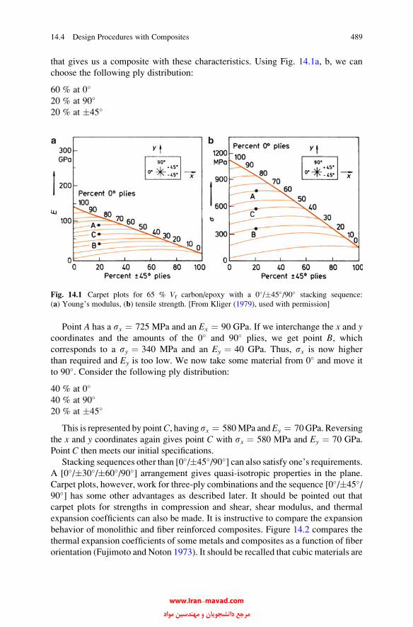
that gives us a composite with these characteristics. Using Fig. 14.1a, b, we can

choose the following ply distribution:

60 % at 0�

20 % at 90�

20 % at �45�

Point A has a sx ¼ 725 MPa and an Ex ¼ 90 GPa. If we interchange the x and ycoordinates and the amounts of the 0� and 90� plies, we get point B, whichcorresponds to a sy ¼ 340 MPa and an Ey ¼ 40 GPa. Thus, sx is now higher

than required and Ey is too low. We now take some material from 0� and move it

to 90�. Consider the following ply distribution:

40 % at 0�

40 % at 90�

20 % at �45�

This is represented by pointC, having sx ¼ 580MPa andEy ¼ 70GPa. Reversing

the x and y coordinates again gives point C with sx ¼ 580 MPa and Ey ¼ 70 GPa.

Point C then meets our initial specifications.

Stacking sequences other than [0�/�45�/90�] can also satisfy one’s requirements.

A [0�/�30�/�60�/90�] arrangement gives quasi-isotropic properties in the plane.

Carpet plots, however, work for three-ply combinations and the sequence [0�/�45�/90�] has some other advantages as described later. It should be pointed out that

carpet plots for strengths in compression and shear, shear modulus, and thermal

expansion coefficients can also be made. It is instructive to compare the expansion

behavior of monolithic and fiber reinforced composites. Figure 14.2 compares the

thermal expansion coefficients of some metals and composites as a function of fiber

orientation (Fujimoto and Noton 1973). It should be recalled that cubic materials are

Fig. 14.1 Carpet plots for 65 % Vf carbon/epoxy with a 0�/�45�/90� stacking sequence:

(a) Young’s modulus, (b) tensile strength. [From Kliger (1979), used with permission]



isotropic in thermal properties, even in single crystal form. Noncubic monolithic

materials in a polycrystalline form, with randomly distributed grains, will also be

practically isotropic in thermal properties. Thus, titanium, steel, and aluminum are

each represented by a single point on this figure. Not unexpectedly, fiber reinforced

composites such as boron/epoxy and carbon/epoxy show highly anisotropic thermal

expansion behavior. Both aramid and carbon fibers have negative expansion

coefficients parallel to the fiber axis. One can exploit such anisotropy quite usefully

to make components that show well-controlled expansion characteristics. Although

aerospace applications of composite materials get much attention, one should

appreciate the fact that composites, in one form or another, have been in use in the

electrical and electronic industry for quite a long time. These applications range

from cables to printed circuit boards. There are many applications of composites in

the electronic packaging industry (Seraphim et al. 1986). An interesting example is

that of the leadless chip carrier (LCC) that allows electronic designers to pack more

electrical connections into less space than is possible with conventional flat packs or

dual inline packages, which involve E-glass/epoxy resin laminates. Glass/epoxy

laminate, however, is not very suitable for LCC as a substrate because it expands and

contractsmuchmore than the alumina chip carrier (the coefficient of expansion, a, ofE-glass/epoxy can vary in the range of 14–17 � 10�6 K�1, while that of alumina is

~8 � 10�6 K�1). Aramid fiber (40–50 v/o)/epoxy composite provides the desired

matching expansion characteristics with those of the alumina chip carrier. Thus, the

thermal fatigue problem associated with the E-glass/epoxy composites and the

ceramic chip carrier is avoided. It should be pointed out that, in general, thermal

Fig. 14.2 Variation of thermal expansion coefficients with orientation y. [From Fujimoto and

Noton (1973), used with permission]



expansion of particulate composites, assuming an isotropic distribution of particles

in the matrix, will be more or less isotropic.

We saw in Chap. 11 that laminated composites show coupling phenomena:

tension-shear, tension-bending, and bending-twisting. We also saw in Chap. 11 that

certain special ply sequences can simplify the analyses. Thus, using a balanced

arrangement (for every +y ply, there is a �y ply in the laminate), we can eliminate

shear coupling. In such an arrangement, the shear distortion of one layer is

compensated by an equal and opposite shear distortion of the other layer. Yet another

simplifying arrangement consists of stacking the plies in a symmetric manner with

respect to the laminate midplane. Such a symmetric laminate gives [Bij] identically

zero and thus eliminates stretching-bending and bending-torsion coupling. The phe-

nomenon of edge effects, described in Sect. 11.7, should also be taken into account

while arriving at a ply stacking sequence. Because of the edge effects, individual

layers of different fiber orientation deformdifferently under tensile stress giving rise to

out-of-plane tensile, compressive, shear and/or bending stresses in the neighborhood

of the free edges. An arrangement that gives rise to compressive stresses in the

thickness direction in the vicinity of the edges is to be preferred over one that gives

rise to tensile stresses. Tensile stresses in the thickness direction near a free edgewould

tend to cause undesirable delamination in the composite. As an example, we show

Fig. 14.3 Delaminations, as

observed by contrast-

enhanced X-ray radiography

in a [0�/�45�/90�]s carbon/epoxy laminate upon fatigue

testing. [From Bergmann




http://dx.doi.org/10.1007/978-0-387-74365-3_11

http://dx.doi.org/10.1007/978-0-387-74365-3_10

http://dx.doi.org/10.1007/978-0-387-74365-3_11#Sect. 7_11

in Fig. 14.3 delaminations as observed by contrast enhanced X-ray radiography, in a

[0�/�45�/90�]s carbon/epoxy laminate upon fatigue testing (Bergmann 1985).

The delaminations proceed fromboth sides toward the specimen center.Mere stacking

choice of the plies can make a big difference. This is shown in Fig. 14.4. The laminate

with the sequence [90�/�45�/0�]s showed relatively less damage than the lami-

nate with the sequence [0�/�45�/90�]s. Figure 14.4 compares the crack patterns at

the free edges of [0�/�45�/90�]s and [90�/�45�/0�]s laminates shortly before failure.

Note the greater degree of delaminations in [0�/�45�/90�]s than in [90�/�45�/0�]s.The reason for this different behavior of these laminates, identical in all respects

except the stacking sequence, is due to the difference in the state of stress near the

free edges. Finite element calculations showed (Bergmann 1985) that in the

[0�/�45�/90�]s sequence there were large interlaminar tensile stresses in the thickness

direction while in the [90�/�45�/0�]s sequence there were mostly compressive inter-

laminar stresses.

A little reflection will convince the reader that computer simulations involving

complex finite element analyses can be used extensively in the design and analyses

of laminated fiber composites. In view of the rather tedious matrix calculations

involved, this should not be surprising at all. Computer codes can be very cost-

effective in the analysis and design of fiber composite structures. Most codes

specify, among other things, the interply layers, laminate failure stresses, laminate

Fig. 14.4 Comparison of crack patterns at the free edges of a carbon/epoxy laminate:

(a) [0�/�45�/90�]s, (b) [90�/�45�/0�]s. Note the greater severity of edge delaminations in

(a) than in (b). [From Bergmann (1985), used with permission]



requirements at critical locations in the composite, etc. Many such codes are

available commercially. An example of commercially available computer code is

the FiberSIM suite of software tools that converts a CAD (computer-aided design)

system into a composite design and manufacturing environment. Among its

features are:

• Composite engineering environment: This allows engineers to work in their

CAD environment with objects such as plies, cores, and tool surfaces. Forms

and menus are used to enter and manage the geometry and other data required to

define a composite part.

• Flat pattern/producibility: This module alerts the engineer to manufacturing

problems such as wrinkling, bridging, and material width limitations. It also

generates net flat patterns for woven and unidirectional complex curvature plies.

• Laminate properties: Exact fiber orientations are obtained for use in generating

properties of a laminated composite.

14.5 Hybrid Composite Systems

An extra degree of flexibility in fiber composites can be obtained by making what

are called hybrid composites, wherein one uses more than one type of fiber; see

Fig. 14.5. Cost-performance effectiveness can be increased by judiciously using

different reinforcement types and selectively placing them to get the highest

strength in highly stressed locations and directions. For example, in a hybrid

composite laminate, the cost can be minimized by reducing the carbon fiber

content, while the performance is maximized by “optimal placement and orienta-

tion of the fiber.” Figure 14.6 shows the increases in specific flexural modulus

(curve A) and specific tensile modulus (curve B) with weight % of carbon fiber in a

hybrid composite (Riggs 1985). Figure 14.7 shows the changes in flexural fatigue

behavior as we go from 100 % unidirectional carbon fibers in polyester (curve A) tounidirectional carbon faces over chopped glass core (curve B) to 100 % chopped

glass in polyester resin (curve C) (Riggs 1985); keeping the fiber volume fraction

constant.

Fig. 14.5 Schematic of a

hybrid laminate composite

containing carbon and glass

fibers

14.5 Hybrid Composite Systems 493


An extension of this concept is the so-called fiber metal laminates such as

GLARE, an acronym for glass fiber/epoxy and aluminum laminates. GLARE

consists of alternating layers of aluminum sheets and glass fiber reinforced epoxy

composite. Such composites are used in the fuselage of the superjumbo aircraft

A380 of Airbus. They show high strength, excellent fatigue, and fracture resistance

combined with the advantages of metal construction such as formability, machin-

ability, toughness, and impact resistance. We discuss this in Chap. 15.

Fig. 14.6 Change in specific

flexural modulus and specific

tensile modulus with wt.%

carbon fibers. [From Riggs

(1985), reprinted by

permission.] A ¼ specific

flexural modulus;

B ¼ specific tensile modulus

Fig. 14.7 Flexural fatigue

behavior of 100 % carbon

fiber composite (curve A),carbon fiber facings with

chopped glass fiber core

(curve B), and 100 % chopped

glass fiber composite (curve

C). [From Riggs (1985),

reprinted by permission]



http://dx.doi.org/10.1007/978-0-387-74365-3_15

References

Bergmann H (1985) Carbon fibres and their composites. Springer, Berlin, p 184

Fujimoto WT, Noton BR (1973) In: Proceedings of the 6th St. Louis symposium on composite

material engineering & design. American Society for Metals, Metals Park, OH, p 335

Kliger HS (Dec. 6, 1979) Mach Des 51:150

Riggs JP (1985) Encyclopedia of polymer science & engineering, vol 2, 2nd edn. Wiley,

New York, p 640

Schier JF, Juergens RJ (1983) Astronaut Aeronaut 44:44–49

Seraphim DP, Barr DE, Chen WT, Schmitt GP (1986) Advanced thermoset composites.

Van Nostrand Reinhold, New York, p 110

Sturgeon JB (1978) In: Creep of engineering materials, a Journal of Strain Analysis Monograph,

175.

Further Reading

Chamis CC (ed) (1974) Structural design and analysis, Parts I and II. Academic, New York



Lubin G (ed) (1982) Handbook of composites. Van Nostrand Reinhold, New York

Swanson SR (1997) Introduction to design and analysis with advanced composite materials.

Prentice Hall, Upper Saddle River, NJ

Problems

14.1. Following are the data for a 60 % Vf, unidirectionally reinforced, carbon fiber/

epoxy composite:

Longitudinal tensile strength ¼ 1; 200MPa

Longitudinal compressive strength = 1,000MPa

Transverse tensile strength = 50MPa

Transverse compressive strength = 250MPa

Calculate F11, F22, F66, F1, F2, and F�12. Take F�

12 ¼ �0:5. Compute the

focal points plot the failure envelope for this composite.

Problems 495


14.2. For a carbon/epoxy composite, the strength parameters are:

F11 GPað Þ�2 ¼ 0:45F22 GPað Þ�2 ¼ 101

F12 GPað Þ�2 ¼ �3:4F66 GPað Þ�2 ¼ 215

F1 GPað Þ�1 ¼ 0

F2 GPað Þ�1 ¼ 21:

Compute the off axis uniaxial strengths of this composite for different yand obtain a plot of sx vs. y.



Chapter 15

Nonconventional Composites

We devote this chapter to some nonconventional composites. Nonconventional

composites include nanocomposites (polymer, metal, and ceramic matrix), self-

healing composites, self-reinforced composites, biocomposites, and laminates

made of bidimensional layers. These topics are in the early stages of their develop-

ment but they are potentially quite important. We provide below a brief description

of these topics.

15.1 Nanocomposites

Nanocomposites are composites that have one component that has at least one

dimension in the nm range; generally it will be the reinforcement phase which may

be nanotubes, nanofibers, or nanoparticles. Although, they can have a polymeric,

metallic, or ceramicmatrix, a polymermatrix ismore common (Barrera 2000; Barrera

et al. 2005; Shofner et al. 2003, 2006). There is a strong potential for producing strong

and wear-resistant metal matrix nanocomposites by liquid processing and powder

processing routes (see, for example, Fukuda et al. 2011). Before that happens,

however, researchers will need to devise processing techniques to make these

materials in bulk, in a cost-effective manner, without voids or other defects.

15.1.1 Polymer Clay Nanocomposites

A special type of nanocomposite, called nanoclay composites, has made good

progress into commercial production. Polymer matrix reinforced with nanoclay

particles has become commercially viable (Ajayan et al. 2003; Koo 2006; Lee et al.

2005; Okada and Usuki 2006; Paul and Robeson 2008). Most of the clay

additives are in the form of platelets that have been organically treated. They are

commonly called nanoclays because their thickness is in the nanometer range.


497


Chemically, these clays are layered magnesium aluminum silicates. Their

dimensions are as follows: thickness of about 1 nm and length or width in the

range of 70–150 nm, which would give an aspect ratio of over 100. Surface

modification of the clays makes it possible to disperse them in thermoplastic

materials. These nanoclay particles can enhance the modulus (function of amount

of particles added) while lowering the coefficient of thermal expansion.

The work in this area was pioneered by Toyota researchers in 1990 when they

first used clay/nylon 6 composites for timing belt covers. Some of the earliest

commercial successes can be credited to Toyota, GM, and Ford. Major automakers

have started making use of nanocomposites in their autos. General Motors Corp., in

particular, in 2001, used a thermoplastic olefin (TPO) step-assist for the ’02 GMC

Astro/Safari van that was enhanced with a clay nanomaterial. GM also used clay

nanocomposites in the Chevrolet Impala. These products are made of thermoplastic

polyolefin–clay nanocomposite. The nanocomposites are lighter, stiffer, and cost-

effective compared to the conventional polymeric materials. The cost-effectiveness

part is important because the automobile industry is loath to use anything that is not

cost-effective, exception being sports cars. Also, the crash requirement in autos is

very important. This characteristic has to do with the energy absorbed in the impact,

which in the case of autos depends more on strain than on stress.

In regard to nanoclay composites, mention should be made of Southern Clay

Products Co. Cloisite® and Nanofil® are commercially available clay additives

from this company that are used in automotive clay nanocomposites. These are

organically modified, nanometer scale, layered magnesium aluminum silicate

platelets. The key issue in nanoclay/polymer composites is that of polymer/clay

compatibility at the interface. This requires that, in most cases, one must impart an

organophilic character to the clay. This is commonly accomplished by adding

amino acids, organic ammonium salts, or tetra organic phosphonium solution.

The surface modification of platelets with an organic graft allows dispersion and

miscibility with the thermoplastic matrix materials. The additives serve to reinforce

thermoplastics resulting in somewhat higher stiffness and lower coefficient

of thermal expansion. The additives also improve gas barrier properties of

thermoplastics. The surface char formation and flame retardance of thermoplastic

systems have also been improved by incorporating the nanoclay particles into the

structure. In the case of hydrophilic polymers and silicate layers pretreatment is not

necessary. Most polymers are hydrophobic and are not compatible with hydrophilic

clays. In such cases, a treatment that results in exfoliation of the clays is needed.

By exfoliation we mean peeling of clay flakes or platelets from one another, and

dispersion into the polymer matrix. There is some confusion about such terminol-

ogy in the literature. Let us define these terms. By intercalation we mean that some

of the organic polymer is inserted between the flakes of the clay, which would

increase the interlayer spacing but individual flakes stay together. In an exfoliated

structure, the layers of the clay are well separated and the individual layers are

distributed throughout the organic matrix. A third alternative is dispersion of

complete clays within the polymer matrix; this is akin to use of the clay as

conventional filler. Figure 15.1 shows schematically three different morphologies:

498 15 Nonconventional Composites


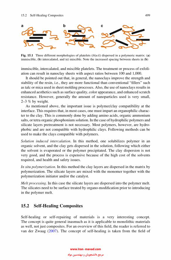
immiscible, intercalated, and miscible platelets. The treatment or process of exfoli-

ation can result in nanoclay sheets with aspect ratios between 100 and 1,000.

It should be pointed out that, in general, the nanoclays improve the strength and

stability of the resin, i.e., they are more functional than conventional “fillers” such

as talc or mica used in sheet molding processes. Also, the use of nanoclays results in

enhanced aesthetics such as surface quality, color appearance, and enhanced scratch

resistance. However, generally the amount of nanoparticles used is very small,

2–3 % by weight.

As mentioned above, the important issue is polymer/clay compatibility at the

interface. This requires that, in most cases, one must impart an organophilic charac-

ter to the clay. This is commonly done by adding amino acids, organic ammonium

salts, or tetra organic phosphonium solution. In the case of hydrophilic polymers and

silicate layers pretreatment is not necessary. Most polymers, however, are hydro-

phobic and are not compatible with hydrophilic clays. Following methods can be

used to make the clays compatible with polymers.

Solution induced intercalation. In this method, one solubilizes polymer in an

organic solvent, and the clay gets dispersed in the solution, following which either

the solvent is evaporated or the polymer precipitated. The clay dispersion is not

very good, and the process is expensive because of the high cost of the solvents

required, and health and safety issues.

In situ polymerization. In this method the clay layers are dispersed in the matrix by

polymerization. The silicate layers are mixed with the monomer together with the

polymerization initiator and/or the catalyst.

Melt processing. In this case the silicate layers are dispersed into the polymer melt.

The silicates need to be surface treated by organo-modification prior to introducing

in the polymer melt.

15.2 Self-Healing Composites

Self-healing or self-repairing of materials is a very interesting concept.

The concept is quite general inasmuch as it is applicable to monolithic materials

as well, not just composites. For an overview of this field, the reader is referred to

van der Zwaag (2007). The concept of self-healing is taken from the field of

Fig. 15.1 Three different morphologies of platelets (black) dispersed in a polymeric matrix: (a)

immiscible, (b) intercalated, and (c) miscible. Note the increased spacing between sheets in (b)

15.2 Self-Healing Composites 499


medicine. The basic premise is that, in a self-healing system, when damage

occurs, the system realizes that something is wrong. Then, without human inter-

vention, the self-healing system makes the necessary adjustments and returns to

normal operation. The process has been called an autonomic healing process

(White et al. 2001). The term autonomic, again borrowed from medicine, refers

to automatic functioning of a system. The self-healing process mimics the spon-

taneous healing processes observed in living systems when they are damaged. In a

living system, damage (for example formation of a bruise) triggers an autonomic

healing process, i.e., when an organism is damaged, there is a natural healing

response. Researchers have applied this concept to synthetic material design and

have developed self-healing materials. The basic idea is to incorporate a healing

agent in the material of interest which will come into action when damage in the

form of a crack appears. It is easy to appreciate the appeal of this concept in

composites by recalling that increasing amounts of PMCs are being used

in civilian infrastructure (bridges, decks, columns, etc.).

The idea of autonomic healing in a composite works is shown schematically in

Fig. 15.2. The healing or repair agent (a kind of cross-linking polymer) encapsulated

in a hollow microsphere (or a hollow fiber) can be embedded in the matrix. The

polymer matrix has a catalyst distributed in it that serves to polymerize the healing

agent. Damage in the form of a crack is shown in Fig. 15.2a. When the crack

propagates and breaks themicrosphere, the healing agent is released through capillary

action. Polymerization occurs when the healing agent encounters the catalyst and

the crack faces are closed by bonding as shown in Fig. 15.2c. A self-healing PMC can

be made by using a microencapsulated healing agent and a solid chemical catalyst,

both dispersed within the polymer matrix phase. Healing or closure of a crack will

occur when the crack propagates through the microcapsules releasing the healing

agent onto the crack plane. The healing agent, under the action of chemical catalyst,

initiates polymerization and bonding of the crack faces. Kessler et al. (2003) used this

approach in a carbon fiber/epoxy composite. The self-healing composite system

consisted of a healing agent, microcapsule shell, chemical catalyst, epoxy matrix,

and carbon fiber. They used the monomer, dicyclopentadiene (DCPD) as the healing

agent, which possesses low viscosity and excellent shelf life when stabilized

with 100–200 ppm p-tert-butylcatechol. The healing agent was encapsulated in

poly-ureaformaldehyde by in situ polymerization (White et al. 2001) to yield the

self-healing PMC.

Self-healing was demonstrated on width-tapered double cantilever beam

fracture specimens in which a mid-plane delamination was introduced, which was

allowed to heal. Specifically, healing at room temperature yielded as much as 45 %

recovery of undamaged value of interlaminar fracture toughness, while healing at

80 �C increased the recovery to over 80 % (Kessler et al. 2003). An extension of this

concept was reported by Kirkby et al. (2007). They embedded shape memory alloy

(SMA) wires in the composite and observed improvements in performance, which

were attributed to three effects: (1) crack closure, which reduces the crack volume

and the amount of healing agent required; (2) heating of the healing agent during

polymerization, which improved the cross-linking; and (3) mechanical registration

of the two crack faces, which resulted in a reduced crack volume on closure.



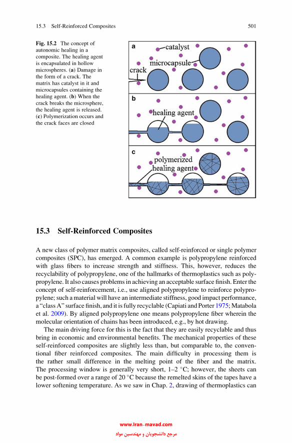
15.3 Self-Reinforced Composites

A new class of polymer matrix composites, called self-reinforced or single polymer

composites (SPC), has emerged. A common example is polypropylene reinforced

with glass fibers to increase strength and stiffness. This, however, reduces the

recyclability of polypropylene, one of the hallmarks of thermoplastics such as poly-

propylene. It also causes problems in achieving an acceptable surface finish. Enter the

concept of self-reinforcement, i.e., use aligned polypropylene to reinforce polypro-

pylene; such amaterial will have an intermediate stiffness, good impact performance,

a “classA” surface finish, and it is fully recyclable (Capiati andPorter 1975;Matabola

et al. 2009). By aligned polypropylene one means polypropylene fiber wherein the

molecular orientation of chains has been introduced, e.g., by hot drawing.

The main driving force for this is the fact that they are easily recyclable and thus

bring in economic and environmental benefits. The mechanical properties of these

self-reinforced composites are slightly less than, but comparable to, the conven-

tional fiber reinforced composites. The main difficulty in processing them is

the rather small difference in the melting point of the fiber and the matrix.

The processing window is generally very short, 1–2 �C; however, the sheets can

be post-formed over a range of 20 �C because the remelted skins of the tapes have a

lower softening temperature. As we saw in Chap. 2, drawing of thermoplastics can

Fig. 15.2 The concept of

autonomic healing in a

composite. The healing agent

is encapsulated in hollow

microspheres. (a) Damage in

the form of a crack. The

matrix has catalyst in it and

microcapsules containing the

healing agent. (b) When the

crack breaks the microsphere,

the healing agent is released.

(c) Polymerization occurs and

the crack faces are closed

15.3 Self-Reinforced Composites 501


http://dx.doi.org/10.1007/978-0-387-74365-3_2

result in some chain alignment, which in turn can lead to an increase in modulus.

Polypropylene (PP) fibers in a polypropylene matrix, called self-reinforced poly-

propylene, are available commercially: Curv® and Moldable Fabric Technology

(MFT) are self-reinforced 100 % PP composites that contain PP fibers in a PP

matrix. The process of making such self-reinforced composites is to heat and

compact highly oriented, small-diameter fibers under suitable time, temperature,

and pressure conditions to form a composite wherein a substantial proportion of the

original molecular orientation of fibers is retained. Generally, in practice, this

means that some 10–20 % of the original fiber gets melted and loses the superior

mechanical characteristics but serves to produce matrix. Figure 15.3 shows the

microstructure of such a composite. The material properties are enhanced through

molecular orientation, resulting in self-reinforcement.

The tapes are woven into fabric to provide ease of handling and balance. This

material offers excellent impact resistance, lightweight, and high stiffness compared

to non-drawn PP. Curv® is used in automotive exterior (bumpers, body panels,

underbody shields, wheel arch liners), interior (load floors, pillar trims, door and

head liners), audio products, sporting and travel goods, as well as ballistic protection.

Fig. 15.3 Microstructure of a self-reinforced composite (PP fabric in a PP matrix)



15.4 Biocomposites

Biocomposites can be defined as composites that have at least one component that

is derived from biological or natural sources. There is a growing interest in these

composites (see, for example, Fuqua and Ulven 2008; Mohanty et al. 2005; Silva

et al. 2008; Sui et al. 2009; Wool and Sun 2005). The main attributes of

biocomposites that are driving the effort in this area are the following:

• Biodegradable

• Renewable

• Cheap

• Natural resource

Biocomposites, based on these attributes, are environmentally friendly. However,

the ultimate test for their success in the commercial arena will depend onwhether they

meet the application requirements. Among the problem areas in their widescale

acceptance are the following:

• High moisture absorption

• Poor wettability of fibers by polymeric resins leading to poor interfacial bonding

• High viscosity of bioresins making processing more difficult

There are many examples of composites found in nature. Shells (abalone and

mussel) are good examples of how living organisms synthesize layered composites

that show high strength and high toughness. Layers of calcium carbonate (CaCO3,

orthorhombic crystal structure) and an organic adhesive are stacked in a brick and

mortar type structure. The mortar gluing together the bricks of calcium carbonate is a

thin film of proteins and polysaccharides. This biocomposite consists of about 95 %

inorganic mineral and 5 % organic polymer, with electrostatic forces acting at the

interface. The organic glue is strong enough to hold layers of calcium carbonate

together, but weak enough to allow the layers to slide and thus absorb the energy of

an impact or to deflect an oncoming crack instead of letting it propagate in a

catastrophic manner through the brittle calcium carbonate. Such ingenius materials

science and engineering work done by nature is a source of work in the field of

biomimetics. Somework related to synthetic laminates is described in the next section.

15.5 Laminates

Laminates are multilayered composite materials. We discussed fiber reinforced

laminates made by appropriately stacking fiber reinforced plies. The laminates we

are discussing in this section are in general made by putting together sheets, except

for variety called fiber metal laminates (see below). Some of these laminates have

been in commercial use for sometime while others are potential candidates for a

15.5 Laminates 503


variety of applications because of their superior properties: high strength (ambient

and high temperature), fatigue resistance, wear resistance, and biocompatibility.

Examples of laminated structural materials can be found in nature and in

historical manmade objects. The unique structure of laminates found in nature

offers desired functional properties. Examples include bones, tooth, shells of

mussels, etc. For example, abalone shell consists of protein layers separating the

mesolayers. Among historic examples, we should mention metallic laminates made

of steel that have been used to make Samurai swords. The famous iron pillar of

Delhi consists of laminae of wrought iron. Other mundane examples include

copper/aluminum and copper/stainless laminates for use in kitchen utensils.

Researchers have explored multilayered composites consisting of metal/metal

and metal/ceramic laminates. Extensive work on ultrahigh carbon steel (UHCS)

laminates, which have compositions very similar to ancient Damascus or Wootz

steels, showed excellent impact properties (Verhoeven et al. 1998; Lesuer et al.

1996).

A general view of the structure of laminates at different length scales is provided

in Fig. 15.4 (Deng et al. 2005; Woerden et al. 2003; Gavens et al. 1999). Here we

wish to highlight the microstructure of the multilayered Al/SiC composites made by

DC/RF magnetron sputtering. Figure 15.5a shows the nanolaminate as observed in

SEM while Fig. 15.5b shows the interface in this system as observed in a transmis-

sion electron microscopy (TEM); no reaction product is observed at the interface

Fig. 15.4 A general view of the structure of laminates at different length scales



Fig. 15.5 (a)Microstructure of SiC/Al nanolaminate. (b) TEMmicrography shows the well-bonded

interface and absence of any reaction product at the interface. SiO2 forms on the surface of SiC

Fig. 15.6 Deformation of SiC/Al nanolaminate in a nanoindenter. Note the well-bonded interface

and the extreme flexibility of SiC, an inherently brittle material


between Al and SiC. The elastic and plastic behavior of the multilayered materials,

as investigated by nanoindentation, showed a high degree of flexibility of brittle

SiC layers, see Fig. 15.6, before and after indentation. Cracking under indentation

started at a depth of 1,000 nm in SiC layers. This occurred at sites where kinks

formed in SiC which appeared to occur at sites of shear localization.

15.5.1 Ceramic Laminates

Multilayered ceramic capacitors (MLCCs) represent a commercially very impor-

tant and successful ceramic/metal laminate system. Barium titanate (BaTiO3) is a

ferroelectric material with a high dielectric constant. MLCCs are laminates made of

alternate layers of BaTiO3 dielectric and inner electrodes of Pd, Pt–Ag, or Ni.

The inner electrodes are exposed at the opposite sides of the laminate. MLCCs are

widely used in the electronics industry. These capacitors, manufactured by alter-

nately layering electrodes and thin dielectric, are small, efficient, reliable, and cost-

effective, and used in virtually every electronic circuit.

Laminated glass is an example of glass/polymer laminate that is widely used but

not appreciated as a sheet laminate composite, which is what it really is. One of the

flat glass products is the automobile windshield (about 25 % total flat glass

production is consumed by the automobile industry in the USA) that amounts to

over $500 million market. The USA and many other countries require by law that

automobile windshields be made of laminated glass. The glass composition is

mostly SiO2 with some Na2O + CaO + K2O + MgO + Al2O3. The laminate is

made of two sheets of tempered glass (each 0.75 mm thick) bonded by a layer

(2.5 mm) of tough plastic (PVB—poly vinyl butaryl) in an autoclave. PVB/glass

has good adhesion. PVB is transparent and can be tinted to protect against UV

radiation. The finished laminated glass is virtually indistinguishable from ordinary

glass, because the PVB is invisible and covered on both sides by the glass. The main

advantage is that if the glass laminate gets broken, the glass shards stick to the

plastic interlayer rather than cleanly breaking apart and do a lot more damage. The

minor disadvantage is that the PVB laminated glass has less strength than ordinary

glass of the same size and thickness.

15.5.2 Hybrid Composites

A novel composite material, erroneously named fiber metal laminate (FML), has

been developed. It consists of a metal sheet (~ 0.3 mm thick) which can

be aluminum, steel, titanium, magnesium, etc. and a polymer matrix composite

(PMC) prepreg which consists of fiber reinforced polymer; see Fig. 15.7. The

composite consists of alternate layers of PMC and metal sheet. In principle,

the fiber can be continuous or not; it can be glass, aramid, or carbon and the resin



matrix can be any polymer but is commonly epoxy. The nomenclature scheme goes

as follows:

• GLARE: GLAss fiber REinforced laminates

• ARALL: ARamid fiber reinforced ALuminum Laminates

• CARE: CArbon fiber REinforced laminates

• TIGR: TItanium/GRaphite-epoxy laminates

Common aircraft fuselage material is an aluminum alloy. In the Airbus A 380

jumbo aircraft the panels for the upper fuselage section of the aircraft are made

GLARE which consists of laminates made of alternate layers of glass fiber/epoxy

(a PMC) and aluminum sheet. Such hybrid composites combine advantages of

metals and PMCs, to wit:

• Excellent fatigue and impact properties

• High strength and stiffness

• Flame resistance

• Easily machined or formed

• Mechanical fastening capability

There is some interesting history with the use of GLARE in aircraft. Earlier,

fuselage construction with ARALL was tried. It was observed that under loading

conditions encountered in an aircraft fuselage, the aramid fibers around a fatigue

crack would break. Once the fiber was broken, the crack was no longer inhibited

and would grow. The growing crack would lead to delamination, which placed a

compressive stress on the aramid fibers, causing buckling. Low compressive stress

of aramid fibers is well known (see Chap. 2; Chawla 1998). It was observed that

aramid fibers would break under rather low compressive loads and it also became

evident that ARALL was also sensitive to strength reductions caused by any holes

that might be drilled in it. Such holes are unavoidable in a large structure such as a

fuselage; they would lead to premature fatigue cracks to develop. Although use of

ARALL was not suitable for fuselage construction, the weight savings by using this

Fig. 15.7 A fiber metal laminate (FML) made of a metal sheet and a polymer matrix composite

(PMC) prepreg which consists of a fiber reinforced polymer composite

15.5 Laminates 507


http://dx.doi.org/10.1007/978-0-387-74365-3_2

material were very attractive. Earlier, ARALL was used in the C-17 military

transport plane. Because of heavy weight problems toward the rear of the plane,

the large aluminum cargo door was replaced with ARALL.

This was followed by replacing aramid with glass fibers in the new FML called

GLARE, which has superior blunt notch strength and the ability to handle greater

compressive stresses than ARALL. GLARE is also more resistant to impact than

ARALL and for this reason the first commercial application of GLARE was in the

cargo floor of Boeing’s 777 plane where the excellent impact properties of GLARE

were put to use. The next stage of use of Glare was in the form of panels for the

fuselage of Airbus’s A380 aircraft. At first the manufactured flat panels lacked the

cost-effectiveness necessary for the material to break ahead of conventional alumi-

num structures despite the excellent mechanical properties. The cost of manufac-

ture of GLARE composites was roughly 7–10 times that of aluminum per kilogram

and the next step was to lower the cost of manufacture (Vlot and Gunnick 2001).

The dimensions of metal sheet with the required 0.3–0.4 mm thickness were limited

to a width of 1.65 m. For the aluminum/S2-glass fiber in epoxy system, failure

occurred primarily at the metal/adhesive interface. The thicker specimens

debonded faster than thinner ones, hence the need for very thin aluminum sheet

to increase the fatigue resistance of GLARE. The manufacture of flat panels of

GLARE in an autoclave, although expensive, was an important step in GLARE

production. The main source of fatigue resistance in Glare is the intact bridging

fibers in the wake of the crack; they restrain crack opening. Figure 15.8 shows the

slow fatigue crack growth characteristics of GLARE compared to monolithic

aluminum alloy.

Yet another type hybrid composite is a composite containingmore than one type of

fiber. We described this in Chap. 13. Such composites, by using two or more types of

fibers, extend the idea of tailor-making a composite material to meet specific property

requirements. Partial replacement of expensive fibers by cheaper but adequate fiber

types is another attractive feature of hybrid composites. Additionally, there is the

possibility of obtaining a synergistic effect in the fatigue behavior of hybrid

composites. Such synergistic results are by no means universal. For example, in the

case of the flexural fatigue strength vs. the number of cycles for 100 % unidirectional

carbon fiber/polyester, 100% chopped glass fiber/polyester, and unidirectional carbon

fiber faces over chopped glass core, the hybrid composite curve was intermediate

between the 100 % carbon and 100 % glass curves (Riggs 1985).

Another version of hybrid laminated MMCs is a family of layered composites

consisting of metallic outer skins with a viscoelastic core material (for example,

polyethylene, nylon, polypropylene, paper, or cork). Such composites will be useful

where sound and vibration damping are required. The viscoelastic layer provides a

high loss factor, i.e., a high capacity to convert vibrational energy to heat.

Although such composites are commonly made of metal and thermoset matrix

PMCs containing continuous fibers, this concept of hybrid composites has been

extended to thermoplastics and discontinuous fibers (Abdullah and Cantwell 2006;

Cortes and Cantwell 2006; Kulkarni et al. 2007).



http://dx.doi.org/10.1007/978-0-387-74365-3_13

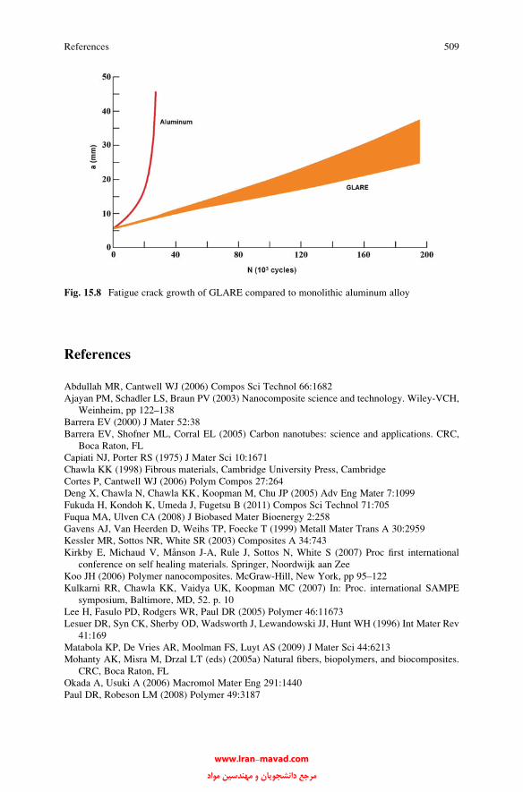
References

Abdullah MR, Cantwell WJ (2006) Compos Sci Technol 66:1682

Ajayan PM, Schadler LS, Braun PV (2003) Nanocomposite science and technology. Wiley-VCH,

Weinheim, pp 122–138

Barrera EV (2000) J Mater 52:38

Barrera EV, Shofner ML, Corral EL (2005) Carbon nanotubes: science and applications. CRC,

Boca Raton, FL

Capiati NJ, Porter RS (1975) J Mater Sci 10:1671

Chawla KK (1998) Fibrous materials, Cambridge University Press, Cambridge

Cortes P, Cantwell WJ (2006) Polym Compos 27:264

Deng X, Chawla N, Chawla KK, Koopman M, Chu JP (2005) Adv Eng Mater 7:1099

Fukuda H, Kondoh K, Umeda J, Fugetsu B (2011) Compos Sci Technol 71:705

Fuqua MA, Ulven CA (2008) J Biobased Mater Bioenergy 2:258

Gavens AJ, Van Heerden D, Weihs TP, Foecke T (1999) Metall Mater Trans A 30:2959

Kessler MR, Sottos NR, White SR (2003) Composites A 34:743

Kirkby E, Michaud V, Manson J-A, Rule J, Sottos N, White S (2007) Proc first international

conference on self healing materials. Springer, Noordwijk aan Zee

Koo JH (2006) Polymer nanocomposites. McGraw-Hill, New York, pp 95–122

Kulkarni RR, Chawla KK, Vaidya UK, Koopman MC (2007) In: Proc. international SAMPE

symposium, Baltimore, MD, 52. p. 10

Lee H, Fasulo PD, Rodgers WR, Paul DR (2005) Polymer 46:11673

Lesuer DR, Syn CK, Sherby OD, Wadsworth J, Lewandowski JJ, Hunt WH (1996) Int Mater Rev

41:169

Matabola KP, De Vries AR, Moolman FS, Luyt AS (2009) J Mater Sci 44:6213

Mohanty AK, Misra M, Drzal LT (eds) (2005a) Natural fibers, biopolymers, and biocomposites.

CRC, Boca Raton, FL

Okada A, Usuki A (2006) Macromol Mater Eng 291:1440

Paul DR, Robeson LM (2008) Polymer 49:3187

Fig. 15.8 Fatigue crack growth of GLARE compared to monolithic aluminum alloy

References 509


Shofner ML, Khabashesku VN, Barrera EV (2006) Chem Mater 18:906

Shofner ML, Rodriguez-Macias FJ, Vaidyanathan R, Barrera EV (2003) Compos A Appl Sci

Manuf 34:1207

Silva FA, Chawla N, Toledo Filho RD (2008) Compos Sci Technol 68:3438

Sui G, Fuqua MA, Ulven CA, Zhong WH (2009) Bioresour Technol 100:1246

Verhoeven JD, Pendray AH, Dauksch WE (1998) JOM 50(9):58

Vlot A, Gunnick JW (2001) Fibre metal laminates: an introduction. Kluwer Academic Publishers,

Dordrecht

White SR, Sottos NR, Geubelle PH, Moore JS, Kessler MR, Sriram SR, Brown EN, Viswanathan S

(2001) Nature 409:794

Woerden HJM, Sinke J, Hooimeijer PA (2003) Appl Comp Mater 10:307

Wool R, Sun XS (2005) Bio-based polymers and composites. Elsevier Academic, Burlington, MA

van der Zwaag S (ed) (2007a) Self healing materials. Springer, Dordrecht

Further Reading

Bakshi SR, Lahiri D, Agarwal A (2010) Int Mater Rev 55:41

Mauldin TC, Kessler MR (2010) Int Mater Rev 55:317

Mohanty AK, Misra M, Drzal LT (eds) (2005b) Natural fibers, biopolymers, and biocomposites.

CRC, Boca Raton

Vlot A, Gunnick JW (2001) Fibre metal laminates: an introduction. Kluwer Academic Publishers,

Dordrecht

Vogelesang LB, Schijve J, Fredell R (1995) In: Demaid A, de Wit JHW (eds) Case studies in

manufacturing with advanced materials, vol 2. Elsevier, Amsterdam. p 253–271

van der Zwaag S (ed) (2007b) Self healing materials. Springer, Dordrecht



Appendix A

Matrices

Definition

A matrix is an array of numbers subject to certain operations. For example,

3 2 9 7

0 �63 49 5

1 5 4 8

24

35 3 rows, 4 columns

a11 a12 � � � a1na21 a22 � � � a2n... ..

. � � � ...

am1 am2 � � � amn

26664

37775 m rows; n columns

The aij are called the elements of the matrix.

Notation

A ¼ A½ � ¼ aij� � ¼ aij

� �m;n

Null Matrix

In a null matrix, all the elements are zero, that is,

N½ � ¼ 0½ �

K.K. Chawla, Composite Materials: Science and Engineering,DOI 10.1007/978-0-387-74365-3, # Springer Science+Business Media New York 2012

511


Any matrix multiplied by a null matrix results in a null matrix. Thus,

A½ � N½ � ¼ N½ �

Square Matrix

The number of rows, called the order of the matrix, is equal to the number of

columns. For example,

A½ � ¼ a11 a12a21 a22

� �

is a square matrix of order 2.

Determinant

Associated with every square matrix [A], there is a numerical value called its

determinant, │A│.

A½ � ¼ aij cof aij� �

where cof aij ¼ ð�1ÞiþjjMijj. cof aij is the cofactor of aij andMij is the minor of aij,obtained by eliminating the row and the column of aij.

Consider the matrix

A½ � ¼ a11 a12a21 a22

� �

Determinant A½ � ¼ a11 a12a21 a22

��

cof a11 ¼ �1ð Þ2 M11j j ¼ M11 ¼ a22

cof a12 ¼ �1ð Þ3 M12j j ¼ �M12 ¼ �a21

cof a21 ¼ �1ð Þ3 M21½ � ¼ �M21 ¼ �a12

cof a22 ¼ �1ð Þ4 M22j j ¼ M22 ¼ a11

Aj j ¼Xni¼1

aij cof aij� � ¼ a11a22 þ a12 �a21ð Þ

¼ a11a22 � a12a21

512 Appendix A


Another example is

½A� ¼1 2 �1

3 4 0

0 3 2

264

375

cof a11 ¼ M11 ¼4 0

3 2

�� ¼ 8� 0 ¼ 8

cof a12 ¼ �M12 ¼3 0

0 2

�� ¼ �6þ 0 ¼ �6

cof a13 ¼ M13 ¼3 4

0 3

�� ¼ 9� 0 ¼ 9

jAj ¼ 1� 8þ 2� ð�6Þ � 1� 9 ¼ 8� 12� 9 ¼ �13

Diagonal Matrix

A square matrix whose nondiagonal elements are zero is called a diagonal matrix.

aij ¼ 0 for i 6¼ j

For example,

3 0 0

0 2 0

0 0 1

24

35

Identity Matrix

A diagonal matrix whose elements are unity is called an identity matrix.

I½ � ¼1 0 0

0 1 0

0 0 1

264

375

I½ � A½ � ¼ A½ �

Appendix A 513


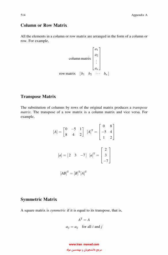
Column or Row Matrix

All the elements in a column or row matrix are arranged in the form of a column or

row. For example,

columnmatrix

a1

a2

..

.

an

266664

377775

rowmatrix b1 b2 � � � bn½ �

Transpose Matrix

The substitution of columns by rows of the original matrix produces a transposematrix. The transpose of a row matrix is a column matrix and vice versa. For

example,

A½ � ¼ 0 �5 1

8 4 2

� �A½ �T ¼

0 8

�5 4

1 2

264

375

a½ � ¼ 2 3 �7½ � ½a�T ¼2

3

�7

264

375

AB½ �T ¼ B½ �T A½ �T

Symmetric Matrix

A square matrix is symmetric if it is equal to its transpose, that is,

AT ¼ A

aij ¼ aij for all i and j

514 Appendix A


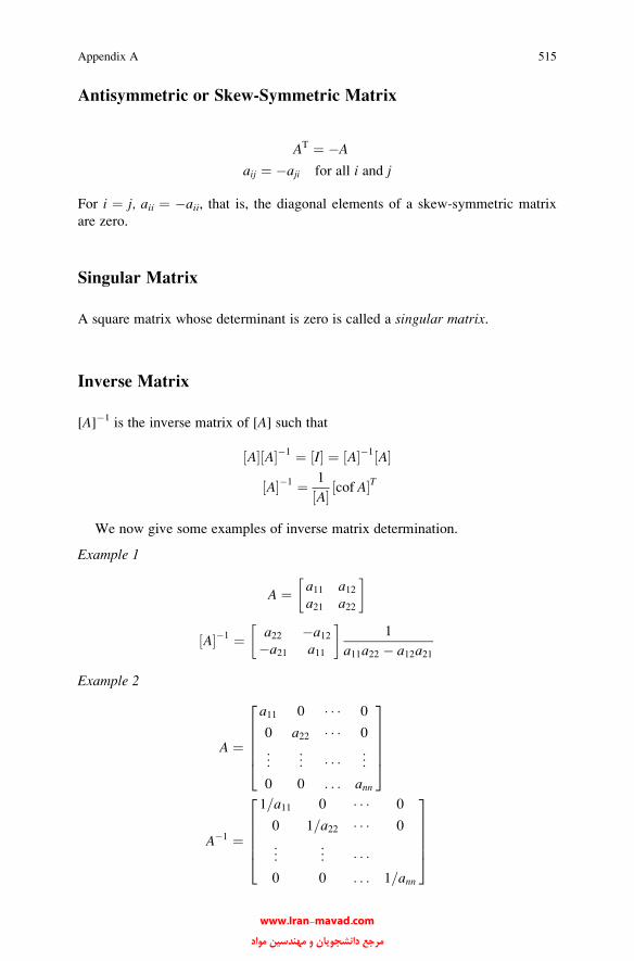
Antisymmetric or Skew-Symmetric Matrix

AT ¼ �A

aij ¼ �aji for all i and j

For i ¼ j, aii ¼ �aii, that is, the diagonal elements of a skew-symmetric matrix

are zero.

Singular Matrix

A square matrix whose determinant is zero is called a singular matrix.

Inverse Matrix

[A]�1 is the inverse matrix of [A] such that

A½ � A½ ��1 ¼ I½ � ¼ A½ ��1 A½ �A½ ��1 ¼ 1

A½ � cof A½ �T

We now give some examples of inverse matrix determination.

Example 1

A ¼ a11 a12a21 a22

� �

A½ ��1 ¼ a22 �a12�a21 a11

� �1

a11a22 � a12a21

Example 2

A ¼

a11 0 � � � 0

0 a22 � � � 0

..

. ... � � � ..

.

0 0 . . . ann

266664

377775

A�1 ¼

1=a11 0 � � � 0

0 1=a22 � � � 0

..

. ... � � �

0 0 . . . 1=ann

266664

377775

Appendix A 515


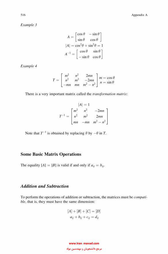
Example 3

A ¼ cos y � sin y

sin y cos y

� �Aj j ¼ cos2yþ sin2y ¼ 1

A�1 ¼ cos y sin y

� sin y cos y

� �

Example 4

T ¼m2 n2 2mnn2 m2 �2mn

�mn mn m2 � n2

24

35m ¼ cos y

n ¼ sin y

There is a very important matrix called the transformation matrix:

Aj j ¼ 1

T�1 ¼m2 n2 �2mn

n2 m2 2mn

mn �mn m2 � n2

264

375

Note that T�1 is obtained by replacing y by �y in T.

Some Basic Matrix Operations

The equality [A] ¼ [B] is valid if and only if aij ¼ bij.

Addition and Subtraction

To perform the operations of addition or subtraction, the matrices must be compati-ble, that is, they must have the same dimension:

A½ � þ B½ � þ C½ � ¼ D½ �aij þ bij þ cij ¼ dij

516 Appendix A


Similarly,

E½ � ¼ A½ � � B½ �eij ¼ aij � bij

Multiplication

To perform the operation of multiplication, the number of columns of one matrix

must be equal to the number of rows of the other matrix:

A½ �m�n B½ �n�r ¼ C½ �m�r

cij ¼Pnk¼1

aikbkj

3 5

9 8

24

35 1 0

4 3

24

35 ¼

3� 1þ 5� 4 3� 0þ 5� 3

9� 1þ 8� 4 9� 0þ 8� 3

264

375 ¼

23 15

41 24

24

35

Matrix multiplication is associative and distributive but not commutative. Thus,

AB½ � C½ � ¼ A½ � BC½ �

A½ � Bþ C½ � ¼ A½ � B½ � þ A½ � C½ �

A½ � B½ � 6¼ B½ � A½ �

The order of the matrix is very important in matrix multiplication.

Appendix A 517


Appendix B

Fiber Packing in Unidirectional Composites

Geometrical Considerations

Consider a composite containing uniaxially aligned fibers. Assume for the sake of

simplicity that the fibers have the same cross-sectional form and area. Then for any

uniaxial arrangement of fibers, we can relate the fiber volume fraction Vf, the fiber

radius r, and the center-to-center spacing of fibers R as

Vf ¼ ar

R

2where a is a constant that depends on the geometry of the arrangement of fibers.

Let S be the distance of closest approach between the fiber surfaces. Then

S ¼ 2 R� rð Þ

or

S ¼ 2aVf

� �1=2r � r

" #¼ 2r

aVf

� �1=2� 1

" #

Thus, the separation between two fibers is less than a fiber diameter when

aVf

� �1=2� 1

" #<1

or

aVf

� �1=2<2


519


or

aVf

<4

or

Vf>a4

The densest fiber packing Vfmaxcorresponds to touching fibers, that is,

aVfmax

� �1=2� 1

" #¼ 0

or

Vfmax¼ a

Table B.1 shows the values of a, a/4, and Vfmaxfor hexagonal and square

arrangements of fibers.

Table B.1 Geometrical fiber

packing parametersArrangement a a/4 Vfmax

Hexagonal p2ffiffi3

p ¼ 0:912 0.228 0.912

Square p4¼ 0:785 0.196 0.785

520 Appendix B


Appendix C

Some Important Units and Conversion Factors

Stress (or Pressure)

1 dyn ¼ 105 newton (N)

1 N m�2 ¼ 10 dyn cm�2 ¼ 1 pascal (Pa)

1 bar ¼ 105 N m�2 ¼ 105 Pa

1 hectobar ¼ 100 bars ¼ 108 cm�2

1 kilobar ¼ 108 N m�2 ¼ 109 dyn cm�2

1 mmHg ¼ 1 torr ¼ 133.322 Pa ¼ 133.322 N m�2

1 kgf mm�2 ¼ 9806.65 kN m�2 ¼ 9806.65 kPa ¼ 100 atmospheres

1 kgf cm�2 ¼ 98.0665 kPa ¼ 1 atmosphere

1 lb in.�2 ¼ 6.89476 kN m�2 ¼ 6.89476 kPa

1 kgf cm�2 ¼ 14.2233 lb in.�2

106 psi ¼ 106 lb in�2 ¼ 6.89476 GN m�2 ¼ 6.89476 GPa

1 GPa ¼ 145,000 psi

Density

1 g cm�3 ¼ 62.4280 lb ft�3 ¼ 0.0361 lb in�3

1 lb in�3 ¼ 27.68 g cm�3

1 g cm�3 ¼ 103 kg m�3

Viscosity

1 poise ¼ 0.1 Pa s ¼ 0.1 N m�2 s

1 GN m�2 s ¼ 1010 poise


521


Energy

1 erg cm�2 ¼ 1 mJ m�2 ¼ 10�3 J m�2

108 erg cm�2 ¼ 47.68 ft lb in.�2 ¼ 572.16 psi in

Fracture Toughness

1 psi in1/2 ¼ 1 lbf in�3/2 ¼ 1.11 kN m�3/2 ¼ 1.11 kPa m�1/2

1 ksi in1/2 ¼ 1.11 MPa m�1/2

1 MPa m�1/2 ¼ 0.90 ksi in1/2

1 kgf mm�2 mm1/2 ¼ 3.16 � 104 N m�2 m1/2

522 Appendix C


Author Index


523

A Abdullah, M.R., 508, 529 Aghajanian, M.K., 202, 245 Ajayan, P.M., 497, 509 Alberino, L.M., 151 Alic, J.A., 458 Allen, S.R., 48, 69 Allison, J.E., 245, 462, 479, 480 Allred, R.E., 193, 194 Anand, K., 424, 447 Anderson, B.W., 170, 194 Andersson, C.H., 59, 60, 68, 70, 220, 206,

249, 247 Ansell, G.S., 95, 101 Arsenault, R.J., 112, 131, 132, 222, 246, 247,

367, 382, 383, 422, 447, 448 Ashbee, K.H.G., 170, 171, 195 Asthana, R., 246, 481 Aveston, J., 281, 290 Awasthi, S., 303, 306 B Babonneau, F., 59, 70 Bacon, R., 29, 68 Baier, R.E., 106, 131 Bail, A.I., 138, 195 Baker, A.A., 26, 27, 68, 174, 194, 219, 245 Balch, D.K., 236, 245 Bansal, R.C., 160, 162, 194, 307 Barber, J.R., 461, 480 Barclay, S.J., 253, 290 Barham, P.J., 37, 68 Barr, D.E., 490, 495 Barrera, E.V., 197, 245, 497, 509, 510 Bascom, W.D., 90, 101 Bastos, A.C., 7, 69

Batchelder, D.N., 376, 382 Batich, C.D., 59, 70 Baughman, J., 210 Beaumont, P.W.R., 468, 479 Becher, P.F., 278, 279, 280, 290, 291, 477,

478, 481 Beever, W.R., 90, 102 Behrens, E., 358, 382 Beier, W., 288, 289, 290, 479 Bender, B.A., 478, 479 Bennett, S.C., 31–33, 68 Bergmann, H.W., 172, 184, 491, 492, 495 Bhatt, H., 359, 382 Bhatt, R.T., 253, 290, 359, 390 Bhattacharjee, P.K., 325, 332 Biggs, W.D., 3, 5 Biro, D.A., 40, 69, 163, 194 Blundell, D.J., 90, 101, 102, 175, 195 Boccaccini, A.R., 267, 268, 286, 290, 291,

472, 479 Bonnen, J.J., 462, 479 Bordia, R.K., 250, 290 Bourell, D.L., 230, 245 Bowen, D.H., 250, 270, 271, 274, 275, 277,

280, 291, 292 Bowen, H.K., 102, 290 Braun, P.V., 497, 509 Brennan, J.J., 250, 280, 290, 291, 481 Brinker, C.J., 14, 69 Broutman, L.J., 125, 131 Brown, E.N., 500, 510 Brown, J.R., 40, 69, 163, 194 Brown, W.S., 56, 63, 70 Budiansky, B., 424, 447 Bunsell, A.R., 59, 62, 69, 70, 71, 418, 482 Burke, J.T., 202, 245 Burkland, C.V., 259, 290


524 Author Index

Bustamante, W.E., 259, 290 Butler, E.P., 271, 290 Butler, E.G., 267, 268, 291 C Cahn, J.W., 108, 131, 132 Callahan, D.L., 197, 245 Cantwell, W.J., 508, 509 Capaccio, G., 38, 69 Capiati, N.J., 501, 509 Caputo, A.J., 259 61, 291 Carroll, D.F., 478, 482 Carter, C.B., 102 Carter, W.C., 271, 290 Carter, W.L., 322, 323, 332 Chamis, C.C., 123, 132, 343, 344, 357, 360,

382, 445 Champion, A.R., 214, 226, 245, 456,

457, 479 Chang, H.W., 40, 69, 163, 194 Chappell, P.J.C., 40, 69, 163, 194 Chawla, K.K., 5, 7, 14, 25, 69, 71, 94, 102,

109, 112, 115, 128, 132, 194, 195, 211, 214, 215, 216, 222, 228, 230, 232, 235, 236, 245, 246, 247, 250, 271, 275, 277, 284, 286, 290. 292, 307, 319, 332, 357, 365, 366, 367, 368, 382, 383, 422, 431, 447, 458, 460, 472, 478–482, 509

Chawla, N., 128, 132, 232, 233, 245, 247, 279, 290, 456, 457, 460–462, 473, 474, 480, 482, 504, 509, 510

Chen, C.H., 169, 194 Chen, S.T., 478, 482 Chen, W.T., 490, 495 Chew, K.W., 59, 69 Chiang, F.P., 416, 417 Chiang, Y-M., 206, 209, 245, 250, 255, 290 Chiou, W.A., 215, 246 Choi, G.J., 59, 70 Chokshi, A.H., 271, 274, 276, 290 Chou, T.W., 234, 381, 382, 466, 480 Christensen, R.M., 400, 417 Christman, T., 222, 482 Christodolou, L., 222, 245 Chu, J.P., 504, 509 Chuang, T-J., 477, 482 Chung, Y-W., 109, 132, 250, 271, 290 Clark, D., 160, 161, 194 Claussen, N., 254, 290–292 Cline, H.E., 111, 132, 215, 245 Clingerman, M.L., 361, 382 Cochran, R.C., 193, 194 Cockayne, B., 55, 69

Cogswell, F.N., 90, 101, 149, 194 Cole, B.W., 442, 446, 448 Coleman, B.D., 432, 435, 447 Collares, C.E., 211, 245 Collings, T.A., 170, 171, 194 Collins, J.M., 205, 209, 245, 250, 255, 290 Cook, A.J., 204, 245 Cook, J., 282, 290 Coons, A.B., 193, 194 Cooper, G.A., 279, 281, 290, 431, 432, 447 Cornie, J.A., 130, 132, 206, 209, 250, 255,

282, 283, 290 Corral, E.L., 497, 509 Cotteret, J., 61, 69 Cottington, R.L., 90, 101 Cottrell, A.H., 101, 428, 447 Cowin, S.C., 445, 447 Cox, H.L., 371, 382 Craven, C.A., 324, 332 Crowe, C.R., 212, 245, 462, 480 Currey, J.D., 3, 5 Cutler, I.B., 63, 69 Cyrot, M., 329, 330, 332 D Daniel, I.M., 400, 416, 417 Daniels, H.E., 436, 447 Dartford, D., 424, 447 Das, S., 201, 246 Datye, A.K., 230, 245 Dauksch, W.E., 504, 510 Davidge, R.W., 271, 274, 280, 290 Davidson, D.L., 462, 480 Day, R.J., 376, 382 de Arrellano-Lopez, A.R., 478, 481 De Jonghe, L.C., 250, 290, 291 de Lamotte, E., 8, 69 De Vries, A.R., 501, 509 DeBolt, H.E., 22, 69 Deng, X., 504, 509 Derby, B., 476, 477, 480 Deslandes, Y., 40, 69, 163, 194 deTeresa, S.J., 48, 69 Deutsch, S., 4, 5 Deve, H.E., 425, 447 Dharan, C.K.H., 431, 432, 448 Dhingra, A.K., 48, 70, 212, 226, 245, 456,

457, 479 DiCarlo, J.A., 22, 23, 69 Diefendorf, R.J., 29–31, 69, 159, 194 Divecha, A.P., 201, 206, 247 Dixmier, J., 61, 69 Dlouhy, A., 475–477, 480

–2


Author Index 525

Doak, T.J., 193, 194 Dobb, M.G., 47, 69 Doerner, M.F., 126, 132 Doherty, R.D., 198, 246 Dominguez, D.D., 35, 70 Dominguez-Rodriguez, A., 478, 481 Donaldson, K.Y., 359, 382 Donnet, J.B., 71, 160, 162, 194, 195, 307 Donomoto, T., 240, 241 Dow, N.F., 371, 382 Dragone, T.L. 477, 480 Dresher, W.H., 8, 69 Drzal, L.T., 129, 132, 162, 194, 503, 509 Duke, J.C., 468, 491 Dukes, R., 454, 481 Dunand, D.C., 230, 245, 476, 477, 480 Dutta, I., 230, 245 Dvorak, G.J., 464, 480 E Eaton, R., 35, 70 Ebert, L.J., 422, 447 Eby, R.K., 109, 132, 160, 161, 194 Eggeler, G., 205, 477, 480 Ehrburger, P., 160, 162, 194 Eldridge, J. I., 129, 132 Elices, M., 3, 5 English, L.K., 87, 88, 101 Enomoto, N., 322, 332 Erdogan, F., 458, 481 Eriksen, R.H., 174, 194 Eshelby, J.D., 345, 381, 382 Esmaeili, A.H., 230, 245 Evans, A.G., 282, 290, 291 Evans, D.F., 133 Ezekiel, H.N., 31, 69 F Faber, K.T., 132, 271, 291, 292 Farris, R.J., 48, 69 Fasulo, P.D., 497, 509 Ferber, M.K., 109, 126, 128, 132, 204, 253,

271, 277, 291 Fietz, W.A., 319, 332 Fine, M.E., 95, 101, 108, 109, 132, 225, 238,

239, 357, 383, 462, 482 Fisher, R.M., 112, 131, 222, 367, 422,

447, 448 Fishman, S.G., 194, 201, 207, 245, 383, 463,

477, 480, 481 Fitzer, E., 259, 265, 276, 290, 307

Fitzgerald, R.W., 97, 101, 236, 245 Flank, A.M., 61, 70 Fleck, N., 424, 447 Flemings, M.C., 204, 207, 230, 246 Flory, P.J., 42, 69 Foecke, T., 504, 509 Foner, S., 319, 332 Fourdeux, A., 34, 69 Fox, J.R., 253, 290 Frevel, L.K., 66, 70 Friedrich, K., 164, 165, 173, 174, 194 Fritz, W., 300, 301, 307 Fu, L.J., 223, 225, 245 Fujimoto, W.T., 489, 490, 495 Fujisawa, K., 454, 480 Fujiwara, C., 217, 245 Fukuda, H., 381, 382 Fuller, E.R. Jr., 271, 290 Funatani, K., 240, 245 Fuqua, M.A., 503, 509 G Gac, F.D., 56, 70, 253, 291 Gadd, J.D., 422, 447 Gadow, R., 259, 265, 290 Gagnon, G., 236, 246 Galasso, F., 20, 22, 69 Galiotis, C., 376, 382 Gasson, D.G., 55, 69 Gavens, A.J., 504, 509 Gabryel, C.M., 218, 245 Geibel, J.F., 90, 102 Geubelle, P.H., 500, 510 Ghosh, A.K., 209, 245 Gibson, A.G., 38, 69 Godefroid, L.B., 458, 480 Goel, A., 171, 172, 194, 455–457, 480 Gomez, J.P., 464, 465, 480 Goodier, J.N., 368, 383, 387, 418 Gordon, J.E., 282, 290 Goretta, K.C., 478, 481 Gosline, J.M., 3, 5 Gouda, M., 457, 480 Goyal, A., 325, 332 Grant, N.J., 95, 101 Grape, J., 424, 447 Greggi, J.G. 225 Gulbransen, L.E., 454, 481 Gungor, M.N., 204, 230, 246 Gunnik, J. W., 508, 510 Gupta, V., 130, 132, 282, 283, 290, 424, 447 Gurganus, T., 219, 246


526 Author Index

H Ha, J-S., 109, 132 Hack, J.E., 457, 480, 481 Hagege, R., 61, 69 Hahn, H.T., 400, 418, 444, 445, 448,

466–468, 480 Hale, D.K., 376, 382, 426, 447 Haley, P.J., 459, 480 Hall, E.O., 94, 101 Halpin, J.C., 346, 382, 400, 417 Han, L.X., 460, 461, 480 Hancox, N.L., 167, 194, 423, 425, 447 Hannerman, R.E., 108, 131 Harada, K., 314, 332 Harmon, D.M., 458, 481 Harris, B., 457, 481 Hartman, H.S., 212, 226, 245, 456, 457, 479 Hartness, J.T., 90, 101 Hartwig, G., 300, 301, 307 Hashin, Z., 343–345, 357, 382, 460, 482 Hasselman, D.P.H., 359, 382 Hasson, D.F., 462, 480 Hayashi, J., 58, 71 Hecht, N.L., 478, 481 Hegen, D., 259, 276, 290 Heine, K., 311, 332 Hellerich, C.L., 115, 132 Helms, H.E., 459, 480 Henneke, E.G., 468, 481 Herron, M., 276, 277, 278, 291 Highsmith, A.L., 467, 480 Hild, D.N., 40, 69 Hill, M.J., 86, 102 Hill, R., 345, 346, 382 Hill, R.G., 115, 132, 215, 245 Hillig, W.B., 255, 291 Hillmann, H., 315, 316, 321, 332 Hlinak, A., 109, 132, 250, 271, 290 Hockey, B.J., 477, 482 Hodder, R.S., 478, 481 Hoenigman, J.R., 478, 481 Hoffman, O., 445, 447 Hoffmann, M.J., 253, 291 Holmes, J.W., 461, 478, 480, 482 Holtz, D., 254, 290 Holtz, R.L., 147, 245 Homeny, J., 253, 291 Hommel, H., 61, 69 Hooimeijer, P.A., 504, 510 Hook, D., 129, 132 Hsu, F.S.L., 309, 332 Hsueh, C-H., 128, 132 Hu, X., 376, 383 Huang, D.D., 454, 455, 481

Hull, D., 156, 158, 175, 194 Hunt, W.H., 234, 245, 246, 504, 509 Hurley, G.F., 253, 291 Hutchinson, J.W., 272, 282, 283, 284, 291 Hüttner, W., 300, 301, 307 I Igata, N., 230, 246 Imai, Y., 230, 246 Inal, O.T., 31, 69 Iosipescu, N., 122, 132 Isaacs, J.A., 218, 245 Ishai, O., 400, 417, 418, 446, 447 Ishida, H., 157, 194 Ishikawa, T., 230, 246 Izuka, Y., 454, 480 J Jaffe, M., 45, 46, 69 Janczak, J., 126, 127, 132, 267, 286, 290 Jangehud, I., 109, 132, 160, 161 Jensen, H.M., 272, 291, Jero, P.D., 271, 291 Johnson, D.J., 47, 69 Johnson, J., 31, 69 Johnson, L.F., 359, 382 Johnson, R.E., 108, 132 Johnson, W., 31, 69 Johnson, W.S., 432, 464, 465, 468, 480 Jones, C., 218, 245 Jones, J.W., 462, 479, 480 Jones, R.H., 260 Jones, R.M., 400. 417, 418 Jones, R.S., 45, 46, 69 Jones, R.W., 14, 69 Juergens, R.J., 4, 5, 485, 495 June, R.R., 423, 448 K Kaas, R.L., 157, 194 Kalb, B., 38, 39, 69 Kamimura, O., 314, 332 Kaminski, B.E., 416, 418 Kannisto, M., 59, 69 Kaplan, S.L., 40, 69, 163, 194 Karandikar, P.G., 466, 480 Kardos, J.L., 156, 157, 194, 346, 382 Karlak, R.F., 230, 246 Karlsson, B., 463, 481 Karmarkar, S.D., 201, 207, 245 Kasai, H., 314, 332


Author Index 527

Katz, A.P., 478, 481 Katzman, H.A., 202, 245 Kaufmann, A.R., 318, 332 Keller, A., 37, 68, 86, 102, 175, 195 Keller, L., 31, 69 Kellett, B., 250, 291 Kelly, A., 195, 281, 290, 292, 348, 371, 379,

382, 383, 422, 426, 430–432, 475, 477, 481 Kerans, R.J., 123, 128, 132, 216, 222, 245,

271, 272, 291 Kerner, E.H., 355, 382 Kessler, M.R., 500, 509 Khabashesku, V.N., 496, 510 Kiely, C.J., 218, 245 Kikuchi, H., 322, 332 Kim, H.M., 478, 481 Kim, J-K., 133 Kim, R.Y., 468, 480 King, J.E., 462, 481 Kirkby, E., 500, 509 Kizer, D., 220, 246 Klacka, R., 259, 290 Kliger, H.S., 488, 489, 495 Knebl, D., 20, 22, 69 Knott, J.F., 462, 481 Knox, C.E., 156, 194 Koch, E.F., 111, 215, 245, 332 Koch, R., 210, 246 Koenig, J.L., 157, 194 Koenig, M.F., 157, 194 Kohyama, A., 230, 246 Koo, J.H., 497, 509 Koopman, M., 129, 132, 194, 455, 504,

508, 509 Kreuger, W.H., 212, 226, 245 Kriven, W.M., 281, 291 Kroeger, D.M., 325, 332 Krukonis, V., 19–22, 69 Kryska, M., 424, 447 Kuhlmann-Wildorf, D., 94, 102 Kulkarni, R.R., 508, 509 Kumai, S., 462, 464, 481 Kunzler, J.E., 309, 332 Kwei, L.K., 472, 481 Kwolek, S.L., 44, 69 L LaBelle, H.E., 53, 69 Lachman, W.L., 299, 301, 307 Laffon, C., 61, 69 Lager, J.R., 423, 448 Lagande, P., 61, 69 Laine, R.M., 59, 69, 71

Laird, C., 460, 482 Lange, F.F., 250, 290 Lara-Curzio, E., 128, 132, 290, 434, 435 Larbalestier, D., 310, 311, 332 Laridjani, M., 61, 69 Latimer, D., 230, 245 Lavengood, R.E., 454, 481 Lavernia, E.J., 208, 246 Layden, G.K., 280, 291 Leca, N., 31, 69 Lee, C.S., 472, 481 Lee, D.F., 325, 332 Lee, H., 497, 509 Lee, H.W., 250, 291 Lee, J-G., 63, 69 Lee, S., 2210, 246 Lee, S.J., 281, 291 Lee, S.M., 123, 132 Lee, W.D., 35, 70 Legrand, A.P., 61, 69 Lemstra, P.J., 38, 70 Lesuer, D.R., 504, 509 Leverant, G.R., 451, 457, 480, 481 Levin, M., 462, 481 Levitt, A.P., 114, 132 Lewandowski, J.J., 234, 245, 246, 504, 509 Lewis, C.R., 381, 382 Lewis, R.W., 168, 195 Li, C.G., 454, 455, 481 Li, Z.F., 40, 70 Liang, F.L., 204, 246, 256, 297 Liaw, P.K., 194, 225, 290,383, 458, 462,

480, 481 Liechti, T., 236, 246 Liggett, G.M., 472, 482 Lilholt, H., 422, 448, 475, 481 Lin, H-T., 477, 478, 481 Line, L., 16, 70 Lipowitz, J., 66, 70 Lipsitt, H.A., 66, 70, 478, 481 Liu, H.Y., 253, 291 Liu, W., 478, 482 Lloyd, D.J., 243, 244, 246 Lloyd, P.F., 129, 132, 160, 194 Lockwood, R.J., 151, 194 Loewenstein, K.L. 12, 70 Logsdon, W.A., 462, 481 Lorenzo, L., 466–468, 480 Love, A.E.H., 350, 382, 387, 417 Lowden, R.A., 126, 132, 259–261,

277, 291 Lowrie, R.E., 12, 70 Luhman, T., 319, 382 Luyt, A.S., 501, 509


528 Author Index

M Mackin, T.J., 271, 291 Madhukar, M., 129, 132 Magat, E.E., 41, 42, 44, 50, 70 Mah, T., 66, 70, 478, 481 Mahajan, Y.R., 476, 477, 481 Majidi, A.P., 234, 246 Mandelkern, L., 78, 102 Mandell, J.F., 454, 455, 481 Mankle, R.A., 65, 70 Manning, C., 219, 246 Manoharan, M., 234, 246 Manson, J.A., 482 Manson, J-A., 193, 500, 509 Marcus, H.L., 223, 225, 245 Margolin, H., 204, 246, 256, 291 Markmann, S., 289, 290 Marom, G.D., 357, 382 Marshall, D.B., 123, 132, 282, 290 Martinez, D., 282, 283, 290 Masur, L.J., 324, 332 Matabola, K.P., 501, 509 Mathys, Z., 40, 69, 163, 193 Matsuda, K., 46, 70 Matsuda, T., 314, 332 Matsuhama, M., 217, 245 Matsumoto, K., 322, 332 Mayer, N.J., 182, 194 McAllister, L.E., 297, 299, 300, 307 McCartney, R.F., 458, 481 McCullough, R.L., 387, 388, 417 McCullum, D.E., 478, 481 McDanels, D.L., 235, 246 McEvily, A.J., 457, 480 McGarry, F.J., 90, 102, 454, 455, 481 McGuire, M.A., 457, 481 McKee, D., 160, 194 McLean, M., 212, 246 McLeod, A.D., 218, 245 Meador, M.A., 109, 132, 160, 161, 194 Merk, N., 475, 477, 480 Metzger, M., 112, 115, 132, 215, 216, 222,

228, 230, 235, 245, 366–368, 422, 447 Meyer, R.W., 141, 194 Meyerer, W., 220, 246 Meyers, J.D., 361, 382 Michaud, V.J., 205, 209, 245, 246, 500, 509 Milewski, J.C., 35, 36, 65, 70 Milliken, J., 197, 245 Mimeault, V., 160, 194 Mimura, M., 322, 332 Mishra, R.S., 476, 477, 481 Misra, M., 503, 509, 510 Mitra, R., 108, 132, 215, 357, 383

Miura, N., 240, 245 Miyake, N., 240, 245 Mlavsky, A.I., 53, 69 Mohanty, A.K., 503, 509, 510 Moolman, F.S., 501, 509 Moore, J.S., 500, 510 Moran, L.A., 35, 70 Morgan, P.W., 41, 69 Morgan, R.J., 81, 102 Mori, T., 345, 382 Morimoto, T., 477, 481 Morrone, A.A., 59, 70 Mortensen, A., 204, 230, 245–247, 290, 362,

383, 479, 486 Mukherjee, S.P., 65, 70 Mumm, D.R., 271, 291 Murday, J.S., 35, 70 Murphy, M.C., 428, 448 N Nagelberg, A.S., 202, 245 Nakagawa, Y., 46,70 Nakajima, M., 322, 332 Nardone, V.C., 229, 246, 381–382, 476,

477, 481 NASA, 186, 194 Naslain, R., 217, 246 Needleman, A., 236, 246, 247, 462, 476, 477,

479, 480 Nelson, R.P., 215, 245 Nembach, E., 319, 332 Netravali, A.N., 40, 70, 163, 194 Neuman, A., 472, 482 Newmeister, G.C., 193, 194 Nguyen, H.X., 40, 69, 163, 194 Nieh, T.G., 230, 246, 476, 477, 481 Nielsen, L.E., 347, 382 Niquel, J.L., 61, 69 Nishihara, T., 46, 70 Nishimura, T., 454, 480 Nix, W.D., 126, 132, 477, 480 Norita, T., 454, 480 Norton, M.G., 102 Northolt, M.G., 48, 70 Noton, B.R., 489, 490, 495 Nourbakhsh, S., 204, 246, 256, 291 Nye, J.F., 342, 343, 382, 387, 417 O O'Brien, T.K., 459, 467, 481 Ochiai, S., 322, 332 O'Conner, J.E., 90, 102


Author Index 529

Ogin, S.L., 467–471, 481 Oh, S.S., 322, 332 Ohama, S., 217, 245 Okada, A., 497, 509 Okamura, K., 58, 61, 71, 238 Olry, P., 31, 69 Omori, M., 58, 71 Oplinger, D.W., 416, 417 Osamura, K., 322, 332, 333 Osika, L.M., 215, 245 Osman, T.M., 234, 245 Otto, A., 324, 332 Overman, O., 16, 70 Owen, W.S., 95, 102 Owens, M.J., 454, 481 Ozawa, S., 46, 70 P Pagano, N.J., 128, 132, 195, 415, 416, 417 Page, R.A., 457, 480, 481 Pailler, R., 217, 248 Pandey, A.B., 476, 477, 481 Paprocki, S., 220, 246 Paris, P.C., 458, 481 Parker, B.S., 416, 417, 476, 481 Parks, D.M., 130, 132 Parrini, L., 230, 246 Parrish, P.A., 212, 245 Parthasarathy, T.A., 123, 128, 132, 216, 222,

245, 271, 272, 291 Partridge, P.G., 211, 218, 246 Paton, A., 22, 69 Paul, D.R., 497, 509 Paul, H., 220, 246 Pavuna, D., 329, 330 Pearce, D.H., 267, 286, 290, 472, 479 Peebles, L.H., 71 Pendray, A.H., 504, 510 Penn, L.S., 123, 132 Pannings, A.J., 38, 39, 69 Perret, R., 34, 69, 70 Perry, A.J., 8, 69 Perry, E.J., 424, 448 Petch, N.J., 94, 102 Petrovic, J.J., 63, 70, 201, 246, 253, 291,

460, 482 Petzow, G., 253, 291 Pfeifer, M., 218, 246, 472, 486 Pfeiffer, N.J., 458, 481 Phillips, D.C., 89, 90, 101, 102, 237,

246, 250, 270, 271, 274, 275, 280, 291, 460, 481

Phillips, L.N., 479

Phillips, W.L., 237, 246 Pickering, S.J., 193, 195 Pickett, J.J., 318, 332 Piddock, V., 376, 382 Piggott, M.R., 423, 424, 448 Pigliacampi, J.J., 48, 70 Pipes, R.B., 132, 174, 195, 415–418, 442,

446, 448 Pleizier, G., 40, 69, 163, 194 Pleuddemann, E.P., 133, 157, 158, 195 Podtburg, E.R., 324, 332 Pollack, J.T.A., 53, 69 Ponton, C.B., 267, 286, 290, 291, 472, 479 Poritsky, H., 366, 382 Porter, J.R., 270, 271, 274, 275, 276, 290 Porter, R.S., 48, 69, 501, 509 Prewo, K.M., 229, 246, 250, 271, 276, 280,

290, 291, 381, 382, 460, 478, 480, 481 Provenzano, V.T., 197, 245 Pruitt, L., 459, 481 Pysher, D.J., 478, 481 R Rabe, J.A., 66, 70 Rack, H.J., 222, 246 Rahaman, M.N., 250, 290 Raj, R., 250, 290 Ray, R.K., 325, 332 Reifsnider, K.L., 467, 480, 481 Reuss, A., 341, 382 Rezai-Aria, F., 236, 246 Rhee, S., 219, 246 Rich, M.J., 162, 194 Richard, R.C., 458, 481 Riester, L., 126, 132 Riew, C.K., 90, 102 Riggs, D.M., 168, 195 Riggs, J.P., 34, 36, 493, 494, 495, 508 Rigsbee, J.M., 218, 246, 447, 472, 481 Riley, G.N. Jr., 322, 323, 332 Risbud, S.H., 276–278, 291 Ritchie, R.O., 462, 463, 481 Roberge, R., 319, 332 Roberts, M.J., 95, 102 Robeson, L.M., 497, 509 Robinson, I.M., 376, 382 Rodgers, W.R., 497, 508 Rodriguez-Macias, F.J., 497, 510 Rohatgi, P.K., 201, 246, 462, 481 Rohr, D.L., 63, 71 Rose, P.W., 40, 69, 163, 194 Rosen, B.W., 343–345, 351, 382, 423, 431,

437, 440, 441, 448, 460, 481


530 Author Index

Routbort, J.L., 478,481 Rowe, E.H., 90, 102 Rowland, R.E., 441, 448 Ruhle, M., 282, 291 Ruland, W., 3, 69, 71 Rule, J., 500, 509 Russ, S.S., 126, 132 Ryder, D.A., 458, 482 S Sachse, W., 40, 70 Sacks, M.D., 59, 70, 250, 291 Saff, C.R., 458, 481 Saghizadeh, H., 431, 432, 448 Sakka, S., 13, 14, 17 Saleem, M., 59, 70 Sambell, R.A.J., 250, 270, 274, 291 Sandhage, R.H., 322, 324, 332 Sandow, F.A., 170, 171, 195 Sandstrom, J.L., 56, 70 Saville, B.P., 47, 69 Scala, E., 114, 132, 371, 383 Scanlan, R.M., 319, 332 Schadler, L.S., 376, 382, 423, 448, 491, 509 Schaler, R., 230, 246 Schapery, R.A., 355, 357, 383 Scheiffele, G.W., 59, 70 Scherer, G., 14, 69 Schioler, L.J., 289, 291 Schlautmann, J.J., 477, 480 Schlichting, J., 259, 290 Schmerling, M., 223, 225, 245 Schmitt, G.P., 490, 495 Schmücker, M., 284, 291, 478, 480 Schneider, H., 254, 284, 291, 478, 480 Schob, O., 17–19, 21, 70 Schoene, C., 114, 132 Schrodt, D.J., 478, 479 Schultheisz, C. R., 425, 440 Schuster, D.M., 243, 246, 371, 383 Schwartz, P., 40, 69, 163, 194 Scott, J.M., 89, 90, 102 Scotto, C., 59, 69 Seeger, A., 94, 102 Sendecky, G.P., 344, 382 Seraphim, D.P., 490, 495 Serrano, A.M., 109, 132, 160, 161, 194 Shalek, P.D., 253, 291 Shang, J.K., 462, 463, 481 Sharfin, E.G., 106, 131 Shen, Y-L., 236, 245, 246 Sherby, O.D., 211, 246, 504, 509 Sherman, R., 457, 481

Shi, N., 228, 229, 245, 246 Shibley, A.M., 138, 195 Shindo, A., 26, 70 Shipman, A., 219, 245 Shirrel, C.D., 170, 171, 195 Shofner, M.L., 497, 509, 510 Shuford, R.J., 168, 195 Simon, G., 59, 70 Sims, J., 197, 245 Singer, L.S., 34, 35, 70 Singh, J., 422, 447 Sinke, J., 504, 510 Skaggs, S.R., 56, 70 Slobodzinsky, A., 146, 195 Smith, B.J.E., 376, 382 Smith, P., 38, 70 Smith, P.A., 467–471, 481 Smith, T.R., 454, 481 Smook, J., 38, 39, 70 Sorensen, B.F., 271, 461 Sottos, N.R., 500, 509, 510 Sowman, H.G., 52, 70 Spain, R.G., 31, 69 Springer, G.S., 169, 194 Sriram, S.R., 500, 510 Srivatsan, T.S., 208, 246 Staab, G.A., 59, 70 St.Clair, A.K., 90, 102 St.Clair, T.L., 90, 102 Stevens, R., 253, 292 Stinchcomb, W.W., 468,481 Stinton, D.P., 259–261, 291 Stoloff, N.S., 458, 482 Stone, D.E.W., 170, 171, 194 Street, K.N., 477, 481 Strife, J.R., 297, 299, 307, 476, 477, 481 Sturgeon, J.B., 173, 174, 195, 488, 495 Suenaga, M., 319, 332 Sugiura, N., 129, 132 Sui, G., 503, 510 Sultan, J.N., 90, 102 Sumi, T., 210, 246 Sun, X.S., 503, 510 Suresh, S., 222, 230, 245, 247, 459–462,

479, 480–482 Syn, C.K., 504, 509 Szweda, A., 457,461, 462, 480 T Tachikawa, K., 318, 319, 332 Talley, C.P., 16, 70 Talreja, R., 467, 482 Tanaka, K., 345, 382


Author Index 531

Tanner, D., 48, 70 Taricco, F., 218, 245 Tarnopol’skiii, Y.M., 138, 195 Taya, M., 247, 475, 481 Taylor, L.G., 458, 482 Taylor, R., 376, 382 Teranishi, H., 230, 246 Termonia, Y., 372, 376, 383 Thebault, J., 217, 246 Tice, W., 20, 22, 69 Tiegs, T.N., 278–280, 291 Timoshenko, S., 368, 383, 387, 418 Tokarsky, E., 29–31, 69 Tonomura, A., 314, 332 Toreki, W., 59, 70 Tressler, R. E., 478, 481 Trozzo, P.S., 458, 481 Tsai, S.W., 346, 382, 400, 418, 443–445, 448 Tur, Y.K., 457, 461, 462, 480 Turley, D.C., 41, 69 Turner, P.S., 355, 383 Tyson, C.N., 31, 69 Tyson, W.R., 475, 477, 481

Ulven, C.A., 503, 509 Upadhyaya, A., 325, 332 Usuki, A., 497, 509 V Vaidya, R.U., 236, 246, 357, 383 Vaidya, U.K., 152, 194, 195, 236, 455–457,

480, 508, 509 Vaidyanathan, R., 497, 510 van der Zwaag, S., 499, 510 Van Heerden, D., 504, 509 van Maaren, A.C., 17–19, 21, 70 Varner, J.R., 482 Vasudevan, A.K., 198, 201, 245, 246 Vaughn, W.L., 253, 291 Vega-Boggio, J., 20–22, 70 Venkatesh, R., 271, 284, 286, 290, 291,

357, 383 Vennett, R.M., 114, 132 Verhoeven, J. D., 504, 510 Vingsbo, O., 20–22, 70 Viswanathan, S., 500, 510 Vlot, A., 508, 510 Vogelsang, M., 112, 132, 367, 368, 383,

422, 448 Voigt, W., 339, 383

W Waas, A.M., 425, 448 Waddon, A.J., 86, 102, 145, 175 Wadsworth, J., 504, 509 Wadsworth, N.J., 160, 161, 194 Wagner, H.D., 3, 5, 133 Wainwright, S.A., 3, 5 Wallace, J.S., 478, 479 Wallis, R.R., 464, 480 Walter, J.L., 212, 213, 245 Wang, S.S., 218, 245 Wang, T.K., 71 Wang, Z.L., 323, 460 Ward, I.M., 38, 69 Ward-Close, C.M., 211, 218, 246 Warner, P.S., 204, 245 Warner, S.B., 7, 70 Warren, A., 254, 291 Warren, P.D., 271, 291 Warren, R., 59, 60, 220, 231, 247, 292 Waterbury, M., 129, 132 Watt, W., 28, 31, 70, 71, 160, 161, 194 Wawner, F.W., 22, 23, 70, 464, 465, 480 Wax, S.G., 58, 70 Weertman, J.R., 215, 246 Wei, G.C., 278, 290 Weihs, T.P., 504, 509 Weinberg, A., 357, 382 Weiner, S., 3, 5 Weintraub, E., 16, 70 Wenzel, R.N., 109, 132 Wereszczak, A.A., 126, 132 Wernick, J.E., 309, 332 Westerveld, W., 17–19, 21, 70 Wetherhold, R.C., 472, 482 White, D.R., 202, 245 White, S.R., 500, 509, 510 Whitney, J.M., 347, 383 Wiederhorn, S.M., 477, 478, 482 Williams, D.R., 225, 238, 239, 247, 462,

463, 482 Williams, T.J., 59, 70 Williams, K.R., 476, 480 Willis, R.R., 65, 70 Wilson, D.M., 53, 70 Woerden, H.J.M., 504, 510 Wolf, S.M., 114, 132 Wolfenden, A., 472, 482 Wolfenstine, J., 210, 246 Wood, J.L., 303, 304, 306 Wool, R., 503, 510 Wu, E.M., 444, 445, 448 Wu, S., 254, 290, 292

U


532 Author Index

Xu, Z.R., 109, 132, 170, 171, 195, 250, 271, 290, 357, 383, 472, 480, 482

Yajima, S., 55, 58, 61, 70, 71 Yamaoka, T., 477, 481 Yang, H.H., 44, 69, 71 Yang, J-M., 478, 482 Yang, M., 253, 259, 290, 292 Yang, X., 376, 383 Yen, C.F., 460, 482 Yoshida, M., 217, 245

You, C.P., 462, 479 Young, R.J., 376, 377, 382, 383 Yu, W., 462, 463, 481 Yuan, J., 282, 283, 290 Yunoki, H., 46, 70 Z Zakikhani, M., 376, 382 Zawada, L.P., 472, 482 Zhang, Z-F., 59, 69 Zhong, W.H., 503, 510 Zisman, W.A., 108, 131 Zweben, C., 440, 448

X

Y


Subject Index

A

Abalone, 503, 504

Ablative properties, 302

Action-in-parallel, 339, 340

Action-in-series, 340, 341

Addition polymerization, 73, 74

Advanced fibers, 7, 15, 16

Advantages of composite materials, 486

Aging of metal matrix composites, 222–224,

230

Airbus A380, 507

Alumina, 7, 9, 10, 14, 50–54, 67, 95, 98, 99,

101

Aluminum acetate, 52

Aluminum alloys, 90, 96

Aluminum carbide, 219, 239, 244

Aluminum/SiC, 498

Amorphous structure, 14, 61

Anisotropy, elastic, 342

Aramid aluminum laminates (ARALL), 507, 508

Aramid fibers

chemical structure, 41, 46

dry jet-wet spinning, 11, 41, 43, 45

knotted, 48

polymer interfaces, 162–163

processing, 11, 41–46

properties and applications, 49–50

structure, 41, 42, 46–49

supramolecular structure, 47

Arrhenius-type relationship, 117

Aspect ratio, 357, 362, 380, 381

A-15 superconductors, 317–321

Atomic registry, 105, 110, 111

Autoclave, 145–148, 172, 179

Autoclave-based methods, 145–148

Autonomic healing, 500, 501

Avimid K, 87

B

Bag molding processes, 145

Ballistic protection, 178

Barium titanate, 506

Basal plane, 26, 32, 33

Bending matrix, 408, 409

Bend tests, 119–123

Biocomposites, 497, 503

Bioresins, 503

Birefringent solution, 42

Bismaleimides (BMI), 84

Boeing787

aspect ratio, 180

wing, 143, 148, 179, 180, 189

Bonding

types of, at interfaces, 113–117

wettability vs., 106–110Bone, 3

Boron, 7, 12, 15–24, 51, 56, 59, 64, 68

Boron fiber(s)

fabrication, 16–19, 21

fracture characteristics, 22

morphology, 19–21

processing, 16–19, 21, 22


residual stresses, 21

structure, 16, 18–21

Boundary layer phenomenon, 416

Brakes, 294, 302–306

Brittleness, 310, 317, 321, 322

Bronze route, 318, 319, 322

Buckling, 422–425

C

Calcium carbonate (CaCO3), 503

Candle-type filter, 287, 289


533


Carbon, 7, 8, 12, 15, 16, 19, 23–36, 39, 48, 51,

55–57, 59, 61, 63, 65–68

Carbon/aluminum composites, 220, 237, 238

Carbon black, 293

Carbon/carbon brakes, 303–305

Carbon/carbon composites

applications, 294, 296, 297, 301–303,

305–306

frustum, 301, 302, 305

processing, 293–297, 301, 303

properties, 293, 294, 296, 298–302

Carbon fiber composites

applications, 154, 186

civil infrastructure applications, 154,

187–188

interfaces, 158–163

mechanical properties, 154, 166, 168

properties, 158, 159, 166, 168, 174, 181,

182, 186, 189

sporting goods, 154, 184

Carbon fiber/epoxy composites, 154, 159–161,

168, 174, 179, 182, 183, 187, 189

Carbon fiber reinforced (CARE), 507

Carbon fibers

ex-cellulose, 28–29

ex-PAN, 26–28, 35

ex-pitch, 29–30, 35

processing, 24, 26, 34


structural changes during processing,

31–32

tensile failure, 32, 33

Carbonization, 24, 25, 27–31

Carboxyl-terminated butadiene-acrylonitrile

copolymers (ctbn), 89, 90

CARE. See Carbon fiber reinforced (CARE)

Carpet plots, 488, 489

CDS. See Characteristic damage state (CDS)

Cellulose, 26, 28, 63

Ceramic, 497, 504, 506

Ceramic composite filters, 287–288

Ceramic fibers, 7, 9, 14, 50–55, 58, 64,

66, 68

Ceramic fiber strength, high-temperature

exposure, 66

Ceramic matrix composites (CMCs)

applications, 249–251, 254, 255, 258, 261,

267, 269, 273, 286–289

interfaces, 249, 257, 260, 263, 269–273,

276–278, 281–285

processing, 249–269, 271, 279, 283

properties, 249, 251, 257, 261, 264,

273–275

thermal shock resistance, 286, 287, 289

toughening mechanisms, 276, 277

toughness, 249, 257, 272, 273, 275–285,

287, 289

Ceramic matrix materials

bonding and structure, 98–100

effect of flaws on strength, 100–101

Ceramic superconductors, 310, 311, 321–328

Characteristic damage state (CDS), 468

Chemical bonding, 114, 116–117, 217–223

at interfaces, 116

in metal matrix composites, 197–244

Chemical bridge theory, 156

Chemical vapor deposition (CVD) technique,

17, 259, 261, 294

for silicon carbide fibers, 55–58

Chemical vapor impregnation (CVI), 259–261

Civil infrastructure applications of carbon fiber

composites, 187–188

Clays, 498, 499

Cloisite®, 498

Coefficient of thermal expansion (CTE), 15,

23, 35, 62, 67, 68, 214, 229, 236,

238, 240, 349, 353–358, 360, 363,

367, 385

of composite materials, 354–358

Coherent interfaces, 111

Coking, 63

Cold pressing and sintering, 250

Commingled fibers, 150–151

Compliances, 391, 396–398

Composite materials, 3–5, 422, 440, 451, 471

advantages, 486

definition, 5

density, 337–339

design, 487–493

elastic constants, 342–344

fatigue, under compression, 351, 459

fracture modes, 425–432

fundamental characteristics, 487

hygral and thermal stresses, 349, 362–371,

409, 493–194

laminated (see Laminated composites)

macromechanics, 344, 387–417, 487

mechanical properties, 339–352

micromechanics, 337–381

multifilamentary superconducting (seeMultifilamentary superconducting

composites)

particulate (see Particulate composites)

thermal conductivity, 358–362

thermal expansion coefficients, 349,

353–356, 358, 360

534 Subject Index


thermal properties, 352–371

thermal stresses, 349, 362–371

unidirectional fiber (see Unidirectionalfiber composites)

Compressive strength of unidirectional fiber


Compressive tests, longitudinal and

transverse, 445

Condensation polymerization, 73, 74, 82

Constitutive relationships for laminated


Contact angle, 106–108, 115

hysteresis, 106

Contracted matrix notation, 389

Coupling phenomena, 487, 491

Crack, 500, 501, 503, 506–509

deflection along interfaces, 431

deflection criteria, 278

deflection mechanism, 277

growth rate, 463

Creep, 270, 274, 275, 281

of ceramic matrix composites, 459

of metal matrix composites, 462

Critical fiber, 428

Critical length of fibers, 129, 357

Crosslinking, 74, 76, 77, 81, 82, 84, 87

Cryogenic stability, design concept, 312

Cryostabilization design concept, 312

Crystallinity, 36, 40

degree of, 11, 38

Crystallites, 76

Crystallographic nature of interfaces,

110–111

CTE. See Coefficient of thermal

expansion (CTE)

Cumulative weakening model of failure, 440

Curv®, 502

Curved neck specimen test, 125

Cutting tool inserts, 287

CVD. See Chemical vapor deposition

technique (CVD)

CVI. See Chemical vapor impregnation (CVI)

Cyclic fatigue, 451, 459–462

D

Damage, 451–453, 459–461, 464–473, 477,

500, 501, 506

Damage mechanics of fatigue, 464–471

Damage zones, 452, 453, 461, 464, 468

Darcy’s law, 142, 149, 206, 209

Debonding, 427–432

Debulking, 164

Delamination, 452, 459, 464, 466–468

Delamination fractures, 427–432

Density, 294–297, 304

Density of composite materials, 337–339

Designing with composite materials, 485–495

Diaphragm forming, 149–150

Diesel piston crown, 240

Diffusion bonding, 209–211, 218, 242

Diffusivity, 112, 117

DIMOX process, 256, 258

Directed oxidation process, 256–259

Direct hot-melt process, 146

Dislocations, 91–96, 100, 201, 215, 222,

228–231, 235, 236, 238, 239, 274,

276, 366–368

Dissolution bonding, 114, 116

Dope, 43, 59

Double cantilever beam specimen, 500

Dry jet-wet spinning, 11, 41, 43, 45

Dry spinning, 10, 43, 53, 59

Duralcan process, 202

Dyneema, 163, 178

E

Edge-defined film-fed growth (EFG), 53

Edge effects, 491

Edge effects in laminae, 415–417

EFG. See Edge-defined film-fed growth (EFG)

E glass fiber, 11, 12, 15, 68

Elastic anisotropy, 282, 284, 342

Elastic constants, 342–345, 351

of composite materials, 339–343, 373–381

of isotropic materials, 390

of laminae, 409

Elastic modulus, 9–11, 26, 28, 50, 66

Elastomers, 78, 79, 90

Electromagnetic shielding, 186

Electron beam curing, 137

Electronic-grade metal matrix composites,

241–243

Electrophoresis, 267

Electrophoretic deposition (EPD), 267, 268

Electroplating, 211

Engineering elastic constants, 397

Environmental moisture, 168

EPD. See Electrophoretic deposition (EPD)

Epoxy, 77, 80–84, 86–90

Eshelby method, 345

Ex-cellulose carbon fibers, 28–29

Exfoliation, 498

Ex-PAN carbon fibers, 26–28, 35

Ex-pitch carbon fibers, 29–30, 35

Subject Index 535


F

Failure criteria, 441, 447

comparison of, 446–447

Failure, cumulative weakening model of, 437

Fatigue, 504, 507–509

crack propagation tests, 458, 479

cyclic, 451, 459–462

damage mechanics, 464–471

low-cycle, 459, 462

parameters for, 453

S-N curves, 451, 453–457, 479

static, 16

thermal, 471–473, 479

Fiber(s), 105, 106, 108–112, 114–130

advanced, 7, 15, 16

aspect ratio, 379, 380

characteristics, 8, 15, 21, 23, 35, 42, 48–50,

57, 67, 68

commingled, 150–151

critical length, 124, 129, 357

stretching and orientation, 11

Fiber bundle strength, 434–437

Fiberization procedure, 25

Fiber length, 357, 375, 377–379

Fiber metal laminate (FML), 503, 506, 507

Fiber microbuckling, 424, 425

Fiber packing, 376

geometry, 345, 375

Fiber placement systems, 144–145

Fiber pullout, 270, 271, 273, 275–277,

279–285, 427–432

Fiber reinforced laminate, 387, 401

Fiber spinning processes, 8, 10–11

Fiber strength, 424, 427, 428, 432–440

variability of, 432–440

Fiber stress, average, 380

Fiber surface area, 105

Fiber ultimate tensile strength, 441

Fick’s law, 168, 170

Fiexure tests, 23

Filament winding, 138–140, 164, 190

Film calendaring process, 146

Film stacking, 149

First-stage extrusion, 318

Flakes, 498

Flexibility, 8–10, 24, 46, 67

Flexural tests, 119–122

Flexure-twisting coupling, 409

Flux motion, 312, 314

Flux pinning, 311–312, 314–316, 319

FML. See Fiber metal laminate (FML)

FOD. See Foreign object damage (FOD)

Foil-fiber-foil process, 209

Foreign object damage (FOD), 181

Four-point bending, 121–123

Fracture(s)

delamination, 427–432

modes, 425–432

monotonic strength and, 421–448

single and multiple, 425–427

toughness, 430, 431

Fragmentation test, 129–130

Frictional properties, 302

Fullerene, Buckminster, 24

G

Gel(s), 14, 38, 39, 51–53

Gel-spun polyethylene fibers, 7, 40

GEnx engine, 181, 183

Glass aluminum laminates (GLARE)

applications, 508

fatigue behavior, 508

Glass-ceramic materials, 99

Glasses, 75, 76, 80–83, 89–91, 98–101

Glass fiber(s)

compositions, 11, 12, 14

fabrication, 12–15

forms, 13–15


schematic of manufacture, 12

structure, 14, 15

Glass fiber/polymer interfaces, 155–158

Glass fiber reinforced resins, 4

Glass-reinforced plastics (GRP), 16

Glass transition temperature, 75–76, 81, 83,

90, 100

Glassy phase(s), 460, 461, 478

intergranular, 460

Grain and substructure strengthening, 228

Graphite, 293, 303–305

Graphite structure, turbostratic, 27

Graphitic structure, 25

Graphitization, 24, 25, 28, 29, 32, 34

Griffith relationship, 100

GRP. See Glass-reinforced plastics (GRP)

Guinier–Preston (G–P) zones, 111

H

Hall–Petch relationship, 94

Halpin–Tsai–Kardos equations, 359

Hand lay-up and spray techniques, 138,

139, 142

High-density polyethylene (HDPE), 38

High pressure processing, 296–297

536 Subject Index


High-temperature exposure of ceramic

fiber(s), 66

HIP. See Hot isostatic pressing (HIP)

Homopolymers, 77

Hooke’s law, 349, 363, 365, 388, 389, 392,

398, 400

Hot isostatic pressing (HIP), 210

Hot pressing, 250–253, 263, 269, 270, 276,

277, 279, 287–289

Hybrid composites, 146, 506–509

Hygral stresses, 362

Hygroscopy, 362

Hygrothermal stresses, 362, 364

I

Immiscible platelets, 499

Incoherent interfaces, 111

Indentation tests, instrumented, 126–129

Indenters, types of, 126

Ineffective length, 438–440

Infiltration, modeling of, 209

Injection molding, 151, 152

In situ chemical reaction techniques,

259–262

In situ composites, 213, 214, 232

Insitu polymerization, 499, 500

Instrumented indentation tests

Intercalated platelets, 499

Intercalation, 498, 499

Interface(s), 249, 257, 260, 263, 269–273,

276–278, 281–285

aramid fiber/polymer, 162–163

carbon fiber composites, 159

glass fiber/polymer, 155–158

interactions, 111–113, 116

mechanical bonding, 113–116

metal matrix composites, 106, 115, 118

physical bonding at, 113, 116

polyethylene fiber/polymer, 163

polymer matrix composites, 137–193

types of bonding, 113–115

Interfacial bonding in metal matrix

composites, 211, 214–223

Interfacial bond strength

optimum, 117–119

tests for measuring, 119–131

Interfacial shear stress, 114, 128, 130

Interfacial zones, 106, 111, 116–118

Interlaminar shear strength (ILSS) test,

121–122, 159–161, 164, 167, 168

Interlaminar stresses, 415–417

Intermetallic compounds, 200–201, 219

Iosipescu shear test, 122

Isostrain, 339, 340

Isostress situation, 341

Isotropic materials, 387–391, 393, 409

K

Kerner’s expression, 355

Kevlar, 167, 176–178

Kevlar/polymer matrix composites, 167,

176–178

Kinetic energy, 303–305

Kirchhoff assumption, 402

L

Lamellae, 76

Laminae

edge effects in, 416, 417

elastic constants of, 387, 391–396

Lamina properties, variation with orientation,

398–400

Laminated composites, 459, 468

analysis of, 387, 388, 400–413

constitutive relationships, 404–413

orthotropic, strength, 401, 409

specially orthotropic, 393, 396, 409

strains in, 405, 413–414

stresses in, 405

symmetric, 401, 409, 410, 413

Laminated glass, 506

Laminates

metal/ceramic, 504

metal/metal, 504

Lamination theory, 415–417

Lanthnum phosphate, 283

Lanxide process, 202, 256–259

Laser Doppler displacement

interferometer, 283

Laser-heated floating zone method, 55

Laser spallation technique, 130–131

LFT. See Long fiber reinforced

thermoplastic (LFT)

Line imperfections, 92

Liquid crystal, 11, 37, 41–44, 46

Liquid infiltration processes, 201,

254–256

Liquid-phase oxidation, 162

Liquid-phase sintering, 262

Liquid-state processes for metal matrix


Lithium aluminosilicate (LAS), glass-ceramic

composite, 460

Subject Index 537


Load transfer

from matrix to fiber

fiber elastic-matrix elastic, 372–378

fiber elastic-matrix plastic, 379–381

parameter, 376

in particulate composite, 381

Logarithmic decrement, 49, 50

Long fiber reinforced thermoplastic (LFT),

152–153

Longitudinal shear test, 445–446

Longitudinal tensile and compressive tests, 445

Longitudinal Young’s modulus, 166, 340, 345

Lorentz force, 312, 314, 322

Lorentz microscopy, 314

Low-cycle fatigue, 459, 462

M

Macromechanics, 387–417

Macromolecules, 73

Magnesium alloys, 95, 199, 200

Magnetically levitated trains, 330

Magnetic resonance imaging (MRI), 309,

329, 331–332

Magnetic vortices, 314

Martensite, 95

Matrix cracking, 256, 262, 264, 265, 269, 270,

272, 273, 275, 277–279, 281, 286

Matrix failure strain, 272, 273

Matrix materials

ceramic, 73, 79, 80, 98–101

common thermoset, 80–85

polymeric, 74, 78, 80–91

thermoplastic, 74, 76–77, 80, 82, 83, 85–91

Matrix microcracking, 98

Matrix notation, contracted, 389

Matrix toughness, 86–91

Matrix ultimate tensile strength, 426

Maximum strain criterion, 443

Maximum stress theory, 441–442

Maximum work criterion, 443–444

Mechanical bonding, 113–116, 215–217, 230

in ceramic matrix composites, 271, 277

at interfaces, 113–116, 277

in metal matrix composites, 197–244, 271

Mechanical properties of composite materials,

339–352

Melt infiltration process, 255, 256

Melt processing, 499

Melt spinning, 324

Melt-textured growth process, 325

Melt viscosities of thermoplastics, 108

Metallic precursor (MP) method, 324

Metal matrix composites (MMCs)

aging, 222–224, 230

applications, 197–200, 209, 218, 236,

239–244

discontinuously reinforced, 197, 223

electronic-grade, 241–243

fatigue and creep, 236–239

interfaces, 197, 202, 210–219, 221–223,

225, 228, 230–232, 236, 244

interfacial bonding, 211, 214–223, 235

liquid-state processes, 201–209

processing, 197, 198, 201–212, 217, 218,

221, 227, 234, 243

properties, 197, 200, 201, 203, 209, 210,

212, 217, 221, 223–239, 241, 244

recycling, 243–244

reinforcements used, 197, 198

solid state processes, 209–211

strength, 198, 199, 201, 203, 220, 226–237,

239, 240, 243

thermal characteristics, 235–236

toughness, 198, 201, 234, 235

types, 197–198, 200, 202, 204, 209, 215,

217, 218, 220, 225, 228, 232,

234–236

Young’s modulus, 199, 216, 222, 225, 226

Metals

fiber reinforcement, 96–98

properties, 95, 96, 98, 100

structure, 91–93

MFT. See Moldable fabric technology (MFT)

Microbuckling, fiber, 425

Microcracking, matrix, 112

Micromechanical approach, 342–346

Micromechanics of composite materials,

337–381

Microspheres, 501

Miscible platelets, 499

Mixed mode fracture, 282, 284

MLCCS. See Multilayered ceramic

capacitors (MLCCs)

MMCs. See Metal matrix composites (MMCs)

Modulus, 498, 502

Modulus reduction rate, 470

Moire technique, 416, 417

Moisture absorption, Fickian, 170, 171

Moisture, environmental, 168

Moldable fabric technology (MFT), 502

Molybdenum disilicide (MoSi2), 201

Moment resultants, 405–409, 413

Monotonic strength, fracture, 421–448

Morphology-dependent properties, 232

MoSi2. See Molybdenum disilicide (MoSi2)

538 Subject Index


MP. See Metallic precursor method (MP)

MRI. See Magnetic resonance imaging (MRI)

Multifilamentary superconducting composites

applications of, 309, 311, 322, 329–331

processing and structure of, 311, 314–328

Multilayered ceramic capacitors

(MLCCs), 506

Mussel, 503, 504

N

Nanocomposites, 497–499

Nanofil®, 498

Nematic liquid crystal, 41–43

Nextel fibers, 14, 51–53

Nicalon fiber/glass matrix composite, 251,

252, 276, 279

Nicalon fibers, 59, 61, 62, 66

Nielsen equations, 347

Niobium tin, 317–320

Niobium-titanium alloys, 314–317

Nonconventional composites, 497–509

Nonoxide fibers, 55–62, 64–65, 478

Nonvibra sheet steel, 241

O

OPIT. See Oxide-powder-in-tube method

(OPIT)

Organic fibers, 26, 36–50

Organosilane compounds, 155

Oriented cyclic structure, 27

Orowan strengthening, 228

Orthorhombic, 503

Orthotropic materials, 343, 344, 358, 388,

391, 392

Orthotropy, 391, 393, 409

Oxidation resistance, 34, 36, 58, 66, 68, 298,

302, 303, 305

Oxidative etching, 160–161

Oxide fibers, 50–55, 66, 68

Oxide-powder-in-tube method (OPIT),

322, 323

Oxide superconductors, 309–311, 317, 321,

325, 330

Oxygen permeability, 298

P

Particulate composites

load transfer, 381

thermal stresses, 367–371

PE. See Polyethylene

PEEK. See Polyetherether ketone (PEEK)Performance charts, 488

Permeability, 142

PES. See Polyethersulfone (PES)Phase transformation toughening, 275,

276, 281

Physical bonding, 113, 116

Pinning centers, 314

Pitch, 25, 29–30, 34, 35, 51

Plain weave, 299, 300

PMCs. See Polymer matrix composites (PMCs)

Poiseuille’s equation, 255

Poisson’s ratio(s), 125, 339, 343–345, 348,

349, 352, 355, 372

Polyester, 77, 80–83, 86, 87, 90

Polyetherether ketone (PEEK), 86–88, 90

Polyethersulfone (PES), 87

Polyethylene (PE), 7, 26, 36, 37, 48, 67, 73,

74, 78, 83

Polyethylene fibers

gel spinning, 38–39

oriented, 39, 40

processing, 37, 38

structure and properties, 37, 39–40

Polyimides, 83, 87, 88, 90

Polymer/aramid fiber interfaces, 162–163

Polymer clay nanocomposites, 497–499

Polymer/glass fiber interfaces, 155–158

Polymeric matrix materials, 80–91

Polymer matrix composites (PMCs)

applications, 176–192

aramid fiber, 138, 162, 163, 166, 168, 174,

176, 178, 188

carbon fiber, 137, 140–143, 145–147, 154,

158–163, 166, 168, 170, 171, 174,

175, 178–189, 193

damping characteristics, 166–168

filament winding, 138–140, 164, 190

fracture, 162, 166, 168, 170, 171, 173,

174, 189

interfaces, 155–164, 168, 173, 174

mechanical properties, 152, 154,

164–175

moisture absorption, 164, 168, 170,

171, 188

processing, 137–154, 157, 159, 164, 172,

175, 179, 190

recycling, 192–193

structural defects, 164

structure and properties, 164–175

Polymer/polyethylene fiber interfaces, 163

Polymer pyrolysis, 263–266

Polymers, 73–91, 100

Subject Index 539


Polymers (cont.)thermal expansion of, 80, 88

Polypropylene, 501, 502, 508

Polyrinyl butaryl (PVB), 506

Polysaccharides, 503

Prepreg(s), 138, 143, 145–149, 174, 175,

179, 180, 190

Pressure infiltration, 203

Pressure vessels, 138, 140, 178–192

Product-type properties, 232

Proteins, 503, 504

Pullout tests, 122–125

Pultrusion, 140–141, 176

Pure bending, 121

PVB. See Polyrinyl butaryl (PVB)Pyrolytic graphite, 293

Q

Quadratic interaction criterion, 442,

444–447

Quasi-isotropic stacking sequence, 410

R

Radiant burner tubes, 258, 289

Radiation, ultraviolet, 171, 172

Raman spectroscopy, 376, 377

Random coils, 77

Rapid solidification processing, 95

Rayon, 25, 28, 29, 35

Reaction bonding processes, 116, 253–254

Reaction injection molding (RIM), 151

Reactive consolidation, 262

Reactive systems, 220

Recycling

polymer matrix composites, 192–193

Reduced stiffnesses, 466–468, 470, 471, 479

Reinforced reaction injection molding

(RRIM), 151

Reinforcements, 7–68

Rejected take-off, 304, 305

Resin transfer molding (RTM), 142

Reversible bond model, 157–158

RIM. See Reaction injection molding (RIM)

Roll bonding, 210

Roughness. See Surface roughnessRRIM. See Reinforced reaction injection

molding (RRIM)

RTM. See Resin transfer molding (RTM)

Rugosity, 115

Rule-of-mixtures, 166, 226, 227, 337, 341,

346, 354, 355, 361, 380

S

Saffil fiber, 52, 53

Satin harness weave, 299, 301

Saturation damage state (SDS), 464

SCS. See Silicon carbide fibers (SCS)

SDS. See Saturation damage state (SDS)

Self-adhesive tack, 145

Self-consistent field methods, 344

Self-healing composites, 499–501

Self-propagating high-temperature synthesis

(SHS), 212, 267–269

Self-reinforced composites, 501–502

Self-similar crack growth/propagation,

458, 479

Semicoherent interfaces, 111

S glass fiber, 11, 12

Shape memory alloy, 500

Shear strain, 388, 390, 395, 396, 403, 408

Shear stress, interfacial, 114, 128, 130

Shear test, 121–122

Iosipescu, 122

longitudinal, 445–446

Sheet molding compound (SMC),

153–154, 193

Shells, 500, 503, 504

Short-beam shear test, 121–122

SHS. See Self-propagating high-temperature

synthesis (SHS)

SiCw. See Silicon carbide (SiCw) whiskers

Sigma fiber, 57

Silane coupling agents, 155–157, 163

Silica glass, 14, 15, 50

Silicon carbide, 7, 9, 10, 55–63, 65, 298, 306

in particulate form, 65

Silicon carbide fibers (SCS), 55–62, 203, 217,

218, 230, 231, 466

Silicon carbide fiber/titanium matrix

composites, 218

Silicon carbide (SiC) whisker(s), 55, 63–65,

224, 236

Siliconized silicon carbide, 262

Silicon nitride fiber(s), 64, 65

Single fiber pullout tests, 122–125

Single polymer composites (SPC), 501

Size(s), 144, 148, 155, 156, 159, 179, 180,

188, 189

Size effect, 8

Skin effect, 11

Sliding resistance, 272

Slurry infiltration process, 250, 251, 253, 263

SMC. See Sheet molding compound (SMC)

S-N curves, 451, 453–457, 479

Sol(s), 14, 51–53, 262, 263, 267

540 Subject Index


Sol-gel technique, 13–15, 50, 262–263

Solid state processes for metal matrix


Solution dip process, 146

Solution induced, 499

Solution spray process, 146

SPC. See Single polymer composites (SPC)

Specially orthotropic laminate, 409

Specific heat, 305

Spectra shield, 178

Sporting goods, 154, 166, 176, 182, 184

Spray forming process, 208–209

Squeeze casting, 203–205

Stabilization, 25, 28, 29

Stacking sequence, 401, 402, 409, 410, 414,

416, 417

quasi-isotropic, 410

Static fatigue, 16

Stiffnesses, reduced, 397–398

Stiffness loss, 461, 464, 466

Stiffness matrix, 389, 393, 395, 419

Strain, 388–391, 393, 394, 396, 398, 399,

403–405, 408, 409, 413–415

laminated composites, 413–414

Strength

of fiber bundle, 425, 434–438

of orthotropic laminated composites,

440–447

Strength distribution function, cumulative, 435

Stress(es)

components, 388, 391, 397, 398, 400, 406,

415, 416

definition, 388

hygral, 362–371

hygrothermal, 362, 364

intensity factor, 100, 101

interlaminar, 402, 415–417

in laminated composites, 413–414

relaxation, 474

resultants, 406–408

thermal (see Thermal stresses)

transverse, 339, 348–352, 372

Structural design, 486

Superconducting composites multifilamentary.

See Multifilamentary

superconducting composites

Superconductivity, 309, 310, 313, 322

Superconductors

A-15, 317

ceramic, 310, 311, 321–328

oxide, 309–311, 314, 317, 321–323, 325,

329, 330

types, 313–314

Surface energy, 106, 109, 112, 113

Surface roughness, 107–110, 115, 272

Surface tension, 112, 113

Surface-to-volume ratio, 105

Sylramic fiber, 62

Symmetric laminate, 409, 410, 413

T

Tack, self-adhesive, 145

Tape-laying, automatic, 143, 144

Technora fiber, properties of, 49, 50

Tensile failure of carbon fibers, 32, 33

Tensile strength

fiber ultimate, 441, 443

matrix ultimate, 426

of unidirectional fiber composites, 421–422

Tensile tests, longitudinal and transverse, 445

Tension-shear coupling, 409

Thermal characteristics of metal matrix


Thermal fatigue, 471–473, 479

Thermal gradient conductivity, composite

materials, 365

Thermal mismatch, 215, 222, 229, 230, 235,

236, 249, 269, 270, 283, 286

Thermal properties of composite materials,

352–371

Thermal protection system (TPS), 302

Thermal shock resistance (TSR), 286,

287, 289

of ceramic matrix composites, 286,

287, 289

Thermal stresses

in composite materials, 349, 362–371

in particulate composites, 367–371

Thermoplastics, 74, 76–77, 83, 85–91, 108

matrix composites, 74, 76–77, 80, 82, 83,

85–91, 148–153, 185

melt viscosities of, 108

tape laying, 150

Thermoset matrix composites, processing,

138–148

Thermoset matrix materials, common, 80–85

Thermosets

curing, 74, 81, 84

electron beam curing, 84–85

Three-point bending, 120–121

TIGR. See Titanium/graphite-epoxy laminates

(TIGR)

Titanium alloys, 199–200, 217, 218

Titanium/graphite-epoxy laminates

(TIGR), 507

Subject Index 541


Toughness, 198, 201, 234, 235, 249, 257, 272,

273, 275–285, 287, 289

of ceramic matrix composites, 249–289

of metal matrix composites, 197–244

TPS. See Thermal protection system (TPS)

Transformed reduced stiffness matrix, 393

Transverse tensile and compressive tests, 445

Tsai–Hill criterion, 443–444

Tsai–Wu criterion, 444, 445

TSR. See Thermal shock resistance (TSR)

Turbostratic graphite structure, 27

Turner’s expression, 355

Twaron, 178

Tyranno fiber, 59, 62

U

Ultra high carbon steel (UHCS), laminates, 504

Ultra-high-molecular-weight polyethylene

(UHMWPE), 38, 40, 163

Ultra-violet radiation, 171, 172

Unidirectional fiber composites, 400

compressive strength of, 422–425

V

Vapor phase growth, 63

Vectran, 151

Viscoelastic core material, 454

VLS process, 63, 65

W

WC/Co composites, 207–208

Weibull statistical distribution function, 432

Wet filament winding, 138, 190

Wettability, 106–110, 115

bonding vs., 107Whiskerization, 160

Wind energy, 188–190

Windmill

dynamic testing, 191

figure of merit, 189

power, 189, 190

protection against lightning, 191

rotor blades, 190

static testing, 191

Wood, 3, 5

Work hardening of matrix, 229, 379

X

XDT process, 212

Y

Yajima process, 58, 61

Young’s equation, 9

Young’s modulus, 166, 189, 199, 216,

222, 225, 226, 274, 275, 283,

286, 293

of ceramic matrix composites, 249–289

longitudinal, 339–341, 345, 348, 349

of metal matrix composites, 197–244

of polymer matrix composites, 137–193

transverse, 341

Z

Zeta potential, 267

542 Subject Index


Chawla_Composite_Materials_ir... - IIS Windows Server - Iran ...

Documents

Transcript of Chawla_Composite_Materials_ir... - IIS Windows Server - Iran ...