Characterization of the South Atlantic marine boundary layer ...

Atmos. Chem. Phys., 8, 4711–4728, 2008www.atmos-chem-phys.net/8/4711/2008/© Author(s) 2008. This work is distributed underthe Creative Commons Attribution 3.0 License.

AtmosphericChemistry

and Physics

Characterization of the South Atlantic marine boundary layeraerosol using an aerodyne aerosol mass spectrometer

S. R. Zorn1,2, F. Drewnick1, M. Schott3, T. Hoffmann3, and S. Borrmann1,2

1Max Planck Institute for Chemistry, Particle Chemistry Department, Mainz, Germany2University of Mainz, Institute for Atmospheric Physics, Mainz, Germany3University of Mainz, Institute of Inorganic and Analytical Chemistry, Mainz, Germany

Received: 31 January 2008 – Published in Atmos. Chem. Phys. Discuss.: 5 March 2008Revised: 23 June 2008 – Accepted: 23 July 2008 – Published: 18 August 2008

Abstract. Measurements of the submicron fraction ofthe atmospheric aerosol in the marine boundary layerwere performed from January to March 2007 (SouthernHemisphere summer) onboard the French research vesselMarion Dufresnein the Southern Atlantic and Indian Ocean(20◦ S–60◦ S, 70◦ W–60◦ E). We used an Aerodyne High-Resolution-Time-of-Flight AMS to characterize the chemi-cal composition and to measure species-resolved size distri-butions of non-refractory aerosol components in the submi-cron range.

Within the “standard” AMS compounds (ammonium,chloride, nitrate, sulfate, organics) “sulfate” is the domi-nant species in the marine boundary layer with concentra-tions ranging between 50 ng m−3 and 3µg m−3. Further-more, what is seen as “sulfate” by the AMS is likely com-prised mostly of sulfuric acid.

Another sulfur containing species that is produced in ma-rine environments is methanesulfonic acid (MSA). Therehave been previously measurements of MSA using an Aero-dyne AMS. However, due to the use of an instrumentequipped with a quadrupole detector with unit mass reso-lution it was not possible to physically separate MSA fromother contributions to the samem/z. In order to identifyMSA within the HR-ToF-AMS raw data and to extract massconcentrations for MSA from the field measurements thestandard high-resolution MSA fragmentation patterns for themeasurement conditions during the ship campaign (e.g. va-porizer temperature) needed to be determined.

To identify characteristic air masses and their source re-gions backwards trajectories were used and averaged concen-trations for AMS standard compounds were calculated for

Correspondence to:S. R. Zorn([email protected])

each air mass type. Sulfate mass size distributions were mea-sured for these periods showing a distinct difference betweenoceanic air masses and those from African outflow. Whilethe peak in the mass distribution was roughly at 250 nm (vac-uum aerodynamic diameter) in marine air masses, it wasshifted to 470 nm in African outflow air. Correlations be-tween the mass concentrations of sulfate, organics and MSAshow a narrow correlation for MSA with sulfate/sulfuric acidcoming from the ocean, but not with continental sulfate.

1 Introduction

Although atmospheric research has become increasingly im-portant in recent years, many processes taking place in theatmosphere are still barely understood (IPCC, 2007). Thisis particularly true for exchange of gases and particles be-tween ocean and atmosphere, an area of study which iscurrently receiving much attention (Meskhidze and Nenes,2006). Aerosol particles play an important role in the atmo-sphere because of their effects on the radiation budget andconsequently on climate and climate change (Kolb, 2002),which is in particular true for aerosols from marine environ-ments (O’Dowd et al., 2002). Currently, a focus is on theirformation and understanding which gaseous compounds par-ticipate in it (O’Dowd et al., 2002).

The major source for marine boundary layer (MBL)aerosol particles in the super-micron size range is seaspray (Warneck, 1988), and consequently these particlesare mainly composed of sodium chloride. However, undercertain conditions a significant fraction of the sub-micronaerosol is of secondary origin, for example organic and in-organic sulfur compounds (Kerminen et al., 1997), but alsoother organic matter (O’Dowd et al., 2004). The mechanisms

Published by Copernicus Publications on behalf of the European Geosciences Union.

http://creativecommons.org/licenses/by/3.0/

4712 S. R. Zorn et al.: Characterization of the South Atlantic MBL aerosol

leading to particle formation and growth from the gas phase(gas-to-particle conversion) are not yet fully understood(O’Dowd et al., 2002).

An important group of species which are quite common inatmospheric aerosol particles are sulfur compounds (Charl-son et al., 1987), which participate in particle formation (Kul-mala et al., 2002). These particles act as cloud condensationnuclei (CCN) which are involved in tropospheric cloud for-mation, but are also important in polar stratospheric cloudswhich play a substantial role in stratospheric ozone depletion(Seinfeld and Pandis, 2006). As the ocean is a large naturalsource for atmospheric sulfur (Barnes et al., 2006), there isinterest in understanding the pathway of aerosol formation ofthese compounds after being emitted from the ocean into theMBL.

Most of the sulfur in aerosol particles is available as sul-furic acid or, if neutralized, as sulfate. However, in coastaland oceanic environments sulfur is also present in organiccompounds. One of the most common organic sulfur com-pounds within these environments is dimethylsulfide (DMS),which is produced by phytoplankton and several types ofanaerobe bacteria (Charlson et al., 1987). DMS accounts forapproximately 75% of the global sulfur cycle, with about 38–40 Gg yr−1 of DMS released from the ocean into the atmo-sphere (Chasteen and Bentley, 2004). According to currentunderstanding, after being emitted into the marine bound-ary layer, DMS will be oxidized mainly by hydroxyl radi-cals, resulting in a variety of products. Of these productsdimethylsulfoxide (DMSO), dimethylsulfone (DMSO2), andespecially methanesulfonic acid (MSA) and sulfuric acid canbe expected to partition into the particle phase (von Glasowand Crutzen, 2004).

Research on DMS oxidation products in the aerosol phasehas been a major topic even beforeCharlson et al.(1987)published the CLAW hypothesis about a possible climateregulating effect due to the DMS sulfur cycle. One of thefirst measurements of MSA in maritime aerosols was per-formed bySaltzman et al.(1983), who identified and quan-tified MSA in filter samples collected in Miami (Florida), atFanning Island and Midway Island (Pacific Ocean), and offthe Somalian coast in the Indian Ocean, with concentrationsranging from 6 ng m−3 (Somalian Coast, in May 1979) up to75 ng m−3 (Midway Island, May 1981). In later, regionallyfocused studies in the Pacific Ocean, Saltzman and coauthors(Saltzman et al., 1985, 1986) found average MSA concentra-tions between 10 ng m−3 (Norfolk Island, June to September1983) and 170 ng m−3 (Shemya, May to September 1981).Offline measurements of MSA were also performed fromsamples taken in the sub-Antarctic and Antarctic Region atthat time (Berresheim, 1987) showing mean MSA concen-trations of 32 ng m−3 (0.33 nmol m−3) for the Drake Passageand 18 ng m−3 (0.19 nmol m−3) for the Gerlache Strait.

Measurements of MSA in aerosols were also reported byWatts et al.(1987), who found mean MSA concentrations of89 ng m−3 during summer and 11 ng m−3 in the winter at acoastal site near Plymouth (Great Britain). These values arewithin the range of the previously mentioned MSA aerosolconcentrations.

Burgermeister and Georgii(1991) collected filter samplesduring two cruises covering the Atlantic Ocean from 42◦ Sto 54◦ N and on a research platform in the North Sea withaveraged MSA concentrations between 4 and 66 ng m−3 thatshowed a strong seasonal and geographical dependency ofthe sampling location. Similar results were found in otherstudies (Li et al., 1993, 1996) showing a variation of MSAin the aerosol phase between 2 and 200 ng m−3. Measure-ments at three different stations in the Antarctic (Minikin etal., 1998) also showed strong annual cycles of MSA withmean concentrations in summer 40 times higher than duringwinter.

Most of these measurements were performed off-line.However, during the second PARFORCE (New Particle For-mation and Fate in the Coastal Environment) campaign(Mace Head, Ireland)Berresheim et al.(2002) used an on-line CIMS (chemical ionization mass spectrometry) systemfor measuring MSA in the coastal marine boundary layer.

Another application of on-line measurements in a marineenvironment took place during the 2002 SOLAS SERIESmeasurement campaign (July 2002).Phinney et al.(2006)used a Q-AMS to characterize the marine aerosol during aniron enrichment experiment in the sub-arctic Northern Pa-cific, including measurements of MSA mass concentrations.

Investigation of the marine aerosol formation is one aimof the OOMPH project (Organics over the Ocean ModifyingParticles in both hemispheres, Sixth Framework Programmeof the European Union). It is known that certain marine mi-croorganisms produce not only DMS but also other organiccompounds that can be released into the atmosphere and par-ticipate in aerosol formation (Berresheim, 1987; O’Dowd etal., 2004; Meskhidze and Nenes, 2006).

To characterize the aerosol in the remote and mostly pris-tine marine boundary layer within that project, we operatedan Aerodyne High-Resolution Time-of-Flight Aerosol MassSpectrometer (HR-ToF-AMS) during a ship campaign in theSouthern Atlantic and Indian Ocean.

Unlike the original Aerodyne AMS (Q-AMS,Jayne et al.,2000) that uses a quadrupole mass spectrometer with unitmass resolution for ion analysis, the AMS used in this ex-periment is equipped with a Time-of-Flight mass spectrom-eter. Currently there are two versions of the ToF-AMS: thecompact Time-of-Flight AMS (c-ToF-AMS,Drewnick et al.,2005), with a mass resolution up to 1200 m/1m, and theHR-ToF-AMS (DeCarlo et al., 2006), which can be run in“V-mode” with a mass resolution of up to 3000 m/1m or in“W-mode” by using a second reflectron, which increases res-olution to 6000 m/1m but decreases sensitivity by approxi-mately one order of magnitude. The HR-ToF-AMS delivers

Atmos. Chem. Phys., 8, 4711–4728, 2008 www.atmos-chem-phys.net/8/4711/2008/

S. R. Zorn et al.: Characterization of the South Atlantic MBL aerosol 4713

quantitative data on non-refractory aerosol composition andspecies-resolved aerosol size distributions for the sub-micronparticle size range. With its high sensitivity, the HR-ToF-AMS is well suited for aerosol measurements in clean envi-ronments, like the remote marine boundary layer. The goodtemporal resolution of the data allows removal of measure-ments contaminated by ship exhaust without losing excessiveamounts of information. Because of the expected low con-centrations within the pristine marine boundary layer, the in-strument was only operated in V-mode during the campaign.

Besides the study byPhinney et al.(2006), mentionedabove, several applications of aerosol mass spectrometry forthe analysis of the marine boundary layer aerosol have beenreported previously. Gieray et al.(1997) used LAMMS(Laser microprobe mass spectrometry) for the analysis ofindividual aerosol particles collected in marine influencedclouds at Great Dunn Fell (Cumbria, UK). They found notonly cloud droplets nucleated on sea salt particles but alsocloud droplets formed on sulfate and methane sulfonate con-taining particles.

During the First Aerosol Characterization Experiment(ACE 1) in 1995,Murphy et al.(1998) used a laser abla-tion aerosol mass spectrometer (PALMS) stationed at CapeGrimm (Tasmania) for on-line analysis of individual aerosolparticles. Sea salt could be found in 90% of the particlespectra, although data also showed indications of MSA insulfate-dominated particles.Topping et al.(2004) used anAerodyne AMS stationed at the Island of Jeju (Korea) forchemical characterization of the aerosol during the ACE Asiacampaign. While the focus of this campaign was mainly theoutflow from Asia,Topping et al.(2004) measured severalmarine influenced air masses that showed a strong variabil-ity and the highest AMS “sulfate” mass loadings during thatperiod.

Another type of laser ablation aerosol mass spectrometer(ATOFMS) was used for on-line characterization of individ-ual aerosol particles during the 2002 North Atlantic MarineBoundary Layer Experiment (NAMBLEX) at the remote ma-rine site at Mace Head (Ireland), butDall’Osto et al.(2004)focused their analysis on sea salt, dust and carbonaceous par-ticles rather than sulfate. However, during this campaign alsoan Aerodyne AMS was used at the same site byCoe et al.(2006). One significant outcome of the NAMBLEX cam-paign was the observation that the submicron fraction of themeasured marine aerosol was dominated by sulfate and or-ganics with little contributions from sea salt and that sea saltdominated the coarse mode.

For the 2002 New England air quality study an AerodyneAMS was installed aboard a ship (Bates et al., 2005). The fo-cus of these measurements was the chemical characterizationof the outflow from New England (USA), and not of marineaerosol components.

Here we present results from one of the first uses of anon-line aerosol mass spectrometer for measuring the chemi-cal aerosol composition of the remote marine boundary layer

0°

10°S

20°S

30°S

40°S

50°S

60°S

70°S

80°W 60°W 40°W 20°W 0° 20°E 40°E 60°E

Leg 12007/01/19-2007/02/05

Leg 22007/03/01-2007/03/23

Antarctic

OutflowAfrica and

Madagascar

Clean Atlantic

OutflowSouth America

Bloom region01/31-02/02

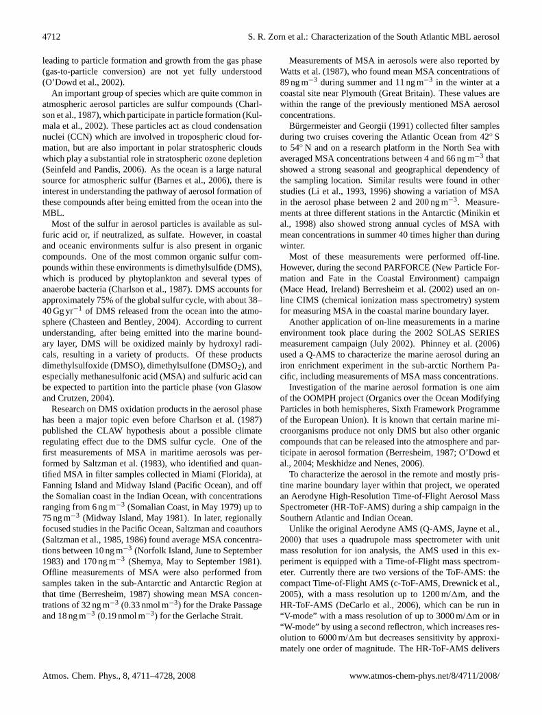
Fig. 1. Itinerary of the OOMPH 2007 Southern Hemisphere cruise.Large arrows show course of air masses for the selected time peri-ods.

in the Southern Hemisphere. For the first time, MSA con-centrations are directly determined from the high-resolutionmass spectra. Furthermore, as the instrument was deployedon a ship crossing the Southern Atlantic Ocean, our measure-ments cover a large spatial area of the Southern Hemisphere.

2 Overview over the 2007 OOMPH Southern Hemi-sphere cruise

The measurements of MBL aerosol were taken during the2007 OOMPH Southern Hemisphere cruise in the 20◦ S to60◦ S latitude band. The OOMPH project is investigatingthe organic chemistry of the ocean and the marine boundarylayer with a focus on organic vapors and their influence onparticle nucleation processes. The cruise onboard the Frenchresearch vesselMarion Dufresnetook place in the SouthernAtlantic Ocean and the Indian Ocean in the late SouthernHemisphere summer and early fall from January to March2007 (Fig.1). The campaign was split into two parts, here-after called leg 1 and leg 2.

Leg 1 started on the 19 January 2007 in Cape Town (SouthAfrica). The ship crossed the Atlantic Ocean staying be-tween 35◦ S and 45◦ S latitude. Upon arrival at the coast ofSouth America, the course shifted south towards the Straitof Magellan. In this area two phytoplankton blooms werecrossed (31 January 2007–2 February 2007, 40◦ S–45◦ S,55◦ W). After passing the Strait of Magellan the ship arrivedon 5 February 2007 in Punta Arenas (Chile) ending leg 1.

On the 1 March 2007 the ship left Punta Arenas headingsouth for leg 2 (Fig.1). This time the ship cruised south-eastwards near 60◦ S latitude until 9 March, when it passed24◦ W longitude. From that point on it headed northeast to-wards Durban (South Africa). After arriving near Durban

www.atmos-chem-phys.net/8/4711/2008/ Atmos. Chem. Phys., 8, 4711–4728, 2008


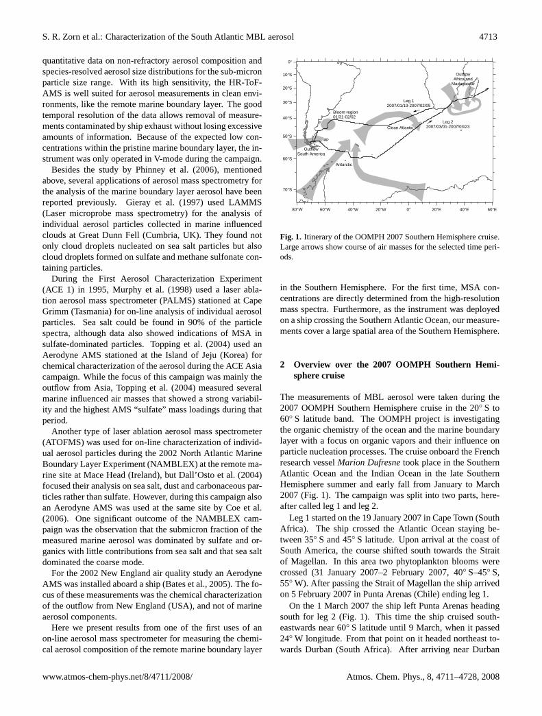
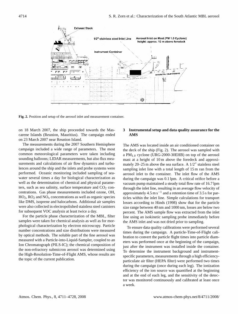
Fig. 2. Position and setup of the aerosol inlet and measurement container.

on 18 March 2007, the ship proceeded towards the Mas-carene Islands (Reunion, Mauritius). The campaign endedon 23 March 2007 near Reunion Island.

The measurements during the 2007 Southern Hemispherecampaign included a wide range of parameters. The mostcommon meteorological parameters were taken includingsounding balloons; LIDAR measurements, but also flux mea-surements and calculations of air flow dynamics and turbu-lences around the ship and the inlets and probe systems wereperformed. Oceanic monitoring included sampling of sea-water several times a day for biological characterization aswell as the determination of chemical and physical parame-ters, such as sea salinity, surface temperature and CO2 con-centrations. Gas phase measurements included ozone, OH,HO2, RO2 and NOx concentrations as well as organic specieslike DMS, isoprene and halocarbons. Additional air sampleswere also collected in electropolished stainless steel canistersfor subsequent VOC analysis at least twice a day.

For the particle phase characterization of the MBL, filtersamples were taken for chemical analysis as well as for mor-phological characterization by electron microscopy. Particlenumber concentrations and size distributions were measuredby optical methods. The soluble part of the fine aerosol wasmeasured with a Particle-into-Liquid-Sampler, coupled to anIon Chromatograph (PILS-IC); the chemical composition ofthe non-refractory submicron aerosol was determined usingthe High-Resolution-Time-of-Flight AMS, whose results arethe topic of the current publication.

3 Instrumental setup and data quality assurance for theAMS

The AMS was located inside an air conditioned container onthe deck of the ship (Fig.2). The aerosol was sampled witha PM1.0 cyclone (URG-2000-30EHB) on top of the aerosolmast at a height of 10 m above the foredeck and approxi-mately 20–25 m above the sea surface. A 1/2′′ stainless steelsampling inlet line with a total length of 15 m ran from theaerosol inlet to the container. The inlet flow of the AMSduring the campaign was 0.1 lpm. A critical orifice before avacuum pump maintained a steady total flow rate of 16.7 lpmthrough the inlet line, resulting in an average flow velocity ofapproximately 4.5 m s−1 and a retention time of 3.5 s for par-ticles within the inlet line. Simple calculations for transportlosses according toHinds (1998) show that for the particlesize range between 40 nm and 1000 nm, losses are below twopercent. The AMS sample flow was extracted from the inletline using an isokinetic sampling probe immediately beforethe AMS inlet and was not dried prior to sampling.

To ensure data quality calibrations were performed severaltimes during the campaign. A particle-Time-of-Flight cali-bration to convert the particle flight times into particle diam-eters was performed once at the beginning of the campaign,just after the instrument was installed inside the container.To determine the instrument background and instrument-specific parameters, measurements through a high efficiency-particulate air filter (HEPA filter) were performed two timesduring the campaign (once during each leg). The ionizationefficiency of the ion source was quantified at the beginningand at the end of each leg, and the sensitivity of the detec-tor was monitored continuously and calibrated at least oncea week.



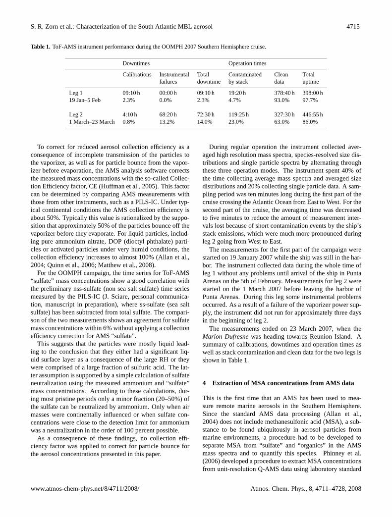
Table 1. ToF-AMS instrument performance during the OOMPH 2007 Southern Hemisphere cruise.

Downtimes Operation times

Calibrations Instrumental Total Contaminated Clean Totalfailures downtime by stack data uptime

Leg 1 09:10 h 00:00 h 09:10 h 19:20 h 378:40 h 398:00 h19 Jan–5 Feb 2.3% 0.0% 2.3% 4.7% 93.0% 97.7%

Leg 2 4:10 h 68:20 h 72:30 h 119:25 h 327:30 h 446:55 h1 March–23 March 0.8% 13.2% 14.0% 23.0% 63.0% 86.0%

To correct for reduced aerosol collection efficiency as aconsequence of incomplete transmission of the particles tothe vaporizer, as well as for particle bounce from the vapor-izer before evaporation, the AMS analysis software correctsthe measured mass concentrations with the so-called Collec-tion Efficiency factor, CE (Huffman et al., 2005). This factorcan be determined by comparing AMS measurements withthose from other instruments, such as a PILS-IC. Under typ-ical continental conditions the AMS collection efficiency isabout 50%. Typically this value is rationalized by the suppo-sition that approximately 50% of the particles bounce off thevaporizer before they evaporate. For liquid particles, includ-ing pure ammonium nitrate, DOP (dioctyl phthalate) parti-cles or activated particles under very humid conditions, thecollection efficiency increases to almost 100% (Allan et al.,2004; Quinn et al., 2006; Matthew et al., 2008).

For the OOMPH campaign, the time series for ToF-AMS“sulfate” mass concentrations show a good correlation withthe preliminary nss-sulfate (non sea salt sulfate) time seriesmeasured by the PILS-IC (J. Sciare, personal communica-tion, manuscript in preparation), where ss-sulfate (sea saltsulfate) has been subtracted from total sulfate. The compari-son of the two measurements shows an agreement for sulfatemass concentrations within 6% without applying a collectionefficiency correction for AMS “sulfate”.

This suggests that the particles were mostly liquid lead-ing to the conclusion that they either had a significant liq-uid surface layer as a consequence of the large RH or theywere comprised of a large fraction of sulfuric acid. The lat-ter assumption is supported by a simple calculation of sulfateneutralization using the measured ammonium and “sulfate”mass concentrations. According to these calculations, dur-ing most pristine periods only a minor fraction (20–50%) ofthe sulfate can be neutralized by ammonium. Only when airmasses were continentally influenced or when sulfate con-centrations were close to the detection limit for ammoniumwas a neutralization in the order of 100 percent possible.

As a consequence of these findings, no collection effi-ciency factor was applied to correct for particle bounce forthe aerosol concentrations presented in this paper.

During regular operation the instrument collected aver-aged high resolution mass spectra, species-resolved size dis-tributions and single particle spectra by alternating throughthese three operation modes. The instrument spent 40% ofthe time collecting average mass spectra and averaged sizedistributions and 20% collecting single particle data. A sam-pling period was ten minutes long during the first part of thecruise crossing the Atlantic Ocean from East to West. For thesecond part of the cruise, the averaging time was decreasedto five minutes to reduce the amount of measurement inter-vals lost because of short contamination events by the ship’sstack emissions, which were much more pronounced duringleg 2 going from West to East.

The measurements for the first part of the campaign werestarted on 19 January 2007 while the ship was still in the har-bor. The instrument collected data during the whole time ofleg 1 without any problems until arrival of the ship in PuntaArenas on the 5th of February. Measurements for leg 2 werestarted on the 1 March 2007 before leaving the harbor ofPunta Arenas. During this leg some instrumental problemsoccurred. As a result of a failure of the vaporizer power sup-ply, the instrument did not run for approximately three daysin the beginning of leg 2.

The measurements ended on 23 March 2007, when theMarion Dufresnewas heading towards Reunion Island. Asummary of calibrations, downtimes and operation times aswell as stack contamination and clean data for the two legs isshown in Table1.

4 Extraction of MSA concentrations from AMS data

This is the first time that an AMS has been used to mea-sure remote marine aerosols in the Southern Hemisphere.Since the standard AMS data processing (Allan et al.,2004) does not include methanesulfonic acid (MSA), a sub-stance to be found ubiquitously in aerosol particles frommarine environments, a procedure had to be developed toseparate MSA from “sulfate” and “organics” in the AMSmass spectra and to quantify this species.Phinney et al.(2006) developed a procedure to extract MSA concentrationsfrom unit-resolution Q-AMS data using laboratory standard



100

80

60

40

20

0

Rel

ativ

e A

bund

ance

10080604020m/z

Vaporizer offT = 160°C

a)

100

80

60

40

20

0

Rel

ativ

e A

bund

ance

10080604020m/z

Vaporizer at 800°Cb)

100

80

60

40

20

0

Rel

ativ

e A

bund

ance

10080604020m/z

Vaporizer at 625°C,interpolated

c)

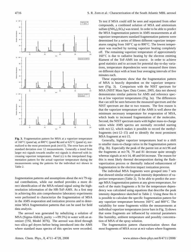
Fig. 3. Fragmentation pattern for MSA at a vaporizer temperatureof 160◦C (panela), at 800◦C (panelb) and at 625◦C (panelc), nor-malized to the most prominent peak (m/z15). The error bars are thestandard deviation over 12 measurements. Generally a trend fromlargerm/zsignals towards smallerm/zsignals is observed with in-creasing vaporizer temperature. Panel (c) is the interpolated frag-mentation pattern for the actual vaporizer temperature during themeasurements using the patterns for the individualm/z shown inTable2.

fragmentation patterns and assumptions about them/z79 sig-nal contributions, while our method provides a more di-rect identification of the MSA-related signal using the high-resolution information of the HR-ToF-AMS. As a first stepin achieving this aim comprehensive laboratory experimentswere performed to characterize the fragmentation of MSAin the AMS evaporation and ionization process and to deter-mine MSA fragmentation patterns that can be used for fielddata analysis.

The aerosol was generated by nebulizing a solution ofMSA (Sigma-Aldrich, purity>=99.5%) in water with an at-omizer (TSI, Model 3076). The aerosol was dried throughtwo silica gel dryers before being introduced into the AMSwhere standard mass spectra of this species were recorded.

To test if MSA could still be seen and separated from othercompounds, a combined solution of MSA and ammoniumsulfate ((NH4)2SO4) was tested. In order to be able to predictthe MSA fragmentation pattern in AMS measurements at allvaporizer temperatures standard fragmentation patterns weredetermined for a series of fifteen different vaporizer temper-atures ranging from 160◦C up to 800◦C. The lowest temper-ature was reached by turning vaporizer heating completelyoff. The remaining vaporizer temperature of approximately160◦C is due to radiative heating by the electron emittingfilament of the ToF-AMS ion source. In order to achievegood statistics and to account for potential day-to-day varia-tions, temperature dependencies were measured three timeson different days with at least four averaging intervals of fiveminutes each.

These experiments show that the fragmentation patternof MSA is heavily dependent on the vaporizer tempera-ture (Fig. 3). Comparison with the NIST spectrum forMSA (NIST Mass Spec Data Center, 2005, data not shown)demonstrates similar patterns for AMS and reference spec-tra at low vaporizer temperatures (Fig.3a). The differencesthat can still be seen between the measured spectrum and theNIST spectrum are due to two reasons. The first reason isthat the vaporizer temperature of the AMS is well above theminimum necessary temperature for evaporation of MSA,which leads to increased fragmentation of the molecules.Second, the NIST spectrum starts with higher mass-to-chargeratios while AMS spectra are normally recorded startingwith m/z12, which makes it possible to record the methyl-fragments (m/z12–15) and to identify the most prominentMSA fragment atm/z15.

Generally, higher vaporizer temperatures lead to a shiftto smaller mass-to-charge ratios in the fragmentation pattern(Fig. 3b). Especially the peak of the parent ion atm/z96 andthe fragments atm/z78, 79 and 81 decrease quite stronglywhereas signals atm/z14, 48 and 64 increase. The reason forthis is most likely thermal decomposition during the flash-vaporization process or thermally induced enhancement offragmentation in the electron impact ionization process.

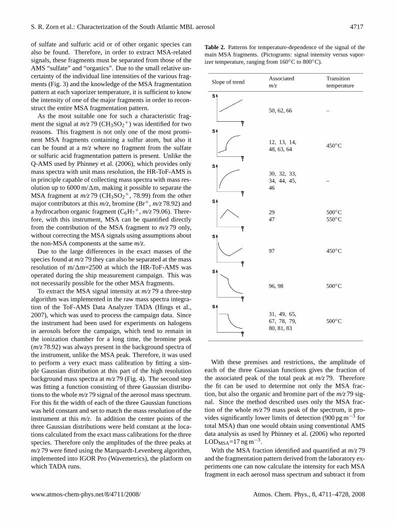
The individual MSA fragments were grouped into 7 setsthat showed similar relative peak intensity dependence of va-porizer temperature (Table2). To be able to predict the aver-age MSA fragmentation pattern at any given temperature, foreach of the main fragments a fit for the temperature depen-dency was calculated using equations that describe the peakintensity dependence sketched in Table2. Using these fits itis possible to calculate the specific fragmentation pattern forany vaporizer temperature between 160◦C and 800◦C. Thevariability for some fragments within the measurements atindividual vaporizer temperatures (error bars in Fig.3) showsthat some fragments are influenced by external parameterslike humidity, ambient temperature and possibly concentra-tion of MSA of the spray solution.

The fragmentation pattern characterization shows thatmost fragments of MSA occur atm/zvalues where fragments



of sulfate and sulfuric acid or of other organic species canalso be found. Therefore, in order to extract MSA-relatedsignals, these fragments must be separated from those of theAMS “sulfate” and “organics”. Due to the small relative un-certainty of the individual line intensities of the various frag-ments (Fig.3) and the knowledge of the MSA fragmentationpattern at each vaporizer temperature, it is sufficient to knowthe intensity of one of the major fragments in order to recon-struct the entire MSA fragmentation pattern.

As the most suitable one for such a characteristic frag-ment the signal atm/z79 (CH3SO2

+) was identified for tworeasons. This fragment is not only one of the most promi-nent MSA fragments containing a sulfur atom, but also itcan be found at am/z where no fragment from the sulfateor sulfuric acid fragmentation pattern is present. Unlike theQ-AMS used byPhinney et al.(2006), which provides onlymass spectra with unit mass resolution, the HR-ToF-AMS isin principle capable of collecting mass spectra with mass res-olution up to 6000 m/1m, making it possible to separate theMSA fragment atm/z79 (CH3SO2

+, 78.99) from the othermajor contributors at thism/z, bromine (Br+, m/z78.92) anda hydrocarbon organic fragment (C6H7

+, m/z79.06). There-fore, with this instrument, MSA can be quantified directlyfrom the contribution of the MSA fragment tom/z79 only,without correcting the MSA signals using assumptions aboutthe non-MSA components at the samem/z.

Due to the large differences in the exact masses of thespecies found atm/z79 they can also be separated at the massresolution of m/1m=2500 at which the HR-ToF-AMS wasoperated during the ship measurement campaign. This wasnot necessarily possible for the other MSA fragments.

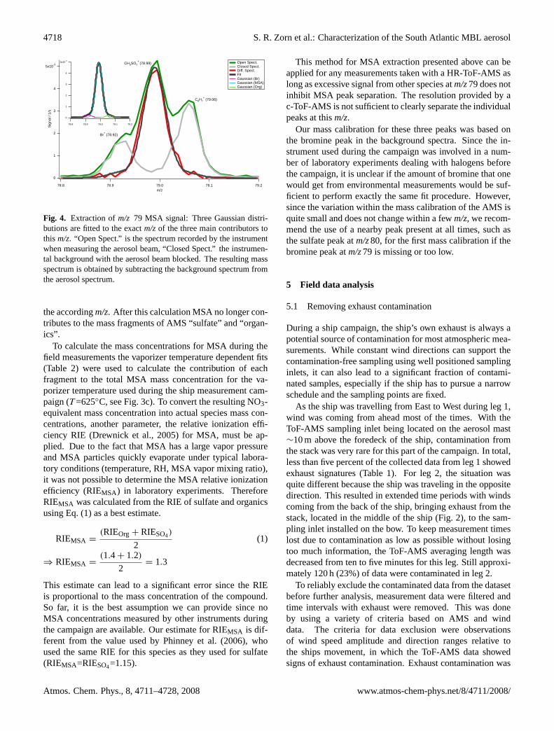
To extract the MSA signal intensity atm/z79 a three-stepalgorithm was implemented in the raw mass spectra integra-tion of the ToF-AMS Data Analyzer TADA (Hings et al.,2007), which was used to process the campaign data. Sincethe instrument had been used for experiments on halogensin aerosols before the campaign, which tend to remain inthe ionization chamber for a long time, the bromine peak(m/z78.92) was always present in the background spectra ofthe instrument, unlike the MSA peak. Therefore, it was usedto perform a very exact mass calibration by fitting a sim-ple Gaussian distribution at this part of the high resolutionbackground mass spectra atm/z79 (Fig.4). The second stepwas fitting a function consisting of three Gaussian distribu-tions to the wholem/z79 signal of the aerosol mass spectrum.For this fit the width of each of the three Gaussian functionswas held constant and set to match the mass resolution of theinstrument at thism/z. In addition the center points of thethree Gaussian distributions were held constant at the loca-tions calculated from the exact mass calibrations for the threespecies. Therefore only the amplitudes of the three peaks atm/z79 were fitted using the Marquardt-Levenberg algorithm,implemented into IGOR Pro (Wavemetrics), the platform onwhich TADA runs.

Table 2. Patterns for temperature-dependence of the signal of themain MSA fragments. (Pictograms: signal intensity versus vapor-izer temperature, ranging from 160◦C to 800◦C).

Slope of trendAssociatedm/z

Transitiontemperature

50, 62, 66 –

12, 13, 14,48, 63, 64

450◦C

30, 32, 33,34, 44, 45,46

–

2947

500◦C550◦C

97 450◦C

96, 98 500◦C

31, 49, 65,67, 78, 79,80, 81, 83

500◦C

With these premises and restrictions, the amplitude ofeach of the three Gaussian functions gives the fraction ofthe associated peak of the total peak atm/z79. Thereforethe fit can be used to determine not only the MSA frac-tion, but also the organic and bromine part of them/z79 sig-nal. Since the method described uses only the MSA frac-tion of the wholem/z79 mass peak of the spectrum, it pro-vides significantly lower limits of detection (900 pg m−3 fortotal MSA) than one would obtain using conventional AMSdata analysis as used byPhinney et al.(2006) who reportedLODMSA=17 ng m−3.

With the MSA fraction identified and quantified atm/z79and the fragmentation pattern derived from the laboratory ex-periments one can now calculate the intensity for each MSAfragment in each aerosol mass spectrum and subtract it from



5x10-3

4

3

2

1

0

Sig

nal /

1/s

79.279.179.078.978.8m/z

5x10-3

4

3

2

1

0

79.279.179.078.978.8

Open Spect. Closed Spect. Diff. Spect. Fit Gaussian (Br) Gaussian (MSA) Gaussian (Org)

Br+ (78.92)

CH3SO2+

(78.99)

C6H7+ (79.06)

Fig. 4. Extraction ofm/z 79 MSA signal: Three Gaussian distri-butions are fitted to the exactm/zof the three main contributors tothis m/z. “Open Spect.” is the spectrum recorded by the instrumentwhen measuring the aerosol beam, “Closed Spect.” the instrumen-tal background with the aerosol beam blocked. The resulting massspectrum is obtained by subtracting the background spectrum fromthe aerosol spectrum.

the accordingm/z. After this calculation MSA no longer con-tributes to the mass fragments of AMS “sulfate” and “organ-ics”.

To calculate the mass concentrations for MSA during thefield measurements the vaporizer temperature dependent fits(Table 2) were used to calculate the contribution of eachfragment to the total MSA mass concentration for the va-porizer temperature used during the ship measurement cam-paign (T =625◦C, see Fig.3c). To convert the resulting NO3-equivalent mass concentration into actual species mass con-centrations, another parameter, the relative ionization effi-ciency RIE (Drewnick et al., 2005) for MSA, must be ap-plied. Due to the fact that MSA has a large vapor pressureand MSA particles quickly evaporate under typical labora-tory conditions (temperature, RH, MSA vapor mixing ratio),it was not possible to determine the MSA relative ionizationefficiency (RIEMSA) in laboratory experiments. ThereforeRIEMSA was calculated from the RIE of sulfate and organicsusing Eq. (1) as a best estimate.

RIEMSA =(RIEOrg + RIESO4)

2(1)

⇒ RIEMSA =(1.4 + 1.2)

2= 1.3

This estimate can lead to a significant error since the RIEis proportional to the mass concentration of the compound.So far, it is the best assumption we can provide since noMSA concentrations measured by other instruments duringthe campaign are available. Our estimate for RIEMSA is dif-ferent from the value used byPhinney et al.(2006), whoused the same RIE for this species as they used for sulfate(RIEMSA=RIESO4=1.15).

This method for MSA extraction presented above can beapplied for any measurements taken with a HR-ToF-AMS aslong as excessive signal from other species atm/z79 does notinhibit MSA peak separation. The resolution provided by ac-ToF-AMS is not sufficient to clearly separate the individualpeaks at thism/z.

Our mass calibration for these three peaks was based onthe bromine peak in the background spectra. Since the in-strument used during the campaign was involved in a num-ber of laboratory experiments dealing with halogens beforethe campaign, it is unclear if the amount of bromine that onewould get from environmental measurements would be suf-ficient to perform exactly the same fit procedure. However,since the variation within the mass calibration of the AMS isquite small and does not change within a fewm/z, we recom-mend the use of a nearby peak present at all times, such asthe sulfate peak atm/z80, for the first mass calibration if thebromine peak atm/z79 is missing or too low.

5 Field data analysis

5.1 Removing exhaust contamination

During a ship campaign, the ship’s own exhaust is always apotential source of contamination for most atmospheric mea-surements. While constant wind directions can support thecontamination-free sampling using well positioned samplinginlets, it can also lead to a significant fraction of contami-nated samples, especially if the ship has to pursue a narrowschedule and the sampling points are fixed.

As the ship was travelling from East to West during leg 1,wind was coming from ahead most of the times. With theToF-AMS sampling inlet being located on the aerosol mast∼10 m above the foredeck of the ship, contamination fromthe stack was very rare for this part of the campaign. In total,less than five percent of the collected data from leg 1 showedexhaust signatures (Table1). For leg 2, the situation wasquite different because the ship was traveling in the oppositedirection. This resulted in extended time periods with windscoming from the back of the ship, bringing exhaust from thestack, located in the middle of the ship (Fig.2), to the sam-pling inlet installed on the bow. To keep measurement timeslost due to contamination as low as possible without losingtoo much information, the ToF-AMS averaging length wasdecreased from ten to five minutes for this leg. Still approxi-mately 120 h (23%) of data were contaminated in leg 2.

To reliably exclude the contaminated data from the datasetbefore further analysis, measurement data were filtered andtime intervals with exhaust were removed. This was doneby using a variety of criteria based on AMS and winddata. The criteria for data exclusion were observationsof wind speed amplitude and direction ranges relative tothe ships movement, in which the ToF-AMS data showedsigns of exhaust contamination. Exhaust contamination was



0.100.080.060.040.020.00

Nitrate

21.01.2007 26.01.2007 31.01.2007 05.02.2007

Date and Time

12 12

8 8

4 4

0 0

Mas

s co

ncen

trat

ion

/ µg

m-3

0.08

0.06

0.04

0.02

0.00

MS

A

0.3

0.2

0.1

0.0

Am

mon

ium 0.020

0.015

0.010

0.005

0.000

Chloride

25201510

50

20

16

12

8

SS

T / °C

1.2 1.2

0.8 0.8

0.4 0.4

0.0 0.0

a) Unfiltered time series

b) Filtered time series

AMS 'sulfate' AMS 'organics'

Tru

e w

ind

/ m/s

Exhaust frompilot ship?

Mass concentration / µg m

-3

Exhaust periodStrait of Magellan

Phytoplankton bloom period

First bloom and continentaloutflow from South America Second bloom

Southern Atlanticocean background

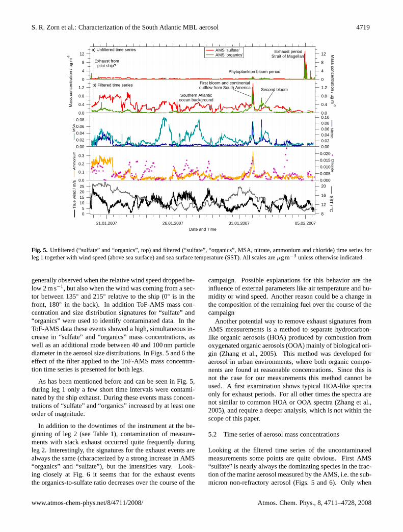
Fig. 5. Unfiltered (“sulfate” and “organics”, top) and filtered (“sulfate”, “organics”, MSA, nitrate, ammonium and chloride) time series forleg 1 together with wind speed (above sea surface) and sea surface temperature (SST). All scales areµg m−3 unless otherwise indicated.

generally observed when the relative wind speed dropped be-low 2 m s−1, but also when the wind was coming from a sec-tor between 135◦ and 215◦ relative to the ship (0◦ is in thefront, 180◦ in the back). In addition ToF-AMS mass con-centration and size distribution signatures for “sulfate” and“organics” were used to identify contaminated data. In theToF-AMS data these events showed a high, simultaneous in-crease in “sulfate” and “organics” mass concentrations, aswell as an additional mode between 40 and 100 nm particlediameter in the aerosol size distributions. In Figs.5 and6 theeffect of the filter applied to the ToF-AMS mass concentra-tion time series is presented for both legs.

As has been mentioned before and can be seen in Fig.5,during leg 1 only a few short time intervals were contami-nated by the ship exhaust. During these events mass concen-trations of “sulfate” and “organics” increased by at least oneorder of magnitude.

In addition to the downtimes of the instrument at the be-ginning of leg 2 (see Table1), contamination of measure-ments with stack exhaust occurred quite frequently duringleg 2. Interestingly, the signatures for the exhaust events arealways the same (characterized by a strong increase in AMS“organics” and “sulfate”), but the intensities vary. Look-ing closely at Fig.6 it seems that for the exhaust eventsthe organics-to-sulfate ratio decreases over the course of the

campaign. Possible explanations for this behavior are theinfluence of external parameters like air temperature and hu-midity or wind speed. Another reason could be a change inthe composition of the remaining fuel over the course of thecampaign

Another potential way to remove exhaust signatures fromAMS measurements is a method to separate hydrocarbon-like organic aerosols (HOA) produced by combustion fromoxygenated organic aerosols (OOA) mainly of biological ori-gin (Zhang et al., 2005). This method was developed foraerosol in urban environments, where both organic compo-nents are found at reasonable concentrations. Since this isnot the case for our measurements this method cannot beused. A first examination shows typical HOA-like spectraonly for exhaust periods. For all other times the spectra arenot similar to common HOA or OOA spectra (Zhang et al.,2005), and require a deeper analysis, which is not within thescope of this paper.

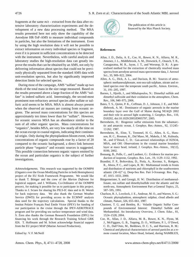
5.2 Time series of aerosol mass concentrations

Looking at the filtered time series of the uncontaminatedmeasurements some points are quite obvious. First AMS“sulfate” is nearly always the dominating species in the frac-tion of the marine aerosol measured by the AMS, i.e. the sub-micron non-refractory aerosol (Figs.5 and6). Only when



0.12

0.08

0.04

0.00

Nitrate

06.03.2007 11.03.2007 16.03.2007 21.03.2007

Date and Time

300 300250 250200 200150 150100 100

50 500 0

Mas

s co

ncen

trat

ion

/ µg

m-3

0.06

0.04

0.02

0.00

MS

A

0.3

0.2

0.1

0.0

Am

mon

ium 0.05

0.040.030.020.010.00

Chloride

25201510

50

2520151050

SS

T / °C

3.0

2.0

1.0

0.0

Mass concentration / µg m

-3

0.8

0.6

0.4

0.2

0.0

Downtimes because of instrumental failures

Continentaloutflow fromAfrica and

Madagascar

'Clean' antarctic background

a) Unfiltered time series

b) Filtered time series

Strongest exhaust periods

AMS 'sulfate' AMS 'organics'

Tru

e w

ind

/ m/s

right scaleleft scale

Fig. 6. Unfiltered (“sulfate” and “organics”, top) and filtered (“sulfate”, “organics”, MSA, nitrate, ammonium and chloride) time series forleg 2 together with wind speed (above sea surface) and sea surface temperature (SST). All scales areµg m−3 unless otherwise indicated.

coming close to coastal areas or when passing through oneof the phytoplankton blooms did organic concentrations ex-ceed those of AMS “sulfate”. The blooms in that region arecaused by the Malvinas Current, a branch of the AntarcticCircumpolar Current flowing northwards along the continen-tal shelf of Chile and Argentina (Legeckis and Gordon, 1998;Garzoli, 1993) bringing nutrient-rich, cold water (6◦C SST)with it (Brandini et al., 2000). The blooms were identified bysatellite data and an increased biological activity was seen bythe strong green color of the ocean. For both bloom eventsa drop in sea surface temperature (SST) can be seen (Fig.5,bottom), especially for the second event in which SST dropsfrom 16◦C to 10◦C, indicating the inflow of cold water. Dur-ing these bloom periods “organics” contribute up to 50 per-cent to the total non-refractory aerosol mass concentrationsin the size fraction below 1µm.

The temporal trends of the time series for methanesulfonicacid (Fig.5 and6) follow those for AMS “sulfate” for timeswhere the aerosol is mainly dominated by marine sources.This is because both, methanesulfonic acid and sulfate, orig-inate from the same source, oxidation of dimethylsulfide(DMS), and because there is no additional sulfate from othersources during the most pristine periods.

For leg 1, generally the ratio between MSA and AMS“sulfate” is higher when air masses did come directly fromAntarctica (24 January 2007–25 January 2007, 26 January2007–28 January 2007) and during the phytoplankton bloomperiods near South America, especially during the secondbloom (1 February 2007–2 February 2007). For periodswhen air masses were coming from the middle of the oceanor had a long residence time there before arriving at the ship(Clean Atlantic, 12 March 2007–15 March 2007), the ratiois much lower. However, the trends for MSA and AMS “sul-fate” time series are still similar, possibly due to longer trans-port from the source region to the ship or due to the laterseason.

Only for the time after passing the phytoplankton bloomregion when – according to backward trajectories (see below)– air masses were continentally influenced by passing overSouth America and inside the Strait of Magellan, this is nolonger true. For these time intervals, MSA is nearly zero,although the time series for AMS “sulfate” show significantconcentrations.

During leg 2 the typical mass concentrations of AMS “sul-fate” and MSA were only half as large as the ones from leg 1,possibly because of lower temperatures (Fig.6) and the tran-sition from summer to autumn in the Southern Hemisphereleading to reduced biological activity. Total organic mass



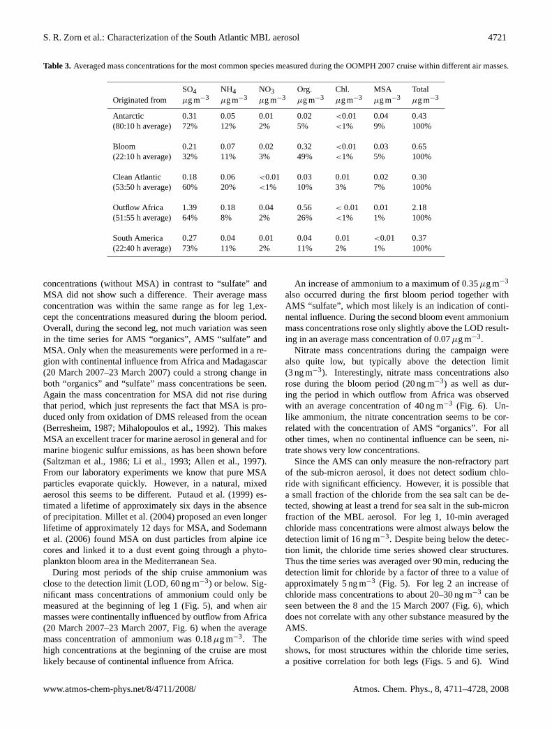
Table 3. Averaged mass concentrations for the most common species measured during the OOMPH 2007 cruise within different air masses.

SO4 NH4 NO3 Org. Chl. MSA TotalOriginated from µg m−3 µg m−3 µg m−3 µg m−3 µg m−3 µg m−3 µg m−3

Antarctic 0.31 0.05 0.01 0.02 <0.01 0.04 0.43(80:10 h average) 72% 12% 2% 5% <1% 9% 100%

Bloom 0.21 0.07 0.02 0.32 <0.01 0.03 0.65(22:10 h average) 32% 11% 3% 49% <1% 5% 100%

Clean Atlantic 0.18 0.06 <0.01 0.03 0.01 0.02 0.30(53:50 h average) 60% 20% <1% 10% 3% 7% 100%

Outflow Africa 1.39 0.18 0.04 0.56 < 0.01 0.01 2.18(51:55 h average) 64% 8% 2% 26% <1% 1% 100%

South America 0.27 0.04 0.01 0.04 0.01 <0.01 0.37(22:40 h average) 73% 11% 2% 11% 2% 1% 100%

concentrations (without MSA) in contrast to “sulfate” andMSA did not show such a difference. Their average massconcentration was within the same range as for leg 1,ex-cept the concentrations measured during the bloom period.Overall, during the second leg, not much variation was seenin the time series for AMS “organics”, AMS “sulfate” andMSA. Only when the measurements were performed in a re-gion with continental influence from Africa and Madagascar(20 March 2007–23 March 2007) could a strong change inboth “organics” and “sulfate” mass concentrations be seen.Again the mass concentration for MSA did not rise duringthat period, which just represents the fact that MSA is pro-duced only from oxidation of DMS released from the ocean(Berresheim, 1987; Mihalopoulos et al., 1992). This makesMSA an excellent tracer for marine aerosol in general and formarine biogenic sulfur emissions, as has been shown before(Saltzman et al., 1986; Li et al., 1993; Allen et al., 1997).From our laboratory experiments we know that pure MSAparticles evaporate quickly. However, in a natural, mixedaerosol this seems to be different.Putaud et al.(1999) es-timated a lifetime of approximately six days in the absenceof precipitation.Millet et al. (2004) proposed an even longerlifetime of approximately 12 days for MSA, andSodemannet al. (2006) found MSA on dust particles from alpine icecores and linked it to a dust event going through a phyto-plankton bloom area in the Mediterranean Sea.

During most periods of the ship cruise ammonium wasclose to the detection limit (LOD, 60 ng m−3) or below. Sig-nificant mass concentrations of ammonium could only bemeasured at the beginning of leg 1 (Fig.5), and when airmasses were continentally influenced by outflow from Africa(20 March 2007–23 March 2007, Fig.6) when the averagemass concentration of ammonium was 0.18µg m−3. Thehigh concentrations at the beginning of the cruise are mostlikely because of continental influence from Africa.

An increase of ammonium to a maximum of 0.35µg m−3

also occurred during the first bloom period together withAMS “sulfate”, which most likely is an indication of conti-nental influence. During the second bloom event ammoniummass concentrations rose only slightly above the LOD result-ing in an average mass concentration of 0.07µg m−3.

Nitrate mass concentrations during the campaign werealso quite low, but typically above the detection limit(3 ng m−3). Interestingly, nitrate mass concentrations alsorose during the bloom period (20 ng m−3) as well as dur-ing the period in which outflow from Africa was observedwith an average concentration of 40 ng m−3 (Fig. 6). Un-like ammonium, the nitrate concentration seems to be cor-related with the concentration of AMS “organics”. For allother times, when no continental influence can be seen, ni-trate shows very low concentrations.

Since the AMS can only measure the non-refractory partof the sub-micron aerosol, it does not detect sodium chlo-ride with significant efficiency. However, it is possible thata small fraction of the chloride from the sea salt can be de-tected, showing at least a trend for sea salt in the sub-micronfraction of the MBL aerosol. For leg 1, 10-min averagedchloride mass concentrations were almost always below thedetection limit of 16 ng m−3. Despite being below the detec-tion limit, the chloride time series showed clear structures.Thus the time series was averaged over 90 min, reducing thedetection limit for chloride by a factor of three to a value ofapproximately 5 ng m−3 (Fig. 5). For leg 2 an increase ofchloride mass concentrations to about 20–30 ng m−3 can beseen between the 8 and the 15 March 2007 (Fig.6), whichdoes not correlate with any other substance measured by theAMS.

Comparison of the chloride time series with wind speedshows, for most structures within the chloride time series,a positive correlation for both legs (Figs.5 and 6). Wind



1.6

1.4

1.2

1.0

0.8

0.6

0.4

0.2

0.0

Org

anic

s / µ

g m

-3

6 7 8 90.001

2 3 4 5 6 7 8 90.01

2 3 4 5 6 7 8

Methanesulfonic acid / µg m-3

Antarctic Bloom Clean Atlantic Outflow Africa South America

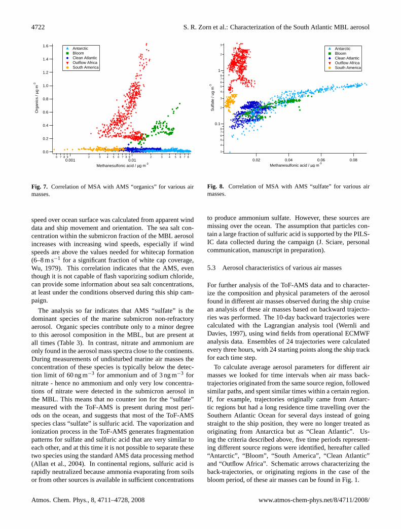
Fig. 7. Correlation of MSA with AMS “organics” for various airmasses.

speed over ocean surface was calculated from apparent winddata and ship movement and orientation. The sea salt con-centration within the submicron fraction of the MBL aerosolincreases with increasing wind speeds, especially if windspeeds are above the values needed for whitecap formation(6–8 m s−1 for a significant fraction of white cap coverage,Wu, 1979). This correlation indicates that the AMS, eventhough it is not capable of flash vaporizing sodium chloride,can provide some information about sea salt concentrations,at least under the conditions observed during this ship cam-paign.

The analysis so far indicates that AMS “sulfate” is thedominant species of the marine submicron non-refractoryaerosol. Organic species contribute only to a minor degreeto this aerosol composition in the MBL, but are present atall times (Table3). In contrast, nitrate and ammonium areonly found in the aerosol mass spectra close to the continents.During measurements of undisturbed marine air masses theconcentration of these species is typically below the detec-tion limit of 60 ng m−3 for ammonium and of 3 ng m−3 fornitrate - hence no ammonium and only very low concentra-tions of nitrate were detected in the submicron aerosol inthe MBL. This means that no counter ion for the “sulfate”measured with the ToF-AMS is present during most peri-ods on the ocean, and suggests that most of the ToF-AMSspecies class “sulfate” is sulfuric acid. The vaporization andionization process in the ToF-AMS generates fragmentationpatterns for sulfate and sulfuric acid that are very similar toeach other, and at this time it is not possible to separate thesetwo species using the standard AMS data processing method(Allan et al., 2004). In continental regions, sulfuric acid israpidly neutralized because ammonia evaporating from soilsor from other sources is available in sufficient concentrations

3

4

5

678

0.1

2

3

4

5

678

1

2

3

Sul

fate

/ ug

m-3

0.080.060.040.02Methanesulfonic acid / µg m

-3

Antarctic Bloom Clean Atlantic Outflow Africa South America

Fig. 8. Correlation of MSA with AMS “sulfate” for various airmasses.

to produce ammonium sulfate. However, these sources aremissing over the ocean. The assumption that particles con-tain a large fraction of sulfuric acid is supported by the PILS-IC data collected during the campaign (J. Sciare, personalcommunication, manuscript in preparation).

5.3 Aerosol characteristics of various air masses

For further analysis of the ToF-AMS data and to character-ize the composition and physical parameters of the aerosolfound in different air masses observed during the ship cruisean analysis of these air masses based on backward trajecto-ries was performed. The 10-day backward trajectories werecalculated with the Lagrangian analysis tool (Wernli andDavies, 1997), using wind fields from operational ECMWFanalysis data. Ensembles of 24 trajectories were calculatedevery three hours, with 24 starting points along the ship trackfor each time step.

To calculate average aerosol parameters for different airmasses we looked for time intervals when air mass back-trajectories originated from the same source region, followedsimilar paths, and spent similar times within a certain region.If, for example, trajectories originally came from Antarc-tic regions but had a long residence time travelling over theSouthern Atlantic Ocean for several days instead of goingstraight to the ship position, they were no longer treated asoriginating from Antarctica but as “Clean Atlantic”. Us-ing the criteria described above, five time periods represent-ing different source regions were identified, hereafter called“Antarctic”, “Bloom”, “South America”, “Clean Atlantic”and “Outflow Africa”. Schematic arrows characterizing theback-trajectories, or originating regions in the case of thebloom period, of these air masses can be found in Fig.1.



For each of these time periods the origin and track of thetrajectories stayed constant at least one day or longer, exceptfor the “Bloom” period, which lasted only a few hours whenthe ship crossed through the phytoplankton bloom area. Asummary of species concentrations measured with the ToF-AMS for each of the air masses is presented in Table3.

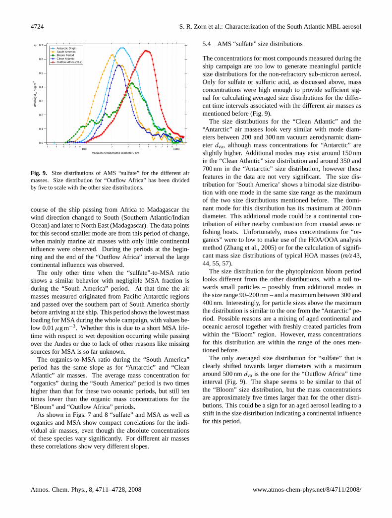
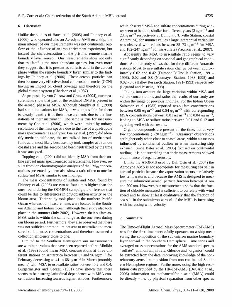
To investigate possible relations between different speciesfor the different regions we calculated correlations betweenthe most abundant species “sulfate”, “organics”, and MSA(Figs.7 and8).

To be classified as “Antarctic”, air masses had to originatein, and come straight from Antarctica (3–5 days accordingto backward trajectories) before arriving at the ship position(Fig. 1). These air masses are characterized by very low con-centrations for most aerosol compounds except “sulfate” andMSA. A large MSA-to-sulfate ratio is quite characteristic forthese air masses as shown in the correlation plot for thesespecies in Fig.8. “organics” show lowest concentrations forthis source region, leading to a very high MSA-to-organicsratio (Fig.7).

The air masses characterized as “Clean Atlantic” are verysimilar to the “Antarctic” period (Table3). Trajectories forthese air masses also came originally from Antarctica butstayed for some days above the Southern Atlantic Ocean go-ing from West to East before approaching the ship from theNorthwest (5–10 days after passing Antarctica). “sulfate”and MSA show similar ratios for “Antarctic” air and “CleanAtlantic” air (Fig. 8), but concentrations are almost a factorof two lower for “Clean Atlantic”. Chloride shows the high-est concentrations for “Clean Atlantic” air masses, causedby high wind speeds for these air masses, leading to an in-crease of small sea salt particles even in the size range be-low 1µm (Figs.5 and6). Finally, the MSA-to-organics ra-tio is on the same correlation branch as for “Antarctic” airmasses (Fig.7). The strong similarities between “Clean At-lantic” and “Antarctic” aerosol composition suggests, that the“Antarctic” aerosol is also dominated by marine emissionscollected during the short time the air spent traveling to theship position or, alternatively, from emissions within the bi-ological active Antarctic shelf region but not by emissionsfrom the Antarctic continent itself.

When arriving in the costal region of South America, theship passed through phytoplankton blooms. Phytoplanktonblooms or algae blooms are areas in which the populationof one or more species of micro algae or marine bacteriais increasing rapidly due to a strong nutrient input. Theseorganisms are known to produce organic compounds whichcan be released into the atmosphere including DMS, halo-carbons (Lovelock et al., 1973) and isoprene (Bonsang et al.,1992). As mentioned above the blooms were indicated bysatellite images and the high biological activity that producedthe green color of the ocean.

During the “Bloom” periods offshore of South America(Fig. 1) “sulfate” mass concentrations were at similar lev-els as for “Clean Atlantic” air masses, but concentrations

for “organics” were significantly higher making up nearly 50percent of the total non-refractory aerosol mass below onemicrometer. Compared to the organic concentrations mea-sured during “Antarctic” and “Clean Atlantic” periods, or-ganic concentrations are approximately 20 times higher dur-ing the “Bloom”. A detailed investigation of this organicaerosol is part of forthcoming analyses and beyond the scopeof this paper.

In fact the bloom period is the only one when “organics”are clearly dominating the aerosol composition. Unfortu-nately, during this time interval air mass trajectories camefrom South America (first bloom event, see Fig.5) and fromthe Pacific Ocean passing briefly over South America (sec-ond bloom event). Although for the second bloom eventthey were only passing over less populated areas of grassland(Patagonia), an influence from continental sources cannot beexcluded.

The MSA-to-“sulfate” ratio for this period (Fig.8) is sim-ilar to that for “Clean Atlantic”, but the concentrations mea-sured during the bloom are higher, although slightly belowthose for “Antarctic” air masses. Interestingly, the organics-to-MSA ratio for the bloom period differs drastically fromthat of the other two air masses. Another indication for con-tinental influence during this period are the relatively high ni-trate mass concentrations (Fig.5). These are approximatelytwice as large as those observed in the “Clean Atlantic” and“Antarctic” air masses. On the other hand – according to theMSA-to-“sulfate” ratio – no significant “sulfate” influencefrom the continent can be seen in the data during the bloom,inconsistent with a major continental influence. However,from the current state of the data no final conclusion can bedrawn.

The only time when nitrate concentrations are even higherthan within the bloom aerosol is during the “Outflow Africa”period. Air masses measured during that period are comingprimarily from the Southern Atlantic (for the first half) andIndian Ocean (second half), but most of them passed overAfrica or Madagascar before arriving at the ships positionand are clearly continentally influenced (Fig.1), as “sulfate”concentrations are at maximum values for these periods. Thesame is true for mass concentrations of ammonium and thetotal non-refractory sub-micron aerosol concentration. Atthe same time MSA concentrations are the lowest observedwithin any of the air masses (Table3). The correlation plot of“organics” and MSA (Fig.7) shows a very large organics-to-MSA ratio as well as a large “sulfate”-to-MSA ratio (Fig.8).This is another indicator for the significant continental influ-ence of the air masses observed during this time period.

The correlation plot (Fig.7) for “organics” with MSAshows two modes for this period, the main one with a largeorganics-to-MSA ratio and a smaller one with a large MSA-to-organics ratio. A detailed inspection of the backward tra-jectories for this time interval and the associated data pointsin Fig. 6 shows that at the beginning of this period the windwas coming from Northwest (Continental Africa). In the



0.7

0.6

0.5

0.4

0.3

0.2

0.1

0.0

dM/d

log

d va

/ µg

m-3

4 5 6 7 8 9100

2 3 4 5 6 7 8 91000

Vacuum Aerodynamic Diameter / nm

Antarctic Origin South America Bloom Period Clean Atlantic Outflow Africa (*0.2)

a)

Fig. 9. Size distributions of AMS “sulfate” for the different airmasses. Size distribution for “Outflow Africa” has been dividedby five to scale with the other size distributions.

course of the ship passing from Africa to Madagascar thewind direction changed to South (Southern Atlantic/IndianOcean) and later to North East (Madagascar). The data pointsfor this second smaller mode are from this period of change,when mainly marine air masses with only little continentalinfluence were observed. During the periods at the begin-ning and the end of the “Outflow Africa” interval the largecontinental influence was observed.

The only other time when the “sulfate”-to-MSA ratioshows a similar behavior with negligible MSA fraction isduring the “South America” period. At that time the airmasses measured originated from Pacific Antarctic regionsand passed over the southern part of South America shortlybefore arriving at the ship. This period shows the lowest massloading for MSA during the whole campaign, with values be-low 0.01µg m−3. Whether this is due to a short MSA life-time with respect to wet deposition occurring while passingover the Andes or due to lack of other reasons like missingsources for MSA is so far unknown.

The organics-to-MSA ratio during the “South America”period has the same slope as for “Antarctic” and “CleanAtlantic” air masses. The average mass concentration for“organics” during the “South America” period is two timeshigher than that for these two oceanic periods, but still tentimes lower than the organic mass concentrations for the“Bloom” and “Outflow Africa” periods.

As shown in Figs.7 and8 “sulfate” and MSA as well asorganics and MSA show compact correlations for the indi-vidual air masses, even though the absolute concentrationsof these species vary significantly. For different air massesthese correlations show very different slopes.

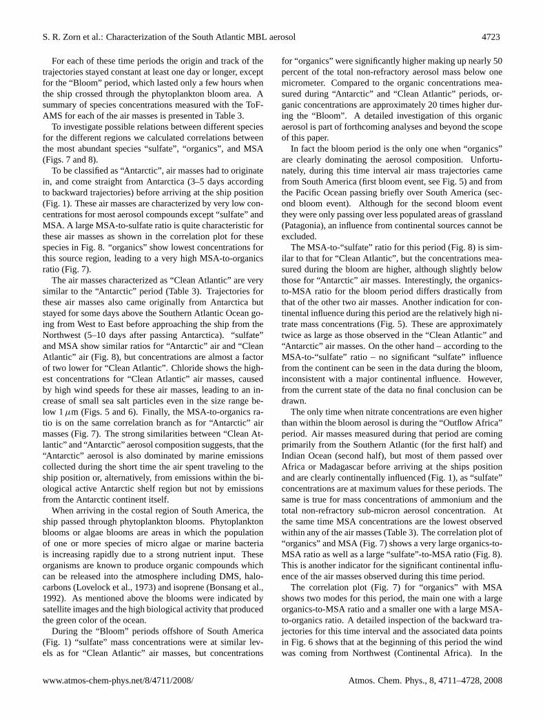
5.4 AMS “sulfate” size distributions

The concentrations for most compounds measured during theship campaign are too low to generate meaningful particlesize distributions for the non-refractory sub-micron aerosol.Only for sulfate or sulfuric acid, as discussed above, massconcentrations were high enough to provide sufficient sig-nal for calculating averaged size distributions for the differ-ent time intervals associated with the different air masses asmentioned before (Fig.9).

The size distributions for the “Clean Atlantic” and the“Antarctic” air masses look very similar with mode diam-eters between 200 and 300 nm vacuum aerodynamic diam-eter dva, although mass concentrations for “Antarctic” areslightly higher. Additional modes may exist around 150 nmin the “Clean Atlantic” size distribution and around 350 and700 nm in the “Antarctic” size distribution, however thesefeatures in the data are not very significant. The size dis-tribution for ’South America’ shows a bimodal size distribu-tion with one mode in the same size range as the maximumof the two size distributions mentioned before. The domi-nant mode for this distribution has its maximum at 200 nmdiameter. This additional mode could be a continental con-tribution of either nearby combustion from coastal areas orfishing boats. Unfortunately, mass concentrations for “or-ganics” were to low to make use of the HOA/OOA analysismethod (Zhang et al., 2005) or for the calculation of signifi-cant mass size distributions of typical HOA masses (m/z43,44, 55, 57).

The size distribution for the phytoplankton bloom periodlooks different from the other distributions, with a tail to-wards small particles – possibly from additional modes inthe size range 90–200 nm – and a maximum between 300 and400 nm. Interestingly, for particle sizes above the maximumthe distribution is similar to the one from the “Antarctic” pe-riod. Possible reasons are a mixing of aged continental andoceanic aerosol together with freshly created particles fromwithin the “Bloom” region. However, mass concentrationsfor this distribution are within the range of the ones men-tioned before.

The only averaged size distribution for “sulfate” that isclearly shifted towards larger diameters with a maximumaround 500 nmdva is the one for the “Outflow Africa” timeinterval (Fig.9). The shape seems to be similar to that ofthe “Bloom” size distribution, but the mass concentrationsare approximately five times larger than for the other distri-butions. This could be a sign for an aged aerosol leading to ashift in the size distribution indicating a continental influencefor this period.



6 Discussion

Unlike the studies ofBates et al.(2005) andPhinney et al.(2006), who operated also an Aerodyne AMS on a ship, themain interest of our measurements was not continental out-flow or the influence of an iron enrichment experiment, butinstead the characterization of the pristine, remote marineboundary layer aerosol. Our measurements show not onlythat “sulfate” is the most abundant species, but even morethey suggest that it is present as sulfuric acid in the aerosolphase within the remote boundary layer, similar to the find-ings by Phinney et al.(2006). These aerosol particles canthen become very effective cloud condensation nuclei (CCN)having an impact on cloud coverage and therefore on theglobal climate system (Charlson et al., 1987).

As proposed byvon Glasow and Crutzen(2004), our mea-surements show that part of the oxidized DMS is present inthe aerosol phase as MSA. AlthoughMurphy et al.(1998)had some indications for MSA, it was impossible for themto clearly identify it in their measurements due to the lim-itations of their instrument. The same is true for measure-ments byCoe et al.(2006), which were limited by unitaryresolution of the mass spectra due to the use of a quadrupolemass spectrometer as analyzer.Gieray et al.(1997) did iden-tify methane sulfonate, the neutralized ion of methanesul-fonic acid, most likely because they took samples at a remotecoastal area and the aerosol had been neutralized by the timeit was analyzed.

Topping et al.(2004) did not identify MSA from their on-line aerosol mass spectrometric measurements. However, re-sults from ion chromatographic analysis of the PM10 concen-trations presented by them also show a ratio of ten to one forsulfate and MSA, similar to our findings.

The mass concentrations of sulfate and MSA found byPhinney et al.(2006) are two to four times higher than theones found during the OOMPH campaign, a difference thatcould be due to differences in phytoplankton activity or thebloom area. Their study took place in the northern PacificOcean whereas our measurements were located in the South-ern Atlantic and Indian Ocean, although their study also tookplace in the summer (July 2002). However, their sulfate-to-MSA ratio is within the same range as the one seen duringour bloom period. Furthermore, they also observed that therewas not sufficient ammonium present to neutralize the mea-sured sulfate mass concentrations and therefore assumed acollection efficiency close to one.

Limited to the Southern Hemisphere our measurementsare within the values that have been reported before.Minikinet al. (1998) found mean MSA concentrations at three dif-ferent stations on Antarctica between 57 and 96 ng m−3 forFebruary decreasing to 41 to 68 ng m−3 in March (monthlymeans) with MSA to nss-sulfate ratios between 0.2 and 0.4.Burgermeister and Georgii(1991) have shown that thereseems to be a strong latitudinal dependence with MSA con-centrations increasing towards higher latitudes. Furthermore,

while observed MSA and sulfate concentrations during win-ter seem to be quite similar for different years (2 ng m−3 and23 ng m−3 respectively at Dumont d’Urville Station, coastalAntarctica), for summer values a large interannual variabilitywas observed with values between 35–73 ng m−3 for MSAand 182–247 ng m−3 for nss-sulfate (Preunkert et al., 2007).

Apparently the MSA to nss-sulfate ratio seems to varysignificantly depending on seasonal and geographical condi-tions. Another study shows that for three different Antarcticstations MSA to nss-sulfate ratios change between approx-imately 0.02 and 0.42 (Dumont D’Urville Station, 1991–1996), 0.02 and 0.8 (Neumayer Station, 1983–1995) and0.02 - 0.6 (Halley Research Station, 1991–1993) respectively(Legrand and Pasteur, 1998).

Taking into account the large variation within MSA andsulfate concentrations and ratios the results of our study arewithin the range of previous findings. For the Indian OceanSaltzman et al.(1983) reported nss-sulfate concentrationsbetween 0.05µg m−3 and 0.84µg m−3 with correspondingMSA concentrations between 0.01µg m−3 and 0.04µg m−3,leading to MSA to sulfate ratios between 0.01 and 0.12 andagreeing well with our results.

Organic compounds are present all the time, but at verylow concentrations (∼20 ng m−3). “Organics” observationsare higher only when close to coastal areas, within air massesinfluenced by continental outflow or when measuring shipexhaust. SinceBates et al.(2005) focused on continentaloutflow, it is not surprising that their measurements showeda dominance of organic aerosols.

Unlike the ATOFMS used byDall’Osto et al.(2004) theAerodyne AMS is not appropriate for measuring sea salt inaerosol particles because the vaporization occurs at relativelylow temperatures and because the AMS is designed to mea-sure the submicron aerosol particle fraction between 70 nmand 700 nm. However, our measurements show that the frac-tion of chloride measured is sufficient to correlate with windspeed and to show at least qualitatively that the fraction ofsea salt in the submicron aerosol of the MBL is increasingwith increasing wind velocity.

7 Summary

The Time-of-Flight Aerosol Mass Spectrometer (ToF-AMS)was for the first time successfully operated on a ship mea-suring the composition of the sub-micron marine boundarylayer aerosol in the Southern Hemisphere. Time series andaveraged mass concentrations for the AMS standard species“sulfate”, ammonium, nitrate, chloride and “organics” couldbe extracted from the data improving knowledge of the non-refractory aerosol composition from non-continental South-ern Hemisphere regions. Furthermore, using the high reso-lution data provided by the HR-ToF-AMS (DeCarlo et al.,2006) information on methanesulfonic acid (MSA) couldbe directly – i.e. by physical separation from other species



fragments at the samem/z– extracted from the data after ex-tensive laboratory characterization experiments and the de-velopment of a new data processing method. The MSAresults presented here not only show the capability of theAerodyne HR-ToF-AMS to measure individual compoundsin particles, but also the limitations of the instrument. Evenby using the high resolution data it will not be possible toextract information on every individual species or fragment,even if it is present in sufficient concentrations to be detectedwith the instrument. Nevertheless, with careful analysis andlaboratory studies the high-resolution data can greatly im-prove the results that can be obtained by an AMS, not only bydelivering information about species that could not be previ-ously physically separated from the standard AMS data withunit-resolution spectra, but also by significantly improveddetection limits for selected species.

During most of the campaign, AMS “sulfate” made up twothirds of the total mass in the size range measured. Based onthe results presented above a large fraction of the AMS “sul-fate” is indeed sulfuric acid. Interestingly, the second-mostprominent non-refractory aerosol species after sulfate or sul-furic acid seems to be MSA. MSA is almost always presentwhen the observed air masses are coming from oceanic re-gions. The aerosol mass concentrations for this species areapproximately ten times lower than for “sulfate”. However,for oceanic sources MSA has an abundance similar to thesum of all other organic species. Mass concentrations for“organics”, besides MSA, are very low nearly all the time onthe ocean except in coastal regions, indicating their continen-tal origin. Only during the phytoplankton bloom event, whenconcentrations of organic compounds rose by a factor of 20compared to the oceanic background, a direct link betweenparticle phase “organics” and oceanic sources is suggested.This possible connection between organic vapors emitted bythe ocean and particulate organics is the subject of furtherinvestigations.

Acknowledgements.This research was supported by the OOMPH(Organics over the Ocean Modifying Particles in both Hemispheres)project of the EU Sixth Framework Programme. We would liketo thank T. Bottger and the crew of theMarion Dufresneforlogistical support, and J. Williams, Co-Ordinator of the OOMPHprocect, for making it possible for us to participate in this project.Thanks to J. Sciare for sharing his PILS-IC data and to H. Wernlifor back trajectory data. We also thank the German WeatherService (DWD) for providing access to the ECMWF analysisdata used for the trajectory calculations. Special thanks to theInstitut Polaire Francais PaulEmile Victor (IPEV) for funding ofour participation in the cruise through the IPEV-AEROTRACEprogram and for providing sea surface temperature and wind data.S. Zorn also thanks the German Research Foundation (DFG) forfinancing his work through the Research Training School GRK826. T. Hoffmann and M. Schott acknowledge financial supportfrom the EU project MAP (Marine Aerosol Production).

Edited by: V. F. McNeill

The publication of this article isfinanced by the Max Planck Society.

References

Allan, J. D., Delia, A. E., Coe, H., Bower, K. N., Alfarra, M. R.,Jimenez, J. L., Middlebrook, A. M., Drewnick, F., Onasch, T. B.,Canagaratna, M. R., Jayne, J. T., and Worsnop, D. R.: A gen-eralised method for the extraction of chemically resolved massspectra from aerodyne aerosol mass spectrometer data, J. AerosolSci., 35, 909–922, 2004.

Allen, A. G., Dick, A. L., and Davison, B. M.: Sources of atmo-spheric methanesulphonate, non-sea-salt sulphate, nitrate and re-lated species over the temperate south pacific, Atmos. Environ.,31, 191–205, 1997.

Barnes, I., Hjorth, J., and Mihalopoulos, N.: Dimethyl sulfide anddimethyl sulfoxide and their oxidation in the atmosphere, Chem.Rev., 106, 940–975, 2006.

Bates, T. S., Quinn, P. K., Coffman, D. J., Johnson, J. E., and Mid-dlebrook, A. M.: Dominance of organic aerosols in the marineboundary layer over the Gulf of Maine during NEAQS 2002and their role in aerosol light scattering, J. Geophys. Res., 110,D18202, doi:10.1029/2005JD005797, 2005.

Berresheim, H.: Biogenioc sulfur emissions from the subantarc-tic and antarctic ocean, J. Geophys. Res.-Atmos., 92, 13 245–13 262, 1987.

Berresheim, H., Elste, T., Tremmel, H. G., Allen, A. G., Hans-son, H. C., Rosman, K., Dal Maso, M., Makela, J. M., Kulmala,M., and O’Dowd, C. D.: Gas-aerosol relationships of H2SO4,MSA, and OH: Observations in the coastal marine boundarylayer at mace head, ireland, J. Geophys. Res.-Atmos., 10(12),8100, 2002.

Bonsang, B., Polle, C., and Lambert, G.: Evidence for marine pro-duction of isoprene, Geophys. Res. Lett., 19, 1129–1132, 1992.

Brandini, F. P., Boltovskoy, D., Piola, A., Kocmur, S., Rottgers,R., Abreu, P. C., and Lopes, R. M.: Multiannual trends in frontsand distribution of nutrients and chlorophyll in the southwesternatlantic (30–62◦ s), Deep-Sea Res. Part I-Oceanogr. Res. Pap.,47, 1015–1033, 2000.

Burgermeister, S. and Georgii, H. W.: Distribution of methanesul-fonate, nss sulfate and dimethylsulfide over the atlantic and thenorth-sea, Atmospheric Environment Part a-General Topics, 25,587–595, 1991.

Charlson, R. J., Lovelock, J. E., Andreae, M. O., and Warren, S. G.:Oceanic phytoplankton, atmospheric sulphur, cloud albedo andclimate, Nature, 326, 655–661, 1987.

Chasteen, T. G. and Bentley, R.: Volatile Organic Sulfur Com-pounds of Environmental Interest: Dimethyl Sulfide andMethanethiol. An Introductory Overview, J. Chem. Educ., 81,1524–1528, 2004.

Coe, H., Allan, J. D., Alfarra, M. R., Bower, K. N., Flynn, M.J., McFiggans, G. B., Topping, D. O., Williams, P. I., O’Dowd,C. D., Dall’Osto, M., Beddows, D. C. S., and Harrison, R. M.:Chemical and physical characteristics of aerosol particles at a re-mote coastal location, Mace Head, Ireland, during NAMBLEX,



Atmos. Chem. Phys., 6, 3289–3301, 2006,http://www.atmos-chem-phys.net/6/3289/2006/.

Dall’Osto, M., Beddows, D. C. S., Kinnersley, R. P., Harrison, R.M., Donovan, R. J., and Heal, M. R.: Characterization of individ-ual airborne particles by using aerosol time-of-flight mass spec-trometry at Mace Head, Ireland, J. Geophys. Res., 109, D21302,doi:10.1029/2004JD004747, 2004.

DeCarlo, P. F., Kimmel, J. R., Trimborn, A., Northway, M. J., Jayne,J. T., Aiken, A. C., Gonin, M., Fuhrer, K., Horvath, T., Docherty,K. S., Worsnop,, D. R., and Jimenez, J. L.: Field-Deployable,High-Resolution, Time-of-Flight Aerosol Mass Spectrometer,Anal. Chem., 78, 8281–8289, 2006.

Drewnick, F., Hings, S. S., DeCarlo, P. F., Jayne, J. T., Gonin, M.,Fuhrer, K., Weimer, S., Jimenez, J. L., Demerjian, K. L., Bor-rmann, S., and Worsnop, D. R.: A New Time-of-Flight AerosolMass Spectrometer (TOF-AMS) – Instrument Description andFirst Field Deployment, Aerosol Sci. Technol., 39, 637–658,2005.

Garzoli, S. L.: Geostrophic velocity and transport variability in thebrazil malvinas confluence, Deep-Sea Res. Part I-Oceanogr. Res.Pap., 40, 1379–1403, 1993.

Gieray, R., Wieser, P., Engelhardt, T., Swietlicki, E., Hansson, H.-C., Mentes, B., Orsini, D., Martinsson, B., Svenningsson, B.,Noone, K. J., and Heintzenberg, J.: Phase Partitioning of AerosolConstituents in Cloud Based on Single-Particle and Bulk Analy-sis, Atmos. Environ., 31, 2491–2502, 1997.

Hinds, W. C.: Aerosol Technology: Properties, Behavior and Mea-surment of Airborne Particles, 2nd ed., Wiley-Interscience, 1998.

Hings, S. S., Walter, S., Schneider, J., Borrmann, S., and Drewnick,F.: Comparison of a quadrupole and a time-of-flight aerosol massspectrometer during the Feldberg aerosol characterization exper-iment 2004, Aerosol Sci. Technol., 41, 679–691, 2007.

Huffman, J. A., Jayne, J. T., Drewnick, F., Aiken, A. C., Onasch, T.,Worsnop, D. R., and Jimenez, J. L.: Design, modeling, optimiza-tion, and experimental tests of a particle beam width probe forthe aerodyne aerosol mass spectrometer, Aerosol Sci. Technol.,39, 1143–1163, 2005.

IPCC, 2007: Climate Change 2007: The Physical Science Basis, in:Contribution of Working Group I to the Fourth Assessment Re-port of the Intergovernmental Panel on Climate Change, editedby: Solomon, S., Qin, D., Manning, M., Chen, Z., Marquis, M.,Averyt, K. B., Tignor, M., and Miller, H. L., Cambridge Uni-versity Press, Cambridge, United Kingdom and New York, NY,USA, 996 pp., 2007.

Jayne, J. T., Leard, D. C., Zhang, X. F., Davidovits, P., Smith, K.A., Kolb, C. E., and Worsnop, D. R.: Development of an aerosolmass spectrometer for size and composition analysis of submi-cron particles, Aerosol Sci. Technol., 33, 49–70, 2000.

Kerminen, V. M., Aurela, M., Hillamo, R. E., and Virkkula, A.:Formation of particulate msa: Deductions from size distributionmeasurements in the finnish arctic, Tellus Series B-Chemical andPhysical Meteorology, 49, 159–171, 1997.

Kolb, C. E.: Iodine’s air of importance, Nature, 417, 597–598,2002.

Kulmala, M., Korhonen, P., Napari, I., Karlsson, A., Berresheim,H., and O’Dowd, C. D.: Aerosol formation during parforce:Ternary nucleation of H2SO4, NH3, and H2O, J. Geophys. Res.-Atmos., 107(11), 8111, 2002.

Legeckis, R. and Gordon, A. L.: Satellite-observations of the

brazil and falkland currents – 1975 to 1976 and 1978, Deep-SeaResearch Part a-Oceanographic Research Papers, 29, 375–401,1982.

Legrand, M. and Pasteur, E. C.: Methane sulfonic acid to non-sea-salt sulfate ratio in coastal antarctic aerosol and surface snow, J.Geophys. Res.-Atmos., 103, 10 991–11 006, 1998.

Legrand, M. and Pasteur, E. C.: Methane sulfonic acid to non-sea-salt sulfate ratio in coastal antarctic aerosol and surface snow, J.Geophys. Res.-Atmos., 103, 10 991–11 006, 1998

Li, S. M., Barrie, L. A., Talbot, R. W., Harriss, R. C., Davidson,C. I., and Jaffrezo, J. L.: Seasonal and geographic variations ofmethanesulfonic acid in the arctic troposphere, Atmospheric En-vironment Part a-General Topics, 27, 3011–3024, 1993.

Li, S. M., Barrie, L. A., and Toom, D.: Seasonal variations ofmethanesulfonate, non-sea-salt sulfate, and sulfur dioxide atthree sites in canada, J. Geophys. Res.-Atmos., 101, 4165–4173,1996.

Lovelock, J. E., Maggs, R. J., and Wade, R. J.: Halogenated Hydro-carbons in and over the Atlantic, Nature, 241, 194–196, 1973.

Matthew, B.M., T.B. Onasch, and A.M. Middlebrook, CollectionEfficiencies in an Aerodyne Aerosol Mass Spectrometer as aFunction of Particle Phase for Laboratory Generated Aerosols.Submitted to Aerosol Science and Technology, in press, 2008.

Meskhidze, N. and Nenes, A.: Phytoplankton and Cloudiness in theSouthern Ocean, Science, 314, 1419–1423, 2006.

Mihalopoulos, N., Nguyen, B. C., Boissard, C., Campin, J. M.,Putaud, J. P., Belviso, S., Barnes, I., and Becker, K. H.: Field-study of dimethylsulfide oxidation in the boundary-layer - vari-ations of dimethylsulfide, methanesulfonic-acid, sulfur-dioxide,non-seasalt sulfate and aitken nuclei at a coastal site, J. Atmos.Chem., 14, 459–477, 1992.

Millet, D. B., Goldstein, A. H., Allan, J. D., Bates, T. S., Boudries,H., Bower, K. N., Coe, H., Ma, Y. L., McKay, M., Quinn, P. K.,Sullivan, A., Weber, R. J., and Worsnop, D. R.: Volatile organiccompound measurements at trinidad head, california, during itct2k2: Analysis of sources, atmospheric composition, and aerosolresidence times, J. Geophys. Res.-Atmos., 109(16), D23S16,doi:10.1029/2003JD004026, 2004.

Minikin, A., Legrand, M., Hall, J., Wagenbach, D., Kleefeld, C.,Wolff, E., Pasteur, E. C., and Ducroz, F.: Sulfur-containingspecies (sulfate and methanesulfonate) in coastal antarcticaerosol and precipitation, J. Geophys. Res.-Atmos., 103, 10 975–10 990, 1998.

Murphy, D. M., Thomson, D. S., Middlebrook, A. M., and Schein,M. E.: In situ single-particle characterization at Cape Grim, J.Geophys. Res., 103, 16485–16491, 1998.

NIST Mass Spec Data Center: Stein, S. E., director, Mass Spectra,NIST Chemistry WebBook, NIST Standard Reference DatabaseNumber 69, edited by: Linstrom, P. J. and Mallard, W. G., Na-tional Institute of Standards and Technology, Gaithersburg MD,20899,http://webbook.nist.gov/, 2005.

O’Dowd, C. D., Jimenez, J. L., Bahreini, R., Flagan, R. C., Seinfeld,J. H., Hameri, K., Pirjola, L., Kulmala, M., Jennings, S. G., andHoffmann, T.: Marine aerosol formation from biogenic iodineemissions, Nature, 417, 632–636, 2002.

O’Dowd, C. D., Facchini, M. C., Cavalli, F., Ceburnis, D., Mircea,M., Decesari, S., Fuzzi, S., Yoon, Y. J., and Putaud, J. P.: Bio-genically driven organic contribution to marine aerosol, Nature,431, 676–680, 2004


http://www.atmos-chem-phys.net/6/3289/2006/

http://webbook.nist.gov/


Phinney, L., Leaitch, W. R., Lohmann, U., Boudries, H., Worsnop,D. R., Jayne, J. T., Toom-Sauntry, D., Wadleigh, M., Sharma,S., and Shantz, N.: Characterization of the aerosol over the sub-arctic north east Pacific Ocean, Deep-Sea Res. II, 53, 2410–2433,2006.

Preunkert, S., Legrand, M., Jourdain, B., Moulin, C., Belviso, S.,Kasamatsu, N., Fukuchi, M., and Hirawake, T.: Interannual vari-ability of dimethylsulfide in air and seawater and its atmosphericoxidation by-products (methanesulfonate and sulfate) at DumontD’Urville, coastal Antarctica (1999–2003), J. Geophys. Res.-Atmos., 112(13), D06306, doi:101.1029/2006JD007585, 2007.

Putaud, J. P., Davison, B. M., Watts, S. F., Mihalopoulos, N.,Nguyen, B. C., and Hewitt, C. N.: Dimethylsulfide and its oxida-tion products at two sites in Brittany (France), Atmos. Environ.,33, 647–659, 1999.

Quinn, P. K., Bates, T. S., Coffman, D., Onasch, T. B., Worsnop,D., Baynard, T., de Gouw, J. A., Goldan, P. D., Kuster, W. C.,Williams, E., Roberts, J. M., Lerner, B., Stohl, A., Pettersson,A., and Lovejoy, E. R.: Impacts of sources and aging on submi-crometer aerosol properties in the marine boundary layer acrossthe gulf of maine, J. Geophys. Res.-Atmos., 111(20), D23S36,doi:10.1029/2006JD007582, 2006.

Saltzman, E. S., Savoie, D. L., Zika, R. G., and Prospero, J. M.:Methane sulfonic acid in the marine atmosphere, J. Geophys.Res., 88, 10 897–10 902, 1983.

Saltzman, E. S., Savoie, D. L., Prospero, J. M., and Zika, R. G.: At-mospheric methanesulfonic-acid and non-sea-salt sulfate at fan-ning and american samoa, Geophys. Res. Lett., 12, 437–440,1985

Saltzman, E. S., Savoie, D. L., Prospero, J. M., and Zika, R. G.:Methanesulfonic-acid and non-sea-salt sulfate in pacific air - re-gional and seasonal variations, J. Atmos. Chem., 4, 227–240,1986

Seinfeld, J. H. and Pandis, S. N.: Atmospheric Chemistry andPhysics: From Air Pollution to Climate Change, 2nd ed., Wiley-Interscience, 2006.

Sodemann, H., Palmer, A. S., Schwierz, C., Schwikowski, M., andWernli, H.: The transport history of two Saharan dust eventsarchived in an Alpine ice core, Atmos. Chem. Phys., 6, 667–688,2006,http://www.atmos-chem-phys.net/6/667/2006/.

Topping, D., Coe, H., McFiggans, G., Burgess, R., Allan, J. D.,Alfarra, M. R., Bower, K., Choularton, T. W., Decesari, S., andFacchini, M. C.: Aerosol chemical characteristics from samplingconducted on the Island of Jeju, Korea during ACE Asia, Atmos.Environ., 38, 2111–2123, 2004.

von Glasow, R. and Crutzen, P. J.: Model study of multiplephaseDMS oxidation with a focus on halogens, Atmos. Chem. Phys.,4, 589–608, 2004,http://www.atmos-chem-phys.net/4/589/2004/.

Warneck, P.: Chemistry of the natural atmosphere, in: InternationalGeophysics Series, Academic Press Inc., 41(7), 278–373, 1988.

Watts, S. F., Watson, A., and Brimblecombe, P.: Measurementsof the aerosol concentrations of methanesulfonic acid, dimethylsulfoxide and dimethyl sulfone in the marine atmosphere of thebritish isles, Atmos. Environ., 21, 2667–2672, 1987.

Wernli, H. and Davies, H. C.: A lagrangian-based analysis of ex-tratropical cyclones. I: The method and some applications, Q. J.Roy. Meteor. Soc., 123, 467–489, 1997.

Wu, J.: Oceanic whitecaps and sea state, J. Phys. Oceanogr., 9,1064–1068, 1979.

Zhang, Q., Alfarra, M. R., Worsnop, D. R., Allan, J. D., Coe, H.,Canagaratna, M. R., and Jimenez, J. L.: Deconvolution and quan-tification of hydrocarbon-like and oxygenated organic aerosolsbased on aerosol mass spectrometry, Environ. Sci. Technol., 39,4938–4952, 2005.




Characterization of the South Atlantic marine boundary layer ...

Documents

Transcript of Characterization of the South Atlantic marine boundary layer ...