Chapter 7: One-Sample Inference - Statistics Using Technology
48
Chapter 7 One-Sample Inference Now that you have all this information about descriptive statistics and prob- abilities, it is time to start inferential statistics. There are two branches of inferential statistics: hypothesis testing and confidence intervals. Hypothesis Testing: making a decision about a parameter(s) based on a statistic(s). Confidence Interval: estimating a parameter(s) based on a statistic(s). This chapter will describe hypothesis testing, but as was stated in Chapter 1, the American Statistical Association (ASA) is suggesting not discussing statis- tical significance and p-values. So this chapter is mostly for background to understand previously published studies. 7.1 Basics of Hypothesis Testing To understand the process of a hypothesis tests, you need to first have an under- standing of what a hypothesis is, which is an educated guess about a parameter. Once you have the hypothesis, you collect data and use the data to make a determination to see if there is enough evidence to show that the hypothesis is true. However, in hypothesis testing you actually assume something else is true, and then you look at your data to see how likely it is to get an event that your data demonstrates with that assumption. If the event is very unusual, then you might think that your assumption is actually false. If you are able to say this assumption is false, then your hypothesis must be true. This is known as a proof by contradiction. You assume the opposite of your hypothesis is true and show that it can’t be true. If this happens, then your hypothesis must be true. All hypothesis tests go through the same process. Once you have the process down, then the concept is much easier. It is easier to see the process by looking at an example. Concepts that are needed will be detailed in this example. 215
-
Upload
khangminh22 -
Category
Documents
-
view
0 -
download
0
Transcript of Chapter 7: One-Sample Inference - Statistics Using Technology

Chapter 7
One-Sample Inference
Now that you have all this information about descriptive statistics and prob-abilities it is time to start inferential statistics There are two branches of inferential statistics hypothesis testing and confidence intervals
Hypothesis Testing making a decision about a parameter(s) based on a statistic(s)
Confidence Interval estimating a parameter(s) based on a statistic(s)
This chapter will describe hypothesis testing but as was stated in Chapter 1 the American Statistical Association (ASA) is suggesting not discussing statis-tical significance and p-values So this chapter is mostly for background to understand previously published studies
71 Basics of Hypothesis Testing
To understand the process of a hypothesis tests you need to first have an under-standing of what a hypothesis is which is an educated guess about a parameter Once you have the hypothesis you collect data and use the data to make a determination to see if there is enough evidence to show that the hypothesis is true However in hypothesis testing you actually assume something else is true and then you look at your data to see how likely it is to get an event that your data demonstrates with that assumption If the event is very unusual then you might think that your assumption is actually false If you are able to say this assumption is false then your hypothesis must be true This is known as a proof by contradiction You assume the opposite of your hypothesis is true and show that it canrsquot be true If this happens then your hypothesis must be true All hypothesis tests go through the same process Once you have the process down then the concept is much easier It is easier to see the process by looking at an example Concepts that are needed will be detailed in this example
215
216 CHAPTER 7 ONE-SAMPLE INFERENCE
711 Example Basics of Hypothesis Testing
Suppose a manufacturer of the XJ35 battery claims the mean life of the battery is 500 days with a standard deviation of 25 days You are the buyer of this battery and you think this claim is incorrect You would like to test your belief because without a good reason you canrsquot get out of your contract
Solution What do you do
Well first you should know what you are trying to measure Define the random variable
Let x = life of a XJ35 battery
Now you are not just trying to find different x values You are trying to find what the true mean is Since you are trying to find it it must be unknown You donrsquot think it is 500 days If you did you wouldnrsquot be doing any testing The true mean 120583 is unknown That means you should define that too
Let 120583 = mean life of a XJ35 battery
Now what
You may want to collect a sample What kind of sample
You could ask the manufacturers to give you batteries but there is a chance that there could be some bias in the batteries they pick To reduce the chance of bias it is best to take a random sample
How big should the sample be
A sample of size 30 or more means that you can use the central limit theorem Pick a sample of size 50
Table 711 contains the data for the sample you collected
Table 711 Data on Battery Life
Batterylt- readcsv( httpskrkozakgithubioMAT160batterycsv)
head(Battery)
life 1 491 2 485 3 503 4 492 5 482 6 490
Now what should you do Looking at the data set you see some of the times are above 500 and some are below But looking at all of the numbers is too difficult It might be helpful to calculate the mean for this sample
217 71 BASICS OF HYPOTHESIS TESTING
df_stats(~life data=Battery mean)
mean_life 1 490
The sample mean is 49142 days Looking at the sample mean one might think that you are right However the standard deviation and the sample size also plays a role so maybe you are wrong
Before going any farther it is time to formalize a few definitions
You have a guess that the mean life of a battery is not 500 days This is opposed to what the manufacturer claims There really are two hypotheses which are just guesses here ndash the one that the manufacturer claims and the one that you believe It is helpful to have names for them
Null Hypothesis historical value claim or product specification The symbol used is 119867119900
Alternate Hypothesis what you want to prove This is what you want to accept as true when you reject the null hypothesis There are two symbols that are commonly used for the alternative hypothesis 119867119886 or 1198671 The symbol 119867119886 will be used in this book
In general the hypotheses look something like this
1198670 ∶ 120583 = 120583119900
119867119886 ∶ 120583 ne 120583119900
where 120583119900 just represents the value that the claim says the population mean is actually equal to
Also 119867119900 can be less than greater than or not equal to though not equal to is more common these days
For this problem
119867119900 ∶ 120583 = 500119889119886119910119904 since the manufacturer says the mean life of a battery is 500 days
119867119886 ∶ 120583 ne 500119889119886119910119904 since you believe that the mean life of the battery is not 500 days
Now back to the mean You have a sample mean of 49142 days Is this different enough to believe that you are right and the manufacturer is wrong How different does it have to be
If you calculated a sample mean of 235 or 690 you would definitely believe the population mean is not 500 But even if you had a sample mean of 435 or 575 you would probably believe that the true mean was not 500 What about 475 or 535 Or 483 or 514 There is some point where you would stop being so sure that the population mean is not 500 That point separates the values of
218 CHAPTER 7 ONE-SAMPLE INFERENCE
where you are sure or pretty sure that the mean is not 500 from the area where you are not so sure How do you find that point
Well it depends on how much error you want to make Of course you donrsquot want to make any errors but unfortunately that is unavoidable in statistics You need to figure out how much error you made with your sample Take the sample mean and find the probability of getting another sample mean less than it assuming for the moment that the manufacturer is right The idea behind this is that you want to know what is the chance that you could have come up with your sample mean even if the population mean really is 500 days
Chances are probabilities So you want to find the probability that the sample mean of 49142 is unusual given that the population mean is really 500 days To compute this probability you need to know how the sample mean is distributed Since the sample size is at least 30 then you know the sample mean is approxi-mately normally distributed Now you want to find the z-value The z-value is119911 = 49142minus500 = minus243radic25
50
This is more than 2 standard deviations below the mean so that seems that the sample mean is usual It might be helpful to find the probability though Since you are saying that the sample mean is different from 500 days then you are asking if it is greater than or less than This means that you are in the tails of the normal curve So the probability you want to find is the probability being more than 243 or less than minus243 This is 119875 (minus243 lt 119911) + 119875 (119911 gt 243) = 0015
pnorm(-243 0 1 lowertail=TRUE)+pnorm(243 0 1 lowertail=FALSE)
[1] 001509882
So the probability of being in the tails is 0015 This probability is known as a p-value for probability-value This is unusual so it is unlikely to get a sample mean of 49142 if the population mean is 500 days
So it appears the assumption that the population mean is 500 days is wrong and you can reject the manufacturerrsquos claim
But how do you quantify really small Is 5 or 10 or 15 really small How do you decide
Before you answer that question a couple more definitions are needed 119909minus120583
radic120590119899
119900Test statistic 119911 = since it is calculated as part of the testing of the
hypothesis
p - value probability that the test statistic will take on more extreme values than the observed test statistic given that the null hypothesis is true It is the probability that was calculated above
Now how small is small enough To answer that you really want to know the types of errors you can make
219 71 BASICS OF HYPOTHESIS TESTING
There are actually only two errors that can be made The first error is if you say that is false when in fact it is true This means you reject when was true The second error is if you say that is true when in fact it is false This means you fail to reject when is false The following table organizes this for you
Type of errors
true false
Reject Type I error No error Fail to reject No error Type II error
Thus
Type I Error is rejecting 119867119900 when 119867119900 is true and
Type II Error is failing to reject 119867119900 when is 119867119900 false
Since these are the errors then one can define the probabilities attached to each error
120572= P(type I error) = P(rejecting 119867119900 given it is true)
120573= P(type II error) = P(failing to reject 119867119900 given it is false)
120572 is also called the level of significance
Another common concept that is used is Power = 1 minus 120573
Now there is a relationship between 120572 and 120573 They are not complements of each other How are they related
If 120572 increases that means the chances of making a type I error will increase It is more likely that a type I error will occur It makes sense that you are less likely to make type II errors only because you will be rejecting more often You will be failing to reject less and therefore the chance of making a type II error will decrease Thus as 120572 increases 120573 will decrease and vice versa That makes them seem like complements but they arenrsquot complements What gives Consider one more factor ndash sample size
Consider if you have a larger sample that is representative of the population then it makes sense that you have more accuracy then with a smaller sample Think of it this way which would you trust more a sample mean of 490 if you had a sample size of 35 or sample size of 350 (assuming a representative sample) Of course the 350 because there are more data points and so more accuracy If you are more accurate then there is less chance that you will make any error By increasing the sample size of a representative sample you decrease both 120572 and 120573 Summary of all of this
1 For a certain sample size n if 120572 increases 120573 decreases
220 CHAPTER 7 ONE-SAMPLE INFERENCE
2 For a certain level of significance 120572 if n increases 120573 decreases
Now how do you find 120572 and 120573 Well 120572 is actually chosen There are only two values that are usually picked for 120572 001 and 005 is very difficult to find 120573 so usually it isnrsquot found If you want to make sure it is small you take as large of a sample as you can afford provided it is a representative sample This is one use of the Power You want to be small and the Power of the test is large The Power word sounds good
Which pick of 120572 do you pick Well that depends on what you are working on Remember in this example you are the buyer who is trying to get out of a contract to buy these batteries If you create a type I error you said that the batteries are bad when they arenrsquot most likely the manufacturer will sue you You want to avoid this You might pick 120572 to be 001 This way you have a small chance of making a type I error Of course this means you have more of a chance of making a type II error No big deal right What if the batteries are used in pacemakers and you tell the person that their pacemakerrsquos batteries are good for 500 days when they actually last less that might be bad If you make a type II error you say that the batteries do last 500 days when they last less then you have the possibility of killing someone You certainly do not want to do this In this case you might want to pick 120572 as 005 If both errors are equally bad then pick 120572 as 005
The above discussion is why the choice of depends on what you are researching As the researcher you are the one that needs to decide what level to use based on your analysis of the consequences of making each error is
If a type I error is really bad then pick 120572= 001
If a type II error is really bad then pick 120572= 005
If neither error is bad or both are equally bad then pick 120572 = 005
Usually 120572 is picked to be 005 in most cases
The main thing is to always pick the 120572 before you collect the data and start the test
The above discussion was long but it is really important information If you donrsquot know what the errors of the test are about then there really is no point in making conclusions with the tests Make sure you understand what the two errors are and what the probabilities are for them
Now it is time to go back to the example and put this all together This is the basic structure of testing a hypothesis usually called a hypothesis test Since this one has a test statistic involving z it is also called a z-test And since there is only one sample it is usually called a one-sample z-test
712 Example Battery Example Revisited 1 State the random variable and the parameter in words
221 71 BASICS OF HYPOTHESIS TESTING
x = life of battery
120583 = mean life of a XJ35 battery
2 State the null and alternative hypothesis and the level of significance
119867119900 ∶ 120583 = 500
119867119886 ∶ 120583 ne 500
120572 = 005 (from above discussion about consequences)
3 State and check the assumptions for a hypothesis test
Every hypothesis has some assumptions that be met to make sure that the results of the hypothesis are valid The assumptions are different for each test This test has the following assumptions
a A random sample of size n is taken
This occurred in this example since it was stated that a random sample of 50 battery lives were taken
b The population standard deviation is known
This is true since it was given in the problem
c The sample size is at least 30 or the population of the random variable is normally distributed
The sample size was 30 so this condition is met
4 Find the sample statistic test statistic and p-value
The test statistic depends on how many samples there are what parameter you are testing and assumptions that need to be checked In this case there is one sample and you are testing the mean The assumptions were checked above
Sample statistic df_stats(~life data=Battery mean)
mean_life 1 490
Test statistic The z-value is 119911 = 49142minus400 = minus24325radic119899
p-value 119875 (minus243 lt 119911) + 119875 (119911 gt 243) = 0015
5 Conclusion
Now what Well this p-value is 0015 This is a lot smaller than the amount of error you would accept in the problem 120572 = 005 That means that finding a sample mean less than 490 days is unusual to happen if is true This should make you think that is not true You should reject 119867119900
222 CHAPTER 7 ONE-SAMPLE INFERENCE
In fact in general
Reject 119867119900 if the p-value lt 120572
Fail to reject 119867119900 if the p-value ge 120572 6 Interpretation
Since you rejected 119867119900 what does this mean in the real world That it what goes in the interpretation Since you rejected the claim by the manufacturer that the mean life of the batteries is 500 days then you now can believe that your hypothesis was correct In other words there is enough evidence to support that the mean life of the battery is less than 500 days
Now that you know that the batteries last less than 500 days should you cancel the contract Statistically there is evidence that the batteries do not last as long as the manufacturer says they should However based on this sample there are only ten days less on average that the batteries last There may not be practical significance in this case Ten days do not seem like a large difference In reality if the batteries are used in pacemakers then you would probably tell the patient to have the batteries replaced every year You have a large buffer whether the batteries last 490 days or 500 days It seems that it might not be worth it to break the contract over ten days What if the 10 days was practically significant Are there any other things you should consider You might look at the business relationship with the manufacturer You might also look at how much it would cost to find a new manufacturer These are also questions to consider before making any changes What this discussion should show you is that just because a hypothesis has statistical significance does not mean it has practical significance The hypothesis test is just one part of a research process There are other pieces that you need to consider
Thatrsquos it That is what a hypothesis test looks like All hypothesis tests are done with the same six steps Those general six steps are outlined below
1 State the random variable and the parameter in words This is where you are defining what the unknowns are in this problem
x = random variable
120583 = mean of random variable if the parameter of interest is the mean There are other parameters you can test and you would use the appropriate symbol for that parameter
2 State the null and alternative hypotheses and the level of significance
119867119900 ∶ 120583 = 120583119900 where 120583119900 is the known mean
119867119886 ∶ 120583 ne 120583119900 You can replace ne with lt or gt but usually you use ne
Also state your level here
3 State and check the assumptions for a hypothesis test
223 71 BASICS OF HYPOTHESIS TESTING
Each hypothesis test has its own assumptions They will be stated when the different hypothesis tests are discussed
4 Find the sample statistic test statistic and p-value
This depends on what parameter you are working with how many samples and the assumptions of the test Technology will be used to find the sample statistic test statistic and p-value
5 Conclusion
This is where you write reject 119867119900 or fail to reject 119867119900 The rule is if the p-value lt 120572 then reject 119867119900 If the p-value ge 120572 then fail to reject 119867119900
6 Interpretation
This is where you interpret in real world terms the conclusion to the test The conclusion for a hypothesis test is that you either have enough evidence to support 119867119886 or you do not have enough evidence to support 119867119886
Sorry one more concept about the conclusion and interpretation First the conclusion is that you reject or you fail to reject 119867119900 Why was it said like this It is because you never accept the null hypothesis If you wanted to accept the null hypothesis then why do the test in the first place In the interpretation you either have enough evidence to support 119867119886 or you do not have enough evidence to support 119867119886 You wouldnrsquot want to go to all this work and then find out you wanted to accept the claim Why go through the trouble You always want to have enough evidence to support the alternative hypothesis Sometimes you can do that and sometimes you canrsquot If you donrsquot have enough evidence to support 119867119886 it doesnrsquot mean you support the null hypothesis it just means you canrsquot support the alternative hypothesis Here is an example to demonstrate this
713 Example Conclusions in Hypothesis Tests In the US court system a jury trial could be set up as a hypothesis test To really help you see how this works letrsquos use OJ Simpson as an example In the court system a person is presumed innocent until heshe is proven guilty and this is your null hypothesis OJ Simpson was a football player in the 1970s In 1994 his ex-wife and her friend were killed OJ Simpson was accused of the crime and in 1995 the case was tried The prosecutors wanted to prove OJ was guilty of killing his wife and her friend and that is the alternative hypothesis In this case a verdict of not guilty was given That does not mean that he is innocent of this crime It means there was not enough evidence to prove he was guilty Many people believe that OJ was guilty of this crime but the jury did not feel that the evidence presented was enough to show there was guilt The verdict in a jury trial is always guilty or not guilty
The same is true in a hypothesis test There is either enough or not enough evidence to support the alternative hypothesis It is not that you proved the
224 CHAPTER 7 ONE-SAMPLE INFERENCE
null hypothesis true
When identifying hypothesis it is important to state your random variable and the appropriate parameter you want to make a decision about If you count something then the random variable is the number of whatever you counted The parameter is the proportion of what you counted If the random variable is something you measured then the parameter is the mean of what you measured (Note there are other parameters you can calculate and some analysis of those will be presented in later chapters)
714 Example Stating Hypotheses Identify the hypotheses necessary to test the following statements
a The average salary of a teacher is different from $30000
Solution
x = salary of teacher
120583 = mean salary of teacher
The guess is that 120583 ne 30000 and that is the alternative hypothesis
The null hypothesis has the same parameter and number with an equal sign
119867119900 ∶ 120583 = 30000 119867119886 ∶ 120583 ne 30000
b The proportion of students who like math is not 10
Solution
x = number of students who like math
p = proportion of students who like math
The guess is that p is not 010 and that is the alternative hypothesis 119867119900 ∶ 119901 = 010 119867119886 ∶ 119901 ne 010
c The average age of students in this class differs from 21
Solution
x = age of students in this class
120583=mean age of students in this class
The guess is that 120583 ne 21 and that is the alternative hypothesis 119867119900 ∶ 120583 = 21 119867119886 ∶ 120583 ne 21
715 Example Stating Type I and II Errors and Picking Level of Significance
a The plant-breeding department at a major university developed a new hybrid raspberry plant called YumYum Berry Based on research data the
225 71 BASICS OF HYPOTHESIS TESTING
claim is made that from the time shoots are planted 90 days on average are required to obtain the first berry with a standard deviation of 92 days A corporation that is interested in marketing the product tests 60 shoots by planting them and recording the number of days before each plant produces its first berry The sample mean is 923 days The corporation wants to know if the mean number of days is more than the 90 days claimed State the type I and type II errors in terms of this problem consequences of each error and state which level of significance to use
Solution
x = time to first berry for YumYum Berry plant
= mean time to first berry for YumYum Berry plant
Type I Error If the corporation does a type I error then they will say that the plants take longer to produce than 90 days when they donrsquot They probably will not want to market the plants if they think they will take longer They will not market them even though in reality the plants do produce in 90 days They may have loss of future earnings but that is all
Type II error The corporation do not say that the plants take longer then 90 days to produce when they do take longer Most likely they will market the plants The plants will take longer and so customers might get upset and then the company would get a bad reputation This would be really bad for the company
Level of significance It appears that the corporation would not want to make a type II error Pick a 5 level of significance 120572 = 005
b A concern was raised in Australia that the percentage of deaths of Abo-riginal prisoners was higher than the percent of deaths of non-indigenous prisoners which is 027 State the type I and type II errors in terms of this problem consequences of each error and state which level of signifi-cance to use
Solution
x = number of Aboriginal prisoners who have died
p = proportion of Aboriginal prisoners who have died
Type I error Rejecting that the proportion of Aboriginal prisoners who died was 027 when in fact it was 027 This would mean you would say there is a problem when there isnrsquot one You could anger the Aboriginal community and spend time and energy researching something that isnrsquot a problem
Type II error Failing to reject that the proportion of Aboriginal prisoners who died was 027 when in fact it is higher than 027 This would mean that you wouldnrsquot think there was a problem with Aboriginal prisoners dying when there really is a problem You risk causing deaths when there could be a way to avoid them
226 CHAPTER 7 ONE-SAMPLE INFERENCE
Level of significance It appears that both errors may be issues in this case You wouldnrsquot want to anger the Aboriginal community when there isnrsquot an issue and you wouldnrsquot want people to die when there may be a way to stop it It may be best to pick a 5 level of significance 120572 = 005 Hint ndash hypothesis testing is really easy if you follow the same recipe every time The only differences in the various problems are the assumptions of the test and the test statistic you calculate so you can find the p-value Do the same steps in the same order with the same words every time and these problems become very easy
716 Homework
For the problems in this section a question is being asked This is to help you understand what the hypotheses are You are not to run any hypothesis tests nor come up with any conclusions in this section
1 The Arizona RepublicMorrisonCronkite News poll published on Mon-day October 20 2016 found 390 of the registered voters surveyed favor Proposition 205 which would legalize marijuana for adults The statewide telephone poll surveyed 779 registered voters between Oct 10 and Oct 15 (Sanchez 2016) Fifty-five percent of Colorado residents supported the le-galization of marijuana Does the data provide evidence that the percent-age of Arizona residents who support legalization of marijuana is different from the proportion of Colorado residents who support it State the ran-dom variable population parameter and hypotheses
2 According to the February 2008 Federal Trade Commission report on con-sumer fraud and identity theft 23 of all complaints in 2007 were for identity theft In that year Alaska had 321 complaints of identity theft out of 1432 consumer complaints (rdquoConsumer fraud andrdquo 2008) Does this data provide enough evidence to show that Alaska had a different pro-portion of identity theft than 23 State the random variable population parameter and hypotheses
3 The Kyoto Protocol was signed in 1997 and required countries to start re-ducing their carbon emissions The protocol became enforceable in Febru-ary 2005 In 2004 the mean CO2 emission was 487 metric tons per capita Is there enough evidence to show that the mean CO2 emission is different in 2010 than in 2004 State the random variable population parameter and hypotheses
4 The FDA regulates that fish that is consumed is allowed to contain 10 mgkg of mercury In Florida bass fish were collected in 53 different lakes to measure the amount of mercury in the fish Do the data provide enough evidence to show that the fish in Florida lakes has a different amount of mercury than the allowable amount State the random variable population parameter and hypotheses
227 72 ONE-SAMPLE PROPORTION TEST
5 The Arizona RepublicMorrisonCronkite News poll published on Mon-day October 20 2016 found 390 of the registered voters surveyed favor Proposition 205 which would legalize marijuana for adults The statewide telephone poll surveyed 779 registered voters between Oct 10 and Oct 15 (Sanchez 2016) Fifty-five percent of Colorado residents supported the le-galization of marijuana Does the data provide evidence that the percent-age of Arizona residents who support legalization of marijuana is different from the proportion of Colorado residents who support it State the type I and type II errors in this case consequences of each error type for this situation from the perspective of the manufacturer and the appropriate alpha level to use State why you picked this alpha level
6 According to the February 2008 Federal Trade Commission report on con-sumer fraud and identity theft 23 of all complaints in 2007 were for identity theft In that year Alaska had 321 complaints of identity theft out of 1432 consumer complaints (rdquoConsumer fraud andrdquo 2008) Does this data provide enough evidence to show that Alaska had a different proportion of identity theft than 23 State the type I and type II errors in this case consequences of each error type for this situation from the perspective of the state of Alaska and the appropriate alpha level to use State why you picked this alpha level
7 The Kyoto Protocol was signed in 1997 and required countries to start re-ducing their carbon emissions The protocol became enforceable in Febru-ary 2005 In 2004 the mean CO2 emission was 487 metric tons per capita Is there enough evidence to show that the mean CO2 emission is lower in 2010 than in 2004 State the type I and type II errors in this case con-sequences of each error type for this situation from the perspective of the agency overseeing the protocol and the appropriate alpha level to use State why you picked this alpha level
8 The FDA regulates that fish that is consumed is allowed to contain 10 mgkg of mercury In Florida bass fish were collected in 53 different lakes to measure the amount of mercury in the fish Do the data provide enough evidence to show that the fish in Florida lakes has different amount of mercury than the allowable amount State the type I and type II errors in this case consequences of each error type for this situation from the perspective of the FDA and the appropriate alpha level to use State why you picked this alpha level
72 One-Sample Proportion Test There are many different parameters that you can test There is a test for the mean such as was introduced with the z-test There is also a test for the
228 CHAPTER 7 ONE-SAMPLE INFERENCE
population proportion p This is where you might be curious if the proportion of students who smoke at your school is lower than the proportion in your area Or you could question if the proportion of accidents caused by teenage drivers who do not have a driversrsquo education class is more than the national proportion
To test a population proportion there are a few things that need to be defined first Usually Greek letters are used for parameters and Latin letters for statis-tics When talking about proportions it makes sense to use p for proportion The Greek letter for p is 120587 but that is too confusing to use Instead it is best to use p for the population proportion That means that a different symbol is needed for the sample proportion The convention is to use 119901 known as p-hat This way you know that p is the population proportion and that 119901 is the sample proportion related to it
Now proportion tests are about looking for the percentage of individuals who have a particular attribute You are really looking for the number of successes that happen Thus a proportion test involves a binomial distribution
Hypothesis Test for One Population Proportion (1-Prop Test)
1 State the random variable and the parameter in words
x = number of successes
p = proportion of successes
2 State the null and alternative hypotheses and the level of significance
119867119900 ∶ 119901 = 119901119900 where 119901119900 is the known proportion
119867119886 ∶ 119901 ne 119901119900 you can also use lt or gt but ne is the more common one to use
Also state your 120572 level here
3 State and check the assumptions for a hypothesis test
a State A simple random sample of size n is taken Check describe how the sample was collected
b State The conditions for the binomial experiment are satisfied Check Show all four properties are true
c State The sampling distribution of 119901 is normally distributed Check you need to show that 119901 lowast 119899 ge 5 and 119902 lowast 119899 ge 5 where 119902 = 1 minus 119901 If this require-ment is true then the sampling distribution of 119901 is well approximated by a normal curve
4 Find the sample statistic test statistic and p-value
This will be computed on R Studio using the command
proptest(r n p=what Ho says)
where r=observed number of successes and n = number of trials
229 72 ONE-SAMPLE PROPORTION TEST
5 Conclusion
This is where you write reject or fail to reject 119867119900 The rule is if the p-value lt 120572 then reject 1198670 If the p-value ge 120572 then fail to reject 119867119900
6 Interpretation
This is where you interpret in real world terms the conclusion to the test The conclusion for a hypothesis test is that you either have enough evidence to support 119867119886 or you do not have enough evidence to support 119867119886
721 Example Hypothesis Test for One Proportion
A concern was raised in Australia that the percentage of deaths of Aboriginal prisoners was different than the percent of deaths of non-Aboriginal prisoners which is 027 A sample of six years (1990-1995) of data was collected and it was found that out of 14495 Aboriginal prisoners 51 died (rdquoIndigenous deaths inrdquo 1996) Do the data provide enough evidence to show that the proportion of deaths of Aboriginal prisoners is different from 027
Solution
1 State the random variable and the parameter in words
x = number of Aboriginal prisoners who die
p = proportion of Aboriginal prisoners who die
2 State the null and alternative hypotheses and the level of significance
119867119900 ∶ 119901 = 00027
119867119886 ∶ 119901 ne 00027
From Example 715 the argument was made to pick 5 for the level of significance So 120572 = 005
3 State and check the assumptions for a hypothesis test
a A simple random sample of 14495 Aboriginal prisoners was taken Check The sample was not a random sample since it was data from six years It is the numbers for all prisoners in these six years but the six years were not picked at random Unless there was something special about the six years that were chosen the sample is probably a representative sample This assumption is probably met
b The properties of a binomial experiment are met There are 14495 prison-ers in this case Check The prisoners are all Aboriginals so you are not mixing Aboriginal with non-Aboriginal prisoners There are only two out-comes either the prisoner dies or doesnrsquot The chance that one prisoner dies over another may not be constant but if you consider all prisoners the same then it may be close to the same probability Thus the conditions for the binomial distribution are satisfied
230 CHAPTER 7 ONE-SAMPLE INFERENCE
c The sampling distribution of 119901 can be approximated with a normal dis-tributed Check In this case p = 00027 and n = 14495 119899lowast119901 = 391365 ge 5 and 119899lowast119902 = 1445586 ge 5 So the sampling distribution for 119901 is normally distributed
4 Find the sample statistic test statistic and p-value
Use the following command in R Studio proptest(51 14495 p=00027)
1-sample proportions test with continuity correction data 51 out of 14495 X-squared = 33084 df = 1 p-value = 006893 alternative hypothesis true p is not equal to 00027 95 percent confidence interval 0002647440 0004661881 sample estimates p 0003518455
Sample Proportion 119901 = 00035
Test Statistic 1205942 = 33085
p-value 119901 minus 119907119886119897119906119890 = 006893
5 Conclusion
Since the 119901 minus 119907119886119897119906119890 ge 005 then fail to reject 119867119900
6 Interpretation
There is not enough evidence to support that the proportion of deaths of Abo-riginal prisoners is different from non-Aboriginal prisoners
722 Example Hypothesis Test for One Proportion
A researcher who is studying the effects of income levels on breastfeeding of infants hypothesizes that countries with a low income level have a different rate of infant breastfeeding than higher income countries It is known that in Germany considered a high-income country by the World Bank 22 of all babies are breastfeed In Tajikistan considered a low-income country by the World Bank researchers found that in a random sample of 500 new mothers that 125 were breastfeeding their infant At the 5 level of significance does this show that low-income countries have a different incident of breastfeeding
Solution
1 State you random variable and the parameter in words
231 72 ONE-SAMPLE PROPORTION TEST
x = number of woman who breastfeed in a low-income country
p = proportion of woman who breastfeed in a low-income country
2 State the null and alternative hypotheses and the level of significance
119867119900 ∶ 119901 = 022
119867119886 ∶ 119901 ne 022
120572 = 005
3 State and check the assumptions for a hypothesis test
a A simple random sample of 500 breastfeeding habits of woman in a low-income country was taken Check This was stated in the problem
b The properties of a Binomial Experiment have been met Check There were 500 women in the study The women are considered identical though they probably have some differences There are only two outcomes either the woman breastfeeds or she doesnrsquot The probability of a woman breast-feeding is probably not the same for each woman but it is probably not very different for each woman The conditions for the binomial distribu-tion are satisfied
c The sampling distribution of 119901 can be approximated with a normal dis-tributed Check In this case n = 500 and p = 022 119899 lowast 119901 = 110 ge 5 and119899 lowast 119902 = 390 ge 5 so the sampling distribution of 119901 is well approximated by a normal curve
4 Find the sample statistic test statistic and p-value
On R studio use the following command
prop_test(125 500 p=022)
1-sample proportions test with continuity correction data 125 out of 500 X-squared = 24505 df = 1 p-value = 01175 alternative hypothesis true p is not equal to 022 95 percent confidence interval 02131062 02908059 sample estimates p 025
Sample Statistic 119901 = 025 test Statistic 1205942 = 24505 p-value 119901 minus 119907119886119897119906119890 = 01175
5 Conclusion
232 CHAPTER 7 ONE-SAMPLE INFERENCE
Since the p-value is more than 005 you fail to reject 119867119900
6 Interpretation
There is not enough evidence to support that the proportion of women who breastfeed in low-income countries is different from the proportion of women in high-income countries who breastfeed
Notice the conclusion is that there wasnrsquot enough evidence to support 119867119886 The conclusion was not that you support 119867119900 There are many reasons why you canrsquot say that 119867119900 is true It could be that the countries you chose were not very representative of what truly happens If you instead looked at all high-income countries and compared them to low-income countries you might have different results It could also be that the sample you collected in the low-income country was not representative It could also be that income level is not an indication of breastfeeding habits It could be that the sample that was taken didnrsquot show evidence but another sample would show evidence There could be other factors involved This is why you canrsquot say that you support 119867119900 There are too many other factors that could be the reason that you failed to reject 1198670
723 Homework
In each problem show all steps of the hypothesis test If some of the assumptions are not met note that the results of the test may not be correct and then continue the process of the hypothesis test
1 The Arizona RepublicMorrisonCronkite News poll published on Mon-day October 20 2016 found 390 of the registered voters surveyed favor Proposition 205 which would legalize marijuana for adults The statewide telephone poll surveyed 779 registered voters between Oct 10 and Oct 15 (Sanchez 2016) Fifty-five percent of Colorado residents supported the le-galization of marijuana Does the data provide evidence that the percent-age of Arizona residents who support legalization of marijuana is different from the proportion of Colorado residents who support it Test at the 1 level
2 In July of 1997 Australians were asked if they thought unemployment would increase and 47 thought that it would increase In November of 1997 they were asked again At that time 284 out of 631 said that they thought unemployment would increase (rdquoMorgan Gallup pollrdquo 2013) At the 5 level is there enough evidence to show that the proportion of Australians in November 1997 who believe unemployment would increase is different from the proportion who felt it would increase in July 1997
3 According to the February 2008 Federal Trade Commission report on con-sumer fraud and identity theft 23 of all complaints in 2007 were for identity theft In that year Arkansas had 1601 complaints of identity theft out of 3482 consumer complaints (rdquoConsumer fraud andrdquo 2008)
233 73 ONE-SAMPLE TEST FOR THE MEAN
Does this data provide enough evidence to show that Arkansas had a different percentage of identity theft than 23 Test at the 5 level
4 According to the February 2008 Federal Trade Commission report on con-sumer fraud and identity theft 23 of all complaints in 2007 were for identity theft In that year Alaska had 321 complaints of identity theft out of 1432 consumer complaints (rdquoConsumer fraud andrdquo 2008) Does this data provide enough evidence to show that Alaska had a different proportion of identity theft than 23 Test at the 5 level
5 In 2001 the Gallup poll found that 81 of American adults believed that there was a conspiracy in the death of President Kennedy In 2013 the Gallup poll asked 1039 American adults if they believe there was a conspiracy in the assassination and found that 634 believe there was a conspiracy (rdquoGallup news servicerdquo 2013) Do the data show that the proportion of Americans who believe in this conspiracy has changed Test at the 1 level
6 In 2008 there were 507 children in Arizona out of 32601 who were diag-nosed with Autism Spectrum Disorder (ASD) (rdquoAutism and developmen-talrdquo 2008) Nationally 1 in 88 children are diagnosed with ASD (rdquoCDC features -rdquo 2013) Is there sufficient data to show that the incident of ASD is different in Arizona than nationally Test at the 1 level
73 One-Sample Test for the Mean
It is time to go back to look at the test for the mean that was introduced in section 71 called the z-test In the example you knew what the population standard deviation 120590 was What if you donrsquot know 120590
If you donrsquot know 120590 then you donrsquot know the sampling distribution of the mean Can it be found another way The answer is of course yes One way is to use a method called resampling The following example explains how resampling is performed
731 Example Resampling
A random sample of 10 body mass index (BMI) were taken from the NHANES Data frame The mean BMI of Australians is 272 1198961198921198982 Is there evidence that Americans have a different BMI from people in Australia Test at the 5 level
Solution The standard deviation of BMI is not known for Australians To answer this questions first look at the sample from NHANES
Table 731 Sample of size 10 from NHANES data frame
234 CHAPTER 7 ONE-SAMPLE INFERENCE
sample_NHANES_10lt-sample_n(NHANES size=10)
sample_NHANES_10
A tibble 10 x 76 ID SurveyYr Gender Age AgeDecade AgeMonths Race1 ltintgt ltfctgt ltfctgt ltintgt ltfctgt ltintgt ltfctgt 1 66193 2011_12 female 25 20-29 NA Black 2 64048 2011_12 female 54 50-59 NA White 3 55614 2009_10 female 4 0-9 56 Mexi~ 4 60144 2009_10 male 57 50-59 690 White 5 56347 2009_10 female 2 0-9 28 Other 6 60392 2009_10 female 11 10-19 134 Black 7 60160 2009_10 female 63 60-69 758 White 8 58215 2009_10 female 54 50-59 659 White 9 71016 2011_12 female 5 0-9 NA Mexi~ 10 63850 2011_12 female 49 40-49 NA White with 69 more variables Race3 ltfctgt Education ltfctgt MaritalStatus ltfctgt HHIncome ltfctgt HHIncomeMid ltintgt Poverty ltdblgt HomeRooms ltintgt HomeOwn ltfctgt Work ltfctgt Weight ltdblgt Length ltdblgt HeadCirc ltdblgt Height ltdblgt BMI ltdblgt BMICatUnder20yrs ltfctgt BMI_WHO ltfctgt Pulse ltintgt BPSysAve ltintgt BPDiaAve ltintgt BPSys1 ltintgt BPDia1 ltintgt BPSys2 ltintgt BPDia2 ltintgt BPSys3 ltintgt BPDia3 ltintgt Testosterone ltdblgt DirectChol ltdblgt TotChol ltdblgt UrineVol1 ltintgt UrineFlow1 ltdblgt UrineVol2 ltintgt UrineFlow2 ltdblgt Diabetes ltfctgt DiabetesAge ltintgt HealthGen ltfctgt DaysPhysHlthBad ltintgt DaysMentHlthBad ltintgt LittleInterest ltfctgt Depressed ltfctgt nPregnancies ltintgt nBabies ltintgt Age1stBaby ltintgt SleepHrsNight ltintgt SleepTrouble ltfctgt PhysActive ltfctgt PhysActiveDays ltintgt TVHrsDay ltfctgt CompHrsDay ltfctgt TVHrsDayChild ltintgt CompHrsDayChild ltintgt Alcohol12PlusYr ltfctgt AlcoholDay ltintgt AlcoholYear ltintgt SmokeNow ltfctgt Smoke100 ltfctgt Smoke100n ltfctgt SmokeAge ltintgt Marijuana ltfctgt AgeFirstMarij ltintgt RegularMarij ltfctgt AgeRegMarij ltintgt HardDrugs ltfctgt SexEver ltfctgt SexAge ltintgt SexNumPartnLife ltintgt SexNumPartYear ltintgt SameSex ltfctgt SexOrientation ltfctgt PregnantNow ltfctgt
The mean BMI from this sample is
235 73 ONE-SAMPLE TEST FOR THE MEAN
df_stats(~BMI data=sample_NHANES_10 mean)
mean_BMI 1 2358889
The sample mean for Americans is different from the mean BMI for Australians but could it just be by chance Suppose you take another sample of size 10 but you only have these 10 BMIs to work with So how could you do this One way is to assume that the sample you took is representative of the entire population and so you create a population by copying this sample over and over again So you could have over 1000 copies of this sample of 10 BMIs Then take a sample of size 10 from this created population When doing this you could conceivably choose the same number several times that was in the original sample and not choose some of the numbers that were in the original sample Instead of physically creating this new population you could just take samples from your original sample but with replacement This means that you randomly pick the first number record it and then put it back that value back before collecting the next number This kind a sampling is called randomization sampling A sample using randomization could be
Table 731a
resample(sample_NHANES_10)
A tibble 10 x 77 ID SurveyYr Gender Age AgeDecade AgeMonths Race1 ltintgt ltfctgt ltfctgt ltintgt ltfctgt ltintgt ltfctgt 1 71016 2011_12 female 5 0-9 NA Mexi~ 2 64048 2011_12 female 54 50-59 NA White 3 55614 2009_10 female 4 0-9 56 Mexi~ 4 71016 2011_12 female 5 0-9 NA Mexi~ 5 55614 2009_10 female 4 0-9 56 Mexi~ 6 60144 2009_10 male 57 50-59 690 White 7 56347 2009_10 female 2 0-9 28 Other 8 60160 2009_10 female 63 60-69 758 White 9 64048 2011_12 female 54 50-59 NA White 10 55614 2009_10 female 4 0-9 56 Mexi~ with 70 more variables Race3 ltfctgt Education ltfctgt MaritalStatus ltfctgt HHIncome ltfctgt HHIncomeMid ltintgt Poverty ltdblgt HomeRooms ltintgt HomeOwn ltfctgt Work ltfctgt Weight ltdblgt Length ltdblgt HeadCirc ltdblgt Height ltdblgt BMI ltdblgt BMICatUnder20yrs ltfctgt BMI_WHO ltfctgt Pulse ltintgt BPSysAve ltintgt BPDiaAve ltintgt BPSys1 ltintgt BPDia1 ltintgt BPSys2 ltintgt BPDia2 ltintgt BPSys3 ltintgt BPDia3 ltintgt Testosterone ltdblgt DirectChol ltdblgt TotChol ltdblgt UrineVol1 ltintgt UrineFlow1 ltdblgt UrineVol2 ltintgt
236 CHAPTER 7 ONE-SAMPLE INFERENCE
UrineFlow2 ltdblgt Diabetes ltfctgt DiabetesAge ltintgt HealthGen ltfctgt DaysPhysHlthBad ltintgt DaysMentHlthBad ltintgt LittleInterest ltfctgt Depressed ltfctgt nPregnancies ltintgt nBabies ltintgt Age1stBaby ltintgt SleepHrsNight ltintgt SleepTrouble ltfctgt PhysActive ltfctgt PhysActiveDays ltintgt TVHrsDay ltfctgt CompHrsDay ltfctgt TVHrsDayChild ltintgt CompHrsDayChild ltintgt Alcohol12PlusYr ltfctgt AlcoholDay ltintgt AlcoholYear ltintgt SmokeNow ltfctgt Smoke100 ltfctgt Smoke100n ltfctgt SmokeAge ltintgt Marijuana ltfctgt AgeFirstMarij ltintgt RegularMarij ltfctgt AgeRegMarij ltintgt HardDrugs ltfctgt SexEver ltfctgt SexAge ltintgt SexNumPartnLife ltintgt SexNumPartYear ltintgt SameSex ltfctgt SexOrientation ltfctgt PregnantNow ltfctgt origid ltchrgt
Notice that some of the unit of observations are repeated That is what happens when you resample Now one resampling isnrsquot enough So you want to resample many times so you can create a resampling distribution
0
20
40
60
minus5 0 5 10mea
coun
t
Resampling Distribution
Figure 71 Resampling distribution
mean_mea sd_mea 1 -2177355 2218221
237 73 ONE-SAMPLE TEST FOR THE MEAN
Notice the sample mean from the resampling is very close to 0 so that means that the US BMI are not that different from the Australian BMI There doesnrsquot seem to be enough evidence to show that the US BMI is different from the Australian BMI One note the sample size used here was 10 so you could see the sample but really the sample size should be more than 100 for this method to be valid
So this is one way to answer the question about if there is evidence to show a population mean is different from a value This is actually the method that Ronald Fisher developed when he create all the foundation work that he did in statistics in the early 1900s However at the time computers didnrsquot exist so taking 100 reampling samples was not possible at that time So other methods had to be developed that could be computed during that time One method was developed by William (WS) Gossett a Chemist who worked for Guinness as their head brewer Gossett developed a distribution called the Studentrsquos T-distribution His process was to use the sample standard deviation s as
119909minus120583an approximation of 120590 This means the test statistic is now 119905 = radic119904119899 This
new test statistic is actually distributed as a Studentrsquos t-distribution developed by WS Gossett There are some assumptions that must be made for this formula to be a Studentrsquos t-distribution These are outlined in the following theorem Note the t-distribution is called the Studentrsquos t-distribution because that is the name he published under because he couldnrsquot publish under his own name due to employer not wanting him to publish under his own name His employer by the way was Guinness and they didnrsquot want competitors knowing they had a chemiststatistician working for them It is not called the Studentrsquos t-distribution because it is only used by students
Theorem If the following assumptions are met
a A random sample of size n is taken
b The distribution of the random variable is normal
Then the distribution of is a Studentrsquos t-distribution with 119899 minus 1 degrees of freedom
Explanation of degrees of freedom Recall the formula for sample standard
deviation is radic sum 119909minus 119899minus1 Notice the denominator is 119899 minus 1 This is the same as the
degrees of freedom This is no accident The reason the denominator and the degrees of freedom are both comes from how the standard deviation is calculated First you take each data value and subtract 119909 If you add up all of these new values you will get 0 This must happen Since it must happen the first data values you have ldquofreedom of choicerdquo but the nth data value you have no freedom to choose Hence you have 119899 minus 1 degrees of freedom Another way to think about it is that if you five people and five chairs the first four people have a choice of where they are sitting but the last person does not They have no freedom of where to sit Only 119899 minus 1 people have freedom of choice
238 CHAPTER 7 ONE-SAMPLE INFERENCE
The Studentrsquos t-distribution is a bell-shape that is more spread out than the nor-mal distribution There are many t-distributions one for each different degree of freedom
(Figure 72) is of the normal distribution and the Studentrsquos t-distribution for df = 1 df = 3 df=8 df=30
minus4 minus2 0 2 4
00
01
02
03
04
Comparison of t Distributions
x value
Den
sity
Distributions
df=1df=3df=8df=30normal
Figure 72 Typical Student t-Distributions
As the degrees of freedom increases the studentrsquos t-distribution looks more like the normal distribution
To find probabilities for the t-distribution again technology can do this for you There are many technologies out there that you can use
Hypothesis Test for One Population Mean (t-Test)
1 State the random variable and the parameter in words
x = random variable
120583 = mean of random variable
2 State the null and alternative hypotheses and the level of significance
119867119900 ∶ 120583 = 120583119900 where 120583119900 is the known mean
119867119886 ∶ 120583 ne 120583119900 you can also use lt or gt but ne is the more modern one to use
Also state your 120572 level here
239 73 ONE-SAMPLE TEST FOR THE MEAN
3 State and check the assumptions for a hypothesis test
a A random sample of size n is taken
b The population of the random variable is normally distributed The t-test is fairly robust to the condition if the sample size is large This means that if this condition isnrsquot met but your sample size is quite large then the results of the t-test are valid
c The population standard deviation 120590 is unknown
4 Find the sample statistic test statistic and p-value
On R Studio the command is ttest(~variable data=data frame mu=what Ho says)
5 Conclusion
This is where you write reject or fail to reject 119867119900 The rule is if the p-value lt 120572 then reject 119867119900 If the p-value ge 120572 then fail to reject 119867119900
6 Interpretation
This is where you interpret in real world terms the conclusion to the test The conclusion for a hypothesis test is that you either have enough evidence to support 119867119886 or you do not have enough evidence to support 119867119886
How to check the assumptions of t-test
In order for the t-test to be valid the assumptions of the test must be true Whenever you run a t-test you must make sure the assumptions are true You need to check them Here is how you do this
1 For the condition that the sample is a random sample describe how you took the sample Make sure your sampling technique is random
2 For the condition that population of the random variable is normal re-member the process of assessing normality from chapter 6
Note if the assumptions behind this test are not valid then the conclusions you make from the test are not valid If you do not have a random sample that is your fault Make sure the sample you take is as random as you can make it following sampling techniques from chapter 1 If the population of the random variable is not normal then take a larger sample If you cannot afford to do that or if it is not logistically possible then you do different tests called non-parametric tests or you can try resampling There is an entire course on non-parametric tests and they will not be discussed in this book
240 CHAPTER 7 ONE-SAMPLE INFERENCE
732 Example Test of the Mean Using One Sample T-test
A random sample of 50 body mass index (BMI) were taken from the NHANES Data frame The mean BMI of Australians is 272 1198961198921198982 Is there evidence that Americans have a different BMI from people in Australia Test at the 5 level
Table 732 BMI of Americans
sample_NHANES_50lt-sample_n(NHANES size=50)
head(sample_NHANES_50)
A tibble 6 x 76 ID SurveyYr Gender Age AgeDecade AgeMonths Race1 ltintgt ltfctgt ltfctgt ltintgt ltfctgt ltintgt ltfctgt 1 67529 2011_12 female 11 10-19 NA White 2 57517 2009_10 male 2 0-9 29 White 3 57586 2009_10 male 37 30-39 453 White 4 61234 2009_10 male 35 30-39 429 White 5 58730 2009_10 male 38 30-39 467 Other 6 55651 2009_10 female 17 10-19 210 Other with 69 more variables Race3 ltfctgt Education ltfctgt MaritalStatus ltfctgt HHIncome ltfctgt HHIncomeMid ltintgt Poverty ltdblgt HomeRooms ltintgt HomeOwn ltfctgt Work ltfctgt Weight ltdblgt Length ltdblgt HeadCirc ltdblgt Height ltdblgt BMI ltdblgt BMICatUnder20yrs ltfctgt BMI_WHO ltfctgt Pulse ltintgt BPSysAve ltintgt BPDiaAve ltintgt BPSys1 ltintgt BPDia1 ltintgt BPSys2 ltintgt BPDia2 ltintgt BPSys3 ltintgt BPDia3 ltintgt Testosterone ltdblgt DirectChol ltdblgt TotChol ltdblgt UrineVol1 ltintgt UrineFlow1 ltdblgt UrineVol2 ltintgt UrineFlow2 ltdblgt Diabetes ltfctgt DiabetesAge ltintgt HealthGen ltfctgt DaysPhysHlthBad ltintgt DaysMentHlthBad ltintgt LittleInterest ltfctgt Depressed ltfctgt nPregnancies ltintgt nBabies ltintgt Age1stBaby ltintgt SleepHrsNight ltintgt SleepTrouble ltfctgt PhysActive ltfctgt PhysActiveDays ltintgt TVHrsDay ltfctgt CompHrsDay ltfctgt TVHrsDayChild ltintgt CompHrsDayChild ltintgt Alcohol12PlusYr ltfctgt AlcoholDay ltintgt AlcoholYear ltintgt SmokeNow ltfctgt Smoke100 ltfctgt Smoke100n ltfctgt SmokeAge ltintgt Marijuana ltfctgt AgeFirstMarij ltintgt RegularMarij ltfctgt AgeRegMarij ltintgt HardDrugs ltfctgt SexEver ltfctgt SexAge ltintgt SexNumPartnLife ltintgt SexNumPartYear ltintgt SameSex ltfctgt
241 73 ONE-SAMPLE TEST FOR THE MEAN
SexOrientation ltfctgt PregnantNow ltfctgt
Solution
1 State the random variable and the parameter in words
x = BMI of an American
120583 = mean BMI of Americans
2 State the null and alternative hypotheses and the level of significance
119867119900 ∶ 120583 = 272
119867119886 ∶ 120583 ne 272
level of significance 120572 = 005
3 State and check the assumptions for a hypothesis test
a A random sample of 50 BMI levels was taken Check A random sample was taken from the NHANES data frame using R Studio
b The population of BMI levels is normally distributed Check gf_density(~BMI data=sample_NHANES_50)
000
001
002
003
004
005
20 30 40 50BMI
dens
ity
Figure 73 Density Plot of BMI from NHANES sample
242 CHAPTER 7 ONE-SAMPLE INFERENCE
gf_qq(~BMI data=sample_NHANES_50)
20
30
40
50
minus2 minus1 0 1 2theoretical
sam
ple
Figure 74 Normal Quantile Plot of BMI from NHANES sample
The density plot looks somewhat skewed right and the normal quantile plot looks somewhat linear However there doesnrsquot seem to be strong evidence that the sample comes from a population that is normally distributed However since the sample is moderate to large the t-test is robust to this assumption not being met So the results of the test are probably valid
4 Find the sample statistic test statistic and p-value
On R Studio the command would be
ttest(~BMI data= sample_NHANES_50 mu=272)
One Sample t-test data BMI t = 088982 df = 47 p-value = 03781 alternative hypothesis true mean is not equal to 272 95 percent confidence interval 2570303 3107156 sample estimates mean of x
243 73 ONE-SAMPLE TEST FOR THE MEAN
2838729
The test statistic is the t in the output the sample statistic is the mean of x in the output and the p-value is the p-value is the output
5 Conclusion
Since the p-value is not less than 5 then fail to reject 119867119900
6 Interpretation
There is not enough evidence to support that Americans have a different BMI from Australians
Note this is the same conclusion that was found when using resampling So the two method could give similar conclusions
733 Example Test of the Mean Using One Sample T-test
In 2011 the average life expectancy for a woman in Europe was 798 years The data in table 733 are the life expectancies for all people in European countries (rdquoWHO life expectancyrdquo 2013) Table 734 filtered the data frame for just males and just year 2000 The year 2000 was randomly chosen as the year to use Do the data indicate that menrsquos life expectancy is different from womenrsquos Test at the 1 level
Table 733 Life Expectancies for European Countries
Expectancylt-readcsv( httpskrkozakgithubioMAT160Life_expectancy_Europecsv)
head(Expectancy)
year WHO_region country sex expect 1 1990 Europe Albania Male 67 2 1990 Europe Albania Female 71 3 1990 Europe Albania Both sexes 69 4 2000 Europe Albania Male 68 5 2000 Europe Albania Female 73 6 2000 Europe Albania Both sexes 71
Table 734 Life Expectancies of males in European Countries in 2000
Expectancy_malelt-Expectancygt filter(sex==Male year==2000)
head(Expectancy_male)
year WHO_region country sex expect 1 2000 Europe Albania Male 68
244 CHAPTER 7 ONE-SAMPLE INFERENCE
2 2000 Europe Andorra Male 76 3 2000 Europe Armenia Male 68 4 2000 Europe Austria Male 75 5 2000 Europe Azerbaijan Male 64 6 2000 Europe Belarus Male 63
Code book for data frame Expectancy
Description This data extract has been generated by the Global Health Obser-vatory of the World Health Organization The data was extracted on 2013-09-19 1310200
This data frame contains the following columns
year year for life expectancies
WHO_region World Health Organizations designation for the location of the country
country country where the epectancies are from
sex sex of the group that expectancies are calculated for
expect average life expectancies of the different groups of the different countries
Source httpappswhointghoathenadatadownloadxslformat= xmlamptarget=GHOWHOSIS_000001ampprofile=excelampfilter=COUNTRYSEXREGIONEUR
References World Health Organization (WHO)
Solution
1 State the random variable and the parameter in words
x = life expectancy for a European man
120583 = mean life expectancy for European men
2 State the null and alternative hypotheses and the level of significance
119867119900 ∶ 120583 = 798
119867119886 ∶ 120583 ne 798
120572 = 001
3 State and check the assumptions for a hypothesis test
a A random sample of 53 life expectancies of European men in 2000 was taken Check The data is actually all of the life expectancies for every country that is considered part of Europe by the World Health Organiza-tion in the year 2000 Since the year 2000 was picked at random then the sample is a random sample
b The distribution of life expectancies of European men in 2000 is normally distributed Check
245 73 ONE-SAMPLE TEST FOR THE MEAN
gf_density(~expect data=Expectancy_male)
000
002
004
006
60 65 70 75expect
dens
ity
Figure 75 Density Plot of Life Expectancies of Males in Europe in 2000
gf_qq(~expect data=Expectancy_male)
This sample does not appear to come from a population that is normally dis-tributed This sample is moderate to large so it is good that the t-test is robust
4 Find the sample statistic test statistic and p-value
On R Studio the command is ttest(~expect data=Expectancy_male mu=798)
One Sample t-test data expect t = -11733 df = 52 p-value = 3145e-16 alternative hypothesis true mean is not equal to 798 95 percent confidence interval 6911930 7223919 sample estimates mean of x
246 CHAPTER 7 ONE-SAMPLE INFERENCE
60
65
70
75
minus2 minus1 0 1 2theoretical
sam
ple
Figure 76 Normal Quantile Plot of Life Expectancies of Males in Europe in 2000
7067925
Sample statistic is 7068 years test statistic is t = -11733 and p-value = 31411988310minus16
5 Conclusion
Since the p-value is less than 1 then reject 119867119900
6 Interpretation
There is enough evidence to support that the mean life expectancy for European men is different than the mean life expectancy for European women of 798 years
Note if you want to conduct a hypothesis test with 119867119886 ∶ 120583 gt 120583119900 then the R Studio command would be
ttest(~variable data=Data Frame mu= alternative=greater)
If you want to conduct a hypothesis test with 119867119886 ∶ 120583 lt 120583119900 then the R Studio command would be
ttest(~variable data=Data Frame mu= alternative=less)
247 73 ONE-SAMPLE TEST FOR THE MEAN
734 Homework
In each problem show all steps of the hypothesis test If some of the assumptions are not met note that the results of the test may not be correct and then continue the process of the hypothesis test
1 The Kyoto Protocol was signed in 1997 and required countries to start re-ducing their carbon emissions The protocol became enforceable in Febru-ary 2005 In 2004 the mean CO2 emission was 487 metric tons per capita Table 735 contains a random sample of CO2 emissions in 2010 (CO2 emissions (metric tons per capita) 2018) Is there enough evidence to show that the mean CO2 emission is different in 2010 than in 2004 Test at the 1 level
Table 735 CO2 Emissions (in metric tons per capita) in 2010
Emission lt- readcsv( httpskrkozakgithubioMAT160CO2_emissioncsv)
head(Emission)
country y1960 y1961 y1962 y1963 1 Aruba NA NA NA NA 2 Afghanistan 004605671 005358884 007372083 007416072 3 Angola 010083534 008220380 021053148 020273730 4 Albania 125819493 137418605 143995596 118168114 5 Andorra NA NA NA NA 6 Arab World 064573587 068746538 076357363 087823769 y1964 y1965 y1966 y1967 y1968 1 NA NA NA NA NA 2 008617361 01012849 01073989 01234095 01151425 3 021356035 02058909 02689414 01721017 02897181 4 111174196 11660990 13330555 13637463 15195513 5 NA NA NA NA NA 6 100305335 11705403 12781736 13374436 15522420 y1969 y1970 y1971 y1972 y1973 1 NA NA NA NA NA 2 008650986 01496515 01652083 01299956 01353666 3 048023402 06082236 05645482 07212460 07512399 4 155896757 17532399 19894979 25159144 23038974 5 NA NA NA NA NA 6 179866893 18103078 20037220 21208746 24095329 y1974 y1975 y1976 y1977 y1978 1 NA NA NA NA NA 2 01545032 01676124 01535579 01815222 01618942 3 07207764 06285689 04513535 04692212 06947369 4 18490067 19106336 20135846 22758764 25306250 5 NA NA NA NA NA 6 22858907 21967827 25843424 26487624 27623331
248 CHAPTER 7 ONE-SAMPLE INFERENCE
y1979 y1980 y1981 y1982 y1983 1 NA NA NA NA NA 2 01670664 01317829 01506147 01631039 02012243 3 06830629 06409664 06111351 05193546 05513486 4 28982085 19350583 26930239 26248568 26832399 5 NA NA NA NA NA 6 28636143 30928915 29302350 27231544 28165670 y1984 y1985 y1986 y1987 y1988 1 NA NA 28683194 72351980 100261792 2 02319613 02939569 02677719 02692296 02468233 3 05209829 04719028 04516189 05440851 04635083 4 26942914 26580154 26653562 24140608 23315985 5 NA NA NA NA NA 6 29813539 30618504 32844996 31978064 32950428 y1989 y1990 y1991 y1992 y1993 1 106347326 263745032 260461298 2144255880 2200078616 2 02338822 02106434 01833636 009619658 008508711 3 04372955 04317436 04155308 041052293 044172110 4 27832431 16781067 13122126 077472491 072379029 5 NA 74673357 71824566 691205339 673605485 6 32566742 30169588 32366449 341548491 366944563 y1994 y1995 y1996 y1997 1 2103624511 2077193616 2031835337 2042681771 2 007580649 006863986 006243461 005664234 3 028811907 078703255 072623346 049636125 4 060020371 065453713 063662531 049036506 5 649420042 666205168 706507147 723971272 6 367435821 342400952 332830368 314553220 y1998 y1999 y2000 y2001 1 2058766915 2031156677 2619487524 2593402441 2 005276322 004072254 003723478 003784614 3 047581516 057708291 058196150 057431605 4 056027144 096016441 097817468 105330418 5 766078389 797545440 801928429 778695000 6 334996719 332834106 370385708 360795615 y2002 y2003 y2004 y2005 1 2567116178 2642045209 2651729342 2720070778 2 004737732 005048134 003841004 005174397 3 072295888 050022540 100187812 098573636 4 122954071 141269720 137621273 141249821 5 759061514 731576071 735862494 729987194 6 360461275 379646741 406856241 418567731 y2006 y2007 y2008 y2009 y2010 1 2694772597 2789502282 262295527 259153221 246705289 2 006242753 008389281 01517209 02383985 02899876 3 110501903 120313400 11850005 12344251 12440915
249 73 ONE-SAMPLE TEST FOR THE MEAN
4 130257637 132233486 14843111 14956002 15785736 5 674605213 651938706 64278100 61215799 61225947 6 428571918 411714755 44089483 45620151 46368134 y2011 y2012 y2013 y2014 y2015 y2016 1 245075162 131577223 8353561 84100642 NA NA 2 04064242 03451488 0310341 02939464 NA NA 3 12526808 13302186 1253776 12903068 NA NA 4 18037147 16929083 1749211 19787633 NA NA 5 58674102 59168840 5901775 58329062 NA NA 6 45594617 48377796 4674925 48869875 NA NA y2017 y2018 1 NA NA 2 NA NA 3 NA NA 4 NA NA 5 NA NA 6 NA NA
Code book for data frame Emission
Description Carbon dioxide emissions are those stemming from the burning of fossil fuels and the manufacture of cement They include carbon dioxide produced during consumption of solid liquid and gas fuels and gas flaring
This data frame contains the following columns
country country around the world
y1960-y2018 weighted averages of CO2 emission for the years 1960 through 2018 in metric tons per capita
Source CO2 emissions (metric tons per capita) (nd) Retrieved July 18 2019 from httpsdataworldbankorgindicatorENATMCO2EPC
References Carbon Dioxide Information Analysis Center Environmental Sci-ences Division Oak Ridge National Laboratory Tennessee United States
2 The amount of sugar in a Krispy Kream glazed donut is 10 g Many people feel that cereal is a healthier alternative for children over glazed donuts Table 736 contains the amount of sugar in a sample of cereal that is geared towards children (breakfast cereal 2019) Is there enough evidence to show that the mean amount of sugar in childrenrsquos cereal is different than in a glazed donut Test at the 5 level
Table 736 Nutrition Amounts in Cereal Sugar lt- readcsv( httpskrkozakgithubioMAT160cerealcsv)
head(Sugar)
name manf age type
250 CHAPTER 7 ONE-SAMPLE INFERENCE
1 100_Bran Nabisco adult cold 2 100_Natural_Bran Quaker_Oats adult cold 3 All-Bran Kelloggs adult cold 4 All-Bran_with_Extra_Fiber Kelloggs adult cold 5 Almond_Delight Ralston_Purina adult cold 6 Apple_Cinnamon_Cheerios General_Mills child cold colories protein fat sodium fiber carb sugar shelf 1 70 4 1 130 100 50 6 3 2 120 3 5 15 20 80 8 3 3 70 4 1 260 90 70 5 3 4 50 4 0 140 140 80 0 3 5 110 2 2 200 10 140 8 3 6 110 2 2 180 15 105 10 1 potassium vit weight serving 1 280 25 1 033 2 135 0 1 -100 3 320 25 1 033 4 330 25 1 050 5 -1 25 1 075 6 70 25 1 075
Code book for data frame Sugar
Description Nutritional information about cereals
This data frame contains the following columns
name the cereal brand
manf manufacturer
age whether the cereal is geared towards children or adults
type whether the cereal is considered a hot or cold cereal
calories the number of calories in the cereal (number)
protein the amount of protein in a serving of the cereal (g)
fat the amount of fat a serving of the cereal (g)
sodium the amount of sodium in a serving of the cereal (mg)
fiber the amount of fiber in a serving of the cereal (g)
carb the amount of complex carbohydrates in a serving of the cereal (g)
sugars the amount of sugar in a serving of the cereal (g)
display shelf what shelf the cereal is on counting from the floor
potassium the amount of potassium in a serving of the cereal (mg)
251 73 ONE-SAMPLE TEST FOR THE MEAN
vit the amount of vitamins and minerals in a serving of the cereal (0 25 or 100)
weight weight in ounces of one serving
serving cups per serving
Source (nd) Retrieved July 18 2019 from httpswwwidvbookcom teaching-aiddata-setsthe-breakfast-cereal-data-set The Best Kidsrsquo Cereal (nd) Retrieved July 18 2019 from httpswwwrankercomlistbest-kids-cerealranker-food
References Interactive Data Visualization Foundations Techniques Applica-tions (Matthew Ward | Georges Grinstein | Daniel Keim)
A new data frame will need to be created of just cereal for children To create that use the following command in R Studio
Table 737 Nutrition Amounts in Childrenrsquos Cereal Sugar_childrenlt-Sugargt
filter(age==child) head(Sugar_children)
name manf age type 1 Apple_Cinnamon_Cheerios General_Mills child cold 2 Apple_Jacks Kelloggs child cold 3 Bran_Chex Ralston_Purina child cold 4 CapnCrunch Quaker_Oats child cold 5 Cheerios General_Mills child cold 6 Cinnamon_Toast_Crunch General_Mills child cold colories protein fat sodium fiber carb sugar shelf 1 110 2 2 180 15 105 10 1 2 110 2 0 125 10 110 14 2 3 90 2 1 200 40 150 6 1 4 120 1 2 220 00 120 12 2 5 110 6 2 290 20 170 1 1 6 120 1 3 210 00 130 9 2 potassium vit weight serving 1 70 25 1 075 2 30 25 1 100 3 125 25 1 067 4 35 25 1 075 5 105 25 1 125 6 45 25 1 075
3 The FDA regulates that fish that is consumed is allowed to contain 10 mgkg of mercury In Florida bass fish were collected in 53 different lakes to measure the health of the lakes The data frame of measurements from
252 CHAPTER 7 ONE-SAMPLE INFERENCE
Florida lakes is in table 738 (NISER 081107 ID Data 2019) Do the data provide enough evidence to show that the fish in Florida lakes has different amounts of mercury than the allowable amount Test at the 10 level
Table 738 Health of Florida lake Fish
Mercurylt- readcsv( httpskrkozakgithubioMAT160mercurycsv)
head(Mercury)
ID lake alkalinity ph calcium chlorophyll 1 1 Alligator 59 61 30 07 2 2 Annie 35 51 19 32 3 3 Apopka 1160 91 441 1283 4 4 Blue_Cypress 394 69 164 35 5 5 Brick 25 46 29 18 6 6 Bryant 196 73 45 441 mercury nosamples min max X3_yr_standmercury age_data 1 123 5 085 143 153 1 2 133 7 092 190 133 0 3 004 6 004 006 004 0 4 044 12 013 084 044 0 5 120 12 069 150 133 1 6 027 14 004 048 025 1
Code book for data frame Mercury
Description Largemouth bass were studied in 53 different Florida lakes to examine the factors that influence the level of mercury contamination Water samples were collected from the surface of the middle of each lake in August 1990 and then again in March 1991 The pH level the amount of chlorophyll calcium and alkalinity were measured in each sample The average of the August and March values were used in the analysis Next a sample of fish was taken from each lake with sample sizes ranging from 4 to 44 fish The age of each fish and mercury concentration in the muscle tissue was measured (Note Since fish absorb mercury over time older fish will tend to have higher concentrations) Thus to make a fair comparison of the fish in different lakes the investigators used a regression estimate of the expected mercury concentration in a three year old fish as the standardized value for each lake Finally in 10 of the 53 lakes the age of the individual fish could not be determined and the average mercury concentration of the sampled fish was used instead of the standardized value ( Reference Lange Royals amp Connor (1993))
This data frame contains the following columns
ID ID number
Lake Name of lake
253 73 ONE-SAMPLE TEST FOR THE MEAN
alkalinity Alkalinity (mgL as Calcium Carbonate)
pH pH
calcium calcium (mgl)
chlorophyll chlorophyll (mgl)
mercury Average mercury concentration (parts per million) in the muscle tissue of the fish sampled from that lake
nosamples How many fish were sampled from the lake
min Minimum mercury concentration among the sampled fish
max Maximum mercury concentration among the sampled fish
X3_yr_Standard_mercury Regression estimate of the mercury concentration in a 3 year old fish from the lake (or = Avg Mercury when age data was not available)
age_data Indicator of the availability of age data on fish sampled
Source Lange TL Royals HE Connor LL (1993) Influence of water chemistry on mercury concentration in largemouth bass from Florida lakes Trans Am Fish Soc 12274-84 Michael K Saiki Darell G Slotton Thomas W May Shaun M Ayers and Charles N Alpers (2000) Summary of Total Mercury Concentrations in Fillets of Selected Sport Fishes Collected during 2000ndash2003 from Lake Natoma Sacramento County California (Raw data is included in appendix) US Geological Survey Data Series 103 1-21 NISER 081107 ID Data (nd) Retrieved July 18 2019 from httpwikistatuclaedusocr indexphpNISER_081107_ID_Data
References NISER 081107 ID Data
4 The data frame Pulse (Table 739) contains various variables about a person including their pulse rates before the subject exercised and after the subject ran in place for one minute The mean pulse rate after running for 1 minute of females who do not drink is 97 beats per minute Do the data show that the mean pulse rate of females who do drink alcohol is higher than the mean pulse rate of females who do not drink Test at the 5 level
Table 739 Pulse Rates Pulse Rates of people Before and After Exercise
Pulselt-readcsv( httpskrkozakgithubioMAT160pulsecsv)
head(Pulse)
height weight age gender smokes alcohol exercise ran 1 170 68 22 male yes yes moderate sat 2 182 75 26 male yes yes moderate sat
254 CHAPTER 7 ONE-SAMPLE INFERENCE
3 180 85 19 male yes yes moderate ran 4 182 85 20 male yes yes low sat 5 167 70 22 male yes yes low sat 6 178 86 21 male yes yes low sat pulse_before pulse_after year 1 70 71 93 2 80 76 93 3 68 125 95 4 70 68 95 5 92 84 96 6 76 80 98
Code book for data frame Pulse see homework problem 325 in section 32
Create a data frame that contains only females who drink alcohol Then test the pulse after for woman who do drink alcohol to the known value for females who do not drink alcohol To create a new data frame with just females who drink alcohol use the following command where the new name is Females
Table 7310 Pulse Rates Pulse Rates of people Before and After Exercise
Femaleslt-Pulsegt
filter(gender==female alcohol==yes) head(Females)
height weight age gender smokes alcohol exercise ran 1 165 60 19 female yes yes low ran 2 163 47 23 female yes yes low ran 3 173 57 18 female no yes moderate sat 4 179 58 19 female no yes moderate ran 5 167 62 18 female no yes high ran 6 173 64 18 female no yes low sat pulse_before pulse_after year 1 88 120 98 2 71 125 98 3 86 88 93 4 82 150 93 5 96 176 93 6 90 88 93
5 The economic dynamism is an index of productive growth in dollars Eco-nomic data for many countries are in table 7311 (SOCR Data 2008 World CountriesRankings 2019) Countries that are considered high-income have a mean economic dynamism of 6029
Table 7311 Economic Data for Countries
255 73 ONE-SAMPLE TEST FOR THE MEAN
Economics lt- readcsv( httpskrkozakgithubioMAT160Economics_countrycsv)
head(Economics)
Id incGroup key name popGroup region key2 1 0 Low al Albania Small Southern_Europe popS 2 1 Middle dz Algeria Medium North_Africa popM 3 2 Middle ar Argentina Medium South_America popM 4 3 High au Australia Medium Australia popM 5 4 High at Austria Small Central_Europe popS 6 5 Low az Azerbaijan Small central_Asia popS ED Edu HI QOL PE OA Relig 1 340862 810164 710244 679240 586742 57 39 2 258057 748027 661951 609347 326054 85 95 3 374511 698825 782683 681559 686647 46 66 4 714888 914802 951707 905729 909629 4 65 5 539431 904578 903415 875630 912073 18 20 6 536457 689880 589512 689572 400390 69 50
Code book for data frame Economics
Description These data represent commonly accepted measures for raking Countries on variety of factors which affect the countryrsquos internal and exter-nal international perception of the countryrsquos rank relative the to rest of the World
This data frame contains the following columns
id Unique country identifier
incGroup Income group Low GNI per capita lt $3946 Middle $3946 lt GNI per capita lt $12195 High GNI per capita gt $12196
key unique 2-letter country code
name Country Name
popGroup Population Group Small Population lt 20 million Medium 20 million lt Population lt 50 million Large Population gt 50 million
region Relative geographic position of the Country
key2 Country Group Classification Label world All countries g7 G7 g20 G20 latin Latin America amp Caribbean eu European Union centasia Europe amp Central Asia pacasia East Asia amp Pacific asean Asean sasia South Asia mideast Middle East amp North Africa africa Sub-Saharan Africa bric Brazil Russia India and China (BRIC)
ED Economic Dynamism Index of Productive growth in dollars (GDPcapita at PPP Avg of GDPcapita growth rate over last ten years GDPcapita growth
256 CHAPTER 7 ONE-SAMPLE INFERENCE
rate over next ten years Economic Dynamism Manufacturing percent of GDP Services percent of GDP percent (100=best 0=worst)
Edu EducationLiteracy Rate (percent of population able to read and write at a specified age)
HI Health Index The average number of years a person lives in full health taking into account years lived in less than full health
QOL Quality of Life Population percent living on lt $2day
PE Political Environment Freedom house rating of political participation (qualitative assessment of voter participationturn-out for national elections citizens engagement with politics)
OA Overall country ranking taking all measures into account
Relig Religiosity of the Country as a percent () of the population
Source SOCR Data 2008 World CountriesRankings (nd) Retrieved July 19 2019 from httpwikistatuclaedusocrindexphpSOCR_Data_2008_ World_CountriesRankingsSOCR_Data_-_Ranking_of_the_top_100_ Countries_based_on_Political2C_Economic2C_Health2C_and_Quality-of-Life_Factors
References SOCR Data 2008 World CountriesRankings Amazon Web-Services Worldrsquos Best Countries
Create a data frame that contains only middle income countries Do the data show that the mean economic dynamism of middle-income countries is less than the mean for high-income countries Test at the 5 level To create a new data frame with just middle income countries use the following command where the new name is Middle_economics
Table 7312 Economic Data for Middle income Countries
Middle_economicslt-Economicsgt
filter(incGroup==Middle) head(Middle_economics)
Id incGroup key name popGroup region key2 1 1 Middle dz Algeria Medium North_Africa popM 2 2 Middle ar Argentina Medium South_America popM 3 7 Middle by Belarus Small central_Asia popS 4 10 Middle bw Botswana Small Africa popS 5 11 Middle br Brazil Large South_America popL 6 12 Middle bg Bulgaria Small Southern_Europe popS ED Edu HI QOL PE OA Relig 1 258057 748027 661951 609347 326054 85 95 2 374511 698825 782683 681559 686647 46 66
257 73 ONE-SAMPLE TEST FOR THE MEAN
3 519150 866155 661951 741467 340501 56 34 4 436952 734608 348049 500875 726833 80 80 5 478506 713735 710244 624238 674131 48 87 6 437178 822277 758537 731197 731686 38 50
6 In 1999 the average percentage of women who received prenatal care per country is 801 Table 7313 contains the percentage of woman receiving prenatal care in a sample of countries over several years (births per woman) 2019) Do the data show that the average percentage of women receiving prenatal care in 2009 (p2009) is different than in 1999 Test at the 5 level
Table 7313 Data of Prenatal Care versus Health Expenditure
Fert_prenatallt-readcsv( httpskrkozakgithubioMAT160fertility_prenatalcsv)
head(Fert_prenatal)
CountryName CountryCode Region 1 Angola AGO Sub-Saharan Africa 2 Armenia ARM Europe amp Central Asia 3 Belize BLZ Latin America amp Caribbean 4 Cote dIvoire CIV Sub-Saharan Africa 5 Ethiopia ETH Sub-Saharan Africa 6 Guinea GIN Sub-Saharan Africa IncomeGroup f1960 f1961 f1962 f1963 f1964 f1965 1 Lower middle income 7478 7524 7563 7592 7611 7619 2 Upper middle income 4786 4670 4521 4345 4150 3950 3 Upper middle income 6500 6480 6460 6440 6420 6400 4 Lower middle income 7691 7720 7750 7781 7811 7841 5 Low income 6880 6877 6875 6872 6867 6864 6 Low income 6114 6127 6138 6147 6154 6160 f1966 f1967 f1968 f1969 f1970 f1971 f1972 f1973 f1974 1 7618 7613 7608 7604 7601 7603 7606 7611 7614 2 3758 3582 3429 3302 3199 3114 3035 2956 2875 3 6379 6358 6337 6316 6299 6288 6284 6285 6287 4 7868 7893 7912 7927 7936 7941 7942 7939 7929 5 6867 6880 6903 6937 6978 7020 7060 7094 7121 6 6168 6177 6189 6205 6225 6249 6277 6306 6337 f1975 f1976 f1977 f1978 f1979 f1980 f1981 f1982 f1983 1 7615 7609 7594 7571 7540 7504 7469 7438 7413 2 2792 2712 2641 2582 2538 2510 2499 2503 2517 3 6278 6250 6195 6109 5992 5849 5684 5510 5336 4 7910 7877 7828 7763 7682 7590 7488 7383 7278 5 7143 7167 7195 7230 7271 7316 7360 7397 7424 6 6369 6402 6436 6468 6500 6529 6557 6581 6602 f1984 f1985 f1986 f1987 f1988 f1989 f1990 f1991 f1992
258 CHAPTER 7 ONE-SAMPLE INFERENCE
1 7394 7380 7366 7349 7324 7291 7247 7193 7130 2 2538 2559 2578 2591 2592 2578 2544 2484 2400 3 5170 5019 4886 4771 4671 4584 4508 4436 4363 4 7176 7078 6984 6892 6801 6710 6622 6536 6454 5 7437 7435 7418 7387 7347 7298 7246 7193 7143 6 6619 6631 6637 6637 6631 6618 6598 6570 6535 f1993 f1994 f1995 f1996 f1997 f1998 f1999 f2000 f2001 1 7063 6992 6922 6854 6791 6734 6683 6639 6602 2 2297 2179 2056 1938 1832 1747 1685 1648 1635 3 4286 4201 4109 4010 3908 3805 3703 3600 3496 4 6374 6298 6224 6152 6079 6006 5932 5859 5787 5 7094 7046 6995 6935 6861 6769 6659 6529 6380 6 6493 6444 6391 6334 6273 6211 6147 6082 6015 f2002 f2003 f2004 f2005 f2006 f2007 f2008 f2009 f2010 1 6568 6536 6502 6465 6420 6368 6307 6238 6162 2 1637 1648 1665 1681 1694 1702 1706 1703 1693 3 3390 3282 3175 3072 2977 2893 2821 2762 2715 4 5717 5651 5589 5531 5476 5423 5372 5321 5269 5 6216 6044 5867 5690 5519 5355 5201 5057 4924 6 5947 5877 5804 5729 5653 5575 5496 5417 5336 f2011 f2012 f2013 f2014 f2015 f2016 f2017 p1986 p1987 1 6082 6000 5920 5841 5766 5694 5623 NA NA 2 1680 1664 1648 1634 1622 1612 1604 NA NA 3 2676 2642 2610 2578 2544 2510 2475 NA NA 4 5216 5160 5101 5039 4976 4911 4846 NA NA 5 4798 4677 4556 4437 4317 4198 4081 NA NA 6 5256 5175 5094 5014 4934 4855 4777 NA NA p1988 p1989 p1990 p1991 p1992 p1993 p1994 p1995 p1996 1 NA NA NA NA NA NA NA NA NA 2 NA NA NA NA NA NA NA NA NA 3 NA NA NA 96 NA NA NA NA NA 4 NA NA NA NA NA NA 832 NA NA 5 NA NA NA NA NA NA NA NA NA 6 NA NA NA NA 576 NA NA NA NA p1997 p1998 p1999 p2000 p2001 p2002 p2003 p2004 p2005 1 NA NA NA NA 656 NA NA NA NA 2 82 NA NA 924 NA NA NA NA 930 3 NA 98 959 1000 NA 98 NA NA 940 4 NA NA 843 876 NA NA NA NA 873 5 NA NA NA 267 NA NA NA NA 276 6 NA NA 707 NA NA NA 843 NA 822 p2006 p2007 p2008 p2009 p2010 p2011 p2012 p2013 p2014 1 NA 798 NA NA NA NA NA NA NA 2 NA NA NA NA 991 NA NA NA NA 3 940 992 NA NA NA 962 NA NA NA 4 848 NA NA NA NA NA 906 NA NA
259 73 ONE-SAMPLE TEST FOR THE MEAN
5 NA NA NA NA NA 339 NA NA 412 6 NA 884 NA NA NA NA 852 NA NA p2015 p2016 p2017 p2018 e2000 e2001 e2002 1 NA 816 NA NA 2334435 5483824 4072288 2 NA 996 NA NA 6505224 6536262 5690812 3 972 972 NA NA 3942030 4228792 3864327 4 NA 932 NA NA 5672228 4850694 4476869 5 NA 624 NA NA 4365290 4713670 4705820 6 NA 843 NA NA 3697726 3884610 4384152 e2003 e2004 e2005 e2006 e2007 e2008 1 4454100 4757211 3734836 3366183 3211438 3495036 2 5610725 8227844 7034880 5588461 5445144 4346749 3 4260178 4091610 4216728 4163924 4568384 4646109 4 4645306 5213588 5353556 5808850 6259154 6121604 5 4885341 4304562 4100981 4226696 4801925 4280639 6 3651081 3365547 2949490 2960601 3013074 2762090 e2009 e2010 e2011 e2012 e2013 e2014 1 3578677 2736684 2840603 2692890 2990929 2798719 2 4689046 5264181 3777260 6711859 8269840 10178299 3 5311070 5764874 5575126 5322589 5727331 5652458 4 6223329 6146566 5978840 6019660 5074942 5043462 5 4412473 5466372 4468978 4539596 4075065 4033651 6 2936868 3067742 3789550 3503983 3461137 4780977 e2015 e2016 1 2950431 2877825 2 10117628 9927321 3 5884248 6121374 4 5262711 4403621 5 3975932 3974016 6 5827122 5478273
Code book for Dataframe Fert_prenatal See Problem 234 in Section 23 homework
7 Maintaining your balance may get harder as you grow older A study was conducted to see how steady the elderly is on their feet They had the subjects stand on a force platform and have them react to a noise The force platform then measured how much they swayed forward and backward and the data is in table 7314 (Maintaining Balance while Concentrating 2019) Do the data show that the elderly sway more than the mean forward sway of younger people which is 18125 mm Test at the 5 level Follow the filtering methods in other homework problems to create a data frame for only Elderly
Table 7314 Sway (in mm) of Elderly Subjects
260 CHAPTER 7 ONE-SAMPLE INFERENCE
Sway lt- readcsv( httpskrkozakgithubioMAT160swaycsv)
head(Sway)
age fbsway sidesway 1 Elderly 19 14 2 Elderly 30 41 3 Elderly 20 18 4 Elderly 19 11 5 Elderly 29 16 6 Elderly 25 24
Code book for data frame Sway
Description How difficult is it to maintain your balance while concentrating It is more difficult when you are older Nine elderly (6 men and 3 women) and eight young men were subjects in an experiment Each subject stood barefoot on a ldquoforce platformrdquo and was asked to maintain a stable upright position and to react as quickly as possible to an unpredictable noise by pressing a hand held button The noise came randomly and the subject concentrated on reacting as quickly as possible The platform automatically measured how much each subject swayed in millimeters in both the forwardbackward and the side-to-side directions
This data frame contains the following columns
Age Elderly or Young
FBSway Sway in forwardbackward direction
SideSwayy Sway in side to side direction
Source Maintaining Balance while Concentrating (nd) Retrieved July 19 2019 from httpwwwstatsciorgdatageneralbalaconchtml
References Teasdale N Bard C La Rue J and Fleury M (1993) On the cognitive penetrability of posture control Experimental Aging Research 19 1-13 The data was obtained from the DASL Data and Story Line online database
Data Sources
Australian Human Rights Commission (1996) Indigenous deaths in custody 1989 - 1996 Retrieved from website httpwwwhumanrightsgovau publicationsindigenous-deaths-custody
CDC features - new data on autism spectrum disorders (2013 November 26) Retrieved from httpwwwcdcgovfeaturescountingautism
73 ONE-SAMPLE TEST FOR THE MEAN 261
Center for Disease Control and Prevention Prevalence of Autism Spectrum Disorders - Autism and Developmental Disabilities Monitoring Network (2008) Autism and developmental disabilities monitoring network-2012 Retrieved from website httpwwwcdcgovncbdddautismdocumentsADDM-2012-Community-Reportpdf
Federal Trade Commission (2008) Consumer fraud and identity theft complaint data January-December 2007 Retrieved from website httpwwwftcgov opa200802fraudpdf
Sanchez Y W (2016 October 20) Poll Arizona voters still favor legal-izing marijuana Retrieved from httpswwwazcentralcomstorynews politicselections20161020poll-arizona-marijuana-legalization-proposition-20592417690
httpappswhointghoathenadatadownloadxslformat=xmlamptarget= GHOWHOSIS_000001ampprofile=excelampfilter=COUNTRYSEXREGIONEUR
CO2 emissions (metric tons per capita) (nd) Retrieved July 18 2019 from httpsdataworldbankorgindicatorENATMCO2EPC
(nd) Retrieved July 18 2019 from httpswwwidvbookcomteaching-aiddata-setsthe-breakfast-cereal-data-set The Best Kidsrsquo Cereal (nd) Retrieved July 18 2019 from httpswwwrankercomlistbest-kids-cerealranker-food
Lange TL Royals HE Connor LL (1993) Influence of water chemistry on mer-cury concentration in largemouth bass from Florida lakes Trans Am Fish Soc 12274-84 Michael K Saiki Darell G Slotton Thomas W May Shaun M Ay-ers and Charles N Alpers (2000) Summary of Total Mercury Concentrations in Fillets of Selected Sport Fishes Collected during 2000ndash2003 from Lake Natoma Sacramento County California (Raw data is included in appendix) US Geo-logical Survey Data Series 103 1-21 NISER 081107 ID Data (nd) Retrieved July 18 2019 from httpwikistatuclaedusocrindexphpNISER_081107_ ID_Data
SOCR Data 2008 World CountriesRankings (nd) Retrieved July 19 2019 from httpwikistatuclaedusocrindexphpSOCR_Data_2008_ World_CountriesRankingsSOCR_Data_-_Ranking_of_the_top_100_ Countries_based_on_Political2C_Economic2C_Health2C_and_Quality-of-Life_Factors
Maintaining Balance while Concentrating (nd) Retrieved July 19 2019 from httpwwwstatsciorgdatageneralbalaconchtml
262 CHAPTER 7 ONE-SAMPLE INFERENCE
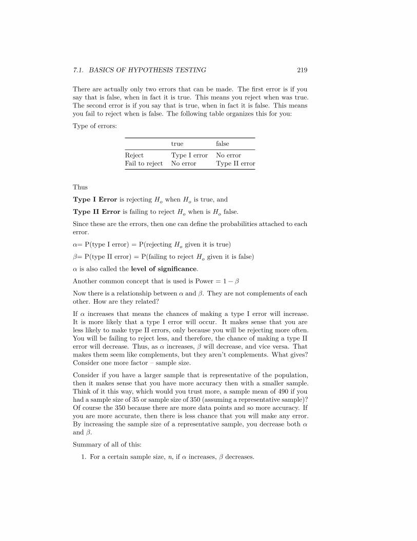
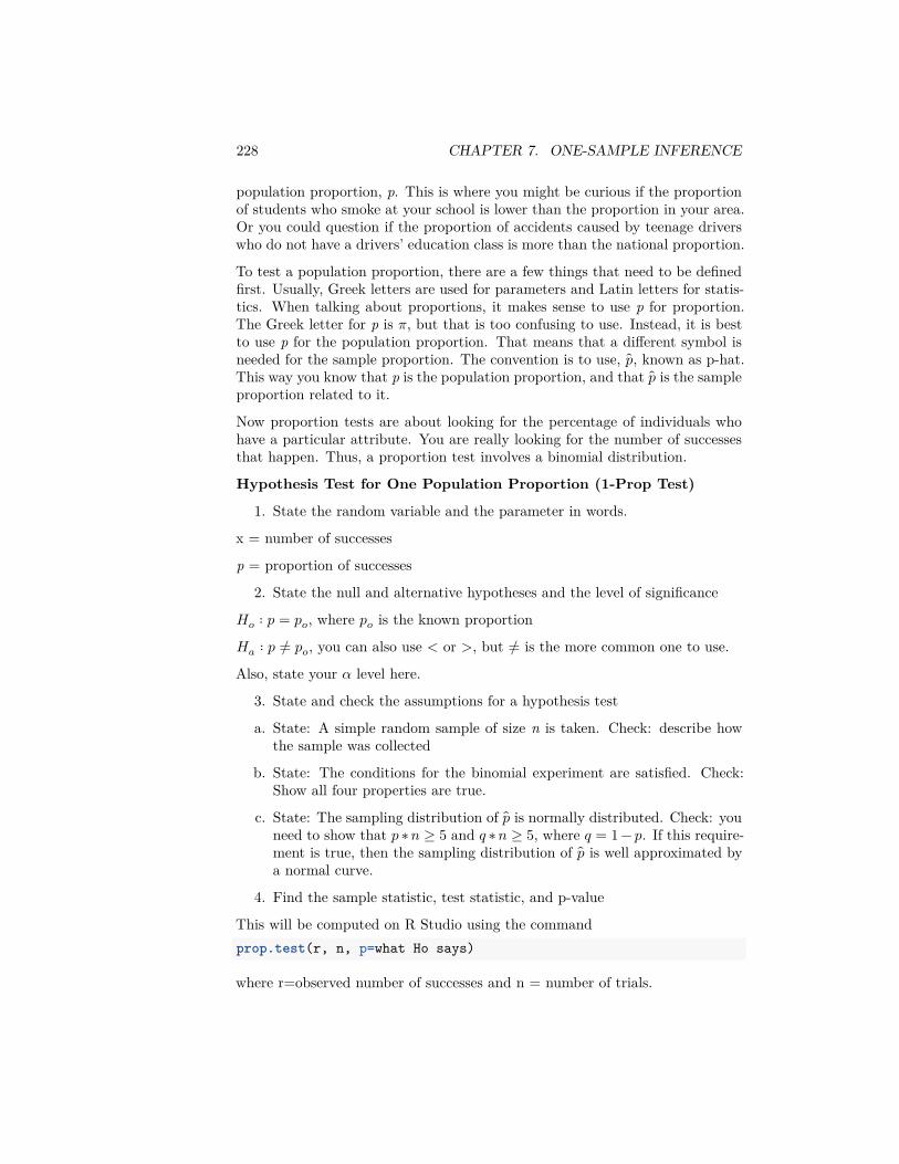
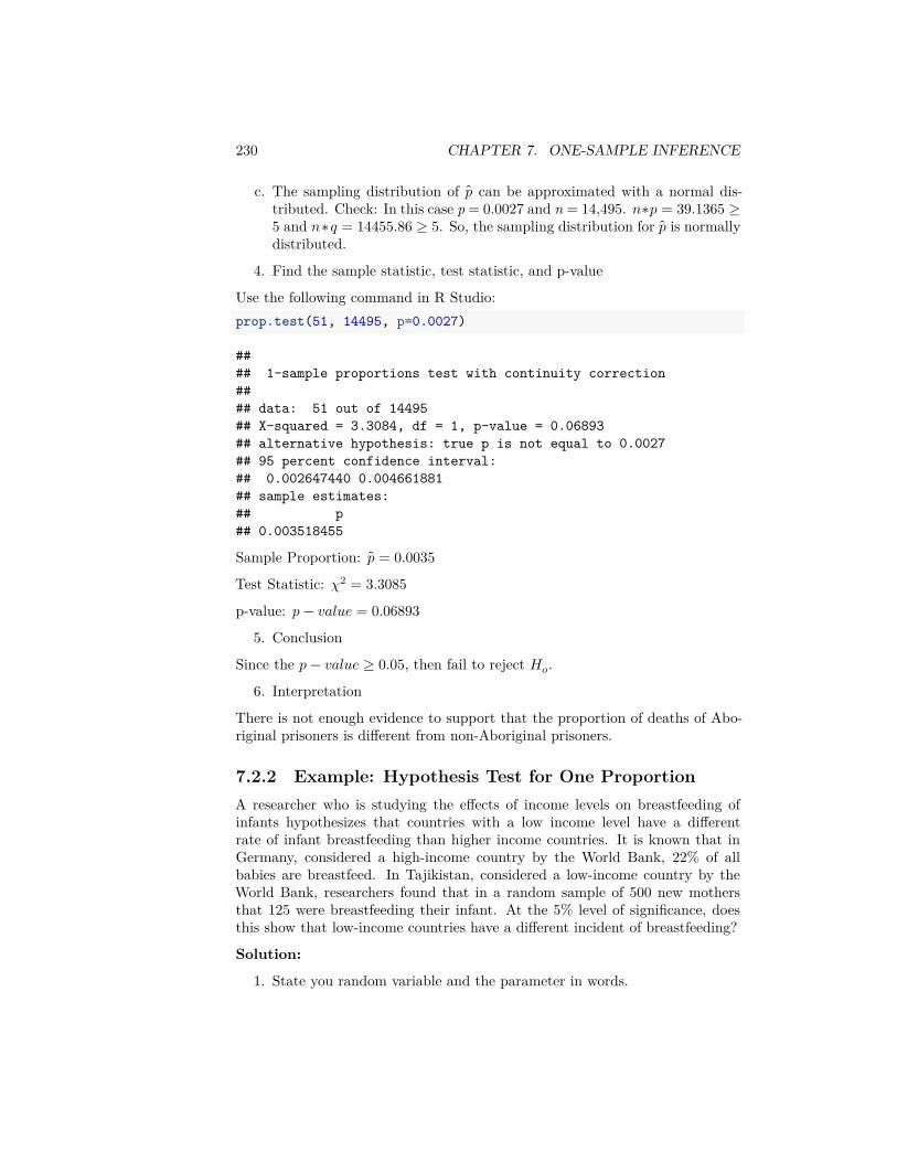
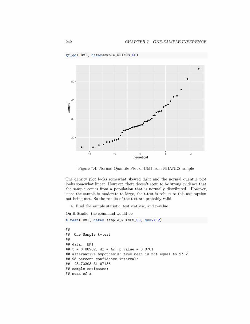

262 CHAPTER 7 ONE-SAMPLE INFERENCE