Chapter 6 Randomization 6.1 Introduction
56
Chapter 6 Randomization 6.1 Introduction As designs grow larger, it becomes more difficult to create a complete set of stimuli needed to check their functionality. You can write a directed test case to check a cer- tain set of features, but you cannot write enough directed test cases when the number of features keeps doubling on each project. Worse yet, the interactions between all these features are the source for the most devious bugs and are the least likely to be caught by going through a laundry list of features. The solution is to create test cases automatically using constrained-random tests (CRT). A directed test finds the bugs you think are there, but a CRT finds bugs you never thought about, by using random stimulus. You restrict the test scenarios to those that are both valid and of interest by using constraints. Creating a CRT environment takes more work than creating one for directed tests. A simple directed test just applies stimulus, and then you manually check the result. These results are captured as a golden log file and compared with future simulations to see whether the test passes or fails. A CRT environment needs not only to create the stimulus but also to predict the result, using a reference model, transfer function, or other techniques. However, once this environment is in place, you can run hun- dreds of tests without having to hand-check the results, thereby improving your productivity. This trade-off of test-authoring time (your work) for CPU time (machine work) is what makes CRT so valuable.
-
Upload
independent -
Category
Documents
-
view
1 -
download
0
Transcript of Chapter 6 Randomization 6.1 Introduction

Chapter 6
Randomization
6.1 Introduction
As designs grow larger, it becomes more difficult to create a complete set of stimulineeded to check their functionality. You can write a directed test case to check a cer-tain set of features, but you cannot write enough directed test cases when the numberof features keeps doubling on each project. Worse yet, the interactions between allthese features are the source for the most devious bugs and are the least likely to becaught by going through a laundry list of features.
The solution is to create test cases automatically using constrained-random tests(CRT). A directed test finds the bugs you think are there, but a CRT finds bugs younever thought about, by using random stimulus. You restrict the test scenarios tothose that are both valid and of interest by using constraints.
Creating a CRT environment takes more work than creating one for directed tests.A simple directed test just applies stimulus, and then you manually check the result.These results are captured as a golden log file and compared with future simulationsto see whether the test passes or fails. A CRT environment needs not only to createthe stimulus but also to predict the result, using a reference model, transfer function,or other techniques. However, once this environment is in place, you can run hun-dreds of tests without having to hand-check the results, thereby improving yourproductivity. This trade-off of test-authoring time (your work) for CPU time (machinework) is what makes CRT so valuable.
Chapter 6:Randomization162
A CRT is made of two parts: the test code that uses a stream of random values to cre-ate input to the DUT, and a seed to the pseudo-random number generator (PRNG),shown in Section 6.16.1. You can make a CRT behave differently just by using a newseed. This feature allows you to leverage each test so that each is the functional equiv-alent of many directed tests, just by changing seeds. You are able to create moreequivalent tests using these techniques than with directed testing.
You may feel that these random tests are like throwing darts. How do you know whenyou have covered all aspects of the design? The stimulus space is too large to generateevery possible input by using for-loops, and so you need to generate a useful subset.In Chap. 9 you will learn how to measure verification progress by using functionalcoverage.
There are many ways to use randomization, and this chapter gives a wide range ofexamples. It highlights the most useful techniques, but you should choose what worksbest for you.
6.2 What to Randomize
When you think of randomizing the stimulus to a design, the first thing you may thinkof are the data fields. These are the easiest to create – just call $random. The problemis that this approach has a very low payback in terms of bugs found: you only finddata-path bugs, perhaps with bit-level mistakes. The test is still inherently directed.The challenging bugs are in the control logic. As a result, you need to randomize alldecision points in your DUT. Wherever control paths diverge, randomization increasesthe probability that you’ll take a different path in each test case.
You need to think broadly about all design input such as the following:
Device configurationEnvironment configurationPrimary input dataEncapsulated input dataProtocol exceptionsDelaysTransaction statusErrors and violations
6.2.1 Device Configuration
What is the most common reason why bugs are missed during testing of the RTLdesign? Not enough different configurations have been tried! Most tests just use thedesign as it comes out of reset, or apply a fixed set of initialization vectors to put it

What to Randomize 163
into a known state. This is like testing a PC’s operating system right after it has beeninstalled, and without any applications; of course the performance is fine, and thereare no crashes.
Over time, in a real world environment, the DUT’s configuration becomes more andmore random. For example, a verification engineer had to verify a time-division mul-tiplexor switch that had 600 input channels and 12 output channels. When the devicewas installed in the end-customer’s system, channels would be allocated and deallo-cated over and over. At any point in time, there would be little correlation betweenadjacent channels. In other words, the configuration would seem random.
To test this device, the verification engineer had to write several dozen lines of Tclcode to configure each channel. As a result, she was never able to try configurationswith more than a handful of channels enabled. Using a CRT methodology, she wrotea testbench that randomized the parameters for a single channel, and then put this in aloop to configure the whole device. Now she had confidence that her tests woulduncover bugs that previously would have been missed.
6.2.2 Environment Configuration
The device that you are designing operates in an environment containing otherdevices. When you are verifying the DUT, it is connected to a testbench that mimicsthis environment. You should randomize the entire environment, including the num-ber of objects and how they are configured.
Another company was creating an I/O switch chip that connected multiple PCI busesto an internal memory bus. At the start of simulation the customer used randomizationto choose the number of PCI buses (1–4), the number of devices on each bus (1–8),and the parameters for each device (master or slave, CSR addresses, etc.). Eventhough there were many possible combinations, this company knew all had beencovered.
6.2.3 Primary Input Data
This is what you probably thought of first when you read about random stimulus: takea transaction such as a bus write or ATM cell and fill it with some random values.How hard can that be? Actually it is fairly straightforward as long as you carefullyprepare your transaction classes. You should anticipate any layered protocols anderror injection.
6.2.4 Encapsulated Input Data
Many devices process multiple layers of stimulus. For example, a device may cre-ate TCP traffic that is then encoded in the IP protocol, and finally sent out insideEthernet packets. Each level has its own control fields that can be randomized to trynew combinations. So you are randomizing the data and the layers that surround it.
Chapter 6:Randomization164
You need to write constraints that create valid control fields but that also allowinjecting errors.
6.2.5 Protocol Exceptions, Errors, and Violations
Anything that can go wrong, will, eventually. The most challenging part of designand verification is how to handle errors in the system. You need to anticipate all thecases where things can go wrong, inject them into the system, and make sure thedesign handles them gracefully, without locking up or going into an illegal state. Agood verification engineer tests the behavior of the design to the edge of the func-tional specification and sometimes even beyond.
When two devices communicate, what happens if the transfer stops partway through?Can your testbench simulate these breaks? If there are error detection and correctionfields, you must make sure all combinations are tried.
The random component of these errors is that your testbench should be able to sendfunctionally correct stimuli and then, with the flip of a configuration bit, start inject-ing random types of errors at random intervals.
6.2.6 Delays
Many communication protocols specify ranges of delays. The bus grant comes one tothree cycles after request. Data from the memory is valid in the fourth to tenth buscycle. However, many directed tests, optimized for the fastest simulation, use theshortest latency, except for that one test that only tries various delays. Your testbenchshould always use random, legal delays during every test to try to find that (hope-fully) one combination that exposes a design bug.
Below the cycle level, some designs are sensitive to clock jitter. By sliding the clockedges back and forth by small amounts, you can make sure your design is not overlysensitive to small changes in the clock cycle.
The clock generator should be in a module outside the testbench so that it createsevents in the Active region along with other design events. However, the generatorshould have parameters such as frequency and offset that can be set by the testbenchduring the configuration phase.
(Note that you are looking for functional errors, not timing errors. Your testbenchshould not try to violate setup and hold requirements. These are better validated usingtiming analysis tools.)

Randomization in SystemVerilog 165
6.3 Randomization in SystemVerilog
The random stimulus generation in SystemVerilog is most useful when used withOOP. You first create a class to hold a group of related random variables, and thenhave the random-solver fill them with random values. You can create constraints tolimit the random values to legal values, or to test-specific features.
Note that you can randomize individual variables, but this case is the least interesting.True constrained-random stimuli is created at the transaction level, not one value at a time.
6.3.1 Simple Class with Random Variables
Sample 6.1 shows a packet class with random variables and constraints, plus test-bench code that constructs and randomizes a packet.
Sample 6.1 Simple random class
class Packet; // The random variables rand bit [31:0] src, dst, data[8]; randc bit [7:0] kind; // Limit the values for src constraint c {src > 10; src < 15;}endclass
Packet p;initial begin p = new();// Create a packet assert (p.randomize()) else $fatal(0, "Packet::randomize failed"); transmit(p);end
This class has four random variables. The first three use the rand modifier, so thatevery time you randomize the class, the variables are assigned a value. Think of roll-ing dice: each roll could be a new value or repeat the current one. The kind variableis randc, which means random cyclic, so that the random solver does not repeat arandom value until every possible value has been assigned. Think of dealing cardsfrom a deck: you deal out every card in the deck in random order, then shuffle thedeck, and deal out the cards in a different order. Note that the cyclic pattern is for asingle variable. A randc array with eight elements has eight different patterns.
A constraint is just a set of relational expressions that must be true for the chosenvalue of the variables. In this example, the src variable must be greater than 10 andless than 15. Note that the constraint expression is grouped using curly braces: {}.This is because this code is declarative, not procedural, which uses begin...end.

Chapter 6:Randomization166
The randomize() function returns 0 if a problem is found with the constraints. Theprocedural assertion is used to check the result, as shown in Section 4.8. This exampleuses a $fatal to stop simulation, but the rest of the book leaves out this extra code.You need to find the tool-specific switches to force the assertion to terminate simula-tion. This book uses assert to test the result from randomize(), but you may wantto test the result, call your special routine that prints any useful information and thengracefully shut down the simulation.
You should not randomize an object in the class constructor. Your testmay need to turn constraints on or off, change weights, or even addnew constraints before randomization. The constructor is forinitializing the object’s variables, and if you called randomize() at thisearly stage, you might end up throwing away the results.
All variables in your classes should be random and public. This givesyour test the maximum control over the DUT’s stimulus and control.You can always turn off a random variable, as show in Section 6.11.2.If you forget to make a variable random, you must edit the environ-ment, which you want to avoid.
6.3.2 Checking the Result from Randomization
The randomize() function assigns random values to any variable inthe class that has been labeled as rand or randc, and also makes surethat all active constraints are obeyed. Randomization can fail if yourcode has conflicting constraints (see next section), and so you shouldalways check the status. If you don’t check, the variables may getunexpected values, causing your simulation to fail.
Sample 6.1 checks the status from randomize() by using a procedural assertion. Ifrandomization succeeds, the function returns 1. If it fails, randomize() returns 0.The assertion checks the result and prints an error if there was a failure. You shouldset your simulator’s switches to terminate when an error is found. Alternatively, youmight want to call a special routine to end simulation, after doing some housekeepingchores like printing a summary report.
6.3.3 The Constraint Solver
The process of solving constraint expressions is handled by the SystemVerilog constraintsolver. The solver chooses values that satisfy the constraints. The values come from Sys-temVerilog’s PRNG, which is started with an initial seed. If you give a SystemVerilogsimulator the same seed and the same testbench, it always produces the same results.
The solver is specific to the simulation vendor, and a constrained-random test maynot give the same results when run on different simulators, or even on different ver-sions of the same tool. The SystemVerilog standard specifies the meaning of theexpressions, and the legal values that are created, but does not detail the precise order

Constraint Details 167
in which the solver should operate. See Section 6.16 for more details on random num-ber generators.
6.3.4 What can be Randomized?
SystemVerilog allows you to randomize integral variables, that is, variables that con-tain a simple set of bits. This includes 2-state and 4-state types, though randomizationonly works with 2-state values. You can have integers, bit vectors, etc. You cannothave a random string, or refer to a handle in a constraint.1
6.4 Constraint Details
Useful stimulus is more than just random values – there are relationships between thevariables. Otherwise, it may take too long to generate interesting stimulus values, orthe stimulus might contain illegal values. You define these interactions in SystemVer-ilog using constraint blocks that contain one or more constraint expressions.SystemVerilog chooses random values so that the expressions are true.
At least one variable in each expression should be random, eitherrand or randc. The following class fails when randomized, unlessage happens to be in the right range. The solution is to add the mod-ifier rand or randc before age.
Sample 6.2 Constraint without random variables
class Child; bit [31:0] age; // Error – should be rand or randc constraint c_teenager {age > 12; age < 20;}endclass
The randomize() function tries to assign new values to random variables and tomake sure all constraints are satisfied. In Sample 6.2, since there are no random vari-ables, randomize() just checks the value of son to see if it is in the boundsspecified by the constraint c_teenager. Unless the variable happens to fall in therange of 13:19, randomize() fails. While you can use a constraint to check that anonrandom variable has a valid value, use an assert or if-statement instead. It ismuch easier to debug your procedural checker code than read through an error mes-sage from the random solver.
1As of late 2007, the IEEE SystemVerilog committee is still working on specifying how to randomize real variables. The issue is that the solver may not be able to solve a constraint such as one_third == 0.333 as the fraction 1/3 cannot be represented precisely as a real number.

Chapter 6:Randomization168
6.4.1 Constraint Introduction
Sample 6.3 shows a simple class with random variables and constraints. The specificconstructs are explained in the following sections.
Sample 6.3 Constrained-random class
class Stim; const bit [31:0] CONGEST_ADDR = 42; typedef enum {READ, WRITE, CONTROL} stim_e; randc stim_e kind; // Enumerated var rand bit [31:0] len, src, dst; bit congestion_test;
constraint c_stim { len < 1000; len > 0; if (congestion_test) { dst inside {[CONGEST_ADDR-100:CONGEST_ADDR+100]}; src == CONGEST_ADDR; } else src inside {0, [2:10], [100:107]}; }endclass
6.4.2 Simple Expressions
Sample 6.3 showed a constraint block with several expressions. The first two controlthe values for the len variable. As you can see, a variable can be used in multipleexpressions.
There can be a maximum of only one relational operator (<, <=,==, >=, or >) in an expression. Sample 6.4 incorrectly tries to gen-erate three variables in a fixed order.
Sample 6.4 Bad ordering constraint
class order; rand bit [7:0] lo, med, hi; constraint bad {lo < med < hi;} // Gotcha!endclass
Constraint Details 169
Sample 6.5 Result from incorrect ordering constraint
lo = 20, med = 224, hi = 164lo = 114, med = 39, hi = 189lo = 186, med = 148, hi = 161lo = 214, med = 223, hi = 201
Sample 6.5 shows the results, which are not what was intended. The constraint bad inSample 6.4 is broken down into multiple binary relational expressions, going fromleft to right: ((lo < med) < hi). First, the expression (lo < med) is evaluated,which gives 0 or 1. Then hi is constrained to be greater than the result. The variableslo and med are randomized but not constrained. The correct constraint is shown inSample 6.6. For more examples, see Sutherland and Mills (2007).
Sample 6.6 Constrain variables to be in a fixed order
class order; rand bit [15:0] lo, med, hi; constraint good {lo < med; // Only use binary constraints med < hi;}endclass
6.4.3 Equivalence Expressions
The most common mistake with constraints is trying to make anassignment in a constraint block, but it can only contain expres-sions. Instead, use the equivalence operator to set a randomvariable to a value, e.g., len==42. You can build complex rela-
tionships between one or more random variables, such as len == header.addr_mode* 4 + payload.size().
6.4.4 Weighted Distributions
The dist operator allows you to create weighted distributions so that some values arechosen more often than others. The dist operator takes a list of values and weights,separated by the := or the :/ operator. The values and weights can be constants orvariables. The values can be a single value or a range such as [lo:hi]. The weightsare not percentages and do not have to add up to 100. The := operator specifies thatthe weight is the same for every specified value in the range, whereas the :/ operatorspecifies that the weight is to be equally divided between all the values.

Chapter 6:Randomization170
Sample 6.7 Weighted random distribution with dist
rand int src, dst;constraint c_dist { src dist {0:=40, [1:3]:=60}; // src = 0, weight = 40/220 // src = 1, weight = 60/220 // src = 2, weight = 60/220 // src = 3, weight = 60/220
dst dist {0:/40, [1:3]:/60}; // dst = 0, weight = 40/100 // dst = 1, weight = 20/100 // dst = 2, weight = 20/100 // dst = 3, weight = 20/100}
In Sample 6.7, src gets the value 0, 1, 2, or 3. The weight of 0 is 40, whereas, 1, 2,and 3 each have the weight of 60, for a total of 220. The probability of choosing 0 is40/220, and the probability of choosing 1, 2, or 3 is 60/220 each.
Next, dst gets the value 0, 1, 2, or 3. The weight of 0 is 40, whereas 1, 2, and 3 sharea total weight of 60, for a total of 100. The probability of choosing 0 is 40/100, andthe probability of choosing 1, 2, or 3 is only 20/100 each.
Once again, the values and weights can be constants or variables. You can use vari-able weights to change distributions on the fly or even to eliminate choices by settingthe weight to zero, as shown in Sample 6.8.
Sample 6.8 Dynamically changing distribution weights
// Bus operation, byte, word, or longwordclass BusOp; // Operand length typedef enum {BYTE, WORD, LWRD } length_e; rand length_e len;
// Weights for dist constraint bit [31:0] w_byte=1, w_word=3, w_lwrd=5;
constraint c_len { len dist {BYTE := w_byte, // Choose a random WORD := w_word, // length using LWRD := w_lwrd}; // variable weights }endclass
In Sample 6.8, the len enumerated variable has three values. With the default weight-ing values, longword lengths are chosen more often, as w_lwrd has the largest value.
Constraint Details 171
Don’t worry, you can change the weights on the fly during simulation to get a differ-ent distribution.
6.4.5 Set Membership and the Inside Operator
You can create sets of values with the inside operator. The SystemVerilog solverchooses between the values in the set with equal probability, unless you have otherconstraints on the variable. As always, you can use variables in the sets.
Sample 6.9 Random sets of values
rand int c; // Random variableint lo, hi; // Non-random variables used as limitsconstraint c_range { c inside {[lo:hi]}; // lo <= c && c <= hi}
In Sample 6.9, SystemVerilog uses the values for lo and hi to determine the range ofpossible values. You can use this to parameterize your constraints so that the test-bench can alter the behavior of the stimulus generator without rewriting theconstraints. Note that if lo > hi, an empty set is formed, and the constraint fails.
You can use $ as a shortcut for the minimum and maximum values for a range, asshown in Sample 6.10. This is helpful when you are building constraints for variableswith different ranges.
Sample 6.10 Specifying minimum and maximum range with $
rand bit [6:0] b; // 0 <= b <= 127rand bit [5:0] e; // 0 <= e <= 63constraint c_range { b inside {[$:4], [20:$}; // 0 <= b <= 4 || 20 <= b <= 127 e inside {[$:4], [20:$}; // 0 <= e <= 4 || 20 <= e <= 63}
If you want any value, as long as it is not inside a set, invert the constraint with theNOT operator: !
Sample 6.11 Inverted random set constraint
constraint c_range { !(c inside {[lo:hi]}); // c < lo or c > hi}
6.4.6 Using an Array in a Set
You can choose from a set of values by storing them in an array.
Chapter 6:Randomization172
Sample 6.12 Random set constraint for an array
rand int f;int fib[5] = ’{1,2,3,5,8};constraint c_fibonacci { f inside fib;}
This is expanded into the following set of constraints:
Sample 6.13 Equivalent set of constraints
constraint c_fibonacci { (f == fib[0]) || // f==1 (f == fib[1]) || // f==2 (f == fib[2]) || // f==3 (f == fib[3]) || // f==5 (f == fib[4]); // f==8}
All values in the set are chosen equally, even if they appear multiple times. You canalso think of the inside constraint as being turned into a foreach constraint, asexplained in Section 6.13.4.
Sample 6.14 chooses values using an inside constraint with repeated value, and alsoprints a histogram of the chosen values and so you can see that they are chosenequally.

Constraint Details 173
Sample 6.14 Repeated values in inside constraint
class Weighted; rand int val; int array[] = ’{1,1,2,3,5,8,8,8,8,8}; constraint c {val inside array;}endclass
Weighted w;initial begin int count[9], maxx[$]; w = new();
repeat (2000) begin assert(w.randomize()); count[w.val]++; // Count the number of hits end
maxx = count.max(); // Get largest value in count
// Print histogram of count foreach(count[i]) if (count[i]) begin $write("count[%0d]=%5d ", i, count[i]); repeat (count[i]*40/maxx[0]) $write("*"); $display; endend
Sample 6.15 Output from inside constraint operator and weighted array
count[1]= 3941 ***************************************count[2]= 4038 ****************************************count[3]= 3978 ***************************************count[5]= 4027 ***************************************count[8]= 4016 ***************************************
The right way to build a weighted distribution is with the dist operator as shown inSection 6.4.4.
Examples 6.16 and 6.17 choose a day of the week from a list of enumerated values.You can change the list of choices on the fly. If you make choice a randc variable,the simulator tries every possible value before repeating.

Chapter 6:Randomization174
Sample 6.16 Class to choose from an array of possible values
class Days; typedef enum {SUN, MON, TUE, WED, THU, FRI, SAT} days_e; days_e choices[$]; rand days_e choice; constraint cday {choice inside choices;}endclass
Sample 6.17 Choosing from an array of values
initial begin Days days; days = new();
days.choices = {Days::SUN, Days::SAT}; assert (days.randomize()); $display("Random weekend day %s\n", days.choice.name);
days.choices = {Days::MON, Days::TUE, Days::WED, Days::THU, Days::FRI}; assert (days.randomize()); $display("Random week day %s", days.choice.name);end
The name() function returns a string with the name of an enumerated value.
If you want to dynamically add or remove values from a set, think twice before usingthe inside operator because of its performance. For example, perhaps you have a setof values that you want to choose just once. You could use inside to choose valuesfrom a queue, and delete them to slowly shrink the queue. This requires the solver tosolve N constraints, where N is the number of elements left in the queue. Instead, usea randc variable that points into an array of choices. Choosing a randc value takes ashort, constant time, whereas solving a large number of constraints is more expensive,especially if your array has more than a few dozen elements.
Constraint Details 175
Sample 6.18 Using randc to choose array values in random order
class RandcInside; int array[]; // Values to choose randc bit [15:0] index; // Index into array
function new(input int a[]); // Construct & initialize array = a; endfunction
function int pick; // Return most recent pick return array[index]; endfunction
constraint c_size {index < array.size();}endclass
initial begin RandcInside ri;
ri = new(’{1,3,5,7,9,11,13}); repeat (ri.array.size()) begin assert(ri.randomize()); $display("Picked %2d [%0d]", ri.pick(), ri.index); end end
Note that constraints and routines can be mixed in any order.
6.4.7 Conditional Constraints
Normally, all constraint expressions are active in a block. What if you want to have anexpression active only some of the time? For example, a bus supports byte, word, andlongword reads, but only longword writes. SystemVerilog supports two implicationoperators, -> and if-else.
When you are choosing from a list of expressions, such as an enumerated type, theimplication operator, ->, lets you create a case-like block. The parentheses around theexpression are not required, but do make the code easier to read.

Chapter 6:Randomization176
Sample 6.19 Constraint block with implication operator
class BusOp; ... constraint c_io { (io_space_mode) -> addr[31] == 1’b1; }
If you have a true-false expression, the if-else operator may be better.
Sample 6.20 Constraint block with if-else operator
class BusOp; ... constraint c_len_rw { if (op == READ) len inside {[BYTE:LWRD]}; else len == LWRD; }
In constraint blocks, you use curly braces, { }, to group multiple expressions. Thebegin...end keywords are for procedural code.
6.4.8 Bidirectional Constraints
By now you may have realized that constraint blocks are not procedural code, execut-ing from top to bottom. They are declarative code, all active at the same time. If youconstrain a variable with the inside operator with the set [10:50] and have anotherexpression that constrains the variable to be greater than 20, SystemVerilog solvesboth constraints simultaneously and only chooses values between 21 and 50.
SystemVerilog constraints are bidirectional, which means that the constraints on allrandom variables are solved concurrently. Adding or removing a constraint on anyone variable affects the value chosen for all variables that are related directly or indi-rectly. Consider the constraint in Sample 6.21.
Sample 6.21 Bidirectional constraint
rand logic [15:0] r, s, t;constraint c_bidir { r < t; s == r; t < 30; s > 25;}

Constraint Details 177
The SystemVerilog solver looks at all four constraints simultaneously. The variable rhas to be less than t, which has to be less than 30. However, r is also constrained tobe equal to s, which is greater than 25. Even though there is no direct constraint onthe lower value of t, the constraint on s restricts the choices. Table 6-1 shows thepossible values for these three variables.
Even the conditional constraints such as -> and if...else, which can look like a pro-cedural if-else statement, are bidirectional. For example, the constraint {(a==1) -> (b==0)} is equivalent to {!(a == 1) || b == 0;}. The solver picks values forthe variables that meet this constraint, and does not first check if a==1, then forceb==0. In fact, if you add the additional constraint {b==1;}, the solver will set a to 0.
6.4.9 Choose the Right Arithmetic Operator to Boost Efficiency
Simple arithmetic operators such as addition and subtraction, bit extracts, and shiftsare handled very efficiently by the solver in a constraint. However, multiplication,division, and modulo are very expensive with 32-bit values. Remember that any con-stant without an explicit size, such as 42, is treated as a 32-bit value.
If you want to generate random addresses that are near a page boundary, where a pageis 4096 bytes, you could write the following code, but the solver may take a long timeto find suitable values for addr.
Sample 6.22 Expensive constraint with mod and unsized variable
rand bit [31:0] addr;constraint slow_near_page_boundary { addr % 4096 inside {[0:20], [4075:4095]};}
Many constants in hardware are powers of 2, and so take advantage of this by usingbit extraction rather than division and modulo. Likewise, multiplication by a power oftwo can be replaced by a shift.
Table 6-1 Solutions for bidirectional constraint
Solution r s t
A 26 26 27
B 26 26 28
C 26 26 29
D 27 27 28
E 27 27 29
F 28 28 29

Chapter 6:Randomization178
Sample 6.23 Efficient constraint with bit extract
rand bit [31:0] addr;constraint near_page_boundry { addr[11:0] inside {[0:20], [4075:4095]};}
6.5 Solution Probabilities
Whenever you deal with random values, you need to understand the probability of theoutcome. SystemVerilog does not guarantee the exact solution found by the randomconstraint solver, but you can influence the distribution. Any time you work with ran-dom numbers, you have to look at thousands or millions of values to average out thenoise. Changing the tool version or random seed can cause different results. Some sim-ulators, such as Synopsys VCS, have multiple solvers to allow you to trade memoryusage vs. performance.
6.5.1 Unconstrained
Start with two variables with no constraints.
Sample 6.24 Class Unconstrained
class Unconstrained; rand bit x; // 0 or 1 rand bit [1:0] y; // 0, 1, 2, or 3endclass
There are eight possible solutions, as shown in Table 6-2. Since there are no con-straints, each has the same probability. You have to run thousands of randomizationsto see the actual results that approach the listed probabilities.2
Table 6-2 Solutions for Unconstrained class
Solution x y Probability
A 0 0 1/8
B 0 1 1/8
C 0 2 1/8
D 0 3 1/8
E 1 0 1/8
F 1 1 1/8
G 1 2 1/8
H 1 3 1/8
2The tables were generated with Synopsys VCS 2005.06 using the run-time switch +ntb_solver_mode=1.
Solution Probabilities 179
6.5.2 Implication
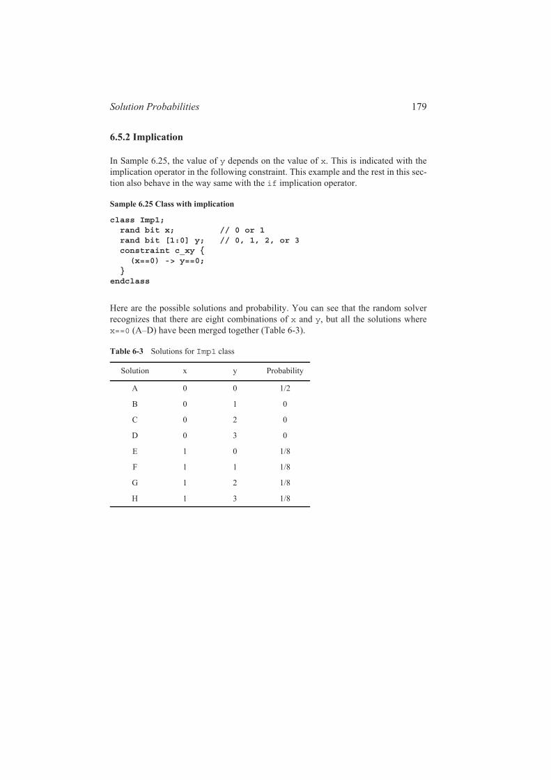
In Sample 6.25, the value of y depends on the value of x. This is indicated with theimplication operator in the following constraint. This example and the rest in this sec-tion also behave in the way same with the if implication operator.
Sample 6.25 Class with implication
class Imp1; rand bit x; // 0 or 1 rand bit [1:0] y; // 0, 1, 2, or 3 constraint c_xy { (x==0) -> y==0; }endclass
Here are the possible solutions and probability. You can see that the random solverrecognizes that there are eight combinations of x and y, but all the solutions wherex==0 (A–D) have been merged together (Table 6-3).
Table 6-3 Solutions for Imp1 class
Solution x y Probability
A 0 0 1/2
B 0 1 0
C 0 2 0
D 0 3 0
E 1 0 1/8
F 1 1 1/8
G 1 2 1/8
H 1 3 1/8

Chapter 6:Randomization180
6.5.3 Implication and Bidirectional Constraints
Note that the implication operator says that when x==0, y is forced to 0, but wheny==0, there is no constraint on x. However, implication is bidirectional in that if ywere forced to a nonzero value, x would have to be 1. Sample 6.26 has the constrainty>0, and so x can never be 0 (Table 6-4).
Sample 6.26 Class with implication and constraint
class Imp2; rand bit x; // 0 or 1 rand bit [1:0] y; // 0, 1, 2, or 3 constraint c_xy { y > 0; (x==0) -> y==0; }endclass
6.5.4 Guiding Distribution with solve...before
You can guide the SystemVerilog solver using the “solve...before” constraint asseen in Sample 6.27.
Table 6-4 Solutions for Imp2 class
Solution x y Probability
A 0 0 0
B 0 1 0
C 0 2 0
D 0 3 0
E 1 0 0
F 1 1 1/3
G 1 2 1/3
H 1 3 1/3

Solution Probabilities 181
Sample 6.27 Class with implication and solve...before
class SolveBefore; rand bit x; // 0 or 1 rand bit [1:0] y; // 0, 1, 2, or 3 constraint c_xy { (x==0) -> y==0; solve x before y; }endclass
The solve...before constraint does not change the solution space, just the probabilityof the results. The solver chooses values of x (0, 1) with equal probability. In 1,000 callsto randomize(), x is 0 about 500 times, and 1 about 500 times. When x is 0, y must be0. When x is 1, y can be 0, 1, 2, or 3 with equal probability (Table 6-5).
However, if you use the constraint solve y before x, you get a very different dis-tribution (Table 6-6).
Table 6-5 Solutions for solve x before y constraint
Solution x y Probability
A 0 0 1/2
B 0 1 0
C 0 2 0
D 0 3 0
E 1 0 1/8
F 1 1 1/8
G 1 2 1/8
H 1 3 1/8
Table 6-6 Solutions for solve y before x constraint
Solution x y Probability
A 0 0 1/8
B 0 1 0
C 0 2 0
D 0 3 0
E 1 0 1/8
F 1 1 1/4
G 1 2 1/4
H 1 3 1/4

Chapter 6:Randomization182
Only use solve...before if you are dissatisfied with how oftensome values occur. Excessive use can slow the constraint solverand make your constraints difficult for others to understand.
6.6 Controlling Multiple Constraint Blocks
A class can contain multiple constraint blocks. One might make sure you have a validtransaction, as described in Section 6.7, but you might need to disable this when test-ing the DUT’s error handling. Or you might want to have a separate constraint foreach test. Perhaps one constraint would restrict the data length to create small transac-tions (great for testing congestion), whereas another would make long transactions.
At run-time, you can use the built-in constraint_mode() routine to turn con-straints on and off. You can control a single constraint withhandle.constraint.constraint_mode(). To control all constraints in anobject, use handle.constraint_mode(), as shown in Sample 6.28.

Valid Constraints 183
Sample 6.28 Using constraint_mode
class Packet; rand int length; constraint c_short {length inside {[1:32]}; } constraint c_long {length inside {[1000:1023]}; }endclass
Packet p;initial begin p = new();
// Create a long packet by disabling short constraint p.c_short.constraint_mode(0); assert (p.randomize());
transmit(p);
// Create a short packet by disabling all constraints // then enabling only the short constraint p.constraint_mode(0); p.c_short.constraint_mode(1); assert (p.randomize()); transmit(p);end
6.7 Valid Constraints
A good randomization technique is to create several constraints to ensure the correct-ness of your random stimulus, known as “valid constraints.” For example, a bus read–modify–write command might only be allowed for a longword data length.
Sample 6.29 Checking write length with a valid constraint
class Transaction; rand enum {BYTE, WORD, LWRD, QWRD} length; rand enum {READ, WRITE, RMW, INTR} opc;
constraint valid_RMW_LWRD { (opc == RMW) -> length == LWRD; }endclass
Now you know the bus transaction obeys the rule. Later, if you want to violate therule, use constraint_mode to turn off this one constraint. You should have a

Chapter 6:Randomization184
naming convention to make these constraints stand out, such as using the prefixvalid as shown above.
6.8 In-line Constraints
As you write more tests, you can end up with many constraints. They can interactwith each other in unexpected ways, and the extra code to enable and disable themadds to the test complexity. Additionally, constantly adding and editing constraints toa class could cause problems in a team environment.
Many tests only randomize objects at one place in the code. SystemVerilog allowsyou to add an extra constraint using randomize() with. This is equivalent to add-ing an extra constraint to any existing ones in effect. Sample 6.30 shows a base classwith constraints, then two randomize() with statements.
Sample 6.30 The randomize() with statement
class Transaction; rand bit [31:0] addr, data; constraint c1 {addr inside{[0:100],[1000:2000]};}endclass
Transaction t;
initial begin t = new();
// addr is 50-100, 1000-1500, data < 10 assert(t.randomize() with {addr >= 50; addr <= 1500; data < 10;});
driveBus(t);
// force addr to a specific value, data > 10 assert(t.randomize() with {addr == 2000; data > 10;});
driveBus(t); end
The extra constraints are added to the existing ones in effect. Use constraint_modeif you need to disable a conflicting constraint. Note that inside the with{} statement,SystemVerilog uses the scope of the class. That is why Sample 6.30 used just addr,not t.addr.
The pre_randomize and post_randomize Functions 185
A common mistake is to surround your in-line constraints withparenthesis instead of curly braces {}. Just remember that con-straint blocks use curly braces, and so your in-line constraint mustuse them too. Braces are for declarative code.
6.9 The pre_randomize and post_randomize Functions
Sometimes you need to perform an action immediately before every randomize()call or immediately afterwards. For example, you may want to set some nonrandomclass variables (such as limits or weights) before randomization starts, or you mayneed to calculate the error correction bits for random data.
SystemVerilog lets you do this with two special void functions, pre_randomize andpost_randomize. Section 3.2 showed that a void function does not return a value,but, because it is not a task, does not consume time. If you want to call a debug rou-tine from pre_randomize or post_randomize, it must be a function.
6.9.1 Building a Bathtub Distribution
For some applications, you want a nonlinear random distribution. For instance, smalland large packets are more likely to find a design bug such as buffer overflow thanmedium-sized packets. So you want a bathtub shaped distribution; high on both ends,and low in the middle. You could build an elaborate dist constraint, but it mightrequire lots of tweaking to get the shape you want. Verilog has several functions fornonlinear distribution such as $dist_exponential but none for a bathtub. Thegraph in Figure 6.1 shows how you can combine two exponential curves to make abathtub curve. The pre_randomize method in Sample 6.31 calculates a point on anexponential curve, and then randomly chooses to put this on the left curve, or right.As you pick points on either the left and right curves, you gradually build a distribu-tion of the combined values.

Chapter 6:Randomization186
Figure 6-1 Building a bathtub distribution
Sample 6.31 Building a bathtub distribution
class Bathtub; int value; // Random variable with bathtub dist int WIDTH = 50, DEPTH=4, seed=1;
function void pre_randomize(); // Calculate an exponental curve value = $dist_exponential(seed, DEPTH); if (value > WIDTH) value = WIDTH;
// Randomly put this point on the left or right curve if ($urandom_range(1)) value = WIDTH - value; endfunction
endclass
Every time this object is randomized, the variable value gets updated. Across manyrandomizations, you will see the desired nonlinear distribution. Since the variable iscalculated procedurally, not through the random constraint solver, it does not need therand modifier.
6.9.2 Note on Void Functions
The functions pre_randomize and post_randomize can only callother functions, not tasks that could consume time. After all, you can-not have a delay in the middle of a call to randomize(). When youare debugging a randomization problem, you can call your displayroutines if you planned ahead and made them void functions.
LeftExponential
RightExponential
Sum is abathtub
Prob
abili
ty
Values WIDTH0
LeftExponential
RightExponential
Sum is abathtub
Prob
abili
ty
Values WIDTH0

Random Number Functions 187
6.10 Random Number Functions
You can use all the Verilog-1995 distribution functions, plus several that are new forSystemVerilog. Consult a statistics book for more details on the “dist” functions.Some of the useful functions include the following.
$random() – Flat distribution, returning signed 32-bit random$urandom() – Flat distribution, returning unsigned 32-bit random$urandom_range() – Flat distribution over a range$dist_exponential() – Exponential decay, as shown in Figure 6-1$dist_normal() – Bell-shaped distribution$dist_poisson() – Bell-shaped distribution$dist_uniform() – Flat distribution
The $urandom_range() function takes two arguments, an optional low value, and ahigh value.
Sample 6.32 $urandom_range usage
a = $urandom_range(3, 10); // Pick a value from 3 to 10a = $urandom_range(10, 3); // Pick a value from 3 to 10b = $urandom_range(5); // Pick a value from 0 to 5
6.11 Constraints Tips and Techniques
How can you create CRT that can be easily modified? There are several tricks youcan use. The most general technique is to use OOP to extend the original class asdescribed in Sections 6.11.8 and 8.2.4, but this also requires more planning. So, firstlearn some simple techniques, but keep an open mind.
6.11.1 Constraints with Variables
Most constraint examples in this book use constants to make them more readable. InSample 6.33, size is randomized over a range that uses a variable for the upperbound.

Chapter 6:Randomization188
Sample 6.33 Constraint with a variable bound
class bounds; rand int size; int max_size = 100; constraint c_size { size inside {[1:max_size]}; }endclass
By default, this class creates random sizes between 1 and 100, but by changing thevariable max_size, you can vary the upper limit.
You can use variables in the dist constraint to turn on and off values and ranges. InSample 6.34, each bus command has a different weight variable.
Sample 6.34 dist constraint with variable weights
typedef enum (READ8, READ16, READ32) read_e;class ReadCommands; rand read_e read_cmd; int read8_wt=1, read16_wt=1, read32_wt=1; constraint c_read { read_cmd dist {READ8 := read8_wt, READ16 := read16_wt, READ32 := read32_wt}; }endclass
By default, this constraint produces each command with equal probability. If youwant to have a greater number of READ8 commands, increase the read8_wt weightvariable. Most importantly, you can turn off generation of some commands by drop-ping their weight to 0.
6.11.2 Using Nonrandom Values
If you have a set of constraints that produces stimulus that is almost what you want,but not quite, you could call randomize(), and then set a variable to the value youwant – you don’t have to use the random one. However, your stimulus values may notbe correct according to the constraints you created to check validity.
If there are just a few variables that you want to override, use rand_mode to makethem nonrandom.

Constraints Tips and Techniques 189
Sample 6.35 rand_mode disables randomization of variables
// Packet with variable length payloadclass Packet; rand bit [7:0] length, payload[]; constraint c_valid {length > 0; payload.size() == length;}
function void display(string msg); $display("\n%s", msg); $write("Packet len=%0d, payload size=%0d, bytes = ", length, payload.size()); for(int i=0; (i<4 && i<payload.size()); i++) $write(" %0d", payload[i]); $display; endfunctionendclass
Packet p;initial begin p = new();
// Randomize all variables assert (p.randomize()); p.display("Simple randomize");
p.length.rand_mode(0); // Make length nonrandom, p.length = 42; // set it to a constant value assert (p.randomize()); // then randomize the payload p.display("Randomize with rand_mode");end
In Sample 6.35, the packet size is stored in the random variable length. The first halfof the test randomizes both the length variable and the contents of the payloaddynamic array. The second half calls rand_mode to make length a nonrandom vari-able, sets it to 42, and then calls randomize(). The constraint sets the payload sizeat the constant 42, but the array is still filled with random values.
6.11.3 Checking Values Using Constraints
If you randomize an object and then modify some variables, you can check that theobject is still valid by checking if all constraints are still obeyed. Call handle.ran-domize(null) and SystemVerilog treats all variables as nonrandom (“statevariables”) and just ensures that all constraints are satisfied.

Chapter 6:Randomization190
6.11.4 Randomizing Individual Variables
Suppose you want to randomize a few variables inside a class. You can call random-ize() with the subset of variables. Only those variables passed in the argument listwill be randomized; the rest will be treated as state variables and not randomized. Allconstraints remain in effect. In Sample 6.36, the first call to randomize() onlychanges the values of two rand variables med and hi. The second call only changesthe value of med, whereas hi retains its previous value. Surprisingly, you can pass anonrandom variable, as shown in the last call, and low is given a random value, aslong as it obeys the constraint.
Sample 6.36 Randomizing a subset of variables in a class
class Rising; byte low; // Not random rand byte med, hi; // Random variable constraint up { low < med; med < hi; } // See Section 6.4.2endclass
initial begin Rising r; r = new(); r.randomize(); // Randomize med, hi; low untouched r.randomize(med); // Randomize only med r.randomize(low); // Randomize only lowend
This trick of only randomizing a subset of the variables is not commonly used in realtestbenches as you are restricting the randomness of your stimulus. You want yourtestbench to explore the full range of legal values, not just a few corners.
6.11.5 Turn Constraints Off and On
A simple testbench may use a data class with just a few constraints. What if youwant to have two tests with very different flavors of data? You could use the impli-cation operators (-> or if-else) to build a single, elaborate constraint controlledby nonrandom variables.
Constraints Tips and Techniques 191
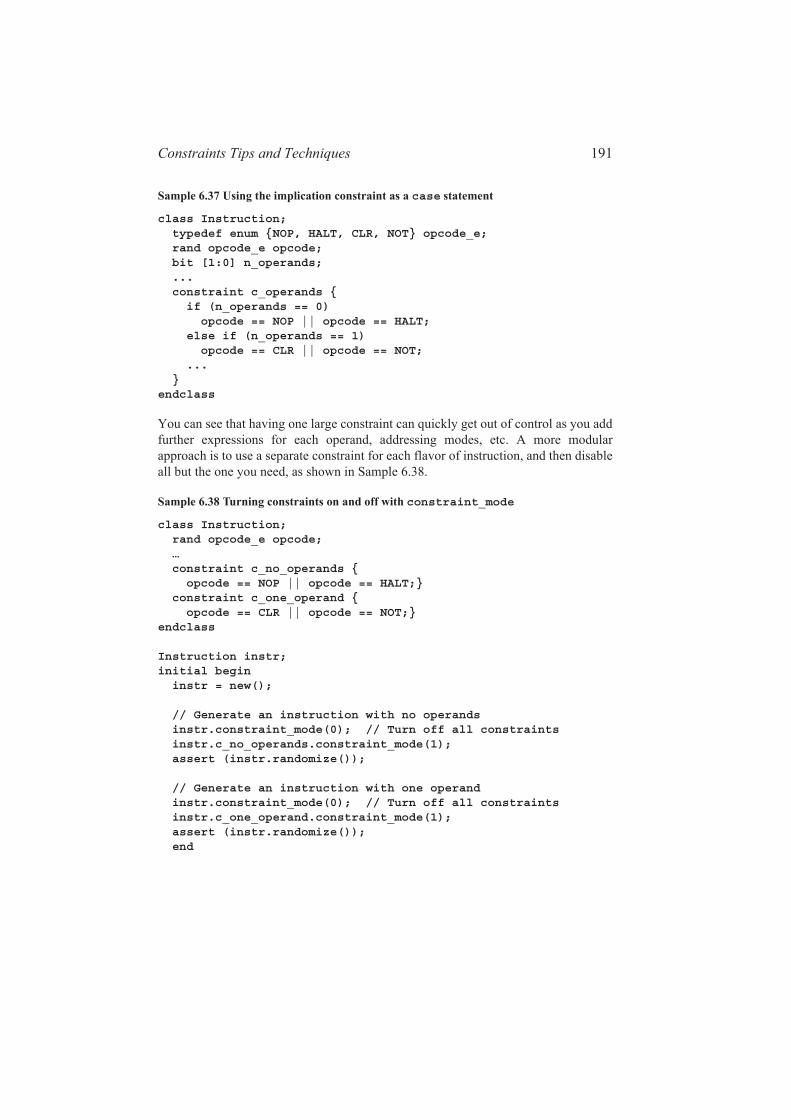
Sample 6.37 Using the implication constraint as a case statement
class Instruction; typedef enum {NOP, HALT, CLR, NOT} opcode_e; rand opcode_e opcode; bit [1:0] n_operands; ... constraint c_operands { if (n_operands == 0) opcode == NOP || opcode == HALT; else if (n_operands == 1) opcode == CLR || opcode == NOT; ... }endclass
You can see that having one large constraint can quickly get out of control as you addfurther expressions for each operand, addressing modes, etc. A more modularapproach is to use a separate constraint for each flavor of instruction, and then disableall but the one you need, as shown in Sample 6.38.
Sample 6.38 Turning constraints on and off with constraint_mode
class Instruction; rand opcode_e opcode; … constraint c_no_operands { opcode == NOP || opcode == HALT;} constraint c_one_operand { opcode == CLR || opcode == NOT;}endclass
Instruction instr;initial begin instr = new();
// Generate an instruction with no operands instr.constraint_mode(0); // Turn off all constraints instr.c_no_operands.constraint_mode(1); assert (instr.randomize());
// Generate an instruction with one operand instr.constraint_mode(0); // Turn off all constraints instr.c_one_operand.constraint_mode(1); assert (instr.randomize()); end
Chapter 6:Randomization192
While many small constraints may give you more flexibility, the process of turningthem on and off is more complex. For example, when you turn off all constraints thatcreate data, you are also disabling all the ones that check the data’s validity.
6.11.6 Specifying a Constraint in a Test Using In-Line Constraints
If you keep adding constraints to a class, it becomes hard to manage and control.Soon, everyone is checking out the same file from your source control system. Manytimes a constraint is only used by a single test, and so why have it visible to everytest? One way to localize the effects of a constraint is to use in-line constraints, ran-domize() with, shown in Section 6.8. This works well if your new constraint isadditive to the default constraints. If you follow the recommendations in Section 6.7to create “valid constraints,” you can quickly constrain valid sequences. For errorinjection, you can disable any constraint that conflicts with what you are trying to do.For example, if a test needs to inject a particular flavor of corrupted data, it wouldfirst turn off the particular validity constraint that checks for that error.
There are several tradeoffs with using in-line constraints. The first is that now yourconstraints are in multiple locations. If you add a new constraint to the original class,it may conflict with the in-line constraint. The second is that it can be very hard foryou to reuse an in-line constraint across multiple tests. By definition, an in-line con-straint only exists in one piece of code. You could put it in a routine in a separate fileand then call it as needed. At that point it has become nearly the same as an externalconstraint.
6.11.7 Specifying a Constraint in a Test with External Constraints
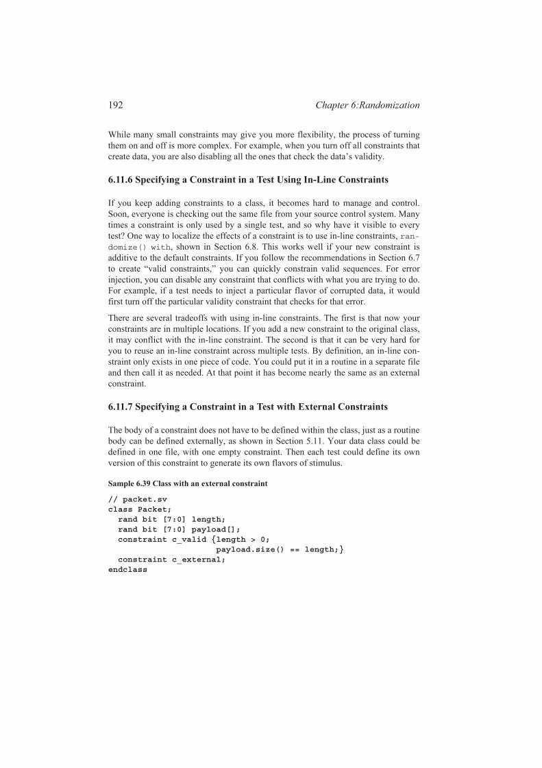
The body of a constraint does not have to be defined within the class, just as a routinebody can be defined externally, as shown in Section 5.11. Your data class could bedefined in one file, with one empty constraint. Then each test could define its ownversion of this constraint to generate its own flavors of stimulus.
Sample 6.39 Class with an external constraint
// packet.svclass Packet; rand bit [7:0] length; rand bit [7:0] payload[]; constraint c_valid {length > 0; payload.size() == length;} constraint c_external;endclass

Common Randomization Problems 193
Sample 6.40 Program defining an external constraint
// test.svprogram test; constraint Packet::c_external {length == 1;} ...endprogram
External constraints have several advantages over in-line constraints. They can be putin a file and thus reused between tests. An external constraint applies to all instancesof the class, whereas an in-line constraint only affects the single call to random-ize(). Consequently, an external constraint provides a primitive way to change aclass without having to learn advanced OOP techniques. Keep in mind that with thistechnique, you can only add constraints, not alter existing ones, and you need todefine the external constraint prototype in the original class.
Like in-line constraints, external constraints can cause problems, as the constraintsare spread across multiple files.
A final consideration is what happens when the body for an external constraint isnever defined. The SystemVerilog LRM does not currently specify what should hap-pen in this case. Before you build a testbench with many external constraints, find outhow your simulator handles missing definitions. Is this an error that prevents simula-tion, just a warning, or no message at all?
6.11.8 Extending a Class
In Chap. 8, you will learn how to extend a class. With this technique, you can take atestbench that uses a given class, and swap in an extended class that has additional orredefined constraints, routines, and variables. See Sample 8.10 for a typical testbench.Note that if you define a constraint in an extended class with the same name as one inthe base class, the extended constraint replaces the base one.
Learning OOP techniques requires a little more study, but the flexibility of this newapproach repays with great rewards.
6.12 Common Randomization Problems
You may be comfortable with procedural code, but writing constraints and under-standing random distributions requires a new way of thinking. Here are some issuesyou may encounter when trying to create random stimulus.
Chapter 6:Randomization194
6.12.1 Use Signed Variables with Care
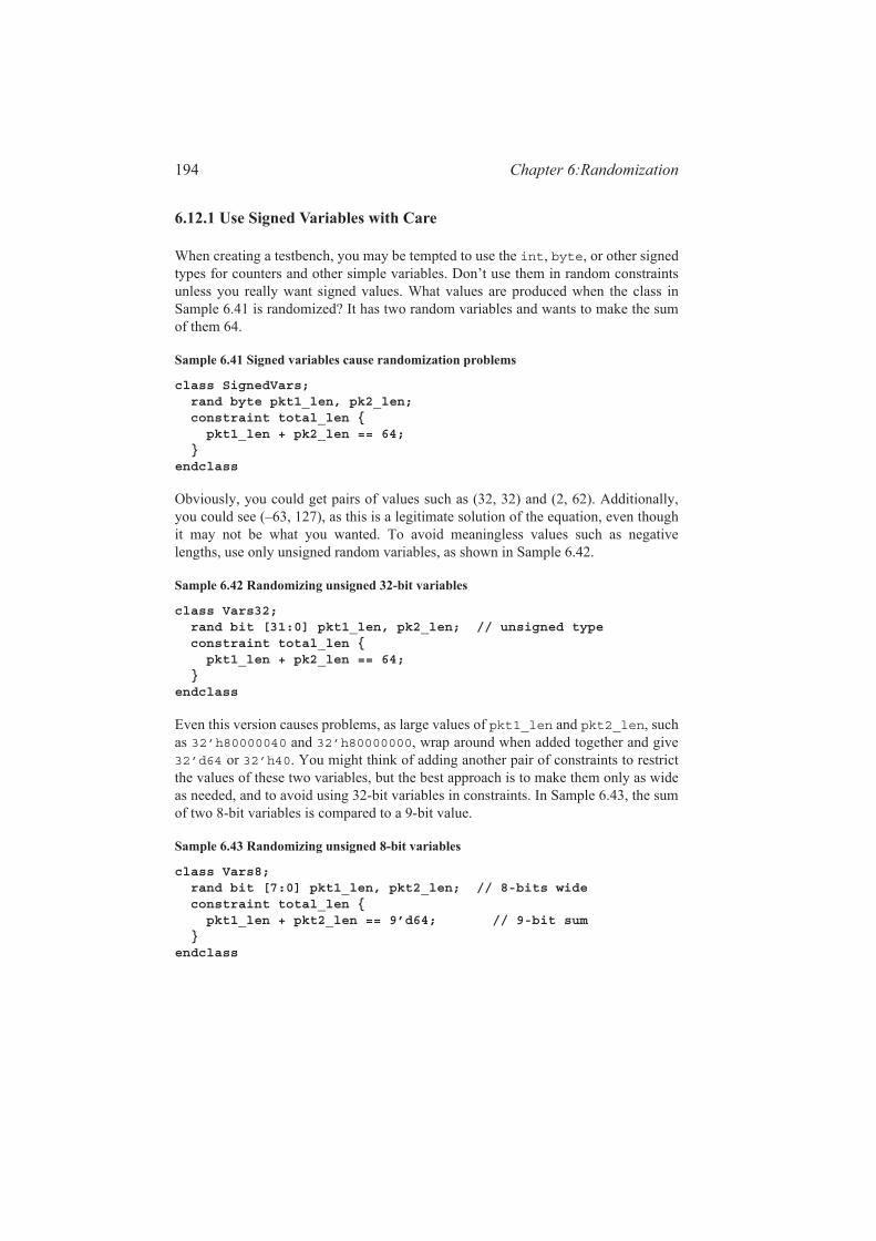
When creating a testbench, you may be tempted to use the int, byte, or other signedtypes for counters and other simple variables. Don’t use them in random constraintsunless you really want signed values. What values are produced when the class inSample 6.41 is randomized? It has two random variables and wants to make the sumof them 64.
Sample 6.41 Signed variables cause randomization problems
class SignedVars; rand byte pkt1_len, pk2_len; constraint total_len { pkt1_len + pk2_len == 64; }endclass
Obviously, you could get pairs of values such as (32, 32) and (2, 62). Additionally,you could see (–63, 127), as this is a legitimate solution of the equation, even thoughit may not be what you wanted. To avoid meaningless values such as negativelengths, use only unsigned random variables, as shown in Sample 6.42.
Sample 6.42 Randomizing unsigned 32-bit variables
class Vars32; rand bit [31:0] pkt1_len, pk2_len; // unsigned type constraint total_len { pkt1_len + pk2_len == 64; }endclass
Even this version causes problems, as large values of pkt1_len and pkt2_len, suchas 32’h80000040 and 32’h80000000, wrap around when added together and give32’d64 or 32’h40. You might think of adding another pair of constraints to restrictthe values of these two variables, but the best approach is to make them only as wideas needed, and to avoid using 32-bit variables in constraints. In Sample 6.43, the sumof two 8-bit variables is compared to a 9-bit value.
Sample 6.43 Randomizing unsigned 8-bit variables
class Vars8; rand bit [7:0] pkt1_len, pkt2_len; // 8-bits wide constraint total_len { pkt1_len + pkt2_len == 9’d64; // 9-bit sum }endclass
Iterative and Array Constraints 195
6.12.2 Solver Performance Tips
Each constraint solver has its strengths and weaknesses, but there are some guidelinesthat you can follow to improve the speed of your simulations with constrained ran-dom variables.
Avoid expensive operators such as division, multiplication, and modulus (%). If youneed to divide or multiply a variable by a power of 2, use the right and left shift oper-ators. A modulus operation with a power of 2 can be replaced with boolean AND witha mask. If you need to use one of these operators, you may get better performance ifyou can use variables less than 32-bits wide.
6.13 Iterative and Array Constraints
The constraints presented so far allow you to specify limits on scalar variables. Whatif you want to randomize an array? The foreach constraint and several array func-tions let you shape the distribution of the values.
Using the foreach constraint creates many constraints that canslow down simulation. A good solver can quickly solve hundredsof constraints but may slow down with thousands. Especially sloware nested foreach constraints, as they produce N 2 constraints foran array of size N. See Section 6.13.5 for an algorithm that usedrandc variables instead of nested foreach.
6.13.1 Array Size
The easiest array constraint to understand is the size() function. You are specifyingthe number of elements in a dynamic array or queue.
Sample 6.44 Constraining dynamic array size
class dyn_size; rand logic [31:0] d[]; constraint d_size {d.size() inside {[1:10]}; }endclass
Using the inside constraint lets you set a lower and upper boundary on the arraysize. In many cases you may not want an empty array, that is, size==0. Remember tospecify an upper limit; otherwise, you can end up with thousands or millions of ele-ments, which can cause the random solver to take an excessive amount of time.
Chapter 6:Randomization196
6.13.2 Sum of Elements
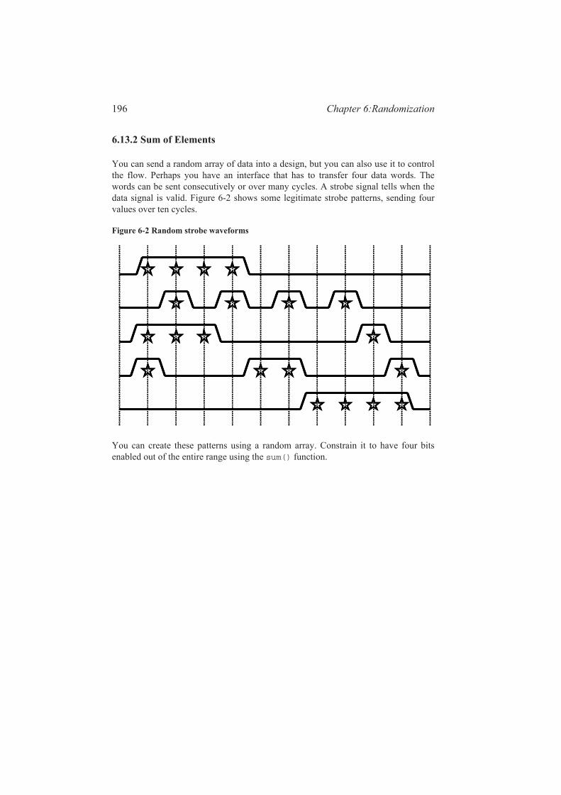
You can send a random array of data into a design, but you can also use it to controlthe flow. Perhaps you have an interface that has to transfer four data words. Thewords can be sent consecutively or over many cycles. A strobe signal tells when thedata signal is valid. Figure 6-2 shows some legitimate strobe patterns, sending fourvalues over ten cycles.
Figure 6-2 Random strobe waveforms
You can create these patterns using a random array. Constrain it to have four bitsenabled out of the entire range using the sum() function.

Iterative and Array Constraints 197
Sample 6.45 Random strobe pattern class
parameter MAX_TRANSFER_LEN = 10;
class StrobePat; rand bit strobe[MAX_TRANSFER_LEN]; constraint c_set_four { strobe.sum() == 4’h4; }endclass
initial begin StrobePat sp; int count = 0; // Index into data array
sp = new(); assert (sp.randomize());
foreach (sp.strobe[i]) begin @bus.cb; bus.cb.strobe <= sp.strobe[i]; // If strobe is enabled, drive out next data word if (sp.strobe[i]) bus.cb.data <= data[count++]; endend
As you remember from Chap. 2, the sum of an array of single-bit elements would nor-mally be a single bit, e.g., 0 or 1. Sample 6.45 compares strobe.sum() to a 4-bitvalue (4’h4), and so the sum is calculated with 4-bit precision. The example uses 4-bit precision to store the maximum number of elements, which is 10.
6.13.3 Issues with Array Constraints
The sum() function looks simple but can cause several problems because of Ver-ilog’s arithmetic rules. Start with a simple problem. You want to generate from one toeight transactions, such that the total length of all of them is less than 1,024 bytes.Sample 6.46 shows a first attempt. The len field is a byte in the original transaction.

Chapter 6:Randomization198
Sample 6.46 First attempt at sum constraint: bad_sum1
class bad_sum1; rand byte len[]; constraint c_len {len.sum < 1024; len.size() inside {[1:8]};} function void display(); $write("sum=%4d, val=", len.sum); foreach(len[i]) $write("%4d ", len[i]); $display; endfunctionendclass
Sample 6.47 Program to try constraint with array sum
program automatic test; bad_sum1 c; initial begin c = new(); repeat (10) begin assert (c.randomize()); c.display(); end endendprogram
Sample 6.48 Output from bad_sum1
sum= 81, val= 62 -20 39sum= 39, val= -27 67 1 76 -97 -58 77sum= 38, val= 60 -22sum= 72, val=-120 29 123 102 -41 -21sum= -53, val= -58 -85-115 112-101 -62
This generates some smaller lengths, but the sum is sometimes negative and is alwaysless than 127 – definitely not what you wanted! Try again, this time with an unsignedfield. (The display function is unchanged.)
Sample 6.49 Second attempt at sum constraint: bad_sum2
class bad_sum2; rand bit [7:0] len[]; // 8 bits constraint c_len {len.sum < 1024; len.size() inside {[1:8]};}endclass

Iterative and Array Constraints 199
Sample 6.50 Output from bad_sum2
sum= 79, val= 88 100 246 2 14 228 169sum= 120, val= 74 75 141 86sum= 39, val= 39sum= 193, val= 31 156 172 33 57sum= 173, val= 59 150 25 101 138 212
Sample 6.50 has a subtle problem: the sum of all transaction lengths is always lessthan 256, even though you constrained the array sum to be less than 1,024. The prob-lem here is that in Verilog, the sum of many 8-bit values is computed using an 8-bitresult. Bump the len field up to 32 bits using the uint type from Chap. 2.
Sample 6.51 Third attempt at sum constraint: bad_sum3
class bad_sum3; rand uint len[]; // 32 bits constraint c_len {len.sum < 1024; len.size() inside {[1:8]};}endclass
Sample 6.52 Output from bad_sum3
sum= 245, val=1348956995 3748256598 985546882 2507174362 sum= 600, val=2072193829 315191491 484497976 3050698208 2300168220 3988671456 3998079060 970369544 sum= 17, val=1924767007 3550820640 4149215303 3260098955 sum= 440, val=3192781444 624830067 1300652226 4072252356 3694386235 sum= 864, val=3561488468 733479692
Wow – what happened here? This is similar to the signed problem in Section 6.12.1,in that the sum of two very large numbers can wrap around to a small number. Youneed to limit the size based on the comparison in the constraint.
Sample 6.53 Fourth attempt at sum_constraint: bad_sum4
class bad_sum4; rand bit [9:0] len[]; // 10 bits constraint c_len {len.sum < 1024; len.size() inside {[1:8]};}endclass

Chapter 6:Randomization200
Sample 6.54 Output from bad_sum4
sum= 989, val= 787 202sum=1021, val= 564 76 132 235 0 8 6sum= 872, val= 624 101 136 11sum= 978, val= 890 88sum= 905, val= 663 242
This does not work either, as the individual len fields are more than 8 bits, and so thelen values are often greater than 255. You need to specify that each len field isbetween 1 and 255, but use a 10-bit field so that they sum correctly. This requiresconstraining every element of the array.
6.13.4 Constraining Individual Array and Queue Elements
SystemVerilog lets you constrain individual elements of an array using foreach.While you might be able to write constraints for a fixed-size array by listing everyelement, the foreach style is more compact. The only practical way to constrain adynamic array or queue is with foreach.
Sample 6.55 Simple foreach constraint: good_sum5
class good_sum5; rand uint len[]; constraint c_len {foreach (len[i]) len[i] inside {[1:255]}; len.sum < 1024; len.size() inside {[1:8]};}endclass
Sample 6.56 Output from good_sum5
sum=1011, val= 83 249 197 187 152 95 40 8sum=1012, val= 213 252 213 44 196 20 20 54sum= 370, val= 118 76 176sum= 976, val= 233 187 44 157 201 81 73sum= 412, val= 172 167 73
The addition of the constraint for individual elements fixed the example. Note that thelen array can be 10 or more bits wide, but must be unsigned.
You can specify constraints between array elements as long as you are careful aboutthe endpoints. The following class creates an ascending list of values by comparingeach element to the previous, except for the first.

Iterative and Array Constraints 201
Sample 6.57 Creating ascending array values with foreach
class Ascend; rand uint d[10]; constraint c { foreach (d[i]) // For every element if (i>0) // except the first d[i] > d[i-1]; // compare with previous element }endclass
How complex can these constraints become? Constraints have been written to solveEinstein’s problem (a logic puzzle with five people, each with five separateattributes), the Eight Queens problem (place eight queens on a chess board so thatnone can capture each other), and even Sudoku.
The 2005 LRM requires a foreach constraint to only have a simplearray name, not hierarchical reference. Thus you cannot use aforeach constraint in one class to constrain an array in subclass.
6.13.5 Generating an Array of Unique Values
How can you create an array of random unique values? If you try to make a randcarray, each array element will be randomized independently, and so you are almostcertain to get repeated values.
You may be tempted to use a constraint solver to compare every element with everyother with nested foreach-loops as shown in Sample 6.58. This creates over 4,000individual constraints, which could slow down simulation.
Sample 6.58 Creating unique array values with foreach
class UniqueSlow; rand bit [7:0] ua[64]; constraint c { foreach (ua[i]) // For every element foreach (ua[j]) if (i != j) // except the diagonals ua[i] != ua[j]; // compare to other elements }endclass
Instead, you should use procedural code with a helper class containing a randc vari-able so that you can randomize the same variable over and over.

Chapter 6:Randomization202
Sample 6.59 Creating unique array values with a randc helper class
class randc8; randc bit [7:0] val;endclass
class LittleUniqueArray; bit [7:0] ua [64]; // Array of unique values
function void pre_randomize; randc8 rc8; rc8 = new(); foreach (ua[i]) begin assert(rc8.randomize()); ua[i] = rc8.val; end endfunctionendclass
Next is a more general solution. For example, you may need to assign ID numbers toN bus drivers, which are in the range of 0 to MAX-1 where MAX >=N.
Sample 6.60 Unique value generator
// Create unique random values in a range 0:max-1class RandcRange; randc bit [15:0] value; int max_value; // Maximum possible value
function new(int max_value = 10); this.max_value = max_value; endfunction
constraint c_max_value {value < max_value;}endclass

Iterative and Array Constraints 203
Sample 6.61 Class to generate a random array of unique values
class UniqueArray; int max_array_size, max_value; rand bit [7:0] a[]; // Array of unique values constraint c_size {a.size() inside {[1:max_array_size]};}
function new(int max_array_size=2, max_value=2); this.max_array_size = max_array_size; // If max_value is smaller than array size, // array could have duplicates, so adjust max_value if (max_value < max_array_size) this.max_value = max_array_size; else this.max_value = max_value; endfunction
// Array a[] allocated in randomize(), fill w/unique vals function void post_randomize; RandcRange rr; rr = new(max_value); foreach (a[i]) begin assert (rr.randomize()); a[i] = rr.value; end endfunction
function void display(); $write("Size: %3d:", a.size()); foreach (a[i]) $write("%4d", a[i]); $display; endfunctionendclass
Here is a program that uses the UniqueArray class.
Sample 6.62 Using the UniqueArray class
program automatic test; UniqueArray ua; initial begin ua = new(50); // Array size = 50
repeat (10) begin assert(ua.randomize()); // Create random array ua.display(); // Display values end endendprogram

Chapter 6:Randomization204
6.13.6 Randomizing an Array of Handles
If you need to create multiple random objects, you might create a random array ofhandles. Unlike an array of integers, you need to allocate all the elements before ran-domization as the random solver never constructs objects. If you have a dynamicarray, allocate the maximum number of elements you may need, and then use a con-straint to resize the array. A dynamic array of handles can remain the same size orshrink during randomization, but it can never increase in size.
Sample 6.63 Constructing elements in a random array
parameter MAX_SIZE = 10;
class RandStuff; rand int value;endclass
class RandArray; rand RandStuff array[]; // Don’t forget rand!
constraint c {array.size() inside {[1:MAX_SIZE]}; }
function new(); array = new[MAX_SIZE]; // Allocate maximum size foreach (array[i]) array[i] = new(); endfunction;endclass
RandArray ra;initial begin ra = new(); // Construct array and all objects assert(ra.randomize()); // Randomize and maybe shrink array foreach (ra.array[i]) $display(ra.array[i].value);end
See Section 5.14.4 for more on arrays of handles.
6.14 Atomic Stimulus Generation vs. Scenario Generation
Up until now, you have seen atomic random transactions. You have learned how tomake a single random bus transaction, a single network packet, or a single processorinstruction. This is a good start; however, your job is to verify that the design workswith real-world stimuli. A bus may have long sequences of transactions such as DMAtransfers or cache fills. Network traffic consists of extended sequences of packets as
Atomic Stimulus Generation vs. Scenario Generation 205
you simultaneously read e-mail, browse a web page, and download music from thenet, all in parallel. Processors have deep pipelines that are filled with the code for rou-tine calls, for-loops, and interrupt handlers. Generating transactions one at a time isunlikely to mimic any of these scenarios.
6.14.1 An Atomic Generator with History
The easiest way to create a stream of related transactions is to have an atomic genera-tor base some of its random values on ones from previous transactions. The classmight constrain a bus transaction to repeat the previous command, such as a write,80% of the time, and also use the previous destination address plus an increment. Youcan use the post_randomize function to make a copy of the generated transactionfor use by the next call to randomize().
This scheme works well for smaller cases but gets into trouble when you need infor-mation about the entire sequence ahead of time. For example, the DUT may need toknow the length of a sequence of network transactions before it starts.
6.14.2 Randsequence
The next way to generate a sequence of transactions is by using the randsequenceconstruct in SystemVerilog. With randsequence, you describe the grammar of thetransaction, using a syntax similar to BNF (Backus-Naur Form).
Sample 6.64 Command generator using randsequence
initial begin for (int i=0; i<15; i++) begin randsequence (stream) stream : cfg_read := 1 | io_read := 2 | mem_read := 5; cfg_read : { cfg_read_task; } | { cfg_read_task; } cfg_read; mem_read : { mem_read_task; } | { mem_read_task; } mem_read; io_read : { io_read_task; } | { io_read_task; } io_read; endsequence end // forend
task cfg_read_task; ...endtask

Chapter 6:Randomization206
Sample 6.64 generates a sequence called stream. A stream can be eithercfg_read, io_read, or mem_read. The random sequence engine randomly picksone. The cfg_read label has a weight of 1, io_read has twice the weight and so istwice as likely to be chosen as cfg_read. The label mem_read is most likely to bechosen, with a weight of 5.
A cfg_read can be either a single call to the cfg_read_task, or a call to the taskfollowed by another cfg_read. As a result, the task is always called at least once,and possibly many times.
One big advantage of randsequence is that it is procedural code and you can debugit by stepping though the execution, or adding $display statements. When you callrandomize() for an object, it either all works or all fails, but you can’t see the stepstaken to get to a result.
There are several problems with using randsequence. The code to generate thesequence is separate and a very different style from the classes with data and con-straints used by the sequence. So if you use both randomize() and randsequence,you have to master two different forms of randomization. More seriously, if you wantto modify a sequence, perhaps to add a new branch or action, you have to modify theoriginal sequence code. You can’t just make an extension. As you will see in Chap. 8,you can extend a class to add new code, data, and constraints without having to editthe original class.
6.14.3 Random Array of Objects
The last form of generating random sequences is to randomize an entire array ofobjects. You can create constraints that refer to the previous and next objects in thearray, and the SystemVerilog solver solves all constraints simultaneously. Since theentire sequence is generated at once, you can then extract information such as thetotal number of transactions or a checksum of all data values before the first transac-tion is sent. Alternatively, you can build a sequence for a DMA transfer that isconstrained to be exactly 1,024 bytes, and let the solver pick the right number oftransactions to reach that goal.
6.14.4 Combining Sequences
You can combine multiple sequences together to make a more realistic flow of trans-actions. For example, for a network device, you could make one sequence thatresembles downloading e-mail, a second that is viewing a web page, and a third that isentering single characters into web-based form.The techniques to combine theseflows is beyond the scope of this book, but you can learn more from the VMM, asdescribed in Bergeron et al. (2005).

Random Control 207
6.15 Random Control
At this point you may be thinking that this process is a great way to create longstreams of random input into your design. Or you may think that this is a lot of workif all you want to do is occasionally to make a random decision in your code. Youmay prefer a set of procedural statements that you can step through using a debugger.
6.15.1 Introduction to randcase
You can use randcase to make a weighted choice between several actions, withouthaving to create a class and instance. Sample 6.65 chooses one of the three branchesbased on the weight. SystemVerilog adds up the weights (1+8+1 = 10), chooses avalue in this range, and then picks the appropriate branch. The branches are not orderdependent, the weights can be variables, and they do not have to add up to 100%.
Sample 6.65 Random control with randcase and $urandom_range
initial begin int len; randcase 1: len = $urandom_range(0, 2); // 10%: 0, 1, or 2 8: len = $urandom_range(3, 5); // 80%: 3, 4, or 5 1: len = $urandom_range(6, 7); // 10%: 6 or 7 endcase $display("len=%0d", len); end
The $urandom_range function returns a random number in the specified range. Youcan specify the arguments as (low, high) or (high, low). If you use just a single argu-ment, SystemVerilog treats it as (0, high).
You can write Sample 6.65 using a class and the randomize() function. For thissmall case, the OOP version is a little larger. However, if this were part of a largerclass, the constraint would be more compact than the equivalent randcasestatement.
Chapter 6:Randomization208
Sample 6.66 Equivalent constrained class
class LenDist; rand int len; constraint c {len dist {[0:2] := 1, [3:5] := 8, [6:7] := 1}; }endclass
LenDist lenD;
initial begin lenD = new(); assert (lenD.randomize()); $display("Chose len=%0d", lenD.len); end
Code using randcase is more difficult to override and modify than random con-straints. The only way to modify the random results is to rewrite the code or usevariable weights.
Be careful using randcase, as it does not leave any tracks behind. For example, youcould use it to decide whether or not to inject an error in a transaction. The problem isthat the downstream transactors and scoreboard need to know of this choice. The bestway to inform them would be to use a variable in the transaction or environment.However, if you are going to create a variable that is part of these classes, you couldhave made it a random variable and used constraints to change its behavior in differ-ent tests.
6.15.2 Building a Decision Tree with randcase
You can use randcase when you need to create a decision tree. Sample 6.67 has justtwo levels of procedural code, but you can see how it can be extended to use more.

Random Number Generators 209
Sample 6.67 Creating a decision tree with randcase
initial begin // Level 1 randcase one_write_wt: do_one_write(); one_read_wt: do_one_read(); seq_write_wt: do_seq_write(); seq_read_wt: do_seq_read(); endcase end
// Level 2task do_one_write; randcase mem_write_wt: do_mem_write(); io_write_wt: do_io_write(); cfg_write_wt: do_cfg_write(); endcaseendtask
task do_one_read; randcase mem_read_wt: do_mem_read(); io_read_wt: do_io_read(); cfg_read_wt: do_cfg_read(); endcaseendtask
6.16 Random Number Generators
How random is SystemVerilog? On the one hand, your testbench depends on anuncorrelated stream of random values to create stimulus patterns that go beyond anydirected test. On the other hand, you need to repeat the patterns over and over duringdebug of a particular test, even if the design and testbench make minor changes.
6.16.1 Pseudorandom Number Generators
Verilog uses a simple PRNG that you could access with the $random function. Thegenerator has an internal state that you can set by providing a seed to $random. AllIEEE-1364-compliant Verilog simulators use the same algorithm to calculate values.
Sample 6.68 shows a simple PRNG, not the one used by SystemVerilog. The PRNGhas a 32-bit state. To calculate the next random value, square the state to produce a64-bit value, take the middle 32 bits, then add the original value.

Chapter 6:Randomization210
Sample 6.68 Simple pseudorandom number generator
reg [31:0] state = 32’h12345678;function logic [31:0] my_random; logic [63:0] s64; s64 = state * state; state = (s64 >> 16) + state; my_random = state;endfunction
You can see how this simple code produces a stream of values that seem random, butcan be repeated by using the same seed value. SystemVerilog calls its PRNG to gen-erate a new value for randomize() and randcase.
6.16.2 Random Stability – Multiple Generators
Verilog has a single PRNG that is used for the entire simulation. What would happenif SystemVerilog kept this approach? Testbenches often have several stimulus gener-ators running in parallel, creating data for the design under test. If two streams sharethe same PRNG, they each get a subset of the random values.
Figure 6-3 Sharing a single random generator
In Figure 6-3, there are two stimulus generators and a single PRNG producing valuesa, b, c, etc. Gen2 has two random objects, and so during every cycle, it uses twice asmany random values as Gen1. A problem can occur when one of the classes changes.Gen1 gets an additional random variable, and so consumes two random values everytime it is called.
class Gen1;Transaction tr;
forever @(int1.cb)tr.randomize()
endclass
class Gen2;Transaction tr1, tr2;
forever @(int2.cb)tr1.randomize();tr2.randomize();endclass
adg
b,ce,fh,i
PRNG
class Gen1;Transaction tr;
forever @(int1.cb)tr.randomize()
endclass
class Gen2;Transaction tr1, tr2;
forever @(int2.cb)tr1.randomize();tr2.randomize();endclass
adg
b,ce,fh,i
PRNG
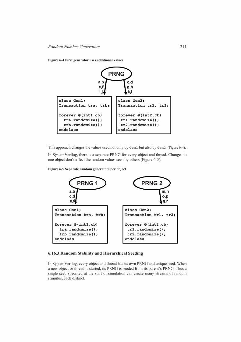
Random Number Generators 211
Figure 6-4 First generator uses additional values
This approach changes the values used not only by Gen1 but also by Gen2 (Figure 6-4).
In SystemVerilog, there is a separate PRNG for every object and thread. Changes toone object don’t affect the random values seen by others (Figure 6-5).
Figure 6-5 Separate random generators per object
6.16.3 Random Stability and Hierarchical Seeding
In SystemVerilog, every object and thread has its own PRNG and unique seed. Whena new object or thread is started, its PRNG is seeded from its parent’s PRNG. Thus asingle seed specified at the start of simulation can create many streams of randomstimulus, each distinct.
class Gen1;Transaction tra, trb;
forever @(int1.cb)tra.randomize();trb.randomize();
endclass
class Gen2;Transaction tr1, tr2;
forever @(int2.cb)tr1.randomize();tr2.randomize();
endclass
a,be,fi,j
c,dg,hk,l
PRNG
class Gen1;Transaction tra, trb;
forever @(int1.cb)tra.randomize();trb.randomize();
endclass
class Gen2;Transaction tr1, tr2;
forever @(int2.cb)tr1.randomize();tr2.randomize();
endclass
a,be,fi,j
c,dg,hk,l
PRNG
class Gen1;Transaction tra, trb;
forever @(int1.cb)tra.randomize();trb.randomize();
endclass
class Gen2;Transaction tr1, tr2;
forever @(int2.cb)tr1.randomize();tr2.randomize();
endclass
a,bc,de,f
m,no,pq,r
PRNG 1 PRNG 2
class Gen1;Transaction tra, trb;
forever @(int1.cb)tra.randomize();trb.randomize();
endclass
class Gen2;Transaction tr1, tr2;
forever @(int2.cb)tr1.randomize();tr2.randomize();
endclass
a,bc,de,f
m,no,pq,r
PRNG 1 PRNG 2

Chapter 6:Randomization212
When you are debugging a testbench, you add, delete, and move code. Even with ran-dom stability, your changes may cause the testbench to generate different randomvalues. This can be very frustrating if you are in the middle of debugging a DUT fail-ure, and the testbench no longer creates the same stimulus. You can minimize theeffect of code modifications by adding any new objects or threads after existing ones.Sample 6.69 shows a routine from testbench that constructs objects, and runs them inparallel threads.
Sample 6.69 Test code before modification
function void build(); pci_gen gen0, gen1; gen0 = new(); gen1 = new(); fork gen0.run(); gen1.run(); joinendfunction : build
Sample 6.70 adds a new generator, and runs it in a new thread. The new object is con-structed after the existing ones, and the new thread is spawned after the old ones.
Sample 6.70 Test code after modification
function void build(); pci_gen gen0, gen1; atm_gen agen; // New ATM generator gen0 = new(); gen1 = new(); new_gen = new(); // Construct new object after old ones
fork gen0.run(); gen1.run(); new_gen.run(); // Spawn new thread after old ones joinendfunction : build
Of course as new code is added, you may not be able to keep the random streams thesame as the old ones, but you might be able to postpone the undesirable side effectsfrom these changes.
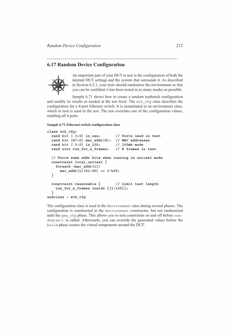
Random Device Configuration 213
6.17 Random Device Configuration
An important part of your DUT to test is the configuration of both theinternal DUT settings and the system that surrounds it. As describedin Section 6.2.1, your tests should randomize the environment so thatyou can be confident it has been tested in as many modes as possible.
Sample 6.71 shows how to create a random testbench configurationand modify its results as needed at the test level. The eth_cfg class describes theconfiguration for a 4-port Ethernet switch. It is instantiated in an environment class,which in turn is used in the test. The test overrides one of the configuration values,enabling all 4 ports.
Sample 6.71 Ethernet switch configuration class
class eth_cfg; rand bit [ 3:0] in_use; // Ports used in test rand bit [47:0] mac_addr[4]; // MAC addresses rand bit [ 3:0] is_100; // 100mb mode rand uint run_for_n_frames; // # frames in test
// Force some addr bits when running in unicast mode constraint local_unicast { foreach (mac_addr[i]) mac_addr[i][41:40] == 2’b00; }
constraint reasonable { // Limit test length run_for_n_frames inside {[1:100]}; }endclass : eth_cfg
The configuration class is used in the Environment class during several phases. Theconfiguration is constructed in the Environment constructor, but not randomizeduntil the gen_cfg phase. This allows you to turn constraints on and off before ran-domize() is called. Afterwards, you can override the generated values before thebuild phase creates the virtual components around the DUT.
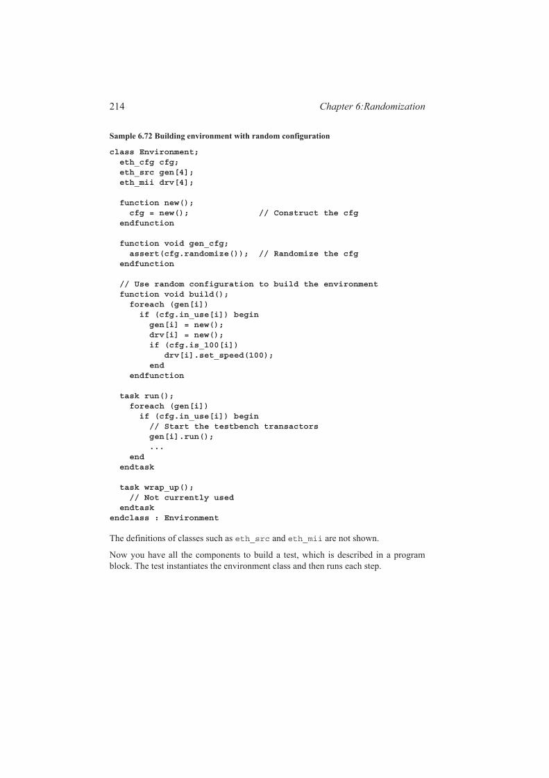
Chapter 6:Randomization214
Sample 6.72 Building environment with random configuration
class Environment; eth_cfg cfg; eth_src gen[4]; eth_mii drv[4];
function new(); cfg = new(); // Construct the cfg endfunction
function void gen_cfg; assert(cfg.randomize()); // Randomize the cfg endfunction
// Use random configuration to build the environment function void build(); foreach (gen[i]) if (cfg.in_use[i]) begin gen[i] = new(); drv[i] = new(); if (cfg.is_100[i]) drv[i].set_speed(100); end endfunction
task run(); foreach (gen[i]) if (cfg.in_use[i]) begin // Start the testbench transactors gen[i].run(); ... end endtask
task wrap_up(); // Not currently used endtaskendclass : Environment
The definitions of classes such as eth_src and eth_mii are not shown.
Now you have all the components to build a test, which is described in a programblock. The test instantiates the environment class and then runs each step.

Random Device Configuration 215
Sample 6.73 Simple test using random configuration
program test; Environment env;
initial begin env = new(); // Construct environment env.gen_cfg; // Create random configuration env.build(); // Build the testbench environment env.run(); // Run the test env.wrap_up(); // Clean up after test & report endendprogram
You may want to override the random configuration, perhaps to reach a corner case.The following test randomizes the configuration class and then enables all the ports.
Sample 6.74 Simple test that overrides random configuration
program test; Environment env;
initial begin env = new(); // Construct environment env.gen_cfg; // Create random configuration
// Override random in-use – turn all 4 ports on env.cfg.in_use = 4’b1111;
env.build(); // Build the testbench environment env.run(); // Run the test env.wrap_up(); // Clean up after test & report endendprogram
Notice how in Sample 6.72 all generators were constructed, butonly a few were run, depending on the random configuration. If youonly constructed the generators that are in use, you would have tosurround any reference to gen[i] with a test of in_use[i], other-
wise your testbench would crash when it tried to refer to the nonexistent generator.The extra memory taken up by these generators that are not used is a small price topay for a more stable testbench.

Chapter 6:Randomization216
6.18 Conclusion
CRTs are the only practical way to generate the stimulus needed to verify a complexdesign. SystemVerilog offers many ways to create a random stimulus and this chapterpresents many of the alternatives.
A test needs to be flexible, allowing you either to use the values generated by defaultor to constrain or override the values so that you can reach your goals. Always planahead when creating your testbench by leaving sufficient “hooks” so that you cansteer the testbench from the test without modifying existing code.