SOLUTIONS ABOUT ORDINARY POINTS 6.1 - SU LMS

SOLUTIONS ABOUT ORDINARY POINTS

REVIEW MATERIAL● Power Series (see any Calculus Text)

INTRODUCTION In Section 4.3 we saw that solving a homogeneous linear DE with constantcoefficients was essentially a problem in algebra. By finding the roots of the auxiliary equation,we could write a general solution of the DE as a linear combination of the elementary functionsxk, xke�x, xke�x cos �x, and xke�xsin �x, where k is a nonnegative integer. But as was pointed outin the introduction to Section 4.7, most linear higher-order DEs with variable coefficients cannotbe solved in terms of elementary functions. A usual course of action for equations of this sort isto assume a solution in the form of infinite series and proceed in a manner similar to the methodof undetermined coefficients (Section 4.4). In this section we consider linear second-order DEswith variable coefficients that possess solutions in the form of power series.

We begin with a brief review of some of the important facts about power series. For a morecomprehensive treatment of the subject you should consult a calculus text.

220 ● CHAPTER 6 SERIES SOLUTIONS OF LINEAR EQUATIONS

6.1

6.1.1 REVIEW OF POWER SERIES

Recall from calculus that a power series in x � a is an infinite series of the form

Such a series is also said to be a power series centered at a. For example, the powerseries is centered at a � �1. In this section we are concernedmainly with power series in x, in other words, power series such as

that are centered at a � 0. The following listsummarizes some important facts about power series.

• Convergence A power series is convergent at aspecified value of x if its sequence of partial sums {SN(x)} converges—that is,

exists. If the limit does not exist at x,

then the series is said to be divergent.• Interval of Convergence Every power series has an interval of convergence.

The interval of convergence is the set of all real numbers x for which the seriesconverges.

• Radius of Convergence Every power series has a radius of convergence R.If R � 0, then the power series converges forand diverges for If the series converges only at its center a,then R � 0. If the series converges for all x, then we write R � . Recall thatthe absolute-value inequality is equivalent to the simultaneousinequality a � R � x � a � R. A power series might or might not convergeat the endpoints a � R and a � R of this interval.

• Absolute Convergence Within its interval of convergence a power seriesconverges absolutely. In other words, if x is a number in the interval ofconvergence and is not an endpoint of the interval, then the series ofabsolute values converges. See Figure 6.1.1.

• Ratio Test Convergence of a power series can often be determined by theratio test. Suppose that cn � 0 for all n and that

limn: � cn�1(x � a)n�1

cn(x � a)n �� x � a � limn: �cn�1

cn� � L.

�n�0 � cn(x � a)n �

� x � a � � R

� x � a � � R.� x � a � � R�

n�0 cn(x � a)n

limN :

SN (x) � limN :

�Nn�0 cn(x � a)n

�n�0 cn(x � a)n

�n�1 2n�1xn � x � 2x2 � 4x3 �

�n�0 (x � 1)n

�

n�0cn(x � a)n � c0 � c1(x � a) � c2(x � a)2 � .

xa a + Ra − R

divergence divergence absolute

convergence

series mayconverge or diverge

at endpoints

FIGURE 6.1.1 Absolute convergencewithin the interval of convergence anddivergence outside of this interval

If L � 1, the series converges absolutely; if L � 1, the series diverges;and if L � 1, the test is inconclusive. For example, for the power series

the ratio test gives

the series converges absolutely for or or1 � x � 5. This last inequality defines the open interval of convergence.The series diverges for , that is, for x � 5 or x � 1. At the leftendpoint x � 1 of the open interval of convergence, the series of constants

is convergent by the alternating series test. At the rightendpoint x � 5, the series is the divergent harmonic series. Theinterval of convergence of the series is [1, 5), and the radius of convergenceis R � 2.

• A Power Series Defines a Function A power series defines a functionwhose domain is the interval of convergence of

the series. If the radius of convergence is R � 0, then f is continuous, differ-entiable, and integrable on the interval (a � R, a � R). Moreover, f�(x)and f (x)dx can be found by term-by-term differentiation and integration.Convergence at an endpoint may be either lost by differentiation orgained through integration. If is a power series in x, thenthe first two derivatives are andNotice that the first term in the first derivative and the first two terms in thesecond derivative are zero. We omit these zero terms and write

(1)

These results are important and will be used shortly.• Identity Property If for all numbers x in the

interval of convergence, then cn � 0 for all n.• Analytic at a Point A function f is analytic at a point a if it can be

represented by a power series in x � a with a positive or infinite radiusof convergence. In calculus it is seen that functions such as ex, cos x, sin x,ln(1 � x), and so on can be represented by Taylor series. Recall, forexample, that

�n�0 cn(x � a)n � 0, R � 0

y� � �

n�1cnnxn�1 and y � �

n�2cnn(n � 1)xn�2.

y � �n�0 n(n � 1)xn�2.y� � �

n�0 nxn�1y � �

n�0 cnxn

f (x) � �n�0 cn(x � a)n

� n�1 (1>n)

�n�1 ((�1)n>n)

� x � 3 � � 2

� x � 3 � � 212 � x � 3 � � 1

limn: � (x � 3)n�1

2n�1(n � 1)

(x � 3)n

2nn� � � x � 3 � lim

n:

n

2(n � 1)�

1

2� x � 3 �;

�n�1(x � 3)n>2nn

6.1 SOLUTIONS ABOUT ORDINARY POINTS ● 221

(2)ex � 1 �x

1!�

x2

2!� . . ., sin x � x �

x3

3!�

x5

5!� . . ., cos x � 1 �

x2

2!�

x4

4!�

x6

6!� . . .

for These Taylor series centered at 0, called Maclaurin series,show that ex, sin x, and cos x are analytic at x � 0.

• Arithmetic of Power Series Power series can be combined through theoperations of addition, multiplication, and division. The procedures forpower series are similar to those by which two polynomials are added,multiplied, and divided—that is, we add coefficients of like powers of x,use the distributive law and collect like terms, and perform long division.For example, using the series in (2), we have

� x � � .

� x � x2 �x3

3�

x5

30� .

� (1)x � (1)x2 � ��1

6�

1

2�x3 � ��1

6�

1

6�x4 � � 1

120�

1

12�

1

24�x5 �

exsin x � �1 � x �x2

2�

x3

6�

x4

24� ��x �

x3

6�

x5

120�

x7

5040� �

EXAMPLE 1 Adding Two Power Series

Write as a single power series whose generalterm involves xk.

SOLUTION To add the two series, it is necessary that both summation indices startwith the same number and that the powers of x in each series be “in phase”; that is, ifone series starts with a multiple of, say, x to the first power, then we want the otherseries to start with the same power. Note that in the given problem the first seriesstarts with x0, whereas the second series starts with x1. By writing the first term of thefirst series outside the summation notation,

we see that both series on the right-hand side start with the same power of x—namely,x1. Now to get the same summation index, we are inspired by the exponents of x; we letk � n � 2 in the first series and at the same time let k � n � 1 in the second series. Theright-hand side becomes

(3)

Remember that the summation index is a “dummy” variable; the fact that k � n � 1in one case and k � n � 1 in the other should cause no confusion if you keep inmind that it is the value of the summation index that is important. In both casesk takes on the same successive values k � 1, 2, 3, . . . when n takes on the valuesn � 2, 3, 4, . . . for k � n � 1 and n � 0, 1, 2, . . . for k � n � 1. We are now in aposition to add the series in (3) term by term:

(4)

If you are not convinced of the result in (4), then write out a few terms on bothsides of the equality.

�

n�2n(n�1)cnxn�2 � �

n�0cnxn�1 � 2c2 � �

k�1[(k � 2)(k � 1)ck�2 � ck�1]xk.

same

same

2c2 � � (k � 2)(k � 1)ck�2xk � � ck�1xk.k�1

k�1

series startswith xfor n � 3

series startswith xfor n � 0

� n(n � 1)cnxn�2 � � cnxn�1 � 2 1c2x 0 � � n(n � 1)cnxn�2 � � cnxn�1,n�2

n�0

n�3

n�0

�n�2 n(n � 1)cnxn�2 � �

n�0 cnxn�1


Since the power series for ex and sin x converge for the productseries converges on the same interval. Problems involving multipli-cation or division of power series can be done with minimal fuss by using aCAS.

SHIFTING THE SUMMATION INDEX For the remainder of this section, as wellas this chapter, it is important that you become adept at simplifying the sum of twoor more power series, each expressed in summation (sigma) notation, to anexpression with a single As the next example illustrates, combining two or moresummations as a single summation often requires a reindexing—that is, a shift in theindex of summation.

�.

� x � � ,

6.1.2 POWER SERIES SOLUTIONS

A DEFINITION Suppose the linear second-order differential equation

(5)

is put into standard form

(6)

by dividing by the leading coefficient a2(x). We have the following definition.

DEFINITION 6.1.1 Ordinary and Singular Points

A point x0 is said to be an ordinary point of the differential equation (5) ifboth P(x) and Q(x) in the standard form (6) are analytic at x0. A point that isnot an ordinary point is said to be a singular point of the equation.

Every finite value of x is an ordinary point of the differential equationy � (ex)y� � (sin x)y � 0. In particular, x � 0 is an ordinary point because, as wehave already seen in (2), both ex and sin x are analytic at this point. The negation in thesecond sentence of Definition 6.1.1 stipulates that if at least one of the functions P(x)and Q(x) in (6) fails to be analytic at x0, then x0 is a singular point. Note that x � 0 is asingular point of the differential equation y � (ex)y� � (ln x)y � 0 because Q(x) � ln xis discontinuous at x � 0 and so cannot be represented by a power series in x.

POLYNOMIAL COEFFICIENTS We shall be interested primarily in the case when(5) has polynomial coefficients. A polynomial is analytic at any value x, and a ratio-nal function is analytic except at points where its denominator is zero. Thus if a2(x),a1(x), and a0(x) are polynomials with no common factors, then both rational functionsP(x) � a1(x)�a2(x) and Q(x) � a0(x)�a2(x) are analytic except where a2(x) � 0. Itfollows, then, that:

x � x0 is an ordinary point of (5) if a2(x0) � 0 whereas x � x0 is a singular pointof (5) if a2(x0) � 0.

For example, the only singular points of the equation (x2 � 1)y � 2xy� � 6y � 0 aresolutions of x2 � 1 � 0 or x � �1. All other finite values* of x are ordinary points.Inspection of the Cauchy-Euler equation ax2y � bxy� � cy � 0 shows that it hasa singular point at x � 0. Singular points need not be real numbers. The equation(x2 � 1)y � xy� � y � 0 has singular points at the solutions of x2 � 1 � 0—namely,x � �i. All other values of x, real or complex, are ordinary points.

We state the following theorem about the existence of power series solutionswithout proof.

THEOREM 6.1.1 Existence of Power Series Solutions

If x � x0 is an ordinary point of the differential equation (5), we can always findtwo linearly independent solutions in the form of a power series centered at x0 ,that is, . A series solution converges at least on someinterval defined by where R is the distance from x0 to the closestsingular point.

� x � x0 � � R,y � �

n�0 cn(x � x0)n

y � P(x)y� � Q(x)y � 0

a2(x)y � a1(x)y� � a0(x)y � 0


*For our purposes, ordinary points and singular points will always be finite points. It is possible for anODE to have, say, a singular point at infinity.

A solution of the form is said to be a solution about theordinary point x0. The distance R in Theorem 6.1.1 is the minimum value or thelower bound for the radius of convergence of series solutions of the differential equa-tion about x0.

In the next example we use the fact that in the complex plane the distancebetween two complex numbers a � bi and c � di is just the distance between the twopoints (a, b) and (c, d ).

EXAMPLE 2 Lower Bound for Radius of Convergence

The complex numbers 1 � 2i are singular points of the differential equation(x2 � 2x � 5)y � xy� � y � 0. Because x � 0 is an ordinary point of the equation,Theorem 6.1.1 guarantees that we can find two power series solutions about 0, that is,solutions that look like Without actually finding these solutions, weknow that each series must converge at least for because is thedistance in the complex plane from 0 (the point (0, 0)) to either of the numbers 1 � 2i(the point (1, 2)) or 1 � 2i (the point (1, �2)). However, one of these two solutions isvalid on an interval much larger than in actual fact this solutionis valid on (�, ) because it can be shown that one of the two power series solutionsabout 0 reduces to a polynomial. Therefore we also say that is the lower bound forthe radius of convergence of series solutions of the differential equation about 0.

If we seek solutions of the given DE about a different ordinary point, say, x � �1,then each series converges at least for becausethe distance from �1 to either 1 � 2i or 1 � 2i is

NOTE In the examples that follow, as well as in Exercises 6.1, we shall, for thesake of simplicity, find power series solutions only about the ordinary point x � 0. Ifit is necessary to find a power series solution of a linear DE about an ordinary pointx0 � 0, we can simply make the change of variable t � x � x0 in the equation (thistranslates x � x0 to t � 0), find solutions of the new equation of the form

and then resubstitute t � x � x0.

FINDING A POWER SERIES SOLUTION The actual determination of a powerseries solution of a homogeneous linear second-order DE is quite analogous to whatwe did in Section 4.4 in finding particular solutions of nonhomogeneous DEs by themethod of undetermined coefficients. Indeed, the power series method of solving alinear DE with variable coefficients is often described as “the method of undeterminedseries coefficients.” In brief, here is the idea: We substitute into thedifferential equation, combine series as we did in Example 1, and then equate all coef-ficients to the right-hand side of the equation to determine the coefficients cn. Butbecause the right-hand side is zero, the last step requires, by the identity property in thepreceding bulleted list, that all coefficients of x must be equated to zero. No, this doesnot mean that all coefficients are zero; this would not make sense—after all, Theorem6.1.1 guarantees that we can find two solutions. Example 3 illustrates how the singleassumption that leads to two sets ofcoefficients, so we have two distinct power series y1(x) and y2(x), both expandedabout the ordinary point x � 0. The general solution of the differential equation isy � C1y1(x) � C2y2(x); indeed, it can be shown that C1 � c0 and C2 � c1.

EXAMPLE 3 Power Series Solutions

Solve y � xy � 0.

SOLUTION Since there are no finite singular points, Theorem 6.1.1 guaranteestwo power series solutions centered at 0, convergent for Substituting� x � � .

y � �n�0 cnxn � c0 � c1x � c2x2 �

y � �n�0 cnxn

y � �n�0 cnt n,

R � 18 � 212.� x � � 212y � �

n�0 cn(x � 1)n

15

�15 � x � 15;

R � 15� x � � 15y � �

n�0 cnxn.

y � �n�0 cn(x � x0)n


and the second derivative (see (1)) intothe differential equation gives

(7)

In Example 1 we already added the last two series on the right-hand side of theequality in (7) by shifting the summation index. From the result given in (4),

(8)

At this point we invoke the identity property. Since (8) is identically zero, it is neces-sary that the coefficient of each power of x be set equal to zero—that is, 2c2 � 0(it is the coefficient of x0), and

(9)

Now 2c2 � 0 obviously dictates that c2 � 0. But the expression in (9), called arecurrence relation, determines the ck in such a manner that we can choose a certainsubset of the set of coefficients to be nonzero. Since (k � 1)(k � 2) � 0 for all val-ues of k, we can solve (9) for ck�2 in terms of ck�1:

(10)

This relation generates consecutive coefficients of the assumed solution one at a timeas we let k take on the successive integers indicated in (10):

and so on. Now substituting the coefficients just obtained into the originalassumption

; c8 is zerok � 9, c11 � �c8

10 � 11� 0

k � 8, c10 � �c7

9 � 10�

1

3 � 4 � 6 � 7 � 9 � 10c1

k � 7, c9 � �c6

8 � 9�

1

2 � 3 � 5 � 6 � 8 � 9c0

; c5 is zerok � 6, c8 � �c5

7 � 8� 0

k � 5, c7 � �c4

6 � 7�

1

3 � 4 � 6 � 7c1

k � 4, c6 � �c3

5 � 6�

1

2 � 3 � 5 � 6c0

; c2 is zerok � 3, c5 � �c2

4 � 5� 0

k � 2, c4 � �c1

3 � 4

k � 1, c3 � �c0

2 � 3

ck�2 � �ck�1

(k � 1)(k � 2) , k � 1, 2, 3, . . . .

(k � 1)(k � 2)ck�2 � ck�1 � 0, k � 1, 2, 3, . . . .

y � xy � 2c2 � �

k�1[(k � 1)(k � 2)ck�2 � ck�1]xk � 0.

y � xy � �

n�2cnn(n � 1)xn�2 � x �

n�0cnxn � �

n�2cnn(n � 1)xn�2 � �

n�0cnxn�1.

y � �n�2 n(n � 1)cnxn�2y � �

n�0 cnxn


y � c0 � c1x � c2x2 � c3x3 � c4x4 � c5x5 � c6x6 � c7x7 � c8x8 � c9x9 � c10x10 � c11x11 � ,

�c1

3 � 4 � 6 � 7x7 � 0 �

c0

2 � 3 � 5 � 6 � 8 � 9x9 �

c1

3 � 4 � 6 � 7 � 9 � 10x10 � 0 � .

y � c0 � c1x � 0 �c0

2 � 3x3 �

c1

3 � 4x4 � 0 �

c0

2 � 3 � 5 � 6x6


we get

After grouping the terms containing c0 and the terms containing c1, we obtainy � c0y1(x) � c1y2(x), where

y2(x) � x �1

3 � 4x4 �

1

3 � 4 � 6 � 7x7 �

1

3 � 4 � 6 � 7 � 9 � 10x10 � � x � �

k�1

(�1)k

3 � 4 (3k)(3k � 1)x3k�1.

y1(x) � 1 �1

2 � 3x3 �

1

2 � 3 � 5 � 6x6 �

1

2 � 3 � 5 � 6 � 8 � 9x9 � � 1 � �

k�1

(�1)k

2 � 3 (3k � 1)(3k)x3k

Because the recursive use of (10) leaves c0 and c1 completely undetermined,they can be chosen arbitrarily. As was mentioned prior to this example, the linearcombination y � c0y1(x) � c1y2(x) actually represents the general solution of thedifferential equation. Although we know from Theorem 6.1.1 that each series solu-tion converges for this fact can also be verified by the ratio test.

The differential equation in Example 3 is called Airy’s equation and isencountered in the study of diffraction of light, diffraction of radio waves around thesurface of the Earth, aerodynamics, and the deflection of a uniform thin verticalcolumn that bends under its own weight. Other common forms of Airy’s equation arey � xy � 0 and y � �2xy � 0. See Problem 41 in Exercises 6.3 for an applicationof the last equation.

EXAMPLE 4 Power Series Solution

Solve (x2 � 1)y � xy� � y � 0.

SOLUTION As we have already seen on page 223, the given differential equation hassingular points at x � �i, and so a power series solution centered at 0 will converge atleast for � 1, where 1 is the distance in the complex plane from 0 to either i or �i.The assumption and its first two derivatives (see (1)) lead toy � �

n�0 cnxn� x �

� x � � ,

(x 2 � 1) � n(n � 1)cnxn�2 � x � ncnxn�1 � � cnxn

n�2

n�1

n�0

� � n(n � 1)cnxn � � n(n � 1)cnxn�2 � � ncnxn � � cnxn

n�2

n�2

n�1

n�0

� 2c2 � c0 � 6c3x � � [k(k � 1)ck � (k � 2)(k � 1)ck�2 � kck � ck]xk

k�2

� 2c2 � c0 � 6c3x � � [(k � 1)(k � 1)ck � (k � 2)(k � 1)ck�2]xk � 0.k�2

� � n(n � 1)cnxn�2 � � ncnxn � � cnxn

n�4

n�2

n�2

� 2c2x 0 � c0x 0 � 6c3x � c1x � c1x � � n(n� 1)cnxn

n�2

k�n

k�n�2 k�n k�n

From this identity we conclude that 2c2 � c0 � 0, 6c3 � 0, and

Thus

Substituting k � 2, 3, 4, . . . into the last formula gives

and so on. Therefore

c10 � �7

10c8 �

3 � 5 � 7

2 � 4 � 6 � 8 � 10c0 �

1 � 3 � 5 � 7

255!c0,

; c7 is zeroc9 � �6

9c7 � 0,

c8 � �5

8c6 � �

3 � 5

2 � 4 � 6 � 8c0 � �

1 � 3 � 5

244!c0


7c5 � 0

c6 � �3

6c4 �

3

2 � 4 � 6c0 �

1 � 3

233!c0


5c3 � 0

c4 � �1

4c2 � �

1

2 � 4c0 � �

1

222!c0

ck�2 �1 � k

k � 2ck , k � 2, 3, 4, . . . .

c3 � 0

c2 �1

2c0

(k � 1)(k � 1)ck � (k � 2)(k � 1)ck�2 � 0.


� c0y1(x) � c1y2(x).

� c01 �1

2x2 �

1

222!x4 �

1 � 3

233!x6 �

1 � 3 � 5

244!x8 �

1 � 3 � 5 � 7

255!x10 � � � c1x

y � c0 � c1x � c2x2 � c3x3 � c4x4 � c5x5 � c6x6 � c7x7 � c8x8 � c9x9 � c10 x10 �

The solutions are the polynomial y2(x) � x and the power series

EXAMPLE 5 Three-Term Recurrence Relation

If we seek a power series solution for the differential equation

we obtain and the three-term recurrence relation

It follows from these two results that all coefficients cn, for n � 3, are expressed interms of both c0 and c1. To simplify life, we can first choose c0 � 0, c1 � 0; this

ck�2 �ck � ck�1

(k � 1)(k � 2), k � 1, 2, 3, . . . .

c2 � 12 c0

y � (1 � x)y � 0,

y � �n�0 cnxn

y1(x) � 1 �1

2x2 � �

n�2(�1)n�11 � 3 � 5 �2n � 3�

2nn!x2n , � x � � 1.

yields coefficients for one solution expressed entirely in terms of c0. Next, ifwe choose c0 � 0, c1 � 0, then coefficients for the other solution are expressedin terms of c1. Using in both cases, the recurrence relation fork � 1, 2, 3, . . . gives

c2 � 12 c0


c5 �c3 � c2

4 � 5�

c0

4 � 5 1

6�

1

2� �c0

30

c4 �c2 � c1

3 � 4�

c0

2 � 3 � 4�

c0

24

c3 �c1 � c0

2 � 3�

c0

2 � 3�

c0

6

c2 �1

2c0

c0 � 0, c1 � 0

c5 �c3 � c2

4 � 5�

c1

4 � 5 � 6�

c1

120

c4 �c2 � c1

3 � 4�

c1

3 � 4�

c1

12

c3 �c1 � c0

2 � 3�

c1

2 � 3�

c1

6

c2 �1

2c0 � 0

c0 � 0, c1 � 0

and so on. Finally, we see that the general solution of the equation isy � c0y1(x) � c1y2(x), where

and

Each series converges for all finite values of x.

NONPOLYNOMIAL COEFFICIENTS The next example illustrates how to find apower series solution about the ordinary point x0 � 0 of a differential equation whenits coefficients are not polynomials. In this example we see an application of themultiplication of two power series.

EXAMPLE 6 DE with Nonpolynomial Coefficients

Solve y � (cos x)y � 0.

SOLUTION We see that x � 0 is an ordinary point of the equation because, as wehave already seen, cos x is analytic at that point. Using the Maclaurin series for cos xgiven in (2), along with the usual assumption and the results in (1),we find

y � �n�0 cnxn

y2(x) � x �1

6x3 �

1

12x4 �

1

120x5 � .

y1(x) � 1 �1

2x2 �

1

6x3 �

1

24x4 �

1

30x5 �

� 2c2 � c0 � (6c3 � c1)x � �12c4 � c2 �1

2c0�x2 � �20c5 � c3 �

1

2c1�x3 � � 0.

� 2c2 � 6c3x � 12c4x2 � 20c5x3 � � �1 �x2

2!�

x4

4!� �(c0 � c1x � c2x2 � c3x3 � )

y � (cos x)y � �

n�2n(n � 1)cnxn�2 � �1 �

x2

2!�

x4

4!�

x6

6!� ��

n�0cnxn

It follows that

2c2 � c0 � 0, 6c3 � c1 � 0, 12c4 � c2 �1

2c0 � 0, 20c5 � c3 �

1

2c1 � 0,

and so on. This gives By group-ing terms, we arrive at the general solution y � c0y1(x) � c1y 2(x), where

Because the differential equation has no finite singular points, both power series con-verge for

SOLUTION CURVES The approximate graph of a power series solutioncan be obtained in several ways. We can always resort to graphing

the terms in the sequence of partial sums of the series—in other words, the graphs ofthe polynomials For large values of N, SN (x) should give us anindication of the behavior of y(x) near the ordinary point x � 0. We can also obtainan approximate or numerical solution curve by using a solver as we did in Section4.9. For example, if you carefully scrutinize the series solutions of Airy’s equation inExample 3, you should see that y1(x) and y2(x) are, in turn, the solutions of the initial-value problems

(11)

The specified initial conditions “pick out” the solutions y1(x) and y2(x) fromy � c0y1(x) � c1y2(x), since it should be apparent from our basic series assumption

that y(0) � c0 and y�(0) � c1. Now if your numerical solver requiresa system of equations, the substitution y� � u in y � xy � 0 gives y � u� � �xy,and so a system of two first-order equations equivalent to Airy’s equation is

(12)

Initial conditions for the system in (12) are the two sets of initial conditions in (11)rewritten as y(0) � 1, u(0) � 0, and y(0) � 0, u(0) � 1. The graphs of y1(x)and y2(x) shown in Figure 6.1.2 were obtained with the aid of a numerical solver.The fact that the numerical solution curves appear to be oscillatory is consistentwith the fact that Airy’s equation appeared in Section 5.1 (page 186) in the formmx � ktx � 0 as a model of a spring whose “spring constant” K(t) � kt increaseswith time.

REMARKS

(i) In the problems that follow, do not expect to be able to write a solution interms of summation notation in each case. Even though we can generate asmany terms as desired in a series solution either through the useof a recurrence relation or, as in Example 6, by multiplication, it might not bepossible to deduce any general term for the coefficients cn. We might have tosettle, as we did in Examples 5 and 6, for just writing out the first few terms ofthe series.

(ii) A point x0 is an ordinary point of a nonhomogeneous linear second-orderDE y � P(x)y� � Q(x)y � f (x) if P(x), Q(x), and f (x) are analytic at x0.Moreover, Theorem 6.1.1 extends to such DEs; in other words, we canfind power series solutions of nonhomogeneouslinear DEs in the same manner as in Examples 3–6. See Problem 36 inExercises 6.1.

y � �n�0 cn (x � x0)n

y � �n�0 cnxn

u� � �xy.

y� � u

y � �n�0 cnxn

y � xy � 0, y(0) � 0, y�(0) � 1.

y � xy � 0, y(0) � 1, y�(0) � 0,

SN (x) � �Nn�0 cnxn.

y(x) � �n�0 cnxn

� x � � .

y1(x) � 1 �1

2x2 �

1

12x4 � and y2(x) � x �

1

6x3 �

1

30x5 � .

c5 � 130 c1, . . . .c4 � 1

12 c0,c3 � �16 c1,c2 � �1

2 c0,


_2 2 4 6 108

1

2

3

x

y1

_2

_ 1

_2

_32 4 6 108

1

x

y2

(a) plot of y1(x) vs. x

(b) plot of y2(x) vs. x

FIGURE 6.1.2 Numerical solutioncurves for Airy’s DE


EXERCISES 6.1 Answers to selected odd-numbered problems begin on page ANS-8.

6.1.1 REVIEW OF POWER SERIES

In Problems 1–4 find the radius of convergence and intervalof convergence for the given power series.

1. 2.

3. 4.

In Problems 5 and 6 the given function is analytic at x � 0.Find the first four terms of a power series in x. Perform themultiplication by hand or use a CAS, as instructed.

5. 6.

In Problems 7 and 8 the given function is analytic at x � 0.Find the first four terms of a power series in x. Perform thelong division by hand or use a CAS, as instructed. Give theopen interval of convergence.

7. 8.

In Problems 9 and 10 rewrite the given power series so thatits general term involves xk.

9. 10.

In Problems 11 and 12 rewrite the given expression as a sin-gle power series whose general term involves xk.

11.

12.

In Problems 13 and 14 verify by direct substitution that thegiven power series is a particular solution of the indicateddifferential equation.

13.

14.

6.1.2 POWER SERIES SOLUTIONS

In Problems 15 and 16 without actually solving the givendifferential equation, find a lower bound for the radius ofconvergence of power series solutions about the ordinarypoint x � 0. About the ordinary point x � 1.

15. (x2 � 25)y � 2xy� � y � 0

16. (x2 � 2x � 10)y � xy� � 4y � 0

y ��

n�0

(�1)n

22n(n!)2x2n, xy � y� � xy � 0

y ��

n�1

(�1)n�1

nxn, (x � 1)y � y� � 0

�

n�2n(n � 1)cnxn � 2 �

n�2n(n � 1)cnxn�2 � 3 �

n�1ncnxn

�

n�12ncnxn�1 ��

n�06cnxn�1

�

n�3(2n � 1)cnxn�3�

n�1ncnxn�2

1 � x

2 � x

1

cos x

e�x cos xsin x cos x

�

k�0k!(x � 1)k�

k�1

(�1)k

10k (x � 5)k

�

n�0

(100)n

n!(x � 7)n�

n�1

2n

nxn

In Problems 17–28 find two power series solutions of thegiven differential equation about the ordinary point x � 0.

17. y � xy � 0 18. y � x2y � 0

19. y � 2xy� � y � 0 20. y � xy� � 2y � 0

21. y � x2y� � xy � 0 22. y � 2xy� � 2y � 0

23. (x � 1)y � y� � 0 24. (x � 2)y � xy� � y � 0

25. y � (x � 1)y� � y � 0

26. (x2 � 1)y � 6y � 0

27. (x2 � 2)y � 3xy� � y � 0

28. (x2 � 1)y � xy� � y � 0

In Problems 29–32 use the power series method to solve thegiven initial-value problem.

29. (x � 1)y � xy� � y � 0, y(0) � �2, y�(0) � 6

30. (x � 1)y � (2 � x)y� � y � 0, y(0) � 2, y�(0) � �1

31. y � 2xy� � 8y � 0, y(0) � 3, y�(0) � 0

32. (x2 � 1)y � 2xy� � 0, y(0) � 0, y�(0) � 1

In Problems 33 and 34 use the procedure in Example 6 tofind two power series solutions of the given differentialequation about the ordinary point x � 0.

33. y � (sin x)y � 0 34. y � exy� � y � 0

Discussion Problems

35. Without actually solving the differential equation(cos x)y � y� � 5y � 0, find a lower bound for theradius of convergence of power series solutions aboutx � 0. About x � 1.

36. How can the method described in this section be used tofind a power series solution of the nonhomogeneousequation y � xy � 1 about the ordinary point x � 0?Of y � 4xy� � 4y � ex? Carry out your ideas bysolving both DEs.

37. Is x � 0 an ordinary or a singular point of the differen-tial equation xy � (sin x)y � 0? Defend your answerwith sound mathematics.

38. For purposes of this problem, ignore the graphs given inFigure 6.1.2. If Airy’s DE is written as y � �xy, whatcan we say about the shape of a solution curve if x � 0and y � 0? If x � 0 and y � 0?

Computer Lab Assignments

39. (a) Find two power series solutions for y � xy� � y � 0and express the solutions y1(x) and y2(x) in terms ofsummation notation.

(b) Use a CAS to graph the partial sums SN (x) fory1(x). Use N � 2, 3, 5, 6, 8, 10. Repeat using thepartial sums SN (x) for y2(x).

(c) Compare the graphs obtained in part (b) withthe curve obtained by using a numerical solver. Usethe initial-conditions y1(0) � 1, y�1(0) � 0, andy2(0) � 0, y�2(0) � 1.

(d) Reexamine the solution y1(x) in part (a). Expressthis series as an elementary function. Then use (5)of Section 4.2 to find a second solution of the equa-tion. Verify that this second solution is the same asthe power series solution y2(x).

6.2 SOLUTIONS ABOUT SINGULAR POINTS ● 231

40. (a) Find one more nonzero term for each of the solu-tions y1(x) and y2(x) in Example 6.

(b) Find a series solution y(x) of the initial-valueproblem y � (cos x)y � 0, y(0) � 1, y�(0) � 1.

(c) Use a CAS to graph the partial sums SN (x) for thesolution y(x) in part (b). Use N � 2, 3, 4, 5, 6, 7.

(d) Compare the graphs obtained in part (c) with thecurve obtained using a numerical solver for theinitial-value problem in part (b).

6.2 SOLUTIONS ABOUT SINGULAR POINTS

REVIEW MATERIAL● Section 4.2 (especially (5) of that section)

INTRODUCTION The two differential equations

y � xy � 0 and xy � y � 0

are similar only in that they are both examples of simple linear second-order DEs with variablecoefficients. That is all they have in common. Since x � 0 is an ordinary point of y � xy � 0, wesaw in Section 6.1 that there was no problem in finding two distinct power series solutions centeredat that point. In contrast, because x � 0 is a singular point of xy � y � 0, finding two infiniteseries—notice that we did not say power series—solutions of the equation about that point becomesa more difficult task.

The solution method that is discussed in this section does not always yield two infinite seriessolutions. When only one solution is found, we can use the formula given in (5) of Section 4.2 to finda second solution.

A DEFINITION A singular point x0 of a linear differential equation

(1)

is further classified as either regular or irregular. The classification again depends onthe functions P and Q in the standard form

(2)

DEFINITION 6.2.1 Regular and Irregular Singular Points

A singular point x0 is said to be a regular singular point of the differentialequation (1) if the functions p(x) � (x � x0) P(x) and q(x) � (x � x0)2Q(x)are both analytic at x0. A singular point that is not regular is said to be anirregular singular point of the equation.

The second sentence in Definition 6.2.1 indicates that if one or both of the func-tions p (x) � (x � x0) P(x) and q(x) � (x � x0)2Q(x) fail to be analytic at x0, thenx0 is an irregular singular point.

y � P(x)y� � Q(x)y � 0.

a2(x)y � a1(x)y� � a0(x)y � 0

6.3.1 BESSEL’S EQUATION

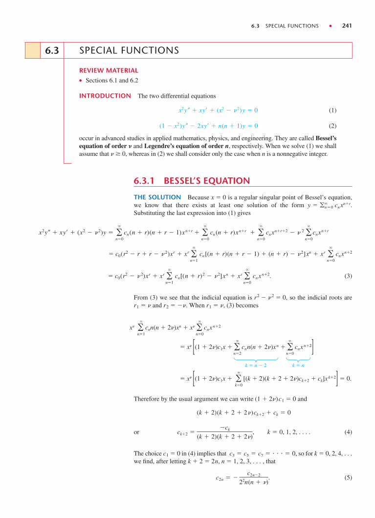
THE SOLUTION Because x � 0 is a regular singular point of Bessel’s equation,we know that there exists at least one solution of the form Substituting the last expression into (1) gives

y � �n�0 cnxn�r.

6.3 SPECIAL FUNCTIONS ● 241

SPECIAL FUNCTIONS

REVIEW MATERIAL● Sections 6.1 and 6.2

INTRODUCTION The two differential equations

(1)

(2)

occur in advanced studies in applied mathematics, physics, and engineering. They are called Bessel’sequation of order � and Legendre’s equation of order n, respectively. When we solve (1) we shallassume that � � 0, whereas in (2) we shall consider only the case when n is a nonnegative integer.

(1 � x2)y � 2xy� � n(n � 1)y � 0

x2y � xy� � (x2 � & 2)y � 0

6.3

(3) � c0(r2 � & 2)xr � xr �

n�1cn[(n � r)2 � & 2]xn � xr �

n�0cnxn�2.

� c0(r2 � r � r � & 2)xr � xr �

n�1cn[(n � r)(n � r � 1) � (n � r) � &2]xn � xr �

n�0cnxn�2

x2y � xy� � (x2 � & 2)y � �

n�0cn(n � r)(n � r � 1)xn�r � �

n�0cn(n � r)xn�r � �

n�0cnxn�r�2 � & 2 �

n�0cnxn�r

From (3) we see that the indicial equation is r2 � �2 � 0, so the indicial roots arer1 � � and r2 � ��. When r1 � �, (3) becomes

Therefore by the usual argument we can write (1 � 2�)c1 � 0 and

or (4)

The choice c1 � 0 in (4) implies that so for k � 0, 2, 4, . . .we find, after letting k � 2 � 2n, n � 1, 2, 3, . . . , that

(5)c2n � �c2n�2

22n(n � &).

c3 � c5 � c7 � � 0,

ck�2 ��ck

(k � 2)(k � 2 � 2&), k � 0, 1, 2, . . . .

(k � 2)(k � 2 � 2&)ck�2 � ck � 0

xn � cnn(n � 2n)xn � xn � cnxn�2

n�1

n�0

� xn [(1 � 2n)c1x � � [(k � 2)(k � 2 � 2n)ck�2 � ck]xk�2] � 0.k�0

� xn [(1 � 2n)c1x � � cnn(n � 2n)xn � � cnxn�2]n�2

n�0

k � n � 2 k � n

Thus

(6)

It is standard practice to choose c0 to be a specific value, namely,

where �(1 � �) is the gamma function. See Appendix I. Since this latter functionpossesses the convenient property �(1 � �) � ��(�), we can reduce the indicatedproduct in the denominator of (6) to one term. For example,

Hence we can write (6) as

for n � 0, 1, 2, . . . .

BESSEL FUNCTIONS OF THE FIRST KIND Using the coefficients c2n justobtained and r � �, a series solution of (1) is This solution is usu-ally denoted by J�(x):

(7)

If � � 0, the series converges at least on the interval [0, ). Also, for the secondexponent r2 � �� we obtain, in exactly the same manner,

(8)

The functions J�(x) and J��(x) are called Bessel functions of the first kind of order �and ��, respectively. Depending on the value of �, (8) may contain negative powersof x and hence converges on (0, ).*

Now some care must be taken in writing the general solution of (1). When � � 0,it is apparent that (7) and (8) are the same. If � � 0 and r1 � r2 � � � (��) � 2�is not a positive integer, it follows from Case I of Section 6.2 that J�(x) and J��(x) arelinearly independent solutions of (1) on (0, ), and so the general solution on theinterval is y � c1J�(x) � c2J��(x). But we also know from Case II of Section 6.2 thatwhen r1 � r2 � 2� is a positive integer, a second series solution of (1) may exist. In thissecond case we distinguish two possibilities. When � � m � positive integer, J�m(x)defined by (8) and Jm(x) are not linearly independent solutions. It can be shown that J�m

is a constant multiple of Jm (see Property (i) on page 245). In addition, r1 � r2 � 2�can be a positive integer when � is half an odd positive integer. It can be shown in this

J�&(x) � �

n�0

(�1)n

n!�(1 � & � n) �x

2�2n�&

.

J&(x) � �

n�0

(�1)n

n!�(1 � & � n) �x

2�2n�&

.

y � �n�0 c2n x2n�&.

c2n �(�1)n

22n�& n!(1 � &)(2 � &) (n � &)�(1 � &)�

(�1)n

22n�& n!�(1 � & � n)

�(1 � & � 2) � (2 � &)�(2 � &) � (2 � &)(1 � &)�(1 � &).

�(1 � & � 1) � (1 � &)�(1 � &)

c0 �1

2&�(1 � &),

c2n �(�1)nc0

22nn!(1 � &)(2 � &) (n � &), n � 1, 2, 3, . . . .

c6 � �c4

22 � 3(3 � &)� �

c0

26 � 1 � 2 � 3(1 � &)(2 � &)(3 � &)

c4 � �c2

22 � 2(2 � &)�

c0

24 � 1 � 2(1 � &)(2 � &)

c2 � �c0

22 � 1 � (1 � &)


*When we replace x by |x |, the series given in (7) and (8) converge for 0 � |x | � .

latter event that J�(x) and J��(x) are linearly independent. In other words, the generalsolution of (1) on (0, ) is

(9)

The graphs of y � J0(x) and y � J1(x) are given in Figure 6.3.1.

EXAMPLE 1 Bessel’s Equation of Order

By identifying we can see from (9) that the general solution of the

equation on (0, ) is

BESSEL FUNCTIONS OF THE SECOND KIND If � � integer, the functiondefined by the linear combination

(10)

and the function J�(x) are linearly independent solutions of (1). Thus another form ofthe general solution of (1) is y � c1J� (x) � c2Y�(x), provided that � � integer. As

m an integer, (10) has the indeterminate form 0�0. However, it can be shownby L’Hôpital’s Rule that exists. Moreover, the function

and Jm(x) are linearly independent solutions of x2y � xy� � (x2 � m2)y � 0. Hencefor any value of � the general solution of (1) on (0, ) can be written as

(11)

Y� (x) is called the Bessel function of the second kind of order �. Figure 6.3.2 showsthe graphs of Y0(x) and Y1(x).

EXAMPLE 2 Bessel’s Equation of Order 3

By identifying �2 � 9 and � � 3, we see from (11) that the general solution of theequation x2y � xy� � (x2 � 9)y � 0 on (0, ) is y � c1J3(x) � c2Y3(x).

DES SOLVABLE IN TERMS OF BESSEL FUNCTIONS Sometimes it is possibleto transform a differential equation into equation (1) by means of a change of vari-able. We can then express the solution of the original equation in terms of Besselfunctions. For example, if we let t � �x, � � 0, in

(12)

then by the Chain Rule,

Accordingly, (12) becomes

dy

dx�

dy

dt

dt

dx� �

dy

dt and

d 2y

dx2 �d

dt �dy

dx�dt

dx� �2 d 2y

dt2 .

x2y � xy� � (a2x2 � & 2)y � 0,

y � c1J&(x) � c2Y&(x).

Ym(x) � lim& :m

Y&(x)

lim& :m Y&(x)& : m,

Y& (x) �cos &�J&(x) � J�&(x)

sin &�

y � c1J1/2(x) � c2J�1/2(x).x2y � xy� � (x2 � 14)y � 0

& 2 � 14 and & � 1

2,

12

y � c1J&(x) � c2J�&(x), & � integer.


2 4 6 8_ 0.4

0.20.40.60.8

1

_ 0.2x

y

J1

J0

FIGURE 6.3.1 Bessel functions ofthe first kind for n � 0, 1, 2, 3, 4

2 4 6 8

1

_3_2.5

_2_ 1.5

_ 1_ 0.5

0.5x

yY0 Y1

FIGURE 6.3.2 Bessel functions ofthe second kind for n � 0, 1, 2, 3, 4

� t

��2

�2 d 2y

dt 2 � � t

��dy

dt� (t2 � & 2)y � 0 or t2 d 2y

dt2 � t dy

dt� (t2 � & 2)y � 0.

The last equation is Bessel’s equation of order � with solution y � c1J�(t) � c2Y�(t). Byresubstituting t � �x in the last expression, we find that the general solution of (12) is

(13)y � c1J&(�x) � c2Y&(�x).

Equation (12), called the parametric Bessel equation of order �, and its generalsolution (13) are very important in the study of certain boundary-value problemsinvolving partial differential equations that are expressed in cylindrical coordinates.

Another equation that bears a resemblance to (1) is the modified Bessel equa-tion of order �,

(14)

This DE can be solved in the manner just illustrated for (12). This time if we lett � ix, where i2 � �1, then (14) becomes

Because solutions of the last DE are J�(t) and Y�(t), complex-valued solutions of (14)are J�(ix) and Y�(ix). A real-valued solution, called the modified Bessel function ofthe first kind of order �, is defined in terms of J�(ix):

(15)

See Problem 21 in Exercises 6.3. Analogous to (10), the modified Bessel function ofthe second kind of order � � integer is defined to be

(16)

and for integer � � n,

Because I� and K� are linearly independent on the interval (0, ) for any value of v,the general solution of (14) is

(17)

Yet another equation, important because many DEs fit into its form by appro-priate choices of the parameters, is

(18)

Although we shall not supply the details, the general solution of (18),

(19)

can be found by means of a change in both the independent and the dependent

variables: If p is not an integer, then Yp in (19) can be

replaced by J�p.

EXAMPLE 3 Using (18)

Find the general solution of xy � 3y� � 9y � 0 on (0, ).

SOLUTION By writing the given DE as

we can make the following identifications with (18):

The first and third equations imply that a � �1 and With these values thesecond and fourth equations are satisfied by taking b � 6 and p � 2. From (19)

c � 12.

1 � 2a � 3, b2c2 � 9, 2c � 2 � �1, and a2 � p2c2 � 0.

y �3

xy� �

9

xy � 0,

z � bxc, y(x) � �z

b�a/c

w(z).

y � xac1Jp(bxc) � c2Yp(bxc)�,

y �1 � 2a

xy� � �b2c2x2c�2 �

a2 � p2c2

x2 �y � 0, p � 0.

y � c1I&(x) � c2K& (x).

Kn(x) � lim& :n

K&(x).

K&(x) ��

2

I�& (x) � I& (x)

sin &�,

I&(x) � i�& J& (ix).

t2 d 2y

dt2 � tdy

dt� (t2 � & 2)y � 0.

x2y � xy� � (x2 � & 2)y � 0.


we find that the general solution of the given DE on the interval (0, ) is

EXAMPLE 4 The Aging Spring Revisited

Recall that in Section 5.1 we saw that one mathematical model for the free undampedmotion of a mass on an aging spring is given by mx � ke�� tx � 0, � � 0. We arenow in a position to find the general solution of the equation. It is left as a problem

to show that the change of variables transforms the differential equation of the aging spring into

The last equation is recognized as (1) with � � 0 and where the symbols xand s play the roles of y and x, respectively. The general solution of the newequation is x � c1J0(s) � c2Y0(s). If we resubstitute s, then the general solution ofmx � ke��tx � 0 is seen to be

See Problems 33 and 39 in Exercises 6.3.

The other model that was discussed in Section 5.1 of a spring whose character-istics change with time was mx � ktx � 0. By dividing through by m, we see that

the equation is Airy’s equation y � �2xy � 0. See Example 3 in

Section 6.1. The general solution of Airy’s differential equation can also be writtenin terms of Bessel functions. See Problems 34, 35, and 40 in Exercises 6.3.

PROPERTIES We list below a few of the more useful properties of Besselfunctions of order m, m � 0, 1, 2, . . .:

(i) (ii)

(iii) (iv)

Note that Property (ii) indicates that Jm(x) is an even function if m is an eveninteger and an odd function if m is an odd integer. The graphs of Y0(x) and Y1(x) inFigure 6.3.2 illustrate Property (iv), namely, Ym(x) is unbounded at the origin. Thislast fact is not obvious from (10). The solutions of the Bessel equation of order 0 canbe obtained by using the solutions y1(x) in (21) and y2(x) in (22) of Section 6.2. It canbe shown that (21) of Section 6.2 is y1(x) � J0(x), whereas (22) of that section is

The Bessel function of the second kind of order 0, Y0(x), is then defined to be the

linear combination for x � 0. That is,

where � � 0.57721566 . . . is Euler’s constant. Because of the presence of thelogarithmic term, it is apparent that Y0(x) is discontinuous at x � 0.

Y0(x) �2

�J0(x)� � ln

x

2� �2

� �

k�1

(�1)k

(k!)2 �1 �1

2� �

1

k��x

2�2k

,

Y0(x) �2

� (� � ln 2)y1(x) �

2

�y2(x)

y2(x) � J0(x)ln x � �

k�1

(�1)k

(k!)2 �1 �1

2� �

1

k��x

2�2k

.

limx:0�

Ym (x) � �.Jm(0) � �0,

1,

m � 0

m � 0,

Jm(� x) � (�1)mJm(x),J�m(x) � (�1)mJm(x),

x �k

mtx � 0

x(t) � c1J0�2

� Bk

me��t / 2� � c2Y0�2

� Bk

me��t / 2�.

s2 d 2x

ds2 � sdx

ds� s2x � 0.

s �2

� Bk

me��t / 2

y � x�1[c1J2(6x1/2) � c2Y2(6x1/2)].


NUMERICAL VALUES The first five nonnegative zeros of J0(x), J1(x), Y0(x), andY1(x) are given in Table 6.1. Some additional function values of these four functionsare given in Table 6.2.


TABLE 6.2 Numerical Values of J0, J1, Y0, and Y1

x J0(x) J1(x) Y0(x) Y1(x)

0 1.0000 0.0000 — —1 0.7652 0.4401 0.0883 �0.78122 0.2239 0.5767 0.5104 �0.10703 �0.2601 0.3391 0.3769 0.32474 �0.3971 �0.0660 �0.0169 0.39795 �0.1776 �0.3276 �0.3085 0.14796 0.1506 �0.2767 �0.2882 �0.17507 0.3001 �0.0047 �0.0259 �0.30278 0.1717 0.2346 0.2235 �0.15819 �0.0903 0.2453 0.2499 0.1043

10 �0.2459 0.0435 0.0557 0.249011 �0.1712 �0.1768 �0.1688 0.163712 0.0477 �0.2234 �0.2252 �0.057113 0.2069 �0.0703 �0.0782 �0.210114 0.1711 0.1334 0.1272 �0.166615 �0.0142 0.2051 0.2055 0.0211

TABLE 6.1 Zeros of J0, J1, Y0, and Y1

J0(x) J1(x) Y0(x) Y1(x)

2.4048 0.0000 0.8936 2.19715.5201 3.8317 3.9577 5.42978.6537 7.0156 7.0861 8.5960

11.7915 10.1735 10.2223 11.749214.9309 13.3237 13.3611 14.8974

DIFFERENTIAL RECURRENCE RELATION Recurrence formulas that relateBessel functions of different orders are important in theory and in applications. In thenext example we derive a differential recurrence relation.

EXAMPLE 5 Derivation Using the Series Definition

Derive the formula

SOLUTION It follows from (7) that

xJ�& (x) � &J&(x) � xJ&�1(x).

The result in Example 5 can be written in an alternative form. Dividingby x gives

J�& (x) �&

xJ&(x) � �J&�1(x).

xJ�& (x) � &J& (x) � �xJ&�1(x)

xJv(x) � � ( )2n�v�

n�0

k � n � 1

(�1)n(2n � �)–––––––––––––––n! (1 � v � n)

x–2

L

� �J�(x) � x � ( )2n��1

n�1

(�1)n

–––––––––––––––––––––(n � 1)! (1 � � � n)

x–2

L

� � � ( )2n�v

n�0

(�1)n

–––––––––––––––n! (1 � � � n)

x–2

L � 2 � ( )2n�v

n�0

(�1)nn–––––––––––––––n! (1 � � � n)

x–2

L

� �J�(x) � x � � �J�(x) � xJ��1(x). ( )2k��1

k�0

(�1)k

–––––––––––––––k! (2 � � � k)

x–2

L

This last expression is recognized as a linear first-order differential equation in J�(x).Multiplying both sides of the equality by the integrating factor x�� then yields

(20)

It can be shown in a similar manner that

(21)

See Problem 27 in Exercises 6.3. The differential recurrence relations (20) and (21)are also valid for the Bessel function of the second kind Y� (x). Observe that when� � 0, it follows from (20) that

(22)

An application of these results is given in Problem 39 of Exercises 6.3.

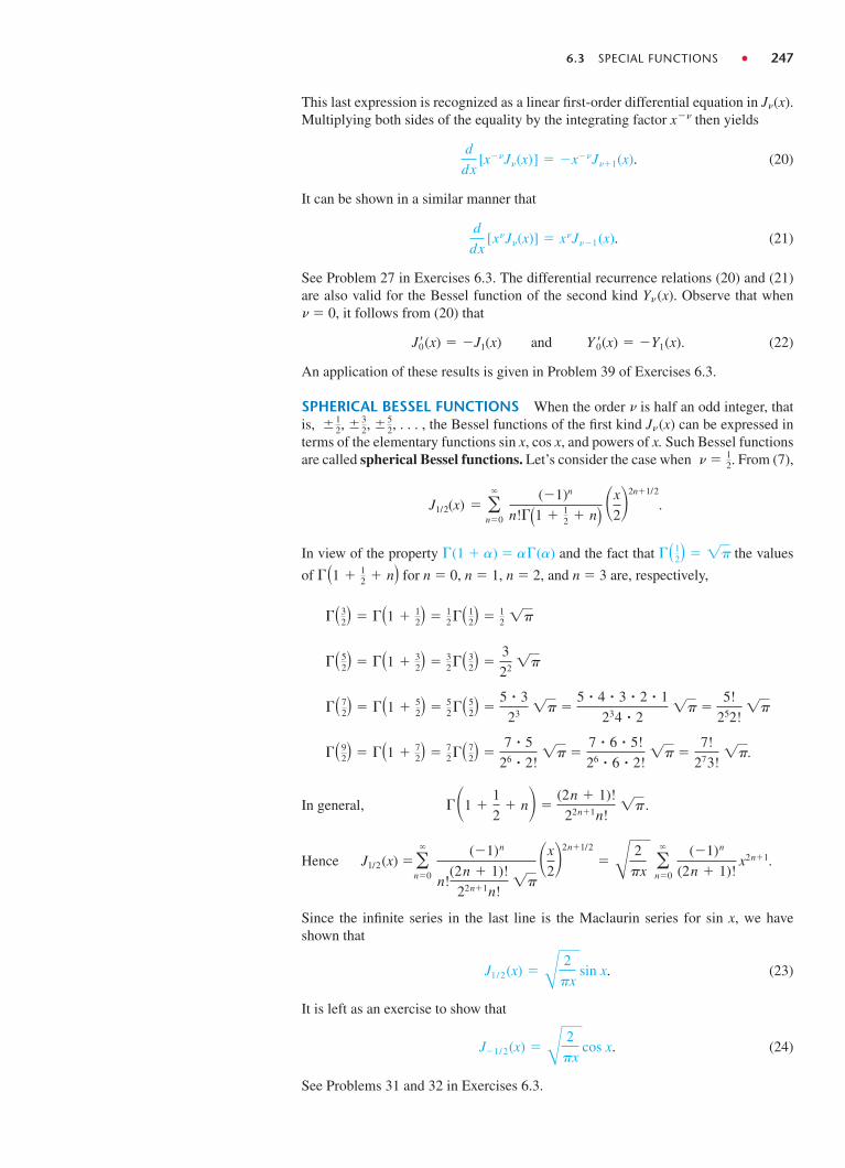
SPHERICAL BESSEL FUNCTIONS When the order � is half an odd integer, thatis, the Bessel functions of the first kind J� (x) can be expressed interms of the elementary functions sin x, cos x, and powers of x. Such Bessel functionsare called spherical Bessel functions. Let’s consider the case when From (7),

In view of the property �(1 � �) � ��(�) and the fact that the values

of for n � 0, n � 1, n � 2, and n � 3 are, respectively,

In general,

Hence

Since the infinite series in the last line is the Maclaurin series for sin x, we haveshown that

(23)

It is left as an exercise to show that

(24)

See Problems 31 and 32 in Exercises 6.3.

J�1/2(x) � B2

�xcos x.

J1/2(x) � B2

�xsin x.

J1/2(x) ��

n�0

(�1)n

n!(2n � 1)!

22n�1n!1�

�x

2�2n�1/2

� B2

�x �

n�0

(�1)n

(2n � 1)!x2n�1.

��1 �1

2� n� �

(2n � 1)!

22n�1n!1� .

�( 92) � �(1 � 7

2) � 72 �( 7

2) �7 � 5

26 � 2!1� �

7 � 6 � 5!

26 � 6 � 2!1� �

7!

273!1�.

�( 72) � �(1 � 5

2) � 52 �( 5

2) �5 � 3

23 1� �5 � 4 � 3 � 2 � 1

234 � 21� �

5!

252!1�

�( 52) � �(1 � 3

2) � 32 �( 3

2) �3

22 1�

�(32) � �(1 � 1

2) � 12 �( 1

2) � 12 1�

�(1 � 12 � n)

�(12) � 1�

J1/2(x) � �

n�0

(�1)n

n!�(1 � 12 � n) �

x

2�2n�1/2

.

& � 12.

�12, �3

2, �52, . . . ,

J�0(x) � �J1(x) and Y �0(x) � �Y1(x).

d

dx[x&J&(x)] � x&J& �1(x).

d

dx[x�&J&(x)] � �x�&J&�1(x).


6.3.2 LEGENDRE’S EQUATION

THE SOLUTION Since x � 0 is an ordinary point of Legendre’s equation (2), wesubstitute the series shift summation indices, and combine series to gety � �

k�0 ckxk ,


� �

j�2 [( j � 2)( j � 1)cj�2 � (n � j)(n � j � 1)cj]x j � 0

(1 � x2)y � 2xy� � n(n � 1)y � [n(n � 1)c0 � 2c2] � [(n � 1)(n � 2)c1 � 6c3]x

which implies that

or

(25)

If we let j take on the values 2, 3, 4, . . . , the recurrence relation (25) yields

and so on. Thus for at least we obtain two linearly independent power seriessolutions:

(26)

Notice that if n is an even integer, the first series terminates, whereas y2(x) is aninfinite series. For example, if n � 4, then

Similarly, when n is an odd integer, the series for y2(x) terminates with xn; that is,when n is a nonnegative integer, we obtain an nth-degree polynomial solution ofLegendre’s equation.

y1(x) � c01 �4 � 5

2!x2 �

2 � 4 � 5 � 7

4!x4� � c01 � 10x2 �

35

3x4�.

�(n � 5)(n � 3)(n � 1)(n � 2)(n � 4)(n � 6)

7!x7 � �.

y2(x) � c1x �(n � 1)(n � 2)

3!x3 �

(n � 3)(n � 1)(n � 2)(n � 4)

5!x5

�(n � 4)(n � 2)n(n � 1)(n � 3)(n � 5)

6!x6 � �

y1(x) � c01 �n(n � 1)

2!x2 �

(n � 2)n(n � 1)(n � 3)

4!x4

� x � � 1

c7 � �(n � 5)(n � 6)

7 � 6c5 � �

(n � 5)(n � 3)(n � 1)(n � 2)(n � 4)(n � 6)

7!c1

c6 � �(n � 4)(n � 5)

6 � 5c4 � �

(n � 4)(n � 2)n(n � 1)(n � 3)(n � 5)

6!c0

c5 � �(n � 3)(n � 4)

5 � 4c3 �

(n � 3)(n � 1)(n � 2)(n � 4)

5!c1

c4 � �(n � 2)(n � 3)

4 � 3c2 �

(n � 2)n(n � 1)(n � 3)

4!c0

cj�2 � �(n � j)(n � j � 1)

( j � 2)( j � 1)cj , j � 2, 3, 4, . . . .

c3 � �(n � 1)(n � 2)

3!c1

c2 � �n(n � 1)

2!c0

( j � 2)( j � 1)cj�2 � (n � j)(n � j � 1)cj � 0

(n � 1)(n � 2)c1 � 6c3 � 0

n(n � 1)c0 � 2c2 � 0

Because we know that a constant multiple of a solution of Legendre’s equationis also a solution, it is traditional to choose specific values for c0 or c1, depending onwhether n is an even or odd positive integer, respectively. For n � 0 we choosec0 � 1, and for n � 2, 4, 6, . . .

whereas for n � 1 we choose c1 � 1, and for n � 3, 5, 7, . . .

For example, when n � 4, we have

LEGENDRE POLYNOMIALS These specific nth-degree polynomial solutions arecalled Legendre polynomials and are denoted by Pn(x). From the series for y1(x)and y2(x) and from the above choices of c0 and c1 we find that the first severalLegendre polynomials are

(27)

Remember, P0(x), P1(x), P2(x), P3(x), . . . are, in turn, particular solutions of thedifferential equations

(28)

The graphs, on the interval [�1, 1], of the six Legendre polynomials in (27) aregiven in Figure 6.3.3.

PROPERTIES You are encouraged to verify the following properties using theLegendre polynomials in (27).

(i)

(ii) (iii)

(iv) (v)

Property (i) indicates, as is apparent in Figure 6.3.3, that Pn(x) is an even or oddfunction according to whether n is even or odd.

RECURRENCE RELATION Recurrence relations that relate Legendre polynomi-als of different degrees are also important in some aspects of their applications. Westate, without proof, the three-term recurrence relation

(29)

which is valid for k � 1, 2, 3, . . . . In (27) we listed the first six Legendre polynomials.If, say, we wish to find P6(x), we can use (29) with k � 5. This relation expresses P6(x)in terms of the known P4(x) and P5(x). See Problem 45 in Exercises 6.3.

(k � 1)Pk�1(x) � (2k � 1)xPk(x) � kPk�1(x) � 0,

P�n(0) � 0, n evenPn(0) � 0, n odd

Pn(�1) � (�1)nPn(1) � 1

Pn(�x) � (�1)nPn(x)

n � 0:

n � 1:

n � 2:

n � 3:

(1 � x2)y � 2xy� � 0,

(1 � x2)y � 2xy� � 2y � 0,

(1 � x2)y � 2xy� � 6y � 0,

(1 � x2)y � 2xy� � 12y � 0,

P0(x) � 1, P1(x) � x,

P2(x) �1

2 (3x2 � 1), P3(x) �

1

2 (5x3 � 3x),

P4(x) �1

8 (35x4 � 30x2 � 3), P5(x) �

1

8 (63x5 � 70x3 � 15x).

y1(x) � (�1)4/2 1 � 3

2 � 4 1 � 10x2 �35

3x4� �

1

8 (35x4 � 30x2 � 3).

c1 � (�1)(n�1) /2 1 � 3 n

2 � 4 (n � 1).

c0 � (�1)n /2 1 � 3 (n � 1)

2 � 4 n,


x

y

1-1-1

-0.5

0.5

1

-0.5 0.5

P1

P0

P2

FIGURE 6.3.3 Legendre polynomialsfor n � 0, 1, 2, 3, 4, 5

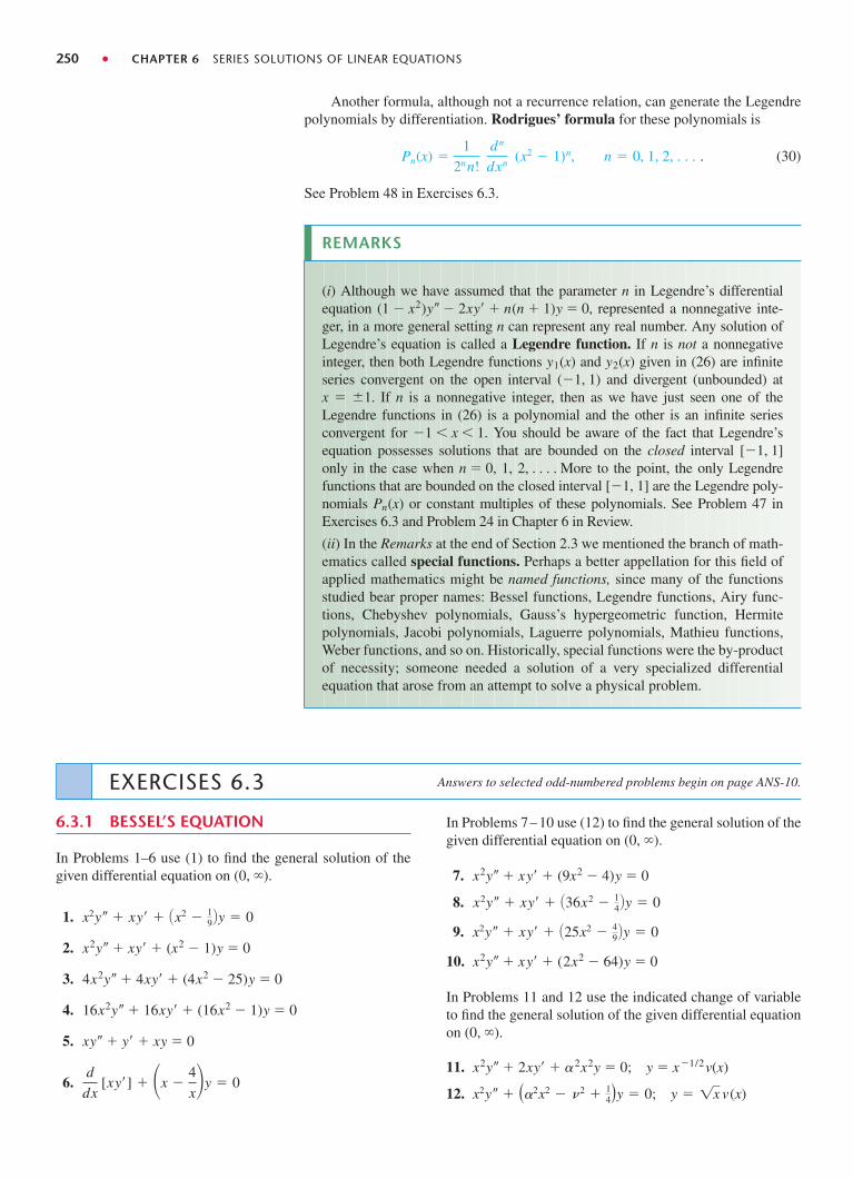
Another formula, although not a recurrence relation, can generate the Legendrepolynomials by differentiation. Rodrigues’ formula for these polynomials is

(30)

See Problem 48 in Exercises 6.3.

REMARKS

(i) Although we have assumed that the parameter n in Legendre’s differentialequation (1 � x2)y � 2xy� � n(n � 1)y � 0, represented a nonnegative inte-ger, in a more general setting n can represent any real number. Any solution ofLegendre’s equation is called a Legendre function. If n is not a nonnegativeinteger, then both Legendre functions y1(x) and y2(x) given in (26) are infiniteseries convergent on the open interval (�1, 1) and divergent (unbounded) atx � �1. If n is a nonnegative integer, then as we have just seen one of theLegendre functions in (26) is a polynomial and the other is an infinite seriesconvergent for �1 � x � 1. You should be aware of the fact that Legendre’sequation possesses solutions that are bounded on the closed interval [�1, 1]only in the case when n � 0, 1, 2, . . . . More to the point, the only Legendrefunctions that are bounded on the closed interval [�1, 1] are the Legendre poly-nomials Pn(x) or constant multiples of these polynomials. See Problem 47 inExercises 6.3 and Problem 24 in Chapter 6 in Review.

(ii) In the Remarks at the end of Section 2.3 we mentioned the branch of math-ematics called special functions. Perhaps a better appellation for this field ofapplied mathematics might be named functions, since many of the functionsstudied bear proper names: Bessel functions, Legendre functions, Airy func-tions, Chebyshev polynomials, Gauss’s hypergeometric function, Hermitepolynomials, Jacobi polynomials, Laguerre polynomials, Mathieu functions,Weber functions, and so on. Historically, special functions were the by-productof necessity; someone needed a solution of a very specialized differentialequation that arose from an attempt to solve a physical problem.

Pn(x) �1

2nn!

dn

dxn (x2 � 1)n, n � 0, 1, 2, . . . .


EXERCISES 6.3 Answers to selected odd-numbered problems begin on page ANS-10.

6.3.1 BESSEL’S EQUATION

In Problems 1–6 use (1) to find the general solution of thegiven differential equation on (0, ).

1.

2. x2y � xy� � (x2 � 1)y � 0

3. 4x2y � 4xy� � (4x2 � 25)y � 0

4. 16x2y � 16xy� � (16x2 � 1)y � 0

5. xy � y� � xy � 0

6.d

dx [xy�] � �x �

4

x�y � 0

x2y � xy� � �x2 � 19�y � 0

In Problems 7–10 use (12) to find the general solution of thegiven differential equation on (0, ).

7. x2y � xy� � (9x2 � 4)y � 0

8.

9.

10. x2y � xy� � (2x2 � 64)y � 0

In Problems 11 and 12 use the indicated change of variableto find the general solution of the given differential equationon (0, ).

11. x2y � 2xy� � �2x2y � 0; y � x�1/2v(x)

12. x2y � (�2x2 � & 2 � 14)y � 0; y � 1x v(x)

x2y � xy� � �25x2 � 49�y � 0

x2y � xy� � �36x2 � 14�y � 0


In Problems 13–20 use (18) to find the general solution ofthe given differential equation on (0, ).

13. xy � 2y� � 4y � 0 14. xy � 3y� � xy � 0

15. xy � y� � xy � 0 16. xy � 5y� � xy � 0

17. x2y � (x2 � 2)y � 0

18. 4x2y � (16x2 � 1)y � 0

19. xy � 3y� � x3y � 0

20. 9x2y � 9xy� � (x6 � 36)y � 0

21. Use the series in (7) to verify that I� (x) � i�� J� (ix) is areal function.

22. Assume that b in equation (18) can be pure imaginary, thatis, b � �i, � � 0, i2 � �1. Use this assumption to expressthe general solution of the given differential equation interms the modified Bessel functions In and Kn.

(a) y � x2y � 0 (b) xy � y� � 7x3y � 0

In Problems 23–26 first use (18) to express the general solu-tion of the given differential equation in terms of Bessel func-tions. Then use (23) and (24) to express the general solution interms of elementary functions.

23. y � y � 0

24. x2y � 4xy� � (x2 � 2)y � 0

25. 16x2y � 32xy� � (x4 � 12)y � 0

26. 4x2y � 4xy� � (16x2 � 3)y � 0

27. (a) Proceed as in Example 5 to show that

xJ��(x) � ��J�(x) � xJ��1(x).

[Hint: Write 2n � � � 2(n � �) � �.]

(b) Use the result in part (a) to derive (21).

28. Use the formula obtained in Example 5 along withpart (a) of Problem 27 to derive the recurrence relation

2�J� (x) � xJ��1(x) � xJ��1(x).

In Problems 29 and 30 use (20) or (21) to obtain the givenresult.

29. 30. J�0 (x) � J�1(x) � �J1(x)

31. Proceed as on page 247 to derive the elementary form ofJ�1/2(x) given in (24).

32. (a) Use the recurrence relation in Problem 28 alongwith (23) and (24) to express J3/2(x), J�3/2(x), andJ5/2(x) in terms of sin x, cos x, and powers of x.

(b) Use a graphing utility to graph J1/2(x), J�1/2(x),J3/2(x), J�3/2(x), and J5/2(x).

�x

0rJ0(r)dr � xJ1(x)

33. Use the change of variables to show

that the differential equation of the aging spring mx � ke�� tx � 0, � � 0, becomes

34. Show that is a solution of Airy’s

differential equation y � �2xy � 0, x � 0, wheneverw is a solution of Bessel’s equation of order thatis, t � 0. [Hint: Afterdifferentiating, substituting, and simplifying, then let

]35. (a) Use the result of Problem 34 to express the general

solution of Airy’s differential equation for x � 0 interms of Bessel functions.

(b) Verify the results in part (a) using (18).

36. Use the Table 6.1 to find the first three positive eigenval-ues and corresponding eigenfunctions of the boundary-value problem

[Hint: By identifying � �2, the DE is the parametricBessel equation of order zero.]

37. (a) Use (18) to show that the general solution of thedifferential equation xy � y � 0 on the interval(0, ) is

(b) Verify by direct substitution that is a particular solution of the DE in the case � 1.


38. Use a CAS to graph the modified Bessel functions I0(x),I1(x), I2(x) and K0(x), K1(x), K2(x). Compare thesegraphs with those shown in Figures 6.3.1 and 6.3.2.What major difference is apparent between Bessel func-tions and the modified Bessel functions?

39. (a) Use the general solution given in Example 4 tosolve the IVP

Also use and alongwith Table 6.1 or a CAS to evaluate coefficients.

(b) Use a CAS to graph the solution obtained in part (a)for 0 � t � .

Y�0(x) � �Y1(x)J�0(x) � �J1(x)

4x � e�0.1tx � 0, x(0) � 1, x�(0) � �12.

y � 1xJ1(21x)

y � c11xJ1(21�x) � c21xY1(21�x).

y(x), y�(x) bounded as x : 0�, y(2) � 0.

xy � y� � �xy � 0,

t � 23 �x3 /2.

t2w � tw� � (t2 � 19)w � 0,

13,

y � x1 /2w(23 �x3 /2)

s2 d 2x

ds2 � sdx

ds� s2x � 0.

s �2

� Bk

me�� t / 2


40. (a) Use the general solution obtained in Problem 35 tosolve the IVP

Use a CAS to evaluate coefficients.

(b) Use a CAS to graph the solution obtained in part (a)for 0 � t � 200.

41. Column Bending Under Its Own Weight A uniformthin column of length L, positioned vertically with oneend embedded in the ground, will deflect, or bend away,from the vertical under the influence of its own weightwhen its length or height exceeds a certain critical value.It can be shown that the angular deflection �(x) of thecolumn from the vertical at a point P(x) is a solution ofthe boundary-value problem:

where E is Young’s modulus, I is the cross-sectionalmoment of inertia, � is the constant linear density, and xis the distance along the column measured from its base.See Figure 6.3.4. The column will bend only for thosevalues of L for which the boundary-value problem has anontrivial solution.

(a) Restate the boundary-value problem by making thechange of variables t � L � x. Then use the resultsof a problem earlier in this exercise set to expressthe general solution of the differential equation interms of Bessel functions.

(b) Use the general solution found in part (a) to find asolution of the BVP and an equation which definesthe critical length L, that is, the smallest value ofL for which the column will start to bend.

(c) With the aid of a CAS, find the critical length Lof a solid steel rod of radius r � 0.05 in., �g � 0.28 A lb/in., E � 2.6 � 107 lb/in.2, A � �r2,and I � 1

4 �r4.

EId 2�

dx2 � $g(L � x)� � 0, �(0) � 0, ��(L) � 0,

4x � tx � 0, x(0.1) � 1, x�(0.1) � �12.

column of uniform cross section and hinged at bothends, the deflection y(x) is a solution of the BVP:

(a) If the bending stiffness factor EI is proportionalto x, then EI(x) � kx, where k is a constant ofproportionality. If EI(L) � kL � M is the maxi-mum stiffness factor, then k � M�L and so EI(x) � Mx�L. Use the information in Problem 37to find a solution of

if it is known that is not zero at x � 0.

(b) Use Table 6.1 to find the Euler load P1 for thecolumn.

(c) Use a CAS to graph the first buckling mode y1(x)corresponding to the Euler load P1. For simplicityassume that c1 � 1 and L � 1.

43. Pendulum of Varying Length For the simple pendu-lum described on page 209 of Section 5.3, suppose thatthe rod holding the mass m at one end is replaced by aflexible wire or string and that the wire is strung over apulley at the point of support O in Figure 5.3.3. In thismanner, while it is in motion in a vertical plane, themass m can be raised or lowered. In other words, thelength l(t) of the pendulum varies with time. Underthe same assumptions leading to equation (6) in Section5.3, it can be shown* that the differential equation forthe displacement angle � is now

(a) If l increases at constant rate v and if l(0) � l0,show that a linearization of the foregoing DE is

(31)

(b) Make the change of variables x � (l0 � vt)�v andshow that (31) becomes

(c) Use part (b) and (18) to express the general solutionof equation (31) in terms of Bessel functions.

(d) Use the general solution obtained in part (c) to solvethe initial-value problem consisting of equation (31)and the initial conditions �(0) � �0, ��(0) � 0.[Hints: To simplify calculations, use a further

change of variable u �2

v1g(l0 � vt) � 2B

g

vx1/ 2.

d 2�

dx 2 �2

x

d�

dx�

g

vx� � 0.

(l0 � vt)� � 2v�� g� � 0.

l� � 2l�� g sin � � 0.

1xY1(21�x)

Mx

L

d 2y

dx2 � Py � 0, y(0) � 0, y(L) � 0

EId 2y

dx2 � Py � 0, y(0) � 0, y(L) � 0.

*See Mathematical Methods in Physical Sciences, Mary Boas, John Wiley& Sons, Inc., 1966. Also see the article by Borelli, Coleman, and Hobsonin Mathematics Magazine, vol. 58, no. 2, March 1985.

x = 0

x

θ

P(x)

ground

FIGURE 6.3.4 Beam in Problem 41

42. Buckling of a Thin Vertical Column In Example 3of Section 5.2 we saw that when a constant verticalcompressive force, or load, P was applied to a thin

CHAPTER 6 IN REVIEW ● 253

Also, recall that (20) holds for both J1(u) and Y1(u).Finally, the identity

will be helpful.]

(e) Use a CAS to graph the solution �(t) of theIVP in part (d) when l0 � 1 ft, �0 � radian,and Experiment with the graph usingdifferent time intervals such as [0, 10], [0, 30],and so on.

(f) What do the graphs indicate about the displacementangle �(t) as the length l of the wire increases withtime?

6.3.2 LEGENDRE’S EQUATION

44. (a) Use the explicit solutions y1(x) and y2(x) ofLegendre’s equation given in (26) and the appropri-ate choice of c0 and c1 to find the Legendre polyno-mials P6(x) and P7(x).

(b) Write the differential equations for which P6(x)and P7(x) are particular solutions.

45. Use the recurrence relation (29) and P0(x) � 1, P1(x) � x,to generate the next six Legendre polynomials.

46. Show that the differential equation

sin �d 2y

d� 2 � cos �dy

d�� n(n � 1)(sin �)y � 0

v � 160 ft/s.

110

�2

�uJ1(u)Y2(u) � J2(u)Y1(u) �

can be transformed into Legendre’s equation by meansof the substitution x � cos �.

47. Find the first three positive values of for which theproblem

has nontrivial solutions.


48. For purposes of this problem ignore the list of Legendrepolynomials given on page 249 and the graphs givenin Figure 6.3.3. Use Rodrigues’ formula (30) to gener-ate the Legendre polynomials P1(x), P2(x), . . . , P7(x).Use a CAS to carry out the differentiations andsimplifications.

49. Use a CAS to graph P1(x), P2(x), . . . , P7(x) on theinterval [�1, 1].

50. Use a root-finding application to find the zeros ofP1(x), P2(x), . . . , P7 (x). If the Legendre polynomialsare built-in functions of your CAS, find zeros ofLegendre polynomials of higher degree. Form a con-jecture about the location of the zeros of any Legendrepolynomial Pn(x), and then investigate to see whether itis true.

y(0) � 0, y(x), y�(x) bounded on [�1,1]

(1 � x2)y � 2xy� � �y � 0,

CHAPTER 6 IN REVIEW Answers to selected odd-numbered problems begin on page ANS-10.

In Problems 1 and 2 answer true or false without referringback to the text.

1. The general solution of x2y � xy� � (x2 � 1)y � 0 isy � c1J1(x) � c2J�1(x).

2. Because x � 0 is an irregular singular point ofx3y � xy� � y � 0, the DE possesses no solution thatis analytic at x � 0.

3. Both power series solutions of y � ln(x � 1)y� � y � 0centered at the ordinary point x � 0 are guaranteedto converge for all x in which one of the followingintervals?

(a) (�, ) (b) (�1, )

(c) (d) [�1, 1]

4. x � 0 is an ordinary point of a certain linear differentialequation. After the assumed solution isy � �

n�0 cnxn

[�12,

12]

substituted into the DE, the following algebraic systemis obtained by equating the coefficients of x0, x1, x2,and x3 to zero:

Bearing in mind that c0 and c1 are arbitrary, write downthe first five terms of two power series solutions of thedifferential equation.

5. Suppose the power series is knownto converge at �2 and diverge at 13. Discuss whetherthe series converges at �7, 0, 7, 10, and 11. Possibleanswers are does, does not, might.

�k�0 ck(x � 4)k

20c5 � 8c4 � c3 � 23 c2 � 0.

12c4 � 6c3 � c2 � 13 c1 � 0

6c3 � 4c2 � c1 � 0

2c2 � 2c1 � c0 � 0


6. Use the Maclaurin series for sin x and cos x along withlong division to find the first three nonzero terms of a

power series in x for the function

In Problems 7 and 8 construct a linear second-order differen-tial equation that has the given properties.

7. A regular singular point at x � 1 and an irregularsingular point at x � 0

8. Regular singular points at x � 1 and at x � �3

In Problems 9–14 use an appropriate infinite series methodabout x � 0 to find two solutions of the given differentialequation.

9. 2xy � y� � y � 0 10. y � xy� � y � 0

11. (x � 1)y � 3y � 0 12. y � x2y� � x y � 0

13. xy � (x � 2)y� � 2y � 0 14. (cos x)y � y � 0

In Problems 15 and 16 solve the given initial-value problem.

15. y � xy� � 2y � 0, y(0) � 3, y�(0) � �2

16. (x � 2)y � 3y � 0, y(0) � 0, y�(0) � 1

17. Without actually solving the differential equation(1 � 2 sin x)y � xy � 0, find a lower bound for theradius of convergence of power series solutions aboutthe ordinary point x � 0.

18. Even though x � 0 is an ordinary point of the differen-tial equation, explain why it is not a good idea to try tofind a solution of the IVP

of the form Using power series, find abetter way to solve the problem.

In Problems 19 and 20 investigate whether x � 0 is an ordi-nary point, singular point, or irregular singular point ofthe given differential equation. [Hint: Recall the Maclaurinseries for cos x and ex.]

19. xy � (1 � cos x)y� � x2y � 0

20. (ex � 1 � x)y � xy � 0

21. Note that x � 0 is an ordinary point of the differentialequation y � x2y� � 2xy � 5 � 2x � 10x3. Use theassumption to find the general solutiony � yc � yp that consists of three power series centeredat x � 0.

22. The first-order differential equation dy�dx � x2 � y2

cannot be solved in terms of elementary functions.However, a solution can be expressed in terms of Besselfunctions.

(a) Show that the substitution leads to the

equation u � x2u � 0.

y � �1

u

du

dx

y � �n�0 cnxn

y � �n�0 cnxn.

y � xy� � y � 0, y(1) � �6, y�(1) � 3

f (x) �sin x

cos x.

(b) Use (18) in Section 6.3 to find the general solutionof u � x2u � 0.

(c) Use (20) and (21) in Section 6.3 in the forms

and

as an aid to show that a one-parameter family ofsolutions of dy�dx � x2 � y2 is given by

23. (a) Use (23) and (24) of Section 6.3 to show that

(b) Use (15) of Section 6.3 to show that

(c) Use part (b) to show that

24. (a) From (27) and (28) of Section 6.3 we knowthat when n � 0, Legendre’s differential equation(1 � x2)y � 2xy� � 0 has the polynomial solu-tion y � P0(x) � 1. Use (5) of Section 4.2 to showthat a second Legendre function satisfying the DEfor �1 � x � 1 is

(b) We also know from (27) and (28) of Section 6.3that when n � 1, Legendre’s differential equation(1 � x2)y � 2xy� � 2y � 0 possesses the polyno-mial solution y � P1(x) � x. Use (5) of Section 4.2to show that a second Legendre function satisfyingthe DE for �1 � x � 1 is

(c) Use a graphing utility to graph the logarithmicLegendre functions given in parts (a) and (b).

25. (a) Use binomial series to formally show that

(b) Use the result obtained in part (a) to show thatPn(1) � 1 and Pn(�1) � (�1)n. See Properties (ii)and (iii) on page 249.

(1 � 2xt � t2)�1/2 � �

n�0Pn(x)tn.

y �x

2 ln�1 � x

1 � x� � 1.

y �1

2 ln�1 � x

1 � x�.

K1/2(x) � B�

2xe�x.

I1/2(x) � B2

�xsinh x and I�1/2(x) � B

2

�x cosh x.

Y1/2(x) � �B2

�x cos x.

y � xJ3 /4( 1

2 x2) � cJ�3 /4( 12 x2)

cJ1/4( 12 x2) � J�1/4( 1

2 x2).

J�& (x) � �&

xJ& (x) � J&�1(x)

J�& (x) �&

xJ& (x) � J&�1(x)

SOLUTIONS ABOUT ORDINARY POINTS 6.1 - SU LMS

Documents

Transcript of SOLUTIONS ABOUT ORDINARY POINTS 6.1 - SU LMS