Chapter 5 - Dimensional Analysis and Similarity

Fluid Mechanics - MTF053

Chapter 5

Niklas Andersson

Chalmers University of Technology

Department of Mechanics and Maritime Sciences

Division of Fluid Mechanics

Gothenburg, Sweden

[email protected]

mailto:[email protected]

Overview

Fluid Dynamics

Basic

Concepts

Pressure

hydrostatic

forces

buoyancy

Fluid Flow

velocity

field

Reynolds

number

flow

regimes

Thermo-

dynamics

pressure,

density,

and tem-

perature

state

relations

speed of

sound

entropy

Fluid

fluid

conceptcontinuum

viscosity

Fluid Flow

Com-

pressible

Flow

shock-

expansion

theory

nozzle

flow

normal

shocks

speed of

sound

External

Flow

separation turbulence

boundary

layer

Reynolds

number

Duct Flow

friction

and losses

turbulent

flow

laminar

flow

flow

regimes

Turbulence

Turbu-

lence

Modeling

Turbu-

lence

viscosity

Reynolds

stressesReynolds

decom-

position

Flow

Relations

Dimen-

sional

Analysis

modeling

and

similarity

nondi-

mensional

equations

The Pi

theorem

Differential

Relations

rotation

stream

function

conser-

vation

relations

Integral

Relations

Bernoulli

conser-

vation

relations

Reynolds

transport

theorem

Learning Outcomes

3 Define the Reynolds number

4 Be able to categorize a flow and have knowledge about how to select

applicable methods for the analysis of a specific flow based on category

17 Explain about how to use nondimensional numbers and the Π theorem

we will learn about how to plan experiments and compare experimental data

using dimensionless numbers

Niklas Andersson - Chalmers 4 / 48

Roadmap - Dimensional Analysis and Similarity

Dimensional analysis

The Π theorem

Nondimensionalized equations

Dimensionless groups

Modeling and similarity

Differential equations


Motivation

”Most practical fluid flow problems are too complex, both geometrically and

physically, to be solved analytically. They mus be tested by experiments or

approximated by CFD”

Dimensional analysis:

I Large data sets may be represented by a few curves or even a single curve

I A systematic tool for data reduction

I Experimental/simulation data are more general in dimensionless form


Dimensions




The Π theorem






Dimensional Analysis

Dimensional analysis is a tool for systematic

planning of experiments

presentation of experimental data

interpretation of measurements



”If a phenomenon depends on n dimensional variables, dimensional analysis

will reduce the problem to only k dimensionless variables, where the reduc-

tion n− k depends on the problem complexity”

”Generally, n− k equals the number of primary dimensions”



Suppose that we know that the force F on a particular body shape in a fluid flow

depends on

I The length of the body L

I The flow velocity V

I The fluid density ρ

I The fluid viscosity µ

F = f(L,V , ρ, µ)



Let’s say that we need ten points to define a curve

We need to test 10 lengths and for each of those, 10 velocities, ....

The result in this case would be 10000 experiments

With dimensional analysis, the problem can be reduced as follows

F

ρV2L2= g

(ρVL

µ

)or CF = g(Re)



Dimensional analysis:

I Gives insight into physical relationships

I Helps in identifying important and unimportant parameters for a specific problem

I Provides scaling laws

I convert data from model-scale to prototype-scaleI similarity between model and prototype


Similarity

Let’s go back to the force example from before

CF = g(Re)

so if Rem = Rep that means that CF ,m = CF ,p (where m is model and p prototype)

CF ,m =Fm

ρmV2mL

2m

and CF ,p =Fp

ρpV2pL

2p

Fm

ρmV2mL

2m

=Fp

ρpV2pL

2p

⇒ Fp

Fm=

ρpρm

(Vp

Vm

)2(Lp

Lm

)2




The Π theorem





�


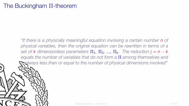
The Buckingham Π-theorem

”If there is a physically meaningful equation involving a certain number n of

physical variables, then the original equation can be rewritten in terms of a

set of k dimensionless parameters Π1, Π2, ..., Πk . The reduction j = n− k

equals the number of variables that do not form a Π among themselves and

is always less than or equal to the number of physical dimensions involved”


The Buckingham Π-theorem

Systematic identification of Π groups:

1. List and count the number of variables in the problem n

2. List the dimensions for each of the n variables

3. Find the reduction j

I initial guess: j equals the number of dimensionsI look for j variables that do not form a ΠI if not possible reduce j by one and start over

4. Select j scaling parameters

5. Add one of the other variables to your j repeating variables and form a power

product

6. Algebraically, find exponents that make the product dimensionless


The Buckingham Π-theorem - Example

F = f(L,U, ρ, µ)

number of variables: n = 5

F L U ρ µ{MLT−2

}{L}

{LT−1

} {ML−3

} {ML−1T−1

}number of dimensions is 3 and thus the reduction is: j ≤ 3

number of dimensionless groups (Πs): k = n− j ≥ 2



I Inspecting the variables, we see that L, U, and ρ cannot form a Π-groupI only ρ contains M (mass)I only U contains T (time)

I L, U, and ρ are selected as the j repeating variables

I The reduction will be j = 3 and thus k = n− j = 2

I One of the Π-groups will contain F and the other will contain µ



Π1 = LaUbρcF ⇒ (L)a(LT−1)b(ML−3)c(MLT−2) = M0L0T0

L : a + b − 3c + 1 = 0M : c + 1 = 0T : − b − 2 = 0

which gives

a = −2, b = −2, c = −1

and thus

Π1 =F

ρU2L2= CF



Π2 = LaUbρcµ−1 ⇒ (L)a(LT−1)b(ML−3)c(ML−1T−1)−1 = M0L0T0

L : a + b − 3c + 1 = 0M : c − 1 = 0T : − b + 1 = 0

which gives

a = b = c = 1

and thus

Π2 =ρUL

µ= Re



If F = f(L,V , ρ, µ), the theorem guaranties that, in this case, Π1 = g(Π2)

F

ρU2L2= g

(ρUL

µ

)or CF = g(Re)




The Π theorem





�

�


Nondimensionalized Equations

Why would one want to make the governing equations nondimensional?

I Understand flow physics

I Gives information about under what conditions terms are negligible

I A way to find important nondimensional groups for a specific flow



The incompressible flow continuity and momentum equations and corresponding

boundary conditions:

Continuity: ∇ · V = 0

Navier-Stokes: ρDVDt

= ρg −∇p+ µ∇2V

Solid surface: no-slip (V = 0 if fixed surface)

Inlet/outlet: known velocity and pressure



I The variables in the continuity and momentum equations contain three primary

dimensions; M, L, and T

I All variables included (ρ,V,p, x, y, z) can be made nondimensional using threeconstants:

I density: ρI reference velocity: UI reference length: L

reference properties are constants characteristic for a specific flow



nondimensional variables are denoted by an asterisk:

V∗ =VU

∇∗ = L∇

(x∗, y∗, z∗) =1

L(x, y, z)

t∗ =tU

L

p∗ =p+ ρgz

ρU2

Check:

∇∗p∗ =L

ρU2∇ (p+ ρgz) =

L

ρU2[∇p− ρg]

∂u

∂x=

∂(Uu∗)

∂(Lx∗)=

U

L

∂u∗

∂x∗



Continuity: ∇∗ · V∗ = 0

Navier-Stokes:DV∗

Dt∗= −∇∗p∗ +

µ

ρUL∇∗2V∗

Solid surface: no-slip (V∗ = 0 if fixed surface)

Inlet/outlet: known velocity and pressure (V∗, p∗)



The Reynolds number appears in the nondimensional Navier-Stokes equations

DV∗

Dt∗= −∇∗p∗ +

µ

ρUL∇∗2V∗

Re =ρUL

µ

Reynolds number - ratio of inertia and viscosity




The Π theorem





�

�

�


Dimensionless Groups

parameter definition interpretation importance

Reynolds number Re =ρUL

µ

inertia

viscosityalmost always

Mach number M =U

a

flowspeed

speedofsoundcompressible flow

Froude number Fr =U2

gL

inertia

gravityfree-surface flow

Weber number We =ρU2L

Υ

inertia

surfacetensionfree-surface flow

Prandtl number Pr =µCp

k

dissipation

conductionheat convection

specific heat ratio γ =Cp

Cv

enthalpy

internalenergycompressible flow

Strouhal number St =ωL

U

oscillation

meanspeedoscillating flow

roughness ratioε

L

wallroughness

bodylengthturbulent flow

pressure coefficient Cp =p− p∞0.5ρU2

staticpressure

dynamicpressureaerodynamics

lift coefficient CL =FL

0.5ρU2A

liftforce

dynamicforceaerodynamics

drag coefficient CD =FD

0.5ρU2A

dragforce

dynamicforceaerodynamics

skin friction coefficient Cf =τwall

0.5ρU2

wallshearstress

dynamicpressureboundary layers


The Reynolds Number

Re =ρUL

µ=

UL

ν

laminar flow

turbulent flow


Compressible Flow

Ma =U

a=

U√γRT

γ =Cp

Cv

https://www.youtube.com/watch?v=wRaDPnpnx04


https://www.youtube.com/watch?v=wRaDPnpnx04

Oscillating Flows

101 102 103 104 105 106 1070

0.1

0.2

0.3

0.4

data spread

St =fL

U

ReD =UD

ν

ReD

St

Von Kármán vortex street


Oscillating Flows


Oscillating Flows

Tacoma bridge collapse 1940

oscillating frequency close to the natural vibration frequency of the bridge structure

https://www.youtube.com/watch?v=XggxeuFDaDU


https://www.youtube.com/watch?v=XggxeuFDaDU

Oscillating Flows https://www.youtube.com/watch?v=ptYrbQGk6DQ


https://www.youtube.com/watch?v=ptYrbQGk6DQ

Example of Successful Dimensional Analysis

101 102 103 104 105 106 1070

1

2

3

4

5

ReD

CD

Cylinder (2D)

Spherecylinder: CD =

FD12ρU

2Ld

sphere: CD =FD

12ρU

2 14πd

2

general: CD =FD

12ρU

2Ap

Ap is the projected area

collection of data from a large number of experiments


Example of Successful Dimensional Analysis

101 102 103 104 105 106 1070

1

2

3

4

5

ReD

CD

Cylinder (2D)

Sphere

collection of data from a large number of experiments




The Π theorem





�

�

�

�


Modeling and Similarity

Scaling of experimental results from model scale to prototype scale:

”Flow conditions for a model test are completely similar if all relevant dimen-

sionless parameters have the same corresponding values for the model and

the prototype”


Geometric Similarity

”A model and prototype are geometrically similar if and only if all body dimen-

sions in all three coordinates have the same linear-scale ratio”

”All angles are preserved in geometric similarity. All flow directions are pre-

served. The orientations of model and prototype with respect to the sur-

roundings must be identical”



Homologous points - points that with the same relative location

40 m

8 m

1 m

10◦

Vp

∗4.0 m

0.8 m

0.1 m

10◦

Vm

∗

1. all dimensions should be scaled with the same linear scaling ratio

2. angle of attach should be the same

3. scaled nose radius

4. scaled surface roughness


Kinematic Similarity

”The motions of two systems are kinematically similar if homologous particles

lie at homologous points at homologous times”

Geometric similarity is probably not sufficient to establish time-scale equivalence

Dynamic considerations:

I Reynolds number equivalenceI Mach number equivalence


Kinematic Similarity

”Incompressible frictionless low-speed flows without free surfaces are kine-

matically similar with independent length and time scales”

Dm = αDp

V∞m = βV∞p

V1m = βV1p

V2m = βV2p

Dp

1

2

V∞

prototype

Dm

1

2

V∞

model


Dynamic Similarity

”Dynamic similarity is achieved when the model and prototype have the same

length scale ratio, time scale ratio, and force scale ratio”

Compressible flow:

1. Reynolds number equivalence

2. Mach number equivalence

3. specific-heat ratio equivalence

Incompressible flow without free surfaces:


Incompressible flow with free surfaces:


2. Froude number equivalence (and if necessary Weber number and/or cavitation

number)


Dynamic Similarity

Finertia = Fpressure + Fgravity + Ffriction

”Dynamic similarity ensures that each of the force components will be in the

same ratio and have the same directions for model and prototype”




The Π theorem





�

�

�

�

�


Chapter 5 - Dimensional Analysis and Similarity

Documents

Transcript of Chapter 5 - Dimensional Analysis and Similarity