Chapter 1, Page 1

Chapter 1: Introduction and general instrument discussion

The Nu Instrument’s Noblesse noble gas mass spectrometer is a state of the artinstrument designed specifically for the analysis of noble gasses and other speciesunder static vacuum conditions. The instrument is a single focussing, 75° magneticsector design, with the magnet radius being 240mm. Due to the non-normal entranceand exit poles, the dispersion at the collector plane is equal to double the magnetradius, corresponding to 480mm. Between the magnet exit pole and the collector areplaced two miniature lens arrays, which are used to provide a field equivalent to anelectrostatic quadrupole. This enables a zoom lens to be incorporated into the vacuumenvelope, allowing for the dispersion to be altered from the figure quote above. Thispatented approach permits the user to undertake multi-collector analyses, without thenecessity of having to move collectors as different elements are studied.

Various different configurations of collector design are offered, normally consistingof at least one faraday collector together with a number of discrete dynode multipliers.Further, to enable analyses of such elements as helium, where the minor 3He isotopehas to be recorded in the presence of the much more intense 4He beam, we alsoprovide a retardation lens assembly to improve the abundance sensitivity of one of theion counting channels. To further increase the dynamic range of some of the detectorchannels, it is also possible to place a multiplier and faraday detector behind a slit, anduse an electrostatic deflector to send the ion beam into one or other of the pair.

The standard source supplied with the instrument is based on the well-known Nierdesign, but has been optimised for working in a static vacuum environment. Greatcare has been taken in the design to optimise the source’s efficiency, as well as it’suser friendliness and longevity of filament life. Although it, and it’s accompanyingelectronics, has been designed to work at up to 8kV acceleration voltage, most userswill not take it to these voltages, since the gain in sensitivity above about 5kV will befound to be small. However, it may be found to be advantageous to work here if theultimate resolution is required, since any aberrations will be reduced as theacceleration voltage is increased.

A getter pump is placed immediately behind the source, in order to minimise anyimpurity peaks levels during analysis. A spare port is also provided on the manifoldentry block, to which a further pump or cold finger may be fitted. Two ion pumps arealso provided as standard, one off the manifold entry block, which is fitted with apneumatic valve, and a second off the collector block, fitted with a manual isolationvalve. It is expected that this second pump will only normally be used when theinstrument is not in use (and during bakeout), and samples will be evacuated afteranalysis using the source ion pump. Finally a 70l/sec turbo pump may also be fitted,together with a dry (scroll) backing pump. This will only normally be used toevacuate the mass spectrometer after venting, although a connection is also providedto enable this pump to evacuate the user’s manifold assembly, if so required.

A dedicated software package is provided to enable the analyses of the isotopic ratioof the gases to be fully automated. The electronic suite provides spare outputs tocontrol the user’s automated manifold valves, and a separate software utility isprovided to enable schematic representations of these manifolds to be drawn, so as toenable them to be incorporated into the main control suite. The software permits two

Chapter 1, Page 2

automatic sequences to be performed simultaneously, thus enabling samples to beprepared whilst the previous is being analysed, and hence optimising samplethroughput. Further, it is also possible to control laser systems from the suite,providing that the laser can communicate via commands sent over a serial link. Themain analysis suite performs time fits of the individual beams (extrapolating the datato time zero) using either an exponential or linear model. The time zero data can thenbe analysed automatically using a further program, to combine the data to obtain therequired isotope data. The runs can also be combined with previous analysis results,this method, for example, allowing blanks to be simply measured. All the beam data isalso available in CSV format, to permit the user to analyse the data using their ownprograms, if more complicated data manipulation is required.

The suite also enables the user to fully characterise the performance of the instrument,and to fully control it from the keyboard. The microprocessor in the system controlunit within the instrument bench is also continually checking the status of all the tripson a 10 millisec time rate, so as to minimise the possibilities of accidental faultscausing any damage to the instrument parts. Further, this unit is also checking toensure that the outputs of many of the units match the required set values, and if anysuch fault is detected, the user is notified via the controlling personal computer screen.

General mass spectroscopy theory:

These paragraphs are not supposed to replace the many textbooks, which areavailable, and which provide a full background to the theory and practice of massspectroscopy, but rather to give a short introduction relevant to the use of thisinstrument. As such it is a very specific selection of some of the more relevant pointswhich are often required to appreciate the terms used to specify this, and similarinstruments.

For a good, general, introduction to this field, perhaps the purchase of:

Mass Spectroscopy (second edition), by H.E. Duckworth, R.C. Barber and V.S.Venkatasbramanian. Cambridge University Press – available in paperback, 1990

would not come amiss.

Absolute basics:

The primary function of the source of the mass spectrometer is to ionise the sample sothat it may be transmitted from the source region towards the detectors. Once ionised,it is extracted from the source using electrostatic fields, and these fields impart a highforward acceleration on these particles, in the region where these fields act. There islittle or no change in the transverse velocity of the ions, and one can imagine theinitial 2π solid angle cone of particle emission (at thermal temperatures), beingnarrowed, as the ions receive this increased forward velocity. The narrower this coneangle, the more likely is that the ions will pass through any physical restriction in themass spectrometer path without being stopped by that restriction. This is the reasonwhy most mass spectrometers use a high voltage to accelerate the ions, and gives riseto higher transmission (= sensitivity). However once this cone angle is small enough

Chapter 1, Page 3

for the ions to pass through without hindrance, there is little to be gained byincreasing the acceleration voltage. Some instruments are designed and require veryhigh voltages to optimise the transmission, whereas others use a lower value. It shouldbe obvious, using the model outlined above, that sensitivity should increase as thesquare root of increase in acceleration voltage, until a plateau is reached when thebeam is no longer restricted by apertures inside the mass spectrometer envelope. Sincethis is a “hard” way to increase sensitivity significantly, due to the square rootrelationship, it is better to design the instrument so as not to require extreme voltages.

The separation of the various particles according to mass is achieved by the magnet.There is the well-known sideways force on the ionised particle as they pass betweenthe poles of the magnet (direction given by the “left hand rule”). If all the ions havethe same energy, the heavier ones are not deflected as much as the lighter ones,permitting the separation by mass to occur. What is not so obvious is that there is alsofocussing of the beam as it enters and exits the field, in both the horizontal andvertical directions. This fact permits one to design a very simple mass spectrometerusing a source slit , a magnet and a collector slit, and the cone of ions emanating fromthe source are brought back to a focus at the collector. If it wasn’t for the fact that themagnet also has this built in lensing property, there would be no well defined image atthe collector slit, and separation of the ions by mass would not be recordable. If the velocity of the ions through the instrument is due solely to the acceleratingpotential, we have:

½ mv2 = zeE (1)

where m is the mass of the ion, v its velocity after being accelerated by field E. z isthe number of charges present on the ion and e is the charge of the electron.

Passing through the magnet, there is a sideways force Bzev, producing an accelerationmv2 / rm towards the centre of the circular path.

Thus Bzev = mv2 / rm (2)

Which gives: rm = √ (2 m E /ez) (3) B

Or (approximately, for ions of unit charge)

rm (cms) = 144 x √ (m(amu) * E(volts) ) B(gauss)

This is the basis of the “single focussing” mass spectrometers, which produce areasonable focussed beam due to all the ions having a similar energy i.e. equation (1)defines the ion velocity accurately. With a gas source such as the one used on theNoblesse instrument this is indeed the case, but it will be worth while looking at otherdesigns, where this may not be the case. If ions of the same mass have differingvelocities, this is equivalent to them having varying energies. This can occur if theinitial starting velocity spread is large, or may result from the initial ionization processproducing an energy spread. Equation (3) tells us that the ions of the same mass no

Chapter 1, Page 4

longer experience the same trajectory through the magnet, but the value of the radiusof curvature also alters. One can see this intuitively. Ions with higher energy will notbe bent as much as those with a lower value.

To overcome this smudging of the image, we may introduce a second element into theion optic path, which can affect the image position depending on energy, but notmass. This can then cancel out this effect. This new element is an electrostaticanalyser (ESA), simply two curved plates which bend the ion beam around a secondcurve. If the voltage on the plates is ± V and the plate separation is 2d, the centralfield is V/d. Passing through the electrostatic analyser, there is now a sideways forcezeV/d, producing an acceleration mv2 / re towards the centre of the circular path.

Thus zeV/d = mv2 / re (4)

Which can be combined with equation (1) to give:

V/d = 2E/ re (5)

Thus we have the required dependence of ion curvature with ion energy, but the massterm is absent. Also it can be shown that the electrostatic analyser also acts ashorizontal lens element, focussing the source slit to an image point, just as the magnetdid (Spherically, rather than cylindrical shaped plates can also focus in the verticaldirection.) If we consider a simple combination of these two elements, we canenvisage an electrostatic analyser producing an intermediate image point, with ions ofhigher energy being brought to a focus on the outside, and ions of lower energy on theinside. Careful thought will show that if we consider these intermediate image pointsas the source for the magnet trajectories, we may be able to compensate for the spreadof focus position caused by the magnet itself. (HINT: consider the ions flying backfrom the final image point through the magnet, and see where they come from.)

Although not straightforward, it can be shown that with the careful choice of magnetand ESA radii, and the drift free path lengths, it is possible to compensate for thisdefocusing of the final image at the collector due to the initial energy spread in the ionbeam. Such as combination of ESA and magnet is termed “double focussing”.Although such an arrangement is symmetric (i.e. it does not matter whether the ESAor magnet comes first), we are interested in the multiple collection of the ion beam (tocompensate for instability in the source), and it is sensible to have the mass separationlast, in front of the collector array. For historical reasons this is called the “normal”geometry, and instruments with the magnet before the ESA are of “reverse”geometry.

With such a simple description, it may be thought that it is relatively easy to produce asharp image of the source at the collector. To totally disillusion you, this is not thecase. In practice it is the job of the instrument designer to calculate as exactly aspossible the paths of all the possible ion trajectories through the instrument, and seehow well they are focussed at the final image plane (which is probably not even flat!).The smudging of the image is technically caused by aberrations, and it is usuallypossible to determine which of these aberrations are dominant in a particular design,and to try to minimise their effect. It is virtually impossible to remove them, one

Chapter 1, Page 5

merely tries to make them to be of a level such as not to adversely affect theperformance of the instrument.

Mass resolution:

This quantifies the smudging of the final image beam. There are many differentdefinitions of this term, but basically it is given by:

Resolution = Actual mass of peak studied Width of peak

Or R = M (6)∆M

The ambiguity comes in the measurement of ∆M, and two common standards apply,the width at half of the peak height or at the 10% positions. If two equal gaussianpeaks are separated by an amount equal to R(10% definition), then the “valley”between them should get to 20% of the baseline.

For precision intensity measurements, it is conventional to have the collector slitwider than the image of the source. This produces a “flat topped” peak (correspondingto that part of the scan when all of the ion beam is collected by the detector). This is asensible regime to work, since the instrument will undoubtedly have minorinstabilities, with the image of the source moving slightly across the detector. Butsince the collector slit is so wide, it still receives the entire beam. If the collector slitwas narrower (or exactly the same size) than the source image, the recorded signalwould be extremely sensitive to such instrument jitter.

If the instrument is set up to have flat-topped peaks, the measured resolution will beless than the theoretical limit of the design. This could be obtained by considering thesides of the observed peak, and it is left to the reader to work out how to do this.

Mass Dispersion:

This quantifies the separation between adjacent masses in terms of a physicaldistance, the Dispersion length (D). Given this value (which is a property of the massspectrometer design) it is a simple matter to calculate the physical distance betweenpeaks at mass M and (M + ∆M). If this distance is (X) then:

D = M (7)X ∆M

We normally are interested in the case with ∆M=1, since this will tell us theseparation between adjacent collectors of a multiple collector array. Since D is fixedfor the instrument design, this formula tells us that as the mass decreases, theseparation between adjacent masses will increase. This is the reason for previousgeneration of mass spectrometers incorporating movable collector arrays. If oneutilises a fixed collector array, one must either magnify or demagnify the final image

Chapter 1, Page 6

using zoom optics, to ensure that they are coincident with the ion beams. The problemthen is not to introduce severe aberrations by so doing.

It can be shown that resolving power and mass dispersion are not independent, whichresults in most instruments having very similar values in practice, given the generalphysical size of a machine.

Abundance Sensitivity:

This describes the tailing of one peak into its neighbour.

The simple theory given above assumes that once the ion leaves the source region, nofurther interactions occur and that its trajectory can be determined by numericalcalculation. In practice the ions can undergo collision during their passage within themass spectrometer. Consider an ion which has passed the magnet, and is calmlyproceeding expecting to enter the collector ahead of it, set up to receive all similarions of its particular mass. Suddenly it experiences a collision with the backgroundgas. Since it is travelling much fasted than this background neutral (remember it hasbeen accelerated through a high voltage), it will probably suffer only a small changein trajectory, but it will no longer be incident in its original collector. If it arrives atone of the neighbouring collectors, we have recorded the ion at the wrong mass. Thisis main cause for the tailing from on mass onto its neighbours, and can be of largesignificance if we are trying to accurately measure a weak peak near to a very strongone.

If the ion beam collides with any part of the mass spectrometer inside surface, andcontinues in a forward direction, it will also have lost energy due to the interaction.This is another common cause for poor abundance sensitivity, but is really a symptomof poor instrument design. A more frustrating case is where a small hair (or such like)protrudes into the ion beam path. This will charge up, and deflect a small percentageof the total ion beam. The net effect is the main peak is unaffected, whilst it sits on aweak, totally out of focus, baseline. This again can look like a case of poor abundancesensitivity.

Detector Design:

The most accurate (and precise!) data is obtained using the Faraday collector. This isbasically a long thin receptacle, into which the ions pass, impinging onto the base ofthe bucket. Ideally, on impact, the ion charge will pass along the wire to the amplifierattached to the detector, and be recorded by the electronic circuitry. Of course life isnot that easy.

Upon impact of the high energy ion, a cascade of events can start. The initial impactwill eject secondary ions and electrons from the surface. (There is an entire analytictechnique – SIMS – which relies on this effect as it’s primary ionisation process.) Ifone of these electrons were to escape from the “bucket”, the net change in currentwould no longer be one, but two (since we have lost a negative charge). Similarly ifan secondary ion were escape, the final recorded signal would become zero! Toovercome these problems, the design of these originally simple devices have becomequite sophisticated. The base material is specially selected to minimise the yield do

Chapter 1, Page 7

secondary species, and is now normally some form of highly porous carbon. Theactual buckets themselves are made as long as possible, to minimise the value of solidescape angle. Some form of magnetic field is also often present, so as to spiral theelectrons into the side walls of the bucket, and so increase the trapping efficiency.

From early work on detectors, it was noticed that many systems showed anomalousnegative dips, at the sides of the recorded peaks. These were identified as comingfrom secondary electrons formed as the ion beam impinged on the detector slit (i.e.the metal shield in front of the actual detector device) and subsequently entering thecollector mouth. This was especially prevalent as the ion beam struck the slit sides,even occurring if very thin slit material was used. This effect was overcome byplacing an extra electrode (the suppressor) after the defining slit, held at –50 to –100v.This repelled the electrons, and had the added bonus of helping to repulse thoseformed inside the bucket itself, back to the base. Care must be taken with suchelectrodes, to ensure that they are not seen by the ion beam itself, since any secondaryelectrons formed from such interaction would be “sucked” into the bucket by itspositive potential with respect to this suppressor.

Where the Faraday detector is not sensitive enough (see below), various forms of ionmultiplier are available. These rely on an avalanche effect, whereby the initial impactproduces a small shower of (say) 5 to 10 electrons. These are accelerated down thedevice by the applied field, and when each electron impinges the surface again,another shower of 5 to 10 electrons occurs. This continues down the multiplier chain,until at its end, a pulse of 106 to 108 electrons is achieved. This then can be observedby “conventional” electron circuitry and recorded as a single event. The multiplier canbe of various forms, discrete dynode devices have each surface which produces a gainincrease as a separate entity, connected to its neighbours by a resistor chain, thusproducing the voltage difference between stages. Continuous dynode devices rely on athin layer of semi-conducting glass inside a curved tube to provide the amplificationstages. The high resistance of this thin layer enables the voltage gradient to bemaintained along its path.

Since there is a much larger current pulse towards the rear of these devices rather thanat the entrance, this is the region where most problems can be found. With thecontinuous dynode device, the high resistance glass itself must provide the current toreplenish the charge. Since many of these devices are quite small, the current carryingcapabilities are limited, and the response at high-count rate often falls off. (This is ontop of the dead time effect – see below.) Also it is often feasible for an ion to beproduced by the electron impact, or for a background gas molecule to be excited bythe electron cloud, as it passes. This ion can then migrate back towards the entrance ofthe device, under the applied voltage to the device. The impact of the ion with thesurface can produce a secondary shower, delayed by as much as few microsecondsfrom the original due to the lower velocity of ions relative to electrons. Whether thisfalse event is counted will depend on the discriminator setting of the detectionelectronics.

Since these devices actually can run quite warm (their resistance is 3 to 30 Mohm andthey work at 2 to 3 kV – the sum is for you to do!), it is best to switch on themultiplier supply some time before use, so as to “boil off” as much of the surfacecontaminant as possible. The large electron current in the rear sections can also

Chapter 1, Page 8

increase the local physical pressure, due to the ejection of surface species, whichagain can mean that this secondary pulse yield can vary until the device is fullyconditioned.

Detector noise:

Faraday systems: It is conventional to convert the small detector current to avoltage by using a high value resistor, normally 1011 ohm, across a high inputimpedance operational amplifier. There is a random noise associated with this highvalue of resistance (Johnson noise), given by:

σ(I) = √ ( 4kT∆f / R )

where k = Boltzmann constant (1.38 x 10-23 JK-1)T = Absolute temperature∆f = measurement bandwidthR = Resistance value

Thus for a 1 second measurement period there is a minimum noise current limit of 4 x10-16 amps rms, and for a 5 second integration period this improves to 1.8 x 10-16

amps rms. This is the absolute limit of this technique, and assumes that all othersources of noise have been eliminated which can be a non trivial task.

Multiplier systems: Here one can use the discriminator settings to lower thepossibility of counting false events. These are not only the secondary pulsesmentioned above, but also any other spurious signal. Such pulses can arise from localbreakdown along the resistor chain (a major problem with the smaller, more compact,devices where the field gradients are larger), events triggered by radioactivebreakdown (a problem if “nuclear” studies are undertaken, or radioactive spikes areused). Noise seen in photomultiplier systems (such as the Daly detector), wherethermionic emission from the photocathode is dominant, normally limits the noise to1-2 cps. With other devices, a level of a few counts per minute is feasible. The limithere is probable defined by the level of cosmic ray activity, and may actually result inpoorer performance at high altitudes. (We assume that the system works correctlyand that the discriminator can be set to give a multiplier gain of about 90%.)

Beam Noise:

As well as any jitter in the observed beam intensity of to instabilities of the sourceitself (which should be minimised by good design), there is a more fundamental limitof to the observable measurement precision with weak beams. Since the beam consistsof a stream of individual particles, there is an uncertainty in the number of particles inthat stream, which may be estimated assuming that the stream has a Poissondistribution. Here, the well known formula:

Counts = n ± √n

that applies to statistical errors in many situations involving counting of independentevents during a fixed interval applies.

Chapter 1, Page 9

An simple example:

Suppose we have a sample which will produce 20,000cps for a period of 100secs.

With a multiplier system we would expect the best measurement precision to be givenby (√2x106)/(2x106), i.e. 0.07%. This ignores any systematic errors due to thedetermination of multiplier gain etc.

With a faraday system, the current is (2x104 x 1.6x10-19) i.e. 3.2x10-15 amps. Theresistor noise is determined above at 4 x10-16 amps for a 1 second integration period.This corresponds to a measurement precision of 12.5% per sec, or 1.25% for the 100second total measurement.

In practice the calculated multiplier precision quoted is optimistic, since it isexceedingly difficult to measure the gain to this level (unless one designs anexperiment whereby the gain is determined as one step in a two step measurementsequence). It should also be noted what occurs if the experiment is redesigned to givea ten times more intense pulse for a correspondingly shorter period. The Faradaydetector precision now improves to 0.39%, whilst the multiplier limit is unchanged.

Ion multiplier dead time:

The counters, which follow the ion multipliers, are triggered whenever a signal is seenwhich has an intensity larger than a certain, pre-set value (the discriminator setting).We trigger on the rising edge of the transition. If you consider what would occur ifthere was a second pulse following the first, an interesting problem arises if the timebetween the pulses is too short. At low count rates the state of affairs is quite simple,the first pulse decays and the second gives rise to a separate voltage pulse, which canbe recorded as the transition from below the discriminator setting to a higher valueoccurs. However if the two pulses are very close together, the output due to the firstpulse from the preamplifier may not decrease to a value below the criticaldiscriminator setting before the second arrives. In such a case the counter will not beincremented by the second event, and the recorded pulse rate will be slightly lowerthan the true value, due to this effect.

To allow for this loss, a mathematical correction is applied to the observed data, andthe formula employed is:

Corrected count rate = ____Observed rate______ 1-observed rate x deadtime

Aberrations:

Simple perception of the trajectory of the ion beam through the mass spectrometerwill give a idealistic impression of what is really occurring. From high school lightoptics knowledge, one expects the final image to be an exact copy of the source, butlife is never so simple. It is actually a DISTORTED copy, and the degree of thisdistortion is a consequence of the aberrations introduced by the ion optical elements inthe path through which the ions have to pass. Let us consider a simple example and

Chapter 1, Page 10

we will sketch out the beam intensity as we do various things to the beam. Firstly wehave the source slit, which will define the intensity profile of the beam entering themass spectrometer. We assume the simple case where the slit is uniformlyilluminated, and it will then produce the following profile as we scan across the beamimmediately after the slit:

In this example we have assumed that the source slit has a width of 0.3mm.

Let us now consider what occurs if this beam is scanned across a collector slit of (say)1mm width, in the absence of any distortions. This is then the case for an idealspectrometer:

In the above sketch, we assume that the beam is just to one side of the slit - themagnet is set to a value, which is just too low to allow any of the beam to enter thecollector slit. Nothing will be recorded on the detector. Now consider what thedetector records as the magnetic field is slowly increased, and the image of the sourceslit is moved from left to right in the above diagram. When the centre of the profile isexactly 0.15 mm from the left hand edge of the collector slit, the detector is just on theverge of recording a signal. If the centre was 0.1mm from the left hand edge, thedetector would record one sixth of the maximum possible signal. I illustrate this casebelow:

Intensity

0.3mm

0.3mm 1.0mm

Chapter 1, Page 11

The detector does not record the maximum possible signal until the magnet hasmoved the profile so that its centre is 0.15mm past the left hand edge of the collectorslit:

If we now consider what this process corresponds to for the RECORDED detectorsignal, it will be obvious that this will have the familiar trapezoidal form:

The peak flat region of this ideal peakshape is seen to be equal to the collector slitwidth LESS the source width, whilst the total width at the recorded peak base is equalto the SUM of these two. The width of the peak at the HALF height positions, is equalto the collector slit width.

In practice the beam, as it is incident on the collector slit, is not the ideal profile, butdistorted. These distortions can be simply grouped into two types. The most annoying

0.1mm

0.05mm

0.15mm

Observed signal

0.7mm

0.15mm

0.15mm1.3mm

Chapter 1, Page 12

(and perhaps common) is the asymmetric distortion, in which the final image shows adistortion to one side:

This is shown, greatly exaggerated above, where I have also started with a narrowersource slit width than previously, to emphasise the effects. It is interesting to considerwhat the observed detector signal would be if such a beam profile was incident on thecollector slit, since this is the observable. The result is something like:

which may well be a familiar shape to many users.

A symmetric distortion of the ion beam could produce an image of the source slit asillustrated below:

I leave it to the reader to obtain the recorded collector intensity as the peak is scannedacross the collector slit, for such an incident beam profile.

Without going into detailed ion optical theory, I merely provide the rule that if there isa symmetric aberration, this can be corrected with the application of an even poweredelectrostatic field. The most common example of this would be the “normal” out offocus beam, when altering the zoom settings (a quadrupole or second order fielddistribution) will bring the beam into focus. The asymmetric recorded beam intensitycan often be corrected by the use of a cubic term to the zoom elements, but this mayonly work with the axial beam, and may add other distortions on the off axescollectors.

Chapter 1, Page 13

Pseudo High Resolution

It is also possible to perform high resolution studies without resorting to narrowcollector slits, as long as the interfering species all lie to one side of the peak ofinterest. To distinguish this technique from the standard method discussed above, wehave termed the name “Pseudo High Res”. However, do not be misled to think thatthis is in any way inferior to the more conventional analysis method. As we showbelow, this can enable peaks to be studied, which cannot be resolved by the standardapproach, and possibly under higher sensitivity conditions.

To illustrate the method, consider the simple case where there are two adjacent peaks,of equal intensity next to each other, one being the peak of interest and the second aninterference. We will ignore any aberrations in what follows.

The beams, as they hit the collector slit, areshown here, where we have two (obviously)equally wide beams, of width (x), separated bya distance 2x. In the first case we will assumethat the collector slit width is also 2x wide.

Consider what occurs as the beams are sweptover the collector slit. When the first beam isx/2 from the slit, the recorded signal will startto rise. As will be seen the sequence of eventswill be recorded as:

1. The signal starts to rise as the first beam crosses the left-hand edge of the slit. 2. The recorded beam then stays constant as the beam traverses the slit (as shown in

the drawing above)3. The beam drops to zero as the first beam leaves the right hand edge of the detector

slit and the second beam just starts to enter on the left.4. The signal starts to rise again as the second beam crosses the left-hand edge of the

slit5. The recorded signal stays constant 6. The signal then goes back to zero.

The observed signal is shown here, where weleave it to the reader to fill in the relativewidth of all the beams. Note that the twopeaks are just totally resolved in this idealexample.

Consider the case where the collector slit is now much wider, and again imagine whatoccurs as the beam moves (from left to right) across the slit:

1. The signal starts to rise as the first beam crosses the left-hand edge of the slit. 2. The recorded beam then stays constant as the beam traverses the slit 3. The recorded beam then continues at the same intensity as the beam continues to

traverses the (now wider) slit, until the second beam just starts to enter on the left.

x2x

2x

Chapter 1, Page 14

4. The signal starts to rise again as the second beam crosses the left-hand edge of theslit

5. The recorded signal stays constant at a value equal to the sum of the twointensities

6. The signal falls to the --- we let the reader continue the sequence.

The important point between these two schemes however is point (3), where in thesecond case we have GAINED an extra region of peak flat. In practice we may notuse this extra flat, since we can make use of the difference in two ways:

• we can “separate” two beams, which are closer together or• we could use a wider source slit (increase the value of x) and still resolve the two

peaks.

The first example gives higher effective resolution whilst the second increasessensitivity.

We illustrate this approach with a spectrum of 38Ar and the overlapping C3H2interference, obtained by using a (very) small air shot. The required resolving powerrequired to separate these two beams is 717, and they are seen to bee easily resolved,with plenty of flat to perform the Argon measurement.

Source considerations:

The ion source supplied with the Noblesse mass spectrometer is a modified Nierdesign. The ionisation process is undertaken by the electron beam, produced using aheated tungsten filament. The electrons are sent through the source region and the

38Ar

38Ar+C3H2

C3H2

Chapter 1, Page 15

majority collected on the electron trap. Wemonitor the total emission, whilst stabilising thetrap current. The difference in these two values are“lost” electrons, but in practice they may betraversing the source chamber region, but not bedetected by the trap, since they are deflected bythe strong electrostatic fields used to extract theions. Due to the different charge on the electronsand ions, these fields have the effect of repellingthe electron beam back into the chamber. If

nothing further were done to control the position of this beam, probably none wouldmake it across to the trap. To minimise the effects of the extraction field, a transversemagnetic field is added, parallel to the electron beam direction. This causes theelectrons to spiral in the field, and helps constrain the beam. Some people believe thatthe magnetic field also increases the path length of the electrons, as they transversethe excitation region, but a simple calculation, which we leave to the reader, will showthat this is an extremely minor contribution.

The loss of some of the electron beam from being collected by the trap, makes itdifficult to compare the relative sensitivities of different designs of source. Obviouslysome of these “lost” electrons can traverse the ionisation region and hit either therepeller of the inner walls of the source box. As such they can ionise sample atoms,contributing to the recorded ion signal. Because of this problem, a better way tocompare sources is ion signal is to use the total electron emission, rather than the trapcurrent.

The electron beam ionises any particle in the source box by a reaction, which can berepresented by:

M + e- → M+ + 2e-

The probability of this reaction depends on the relative energy of the incidentelectrons. Studies have shown that this probability rises from zero below theionisation energy of the species M, then rises to a maximum at about 70ev (for mostspecies) before slowly falling again as the relative energy is increased. Behind the electron stream is placed a small electrode, called the “repeller”. Again itis conventionally thought that this helps to repel the ions out of the source chamber,but since the voltage applied (for maximum observed ion signal) is usually negative, itwill be seen that this simple explanation is superficial. In practice its effect on theelectron beam cannot be ignored, whilst it is also helpful in compensating for the largefield gradients caused as the extraction field penetrates the ion box through the ionexit slit.

The source box region is maintained a positive high voltage (3 to 8kv) with respect tothe rest of the mass spectrometer. This draws out the positive ions from the sourceregion, and accelerates them in the forward direction. The design of extraction lensesused in the source fitted consists of a set of extraction electrodes immediately after thesource block region (shown as the “half plates” in the diagram above), followed by anearthed slit (“zero plate” in the diagram) further downstream. The half plates have a

Chapter 1, Page 16

dual role. They are used to provide the extraction voltage to pull the ions out of thesource block, whilst since a small difference in voltage between the two halves canalso be applied (hence their name), beam steering in the horizontal direction can alsobe achieved. It can be shown that the field produced by the half plate and the otherelements, focuses the ion beam to a narrow “virtual image” in the region of the zeroplate, which acts as the source image for the mass spectrometer. This “virtual image”is in fact extremely narrow, and is in practice normally narrower than the actual slitwidth employed in the zero plate. If you are interested, its width may be estimated bymeasuring the width of the slope of the recorded peak shape, as indicated above.

Since the extraction of the ions from the source box depends on field penetrationthrough the ion exit slit, the tuning tends to depend on the absolute value of the halfplate voltage to the source block potential. Thus as the absolute HT of the sourceblock is altered (say from 4kv to 6kv), it will be seen that the absolute value of sourceHT value less the half plate voltage remains approximately constant. For this reasonwe do not refer to the half plate voltage as a percentage of HT, as do othermanufactures, since again this is not a useful parameter.

Finally, beyond the zero plate (and not shown in the above diagram), we have placeda pair of vertical lenses. These provide both steering in the vertical plane as well assome vertical focussing. It can be shown that the sensitivity of the source does notincrease much as the source HT is increased above about 4kv. If the ion beam wasover-filling the aperture in the flight tube (which defines the horizontal and verticalacceptance angle of the mass spectrometer), it would be expected that the signalshould increase as HT ½, as discussed earlier. Since the gain in signal is less than thistheoretical value, it will be seen that the design nicely matches the mass spectrometeroptics, and it will not be surprising that the vertical lens has little effect.

The Zoom Optics:

The provision of the two quadrupole lenses which together act as a zoom lens,(similar to a zoom lens on a camera) can alter the image magnification at the detector

Chapter 1, Page 17

array, which means that, for this instrument, the dispersion is no longer a constantterm. The operation of the lenses is shown above, in which we consider two cases of aset of ion beams incident on an array of detector elements.

Firstly exact coincidence with every third collector of the array is assumed withoutany required “assistance” from the zoom lens. In the second example the zoom lens isactivated to produce a demagnification of 2/3 so that the beams are now coincidentwith every second collector. Although the user may just utilise a lookup table to findthe settings required for any particular element, it is perhaps worth while in havingsome feel for the process involved.

Comparison with conventional light optics will probable assist here. To produce ademagnification of 2/3 of an image would result in the acceptance angle at the imageplane increasing by 1.5 (angle x magnification is constant). Thus if we have toincrease the acceptance angle on the detector array, we should try to open out thebeam at the first lens and then refocus it back down with the second. This is achievedin light optics with a concave lens followed by a convex one, as shown above. Toopen out the ion beam we must attract the ions away from the centre path by the firstlens, which means (for a positive ion beam) that we apply a negative voltage to theoutside plates of the first zoom lens array stack. To focus the beam back at the secondstack we must repel the ions back towards the centre, and hence a positive potentialshould be applied to the outer plates of the second zoom element.

Chapter 2, Page 1

Chapter 2: Electronic units; general discussion

A number of special designed and built electronic units are used on this instrument.

Communication between the controlling PC and any unit on the instrument is directedvia the system micro (or system control), which contains a microprocessor card andtwo serial communication cards. Communication between this unit and the PC is viastandard RS232 protocol, at 58.6k baud. The communication between units within theinstrument itself is via RS422 protocol. The pin-out of the 9 way ‘D’ connectors havebeen chosen to permit simple ribbon cable wiring to be used and is given in thechapter describing these units in detail.

Each serial card has eight outputs; thus up to 16 devices can be connected before anextra card is required. The assignment of the outputs to the various units is, like all theassignments, configurable in software, and is discussed fully later.

The other units present in the instrument are:

• Twin channel digital voltmeter: Used to record the output from the Faradaycollector(s).

• Ion counting unit: Provides up to four independent preamplifiers,discriminators and counters for the ion counting detectors.

• 1000v deflection units: Two are supplied as standard with eachinstrument. They each have 16 channels of programmable +1000v to –1000voutput and are used for all deflectors, the voltages on the quad lenses, and thesuppressor voltages for the Faraday array. Assignment of outputs is softwareprogrammable.

• Magnet slave: With the Hall probe and magnet control(mounted on the back of the magnet) used to control the field in the magnet. Istotally bipolar, although this feature should not be required here.

• Magnet control: Contains a precision D to A and hall probeamplifier, to control the magnet field.

• Utility Unit: Provides a 24 volt and +/-15 volt ring voltagefor the instrument together with providing the interface between the variousgauges and relays and switches used.

• Preamplifier Bin: Houses the Faraday preamplifier(s) and theconnection circuitry for the multiplier units.

• High Voltage supply: Provides the source HT and half plate(extraction) voltage together with three independent multiplier high voltagesupplies. A second unit may be present if a retardation filter is fitted to theinstrument.

• Source supply unit: Contains all the filament supplies and relatedsource output. Can be controlled either from the front panel or via the PC.

• Ion Pump Supplies: Two SPC units are fitted as standard, thepressures being read by the PC.

• Getter Supply For activating, and reactivating the SAES getterfitted to the instrument.

Chapter 2, Page 2

The system control undergoes a code loop every 10 milliseconds, whereby the statusof any input can be monitored. This process is used to provide the trips on theinstrument, and as such extra trip wiring is not required since the serial highway isutilised for this process. This approach also permits the addition of extra trips or themodification of existing ones to be easily undertaken. Nu Instruments cannothowever be responsible if damage is caused be the alteration of this code. If youwish to alter this code please talk to us first!

Pneumatic Panel

The two automatic vacuum valves (Manifold to Mass Spectrometer valve and theSource Ion Pump valve) supplied as standard on the instrument, are controlled bycompressed air. The solenoid valves to provide this control, and the regulator tosupply them with a constant pressure gas supply, are mounted in the end of the sourcebay of the instrument sub bench. The recommended pressure for the regulator is 50 to60 psi.

All the solenoid valves are fitted with LEDs to allow the state of the control to beeasily seen. Mounted on a 5-station manifold, the assignment is as follows:

1 (Rear of instrument) Manifold Valve2 Source Ion Pump3 Not Used4 Not Used

5 (Instrument front) Not Used

The distribution block, beneath the solenoid manifold, contains wiring for the twosupplied outputs, and four spares. If these are required to control the users manifoldvalves, the extra solenoids can be added to the manifold or placed elsewhere.

System Philosophy

The separate units are designed to be device (chip) independent, such that if thepresent generation of devices used become unavailable, a replacement unit can beeasily designed. As such each unit is a small discrete entity, with a well-defined task,which communicates with its colleagues over a simple, industry standard RS422 serialbus. Since the signal levels for this bus are defined, but the wiring assignments for theconnectors are not, we have chosen to implement our own, elegant solution here, suchthat the interconnecting cables can be produced using a ribbon connector, forreliability and simplicity. The pin out for this RS422 port together with all otherconnector assignments are given below, so that all the connections for the electronicunit connections are to be found in this chapter.

The serial bus used is a star configuration, with the controlling PC talking to thesystem micro via a RS232 port, and a series of independent serial ports thencommunicating with the individual units. The system micro provides an area of sharedmemory for each port, so that the data to be sent out to the remote module and thedata to send back, can be accessed both by the serial drivers and the micro itself,enabling data transfer from and to the user’s PC. Communication between the PC andthe system micro is via a well-defined protocol (discussed later) and is implemented

Chapter 2, Page 3

in software, rather than rely on a hardware specific version. Simple commands aresent to the micro from the PC, which then decodes them and the communication withthe separate units becomes transparent to the user.

We will discuss each unit separately, at a level so that the user can understand the roleand capabilities of each device. We also list some of the commands which areemployed to control each device, although this is in practice the high level languagewhich is then decoded by the serial card drivers, and give details of the connectionsfor each unit. We will not go into enough detail to enable the units to be serviced. It isthe philosophy to provide redundancy in outputs together with reliability and if a unitshould fail, we would expect to replace a board or the whole unit, rather thanundertake field service.

System Micro

This unit contains three main parts, a back plane into which a series of 4U high cardsmay be placed, the micro card itself and a couple of serial cards. The unit is poweredby 240 v AC and is fitted with a third party switched mode power supply.

Micro Card: This fits into the left most slot (identified as slot zero in theassignments). This slot is unique on the backplane and must be used for this card. Thepresent generation is fitted with a 68EC020 microprocessor due to its reliability andfreedom from bugs. There are three ports on the rear of the card, a RS485 used fordevelopment work (9 way ‘D’ male plug), a RS232 port used as the connection to thePC (9 way ‘D’ female socket) and a 25 way ‘D’ female socket also assigned fordevelopment purposes. The connection cable to connect to the PC is wired as follows:

PC Connector (9 pin female) System Micro End (9 pin male)Pin 5 Pin 5 via the shieldPin 2 Pin 2Pin 3 Pin 3Pin 7 Pin 7Pin 8 Pin 8

Pins 1, 4 and 6 are also joined together at each end, and pin 9 is linked to pin 5 at thePC end.

Serial Card: Two are supplied as standard with each instrument. Each card provideseight RS422 bi-directional ports using 9 way ‘D’ male plugs. Port 0 is on the bottomleft of the rear panel, port 1 above it etc. The panel contains the port identification silkscreened on it.

The assignment used for the RS422 connector is:

Connector number Assignment1 Rx+2 CTS+3 Earth4 RTS+5 Tx+6 Rx-

Chapter 2, Page 4

7 CTS-8 RTS-9 Tx-

The software drivers for both types of card are, as described later, downloaded fromthe PC if required, and are not permanently resident on the boards.

DVM Unit

Contains two precision analogue to digital converter channels. The unit is poweredfrom 240v AC and contains a purpose built linear power supply to minimise noisepickup by the precision components.

The rear of the unit contains a RS422 port (9 way ‘D’ male plug) to connect to thesystem micro serial cards and a development port (9 way ‘D’ female socket), which isnot available for general use. Connection to the A to D converter inputs is via a 37way ‘D’ female socket. The assignments used on this connector are:

1 Channel 0 + 20 Channel 0 - 2 Channel 1 + 21 Channel 1 -

16 + 34 +5 volts17 + 35 +15 volts18 + 36 0 volts19 + 37 -15 volts

The following software control is provided.

Writing an integer value (up to 256) to the address nSamples of the serial port drivingthe unit will produce an integration period equal to this value divided by 10, i.e. thesmallest integration period is 0.1 secs.Setting Reset_F to “true” (all bits set) will reset the unit. The flag value will change to“false” after the command has been accepted.Setting Calibrate_F to “true” will cause the unit to undergo a self-calibration cycle onall channels. The inputs will be disconnected internally during this process.Setting Restart_F to “true” will cause the present integration to cease after the next0.1 second time slot and a new integration cycle to commence.After a new set or integration data is received by the system micro, the value stored inthe memory location called Sample_No will be increased by one. The values cyclearound a 32 bit word, and so checking that merely the value has changed by unityover the previous value can cause problems.The observed integrated beam values are stored in the array VI0 to VI1 in the sharedmemory in the system micro. The value returned corresponds to a 24 bit number for a+12.5 to –12.5 volt dynamic measurement range.

1000 volt unit

Chapter 2, Page 5

Provides sixteen independent programmable dual polarity 1000 volt outputs. Poweredby the 24v supply, the unit has its own switched mode voltage converters. Thevoltage inside this unit could be lethal and so it should not be opened for servicework. The units can be switched on and off from the mains distribution panel.

The 16 outputs are assigned by labels on the rear of the unit, output 0 being closest tothe 24 volt power input, output 15 furthest. Also present on the rear panel is a 9 way‘D’ plug which provides the RS422 connection to the system micro, and an earth stud.

The 24v connector has the following connections:

Pin 1 GroundPin 2 +24 voltsPin 3 0 volts.

(Note however that pin 3 lies between pins 1 and 2 for this connector.)

The units may be controlled in a similar manner to the analogue outputs and inputs ofthe multiple IO card (see below). Thus sixteen analogue output channels VO0 to V015can be sent data to define the outputs, whilst the corresponding sixteen analogue inputchannels VI0 to VI15 read the actual output voltages via sensing resistors. The stringsent to any channel is a integer of value ten times the required output (including sign).Thus a resolution of 0.1volt is possible. The corresponding values may be read backto monitor the outputs.

Magnet control units

The magnet control consists of three separate parts. The Hall probe, which is placed inthe centre rear gap of the magnet poles, has its own in-built heater and platinumresistance thermometer. This connects to the magnet control unit via a 9 way ‘D’plug. The unit is mounted on the rear of the magnet yoke, so as to minimise thepossibility of interference pickup of the small controlling signals, and contains, notonly the Hall probe reading and temperature control circuit, but also a precision 20 bitDAC and associated circuitry to enable the magnet field to be set to the requiredvalue.

This magnet control unit is also connected to the magnet slave, which is mounted in a19 inch rack section, via a 25 way ‘D’ to 25 way ‘D’ cable, which is wired pin to pin.(In practice less than 25 connections are required so not all pins need be connected)This cable carries power, digital and control signals to define the output requirementsfor the slave. Communication between the system control and the magnet controlcircuitry is via the RS422 connector mounted on the rear of the magnet slave unit.Other connectors at the rear of this unit are the mains in (240vAC) and the magnetpower connectors. These are polarised and the positive connection (Red) should go tothe upper of the two magnet coil connectors, with the negative output going to thelower.

The complete magnet control is bipolar, and is capable of providing a + or – 25ampcurrent through the magnet coils. This design approach is necessary, not because thereare negative ions to study , but because the voltage overhead will define the speed of

Chapter 2, Page 6

complete magnet system, and the negative drive capability will permit a fast decreasein magnet field, just as the positive overhead permits a fast ramp up in field.

The magnet may be set by sending a long (32 bit) word to the relevant port memorylocation corresponding to the DAC output required (a signed value). The calibrationof the DAC to observed magnetic field is achieved by the PC control software, and iscompletely transparent to the system micro.

The slave unit contains an EEROM with the calibration constants necessary for unitrunning. The assignments of these constants are given below, in the form of localaddress and their approximate value:

Address Value Description0 0 Default error flag state. Normally this should be set to 0.1 2000 Scale factor for VCC calibration2 7400 Scale factor for HV+ (+30V)3 7400 Scale factor for HV- (-30V)4 4010 Scale factor for LV+ (+12V)5 4010 Scale factor for LV- (-12V)6 4010 Scale factor for +15V analogue supply7 4010 Scale factor for -15V analogue supply8 2000 Scale factor for temperature sensor 19 2000 Scale factor for temperature sensor 210 2000 Scale factor for demand voltage11 7400 Scale factor for Amplifier output voltage12 7400 Scale factor for Buffer output voltage13 7290 Scale factor for Buffer output current

16 550 Max. allowable VCC voltage, 550 = 5.50V17 450 Min. allowable VCC voltage, 450 = 4.50V18 1600 Max. allowable +15V analogue supply voltage, 1600 = 16.00V19 1400 Min. allowable +15V analogue supply voltage, 1400 = 14.00V20 1600 Max. allowable -15V analogue supply voltage, 1600 = -16.00V21 1400 Min. allowable -15V analogue supply voltage, 1400 = -14.00V

34 8000 Max. allowable heat sink temperature, 8000 = 80.00 °C35 4000 Max. allowable output current, 4000 = 40.00A

A utility is provided in the software to alter these parameters. When in use, the unit performs checks to ensure that it is within a safe operatingmode, and if it is not, it will limit its output or shut down, so as to protect itself.

MIO Cards

There are a number of these “Multiple Input and Output” cards placed around theinstrument to control various units, each featuring sixteen of;

16-bit analogue output. Outputs are bipolar and can drive between +10v to –10v.16-bit analogue input. Inputs are bipolar and can monitor between +10v and –10v.

Chapter 2, Page 7

Digital output. These are FET devices that will pull down to (digital) ground whenenabled.Digital input. These are optically isolated inputs designed to switch at about 2.5 to 3volts. These inputs are protected to approximately 50 volts.

The cards require a ±12 to ±15 volt supply for operation and have a built in +5 voltregulated output for board use.

Pin 1 - 12V supplyPin 2 Analogue groundPin 3 Analogue groundPin 4 + 12V supplyPin 5 Digital groundPin 6 +5V output.

Connection for the serial control of the card is via a 10-pin IDC header. This isnormally wired pin to pin (pin 1 to 1) to a 9 way ‘D’ male plug (pin 10 not connected)to enable a standard RS422 connection to the system control.

Outputs are in four banks along the long edges of the card. Each connector willservice either eight inputs or outputs, and each connection has an associated earth pin.The socket positions are identified on the board. DO0 is the digital out port zero, DO7the digital out port 7. Both types of output connectors are shown, although only onetype is fitted on a single card.

In the top centre of the board is an 8-way switch bank.

Switches

1-3 Define the address of the board in binary. Thus if switch 1 is on theaddress is 1 etc. The board when used on its own (i.e. is not used in a

Off ↔ On

Chapter 2, Page 8

multi-drop mode) should have the address set to 1, otherwise it willcorrespond to the multi-drop address.

4-7 Defines whether the digital outputs are to be used in straightforwardswitch manner, or to control stepper motors, with groups of fouroutputs ganged together. Thus if switch 5 is set, it will define that thedigital outputs 4 to 7 are to control a stepper motor, whilst theremaining ports act as conventional and independent switches.

8 Set the terminating resistor for the digital RS422 connection. Should beset if the board is used on it own, or if the board is the last in the line ofa multi-drop set.

Software control. In the simple 16 channel independent control input and output modes, we merely haveeither to write (for control) or read (if used as an input) from the relevant micromemory location. These locations are labelled AI0 to AI15 for the analogue inputmonitoring ports and AO0 to AO15 for the analogue outputs. A 16 bit word is usedsuch that the value zero corresponds to a zero input or output, 32767 to a 10 volt and –32767 to a –10 volt signal. The scaling is voltage thus the responsibility of the PCcontrol software. To set a digital output, one must set the relevant micro memoryaddress (DO0 to DO15) to “true”, whilst a “false” value (all bit equal to zero) willturn the switch off. The corresponding values are reported for the digital inputs (DI0to DI15).

If the cards are used in a stepper mode the following commands are used:

Disp_0_A Sending a value of X (16 bit) to this address will cause the motor on thefirst port (corresponding to the digital output ports 0 to 4 in thisexample) of the first MIO card of a pair of a multi-drop set (i.e. card A)to move by X steps. This is a signed value, to enable control of themotion of the motors in either direction. The card supports halfstepping, and as such for the 200 steps per revolution motors used, avalue of X of 400 will result in the motors turning one completerevolution. The software driver will reset the value of this memorylocation to zero after it has downloaded the data to the card.

Moving_3_B Set to “true” by the driver if the motor on port 3 of card B (in thisexample) is moving, “false” otherwise.

Stop_F_1_A Setting this memory location to “true” will cause the motor on port 1 ofcard A to stop moving.

As will be seen, there is no provision in this command set to keep track of theabsolute positions of the stepper motors This is because it is a trivial task for thesystem control to undertake this during its 10milliSec code loop. The MIO cards are updated by the system control at the 10milliSec rate, although theports are updated in a cyclic manner to minimise system overhead. If the card isswitched off, or otherwise disconnected from the system control, after reconnectionthe board outputs will be reconfigured to their original settings.

Chapter 2, Page 9

Utility Unit

This unit house the 24 volt and +/-15 volt power supplies used to provide the powerfor valves, 1000 volt units and the various MIO cards within the instrument frame. Italso provides a general monitoring and control point for many of the smaller deviceson the instrument..The two power supplies are wired to the 230v AC input, and connect their outputs viaa 3-pin XLR socket for the 24V supply and 5-pin XLR socket for the ± 15V.

24V 3-pin connector: Pin 2 +24 voltPin 3 0 volt.

Note that pin 3 lies between pins 1 and 2 of the 3-pin connector.

± 15V 5-pin connector:

Pin 1 0 voltPin 3 +15 voltPin 5 -15 volt.

The unit contains a small PCB used to simplify the interconnection between a numberof output connectors and the MIO card. Four LED’s indicate the status of the powersupply outputs, the 5v output being derived from the MIO board. The five square 8-way RJ45 connectors are inputs for the active gauges on theinstrument with one spare. The Penning connector provides a switched output. Thepin connections of these sockets can be found from the Edward’s manual.

Preamp1+2 9-way ‘D’ socket, provide supply to power a small remote operationalamplifier device, and an input to record the observed signal. Connections are asshown:

Pin 1 + SignalPin 2 - SignalPin 7 +15 volt supplyPin 8 0 volt supplyPin 9 -15volt supply.

Chapter 2, Page 10

Monitor1+2 9-way ‘D’ plug, provide some extra general analogue monitoringcapability for the unit.

Pin 1 Analogue signal input 1Pin 6 Analogue groundPin 2 Analogue signal input 2Pin 7 Analogue ground

This pattern repeated through!Pin 5 +5 volt supply.

The assignments currently used are:

Monitor 1 Monitor 2Pin 1 Turbo 1 speed (+) Pin 1 UnassignedPin 6 Turbo 1 speed (0) Pin 6 UnassignedPin 2 Unassigned Pin 2 UnassignedPin 7 Unassigned Pin 7 UnassignedPin 3 Unassigned Pin 3 UnassignedPin 8 Unassigned Pin 8 UnassignedPin 4 Turbo Temperature sensor (sig.) Pin 4 UnassignedPin 9 Turbo Temperature sensor (gnd.) Pin 9 UnassignedPin 5 Turbo Temperature sensor (+Vs) Pin 5 Unassigned

Two 15-way sockets provide digital output switching signals; one 15-way plugprovides digital monitoring capability. The assignments of these connectors are givenbelow, where pin 9 to 15 is assigned to the digital earth.

Digital Out

Digital Out (1) Digital Out (2)Pin 1 Manifold Valve Pin 1 UnassignedPin 2 Source Ion Pump Valve Pin 2 UnassignedPin 3 To Bake-out Enable Relay Pin 3 UnassignedPin 4 Turbo Isolation Valve Pin 4 UnassignedPin 5 Spare Valve 2 Pin 5 UnassignedPin 6 Spare Valve 3 Pin 6 UnassignedPin 7 Spare Valve 4 Pin 7 Unassigned

Digital In

Pin 1 Monitor “Manifold In” valve statePin 2 Monitor “Source ion pump” valve statePin 3 Monitor 1kv units Power SwitchPin 4 Monitor High Voltage Power SwitchPin 5 Monitor “Turbo Isolate” valve statePin 6 UnassignedPin 7 Unassigned

Chapter 2, Page 11

Filament Supply

This unit has been specially designed using the latest technology. The filament isheated using a high frequency AC current, and the emitted electron current monitoredvia the source trap, which is used as feed back to control the power being applied tothe filament. The maximum output power may be set using the PC, a facility that isuseful during instrument bakeout when the collimating magnets have to be removed,resulting in poor regulation if the standard trap current method is utilised. The unitalso provides the voltages to float the filament from the source block, the repellervoltage and the (delta) half plate steering voltage. The actual voltage of the trap to thesource block may also be altered, although it is not recommended that this be done.Please note that the voltages inside this unit are lethal, even if the source HT andhalf plate extraction voltages are set to zero, and the lid should not be removed.

The actual source HT potential and half plate (extraction) voltage are supplied by theseparate Supplies unit, and hence controlled separately.

The unit also monitors the drive power to the filament, and the total filament emissioncurrent, both being displayed on the front panel as well on the controlling computerscreen. The actual power shown is the total drive power being supplied by the unit,this being made up of several parts:

The power dissipated in the filament supply unit itself (both the low voltageand high voltage sides)Any losses down the connecting wires – which obviously can become quiteconsiderable if long leads are used.The power used by the filament itself.

As such, please be careful when comparing the recorded figure between instruments.

The input and output of the unit consists of 10kv rated SHV connectors. Under nocircumstances should the unit be run with the connectors disconnected.

The system micro monitors the set and actual required outputs for this unit (as withmost other units) and if these disagree, the controlling PC will flag a warning. This isdone in case the unit is taken out of remote control (i.e. the PC can no longer controlit) so as to indicate that any runs undertaken may not be at the settings displayed.

To enable the unit (assuming it is powered on by the “Source” switch on the mainsdistribution unit being enabled), double press the knob on the front panel. If the PChas been set to “remote control”, the display should flash “Remote”, otherwise it isunder local control. If local control is enabled, the various setting may be altered by:

1. Selecting which value requires changing by turning the rotary knob, and thendepressing the knob once. The selected value will the flash.

2. Change the value by turning the knob3. The value may be set once the knob is depressed again.

To disable the unit, either switch off at the “Source” switch on the Mains DistributionUnit, or depress the rotary knob on the front panel for about 3 seconds.

Chapter 2, Page 12

Source supplies unit

This comprises of a number of, industry standard, high voltage bricks, controlledusing an MIO card. The input for this unit comprises of a ±24 connector, suppliedfrom the utility unit. To overcome earth loops, the ±12 volt required to power theMIO card is derived via a dedicated DC-DC converter within the unit, rather thanfrom the utility unit output.

The unit is fitted with two relays, which allow the source high voltages to becontrolled independently from the multiplier voltages. These relays switch the 24vpower to the relevant bricks, and are controlled via the digital output ports of theMIO. The analogue output control of the card controls the actual high voltages of thebricks, whilst these outputs are independently monitored via the analogue input ports.

Ion counting Unit

Each unit may be fitted to monitor the output from up to four ion or electronmultipliers. Each channel has its dedicated preamplifier board, whose input is via a50ohm BNC connector, protruding from the units back panel. These preamplifiersplug into the unit motherboard, and so may be simply replaced if one should fail (arare occurrence). The output of the preamplifier is then routed via a fast discriminator,and then into the counter array. The discriminator is completely bipolar and set via thecontrolling PC. Care is therefore required to insure that you set the correct polarity forthe discriminators (if you should need to change them). For the multiplierarrangement used on the instrument, the discriminators should be set with aNEGATIVE threshold, corresponding to a pulse of electrons.

The unit monitors each output of each counter to see if the signals correspond to avalue greater than a given pre-set value, defined by the user via the PC program or thecode in the system micro. We conventionally set this value to be 107 cps,corresponding to 105 counts in each 10 millsec time slot. If this value is exceeded onany of the four channels a trip flag is set, which is used by the system micro to protectthe multipliers (by deflecting off the beam). This is the only flag that is set withoutchecking for validity (i.e. by seeing if it is repeated), and as such may be set byoutside electrical interference, rather than a true excess beam. Once set the controllingPC program will indicate a trip, and show the multipliers as “protected” in therelevant window (see below).

Mains Distribution Unit

This controls all the power to the instrument, as well as being the area from where thebakeout may be set. The input power is separated into two lines (Labelled“Instrument” and “Bakeout”), to enable the provision of a non-interruptible supply forthe main instrument control and vacuum power, if required. The various regions of theinstrument are switched separately, as indicated by the front panel labelling. Pleasenote that the turbo will only come on if the rotary is powered (i.e. switched on), whichmay cause momentary confusion if you are using a separate rotary to back the turbo.

The bake out control is set from the front of this unit. The bakeout is split into threeregions, source, flight tube and collector, each with its own thermocouple sensor and

Chapter 2, Page 13

power controller. The source and collector thermocouples are permanently fitted tothe instrument through the bench, and connected to the unit at the side. The flight tubesensor, which should be fitted to the flight tube with tape when the magnet has beenretracted, is connected via the unit’s front panel.

Although powered via the switches on the front of the unit, there is only any power tothe heaters when the relevant output in the utility unit is set. This facility allows thePC to control when the bakeout is ended, thus allowing the system to cool downbefore the user arrives, if so desired (see below).

Getter Supply

The use of this unit is described fully in Chapter 9.

Source wiring connections

These are shown in the diagram,which shows the view from thesource.

Chapter 3, Page 1

Chapter 3: Micro Code description

The system control may be programmed by down loading of code from the PC. Acomplete set of tools, including a dedicated compiler, is provided for this purpose.

The downloaded code consists of a number of parts, first of which are the drivers forthe various system control devices and outputs. Thus a driver exists for:

The CPU cardThe MIO interface cards The HV1000 unitsThe DVM unitThe Ion Counter unitThe Magnet Slave unitThe Serial Output cardsThe SPC (Ion pump controller)The Filament unitA general serial communication utility

Other drivers may be added as necessary.

This approach enables updates to be undertaken without hardware modification andensures new devices may be easily added to the instrument control suite at a later datewithout having to modify the system micro.

Next comes an assignment section, in which the various high level names for thevarious outputs and inputs, as recognized by the PC control software, are assigned tothe various ports of the instruments. An example of this code is given below:

driver CPU is "cpu_v101.os"driver RS485A is "Dd485a_8.os" driver MIO is "Dmiov101.drv" driver MIO2 is "Dmmio104.drv" // multi-drop MIOdriver HV1000 is "Dhv_v100.drv" driver DVMB is "Dvm_v303.drv" // DVMdriver IC is "dionv100.drv" // Ion Counter driver MAG is "Dmagv200.drv" // Magnet Slavedriver Para is "Dps_v100.drv" // Diagnosticsdriver IONPUMP is "Dspcv103.drv" // SPC Ion pump Controllerdriver SerialSend is "DSERV100.drv" // General serial driverdriver Source_Supply is "Philv100.drv" // Source supplies

// Now, define the slots

slot 0 is CPU // The main OS { vars Status is CPU_Stat

Chapter 3, Page 2

}

slot 1 is RS485A // This is an 8-way serial card{ vars Status is SS PortActiveFlags are PA_F PortErrorFlags are PE_F

port SIO0 is DVMS { vars Status is U0_Status nSamples is Num_Samples Reset_F is Reset_DVMS Restart_F is Restart_DVMS Calibrate_F is Calibrate_DVMS Sample_No is DVM_Sample_No VI0 is DVM0 VI1 is DVM1} }

Etc etc.

The first part of this example (e.g. driver CPU is "cpu.drv") permits the compiler toassign the required driver files for downloading to the system control. Next we assignthe physical slots of the micro crate to their occupants (e.g. slot 0 is CPU , slot 1 isRS485A). This states that the first slot of the crate houses the CPU board, whilst thesecond houses a serial card.

Next are some status flag assignments, and finally in this example we assign the portsof the first serial card to identify what it is connected to (in this case port number zerois connected to the DVM unit).

Under the section labeled “vars” come the assignments, which relate micro addressesto PC understood, high level, names. Thus in the computer program controlling theinstrument, variables such as “DVM0”, DVM1” are employed (they are the DVMreading of beam 0 and 1 etc) as well as variables such as “Calibrate_DVMS” (used torecalibrate the relative gain of the DVMS). A fuller description of the commandsassociated with each unit is provided in the section describing the unit in detail. Notethat the compiler is case sensitive and that Dvm is not the same as DVM.

A section where code can be written which is serviced every 10 milli seconds by thesystem micro then follows. An example is given below:

code

Chapter 3, Page 3

long Digital_state = 0 // contains all switch infolong Error_state = 0 // contains error status//

Digital_state &= #40000000 //reset to zero apart from trip bit

Digital_state |= (To_Manifold and #00000001)Digital_state |= (Source_Ion_Pump and #00000002)Digital_state |= (Remote_Control and #00000004)etc etc.

This section starts with the keyword “code” and in this example is followed by someassignments. The language is integer based and may contain long (32 bit) or word (16bit) parameters. Since the processor is 32 bit, the long computations are actuallyaccomplished faster than 16 bit ones. The parameters such as “Error_state” may bedirectly accessed by the PC program code. The final part of the example illustrates thegeneral format of the language, which has been optimized to permit rapid execution.The first statement

Digital_state &= #40000000

is stating that the parameter “Digital_state” is equal to the original value of“Digital_state” ANDed with 4000000HEX. This has the effect of setting bit 30 to onewith all the rest set to zero. In the next statement the value of “Digital_state” is ORedwith the result of the AND operation of the state of “To_Manifold” and bit 1. If“To_Manifold” is set its value is true and all its bits are set to one, otherwise it is falseand all the bits are zero. This operation therefore has the effect of setting bit 1 of“Digital_state” if the manifold valve is open, and setting it to zero if it is closed.

This “code” part of the program is used to provide the software trips of the instrumentas well as to undertake such tasks as setting the voltages of the individual plates of thelens arrays, from a single setting value sent down by the controlling PC.

The Language

The following is supported (note that everything is case sensitive, and all the nounsand verbs are lower case):

long Name = xyz The noun long assigns Name to be a 32 bit variable which maybe accessed by the PC program. The variable is assigned a initial value of xyz at startup.word Name1 = xyz The noun long assigns Name1 to be a 16-bit variable whichmay be accessed by the PC program. The variable is assigned a initial value of xyz atstart up.false Sets all bits to zero. true Sets all bits to one.:= The assignment, similar to Pascal. Can be read as “becomes equal to”if The condition which follows is checked. If it is true the followingstatement(s) are executed. The keyword “then” is not required.else used with “if” to determine those statements to be executed if thecondition is false.

Chapter 3, Page 4

and The bits of two parameters are ANDed together – if both are one theresult is one, otherwise it is zero.or The bits of two parameters are ORed together – if either is one theresult is set to one.not Produces the result of inverting all bits of the parameter which follows+ arithmetic plus operation- arithmetic minus operation* arithmetic multiply operation/ arithmetic division operation< Less than> Greater than{ Start of section of code} End of section of code// Comment follows# Indicates that the number following is in hexadecimal nomenclatureTabc-- The parameter Tabc is decremented by one each time the line isactioned in the codeTabc++ The parameter Tabc is incremented by one each time the line isactioned in the codeA |= B equivalent, but much more efficient, to A := A or BA &= B equivalent, but much more efficient, to A := A and B

Since this code section is actioned every 10 milli seconds, it is strongly recommendedthat care be taken to ensure that efficient coding practices are followed. Please contactus for further advice if you wish to alter or add to this section.

The source code for this software, together with other micro code utilities, shouldreside in a sub-directory call Ms-code under the main directory containing the PCcontrol software. This will allow the compiled code to be downloaded to the systemcontrol by the PC operating suite, without the resort to a browse facility beingrequired to discover the whereabouts of these routines.

Micro Code Utilities

The following are the minimum requirements for working with the micro code:

Hard.exe The compiler / optimizer to convert the source code into thecompiled form necessary for downloading to the system micro.T.Bat A batch file provided to automatically perform the compilationoperation. Once the source has been saved (in Ms.def – see below), double clicking onT.Bat from within the Windows Explorer will perform the compilation.Rep.txt This is a text file produced automatically by T.Bat to report thesuccess or failure of the compilation process. The format of Rep.txt is shown below,and this can display may be produced merely by double clicking on the filename fromwithin Windows Explorer, rather than using a text editor to view the file contents.If an error is detected within the compilation process, this will also be reported insideRep.txt. The line number of the (first) detected error will be shown, although like inall programming, one should always be aware that other errors may still be present

Chapter 3, Page 5

later in the code. These, if present, will be highlighted in subsequent compilationattempts.

Ms.def Contains the source code.Ms.syn A file produced on compilation of the source in which theaddresses of all the parameters used in Ms.def within the system micro address spaceare shown. This file is used by the PC program to convert the high level names (suchas Protect_Vacuum) into micro software compatible addresses. It is accessed eachtime the PC code is started or the micro code is downloaded. Since the addresses maychange as the source is modified (e.g. if the port assignments are changed), thislookup table enables such changes to be transparent to the user.Ms.out The compiled code is stored here and it is this file which isdownloaded to the system control.MS.cod Also produced upon compilation – used in development.ABC.drv A series of drivers which contain the code to control the actionsof the various ports (see above). Also downloaded to the system micro.Ddip1.exe A utility provided to view the device driver parameters etc.Upon running this utility (double click on the file from within Windows Explorer),the required driver can be selected via the File menu. A sample screen is shown belowfor the 12 channel DVM driver and this corresponds to part of the assignment microcode which we used above. For convenience we repeat the relevant portion of thecode here:

port SIO0 is DVMS { vars Status is U0_Status nSamples is Num_Samples Reset_F is Reset_DVMS Restart_F is Restart_DVMS Calibrate_F is Calibrate_DVMS Sample_No is DVM_Sample_No

Chapter 3, Page 6

VI0 is DVM0 VI1 is DVM1}

The parameters on the left of the code section assignments refer to the driver variables(e.g. Rstart_F) and they can be seen in the right hand window of the device driverutility. Also shown is the bit length for these parameters. Thus, in this example,Rstart_F is a 16 bit (word) parameter whilst VI0 etc are all 32 bit (long) parameters.Thus this utility will allow one to discover what variables are provided, their names(which must match exactly when used in the source code) and their bit length. Theleft-hand window shows the default values for the (given) control parameters used bythe driver. These may be altered from within the source code section. Finally the titleat the top of the window defines the driver under which the DVM driver must operate,i.e. the DVM driver sits on a RS485 port (software equivalent to RS422)

To change assignments

Probably the only time in which the micro code will require changing is if a port oroutput assignment requires changing. (It is very unlikely that a slot reassignment willoccur.) Before any changes are made to the Ms.def file, it is strongly recommendedthat a copy of the present version is made under a new name (e.g. Ms.old).

To change ports

Suppose you wish to move the DVM unit from port 0 in the above example to port 5(say). We presume that port 5 is at present unassigned. Simply change the 0 to 5 using

Chapter 3, Page 7

a text editor (e.g. Notepad in the Windows Accessories) and save the modified sourcecode to file.

Compile the code using the T.bat utility, and check in Rep.txt Exit the PC control software to ensure that the present running conditions are

saved to the PC hard disk, since the present operating values stored in the microwill be overwritten when the Nu Noble program is exited. Restart the controlprogram. This could be done at any time before the download is carried out, and ifthe run parameters have not been altered recently, may not even be necessary.

Down load the software to the system micro using the relevant software menuprovided (see software section below).

Remove the serial ribbon from port 0 and plug into port 5. The instrument shouldnow work as before.

To change output assignments

Consider the following segment of code which defines the output assignments for oneof the HV1000 units.

VO5 is Z_Plus VI5 is Read_Z_Plus

VO6 is Z_MinusVI6 is Read_Z_Minus

Suppose (for some reason) output 5 has failed and you wish to use another (spare)port.

First, simply change the address VO5 to that of the new port VO2 (say). Since inthis example we also monitor the read back value (via the old VI5 input, it is alsonecessary to change this address to the new one.

Exit the PC software to ensure that the present running conditions are saved to thePC hard disk, since the present operating values stored in the micro will beoverwritten when it is rebooted. Restart the control program.

Down load the software to the system micro using the relevant software menuprovided (see software section below).

Remove the output lead from output 5 of the HV1000 unit and plug it into port 2.The old voltage, which was on Z_Plus will still be present on the relevant plate.Any actions defined by the code section of micro program which referred toZ_Plus will still function.

System Micro Protection Routines

We have provided a number of intelligent software trips in the supplied Micro code,which we will now discuss. We will refer to actual variables used in the code to helpnavigate it, and you may find it useful to have a full listing of the source codeavailable.

Ion counting protection This routine monitors the status of the “OverBeam” output provided by the ion counting unit. If it is set, it immediately changesthe output on the z plates to deflect the beam away from the multipliers. The routinealso alters the value of the long word “Digital_State” (whose bit 30 is used by the PC

Chapter 3, Page 8

program to monitor for trips) and the long word “Error_State”, so that the PC candecode what error has occurred.

The reader will also notice the use of the variable Digital_state, whose bits areassigned depending on the state of various flags outputs. Thus, for example, bit 2 ofDigital_state defines the state of the source ion pump valve. This is done so that byreading only the one variable Digital_state, the PC can know if any of (up to) 32digital switches has changed (by merely seeing if the value of the Digital_state haschanged from its previous state). This is much more efficient in overall instrumenttime since the micro code overhead in recalculating the bit patterns every 10milliseconds is much less than would be involved in transferring the 32 individual flagvalues to the PC as separate variables.

The use of the variable Digital_state is slightly complicated by the requirement of thePC code to know the addresses of the various switches referenced. To speed up thiscontrol, the code assumes that the address of the nth item in the sequence is n wordsafter the address of the “To_Manifold” output. This is the reason that the outputs arereferred to in the slightly odd, round about way. Firstly the addresses are defined bythe list:

Digital1 := To_ManifoldDigital2 := Source_Ion_PumpDigital3 := Remote_ControlDigital4 := Bakeout Etc

This assures that the address are sequential, and in the correct order. The actualoutputs are defined as:

DO0 is Digital1 // To manifold valve

in the assignment section at the top of the code.

Also in this part of the code section is a sequence of checks to ensure that the outputof the deflector units (HV1000) and the high voltage bricks corresponds to therequired set values. The status of these checks is only reported if the units are on, aswill be seen by studying the code. Obviously a false error would be reportedotherwise. Each output is checked to ensure that the measured output is within thepreset variable “limit” of the set value. If it is not a bit is set in the flag “Elect_error”,which can be read by the PC. The PC is informed of a problem by the state of bit 29of “Digital_state” which is set if the error is present for more than (approximately) 2seconds continuously. These flags may be reset from the menu bar of the Nu Noblecontrol software, as will be discussed fully below.

Chapter 4, Page 1

Chapter 4: Software Overview

The Nu Noble control software is written using Microsoft Visual Basic 5. Theprogram will run under both Windows 9x and Windows XP,NT and 2000 on PC fittedwith a Pentium 350 or faster processor. Source code is supplied with the instrumentand the user is at liberty to alter and / or customise the code as required. Although NuInstruments can provide help to undertake such modifications, it cannot be heldresponsible for the performance of the instrument running under non-standard code.

As with all Visual Basic programs, the control software may be run in two modes,either from within the Visual Basic environment in an interpreted mode or as a stand-alone executable program. The former approach obviously requires the user to have afull working copy of Visual Basic 5 or 6 (Professional Edition) on their computer, andthis is to be recommended if you feel that you may wish to experiment with the code.It also means that if a bug is experienced, the program will stop in a semi helpfulmode and allow one to interrogate the variables to allow the cause of the problem tobe found. When run as an executable, a bug will result in the program falling over in(what appears to be) a heap, with an incomprehensible error message.

Although the main control program is supplied and need not be altered by the user,the analysis routines will undoubtable be changed and added to. These routines arecompletely separate from the main control software and are called only whenrequired. A selection of analysis routines are supplied, and some will be discussed indetail below, and they will form the basis of user specific routines. These are writtenin a specially written compiler (to remove the requirement for the user to use VisualBasic compilers unless they so wish), which is interpreted by the main program andincorporated into it seamlessly.

There now follows a brief description of the software layout, which you may wish toskip on the first read through.

Software Layout

For users with experience in programming only in DOS, or similar text basedoperating systems, Windows programming is a new experience! As well as having toworry about writing code to control the instrument and analyse data, one has toprovide the Graphical User Interface (GUI), which is the part that the operator spendsmost time interacting with. Also, as discussed below, you can no longer be sure thatprocesses occur exactly when you think it should, or even in the order in which yourequest them from the keyboard or mouse. Luckily most of the code for producingthese Windows displays is now available from the Visual Basic environment and ismostly transparent to the author of the code. Many books (including the VB5 and 6manuals!) describe how to write such code, and only the briefest overview is givenhere.

Windows programs are (obviously) based on a series of windows on the computerscreen. Usually, but not always, unless the window is minimised, the user is notinterested in the actions of those windows which have not been activated. Thus thecode associated with a particular window is (normally) only loaded into memorywhen the window is activated, and is removed when the window is closed. Each

Chapter 4, Page 2

window can be thought of as an independent unit, although it will undoubtedly callgeneral routines, which the operating system or the author provides. One window mayonly call on another if access has been permitted, and if the window is loaded. If it isnot loaded, the operating system will automatically load it, in order for the code to beaccessed, and this occasionally produces unexpected results when (in poorly writtencode), extra windows suddenly appear, apparently out of nowhere.

In a large program, such as the Nu Noble suite, there is a “top level” window and aseries of subsidiary windows, which can be placed within it. The “top level” windowis called the parent and subsidiary windows are termed child windows. The operatingsystem ensures that the child is always within the parent area and it moves as theparent is moved. If the parent is closed, all the children also terminate. In the NuNoble suite, the various child routines are activated using a menu driven structure.Each of these child windows has a form associated with it, on which the controlsvisible during program running were placed at the design stage of the program. Someof these controls accept user input, such as command buttons, text boxes and spinbuttons, whilst others are just used to display information to the user. Every time oneof the input controls is used, the operating system activates a section of code. Thus,for example if one was to click on a button labelled “Exit” the section of code toclose the window should, hopefully, be processed.

The program also uses a series of timers. These produce an interrupt after a definedtime period and causes a jump to specified section of code, without any userinteraction. However (it appears) that you cannot always guarantee that a timerinterrupt will be serviced and this can again produce some interesting results. Most ofthe time, however, the operating system is idle, (i.e. the program has serviced alloutstanding actions), and when this mode is in operation, everything will runsmoothly. If there is too much for the system to undertake within the time available,(and this can be important if a slow processor is used, or you play games on it), thesystem will just grind to a halt (crash). The most likely place for this to occur is if theprogram is written such that a routine (inadvertently) calls itself, and is therefore in aninfinite loop. Another possibility is if too much traffic is being sent down the serialcommunication line to the system micro such that it takes longer to send and receivethe reply than the period allocated.

Within the Nu Noble program are a large number of independent routines to performthe various control actions required. The more general routines are contained withinbasic Modules (e.g. Main_Module.BAS and Decoder.BAS) whilst the more specificroutines are contained within the code associated with their Forms (e.g. Serial_formand Peak_parallism). The layout may be seen by running Visual Basic and loading theNu Noble code.

In the default mode of operation, little is occurring with the program. Every 0.1seconds a timer is actuated which instigates a series of requests being sent by the PCto the system micro in order that the value of various parameters may be displayed.Depending on which windows are present on the desktop, various different types ofdata may be required, such as ion beam intensities, vacuum pressures and valve status(open or shut). It may also be necessary to send data from the PC to the system micro;for example if a valve is to be opened the required command must be transmitteddown to the system micro for subsequent transfer to the relevant electronic unit

Chapter 4, Page 3

(utility unit in this example). Being a multi-tasking program, it is possible for all thesewindows to be working asynchronously. This could result in the request for data fromone window interrupting an existing request, making it difficult to keep track of whichreply corresponds to which question. For this reason the requests are all stacked upand sent out in an orderly queue in a routine called “General_Read_Loop”. For asimilar reason one cannot guarantee that a command will be immediately sent outwhen the user clicks on the relevant button. For this reason the control may feel“spongier” than in non-multitasking suites and we have to take more care whencollecting time critical data.

Directory structure

The directory layout used by the program has a number of constrains applied to it bythe program. The main directory containing all the code and other associated files canreside wherever required, but as written this directory must contain the sub directoryMs_code, which contains the micro code for the system micro. Once the program hasbeen run once, the path for the main directory is stored in the system registry, so as toenable the operating system to find the required data files on subsequent boot up.

This approach should not produce any problems unless the user wises to experimentwith different versions of the code, since running a modified copy from a differentdirectory will still result in the data files from the original path being accessed. Thus ifgross changes of the code are to be tested in which the format of the data files arechanged, it is safest to rename the directory originally used, so that it cannot be foundon starting the modified version of code for the first time. The user will then beprompted to provide the path for the running suite, which will then be stored in theregistry, overwriting the previous settings.

Running “Offline”

To assist with program development, the code has been designed to run on a stand-alone PC, when not connected to a system micro. This is achieved in two ways, bysetting the relevant flag in the “Setup” + “Preferences” window of the program, or bymerely starting the program whilst disconnected from the System Micro. On startingthe program, if there is no reply from the system micro (and a timeout occurs) it willset the “Offline” flag itself. If communication is disrupted at any other time of theprogram execution, a standard timeout (with a beep and timeout error reported in themonitor window) occurs, but the PC tries to remain on-line. The fact that the systemis running “Offline” is reported on the Title Bar of the Nu Noble main window. Veryoccasionally communication with the system micro is corrupted on starting theprogram and so the system will boot up into this off-line mode. In such cases it is bestjust to exit and restart the program.

Constant and Data files

To ensure the most flexible mode of operation, all constants used by the program arestored in comma separated ASCII format in separate files within the main directory.These files may be edited using a standard text editor (e.g. Notepad from theAccessories section of the Windows Desktop). They are read by the program on bootup, and the user may force a re-initialisation using the “Setup” + “Constants” menu.

Chapter 4, Page 4

These files are labelled in the format ABC.dat and some are described below. Not allthe more obviously named are fully described:

Collector Data.dat Contains the information which allows the program to definethe collector array present in your instrument. Is split into two main sections,for the faraday(s) and ion counters. Has information describing the actualposition of the detectors (in millimetres from the axial position) and theaddresses of the reading channel.

Deadtime.dat Contains the ion-counting multiplier dead times, innanoseconds. The first number is for channel zero etc.

Deflect.dat Contains the text description of the controls shown when thesupplies control window is activated by the program (under the “Control” +“Supplies” menu tree). If these description require changing, they can bealtered here, but please note that these descriptions must exactly match thosein the MS.Def files (apart from a space being replaced by the underscorecharacter), and so the change must also be done in this file. (See Chapter 3 onthe micro code for instructions on how to alter this.) There then follows twodummy entries. The first may either be the word “DUMMY” or a randomnumber. The “DUMMY” label is used by the program to indicate that theactual output value does not directly control a voltage, but rather defines aseries of outputs. An example of this is the “Quad” settings, whose outputsdefine a SERIES of voltages applied to a set of plates of the lens array. Assuch a directly monitored output is not available. The main program uses thesecond entry to decide on how the plates are wired. If the second address is aminus sign, ‘-’, nothing further is done when the deflector value is altered. If adummy value is present, this is the key to tell the program that this controloperates a pair of plates. Within the Ms.def file there should be an name suchas Plate@pair. This is the paired plate and the program will be able to find itsaddress from the MS.sym file. Every time the value of the voltage on “Plate”is change by the user or program, the opposite signed voltage is automaticallysent to this paired output. The next number is defines the tab (one of three) on which the control appearsin the supplies control window. The final four values are the step size to be employed if the “Up – down”buttons are used, the maximum and minimum possible values to be output,and a conversion factor to convert the required output to the actual binarynumber sent to the system micro.

Gain.dat Contains the relative gains of the Faraday and ion countingdetectors. The data is relative to that for the lowest numbered Faraday. TheFaraday data values occur first, in ascending order, followed by the ion-counting channel values.

Mag_Cal.dat Contains the data for calibrating the Hall probe. This isautomatically saved after a calibration is undertaken. The first line containsthe order of the fit used (note order 1 has 2 constants since the formula used inthis case is y = a + bx), followed by the number of data points used in the fit.

Chapter 4, Page 5

There then follows the constants calculated by the fit (these being used by theprogram to convert a mass value in amu to a field output value in DAC steps).The final data in this file are the raw data values used to obtain the fit, so thatthey may be edited at a later time from within the Nu Noble program, ifrequired.

Monitor.dat This is a fairly complicated looking file, designed to enable thecustomisation of the monitoring capabilities of the program, being associatedwith many of the windows under the “Monitor” menu bar. Each entry defineswhich group the following monitor point is from (e.g. magnet, vacuum etc),followed by its text description. This is followed for the non-digital entries(digital controls can only have an ON or OFF value) by the units which theentry is measured in (e.g. volts, mbar) which will be displayed by the NuNoble program. There then follows the constants necessary to convert theobserved voltage reading from the analogue to digital converters to therequired measurement. Two forms of conversion are catered for in theprogram, the simple linear fit:

Y = a + bx + cx2 + d x3 + etcor a log fit, used mainly in pressure measurement:

Log(Y) = a + bx + cx2 + d x3 + etc.The number of constants (i.e. one more than the fit order) and the values forthese constants then follow.

The user should also be aware that although contained in this monitor file,those “Digital” controls can be both digital control outputs as well as inputs (e.g. “Manifold Valve” is an input whilst “Remote Control” is an output).

Quad_setting.dat Contains the values for different axial masses for the Quad 1and Quad 2 voltages, to ensure that coincidence is achieved. Data can beadded automatically from the “Setup” + “Quad Values” menu window, and isused to estimate settings if the values are not known and by the “Optimise”routine in the magnet scan window, which can automatically set the zoomconstants. The third figure after each data set, is 1 if “normal” zoom conditions apply(i.e. the data can be used in a least squares fit to estimate new data points), andzero otherwise.

Setting.dat Contains the values of the control outputs the last time that theprogram was (properly) closed, i.e. from the “File” + “Exit” menu or the“Close” button on the parent window. To aid deciphering of this data, the textdescription is also included. These values are used whenever the system microis rebooted, and may also be employed (but only if required i.e. the user isasked if this is required before this is done) from the “Setup” + “Constants”menu. If these values have not been updated recently, and a reboot is required(e.g. because a reassignment of ports is necessary), it is recommended that theuser exits the program and restarts it, before the download, so as to updatethese data.

Switch.dat This file contains the information of the switch outputs used tocontrol accessories to the instrument. The data in this file is used by the

Chapter 4, Page 6

program to construct the “Switches” menu by which these devices can becontrolled. The format of this file is as follows:

1. A code flag. :0 = A “normal switch is being controlled – so just change the state of

the digital switch1 = the output is talking to an “intelligent” device for example via a

serial link.If the code is zero the following describes the strings:

2. The name given to the output being controlled, as used in the Ms.def file.This data is checked each time the menu is called to ensure that the nameis valid. This means that the file may be changed without rebooting theprogram, so that if a number of accessories are present, different versionsof the file may be used depending on the required configuration, without alarge number of switch names appearing on the screen.

3. The description to appear on the control bar when the switch is disabled(set off). Thus if the switch controls the firing of a laser, when the laser isoff, the description could read “Start Laser”.

4. The description to appear on the control bar when the switch is enabled(set on). Thus if the switch controls the firing of a laser, when the laser ison (i.e. lasing), the description could read “Stop Laser”.

Otherwise the following applies:

2. The first part of the string must correspond to one of the “supported”commands, described later in the section describing the automaticsequencing. There then follows the number of required input parameters,an address followed by the list of these parameters.

The file is ended with “EOF”, and the program will ignore any data after this.

Startup Parameters.dat Contains all the values of parameters necessary todefine the running state of the instrument. The values are written when theprogram shuts down, so enabling seamless operation of the instrument whenthe program is restarted. A description of most of the parameters is written tothe file, to aid readability. If you change the instrument configuration, it willprobably be necessary to change the corresponding entry in the “StartupParameters.dat” file. To do this, exit the NU Noble program and then changethe entry. If you do it whilst the program is running, your change will beoverwritten when the program ends!

Supported Commands.dat Contains a list of all the commands which areinterpreted by the automatic sequences. Used by the utility which allows theuser to automatically write a sequence of commands to be followed (theautomatic scripting program)

Tau.dat Contains the values for the measured constants from theFaraday Tau correction routines. The routine to fit the data is:

Y = A(1) + A(2)exp(-x/A(3)) + A(4)exp(-x/A(5)) .

Chapter 4, Page 7

Since the first term is merely the zero offset, although it is calculated in thenon-linear least squares fit in the Nu Noble program, it is not needed to bestored in order that the software Tau correction be undertaken.

A series of files under the generic name “T_beamX” are also present. These containthe observed raw data from the last Tau run, to enable off line testing to beundertaken.

XXX.nsf Contains the output from the “Designer” softwarepackage supplied with the software suite, and is the compacted informationwhich is used by the program to produce the “vacuum” and “prep system”schematics. You will not be able to read this file!!!

Analysis Files

A number of analysis related files are also present, which contain data in a commaseparated ASCII format, and permit the Nu Noble program to undertake the required,user defined, analysis operations.

Isotopic analysis files: Has the “MDF” (Mass Data File) extension, andcontain the information necessary to undertake the required analysis of isotopicintensities. Is created from input from the mass table window.

Each parameter is prefaced with a string, which identifies the meaning of the term.

Each analysis file should have associated with it an executable .ncc (Nu CompiledCode) file with the same basic name (i.e. ABC.mdf requires a file ABC.ncc) whichcontains the analysis maths for the run. It must reside in the same directory as theMDF file, and this is checked before the Nu Noble program starts each analysis. Sincethe exe file is produced using the NICE (Nu Instruments Calculation Editor), therewill undoubtedly be source code file for the analysis, with a .crf extension(Calculation Routine File) in the ABC group.

Batch and sequence files: Contains the information for a series of sequences to berun automatically (held in a file with a .txt extension), or the single sequencesthemselves (with the .seq extension).

The sequences are a list of commands, which is conveniently created in the correctformat using the supplied utility within the Nu Noble environment. These define asequence of actions such as open or closing valves, talking to “intelligent” peripheralsvia serial interfaces, and running analysis programs. Branching, depending on thestate of an analogue input is also supported. There is a whole chapter devoted to thisfacility, and we will not discuss it further here.

Communication with the System Micro

Communication between the PC and the system micro is undertaken via the serial portof the PC and the RS232 port of the microprocessor card of the micro. The system

Chapter 4, Page 8

micro connector has been assigned to enable pin to pin wiring for the cable to beemployed, but unfortunately, due to problems at the PC end, it has been foundnecessary to hard wire a number of the control lines to ground, to stop flags being setunintentionally. The wiring used is given in Chapter 3, Electronic Unit Description.

The setting of the port is:

Baud Rate: 57600Parity: NoneData bits: 8Stop bits: 2.

Software protocol

The communication between the PC and the system micro can be in two forms. Themost vigorous has a software Acknowledge (Ack) (character 1B hex) after each datastring is received correctly, or its inverse (a Nak) (character 1C hex) if data iscorrupted. The characters used in this mode have to be removed from any string beingtransmitted. This in turn means extra calculations are required for each string sent andreceived. However it has been found not to be necessary to use this protocol, andother checks are used in order for the simpler method to be employed. If you requiremore information on this protocol, please contact us.

The strings sent between the two devices are split into up to five parts:

1. A start of string byte. The character A6 hex (116 decimal) is used. Everystring must start with this character.

2. A Command byte. The following assignments are used:♦ 1: require to read a 16 bit data value from the address which

follows♦ 2: a 16 bit data value is being transmitted♦ 3: require to read a 32 bit data value from the address which

follows♦ 4: a 32 bit data value is being transmitted♦ 7 to 10: used to indicate that various micro code sections are being

transmitted to the system micro – please contact us for more information.

3. The Micro Address. The address in the system micro where the data is to besent, or read from. These addresses are contained in the MS.sym file discussedpreviously, and this is used to convert between readable “high level” names usedin the PC code to the 4-byte addresses used for this data transmission.

4. The Data. If data is being sent, this next portion of the messagecontains that data. Thus if a 16 bit value is being sent, the next two bytes are filledwith its value, if a 32 bit value is required then four bytes are necessary.

5. A checksum byte. This is calculated by summing all the previous bytesand ignoring all but the lowest byte value. The value of the checksum employed is

Chapter 4, Page 9

the byte which must be added to this calculated sum so as to produce 256. Thecode necessary to do this sum is:

Sum = 256 - (Sum Mod 256) If Sum = 256 Then Sum = 0.

Within the program as supplied, the software undertakes the following checks beforethe data is accepted:

1. The length of the replied message is correct. Nine bytes should be received forevery 16 bit value requested and eleven bytes for a 32 bit value

2. The address in the request string exactly matches the address in the replystring

3. The check sum for the reply string is correct

If any of these checks fail, the request is reissued, with up to four attempts beingpermitted before a communication error is reported.

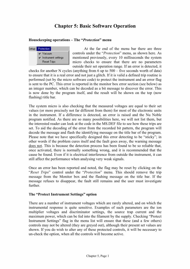
Chapter 5, Page 1

Chapter 5: Basic Software Operation

Housekeeping operations – The “Protection” menu

At the far end of the menu bar there are threecontrols under the “Protection” menu, as shown here. Asmentioned previously, every 10 milliseconds the systemmicro checks to ensure that there are no parametersoutside their set operation range. If an error is detected, it

checks for another N cycles (anything from 6 up to 500 – five seconds worth of data)to ensure that it is a real error and not just a glitch. If it is valid a defined trip routine isperformed (set by the micro software code) to protect the instrument and an error flagis sent to the PC. This error is reported in the monitor box error section (see below) asan integer number, which can be decoded as a bit message to discover the error. Thisis now done by the program itself, and the result will be shown on the top (nowflashing) title bar.

The system micro is also checking that the measured voltages are equal to their setvalues (or more precisely not far different from them) for most of the electronic unitsin the instrument. If a difference is detected, an error is raised and the Nu Nobleprogram notified. As there are so many possibilities here, we will not list them, butthe interested reader can look at the code in the MS.DEF file to see how these trips areset. To aid the decoding of the error from the recorded bit pattern, the program willdecode the message and flash the identifying message on the title bar of the program.Please note that we have specifically designed this error detecting to be “sticky”; inother words if the problem cures itself and the fault goes away, the warning messagedoes not. This is because the detection process has been found to be so reliable that,once activated, there is normally something wrong, and it is recommended that thecause be found. Even if it is electrical interference from outside the instrument, it canstill affect the performance when analysing very weak signals.

Once an error has been reported and noted, the flag may be reset by clicking on the“Reset Trips” control under the “Protection” menu. This should remove the tripmessage from the Monitor box and the flashing message on the title bar. If themessage refuses to disappear, the fault still remains and the user must investigatefurther.

The “Protect Instrument Settings” option

There are a number of instrument voltages which are rarely altered, and on which theinstrumental response is quite sensitive. Examples of such parameters are the ionmultiplier voltages and discriminator settings, the source trap current and themaximum power, which can be fed into the filament by the supply. Checking “ProtectInstrument Settings” flag in the menu list will ensure that these (and a few others)controls may not be altered (they are greyed out), although their present set values areshown. If you do wish to alter any of these protected controls, it will be necessary toun-check the option, when all the controls will become active.

Chapter 5, Page 2

The “Setup” menu

Preferences

On clicking on the “Preferences” option the following screen is displayed. A series ofCheck boxes are present, which define how the program will run. It is not expectedthat these will be altered very often.

Run offline: Tells the program that communication with the system micro isnot required, allowing the PC to run in a demonstration or debugging mode,disconnected from the instrument. If communication cannot be establishedwith the instrument immediately on starting the program, this mode ofoperation will be used by default. If this is not required, try rebooting the PCprogram. When this mode is in use, the title bar of the Nu Noble programprovides a visible feedback, since random numbers are being used for all datainput, which can produce some interesting effects if unnoticed!

Print Run Results: Enables the printer to record the results of analysisroutines. If not set, the results are still calculated and data stored to file, but nohardcopy output is provided during batch runs. In practice will probably not bealtered.

Do Tau Correction: Enables the software Tau correction to be used in theanalysis routines. In practice this should not be disabled since this will resultin (small) errors occurring in the recorded data. The facility to disable this isprovided merely to enable debugging to be undertaken if a problem issuspected with the Tau routines.

Chapter 5, Page 3

Use IC Gains: Enables the measured ion multiplier collector gains to be usedin each measurement, if they have been measured and input into the“Gain.dat” file, and not left at the default value of unity! This option is usefulif you wish to measure the gains, when disabling this option means that youdon’t have to deconvolute the old gain value from the recorded beam intensity.

Ion counting Enabled: Enables the ion counting beams to be recorded by theoperating system.

Zero with beam deflected: During the analysis routine, if this is ticked, during thezero cycle measurements, the beams will be deflected vertically at the source,so as not to pass down the flight tube.

Within the Serial Port Frame in the window are a series of Option (or Radio) Buttons.Only one of these buttons may be set at one time, if the setting is changed by enablinga new option, the present set one will be disabled. The settings within this framedefine which communications port is to be used for talking to the system micro. Inpractice the setting need not be altered unless a new PC is to be used. In such a case, ifthe port is different from that shown, the program will boot up in the “Off Line” mode,and the assignment can then be achieved (either by reference to the PC manual or bytrail and error) before the online communication is activated.

The second Frame identifies the directory where the raw data obtained duringanalysis runs together with the instrument run parameters at that time are stored. Thedirectory can be altered by selecting the “Change” button, whence the directory treewill be displayed. After selecting the new directory, use of the “Accept” button willensure that this path is used in future, whilst no change occurs if the “Quit” button isused.

The third frame identifies the analysis method to be employed during the datareduction program, and is discussed in depth in the relevant chapter.

The rejection level text box defines the value to be used by the analysis program whenit rejects noisy data points. With the illustrated value of 2, approximately 5% of thedata will be excluded from the data fits. If you wish to include more of the data, thisvalue should be increased using standard statistical considerations.

The Exit button will close this window, when the new settings will be stored withinmemory. Storage to file only occurs when the Nu Noble program is terminated.

MonitorThe monitor control produces the screen shown below for defining which instrumentparameters are displayed in the monitor window and updated each measurementcycle. Up to three ion beams may be selected and up to four general monitor pointscan also be serviced here. All the monitor parameters can be accessed and displayedusing other windows, so this approach does not limit the system monitoring, but ismerely provided to enable the points of most interest to be easily accessible.

Detector selection: Up to six ion beams may be selected for display in themonitor window. In practice the total number of beams and “machine monitor

Chapter 5, Page 4

items” (see below) is six, and if more than three beams are required, it may benecessary to deselect some “machine monitor items. If the full complementhave been requested for display, the program will not permit a further beam tobe selected. To choose a new beam, it will be necessary to deselect one ofthose already enabled first.

Machine Monitor selection: Up to three items can be enabled from the list, and aspreviously hinted, if three have been selected it will be necessary to deselectone before a new selection is permitted. The text shown is picked up from theMonitor.dat file, and may be altered if required. The selection shown enabledin this example refers to the output from source HT brick. This could be usedto monitor voltage breakdown in the source, for example. The output from thelast displayed machine monitor can also be plotted in real time in the magnetscans window (see below).

The Exit button will close this window, when the new setting will be stored withinmemory. The assignment of the displayed ion beams are stored on closing down thecontrol program, but the monitor selection information will be lost, since this isregarded as non-vital information.

Quad Values

This window enables the operating values for the two quadrupole lenses to be storedfor future reference. The form of the window is shown below.

The window consists of two main areas, the top being the data entry area, whilstbelow it is displayed the data which has already been input (and hence stored to file)previously. The data consists of four parameters, the axial (or reference) mass atwhich the observed quad values were obtained, the observed values of the quad(1)and quad(2) lens voltage, and a flag to say whether this data correspond to the“natural” zoom setting of the instrument. To see what this means, consider the case ofxenon, where, if we have an instrument with collectors set to record the Ar36,38 and

Chapter 5, Page 5

40 peaks, the “natural” zoom settings would have 6 amu between adjacent collectors.However it is useful in the case of xenon to have (say) 5amu between collectors forsome measurements. This data should then be entered with the “Standard ZoomUsage” unchecked. This will ensure that this particular set of data is NOT used in theleast squares fits of the quad voltages, within the program.

The utility allows one to estimate the zoom settings for masses not previously studied,by merely typing in the required axial mass, and depressing the “Estimate” button.The quad values may be downloaded to the mass spectrometer by use of the “Set”button.

If one wishes to edit an entry, or to use the utility to download a previouslydetermined value to the mass spectrometer, it is merely necessary to double click therelevant entry in the table, which will then load the selected values into the text boxes.

Setup Constants

If activated by clicking on with the mouse, twooptions are displayed, as shown here. If the“Instrument” option is selected, one can reset theinstrument to the complete set of runningparameters, which was stored when the programwas last shut down. These include the collectorgain values, the magnet calibration constants and

the Faraday Tau readings. This update is done automatically, but after this hasoccurred, the user is given theopportunity to download thelast saved HT and deflectorsettings to the system micro.The message box shown hereis displayed.

Chapter 5, Page 6

Whenever a message box is displayed, it must be acknowledged before normal controlof the program can resume. Thus one of the two options (Yes or No) must be chosenbefore you can continue. Since the option of not downloading the parameters is thesafest in this case, the program has been written to make that the default option, asshown by the command button being the more prominent of the two. As such hittingthe return button of the keyboard will select this option, or the mouse (left) button canbe used as normal. Selecting “Yes” will download these saved parameters.

It is also possible to save the present running parameters, via the “Save” option, andthe print out a hard copy, via the “Print” option.

It is also possible to save and update the run parameters (not the gains etc here) forindividual tuning conditions to and from named files. This option is useful, forexample, if one is studying more than one element, where the different element sourcetunings can be stored in different files. The standard file window is opened on eitherof these options, allowing the user to select the required filename, and if the“Initialise” option is chosen, the new parameters read from the selected file areautomatically sent to the instrument without the above message box appearing. Setup Mass Spec

This procedure will download the micro code to the system control, and as such isused if the mass spectrometer powerhas been disrupted, when themicro’s memory will have beenwiped, or if modification to the codehas occurred, for example if areassignment of ports was necessary.Due to the drastic effects this canhave to the unexpecting button pusher, a confirmation message box has to beanswered before the routine is started. This is shown here.

Again, the message box must be responded to before any further inputs to the mainprogram can occur. The default input is again defined to produce a “safe”, no-action,response by the program.

If activated the Nu Noble program will firstly down-load all the required drivers to thesystem control. The monitor box will display (in a slightly cryptic manner) theprogress during this operation. If the download is successful, a second message box isdisplayed, reporting this fact, which again must be acknowledged. Since the defaultstate of all variables has been predefined to be in whatever the save mode is, allvoltages will at this time be zero and all valves will close etc. The values for theseparameters saved to file, at the last occasion that the Nu Noble program was closed,are now downloaded to the micro. This results in a sequence of audible valve changesoccurring during this download process, but this is quite normal and should beperfectly safe. It is advisable not to try to carry out any operations during thisdownload and reassignment of operating parameters, since it cannot be guaranteedthat they will be correctly decoded until the micro re-initialisation process iscompleted.

Chapter 5, Page 7

File Menu

This menu provides a number of utilities of general interest for control of the printer.

Print Setup The first allows the printer format to be changed, which can be useful in the analysisroutines for reporting the observed results. On clicking on this option the standardprinter window appears. This window is the standard one provided by the Windowsoperating system for altering the printer properties. The form of this window can varydepending on the printer attached, although it’s use should be obvious.

Printer Font

This routine allows one to alter the default printer font and size used in recording theanalysis run results. The fonts available will vary depending on the printer andcomputer set-up, but it is recommended that a non proportional (i.e. fixed separation)font is used where each character uses the same width of printed output. This willensure that columns of data line up with themselves rather than producing a jaggedoutput. The window is shown below:

The names of the availablefonts are held in the drop-downlist, which may be accessed byclicking on the down arrow atthe right hand end of the textwindow. This is shownactivated in this example and assuch all the available fonts areshown in the list form and onemay be selected by doubleclicking on the required name.Using the “Test Fonts” buttonwill print out example text foreach of the available loadedsets. As mentioned above , a

non-proportional font such as “Courier New” is recommended.

The font size may also be selected from the available options using the smaller drop-down text box. If a size greater than 10 is chosen, it may be necessary to use alandscape paper orientation in order to ensure all the analysis data is correctly writtenon each line.

The final option under the “File” menu family is “Exit”. Clicking here will close theNu Noble program, storing to file the latest used values of the system operatingparameters, as it does so. If exiting is done using the “Close” button at the right handextreme of the title bar, the user is prompted to confirm that this is required. This

Chapter 5, Page 8

approach is adopted to ensure accidental closure does not occur if this button isclicked instead of its neighbour.

Magnet Scans

This routine is one of the major ones used and it will be well worth being familiarwith the various controls provided.

The window is shown above. On the right hand side are the check boxes to definewhich ion collectors are displayed. In this examples only the faraday is beingmonitored. The traces are colour coded to aid identification. If the “Ion Counting”option has been enabled from the “Setup” menu then the extra check boxes,corresponding to the extra possible multiplier channels, are shown corresponding totheir actual physical placements (as specified in the “Collector.dat” file, see above).Any number of detectors can be enabled, although obviously the screen can get a bitcrowded if too many are shown at once.

The scan range used is shown in the two text boxes at each lower extreme of the plotwindow. This range is divided into a number of discrete steps (in this example 100),and the scan process employed is to increment the magnet by a single step, wait for0.1 second and then read the required beams, after which the magnet is incrementedagain. The values used in these three text boxes by be altered by clicking the “EditScan” command button, when the boxes will no longer be greyed out (disabled), andnew values will be accepted. Clicking the “Save Scan” command button (the samebutton is now re-named) will permit these new values to be accepted, clear the screenand start a new trace. The program will protect against stupid values beingaccidentally input (e.g. a mass greater than 500) and if an error is detected the user

DAC Value

CurrentMass

Chapter 5, Page 9

must correct the mistake before the text boxes revert to their standard “greyed out”mode. Scan ranges where the start and end values are the same (to allow the user to siton the top of a peak for optimisation purposes) or the end is less than the start value(reverse scan) are acceptable.

Three modes of display are provided, as defined by the option buttons in the bottomright hand corner of the window:• Single trace: the scan is overwritten each cycle• Integrate trace: the scan displayed corresponds to the integrated average of the

beam from the time the scan region was last cleared. The number of the presentcycle will be displayed if this option is chosen.

• Overprint trace: the scan is overprinted each cycle. This mode of operationpermits one to compare peak shapes as (for example) the zoom lens settings arealtered and so find the optimised settings.

The “Stop” button (obviously) stops the trace at the present position. The caption thenchanges to “Start”. A number of buttons are disabled during the stop stage, to preventclashes due to timer problems. When the scan is stopped the “Set Magnet” button isactivated. Depressing it will cause the upper and lower values of the scan range to beset to the present values of the cursor, and the scan restarts, although obviously themagnet value does not change from the selected value. This facility is often used forbeam tuning, where one wishes to sit on a peak top. If selected, the button caption ischanged to “Restore Range”, and a second press will restore the previous upper andlower values.

When the scan is stopped, it is also possible to move the cursor (and obviously themagnet) by dragging it with the right mouse button depressed. Further double clickingthe left mouse button at any two points of the scan will reset the upper and lowermasses of the scan range to the values selected. This facility is often used to zoom inon a narrow peak to study its shape in finer detail.

The “Clear” will clear the display and restart the trace from the “Start Scan” value. Ifthe integrate mode of display is active, the sequence reinitialises itself and startsafresh, i.e. all previous information will be lost.

The “Print” button will result in a bit image of the window being sent to the activeprinter. The code automatically ensures that the maximum print size is obtained, andprints the date and time of the dump at the paper top. It is not necessary to change theprinter page orientation (using the “Printer Setup” menu) to ensure this pagealignment.

The “Exit” button will close this application, although there is a slight (1 sec) delaybefore this occurs to overcome timer clashes. The button is disabled once thecommand is accepted to give the user feedback that things are about to happen.

The current value of the magnet setting (in atomic mass units) is displayed at the topright of the scan region. This is the normal display. However to calibrate the magnetDAC (Digital to Analogue converter), which is required so that when you say “jumpto mass M”, the micro knows the DAC setting corresponding to mass M, one needs toknow the bit setting being sent to the system micro. This may be displayed if the

Chapter 5, Page 10

“Display Field” check box is enabled, as in the example show above. In this case asecond text window is displayed to the left of the mass value window, and this willreport the current DAC bit setting.

The present values for the maximum and minimum of the plotted beams are shown tothe left of the collector selection tick box. The values may be altered by doubleclicking on the required box, when a new text box will appear for the new requiredvalue to be entered. The value is accepted via the “ENTER” key, but if an error isdetected (e.g. the new maximum value is less than the present minimum) the text boxwill not be removed, and a valid data entry will be required.

Clicking the “Grid” check box will cause faint horizontal grid lines to be drawn on theplotting area, which is useful for monitoring peak quality.

In the example shown, we have checked the “Plot Monitor” check box in the lowerright hand side of the window. This has caused the extra check box labelled “MON”to appear below the ion collector boxes. If this check box is enabled, the program willplot the value of the last displayed instrument parameter displayed in the monitorwindow. This is useful if one suspects an intermittent fault with one of the instrumentoutputs, where glitches can now be plotted in real time.

If only one detector is selected (as in the case illustrated) the save to file button isenabled. This will allow the last completed scan to be output to a selected file (in CSVformat) for finer study offline.

Finally there are two options selectable when the scan is stopped, depending on thenumber of detectors enabled. If only one is checked, the button is labelled “Set (DeltaM)” as in the example shown. This is used if one is analysing in a high-resolutionmode, and requires the analysis program to sit on a plateau of a double peak. Thisoption is used to tell the program how far from the half height position of the peak tosit during the analysis, since (obviously) the normal peak centre position has nomeaning with such a profile. To use this facility, obtain a (good) peak shape of therequired composite profile, and then stop the scan. Move the cursor (using the rightmouse button) to the position at which you wish the analysis program to perform itsmeasurement, and depress the (now activated) “Set (Delta M)” button. The programwill calculate the offset from the selected point to the half height position and willreport the value in a message box. If you feel that the value is correct, accept it,otherwise reject it and have another go. During analysis the “Peak Centre” programwill determine the position of the half height and set the magnet at the stored offsetvalue from this observed mass.

If more than one collector is selected, the button caption shows “Optimise”. With thescan stopped, this feature allows one to automatically find the quad values which willresult in two selected beams being coincident. To operate, select the two beamsrequired (if more than two were initially enabled), depress the start button and followthe instructions in the message boxes displayed. Since the program uses the storedquad values to produce a least squares fit of these data in calculating the optimumvalues, this facility will only produce a sensible fit if the quad setting are reasonablyaccurate.

Chapter 5, Page 11

The Monitor Window

This will normally come up automatically in the bottom right hand part of the maincontrol window, and stays in position as this window is scaled (as opposed to theother windows, which keep their absolute position and may be clipped if the mainwindow is reduced in size). It contains four main areas for displaying information.

The values of (up to) three ion beams may be displayed on the right hand side of thiswindow. The identification of the beams displayed may be set from the “Setup” +“Monitor” window as explained above. The display units is volts for the faradaydetectors, which may be converted to the ion beam current by multiplication by thecorresponding preamplifier board resistor value (usually 1x1011 ohms) and cps for themultipliers.

The General monitor area can display the values of up to four monitor points, againselected from the “Setup” + “Monitor” window as explained above. Since these valuesare updated serially, if four are selected for display, each value is only updated onceevery four cycles. For this reason we normally recommend that the minimum requiredare shown, as in the example here where the source HT output is selected.

The message area contains a series of information messages to provide a history of themachine operation. Only the previous 100 items are displayed, and if more items arepresent than can be displayed, a scroll bar will appear on the left of this area to permitthe previous entries to be observed.

The trip area records the value of any instrument trips which have been detected bythe system micro. After the fault has been rectified, this trip area may be cleared byuse of the “Protection” + “Reset Trips” menu option.

To the right of this area, we report electronic errors, again using a bit code to indicatethe faulty control. Since the observed output value will only be (even approximately)equal to the set value if the unit is on, the code only checks these setting if the unit ison and often if the vacuum protection is enabled. The reported error may be clearedusing the “Protection” + “Reset Trips” menu option as above, and the faultinvestigated further using the independent monitor windows.

In the bottom right hand corner we display the current magnet mass, so that the userhas a visual check that the correct peak is being analysed during analyses runs etc.

Trip Area

Beam Area General Monitor Area

Message AreaElectronic Status

Chapter 6, Page 1

Chapter 6: Software Operation – The Control, Monitor,Calibrate and Utility menus

Control:

This section describes the use of the various windowsemployed in controlling the voltages and valves of the NuInstrument’s Noblesse mass spectrometer. On virtually alloutputs, the system micro can provide independentmonitoring of the actual (as opposed to set) voltages andthis section describes how this information can beaccessed. The family of windows under the “Control”button permit most of the required instrument parametersto be altered by the user, as is shown below. Clicking onthe relevant menu will result in the required window

appearing in the workspace.

We will describe each window in detail below, in order of (probable) use.

Preferred

This is a one-press shortcut to load the (most useful) of the windows accessible fromthis menu. It will load the Supplies, Vacuum, Digital and (if enabled in the Setupmenu) the IC supplies windows.

The “Vacuum” window

This displays the window representing the mass spectrometer vacuum envelope, anddisplays the pressures of the two ion pumps and the turbo speed, as well as the statesof the two pneumatic valves fitted as standard. The window also allows one to openand close these valves, by double clicking on the box representing the valve in thewindow. The box is dark, with a cross, if the valve is closed, and light if open. Asingle click over a valve will have no effect, for safety reasons.

Chapter 6, Page 2

The actual schematic was generated using the “Designer” software package suppliedwith the Nu Noble suite, and as such may be modified by the user, if so required.However, since the valve’s names are also hard coded into the software, please ensurethat these names are not altered.

Prep Systems

This option will appear if the user has createdanother schematic to represent part of thepreparation system, and which is connected to theinstrument.

We show the “Demo Prep” window, which isreferred to in the “Designer” documentation, inwhich two valves, a pressure gauge and a rotarypump have been drawn. Due to the intimatecoupling between the files generated by the“Designer” package and the Nu Noble software

suite, the valves may be operated in the same manner as with the main “Vacuum”window (double clicking), and the gauge readings are also updated continuously. Thesoftware “knows” of the presence of this second vacuum schematic from the relevantentries in the “Startup Parameters.dat” file. Please see the relevant documentation onthe “Designer” package for more information.

The “Supplies” window

This allows the user to alter the maininstrument source, quad and Faraday collectorvoltages. As may be seen, the window splitsthese tree groups into three “tab”, any one ofwhich may be selected by clicking on therelevant identifier at the top of the forms. Weshow the source tab, in which two of theparameters are “protected” to stop accidentalalteration. They may be enabled from the“Protection” menu, as mentioned previously.

The value of any of the parameters may bealtered, either by selecting it by swiping thepresent value with the left hand mouse buttondepressed, and then typing in the new value.The data is then accepted by use of the“ENTER” key on the keyboard. To avoid theproblem of a new value being typed in, but not sent out, the colour changes to greenuntil it has been accepted. Alternatively the value may be changed by use of the spinbuttons to the right of the displayed entry. These cause the value to alter in equalsteps, whose step size is set in the file “Deflector.dat” as discussed previously. Theprogram will not accept entries which exceed the minimum or maximum values foreach parameter, again as defined in the file.

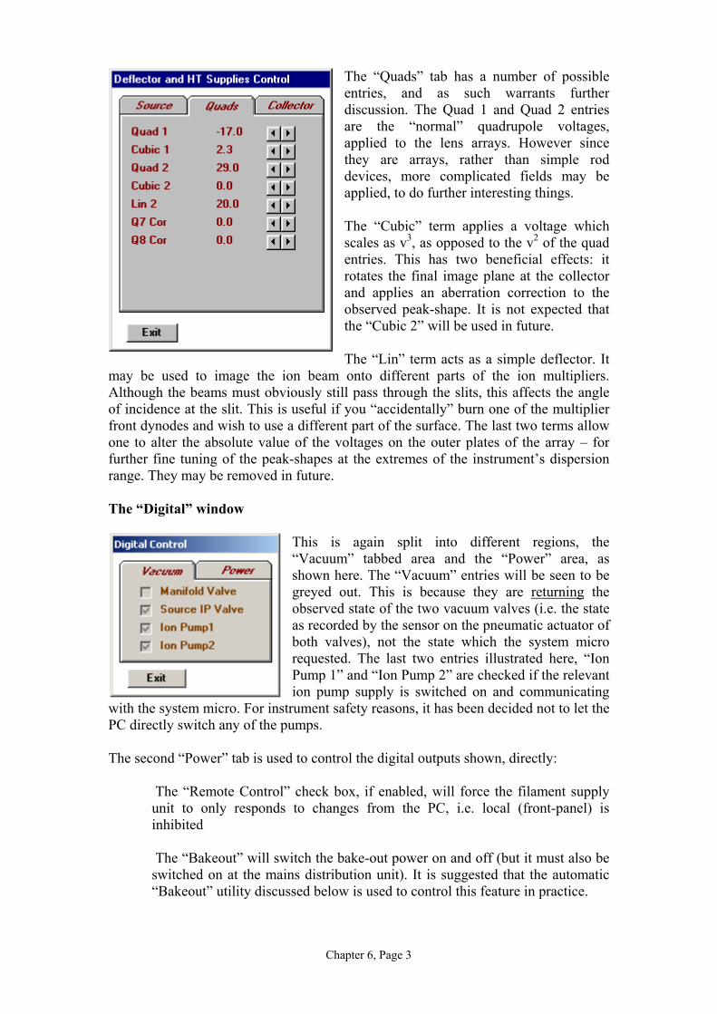
Chapter 6, Page 3

The “Quads” tab has a number of possibleentries, and as such warrants furtherdiscussion. The Quad 1 and Quad 2 entriesare the “normal” quadrupole voltages,applied to the lens arrays. However sincethey are arrays, rather than simple roddevices, more complicated fields may beapplied, to do further interesting things.

The “Cubic” term applies a voltage whichscales as v3, as opposed to the v2 of the quadentries. This has two beneficial effects: itrotates the final image plane at the collectorand applies an aberration correction to theobserved peak-shape. It is not expected thatthe “Cubic 2” will be used in future.

The “Lin” term acts as a simple deflector. Itmay be used to image the ion beam onto different parts of the ion multipliers.Although the beams must obviously still pass through the slits, this affects the angleof incidence at the slit. This is useful if you “accidentally” burn one of the multiplierfront dynodes and wish to use a different part of the surface. The last two terms allowone to alter the absolute value of the voltages on the outer plates of the array – forfurther fine tuning of the peak-shapes at the extremes of the instrument’s dispersionrange. They may be removed in future.

The “Digital” window

This is again split into different regions, the“Vacuum” tabbed area and the “Power” area, asshown here. The “Vacuum” entries will be seen to begreyed out. This is because they are returning theobserved state of the two vacuum valves (i.e. the stateas recorded by the sensor on the pneumatic actuator ofboth valves), not the state which the system microrequested. The last two entries illustrated here, “IonPump 1” and “Ion Pump 2” are checked if the relevantion pump supply is switched on and communicating

with the system micro. For instrument safety reasons, it has been decided not to let thePC directly switch any of the pumps.

The second “Power” tab is used to control the digital outputs shown, directly:

The “Remote Control” check box, if enabled, will force the filament supplyunit to only responds to changes from the PC, i.e. local (front-panel) isinhibited

The “Bakeout” will switch the bake-out power on and off (but it must also beswitched on at the mains distribution unit). It is suggested that the automatic“Bakeout” utility discussed below is used to control this feature in practice.

Chapter 6, Page 4

“IC Enabled” switches on and off the high voltage supplies to the ionmultipliers (and retardation filter if fitted)

“HT” controls the high voltage and extraction potentials of the source.

If one is switching on the high voltage to the source, the program will temporally setthe HT and extraction voltage to zero, then switch on the supplies, and then slowlyramp up the two voltages to their former values. This is done to minimise thepossibilities for flashover.

The “IC Supplies” window

This option is only enabled if the “IC Enabled”option is selected in the “Setup” window.

It permits the user to control the voltages on the ionmultipliers, the discriminator settings for each ICdetector channel and the voltages on the retardationfilter (if fitted). Since many of these parametersshould not be altered without due thought, they areprotected via the “Instrument Setting” protectionroutine described previously.

Also present in the window is a button used to “protect” the multipliers from largesignals. It has two states, the “pass” state as shown above, and the protected state

shown on the left, where the traffic light is on red and the electroncloud is absent from the multiplier dynode chain. Although youwill probably not protect the multipliers yourself, during normaloperation (since it will also kill the beams to the faraday), if theinstrument is forced to protect them automatically (due to a trip

state being reported), you will find that the protect state will be shown. To continue touse the instrument, it will be necessary to manually reset the button, since this is notan operation which can safely be left to automatic control.

The “Bakeout” window

This facility enables the bakeout operation to be terminated at a defined time, so as toallow the instrument to cool down before the morning shift arrives. The actualtemperature control of the heaters is by the regulators fitted to the mains distributionunit, but there is no power output unless the “Bakeout” digital output control is set.This utility controls this output.

It is also possible to control the power being applied to the filament during thebakeout process from this window. As may be seen, it is possible to ramp the filamentfrom a lower, to a maximum power value over a set number of hours. If this is active,the “Max Power” control on the “Source Supplies” tab (see above” will flash“Bakeout” to warn the user that it may not be set to the normal running condition.This option is only activated if the maximum power is equal or less than the “starting”value at the commencement of the bakeout process. Otherwise the program has toassume that the user has set the desired value automatically, and it will not change thesettings. Thus in order to use this option it will be necessary to manually bring the

Chapter 6, Page 5

maximum power down to (say) 3 watts before the bakeout cycle commences. Inpractice this is not a silly restriction, since it is not sensible to switch the power to thefilament to its full value until most of any impurities introduced during the ventinghave been removed.

Since the program can monitor the observed ion pump pressures, we also provide thefacility to suspend the heating either of their values exceeds the input set point. Due tothe time delay from ceasing the power to the heaters, and the pressure stopping to rise,if a problem is experienced, the value shown is considered a reasonable maximum.Also, to avoid any problems from a rapid change in temperature, the rate of rise canbe limited.

The “Switches” window

This may not be often used by the user, but permitsdirect control to a number of digital outputs andintelligent peripherals, fitted to the instrument. Theactual captions, and hence commands executed by thiswindow depends on the contents of the file“Switches.dat”, discussed above. In the exampleshown, we have set the file so that the two standardpneumatic valves are controllable by pressing thecorresponding button, and the awake user will noticethat the observed states shown agree with the

“Vacuum” window shown above. Also a series of “complex” commands aresupported, which may be displayed by clicking the downward arrow to the right of thecombo box. The command illustrated “Test SPC1” sends a serial string to the ionpump controller “SPC1, and the reply from that unit would be displayed in the toptext box. To send these commands, one uses the “GO!” button.

Possibly the most use of this option would be to check that remote “intelligent”peripherals are communicating before a batch run is started. Experience has shownthat many of the interfaces of such systems are not as robust as they should be, andthe use of a command such as “Send Version Number” or the equivalent, which

Chapter 6, Page 6

should cause a talking unit to respond with their current software version, isrecommended to check communications are OK. We have found a reboot of thecontrolling computer (not ours!) often reinstates control.

The Monitor Menus:

The various windows accessible under this menu bar are shown on the left. The maybe split into two main areas, those which just report themeasured value of an instrument parameter (not the set one),and the last two options which perform a series of tests tomonitor the instrument performance. The top option “Window”merely brings up the monitor window, which resides in thebottom right hand part of the main Nu Noble window. It willprobably only be necessary to use this option if you are runningthe program off-line, since the on-line mode will call up thewindow automatically. The layout of this window was

discussed previously.

The Supplies, IC Supplies, Vacuum and Magnet windows

We will deal with this group together since they are very similar. We show below theform of the supplies window, where it will be seen that most of the outputs controlling

the source and quad lenses are to be found. Many of these parameters were set upfrom the “Monitor.dat” file, and we show here part of that file to illustrate how thesewindows may be customised:

"VACUUM","Turbo1 Speed","%","LIN",2,0,10"SUPPLIES","Read Source HT", "kV","LIN",2,0,1"SUPPLIES","Read Half Plate V", "kV","LIN",2,0,1

The first line in this example (which isn’t the first line of the file) shows how the entrymonitoring the speed of the turbo will be reported on the “Vacuum” window. Thedescription , "Turbo1 Speed" must match the corresponding name in the MS.DEF filein order that the program knows where to pick up the required information. The finalparts of the string shows that the fit of the measured output (nominally a 0 to 10 voltsignal) is related to the required parameter (turbo speed in percent). The next twoentries are to appear on the “Supplies” window, and it will be seen that (in this case)the leading part of the string (the “Read “ part) has been striped off by the program.

This window also shows that the individual parts of the quad plate outputs are alsobeing monitored. We could have added this to the “Monitor.dat” file, but in practicethis part has been hard coded into the Nu Noble software for simplicity.

Chapter 6, Page 7

The Peak Flat Window

This window will run a peak flat analysis, simultaneously over a number of collectorsif so required (one of the marvels of multiple collection!). The form is shown below.

The collectors, which need to be characterised, are selected using the tick boxes (thetwo ion counters in the example shown) and the masses identified. The program is“intelligent” in that if one mass is entered, the others are automatically calculated(using the mass dispersion and input collector positions from the “Collector.dat” file.The peak to centre on is identified by double clicking the required mass, when itcolour changes to purple, as shown for the mass 36 in IC1 collector in the example.One must then also specify the mass for the zero measurement to be undertaken andthe time for the zero measurement, corresponding to the mass of collector selected forthe “centring”. The measurement process is split in to a series of cycles starting at thelow-mass extreme of the peak, taking seven measurements through the centre to thehigh mass extreme, and then back down to the low mass end again. This is done to tryto compensate for any beam intensity drift during the measurement process. The usercan specify the number of cycles per bloc, as well as the number of blocks in thewhole process. The program will limit the total number of cycles to 100.

If one wishes to change the total range of the analysis program (in the example it is setto ±100ppm) the new range may be entered in the text box in the lower right handcorner. To accept the value use the “ENTER” key on the keyboard, as normal, whenthe captions at the top of the window will also change.

To start the run, use the “Start” button. Each block is preceded with a peak-center run,and after each block is finished the intensities for the peaks, relative to the centreintensity, is reported in the relevant slot. This feature may be the main reason to splitthe measurement into a number of blocks, since the total program may take quitesome time to run, if a large number of cycles is selected. The program also reports thestandard deviation of each measurement. If the measurement is noisy, and the error islarge, it will default to printing a set of stars, so as not to overfill the text box.

Chapter 6, Page 8

The Faraday Noise Test

This utility records 20 individual measurements onall the faraday collectors present on the system,and then calculates the noise on that measurement.By default the integration time of one second permeasurement is used for each measurement, butthis may be changed to 5 seconds by checking thebox in the bottom right of the window.

To ensure that you are only measuring the noise ofthe detector, and the associated electronics, it isobviously necessary to ensure that there is no ionbeam (even a small one!) incident on the detectors.

The output may be printed, after the run, if a hardcopy is required.

The “Calibrate” Menus

Two utilities are provided under this heading, as shown here.

The Magnet calibration routine:

This utility is used to provide a least squares fit of the observed mass against therequired digital to analogue converter output in the magnet controller, the form beingshown below.

As discussed in the section on the magnet scans, it is possible to obtain the DACsettings at any time from that window. Thus using a series of impurity peaks, or peaksfrom an air slug, a set of data spanning the required range of use of the instrumentmay be obtained. These can then be input into the text boxes at the top of the presentwindow, the desired order of fit selected (usually 2 or 3) and the fit calculated via theuse of the “Calculate” button. The data set may be reanalysed as often as required,changing the fit order or removing or editing entries.

To select an entry from the editable section of the table, simply double click therequired entry, which will then result in the data being transferred into the data entrytext boxes. Once a satisfactory fit is achieved, the data may be stored to file using the“Save” button.

Since the formula relating the magnet radius, mass of the ion and the magnetic field isof the form:

_______Radius = K x √ ( mass) / field

Chapter 6, Page 9

where K is a constant at fixed acceleration energy, we see that to first order that themagnetic field is proportional to the square root of the mass. We have therefore used aroutine to fit the DAC setting (i.e. field) to the square root of mass, in the form:

DAC setting = A + B * (mass)½ + C * (mass) + +

This approach will be found to be much more satisfactory than the more normalapproach of fitting DAC steps to a straightforward power relationship in mass, whenhigher orders in the fit are required.

The user should be a aware that when a new data set is stored, any data stored by thepeak centring routine will be obsolete. As such the files associated with this routine(see below) are purged, and the program will start with a new slate.

The Tau Correction routine

The “Tau correction” refers to the decay experienced by the faraday detectors whenthe incident intensity suddenly changes. Since the feedback resistor in thepreamplifier is so large (normally 1011 ohm), any small parasitic capacitance canresult in unexpectedly large decays as the intensity changes. Thus a 1 pico Faradcapacitance will give a decay constant of 0.1 secs, which will mean that the signal willdecay to only 45ppm of the original intensity after one second. This is the limitingfactor for undertaking fast measurements with a faraday, since in practice thelaminated magnet can normally move faster than this.

To compensate for this effect, we have provided a utility to measure this decay, andthe analysis program then uses this data to “correct” for the observed decay to emulatethe response of an “ideal” system with minimal stray capacitance.

The program performs the following series of actions:

Editable section

Chapter 6, Page 10

Firstly the beam is switched off the collector and the zero is obtained. This value isnot critical, since it is merely an offset, but a reasonably accurate value ensures thatthe displays are drawn sensibly during the run.

A series of measurements follow, in which the beam is placed onto the detector for 10seconds, and the switched off (by going to the half mass position). The intensity of theobserved signal is then recorded for the following 30 seconds. The data is integratedfor the required number of cycles (10 in the given example), and at the end of themeasurement the data fitted to a double exponential decay. The program then showsthe “ideal” fit, the observed data set, and the observed data set corrected with the idealfit.

If the run is satisfactory the data should be saved.

The “Utilities” menu

Three menu options will be discussed here, the other two (“Reanalysis” and “CreateAuto Sequence”) being more conveniently covered in later chapters.

Two of these other utilities are provided to produce low level control of theinstrument, and may well not be ever used on site. The “Hysterisis” routine willenable the magnet to be de-gaussed, if ever required, by sending it through everdecreasing field cycles (starting with full maximum to full minimum, reversed, fieldextremes). The window also “hides” the routine to download the parameters to themagnet slave unit (See chapter 2), which may be accessed by dragging the right handedge of the window sideways.

The “Interrogate Micro” utility will allow the user to directly access the individualmemory locations of the system micro. The utility accepts both integer and Hex wordinput, and can both read and write to the designated memory location. It also accepts

Chapter 6, Page 11

both the normal (16-bit) word and (32-bit) long word formats, selected using thecheck box on the form.

The final utility discussed here, enables the multiplier running voltage to be found.Basically the utility will alter the tuberunning voltage and plot the observedresponse as it does so. To use this utility,firstly set the magnet so that a peak of afew thousand cps is incident on themultiply you wish to use. We assume thisis IC1 in what follows. The select the“Find IC Plateau” menu option, when thewindow shown here is displayed. Selectthe required detector from the list, andchange the values shown for the voltagerange and maximum beam permitted, ifthe default values are not suitable. Hittingthe “Start” button will cause the following

window to pop up, and the scan will automatically start. When completed, the entrymultiplier voltage will be shown as the dotted line. If you wish to change the setvoltage, do so via the “IC Supplies” window, and (probably) repeat the plot using the“Rescan” button.

Chapter 7, Page 1

Chapter 7: Data Acquisition

Overview

This chapter describes the data acquisition process with Noblesse.

We start by describing how to a create a basic mass-data-file (mdf file); this filespecifies which masses and collectors to use and measurement times.

Having created the mass data file; we must then create a corresponding calculation-run-file (or NICE file). NICE is Nu Instruments Calculation Editor; we use it to obtainuseful results by doing calculations involving the parameters measured by the mdf file(for example, subtracting a detector baseline, or calculating the ratio of two isotopes).

Next we describe how to start a single data acquisition run. Finally, we describe batch and sequence files, to show how Noblesse may be used toobtain data in batch mode.

Data analysis is described in chapter 8.

Starting from Scratch – the mass data files

We will firstly discuss the setting up of theanalysis files which will define the sequence ofevents to be undertaken during the analysis.Assuming that a completely new analysis is to beundertaken, select the “New Routine” from the

pull down menu, when thewindow shown here will appear:

We will now describe each entrysection in detail.

Collector identification: Theprogram produces a series ofcheck boxes, representing theapproximate position of thecollectors fitted to the instrument,as shown above for a quad (3×ICplus high mass Faraday)configuration. This information isobtained from the “Collector.dat”file. Ensure that you check thedetectors that you wish theprogram to monitor during theanalysis you are designing.

Chapter 7, Page 2

Number of zeros and steps: This defines the number of zero measurements(obviously), up to a maximum of two, to be carried out prior to each sequence ofbeam measurements. We call the number of succeeding different beam measurementsthe “number of steps” in this table. Thus suppose an experiment was being designedusing only the axial Faraday (in this example configuration) and you wished toperform a series of measurements of argon, recording the following sequence for anumber of times:

Measure zero 1 at mass 39.5Measure zero 2 at mass 40.5Measure mass 40Measure mass 36Measure mass 37Measure mass 38Measure mass 39

This set of measurements would be identified as two zero measurements followed byfive steps of measurement. The actual values may be selected using the up-down spinbuttons at the right hand side of the relevant entry box.

Use Standard Mass Dispersion: When the next window is displayed, theprogram will try to be “intelligent” and fill in all the masses for each cycle, when anyone mass is entered. This can obviously save a lot of typing, but it does need to makea number of assumptions to get this correct. The definition of “standard” is the sameas discussed previously under the Quad Values window discussion in Chapter 5, andwill not be repeated here. However if any one of the analysis cycles does not use thestandard dispersion value for the instrument of 480mm, uncheck the tick box and youwill need to give the (approximate) values in the next window. In practice this is onlylikely to occur for Xenon analyses.

Peak Centre Mode: There are two possible analysis modes to use with theinstrument. The first, most common one, assumes one has a clean, single peak, andthe program can undertake a “standard” peak centre and sit in the mid point (asdefined as the mid way between the half height at the start of the peak to thecorresponding half height position at the end of the peak). The other mode ofoperation analyses a peak which has a shoulder before (or after) part of the peakcontaining two components. The peak centring routine will then find the half heightposition at the start (or end) of the observed peak profile, and sit at a defined offsetposition from this point. The section describing the magnet scans described how to setup this offset. It is possible to mix these two types of requirement in an analysis, but ifany of the peaks are of the shoulder type, it is necessary to select this option at thisstage, and you can define which step does what later.

Quad Control: The Nu Instruments’ Noblesse mass spectrometer is unique inthat it can allow multiple collection of beams, and change the dispersion during theanalysis. This enables coincident detection to be achieved at differing axial masses.To achieve this, the voltages on the quadrupole lens arrays are altered during theanalysis sequence, and the option boxes in this section define the three ways this maybe done. Obviously no change in quad settings will not maintain exact coincidence

Chapter 7, Page 3

during the analysis, but the option has been added for completeness. However, it isalso the option used (obviously) if only a single collector run is being contemplated.The “Best Calculated Value” option will use a least squares fit of the data saved bythe “Quad values” form, again emphasising why this data should be accurate.

Preferred analysis Method: Since different methods are provided to analysethe time decaying data, it has been noted that different methods may be optimal fordifferent gases. By defining the preferred method with the analysis file permits multigas analyses (eg Helium followed by neon) to be more conveniently undertaken. Thechoice may be altered during reanalyses by altering using the “Setup” + “Preferences”menu, discussed in Chapter 5.

Once this form has been completed, you can proceed to the next one by depressing the“Continue” Button. We will firstly look at a simple, single collector analysis and thencontinue with a more complicated example.

A simple example:

The window corresponding to the argon analysis described above is shown below. Nomasses have yet been entered, but we were in the process of typing in the mass valuefor the first zero cycle, when the screen capture was made. Moving the cursor to therelevant box and pressing the left-hand mouse button will result in the verticalflashing cursor to appear, and the required data can then be entered. Once it is input,the data is accepted using the “ENTER” key of the keyboard, as usual. Thus we wouldtype 39.5 into the first text box illustrated, if we were setting up the analysis discussedabove.

Once the masses have been input, the required integration times for each measurementshould be decided upon and entered. The magnet delay time (the time between the endof one measurement and the start of the next, allowing the magnet to settle after themove, and the signal to decay to a reasonable level, as discussed above under TauCorrection) and the total number of cycles input should then be decided and input. If

Chapter 7, Page 4

you do not wish to undertake a zero measurement each cycle (for instance if you aregetting this data from a previous analysis and passing the data to this run (see below)then uncheck the relevant box. (If you do not wish to record any zero measurementsas part of the analysis, the set-up form will allow a zero input for the number of zerocycles.)

Finally you should decide which peaks should be used for peak centring. This is doneby double clicking the required mass, whereupon the selected box will have a yellowbackground, to mark the selection. Double clicking again will undo the selection.

The ‘rules’ regarding the centring requirements are as follows:

It is permissible to have no selection, as for example would be done for “Blank” runs.In this case (obviously) no selection should be made. In this case the program willsearch the database kept by the peak centring program to find the last time that themass was successfully centred, and it will then use the stored “correction factor” toextrapolate from the typed input mass to the actual, observed, central mass. If no datais present (the peak had not been previously centred) the program uses the values ofthe correction factor for the first peak it finds in the list of the required masses,starting by searching for entries for masses entered in the table prior to the one inquestion, and if none are found, the program will search for the succeeding massentries.

Any number of beams may be selected for centring, but if any are, then the firstmeasurement step must be one of them. The reason for this is due to the way theprogram allocates the “correction factor” to go from the input mass to the actual,observed, central mass. The program will always search for the data for previous massentries in this case. This is done to allow for the case where one analysis is used tomeasure two elements. Thus a simple Argon followed by Neon analysis could use themass 40amu beam to determine the correction offsets for all the following argonbeams in the list, and the neon 20 beam could then be centred to give the correctionfactor for the subsequent neon peaks.

The analysis program will also use the correction factor measured for the firstmeasurement step to calculate the actual mass to be used for the zero measurements.This is unlikely to be a problem in blank measurements, again making therequirements less severe for the case where no centring is requested.

Once the table has been set up, the data may be saved using the “Save” button. Theprogram then performs a series of checks before proceeding, to ensue all data hasbeen input and is valid. If the number of centring masses is less than the number ofanalysis steps, it obviously does not know whether this is correct, or that an error hasoccurred and the table has accidentally not been set up properly. In this case thefollowing message box will appear:

Chapter 7, Page 5

In this example, centring is only required in the case of the 40Ar beam, and itscorrection factor will be used for the subsequent measurements. Since this is intended,answer “Yes” to the question (the default reply) and the program will continue withits checks.

Once these have beensuccessfully completed, thestandard “Save” Windowsdialogue window will appear,permitting the user to save thefile with whatever name isrequired. To enable the NuNoble program to find the fileduring subsequent analyses, theextension is restricted to theMDF type shown. Also notethat the user will have toprovide a program to convertthe observed beam intensitiesinto required isotopic ratios, andthis will be achieved using the Nu Instruments Calculation Editor program, which isdiscussed later. However the files created by that program must match the names ofthe files saved here, again to allow the Nu Noble software to find these programs.

A more complicated example:

Here we have chosen just about every combination possible, to illustrate the variousentries.

Firstly, we unchecked the“Use Standard Dispersion”box, since we will set up astep measuring 128Xe with134Xe (which can beregarded as “standard”) aswell as one simultaneouslymeasuring 129Xe and 134Xe,which is not. Thus enteringthe mass “134” in the step1,

Chapter 7, Page 6

IC0 box will produce the entry “128” in the IC1 box, but to obtain the required “129”entry for the second step, one has to increase the dispersion to about 580. Note twothings here. Firstly the form loaded with the standard dispersion value filled into allthe entries of the relevant, dispersion, row. Only in the case of the steps that are non-standard is any extra data required. Also you can use the form itself to estimate therequired dispersion value. Simple keep trying different values as you re-enter the firstmass, until the other masses correspond to their required values.

Since the quad values will be completely different for these two measurements, wehave selected to type in their values into the table. They can be found most easilyusing the “optimise” feature in the magnet scans window, as described previously.

Finally we have assumed that in one of the cases, we will study the peak in a doubletform. In this case we have to indicate this by double clicking the “Use Offset” box forthe corresponding step, whereupon a “YES” will appear in that box.

The final, completed, form isshown here. We have assumedthat the 124 peak has a smallimpurity under it, which can beresolved out to produce adoublet with a shoulder for thepure 124Xe. Notice also the useof two slightly different inputmasses to represent the 134Xepeak, which will be centred onin two different steps. The reason for the use of these different masses is because thepeak centre routine keeps a database of the successful centring sequences, and wewish to distinguish between the case of normal zoom and the larger dispersion case.This ensures that the program doesn’t try to use the data from the first peak centre inthe second case, where the mass correction factor is expected to be completelydifferent, due to the differing zoom values.

Modifying an old analysis routine

The routine to be edited may be selected via the “Old Routine” menu option,whereupon one can select the required routine for the “Open File” dialogue box. Theprogram will then load the completed table for you to edit as required.

You must now provide the Calculation code to go with this analysis.

The Nu Instruments Calculation Editor (NICE)

This program is provided to interface with the main control suite of the NuInstruments Noblesse mass spectrometer. The control programs themselves do notconvert observed beam signals into “useful” values, such as isotope ratios, since thereare too many different possible combinations. It would not be sensible to try to hardcode all these possibilities. Instead we have taken the approach of separating the

Chapter 7, Page 7

recording of the beam intensities from their conversion into “useful” data. Whathappens in practice is as follows.

The main controlling software will record the beam intensities on the detectorsselected. These intensities are then sent across to a second, independent, routine wherethe individual values are combined to give the required results, they are then sent backto the main program to be displayed, and statistically treated, if required. Thussuppose we have a simple two-collector experiment, where beams are recorded ondetectors number zero and one. The signals recorded by detector number zero may be2.5 units, whilst that recorded on the detector number one is 7.5 units. This would beall that the controlling software is aware of, but the user may be interested only in theisotopic ratio given by the ratio of these two signals. (We will ignore such things aszero offsets in this example!) It is the job of the second routine to do this conversion.In this simple example the formula may be:

Required Result = Signal(1) / Signal(0)

which then gives the measured isotope ratio of 3.0.

This number can then be sent back to the main controlling software.

As will be obvious from this simple example, there is one more piece of information,which we need to send to the controlling software suite, namely the description for theresult. It is of little use displaying a table of the form:

First Result 1.2345Second Result 2.3456Third Result 3.4567

Rather we might wish the display to be in the form:

132 / 130 observed ratio 1.2345134 / 130 observed ratio 2.3456136 / 130 observed ratio 3.4567

The second job of the editor is thus to define these titles.

For most noble gas analyses, it is necessary to take into account the variation of thebeams during the analysis time, and extrapolate the data to obtain the signals at gasinlet time. The Noblesse software has a comprehensive set of curve-fitting features,which are described fully in chapter 8. For the time being, we note that the crf filemust be set up prior to acquiring the data, independently of the details of the curvefitting.

Running the Editor:

The editor may be launched via the NICE icon on the desktop. The basic form of theeditor can be seen from the example shown on the next page, which has obviously hadsome code typed into it.

Chapter 7, Page 8

The menu bar is of the conventional format. Files may be read in, saved or printed bypressing the “File” menu and choosing the required option from the drop-down list.Editing of the code may be undertaken via the “Edit” menu options, although thestandard shortcut keys also work:

Crtl + “z” CutCrtl + “c” CopyCrtl + “v” PasteCtrl + “z” Undo.

Since the compiler is line-number aware (you will already have noticed that the statusbar at the bottom of the screen shows that the cursor is on line 16 – in fact on the

Chapter 7, Page 9

extreme RHS), we have also added a “Go to” line option under this heading. The codemay be “compiled” into the required format, by using the “Project” menu.

New analyses may be saved via the “Save As” menu option, which will prompt theuser to type in the new file name, whilst the “Save” option will overwrite the originalfile with the new one. The original file name is shown in the leftmost panel of thestatus bar on the bottom of the editor screen. The name used should be the same asthat of the corresponding mass data file (“Ar3638multi” in the example shown),and is saved with the “CRF” (Calculation Run File) extension.

The Editor language:

A simple glance at the above example will show most (but not all) of the languagesyntax.

The top of the code area should hold the declarations of all the variables and constantsto be used in the program. The compiler is very “strict” in this manner – everythingmust be declared, but then any “typos” or other simple errors will be found early on.All variables are treated as 32bit (double precision) numbers and there is norequirement to distinguish between integers and non-integers. All constants declaredhere (see below) are similarly held to this precision. The names are totally caseinsensitive. Thus the following are all equivalent:

NAME1 name1 Name1 NaMe1,

and any other combinations you wish. Obviously some are more sensible than others.

The words “Dim” and “Const” are two examples of what is called “reserved” words.These are words which have a special meaning to the compiler, and may not be usedas general variable names. The full list of these reserved names is:

DimConstRetainRetain KeyMass( , )Zero( , )Calib( )Result( ).

and their meanings will become apparent as we progress.

Comments can appear anywhere in the code. All characters after and including thesingle quote (‘) are ignored by the compiler. To aid readability, these comments areshown in green by the editor, as soon as the line is changed. We recommend the fulluse of comments, since you will probably not be able to follow the logic of theprogram when you revisit it after a long absence if they were absent.

The observed intensities measured by the main instrument controlling software areheld in the arrays “Zero(X,Y)” and “Mass (A,B)”. The first of the two parameters

Chapter 7, Page 10

inside the brackets define the step of the measurement sequence. Thus for the NuNoble software suite, two zero steps are possible, and twenty measurements steps arepermitted, giving the possibility of X having the value 1 or 2, whilst A can range from1 to 20. Unfortunately it is not possible for the compiler to check that valid parametersare entered here, although the main program will check the compiled code, so pleasetry to ensure their validity as the code is written. The second parameter (Y and Brespectively), define the collector identification, starting with collector zero as the onein the highest mass position. The numbering goes from zero to the total number ofcollectors minus one. Be careful with this notation: in the examples shown, thecollectors were IC0 (high mass side), Faraday (axial), IC1 (low mass side). It does notnecessarily follow that collector ICn is always collector n! Normally we are notinterested in the values of these variables, but their corresponding differences, whichis the signal due to the beam (removing any electronic offsets), and the first part of theillustrated code shows these values being obtained:

Ar40 = Mass(2, 1) - Zero(1, 1)

Thus the Argon40 beam is the difference between the intensities measured oncollector one in the second measurement step and the zero beam measurement, etc.

The answers to be returned to the main instrument controlling software are given bythe array “Result(Z)”. Up to thirty results may be determined, corresponding to the Zparameter having a value between 0 and 29 inclusive. The actual number beingcalculated may be set by using the up-down “Spin” selector at the upper right of thewindow. In the given example, six results are calculated, but not all of the code isvisible in the window. The scroll bar at the right of the code window would havepermitted the rest of the code to become visible in the real case. The answer captioncorresponding to each of these returned results may be entered in the table above thecode region, which in this example is displaying the first four captions. Ensure thatthe “ENTER” key is pressed after changing or adding a new caption, to force theprogram to accept it.

As implied above, it is also possible to define constants in the body of the text. Thusfor example, we could define True_R as a variable, and add the line:

True_R = 0.7219

or use the definition :

Const True_R = 0.7219

at the top of the form after the “Dim” statements. This approach is not recommendedhowever, since it will only store the constant to 16 bit (single precision) accuracy, andthe first method of defining the constants at the top of the program is stronglyrecommended.

The arithmetical functions supported are:

+ (add), - (subtract), * (multiply), / (divide) , ^ (raise to the power), Sqrt (the squareroot of), Exp (exponential), Log (natural logarithm) and = (equals).

Chapter 7, Page 11

To aid readability of the source code, the editor will check that any constants orvariables match the case as typed. Thus if the variable “Ar40” is defined at the top ofthe program, the editor will match this typing all through the code, with the first letterbeing upper case. Similarly, if you decide to change this at a later stage for somereason to “ar40”, the editor will automatically update all references throughout thetext. Further, as a second aid to readability, reserved words such a “Mass” and “Zero”appear in a different colour to the main text. Finally, the number of spaces isautomatically sorted to sensible values.

Passing data from one analysis to another:

Sometimes it is useful to use data from one experiment in a subsequent one. Oneexample of this would be if one wished to measure the “blank” rather than use beamzeros in the calculation process.

To facilitate this process, we have provided the “Retain” feature. To illustrate this, wewill consider the case where the blanks are measured in the first experiment, and theirvalues used in a second (as shown in the example above).

1) The calibration process (saving parameters for use in a later analysis) The required code to do this is shown below:

The “Retain” statements tell the compiler which of the results are to be stored, whilstthe key ensures that the correct calibrations are picked up by the following analyses,and not some determined in an entirely different program.

2) The use of these values in another routine (reading in parameters from an earlieranalysis)

At the top of the code in the program used with the samples, add the same RetainKey:

Retain Key = AnyNameYouWishAsOneWord

You can then use the Calib variables in the code that follows, and the main programwill inset the final, averaged, values determined by the previous standard run. Theprintout of these analyses will show these values amongst the heading information, to

Chapter 7, Page 12

enable you to be sure of what has happened. Note how the example given allows forany changes in electronic zeros between the two measurements (although this shouldbe minimal).

The Compilation Process:

To initiate the compilation, use the “Project” + “Compile” menu tree, as mentionedabove. This option is only active if the source has been saved.

The compiler will try to find any errors before finalising the compilation process. Theprocess is stopped at the first error found, the form of the error indicated in a messageand the editor then highlights the line in which the problem is located. If no errors arefound, it will produce a file with the “NCC” (Nu Compiled Code) extension, which isused by the main program to obtain the required displayed answers. The analysis file,calculation file and compiled file should all be in the same directory, since the maininstrument program uses the selected path of the analysis file to look for thecompilation code.

Successful compilation is indicated in the rightmost panel of the status bar at thebottom of the editor window. Although the compiled code will be automaticallystored, the source code is not. Thus if you have to make corrections to get thecompilation process to go to completion, please ensure that you also save the finalsource. Obviously any subsequent changes will also require the new code to be savedand the new version has also to be recompiled.

Some errors may only become apparent once the analysis is run. The most common iswhen one of the variables has a zero value due to a mistake in the code and it is usedon the bottom line of a division. With previous editors, the user is given littleassistance in finding where the problem lies. However we have designed this editor tobe as user friendly as possible, and if such a problem does arise, the line where theerror occurred will now be indicted by the main instrument program.

Single Data Acquisition RunsPreliminaries

Clicking the “Do Analysis” menu option under the “Data Acquisition” header willresult in the following window being displayed:

Chapter 7, Page 13

This will allow the user to browse the directories for the required (.mdf) analysisroutine, via the standard “Open” dialogue window. The two options on the windowallow the user disable the automatic peak centring when the run is started, and tocontinue if an error is detected, rather than the default of stopping in such a situation.

Once the file has been selected, the “Start Run” button is enabled and on pressing itthe main analysis window is loaded.

The Analysis window

When originally loaded, it is fairly bland, with only the predominant “Start” buttoncatching the eye. However the user will note that the program has picked up the activecollectors and displayed them in the centre top of the window. Also the sample nametext box can be filled in at this time (and it is probably sensible to do so before it isforgotten).

Once started the program will reference all timings to the time the start button waspressed, so if you are letting in a sample from a manifold it is best to start the analysisas soon as the manifold valve is opened. Ways to allow for this accurately duringautomatic runs are discussed in Chapter 9. Obviously this is easier if the run isautomated, but that comes later!

After the start is pressed, the program will automatically peak centre the requiredmasses (as long as this option wasn’t disabled in the window shown above), and thenstart the data collection process. In a simple analysis this will involve:1. Move the magnet to the position for the first zero step2. Wait the “magnet settle time”3. Measure the first Zero intensities4. Move the magnet to the position for the second zero step (assuming two zeros)5. Wait the “magnet settle time”6. Measure the second Zero intensities7. Move the magnet to the position for the first measurement cycle8. Wait the “magnet settle time”9. Measure the first set of beam intensities

Etc etc.

The program uses one second integration periods for all its data collection, and thecurrent time during the run will be shown in the right most text box at the windowtop, 76 seconds into the run in the example shown here. Please note that this time isthe time since actual data acquisition started (i.e. excludes the time for peak centringetc) and not the time from the commencement of the run the pressing of the startbutton. The difference is stored in the memory and used in any analysis.

Chapter 7, Page 14

The program plots all the beams being recorded, and hence the trace can be a bitconfusing if more than a couple of detectors are enabled. By default the program picksup the beam scaling (maximum and minimum values) from the magnet scans window.

In the trace shown, the recorded signal is showing the following measurements:1. The zero measurement2. The 40Ar signal (off scale here)3. The 38Ar signal4. The 36Ar signal

The process is then repeated. The green vertical line indicates the separation betweeneach cycle of measurements, and each cycle is identified, as shown.

For the form, it is also possible to:

Plot the data in a log, rather than linear, format Plot the isotopic ratios, rather than absolute intensities (if more than one beam is

measured!). All plots are to the same denominator signal. Alter the scaling of any, or all, of the recorded signals. Look back at previously recorded data using the slider bar at the bottom of the

trace. Show a different time scan by altering the “Scan Range” value box

However it is not recommended that you try to do too many of these thing while theinstrument is collecting data, rather please wait until the acquisition has finished.

Chapter 7, Page 15

The “Scaling” window

This allows the minimum andmaximums of the recorded beamsto be altered. The collector isselected by double clicking theentry on the list, whence theentries are transferred to the twotext boxes. In the example shownthe Faraday entries have beenselected for editing. The valuesmay then be changed and the datastored via the “ENTER” key, asnormal. The program stores the

plotting range, with other information (see below) and so once altered, the ranges willbe permanently related to this data run.

The plots will be seen to alter as soonas the new values are entered.

If the ratio plot is enabled, the scalingwindow will permit the denominatorbeam to be altered, as well as changethe plot intensity range of the scans.To change the denominator, click the“Select Denominator” button, and aset of option buttons will permit thereference beam to be changed.

Batch Runs

Preliminaries

The Nu Noble software suite can handle automatic sequences (including analysis), toenables automatic preparation system to be controlled. Two independent sequencescan be run simultaneously, allowing, for example, a sample to be prepared in themanifold whilst its predecessor is being analysed in the mass spectrometer.

The program accepts a series of types of commands, which are concatenated to form ascript-like series of instructions. The sequences are stored as readable text, and thesequences could therefore be generated using any standard text editor. We alsoprovide as utility to generate these files, and the user is recommended to use thisapproach to minimise any errors, and to make use of the internal checking facilitiesthe utility undertakes before the data is saved to file.

Chapter 7, Page 16

Supported Commands

We will separate the current commands into to sets, the first consisting of simpledirect commands, whilst the second group permit control of “intelligent” peripheralsusing a serial interface. The list is contained in the file “Supported Commands.DAT”,and you may wish to separate out those which you do not think you will use, and thusrestrict the choice in the pull down list in the window used to create the run sequences(see below).

The current full contents of the file is shown here, where the commands and theirstructure can be seen:

"Switch On",1,"Name""Switch Off",1,"Name""Switch On Identified",2,"First Part", "Identifier""Switch Off Identified",2,"First Part", "Identifier""If Beam(I)<=X",3,"Axial Mass","Collector","Test Value(X)""If Beam(I)>=X",3,"Axial Mass","Collector","Test Value(X)""If B>=X",2,"Sensor(B)","Test Value(X)""If B<=X",2,"Sensor(B)","Test Value(X)""If B is True",1,"Input(B)""If B is False",1,"Input(B)""Delay",1,"Secs""Acquire",0"Set Start Time",0"Wait for OK to Start",0"OK to Start",0"Wait for OK to Proceed",1,"Analysis File""OK to Proceed",0"Go To",1,"Step""Abort Batch",0"Load Tuning",1,"File Name""Send String(1)",2,"Port","String""Send String(2)",3,"Port", "String(a)","String(b)""Send String(3)",4,"Port", "String(a)","String(b)","String(c)""If Reply is NOT(1)",3,"Port","String","Reply""If Reply is NOT(2)",4,"Port","String(a)","String(b)","Reply""If Reply is NOT(3)",5,"Port","String(a)","String(b)","String(c)","Reply""If Reply is NOT(with Timeout)(1)",4,"Port","String","Reply","Secs""If Reply is NOT(with Timeout)(2)",5,"Port","String(a)","String(b)","Reply","Secs""If Reply is (with Timeout)(3)",6,"Port","String(a)","String(b)","String(c)","Reply","Secs""EOF"

As will be seen the format is the command name followed by the number of inputparameters, which are required to be associated with the command. The nextparameters in the string will be the title of the prompt, to identify the parameter in theinput utility. For example, with the “Delay” command, one will need to specify thenumber of seconds for the delay, so the identifier has been called “Secs”.

We will now discuss the individual commands in detail.

Chapter 7, Page 17

The “Direct” commands:

OK to Start, Wait for OK to start, OK to Proceed and Wait for OK to Proceed

In order to have two sequences running concurrently, the program needs some way ofknowing:

a) when it is safe for the next sequence to startb) when it is safe to let the gas into the mass spectrometer.

Although there are many ways of achieving this, the way we have chosen relies on theuse of the tokens, “OK to Start” and “OK to Proceed”. These are both set as theprogram starts, and if the sequences all start with the “Wait for OK to Start”command, the first will start, which then automatically sets the flag “OK to Start” tofalse, so preventing the second sequence from commencing. The “OK to Proceed”flag is used to control the entry of gas into the mass spectrometer. As the firstsequence prepares its sample of gas, when it is ready to do the sequence of events toadmit the sample for analysis, you place the “Wait for OK to Proceed” command.This first sequence will find it set to “true”, so continuing to admit the gas. Howeverthis will automatically set the flag to “false”, preventing the second sequence frominterrupting the analysis. This first sequence can then commence the pump-out of anyremaining gas in the preparation system, set the “OK to Start” back to “true” by use ofthe command, and start the data acquisition.

Similarly when the first sequence has finished its data analysis and pumped out themass spectrometer, it can reset the “OK to Proceed” flag to tell the subsequentsequence that it can now let gas in.

Switch ON and Switch OFF

This will control any digital output, and is hence normally used to open and closepneumatic valves. The name must correspond to a valid name used in the MS.DEFfile, but is not case sensitive, and the underscore (_) character required in the MS.DEFfile can be replaced with a space.

Switch ON Identified and Switch OFF Identified.

If on has a very large manifold, one can simply refer to the ports with such names asPort 1, Port 2, Port 3 etc. To help with the input of these names in the batch files, wehave provided the “identified” command, where the name of the digital output is splitin to two parts. In use with the given example names, one would assign the first partparameter to “Port ” (don’t forget the space), and set up the batch file entry so that theuser has merely to specify the port number (1,2, 3 etc) associated with each sample.This sort of entry will be discussed further below.

Chapter 7, Page 18

Delay

This provides a simple delay, for an given number of seconds. This will obviously beused mainly after a valve is opened in order to let the gas equilibrate or a pump-out tobe effective.

If Beam(I)<=X and If Beam(I)<=X

These two commands allow the sequences to automatically check for over beamsamples, to permit the gas slug to be split (using further sequence commands). Thismay be achieved by, for example, closing the manifold valve, pumping the massspectrometer portion away, and then readmitting the manifold portion into the massspectrometer. It could also be used to check that a sample is actually present, beforecontinuing. The parameters to be input with these commands are the AXIAL masswhen the required collector is monitoring the required peak, the identification of thisdetector, and the test value for checking.

Before jumping the magnet to the required mass, the program checks to see if thatmass has been previously centred using that detector, and if so uses the correctionfactor found during the last centring. Otherwise the input value is used.

If B>=X and If B<=X

This provides a simple decision process to be performed. For instance if you wish toensure that the pump-out process has proceeded to its conclusion, you could envisagethe following sequence of events:

a) Open the ion pump valveb) Wait 30 secondsc) See if the ion pump pressure is greater (or equal to) a given valued) If it is then go back to (b)

otherwise continue

This would involve the “If” statement. It will also be necessary for the program toknow where the sequence of commands to be executed if the “If” statement is trueactually ends. This is done by the use of the “End If” command. In practice, if theutility is used to create the sequence, the “End If” statement will automatically becreated whenever the “If” is selected. (Similarly if the statement is deleted theprogram will automatically also remove the corresponding “End If”!)

In the statement, the A parameter is some analogue input address, which must bepresent in the MS.DEF file, whilst the B parameter is the required, numerical testvalue.

If B is True and If B is False

Similar to the above, but checks the state of a named digital input. Useful if twosystems communicate by toggling output lines.

Chapter 7, Page 19

Abort Batch

The program will force the sequences to end. Useful, for example, if a peripheraldevice ceases to communicate (see below).

Set Start Time

In the analysis of the recorded run data, all the beam intensities are referred to “timezero” (see Chapter 8). Normally this should be the time that the manifold valve wasopened, and the sample let into the mass spectrometer. This command can be used todefine exactly where in the sequence you wish this “zero time” to be placed. If thecommand is not invoked, the program will use the time the actual analysis routine isstarted (i.e. before such actions as peak centring etc), as is the case if manual analysesare undertaken.

Go To

Often despised by “Pure” programmers, the “GO TO” command is very useful, andprovided for use with the “If” conditional statements. The line number referred to isthe target command line number.

Acquire

This will start an analysis run, automatically loading the data acquisition formdiscussed in Chapter 8. The actual run file to be used will be defined in a manner to bediscussed later. It is possible to have more than one “acquire” command in any set ofsequence events, and each may reference a different file. This may be required, forexample, if one of the beams is found to be larger than expected, and a more optimumanalysis routine could then automatically be employed.

Load Tuning

This is provided for the case when more than one element is expected to be analysedin a batch situation. If the source tuning parameters are to be changed before ananalysis (for example if a Neon analysis follows one for Helium on a sample using aprogrammable cryo trap), one should load the new tuning file as early as possible inthe relevant sequence. Again, only one tuning file may be associated with onesequence.

The Serial Commands:

Preamble

The program can talk to other serial devices using one of the ports on the systemmicro. A driver is provided to control the protocol of the conversation, and the generalform of the driver code in the MS.DEF file is as follows:

Chapter 7, Page 20

port SIO5 is GenSerial { opts

Baud_Rate := 9600Parity := 4nStops := 7 //encodes one stop bitnBits := 8Rx_Term := 13 // Receive terminator is Chr$(13) CRRx_IgnoreLF := 1 // will ignore any line feeds returned

varsTx_nBytes is Transmit_Byte_Nos2Rx_nBytes is Receive_Byte_Nos2TxBase is Transmit_Base2RxBase is Receive_Base2Status is Gen_Status2

}

Although you do not to know too much about the code here, it will be useful tounderstand some thing about the processes involved if you are to obtain the maximumbenefit from this facility.

Here we have defined the port 5 of one of the serial cards (the program segment doesnot give us information as to which slot is being used here) for the general serialinterface driver. From the section after the “vars” (for variables) statement, you willnotice that all the names end with “2”, for example Transmit_Byte_Nos2. Thisdefines that this will be identified as serial port number two in all calls by thesequence code. Up to eight serial ports can be set up in this way, numbered 0 to 8.One trusts that the meaning of options at the top of the example is obvious.

Send String(N)

This is the simplest serial command. The are two parts to the command, the first beingthe port number (0 to 8 as discussed above), whilst the second part describes the stringto be sent. This can be a concatenation of up to three parts (the maximum value of Nthus being three), allowing the user to make up string such as “Go to position XX”.Here the first part (“Go to position ”) is the first of two parameters, and wouldprobably be a common part for many samples, whilst the second part (“XX”)represents a spot number for a laser blast, and would probably be set up as data entryterm in the program used to set up a batch run. NOTE: Whether the string is casesensitive will depend on the remote device. Please check.

If Reply is NOT(N)

Similar to the above, except a reply is expected. The program will wait until the replyis received and continue to execute the next section if the actual reply exactly matchesthe input value, otherwise it will jump to the code after the corresponding “End If”statement.. This is normally used if the remote device returns a message such as “OK”when it has completed its operation, so that our program knows it is safe to continue.In practice this is the same as the following command, with a default timeout value of5 seconds being imposed, to ensure that the program doesn’t “hang” if no reply isreceived. The command incorporates the negative, so that the action to follow if thereply is incorrect (or a timeout occurs) follows this statement immediately, up to the

Chapter 7, Page 21

“End If” line. Subsequent commands in the list then define the “normal” sequence tofollow when the correct reply is received. The received reply has been made non casesensitive.

If Reply is NOT(with Timeout)(N)

This performs the same function as the above, but permits other timeout values to beinput. Although it may be used if you feel that a longer time is required, in practice itwould be better to write the code in a loop, re-sending the question after a short delayand use a short (say 0.5 secs) timeout value. The reason for this is that the programwill wait for the required time before continuing, and if a second sequence is runningconcurrently with the on containing this command, this sequence will also besuspended for this period.

The Sequence Editor

This may be accessed from under the “Utilities” + “Create Auto Sequence” menutree. Once loaded, either a previously created sequence can be opened, using the“Open” button in the bottom segment of the window (as was done with the exampleshown), or a new sequence created.

The various supported commands may be found in the pull down combo list in thecentral section of the window. In the example we have selected the “If Beam(I)>=X”Command, and the program has found that three input parameter are associated withthis entry, and the associated title are shown. This can be confirmed by reference tothe print out of the “Supported Commands.DAT” file, given above.

To add a new command to the sequence, select the required command from the list.The selection process will automatically open the required number of text boxes withtheir titles. Previous entries in the boxes may be left, but since it is necessary to fill in

Chapter 7, Page 22

the required terms in all the boxes, this should cause no problems. Once all the boxeshave been filled in, the entry may be added to the list via the “Append” button. Aswill be seen the entry in the list consists of the entry number (required for the “Go To”statement), the command itself, and the list of the input parameters, in parentheses.Entries may be edited by double clicking the required entry, or selecting the line andusing the “Edit” button. After the edit has been done the “Replace” button (the editbutton being renamed during the editing operation) will overwrite the old entry.Facility is also provided to insert entries into the list and to delete entries.

If a data acquisition is to done during the sequence run , it is necessary to identify theassociated analysis routine. This may most conveniently be found using the “Browse”button, which appears when this command is selected and which will allow thestandard directory search facilities to be opened.

If the command “Load Tuning” is chosen, again thestandard text boxes with titles is replaced with a new one,with its dedicated “Browse” button. This will allow thetuning file to be found using the normal dialoguewindows.

The sequence can be saved to file, using the “Save” button. A number of checks areundertaken before the “Save To” dialogue box appears, to ensure that all thecommands have valid data present. If an error is found, a message will be presented,identifying the problem, which must be fixed before the save process can occur. Thefiles are saved with a .SEQ extension, although, as usual they are in CSV format andmay be read (and edited, but this is not recommended) with any standard text editor.Once the new sequence is saved, a hard copy may be printed.

The use of unassigned Parameters

Chapter 7, Page 23

If one is combining a series of similar analyses in a batch run, as for example if one isanalysing a series of laser spots or samples from a series of different ports, it would beuseful not to define the laser spot position or port address at this stage of creating thesequence, but rather add it later when the batch is compiled. This feature may beachieved by using the reserved word “ParamN” (where N is an integer between 1 and6) as the relevant input in the text box. Thus, if we use the example referred to earlierwith a number of ports whose valves are labelled Port N, we can use the “Switch OnIdentified” command and enter “Port ” for the first parameter, and (say) “Param1” forthe second. When we come to the command to close the valve we then use thecommand “Switch off Identified”, with the same two parameters entries.

If two (or more) parameters are to be input in a single command, the program willcheck to see if they are adjacent, and it they are, automatically add a coma betweenthem. This facility will allow a set of X and Y coodinates to be set up, as for example,in a command such as “SetPosition X,Y”, when each X,Y co-ordinate will correspondto a different sample in the batch.

When the sequence is run in a batch the program will know that there is oneparameter which must be input (assuming only one ParamN value is specified)whenever the sequence is loaded, and will prompt the user to type in its value duringthe entry process.

When you come to save the sequence file, the program will prompt you for theidentifier for each parameter (one in the example shown) which you wish to identifythe text box on batch data entry, as shown above. A possible caption for this examplecould be “Port number” or “Port ID”.

Testing the Sequence

It is recommended that the sequence be run in isolation, before being combined into abatch of samples, to enable any errors in the logic to be determined. This is possibleusing the “Run Batch” menu, described in more detail below, when access to the.SEQ files may be achieved by use of the down arrow in the file type selection box ofthe “Run File Type” dialogue box. Only files which do not contain any ParamNvariables may be run or tested in isolation, but obviously the sequence may betemporally set up with the parameter set to one of the possible values for this test to beundertaken.

Setting up a Batch Run

The batch run may be set up using the “SetupBatch” menu, as shown here. This will load awindow, similar to the Sequence Editor format, inwhich a list of sequences may be defined, thecombination of which will result in the definition of

the batch run. As above, previously created batches may be opened for editing on theform.

Chapter 7, Page 24

We show below on such file, which has been loaded for editing, since this illustrateshow the program runs. After each new sequence is loaded for running in the batch, thesequence is labelled by marking it “DONE”, as for the first three sequences in theexample shown. Thus, in this case, if you want to continue the batch after aninterruption, the program will start from sequence four, as required. However thenormal way the batches appear to be used is for a set to be created, and the same fileused continually. To rerun the batch, it would be necessary to remove all the “DONE”statements from every sequence in the batch list. To enable this to be done with theminimum of effort, the “Reset All” button has been provided, which willautomatically do this job.

In order to create the batch list, the list of existing sequences can be found by use ofthe “Browse” button. Each entry should be labelled with the required sample name atthis stage, and this will be the name used during any data acquisition. As usual, newentries can be added using the “Append” button, whilst entries may be edited, deletedor inserted to change the run order.

If the sequence contains on of the ParamN input variables, the required number of textboxes will automatically be shown, together with their associated titles, to permit thevalues of these parameter to be input at this stage.

Once the batch list has been completed, it can be saved to file, and is saved with a.TXT extension. This is to enable other programs to easily alter the entries, if sorequired.

Once saved the batch can be run, either directly, using the (now enabled) “Run”button, or via the “Run Batch” menu option.

Chapter 7, Page 25

The Run Batch Option

If selected, this will load a window from which the required batch file may beselected, and the run started via the “Start Run” Button. (See the top of chapter 8.) Ifthe stop on error is unchecked, the program will ignore any detected errors. Since thiscould result in your samples being used, without a correct analysis being undertaken,it is obviously not recommended!

The Batch Run

During the running of the batch, the window shown below is present, in which thepresent status of both current sequences is shown.

In the example shown here, the second sequence has been “held” up, by the first, andonly permitted to commence once the “OK to Start” flag has been set, as discussedabove. This can be confirmed by reference to the times given on the left of each line.The first sample is just about to start its data acquisition, as indicated, which hascleared the way for the subsequent sequence to let gas into the manifold. Obviously,

the first sequence can also stop thesubsequent ones from using themass spectrometer via the “OK toProceed” Flag.

The batch may be aborted eitherby use of the “Abort” button, asshown here, or by the “Stop”button on the Analysis form,which will also stop any furthersequences from running, notmerely the present one. If the abortis invoked, it may take a fewseconds for the “Exit” button to beenabled, especially if the sequence

is executing a delay when the button was depressed. This is because the abort willonly stop at the end of the present operation, to ensure that the program is exitedcleanly, and hence the outstanding delay must be completed before control is returnedfor manual operation.

Interacting with other computers

Some users have preparation systems controlled separately, with another computer,and wish to use this as the “master” during batch runs. Although the interfacing is theresponsibility of the user, the following comments may help.

There are two possible ways for the two computers to communicate, via a set ofdigital input and output lines or using a dedicated serial (RS232) line to the systemmicro.

The latter case is more complicated, and will not be discussed here, since the NuNoble software suite cannot respond to unsolicited serial communication. The serial

Chapter 7, Page 26

communication protocol provided is discussed above, and the user will need to definea set of commands to be used in a set of sequences, to enable the communication tooccur. The basic theory of the method, however, is similar to that discussed next.

The simplest method of ensuring the Noblesse software waits for the preparationsystem is to use a set of digital inputs and outputs as a signalling system. Thus onecomputer can set one of it’s outputs to tell the other it is ready for the next step to becarried out, and (preferably) the receiving computer can then acknowledge receipt ofthis signal by setting one of it’s own outputs, in reply. The sequence can have asimple polling routine written, whereby the Nu Noble software waits in a loop untilthe digital input state is set, before proceeding to the next step. The code used wouldlook like:

If B is false (where B is assigned to a digital input address)Delay for N secsGo to top of loopEnd ifContinue here when B is set

It is also possible for the preparation computer to define which analysis sequence isrun, if the batch file being used is overwritten before the digital state is changed. Sincethe batch editor will run the next sequence which does NOT have the “DONE” stringset at it’s start, merely writing the file in the correct format, with new entries willenable the second computer to control the choice of sequences. The required formatcan easily be inferred by printing out some of the batch files (which are saved with aABC.txt name for easy manipulation). Such high level communication is done usingstandard network file writing methods. However, if this level of control is used, pleasebe aware that the batch control program is intelligent enough to know that if only onesequence (or two at the start of the batch) is left in the text file, once that one is readin, the batch will end. In this case it would not be necessary to read the file again. To“fool” the batch program to keep reading the text file, it may therefore be necessary tohave dummy sequences following the one you are adding, rather than just append therequired sequence to the end of the existing batch.

Since, by using such approaches, the degree of flexibility for sample analysis isalmost endless, it may also be useful for the secondary computer to keep track of thedata filenames for each analysis. To enable the secondary computer to define theidentifier, rather than use the normal incrementing run number, the analysis routinewill read the file “Batch_Run_Info.DAT” in the RESULT directory being used for theanalysis (as defined in the “SETUP” window). If this exists and has been modifiedless than 60 minutes prior to the analysis being started, the string in this file will beused as the identifier, otherwise the normal DATA_nnn.RUN name is employed.

Chapter 8, Page 1

Chapter 8: Data Analysis

Overview

This chapter describes data analysis, i.e. how we derive ‘useful’ quantities from the‘raw’ data obtained during data acquisition. As far as the Noblesse software isconcerned, the processes involved fall into two, distinct, categories:

• Subtraction of detector baselines, or calculation of isotope ratios. Theseprocesses are defined by the calculation run file (NICE file), which wascreated by the NICE software described in the previous chapter.

• Fitting a curve (or straight line, or a simple mean) to a quantity versus time, inorder to estimate the value of that quantity at gas inlet time. This quantity canbe a beam measurement, a baseline (zero), or even a ratio of two isotopes.

In the following, it will be helpful to remember that

Beams refers to directly measured quantities, either the ion beams themselvesor the zeros (baselines), whilst

Answers refers to quantities calculated following the procedures defined in theNICE files.

The program can combine the above processes in two different ways. One methodinvolves curve-fitting the beam data to get the beams at time zero, then applying theNICE procedures to the time-zero beams to calculate the answers. The second methodinvolves computing the answers for each cycle, then fitting a straight line to theseanswers to derive the answer at time zero. The second method allows us to plot anisotope ratio versus time.

This chapter also describes the format of the raw data files.

Configuring the data analysis

Part of the data analysis procedure has already been specified using NICE (describedin the previous chapter). The remainder of the procedure is set via the setup –preferences menu.

How to do the data analysis

Once the analysis ends, either by the required number of cycles (as defined by theanalysis set-up window) being completed, or the “Stop” button being pressed, the“Calculate” button becomes enabled, permitting data reduction to be undertaken.

Chapter 8, Page 2

At the start of the recorded data, a vertical dotted red line will be seen. (Move the plotarea using the slider bar if the lower time slice of zero is not visible.) Further, the endof the data set is marked with a purple dotted line. These two markers define the rangeof data, which will be used for the analysis routine. These markers may be moved bydragging with the right hand mouse button depressed, if so desired. These terminatorswill tend to “jump” to the nearest completed cycle marker when released, so as toensure that the maximum data set is analysed. It is not expected that you will use thisfacility unless, for example, something happens half way during a run, when the latterpart of the data set may need to be discarded.

Having pressed the calculate button, the final results(answers) are shown in a frame on the right of the plotarea. If a large number of results are required, theremay not be room to show all of the required answers,but if the “Print Results” button is clicked, thecomplete analysis result set is sent to the printer,together with the fits of the individual beams.

The form of the fit is also shown, as seen here. If youwish to change the analysis method (e.g. fromexponential to linear fit) just select the requiredmethod from the Set-up window and reanalyse thedata using the “Calculate” button.

If the data set is calculated, the program assumes thatthe measurement was valid, and saves all beam and run time data to file. The data issaved in CSV format in the given “Result” directory (as defined on the Set-upwindow form) under the name Date_NNN.run, where NNN is an automaticallyincremented integer. The program will not resave this data set if a re-calculation isinvoked. The format of the saved data file is discussed fully below. The fullidentification of the filename is given at the top of the hardcopy of the data analysisprintout.

It is possible to view the fits to the beam intensities bychecking the “Show Result Plots” box. As will be seen, a dropdown list can be accessed, which refers to all the beams (andzeros) referenced by the analysis program. This limitation isdone to minimise the number of traces to those with requiredinformation. If you wish to monitor a beam during the analysis,but the intensity of this signal is not used in the analysis,simply refer to it using a dummy assignment in the program toensure that data is shown.

Once a beam is selected the program will show the data, best fit and numerical valuesfor the constants. The result frame also gives the time zero calculated intensity,together with its standard error. The number of data points used in the fit (out of thetotal available) is also recorded.

Chapter 8, Page 3

As mentioned above, this data is also printed out when the “Print Results” button ispressed. However, sometimes a hard copy of the plot itself is also required. This maybe obtained using the other “Print Plot” button.

As may be seen in the example shown here, the data “groups” according to the dataacquisition slots. Also the data does not start at time zero, indicating the time spent inpeak-centring this particular run.

If the signal is very small, as in ion multiplier zero measurements, the plots mayappear odd, in that the data will group together in discrete values. An extremeexample of this would be a data set with either zero counts or 1 count only. Theprogram traps this example for the exponential decay to stop errors occurring.

Data Reanalysis

Previously stored data sets may be re-analysed using theabove program, via the “Utilities” + “Reanalyse” menutree, as shown here. The usual “Open” dialogue box willappear, and once the required file has been chosen, theprogram will plot the data as previously. The reader willhave noticed that the above plot was obtained by this

manner, since the window header identifies the file referenced. It is possible to haveany number of reanalysis forms opened at one time (e.g. for comparing peak tracesetc), and to reanalyse one form whilst data is being collected. However, since theprogram is running under a Microsoft operating system, this is not recommended!

Chapter 8, Page 4

How the data analysis is done

As mentioned above, two methods of calculating the required answers from theobserved beams are provided; in both cases the calculated beams are sent to the NuInstruments Calculation Editor (NICE) package to evaluate the required answers. Inthe first method, the values of the beams (including any zero measurements) areextrapolated to time zero, and these “Time Zero” beams are used to obtain therequired results. The second method calculated the values of all the beams (and zeros)at the mid point time of each measurement cycle, and uses these data, with theirassociated errors, to calculate a set of answers for each cycle. These answers are thencombined in either a linear time decay to obtain the “Time Zero” results, or simplyaveraged. The method used is defined in the “Setup” + “Preferences” menu option.

Method 1: Extrapolate beams to time zero; then compute answers

This method is used if the ‘Ratios Extrapolation’ box is not ticked.

Firstly, the program fits curves to all the beam data sets (see Curve Fitting, below),so as to identify any measurements which should be rejected due to noise spike etc.Often you will have the program automatically select whether to use an exponentialdecay, straight line or simple mean, but you can force it to choose a particular type offit if you wish. Each beam is fitted, the standard deviation of the fit calculated, andany data points lying outside the required n SD acceptance window, are marked so asnot to be used in further calculations. (The value of n can be set in the “Setup” +“Preferences” menu option.) Both peaks (actual ion beams) and zeros (baselines) arefitted.

Next, the time zero values of both beams and zeros are computed.

Finally, the answers are computed by sending these results to the NICE package.

When you print the results, you will get both the parameters of the fitted curve, andthe answers calculated by NICE.

Method 2: Plot answers versus time; extrapolate answer to time zero

This method is used if the ‘Ratios Extrapolation’ box is ticked.

Firstly, all the beam data sets are analysed using the “Automatic Analysis” procedure(see Curve Fitting, below), so as to identify any measurements which should berejected due to noise spike etc. Each beam is fitted to the decay curve identified asappropriate, the standard deviation of the fit calculated, and any data points lyingoutside the required n SD acceptance window, are marked so as not to be used infurther calculations. (The value of n can be set in the “Setup” + “Preferences” menuoption.) Both peaks (actual ion beams) and zeros (baselines) are fitted.

Chapter 8, Page 5

Obtaining answers at the midpoint of each cycle

In general, plotting isotope ratios versus time is not straightforward. This is because ifany peak switching is used, the two isotopes of interest may not be measuredsimultaneously. Also, the baselines (zeros) cannot have been measuredsimultaneously with the beams and if there is any time variation with the baseline, thistoo must be considered. The program has been written to handle this general case.

Suppose that we want to plot (A-Z1)/(B-Z2) against time. We must evaluate A, B, Z1and Z2 at the same times – the program does this at the mid point of each cycle.

To evaluate, say, A at the midpoint of, say, cycle 5, consider a plot, against time, ofthe deviations of the individual data points from the global fit. (The global fit willtypically be an exponential decay/increase – what we are doing here is removing anytrend and making the data array horizontal). The value of A at the mid point of cycle5 is taken as [global fit value at mid point of cycle 5] + [average of deviations forcycles 4, 5, and 6]. For the first and last cycles, we take the average of deviations fromjust two cycles, rather than three.

This procedure is repeated for B, Z1 and Z2. Next, these mid-cycle-time beam valuesare fed to the NICE procedure to evaluate the mid-cycle-time answers. NICE alsocomputes an error in the answer; in this instance this would be derived from the errorsin A, B, Z1 and Z2. Note that if there are n measurements per cycle, then A at the cyclemid point is derived by taking the mean of 3n measurements, but the error in A not theerror in the mean of these 3n measurements, but rather √3 times the error in the mean,to allow for the fact that each point is used three times. (For the first and last cycles,read 2n and √2 instead). The errors in B, Z1 and Z2 are calculated in the same way.

Plotting answers (e.g. ratios) versus time These cycle-mid-time answers and their errors can now be plotted. The program willeither fit a straight line to, or take the mean of, these answers. Exponential fitting isnot available when extrapolating answers to time zero. The program computes theerror in the intercept by two methods from the error bars on the points, and fromthe weighted scatter of the points about the fit and takes the larger of the two. (Inother words, if we were taking the mean and the error bars were all the same, wewould compare [error bar]/√n and [standard deviation of points]/√n, and take thelarger of the two).

In this plot, the error bars should give a good indication of the uncertainty in anindividual mid-cycle-time answer if we consider the points from that one cycle; andthese are used to obtain the error in the time-zero intercept. But the actual plottedpoints were obtained using a running average (apart from the first and last scans, scann is also averaged with scans n−1 and n+1). This is the reason why the rms scatter ofthe points is less than the size of the error bar, or – put another way – why almost allthe error bars cross the fitted line.

The example thus far considered is a very simple one, where we just require the ratioof A/B, after baseline subtraction. In some cases, you may even wish to omit thebaseline subtraction. A few other cases deserve special comment:

Chapter 8, Page 6

Blank subtractions

As you will be aware, having read the part of this manual concerning the NICEsoftware package (!) it is simple to pass results from one analysis to a subsequent one.This would then enable the blank to be measured, and then employed in the nextsample measurement. However, it will be appreciated that what has been saved is the“Time Zero” blank value (with the error in its determination); the actual decay form isnot stored. Thus to use these data with the method of determining answers every cycleis not ideal and is not recommended.

Errors in previously determined parameters

If data are imported from a previous analysis, the error in that data set is fully allowedfor in the final computation. If the input data set is poorly defined (e.g. you measure amultiplier gain, but don’t do it very well), the final result set will have similarly large(and probably unexpected) errors. In such a case, the original “constants” can beredetermined, and the sample data set reanalysed as discussed below, when the newconstants will be picked up automatically. It should not be necessary to rerun thesample.

Don’t plot ‘answers versus time’ to get an amount at time zero

Finally, beware of using this method 2 to get an amount at time zero. It may be betterto use method 1 instead. The reason is simply, that although you can define an answeras (A−Z1), in using method 2, the program will calculate the answer at cycle mid-time(which is an unnecessary complication) and then usually extrapolate to time zerousing a linear fit. Since decay curves are frequently exponential, this last step may becompletely inappropriate. Nevertheless, the beam data are available on the printout,and these may use an exponential fit. General Comment on Curve Fitting

Fitting data using different models (e.g. linear or averaging) can yield similar results,but one method may give a lower error. It does not necessarily mean the model isbetter, since, for example, averaging has a lower number of degrees of freedom than alinear fit. You must check the data, and not just rely on the numerical results. Weshow below what you may be missing (obtained from an instrument early on in testwhen still not clean)!

Chapter 8, Page 7

Curve Fitting

Depending on what was set in the setup-preferences menu, the software will fit anexponential, a straight line, or a mean to the data. It can choose between these fittingmethods automatically if you wish.

Exponential decayThis is probably the standard decay method to be used. The set of beam intensities isfitted to the equation:

Observed Intensity = A + B exp( −Time / C)

where the time used is the time from the start of the data run, not from the time of thefirst measured beam. The fit uses a non-linear algorithm, and determines the values ofthe constants A,B and C, as well as their errors. The data is then tested to see if anypoints lie outside the two-sigma band of the measurement set. Those outside arerejected and the data set reanalysed to give the final values for the constants.

The fit is based on the Levenberg-Marquardt method, with the program code based onthat given in the book Numerical Recipes, Cambridge University Press 1986, ISBN 0-521-30811-9. From the calculated fit of the data, the standard deviation of the analysisis calculated and this data then used to obtain the standard errors of each parameter.

The program then determines the value at time zero for the beam, and the error of itsmeasurement. These are the values used to determine the required answers. Theprogram calculates these data for all beams referred to in the calculation program, andthen uses these calculated time zero intensities to give the required results, togetherwith their errors by passing the values to the compiled NICE calculation program. Thereported error is the one standard deviation value.

Chapter 8, Page 8

Linear decay The data is fitted to the equation:

Observed Intensity = A + (B × Time)

where the same comments as to the time zero point apply as above. The dataundergoes two-sigma rejection testing and is then the two constants of the fit re-determined. Again the time zero values for all the beams referred to in the analysisprogram is calculated, together with their errors, and these data are then used by thecalculation program to obtain the required results.

No time decayHere the data from the analysis is averaged, to obtain a single value for each beam andzero measurement. The data is sent through a noise filter to remove any measurementsthat lie outside the two-sigma band for each particular data set. These data are thenanalysed by the NICE calculation program to give a single set of required results.

Since the beams obviously decay during the run, it is unlikely that this non-decayapproach will be used, apart from with ion counting zero measurements.

Automatic AnalysisThis approach uses a statistical test to determine which of the three decaypossibilities, discussed above, should be used. Each beam set is treated independently,so it is quite possible that zero data will be analysed using a linear fit (or even no timedecay) whilst the beams themselves are fitted to the exponential decay. To decidewhich fit to use, the program initially uses a linear decay, and calculates the range ofthe fitted line between the start and end of the analysis time region. This is thencompared to the standard deviation (SD) of the fit. If the range is less than one SD, thenon-time decay is used. If it is greater, then it refits the data to a quadratic. If the SDof the new fit is lower than 0.9 of the previous (linear) value, we assume that thedecay is curved and an exponential fit will be invoked, otherwise a linear fit isassumed. However since there may be a weak isotope present in the analysis whichwould be analysed using a linear fit, whilst the stronger members would be fitted withan exponential, we have added a extra check, such that if one of the beams isdefinitely exponential, any linear candidates are also force to be analysedexponentially. Since the calculated precision of the time zero extrapolation is directlyrelated to the number of degrees of freedom (e.g. exponential has three), this approachminimises the reported errors. Obviously there is no sense in using a fit with moredegrees of freedom than is statistically significant, and if this approach is not selected,the user may have to manually analyse the data using the different decay approaches,and combine the time zero data off-line.

Format of the saved data file

The data is stored in ASCII to the data file, and so can be read by any text editor, andeasily imported into spreadsheets for off-line analysis, if so required.

The form of the file is as follows:

Chapter 8, Page 9

1. The version number2. Data defining the run. Output with a string to identify each parameter.3. The start time of the cycles, in a list.4. A list giving the active detectors, the plot ranges for the plots (both normal and

ratio plots) and the identifier of the denominator beam for the ratio plot.5. Information defining how many of the beams were centred at the start of the

analysis. If centring occurred, the success, or otherwise is noted in each case. (It isobviously important to know of an error in the run!)

6. The setting of the instrument at the run end. If differing quad values wereemployed during the analysis, due to changing the zoom settings, this informationwill have to be recovered from the .MDF analysis set up file.

7. The full name of the analysis file8. The name given to the sample9. A spare line

The recorded beam data then follows. We show a (small) sample to illustrate how todecode the information:

1.453786E-04,.6223997,1.933494E-03,15,05.287237E-07,4.543092E-02,2.105193E-03,16,05.607676E-07,-4.156246E-03,2.09804E-03,17,102

This data set comes from a analysis undertaken using three detectors. Only beamsfrom the detectors enabled in the +original run set-up file are measured and recorded.The beam intensities are recorded even if the calculation program does not use them.The first three numbers of each line therefore correspond to the observed intensitieson these three active detectors. The penultimate number gives the time of themeasurement (starting from zero for the first measurement whilst the offset time isgiven in the data set at the top of the file), the first line being recorded fifteen secondsinto the run. The final number is a code to identify what is being measured. The codeis:

0 A wait state1 The first zero measurement step2 The second zero measurement step101 The first analysis measurement step102 The second analysis measurement step103 The third analysis measurement step

etc, etc.

Chapter 9, Page 1

Chapter 9: General Instrument Service

Changing a filament

Hopefully this should be the only time that the user will have to break the instrumentvacuum and do general maintenance inside the vacuum envelope.

The replacement filaments are available from Nu Instruments, under the stock number1030015, and may be purchased as required. One spare is supplied with theinstrument. Since it is likely that the filament has been sitting around for some quitesome period before use, it is recommended that it be thoroughly cleaned before use.We recommend a good ultrasonic clean in a mild solution of pH neutral detergentsuch as “Decon Neutracon” for at least 15 minutes, followed by at least 4 ultrasonicwashes in distilled water. Please do not use standard “Decon” to clean these items,since, although this detergent is ideal for cleaning stainless steel, it is too basic to usewhere differing metals are present.

It is also recommended at this time that a set of tools is thoroughly cleaned forworking on the source region. You will require at least a good small electricalscrewdriver, capable of working on small bolts (M1.6 and M2), and a good pair oftweezers for picking up both the filament and small bolts, which may be removedfrom the source assembly. The filament may be changed with the source in place, asdiscussed below, or the source may be removed from the flange, and the filamentchanged with the source on a (clean!) bench. In the latter case an Allen key is requiredto undo the (vented) M4 socket bolts which attach the source baseplate to the flange(3mm across flats). You should also prepare a new gasket for the source housing seal.We recommend a silver plated gasket for this purpose, and they can be obtained fromNu Instruments (part number 1004517) or from most vacuum catalogue suppliers.(The flange has an outside diameter of 114mm.) We recommend that the gasket becleaned in the same manner as the filament (i.e. with a neutral detergent followed bydistilled water, rather than the more conventional “wipe” with acetone. Obviously it isessential that you use gloves at all times when dealing with all internal parts of themass spectrometer. Finally you will need a 13mm AF spanner to undo the flangebolts. All tools were supplied as part of the spares kit with the mass spectrometer.

The instrument should now be prepared for venting. Firstly switch off the sourcesupply, the detectors, high voltage units and “1kV” units at the Mains DistributionUnit at the bottom of the central rack of the instrument bench. This may be done usingthe middle of the three rows of mains switches on the left hand side of the front of theunit. The magnet may be left on during this whole process, but if you prefer it may beswitched off using the relevant switch on the mains distribution unit.

Leave the instrument for at least an hour in this state since, not only will the source behot, but the multipliers also run quite warm during normal operation, and all theseitems take a surprisingly long time to cool under high vacuum conditions.

Although the instrument can be vented and evacuated via the getter assembly and thetwo valves surrounding it, this approach will fill the whole getter area with air for along period, requiring it to be reactivated after the filament change, and subsequentbake. If at all possible therefore, we recommend the venting and initial instrument

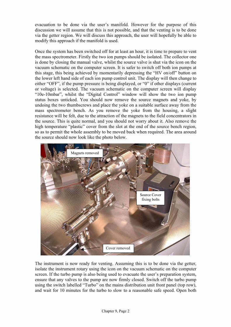
Chapter 9, Page 2

evacuation to be done via the user’s manifold. However for the purpose of thisdiscussion we will assume that this is not possible, and that the venting is to be donevia the getter region. We will discuss this approach, the user will hopefully be able tomodify this approach if the manifold is used.

Once the system has been switched off for at least an hour, it is time to prepare to ventthe mass spectrometer. Firstly the two ion pumps should be isolated. The collector oneis done by closing the manual valve, whilst the source valve is shut via the icon on thevacuum schematic on the computer screen. It is safer to switch off both ion pumps atthis stage, this being achieved by momentarily depressing the “HV on/off” button onthe lower left hand side of each ion pump control unit. The display will then change toeither “OFF”, if the pump pressure is being displayed, or “0” if other displays (currentor voltage) is selected. The vacuum schematic on the computer screen will display“10e-10mbar”, whilst the “Digital Control” window will show the two ion pumpstatus boxes unticked. You should now remove the source magnets and yoke, byundoing the two thumbscrews and place the yoke on a suitable surface away from themass spectrometer bench. As you remove the yoke from the housing, a slightresistance will be felt, due to the attraction of the magnets to the field concentrators inthe source. This is quite normal, and you should not worry about it. Also remove thehigh temperature “plastic” cover from the slot at the end of the source bench region,so as to permit the whole assembly to be moved back when required. The area aroundthe source should now look like the photo below.

The instrument is now ready for venting. Assuming this is to be done via the getter,isolate the instrument rotary using the icon on the vacuum schematic on the computerscreen. If the turbo pump is also being used to evacuate the user’s preparation system,ensure that any valves to the pump are now firmly closed. Switch off the turbo pumpusing the switch labelled “Turbo” on the mains distribution unit front panel (top row),and wait for 10 minutes for the turbo to slow to a reasonable safe speed. Open both

Cover removed

Magnets removed

Source Coverfixing bolts

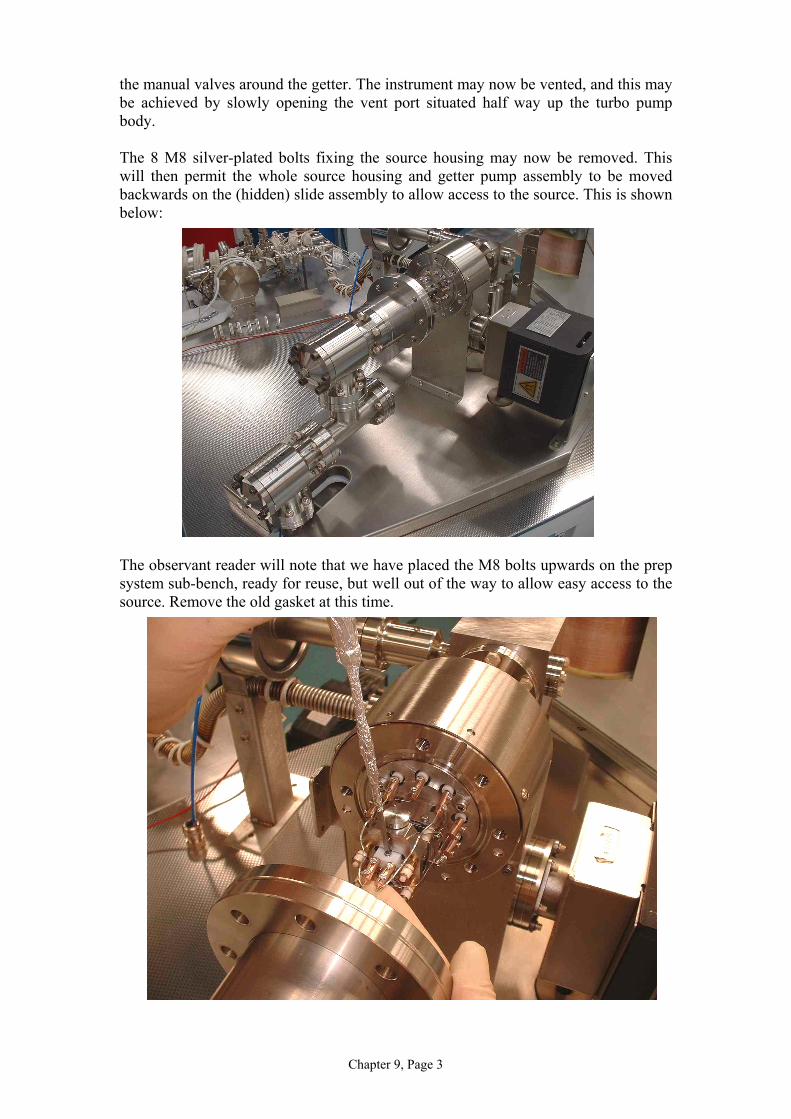
Chapter 9, Page 3

the manual valves around the getter. The instrument may now be vented, and this maybe achieved by slowly opening the vent port situated half way up the turbo pumpbody.

The 8 M8 silver-plated bolts fixing the source housing may now be removed. Thiswill then permit the whole source housing and getter pump assembly to be movedbackwards on the (hidden) slide assembly to allow access to the source. This is shownbelow:

The observant reader will note that we have placed the M8 bolts upwards on the prepsystem sub-bench, ready for reuse, but well out of the way to allow easy access to thesource. Remove the old gasket at this time.

Chapter 9, Page 4

The filament will be seen to be at the top of the source block and can be easilyremoved. It is connected to the feedthroughs using solid silver wire and theconnections made between the wire and the filament legs via small copper alloyconnecting blocks. Firstly undo the bolts in these connecting blocks closest to thefilament and remove the connector from the filament leg. The filament may then beremoved by undoing the small M1.6 bolt through the centre of the filament ceramicbody. The replacement filament may now be inserted in the source. You will find thatit locates “automatically” via the small step on the ceramic block. Reconnect the twowire connecting blocks.

If you wish to remove the complete source assembly from the flange, firstly release allthe connecting blocks from the source flange feedthroughs. If they are tight, removethe wire from the connector rather than trying to force the connector off thefeedthrough central conductor. The source assembly may then be removed from theflange by releasing the three M4 socket head bolts, and taking the whole sourcebackwards. The filament may then be removed, and replaced, as outlined above, butyou may also wish to check the alignment before reassembling the assembly on theflange. To do this first remove the two field concentrator slugs, by removing theirrespective fixing bolts. Note that these are quite long, and fit into recesses in the slugs,to firmly fix and align them. Then remove one of the two bolts fixing the trap to theblock (on the other side of the block from the filament), and loosen the second. Thetrap may then be swung out of the way to permit a direct line of sight view throughthe block to the filament coil. You may find use of a torch helps illuminate the coil.When you are satisfied with the alignment, reassemble and replace the source onto theflange. Reconnect all the wires.

Place the new gasket over the source and carefully push back the housing to cover it.You may find it simpler to place in two of the lower bolts through the cover into thesource flange, and rest the gasket on them, to hold it in place as the cover is broughtup to enclose the assembly. At this stage we would recommend that you check thatthere are no shorts from the internal wires, or block, to other wires or the outerhousing. This may be done by removing the connectors from the back of the filamentunit and “bussing” out the central pins to ground and other connectors. Alternativelythe top part of the source flange wire cover can be removed to permit access to theoutside of the source feedthroughs. Even if this approach is used, it is stillrecommended that the connectors at the rear of source unit be removed, sinceotherwise false reading will occur due to the circuitry in that supply. Since there isonly the minimal amount of spare room in the housing, accidental shorts to the outerhousing can be quite common, and it is best to confirm there are none at this stage.The only “short” which should be recorded is between the two connectors feeding thefilament wire itself! Once this has been done, plug back in the filament unitconnectors, before you forget.

Once you are convinced no shorts exist, tighten up the source housing using all of theeight bolts. Ensure that the flanges are face to face, or leaks may develop after thebaking. Close the vent port on the turbo, and open valve above the instrument rotaryusing the icon on the vacuum schematic on the computer screen. Switch on the turbopump supply, via the mains switch on the mains distribution front panel. Monitor theturbo speed on the vacuum schematic, and it should rise to 100% smoothly over about5 minutes. Leave the instrument pumping on the turbo for at least one hour, after

Chapter 9, Page 5

which the ion pumps may be opened. As long as the filament change has proceededreasonably smoothly, and the instrument hasn’t been vented for too long a period, itshould be possible to start the ion pumps at this time. If they do not start smoothly andgo virtually immediately into the 10-6 bar range (within about 5 minutes), switch offthe ion pump controller, and wait a further hour before trying to start then again. Theinstrument is now ready for baking.

Changing the scrolls in the backing pump

If the pump is kept on at all times, this should be done at least once a year. Assumingthe standard pump has been supplied with the instrument (Edwards’ XDS5 pump) thespare seal kit can be purchased either from Nu Instruments (part number 1010113) ordirectly from Edwards (their part number is A726-01-805).

The kit contains full instructions on how to perform the seal replacement itself, wewill only therefore discuss how to prepare the pump for this simple operation.

Firstly ensure that all valves to the turbo pump line are firmly closed. This includesthe source getter isolation valve (closed during normal instrument operation), but alsoany valves to the user’s preparation system. In practice we shall not be venting theturbo, but closing all valves is good practice in case of any problems. Close theisolation valve above the scroll pump via the icon on the vacuum schematic on thecomputer screen. Now switch off the turbo and scroll pumps using the mains switchon the front panel of the Mains Distribution Unit situated at the bottom of the centralbay of the instrument. The switches are on the top of the three rows to the left of theunit and labelled “Turbo” and “Rotary”. Unplug the IEC mains lead from the pump.The pump may now be removed from the instrument bench by disconnecting theisolation valve immediately above the scroll pump. This then ensures that the backingline and turbo region remains evacuated during the service. Since the pump is quiteheavy, it is recommended that two people lift it out from under the bench. Follow allrecommended procedures during this process.

Replace the scroll tips as per the instructions provided in the packet.

Once done, replace the pump in the instrument bench, re-connect the mains lead andrefit the isolation valve. Switch on the rotary via the Mains Distribution Unit switch,and leave it pumping for about 10 minutes. After this time the isolation valve may beopened (using the icon on the computer screen) and the turbo switched on. Monitorthe speed until it achieves 100%, but leave to stabilise for about 30 minutes beforeusing the turbo to pump out the instrument (shouldn’t be necessary in normaloperation) or prep system.

Re-activating the Source Getter

Although we will only discuss the source getter, the discussion is also relevant for anygetter pumps fitted to the user’s preparation system.

Firstly, please be aware that during the re-activation process, the getter itself can beheated up to 800°C, and the housing and flanges will therefore rise to over 100°C.

Chapter 9, Page 6

The connector and plug are both designed to work at this elevated temperature, butyour fingers are not!

To activate the getter the following protocol is recommended:

Firstly isolate the getter volume from the mass spectrometer, and open the valve to theturbo pump. This will ensure that any dirt or vapours produced during the heating donot pollute the instrument, but will be pumped away via the turbo. If not alreadyconnected, connect the BNC connector to the socket in the Getter flange. Ensure thatthe large control knob on front left of the Getter supply is turned fully anti-clockwise(i.e. off) before switching the unit on, which may be done using the large green rockerswitch on the unit front panel.

Once on, slowly raise the current using the control knob, until the required 1.15ampvalue is reached. The current being drawn is shown on the red LED display to theright of the unit’s front panel. This process should take at least 30 seconds. If youraise the power too quickly, the getter heater may destroy itself, this being especially aproblem on the first activation. Leave the unit at this full power setting for therequired amount of time, normally about 30 minutes, and then slowly wind down thecontrol knob and switch off the unit.

Once completed, leave the getter pumping for at least a further 30 minutes. Thereason for this is twofold. Firstly since the element is suspended in vacuum, there isno means for the heat to be lost, apart from (slow) radiation cooling. Thus the elementis still in a position to pollute the mass spectrometer for a greater period than may beat first apparent. The second reason is that during the heating process, the seat of thevalve to the turbo would have experienced quite a large amount of direct line of sightradiative heating. This must also be allowed to full cool before the valve is closed.

Once enough time has elapsed for the system to cool, the valve to the massspectrometer can be slowly opened, and an eye kept on the ion pump pressures toensure that they do no rise during this process (thus ensuring that no gas is still beingemitted by the hot surfaces). Once this valve is fully open, the turbo isolation valvemay be closed.

Baking the instrument

The instrument has been carefully designed to ensure that the bakeout process is asimple as possible. As such, the source leads do not need to be disconnected, and allbut one temperature sensor is already in place.

To carry out a bakeout the following procedure is recommended.

Firstly switch off the detectors, high voltage units and “1kV” units at the mainsdistribution unit at the bottom of the central rack of the instrument bench. This may bedone using the middle of the three rows of mains switches to the left on the front ofthe unit. The magnet may be left on during this whole process, but if you prefer it mayalso be switched off using the relevant switch on the Mains Distribution Unit. Leavethe source supply on, since we shall keep source region warm using the filamentduring the bake. Remove the quadruple lens array leads by undoing the connector at

Chapter 9, Page 7

the quad feedthrough flange, and lay them out of the way over the bench side, awayfrom the instrument. Similarly unplug all the wires to the collector preamplifier, andsimilarly lay all the wires out of the way over the bench sides. Similarly, if the sourcegetter lead is connected to the getter, unplug it and leave it lying out of the way.

Ensure that the turbo and rotary pump are both on!

From the menu bar of the Noblesse software, un-tick the ”Instrument Settings” menuoption. This will allow you to change the “Max Power”filament current setting on the “Deflectors and HTsupplies control” window. Before you change it, ensurethat you make a note of the original setting. Set the valueto 3 watts, and check that the filament control unit displaynow shows this value (it may not be totally stable at 3 watts in this mode of operation,but this should not be a problem).

Remove the collector preamplifier, by carefully undoing the four mounting bolts. Tryto remove this unit squarely, by supporting it as the bolts are released, so as not toplace any undue strain on either the spring-pin connectors or the ceramicfeedthroughs. Having checked that the maximum power to the filament is now limitedto the safe value of 3 watts, you should now remove the source magnets and yoke, byundoing the two thumbscrews and place the yoke on a suitable surface away from themass spectrometer bench. As you remove the yoke from the housing, a slightresistance will be felt, due to the attraction of the magnets to the field concentrators inthe source. This is quite normal, and you should not worry about it. If you have justreplaced the filament with a new one, as described at the start of this chapter, replacethe high temperature plastic slot cover that was removed to allow the source housingand getter assembly to be slid back.

Ensure that all valves on the mass spectrometer are fully open. This includes theautomatic valve to the source ion pump, which should be opened via the icon on thevacuum schematic on the computer screen, and any valves to the user’s preparationsystem. We have found it best (and safest) to bake with all the valves open, and haveprovided an automatic valve above the system rotary specifically for this purpose. If apower cut should occur during the bakeout process, this valve would close, protectingthe system from any air ingress, and the bakeout process cease. It will not restart whenthe power is reinstated, and the valve will remain closed.

Since a lot of heat is unfortunately lost below the bench top during the bakeoutprocess, you should now remove as many of the bench covers as possible. This willpermit air to flow freely around the electronic units during the bakeout, and preventany damage due to overheating. To put this into context, during the bakeout processitself, the ion pump pressure will increase, which in turn increases the power whichthe controllers have to supply. They must have free air circulation during this time.

The magnet should now be moved to the rear of its travel (to the front of the bench).To free it from it’s set position, undo the central knurled nut at the end plate below themagnet coils. Do not alter either of the outer two set bolts on this plate, since thesedefine the magnet position when it is pushed back into place. If the “earthquake” boltis fitted into the bottom of the magnet below the bench top of the instrument, it will

Chapter 9, Page 8

also be necessary to unbolt it. Slowly push the magnet to the rear of its travel (takecare not to trap the wires to the coils or magnet control box), and preferably lock itinto place using the “earthquake” bolt under the bench top surface. It is now necessary

to fix the central thermocouple to the flight tube centre, using a piece of fibreglasstape. Plug in the thermocouple connector to the socket under the central controller(labelled “Flight Tube” in the bakeout control region of the Mains Distribution Unit.

You should now cover the exposed ceramicfeedthroughs with some aluminium foil.Standard cooking foil is quite adequate. Thiswill ensure that the fragile ceramic areas do notexperience undue heating stress from any directline of sight heating.

Now fit the ovens. This should be done in the order indicated in the following picture:

Please note that cover 4 should be lowered over the mass spectrometer from above, soas to ensure that the heaters do not hit any of the vacuum enclosure. Similarly item 5should be lowered onto the bench from above, and then gently slid into contact withitem 1. In tis manner, the manifold connection tube, and automatic manifold valve (iffitted) will be easily accomadated in the slots cut out of the side of this item. Lock theseparate oven sections together using the latches fixed at their edges.

Plug in the heater wires into the relevent sockets in the bakeout region of the MainsDistribution Unit. Note that item 1 and 5 are powered from the same supply, and sothe leadd from the heater of item 1 should be plugged into the spare connector of the 3

Thermocouple Fibreglass Tape

1

2

3

4 5

Chapter 9, Page 9

way splitter cable, befor the plug of this cable is inserted into the “Source” output.Plug in the fan supply cable (seen laying over the magnet in the picture above) intothe output labled “Fan” on the bottom row of the bakeout sockets. Ensure that thebakeout switches are both switched on (a small green switch on the bottom right ofthe MDU unit, and the large circuit breaker to the left).

Set the three temperature controllers to the require bakeout temperature (we do norecommend going above 300° C since the ion pump magnets undergo a permanentmagnet transition above this temperature. If a significantly higher bakeouttemperature is require, it will be necessary to remove these magnets from the ionpumps.

It is now possible to start the bakeout process, using the bakeout window from themenu list of the main software suite (see chapter 6). It is recommended that you usethe default settings loaded, since this ensure that the rate of temperature rise is not toofast, and the system will protect against excessive rise of pressure. Also be stoppingthe bakeout at about 5am in the morning, should ensure that the rate of temperaturefall is also safe.

At the end of the bakeout, the ovens should be unplugged and carefully removed.When the vacuum envelope has cooled sufficiently to be only warm to the touch(obviously test this with care!), the collector preamplifier may be fitted, and all thecables reconnected. Once the source magnets have been placed back over the sourcehousing, the “Max Power” to the filament should be slowly raised to the originalsetting, and the “Instrument Setting” protection re-enabled.

Once the envelope has full cooled, you may wish to re-activate the source getter, asdescribed above.

Chapter 10, Page 1

Chapter 10: The Nu Designer Utility

This program allows the user to create diagrammatic representations of preparationsystems and add-ons to the Nu Instruments Noblesse mass spectrometer. These diagramscan be read and displayed by the programs controlling the mass spectrometer, and canprovide user interaction with valves and switches, as well as provide feedback of theobserved outputs from a range of sensors. It thus provides the user with a means ofextending the powerful control provided with the mass spectrometer, to custom designedaccessories.

The utility is in the form of a basic drawing package, which allows a schematicrepresentation of the accessory to be input, and overlaid with valves, pipework, gauges andtext descriptions. The utility further provides the user with an interface to input informationconcerning the valves and gauges, such that the main, mass spectrometer, control programcan talk to and read these active items. As such it removes the necessity to resort toseparate control systems for preparation systems, whilst permitting them to be fullyintegrated into the main suite; thus enabling full automatic control of the completepreparation and analysis package.

The Workbench Environment:

On starting the “Designer” program, the user will find the following window:

There are three main areas of interest:

Chapter 10, Page 2

Along the top is a set of menu buttons, split into two groups. The left-hand side set permitsthe target drawing to be manipulated, whilst the second group contains the familiar fileoperation buttons.

The right hand window (identified as the “Target Window”) is the region in which thedesired schematic can be drawn and manipulated. Within this window is a dotted box(whose size may be altered), which represents the final size of the target window. Thecaption above this area (containing the words “No Name”) represents the title bar of thefinal window.

The toolbox to the left holds the five component types, which are used to create the finalwindow.

We will illustrate the use of the package to create asimple preparation system consisting of two valves,interconnecting pipework, a pump and a simple pressuregauge. We show this simple example on the left. Youwill have seen this example earlier, in chapter 6, where ithad been imported into the main program.

Creating the Diagram:

Placing Valves on the canvas:

To add a valve, select the “Add Item” menu option on the top menu bar. When the cursoris moved over the toolbox items, as it passes over each one, it will be seen to change fromthe standard sloping arrow to a hand, as it passes over each diagrammatic representation.Move the arrow to the “valve” tool, and when the hand appears, depress the left mousebutton. The text of the selected item changes from black to red, identifying the item, whichcan now be added to the canvas. With the valve tool selected, move the mouse over to thetarget window, where the cursor will change to a cross. Depressing the left-hand mousebutton a second time will result in a valve icon being drawn at the selected position.Further valves may be added by repeating this procedure.

Moving Valves over the canvas:

Most moving will be done by using the “Move Item” menu option on the top menu bar.With this depressed, the required item may be “picked up” as the cursor moves over it, bydepressing the left-hand mouse button. By keeping this button down, and moving themouse will drag the item with the cursor. It can be deposited at its final destination byreleasing the mouse button. If it is dropped outside the target window area, the programassumes the item is no longer required and it is deleted from memory. (Other ways ofdeleting some of the items will be discussed below).

Sometimes, a whole series of valves may be present, such as in a simple manifoldarrangement, where up to 10 or 20 valves could be present. Obviously in cases like these, it

Chapter 10, Page 3

is sensible to try to lay out the valveicons in a geometric arrangement, withequal spacing between each icon.Rather than use the “Move Item”button to achieve this affect, theprogram provides a simple method forautomating this task. To illustrate thisoption, place a number of valves onthe form, and then depress the “SelectItem” menu option on the top menubar. If you press the left-hand mousebutton as the cursor passes over an

icon, which you wish to select for further manipulation, the item becomes “selected” andwill flash. You may select as many valves as you wish to become simultaneously“selected”, and this option will allow the automatic moving to be achieved. With say threevalves “selected”, depress the right hand mouse button as the cursor passes over one ofthese icons. A floating menu bar will then appear, as shown here. Choosing the “AlignTop” option for the three selected valve icons (shown without the border in the example)will place the three icons level with the highest of the group selected, the “Align Sides”option doing the corresponding placement to the leftmost icon. Aligning the three to top,followed by aligning to the sides, will place all three icons on top of each other, which is asrequired, but a bit disconcerting if you don’t realise what has happened. They may beseparated using the “Move Item” menu option. The “Evenly Space horizontal” and“Evenly Space vertical” menu options can be used to uniformly space the icons.

Placing Pipes on the canvas:

As you would expect, to place a pipe on the canvas, it is first necessary to select the “AddItem” menu option from the top menu bar, and select the pipe tool from the toolbox. Toadd a pipe is slightly different form a simple valve, in that a pipe obviously has two ends.Thus when you move the cursor over to the target area, and turns to the cross, the first endof the pipe is placed where you first give a left-hand mouse click, and the pipe drawn to theposition of the second click. However, other aids are provided to make the job ofconnecting items easier. Firstly the pipe tool draws orthogonally, from the first endplacement. Of more interest is when ends of the pipe join valves. Here, the programautomatically centres the pipe to the relevant valve edge, ensuring that the drawing looksneat. If the two valves are not aligned, the centring is to the second icon. Further theprogram will try to join pipes together intelligently if complicated pipework arrangementsare required. If you prefer not to use this feature, or the program doesn’t produce thenetwork you require, the pipes can of course be moved manually via the “Move Item”menu option button.

Pictures:

When you attempt to place a picture on the target canvas, using the picture placement tool,after the position for the placement has been marked using the left hand mouse button, theprogram will display the “Open File” Windows Dialog Box. This is to enable the requiredpicture to the identified. Three file extensions are supported:

GIF Images (with the .gif extension)

Chapter 10, Page 4

Bitmap Images (with a .bmp extension)Icons (with the .ico extension)

The rotary pump shown in the example above is supplied as the file “Rotary.gif”, whilst aturbo pump may be found in the file “turbo.gif”. Obviously you can create any other imageyou wish using commercial drawing packages. It is probably sensibly to load the requiredimage anywhere on the target area, and move it later to it’s required position via the “MoveItem” menu option.

As in all composite designs, the various components are drawn on different “layers”. Wehave adopted the convention of placing pictures on the lower level, and the other items ona higher level. This enables one to have a large picture (for instance representing thecomplete instrument) and having valves, gauges and text shown on top of it. If the otherway of ordering items was used, the picture would mask these items. This usually is not aproblem, but if one moves a picture, some unexpected effects are seen. During the move,the picture becomes the item of focus, and masks these other items. Put another way, theydisappear, which can be very disconcerting! To regain the normal ordering of things, selectthe picture with the “Select Item” button, and depress the right-hand mouse button. Thiswill cause the picture to be place onto the lowest level, once again, and those hidden itemswill magically reappear.

Adding Text to the canvas:

This is done in two stages. Firstly a text box is placed in (approximately) the requiredposition using the “Add Item” menu button. The empty text box is shown as a smallrectangle, with nothing inside. The actual text is then added by selecting the textbox usingthe left-hand mouse button after the “Select Item” menu button has been depressed.Clicking the Right-hand mouse button with the cursor over the text box will then bring upfloating menu bar which will allow for text input via the “Edit” option. It is also possible todefine the font, font size and colour using other menu options.

Placing Gauges on the canvas:

This is achieved, as expected, using the “Add Item” Menu button and dragging a gaugefrom the toolbox onto the target area.

Customising Gauges and Valves:

It is necessary to identify the valves and gauges added to the canvas so that the maininstrument program can control and read them. This is achievedvia the “Properties” menu option on the floating menu bar whichmay be accessed using the “Select Item” menu button, followedby a right-hand mouse button click over the relevant icon. Theadjacent window shows the valve property version. The “Valvewidth” and “Valve height” entry boxes are obvious (note allentries are in pixels units), and may be altered as required. The

Valve name entry MUST correspond to an entry in the “MS.DEF” file, which has beendownloaded to the system micro. This restriction is actually sensible, since when a userclicks on the valve icon on the main controlling PC screen, something will be expected tohappen with the relevant valve, namely toggle its state. Thus the system must be able to

Chapter 10, Page 5

properly identify each valve shown, and this is only possible if the name used is alsodefined in the “MS.DEF” file. The match has to be exact, and although the names are casesensitive, the host PC will convert all to upper case, so as to make input easier. Also,spaces are not valid character in the “MS.DEF” file, but will be allowed here. Theunderscore is often used in their stead, as shown in the example given. Again the host PCwill convert, but the user should be aware of what is occurring if similar names are used.Thus “Valve_5” will be the same as “Valve 5”, but different from “Valve5” (with nospace). However this makes the code difficult to check and maintain, and so using differingconventions is not recommended. When the main PC program tries to read the filegenerated by the “Designer” program, it will check that all entries are valid, and an errorwill be raised if the names do not match. The form of the “MS.DEF” file is discussed inmore depth in chapter 3.

The Gauge customisation is a little more difficult, in that notonly must the host PC be able to talk to the gauge (and henceknow its name) but it must be able to convert it’s output(normally 0-10volts) to some meaningful, for example, pressureor temperature. The window to input these data is shown here,using a Pirani gauge as an example. Often modern gauges havebuilt in intelligence, and the output is simply related to pressure(they are said to be “linearised”). Others require the user to dothis conversion. As has been mentioned previously, The host PCprogram undertakes two forms of data conversion:

linear: True reading = A + Bx +Cx2 +Dx3

and exponential:True reading = exp(A + Bx +Cx2 +Dx3)

As can be seen the example given uses the exponential fit with all four coefficients beingnecessary to achieve a necessary precision. The coefficients were found (in this case) byusing the manufacturer’s data and fitting to the third order (4 coefficients) equation. Pleasenote that since an exponential fit is used, if the gauge is “linearised”, such that 10-9 mbarhas a gauge output of 1 volt, 10-8 mbar an output of 2 volts etc, the factor 2.3026 will haveto appear in the coefficients in order to convert between natural logs, and logarithms tobase 10.

The “Units” input field has been added to allow any general sensor to be monitored, ratherthan limiting the selection to pressure sensors. The input characters will be displayed in thegauge textbox, as shown in the example of the “Demo Prep” shown above.

Changing the Title of the Window:

This is simply achieved by using the “Select Item” and right-hand mouse button when thecursor is above the dummy named window bar, and using the “Edit” menu. This isidentical to changing text in the standard textboxes.

Changing the Size of the Window:

Chapter 10, Page 6

With any of the left-hand menu buttons depressed, as the cursor passes over any of thedotted boundary lines, it changes to a double-sided arrow. Depressing the left-hand mousebutton with the cursor in this state will cause the dotted line (and hence window boundary)to be altered.

File Control:

Once you have produced your masterpiece, it may be saved using the “Save” menu buttonon the top menu bar. Depressing the button will result in the standard “Save” dialoguewindow being displayed, and the file is saved with the “.nsf” extension, as required by thehost PC program. Existing files may be viewed using the “Open” menu button, but againonly those files with the correct extension are listed in the dialogue window.

Modifying the host PC program to show the new window:

The required information is normally held in the file “Startup Parameters.DAT” in the“Instruments Settings” folder of the main control software suite. The only “trick” toremember here is that this file is overwritten whenever the main program is stopped, sothat, in order to have the change registered, it is important to exit from the main program.If this is not done, the changes you do will magically disappear the first time that they aretried out!

So with the main program fully stopped, look in the file “Startup Parameters.DAT” forsome lines similar to the following:

"Number of manifold form files ",1"Form file number 1 ","C:\ Nu Noble\Instrument Settings\NG.nsf"

This example tells the main program that only one file is to be loaded (the default, whichshould only be changed if you know what you are doing!). To add the second file thenumber of form files is incremented and the location of the new file given after the firstlocation. The input will then look similar to:

"Number of manifold form files ",2"Form file number 1 ","C:\ Nu Noble\Instrument Settings\NG.nsf""Form file number 2 ","C:\ Instrument Settings\Demo Prep.nsf"

where we have now added the “Demo Prep” window. Please note that the name of the fileneed not be the same as the title shown for the window, although it may be sensible to useobvious names if you intend to create a large number of these windows. The host PCprogram is limited to five files in total.