Atmospheric Environment Vol. 22, No. 3. pp. 441-449. 1988. 00046981,88 13.00+0.00

Printed in Great Britain. Pergamon Press pk.

CHANGES IN THE GEOGRAPHICAL DISTRIBUTIONS OF GLOBAL EMISSIONS OF NO, AND SO, FROM FOSSIL-FUEL

COMBUSTION BETWEEN 1966 AND 1980

SULTAN HAMEED and JANE DIGNON

Laboratory for Planetary Atmospheres Research and Department of Mechanical Engineering, State University of New York, Stony Brook, NY 11794, U.S.A.

(First received 26 June 1986 and in&w1 form 13 JuIy 1987)

Abstract-The amount of a fossil-fuel related pollutant released in a region must be functionally dependent on the amount of fuel consumed. Appealing to this general principle we obtained regression relationships between fuel consumption and NO, and SO, generated in the combustion of these fuelsfor countries where emission data are available. The statistical relationships were then used to estimate NO, and SO, emissions in other countries. In this manner statistically consistent geographical maps of emissions can be produced for each year for which fuel consumption estimates are available. We illustrate the usefulness of the method by presenting global emissions for 1966 and 1980 on a latitude-longitude grid appropriate for general circulation models of the atmosphere. The results show that, ahhough the greatest rates of emission occur in the northern Ed-latitudes, the greatest increases from 1966 to 1980 have taken place in the tropics.

Key word index: Combustion, emissions, fossil fuel, NO,, SO,, trace gases.

1. INTRODUCIION

Nitrogen and sulfur oxides (NO, and SO,) play important roles in atmospheric chemistry on local, regional and global s&es; consequently, there is considerabie interest in estimating theiranthropogenic emissions on all of these geographical scales. The significance of these pollutants to the atmospheric environment arises chiefly from their roles as contribu- tors to acidic wet and dry deposition (Pruppacher et al., 1983). In the lower atmosphere NO, also take part in photochemical production of 03, whichcontributes to the greenhouse effect (Fishman et al., 1979; Hameed et ai., 1980).

Recently we have introduced a statistical method that relates annual combustion emissions of NO, to annual fossil-fuel consumption (Dignon and Hameed, 1985). Since then we have applied this method to the emissions of SO,. Regression relationships between emissions and fuel consumptions were derived from available data in the U.S. and other member countries of the Org~ization of Economic Co-operation and Development (OECD), which includes Australia, Canada, Japan and western European countries. It was found that these regressions could be combined in two emission models to obtain global rates of emissions from combustion of fossil fuels.

The purpose of this paper is to present estimates of changes in combustion generated emissions of NO, and SO, between 1966 and 1980 in terms of the global trends as we11 as the geographical distri- butions. The results show that NO, and SO, emissions are very unevenly distributed over the globe, thus causing large local and regional variations from the global mean fluxes. The results are presented on a

latitude-longitude grid suitable for use in a three- dimensional general circulation model of the atmos- phere. This may further the study ofphotochemistry as well as transport and deposition of these species.

An outline of the statistical method and the basic assumptions of these cakulations are presented in section 2. There we present the approximately linear relationship between fuel consumption and gaseous pollutant emission. Examination of government poli- cies for air pollution limits, controls and their enforce- ment show that they will influence this relationship. Treatment of these controls within the calculations is also taken up in section 2. Results on model-estimated emissions are presented in sections 3 and 4 for NO, and SO,, respectively.

It should be noted that our method aims to estimate only those emissions resulting from combustion of fossil fuels. Although these are expected to be the dominant contributors to the anthropogenic emissions of these pollutants, other man-made sources of these pollutants exist and have considerable magnitudes. For NO, probably the largest source of anthropogenic emissions not included is in the burning of biomass (Crutzen et al., 1979). For SO,, between 15 and 20 % of anthropogenic emissions are estimated to originate from non-combustion industrial processes, chiefly ore- smelting and manufacturing F&SO4 (Brown, 1973; EPA; 1975; Fjeld and Ottar, 1975).

2. STATISTICAL MODEL

To estimate the mass of any pollutant gas emitted during the combustion process, we assume that the

441 liE 2.?:3-1

emission is some function of the amount of’ fossil fuel consumed. Fuel consumption data by country are readily available from the United Nations (UN, 1981) and pollutant-emission data for the period from 1966 to the present are available for most countries in the OECD (U.S. Public liealth Service, 1970; Cavender et ul.. 1973: EPA, 1978a. b, 1982: EPS. 1978; Pehen, 1978; Semb. 197X: Aplinget al., 1979; OECD. 1979.1985a. b: Kolstee, 1982; Laulainen, 1982; Lindau, 1982; Zoetmann and van Beckhoven, 1982). Using these data we found that the emissions may be adequately represented by a least-square fine

y=hx+lI tfa.1

under uniform emission controls. In this expression y is the predicted pollu~nt emission for a specific annual fuel consumption x. Later in this report, equations similar to (la) will be derived using available data from the U.S. and some other OECD countries that emit large quantities of NO, and SO, annually. However, it will be necessary to apply the statistical equations to estimate emissions in countries that consume much less fuel by comparison. More realistic estimates for the latter counties are likely to be obtained if the intercept a in Equation (la) is zero. For this reason we modify (la) by using the condition that there will be no emission if there is no fuel combustion, and express it in the form

4’=&b’x. fib)

This assumption can be validated for each regression line by performing a Student’s t-test on the hypothesis fi,: a J: 0. If this hypothesis test fails, then a is not significa~tiy different from zero and the prediction line is justifiably fitted through the origin. Further dis- cussion of this statistical method can be found in Snedecor and Cochrane (19SO).

Controls implemented to restrict pollutant emis- sions will a&t this statistical relationship, i.e. empiri- cally derived relationships such as (la) or (lb) will be useful only over a region and time interval with nearly uniform levels of emission controls. It is therefore desirable to divide the globe into regions and periods of quasi-homogeneous controls and seek separate relationships in each of them between fuel consump tion and emissions. The U.S. first adopted signi~~nt restrictions on air pollution, including NO, and SO,, in 1970 under the Clean Air Act Amendments (U.S. Congress, 1970). In the early 1970s western European countries as well as Australia, Canada and Japan started implementing less stringent and more gradual control policies (Apling er ul., 1979; EPS. 1980: Lundqvist, 1980). Eastern European nations are aIf0 large consumers of fossil fuels. However, uno~cial estimates indicate a genera1 lack of controls on emis- sion sources because they are considered either too costly or poorly implemented {Komarov, 1980). This picture of air pollution emissions is also appli~ble to most developing nations (see e.g., World Bank, f985).

We conclude that, broadly speaking, there were hardly any controls on the emissions of NO,, and SO, before 1970. Emission rates in the U.S. have been reduced since then by the implementation of the C’lean Air Act Amendments. Somewhat less restrictive and geographically less uniform emission controls habe also been introduced in other OECD countries. To arrive at simple estimates of global emissions. we have divided the world into three emission regions: (11 the U.S.; (II) OECD nations other than the U.S. (western Europe, Australia, Canada and Japan); and (III) rest ot the world. These regions are then used in the following emission models, which try to account for different national policies on air pollution.

A statistical relationship between annual emissions and fuel consumption is sought from the U.S. data for the pre-control era, i.e. before 1970. This relationship is assumed to be valid for estimating the amount of pollutant emitted if no controls exist, i.e. it is assumed to hold for the emission Regions II and III throughout the period 1966-1980. The U.S. is treated separately in this model simply because more detailed emission estimates are available for the U.S. for each of these years. This model probably overestimates emissions in Region II after 1970; it is also likely that the emissions from eastern European and developing nations are underestimate because of generally inadequate main- tenance of vehicles and machinery (Komarov. i 980),

In this model we attempt to take into account the effect of emission controls imposed in Region II since 1970. Information on emissions of NO, and SO, was not available for all of the countries in the region during this period. It is assumed that emission controls in these countries are generally consistent with each other, and regression analyses performed on the available data are applicable to the entire region.. The relationship from pre-1970 U.S. emissions, derived in Model 1, is still used for emission Region III from 1966 to 1980 and for emission Region II prior to 1970. Again, published U.S. data will serve for Region I. Emission estimates from this model are expected to be lower than those of Model 1.

Models 1 and 2 allow us to estimate the gaseous emissions of NO, and SO% for any country and year for which fuel consumption data are available. Each nation’s annual pollutant emissions were estimated and geographically parameter&d onto a fixed grid of IO” longitude and 8” latitude corresponding to the GISS (Goddard Institute for Space Studies) general circulation model (Pinto et al., 1983). For a country that lies across the grid, the estimated emission was divided between grid boxes according to their respect- ive populations (thus making the assumption that per capita emission is uniform throughout the country). Population data for individual nations were taken

Changes in the geographical distributions of global emissions of NO, and SO, 443

from the Encyclopedia Britannica (19791, and their spatial distributions were assumed to be constant during the period from 1966 to 1980.

3. ~MI~IONS OF NIT~O~EN OXIDES

Efforts to estimate the global NO, anthropogenic emissions have been made since it was discovered that odd N plays a critical role in the photochemistry of atmospheric OS. Some of the more recent attempts include the 1970 global emission estimate of Pratt et at. (1977) of 20 Mt (N)a-*, the 1975 estimate of Bauer (1982) of 18.9 Mt (N) a-’ and the Logan (1983) es- timate of 21 Mt (N) a- ’ for 1979. Additional estimates by Siiderlund and Svensson (1975) and Battger et al. (1978) are 19 Mt (N) a- ’ and 15 & 6.4 Mt (N) a- ‘, respectively. Here 1 Mt (N) = 1 Mt of nitrogen. In the following we shall use statistical relationships between fuel consumption and NO, emissions in Models 1 and 2 to arrive at estimated emissions in individuai countries.

Estimates of NO, emissions in the U.S. prior to 1970 (U.S. Public Health Service, 1970; Cavender et a!., 1973; EPA, 1918a, b, 1982; Pehen, 1978) were used by Dignon and Hameed (1985) to obtain the fitted statistical relationship.

y = 0.0095x. (2)

In this equation y is the NO, emission in Mt (NOz) and x is the total fuel consumed in Mt of coal equivalent. The least-squares line has a correlation coefkient of 0.98 and an F ratio of 109 for a better than 99% statistical significance. Note that the total fuel consumption was used in this calculation as the independent variable. &vender et at. (1973) indicate that mobile and stationary sources contribute nearly equally to anthropogenic NO, emissions. A regression analysis of NO, emissions vs liquid-fuel consumption for the same years yields a relationship which is nearly as good in statistical terms, giving a correlation coefficient of 0.96 and an F value of 59.

The regression performed for emission Region II to be employed by Model 2 utilized the available data from western European countries and Canada for the post-1970 period listed in Table 1 of Dignon and Hameed (1985) and yielded the relationship

y = 0.~59x. (31

Statistical results yield a 0.99 correlation coefficient for the least-squares line with an F value of 238. Again this presents a better than 99 7; significance.

Recently, additional data on NO, emissions in several countries of Region II became availabie to us. These are from publ~ations of the Organ~tion of Economic Co-operation and ~velopment (OECD, 1979,1985) and are given in Table 1 together with fuel consumption data from UN (1981). When these data are combined with those given in Table 1 of Dignon

Table 1. Fuel consumption and NO, emission data for some countries in Region II. Consumption of fuel is given in Mt of coal equivalent and emissions are expressed as

Mt of equivalent NOz

Country Fuel NQX

Year consumption emissions

Canada Japan Australia Austria Denmark Finland France Germany Italy Netherlands Norway Portugal Spain Sweden Switzerland U.K.

1976 226.1 1975 414.1 1971 70.9 1974 29.3 1974 25.8 1975 23.4 1975 225.2 1.32 1975 355.2 1.91 f972 160.0 1975 83.7 1975 20.2 1975 0.93 197s 78.0 1975 48.0 1975 22.8 1975 288.5

I.93 2.22 0.85 0.11 0.045 0.25

0.92 0.41 0.10 0.19 0.22 0.31 0.015 1.68

and Hameed (1985) and a regression performed~ the result is

y = 0.0060x. (4)

Comparison of (3) and (4) suggests that the regression obtained is robust and likely to yield reliable estimates of NO, emissions in this region.

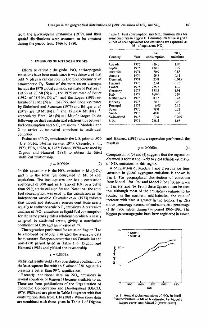
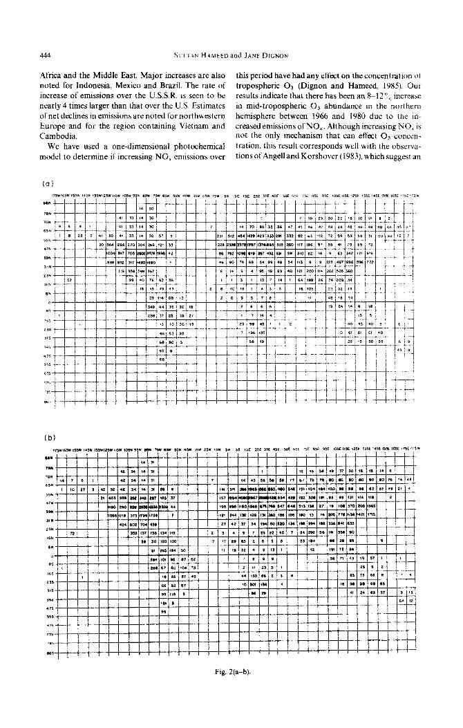
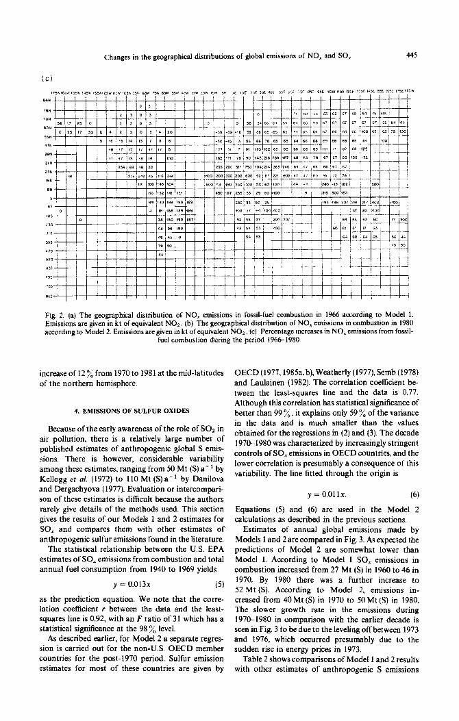
A comparison of Models 1 and 2 results for time variation in global aggregate emissions is shown in Fig. 1. The geogmphica1 distribution of emissions from Model 1 for 1966 and Model 2 for 1980 are given in Fig. 2(a) and (b). From these figures it can be seen that although most of the emissions continue to be located in the northern mid-latitudes, the rate of increase with time is greater in the tropics; Fig. 2(c) shows percentage increase of emissions, as a percentage of the 1966 values, during the period 1966-1980. The biggest percentage gains have been registered in North

Fig. 1. Annual global emissions of NO, in fossil- fuel combustion in Mt of N estimated by Model 1

(upper curve) and Model 2 (lower curve).

444 St I.JAX HA~EEDand JANE DIGNON

Africa and the Middle East. Major increases are also noted for Indonesia, Mexico and Brazil. The rate of increase of emissions over the U.S.S.R. is seen to be nearly 4 times larger than that over the U.S. Estimates of net declines in emissions are noted for northwestern Europe and for the region containing Vietnam and Cambodia.

We have used a one-dimensiona phot~hemi~l model to determine if increasing NO, emissions over

this period have had any effect on the concentration ol tropospheric O3 (Dignon and Hameed, 1985). Our results indicate that there has been an 8-12 “” increase in mid”tropospheric O3 abundance in the northern hemisphere between 1966 and 1980 due to the in- creased emissions of NO,. Although increasing NO., is not the only m~hanism that can effect O3 concen- tration. this result corresponds well with the observa- tions of Angelland Korshover (1983), which suggest an

Changes in the geographical distributions of global emissions of NO, and SO, 445

Fig. 2. (a) The geographical distribution of NO, emissions in fossil-fuel combustion in 1966 according to Model 1. Emissions are given in kt of equivalent NOI. (b) The geographical distribution of NO, emissions in combustion in 1980 according to Model 2. Emissions are given in kt of equivalent NO*. (c) Percentage increases in NO, emissions from fossii-

fuel combustion during the period 1966-1980.

increase of 12 y0 from 1970 to 1981 at the mid-latitudes of the northern hemisphere.

4. EMISSIONS OF SULFUR OXIDES

Because of the early awareness of the role of SO2 in air pollution, there is a relatively large number of published estimates of anthropogenic global S emis- sions. There is however, considerable variability among these estimates, ranging from 50 Mt (S) a- ’ by Kellogg et nl. (1972) to 110 Mt (S) a- ’ by Danilova and Dergachyova (1977). Evaluation or intercompari- son of these estimates is difficult because the authors rarely give details of the methods used. This section gives the results of our Models 1 and 2 estimates for SO, and compares them with other estimates of anthropogenic sulfur emissions found in the literature.

The statistical relationship between the U.S. EPA estimates of SO, emissions from combustion and total annual fuel consumption from 1940 to 1969 yields

y = 0.013x (5)

as the prediction equation. We note that the corre- lation coef%cient I between the data and the least- squares line is 0.92, with an F ratio of 31 which has a statistical significance at the 98 y0 level.

As described earlier, for Model 2 a separate regres- sion is carried out for the non-US. OECD member countries for the post-1970 period. Sulfur emission estimates for most of these countries are given by

OECD (1977,1985a, b), Weatherly (1977), Semb (1978) and Laulainen (1982). The correlation coefficient be- tween the least-squares line and the data is 0.77. Although this correlation has statistical significance of better than 99 %, it explains oniy 59 % of the variance in the data and is much smaller than the values obtained for the regressions in (2) and (3). The decade 1970-1980 was characterized by increasingly stringent controls of SO, emissions in OECD countries, and the lower correlation is presumably a consequence of this variability. The line fitted through the origin is

y = 0.01 lx. (6)

Equations (5) and (6) are used in the Model 2 calculations as described in the previous sections.

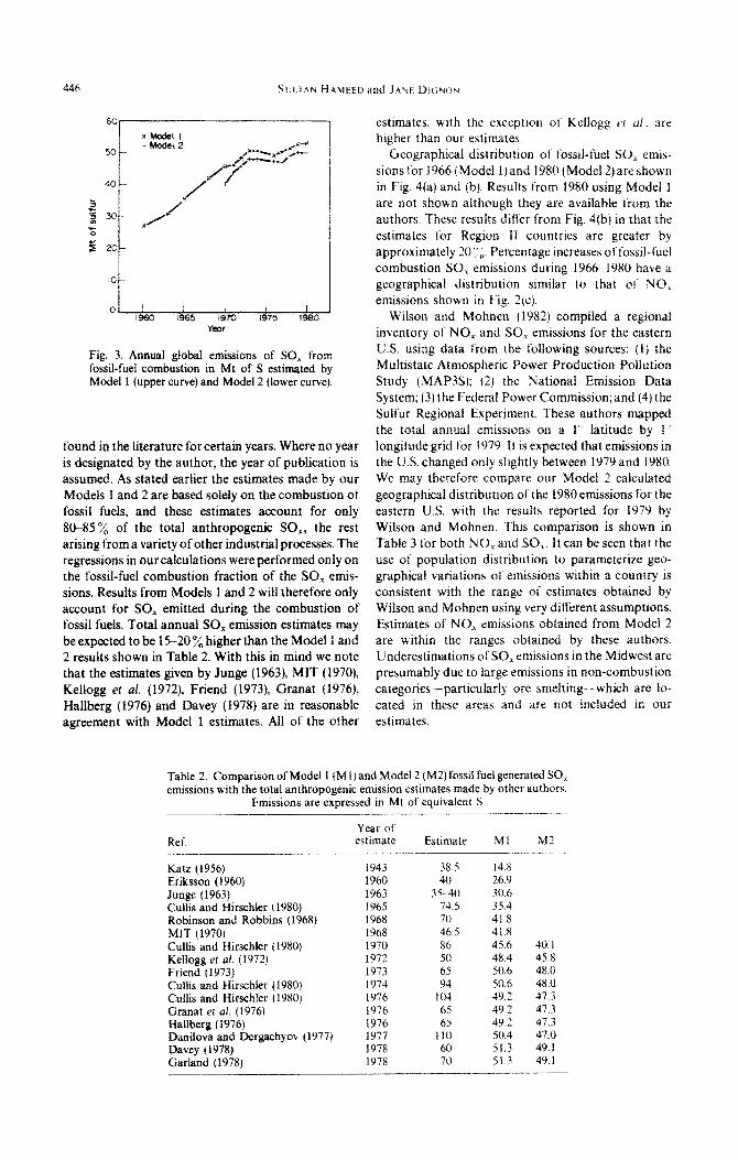
Estimates of annual global emissions made by Models 1 ?nd 2 are compared in Fig. 3. As expected the predictions of Model 2 are somewhat lower than Model 1. According to Model 1 SO, emissions in combustion increased from 27 Mt (S) in 1960 to 46 in 1970. By 1980 there was a further increase to 52 Mt (S). According to Model 2, emissions in- creased from 40 Mt (S) in 1970 to 50 Mt (S) in 1980. The slower growth rate in the emissions during 1970-1980 in comparison with the earlier decade is seen in Fig. 3 to be due to the leveling off between 1973 and 1976, which occurred presumably due to the sudden rise in energy prices in 1973.

Table 2 shows comparisons of Model 1 and 2 results with other estimates of anthropogenic S emissions

IO-.

0‘ / I i I I 1960 I965 1970 I975 1980

YWf

Fig. 3. Annual gfohl emissions of SO, from fossil-fuel combustion in Mt of S estimated by Model 1 (upper curve) and Model 2 (lower curve).

found in the literature for certain years. Where no year is designated by the author, the year of publication is assumed. As stated earlier the estimates made by our Models 1 and 2 are based safely on the combustion of fossil fuels, and these estimates account for only SO-850/ of the total anthropogenic SO,, the rest arising from a variety of other industrial processes. The regressions in our calculations were performed onfy on the fossil-fuel combustion fraction of the SO, emis- sions. Results from Models 1 and 2 will therefore only account for SO, emitted during the combustion of fossil fuels. Total annual SO, emission estimates may be expected to be 15-20 “/, higher than the Model 1 and 2 results shown in Table 2. With this in mind we note that the estimates given by Junge (1963), MIT (1970), Kellogg et al. (1972), Friend (1973), Granat (1976) Ha&erg (1976) and Davey (X978) are in reasonabte agreement with Model 1 estimates. All of the other

estimates, with the exceptron ol‘ Kellogg (“I ul.. are higher than our estimates.

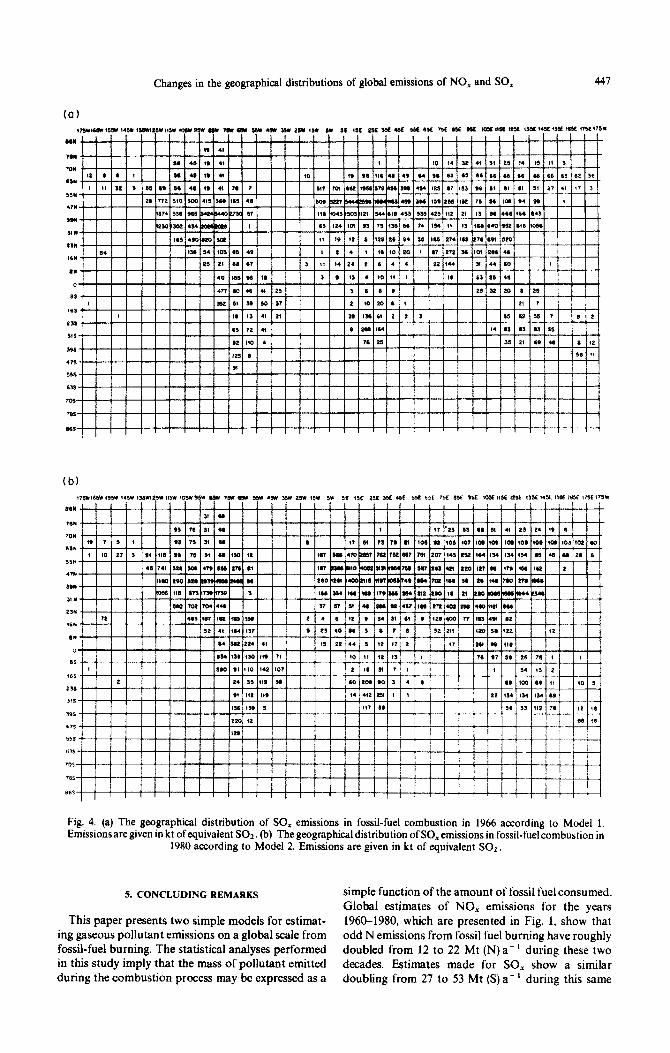
Geographical distribution of fossil-fuel SO, emis- sions for 1966 (Model I)and 1980 (Model 2)are shown in Fig. 4(a) and (b). Results from 1980 using Model 1 are not shown although they are available from the authors. These results ditkr from Fig. 4(b) in that the estimates for Region 11 countries are greater by approximately 20’!,. Percentage mcreases of fossil-fuel combustion SO, emissions during 19661980 have a geographical distribution similar to that 01 NO, emissions shown in Fig. 2(c).

Wilson and Mohnen (1982) compiled a regional inventory of NO, and SO, emissions for the eastern U.S. using data from the following sources: (I) the Multistate Atmospheric Power Production Pollution Study (MAP3S); (2) the National Emission Data System; (3) the Federal Power Commission;and (4) the Sulfur Regional Experiment. These authors mapped the total annual emissions on a 1 latitude by 1 longitude grid for 1979. It is expected that emissions in the U.S. changed only slightly between 1979 and 1980. We may therefore compare our Model 2 calculated geographjcal dist~bution of the 198Oemissions for the eastern U.S. with the results reported for 1979 by Wilson and Mohnen. This comparison is shown in Table 3 for both NO, and SO,. It can be seen that the use of population distribution to parameterize geo- graphical variations of emissions within a country is consistent with the range of estimates obtained by Wilson and Mohnen using very diRerent assumptions. Estimates of NO, emissions obtained from Model 2 are within the ranges obtained by these authors. Underestimations of SO,, emissions in the Midwest are presumably due to large emissions in non-combustion categories --particularly ore smelting-which are lo- cated in these areas and are not included in our

estimates.

Table 2. Comparison of Model 1 (Ml) and Model 2 (M2) fossil fuel generated SO, emissions with the total anthropogenic emission estimates made by other authors.

Emissions are expressed in Mt of equivalent S

Ref. Year oi estimate Estimate Ml M?

Katz (1956) 1943 38.5 14.8 Eriksson (1960) 1960 40 26.9 Junge (1963) 1963 35” 40 30.6 Cuilis and Hirschier (1980) 1965 74.5 35.4 Robinson and Robbins (1968) 1968 70 41.8 MIT (1970) 1968 46.5 41.8 Cullis and Hirsehler (1980) lY70 86 45.6 Kellogg et al. (1972) 1972 50 48.4 Friend (1973) 1973 65 SO.6 Culhs and Hirsehier (1980) 1974 Y4 SO.6 Cullis and Hirschler (1980) 1976 104 49.2 Granat et al. (1976) 1976 65 49.2 HaiIberg (1976) 1976 65 49.2 Danilova and Dergachyov (1977) 1977 IlO 50.4 Davey (1978) 1978 60 51.3 Garland (1978) 1478 70 51.3

40. I 45.8 48.0 48.0 47.3 47.3 47.3 47.0 49.1 49.1

Changes in the geographical distributions of global emissions of NO, and SO,

(a)

Fig. 4. (a) The geographical distribution of SO, emissions in fossil-fuel combustion in 1966 according to Model 1. Emissions are given in kt of equivalent SO2. (b) The geographical distribution of SO, emissions in fossil-fuel combustion in

1980 according to Model 2. Emissions are given in kt of equivalent S02.

5. CONCLUDING REMARKS simple function ofthe amount of fossil fuel consumed. Global estimates of NO, emissions for the years

This paper presents two simple models for estimat- 1960-1980, which are presented in Fig. 1, show that ing gaseous pollutant emissions on a global scale from odd N emissions from fossil fuel burning have roughly fossil-fuel burning. The statistical analyses performed doubled from 12 to 22 Mt (N)a-r during these two in this study imply that the mass of pollutant emitted decades. Estimates made for SO, show a similar during the combustion process may be expressed as a doubting from 27 to 53 Mt (S) a-’ during this same

448 SI LTAN HAMEW and JANE DIGNO&

.Table 3. Spatial distribution ot 1980 NO, and SO, emissions estimates for the eastern United States. Emissions are ex- pressed as Mt of equivalent NO1. and equivalent SO,,

respectively

Grid box Wilson and Mohnen (1982) Model 2 -___

NO, 31.-39 N

7%-85 W 1325-3325 1739 85-95 W 14254050 1739

39-47 N 65-75 w 1125-2425 2329 7>-85 W 2475-5115 4635 8595 W 260&4640 2939

SO,

31-39 N 75-85‘ w 20754525 173Y 8s-95’ W 440&7200 1739

3947 N 65-75’W 8w21OO 2939 75-85 W 445@6925 4958 85-95 W 235&4900 2466

period (Fig. 3). Increases for both pollutants show a slight leveling off during the mid and late 197Os, which may be attributed to the jumps in energy costs in 1973 and 1978.

Comparisons of our model estimates for global emissions with those of other authors for individual years are generally consistent. Although this is a satisfactory feature it should not detract from the approximate nature of the estimates. Our regressions are based on estimates of annual emissions prepared by state agencies in the U.S. and other OECD countries. Preparation of these estimates is a complex procedure requiring detailed information on emission factors, types of sources, etc. It is likely that the accuracy of this information is not uniformly high for all countries and all years. Similarly, data on annual fuel consumption for individual countries are gathered by cumbersome procedures prone to errors. The chief advantage of our method is its simplicity and its ability to give consistent estimates for all countries of the world. Further improvements of our method may be expected as more countries publish increasingly re- liable emission data and separate regressions be-come possible for regions smaller than the three employed in this paper.

NO, and SO, emissions from fossil-fuel combus- tion, as functions of latitude and longitude for the years 1966 and 1980, were estimated to show the change in global distribution. These results are pre- sented in Figs 2 and 4, and demonstrate that the largest rates of increase are found in industrially developing countries. If such rates of increase are sustained, we may expect substantial perturbations of chemical composition of air and precipitation in large regions of the tropics and the southern hemisphere, similar to those already observed in northern latitudes.

The NO, source distribution for 198U. shown m Fig. 2(a), has recently been used in a three-dimenslonal chemistry-transport model to calculate tropospheric concentrations of NO, and HNO, as well ;ib the distribution of wet and dry deposition 01‘ llNOj around the globe (Hameed PI ul.. 1987: Walton t21 ul.. 1987).

Acknowledgemenfs--We wish to thank Dr Anne M Thompson of NASA Goddard Space Flight Center and Dr Michael C. MacCracken of Lawrence Livermore Laboratory for their critical comments on this manuscript.

REFERENCES

Angel1 J. K. and Korshover J. (1983) Global variation in total ozone and layer-mean ozone: an update through 1981. .I. Climate appl..Met. 22, 161 l-1626.

Aoline A. J.. Potter C. J. and Williams M. L. 11Y791 Air ‘pollution from oxides of nitrogen, carbon monoxide and hydrocarbons. Warren Spring Laboratory, Report No. LR 306(AP), Hertfordshire, U.K.

Bauer E. (1982) Natural and anthropogenic sources ol’oxides of nitrogen (NO, for the troposphere). U.S. Dept of Transportation, Report No. FAA-EE-82-7). Washington. D.C.

BGttger A., Gravenhorst G. and Ehhalt D. H. (1978) Atmosphlrische Kreisla’ufe von Stickoxiden und Am- moniak. KFA Jiilich Report No. 1558.

Brown D. (1973) Nationalinventory ofpollutants. Gun. Yuint Finish 49, 29.

Cavender J. H., Kirscher D. S. and Hoffman A. J. (lY73) Nationwide Air Pollutant Emission Trends 1940--1970. EPA, Washington, D.C.

Cullis C. F. and Hirschler M: M. (1980) Atmospheric sulfur: natural and man-made sources. Atmospheric Environment 14, 1263-1278.

Crutzen P. J., Heidt L. E.. Krasnec J. P., Pollock W. H. and Seiler W. (1979) Biomass burning as a source of atmos- pheric gases CO, Hz. N,O. NO. CH,CI and COS. Nuture. Land. 282, 253-256.

Danilova S. T. and Dergachyova N. F. (1977) Assessment ol emission to the atmosphere from thermal power stations. Rate Setting and Control of industrial Emissions to the Atmosphere, pp. 37-43. Hydrometeoizdat, Leningrad.

Davey T. R. A. (1978) Anthropogenic balance for Australia. 1976. Australian Mineral Industries Council Emironmental Workshop, Hobart, October.

Derwent R. G. and Stewart H. N. M. (1973) Air pollution from oxides of nitrogen. Atmosphe#?c &Gronmenr 7, 385401.

Dignon J. and Hameed S. (1985) A model investigation of the impact of increases in anthropogenic NO, emission be- tween 1967 and 1980 on tropospheric ozone. J. atmos. Chem. 3,491-506

Encyclopedia Britannica (1979) The New Encyclopedia Britannica, 15th edn. Chicago, Illinois.

Engdahl R. B. (1973) A critical review of regulations for the control of sulfur oxide emissions. JAPCA 23, 364-375.

EPA (1975) Position paper on regulation of atmospheric sulfates. US. EPA Report No. 450/2-75-007, Washington. D.C.

EPA (1978a) National air pollutant emissions estimates 1970-1976. U.S. EPA Report No. EPA-450/l-78-003, Washington, D.C.

EPA (1978b) National air quality, monitoring and emissions trends report. US. EPA Report No. EPA-450/2-78-052. Washington, D.C.

Changes in the geographical distributions of global emissions of NO, and SO, 449

EPA (1982) National air pollutant emissions estimates 197&1980. US. EPA Report No. EPA-450/4-82-001, Washington, D.C.

EPS (1978) A nationwide inventory of emissions of air contaminants 1974, Environment Canada. Canadian EPS Report No. EPS3-AP-78, 2, Montreal.

Eriksson E. (1960) The yearly circulation of chloride and sulphur in nature. Tellus 12, 63-109.

Fishman J., Ramanathan V., Crutzen P. J. and Liu S. C. (1979) Tropospheric ozone and climate. Nature, Land. 282, 818.

Fjeld H. and Ottar B. (1975) Draft report on the experience gained in determination of sources of SO* emission. O.N. EEC. Document ENN/WP.lRll, Geneva.

Friend J. P. (1973) The global sulfur cycle. In Chemistry of‘the Lower Atmosphere (edited by Rasool S. I.), pp. 177-201. Plenum Press, New York.

Garland J. A. (1978) Dry and wet removal of sulphur from the atmosphere. Atmospheric‘Environment 12, 349-362.

Granat L. (1976) A global atmospheric sulphur budget. SCOPE Report 7. Ecol. Bull. (Stockholm) 22, 102-122.

Hameed S., Cess R. D. and Hogan J. S. (1980) Response of the global climate to changes in atmospheric chemical com- position due to fossil fuel burning. J. geophys. Res. 85, 77537-77545.

Hameed S., Walton J. J. and Wuebbles D. J. (1987) Simulation of global wet and dry deposition of nitric acid in a general circulation model. EOS Trans., Am. geophys. Un. 68, 270.

Junge C. E. (1963) Sulphur in the atmosphere. J. geophys. Res. 68, 397s3976.

Katz M. (1956) City planning industrial plant location and air pollution. In Air Pollution Handbook (edited by Holden P. L. and Ackley A. L.), pp. 2.1-2.53. McGraw-Hill, New York.

Kellogg W. W., Cadle R. D., Allen E. R., Lazarus A. L. and Martell A. E. (1972) The sulphur cycle. Science 175, 587-596.

Kolstee M. J. (1982) Methodology of a general emission inventory in the Netherlands and some results with respect to NO,. In Air Pollution by Nitrogen Oxides (edited by Schneider T. and Grant L.), pp. 143152. Elsevier Scientific, Amsterdam.

Komarov B. (1980) The Destruction of Nature in the Souiet union. M. E. Sharpe, White Plains, New York.

Laulainen N. (1982) North American NO, emissions in- ventories for long range transport model evaluation. In Air Pollution by Nitrogen Oxides (edited by Schneider T. and Grant L.). pp. 153-167. Elsevier Scientific, Amsterdam.

Lindau L. (1982) NO, policy in Sweden. In Air Pollution by Nitrogen Oxides (edited by Schneider T. and Grant L.), pp. 100%1012. Elsevier Scientific, Amsterdam.

Logan J. A. (1983) Nitrogen oxides in the troposphere: global and regional budgets. J. geophys. Res. 88, 10,78>10,807.

Lundqvist L. J. (1980) The Hare and the Tortoise: Clean Air Policies in the United States and Sweden. University of Michigan Press, Ann Arbor, Michigan.

MIT (1970) Man’s impact on the Global Environment. MIT Press, Cambridge, Massachusetts.

OECD (1979) 7he State ofthe Environment in OECD Member

Countries. OECD Publications Office, Paris, France. OECD (1985a) The State of the Environment 1985. OECD

Publications Office, Paris, France. OECD (1985b) OECD Environmental Data Compendium

1985. OECD Publication Office, Paris, France. Pehen E. H. (1978) An air emissions analysis of energy

projections for the annual report to Congress. U.S. DC% Renort No. DOE-ElA-0102/16. Washington. D.C.

Pint: J. P., Yung T. L., Rind b., Russell GTL., Lerner J. A., Hansen J. E. and Hameed S. (1983) A general circulation model study of atmospheric carbon monoxide. J. geophys. Res. 88, 3691-3702.

Pratt et al. (1977) Effect of increased nitrogen on stratos- pheric ozone. Climatic Change 1, 109-1357

Pruonacher H. R.. Semonin R. G. and Slinn W. (19831 drdcipilation Scavenging, Dry Deposition and Resuspetzsion: Elsevier, New York.

Robinson E. and Robbins R. C. (1968) Sources, abundance and fate of gaseous atmospheric pollutants. Final Report. Proj. PR-6755, Stanford Research Institute, Menlo Park, California.

Semb A. (1978) Sulphur emissions in Europe. Atmospheric Environment 12, 455-460.

Snedecor G. W. and Cochrane W. G. (1980) Statistical Methods. Iowa State University Press, Ames, Iowa.

Stierlund R. and Svensson B. H. (1975) The global nitrogen cycle. SCOPE Report 7. Ecol. Bull. (Stockholm) 22,2373.

UN (1976) World Energy Supplies 195&1974. STiESA/ STAT/SER. J/19, United Nations, New York.

UN (1981) 1980 Yearbook of World Energy Staristics, United Nations, New York.

U.S. Congress, Clean Air Act Amendments of 1970, PL91-604 (1974) A Legislative History of the Clean Air Act Amendments of 1970. US. Govt Printing Office, Washington, DC.

U.S. Public Health Service (1970) Nationwide lnvenloryof Air Pollutant Emissions 1968. U.S. Dept of Health, Education and Welfare, Washington, DC.

Walton J. J., Wuebbles D. J. and Hameed S. (1987) Simulation of global wet and dry deposition of nitric acid in a three- dimensional chemistry-transport model. Lawrence Livermore National Laboratory Preprint UCRL 96286, to be presented at the International Rain Conference, Lisbon, Portugal, l-3 September 1987.

Warren Spring Laboratory (1972) National Survey of Air Pollutioi 1961-1971, V&i. 1, AMSO, Hertfordshire,-U.K.

Weatherlv (1977) Estimates of smoke and sulfur dioxide polluti&‘fro& fuel combustion in the U.K. for 1975 and i976. Clean Air Winter 1977.

Wilson J. W. and Mohnen V. A. (1982) An analvsis of snacial variability of the dominant ions. Wirer, Air s6il Poll& 18, 19‘+213.

World Bank (1985) China: The Energy Sector. World Bank, Washington, DC.

Zoetmann B. C. J. and van Beckhoven L. C. (1982) NO, policy in Sweden. In Air Pollution by Nitrogen Oxides (edited by Schneider T. and Grant L.), pp. 979-987. Elsevier Scientific, Amsterdam.