CERGECenter for Economic Research and Graduate Education

Charles University

Master Thesis

2021 Martin Kosık

CERGECenter for Economic Research and Graduate Education

Charles University

The Effect of Military Campaigns onPolitical Identity: Evidence from

Sherman’s March

Martin Kosık

Master Thesis

Prague, September 2021

Author: Martin KosıkSupervisor: Vasily Korovkin, Ph.D.Academic Year: 2020/2021

iii

Declaration of Authorship

I hereby proclaim that I wrote my master thesis on my own under the leadershipof my supervisor and that the references include all resources and literature Ihave used.

I grant a permission to reproduce and to distribute copies of this thesis documentin whole or in part.

Prague, 27th July 2021

Signature

The Master Thesis Proposal

Author of the master thesis: Martin KosıkSupervisor of the master thesis: Vasily Korovkin, Ph.D..

Title: The Effect of Military Campaigns on Political Identity:Evidence from Sherman’s March

Research question and motivationCauses and consequences of civil wars have received increased at-tention within economics in the past decade (Blattman and Miguel2010). Study of the political and social effects of wartime viol-ence is important for understanding why some societies spiral backinto violence whereas others experience rapid recovery and sustainedpeace. The nascent literature on this topic shows that exposure toviolence in war can increase cooperation and pro-social behavior, al-though this seems to be directed only to in-group members (Baueret al. 2016). The evidence on the effect on political identity andbehavior is much more limited and ambiguous. Blattman (2009)and Bellows and Miguel (2009) report higher community particip-ation and political engagement among individuals directly exposedto war violence in northern Uganda and Sierra Leone, respectively.However, Adhvaryu and Fenske (2014) fail to find any significanteffect of exposure to violent conflict in childhood on political beliefsor engagement using surveys of 17 countries in sub-Saharan Africa.Tangent literature within political science studies the long-term ef-fects of repression instead of civil wars but the evidence is not clearhere either. Lupu and Peisakhin (2017) show that repression in-crease political engagement, while Zhukov and Talibova (2018) findthe opposite.ContributionMy thesis would contribute new credible evidence to relatively smallliterature on the effect of military campaigns on political outcomes.Moreover, unlike most previous work which studies recent conflictsI could measure how persistent the potential effects are.

In addition, existing literature focuses mainly on civil wars insub-Saharan Africa or other developing regions. These conflicts fea-ture asymmetric and irregular warfare of insurgents against govern-

ment. In contrast, the American Civil War was by and large foughtin conventional manner and therefore my thesis could bring newperspective.MethodologyThe data will come from various sources. First, I plan to digit-ize the 1865 US War Department map of Sherman’s march andcombine it with important economic and social indicators from his-torical US censuses (including the share of population that wereenslaved in 1860) that are typically used in the literature on thisperiod (Acharya, Blackwell, and Sen 2016). These data would becomplemented by panel of county-level results of presidential andcongressional elections from 1840 to present (Clubb, Flanigan, andZingale 2006). I would also use the survey of Confederate monu-ments and memorials conducted by the Southern Poverty Law Cen-ter (SPLC 2019). Finally, if the computational demands are nottoo high, I plan to download the names of all streets, roads, andschools in the relevant area using the OpenStreetMap database tomeasure what percentage are named after Confederate politiciansand generals.

The identification strategy of the march’s effect on outcomes forwhich antebellum county-level panel data is available (e.g. theDemocratic party’s vote share) will be based on a difference-in-differences design. The synthetic control method could be also ap-plied as a robustness check in case of a possible violation of paralleltrends assumption.

For the other outcome variables (e.g. the density of the Con-federate memorials), I will follow Feigenbaum, Lee, and Mezzanotti(2018) and use the straight-line segment between the three maincities that the march targeted (Atlanta, Savannah, and Columbia)as an instrumental variable, as counties within this segment had ahigher probability of exposure to the march but for a reason that islikely exogenous to later political outcomes.Outline

1. Introduction

2. Literature Review

3. Historical Background

4. Identification Strategy

5. Results

6. Conclusion

References:

Adhvaryu, Achyuta and Fenske, James (2014), Conflict and the Formation ofPolitical Beliefs in Africa, tech. rep. 164, HiCN Working Papers.

Bauer, Michal, Blattman, Christopher, Chytilova, Julie, Henrich, Joseph, Miguel,Edward and Mitts, Tamar (2016), ‘Can War Foster Cooperation?’, Journalof Economic Perspectives 30 (3), pp. 249–274, doi: 10.1257/jep.30.3.249.

Bellows, John and Miguel, Edward (2009), ‘War and local collective action inSierra Leone’, Journal of Public Economics 93 (11), pp. 1144–1157, doi:10.1016/j.jpubeco.2009.07.012.

Blattman, Christopher (2009), ‘From violence to voting: War and political par-ticipation in Uganda’, American political Science review 103 (2), pp. 231–247.

Clubb, Jerome M., Flanigan, William H. and Zingale, Nancy H. (2006), Elect-oral Data for Counties in the United States: Presidential and CongressionalRaces, 1840-1972: Version 1, tech. rep., ICPSR - Interuniversity Consortiumfor Political and Social Research.

Feigenbaum, James J., Lee, James and Mezzanotti, Filippo (2018), Capital De-struction and Economic Growth: The Effects of Sherman’s March, 1850–1920,Working Paper.

Lupu, Noam and Peisakhin, Leonid (2017), ‘The legacy of political violenceacross generations’, American Journal of Political Science 61 (4), pp. 836–851.

SPLC (2019), Whose Heritage? Public Symbols of the Confederacy, https :

//www.splcenter.org/20190201/whose-heritage-public- symbols-

confederacy [accessed: 12.4. 2020].

Zhukov, Yuri M. and Talibova, Roya (2018), ‘Stalin’s terror and the long-termpolitical effects of mass repression:’ Journal of Peace Research, doi: 10.1177/0022343317751261.

Contents

Acknowledgments ix

Abstract x

Introduction 1

1 Literature Review 3

2 Historical Background 82.1 Sherman’s March . . . . . . . . . . . . . . . . . . . . . . . . . . . 82.2 Political Development in the South after the Civil War . . . . . . 10

3 Data 133.1 Data on Naming Patterns . . . . . . . . . . . . . . . . . . . . . . 17

4 Identification Strategies 214.1 Selection on Observables with OLS . . . . . . . . . . . . . . . . . 234.2 Instrumental Variable . . . . . . . . . . . . . . . . . . . . . . . . 254.3 Difference-in-differences . . . . . . . . . . . . . . . . . . . . . . . 27

5 Main Results 295.1 Selection on Observables with OLS . . . . . . . . . . . . . . . . . 295.2 Instrumental Variable . . . . . . . . . . . . . . . . . . . . . . . . 345.3 Difference-in-differences . . . . . . . . . . . . . . . . . . . . . . . 38

6 Robustness checks 406.1 Different Measure of Exposure to Sherman’ march . . . . . . . . 406.2 Sensitivity to Selection on Unobservables . . . . . . . . . . . . . 406.3 Selection on Observables using DML . . . . . . . . . . . . . . . . 436.4 Instrumental variable using DML . . . . . . . . . . . . . . . . . . 44

7 Conclusion 45

References 45

Acknowledgments

I am grateful to Vasily Korovkin for his valuable advice and kind guidance. I

would also want to thank to Christian Ochsner, Nikolas Mittag, and Michal

Bauer for their comments and suggestions that helped improve the thesis. I am

also indebted to Jan Zemlicka and Lukas Supik for their support throughout

the master studies.

ix

Abstract

I use the military march of Union general William Sherman during the American

Civil War to estimate the effects of wartime violence and destruction on post-war

voting behavior and personal identity. First, I examine how the march influenced

the support for the Democrats throughout the 19th and 20th centuries. Second,

to proxy for the strength of Southern identity, I construct several variables

from both historical and contemporary sources. These variables include the

share of individuals likely named after famous Confederate generals, the relative

frequency of streets likely named after Confederate figures, and the presence

of Confederate monuments. The results show mostly small and statistically

insignificant effects of the march on Democratic vote share. For some outcomes

proxying for Southern identity, I find a significant positive effect; however, these

results are not robust across different model specifications. Overall, the results

suggest that Sherman’s march did not have a transformative impact on the

politics and personal identity in the US South.

x

Abstrakt

Pouzıvam vojensky pochod generala Unie Williama Shermana behem Amer-

icke obcanske valky k estimaci efektu valecneho nasilı a destrukce na povalecne

volebnı chovanı a osobnı identitu. Zaprve, zkoumam jak tento pochod ovlivnil

podporu Demokraticke strany behem 19. a 20. stoletı. Zadruhe, vytvoril

jsem nekolik promennych na zaklade jak historickych tak soucasnych zdroju

k tomu abych zachytil sılu Jizanske identity. Tyto promenne zahrnujı podıl

osob, ktere jsou pravdepodobne pojmenovane po generalech Konfederace, re-

lativnı frekvenci ulic pravdepodobne pojmenovanych po osobnostech Konfed-

erace a prıtomnost pomnıku Konfederace. Vysledky ukazujı prevazne male

a statisticky nevyznamne efekty pochodu na volebnı podıl Demokratu. Pro

nektere zavisle promenne, ktere zachycujı jizanskou identitu, nachazım signi-

fikantnı pozitivnı efekty, nicmene tyto vysledky nejsou robustnı naprıc ruznymi

specifikacemi modelu. Celkove vysledky naznacujı, ze Shermanuv pochod nemel

transformativnı dopad na politiku a osobnı identitu v Jihu Spojenych statu.

xi

Introduction

A growing number of empirical and theoretical studies have highlighted personal

identity as an important determinant of economic and political behavior (Aker-

lof and Kranton, 2000; Benjamin et al., 2010; Shayo and Zussman, 2011; Cohn

et al., 2015; Atkin, 2016; Grossman and Helpman, 2021). The overwhelming

majority of the studies have treated personal identity as given and exogenous.

However, this neglects the fact that individuals choose their personal identity

and their identification with a particular group can change in response to ex-

ternal forces. A nascent strand of literature attempts to fill this gap by studying

the process of identity formation and choice (Shayo, 2009; Atkin et al., 2021).

Several empirical studies show that exposure to certain significant events (e.g.,

economic downturn), especially at an early age, can have long-lasting impact

on preferences and personal identity (Yanagizawa-Drott and Madestam, 2011;

Giuliano and Spilimbergo, 2014).

The focus of this thesis is the effect of wartime destruction on identity form-

ation. Although the causes and consequences of wars have received increased

attention within economics in the past decade (Blattman and Miguel, 2010),

the impact of violence on personal identity have been studied relatively little.

The existing literature has mostly focused on how exposure to violence in war

influences cooperation and pro-social behavior (Bauer et al., 2016).

The potential effects of war on political behaviour and identity could pos-

sibly explain some previous findings in the literature. Specifically, several studies

have reported strong correlations between historical conflict and various aspects

of institutions (Besley and Reynal-Querol, 2014; Ray and Esteban, 2017). This

may seem difficult to reconcile with other studies which suggest that the de-

struction in war does not generate persistent poverty traps and the economy is

able recover from these shocks relatively fast.1 Given the recent literature show-

ing high persistence of culture (Nunn and Wantchekon, 2011; Voigtlander and

Voth, 2012; Alesina et al., 2013), it is possible that certain aspects of political

identity and behaviour could be affected by historical conflict and influence the

character of the present-day institutions even if the economy had fully recovered.

I estimate the long-run effects of the notoriously destructive military march

1See Miguel and Roland (2011) for the long-run economic effects of bombing Vietnam,Davis and Weinstein (2002) for the effects of Allied bombing of Japan during World WarII, and Brakman et al. (2004) for the impact of destruction of German cities during WorldWar II. All of these studies find no evidence of persistent poverty traps. A small exception isFeigenbaum et al. (2018) (which is further discussed in subsection 2.1).

1

of Union General William Sherman during the American Civil War on political

outcomes. Specifically, I examine if the march influenced the vote share of

the Democratic party in presidential elections (which prior to the 1960s was

associated in the South with support for segregation and opposition to attempts

to enforce civil rights by the federal government), the proportion of individuals

sharing their first names with famous Confederate generals, the share of streets

likely named after famous Confederate figures, the construction of Confederate

monuments, and lynchings. I find small and mostly statistically insignificant

effects, suggesting that the march did not substantially influence the politics or

identity in affected areas of the US South.

This thesis also closely relates to Feigenbaum et al. (2018) who examined

the economic effects of Sherman’s march. They find that the value of farms

partially recovered after 20 years, although lower agricultural investment lasted

at least to the 1920s. Moreover, there was a large and persistent increase in

land concentration in the counties hit by Sherman’s march. In light of this, the

small effects on voting outcomes I find in this thesis are somewhat surprising

given that there is extensive literature emphasizing the importance of wealth

inequality for politics (e.g., Acemoglu and Robinson, 2005).

The structure of the rest of the thesis is as follows. Section 1 reviews the

relevant literature, section 2 summarizes the historical context of the study,

specifically Sherman’s march (subsection 2.1) and the political development in

the US South after the Civil War (subsection 2.2). The sources and construction

of the data used in this thesis are described in section 3. In section 4, I discuss

the three approaches to identification in this context: selection on observables,

instrumental variable, and difference-in-differences. The main results of these

three methods are presented in section 5. In section 6, I assess the sensitivity of

the main results using various robustness checks including alternative definitions

of the treatment, the stability of coefficients after dropping some controls and

the double machine learning method.

2

1 Literature Review

This paper relates to several different strands of literature. First is the empir-

ical literature on the effects of wars on social and political preferences. Voors

et al. (2012) study the impact of exposure to conflict on social, risk, and time

preferences using data from a field experiment in rural Burundi. They show

that individuals from villages that experienced greater levels of violence are

more altruistic, more-risk seeking, and less patient (i.e., have higher discount

rates). Cassar et al. (2013) examine the effect of exposure to conflict in the

context of Tajikistan using survey and experimental data, and find that more

violence-exposed individuals within the same localities exhibit lower willingness

to participate in impersonal exchange and greater reliance on kinship-based

norms in resolving disputes. Bauer et al. (2014) conducted social-choice ex-

periments (Sharing and Envy Games) in conflict-affected areas in Georgia and

Sierra Leone. The results show an increase in egalitarian choices of individuals

with greater exposure to violence, however only towards their ingroup but not

their outgroup. Furthermore, the effects are present only if an individual was

exposed during a developmental window starting at around 8 years of age and

ending at 20 years of age.

Cecchi et al. (2016) also study the impact of violence in Sierra Leone and

find lower risk aversion and higher altruism of conflict-exposed individuals, con-

firming the results of the previous studies. In addition, they also observe that

exposure to conflict leads to a greater willingness to compete toward the out-

group. Bauer et al. (2016) conduct a meta-analysis of 16 experimental studies

from various settings on the effects of war on social preferences. The results

provide fairly strong evidence that there are fairly large positive effects of war

on prosociality of allocations in experimental games, social group participation,

and community leadership. On the other hand, the effects on trust, voting,

and interest in politics are much smaller and not significantly different from

zero under the random effects model (in which the true effects are assumed to

vary across the studies although they all are drawn from the same distribu-

tion). Bauer et al. (2018) show that former child soldiers forcibly recruited by

the Lord’s Resistance Army in northern Uganda engage more in the local com-

munity and are perceived as more trustworthy. Blattman (2009) and Bellows

and Miguel (2009) report higher community participation and political engage-

ment among individuals directly exposed to war violence in northern Uganda

and Sierra Leone, respectively. On the other hand, Adhvaryu and Fenske (2014)

3

fail to find any significant effect of exposure to violent conflict in childhood on

political beliefs or engagement using surveys of 17 countries in sub-Saharan

Africa.

Tangent literature within political science studies the long-term effects of

repression instead of civil wars but the evidence is not clear here either. Lupu

and Peisakhin (2017) show that repression increases political engagement, while

Zhukov and Talibova (2018) find the opposite. The common challenge of the

studies mentioned studies is potential non-random targeting of violence and

non-random attrition of the sample. There are several different approaches to

addressing this issue used in the literature. Some studies include various control

variables to account for differences in the observable characteristics, while others

employ an instrumental variable approach. Finally, in some cases, the authors

argue that in the specific context they study the violence was indiscriminate and

unlikely to be targeted (e.g., Bauer et al. (2014)). In this paper, I will use both

approaches (selection on observables and instrumental variable) and compare

their results to assess the robustness.

The second strand of literature relevant to this thesis reflects the growing

interest within economics in understanding the impact and formation of per-

sonal identity (Shayo, 2020). Akerlof and Kranton (2000) incorporate identity

or self-image considerations into a simple utility-maximization problem. In their

model, a person is assigned a social identity, which is associated with certain

prescriptions. An individual then might suffer a loss of utility if his or her be-

havior deviates from the prescriptions. Akerlof and Kranton (2000) show that

the inclusion of identity can substantively change the predictions of models of

gender discrimination, poverty, and division of labor within households. Shayo

(2009) develops a more general model of social identity in which both the iden-

tity and behavior are determined endogenously, and applies it to the political

economy of redistribution. In the model, individuals receive higher utility from

identifying with a high-status group; however, they suffer a loss if they identify

with a group whose average (prototypical) member is substantially different

from them. The equilibrium is then defined as a steady state in which the be-

havior of an individual is consistent with his or her identity, the identities are

consistent with the social environment, and the social environment is determ-

ined by the behavior of the individuals. Grossman and Helpman (2021) build

a model in the spirit of Shayo (2009) to study the implication of identity for

trade policies.

In addition to the theoretical work discussed so far, there is a large empirical

4

literature studying the impact of identity on behavior. First, there are several

experimental studies that use priming to increase the salience of a certain iden-

tity. For example, Benjamin et al. (2010) test how Asian-American identity,

which is hypothesized to be associated with patience, influences the implied

discount rates in experimental decisions. They show that Asian-American sub-

jects, whose ethnic identity was primed by asking them about languages spoken

in their family, made more patient choices than Asian-American subjects not

exposed to the prime. Cohn et al. (2014) and Cohn et al. (2015) conducted

similar studies examining the impact of banking culture and criminal identity,

respectively, on dishonesty. Second, several studies use observational data com-

bined with plausibly exogenous variation in salience of identity to investigate

its effects in a real-world setting. Shayo and Zussman (2011) exploit the effect-

ively random assignment of cases to the judges of Israeli small claims courts

to estimate the amount of ingroup bias. They find that the degree of ingroup

bias is relatively small during periods of peace, but the bias rises sharply in the

aftermath of terrorist attacks. Moreover, Shayo and Zussman (2017) show that

the effects of ingroup bias persist for more than 3 years and appear to be driven

by divergent dynamics in areas affected by terrorism rather than by personal

exposure of the judges. Nevertheless, Fisman et al. (2020) provide evidence that

personal exposure is also important. Specifically, they find that Hindu officers in

an Indian bank that were exposed to religion-based communal violence during

their youth lend more to Muslims, and these loans have a lower default rate,

which is consistent with greater taste-based discrimination of violence-exposed

officers.

More recently, the questions of identity formation and the choices made

by individuals between various personal identities have received greater atten-

tion within the empirical literature. Atkin et al. (2021) exploit the differences

in food prescriptions and taboos between various Indian ethnic and religious

groups to estimate a structural model of personal identity choice fitted on food

consumption data. Atkin et al. (2021) use this model to estimate the frequency

of changes in identity and its implications for voting, health, and welfare. Eifert

et al. (2010) find that individuals in Africa are more likely to identify themselves

in ethnic terms (as opposed to religion, class/occupation, or gender) during peri-

ods of heightened political competition, which suggests that ethnic identities are

used for political mobilization. Relatedly, regions in Namibia that were historic-

ally subject to indirect colonial rule, in which the traditional local chiefs were in

charge of internal affairs (in contrast to directly ruled areas which were admin-

5

istered by centralized bureaucracies), exhibit greater salience of ethnicity today

(McNamee, 2019). This is also consistent with evidence by Ali et al. (2019) who

use regression discontinuity design to show that in sub-Saharan Africa citizens

of anglophone countries are more likely to identify in ethnic terms in comparison

to citizens of francophone countries. Whereas the British instituted an indir-

ect rule in most of its African colonies, France encouraged language integration

and centralization. Ananyev and Poyker (2019) use difference-in-differences to

show that individuals in Mali more exposed to deterioration of state capacity

(due to the insurgency caused by demise of Gaddafi) self-identify less with the

nation state. Rohner et al. (2013) present evidence showing that individuals in

regions of Uganda which experienced greater intensity of civil conflict exhibit

lower generalized trust and identify more in ethnic terms. More recent empirical

work also suggests that shared collective experience can build a sense of common

identity. Depetris-Chauvin et al. (2020) show that individuals in sub-Saharan

Africa are more likely to identify with their national identity (over ethnic iden-

tity) and are more likely to trust other ethnic groups in the days after their

national football team won an important match. Moreover, the countries whose

teams barely qualified into the Africa Cup of Nations exhibit less civil conflict

in the following months than countries that did not. Yanagizawa-Drott and

Madestam (2011) find that the individuals in the US who experienced rain-free

Fourth of Julys as children are more likely to identify as Republicans and have

higher voter turnout. Yanagizawa-Drott and Madestam (2011) explain this by

rainfall leading to the cancellation of Fourth of July celebrations, which induce

patriotic values associated with the Republican Party.

Third, this paper also contributes to the literature on the origins and evolu-

tion of identity and politics in the US South. Significant parts of this literature

have emphasized the culture of the British immigrants that first settled the

South (Fischer, 1989; Woodard, 2012). This work (together with e.g., Cobb,

2007 and Cooper and Knotts, 2017) is more qualitative in nature. Acharya

et al. (2016b) examine the legacy of slavery and how it affects a wide range of

contemporary political attitudes of the white population from partisanship to

support for affirmative action. The influence of slavery on local levels of taxa-

tion and bureaucratic capacity is studied by Suryanarayan and White (2021).

They find that counties with a higher slave population before the Civil War had

higher levels of taxation during the Reconstruction (when there was a greater

presence of the federal government to enforce rights of the former slaves) but

lower levels of taxation after Reconstruction ended.

6

Naidu (2012) examines the effects of various laws that effectively disenfran-

chised the vast majority of black citizens passed by many Southern states in the

late 19th century. The results show that the disenfranchisement laws lowered

turnout increased the Democratic vote share and lead to lower investment into

black schools (measured by the child-teacher ratio). Hornbeck and Naidu (2014)

investigate the effect of the Great Mississippi Flood of 1927 on agricultural de-

velopment. They find that flooded counties underwent greater mechanization

and modernization of agriculture in the subsequent years. They interpret these

results as the consequence of the large and persistent out-migration of the black

population in the flooded counties, which induced landowners to invest in labor-

saving technologies. Ager et al. (2019) use linked census data to document the

persistence of the white Southern elite. Specifically, they show that even though

the former Southern slaveholders lost a substantial fraction of their wealth after

the Civil War, their sons and grandsons were able to recover from this shock and

even surpass the educational and occupational attainment of sons and grand-

sons from families holding a similar amount of (non-slave) wealth prior to the

Civil War. Ager (2013) finds that counties, where the planter elite owned more

wealth before the Civil War had the worse economic performance in the sub-

sequent post-war decades (and even after World War II). Ager (2013) interprets

this as a consequence of the lower support for mass education by the planter

elite. Finally, Feigenbaum et al. (2020) show that the institutions of the South

became less coercive in response to a negative economic shock in the form of

boll weevil infestation, with fewer lynchings and less construction of Confed-

erate monuments. Nonetheless, the impact of violence and destruction caused

by the Civil War on the political outcomes in the US South has not been yet

studied quantitatively.

7

2 Historical Background

2.1 Sherman’s March

While the military situation in the Eastern theater (mostly in Virginia) of the

American Civil War had mostly remained in stalemate, during the fall of 1864,

Union General William Sherman successfully concluded a series of military cam-

paigns in Georgia by capturing Atlanta in September 1864. The campaigns fea-

tured, for the most part, conventional warfare consisting of a series of small and

large clashes of the Union and Confederate armies (although the siege of At-

lanta did lead to the destruction of infrastructure and industries and expulsion

of some of the civilian population).

Sherman hoped that he could put pressure on the Confederate army fight-

ing in Virginia by damaging the Southern economy and its warfare capacity

(Trudeau, 2009). This would involve destroying critical infrastructure including

railroads and telegraph lines, and also mills and cotton gins. Sherman con-

sidered several possible avenues for the campaign. First, he could march west

towards Charleston or Savannah, where he would be in a good position to poten-

tially threaten the Confederate armies of Robert E. Lee in Virginia (Marszalek,

2007, p. 295). Second, he could move his armies towards Albany, Georgia and

liberate prisoners in Andersonville and destroy cotton plantations along the way

(Marszalek, 2007, p. 295). Finally, he could march towards Pensacola, Florida,

and combine forces with E. R. S. Canby’s to capture Mobile (Marszalek, 2007,

p. 295).

Sherman decided for the first option to march towards Savannah, as accord-

ing to him it ”would have a material effect upon ... [the] campaign in Virginia”

(Marszalek, 2007, p. 295). However, this route left the Union Army without se-

cured supply lines since it was operating deep in the Confederate territory. For

this reason, the Union soldiers had to confiscate food from the local population,

which made Sherman and his army especially unpopular among the Southern

whites (Campbell, 2005). When planning the specific path his troops would

take, Sherman used the statistics from the 1860 Census of Agriculture in order

to target counties that were important for agricultural production (Trudeau,

2009, p. 538). After reaching Savannah, Sherman began moving his army north

to capture Colombia, North Carolina and from Colombia towards Virginia in

order to eventually support the Union’s campaigns against Lee there. The de-

struction of infrastructure by Sherman’s soldiers continued in this second part

8

of the march as well. The last clashes of Sherman’s troops against the Confed-

erate Army took place near Goldsboro, North Carolina from March 19 to 21,

1865. Lee’s army surrendered on April 9, which effectively ended the war as

other Confederate generals also quickly surrendered.

The capital destruction caused by Sherman’s march had a large negative

effect on the local economy; however, most sectors experienced a fast recovery.

Feigenbaum et al. (2018) study the economic impact of Sherman’s march em-

pirically using county-level US census data from 1850 to 1920. They show that

the farms in counties on the path of Sherman’s march had almost 20% lower

value in 1870 than the farms in other counties in South and North Carolinas and

Georgia. However in 1880, the value of farms was only 3% lower (furthermore

this estimate is not statistically significant), which suggests a fast recovery. A

similar pattern also holds for the value of livestock. In addition, there were no

effects on the population size (not even in 1870), the share of African Americans,

or the total length of the railroad in a county. In contrast, the effects on agricul-

tural investment exhibit greater persistence. Specifically, the share of improved

land in the march counties was around 15% lower from 1870 through 1920 with

no sign of reversion to the mean. The growth of manufacturing employment,

capital, and production in march-exposed counties also lagged behind in 1870,

although it is not possible to assess the persistence due to limitations of the

data. Finally, Feigenbaum et al. (2018) document large and persistent increases

in the concentration of farmland in the march counties. They interpret this as

a consequence of the lack of access to credit in some parts of the South. In par-

ticular, according to Feigenbaum et al. (2018), small farmers, who experienced

negative shock due to capital destruction, were credit constrained and there-

fore had to sell some of their land to the wealthy landowners at lower prices,

which led to a permanent increase in land concentration. This has important

implications for this paper. Since the land concentration might have a direct

effect on political outcomes, it is challenging to distinguish between the direct

effect of Sherman’s march and the effect via the increases in land concentration.

Due to the data limitations, I will not be able to distinguish between these two

channels. Therefore it is important to take this into account when interpreting

the results.

9

2.2 Political Development in the South after the Civil War

After the Civil War, there were efforts by the federal government to substantially

alter the social relations in the formerly Confederate states. This period is

known as the Reconstruction era and is usually2 dated from 1865 to 1877 (Foner,

2014). The most significant changes brought by Reconstruction were declared

in three amendments to the US Constitution. The Thirteenth Amendment

(ratified in 1865) abolished slavery, the Fourteenth Amendment (ratified in 1868)

granted the former slaves citizenship and stipulated equal protection under the

law, and the Fifteenth Amendment (ratified in 1870) prohibits discrimination in

voting based on race or former enslavement. Furthermore, the US government

operated the Freedmen’s Bureau (from 1865 to 1872) which helped the former

slaves to meet basic needs.3

The enfranchisement of former slaves radically altered the political land-

scape of the South during Reconstruction. African Americans became the key

constituency of the Republican Party, which advocated both for their political

rights and for greater redistribution towards them. Furthermore, black Amer-

icans gained representation (running virtually exclusively for the Republican

Party) in both state and local governments. According to Foner (2014) (as

quoted by Naidu, 2012) “In virtually every county with a sizable black popula-

tion, blacks served in at least some local office during Reconstruction ... assumed

such powerful offices as county supervisor and tax collector, especially in states

where these posts were elective.”

There was significant resistance to these changes by the parts of Southern

society, which benefited from the pre-war social order. These views were chiefly

represented by the Democratic Party, which advocated for greater autonomy of

the Southern states so that the social changes could be rolled back. In a more

extreme form, this opposition sometimes manifested itself in violence against

freed people (in the forms of riots or lynchings). Nevertheless, despite the

resistance, the Reconstruction policies were still enforced (albeit imperfectly)

partly due to the substantial presence of federal troops in the South (which

were remnants of the Union Army that operated in the South during the Civil

War).

Progress made by Reconstruction started to be reversed during the 1870s

2Some historians (most notably Foner (2014)) consider Emancipation Proclamation, issuedon January 1, 1863, to be the start of Reconstruction.

3For empirical investigation of the long-term effects of the Freedmen’s Bureau see Rogowski(2018).

10

with gradual withdrawal of the federal troops and lesser commitment of the

Northern Republicans to enforcing equality in the South (Foner, 2014). This

process was completed by the Compromise of 1877, which was an unwritten

agreement according to which the Democrats would award the presidency to

Republican Rutherford Hayes in exchange for the federal government pulling

the last troops out of the South and the Republican Party would refrain from

interfering in the South’s local affairs. During the 1890s Southern states started

to pass laws aiming to effectively disenfranchise black voters. This was done

by imposing restrictions on voting, such as poll taxes or literacy tests, that

disproportionately affected black voters (and to some extent poor whites) to

ensure formal compliance with the Fifteenth Amendment (Kousser, 1974). Fur-

thermore, violence and intimidation were often used to reduce black political

participation and impose white supremacy.4 As a consequence, the Democrats

overwhelmingly dominated the politics of the South in the subsequent decades.

In addition, various laws (usually referred to by historians as Jim Crow laws)

that mandated racial segregation in public schools, transportation, and public

places were enacted during the end of the 19th and early 20th centuries.

However, after World War II there started to be stronger disagreements

between the Southern Democrats and the Democrats from northern and west-

ern states. This reflected the demographic shift within the Democratic coali-

tion in the preceding years (Rae, 1994). Specifically, black voters in northern

states largely left the Republican Party, since the Democrats’ New Deal agenda

aligned better with their economic interests (as opposed to pro-business policies

advocated by the Republicans). As a consequence, some northern Democrats

started to demand desegregation, which was strongly opposed by the Southern

Democrats. When Harry Truman instituted desegregation in the military in

1948, some Southern Democrats founded the States’ Rights Democratic Party

(member of which were often called Dixiecrats), whose 1948 presidential can-

didate Strom Thurmond won 4 states. Nevertheless, after the 1948 elections,

most Dixiecrats returned to the Democratic Party (Frederickson, 2001). A

more permanent exodus of Dixiecrats took place in 1964 in response to Demo-

cratic President Lyndon B. Johnson’s support for the Civil Rights Act of 1964,

which had outlawed discrimination based on race and prohibited racial segreg-

ation in public schools, public accommodations, and public facilities. Most

4Jones et al. (2017) studies quantitatively the effect of violence on black political particip-ation in the post-Reconstruction period. Their estimates suggest that exposure to lynchingdecreased local black voter turnout by around 2.5 percentage points

11

former Dixiecrats joined the Republican Party, whose 1964 presidential can-

didate, Barry Goldwater, opposed the Civil Rights Act on the grounds that it

would violate the states’ rights (Rae, 1994). This caused an important realign-

ment in American politics. The 1964 presidential election was the first time a

Republican candidate won the states of the Deep South (specifically, Louisiana,

Mississippi, Georgia, Alabama and, South Carolina) for the first time since the

end of Reconstruction. However, Johnson achieved a strong victory nonetheless,

carrying 44 states (all states except Arizona, the home state of Goldwater, and

the Deep South). Johnson used this strong mandate to pass the Voting Rights

Act of 1965. This prohibited racial discrimination in voting and outlawed liter-

acy tests and similar restrictions put in place during the Jim Crow period in the

South. This led to dramatic increases in black voter registration in the South-

ern states.5 In the 1968 presidential election, Nixon made an effort to gain the

support of the Southern white voters, but this strategy was partly negated by

the independent candidacy of segregationist George Wallace, former Democratic

governor of Alabama, who won in the Deep South (Maxwell and Shields, 2021).

Nevertheless, Nixon’s Southern strategy did succeed in the 1972 election and

the South became a Republican stronghold ever since. Several recent empirical

studies6 provide evidence that is consistent with qualitative narratives (e.g., of

E. Black and M. Black, 2003), which have emphasized racial resentment as a

main cause of the Southern realignment (as opposed to e.g., economic factors).

5Cascio and Washington (2014) employ a triple-differencing strategy to show that theremoval of literacy tests at registration led to higher voter turnout and state transfers tocounties with higher black populations.

6Kuziemko and Washington (2018) use a triple difference-in-differences strategy onindividual-level Gallup and General Social Survey data to estimate the impact of racial at-titudes on the partisan shifts. In particular, Kuziemko and Washington (2018) compare thechanges in identification with the Democratic Party before and after spring of 1963 (the firstdifference), when the civil rights issues became salient, for individuals who reside in South-ern states (the second difference) and were unwilling to vote for a black president (the thirddifference). The results show that the partisan shift of racially conservative Southern whitescan explain the entire decline in the Democratic Party identification from 1958 to 1980.

12

3 Data

The data come from several different sources. First, I georeferenced the digitized

1865 US War Department map of Sherman’s march7 (shown in figure A1 in the

appendix) and combined it with the historical boundaries of the counties in

the US states of Georgia, North Carolina, and South Carolina as provided by

Mullen and Bratt (2018). The resulting map of counties with lines indicating

the movements of Sherman’s army8 is shown in figure 1. I follow Feigenbaum

et al. (2018) and define the “Sherman” counties (i.e., those that were on the

march’s path) as all counties that intersect within 5 mile band around any of

the army movement lines. Feigenbaum et al. (2018) justify this by referencing

historical accounts, according to which the soldiers did not deviate far from the

path of their armies.

Sherman's March 0 1

Figure 1: Map of US counties and Sherman March’s PathNote: The different lines represent the paths of the different armies participating inSherman’s march (specifically, the 14th. 15th, 17th, and 20th Army Corps and theCavalry).

The most historical data on the county level were obtained from the rep-

7The scanned image of the map can be downloaded from https://www.loc.gov/item/

99447077/8Specifically, Sherman’s army consisted of the 14th, 15th, 17th, and 20th Army Corps and

the Calvary.

13

lication files of Acharya et al. (2016a) who collected a wide range of variables

from various sources. The demographic (e.g., total population, the share of

the population that are slaves) and agricultural (e.g., total farm value per acre

of farmland, total acres of improved land, inequality in land ownership) char-

acteristics of the counties are taken from the Census of Population and the

Census of Agriculture, respectively (both in 1860). Acharya et al. (2016a) also

assembled information from other studies into one unified dataset. For county-

level vote shares of the Democratic Party for presidential elections from 1844

to 1968, they used the dataset by Clubb et al. (2006). They complemented

it with contemporary public opinion data, pooling Cooperative Congressional

Election Study (CCES) surveys (Ansolabehere and Schaffner, 2012) from the

years 2006, 2008, 2009, 2010, and 2011 into one large dataset with over 157,000

respondents. The number of lynchings in the counties between 1882 and 1929

is based on the dataset created by Bailey et al. (2011). Finally, access to rail-

ways in a given county in 1860 was computed based on the GIS shapefiles by

Atack (2015). An important challenge that faced Acharya et al. (2016a) when

constructing this dataset spanning more than a century is that there were some

changes to the county boundaries throughout the years. Acharya et al. (2016a)

decided that they would use the modern county boundaries (as of 2000) and

they would interpolate the 1860 census results onto these modern boundaries.

In particular, Acharya et al. (2016a) use areal interpolation, in which a histor-

ical outcome for a modern county is constructed as a weighted average of the

historical counties’ outcomes where the weights correspond to the proportion of

the historical counties’ area that is contained in the modern county (the details

are described in the appendix A of Acharya et al., 2016b).

The descriptive statistics for several variables are provided in table 1. The

march and non-march counties do not appear to differ systematically in their

vote share for the Democratic party prior to the Civil War. We also do not

observe any significant differences in pre-war agricultural investment as meas-

ured by the acres of improved land in 1860. The total farm value per acre and

land inequality (as measured by the Gini coefficient) appear to be fairly similar

too. However, the counties on the march’s path do have a significantly higher

proportion of the population that were slaves in 1860. The spatial pattern of

prevalence of slavery, which can be seen in figure A2 depicting the slave share in

1860 on a map, confirms this. This is consistent with the historical sources that

emphasize that Sherman targeted areas with large plantations to undermine the

Confederate economy (Trudeau, 2009). Since the legacy of slavery at the local

14

level has been shown to have a persistent impact on various political outcomes

and behavior (Acharya et al., 2016b), it will be necessary to control for this in

the empirical analysis.

Another issue that table 1 reveals is the large fraction of missing data for the

Democratic vote share for the earlier election years (especially prior to 1860).

For the 1848 presidential election, the data are missing for 46.6% of all counties

in the three states. The proportion of missing election results is somewhat lower

for later years, with 30.5% missing data in 1860, 15.7% in 1827, and only 10.8%

in 1900. One of the reasons is that South Carolina did not conduct a popular

vote for presidential elections until 1860 (inclusive) since all of the Electors

were appointed by the state legislature. In addition to this, there are more

idiosyncratic factors that lead to the missingness of election results for some

counties. The large fraction of missing data has important implications for the

application of difference-in-differences, which are discussed in subsection 4.3.

15

Table 1: Summary statistics I

Off march’s path On march’s path Overall(N=229) (N=76) (N=305)

Total population in 1860

Mean (SD) 8230 (5920) 11300 (5640) 8990 (5990)Median [Min, Max] 6910 [698, 40100] 10500 [2440, 31000] 7820 [698, 40100]

Share of slaves in 1860

Mean (SD) 0.349 (0.201) 0.503 (0.157) 0.388 (0.202)

Median [Min, Max] 0.326 [0.0210, 0.850] 0.497 [0.197, 0.812] 0.394 [0.0210, 0.850]

Land inequality in 1860Mean (SD) 0.484 (0.0579) 0.461 (0.0563) 0.478 (0.0583)

Median [Min, Max] 0.485 [0.297, 0.642] 0.459 [0.314, 0.620] 0.478 [0.297, 0.642]

Acres of improv. land in 1860Mean (SD) 55200 (44800) 84400 (45300) 62500 (46600)

Median [Min, Max] 45200 [3110, 300000] 82600 [17300, 220000] 52800 [3110, 300000]

Farm value per acre in 1860

Mean (SD) 23.5 (8.81) 24.8 (13.1) 23.8 (10.0)Median [Min, Max] 21.8 [6.40, 97.2] 23.6 [6.25, 104] 22.2 [6.25, 104]

Railway access in 1860

Mean (SD) 0.310 (0.464) 0.592 (0.495) 0.380 (0.486)

Median [Min, Max] 0 [0, 1.00] 1.00 [0, 1.00] 0 [0, 1.00]

Lynch rate (1882 to 1929)Mean (SD) 0.0121 (0.0179) 0.0118 (0.0142) 0.0120 (0.0170)

Median [Min, Max] 0.00527 [0, 0.101] 0.00698 [0, 0.0650] 0.00626 [0, 0.101]

Missing 6 (2.6%) 0 (0%) 6 (2.0%)

Dem. vote share in 1848

Mean (SD) 44.3 (19.0) 46.9 (16.4) 45.0 (18.4)

Median [Min, Max] 44.2 [1.90, 90.3] 46.8 [4.20, 89.8] 45.7 [1.90, 90.3]Missing 108 (47.2%) 34 (44.7%) 142 (46.6%)

Dem. vote share in 1860

Mean (SD) 5.23 (8.49) 13.2 (15.7) 6.95 (10.9)

Median [Min, Max] 2.50 [0, 54.8] 7.35 [0, 70.2] 2.80 [0, 70.2]Missing 63 (27.5%) 30 (39.5%) 93 (30.5%)

Dem. vote share in 1872

Mean (SD) 52.4 (19.7) 48.5 (24.4) 51.4 (21.0)Median [Min, Max] 50.3 [8.30, 100] 44.5 [6.10, 100] 49.5 [6.10, 100]Missing 37 (16.2%) 11 (14.5%) 48 (15.7%)

Dem. vote share in 1900

Mean (SD) 63.0 (17.6) 75.3 (17.5) 66.1 (18.4)Median [Min, Max] 57.6 [20.0, 99.7] 74.1 [36.8, 99.9] 62.7 [20.0, 99.9]

Missing 26 (11.4%) 7 (9.2%) 33 (10.8%)

16

3.1 Data on Naming Patterns

Choice of a first name can be revealing about the personal identity of the parents.

This has been used by several studies to measure the importance and expression

of cultural or ethnic identity (e.g., Fryer and Levitt, 2004; Abramitzky et al.,

2016; Fouka, 2020; Jurajda and Kovac, 2021). In our context, naming children

after famous Confederate generals or politicians likely reflects a strong expres-

sion of a specific “Southern” identity. For this reason, I use individual-level

census data with information on first names digitized by IPUMS (Integrated

Public Use Microdata Series) project (IPUMS, 2020). For the 1880 census, a

complete count with over 50 million individuals is available (Steven Ruggles

et al., 2010). However, we are interested only in white individuals born after

Sherman’s march (who in 1880 were 15 years old or younger) which substan-

tially reduces our sample size. Unfortunately, the full count data from IPUMS

for other census years do not contain the first name. More detailed information

(including the first name) is available only for a random sample of census records

of a given year. Therefore I complement the 1880 census data with a 5% sample

of the 1930 census. This has the advantage that the vast majority of individuals

in this census were born after Sherman’s march (individuals born prior would

be more than 65 years old); however, at the cost of sampling only 5% of the

population. Another issue with the 1880 census is that some counties could not

be matched to our main dataset (due county boundary changes), which leads

to missing data. The main variable measuring the frequency of Confederate

names is constructed as the number of white individuals born after 1865 (in-

clusive) having Confederate first name in a given county divided by the total

number of whites born after 1865 in a given county. The question then is which

given names to classify as Confederate. If we counted all individuals who shared

their first name with a famous Confederate general, we would likely misclassify

many cases and capture spurious patterns. We could use the information on

the middle names, although for most individuals only the initials of the middle

name are available. I decided to apply a more conservative approach which

labels names as Confederate only in cases where there can be a sufficient degree

of certainty. First, I focus on those likely named after Robert Edward Lee, a

commander of the Confederate Army, who became a cultural icon in the South

after the Civil War. I classify all individuals with the first name “Robert” and

the middle name initial “L” or “E” in the cases where the only middle name

initial is available as having a Confederate name. If the full middle name is

17

available, I require it to be “Lee”, or a name starting with“Ed”. Second, I

also consider Confederate generals with very rare first names where the risk of

misclassification is probably low. In particular, I classify as Confederate those

with the first names of “Braxton” (after Braxton Bragg), “Jubal” (after Jubal

Early), and “Stonewall” (after Thomas Jonathan “Stonewall” Jackson). The

vast majority of the names I classify as Confederate are based on the Robert

E. Lee match, which underscores his popularity in the South. Figure A3 in

the appendix provides some validation for this approach. It shows the evolu-

tion of the share of Confederate names by the decade of birth using the full

count of the 1880 census for Georgia and North and South Carolinas. We see

that while before 1860, the share of Confederate names was negligible (less than

0.01 percent), it sharply increased to more than 0.15 percent during the decade

from 1861 to 1870, and it persisted above 0.10 percent even during the follow-

ing decade (from 1871 to 1880). This suggests that our classification method

does capture the real historical changes and not only some spurious and ran-

dom patterns. Nevertheless, since all of the Confederate figures I consider here

were generals, it is possible that these names reflect certain admiration for the

military rather than Southern identity.

In addition, I also examine possible effects on the presence of Confederate

symbols in public places today. First, I use the database of Confederate monu-

ments assembled by the Southern Poverty Law Center (SPLC, 2019), which

includes the year of construction, longitude, and latitude of the monuments.

Second, I downloaded the OpenStreetMap data files9 for South Carolina, North

Carolina, and Georgia to obtain the names and locations of all streets and roads

in those states. In total the dataset contains 3,055,272 streets and roads (I will

refer to both streets and roads as simply streets henceforth) in the three states,

963,159 of which are named (I dropped the unnamed streets from the analysis).

I extracted a centroid from every named road and based on that I assigned the

roads to the counties. The final variable measuring the relative frequency of

Confederate streets was created as a ratio of the number of streets that contain

a name of a famous Confederate figure10 in a given county to the total number

9In particular, the files were downloaded from http://download.geofabrik.de/

north-america/us.html on July 2, 2021 (the files are updated daily).10Specifically, I define the street to be Confederate if its name contains any of the fol-

lowing (the full name of the Confederate figure it refers to is in the parenthesis): “Lee”(Robert E. Lee), “Davis” (Jefferson Davis), “Stonewall” (Stonewall Jackson), “Beauregard”(P.G.T. Beauregard), “Forrest” (Nathan Bedford Forrest), “Longstreet” (James Longstreet),“Hood” (John B. Hood), “Hampton” (Wade Hampton), “Kershaw” (Joseph Brevard Ker-shaw), “Rodes” (Robert E. Rodes), “Van Dorn” (Earl Van Dorn), “Maury” (Matthew Fon-

18

of streets in a given county. Since many street names contain only surname, it

cannot be determined with certainty whether a particular street is named after

a Confederate figure (e.g., Robert E. Lee) or only after someone with the same

surname. Therefore for any classification method, there is a tradeoff between

type I and type II errors. As a baseline, I consider a street to be Confederate

if a surname of any Confederate figure appears in the street’s name.11 This

more lenient approach will likely identify a greater number of true Confederate

streets; however, at the cost of more false positives. Indeed, the more lenient

method labels 5,961 out of 954,756 named streets as Confederate, whereas the

more restrictive approach (using both first name and surname) classifies only

386 streets as Confederate. This suggests that that the more restrictive ap-

proach is too stringent for our application and therefore I will not use it for the

analysis.

Table 2 shows the summary statistics for the variables mentioned above ag-

gregated on the county level. First, we see that explicit Confederate first names

are relatively rare. In an average county, only 0.359 percent of whites born

after 1865 had Confederate first name in the 1880 census and only 0.244 in the

1930 census.12 However, there is fairly large variation across the counties with

the minimum Confederate first name in the 1930 census being 0 percent and

the maximum being 1.43 percent. A similar pattern holds for the Confederate

street names when the lenient method is used (i.e., matching only on surname).

In that case, 0.707 percent of streets are classified as Confederate in an average

county. In contrast, when the strict approach is used (i.e., matching on both

first and last name) only 0.0475 percent of streets are labeled as Confederate

in an average county. Furthermore, a median county has 0 percent of Confed-

erate streets highlighting the strictness of this approach. Finally, Confederate

monuments appear to be fairly prevalent with 66.9 percent of counties having

at least one.

taine Maury), “Mosby” (John Mosby), “Ewell” (Richard Ewell),11For this method, I exclude the following Confederate generals with very common sur-

names: Joseph E. Johnston, Albert Sidney Johnston, Nathan G. Evans, Bill Anderson.12Nevertheless, it is important to keep in mind that for the 1880 census we are using full

count data, whereas for the 1930 only 5 percent samples are used.

19

Table 2: Summary statistics II

Off march’s path On march’s path Overall(N=229) (N=76) (N=305)

Conf. names share (%)-1880 census

Mean (SD) 0.149 (0.152) 0.155 (0.117) 0.150 (0.144)Median [Min, Max] 0.112 [0, 0.835] 0.137 [0, 0.533] 0.120 [0, 0.835]

Missing 33 (14.4%) 10 (13.2%) 43 (14.1%)

Conf. names share (%)-1930 census

Mean (SD) 0.463 (0.658) 0.685 (0.579) 0.518 (0.646)Median [Min, Max] 0.364 [0, 7.41] 0.602 [0, 3.03] 0.427 [0, 7.41]

Conf. monuments (dummy)

Mean (SD) 0.633 (0.483) 0.776 (0.419) 0.669 (0.471)

Median [Min, Max] 1.00 [0, 1.00] 1.00 [0, 1.00] 1.00 [0, 1.00]

Conf. streets share (%)-lenient

Mean (SD) 0.673 (0.568) 0.812 (0.534) 0.707 (0.562)

Median [Min, Max] 0.508 [0, 4.80] 0.695 [0, 3.50] 0.571 [0, 4.80]

Conf. streets share (%)-strictMean (SD) 0.0449 (0.304) 0.0553 (0.286) 0.0475 (0.299)

Median [Min, Max] 0 [0, 3.43] 0 [0, 2.40] 0 [0, 3.43]

20

4 Identification Strategies

Before proceeding to the discussion of the identification strategies, I will de-

scribe the main outcome variables of interest. The outcomes of interest can be

categorized into two broad classes, the ones relating to the election results and

the ones relating to identity and symbolism. The main electoral outcome of

this study is the vote share of the Democratic Party candidates in presidential

elections from 1848 to 1968. As discussed in greater detail in subsection 2.2,

prior to 1964 the Democratic Party in the South was associated with Confeder-

ate elites, who strongly opposed the abolition of slavery prior to the Civil war.

After the Civil war, the Southern Democrats supported segregation in public

places and, in effect, disenfranchisement of African Americans. After the Civil

war, the Southern Democrats passed various “Jim Crow” laws in the state legis-

latures, which in effect disenfranchised African Americans and mandated racial

segregation in public places. Therefore we can use support for the Democrats

in the South as a measure of values associated with the Confederacy (such as

opposition towards the involvement of the federal government and racial re-

sentment). In addition to the support for the Democrats, I will also consider

the vote shares of Strom Thurmond in 1948 and George Wallace in 1968, both

prominent Southern segregationists (more on them in subsection 2.2). The ad-

vantage of using the vote share data is that the long panel of the presidential

election results gives us an opportunity to examine the persistence of the po-

tential effects of Sherman’s march and enables us to apply panel data methods

(such as difference-in-differences).

Nevertheless, there are several disadvantages too. First, the Democratic

nominees across the different presidential elections had different agendas, and

therefore the extent to which voting for the Democratic candidate reflected some

kind of Southern identity might have changed. For this reason, it is important

to keep in mind the historical context of the elections. Second, since we do not

observe the individual voting intentions, we cannot determine how the composi-

tion of the voting population. In particular, we cannot distinguish whether lower

vote share for the Democrats in a given county during the Reconstruction period

was driven by the higher turnout of African Americans (who voted overwhelm-

ingly for the Republicans) or by lower support for the Democrats among whites.

This is especially relevant given that the share of blacks in the population was

fairly large in some counties and given that the strength of implementation of

the Jim Crow voting restrictions could vary across regions. These issues could

21

be addressed by using individual-level data on voting intentions. Unfortunately,

these are not available for presidential elections in the late 19th century or 20th

century (or at least not with the sample sizes necessary for our purposes). How-

ever, we can at least use the CCES surveys for present-day political opinions

(the general background on the CCES survey is described in greater detail in

section 3). I will focus on three main outcomes: self-identification with the

Democrats, self-identification with the Republicans, and the support for affirm-

ative action policies. The CCES survey asks the respondents if they think of

themselves as a Democrat, a Republican, or an independent based on which the

respective county-level shares can be constructed. The support for affirmative

action policies is measured as the share of respondents who strongly or weakly

support “programs [that] give preference to racial minorities and to women

in employment and college admissions in order to correct for discrimination”

(Ansolabehere, 2013). For all these three outcomes, only the answers of white

respondents are considered (which addresses the concerns about the spurious

effects only due to the demographic composition).

The second class of outcomes is more relates to culture, identity, and sym-

bolism. First, I consider the impact on the first names that the parents gave

to their children and in particular, the relative frequency of first names that

likely refer to famous Confederate politicians or generals obtained from the full

count data of the 1880 census and the 5% sample of the 1930 census (more

on the exact definition of the variables is in subsection 3.1). However, these

“Confederate” first names were relatively rare and we might be worried that

the 5% samples (and even the 1880 full count data since we are considering only

those born after 1865) might be too small to capture the preference for Con-

federate first names with sufficient precision. Second, I examine how frequently

are present-day streets named after Confederate figures using the OpenStreet-

Map data with over 900,000 named roads and streets. Nonetheless, despite the

large size of the data, only 5,961 streets are classified as named after a famous

Confederate general or politician (using the more lenient method). The third

outcome in this class is an indicator variable for the presence of a Confederate

monument in the county.

The last outcome I consider is the lynch rate, that is the number of lynchings

from 1882 to 1930 per 10,000,000 residents (with the number of residents being

measured by the 1920 census). Lynching became more common in the South

after the Civil war as a mean, by which the Southern whites could maintain

their social dominance.

22

Below I propose several different methods to identify the effect of Sherman’s

march. Each one relies on a somewhat different set of assumptions and has its

own potential drawbacks. Therefore the range of the estimates across specifica-

tions might indicate how sensitive our conclusions are to different assumptions.

4.1 Selection on Observables with OLS

Arguably, the most straightforward identification strategy is to assume that,

conditional on a set of observable (control) variables, Sherman’s march was

as-if randomly assigned. If we further assume the linear form for the control

variables, we can write our specification as

yis = α+ βmarchis + δs + x′isγ + ϵis (1)

where yis is an outcome for county i in state s, marchi is a dummy vari-

able that equals one if county i was on the path of Sherman’s march and zero

otherwise, δs are state fixed effects, and xi is a vector of control variables. Im-

portantly, ϵis is assumed to be uncorrelated with marchis dummy.

As discussed in section 2, Sherman tended to target counties with large

slave plantations according to historical sources. I will therefore include several

variables from the 1860 census as controls to capture this. The first is the

proportion of slaves in the total population in 1860. The second set of variables

relates to local agriculture. These are: (i) the logarithm of the total value of

farms per improved acre of farmland in the county, (ii) the logarithm of the total

acres of improved farmland, and (iii) Gini coefficient of the farmland ownership,

to measure inequality in the distribution of land (all from the 1860 census).

To control for possible targeting of transport infrastructure, I add a dummy

variable for access to railways in 1860. Finally, I also include the logarithm of

the total population in 1860. Finally, the state fixed effects should capture the

range of factors that have a uniform effect across counties within a given state

such as some state laws or regulations.

There are several concerns with this approach. The main one is there could

be some unobserved variables that influence both the probability of being on

the march’s path and the outcomes of interest. The absence of selection on

unobservables cannot be tested from the data without imposing additional as-

sumptions or availability of additional information (e.g., an instrument).

Nevertheless, there are methods that can probe the plausibility of this as-

23

sumption under specific conditions. One popular approach in the applied work

has been to include or remove certain control variables from the regression and

observe how the coefficient on the treatment changes. If the coefficient changes

only slightly, the researchers tend to view that as evidence against selection on

unobservables, whereas substantial changes in the coefficient are perceived as a

worrying sign. Several recent studies have formalized the assumptions behind

this practice (Altonji et al., 2005; Oster, 2019). The necessary condition for

these arguments to apply is that the bias arising due to the omission of the

observed covariates is informative about the bias due to the unobserved cov-

ariates. Altonji et al. (2005) make the most optimistic assumption that the

correlation of treatment and unobservables can be fully recovered from the cor-

relation between treatment and observables (specifically, the unobservables have

the same covariance with the treatment as the observables). Oster (2019) ex-

tends and generalizes this approach by taking into account the changes in R2

to estimate how much variation in the dependent variable a given set of control

explains. In essence, the coefficient stability after removing controls that lead

to little changes in R2 are not very informative about the degree of selection on

unobservables since this might be only because the controls are not important

in explaining the outcome. Based on this insight, Oster (2019) develops several

methods to assess the robustness of the results. First, given a value of R2 that

would be achieved if both observables and unobservables were included in the

regression13 (denoted as R2max), a researcher can calculate how much stronger

the selection on unobservables relative to observables would have to be (denoted

as δ) for the true effect of the treatment to be zero. The confidence for the deltas

can be obtained using a bootstrap procedure. Second, Oster (2019) proposes

a partial identification approach for the treatment effect that works the other

way. That is, given a bounds δ and R2max, a researcher can calculate the implied

bounds for the treatment effect. Oster (2019) recommends that a sensible in-

terval for δ is between zero (which would imply no selection on unobservables)

and one (which would imply equally strong selection on observables and un-

observables). For R2max, Oster (2019) recommends the R2 from the regression

with all observed controls as a lower bound (which would imply no selection on

unobservables) and one as an upper bound. Third, for δ = 1, given a value for

R2max Oster (2019) proposes a point estimator for the bias-adjusted treatment

13Note that in many applications, a natural value for R2max is one. However, in some

settings, there might some idiosyncratic variation in the outcome which leads to R2max of less

than one.

24

effect (under the assumptions mentioned above including the observables and

unobservables sharing the same covariance properties with the treatment). In

subsection 6.2, I apply these methods to the OLS regressions for the effect of

Sherman’s march to obtain a bias-adjusted estimate of the treatment effect and

an estimate of δ.

Second, the linear function imposed for the effect of the control variables on

the outcomes can be too restrictive. To address the second concern, I present

the estimates for the effect of Sherman’s march using Double Machine Learning

(DML) approach by Chernozhukov et al. (2018), which allows for more flexible

functional form, in section 6.3 as a robustness check.

As the default, I will use heteroskedasticity-robust standard errors (specific-

ally, the HC2 variance estimator). However, there might a concern that these

standard errors might be biased downwards since they do not account for the

spatial correlation potentially present in the data. In the future work, I will

also present the results using Conley (1999) variance estimators, which allows

for the correlation of errors between counties whose distance is smaller than

some pre-specified threshold to address this issue.

4.2 Instrumental Variable

If we suspect that the variable marchi is endogenous, then OLS is inconsistent.

Luckily, we can still identify the effect of the march if a valid and relevant in-

strumental variable is available. I follow Feigenbaum et al. (2018) who proposes

to use a straight line between the three main cities on the march’s path (Atlanta

- the starting point of the march, Savannah, and Columbia) as an instrument.14

In particular, I draw a straight line from the centers of Atlanta to Savannah

and from Savannah to Columbia and then I define that a county receives the

instrument if its area intersects with a 10 km band around the straight lines (all

other counties do not receive the instrument).

The underlying idea is the following: Sherman planned to march through

Atlanta, Savannah, and Columbia; however, the counties between these cities

were to some extent visited only because they happened to be on the way. This

leads to the following two-equation model

yis = α1 + βmarchis + δs + x′isγ + νis (2)

14Straight-line instruments have been especially frequently in the literature on the effects oftransportation infrastructure where the straight-lines are based on minimal distances betweenimportant cities (see e.g., Ghani et al., 2016; Banerjee et al., 2020).

25

marchis = α2 + ϕlineis + δs + x′isψ + ηis (3)

where lineis is equal to one if county i in state s intersects with a 10-km wide

buffer around the straight line that connects Atlanta to Savannah and Savannah

to Columbia, and zero otherwise. Other variables are defined as in specification

1. I will estimate the parameters using two stage least squares (2SLS).

There are two main conditions for a valid instrumental variable design: exo-

geneity and relevance. In terms of the model, exogeneity implies that condi-

tional on the convariates there is no correlation between the error term in the

first stage, ηis, and the endogenous variable, marchis. Exogeneity would be vi-

olated if being located on the line between major cities would have an effect on

the outcomes of interest via other channels than changing the probability of be-

ing on Sherman’s march path. Second, condition for identification is relevance,

which means that the instrument have some non-zero effect on the endogenous

variable. In terms the model, it implies that the coefficient ϕ is non-zero. Unlike

exogeneity, relevance can be easily tested from data using standard methods.

However, even if both exogeneity and relevance are satisfied, the IV estimator

could still be highly unreliable if the instrument is weak, i.e., is if the correlation

between the endogenous variable and the instrument is very close to zero. Under

weak instruments, the true distribution of the estimators can be highly non-

normal the and the conventional asymptotic approximation fails (Andrews et

al., 2019). There have been two main approaches in the literature to address this

issue (see Andrews et al., 2019 for a review). The first is to detect the weakness of

an instrument. A number of different tests have been proposed. The Stock and

Yogo (2005) test is based on adjustment of critical values for the (non-robust)

first stage F -statistic so that under the null hypothesis the instrument is weak

(and not only irrelevant). The researcher only needs to specify what degree of

instrument weakness is he or she willing to tolerate. This is done by selecting

the minimum percentage of the worst-case bias that the IV estimators would

suffer from under the null hypothesis due to the instrument weakness (Olea

Montiel and Pflueger (2013) denote this as τ). Importantly, the Stock and Yogo

(2005) test assumes homoskedasticity of the errors, which is likely not satisfied

in many empirical settings. Olea Montiel and Pflueger (2013) propose a test

based on scaling the non-robust F -statistic, which relaxes the homoskedasticity

assumption. Conveniently, in the case of a single instrument the test of Olea

Montiel and Pflueger (2013) is equivalent to using heteroskedasticity-robust F -

26

statistic with the Stock and Yogo (2005) critical values. This is the test I use

in this paper to test for weakness of the instrument. The second approach is to

use inference procedures that are valid regardless of regardless of whether the

instrument is weak or not. For just-identified models (which is our case as well),

there is strong recommendation to use the Anderson and Rubin, 1949 test and

the confidence sets based on it due to the result of Moreira (2009) who showed

that AR test is uniformly most powerful unbiased in these settings. However,

the robustness of the AR tests might come at the cost of inefficiency when the

instrument is strong (Andrews et al., 2019). Since I soundly reject weakness of

the instrument used in this paper, I use the conventional confidence intervals

(and not the AR confidence sets) as the default.

4.3 Difference-in-differences

The panel nature of the data on voting outcomes should in principle enable

us to apply a difference-in-differences type design. However, there are several

practical challenges. The most important is the missing data problem. For the

1860 presidential election (the last before the Civil war), the elections results

are missing for 93 counties from 305 in the three states of interest, which is

partly caused by the fact that South Carolina did not have a popular vote until

1872 (the Electors of the state were free to vote for whichever candidate they

wanted). For elections prior to 1860, the missing rate is even higher. Keeping

these problems in mind, I estimate the following specification using only the

data from Georgia and North Carolina

vit − vi1860 = α0 + βmarchi + x′iγ + ϵi (4)

where vit is the vote share of the Democratic Party in county i in year t, and

other variables are defined as above.

The identifying assumption is that in the absence of Sherman’s march the

Democratic vote shares in 1860 and 1872 would have evolved in parallel. The

simplicity of this assumption can be considered to be an advantage of difference-

in-differences as it is fairly easy to imagine under conditions it will be violated.

On the other hand, parallel trends can be viewed as a strong assumption since it

may be sensitive to the functional form of the outcome15 (which in this context

15Note that this stands in contrast to selection on observables or instrumental variablestrategies where the identification comes from the assumptions on the assignment of thetreatment (or the instrument). Even if the linear models used for estimation under selection

27

means that the assumption is invariant to strictly monotonic transformations of

the outcome). In particular, Roth and Sant’Anna (2021) show that the parallel

trends assumption does not depend on the functional form of the outcome only

if either (i) the treatment is as-if randomly assigned or (ii) the entire distribu-

tion of the potential outcomes for the untreated group can be inferred. If the

treatment is as-if randomly assigned then other methods (e.g., a simple differ-

ence in means) can provide unbiased estimates and difference-in-differences may

seem redundant. On the other hand, imposing the condition (ii) may not be

justifiable in many cases. Since none of these conditions seems appropriate for

the application in this paper, it is necessary to keep in mind that our parallel

trends assumption will be sensitive to functional form.

Besides the potential violations of parallel trends, the high fraction of miss-

ingness of data for 1860 elections presents another set of challenges for this

method. First, due to the absence of popular vote in South Carolina, we can

only study the effects of Sherman’s march in Georgia and North Carolina. How-

ever, there remains some missing data even when we entirely exclude South

Carolina. The consequences of this for the analysis depend on the nature of the

process that generates missingness. If the data is missing completely at random

(in the best case), it will cause only the reduction in the statistical power of

the estimators. However, if the missingness is correlated with some unobserved

factors, it can even cause bias and inconsistency. For these reasons, I would

consider difference-in-differences to be less credible in this setting than either

instrumental variable or selection on observables designs.

on observables or in the instrumental variable design are misspecified, the OLS and the linearIV still recover a weighted average of the causal effects (Roth and Sant’Anna, 2021).

28

5 Main Results

5.1 Selection on Observables with OLS

First, let us consider the effect on the voting outcomes. I ran the same cross-

sectional specification (1) separately for every presidential election from 1848

to 1964 (with a gap during and several years after the Civil War) with the

vote share of the Democratic Party presidential candidate as the dependent

variable.16 In addition, I also included vote shares for two segregationist third

party candidates: Strom Thurmond in 1948 and George Wallace in 1968 (more

information on them is provide in subsection 2.2). The estimated coefficients on

Sherman’s march dummy from all of those specifications are plotted in figure

2. First, notice the estimates for elections prior to 1864. These can serve as

placebo specifications of a certain kind, since we would not expect Sherman’s

march to have any effect on voting outcome before it took place. However, we

see that the pre-march coefficients are, in fact, fairly large for some election

years (in particular for 1852 and 1860). This might potentially indicate that

our identifying assumptions are violated and invalidate the OLS results. On the

other hand, there could be other explanations as well. Recall that there is much

larger fraction of missing data for the elections before 1860, partly due to South

Carolina not holding a popular vote. As a result, the confidence intervals for

the effects in those years are much wider. Furthermore, none of the pre-1860

estimates are significant at 5 percent level (although 1860 is very close with

the p-value of 0.59). Therefore the larger pre-1860 coefficients could only be a

consequence of the estimates being noisier. If we change the focus and consider

the period from 1872 to 1968, we see that the estimates for almost all the election

years are small (usually between -2.5 and 2.5 percent) and include zero in their

95 percent confidence intervals. However, the vote share of Thurmond running

under the States’ Rights Democratic Party in 1948 is an exception that seems

to stand out. The estimate implies that Thurmond received about 5 percentage

point higher vote share which is fairly large compared to the overall county-mean

of 26 that he received in the three states. This could be due to the strongly

segregationist nature of his candidacy, which is something that was perhaps

not the central issue during other election years. Interestingly, we observe only

very small negative effects for Wallace in 1968 whose campaign was very similar

in spirit to Thurmond’s. One explanation could be that this is due to the

16For 1868 elections the data for almost all counties are missing and therefore I did notestimate the model for this.

29

Voting Rights Act of 1965 and its effect on black voter turnout. Until 1965,

the election results largely reflected only the preferences of white voters, since

most of blacks were subjects to many Jim Crow voting restriction. Therefore

this could potentially explain the differences in the estimated coefficients for

Thurmond and Wallace. Taken together, these results do not provide strong

evidence that Sherman’s march would boost support for Democratic presidential

candidates in the subsequent presidential elections. Nevertheless, there seems

to be some weaker evidence suggesting that strongly segregationist candidate

Storm Thurmond did receive greater vote share in the march counties.

●

●

●

●

●

●

● ●

●

●●

●

●

●

●

●●

●

●

● ● ●

●

●

●●

●

●

●

●

−10

−5

0

5

10

1850 1875 1900 1925 1950Year

Effe

ct o

n vo

te s

hare

s of

pre

s. c

andi

date

s (%

)

Candidate ● ● ●Democrat Thurmond Wallace

The error bars show 95% confidence intervals

Figure 2: Democrats vote share - OLS - full controls

I also examine if there are long-term effects of Sherman’s march for the

present-day politics. I use pooled CCES survey data (which asked the respond-

ents about their party identification and policy preference) aggregated at the

county level. Table 3 displays the results. There is no significant effect of the

march on the identification with either the Democrats or Republicans (among

white respondents). There is slightly lower share of white respondents who sup-

port affirmative action policies although it is significant only at the 10 percent

level.

Next, I consider the effect on other outcomes more related to identity using

the same specification. All the results are provided in table 4. First, notice the

30

Table 3: CCES outcomes - OLS results

Dem. share (%) Rep. share (%) Affirm. action sup. (%)

(Intercept) 96.497** 25.147 7.491(40.475) (41.211) (46.076)

Sherman’s march 2.805 1.619 -5.321*(3.302) (3.798) (3.140)

Slave share -6.015 11.186 -13.331(9.190) (10.139) (9.932)

Land inequality -26.988 2.520 -3.903(38.055) (34.615) (40.535)

Log of acres of improved land -10.642* 0.152 5.970(5.810) (5.639) (6.725)

Log of farm value per ac. -5.272 -4.286 13.528**(6.085) (6.773) (5.408)

Railway access 2.806 -3.492 4.036(3.048) (3.926) (3.330)

Log of total population 8.029 4.143 -9.638(6.169) (6.105) (6.864)

Number of observations 281 281 281Dep. var. mean 28.102 52.123 23.804R2 0.088 0.044 0.060

* p < 0.1, ** p < 0.05, *** p < 0.01All the control variables show their value as of 1860 (i.e. slave sharein 1860 etc.). The standard errors based on HC2 variance estimator arein the parentheses. State fixed effects are included in allspecifications. Dem. (Rep.) share (in %) is defined as the proportion ofrespondents in a given county who identify as a Democrat (Republican).Affirm. action sup. us defined as the share of respondents (in %) in a givencounty who support affirmative action policies. All three dependentvariables are based on answers in CCES surveys and the shares arecalculated only among white respondents.

31

coefficients on the Sherman’s march dummy for the share of Confederate names

using the 1880 and 1930 censuses. While when the data from the 1880 census

is used, the coefficient is very close to zero and not statistically significant, the

coefficient estimated using the 1930 census samples is fairly large positive and

significant at 5% level (it implies Sherman’s march led to 0.209 percentage point

increase in the share of Confederate names compared to the overall county-level

mean of 0.518 percent). Second, we also observe a positive and significant ef-

fect on the present-day share of streets and roads named after a Confederate

figure. Specifically, the estimated effect size is 0.146 which is fairly large in

comparison with the overall mean of 0.707 percent. In contrast, the presence of

any Confederate monuments in a county does not appear to be strongly influ-

enced by Sherman’s march or any other control variable in our model as none of

the estimated coefficients is significantly different from zero even at 10 percent

level. This might reflect that deeper historical factors included in this regression

are not important predictors for decisions to build Confederate monuments and

contemporaneous events were perhaps more relevant (i.e. people were building

the monuments in reactions to the events at the time). Finally for the rate of

lynching, Sherman’s march appears to have a negative and borderline signific-

ant effect. On the other hand, the slave share in 1860 has a strong and positive

effect and seems to be the most important predictor, which is consistent with

the work of Acharya et al. (2016b) (although it could also be only a mechanical

effect of lynchings being relatively more common in regions where the share of

blacks was higher).

As robustness exercises, I apply several additional methods in section 6.

First, I re-define the treatment to include counties that have greater distance

from the march’s path. Second, I use the methods by Oster (2019) to assess

sensitivity to selection on unobservables. Third, I estimate the march’s effect

using the Double machine learning methods to account for the potential non-

linearities in the effect of the controls variables.

32

Table 4: Other outcomes - OLS results

First names (1880) First names (1930) Street names Monuments Lynch rate

(Intercept) -0.272 -0.083 1.044 -1.117 0.030(0.222) (0.694) (0.784) (0.679) (0.027)

Sherman’s march -0.006 0.209** 0.146** 0.032 -0.004*(0.020) (0.081) (0.069) (0.061) (0.002)

Slave share -0.021 -0.104 -0.085 -0.013 0.023***(0.076) (0.216) (0.168) (0.179) (0.006)

Land inequality 0.069 -0.869 0.658 -0.272 -0.016(0.192) (0.661) (0.680) (0.573) (0.021)

Log of acres of improved land 0.081** -0.012 0.201* 0.096 0.006(0.035) (0.105) (0.118) (0.099) (0.004)

Log of farm value per ac. 0.008 0.026 0.088 0.057 0.003(0.034) (0.097) (0.100) (0.110) (0.004)

Railway access -0.018 -0.008 0.127** 0.017 -0.001(0.021) (0.088) (0.057) (0.061) (0.002)

Lof of total population -0.053 0.126 -0.348*** 0.075 -0.009**(0.038) (0.105) (0.134) (0.104) (0.004)

Number of observations 262 305 305 305 299Dep. var. mean 0.150 0.518 0.707 0.669 0.012R2 0.059 0.048 0.082 0.144 0.261

* p < 0.1, ** p < 0.05, *** p < 0.01All the control variables show their value as of 1860 (i.e. slave share in 1860 etc.). Thestandard errors based on HC2 variance estimator are in the parentheses. State fixed effects areincluded in all specifications. First names (1880) is the share (in %) of whites born after1865 in a given county with first name that we classified as Confederate in 1880 census. Firstnames (1930) is defined the same, only 1930 census is used. Street names is the share (in %)of streets and roads in a given that contain a surname of a Confederate figure in their name.Monuments is a an indicator variable that equals one if a Confederate monument was present in acounty in 2019. Lynch rate is defined as the number of lynchings in a county from 1882 to 1929per 10,000,000 residents.

33

5.2 Instrumental Variable

First, let us consider the first stage to assess the strength of the straight-line

instrument. The estimated coefficients from the regression of Sherman’s march

dummy on the instrument and the other exogenous variables are shown in table

5. We see that the instrument has a large and significant effect on the probability

of being on the march’s path (in particular the instrument increase the prob-

ability by 75.6 percentage points) while the exogenous variables do not appear

to have any significant effect. Nevertheless, I also apply the Montiel-Pflueger

(2013) test for weakness of an instrument. Note that under the null hypothesis

of this test the instrument is weak. The parameter τ of the test then sets the

minimum bias that the weak instrument causes to the estimator under the null,

expressed as a percentage of the worst case bias. Therefore higher τ means a

more lenient test since greater bias is tolerated under the null. The results of

the test are also provided in table 5. The test statistic (effective F -statistic) is

172.22, which is very high. For the test size (α) of 5 percent and the worst case

bias percentage (τ) of 5 percent, the critical value is 37.42. This means that we

can soundly reject the null hypothesis of the instrument weakness.

Figure 3 plots the coefficients on the march dummy from the instrumental

variable specification, with the vote share of a given presidential candidate in

the respective election year as the dependent variable. All the control variables

are assumed to be exogenous (i.e., Sherman’s march dummy is assumed to

be the only endogenous variable). The overall results are similar to the OLS

estimates in the their broad pattern. First, for some of the pre-1860 elections

we observe relatively large estimates, but as in the OLS case they all have fairly

wide confidence intervals and none of them is significant at the conventional

levels. The coefficients between 1872 and 1952 tend to hover very close to zero.

Somewhat surprisingly, after 1952 the coefficients decrease to around -10 percent

and become significant. This could be related to increasing support for civil

rights within some parts of the Democratic Party but this is only a speculation.

In comparison with the OLS results, the estimated effect for Thurmond’s vote

share in 1948 is slightly lower and no longer significant although it still has the

same sign. Moreover, we do not see any significant effects on the vote share of

Wallace in 1968 either.

The results testing for the potential impact on present-day party identific-

ation and policy opinion using the CCES data are provided in table A2 in the

appendix. As one would expect based on the lack of any strong short-term or

34

Table 5: IV - first stage

Sherman’s march

(Intercept) -0.757*(0.435)

Straight-line instrument 0.756***(0.050)

Slave share 0.152(0.099)

Land inequality 0.201(0.445)

Log of acres of improved land 0.082(0.065)

Log of farm value per ac. 0.040(0.062)

Railway access 0.012(0.044)

Log of total population -0.032(0.069)

R2 0.475N 305

Montiel-Pflueger (2013) weak. inst. testConfidence level (α) 5%Effective F -statistic 172.222Critical value for τ = 5% (2SLS) 37.418

* p < 0.1, ** p < 0.05, *** p < 0.01All the control variables show their value as of 1860 (i.e.slave share in 1860 etc.). The standard errors based onHC2 variance estimator are in the parentheses. Statefixed effects are included. τ sets the minimum bias thatthe weak instrument leads to under the null hypothesis,expressed as a percentage of the the worst case bias(higher τ imply a more lenient test since greater bias istolerated under the null).

35

medium-term voting outcomes shown above, the estimates for the effects on the

identification with either the Democratic or the Republican party and on the

support for affirmative action policies all cannot rejected the null of zero effect

not even at the 10 percent level.

●

●

●

●

●

●

●●

●

● ●● ●

●●

●

● ● ● ●● ●

●

●●

●●

●

●

●

−10

0

10

20

1850 1875 1900 1925 1950Year

Effe

ct o

n vo

te s

hare

s of

pre

s. c

andi

date

s (%

)

Candidate ● ● ●Democrat Thurmond Wallace

The error bars show 95% confidence intervals

Figure 3: Democrats vote share - IV results

The coefficients from the second stage for the effects on the other outcomes

are presented in table A1. The overall results seem to be rather different from

the OLS estimates. In particular, the point estimate of the march’s effect for

Confederate first names using 1880 census is almost the same as when OLS is

used (i.e., very small and not significant). However, the 2SLS estimate with

the 1930 data is much smaller than the corresponding OLS estimate (0.074 vs.

0.209). Similar pattern holds for the effect on Confederate street names where

the 2SLS estimate is less than half of its OLS equivalent (0.064 vs. 0.146)

and is no longer statistically different from zero at the conventional significance

levels. The estimated effect for the presence of any Confederate monuments is

actually higher when 2SLS is used, nevertheless its size is still very small and not

significant. Finally, the point estimates for the lynch rate are almost the same

for both methods, only the 2SLS coefficient has a wider confidence interval.

36

Table 6: Other outcomes - IV - second stage

First names (1880) First names (1930) Street names Monuments Lynch rate

(Intercept) -0.272 -0.181 0.984 -1.095 0.029(0.223) (0.690) (0.785) (0.675) (0.027)

Sherman march -0.006 0.074 0.064 0.061 -0.004(0.033) (0.134) (0.120) (0.102) (0.004)

Slave share -0.021 -0.062 -0.060 -0.022 0.023***(0.077) (0.223) (0.172) (0.180) (0.006)

Land inequality 0.069 -0.835 0.679 -0.280 -0.016(0.192) (0.668) (0.683) (0.571) (0.021)

Log of acres of improved land 0.081** 0.001 0.209* 0.093 0.006(0.035) (0.107) (0.118) (0.098) (0.004)

Log of farm value per ac. 0.008 0.017 0.083 0.059 0.003(0.034) (0.099) (0.100) (0.111) (0.004)

Railway access -0.018 0.001 0.132** 0.015 -0.001(0.021) (0.090) (0.057) (0.061) (0.002)

Log of total population -0.053 0.125 -0.349*** 0.076 -0.009**(0.038) (0.106) (0.133) (0.104) (0.004)

Number of observations 262 305 305 305 299Dep. var. mean 0.150 0.518 0.707 0.669 0.012R2 0.059 0.041 0.079 0.143 0.261

* p < 0.1, ** p < 0.05, *** p < 0.01All the control variables show their value as of 1860 (i.e. slave share in 1860 etc.). Thestandard errors based on HC variance estimator are in the parentheses. State fixed effects areincluded in all specifications. First names (1880) is the share (in %) of whites born after1865 in a given county with first name that we classified as Confederate in 1880 census. Firstnames (1930) is defined the same, only 1930 census is used. Street names is the share (in %)of streets and roads in a given that contain a surname of a Confederate figure in their name.Monuments is a an indicator variable that equals one if a Confederate monument was present in acounty in 2019. Lynch rate is defined as the number of lynchings in a county from 1882 to 1929per 10,000,000 residents.

37

5.3 Difference-in-differences

The results of difference-in-differences for specification (4) are provided in table

7. When no controls are included, the effect of Sherman’s march on the per-

centage point change in the Democratic vote share between 1860 and 1872 is

estimated to be -3.099. When our standard set of controls are included, the es-

timated effect reverses sign to 1.966 percentage points. However, note that the

standard errors in both cases are larger than the absolute value of the estimates

and therefore they are hardly significant at any conventional level. Similar de-

scription applies to the difference in the Democratic vote share between 1860 and

1900. Here too are the estimates very small (1.037 percentage points without

controls and -2.381 percentage points with controls) and not significant. Over-

all, we find little evidence that Sherman’s march would have any effects on the

electoral support for the Democrats. Nevertheless, it is important to consider

that the results could be affected by the missingness of large fraction of observa-

tion (specifically, all counties of South Carolina had to be excluded since South

Carolina did not conduct popular vote through 1860). This not only reduced

statistical power but also changes the estimand if the there is heterogeneity in

the match’s effect across states.

It is interesting to compare how the effect of pre-war prevalence of slavery

changes in times, even though it is not the main focus of this paper. In par-

ticular, while the coefficient on the share of population that were slaves in

1860 is almost -40 percentage point for the difference in Democratic vote shares

between 1860 and 1872, the same coefficient is over 28 percentage points for

vote share difference between 1860 and 1900 (both are highly significant). The

most compelling explanation for this seems to be the end of Reconstruction and

the gradual rise of Jim Crow. That is, counties with higher share of slaves in

1860 had larger black population who voted overwhelmingly for Republicans in

1872 elections. However by 1900, most blacks were effectively disenfranchised

due to various voter-restriction laws (see e.g., Naidu, 2012).

38

Table 7: Democratic vote share difference (in percentage points)

1860-1872 1860-1900

(1) (2) (3) (4)

Intercept 48.438*** 94.562** 55.181*** 64.830**

(1.482) (37.318) (1.236) (30.560)

Sherman’s march -3.099 1.966 1.037 -2.381

(3.590) (3.464) (3.334) (3.604)

Slave share -39.513*** 28.553***

(7.940) (7.952)

Land inequality -9.646 -19.086

(25.380) (23.193)

Log of acres of improved land 11.420** -1.567

(4.877) (4.059)

Log of farm value per acre 6.458 3.563

(4.644) (3.985)

Railway access -4.080 1.098

(2.677) (2.755)

Log of total population -18.683*** -0.351

(5.353) (4.246)

North Carolina dummy -8.573*** -3.580

(2.531) (2.569)

Number of observations 210 210 212 212

Dep. var. mean 47.759 47.759 55.406 55.406

R2 0.004 0.296 0.001 0.139

* p < 0.1, ** p < 0.05, *** p < 0.01

All the control variables show their value as of 1860 (i.e. slave share in 1860 etc.).

The standard errors based on HC2 variance estimator are in the parentheses.

39

6 Robustness checks

6.1 Different Measure of Exposure to Sherman’ march

In our baseline specifications, a county was defined to be exposed to Sherman’s

march if it intersected with a 5 mile band around the path of any of Sherman’s

armies. This was chosen to reflect that the deviations of the individual soldiers

from the main path of their armies were rather limited. Nevertheless, the 5

mile band cutoff is somewhat arbitrary and therefore I present the results for

different cutoff sizes (specifically, for the 10, 20, and 50 mile bands).

The estimates of the baseline OLS specification for the effect on other out-

comes with varying band lengths are provided in table A3 in the appendix. If

we compare it with the results for the 5 mile band in table 4, we see that the

estimates that use the 10 and 20 mile bands are broadly similar. In particular,

the effects on the share of Confederate first names (from the 1930 census), the

share of Confederate street names and the lynch rate are all significant at at

least the 10 percent level with the same sign and comparable effect sizes. How-

ever, the results start to diverge for the 50 mile band at which point none of

the estimates are significant at the conventional levels anymore.

6.2 Sensitivity to Selection on Unobservables

As discussed in greater detail in subsection, the methods by Oster (2019) can

be used to assess the sensitivity of the results to selection on unobsevables and

obtain bounds on the treatment effect under the assumption that the selection

on observables is informative about selection on unobservables. I apply these

method the OLS regression results presented in subsection 5.1. I estimate two

kinds of parameters. First one is bias-adjusted treatment effect. This based on

two very strong assumptions that the selection on unobservables and observables

are equally important (i.e., that δ = 1) and that have the same covariance

properties with the treatment. Second parameter (denoted as δ) gives us by how

much the relative strength of selection on observables compared to unobservables

would have to be to fully explain away the estimated treatment effect (i.e., so

that the true treatment effect is zero).

The estimates of both of these parameters together with their 95% confidence

intervals based on a bootstrap procedure are provided in table 8. We see that

for virtually dependent variables the confidence intervals on the estimates of

both the bias-adjusted treatment effect and δ are too wide to be informative.

40

This could be due to the relatively small sample size and large error variance

even after the observed controls are included.

41

Table 8: Sensitivity to unobservables using Oster (2019) methods

Bias-adj. treament effect Strength of sel. on unob. (δ)

Est. 95% CI (l.) 95% CI (u.) Est. 95% CI (l.) 95% CI (u.)

Democrats’ share in 1872 10.291 -2.826 23.407 -0.072 -3.843 3.700Democrats’ share in 1900 -8.768 -16.976 -0.560 0.286 -0.230 0.803Thurmond’s share in 1948 -0.284 -5.838 5.270 1.030 0.140 1.919Conf. first names share-1880 census -0.670 -51.851 50.511 -0.036 -5.187 5.116Conf. first names share-1930 census 0.335 -612.692 613.363 0.165 -6.418 6.749Conf. streets share 42.748 -2416.738 2502.235 0.255 -32.577 33.087Conf. monument dummy -1.339 -2.590 -0.087 0.050 -0.129 0.229Lynch rate -0.026 -0.070 0.018 -27.523 -1700.354 1645.308

The table shows the mean and the confidence intervals of bootstrapped estimated of the bias-adjusted treatment effectand relative strength of selection on unobservables compared to observables under zero treatment effect (δ). For eachspecification. 1000 bootstrapped samples were generated. First names (1880) is the share (in %) of whites born after1865 in a given county with first name that we classified as Confederate in 1880 census. First names (1930) is defined thesame, only 1930 census is used. Street names is the share (in %) of streets and roads in a given that contain a surnameof a Confederate figure in their name. Monuments is a an indicator variable that equals one if a Confederate monumentwas present in a county in 2019. Lynch rate is defined as the number of lynchings in a county from 1882 to 1929 per10,000,000 residents.

42

6.3 Selection on Observables using DML

Even if we assume selection on observables, imposing linear functional form on

the effect of control variables might be too restrictive. We can relax assumption

with regard to linearity of control variables and instead consider the following

partially linear model

yi = βmarchi + g0(xi) + εi (5)

marchi = m0(xi) + νi (6)

where E[εi|marchi, xi] = 0 and E[νi|xi] = 0. We include the same set of control

variables as in the fully linear case. The double/debiased machine learning

(DML) method by Chernozhukov et al. (2018) consists of estimating g0 and m0

using flexible machine learning models. That is, first we estimate m0(xi) and

obtain the residuals νi = marchi − m(xi) where m(xi) is the machine learning

prediction fitted “out-of-sample” (cross-fitting). Second, the estimate of g0(xi)

is obtained, again, using cross-fitting. Finally, the parameter of interest, β is

estimated as

β =

(∑i∈I

νimarchi

)−1∑i∈I

νi (yi − g(xi))

The regularisation bias in the estimation of β is addressed by using Neyman

orthogonal moments. Chernozhukov et al. (2018) show that the DML estimator

of β is approximately unbiased and normally distributed. However, note that

the DML requires the ML prediction m(Xi) and g(Xi) to converge uniformly

to their true values at least at the rate N− 14 .

The R package by Bach et al. (2021) was used to implement the DML. The

predictions for g0(xi) and m0(xi) were obtained by cross-fitting a random forest

with 500 trees, 4 randomly sampled control variables, maximum tree depth

of 5, and minimum node size of 2. The results for the voting outcomes are

provided in figure A4. The overall pattern is very similar to the OLS results,

suggesting that potential non-linearities in the effect of control variables do not

have a large impact for the estimated coefficient on the Sherman march dummy.

Nevertheless, the confidence intervals seem slightly shorter, which could be due

to the lower residual variance of the DML.

43

6.4 Instrumental variable using DML

Similarly to the selection on observables case, the DML method can be used to

estimate partially linear instrumental variable models as well. Here again, the

main advantage is to allow for non-linear effect both in the first stage (i.e., for

the regression of the exogenous variables on the instrument) and in the second

stage (i.e., for the regression of the exogenous control variables on the outcome).

I will consider the following semiparametric instrumental variable model

yi = βmarchi + g0(xi) + εi (7)

linei = m0(xi) + νi (8)

where E[εi|linei, xi] = 0 and E[νi|xi] = 0. Again all the other variables are

defined as in specifications 2 and 3. Note that I included two state dummy

variables in the control vector xi. To obtain predictions for g0(xi) and m0(xi),

I again fitted random forest models with the same hyperparameters as in sub-

section 6.3 (i.e., 500 trees, minimum node size of 2, etc.).

The estimates and the confidence intervals for the effect of Sherman’s march

on the Democratic vote share in presidential elections throughout the years

are plotted in figure A5 in the appendix. If we compare it with the results in

figure 3, there is relatively little difference between the two sets of estimates

(although, again, the confidence intervals are slightly shorter in some cases),

which suggests that potential non-linearities in the effects of controls do not

have strong influence on the IV estimates.

44

7 Conclusion

In this thesis, I estimated the long-term effects of a destructive military cam-

paign, Sherman’s march through Georgia, South and North Carolina, on sub-

sequent political outcomes and identity. I considered a wide range of outcomes

including voting in presidential elections, the share of individuals likely named

after famous Confederate generals, the presence of a Confederate monument,

and the relative frequency of lynchings. Overall, the results do not seem to sup-

port the view that Sherman’s march had a transformative effect or even that

it significantly boosted Southern resentment as some of the historical literature

would argue (e.g., Campbell, 2005).

Nevertheless, there are several ways in which this work could be further

extended. First, additional data sources could be collected. For example, if

the IPUMS project makes available the information on names of individuals

for the full count census data (for years other than 1880), it could be used

to update the estimates in this paper. Second, one important limitation of

this paper is that the dataset used is rather small (only 305 counties for the

three states) and in some cases the data are missing, which leads to lower

statistical power. This is due to the fact that for most of the variables necessary

for the analysis, the county is the smallest level of aggregation. The census

datasets usually do contain identifiers for enumeration districts, which offer

much greater granularity, but most of the enumeration district maps have not

been georeferenced yet and doing so would require substantial effort.

References

Abramitzky, Ran, Boustan, Leah Platt and Eriksson, Katherine (2016), Cul-

tural Assimilation during the Age of Mass Migration, Working Paper 22381,

Series: Working Paper Series, National Bureau of Economic Research, doi:

10.3386/w22381.

Acemoglu, Daron and Robinson, James A. (2005), Economic Origins of Dictat-

orship and Democracy, Cambridge: Cambridge University Press, doi: 10.

1017/CBO9780511510809.

Acharya, Avidit, Blackwell, Matthew and Sen, Maya (2016a), ‘Replication Data

for: The Political Legacy of American Slavery’, Publisher: Harvard Data-

verse, doi: 10.7910/DVN/CAEEG7.

45

Acharya, Avidit, Blackwell, Matthew and Sen, Maya (2016b), ‘The Political

Legacy of American Slavery’, The Journal of Politics 78 (3), Publisher: The

University of Chicago Press, pp. 621–641, doi: 10.1086/686631.

Adhvaryu, Achyuta and Fenske, James (2014), Conflict and the Formation of

Political Beliefs in Africa, tech. rep. 164, HiCN Working Papers.

Ager, Philipp (2013), The Persistence of de Facto Power: Elites and Economic

Development in the US South, 1840-1960, tech. rep. 0038, Publication Title:

Working Papers, European Historical Economics Society (EHES).

Ager, Philipp, Boustan, Leah Platt and Eriksson, Katherine (2019), The In-

tergenerational Effects of a Large Wealth Shock: White Southerners After

the Civil War, Working Paper 25700, Series: Working Paper Series, National

Bureau of Economic Research, doi: 10.3386/w25700.

Akerlof, George A. and Kranton, Rachel E. (2000), ‘Economics and identity’,

The quarterly journal of economics 115 (3), Publisher: MIT Press, pp. 715–

753.

Alesina, Alberto, Giuliano, Paola and Nunn, Nathan (2013), ‘On the Origins

of Gender Roles: Women and the Plough *’, The Quarterly Journal of Eco-

nomics 128 (2), pp. 469–530, doi: 10.1093/qje/qjt005.

Ali, Merima, Fjeldstad, Odd-Helge, Jiang, Boqian and Shifa, Abdulaziz B (2019),

‘Colonial Legacy, State-building and the Salience of Ethnicity in Sub-Saharan

Africa’, The Economic Journal 129 (619), pp. 1048–1081, doi: 10.1111/

ecoj.12595.

Altonji, Joseph G., Elder, Todd E. and Taber, Christopher R. (2005), ‘An Evalu-

ation of Instrumental Variable Strategies for Estimating the Effects of Cath-

olic Schooling’, The Journal of Human Resources 40 (4), Publisher: [Uni-

versity of Wisconsin Press, Board of Regents of the University of Wisconsin

System], pp. 791–821.

Ananyev, Maxim and Poyker, Michael (2019), State Capacity and Demand for

Identity: Evidence from Political Instability in Mali, tech. rep. 97, Institute

for New Economic Thinking.

Anderson, T. W. and Rubin, Herman (1949), ‘Estimation of the Parameters

of a Single Equation in a Complete System of Stochastic Equations’, The

46

Annals of Mathematical Statistics 20 (1), pp. 46–63, doi: 10.1214/aoms/

1177730090.

Andrews, Isaiah, Stock, James H. and Sun, Liyang (2019), ‘Weak Instruments

in Instrumental Variables Regression: Theory and Practice’, Annual Review

of Economics 11 (1), pp. 727–753, doi: 10.1146/annurev- economics-

080218-025643.

Ansolabehere, Stephen (2013), ‘CCES, Common Content, 2008’, Publisher: Har-

vard Dataverse Type: dataset, doi: 10.7910/DVN/YUYIVB.

Ansolabehere, Stephen and Schaffner, Brian (2012), ‘CCES common content,

2012’, Harvard Dataverse.

Atack, Jeremy (2015), Historical Geographic Information Systems (GIS) data-

base of U.S. Railroads for 1860, tech. rep.

Atkin, David (2016), ‘The Caloric Costs of Culture: Evidence from Indian Mi-

grants’, American Economic Review 106 (4), pp. 1144–1181, doi: 10.1257/

aer.20140297.

Atkin, David, Colson-Sihra, Eve and Shayo, Moses (2021), ‘How do we choose

our identity? a revealed preference approach using food consumption’, Journal

of Political Economy 129 (4), Publisher: The University of Chicago Press

Chicago, IL, pp. 1193–1251.

Bach, Philipp, Chernozhukov, Victor, Kurz, Malte S. and Spindler, Martin

(2021), ‘DoubleML – An Object-Oriented Implementation of Double Ma-

chine Learning in R’, arXiv:2103.09603 [cs, econ, stat].

Bailey, Amy Kate, Tolnay, Stewart E., Beck, E. M. and Laird, Jennifer D.

(2011), ‘Targeting Lynch Victims: Social Marginality or Status Transgres-

sions?’, American Sociological Review 76 (3), pp. 412–436, doi: 10.1177/

0003122411407736.

Banerjee, Abhijit, Duflo, Esther and Qian, Nancy (2020), ‘On the road: Access

to transportation infrastructure and economic growth in China’, Journal of

Development Economics 145, p. 102442, doi: 10.1016/j.jdeveco.2020.

102442.

Bauer, Michal, Blattman, Christopher, Chytilova, Julie, Henrich, Joseph, Miguel,

Edward and Mitts, Tamar (2016), ‘Can War Foster Cooperation?’, Journal

of Economic Perspectives 30 (3), pp. 249–274, doi: 10.1257/jep.30.3.249.

47

Bauer, Michal, Cassar, Alessandra, Chytilova, Julie and Henrich, Joseph (2014),

‘War’s Enduring Effects on the Development of Egalitarian Motivations and

In-Group Biases’, Psychological Science 25 (1), pp. 47–57, doi: 10.1177/

0956797613493444.

Bauer, Michal, Fiala, Nathan and Levely, Ian (2018), ‘Trusting Former Rebels:

An Experimental Approach to Understanding Reintegration after Civil War’,

The Economic Journal 128 (613), pp. 1786–1819, doi: 10 . 1111/ ecoj .

12503.

Bellows, John and Miguel, Edward (2009), ‘War and local collective action in

Sierra Leone’, Journal of Public Economics 93 (11), pp. 1144–1157, doi:

10.1016/j.jpubeco.2009.07.012.

Benjamin, Daniel J., Choi, James J. and Strickland, A. Joshua (2010), ‘Social

Identity and Preferences’, American Economic Review 100 (4), pp. 1913–

1928, doi: 10.1257/aer.100.4.1913.

Besley, Timothy and Reynal-Querol, Marta (2014), ‘The legacy of historical

conflict: Evidence from Africa’, American Political Science Review, pp. 319–

336.

Black, Earl and Black, Merle (2003), The Rise of Southern Republicans.

Blattman, Christopher (2009), ‘From violence to voting: War and political par-

ticipation in Uganda’, American political Science review 103 (2), pp. 231–

247.

Blattman, Christopher and Miguel, Edward (2010), ‘Civil war’, Journal of Eco-

nomic literature 48 (1), pp. 3–57.

Brakman, Steven, Garretsen, Harry and Schramm, Marc (2004), ‘The stra-

tegic bombing of German cities during World War II and its impact on city

growth’, Journal of Economic Geography 4 (2), Publisher: Oxford University

Press, pp. 201–218.

Campbell, Jacqueline Glass (2005), When Sherman Marched North from the

Sea: Resistance on the Confederate Home Front, First Edition, Chapel Hill,

N.C.; London: University of North Carolina Press.

Cascio, Elizabeth U. and Washington, Ebonya (2014), ‘Valuing the Vote: The

Redistribution of Voting Rights and State Funds following the Voting Rights

48

Act of 1965’, The Quarterly Journal of Economics 129 (1), pp. 379–433, doi:

10.1093/qje/qjt028.

Cassar, Alessandra, Grosjean, Pauline and Whitt, Sam (2013), ‘Legacies of vi-

olence: trust and market development’, Journal of Economic Growth 18 (3),

pp. 285–318, doi: 10.1007/s10887-013-9091-3.

Cecchi, Francesco, Leuveld, Koen and Voors, Maarten (2016), ‘Conflict Expos-

ure and Competitiveness: Experimental Evidence from the Football Field

in Sierra Leone’, Economic Development and Cultural Change 64 (3), Pub-

lisher: The University of Chicago Press, pp. 405–435, doi: 10.1086/684969.

Chernozhukov, Victor, Chetverikov, Denis, Demirer, Mert, Duflo, Esther, Hansen,

Christian, Newey, Whitney and Robins, James (2018), ‘Double/debiased ma-

chine learning for treatment and structural parameters’, The Econometrics

Journal 21 (1), pp. C1–C68, doi: 10.1111/ectj.12097.

Clubb, Jerome M., Flanigan, William H. and Zingale, Nancy H. (2006), Elect-

oral Data for Counties in the United States: Presidential and Congressional

Races, 1840-1972: Version 1, tech. rep., ICPSR - Interuniversity Consortium

for Political and Social Research.

Cobb, James C. (2007), Away Down South: A History of Southern Identity,

Reprint edition, Oxford: Oxford University Press.

Cohn, Alain, Fehr, Ernst and Marechal, Michel Andre (2014), ‘Business cul-

ture and dishonesty in the banking industry’, Nature 516 (7529), Publisher:

Nature Publishing Group, pp. 86–89.

Cohn, Alain, Marechal, Michel Andre and Noll, Thomas (2015), ‘Bad Boys: How

Criminal Identity Salience Affects Rule Violation’, The Review of Economic

Studies 82 (4), pp. 1289–1308, doi: 10.1093/restud/rdv025.

Conley, T. G. (1999), ‘GMM estimation with cross sectional dependence’, Journal

of Econometrics 92 (1), pp. 1–45, doi: 10.1016/S0304-4076(98)00084-0.

Cooper, Christopher A. and Knotts, H. Gibbs (2017), The resilience of Southern

identity: Why the South still matters in the minds of its people, UNC Press

Books.

Davis, Donald R. and Weinstein, David E. (2002), ‘Bones, Bombs, and Break

Points: The Geography of Economic Activity’, American Economic Review

92 (5), pp. 1269–1289, doi: 10.1257/000282802762024502.

49

Depetris-Chauvin, Emilio, Durante, Ruben and Campante, Filipe (2020), ‘Build-

ing Nations through Shared Experiences: Evidence from African Football’,

American Economic Review 110 (5), pp. 1572–1602, doi: 10.1257/aer.

20180805.

Eifert, Benn, Miguel, Edward and Posner, Daniel N. (2010), ‘Political Com-

petition and Ethnic Identification in Africa’, American Journal of Political

Science 54 (2), pp. 494–510, doi: 10.1111/j.1540-5907.2010.00443.x.

Feigenbaum, James J., Lee, James and Mezzanotti, Filippo (2018), Capital De-

struction and Economic Growth: The Effects of Sherman’s March, 1850–1920,

Working Paper.

Feigenbaum, James J., Mazumder, Soumyajit and Smith, Cory B. (2020), When

Coercive Economies Fail: The Political Economy of the US South After the

Boll Weevil, tech. rep. w27161, National Bureau of Economic Research, doi:

10.3386/w27161.

Fischer, David Hackett (1989), Albion’s Seed: Four British Folkways in America,

Illustrated edition, New York, NY: Oxford University Press.

Fisman, Raymond, Sarkar, Arkodipta, Skrastins, Janis and Vig, Vikrant (2020),

‘Experience of Communal Conflicts and Intergroup Lending’, Journal of

Political Economy 128 (9), pp. 3346–3375, doi: 10.1086/708856.

Foner, Eric (2014), Reconstruction: America’s Unfinished Revolution, 1863-1877.

Fouka, Vasiliki (2020), ‘Backlash: The Unintended Effects of Language Prohib-

ition in U.S. Schools after World War I’, The Review of Economic Studies

87 (1), pp. 204–239, doi: 10.1093/restud/rdz024.

Frederickson, Kari (2001), The Dixiecrat Revolt and the End of the Solid South,

1932-1968.

Fryer Jr., Roland G. and Levitt, Steven D. (2004), ‘The Causes and Con-

sequences of Distinctively Black Names’, The Quarterly Journal of Econom-

ics 119 (3), pp. 767–805, doi: 10.1162/0033553041502180.

Ghani, Ejaz, Goswami, Arti Grover and Kerr, William R. (2016), ‘Highway

to Success: The Impact of the Golden Quadrilateral Project for the Loc-

ation and Performance of Indian Manufacturing’, The Economic Journal

126 (591), pp. 317–357, doi: 10.1111/ecoj.12207.

50

Giuliano, Paola and Spilimbergo, Antonio (2014), ‘Growing up in a Recession’,

The Review of Economic Studies 81 (2), pp. 787–817, doi: 10.1093/restud/

rdt040.

Grossman, Gene M. and Helpman, Elhanan (2021), ‘Identity politics and trade

policy’, The Review of Economic Studies 88 (3), pp. 1101–1126.

Hornbeck, Richard and Naidu, Suresh (2014), ‘When the Levee Breaks: Black

Migration and Economic Development in the American South’, American

Economic Review 104 (3), pp. 963–990, doi: 10.1257/aer.104.3.963.

IPUMS (2020), Integrated Public Use Microdata Series, International: Version

7.3 [dataset], Minneapolis: Minnesota Population Center.

Jones, Daniel B., Troesken, Werner and Walsh, Randall (2017), ‘Political parti-

cipation in a violent society: The impact of lynching on voter turnout in the

post-Reconstruction South’, Journal of Development Economics 129, Pub-

lisher: Elsevier, pp. 29–46.

Jurajda, Stepan and Kovac, Dejan (2021), ‘Names and behavior in a war’,

Journal of Population Economics 34 (1), pp. 1–33, doi: 10.1007/s00148-

020-00782-6.

Kousser, J. Morgan (1974), The Shaping of Southern Politics: Suffrage Restric-

tion and the Establishment of the One-Party South, 1880-1910, New Haven:

Yale University Press.

Kuziemko, Ilyana and Washington, Ebonya (2018), ‘Why Did the Democrats

Lose the South? Bringing New Data to an Old Debate’, American Economic

Review 108 (10), pp. 2830–2867, doi: 10.1257/aer.20161413.

Lupu, Noam and Peisakhin, Leonid (2017), ‘The legacy of political violence

across generations’, American Journal of Political Science 61 (4), pp. 836–

851.

Marszalek, John F. (2007), Sherman: A Soldier’s Passion for Order.

Maxwell, Angie and Shields, Todd (2021), The Long Southern Strategy: How

Chasing White Voters in the South Changed American Politics, Reprint edi-

tion, Oxford University Press.

51

McNamee, Lachlan (2019), ‘Indirect colonial rule and the salience of ethnicity’,

World Development 122, pp. 142–156, doi: 10.1016/j.worlddev.2019.

05.017.

Miguel, Edward and Roland, Gerard (2011), ‘The long-run impact of bombing

Vietnam’, Journal of Development Economics 96 (1), pp. 1–15, doi: 10.

1016/j.jdeveco.2010.07.004.

Moreira, Marcelo (2009), ‘Tests with correct size when instruments can be ar-

bitrarily weak’, Journal of Econometrics 152 (2), pp. 131–140.

Mullen, Lincoln A. and Bratt, Jordan (2018), ‘USAboundaries: Historical and

Contemporary Boundaries of the United States of America’, Journal of Open

Source Software 23 (3), doi: 10.21105/joss.00314.

Naidu, Suresh (2012), Suffrage, Schooling, and Sorting in the Post-Bellum U.S.

South, Working Paper 18129, Series: Working Paper Series, National Bureau

of Economic Research, doi: 10.3386/w18129.

Nunn, Nathan and Wantchekon, Leonard (2011), ‘The Slave Trade and the

Origins of Mistrust in Africa’, American Economic Review 101 (7), pp. 3221–

3252, doi: 10.1257/aer.101.7.3221.

Olea Montiel, Jose Luis and Pflueger, Carolin (2013), ‘A Robust Test for Weak

Instruments’, Journal of Business & Economic Statistics 31 (3), pp. 358–

369, doi: 10.1080/00401706.2013.806694.

Oster, Emily (2019), ‘Unobservable Selection and Coefficient Stability: Theory

and Evidence’, Journal of Business & Economic Statistics 37 (2), Publisher:

Taylor & Francis eprint: https://doi.org/10.1080/07350015.2016.1227711,

pp. 187–204, doi: 10.1080/07350015.2016.1227711.

Rae, Nicol C. (1994), Southern Democrats, 1st edition, New York: Oxford Uni-

versity Press.

Ray, Debraj and Esteban, Joan (2017), ‘Conflict and Development’, Annual Re-

view of Economics 9 (1), pp. 263–293, doi: 10.1146/annurev-economics-

061109-080205.

Rogowski, Jon C. (2018), Reconstruction and the State : The Political and Eco-

nomic Consequences of the Freedmen’s Bureau, tech. rep.

52

Rohner, Dominic, Thoenig, Mathias and Zilibotti, Fabrizio (2013), ‘Seeds of

distrust: Conflict in Uganda’, Journal of Economic Growth 18 (3), Publisher:

Springer, pp. 217–252.

Roth, Jonathan and Sant’Anna, Pedro H. C. (2021), ‘When Is Parallel Trends

Sensitive to Functional Form?’, arXiv:2010.04814.

Shayo, Moses (2009), ‘A Model of Social Identity with an Application to Political

Economy: Nation, Class, and Redistribution’, American Political Science

Review 103 (2), pp. 147–174, doi: 10.1017/S0003055409090194.

Shayo, Moses (2020), ‘Social Identity and Economic Policy’, Annual Review

of Economics 12 (1), pp. 355–389, doi: 10.1146/annurev- economics-

082019-110313.

Shayo, Moses and Zussman, Asaf (2011), ‘Judicial Ingroup Bias in the Shadow

of Terrorism *’, The Quarterly Journal of Economics 126 (3), pp. 1447–1484,

doi: 10.1093/qje/qjr022.

Shayo, Moses and Zussman, Asaf (2017), ‘Conflict and the Persistence of Ethnic

Bias’, American Economic Journal: Applied Economics 9 (4), pp. 137–165,

doi: 10.1257/app.20160220.

SPLC (2019), Whose Heritage? Public Symbols of the Confederacy, https :

//www.splcenter.org/20190201/whose-heritage-public- symbols-

confederacy [accessed: 12.4. 2020].

Steven Ruggles et al. (2010), USA 1880: Integrated Public Use Microdata Series:

Version 5.0 [Machine-readable database], Minneapolis: University of Min-

nesota.

Stock, James H. and Yogo, Motohiro (2005), ‘Testing for Weak Instruments in

Linear IV Regression’, Identification and Inference for Econometric Models:

Essays in Honor of Thomas Rothenberg, ed. by Donald W. K. Andrews and

James H. Stock, Cambridge: Cambridge University Press, pp. 80–108, doi:

10.1017/CBO9780511614491.006.

Suryanarayan, Pavithra andWhite, Steven (2021), ‘Slavery, Reconstruction, and

Bureaucratic Capacity in the American South’, American Political Science

Review 115 (2), Publisher: Cambridge University Press, pp. 568–584, doi:

10.1017/S0003055420000933.

53

Trudeau, Noah Andre (2009), Southern Storm: Sherman’s March to the Sea,

Illustrated edition, New York: Harper Perennial.

Voigtlander, Nico and Voth, Hans-Joachim (2012), ‘Persecution Perpetuated:

The Medieval Origins of Anti-Semitic Violence in Nazi Germany*’, The

Quarterly Journal of Economics 127 (3), pp. 1339–1392, doi: 10.1093/

qje/qjs019.

Voors, Maarten J., Nillesen, Eleonora E. M., Verwimp, Philip, Bulte, Erwin H.,

Lensink, Robert and Van Soest, Daan P. (2012), ‘Violent Conflict and Beha-

vior: A Field Experiment in Burundi’, American Economic Review 102 (2),

pp. 941–964, doi: 10.1257/aer.102.2.941.

Woodard, Colin (2012), American Nations: A History of the Eleven Rival Re-

gional Cultures of North America, Penguin Books.

Yanagizawa-Drott, David and Madestam, Andreas (2011), Shaping the Nation:

The Effect of Fourth of July on Political Preferences and Behavior in the

United States, SSRN Scholarly Paper ID 2098048, Rochester, NY: Social

Science Research Network, doi: 10.2139/ssrn.2098048.

Zhukov, Yuri M. and Talibova, Roya (2018), ‘Stalin’s terror and the long-term

political effects of mass repression:’ Journal of Peace Research, doi: 10.

1177/0022343317751261.

54

Appendix

Figure A1: Map of Sherman’s March, War Department

55

0.2

0.4

0.6

0.8

Proportion of slaves in 1860

Figure A2: Map of slave share of population across counties in 1860Note: The different lines represent the paths of the different armies participating in Sherman’smarch (specifically, the 14th. 15th, 17th, and 20th Army Corps and the Cavalry).

●

●

●

●

0.00

0.05

0.10

0.15

before 1850 1851 to 1860 1861 to 1870 1871 to 1880Year of birth

Sha

re o

f whi

te m

ales

with

Con

fede

rate

firs

t nam

e (in

%)

Figure A3: Share of Confederate first names by decade of birthNote: The source of the data is the full count of 1880 census. Only data from Georgia, SouthCarolina, and North Carolina were used.

56

●

●

●

●

●

●

● ●

●

●

●

●

●

● ●● ●

● ● ●

●●

●

●

●●

●

●

●

●

−10

0

10

1850 1875 1900 1925 1950Year

Effe

ct o

n vo

te s

hare

s of

pre

s. c

andi

date

s (%

)

Candidate ● ● ●Democrat Thurmond Wallace

The error bars show 95% confidence intervals

Figure A4: Democrats vote share - Partially linear model using DML

●

●

●

●

●

●

● ●

●

●

●

●

●

●

●●

●

●

●●

● ● ●

●

●

●

●

●

●

●

−10

0

10

20

1850 1875 1900 1925 1950Year

Effe

ct o

n vo

te s

hare

s of

pre

s. c

andi

date

s (%

)

Candidate ● ● ●Democrat Thurmond Wallace

The error bars show 95% confidence intervals

Figure A5: Democrats vote share - Partially linear IV using DML

57

Table A1: Other outcomes - IV - second stage

First names (1880) First names (1930) Street names Monuments Lynch rate

(Intercept) -0.272 -0.181 0.984 -1.095 0.029(0.223) (0.690) (0.785) (0.675) (0.027)

Sherman march -0.006 0.074 0.064 0.061 -0.004(0.033) (0.134) (0.120) (0.102) (0.004)

Slave share -0.021 -0.062 -0.060 -0.022 0.023***(0.077) (0.223) (0.172) (0.180) (0.006)

Land inequality 0.069 -0.835 0.679 -0.280 -0.016(0.192) (0.668) (0.683) (0.571) (0.021)

Log of acres of improved land 0.081** 0.001 0.209* 0.093 0.006(0.035) (0.107) (0.118) (0.098) (0.004)

Log of farm value per ac. 0.008 0.017 0.083 0.059 0.003(0.034) (0.099) (0.100) (0.111) (0.004)

Railway access -0.018 0.001 0.132** 0.015 -0.001(0.021) (0.090) (0.057) (0.061) (0.002)

Log of total population -0.053 0.125 -0.349*** 0.076 -0.009**(0.038) (0.106) (0.133) (0.104) (0.004)

Number of observations 262 305 305 305 299Dep. var. mean 0.150 0.518 0.707 0.669 0.012R2 0.059 0.041 0.079 0.143 0.261

* p < 0.1, ** p < 0.05, *** p < 0.01All the control variables show their value as of 1860 (i.e. slave share in 1860 etc.). Thestandard errors based on HC variance estimator are in the parentheses. State fixed effects areincluded in all specifications. First names (1880) is the share (in %) of whites born after1865 in a given county with first name that we classified as Confederate in 1880 census. Firstnames (1930) is defined the same, only 1930 census is used. Street names is the share (in %)of streets and roads in a given that contain a surname of a Confederate figure in their name.Monuments is a an indicator variable that equals one if a Confederate monument was present in acounty in 2019. Lynch rate is defined as the number of lynchings in a county from 1882 to 1929per 10,000,000 residents.

58

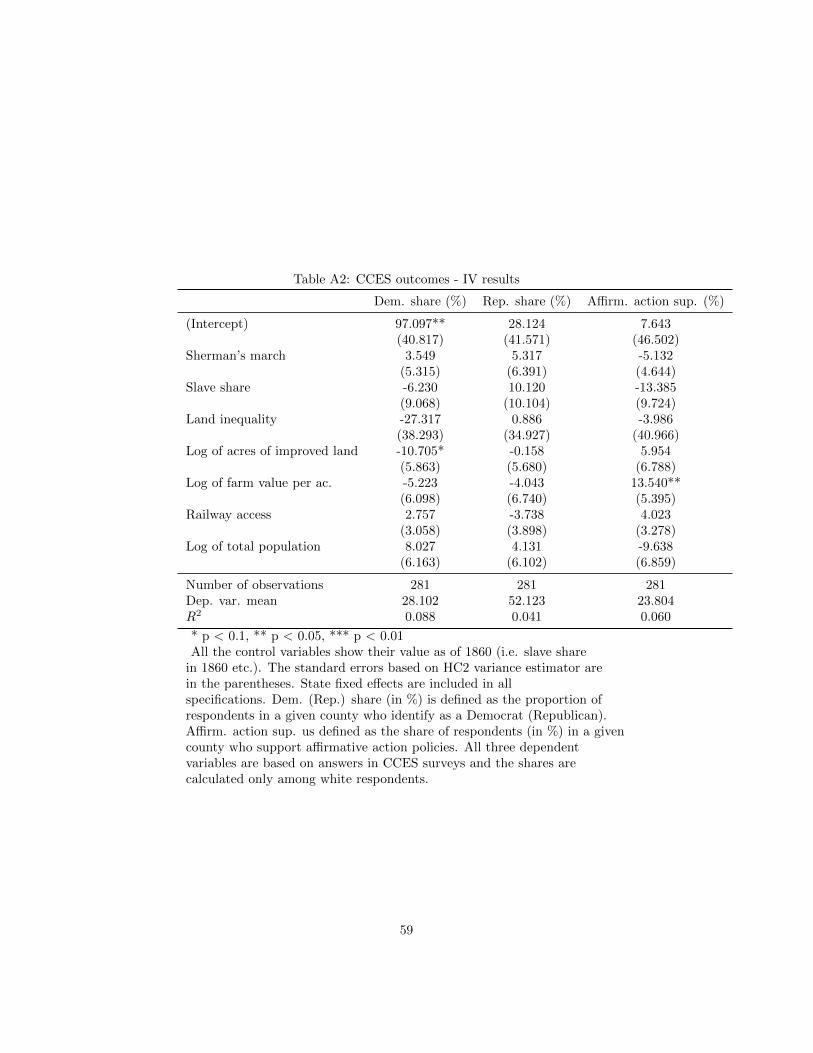
Table A2: CCES outcomes - IV results

Dem. share (%) Rep. share (%) Affirm. action sup. (%)

(Intercept) 97.097** 28.124 7.643(40.817) (41.571) (46.502)

Sherman’s march 3.549 5.317 -5.132(5.315) (6.391) (4.644)

Slave share -6.230 10.120 -13.385(9.068) (10.104) (9.724)

Land inequality -27.317 0.886 -3.986(38.293) (34.927) (40.966)

Log of acres of improved land -10.705* -0.158 5.954(5.863) (5.680) (6.788)

Log of farm value per ac. -5.223 -4.043 13.540**(6.098) (6.740) (5.395)

Railway access 2.757 -3.738 4.023(3.058) (3.898) (3.278)

Log of total population 8.027 4.131 -9.638(6.163) (6.102) (6.859)

Number of observations 281 281 281Dep. var. mean 28.102 52.123 23.804R2 0.088 0.041 0.060

* p < 0.1, ** p < 0.05, *** p < 0.01All the control variables show their value as of 1860 (i.e. slave sharein 1860 etc.). The standard errors based on HC2 variance estimator arein the parentheses. State fixed effects are included in allspecifications. Dem. (Rep.) share (in %) is defined as the proportion ofrespondents in a given county who identify as a Democrat (Republican).Affirm. action sup. us defined as the share of respondents (in %) in a givencounty who support affirmative action policies. All three dependentvariables are based on answers in CCES surveys and the shares arecalculated only among white respondents.

59

Table A3: Other outcomes - OLS - different treatment definitions

First names (1880) First names (1930) Street names Monuments Lynch rate

Sherman’s march (10 miles) -0.017 0.210*** 0.126* 0.018 0.126*(0.020) (0.080) (0.065) (0.059) (0.065)

Sherman’s march (20 miles) 0.004 0.186** 0.134* -0.004 0.134*(0.020) (0.082) (0.079) (0.057) (0.079)

Sherman’s march (50 miles) 0.007 -0.042 0.055 0.080 0.055(0.022) (0.103) (0.078) (0.061) (0.078)

a The standard set of controls was included in all specifications. The standard errors based onHC2 variance estimator are in the parentheses. First names (1880) is the share (in %) ofwhites born after 1865 in a given county with first name that we classified as Confederate in1880 census. First names (1930) is defined the same, only 1930 census is used. Street names isthe share (in %) of streets and roads in a given that contain a surname of a Confederatefigure in their name. Monuments is a an indicator variable that equals one if a Confederatemonument was present in a county in 2019. Lynch rate is defined as the number of lynchings in acounty from 1882 to 1929 per 10,000,000 residents.

60