Causal networks for risk and compliance: Methodology and application

1 Causal networks for risk and2 compliance: Methodology3 and application

A. ElisseeffJ.-P. PelletE. Pratsini

4 This paper presents a statistical approach to quantitatively measure5 the current exposure of a company to failures and defects in product6 quality or to compliance to government regulations. This approach is7 based on causal networks, which have previously been applied to8 other fields, such as systems maintenance and reliability. Causal9 networks allow analysts to causally explain the values of variables10 (an explanatory approach), to assess the effect of interventions on the11 structure of the data-generating process, and to evaluate Bwhat-if[12 scenarios, that is, alternative methods or policies (an exploratory13 approach). Building the causal structure raises some challenges.14 In particular, there is no automated way to collect the needed data.15 We present a methodology for model selection and probability16 elicitation based on expert knowledge. We apply the proposed17 approach to the case of pharmaceutical manufacturing processes.18 The use of such networks allows for a more rigorous comparison of19 practices across different manufacturing sites, creates the20 opportunity for risk remediation, and allows us to evaluate21 alternative methods and approaches.

22 Introduction23 This paper concerns the development of a risk-assessment24 model for quantifying the risk hazard in a setting in which25 risk involves various challenges related to government26 compliance and product quality and availability. One of the27 initial motivations to develop such models was the recent28 initiative of the U.S. Food and Drug Administration (FDA)29 referred to as Pharmaceutical Current Good Manufacturing30 Practices for the 21st Century [1], which launched a series31 of projects to provide Bthe most effective public health32 protection.[One key aspect of this initiative is the use of quality33 and risk management techniques to better identify the highest34 risk elements in a drug manufacturing process [2]. This calls35 for the development of risk management tools to manage36 manufacturing process risks not only for the FDA but also for37 the pharmaceutical companies that must make sure that38 their plants do not have a high risk of producing defective39 drugs or a high risk of not being compliant with the FDA.40 Therefore, we have devised a general methodology to41 build risk-assessment models based on causal networks.42 Our approach can also be employed in other contexts

43characterized by scarce or unreliable data, considerable44qualitative information, and expert knowledge.45Risk quantification is key to many industries and has been46performed using a plethora of different tools, ranging from47statistical methods that offer no insight or justification of their48output to management techniques and expert brainstorming.49In this paper, we will adopt an approach whose central50concept is a causal network, a graph representing the51different sources of risk and their interrelationships. We build52this network using principles that have been defined in the53mid-1980s [3] using expert-driven modeling. Causal54networks can be viewed as Bayesian networks with the55additional causal interpretation of the arcs in the network56structure [4]. Bayesian networks have been used in different57areas in which the overall risk assessment is as important58as finding the most probable or the most risky variable.59Contrary to Bayesian networks, causal networks can be60used to estimate the effect of structural changes in the61dependencies induced by the data-generating process.62They can also assess the effect of interventions on variables63in an unbiased way, even in the presence of confounding64factors [4].65When data are easily available, automatic construction of66the network is possible to some extent. Applications

�Copyright 2010 by International Business Machines Corporation. Copying in printed form for private use is permitted without payment of royalty provided that (1) each reproduction is done withoutalteration and (2) the Journal reference and IBM copyright notice are included on the first page. The title and abstract, but no other portions, of this paper may be copied by any means or distributed

royalty free without further permission by computer-based and other information-service systems. Permission to republish any other portion of this paper must be obtained from the Editor.

A. ELISSEEFF ET AL. 6 : 1IBM J. RES. & DEV. VOL. 54 NO. 3 PAPER 6 MAY/JUNE 2010

0018-8646/10/$5.00 B 2010 IBM

Digital Object Identifier: 10.1147/JRD.2010.2045251

67 performing this construction include hard-drive failure68 diagnosis tools [5] and other computer diagnostic tools [6],69 medical decision support systems [7, 8], production line70 analysis [9], and others [10, 11]. The construction of the71 network in studies of process performance raises some72 challenges that are not easily overcome, the main and73 foremost being the lack of quantitative variables. Many74 processes involve variables that are difficult to rigorously75 quantify and analyze, such as education of employees and76 organizational clarity; thus, defining the level of granularity,77 the structure of the network, and its parameters involve78 additional challenges. Such processes include those that79 involve reliability analysis [12], defect prediction [13, 14],80 software cost estimation [15], or accident causation [16], to81 name a few.82 When asked about the causes that might induce a decrease83 in process performance, two experts might contradict each84 other not only about the causes of risk but also about the85 strength of the cause–effect relationship. To extract86 quantitative risk measures from a pool of experts, some87 methods can be applied, such as the Delphi approach [17]88 or Six Sigma�� [18]. However, those methods cannot89 manage data and expert knowledge at the same level.90 The fishbone/Ishikawa cause–effect diagrams [19] are, for91 instance, recommended by Six Sigma experts to perform92 root–cause analysis. These diagrams are graphs of potential93 causes for defects that are entirely built from expert94 knowledge. Data might be collected for further analysis95 but are not used to update and define the causal links. On96 the other hand, causal networks can be interpreted as97 cause–effect diagrams in which both the structure and the98 strength of causal links are assessed by experts and can be99 updated with data. Therefore, they can be perceived as a

100 complement to an Ishikawa diagram. Similarly, they were101 shown in [20] to extend causal maps [21].102 In this paper, we describe how to build a causal network103 from expert knowledge to assess the risk of quality failure of104 a process. This paper is organized as follows: The section105 BCausal reasoning[ describes causal reasoning, causal106 networks, and their diagnostic capabilities. The section107 BCausal networks for assessing quality risk of processes[108 shows how to define such a network to analyze the quality109 risk. The section BApplication to pharmaceutical110 manufacturing processes[ describes the application of our111 methodology to compute the quality risk of pharmaceutical112 manufacturing processes. The section BDiscussion[113 describes the use of causal networks and related tools for114 process risk analysis, and the section BConclusion[115 concludes this paper.

116 Causal reasoning117 This section formally presents causal networks as118 probabilistic modeling tools. We mostly focus on the119 techniques to easily build the structure of a network and its

120parameters using expert knowledge and on the methods used121to draw causal conclusions based on the generated model.122For more details on the structure learning and inference123algorithms, see [22, 23]. The models described in this paper124are created using the GeNIe modeling environment125developed by the Decision Systems Laboratory of the126University of Pittsburgh [24]. Throughout this paper, as a127notational convention, we use small caps for random128variables, boldface for sets and vectors, and italics for scalars.

129Causal networks130We first introduce Bayesian networks, upon which causal131networks are based. For this entire section, the readers are132referred to [4, 23] for background information.133Bayesian networks are an efficient tool for probabilistic134reasoning. Suppose we are interested in a problem involving135d variables of interest V ¼ fXigi¼1;...;d . In a Bayesian136network, these variables are represented as the nodes of a137directed acyclic graph (DAG), and dependencies between the138variables are represented by the links between the139corresponding nodes. The joint probability PðVÞ can then be140computed as

PðVÞ ¼Yd

i¼1PiðXijPaiÞ

141where Pai is the set of parents of Xi, i.e., all nodes that are142linked to Xi by a direct link oriented into Xi. The full graph143over V can thus represent any joint probability by the chain144rule of probability

PðVÞ ¼Yd

i¼1PiðXijX1;X2; . . . ;Xi�1Þ:

145Bayesian networks are particularly useful when (conditional)146independencies of the form PðXijXjXkÞ ¼ PðXijXkÞ can be147found in the data. In this case, Xj need not appear in the148conditional probability distribution for Xi, and thus, there149need not be a link from Xj to Xi in the graph. As more150independencies are found, the simpler the model becomes;151there are fewer links in the graph, and thus, fewer parameters152are needed to specify the conditional probability tables.153Bayesian networks are widely used to efficiently solve154inference tasks of the type PðXjE ¼ eÞ, which may be read155as Bwhat is the marginal probability of the variables X V,156given that I observe the evidence E ¼ e (where E V).[157For instance, a node C representing COUNTRY would be set to158BFrance[ if the process is running in France, and inference159algorithms would be run to assess the probability of a given160level of the target risk variable T as PðT jC ¼ FranceÞ. The161more independencies there are in P, the sparser G is, the162simpler B is in terms of number of parameters, and the more

6 : 2 A. ELISSEEFF ET AL. IBM J. RES. & DEV. VOL. 54 NO. 3 PAPER 6 MAY/JUNE 2010

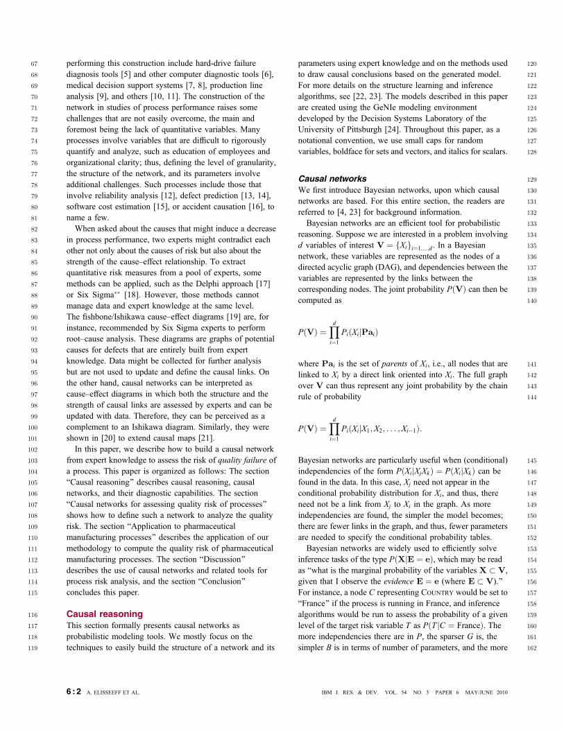
163 efficient the inference task can be. The belief–propagation164 algorithm [3], the sum–product algorithm [25], and other165 variants can efficiently solve such tasks. See [26] for a more166 complete introduction to Bayesian networks.167 The definition of a causal network refines that of a168 Bayesian network in that each directed link from Xj to Xi is169 additionally required to denote a causal effect: Xj must170 have a direct causal effect on Xi in the sense that this causal171 effect is not mediated by any other variable in V and that172 the observed dependency between Xj and Xi is not due to a173 confounding factor (e.g., a hidden common cause).174 Whereas a Bayesian network structure is only concerned175 with statistical dependencies, the causal network structure176 denotes a set of direct cause–effect relationships.177 Consider, for instance, the graph in Figure 1(a). If178 interpreted as a Bayesian network, then this graph indicates179 that the existence of a traffic jam is related to whether one180 arrives late at work, that arriving late at work is related to181 missing a meeting, and that the only way that the traffic jam182 and the missed meeting are related is through the fact that183 one may be late at work. Bayesian networks do not depend184 on any notion of causality; actually, the orientation of the185 two arrows could be reversed and would imply the same186 conclusions as a Bayesian network. If interpreted as a causal187 network, however, then this structure additionally tells us188 that the traffic jam is causing the late arrival, which in turn189 causes the meeting to be missed. Causal networks can190 account for interventions on the variables: Forcing someone191 to be late at work will have an effect on whether he192 misses the meeting but will not affect traffic. This conclusion193 can only be drawn if the links carry a causal meaning.194 Reversing the direction of the arrows in Figure 1(a) would195 be meaningless in a causal context.

196 Inference and diagnostics capabilities197 Bayesian networks and causal networks have a common198 characteristic, namely, they comprise a qualitative part, i.e.,199 the graphical structure, and a quantitative part, i.e., the200 parameters encoding the conditional probability distributions201 at each node. To obtain a full model, both have to be202 determined. Generally, the parameters and the structure

203(up to an equivalence class) can be learned from data.204However, in some cases, such as when analyzing the quality205risk, data are not available or cannot be trusted. In the206methodology described in the next section, we describe how207to iteratively build the model with a team of experts and208how to fill the probability tables.209Whereas Bayesian networks are mainly used to solve210inference tasks by marginalizing out the observed variables,211causal networks can also assess the direct causal effect of212any given link in the causal graph. Contrary to what could be213expected, this information is neither directly readable from214conditional probability tables nor directly readable from a215simple marginalization. This is demonstrated by the216following example.217Assume that the efficacy of a new drug must be assessed.218A study is conducted; the resulting data are collected in219Table 1. Examining the combined table for both males and220females, we conclude that the new drug has a positive221effect on the recovery rate [see bold percentages in222Table 1(a)]. Examining the separate tables for male and223female patients, however, leads us to conclude that the drug224has a negative effect [Table 1(b)]. This surprising225phenomenon has been known for more than half a century226[4, 27] and is called Simpson’s paradox: different227stratifications of the data can lead to seemingly contradicting228conclusions. In this case, we see that males naturally229recover better, and that the fraction of patients given the drug230was greater for males than for females. Building the231corresponding causal model, shown in Figure 1(b), helps us232understand the data. We are interested in knowing the233direct effect of the drug on the recovery rateVthat is, the234Bstrength[ of the link from DRUG GIVEN to RECOVERY.

Figure 1

Networks and graphs. (a) Sample Bayesian network that is causal.(b) Causal graph that helps us solve our example of Simpson’s paradox.

Table 1 Drug efficacy study. (a) Combined tables from the drugefficacy study. (b) Separate tables by gender.


235 Looking at the combined table means that we are measuring236 the effect of not only this direct link but also the237 Binfluence path[ that goes from DRUG GIVEN to RECOVERY238 through GENDER. Therefore, the conditional probability239 PðRECOVERYjDRUG GIVENÞ does not represent the causal240 effect of the drug on recovery but an aggregation of the true241 causal effect and of the gender bias introduced in the242 study. An examination of the separate tables amounts to243 holding the value of GENDER constant, thus Bneutralizing[244 the influence path through GENDER, which effectively allows245 us to assess the effect of the drug on the recovery rate.246 We have adjusted for the variable GENDER and found that the247 conditional probability PðRECOVERYjDRUG GIVEN;GENDERÞ248 indeed represents the causal effect of the drug.249 This is a small example; however, in larger networks,250 it can become more difficult for experts to determine which251 variables to adjust. Such adjustments can automatically be252 made with Pearl’s rules for the do-calculus [4, Chapter 7].253 Describing such a calculus in depth is beyond the scope of254 this paper, but it is worth noting that causal networks provide255 a way to adjust for bias in data collection, given the joint256 probability distribution and the causal structure. Essentially,257 what the do-calculus does is assess the effect of an258 intervention on a variable Xj on another variable Xi, which is259 denoted by PðXi j doðXj ¼ xjÞÞ. This is computed by260 shielding the target variable Xi from influence paths261 involving causes of Xj, which bias the estimate of the true262 causal effect. In the example of Table 1, we are interested in263 evaluating PðRECOVERYjdoðDRUG GIVENÞÞ, and we have264 already demonstrated that this is not equal to265 PðRECOVERYjDRUG GIVENÞ. The rules of do-calculus show us266 that, given the causal structure in Figure 1(b)

P RECOVERYjdoðDRUG GIVENÞð Þ¼ PðRECOVERYjDRUG GIVEN;GENDERÞ PðGENDERÞ

267 so that the overall probability of recovery with the drug is268 actually 50% with a placebo and 40% with the drug. This269 correctly reflects a 10% drop in recovery observed with both270 male and female patients.271 In Bayesian networks, it is possible to identify the most272 probable configuration that leads to a defect. Such a273 configuration is called an explanation. Given some target274 variable indicating a disease D, a doctor might be interested,275 independent of any observation, to know the profile of the276 most risky patient given the network containing D and all its277 potential causes X ¼ fXigi¼1;...;n. An explanation is, thus,278 a list of assignments H ¼ h, where H X. The details of279 how to choose H and how to compute h are left to the280 specific explanation algorithms. For instance, the most281 probable explanation approach [3] involves choosing to assign282 all variables (i.e.,H ¼ X) and finds the assignment x that283 maximizes PðX ¼ xjD ¼ presentÞ. One of the problems with

284this approach is that it returns a single Bexplanation,[ which285is quite long, and the most likely value of all potential causes is286returned. Often, several explanations can be considered287equally valid, and shorter explanations make more sense to the288end user. Additionally, there is no prioritization between the289causes. With causal networks, we can use the causal290explanation tree (CET) approach [28]. Explanation trees291represent in a tree structure several good explanations and score292them according to how much more likely the given target293variable state is (e.g., the presence of some disease) [29].294In the section BApplication to pharmaceutical manufacturing295processes,[ we show examples of causal explanation trees296to explain why an employee would badly perform.297The other diagnostic capabilities of Bayesian/causal298networks include the finding of which test to perform to obtain299more information on a given variable. If a patient has 50%300chance of having a disease, then this query would return the301first test to perform to know more, that is, to get a probability302closer to 0 or 1, corresponding to whether the patient has a303disease or not. For an overview of other inferences available in304Bayesian/causal networks, the reader is referred to [23].

305Causal networks for assessing the quality306risk of processes307This section describes a methodology to construct the308structure and the parameters of causal networks to assess the309quality risk.310Assuming a set of severity levels fs1; . . . ; sng, the quality311risk measures the frequency of the following failures in312different severity levels. On one hand, fitness-for-use failures313occur when the quality, efficacy, or safety of the end314product or service is not ensured. Quality relates to a product315conforming to its specification. Efficacy ensures that a316product has a positive effect (e.g., a drug treats a patient or a317service brings value to the customer). Safety assumes that318the end product is not harmful (e.g., no patient suffers from319fatal side effects or no service damages other business units).320In the case of pharmaceutical manufacturing processes, a321problem with the raw material, blending, or product322compounds is typically related to fitness-for-use risk. It has a323direct impact on the physical product or how it is processed.324On the other hand, compliance failures occur when quality,325efficacy, or safety in the process fails to be controlled.326These two components of the quality risk are orthogonal327and do not imply each other. A manufacturing plant, for328instance, can produce high-quality products but might not329report any information about the manufacturing process. Its330fitness-for-use risk is low, but its compliance risk is high.331Conversely, another site might have many controls in place332to ensure that all good manufacturing practice (GMP)333systems are implemented. This does not mean that its yield is334high, since many batches might have to be reprocessed or335discarded because of low-quality products.336Assuming that the process is stationary, a frequency


337 measure is sufficient to account for failures at different time338 scales: The number of failures over T time periods is339 simply the product of the unit frequency times T . Therefore,340 the quality risk can also be interpreted as a measure of the341 required duration for one failure to occur. High-risk342 processes would, for instance, generate a failure every hour,343 whereas low-risk processes might induce only one failure344 every year.345 A seemingly straightforward approach to compute the346 quality risk would be to collect all reports on defective end347 products and noncompliance events, to count the number of348 times such events occurred, and to return the corresponding349 frequencies as defined in the quality risk. Unfortunately,350 this approach does not work if data collection is not carefully351 controlled and monitored. Lack of failure reports does not352 mean no events, it only means no reporting of events, which353 may be due to political or cultural factors. One way to354 avoid such issues is to extract knowledge from nonstatistical355 sources such as experts. This does not preclude any use of356 data but adds assumptions about how statistics should be357 interpreted. The remainder of this section describes a358 method based on causal networks that allows for such expert359 knowledge to be used in conjunction with statistics.

360 Determining the structure361 There are a few methodologies and guidelines to build the362 structure from expert data. For instance, [30] describes a363 general approach to build large-scale Bayesian networks and364 shows how to choose the suitable level of granularity.365 Reference [31] describes how Bayesian networks can be built366 from event trees or fault trees in the context of safety367 assessment. Reference [32] develops specialized inference368 algorithms for these trees. In this paper, we propose to369 build the structure starting from a fishbone diagram. The370 fishbone (or Ishikawa) diagram is a cause–effect graph built371 by a panel of experts to identify potential causes for a372 problem. It is the result of a technique designed by373 Ishikawa [19] in the 1960s to track the root causes for374 out-of-specification measurements. The diagram at the top375 portion of Figure 2 was designed by industry experts to376 analyze the poor performance of pharmaceutical377 manufacturing processes. It is composed of a main horizontal378 line representing the first layer of causes (horizontal arrow379 pointing to the poor process performance box). The other380 arrows correspond to the categories of causes. The leaves of381 this tree-structured diagram are the potential causes. The382 latter can then be ranked for further analysis and are meant to383 be investigated individually.384 The causal network adds further structure to the approach385 by providing a way to investigate links between the386 causes (bottom of Figure 2). These links should be direct387 cause–effect relationships and can appear between causes388 that are not in the same branch of the Ishikawa diagram.389 The art of building the causal network involves how

390accurately we can represent the causal influences between391the causes listed by the Ishikawa diagram. Whereas the392Ishikawa diagram can be constructed by tracking back the393causes of a failure by repeatedly asking Bwhy?[ until a root394cause is identified [19], the causal network requires that,395for each potential cause, one should determine the direct396effects. Once these are established, the structure of the causal397network is almost defined. We list a simple procedure for398building the structure of a causal graph given an Ishikawa399diagram. For each step, we assume that a moderator asks the400experts questions and that the experts are in discussion to401reach a consensus.402The following steps allow one to build the structure of a403causal network from expert knowledge:

4041. Obtain an Ishikawa diagram and define an initial set405of variables/nodes for the causal network by flattening the406hierarchy appearing in the diagram.4072. Start from the initial causes by asking BWhat other408variable can be directly influenced by this one?[ and409connect the variables to the causes by a directed link.410Repeat with all the variables until no new link is added.4113. Draw the full resulting graph and submit it for review to412the team of experts, asking again, for each link, if the413link represents a direct cause–effect relationship. Remove414the links if the perceived causal effect can be accounted415for by another causal path in the graph.4164. For each variable, determine its levels (e.g., severity417levels) or states.

418Estimating the parameters: Probability419elicitation techniques420Once the structure of the causal network is defined, the421parameters determining the conditional probability tables422must be estimated. Without data, there is only a limited set of423information sources that can be used. The first source of424information is literature, such as survey reports [33]. The425second and main source of information is expert knowledge.426The structure of the causal network can be used to develop a427questionnaire, and the graph provides the variable to measure428and the values to consider. However, providing a value for429all the entries of a probability table is usually cumbersome430and not easy to grasp for someone not trained in statistics.431Furthermore, complex interactions between several causes432are usually difficult to directly assess. Parameterized433probabilistic models such as noisy-OR or noisy-MAX can be434used to make conditional probability elicitation at each node435more intuitive.436The noisy-OR model [3] can be applied with binary437variables and assumes independence between all the causes438of a variable. In a medical setting, for instance, an effect439variable Y (e.g., a disease) might independently be caused by440any of the anomalies X1; . . . ;Xn. Each of these n causes is441assumed to have an independent probability pi of causing Y .


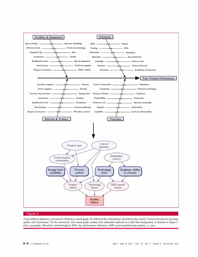
Figure 2

(Top) Ishikawa diagram is converted to (bottom) a causal graph. We followed the methodology described in the section BCausal networks for assessingquality risk of processes[ for the conversion. The causal graph contains four submodels depicted on a dark blue background, as detailed in Figure 3.(Geo: geography; Microbiol: microbiological; KPIs: key performance indicators; GMP: good manufacturing practice; y: year.)


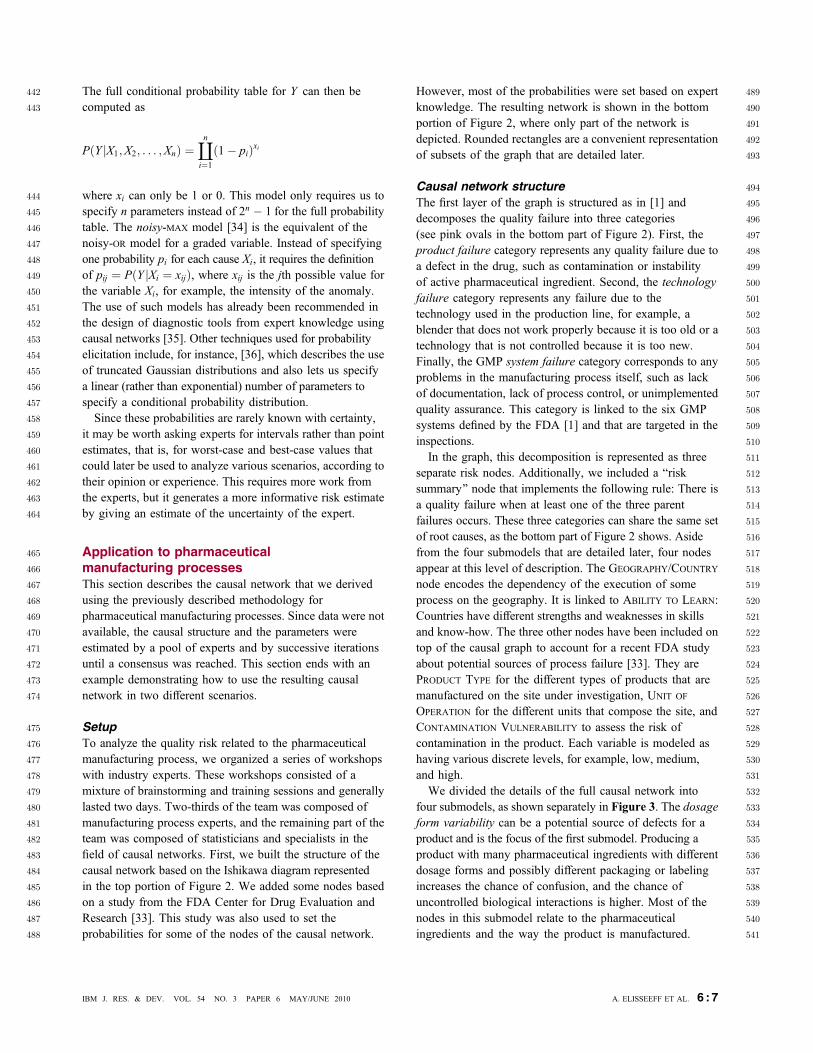
442 The full conditional probability table for Y can then be443 computed as

PðY jX1;X2; . . . ;XnÞ ¼an

i¼1ð1� piÞxi

444 where xi can only be 1 or 0. This model only requires us to445 specify n parameters instead of 2n � 1 for the full probability446 table. The noisy-MAX model [34] is the equivalent of the447 noisy-OR model for a graded variable. Instead of specifying448 one probability pi for each cause Xi, it requires the definition449 of pij ¼ PðY jXi ¼ xijÞ, where xij is the jth possible value for450 the variable Xi, for example, the intensity of the anomaly.451 The use of such models has already been recommended in452 the design of diagnostic tools from expert knowledge using453 causal networks [35]. Other techniques used for probability454 elicitation include, for instance, [36], which describes the use455 of truncated Gaussian distributions and also lets us specify456 a linear (rather than exponential) number of parameters to457 specify a conditional probability distribution.458 Since these probabilities are rarely known with certainty,459 it may be worth asking experts for intervals rather than point460 estimates, that is, for worst-case and best-case values that461 could later be used to analyze various scenarios, according to462 their opinion or experience. This requires more work from463 the experts, but it generates a more informative risk estimate464 by giving an estimate of the uncertainty of the expert.

465 Application to pharmaceutical466 manufacturing processes467 This section describes the causal network that we derived468 using the previously described methodology for469 pharmaceutical manufacturing processes. Since data were not470 available, the causal structure and the parameters were471 estimated by a pool of experts and by successive iterations472 until a consensus was reached. This section ends with an473 example demonstrating how to use the resulting causal474 network in two different scenarios.

475 Setup476 To analyze the quality risk related to the pharmaceutical477 manufacturing process, we organized a series of workshops478 with industry experts. These workshops consisted of a479 mixture of brainstorming and training sessions and generally480 lasted two days. Two-thirds of the team was composed of481 manufacturing process experts, and the remaining part of the482 team was composed of statisticians and specialists in the483 field of causal networks. First, we built the structure of the484 causal network based on the Ishikawa diagram represented485 in the top portion of Figure 2. We added some nodes based486 on a study from the FDA Center for Drug Evaluation and487 Research [33]. This study was also used to set the488 probabilities for some of the nodes of the causal network.

489However, most of the probabilities were set based on expert490knowledge. The resulting network is shown in the bottom491portion of Figure 2, where only part of the network is492depicted. Rounded rectangles are a convenient representation493of subsets of the graph that are detailed later.

494Causal network structure495The first layer of the graph is structured as in [1] and496decomposes the quality failure into three categories497(see pink ovals in the bottom part of Figure 2). First, the498product failure category represents any quality failure due to499a defect in the drug, such as contamination or instability500of active pharmaceutical ingredient. Second, the technology501failure category represents any failure due to the502technology used in the production line, for example, a503blender that does not work properly because it is too old or a504technology that is not controlled because it is too new.505Finally, the GMP system failure category corresponds to any506problems in the manufacturing process itself, such as lack507of documentation, lack of process control, or unimplemented508quality assurance. This category is linked to the six GMP509systems defined by the FDA [1] and that are targeted in the510inspections.511In the graph, this decomposition is represented as three512separate risk nodes. Additionally, we included a Brisk513summary[ node that implements the following rule: There is514a quality failure when at least one of the three parent515failures occurs. These three categories can share the same set516of root causes, as the bottom part of Figure 2 shows. Aside517from the four submodels that are detailed later, four nodes518appear at this level of description. The GEOGRAPHY/COUNTRY519node encodes the dependency of the execution of some520process on the geography. It is linked to ABILITY TO LEARN:521Countries have different strengths and weaknesses in skills522and know-how. The three other nodes have been included on523top of the causal graph to account for a recent FDA study524about potential sources of process failure [33]. They are525PRODUCT TYPE for the different types of products that are526manufactured on the site under investigation, UNIT OF527OPERATION for the different units that compose the site, and528CONTAMINATION VULNERABILITY to assess the risk of529contamination in the product. Each variable is modeled as530having various discrete levels, for example, low, medium,531and high.532We divided the details of the full causal network into533four submodels, as shown separately in Figure 3. The dosage534form variability can be a potential source of defects for a535product and is the focus of the first submodel. Producing a536product with many pharmaceutical ingredients with different537dosage forms and possibly different packaging or labeling538increases the chance of confusion, and the chance of539uncontrolled biological interactions is higher. Most of the540nodes in this submodel relate to the pharmaceutical541ingredients and the way the product is manufactured.


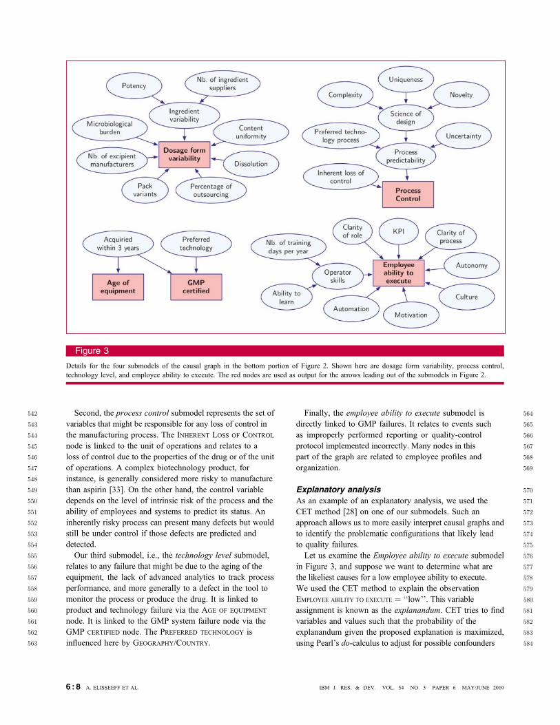
542 Second, the process control submodel represents the set of543 variables that might be responsible for any loss of control in544 the manufacturing process. The INHERENT LOSS OF CONTROL545 node is linked to the unit of operations and relates to a546 loss of control due to the properties of the drug or of the unit547 of operations. A complex biotechnology product, for548 instance, is generally considered more risky to manufacture549 than aspirin [33]. On the other hand, the control variable550 depends on the level of intrinsic risk of the process and the551 ability of employees and systems to predict its status. An552 inherently risky process can present many defects but would553 still be under control if those defects are predicted and554 detected.555 Our third submodel, i.e., the technology level submodel,556 relates to any failure that might be due to the aging of the557 equipment, the lack of advanced analytics to track process558 performance, and more generally to a defect in the tool to559 monitor the process or produce the drug. It is linked to560 product and technology failure via the AGE OF EQUIPMENT561 node. It is linked to the GMP system failure node via the562 GMP CERTIFIED node. The PREFERRED TECHNOLOGY is563 influenced here by GEOGRAPHY/COUNTRY.

564Finally, the employee ability to execute submodel is565directly linked to GMP failures. It relates to events such566as improperly performed reporting or quality-control567protocol implemented incorrectly. Many nodes in this568part of the graph are related to employee profiles and569organization.

570Explanatory analysis571As an example of an explanatory analysis, we used the572CET method [28] on one of our submodels. Such an573approach allows us to more easily interpret causal graphs and574to identify the problematic configurations that likely lead575to quality failures.576Let us examine the Employee ability to execute submodel577in Figure 3, and suppose we want to determine what are578the likeliest causes for a low employee ability to execute.579We used the CET method to explain the observation580EMPLOYEE ABILITY TO EXECUTE ¼ ‘‘low’’. This variable581assignment is known as the explanandum. CET tries to find582variables and values such that the probability of the583explanandum given the proposed explanation is maximized,584using Pearl’s do-calculus to adjust for possible confounders

Figure 3

Details for the four submodels of the causal graph in the bottom portion of Figure 2. Shown here are dosage form variability, process control,technology level, and employee ability to execute. The red nodes are used as output for the arrows leading out of the submodels in Figure 2.


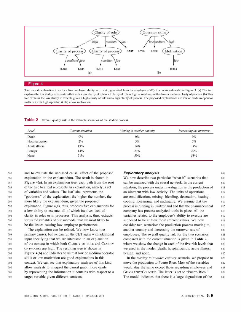
585 and to evaluate the unbiased causal effect of the proposed586 explanation on the explanandum. The result is shown in587 Figure 4(a). In an explanation tree, each path from the root588 of the tree to a leaf represents an explanation, namely, a set589 of variables and values. The leaf label represents the590 Bgoodness[ of the explanation: the higher the number, the591 more likely the explanandum, given the proposed592 explanation. Figure 4(a), thus, proposes five explanations for593 a low ability to execute, all of which involves lack of594 clarity in roles or in processes. This analysis, thus, extracts595 for us the variables of our submodel that are most likely to596 be the issues causing low employee performance.597 The explanation can be refined. We now know two598 primary causes, but we can run the CET again with additional599 input specifying that we are interested in an explanation600 of the context in which both CLARITY OF ROLE and CLARITY601 OF PROCESS are high. The resulting tree is shown in602 Figure 4(b) and indicates to us that low or medium operator603 skills or low motivation are good explanations in this604 context. We can see that explanatory analyses of this kind605 allow analysts to interpret the causal graph more easily606 by representing the information it contains with respect to a607 target variable given different contexts.

608Exploratory analysis609We now describe two particular Bwhat-if[ scenarios that610can be analyzed with the causal network. In the current611situation, the process under investigation is the production of612an ointment with low activity. The units of operations613are emulsification, mixing, blending, deaeration, heating,614cooling, measuring, and packaging. We assume that the615process is running in Switzerland and that the pharmaceutical616company has process analytical tools in place. All the617variables related to the employee’s ability to execute are618supposed to be at their most efficient values. We now619consider two scenarios: the production process moving to620another country and increasing the turnover rate of621employees. The overall quality risk for the two scenarios622compared with the current situation is given in Table 2,623where we show the change in each of the five risk levels that624we used in the model: death, hospitalization, acute illness,625benign, and none.626In the moving to another country scenario, we propose to627move the production to Puerto Rico. Most of the variables628would stay the same except those regarding employees and629GEOGRAPHY/COUNTRY. The latter is set to BPuerto Rico.[630The model indicates that there is a large degradation of the

Figure 4

Two causal explanation trees for a low employee ability to execute, generated from the employee ability to execute submodel in Figure 3. (a) This treeexplains the low ability to execute either with a low clarity of role or (if clarity of role is high or medium) with a low or medium clarity of process. (b) Thistree explains the low ability to execute given a high clarity of role and a high clarity of process. The proposed explanations are low or medium operatorskills or (with high operator skills) a low motivation.

Table 2 Overall quality risk in the example scenarios of the studied process.


631 employee’s ability to execute: 53% is rated Bhigh[ in the632 current situation, which drops to 15% in this scenario.633 This is due to a decrease in the clarity of role and the634 autonomy, which are nearly perfect without moving. The635 impact on the quality risk is a decrease from 71% to 59%636 for the probability of not having any quality failure,637 which is less than the employee’s ability to execute as the638 latter only has a partial influence on the quality risk.639 Process control and technology are also important and are640 supposed in this scenario to be performing well. The variables641 that would individually have the most impact on risk642 reduction are OPERATOR SKILLS, MOTIVATION, CLARITY OF

643 ROLE, and CULTURE. Obviously, the employee ability to644 execute has a strong impact on the quality risk. On645 the other hand, technology is not as critical. This example646 shows that introducing a change in a manufacturing647 process implies an increase of the quality risk. This seems648 natural and unavoidable since, for example, clarity of649 role and autonomy are degraded. On the other hand, it is650 unclear which change would least degrade the651 quality risk.652 In the increasing the turnover scenario, we assume that653 50% of the employees decide to leave and are replaced by654 new hires. The employee ability-to-execute model will655 therefore be changed based on the new configuration. In656 accord with experts, we expect AUTONOMY and CLARITY OF

657 ROLE to be reduced. Compared with the previous example,658 the model tells us that the autonomy is Bworse[ here:659 new employees are supposed to be less autonomous than660 existing employees. Their culture has been changed as well661 to slightly involve more risk taking. Their motivation is662 higher than before, hypothesizing that new employees are663 eager to perform well. Overall, employees would not execute664 as well as in the first scenario: the part of them rated as665 having a low ability increases from 10% to 52%. The666 difference is smoothed in the end quality risk, as shown in667 Table 2. There is only at most 1% difference between the668 frequencies of the two scenarios (compare columns 3 and 4669 in Table 2). This shows that technology and product670 quality being well under control in both cases; moving to671 another country is an action that is less prone to quality672 failures than renewing half of the production staff.673 The difference is small and might change depending on the674 hypothesis, that is, on the distributions that are assumed675 for some of the variables. However, by using such676 probabilistic tools, we have the assurance that we derive677 conclusions that are compatible with the knowledge that was678 entered during construction.

679 Discussion680 So far, causality has mostly been applied to the economy and681 medical domain and to sociology and artificial intelligence682 but has not been used very much to analyze processes. Aside683 from their qualitative nature, we believe that processes are

684associated with extra challenges that explain this late685adoption with respect to causality. First, most business686processes are complex and require a deep understanding of687an industry. Causality is just as complex. Therefore, an688unconventionally large gap exists between statisticians and689consultants or industry experts. Second, experts have to690formalize a knowledge that is generally built from691experience and does not correspond to any tangible object.692Contrary to analyzing the potential failures in a hard drive,693investigating the potential causes of low process performance694involves such considerations as motivation, culture, or695other concepts that are difficult to measure or even to define.696These difficulties make the entire application of causal697networks to processes more tedious and resource698consuming.699On the other hand, the gains achieved by constructing700causal networks can be worth the investment. First, building701a causal network encourages experts to agree on the702appropriate information to collect in order to understand703and monitor a process. Not only do they consider the704potential causes for problems that occur now, but they also705think about all sources of failures that might explain poor706process quality. Once the network is built, experts can then707compare and build scenarios, constantly validating the708adequacy of the resulting probabilities with their own709knowledge. In particular, they can ensure that the decision710they make is compatibleVusing probability rulesVwith the711knowledge they formalized with the causal network.712Ultimately, if the data are properly collected, then this713knowledge could be enhanced by objective facts, which714would lead to more efficient and motivated decisions.715Finally, causal networks provide a natural tool for sharing716knowledge and storing it in a form that can be used and717queried by others.

718Conclusion719We have described a methodology to build a causal network720to compute process quality risk and demonstrated it with721pharmaceutical manufacturing processes. Rather than722presenting objective results based on a clearly defined723experimental design, we adopted a presentation that724resembles the type of process we study and that may be725thought of as being positioned between subjective and726objective information. We mostly focused on showing how727causal networks could be used to analyze and communicate728the quality risk for processes. We argued that causal729networks are the appropriate tool to use. The end result of the730approach is a causal model that computes the quality risk731under different conditions and provides insight on the key732causes increasing the risk. Finding the individual action that733would reduce the risk most is possible, but when multiple734actions are simultaneously taken, other optimization735techniques would be required, such as those736developed in [37].


737 Acknowledgments738 The authors would like to thank L. Mazaferro and M. Ricci739 for their fruitful collaboration and help in building the740 causal network for pharmaceutical manufacturing processes.

741 ��Trademark, service mark, or registered trademark of Motorola, Inc.,742 in the United States, other countries, or both.

743 References744 1. U.S. Food and Drug Administration, Pharmaceutical CGMPs for745 the 21st Century: A Risk-Based Approach, Aug. 2002. [Online].746 Available: http://www.fda.gov/oc/guidance/gmp.html747 2. Department of Health and Human Services, U.S. Food and Drug748 Administration, Risk-Based Method for Prioritizing CGMP749 Inspections of Pharmaceutical Manufacturing SitesVA Pilot Risk750 Ranking Model, 2004, Tech. Rep.751 3. J. Pearl, BFusion, propagation, and structuring in belief networks,[752 Artif. Intell., vol. 29, no. 3, pp. 241–288, Sep. 1986.753 4. J. Pearl, Causality: Models, Reasoning and Inference.754 Cambridge, U.K.: Cambridge Univ. Press, Mar. 2000.755 5. S. Fine and A. Ziv, BCoverage-directed test generation for756 functional verification using Bayesian networks,[ in Proc.757 40th Conf. Design Autom., 2003, pp. 286–291.758 6. M. Brodie, I. Rish, and S. Ma, BIntelligent probing:759 A cost-effective approach to fault diagnosis in computer760 networks,[ IBM Syst. J., vol. 41, no. 3, pp. 372–385, Jul. 2002.761 7. D. E. Heckerman, E. J. Horviz, and B. N. Nathwani, BTowards762 normative expert systems: Part I. The pathfinder project,[763 Methods Inf. Med., vol. 31, no. 2, pp. 90–105, Jun. 1992.764 8. D. E. Heckerman and B. N. Nathwani, BToward normative expert765 systems: Part II. Probability-based representations for efficient766 knowledge acquisition and inference,[ Methods Inf. Med., vol. 31,767 pp. 106–116, 1992.768 9. E. Wolbrecht, B. D’Ambroio, and R. P. D. Kirby, BMonitoring and769 diagnosis of a multistage manufacturing process using Bayesian770 networks,[ Artif. Intell. Eng. Design Manuf., vol. 14, no. 1,771 pp. 53–67, Jan. 2000.772 10. D. E. Heckerman, A. Mamdani, and M. P. Wellman, BReal-world773 applications of Bayesian networks,[ Commun. ACM, vol. 38,774 no. 3, pp. 24–26, Mar. 1995.775 11. M. Neil, M. Tailor, D. Marquez, N. E. Fenton, and P. Hearty,776 BModelling dependable systems using hybrid Bayesian777 networks,[ Reliab. Eng. Syst. Saf., vol. 93, no. 7, pp. 933–939,778 Jul. 2008.779 12. M. Neil, N. E. Fenton, S. Forey, and R. Harris, BUsing Bayesian780 belief networks to predict the reliability of military vehicles,[781 IEEE Comput. Control Eng. J., vol. 12, no. 1, pp. 11–20,782 Feb. 2001.783 13. N. E. Fenton, M. Neil, W. Marsh, P. Hearty, L. Radlinski, and784 P. Krause, BOn the effectiveness of early life cycle defect785 prediction with Bayesian nets,[ Empirical Softw. Eng., vol. 13,786 no. 5, pp. 499–537, Oct. 2008.787 14. N. E. Fenton, M. Neil, W. Marsh, P. Hearty, D. Marquez,788 P. Krause, and R. Mishra, BPredicting software defects in varying789 development lifecycles using Bayesian nets,[ Inf. Softw. Technol.,790 vol. 49, no. 1, pp. 32–43, Jan. 2007.791 15. I. Stamelosa, L. Angelisa, P. Dimoua, and P. Sakellaris, BOn the792 use of Bayesian belief networks for the prediction of software793 productivity,[ Inf. Softw. Technol., vol. 45, no. 1, pp. 51–60,794 Jan. 2005.795 16. W. Marsh and G. Bearfield, BUsing Bayesian networks to model796 accident causation in the UK railway industry,[ in Proc. 7th Int.797 Conf. Probab. Safety Assessment Manage., Berlin, Germany,798 2004.799 17. M. Turoff and S. R. Hiltz, BGazing into the oracle: The Delphi800 method and its application to social policy and public health,[ in801 Computer-Based Delphi Processes. Amsterdam,802 The Netherlands: Jessica Kingsley Publishers, 1996.

80318. M. Barney and T. McCarty, The New Six Sigma: A Leader’s Guide804to Achieving Rapid Business Improvement and Sustainable805Results. Upper Saddle River, NJ: Pearson Education, 2002.80619. K. Ishikawa, Introduction to Quality Control. New York:807Productivity Press, 1990 (Translator: J. H. Loftus).80820. S. Nadkarni and P. P. Shenoy, BA Bayesian network approach to809making inferences in causal maps,[ Eur. J. Oper. Res., vol. 128,810no. 3, pp. 479–498, Feb. 2001.81121. C. F. Eden, F. Ackermann, and S. Cropper, BThe analysis of cause812maps,[ J. Manage. Stud., vol. 29, no. 3, pp. 309–323, 1992.81322. F. V. Jensen, Bayesian Networks and Decision Graphs, Statistics814for Engineering and Computer Science. Berlin, Germany:815Springer-Verlag, 2001.81623. R. E. Neapolitan, Learning Bayesian Networks. Englewood817Cliffs, NJ: Prentice-Hall, 2003, ser. Artificial Intelligence.81824. Decision System Laboratory, University of Pittsburg, GeNIe:819Graphical Network Interface. [Online]. Available: http://genie.sis.820pitt.edu/82125. F. R. Kschischang, B. J. Frey, and H.-A. Loeliger, BFactor graphs822and the sum–product algorithm,[ IEEE Trans. Inf. Theory, vol. 47,823no. 2, pp. 498–519, Feb. 2001.82426. E. Charniak, BBayesian networks without tears,[ AI Mag., vol. 12,825no. 4, pp. 50–63, 1991.82627. E. H. Simpson, BThe interpretation of interaction in contingency827tables,[ J. Roy. Stat. Soc. B, vol. 13, no. 2, pp. 238–241, 1951.82828. U. H. Nielsen, J.-P. Pellet, and A. Elisseeff, BExplanation trees for829causal Bayesian networks,[ in Proc. 24th Conf. Uncertainty Artif.830Intell., 2008, pp. 427–434.83129. M. J. Flores, BBayesian networks inference: Advanced algorithms832for triangulation and partial abduction,[ Ph.D. dissertation,833Universidad De Castilla-La Mancha, Castilla-La Mancha, Spain,8342005.83530. M. Neil, N. Fenton, and L. Nielsen, BBuilding large-scale836Bayesian networks,[ Knowl. Eng. Rev., vol. 15, no. 3, pp. 257–284,837Sep. 2000.83831. D. W. R. Marsh and G. Bearfield, BGeneralising event trees using839Bayesian networks with a case study of train derailment,[840Proc. Inst. Mech. Eng. Part O, J. Risk Reliab., vol. 222, no. 2,841pp. 105–114, 2008.84232. D. Marquez, M. Neil, and N. E. Fenton, BSolving dynamic fault843trees using a new hybrid Bayesian network inference algorithm,[844in Proc. 16th Mediterranean Conf. Control Autom., 2008,845pp. 609–614.84633. N. L. Tran, B. Hasselbalch, K. Morgan, and G. Claycamp,847BElicitation of expert knowledge about risks associated with848pharmaceutical manufacturing processes,[ Pharm. Eng., vol. 25,849no. 4, pp. 26–38, 2005.85034. F. J. Dıez, BParameter adjustment in Bayes networks:851The generalized noisy-OR gate,[ in Proc. 9th Conf. Uncertainty852Arti. Intell., 1993, pp. 99–105.85335. P. C. Kraaijeveld and M. J. Druzdzel, BGeNIeRate: An interactive854generator of diagnostic Bayesian network models,[ in Proc. 16th855Int. Workshop Principles Diagnosis, Monterey, CA, 2005.85636. N. E. Fenton, M. Neil, and J. Gallan, BUsing ranked nodes to857model qualitative judgments in Bayesian networks,[ IEEE Trans.858Knowl. Data Eng., vol. 19, no. 10, pp. 1420–1432, Oct. 2007.85937. E. Pratsini and D. Dean, BRegulatory compliance of860pharmaceutical supply chains,[ ERCIM News, vol. 60, pp. 51–52,8612005.

862

863Received March 15, 2009; accepted for publication864May 26, 2009.


http://genie.sis.pitt.edu/

http://genie.sis.pitt.edu/

865 Andre Elisseeff Nhumi Technologies GmbH, 8003 Zurich,866 Switzerland ([email protected]). Dr. Elisseeff received the Ph.D.867 degree in machine learning from Ecole Normale Superieure de Lyon,868 Lyon, France, in 2000. He was a Researcher with the IBM Zurich869 Laboratory, where he worked on data-mining projects and in particular870 on causal networks with applications in health care, marketing, and871 information technology. He is the Founder and the Chief Executive872 Officer of Nhumi Technologies, Zurich, Switzerland, which873 specializes in providing comprehensive access of electronic health care874 data. His area of expertise is machine learning, data mining, and875 bioinformatics.

876 Jean-Philippe Pellet IBM Research Division, Zurich Research877 Laboratory, 8803 Ruschlikon, Switzerland ([email protected]).878 Mr. Pellet is a predoctoral student with the Data Analytics Group,879 IBM Zurich Research Laboratory, Ruschlikon, Switzerland, and is880 writing a thesis on causality. His main interests include automatic881 causal structure learning from data and practical applications of causal882 techniques in client projects.

883 Eleni Pratsini IBM Research Division, Zurich Research884 Laboratory, 8803 Ruschlikon, Switzerland ([email protected]).885 Dr. Pratsini received the Ph.D. degree in quantitative analysis from the886 University of Cincinnati, Cincinnati, OH, in 1990, the M.B.A. degree887 from the University of California at Los Angeles (UCLA), Los888 Angeles, in 1985, and the B.Sc. degree in civil engineering from the889 University of Birmingham, Birmingham, U.K., in 1983. She was890 previously a tenured faculty member with the Decision Sciences891 Department, Miami University, and a Visiting Scientist with the892 Swiss Federal Institute of Technology, Zurich. She is currently the893 Manager of mathematical and computational sciences with the894 IBM Zurich Research Laboratory, Ruschlikon, Switzerland. Her area895 of expertise is supply chain modeling and optimization with a particular896 interest in the analysis of risk in uncertainty in the models. Since897 joining IBM, she has been involved in projects bringing innovation898 through advanced analytics to clients.


AUTHOR QUERY

No query

Causal networks for risk and compliance: Methodology and application

Documents

Transcript of Causal networks for risk and compliance: Methodology and application