HAL Id: hal-02971865https://hal.archives-ouvertes.fr/hal-02971865v2

Preprint submitted on 25 May 2021

HAL is a multi-disciplinary open accessarchive for the deposit and dissemination of sci-entific research documents, whether they are pub-lished or not. The documents may come fromteaching and research institutions in France orabroad, or from public or private research centers.

L’archive ouverte pluridisciplinaire HAL, estdestinée au dépôt et à la diffusion de documentsscientifiques de niveau recherche, publiés ou non,émanant des établissements d’enseignement et derecherche français ou étrangers, des laboratoirespublics ou privés.

Causal Models for Real Time Bidding with RepeatedUser Interactions

Martin Bompaire, Alexandre Gilotte, Benjamin Heymann

To cite this version:Martin Bompaire, Alexandre Gilotte, Benjamin Heymann. Causal Models for Real Time Bidding withRepeated User Interactions. 2021. �hal-02971865v2�

Causal Models for Real Time Bidding with Repeated UserInteractions

Martin Bompaire∗

Criteo AI Lab

Paris, France

m.bompaire@criteo.com

Alexandre Gilotte∗

Criteo AI Lab

Paris, France

a.gilotte@criteo.com

Benjamin Heymann∗

Criteo AI Lab

Paris, France

b.heymann@criteo.com

ABSTRACTA large portion of online advertising displays are sold through an

auction mechanism called Real Time Bidding (RTB). Each auction

corresponds to a display opportunity, for which the competing ad-

vertisers need to precisely estimate the economical value in order to

bid accordingly. This estimate is typically taken as the advertiser’s

payoff for the target event – such as a purchase on the merchant

website attributed to this display – times this event estimated prob-

ability. However, this greedy approach is too naive when several

displays are shown to the same user. The purpose of the present

paper is to discuss how such an estimation should be made when

a user has already been shown one or more displays. Intuitively,

while a user is more likely to make a purchase if the number of dis-

plays increases, the marginal effect of each display is expected to be

decreasing. In this work, we first frame this bidding problem with

repeated user interactions by using causal models to value each

display individually. Then, based on this approach, we introduce a

simple rule to improve the value estimate. This change shows both

interesting qualitative properties that follow our previous intuition

as well as quantitative improvements on a public data set and online

in a production environment.

KEYWORDSreal-time bidding; causality; incrementality; attribution

1 INTRODUCTIONDisplay advertising is a form of online advertising in which a mar-

keter pays a website owner (the publisher) for the right to show

banners to its visitors (users) in the hope of triggering some future

sales. It is a large industry: last year, it was estimated that display

advertising generated more than 57 billions USD in the United

States [Fisher, 2019].

When the internet user reaches the publisher page, he triggers

a complex mechanism called Real Time Bidding (RTB). Real Time

Bidding involves several intermediaries (DSP, Ad exchange, SSP, ...)

in a chain of calls that finishes its run in the advertisers’ server in

the form of a bid request. In each advertiser’s server lives an algo-

rithmic bidding agent (the bidder) that implements the advertiser’s

strategy. When the bidder receives the bid request, it only has a

few milliseconds to answer with a bid. Then, the highest bidder

receives the right to show a banner to the user, in exchange for a

payment that depends on the chosen auction system. The bidder

can make a marketing campaign succeed or fail, because it decides

for whom, when, where and at which price to buy a banner.

∗The three authors contributed equally to this research.

The bidding strategy heavily relies on the display valuation,

usually predicted with a machine learning algorithm. The purpose

of the present paper is to discuss how such an estimation should be

made when a user has already been shown one or more displays.

More precisely we propose to correct the greedy formula that values

the action of making a display 𝐷𝑡 = 1 to a user in a state 𝑥𝑡 as the

product of the target event payoff 𝐶𝑃𝐴 (Cost per Action) and the

expected number of target events 𝑆𝑡 that will be attributed to this

display:

𝐶𝑃𝐴 · E(𝑆𝑡 |𝑋𝑡 = 𝑥𝑡 , 𝐷𝑡 = 1) .The target event 𝑆𝑡 is typically a purchase of the user made on the

merchant website after he clicked on this particular display 𝐷𝑡 . But

when a user has clicked on several displays all the credit will be

arbitrary assigned to only one of them, typically the last clicked

display before the purchase. As a consequence, a single display in

the sequence will be labeled with 𝑆𝑡 = 1 while all the other will

be labeled 𝑆𝑡 = 0, implying that the machine learning algorithm

will learn them as useless. We argue that this arbitrary assignment

is sub-optimal and propose to value a display with the expected

number of additional target events in the future Δ𝑆 whether they

are attributed to this display 𝐷𝑡 or not. To do so, we introduce a

new factor 𝛼 (𝑥𝑡 ) that estimates the probability that the display 𝐷𝑡

will cause a purchase in the future 𝑆 . The display valuation then

becomes

𝐶𝑃𝐴 · 𝛼 (𝑥𝑡 ) · E(𝑆 |𝑋𝑡 = 𝑥𝑡 , 𝐷𝑡 = 1) .In this work, we make the common approximation that having

no click on display 𝐷𝑡 has no more effect on the user purchase

probability than showing no display at all. As a consequence, we

estimate this factor 𝛼 (𝑥𝑡 ) as a function of the expected number of

purchases given that the displays 𝐷𝑡 is clicked𝐶𝑡 = 1 or not𝐶𝑡 = 0:

𝛼 (𝑥𝑡 ) = 1 −E(𝑆 |𝐶𝑡 = 0, 𝑋𝑡 = 𝑥𝑡 , 𝐷𝑡 = 1

)E(𝑆 |𝐶𝑡 = 1, 𝑋𝑡 = 𝑥𝑡 , 𝐷𝑡 = 1

) .It equals 1 if the sales are fully incremental, namely, the user would

not have purchased without the click and 0 if there is no incremen-

tality, that is if the click did not increase the sales probability.

In this work, we first review the literature existing on RTB and

exhibit its limitations for display valuation in Section 2. Then, the

technical contributions we present are the following:

(1) Statement of the bidder problem. In Section 3, we provide a

detailed description of the bidder’s problem and the hypotheses we

need to turn it into an optimization procedure solved with classic

statistical tools. From there, we challenge the greedy formula and

state why, to maximize its revenue, a bidder should consider the

expected number of additional sales Δ𝑆 this display might cause in

the future rather than the expected number of sales 𝑆𝑡 that will be

attributed to this display.

1

(2) A model using the causal effect of clicks. In Section 4, we

introduce a new model to estimate the display valuation in line

with the optimization procedure stated in the previous section. This

model is based on the causal effect of clicks on sales modeled with

the factor 𝛼 (𝑥𝑡 ). It relies on clearly stated hypotheses on the causal

links between displays and sales.

(3) A metric to measure incrementality. In Section 5, we propose

a new metric meant to evaluate how well a model predicts the

expected number of additional sales Δ𝑆 . This measure of incremen-

tality is complex since for a display opportunity, we cannot observe

both the number of sales obtained with and without showing a

display.

(4) Reproducible and online experimental results. Finally, in Sec-

tion 6 we present reproducible offline experiments on a public data

set from Criteo, a large Demand Side Platform that allows its clients

to externalize the bidding process. We show interesting qualitative

results for the factor 𝛼 (𝑥𝑡 ) as well as quantitative improvements

over the greedy formula measured with the incrementality metric.

We also provide online results we have obtained online in a large

scale production environment. While our methodology is simple,

our experimental results indicate that it is robust enough to allow

for the theoretical assumptions and implementation choices we

made.

2 RELATEDWORK AND CONTRIBUTIONReal Time Bidding (RTB) has been the standard for selling ad in-

ventory on the Internet for almost one decade, fueling an extensive

literature [Choi et al., 2020, Wang et al., 2017] on online bidding. In

the early stages, the bidders were typically getting revenue from

clicks, and much work was thus done on click prediction mod-

els [Chapelle et al., 2015, McMahan et al., 2013].

Clicks however are not the ultimate goal of advertising. What

matters the most is to increase the number of sales on the adver-

tiser’s website. To bridge the gap between clicks and sales, one may

rely on heuristics to determine which clicked display, if any, would

have caused a sale. On one hand, last click – the most common

attribution rule – states that a sale should be attributed to the last

click preceding it. On the other hand, several more sophisticated

attribution rules rely on advanced Machine Learning models [Da-

lessandro et al., 2012, Ji et al., 2016, Singal et al., 2019, Zhang et al.,

2014]. Bidders are then incentivized on attributed sales, so that it is

now usual to estimate the value of a display as “Cost Per Action

(CPA) × Probability that the display will receive an attribution”. A

game theoretical analysis of the situation is provided in [Berman,

2018].

Over the decade, the bid formula shifted from this display value

estimate for several reasons. First, the market globally moved from

second-price auctions to first-price auctions [Despotakis et al., 2019,

Heymann, 2020]. The bidder now needs to estimate the distribution

of the price to beat – the highest bid of the competition – to compute

its optimal bid [Krishna, 2009]. Second, it is common for the bidder

to have some constraints on the advertising campaign, such as a

maximum budget per day, or a maximum cost per click [Conitzer

et al., 2018, Heymann, 2019]. While in several cases a linear scaling

applied to the display valuation may be enough to optimally satisfy

a budget constraint, the value of this scaling factor is not known in

advance, and several articles propose to update the bidding strategy

to better take such constraint into account [Cai et al., 2017, Grislain

et al., 2019, Lee et al., 2013, Yang et al., 2019]. In the present work,

we do not consider such constraints, but those methods might be

applied on top of ours. Finally, bidding with the probability that a

sale is attributed to current display may not be optimal when there

are several display opportunities on the same user. The authors

of [Diemert et al., 2017] present a simple but efficient heuristic for

taking into account user sequences with several clicks, explicitly

lowering the bids right after a click. The idea that showing several

displays in a row does not serve the advertiser well is at the origin

of several works on pacing and probabilistic throttling. While an

analytical solution of the pacing problem for display advertising

is presented in [Fernandez-Tapia, 2019], most industrial solutions

rely on heuristics [Agarwal et al., 2014, Chen et al., 2011, Lee et al.,

2013, Xu et al., 2015].

We propose in Section 3 a formulation of the bidder problem on

the sequence of bid requests for one user, and retrieve the intuitive

result that we should account for the probability that the display

caused the attributed sale. Our formulation is closely inspired by

Reinforcement Learning [Sutton et al., 1998], defining the sequences

of requests for one user as an episode.While Reinforcement learning

has already been proposed to improve the bidder in [Cai et al., 2017],

previous approaches only encoded the remaining budget into the

state, assuming i.i.d. requests.

Closely related to the sequentiality of the interactions with the

user, the question of incrementality is an attractive field of re-

search [Lewis and Rao, 2015, Lewis et al., 2011]. Incremental sales

are those that needed the display to happen and may be measured

with an A/B test by switching the bidder off on a part of the popula-

tion. As argued in [Xu et al., 2016], it would be in the interest of the

advertiser that the bidders value a display with the lift, which we

may understand as the probability that the display cause the sale.

The difficulty here is that we never directly observe incremental

sales. We either observe a sale on a user after a sequence of displays,

or – in the case of an A/B test of incrementality – after no display

at all. This is a typical case of a causal inference problem, where

we want to estimate the effect of a treatment (here bidding to buy

display ads) on an outcome (in this case the sale).

Several works have already proposed bidding methods optimized

for incremental sales. For instance, [Diemert et al., 2018] proposed to

estimate the causal effect on sales of bidding on a user, by applying

randomized bid factor on each user. This allows learning models

predicting which users are impacted by display ads. However, if

those users are seeing several displays, as it is typical, it does not

allow retrieving which of those displays caused the sale. Similar

to our work [Rahier et al., 2020] leverage the way the causal effect

is mediated to derive an uplift estimate. A method to decrease the

noise of incremental sales measurement is presented in [Johnson

et al., 2017]

Some authors also proposed to use observational data to esti-

mate the causal impact of a display. Observational studies typically

require to assume that there are no unobserved confounders; but

because of the large state space they usually also need additional

assumptions to lower the variance. [Xu et al., 2016] propose to sam-

ple user states of random times, and instead of looking if a specific

display is won, they rather check if there is at least one won display

2

in the following time window. The (implicit) hypotheses here seems

to be that the display only impact the sale through the “number

of displays in a time window” variable. Similarly [Moriwaki et al.,

2020] propose to unbias a model estimating the probability that

a user is led to buy after a request by using inverse propensity

weights, but also summarize the impact of winning a display by

the increase of the variable “number of displays”. Such hypothesis

seems imperfect, as variables such as the size of the display or the

quality of the publisher are known to have a huge impact at least on

clicks or attributed sales; and it seems therefore likely that they also

have great impact on incremental sales. By contrast, our methodol-

ogy allows taking into account all the information available on the

user and the display opportunity. Finally, another issue of bidding

for incremental sales is that the bidder is not paid for incremental

sales.

Our aim is to show that tools from causal reasoning [Pearl, 1995,

2009, Peters et al., 2017] can indeed improve the performance of

a bidder. However, what we propose is slightly different from the

above-mentioned literature: we use causal methods to increase the

performance of a biddermeasured with an attribution rule instead ofbeing measured as the total number of sales. The motivation behind

focusing on the received attribution is threefold: (a) the attribution

is still the main metric in the industry, which is something that

might persist because of the business models of digital advertising,

(b) our approach can ingest causally motivated attribution as input,

which is currently an active track of research [Dalessandro et al.,

2012, Singal et al., 2019], (c) from a practical and methodological

perspective, it is easier to work with attributed sales – for which

we have methodologies, models and benchmarks – than with in-

cremental sales, so while the models to address the two questions

are similar, it is much easier, to test, measure, compare results and

improve with attributed sales than it is with incremental sales.

This paper assumes a given attribution mechanism but does not

challenge it. To better align bidders and advertisers objectives, a

better attribution, based on causality, seems to be necessary.

3 THE BIDDING PROBLEMIn this section, we propose a formalization of the bidder’s problem

trying to maximize its revenue. In particular, we carefully consider

the fact that a bidder will have a sequence of opportunities to dis-

play ads to the same user. Our framework takes as an input the

compensation mechanism chosen by the advertiser and is general

enough to apply to a bidder paid for either attributed sales or incre-

mental sales. The main result of this section is Theorem 3.1, which

states that a display valuation should be the difference of two terms:

• Its impact on the expectation of additional attributed sales.

• And its impact on expected cost paid by the bidder at later

time steps.

The bidder should then find the bid which maximizes the expected

difference of display value and cost on the current auction. For

example, when the auction is second price, it must bid directly with

the display value. While intuitively simple, this result allows us to

cleanly separate the display valuation from all the issues related to

the type of auction. The correct mathematical definition of those

terms requires a few technical hypotheses. We decide to state these

hypotheses explicitly while they are often implicitly used by most

authors.

3.1 Mathematical formulationWhen a user browses the internet, he encounters pages with ad

banners to display. Each of these will trigger an auction, where

advertisers may bid to buy the display opportunity. The highest

bidder will then show a display to the user, and pay a price to the

auctioneer. From the point of view of a bidder, the sequence of bid

requests for a given user defines a stochastic process, where at each

time step 𝑡 :

(1) A bidder receives a bid request containing the state 𝑋𝑡 of the

user. It encodes everything relevant on this user and request,

such as the user past interactions with the partner website,

the timestamp, the displays made at previous time steps, the

current website from which the request is received, the size

of the ad on this page, etc.

(2) The bidder outputs a bid 𝑏𝑡 for this auction based on its own

valuation of the display opportunity.

(3) It then receives a binary variable 𝐷𝑡 telling if it did win thedisplay (in which case 𝐷𝑡 = 1) or not (and then 𝐷𝑡 = 0) ,

and the associated cost 𝐶𝑜𝑠𝑡𝑡 (the cost is by definition 0 if

𝐷𝑡 = 0).

(4) If the bidder wins, it can also later observe the click 𝐶𝑡 ,

defined as 1 if the display is clicked and 0 if it is not. Note

that clicks are not what the bidder optimizes for, so they

could be ignored to define the bidder’s problem. Still, we will

use clicks in the model of Section 4.

During the sequence, the user may buy some items, and at the end

of the sequence, the advertiser may decide to attribute some of

those sales to the bidder. The bidder thus observes the number of

attributed sales 𝑆 at the end of the sequence, and receives a payment𝑆 ·𝐶𝑃𝐴 where 𝐶𝑃𝐴 is a constant defining the value (in euro) of an

attributed sale. The bidder processes in parallel the sequences of

the thousand or sometimes millions of users in its campaign. To

respond to all these requests, the bidder chooses a bidding policy 𝜋 ,

which is formally a mapping from the space of states to distributions

on bids (so the bid at time 𝑡 𝑏𝑡 is sampled from 𝜋 (𝑥𝑡 )). The biddermaximizes its expected payoff:

E

[𝑆 ·𝐶𝑃𝐴 −

∑𝑡 ∈𝑠𝑒𝑞𝑢𝑒𝑛𝑐𝑒

𝐶𝑜𝑠𝑡𝑡

].

Note that this expectation depends on 𝜋 , even if we do not write it

explicitly to simplify the notations.

3.2 AssumptionsIn order to derive a bidding formula from this model we formulate

a series of assumptions.

Assumptions 1 (Fully observable MDP). The state 𝑋𝑡 is fullyobservable, and the sequence (𝑋𝑡 , 𝑏𝑡 ) of states and bids on a givenuser forms a Markov Decision Process (MDP).

Assumptions 2 (Independent users). Each user is an indepen-dent instance of this MDP.

With the first two hypotheses, the proposed framework would

become an instance of a Reinforcement Learning (RL) problem,

3

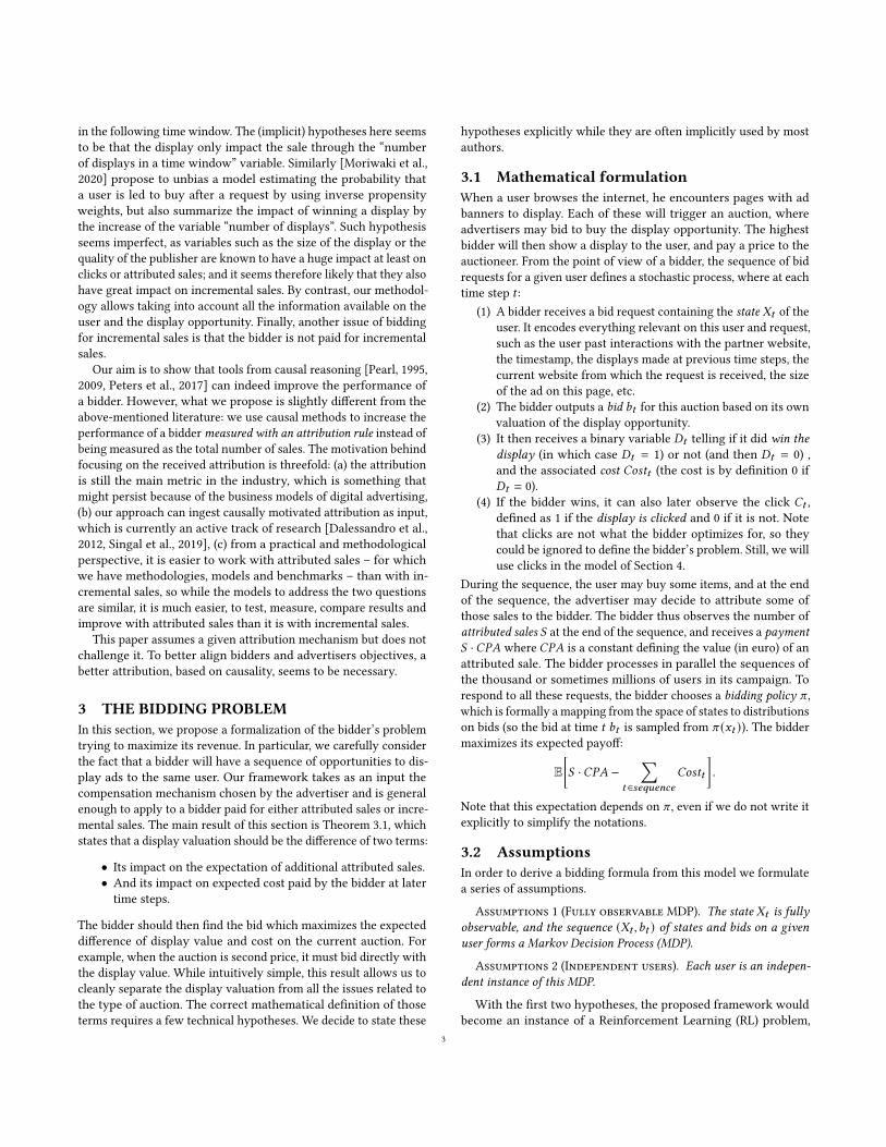
𝑋𝑡 𝐵𝑖𝑑𝑡 𝐷𝑡 𝐶𝑜𝑠𝑡𝑡𝑋𝑡 𝐵𝑖𝑑𝑡 𝐷𝑡 𝐶𝑜𝑠𝑡𝑡𝜋

𝑋𝑡+1 𝐵𝑖𝑑𝑡 𝐷𝑡 𝐶𝑜𝑠𝑡𝑡𝑋𝑡+1 𝐵𝑖𝑑𝑡+1 𝐷𝑡+1 𝐶𝑜𝑠𝑡𝑡+1𝜋

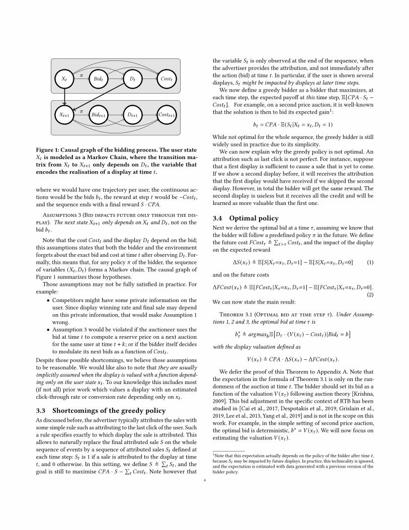
Figure 1: Causal graph of the bidding process. The user state𝑋𝑡 is modeled as a Markov Chain, where the transition ma-trix from 𝑋𝑡 to 𝑋𝑡+1 only depends on 𝐷𝑡 , the variable thatencodes the realisation of a display at time 𝑡 .

where we would have one trajectory per user, the continuous ac-

tions would be the bids 𝑏𝑡 , the reward at step 𝑡 would be −𝐶𝑜𝑠𝑡𝑡 ,and the sequence ends with a final reward 𝑆 ·𝐶𝑃𝐴.

Assumptions 3 (Bid impacts future only through the dis-

play). The next state 𝑋𝑡+1 only depends on 𝑋𝑡 and 𝐷𝑡 , not on the

bid 𝑏𝑡 .

Note that the cost 𝐶𝑜𝑠𝑡𝑡 and the display 𝐷𝑡 depend on the bid;

this assumptions states that both the bidder and the environment

forgets about the exact bid and cost at time 𝑡 after observing𝐷𝑡 . For-

mally, this means that, for any policy 𝜋 of the bidder, the sequence

of variables (𝑋𝑡 , 𝐷𝑡 ) forms a Markov chain. The causal graph of

Figure 1 summarizes those hypotheses.

Those assumptions may not be fully satisfied in practice. For

example:

• Competitors might have some private information on the

user. Since display winning rate and final sale may depend

on this private information, that would make Assumption 1

wrong.

• Assumption 3 would be violated if the auctioneer uses the

bid at time 𝑡 to compute a reserve price on a next auction

for the same user at time 𝑡 + 𝑘 ; or if the bidder itself decidesto modulate its next bids as a function of 𝐶𝑜𝑠𝑡𝑡 .

Despite those possible shortcomings, we believe those assumptions

to be reasonable. We would like also to note that they are usuallyimplicitly assumed when the display is valued with a function depend-ing only on the user state 𝑥𝑡 . To our knowledge this includes most

(if not all) prior work which values a display with an estimated

click-through rate or conversion rate depending only on 𝑥𝑡 .

3.3 Shortcomings of the greedy policyAs discussed before, the advertiser typically attributes the sales with

some simple rule such as attributing to the last click of the user. Such

a rule specifies exactly to which display the sale is attributed. This

allows to naturally replace the final attributed sale 𝑆 on the whole

sequence of events by a sequence of attributed sales 𝑆𝑡 defined at

each time step: 𝑆𝑡 is 1 if a sale is attributed to the display at time

𝑡 , and 0 otherwise. In this setting, we define 𝑆 ≜∑𝑡 𝑆𝑡 , and the

goal is still to maximise 𝐶𝑃𝐴 · 𝑆 − ∑𝑡 𝐶𝑜𝑠𝑡𝑡 . Note however that

the variable 𝑆𝑡 is only observed at the end of the sequence, when

the advertiser provides the attribution, and not immediately after

the action (bid) at time 𝑡 . In particular, if the user is shown several

displays, 𝑆𝑡 might be impacted by displays at later time steps.We now define a greedy bidder as a bidder that maximizes, at

each time step, the expected payoff at this time step, E[𝐶𝑃𝐴 · 𝑆𝑡 −𝐶𝑜𝑠𝑡𝑡 ]. For example, on a second price auction, it is well-known

that the solution is then to bid its expected gain1:

𝑏𝑡 = 𝐶𝑃𝐴 · E(𝑆𝑡 |𝑋𝑡 = 𝑥𝑡 , 𝐷𝑡 = 1)

While not optimal for the whole sequence, the greedy bidder is still

widely used in practice due to its simplicity.

We can now explain why the greedy policy is not optimal. An

attribution such as last click is not perfect. For instance, suppose

that a first display is sufficient to cause a sale that is yet to come.

If we show a second display before, it will receives the attribution

that the first display would have received if we skipped the second

display. However, in total the bidder will get the same reward. The

second display is useless but it receives all the credit and will be

learned as more valuable than the first one.

3.4 Optimal policyNext we derive the optimal bid at a time 𝜏 , assuming we know that

the bidder will follow a predefined policy 𝜋 in the future. We define

the future cost 𝐹𝐶𝑜𝑠𝑡𝜏 ≜∑𝑡>𝜏 𝐶𝑜𝑠𝑡𝑡 , and the impact of the display

on the expected reward

Δ𝑆 (𝑥𝜏 ) ≜ E[𝑆 |𝑋𝜏=𝑥𝜏 , 𝐷𝜏=1] − E[𝑆 |𝑋𝜏=𝑥𝜏 , 𝐷𝜏=0] (1)

and on the future costs

Δ𝐹𝐶𝑜𝑠𝑡 (𝑥𝜏 ) ≜ E[𝐹𝐶𝑜𝑠𝑡𝜏 |𝑋𝜏=𝑥𝜏 , 𝐷𝜏=1] −E[𝐹𝐶𝑜𝑠𝑡𝜏 |𝑋𝜏=𝑥𝜏 , 𝐷𝜏=0] .(2)

We can now state the main result:

Theorem 3.1 (Optimal bid at time step 𝜏). Under Assump-tions 1, 2 and 3, the optimal bid at time 𝜏 is

𝑏∗𝜏 ≜ argmax𝑏E[𝐷𝜏 · (𝑉 (𝑥𝜏 ) −𝐶𝑜𝑠𝑡𝜏 ) |𝐵𝑖𝑑𝑡 = 𝑏

]with the display valuation defined as

𝑉 (𝑥𝜏 ) ≜ 𝐶𝑃𝐴 · Δ𝑆 (𝑥𝜏 ) − Δ𝐹𝐶𝑜𝑠𝑡 (𝑥𝜏 ).

We defer the proof of this Theorem to Appendix A. Note that

the expectation in the formula of Theorem 3.1 is only on the ran-

domness of the auction at time 𝑡 . The bidder should set its bid as a

function of the valuation 𝑉 (𝑥𝜏 ) following auction theory [Krishna,

2009]. This bid adjustment in the specific context of RTB has been

studied in [Cai et al., 2017, Despotakis et al., 2019, Grislain et al.,

2019, Lee et al., 2013, Yang et al., 2019] and is not in the scope on this

work. For example, in the simple setting of second price auction,

the optimal bid is deterministic, 𝑏∗ = 𝑉 (𝑥𝜏 ). We will now focus on

estimating the valuation 𝑉 (𝑥𝜏 ).

1Note that this expectation actually depends on the policy of the bidder after time 𝑡 ,

because 𝑆𝑡 may be impacted by future displays. In practice, this technicality is ignored,

and the expectation is estimated with data generated with a previous version of the

bidder policy.

4

4 MODELING THE CAUSAL EFFECT OFCLICKS

According to Theorem 3.1, we need to estimate the impact of the

display on the additional attributed sales Δ𝑆 (𝑋𝜏 ) and future cost

Δ𝐹𝐶𝑜𝑠𝑡 (𝑋𝜏 ). In this paper, we propose a new method to estimate

Δ𝑆 (𝑋𝑡 ) by leveraging the randomness of clicks. As we believe the

biggest source of inefficiency in the greedy bidder is the attribution

of sales to the last click, in this work we will only focus on estimat-

ing the term Δ𝑆 (𝑋𝑡 ) and approximate the term Δ𝐹𝐶𝑜𝑠𝑡 (𝑋𝜏 ) by 0

in our experiments.

Let us notice that for a given sample, we observe either what

happens after 𝐷𝑡 = 1 or after 𝐷𝑡 = 0, but never both: we need

here to estimate the causal effect of the display 𝐷𝑡 on the reward in

Equation (1). Although we assume that all variables are observed,

this may still be challenging in practise due to the large dimension

of the state space, and the high probability that 𝑆 = 0.

In this section, we sometimes drop the index 𝑡 for simplicity,

as we now only care about variables at time of the bid. More-

over, we assimilate binary random variables such as 𝐷 and 𝐶 to

the events 𝐷 = 1, 𝐶 = 1. Thus we write 𝑃 (𝐶 |𝐷,𝑋=𝑥) for of

𝑃 (𝐶𝑡=1|𝐷𝑡=1, 𝑋𝑡=𝑥); and we note 𝐷 , 𝐶 the events 𝐷 = 0 or 𝐶 = 0.

Finally, since in practice having several sales is very rare, we assume

that 𝑆 is binary, and thus note 𝑆 the event 𝑆 > 0. This also allows

us to fit 𝑆 with a logistic regression. Hence Equation (1) becomes

Δ𝑆 (𝑥) = P(𝑆 |𝑋 = 𝑥, 𝐷) − P(𝑆 |𝑋 = 𝑥, 𝐷) .This quantity can be understood as “the causal effect of display

𝐷 on the attributed sale 𝑆”. We are thus trying to retrieve which

display(s) caused the sale attribution to the bidder. Also, because a

user is typically exposed to dozens of displays on a single day and

a sale is a rare event, the dilution of the sale signal prevents the use

of directly fitting the model P(𝑆 |𝑋 = 𝑥, 𝐷). We thus rely on a few

more assumptions.

4.1 AssumptionsA common assumption used implicitly by most attribution systems,

is that non clicked displays have no impact on sales. This greatly

reduces the number of displays one should consider when trying

to find “which display might have caused the sale”.

Assumptions 4 (No Post Display Effect.). The system is wellrepresented by the causal graph in Figure 2. In particular, 𝐶𝑡 blocksall directed paths starting from 𝐷𝑡 and finishing to 𝑆 .

In other words, displays may only cause a sale through a click.

We now have:

P(𝑆 |𝑋 = 𝑥, 𝐷) = P(𝑆 |𝑋 = 𝑥, 𝐷,𝐶) = P(𝑆 |𝑋 = 𝑥, 𝐷,𝐶) .The first equality comes from the fact that a click cannot occur

without a display. The second equality can be derived using Pearl’s

d-separation, after observing that 𝑆 ⊥⊥ 𝐷 | (𝑋,𝐶), where ⊥⊥ is the

d-separation symbol.

Remark 1 (Discussion on Assumption 4).

• The no post display effect assumption is quite commonly as-sumed in the industry when attributing the sales. For example,in the case of a “last click” attribution, only clicked displayscan be credited for a sale which implicitly implies the not post

𝑆𝑋𝑡 𝐷𝑡 𝐶𝑡𝑋𝑡 𝐷𝑡 𝐶𝑡

𝑋𝑡+1 𝐷𝑡+1 𝐶𝑡+1𝑋𝑡+1 𝐷𝑡+1 𝐶𝑡+1

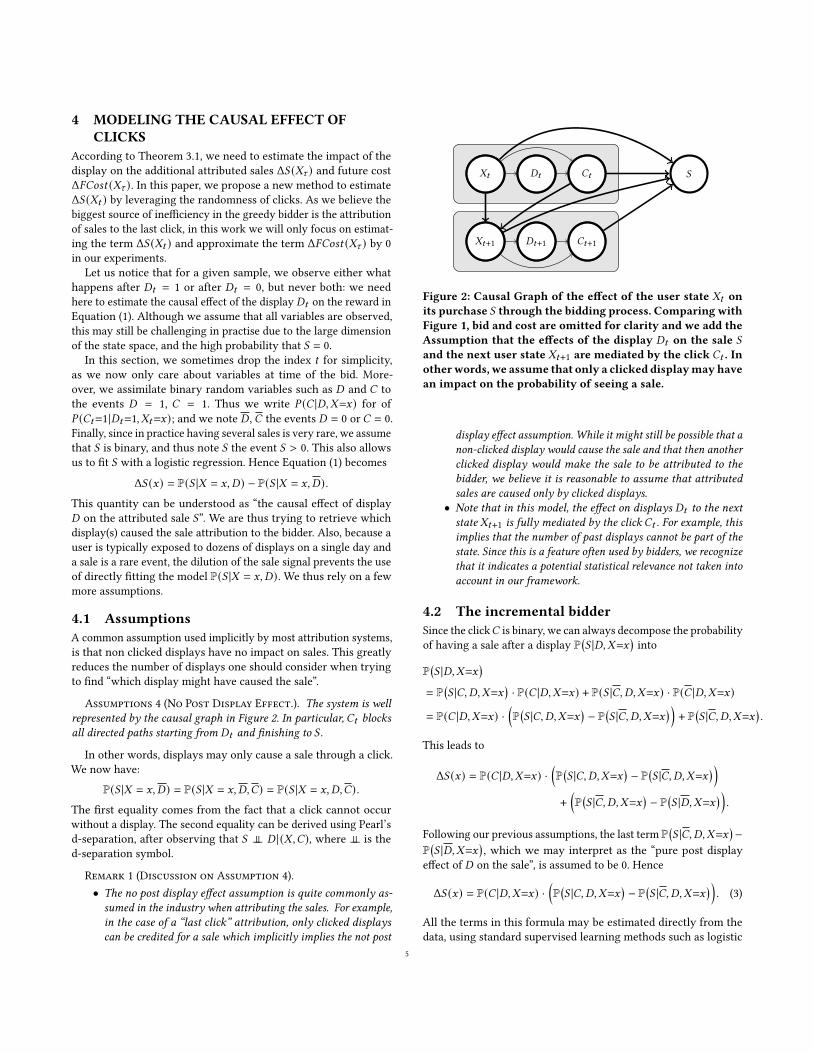
Figure 2: Causal Graph of the effect of the user state 𝑋𝑡 onits purchase 𝑆 through the bidding process. Comparing withFigure 1, bid and cost are omitted for clarity and we add theAssumption that the effects of the display 𝐷𝑡 on the sale 𝑆

and the next user state 𝑋𝑡+1 are mediated by the click 𝐶𝑡 . Inotherwords, we assume that only a clicked displaymayhavean impact on the probability of seeing a sale.

display effect assumption. While it might still be possible that anon-clicked display would cause the sale and that then anotherclicked display would make the sale to be attributed to thebidder, we believe it is reasonable to assume that attributedsales are caused only by clicked displays.

• Note that in this model, the effect on displays 𝐷𝑡 to the nextstate 𝑋𝑡+1 is fully mediated by the click 𝐶𝑡 . For example, thisimplies that the number of past displays cannot be part of thestate. Since this is a feature often used by bidders, we recognizethat it indicates a potential statistical relevance not taken intoaccount in our framework.

4.2 The incremental bidderSince the click𝐶 is binary, we can always decompose the probability

of having a sale after a display P(𝑆 |𝐷,𝑋=𝑥

)into

P(𝑆 |𝐷,𝑋=𝑥

)= P

(𝑆 |𝐶, 𝐷,𝑋=𝑥

)· P(𝐶 |𝐷,𝑋=𝑥) + P(𝑆 |𝐶, 𝐷,𝑋=𝑥) · P(𝐶 |𝐷,𝑋=𝑥)

= P(𝐶 |𝐷,𝑋=𝑥) ·(P(𝑆 |𝐶, 𝐷,𝑋=𝑥

)− P

(𝑆 |𝐶, 𝐷,𝑋=𝑥

) )+ P

(𝑆 |𝐶, 𝐷,𝑋=𝑥

).

This leads to

Δ𝑆 (𝑥) = P(𝐶 |𝐷,𝑋=𝑥) ·(P(𝑆 |𝐶, 𝐷,𝑋=𝑥

)− P

(𝑆 |𝐶, 𝐷,𝑋=𝑥

) )+(P(𝑆 |𝐶, 𝐷,𝑋=𝑥

)− P

(𝑆 |𝐷,𝑋=𝑥

) ).

Following our previous assumptions, the last term P(𝑆 |𝐶, 𝐷,𝑋=𝑥

)−

P(𝑆 |𝐷,𝑋=𝑥

), which we may interpret as the “pure post display

effect of 𝐷 on the sale”, is assumed to be 0. Hence

Δ𝑆 (𝑥) = P(𝐶 |𝐷,𝑋=𝑥) ·(P(𝑆 |𝐶, 𝐷,𝑋=𝑥

)− P

(𝑆 |𝐶, 𝐷,𝑋=𝑥

) ). (3)

All the terms in this formula may be estimated directly from the

data, using standard supervised learning methods such as logistic

5

regression. With a simple rewriting, if P(𝑆 |𝐶, 𝐷,𝑋=𝑥

)> 0, Equa-

tion (3) becomes

Δ𝑆 (𝑥) = P(𝐶 |𝐷,𝑋=𝑥) ·P(𝑆 |𝐶, 𝐷,𝑋=𝑥

)·(1−P(𝑆 |𝐶, 𝐷,𝑋=𝑥

)P(𝑆 |𝐶, 𝐷,𝑋=𝑥

) ), (4)where we call the last term the incrementality factor. It is usuallybetween 0 and 1 and we might think about it as “the probability that

the click caused the sale”. It equals 1 if the sale is fully incremental,

namely, it could not have occurred without the click: P(𝑆 |𝐶, 𝐷,𝑋

)=

0. On the contrary it is valued 0 if there is no incrementality, namely

if the click did not increase the sales probability: P(𝑆 |𝐶, 𝐷,𝑋

)=

P(𝑆 |𝐶, 𝐷,𝑋

). While it could in theory be negative (if the click caused

the user not to buy) it remains rare and in such a case wemay simply

submit a bid of 0, which is enough to ensure we loose the display.

We clarify that the bidder is incremental in the sense that it bids the

lift of attributed sales – or whatever is measured by the variable 𝑆 :

if 𝑆 was actually standing for the total number of sales, the bidder

would optimize for the incremental sales.

Remark 2 (Difference between greedy and incremental

bidders). With a greedy bidder, a display is typically valued 𝐶𝑃𝐴 ·P(𝐶𝑡 |𝐷𝑡 , 𝑋=𝑥) · P

(𝑆𝑡 |𝐶𝑡 , 𝐷𝑡 , 𝑋=𝑥

). The proposed model makes two

changes compared to this greedy bidder:

(1) We multiply by the incrementality factor from Equation (4).(2) We replace 𝑆𝑡 , the sale attributed to display 𝐷𝑡 by 𝑆 (sales

attributed to the whole sequence), in the P(𝑆 |𝐶, 𝐷,𝑋=𝑥) partof the model. We pinpoint that our model does not depend onthe method used to attribute sales to displays (typically lastclick) as long as it is attributed to the displays sequence madeto the user.

5 AN INCREMENTALITY METRICWe are interested in valuing more the displays that lead a user

to make a purchase in the future while he would not have not

without. Namely, we would like to evaluate how good our model

is at predicting Δ𝑆 (𝑥). Given Equation (3), Δ𝑆 (𝑥) can be split into

two parts, first P(𝐶 |𝐷,𝑋=𝑥) that is a quite mature model in the

industry and a second model P(𝑆 |𝐶, 𝐷,𝑋=𝑥

)− P

(𝑆 |𝐶, 𝐷,𝑋=𝑥

)that

we have introduced in Section 4.2. Since we cannot observe both

the clicked display and its counterfactual, assessing the quality of

such a model offline is a complex task. In this Section, we build a

random variable 𝑌 such that

P(𝑌 |𝐶, 𝐷,𝑋=𝑥

)= P

(𝑆 |𝐶, 𝐷,𝑋=𝑥

)− P

(𝑆 |𝐶, 𝐷,𝑋=𝑥

)that we cannot observe. However, we introduce a metric that is

able to evaluate the capacity of our model to predict this variable 𝑌

while observing only the click 𝐶 and sales 𝑆 outcomes.

5.1 The generative modelAs in Section 4.2 we consider only won displays, that are described

by a context𝑋 , and have two observable effects: they can be clicked

𝐶 or not𝐶 and they can be followed by a sales 𝑆 or not 𝑆 . Intuitively,

we would like to divide those displays in four classes, which we

call their display type 𝑇 ∈ {𝑎, 𝑛,𝑦, 𝑑}:(1) The displays that always lead to a sale whether they are

clicked or not : 𝑇 = 𝑎.

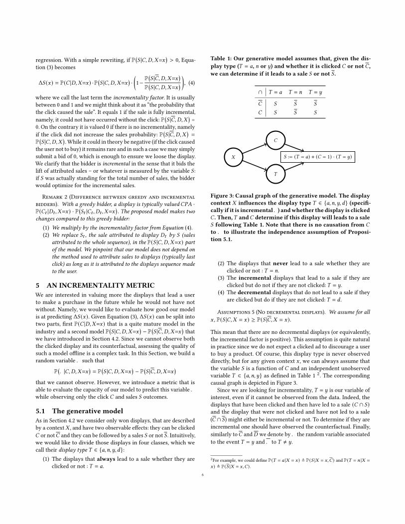
Table 1: Our generative model assumes that, given the dis-play type (𝑇 = 𝑎, 𝑛 or 𝑦) and whether it is clicked 𝐶 or not 𝐶,we can determine if it leads to a sale 𝑆 or not 𝑆 .

∩ 𝑇 = 𝑎 𝑇 = 𝑛 𝑇 = 𝑦

𝐶 𝑆 𝑆 𝑆

𝐶 𝑆 𝑆 𝑆

𝑋

𝐶

𝑇

𝑆 := (𝑇 = 𝑎) + (𝐶 = 1) · (𝑇 = 𝑦)

Figure 3: Causal graph of the generative model. The displaycontext 𝑋 influences the display type 𝑇 ∈ {𝑎, 𝑛,𝑦, 𝑑} (specifi-cally if it is incremental𝑌 ) andwhether the display is clicked𝐶. Then,𝑇 and𝐶 determine if this display will leads to a sale𝑆 following Table 1. Note that there is no causation from 𝐶

to 𝑌 to illustrate the independence assumption of Proposi-tion 5.1.

(2) The displays that never lead to a sale whether they are

clicked or not : 𝑇 = 𝑛.

(3) The incremental displays that lead to a sale if they are

clicked but do not if they are not clicked: 𝑇 = 𝑦.

(4) The decremental displays that do not lead to a sale if they

are clicked but do if they are not clicked: 𝑇 = 𝑑 .

Assumptions 5 (No decremental displays). We assume for all𝑥 , P(𝑆 |𝐶,𝑋 = 𝑥) ≥ P(𝑆 |𝐶,𝑋 = 𝑥).

This mean that there are no decremental displays (or equivalently,

the incremental factor is positive). This assumption is quite natural

in practice since we do not expect a clicked ad to discourage a user

to buy a product. Of course, this display type is never observed

directly, but for any given context 𝑥 , we can always assume that

the variable 𝑆 is a function of 𝐶 and an independent unobserved

variable 𝑇 ∈ {𝑎, 𝑛,𝑦} as defined in Table 12. The corresponding

causal graph is depicted in Figure 3.

Since we are looking for incrementality, 𝑇 = 𝑦 is our variable of

interest, even if it cannot be observed from the data. Indeed, the

displays that have been clicked and then have led to a sale (𝐶 ∩ 𝑆)and the display that were not clicked and have not led to a sale

(𝐶 ∩ 𝑆) might either be incremental or not. To determine if they are

incremental one should have observed the counterfactual. Finally,

similarly to𝐶 and𝐷 we denote by𝑌 the random variable associated

to the event 𝑇 = 𝑦 and 𝑌 to 𝑇 ≠ 𝑦.

2For example, we could define P(𝑇 = 𝑎 |𝑋 = 𝑥) ≜ P(𝑆 |𝑋 = 𝑥,𝐶) and P(𝑇 = 𝑛 |𝑋 =

𝑥) ≜ P(𝑆 |𝑋 = 𝑥,𝐶) .6

5.2 Reverted incremental likelihood𝑌 is a Bernoulli variable, hence if we have an estimator 𝑓 that

predicts 𝑌 given 𝑋 its log-likelihood is

LLHB (𝑌, 𝑓 (𝑋 )) = 𝑌 log 𝑓 (𝑋 ) + 𝑌 log(1 − 𝑓 (𝑋 )) .

Since we cannot observe 𝑌 , we cannot compute this likelihood di-

rectly from the data. However, Proposition 5.1 gives us an unbiased

estimate of this likelihood based only on the observed values 𝐶

and 𝑆 . This unbiased estimate reverts the label as in [Jaskowski and

Jaroszewicz, 2012] while taking into account the partial randomness

of the clicks.

Proposition 5.1. With the generative model of Figure 3 and As-sumption 5, the reverted incremental likelihood

RLLHB (𝐶, 𝑆, 𝑓 (𝑋 )) = 𝐶

P(𝐶 |𝑋 ) LLHB (𝑆, 𝑓 (𝑋 ))+ 𝐶 ∩ 𝑆

P(𝐶 |𝑋 )log

1 − 𝑓 (𝑋 )𝑓 (𝑋 )

is an unbiased estimator of the direct incremental likelihoodLLHB (𝑌, 𝑓 (𝑋 )), for any predictor 𝑓 .

We defer the proof of Proposition 5.1 to Appendix C. Provided we

have a correct P(𝐶 |𝑋 ) model, we can thus estimate the incremental

likelihood from observable data. This is interesting in practice since

it allows to us to evaluate offline the incremental performance of

our models to perform model selection. In the case of the incre-

mental bidder, it is useful to assess the quality of the incremental

factor as a whole instead of evaluating P(𝑆 |𝐶, 𝐷,𝑋=𝑥

)on one hand

and P(𝑆 |𝐶, 𝐷,𝑋=𝑥

)on the other while having no guarantee on the

quality of their ratio. Note that this still requires a click prediction

model to estimate P(𝐶 |𝑋 ). Relying on a model to assess the perfor-

mances of another is not ideal but since the click prediction models

are mature in the industry and trained on much more data, we can

safely use them to evaluate sales prediction models. In Appendix D,

we illustrate Proposition 5.1 on a data set that we simulate such that

we can observe the hidden variable 𝑇 . That allows us to compute

the direct incremental likelihood and to compare it the reverted

one to assess the performance of the incremental bidder.

6 EXPERIMENTAL RESULTS6.1 Offline analysisIn order to evaluate our methodology, we run experiments on the

Criteo Attribution Modeling for Bidding public data set [Diemert

et al., 2017]. This data set consists in 16 million displays sent by

Criteo to 6 million users over a period of 30 days. To each display is

associated a set of context features (that we have denoted by 𝑋𝑡 so

far), if the display was clicked (denoted by 𝐶𝑡 so far), and if it has

led to a sale that was attributed to Criteo (denoted by 𝑆𝑡 so far). For

simplicity, we assume the value of an attributed sale (denoted by

𝐶𝑃𝐴) to equal 1. As a baseline, we train the greedy bidder that values

a display with context features 𝑥 by P(𝐶𝑡 |𝑋=𝑥) ·P(𝑆𝑡 |𝐶𝑡 , 𝑋𝑡=𝑥

)(see

Remark 2). Note that the context features are hashed [Weinberger

et al., 2009], and each context 𝑥 ends up being represented by sparse

vector of dimension 216. Then, since we have access to the user

identifier, we can reconstruct the user timelines. Specifically, we

can determine if the sequence of displays has led to an attributed

sales (denoted by 𝑆 so far). With this label, we train the incremental

0 200 400 600Hours since last click

0.5

0.6

0.7

0.8

0.9

1 (S|C)(S|C)

0 5 10 15 20Number of clicks before display

0.78

0.79

0.80

0.81

0.82

0.831 (S|C)

(S|C)

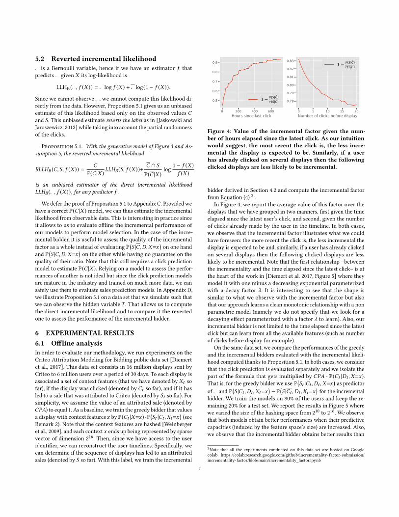
Figure 4: Value of the incremental factor given the num-ber of hours elapsed since the latest click. As our intuitionwould suggest, the most recent the click is, the less incre-mental the display is expected to be. Similarly, if a userhas already clicked on several displays then the followingclicked displays are less likely to be incremental.

bidder derived in Section 4.2 and compute the incremental factor

from Equation (4)3.

In Figure 4, we report the average value of this factor over the

displays that we have grouped in two manners, first given the time

elapsed since the latest user’s click, and second, given the number

of clicks already made by the user in the timeline. In both cases,

we observe that the incremental factor illustrates what we could

have foreseen: the more recent the click is, the less incremental the

display is expected to be and, similarly, if a user has already clicked

on several displays then the following clicked displays are less

likely to be incremental. Note that the first relationship –between

the incrementality and the time elapsed since the latest click– is at

the heart of the work in [Diemert et al. 2017, Figure 5] where they

model it with one minus a decreasing exponential parameterized

with a decay factor _. It is interesting to see that the shape is

similar to what we observe with the incremental factor but also

that our approach learns a clean monotonic relationship with a non

parametric model (namely we do not specify that we look for a

decaying effect parameterized with a factor _ to learn). Also, our

incremental bidder is not limited to the time elapsed since the latest

click but can learn from all the available features (such as number

of clicks before display for example).

On the same data set, we compare the performances of the greedy

and the incremental bidders evaluated with the incremental likeli-

hood computed thanks to Proposition 5.1. In both cases, we consider

that the click prediction is evaluated separately and we isolate the

part of the formula that gets multiplied by 𝐶𝑃𝐴 · P(𝐶𝑡 |𝐷𝑡 , 𝑋=𝑥).That is, for the greedy bidder we use P

(𝑆𝑡 |𝐶𝑡 , 𝐷𝑡 , 𝑋=𝑥

)as predictor

of 𝑌 and P(𝑆 |𝐶𝑡 , 𝐷𝑡 , 𝑋𝑡=𝑥

)− P

(𝑆 |𝐶𝑡 , 𝐷𝑡 , 𝑋𝑡=𝑥

)for the incremental

bidder. We train the models on 80% of the users and keep the re-

maining 20% for a test set. We report the results in Figure 5 where

we varied the size of the hashing space from 210

to 216. We observe

that both models obtain better performances when their predictive

capacities (induced by the feature space’s size) are increased. Also,

we observe that the incremental bidder obtains better results than

3Note that all the experiments conducted on this data set are hosted on Google

colab https://colab.research.google.com/github/incrementality-factor-submission/

incrementality-factor/blob/main/incrementality_factor.ipynb

7

0 20000 40000 60000size of features space

0.122

0.120

0.118

0.116

0.114

0.112

0.110

Incremental likelihood on train set

incremental biddergreedy bidder

0 20000 40000 60000size of features space

0.124

0.123

0.122

0.121

0.120

0.119

0.118

0.117

Incremental likelihood on test set

incremental biddergreedy bidder

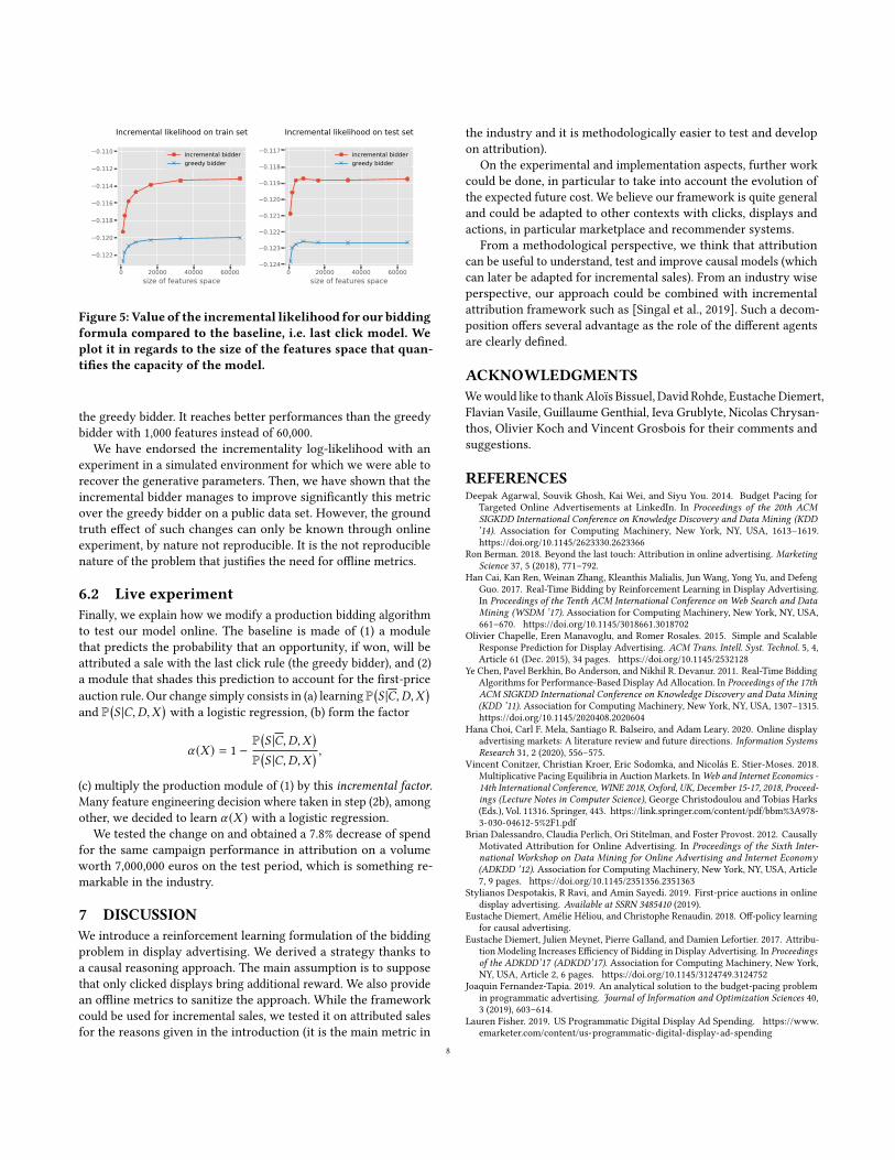
Figure 5: Value of the incremental likelihood for our biddingformula compared to the baseline, i.e. last click model. Weplot it in regards to the size of the features space that quan-tifies the capacity of the model.

the greedy bidder. It reaches better performances than the greedy

bidder with 1,000 features instead of 60,000.

We have endorsed the incrementality log-likelihood with an

experiment in a simulated environment for which we were able to

recover the generative parameters. Then, we have shown that the

incremental bidder manages to improve significantly this metric

over the greedy bidder on a public data set. However, the ground

truth effect of such changes can only be known through online

experiment, by nature not reproducible. It is the not reproducible

nature of the problem that justifies the need for offline metrics.

6.2 Live experimentFinally, we explain how we modify a production bidding algorithm

to test our model online. The baseline is made of (1) a module

that predicts the probability that an opportunity, if won, will be

attributed a sale with the last click rule (the greedy bidder), and (2)

a module that shades this prediction to account for the first-price

auction rule. Our change simply consists in (a) learning P(𝑆 |𝐶, 𝐷,𝑋

)and P

(𝑆 |𝐶, 𝐷,𝑋

)with a logistic regression, (b) form the factor

𝛼 (𝑋 ) = 1 −P(𝑆 |𝐶, 𝐷,𝑋

)P(𝑆 |𝐶, 𝐷,𝑋

) ,(c) multiply the production module of (1) by this incremental factor.Many feature engineering decision where taken in step (2b), among

other, we decided to learn 𝛼 (𝑋 ) with a logistic regression.

We tested the change on and obtained a 7.8% decrease of spend

for the same campaign performance in attribution on a volume

worth 7,000,000 euros on the test period, which is something re-

markable in the industry.

7 DISCUSSIONWe introduce a reinforcement learning formulation of the bidding

problem in display advertising. We derived a strategy thanks to

a causal reasoning approach. The main assumption is to suppose

that only clicked displays bring additional reward. We also provide

an offline metrics to sanitize the approach. While the framework

could be used for incremental sales, we tested it on attributed sales

for the reasons given in the introduction (it is the main metric in

the industry and it is methodologically easier to test and develop

on attribution).

On the experimental and implementation aspects, further work

could be done, in particular to take into account the evolution of

the expected future cost. We believe our framework is quite general

and could be adapted to other contexts with clicks, displays and

actions, in particular marketplace and recommender systems.

From a methodological perspective, we think that attribution

can be useful to understand, test and improve causal models (which

can later be adapted for incremental sales). From an industry wise

perspective, our approach could be combined with incremental

attribution framework such as [Singal et al., 2019]. Such a decom-

position offers several advantage as the role of the different agents

are clearly defined.

ACKNOWLEDGMENTSWewould like to thankAloïs Bissuel, David Rohde, EustacheDiemert,

Flavian Vasile, Guillaume Genthial, Ieva Grublyte, Nicolas Chrysan-

thos, Olivier Koch and Vincent Grosbois for their comments and

suggestions.

REFERENCESDeepak Agarwal, Souvik Ghosh, Kai Wei, and Siyu You. 2014. Budget Pacing for

Targeted Online Advertisements at LinkedIn. In Proceedings of the 20th ACMSIGKDD International Conference on Knowledge Discovery and Data Mining (KDD’14). Association for Computing Machinery, New York, NY, USA, 1613–1619.

https://doi.org/10.1145/2623330.2623366

Ron Berman. 2018. Beyond the last touch: Attribution in online advertising. MarketingScience 37, 5 (2018), 771–792.

Han Cai, Kan Ren, Weinan Zhang, Kleanthis Malialis, Jun Wang, Yong Yu, and Defeng

Guo. 2017. Real-Time Bidding by Reinforcement Learning in Display Advertising.

In Proceedings of the Tenth ACM International Conference on Web Search and DataMining (WSDM ’17). Association for Computing Machinery, New York, NY, USA,

661–670. https://doi.org/10.1145/3018661.3018702

Olivier Chapelle, Eren Manavoglu, and Romer Rosales. 2015. Simple and Scalable

Response Prediction for Display Advertising. ACM Trans. Intell. Syst. Technol. 5, 4,Article 61 (Dec. 2015), 34 pages. https://doi.org/10.1145/2532128

Ye Chen, Pavel Berkhin, Bo Anderson, and Nikhil R. Devanur. 2011. Real-Time Bidding

Algorithms for Performance-Based Display Ad Allocation. In Proceedings of the 17thACM SIGKDD International Conference on Knowledge Discovery and Data Mining(KDD ’11). Association for Computing Machinery, New York, NY, USA, 1307–1315.

https://doi.org/10.1145/2020408.2020604

Hana Choi, Carl F. Mela, Santiago R. Balseiro, and Adam Leary. 2020. Online display

advertising markets: A literature review and future directions. Information SystemsResearch 31, 2 (2020), 556–575.

Vincent Conitzer, Christian Kroer, Eric Sodomka, and Nicolás E. Stier-Moses. 2018.

Multiplicative Pacing Equilibria in Auction Markets. InWeb and Internet Economics -14th International Conference, WINE 2018, Oxford, UK, December 15-17, 2018, Proceed-ings (Lecture Notes in Computer Science), George Christodoulou and Tobias Harks

(Eds.), Vol. 11316. Springer, 443. https://link.springer.com/content/pdf/bbm%3A978-

3-030-04612-5%2F1.pdf

Brian Dalessandro, Claudia Perlich, Ori Stitelman, and Foster Provost. 2012. Causally

Motivated Attribution for Online Advertising. In Proceedings of the Sixth Inter-national Workshop on Data Mining for Online Advertising and Internet Economy(ADKDD ’12). Association for Computing Machinery, New York, NY, USA, Article

7, 9 pages. https://doi.org/10.1145/2351356.2351363

Stylianos Despotakis, R Ravi, and Amin Sayedi. 2019. First-price auctions in online

display advertising. Available at SSRN 3485410 (2019).Eustache Diemert, Amélie Héliou, and Christophe Renaudin. 2018. Off-policy learning

for causal advertising.

Eustache Diemert, Julien Meynet, Pierre Galland, and Damien Lefortier. 2017. Attribu-

tion Modeling Increases Efficiency of Bidding in Display Advertising. In Proceedingsof the ADKDD’17 (ADKDD’17). Association for Computing Machinery, New York,

NY, USA, Article 2, 6 pages. https://doi.org/10.1145/3124749.3124752

Joaquin Fernandez-Tapia. 2019. An analytical solution to the budget-pacing problem

in programmatic advertising. Journal of Information and Optimization Sciences 40,3 (2019), 603–614.

Lauren Fisher. 2019. US Programmatic Digital Display Ad Spending. https://www.

emarketer.com/content/us-programmatic-digital-display-ad-spending

8

Nicolas Grislain, Nicolas Perrin, and Antoine Thabault. 2019. Recurrent Neural Net-

works for Stochastic Control in Real-Time Bidding. In Proceedings of the 25thACM SIGKDD International Conference on Knowledge Discovery & Data Mining(KDD ’19). Association for Computing Machinery, New York, NY, USA, 2801–2809.

https://doi.org/10.1145/3292500.3330749

Benjamin Heymann. 2019. Cost per Action Constrained Auctions. In Proceedings of the14th Workshop on the Economics of Networks, Systems and Computation (NetEcon’19). Association for Computing Machinery, New York, NY, USA, Article 1, 8 pages.

https://doi.org/10.1145/3338506.3340269

Benjamin Heymann. 2020. How to bid in unified second-price auctions when requests

are duplicated. Operations Research Letters 48, 4 (2020), 446–451. https://doi.org/

10.1016/j.orl.2020.05.010

Maciej Jaskowski and Szymon Jaroszewicz. 2012. Uplift modeling for clinical trial data.

In ICML Workshop on Clinical Data Analysis, Vol. 46.Wendi Ji, Xiaoling Wang, and Dell Zhang. 2016. A probabilistic multi-touch attribution

model for online advertising. International Conference on Information and KnowledgeManagement, Proceedings 24-28-Octo (2016), 1373–1382. https://doi.org/10.1145/

2983323.2983787

Garrett A. Johnson, Randall A. Lewis, and Elmar I. Nubbemeyer. 2017. Ghost Ads:

Improving the economics of measuring online ad effectiveness. Journal of MarketingResearch 54, 6 (Dec. 2017), 867–884. https://doi.org/10.1509/jmr.15.0297

Vijay Krishna. 2009. Auction theory. Academic press.

Kuang-Chih Lee, Ali Jalali, and Ali Dasdan. 2013. Real Time Bid Optimization with

Smooth Budget Delivery in Online Advertising. In Proceedings of the Seventh Inter-national Workshop on Data Mining for Online Advertising - ADKDD ’13. ACM Press,

New York, New York, USA, 1–9. https://doi.org/10.1145/2501040.2501979

Randall A. Lewis and Justin M. Rao. 2015. The unfavorable economics of measuring the

returns to advertising. Quarterly Journal of Economics 130, 4 (Nov. 2015), 1941–1973.https://doi.org/10.1093/qje/qjv023

Randall A. Lewis, Justin M. Rao, and David H. Reiley. 2011. Here, There, and Every-

where: Correlated Online Behaviors Can Lead to Overestimates of the Effects of

Advertising. In Proceedings of the 20th International Conference on World Wide Web(WWW ’11). Association for Computing Machinery, New York, NY, USA, 157–166.

https://doi.org/10.1145/1963405.1963431

H. Brendan McMahan, Gary Holt, D. Sculley, Michael Young, Dietmar Ebner, Julian

Grady, Lan Nie, Todd Phillips, Eugene Davydov, Daniel Golovin, Sharat Chikkerur,

Dan Liu, Martin Wattenberg, Arnar Mar Hrafnkelsson, Tom Boulos, and Jeremy

Kubica. 2013. Ad Click Prediction: A View from the Trenches. In Proceedings ofthe 19th ACM SIGKDD International Conference on Knowledge Discovery and DataMining (KDD ’13). Association for Computing Machinery, New York, NY, USA,

1222–1230. https://doi.org/10.1145/2487575.2488200

Daisuke Moriwaki, Yuta Hayakawa, Isshu Munemasa, Yuta Saito, and Akira Matsui.

2020. Unbiased Lift-based Bidding System. arXiv preprint arXiv:2007.04002 (2020).Judea Pearl. 1995. Causal diagrams for empirical research. Biometrika 82, 4 (1995),

669–688.

Judea Pearl. 2009. Causality. Cambridge University Press. 1689–1699 pages. https:

//doi.org/10.1088/1751-8113/44/8/085201

Jonas Peters, Dominik Janzing, and Bernhard Schölkopf. 2017. Elements of causalinference. The MIT Press.

Thibaud Rahier, Amélie Héliou, Matthieu Martin, Christophe Renaudin, and Eustache

Diemert. 2020. Individual Treatment Effect Estimation in a Low Compliance Setting.

arXiv:stat.ML/2008.03235

Raghav Singal, Omar Besbes, Antoine Desir, Vineet Goyal, and Garud Iyengar. 2019.

Shapley Meets Uniform: An Axiomatic Framework for Attribution in Online Ad-

vertising. In The World Wide Web Conference (WWW ’19). Association for Comput-

ing Machinery, New York, NY, USA, 1713–1723. https://doi.org/10.1145/3308558.

3313731

Richard S. Sutton, Andrew G. Barto, et al. 1998. Introduction to reinforcement learning.Vol. 135. MIT Press Cambridge.

Jun Wang, Weinan Zhang, and Shuai Yuan. 2017. Display Advertising with Real-TimeBidding (RTB) and Behavioural Targeting. Now Publishers Inc., Hanover, MA, USA.

Kilian Weinberger, Anirban Dasgupta, John Langford, Alex Smola, and Josh Attenberg.

2009. Feature Hashing for Large Scale Multitask Learning. In Proceedings of the26th Annual International Conference on Machine Learning (ICML ’09). Associationfor Computing Machinery, New York, NY, USA, 1113–1120. https://doi.org/10.

1145/1553374.1553516

Jian Xu, Kuang-chih Lee, Wentong Li, Hang Qi, and Quan Lu. 2015. Smart Pacing for

Effective Online AdCampaignOptimization. In Proceedings of the 21th ACM SIGKDDInternational Conference on Knowledge Discovery and Data Mining. Association for

Computing Machinery, New York, NY, USA, 2217–2226. https://doi.org/10.1145/

2783258.2788615

Jian Xu, Xuhui Shao, Jianjie Ma, Kuang-chih Lee, Hang Qi, and Quan Lu. 2016. Lift-

Based Bidding in Ad Selection. In Proceedings of the Thirtieth AAAI Conference onArtificial Intelligence (AAAI’16). AAAI Press, 651–657.

Xun Yang, Yasong Li, Hao Wang, Di Wu, Qing Tan, Jian Xu, and Kun Gai. 2019. Bid

Optimization by Multivariable Control in Display Advertising. (2019), 1966–1974.

https://doi.org/10.1145/3292500.3330681

Ya Zhang, YiWei, and Jianbiao Ren. 2014. Multi-touchAttribution inOnline Advertising

with Survival Theory. Proceedings - IEEE International Conference on Data Mining,ICDM 2015-Janua, January (2014), 687–696. https://doi.org/10.1109/ICDM.2014.130

9

Appendices

A PROOF OF THEOREM 3.1First we pinpoint that Equations (1) and (2) only refer to observa-

tional data. The following result, that relies on using Pearl’s dooperator [Pearl, 1995, 2009, Peters et al., 2017], tells us that we cannonetheless interpret them as interventional quantities.

Proposition A.1.

Δ𝑆 (𝑥𝜏 ) = E[𝑆 |𝑋𝜏=𝑥𝜏 , 𝑑𝑜 (𝐷𝜏=1)] − E[𝑆 |𝑋𝜏=𝑥𝜏 , 𝑑𝑜 (𝐷𝜏=0)]and

Δ𝐹𝐶𝑜𝑠𝑡 (𝑥𝜏 ) = E[𝐹𝐶𝑜𝑠𝑡𝜏 |𝑋𝜏=𝑥𝜏 , 𝑑𝑜 (𝐷𝜏=1)]− E[𝐹𝐶𝑜𝑠𝑡𝜏 |𝑋𝜏=𝑥𝜏 , 𝑑𝑜 (𝐷𝜏=0)]

Proof. The variables 𝑆 and 𝐷𝜏 are d-separated in a graph were

the outcoming edges from 𝐷𝜏 are removed. We can thus apply

Pearl’s Action/observation exchange [Pearl, 1995] . A similar argu-

ment applies for 𝐹𝑐𝑜𝑠𝑡𝜏 and 𝐷𝜏 . □

We can now prove Theorem 3.1.

Proof. Noting that the cost paid at previous steps,

∑𝑡<𝜏 𝐶𝑜𝑠𝑡𝑡 ,

can now be viewed as a constant and thus removed from the optimi-

sation problem, the bidder wants to maximize the expected payoff

after a bid 𝑏𝜏 :

E[𝐶𝑃𝐴 · 𝑆 − 𝐹𝐶𝑜𝑠𝑡𝜏 −𝐶𝑜𝑠𝑡𝜏 |𝑋𝜏 = 𝑥𝜏 , 𝑏𝜏 ]Since the bid only impacts future through the display, when the

bidder looses this auction (𝐷𝜏 = 0), its payoff is:

𝐶𝑃𝐴 · E[𝑆 |𝑋𝜏 = 𝑥𝜏 , 𝐷𝜏 = 0] − E[𝐹𝐶𝑜𝑠𝑡𝜏 |𝑋𝜏 = 𝑥𝜏 , 𝐷𝜏 = 0] . (5)

While if he wins (𝐷𝜏 = 1), he would receive

𝐶𝑃𝐴 · E[𝑆 |𝑋𝜏 = 𝑥𝜏 , 𝐷𝜏 = 1] − E[𝐹𝐶𝑜𝑠𝑡𝜏 |𝑋𝜏 = 𝑥𝜏 , 𝐷𝜏 = 1] (6)

and pay the cost 𝐶𝑜𝑠𝑡𝜏 . Assumption 3 implies that expectations on

the future of the sequence after a display (or after no display) of the

quantities in Equations (5) and (6) only depend on the policy of the

bidder after time 𝑡 , not on its exact bid at time 𝑡 . Up to a constant

term, the payoff of the bidder is thus 𝐷𝜏 · (𝑉 (𝑥𝜏 ) −𝐶𝑜𝑠𝑡𝜏 ). □

B POLICY ITERATION AND CONVERGENCEWhile we are not strictly in a Reinforcement Learning setup, we

may define a policy iteration, which converges to the optimal pol-

icy [Sutton et al., 1998] under mild technical assumptions4.

To be more specific: we have only derived the optimal bid at

some time step 𝜏 , when the policy 𝜋 at the next time steps is frozen.

From this, we then build a new policy: at every time step, answer

with the bid which would be optimal if 𝜋 was used in the future.

A recursion argument shows that this policy is an improvement

(i.e. has a higher expected return) on 𝜋 at every state. Theoretically,

we can then define a sequence of policies by iterating this policy

improvement process, converging to an optimal policy –which can

be shown with a recursion on the length of the sequence when

those sequences are of bounded length– exactly as in the usual case

of policy iteration in Reinforcement Learning.

4It is sufficient to assume a finite upper bound on the length of sequences.

C PROOF OF PROPOSITION 5.1With Assumption 5, 𝑌 is the disjoint union of 𝑇 = 𝑎 and 𝑇 = 𝑛,

hence

P[𝑌 |𝑋 ] = P[𝑇 = 𝑎 |𝑋 ] + P[𝑇 = 𝑛 |𝑋 ] .As the display types 𝑇 are built independently of 𝐶 given X, the

previous equality can be written as

P[𝑌 |𝑋 ] = P[𝐶 ∩𝑇 = 𝑎 |𝑋 ]P(𝐶 |𝑋 )

+ P[𝐶 ∩𝑇 = 𝑛 |𝑋 ]P(𝐶 |𝑋 ) .

Finally, since we can identify event 𝐶 ∩ (𝑇 = 𝑎) to 𝐶 ∩ 𝑆 and

𝐶 ∩ (𝑇 = 𝑛) to 𝐶 ∩ 𝑆 (see Table 1), it writes

P[𝑌 |𝑋 ] = P[𝐶 ∩ 𝑆 |𝑋 ]P(𝐶 |𝑋 )

+ P[𝐶 ∩ 𝑆 |𝑋 ]P(𝐶 |𝑋 ) ,

and

P[𝑌 |𝑋 ] = P[𝐶 ∩ 𝑆 |𝑋 ]P(𝐶 |𝑋 ) − P[𝐶 ∩ 𝑆 |𝑋 ]

P(𝐶 |𝑋 ). (7)

Using this identity we compute the expectation of the incremental

likelihood

E𝑋,𝑌 [LLHB (𝑌, 𝑓 (𝑋 ))]

= E𝑋[E𝑌 [𝑌 log 𝑓 (𝑋 ) + 𝑌 log(1 − 𝑓 (𝑋 )) |𝑋 ]

]= E𝑋

[P(𝑌 |𝑋 ) log 𝑓 (𝑋 ) + P(𝑌 |𝑋 ) log(1 − 𝑓 (𝑋 ))

]= E𝑋

[(P[𝐶 ∩ 𝑆 |𝑋 ]P(𝐶 |𝑋 ) − P[𝐶 ∩ 𝑆 |𝑋 ]

P(𝐶 |𝑋 )

)log 𝑓 (𝑋 )

+(P(𝐶 ∩ 𝑆 |𝑋 )P(𝐶 |𝑋 )

+ P[𝐶 ∩ 𝑆 |𝑋 ]P(𝐶 |𝑋 )

)log(1 − 𝑓 (𝑋 ))

]Since all is conditioned on 𝑋 and 𝐶 and 𝑆 are Bernouilli variables,

E𝑋,𝑌 [LLHB (𝑌, 𝑓 (𝑋 ))]

= E𝑋,𝐶,𝑆

[(𝐶 ∩ 𝑆

P(𝐶 |𝑋 ) −𝐶 ∩ 𝑆

P(𝐶 |𝑋 )

)log 𝑓 (𝑋 )

+(𝐶 ∩ 𝑆

P(𝐶 |𝑋 )+ 𝐶 ∩ 𝑆

P(𝐶 |𝑋 )

)log(1 − 𝑓 (𝑋 ))

]= E𝑋,𝑆,𝐶

[𝐶

P(𝐶 |𝑋 ) LLHB (𝑆, 𝑓 (𝑋 ))

+ 𝐶 ∩ 𝑆

P(𝐶 |𝑋 )log

1 − 𝑓 (𝑋 )𝑓 (𝑋 )

].

D COMPARISON OF DIRECT AND REVERTEDINCREMENTAL LIKELIHOOD ON ASIMULATED DATA SET

In order to manifest the consistency of the incremental metric

introduced in Proposition 5.1 and link it to the incremental factor,

we generate a toy data set where the displays are described by a

2-dimensional feature vector 𝑥 , allowing us to represent them on a

2d graph. Then, following our generative model, we assume that

each display 𝑖 , gets clicked with a probability 𝜓 (𝑥𝑖 ) ∈ (0, 1) andis of type 𝑡𝑖 = 𝑎, 𝑦 or 𝑐 with a probability that also depends on 𝑥𝑖 .

Figure 6 shows 𝑛 = 60 displays represented by their feature vector

𝑥𝑖 ∈ R2 and their click 𝑐𝑖 , type 𝑡𝑖 and sales 𝑠𝑖 characteristics for

𝑖 = 1, . . . 𝑛.

10

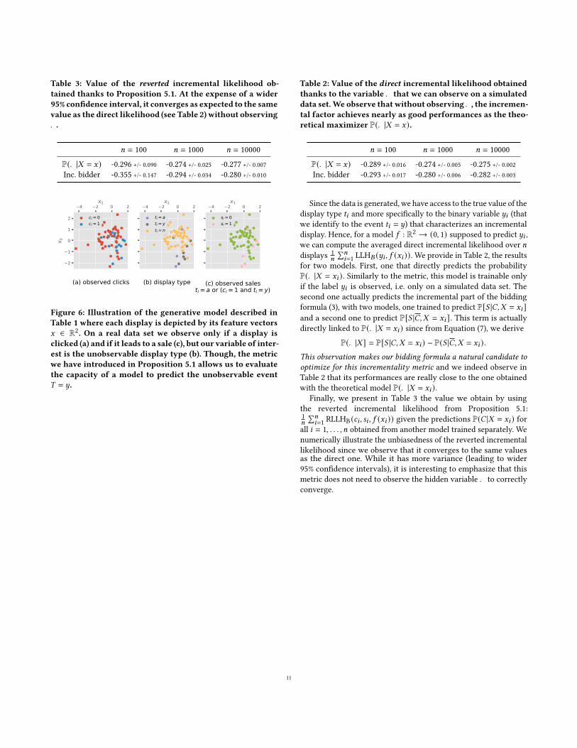
Table 3: Value of the reverted incremental likelihood ob-tained thanks to Proposition 5.1. At the expense of a wider95% confidence interval, it converges as expected to the samevalue as the direct likelihood (see Table 2) without observing𝑌 .

𝑛 = 100 𝑛 = 1000 𝑛 = 10000

P(𝑌 |𝑋 = 𝑥) -0.296 +/- 0.090 -0.274 +/- 0.025 -0.277 +/- 0.007

Inc. bidder -0.355 +/- 0.147 -0.294 +/- 0.034 -0.280 +/- 0.010

4 2 0 2x1

2

1

0

1

2

x 2

(a) observed clicks

ci = 0ci = 1

4 2 0 2x1

(b) display type

ti = ati = yti = n

4 2 0 2x1

(c) observed salesti = a or (ci = 1 and ti = y)

si = 0si = 1

Figure 6: Illustration of the generative model described inTable 1 where each display is depicted by its feature vectors𝑥 ∈ R2. On a real data set we observe only if a display isclicked (a) and if it leads to a sale (c), but our variable of inter-est is the unobservable display type (b). Though, the metricwe have introduced in Proposition 5.1 allows us to evaluatethe capacity of a model to predict the unobservable event𝑇 = 𝑦.

Table 2: Value of the direct incremental likelihood obtainedthanks to the variable 𝑌 that we can observe on a simulateddata set.We observe that without observing𝑌 , the incremen-tal factor achieves nearly as good performances as the theo-retical maximizer P(𝑌 |𝑋 = 𝑥).

𝑛 = 100 𝑛 = 1000 𝑛 = 10000

P(𝑌 |𝑋 = 𝑥) -0.289 +/- 0.016 -0.274 +/- 0.005 -0.275 +/- 0.002

Inc. bidder -0.293 +/- 0.017 -0.280 +/- 0.006 -0.282 +/- 0.003

Since the data is generated, we have access to the true value of the

display type 𝑡𝑖 and more specifically to the binary variable 𝑦𝑖 (that

we identify to the event 𝑡𝑖 = 𝑦) that characterizes an incremental

display. Hence, for a model 𝑓 : R2 → (0, 1) supposed to predict 𝑦𝑖 ,

we can compute the averaged direct incremental likelihood over 𝑛

displays1

𝑛

∑𝑛𝑖=1 LLH𝐵 (𝑦𝑖 , 𝑓 (𝑥𝑖 )). We provide in Table 2, the results

for two models. First, one that directly predicts the probability

P(𝑌 |𝑋 = 𝑥𝑖 ). Similarly to the metric, this model is trainable only

if the label 𝑦𝑖 is observed, i.e. only on a simulated data set. The

second one actually predicts the incremental part of the bidding

formula (3), with two models, one trained to predict P[𝑆 |𝐶,𝑋 = 𝑥𝑖 ]and a second one to predict P[𝑆 |𝐶,𝑋 = 𝑥𝑖 ]. This term is actually

directly linked to P(𝑌 |𝑋 = 𝑥𝑖 ) since from Equation (7), we derive

P(𝑌 |𝑋 ] = P[𝑆 |𝐶,𝑋 = 𝑥𝑖 ) − P(𝑆 |𝐶,𝑋 = 𝑥𝑖 ).This observation makes our bidding formula a natural candidate tooptimize for this incrementality metric and we indeed observe in

Table 2 that its performances are really close to the one obtained

with the theoretical model P(𝑌 |𝑋 = 𝑥𝑖 ).Finally, we present in Table 3 the value we obtain by using

the reverted incremental likelihood from Proposition 5.1:

1

𝑛

∑𝑛𝑖=1 RLLHB (𝑐𝑖 , 𝑠𝑖 , 𝑓 (𝑥𝑖 )) given the predictions P(𝐶 |𝑋 = 𝑥𝑖 ) for

all 𝑖 = 1, . . . , 𝑛 obtained from another model trained separately. We

numerically illustrate the unbiasedness of the reverted incremental

likelihood since we observe that it converges to the same values

as the direct one. While it has more variance (leading to wider

95% confidence intervals), it is interesting to emphasize that this

metric does not need to observe the hidden variable 𝑌 to correctly

converge.

11