University of VermontScholarWorks @ UVM

Graduate College Dissertations and Theses Dissertations and Theses

2014

Causal modeling and prediction over event streamsSaurav AcharyaUniversity of Vermont

Follow this and additional works at: https://scholarworks.uvm.edu/graddis

Part of the Computer Sciences Commons

This Dissertation is brought to you for free and open access by the Dissertations and Theses at ScholarWorks @ UVM. It has been accepted forinclusion in Graduate College Dissertations and Theses by an authorized administrator of ScholarWorks @ UVM. For more information, please contactdonna.omalley@uvm.edu.

Recommended CitationAcharya, Saurav, "Causal modeling and prediction over event streams" (2014). Graduate College Dissertations and Theses. 286.https://scholarworks.uvm.edu/graddis/286

Causal modeling and prediction over eventstreams

A Dissertation Presented

by

Saurav Acharya

to

The Faculty of the Graduate College

of

The University of Vermont

In Partial Fullfillment of the Requirementsfor the Degree of Doctor of Philosophy

Specializing in Computer Science

October, 2014

Accepted by the Faculty of the Graduate College, The University of Vermont, in partial ful-fillment of the requirements for the degree of Doctor of Philosophy specializing in ComputerScience.

Dissertation Examination Committee:

AdvisorProfessor Byung S. Lee, Ph.D.

Professor Xindong Wu, Ph.D.

Professor Robert Snapp, Ph.D.

ChairpersonProfessor Taras I. Lakoba, Ph.D.

Dean, Graduate CollegeCynthia J. Forehand, Ph.D.

Date: August 28, 2014

Abstract

In recent years, there has been a growing need for causal analysis in many modern streamapplications such as web page click monitoring, patient health care monitoring, stock marketprediction, electric grid monitoring, and network intrusion detection systems. The detectionand prediction of causal relationships help in monitoring, planning, decision making, andprevention of unwanted consequences.

An event stream is a continuous unbounded sequence of event instances. The avail-ability of a large amount of continuous data along with high data throughput poses newchallenges related to causal modeling over event streams, such as (1) the need for incremen-tal causal inference for the unbounded data, (2) the need for fast causal inference for thehigh throughput data, and (3) the need for real-time prediction of effects from the eventsseen so far in the continuous event streams.

This dissertation research addresses these three problems by focusing on utilizing tem-poral precedence information which is readily available in event streams: (1) an incrementalcausal model to update the causal network incrementally with the arrival of a new batch ofevents instead of storing the complete set of events seen so far and building the causal net-work from scratch with those stored events, (2) a fast causal model to speed up the causalnetwork inference time, and (3) a real-time top-k predictive query processing mechanismto find the most probable k effects with the highest scores by proposing a run-time causalinference mechanism which addresses cyclic causal relationships.

In this dissertation, the motivation, related work, proposed approaches, and the resultsare presented in each of the three problems.

CitationsMaterial from this dissertation has been published in the following form:

Acharya, S., Lee, B.S.. (2013). Fast Causal Network Inference over Event Streams, Proceed-ings of the 15th International Conference on Data Warehousing and Knowledge Discovery(DaWaK), Prague, Czech Republic, August 26-29.

Acharya, S., Lee, B.S.. (2014). Incremental Causal Network Construction over EventStreams, Information Sciences, Elsevier, Volume 261, Pages 32-51, March.

Material from this dissertation has been accepted for publication with minor revisions inTransactions on Large Scale Data and Knowledge Centered Systems, Springer in the fol-lowing form:

Acharya, S., Lee, B.S.. (2014). Enhanced Fast Causal Network Inference over EventStreams, Transactions on Large Scale Data and Knowledge Centered Systems, Springer.

Material from this dissertation has been submitted for publication to Information Sciences,Elsevier in the following form:

Acharya, S., Lee, B.S., Hines, P.. (2014). Real-time Top-k Predictive Query Processing overEvent Streams, Information Sciences, Elsevier.

ii

To my parents - for everything...

iii

Acknowledgements

I would have never been able to finish my dissertation without the guidance of my committee

members, help from friends, and support from my family.

First and foremost, I’d like to express my utmost gratitude to my advisor, Professor

Byung S. Lee, for his excellent guidance, care, patience, and for providing me with a good

atmosphere for doing research. Thank you for those countless hours of brainstorming,

which gave me the very best experience of my PhD life and for contributing not only to my

graduate studies but also to my career planning and preparation. I would like to thank Dr.

Paul Hines and Dr. Benjamin Littenberg for sharing their valuable insights in problems

related to my research. I would like to also thank Dr. Joseph Roure Alcobé for kindly

lending me his code to use in one of my research projects.

Many thanks and appreciation to the members of my studies committee, Dr. Xindong

Wu, Dr. Robert Snapp - thank you for your insights and advice on my research. Special

thanks go to Dr. Taras I. Lakoba, who kindly agreed to chair my dissertation defense

committee.

Finally, I would like to thank my parents, sister, and fiancee. They always supported

me and encouraged me with their best wishes through good times and bad times.

iv

Table of ContentsDedication . . . . . . . . . . . . . . . . . . . . . . . . . . . . . . . . . . . . . . . . iiiAcknowledgements . . . . . . . . . . . . . . . . . . . . . . . . . . . . . . . . . . . ivList of Figures . . . . . . . . . . . . . . . . . . . . . . . . . . . . . . . . . . . . . xList of Tables . . . . . . . . . . . . . . . . . . . . . . . . . . . . . . . . . . . . . . xi

1 Introduction 11.1 Background . . . . . . . . . . . . . . . . . . . . . . . . . . . . . . . . . . . . 3

1.1.1 Event streams . . . . . . . . . . . . . . . . . . . . . . . . . . . . . . 41.1.2 Causality and Causal network . . . . . . . . . . . . . . . . . . . . . . 51.1.3 Conditional independence tests . . . . . . . . . . . . . . . . . . . . . 7

1.2 Research Problems, Motivations, and Contributions . . . . . . . . . . . . . 81.2.1 Incremental Causal Modeling over Event Streams . . . . . . . . . . . 91.2.2 Fast causal modeling over event streams . . . . . . . . . . . . . . . . 111.2.3 Continuous prediction over event streams . . . . . . . . . . . . . . . 14

1.3 Dissertation Outline . . . . . . . . . . . . . . . . . . . . . . . . . . . . . . . 16

2 Incremental Causal Network Construction over Event Streams 17Abstract . . . . . . . . . . . . . . . . . . . . . . . . . . . . . . . . . . . . . . . . . 172.1 Introduction . . . . . . . . . . . . . . . . . . . . . . . . . . . . . . . . . . . . 182.2 Preliminaries . . . . . . . . . . . . . . . . . . . . . . . . . . . . . . . . . . . 21

2.2.1 Event stream, instance, type . . . . . . . . . . . . . . . . . . . . . . 212.2.2 Causality and causal network . . . . . . . . . . . . . . . . . . . . . . 23

2.3 Problem Formulation and the Proposed Approach . . . . . . . . . . . . . . 242.3.1 Problem . . . . . . . . . . . . . . . . . . . . . . . . . . . . . . . . . . 242.3.2 Overview of the approach . . . . . . . . . . . . . . . . . . . . . . . . 25

2.4 Incremental Bayesian Network . . . . . . . . . . . . . . . . . . . . . . . . . 262.4.1 Bayesian network model . . . . . . . . . . . . . . . . . . . . . . . . . 262.4.2 Incremental Bayesian network construction algorithm . . . . . . . . 272.4.3 DAG-TO-CPDAG algorithm . . . . . . . . . . . . . . . . . . . . . . 29

2.5 Incremental Temporal Network . . . . . . . . . . . . . . . . . . . . . . . . . 322.5.1 Temporal network model . . . . . . . . . . . . . . . . . . . . . . . . 322.5.2 Incremental temporal network construction algorithm . . . . . . . . 34

2.6 Incremental Causal Network . . . . . . . . . . . . . . . . . . . . . . . . . . . 372.6.1 Causal network model . . . . . . . . . . . . . . . . . . . . . . . . . . 372.6.2 Incremental causal network construction algorithm . . . . . . . . . . 40

2.7 Performance Evaluation . . . . . . . . . . . . . . . . . . . . . . . . . . . . . 422.7.1 Experiment setup . . . . . . . . . . . . . . . . . . . . . . . . . . . . . 42

2.7.1.1 Evaluation metrics . . . . . . . . . . . . . . . . . . . . . . . 422.7.1.2 Datasets . . . . . . . . . . . . . . . . . . . . . . . . . . . . 432.7.1.3 Platform . . . . . . . . . . . . . . . . . . . . . . . . . . . . 45

2.7.2 Experiment results . . . . . . . . . . . . . . . . . . . . . . . . . . . . 45

v

2.7.2.1 Comparison of the network topologies from ICNC and IHCMC 462.7.2.2 Comparison of the edge direction of the networks from ICNC

and IHCMC . . . . . . . . . . . . . . . . . . . . . . . . . . 522.7.2.3 Comparison of the running time between ICNC and IHCMC 54

2.8 Related Work . . . . . . . . . . . . . . . . . . . . . . . . . . . . . . . . . . . 542.9 Conclusion and Future Work . . . . . . . . . . . . . . . . . . . . . . . . . . 572.10 Acknowledgments . . . . . . . . . . . . . . . . . . . . . . . . . . . . . . . . . 57

3 Fast Causal Network Inference over Event Streams 68Abstract . . . . . . . . . . . . . . . . . . . . . . . . . . . . . . . . . . . . . . . . . 683.1 Introduction . . . . . . . . . . . . . . . . . . . . . . . . . . . . . . . . . . . . 693.2 Related Work . . . . . . . . . . . . . . . . . . . . . . . . . . . . . . . . . . . 713.3 Basic Concepts . . . . . . . . . . . . . . . . . . . . . . . . . . . . . . . . . . 72

3.3.1 Event streams, type, and instance . . . . . . . . . . . . . . . . . . . 723.3.2 Conditional Mutual Information . . . . . . . . . . . . . . . . . . . . 733.3.3 The PC algorithm . . . . . . . . . . . . . . . . . . . . . . . . . . . . 74

3.4 Learning Temporal Precedence Relationships . . . . . . . . . . . . . . . . . 753.4.1 Temporal Network Model . . . . . . . . . . . . . . . . . . . . . . . . 753.4.2 Temporal Network Inference Algorithm . . . . . . . . . . . . . . . . 77

3.5 Learning Causal Network in Reduced Time . . . . . . . . . . . . . . . . . . 783.5.1 Fast Causal Network Inference Algorithm . . . . . . . . . . . . . . . 793.5.2 Complexity Analysis . . . . . . . . . . . . . . . . . . . . . . . . . . . 80

3.6 Performance Evaluation . . . . . . . . . . . . . . . . . . . . . . . . . . . . . 813.6.1 Experiment setup . . . . . . . . . . . . . . . . . . . . . . . . . . . . . 82

3.6.1.1 Evaluation metrics. . . . . . . . . . . . . . . . . . . . . . . 823.6.1.2 Platform. . . . . . . . . . . . . . . . . . . . . . . . . . . . 82

3.6.2 Datasets . . . . . . . . . . . . . . . . . . . . . . . . . . . . . . . . . . 823.6.3 Experiment results . . . . . . . . . . . . . . . . . . . . . . . . . . . . 83

3.6.3.1 Comparison of the accuracy of the PC and FCNI algorithms. 843.6.3.2 Comparison of the running time of the PC and FCNI algo-

rithms. . . . . . . . . . . . . . . . . . . . . . . . . . . . . . 843.6.3.3 Comparison of the number of CI tests of the PC and FCNI

algorithms. . . . . . . . . . . . . . . . . . . . . . . . . . . 853.7 Conclusion and Future Work . . . . . . . . . . . . . . . . . . . . . . . . . . 86

4 Enhanced Fast Causal Network Inference over Event Streams 974.1 Introduction . . . . . . . . . . . . . . . . . . . . . . . . . . . . . . . . . . . . 984.2 Related Work . . . . . . . . . . . . . . . . . . . . . . . . . . . . . . . . . . . 1014.3 Basic Concepts . . . . . . . . . . . . . . . . . . . . . . . . . . . . . . . . . . 103

4.3.1 Event streams . . . . . . . . . . . . . . . . . . . . . . . . . . . . . . 1034.3.2 Causal networks . . . . . . . . . . . . . . . . . . . . . . . . . . . . . 1054.3.3 Conditional mutual information . . . . . . . . . . . . . . . . . . . . . 1064.3.4 The PC algorithm . . . . . . . . . . . . . . . . . . . . . . . . . . . . 107

vi

4.4 Learning Temporal Precedence Relationships . . . . . . . . . . . . . . . . . 1094.4.1 Temporal network model . . . . . . . . . . . . . . . . . . . . . . . . 1094.4.2 Order-aware temporal network inference algorithm . . . . . . . . . . 111

4.5 Learning Causal Network in Reduced Time . . . . . . . . . . . . . . . . . . 1134.5.1 Key ideas . . . . . . . . . . . . . . . . . . . . . . . . . . . . . . . . . 1134.5.2 Enhanced fast causal network inference algorithm . . . . . . . . . . 1154.5.3 Correctness of the algorithm . . . . . . . . . . . . . . . . . . . . . . 1174.5.4 Complexity analysis . . . . . . . . . . . . . . . . . . . . . . . . . . . 118

4.6 Performance Evaluation . . . . . . . . . . . . . . . . . . . . . . . . . . . . . 1194.6.1 Experiment setup . . . . . . . . . . . . . . . . . . . . . . . . . . . . . 120

4.6.1.1 Evaluation metrics. . . . . . . . . . . . . . . . . . . . . . . 1204.6.1.2 Platform. . . . . . . . . . . . . . . . . . . . . . . . . . . . 120

4.6.2 Datasets . . . . . . . . . . . . . . . . . . . . . . . . . . . . . . . . . . 1204.6.3 Experiment results . . . . . . . . . . . . . . . . . . . . . . . . . . . . 122

4.6.3.1 Comparison of the accuracies of the PC, FCNI, and EFCNIalgorithms. . . . . . . . . . . . . . . . . . . . . . . . . . . . . . . . . 124

4.6.3.2 Comparison of the running time of the PC, FCNI, and EFCNIalgorithms. . . . . . . . . . . . . . . . . . . . . . . . . . . 127

4.6.3.3 Comparison of the number of CI tests of the PC, FCNI, andEFCNI algorithms. . . . . . . . . . . . . . . . . . . . . . . 129

4.6.3.4 Summary of experiment results. . . . . . . . . . . . . . . . . . . . . . . . . . . . . . . . . 132

4.7 Conclusion and Future Work . . . . . . . . . . . . . . . . . . . . . . . . . . 134

5 Real-time Top-K Predictive Query Processing over Event Streams 1455.1 Introduction . . . . . . . . . . . . . . . . . . . . . . . . . . . . . . . . . . . . 1465.2 Related Work . . . . . . . . . . . . . . . . . . . . . . . . . . . . . . . . . . . 1505.3 Preliminaries . . . . . . . . . . . . . . . . . . . . . . . . . . . . . . . . . . . 151

5.3.1 Event Streams . . . . . . . . . . . . . . . . . . . . . . . . . . . . . . 1525.3.2 Causal Networks . . . . . . . . . . . . . . . . . . . . . . . . . . . . . 1535.3.3 Conditional Independence Tests . . . . . . . . . . . . . . . . . . . . . 154

5.4 Problem Formulation and Proposed Approach . . . . . . . . . . . . . . . . . 1565.4.1 Problem Formulation . . . . . . . . . . . . . . . . . . . . . . . . . . 1565.4.2 Proposed Approach . . . . . . . . . . . . . . . . . . . . . . . . . . . 158

5.5 Event Precedence Model . . . . . . . . . . . . . . . . . . . . . . . . . . . . . 1595.5.1 Model . . . . . . . . . . . . . . . . . . . . . . . . . . . . . . . . . . . 1595.5.2 Algorithm . . . . . . . . . . . . . . . . . . . . . . . . . . . . . . . . . 1625.5.3 Complexity Analysis . . . . . . . . . . . . . . . . . . . . . . . . . . . 164

5.6 Top-K Predictive Query Processing . . . . . . . . . . . . . . . . . . . . . . . 1645.6.1 Predictive Query Processing Model . . . . . . . . . . . . . . . . . . . 1645.6.2 Exhaustive Search Algorithm . . . . . . . . . . . . . . . . . . . . . . 167

5.6.2.1 Approach . . . . . . . . . . . . . . . . . . . . . . . . . . . . 167

vii

5.6.2.2 Algorithm . . . . . . . . . . . . . . . . . . . . . . . . . . . 1695.6.3 Reduced Search Early Termination Algorithm . . . . . . . . . . . . . 171

5.6.3.1 Approach . . . . . . . . . . . . . . . . . . . . . . . . . . . . 1715.6.3.2 Algorithm . . . . . . . . . . . . . . . . . . . . . . . . . . . 173

5.7 Performance Evaluation . . . . . . . . . . . . . . . . . . . . . . . . . . . . . 1775.7.1 Experiment Setup . . . . . . . . . . . . . . . . . . . . . . . . . . . . 177

5.7.1.1 Evaluation Metrics . . . . . . . . . . . . . . . . . . . . . . . 1775.7.1.2 Datasets . . . . . . . . . . . . . . . . . . . . . . . . . . . . 1795.7.1.3 Experiment Platform . . . . . . . . . . . . . . . . . . . . . 181

5.7.2 Experiment Results . . . . . . . . . . . . . . . . . . . . . . . . . . . 1815.7.2.1 Accuracy . . . . . . . . . . . . . . . . . . . . . . . . . . . . 1825.7.2.2 Runtime . . . . . . . . . . . . . . . . . . . . . . . . . . . . 1885.7.2.3 Discussion of experiment results . . . . . . . . . . . . . . . 191

5.8 Conclusion . . . . . . . . . . . . . . . . . . . . . . . . . . . . . . . . . . . . 192

6 Concluding Remarks 2046.1 Summary . . . . . . . . . . . . . . . . . . . . . . . . . . . . . . . . . . . . . 2046.2 Future Work . . . . . . . . . . . . . . . . . . . . . . . . . . . . . . . . . . . 206

viii

List of Figures

1.1 Research space of this dissertation . . . . . . . . . . . . . . . . . . . . . . . 31.2 Sample of event instances in a stream . . . . . . . . . . . . . . . . . . . . . 41.3 Event stream . . . . . . . . . . . . . . . . . . . . . . . . . . . . . . . . . . . 51.4 Causal network for the sample of seven event types of the events . . . . . . 6

2.1 Causal network for Example 1 . . . . . . . . . . . . . . . . . . . . . . . . . . 242.2 Illustration of DAG-TO-CPDAG. . . . . . . . . . . . . . . . . . . . . . . . . 312.3 Partitioned window of events. . . . . . . . . . . . . . . . . . . . . . . . . . . 322.4 Illustration of temporal network construction from the event stream in Fig-

ure 2.3. . . . . . . . . . . . . . . . . . . . . . . . . . . . . . . . . . . . . . . 372.5 Two-layered causal network. . . . . . . . . . . . . . . . . . . . . . . . . . . . 392.6 Relative number of spurious edges in the causal network (CN) and the Bayesian

network (BN) for the synthetic datasets. . . . . . . . . . . . . . . . . . . . . 472.7 Relative number of missing edges in the causal network (CN) and the Bayesian

network (BN) for the synthetic datasets. . . . . . . . . . . . . . . . . . . . . 472.8 Causal and Bayesian networks from the synthetic dataset DS3. . . . . . . . 482.9 Causal and Bayesian networks from the real dataset. . . . . . . . . . . . . . 502.10 Relative number of erroneous edges in the causal network (CN) and the

Bayesian network (BN) for the real dataset. . . . . . . . . . . . . . . . . . . 512.11 Relative number of reversed edges in the causal network (CN) and the Bayesian

network (BN) for the synthetic datasets. . . . . . . . . . . . . . . . . . . . . 53

3.1 Partitioned window of events. . . . . . . . . . . . . . . . . . . . . . . . . . . 763.2 Comparison of the PC and FCNI algorithms . . . . . . . . . . . . . . . . . . 85

4.1 Partitioned window of events. . . . . . . . . . . . . . . . . . . . . . . . . . . 1044.2 Causal network. . . . . . . . . . . . . . . . . . . . . . . . . . . . . . . . . . . 1054.3 Comparison of the running time of the PC, FCNI and EFCNI algorithms for

in-order event streams. . . . . . . . . . . . . . . . . . . . . . . . . . . . . . . 1284.4 Comparison of the running time of the PC, FCNI, and EFCNI algorithms

for out-of-order event streams. . . . . . . . . . . . . . . . . . . . . . . . . . 1294.5 Comparison of the running time of the PC, FCNI, and EFCNI algorithms

for changing event streams. . . . . . . . . . . . . . . . . . . . . . . . . . . . 1304.6 Comparison of the number of CI tests of the PC, FCNI, and EFCNI algo-

rithms for out-of-order event streams. . . . . . . . . . . . . . . . . . . . . . 1324.7 Comparison of the number of CI tests of the PC, FCNI, and EFCNI algo-

rithms for changing event streams. . . . . . . . . . . . . . . . . . . . . . . . 133

5.1 Sample of event instances in a stream from Example 4. . . . . . . . . . . . . 1525.2 Event stream. . . . . . . . . . . . . . . . . . . . . . . . . . . . . . . . . . . . 1535.3 Causal network. . . . . . . . . . . . . . . . . . . . . . . . . . . . . . . . . . . 154

ix

5.4 Top-k real-time causal prediction framework. . . . . . . . . . . . . . . . . . 1595.5 Illustration of event precedence network construction from the event stream

in Figure 5.2. . . . . . . . . . . . . . . . . . . . . . . . . . . . . . . . . . . . 1635.6 Views from the EOPs for Figure 5.5(b). . . . . . . . . . . . . . . . . . . . . 1655.7 Need for a causal search order. . . . . . . . . . . . . . . . . . . . . . . . . . 1675.8 Causal search order from EOPs in the EPN of Figure 5.5(b). . . . . . . . . 1685.9 Hit-or-miss accuracies of the RSET, ES, and FCNI algorithms w.r.t EOP

index (δ) for MSNBC dataset. (Note that the EOP index δ is the position of themost recent event in the sequence of cause events in the same partition.) . . . . . 183

5.10 Weighted accuracies of the RSET, ES, and FCNI algorithms w.r.t EOP index(δ) for MSNBC dataset. . . . . . . . . . . . . . . . . . . . . . . . . . . . . . 184

5.11 Hit-or-miss accuracies of the RSET, ES, and FCNI algorithms w.r.t EOPindex (δ) for the power grid dataset. . . . . . . . . . . . . . . . . . . . . . . 185

5.12 Weighted accuracies of the RSET, ES, and FCNI algorithms w.r.t EOP index(δ) for the power grid dataset. . . . . . . . . . . . . . . . . . . . . . . . . . . 186

5.13 Accuracies of the RSET, ES, and FCNI algorithms w.r.t k for MSNBC dataset.1875.14 Accuracies of the RSET, ES, and FCNI algorithms w.r.t k for the power grid

dataset. . . . . . . . . . . . . . . . . . . . . . . . . . . . . . . . . . . . . . . 1875.15 Runtime of the RSET, ES, and FCNI algorithms w.r.t EOP index (δ) for

MSNBC dataset. . . . . . . . . . . . . . . . . . . . . . . . . . . . . . . . . . 1895.16 Runtime of the RSET, ES, and FCNI algorithms w.r.t EOP index (δ) for the

power grid dataset. . . . . . . . . . . . . . . . . . . . . . . . . . . . . . . . . 1905.17 Runtime of the RSET, ES, and FCNI algorithms w.r.t k. . . . . . . . . . . 191

x

List of Tables

2.1 Control parameters for synthetic event stream generation. . . . . . . . . . . 432.2 Profiles of the five synthetic datasets. . . . . . . . . . . . . . . . . . . . . . . 442.3 Event types defined from the diabetes dataset. . . . . . . . . . . . . . . . . 452.4 Optimal threshold values in the synthetic dataset experiments. . . . . . . . 472.5 Running time of IHCMC and ICNC algorithms. . . . . . . . . . . . . . . . . 54

3.1 Profiles of the five synthetic datasets. . . . . . . . . . . . . . . . . . . . . . . 833.2 Number of erroneous edges. . . . . . . . . . . . . . . . . . . . . . . . . . . . 85

4.1 Control parameters for synthetic event stream generation. . . . . . . . . . . 1214.2 Profiles of the five synthetic datasets. . . . . . . . . . . . . . . . . . . . . . . 1224.3 Event types defined from the diabetes dataset. . . . . . . . . . . . . . . . . 1234.4 Number of erroneous edges in an in-order event stream. . . . . . . . . . . . 1254.5 Number of erroneous edges in an out-of-order event stream for different de-

grees of out-of-order (doo) (datasets: DS4 and DS5). . . . . . . . . . . . . . 1264.6 Number of erroneous edges in a changing event stream over the six observa-

tion points t1 through t6 (datasets: DS4 and DS5). . . . . . . . . . . . . . . 127

5.1 Definitions of main symbols. . . . . . . . . . . . . . . . . . . . . . . . . . . . 1565.2 Profiles of the datasets. . . . . . . . . . . . . . . . . . . . . . . . . . . . . . 179

xi

Chapter 1

Introduction

Modern applications in diverse areas such as patient healthcare, stock market, world wide

web, telecommunications, electric grids, and sensor networks produce data continuously and

unboundedly at an unprecedented rate. These data-intensive applications need to monitor

the event streams continuously to infer the cause of abnormal activities immediately and

to predict the likely effects of current activities in real-time, so that informed and timely

actions can be taken. In prediction, end-users are particularly interested in the top k most

probable effects in the potentially huge answer space. Causal modeling and prediction is

thus essential for real-time monitoring, planning, and decision support in these applications.

With the emergence of streaming applications, research on causal modeling and predic-

tion faces new challenges due to three main characteristics of event streams - the continuous

and unbounded nature of data, the high throughput of data, and the need for real-time re-

sponse. Our research addresses these challenges with a primary emphasis on the following

aspects:

• Incremental causal modeling: The availability of continuous and unbounded data

makes it infeasible to reprocess the old data and to rebuild the model from scratch

every time new data arrives. However, the existing causal models (Borchani et al.,

2007; Ellis and Wong, 2008; Heckerman, 1995; Li and Leong, 2009; Meganck et al.,

1

2006) are designed for an environment where a complete dataset is available all at once.

Therefore, a streaming environment necessitates new incremental causal modeling

approach which revises, instead of rebuilding from scratch, already learned model in

the light of new data.

• Fast causal modeling: In addition to the unbounded and continuous events, many

event streams demand very high throughput processing. The rapid arrival of events

makes a fast causal modeling approach imperative. The existing approaches (Pearl,

2009; Spirtes et al., 1990; Spirtes et al., 2000; Cheng et al., 2002; Heckerman, 1995) are

slow, and therefore inapplicable, specifically for two reasons. First, the running time

complexity of these approaches increases exponentially with an increase in the num-

ber of variables in the event stream. Second, these approaches perform unnecessary

computations even when there is no change in the distribution of event streams.

• Continuous causal prediction: The causal prediction over event streams need be per-

formed continuously in real-time. In many applications, the users are mostly inter-

ested in knowing the most probable k effects. However, there is lack of such top-k

prediction algorithms over event streams. One solution is to construct a traditional

causal network over an event stream and then run a predictive top-k query over it to

answer the most likely k effects with the highest scores. However, such a brute force

approach has two major limitations. First, the traditional causal model is a directed

acyclic graph, and thus does not support cyclic causality. Second, the traditional

causal modeling approach employs a conservative approach, which ends up removing

significant causal relationships. Furthermore, there exists no top-k predictive query

processing mechanism except a naive approach involving an exhaustive searching and

sorting of all possible answers, which is inefficient in real-time situations such as event

streams.

This dissertation research involves the above three directions (see Figure 1.1). Specifi-

2

cally, we study three research areas pertaining to causal modeling and prediction over event

streams. First, we study the problem of incremental causal modeling in a continuous and

unbounded streaming environment (Research Problem I). Second, we study the problem

of faster construction of causal network over event streams (Research Problem II). Third,

we study the problem of continuous prediction of top-k effects in real-time given a set of

observed events (Research Problem III).

Figure 1.1: Research space of this dissertation

In the rest of this chapter, we provide in Section 1.1 relevant backgrounds on event

streams, causality, causal network, and conditional independence tests. Then, in Sec-

tion 1.2, we introduce the research problems with motivations and contributions. Finally,

in Section 1.3, we outline the organization of this dissertation,

1.1 Background

Our work draws from and extends the concepts of causal network modeling to make them

applicable over event streams. We provide some backgrounds on the concepts used, based

on Chapters 2, 3, 4, and 5.

3

1.1.1 Event streams

An event stream is a discrete and indefinitely long ordered sequence of event instances. Any

timestamped action which has an effect is called an event instance (or event). The events

are created from their prototype called event type. Each event instance is created by one

event owner. An event type can have many instances, and an event owner can create many

instances of any type. Two events are related to each other if they share common attributes

such as event owner, location, and time. These attributes are called common relational

attributes (CRAs). For example, session id might be the CRA in user click stream data.

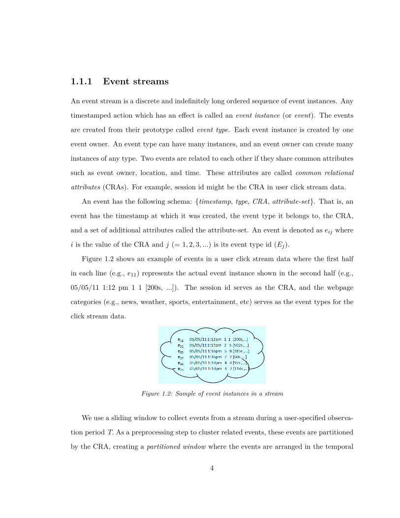
An event has the following schema: {timestamp, type, CRA, attribute-set}. That is, an

event has the timestamp at which it was created, the event type it belongs to, the CRA,

and a set of additional attributes called the attribute-set. An event is denoted as eij where

i is the value of the CRA and j (= 1, 2, 3, ...) is its event type id (Ej).

Figure 1.2 shows an example of events in a user click stream data where the first half

in each line (e.g., e11) represents the actual event instance shown in the second half (e.g.,

05/05/11 1:12 pm 1 1 [200s, ...]). The session id serves as the CRA, and the webpage

categories (e.g., news, weather, sports, entertainment, etc) serves as the event types for the

click stream data.

Figure 1.2: Sample of event instances in a stream

We use a sliding window to collect events from a stream during a user-specified observa-

tion period T. As a preprocessing step to cluster related events, these events are partitioned

by the CRA, creating a partitioned window where the events are arranged in the temporal

4

(a) Raw event stream. (b) Partitioned window.

Figure 1.3: Event stream

order in each partition. Figure 1.3 shows the partitioned window for the event stream shown

in Figure 1.2. Once the observation period expires, the window slides to the next batch of

events.

Definition 1 (Partition) A partition in a partitioned window is defined as the set of

observed events arranged in the temporal order over a time period T, that is

Wi = {eij(t)|t ≤ T, i ∈ A, j ∈ [1, N ]}

where A is the set of CRA values, j is the event type, N is the number of event types, and

t is the timestamp.

1.1.2 Causality and Causal network

Causality (or causal relationship) is a relationship where a cause leads to an effect. An

event can have multiple cause events; similarly, an event can have multiple effect events.

Popper defines causality as a relationship between variables that meets three conditions:

temporal precedence of a cause over an effect, dependency of the effect on the cause, and

absence of other plausible causes (Popper, 1959). The conceptual basis of causality in this

dissertation is Popper’s definition of causality. Specifically, we use the following notion of

causality.

5

Definition 2 (Causality) An event type Ei is a cause of another event type Ej (i 6= j)

if a majority of instances of Ei and a majority of instances of Ej are dependent and a

majority of instances of Ei precede a majority of instances of Ej. (The specifics of how

many constitute a “majority” is application-dependent.) The causal relationship between

these event types is true in the presence of any other event types. In addition, an event

instance eki is said to be a cause of another event instance ekj (i 6= j) if they have causality

at the event type level and eki precedes ekj. Note that these two instances share the same

CRA (i.e., k).

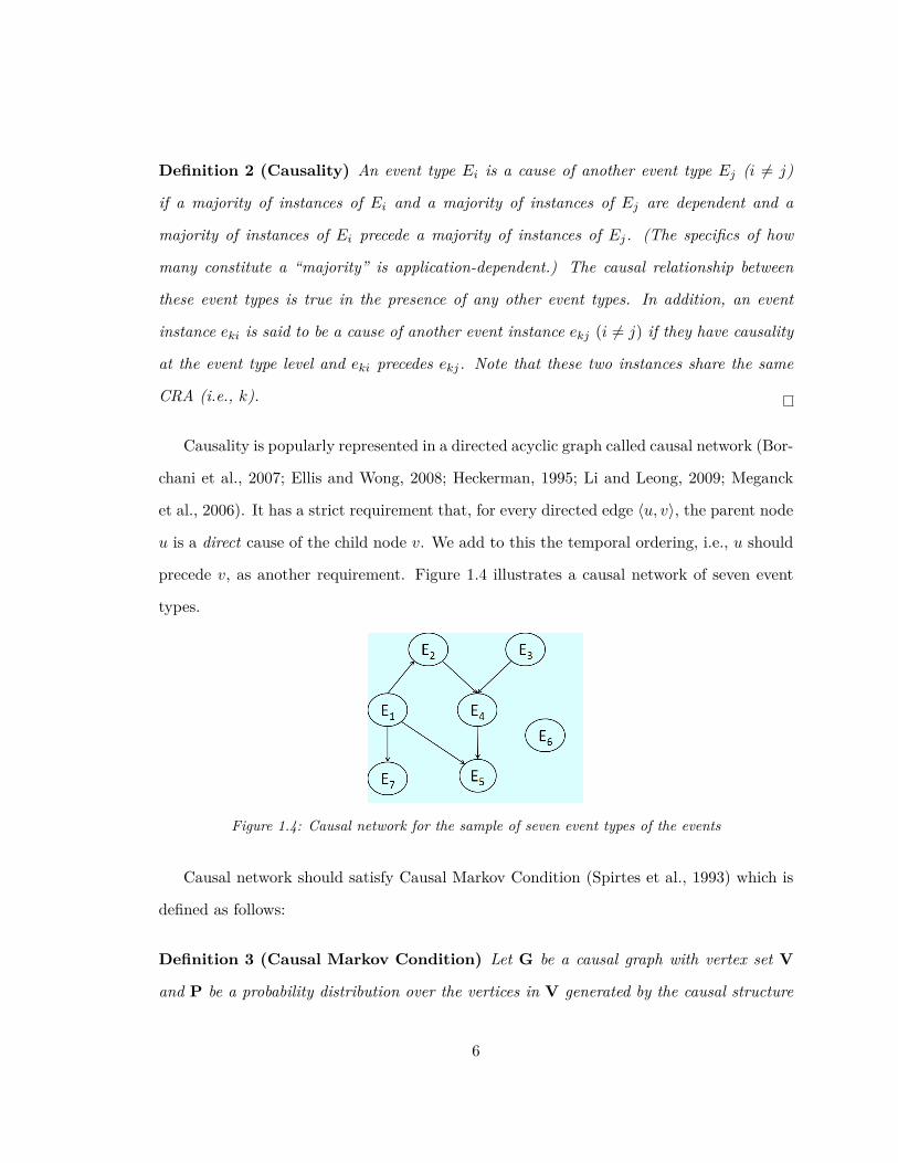
Causality is popularly represented in a directed acyclic graph called causal network (Bor-

chani et al., 2007; Ellis and Wong, 2008; Heckerman, 1995; Li and Leong, 2009; Meganck

et al., 2006). It has a strict requirement that, for every directed edge 〈u, v〉, the parent node

u is a direct cause of the child node v. We add to this the temporal ordering, i.e., u should

precede v, as another requirement. Figure 1.4 illustrates a causal network of seven event

types.

Figure 1.4: Causal network for the sample of seven event types of the events

Causal network should satisfy Causal Markov Condition (Spirtes et al., 1993) which is

defined as follows:

Definition 3 (Causal Markov Condition) Let G be a causal graph with vertex set V

and P be a probability distribution over the vertices in V generated by the causal structure

6

represented by G. G and P satisfy the Causal Markov Condition if and only if for every

X in V, X is independent of V(Descendants(X) ∪Parents(X)) given Parents(X).

Given a set of N event types E ≡ {E1, ..., EN}, the joint probability distribution of

event types in a causal network is specified as

P (E) =N∏i=1

P (Ei|Pai)

where Pai is the set of parent nodes of the event type Ei.

1.1.3 Conditional independence tests

As described in Section 1.1.2, causality requires dependence of effect variables on the cause

variables. In other words, as Causal Markov Condition specifies, non-causal variables in

a causal network are independent of each other given one or more variables. Conditional

independence tests are widely used to determine the independence between variables in the

presence of other variables. A popular approach for testing the conditional independence

(CI) between two random variables X and Y given a subset of random variables, C, is

conditional mutual information(CMI) (Cheng et al., 2002; de Campos, 2006). CMI gives

the strength of dependency between variables in a measurable quantity, which helps to

identify the weak (spurious) causal relationships.

CMI(X,Y |C) =∑x∈X

∑y∈Y

∑c∈|C

p(x, y, c)log2p(x, y|c)

p(x|c)p(y|c)

where p is the probability mass function calculated from the frequencies of variables.

In the traditional CMI, two variablesX and Y are said to be independent if CMI(X,Y |C)

= 0, and dependent otherwise. In many cases even though the CMI is positive, we need to

distinguish between stronger and weaker dependencies, for example between CMI(X,Y |C)

= 10 and CMI(X,Y |C) = 10−3. With a higher value of CMI(X,Y |C), the dependency

7

between X and Y grows stronger. Thus, to prune out weak dependencies which are more

likely to be spurious, we set a threshold CMI value, below which we consider the evidence

weak. To do so, we relate CMI with the G2 test statistics (Bishop et al., 1975; Spirtes et al.,

2000) as below.G2(X,Y |C) = 2 ·Ns · loge2 · CMI(X,Y |C)

where Ns is the number of samples (i.e., event instances).

Under the independence assumption, G2 follows the χ2 distribution (Kullback, 1968)

with the degree of freedom df equal to (nx − 1)(ny − 1)∏s∈S ns, where nx, ny, and ns are

the number of possible distinct values of X, Y, and S, respectively. So, we perform χ2 test,

which provides a threshold based on df and significance level α, to validate the result. We

set α as the generally accepted value of 95%.

A boolean function IsIndependent(X,Y,C) is defined to test the conditional indepen-

dence between two variables X and Y, given a condition set of variables C, using the G2 test

statistics. It returns true if these two variables are conditionally independent; otherwise, it

returns false.

The unbounded and continuous nature of the event stream warrants an incremental

approach and, therefore, the independence test procedure needs to be incremental in our

case. So, as a new batch of events arrives, only the record of the frequency of observations

should be updated without keeping the old events.

1.2 Research Problems, Motivations, and Contri-

butions

In this journal-format dissertation, as discussed earlier, we investigate three research areas

of causal modeling and prediction over event streams. In the first part of the dissertation

(Chapter 2), we study the research problem regarding incremental causal modeling. In the

8

second part of this dissertation (Chapters 3 and 4), we study the research problems to speed

up the causal modeling process and to support out-of-order events arrival. In the third part

of this dissertation (Chapter 5), we study the problem of continuous causal prediction in

real-time over event streams to predict the top k most likely effects given a set of observed

events. In these three research areas, we use the temporal precedence information, which

is readily available in the event streams, as an important clue for determining causality.

According to Barber (Barber, 2012), causality requires explicit temporal information in the

model, otherwise only correlation or dependencies can be inferred. A distribution P (E1, E2)

can be written as either P (E1|E2)P (E2) or P (E2|E1)P (E1) representing E2 causes E1 or

E1 causes E2, respectively. Clearly, without the temporal information, causality is difficult

to infer since both these cases represent exactly the same distribution. Note that a cause

always precedes its effect (Popper, 1959).

1.2.1 Incremental Causal Modeling over Event Streams

The traditional causal modeling algorithms (Borchani et al., 2007; Ellis and Wong, 2008;

Heckerman, 1995; Li and Leong, 2009; Meganck et al., 2006; Pearl, 2009; Chandra and

Kshemkalyani, 2005; Mani et al., 2010) assume that a complete set of data is available at

once. For a large number of modern applications, however, the data arrive in a stream

continuously and unboundedly. To model causality in such streaming data, the available

approach is to rebuild the model from scratch (starting from the first batch of observed data)

in light of new data. However, this approach is inefficient in two aspects. First, all the data

need to be stored, which is resource intensive. Second, the rebuilding of the model from

scratch takes a long time, and therefore is redundant and inefficient. Motivated by these

observations, in this dissertation we extend the support for incremental causal modeling

over event streams. In an incremental model, with the arrival of new data the model is

simply revised instead of being rebuilt completely. The old data can then be discarded.

9

Unfortunately, there exists no specific work for incremental causal network inference

over event streams. While Bayesian networks are very popular and widely used for non-

incremental causal modeling (Borchani et al., 2007; Ellis and Wong, 2008; Heckerman, 1995;

Li and Leong, 2009; Meganck et al., 2006; Mani et al., 2010) and there has been some effort

towards constructing a Bayesian network incrementally (Alcobé, 2004b; Alcobé, 2004a), the

Bayesian network itself is not a causal network for two reasons. First, in a causal network

there is a strict requirement that the parent of a node is its direct cause, but the same is

not true in a Bayesian network. Second, two or more Bayesian network structures, called

equivalence classes (Chickering, 2002), may represent the same probability distribution and,

consequently, the causal directions between nodes in the network are often random. The

experimental intervention method, most commonly used for experimental static data to

alleviate these problems, is unfortunately not applicable in the stream environment where

the entire dataset is not available at any given time.

Thus, in this research, we propose a new algorithm which incrementally constructs a

causal network while addressing the problems mentioned above (Acharya and Lee, 2014b).

The key approach is to construct a causal network by merging a temporal network and a

Bayesian network. Note that causality requires temporal precedence and dependency be-

tween cause and its effect. The temporal precedence direction between nodes is a strong

indicator of the causal direction as cause precedes its effect. We model the temporal prece-

dence information incrementally in a temporal network whereas a state-of-the-art incremen-

tal Bayesian network algorithm (Alcobé, 2004b; Alcobé, 2005; Alcobé, 2004a) learns the

statistical dependencies incrementally. Furthermore, we provide measures to eliminate spu-

rious causalities that do not indicate strong enough causality. In this regard, our approach

supports Popper’s three conditions for inferring causality, which are temporal precedence,

dependency, and no confounding causality (Popper, 1959). We introduce a novel two lay-

ered incremental causal network structure to represent causality at both the event type

10

level and the event instance level. The first layer contains the event types whereas the

second layer, which is a virtual layer, contains event instances. The motivations for this

two layered causal network model are twofold. First, it allows for an incremental refinement

of the network structure at the event type level in light of new event instances. Second,

the idea of a virtual layer makes the model flexible enough to add new or discard old event

instances (when they expire). In addition to the structural novelty, the causal network is

semantically enriched with the notions of causal strength and causal direction confidence

associated with each edge.

We conduct two sets of experiments, using real dataset and synthetic datasets, to eval-

uate the proposed incremental causal network construction algorithm against an existing

incremental Bayesian network algorithm. First, the evaluation is focused on the resultant

network structure. One evaluation is with respect to the topologies of the resulting net-

works, and the other evaluation is with respect to the edge directions. In both cases, the

networks generated by the two algorithms are compared against a true causal network un-

known to the algorithms. Second, the run-time overhead of our incremental algorithm is

evaluated against that of the existing Bayesian network algorithm.

1.2.2 Fast causal modeling over event streams

The availability of a large amount of data with high throughput in event streams warrants

fast causal inference operations. The existing two approaches – score-based and constraint-

based – are slow and their running time increases exponentially with an increase in the

number of variables in the event stream. In addition, these approaches do not leverage the

changes in the probability distribution of the event streams to avoid unnecessary compu-

tations. The first approach, score-based (Heckerman, 1995; Ellis and Wong, 2008; Li and

Leong, 2009; Meganck et al., 2006), performs greedy search (usually hill climbing) over

all possible network structures to find the best network that represents the data based on

11

the highest score. This approach, however, has two problems. First, it is slow due to the

exhaustive search for the best network structure. An increase in the number of variables in

the dataset increases the computational complexity exponentially. Second, two or more net-

work structures, called the equivalence classes (Chickering, 2002), may represent the same

probability distribution, and consequently the causal directions between nodes are quite

random. Unfortunately, there is no technique for alleviating these problems in a streaming

environment. Thus, score-based algorithms are not suitable for streams.

The second approach, constraint-based (Pearl, 2009; Spirtes et al., 1990; Spirtes et al.,

2000; Cheng et al., 2002), does not have the problem of equivalence classes. However,

it is slow as it starts with a completely connected undirected graph and thus performs a

large number of conditional independence (CI) tests to remove the edges between condi-

tionally independent nodes. Clearly, the number of CI tests increases exponentially with

the increase in the number of variables in the dataset. To alleviate this problem, some

constraint-based algorithms start with a minimum spanning tree to reduce the initial size

of condition sets. However, this idea trades the speed with the accuracy of the causal in-

ference. The constraint-based algorithms such as IC* (Pearl, 2009), SGS (Spirtes et al.,

1990), PC (Spirtes et al., 2000), and FCI algorithm (Spirtes et al., 2000) start with a com-

pletely connected undirected graph. To reduce the computational complexity, CI tests are

performed in several steps. Each step produces a sparser graph than the earlier step, and

consequently, the condition set decreases in the next step. However, the number of CI tests

is still large. Therefore, these current constraint-based algorithms are not suitable for fast

causal inference over streams.

Given these observations, we overcome the drawbacks of the existing approaches as

follows. To speed up the causal modeling process, we propose a new time-centric causal

modeling approach (Acharya and Lee, 2013). Every causal relationship implies temporal

precedence relationship (Popper, 1959). So, temporal precedence information is used as an

12

important clue in reducing the number of required CI tests and thus maintaining feasible

computational complexity. This idea performs fewer computations of CI test due to two

factors. First, since causality requires temporal precedence, the nodes with no temporal

precedence relationship between them are ignored. Second, in the CI test of an edge, we

exclude those nodes from the condition set which do not have temporal precedence relation-

ship with either of the end nodes of the edge. Thus, it reduces the size of the condition set,

to the effect of alleviating exponential computational complexity. In addition, the tempo-

ral precedence relationship orients the causal edge, unlike the constraint-based algorithms

which need a separate set of rules infers the causal direction. The temporal precedence

relationships between event types are represented in a temporal network structure, and we

propose an algorithm to construct the temporal network applicable in a streaming environ-

ment.

We also study the problem of causal inference over out-of-order event streams (Acharya

and Lee, 2014a). Since the time-centric causal modeling approach relies on the temporal

precedence between events, a larger number of out-of-order events makes such an approach

less reliable. In addition, we present a novel change-driven strategy which updates the

causal network only when there is strong enough change in te probability distribution of

the event streams (Acharya and Lee, 2014a). This idea thus avoids unnecessary causal

inference computations.

We demonstrate the utility of the proposed algorithms by conducting two sets of exper-

iments using synthetic and real datasets. The results of the experiments demonstrate the

advantages of the proposed algorithm in terms of the running time and the total number of

CI tests required for the learning of a causal network by comparing it against the state-of-

art constraint-based algorithm for causal network inference. Specifically, we conduct three

sets of experiments, first in terms of the accuracies of the resulting causal networks, second

the running time, and third the number of CI tests required, to compare our proposed algo-

13

rithm against the state-of-the-art algorithm. In each set of experiments, we consider both

cases of stream being in order and out of order, and also observe the effect of the proposed

change-driven causal modeling strategy in reducing the running time. We show that the

large number of conditional independence tests is the bottleneck to achieving fast causal

modeling.

1.2.3 Continuous prediction over event streams

In this research, we study the problem of continuous prediction of effects over event streams

in real-time. Specifically, we address the prediction of top-k most likely effects given a

stream of events observed thus far (Acharya et al., 2014). The large answer space and the

continuous and unbounded nature of the high throughput streams make such prediction a

challenging problem. The brute force approach is to construct a traditional causal network

over event stream and then run a predictive top-k query over it to identify the k most

probable effects with the highest scores. This approach for causal prediction over the event

streams, however, presents new challenges.

The first challenge is the lack of support for cyclic causality in the causal network. In

the real world, an instance of type E1 can cause another instance of type E2 in one scenario

while an instance of type E2 can cause another instance of type E1 in another scenario.

In the traditional acyclic causal model, only one of these two alternatives, either E1 → E2

or E2 ← E1, is possible. This limitation renders the causal network to be an inaccurate

prediction model. So, a novel causal modeling approach is necessary to accommodate all

possible causal relationships. To address this challenge, we propose a new event precedence

model which learns every possible temporal precedence relationship, a required criterion for

causal relationship, between events to generate a cyclic network structure of the precedence

relationships, called the event precedence network (EPN).

The second challenge is that the traditional causal model employs a conservative ap-

14

proach to avoid any suspicious and weak relationships, which exhaustively checks and re-

moves all relationships which are independent in the presence of one or more events. This

property of the traditional causal network is the causal Markov condition. However, it often

ends up removing significant causal relationships. We call it causal information loss.

To meet these two challenges, we propose a strategy for inferring causality at runtime

from the EPN. The intuition behind such a strategy is that relevant causal inference is

possible only after the top-k query variables are known. This approach helps to overcome

cyclic causality. Furthermore, since the causal inference is performed at runtime, it only

considers the variables which are causally relevant to the query and therefore reduces the

causal information loss. In addition, as the EPN retains all precedence relationships (in-

cluding cyclic relationships), the runtime causal inference overcomes the lack of support

for cyclic causality and causal information loss. This approach is naturally adaptive to the

changes in the event streams and, therefore, is suitable for streaming environment.

The third challenge is to efficiently process a predictive query in real-time over event

streams so that the top-k most likely effects are known. A naive approach is to perform an

exhaustive searching and sorting among all possible event types, which is inefficient for real-

time event streams. Thus, there is a need for an efficient approach to perform only required

search over the possibly huge search space to predict the results. We propose two top-k

query processing algorithms to determine the top k effects with the highest scores. One

algorithm formalizes the exhaustive search approach, while the other algorithm employs

ideas to reduce the search space and terminate as early as possible for real-time query

processing.

We conduct extensive experiments with two real datasets. The experiments evaluate the

runtime causal inference model and the top-k query processing mechanism in the proposed

algorithms. One evaluation is with respect to the accuracy of the top k results, and the

other evaluation is with respect to the running time. We demonstrate that the proposed

15

approach overcomes the two main limitations of the traditional causal inference approach

- acyclic causality and causal information loss. In addition, we show the merits of the

real-time query processing over exhaustive query processing in terms of the running time.

1.3 Dissertation Outline

This dissertation is organized in a journal format according to the University guidelines. It

comprises three parts. The first part (Chapter 2) presents the study of the research area

regarding incremental causal modeling. It address the problem of constructing a causal

network incrementally over event streams.

The second part of the dissertation (Chapters 3 and 4) presents two research problems in

supporting fast causal network construction. Chapter 3 addresses the problem of reducing

the number of conditional independence tests to speed up the causal modeling process.

Chapter 4 extends the work of Chapter 3 to address the problem of redundant causal

modeling computations based on a change-driven strategy and also examines the effect of

time-centric approach on causal modeling for out-of-order events.

The third part of the dissertation (Chapter 5) presents the research area involving

the top-k prediction of possible effects based on the events observed so far. Specifically,

the problems involving runtime causal inference and real-time top-k query processing are

addressed.

Finally, Chapter 6 summarizes the dissertation and suggests further research.

16

Chapter 2

Incremental Causal Network Construction

over Event Streams

Abstract

This paper addresses modeling causal relationships over event streams where data are un-

bounded and hence incremental modeling is required. There is no existing work for in-

cremental causal modeling over event streams. Our approach is based on Popper’s three

conditions which are generally accepted for inferring causality – temporal precedence of

cause over effect, dependency between cause and effect, and elimination of plausible alter-

natives. We meet these conditions by proposing a novel incremental causal network con-

struction algorithm. This algorithm infers causality by learning the temporal precedence

relationships using our own new incremental temporal network construction algorithm and

the dependency by adopting a state of the art incremental Bayesian network construction

algorithm called the Incremental Hill-Climbing Monte Carlo. Moreover, we provide a mech-

anism to infer only strong causality, which provides a way to eliminate weak alternatives.

This research benefits causal analysis over event streams by providing a novel two layered

causal network without the need for prior knowledge. Experiments using synthetic and real

17

datasets demonstrate the efficacy of the proposed algorithm.

2.1 Introduction

People tend to build their understanding of events in terms of cause and effect, to answer

such questions as “What caused the IBM stock to drop by 20% today?” or “What caused

the glucose measurement of this diabetic patient to increase all of a sudden?”. In recent

years, there has been growing need for active systems that can perform such causal analysis

in diverse applications such as patient healthcare monitoring, stock market prediction, user

activities monitoring and network intrusion detection systems. These applications need to

monitor the events continuously and update an appropriate causal model, thereby enabling

causal analysis among the events observed so far.

In this paper, we consider the problem of modeling causality over event streams (not

necessarily real-time) with a focus on constructing a causal network. The causal network,

a widely accepted graphical structure to represent causal relationships, is an area of active

research. All the existing works (Borchani et al., 2007; Ellis and Wong, 2008; Heckerman,

1995; Li and Leong, 2009; Meganck et al., 2006; Pearl, 2009; Chandra and Kshemkalyani,

2005; Mani et al., 2010) in this area have been done for an environment where a complete

dataset is available at once. However, event instances in an event stream are unbounded,

and in such a case an incremental approach is imperative. Thus, the goal of our work is to

model causal relationships in a causal network structure incrementally over event streams.

To the best of our knowledge, there exists no work done by others with this objective.

Bayesian networks are in popular use for non-incremental causal modeling (Borchani

et al., 2007; Ellis and Wong, 2008; Heckerman, 1995; Li and Leong, 2009; Meganck et al.,

2006; Mani et al., 2010). While the Bayesian network encodes dependencies among all

variables, it by itself is not the causal network. First, the causal network strictly requires

that the parent of a node is its direct cause, but the Bayesian network does not. Second, two

18

or more Bayesian network structures, called the equivalence classes (Chickering, 2002), can

represent the same probability distribution and, consequently, the causal directions between

nodes are quite random. There is no technique for alleviating these problems in an event

stream environment where the entire dataset is not available at any given time.

To overcome this lack of suitable approach for incremental causal modeling over event

streams, we propose the Incremental Causal Network Construction(ICNC) algorithm. The

ICNC algorithm is a hybrid method to incrementally model a causal network, using the

concepts and techniques of both temporal precedences and statistical dependencies. Alone,

neither dependency nor temporal precedence provides enough clue about causal relation-

ships. The temporal precedence information is learned incrementally in a temporal network

with the proposed Incremental Temporal Network Construction (ITNC) algorithm (see Sec-

tion 2.5.2) whereas the statistical dependencies are learned incrementally with a state of

the art algorithm called the Incremental Hill Climbing Markov Chain (IHCMC) (Alcobé,

2004b; Alcobé, 2005; Alcobé, 2004a). There are a few works (Hamilton and Karimi, 2005;

Liu et al., 2010) where temporal precedence information is used to identify causal rela-

tionships between variables (see Section 2.8), but none of them is for constructing causal

networks. In our approach, we further provide measures to eliminate confounding causalities

that do not indicate strong enough causality. In this regard, our approach supports Pop-

per’s three conditions for inferring causality, which are temporal precedence, dependency,

and no confounding causality (Popper, 1959).

We model an incremental causal network with a novel two layered network structure.

The first layer is a network of event types where an edge between two event types reflects

the causality relationship observed between them so far in a stream. The second layer is a

network of event instances. It is a virtual layer in that there is no explicit link between event

instances. Instead, each event type in the first layer maintains a list of its instances which

are then connected to instances of another event type through a unique relational attribute

19

(more on this in Section 2.6.1). The motivations for this two layered causal network model

are as follows. First, it allows for an incremental modification of the network structure at

the event type level in light of new event instances. Second, the idea of a virtual layer makes

the model flexible enough to add new or drop old event instances (drop when the volume of

event instances grows too much) while maintaining the overall causal relationships at the

event type layer. In addition to the structural novelty, the causal network is semantically

enriched with the notions of causal strength and causal direction confidence associated with

each edge.

We conduct experiments to evaluate the performance of the proposed ICNC algorithm

using both synthetic and real datasets. The experiments measure how closely the con-

structed causal network resembles the true target causal network. Specifically, we compare

the Bayesian network produced by IHCMC and the causal network produced by ICNC

against a target network. The results show considerable improvements in the accuracy of

the causal network over the Bayesian network by the use of temporal precedence relationship

between events.

The contributions of this paper are summarized as follows.

• It presents a temporal network structure to represent temporal precedence relation-

ships between event types and proposes an algorithm to construct a temporal network

incrementally over event streams.

• It introduces a two-layered causal network with rich causality semantics, and proposes

an incremental causal network construction algorithm over event streams. The novelty

of the algorithm is in combining temporal precedence and statistical dependency of

causality to construct a causal network.

• It empirically demonstrates the advantages of the proposed algorithm in terms of how

the temporal network increases the accuracy of the causal network and how close the

generated causal network is to the true unknown target causal network.

20

The rest of the paper is organized as follows. Section 2.2 presents some preliminary con-

cepts. Section 2.3 formulates the specific problem addressed in this paper and outlines the

proposed approach. Section 2.4 describes the incremental Bayesian network construction.

Section 2.5 and Section 2.6 propose the incremental temporal network construction and the

incremental causal network construction, respectively. Section 2.7 evaluates the proposed

ICNC algorithm. Section 2.8 discusses related work. Section 2.9 concludes the paper and

suggests future work.

2.2 Preliminaries

In this section, we present some key concepts needed to understand the rest of the paper.

The concepts are illustrated with a representative use case – diabetic patient monitoring sys-

tem (Frank and Asuncion, 2010). We select a few important attributes from this real-world

case to make the explanations intuitive, and use them in a running example throughout the

paper.

2.2.1 Event stream, instance, type

An event stream in our work is a sequence of continuous and unbounded timestamped

events. An event refers to any action that has an effect. One event can trigger another

event in chain reactions. Each event instance belongs to one and only one event type which

is a prototype for creating the instances. We support concurrent events. In this paper an

event instance is often called simply an event or an instance if the context makes it clear.

Each event instance is created by one event owner. An event type can have many

instances, and an event owner can create many instances of any type. Two event instances

are related to each other if they share common attributes such as event owner, location, and

time. We call these attributes common relational attributes(CRAs). In Example 1, patient

21

ID may be the CRA, as the events of the same patient are causally related.

In this paper we denote an event type as Ej and an event instance as eij , where i

indicates the CRA and j indicates the event type ID.

Example 1 Consider a diabetic patient monitoring system in a hospital. There are hun-

dreds of patients admitted to a hospital, and a majority of the actions are related to clinical

tests and measurements. Each patient is uniquely identifiable, and each test or action of

each patient makes one event instance. For example, a patient is admitted to the hos-

pital, has blood pressure and glucose level measured, and takes medication, creating the

instances of the above event types as a result. These instances are repeated for a cou-

ple of weeks or months till the patient is discharged. Typical event types from these ac-

tions would include NPH-insulin-dose-given (NIDG), regular-insulin-dose-given (RIDG),

and hypoglycemic-symptoms-exists (HSE), blood-glucose-measurement-decreased (BGMD),

blood-glucose-measurement-increased (BGMI), etc. (more in Table 2.3 in Section 2.7.1.2).

An event type has the following schema: [type ID, type name, event container], where

type ID is the primary key and event container is a list of all instances of the type. An event

instance has the following schema: [type ID, CRA, timestamp, lifetime, attribute container],

where type ID, CRA and timestamp together make the primary key, lifetime is the time

duration up to which the event is alive, and attribute container is the set of attribute-value

pairs storing any additional information. Note that an event stream contains an indefinitely

large number of event instances; hence, an event container, with limited space, cannot store

all of them, and therefore an event instance is removed from the event container once its

lifetime expires.

22

2.2.2 Causality and causal network

Causality (or causal relationship) is a relationship between a cause and an effect. An event

can have multiple cause events; similarly, it can have multiple effect events. The conceptual

basis of causality in our work is that the effect is dependent on the cause to occur and the

cause must precede the effect. More specifically, we use the following notion of causality.

Definition 4 (Causality) An event type Ei is a cause of another event type Ej (i 6= j)

if a majority of instances of Ei and a majority of instances of Ej are dependent and a

majority of instances of Ei precede a majority of instances of Ej. (The specifics of how

many constitute a “majority” is application-dependent.) In addition, an event instance eki

is said to be a cause of another event instance ekj (i 6= j) if they have causality at the event

type level and eki precedes ekj. Note that these two instances share the same CRA (k).

Causal network is a popularly used data structure for representing causality (Borchani

et al., 2007; Ellis and Wong, 2008; Heckerman, 1995; Li and Leong, 2009; Meganck et al.,

2006). It is a directed acyclic graph with a strict requirement that, for every directed edge

〈u, v〉, the parent node u is a direct cause of the child node v. We add to this the temporal

ordering, i.e., u should precede v, as another requirement.

Figure 2.1(a) illustrates a causal network of the five event types mentioned in Example 1.

The intuitions of the causality among them are as follows – (1) an insulin dose is given to

a patient (RIDG or NIDG) to decrease the blood glucose level (BGMD), hence the edge

from RIDG and NIDG to BGMD; (2) an increasing blood glucose level (BGMI) triggers the

administration of a regular insulin dose (RIDG), hence the edge from BGMI to RIDG; (3)

it is common medical knowledge that a decrease in blood glucose level (BGMD) can cause

hypoglycemic symptom (HSE), hence the edge from BGMD to HSE. (From here on, we

denote BGMI, RIDG, NIDG, BGMD, and HSE with E1, E2, E3, E4, and E5, respectively,

as shown in Figure 2.1(b).)

23

(a) Network with the actualevent type names.

(b) Network with the simplifiedevent type notations.

Figure 2.1: Causal network for Example 1

2.3 Problem Formulation and the Proposed Ap-

proach

2.3.1 Problem

There are three issues that constitute the problem addressed in this paper. First, due to

the existence of equivalence classes, the directions of edges in the Bayesian network are not

reliable and prone to being incorrect. Therefore, we need a method to learn the correct

directions of causal relationships and thereby reduce the number of reversed edges in the

causal network. Second, there may be a number of spurious or missing causal relationships

in a causal network.1 The number of spurious edges and the number of missing edges are

competing factors bringing a tradeoff in the accuracy of the resulting causal network. Thus,

an optimal causal network should have the minimum total number of spurious and missing

causal relationships. Third, an event stream is unbounded. Unlike the existing works (Bor-

chani et al., 2007; Ellis and Wong, 2008; Heckerman, 1995; Li and Leong, 2009; Meganck1The causal network has a strict requirement that the parents of a node are its direct causes. However,

the same is not true for a Bayesian network, and, therefore, dependencies between event types detected in aBayesian network may not be causal relationships. Such dependencies lead to spurious causal relationshipsin the causal network.

24

et al., 2006) where a complete dataset is expected to be available for causal modeling, we

need an algorithm that constructs a causal network incrementally. In summary, the prob-

lem addressed is to construct a causal network incrementally over event streams and while

doing so, to reduce the number of reversed edges and minimize the total number of missing

and spurious edges in the resultant causal network.

2.3.2 Overview of the approach

To learn a causal network incrementally over event streams, we propose the Incremental

Causal Network Construction (ICNC) algorithm (see Section 2.6.1) which models the causal

relationships in a two layered network. In the algorithm, we meet Popper’s three condi-

tions for inferring causality – temporal precedence, dependency and no confounding causal-

ity (Popper, 1959). We propose the Incremental Temporal Network Construction(ITNC)

algorithm (see Section 2.5) to model the temporal precedences from an event stream into

a temporal network incrementally. As mentioned earlier, Bayesian network is reliable to

model statistical dependencies and thus we adopt an incremental Bayesian network con-

struction algorithm, the Incremental Hill-Climbing Monte Carlo (IHCMC) algorithm (see

Section 2.4.2). To resolve the equivalence class problem in Bayesian networks, we use the

DAG-TO-CPDAG algorithm (Chickering, 2002) to generate a complete partial directed

acyclic graph (CPDAG) where unreliable edges are rendered undirected. Then, the ICNC

algorithm integrates the temporal network and the CPDAG. During the integration, spuri-

ous edges which do not indicate strong enough causality are removed and edges which indi-

cate strong evidence of causality are added with the aim of minimizing the total number of

missing and spurious edges, respectively. We rely on the temporal precedence information

in the temporal network to identify the correct causal directions of the undirected edges.

Section 2.6 describes the rule for this integration and the algorithm for constructing the

incremental causal network.

25

2.4 Incremental Bayesian Network

2.4.1 Bayesian network model

Bayesian network is a directed acyclic graph which encodes a joint probability distribution

over a set of random variables. The joint probability distribution of a set of n variables

X ≡ {X1, ..., Xn} is specified as

P (X) =n∏i=1

P (Xi|Pai)

where Pai is the set of parent nodes of the variable Xi.

Bayesian network encodes the assertions of conditional independence between variables

and, thus, is an appropriate network structure to represent statistical dependency between

events. Figure 2.2(a) (in Section 2.4.3) shows the Bayesian network corresponding to Ex-

ample 1.

As already mentioned, however, the same probability distribution can be represented

by different Bayesian network structures that are in the same equivalence class (Chickering,

2002). For example in Figure 2.2(a), E1 → E2 → E3 and E1 ← E2 → E3 may represent the

same joint probability distribution and hence the same network topology. The differences

in their network structures are in the directions of the edges. Since the edge direction in a

causal network indicates the causal direction between events, the causal meaning becomes

entirely different with the change in the edge direction. This ambiguity makes Bayesian

networks unsuitable to be used as causal networks. In the example above, the causal

direction E1 → E2 (recall E1 and E2 are BGMI and RIDG, respectively) makes sense as an

increase in blood glucose measurement (BGMI) causes the use of insulin (RIDG). However,

the reverse causal direction E1 ← E2 (in the Bayesian network of Figure 2.2(a)) is incorrect

as the use of insulin does not increase the blood glucose measurement. So, a Bayesian

26

network cannot be trusted to detect the causal direction between events.

Bayesian variables in the constructed network represent event types. They are boolean

variables indicating whether an instance of the represented event type exists or not in the

event stream.

2.4.2 Incremental Bayesian network construction algorithm

With the continuous arrival of an event stream with no definite end, it is imperative to con-

struct a Bayesian network incrementally by refining the existing network every time a new

batch of data becomes available. Discarding and reconstructing the entire network from

scratch every time would be too expensive. As already mentioned, we use the Incremental

Hill-Climbing Monte Carlo (IHCMC), an incremental version of the HCMC algorithm (Al-

cobé, 2004b; Alcobé, 2004a). In this subsection we summarize the HCMC and the IHCMC

algorithms implemented based on Alcobé’s work (Alcobé, 2004b; Alcobé, 2004a).

The HCMC algorithm begins with a network with no edge and, at each iteration, enu-

merates the neighboring states of the current network state (in the search space) by ran-

domly adding, removing, or reversing edges, and then keeps the network with the highest

score. The algorithm terminates when none of the neighboring networks improves the score

over the current network. Algorithm 1 summarizes the implemented HCMC algorithm. In

the algorithm, the NR (no reversal) neighborhood refers to all DAGs with one arc more or

less and do not introduce a directed cycle, whereas the NCR(non-covered reversal) neight-

borhood refers to the NR neighborhood plus all DAGs with one non-covered edge reversed

and does not introduce a directed cycle. (An edge x→ y in a DAG G is said to be covered

in G if parents(x) ∪ x = parents(y), that is, all and only the parents of x are the parents

of y.)

Initially, the IHCMC algorithm behaves exactly like the HCMC algorithm, which finds a

network structure achieving the highest score given the provided data. During this process,

27

Algorithm 1 HCMCRequire: a dataset D on {X1, ....., Xn} variables, a variable ncr indicating whether to use

NCR neighorhood or NR neighborhood, a constant MAXTRIALS, a positive integer n1: localMaximum = false, trials = 0;2: Let G be an edgeless DAG.3: Calculate the initial neighborhood N(G) (based on ncr) and sufficient statistics for D;4: while localMaximum is false do5: Reverse n randomly chosen edges in G; {//Escape from the local maximum to find

the global maximum by randomly reversing edges.}6: Let G′ be the highest-score DAG in the neighborhood N(G). {//Select the best

network structure in the neighborhood.}7: if score(G) ≥ score(G′) then localMaximum = true; {//There are no network struc-

tures with higher score than the current one.}8: if localMaximum is false {//The local maximum has not been reached.} then9: trials = 0;

10: G = G′;11: else if trials < MAXTRIALS {//Repeat the trial up to MAXTRIALS times to find

the global maximum.} then12: trials = trials + 1;13: localMaximum = false;14: end if15: end while

the order in which the operators (i.e., add, delete, reverse) coupled with edges are applied is

stored for use in the next learning step. Then, with the arrival of a new dataset, the IHCMC

algorithm updates the “sufficient statistics” of the old dataset to reflects the new data.

(Sufficient statistics is a statistical summary of the dataset which contains all information

necessary to calculate the scores of the Bayesian network.) Using the new sufficient statistics

and the order of operations from the previous step, it determines whether the current

network structure should be revised for the new dataset. If a revision is needed, the IHCMC

algorithm starts with the highest-score network in the previous step as the initial model.

This approach makes the algorithm efficient. When updating the network for the new

dataset, IHCMC reduces the search space by restricting the set of operators and edges

considered. In order to do that, a certain (used-defined) number of pairs of operators and

edges that give the score closest to the best one are stored for the next learning step, and

28

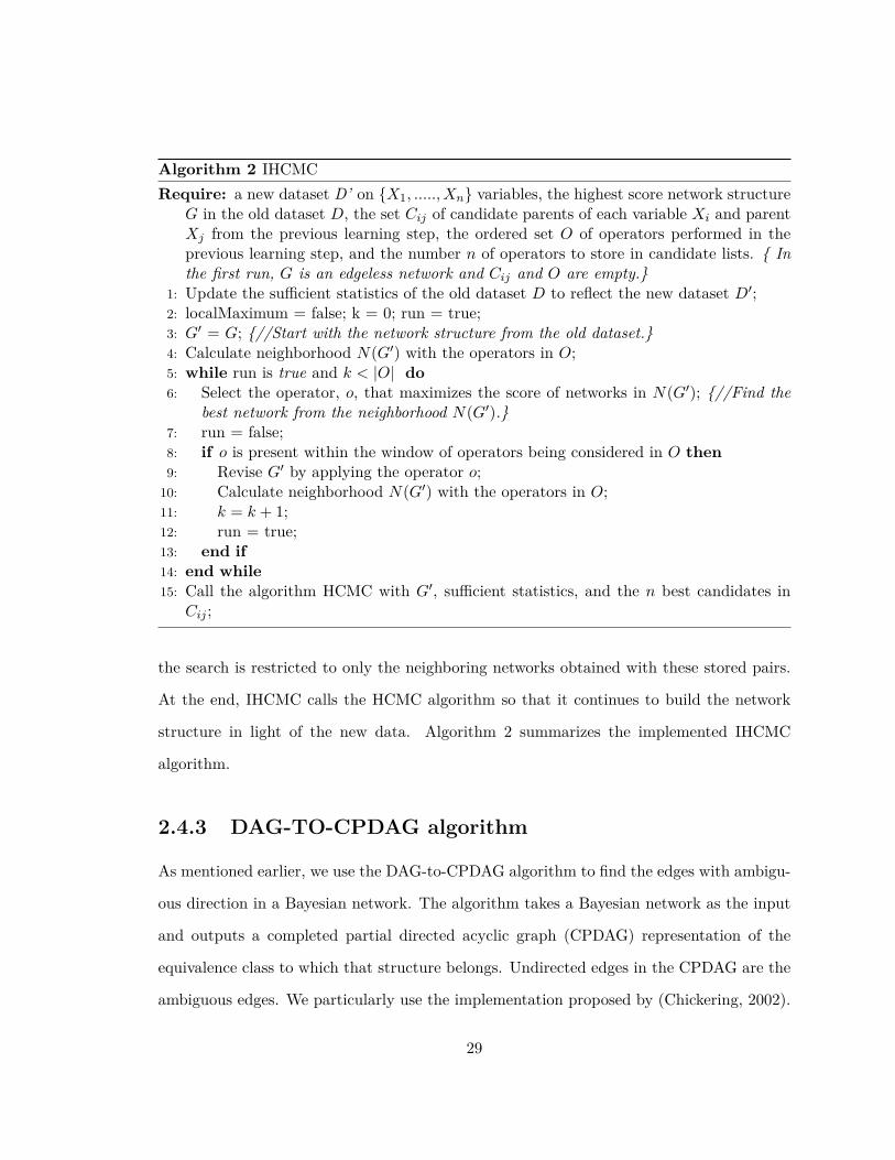
Algorithm 2 IHCMCRequire: a new dataset D’ on {X1, ....., Xn} variables, the highest score network structure

G in the old dataset D, the set Cij of candidate parents of each variable Xi and parentXj from the previous learning step, the ordered set O of operators performed in theprevious learning step, and the number n of operators to store in candidate lists. { Inthe first run, G is an edgeless network and Cij and O are empty.}

1: Update the sufficient statistics of the old dataset D to reflect the new dataset D′;2: localMaximum = false; k = 0; run = true;3: G′ = G; {//Start with the network structure from the old dataset.}4: Calculate neighborhood N(G′) with the operators in O;5: while run is true and k < |O| do6: Select the operator, o, that maximizes the score of networks in N(G′); {//Find the

best network from the neighborhood N(G′).}7: run = false;8: if o is present within the window of operators being considered in O then9: Revise G′ by applying the operator o;

10: Calculate neighborhood N(G′) with the operators in O;11: k = k + 1;12: run = true;13: end if14: end while15: Call the algorithm HCMC with G′, sufficient statistics, and the n best candidates in

Cij ;

the search is restricted to only the neighboring networks obtained with these stored pairs.

At the end, IHCMC calls the HCMC algorithm so that it continues to build the network

structure in light of the new data. Algorithm 2 summarizes the implemented IHCMC

algorithm.

2.4.3 DAG-TO-CPDAG algorithm

As mentioned earlier, we use the DAG-to-CPDAG algorithm to find the edges with ambigu-

ous direction in a Bayesian network. The algorithm takes a Bayesian network as the input

and outputs a completed partial directed acyclic graph (CPDAG) representation of the

equivalence class to which that structure belongs. Undirected edges in the CPDAG are the

ambiguous edges. We particularly use the implementation proposed by (Chickering, 2002).

29

Algorithm 3 outlines the three steps in the algorithm. First, it performs a topological sort

on the vertices in the input Bayesian network so that, for any pair of vertices x and y, x

must precede y if x is an ancestor of y. Second, based on the topological sorting, the edges

are sorted first in the ascending order of the incident vertices and then in the descending

order of the outgoing vertices. Finally, the ordered edges are labeled either “compelled” or

“reversible”. The “reversible” edges are made undirected while preserving the edge direction

of the “compelled” edges in the final CPDAG.

Algorithm 3 DAG-TO-CPDAGRequire: BayesianNetwork G.1: Sort the vertices in G such that x precedes y if and only if x is an ancestor of y;2: Based on the topological order of the vertices, sort the edges in G, first in the ascending

order of the incident vertices and then in the descending order of the outgoing vertices;

3: Label every edge in G as “unknown”;4: while there exists an edge labeled “unknown” in G do5: Select the edge of the lowest order, x→ y, that is labeled “unknown”;6: run = true;7: for every edge z → x labeled “compelled” do8: if z is not a parent of y {//If the path is z → x→ y} then9: Label x→ y and every edge incident into y as “compelled”;

10: run = false;11: End this FOR Loop;12: else13: {//If the path is z → x, z → y.}14: Label z → y as “compelled”;15: end if16: end for17: if run is true then18: if there exists an edge w → y such that w 6= x and w is not a parent of x then19: Label x→ y and every “unknown” edge incident to y as “compelled”;20: else21: Label x→ y and every “unknown” edge incident to y as “reversible”;22: end if23: end if24: end while25: Make all “reversible” edges undirected;

30

(a) Input Bayesian Net-work

(b) Output CPDAG

Figure 2.2: Illustration of DAG-TO-CPDAG.

Figure 2.2 illustrates the Chickering’s algorithm (Chickering, 2002). Given the input

Bayesian network in Figure 2.2(a), the first step (topological sorting of the vertices) gives

E2, E3, E1, E4, and E5; then, the second step sorts the edges in the following order:

E2 → E3, E2 → E4, E2 → E1, E3 → E4, and E4 → E5; finally, the third step labels the

edge E2 → E1 as “reversible” and the remaining edges as “compelled” and, therefore, the

“reversible” edge E2 → E1 is made undirected, resulting in the final output CPDAG shown

in Figure 2.2(b).

Note that the Chickering’s algorithm does not check repeatedly on all edges, hence

computationally more efficient than previous rule-based algorithms (Meek, 1995; Pearl and

Verma, 1991). In these algorithms, the idea is to undirect every edge in a DAG, except for

those edges that participate in a v-structure. (Three nodes x, y and z are said to have a

v-structure if their edges form the structure x→ y ← z.) The rules are applied repeatedly

on every edge to determine the edge direction until no rule has any effect on the PDAG,

that is, no edge becomes undirected.

31

2.5 Incremental Temporal Network

2.5.1 Temporal network model

In this paper the temporal network models the temporal precedences between pairs of

events. It is a directed acyclic graph of nodes representing event types. Its construction

has to be incremental as well, as it is over a stream. For this purpose, we place a window

over the stream. The semantics of the window can be dependent on the application, and we

use a time-based window here without loss of generality. Typically, the application offers a

natural observation period (e.g., day) that makes a window.

As mentioned in Definition 4, causality is defined between events with the same common

relational attribute(CRA). So, we arrange the events in a window by CRA as they arrive,

producing a partitioned window as a result. Events in the same partition have the same

CRA and are ordered by the timestamp. Figure 2.3 illustrates it with an event stream from

the patient diabetes monitoring system described in Example 1.

(a) Events collected during an observation period (window).

(b) Events in the window partitioned by CRA.

Figure 2.3: Partitioned window of events.

We assume events farther apart temporally are less likely to have a causal relationship

between them. So, in a partitioned window, we observe temporal relationships only between

events that are near to each other, that is, at most k instances apart. (We refer to k as

the adjacency span of events.) For example, given a sequence of events {ei1, ei2, ei3, ei4},

and k specified as 3, we observe the frequencies of event pairs {ei1, ei2}, {ei1, ei3}, {ei1, ei4},

32

{ei2, ei3}, {ei2, ei4}, and {ei3, ei4}. These events instances have the same CRA (subscript i)

but belong to different event types (E1, E2, E3 and E4).

With the arrival of a new batch of event instances, we augment each partition in the

new window by prefixing it with the last k instances of the partition with the same CRA

value in the previous window. This is necessary in order to identify the temporal precedence

between instances that are separated into the two consecutive batches.

To determine when an edge, say Ei → Ej , should be added in a temporal network,

a measure providing an evidence of temporal precedence between the event types should

be defined. The evidence we use is that the observation of an instance of Ej following an

instance of Ei is made frequently enough. So, we use the measure temporal strength, as

defined below.

Definition 5 (Temporal strength) Consider an edge Ei → Ej (i 6= j) in a temporal

network. Let fij be the total number of observations in which an event of type Ei precedes

an event of type Ej over all partitions in the partitioned window. Then, we define temporal

strength, sij, of the edge Ei → Ej as

sij ,fij∑(NET−1)

k=0 fik(2.1)

where NET is the number of event types.

There are two relevant issues in selecting the edges in a temporal network. First, a tem-

poral strength threshold (δs1) should be provided. Only those edges whose temporal strength

is greater than δs1 are included in the temporal network. (There is another threshold, δs2

(> δs1) used in our work. The temporal strength of an edge higher than δs2 indicates even

higher probability of the edge representing a causal relationship (see Definition 4). In Sec-

tion 2.6, we use δs2 to add a causal relationship missing in the Bayesian network.) Second,

a criterion should be set to handle a case in which both an edge and its reverse edge have

33

temporal strengths higher than δs1. For this, we use a gap threshold (δg) which makes sure

that when the stronger edge direction is selected, the difference between the two opposite

temporal strengths is significant enough. For example, an edge Ei → Ej (with frequency

fij) is selected instead of its reverse edge Ej → Ei (with frequency fji) if and only if fij−fjifij+fji

> δg.

2.5.2 Incremental temporal network construction algorithm

The idea behind the Incremental Temporal Network Construction (ITNC) algorithm is

to collect events from an event stream in a window and then use temporal precedence

information from the sequence of event pairs in the window to construct a temporal network

at the event type level.

The algorithm has three steps. The overall algorithm is centered on a attenuated fre-

quency matrix, which is initially empty (i.e., all zero elements) and updated with each new

batch of events.

1. Update the attenuated frequency matrix AFM by observing the precedence relation-

ships of event pairs within the adjacency span in the partitioned window (see lines

1 − 14 of Algorithm 4). An element fij in AFM reflects the total number of times

events of type Ei precede events of type Ej (i 6= j). Each time we observe an event

pair (eoi, eoj) in the event stream such that eoi precedes eoj , we increase the value of

fij by e−dτ where d is the distance between the two events and τ ∈ (0, 1) is an atten-

uation constant. The rationale for the attenuation is that, as the distance between

events increases, the probability of them being cause and effect decreases.

2. Calculate the temporal strength of each edge in AFM and store it in a strength matrix

SM (see lines 15 − 26 Algorithm 4). For each pair of an edge and its reversed edge,

set the strength of the edge with the lower frequency to zero. The calculated strength

of the selected edge, e.g., Ei → Ej , is stored in the element sij of SM.

34

Algorithm 4 Incremental Temporal Network ConstructionRequire: window W , event adjacency span (k), gap threshold (δg), temporal strength

threshold (δs1), attenuation constant τ , an edgeless network structure TN, attenuatedfrequency matrix (AFM).

1: Let Bp and Bc be two empty buffers (used to store “parent” events and “child” events,respectively).

2: for each partition P (corresponding to CRA a) in W {//Consider one partition at atime as the events of two partitions are unrelated and therefore independent of eachother.} do

3: for each unique ith timestamp ti in P do4: Clear Bp and Insert all events with timestamp ti into Bp;5: for d = 1 to k such that i + d ≤ sizeOf(P ) {//Iterate over all succeeding events

within the adjacency span “k" in the same partition.} do6: Clear Bc and Insert all events with timestamp ti+d into Bc;7: for each event instance eac and eap in Bc and Bp, respectively do8: if type(eac) 6= type(eap) {//There cannot be causal relationships between events

of the same type.} then9: Increase the frequency of element ftype(eap),type(eac) in AFM by e−(d−1)τ ;10: end if11: end for12: end for13: end for14: end for15: Let SM be an empty strength matrix.16: for each pair of elements fij and fji in AFM do17: //Calculate the temporal strength of only those edges of which the temporal precedence

directions are not ambiguous.18: Calculate the evidence of temporal edge direction, dij = fij−fji

fij+fji ;19: if the value of |dij | is greater than δg then20: if dij is positive (i.e., the evidence of fij is greater than fji) then21: Calculate Sij (see equation 2.1) and set Sji to 0;22: else if dij is negative (i.e., the evidence of fji is greater than fij) then23: Calculate Sji (see equation 2.1) and set Sij to 0;24: end if25: end if26: end for27: for each pair of elements sij and sji in SM do28: //Add only those edges whose temporal strengths are greater than δs1.29: if sij > δs1 then30: Add an edge Ei → Ej in TN ;31: else if sji > δs1 then32: Add an edge Ej → Ei in TN ;33: end if34: if an edge is added and it introduces cycle in TN then remove the edge with the

lowest temporal strength (in SM ) in the cycle;35: end for

35

3. Determine the edges of the temporal network using the strength matrix (see lines

27− 35 of Algorithm 4). Only those edges whose temporal strengths are greater than

the strength threshold δs1 are added. If a cycle is introduced, we remove the edge

with the lowest temporal strength in the cycle.

Let us illustrate the ITNC algorithm considering the event stream shown in Figure 2.3.

Suppose the adjacency span (k) and the attenuation constant (τ) are set to 2 and 0.5,

respectively. Then, in the first step, Algorithm 4 (lines 1 − 14) constructs an attenuated

frequency matrix shown in Figure 2.4(a) from the event stream. In addition, suppose the

gap threshold (δg) is set to 10%. Then, in the second step, Algorithm 4 (lines 15 − 26)

constructs a strength matrix shown in Figure 2.4(b). Note that the edge E5 → E4 fails the

gap threshold test and, therefore, its strength is set to 0. In addition, suppose the temporal

strength threshold (δs1) is set to 25%. Then, in the third step, Algorithm 4 (lines 27− 35)

constructs from the strength matrix the temporal network shown below in Figure 2.4. Note

that the strengths of the edges E2 → E3 and E2 → E5 (21% and 16%, respectively) are

lower than the temporal strength threshold and, consequently, are pruned out.

The computational complexity of the ITNC algorithm for a temporal network is poly-

nomial. Let n and ncra be the number of event types and the number of CRAs, respectively.

As explained earlier in Section 2.5.1, a partitioned window has ncra partitions. For a new

batch of events, the step 1 (attenuated frequency matrix construction) of the ITNC algo-

rithm goes through all of ncra partitions to calculate the attenuated frequency. For each

partition P, we find the temporal precedence relationship between each event at a unique

timestamp and another event at a later timestamp (within the k adjacency span). The

maximum number of events that can occur at any timestamp is n, and the maximum value

of k is the size of the partition, |P |; so, for one partition the worst case running time is

O(|P | · k · n2), which equals O(|P |2 · n2) since k ≤ |P |. Thus, the running time of the step

1, for ncra partitions, is O(|P |2 · n2 · ncra). In the step 2 (strength matrix construction),

36

0 3 0 1.104 00 0 1 3 0.7360 0 0 2 0.7360 0 0 0 40 0 0 1 0

(a) Attenuated frequency matrix

0 0.73 0 0.27 00 0 0.21 0.63 0.160 0 0 0.73 0.270 0 0 0 10 0 0 0 0

(b) Strength matrix

(c) Output temporal network

Figure 2.4: Illustration of temporal network construction from the event stream in Figure 2.3.

the running time is O(n2) as the algorithm iterates n2/2 times on the frequency matrix.

The step 3 (temporal network construction) iterates n2/2 times on the strength matrix. At

each iteration, the algorithm checks for a cycle if an edge is added to the network. In the

worst case, every edge in the network is inspected for a cycle to be detected and there are

at most n · (n − 1)/2 edges in the network. So, the running time of the step 3 is O(n4).

Hence, the total running time for the ITNC algorithm is O(|P |2 · n2 · ncra + n2 + n4) which

equals O(n2 · (|P |2 · ncra + n2)).

2.6 Incremental Causal Network

2.6.1 Causal network model

As mentioned earlier, we propose to organize the causal network in two layers for compact

and yet versatile causal modeling. Representing causality of an unbounded event stream

in a single causal network is not only complex but also raises challenges in maintaining

37

the network with the arrival of new events. So, we prefer a simple network that should be

able to represent causality at both the event type level and the event instance level. In the

proposed causal network model, the first layer is a network of event types. That means,

several thousands of events are aggregated to several dozens of event types, which gives

general causal relationships for a majority of the events in the event stream and greatly

reduces the size and complexity of the network. The second layer has event instances, and

it holds specific causal relationships among them. The event instances are stored in the

event container of an event type. So, the event instances assume the causal relationship of

their event types and an event instance of one event type is causally related to an event

instance of another event type through a uniquely identifiable CRA. The temporal prece-

dence relationships between events play a key role in identifying their causal relationship.

In short, an event ea1i is the cause of another event ea2j if and only if (a) they share the

same CRA (i.e., a1 = a2), (b) there exists an edge from Ei to Ej (i 6= j) in the causal

network (at the type level), and (c) ea1i precedes ea2j within the adjacency span.

Figure 2.5 illustrates the causal network structure, for the event stream shown in Fig-

ure 2.3. The causality among event types are modeled in the first layer. Both E2 and E3 are

the direct causes of E4, while E1 causes E2 and E4 causes E5. The second (virtual) layer

holds the causal relationships between event instances. For example, suppose the adjacency

span is 2. Then, the event e33 is a cause of the event e34, as there is an edge from E3 to

E4 and e33 precedes e34 within the adjacency span of the same partition (i.e., under the

same CRA) (see Figure 2.3); on the other hand, e72 does not cause e73 even though e72

immediately precedes e73, as there is no edge from E2 to E3; similarly, e42 does not cause

e45, as there is no path between them.

Note that the temporal strength gives a measure of the temporal precedence between

event types, that is, how often the instances of an event type occur after the instances of

another event type. What is deemed more appropriate for causality, however, is a prob-

38

Figure 2.5: Two-layered causal network.

abilistic measure which determines the strength among all likely causes of an event type.

This measure is the causal strength defined below. The highest causal strength gives the

most likely cause of an event type.

Definition 6 (Causal strength) Consider an edge Ei → Ej (i 6= j) in the causal network

and its frequency fij in the temporal network. Then, we define the causal strength, cij, of

the edge Ei → Ej as

cij ,fij∑

k∈parents(Ej) fkj

In addition to the causal strength, we need a measure of the confidence in the causal

direction of an edge.

Definition 7 (Causal direction confidence) Consider an edge Ei → Ej (i 6= j) in the

causal network and its frequency fij in the temporal network. If its reversed edge has a

frequency fji, then we define the causal direction confidence, dij, of the edge Ei → Ej as

dij ,|fij − fji|fij + fji

Based on the notion of causality in Definition 4, now we propose the rule for merging a

temporal network and a Bayesian network.

39

Rule 1 (Temporal and Bayesian network integration) Given two event types, we add

an edge in the causal network if there exists an edge between them in both the Bayesian net-

work and the temporal network. Moreover, if the temporal strength of an edge in the temporal

network is greater than the higher threshold value δs2, then the edge is added to the causal

network even if it does not exist in the Bayesian network. If there are any undirected edges

in the Bayesian network (as a result of DAG-to-CPDAG), the direction is set as in the

temporal network.

Note that an edge direction in the Bayesian network can be ambiguous due to the

existence of equivalence classes. Note as well that an edge can be removed or added in the

causal network depending on the values of the temporal strength thresholds (δs1, δs2) and

the gap threshold (δg).

2.6.2 Incremental causal network construction algorithm

The algorithm requires an event stream, an observation period (during which a new set

of events are collected from the stream) and a list of event types. Initially, an edgeless causal

network structure of the given number of nodes is built. Then it is updated incrementally

as soon as a new batch of events arrives, as outlined in Algorithm 5.

Recall that the Bayesian network is reliable in judging the existence of statistical depen-

dency between two event types but not the direction of the dependency. So, the key idea of

the algorithm is to rely on the statistical dependency given by the Bayesian network and the

causal direction given by the temporal network. In addition, the temporal precedence rela-

tionships can provide important clues for spurious edge removal or missing edge addition.

The algorithm adopts the IHCMC algorithm which finds incrementally a Bayesian network

structure achieving the highest score. The Bayesian network thus obtained, however, is one

of many possible equivalent network structures and so the edge directions are not reliable.

Thus, we run the DAG-To-CPDAG algorithm (Chickering, 2002) which may render some

40

Algorithm 5 Incremental Causal Network ConstructionRequire: event stream, a list of event types, temporal strength threshold δs21: Construct an edgeless causal network CN with the nodes representing the given event

types;2: for each batch in the event stream do3: Run the IHCMC algorithm to update the Bayesian network BN’ and then run the

DAG-TO-CPDAG algorithm (Chickering, 2002) on BN’ to obtain BN ; //DAG-TO-CPDAG removes the edge direction of ambiguous edges.

4: Run the ITNC algorithm to update the temporal network TN ;5: // Merge TN and BN using Rule 1.6: for each pair of event types Ei and Ej (i 6= j) do7: if there is an edge in both BN and TN then8: Add an edge in CN; set its direction as in BN if the edge in BN is directed or as

in TN if undirected;9: Calculate the causal strength as in Definition 6 and the causal direction confi-

dence as in Definition 7;10: else if there is no edge in BN but an edge in TN and its temporal strength is

greater than δs2 then11: Add an edge in CN and set its direction as in TN;12: else13: Add no edge in CN;14: end if15: if an edge is added and it introduces a cycle in CN then16: Remove the edge with the lowest causal strength in the cycle;17: end if18: end for19: end for

edges undirected if it regards them ambiguous. The temporal network is constructed using

the ITNC algorithm (see Section 2.5). The remaining key task is to integrate them accord-

ing to Rule 1 as they are updated incrementally with a new batch of dataset. If a cycle is

introduced in the causal network, we remove the edge with the lowest causal strength in

the cycle.

It is well known that the learning of Bayesian network structure, i.e., IHCMC in our case,

is a NP hard problem (Chickering et al., 2004). Since the computational complexity of the

ITNC algorithm is polynomial (as shown in Section 2.5.2), the computational complexity of

the ICNC algorithm is governed by the computational complexity of the IHCMC algorithm.

41

2.7 Performance Evaluation

We conduct experiments to evaluate the proposed ICNC algorithm against the IHCMC

algorithm. The main focus of the evaluation is on the resultant network structure. One

evaluation is with respect to the topologies of the resulting networks, and the other evalua-

tion is with respect to the edge directions. In both cases, the networks generated by ICNC

and IHMC are compared against a true causal network unknown to the algorithms. In ad-

dition, the run-time overhead of ICNC is evaluated against IHCMC. Section 2.7.1 describes

the experiment setup, including the evaluation metrics, datasets and the platform used, and

Section 2.7.2 presents the experiment results.

2.7.1 Experiment setup

2.7.1.1 Evaluation metrics

Intuitively, the performances of causal network construction algorithms are best evalu-

ated by examining how closely the constructed causal network structures resemble the

target causal network. In this regard, we adopt the structural Hamming distance proposed

by (Tsamardinos et al., 2006) as the quality metric of the output causal network. The nodes

(i.e., event types) are fixed as given to the algorithms, and therefore the network structures

are compared with respect to the edges between nodes.

There are three kinds of possible errors in the causal network construction: reversed

edges, missing edges, and spurious edges. We use the relative number of the erroneous

edges of each kind with respect to the maximum possible number of erroneous edges of that

kind as the evaluation metric here. The maximum number of reversed or missing edges is

the actual number of edges in the target causal network. On the other hand, the maximum

number of spurious edges is given as NET (NET−1)2 −Nedges, where NET and Nedges are the

number of nodes (= number of event types) and the number of edges, respectively, in the

42

Parameter MeaningNO Number of event owners (with unique ID)NET Number of event types (i.e., nodes)

MaxNC Maximum number of cause events (parents)MaxNE Maximum number of effect events (children)

Table 2.1: Control parameters for synthetic event stream generation.

target network.

2.7.1.2 Datasets

Experiments are conducted using both synthetic and real datasets.

Synthetic datasets

A synthetic dataset is reverse-engineered from a target causal network. Given control

parameters in Table 2.1, the idea is to generate a random causal network, and then convert

the causal network to an event stream which reflects the underlying probability distribution

of the causal network. Specifically, there are three steps. First, NET nodes are created and

edges are added randomly, and random conditional probabilities are assigned to each edge.

Each node can have up to MaxNC edges from cause nodes and up to MaxNE edges to effect

nodes. (We set bothMaxNC andMaxNE to 3 for the experiments presented here.) Second, a

joint probability distribution (JPD) table is built from the conditional probabilities assigned

to edges of the target causal network. The rows of the JPD table collectively cover all event

sequences possible, while each row has its own probability. Third, the probability for each

row in the JPD table is multiplied by NO to calculate the number of repetitions of that

event sequence in the dataset. We assume that the event owner is the CRA for the dataset.

The size of a JPD table grows exponentially with NET and therefore we use parallel

processing for the event stream generation. The JPD table is divided into multiple partitions

and the dataset is created by running parallel processes over each of these partitions. The

43

Dataset NET Nedges NO NinstancesDS1 4 4 5000 15128DS2 8 15 30000 124475DS3 12 22 500000 3173246DS4 16 39 6553600 50247293DS5 20 49 52428800 510971687

(Nedges is the number of actual edges in the network. Ninstances is the average number of eventinstances in the datasets of each case.)

Table 2.2: Profiles of the five synthetic datasets.

dataset is thus represented by a collection of files in which the events are shuffled according

to the owner ID while preserving the temporal order.

There are five cases of datasets, DS1 through DS5, according to the number of nodes in

the represented target causal networks (see their profiles in Table 2.2). The target causal

networks have 4, 8, 12, 16 and 20 nodes, respectively, They are created with 1, 2, 16, 64 and

512 parallel processes, respectively, thus consisting of 1, 2, 16, 64 and 512 files, respectively.

Each case has 100 different datasets. So, there are a total of 500 different synthetic datasets

representing 500 random causal networks. Each row of a synthetic dataset represents one

event instance with the schema [type ID, CRA, timestamp, lifetime, attribute container] as

discussed in Section 2.2.1.

Real dataset

The real dataset contains diabetes lab test results (Frank and Asuncion, 2010) of 70 different

patients over a period ranging from a few weeks to a few months. The dataset has a total

28143 records, about 402 records for each patient. Each record has four fields – date,

time, test code, test value. The clinical data of a patient is independent of other patients.

Therefore, the patient ID is the CRA for this dataset. There are 20 different test codes

appearing in the file (shown in the left column of Table 2.3). We define event types of

interest from these test codes (shown in the right column of Table 2.3).

44

Test Code Event TypeRegular insulin dose Regular-insulin-dose-given(RIDG)NPH insulin dose NPH-insulin-dose-given(NIDG)

UltraLente insulin dose UltraLente-insulin-dose-given(UIDG)Unspecified BGM*

Pre-breakfast BGM*

Post-breakfast BGM* Blood-glucose-Pre-lunch blood BGM* measurement-increased(BGMI)

Post-lunch BGM* Blood-glucose-Pre-supper BGM* measurement-decreased(BGMD)Post-supper BGM*

Pre-snack BGM*

Hypoglycemic symptoms Hypoglycemic-symptoms-exist(HSE)Typical meal ingestion Typical-meal-ingested(TMI)

More than usual meal ingestion More-than-usual-meal-ingested(MTUMI)Less than usual meal ingestion Less-than-usual-meal-ingested(LTUMI)

Typical exercise activity Typical-exercise-taken(TET)More than usual exercise activity More-than-usual-exercise-taken(MTUET)Less than usual exercise activity Less-than-usual-exercise-taken(LTUET)

(Note BGM* : blood glucose measurement)

Table 2.3: Event types defined from the diabetes dataset.

2.7.1.3 Platform

The experiments are conducted on RedHat Enterprise Linux 5 operating system using

GCC 4.1.2 in Vermont Advanced Computing Core (VACC) cluster computers. VACC uses

the IBM Bluemoon cluster with 364 nodes providing roughly 3,000 computing cores.

2.7.2 Experiment results

We run the ICNC and IHCMC algorithms over each of the five cases of synthethic datasets

and the real dataset. First, we compare the topologies of the generated networks against

the target causal network and determine how closely they resemble the true causal network.

Specifically, we count the number of spurious edges and the number of missing edges.

Second, we compare the number of reversed edges in the generated networks with the

target causal network to evaluate the causal edge directions. In addition, we compare the

45

running time of the ICNC and IHCMC algorithms. In these experiments, we choose the

median value of NET/2 for the adjacency span (which ranges from 1 to NET). Similarly,

we select the median value of 0.5 for the attenuation constant τ . We assume events in the

stream are in temporal order.

We train and test the causal model to evaluate the performance of the ICNC algorithm.

In the training phase, we run the simulated annealing algorithm (Kirkpatrick et al., 1983)

(SIMULANEALBND function available in MATLAB) to determine the optimal values of

temporal strength and gap thresholds (δs1, δs2, δg) at which the topology of the causal

network is closest to the target causal network. As discussed in Section 2.6.1, this topology

is influenced by the threshold values. The upper and lower bounds of each threshold are

set to 0 and 100%. The optimized thresholds are then used against a new stream of events

in the testing phase.

For the synthetic dataset experiment, we randomly divide each dataset into 70% and

30% for training and testing the causal model, respectively. The experiment is repeated

ten times for each dataset of each case (DS1 through DS5) to calculate the average relative

number of erroneous edges. For the real dataset experiment, we randomly select 70% of the

data for training; to test the model, since the dataset is not big enough, we take 50% of the

data (30% of the remaining data excluded in the training and 20% of the data used in the

training).

2.7.2.1 Comparison of the network topologies from ICNC and IHCMC

The accuracy of the causal network topology is evaluated by the average relative number

of spurious and missing edges.

Synthetic dataset experiment

Figures 2.6 and 2.7 show the results of the generated causal network (CN) and Bayesian

46

0

0.1

0.2

0.3

0.4

0.5

0.6

0.7

0.8

0.9

1

DS1 DS2 DS3 DS4 DS5

Rel

ativ

e #

of s

purio

us e

dges

Dataset

CNBN

(a) Mean relative number of spurious edgesfor each case of dataset.

(b) Mean and Standard deviation of the relativenumber of spurious edges for each case of dataset.

Figure 2.6: Relative number of spurious edges in the causal network (CN) and the Bayesiannetwork (BN) for the synthetic datasets.

0

0.1

0.2

0.3

0.4

0.5

0.6

0.7

0.8

0.9

1

DS1 DS2 DS3 DS4 DS5

Rel

ativ

e #

of m

issi

ng e

dges

Dataset

CNBN

(a) Mean relative number of missing edgesfor each case of dataset.

(b) Mean and Standard deviation of the relativenumber of missing edges for each case of dataset.

Figure 2.7: Relative number of missing edges in the causal network (CN) and the Bayesiannetwork (BN) for the synthetic datasets.

Dataset δg δs1 δs2DS1 18.3 7.1 84.7DS2 6.2 0.5 69.8DS3 23.3 5.6 91.4DS4 33.7 15.1 86.6DS5 30.5 3.8 78.4

Table 2.4: Optimal threshold values in the synthetic dataset experiments.

47

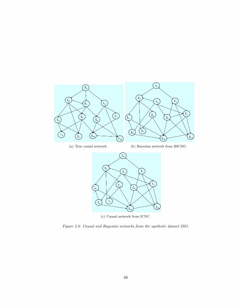
(a) True causal network. (b) Bayesian network from IHCMC.

(c) Causal network from ICNC.

Figure 2.8: Causal and Bayesian networks from the synthetic dataset DS3.

48

network (BN). (The results are shown in a chart form as well as a tabular form.) The

optimal threshold values obtained in the training phase are shown in Table 2.4. In addition,

Figure 2.8 shows the true causal network, the causal network generated by ICNC, and the

Bayesian network generated by IHCMC, given the dataset DS3. (Those for the other

datasets are omitted in the interest of space.)

Figure 2.6 shows that the average relative number of spurious edges in CN is smaller

than that in BN. It is because the ICNC algorithm, through the temporal network, prunes

out all edges whose temporal strengths are below δs1 in the temporal network. Figure 2.7

shows that the average relative number of missing edges in CN is also smaller than that of

BN. This is due to the ICNC algorithm’s ability to add edges even if they do not exist in BN

when they have temporal strengths greater than δs2 in the temporal network. Moreover,

Figures 2.6(b) and 2.7(b) show that the standard deviation in the relative number of spurious

edges and missing edges, respectively, is larger for BN than for CN. It is due to the reduction

in the number of spurious and missing edges in CN by using the temporal information.

These results confirm the important role of the temporal network and the threshold

mechanism to reduce the number of spurious and missing causal relationships.

Real dataset experiment

For the diabetes lab test dataset, the optimal values of δg, δs1 and δs2 are 26, 23 and 78,

respectively. The causal network shown in Figure 2.9(a) is used as the true causal network

against which the causal model is trained to determine the optimum threshold values.

Figures 2.9(b) and 2.9(c) are the causal network and the Bayesian network generated by

ICNC and IHCMC, respectively. Their relative numbers of spurious and missing edges are

compared in Figure 2.10.

The causal network from ICNC has only one spurious relationship (RIDG causes NIDG)

out of the 55 possible spurious relationships. Clearly, there are a higher number of spurious

49

(a) True causal network.

(b) Causal network from ICNC.

(c) Bayesian network from IHCMC.

Figure 2.9: Causal and Bayesian networks from the real dataset.

edges in the Bayesian network from IHCMC – 12 (i.e, 22% of the possible spurious rela-

tionships). It is considered to be due to the fact that the parent of a node in a Bayesian

network may not necessarily be its cause (unlike the causal network where the parent of a

node is always its cause). The lower number of spurious edges in the causal network is due

50

0

0.1

0.2

0.3

0.4

0.5

0.6

0.7

0.8

0.9

1

Spurious Missing Reversed

Rel

ativ

e #

of e

rron

eous

edg

esErroneous edges

CNBN

Figure 2.10: Relative number of erroneous edges in the causal network (CN) and the Bayesiannetwork (BN) for the real dataset.

to the temporal strength threshold δs1 and the gap threshold δg which prune out the edges

with lower temporal strength and narrower gap.

The causal network from the ICNC algorithm has no missing causal relationships out of

the 11 causal relationships, whereas the Bayesian network from the IHCMC algorithm has

one edge (BGMI causes LTUMI) missing. Evidently, the IHCMC algorithm has failed to

identify the causal relationship between BGMI and LTUMI. The ICNC algorithm, on the

other hand, has identified the edge as missing and added it, because the edge has temporal

strength higher than the threshold δs2 in the temporal network.

The target causal network (Figure 2.9(a)), vetted by a physician, encodes the true causal

relationships. We can confirm visually that the causal network from ICNC (Figure 2.9(b))

is an almost exact replica of the true causal network. Note the additional causal strength

and causal direction confidence labeled on each edge. The resultant causal network shows

that NIDG and RIDG respectively cause BGMD. Indeed, it is well known that insulin

decreases the blood glucose level2; this also explains why BGMI causes RIDG. BGMI also

causes LTUMI. Clearly, patients with high blood glucose level are encouraged for less than

usual meal ingestion. In addition, BGMI causes MTEUT, which in turn causes BGMD2UIDG does not show causing BGMD. In fact, Ultralente insulin is not meant to decrease glucose level.

Rather, it provides a baseline level of insulin to support minimum metabolism regardless of ingestion oractivity. So, this makes sense.

51

and MTUMI. It is common knowledge that physical activity burns calories, resulting in a

decreased blood glucose level (BGMD) and stronger appetite (MTUMI). Note, however,

the causal strengths for these two relationships are low, which means MTUET is not a

major cause of BGMD. (RIDG and NIDG are the major causes of BGMD.) In addition,

BGMD is a strong cause of HSE, LTUET and MTUMI. It is a well-known medical fact that

HSE is caused by BGMD and the lower glucose level causes the patients to be prescribed

to take less exercise and heavy meal. In fact, HSE, effect of the decrease in blood glucose

measurement, is the reason for more than usual meal ingestion(MTUMI).

In summary, these synthetic and real dataset experiments confirm that IHCMC alone

is not suitable for building an accurate causal network topology. We observe that ICNC is

far superior to IHCMC at detecting causally related event types correctly. The results show

that the gap threshold and the temporal strength threshold in the ICNC algorithm provides

an effective mechanism to identify and remove spurious relationships or add missing causal

relationships.

2.7.2.2 Comparison of the edge direction of the networks from ICNC and

IHCMC

We compare the causal edge directions of the network structures generated by the ICNC

and IHCMC algorithms.

Synthetic dataset experiment

Figure 2.11 shows that the average relative number of reversed edges in CN is zero for

every dataset. This demonstrates that the ITNC algorithm always detects correct temporal

directions from the event stream when generating the temporal network (TN) and the CN

generated by the ICNC algorithm inherits these correct temporal directions from TN. In

contrast, BN has a higher average relative number of reversed edges for every dataset. In

52

0

0.1

0.2

0.3

0.4

0.5

0.6

0.7

0.8

0.9

1

DS1 DS2 DS3 DS4 DS5

Rel

ativ

e #

of r

ever

sed

edge

s

Dataset

CNBN

(a) Mean relative number of reversed edgesfor each case of dataset.

(b) Mean and Standard deviation of the relativenumber of reversed edges for each case of dataset.

Figure 2.11: Relative number of reversed edges in the causal network (CN) and the Bayesiannetwork (BN) for the synthetic datasets.

addition, the standard deviation of the relative number of reversed edges in BN is particu-

larly larger than those of spurious or missing edges. This is the effect of equivalence classes

in BN construction which typically involves different edge orientations. It confirms that a

Bayesian network cannot be relied upon for the causal direction.

Real dataset experiment

From the causal network and the Bayesian network shown in Figures 2.9(b) and 2.9(c),

we can count the relative number of reversed edges as shown in Figure 2.10. Not surprisingly,

the Bayesian network has a large number (27%) of reversed causal relationships – for ex-

ample, the edges between HSE and BGMD, BGMI and MUTET, and BGMD and LTUET.

On the other hand, the causal network does not have any reversed causal relationship due

to the correct causal direction identified in the temporal network.

Clearly, these synthetic and real dataset experiments confirm that ICNC always gives

correct causal directions, thus confirming the crucial merit of temporal precedence relation-

ships in detecting causality. On the other hand, IHCMC can not be relied upon for the

causal edge direction.

53

Datasets CPU Time (ms) Nw CPU time/window (ms)IHCMC ICNC IHCMC ICNC

DS1 19 22 1 19 22DS2 365 412 2 182.50 206DS3 17790 20081 16 1111.87 1255.06DS4 525268 560536 64 8207.21 8758.37DS5 5899505 6280634 512 11522.47 12266.86DSR 14853 15094 4 3713.25 3773.5

(Nw and DSR are the number of partitioned windows observed and the real dataset, respectively.)

Table 2.5: Running time of IHCMC and ICNC algorithms.

2.7.2.3 Comparison of the running time between ICNC and IHCMC

Table 2.5 shows the CPU time spent on processing the complete event stream and the

average CPU time per window, for the IHCMC and ICNC algorithms. As expected, running

time of the ICNC algorithm is very close to that of the IHCMC algorithm. The running

time of the ICNC algorithm is 15.78%, 12.87%, 12.86%, 6.71%, 6.46%, and 16.23% longer

than that of the IHCMC algorithm in DS1, DS2, DS3, DS4, DS5, and the real dataset,

respectively. This confirms that the IHCMC part consumes most of the running time of the

ICNC algorithm and that the running time overhead of the ITNC part is negligible.

2.8 Related Work

We discuss related work first with respect to the two main approaches used in our work

for causal analysis – dependency-based incremental Bayesian network construction and

precedence-based incremental temporal network construction. Then, we discuss other work

related to causality over data streams and show the uniqueness of our work.

As already mentioned, we use the IHCMC algorithm (Alcobé, 2004b; Alcobé, 2005) for

incremental Bayesian network construction to model the statistical dependencies among

events arriving in a stream. Our study concludes that IHCMC is superior to any other

existing approaches (Buntine, 1991; Friedman and Goldszmidt, 1997; Lam and Bacchus,

54

1994). Buntine’s approach (Buntine, 1991) can construct an alternative Bayesian networks

incrementally given a dataset and a proper ordering of the variables, but is designed to

update the posterior probabilities only, not the network structure itself. Therefore, this

approach is not applicable as we are concerned about learning the network structure and

updating it with an arrival of new batch of events. Lam and Bachhus’s approach (Lam

and Bacchus, 1994) only refines an already existing network under the assumption that

it correctly reflects an accurate model and thus the resulting network is biased toward

the existing network structure. So, this approach is not suitable for event streams as the

network structure needs to be updated as new events arrive. (Friedman and Goldszmidt,

1997) present three approaches which are not appropriate due to the following reasons.

The first approach stores all data items, hence is very memory-inefficient. In contrast, the

second approach (called Maximum A Posteriori probability) stores only one single network

as the summary of past data, and consequently the learning procedure for new data is

biased towards it. The third approach balances between the two, that is, it sacrifices the

quality of the constructed network for the reduction in required memory space. Alcobé

in his work (Alcobé, 2004b; Alcobé, 2005; Alcobé, 2004a) has converted four well known

batch-mode Bayesian network construction algorithms (i.e., CL, K2, B and HCMC) to their

incremental versions(i.e., ICL, IK2, IB and IHCMC, respectively). Among these, IHCMC

performs the most exhaustive search and yields a Bayesian network of the highest quality

within a reasonable time (Alcobé, 2004b).

There is rich literature about temporal modeling or reasoning based on temporal prece-

dence (Glüge et al., 2010; Hamilton and Karimi, 2005; Holme and Saramäki, 2011; Krishna

et al., 2010; Liu et al., 2010). The most relevant to our project are TIMERS II algorithm by

(Hamilton and Karimi, 2005) and temporal causal graph construction by (Liu et al., 2010),

as both propose to use temporal information towards causal analysis. However, neither aims

at constructing a causal network as proposed in our work. Specifically, TIMERS II (Hamil-

55

ton and Karimi, 2005) classifies the relationship between decision attribute and condition

attributes into instantaneous, causal, or acausal based on temporal information, but it does

not build a causal network and only uses simple temporal conditions and decision tree

to determine the nature of causal relationship. The temporal causal graph in Liu et al.’s

work (Liu et al., 2010) uses the Granger causality (Granger, 1969), the well known approach

for determining causal relationships in a time series data. Given two variables, say X and

Y , Granger causality determines that X is a cause of Y if the past value of X can be used

(via regression) to predict the future value of Y . This notion of causality is very different

from what is proposed in our work in that ours is based on the frequency of the occurrences

of the variable values, not the values themselves, and that each variable in our work can

represent any event type, not only a time series variable.

The only existing work we find on causal relationships over data streams is by (Kwon and

Li, 2009). It is about using temporal, spatial, and spatio-temporal relationships between

cause and effect to perform causality join query processing on sensor streams. Similarly,

there has been recent work by (Meliou et al., 2010) to support causal query processing in

databases. However, none of these works addresses causal modeling at all. To the best

of our knowledge, there has been no previous work done for causal network modeling by

constructing a causal network in a dynamic environment (over event streams). On the

other hand, there exists a significant amount of research done on causal analysis in a static

environment (Borchani et al., 2007; Ellis and Wong, 2008; Heckerman, 1995; Li and Leong,

2009; Meganck et al., 2006). Semantically, the work by (Ishii et al., 2010) is closer to the

work we are proposing. Their incremental approach is to extract causality for news articles

and documents. They employ a lexical approach by comparing subject-verb-object (SVO)

tuples for causality detection using natural language processing for each news item. Thus,

their work does not infer causality from the observations of the overall data which we are

doing in this paper. Our focus is on causality inference over event stream. Besides, it is

56

not useful in event streams where the lexical approach is not a viable option and the causal

relationships need to be inferred from the observation of unbounded events.

2.9 Conclusion and Future Work

In this paper, we focused on the problem of constructing a causal network over continu-

ous event streams incrementally. We proposed a two layered causal network model and

presented an algorithm izing temporal precedence relationships and statistical dependency

between events in combination. For the temporal precedence relationships, we presented

a temporal network model and the temporal network construction algorithm. Then, we

combined it with an existing incremental Bayesian network construction algorithm to pro-

pose the incremental causal network constructing algorithm, and then through experiments

demonstrated that the proposed approach increases the accuracy of causality detection

significantly.

In this paper, we assumed the events in a stream are in temporal order. For the future

work, we plan to consider the out-of-order event stream which may introduce reversed

edges in the temporal network, thereby reducing the reliability of the temporal network.

Another interesting direction for the future work is the inclusion of predictive causal query

processing. There are applications which can benefit from predicting upcoming events based

on the history of prior events.

2.10 Acknowledgments

We thank Joseph Roure Alcobé for providing the initial code base for the IHCMC algorithm

and Benjamin Littenberg for his comments on the causal network from the diabetes lab test

result data set.

57

Bibliography

Acharya, S. and Lee, B. (2013). Fast causal network inference over event streams. In Data

Warehousing and Knowledge Discovery, volume 8057 of Lecture Notes in Computer

Science, pages 222–235. Springer Berlin Heidelberg.

Acharya, S. and Lee, B. S. (2014a). Enchanced fast causal network inference over event

streams. Transactions on Large Scale Data and Knowledge Centered Systems.

Acharya, S. and Lee, B. S. (2014b). Incremental causal network construction over event

streams. Information Sciences, 261(0):32 – 51.

Acharya, S., Lee, B. S., and Hines, P. (2014). Real-time top-k predictive query processing

over event streams. Information Sciences.

Akdere, M., Çetintemel, U., and Upfal, E. (2010). Database-support for continuous pre-

diction queries over streaming data. Proc. VLDB Endow., 3(1-2):1291–1301.

Alcobé, J. R. (2004a). Incremental hill-climbing search applied to Bayesian network

structure learning. In First International Workshop on Knowledge Discovery in Data

Streams, 2004.

Alcobé, J. R. (2004b). Incremental Methods for Bayesian Network Structure Learning.

PhD thesis, Department of Computer Science, Universitat Politècnica de Catalunya.

Alcobé, J. R. (2005). Incremental methods for Bayesian network structure learning. Ar-

tificial Intelligence Communications, 18(1):61–62.

58

Barber, D. (2012). Bayesian Reasoning and Machine Learning. Cambridge University

Press.

Barga, R. S., Goldstein, J., Ali, M. H., and Hong, M. (2007). Consistent streaming

through time: A vision for event stream processing. In Proceedings of the Third Bi-

ennial Conference on Innovative Data Systems Research, CIDR’07, pages 363–374.

Bishop, Y. M., Fienberg, S. E., and Holland, P. W. (1975). Discrete Multivariate Analysis:

Theory and Practice. MIT Press.

Borchani, H., Chaouachi, M., and Ben Amor, N. (2007). Learning causal bayesian net-

works from incomplete observational data and interventions. In Proceedings of the 9th

European Conference on Symbolic and Quantitative Approaches to Reasoning with

Uncertainty, ECSQARU ’07, pages 17–29, Berlin, Heidelberg. Springer-Verlag.

Bowes, J., Neufeld, E., Greer, J., and Cooke, J. (2000). A comparison of association rule

discovery and bayesian network causal inference algorithms to discover relationships in

discrete data. In Hamilton, H., editor, Advances in Artificial Intelligence, volume 1822

of Lecture Notes in Computer Science, pages 326–336. Springer Berlin Heidelberg.

Buntine, W. (1991). Theory refinement on Bayesian networks. In Proceedings of the sev-

enth conference (1991) on Uncertainty in artificial intelligence, pages 52–60, San

Francisco, CA, USA. Morgan Kaufmann Publishers Inc.

Chandra, P. and Kshemkalyani, A. D. (2005). Causality-based predicate detection across

space and time. IEEE Transactions on Computerts, 54:1438–1453.

Cheng, J. and Druzdzel, M. J. (2000). Ais-bn: An adaptive importance sampling algo-

rithm for evidential reasoning in large Bayesian networks. J. Artif. Intell. Res. (JAIR),

13:155–188.

Cheng, J. and Druzdzel, M. J. (2001). Confidence inference in Bayesian networks. In

Proceedings of the Seventeenth conference on Uncertainty in artificial intelligence,

59

UAI’01, pages 75–82, San Francisco, CA, USA. Morgan Kaufmann Publishers Inc.

Cheng, J., Greiner, R., Kelly, J., Bell, D., and Liu, W. (2002). Learning Bayesian networks

from data: an information-theory based approach. Artificial Intelligence, 137(1-2):43–

90.

Chickering, D. M. (2002). Learning equivalence classes of Bayesian-network structures.

Journal of Machine Learning Research, 2:445–498.

Chickering, D. M., Heckerman, D., and Meek, C. (2004). Large-sample learning of

bayesian networks is np-hard. J. Mach. Learn. Res., 5:1287–1330.

Chow, Y. S. and Teicher, H. (1978). Probability theory : independence, interchangeability,

martingales. Springer-Verlag, New York.

de Campos, L. M. (2006). A scoring function for learning Bayesian networks based on mu-

tual information and conditional independence tests. J. Machine Learning Research,

7:2149–2187.

Ellis, B. and Wong, W. H. (2008). Learning causal Bayesian network structures from

experimental data. Journal of the American Statistical Association, 103(482):778–789.

Elloumi, M. and Zomaya, A. Y. (2013). Biological Knowledge Discovery Handbook: Pre-

processing, Mining and Postprocessing of Biological Data, volume 23. John Wiley &

Sons.

Eppstein, M. and Hines, P. (2012). A "Random Chemistry" algorithm for identifying

collections of multiple contingencies that initiate cascading failure. IEEE Transactions

on Power Systems, 27(3):1698–1705.

Frank, A. and Asuncion, A. (2010). UCI machine learning repository.

Friedman, N. and Goldszmidt, M. (1997). Sequential update of bayesian network struc-

ture. In Proceedings of the Thirteenth conference on Uncertainty in artificial intelli-

60

gence, UAI’97, pages 165–174, San Francisco, CA, USA. Morgan Kaufmann Publish-

ers Inc.

Friedman, N., Linial, M., Nachman, I., and Pe’er, D. (2000). Using Bayesian networks to

analyze expression data. In Proceedings of the Fourth Annual International Conference

on Computational Molecular Biology, RECOMB ’00, pages 127–135, New York, NY,

USA. ACM.

Geiger, D. and Pearl, J. (1988). On the logic of causal models. In Proceedings of the

Fourth Annual Conference on Uncertainty in Artificial Intelligence, UAI ’88, pages

3–14.

Glüge, S., Hamid, O. H., and Wendemuth, A. (2010). A simple recurrent network for

implicit learning of temporal sequences. Cognitive Computation, 2(4):265–271.

Glymour, C. (2003). Learning, prediction and causal Bayes nets. Trends in cognitive

sciences, 7(1):43–48.

Granger, C. W. J. (1969). Investigating Causal Relations by Econometric Models and

Cross-spectral Methods. Econometrica, 37(3):424–438.

Guyon, I., Aliferis, C. F., Cooper, G. F., Elisseeff, A., Pellet, J.-P., Spirtes, P., and

Statnikov, A. R. (2008). Design and analysis of the causation and prediction challenge.

In IEEE World Congress on Computational Intelligence Causation and Prediction

Challenge, pages 1–33.

Hamilton, H. J. and Karimi, K. (2005). The timers ii algorithm for the discovery of

causality. In Proceedings of the 9th Pacific-Asia conference on Advances in Knowledge

Discovery and Data Mining, PAKDD’05, pages 744–750, Berlin, Heidelberg. Springer-

Verlag.

Heckerman, D. (1995). A Bayesian approach to learning causal networks. In Proceedings

of the Eleventh conference on Uncertainty in artificial intelligence, UAI’95, pages

61

285–295, San Francisco, CA, USA. Morgan Kaufmann Publishers Inc.

Heckerman, D. (1999). UCI machine learning repository

[http://archive.ics.uci.edu/ml/datasets/msnbc.com+

anonymous+web+data].

Henrion, M. (1991). Search-based methods to bound diagnostic probabilities in very large

belief nets. In Proceedings of the Seventh conference on Uncertainty in Artificial In-

telligence, UAI’91, pages 142–150, San Francisco, CA, USA. Morgan Kaufmann Pub-

lishers Inc.

Holme, P. and Saramäki, J. (2011). Temporal networks. CoRR, abs/1108.1780.

Ishii, H., Ma, Q., and Yoshikawa, M. (2010). An incremental method for causal network

construction. In Proceedings of the 11th international conference on Web-age infor-

mation management, WAIM’10, pages 495–506, Berlin, Heidelberg. Springer-Verlag.

Jiang, X.-R. and Gruenwald, L. (2005). Microarray gene expression data association rules

mining based on BSC-tree and FIS-tree. Data & Knowledge Engineering, 53(1):3 –

29.

Johnson, T., Muthukrishnan, S., and Rozenbaum, I. (2007). Monitoring regular expres-

sions on out-of-order streams. In Proceedings of the IEEE 23rd International Confer-

ence on Data Engineering, ICDE’07, pages 1315–1319.

Kemeny, J. and Snell, J. (1969). Finite Markov chains. University series in undergraduate

mathematics. VanNostrand, New York, repr edition.

Kirkpatrick, S., Gelatt, C. D., and Vecchi, M. P. (1983). Optimization by simulated

annealing. Science, 220:671–680.

Kłopotek, M. A. (2006). Cyclic Bayesian network–Markov process approach. Studia In-

formatica, 1(2):7.

62

Krishna, R., Li, C.-T., and Buchanan-Wollaston, V. (2010). A temporal precedence based

clustering method for gene expression microarray data. BMC Bioinformatics, 11:68.

Kullback, S. (1968). Information Theory and Statistics. Dover Publication, 2nd edition.

Kwon, O. and Li, K.-J. (2009). Causality join query processing for data streams via a

spatiotemporal sliding window. Journal of Universal Computer Science, 15(12):2287–

2310.

Lam, W. and Bacchus, F. (1994). Using new data to refine a Bayesian network. In Pro-

ceedings of the Tenth international conference on Uncertainty in artificial intelligence,

UAI’94, pages 383–390, San Francisco, CA, USA. Morgan Kaufmann Publishers Inc.

Li, G. and Leong, T.-Y. (2009). Active learning for causal bayesian network structure

with non-symmetrical entropy. In Proceedings of the 13th Pacific-Asia Conference on

Advances in Knowledge Discovery and Data Mining, PAKDD ’09, pages 290–301,

Berlin, Heidelberg. Springer-Verlag.

Li, J., Tufte, K., Shkapenyuk, V., Papadimos, V., Johnson, T., and Maier, D. (2008).

Out-of-order processing: A new architecture for high-performance stream systems.

Proceegins of the VLDB Endowment, 1(1):274–288.

Li, M., Liu, M., Ding, L., Rundensteiner, E. A., and Mani, M. (2007). Event stream

processing with out-of-order data arrival. In Proceedings of the 27th International

Conference on Distributed Computing Systems Workshops, ICDCSW ’07, pages 67–

74, Washington, DC, USA. IEEE Computer Society.

Lin, T. Y., Xie, Y., Wasilewska, A., and Liau, C.-J., editors (2008). Data Mining: Foun-

dations and Practice, volume 118 of Studies in Computational Intelligence. Springer.

Liu, M., Li, M., Golovnya, D., Rundensteiner, E., and Claypool, K. (2009). Sequence

pattern query processing over out-of-order event streams. In Proceedings of the IEEE

25th International Conference on Data Engineering, ICDE ’09, pages 784–795.

63

Liu, Y., Niculescu-Mizil, A., Lozano, A. C., and Lu, Y. (2010). Learning temporal causal

graphs for relational time-series analysis. In ICML, pages 687–694. Omnipress.

MacKay, D. J. C. (1999). Introduction to Monte Carlo methods. In Learning in graphical

models, pages 175–204. MIT Press, Cambridge, MA, USA.

Mani, S., Aliferis, C. F., and Statnikov, A. R. (2010). Bayesian algorithms for causal data

mining. Journal of Machine Learning Research, 6:121–136.

Mazlack, L. J. (2004). Mining causality from imperfect data. In Proceedings of the sixth

International FLINS Conference on Applied Computational Intelligence Proceedings,

Applied Computational Intelligence, pages 155–160.

Meek, C. (1995). Causal inference and causal explanation with background knowledge.

In Proceedings of the Eleventh Conference Annual Conference on Uncertainty in Ar-

tificial Intelligence (UAI-95), pages 403–410, San Francisco, CA. Morgan Kaufmann.

Meganck, S., Leray, P., and Manderick, B. (2006). Learning causal bayesian networks

from observations and experiments: a decision theoretic approach. In Proceedings of

the Third international conference on Modeling Decisions for Artificial Intelligence,

MDAI’06, pages 58–69, Berlin, Heidelberg. Springer-Verlag.

Meliou, A., Gatterbauer, W., Moore, K. F., and Suciu, D. (2010). Why so? or why no?

functional causality for explaining query answers. In MUD, 2010, pages 3–17.

Mohammad, Y. and Nishida, T. (2010). Mining causal relationships in multidimensional

time series. In Szczerbicki, E. and Nguyen, N., editors, Smart Information and Knowl-

edge Management, volume 260 of Studies in Computational Intelligence, pages 309–

338. Springer Berlin Heidelberg.

Moral, P., Doucet, A., and Jasra, A. (2012). An adaptive sequential Monte Carlo method

for approximate Bayesian computation. Statistics and Computing, 22:1009–1020.

Pearl, J. (1995). Causal diagrams for empirical research. Biometrika, 82:669–710.

64

Pearl, J. (1998). Graphs, causality, and structural equation models. Sociological Methods

and Research, 27:226–84.

Pearl, J. (2009). Causality: Models, Reasoning and Inference. Cambridge University

Press, New York, NY, USA, second edition edition.

Pearl, J. and Verma, T. (1991). A theory of inferred causation. In KR, 1991, pages

441–452.

Popper, K. (1959). The Logic of Scientific Discovery. Routledge Classics.

Prakasa Rao, B. (2009). Conditional independence, conditional mixing and conditional

association. Annals of the Institute of Statistical Mathematics, 61(2):441–460.

Rottman, B. M. and Hastie, R. (2014). Reasoning about causal relationships: Inferences

on causal networks. Psychological Bulletin, 140(1):109–139.

Rudin, C., Letham, B., Salleb-Aouissi, A., Kogan, E., and Madigan, D. (2011). Sequential

event prediction with association rules. In Proceedings of the 24th Annual Conference

on Learning Theory, COLT ’11, pages 615–634.

Shachter, R. D. (1990). Evidence absorption and propagation through evidence reversals.

In Proceedings of the Fifth Annual Conference on Uncertainty in Artificial Intelligence,

UAI ’89, pages 173–190, Amsterdam, The Netherlands.

Silverstein, C., Brin, S., Motwani, R., and Ullman, J. (2000). Scalable techniques for

mining causal structures. Data Mining and Knowledge Discovery, 4(2-3):163–192.

Spirtes, P., Glymour, C., and Scheines, R. (1993). Causation, Prediction, and Search.

Ima Volumes in Mathematics and Its Applications. Springer-Verlag.

Spirtes, P., Glymour, C., and Scheines, R. (2000). Causation, Prediction, and Search.

MIT Press.

Spirtes, P., Glymour, C. N., and Scheines, R. (1990). Causality from probability. In

Proceedings of the Conference on Advanced Computing for the Social Sciences, ACSS

65

’90.

Spirtes, P. and Meek, C. (1995). Learning Bayesian networks with discrete variables from

data. In Proceedings of the First International Conference on Knowledge Discovery

and Data Mining, KDD’95, pages 294–299.

Tsamardinos, I., Brown, L. E., and Aliferis, C. F. (2006). The max-min hill-climbing

bayesian network structure learning algorithm. Mach. Learn., 65(1):31–78.

Tulupyev, A. L. and Nikolenko, S. I. (2005). Directed cycles in Bayesian belief networks:

probabilistic semantics and consistency checking complexity. In Proceedings of the 4th

Mexican international conference on Advances in Artificial Intelligence, pages 214–

223. Springer.

US-Canada Power System Outage Task Force (2004). Final Report on the August 14,

2003 Blackout in the United States and Canada. Technical report.

Utrera, A. C., Olmedo, M. G., and Callejon, S. M. (2008). A score based ranking of the

edges for the pc algorithm. In Proceedings of the 4th European workshop on proba-

bilistic graphical models, PGM’08, pages 41 – 48.

Vaiman, M., Bell, K., Chen, Y., Chowdhury, B., Dobson, I., Hines, P., Papic, M., Miller,

S., and Zhang, P. (2012). Risk assessment of cascading outages: Methodologies and

challenges. IEEE Transactions on Power Systems, 27(2):631–641.

Veloso, A. A., Almeida, H. M., Gonçalves, M. A., and Meira Jr., W. (2008). Learning

to rank at query-time using association rules. In Proceedings of the 31st Annual In-

ternational ACM SIGIR Conference on Research and Development in Information

Retrieval, SIGIR ’08, pages 267–274, New York, NY, USA. ACM.

Verma, T. and Pearl, J. (1988). Causal networks: Semantics and expressiveness. In Pro-

ceedings of the Fourth Annual Conference on Uncertainty in Artificial Intelligence,

UAI ’88, pages 69–78.

66

Wang, K. and Yu, Y. (2013). A query-matching mechanism over out-of-order event stream

in iot. Int. J. Ad Hoc Ubiquitous Comput., 13(3/4):197–208.

Young, S. S. and Karr, A. (2011). Deming, data and observational studies. Significance,

8(3):116–120.

Zhang, N. L. and Poole, D. (1996). Exploiting causal independence in Bayesian network

inference. J. Artif. Int. Res., 5(1):301–328.

Zhang.N.L. and D., P. (1994). A simple approach to Bayesian network computations. In

Proceedings of the Tenth Canadian Conference on Artificial Intelligence, CCAA ’94,

pages 171–178.

Zhao, Y. and Strom, R. (2001). Exploitng event stream interpretation in publish-subscribe

systems. In Proceedings of the Twentieth Annual ACM Symposium on Principles of

Distributed Computing, PODC ’01, pages 219–228.

67

Chapter 3

Fast Causal Network Inference over Event

Streams

Abstract

This paper addresses causal inference and modeling over event streams where data have

high throughput and are unbounded. The availability of large amount of data along with

the high data throughput present several new challenges related to causal modeling, such

as the need for fast causal inference operations while ensuring consistent and valid results.

There is no existing work specifically for such a streaming environment. We meet the

challenges by introducing a time-centric causal inference strategy that leverages temporal

precedence information to decrease the number of conditional independence tests required

to establish the dependencies between the variables in a causal network. Dependency and

temporal precedence of cause over effect are the two properties of a causal relationship. We

also present the Temporal Network Inference algorithm to model the temporal precedence

relations into a temporal network. Then, we propose the Fast Causal Network Inference

algorithm for faster learning of causal network using the temporal network. Experiments

using synthetic and real datasets demonstrate the efficacy of the proposed algorithms.

68

3.1 Introduction

In recent years, there has been a growing need for active systems that can perform causal

inference in diverse applications such as health care, stock markets, user activity monitor-

ing, smart electric grids, and network intrusion detection. These applications need to infer

the cause of abnormal activities immediately such that informed and timely preventive mea-

sures are taken. As a case in point, consider a smart electric grid monitoring application.

The failure of a component can cause cascading failures, effectively causing a massive black-

out. Therefore, the identification of such cause and effect components in a timely manner

enables preventive measures in the case of failure of a cause component, thereby preventing

blackouts.

Causal network, a directed acyclic graph where the parent of each node is its direct

cause, has been popularly used to model causality (Heckerman, 1995; Ellis and Wong, 2008;

Li and Leong, 2009; Meganck et al., 2006; Pearl, 2009; Spirtes et al., 1990; Spirtes et al.,

2000). There are two distinct types of algorithms for learning a causal network: score-

based (Heckerman, 1995; Ellis and Wong, 2008; Li and Leong, 2009; Meganck et al., 2006)

and constraint-based (Pearl, 2009; Spirtes et al., 1990; Spirtes et al., 2000; Cheng et al.,

2002). Both types of algorithms are slow and, therefore, not suitable for event streams

where prompt causal inference is required. Score-based algorithms perform a greedy search

(usually hill climbing) to select a causal network with the highest score from a large number

of possible networks. With an increase in the number of variables in the dataset, the number

of possible networks grows exponentially, resulting in slow causal network inference. On the

other hand, constraint-based algorithms (e.g., PC algorithm (Spirtes et al., 2000)) discover

the causal structure via a large number of tests on conditional independence(CI). There can

be no edge between two conditionally independent variables in the causal network (Pearl,

1995). In a causal network of n variables, two variables X and Y are said to be conditionally

69

independent given a condition set S if there is at least one variable in S such that X and

Y are independent. The condition set S consists of all possible 2n−2 combinations of the

remaining n− 2 variables, and therefore the computational complexity grows exponentially

as the number of variables increases. So, the current techniques for causal inference are

slow and not suitable for event streams which have a high data throughput and where the

number of variables (i.e., event types) is large.

With this concern, this paper describes a new time-centric causal modeling approach to

speed up the causal network inference. Every causal relationship implies temporal prece-

dence relationship (Popper, 1959). So, the idea is to incorporate temporal precedence

information as an important clue to reducing the number of required CI tests and thus

maintaining feasible computational complexity. This idea achieves fewer computations of

CI test due to two factors. First, since causality requires temporal precedence, we ignore

the causality test for those nodes with no temporal precedence relationship between them.

Second, in the CI test of an edge, we exclude those nodes from the condition set which

do not have temporal precedence relationship with the nodes of the edge. Therefore, it re-

duces the size of the condition set which is a major cause of the exponential computational

complexity. In addition, the temporal precedence relationship intuitively orients the causal

edge unlike the constraint-based algorithms where a separate set of rules are needed to infer

the causal direction (details in Section 3.3.3).

The contributions of this paper are summarized as follows. First, it presents a temporal

network structure to represent temporal precedence relationships between event types and

proposes an algorithm, Temporal Network Inference(TNI), to construct a temporal network

applicable in streaming environment. Second, it introduces a time-centric causal modeling

strategy and proposes an algorithm, Fast Causal Network Inference(FCNI), to speed up

the learning of causal network. Finally, it empirically demonstrates the advantages of the

proposed algorithm in terms of the running time and the total number of CI tests required

70

for the learning of causal network by comparing it against the state-of-art algorithm for

causal network inference, called the PC algorithm (details in Section 3.3.3).

The rest of this paper is organized as follows. Section 3.2 reviews the existing work

on causal network inference. Section 3.3 presents the basic concepts used in the paper.

Section 3.4 and Section 3.5 propose the learning of temporal network and faster causal net-

work, respectively. Section 3.6 evaluates the proposed FNCI algorithm. Finally, Section 3.7

concludes the paper and mentions further research.

3.2 Related Work

As explained earlier, there are two main approaches for causal network inference.

The first approach, score-based (Heckerman, 1995; Ellis and Wong, 2008; Li and Leong,

2009; Meganck et al., 2006), performs greedy search (usually hill climbing) over all possible

network structures in order to find the network that best represents the data based on

the highest score. This approach, however, has two problems. First, it is slow due to the

exhaustive search for the best network structure. An increase in the number of variables in

the dataset increases the computational complexity exponentially. Second, two or more net-

work structures, called the equivalence classes (Chickering, 2002), may represent the same

probability distribution, and consequently the causal directions between nodes are quite

random. There is no technique for alleviating these problems in a streaming environment.

Thus, score-based algorithms are not viable for streams.

The second approach, constraint-based (Pearl, 2009; Spirtes et al., 1990; Spirtes et al.,

2000; Cheng et al., 2002), does not have the problem of equivalence classes. However, it is

slow as it starts with a completely connected undirected graph and thus performs a large

number of CI tests to remove the edges between conditionally independent nodes. The

number of CI tests increases exponentially with the increase in the number of variables

in the dataset. To alleviate this problem, some constraint-based algorithms start with

71

a minimum spanning tree to reduce the initial size of condition sets. However, this idea

trades the speed with the accuracy of the causal inference. The constraint-based algorithms

include IC* (Pearl, 2009), SGS (Spirtes et al., 1990), PC (Spirtes et al., 2000), and FCI

algorithm (Spirtes et al., 2000). The FCI algorithm focuses on the causal network discovery

from the dataset with latent variables and selection bias, which is quite different from

the scope of this paper. The PC algorithm is computationally more efficient than IC* and

SGS. This is why we evaluate the proposed FCNI algorithm by comparing it against the PC

algorithm. Like the others, the PC algorithm starts with a completely connected undirected

graph. To reduce the computational complexity, it performs CI tests in several steps. Each

step produces a sparser graph than the earlier step, and consequently, the condition set

decreases in the next step. However, the computational complexity is still O(n2 ·2n−2). (The

details are explained in Section 3.3.3.) Therefore, the current constraint-based algorithms

are not suitable for fast causal inference over streams.

To the best of our knowledge, there exists no specific work in the causal network inference

in a streaming environment. A new approach is needed for faster causal network inference.

3.3 Basic Concepts

This section presents some key concepts needed to understand the paper.

3.3.1 Event streams, type, and instance

An event stream in our work is a sequence of continuous and unbounded timestamped

events. An event refers to any action that has an effect and is created by one event owner.

One event can trigger another event in chain reactions. Each event instance belongs to

one and only one event type which is a prototype for creating the instances. Two event

instances are related to each other if they share common attributes such as event owner,

72

location, and time. We call these attributes common relational attributes(CRAs).

In this paper we denote an event type as Ej and an event instance as eij , where i

indicates the CRA and j indicates the event type.

Example 2 Consider a diabetic patient monitoring system in a hospital. Each patient is

uniquely identifiable, and each clinical test or measurement of each patient makes one event

instance. For example, a patient is admitted to the hospital, has their blood pressure and glu-

cose level measured, and takes medication over a period of time. This creates the instances

of the above event types as a result. Typical event types from these actions include regular-

insulin-dose-given, hypoglycemic-symptoms-exists, blood-glucose-measurement-decreased, in-

creased, etc. Note that the patient ID is the CRA, as the events of the same patient are

causally related.

3.3.2 Conditional Mutual Information

A popular approach for testing the conditional independence, with respect to the joint

probability P , of two random variables X and Y given a subset of random variables S is

conditional mutual information(CMI) (Cheng et al., 2002; de Campos, 2006). CMI gives the

strength of dependency between variables in a measurable quantity, which helps to identify

strong and weak causal relationships in the final causal network.

To test whether X and Y are conditionally independent given S, we compute the con-

ditional mutual information IMI(X,Y |S) as

IMI(X,Y |S) =∑x∈X

∑y∈Y

∑s∈S

pX,Y,S(x, y, s)log2pX,Y |S(x, y|s)

pX|S(x|s)pY |S(y|s)

where p is the probability mass function calculated from the frequencies of variables.

We only keep the record of these frequencies, not the whole events, by updating them as

a new batch of events arrives. Consequently, the independence test procedure is incremental

73

in our case.

It is said that two variables X and Y are independent when IMI(X,Y |S) = 0; other-

wise, they are dependent. However, this presents us with the risk of spurious relationships

due to weak dependencies (we cannot assume IMI(X,Y |S) = 10−5 and IMI(X,Y |S) = 10

provide the same degree of confidence in the dependency). With an increase in the value

of IMI(X,Y |S), the dependency between the variables X and Y grows stronger. Therefore,

to prune out the weak dependencies, we need to set a threshold value of mutual informa-

tion below which we ignore the evidence as weak. To do so, we relate CMI with G2 test

statistics (Spirtes et al., 2000; Bishop et al., 1975) as below where Ns is the number of

samples.

G2(X,Y |S) = 2 ·Ns · loge2 · IMI(X,Y |S)

Under the independence assumption, G2 follows the χ2 distribution (Kullback, 1968), with

the degree of freedom df equal to (rx − 1)(ry − 1)∏s∈S rs, where rx, ry, and rs are the

number of possible distinct values of X, Y, and S, respectively. So, we use χ2 test, which

provides a threshold based on df and significance level α, to validate the dependency result.

We set α as the universally accepted value of 95%.

3.3.3 The PC algorithm

The PC algorithm (Spirtes et al., 2000) (Algorithm 6) starts with a completely connected

undirected graph on which the CI tests are performed to remove edges between independent

nodes. The key idea is that a causal network has an edge between X and Y in the topology

if and only if X and Y are not independent given all condition subsets of the remaining

neighbor nodes (Spirtes and Meek, 1995). In Algorithm 6, the topology of the causal

network is learned in the steps 1 to 10. The network topology is then assigned causal

direction in the steps 11 to 17.

74

Algorithm 6 PC algorithm1: Construct the completely connected undirected graph G on the n nodes;2: Initialize Neighbors(G,X) as the set of nodes adjacent to the node X in G, and

SepSet(X,Y), a set of nodes that causes independence between X and Y nodes, as empty;

3: k ← 0;4: repeat5: repeat6: Select any edge X − Y such that |Neighbors(G,X)\Y | ≥ k;7: repeat8: Select any subset S of Neighbors(G,X)\Y such that |Neighbors(G,X)\Y | = k;

9: If X and Y are independent given S, remove X − Y from G, remove Y fromNeighbors(G,X), remove X from Neighbors(G,Y), and add S to SepSet(X,Y) andSepSet(Y,X);

10: until every subset S of Neighbors(G,X)\Y such that |Neighbors(G,X)\Y | = khas been selected.

11: until every edge X − Y such that |Neighbors(G,X)\Y | ≥ k has been selected.12: k = k + 1;13: until every edge X ′ − Y ′ satisfies |Neighbors(G,X ′)\Y ′| < k.14: for each triplet of nodes X, Y, Z such that the edges X − Y and Y −X exist in G but

not X − Z do15: Orient X − Y − Z as X→Y←Z if and only if SepSet(X,Z) does not contain Y;16: end for17: repeat18: If there exists X → Y and Y − Z, but not X − Z, then orient Y − Z as Y → Z;19: If there exists X−Y and a directed path from X to Y, then orient X−Y as X → Y ;20: until no edge can be oriented.

3.4 Learning Temporal Precedence Relationships

In this section, we describe an incremental approach to model temporal precedence rela-

tionships from time-stamped events into a temporal network.

3.4.1 Temporal Network Model

A temporal network is a directed acyclic graph of nodes representing event types where an

edge between two nodes represents the temporal precedence relationship between them. To

75

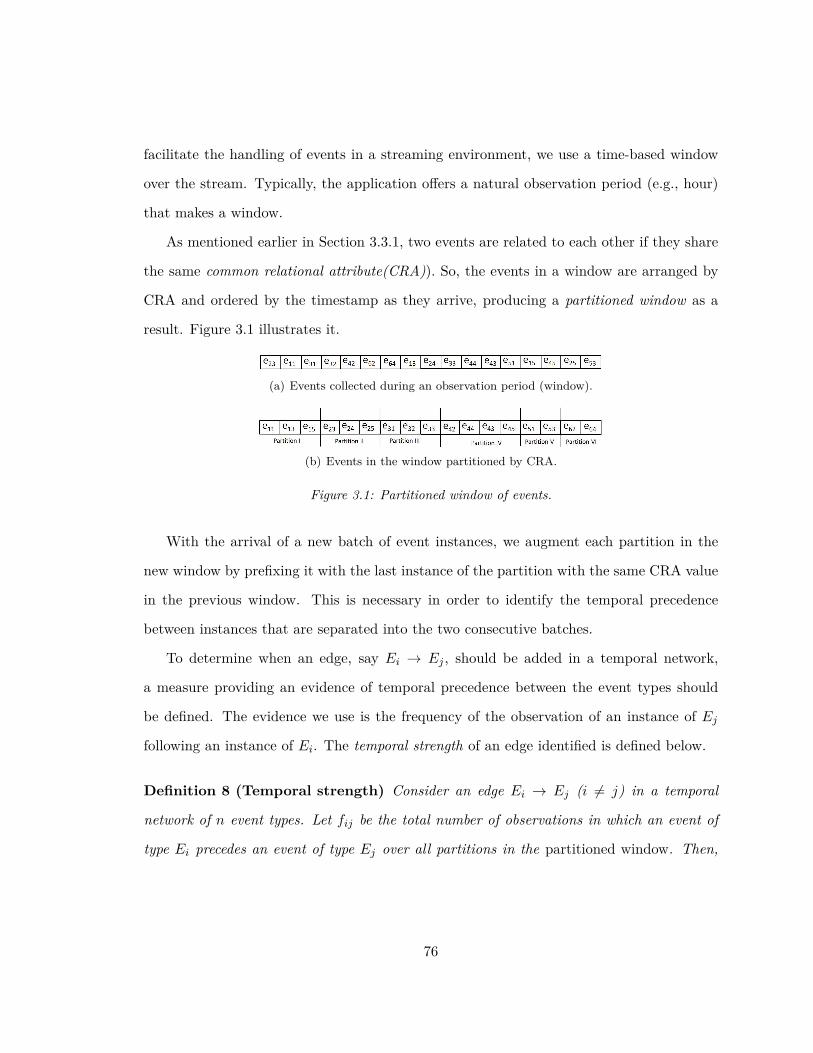
facilitate the handling of events in a streaming environment, we use a time-based window

over the stream. Typically, the application offers a natural observation period (e.g., hour)

that makes a window.

As mentioned earlier in Section 3.3.1, two events are related to each other if they share

the same common relational attribute(CRA)). So, the events in a window are arranged by

CRA and ordered by the timestamp as they arrive, producing a partitioned window as a

result. Figure 3.1 illustrates it.

(a) Events collected during an observation period (window).

(b) Events in the window partitioned by CRA.

Figure 3.1: Partitioned window of events.

With the arrival of a new batch of event instances, we augment each partition in the

new window by prefixing it with the last instance of the partition with the same CRA value

in the previous window. This is necessary in order to identify the temporal precedence

between instances that are separated into the two consecutive batches.

To determine when an edge, say Ei → Ej , should be added in a temporal network,

a measure providing an evidence of temporal precedence between the event types should

be defined. The evidence we use is the frequency of the observation of an instance of Ej

following an instance of Ei. The temporal strength of an edge identified is defined below.

Definition 8 (Temporal strength) Consider an edge Ei → Ej (i 6= j) in a temporal

network of n event types. Let fij be the total number of observations in which an event of

type Ei precedes an event of type Ej over all partitions in the partitioned window. Then,

76

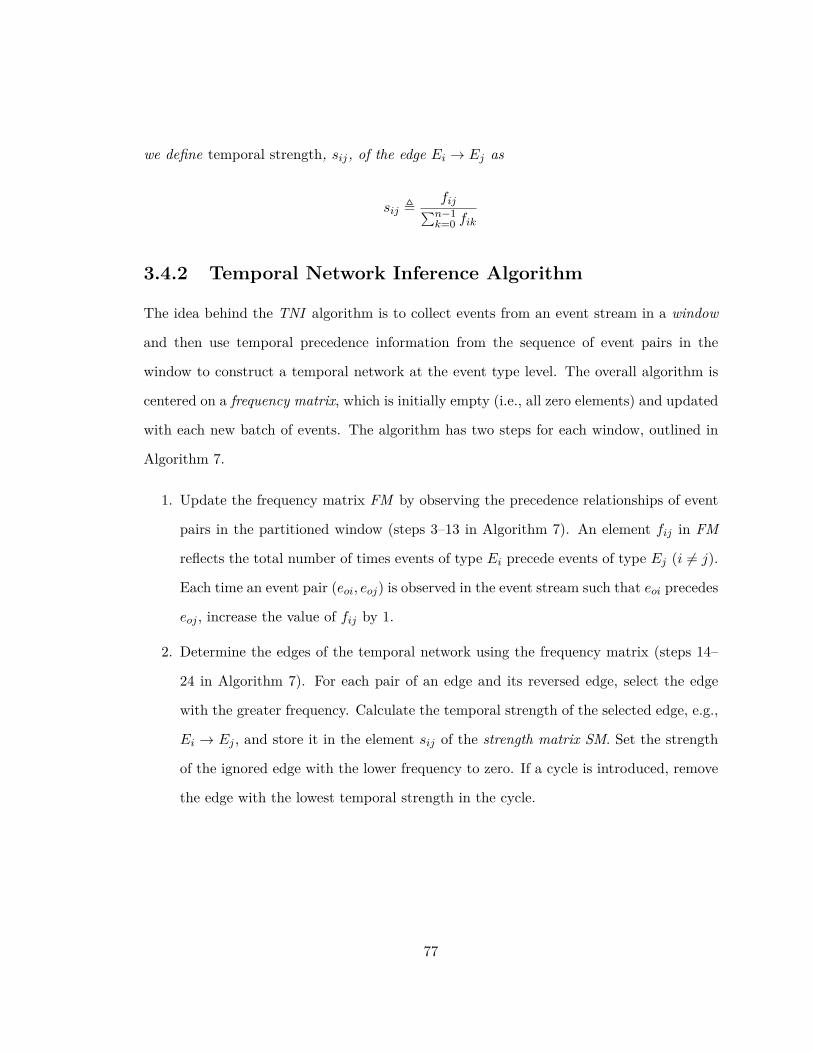
we define temporal strength, sij, of the edge Ei → Ej as

sij ,fij∑n−1k=0 fik

3.4.2 Temporal Network Inference Algorithm

The idea behind the TNI algorithm is to collect events from an event stream in a window

and then use temporal precedence information from the sequence of event pairs in the

window to construct a temporal network at the event type level. The overall algorithm is

centered on a frequency matrix, which is initially empty (i.e., all zero elements) and updated

with each new batch of events. The algorithm has two steps for each window, outlined in

Algorithm 7.

1. Update the frequency matrix FM by observing the precedence relationships of event

pairs in the partitioned window (steps 3–13 in Algorithm 7). An element fij in FM

reflects the total number of times events of type Ei precede events of type Ej (i 6= j).

Each time an event pair (eoi, eoj) is observed in the event stream such that eoi precedes

eoj , increase the value of fij by 1.

2. Determine the edges of the temporal network using the frequency matrix (steps 14–

24 in Algorithm 7). For each pair of an edge and its reversed edge, select the edge

with the greater frequency. Calculate the temporal strength of the selected edge, e.g.,

Ei → Ej , and store it in the element sij of the strength matrix SM. Set the strength

of the ignored edge with the lower frequency to zero. If a cycle is introduced, remove

the edge with the lowest temporal strength in the cycle.

77

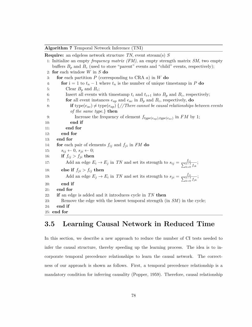
Algorithm 7 Temporal Network Inference (TNI)Require: an edgeless network structure TN, event stream(s) S1: Initialize an empty frequency matrix (FM), an empty strength matrix SM, two empty

buffers Bp and Bc (used to store “parent” events and “child” events, respectively);2: for each window W in S do3: for each partition P (corresponding to CRA a) in W do4: for i = 1 to tn − 1 where tn is the number of unique timestamp in P do5: Clear Bp and Bc;6: Insert all events with timestamp ti and ti+1 into Bp and Bc, respectively;7: for all event instances eap and eac in Bp and Bc, respectively, do8: if type(eac) 6= type(eap) {//There cannot be causal relationships between events

of the same type.} then9: Increase the frequency of element ftype(eap),type(eac) in FM by 1;

10: end if11: end for12: end for13: end for14: for each pair of elements fij and fji in FM do15: sij ← 0, sji ← 0;16: if fij > fji then17: Add an edge Ei → Ej in TN and set its strength to sij = fij∑n−1

k=0 fik;

18: else if fji > fij then19: Add an edge Ej → Ei in TN and set its strength to sji = fji∑n−1

k=0 fjk;

20: end if21: end for22: if an edge is added and it introduces cycle in TN then23: Remove the edge with the lowest temporal strength (in SM ) in the cycle;24: end if25: end for

3.5 Learning Causal Network in Reduced Time

In this section, we describe a new approach to reduce the number of CI tests needed to

infer the causal structure, thereby speeding up the learning process. The idea is to in-

corporate temporal precedence relationships to learn the causal network. The correct-

ness of our approach is shown as follows. First, a temporal precedence relationship is a

mandatory condition for inferring causality (Popper, 1959). Therefore, causal relationship

78

subsumes temporal precedence relationship, that is, the causal network is a subgraph of

the temporal network. Second, a causal network should satisfy the Causal Markov Con-

dition (CMC) (Spirtes et al., 1990; Pearl, 1995; Pearl, 1998) where for every node X in

the set of nodes N , X is independent of its non-descendants excluding its parents (i.e.,

N\(Descendants(X) ∪ Parents(X))) conditional on its parents. In a temporal network

of vertex (or node) set N, a node is temporally independent, and therefore causally inde-

pendent, of all its non-descendants (except its parents) given its parents. In other words,

the temporal network obeys CMC which is a necessary condition for the causal network.

Therefore, our idea of considering a temporal network as an initial causal network is correct.

3.5.1 Fast Causal Network Inference Algorithm

The idea behind FCNI algorithm is to reduce the number of CI tests by incorporating

temporal precedence information. The algorithm has two steps, as outlined in Algorithm 8.

1. The first step is to construct a temporal network by running the TNI algorithm.

The temporal network is set as the initial causal network. Note that since tempo-

ral precedence is a requirement for a causal relationship, all causal relationships are

theoretically guaranteed be in the temporal network.

2. The second step is to adapt the ideas of constraint-based algorithms to learn the final

causal network by pruning out the edges between independent nodes. We perform CI

tests on every edge between nodes in the initial causal network to verify dependency

between them. Conditionally independent nodes are considered to be spurious and

hence the edge between them is removed. Steps 2 to 22 perform this step. The main

difference from the PC algorithm is the manner in which CI tests are performed. In

the PC algorithm, the condition set S for an edge Ei −Ej considers the neighbors of

both Ei and Ej whereas in the FCNI algorithm, as the edges are already directed,

the condition set S for an edge Ei → Ej needs to consider only the parents of Ej (Ej

79

is independent of the parents of Ei that do not have edge to Ej). Consequently, we

need fewer CI tests.

Algorithm 8 Fast Causal Network Inference (FCNI)Require: Window W, Edgeless Causal Network G = (N , ξ).{N and ξ are the set of nodes

and the set of edges, respectively.}1: Run the TNI algorithm and initialize G with the learned temporal network;2: for each directed edge (Ei, Ej) ∈ ξ do3: independent = IsIndependent(Ei, Ej , φ), where φ is the empty set;

{IsIndependent(Ei, Ej , S) calculates IMI(Ei, Ej |S) for CI test.}4: if independent is true then5: Remove (Ei, Ej) from ξ;6: end if7: end for8: k ← 0;9: repeat

10: for each directed edge (Ei, Ej) ∈ ξ do11: Construct a set of condition sets, Z, each of cardinality k from the parents of Ej

excluding Ei;12: repeat13: Select any subset S from Z;14: independent = IsIndependent(Ei, Ej , S);15: Remove S from Z;16: until Z is empty or independent is true17: if independent is true then18: Remove (Ei, Ej) from ξ;19: end if20: end for21: k = k + 1;22: until number of parents of E′j in every directed edge (E′i, E′j) ∈ ξ is less than k.

3.5.2 Complexity Analysis

The complexity of the FNCI algorithm for a causal network G is bounded by the largest

degree of each node. Let n be the number of nodes (i.e., event types). Then in the worst

case, since the causal network inference starts with a temporal network, the number of CI

tests required by the algorithm is given as

80

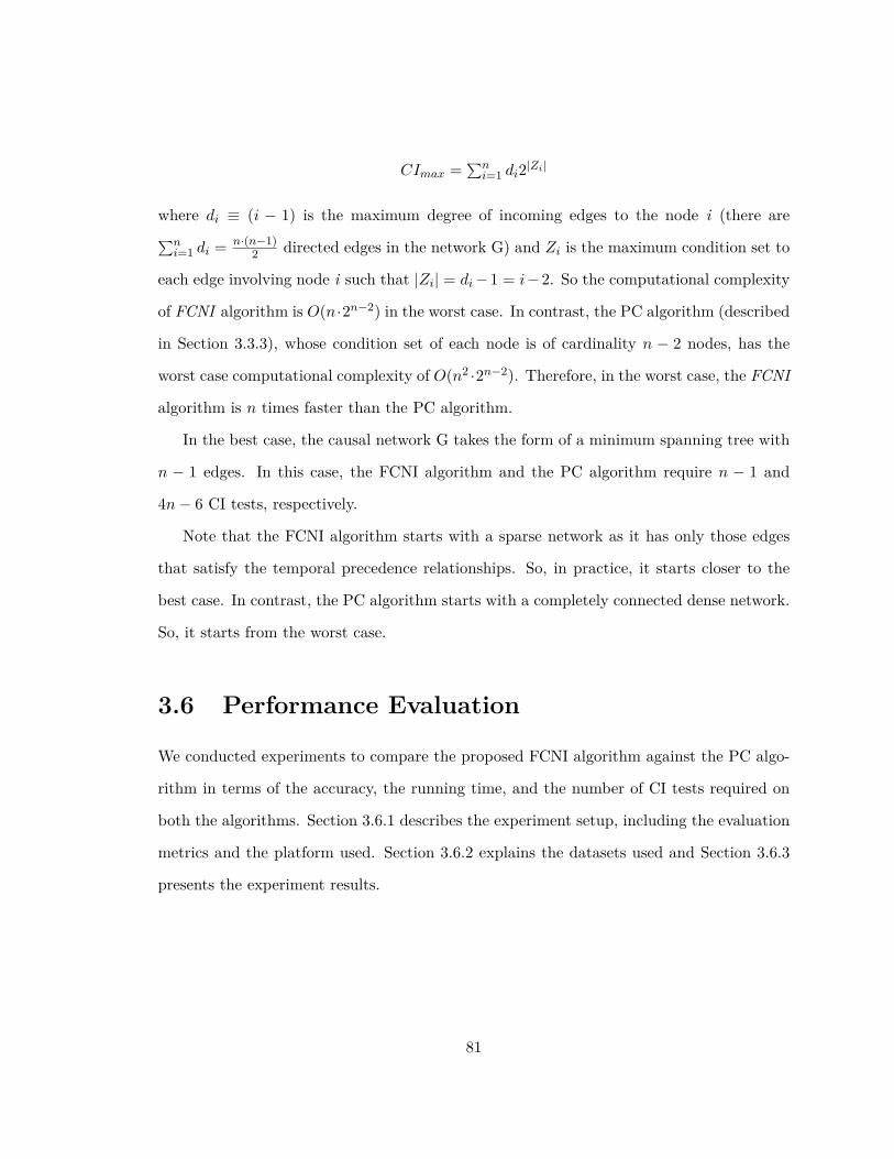
CImax =∑ni=1 di2|Zi|

where di ≡ (i − 1) is the maximum degree of incoming edges to the node i (there are∑ni=1 di = n·(n−1)

2 directed edges in the network G) and Zi is the maximum condition set to

each edge involving node i such that |Zi| = di−1 = i−2. So the computational complexity

of FCNI algorithm is O(n·2n−2) in the worst case. In contrast, the PC algorithm (described

in Section 3.3.3), whose condition set of each node is of cardinality n − 2 nodes, has the

worst case computational complexity of O(n2 ·2n−2). Therefore, in the worst case, the FCNI

algorithm is n times faster than the PC algorithm.

In the best case, the causal network G takes the form of a minimum spanning tree with

n − 1 edges. In this case, the FCNI algorithm and the PC algorithm require n − 1 and

4n− 6 CI tests, respectively.

Note that the FCNI algorithm starts with a sparse network as it has only those edges

that satisfy the temporal precedence relationships. So, in practice, it starts closer to the

best case. In contrast, the PC algorithm starts with a completely connected dense network.

So, it starts from the worst case.

3.6 Performance Evaluation

We conducted experiments to compare the proposed FCNI algorithm against the PC algo-

rithm in terms of the accuracy, the running time, and the number of CI tests required on

both the algorithms. Section 3.6.1 describes the experiment setup, including the evaluation

metrics and the platform used. Section 3.6.2 explains the datasets used and Section 3.6.3

presents the experiment results.

81

3.6.1 Experiment setup

3.6.1.1 Evaluation metrics.

Intuitively, the quality of causal network learning algorithms are best evaluated by ex-

amining how closely the constructed causal network structures resemble the target causal

network. In this regard, we adopt the structural Hamming distance proposed by (Tsamardi-

nos et al., 2006) as the quality metric of the output causal network. The nodes (i.e., event

types) are fixed as given to the algorithms, and therefore the network structures are com-

pared with respect to the edges between nodes. There are three kinds of possible errors in

the causal network construction: reversed edges, missing edges, and spurious edges. We use

the number of the erroneous edges of each kind as the evaluation metric.

3.6.1.2 Platform.

The experiments are conducted on RedHat Enterprise Linux 5 operating system using

Java(TM) 2 Runtime Environment–SE 1.5.0_07 in Vermont Advanced Computing Core

(VACC) cluster computers.

3.6.2 Datasets

Experiments are conducted using both synthetic and real datasets.

Synthetic datasets.

A synthetic dataset is reverse-engineered from a target causal network. Given the control

parameters – the number of event owners no and the number of event types n, the idea is to

generate a random causal network, and then convert the causal network to an event stream

which reflects the underlying probability distribution of the causal network. In the interest

of space, the details of the event stream generation are not described here. We assume that

82

the event owner is the CRA. The dataset is represented by a collection of files in which

the events are shuffled according to the owner ID while preserving the temporal order. We

create five datasets (see their profiles in Table 3.1), representing target causal networks of

4, 8, 12, 16 and 20 nodes each.

Dataset n nedges no ninstancesDS1 4 4 5000 13108DS2 8 16 30000 108334DS3 12 32 500000 3163237DS4 16 46 6553600 49008538DS5 20 62 52428800 511972810

(nedges is the number of actual edges in the network. ninstances is the number of event instances inthe dataset.)

Table 3.1: Profiles of the five synthetic datasets.

Real dataset.

The real dataset DR contains diabetes lab test results (Frank and Asuncion, 2010) of 70

different patients over a period ranging from a few weeks to a few months. The dataset

has a total 28143 records, about 402 records for each patient. Each record has four fields

– date, time, test code, test value. The clinical data of a patient is independent of other

patients. Therefore, the patient ID is the CRA for this dataset. There are 20 different test

codes appearing in the file from which we define 13 different event types of interest. The

details of the event types are omitted due to the space limit.

3.6.3 Experiment results

We ran the FCNI and PC algorithms over each of the five synthetic datasets and the real

dataset. We present our evaluation results in three parts. First, we compare the quality of

the generated networks against the target causal network and determine how closely they

resemble the true causal network. (The details of the true causal networks are omitted due

83

to the space limit.) Specifically, we count the number of spurious edges, the number of

missing edges, and the number of reversed edges. Second, we compare the running time

(CPU time) of the two algorithms, and finally, we evaluate the number of CI tests performed

on both algorithms. We show that reducing the number of CI tests is the key to reducing

the running time of causal network inference. The experiment is repeated ten times for each

dataset (DS1 through DS5 and DR) to calculate the average number of erroneous edges,

the average running time, and the average number of CI tests. We assume the events are

in temporal order.

3.6.3.1 Comparison of the accuracy of the PC and FCNI algorithms.

Table 3.2 presents the number of erroneous edges in the causal network produced by the

PC and FCNI algorithms. The results show that the quality of the causal network from

the FCNI algorithm is similar to that of the PC algorithm. First, the number of missing

and spurious edges are comparable. This is due to the reliance of both algorithms on

the same test statistics (CMI in our case) to infer the independence of two event types.

Second, the number of reversed edges is zero for the FCNI algorithm. Clearly the FCNI

algorithm, through the temporal network, is much better at determining the correct causal

edge direction. It is because the fact that the cause always precedes its effect is embodied

in its temporal precedence relationship. Overall, we conclude that the FCNI algorithm

produces almost the same topology as the PC algorithm, while the accuracy of the causal

direction is improved.

3.6.3.2 Comparison of the running time of the PC and FCNI algorithms.

Figure 3.2(a) plots the average running time of FCNI and PC algorithms against the number

of event types (n) in the synthetic dataset. In all cases, the FCNI algorithm is much faster

than the PC algorithm. Clearly, the temporal precedence information helps to reduce the

size of condition set and the edges to test. As n increases, the running times of both PC

84

Algorithms DS1 DS2 DS3 DS4 DS5 DRMissing Edges PC 0 0 0 0 1 1

FCNI 0 1 0 0 1 1Reversed Edges PC 0 2 0 2 3 2

FCNI 0 0 0 0 0 0Spurious Edges PC 0 3 0 4 3 1

FCNI 0 3 0 4 3 1

Table 3.2: Number of erroneous edges.

0

5000

10000

15000

20000

25000

4 8 12 16 20

Tim

e (m

sec)

Number of Event Types (n)

PCFNCI

(a) Running time for varying number ofevent types.

0

20000

40000

60000

80000

100000

120000

140000

160000

4 8 12 16 20N

umbe

r of

CI t

ests

Number of Event Types (n)

PCFNCI

(b) Number of CI tests for varying num-ber of event types.

Figure 3.2: Comparison of the PC and FCNI algorithmsand FCNI algorithms increase. However, the rate of increase of the running time of the PC

algorithm is much higher than that of the FCNI algorithm. Therefore, with an increase in

n, the ratio of running time between the two algorithms increases. The same observation is

made in the real dataset where the running time of the PC and FCNI algorithms are 817

and 118 msecs, respectively. These results verify the important role of temporal precedence

relationships to reduce the running time.

3.6.3.3 Comparison of the number of CI tests of the PC and FCNI algorithms.

Figure 3.2(b) shows that the FCNI algorithm performs fewer CI tests than the PC algo-

rithm in all synthetic datasets. The CI tests required are minimized, due to the temporal

precedence information, by reducing the size of the condition set and the number of edges

85

to test. With an increase in the number of event types (n), the rate of increase of the

number of CI tests in the PC algorithm is much higher than that in the FCNI algorithm. A

similar observation is made in the real dataset where the number of CI tests of the PC and

FCNI algorithms are 1239 and 192, respectively. These results confirm the important role

of temporal precedence relationships in reducing the number of CI tests. Note the result of

CI tests (Figure 3.2(b)) looks almost the same as that of the running time (Figure 3.2(a)).

This demonstrates that CI tests are the major performance bottleneck and validates the

key idea of our work that reducing the number of CI tests reduces the run time.

3.7 Conclusion and Future Work

In this paper, we presented a novel strategy to incorporate temporal precedence relationships

to learn the causal network over event streams. First, we introduced the Temporal Network

Inference algorithm to model temporal precedence information. Then, we presented the

Fast Causal Network Inference algorithm to reduce the running time complexity of learning

causal network by eliminating unnecessary CI tests. We showed the experiment results to

validate our approach by comparing against the state-of-the-art PC algorithm. For the

future work, we plan to explore the temporal semantics further for causal network inference

over out-of-order event streams.

86

Bibliography

Acharya, S. and Lee, B. (2013). Fast causal network inference over event streams. In Data

Warehousing and Knowledge Discovery, volume 8057 of Lecture Notes in Computer

Science, pages 222–235. Springer Berlin Heidelberg.

Acharya, S. and Lee, B. S. (2014a). Enchanced fast causal network inference over event

streams. Transactions on Large Scale Data and Knowledge Centered Systems.

Acharya, S. and Lee, B. S. (2014b). Incremental causal network construction over event

streams. Information Sciences, 261(0):32 – 51.

Acharya, S., Lee, B. S., and Hines, P. (2014). Real-time top-k predictive query processing

over event streams. Information Sciences.

Akdere, M., Çetintemel, U., and Upfal, E. (2010). Database-support for continuous pre-

diction queries over streaming data. Proc. VLDB Endow., 3(1-2):1291–1301.

Alcobé, J. R. (2004a). Incremental hill-climbing search applied to Bayesian network

structure learning. In First International Workshop on Knowledge Discovery in Data

Streams, 2004.

Alcobé, J. R. (2004b). Incremental Methods for Bayesian Network Structure Learning.

PhD thesis, Department of Computer Science, Universitat Politècnica de Catalunya.

Alcobé, J. R. (2005). Incremental methods for Bayesian network structure learning. Ar-

tificial Intelligence Communications, 18(1):61–62.

87

Barber, D. (2012). Bayesian Reasoning and Machine Learning. Cambridge University

Press.

Barga, R. S., Goldstein, J., Ali, M. H., and Hong, M. (2007). Consistent streaming

through time: A vision for event stream processing. In Proceedings of the Third Bi-

ennial Conference on Innovative Data Systems Research, CIDR’07, pages 363–374.

Bishop, Y. M., Fienberg, S. E., and Holland, P. W. (1975). Discrete Multivariate Analysis:

Theory and Practice. MIT Press.

Borchani, H., Chaouachi, M., and Ben Amor, N. (2007). Learning causal bayesian net-

works from incomplete observational data and interventions. In Proceedings of the 9th

European Conference on Symbolic and Quantitative Approaches to Reasoning with

Uncertainty, ECSQARU ’07, pages 17–29, Berlin, Heidelberg. Springer-Verlag.

Bowes, J., Neufeld, E., Greer, J., and Cooke, J. (2000). A comparison of association rule

discovery and bayesian network causal inference algorithms to discover relationships in

discrete data. In Hamilton, H., editor, Advances in Artificial Intelligence, volume 1822

of Lecture Notes in Computer Science, pages 326–336. Springer Berlin Heidelberg.

Buntine, W. (1991). Theory refinement on Bayesian networks. In Proceedings of the sev-

enth conference (1991) on Uncertainty in artificial intelligence, pages 52–60, San

Francisco, CA, USA. Morgan Kaufmann Publishers Inc.

Chandra, P. and Kshemkalyani, A. D. (2005). Causality-based predicate detection across

space and time. IEEE Transactions on Computerts, 54:1438–1453.

Cheng, J. and Druzdzel, M. J. (2000). Ais-bn: An adaptive importance sampling algo-

rithm for evidential reasoning in large Bayesian networks. J. Artif. Intell. Res. (JAIR),

13:155–188.

Cheng, J. and Druzdzel, M. J. (2001). Confidence inference in Bayesian networks. In

Proceedings of the Seventeenth conference on Uncertainty in artificial intelligence,

88

UAI’01, pages 75–82, San Francisco, CA, USA. Morgan Kaufmann Publishers Inc.

Cheng, J., Greiner, R., Kelly, J., Bell, D., and Liu, W. (2002). Learning Bayesian networks

from data: an information-theory based approach. Artificial Intelligence, 137(1-2):43–

90.

Chickering, D. M. (2002). Learning equivalence classes of Bayesian-network structures.

Journal of Machine Learning Research, 2:445–498.

Chickering, D. M., Heckerman, D., and Meek, C. (2004). Large-sample learning of

bayesian networks is np-hard. J. Mach. Learn. Res., 5:1287–1330.

Chow, Y. S. and Teicher, H. (1978). Probability theory : independence, interchangeability,

martingales. Springer-Verlag, New York.

de Campos, L. M. (2006). A scoring function for learning Bayesian networks based on mu-

tual information and conditional independence tests. J. Machine Learning Research,

7:2149–2187.

Ellis, B. and Wong, W. H. (2008). Learning causal Bayesian network structures from

experimental data. Journal of the American Statistical Association, 103(482):778–789.

Elloumi, M. and Zomaya, A. Y. (2013). Biological Knowledge Discovery Handbook: Pre-

processing, Mining and Postprocessing of Biological Data, volume 23. John Wiley &

Sons.

Eppstein, M. and Hines, P. (2012). A "Random Chemistry" algorithm for identifying

collections of multiple contingencies that initiate cascading failure. IEEE Transactions

on Power Systems, 27(3):1698–1705.

Frank, A. and Asuncion, A. (2010). UCI machine learning repository.

Friedman, N. and Goldszmidt, M. (1997). Sequential update of bayesian network struc-

ture. In Proceedings of the Thirteenth conference on Uncertainty in artificial intelli-

89

gence, UAI’97, pages 165–174, San Francisco, CA, USA. Morgan Kaufmann Publish-

ers Inc.

Friedman, N., Linial, M., Nachman, I., and Pe’er, D. (2000). Using Bayesian networks to

analyze expression data. In Proceedings of the Fourth Annual International Conference

on Computational Molecular Biology, RECOMB ’00, pages 127–135, New York, NY,

USA. ACM.

Geiger, D. and Pearl, J. (1988). On the logic of causal models. In Proceedings of the

Fourth Annual Conference on Uncertainty in Artificial Intelligence, UAI ’88, pages

3–14.

Glüge, S., Hamid, O. H., and Wendemuth, A. (2010). A simple recurrent network for

implicit learning of temporal sequences. Cognitive Computation, 2(4):265–271.

Glymour, C. (2003). Learning, prediction and causal Bayes nets. Trends in cognitive

sciences, 7(1):43–48.

Granger, C. W. J. (1969). Investigating Causal Relations by Econometric Models and

Cross-spectral Methods. Econometrica, 37(3):424–438.

Guyon, I., Aliferis, C. F., Cooper, G. F., Elisseeff, A., Pellet, J.-P., Spirtes, P., and

Statnikov, A. R. (2008). Design and analysis of the causation and prediction challenge.

In IEEE World Congress on Computational Intelligence Causation and Prediction

Challenge, pages 1–33.

Hamilton, H. J. and Karimi, K. (2005). The timers ii algorithm for the discovery of

causality. In Proceedings of the 9th Pacific-Asia conference on Advances in Knowledge

Discovery and Data Mining, PAKDD’05, pages 744–750, Berlin, Heidelberg. Springer-

Verlag.

Heckerman, D. (1995). A Bayesian approach to learning causal networks. In Proceedings

of the Eleventh conference on Uncertainty in artificial intelligence, UAI’95, pages

90

285–295, San Francisco, CA, USA. Morgan Kaufmann Publishers Inc.

Heckerman, D. (1999). UCI machine learning repository

[http://archive.ics.uci.edu/ml/datasets/msnbc.com+

anonymous+web+data].

Henrion, M. (1991). Search-based methods to bound diagnostic probabilities in very large

belief nets. In Proceedings of the Seventh conference on Uncertainty in Artificial In-

telligence, UAI’91, pages 142–150, San Francisco, CA, USA. Morgan Kaufmann Pub-

lishers Inc.

Holme, P. and Saramäki, J. (2011). Temporal networks. CoRR, abs/1108.1780.

Ishii, H., Ma, Q., and Yoshikawa, M. (2010). An incremental method for causal network

construction. In Proceedings of the 11th international conference on Web-age infor-

mation management, WAIM’10, pages 495–506, Berlin, Heidelberg. Springer-Verlag.

Jiang, X.-R. and Gruenwald, L. (2005). Microarray gene expression data association rules

mining based on BSC-tree and FIS-tree. Data & Knowledge Engineering, 53(1):3 –

29.

Johnson, T., Muthukrishnan, S., and Rozenbaum, I. (2007). Monitoring regular expres-

sions on out-of-order streams. In Proceedings of the IEEE 23rd International Confer-

ence on Data Engineering, ICDE’07, pages 1315–1319.

Kemeny, J. and Snell, J. (1969). Finite Markov chains. University series in undergraduate

mathematics. VanNostrand, New York, repr edition.

Kirkpatrick, S., Gelatt, C. D., and Vecchi, M. P. (1983). Optimization by simulated

annealing. Science, 220:671–680.

Kłopotek, M. A. (2006). Cyclic Bayesian network–Markov process approach. Studia In-

formatica, 1(2):7.

91

Krishna, R., Li, C.-T., and Buchanan-Wollaston, V. (2010). A temporal precedence based

clustering method for gene expression microarray data. BMC Bioinformatics, 11:68.

Kullback, S. (1968). Information Theory and Statistics. Dover Publication, 2nd edition.

Kwon, O. and Li, K.-J. (2009). Causality join query processing for data streams via a

spatiotemporal sliding window. Journal of Universal Computer Science, 15(12):2287–

2310.

Lam, W. and Bacchus, F. (1994). Using new data to refine a Bayesian network. In Pro-

ceedings of the Tenth international conference on Uncertainty in artificial intelligence,

UAI’94, pages 383–390, San Francisco, CA, USA. Morgan Kaufmann Publishers Inc.

Li, G. and Leong, T.-Y. (2009). Active learning for causal bayesian network structure

with non-symmetrical entropy. In Proceedings of the 13th Pacific-Asia Conference on

Advances in Knowledge Discovery and Data Mining, PAKDD ’09, pages 290–301,

Berlin, Heidelberg. Springer-Verlag.

Li, J., Tufte, K., Shkapenyuk, V., Papadimos, V., Johnson, T., and Maier, D. (2008).

Out-of-order processing: A new architecture for high-performance stream systems.

Proceegins of the VLDB Endowment, 1(1):274–288.

Li, M., Liu, M., Ding, L., Rundensteiner, E. A., and Mani, M. (2007). Event stream

processing with out-of-order data arrival. In Proceedings of the 27th International

Conference on Distributed Computing Systems Workshops, ICDCSW ’07, pages 67–

74, Washington, DC, USA. IEEE Computer Society.

Lin, T. Y., Xie, Y., Wasilewska, A., and Liau, C.-J., editors (2008). Data Mining: Foun-

dations and Practice, volume 118 of Studies in Computational Intelligence. Springer.

Liu, M., Li, M., Golovnya, D., Rundensteiner, E., and Claypool, K. (2009). Sequence

pattern query processing over out-of-order event streams. In Proceedings of the IEEE

25th International Conference on Data Engineering, ICDE ’09, pages 784–795.

92

Liu, Y., Niculescu-Mizil, A., Lozano, A. C., and Lu, Y. (2010). Learning temporal causal

graphs for relational time-series analysis. In ICML, pages 687–694. Omnipress.

MacKay, D. J. C. (1999). Introduction to Monte Carlo methods. In Learning in graphical

models, pages 175–204. MIT Press, Cambridge, MA, USA.

Mani, S., Aliferis, C. F., and Statnikov, A. R. (2010). Bayesian algorithms for causal data

mining. Journal of Machine Learning Research, 6:121–136.

Mazlack, L. J. (2004). Mining causality from imperfect data. In Proceedings of the sixth

International FLINS Conference on Applied Computational Intelligence Proceedings,

Applied Computational Intelligence, pages 155–160.

Meek, C. (1995). Causal inference and causal explanation with background knowledge.

In Proceedings of the Eleventh Conference Annual Conference on Uncertainty in Ar-

tificial Intelligence (UAI-95), pages 403–410, San Francisco, CA. Morgan Kaufmann.

Meganck, S., Leray, P., and Manderick, B. (2006). Learning causal bayesian networks

from observations and experiments: a decision theoretic approach. In Proceedings of

the Third international conference on Modeling Decisions for Artificial Intelligence,

MDAI’06, pages 58–69, Berlin, Heidelberg. Springer-Verlag.

Meliou, A., Gatterbauer, W., Moore, K. F., and Suciu, D. (2010). Why so? or why no?

functional causality for explaining query answers. In MUD, 2010, pages 3–17.

Mohammad, Y. and Nishida, T. (2010). Mining causal relationships in multidimensional

time series. In Szczerbicki, E. and Nguyen, N., editors, Smart Information and Knowl-

edge Management, volume 260 of Studies in Computational Intelligence, pages 309–

338. Springer Berlin Heidelberg.

Moral, P., Doucet, A., and Jasra, A. (2012). An adaptive sequential Monte Carlo method

for approximate Bayesian computation. Statistics and Computing, 22:1009–1020.

Pearl, J. (1995). Causal diagrams for empirical research. Biometrika, 82:669–710.

93

Pearl, J. (1998). Graphs, causality, and structural equation models. Sociological Methods

and Research, 27:226–84.

Pearl, J. (2009). Causality: Models, Reasoning and Inference. Cambridge University

Press, New York, NY, USA, second edition edition.

Pearl, J. and Verma, T. (1991). A theory of inferred causation. In KR, 1991, pages

441–452.

Popper, K. (1959). The Logic of Scientific Discovery. Routledge Classics.

Prakasa Rao, B. (2009). Conditional independence, conditional mixing and conditional

association. Annals of the Institute of Statistical Mathematics, 61(2):441–460.

Rottman, B. M. and Hastie, R. (2014). Reasoning about causal relationships: Inferences

on causal networks. Psychological Bulletin, 140(1):109–139.

Rudin, C., Letham, B., Salleb-Aouissi, A., Kogan, E., and Madigan, D. (2011). Sequential

event prediction with association rules. In Proceedings of the 24th Annual Conference

on Learning Theory, COLT ’11, pages 615–634.

Shachter, R. D. (1990). Evidence absorption and propagation through evidence reversals.

In Proceedings of the Fifth Annual Conference on Uncertainty in Artificial Intelligence,

UAI ’89, pages 173–190, Amsterdam, The Netherlands.

Silverstein, C., Brin, S., Motwani, R., and Ullman, J. (2000). Scalable techniques for

mining causal structures. Data Mining and Knowledge Discovery, 4(2-3):163–192.

Spirtes, P., Glymour, C., and Scheines, R. (1993). Causation, Prediction, and Search.

Ima Volumes in Mathematics and Its Applications. Springer-Verlag.

Spirtes, P., Glymour, C., and Scheines, R. (2000). Causation, Prediction, and Search.

MIT Press.

Spirtes, P., Glymour, C. N., and Scheines, R. (1990). Causality from probability. In

Proceedings of the Conference on Advanced Computing for the Social Sciences, ACSS

94

’90.

Spirtes, P. and Meek, C. (1995). Learning Bayesian networks with discrete variables from

data. In Proceedings of the First International Conference on Knowledge Discovery

and Data Mining, KDD’95, pages 294–299.

Tsamardinos, I., Brown, L. E., and Aliferis, C. F. (2006). The max-min hill-climbing

bayesian network structure learning algorithm. Mach. Learn., 65(1):31–78.

Tulupyev, A. L. and Nikolenko, S. I. (2005). Directed cycles in Bayesian belief networks:

probabilistic semantics and consistency checking complexity. In Proceedings of the 4th

Mexican international conference on Advances in Artificial Intelligence, pages 214–

223. Springer.

US-Canada Power System Outage Task Force (2004). Final Report on the August 14,

2003 Blackout in the United States and Canada. Technical report.

Utrera, A. C., Olmedo, M. G., and Callejon, S. M. (2008). A score based ranking of the

edges for the pc algorithm. In Proceedings of the 4th European workshop on proba-

bilistic graphical models, PGM’08, pages 41 – 48.

Vaiman, M., Bell, K., Chen, Y., Chowdhury, B., Dobson, I., Hines, P., Papic, M., Miller,

S., and Zhang, P. (2012). Risk assessment of cascading outages: Methodologies and

challenges. IEEE Transactions on Power Systems, 27(2):631–641.

Veloso, A. A., Almeida, H. M., Gonçalves, M. A., and Meira Jr., W. (2008). Learning

to rank at query-time using association rules. In Proceedings of the 31st Annual In-

ternational ACM SIGIR Conference on Research and Development in Information

Retrieval, SIGIR ’08, pages 267–274, New York, NY, USA. ACM.

Verma, T. and Pearl, J. (1988). Causal networks: Semantics and expressiveness. In Pro-

ceedings of the Fourth Annual Conference on Uncertainty in Artificial Intelligence,

UAI ’88, pages 69–78.

95

Wang, K. and Yu, Y. (2013). A query-matching mechanism over out-of-order event stream

in iot. Int. J. Ad Hoc Ubiquitous Comput., 13(3/4):197–208.

Young, S. S. and Karr, A. (2011). Deming, data and observational studies. Significance,

8(3):116–120.

Zhang, N. L. and Poole, D. (1996). Exploiting causal independence in Bayesian network

inference. J. Artif. Int. Res., 5(1):301–328.

Zhang.N.L. and D., P. (1994). A simple approach to Bayesian network computations. In

Proceedings of the Tenth Canadian Conference on Artificial Intelligence, CCAA ’94,

pages 171–178.

Zhao, Y. and Strom, R. (2001). Exploitng event stream interpretation in publish-subscribe

systems. In Proceedings of the Twentieth Annual ACM Symposium on Principles of

Distributed Computing, PODC ’01, pages 219–228.

96

Chapter 4

Enhanced Fast Causal Network Inference

over Event Streams

Abstract

This paper addresses causal inference and modeling over event streams where data have high

throughput, are unbounded, and may arrive out of order. The availability of large amount of

data with these characteristics presents several new challenges related to causal modeling,

such as the need for fast causal inference operations while ensuring consistent and valid

results. There is no existing work specifically for such a streaming environment. We meet the

challenges by introducing a time-centric causal inference strategy which leverages temporal

precedence information to decrease the number of conditional independence tests required to

establish the causalities between variables in a causal network. (Dependency and temporal

precedence of cause over effect are the two properties of a causal relationship.) Moreover, we

employ change-driven causal network inference to safely reduce the running time further. In

this paper we present the Order-Aware Temporal Network Inference algorithm to model the

temporal precedence relationships into a temporal network and then propose the Enhanced

Fast Causal Network Inference algorithm for learning a causal network faster using the

97

temporal network. Experiments using synthetic and real datasets demonstrate the efficacy

of the proposed algorithms.

4.1 Introduction

In recent years, there has been a growing need for active systems that can perform causal

inference in diverse applications such as health care, stock markets, user activity monitoring,

smart electric grids, and network intrusion detection. These applications need to infer

the cause of abnormal activities immediately from their event streams, where the event

arrival may be in order (e.g., (Barga et al., 2007; Zhao and Strom, 2001)) or out of order

(e.g., (Johnson et al., 2007; Li et al., 2007; Liu et al., 2009; Li et al., 2008; Wang and Yu,

2013)) such that informed and timely preventive measures can be taken. As a case in point,

consider a smart electric grid monitoring application. The failure of a component can cause

cascading failures, effectively causing a massive blackout. The identification of such cause

and effect components in a timely manner enables preventive measures in the case of failure

of a cause component, thereby preventing blackouts.

Causal network, a directed acyclic graph where the parent of each node is its direct

cause, has been popularly used to model causality (Heckerman, 1995; Ellis and Wong, 2008;

Li and Leong, 2009; Meganck et al., 2006; Pearl, 2009; Spirtes et al., 1990; Spirtes et al.,

2000). There are two distinct types of algorithms for learning a causal network: score-

based (Heckerman, 1995; Ellis and Wong, 2008; Li and Leong, 2009; Meganck et al., 2006)

and constraint-based (Pearl, 2009; Spirtes et al., 1990; Spirtes et al., 2000; Cheng et al.,

2002). Both types of algorithms are slow and, therefore, not suitable for event streams

where prompt causal inference is required. Score-based algorithms perform a greedy search

(usually hill climbing) to select a causal network with the highest score from a large num-

ber of possible networks. With an increase in the number of variables in the dataset, the

number of possible networks grows exponentially, resulting in slow causal network inference.

98

On the other hand, constraint-based algorithms (e.g., PC algorithm (Spirtes et al., 2000))

discover the causal structure via a large number of tests on conditional independence(CI).

There can be no edge between two conditionally independent variables in the causal net-

work (e.g., (Pearl, 1995; Spirtes and Meek, 1995)). Two variables X and Y are said to be

conditionally independent given a condition set S if there is at least one variable in S such

that X and Y are independent (e.g., (Chow and Teicher, 1978; Prakasa Rao, 2009)). In

a causal network of n variables, the condition set S consists of all possible 2n−2 combina-

tions of the remaining n − 2 variables, and therefore the computational complexity grows

exponentially as the number of variables increases. So, the current techniques for causal

inference are slow and not suitable for event streams which have a high data throughput and

where the number of variables (i.e., event types) is large. Besides, these techniques perform

the time-consuming causal inference computations every time a new batch of events arrives

even though there may not be significant enough changes in the event stream statistic.

With these concerns, this paper describes a new time-centric causal modeling approach

to speed up the causal network inference. Every causal relationship implies temporal prece-

dence relationship (e.g., (Popper, 1959; Hamilton and Karimi, 2005)). So, the idea is to

exploit temporal precedence information as an important clue to reducing the number of re-

quired CI tests and thus maintaining feasible computational complexity. Four strategies are

employed utilizing this idea to achieve fewer computations of CI tests. First, since causality

requires temporal precedence, we ignore the causality test for those nodes with no temporal

precedence relationship between them. Second, in the CI test of an edge, we exclude those

nodes from the condition set which do not have temporal precedence relationship with the

nodes of the edge; this strategy reduces the size of the condition set which is a major cause

of the exponential computational complexity. Third, we perform the CI tests for weaker

edges (i.e., having lower temporal strength) earlier to reduce the size of the condition set

of stronger edges, thereby reducing the overall number of CI tests. The rationale for this

99

is that weaker edges are more likely to be eliminated than stronger edges (Utrera et al.,

2008). Fourth, we perform the causal inference computations only if there is a significant

enough change in the temporal precedence relationships, which is a necessary condition for

a change to occur in the resulting causal relationships. Such a change detection strategy

helps to avoid unnecessary causal inference computations, and therefore, saves time.

Due to the reliance on the temporal precedence relationships in an event stream, events

arriving out of order can bring ambiguities in the resulting causal directions. For instance,

the precedence relationships represented in an edge and its reversed edge in a temporal

network, which models the temporal precedence relationships, may not be significantly

different enough to determine the edge direction. Intuitively, an undirected edge can be used

to signify such an ambiguity. Thus, we propose a mechanism to decide between directed

and undirected edge in the temporal network in such cases. Note that the constraint-based

algorithms like the PC algorithm naturally handle out-of-order event arrivals, as these

algorithms do not depend on the temporal ordering of events, and so they can provide a

suitable baseline to evaluate the handling of out-of-order events in our proposed method.

The main contributions of this paper are summarized as follows. First, it presents a

temporal network structure to represent temporal precedence relationships between event

types and proposes an algorithm, Order-Aware Temporal Network Inference (OATNI), to

construct a temporal network applicable in the streaming environment. Second, it intro-

duces a time-centric causal modeling strategy and proposes an algorithm, Enhanced Fast

Causal Network Inference (EFCNI), to speed up the learning of causal network. Third,

it empirically demonstrates the advantages of the proposed algorithm in terms of the ac-

curacy and speed of learning the causal network by comparing it against two state-of-art

algorithms, the PC algorithm (details in Sections 4.3.4) and the FCNI algorithm (Acharya

and Lee, 2013).

This paper contains the results of a comprehensive study extended from our earlier

100

work (Acharya and Lee, 2013). The two algorithms in our prior work, the Temporal Net-

work Inference (TNI) and the Fast Causal Network Inference (FCNI), are extended to the

OATNI and the FECNI algorithms, respectively. Specifically, two major extensions have

been made. First, the speed of the causal inference mechanism has been increased with

two strategies. As the first strategy, the CI tests are performed in the increasing order of

the temporal strengths of the edges in order to remove the most probable spurious edge as

early as possible, which decreases the condition set size. As the second strategy, presumably

unnecessary causal inference computations are avoided by determining whether the changes

in temporal precedence information in the event stream are significant enough to warrant

such computations. Second, the previous work made an assumption that the event stream

is in order. In this paper, the support for fast causal modeling over an out-of-order event

stream is added so that the temporal precedence relationships cannot be relied upon as

they are. In addition to these two major extensions, the presentation has been extended

throughout in many parts of the paper.

The rest of this paper is organized as follows. Section 4.2 reviews the existing work

on causal network inference. Section 4.3 presents the basic concepts used in the paper.

Section 4.4 and Section 4.5 propose the learning algorithms of temporal network (OATNI)

and faster causal network (EFCNI), respectively. Section 4.6 evaluates the proposed EFNCI

algorithm. Section 4.7 concludes the paper and suggests further research.

4.2 Related Work

As explained earlier, there are two main approaches for causal network inference.

The first approach, score-based (Heckerman, 1995; Ellis and Wong, 2008; Li and Leong,

2009; Meganck et al., 2006), performs greedy search (usually hill climbing) over all possible

network structures in order to find the network that best represents the data based on

the highest score. This approach, however, has two problems. First, it is slow due to the

101

exhaustive search for the best network structure. An increase in the number of variables in

the dataset increases the computational complexity exponentially. Second, two or more net-

work structures, called the equivalence classes (Chickering, 2002), may represent the same

probability distribution, and consequently the causal directions between nodes are quite

random. There is no technique for alleviating these problems in a streaming environment.

Thus, score-based algorithms are not suitable for streams.

The second approach, constraint-based (Pearl, 2009; Spirtes et al., 1990; Spirtes et al.,

2000; Cheng et al., 2002), does not have the problem of equivalence classes. However, it is

slow as it starts with a completely connected undirected graph and thus performs a large

number of CI tests to remove the edges between conditionally independent nodes. The

number of CI tests increases exponentially with the increase in the number of variables

in the dataset. To alleviate this problem, some constraint-based algorithms start with

a minimum spanning tree to reduce the initial size of condition sets. However, this idea

trades the speed with the accuracy of the causal inference. The constraint-based algorithms

include IC* (Pearl, 2009), SGS (Spirtes et al., 1990), PC (Spirtes et al., 2000), and FCI

algorithm (Spirtes et al., 2000). The FCI algorithm focuses on the causal network discovery

from the dataset with latent variables and selection bias, which is quite different from the

scope of this paper. The PC algorithm is computationally more efficient than IC* and SGS.

This is why we evaluate the proposed EFCNI algorithm by comparing it against the PC

algorithm. Like the others, the PC algorithm starts with a completely connected undirected

graph. To reduce the computational complexity, it performs CI tests in several steps. Each

step produces a sparser graph than the earlier step, and consequently, the condition set

decreases in the next step. However, the computational complexity is still O(n2 ·2n−2). (The

details are explained in Section 4.3.4.) Therefore, the current constraint-based algorithms

are not suitable for fast causal inference over streams.

There have been a number of research works on handing out-of-order event streams (John-

102

son et al., 2007; Li et al., 2007; Liu et al., 2009; Li et al., 2008; Wang and Yu, 2013). To

the best of our knowledge, however, there exists no work applicable to the causal network

inference. (Thus, a new approach is needed, and our approach is to allow undirected edges

in the temporal network.) Johnson et al. (Johnson et al., 2007) propose an algorithm for

regular expression matching on streams with out-of-order data, which is not related to

causal inference. The works by Li et al. (Li et al., 2007) and Liu et al. (Liu et al., 2009)

discuss the problem of processing event pattern queries over event streams that may contain

out-of-order data. Li et al. (Li et al., 2008) present a new architecture for stream systems

for out-of-order query processing whereas Wang and Yu (Wang and Yu, 2013) propose al-

gorithms for generating and matching queries to raise accuracy and shorten the response

time as much as possible over out-of-order events. None of these works is related to causal

network inference.

4.3 Basic Concepts

This section presents some key concepts needed to understand the paper.

4.3.1 Event streams

An event stream in our work is a sequence of continuous and unbounded timestamped

events. An event refers to any action that has an effect and is created by an event owner.

One event can trigger another event in chain reactions. Each event instance belongs to

one and only one event type which is a prototype for creating the instances. Two event

instances are related to each other if they share common attributes such as event owner,

location, and time. We call these attributes common relational attributes (CRAs).

In this paper we denote an event type as Ej and an event instance as eij , where i

indicates the CRA and j indicates the event type.

103

Example 3 Consider a diabetic patient monitoring system in a hospital. Each patient is

uniquely identifiable, and each clinical test or measurement of each patient makes one event

instance. For example, a patient is admitted to the hospital, has their blood pressure and

glucose level measured, and takes medication over a period of time. This creates the in-

stances of the above event types as a result. Typical event types from these actions include

hypoglycemic-symptoms-exists, blood-glucose-measurement-decreased, increased, regular-insulin-

dose-given, etc. Note that the patient ID is the CRA, as the events of the same patient are

causally related.

To facilitate the handling of events in a streaming environment, we use a time-based

window over the stream. Typically, the application offers a natural observation period (e.g.,

hour) that makes a window. The causal relationship is only possible between events with

the same CRA. Therefore, the events in a window are arranged by CRA and then ordered

by the timestamp as they arrive, producing a partitioned window as a result. Figure 4.1

illustrates it. (We refer to the partitioned window simply as the window for the rest of the

paper.)

With the arrival of a new batch of event instances, we augment each partition in the

new window by prefixing it with the last instance of the partition with the same CRA value

in the previous window. This is necessary in order to identify the related instances that are

separated into the two consecutive batches.

(a) Events collected during an observation period (window).

(b) Events in the window partitioned by CRA.

Figure 4.1: Partitioned window of events.

We support event streams which may be in order or out of order. An event stream is said

104

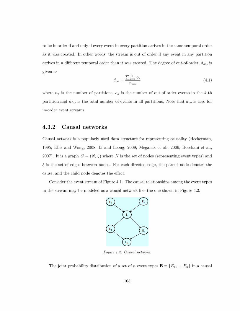
to be in order if and only if every event in every partition arrives in the same temporal order

as it was created. In other words, the stream is out of order if any event in any partition

arrives in a different temporal order than it was created. The degree of out-of-order, doo, is

given as

doo =∑npk=1 oknins

(4.1)

where np is the number of partitions, ok is the number of out-of-order events in the k-th

partition and nins is the total number of events in all partitions. Note that doo is zero for

in-order event streams.

4.3.2 Causal networks

Causal network is a popularly used data structure for representing causality (Heckerman,

1995; Ellis and Wong, 2008; Li and Leong, 2009; Meganck et al., 2006; Borchani et al.,

2007). It is a graph G = (N, ξ) where N is the set of nodes (representing event types) and

ξ is the set of edges between nodes. For each directed edge, the parent node denotes the

cause, and the child node denotes the effect.

Consider the event stream of Figure 4.1. The causal relationships among the event types

in the stream may be modeled as a causal network like the one shown in Figure 4.2.

Figure 4.2: Causal network.

The joint probability distribution of a set of n event types E ≡ {E1, ..., En} in a causal

105

network is specified as

P (E) =n∏i=1

P (Ei|Pai)

where Pai is the set of the parent nodes of event type Ei.

4.3.3 Conditional mutual information

A popular approach for testing the conditional independence, with respect to the joint

probability P , of two random variables X and Y given a subset S of random variables is

conditional mutual information(CMI) (e.g., (Cheng et al., 2002; de Campos, 2006)). CMI

gives the strength of dependency between variables in a measurable quantity, which helps

to identify strong and weak causal relationships in the final causal network.

To test whether X and Y are conditionally independent given S, we compute the con-

ditional mutual information IMI(X,Y |S) as

IMI(X,Y |S) =∑x∈X

∑y∈Y

∑s∈S

pX,Y,S(x, y, s)log2pX,Y |S(x, y|s)

pX|S(x|s)pY |S(y|s)

where p is the probability mass function calculated from the frequencies of variables.

We only keep the record of these frequencies, not the whole events, by updating them as

a new batch of events arrives. Consequently, the independence test procedure is incremental

in our case.

It is said that two variables X and Y are independent when IMI(X,Y |S) = 0; other-

wise, they are dependent. However, this presents us with the risk of spurious relationships

due to weak dependencies (we cannot assume IMI(X,Y |S) = 10−5 and IMI(X,Y |S) = 10

provide the same degree of confidence in the dependency). With an increase in the value

of IMI(X,Y |S), the dependency between the variables X and Y grows stronger. Therefore,

to prune out weak dependencies, we need to set a threshold value of mutual information

below which we ignore the evidence as weak. To do so, we relate CMI with G2 test statis-

106

tics (Spirtes et al., 2000; Bishop et al., 1975) as below, where Ns is the sample size.

G2(X,Y |S) = 2 ·Ns · loge2 · IMI(X,Y |S)

G2 follows the χ2 distribution (Kullback, 1968), with the degree of freedom df equal to

(rx − 1)(ry − 1)∏s∈S rs, where rx, ry, and rs are the number of possible distinct values of

X, Y, and S, respectively. So, we use χ2 test, which provides a threshold based on df and

significance level α, to validate the dependency result. We set α to the universally accepted

value of 95%.

4.3.4 The PC algorithm

The key idea of the PC algorithm (Spirtes et al., 2000) is that a causal network has an

edge between two nodes, X and Y , if and only if X and Y are not independent given any

of the condition subsets of the remaining neighbor nodes (Pearl, 1995; Spirtes and Meek,

1995). Algorithm 9 outlines the PC algorithm.

The algorithm has two parts. In the first part, the algorithm learns the topology of

the causal network (Lines 1– 18). It starts with a completely connected undirected graph

G of n nodes. Two sets are used for bookkeeping – Neighbors(G,X) and SepSet(X,Y ).

Neighbors(G,X) gives the set of nodes adjacent to X, and SepSet(X,Y ) gives the set of

nodes which causes X and Y to be conditionally independent. Initially, Neighbors(G,X)

has the remaining n−1 nodes and SepSet(X,Y) is empty. Then, the CI tests are performed

between every pair of nodes that have an edge between them to determine whether they

are conditionally independent of any other nodes in G. The edge between the conditionally

independent nodes is removed. To ensure that all possible combination of nodes are consid-

ered in the condition set, the algorithm starts with an empty condition set and ends with

the condition set with the maximum possible number of nodes. That is, in the algorithm

k refers to the number of nodes in the condition set and is initially set to 0 to denote an

107

Algorithm 9 PC algorithmRequire: Window W1: Construct the completely connected undirected graph G of all nodes;2: for each node X in G do3: Initialize Neighbors(G,X) as the set of nodes adjacent to X in G;4: end for5: for each pair of nodes X and Y in G do6: Initialize an empty set SepSet(X,Y ) as the set of nodes that causes independence

between X and Y in G;7: end for8: k ← 0;9: repeat

10: repeat11: Select any edge X − Y such that |Neighbors(G,X)\Y | ≥ k;12: repeat13: Select any subset S of Neighbors(G,X)\Y such that |Neighbors(G,X)\Y | = k;

14: If X and Y are independent given S, remove X − Y from G, remove Y fromNeighbors(G,X), remove X from Neighbors(G,Y), and add S to SepSet(X,Y) andSepSet(Y,X);

15: until every subset S of Neighbors(G,X)\Y such that |Neighbors(G,X)\Y | = khas been selected.

16: until every edge X − Y such that |Neighbors(G,X)\Y | ≥ k has been selected.17: k = k + 1;18: until no edge X ′ − Y ′ satisfies |Neighbors(G,X ′)\Y ′| ≥ k.19: for each triplet of nodes X, Y, Z such that the edge X − Y and Y −Z exists in G but

not X − Z do20: Orient X − Y − Z as X→Y←Z if and only if SepSet(X,Z) does not contain Y;21: end for22: repeat23: If there exists X → Y and Y − Z, but not X − Z, then orient Y − Z as Y → Z;24: If there exists X−Y and a directed path from X to Y, then orient X−Y as X → Y ;25: until no edge can be oriented.

empty condition set, and then k is gradually increased (by 1 at each iteration) and the

CI tests are performed between every pair of nodes with the condition set of size k. This

process is repeated until there is no edge left in G whose condition set size is greater than

k. Eventually, an undirected network is obtained where an edge between two nodes denotes

that these nodes are not conditionally independent in the presence of any of the other n−2

108

nodes.

In the second part, the undirected network topology is assigned causal directions (Lines

19 – 25). It is done in three steps. First, if there are two edges X − Y and Y − Z but not

X−Z and SepSet(X,Z) does not contain Y , then X−Y −Z is assigned the edge orientations

X → Y ← Z. The reason is that X and Z are dependent given Y , as the absence of Y

in SepSet(X,Z) indicates that X and Z are not conditionally independent given Y (Verma

and Pearl, 1988; Geiger and Pearl, 1988). Second, if there are edges X → Y and Y − Z

but not X − Z, then Y − Z is oriented as Y → Z. The absence of an edge between X

and Z means that X and Z are not dependent. A directed edge from X to Y and Y to Z

with no edge between X and Z makes X and Z independent of Y (Verma and Pearl, 1988;

Geiger and Pearl, 1988). Thus, the edge between Y and Z is oriented as Y → Z. Third,

if there are edges X − Y and a directed path from X to Y through any number of nodes,

then X −Y is oriented as X → Y . This is necessary to make the graph acyclic, as the edge

direction X ← Y would make the graph cyclic.

4.4 Learning Temporal Precedence Relationships

In this section, we describe an incremental approach to model temporal precedence rela-

tionships from time-stamped events into a temporal network.

4.4.1 Temporal network model

A temporal network is a network of nodes representing event types where an edge between

two nodes represents the temporal precedence relationship between them. To determine

when an edge should be added in a temporal network, a measure providing an evidence of

temporal precedence between the event types should be defined. The evidence we use is the

frequency of the observation of an instance of Ej following an instance of Ei. We call this

109

the precedence frequency.

Definition 9 (Precedence frequency) The precedence frequency fij between two event

types Ei and Ej is the total number of observations in which an event of type Ei precedes

an event of type Ej over all partitions in the partitioned window.

fij =np∑k=1

n(eki,ekj)

where np is the number of partitions and n(eki,ekj) is the number of observations in which

an event of type Ei precedes an event of type Ej in the k-th partition.

In our prior work (Acharya and Lee, 2013), we assume that the event stream is in order

and the temporal network from such an event stream is directed and acyclic. However, in

an event stream with out-of-order event arrivals, the reliance on the temporal order for a

definite temporal edge direction between event types may lead to ambiguous scenarios. For

instance, the precedence frequencies between two event types Ei and Ej of an edge Ei → Ej

and its reversed edge Ei ← Ej may not differ significantly enough to determine an edge

direction between them. An undirected edge Ei − Ej is warranted to reflect such ambigu-

ity. Thus, we support undirected edges as well as directed edges in the temporal network

model. A directed edge between two nodes reflects a strong temporal precedence relation-

ship between them, whereas an undirected edge reflects an ambiguous temporal precedence

relationship between them. A threshold called the temporal confidence (θ) is used to select

between directed and undirected edges, as presented in Rule 1 below.

Rule 1. Temporal edge direction selection

Suppose the precedence frequencies of an edge Ei → Ej and its reversed edge Ei ← Ei

are fij and fji such that either fij > 0 or fji > 0, respectively. Then, the edge direction

110

between these two event types Ei and Ej (i.e., Ξ(Ei, Ej)) is selected as follows.

Ξ(Ei, Ej) =

Ei → Ej iffij−fjifij+fji > θ

Ei ← Ej iffji−fijfij+fji > θ

Ei − Ej if|fij−fjifij+fji | ≤ θ

Given a temporal network, we define the edge strength, called the temporal strength, as

follows.

Definition 10 (Temporal strength) Consider an edge Ei → Ej (i 6= j) in a temporal

network of n event types. Let fij be the precedence frequency from the event type Ei to the

event type Ej. Then, we define the temporal strength, sij, of the edge Ei → Ej as

sij ,fij∑nk=1 fik

That is, the temporal strength of Ei → Ej is the precedence frequency of (Ei, Ej) relative

to the total precedence frequency over all children nodes of Ei.

4.4.2 Order-aware temporal network inference algorithm

The idea behind the OATNI algorithm is to collect events from an event stream in a

window and then use temporal precedence information from the sequence of event pairs in

the window to construct a temporal network at the event type level. The overall algorithm is

centered on a frequency matrix, which is initially empty (i.e., all zero elements) and updated

with each new batch of events.

The algorithm has two steps for each window, as outlined in Algorithm 10.

1. Update the frequency matrix FM by observing the precedence relationships of event

111

Algorithm 10 Order-Aware Temporal Network Inference (OATNI)Require: Edgeless network structure TN, Event stream(s) S, Temporal confidence θ1: Initialize an empty frequency matrix FM, an empty strength matrix SM, two empty

buffers Bp and Bc (used to store “parent” events and “child” events, respectively);2: for each window W in S do3: for each partition P (corresponding to CRA a) in W do4: for i = 1 to tn − 1 where tn is the number of unique timestamps in P do5: Clear Bp and Bc;6: Insert all events with timestamp ti and ti+1 into Bp and Bc, respectively;7: for each event instance eap in Bp do8: for each event instances eac in Bc do9: if type(eac) 6= type(eap) {//There cannot be causal relationships between

events of the same type.} then10: Increase the frequency of element ftype(eap),type(eac) in FM by 1;11: end if12: end for13: end for14: end for15: end for16: for each pair of elements fij and fji such that fij > 0 or fji > 0 in FM do17: sij ← 0, sji ← 0;18: if fij−fji

fij+fji > θ then19: Add an edge Ei → Ej in TN and set its strength to sij = fij∑n

k=1 fik;

20: else if fji−fijfij+fji > θ then

21: Add an edge Ei ← Ej in TN and set its strength to sji = fji∑n

k=1 fjk;

22: else if |fij−fji|fij+fji ≤ θ then23: Add an edge Ei − Ej in TN and set the strengths to sij = fij∑n

k=1 fjkand sji =

fji∑n

k=1 fjk;

24: end if25: end for26: end for

pairs in the partitioned window (Lines 3–15). An element fij in FM reflects the total

number of times events of type Ei precede events of type Ej (i 6= j). Each time an

event pair (eoi, eoj) is observed in the event stream such that eoi precedes eoj , increase

the value of fij by 1.

112

2. Determine the edges of the temporal network using FM (Lines 16–25). For each pair

of nodes, add an edge according to Rule 1. For a directed edge added, e.g., Ei → Ej ,

calculate its temporal strength and store it in sij of SM. For an undirected edge added,

e.g., Ei − Ej , calculate the temporal strengths of both directions and store them in

sij and sji of SM.

Note that when the events arrive in order, the OATNI algorithm reduces to the TNI algo-

rithm by setting the threshold θ to 0 so that Rule 1 always chooses between the first two

cases.

4.5 Learning Causal Network in Reduced Time

In this section, we describe a new approach which reduces the number of CI tests needed to

infer the causal structure, thereby speeding up the learning process. Specifically, we explain

the key ideas employed and discuss the concrete algorithm. We then prove the correctness

of the algorithm and analyze its computational complexity.

4.5.1 Key ideas

Given that the key approach is to exploit temporal precedence relationships to learn the

causal network, there are a number of ideas employed to reduce the causal network con-

struction time. We begin by proposing some preliminary lemmas.

Lemma 4.5.1 A CI test between two event types with no temporal precedence relationship

is unnecessary.

Proof 4.5.2 Two event types can a have causal relationship only if they have a temporal

precedence relationship. Therefore, it is not necessary to perform a CI test (for detecting

causality) between two event types which are not temporally related.

113

Lemma 4.5.3 Event types which do not have temporal precedence relationships with either

of the two event types being tested for causality are not needed in the condition set of the

CI test.

Proof 4.5.4 Consider two event types, Ei and Ej, tested for causality, and consider an-

other event type Ek (k 6= i, j). Ek can causally influence Ei (or Ej) only if Ek has a

temporal precedence relationship with Ei (or Ek). Therefore, the CI tests between Ei and

Ej can safely exclude from the condition set those event types (i.e., Ek) which are not

temporally related to either of them.

Based on Lemma 4.5.1, the CI tests are performed only for the edges in the temporal

network. That is, not every possible edges are considered for the CI tests leading to a

reduced number of CI tests. Moreover, since the size of the condition set contributes to the

number of CI tests exponentially, we use Lemma 4.5.3 to reduce the condition set size by

including only those event types which have temporal relationships, hence possibly causal

relationships, to the event types being tested.

We employ another idea to speed up the network inference further, based on Lemma 4.5.5

below.

Lemma 4.5.5 The number of CI tests performed in the causal network inference decreases

if the CI tests between event types are performed in an increasing order of their temporal

strength.

Proof 4.5.6 Event types with weaker temporal strengths between them have higher likelihood

of being conditionally independent than those with stronger temporal strengths. Therefore,

if the CI tests are performed between event types with the lowest temporal strength first,

then the initial causal network becomes sparser faster and, consequently, the condition sets

for the CI tests between event types become smaller faster. This leads to the reduction in

the total number of CI tests performed through the causal network inference.

114

Evidently, the reduction in the number of CI tests brings the reduction of running time.

Further, we employ the idea of reducing the overhead of causal network inference by

performing it only when there are significant enough changes in temporal precedence rela-

tionships in the event stream. The rationale for this is that the causal network tends to

absorb changes in the temporal network until the changes are significant enough.

We introduce the temporal precedence probability as the measure to normalize the prece-

dence frequencies between event types. The changes in the precedence probabilities give a

normalized measure of the changes that have occurred in the temporal network since the

last batch of events in the stream.

Definition 11 (Precedence probability) The precedence probability pij between two event

types Ei and Ej is defined as the ratio of fij and the summation of all precedence frequencies.

pij = fij∑nx=1

∑ny=1 fxy

Let PM@ti and PM@ti+1 be the matrices representing the precedence probabilities at

the timestamps ti and ti+1, respectively. Then, the measure of change in the precedence

information at ti+1, called precedence change (Cp), is calculated as follows.

Cp@ti+1 =n∑x=1

n∑y=1|pxy@ti+1 − pxy@ti|

where pxy is the element at the position (x, y) (i.e., event types (Ex, Ey)) in PM. Given this

change measure, we update the causal network only if the calculated Cp exceeds a certain

threshold, called the precedence change confidence (δ).

4.5.2 Enhanced fast causal network inference algorithm

115

Algorithm 11 Enhanced Fast Causal Network Inference (EFCNI)Require: Window W, Precedence change confidence δ, Edgeless causal network G.1: Run theOATNI algorithm and initialize G = (N, ξ) with the learned temporal network;

{N and ξ are the set of nodes and the set of edges, respectively.}2: Calculate Cp. If Cp < δ, then exit; {Stop if there is no significant change in the event

stream.}3: Sort the edges in ξ in the increasing order of their temporal strength.4: for each edge (Ei, Ej) ∈ ξ do5: independent = IsIndependent(Ei, Ej , φ), where φ is the empty set;

{IsIndependent(Ei, Ej , S) calculates IMI(Ei, Ej |S) for CI test.}6: if independent is true then7: Remove (Ei, Ej) from ξ;8: end if9: end for

10: k ← 0;11: repeat12: for each edge (Ei, Ej) ∈ ξ do13: Construct a set of condition sets, Z, each of cardinality k from the parents of Ej

excluding Ei;14: repeat15: Select any subset S from Z;16: independent = IsIndependent(Ei, Ej , S);17: Remove S from Z;18: until Z is empty or independent is true19: if independent is true then20: Remove (Ei, Ej) from ξ;21: end if22: end for23: k = k + 1;24: until there is no Ej in any edge (Ei, Ej) ∈ ξ with k incident edges.

The algorithm has four steps, as outlined in Algorithm 11.

1. The first step (Line 1) learns a temporal network by running the OATNI algorithm.

The temporal network, which can have both directed and undirected edges, is set as

the initial causal network.

2. The second step (Line 2) checks if there has been a significant enough change in the

temporal precedence statistic (i.e., Cp) in the event stream from the last observation

116

period, and stops if not.

3. The third step (Line 3) sorts the edges of the initial causal network in the increasing

order of their temporal strength.

4. The fourth step (Lines 4–24) constructs the final causal network by pruning out the

edges between independent nodes. CI tests are performed on every edge between ad-

jacent nodes in the initial causal network to verify dependency between them. Condi-

tionally independent nodes are considered spurious, and hence the edge between them

is removed.

The main difference from the PC algorithm is the manner in which the CI tests are per-

formed. In the PC algorithm, the condition set S for an edge Ei−Ej (undirected) considers

the neighbors of both Ei and Ej whereas in the EFCNI algorithm, the condition set S for

an edge Ei → Ej (directed) needs to consider only the parents of Ej . (Ej is independent of

the parents of Ei that do not have edge to Ej .) Consequently, fewer CI tests are needed.

In addition, note that the EFCNI algorithm reduces to the FCNI algorithm by omitting

the second and the third steps.

4.5.3 Correctness of the algorithm

To prove the correctness of the algorithm, it suffices to prove the correctness of our approach

which starts with a temporal network as the initial causal network and removes edges

through CI tests on them. We show the correctness as follows. First, a temporal precedence

relationship is a necessary condition for inferring causality (Popper, 1959). Therefore, causal

relationship subsumes temporal precedence relationship, that is, the causal network is a

subgraph of the temporal network (Lemma 4.5.1). Second, a causal network should satisfy

the Causal Markov Condition (CMC) (Spirtes et al., 1990; Pearl, 1995; Pearl, 1998) where

for every node X in the set of nodes N , X is independent of its non-descendants excluding

117

its parents (i.e., N\(Descendants(X) ∪ Parents(X))) given its parents. In a temporal

network of vertex (or node) set N, a node is temporally independent, and therefore causally

independent, of all its non-descendants (except its parents) given its parents (Lemma 4.5.3).

4.5.4 Complexity analysis

Given n nodes, the computational complexity of the EFCNI algorithm is O(n2 ·

2n−2) in the worst case and O(n) in the best case.

Proof 4.5.7 The computational complexity of the EFCNI algorithm is governed by the

total number of possible CI tests which is calculated by summing up the number of CI

tests involving each edge. In the worst case, the number of edges in the network is that

of a completely connected graph and all edges are undirected. The number of edges in

a completely connected graph of n nodes is n(n−1)2 . For every edge between two nodes,

the remaining n − 2 nodes are considered in the condition set, as the graph is completely

connected and undirected. Therefore, to test conditional independence between a pair of

nodes in an edge, there are 2n−2 CI tests to perform. Consequently, the total number of CI

tests for all edges is n(n−1)2 ·2n−2, resulting in the computational complexity of O(n2 ·2n−2).

In the best case, the initial causal network (i.e., temporal network) is a directed linear

graph and the number of edges is the minimum (i.e., n − 1). In such a graph, there are

n − 2 edges with one incoming edge to either of the nodes and one edge with no incoming

edge to either of the nodes. For the edges with one incoming edge, the condition set size is

one, and therefore there are two CI tests to perform. For n− 2 such edges, there are 2n− 4

CI tests. For the remaining one edge with no incoming edge to either of the nodes, there

is only one CI test to perform. Therefore, there are 2n − 3 CI tests to perform in the best

case, resulting in the computational complexity of O(n).

The computational complexity of the PC algorithm is O(n) in the best case and O(n2 ·

2n−2) in the worst case (Spirtes et al., 2000). Note that, while the computational complexi-

118

ties are the same, the EFCNI algorithm starts with a sparse network as the use of temporal

precedence relationships removes many of the edges. So, it starts closer to the best case. In

contrast, the PC algorithm always starts with a completely connected dense network. So, it

starts from the worst case. As a result, in practice the EFCNI algorithm shows significant

improvement in runtime over the PC algorithm.

The computational complexity of the FCNI algorithm is O(n) in the best case and

O(n · 2n−2) in the worst case (Acharya and Lee, 2013). FCNI’s worst case computation

complexity is lower than that of EFCNI by a factor of n. However, unlike the EFCNI

algorithm, the FCNI algorithm is not suitable for out-of-order event streams. Moreover, as

mentioned earlier, the EFCNI algorithm reduces to the FCNI algorithm when the events are

in order and θ is zero. As a result, in practice the EFCNI algorithm is at least as fast and

accurate as the FCNI algorithm when the events are in order and preserves the accuracy in

the face of out-of-ordered events, compromising the runtime to some extent as an increasing

number of events arrive out of order.

4.6 Performance Evaluation

We conducted experiments to compare the proposed EFCNI algorithm against the FCNI

and the PC algorithms. There are three sets of experiments – first in terms of the accuracies

of the resulting causal networks, second the running time, and third the number of CI tests

required. In each set of experiments, we consider both the cases of stream being in order and

out of order and also see the effect of the EFCNI’s change-driven causal network construction

strategy by comparing it with FCNI and PC when there are changes in the event stream

statistic. Section 4.6.1 describes the experiment setup, Section 4.6.2 explains the datasets

used, and Section 4.6.3 presents the experiment results.

119

4.6.1 Experiment setup

4.6.1.1 Evaluation metrics.

The evaluation metrics are the speed of the causal network generation and the accuracy

of the generated causal network. The running time is the CPU time, and the number of

performed CI tests affects the speed. The accuracy is evaluated by examining how closely

the constructed causal network structure resembles the target causal network. For this, we

adopt the structural Hamming distance proposed by Tsamardinos et al. (Tsamardinos et al.,

2006) as the measure. The nodes (i.e., event types) are fixed as given to the algorithms,

and therefore the network structures are compared with respect to the edges between nodes.

There are three kinds of possible errors in the causal network construction: reversed edges,

missing edges, and spurious edges. We use the number of erroneous edges of each kind as

the evaluation metric.

4.6.1.2 Platform.

The experiments are conducted on RedHat Enterprise Linux 5 operating system using

Java(TM) 2 Runtime Environment–SE 1.5.0_07 in Vermont Advanced Computing Core

(VACC) cluster computers.

4.6.2 Datasets

Experiments are conducted using both synthetic and real datasets.

Synthetic datasets.

A synthetic dataset is reverse-engineered from a target causal network. Given control

parameters in Table 4.1, the idea is to generate a random causal network, and then convert

the causal network to an event stream which reflects the underlying probability distribution

120

Parameter MeaningNO Number of event owners (with unique ID)NET Number of event types (i.e., nodes)

MaxNC Maximum number of cause events (parents)MaxNE Maximum number of effect events (children)

Table 4.1: Control parameters for synthetic event stream generation.

of the causal network. Specifically, there are three steps. First, NET nodes are created and

edges are added randomly, and random conditional probabilities are assigned to each edge.

Each node can have up to MaxNC edges from cause nodes and up to MaxNE edges to effect

nodes. (We set bothMaxNC andMaxNE to 3 for the experiments presented here.) Second, a

joint probability distribution (JPD) table is built from the conditional probabilities assigned

to edges of the target causal network. The rows of the JPD table collectively cover all event

sequences possible, while each row has its own probability. Third, the probability for each

row in the JPD table is multiplied by NO to calculate the number of repetitions of that

event sequence in the dataset. We assume that the event owner is the CRA for the dataset.

The size of a JPD table grows exponentially with NET and therefore we use parallel

processing for the event stream generation. The JPD table is divided into multiple partitions

and the dataset is created by running parallel processes over each of these partitions. The

dataset is thus represented by a collection of files in which the events are shuffled according

to the owner ID while preserving the temporal order.

There are five cases of datasets, DS1 through DS5, according to the number of nodes in

the represented target causal networks (see their profiles in Table 4.2). The target causal

networks have 4, 8, 12, 16 and 20 nodes, respectively. They are created with 1, 2, 16, 64 and

512 parallel processes, respectively, thus consisting of 1, 2, 16, 64 and 512 files, respectively.

Each row of a synthetic dataset represents one event instance. To obtain out-of-order event

streams, each case of datasets is shuffled randomly up to the required degree of out-of-

order (see Equation 4.1). Changes in the event stream statistic is achieved by altering the

precedence frequencies of events. Specifically, we generate six batches of the event stream for

121

Dataset NET Nedges NO NinsDS1 4 4 5000 15128DS2 8 15 30000 124475DS3 12 22 500000 3173246DS4 16 39 6553600 50247293DS5 20 49 52428800 510971687

(Nedges is the number of actual edges in the network. Nins is the average number of event instancesin the datasets of each case.)

Table 4.2: Profiles of the five synthetic datasets.

six observation points (t1 through t6) with the Cp values of 14%, 16%, 4%, 6%, 10%, and12%,

respectively, for each case of the datasets. The six batches are equal-sized for each dataset

specified in Table 4.2, so the number of instances in a single batch is 2521, 20745, 528874,

8374548, and 85161947 for the dataset D1, D2, D3, D4, D5, and D6, respectively.

Real dataset.

The real dataset DR contains diabetes lab test results (Frank and Asuncion, 2010) of 70

different patients over a period ranging from a few weeks to a few months. The dataset

has a total 28143 records, about 402 records for each patient. Each record has four fields

– date, time, test code, test value. The clinical data of a patient is independent of other

patients. Therefore, the patient ID is the CRA for this dataset. There are 20 different test

codes appearing in the file (shown in the left column of Table 4.3) from which we define

event types of interest (shown in the right column of Table 4.3).

4.6.3 Experiment results

We run the EFCNI, FCNI and PC algorithms over each type of the five synthetic datasets

and the real dataset. We present our evaluation in each of the three sets of experiments.

First, we evaluate the accuracy of the generated causal networks against the target causal

network and determine how closely they resemble the true causal network. Specifically, we

count the number of spurious edges, the number of missing edges, and the number of reversed

122

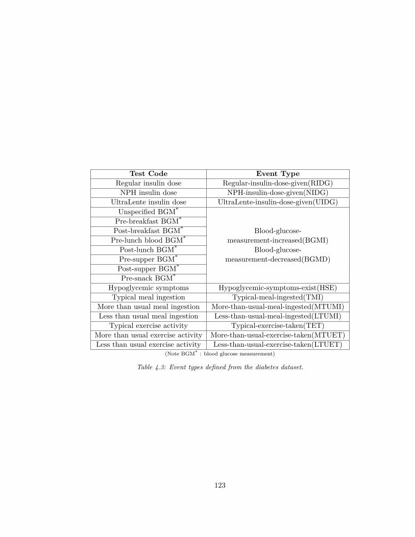
Test Code Event TypeRegular insulin dose Regular-insulin-dose-given(RIDG)NPH insulin dose NPH-insulin-dose-given(NIDG)

UltraLente insulin dose UltraLente-insulin-dose-given(UIDG)Unspecified BGM*

Pre-breakfast BGM*

Post-breakfast BGM* Blood-glucose-Pre-lunch blood BGM* measurement-increased(BGMI)

Post-lunch BGM* Blood-glucose-Pre-supper BGM* measurement-decreased(BGMD)Post-supper BGM*

Pre-snack BGM*

Hypoglycemic symptoms Hypoglycemic-symptoms-exist(HSE)Typical meal ingestion Typical-meal-ingested(TMI)

More than usual meal ingestion More-than-usual-meal-ingested(MTUMI)Less than usual meal ingestion Less-than-usual-meal-ingested(LTUMI)

Typical exercise activity Typical-exercise-taken(TET)More than usual exercise activity More-than-usual-exercise-taken(MTUET)Less than usual exercise activity Less-than-usual-exercise-taken(LTUET)

(Note BGM* : blood glucose measurement)

Table 4.3: Event types defined from the diabetes dataset.

123

edges. Second, we evaluate the running time (CPU time), and third, we evaluate the number

of CI tests performed. We show that reducing the number of CI tests is the key to reducing

the running time of causal network inference. In each set of experiments, the evaluation

covers the scenarios of the event stream being in order and out of order, and, additionally,

the scenario of the event stream statistic changing. For the latter scenario, the value of the

precedence change confidence δ is set to 9% for all synthetic datasets (DS1 through DS5).

For the experiments involving in-order event streams, the temporal precedence confidence θ

is set to zero (so EFCNI reduces to FCNI) and, for the experiments involving out-of-order

event streams, it is set to 24.80%, 17.23%, 18.19%, 21.97%, 26.50% (each determined after

training from 70% of the data) for all synthetic datasets. The experiment is repeated ten

times for each dataset (DS1 through DS5 and DR) to calculate the average.

4.6.3.1 Comparison of the accuracies of the PC, FCNI, and EFCNI algorithms

4.6.3.1.1 When the events arrive in order

Table 4.4 presents the number of erroneous edges in the causal network produced by

the PC, FCNI, and EFCNI algorithms. The results show that the accuracy of the causal

network from the EFCNI algorithm is similar to that of the FCNI and PC algorithms. First,

the number of missing and the number of spurious edges are comparable among all three

algorithms. This is due to the reliance of the three algorithms on the same test statistics

(CMI in our case) to infer the independence of two event types. Additionally, each number is

the same between EFCNI and FCNI because EFCNI reduces to FCNI. Second, the number

of reversed edges is zero for both the FCNI and EFCNI algorithms. Clearly the FCNI

and EFCNI algorithms, through the temporal network, are much better at determining the

correct causal edge directions. It is because of the fact that the cause always precedes its

effect is embodied in the temporal precedence relationship. Overall, the results show that,

124

Type of Algorithm DatasetErroneous Edges DS1 DS2 DS3 DS4 DS5 DR

Missing PC 0 0 0 0 1 1FCNI 0 1 0 0 1 1EFCNI 0 1 0 0 1 1

Reversed PC 0 2 0 2 3 2FCNI 0 0 0 0 0 0EFCNI 0 0 0 0 0 0

Spurious PC 0 3 0 4 3 1FCNI 0 3 0 4 3 1EFCNI 0 3 0 4 3 1

Table 4.4: Number of erroneous edges in an in-order event stream.

when the event stream is in order, the EFCNI algorithm produces the same topology as the

FCNI algorithm and almost the same topology as the PC algorithm, while the accuracy of

the causal directions in the EFCNI algorithm remains the same as the FCNI algorithm and

is improved over the PC algorithm.

4.6.3.1.2 When the events arrive out of order

Table 4.5 presents the number of erroneous edges in the causal network produced by

the three algorithms for varying degree of out-of-order in the event stream. We show the

results for the two datasets DS4 and DS5 only; the results from the other datasets are

consistent with the results from the two datasets. We make two observations from the

results. First, the PC algorithm is more resilient to the out-of-order event arrival than

the FCNI or EFCNI algorithm. The number of spurious edges and the number of missing

edges are higher in the EFCNI algorithm than in the PC algorithm when the degree of

out-of-order is large (i.e., doo = 20%, 25%). The reason is that the PC algorithm does

not depend on the temporal precedence order for causal network inference at all whereas

FCNI and EFCNI do. Second, between the FCNI algorithm and the EFCNI algorithm,

EFCNI results in a comparable number of erroneous edges as PC while FCNI results in

a larger number of erroneous edges than EFCNI or PC. The FCNI algorithm completely

125

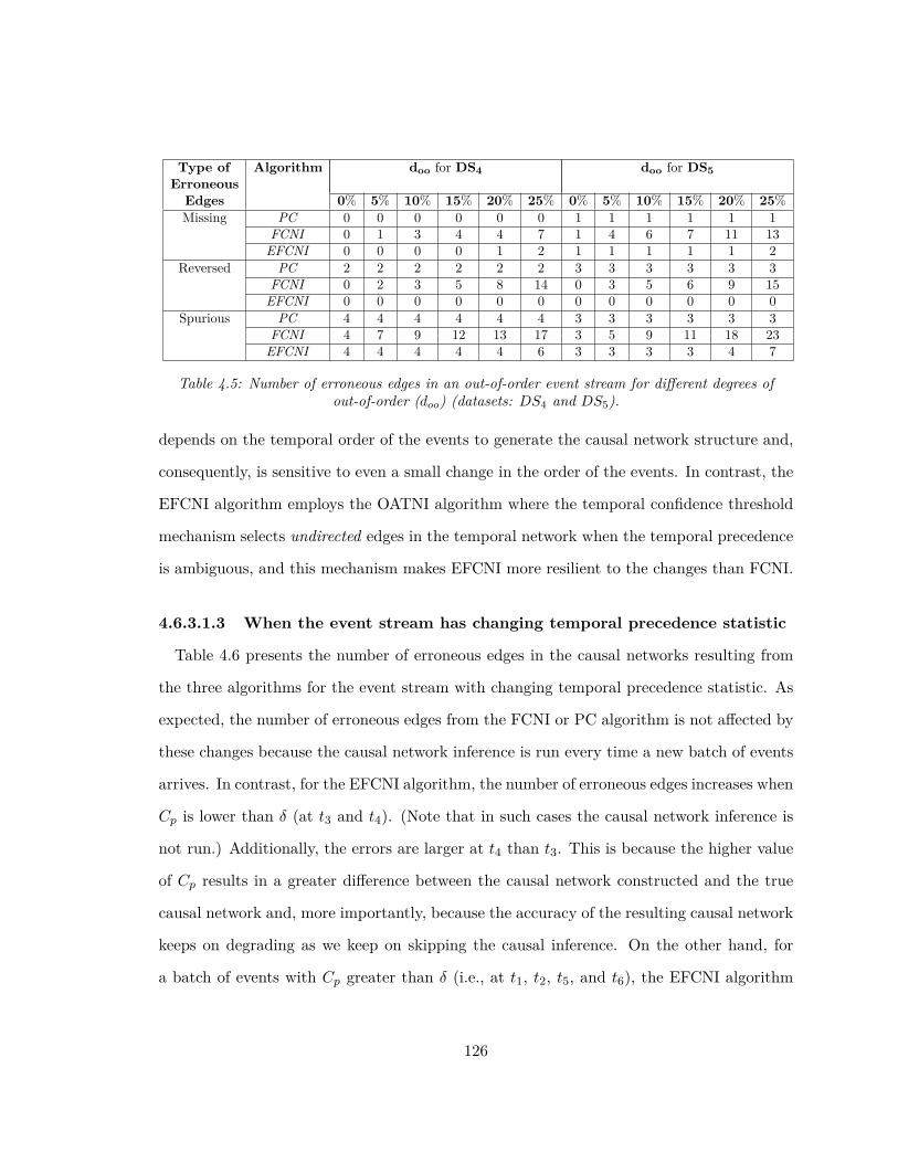
Type of Algorithm doo for DS4 doo for DS5ErroneousEdges 0% 5% 10% 15% 20% 25% 0% 5% 10% 15% 20% 25%Missing PC 0 0 0 0 0 0 1 1 1 1 1 1

FCNI 0 1 3 4 4 7 1 4 6 7 11 13EFCNI 0 0 0 0 1 2 1 1 1 1 1 2

Reversed PC 2 2 2 2 2 2 3 3 3 3 3 3FCNI 0 2 3 5 8 14 0 3 5 6 9 15EFCNI 0 0 0 0 0 0 0 0 0 0 0 0

Spurious PC 4 4 4 4 4 4 3 3 3 3 3 3FCNI 4 7 9 12 13 17 3 5 9 11 18 23EFCNI 4 4 4 4 4 6 3 3 3 3 4 7

Table 4.5: Number of erroneous edges in an out-of-order event stream for different degrees ofout-of-order (doo) (datasets: DS4 and DS5).

depends on the temporal order of the events to generate the causal network structure and,

consequently, is sensitive to even a small change in the order of the events. In contrast, the

EFCNI algorithm employs the OATNI algorithm where the temporal confidence threshold

mechanism selects undirected edges in the temporal network when the temporal precedence

is ambiguous, and this mechanism makes EFCNI more resilient to the changes than FCNI.

4.6.3.1.3 When the event stream has changing temporal precedence statistic

Table 4.6 presents the number of erroneous edges in the causal networks resulting from

the three algorithms for the event stream with changing temporal precedence statistic. As

expected, the number of erroneous edges from the FCNI or PC algorithm is not affected by

these changes because the causal network inference is run every time a new batch of events

arrives. In contrast, for the EFCNI algorithm, the number of erroneous edges increases when

Cp is lower than δ (at t3 and t4). (Note that in such cases the causal network inference is

not run.) Additionally, the errors are larger at t4 than t3. This is because the higher value

of Cp results in a greater difference between the causal network constructed and the true

causal network and, more importantly, because the accuracy of the resulting causal network

keeps on degrading as we keep on skipping the causal inference. On the other hand, for

a batch of events with Cp greater than δ (i.e., at t1, t2, t5, and t6), the EFCNI algorithm

126

Type of Algorithm DS4 DS5Erroneous Edges t1 t2 t3 t4 t5 t6 t1 t2 t3 t4 t5 t6

Missing PC 0 0 0 0 0 0 1 1 1 1 1 1FCNI 0 0 0 0 0 0 1 1 1 1 1 1EFCNI 0 0 1 2 0 0 1 1 2 4 1 1

Reversed PC 2 2 2 2 2 2 3 3 3 3 3 3FCNI 0 0 0 0 0 0 0 0 0 0 0 0EFCNI 0 0 0 1 0 0 0 0 1 2 0 0

Spurious PC 4 4 4 4 4 4 3 3 3 3 3 3FCNI 4 4 4 4 4 4 3 3 3 3 3 3EFCNI 4 4 5 7 4 4 3 3 5 8 3 3

Table 4.6: Number of erroneous edges in a changing event stream over the six observation points t1through t6 (datasets: DS4 and DS5).

rebuilds the causal network and, consequently, the resulting causal network reflects the true

causal network representing the event stream seen thus far. Therefore, at these time points

the number of erroneous edges remains the same as if the event stream had no change.

4.6.3.2 Comparison of the running time of the PC, FCNI, and EFCNI algo-

rithms.

4.6.3.2.1 When the events arrive in order

Figure 4.3(a) shows the average running time of the EFCNI, FCNI, and PC algorithms for

varying number of event types in the synthetic datasets. In all cases, the running time of the

EFCNI algorithm is the shortest while the running time of the PC algorithm is the longest.

Clearly, the temporal precedence information helps to reduce the size of condition set and

the number of edges for CI tests in both the FCNI and EFCNI algorithms. In addition,

the EFCNI algorithm sorts the edges based on their temporal strength and then tests the

conditional independence of the weaker edges, which are more likely to fail the tests, earlier

and therefore further reduces the running time. As the number (n) of event types increases,

the running time increases in all three algorithms, but the rate of increase is the highest for

the PC algorithm and the lowest for the EFCNI algorithm. The same observation is made

in the real dataset where the running time of the PC, FCNI, and EFCNI algorithms are

127

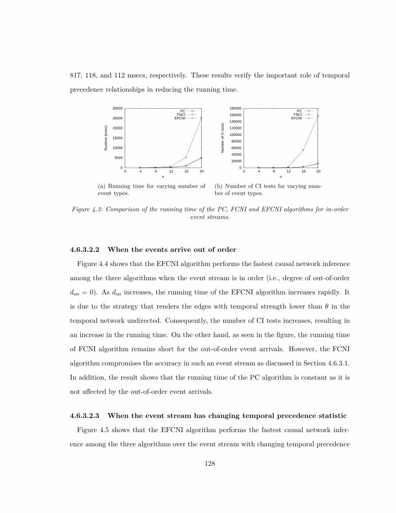
817, 118, and 112 msecs, respectively. These results verify the important role of temporal

precedence relationships in reducing the running time.

0

5000

10000

15000

20000

25000

30000

0 4 8 12 16 20

Run

time

(mse

c)

n

PCFNCI

EFCNI

(a) Running time for varying number ofevent types.

0

20000

40000

60000

80000

100000

120000

140000

160000

180000

0 4 8 12 16 20

Num

ber

of C

I tes

ts

n

PCFNCI

EFCNI

(b) Number of CI tests for varying num-ber of event types.

Figure 4.3: Comparison of the running time of the PC, FCNI and EFCNI algorithms for in-orderevent streams.

4.6.3.2.2 When the events arrive out of order

Figure 4.4 shows that the EFCNI algorithm performs the fastest causal network inference

among the three algorithms when the event stream is in order (i.e., degree of out-of-order

doo = 0). As doo increases, the running time of the EFCNI algorithm increases rapidly. It

is due to the strategy that renders the edges with temporal strength lower than θ in the

temporal network undirected. Consequently, the number of CI tests increases, resulting in

an increase in the running time. On the other hand, as seen in the figure, the running time

of FCNI algorithm remains short for the out-of-order event arrivals. However, the FCNI

algorithm compromises the accuracy in such an event stream as discussed in Section 4.6.3.1.

In addition, the result shows that the running time of the PC algorithm is constant as it is

not affected by the out-of-order event arrivals.

4.6.3.2.3 When the event stream has changing temporal precedence statistic

Figure 4.5 shows that the EFCNI algorithm performs the fastest causal network infer-

ence among the three algorithms over the event stream with changing temporal precedence

128

0

50

100

150

200

0 5 10 15 20 25

Run

time

(mse

c)

Degree of out-of-order

PCFNCI

EFCNI

(a) n = 8.

0

100

200

300

400

500

600

700

0 5 10 15 20 25

Run

time

(mse

c)

Degree of out-of-order

PCFNCI

EFCNI

(b) n = 12.

0

1000

2000

3000

4000

5000

6000

0 5 10 15 20 25

Run

time

(mse

c)

Degree of out-of-order

PCFNCI

EFCNI

(c) n = 16.

0

5000

10000

15000

20000

25000

30000

0 5 10 15 20 25

Run

time

(mse

c)

Degree of out-of-order

PCFNCI

EFCNI

(d) n = 20.

Figure 4.4: Comparison of the running time of the PC, FCNI, and EFCNI algorithms forout-of-order event streams.

statistic. In the figure, for all values of n, the FCNI and PC algorithms perform the CI

tests for the causal network inference every time a new batch of events arrives. On the

other hand, the EFCNI algorithm performs it only when the precedence statistic changes

significantly enough in the event stream. (Cp is greater than δ at t1, t2, t5, and t6.) The

EFCNI algorithm skips the causal inference at t3 and t4, which helps to reduce the overall

running time.

4.6.3.3 Comparison of the number of CI tests of the PC, FCNI, and EFCNI

algorithms.

4.6.3.3.1 When the events arrive in order

Figure 4.3(b) shows that the EFCNI algorithm performs fewer CI tests than the PC and

129

0

50

100

150

200

t1 t2 t3 t4 t5 t6

Run

time

(mse

c)

Observation time

PCFCNI

EFCNI

(a) n = 8.

0

100

200

300

400

500

600

700

800

t1 t2 t3 t4 t5 t6

Run

time

(mse

c)

Observation time

PCFCNI

EFCNI

(b) n = 12.

0

1000

2000

3000

4000

5000

6000

t1 t2 t3 t4 t5 t6

Run

time

(mse

c)

Observation time

PCFCNI

EFCNI

(c) n = 16.

0

5000

10000

15000

20000

25000

30000

t1 t2 t3 t4 t5 t6

Run

time

(mse

c)

Observation time

PCFCNI

EFCNI

(d) n = 20.

Figure 4.5: Comparison of the running time of the PC, FCNI, and EFCNI algorithms for changingevent streams.

FCNI algorithms in all synthetic datasets. The CI tests are decreased by reducing the size of

the condition set and the number of edges to test with the help of the temporal precedence

information. In addition, the sorting of the edges (based on the their temporal strengths)

helps to reduce the number of CI tests. With an increase in the number of event types (n),

the rate of increase in the number of CI tests of the PC algorithm is much higher than that

of the EFCNI and FCNI algorithms. A similar observation is made in the real dataset where

the number of CI tests of the PC, FCNI, and EFCNI algorithms are 1239, 192, and 176,

respectively. These results confirm the important role of temporal precedence relationships

in reducing the number of CI tests. Note the result of CI tests (Figure 4.3(b)) looks almost

the same as that of the running time (Figure 4.3(a)). This demonstrates that CI tests are

the major performance bottleneck and validates the key idea of our work that reducing the

130

number of CI tests reduces the run time.

4.6.3.3.2 When the events arrive out of order

Figure 4.6 shows that, as the degree of out-of-order increases, the number of CI tests of the

EFCNI algorithm increases. A higher degree of out-of-order leads to the temporal strengths

of more edges lower than the temporal confidence threshold (i.e., θ), and this results in

rendering more edges undirected and therefore performing more CI tests. Consequently,

as the degree of out-of-order increases, the number of CI tests of the EFCNI algorithm

becomes closer to that of the PC algorithm. Note that the PC algorithm is not affected

by the out-of-order event arrivals and, thus, the number of CI tests does not change for

varying degree of out-of-order. The results also show that the FCNI algorithm performs

the smallest number of CI tests when the events arrive out of order. However, its accuracy

is the worst among the three algorithms as discussed in Section 4.6.3.1.

4.6.3.3.3 When the event stream has changing temporal precedence statistic

Figure 4.7 shows that the EFCNI algorithm performs the smallest number of CI tests

among the three algorithms over the event stream with changing temporal precedence statis-

tic. As discussed earlier, the FCNI and PC algorithms regenerate the causal network with

the arrival of every new batch of events while the EFCNI algorithm does it only when the

change in the event stream (i.e., Cp) is greater than δ (as seen at t1, t2, t5, and t6). As a

result, the EFCNI algorithm skips causal inference computations involving a large number

of CI tests at t3 and t4 where the value of Cp is less than δ. As expected, the number of

CI tests is highest for the PC algorithm at every observation point t1 through t6 due to its

highest computational complexity.

131

0

50

100

150

200

250

300

0 5 10 15 20 25

Num

ber

of C

I tes

ts

Degree of out-of-order

PCFNCI

EFCNI

(a) n = 8.

0

200

400

600

800

1000

1200

1400

0 5 10 15 20 25

Num

ber

of C

I tes

ts

Degree of out-of-order

PCFNCI

EFCNI

(b) n = 12.

0

10000

20000

30000

40000

50000

60000

0 5 10 15 20 25

Num

ber

of C

I tes

ts

Degree of out-of-order

PCFNCI

EFCNI

(c) n = 16.

0

50000

100000

150000

200000

0 5 10 15 20 25

Num

ber

of C

I tes

ts

Degree of out-of-order

PCFNCI

EFCNI

(d) n = 20.

Figure 4.6: Comparison of the number of CI tests of the PC, FCNI, and EFCNI algorithms forout-of-order event streams.

4.6.3.4 Summary of experiment results

The EFCNI algorithm is faster than the FCNI algorithm for an event stream where the

events arrive in order. The EFCNI algorithm enhances the FCNI algorithm with two

additional strategies to reduce the number of CI tests. It has been demonstrated that

the CI tests are the performance bottleneck and thus the reduction in the number of CI

tests is the key to decreasing the running time of the algorithm. Moreover, unlike the FCNI

algorithm which requires events to arrive in order, the EFCNI algorithm can perform the

causal network inference accurately even when the events arrive out of order. As the degree

of out-of-orderness doo increases, the accuracy of the EFCNI algorithm comes at the expense

of the running time (i.e., the number of CI tests) to some extent.

132

0

50

100

150

200

250

300

350

400

t1 t2 t3 t4 t5 t6

Num

ber

of C

I tes

ts

Observation time

PCFCNI

EFCNI

(a) n = 8.

0

200

400

600

800

1000

1200

1400

t1 t2 t3 t4 t5 t6

Num

ber

of C

I tes

ts

Observation time

PCFCNI

EFCNI

(b) n = 12.

0

10000

20000

30000

40000

50000

60000

t1 t2 t3 t4 t5 t6

Num

ber

of C

I tes

ts

Observation time

PCFCNI

EFCNI

(c) n = 16.

0

50000

100000

150000

200000

t1 t2 t3 t4 t5 t6

Num

ber

of C

I tes

ts

Observation time

PCFCNI

EFCNI

(d) n = 20.

Figure 4.7: Comparison of the number of CI tests of the PC, FCNI, and EFCNI algorithms forchanging event streams.

The EFCNI algorithm is much faster than the PC algorithm in all experiments. In some

scenarios (e.g., medical applications like patient health tracking), the accuracy of the result

may be more important than the runtime. In case the accuracy of the EFCNI algorithm is

not satisfactory in such scenarios – for example, if the event stream has many out-of-order

events (i.e., with large doo) – then the OATNI algorithm can be tweaked to increase the

EFCNI algorithm’s accuracy by setting θ to a larger value (e.g., toward 100%). A larger θ

value forces the edges more to be undirected and, therefore, makes the EFCNI algorithm

behave more like the PC algorithm, thus achieving higher accuracy.

Furthermore, the EFCNI algorithm saves time by avoiding causal inference computations

when there is not significant enough changes in the statistic of the event stream.

133

4.7 Conclusion and Future Work

In this paper, we presented a novel strategy to exploit temporal precedence relationships

to learn the causal network over event streams. First, we introduced the Order-Aware

Temporal Network Inference algorithm to model temporal precedence information. Then,

we presented the Enhanced Fast Causal Network Inference algorithm to reduce the running

time of learning causal network by reducing the number of performed CI tests significantly.

These algorithms efficiently handle the event streams even if the events are out of order

and saves the running time further by performing causal inference only if the temporal

precedence statistic changes significantly enough. We showed the experiment results to

validate our approach by comparing against the state-of-the-art PC and FCNI algorithms.

There are a number of future work in the plan. First, we plan to support cyclic causality.

Second, we plan to investigate the effect of concept drift in the causal network inference so

that the computations are performed only among the event types affected by the changes.

Third, we plan to perform the experiments on datasets with a much larger number (i.e.,

hundreds to thousands) of event types to show the practicality of our proposed algorithms

in a big data environment.

134

Bibliography

Acharya, S. and Lee, B. (2013). Fast causal network inference over event streams. In Data

Warehousing and Knowledge Discovery, volume 8057 of Lecture Notes in Computer

Science, pages 222–235. Springer Berlin Heidelberg.

Acharya, S. and Lee, B. S. (2014a). Enchanced fast causal network inference over event

streams. Transactions on Large Scale Data and Knowledge Centered Systems.

Acharya, S. and Lee, B. S. (2014b). Incremental causal network construction over event

streams. Information Sciences, 261(0):32 – 51.

Acharya, S., Lee, B. S., and Hines, P. (2014). Real-time top-k predictive query processing

over event streams. Information Sciences.

Akdere, M., Çetintemel, U., and Upfal, E. (2010). Database-support for continuous pre-

diction queries over streaming data. Proc. VLDB Endow., 3(1-2):1291–1301.

Alcobé, J. R. (2004a). Incremental hill-climbing search applied to Bayesian network

structure learning. In First International Workshop on Knowledge Discovery in Data

Streams, 2004.

Alcobé, J. R. (2004b). Incremental Methods for Bayesian Network Structure Learning.

PhD thesis, Department of Computer Science, Universitat Politècnica de Catalunya.

Alcobé, J. R. (2005). Incremental methods for Bayesian network structure learning. Ar-

tificial Intelligence Communications, 18(1):61–62.

135

Barber, D. (2012). Bayesian Reasoning and Machine Learning. Cambridge University

Press.

Barga, R. S., Goldstein, J., Ali, M. H., and Hong, M. (2007). Consistent streaming

through time: A vision for event stream processing. In Proceedings of the Third Bi-

ennial Conference on Innovative Data Systems Research, CIDR’07, pages 363–374.

Bishop, Y. M., Fienberg, S. E., and Holland, P. W. (1975). Discrete Multivariate Analysis:

Theory and Practice. MIT Press.

Borchani, H., Chaouachi, M., and Ben Amor, N. (2007). Learning causal bayesian net-

works from incomplete observational data and interventions. In Proceedings of the 9th

European Conference on Symbolic and Quantitative Approaches to Reasoning with

Uncertainty, ECSQARU ’07, pages 17–29, Berlin, Heidelberg. Springer-Verlag.

Bowes, J., Neufeld, E., Greer, J., and Cooke, J. (2000). A comparison of association rule

discovery and bayesian network causal inference algorithms to discover relationships in

discrete data. In Hamilton, H., editor, Advances in Artificial Intelligence, volume 1822

of Lecture Notes in Computer Science, pages 326–336. Springer Berlin Heidelberg.

Buntine, W. (1991). Theory refinement on Bayesian networks. In Proceedings of the sev-

enth conference (1991) on Uncertainty in artificial intelligence, pages 52–60, San

Francisco, CA, USA. Morgan Kaufmann Publishers Inc.

Chandra, P. and Kshemkalyani, A. D. (2005). Causality-based predicate detection across

space and time. IEEE Transactions on Computerts, 54:1438–1453.

Cheng, J. and Druzdzel, M. J. (2000). Ais-bn: An adaptive importance sampling algo-

rithm for evidential reasoning in large Bayesian networks. J. Artif. Intell. Res. (JAIR),

13:155–188.

Cheng, J. and Druzdzel, M. J. (2001). Confidence inference in Bayesian networks. In

Proceedings of the Seventeenth conference on Uncertainty in artificial intelligence,

136

UAI’01, pages 75–82, San Francisco, CA, USA. Morgan Kaufmann Publishers Inc.

Cheng, J., Greiner, R., Kelly, J., Bell, D., and Liu, W. (2002). Learning Bayesian networks

from data: an information-theory based approach. Artificial Intelligence, 137(1-2):43–

90.

Chickering, D. M. (2002). Learning equivalence classes of Bayesian-network structures.

Journal of Machine Learning Research, 2:445–498.

Chickering, D. M., Heckerman, D., and Meek, C. (2004). Large-sample learning of

bayesian networks is np-hard. J. Mach. Learn. Res., 5:1287–1330.

Chow, Y. S. and Teicher, H. (1978). Probability theory : independence, interchangeability,

martingales. Springer-Verlag, New York.

de Campos, L. M. (2006). A scoring function for learning Bayesian networks based on mu-

tual information and conditional independence tests. J. Machine Learning Research,

7:2149–2187.

Ellis, B. and Wong, W. H. (2008). Learning causal Bayesian network structures from

experimental data. Journal of the American Statistical Association, 103(482):778–789.

Elloumi, M. and Zomaya, A. Y. (2013). Biological Knowledge Discovery Handbook: Pre-

processing, Mining and Postprocessing of Biological Data, volume 23. John Wiley &

Sons.

Eppstein, M. and Hines, P. (2012). A "Random Chemistry" algorithm for identifying

collections of multiple contingencies that initiate cascading failure. IEEE Transactions

on Power Systems, 27(3):1698–1705.

Frank, A. and Asuncion, A. (2010). UCI machine learning repository.

Friedman, N. and Goldszmidt, M. (1997). Sequential update of bayesian network struc-

ture. In Proceedings of the Thirteenth conference on Uncertainty in artificial intelli-

137

gence, UAI’97, pages 165–174, San Francisco, CA, USA. Morgan Kaufmann Publish-

ers Inc.

Friedman, N., Linial, M., Nachman, I., and Pe’er, D. (2000). Using Bayesian networks to

analyze expression data. In Proceedings of the Fourth Annual International Conference

on Computational Molecular Biology, RECOMB ’00, pages 127–135, New York, NY,

USA. ACM.

Geiger, D. and Pearl, J. (1988). On the logic of causal models. In Proceedings of the

Fourth Annual Conference on Uncertainty in Artificial Intelligence, UAI ’88, pages

3–14.

Glüge, S., Hamid, O. H., and Wendemuth, A. (2010). A simple recurrent network for

implicit learning of temporal sequences. Cognitive Computation, 2(4):265–271.

Glymour, C. (2003). Learning, prediction and causal Bayes nets. Trends in cognitive

sciences, 7(1):43–48.

Granger, C. W. J. (1969). Investigating Causal Relations by Econometric Models and

Cross-spectral Methods. Econometrica, 37(3):424–438.

Guyon, I., Aliferis, C. F., Cooper, G. F., Elisseeff, A., Pellet, J.-P., Spirtes, P., and

Statnikov, A. R. (2008). Design and analysis of the causation and prediction challenge.

In IEEE World Congress on Computational Intelligence Causation and Prediction

Challenge, pages 1–33.

Hamilton, H. J. and Karimi, K. (2005). The timers ii algorithm for the discovery of

causality. In Proceedings of the 9th Pacific-Asia conference on Advances in Knowledge

Discovery and Data Mining, PAKDD’05, pages 744–750, Berlin, Heidelberg. Springer-

Verlag.

Heckerman, D. (1995). A Bayesian approach to learning causal networks. In Proceedings

of the Eleventh conference on Uncertainty in artificial intelligence, UAI’95, pages

138

285–295, San Francisco, CA, USA. Morgan Kaufmann Publishers Inc.

Heckerman, D. (1999). UCI machine learning repository

[http://archive.ics.uci.edu/ml/datasets/msnbc.com+

anonymous+web+data].

Henrion, M. (1991). Search-based methods to bound diagnostic probabilities in very large

belief nets. In Proceedings of the Seventh conference on Uncertainty in Artificial In-

telligence, UAI’91, pages 142–150, San Francisco, CA, USA. Morgan Kaufmann Pub-

lishers Inc.

Holme, P. and Saramäki, J. (2011). Temporal networks. CoRR, abs/1108.1780.

Ishii, H., Ma, Q., and Yoshikawa, M. (2010). An incremental method for causal network

construction. In Proceedings of the 11th international conference on Web-age infor-

mation management, WAIM’10, pages 495–506, Berlin, Heidelberg. Springer-Verlag.

Jiang, X.-R. and Gruenwald, L. (2005). Microarray gene expression data association rules

mining based on BSC-tree and FIS-tree. Data & Knowledge Engineering, 53(1):3 –

29.

Johnson, T., Muthukrishnan, S., and Rozenbaum, I. (2007). Monitoring regular expres-

sions on out-of-order streams. In Proceedings of the IEEE 23rd International Confer-

ence on Data Engineering, ICDE’07, pages 1315–1319.

Kemeny, J. and Snell, J. (1969). Finite Markov chains. University series in undergraduate

mathematics. VanNostrand, New York, repr edition.

Kirkpatrick, S., Gelatt, C. D., and Vecchi, M. P. (1983). Optimization by simulated

annealing. Science, 220:671–680.

Kłopotek, M. A. (2006). Cyclic Bayesian network–Markov process approach. Studia In-

formatica, 1(2):7.

139

Krishna, R., Li, C.-T., and Buchanan-Wollaston, V. (2010). A temporal precedence based

clustering method for gene expression microarray data. BMC Bioinformatics, 11:68.

Kullback, S. (1968). Information Theory and Statistics. Dover Publication, 2nd edition.

Kwon, O. and Li, K.-J. (2009). Causality join query processing for data streams via a

spatiotemporal sliding window. Journal of Universal Computer Science, 15(12):2287–

2310.

Lam, W. and Bacchus, F. (1994). Using new data to refine a Bayesian network. In Pro-

ceedings of the Tenth international conference on Uncertainty in artificial intelligence,

UAI’94, pages 383–390, San Francisco, CA, USA. Morgan Kaufmann Publishers Inc.

Li, G. and Leong, T.-Y. (2009). Active learning for causal bayesian network structure

with non-symmetrical entropy. In Proceedings of the 13th Pacific-Asia Conference on

Advances in Knowledge Discovery and Data Mining, PAKDD ’09, pages 290–301,

Berlin, Heidelberg. Springer-Verlag.

Li, J., Tufte, K., Shkapenyuk, V., Papadimos, V., Johnson, T., and Maier, D. (2008).

Out-of-order processing: A new architecture for high-performance stream systems.

Proceegins of the VLDB Endowment, 1(1):274–288.

Li, M., Liu, M., Ding, L., Rundensteiner, E. A., and Mani, M. (2007). Event stream

processing with out-of-order data arrival. In Proceedings of the 27th International

Conference on Distributed Computing Systems Workshops, ICDCSW ’07, pages 67–

74, Washington, DC, USA. IEEE Computer Society.

Lin, T. Y., Xie, Y., Wasilewska, A., and Liau, C.-J., editors (2008). Data Mining: Foun-

dations and Practice, volume 118 of Studies in Computational Intelligence. Springer.

Liu, M., Li, M., Golovnya, D., Rundensteiner, E., and Claypool, K. (2009). Sequence

pattern query processing over out-of-order event streams. In Proceedings of the IEEE

25th International Conference on Data Engineering, ICDE ’09, pages 784–795.

140

Liu, Y., Niculescu-Mizil, A., Lozano, A. C., and Lu, Y. (2010). Learning temporal causal

graphs for relational time-series analysis. In ICML, pages 687–694. Omnipress.

MacKay, D. J. C. (1999). Introduction to Monte Carlo methods. In Learning in graphical

models, pages 175–204. MIT Press, Cambridge, MA, USA.

Mani, S., Aliferis, C. F., and Statnikov, A. R. (2010). Bayesian algorithms for causal data

mining. Journal of Machine Learning Research, 6:121–136.

Mazlack, L. J. (2004). Mining causality from imperfect data. In Proceedings of the sixth

International FLINS Conference on Applied Computational Intelligence Proceedings,

Applied Computational Intelligence, pages 155–160.

Meek, C. (1995). Causal inference and causal explanation with background knowledge.

In Proceedings of the Eleventh Conference Annual Conference on Uncertainty in Ar-

tificial Intelligence (UAI-95), pages 403–410, San Francisco, CA. Morgan Kaufmann.

Meganck, S., Leray, P., and Manderick, B. (2006). Learning causal bayesian networks

from observations and experiments: a decision theoretic approach. In Proceedings of

the Third international conference on Modeling Decisions for Artificial Intelligence,

MDAI’06, pages 58–69, Berlin, Heidelberg. Springer-Verlag.

Meliou, A., Gatterbauer, W., Moore, K. F., and Suciu, D. (2010). Why so? or why no?

functional causality for explaining query answers. In MUD, 2010, pages 3–17.

Mohammad, Y. and Nishida, T. (2010). Mining causal relationships in multidimensional

time series. In Szczerbicki, E. and Nguyen, N., editors, Smart Information and Knowl-

edge Management, volume 260 of Studies in Computational Intelligence, pages 309–

338. Springer Berlin Heidelberg.

Moral, P., Doucet, A., and Jasra, A. (2012). An adaptive sequential Monte Carlo method

for approximate Bayesian computation. Statistics and Computing, 22:1009–1020.

Pearl, J. (1995). Causal diagrams for empirical research. Biometrika, 82:669–710.

141

Pearl, J. (1998). Graphs, causality, and structural equation models. Sociological Methods

and Research, 27:226–84.

Pearl, J. (2009). Causality: Models, Reasoning and Inference. Cambridge University

Press, New York, NY, USA, second edition edition.

Pearl, J. and Verma, T. (1991). A theory of inferred causation. In KR, 1991, pages

441–452.

Popper, K. (1959). The Logic of Scientific Discovery. Routledge Classics.

Prakasa Rao, B. (2009). Conditional independence, conditional mixing and conditional

association. Annals of the Institute of Statistical Mathematics, 61(2):441–460.

Rottman, B. M. and Hastie, R. (2014). Reasoning about causal relationships: Inferences

on causal networks. Psychological Bulletin, 140(1):109–139.

Rudin, C., Letham, B., Salleb-Aouissi, A., Kogan, E., and Madigan, D. (2011). Sequential

event prediction with association rules. In Proceedings of the 24th Annual Conference

on Learning Theory, COLT ’11, pages 615–634.

Shachter, R. D. (1990). Evidence absorption and propagation through evidence reversals.

In Proceedings of the Fifth Annual Conference on Uncertainty in Artificial Intelligence,

UAI ’89, pages 173–190, Amsterdam, The Netherlands.

Silverstein, C., Brin, S., Motwani, R., and Ullman, J. (2000). Scalable techniques for

mining causal structures. Data Mining and Knowledge Discovery, 4(2-3):163–192.

Spirtes, P., Glymour, C., and Scheines, R. (1993). Causation, Prediction, and Search.

Ima Volumes in Mathematics and Its Applications. Springer-Verlag.

Spirtes, P., Glymour, C., and Scheines, R. (2000). Causation, Prediction, and Search.

MIT Press.

Spirtes, P., Glymour, C. N., and Scheines, R. (1990). Causality from probability. In

Proceedings of the Conference on Advanced Computing for the Social Sciences, ACSS

142

’90.

Spirtes, P. and Meek, C. (1995). Learning Bayesian networks with discrete variables from

data. In Proceedings of the First International Conference on Knowledge Discovery

and Data Mining, KDD’95, pages 294–299.

Tsamardinos, I., Brown, L. E., and Aliferis, C. F. (2006). The max-min hill-climbing

bayesian network structure learning algorithm. Mach. Learn., 65(1):31–78.

Tulupyev, A. L. and Nikolenko, S. I. (2005). Directed cycles in Bayesian belief networks:

probabilistic semantics and consistency checking complexity. In Proceedings of the 4th

Mexican international conference on Advances in Artificial Intelligence, pages 214–

223. Springer.

US-Canada Power System Outage Task Force (2004). Final Report on the August 14,

2003 Blackout in the United States and Canada. Technical report.

Utrera, A. C., Olmedo, M. G., and Callejon, S. M. (2008). A score based ranking of the

edges for the pc algorithm. In Proceedings of the 4th European workshop on proba-

bilistic graphical models, PGM’08, pages 41 – 48.

Vaiman, M., Bell, K., Chen, Y., Chowdhury, B., Dobson, I., Hines, P., Papic, M., Miller,

S., and Zhang, P. (2012). Risk assessment of cascading outages: Methodologies and

challenges. IEEE Transactions on Power Systems, 27(2):631–641.

Veloso, A. A., Almeida, H. M., Gonçalves, M. A., and Meira Jr., W. (2008). Learning

to rank at query-time using association rules. In Proceedings of the 31st Annual In-

ternational ACM SIGIR Conference on Research and Development in Information

Retrieval, SIGIR ’08, pages 267–274, New York, NY, USA. ACM.

Verma, T. and Pearl, J. (1988). Causal networks: Semantics and expressiveness. In Pro-

ceedings of the Fourth Annual Conference on Uncertainty in Artificial Intelligence,

UAI ’88, pages 69–78.

143

Wang, K. and Yu, Y. (2013). A query-matching mechanism over out-of-order event stream

in iot. Int. J. Ad Hoc Ubiquitous Comput., 13(3/4):197–208.

Young, S. S. and Karr, A. (2011). Deming, data and observational studies. Significance,

8(3):116–120.

Zhang, N. L. and Poole, D. (1996). Exploiting causal independence in Bayesian network

inference. J. Artif. Int. Res., 5(1):301–328.

Zhang.N.L. and D., P. (1994). A simple approach to Bayesian network computations. In

Proceedings of the Tenth Canadian Conference on Artificial Intelligence, CCAA ’94,

pages 171–178.

Zhao, Y. and Strom, R. (2001). Exploitng event stream interpretation in publish-subscribe

systems. In Proceedings of the Twentieth Annual ACM Symposium on Principles of

Distributed Computing, PODC ’01, pages 219–228.

144

Chapter 5

Real-time Top-K Predictive Query Process-

ing over Event Streams

Abstract

This paper proposes and compares new methods for predicting the k events that are most

likely to occur next, given real-time and historical event streams. Existing approaches to

causal prediction queries have a few limitations. First, they exhaustively search over an

acyclic causal network to find the most likely k effect events; unfortunately, however, data

from real event streams frequently reflect cyclic causality. Second, they are so conservative

in determining the causal relationships between events that they end up omitting many

significant causal links. We overcome these limitations by proposing a novel event prece-

dence model and a run-time causal inference mechanism. The event precedence model

is a network, constructed incrementally over event streams, representing every temporal

precedence relationship among events. The temporal precedence relationship is a necessary

condition for causality. The proposed run-time causal inference mechanism learns causal

relationships dynamically during query processing. Specifically, this paper presents two

query processing algorithms – one performs the exhaustive search and the other performs

145

a more efficient reduced search with early termination. Experiments using two real datasets

verify the effectiveness of the probabilistic top-k prediction queries and the efficiency of the

algorithms.

5.1 Introduction

Causal prediction (e.g. (Glymour, 2003; Guyon et al., 2008; Spirtes et al., 2000)) is emerging

as an essential field for real-time monitoring, planning and decision support in diverse

applications such as stock market analysis, electric power grid monitoring, sensor network

monitoring, network intrusion detection, and web click-stream analysis. There is a need

for active systems to continuously monitor the event streams from these applications to

allow for the prediction of future effect events in real time. Specifically, given a sequence of

potentially causal events, many applications would benefit from good algorithms to predict

the next most likely (namely, top k) effect events. The potentially huge answer space,

however, and the unknown dynamics as well as the unbounded and evolving nature of event

streams make such top-k prediction a challenging task.

Consider the following two scenarios as motivating examples.

Example 4 Web page click stream: Consider web-based online systems. A majority of

them display the same content for everyone. However, the user experience can be more

productive with a dynamic system where content is displayed based on real-time prediction

of users’ most likely activities, given historical data. One can use the results (i.e., the web

pages/links most likely to be visited next) to display the most relevant links, contents, and

advertisements at each step of the user activity. Such an arrangement may help to retain

the user longer by displaying the most relevant information, thereby increasing the content

consumption (e.g., sales, page visits, ad clicks).

Example 5 Electric power grid: Consider an electric power grid. When components of

146

a power grid fail, as a result of a storm, malfunction or cyber-attack, a cascading sequence

of subsequent component failures may result, which may lead to a very large blackouts

(e.g., (Vaiman et al., 2012)). Thus, a timely prediction of the components that are most

likely to fail next, given a list of a few components that have failed, may enable operators to

take mitigating actions (like shutting down sections of the power grid) before a large-scale

blackout occurs. Cascading blackouts typically progress slowly (minutes to tens of minute)

in the initial stages; a few seconds delay to compute and implement emergency controls is

generally sufficient.

In this paper, we consider the problem of continuously predicting the top-k most proba-

ble next effects over event streams in real time. To the best of our knowledge, there exists no

efficient top-k query processing mechanism suitable for event streams for continuous causal

prediction. In addition, much of the previous work on the prediction of effect events given

one or more cause events is based on exhaustive search over a causal network (e.g., (Akdere

et al., 2010; Zhang and Poole, 1996)). A causal network represents the cause and effect

relationships, called causality, in a directed acyclic graph. This traditional causal network

model (e.g., (Ellis and Wong, 2008; Heckerman, 1995; Li and Leong, 2009; Meganck et al.,

2006; Pearl, 2009; Spirtes et al., 2000; Spirtes et al., 1990)) has three major limitations

and, therefore, can not be trusted for causal prediction. First, since it is acyclic, it cannot

have loops, such as A → B → C → A or bidirectional relationships such as A ↔ B, and

consequently, does not support cyclic causality (e.g., (Friedman et al., 2000; Rottman and

Hastie, 2014)). However, the event streams from many applications do show cyclic rela-

tionships. For example, a visitor to a news web site may visit the home page, proceed to

read an article, and then return to the home page, creating a cyclic relationship between

these vertices in the graph. Second, the causal Markov condition, often considered an es-

sential property of traditional causal networks, is conservative in the causal inference, and

as a result removes many important causal relationships from the causal network (Pearl,

147

1995; Pearl, 1998; Rottman and Hastie, 2014; Spirtes et al., 1990). That is, the causal

Markov condition calls for the removal of those relationships which could potentially be

independent in the presence of one or more events. The rationale for this is to avoid any

suspicious and weak relationships. It, however, often backfires and ends up removing signif-

icant causal relationships (Rottman and Hastie, 2014). We call this phenomenon the causal

information loss. Third, the evolving and unbounded nature of event streams warrants

an adaptive causal modeling approach, which is not readily available from the traditional

causal networks.

To overcome this lack of a suitable approach for top-k prediction over event streams, we

propose the following novel techniques: (1) event precedence modeling, (2) run-time causal

inference, and (3) two top-k query processing algorithms – Exhaustive Search (ES) and

Reduced Search Early Termination (RSET). The event precedence model learns every pos-

sible temporal precedence relationship, a required criterion for causal relationship, between

events and represents them in a network structure, called the event precedence network

(EPN). The run-time causal inference allows for inferring causality at run time from the

EPN. This run-time approach is naturally adaptive to the changes in the event streams

and, therefore, is suitable for streaming environment. Furthermore, as the EPN retains

all precedence relationships (including cyclic relationships), the run-time causal inference

can overcome the two limitations of the traditional causal model discussed earlier (i.e., lack

of support for cyclic causality and loss of many important causal relationships). The two

top-k query processing algorithms (i.e., ES and RSET) determine the top k effects with

the highest scores. The ES algorithm formalizes the exhaustive search approach, while the

RSET algorithm presents a partial search approach with an early termination condition for

faster query processing.

We conduct experiments to evaluate the performance of the proposed ES and RSET

algorithms using two real datasets. For each dataset we perform two sets of experiments

148

to evaluate their accuracies and runtimes, respectively. In each evaluation, there are two

objectives. The first objective is to compare the run-time causal inference mechanism of

the proposed algorithms (i.e., ES, RSET) against the state-of-the-art traditional causal

inference mechanism called the Fast Causal Network Inference (FCNI) algorithm (Acharya

and Lee, 2013). The FCNI algorithm is essentially inapplicable to our problem due to

its lack of ability to handle cyclic causality and run-time causal inference, but is the best

available in the state of the art. The second objective is to compare the query processing

mechanisms between the ES algorithm and the RSET algorithm.

The contributions of this paper are summarized as follows.

1. It presents an event precedence model to represent the temporal precedence relation-

ships between event types and proposes an algorithm to construct an event precedence

network incrementally over event streams.

2. It introduces a run-time causal inference mechanism to infer the causal relationships

in real time, and proposes two query processing algorithms: Exhaustive Search and

Reduced Search Early Termination, to continuously predict the top-k next effects over

event streams.

3. It empirically demonstrates the advantages of the proposed run-time causal inference

mechanism and the query processing algorithms in terms of the prediction accuracy

and the runtime.

The rest of the paper is organized as follows. Section 5.2 discusses the related work, and

Section 5.3 presents some preliminary concepts. Section 5.4 formulates the specific problem

addressed in this paper and outlines the proposed framework. Sections 5.5 and 5.6 describe

the event precedence model and the query processing model, respectively. Section 5.7

evaluates the proposed query processing algorithms. Section 5.8 concludes the paper and

suggests future work.

149

5.2 Related Work

This section first discusses conventional causal inference techniques and then describes how

this paper makes unique contributions relative to other work related to causal prediction.

There are two approaches for constructing a traditional causal network. The first ap-

proach, search and score based (e.g., (Ellis and Wong, 2008; Heckerman, 1995; Li and

Leong, 2009; Meganck et al., 2006)), performs greedy search (usually hill climbing) over

all possible causal networks of the data to select the network with the highest score. This

approach, however, has two limitations. First, the computational complexity increases ex-

ponentially as the number of variables in the causal network increases. Second, the problem

of equivalence classes (Chickering, 2002), where two or more network structures represent

the same probability distribution, makes the causal direction between nodes quite random

and therefore unreliable. The second approach, constraint-based (e.g., (Cheng et al., 2002;

Pearl, 2009; Spirtes et al., 2000; Spirtes et al., 1990)), which performs a large number of

conditional independence tests between variables to construct a causal network, does not

have the problem of equivalence classes. The state-of-the-art Fast Causal Network Inference

(FCNI) algorithm (Acharya and Lee, 2013) presents a traditional constraint-based causal

network inference mechanism over event streams. Thus, we consider the FCNI algorithm

as the representative of the traditional causal network approach in this paper.

In addition, there has been some work (e.g., (Elloumi and Zomaya, 2013; Kłopotek, 2006;

Tulupyev and Nikolenko, 2005)) to support cyclic Bayesian network which aims to handle

the cyclic causality in Bayesian networks. This work, however, still carries the drawbacks

inherent in the Bayesian network approach – that is, the ambiguity of equivalence classes

and the inability to meet the requirement of a causal network that the parent node in the

network should always represent the direct cause – and hence is not useful in our work.

The existing body of work on prediction only addresses inference of the likelihood of

150

occurrence of an effect variable given a cause variable (e.g., (Cheng and Druzdzel, 2000;

Cheng and Druzdzel, 2001; MacKay, 1999; Moral et al., 2012; Shachter, 1990; Zhang.N.L.

and D., 1994)), while the prediction of top k effects requires finding the most likely k effects

among all possible effect variables. Therefore, the only way to find the top-k next effects

is to construct a traditional causal network, which ignores cyclic causality and suffers from

causal information loss, over event streams and then infer the top k effects of the cause

exhaustively(e.g., (Akdere et al., 2010; Henrion, 1991; Zhang and Poole, 1996)). To the

best of our knowledge, there is no solution to address cyclic causality, mitigate the causal

information loss, and perform only necessary partial search to find the top-k effects of the

given causes over event streams.

The well-established association rule mining algorithms (e.g., (Jiang and Gruenwald,

2005; Rudin et al., 2011; Veloso et al., 2008)) are extensively used for prediction and

recommendation. However, association does not necessarily imply causation (e.g., (Bowes

et al., 2000; Lin et al., 2008; Mazlack, 2004; Mohammad and Nishida, 2010; Silverstein

et al., 2000; Young and Karr, 2011)). Therefore, they are not useful to our problem due

to the exclusion of the fundamental concept of causality. That is, two variables that are

associated require stronger conditions, such as temporality and strength, to be considered

causally related.

5.3 Preliminaries

In this section, we introduce the concepts that are central to the techniques explained in

the paper.

151

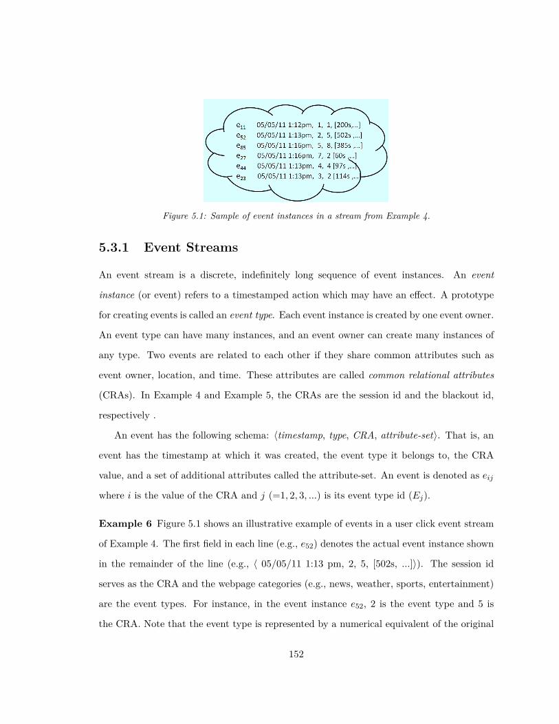
Figure 5.1: Sample of event instances in a stream from Example 4.

5.3.1 Event Streams

An event stream is a discrete, indefinitely long sequence of event instances. An event

instance (or event) refers to a timestamped action which may have an effect. A prototype

for creating events is called an event type. Each event instance is created by one event owner.

An event type can have many instances, and an event owner can create many instances of

any type. Two events are related to each other if they share common attributes such as

event owner, location, and time. These attributes are called common relational attributes

(CRAs). In Example 4 and Example 5, the CRAs are the session id and the blackout id,

respectively .

An event has the following schema: 〈timestamp, type, CRA, attribute-set〉. That is, an

event has the timestamp at which it was created, the event type it belongs to, the CRA

value, and a set of additional attributes called the attribute-set. An event is denoted as eij

where i is the value of the CRA and j (=1, 2, 3, ...) is its event type id (Ej).

Example 6 Figure 5.1 shows an illustrative example of events in a user click event stream

of Example 4. The first field in each line (e.g., e52) denotes the actual event instance shown

in the remainder of the line (e.g., 〈 05/05/11 1:13 pm, 2, 5, [502s, ...]〉). The session id

serves as the CRA and the webpage categories (e.g., news, weather, sports, entertainment)

are the event types. For instance, in the event instance e52, 2 is the event type and 5 is

the CRA. Note that the event type is represented by a numerical equivalent of the original

152

(a) Raw Event Stream.

(b) Partitioned Window.

(eijs are abbreviations of actual event instances such as shown in Figure 5.1.)

Figure 5.2: Event stream.

event type (e.g., news = 1, weather = 2, sports = 3, entertainment = 4).

We use a sliding window, specifically called partitioned window (Acharya and Lee, 2013),

to accumulate the events from the stream for a user-specified observation period T. As a

preprocessing step to cluster related events in the window, these events are partitioned

by the CRA and then arranged in temporal order in each partition. Figure 5.2 shows

what a partitioned window looks like for the event stream shown in Figure 5.1. Once the

observation period expires, the window slides to the next batch of events.

Definition 12 (Partition) A partition Wi in a partitioned window is defined as a set of

observed events sharing the same CRA value i and arranged in the temporal order over a

time period T , that is

Wi = {eij(t)|t ≤ T, i ∈ A, j ∈ [1, N ]}

where t is the timestamp, A is the set of all possible CRA values, j is the event type id,

and N is the number of event types.

5.3.2 Causal Networks

A causal network (or causal Bayesian network) is a directed acyclic graph G = (V, Ξ) to

encode causality, where V is the set of nodes (representing event types) and Ξ is the set of

153

Figure 5.3: Causal network.

edges between nodes. For each directed edge, the parent node denotes the cause, and the

child node denotes the effect.

The joint probability distribution of a set of N event types E ≡ {E1, ..., EN} in a causal

network is specified as

P (E) =N∏i=1

P (Ei|Pai)

where Pai is the set of the parent nodes of event type Ei.

Consider the event stream of Figure 5.2. The causal relationships among the event types

in the stream may be modeled as a causal network like the one shown in Figure 5.3.

5.3.3 Conditional Independence Tests

A popular approach for testing the conditional independence (CI) between two random

variables X and Y in a set of random variables, C, is conditional mutual information (CMI)

(e.g., (Cheng et al., 2002; de Campos, 2006)).

CMI(X,Y |C) =∑x∈X

∑y∈Y

∑c∈C

P (x, y, c)log2P (x, y|c)

P (x|c)P (y|c)

where P is the probability mass function calculated from the frequencies of variables. CMI

gives the strength of dependency between variables in a measurable quantity, which helps

to identify the weak (or spurious) causal relationships.

154

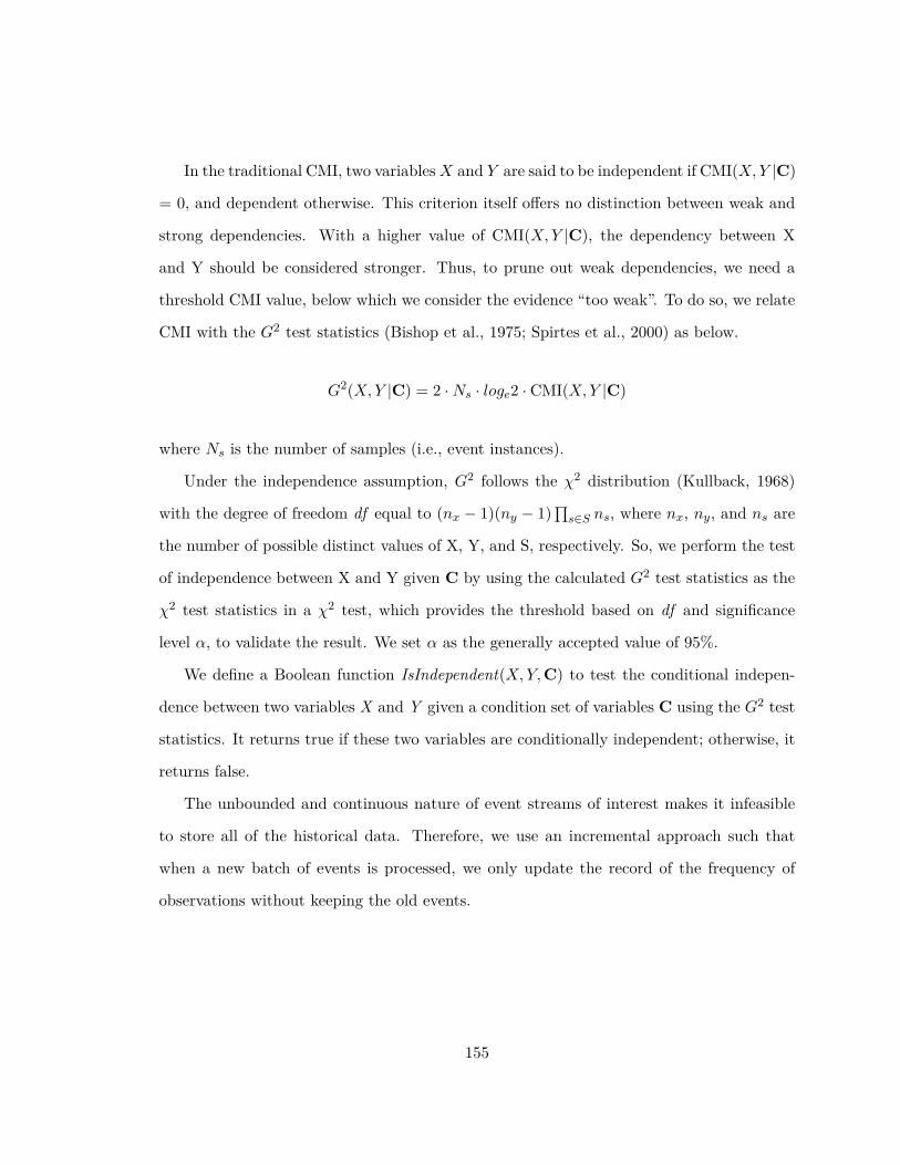
In the traditional CMI, two variablesX and Y are said to be independent if CMI(X,Y |C)

= 0, and dependent otherwise. This criterion itself offers no distinction between weak and

strong dependencies. With a higher value of CMI(X,Y |C), the dependency between X

and Y should be considered stronger. Thus, to prune out weak dependencies, we need a

threshold CMI value, below which we consider the evidence “too weak”. To do so, we relate

CMI with the G2 test statistics (Bishop et al., 1975; Spirtes et al., 2000) as below.

G2(X,Y |C) = 2 ·Ns · loge2 · CMI(X,Y |C)

where Ns is the number of samples (i.e., event instances).

Under the independence assumption, G2 follows the χ2 distribution (Kullback, 1968)

with the degree of freedom df equal to (nx − 1)(ny − 1)∏s∈S ns, where nx, ny, and ns are

the number of possible distinct values of X, Y, and S, respectively. So, we perform the test

of independence between X and Y given C by using the calculated G2 test statistics as the

χ2 test statistics in a χ2 test, which provides the threshold based on df and significance

level α, to validate the result. We set α as the generally accepted value of 95%.

We define a Boolean function IsIndependent(X,Y,C) to test the conditional indepen-

dence between two variables X and Y given a condition set of variables C using the G2 test

statistics. It returns true if these two variables are conditionally independent; otherwise, it

returns false.

The unbounded and continuous nature of event streams of interest makes it infeasible

to store all of the historical data. Therefore, we use an incremental approach such that

when a new batch of events is processed, we only update the record of the frequency of

observations without keeping the old events.

155

Symbols DefinitionsNp Number of partitionsNei Number of event instances in the i-th partitionNe Total number of event instances in all partitionsEi Event type with id ieij Event instance of type j and CRA iN Number of event typesCi Cause event type at position iTi Effect event type at position iO Causal search orderSi Event type at the i-th position in OCδ The most recent cause event typeE Set of N event types in the data {E1, E2, ..., EN}Rk Ranked list of the top-k event typesNinstances Number of event instancesNCRA Number of common relational attributesf(Ei, Ej) Number of observations of the instances of type Ei followed

by the instances of type Ej

Table 5.1: Definitions of main symbols.

5.4 Problem Formulation and Proposed Approach

In this section, we formulate the problem, identify the research issues and then propose a

framework to solve these issues. Table 5.1 summarizes the key notations used in this paper.

5.4.1 Problem Formulation

Causal prediction of the top k effects in an event stream presents two problems. First,

it requires inference of the causal relationships among event types, based on the events

observed thus far, at run time. Such an approach is necessary to adapt to an evolving

stream of events and to overcome the limited causal inference power (i.e., lack of support

for cyclic causality and causal information loss) of the traditional causal modeling methods.

Second, there is a need for an efficient and continuous query processing method to perform

only the necessary partial search over the possibly huge search space to predict the results.

156

The naive approach to determine the top most likely k event types by performing exhaustive

searching and sorting among all possible event types is inefficient in a real-time situation.

Based on the above facts, we derive from the top-k predictive query problem the following

three central research issues.

1. How can we model the relationships among events to avoid causal information loss

and to adapt to changes in event streams?

2. How can we address cyclic causality in the causal model?

3. How can we efficiently run a causal predictive query on this causal model to continu-

ously forecast the top-k probable effects?

In our work, the predictive query is a standing continuous query, so the ranked result

list may change every time a new event is observed. The events which are being predicted

are effect events while the events which are used for prediction are cause events. For clarity

in the rest of the paper, we denote the cause event type and the effect event type as Ci ∈ E

and Tj ∈ E, respectively, where i and j are the positions of the events in each sequence.

Note that Ci and Ei are not necessarily the same, and Tj and Ej are not, either.

Definition 13 (Top-K Predictive Query) Given a set of event types E = {E1, E2, ......}

and a set of observed events ϕe = {eij , eik, ......} such that

(∀k)eik.type ∈ E, the top-k predictive query Q(ϕe,E) is a conjunctive query that returns

the most probable k next event types paired with the top k highest scores, that is, returns

{(T1, S1), (T2, S2), ..., (Tk, Sk)} where Tj ∈ E (j = 1, 2, ..., k) is the event type in the j-th

position in the top-k results and Sj (j = 1, 2, ..., k) is the probabilistic score of Tj such that

S1 ≥ S2 ≥ .. ≥ Sk.

Given the uncertain nature of an event stream, a probabilistic scoring function is needed

for prediction. We now define the effect scoring function which gives a measure of how likely

the effect is to occur.

157

Definition 14 (Effect Scoring Function) Given a set of cause event types C = {C1, C2, ...., Cm},

we define the effect scoring function as the probability of the occurrence of an effect event

type, Ti, as follows.

P (Ti|C) = P (Ti,C)P (C)

where P is the probability mass function formulated from the frequencies of the instances of

the argument event types.

5.4.2 Proposed Approach

We propose a framework, illustrated in Figure 5.4, to address the three research issues

identified in Section 5.4.1.

First, we propose an event precedence model (EPM) (Section 5.5) to capture all the

precedence relationships between events in a cyclic network structure. (Note that the basic

requirement of the cause and effect relationship is the temporal precedence of cause over

effect (Popper, 1959).) This inclusion of all temporal precedence – hence, likely causal–

relationships help to avoid the causal information loss. EPM takes the partitioned window

(collected from the event stream) as an input and incrementally builds a model to reflect all

precedence relationships in the input data. The actual data is discarded once a new batch

of events arrives. Such an adaptive approach is essential for a streaming environment with

continuous and unbounded data.

Second, since the precedence relationship alone does not necessarily imply a casual

relationship, based on the EPM the causal inference is performed “on the fly” during query

processing (Section 5.6). Such a run-time causal inference mechanism is needed to handle

the cyclic causal relationships and to avoid the causal information loss. It is only after each

query run is finished that the set of relevant cause events, from which causal prediction is

done, is known and then the causal direction in a cyclic causality is selected based on the

cause events.

158

Event

Precedence

Model

Constructor

Runtime Causal

Inference

Top-K

Query Processor

Request

EPM

Send

EPM

Top-K Predictive Query Processing Engine

Query

Top k

effects

{(E1

, s1

),

(E2

, s2

),

…,

(Ek

, sk

)}

Event

stream

Figure 5.4: Top-k real-time causal prediction framework.

Third, we present two query processing algorithms – the Exhaustive Search algorithm

(Section 5.6.2) and the Reduced Search Early Termination algorithm (Section 5.6.3) – to

continuously predict the top k event types with the highest scores based on the inferred

causal relationships.

5.5 Event Precedence Model

In this section, we introduce a novel incremental mechanism to model the precedence rela-

tionships between events in a network structure.

5.5.1 Model

To overcome the limitations of the existing causal models described in Section 5.4.1, we

propose the event precedence model (EPM). It represents the temporal precedence relation-

ships in a graphical network structure, called event precedence network (EPN), over which

further analysis is done to predict the probable effect events based on the observed cause

events. Note that the temporal precedence is a required criterion of a causal relationship.

To avoid any information loss, evidence of the precedence between every two events in the

stream is preserved.

We make the following assumptions in the event precedence model.

159

• Given an ordered sequence of cause event types {C0,

C1, ...., Cδ}, an instance of the effect event type T0 can not occur without the oc-

currence of an instance of the most recent cause event type Cδ. Moreover, while

all past events influence the future events, the strongest influence is exerted by the

immediately preceding event of the effect event. With this in mind, the precedence

relationships only between every two consecutive events are considered.

• There can not be a causal relationship between events of the same type and, therefore,

such precedence relationships are ignored.

• The cause and effect events should share the same CRA value. As described in

Section 5.3.1, the events are grouped into partitions based on their CRA values (e.g.,

session id and blackout id in Examples 4 and 5, respectively). In other words, two

events are not related to each other if they have different CRA values.

The proposed EPM is a first order absorbing Markov chain (Kemeny and Snell, 1969)

where an observation is independent of all previous observations except the most recent one

and every state can reach an absorbing (a.k.a., terminating) state. Thus, the probability of

occurrence of an effect event given past cause events is given as follows.

P (T0|C0, C1, ..., Cδ) = P (T0|Cδ).

This can be further written as below.

P (T0|Cδ) = P (T0, Cδ)P (Cδ)

(5.1)

which can be estimated as

P (T0, Cδ)P (Cδ)

≡ f(T0, Cδ)∑Ej∈children(Cδ) f(Ej , Cδ)

(5.2)

160

where f(Ei, Ej) denotes the number of observations in which instances of the type Ei

precedes instances of the type Ej .

In summary, EPM allows us to automatically build a tractable probabilistic graphical

model from the events, discovering the existing dependencies among the event types in the

event stream. These dependencies are represented by a graph, as illustrated in Figure 5.5(b),

where the conditional probabilities are stored at the node level.

Algorithm 12 Event Precedence ModelRequire: A partitioned window P for a batch of new events.

Observation:1: for each partition Wk ∈ P where k is the CRA value do2: for each pair of consecutive events (of type Ei and Ej such that i 6= j) in Wk do3: f(Ei, Ej)++ i.e., increase the observed frequency by 1;4: end for5: end for

Graph Generation:6: Construct an edgeless network G = (V,Ξ);7: for each pair of event types, Ei and Ej such that i 6= j, do8: if f(Ei, Ej) > 0 then9: Ξ← {Ξ ∪ {Ei → Ej}} i.e., add an edge Ei → Ej ;

10: P (Ej |Ei)← f(Ei,Ej)∑Ek∈children(Ei)

f(Ei,Ek) ;

11: else12: P (Ej |Ei)← 0;13: end if14: if f(Ej , Ei) > 0 then15: Ξ← {Ξ ∪ {Ej ← Ei}} i.e., add an edge Ej → Ei;16: P (Ei|Ej)← f(Ej ,Ei)∑

Ek∈children(Ej) f(Ej ,Ek) ;

17: else18: P (Ei|Ej)← 0;19: end if20: end for

161

5.5.2 Algorithm

Algorithm 12 outlines the event precedence network construction algorithm. It has three

steps: observation, graph generation, and evidence inscription. These steps are discussed

below.

1. Observation : This step observes the adjacent neighbor events in each partition of the

window to learn the precedence relationships. Note that, based on the assumptions

stated earlier, the precedence relationships should be between events in the same

partition and between events of different types. Suppose Ei and Ej are the event

types of two adjacent events. Then, their count f(Ei, Ej) is increased by 1.

2. Graph Generation : This step starts with an edgeless graph G = (V,Ξ) where V is

the set of nodes (event types) and Ξ is an empty set of edges. Then, for any evidence

of the precedence relationship between event types Ei and Ej (i.e., f(Ei, Ej) > 0), an

edge is added between the two nodes representing these event types. Note that the

graph supports anti-parallel edges between nodes; in addition, a cyclic loop of edges

is also supported. Thus, the graphical model offers the flexibility to incorporate all

possible types of relationships, unlike in the traditional systems where only directed

edges are supported. In addition, for every edge added in the graph, the probability

of an event type given its parent event type is calculated using Equation 5.2. The

calculated probabilities are then stored in the nodes.

Example 7 Let us illustrate Algorithm 12 considering the event stream shown in Fig-

ure 5.2. First, as explained earlier, the observation step counts the number of observations

of the precedence relationships between the types of consecutive events in every partition

of the partitioned window. These counts are reflected in a matrix form in Figure 5.5(a).

Second, for those pairs of event types whose precedence counts in Figure 5.5(a) are greater

than zero, we connect them with directed edges as shown in Figure 5.5(b). Clearly, the fig-

162

0 0 2 0 0 0 00 0 1 0 0 0 02 0 0 3 1 0 00 0 1 0 0 0 00 0 1 0 0 2 10 0 0 0 1 0 00 0 0 0 0 0 0

(a) Observation

(b) Graph Generation

0 0 1 0 0 0 00 0 0.50 0 0 0 0

0.333 0 0 0.50 0.167 0 00 0 1 0 0 0 00 0 0.25 0 0 0.50 0.250 0 0 0 1 0 00 0 0 0 0 0 0

(c) Probabilities of the edges

Figure 5.5: Illustration of event precedence network construction from the event stream inFigure 5.2.

ure shows that the precedence network supports cyclic relationships, thereby allowing cyclic

causality on further causal inference. In addition, the EPN encodes all possible evidences of

the precedence relationship, whether weak or strong. Therefore, the causal information loss

can be avoided in subsequent causal inference. The conditional probability of each node

in the network given its parent is calculated using Equation 5.2. The result is shown in a

matrix form in Figure 5.5(c).

163

5.5.3 Complexity Analysis

The running time complexity of the algorithm is polynomial with the total number of events

that have arrived thus far and the number of event types.

Runtime Analysis. The observation step counts every pair of consecutive events

in every partition of the window. Clearly, for each partition, the number of the counts is

always one less than the number of events in it. If Ne and Np are the number of events

and the number of partitions, respectively, then the running time complexity is given as

O(∑Np

i=1(Nei − 1))≈ O

(Ne), where Nei is the number of events in the i-th partition.

The graph generation phase checks for the evidence of the precedence relationships

between every pair of event types. In the worst case, the event precedence network is

completely connected (including cyclic edges and self referencing edges) and has N2 edges.

So, the running time complexity is given as O(N2). So, the running time complexity of this

step is proportional to N(N − 1) or O(N2).

Hence, the total running time is given as O(Ne)+ O

(N2) = O

(Ne +N2).

5.6 Top-K Predictive Query Processing

In this section, we first describe the predictive query processing model and then present

the two top-k continuous predictive query processing algorithms – Exhaustive Search (ES)

algorithm and the more efficient Reduced Search Early Termination (RSET) algorithm.

5.6.1 Predictive Query Processing Model

The predictive query processing problem can be formulated as a search problem to find

the possible effects of a given set of observed events in a causal network. However, the

traditional causal network cannot be used for query processing due to the causal information

loss and its lack of support for cyclic causality. To address this issue, since we already know

164

(a) E3 as EOP (b) E4 as EOP

Figure 5.6: Views from the EOPs for Figure 5.5(b).

that every causal relationship is always a temporal precedence relationship, we propose to

infer causality during query processing from the event precedence network to determine the

possible effects.

The idea is to explore the event precedence network (EPN), which represents all the

precedence relationships (including cyclic precedence relationships) among the event types,

to answer the predictive queries when evidence is available. Indeed, the effect events are

always the descendants of the cause events. Therefore, an outward breadth first search

on the EPN is required to find the effect events. In situations where a visited node is

encountered again, as EPN is cyclic, we ignore it. As discussed in Section 5.5, the next

effect events can not occur without the existence of the most recent cause event. Therefore,

the starting point for exploring the EPN is always the event type Cδ of the most recent

cause event. We call this event type the effect observation point (EOP). For instance, in

Figure 5.5(b), consider the two event types E3 and E4. E3 is the effect of E4 when E4 is

the EOP whereas E4 is the effect of E3 when E3 is the EOP, as illustrated in Figure 5.6.

However, there are two issues which make EPN not directly usable to answer a predictive

query. First, a precedence relationship is not necessarily a causal relationship. So, we

have to remove from the precedence relationships those that are not causal. Second, two

variables may have causal relationship in the absence of other variables, but may not exhibit

causality in the presence of certain condition variables. For example, rain and wet ground

are dependent variables, as rain causes wet ground. However, they are independent in the

presence of a roof over the ground (which is a conditional variable), as rain does not cause

165

wet ground, given the existence of a roof. Therefore, we test causal relationships to resolve

these issues during query processing for finding possible effects. To determine causality, the

conditional independence tests, as described in Section 5.3.3, are performed between two

event types with an edge in the EPN.

The ranking score of the predicted effect event type Ei, given a set of causal event

types C, is calculated as P (Ei|C) (Definition 14). Note that the conditional probability of

every child node given its parent node is recorded in the EPN. To calculate the scores in

our graphical model, we use the multiplicative property of the conditional probability (i.e.,

P (X|Z) = P (X|Y ) · P (Y |Z)), so that the score of a node can be computed based on the

score of its parents, as follows.

P (Ei|C) =∑

Ep∈Sparents(Ei)P (Ei|Ep)P (Ep|C) (5.3)

where Sparents(Ei) is the set of the parents of Ei.

Lemma 5.6.1 In a causal network G = (V,Ξ) constructed so far during query processing

at runtime, given a set of cause event types C, the ranking score of a parent node (Ep) is

never lower than that of its child node (Ec). i.e., P (Ec|C) ≤ P (Ep|C).

Proof 5.6.2 The proof is straightforward. From Equation 5.3, we know that

P (Ec|C) =∑

Ep∈Sparents(Ec)P (Ec|Ep)P (Ep|C)

where Sparents(Ec) is the set of the parents of Ec. As described earlier (Section 5.5.1), we

assume that the causal influence for an effect event type Ec is exerted only by its immediately

preceding event type Ep. Therefore, we obtain P (Ec|C) = P (Ec|Ep) · P (Ep|C). Since

P (Ec|Ep) ≤ 1 always holds, we further obtain P (Ec|C) ≤ P (Ep|C).

166

Score of Ej is P (Ej |Ei) ·P (Ei|C)+P (Ej |El) ·P (El|C). Note that El is ex-plored only after Ej . Therefore, P (El|C) is unknown during the calculationof Ej ’s score

Figure 5.7: Need for a causal search order.

5.6.2 Exhaustive Search Algorithm

5.6.2.1 Approach

The most straightforward solution to the top-k prediction problem is to search for all possible

effects exhaustively during the run-time causal inference over EPN and then sort them,

according to their scores, in non-increasing order to determine the k effects with the top

scores. We call this solution the Exhaustive Search (ES) approach.

The ES approach should have a robust strategy for exploring the EPN to infer effects.

As discussed earlier, an outward breadth first search may be run over the EPN for run-time

causal inference. However, the score calculation of the effects is a bit challenging. To apply

Equation 5.3, the scores of the parents of an event type should be known before its score

can be calculated, but it is not always possible as demonstrated in Figure 5.7. Therefore,

we define a search order, called causal search order, before exploring the EPN for run-time

causal inference.

Definition 15 (Causal Search Order). The causal search order O is an ordered set

of event types {S1, S2, ...., SN} observed during the outward breadth first search of the EPN

such that Si+j is never an ancestor of Si, where j > 0 and i+ j ≤ N .

167

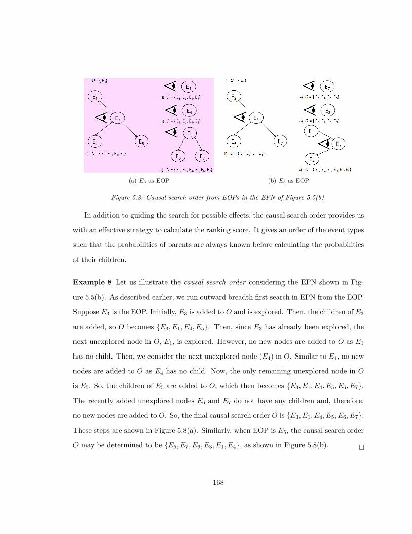
(a) E3 as EOP (b) E5 as EOP

Figure 5.8: Causal search order from EOPs in the EPN of Figure 5.5(b).

In addition to guiding the search for possible effects, the causal search order provides us

with an effective strategy to calculate the ranking score. It gives an order of the event types

such that the probabilities of parents are always known before calculating the probabilities

of their children.

Example 8 Let us illustrate the causal search order considering the EPN shown in Fig-

ure 5.5(b). As described earlier, we run outward breadth first search in EPN from the EOP.

Suppose E3 is the EOP. Initially, E3 is added to O and is explored. Then, the children of E3

are added, so O becomes {E3, E1, E4, E5}. Then, since E3 has already been explored, the

next unexplored node in O, E1, is explored. However, no new nodes are added to O as E1

has no child. Then, we consider the next unexplored node (E4) in O. Similar to E1, no new

nodes are added to O as E4 has no child. Now, the only remaining unexplored node in O

is E5. So, the children of E5 are added to O, which then becomes {E3, E1, E4, E5, E6, E7}.

The recently added unexplored nodes E6 and E7 do not have any children and, therefore,

no new nodes are added to O. So, the final causal search order O is {E3, E1, E4, E5, E6, E7}.

These steps are shown in Figure 5.8(a). Similarly, when EOP is E5, the causal search order

O may be determined to be {E5, E7, E6, E3, E1, E4}, as shown in Figure 5.8(b).

168

5.6.2.2 Algorithm

Algorithm 13 outlines the ES algorithm. The input to the algorithm is the size of the result

k, the event precedence network G, and the set of the recently observed δ cause event types

arranged in temporal order {C1, C2, ...., Cδ}.

The four main steps of the algorithm are given as follows.

1. First, an outward breadth first search over G from EOP (the most recent cause event

type Cδ) is run to determine the causal search order O. Line 1 shows this step.

2. Second, the marginal independence tests (i.e., CI tests with an empty condition set

φ) are performed between the event types during the search to remove any weak

relationships (lines 2- 7).

3. Third, G is searched to find the effects of every unexplored node Ej based on the

ordering of the event types in O. Lines 8 - 19 shows this step. The CI tests between

Ej and each of its parents are performed as only the parents of Ej can have effect

on it. These tests are required to make sure that the event types being considered

are not independent in the presence of other event types. In case of independence

between Ej and its parent, the edge representing their precedence relationship in G

is removed. Lines 9 - 16 shows this step.

Then, the score of the node Ej is calculated and stored, as shown in lines 17 and 18.

4. Finally, the ranking scores of all event types explored in non-increasing order are

sorted and then the k event types with the top scores are selected (line 20).

Example 9 Let us illustrate the ES algorithm considering the EPN shown in Figure 5.5(b).

Suppose C is {E2, E3} and k is 2.

1. First, the causal search order O, from the EOP (i.e., E3), is determined as {E3, E1,

E4, E5, E6, E7}.

169

Algorithm 13 ES AlgorithmRequire: A temporally ordered set of recently observed δ cause event types S ={C1, C2, ...., Cδ}, the size of the result k, an empty buffer BT to store the effect eventtypes and their scores, and the event precedence network G = (V,Ξ).

1: Determine causal search order, O, with the outward breadth first search in G from theEOP (Cδ).

2: for every edge Ei → Ej ∈ Ξ do3: isIndependent ← IsIndependent(Ei, Ej , φ));4: if isIndependent is true then5: Ξ← Ξ− {Ei → Ej} (//remove the weak relationship.)6: end if7: end for8: for every node Ej ∈ (O − Cδ) do9: Sparents ← parents of Ej ;

10: for every parent node Ei ∈ Sparents do11: isIndependent ← ICMI(Ei, Ej , Sparents − {Ei})12: if isIndependent is true then13: Ξ← Ξ− {Ei → Ej};14: Sparents ← Sparents − {Ei};15: end if16: end for17: P (Ej |C)←

∑Ep∈Sparents P (Ej |Ep)P (Ep|C);

18: Insert the pair (Ej , P (Ej |C)) into BT ;19: end for20: Sort the nodes in BT in the non-increasing order of the score and return the top k

results from BT .

2. Then, the marginal independence tests are performed on each edge in EPN. For sim-

plicity in illustration, we assume that these tests fail to remove any edges.

3. Now, the score of each event type in O is calculated and stored into the buffer BT

based on their ordering in O.

(a) The score of the first unexplored event type E1 is calculated and updated in BT

as follows.

• Determine the parents of E1, Sparents = {E3}

• Perform CI tests between every parent of E1 (i.e., Sparents) and E1. Suppose

the CI test succeeds, and thus no edge is removed.

170

• Calculate the score of E1: P (E1|C) = P (E1|E3) · P (E3|C) = 0.333.

• Update BT as {(E1, 0.333)}.

(b) The score of the next unexplored event type E4 is calculated similarly as above,

and BT is updated to {(E1, 0.333), (E4, 0.50)}.

(c) Following the same step as above, BT is updated to {(E1, 0.333), (E4,

0.50), (E5, 0.167)} for the next event type E5.

(d) Next, BT is updated to {(E1, 0.333), (E4, 0.50), (E5, 0.167), (E6, 0.0835)} for the

event type E6.

(e) BT is updated to {(E1, 0.333), (E4, 0.50), (E5, 0.167), (E6, 0.0835),

(E7, 0)} for the event type E7. Note that the score P (E7|C) of E7 is assigned

as zero. For the parent event type E5, the probability of its child E7 is much

lower (half) than the probability of its other child E6. Thus, for this illustration,

we assume the CI test between E7 and E5 fails. Consequently, there is no edge

between them.

4. Finally, BT is sorted in non-increasing order of the score as {(E4, 0.50), (E1,

0.333), (E5, 0.167), (E6, 0.0835), (E7, 0)}. Then, the top-2 predicted next event types

are selected from BT as {(E4, 0.50), (E1, 0.333)}.

5.6.3 Reduced Search Early Termination Algorithm

5.6.3.1 Approach

The ES algorithm searches exhaustively in the EPN during query processing to determine

the top-k results and, therefore, may well be slow. Naturally there is a need for an alternative

method that is faster. There are two issues to deal with for that purpose.

171

1. Running time : With the exhaustive search of ES on EPN to find all possible results,

the search space increases with the number of variables and it performs unnecessary

computations. A good query processing method should avoid redundant and unnec-

essary computations to reduce the running time.

2. Accuracy : Usually, the tradeoff for reducing running time is the loss in the accuracy

of the results. The running time is decreased by reducing the search space, which

may skip the correct effect events. The query processing method should avoid such

an incident as much as possible.

To achieve faster running time while predicting accurate and consistent results, we

propose a new algorithm called the Reduced Search Early Termination (RSET) algorithm

with the following strategies.

1. To reduce the running time. There are two ideas to reduce the running time. First, we

reduce the search space by exploring only the descendants of the nodes in the current

top-k during query execution. The nodes not in the top-k or their descendants, due

to Lemma 5.6.1, have lower scores, thereby disqualified from being top k candidates.

Second, we use a priority-based breadth-first search with an early termination criterion

such that the query execution is stopped as soon as it is certain that the top k

results have been found. The priority-based breadth-first search always chooses the

unexplored descendant node with the highest score to explore its children. The early

termination criterion is met if there is no change in the list of event types in the top-k;

that means, there is no more descendant node whose score can be greater than those

in the current top-k. Consequently, the search space is only partially explored. For

this reason, even though the causal inference is done at runtime, it incurs only a small

overhead.

2. To predict accurate results. In an effort to achieve the same level of accuracy as the

172

exhaustive search, we employ two strategies. First, we utilize the evidence from all

explored nodes to calculate the ranking score. Second, we perform the breadth-first

search of the EPN in such a way that the events with greater score are processed

earlier. It is worth noting that the ancestors always have higher or the same (in the

worst condition) score as their descendants (see Lemma 5.6.1).

5.6.3.2 Algorithm

Algorithm 14 outlines the RSET algorithm and can be described as follows.

1. First, two empty buffers, BC and Bk, are created to store the event types explored

during query processing and the top k effect event types computed, respectively. Bk

can hold maximum k event types. Line 1 states this step.

2. Second, we add the EOP , Cδ, with 1 as its score to both these buffers. Cδ has the

probability of 1 since the event type has already been observed. Line 2 states this

step.

3. Then, the algorithm employs the following strategies to (a) reduce the search space,

(b) predict accurate results, and (c) terminate as early as possible.

• To reduce the search space. Two ideas are employed to reduce the search

space. First, it explores only the children of EOP or the event types in the buffer

Bk for further computation. Line 3 reflects this strategy. For any event type

Ec not in Bk (i.e., top-k ), Ec and its descendants are ignored, thus reducing

the search space. Lemma 5.6.1 ensures that the probabilities of the children of

Ec remain much lower than that of Ec, or equal even in the (rare) best case.

Second, the buffer Bk is always sorted in non-increasing order of the score after

a new event type is added to it (lines 18–19 and 23–24). So, the priority for

network exploration is always given to the unvisited node with the highest score.

173

This means that we consider the fact that its children might have higher ranking

scores than the unvisited nodes already in Bk. Consequently, the nodes with

the lowest probability (Elowest) in Bk can be removed if Bk is full, which further

reduces the search space. Lines 3 and 23 reflect this mechanism.

• To predict accurate results. It keeps in Bc the record of all event types

visited. Basically, the event types in EPN are explored in the breadth-first search.

Therefore, the parents of a node have already been explored by the time the

algorithm considers the child node. While doing so, the causal relationships are

tested in lines 7 – 14. Although the first strategy above reduces the search space,

the algorithm still keeps all ancestors in Bc by recording all visited nodes so far.

Due to this search strategy, only the nodes with lower scores are not visited.

So, the ranking score calculation is not affected by the reduced search space.

Consequently, the accuracy of prediction result is not degraded. Lines 7, 15, and

16 make use of this strategy.

• To terminate as early as possible. An early termination is possible if there

is no change in the list of event types in Bk after exploring their children. It

means, due to Lemma 5.6.1, there are no more event types further down the

current level of exploration that can have higher probability than those already

in Bk. Checking only unvisited nodes in line 3 reflects this strategy.

Example 10 Let us illustrate the RSET algorithm considering the EPN shown in Fig-

ure 5.5(b). Suppose C is {E2, E3} and k is 2.

1. First, two empty buffers BC and Bk are created to store all the event types explored

so far and to store the current top k predicted event types, respectively.

2. Then, the search starts with the EOP (E3) and updates BC to {(E3, 1)}.

174

Algorithm 14 RSET AlgorithmRequire: A temporally ordered set of recently observed δ cause event types C ={C1, C2, ....., Cδ}, the size of the result k, and event precedence network G = (V,Ξ).

1: BC ← {}, Bk ← {} i.e., create two buffers BC and Bk;2: BC ← BC ∪ {(Cδ, 1)};3: for every unvisited node Ec ∈ ({Cδ}∪ (set of event types in Bk)) with the highest score

do4: Mark Ec as visited.5: Schildren ← children of Ec;6: for each node Ej ∈ Schildren do7: “Visited” parents Sparents ← (set of parents of Ej) ∩BC ;8: for every node Ei ∈ Sparents do9: isIndependent ← ICMI(Ei, Ej , Sparents − {Ei})

10: if isIndependent is true then11: Ξ← Ξ− {Ei → Ej};12: Sparents ← Sparents − {Ei};13: end if14: end for15: P (Ej |C)←

∑Ep∈Sparents P (Ej |Ep)P (Ep|C);

16: BC ← BC ∪ {(Ej , P (Ej |C))};17: if |Bk| ≤ k then18: Bk ← Bk ∪ {(Ej , P (Ej |C))};19: Sort the event types in Bk in non-increasing order of their scores;20: else21: Find the entry with the lowest score, (Elowest, Plowest), in Bk.22: if P (Ej |C) > the lowest value in Bk then23: Bk ← (Bk − {(Elowest, Plowest)}) ∪ {(Ej , P (Ej |C))};24: Sort the event types in Bk in non-increasing order of their scores;25: end if26: end if27: end for28: end for

3. Now, every unvisited event type is explored as follows. For simplicity in illustration,

we assume that the CI tests return false and hence the edges are not removed.

(a) The first unvisited event type, E3, is marked as visited and its children, Schildren

(= {E1, E4, E5}), are explored.

i. The score of the first unexplored child, E1, is calculated and added to the

175

two buffers as follows.

• Determine the parents of E1; Sparents i set to {E3}.

• Perform CI test of the edge between E1 and E3 given Sparents.

• Calculate the score of E1 as P (E1|C) = P (E1|E3)P (E3|C) = 0.333.

• Update BC to {(E3, 1), (E1, 0.333)}.

• Update and sort Bk to {(E1, 0.333)}.

ii. The same steps as above are followed for the next unexplored child E4. The

two buffers BC and Bk are updated to {(E3, 1), (E1,

0.333), (E4, 0.50)} and {(E4, 0.50), (E1, 0.333)}, respectively.

iii. BC and Bk are updated to {(E3, 1), (E1, 0.333),

(E4, 0.50), (E5, 0.167)} and {(E4, 0.50),

(E1, 0.333)}, respectively, for the next unexplored child E5.

(b) Now, the next unvisited event type, E4 in Bk, is marked as visited and its

children are explored. However, there are no child of E4, i.e., Schildren is empty.

Therefore, there is no computation to be performed.

(c) The same result is seen for the next event type, E1, as well. As it has no child

(i.e., Schildren is empty), there is no computation to be performed.

4. The top-k result in Bk is obtained as {(E4, 0.50),

(E1, 0.333)}.

For the same C, the RSET algorithm considered only four event types – E3, E1, E4,

E5 and the ES algorithm considered all event types – E3, E1, E4, E5, E6, E7. Note that in

this example, RSET produced the same result (i.e., Bk = {(E4, 0.50),

(E1, 0.333)}) as ES (which is typical unless the value of k is significantly large). It shows

the merit of the early terminating reduced search approach of the RSET algorithm against

the exhaustive search approach of the ES algorithm.

176

5.7 Performance Evaluation

We conduct experiments to evaluate the run-time causal inference model and the top-k

query processing mechanism in the proposed RSET algorithm and the ES algorithm. One

evaluation is with respect to the accuracy of the top-k results, and the other evaluation

is with respect to the runtime. Section 5.7.1 describes the experiment setup, including

the evaluation metrics, datasets and the platform used, and Section 5.7.2 presents the

experiment results.

5.7.1 Experiment Setup

5.7.1.1 Evaluation Metrics

Intuitively, the performances of the top-k query processing algorithms are best evaluated by

examining two important evaluation criteria – accuracy and runtime.

1. Accuracy. Suppose Rk is the ranked list of the top k effects predicted from the set

of cause event types, C, observed so far in the test sequence. To measure accuracy,

the next event type observed in the test sequence, Eo (o ∈ [1, N ]), is checked against

the predicted ranked list Rk. If Eo exists in Rk, we say the prediction is correct (hit);

otherwise we say the prediction is incorrect (miss).

There are two methods for deciding the correctness of a top-k predicted result. First,

in some scenarios, a hit may be a sufficient condition for correctness. In such a case,

we say the accuracy is 100% for a hit and 0% for a miss. We call this perspective

hit-or-miss (non-weighted). Second, in other scenarios, the rank of the predicted

result may also play an important role in determining the accuracy. Clearly, if the

algorithm predicts Eo as the most likely effect (i.e., at the top of Rk with the highest

probability), then the accuracy is 100%. As we go down the list in Rk, the accuracy

177

decreases. Therefore, to reflect this point, we take the probability of each event in Rk

into consideration when calculating the prediction accuracy. We call this perspective

weighted.

Hit-or-miss accuracy. Let nhits and nmisses be the number of hits and the number

of misses, respectively out of ntests tests. Then, the hit-or-miss accuracy of the result,

αhm, is calculated as follows.

αhm = nhitsntests

= nhitsnhits + nmisses

(5.4)

Weighted accuracy. Suppose P (Eo) is the score of Eo in Rk. As discussed

earlier, the rank of Eo in Rk contributes towards the calculation of the prediction

accuracy. The rank is based on the score; therefore, we normalize the score such that

the prediction accuracy decreases gradually with the decrease in the rank of Eo in Rk.

The accuracy of Eo, in the case of a miss, is 0% whereas the accuracy of Eo, in the

case of a hit, is P (Eo)max{P (Ej)|Ej∈Rk} , where the denominator is the highest probability

among all event types in Rk. (Note that this measure gives the top event type the

accuracy of 100%.)

Let nhits and nmisses be the same as above. Then, the weighted accuracy of the result,

αweighted, is computed as follows.

αweighted =

∑ntestsi=1

P (Eoi )max{P (Eji )|Eji∈Rki}

ntests

where Eoi is the i-th observed event type in the test data.

As mentioned earlier, the accuracy of a miss is 0%. Therefore, we can consider only

178

Dataset N Ninstances CRA NCRAMSNBC 17 4698795 session id 989818

Power grid 565 94339 blackout id 4492(NCRA is the number of different CRA values. Ninstances is the number of event instances in the

dataset.)

Table 5.2: Profiles of the datasets.

the hits in the numerator.

αweighted =

∑nhitsh=1

P (Eoh)max{P (Ejh )|Ejh∈Rkh}

nhits + nmisses(5.5)

where Eoh is the h-th observed event type which has the result hit in the test data.

2. Runtime. The runtime is the CPU time taken during query processing. Note

that the event precedence network construction is not part of the query processing

mechanism. Therefore, we do not include it in the measurement of the runtime. In

the query processing with the RSET algorithm and the ES algorithm, there is an

overhead of run-time causal inference and it is included in the runtime. In contrast,

the query processing with the traditional causal inference (i.e., FCNI algorithm) does

not include the causal network construction time in the runtime as the causal infer-

ence is performed only once (during the causal network construction) prior to query

processing. In our work, latency is the interval between the arrival of a new event and

the identification of its top k effect events. However, as the time for EPN update is

insignificant (see the polynomial runtime in Section 5.5.3) compared to the time for

query processing (which is exponential), latency is essentially the query processing

time.

5.7.1.2 Datasets

Experiments are conducted using two real-world datasets (summary in Table 5.2) to evaluate

the proposed algorithms.

179

5.7.1.2.1 Electric power grid dataset. This dataset contains simulated temporal

sequences of cascading electric power grid component outages, such as those that can lead

to very large blackouts (e.g., (US-Canada Power System Outage Task Force, 2004)). The

sequences were generated using a model of the Polish power network, which is described

in (Eppstein and Hines, 2012). Each sequence represents the order in which the components

failed, as well as the time of the failure. Each grid component is considered an event type,

whereas a component failure is an event instance. This dataset includes 4492 cascade

sequences and 565 distinct event types.

In the original dataset, each file, representing one blackout, has a list of the components

that failed in that blackout. The original schema of the power grid data is as follows: 〈event

indicator, timestamp, component id〉. The event indicator can be one of 0, 1, and -1, which

refer to an initiating event, a dependent event, and a stop event, respectively. There is

always at least one initiating event at the beginning of each component failure sequence

(with 0 as its starting time). Since these events are always at the beginning of the sequence,

there is no inward edge towards them in the event precedence network. A dependent event

is the result of the initiating event or another dependent event. A blackout sequence always

has at least one dependent event. We treat both an initiating event and a dependent event

in the same way. On the other hand, a stop event denotes the end of the blackout and is

not a real event. Therefore, we ignore stop events. The timestamp and the component id

are respectively the starting time of an event and the attribute that uniquely identifies a

grid component.

To create an event stream, we modify the schema and randomly mix the data from the

files while preserving the temporal order of the component failures in each blackout. The

modified schema, 〈timestamp, component id, blackout id, event indicator〉, has an additional

tag blackout id to identify the blackout to which the component failure belongs to. So, the

blackout id is the CRA in the power grid dataset.

180

5.7.1.2.2 MSNBC.com web dataset. This dataset consists of click-stream data of

989818 sequences obtained from the UCI repository. Each sequence reflects the browsing

activities, arranged in temporal order, in one user session. The dataset gives a random

sample of the length of visits of users browsing the msnbc.com web site on the whole day

of September 28, 1999. The length of the visit is an estimate of the total number of clicks

or pages seen by each user and is based on the “Internet Information Server (IIS) logs for

msnbc.com and news-related portions of msn.com” (Heckerman, 1999). A webpage category

is an event type, and a webpage visit is an event instance. The session id of the visit is the

CRA for its event instance.

The number of distinct event types is 17. That is, a sequence can have web activities

related to 17 different webpage categories. These event types (i.e., webpage categories)

are frontpage, news, technology, local, opinion, on-air, miscellaneous, weather, msn-news,

health, living, business, msn-sports, sports, summary, bbs, and travel. The total number of

event instances (i.e., page visits) is 4698795.

To create an event stream, we randomly mix the events while preserving the temporal

order of the events for each session. The schema of the events is 〈timestamp, webpage

category, session id, Φ〉, where Φ denotes an empty attribute set.

5.7.1.3 Experiment Platform

The experiments are conducted on a 2.3 GHz Intel Core i5 machine with 4GB of memory,

running Windows 7. The algorithms are implemented in Java 1.7.0.

5.7.2 Experiment Results

We perform two sets of experiments to evaluate the RSET and ES algorithms. One set of

experiments is to evaluate the prediction accuracy, and the other set of experiments is to

evaluate the runtime. There are two objectives in each set of experiments. The first objective

181

is to compare the query processing with the run-time causal inference mechanism (of RSET

and ES) against the query processing with the traditional causal inference mechanism (of the

FCNI algorithm). For a fair comparison, as the goal is only to compare the causal inference

mechanisms, the query processing mechanism of either RSET algorithm or ES algorithm can

be used in the FCNI algorithm, and, in this experiment, we choose the RSET algorithm.

The second objective is to compare the query processing mechanism between the RSET

algorithm and the ES algorithm. In addition, the effects of k on the proposed algorithms

are studied in each set of experiments.

We randomly divide each dataset into 70% and 30% for training and testing the proposed

algorithms, respectively. From the training dataset, EPN is constructed as an input to the

RSET and ES algorithms, whereas a causal network is constructed as an input to the FCNI

algorithm. The testing data simulates event stream. As soon as a new event arrives, it is

added to the partitioned window. Then, the top-k prediction query execution is triggered

in response to the most recent event at position δ (called the EOP index) in the sequence of

cause events in the same partition. Note that the RSET and ES algorithms perform query

processing over the EPN whereas the FCNI algorithm does so over the causal network.

Upon the arrival of a new event, the measurements of prediction accuracy and runtime are

repeated and the calculated average accuracy and average runtime are reported.

5.7.2.1 Accuracy

Figures 5.9 and 5.10, respectively, show the hit-or-miss and the weighted accuracies for the

MSNBC dataset and Figures 5.11 and 5.12 show them for the power grid dataset. In these

figures, the accuracies of the RSET algorithm, the ES algorithm, and the FCNI algorithm

are compared for different values of the EOP index (δ) over the sequence of events in the

condition set. In addition, Figures 5.13 and 5.14 show the average hit-or-miss and weighted

accuracies for different values of k in the MSNBC dataset and the power grid dataset,

182

0

0.2

0.4

0.6

0.8

1

0 5 10 15 20 25 30

Acc

urac

y

δ

RSETES

FCNI

(a) k =1

0

0.2

0.4

0.6

0.8

1

0 5 10 15 20 25 30

Acc

urac

y

δ

RSETES

FCNI

(b) k = 3

0

0.2

0.4

0.6

0.8

1

0 5 10 15 20 25 30

Acc

urac

y

δ

RSETES

FCNI

(c) k = 5

0

0.2

0.4

0.6

0.8

1

0 5 10 15 20 25 30A

ccur

acy

δ

RSETES

FCNI

(d) k = 7

0

0.2

0.4

0.6

0.8

1

0 5 10 15 20 25 30

Acc

urac

y

δ

RSETES

FCNI

(e) k = 9

Figure 5.9: Hit-or-miss accuracies of the RSET, ES, and FCNI algorithms w.r.t EOP index (δ) forMSNBC dataset. (Note that the EOP index δ is the position of the most recent event in the

sequence of cause events in the same partition.)

respectively.

As expected, for all cases, the hit-or-miss accuracy is never lower than the weighted

accuracy. Clearly, a hit in the hit-or-miss accuracy always receives the score of 1 while a

hit in the weighted accuracy receives a score lower than 1 unless the observed event type

in the test data has the highest score in the ranked list. When k is one, the size of the

183

0

0.2

0.4

0.6

0.8

1

0 5 10 15 20 25 30

Acc

urac

y

δ

RSETES

FCNI

(a) k =1

0

0.2

0.4

0.6

0.8

1

0 5 10 15 20 25 30

Acc

urac

y

δ

RSETES

FCNI

(b) k = 3

0

0.2

0.4

0.6

0.8

1

0 5 10 15 20 25 30

Acc

urac

y

δ

RSETES

FCNI

(c) k = 5

0

0.2

0.4

0.6

0.8

1

0 5 10 15 20 25 30A

ccur

acy

δ

RSETES

FCNI

(d) k = 7

0

0.2

0.4

0.6

0.8

1

0 5 10 15 20 25 30

Acc

urac

y

δ

RSETES

FCNI

(e) k = 9

Figure 5.10: Weighted accuracies of the RSET, ES, and FCNI algorithms w.r.t EOP index (δ) forMSNBC dataset.

result ranked list is one, hence Equation 5.5 reduces to Equation 5.4, and therefore the two

accuracy measures give the same value.

Comparison of the causal inference mechanisms

All results show that the prediction accuracies of both ES and RSET algorithms are sig-

nificantly higher than that of the FCNI algorithm at every EOP index (δ). This difference

184

0

0.2

0.4

0.6

0.8

1

0 5 10 15 20 25 30

Acc

urac

y

δ

RSETES

FCNI

(a) k =1

0

0.2

0.4

0.6

0.8

1

0 5 10 15 20 25 30

Acc

urac

y

δ

RSETES

FCNI

(b) k = 5

0

0.2

0.4

0.6

0.8

1

0 5 10 15 20 25 30

Acc

urac

y

δ

RSETES

FCNI

(c) k = 10

0

0.2

0.4

0.6

0.8

1

0 5 10 15 20 25 30A

ccur

acy

δ

RSETES

FCNI

(d) k = 15

0

0.2

0.4

0.6

0.8

1

0 5 10 15 20 25 30

Acc

urac

y

δ

RSETES

FCNI

(e) k = 20

Figure 5.11: Hit-or-miss accuracies of the RSET, ES, and FCNI algorithms w.r.t EOP index (δ)for the power grid dataset.

in accuracy comes from the difference in their causal models. (Recall that for fairness the

FCNI algorithm uses the same query processing mechanism used in the RSET algorithm.)

Thus, it confirms the expectation that the traditional causal model (of the FCNI algorithm)

is so limited due to its lack of support for cyclic causality and the loss of causal information

that the prediction accuracy is compromised significantly. On the other hand, the RSET

and ES algorithms both use run-time causal inference which can handle cyclic causality and

185

0

0.2

0.4

0.6

0.8

1

0 5 10 15 20 25 30

Acc

urac

y

δ

RSETES

FCNI

(a) k =1

0

0.2

0.4

0.6

0.8

1

0 5 10 15 20 25 30

Acc

urac

y

δ

RSETES

FCNI

(b) k = 5

0

0.2

0.4

0.6

0.8

1

0 5 10 15 20 25 30

Acc

urac

y

δ

RSETES

FCNI

(c) k = 10

0

0.2

0.4

0.6

0.8

1

0 5 10 15 20 25 30A

ccur

acy

δ

RSETES

FCNI

(d) k = 15

0

0.2

0.4

0.6

0.8

1

0 5 10 15 20 25 30

Acc

urac

y

δ

RSETES

FCNI

(e) k = 20

Figure 5.12: Weighted accuracies of the RSET, ES, and FCNI algorithms w.r.t EOP index (δ) forthe power grid dataset.

causal information loss, thereby achieving higher prediction accuracies.

The results also show that the accuracy of all three algorithms increases with the increase

of k. The reason for this is that more event types are considered as the probable next

effects. Moreover, the accuracy in the ES and the RSET algorithms is always higher than

in the FCNI algorithm. This indicates that the deficiencies of the FCNI algorithm (i.e.,

acyclic causality and causal information loss) leads to excluding many important causal

186

0

0.2

0.4

0.6

0.8

1

1 3 5 7 9

Acc

urac

y

k

RSETES

FCNI

(a) hit-or-miss

0

0.2

0.4

0.6

0.8

1

1 3 5 7 9

Acc

urac

y

k

RSETES

FCNI

(b) weighted

Figure 5.13: Accuracies of the RSET, ES, and FCNI algorithms w.r.t k for MSNBC dataset.

0

0.2

0.4

0.6

0.8

1

1 5 10 15 20

Acc

urac

y

k

RSETES

FCNI

(a) hit-or-miss

0

0.2

0.4

0.6

0.8

1

1 5 10 15 20

Acc

urac

y

k

RSETES

FCNI

(b) weighted

Figure 5.14: Accuracies of the RSET, ES, and FCNI algorithms w.r.t k for the power grid dataset.

relationships and, as a result, the accuracy is always much lower than that of the ES and

the RSET algorithms regardless of the value of k.

Comparison of the query processing mechanisms

Three observations are made from the results. First, all results show that the prediction

accuracy of the ES algorithm is always higher than that of the RSET algorithm. This is

evident from the fact that the ES algorithm performs an exhaustive search whereas the

RSET algorithm performs only a partial search.

Second, the accuracy of the RSET algorithm is more comparable to that of the ES

algorithm in the power grid dataset than in the MSNBC dataset. This can be explained

187

as follows. When the ratio of k to N is larger, both algorithms have higher probabilities

of making correct predictions but the gap between their accuracies is larger because ES

performs exhaustive search while RSET performs partial. Note that k/N is smaller in the

power grid dataset (the largest k/N considered is 0.035) than in the MSNBC dataset (the

largest k/N considered is 0.53), and therefore the gap is smaller for the power grid dataset.

Third, as discussed earlier, as the value of k increases, the accuracies of all three al-

gorithms increase. Here we add further evaluation on the ES algorithm and the RSET

algorithm with a focus on their search mechanisms. As k increases, the search space of

the RSET algorithm increases, leading to a higher gain in the accuracy. In the case of the

ES algorithm, the search space remains constant regardless of k, but the number of candi-

date effects from which the highest k is selected increases and, consequently, the accuracy

still increases. Intuitively, the rate of increase in the accuracy is higher for the hit-or-miss

accuracy metric than the weighted accuracy metric in both algorithms.

5.7.2.2 Runtime

In this experiment, we compare the runtime among the three algorithms (RSET, ES, FCNI).

In addition, we analyze the effects of k on the runtime.

Figures 5.15 and 5.16 show the runtime for the MSNBC dataset and the power grid

dataset, respectively. In these figures, the runtime of the three algorithms are compared

for different values of the EOP index (δ) over the sequence of events in the condition set.

In addition, Figure 5.17 shows the runtime for different values of k in the MSNBC and the

power grid datasets.

Comparison of the causal inference mechanisms.

The results show that the runtimes of the RSET and ES algorithms are longer than that of

the FCNI algorithm at every EOP index for every value of k. As discussed in Section 5.6.3,

the RSET and ES algorithms have an overhead of the run-time causal inference during

188

0

0.5

1

1.5

2

2.5

3

3.5

4

0 5 10 15 20 25 30

Run

time

(mse

c)

δ

RSETES

FCNI

(a) k =1

0

0.5

1

1.5

2

2.5

3

3.5

4

0 5 10 15 20 25 30

Run

time

(mse

c)

δ

RSETES

FCNI

(b) k = 3

0

0.5

1

1.5

2

2.5

3

3.5

4

0 5 10 15 20 25 30

Run

time

(mse

c)

δ

RSETES

FCNI

(c) k = 5

0

0.5

1

1.5

2

2.5

3

3.5

4

0 5 10 15 20 25 30R

untim

e (m

sec)

δ

RSETES

FCNI

(d) k = 7

0

0.5

1

1.5

2

2.5

3

3.5

4

0 5 10 15 20 25 30

Run

time

(mse

c)

δ

RSETES

FCNI

(e) k = 9

Figure 5.15: Runtime of the RSET, ES, and FCNI algorithms w.r.t EOP index (δ) for MSNBCdataset.

query processing while FCNI algorithm does not as it uses a pre-built causal network for

prediction. Therefore, the runtimes for the ES and RSET algorithms are always longer than

that of the FCNI algorithm. Interestingly, the runtimes of the three algorithms are longer

in the power grid dataset than the MSNBC dataset. This is due to a larger number of event

types (i.e., N) in the power grid dataset.

189

0

1000

2000

3000

4000

5000

6000

7000

0 5 10 15 20 25 30

Run

time

(mse

c)

δ

RSETES

FCNI

(a) k =1

0

1000

2000

3000

4000

5000

6000

7000

0 5 10 15 20 25 30

Run

time

(mse

c)

δ

RSETES

FCNI

(b) k = 5

0

1000

2000

3000

4000

5000

6000

7000

0 5 10 15 20 25 30

Run

time

(mse

c)

δ

RSETES

FCNI

(c) k = 10

0

1000

2000

3000

4000

5000

6000

7000

0 5 10 15 20 25 30R

untim

e (m

sec)

δ

RSETES

FCNI

(d) k = 15

0

1000

2000

3000

4000

5000

6000

7000

0 5 10 15 20 25 30

Run

time

(mse

c)

δ

RSETES

FCNI

(e) k = 20

Figure 5.16: Runtime of the RSET, ES, and FCNI algorithms w.r.t EOP index (δ) for the powergrid dataset.

Comparison of the query processing mechanisms.

The results suggest three observations. First, as expected, the runtime of the RSET algo-

rithm is always shorter than the ES algorithm. The main reason is in the differen search

scope (i.e., exhaustive in ES and partial in RSET) as discussed in Section 5.6. In addition,

there is an overhead in the ES algorithm, unlike the RSET algorithm, to calculate the causal

190

0

0.5

1

1.5

2

2.5

3

3.5

4

1 3 5 7 9

Run

time

(mse

c)

k

RSETES

FCNI

(a) MSNBC

0

1000

2000

3000

4000

5000

6000

7000

1 5 10 15 20

Run

time

(mse

c)

k

RSETES

FCNI

(b) Powergrid

Figure 5.17: Runtime of the RSET, ES, and FCNI algorithms w.r.t k.

search order.

Second, the runtime difference between the RSET algorithm and the ES algorithm is

smaller for the MSNBC dataset (Figure 5.15) than for the power grid dataset (Figure 5.16).

This is due to the larger network size (i.e., N) in the power grid dataset (than in the MSNBC

dataset). That is, a larger network size results in a larger search space (which is typical

over event streams) and thus requires longer runtime for query processing.

Third, the runtime of the ES algorithm does not change with an increase in k. The ES

algorithm always runs an exhaustive search, irrespective of the value of k, and uses k only

to filter out the top-k event types out of N event types at the end, which has insignificant

effect on the overall runtime. On the other hand, the runtime of the RSET algorithm does

increase with an increase in k. The search space covered by the RSET algorithm increases

with k, leading to the increased runtime.

5.7.2.3 Discussion of experiment results

The proposed run-time causal inference mechanism, in the RSET and ES algorithms, han-

dles the cyclic causality and avoids the causal information loss, and thus improves the

prediction accuracy significantly. The FCNI algorithm, on the other hand, performs worse

than both the RSET and ES algorithms as it cannot handle cyclic causality. The ratios

191

of the number of cycles over the number of edges in the EPN are 0.69 and 0.85 for the

power grid dataset and the MSNBC dataset, respectively. Intuitively, the accuracy of the

FCNI algorithm would suffer increasingly more as the number of cycles increases. Thus,

despite its reduced runtime, the FCNI algorithm is not suitable for top-k predictive query

processing over event streams.

The accuracy of the RSET algorithm is comparable to the accuracy of the ES algorithm.

Therefore, the RSET algorithm, as it is much faster than the ES algorithm, is more suitable

for real-time continuous top-k query processing over event streams whereas the ES algorithm

is more suitable when the time is of lesser importance.

Between the two datasets, the runtime for the power grid dataset is much longer than

the runtime for the MSNBC dataset. This is due to the difference in the numbers of event

types in these two datasets. That is, the much larger number of event types in the power

grid dataset leads to much more conditional independence tests during the run-time causal

inference, thus resulting in slower query execution. In our work, the runtime measurements

were made on a low-end laptop. The use of a more powerful computational setup (e.g.,

parallel processing) would help to further reduce the runtime.

5.8 Conclusion

In this paper, we focused on the problem of continuous top-k prediction over event streams.

We proposed a novel causal inference mechanism, called run-time causal inference, to sup-

port the cyclic causal relationships and overcome the causal information loss. Then, we pro-

posed two query processing algorithms, called the RSET algorithm and the ES algorithm,

which use the concept of the run-time causal inference to predict top k effects continuously.

Finally, through experiments, we demonstrated that the proposed approach overcomes the

two main limitations of the traditional causal inference approach – acyclic causality and

causal information loss. We showed that the proposed RSET and ES algorithms greatly

192

improved the causal inference power for real data seen these days in various applications.

In this paper, we assumed the events in a stream are in temporal order. For the future

work, we plan to consider out-of-order event streams which may introduce erroneous rela-

tionships in the event precedence network, thereby increasing the speed of the prediction.

193

Bibliography

Acharya, S. and Lee, B. (2013). Fast causal network inference over event streams. In Data

Warehousing and Knowledge Discovery, volume 8057 of Lecture Notes in Computer

Science, pages 222–235. Springer Berlin Heidelberg.

Acharya, S. and Lee, B. S. (2014a). Enchanced fast causal network inference over event

streams. Transactions on Large Scale Data and Knowledge Centered Systems.

Acharya, S. and Lee, B. S. (2014b). Incremental causal network construction over event

streams. Information Sciences, 261(0):32 – 51.

Acharya, S., Lee, B. S., and Hines, P. (2014). Real-time top-k predictive query processing

over event streams. Information Sciences.

Akdere, M., Çetintemel, U., and Upfal, E. (2010). Database-support for continuous pre-

diction queries over streaming data. Proc. VLDB Endow., 3(1-2):1291–1301.

Alcobé, J. R. (2004a). Incremental hill-climbing search applied to Bayesian network

structure learning. In First International Workshop on Knowledge Discovery in Data

Streams, 2004.

Alcobé, J. R. (2004b). Incremental Methods for Bayesian Network Structure Learning.

PhD thesis, Department of Computer Science, Universitat Politècnica de Catalunya.

Alcobé, J. R. (2005). Incremental methods for Bayesian network structure learning. Ar-

tificial Intelligence Communications, 18(1):61–62.

194

Barber, D. (2012). Bayesian Reasoning and Machine Learning. Cambridge University

Press.

Barga, R. S., Goldstein, J., Ali, M. H., and Hong, M. (2007). Consistent streaming

through time: A vision for event stream processing. In Proceedings of the Third Bi-

ennial Conference on Innovative Data Systems Research, CIDR’07, pages 363–374.

Bishop, Y. M., Fienberg, S. E., and Holland, P. W. (1975). Discrete Multivariate Analysis:

Theory and Practice. MIT Press.

Borchani, H., Chaouachi, M., and Ben Amor, N. (2007). Learning causal bayesian net-

works from incomplete observational data and interventions. In Proceedings of the 9th

European Conference on Symbolic and Quantitative Approaches to Reasoning with

Uncertainty, ECSQARU ’07, pages 17–29, Berlin, Heidelberg. Springer-Verlag.

Bowes, J., Neufeld, E., Greer, J., and Cooke, J. (2000). A comparison of association rule

discovery and bayesian network causal inference algorithms to discover relationships in

discrete data. In Hamilton, H., editor, Advances in Artificial Intelligence, volume 1822

of Lecture Notes in Computer Science, pages 326–336. Springer Berlin Heidelberg.

Buntine, W. (1991). Theory refinement on Bayesian networks. In Proceedings of the sev-

enth conference (1991) on Uncertainty in artificial intelligence, pages 52–60, San

Francisco, CA, USA. Morgan Kaufmann Publishers Inc.

Chandra, P. and Kshemkalyani, A. D. (2005). Causality-based predicate detection across

space and time. IEEE Transactions on Computerts, 54:1438–1453.

Cheng, J. and Druzdzel, M. J. (2000). Ais-bn: An adaptive importance sampling algo-

rithm for evidential reasoning in large Bayesian networks. J. Artif. Intell. Res. (JAIR),

13:155–188.

Cheng, J. and Druzdzel, M. J. (2001). Confidence inference in Bayesian networks. In

Proceedings of the Seventeenth conference on Uncertainty in artificial intelligence,

195

UAI’01, pages 75–82, San Francisco, CA, USA. Morgan Kaufmann Publishers Inc.

Cheng, J., Greiner, R., Kelly, J., Bell, D., and Liu, W. (2002). Learning Bayesian networks

from data: an information-theory based approach. Artificial Intelligence, 137(1-2):43–

90.

Chickering, D. M. (2002). Learning equivalence classes of Bayesian-network structures.

Journal of Machine Learning Research, 2:445–498.

Chickering, D. M., Heckerman, D., and Meek, C. (2004). Large-sample learning of

bayesian networks is np-hard. J. Mach. Learn. Res., 5:1287–1330.

Chow, Y. S. and Teicher, H. (1978). Probability theory : independence, interchangeability,

martingales. Springer-Verlag, New York.

de Campos, L. M. (2006). A scoring function for learning Bayesian networks based on mu-

tual information and conditional independence tests. J. Machine Learning Research,

7:2149–2187.

Ellis, B. and Wong, W. H. (2008). Learning causal Bayesian network structures from

experimental data. Journal of the American Statistical Association, 103(482):778–789.

Elloumi, M. and Zomaya, A. Y. (2013). Biological Knowledge Discovery Handbook: Pre-

processing, Mining and Postprocessing of Biological Data, volume 23. John Wiley &

Sons.

Eppstein, M. and Hines, P. (2012). A "Random Chemistry" algorithm for identifying

collections of multiple contingencies that initiate cascading failure. IEEE Transactions

on Power Systems, 27(3):1698–1705.

Frank, A. and Asuncion, A. (2010). UCI machine learning repository.

Friedman, N. and Goldszmidt, M. (1997). Sequential update of bayesian network struc-

ture. In Proceedings of the Thirteenth conference on Uncertainty in artificial intelli-

196

gence, UAI’97, pages 165–174, San Francisco, CA, USA. Morgan Kaufmann Publish-

ers Inc.

Friedman, N., Linial, M., Nachman, I., and Pe’er, D. (2000). Using Bayesian networks to

analyze expression data. In Proceedings of the Fourth Annual International Conference

on Computational Molecular Biology, RECOMB ’00, pages 127–135, New York, NY,

USA. ACM.

Geiger, D. and Pearl, J. (1988). On the logic of causal models. In Proceedings of the

Fourth Annual Conference on Uncertainty in Artificial Intelligence, UAI ’88, pages

3–14.

Glüge, S., Hamid, O. H., and Wendemuth, A. (2010). A simple recurrent network for

implicit learning of temporal sequences. Cognitive Computation, 2(4):265–271.

Glymour, C. (2003). Learning, prediction and causal Bayes nets. Trends in cognitive

sciences, 7(1):43–48.

Granger, C. W. J. (1969). Investigating Causal Relations by Econometric Models and

Cross-spectral Methods. Econometrica, 37(3):424–438.

Guyon, I., Aliferis, C. F., Cooper, G. F., Elisseeff, A., Pellet, J.-P., Spirtes, P., and

Statnikov, A. R. (2008). Design and analysis of the causation and prediction challenge.

In IEEE World Congress on Computational Intelligence Causation and Prediction

Challenge, pages 1–33.

Hamilton, H. J. and Karimi, K. (2005). The timers ii algorithm for the discovery of

causality. In Proceedings of the 9th Pacific-Asia conference on Advances in Knowledge

Discovery and Data Mining, PAKDD’05, pages 744–750, Berlin, Heidelberg. Springer-

Verlag.

Heckerman, D. (1995). A Bayesian approach to learning causal networks. In Proceedings

of the Eleventh conference on Uncertainty in artificial intelligence, UAI’95, pages

197

285–295, San Francisco, CA, USA. Morgan Kaufmann Publishers Inc.

Heckerman, D. (1999). UCI machine learning repository

[http://archive.ics.uci.edu/ml/datasets/msnbc.com+

anonymous+web+data].

Henrion, M. (1991). Search-based methods to bound diagnostic probabilities in very large

belief nets. In Proceedings of the Seventh conference on Uncertainty in Artificial In-

telligence, UAI’91, pages 142–150, San Francisco, CA, USA. Morgan Kaufmann Pub-

lishers Inc.

Holme, P. and Saramäki, J. (2011). Temporal networks. CoRR, abs/1108.1780.

Ishii, H., Ma, Q., and Yoshikawa, M. (2010). An incremental method for causal network

construction. In Proceedings of the 11th international conference on Web-age infor-

mation management, WAIM’10, pages 495–506, Berlin, Heidelberg. Springer-Verlag.

Jiang, X.-R. and Gruenwald, L. (2005). Microarray gene expression data association rules

mining based on BSC-tree and FIS-tree. Data & Knowledge Engineering, 53(1):3 –

29.

Johnson, T., Muthukrishnan, S., and Rozenbaum, I. (2007). Monitoring regular expres-

sions on out-of-order streams. In Proceedings of the IEEE 23rd International Confer-

ence on Data Engineering, ICDE’07, pages 1315–1319.

Kemeny, J. and Snell, J. (1969). Finite Markov chains. University series in undergraduate

mathematics. VanNostrand, New York, repr edition.

Kirkpatrick, S., Gelatt, C. D., and Vecchi, M. P. (1983). Optimization by simulated

annealing. Science, 220:671–680.

Kłopotek, M. A. (2006). Cyclic Bayesian network–Markov process approach. Studia In-

formatica, 1(2):7.

198

Krishna, R., Li, C.-T., and Buchanan-Wollaston, V. (2010). A temporal precedence based

clustering method for gene expression microarray data. BMC Bioinformatics, 11:68.

Kullback, S. (1968). Information Theory and Statistics. Dover Publication, 2nd edition.

Kwon, O. and Li, K.-J. (2009). Causality join query processing for data streams via a

spatiotemporal sliding window. Journal of Universal Computer Science, 15(12):2287–

2310.

Lam, W. and Bacchus, F. (1994). Using new data to refine a Bayesian network. In Pro-

ceedings of the Tenth international conference on Uncertainty in artificial intelligence,

UAI’94, pages 383–390, San Francisco, CA, USA. Morgan Kaufmann Publishers Inc.

Li, G. and Leong, T.-Y. (2009). Active learning for causal bayesian network structure

with non-symmetrical entropy. In Proceedings of the 13th Pacific-Asia Conference on

Advances in Knowledge Discovery and Data Mining, PAKDD ’09, pages 290–301,

Berlin, Heidelberg. Springer-Verlag.

Li, J., Tufte, K., Shkapenyuk, V., Papadimos, V., Johnson, T., and Maier, D. (2008).

Out-of-order processing: A new architecture for high-performance stream systems.

Proceegins of the VLDB Endowment, 1(1):274–288.

Li, M., Liu, M., Ding, L., Rundensteiner, E. A., and Mani, M. (2007). Event stream

processing with out-of-order data arrival. In Proceedings of the 27th International

Conference on Distributed Computing Systems Workshops, ICDCSW ’07, pages 67–

74, Washington, DC, USA. IEEE Computer Society.

Lin, T. Y., Xie, Y., Wasilewska, A., and Liau, C.-J., editors (2008). Data Mining: Foun-

dations and Practice, volume 118 of Studies in Computational Intelligence. Springer.

Liu, M., Li, M., Golovnya, D., Rundensteiner, E., and Claypool, K. (2009). Sequence

pattern query processing over out-of-order event streams. In Proceedings of the IEEE

25th International Conference on Data Engineering, ICDE ’09, pages 784–795.

199

Liu, Y., Niculescu-Mizil, A., Lozano, A. C., and Lu, Y. (2010). Learning temporal causal

graphs for relational time-series analysis. In ICML, pages 687–694. Omnipress.

MacKay, D. J. C. (1999). Introduction to Monte Carlo methods. In Learning in graphical

models, pages 175–204. MIT Press, Cambridge, MA, USA.

Mani, S., Aliferis, C. F., and Statnikov, A. R. (2010). Bayesian algorithms for causal data

mining. Journal of Machine Learning Research, 6:121–136.

Mazlack, L. J. (2004). Mining causality from imperfect data. In Proceedings of the sixth

International FLINS Conference on Applied Computational Intelligence Proceedings,

Applied Computational Intelligence, pages 155–160.

Meek, C. (1995). Causal inference and causal explanation with background knowledge.

In Proceedings of the Eleventh Conference Annual Conference on Uncertainty in Ar-

tificial Intelligence (UAI-95), pages 403–410, San Francisco, CA. Morgan Kaufmann.

Meganck, S., Leray, P., and Manderick, B. (2006). Learning causal bayesian networks

from observations and experiments: a decision theoretic approach. In Proceedings of

the Third international conference on Modeling Decisions for Artificial Intelligence,

MDAI’06, pages 58–69, Berlin, Heidelberg. Springer-Verlag.

Meliou, A., Gatterbauer, W., Moore, K. F., and Suciu, D. (2010). Why so? or why no?

functional causality for explaining query answers. In MUD, 2010, pages 3–17.

Mohammad, Y. and Nishida, T. (2010). Mining causal relationships in multidimensional

time series. In Szczerbicki, E. and Nguyen, N., editors, Smart Information and Knowl-

edge Management, volume 260 of Studies in Computational Intelligence, pages 309–

338. Springer Berlin Heidelberg.

Moral, P., Doucet, A., and Jasra, A. (2012). An adaptive sequential Monte Carlo method

for approximate Bayesian computation. Statistics and Computing, 22:1009–1020.

Pearl, J. (1995). Causal diagrams for empirical research. Biometrika, 82:669–710.

200

Pearl, J. (1998). Graphs, causality, and structural equation models. Sociological Methods

and Research, 27:226–84.

Pearl, J. (2009). Causality: Models, Reasoning and Inference. Cambridge University

Press, New York, NY, USA, second edition edition.

Pearl, J. and Verma, T. (1991). A theory of inferred causation. In KR, 1991, pages

441–452.

Popper, K. (1959). The Logic of Scientific Discovery. Routledge Classics.

Prakasa Rao, B. (2009). Conditional independence, conditional mixing and conditional

association. Annals of the Institute of Statistical Mathematics, 61(2):441–460.

Rottman, B. M. and Hastie, R. (2014). Reasoning about causal relationships: Inferences

on causal networks. Psychological Bulletin, 140(1):109–139.

Rudin, C., Letham, B., Salleb-Aouissi, A., Kogan, E., and Madigan, D. (2011). Sequential

event prediction with association rules. In Proceedings of the 24th Annual Conference

on Learning Theory, COLT ’11, pages 615–634.

Shachter, R. D. (1990). Evidence absorption and propagation through evidence reversals.

In Proceedings of the Fifth Annual Conference on Uncertainty in Artificial Intelligence,

UAI ’89, pages 173–190, Amsterdam, The Netherlands.

Silverstein, C., Brin, S., Motwani, R., and Ullman, J. (2000). Scalable techniques for

mining causal structures. Data Mining and Knowledge Discovery, 4(2-3):163–192.

Spirtes, P., Glymour, C., and Scheines, R. (1993). Causation, Prediction, and Search.

Ima Volumes in Mathematics and Its Applications. Springer-Verlag.

Spirtes, P., Glymour, C., and Scheines, R. (2000). Causation, Prediction, and Search.

MIT Press.

Spirtes, P., Glymour, C. N., and Scheines, R. (1990). Causality from probability. In

Proceedings of the Conference on Advanced Computing for the Social Sciences, ACSS

201

’90.

Spirtes, P. and Meek, C. (1995). Learning Bayesian networks with discrete variables from

data. In Proceedings of the First International Conference on Knowledge Discovery

and Data Mining, KDD’95, pages 294–299.

Tsamardinos, I., Brown, L. E., and Aliferis, C. F. (2006). The max-min hill-climbing

bayesian network structure learning algorithm. Mach. Learn., 65(1):31–78.

Tulupyev, A. L. and Nikolenko, S. I. (2005). Directed cycles in Bayesian belief networks:

probabilistic semantics and consistency checking complexity. In Proceedings of the 4th

Mexican international conference on Advances in Artificial Intelligence, pages 214–

223. Springer.

US-Canada Power System Outage Task Force (2004). Final Report on the August 14,

2003 Blackout in the United States and Canada. Technical report.

Utrera, A. C., Olmedo, M. G., and Callejon, S. M. (2008). A score based ranking of the

edges for the pc algorithm. In Proceedings of the 4th European workshop on proba-

bilistic graphical models, PGM’08, pages 41 – 48.

Vaiman, M., Bell, K., Chen, Y., Chowdhury, B., Dobson, I., Hines, P., Papic, M., Miller,

S., and Zhang, P. (2012). Risk assessment of cascading outages: Methodologies and

challenges. IEEE Transactions on Power Systems, 27(2):631–641.

Veloso, A. A., Almeida, H. M., Gonçalves, M. A., and Meira Jr., W. (2008). Learning

to rank at query-time using association rules. In Proceedings of the 31st Annual In-

ternational ACM SIGIR Conference on Research and Development in Information

Retrieval, SIGIR ’08, pages 267–274, New York, NY, USA. ACM.

Verma, T. and Pearl, J. (1988). Causal networks: Semantics and expressiveness. In Pro-

ceedings of the Fourth Annual Conference on Uncertainty in Artificial Intelligence,

UAI ’88, pages 69–78.

202

Wang, K. and Yu, Y. (2013). A query-matching mechanism over out-of-order event stream

in iot. Int. J. Ad Hoc Ubiquitous Comput., 13(3/4):197–208.

Young, S. S. and Karr, A. (2011). Deming, data and observational studies. Significance,

8(3):116–120.

Zhang, N. L. and Poole, D. (1996). Exploiting causal independence in Bayesian network

inference. J. Artif. Int. Res., 5(1):301–328.

Zhang.N.L. and D., P. (1994). A simple approach to Bayesian network computations. In

Proceedings of the Tenth Canadian Conference on Artificial Intelligence, CCAA ’94,

pages 171–178.

Zhao, Y. and Strom, R. (2001). Exploitng event stream interpretation in publish-subscribe

systems. In Proceedings of the Twentieth Annual ACM Symposium on Principles of

Distributed Computing, PODC ’01, pages 219–228.

203

Chapter 6

Concluding Remarks

In this dissertation research, we conducted studies on causal modeling and prediction over

event streams. With the emergence of streaming data in many real-world applications, the

results of this research advances our understanding and enhances the state-of-the-art in this

research area.

6.1 Summary

In the first part of this dissertation, we conducted research on the problem of incremental

causal modeling over event streams where the data is unbounded and continuous. The

research studied the fundamental properties of causality in the context of such streaming

environment which led us to propose two novel algorithms. First, we proposed an incremen-

tal temporal network construction algorithm to learn the temporal precedence relationships

between the event types in the stream. Second, we proposed a hybrid method for incre-

mental causal network construction by combining the state-of-the-art incremental Bayesian

network algorithm and the proposed incremental temporal network construction algorithm.

We demonstrated the necessity of such a hybrid approach for causal modeling in observa-

tional data such as event streams where the experimental intervention, most commonly used

204

in the conventional Bayesian methods to determine causality in experimental static data, is

not feasible. We demonstrated the importance of the research we engaged by showing the

utility of the proposed algorithm in real world application. Our performance study showed

the merits of our approach in terms of accurate causal modeling.

In the second part of this dissertation, we dealt with three detailed studies regarding fast

construction of causal networks over event streams. First, we investigated and successfully

identified the bottleneck in the conventional causal modeling approach that was preventing

the fast causal modeling process. Based on this study, we proposed a novel algorithm using

temporal precedence semantics to reduce the number of conditional independence tests

required for the causal modeling. Second, we studied the effect of changes in probability

distribution of the event streams in the learning of causal network structure and leveraged

it to propose a change-driven approach to further speed up the learning process. Third,

we added the support for out-of-order events in our time-centric causal modeling approach.

Results from this study led us to better understand the factors affecting the speed of the

causal modeling process.

In the third part of this dissertation, we focused on the problem of top-k causal prediction

in real-time over event streams. Specifically, we addressed two research areas of causal

prediction - causal modeling and top-k predictive query processing. For causal modeling,

we proposed a runtime causal inference strategy to address cyclic causality and causal

information loss. For top-k predictive query processing, we proposed two algorithms to

answer causal query in real-time by reducing the search space and terminating as soon as

the top k answers are found. Our performance study showed the merits of the runtime

causal inference and verified the real-time speed of our query processing algorithms.

205

6.2 Future Work

Our studies centered on causal modeling and prediction over event streams open new di-

rections to several interesting future works, including the following ones. First, while we

support causal modeling of discrete variables, the work can be further extended to support

continuous variables. In many applications, it is necessary to quantify the value of the effect

variables depending on the value of the cause variables. Second, the temporal information

used in our work to model the causality can be extended to include interval based time.

There may be many scenarios in which both the start time and the end time need to be con-

sidered to correctly identify cause and effect relationships. Third, our work can be further

extended to address causality in time series data. In such a case, the pattern of temporal

relationships between two variables need to be identified over a period of time to establish

causal relationships between them. Fourth, the work can be extended to event streams with

non-stationary data distribution. Finally, a stopping criteria can be introduced in our work

so that the algorithm stops as the arrival of new event instances does not alter the existing

causal model.

For fast causal modeling over data streams, potential future work includes the following.

The change-driven strategy we proposed to update a causal model either completely revises

the model or completely avoids the revision. Instead of a complete revision of the model,

our work can be extended further be revise only those causal relationships affected by the

changes in the stream. The objective is to minimize the number of conditional independence

tests by reducing the number of variables to consider.

Another interesting application for causal prediction is to identify the top-k influencers

in a social network. The goal is to monitor the user activities, such as tweets, retweets, or

likes, to build an influence graph and predict how a user, called influencer, can influence

the activities of other users, called followers. It can be used for many real-world problems

206

such as targeted advertisements.

Furthermore, one promising direction for future work is to broaden the scope of causality

across different domains. In a complex system, an event in one domain may cause an event

in another domain. In such a case, there should be causal models maintained across the

domains as well as in each domain. Another interesting future work would be to perform

the experiments on datasets with a much larger number (i.e., hundreds to thousands) of

event types to show the practicality of our proposed algorithms in a big data environment.

207

Bibliography

Acharya, S. and Lee, B. (2013). Fast causal network inference over event streams. In Data

Warehousing and Knowledge Discovery, volume 8057 of Lecture Notes in Computer

Science, pages 222–235. Springer Berlin Heidelberg.

Acharya, S. and Lee, B. S. (2014a). Enchanced fast causal network inference over event

streams. Transactions on Large Scale Data and Knowledge Centered Systems.

Acharya, S. and Lee, B. S. (2014b). Incremental causal network construction over event

streams. Information Sciences, 261(0):32 – 51.

Acharya, S., Lee, B. S., and Hines, P. (2014). Real-time top-k predictive query processing

over event streams. Information Sciences.

Akdere, M., Çetintemel, U., and Upfal, E. (2010). Database-support for continuous pre-

diction queries over streaming data. Proc. VLDB Endow., 3(1-2):1291–1301.

Alcobé, J. R. (2004a). Incremental hill-climbing search applied to Bayesian network

structure learning. In First International Workshop on Knowledge Discovery in Data

Streams, 2004.

Alcobé, J. R. (2004b). Incremental Methods for Bayesian Network Structure Learning.

PhD thesis, Department of Computer Science, Universitat Politècnica de Catalunya.

Alcobé, J. R. (2005). Incremental methods for Bayesian network structure learning. Ar-

tificial Intelligence Communications, 18(1):61–62.

208

Barber, D. (2012). Bayesian Reasoning and Machine Learning. Cambridge University

Press.

Barga, R. S., Goldstein, J., Ali, M. H., and Hong, M. (2007). Consistent streaming

through time: A vision for event stream processing. In Proceedings of the Third Bi-

ennial Conference on Innovative Data Systems Research, CIDR’07, pages 363–374.

Bishop, Y. M., Fienberg, S. E., and Holland, P. W. (1975). Discrete Multivariate Analysis:

Theory and Practice. MIT Press.

Borchani, H., Chaouachi, M., and Ben Amor, N. (2007). Learning causal bayesian net-

works from incomplete observational data and interventions. In Proceedings of the 9th

European Conference on Symbolic and Quantitative Approaches to Reasoning with

Uncertainty, ECSQARU ’07, pages 17–29, Berlin, Heidelberg. Springer-Verlag.

Bowes, J., Neufeld, E., Greer, J., and Cooke, J. (2000). A comparison of association rule

discovery and bayesian network causal inference algorithms to discover relationships in

discrete data. In Hamilton, H., editor, Advances in Artificial Intelligence, volume 1822

of Lecture Notes in Computer Science, pages 326–336. Springer Berlin Heidelberg.

Buntine, W. (1991). Theory refinement on Bayesian networks. In Proceedings of the sev-

enth conference (1991) on Uncertainty in artificial intelligence, pages 52–60, San

Francisco, CA, USA. Morgan Kaufmann Publishers Inc.

Chandra, P. and Kshemkalyani, A. D. (2005). Causality-based predicate detection across

space and time. IEEE Transactions on Computerts, 54:1438–1453.

Cheng, J. and Druzdzel, M. J. (2000). Ais-bn: An adaptive importance sampling algo-

rithm for evidential reasoning in large Bayesian networks. J. Artif. Intell. Res. (JAIR),

13:155–188.

Cheng, J. and Druzdzel, M. J. (2001). Confidence inference in Bayesian networks. In

Proceedings of the Seventeenth conference on Uncertainty in artificial intelligence,

209

UAI’01, pages 75–82, San Francisco, CA, USA. Morgan Kaufmann Publishers Inc.

Cheng, J., Greiner, R., Kelly, J., Bell, D., and Liu, W. (2002). Learning Bayesian networks

from data: an information-theory based approach. Artificial Intelligence, 137(1-2):43–

90.

Chickering, D. M. (2002). Learning equivalence classes of Bayesian-network structures.

Journal of Machine Learning Research, 2:445–498.

Chickering, D. M., Heckerman, D., and Meek, C. (2004). Large-sample learning of

bayesian networks is np-hard. J. Mach. Learn. Res., 5:1287–1330.

Chow, Y. S. and Teicher, H. (1978). Probability theory : independence, interchangeability,

martingales. Springer-Verlag, New York.

de Campos, L. M. (2006). A scoring function for learning Bayesian networks based on mu-

tual information and conditional independence tests. J. Machine Learning Research,

7:2149–2187.

Ellis, B. and Wong, W. H. (2008). Learning causal Bayesian network structures from

experimental data. Journal of the American Statistical Association, 103(482):778–789.

Elloumi, M. and Zomaya, A. Y. (2013). Biological Knowledge Discovery Handbook: Pre-

processing, Mining and Postprocessing of Biological Data, volume 23. John Wiley &

Sons.

Eppstein, M. and Hines, P. (2012). A "Random Chemistry" algorithm for identifying

collections of multiple contingencies that initiate cascading failure. IEEE Transactions

on Power Systems, 27(3):1698–1705.

Frank, A. and Asuncion, A. (2010). UCI machine learning repository.

Friedman, N. and Goldszmidt, M. (1997). Sequential update of bayesian network struc-

ture. In Proceedings of the Thirteenth conference on Uncertainty in artificial intelli-

210

gence, UAI’97, pages 165–174, San Francisco, CA, USA. Morgan Kaufmann Publish-

ers Inc.

Friedman, N., Linial, M., Nachman, I., and Pe’er, D. (2000). Using Bayesian networks to

analyze expression data. In Proceedings of the Fourth Annual International Conference

on Computational Molecular Biology, RECOMB ’00, pages 127–135, New York, NY,

USA. ACM.

Geiger, D. and Pearl, J. (1988). On the logic of causal models. In Proceedings of the

Fourth Annual Conference on Uncertainty in Artificial Intelligence, UAI ’88, pages

3–14.

Glüge, S., Hamid, O. H., and Wendemuth, A. (2010). A simple recurrent network for

implicit learning of temporal sequences. Cognitive Computation, 2(4):265–271.

Glymour, C. (2003). Learning, prediction and causal Bayes nets. Trends in cognitive

sciences, 7(1):43–48.

Granger, C. W. J. (1969). Investigating Causal Relations by Econometric Models and

Cross-spectral Methods. Econometrica, 37(3):424–438.

Guyon, I., Aliferis, C. F., Cooper, G. F., Elisseeff, A., Pellet, J.-P., Spirtes, P., and

Statnikov, A. R. (2008). Design and analysis of the causation and prediction challenge.

In IEEE World Congress on Computational Intelligence Causation and Prediction

Challenge, pages 1–33.

Hamilton, H. J. and Karimi, K. (2005). The timers ii algorithm for the discovery of

causality. In Proceedings of the 9th Pacific-Asia conference on Advances in Knowledge

Discovery and Data Mining, PAKDD’05, pages 744–750, Berlin, Heidelberg. Springer-

Verlag.

Heckerman, D. (1995). A Bayesian approach to learning causal networks. In Proceedings

of the Eleventh conference on Uncertainty in artificial intelligence, UAI’95, pages

211

285–295, San Francisco, CA, USA. Morgan Kaufmann Publishers Inc.

Heckerman, D. (1999). UCI machine learning repository

[http://archive.ics.uci.edu/ml/datasets/msnbc.com+

anonymous+web+data].

Henrion, M. (1991). Search-based methods to bound diagnostic probabilities in very large

belief nets. In Proceedings of the Seventh conference on Uncertainty in Artificial In-

telligence, UAI’91, pages 142–150, San Francisco, CA, USA. Morgan Kaufmann Pub-

lishers Inc.

Holme, P. and Saramäki, J. (2011). Temporal networks. CoRR, abs/1108.1780.

Ishii, H., Ma, Q., and Yoshikawa, M. (2010). An incremental method for causal network

construction. In Proceedings of the 11th international conference on Web-age infor-

mation management, WAIM’10, pages 495–506, Berlin, Heidelberg. Springer-Verlag.

Jiang, X.-R. and Gruenwald, L. (2005). Microarray gene expression data association rules

mining based on BSC-tree and FIS-tree. Data & Knowledge Engineering, 53(1):3 –

29.

Johnson, T., Muthukrishnan, S., and Rozenbaum, I. (2007). Monitoring regular expres-

sions on out-of-order streams. In Proceedings of the IEEE 23rd International Confer-

ence on Data Engineering, ICDE’07, pages 1315–1319.

Kemeny, J. and Snell, J. (1969). Finite Markov chains. University series in undergraduate

mathematics. VanNostrand, New York, repr edition.

Kirkpatrick, S., Gelatt, C. D., and Vecchi, M. P. (1983). Optimization by simulated

annealing. Science, 220:671–680.

Kłopotek, M. A. (2006). Cyclic Bayesian network–Markov process approach. Studia In-

formatica, 1(2):7.

212

Krishna, R., Li, C.-T., and Buchanan-Wollaston, V. (2010). A temporal precedence based

clustering method for gene expression microarray data. BMC Bioinformatics, 11:68.

Kullback, S. (1968). Information Theory and Statistics. Dover Publication, 2nd edition.

Kwon, O. and Li, K.-J. (2009). Causality join query processing for data streams via a

spatiotemporal sliding window. Journal of Universal Computer Science, 15(12):2287–

2310.

Lam, W. and Bacchus, F. (1994). Using new data to refine a Bayesian network. In Pro-

ceedings of the Tenth international conference on Uncertainty in artificial intelligence,

UAI’94, pages 383–390, San Francisco, CA, USA. Morgan Kaufmann Publishers Inc.

Li, G. and Leong, T.-Y. (2009). Active learning for causal bayesian network structure

with non-symmetrical entropy. In Proceedings of the 13th Pacific-Asia Conference on

Advances in Knowledge Discovery and Data Mining, PAKDD ’09, pages 290–301,

Berlin, Heidelberg. Springer-Verlag.

Li, J., Tufte, K., Shkapenyuk, V., Papadimos, V., Johnson, T., and Maier, D. (2008).

Out-of-order processing: A new architecture for high-performance stream systems.

Proceegins of the VLDB Endowment, 1(1):274–288.

Li, M., Liu, M., Ding, L., Rundensteiner, E. A., and Mani, M. (2007). Event stream

processing with out-of-order data arrival. In Proceedings of the 27th International

Conference on Distributed Computing Systems Workshops, ICDCSW ’07, pages 67–

74, Washington, DC, USA. IEEE Computer Society.

Lin, T. Y., Xie, Y., Wasilewska, A., and Liau, C.-J., editors (2008). Data Mining: Foun-

dations and Practice, volume 118 of Studies in Computational Intelligence. Springer.

Liu, M., Li, M., Golovnya, D., Rundensteiner, E., and Claypool, K. (2009). Sequence

pattern query processing over out-of-order event streams. In Proceedings of the IEEE

25th International Conference on Data Engineering, ICDE ’09, pages 784–795.

213

Liu, Y., Niculescu-Mizil, A., Lozano, A. C., and Lu, Y. (2010). Learning temporal causal

graphs for relational time-series analysis. In ICML, pages 687–694. Omnipress.

MacKay, D. J. C. (1999). Introduction to Monte Carlo methods. In Learning in graphical

models, pages 175–204. MIT Press, Cambridge, MA, USA.

Mani, S., Aliferis, C. F., and Statnikov, A. R. (2010). Bayesian algorithms for causal data

mining. Journal of Machine Learning Research, 6:121–136.

Mazlack, L. J. (2004). Mining causality from imperfect data. In Proceedings of the sixth

International FLINS Conference on Applied Computational Intelligence Proceedings,

Applied Computational Intelligence, pages 155–160.

Meek, C. (1995). Causal inference and causal explanation with background knowledge.

In Proceedings of the Eleventh Conference Annual Conference on Uncertainty in Ar-

tificial Intelligence (UAI-95), pages 403–410, San Francisco, CA. Morgan Kaufmann.

Meganck, S., Leray, P., and Manderick, B. (2006). Learning causal bayesian networks

from observations and experiments: a decision theoretic approach. In Proceedings of

the Third international conference on Modeling Decisions for Artificial Intelligence,

MDAI’06, pages 58–69, Berlin, Heidelberg. Springer-Verlag.

Meliou, A., Gatterbauer, W., Moore, K. F., and Suciu, D. (2010). Why so? or why no?

functional causality for explaining query answers. In MUD, 2010, pages 3–17.

Mohammad, Y. and Nishida, T. (2010). Mining causal relationships in multidimensional

time series. In Szczerbicki, E. and Nguyen, N., editors, Smart Information and Knowl-

edge Management, volume 260 of Studies in Computational Intelligence, pages 309–

338. Springer Berlin Heidelberg.

Moral, P., Doucet, A., and Jasra, A. (2012). An adaptive sequential Monte Carlo method

for approximate Bayesian computation. Statistics and Computing, 22:1009–1020.

Pearl, J. (1995). Causal diagrams for empirical research. Biometrika, 82:669–710.

214

Pearl, J. (1998). Graphs, causality, and structural equation models. Sociological Methods

and Research, 27:226–84.

Pearl, J. (2009). Causality: Models, Reasoning and Inference. Cambridge University

Press, New York, NY, USA, second edition edition.

Pearl, J. and Verma, T. (1991). A theory of inferred causation. In KR, 1991, pages

441–452.

Popper, K. (1959). The Logic of Scientific Discovery. Routledge Classics.

Prakasa Rao, B. (2009). Conditional independence, conditional mixing and conditional

association. Annals of the Institute of Statistical Mathematics, 61(2):441–460.

Rottman, B. M. and Hastie, R. (2014). Reasoning about causal relationships: Inferences

on causal networks. Psychological Bulletin, 140(1):109–139.

Rudin, C., Letham, B., Salleb-Aouissi, A., Kogan, E., and Madigan, D. (2011). Sequential

event prediction with association rules. In Proceedings of the 24th Annual Conference

on Learning Theory, COLT ’11, pages 615–634.

Shachter, R. D. (1990). Evidence absorption and propagation through evidence reversals.

In Proceedings of the Fifth Annual Conference on Uncertainty in Artificial Intelligence,

UAI ’89, pages 173–190, Amsterdam, The Netherlands.

Silverstein, C., Brin, S., Motwani, R., and Ullman, J. (2000). Scalable techniques for

mining causal structures. Data Mining and Knowledge Discovery, 4(2-3):163–192.

Spirtes, P., Glymour, C., and Scheines, R. (1993). Causation, Prediction, and Search.

Ima Volumes in Mathematics and Its Applications. Springer-Verlag.

Spirtes, P., Glymour, C., and Scheines, R. (2000). Causation, Prediction, and Search.

MIT Press.

Spirtes, P., Glymour, C. N., and Scheines, R. (1990). Causality from probability. In

Proceedings of the Conference on Advanced Computing for the Social Sciences, ACSS

215

’90.

Spirtes, P. and Meek, C. (1995). Learning Bayesian networks with discrete variables from

data. In Proceedings of the First International Conference on Knowledge Discovery

and Data Mining, KDD’95, pages 294–299.

Tsamardinos, I., Brown, L. E., and Aliferis, C. F. (2006). The max-min hill-climbing

bayesian network structure learning algorithm. Mach. Learn., 65(1):31–78.

Tulupyev, A. L. and Nikolenko, S. I. (2005). Directed cycles in Bayesian belief networks:

probabilistic semantics and consistency checking complexity. In Proceedings of the 4th

Mexican international conference on Advances in Artificial Intelligence, pages 214–

223. Springer.

US-Canada Power System Outage Task Force (2004). Final Report on the August 14,

2003 Blackout in the United States and Canada. Technical report.

Utrera, A. C., Olmedo, M. G., and Callejon, S. M. (2008). A score based ranking of the

edges for the pc algorithm. In Proceedings of the 4th European workshop on proba-

bilistic graphical models, PGM’08, pages 41 – 48.

Vaiman, M., Bell, K., Chen, Y., Chowdhury, B., Dobson, I., Hines, P., Papic, M., Miller,

S., and Zhang, P. (2012). Risk assessment of cascading outages: Methodologies and

challenges. IEEE Transactions on Power Systems, 27(2):631–641.

Veloso, A. A., Almeida, H. M., Gonçalves, M. A., and Meira Jr., W. (2008). Learning

to rank at query-time using association rules. In Proceedings of the 31st Annual In-

ternational ACM SIGIR Conference on Research and Development in Information

Retrieval, SIGIR ’08, pages 267–274, New York, NY, USA. ACM.

Verma, T. and Pearl, J. (1988). Causal networks: Semantics and expressiveness. In Pro-

ceedings of the Fourth Annual Conference on Uncertainty in Artificial Intelligence,

UAI ’88, pages 69–78.

216

Wang, K. and Yu, Y. (2013). A query-matching mechanism over out-of-order event stream

in iot. Int. J. Ad Hoc Ubiquitous Comput., 13(3/4):197–208.

Young, S. S. and Karr, A. (2011). Deming, data and observational studies. Significance,

8(3):116–120.

Zhang, N. L. and Poole, D. (1996). Exploiting causal independence in Bayesian network

inference. J. Artif. Int. Res., 5(1):301–328.

Zhang.N.L. and D., P. (1994). A simple approach to Bayesian network computations. In

Proceedings of the Tenth Canadian Conference on Artificial Intelligence, CCAA ’94,

pages 171–178.

Zhao, Y. and Strom, R. (2001). Exploitng event stream interpretation in publish-subscribe

systems. In Proceedings of the Twentieth Annual ACM Symposium on Principles of

Distributed Computing, PODC ’01, pages 219–228.

217