CAREGIVING TO ELDERLY PARENTS AND

EMPLOYMENT STATUS OF EUROPEAN MATURE WOMEN

Laura Crespo and Pedro Mira

CEMFI Working Paper No. 1007

September 2010

CEMFI Casado del Alisal 5; 28014 Madrid

Tel. (34) 914 290 551 Fax (34) 914 291 056 Internet: www.cemfi.es

We would like to thank Olympia Bover and Agar Brugiavini for insightful discussions and Manuel Arellano and Stephane Bonhomme for useful conversations. This work also benefited from the comments of seminar participants at CEMFI, CREST, Universidad de Alicante, Universidad Autónoma de Barcelona, Universidad Carlos III and University of St. Gallen. This paper is based on and supersedes earlier work entitled “Caring for Parents and Employment Status of European Middle-Aged Women” by Crespo (2008), which was part of her Ph.D dissertation at the University of Alicante. This author would also like to thank Lola Collado, Martin Browning, Edward Norton, Ernesto Villanueva, and Julie Zissimopoulos for helpful comments and suggestions. The usual disclaimer applies. Financial support provided by IMSERSO for this research project is also gratefully acknowledged.

CEMFI Working Paper 1007 September 2010

CAREGIVING TO ELDERLY PARENTS AND EMPLOYMENT STATUS

OF EUROPEAN MATURE WOMEN

Abstract We study the prevalence of informal caregiving to elderly parents by their mature daughters in Europe and the effect of intense (daily) caregiving and parental health on the employment status of the daughters. We group the data from the first two waves of SHARE into three country pools (North, Central and South) which strongly differ in the availability of public formal care services and female labour market attachment. We use a time allocation model to provide a link to an empirical IV-treatment effects framework and to interpret parameters of interest and differences in results across country pools and subgroups of daughters. We estimate the average effect of parental disability on employment and daily care-giving choices of daughters and the ratio of these effects which is a Local Average Treatment effect of daily care on labour supply under exclusion restrictions. We find that there is a clear and robust North-South gradient in the (positive) effect of parental ill-health on the probability of daily care-giving. The aggregate loss of employment that can be attributed to daily informal caregiving seems negligible in northern and central European countries but not in southern countries. Large and significant impacts are found for particular combinations of daughter characteristics and parental disability conditions. The effects linked to longitudinal variation in the health of parents are stronger than those linked to cross-sectional variation. Keywords: Informal care, employment, instrumental variables, treatment effects. JEL Codes: J2, C3, D1. Laura Crespo CEMFI crespo@cemfi.es

Pedro Mira CEMFI mira@cemfi.es

1 Introduction

Population ageing is one of the most important demographic changes and challenges inall European countries. As a result of ageing the demand for care by the elderly is alreadyvery high and may increase in the future. Regarding how the disabled elderly get theircare, it is also well known that the family represents one of the most important sources ofhelp, specially daughters in their mature age (Attias-Donfut et al. (2005)). In this paperwe use recently released data from the �rst two waves of the Survey of Health, Ageingand Retirement in Europe (SHARE) to study the prevalence of informal caregiving todisabled parents by their mature daughters across European countries, as well as thee¤ect of intense caregiving on the employment status of the daughters.Evaluating the prevalence of women who take up the caregiving of their elderly and

the opportunity costs that this may represent for them in terms of reduced employmentis relevant in debate about the design of optimal public long-term care systems and in theimplementation of programs to support informal caregivers. Furthermore, the analysis ofthis question across European countries is of particular interest. On the one hand, theresults provided by the European Commission and the Council (2003) show a substan-tial degree of heterogeneity among European countries with respect to the availabilityand generosity of public formal care services and long-term care bene�ts, with the north-ern countries having extremely generous and universal long-term care systems and thesouthern countries covering only basic needs of the poorest elderly. On the other hand,there is an important di¤erence in the degree of labour force attachment and the levelof education that runs from northern to southern countries with northern mature-agedwomen having much higher employment rates. These two factors are important sourcesof variation for the question under study. For example, one may hypothesize that vari-ation in the availability of alternative sources of caregiving may lead to variation in theprevalence of women willing to undertake informal care. Furthermore, a stronger labourforce attachment may be re�ected in a lower prevalence of informal caregivers but also inhigher opportunity costs in terms of reduced employment for caregiver women. This paperexploits the cross-country variation represented in the SHARE data to learn about therelationship between parental ill health, informal caregiving and employment of matureEuropean women.1

Our paper is closely related to the literature which has sought to estimate the causale¤ect of informal caregiving on the labour supply of caregivers. Most papers in this litera-ture have speci�ed empirical reduced form relationships between labour supply outcomesand measures of informal care. In most cases the outcomes covered both the extensive and

1This paper uses data from SHAREWaves 1 & 2 as of December 2008. SHARE data collection in 2004-2007 was primarily funded by the European Comission through the 5th and 6th framework programme(project numbers QLK6-CT-2001-00360;RII-CT-2006-062193; CIT5-CT-2005-028857). Additional fund-ing came from the US National Institute on Aging (grant numbers U01 AG09740-13S2; P01 AG005842;P01 AG08291, P30 AG12815; Y1-AG-4553-01; OGHA 04-064; R21 AG025169) as well as by variousnational sources is gratefully acknowledged (see http://www.share-project.org for a full listing of fundinginstitutions).

2

intensive labour margins, whereas the measures of informal care were binary. The focusof the empirical investigation was usually the sign and signi�cance of the coe¢ cient(s) oninformal care and the calculation of �average e¤ects�of care on labour supply. In orderto deal with the simultaneity-endogeneity of informal care several instruments were pro-posed and their relevance and validity were more or less informally discussed. The largestnumber of studies have used data from the US, e.g., Ettner (1995, 1996), Johnson andLo Sasso (2000), Wolf and Soldo (1994)). There has been less work on this topic usingEuropean data, e.g. Heitmueller and Michaud (2006), Spiess and Schneider (2003), Bolinet al. (2008), Casado et al. (2010) and Crespo (2008). The estimates of the impact ofinformal caregiving on labour supply range from signi�cant and clearly negative, to verysmall or not signi�cantly di¤erent from zero. The lack of a clear consensus may be due todi¤erences in the samples studied, in the choice of instruments or, probably, to di¤erencesin the binary care indicators because information on the intensity of informal care hasbeen used in di¤erent ways, or was not available.2

In this paper we revisit the estimation of the e¤ect of the provision of informal care toelderly parents on employment of their daughters.3 We make the following contributions:1) Our empirical work is based on an instrumental variable-treatment e¤ects framework(IV-TE), e.g. Imbens and Angrist (1994) and Heckman and Vytlacil (2002). The IV-TEframework emphasizes heterogeneity of treatment e¤ects and shows what causal parame-ters can be (non-parametrically) identi�ed by IV estimates when selection into treatmentis not random. This is relevant because, given the extent of variation in labour market be-havior of mature daughters within and across European countries, it is highly implausiblethat the e¤ect of providing informal care on employment is homogenous. 2) We providea simple model of time allocation decisions of the daughters between labour supply andinformal care which includes the utility derived from the well being of the care recipient.We use the model to make a link to the empirical IV-TE framework and to discuss severalcausal parameters of interest and the di¤erent sets of assumptions needed to estimateeach of them. The model predicts that the reservation wage when caring is higher thanwhen not caring. Thus the �treatment e¤ect�of daily caring on employment is likely tobe non-monotonic in potential wages, i.e., zero for low and high wages and -1 betweenthe two reservation wages. We argue that two parameters of obvious interest which theliterature has neglected are the direct impact of parental disability on the aggregate ratesof employment and caregiving of daughters. Under exclusion restrictions the ratio of thesetwo impacts is a Local Average Treatment e¤ect of daily care on employment. We alsodecompose the population of daughters into �always-taker�, �complier�and �never taker�subpopulations based on the relationship between informal care and parental health. Wenote that these decompositions and LATE�s two components can be consistently estimatedeven if the parental health instruments do not satisfy exclusion restrictions. 3) The com-parison across country groups de�ned by variation in the availability and generosity ofpublic long-term care bene�ts has center stage in our paper. In particular, we perform all

2In some cases co-residence and parental disability status were used to construct the care indicator.3A short progress report of the �rst stages of this research can be found in Crespo and Mira (2008)

which was prepared for the First Results Book that was released with the second wave of SHARE.

3

our estimations separately for each group of countries and we use the behavioral model asa guide to interpret and rationalize the di¤erences found across countries.4 4) We exploitthe richness of the SHARE data, including its longitudinal dimension and the availabilityof multidimensional measures of the health of parents and of the care they receive fromsources other than their daughter.5

Our analysis is limited to binary indicators of labour supply and informal care. Ourmeasure of labour supply is an employment indicator, and we focus on informal careprovided on a daily basis because this help is much more likely to represent a signi�cantburden competing with labour supply in the time allocation of these women. We showthat these extensive margins are very important in the data and cannot be ignored,so the only alternative would be to consider mixed discrete-continuous models for bothoutcomes. However, it does not seem feasible to implement an empirical IV-TE frameworkfor a mixed discrete-continuous treatment and to provide careful interpretation within anexplicit behavioral model.6

The main empirical �ndings are as follows. For women between ages 50 and 60,the aggregate loss of employment that can be attributed to daily informal caregiving isnegligible in northern and central European countries but not in southern countries. Mostwomen in all countries will never take up daily caregiving, but in Southern countries thereis a sizeable group willing to provide daily care to disabled parents. In the South a broadmeasure of parental disability induces approximately 20 % of daughters to take up dailycare. Of these, 50 % drop out of employment, i.e., LATE is around -0.5. These estimatesare not very precise, but even larger and strongly signi�cant employment and care-givingimpacts are found for particular combinations of daughter characteristics and parentaldisability conditions, e.g. low-skilled daughters who work but are close to the margin ofnon-participation, or daughters whose parents su¤er from dementia. Our model o¤ersplausible interpretations of most of these patterns.The structure of the paper is the following: Section 2 describes the data: samples,

4Bolin et al. (2008) use the �rst wave of the SHARE data to estimate the e¤ect of hours of informalcare provided to elderly parents on employment, hours of work and wages for men and women agedbetween 50 and 64 years old. Their results imply that one extra (weekly) hour of informal care has anegative e¤ect on the probability of employment of -0.032 percent and -0.028 percent for men and women,respectively, and signi�cantly di¤erent from zero at 10 percent level. In their main speci�cation informalcare is found to be exogenous in the employment equation and it is assumed that it is homogenous for allcountries. When including group dummies to account for di¤erential e¤ects relating to the North-Southgradient in the availability of publicly �nanced long-term care services their estimates do not reveal anypatterns that can be linked to institutional di¤erences.

5We are not the �rst to use longitudinal data to bear on this topic. Johnson and Lo Sasso (2000),Heitmuller and Michaud (2006) and Casado et al. (2010) estimate panel data models with permanentunobserved heterogeneity in order to improve identi�cation of the causal e¤ect of caring on labor supply.Instead, we focus on the impact of longitudinal variation in the health of parents on the cross-sectionaljoint distribution of employment and care-giving choices.

6As mentioned in our brief review, most of the papers before ours have used empirical models whichcombined a mixed discrete-continuous outcome (labor supply) with a binary treatment (care-giving).However, interpreting the e¤ect of binary care-giving on continuous hours worked in terms of a behavioralmodel is less interesting.

4

variables, descriptive statistics and correlations. Section 3 contains the conceptual frame-work: we present a simple time allocation model and we discuss the parameters of interest,the assumptions needed to estimate them and the predictions of the model about di¤er-ences across country pools. Section 4 reports the empirical results: �rst, evidence basedin cross-sectional variation in the health of parents; second, evidence based on longitudi-nal variation in the health of parents; and third, evidence based on multiple measures ofparental disability.

2 The Data

The data used in this analysis comes from the �rst two waves of SHARE. Speci�cally,we use data from Wave 1 and Wave 2, that were collected by personal interviews in 2004and 2006/07 respectively. The main purpose of this survey is to provide detailed andspeci�c information about the living conditions of people aged 50 and older for severalcountries in Europe. SHARE collects information on demographics, employment andretirement, physical and mental health, social support and networks, housing, incomeand consumption, both at household and individual level.The target population of this study is women at risk of having to combine the provi-

sion of care to elderly parents and paid employment. We are interested in women becausedaughters are often named as the most important source of help by elders. This is sup-ported by Figure 1 which shows how daughters in their mature age become the maincaregivers of the elderly in the family in northern, continental and southern Europeancountries (SHARE, 2004).7 Speci�cally, we focus on women aged between 50 and 60 withat least one living parent at the moment of the interview. Women in this range of age arethe most likely to be involved in personal care mainly with their elderly parents (Attias-Donfut et al. (2005)) and, at the same time, they can be still part of the labour force.We exclude women older than 60 to minimize issues related to retirement decisions.8

Samples: Given the information provided by SHARE one may think of drawing twodi¤erent samples of women with elderly living parents. The �rst possibility is to considera sample of women between ages 50 and 60 who are age-elegible respondents of the survey(the "daughers-sample"), who provide some information on their living natural parents,such as their age, health status, and closeness of residence. The second possibility is toconstruct a sample of women in the same age interval who are daughters of (older) age-eligible respondents (the "parents-sample"). In this case, the respondents are the elderlyparents. This sample can be identi�ed since each respondent at the couple level providessome information about their living children (gender, age and residence closeness, type ofchildren, marital status, frequency of contact, occupation status, education and number

7In SHARE, both members of the couple provide information about their living parents. However,in this analysis we do not consider caregiving to parents-in-law given that a substantial percentage ofspouses/partners did not complete the interview in countries like Italy and Spain.

8We exclude from the sample those women who report to be permanently sick or disabled or retiredas their current job status.

5

of children).9 Both samples are potentially useful for analysing the question at handsince they are composed by women from the same cohorts and population. However, thevariables available in each case are not exactly the same. Each of these samples presentssome advantages and disadvantages. On the one hand, in the "daughters-sample" thereis better information on the daughter including age, education, current marital status,health status, income, living children and siblings, employment status and hours worked,and informal care given. With respect to their parents we observe age, proximity, and acategorical variable on their general health status as perceived by the daughters. On theother hand, the main advantage of the "parents-sample" is that it provides comprehensiveinformation reported by the elderly parents themselves on their health status and theiraccess to di¤erent sources of care, in addition to informal care provided by their daughter.In addition to the self-reported general health, more objective health measures basedon self reported diagnosed chronic conditions, functional limitations, ADL and IADLlimitations, symptoms and mental health are available. This allows us to contruct moredetailed parents�health indicators. Besides, we observe each parent�s age and income,and the selected daughters�employment status and age, education, current marital status,children, siblings and proximity. However, in this sample we do not observe the daughters�own health status or �nancial situation. We decided to use the "daughters-sample" for themain part of our analysis because the most relevant information relating to employmentand caregiving decisions is reported by the daughthers, who are the decision makers inour analysis. Nevertheless, the main results are replicated using the "parents-sample" andexploting additional information included therein.10 The results for the parents sampleare shown in section 4.3.11

Country pools: Since samples sizes are too small at the country level we group countriesaccording to the availability and generosity of public formal care services and long-termcare bene�ts. The results provided by the European Commission and the Council (2003,a)show that there exists a substantial degree of heterogeneity among European countrieswith respect to the availability and generosity of public formal care services and long-term care bene�ts. On the one hand, northern countries like Denmark, Sweden, andThe Netherlands are characterized by extremely generous and universal long-term caresystems. In fact, these countries exhibit the highest levels of public expenditure on long-

9The information about type of children, marital status, frequency of contact, occupation status,education and number of children is only asked about up to four children. When there are more thanfour children, the selection is not random but follows a set of criteria. First, children are sorted inascending order by minor, proximity, and birth year, where minor is de�ned as 0 for all children aged 18and over and 1 for all others. Second, the �rst four are picked. When all sorting variables are equal, achild is selected randomly.10Another important advantage of the "daughters-sample" is that it is much easier to build longitudinal

linkages between waves since in this sample the daughters are the respondents of the survey. However,for the "parents-sample", this linkage is very complicated since children do not have to be reported in thesame order and do not have identi�cation numbers to be uniquely identi�ed between waves. Therefore,the longitudinal analysis of the data is just based on the "daughters-sample".

11For the "daughters-sample", we use data from Wave 1 release 2.0.1 and Wave 2 release 0. For the"parents-sample", we use data from Wave 2 release 1.0.1.

6

term care as a percentage of GDP (from 3 percent in Denmark to 2.5 percent in TheNetherlands). On the other hand, southern countries like Greece, Italy and Spain havebeen characterized until very recently by social assistance systems providing public care tomeet very basic needs of poor elderly. Therefore, in these countries the public provision offormal care has been very limited in quality and quantity. In fact, according to EuropeanCommission and the Council (2003,a)�s results, these countries exhibit the lowest levelsof public expenditures on long-term (0.6 percent for Italy and even lower for Greece andSpain). Moreover, the informal help provided by the family, especially by women, hasbeen the most important pattern of social support to the elderly in these societies. Finally,central European countries like Austria, Belgium, France, Germany and Switzerland fallin an intermediate situation. Regarding the level of public expenditure on long-term careas a percentage of GDP, this indicator ranges from 1.2 percent in Germany to 0.7 inAustria and France. This North-Central-South gradient in the patterns of social supportto dependent elderly is also re�ected in Figure 2, based on data from the �rst wave ofSHARE. In particular, this �gure shows striking di¤erences in the use of formal careservices (i.e, being in a nursing home or receiving formal care at home) in these threegroups of countries. In the northern countries, more than 80 percent of respondentsaged 80+ who report receiving help in a regular basis had formal care. In continentalcountries, these were 70 percent, and in southern countries, this percentage does notreach 30 percent. An inverse picture is obtained for the use of regular informal care bythese elders. Based on this we group the SHARE longitudinal countries into the followingpools: the northern countries (NC) including Denmark, Sweden and The Netherlands; thecentral countries (CC), including Austria, Belgium, France, Germany and Switzerland;and the southern countries (SC) including Greece, Italy and Spain.Main variables: The main variables of interest are those that measure the daughters�

decisions about labour supply and caregiving activities. Regarding employment, SHARErespondents are asked about their current job situation. Based on this information, theemployment decision is de�ned by an indicator variable, LP, that equals 1 if the womanreports to be employed or self-employed (including working for family business) and 0otherwise.12 Even though those who are working are also asked about the number ofcontracted and usual weekly hours of work in all jobs, we will only focus on the employmentdecision. The main reason for this is that the extensive margin is the most importantsource of variation in labour supply. This is specially the case for the Mediterraneancountries given lower labour market attachment and the especially high prevalence of full-time jobs with �xed working-schedules. To assess whether the intensive margin of laboursupply may play an important or di¤erent role in these three groups of countries, TableA1.1 and Figure A1.1 in Appendix A1 show some summary statistics and kernel densityestimates of the distribution of weekly hours worked conditional on being employed acrosscountry pools. From this comparison we can highlight several facts. First, di¤erences in

12Our LP binary indicator is equal to 0 for unemployed women since our focus is on the employmentdecision and unemployment is not modeled in our theoretical framework given its low prevalence in oursample (5 percent for NC, 8.7 percent in CC and 3.8 percent in SC). Therefore, the variable LP shouldbe interpreted as women�s employment status taking into account these considerations.

7

weekly hours worked are negligible between northern and continental countries. Second,di¤erences between the former and southern countries are small and attributable to asmaller prevalence of part-time in Mediterranean countries.13 However, variation in theintensive margin does not seem to be crucial given these �gures.Parental caregiving activities are identi�ed from the information reported by each

respondent about the provision of help to elderly parents living inside or outside thehousehold in the last twelve months. This help refers to personal care, practical householdhelp, and help with paperwork. Respondents that reported to have provided care tosomeone living outside the household also report information about the frequency ofthis care (i.e., almost daily, almost every week, almost every month, less often) and itsintensity (hours). For those that reported to have provided care to an elderly parentliving in the same household, it has to be daily because a �daily��lter is included in theopening question but no information on hours is reported in this case. Table 1 showsthe prevalence of caregiving activities in our sample for the three groups of countries.The variable Caregiver indicates whether the woman has provided any help to at leastone elderly parent in the last 12 months regardless of the frequency of this activity.14

We observe that the prevalence of being a caregiver is high. Furthermore, according tothis measure northern women are more likely to be caregivers whereas southern countriesshow the lowest percentage. However, information on the intensity or the frequency ofthe provision of informal care may be crucial in this context to focus on those caregivingactivities that are more likely to represent a signi�cant burden for these women. Inline with this, the top panel of Table 1 provides the percentages of women who reportproviding care to elderly parents on a daily or weekly basis and of those that do itdaily within the sample of caregivers. These are the so-called intensive caregivers (IC ).Once we condition on being a caregiver a di¤erent gradient emerges among these threegroups of countries. Speci�cally, the gradient runs clearly from the southern countrieswhere more than 80 percent of women who report taking care of elderly parents havedone it on a daily or weekly basis to the northern countries where only 41 percent doso regularly. This suggests that women in the southern countries are much more likelyto be involved in intensive caregiving activities. However, the bottom panel of Table 1shows that this measure of intensive caregiving may still not be homogeneous since withinthe sample of daily/weekly caregivers only 12 percent of women in northern countries aredaily caregivers whereas this percentage is higher than 50 percent in southern countries.Therefore, hereafter in our analysis we de�ne intensive caregivers as those who have

13Regarding part-time, the percentage of women who work between 10 and 20 hours per week in thesample of workers is the following: 15.36 for northern countries, 18.89 for continental and 8.72 for thesouthern.14One may argue that co-residential and extra-residential care should not be pooled in the same care-

giving measure. However, in our case this does not constitute a major limitation since in our sample ofmature women the number of respondents that report to provide care to a coresident elderly parent isvery low. In northern countries the fraction of respondents that gave informal care to a parent in thehousehold was zero whereas in continental countries and southern countries is 1.04 and 2.48, respectively.By country, the proportion ranges from zero in Denmark, Sweden and The Netherlands to near 6 percentin Spain, which presents the highest rate. This is consistent with Bolin et al.(2008).

8

provided care on a daily basis in order to obtain a homogeneous measure of the burden ofcaregiving. To further check whether daily caregiving implies similar burdens in terms ofdaily hours in these three pools of countries, Table A1.1 and Figure A1.2 in Appendix A1show some summary statistics and kernel density estimates of the distribution of weeklyhours of care conditional on proving care daily to at least one parent living outside thehousehold. In particular, these �gures show that weekly hours of care for these caregiversare somewhat larger in the South, but distributions are not very di¤erent among the threepools of countries.Table 2 shows the joint distribution of the employment and the intensive caregiving

decisions. This gives a �rst insight about the relationship between both variables. Inparticular, these simple cross-tabulations show that in all countries women who take upintensive caregiving to an elderly parent are less likely to be employed on average thanwomen who do not. This di¤erence is specially remarkable for continental countries where57 percent of daily caregivers are employed, compared to 71 percent among non-dailycaregivers.Of central importance for this study is the use of some measure of the health status

of elderly parents as an instrumental variable for the caregiving decision. Speci�cally,SHARE asks respondents to rate their living parents�health status according to a cate-gorical variable. However, di¤erent versions of this item are applied in Wave 1 and Wave2. Whereas in Wave 1 the EU (European) version (Very Good, Good, Fair, Poor, andVery Poor) is used, in Wave 2 the US (United States) version (Excellent, Very Good,Good, Fair, and Poor) is applied. Based on results shown in Jürges et al. (2007), a simpleand quite accurate way of mapping one scale into the other is to collapse the two topcategories of the US version as category �Very Good�, and the two bottom categories ofthe EU version as category �Poor�. This results in a four-point comparable scale (VeryGood, Good, Fair, Poor). In particular, for the "daughters- sample" our instrument isde�ned by a binary variable, Parental Health (PH) that equals to 1 if at least one parentis in a poor health status. In section 4.3 we show how we use the richer information onthe health of parents which is available in the "parents-sample".Other covariates: Apart from the potential simultaneous relationship between em-

ployment and caregiving activities, both decisions are functions of other variables thataccount for preferences and other daughters�characteristics like education, marital status,children, health status, age, non-labour income, residence closeness, and siblings. De�-nitions and more speci�c details about these control variables are provided in AppendixA1.Table 3 reports the means of the variables used in the analysis for the resulting sample

of 2429 women drawn from Wave 2. These results show a remarkable North-Central-South gradient in some characteristics of these women in their mature age. For example,regarding employment this di¤erence runs from the highest employment rates in northerncountries (83 percent) to the lowest rates in the southern countries (45 percent). Asimilar gradient is observed for education where northern women are more educated (thepercentage of women with the lowest level of education is 3.6 in the northern area and32.2 in the southern area whereas the percentage of the highest educated women is 47.4

9

in the northern area and 20.7 in the southern area), and for health where the percentageof women reporting an excellent or very good health status is also substantially higher innorthern countries. With respect to income variables, northern and continental womenhave on average higher non-wage income. However, women in the South live closer totheir elderly parents as it is shown by the dummy variables that indicate whether thedaughter has at leas one parent living in the same household or outside the householdbut less than 5 kms away. Finally, there is not a remarkable di¤erence in the prevalenceof parents in bad health. Overall, around a 20 percent of women have at least one parentin this status.Next, we compare the employment status and other individual characteristics between

the sub-samples of daily caregivers and non-daily caregivers. The results from this com-parison are shown in Table 4.15 As we noted above, daily caregivers are less likely to beemployed than women who do not provide daily care. They are also more likely to haveparents in poorer health status. With respect to characteristics related to labour marketattachment, we can see that northern and southern daily caregivers are less educatedon average than non-intensive caregivers whereas no di¤erence is found for continentalwomen. Moreover, daily caregivers are more likely to be married than non-daily care-givers in the three pools of countries. The availability of alternative sources of care aremeasured by the variables Sisters and Brothers, which indicate the number of living sis-ters and brothers, respectively. Regarding this, our cross-tabulates suggest that dailycaregivers have less sisters on average whereas the same result holds for brothers only incontinental and southern countries. Besides, there is also a negative correlation betweendaily care and distance for the three pools of countries.Finally, given that we will exploit the health status of elderly parents as a source

of variation in the care-giving and labour supply choices, we compare the prevalence ofthese two decisions and other individual characteristics between women with parents inpoor health and those without parents in such situation. Results are shown in Table 5.From these simple cross-tabulations we can see that in all pools women with parents inbad health are less likely to be employed. This di¤erence is particularly remarkable forsouthern countries where 38 percent of women with parents in poor health are employed,compared to 47 percent for women with no parents in such health status. With respect tothe provision of intensive informal care, the table clearly shows that there exists a positiverelationship between having parents in bad health and providing daily care for all groupsof countries, especially for the South.

15We should note that some of these descriptive results could be a¤ected by the extremely small sizeof some samples, especially for daily caregivers in northern countries.

10

3 Conceptual Framework

3.1 A simple behavioural model

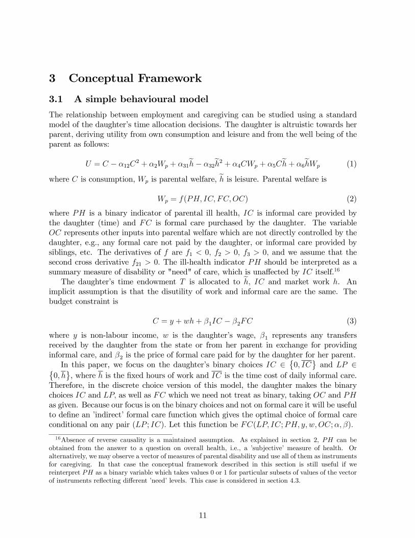
The relationship between employment and caregiving can be studied using a standardmodel of the daughter�s time allocation decisions. The daughter is altruistic towards herparent, deriving utility from own consumption and leisure and from the well being of theparent as follows:

U = C � �12C2 + �2Wp + �31eh� �32eh2 + �4CWp + �5Ceh+ �6ehWp (1)

where C is consumption, Wp is parental welfare, eh is leisure. Parental welfare isWp = f(PH; IC; FC;OC) (2)

where PH is a binary indicator of parental ill health, IC is informal care provided bythe daughter (time) and FC is formal care purchased by the daughter. The variableOC represents other inputs into parental welfare which are not directly controlled by thedaughter, e.g., any formal care not paid by the daughter, or informal care provided bysiblings, etc. The derivatives of f are f1 < 0; f2 > 0; f3 > 0; and we assume that thesecond cross derivative f21 > 0: The ill-health indicator PH should be interpreted as asummary measure of disability or "need" of care, which is una¤ected by IC itself.16

The daughter�s time endowment T is allocated to eh; IC and market work h. Animplicit assumption is that the disutility of work and informal care are the same. Thebudget constraint is

C = y + wh+ �1IC � �2FC (3)

where y is non-labour income, w is the daughter�s wage, �1 represents any transfersreceived by the daughter from the state or from her parent in exchange for providinginformal care, and �2 is the price of formal care paid for by the daughter for her parent.In this paper, we focus on the daughter�s binary choices IC 2

�0; IC

and LP 2�

0; h, where h is the �xed hours of work and IC is the time cost of daily informal care.

Therefore, in the discrete choice version of this model, the daughter makes the binarychoices IC and LP; as well as FC which we need not treat as binary, taking OC and PHas given. Because our focus is on the binary choices and not on formal care it will be usefulto de�ne an �indirect�formal care function which gives the optimal choice of formal careconditional on any pair (LP ; IC): Let this function be FC(LP; IC;PH; y; w;OC;�; �):

16Absence of reverse causality is a maintained assumption. As explained in section 2, PH can beobtained from the answer to a question on overall health, i.e., a �subjective�measure of health. Oralternatively, we may observe a vector of measures of parental disability and use all of them as instrumentsfor caregiving. In that case the conceptual framework described in this section is still useful if wereinterpret PH as a binary variable which takes values 0 or 1 for particular subsets of values of the vectorof instruments re�ecting di¤erent �need�levels. This case is considered in section 4.3.

11

A potentially important issue neglected in this model is the type of living arrange-ments, e.g., co-residence between daughter and parent versus separate households. This,as well as the daughter�s other choices and the other informal and formal care inputs OC,may be jointly determined as the outcome of a game played between di¤erent units ofan extended family. With this broader perspective some of our simple model�s parame-ters such as �1 or IC could also be endogenous. We can still interpret our model of thedaughter�s individual decision-making as part of that larger model in which the values ofparameters such as (IC; �1; y) are jointly determined, and we will attempt to keep this inmind in the discussion that follows.17

3.2 Discussion of parameters and empirical models

Heterogeneity: The optimal decision rules for employment and care are a pair of binary-valued functions with parameters and arguments (�; �; h; IC;PH; y; w;OC): Our econo-metric models approximate decision rules as functions of parental health PH and a vec-tor of controls X which includes country dummies, the daughter�s non-labour incomey measured as household income net of her own earnings, preference shifters, observ-able determinants of wages (e.g., education) and observables relating to other sources ofcare (e.g., number of siblings). Conditional on (PH;X); the data give joint probabilitydistributions for the discrete pair (LP ; IC): We interpret these distributions as the in-tegrals of the model�s decision rules over the distribution of unobserved components of(a; �; h; IC; y; w;OC): All the empirical work we report in Section 4 consists of estimatesof the impact of PH in these decision rules, based on non-parametric and parametricapproximations, and ratios of these estimates which are local average treatment e¤ects.The rest of this section uses the behavioral model to guide a detailed discussion of theassumptions needed to give a causal interpretation to these estimates and to make predic-tions about their sign and size. We argue that these estimates can answer the followingquestions of interest.

Questions & parameters of interest : 1) What is the e¤ect of a change in parents�healthstatus on daily caregiving and employment decisions of their mature daughters? 2) Doesdaily caregiving reduce employment? Can all daily care-giving services be attributed toill-health of parents, or are some daughters providing daily care to parents in reasonablygood health? 3) Are the answers to these questions di¤erent across our pools of countries- and why?

IV-treatment e¤ects and the behavioral model : In order to further clarify the questions

17Using a complete model along these lines to guide the analysis in this section is beyond the scopeof this paper. To the best of our knowledge, no such model has been used in empirical work. Byrneet al. (2009) propose and structuraly estimate a (non cooperative) game-theoretic model in which eachsibling chooses labor supply, hours of informal care and contributions to formal care, taken (separate)living arrangements as given. Pezzin and Schone (1994) model co-residence and the daughter�s decisionto work and to provide informal care in a cooperative framework in single daughter-parent pairs. Othergame-theoretic models include Checkovich and Stern (2002), Engers and Stern (2002), and Heidemanand Stern (1999).

12

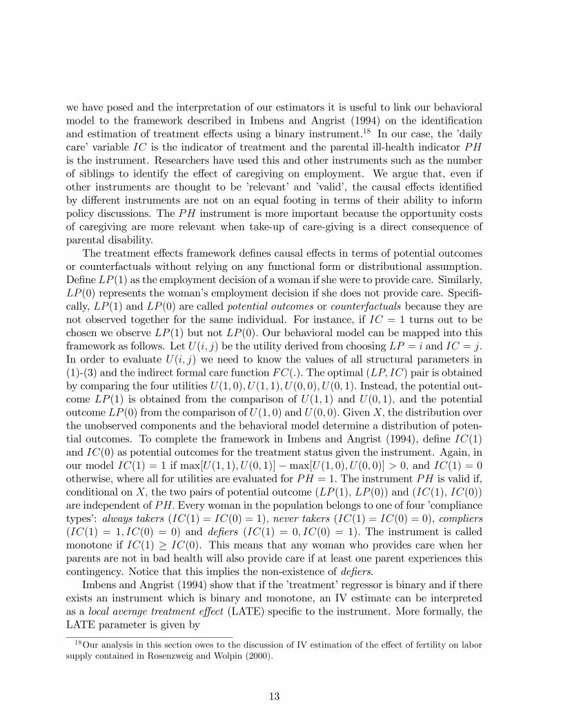
we have posed and the interpretation of our estimators it is useful to link our behavioralmodel to the framework described in Imbens and Angrist (1994) on the identi�cationand estimation of treatment e¤ects using a binary instrument.18 In our case, the �dailycare�variable IC is the indicator of treatment and the parental ill-health indicator PHis the instrument. Researchers have used this and other instruments such as the numberof siblings to identify the e¤ect of caregiving on employment. We argue that, even ifother instruments are thought to be �relevant� and �valid�, the causal e¤ects identi�edby di¤erent instruments are not on an equal footing in terms of their ability to informpolicy discussions. The PH instrument is more important because the opportunity costsof caregiving are more relevant when take-up of care-giving is a direct consequence ofparental disability.The treatment e¤ects framework de�nes causal e¤ects in terms of potential outcomes

or counterfactuals without relying on any functional form or distributional assumption.De�ne LP (1) as the employment decision of a woman if she were to provide care. Similarly,LP (0) represents the woman�s employment decision if she does not provide care. Speci�-cally, LP (1) and LP (0) are called potential outcomes or counterfactuals because they arenot observed together for the same individual. For instance, if IC = 1 turns out to bechosen we observe LP (1) but not LP (0): Our behavioral model can be mapped into thisframework as follows. Let U(i; j) be the utility derived from choosing LP = i and IC = j.In order to evaluate U(i; j) we need to know the values of all structural parameters in(1)-(3) and the indirect formal care function FC(:): The optimal (LP; IC) pair is obtainedby comparing the four utilities U(1; 0); U(1; 1); U(0; 0); U(0; 1): Instead, the potential out-come LP (1) is obtained from the comparison of U(1; 1) and U(0; 1); and the potentialoutcome LP (0) from the comparison of U(1; 0) and U(0; 0): GivenX; the distribution overthe unobserved components and the behavioral model determine a distribution of poten-tial outcomes. To complete the framework in Imbens and Angrist (1994), de�ne IC(1)and IC(0) as potential outcomes for the treatment status given the instrument. Again, inour model IC(1) = 1 if max[U(1; 1); U(0; 1)] �max[U(1; 0); U(0; 0)] > 0; and IC(1) = 0otherwise, where all for utilities are evaluated for PH = 1: The instrument PH is valid if,conditional on X; the two pairs of potential outcome (LP (1); LP (0)) and (IC(1); IC(0))are independent of PH: Every woman in the population belongs to one of four �compliancetypes�: always takers (IC(1) = IC(0) = 1); never takers (IC(1) = IC(0) = 0), compliers(IC(1) = 1; IC(0) = 0) and de�ers (IC(1) = 0; IC(0) = 1): The instrument is calledmonotone if IC(1) � IC(0). This means that any woman who provides care when herparents are not in bad health will also provide care if at least one parent experiences thiscontingency. Notice that this implies the non-existence of de�ers.Imbens and Angrist (1994) show that if the �treatment�regressor is binary and if there

exists an instrument which is binary and monotone, an IV estimate can be interpretedas a local average treatment e¤ect (LATE) speci�c to the instrument. More formally, theLATE parameter is given by

18Our analysis in this section owes to the discussion of IV estimation of the e¤ect of fertility on laborsupply contained in Rosenzweig and Wolpin (2000).

13

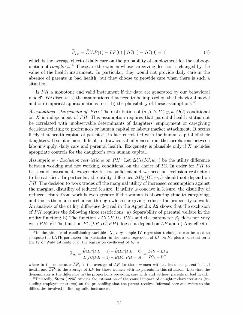
b�IV = bE[LP (1)� LP (0) j IC(1)� IC(0) = 1] (4)

which is the average e¤ect of daily care on the probability of employment for the subpop-ulation of compliers.19 These are the women whose caregiving decision is changed by thevalue of the health instrument. In particular, they would not provide daily care in theabsence of parents in bad health, but they choose to provide care when there is such asituation.

Is PH a monotone and valid instrument if the data are generated by our behavioralmodel? We discuss: a) the assumptions that need to be imposed on the behavioral modeland our empirical approximations to it; b) the plausibility of these assumptions.20

Assumptions - Exogeneity of PH: The distribution of (a; �; h; IC; y; w;OC) conditionalon X is independent of PH: This assumption requires that parental health status notbe correlated with unobservable determinants of daughters� employment or caregivingdecisions relating to preferences or human capital or labour market attachment. It seemslikely that health capital of parents is in fact correlated with the human capital of theirdaughters. If so, it is more di¢ cult to draw causal inferences from the correlations betweenlabour supply, daily care and parental health. Exogeneity is plausible only if X includesapropriate controls for the daughter�s own human capital.

Assumptions - Exclusion restrictions on PH: Let �UL(IC;w; :) be the utility di¤erencebetween working and not working, conditional on the choice of IC: In order for PH tobe a valid instrument, exogeneity is not su¢ cient and we need an exclusion restrictionto be satis�ed. In particular, the utility di¤erence �UL(IC;w; :) should not depend onPH: The decision to work trades o¤ the marginal utility of increased consumption againstthe marginal disutility of reduced leisure. If utility is concave in leisure, the disutility ofreduced leisure from work is even greater if the woman is allocating time to caregiving,and this is the main mechanism through which caregiving reduces the propensity to work.An analysis of the utility di¤erence derived in the Appendix A2 shows that the exclusionof PH requires the following three restrictions: a) Separability of parental welfare in theutility function; b) The function FC(LP; IC; PH) and the parameter �1 does not varywith PH; c) The function FC(LP; IC; PH) does not depend on LP and d) Any e¤ect of

19In the absence of conditioning variables X; very simple IV regression techniques can be used tocompute the LATE parameter. In particular, in the linear regression of LP on IC plus a constant termthe IV or Wald estimate of �, the regression coe¢ cient of IC is

b�IV = bE(LP jPH = 1)� bE(LP jPH = 0)bE(ICjPH = 1)� bE(ICjPH = 0)=LP 1 � LP 0IC1 � IC0

where in the numerator LP 1 is the average of LP for those women with at least one parent in badhealth and LP 0 is the average of LP for those women with no parents in this situation. Likewise, thedenominator is the di¤erence in the proportions providing care with and without parents in bad health.20Relatedly, Stern (1995) studies the estimation of the causal impact of daughter characteristics (in-

cluding employment status) on the probability that the parent receives informal care and refers to thedi¢ culties involved in �nding valid instruments.

14

PH on co-residence status of daughther and parent, or on how close the daughter choosesto live from her parent, operates exclusively through the daughter�s care-giving decision.Restriction b) is not necessary if the utility function is linear in consumption. We discussthese restrictions in more detail below.Separability of parental welfare: �4 = �6 = 0; i.e., the marginal utilities of consumption

and leisure do not depend on parental welfare.21

Formal care purchased by the daughter : FC(LP; IC; PH; :) = FC(IC): Conditionalon her choice of informal care, spending by the daughter on formal care does not vary withemployment or with parental health.22 We show in the Appendix A2 that this restrictionneed not hold in general. An example of behavior that would violate it is as follows.Suppose a daughter decides not to provide daily care; having decided this, if her parentis in poor health and does not have another source of care she would pay for formal carebut she can only a¤ord to if she is working. Behavior like this seems more likely to occurin southern countries. Even if this failure of exclusion is plausible the bias in IV estimatesis likely to be small in practice to the extent that it is unusual for daughters to pay forformal care out of their own pocket.23

Transfers received by the daughter in exchange for informal care: The parameter �1in the daughter�s budget constraint measures transfers she may receive, private or public,if she provides daily informal care. A necessary exclusion restriction is that �1 should notdepend on PH; i.e., conditional on the daughter providing daily care any transfers shemight receive do not vary with the parents�actual disability status. This restriction doesnot seem entirely plausible, e.g., public transfers are likely to be conditional on su¢ cientdisability or need.Linear-in-consumption utility: The exclusion of PH from in the FC(�) function and

from �1 are needed because the marginal utility of consumption from working depends onthe �baseline�level of consumption when not working, and this in turn could depend onPH through formal or informal care choices. Therefore, exclusion restrictions on FC(�)and �1 are not needed if the marginal utility of consumption is constant.

24

Co-residence and distance between parents and daughters: The value of parameter IC;

21If they do, the marginal utility and the marginal disutility from working will depend on parentalwelfare Wp, and the instrument PH has a direct e¤ect on this.22Consider �rst the exclusion of LP: If spending by the daughter on formal care depends on whether

she works or not, even after conditioning on IC and PH, then the gain from working will include anincrease in the welfare of parents the size of which depends on their health. The reason why the exclusionof PH in the FC() function is needed is explained below under "Linear-in-consumption utility".23Expenditures on formal care by daughters are not directly observed. However, daughters are asked

about "�nancial or material gifts or support" given to at least one parent in excess of 250 euros in thelast year. The number of �yes�answers is small: 8 women in the North, 15 in the Center and 11 in theSouth. Of these, only 4 women in the Center and one in the South report that the reason for the transferwas "to help following a bereavement or illness". Even if direct information on purchases of formal carewere available, testing the exclusion restriction would be di¢ cult because the FC(�) function describespotential outcomes so estimating the coe¢ cients on LP; IC and PH poses some of the same challengeswe are trying to deal with in the �rst place.24The marginal utility of consumption is constant i¤ �5 = �12 = 0: Moreover, one can show that in

this case the function FC(�) does not depend on LP so this exclusion restriction is also not needed.

15

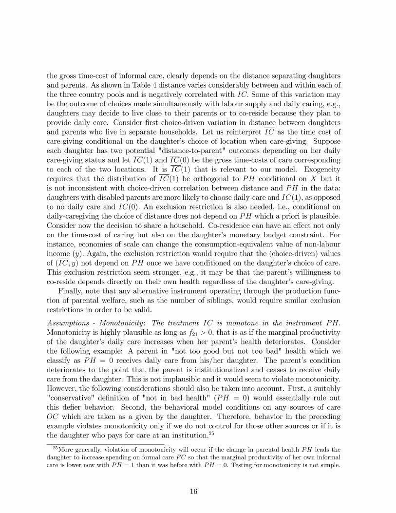
the gross time-cost of informal care, clearly depends on the distance separating daughtersand parents. As shown in Table 4 distance varies considerably between and within each ofthe three country pools and is negatively correlated with IC: Some of this variation maybe the outcome of choices made simultaneously with labour supply and daily caring, e.g.,daughters may decide to live close to their parents or to co-reside because they plan toprovide daily care. Consider �rst choice-driven variation in distance between daughtersand parents who live in separate households. Let us reinterpret IC as the time cost ofcare-giving conditional on the daughter�s choice of location when care-giving. Supposeeach daughter has two potential "distance-to-parent" outcomes depending on her dailycare-giving status and let IC(1) and IC(0) be the gross time-costs of care correspondingto each of the two locations. It is IC(1) that is relevant to our model. Exogeneityrequires that the distribution of IC(1) be orthogonal to PH conditional on X but itis not inconsistent with choice-driven correlation between distance and PH in the data:daughters with disabled parents are more likely to choose daily-care and IC(1); as opposedto no daily care and IC(0): An exclusion restriction is also needed, i.e., conditional ondaily-caregiving the choice of distance does not depend on PH which a priori is plausible.Consider now the decision to share a household. Co-residence can have an e¤ect not onlyon the time-cost of caring but also on the daughter�s monetary budget constraint. Forinstance, economies of scale can change the consumption-equivalent value of non-labourincome (y): Again, the exclusion restriction would require that the (choice-driven) valuesof (IC; y) not depend on PH once we have conditioned on the daughter�s choice of care.This exclusion restriction seem stronger, e.g., it may be that the parent�s willingness toco-reside depends directly on their own health regardless of the daughter�s care-giving.Finally, note that any alternative instrument operating through the production func-

tion of parental welfare, such as the number of siblings, would require similar exclusionrestrictions in order to be valid.

Assumptions - Monotonicity: The treatment IC is monotone in the instrument PH:Monotonicity is highly plausible as long as f21 > 0; that is as if the marginal productivityof the daughter�s daily care increases when her parent�s health deteriorates. Considerthe following example: A parent in "not too good but not too bad" health which weclassify as PH = 0 receives daily care from his/her daughter. The parent�s conditiondeteriorates to the point that the parent is institutionalized and ceases to receive dailycare from the daughter. This is not implausible and it would seem to violate monotonicity.However, the following considerations should also be taken into account. First, a suitably"conservative" de�nition of "not in bad health" (PH = 0) would essentially rule outthis de�er behavior. Second, the behavioral model conditions on any sources of careOC which are taken as a given by the daughter. Therefore, behavior in the precedingexample violates monotonicity only if we do not control for those other sources or if it isthe daughter who pays for care at an institution.25

25More generally, violation of monotonicity will occur if the change in parental health PH leads thedaughter to increase spending on formal care FC so that the marginal productivity of her own informalcare is lower now with PH = 1 than it was before with PH = 0. Testing for monotonicity is not simple.

16

Estimation of parameters of interest:Most papers cited in our review of the literature speci�ed a reduced form parametric

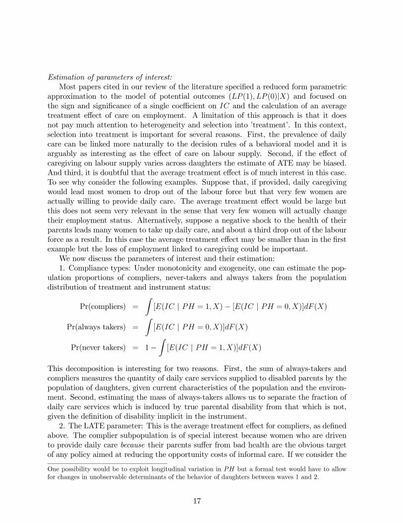
approximation to the model of potential outcomes (LP (1); LP (0)jX) and focused onthe sign and signi�cance of a single coe¢ cient on IC and the calculation of an averagetreatment e¤ect of care on employment. A limitation of this approach is that it doesnot pay much attention to heterogeneity and selection into �treatment�. In this context,selection into treatment is important for several reasons. First, the prevalence of dailycare can be linked more naturally to the decision rules of a behavioral model and it isarguably as interesting as the e¤ect of care on labour supply. Second, if the e¤ect ofcaregiving on labour supply varies across daughters the estimate of ATE may be biased.And third, it is doubtful that the average treatment e¤ect is of much interest in this case.To see why consider the following examples. Suppose that, if provided, daily caregivingwould lead most women to drop out of the labour force but that very few women areactually willing to provide daily care. The average treatment e¤ect would be large butthis does not seem very relevant in the sense that very few women will actually changetheir employment status. Alternatively, suppose a negative shock to the health of theirparents leads many women to take up daily care, and about a third drop out of the labourforce as a result. In this case the average treatment e¤ect may be smaller than in the �rstexample but the loss of employment linked to caregiving could be important.We now discuss the parameters of interest and their estimation:1. Compliance types: Under monotonicity and exogeneity, one can estimate the pop-

ulation proportions of compliers, never-takers and always takers from the populationdistribution of treatment and instrument status:

Pr(compliers) =

Z[E(IC j PH = 1; X)� [E(IC j PH = 0; X)]dF (X)

Pr(always takers) =

Z[E(IC j PH = 0; X)]dF (X)

Pr(never takers) = 1�Z[E(IC j PH = 1; X)]dF (X)

This decomposition is interesting for two reasons. First, the sum of always-takers andcompliers measures the quantity of daily care services supplied to disabled parents by thepopulation of daughters, given current characteristics of the population and the environ-ment. Second, estimating the mass of always-takers allows us to separate the fraction ofdaily care services which is induced by true parental disability from that which is not,given the de�nition of disability implicit in the instrument.2. The LATE parameter: This is the average treatment e¤ect for compliers, as de�ned

above. The complier subpopulation is of special interest because women who are drivento provide daily care because their parents su¤er from bad health are the obvious targetof any policy aimed at reducing the opportunity costs of informal care. If we consider the

One possibility would be to exploit longitudinal variation in PH but a formal test would have to allowfor changes in unobservable determinants of the behavior of daughters between waves 1 and 2.

17

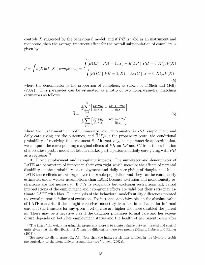
controls X suggested by the behavioural model, and if PH is valid as an instrument andmonotone, then the average treatment e¤ect for the overall subpopulation of compliers isgiven by

� =

Z�(X)dF (X j compliers) =

Z[E(LP j PH = 1; X)� E(LP j PH = 0; X)]dF (X)Z[E(IC j PH = 1; X)� E(IC j X = 0; X)]dF (X)

(5)where the denominator is the proportion of compliers, as shown by Frölich and Melly(2007). This parameter can be estimated as a ratio of two non-parametric matchingestimators as follows

b� =1N

NXi=1

hLPiPHib�(Xi) � LPi(1�PHi)

1�b�(Xi)i

1N

NXi=1

hICiPHib�(Xi) � ICi(1�PHi)

1�b�(Xi)i (6)

where the "treatment" in both numerator and denominator is PH; employment anddaily care-giving are the outcomes, and b�(Xi) is the propensity score, the conditionalprobability of receiving this treatment.26 Alternatively, as a parametric approximation,we compute the corresponding marginal e¤ects of PH on LP and IC from the estimationof a bivariate probit model for labour market participation and daily care-giving with PHas a regressor.27

3. Direct employment and care-giving impacts: The numerator and denominator ofLATE are parameters of interest in their own right which measure the e¤ects of parentaldisability on the probability of employment and daily care-giving of daughters. UnlikeLATE these e¤ects are averages over the whole population and they can be consistentlyestimated under weaker assumptions than LATE because exclusion and monotonicity re-strictions are not necessary. If PH is exogenous but exclusion restrictions fail, causalintepretations of the employment and care-giving e¤ects are valid but their ratio may es-timate LATE with bias. Our analysis of the behavioral model�s utility di¤erences pointedto several potential failures of exclusion. For instance, a positive bias in the absolute valueof LATE can arise if the daughter receives monetary transfers in exchange for informalcare and the transfers for any given level of care are higher the more disabled the parentis. There may be a negative bias if the daughter purchases formal care and her expen-diture depends on both her employment status and the health of her parent, even after

26The idea of the weighting using the propensity score is to create balance between treated and controlunits given that the distribution of X may be di¤erent in these two groups (Hirano, Imbens and Ridder(2003)).27See more details in Appendix A3. Note that the index restrictions implicit in the bivariate probit

are equivalent to the monotonicity assumption (see Vytlacil (2002)).

18

conditioning on informal care. If the daughter�s co-residence status or the distance thatseparates her from her parent varies with the health of the parent even after we conditionon informal care, then a negative bias results through the time cost of care, and a positiveone through economies of scale in consumption.

Some issues in speci�cation and causal interpretations:a) Using the longitudinal dimension: Our �rst set of estimates reported in section

4.1 is obtained using the second wave of the SHARE data. One concern is that, in thecross section, parental health could be correlated with unobservable determinants of LPand IC (preference shifters, human capital), even after controlling for the daughter�s ownhealth and education, etc. One may argue that longitudinal variation in the parentalhealth instrument is less likely to be subject to this problem. In particular, reestimationof the parameters of interest using the subsample of women in 2006 for which PH2004 = 0would allow us to mitigate any systematic correlation that may exist between PH andunobservables factors of daughter�s preferences or human capital and to move closer tothe �ideal�experiment in which we observe the (caeteris paribus) e¤ect of an exogenousshock to the health of parents. Furthermore, results obtained from this sample remaininterpretable in terms of our static model. Finally, even if we focus on the second waveoutcomes we can control for the daughter�s lagged participation for which there is a solidbasis in labour economics. Estimates which exploit the longitudinal dimension using the�rst and second waves are reported in section 4.2.b) Co-residence and distance between parents and daughters: Given that the dis-

tance between daughter and parents is observable, should we include it as a control?We have argued above that heterogeneity in distance induced by parental disabilityPH and care-giving does not necessarily invalidate causal interpretations of our esti-mators. Moreover, if distance is chosen jointly with informal care, then conditioning ondistance is likely to produce systematic correlation between PH and other componentsof (a; �; h; IC; w;OC):Therefore, we conclude that it is better not to include distance asa control. However, because the literature has often distinguished bewteen employmente¤ects of care-giving for co-resident and extra-residential daughters, we have computedseveral of our estimators for the subsample of extra-residential daughters (see footnotesin the section of results for further details).c) Other sources of care: The behavioral model suggests that the e¤ect of PH on

employment and daily care should be measured net of other sources of care, which thedaughter takes as given. In the daughters sample this information is not available but weinclude the number of sisters as a proxy. In the parents sample information on other formaland informal care received is available. If parental disability PH correlates positivelywith the receipt of other care and measures of OC are omitted, the estimates of thee¤ect of PH on the daughter�s employment and care could be smaller (in absolute value)than the behavioral model�s parameters. On the other hand if OC is determined jointlywith the daughter�s choices within an extended decision unit failure to include commondeterminants can lead to biases. However, it is not clear that the bias on coe¢ cientsof interest would be important. For these reasons we compare speci�cations with andwithout controls for OC.

19

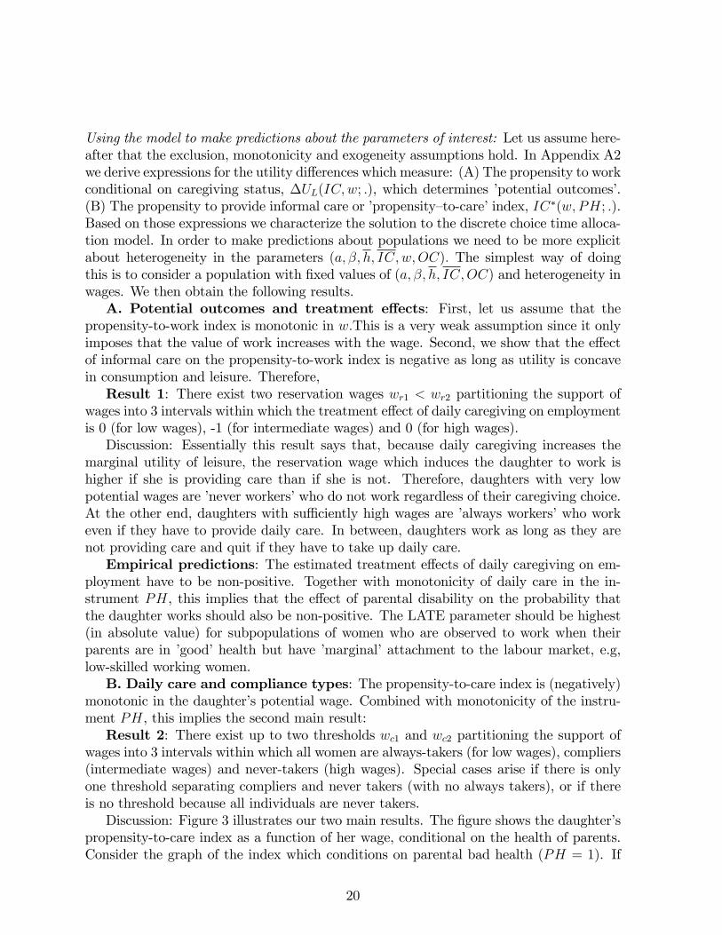
Using the model to make predictions about the parameters of interest: Let us assume here-after that the exclusion, monotonicity and exogeneity assumptions hold. In Appendix A2we derive expressions for the utility di¤erences which measure: (A) The propensity to workconditional on caregiving status, �UL(IC;w; :), which determines �potential outcomes�.(B) The propensity to provide informal care or �propensity�to-care�index, IC�(w;PH; :).Based on those expressions we characterize the solution to the discrete choice time alloca-tion model. In order to make predictions about populations we need to be more explicitabout heterogeneity in the parameters (a; �; h; IC; w;OC): The simplest way of doingthis is to consider a population with �xed values of (a; �; h; IC;OC) and heterogeneity inwages. We then obtain the following results.A. Potential outcomes and treatment e¤ects: First, let us assume that the

propensity-to-work index is monotonic in w:This is a very weak assumption since it onlyimposes that the value of work increases with the wage. Second, we show that the e¤ectof informal care on the propensity-to-work index is negative as long as utility is concavein consumption and leisure. Therefore,Result 1: There exist two reservation wages wr1 < wr2 partitioning the support of

wages into 3 intervals within which the treatment e¤ect of daily caregiving on employmentis 0 (for low wages), -1 (for intermediate wages) and 0 (for high wages).Discussion: Essentially this result says that, because daily caregiving increases the

marginal utility of leisure, the reservation wage which induces the daughter to work ishigher if she is providing care than if she is not. Therefore, daughters with very lowpotential wages are �never workers�who do not work regardless of their caregiving choice.At the other end, daughters with su¢ ciently high wages are �always workers�who workeven if they have to provide daily care. In between, daughters work as long as they arenot providing care and quit if they have to take up daily care.Empirical predictions: The estimated treatment e¤ects of daily caregiving on em-

ployment have to be non-positive. Together with monotonicity of daily care in the in-strument PH, this implies that the e¤ect of parental disability on the probability thatthe daughter works should also be non-positive. The LATE parameter should be highest(in absolute value) for subpopulations of women who are observed to work when theirparents are in �good�health but have �marginal�attachment to the labour market, e.g,low-skilled working women.B. Daily care and compliance types: The propensity-to-care index is (negatively)

monotonic in the daughter�s potential wage. Combined with monotonicity of the instru-ment PH, this implies the second main result:Result 2: There exist up to two thresholds wc1 and wc2 partitioning the support of

wages into 3 intervals within which all women are always-takers (for low wages), compliers(intermediate wages) and never-takers (high wages). Special cases arise if there is onlyone threshold separating compliers and never takers (with no always takers), or if thereis no threshold because all individuals are never takers.Discussion: Figure 3 illustrates our two main results. The �gure shows the daughter�s

propensity-to-care index as a function of her wage, conditional on the health of parents.Consider the graph of the index which conditions on parental bad health (PH = 1). If

20

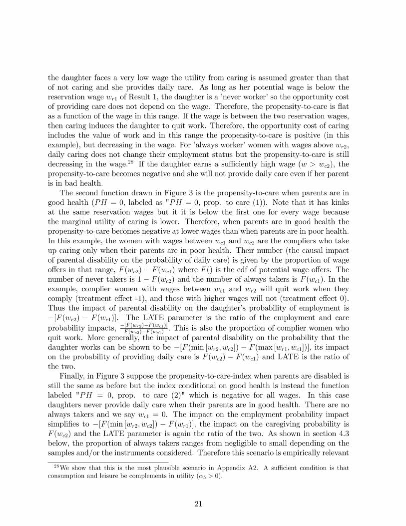
the daughter faces a very low wage the utility from caring is assumed greater than thatof not caring and she provides daily care. As long as her potential wage is below thereservation wage wr1 of Result 1, the daughter is a �never worker�so the opportunity costof providing care does not depend on the wage. Therefore, the propensity-to-care is �atas a function of the wage in this range. If the wage is between the two reservation wages,then caring induces the daughter to quit work. Therefore, the opportunity cost of caringincludes the value of work and in this range the propensity-to-care is positive (in thisexample), but decreasing in the wage. For �always worker�women with wages above wr2,daily caring does not change their employment status but the propensity-to-care is stilldecreasing in the wage.28 If the daughter earns a su¢ ciently high wage (w > wc2), thepropensity-to-care becomes negative and she will not provide daily care even if her parentis in bad health.The second function drawn in Figure 3 is the propensity-to-care when parents are in

good health (PH = 0; labeled as "PH = 0, prop. to care (1)). Note that it has kinksat the same reservation wages but it it is below the �rst one for every wage becausethe marginal utility of caring is lower. Therefore, when parents are in good health thepropensity-to-care becomes negative at lower wages than when parents are in poor health.In this example, the women with wages between wc1 and wc2 are the compliers who takeup caring only when their parents are in poor health. Their number (the causal impactof parental disability on the probability of daily care) is given by the proportion of wageo¤ers in that range, F (wc2) � F (wc1) where F () is the cdf of potential wage o¤ers. Thenumber of never takers is 1 � F (wc2) and the number of always takers is F (wc1): In theexample, complier women with wages between wc1 and wr2 will quit work when theycomply (treatment e¤ect -1), and those with higher wages will not (treatment e¤ect 0).Thus the impact of parental disability on the daughter�s probability of employment is�[F (wr2) � F (wc1)]. The LATE parameter is the ratio of the employment and careprobability impacts, �[F (wr2)�F (wc1)]

F (wc2)�F (wc1) : This is also the proportion of complier women whoquit work. More generally, the impact of parental disability on the probability that thedaughter works can be shown to be �[F (min [wr2; wc2]) � F (max [wr1; wc1])]; its impacton the probability of providing daily care is F (wc2) � F (wc1) and LATE is the ratio ofthe two.Finally, in Figure 3 suppose the propensity-to-care-index when parents are disabled is

still the same as before but the index conditional on good health is instead the functionlabeled "PH = 0, prop. to care (2)" which is negative for all wages. In this casedaughters never provide daily care when their parents are in good health. There are noalways takers and we say wc1 = 0. The impact on the employment probability impactsimpli�es to �[F (min [wr2; wc2]) � F (wr1)]; the impact on the caregiving probability isF (wc2) and the LATE parameter is again the ratio of the two. As shown in section 4.3below, the proportion of always takers ranges from negligible to small depending on thesamples and/or the instruments considered. Therefore this scenario is empirically relevant

28We show that this is the most plausible scenario in Appendix A2. A su¢ cient condition is thatconsumption and leisure be complements in utility (�5 > 0).

21

and we will take it into account to derive some of the comparative statics results whichfollow.C. Some comparative statics:(C1) Caeteris paribus, an increase in other sources of care OC received by parents

(e.g. public formal care) has no e¤ect on the daughter�s reservation wages.29 However,the increased availability of other care reduces the marginal utility of her own informalcare and shifts the two propensity-to-care functions of Figure 3 downwards. Therefore, thecompliance type thresholds wc1 and wc2 move left. The mass of compliers plus always-takers decreases. Furthermore, if there are no always takers we get a sharper result:increased availability of other care (weakly) reduces the impact of parental health on theemployment probability of daughters and it also reduces the impact on the probability ofcaregiving, i.e., the mass of compliers. However, the e¤ect on LATE is ambiguous.(C2) A reduction of the time-cost of informal care IC ( e.g., because the daughter

lives closer to her parents) shifts the propensity-to-care functions upwards and reduceswr2, narrowing the range of wages for which the treatment e¤ect is -1. Therefore, themass of compliers plus always-takers increases but the e¤ect on the employment impactand on LATE are ambiguous.(C3) Suppose monetary payments are o¤ered to daughters providing daily caregiving.

That is, �1 > 0. This shifts the propensity-to-care functions upwards and increases wr2,widening the range of wages for which the treatment e¤ect is -1. This type of supporthas been put in place, for instance, as part of the new public long-term care system inSpain. Our simple model predicts that it should increase the supply of daily caregivingand reduce labour supply.D. Comparisons across country pools: Suppose the main di¤erences across the

three country pools (North-Central-South) are: i) The availability of formal care, inter-pretable as variation in the distribution of OC; to focus, consider the simplest case wherethere is a single value of OC within pools, which grows from South to North. ii) Dif-ferences in labour market attachment of daughters - interpretable as di¤erences in thedistribution of wages w: Let the distributions of wages be ordered from North to South,in the sense of stochastic dominance. We obtain the following empirical predictions:(1) The mass of compliers plus always takers should increase from North to South.

This follows both from comparative statics result (C1) and from the ordering of thedistribution of wages. This prediction is reinforced by comparative statics result (C2) tothe extent that the �average�time cost of daily care (IC) is smaller in the South becausedaughters tend to live closer to their parents.(2) The estimated impact of parental disability on the employment probability of

daughters should grow from North to South. This sharp prediction obtains as long asthe proportion of daughters who are always takers is zero or very small. It follows partlyfrom comparative statics result (C1). Furthermore, recall that the impact on employmentprobability predicted by the model is �[F (min [wr2; wc2]) � F (wr1)] which measures theproportion of daughters just above the margin of participation but close to it. We also

29An implication of this is that increased availability of care has no e¤ect on the average treatmente¤ect of care on employment.

22

expect this to grow from North to South.(3) There is no clear prediction ordering the LATE parameters across country pools.30

4 Empirical Results

We report estimates of the impact of a change in the parental disability instrument (PH =0 to PH = 1) on the daughter�s employment (�numerator�) and daily caregiving choices(�denominator�), as well as the ratio of the two impacts which is the LATE parameter. Wecompute non-parametric and bivariate probit estimates with di¤erent sets of controls fordi¤erent samples and di¤erent de�nitions of the instrument. In every case we �rst reportimpact estimates with no controls which show the unconditional correlations in the data.Ideally we would next introduce as many controls as suggested by theory in non-parametricmatching estimators, which impose minimal assumptions on the distribution of impacts.Because sample sizes limit the precision of non-parametric estimates it is clear that thereis a trade-o¤between increasing the number of controls and allowing for more �exibility inthe speci�cation of causal impacts. Our strategy is to explore increasing sets of controls,to compare non-parametric estimates to those obtained from bivariate probit models andto switch to bivariate probits when sample sizes are too small, e.g., to obtain estimatesfor speci�c subpopulations of daughters.

4.1 Evidence from cross-sectional variation in parental health

The top panel of Table 6 shows the components of the Wald estimate and the non-parametric estimates conditional on a reduced vector of controls X for the sample ofdaughters interviewed in wave 2 (2006), who were between 50 and 60 at the time ofthe interview and had at least one living parent. The controls are the daughter�s age,education and the number of living sisters. We do not report other estimates whichwe computed using the bivariate probit model and/or including a more extensive set ofcontrols. The results were very similar, from which we concluded that the normality andfunctional form assumptions in the biprobit model and the use of a reduced set of controlsprovide good approximations.31 The lower panel shows estimates for the longitudinalsubsample of women who were interviewed in both waves. In this case we report thecomponents of the Wald estimate and biprobit estimates conditional on two di¤erentvectors of controls. First we condition on the same controls as in the cross-sectionalsample. Next we add the �rst lag of LP: On both theoretical and empirical groundsthis is a potentially relevant variable which is correlated with PH and omitted from the

30One can show that the predictions on the ordering of ATE (the average treatment e¤ect) acrosscountry pools are not any sharper.31The complete set of controls includes the woman�s age, number of children, dummies for di¤erent

education level, number of brothers and sisters, marital status, annual non-wage income, and dummiesfor health status. For a more detailed description on these covariates, see Appendix A1. Results on theestimations including the complete set of controls are available upon request.

23

cross-sectional speci�cation.32

Columns 4-6 of the table report estimators of the denominators. For the Wald estimatethese are just the di¤erence in the proportion of daily caregivers between women withand without a parent in bad health. For the matching estimators and the biprobits thedenominator is obtained by averaging the di¤erences in conditional means across thedistribution of the covariate vector X: If PH is exogenous this estimate gives the causale¤ect of having a parent in bad health (PH = 1) on the daughters�decision to providedaily care. It is also the mass of compliers. For Wald estimators the mass of compliersis positive and signi�cantly di¤erent from zero in all three groups of countries, rangingbetween 4.4% in the North to 17.2% in the South in the �rst row of Table 6. The otherrows show that the results are qualitatively the same when we introduce the controls:there is a large and signi�cant e¤ect of PH on IC in southern countries, and smallerbut still signi�cant e¤ect in central and northern countries. We thus �nd a North-Southgradient in the proportion of compliers which mirrors the negative North-South gradientin the development of public long-term care systems. As predicted by the time allocationmodel, the greater the availability of public formal care the smaller the proportion ofwomen who are induced to take up informal care.33

The �rst three columns of Table 6 report the estimators of the numerators. Thisparameter is the causal e¤ect of having parents in poor health on the employment ratesof women under the assumption of exogeneity of PH. When no controls are includedall estimates are negative as suggested by theory and increasing (in absolute value) fromNorth to South. For southern countries, we obtain that women with at least one parentin bad health are 9 percent less likely to be at work than women with no parents inthat situation. However, the size and signi�cance and (to a lesser extent) the gradientof the PH e¤ect on LP do not seem robust to the inclusion of covariates which accountfor the human capital and labour market attachment of daughters. In particular, theestimated impacts decrease substantially and are no longer signi�cant when we controlfor the daughter�s education, and they almost fade away when we also control for laggedparticipation in the longitudinal sample. In summary our point estimates show negativeimpacts of PH on employment of daughters across speci�cations and country pools, butbased on this table the e¤ect of ill-health of parents on the aggregate employment ratesof their daughters would seem very small.The last columns of Table 6 shows the estimates of LATE for southern countries.

This parameter attributes any e¤ect of parents�bad health on the employment rate ofwomen to its e¤ect on the provision of daily informal care, under exogeneity and exclu-sion restrictions. We �rst note that our estimates of LATE are very imprecise and for

32Lagged participation is a good proxy for labor market attachment and potential wages. Furthermoreit may reduce search costs and is well known to be a strong predictor of current participation (see Ecksteinand Wolpin (1989), Hyslop (1999)). On the other hand including lags of the endogenous variables LPand IC could bias the estimate of the causal impact of PH when PH is serially correlated. On balancewe choose to include lagged LP but not lagged IC.33The prediction we derived from the model applied to the sum of always takers and compliers and we

are only looking at compliers here. However, in section 4.3 we show that the North-South gradient is alsoobserved for always takers and that the sum of always takers and compliers is dominated by the latter.

24

this reason we do not report estimates for northern and central country pools.34 Sec-ond, point estimates are negative in most cases but they are small and not signi�cantlydi¤erent from zero once we introduce controls. Rather than standard errors we reportthe percentage of bootstrapped replicas for which point estimates fall in the intervals(�1;�1); [�1;�0:5); [�0:5; 0); [0;1). For instance, the point estimate of LATE in thelongitudinal sample is -0.230 and there is 59% probability that the true value of the para-meter is between 0 and �0:5. That is, the largest mass of the distribution of the estimatorof LATE is in negative values close to zero. The most plausible interpretation in our viewis that LATE for the whole population is not very large because most women in their 50�swho take up daily informal care are never workers or always workers.35

4.2 Evidence from longitudinal variation in parental health

Table 7 reports new estimates of the impact of the health of parents in 2006 on theemployment and daily care choices of their daughters in 2006. The estimates are nowobtained for the subsample of women who had parents in good health in 2004. Estimationon this "conditional" longitudinal sample exploits the impact of longitudinal variation inthe instrument on the cross-sectional distribution of employment and care-giving. Asargued above this should move us closer to the �ideal�experiment in which we observethe (caeteris paribus) e¤ect of an exogenous shock to the health of parents, while theestimates have exactly the same (causal) interpretation in terms of the static behavioralmodel.36 On the down side the sample size is smaller and the parental health instrumenthas less variation in the longitudinal dimension than in the cross section as it is shown inthe last panel of Table 7, both of which reduce the precision of the estimates.

34Lack of precision is partly explained by the relatively small mass of compliers (see Appendix A4 forfurther comment).35However, the exclusion restriction is a maintained assumption so we cannot rule an alternative in-

terpretation which is that the causal e¤ect of daily care on employment is considerably larger but theexclusion restriction is not valid and parental ill-health increases employment of daughters through chan-nels other than informal care.36If there is no systematic correlation between PH and unobservable determinants of LP and IC in

the cross-section, then the estimates obtained from the "conditional" longitudinal sample and from thefull cross-section sample (top panel of Table 6) with the same set of controls should be similar. However,there is an obstacle to making this comparison because we have evidence of important di¤erences inthe distribution of observables between the cross-section and the longitudinal samples for 2006 due todi¤erential panel attrition by observables. This problem is of special relevance in southern countries.In order to address this issue we also did the following. We estimated the biprobit model for 2006including the vector of 3 covariates and using the longitudinal sample of women with parents in goodhealth in 2004. The estimated coe¢ cients from this conditional subsample were used to compute ourparameters of interest using both the cross-section and the full longitudinal sample. Then the twovectors of estimated parameters would be compared to our baseline estimates. This strategy allows us tocompare the estimates obtained exploiting the cross-sectional or longitudinal variation of the instrumentbut keeping the distribution of observables of X 0s constant: Signi�cant di¤erences between these two setsof estimated parameters would point to a problem of the validity of our cross-sectional instrument as itis de�ned in our paper. The results of this exercise suggest that changes in the distribution of X 0s donot play a major role.

25

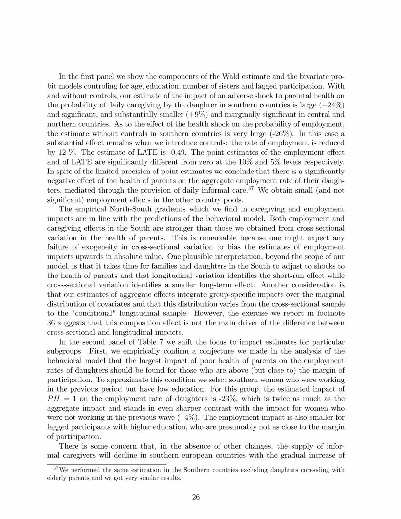
In the �rst panel we show the components of the Wald estimate and the bivariate pro-bit models controling for age, education, number of sisters and lagged participation. Withand without controls, our estimate of the impact of an adverse shock to parental health onthe probability of daily caregiving by the daughter in southern countries is large (+24%)and signi�cant, and substantially smaller (+9%) and marginally signi�cant in central andnorthern countries. As to the e¤ect of the health shock on the probability of employment,the estimate without controls in southern countries is very large (-26%). In this case asubstantial e¤ect remains when we introduce controls: the rate of employment is reducedby 12 %. The estimate of LATE is -0.49. The point estimates of the employment e¤ectand of LATE are signi�cantly di¤erent from zero at the 10% and 5% levels respectively.In spite of the limited precision of point estimates we conclude that there is a signi�cantlynegative e¤ect of the health of parents on the aggregate employment rate of their daugh-ters, mediated through the provision of daily informal care.37 We obtain small (and notsigni�cant) employment e¤ects in the other country pools.The empirical North-South gradients which we �nd in caregiving and employment

impacts are in line with the predictions of the behavioral model. Both employment andcaregiving e¤ects in the South are stronger than those we obtained from cross-sectionalvariation in the health of parents. This is remarkable because one might expect anyfailure of exogeneity in cross-sectional variation to bias the estimates of employmentimpacts upwards in absolute value. One plausible interpretation, beyond the scope of ourmodel, is that it takes time for families and daughters in the South to adjust to shocks tothe health of parents and that longitudinal variation identi�es the short-run e¤ect whilecross-sectional variation identi�es a smaller long-term e¤ect. Another consideration isthat our estimates of aggregate e¤ects integrate group-speci�c impacts over the marginaldistribution of covariates and that this distribution varies from the cross-sectional sampleto the "conditional" longitudinal sample. However, the exercise we report in footnote36 suggests that this composition e¤ect is not the main driver of the di¤erence betweencross-sectional and longitudinal impacts.In the second panel of Table 7 we shift the focus to impact estimates for particular

subgroups. First, we empirically con�rm a conjecture we made in the analysis of thebehavioral model that the largest impact of poor health of parents on the employmentrates of daughters should be found for those who are above (but close to) the margin ofparticipation. To approximate this condition we select southern women who were workingin the previous period but have low education. For this group, the estimated impact ofPH = 1 on the employment rate of daughters is -23%, which is twice as much as theaggregate impact and stands in even sharper contrast with the impact for women whowere not working in the previous wave (- 4%). The employment impact is also smaller forlagged participants with higher education, who are presumably not as close to the marginof participation.There is some concern that, in the absence of other changes, the supply of infor-

mal caregivers will decline in southern european countries with the gradual increase of

37We performed the same estimation in the Southern countries excluding daughters coresiding withelderly parents and we got very similar results.

26

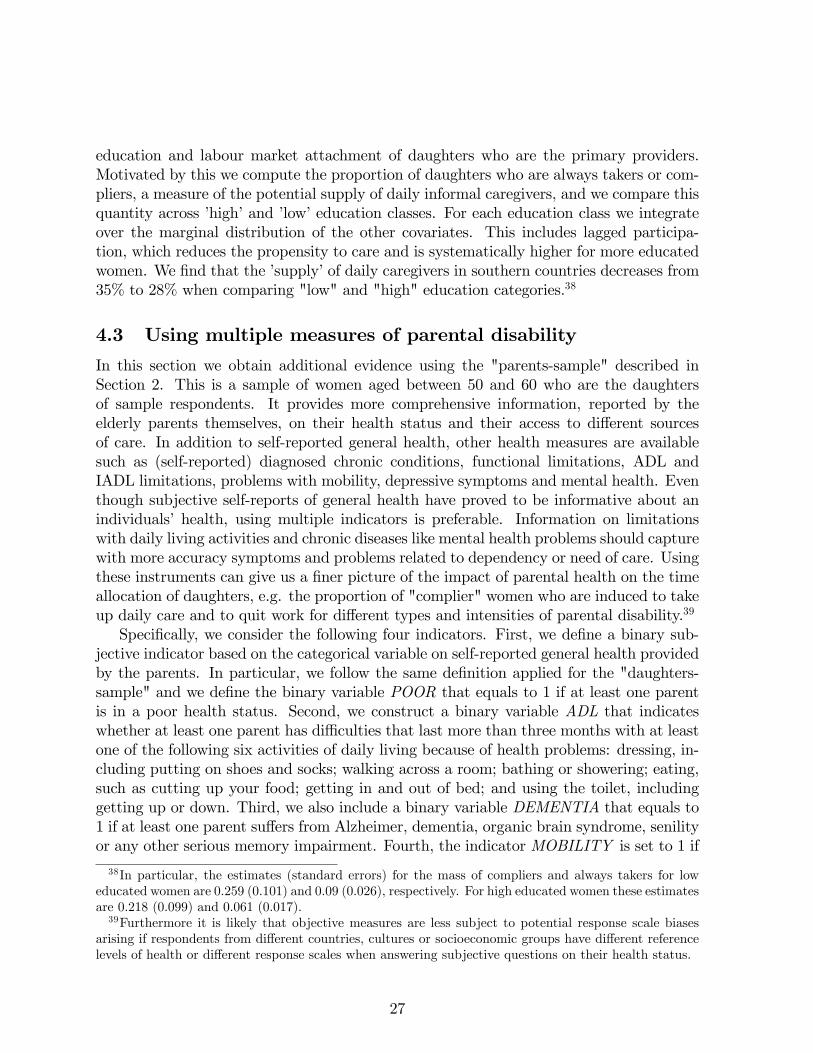
education and labour market attachment of daughters who are the primary providers.Motivated by this we compute the proportion of daughters who are always takers or com-pliers, a measure of the potential supply of daily informal caregivers, and we compare thisquantity across �high�and �low�education classes. For each education class we integrateover the marginal distribution of the other covariates. This includes lagged participa-tion, which reduces the propensity to care and is systematically higher for more educatedwomen. We �nd that the �supply�of daily caregivers in southern countries decreases from35% to 28% when comparing "low" and "high" education categories.38

4.3 Using multiple measures of parental disability

In this section we obtain additional evidence using the "parents-sample" described inSection 2. This is a sample of women aged between 50 and 60 who are the daughtersof sample respondents. It provides more comprehensive information, reported by theelderly parents themselves, on their health status and their access to di¤erent sourcesof care. In addition to self-reported general health, other health measures are availablesuch as (self-reported) diagnosed chronic conditions, functional limitations, ADL andIADL limitations, problems with mobility, depressive symptoms and mental health. Eventhough subjective self-reports of general health have proved to be informative about anindividuals� health, using multiple indicators is preferable. Information on limitationswith daily living activities and chronic diseases like mental health problems should capturewith more accuracy symptoms and problems related to dependency or need of care. Usingthese instruments can give us a �ner picture of the impact of parental health on the timeallocation of daughters, e.g. the proportion of "complier" women who are induced to takeup daily care and to quit work for di¤erent types and intensities of parental disability.39

Speci�cally, we consider the following four indicators. First, we de�ne a binary sub-jective indicator based on the categorical variable on self-reported general health providedby the parents. In particular, we follow the same de�nition applied for the "daughters-sample" and we de�ne the binary variable POOR that equals to 1 if at least one parentis in a poor health status. Second, we construct a binary variable ADL that indicateswhether at least one parent has di¢ culties that last more than three months with at leastone of the following six activities of daily living because of health problems: dressing, in-cluding putting on shoes and socks; walking across a room; bathing or showering; eating,such as cutting up your food; getting in and out of bed; and using the toilet, includinggetting up or down. Third, we also include a binary variable DEMENTIA that equals to1 if at least one parent su¤ers from Alzheimer, dementia, organic brain syndrome, senilityor any other serious memory impairment. Fourth, the indicator MOBILITY is set to 1 if

38In particular, the estimates (standard errors) for the mass of compliers and always takers for loweducated women are 0.259 (0.101) and 0.09 (0.026), respectively. For high educated women these estimatesare 0.218 (0.099) and 0.061 (0.017).39Furthermore it is likely that objective measures are less subject to potential response scale biases

arising if respondents from di¤erent countries, cultures or socioeconomic groups have di¤erent referencelevels of health or di¤erent response scales when answering subjective questions on their health status.

27

there is at least one parent with 3 or more functional limitations due to health problems.40

The main outcome variables (employment and daily caregiving) are analogous to thosede�ned from the information reported by daughters. De�nitions and more speci�c detailsof these variables and other daughters� characteristics (education, age, marital status,residence closeness, number of children and siblings) are provided in Appendix A1. Thedescriptive statistics presented in Table A1.2 of Appendix A1 for this sample are in almostevery case very similar to those of the "daughters-sample". Therefore, the samples seemquite comparable, with the exception of the percentage of daughters coresiding with anelderly parent in the Southern countries, which is is larger in the "parents-sample". Inaddition, the table also shows the important gradient in the use of formal care servicesamong the three groups of countries, which increases from South to North. Regardingthe prevalence of each of the health conditions considered, there is also a clear gradientincreasing from South to North. It is noteworthy that no such clear health gradient waspresent in the data reported by the daughters.With respect to parameters of interest we do not have a binary instrument anymore

but a vector of binary instruments Z = (POOR;ADL;DEMENTIA;MOBILITY ).Di¤erent values of Z describe di¤erent forms and intensities of disability and parents�needof care. The conceptual framework described in section 3 is still useful if we reinterpretthe variable PH in the behavioral model as an indicator which takes values 0 or 1 forparticular values or subsets of values of the vector of instruments Z re�ecting di¤erent(and increasing) levels of disability.In Panel A of Table 8 we show estimates of the proportion of daughters who are �always

takers�, �compliers�and �never takers�when the health of their parents is summarized ina single binary instrument so the events PH = 0 and PH = 1 are complements. Wefocus on the sensitivity of the mass of always takers and compliers to changes in thede�nition of the �good health�state (PH = 0). In the �rst row we only use one of theindicators in Z, the subjective report of health. As we did for the daughters sample,PH = 1 correponds to "at least one parent is in poor or very poor health" and PH = 0is the complement. We con�rm the increasing North-South gradient in the proportion ofcompliers (from 0 to 8 % to 19 %) and we observe the same gradient in the proportionof always takers (from 1% to 3% to 10%). However, the comparisons across rows inthe table are more interesting. In the second row PH = 0 if 3 of the indicators in Z- POOR;ADL;DEMENTIA - are all zero, and in the third row PH = 0 if all fourindicators are zero. The behavioral model predicts that, as we consider increasingly strictde�nitions of �good health�, the marginal utility of caregiving when PH = 0 should falland the proportion of �always taker� daughters should decrease. This is con�rmed inthe data. There are two additional implications of the model: �rst, daughthers who are

40This refers to walking 100 meters, sitting for two hours, getting up from a chair, climbing several�ights of stairs, climbing one �ight of stairs, getting up from a chair after sitting for long periods, climbingseveral �ights of stairs without resting, climbing one �ight of stairs without resting, stooping, kneeling orcrouching, reaching or extending arms above shoulder level. pulling or pushing large objects like a livingroom chair, lifting or carrying weights over 5 kilos, like a heavy bag of groceries, or picking up a smallcoin from a table.

28

not always takers any more become compliers; and second, it is quite likely that thetreatment e¤ect is -1 for women whose compliance status switches from always taker tocomplier. Therefore a more subtle prediction of the model is that a broader de�nition ofthe benchmark �good health�can reduce the estimated impact of parental disability onthe employment rates of daughters. We also see that as we narrow the de�nition of goodhealth the prevalence of �poor health�increases and the estimated proportion of complierstends to fall. The former is a mechanical e¤ect, while the latter is not: on the one hand,some always takers are now classi�ed as compliers as explained above; on the other hand,�poor health�has been broadened to include less serious conditions which induce fewercompliers. Thus when the summary instrument uses all four disability conditions, theproportion of never takers is as high 98 % in the North, 93 % in the Center and 82 % inthe South.We now consider the impact of parental health changes from the benchmark value

Z0 = (0; 0; 0; 0); the best level of health that is observable, to other values of the vector,say Zj.41 There are two good reasons to use Z0 as benchmark: �rst, changes from thatparticular benchmark make the assumption of monotonicity most plausible; and second, asexplained above using a broader de�nition of good health may re-classify some compliersas always takers and hide part of the impact of parental disability on the employment ofdaughters. The LATE parameter for the particular subpopulation of compliers de�ned asthose women whose caregiving decision is changed when going from the state Z0 to Zj isgiven by

�j =

R[E(LP jZ = Zj; X)� E(LP jZ = Z0; X)]dF (X)R[E(ICjZ = Zj; X)� E(ICjZ = Z0; X)]dF (X) (7)

where the denominator measures the mass of compliers among daughters whose parentstransit from good health to condition Zj:With 4 disability indicators there are 24�1 = 31possible values of Zj: Alternatively, with PH = 0 still meaning Z = Z0 we can attachthe label PH = 1 to any arbitrary set of values of Z which does not include Z0. Let eZdenote one such set. For instance, if we de�ne PH = 1 as "having at least one parentwith poor mental health" the set eZ includes all vectors of the form (:; :; 1; :; :). The LATEparameter is e� = R

[E(LP jZ 2 eZ;X)� E(LP jZ = Z0; X)]dF (X)R[E(ICjZ 2 eZ;X)� E(ICjZ = Z0; X)]dF (X) (8)

Panel B of Table 8 shows estimates for four di¤erent eZ sets which partition the wholespace of conditions.42 The �rst row ("ADL") corresponds to Z values of the form (0,1,0,.).

41Note than in this case the events PH = 0 and PH = 1 are not necessarily complements.42One can show that

e� =R XZj2eZ

(([E(LP jZ = Zj ; X)� E(LP jZ = Z0; X)] Pr(Z = Zj ; X))=XZj2eZ

Pr(Z = Zj ; X))dF (X)

R XZj2eZ

(([E(LP jZ = Zj ; X)� E(LP jZ = Z0; X)] Pr(Z = Zj ; X))=XZj2eZ

Pr(Z = Zj ; X))dF (X)

29

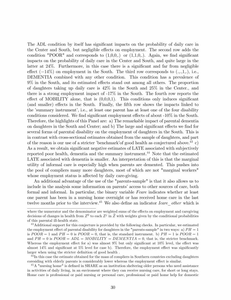
The ADL condition by itself has signi�cant impacts on the probability of daily care inthe Center and South, but negligible e¤ects on employment. The second row adds thecondition "POOR" and corresponds to (1,0,0,.) or (1,1,0,.). Again, we �nd signi�cantimpacts on the probability of daily care in the Center and South, and quite large in thelatter at 24%. Furthermore, in this case there is a signi�cant and far from negligiblee¤ect (�14%) on employment in the South. The third row corresponds to (.,.,1,.), i.e.,DEMENTIA combined with any other condition. This condition has a prevalence of9% in the South, and its estimated e¤ects stand out among all others. The proportionof daughters taking up daily care is 42% in the South and 25% in the Center., andthere is a strong employment impact of -17% in the South. The fourth row reports thee¤ect of MOBILITY alone, that is (0,0,0,1). This conditions only induces signi�cant(and smaller) e¤ects in the South. Finally, the �fth row shows the impacts linked tothe �summary instrument�, i.e., at least one parent has at least one of the four disabilityconditions considered. We �nd signi�cant employment e¤ects of about -10% in the South.Therefore, the highlights of this Panel are: a) The remarkable impact of parental dementiaon daughters in the South and Center; and b) The large and signi�cant e¤ects we �nd forseveral forms of parental disability on the employment of daughters in the South. This isin contrast with cross-sectional estimates obtained from the sample of daughters, and partof the reason is our use of a stricter �benchmark�of good health as conjectured above.43 c)As a result, we obtain signi�cant negative estimates of LATE associated with subjectivelyreported poor health, dementia and the summary instrument.44 Note that the estimatedLATE associated with dementia is smaller. An interpretation of this is that the marginalutility of informal care is especially high when parents are demented. This pushes intothe pool of compliers many more daughters, most of which are not "marginal workers"whose employment status is a¤ected by daily care-giving.An additional advantage of the use of the "parents-sample" is that it also allows us to

include in the analysis some information on parents�access to other sources of care, bothformal and informal. In particular, the binary variable Fcare indicates whether at leastone parent has been in a nursing home overnight or has received home care in the lasttwelve months prior to the interview.45 We also de�ne an indicator Icare_other which is

where the numerator and the denominator are weighted sums of the e¤ects on employment and caregivingdecisions of changes in health from Z0 to each Zj in eZ with weights given by the conditional probabilitiesof this parental ill-health state.43Additional support for this conjecture is provided by the following checks. In particular, we estimated

the employment e¤ect of parental disability for daughters in the "parents-sample" in two ways: a) PH = 1is POOR = 1 and PH = 0 is POOR = 0; that is, the standard instrument. b) PH = 1 is POOR = 1and PH = 0 is POOR = ADL = MOBILITY = DEMENTIA = 0, that is, the stricter benchmark.Whereas the employment e¤ect for a) was almost 9% but only signi�cant at 10% level, the e¤ect wasalmost 14% and signi�cant at 5% level for case b). Therefore, the employment e¤ect was signi�cantlylarger when using the stricter de�nition of good health :44In this case the estimate obtained for the mass of compliers in Southern countries excluding daughters

coresiding with elderly parents is considerably lower whereas the employment e¤ect is similar.45A "nursing home" is de�ned in SHARE as an institution sheltering older persons who need assistance

in activities of daily living, in an enviroment where they can receive nursing care, for short or long stays.Home care is professional or paid nursing or personal care, professional or paid home help for domestic

30

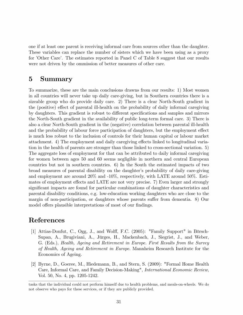
one if at least one parent is receiving informal care from sources other than the daughter.These variables can replace the number of sisters which we have been using as a proxyfor �Other Care�. The estimates reported in Panel C of Table 8 suggest that our resultswere not driven by the ommission of better measures of other care.

5 Summary

To summarize, these are the main conclusions drawns from our results: 1) Most womenin all countries will never take up daily care-giving, but in Southern countries there is asizeable group who do provide daily care. 2) There is a clear North-South gradient inthe (positive) e¤ect of parental ill-health on the probability of daily informal caregivingby daughters. This gradient is robust to di¤erent speci�cations and samples and mirrorsthe North-South gradient in the availability of public long-term formal care. 3) There isalso a clear North-South gradient in the (negative) correlation between parental ill-healthand the probability of labour force participation of daughters, but the employment e¤ectis much less robust to the inclusion of controls for their human capital or labour marketattachment. 4) The employment and daily caregiving e¤ects linked to longitudinal varia-tion in the health of parents are stronger than those linked to cross-sectional variation. 5)The aggregate loss of employment for that can be attributed to daily informal caregivingfor women between ages 50 and 60 seems negligible in northern and central Europeancountries but not in southern countries. 6) In the South the estimated impacts of twobroad measures of parental disability on the daughter�s probability of daily care-givingand employment are around 20% and -10%, respectively, with LATE around 50%. Esti-mates of employment e¤ects and LATE are not very precise. 7) Even larger and stronglysigni�cant impacts are found for particular combinations of daughter characteristics andparental disability conditions, e.g. low-education working daughters who are close to themargin of non-participation, or daughters whose parents su¤er from dementia. 8) Ourmodel o¤ers plausible interpretations of most of our �ndings.

References

[1] Attias-Donfut, C., Ogg, J., and Wol¤, F.C. (2005): "Family Support" in Börsch-Supan, A., Brugiviani, A., Jürges, H., Mackenbach, J., Siegrist, J., and Weber,G. (Eds.), Health, Ageing and Retirement in Europe. First Results from the Surveyof Health, Ageing and Retirement in Europe. Mannheim Research Institute for theEconomics of Ageing.

[2] Byrne, D., Goeree, M., Hiedemann, B., and Stern, S. (2009): "Formal Home HealthCare, Informal Care, and Family Decision-Making", International Economic Review,Vol. 50, No. 4, pp. 1205-1242.

tasks that the individual could not perform himself due to health problems, and meals-on-wheels. We donot observe who pays for these services, or if they are publicly provided.

31

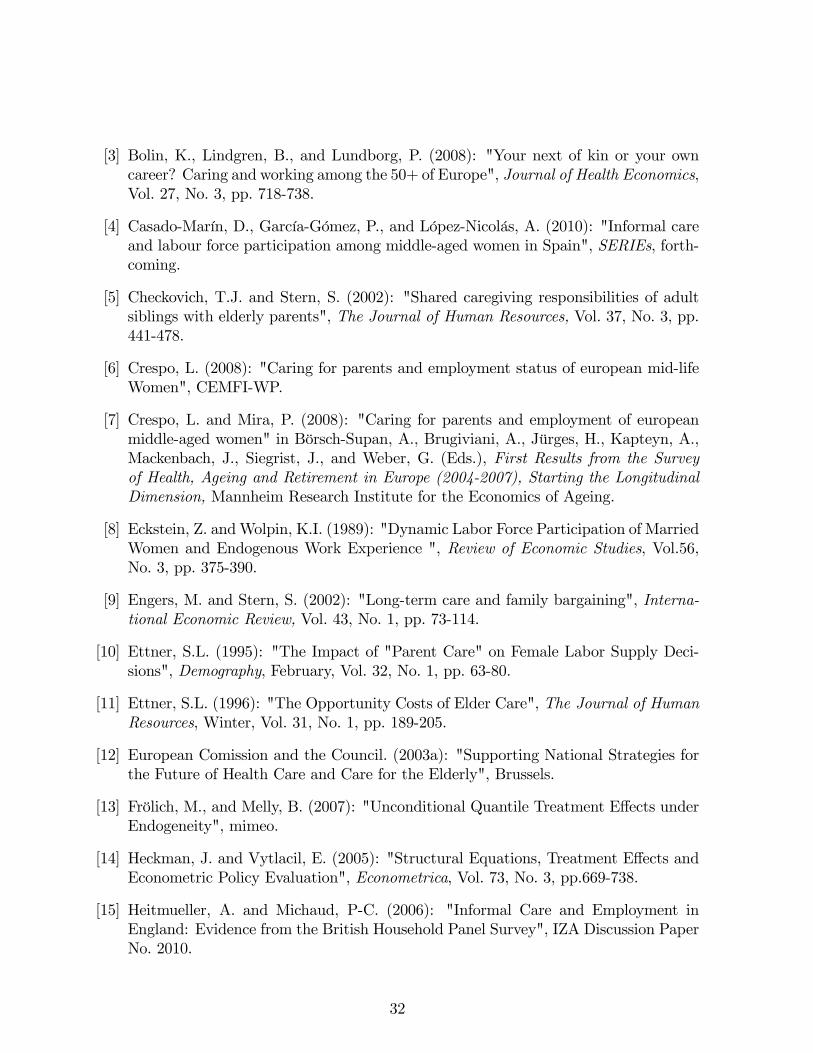
[3] Bolin, K., Lindgren, B., and Lundborg, P. (2008): "Your next of kin or your owncareer? Caring and working among the 50+ of Europe", Journal of Health Economics,Vol. 27, No. 3, pp. 718-738.

[4] Casado-Marín, D., García-Gómez, P., and López-Nicolás, A. (2010): "Informal careand labour force participation among middle-aged women in Spain", SERIEs, forth-coming.

[5] Checkovich, T.J. and Stern, S. (2002): "Shared caregiving responsibilities of adultsiblings with elderly parents", The Journal of Human Resources, Vol. 37, No. 3, pp.441-478.

[6] Crespo, L. (2008): "Caring for parents and employment status of european mid-lifeWomen", CEMFI-WP.

[7] Crespo, L. and Mira, P. (2008): "Caring for parents and employment of europeanmiddle-aged women" in Börsch-Supan, A., Brugiviani, A., Jürges, H., Kapteyn, A.,Mackenbach, J., Siegrist, J., and Weber, G. (Eds.), First Results from the Surveyof Health, Ageing and Retirement in Europe (2004-2007), Starting the LongitudinalDimension, Mannheim Research Institute for the Economics of Ageing.

[8] Eckstein, Z. andWolpin, K.I. (1989): "Dynamic Labor Force Participation of MarriedWomen and Endogenous Work Experience ", Review of Economic Studies, Vol.56,No. 3, pp. 375-390.

[9] Engers, M. and Stern, S. (2002): "Long-term care and family bargaining", Interna-tional Economic Review, Vol. 43, No. 1, pp. 73-114.

[10] Ettner, S.L. (1995): "The Impact of "Parent Care" on Female Labor Supply Deci-sions", Demography, February, Vol. 32, No. 1, pp. 63-80.

[11] Ettner, S.L. (1996): "The Opportunity Costs of Elder Care", The Journal of HumanResources, Winter, Vol. 31, No. 1, pp. 189-205.

[12] European Comission and the Council. (2003a): "Supporting National Strategies forthe Future of Health Care and Care for the Elderly", Brussels.

[13] Frölich, M., and Melly, B. (2007): "Unconditional Quantile Treatment E¤ects underEndogeneity", mimeo.

[14] Heckman, J. and Vytlacil, E. (2005): "Structural Equations, Treatment E¤ects andEconometric Policy Evaluation", Econometrica, Vol. 73, No. 3, pp.669-738.

[15] Heitmueller, A. and Michaud, P-C. (2006): "Informal Care and Employment inEngland: Evidence from the British Household Panel Survey", IZA Discussion PaperNo. 2010.

32

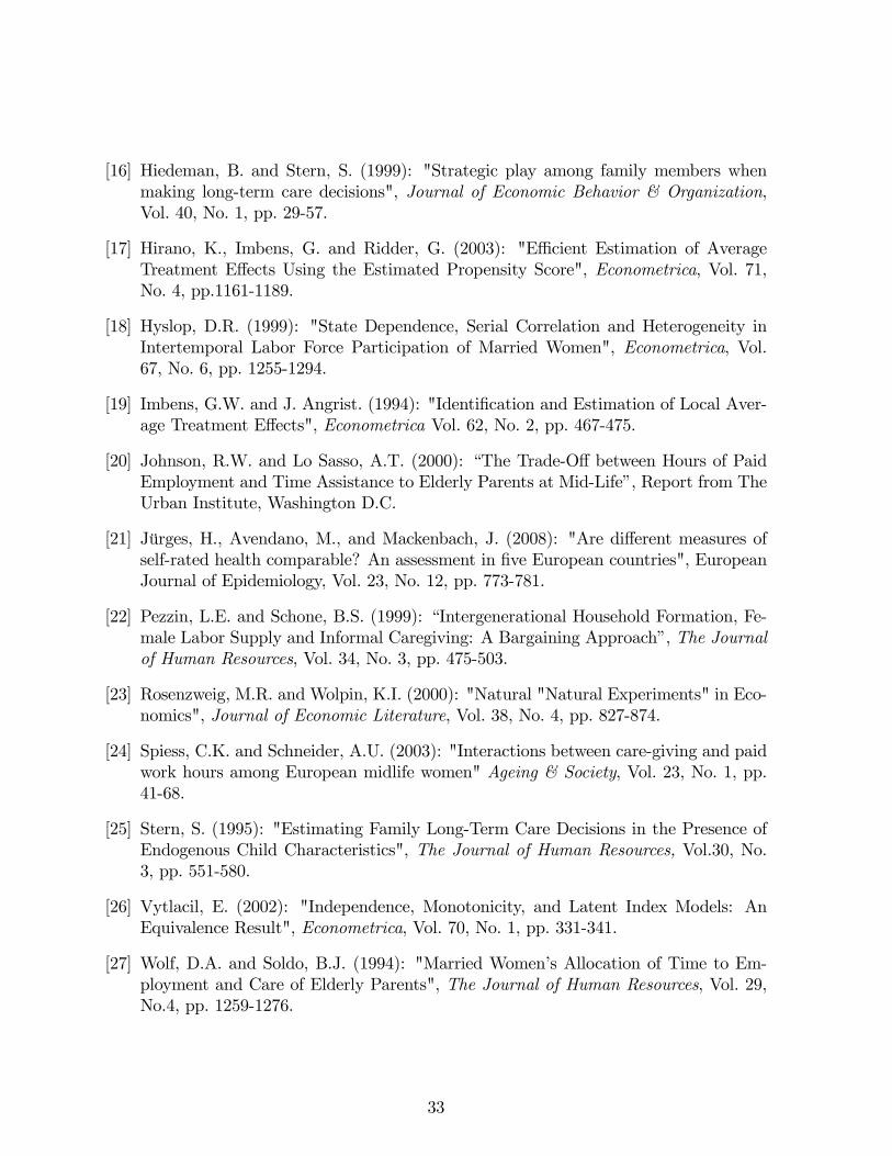
[16] Hiedeman, B. and Stern, S. (1999): "Strategic play among family members whenmaking long-term care decisions", Journal of Economic Behavior & Organization,Vol. 40, No. 1, pp. 29-57.

[17] Hirano, K., Imbens, G. and Ridder, G. (2003): "E¢ cient Estimation of AverageTreatment E¤ects Using the Estimated Propensity Score", Econometrica, Vol. 71,No. 4, pp.1161-1189.

[18] Hyslop, D.R. (1999): "State Dependence, Serial Correlation and Heterogeneity inIntertemporal Labor Force Participation of Married Women", Econometrica, Vol.67, No. 6, pp. 1255-1294.

[19] Imbens, G.W. and J. Angrist. (1994): "Identi�cation and Estimation of Local Aver-age Treatment E¤ects", Econometrica Vol. 62, No. 2, pp. 467-475.

[20] Johnson, R.W. and Lo Sasso, A.T. (2000): �The Trade-O¤ between Hours of PaidEmployment and Time Assistance to Elderly Parents at Mid-Life�, Report from TheUrban Institute, Washington D.C.

[21] Jürges, H., Avendano, M., and Mackenbach, J. (2008): "Are di¤erent measures ofself-rated health comparable? An assessment in �ve European countries", EuropeanJournal of Epidemiology, Vol. 23, No. 12, pp. 773-781.

[22] Pezzin, L.E. and Schone, B.S. (1999): �Intergenerational Household Formation, Fe-male Labor Supply and Informal Caregiving: A Bargaining Approach�, The Journalof Human Resources, Vol. 34, No. 3, pp. 475-503.

[23] Rosenzweig, M.R. and Wolpin, K.I. (2000): "Natural "Natural Experiments" in Eco-nomics", Journal of Economic Literature, Vol. 38, No. 4, pp. 827-874.

[24] Spiess, C.K. and Schneider, A.U. (2003): "Interactions between care-giving and paidwork hours among European midlife women" Ageing & Society, Vol. 23, No. 1, pp.41-68.

[25] Stern, S. (1995): "Estimating Family Long-Term Care Decisions in the Presence ofEndogenous Child Characteristics", The Journal of Human Resources, Vol.30, No.3, pp. 551-580.

[26] Vytlacil, E. (2002): "Independence, Monotonicity, and Latent Index Models: AnEquivalence Result", Econometrica, Vol. 70, No. 1, pp. 331-341.

[27] Wolf, D.A. and Soldo, B.J. (1994): "Married Women�s Allocation of Time to Em-ployment and Care of Elderly Parents", The Journal of Human Resources, Vol. 29,No.4, pp. 1259-1276.

33

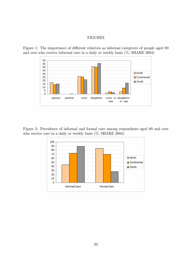
FIGURES

Figure 1: The importance of di¤erent relatives as informal caregivers of people aged 80and over who receive informal care in a daily or weekly basis (%, SHARE 2004)

05

101520253035404550

    spouse    parents       sons  daughters    sons ­ in­ law

daughters­in ­ law

NorthContinentalSouth

Figure 2: Prevalence of informal and formal care among respondents aged 80 and overwho receive care in a daily or weekly basis (%, SHARE 2004)

0102030405060708090

100

Informal Care Formal Care

North

Continental

South

34

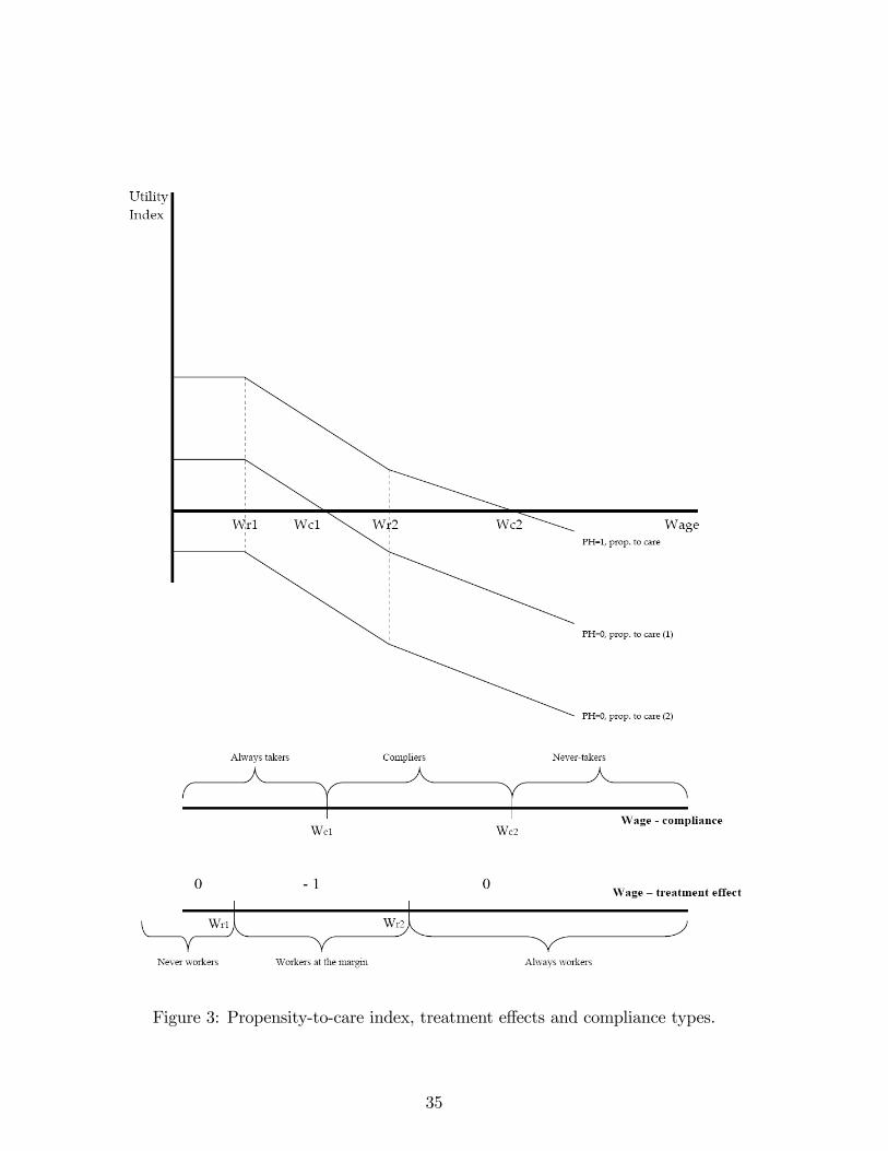
Figure 3: Propensity-to-care index, treatment e¤ects and compliance types.

35

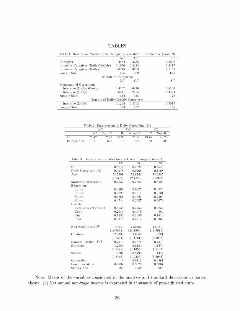
TABLES

Table 1. Descriptive Statistics for Caregiving Variables in the Sample (Wave 2)NC CC SC

Caregiver 0.4584 0.3286 0.2598Intensive Caregiver (Daily/Weekly) 0.1956 0.2238 0.2117Intensive Caregiver (Daily) 0.0248 0.0708 0.1168Sample Size 685 1059 685

Sample of CaregiversNC CC SC

Frequency of CaregivingIntensive (Daily/Weekly) 0.4267 0.6810 0.8146Intensive (Daily) 0.0541 0.2155 0.4494

Sample Size 314 348 178Sample of Daily/Weekly Caregivers

Intensive (Daily) 0.1269 0.3164 0.5517Sample Size 134 237 145

Table 2. Employment & Daily Caregiving (%)NC CC SC

IC Non-IC IC Non-IC IC Non-ICLP 76.47 82.93 57.33 71.24 38.75 46.28Sample Size 17 668 75 984 80 605

Table 3. Descriptive Statistics for the Overall Sample (Wave 2)NC CC SC

LP 0.8277 0.7025 0.4540Daily Caregivers (IC) 0.0248 0.0708 0.1168Age 54.5401 54.6742 54.3985

(2.9583) (2.7779) (2.8929)Married/Partnership 0.7839 0.7583 0.8525EducationEduc1 0.0365 0.0925 0.3226Educ2 0.2029 0.1511 0.2131Educ3 0.2861 0.4627 0.2569Educ4 0.4744 0.2937 0.2073

HealthExcellent/Very Good 0.5635 0.4353 0.3854Good 0.2934 0.4079 0.4Fair 0.1255 0.1350 0.1810Poor 0.0175 0.0217 0.0336

Non-wage Income(2) 19.940 21.0363 14.9879(19.7832) (24.7994) (16.9971)

Children 2.3182 2.0651 1.9781(1.2534) (1.1701) (0.9902)

Parental Health (PH) 0.2219 0.1879 0.2073Brothers 1.2686 0.9254 1.1474

(1.2499) (1.1655) (1.1187)Sisters 1.2204 0.9792 1.1474

(1.3463) (1.2226) (1.2956)Co-resident 0 0.0113 0.0467Less than 5kms 0.2934 0.3673 0.5007Sample Size 685 1059 685

Note: Means of the variables considered in the analysis and standard deviations in paren-theses. (2) Net annual non-wage income is expressed in thousands of ppp-adjusted euros.

36

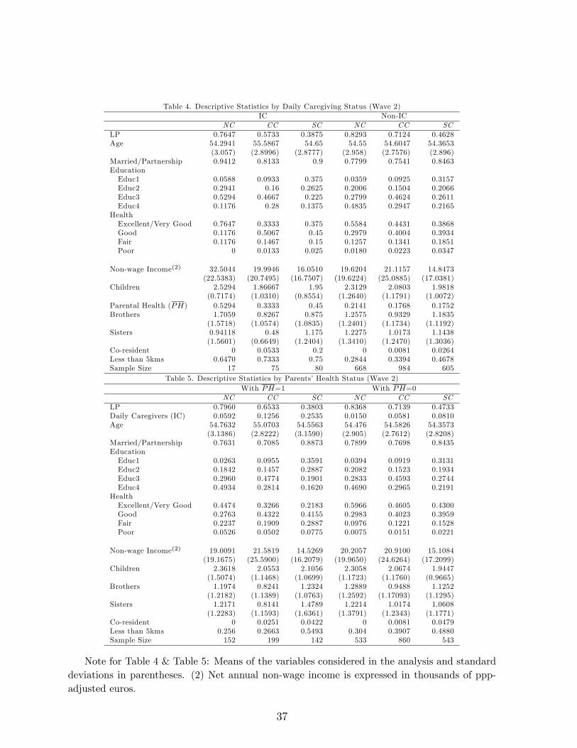
Table 4. Descriptive Statistics by Daily Caregiving Status (Wave 2)IC Non-IC

NC CC SC NC CC SCLP 0.7647 0.5733 0.3875 0.8293 0.7124 0.4628Age 54.2941 55.5867 54.65 54.55 54.6047 54.3653

(3.057) (2.8996) (2.8777) (2.958) (2.7576) (2.896)Married/Partnership 0.9412 0.8133 0.9 0.7799 0.7541 0.8463EducationEduc1 0.0588 0.0933 0.375 0.0359 0.0925 0.3157Educ2 0.2941 0.16 0.2625 0.2006 0.1504 0.2066Educ3 0.5294 0.4667 0.225 0.2799 0.4624 0.2611Educ4 0.1176 0.28 0.1375 0.4835 0.2947 0.2165

HealthExcellent/Very Good 0.7647 0.3333 0.375 0.5584 0.4431 0.3868Good 0.1176 0.5067 0.45 0.2979 0.4004 0.3934Fair 0.1176 0.1467 0.15 0.1257 0.1341 0.1851Poor 0 0.0133 0.025 0.0180 0.0223 0.0347

Non-wage Income(2) 32.5044 19.9946 16.0510 19.6204 21.1157 14.8473(22.5383) (20.7495) (16.7507) (19.6224) (25.0885) (17.0381)

Children 2.5294 1.86667 1.95 2.3129 2.0803 1.9818(0.7174) (1.0310) (0.8554) (1.2640) (1.1791) (1.0072)

Parental Health (PH) 0.5294 0.3333 0.45 0.2141 0.1768 0.1752Brothers 1.7059 0.8267 0.875 1.2575 0.9329 1.1835

(1.5718) (1.0574) (1.0835) (1.2401) (1.1734) (1.1192)Sisters 0.94118 0.48 1.175 1.2275 1.0173 1.1438

(1.5601) (0.6649) (1.2404) (1.3410) (1.2470) (1.3036)Co-resident 0 0.0533 0.2 0 0.0081 0.0264Less than 5kms 0.6470 0.7333 0.75 0.2844 0.3394 0.4678Sample Size 17 75 80 668 984 605

Table 5. Descriptive Statistics by Parents�Health Status (Wave 2)With PH=1 With PH=0

NC CC SC NC CC SCLP 0.7960 0.6533 0.3803 0.8368 0.7139 0.4733Daily Caregivers (IC) 0.0592 0.1256 0.2535 0.0150 0.0581 0.0810Age 54.7632 55.0703 54.5563 54.476 54.5826 54.3573

(3.1386) (2.8222) (3.1590) (2.905) (2.7612) (2.8208)Married/Partnership 0.7631 0.7085 0.8873 0.7899 0.7698 0.8435EducationEduc1 0.0263 0.0955 0.3591 0.0394 0.0919 0.3131Educ2 0.1842 0.1457 0.2887 0.2082 0.1523 0.1934Educ3 0.2960 0.4774 0.1901 0.2833 0.4593 0.2744Educ4 0.4934 0.2814 0.1620 0.4690 0.2965 0.2191

HealthExcellent/Very Good 0.4474 0.3266 0.2183 0.5966 0.4605 0.4300Good 0.2763 0.4322 0.4155 0.2983 0.4023 0.3959Fair 0.2237 0.1909 0.2887 0.0976 0.1221 0.1528Poor 0.0526 0.0502 0.0775 0.0075 0.0151 0.0221

Non-wage Income(2) 19.0091 21.5819 14.5269 20.2057 20.9100 15.1084(19.1675) (25.5900) (16.2079) (19.9650) (24.6264) (17.2099)

Children 2.3618 2.0553 2.1056 2.3058 2.0674 1.9447(1.5074) (1.1468) (1.0699) (1.1723) (1.1760) (0.9665)

Brothers 1.1974 0.8241 1.2324 1.2889 0.9488 1.1252(1.2182) (1.1389) (1.0763) (1.2592) (1.17093) (1.1295)

Sisters 1.2171 0.8141 1.4789 1.2214 1.0174 1.0608(1.2283) (1.1593) (1.6361) (1.3791) (1.2343) (1.1771)

Co-resident 0 0.0251 0.0422 0 0.0081 0.0479Less than 5kms 0.256 0.2663 0.5493 0.304 0.3907 0.4880Sample Size 152 199 142 533 860 543

Note for Table 4 & Table 5: Means of the variables considered in the analysis and standarddeviations in parentheses. (2) Net annual non-wage income is expressed in thousands of ppp-adjusted euros.

37

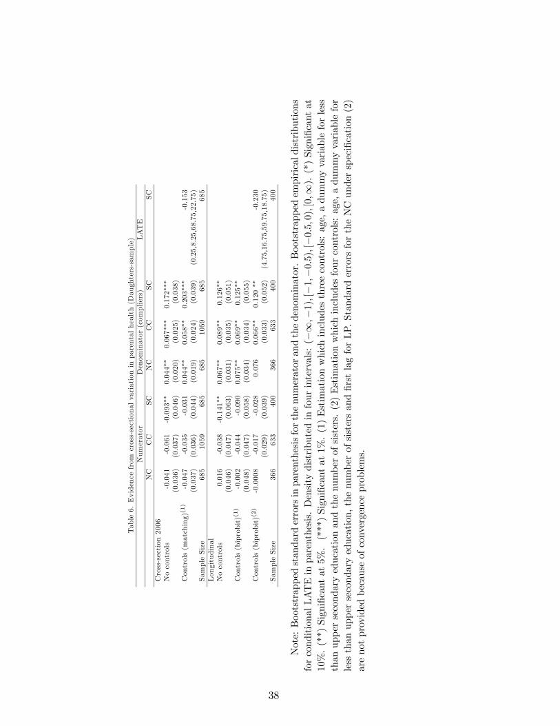
Table6.Evidencefrom

cross-sectionalvariationinparentalhealth(Daughters-sample)

Numerator

Denominator(compliers)

LATE

NC

CC

SC

NC

CC

SC

SC

Cross-section2006

Nocontrols

-0.041

-0.061

-0.093��

0.044��

0.067���

0.172���

(0.036)

(0.037)

(0.046)

(0.020)

(0.025)

(0.038)

Controls(matching)(1)

-0.047

-0.035

-0.031

0.044��

0.058��

0.203���

-0.153

(0.037)

(0.036)

(0.044)

(0.019)

(0.024)

(0.039)

(0.25,8.25,68.75,22.75)

SampleSize

685

1059

685

685

1059

685

685

Longitudinal

Nocontrols

0.016

-0.038

-0.141��

0.067��

0.089��

0.126��

(0.046)

(0.047)

(0.063)

(0.031)

(0.035)

(0.051)

Controls(biprobit)(1)

-0.002

-0.044

-0.090

0.075��

0.069��

0.125��

(0.048)

(0.047)

(0.058)

(0.034)

(0.034)

(0.055)

Controls(biprobit)(2)

-0.0008

-0.017

-0.028

0.076

0.066��

0.120��

-0.230

(0.029)

(0.039)

(0.033)

(0.052)

(4.75,16.75,59.75,18.75)

SampleSize

366

633

400

366

633

400

400

Note:Bootstrappedstandarderrorsinparenthesisforthenumeratorandthedenominator.Bootstrappedempiricaldistributions

forconditionalLATEinparenthesis.Densitydistributedinfourintervals:(�1;�1);[�1;�0:5);[�0:5;0);[0;1).(*)Signi�cantat

10%.(**)Signi�cantat5%.(***)Signi�cantat1%.(1)Estimationwhichincludesthreecontrols:age,adummyvariableforless

thanuppersecondaryeducationandthenumberofsisters.(2)Estimationwhichincludesfourcontrols:age,adummyvariablefor

lessthanuppersecondaryeducation,thenumberofsistersand�rstlagforLP.StandarderrorsfortheNCunderspeci�cation(2)

arenotprovidedbecauseofconvergenceproblems.

38

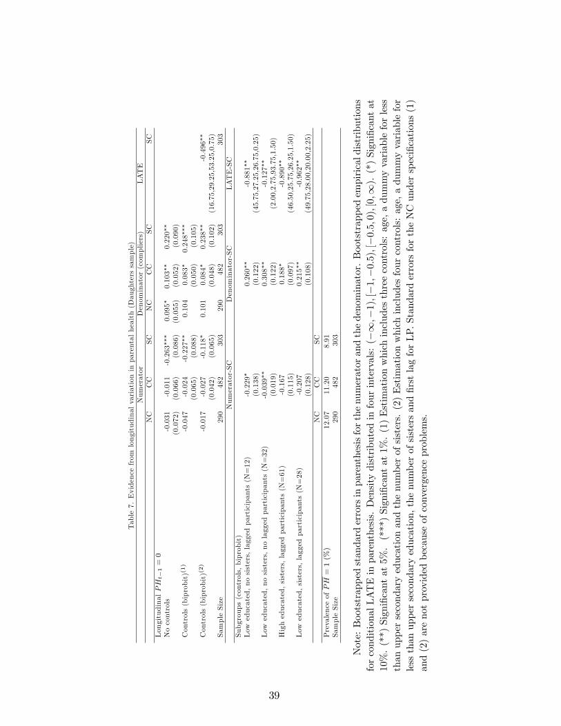
Table7.Evidencefrom

longitudinalvariationinparentalhealth(Daughterssample)

Numerator

Denominator(compliers)

LATE

NC

CC

SC

NC

CC

SC

SC

LongitudinalPHt�1=0

Nocontrols

-0.031

-0.011

-0.263���

0.095�

0.103��

0.220��

(0.072)

(0.066)

(0.086)

(0.055)

(0.052)

(0.090)

Controls(biprobit)(1)

-0.047

-0.024

-0.227��

0.104

0.083�

0.248���

(0.065)

(0.088)

(0.050)

(0.105)

Controls(biprobit)(2)

-0.017

-0.027

-0.118�

0.101

0.084�

0.238��

-0.496��

(0.042)

(0.065)

(0.048)

(0.102)

(16.75,29.25,53.25,0.75)

SampleSize

290

482

303

290

482

303

303

Numerator-SC

Denominator-SC

LATE-SC

Subgroups(controls,biprobit)

Low

educated,nosisters,laggedparticipants(N=12)

-0.229�

0.260��

-0.881��

(0.138)

(0.122)

(45.75,27.25,26.75,0.25)

Low

educated,nosisters,nolaggedparticipants(N=32)

-0.039��

0.308��

-0.127��

(0.019)

(0.122)

(2.00,2.75,93.75,1.50)

Higheducated,sisters,laggedparticipants(N=61)

-0.167

0.188�

-0.890��

(0.115)

(0.097)

(46.50,25.75,26.25,1.50)

Low

educated,sisters,laggedparticipants(N=28)

-0.207

0.215��

-0.962��

(0.128)

(0.108)

(49.75,28.00,20.00,2.25)

NC

CC

SC

PrevalenceofPH=1(%)

12.07

11.20

8.91

SampleSize

290

482

303

Note:Bootstrappedstandarderrorsinparenthesisforthenumeratorandthedenominator.Bootstrappedempiricaldistributions

forconditionalLATEinparenthesis.Densitydistributedinfourintervals:(�1;�1);[�1;�0:5);[�0:5;0);[0;1).(*)Signi�cantat

10%.(**)Signi�cantat5%.(***)Signi�cantat1%.(1)Estimationwhichincludesthreecontrols:age,adummyvariableforless

thanuppersecondaryeducationandthenumberofsisters.(2)Estimationwhichincludesfourcontrols:age,adummyvariablefor

lessthanuppersecondaryeducation,thenumberofsistersand�rstlagforLP.StandarderrorsfortheNCunderspeci�cations(1)

and(2)arenotprovidedbecauseofconvergenceproblems.

39

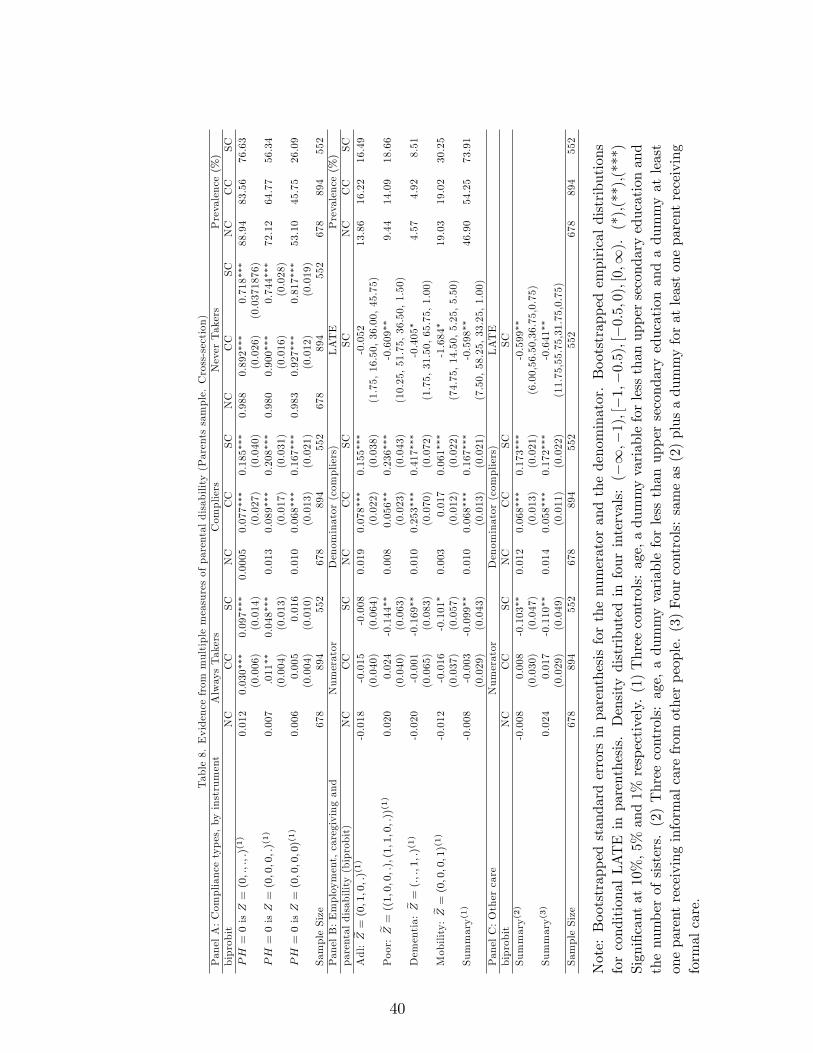
Table8.Evidencefrom

multiplemeasuresofparentaldisability(Parentssample.Cross-section)

PanelA:Compliancetypes,byinstrument

AlwaysTakers

Compliers

NeverTakers

Prevalence(%)

biprobit

NC

CC

SC

NC

CC

SC

NC

CC

SC

NC

CC

SC

PH=0isZ=(0;:;:;:)(1)

0.012

0.030���

0.097���

0.0005

0.077���

0.185���

0.988

0.892���

0.718���

88.94

83.56

76.63

(0.006)

(0.014)

(0.027)

(0.040)

(0.026)

(0.0371876)

PH=0isZ=(0;0;0;:)(1)

0.007

.011��

0.048���

0.013

0.089���

0.208���

0.980

0.900���

0.744���

72.12

64.77

56.34

(0.004)

(0.013)

(0.017)

(0.031)

(0.016)

(0.028)

PH=0isZ=(0;0;0;0)(1)

0.006

0.005

0.016

0.010

0.068���

0.167���

0.983

0.927���

0.817���

53.10

45.75

26.09

(0.004)

(0.010)

(0.013)

(0.021)

(0.012)

(0.019)

SampleSize

678

894

552

678

894

552

678

894

552

678

894

552

PanelB:Employment,caregivingand

Numerator

Denominator(compliers)

LATE

Prevalence(%)

parentaldisability(biprobit)

NC

CC

SC

NC

CC

SC

SC

NC

CC

SC

Adl:e Z=

(0;1;0;:)(1)

-0.018

-0.015

-0.008

0.019

0.078���

0.155���

-0.052

13.86

16.22

16.49

(0.040)

(0.064)

(0.022)

(0.038)

(1.75,16.50,36.00,45.75)

Poor:e Z=

((1;0;0;:);(1;1;0;:))(1)

0.020

0.024

-0.144��

0.008

0.056��

0.236���

-0.609��

9.44

14.09

18.66

(0.040)

(0.063)

(0.023)

(0.043)

(10.25,51.75,36.50,1.50)

Dementia:e Z=

(:;:;1;:)(1)

-0.020

-0.001

-0.169��

0.010

0.253���

0.417���

-0.405�

4.57

4.92

8.51

(0.065)

(0.083)

(0.070)

(0.072)

(1.75,31.50,65.75,1.00)

Mobility:

e Z=(0;0;0;1)(1)

-0.012

-0.016

-0.101�

0.003

0.017

0.061���

-1.684�

19.03

19.02

30.25

(0.037)

(0.057)

(0.012)

(0.022)

(74.75,14.50,5.25,5.50)

Summary(1)

-0.008

-0.003

-0.099��

0.010

0.068���

0.167���

-0.598��

46.90

54.25

73.91

(0.029)

(0.043)

(0.013)

(0.021)

(7.50,58.25,33.25,1.00)

PanelC:Othercare

Numerator

Denominator(compliers)

LATE

biprobit

NC

CC

SC

NC

CC

SC

SC

Summary(2)

-0.008

0.008

-0.103��

0.012

0.068���

0.173���

-0.599��

(0.030)

(0.047)

(0.013)

(0.021)

(6.00,56.50,36.75,0.75)

Summary(3)

0.024

0.017

-0.110��

0.014

0.058���

0.172���

-0.641��

(0.029)

(0.049)

(0.011)

(0.022)

(11.75,55.75,31.75,0.75)

SampleSize

678

894

552

678

894

552

552

678

894

552

Note:Bootstrappedstandarderrorsinparenthesisforthenumeratorandthedenominator.Bootstrappedempiricaldistributions

forconditionalLATEinparenthesis.Densitydistributedinfourintervals:(�1;�1);[�1;�0:5);[�0:5;0);[0;1).(*),(**),(***)

Signi�cantat10%,5%

and1%

respectively.(1)Threecontrols:age,adummyvariableforlessthanuppersecondaryeducationand

thenumberofsisters.(2)Threecontrols:age,adummyvariableforlessthanuppersecondaryeducationandadummyatleast

oneparentreceivinginformalcarefrom

otherpeople.(3)Fourcontrols:sameas(2)plusadummyforatleastoneparentreceiving

formalcare.

40

Appendix A1. Description of variables and some statistics1. Description of variables: We enumerate the list of variables used in the analysis

and the codes of the variables of SHARE used for their construction:1.1. "Daughters-sample": The main variables of interest are de�ned according to

the section 2. The variable LP is equal to 1 if the woman reports in variable ep005 tobe employed or self-employed (including working for family business). The variable ICequals to one if the woman reports to have provided care to at least one elderly parenton a daily basis in the last 12 months. This indicator is constructed using the variablessp008, sp009, sp011, and sp019. The variable PH equals to 1 if at least one parent isin poor health and is contructed using the variable dn033. Regarding covariates, we useinformation on the daughter�s age, current marital status, education, health, income, chil-dren, living parents and siblings. The variable Age is constructed based on dn003. Thedummy variable Married/Partnership is equal to one if the woman is married or engagedin a registered partnership (dn014). Education is measured by four dummy variables(Educ1, Educ2, Educ3, and Educ4 ) generated from the highest level of education com-pleted according to the ISCED-97 code (isced_r).46 The �rst dummy corresponds to noschooling, still in school or primary education (ISCED-97 code 1), the second one refersto lower secondary education (ISCED-97 code 2), the third corresponds to (upper) sec-ondary education (ISCED-97 code 3) and, the last one re�ects graduate, undergraduateor second level of professional studies (post-secondary, non-tertiary, �rst stage of tertiaryand second stage of tertiary. ISCED-97 code 4-6). Health is measured by the respondent�sself-perceived health status (ph003) with one generated dummy variable for each of thecategories (Excellent/Very Good, Good, Fair, and Poor). Non-wage income (Non-wageIncome) is computed as the di¤erence between the gross annual total household income(YhhP) and the gross annual individual income derived from employment (YindP) andself-employment (YdipP), expressed in thousands of ppp-adjusted euros.47 We also con-sider in the analysis variables re�ecting other family responsibilities as the number ofliving children (Children) based on variable ch001,48 and alternative potential sources ofinformal care for elderly parents as the number of the respondent�s siblings (Brothers,Sisters) based on variables dn036 and dn037. Finally, residence closeness is measured bytwo dummies variables (Co-resident and Less 5 kms) that indicate respectively whetherthe daughter has at least one parent living in the same household, or living outside thehousehold but less than 5 kms away and is based on the variable dn030.2.1. "Parents-sample": The variable LP is equal to 1 if the family respondent reports

in ch016 that the daughter is full-time employed, part-time employed or self-employed orworking for own family business. The variable IC equals to one if at least one parentreports to have received care from the daughter on a daily basis in the last 12 months.This indicator is constructed using the variables sp002, sp003, sp005, and sp021. The

46ISCED stands for International Standard Classi�cation of Education.47The amounts of euros have been corrected for PPP to control for the di¤erences in the price levels

among countries.48It is important to remark that these children could be natural, fostered, adopted or stepchildren. For

couples, they could be from one member of the couple or from both of them.

41

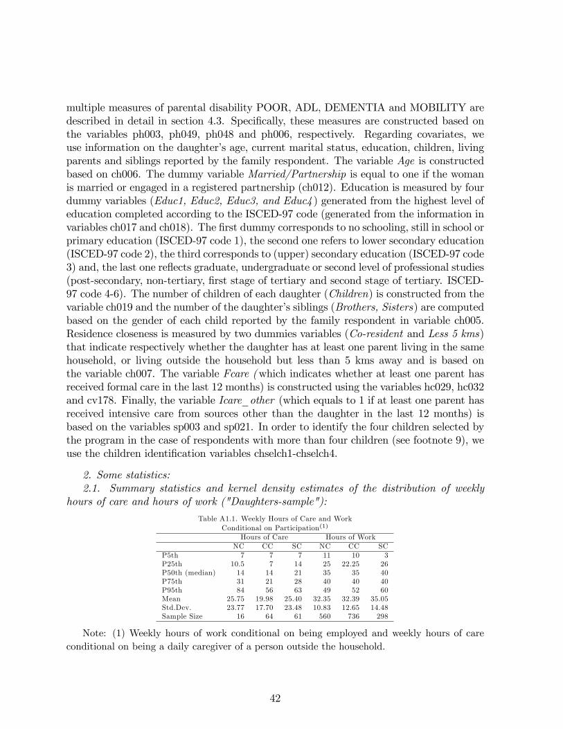
multiple measures of parental disability POOR, ADL, DEMENTIA and MOBILITY aredescribed in detail in section 4.3. Speci�cally, these measures are constructed based onthe variables ph003, ph049, ph048 and ph006, respectively. Regarding covariates, weuse information on the daughter�s age, current marital status, education, children, livingparents and siblings reported by the family respondent. The variable Age is constructedbased on ch006. The dummy variable Married/Partnership is equal to one if the womanis married or engaged in a registered partnership (ch012). Education is measured by fourdummy variables (Educ1, Educ2, Educ3, and Educ4 ) generated from the highest level ofeducation completed according to the ISCED-97 code (generated from the information invariables ch017 and ch018). The �rst dummy corresponds to no schooling, still in school orprimary education (ISCED-97 code 1), the second one refers to lower secondary education(ISCED-97 code 2), the third corresponds to (upper) secondary education (ISCED-97 code3) and, the last one re�ects graduate, undergraduate or second level of professional studies(post-secondary, non-tertiary, �rst stage of tertiary and second stage of tertiary. ISCED-97 code 4-6). The number of children of each daughter (Children) is constructed from thevariable ch019 and the number of the daughter�s siblings (Brothers, Sisters) are computedbased on the gender of each child reported by the family respondent in variable ch005.Residence closeness is measured by two dummies variables (Co-resident and Less 5 kms)that indicate respectively whether the daughter has at least one parent living in the samehousehold, or living outside the household but less than 5 kms away and is based onthe variable ch007. The variable Fcare (which indicates whether at least one parent hasreceived formal care in the last 12 months) is constructed using the variables hc029, hc032and cv178. Finally, the variable Icare_other (which equals to 1 if at least one parent hasreceived intensive care from sources other than the daughter in the last 12 months) isbased on the variables sp003 and sp021. In order to identify the four children selected bythe program in the case of respondents with more than four children (see footnote 9), weuse the children identi�cation variables chselch1-chselch4.

2. Some statistics:2.1. Summary statistics and kernel density estimates of the distribution of weekly

hours of care and hours of work ("Daughters-sample"):

Table A1.1. Weekly Hours of Care and WorkConditional on Participation(1)

Hours of Care Hours of WorkNC CC SC NC CC SC

P5th 7 7 7 11 10 3P25th 10.5 7 14 25 22.25 26P50th (median) 14 14 21 35 35 40P75th 31 21 28 40 40 40P95th 84 56 63 49 52 60Mean 25.75 19.98 25.40 32.35 32.39 35.05Std.Dev. 23.77 17.70 23.48 10.83 12.65 14.48Sample Size 16 64 61 560 736 298

Note: (1) Weekly hours of work conditional on being employed and weekly hours of careconditional on being a daily caregiver of a person outside the household.

42

Figure A1.1: Kernel density estimates of the distribution of weekly hours of work condi-tional on being employed across country pools.

0.0

1.0

2.0

3.0

4.0

5D

ensi

ty

0 20 40 60 80weekly hours of work

Southern Countries

0.0

1.0

2.0

3.0

4.0

5D

ensi

ty

0 20 40 60 80weekly hours of work

Northern Countries

0.0

1.0

2.0

3.0

4.0

5D

ensi

ty

0 20 40 60 80weekly hours of work

Continental countries

43

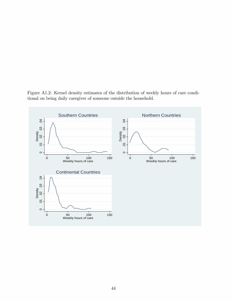
Figure A1.2: Kernel density estimates of the distribution of weekly hours of care condi-tional on being daily caregiver of someone outside the household.

0.0

1.0

2.0

3.0

4D

ensi

ty

0 50 100 150Weekly hours of care

Southern Countries

0.0

1.0

2.0

3.0

4D

ensi

ty

0 50 100 150Weekly hours of care

Northern Countries

0.0

1.0

2.0

3.0

4D

ensi

ty

0 50 100 150Weekly hours of care

Continental Countries

44

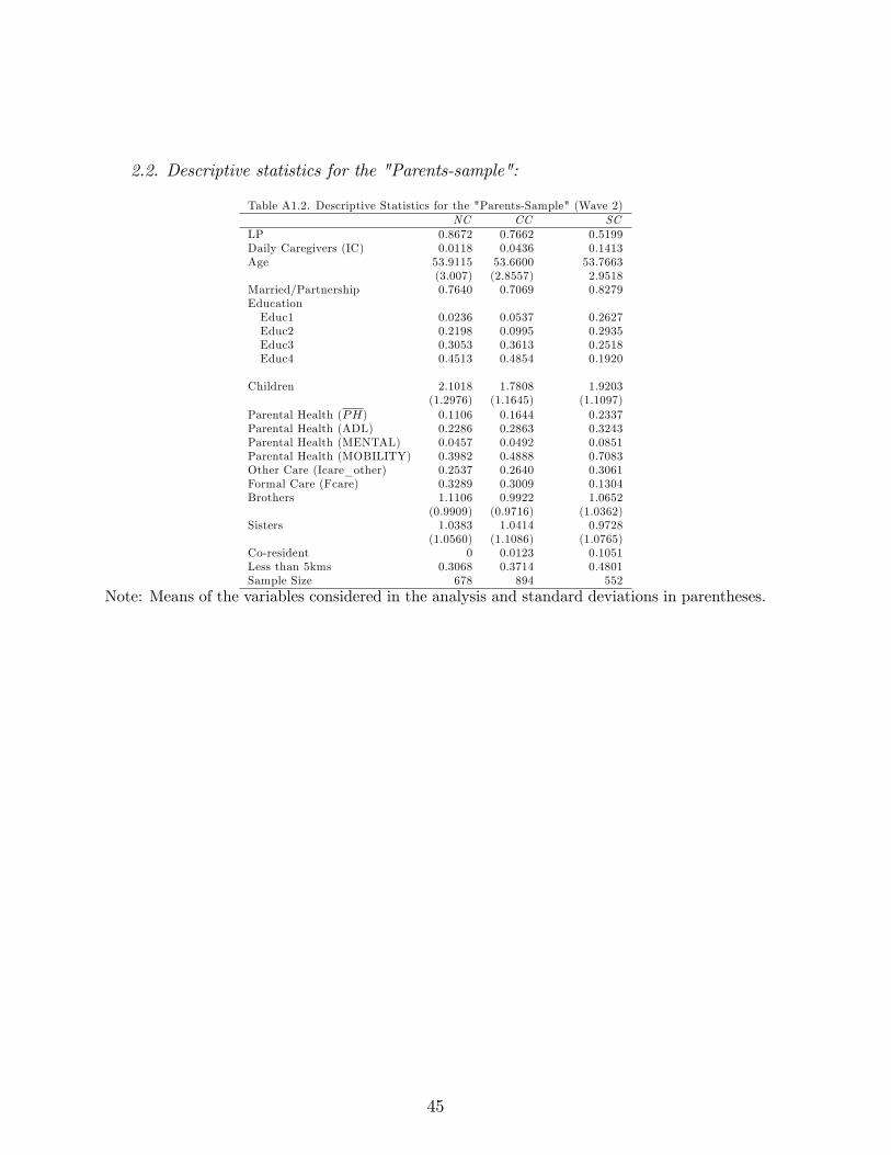
2.2. Descriptive statistics for the "Parents-sample":

Table A1.2. Descriptive Statistics for the "Parents-Sample" (Wave 2)NC CC SC

LP 0.8672 0.7662 0.5199Daily Caregivers (IC) 0.0118 0.0436 0.1413Age 53.9115 53.6600 53.7663

(3.007) (2.8557) 2.9518Married/Partnership 0.7640 0.7069 0.8279EducationEduc1 0.0236 0.0537 0.2627Educ2 0.2198 0.0995 0.2935Educ3 0.3053 0.3613 0.2518Educ4 0.4513 0.4854 0.1920

Children 2.1018 1.7808 1.9203(1.2976) (1.1645) (1.1097)

Parental Health (PH) 0.1106 0.1644 0.2337Parental Health (ADL) 0.2286 0.2863 0.3243Parental Health (MENTAL) 0.0457 0.0492 0.0851Parental Health (MOBILITY) 0.3982 0.4888 0.7083Other Care (Icare_other) 0.2537 0.2640 0.3061Formal Care (Fcare) 0.3289 0.3009 0.1304Brothers 1.1106 0.9922 1.0652

(0.9909) (0.9716) (1.0362)Sisters 1.0383 1.0414 0.9728

(1.0560) (1.1086) (1.0765)Co-resident 0 0.0123 0.1051Less than 5kms 0.3068 0.3714 0.4801Sample Size 678 894 552

Note: Means of the variables considered in the analysis and standard deviations in parentheses.

45

Appendix A2. Analysis of the discrete choice model of time allocation.Unless otherwise stated, we assume that the exclusion and monotonicity restrictions

hold. Then the utility di¤erence giving the propensity to work conditional on treatmentIC is

�UL(IC;w; :) = U(1; IC; :)� U(0; IC; :)= wh� �12

�(wh)2 + 2C0wh

�� �31h� �32

�h2 � 2heh0�

+�5�wh(T � h� IC)� C0h

�where C0 = y + �1IC � �2FC(IC) is consumption when the daughter does not work

and eh0 = T � IC is her leisure when she does not work. Therefore, the e¤ect of informalcare on the propensity-to-work index is

�2U(w; :) = �2�32hIC � 2�12(wh)�C0 � �5h(wIC +�C0)

which will (almost certainly) be negative if utility is concave in consumption and leisure.Note that �C0 = �1IC � �2(FC1 � FC0) is the di¤erence in the �no work� level ofconsumption when caring and not caring, and we assume �C0 > 0:[A su¤cient conditionis that spending on formal care is lower when the daughter provides daily informal care.]Finally, the treatment e¤ect is

TE(:) = I(�UL(0; w; :) + �2U(w; :) > 0)� I(�UL(0; w; :) > 0)

which has to be 0 or -1 if �2U(w; :) < 0.We now derive the utility di¤erence which determines the caregiving choice. Let

U(0; 0;PH) be the baseline utility when the daughter does not work and does not provideinformal care. Let �UC(PH) denote the utility di¤erence or �propensity to care�for adaughter who does not work. That is,

�UC(PH) = �C0 � �12�(�C0)

2 � 2y(�C0)�+ �5

�(�C0)(T � IC)� yIC

�+

+�2@Wp

@IC()�

h�31IC + �32(IC

2 � 2TIC)i

where the last two terms are the marginal utility of parental welfare and the (leisure)disutility of care, and the terms in the �rst line are cross terms and the marginal utilityof consumption changes brought about by caring.Recall from section 3.2 that the daughter provides care i¤ max[U(1; 1); U(0; 1)] �

max[U(1; 0); U(0; 0)] > 0: We can now write this "propensity to care" utility index interms of a baseline utility and three utility di¤erences as follows:

IC�(w;PH; :) = max[U(1; 1); U(0; 1)]�max[U(1; 0); U(0; 0)]= max[U(0; 0;PH) + �UL(0; :) + �

2U(:) + �UC(PH); U(0; 0;PH)

+�UC(PH)]�max[U(0; 0;PH) + �UL(0; :); U(0; 0;PH)]

46

where U(0; 0;PH) is baseline utility, �UC(PH) is propensity to care when not working,�UL(0; :) is propensity to work when not caring, and �2U(:) is "treatment e¤ect" of careon the propensity to work. Note that the �rst two terms depend on PH but not on thewage, whereas the third and fourth term depend on the wage but not on PH:Remark 1: The treatment e¤ects thresholds of Result 1 in section 3.2 are the reserva-

tion wages wr1 and wr2 that satisfy�UL(0; wr1; :) = 0; and�UL(0; wr2; :)+�2U(wr2; :) = 0respectively. When w < wr1 the wage is so low that the daughter will never work andthe "treatment" e¤ect of daily caregiving on employment is 0. When wr1 < w < wr2 thedaughter works if she is not caring but does not work if she provides care so the treatmente¤ect is -1. When w > wr2 the daughter always works and the treatment e¤ect is zero. Weknow that wr2 > wr1 because �2U() is negative, and this also implies that the treatmente¤ect cannot be positive. [If we relax the exclusion restrictions then the two reservationwages may depend on PH:]Remark 2: For �xed PH; consider the IC� index as a function of the wage. For

w < wr1 it is a constant. For wr1 < w < wr2 it is clearly decreasing in w: For w > wr2we have IC�(w; :) = �2U(w:) + �UC(PH): So the slope of the index is the slope of�2U(w:): The leading terms of �2U(w:) are �2�32hIC � �5hICw because �C0 is likelyto be negligible. If consumption and leisure are complements in utility then IC�() isstill decreasing in this range. Even if it is not, the slope should be small - it seem veryimplausible that increasing the wage would increase the propensity to provide daily careof a daughter who works. To conclude, the IC� index for both values of PH is �at forlow wages, and decreasing therafter.Remark 3: For any �xed w; the IC� is strictly greater for PH = 1 than for PH = 0 as

long as f21 > 0: This implies monotonicity of the instrument, and it is straightforward toprove from the expression for IC� above, which is based on the Exclusion and Separabilityrestrictions. [The result follows because �UC(1) > �UC(0); and the di¤erence betweenthe IC� indexes for PH = 1 and PH = 0 is constant in the wage.]Remark 4: Result 2 establishing the existence of "compliance type" thresholds wc1

and wc2 follows from Remarks 2 and 3. The thresholds wc1 and wc2 are de�ned by theconditions IC�(wc1; 0) = 0; and IC�(wc2; 1) = 0 respectively (see Figure 3). For w < wc1daughters are always takers, for wc1 < w < wc2 daughters are compliers and for w > wc2daughters are never takers.Remark 5: The �rst part of Result C1 is trivial from the expression for IC�(): The

second part follows from the plausible assumption that f24 < 0; because this implies that@�UC@OC

() < 0 for both values of PH:Remark 6 - the FC() function: The optimal level of formal care paid for by the

daughter trades o¤ the marginal disutility of consumption (lost through payment) againstthe marginal utility of parental welfare. More precisely the optimal level FC(LP; IC)satis�es the following conditions:

�2@Wp

@FC(PH; IC; FC(LP ; IC); OC) = �2[1� 2�12C(LP; IC; FC(LP; IC))

+�5(T � LPh� ICIC)]

47

if FC(LP; IC) > 0; and

�2@Wp

@FC(PH; IC; 0; OC) < �2

�1� 2�12C(LP; IC; 0) + �5(T � LPh� ICIC)

�if FC(LP; IC) = 0; where C(LP; IC; FC) is the level of consumption corresponding tochoice (LP; IC; FC): From these conditions it is straightforward to see that FC() will ingeneral depend on LP; unless �12 = �5 = 0 makes the marginal utility of consumptioncosntant.

48

Appendix A3. Formulas for the compliance types and the LATE parameter based on abiprobit model.In our context, an alternative speci�cation to the matching estimator considered in

(6) is given by a parametric estimator based on the following model:

LP = I( 0 + 1PH + �0X + " � 0);

IC = I(�0 + �1PH + �0X + � � 0):

where I(�) is the indicator function that is equal to one if the condition in parenthesisholds and zero otherwise and ("; �)0 is the vector of unobservable characteristics of thedaughters or parents that could also potentially in�uence their choices. These error termsare assumed to be iid and follow a bivariate normal distribution�

"�

�j PH;X � N

�0;

�1 �� 1

��where � is the correlation of the errors and the variances are normalized to 1. Given thisspeci�cation, we can decompose the population in compliers, always takers and never tak-ers using the fact that the index model assumption for IC is equivalent to the monotonic-ity assumption on the relationship between IC and PH: In particular, the two potentialoutcomes for IC are the following

IC1 = I(�0 + �1 + �0X + v � 0)

IC0 = I(�0 + �0X + v � 0)

If we assume that �1 � 0; the compliance type depends on the individual�s value of vas follows:Compliers: Units with IC1 = 1; IC0 = 0 =) v � ��0 � �1 � �0X but v < ��0 � �0X:Always takers: Units with IC1 = 1; IC0 = 1 =) v � ��0 � �0X:Never takers Units with IC1 = 0; IC0 = 0 =) v < ��0 � �1 � �0X:Therefore, the mass of each group is given byZ

[�(�0 + �1 + �0X)� �(�0 + �0X)]dF (X) for compliersZ

[�(�0 + �0X)]dF (X) for always takersZ

[1� �(�0 + �1 + �0X)]dF (X) for never takers

where � denotes the standard normal distribution.And the average treatment e¤ect for the compliers or LATE based on this parametric

speci�cation has the following expression

b� =NXi=1

[�(b 0 + b 1 + b�0X)� �(b 0 + b�0Xi)]

NXi=1

[�(b�0 + b�1 + b�0X)� �(b�0 + b�0Xi)]

:

49

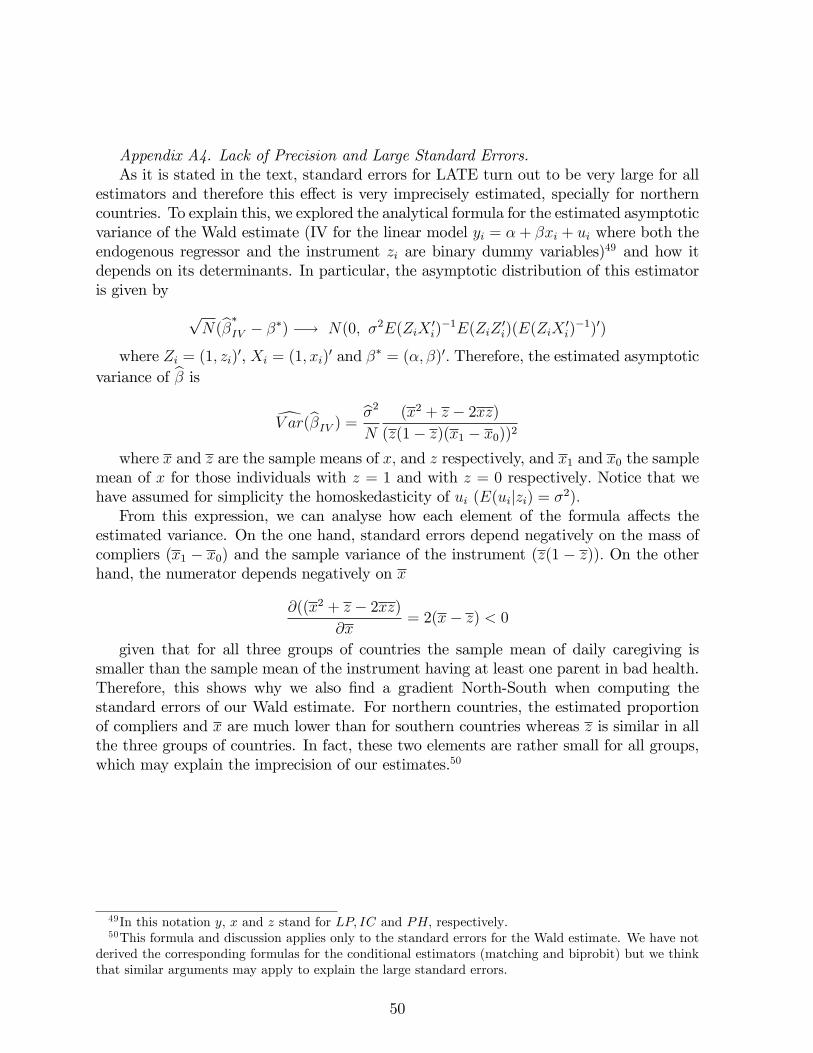
Appendix A4. Lack of Precision and Large Standard Errors.As it is stated in the text, standard errors for LATE turn out to be very large for all

estimators and therefore this e¤ect is very imprecisely estimated, specially for northerncountries. To explain this, we explored the analytical formula for the estimated asymptoticvariance of the Wald estimate (IV for the linear model yi = �+ �xi + ui where both theendogenous regressor and the instrument zi are binary dummy variables)49 and how itdepends on its determinants. In particular, the asymptotic distribution of this estimatoris given by

pN(b��IV � ��) �! N(0; �2E(ZiX

0i)�1E(ZiZ

0i)(E(ZiX

0i)�1)0)

where Zi = (1; zi)0, Xi = (1; xi)0 and �� = (�; �)0: Therefore, the estimated asymptotic

variance of b� isdV ar(b�IV ) = b�2

N

(x2 + z � 2xz)(z(1� z)(x1 � x0))2

where x and z are the sample means of x; and z respectively, and x1 and x0 the samplemean of x for those individuals with z = 1 and with z = 0 respectively: Notice that wehave assumed for simplicity the homoskedasticity of ui (E(uijzi) = �2):From this expression, we can analyse how each element of the formula a¤ects the

estimated variance. On the one hand, standard errors depend negatively on the mass ofcompliers (x1 � x0) and the sample variance of the instrument (z(1 � z)): On the otherhand, the numerator depends negatively on x

@((x2 + z � 2xz)@x

= 2(x� z) < 0

given that for all three groups of countries the sample mean of daily caregiving issmaller than the sample mean of the instrument having at least one parent in bad health.Therefore, this shows why we also �nd a gradient North-South when computing thestandard errors of our Wald estimate. For northern countries, the estimated proportionof compliers and x are much lower than for southern countries whereas z is similar in allthe three groups of countries. In fact, these two elements are rather small for all groups,which may explain the imprecision of our estimates.50

49In this notation y, x and z stand for LP; IC and PH; respectively:50This formula and discussion applies only to the standard errors for the Wald estimate. We have not

derived the corresponding formulas for the conditional estimators (matching and biprobit) but we thinkthat similar arguments may apply to explain the large standard errors.

50

CEMFI WORKING PAPERS

0801 David Martinez-Miera and Rafael Repullo: “Does competition reduce the risk of bank failure?”.

0802 Joan Llull: “The impact of immigration on productivity”.

0803 Cristina López-Mayán: “Microeconometric analysis of residential water demand”.

0804 Javier Mencía and Enrique Sentana: “Distributional tests in multivariate dynamic models with Normal and Student t innovations”.

0805 Javier Mencía and Enrique Sentana: “Multivariate location-scale mixtures of normals and mean-variance-skewness portfolio allocation”.

0806 Dante Amengual and Enrique Sentana: “A comparison of mean-variance efficiency tests”.

0807 Enrique Sentana: “The econometrics of mean-variance efficiency tests: A survey”.

0808 Anne Layne-Farrar, Gerard Llobet and A. Jorge Padilla: “Are joint negotiations in standard setting “reasonably necessary”?”.

0809 Rafael Repullo and Javier Suarez: “The procyclical effects of Basel II”.

0810 Ildefonso Mendez: “Promoting permanent employment: Lessons from Spain”.

0811 Ildefonso Mendez: “Intergenerational time transfers and internal migration: Accounting for low spatial mobility in Southern Europe”.

0812 Francisco Maeso and Ildefonso Mendez: “The role of partnership status and expectations on the emancipation behaviour of Spanish graduates”.

0813 Rubén Hernández-Murillo, Gerard Llobet and Roberto Fuentes: “Strategic online-banking adoption”.

0901 Max Bruche and Javier Suarez: “The macroeconomics of money market freezes”.

0902 Max Bruche: “Bankruptcy codes, liquidation timing, and debt valuation”.

0903 Rafael Repullo, Jesús Saurina and Carlos Trucharte: “Mitigating the procyclicality of Basel II”.

0904 Manuel Arellano and Stéphane Bonhomme: “Identifying distributional characteristics in random coefficients panel data models”.

0905 Manuel Arellano, Lars Peter Hansen and Enrique Sentana: “Underidentification?”.

0906 Stéphane Bonhomme and Ulrich Sauder: “Accounting for unobservables in comparing selective and comprehensive schooling”.

0907 Roberto Serrano: “On Watson’s non-forcing contracts and renegotiation”.

0908 Roberto Serrano and Rajiv Vohra: “Multiplicity of mixed equilibria in mechanisms: a unified approach to exact and approximate implementation”.

0909 Roland Pongou and Roberto Serrano: “A dynamic theory of fidelity networks with an application to the spread of HIV / AIDS”.

0910 Josep Pijoan-Mas and Virginia Sánchez-Marcos: “Spain is different: Falling trends of inequality”.

0911 Yusuke Kamishiro and Roberto Serrano: “Equilibrium blocking in large quasilinear economies”.

0912 Gabriele Fiorentini and Enrique Sentana: “Dynamic specification tests for static factor models”.

0913 Javier Mencía and Enrique Sentana: “Valuation of VIX derivatives”.

1001 Gerard Llobet and Javier Suarez: “Entrepreneurial innovation, patent protection and industry dynamics”.

1002 Anne Layne-Farrar, Gerard Llobet and A. Jorge Padilla: “An economic take on patent licensing: Understanding the implications of the “first sale patent exhaustion” doctrine.

1003 Max Bruche and Gerard Llobet: “Walking wounded or living dead? Making banks foreclose bad loans”.

1004 Francisco Peñaranda and Enrique Sentana: “A Unifying approach to the empirical evaluation of asset pricing models”.

1005 Javier Suarez: “The Spanish crisis: Background and policy challenges”.

1006 Enrique Moral-Benito: “Panel growth regressions with general predetermined variables: Likelihood-based estimation and Bayesian averaging”.

1007 Laura Crespo and Pedro Mira: “Caregiving to elderly parents and employment status of European mature women”.