Carbon dynamics of different land use systems in NW Ethiopian

University of Natural Resources and Life Sciences, Vienna

Institute of Forest Ecology

Carbon dynamics of different land use systems in

NW Ethiopian

Dissertation

A thesis submitted in conformity with the requirements for the degree of Doctor of

Philosophy (Dr. nat. techn.) at University of Natural Resources and Life Sciences,

Vienna

Submitted by

MSc. Dessie Assefa

Supervisor: Univ. Prof. Ph.D. Dr. Douglas L. Godbold1

Co-supervisor: Ass. Prof. Dipl.-Biol. Dr.rer.nat. Boris Rewald1

March 2017

Vienna, Austria

1Institute of Forest Ecology at Department of Forest and Soil Science

I

Abstract

The amount of carbon (C) stored in the upper 100 cm soil is about three times greater than C stored in vegetation and twice as much as C present in the atmosphere. Soil organic carbon (SOC) is accumulated if inputs from leaf litterfall, root turnover, and other biomass are greater than losses by mineralization, erosion, and other processes. Potential shifts in SOC stocks and rising atmospheric CO2 concentrations are major concerns of climate change. Despite the large quantity of C stored in soil, consensus is lacking on the dynamics and the extent of land use change effects on soil C storage especially for tropical ecosystems. Several field and laboratory techniques were carried out to examine the magnitude of SOC stock changes due to land use conversion, the spatial distribution of SOC stocks, the origin, chemical composition of input materials and their decomposition rates, and substrate and temperature dependency of microbial respiration. The study was conducted in the NW Ethiopian highlands and a semi-arid savannah woodland. The land use systems studied were natural forest, eucalyptus plantation, exclosure, grazing land, and cropland. Total C and N stocks were determined along a climatic gradient. Litterfall was determined by litter traps and fine root production was estimated using sequential coring, ingrowth core and ingrowth net methods. Litter decomposition rates of leaves and fine roots were estimated using a litterbag technique. Chemical compositions of input materials were characterized by sequential extraction. Individual biomarkers were identified and quantified by gas chromatography and mass spectrometry at a molecular level. The temperature sensitivity of soil respiration was measured using a MicroResp method - glucose, lignin, and starch were added as a proxy for substrate availability and nitrogen and phosphorous were supplied as nutrient proxies to determine the factors limiting microbial respiration. Results showed that land use conversion from native forest to cropland or grazing land reduced SOC stocks by 70-90% in less than 50 years. Afforestation and exclosure led to an increase of SOC; however, the rate of increase (ca. 0.3 kg m-2 yr-1) was lower than losses (ca. 0.4 kg m-2 yr-1). The geomarker analysis (Sr/Ca and Ba/Ca ratio) and vertical distribution of carbon suggests that the major factor for SOC reduction is erosion while the C loss through mineralization ranged from 1.6-3.9 mg g soil-1 yr-1 and increased with increasing temperature. This is consistent with C availability in the soil. Soils supplemented with glucose increased heterotrophic respiration by 10-fold. The annual litterfall production in the natural forest ecosystem was about 1100 g m-2 of which leaf comprised 65%. Above-ground litter inputs in eucalyptus, cropland, and grazing land are estimated to be minor due to leaf litter raking, complete residual harvest, and overgrazing. The annual fine root production was estimated to be 700 g m-2 in natural forest and eucalyptus whereas fine root production in grazing land and cropland was about 50-60 g m-2. This illustrates that conversion of native forest to grazing land and cropland resulted in the reduction of C input into the soil by >90%. Fine roots decomposed slower than leaf litters with decomposition rate constant of 1.7 yr-1 for fine roots and 2.5 yr-1 for leaves. The variation in decomposition is due to their chemical composition. The acid-insoluble fraction in fine roots (50%) was greater than leaves (42%). Thus, fine roots contributed about 1.5 times more recalcitrant C input into the soil than leaf litters. From the biomarker analysis, the amount of suberin was 2-times that of cutin further confirming higher inputs of recalcitrant carbon from fine roots. The ratio of lignin-derived phenols of syringyls to vanillyls suggested that angiosperm plants are the predominant sources for lignin. The dominance of aliphatic lipids and lignin in SOC revealed that higher plants are a major input of SOC while microbial inputs were present as minor components (<1%). Overall, conversion of native forest to open lands in Ethiopian highland resulted in substantial loss of SOC stock due to both erosion and mineralization. The major inputs of SOC are fine roots of angiosperm plants due to their larger carbon, lignin and suberin contents and this slower decomposition. The results suggest C loss due to land use change in the Amhara region needs urgent attention. Future land use management need to raise awareness on the importance of SOC management as the basis for essential ecosystem functions and improve food security.

II

Abstrakt

Die Menge an gespeichertem Kohlenstoff (C) in den oberen 100 cm Boden ist etwa dreimal mehr als die der Vegetation und doppelt so viel wie in der Atmosphäre vorhandene C. Organischer Kohlenstoff im Boden (SOC) wird akkumuliert, wenn der C Eintrag durch Laubfall, Wurzelumsatz und andere Biomasse größer ist als die Verluste durch Mineralisierung, Erosion und andere Prozesse. Trotz der großen Wichtigkeit von Bodenkohlenstoff für globale biogeochemische Prozesse ist der Stand des Wissens über die SOC-Dynamik im Allgemeinen und die Auswirkungen von Landnutzungsänderungen im Speziellen vor allem für tropische Ökosysteme noch sehr limitiert. In dieser Studie wurden daher verschiedenste Feld- und Laboruntersuchungen durchgeführt um SOC-Bestandsveränderungen aufgrund von Landnutzungsumwandlung, die räumlichen Verteilung der SOC-Bestände, der Herkunft und chemische Zusammensetzung der Ausgangsmaterialien und ihrer Zersetzungsraten, sowie die Substrat- und Temperaturabhängigkeit der mikrobiellen Atmung zu untersuchen. Die untersuchten Landnutzungssysteme im Äthiopischen Hochland und der Savanne waren artenreiche Mischwälder, eine Eukalyptus-Plantage, eine Weideausschlußfläche, sowie Weide- und Ackerland. Gesamtbodenkohlenstoff und -stickstoff wurden entlang eines Klimagradienten bestimmt. Der Laubfall wurde mit Streusammlern, die Feinwurzelproduktion unter Verwendung von sequenzieller Bohrkernbeprobung, und Einwuchssäulen und -netzen bestimmt. Zersetzungsraten von Blättern und Feinwurzeln wurden unter Verwendung von litterbags gemessen. Die chemische Zusammensetzung der Ausgangsmaterialien wurden durch sequentielle Extraktion charakterisiert. Einzelne Biomarker wurden durch Gaschromatographie und Massenspektrometrie auf molekularer Ebene identifiziert und quantifiziert. Die Temperaturempfindlichkeit und Substratabhängigkeit der Bodenatmung wurde unter Verwendung eines MicroResp-Verfahrens gemessen. Die Ergebnisse zeigen, dass die Umwandlung von natürlichen Wäldern zu Acker- oder Weideland den Bodenkohlenstoffvorrat in weniger als 50 Jahren um 70-90% reduziert. Aufforstung und Ausschluss von Weidetieren führen zu einer Erhöhung des SOC-Vorrats. Allerdings ist die Akkumulationsrate (ca. 0,3 kg m-2 a-1) niedriger als die Verlustrate (ca. 0,4 kg m-2 a-1). Die Geomarker-Analyse (Sr:Ca- bzw. Ba:Ca-Verhältnisse) und die vertikale Verteilung von Kohlenstoff deuten darauf hin, dass Erosion der Hauptfaktor für die SOC-Abnahme war. Die heterotrophe Atmung ist durch die Kohlenstoffverfügbarkeit im Boden eingeschränkt. Die jährliche oberirdische Streuproduktion im Naturwald beträgt etwa 1100 g m-2, wobei der Blattanteil 65% betrug. Überirdische Streueinträge sind in der Eukalyptusplantage, sowie im Acker- und Weideland vernachlässigbar. Die jährliche Feinwurzelproduktion wurde in beiden Waldwirtschaftsformen auf ca. 700 g m-2 geschätzt, in Weide- und Ackerland auf etwa 50-60 g m-2. Dies zeigt, dass die Umwandlung von Wald zu Weide- bzw. Ackerland den Kohlenstoffeintrag in den Boden um >90% verringert. Die Feinwurzeln der untersuchten Bäume zersetzten sich langsamer als deren Blätter, mit einer Abbaukonstante von 1,7 a-1 für Feinwurzeln und 2,5 a-1 für Blätter. Die Zersetzungsrate ist abhängig von der chemische Zusammensetzung, insbesondere ist die säureunlösliche Fraktion in Feinwurzeln (50%) größer als in Blättern (42%). In der Schlussfolgerung tragen im untersuchten Waldsystem die Wurzeln etwa 1,5-mal mehr zum Eintrag recalcitranten Kohlenstoffs in den Boden bei als Blattstreu. Dies wird auch durch die Ergebnisse der Biomarkeranalyse gestützt. Diese zeigen, dass die Menge an Suberin (aus Wurzeln) im Boden die des Cutins (aus Blättern) um das Zweifache übersteigt. Die Biomarker zeigen zudem, dass der überwiegende Teil des Bodenkohlenstoffs von höheren Pflanzen im Allgemeinen und Angiospermen im Besonderen stammt. Insgesamt führte die Umwandlung von Wald in landwirtschaftlich genutzte Flächen im äthiopischen Hochland zu einer erheblichen Reduzierung des Bodenkohlenstoffvorrats, insbesondere durch verstärkte Erosion und Mineralisierungsraten. Der Bodenkohlenstoff stammt hauptsächlich von Feinwurzeln von Angiospermen, diese weisen größere Kohlenstoff-, Lignin- und Suberin-Gehalte auf als Blätter und zersetzen sich langsamer. Die Ergebnisse der Arbeit verdeutlichen, dass der Verlust von Bodenkohlenstoff aufgrund von Landnutzungsänderungen in der Region Amhara ein extremes Ausmaß angenommen hat und die Lösung dringend politische Aufmerksamkeit erfordert. Ein zukünftiges Landnutzungsmanagement muss vor Allem das Bewusstsein für die Wichtigkeit von Bodenkohlenstoff zur Aufrechterhaltung wesentlicher Ökosystemfunktionen stärken um u.a. die landwirtschaftliche Produktion zu stabilisieren und damit die Ernährungssicherheit in der Region zu gewährleisten.

III

Acknowledgment

I sincerely thank Prof. Douglas L. Godbold, who has always encouraged, supported my

research activities, and provided me the opportunity to become a PhD student at the Institute

of Forest Ecology, University of Natural Resources and Life Science in Austria. I appreciate

that he was always available when I needed his help and gave generous amounts of advice. I

would also like to thank Ass. Prof. Boris Rewald for his enthusiasm and fruitful discussions of

the numerous experiments and manuscripts. I am grateful to PD Hans Sandén for his support,

guidance, and useful suggestions throughout this study including his advice during numerous

field trips. I additionally thankful to Prof. Egbert Matzner and PD Gernot Bodner for their

willingness and time to serve on my comprehensive exam and defense committee.

I am thankful to Christoph Rosinger, Marcel Hirsch, and Frauke Neuman for their technical

advice and assistance with sample analysis in the laboratory. I am grateful to Dr. Karin

Wriessnig for her kind help during importing process for plant and soil samples for the last three

years as well as training me on laboratory analysis. Many thanks to Astrid Hobel and Prof. Axel

Mentler, from the Institute of Soil Science, for training me on gas chromatograph - mass

spectrometer (GC-MS), high performance liquid chromatography (HPLC), and other various

instruments in the laboratory – this thesis would not have been possible without their help!

I want to give my special thanks to Sigrid Gubo, for her dedication and help on my private

matters – making my life in Vienna very easy and enjoyable. I am also thankful to Martin

Wresowar for his quick technical support related to software whenever needed. I would like to

express my special thanks to members of the Institute of Forest Ecology and my officemates

and friends Dr. Iftekhar Ahmed and Dr. Norbu Wangdi. Many thanks should go to Dr. Mathias

Mayer, and Dr. Bradley Matthews who supported me mentally and cheered me up in the past

three years. It was a great working, talking, and laughing with members of the Institute of Forest

Ecology, which I could not mention all your names here and thank you for making my stay in

Vienna so much memorable.

I am very grateful to my wife, Nebyate Kebede, for her help during root washings. Washing

more than 5,000 root samples would not be possible without her help. Thank you for sharing

life in Vienna with me. Special thanks to Peter Kube and Christiane from Germany for their

love, encouragement, and for their frequent visits.

Finally, this work was carried out within the project (“Carbo-part”) funded by the Austrian

Ministry of Agriculture, Forestry, Environment, and Water Management. It would have not been

possible without the financial help of this project (“Carbo-part”) and the Austrian government.

IV

Table of contents

Abstract ....................................................................................................................... I

Abstrakt ...................................................................................................................... II

Acknowledgment ....................................................................................................... III

Table of contents ....................................................................................................... IV

List of figures ........................................................................................................... VIII

List of tables ............................................................................................................... X

1 General Introduction ............................................................................................. 1

1.1 Land degradation in the Amhara region: history, extent, causes, and consequences .................................................................................................................................. 1

1.2 The nature and formation of soil organic carbon ...................................................... 4

1.2.1 Soil carbon stock and temporal changes after land use change ..................................... 4

1.2.2 Mechanisms for soil organic carbon accumulation .......................................................... 6

1.2.3 Tracing the biological origin and degradation status of organic carbon in soil ................ 9

1.3 Aims and outline .....................................................................................................11

1.4 Hypotheses ............................................................................................................12

2 Soil organic carbon dynamics after land use change in Northwest Ethiopia ...... 13

2.1 Abstract ..................................................................................................................13

2.2 Introduction ............................................................................................................13

2.3 Material and methods .............................................................................................16

2.3.1 Research sites ............................................................................................................... 16

2.3.2 Soil sampling ................................................................................................................. 19

2.3.3 Bulk density determination ............................................................................................ 19

2.3.4 Total C and N stock determination ................................................................................ 20

2.3.5 Strontium, calcium and barium elemental analysis ....................................................... 21

2.3.6 Determination of soil pH ................................................................................................ 21

2.3.7 Particle size determination ............................................................................................ 21

2.3.8 Data analysis ................................................................................................................. 22

2.4 Results ...................................................................................................................23

2.4.1 Soil carbon and nitrogen stocks .................................................................................... 23

2.4.2 Vertical distributions of C and N .................................................................................... 26

2.4.3 Soil bulk density ............................................................................................................. 28

2.4.4 Strontium:calcium and barium:calcium ratios ................................................................ 29

2.4.5 Factors effecting soil carbon stocks .............................................................................. 29

2.5 Discussion ..............................................................................................................31

2.5.1 Soil organic carbon and nitrogen stocks ....................................................................... 31

2.5.2 Effect of land use change on carbon stock ................................................................... 32

2.5.3 Potentials of soil carbon gain due to afforestation and exclosure ................................. 35

2.5.4 Magnitude of soil carbon loss due to deforestation ....................................................... 36

2.6 Conclusion .............................................................................................................36

V

3 Fine root dynamics in Afromontane forest and adjacent land uses in the Ethiopian highlands .................................................................................................. 37

3.1 Abstract ..................................................................................................................37

3.2 Introduction ............................................................................................................37

3.3 Materials and Methods ...........................................................................................40

3.3.1 Site descriptions ............................................................................................................ 40

3.3.2 Root sampling ................................................................................................................ 41

3.3.3 Soil sampling ................................................................................................................. 43

3.3.4 Estimation of annual fine root production, mortality, and decomposition ...................... 43

3.3.5 Calculation of fine root turnover ..................................................................................... 47

3.3.6 Fine root vertical distribution .......................................................................................... 47

3.3.7 Carbon and nitrogen analysis ........................................................................................ 47

3.3.8 Statistical analyses ........................................................................................................ 48

3.4 Results ...................................................................................................................48

3.4.1 Fine root biomass, necromass and distribution with depth ........................................... 48

3.4.2 Seasonal variation of root stocks ................................................................................... 51

3.4.3 Fine root production, mortality, and turnover ................................................................. 52

3.4.4 Annual C and N flux into the soil ................................................................................... 57

3.5 Discussion ..............................................................................................................57

3.5.1 Effect of land use change on fine root stocks and production ....................................... 57

3.5.2 Seasonal variation of fine root mass ............................................................................. 59

3.5.3 Limitations of sampling methods ................................................................................... 60

3.5.4 Implications of fine root turnover in ecosystem carbon cycling ..................................... 63

3.6 Conclusion .............................................................................................................63

4 Fine root morphology, biochemistry and litter quality indices of fast- and slow-growing woody species in Ethiopian highland forests ............................................... 64

4.1 Abstract ..................................................................................................................64

4.2 Introduction ............................................................................................................65

4.3 Materials and methods ...........................................................................................67

4.3.1 Study site ....................................................................................................................... 67

4.3.2 Root sampling ................................................................................................................ 68

4.3.3 Root morphology ........................................................................................................... 68

4.3.4 Root biochemistry and construction costs ..................................................................... 69

4.3.5 Statistical analysis ......................................................................................................... 70

4.4 Results ...................................................................................................................71

4.4.1 Root morphology ........................................................................................................... 71

4.4.2 Root biochemistry .......................................................................................................... 73

4.4.3 Carbon cost of root production ...................................................................................... 75

4.4.4 Correlation of morphological and biochemical fine root traits ....................................... 77

4.5 Discussion ..............................................................................................................78

4.5.1 Root morphological traits and growth pattern ................................................................ 78

4.5.2 Root biochemistry and carbon cost implications for root litter quality ........................... 80

VI

4.6 Conclusion .............................................................................................................84

5 Litter production, chemistry, and turnover in a pristine forest ecosystem in the Ethiopian highland .................................................................................................... 85

5.1 Abstract ..................................................................................................................85

5.2 Introduction ............................................................................................................86

5.3 Materials and methods ...........................................................................................88

5.3.1 Description of the study site .......................................................................................... 88

5.3.2 Litterfall collection and fine root biomass determination ................................................ 89

5.3.3 Litter (leaf and root) decomposition using litterbag technique ....................................... 89

5.3.4 Chemical analysis .......................................................................................................... 90

5.3.5 Calculations of decomposition parameters, C and N input into the soil ........................ 91

5.3.6 Statistical analysis ......................................................................................................... 91

5.4 Results ...................................................................................................................92

5.4.1 Annual litterfall production ............................................................................................. 92

5.4.2 Fine root biomass, production, and turnover ................................................................. 93

5.4.3 Initial litter chemistry ...................................................................................................... 94

5.4.4 Litter decay measurement and turnover rate ................................................................ 96

5.4.5 C and N fluxes into the soil ............................................................................................ 99

5.5 Discussion ............................................................................................................ 101

5.5.1 Above-ground litter production and seasonal pattern .................................................. 101

5.5.2 Factors controlling leaf litter decomposition ................................................................ 102

5.5.3 Fine root and coarse root decomposition .................................................................... 105

5.5.4 Biochemical fluxes from litters into the soil .................................................................. 106

5.6 Conclusion ........................................................................................................... 107

6 The biological origin of soil organic carbon and response to land use change based on biomarker analysis .................................................................................. 108

6.1 Abstract ................................................................................................................ 108

6.2 Introduction .......................................................................................................... 109

6.3 Methodology......................................................................................................... 112

6.3.1 Study area ................................................................................................................... 112

6.3.2 Soil sampling, C and N analysis .................................................................................. 112

6.3.3 Sequential extraction procedures ................................................................................ 113

6.3.4 Base hydrolysis ............................................................................................................ 113

6.3.5 CuO oxidation .............................................................................................................. 114

6.3.6 Derivatization and GC/MS Analysis ............................................................................. 114

6.3.7 Origin and degradation parameters ............................................................................. 115

6.4 Results .............................................................................................................. 117

6.4.1 Soil C and N content and yields of sequential extractions .......................................... 117

6.4.2 Composition and distribution of solvent-extractable free lipids ................................... 118

6.4.3 Composition and distribution of bound lipids ............................................................... 120

6.4.4 Composition and distributions of lignin compounds .................................................... 121

6.5 Discussion ............................................................................................................ 122

VII

6.5.1 Biological origin of organic carbon in the soil .............................................................. 122

6.5.2 Degradation stage of plant organic matter .................................................................. 129

6.6 Conclusions.......................................................................................................... 132

7 Microbial soil respiration and its dependency on substrate availability and temperature in four contrasting land use systems .................................................. 133

7.1 Abstract ................................................................................................................ 133

7.2 Introduction .......................................................................................................... 134

7.3 Materials and methods ......................................................................................... 137

7.3.1 Site description ............................................................................................................ 137

7.3.2 Soil sampling ............................................................................................................... 137

7.3.3 Total C, N, and soil pH analysis .................................................................................. 138

7.3.4 Determination of moisture content and water holding capacity ................................... 138

7.3.5 Preparation of carbon and nutrient sources ................................................................ 138

7.3.6 Preparing agar and indicator solution for the MicroResp ............................................ 139

7.3.7 Soil filling and incubation ............................................................................................. 139

7.3.8 Measurement of soil respiration .................................................................................. 140

7.3.9 Quantifying CO2 efflux and biological indices .............................................................. 140

7.4 Results ................................................................................................................. 142

7.4.1 Soil chemical and physical properties in four land use systems ................................. 142

7.4.2 Basal respiration in the four land use systems ............................................................ 143

7.4.3 Microbial respiration in response to substrate availability ........................................... 144

7.4.4 Soil microbial biomass carbon ..................................................................................... 145

7.4.5 Temperature effect on CO2 efflux at different land use systems ................................. 146

7.5 Discussion ............................................................................................................ 148

7.5.1 Resource availability and carbon use efficiency of microorganisms ........................... 148

7.5.2 Biological indicators for eco-physiological stress ........................................................ 150

7.5.3 Effect of temperature on microbial decomposition ...................................................... 151

7.6 Conclusion ........................................................................................................... 153

8 Summary and conclusions ............................................................................... 154

References ............................................................................................................. 159

Appendices ............................................................................................................. 184

Appendix 1. Supplementary materials for Chapter 2 ....................................................... 184




Appendix 5 Data not used in this thesis .......................................................................... 200

VIII

List of figures

Figure 2 1 Stocks (kg m-2, mean ±SE) of soil organic carbon (filled bars) and soil nitrogen (unfilled bars) in different land use types at a range of sites in the Amhara region of Northern Ethiopia. Shown are the pooled data of different land use systems from three highland areas (a) and two land use systems of the lowland area (b) (see legend Table 2.2). Bars without the same letters (small case letters for filled bars and capital case letters for unfilled bars) are significantly different

(mean ±SE; Scheffe, P<0.05, n (highland) = 30, and n (lowland) = 10). ................................................... 24

Figure 2 2 Vertical distribution of soil C concentrations in the highland land-use system a) and the relative cumulative SOC stock fraction across soil depth for each land use type b). Shown are the means of the pooled data of the individual sites. Different small case letters for panel (a) indicate significant differences of data points along soil depth within a land use type whereas capital case letters indicate differences between land use type for each depth (mean ±SE; Scheffe, P<0.05, n (forest) = 40, n (eucalyptus, grazing land, cropland) = 30). The panel (b) is Y = 1– ßd, where Y is the cumulative SOC fraction from the surface (proportion between 0 and 1) to soil depth (d in cm) and ß is the fitted parameter of the asymptotic nonlinear model (Gale and Grigal 1987). A Y value of 0.75 at 30 depth means that 75% of the total SOC storage is located above 30 cm soil depth. Higher ß index value indicates the relative proportion of SOC to lower

profile is greater in the specific land use, or the relative change of SOC across depth is smaller. ....... 26

Figure 2 3 Soil organic carbon stocks in relation to soil depth of different land use types in the Ambober site. Small case letters indicate a significant difference between SOC stocks at different soil depths, while capital letters indicate a significant difference between land use systems at one

depth (mean ±SE; Scheffe, P<0.05, n = 10). ................................................................................................. 28

Figure 2 4 Strontium (Sr) to calcium (Ca) and barium (Ba) to calcium ratios at different soil depths in forests (filled bars) and cropland (unfilled bars) at Katassi and Gelawdios. Within a ratio and land use bars with different letters are significantly different (mean ±SE; Scheffe, P<0.05, n = 10).

.............................................................................................................................................................................. 29

Figure 2 5 Soil carbon stocks (kg m-2) in relation to N stock (a, forest; b, cropland) and soil pH (c, forest; d, cropland). Different symbols represent a research site and values are individual samples

(n = 10)................................................................................................................................................................. 30

Figure 2 6 The relationship between soil carbon stock (kg m-2) and a) mean annual precipitation

(MAP); b) mean annual temperature. (Mean ±SE; Scheffe, P<0.05, n = 10). ........................................... 31 Figure 3 1 Cumulative root fraction distribution at Gelawdios natural forest as a function of root depth for different root categories (very fine roots vs fine roots, biomass vs necromass, and herbaceous roots vs roots from trees). Fit equation is Y = 1– ßd, where Y is the cumulative root fraction from the surface (proportion between 0 and 1) to soil depth (d in cm in the middle) and ß is the fitted parameter of the asymptotic nonlinear model (Gale and Grigal 1987). Larger β values imply deeper rooting profiles. E.g., a Y value of 0.75 at 30 cm depth means that 75% of the root biomass is located above 30 cm or, conversely, 25% of the root biomass is located below 30 cm

soil depth. ............................................................................................................................................................ 51

Figure 3 2 Seasonal variation of fine root biomass and necromass (g m-2) at Gelawdios a) forest; b) eucalyptus stand. Fine root estimates are based on coring method. Bars with different small case letters are significantly different for filled bars (biomass), and different upper case letters indicate significant differences for unfilled bars (necromass). Error bars represent mean±1SE

(p<0.05; n=10). ................................................................................................................................................... 52

Figure 3 3 Comparison of fine root production between land use types from in-growth core samples. Values for each stock were calculated based on the Decision Matrix method. Samples from grazing land and cropland was taken during the growing season only, assuming no new root production during dry time and after crop harvest. Error bars represent mean±SE (p<0.05; n=10

for forest and eucalyptus, n = 5 for grazing and cropland)........................................................................... 55

IX

Figure 3 4 Estimated fine root production (g m-2 yr-1) to a depth of 40 cm (filled bars) and 20 cm (unfilled bars) for the natural forest ecosystem with different sampling methods. In the unfilled bars, values for sequential coring and in-growth cores methods were calculated to a depth of 20 cm for uniformity with the in-growth net method because the latter was established to only 20 cm

depth. Error bars represent mean±1SE (p<0.05; n=10). .............................................................................. 56

Figure 3 5 Relationship between total root mass (biomass + necromass) with C stock a) and N stock b) for four land use systems at Gelawdios, Ethiopia. n=10 (forest and eucalyptus), and 5

(cropland and grazing land). ............................................................................................................................. 62 Figure 4 1 Non-linear regression model of relative diameter class length distribution (rDCL; cm) (n = 15) of fine roots ≤2 mm diameter of ten tropical tree and shrub species from Gelawdios forest

in the Ethiopian highlands. ................................................................................................................................ 72

Figure 4 2 Calculated amount of glucose needed to produce one gram of fine root biomass (g glucose g-1 dw) in fast- and slow-growing woody species of the Gelawdios forest, NW Ethiopia. Small case letters indicate significant differences between groups (mean±SE; Tukey, p<0.05; n = 5). .......................................................................................................................................................................... 76

Figure 4 3 Linear correlations of carbon content (C, %) in fine roots of five fast- and five slow-growing woody species of the Gelawdios forest, NW Ethiopia with a) nitrogen content (N; %); b) lignocellulose index (AIF/cell wall fraction ratio); c) acid-insoluble fractions (AIF; %); and d) root

tissue density (RTD; g cm-3) (mean±SE; Tukey, p<0.05; n = 3).................................................................. 78 Figure 5 1 Seasonal patterns of litterfall a) and monthly distributions of total litterfall, leaves, woody, reproductive organs, and miscellaneous b) (g m-2). Bars with different small case letters are significantly different. Error bars represent mean±SE (p<0.05; n=10). Each point in the monthly distributions of litterfall represents a monthly mean calculated value from ten litter collections. ........................................................................................................................................................... 93

Figure 5 2 Litter decay of four species and one mixed over one year expressed as percentage remaining of original mass in litter bags at various time intervals for a) coarse roots; b) fine roots;

c) leaves; d) coarse roots, fine roots, and leaves. ......................................................................................... 97

Figure 5 3 Linear correlations between decomposition rate (k) with a) Nitrogen (N) content; b) Carbon (C) to N ratio; c) acid insoluble fraction (AIF) to N ratio; d) extractive fractions; e) acid soluble fraction (ASF); f) AIF. Filled dots represent for fine roots and unfilled dots represent for

leaf litters. ............................................................................................................................................................ 98

Figure 5 4 Linear correlation between soil carbon stocks with a) annual fine root production; b) annual litterfall production; c) total biomass input (litterfall + fine roots). ................................................. 100 Figure 6 1 Soil C (filled bars) and N content (unfilled bars) for four land use systems from Gelawdios, Ethiopia. Values are mean±SE, n= 10. Different lower case letters indicate significant differences in soil carbon content, upper case letters significant differences in N content between land use systems. ............................................................................................................................................. 117

Figure 6 2 Carbon-normalized extract yields of solvent, base hydrolysis, and CuO oxidation

products of four land use systems from Gelawdios, Ethiopia. Values are mean±SE, n= 3. ................. 118

Figure 6 3 Lignin source parameters of the monomeric cinnamyl/vanillyl (C/V) and syringyl/vanillyl

(S/V) phenols of four land use systems. Boxes are drawn according to Goñi et al. (2000). ................. 127 Figure 7 1 Linear regression of SOC with panel a) water holding capacity (WHC), panel b) basal

respiration (BR), and panel c) microbial biomass carbon (MBc) for the four land use soils. ................ 144

Figure 7 2 Correlation of microbial biomass carbon (MBc) with basal respiration a) and soil pH b)

for the four land use soils. ............................................................................................................................... 145

X

Figure 7 3 Comparison of total C mineralized at different carbon sources with a range of recalcitrance (glucose, lignin, starch) and nutrient sources (phosphate and ammonium nitrate) in four land use systems a) forest soil; b) eucalyptus plantation soil; c) grazing land soil; and d) cropland soil. Substrates were supplemented with 25µl of each substance in solution at a concentration of 30 mg ml-1 of soil water. Control samples were amended with distilled water so that all samples were maintained at the same moisture content (ca. 60%). The average data were best fit using an Arrhenius type relationship between respiration rate and temperature (equation

8). ........................................................................................................................................................................ 147 Figure A4.1 Total ion GC–MS chromatograms (TIC) of the silylated solvent extracts of four land use systems from Gelawdios, Ethiopia. , n-Alkanols; +, n-alkanes; Δ, n-Alkanoic acids; #, carbohydrates (gl, glucose; ma, mannose; su, sucrose); MAG, Monoacylglycerides; S1-S7, steroids; T1-T5, Triterpenoids, U1, Unknown. Numbers refer to total carbon numbers in aliphatic lipid series. Detail description of each compound with its quantity, molecular formula, and

molecular weight are described in Table A4.1. ............................................................................................ 190

Figure A4.2 Total ion GC–MS chromatograms (TIC) of the methylated and silylated extracts after base hydrolysis of four land use systems from Gelawdios, Ethiopia. , n-Alkanols; +, n-alkanes; Δ, n-Alkanoic acids; iso- alkanoic acids; α- alkanoic acids; α, ω-alkanedioic acids; ω-hydroxyalkanoic acids; #, MAG, Monoacylglycerides; steroids (β-Sitpsterol); organophosphate; phenols, and U1-U5, Unknown. Numbers refer to total carbon numbers in aliphatic lipid series. Detail description of each compound with its quantity, molecular formula, and molecular weight are described in Table A4.2. ........................................................................................................................... 191

Figure A4.3 Total ion GC–MS chromatograms (TIC) of the silylated CuO oxidation products of four land use systems from Gelawdios, Ethiopia. U1-U7, Unknowns. Detail description of each compound with its quantity, molecular formula, and molecular weight are described in Table A4.3.

............................................................................................................................................................................ 192 Figure A5 1 Vertical distributions of fine root mass (g m-2) estimated from coring methods during March 2014. Each line represented one site and same letters within site are not significantly different between soil depths at p<0.005 and values are means of 20 samples ± 1SE and for

Ambober n= 10 core samples. ....................................................................................................................... 200

Figure A5 2 Fine root stock comparison between research sites in the forest ecosystem and exclosure area (Ambober) as estimated by coring method. Different small case letters are significantly different between biomass (filled bars), while upper case letters indicate significant differences between necromass (unfilled bars). (Mean ±SE; n = 20 except Ambober n = 10. Note:

* in Ambober refers to Exclosure. .................................................................................................................. 200

List of tables

Table 2 1 Site characteristics of a range of sites in the highlands or lowlands of the Amhara region

of Northwestern Ethiopia. .................................................................................................................................. 17

Table 2 2 Stocks (kg m-2, mean ±SE) of soil organic carbon (SOC) and soil nitrogen (N) in different land use types at a range of sites in the highlands or lowlands of the Amhara region of Northwestern Ethiopia. Values are for a soil depth of 50 cm. All woodlands apart from Ambober are mature forests; the site at Ambober is a developing exclosure. Different letters (abc) indicate significant difference between site for one land use and the letters (ABC) indicate significant

difference between land use types at one site (P ≤0.05, n = 10). .............................................................. 25 Table 3 1 Simplified Decision Matrix for estimating fine root production, mortality, and decomposition according to McClaugherty et al. (1982), Osawa and Aizawa (2012), and Yuan and Chen (2013). The appropriate quadrant is selected according to the direction of change in biomass (B) and necromass (N) during the interval between two sampling times. Production (P), mortality (M), and decomposition (D) for the sampling interval are calculated using the equations

XI

in the chosen quadrant. Vertical bars indicate the absolute values. Annual estimates are

calculated by summing the estimates from all sampling intervals within the year. ................................... 45

Table 3 2 Vertical distribution of fine root mass (g m-2) to a soil depth of 40 cm for native forest, eucalyptus stand, grazing land and cropland. Fine roots are categorized as tree vs herbaceous roots, biomass (live roots) vs necromass (dead roots) and very fine roots (<1 mm) vs fine roots (1-2 mm) for both native forest and eucalyptus plantations. Values for forest and eucalyptus were determined based on sequential coring. Roots from cropland and grazing land are taken from the last in-growth core harvest, assuming peak rooting time at the end of the rainy season. Roots from these land use systems are entirely herbaceous and mostly <1 mm. Values are mean±SE;

n=10 (forest and eucalyptus); n=5 (cropland and grazing land). ................................................................. 50

Table 3 3 Fine root biomass (mean, maximum), production (biomass (B), necromass (N), decomposition (D), total production (TP)), and turnover rate to a depth of 40 cm for natural forest and eucalyptus plantation. The annual productions are calculated from sequential coring data based on Decision Matrix and Maximum-Minimum methods, and the turnover rates are calculated by dividing the annual production by the mean biomass (Bmean) or by maximum biomass (Bmax).

Samples in sequential coring were collected in quarterly intervals. Values are mean±SE; n=10. ......... 54

Table 3 4 Root production estimates using in-growth cores and in-growth nets to 20 cm depth. Sampling corresponded to 1, 2, 3, 4, 6, 8, and 12-month interval times. Fine root biomass, necromass, decomposition, and total production are calculated based on the mass balance method according to Santantonio and Grace (1987), Osawa and Aizawa (2012), and Li et al. (2013). Small case letters indicate significant difference between land use types and upper case letters indicate significant difference between sampling methods. Values are mean±SE; n=10

(forest and eucalyptus), n=5 (grazing land and cropland). ........................................................................... 55

Table 3 5 Total C and N flux (g m-2 yr-1) to soils via fine roots in four land use systems at Gelawdios, Ethiopia. Element fluxes were calculated according to Xia et al. (2015) from element concentrations in the roots multiplied by annual fine root production estimated from in-growth cores. Numbers in brackets are number of samples. For elemental analysis in forests and eucalyptus, all categories were considered (i.e. three each: roots <1 mm, roots 1-2 mm, and herbaceous roots), whereas samples from grassland and cropland were all herbaceous and we

took only three samples. ................................................................................................................................... 57 Table 4 1 Morphological traits of fine roots of ten woody species. SRA, specific root area; SRL, specific root length; RTD, root tissue density. Species are grouped into fast- (FG) and slow-growing (SG) species (see Supplementary Information Table A2.2 for details). Different small case letters indicate significant trait differences between species irrespective of group, and upper case letters indicate differences between FG and SG group averages (mean±SE; Tukey, p<0.05;

nspecies = 15, ngroup = 5). ...................................................................................................................................... 72

Table 4 2 Major biochemical fractions of fine roots of ten woody species. Shown are nonpolar extractives (NPE), polar extractives (PE), extractives fraction (EF, sum of NPE and PE), acid-soluble fraction (ASF), acid insoluble fraction (AIF), and ash content. Species are grouped into fast- (FG) and slow-growing (SG) species. Different small case letters indicate significant differences between species and upper case letters indicate significance differences between FG

and SG group averages (mean±SE; Tukey, p<0.05; nspecies = 3, ngroup = 5). ............................................. 74

Table 4 3 Litter quality indices of ten woody species. Shown are carbon (C) and nitrogen (N) contents, C/N ratio, acid insoluble fraction (AIF) to N ratio, and lignocellulose index. Species are grouped into fast- (FG) and slow-growing (SG) species; see Supplementary Information Table A2.2 for details. Lignocellulose index is the ratio of AIF to cell wall fraction. Small case letters indicate significant differences between species and upper case letter indicate differences

between FG and SG group averages (mean±SE; Tukey, p<0.05; nspecies = 3, ngroups = 5). ..................... 75

Table 4 4 Estimated glucose investment for fine root biomass production of ten woody species. Species are grouped into fast- (FG) and slow-growing (SG) species; see Supplementary Information Table A2.2 for details. Small case letters indicate significant differences between species and upper case letter indicate differences between group averages (mean±SE; Tukey,

p<0.05; nspecies = 3, ngroups = 5). ......................................................................................................................... 76

XII

Table 4 5 Pearson correlation matrix of root morphological and chemical traits. Values are the Pearson (r) value of the 4 morphological and 6 chemical traits across 10 co-occurring woody species in the Gelawdios forest, NW Ethiopia (n=10). Significant correlations (p<0.05) are indicated in bold. NPE, nonpolar extractives; PE, polar extractives; EF, extractive fraction; ASF, acid-soluble fraction; AIF, acid-insoluble fraction; SRL, specific root length; SRA, specific root

area; RTD, root tissue density; AD, average root diameter. ........................................................................ 77 Table 5 1 Soil physical and chemical properties at the Gelawdios forest. Values of carbon (C),

nitrogen (N), C:N ratio, and pH are mean±SE. .............................................................................................. 88

Table 5 2 Average annual litterfall production (g m-2 yr-1) by components between July 2015 and June 2016, at Gelawdios natural forest, Ethiopia. Values with the same letter are not significantly

different (mean±SE; n = 10; p < 0.05). ............................................................................................................ 92

Table 5 3 Average fine root stock (biomass and necromass), production, and turnover rate at

Gelawdios forest, Ethiopia. Values are mean±SE (n=10; α = 0.05). .......................................................... 94

Table 5 4 Initial litter chemistry and litter quality indices of the four dominant species at Gelawdios forest, Ethiopia. AIF, acid-insoluble fraction; ASF, acid-soluble fractions; CC, carbon cost; EF, extractive fractions; NPE, non-polar extractives; and PE, polar extractives. EF is the sum of polar and non-polar extractives. Values are means±SE of three replicates. Different small case letters in the same row indicate significant differences between species (P<0.05). Upper case letters

indicate significance differences between leaves and roots of the same variable (p<0.05). .................. 95

Table 5 5 Litter decay rate coefficients and residence time for leaves, fine roots, and coarse roots of the four monospecies, two possible combinations for leaves and four species combinations for all categories. The decomposition rates (k) were estimated using a single exponential decay model as Mt = M0*e-kt according to Olson, (1963). Where Mt is the litter dry mass at time t, M0 is the initial litter mass, t is the sampling time interval, and k is the annual decay constant. Mean residence time (Rt) of litter in each treatment was estimated by the inverse of k calculated. T(0.5) is a half-life period calculated as 0.693/k, whereas the T(95) and T(99) are the time needed for 95% and 99% mass loss and calculated as 3/k and 5/k, respectively. Values in decay rate constant (k)

are mean±SE; n=3. ............................................................................................................................................ 99

Table 5 6 Mean flux of each biochemical class to soil via leaf litter, fine roots (<2 mm), and the proportion (%) of the combined flux of leaf litter and fine root flux contributed by fine roots. AIF,

acid-insoluble fraction; RCC, carbon cost; EF, extractive fractions; ASF, acid soluble fractions. ........ 100 Table 6 1 Occurrence and quantities of compounds (µg/g C) identified in the solvent extracts of

soil samples of different land use systems in Gelawdios, Ethiopia. Values are mean±SE, n= 3. ........ 119

Table 6 2 Occurrence and quantities of compounds (µg/g C) identified from base hydrolysis of

soil samples in different land use systems in Gelawdios, Ethiopia. Values are mean±SE, n= 3. ........ 120

Table 6 3 Occurrence and quantities of major compounds (µg/g C) identified in the CuO oxidation extracts of soil samples in different land use systems in Gelawdios, Ethiopia. Values are

mean±SE, n= 3 ................................................................................................................................................. 122

Table 6 4 Source and degradation parameters of major biomarker classes in different land use

systems in Gelawdios, Ethiopia. .................................................................................................................... 130 Table 7 1 Average physico-chemical characteristics of soil samples (0-10 cm depth) in four land

use systems (Mean ±SE; n=3 except texture n = 1). .................................................................................. 143

Table 7 2 Soil microbial parameters in the sampled soils at 25°C. The amount of glucose added in the substrate induced respiration (SIR) used a standard concentration designed to deliver 30 mg ml-1 of soil water at 40% of water holding capacity in the MicroResp (Campbell et al. 2003). Metabolic quotient (qCO2) was calculated as the ratio of soil basal respiration to microbial biomass carbon (MBc) (Anderson and Domsch 1978). Values denote means and standard errors of three replicates. Different letters show significant differences between land use systems

following Tukey’s HSD test (p<0.05). ............................................................................................................ 144

XIII

Table 7 3 Soil CO2 efflux and temperature sensitivity of four land use soils with different C source and nutrient addition. The amount of substrates added used a standard concentration designed to deliver 30 mg ml-1 of soil water at 40% of water holding capacity in the MicroResp (Campbell et al. 2003). Temperature sensitivity indices (Q10) were calculated as a function of soil respiration and temperature. Soil respiration = R*Q10

((T-10)/10) according to Schindlbacher et al. (2010), where

R and Q10 are fitted parameters. Values are mean±SE of triplicate values. .......................................... 146 Table A1.1 Soil texture, carbon (C) and nitrogen (N) concentrations and stocks, bulk density (BD) and soil pH at all study plots (labelled as site and land use type) and four soil depths (mean±SE;

n(texture) = 3, n(BD/pH) = 5, n(C/N) = 10). .................................................................................................. 184

Table A1.2 Concentrations (mg g-1) of calcium (Ca), strontium (Sr) and barium (Ba) at Katassi

and Gelawdios forests and croplands at four soil depth (Mean±SE; n=10). ........................................... 186 Table A2 1 Edaphic characteristics of the study site at Gelawdios forest, NW Ethiopia. Values

are Mean±SE; npH = 5, nC,N = 10, ntexture = 3. ................................................................................................ 186

Table A2 2 Scientific and local names of the ten studied woody species with family, and growth form within the Gelawdios forest, NW Ethiopia. The species are classified as either fast- or slow-growing based on previous studies and information from local experts. Species characteristics are shortly outlined. .......................................................................................................................................... 187 Table A3 1 Average annual litterfall (g dw m-2) by species/Class. Values are mean±SE (n=3). ......... 188

Table A3 2 Decay rate (% of mass loss) by species. Values are mean±SE (n=3). ............................... 189 Table A4 1 Occurrence and quantities of compounds (µg/g C) identified in the solvent extracts of soil samples at different land use systems in Gelawdios, Ethiopia. MF, molecular formula; MW,

molecular weight. Values are mean+SE; n =1-3 (see below footnotes). ................................................. 193

Table A4 2 Occurrence and quantities of compounds (µg/g C) with molecular formula (MF) and molecular weight (MW) identified from base hydrolysed of soil samples at different land use systems in Gelawdios, Ethiopia. MF, molecular formula; MW, molecular weight. Values are

mean+SE; n =1-3 (see below footnotes). ..................................................................................................... 195

Table A4 3 Occurrence and quantities of major compounds (µg/g C) identified in the CuO oxidation extracts of soil samples at different land use systems in Gelawdios, Ethiopia. MF,

molecular formula; MW, molecular weight. Values are mean+SE; n =1-3 (see below footnotes). ...... 198 Table A5 1 Proportions of fine roots (g m-2) based on diameter class, type of roots (herbaceous vs tree roots), and biomass (living) and necromass (dead) roots for different ecosystems as determined by coring method. Values are mean(±1SE); (n(highland forest) = 80, n(lowland forest) = 20, n(eucalyptus) = 30, n(exclosure) = 10). ..................................................................................... 201

Table A5 2 Fine root stock per depth (g m-2) for each research sites in the forest ecosystem and exclosure area (Ambober) as estimated by coring method. Values are mean (±SE); n = 20 except Ambober n = 10. Note: * in Ambober refers to Exclosure; na, not available ....................................... 201

Table A5 3 Carbon fractionation per depth (%) for each research site and land use systems. LC I, labile carbon one; LC II, labile carbon two (medium); RC, recalcitrant carbon. Similar fractionation for nitrogen (N). Values are mean of five samples. ........................................................ 202

Table A5 4 Total quantity of ergosterol as determined by high performance liquid chromatography

(HPLC) for Gelawdios site and Mahibere-Selassie savanna woodland. ............................................. 204

Table A5 5 Soil organic carbon row data collected at large scale based on grid coordinates. Values were determined by los of ignition. .......................................................................................... 204

Table A5 6 Soil moisture content and water holding capacity of soils during the time of carbon measurement. Values are mean±SE of the mean (n=3). .................................................................... 215

1

1 General Introduction

1.1 Land degradation in the Amhara region: history, extent, causes,

and consequences

The Amhara region is located in the northwestern part of Ethiopia between latitude 9°

to 13°45' N and longitude 36° to 40°30' E, with a total area of 170,152 km2 (Desta et al.

2000). The region is topographically divided into two main parts, namely highlands and

lowlands. The highlands are above 1,500 m above sea level (a.s.l.) and comprise the

largest part of the northern and eastern parts of the region including the highest peak

in the country (4,620 m a.s.l.). The lowlands cover mainly the western and eastern parts

of the region (31%), with altitudes from 500-1500 m a.s.l. (UNECA 1996). The highland

part comprises extensive volcanic plateaus and mountainous landscapes, generally

known for very rugged and severely broken steep slopes with angles of greater than

15%. According to UNECA (1996), about 34% of the land in the region is estimated to

feature a slope grade of over 35%.

The annual mean temperatures of the region is between 15°C and 21°C (UNECA 1996,

Ayalew et al. 2012). Relatively high temperatures occur in some valleys and in marginal

areas exhibiting arid climate and can exceed 27°C (Ayalew et al. 2012). The distribution

of rainfall largely depends upon the direction of moisture-bearing monsoon winds and

altitude. The central part of the region receives about 1600 mm of mean annual rainfall,

partially exceeding 2000 mm (Awulachew et al. 2009). The amount of rainfall is lowest

(<700 mm) in the northwest and northeast parts along the border to Sudan and Tigray

and Afar regions (Bewket and Conway 2007). About 80% of the total rain falls during

the summer months, starting in mid-June and ending early in September (UNECA

1996).

In 2007, the population of the region was estimated to be 17 million with an equal sex

ratio (CSA 2008). This represents 23% of the Ethiopian population. Of these, 87% live

in rural areas. The highlands are over-populated due to favourable climatic conditions,

whereas the lowlands are sparsely populated due to the harsh climate (Desta et al.

2000). The Amhara region, by virtue of its proximity to the ancient and medieval centres

of Ethiopian civilization, was one of the earliest settled parts of the country, with

agricultural activities dating back more than 3,000 years (UNECA 1996). From the early

2

15th to the late 19th century, the region was the centre of Ethiopia's culture and politics

(UNECA 1996).

Although accurate records on forest cover and reliable data on the rate of deforestation

are scarce (Pankhurst, 1995), an assessment by the Bureau of Agriculture indicates

that natural forest covered 0.48% of the total area, or 81,047 ha before 2007 (Bane et

al. 2007). That report also indicates that woodland and plantation forests account for

4.2% and 1.23% of land cover, respectively. The Woody Biomass Inventory and

Strategic Planning (WBISP) project (WBISP 2004) report, the only credible nation-wide

vegetation assessment in Ethiopia, shows that in the Amhara region, natural forest

covered 2.3%, woodland 4%, and shrub land 16% of the area in 2003. Since then, the

expansion of agricultural areas as a result of population growth and the need for new

farmland (Teketay et al. 2010) resulted in the permanent devastation of almost all the

highland forests. Biomass energy at the national level provides more than 99.6% of the

total domestic energy consumption: 78% from woody biomass, 8% from crop residue,

11% from animal dung and 3.1% from modern energy (WBISP 2004). About 20,000

hectares of forest are cleared annually in the Amhara region for the expansion of

farmland and fuelwood (Meseret 2016). Currently, no more forest area is available to

be cleared for cultivation in the densely populated highlands, but the practice continues

in the lowland woodlands. At present, remnants of the original vegetation are found

mainly around churches, monasteries and along very inaccessible mountainsides and

gorges. The numerous monasteries and churches have played major roles in forest

conservation (Aerts et al. 2016). To combat the deforestation trend, restoration of

vegetation cover through afforestation or establishment of exclosures (protecting it from

animal and human interference) have been widely practiced since the 1980s (Girmay

et al. 2008). In relation to afforestation, most of the planting involves exotic species,

especially eucalyptus species because of their fast growth and high economic return.

The plantation forests in the region are estimated at 44,600 ha, of which 18,000 ha are

covered by Eucalyptus species (Bekele 2011).

More than 87% of the human population is engaged in mixed farming; about 30% of

the region is devoted to agriculture (Desta et al. 2000, CSA 2008). Cropping is

predominantly rain fed and is based on inefficient methods of cultivation. Despite

inefficient utilization of the land, the region has abundant water resources, suitable for

crop production and livestock husbandry. This pertains to certain areas of the western

3

lowlands and to parts of the central plateaus. The Amhara region is one of the major

‘teff’ (Eragrostis teff) producing areas in the country. Barley, wheat, oil seeds, cotton,

maize, sorghum, and sesame are also major crops produced here in large quantities.

Nonetheless, agricultural production far from meets the food demands of the population

(UNECA 1996). Primitive farm implements and poor management of land use,

exacerbated by high soil erosion, are deemed to be the major factors for low agricultural

productivity (UNECA 1996, Desta et al. 2000, Meseret 2016). Thus, agricultural

practices have remained traditional (no modern technological intervention) and the

same plots of lands have been cultivated repeatedly until they become exhausted. Land

which was once considered unsuitable for farming by the local people is now being

brought into use.

The major environmental problem in the highlands of the Amhara region is land

degradation due to soil erosion (Meseret 2016, Molla and Sisheber 2017). The

estimated annual rate of soil loss here due to water erosion is about 119 million tons,

equivalent to 70% of the total soil loss in Ethiopia (Meseret 2016). Accordingly, most

highland farms are badly eroded, with the soil becoming too shallow and stony to

support crops. Previous studies estimate that the soil loss from arable land is 42-79 t

ha-1 yr-1 (Shiferaw and Holden 1999, Bewket and Sterk 2003, Brhane and Mekonen

2009), underlying a yield reduction of 1% to 2% per year (UNECA 1996). In 1990, land

degradation at the Ethiopian highlands reduced the production by 465,000 t of grain,

equivalent to $70 million y-1 (Girmay et al. 2008). The Amhara region started to

implement land rehabilitation measures through a comprehensive soil and water

conservation (SWC) program in the 1970s, following severe famine (Meseret 2016).

However, land degradation through soil erosion remains a serious problem (Molla and

Sisheber 2017) and is predicted to become even more severe in the future (Meseret

2016).

Livestock are integral to the farming system, supplying power for cultivation (oxen

plowing system), food, and income to households. About 35% of Ethiopia's livestock

population are located in the Amhara region (Desta et al. 2000, Meseret 2016). The

natural vegetation of the grazing land is the main source of animal feed, followed by

crop residues. The livestock density is estimated to be about 23 livestock units (LU) per

ha, whereas the carrying capacity has been estimated to be 2 LU ha-1 (Desta et al.

2000). Accordingly, overgrazing and trampling cause damage and virtually denude the

4

vegetation cover: most communal grazing lands are bare ground even during the rainy

season (Nedessa et al. 2005). The traditional practice of free grazing in the region is

thus a major cause of land degradation. Land degradation due to land-use change,

erosion and overgrazing is a negative factor in ecosystem functioning and in stabilizing

carbon (C) levels in soil. Thus, quantifying the effects of land use change and

management on C dynamics is important in terms of estimating local and global C

cycling, climate change effects, and the vulnerability of smallholder farmers. The

vulnerability of the soil organic carbon (SOC) stock is expected to be more intense and

faster in the Amhara region compared to other parts of Ethiopia due to high annual

rainfall and a steep topography facilitating losses through topsoil erosion.

1.2 The nature and formation of soil organic carbon

1.2.1 Soil carbon stock and temporal changes after land use change

Organic carbon stored in soils is the largest terrestrial carbon pool, with global

estimates ranging from 2376-2456 Pg of C in the upper 200 cm (Batjes 1996, Jobbágy

and Jackson 2000). This pool is more than four times the size of the biotic carbon pool

(550 Pg C; Eswaran et al., 1993) and three times the amount of carbon in the

atmosphere (750 Pg C; Batjes 1996, Hiederer and Köchy 2011, Fan et al. 2016).

Geographically, 32% of the total carbon pool in soil is located in the tropics; 40% of this

C is stored in forest soils (Eswaran et al. 1993). The C sink potential of global forest

ecosystems was calculated as 3.1 Pg of C per year for the period 2006-2015 (Le Quéré

et al. 2016), sequestrating about one third of anthropogenic C emissions (Fan et al.

2016). Tropical forest ecosystems account for one third of the terrestrial net primary

production (Malhi et al. 2011) and contain roughly 25% of the terrestrial biosphere C

(Becker et al. 2015). Tropical forests have more carbon stored in biomass (56%) and

less in soil (32%); boreal forests, in contrast, have on average less C stored in biomass

(20%) and more in soil (60%) (Pan et al. 2011).

The world has experienced dramatic land use changes during the past few decades,

including conversion of natural forests to agriculture, grazing land or plantations (Guo

and Gifford 2002). The sub-Saharan African region has experienced the fastest

conversion of forestland to agriculture in the past 20 years (Nkonya et al. 2013). Land

use change plays a major role in determining C storage in ecosystems (Le Quéré et al.

2016). The greatest SOC losses result from conversion of forests to open lands

5

(cropland and grazing land) (Chapter 2). Globally, average estimates showed that

conversion of forest to cropland reduces SOC by 30-35% within the first 30 years in the

top 10 cm soil (Oertel et al. 2016). A study in southern Ethiopia showed that SOC fell

by 62% in 10 years and by 75% in 53 years of cultivation after deforestation (Lemenih

et al. 2006). Carbon loss from ecosystems is mainly accomplished through erosion of

topsoil and mineralization (Yuste et al. 2007, Feng and Simpson 2008). Indeed, in the

highlands of the Amhara region, substantial amounts of topsoil are removed due to

erosion as a result of poor vegetation cover (Chapter 2; Hurni et al. 2010). A previous

study on the Ethiopian highlands showed an estimated rate of soil loss from cultivated

fields of up to 79 Mg ha-1 yr-1 (Bewket and Sterk 2003). This far exceeds the rate of soil

formation. In contrast, conversion of cropland to plantation forests increased the soil

carbon stocks by 29% worldwide (Don et al. 2011), illustrating the great potential of

recovering C stock by ecological restoration.

Another major pathway of carbon loss from terrestrial ecosystem is through respiration,

particularly soil respiration. Soil respiration is a measure of CO2 released from the soil

after decomposition of soil organic matter (SOM) by soil microbes (mineralization) and

respiration by plant roots and soil fauna (Rochette and Hutchinson 2005). Globally, soil

respiration by both plant roots and microbes releases about 90 Pg C yr−1 into the

atmosphere (Hashimoto et al. 2015). About half of the soil respiration (55%) has been

estimated to derive from metabolic activity of roots and associated mycorrhizae

(autotrophic respiration) (Saiz et al. 2007). The reminder is associated with

heterotrophic respiration from microbial communities using organic material as an

energy substrate (Ryan and Law 2005, Saiz et al. 2007). Land use conversion,

particularly from forests to open lands (e.g. cropland or grazing land), results in

substantial SOC losses that may elevate atmospheric CO2 concentrations (Batjes

1996, Lorenz et al. 2007). Historically, soils have a net loss of about 90 Pg C globally

through respiration due to cultivation (Smith 2007). Global estimates during the 1990s

showed that the annual net CO2 flux after land use change was 2.2 Pg C yr-1 (Houghton

and Goodale 2004). This value is almost entirely from the tropics, whereas outside the

tropics the average flux was a sink of 0.01 Pg C yr-1 (Houghton and Goodale 2004).

However, this CO2 flux due to land use change was reduced to 1.0 Pg C yr-1 for 2009-

2015 (Le Quéré et al. 2016). Soil carbon exchange with the atmosphere is an important

component of the global carbon cycle and this strongly influences the net carbon

6

accumulation in the atmosphere (Ryan and Law 2005). The CO2 concentration in the

atmosphere has increased from approximately 277 parts per million (ppm) in 1750, the

beginning of the industrial era, to 399 ppm in 2015 (Le Quéré et al. 2016) and is a major

concern with respect to climate change. Compared with direct anthropogenic

emissions, roughly nine times more CO2 is released from soils to the atmosphere via

soil respiration on an annual basis (Carey et al. 2016).

The level of SOC and ecosystem net exchange are determined by many factors

including temperature (Bradford et al. 2008), moisture (Meisner et al. 2015), carbon

input (Yuste et al. 2007) and nutrients such as N and P (Gnankambary et al. 2008,

Birgander et al. 2014). For example, previous studies showed that soil respiration

increases with rising temperatures (Reynolds et al. 2015, Mayer et al. 2016). However,

the magnitude of this effect remains uncertain because other studies show neutral or

even negative responses to warming, often attributed to other controlling factors (Ryan

1991, Suseela et al. 2012, Reynolds et al. 2015). For example, Carey et al. (2016)

reported that there is limited evidence of acclimation of soil respiration to experimental

warming in several major biome types. The amount of substrate availability and quality

(recalcitrance), land use management, and the below-ground community are important

to control the rate and extent of soil respiration (Chapter 7; Ryan and Law 2005,

Reichstein et al. 2005, Conant and et.al. 2011, Giesler et al. 2012).

1.2.2 Mechanisms for soil organic carbon accumulation

The organic carbon pool in the soil accumulates after the partial decomposition of

various organisms (Kögel-Knabner 2000, Kuzyakov and Domanski 2000, Angst et al.

2016). Net SOC accumulation is a result of a positive imbalance between organic

matter production and its losses through mineralization and other processes such as

topsoil erosion (Batjes and Sombroek 1997, Hairiah et al. 2001, Lorenz et al. 2007).

A major sources of SOC derive from plant litter (Chapter 3, 5; Kuzyakov and Domanski,

2000; Maeght et al., 2013). Soil fauna and microorganisms – as part of the food chain

– also provide important parent materials for SOM formation (Chapter 6; Kögel-

Knabner, 2002; Pautler et al., 2010; Wild et al., 2016). The two main inputs of plant-

derived carbon into the soil are below-ground root litter (Chapter 3) and above-ground

litterfall (Chapter 5; Jia et al., 2016). The amount of plant litter, its chemical composition

(Chapter 4), and the activity of the microbial community (Chapter 7) are essential

7

controlling factors for the formation and accumulation of soil organic matter and for

biogeochemical cycles in terrestrial ecosystems (Kögel-Knabner 2002, Solly et al.

2014). During the decomposition processes, one fraction of organic carbon is

stabilized in the soil, one part of C is incorporated into the decomposer biomass, and

another part is respired as CO2 (Wutzler and Reichstein 2008, Solly et al. 2014). The

amount and quality of litter varies considerably between regions (Macinnis-Ng and

Schwendenmann 2015), seasons (Chapter 3 and 5, Zhang et al., 2014), and with tree

species composition (Chapter 4, Becker et al., 2015). Litterfall is an important and

regular source of organic matter, making its quantification and turnover important for

understanding the productivity, temporal patterns, biogeochemical cycles, and carbon

dynamics in forest ecosystems (Vitousek 1984).

Regarding below-ground plant litter, mainly fine roots (defined as those roots with a

diameter <2 mm) are the most dynamic part of the root system (Lukac 2012). Fine

roots make up less than 5% of the total root biomass but may account for as much as

67-70% of the net primary production (NPP) of forest ecosystems and are highly

important in biogeochemical cycling (Vogt et al. 1996, Jackson et al. 1997). Even

though fine roots constitute a relatively small fraction of the total tree biomass

(Makkonen and Helmisaari 1999), the below-ground C allocation of plant litter

commonly exceeds the above-ground litterfall C input (Chapter 5; Trumbore et al.,

1995). Due to high turnover, fine roots can contribute 2-5 times more organic carbon to

the soil than the above-ground parts (Kucbel et al. 2011, Xia et al. 2015). The root-

derived C has a high potential to be stabilized long-term for soil C sequestration (Angst

et al. 2016). Nonetheless, studies on below-ground ecosystem processes are relatively

rare compared to those dealing with above-ground traits of plants. This reflects their

difficulty, the reliability of technological methods, economic limitations, and the

widespread assumption that fine roots are a rather marginal component of plants (Vogt

et al. 1998, Waisel et al. 2002, Maeght et al. 2013).

Fine root biomass is affected by climate variables such as temperature and precipitation

(Leppälammi-Kujansuu 2014), altitude, soil fertility (Finér et al. 2011), and above-

ground stand characteristics (Kucbel et al. 2011). Fine root biomass and production

generally increased with increasing mean annual temperature and precipitation, and

decreased with latitude (Yuan and Chen 2010). Interestingly, empirical evidence

indicates that the fine root biomass stock in terrestrial ecosystems is higher in

8

temperate deciduous forests (780 g m-2) than in boreal forests (600 g m-2) and tropical

evergreen or deciduous forests (570 g m-2) (Jackson et al. 1997). However, estimates

of below-ground biomass are uncertain and vary depending on methodology (Chapter

3). In the last decade, several methods have been developed to estimate fine root

production, mortality and turnover in forest ecosystems (Majdi et al. 2005, Lukac 2012,

Maeght et al. 2013). The most commonly used methods to estimate root production

and turnover are sequential coring, ingrowth cores, ingrowth nets and minirhzotron

techniques (Chapter 3; Johnson et al., 2001; Lukac and Godbold, 2001).

Litterfall (including leaves, flowers, fruits, bark and twigs) is also an important pathway

of carbon from vegetation to soil (Clark et al. 2001, Macinnis-Ng and Schwendenmann

2015). Previous studies show that total litterfall represents about 30% of forest net

primary productivity (Aragão et al. 2009). Numerous studies underline that the amount

of litterfall is heavily influenced by climatic conditions (Zhang et al. 2014, Becker et al.

2015) and vegetation diversity (Celentano et al. 2011, Moura et al. 2016). For example,

litterfall can increase with the onset of drought (Brando et al. 2008) and be higher in

diverse mixed stands compared to monocultures (Tang et al. 2010, Celentano et al.

2011).

Litter turnover rates are mainly controlled by climatic and edaphic properties such as

soil moisture and temperature (Gill et al. 1999). Tissue chemistry is another parameter

that explains a major amount of variability (Silver and Miya 2001, Solly et al. 2014).

This chemical composition may reveal further important aspects of biogeochemical

cycles (Chapter 4-7; Xia et al. 2015). Thus, the chemical compositions of roots (Chapter

4) and leaves (Chapter 5), e.g. indicated by labile and recalcitrant fractions, varies with

species and largely determines the rate of decay (Couteaux et al. 1995, Silver and Miya

2001, Sun et al. 2013) as well as the quality of C input into soil systems (Rasse et al.

2005). For example, recalcitrant tissues are characterized by relatively low

concentrations of easily degraded substrates such as lignin (Xia et al. 2015). Such

tissues are important to estimate the long-term carbon input into the soil system

(Chapter 4-6).

Beyond examining chemical composition, fine root morphological characteristics of tree

species are important with regard to plant growth strategy and carbon cycling (Comas

et al. 2002, Bardgett et al. 2014, McCormack et al. 2015, Kong et al. 2016). Root

9

morphological parameters such as root diameter (mm), specific root surface area (SRA;

cm2 g–1), specific root length (SRL; m g–1), and root tissue density (RTD; g cm–3) are

key traits in the root economics spectrum because they reflect a plant’s ecological

strategies of gaining access to soil resources (Comas et al. 2002, Weemstra et al.

2016). Some studies reported that roots of fast-growing species feature a high SRL or

low RTD (Chapter 4), both of which are associated with a resource acquisition strategy

involving short root life spans (Eissenstat 1991, Comas et al. 2002). The fine root

morphological parameters have also been interpreted to indicate the cost-benefit ratio

of roots, which determines litter quality and the root decomposition rate (Sun et al. 2013,

Collins et al. 2016). For example, root lifespan is negatively related to SRL (Silver and

Miya 2001, McCormack et al. 2012). Root traits also impact soil C cycling indirectly by

influencing the composition of the soil microbial community (Bardgett et al. 2014). In

summary, the amount of plant litter (both above- and below-ground), its biochemical

composition, and the activity of the microbial community are essential controlling factors

for the formation and accumulation of soil organic matter in terrestrial ecosystems

(Kögel-Knabner 2002). To date, information on below- or above-ground litter production

and turnover and the contribution to total ecosystem carbon budgets, particularly for

the Ethiopian highlands, remains scarce.

1.2.3 Tracing the biological origin and degradation status of organic carbon in

soil

Soil organic matter (SOM) is a chemically heterogeneous mixture of organic

compounds of plant, animal, and microbial origin exhibiting different stages of biological

oxidation (Amelung et al. 2008, Feng and Simpson 2011). Dead plant material (litter)

and animal residues are gradually decomposed until their original identity is no longer

recognizable, at which point they are considered SOM (Chapin et al. 2011). Once SOM

is incorporated into soil, however, it is difficult to infer its biological origin at the

molecular level (Amelung et al. 2008). Thus, the contribution of various biological

components to SOM accumulation remains largely unknown in general (Feng and

Simpson 2011). More specifically, the biological origin and degradation status of soil

organic carbon at the molecular level has been studied to a lesser extent in African

regions compared to temperate ecosystems. This calls for examining the molecular

composition of SOM and its degradation status to better understand the soil carbon

dynamics and biogeochemical processes here. In particular, biomarker analysis can

10

provide useful information and quantitative evidence to reconstruct the biological origin

of parent material (Kögel-Knabner 2000, Poirier et al. 2005, Otto and Simpson 2007,

Amelung et al. 2008). Biomarkers are soil organic compounds with a defined structure

carrying information of their origins, e.g. from plants, microorganisms, animals, or

anthropogenic sources in soil (Simoneit 2002, Amelung et al. 2008). The isolation and

quantification of biomarkers include: total solvent extraction of free lipids (of plant and

microbial origin), base hydrolysis to obtain bound lipids (from leaf cutin and the suberin

of roots), and copper (II) oxide (CuO) oxidation to obtain lignin-derived phenols (Otto

and Simpson 2007, Pisani et al. 2013, Spielvogel et al. 2014).

Solvent-extractable (free) lipids usually comprise less than 10% of SOM and can be

isolated using solvents that have different polarities, such as methanol,

dichloromethane, or ether (Otto et al. 2005). In contrast, ester-bound lipids are not

extractable with organic solvents, but they can be cleaved from SOM using chemolytic

methods such as base hydrolysis (Riederer et al. 1993, Nierop et al. 2005, 2006, Otto

et al. 2005). In general, soil lipids are primarily plant-derived and they range from simple

structures such as alkanes, alkanols, alkanoic acids, and steroids to complex unknown

lipids including plant waxes and biopolymers (such as suberin in the periderms of barks

and roots and cutin in leaf cuticles) (Mendez-Millan et al. 2011, Spielvogel et al. 2014).

The predominant long-chain ω-hydroxyalkanoic and α, ω-alkanedioic acids are typical

biomarkers for suberin, primarily indicating root or bark inputs into the soil (Chapter 6;

Otto et al., 2005). C16 and C18 ω-hydroxyalkanoic acids with mid-chain hydroxy or epoxy

groups are biomarkers for cutin or leaf inputs (Otto et al. 2005, Mendez-Millan et al.

2011, Spielvogel et al. 2014). Bound lipids such as suberin and cutin are more stable

than solvent-extractable lipids (Kögel-Knabner et al. 1989). Microorganisms are minor

contributors to soil lipids, such as branched short-chain (<C20) alkanoic acids,

hopanoids, and ergosterol from fungi (Kögel-Knabner 2002, Otto et al. 2005, Feng

2009).

Lignin is the second most abundant biopolymer (after cellulose and hemicellulose) in

nature and a major contributor to SOM (Kögel-Knabner 2002). Alkaline CuO oxidation

yields lignin-derived phenols classified as vanillyl, syringyl, and cinnamyl compounds

(Goñi and Hedges 1992, Pautler et al. 2013, Conti et al. 2016). The composition of

lignin monomers is commonly used to describe the major sources of plant groups

(angiosperms, gymnosperms) and tissue types (woody, non-woody) (Hedges and

11

Mann 1979a, Feng and Simpson 2011). Ratios of lignin-derived phenolic acids to their

corresponding aldehydes (Ad/Al) are useful tools for determining the stage of lignin

degradation in soils (Otto et al. 2005, Feng and Simpson 2011). Lignin is considered to

be a recalcitrant organic compound, but, polymethylene compounds (cutin, suberin) are

the most recalcitrant components of soil OM (Kögel-Knabner et al. 1989, Simpson et

al. 2005, Hamer et al. 2012). Many studies reported that enrichment of root-derived

suberin in soils suggests preferential stabilization of recalcitrant root-derived carbon

(Nierop 1998, Feng and Simpson 2007, Otto and Simpson 2007, Mendez-Millan et al.

2010). Other studies, however, found that plant roots possess on average higher

concentrations of lignin compared to leaves and stems (Abiven et al. 2005, de Leeuw

et al. 2005, Lorenz et al. 2007, Sun et al. 2013, Xia et al. 2015). This may be responsible

for a reduced mass loss rate of roots during decomposition compared to leaves

(Chapter 5).

1.3 Aims and outline

The overall objective of the thesis was to investigate the impact of land use change on

soil carbon dynamics, biochemistry, biological origin, and degradation status at the

landscape level of Ethiopian highland soils.

First, I investigated the soil carbon stocks of five land use systems that include natural

forest, eucalyptus plantations, exclosure, cropland, and grazing land. Here, the specific

objective was to determine the effect of land use conversion on SOC stocks and the

effectiveness of ecological restoration on SOC stock levels through afforestation and

natural regeneration (exclosure). Because soil carbon stock changes are the result of

differences between above- and below-ground litter inputs and losses, I subsequently

determined the above- and below-ground litter production, turnover, and changes in

response to land use conversion to estimate the amount of carbon fluxes into the soil.

The morphological traits and the intrinsic differences in the species-specific chemical

composition of ten dominant woody species were investigated to elucidate the

decomposition rate of plant materials and the quality of carbon deposition into the soil.

Subsequently, a decomposition experiment was conducted with single and mixed litters

of both fine roots and leaves of the four most dominant tree species, assuming that the

occurrence of highly degradable litter favors the breakdown of more recalcitrant litter in

the mixtures. A biomarker analysis was conducted to reconstruct the biological origin

12

of soil organic carbon based on their carbon skeleton. The extent of carbon loss by

heterotrophic respiration (CO2 efflux) was investigated following temperature change

with or without carbon and nutrient substrates.

1.4 Hypotheses

Land-use change from natural forest to cropland or grazing land results in a rapid loss

of SOC stocks, and reestablishment of perennial vegetation cover on degraded lands

restores SOC, but not to the original level.

Fine roots are more biochemically resistant to decomposition than leaf litter due to

intrinsic variations in tissue chemistry, and thus fine roots are major contributors of

recalcitrant organic carbon to soil in the Ethiopian highlands.

The efficiency of microbes in decomposing soil organic matter and the CO2 efflux to the

atmosphere is limited more by availability of C substrates and by N and P deficiencies

than by temperature.

Pre-publication of parts of this thesis

Chapter 2 – a manuscript from this section has been accepted for publication as

follows:

Assefa, D., Rewald, B., Sandén, H., Rosinger, C., Abiyu, A., Yitaferu, B., Godbold,

D.L., 2017. Deforestation and land use strongly effect soil organic carbon and

nitrogen stock in Northwest Ethiopia. Catena 153:89-99.

Chapter 4 – a manuscript from this section has been accepted with major changes for

publication in Ecosytems as:

Assefa, D., Rewald, B., Abiyu, A., Godbold, D.L., 2017. Fine root morphology,

biochemistry and litter quality indices of fast- and slow-growing woody species in the

Ethiopian highland forests.

13

2 Soil organic carbon dynamics after land use change in

Northwest Ethiopia

2.1 Abstract

Soil is the largest terrestrial organic carbon pool and can act as a source or sink for

atmospheric CO2. Although reliable soil carbon (SOC) stock measurements of major

ecosystems are essential for predicting the influence of advancing climate change,

comprehensive data on SOC stocks is still scarce for most ecosystems in subtropical

areas. In this study, SOC and N stocks of different land use systems were investigated

along a climatic gradient in Northwest Ethiopia. The land use systems ranged from dry

subtropical Afromontane forest, as the baseline, to cropland as the most degraded

system. In addition, we investigated the changes of SOC stocks after interventions to

recover vegetation cover; these were eucalyptus plantations and an exclosure to

prevent grazing. Total SOC varied between land use systems and ranged from 3.1 kg

C m-2 in croplands to 23.9 kg C m-2 in natural forest, and average N stock ranged from

0.4 kg N m-2 in croplands to 2.1 kg N m-2 in natural forest. In forests, there were a clear

vertical gradient in SOC and N stock down the soil profile, and 60% of the total SOC

and N stocks were found in the upper 10 cm soil depth. Using the Sr/Ca and Ba/Ca

ratios and the vertical distribution of the C/N ratio of the soil, the losses of SOC were

shown to be due to loss of the of the upper soil layer. Afforestation of degraded

croplands and grazing lands with eucalyptus increased SOC stocks to nearly 70% of

the natural forest levels within 30 years. Exclosure, which removed grazing pressure

and allowed regeneration of native vegetation, increased SOC in the top soil only.

Key words: land use change, eucalyptus, grazing land, exclosure, strontium

2.2 Introduction

Soil is a key factor in the global carbon cycle and can act either as a source or as a sink

to atmospheric CO2. Worldwide, soils are estimated to hold 3150 Pg of carbon (C) which

is more than four times the amount of carbon stored in terrestrial plant biomass (650

Pg C) or the atmosphere (750 Pg C) (Fan et al. 2016). The size of the pool of soil

organic carbon (SOC) is determined by the input of plant-derived carbon, the potential

14

to sequester carbon through physical and bio-chemical processes, and the loss of SOC

through heterotrophic respiration, leaching, and erosion (Jobbágy and Jackson 2000,

De Deyn et al. 2008).

Reliable SOC stock measurements of major ecosystems are essential to parameterize

models estimating net C stocks and changes in different biomes (Zimmermann et al.

2009, Powers et al. 2011). While current models are used to estimate global and

regional soil carbon pools and for predicting the influence of advancing climate change

on those pools (Jones et al. 2005), comprehensive data on SOC stocks is still scarce

for some ecosystems at scales relevant to local management as well as national carbon

inventories (Victoria et al. 2012). Because the impact of land use conversion (LUC)

varies depending on the land use type and the abiotic factors present, regional and

ecosystem level studies are important (Milne et al. 2007, Schulp et al. 2008, Schrumpf

et al. 2011). In Ethiopia, extensive soil carbon surveys are especially scarce for the

remnant natural forests of the NW Ethiopian highlands and the land use systems

established on previously naturally forested area since 1950 (Zeleke and Hurni 2001).

Natural forests and woodlands cover less than 9.5% of the Amhara region and about

60% of the total area is used as cropland and grazing land (Desta et al. 2000, Bekele

2011). Eucalyptus globules (Labill.) has been planted in the central highlands of

Ethiopia since 1895 (Pohjonen and Pukkala 1990). It is the dominant exotic species

planted in the highland areas because of its fast growth (Pohjonen and Pukkala 1990),

non-palatability to livestock, multiple use and high economic return .

Soil carbon stocks are influenced by factors such as climate, geology and weathering

history, and biotic variables such as species composition and density (Fernandez et al.

2013, Vesterdal et al. 2013). The most important human effect on the rate of changes

in SOC stock is attributed to LUC (Guo and Gifford 2002, Houghton and Goodale 2004,

Don et al. 2011), and LUC is a significant factor in global emissions of CO2 (IPCC,

2014). The contribution of LUC to anthropogenic CO2 emissions have recently been

estimated at 1.2 Pg yr-1, or about 12-15% of total anthropogenic emissions (Deng et al.

2016b). Many studies have shown that the conversion of natural vegetation to cropland

often leads to a depletion of SOC stocks (Guo and Gifford 2002, Poeplau et al. 2011,

Abu-hashim et al. 2016). For example, Del Galdo et al. (2003) reported that cropland

soils had a 48% lower SOC content in the top 10 cm compared to permanent grassland.

The reduction of original SOC stock is more intense and faster in tropical ecosystems

15

with loss of up to 60% in a few years compared to humid temperate ecosystems with

loss of 30% in 60 years of cultivation (Victoria et al. 2012). Within the complex of LUC,

two of the major environmental factors influencing SOC stocks are temperature and

moisture that affect heterotrophic soil respiration and hence SOC stocks (Wynn et al.

2006, Feng and Simpson 2008, Chen et al. 2013). In addition to affecting soil moisture

in high rainfall areas, precipitation can also have physical effects on soils such as

erosion (Guo and Gifford 2002). Guo and Gifford (2002) hypothesized that after

conversion of forest to croplands, especially in areas with high annual rainfall, topsoil

erosion causes a major loss of carbon. Mean annual precipitation in the central

highlands of Ethiopia is ca.1600 mm, but can reach up to 2000 mm within the three

main rainy months (Awulachew et al. 2009). Due to such heavy seasonal rainfall

combined with a topography of steep slopes, extensive topsoil erosion after heavy

rainfall events is common in the Ethiopian highlands (Shiferaw and Holden 1999).

To gain an insight into changes in soils, strontium (Sr) to calcium (Ca) and barium (Ba)

to calcium ratios have been widely used as markers to reconstruct environmental

history (Bullen et al. 2005, Tabouret et al. 2010) and biogeochemical properties of the

ecosystem (Capo et al. 1998, Kabata-Pendias 2010). Biologically, Sr2+ is considered to

be a non-essential element, however, it is strongly associated with and chemically very

similar to Ca (Capo et al. 1998) with a similar ionic radius and charge (Bullen et al.

2005). Strontium/Ca and Ba/Ca ratios can be a powerful tool in studies of chemical

weathering and soil genesis. These ratios often combined with measurements of

isotopic 87Sr/86Sr ratios have been used to trace the relative contributions of

atmospheric dust input and mineral weathering to soil formation (Bullen et al. 2005,

Derry and Chadwick 2007, Li et al. 2016). For example, Li et al. (2016) could show that

atmospheric dust inputs from continental Asia are an important factor in soil

development in Hainan Island of the coast of China. In study of European forest soils,

Lequy et al. (2012) showed that up to 30% of nutrient inputs to the soil resulted from

inputs of Aeolian dust.

In this study, we hypothesized that land-use change for forest to cropland results in a

rapid loss of SOC stocks, and that reestablishment of vegetation cover on degraded

lands results in a restoration of SOC. To test this hypothesis, we determined SOC

stocks of different land-use types in ecosystems typical for Eastern Africa. In addition,

we investigated the effectiveness of planting eucalyptus (afforestation) and excluding

16

grazing on degraded ecosystems (exclosure) in restoring SOC stock levels. Total C

and N stocks were estimated in five land use systems: natural forest, eucalyptus

plantation, exclosure (a degraded area excluded from animal and human interventions

for rehabilitation), cropland, and grazing land at elevations ranging from 800 to 2500 m

a.s.l. (above sea level). In addition, Sr/Ca and Ba/Ca ratios were used as putative

markers of soil loss.

2.3 Material and methods

2.3.1 Research sites

The study was conducted in the Amhara National Regional State (170,752 km2) located

in the North-central parts of Ethiopia. Elevations range from approximately 500 m a.s.l.

near to the Sudanese boarder to 4620 m in the highlands. Thirty one percent of the

Amhara region can be classified as lowlands (<1500 m) and 69% as highlands

(Awulachew et al. 2009, Ayalew et al. 2012). The mean annual temperatures varies

from 11°C in the highlands (Betrie et al. 2011) to 27°C in the lowlands (Ayalew et al.

2012). The average annual rainfall in lowland areas is around 700 mm (Bewket and

Conway 2007) whereas highlands often receive over 2000 mm of precipitation

(Awulachew et al. 2009). While Ethiopia is located in the tropics, the climate of the study

areas in the highlands are temperate with dry winters and warm summers, and are

classified as Cwb according to the Köppen-Geiger climate classification system (Peel

et al. 2007). The majority of the area has a unimodal rainfall characteristic with the main

rainfall months between June and September whereas the dry months are from

October to May with little rain in April and May. Climate data for the sites (Table 2.1)

were obtained from previous studies (Moges and Kindu 2006, Workneh and Glatzel

2008, Wassie et al. 2009, Abiyu 2012, Assaye et al. 2013).

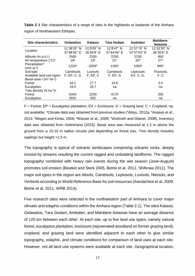
17

Table 2 1 Site characteristics of a range of sites in the highlands or lowlands of the Amhara

region of Northwestern Ethiopia.

Site characteristics Gelawdios Katassi Tara Gedam Ambober Mahibere-Selassie

Location 11°38’25’’ N

37°48’55’’ E

11°0’05’’ N

36°44’8’’ E

12°8’47’’ N

37°44’45’’ E

12°31’15’’ N

37°31’53’’ E

12°32’20’’ N

36°35’9’’ E

Altitude (m a.s.l.) 2500 2200 2230 2230 850 Air temperature (°C)* 19a 15b 21c 20d 27e Precipitation* (mm yr-1)

1220a 2200b 1100c 1083d 965e

Soil type Cambisols Luvisols Cambisols Leptosols Fluvisols Available land use types F, EP, C, G F, EP, C F, EP, G EX, C, G, F, C Basal area g (m2 ha-1) Forest 34.1 17.7 19.8 3.4 Eucalyptus 19.0 16.7 na na Tree density (N ha-1)g Forest 6334 2293 4170 205 Eucalyptus 3031 552 na na

F = Forest; EP = Eucalyptus plantation; EX = Exclosure; G = Grazing land; C = Cropland; na,

not available. *Climate data was obtained from previous studies (dAbiyu, 2012a; bAssaye et al.,

2013; eMoges and Kindu, 2006; aWassie et al., 2009; cWorkneh and Glatzel, 2008). Inventory

data was obtained from Gebrehana (2015). Basal area was measured at 1.3 m above the

ground from a 10-15 m radius circular plot depending on forest size. Tree density includes

saplings but height >1.5 m.

The topography is typical of volcanic landscapes comprising volcanic rocks, deeply

incised by streams resulting the current ragged and undulating landforms. The ragged

topography combined with heavy rain events during the wet season (June-August)

promotes soil erosion (Bewket and Sterk 2005, Betrie et al. 2011, Shiferaw 2011). The

major soil types in the region are Alisols, Cambisols, Leptosols, Luvisols, Nitosols, and

Vertisols according to World Reference Base for soil resources (Awulachew et al. 2009,

Betrie et al. 2011, WRB 2014).

Five research sites were selected in the northwestern part of Amhara to cover major

climatic and edaphic conditions within the Amhara region (Table 2.1). The sites Katassi,

Gelawdios, Tara Gedam, Ambober, and Mahibere-Selassie have an average distance

of 120 km between each other. At each site, up to five land use types, namely natural

forest, eucalyptus plantation, exclosure (rejuvenated woodland on former grazing land),

cropland, and grazing land were identified adjacent to each other to give similar

topography, edaphic, and climate conditions for comparison of land uses at each site.

However, not all land use systems were available at each site. Geographical location,

18

climate, soil, and vegetation characteristics of each site as well as the available land

use systems are described in Table 2.1. Forests at Gelawdios, Katassi, and Tara

Gedam are dry Afromontane remnant pristine forests composed of mostly an intimate

mixture of indigenous tree species. These forests (except Katassi) are traditionally

better protected by local institutions and mostly confined to sacred groves associated

with churches and monasteries (Aerts et al. 2016). The dominant tree species for

highland areas (Gelawdios, Katassi, and Tara Gedam) are Albizia schimperiana,

Apodytes dimidiata, Calpurnia aurea, Carissa edulis, Croton macrostachyus, Ekebergia

capensis, Maytenus arbutifolia, Olea europaea, Prunus africana, and Schefflera

abyssinica. The extensive lowland semiarid forest around Mahibere-Selassie

monastery is a savannah woodland dominated by grasses with some scattered trees.

This site, which represents the typical lowland forest type of this region, is subject to

frequent man-made fires that burn off the grass cover but does not cause extensive

damage to the trees. Characteristic tree species in the lowland are Acacia polyacantha,

Balanites aegyptica, Boswellia papyrifera, Diospyros abbyssinica, Ficus sycomorus,

Pterocarpus lucens, Sterculea setigera, Oxytenanthra abyssinica, and Ziziphus

spinachrist. The Eucalyptus globules plantations at Katassi and Gelawdios were

planted on grazing land around 1985, and were thus ca. 30 years old at the time of

sampling. In Tara Gedam, Eucalyptus camaldunesis was planted on former cropland

and has been cut 3 times since planting. The date of planting is unknown but as in this

part of Ethiopia, the coppicing intervals are between 5 to 10 years, the site must be

between 20 to 40 years old and more likely 40 years old. Details of tree and basal area

densities in the four natural forests and two eucalyptus stands can be found in

Table 2.1. The exclosure at Ambober was established in 2007 on former grazing land

(Abiyu 2012). The exclosure system is commonly used to rehabilitate degraded land

by protecting land areas from further animal grazing and human interference. In

addition to preventing grazing, enrichment planting of seedlings of indigenous and

some exotic tree species was carried out. Since inception, natural revegetation has

returned to the area and it is now covered in an extensive bush woodland. The

management, utilization and protection of the site is undertaken by the local community

(Girmay et al. 2008). All studied croplands and grazing lands were converted from

natural forest within the last 50 years. Grazing lands used as common land to graze

herds of cattle, sheep, goats, and donkeys. The number of years that the cropland was

continuously cultivated after conversion of forest was obtained from local knowledge

19

(Nyssen et al. 2008). Croplands are ox-ploughed to a depth of approximately 30 cm.

Owing to the nature of climate, crops such as Eragrostis tef, Eleusine coracana,

Sorghum bicolor, Zea mays, Triticum aestivum, and Vicia faba are grown during the

wet season. Between years, the crop planted is changed.

2.3.2 Soil sampling

Soil sampling took place during two sampling campaigns, one in March 2014 (end of

the dry season), and another during the wet season in June 2015. In the natural forests,

10 sampling points were marked every 50-100 m along a transect line. At each point,

two soil samples were taken at a distances of about 2 m apart. In eucalyptus

plantations, exclosure, croplands, and grazing lands, one soil sample was taken at 10

sampling points. The distance between sampling points along transects in these land

use systems was 20-50 m according to plot size. After removing the litter layer (if

present), a soil corer (6.6 cm internal diameter) was driven to a maximum of 50 cm

depth or until the bedrock was reached. Soil samples were extracted into a Styrofoam

tray and morphologically described, using the terminology of World Reference Base for

soil resources (WRB 2014). In total, 190 soil cores were collected from all land use

systems and cores were divided into depth classes of 0-10 cm, 10-20 cm, 20-30 cm,

and 30-50 cm. For the samples from the natural forest, a composite sample for each

depth was made from the two cores taken at each sampling point. Each soil sample

was sieved using a 2 mm sieve, homogenised, and placed in a plastic bag. The

samples were then transported to Vienna for laboratory analysis.

2.3.3 Bulk density determination

Bulk soil density samples were taken at five sampling points, every second sampling

point along the transect line. The samples were taken during the onset of wet season

when the soil had no drying cracks. At the edge of each sampling plot, a profile was

dug to 60 cm. Soil samples of known volume were taken from the sides of the profile

centred at 5, 15, 25, and 40 cm depth using a stainless steel bulk density ring. Using a

trowel, the ring was removed from the horizon and the soil trimmed to the tops and

bottoms of the ring using a sharp knife. Any stones (>2 mm) were sieved out and

weighed separately. The volume of stones was quantified by displacement in a water

bath. Bulk density (soil particle <2 mm) was determined after oven dry at 105°C as a

stone free dry weights according to Don et al. (2007).

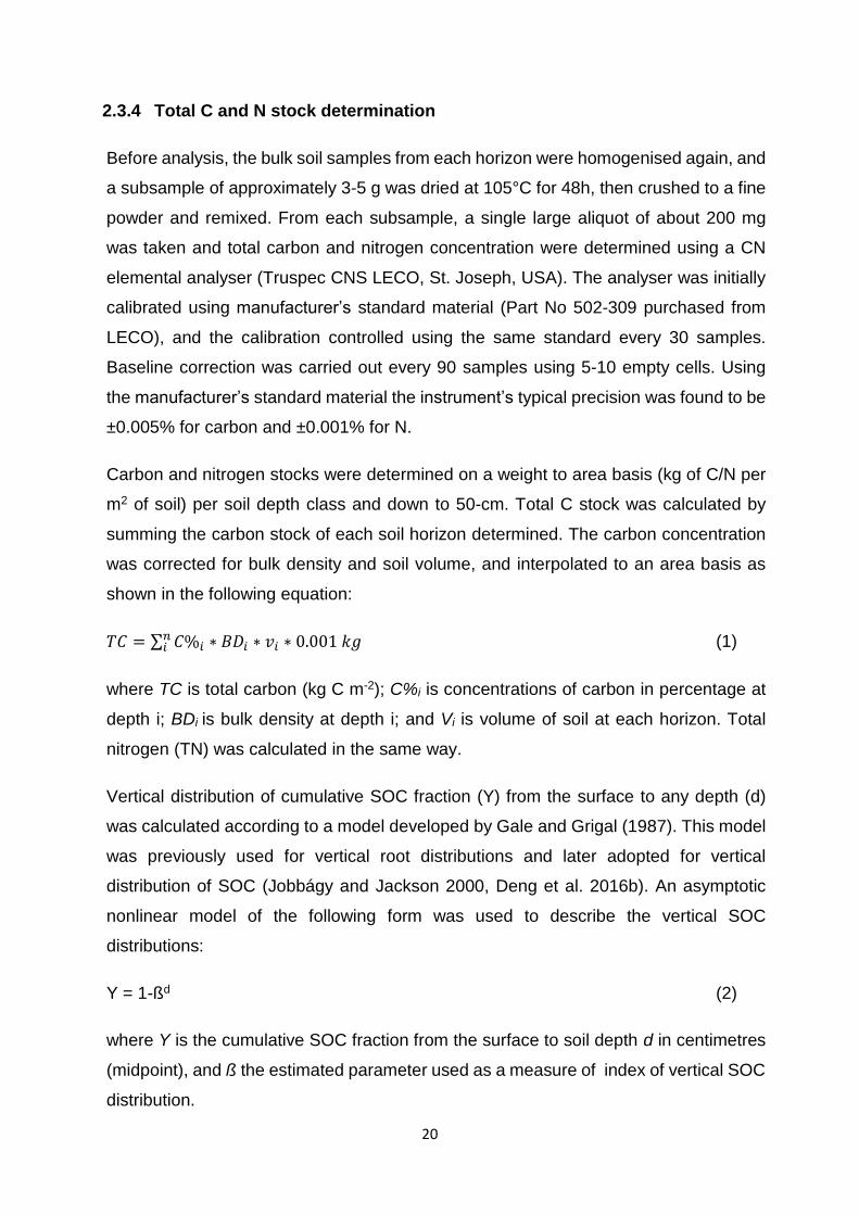
20

2.3.4 Total C and N stock determination

Before analysis, the bulk soil samples from each horizon were homogenised again, and

a subsample of approximately 3-5 g was dried at 105°C for 48h, then crushed to a fine

powder and remixed. From each subsample, a single large aliquot of about 200 mg

was taken and total carbon and nitrogen concentration were determined using a CN

elemental analyser (Truspec CNS LECO, St. Joseph, USA). The analyser was initially

calibrated using manufacturer’s standard material (Part No 502-309 purchased from

LECO), and the calibration controlled using the same standard every 30 samples.

Baseline correction was carried out every 90 samples using 5-10 empty cells. Using

the manufacturer’s standard material the instrument’s typical precision was found to be

±0.005% for carbon and ±0.001% for N.

Carbon and nitrogen stocks were determined on a weight to area basis (kg of C/N per

m2 of soil) per soil depth class and down to 50-cm. Total C stock was calculated by

summing the carbon stock of each soil horizon determined. The carbon concentration

was corrected for bulk density and soil volume, and interpolated to an area basis as

shown in the following equation:

𝑇𝐶 = ∑ 𝐶%𝑖 ∗ 𝐵𝐷𝑖 ∗ 𝑣𝑖 ∗ 0.001 𝑘𝑔𝑛𝑖 (1)

where TC is total carbon (kg C m-2); C%i is concentrations of carbon in percentage at

depth i; BDi is bulk density at depth i; and Vi is volume of soil at each horizon. Total

nitrogen (TN) was calculated in the same way.

Vertical distribution of cumulative SOC fraction (Y) from the surface to any depth (d)

was calculated according to a model developed by Gale and Grigal (1987). This model

was previously used for vertical root distributions and later adopted for vertical

distribution of SOC (Jobbágy and Jackson 2000, Deng et al. 2016b). An asymptotic

nonlinear model of the following form was used to describe the vertical SOC

distributions:

Y = 1-ßd (2)

where Y is the cumulative SOC fraction from the surface to soil depth d in centimetres

(midpoint), and ß the estimated parameter used as a measure of index of vertical SOC

distribution.

21

2.3.5 Strontium, calcium and barium elemental analysis

For analysis of strontium, calcium, and barium from the bulk soil sample of Gelawdios

and Katassi natural forest and cropland, a further 20 g subsample was taken from each

sample, dried for 3 days at 50°C, and remixed. Before analysis, residual moisture was

removed by drying at 105°C for 30 minutes. From each sample, a 500 - 600 mg aliquot

of dried soil was added into a 75 ml fusion tube with 20 ml of Aqua regia (3:1 HCl and

HNO3). To prevent the solution from foaming, 10 μl of Octanol was added.The soil

samples were shaken for 4.5 h and then digested at 125°C for 2 h. The cooled samples

were then made up to a volume of 75 ml with deionized water and filtered with Whatman

Grade 589/1 paper. The concentrations of total strontium (Sr), calcium (Ca), and barium

(Ba) were determined by inductively coupled plasma optical emission spectroscopy

(Perkin Elmer Optima 8300; ICP-OES Spectrometer, Waltham, USA) using external

calibration in line with ÖNORM L 1085. Two samples of a standard soil were used as

internal standards (ICP Multi-element Standard solution XIV, CertiPUR, purchased

from Merck KGaA, Germany).

2.3.6 Determination of soil pH

Soil pH was determined in 1:3 soil suspensions in both deionized water and 0.01 M

CaCl2 solution using a digital potentiometric pH-meter. Five samples per site and

horizon were analyzed for each land use type.

2.3.7 Particle size determination

For soil texture analysis from the 10-bulk soil sample per horizon, equal amounts of soil

of between 4-5 g were taken and thoroughly mixed. About 30 g of the composite soil

samples were taken per horizon for soil texture analysis. Soil texture was determined

by a combination of wet sieving and sedimentation methods (Kettler et al. 2001). Soil

particle were dispersed in 3% aqueous sodium hexametaphosphate (HMP, (NaPO3)n)

using a 3:1 HMP (90 mL) to soil (30 g) ratio, and shaking for 16 h (overnight). After

dispersion, the soil slurry was passed through a range of sieves of different mesh sizes

(0.5 – 0.053 mm) to separate sand particles and particulate organic matter (POM). The

collected sand particles (>0.053 mm) were dried at 105°C to constant weight, and

residual POM was then removed by ignition at 450°C for 4 h. The sand percentage was

calculated based on its fraction of the original sample mass after ignition at 450°C. The

22

solution (containing silt + clay) passing the sieve was collected in a 500 mL pre-weighed

beaker, stirred thoroughly to achieve suspension of all soil particles, and then left

undisturbed at room temperature (18-24°C) for 6h to allow silt particles to settle. After

sedimentation period, the supernatant containing the suspended clay was decanted,

and the settled silt fraction was then dried in the beaker at 105°C to constant weight.

The sand, silt, and clay percentages were calculated based on their fraction of the

original sample mass as follows.

Sand% = (Sand mass/original sample mass)*100% (3)

Silt% = (silt mass/original sample mass)*100% (4)

Clay% = 100 – (Sand% + Silt%) (5)

To assign texture classes, the USDA particle size classes of sand (2.0-0.053 mm), silt

(0.053-0.002 mm), and clay (0.002 mm) were used.

2.3.8 Data analysis

If the data was not normally distributed, it was square-root-transformed to reach

normality. Analysis of variance (ANOVA) was used to test the significance of mean

differences in total carbon and nitrogen as dependent variable and land use systems,

climate variables, and soil depths as factors. To determine differences between groups

Scheffe post hoc tests were used. Linear regression was used to evaluate the

relationships between the dependent variable (total C stock) with total N, pH, bulk

density, soil texture, mean annual precipitation (MAP) and mean annual temperature

(MAT) as independent variable. The IBM SPSS analytical software package (version

21) and SigmaPlot (version 13) were used for all statistical analyses and graphs.

Significant level determined at α = 0.05. Data are presented as mean ± standard error

(SE).

23

2.4 Results

2.4.1 Soil carbon and nitrogen stocks

Total SOC and N stocks varied considerably between land uses systems. The average

C stock (0-50 cm soil depth) was significantly higher in the forest ecosystems than other

land use systems and cropland had the lowest C stock (Fig. 2.1a). The average C

stocks per land use type can be ranked as, forest (22.0 kg C m-2) > eucalyptus

plantation (15.7 kg C m-2) > grazing land (9.3 kg C m-2) > cropland (6.8 C kg m-2),

however the difference between grazing land and cropland was not significant.

Similarly, soil N stock was also showed significant differences between the land use

systems and followed a similar trend to C stock (Fig. 2.1a). In the mature woodland

ecosystems, the lowest C and N stocks were found in the lowland semiarid forest at

Mahibere-Selassie (Table 2.2). There was no significant difference found in soil C or N

stock between Gelawdios, Tara Gedam, and Katassi. At Mahibere-Selassie, in contrast

to all the other mature forest sites, the C and N stocks of cropland were significantly

higher than that of the corresponding forest (Fig. 2.1b; P < 0.001). Total C and N stock

did not differ significantly among three land uses in Ambober (Table 2.2; Appendix 1

Table 1 (Table A1.1). Soil organic carbon stock of the eucalyptus plantation was similar

at Katassi and Tara Gedam but was significantly lower at Gelawdios compared to the

other two sites. Soil organic carbon stock of the eucalyptus plantation was on average

57% and 40% higher than the respective cropland and grazing land, but was on

average 29% lower than the SOC stock of the natural forest (Table 2.2). Similarly, soil

N stock was 47% and 29% higher in eucalyptus soil than the cropland and grazing land

soils.

The C/N ratios of soils were similar for all sites and land use types except for the

croplands. The values of the C/N ratios were between 10.9 and 13.6, and higher in

eucalyptus than the natural forests and grazing lands. The cropland at Katassi had a

very low C/N ratio (6.3) and was significantly different from all the other sites. The

highest C/N ratio was recorded at Mahibere-Selassie cropland (14.3; Table 2.2).

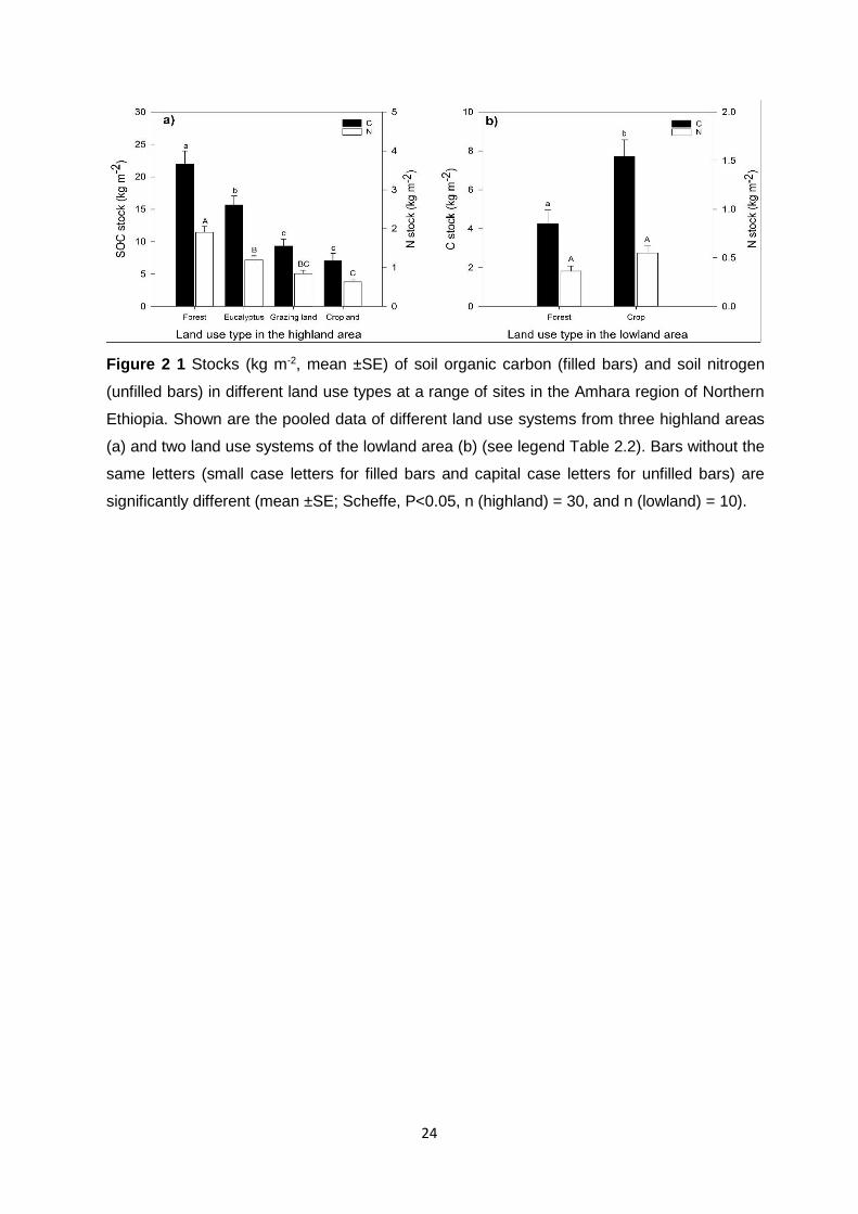
24

Figure 2 1 Stocks (kg m-2, mean ±SE) of soil organic carbon (filled bars) and soil nitrogen

(unfilled bars) in different land use types at a range of sites in the Amhara region of Northern

Ethiopia. Shown are the pooled data of different land use systems from three highland areas

(a) and two land use systems of the lowland area (b) (see legend Table 2.2). Bars without the

same letters (small case letters for filled bars and capital case letters for unfilled bars) are

significantly different (mean ±SE; Scheffe, P<0.05, n (highland) = 30, and n (lowland) = 10).

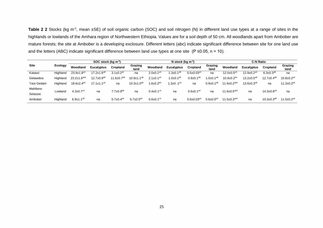
25

Table 2 2 Stocks (kg m-2, mean ±SE) of soil organic carbon (SOC) and soil nitrogen (N) in different land use types at a range of sites in the

highlands or lowlands of the Amhara region of Northwestern Ethiopia. Values are for a soil depth of 50 cm. All woodlands apart from Ambober are

mature forests; the site at Ambober is a developing exclosure. Different letters (abc) indicate significant difference between site for one land use

and the letters (ABC) indicate significant difference between land use types at one site (P ≤0.05, n = 10).

Site Ecology

SOC stock (kg m-2) N stock (kg m-2) C:N Ratio

Woodland Eucalyptus Cropland Grazing

land Woodland Eucalyptus Cropland

Grazing land

Woodland Eucalyptus Cropland Grazing

land

Katassi Highland 23.9±1.8aA 17.2±1.6aB 3.1±0.2aC na 2.0±0.1aA 1.3±0.1aB 0.5±0.03aC na 12.0±0.5aA 12.9±0.2aA 6.3±0.3aB na

Gelawdios Highland 23.2±1.6abA 12.7±0.9bB 11.6±0.7bB 10.9±1.1aB 2.1±0.1aA 1.0±0.1bB 0.9±0.1bB 1.0±0.1aB 10.9±0.2bA 13.2±0.5aB 12.7±0.4bB 10.8±0.2aA

Tara Gedam Highland 18.6±2.4bA 17.1±1.1aA na 10.3±1.0aB 1.6±0.2bA 1.3±0 .1aA na 0.9±0.1aB 11.9±0.2abA 13.6±0.3aB na 11.3±0.2aA

Mahibere

Selassie Lowland 4.3±0.7cA na 7.7±0.9bB na 0.4±0.1cA na 0.6±0.1aA na 11.6±0.5abA na 14.3±0.8cB na

Ambober Highland 6.9±1.1dA na 5.7±0.4dA 6.7±0.5bA 0.6±0.1cA na 0.6±0.03aA 0.6±0.0bA 11.5±0.3abA na 10.3±0.3dB 11.0±0.2aA

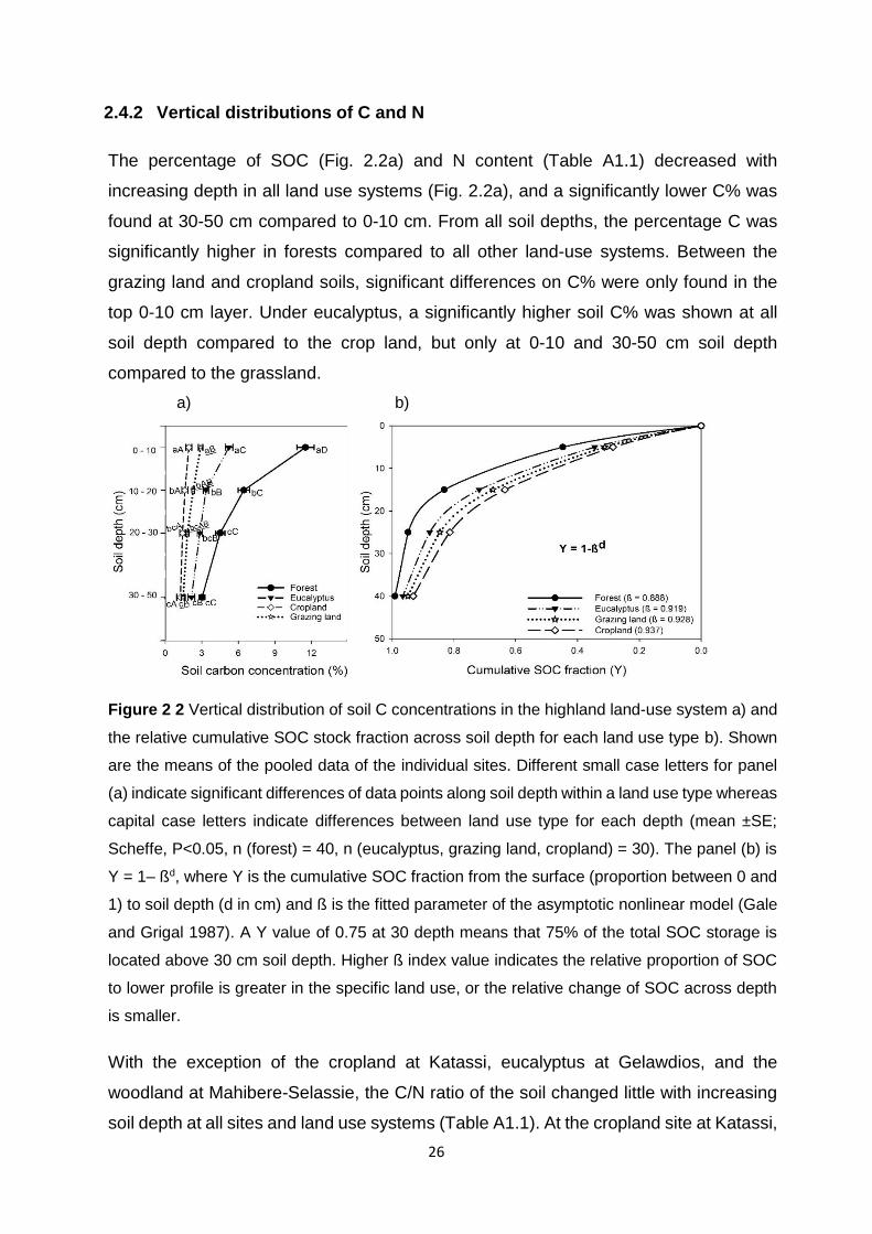
26

2.4.2 Vertical distributions of C and N

The percentage of SOC (Fig. 2.2a) and N content (Table A1.1) decreased with

increasing depth in all land use systems (Fig. 2.2a), and a significantly lower C% was

found at 30-50 cm compared to 0-10 cm. From all soil depths, the percentage C was

significantly higher in forests compared to all other land-use systems. Between the

grazing land and cropland soils, significant differences on C% were only found in the

top 0-10 cm layer. Under eucalyptus, a significantly higher soil C% was shown at all

soil depth compared to the crop land, but only at 0-10 and 30-50 cm soil depth

compared to the grassland.

a) b)

Figure 2 2 Vertical distribution of soil C concentrations in the highland land-use system a) and

the relative cumulative SOC stock fraction across soil depth for each land use type b). Shown

are the means of the pooled data of the individual sites. Different small case letters for panel

(a) indicate significant differences of data points along soil depth within a land use type whereas

capital case letters indicate differences between land use type for each depth (mean ±SE;

Scheffe, P<0.05, n (forest) = 40, n (eucalyptus, grazing land, cropland) = 30). The panel (b) is

Y = 1– ßd, where Y is the cumulative SOC fraction from the surface (proportion between 0 and

1) to soil depth (d in cm) and ß is the fitted parameter of the asymptotic nonlinear model (Gale

and Grigal 1987). A Y value of 0.75 at 30 depth means that 75% of the total SOC storage is

located above 30 cm soil depth. Higher ß index value indicates the relative proportion of SOC

to lower profile is greater in the specific land use, or the relative change of SOC across depth

is smaller.

With the exception of the cropland at Katassi, eucalyptus at Gelawdios, and the

woodland at Mahibere-Selassie, the C/N ratio of the soil changed little with increasing

soil depth at all sites and land use systems (Table A1.1). At the cropland site at Katassi,

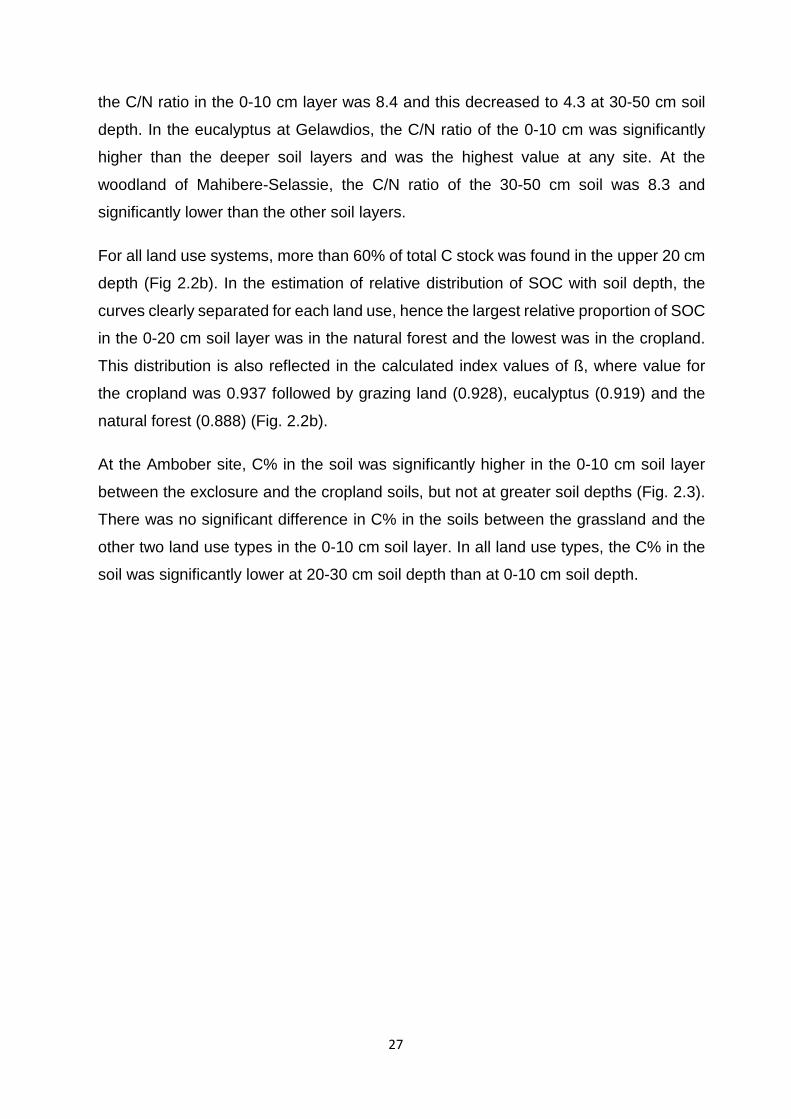
27

the C/N ratio in the 0-10 cm layer was 8.4 and this decreased to 4.3 at 30-50 cm soil

depth. In the eucalyptus at Gelawdios, the C/N ratio of the 0-10 cm was significantly

higher than the deeper soil layers and was the highest value at any site. At the

woodland of Mahibere-Selassie, the C/N ratio of the 30-50 cm soil was 8.3 and

significantly lower than the other soil layers.

For all land use systems, more than 60% of total C stock was found in the upper 20 cm

depth (Fig 2.2b). In the estimation of relative distribution of SOC with soil depth, the

curves clearly separated for each land use, hence the largest relative proportion of SOC

in the 0-20 cm soil layer was in the natural forest and the lowest was in the cropland.

This distribution is also reflected in the calculated index values of ß, where value for

the cropland was 0.937 followed by grazing land (0.928), eucalyptus (0.919) and the

natural forest (0.888) (Fig. 2.2b).

At the Ambober site, C% in the soil was significantly higher in the 0-10 cm soil layer

between the exclosure and the cropland soils, but not at greater soil depths (Fig. 2.3).

There was no significant difference in C% in the soils between the grassland and the

other two land use types in the 0-10 cm soil layer. In all land use types, the C% in the

soil was significantly lower at 20-30 cm soil depth than at 0-10 cm soil depth.

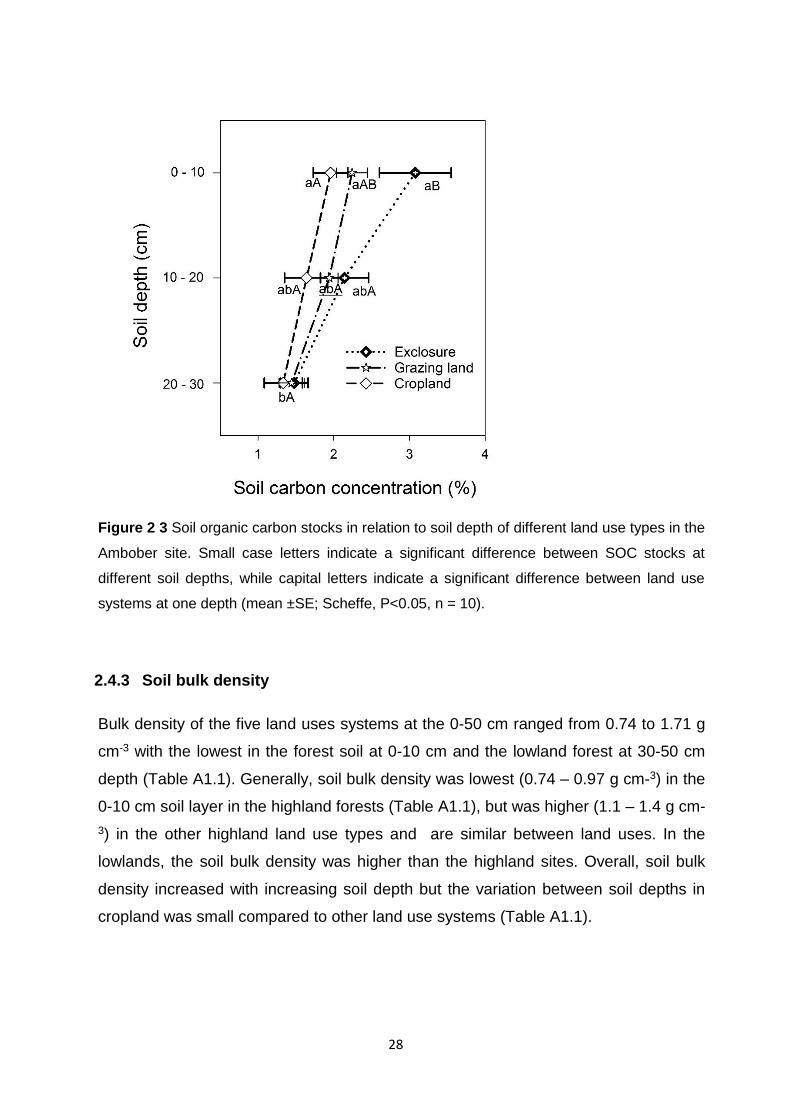
28

Figure 2 3 Soil organic carbon stocks in relation to soil depth of different land use types in the

Ambober site. Small case letters indicate a significant difference between SOC stocks at

different soil depths, while capital letters indicate a significant difference between land use

systems at one depth (mean ±SE; Scheffe, P<0.05, n = 10).

2.4.3 Soil bulk density

Bulk density of the five land uses systems at the 0-50 cm ranged from 0.74 to 1.71 g

cm-3 with the lowest in the forest soil at 0-10 cm and the lowland forest at 30-50 cm

depth (Table A1.1). Generally, soil bulk density was lowest (0.74 – 0.97 g cm-3) in the

0-10 cm soil layer in the highland forests (Table A1.1), but was higher (1.1 – 1.4 g cm-

3) in the other highland land use types and are similar between land uses. In the

lowlands, the soil bulk density was higher than the highland sites. Overall, soil bulk

density increased with increasing soil depth but the variation between soil depths in

cropland was small compared to other land use systems (Table A1.1).

29

2.4.4 Strontium:calcium and barium:calcium ratios

At both the Katassi and Gelawdios forest sites, the ratios of Sr/Ca and Ca/Ba increased

with increasing soil depth (Fig. 2.4). With the exception of Sr/Ca at Katassi, the ratios

of Sr/Ca and Ca/Ba were significantly lower in the 0-10 cm soil than in the 20-30 cm

soil. Significant differences in the ratios of both Sr/Ca and Ca/Ba were found at both

sites if the 0-10 cm and 30-50 cm soil depths are compared. In contrast, in the cropland

soil profile, the ratios of Sr/Ca and Ca/Ba did not change with soil depth at either site.

The changes in ratios of Sr/Ca and Ca/Ba shown in the forest soil profiles were primarily

due to differences in the levels of Ca between the soils layers (Table A1.2). In both

forests sites higher levels of Ca were determined in the 0-10 cm soil layer than the

deeper soil layers. In cropland soils, the levels of Ca were similar at all soil depths.

Figure 2 4 Strontium (Sr) to calcium (Ca) and barium (Ba) to calcium ratios at different soil

depths in forests (filled bars) and cropland (unfilled bars) at Katassi and Gelawdios. Within a

ratio and land use bars with different letters are significantly different (mean ±SE; Scheffe,

P<0.05, n = 10).

2.4.5 Factors effecting soil carbon stocks

Total SOC in both the forest (Fig. 2.5a) and cropland (Fig. 2.5b) showed a strong

positive correlation with N stock (R2 = 0.96 and 0.83 respectively; P<0.001). Soil pH

showed a negative correlation with SOC in the forest soil (R2 = 0.80; P<0.001; Fig. 2.5c)

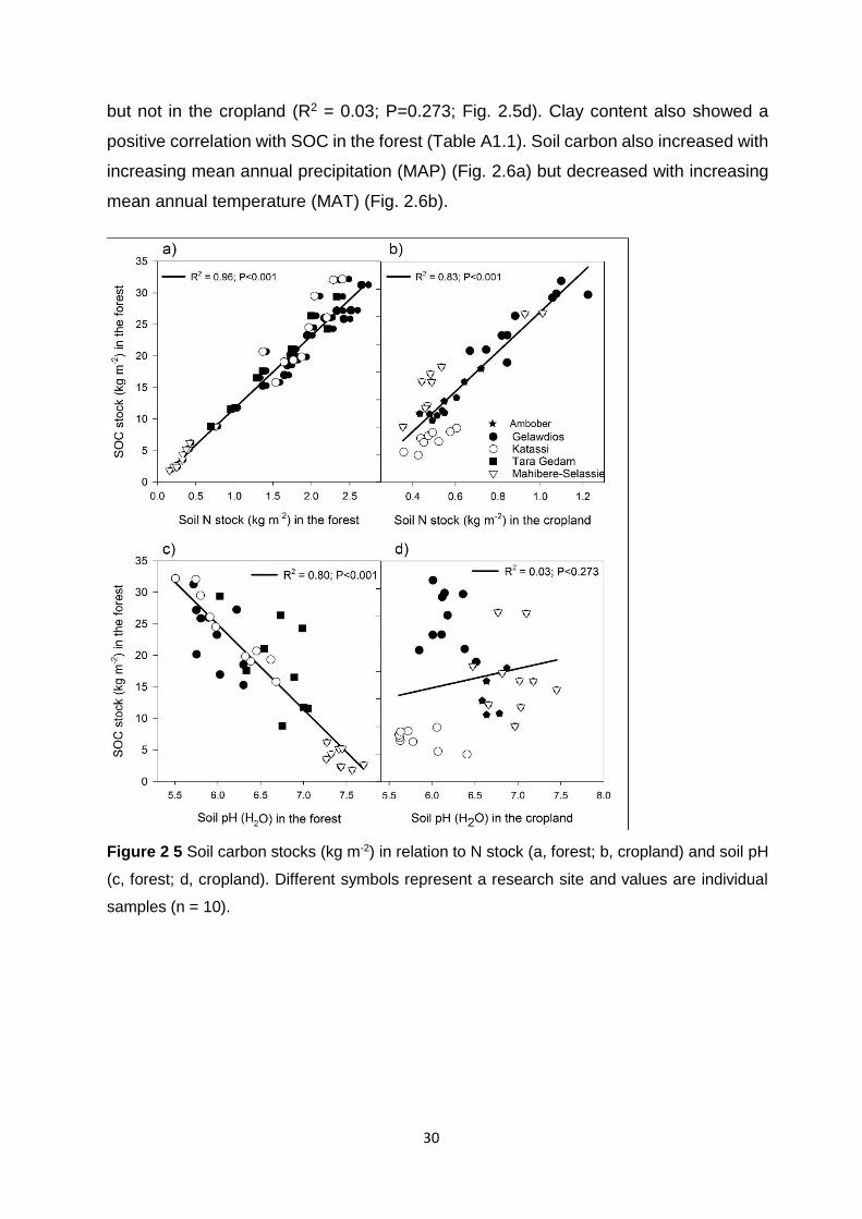
30

but not in the cropland (R2 = 0.03; P=0.273; Fig. 2.5d). Clay content also showed a

positive correlation with SOC in the forest (Table A1.1). Soil carbon also increased with

increasing mean annual precipitation (MAP) (Fig. 2.6a) but decreased with increasing

mean annual temperature (MAT) (Fig. 2.6b).

Figure 2 5 Soil carbon stocks (kg m-2) in relation to N stock (a, forest; b, cropland) and soil pH

(c, forest; d, cropland). Different symbols represent a research site and values are individual

samples (n = 10).

31

Figure 2 6 The relationship between soil carbon stock (kg m-2) and a) mean annual precipitation

(MAP); b) mean annual temperature. (Mean ±SE; Scheffe, P<0.05, n = 10).

2.5 Discussion

2.5.1 Soil organic carbon and nitrogen stocks

There were large difference in the carbon stock in soil between the different land use

systems, and differences in pattern between the highland and lowland systems. In the

highlands (Fig. 2.1a), greater SOC stocks were found in the natural forest and

eucalyptus plantation than in the grazing or croplands. In the lowlands, a greater SOC

stock was found in the cropland than in the savannah woodland (Fig. 2.1b). The overall

soil carbon stock in forests ranged from 4 kg SOC m-2 in the lowlands to 24 kg SOC m-

2 in the highlands. These values fall within the range of estimates of global tropical

means (3 - 41 kg C m-2; Batjes, 1996), and are similar to other studies in southern

Ethiopia (4 - 21 kg C m-2; Lemenih and Itanna, 2004). In the highland soils, the large

differences in SOC stock were due to higher SOC levels in the top 10 cm of soil. In the

natural forest, more than 60% of the SOC stock was in the first 10 cm of soil. Overall,

for all land use systems, more than 70-90% of total SOC stock was found in the upper

20 cm depth of soil (Fig. 2.2b, Table A1.1). This finding is consistent with other similar

studies of C distribution with soil depth (Alvarez and Lavado 1998, Tesfaye et al. 2016).

In the forests, biomass input into SOC comes from both above-ground leaf and

deadwood litter and below-ground root litter, whereas in the eucalyptus plantations, leaf

32

litter is raked and removed. In the cropland system, all above ground biomass is

removed for fodder. The grasslands are also so heavily grazed that biomass input to

soils must be primarily from root litter inputs (Kuzyakov and Domanski 2000).

Investigation of fine root biomass in the forest and eucalyptus plantations showed a

similar distribution to the SOC stock down the soil profile (Chapter 3). Jobbágy and

Jackson (2000) suggested that the vertical distributions of SOC in forests could be

explained in part by root distribution and the associated root turnover.

Soil organic carbon stock increased with increasing MAP and decreased with

increasing MAT (Fig. 2.6a and b). Other similar studies showed that soil C stores are

positively correlated with MAP and negatively correlated with MAT (Alvarez and Lavado

1998, Deng et al. 2016b). Deng et al. (2014) reported that higher temperature leads to

higher losses of soil carbon through decomposition of soil organic matter. At the global

scale, the SOC stocks showed a tendency of increasing from temperate regions to

subtropical regions (Post and Kwon 2000).

A clear relationship was found between SOC stocks and N stocks in both forest and

cropland soils (Fig. 2.5a and b). The C/N ratio in the soil was similar in all land use

types and sites (ca. 11-13) with the exception of the cropland at Katassi, which had a

C/N ratio of 6.2. The strong correlation between C and N suggests that, even in the

cropland soils, the storage of N is directly related to the levels of SOC within the soil,

and that C inputs control N stocks. The very low value of C/N ratio in the cropland soils

of Katassi at 30-50 cm soil depth (Table A1.1) corresponds to a very low level of SOC

of <1%. Decreasing C/N ratios of SOM with increasing soil depth have been shown in

many soils (Lal 1995) and have been attributed to the SOM being older and more

processed by microbes than SOM in upper soil layers (Lal 1995, Callesen et al. 2007).

The low C/N ratio in the whole soil profile of the cropland at Katassi is more

representative of subsoil layers than surface soil layers.

2.5.2 Effect of land use change on carbon stock

At the two highland sites, conversion of natural forests into croplands induced a strong

reduction of organic carbon in the soil. At Katassi and Gelawdios, the SOC stock was

reduced by 87% and 50% respectively that seems the average rate of loss of SOC is

0.42 kg m-2 yr-1 at Katassi and 0.23 kg m-2 yr-1 at Gelawdios for the 50-year period (Fig.

2.1a). However, chronosequence studies have shown that the conversion of forests to

33

cropland caused a rapid initial decrease in SOC stocks, followed by a slow decline (Wei

et al. 2014, Deng et al. 2016b). Similar results have also been reported for other sites

in Northern Ethiopia, where cultivation land had a 58% lower SOC level compared to

forest land in Northwest Tigray (Gebremariam and Kebede 2010), and 63% lower SOC

level in cropland compared to forest after a 30 years of cultivation period in the southern

highlands of Ethiopia (Solomon et al. 2002). Similarly, studies at sites in Southern

Ethiopia with a similar climate to the highland sites showed that SOC was reduced by

70% within 33 years (Lemenih et al. 2006) and 75% in a 53 year cultivation period in

the top 10 cm of soil (Lemenih et al. 2005).

Above-ground and below-ground litter inputs may be a determinant factor for the high

accumulation of C in the forest soil (Berg 2000, Smith 2007, Fernandez et al. 2013)

compared to small carbon inputs from grazing and cropland, where potential inputs are

limited and occur only during growing season. The reduction of carbon stock in the

cropland is exacerbated by complete removal of crop residue for cattle feeding. Malhi

et al. (1999) and Balesdent et al. (1998) estimated that, after forest clearance, rates of

decay of soil C were 10 times higher in cultivated soil than in forest soil, and that soil C

in some factions had become unprotected. However, our data also suggests that much

of the SOC has been lost in crop lands by direct erosion in addition to losses from

increased heterotrophic respiration after cultivation (Tosi et al. 2016). The SOC level in

cropland topsoil (0-10 cm) at Katassi (1.1 kg m-2) is less than the SOC stock of the

adjacent forest soil at the depth of 30-50 cm (3.2 kg m-2; Table A1.1). Similarly, at the

Gelawdios site, cropland carbon stock at 0-10 cm (3.1 kg m-2) was nearly comparable

to the adjacent forest carbon stock (3.7 kg m-2) at 20-30 cm depth. In addition, the

higher distribution of relative SOC stock in the lower soil profile of cropland (ß = 0.937)

than forest (ß = 0.888) indicates that the variation down the soil depth in cropland is

minor. As stated above, the C/N ratio of the cropland soil at Katassi is indicative of

subsoils rather than surface soils. This is not however the case at Gelawdios where the

cropland soil has similar C/N ratios to that of the adjacent forest.

Strontium (Sr) to calcium (Ca) and barium (Ba) to calcium ratios are widely used as

markers of environmental history (Bullen et al. 2005, Tabouret et al. 2010) and

biogeochemical properties of the ecosystem (Kabata-Pendias 2010). The Sr/Ca and

Ba/Ca ratio at 30-50 cm depth in the forest soil profile is comparable to the 0-10 cm

depth of cropland soil at both Katassi and Gelawdios (Fig. 2.3). At both sites in forests,

34

the lower Sr/Ca and Ba/Ca ratios in the upper soil profile are due to higher levels of Ca

in these soil horizons, particularly in the 0-10 cm layer. The higher levels of Ca may be

due to inputs of Ca rich leaf litter (Dauer et al. 2007) or atmospheric dust inputs (Bullen

et al. 2005, Derry and Chadwick 2007), but whatever the source of Ca, this layer is

clearly missing in the cropland soils. Taken together, both the soil profile distribution of

C and the C/N ratio as well as element ratios suggest the upper soil profile has been

lost in cropland soils. The most probable reason for the loss of the upper soil profile in

croplands is direct erosion, as if the soil C and C/N ratio had changed due to an increase

in heterotrophic respiration (Deng et al. 2014) this would have not led to a concomitant

loss of soil Ca in the cropland soils. Climate conditions in Ethiopia such as heavy rainfall

events are known to result in a high rate of soil erosion (Bewket and Sterk 2005, Betrie

et al. 2011, Shiferaw 2011). In addition, after the protective tree canopy has been

removed, the low bulk density of the upper soil layers in the natural forest may make

these soils highly sensitive to wind or water erosion (Jepsen et al. 1997).

At the highland sites, conversion of natural forest to grazing land also significantly

reduced SOC stock in the soil by 53%. Bewket and Stroosnijder (2003) showed on

other highlands sites that grazing land had 48% lower levels of SOM than natural forest.

These results are in contrast to studies of productive grasslands in tropical climates

where grassland often have similar or greater SOC storage compared to forests

(Conant et al. 2001), and even conversion of forest to grassland tends to increase C

stock in the soil (Conant et al. 2001, Guo and Gifford 2002). Guo and Gifford (2002) in

their review showed that accumulation of SOC after conversion from forest to grassland

occurred in climates between 2000-3000 mm, but not at < 2000 mm precipitation.

However, poor management of grasslands after conversion led to a decrease in SOC

even in wet tropical areas (Fearnside et al. 1998). The high levels of SOC often found

in productive grasslands are produced by high biomass inputs from roots (Kuzyakov

and Domanski 2000). At the highland sites in this study, the levels of fine root biomass

in grasslands are only 10% of those in the natural forest (Chapter 3), and thus

necromass inputs must have greatly decreased. In addition, most of the grasslands are

degraded due to overgrazing. Often the grazing land is completely denuded. Desta et

al. (2000) estimated for the grasslands that the stocking density (23 livestock unit (LU)

ha-1) is ten times the carrying capacity (2-3 LU ha-1).

35

The lowland savannah woodland at Mahibere-Selassie has a SOC stock of ca. 20% of

the highland sites. The lower SOC stocks were clearly related to the lower MAP and

higher MAT, which is likely to affect rates of SOC turnover, but also strongly affects the

vegetation structure. The basal area and stocking density of the tree of the savannah

woodland (Table 2.1) are only a fraction of that of the highland sites, and thus biomass

inputs from the trees will be low. In addition, the grass cover of the woodland is regularly

burnt, which potentially decreases SOC stocks (Knicker 2007). Furthermore, the soil of

the savannah woodland has a very low clay content and a high sand content compared

to the adjacent cropland and all the highland forest sites (Table A1.1). Exceptionally,

cropland at Mahibere-Selassie had a 60% higher SOC stock than the woodland (Fig.

2.1b). The higher SOC stock may in part be due to the higher clay content of the soil

(Ajami et al. 2016), but could also be due to the different farming systems in the

lowlands. Ajami et al. (2016) could also show a linear relationship between SOC stock

and soil clay content in loess soils in Iran after deforestation.

2.5.3 Potentials of soil carbon gain due to afforestation and exclosure

At two sites, Katassi and Tara Gedam, the soils under eucalyptus had higher SOC

stocks than either the cropland or the grazing land soil. However, at Gelawdios, the

SOC stocks were similar in the eucalyptus, grazing land, or cropland soils. Assuming

the eucalyptus plantation at Katassi and Tara Gedam are ca. 30 and 40 years old, the

rates of SOC accumulation is 0.49 kg m-2 yr-1 at Katassi and 0.17 kg m-2 yr-1 at Tara

Gedam, which is a similar to the rate of loss of SOC after forest removal. A study in

Southern Ethiopia, (Tesfaye et al. 2016) determined similar levels of SOC in 28 year

old Eucalyptus saligna plantations, and represents an annual SOC accumulation of

0.18 kg m-2 yr-1 compared to the levels of SOC determined in cropland. At Katassi and

Gelawdios, the SOC stock in the natural forest exceeded that of the eucalyptus

plantation by 29 and 55% respectively, but was similar between the two land uses at

Tara Gedam. Tesfaye et al. (2016) reported a 30% greater SOC storage in natural

forests compared to the Eucalyptus saligna plantations. These results suggest that

eucalyptus can restore SOC storage in soils even under management systems using

leaf litter raking and removal. However, the low bulk density of the surface layers of the

natural forests was not restored. The negative ecological consequences of eucalyptus

plantations also needs to be considered (Martins et al. 2013).

36

The conversion of heavily degraded grazing land to exclosure in Ambober significantly

increased SOC stock in the 0-10 cm soil layer by 42% compared to cropland after an 8

years exclosure period (Fig. 2.3). Other studies (Girmay et al. 2008, Mekuria et al. 2009,

Li et al. 2012) have also shown the positive effects of exclosure on carbon stock. For

example, Li et al., (2012) reported that on rangelands in inner Mongolia, SOC stock in

the top 10 cm layer increased from 93 to 638 g m-2 in 26 years exclosure period at the

rate of 31 g C m-2 yr-1, but these authors found no significant difference after 8 years

exclosure period (107 g m-2). The increase of SOC stock in exclosure area indicates

that an increase of vegetation growth and input of carbon can begin to restore SOC

stocks, but it takes long recovery period to obtain the approximate original SOC stock

levels.

2.5.4 Magnitude of soil carbon loss due to deforestation

Land use conversion from forest to cropland or grazing land reduced soil carbon stock

up to 88%. Using the SOC storage of current remnant forests and assuming a 40%

forest cover, the SOC stock of the Amhara region before 50 years ago was about 1.5

Gt C. Forest cover of the Amhara region is currently estimated to be about 9.5%

(Government unpublished report) giving a SOC stock of 0.3 Gt. Hence, it is clearly

important to determine if this substantial loss of 1.2 Gt has been displaced in the

landscape by erosion or lost to the atmosphere by increased SOC turnover. Our data

suggest that SOC may not only be lost to the atmosphere as CO2 (Balesdent et al.

1998) but may also be lost due to erosion. The fate of this lost SOC in the landscape is

unknown.

2.6 Conclusion

Removal of natural forests resulted in substantial loss of SOC stock, which appears to

be due to both erosion of sensitive low bulk density soil of surface layers and possibly

increased rates of SOC turnover. Afforestation with eucalyptus has the potential to

restore the levels of SOC storage partially but does not restore the physical properties

of the soil. Exclosure, and thus exclusion of the degraded land from grazing, also results

in a recovery of SOC stocks in the upper soil layer.

37

3 Fine root dynamics in Afromontane forest and adjacent

land uses in the Ethiopian highlands

3.1 Abstract

Fine roots are a major pathway of C flow from plants to soil, but information on root

dynamics in east African ecosystems is scarce. The aim of this study was to quantify

fine rootstock, production, and turnover and to examine the impact of land use change

on fine root dynamics. The study was conducted in a remnant Afromontane forest and

other land use types in NW Ethiopia using three different methods: sequential coring,

in-growth cores, and in-growth nets. Soil cores for sequential analyses were taken in

quarterly intervals, while in-growth cores and nets were harvested corresponding to 1,

2, 3, 4, 6, 8, and 12-month interval. Fine rootstocks averaged 564, 425, 56, and 46 g

m-2 in the forest, eucalyptus, grazing land, and cropland ecosystems, respectively,

based on sequential coring. The values decreased exponentially with increasing soil

depth. The root production averaged 723 and 694 g m-2 yr-1, while necromass loss due

to decomposition was 416 and 282 g m-2 yr-1, in the forest and eucalyptus, respectively,

based on sequential coring. Fine root production based on in-growth coring averaged

468, 293, 70, and 52 g m-2 yr-1 for forest, eucalyptus, grazing land, and cropland,

respectively. In general, land use conversion from forest to grazing land or cropland

reduced fine rootstock and production by 85-91%.The turnover rate of fine roots based

on mean biomass was 1.5 for forest and 2.1 for eucalyptus soil. From in-growth core

estimations, the annual C flux into the soil averaged 226, 133, 32, and 24 g m-2 yr-1 in

the forest, eucalyptus, grazing land, and cropland ecosystems.

Key words: biomass, necromass, root production, sequential coring, in-growth core, turnover

rate, carbon efflux, decision matrix

3.2 Introduction

Assessments of fine roots by simple excavation techniques were started as early as

the 18th century (Bohm 1979). Since then, in forests, most ecological studies on fine

roots, their biomass distribution and turnover have been carried out in temperate and

boreal ecosystems (Leuschner and Hertel 2003, Pinno et al. 2010, Yuan and Chen

2010, McCormack et al. 2012), while information for tropical areas in general, and

38

African ecosystems in particular, is scarce. Subsequently, worldwide and regional

ecosystem estimates of fine root production, turnover, and carbon fluxes remain

uncertain (Gill and Jackson 2000). Due to a limited understanding of below-ground

process as well as the inherent difficulties in measuring fine root turnover compared to

above-ground components of trees (Santantonio and Grace 1987, Johnson et al. 2001,

Yuan and Chen 2010), parameterising C input models is difficult for different land use

ecosystems. Although several methods have been developed for measuring fine root

production, mortality, and eventually decomposition in situ (Vogt et al. 1998), all have

drawbacks and are often confounded by artifacts (Hertel and Leuschner 2002, Lukac

2012, Andreasson et al. 2015). For example, the sequential coring method has been

widely used (Yuan and Chen 2013, Sun et al. 2015) but may miss root turnover

between sampling dates. This results in a zero estimate (Brunner et al. 2012) because

root mortality and production occur simultaneously (Hansson 2013). The sequential

coring method also relies on a calculated rather than measured estimate of fine root

production. Direct measurements of fine root production can be obtained using in-

growth cores (Lukac 2012) or in-growth nets (Lukac and Godbold 2010). One problem

with the in-growth core method is that it greatly modifies the soil physical properties and

can thus affect root growth (Makkonen and Helmisaari 1999) and either overestimate

(Neill 1992) or underestimate root production (Hertel and Leuschner 2002). In-growth

nets are often difficult to insert or remove in heavy, stony soils. Thus, to obtain more

robust estimations of fine root production and turnover rates, a combination of sampling

techniques and calculation methods should be employed (Majdi et al. 2005).

Estimates of fine root production in pan-tropical forests range from 75 to 2193 g m-2 y-

1 (Hertel and Leuschner 2002). Importantly, estimated values of fine root biomass,

production, and turnover are also influenced by environmental and seasonal factors

(Yang et al. 2004a), which may be strong factors in highly seasonal environments such

as the Ethiopian highlands. For example, fine root growth has been shown to rapidly

increase following soil rewetting (Comas et al. 2013). Moreover, soil characteristics may

also influence fine root biomass and rates of fine root turnover (Helmisaari and

Hallbäcken 1999, Godbold et al. 2003). Fine root biomass was reported to be higher

under low nutrient availability (Priess et al. 1999, Yuan and Chen 2010) or in acidified

soils (Godbold et al. 2003). Other studies, however, reported no effect of these factors

39

on fine root biomass (Ruess et al. 2006) or even lower values of fine root biomass

(Yang et al. 2004a).

Forest conversion to other land use systems is a common phenomenon in the

highlands of Ethiopia, mainly because of population growth and the need for new

agricultural lands (Nyssen et al. 2004). The conversion of natural forests often leads to

land degradation (Meshesha et al. 2014) and to losses of soil C and N stocks (Chapter

2). Much of the original forest that still remains is confined to areas around churches

and monasteries (Wassie et al. 2009, Aerts et al. 2016). Natural forests including

church forests and woodlands cover less than 9.5% of the Amhara region (Desta et al.

2000, Bekele 2011). Investigation of these church forests provides an opportunity to

determine the baseline for this landscape in terms of C storage and the C dynamics

that contribute to this storage. Most previous investigations of church forests have

focussed on above-ground aspects such as species richness (Wassie et al. 2009), and

little is known about the below-ground ecology here. To reverse the negative impacts

of deforestation and to provide a wood supply, degraded lands have often been planted

with eucalyptus. Eucalyptus globules (Labill.) plantations have been established in the

central highlands of Ethiopia since 1895 (Pohjonen and Pukkala 1990) and are

estimated to cover 172 km2 of the region (Bekele 2011). Planting of eucalyptus

increases soil C stocks after ca. 30 years (Chapter 2), but not to the levels found in

natural forests. Although the proportion of the tree biomass constituted by fine roots

(diameter <2 mm) is estimated at <5% (Vogt et al. 1996), fine roots are major

contributors to carbon input into the soil because of their rapid turnover (Vogt et al.

1998, Majdi et al. 2005, Ruess et al. 2006, Lukac 2012). Across terrestrial ecosystems,

fine root biomass is estimated to account for 14-33% of annual net primary production

(Jackson et al. 1997, Malhi et al. 2011, McCormack et al. 2015) and can contribute up

to two-fold higher organic carbon to the soil than leaf litter (Xia et al. 2015). Due to the

importance of fine root turnover in soil C storage (King et al. 2001, Leppälammi-

Kujansuu 2014), we investigated the fine root biomass and turnover on a remnant

church forest, eucalyptus plantation, grazing land, and cropland in the Ethiopian

highland landscapes of the Amhara region. The objective of this study was to assess

the fine rootstock, production, and turnover and to examine the impact of land use

change on fine root dynamics. In the tropics, where temperature permits year-round

growth, the timing of leaf production is probably a result of the availability of moisture

40

during the rainy season (Mulkey et al. 1996). Root production might also follow leaf

phenology because fine root growth depends heavily on newly fixed carbon from the

canopy (Joslin et al. 2001, Steinaker and Wilson 2008). We therefore expected that fine

root biomass and necromass would be greater during the rainy season, when trees

were physiologically active to capture nutrients, than during the dry season.

3.3 Materials and Methods

3.3.1 Site descriptions

The study was conducted at a natural remnant forest at Gelawdios and on adjacent

land use systems (eucalyptus plantation, grazing land, and cropland) situated in the

Amhara National Regional State (11°38’25’’ N 37°48’55’’ E) in northwest Ethiopia. The

altitude of the study area is 2500 m a.s.l. The monsoonal climate features a mean

annual temperature of 19°C and a mean annual precipitation of about 1200 mm, with

the main rainy season between June and September (Wassie et al. 2009). The climate

is classified as temperate with a dry winter and warm summer (Cwb) according to the

Köppen-Geiger climate classification (Peel et al. 2007). The soils of the study area are

Cambisols (WRB 2014) with weak horizon differentiation and rocks below 50 cm depth.

The forest at Gelawdios has an area of about 100 ha (Wassie et al. 2009) and is a

remnant of natural pristine forest composed mostly of a mixture of indigenous tree

species. The forest type is a dry Afromontane forest. This forest with old remnant trees

has been protected because it is a church forest. The church was built around 1500

A.D. (Wassie et al. 2009). The dominant tree species are Chionanthus mildbraedii,

Albizia schimperiana, Apodytes dimidiata, Calpurnia aurea, Croton macrostachyus,

Ekebergia capensis, Maytenus arbutifolia, and Schefflera abyssinica. The Eucalyptus

globules plantation was established on previous grazing land around 1985 and was

successively thinned. The cropland and grazing land were converted from natural forest

within the last 50 years (specific date not known). The number of years that the land

was continuously cultivated after conversion from forest was obtained from local

records and knowledge. The cropland is ploughed 2-3 times per year to ca. 30 cm depth

using an ox-drawn plough. During the sampling year (2014), the farmland was planted

with Eragrostis tef, and partly with Triticum aestivum in June and July, and was

harvested in September and October, respectively. Grazing lands are common land

used to graze herds of cattle, sheep, goats, and donkeys.

41

3.3.2 Root sampling

In the natural forest and eucalyptus plantation, ten permanent circular plots with an

area of 100 m2 each were established along a transect line with a minimum distance of

100 m between the plots. In the grazing land and cropland, plots were established along

a transect line with ca. 20 m distance between each plot. Three methods were used for

rootstock and production estimations: sequential coring, in-growth cores, and in-growth

net methods.

Sequential coring

Standing fine roots (<2 mm diameter) were determined using sequential soil coring.

The fine roots were later divided into live fine roots (biomass) and dead fine roots

(necromass). Intact soil cores were extracted with a stainless steel corer (6.6 cm

diameter) to a depth of 40 cm or until the bedrock was reached. In the eucalyptus

plantation, grazing land, and cropland, one core was taken per plot at each sampling

date from each of the ten permanent plots. Due to the greater heterogeneity in the

natural forest, two cores ca. 2 m apart were taken per plot. Soil samples were divided

into 0-10, 10-20, 20-30 and 30-40 cm soil depths. For the two cores from the natural

forest, the fine roots from each corresponding depth increment were combined to give

a single sample. Soil cores were taken in March, June, and September 2014 and in

February 2015. The timing of sampling took into account seasonal variations in rainfall

and temperature, and the planting time of the crop field. The March and February

sampling times are during the dry season, the June and September samplings times

are during the rainy season.

In-growth core and net methods

Root production was estimated from the above sequential coring as well as using in-

growth cores (Leppälammi-Kujansuu et al. 2014) and in-growth nets (Godbold et al.

2003). In the natural forest and eucalyptus plantation, five in-growth cores per plot were

established (50 cores per land use type in total) in late June 2014. One in-growth core

was positioned at the centre of the plot and the four others 2 m from the centre in N, E,

W, and S directions. Soil cores were extracted using a soil corer (6.6 cm internal

diameter*40 cm length) as described above, and the holes were lined with a 2 mm

mesh size polyethylene net and filled with the root-free soil taken from the cores. An

effort was made to restore the original soil horizons and compact the soil back to

42

approximately the original soil bulk density. In the grazing land and cropland plots, three

soil cores per plot (30 in total for each land use type) were established as described

above. One in-growth core was positioned at the centre of the plot and two others 2 m

away from the centre. One in-growth core per plot was removed from natural forest and

eucalyptus plantation in late July, August, September 2014 and February and June

2015, corresponding to 1, 2, 3, 8 and 12 months in-growth. In cropland and grazing

land, one core per plot was retrieved in July, August, and September 2014,

corresponding to 1, 2 and 3 months. Each time an in-growth core was removed, a new

in-growth core per plot (ten in total per land use) was established in a new position to

estimate root production and mortality between each sampling date. In total, the

sampling dates correspond to 1, 2, 3, 4, 6, 8, and 12-month time intervals from the

beginning of measurement. After removal, the in-growth cores were carefully divided

into 0-10, 10-20, 20-30, and 30-40 cm depths. Soil from the cores was spread on a

plastic sheet, and fine roots were handpicked from soil.

Similarly, in the natural forest and eucalyptus plantation, per plot, five in-growth nets of

10 cm width and 20 cm length with mesh size of 1 mm (Franz Eckert GmbH, D-79183

Waldkirch, Germany) were inserted into the soil about 30 cm away from the in-growth

cores; three nets per plot were inserted into the cropland and grazing land. As in an

earlier trial, it proved difficult to insert and remove the nets in the stony soil. To insert

the nets, a 10 cm wide and 5 cm thick soil column was excavated to a depth of 20 cm.

The 10 cm wide and 20 cm long nylon nets were inserted in the holes on one face and

the holes were refilled with the root-free soil and compacted to approximately the

original bulk density. In the natural forest and eucalyptus plantation, one net per plot

was removed by cutting a soil column (10 cm wide, 20 cm deep) using a long knife in

late July, August, September 2014, February 2015, and June 2015, corresponding to

1, 2, 3, 8, and 12 months in-growth. Similarly, in the cropland and grazing land, one net

per plot was removed in July, August, and September 2014, corresponding to 1, 2, and

3 months in-growth. For additional measurements between sampling dates, again, a

new net was inserted each time and an in-growth net was removed, yielding 1, 2, 3, 4,

6, 8, and 12-month time intervals. After removal, the nets were divided into 0-10 and

10-20 cm soil depths, and then roots penetrating into the nets were carefully removed

by hand.

43

For both in-growth cores and in-growth nets, the root samples were placed in separate

plastic bags and transported to Vienna (Austria) for further analysis. Samples were

stored at 4°C until processed. In Vienna, fine roots were placed on a 1 mm sieve and

soil was washed away under running tap water, and then the roots were handpicked

with forceps from the sieve. Fine roots were classified as tree roots and grass roots as

well as live and dead based on colour, breakability, wrinkled bark (texture consistency),

and other visual factors (Vogt et al. 1998, Godbold et al. 2003). Roots were further split

into two diameter classes using a digital calliper: very fine roots (<1 mm) and fine roots

(1-2 mm). All root samples were oven dried to constant weight at 70°C, weighed to the

nearest 0.01 g, and converted to g m-2.

3.3.3 Soil sampling

Soil sampling took place during March 2014 at the time of the first root sampling using

a stainless steel corer (6.6 cm diameter) as described above. Soil cores were laid onto

a Styrofoam tray and morphologically described using the terminology of the World

Reference Base for soil resources (WRB 2014). After dividing the soil corers into 0-10,

10-20, 20-30, and 30-40 cm depths, fine roots were collected for root biomass analysis

as stated above and each root-free soil sample per depth was sieved in 2 mm mesh

sieve and then homogenised. From the natural forest, two composite soil samples per

plot per depth, and from other land use systems one sample per plot per depth were

taken at ten sampling points each and placed in plastic bags in Ethiopia. The samples

were then transported to Vienna for laboratory analysis.

3.3.4 Estimation of annual fine root production, mortality, and decomposition

Using the values of standing fine root biomass and necromass from sequential coring,

two methods were used to estimate fine root production, the ‘Maximum-Minimum’ (Max-

Min) and Decision Matrix calculation techniques according to Brunner et al. (2012) and

Yang et al. (2004) . For in-growth cores and in-growth nets, fine root production (P) was

estimated using a simple ‘balancing model’ proposed by Li et al. (2013), Osawa and

Aizawa (2012), and Santantonio and Grace (1987) with some modifications.

Using the Max-Min method the annual fine root production (g m-2 yr-1) was calculated

by subtracting the lowest biomass or necromass (Bmin, Nmin) from the highest biomass

44

or necromass value (Bmax or Nmax). This method assumes a single annual pulse of fine

root production (McClaugherty et al. 1982, Brunner et al. 2012).

P (g m-2 yr-1) = Bmax- Bmin (1)

The Decision Matrix (DM) calculates the annual fine-root production by summing all

calculated productions between each pair of consecutive sampling dates throughout a

full year. The production (Pj) between two sampling dates is calculated by adding the

differences in biomass (∆B), necromass (∆N), and decomposition (D) (McClaugherty et

al. 1982, Yang et al. 2004a, Brunner et al. 2012).

Annual production (P; g m−2 yr-1) = ∑ 𝑃𝑗𝑛𝑗=1 = ∑ (∆𝐵𝑗 + ∆𝑁𝑗 + 𝐷𝑗)𝑛

𝑗=1 (2)

where the superscript j refers to a definite interval t to t + 1.

The change in standing crop of live fine roots (∆Bj) at a given time (t) equals production

(Pj) minus mortality (M)

dB/dt = dP/dt – dM/dt = ∆Bj = Bt+1 – Bt (3)

where Bt and Bt+1 represent fine root biomass at the start of the growing season and at

time t+1, respectively. All terms have the unit g m−2.

The change in standing crop of dead fine roots (∆Nj) equals mortality minus

decomposition (D).

dN/dt = dM/dt – dD/dt = ∆Nj = Nt+1 – Nt (4)

where Nt and Nt+1 represent fine root necromass at the start of the growing season and

at time t+1, respectively.

The condition under which the Decision Matrix was used as the basis for calculations

of P between sampling dates is shown in Table 3.1. In this study, all differences in

biomass and necromass from interim periods were taken into account, assuming that

the biomass and necromass pool are continuously changing (Brunner et al. 2012).

Mortality is the decrease in fine root biomass between two consecutive sampling dates.

When estimating annual root production, mortality was included to either necromass or

partly to decomposition depending on the mass change of necromass due to this

mortality. Decomposition was therefore calculated from a decrease in necromass or a

decrease in fine root biomass that was not compensated by an increase in necromass

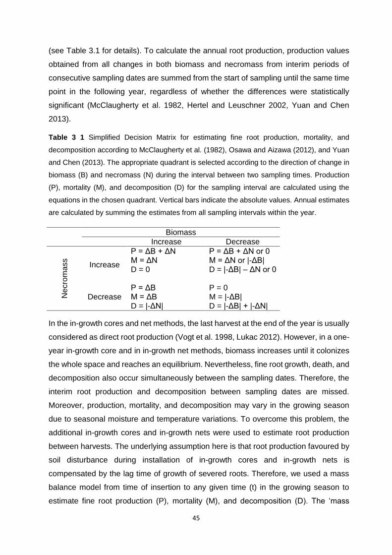
45

(see Table 3.1 for details). To calculate the annual root production, production values

obtained from all changes in both biomass and necromass from interim periods of

consecutive sampling dates are summed from the start of sampling until the same time

point in the following year, regardless of whether the differences were statistically

significant (McClaugherty et al. 1982, Hertel and Leuschner 2002, Yuan and Chen

2013).

Table 3 1 Simplified Decision Matrix for estimating fine root production, mortality, and

decomposition according to McClaugherty et al. (1982), Osawa and Aizawa (2012), and Yuan

and Chen (2013). The appropriate quadrant is selected according to the direction of change in

biomass (B) and necromass (N) during the interval between two sampling times. Production

(P), mortality (M), and decomposition (D) for the sampling interval are calculated using the

equations in the chosen quadrant. Vertical bars indicate the absolute values. Annual estimates

are calculated by summing the estimates from all sampling intervals within the year.

Biomass

Increase Decrease

Necro

ma

ss

Increase

P = ΔB + ΔN M = ΔN D = 0

P = ΔB + ΔN or 0 M = ΔN or |-ΔB| D = |-ΔB| – ΔN or 0

Decrease P = ΔB M = ΔB D = |-ΔN|

P = 0 M = |-ΔB| D = |-ΔB| + |-ΔN|

In the in-growth cores and net methods, the last harvest at the end of the year is usually

considered as direct root production (Vogt et al. 1998, Lukac 2012). However, in a one-

year in-growth core and in in-growth net methods, biomass increases until it colonizes

the whole space and reaches an equilibrium. Nevertheless, fine root growth, death, and

decomposition also occur simultaneously between the sampling dates. Therefore, the

interim root production and decomposition between sampling dates are missed.

Moreover, production, mortality, and decomposition may vary in the growing season

due to seasonal moisture and temperature variations. To overcome this problem, the

additional in-growth cores and in-growth nets were used to estimate root production

between harvests. The underlying assumption here is that root production favoured by

soil disturbance during installation of in-growth cores and in-growth nets is

compensated by the lag time of growth of severed roots. Therefore, we used a mass

balance model from time of insertion to any given time (t) in the growing season to

estimate fine root production (P), mortality (M), and decomposition (D). The ‘mass

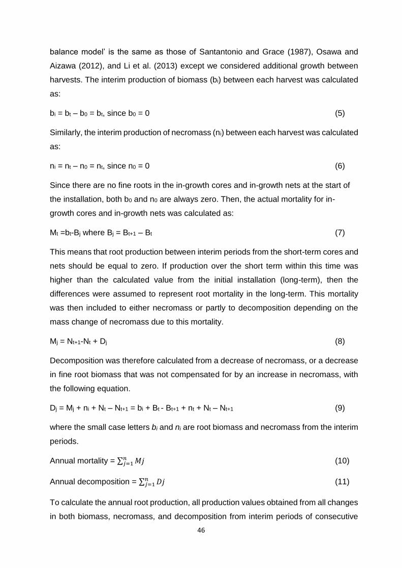
46

balance model’ is the same as those of Santantonio and Grace (1987), Osawa and

Aizawa (2012), and Li et al. (2013) except we considered additional growth between

harvests. The interim production of biomass (bi) between each harvest was calculated

as:

bi = bt – b0 = bt, since b0 = 0 (5)

Similarly, the interim production of necromass (ni) between each harvest was calculated

as:

ni = nt – n0 = nt, since n0 = 0 (6)

Since there are no fine roots in the in-growth cores and in-growth nets at the start of

the installation, both b0 and n0 are always zero. Then, the actual mortality for in-

growth cores and in-growth nets was calculated as:

Mt =bt-Bj where Bj = Bt+1 – Bt (7)

This means that root production between interim periods from the short-term cores and

nets should be equal to zero. If production over the short term within this time was

higher than the calculated value from the initial installation (long-term), then the

differences were assumed to represent root mortality in the long-term. This mortality

was then included to either necromass or partly to decomposition depending on the

mass change of necromass due to this mortality.

Mj = Nt+1-Nt + Dj (8)

Decomposition was therefore calculated from a decrease of necromass, or a decrease

in fine root biomass that was not compensated for by an increase in necromass, with

the following equation.

Dj = Mj + ni + Nt – Nt+1 = bi + Bt - Bt+1 + nt + Nt – Nt+1 (9)

where the small case letters bi and ni are root biomass and necromass from the interim

periods.

Annual mortality = ∑ 𝑀𝑗𝑛𝑗=1 (10)

Annual decomposition = ∑ 𝐷𝑗𝑛𝑗=1 (11)

To calculate the annual root production, all production values obtained from all changes

in both biomass, necromass, and decomposition from interim periods of consecutive

47

sampling dates were summed from the start of sampling until the same time point in

the following year (same as equation 2).

3.3.5 Calculation of fine root turnover

Root turnover rate (yr-1) was calculated as the ratio between annual root production

and average root biomass (McClaugherty et al. 1982, Aerts et al. 1992) or the highest

(maximum) biomass value (Gill and Jackson 2000). Mean residence time of roots is the

reciprocal of turnover rate.

Annual carbon inputs from fine roots into soil were calculated using fine root production

along with the C and N concentrations in the roots, assuming that there was no

translocation during root senescence. Hence, the annual fluxes of C and N into soil

(expressed in g m-2 yr-1) were estimated according to Xia et al. (2015) as:

Ia = P*C/N% (12)

Ia, annual input of C or N into the soil (g m-2 yr-1): P, annual fine root production (g m-2);

C/N, concentration of C or N in the fine roots (%).

3.3.6 Fine root vertical distribution

Vertical root distribution or cumulative root fraction (Y) from the surface to any depth

(d) was calculated according to a model developed by (Gale and Grigal 1987). An

asymptotic nonlinear model of the following form was fitted to describe the vertical root

distributions:

Y = 1-ßd (13)

where Y is the cumulative root fraction from the surface to soil depth d in centimetres

(midpoint), and ß the estimated parameter used as a measure of index of vertical root

distribution. The parameter ß can have values from 0 to 1, whereby higher values

indicate a greater proportion of roots at deeper soil (Jackson et al. 1997, Valverde-

Barrantes et al. 2007, Kucbel et al. 2011).

3.3.7 Carbon and nitrogen analysis

A very limited dry mass of fine roots and herbaceous roots was available. Accordingly,

to determine the total C and N concentrations in root materials, the original ten samples

48

were pooled by category to form nine samples each from the forest and eucalyptus,

and three samples each from grazing land and cropland. The nine samples from the

forest ecosystem were further processed to form three categories: roots <1 mm

diameter, roots from 1-2 mm diameter, and herbaceous roots. Each had three

replicates. The roots were dried at 70°C and ground to a fine powder (Fritsch

Pulverisette 5, Idar-Oberstein, Germany). Sub-samples of about 160 mg were taken

from each sample for C and N determinations using a CN elemental analyser (Truspec

CNS LECO, St. Joseph, USA). In addition, the soils from each sampling point and depth

were taken during root sampling and were dried at 105°C until constant weight. Ten

samples per land use system were analysed for total C and N concentration using 200

mg samples on the same CN elemental analyser as described above. Soil bulk density

was taken from values presented in Chapter 2.

3.3.8 Statistical analyses

Means and standard errors were calculated using the SPSS analytical software

package (version 21), and graphs were prepared using SigmaPlot (version 13). The

significance level was set at α = 0.05. Throughout the paper, error bars to the mean

are ±1SE. The relationships between different variables were analysed using one-way

analysis of variance and the Scheffe comparison method as well as simple regression

analysis. Assumptions of normality and homogeneous variance were examined by

Shapiro-Wilk’s and Levene’s test, respectively. When the assumptions of normality

were not met, the data were log10-transformed to normalize the distribution.

3.4 Results

3.4.1 Fine root biomass, necromass and distribution with depth

Fine root biomass and necromass to 40 cm soil depth for all land use systems is shown

in Table 3.2. Total weight of fine roots (biomass and necromass) in the soil layer 0–40

cm was higher in natural forest (564 g m-2) than in the eucalyptus stand (425 g m-2).

From the total root mass, living roots represented 83% in the natural forest and 79% in

eucalyptus plantation, whereas the necromass (dead roots) accounted for 17% in the

natural forest and 21% in the eucalyptus plantation (Table 3.2). The necromass,

however, was not significantly different between the forest (98±13 g m-2) and

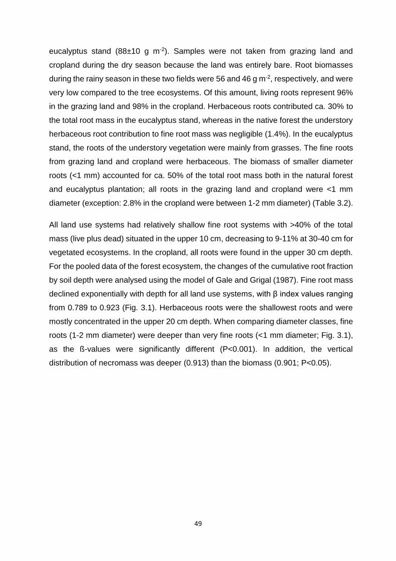
49

eucalyptus stand (88±10 g m-2). Samples were not taken from grazing land and

cropland during the dry season because the land was entirely bare. Root biomasses

during the rainy season in these two fields were 56 and 46 g m-2, respectively, and were

very low compared to the tree ecosystems. Of this amount, living roots represent 96%

in the grazing land and 98% in the cropland. Herbaceous roots contributed ca. 30% to

the total root mass in the eucalyptus stand, whereas in the native forest the understory

herbaceous root contribution to fine root mass was negligible (1.4%). In the eucalyptus

stand, the roots of the understory vegetation were mainly from grasses. The fine roots

from grazing land and cropland were herbaceous. The biomass of smaller diameter

roots (<1 mm) accounted for ca. 50% of the total root mass both in the natural forest

and eucalyptus plantation; all roots in the grazing land and cropland were <1 mm

diameter (exception: 2.8% in the cropland were between 1-2 mm diameter) (Table 3.2).

All land use systems had relatively shallow fine root systems with >40% of the total

mass (live plus dead) situated in the upper 10 cm, decreasing to 9-11% at 30-40 cm for

vegetated ecosystems. In the cropland, all roots were found in the upper 30 cm depth.

For the pooled data of the forest ecosystem, the changes of the cumulative root fraction

by soil depth were analysed using the model of Gale and Grigal (1987). Fine root mass

declined exponentially with depth for all land use systems, with β index values ranging

from 0.789 to 0.923 (Fig. 3.1). Herbaceous roots were the shallowest roots and were

mostly concentrated in the upper 20 cm depth. When comparing diameter classes, fine

roots (1-2 mm diameter) were deeper than very fine roots (<1 mm diameter; Fig. 3.1),

as the ß-values were significantly different (P<0.001). In addition, the vertical

distribution of necromass was deeper (0.913) than the biomass (0.901; P<0.05).

50

Table 3 2 Vertical distribution of fine root mass (g m-2) to a soil depth of 40 cm for native forest,

eucalyptus stand, grazing land and cropland. Fine roots are categorized as tree vs herbaceous

roots, biomass (live roots) vs necromass (dead roots) and very fine roots (<1 mm) vs fine roots

(1-2 mm) for both native forest and eucalyptus plantations. Values for forest and eucalyptus

were determined based on sequential coring. Roots from cropland and grazing land are taken

from the last in-growth core harvest, assuming peak rooting time at the end of the rainy season.

Roots from these land use systems are entirely herbaceous and mostly <1 mm. Values are

mean±SE; n=10 (forest and eucalyptus); n=5 (cropland and grazing land).

Land use Depth Total root

mass

Live and dead roots Diameter class Plant type

Biomass Necromas

s Roots <1

mm Roots 1-2

mm Tree roots

Herbaceous roots

Forest Total 564.2±41.7 466.5±31.6 97.7±12.8 272.9±18.2 291.4±27.7 555.8±42.2 8.4±3.2

0-10 239.5±18.5 195.5±14.7 46.4±6.9 137.5±9.5 108.1±12.1 232.1±18.9 7.5±2.9

10-20 174.2±15.2 153.3±11.8 30.1±4.5 81.4±6.5 101.9±10.5 177.9±15.0 0.7±0.4

20-30 90.0±11.3 74.0±8.4 17.8±3.9 37.2±2.8 61.4±10.4 89.8±11.3 0.2±0.2

30-40 60.5±8.4 55.6±8.3 12.6±2.2 27.1±3.7 44.3±6.8 65.4±8.6 na

Eucalyptus Total 424.7±36.9 336.8±30.5 87.9±10.2 211.8±17.1 223.0±22.8 302.6±28.9 122.1±15.1

0-10 231.4±19.8 176.2±16.5 55.2±6.7 123.6±12.1 107.8±11.4 140.5±11.8 90.9±13.2

10-20 93.6±12.7 75.8±11.0 20.9±4.0 45.4±4.5 60.3±10.9 74.2±12.1 19.4±3.1

20-30 58.1±7.5 48.7±7.0 12.5±1.6 27.1±2.9 41.3±6.7 50.6±7.7 8.7±1.7

30-40 41.6±14.3 41.2±15.5 9.7±1.9 17.4±2.8 47.2±21.7 44.0±16.2 3.1±0.7

Grazing land

Total 55.5±13.3 53.2±12.7 3.4±1.6 55.5±13.3 na na 55.5±13.3

0-10 31.9±7.8 29.8±7.1 2.1±1.3 31.9±7.8 na na 31.9±7.8

10-20 13.3±5.6 13.3±5.6 na 13.3±5.6 na na 13.3±5.6

20-30 6.4±1.7 5.9±1.6 0.5±0.0 6.4±1.7 na na 6.4±1.7

30-40 4.9±2.1 4.1±1.5 0.8±1.3 4.9±2.1 na na 4.9±2.1

Cropland Total 46.1±4.4 45.3±3.9 0.8±0.6 44.8±3.4 1.3 na 46.1±4.4

0-10 31.2±3.2 30.6±6.3 0.7±0.0 31.2±3.2 na na 31.2±3.2

10-20 13.2±4.2 13.0±4.2 0.2±0.0 11.9±3.1 1.3 na 13.2±4.2

20-30 1.7±1.1 1.7±1.1 na 1.7±1.1 na na 1.7±1.1

30-40 na* na na na na na na

*na, not available

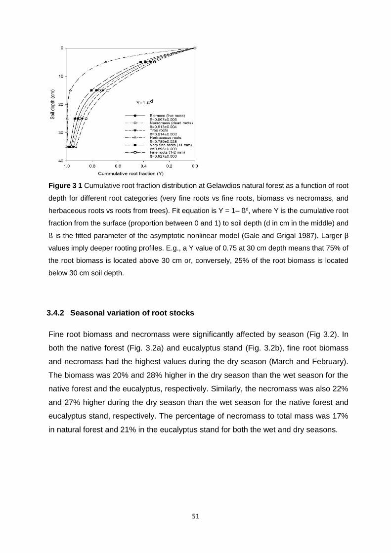
51

Figure 3 1 Cumulative root fraction distribution at Gelawdios natural forest as a function of root

depth for different root categories (very fine roots vs fine roots, biomass vs necromass, and

herbaceous roots vs roots from trees). Fit equation is Y = 1– ßd, where Y is the cumulative root

fraction from the surface (proportion between 0 and 1) to soil depth (d in cm in the middle) and

ß is the fitted parameter of the asymptotic nonlinear model (Gale and Grigal 1987). Larger β

values imply deeper rooting profiles. E.g., a Y value of 0.75 at 30 cm depth means that 75% of

the root biomass is located above 30 cm or, conversely, 25% of the root biomass is located

below 30 cm soil depth.

3.4.2 Seasonal variation of root stocks

Fine root biomass and necromass were significantly affected by season (Fig 3.2). In

both the native forest (Fig. 3.2a) and eucalyptus stand (Fig. 3.2b), fine root biomass

and necromass had the highest values during the dry season (March and February).

The biomass was 20% and 28% higher in the dry season than the wet season for the

native forest and the eucalyptus, respectively. Similarly, the necromass was also 22%

and 27% higher during the dry season than the wet season for the native forest and

eucalyptus stand, respectively. The percentage of necromass to total mass was 17%

in natural forest and 21% in the eucalyptus stand for both the wet and dry seasons.

52

Figure 3 2 Seasonal variation of fine root biomass and necromass (g m-2) at Gelawdios a)

forest; b) eucalyptus stand. Fine root estimates are based on coring method. Bars with different

small case letters are significantly different for filled bars (biomass), and different upper case

letters indicate significant differences for unfilled bars (necromass). Error bars represent

mean±1SE (p<0.05; n=10).

3.4.3 Fine root production, mortality, and turnover

The methods used for calculating annual fine root production from the sequential coring

data were the decision matrix and minimum-maximum method (Table 3.3); the mass

balance method was used for in-growth cores and in-growth net measurements (Table

3.4). Root production for all methodological approaches (sequential coring, in-growth

cores, and in-growth nets methods) clearly differed between land use types (Table 3.3

and 3.4; Fig. 3.3). For example, based on in-growth core methods, the annual root mass

produced in the forest ecosystem down to 40 cm was 468 g m-2 yr-1, which is about

37%, 87% and 90% higher than in the eucalyptus stand, grazing land, and cropland

ecosystems, respectively (Fig. 3.3). The highest annual root production was obtained

by sequential coring in the forest ecosystem (723±93 g m-2 yr-1), of which more than

58% (416±66 g m-2) was from mass loss due to decomposition (Table 3.3). Similarly,

the annual root mass production in the eucalyptus stand at the same depth was 694±95

g m-2 yr-1, necromass accounted for 14% of the total mass, and the mass loss due to

decomposition was ca. 41% (282±71 g m-2; Table 3.3). Fine root production estimated

based on the Decision Matrix was higher than the total standing mass by 22% and 39%

in the natural forest and eucalyptus, respectively. However, the annual root production

estimated by the in-growth core and in-growth net methods were ca. 43 and 62% lower

53

than the standing rootstock. The annual fine root production down to 40 cm was 60 g

m-2 yr-1 in grazing land and 52 g m-2 yr-1 in cropland based on the in-growth core method

with the mass balance calculation technique (Fig 3.3). This value was significantly lower

than in the forest and eucalyptus. Note that root growth in grazing land and cropland

was limited to the rainy season. When comparing the sampling methods, fine root

production in the forest ecosystem to 0-20 cm soil depth was highest (531±76 g m-2 yr-

1) with sequential coring, followed by the in-growth core method (329±51 g m-2 yr-1) and

the in-growth net method (218±18 g m-2 yr-1) (Fig 3.4). Except for the forest ecosystem,

the fine root production values obtained with the in-growth core and in-growth net

methods did not differ significantly in any land use system (Table 3.4). Root production

estimates using the in-growth cores and in-growth nets showed a consistent increase

over the course of the year. In the forest ecosystem, fine root production increased from

63 to 360 g m-2 from first month to the 12th month after installation of in-growth cores.

In the last four months, the average increment per month was 30 g m-2. Similarly, fine

root production as estimated with the in-growth net method increased from 42 to 191 g

m-2 with an average increment of 17 g m-2 in each of the last four months. Calculation

methods also affected the estimation of fine root production: the Decision Matrix always

showed a higher estimation than the Max-Min method (Table 3.3).

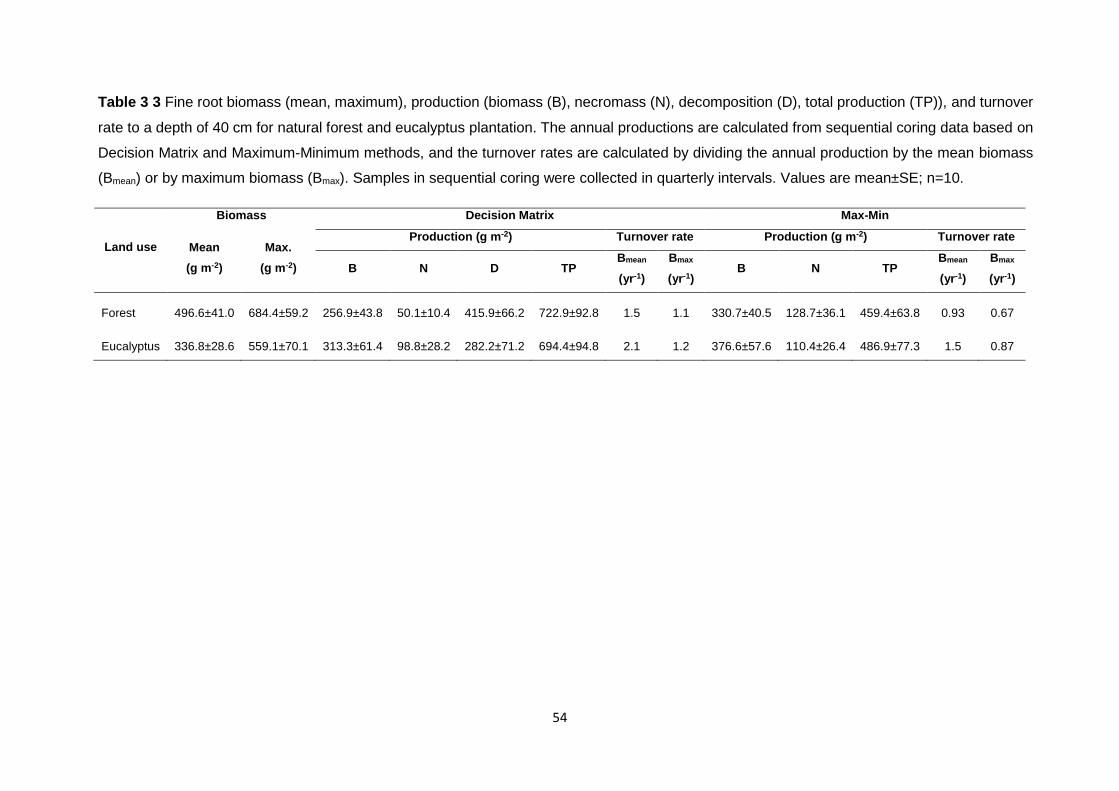
54

Table 3 3 Fine root biomass (mean, maximum), production (biomass (B), necromass (N), decomposition (D), total production (TP)), and turnover

rate to a depth of 40 cm for natural forest and eucalyptus plantation. The annual productions are calculated from sequential coring data based on

Decision Matrix and Maximum-Minimum methods, and the turnover rates are calculated by dividing the annual production by the mean biomass

(Bmean) or by maximum biomass (Bmax). Samples in sequential coring were collected in quarterly intervals. Values are mean±SE; n=10.

Land use

Biomass Decision Matrix Max-Min

Mean

(g m-2)

Max.

(g m-2)

Production (g m-2) Turnover rate Production (g m-2) Turnover rate

B N D TP Bmean

(yr-1)

Bmax

(yr-1) B N TP

Bmean

(yr-1)

Bmax

(yr-1)

Forest 496.6±41.0 684.4±59.2 256.9±43.8 50.1±10.4 415.9±66.2 722.9±92.8 1.5 1.1 330.7±40.5 128.7±36.1 459.4±63.8 0.93 0.67

Eucalyptus 336.8±28.6 559.1±70.1 313.3±61.4 98.8±28.2 282.2±71.2 694.4±94.8 2.1 1.2 376.6±57.6 110.4±26.4 486.9±77.3 1.5 0.87

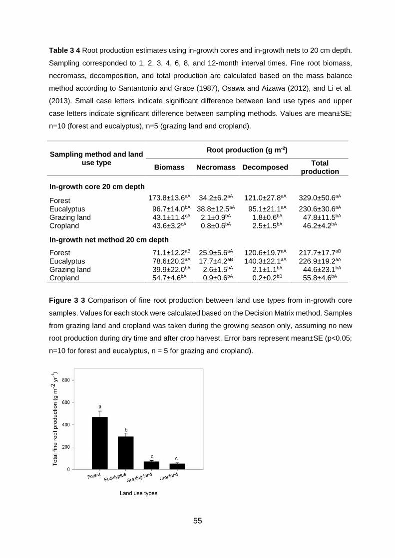
55

Table 3 4 Root production estimates using in-growth cores and in-growth nets to 20 cm depth.

Sampling corresponded to 1, 2, 3, 4, 6, 8, and 12-month interval times. Fine root biomass,

necromass, decomposition, and total production are calculated based on the mass balance

method according to Santantonio and Grace (1987), Osawa and Aizawa (2012), and Li et al.

(2013). Small case letters indicate significant difference between land use types and upper

case letters indicate significant difference between sampling methods. Values are mean±SE;

n=10 (forest and eucalyptus), n=5 (grazing land and cropland).

Sampling method and land use type

Root production (g m-2)

Biomass Necromass Decomposed Total

production

In-growth core 20 cm depth

Forest 173.8±13.6aA 34.2±6.2aA 121.0±27.8aA 329.0±50.6aA

Eucalyptus 96.7±14.0bA 38.8±12.5aA 95.1±21.1aA 230.6±30.6aA Grazing land 43.1±11.4cA 2.1±0.9bA 1.8±0.6bA 47.8±11.5bA Cropland 43.6±3.2cA 0.8±0.6bA 2.5±1.5bA 46.2±4.2bA

In-growth net method 20 cm depth

Forest 71.1±12.2aB 25.9±5.6aA 120.6±19.7aA 217.7±17.7aB Eucalyptus 78.6±20.2aA 17.7±4.2aB 140.3±22.1aA 226.9±19.2aA Grazing land 39.9±22.0bA 2.6±1.5bA 2.1±1.1bA 44.6±23.1bA Cropland 54.7±4.6bA 0.9±0.6bA 0.2±0.2bB 55.8±4.6bA

Figure 3 3 Comparison of fine root production between land use types from in-growth core

samples. Values for each stock were calculated based on the Decision Matrix method. Samples

from grazing land and cropland was taken during the growing season only, assuming no new

root production during dry time and after crop harvest. Error bars represent mean±SE (p<0.05;

n=10 for forest and eucalyptus, n = 5 for grazing and cropland).

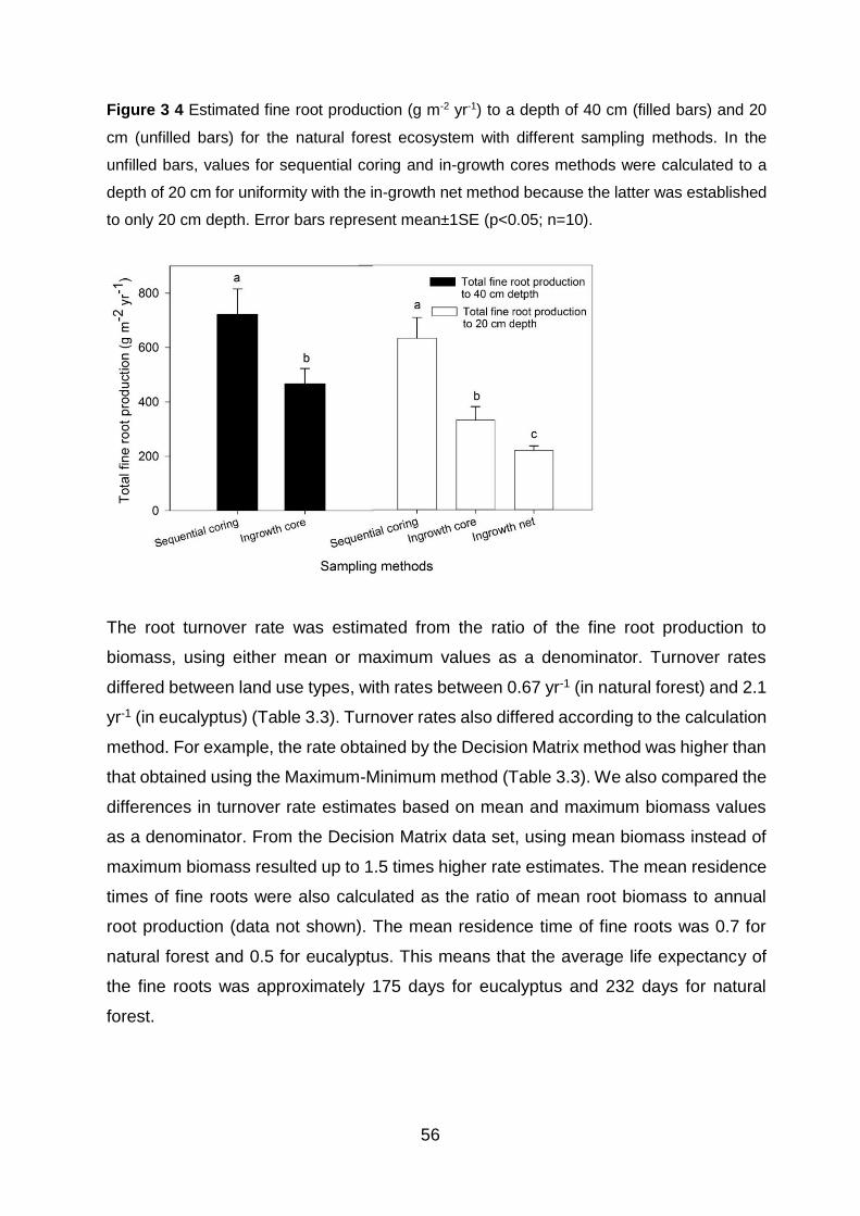
56

Figure 3 4 Estimated fine root production (g m-2 yr-1) to a depth of 40 cm (filled bars) and 20

cm (unfilled bars) for the natural forest ecosystem with different sampling methods. In the

unfilled bars, values for sequential coring and in-growth cores methods were calculated to a

depth of 20 cm for uniformity with the in-growth net method because the latter was established

to only 20 cm depth. Error bars represent mean±1SE (p<0.05; n=10).

The root turnover rate was estimated from the ratio of the fine root production to

biomass, using either mean or maximum values as a denominator. Turnover rates

differed between land use types, with rates between 0.67 yr-1 (in natural forest) and 2.1

yr-1 (in eucalyptus) (Table 3.3). Turnover rates also differed according to the calculation

method. For example, the rate obtained by the Decision Matrix method was higher than

that obtained using the Maximum-Minimum method (Table 3.3). We also compared the

differences in turnover rate estimates based on mean and maximum biomass values

as a denominator. From the Decision Matrix data set, using mean biomass instead of

maximum biomass resulted up to 1.5 times higher rate estimates. The mean residence

times of fine roots were also calculated as the ratio of mean root biomass to annual

root production (data not shown). The mean residence time of fine roots was 0.7 for

natural forest and 0.5 for eucalyptus. This means that the average life expectancy of

the fine roots was approximately 175 days for eucalyptus and 232 days for natural

forest.

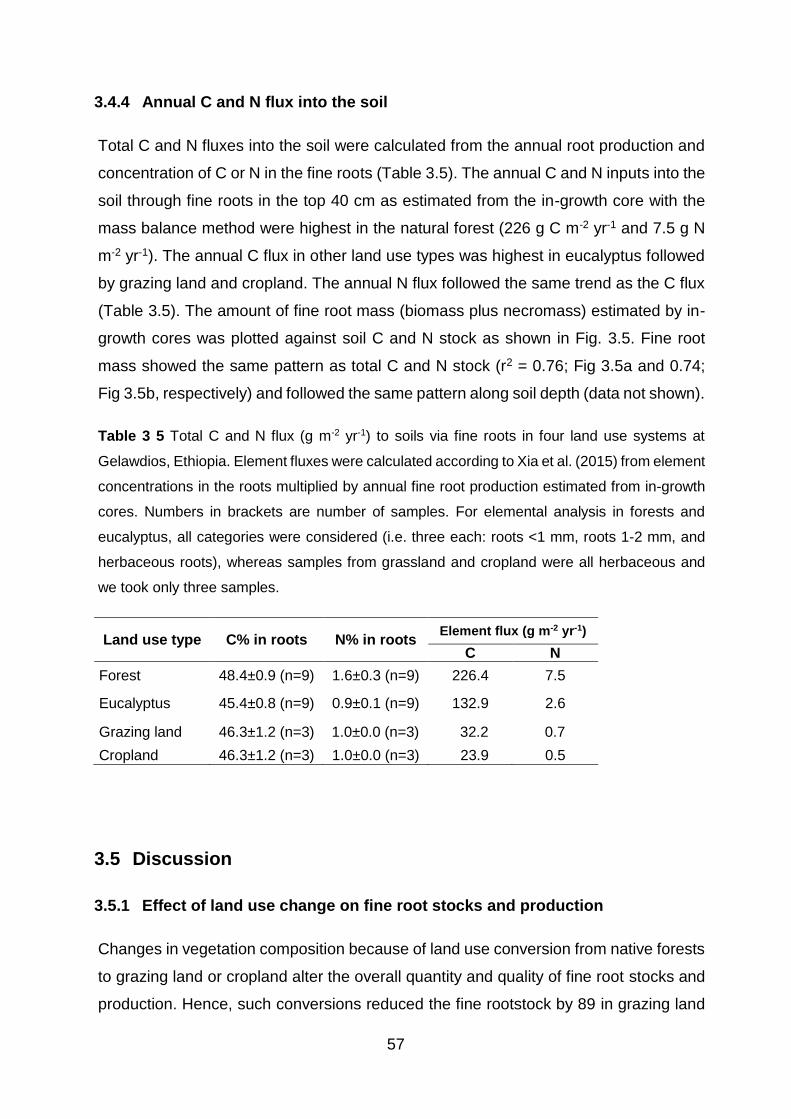
57

3.4.4 Annual C and N flux into the soil

Total C and N fluxes into the soil were calculated from the annual root production and

concentration of C or N in the fine roots (Table 3.5). The annual C and N inputs into the

soil through fine roots in the top 40 cm as estimated from the in-growth core with the

mass balance method were highest in the natural forest (226 g C m-2 yr-1 and 7.5 g N

m-2 yr-1). The annual C flux in other land use types was highest in eucalyptus followed

by grazing land and cropland. The annual N flux followed the same trend as the C flux

(Table 3.5). The amount of fine root mass (biomass plus necromass) estimated by in-

growth cores was plotted against soil C and N stock as shown in Fig. 3.5. Fine root

mass showed the same pattern as total C and N stock (r2 = 0.76; Fig 3.5a and 0.74;

Fig 3.5b, respectively) and followed the same pattern along soil depth (data not shown).

Table 3 5 Total C and N flux (g m-2 yr-1) to soils via fine roots in four land use systems at

Gelawdios, Ethiopia. Element fluxes were calculated according to Xia et al. (2015) from element

concentrations in the roots multiplied by annual fine root production estimated from in-growth

cores. Numbers in brackets are number of samples. For elemental analysis in forests and

eucalyptus, all categories were considered (i.e. three each: roots <1 mm, roots 1-2 mm, and

herbaceous roots), whereas samples from grassland and cropland were all herbaceous and

we took only three samples.

Land use type C% in roots N% in roots Element flux (g m-2 yr-1)

C N

Forest 48.4±0.9 (n=9) 1.6±0.3 (n=9) 226.4 7.5

Eucalyptus 45.4±0.8 (n=9) 0.9±0.1 (n=9) 132.9 2.6

Grazing land 46.3±1.2 (n=3) 1.0±0.0 (n=3) 32.2 0.7

Cropland 46.3±1.2 (n=3) 1.0±0.0 (n=3) 23.9 0.5

3.5 Discussion

3.5.1 Effect of land use change on fine root stocks and production

Changes in vegetation composition because of land use conversion from native forests

to grazing land or cropland alter the overall quantity and quality of fine root stocks and

production. Hence, such conversions reduced the fine rootstock by 89 in grazing land

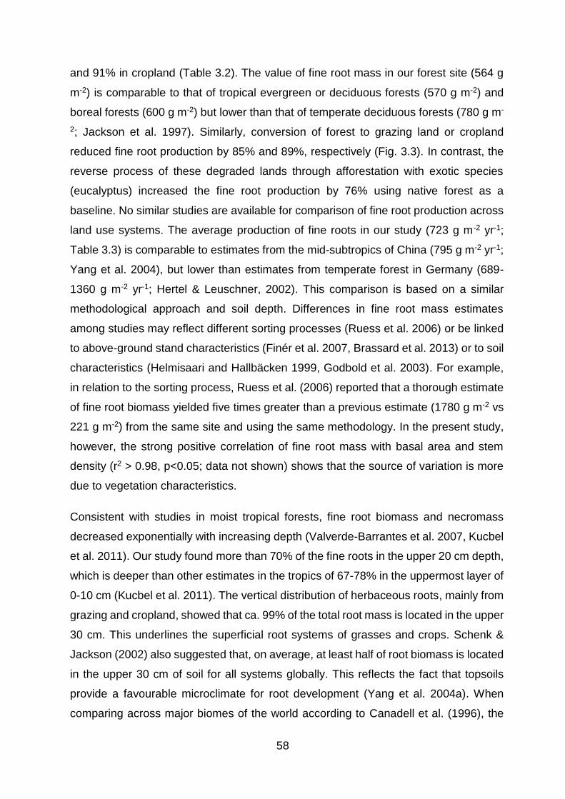
58

and 91% in cropland (Table 3.2). The value of fine root mass in our forest site (564 g

m-2) is comparable to that of tropical evergreen or deciduous forests (570 g m-2) and

boreal forests (600 g m-2) but lower than that of temperate deciduous forests (780 g m-

2; Jackson et al. 1997). Similarly, conversion of forest to grazing land or cropland

reduced fine root production by 85% and 89%, respectively (Fig. 3.3). In contrast, the

reverse process of these degraded lands through afforestation with exotic species

(eucalyptus) increased the fine root production by 76% using native forest as a

baseline. No similar studies are available for comparison of fine root production across

land use systems. The average production of fine roots in our study (723 g m-2 yr-1;

Table 3.3) is comparable to estimates from the mid-subtropics of China (795 g m-2 yr-1;

Yang et al. 2004), but lower than estimates from temperate forest in Germany (689-

1360 g m-2 yr-1; Hertel & Leuschner, 2002). This comparison is based on a similar

methodological approach and soil depth. Differences in fine root mass estimates

among studies may reflect different sorting processes (Ruess et al. 2006) or be linked

to above-ground stand characteristics (Finér et al. 2007, Brassard et al. 2013) or to soil

characteristics (Helmisaari and Hallbäcken 1999, Godbold et al. 2003). For example,

in relation to the sorting process, Ruess et al. (2006) reported that a thorough estimate

of fine root biomass yielded five times greater than a previous estimate (1780 g m-2 vs

221 g m-2) from the same site and using the same methodology. In the present study,

however, the strong positive correlation of fine root mass with basal area and stem

density (r2 > 0.98, p<0.05; data not shown) shows that the source of variation is more

due to vegetation characteristics.

Consistent with studies in moist tropical forests, fine root biomass and necromass

decreased exponentially with increasing depth (Valverde-Barrantes et al. 2007, Kucbel

et al. 2011). Our study found more than 70% of the fine roots in the upper 20 cm depth,

which is deeper than other estimates in the tropics of 67-78% in the uppermost layer of

0-10 cm (Kucbel et al. 2011). The vertical distribution of herbaceous roots, mainly from

grazing and cropland, showed that ca. 99% of the total root mass is located in the upper

30 cm. This underlines the superficial root systems of grasses and crops. Schenk &

Jackson (2002) also suggested that, on average, at least half of root biomass is located

in the upper 30 cm of soil for all systems globally. This reflects the fact that topsoils

provide a favourable microclimate for root development (Yang et al. 2004a). When

comparing across major biomes of the world according to Canadell et al. (1996), the

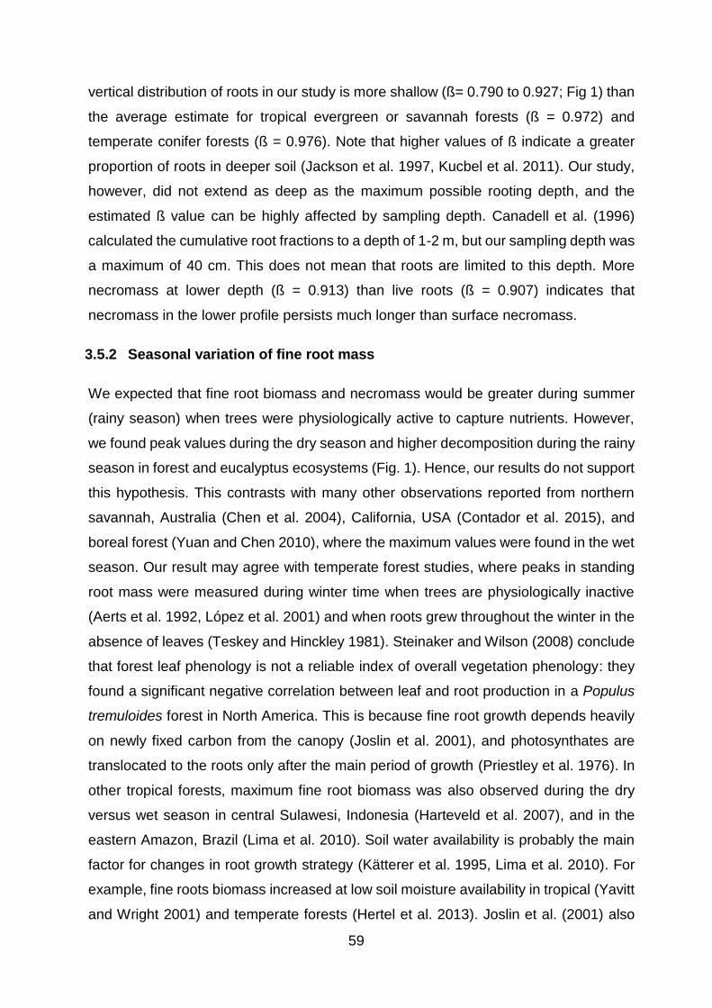
59

vertical distribution of roots in our study is more shallow (ß= 0.790 to 0.927; Fig 1) than

the average estimate for tropical evergreen or savannah forests (ß = 0.972) and

temperate conifer forests (ß = 0.976). Note that higher values of ß indicate a greater

proportion of roots in deeper soil (Jackson et al. 1997, Kucbel et al. 2011). Our study,

however, did not extend as deep as the maximum possible rooting depth, and the

estimated ß value can be highly affected by sampling depth. Canadell et al. (1996)

calculated the cumulative root fractions to a depth of 1-2 m, but our sampling depth was

a maximum of 40 cm. This does not mean that roots are limited to this depth. More

necromass at lower depth (ß = 0.913) than live roots (ß = 0.907) indicates that

necromass in the lower profile persists much longer than surface necromass.

3.5.2 Seasonal variation of fine root mass

We expected that fine root biomass and necromass would be greater during summer

(rainy season) when trees were physiologically active to capture nutrients. However,

we found peak values during the dry season and higher decomposition during the rainy

season in forest and eucalyptus ecosystems (Fig. 1). Hence, our results do not support

this hypothesis. This contrasts with many other observations reported from northern

savannah, Australia (Chen et al. 2004), California, USA (Contador et al. 2015), and

boreal forest (Yuan and Chen 2010), where the maximum values were found in the wet

season. Our result may agree with temperate forest studies, where peaks in standing

root mass were measured during winter time when trees are physiologically inactive

(Aerts et al. 1992, López et al. 2001) and when roots grew throughout the winter in the

absence of leaves (Teskey and Hinckley 1981). Steinaker and Wilson (2008) conclude

that forest leaf phenology is not a reliable index of overall vegetation phenology: they

found a significant negative correlation between leaf and root production in a Populus

tremuloides forest in North America. This is because fine root growth depends heavily

on newly fixed carbon from the canopy (Joslin et al. 2001), and photosynthates are

translocated to the roots only after the main period of growth (Priestley et al. 1976). In

other tropical forests, maximum fine root biomass was also observed during the dry

versus wet season in central Sulawesi, Indonesia (Harteveld et al. 2007), and in the

eastern Amazon, Brazil (Lima et al. 2010). Soil water availability is probably the main

factor for changes in root growth strategy (Kätterer et al. 1995, Lima et al. 2010). For

example, fine roots biomass increased at low soil moisture availability in tropical (Yavitt

and Wright 2001) and temperate forests (Hertel et al. 2013). Joslin et al. (2001) also

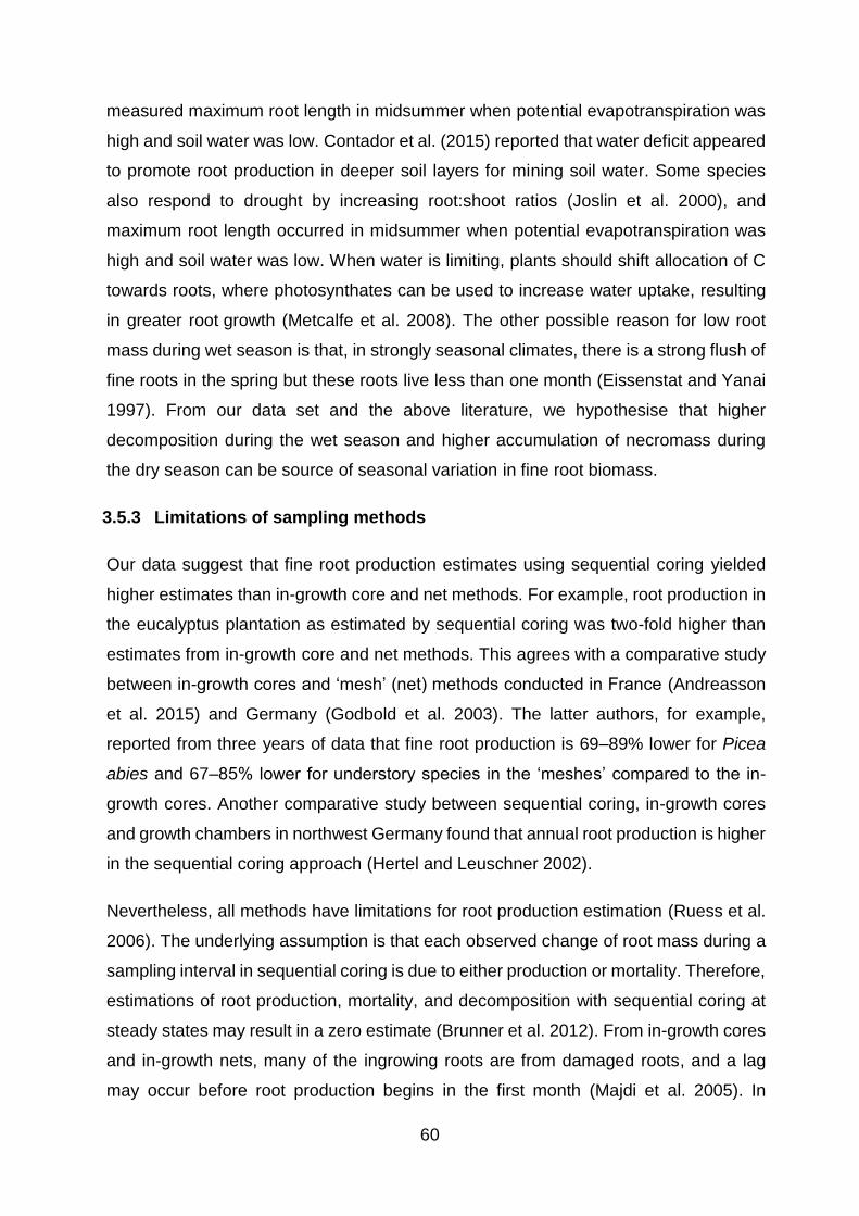
60

measured maximum root length in midsummer when potential evapotranspiration was

high and soil water was low. Contador et al. (2015) reported that water deficit appeared

to promote root production in deeper soil layers for mining soil water. Some species

also respond to drought by increasing root:shoot ratios (Joslin et al. 2000), and

maximum root length occurred in midsummer when potential evapotranspiration was

high and soil water was low. When water is limiting, plants should shift allocation of C

towards roots, where photosynthates can be used to increase water uptake, resulting

in greater root growth (Metcalfe et al. 2008). The other possible reason for low root

mass during wet season is that, in strongly seasonal climates, there is a strong flush of

fine roots in the spring but these roots live less than one month (Eissenstat and Yanai

1997). From our data set and the above literature, we hypothesise that higher

decomposition during the wet season and higher accumulation of necromass during

the dry season can be source of seasonal variation in fine root biomass.

3.5.3 Limitations of sampling methods

Our data suggest that fine root production estimates using sequential coring yielded

higher estimates than in-growth core and net methods. For example, root production in

the eucalyptus plantation as estimated by sequential coring was two-fold higher than

estimates from in-growth core and net methods. This agrees with a comparative study

between in-growth cores and ‘mesh’ (net) methods conducted in France (Andreasson

et al. 2015) and Germany (Godbold et al. 2003). The latter authors, for example,

reported from three years of data that fine root production is 69–89% lower for Picea

abies and 67–85% lower for understory species in the ‘meshes’ compared to the in-

growth cores. Another comparative study between sequential coring, in-growth cores

and growth chambers in northwest Germany found that annual root production is higher

in the sequential coring approach (Hertel and Leuschner 2002).

Nevertheless, all methods have limitations for root production estimation (Ruess et al.

2006). The underlying assumption is that each observed change of root mass during a

sampling interval in sequential coring is due to either production or mortality. Therefore,

estimations of root production, mortality, and decomposition with sequential coring at

steady states may result in a zero estimate (Brunner et al. 2012). From in-growth cores

and in-growth nets, many of the ingrowing roots are from damaged roots, and a lag

may occur before root production begins in the first month (Majdi et al. 2005). In

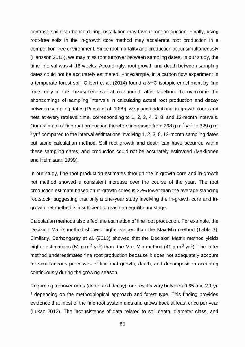
61

contrast, soil disturbance during installation may favour root production. Finally, using

root-free soils in the in-growth core method may accelerate root production in a

competition-free environment. Since root mortality and production occur simultaneously

(Hansson 2013), we may miss root turnover between sampling dates. In our study, the

time interval was 4–16 weeks. Accordingly, root growth and death between sampling

dates could not be accurately estimated. For example, in a carbon flow experiment in

a temperate forest soil, Gilbert et al. (2014) found a δ13C isotopic enrichment by fine

roots only in the rhizosphere soil at one month after labelling. To overcome the

shortcomings of sampling intervals in calculating actual root production and decay

between sampling dates (Priess et al. 1999), we placed additional in-growth cores and

nets at every retrieval time, corresponding to 1, 2, 3, 4, 6, 8, and 12-month intervals.

Our estimate of fine root production therefore increased from 268 g m-2 yr-1 to 329 g m-

2 yr-1 compared to the interval estimations involving 1, 2, 3, 8, 12-month sampling dates

but same calculation method. Still root growth and death can have occurred within

these sampling dates, and production could not be accurately estimated (Makkonen

and Helmisaari 1999).

In our study, fine root production estimates through the in-growth core and in-growth

net method showed a consistent increase over the course of the year. The root

production estimate based on in-growth cores is 22% lower than the average standing

rootstock, suggesting that only a one-year study involving the in-growth core and in-

growth net method is insufficient to reach an equilibrium stage.

Calculation methods also affect the estimation of fine root production. For example, the

Decision Matrix method showed higher values than the Max-Min method (Table 3).

Similarly, Berhongaray et al. (2013) showed that the Decision Matrix method yields

higher estimations (51 g m-2 yr-1) than the Max-Min method (41 g m-2 yr-1). The latter

method underestimates fine root production because it does not adequately account

for simultaneous processes of fine root growth, death, and decomposition occurring

continuously during the growing season.

Regarding turnover rates (death and decay), our results vary between 0.65 and 2.1 yr-

1 depending on the methodological approach and forest type. This finding provides

evidence that most of the fine root system dies and grows back at least once per year

(Lukac 2012). The inconsistency of data related to soil depth, diameter class, and

62

methodological approaches in the literature complicates comparing our turnover

estimates across studies. Nonetheless, our results are in the range of turnover rates of

European forests (0.17-3.10 yr-1) as compiled by Brunner et al. (2012). Turnover rate

estimates using mean biomass instead of maximum biomass as a denominator yielded

higher estimates (Table 3). This result is in agreement with estimates in a European

forest, with a mean difference of about 30% (Brunner et al. 2012). As in root production,

calculation methods also affect the estimation of the fine-root turnover rate. In this case,

the Decision Matrix showed a higher rate (Table 3). A comparison analysis by Brunner

et al. (2012) found that the rates calculated with the Decision Matrix were significantly

higher (approximately double, 1.14 yr-1) than those calculated with the Max-Min method

(0.57 yr-1). They suggested that the latter method is suitable for ecosystems with strong

annual fluctuations. Fine roots grow, die and decompose throughout the year. The

proportion of dead roots that have been replaced by new growth is calculated as root

production over biomass at steady state on an annual basis (McClaugherty et al. 1982).

Hence, we always underestimate root production because we miss the root growth and

death between the sampling dates. We therefore suggest that using mean biomass, as

a denominator, is more representative of average live roots than using maximum

biomass to estimate root turnover rate.

Figure 3 5 Relationship between total root mass (biomass + necromass) with C stock a) and

N stock b) for four land use systems at Gelawdios, Ethiopia. n=10 (forest and eucalyptus), and

5 (cropland and grazing land).

63

3.5.4 Implications of fine root turnover in ecosystem carbon cycling

Our fine rootstock and production estimates tended to show the same pattern of soil C

and N stocks in the soil (r2 = 0.76; P<0.001 for C and r2 = 0.74; P< 0.001 for N; Fig.

3.5). This suggests that fine roots are the major contributors of C and N input in the soil.

Similarly, Hansson et al. (2013) reported that the fine root stock distribution followed

the same pattern as the soil C and N distribution in the stands. Nonetheless, our annual

C flux estimate based on fine roots in the forest to 40 cm depth (224 g of C m-2 yr-1;

Table 3.5) was much smaller than estimates from tropical forests in Indonesia (233 g

of C m-2 yr-1 from the top 20 cm only; Hertel et al., 2008). The annual C flux from fine

roots in the eucalyptus stand, grazing land, and cropland was about 37%, 85% and

89% lower, respectively, compared to native forest. This suggests that conversion of

native forest to grazing land and cropland resulted in a ca. 85-89% C input reduction

into the soil. Previously, our carbon stock analysis (Chapter 2) showed that land use

change resulted in an up to 88% of carbon reduction at the site level. Based on the

current forest cover of the region (9.5%, unpublished government report), the total C

input to the soil through fine roots is very roughly estimated to be 3.6 mega tons

(1Mt=1012) of C yr-1. If we take the former forest cover of the country (40%, about 50

years ago; Bekele 2011) for the study area, and if there is no C translocation, then the

region lost an annual input of 11.1 Mt of C yr-1 through fine roots into soil for the last 50

years due to deforestation. This estimate is certainly conservative. The result of this

analysis suggests that forest protection against deforestation alone sequesters about

90% more carbon compared to grazing land or croplands.

3.6 Conclusion

Conversions of land use from native forest to other land use types such as grazing land

or cropland strongly reduce root production (ca. 85-89%). Root production and turnover

were also strongly affected by seasonal variations, with peak values in the dry season.

This indicates accumulation of root mass under moisture-limiting conditions. With

regard to vertical distribution, there was always a decreasing trend of root mass with

soil depth. This spatial pattern was similar to that of the C and N stock in the mineral

soil, indicating a significant contribution of roots to soil C and N pools.

64

4 Fine root morphology, biochemistry and litter quality

indices of fast- and slow-growing woody species in

Ethiopian highland forests

4.1 Abstract

Fine roots of trees are the major channels of carbon flows into the soil. Nonetheless,

the quality of carbon input into the soil via fine roots is influenced by morphological traits

and chemical composition. This study was designed to examine whether root traits

varied with species and to correlate such variations with biochemistry via proxy carbon

fractionations. Fine roots of ten tropical woody species collected from the northern

highlands of Ethiopia were analysed for root morphological indices and root chemistry

using a series of acid digestions. Fast- growing species exhibited higher specific root

length and specific root area, but lower root tissue density (RTD) than slow-growing

species. Differences in morphological parameters of fine roots in fast- and slow-growing

species reflect the ecological strategy they employ. In roots of all species, the acid-

insoluble fractions (AIF) were the highest fraction. The carbon content, AIF, and the

lignocellulose index were higher for slow-growing species and showed a strong positive

correlation with RTD. This reflects a higher carbon investment to construct fine roots of

slow growing species.

Key words: Carbon fractions, root tissue density, specific root length, acid-insoluble

fraction, carbon cost, root traits, lignin

65

4.2 Introduction

The importance of fine roots for both plant and ecosystem functioning is increasingly

recognized. At the same time, our understanding of root trait variation between plant

species and its effects on ecological processes such as biogeochemical cycling

remains limited (Xia et al. 2015, Valverde-Barrantes et al. 2016, Weemstra et al. 2016).

Despite increasing information on root traits of plants in temperate and boreal (forest)

ecosystems (Comas et al. 2002, Pinno et al. 2010), corresponding data on fine root

characteristics of tropical tree species are rare, particularly for African ecosystems.

Parameters such as specific root length (SRL) and root tissue density (RTD) of ‘fine

roots’ (< 2 mm in diameter) are key traits of a root economics spectrum. This is because

they are apparently closely linked to the carbon (C) use strategy and/or resource uptake

efficiency of trees (Comas and Eissenstat 2004, Birouste et al. 2014, Weemstra et al.

2016). From an ecological point of view, fine roots with higher RTD affect several

processes of root functioning such as soil fertility (Valverde-Barrantes et al. 2016),

respiration rate (Makita et al. 2012, Rewald et al. 2014), growth rate (Birouste et al.

2014), and longevity (McCormack et al. 2012). Similarly, other root morphology

parameters such as specific root length (SRL) have been widely used as indicators of

resource use efficiency (Comas and Eissenstat 2004, Ostonen et al. 2007).

Interestingly, SRL and RTD are not necessary correlated across phylogenetic groups

(Valverde-Barrantes et al. 2016).

The chemical composition of fine root tissue may reveal further important aspects of

carbon-use strategies of plants. For example, the fine root longevity of temperate tree

species significantly increases with decreasing C:N ratios (McCormack et al. 2012).

Beyond C:N ratios, the chemical composition of fine roots regarding labile (e.g.,

carbohydrates) and recalcitrant fractions (e.g., lignin) may further enhance our

understanding of (tree) root economic strategies (Kong et al. 2016). The pioneer work

of Kong and colleagues, however, also again emphasizes that root trait patterns are

complicated and that further studies are needed. This pertains especially to

consolidating our understanding of the relations between specific C and N fractions and

morphological parameters and to improving our trait interpretations regarding (tree) fine

root economic spectra. In particular, we need information on morphological and

chemical root traits linked to plant growth strategies (e.g. fast or slow above-ground

66

growth) (Comas et al. 2002, Comas and Eissenstat 2004) and to trait interrelationships.

Currently, evidence for correlations within and between root traits, and the wider plant

economic spectrum, is weak at best. This is probably because root system function can

be optimized using a much more diverse set of traits compared to leaves (Valverde-

Barrantes et al. 2016, Weemstra et al. 2016).

Beside their key role for plant functioning, it is increasingly recognized that fine roots

also play major roles in global biogeochemical cycles, including carbon sequestration

(Xia et al. 2015). Plant roots account for up to 48% of annual plant litter inputs (Freschet

et al. 2013) and are estimated to contribute an average of two-fold more to soil organic

C than leaf litter (Rasse et al. 2005). While root litter is thus a major source of soil

organic matter, species-specific root decomposition rates and impacts on soil organic

carbon turnover remain uncertain. The parameters that explain the largest amount of

variability in root decay are abiotic environmental factors such as temperature and

precipitation as well as root tissue chemistry (Silver and Miya 2001, Solly et al. 2014).

The chemical compositions of roots, e.g. indicated by labile and recalcitrant fractions,

varies with species and largely determines the rate of decay (Couteaux et al. 1995,

Silver and Miya 2001, Sun et al. 2013) and the quality of C input into soil systems

(Rasse et al. 2005). One approach for quantitative determination of fine root carbon

chemistry is chemical fractionation. According to Ryan et al. (1990) and Sun et al.

(2013), organic compounds of tissues can be placed into three broad fractions. 1)

Extractable labile C compounds consisting of nonpolar constituents such as fats, oils,

waxes, and polar constituents such as nonstructural carbohydrates and water-soluble

polyphenols removed using a two-stage extraction in dichloromethane and boiling

water, respectively. 2) Acid-hydrolysable structural components that are moderately

degradable C compounds consisting primarily of cellulose and hemicellulose, removed

using a two-stage digestion in 72% and 2.5% H2SO4. 3) Acid-insoluble aromatic

compounds that are highly recalcitrant C compounds conventionally referred to as

lignin (Preston et al. 2000, Xia et al. 2015) but also consisting of other highly reduced

compounds such as suberin, cutin, and tannin-protein complexes, which are the

residual of the two-stage sulfuric acid digestion minus ash mass (Sun et al. 2013). The

recalcitrant tissues are characterized by relatively low concentrations of easily

degraded substrates (Xia et al. 2015). The values obtained can be used as an estimate

of long-term carbon input into the soil system by roots.

67

This study was conducted on ten dominant woody species of a diverse, pristine

community of tropical woody species, namely a remnant church forest of the north-

central Ethiopian highland. The aim was to characterize fine root morphology,

biochemistry, and their interrelationships. The specific objectives were to determine 1)

how fine root morphology and biochemistry varies between fast- and slow-growing

woody species, and 2) if or how fine root morphological traits are correlated to root

biochemistry. We hypothesize that fast-growing species build ‘cheaper’ roots of lower

root tissue density (RTD) and that roots with a lower RTD contain less recalcitrant

carbon fractions (less lignified roots). The results are discussed in the light of root

economic strategies and the potential effects on root litter quality and quality of C input

into soil systems.

4.3 Materials and methods

4.3.1 Study site

This study was carried out at the remnant Afromontane forest of Gelawdios in the

Amhara National Regional State, north-central Ethiopia. Gelawdios (11°38’25’’N,

37°48’55’’E) is located east of Lake Tana at an altitude of 2466-2526 m above sea level.

While Ethiopia is located in the tropics, the climate of the study area is temperate with

dry winters and warm summers (Cwb) according to the Köppen-Geiger climate

classification (Peel et al. 2007). The mean annual precipitation is 1220 mm, with the

main rainy season from June to September and with low-intensity precipitation from

March to May (Wassie et al. 2009). The distribution of rainfall largely depends upon the

direction of moisture-bearing monsoon winds and altitude. The annual mean air

temperature is 19°C (Wassie et al. 2009). The soils are classified as Cambisols;

edaphic characteristics are summarized in Supplementary Information Table A1.1. The

Afromontane Gelawdios forest is a small, isolated, but pristine forest fragment (‘church

forest’) covering about 100 ha in the otherwise almost completely deforested Ethiopian

highlands (Wassie et al. 2009, Aerts et al. 2016).

Ten dominant, native woody species were studied: Allophylus abyssinicus (Hochst.)

Radlk., Apodytes dimidiata E. Mey ex. Arn., Calpurnia aurea (Ait.) Benth., Chionanthus

mildbraedii (Gilg & Schellenb.) Stearn, Combretum collinum Fresen., Dovyalis

abyssinica (A. Rich.) Warb., Ekebergia capensis (Sparm.), Maytenus arbutifolia (A.

68

Rich.) Wilczek, Podocarpus falcatus (Thunb.) Mirb., and Teclea nobilis (Del.). The

species were categorized into five fast- and five slow-growing species according to a

literature review (Fichtl and Adi 1994, Katende et al. 1995, Hedberg 2003, Bekele 2007,

Orwa et al. 2009) and information from indigenous knowledge. Species category,

characteristics, and their corresponding local names are provided in Table A2.2.

4.3.2 Root sampling

Roots were sampled in September 2014, corresponding to peak aboveground growth

and the end of the rainy season. Intact fine root branches (diameter <2 mm) were

collected from the topsoil under five randomly chosen tree individuals of each species

along a transect line; the minimum distance between sampling locations under the

same species was about 100 m. In the diverse and relatively dense forest stand, fine

root taxa for the species of interest were identified by carefully tracking coarse roots

from the tree base (Rewald et al. 2012). At each tree individual, three sample locations

were selected. At each of the locations, one intact fine root branch was carefully

extracted from a soil monolith (approx. 20 cm × 10 cm; top 20 cm of soil) with forceps;

remaining soil on roots was carefully brushed away (Wang et al. 2006). In total, fifteen

root branches per species were separately placed into sealed plastic bags, kept in a

cooling box/fridge (4-8°C), and transported to Vienna, Austria, for subsequent root

processing within 1 week after sampling. Moist paper towels were placed inside the

plastic bags to prevent desiccation.

4.3.3 Root morphology

Fine root branches were cleaned of residual soil particles with water before being

submerged and spread out individually on an A3-sized transparent tray for scanning

(Epson Expression 10000XL with transparency adapter; grey scale, 600 dpi). The PC

software WinRhizo Pro 2012b (Regent Instruments Inc., Canada) was used to

determine average root diameter (mm), total root length (cm) and root length per

diameter class (cm), total root surface area (cm2), and total root volume (cm3). Twenty

diameter classes (0-2 mm) with a class width of 0.1 mm each were set. Subsequently,

samples were dried (70°C, to constant mass) and weighed with an accuracy of ±0.1

mg. The following fine root traits were calculated: specific root area (SRA; cm2 g-1),

specific root length (SRL; m g-1), and root tissue density (RTD; g cm-3). Since root

branches had different sizes, the value of a given length per diameter class was

69

normalized using total root length, yielding a proportion of relative diameter class length

( rDCL; Zobel et al. 2007).

4.3.4 Root biochemistry and construction costs

Oven-dry root samples of each species were pooled, due to the very limited dry mass

available, and ground to powder (Fritsch Pulverisette 5, Idar-Oberstein, Germany).

Three technical replicates per species were analyzed for total C and N contents using

a CN analyser (Truspec CNS; LECO, St. Joseph, USA). Three other subsamples per

species were analysed for carbon fractions using procedures adapted from Ryan et al.

(1990), Sun et al. (2013), and Kong et al. (2016). Root carbon fractions, including non-

polar extractives (fats, oil, wax), polar extractives (carbohydrates, polyphenols), acid-

soluble structural components (cellulose, hemicellulose), acid-insoluble structural

components (mainly lignin, suberin), and ash were assessed using a series of digestion

techniques (Ryan et al. 1990).

Extractives were determined using a two-stage solvent extraction. Nonpolar fractions

(NPE) were extracted from 1 g material with 75 mL dichloromethane according to

Sluiter et al. (2005). The sample was sonicated for 30 min and the supernatant was

centrifuged at 1050 g (gravitational force) for 30 min and decanted to a dried, pre-

weighed flask. The residues were oven-dried at 60°C overnight to remove the residual

solvent (Sluiter et al. 2005), and polar fractions (PE) were extracted using hot water.

Seventy-five ml of deionized water was added in a flask containing the residue, boiled

under reflux for 3 h, and allowed to cool. After centrifugation at 1050 g for 30 min, the

supernatant was decanted into clean tubes and evaporated at 60°C until constant

weight. The residues remaining in the tubes were weighed. The two extractions

removed both polar and nonpolar extractives, considered readily decomposable,

leaving highly cross-linked cell wall components in the residue (Ryan et al. 1990, Xia

et al. 2015). The sum of polar (PE) and nonpolar (NPE) extractives is named “solvent

extractives” (EF) and the remaining residue “cell wall fraction.” Thus, the extractive

fraction is the difference between the initial weight and the weight of the cell wall fraction

plus ash (Ryan et al. 1990, Xia et al. 2015).

The cell wall fraction was subsequently divided into acid-soluble and acid-insoluble

fractions. The acid-soluble fraction (ASF), dominated by polysaccharides, was

extracted using a two-stage digestion with sulfuric acid (Ryan et al. 1990). Oven-dried

70

residues (60°C, to constant mass) were transferred to a test tube, and 3 ml of 72%

(w/w) H2SO4 was added and stirred. Test tubes were placed in a water bath (30°C, 3

h) and periodically stirred. Afterwards, the samples were transferred to 250 ml Pyrex

bottles (with Teflon-lined screw caps) by using 84 ml of distilled water, resulting in a

2.5% acid solution. The sealed bottles were autoclaved (121°C, 1 h). After cooling, the

solutions were decanted and evaporated at 60°C to constant mass. This acid-soluble

fraction (ASF) consists of hydrolyzed carbohydrates. The residue of the two-stage

sulfuric acid digestion minus the ash mass was used to determine the acid insoluble

fraction (AIF) containing structural components (lignin). The ash content of the residues

(dried at 105°C, 24 h) was determined in pre-weighed, oven-dried crucibles placed in

a muffle furnace at 575°C for 8 h (until no black residue remained). After ignition, the

crucible+ash was cooled in a desiccator and weighed. All root chemical fractions were

expressed as ash-free dry matter (DM). Litter quality indices such as C/N and AIF/N

ratios and the lignocellulose index were calculated. The lignocellulose index was

calculated as the ratio of AIF to cell wall fraction (ASF+AIF; Xia et al., 2015).

Root construction costs (CC; g glucose g dw-1) were calculated according to Vertregt

and De Vries (1987) as modified by Poorter (1994). This method is widely used on both

herbaceous and woody roots (Poorter et al. 2006, Vivin et al. 2015). CC is derived from

the C (Cdw), N (Ndw) and ash (Ashdw) contents of dry fine roots, expressed in mg g-1:

CC = (-1.041-5.077*Cdw)*(1- Ashdw)+(5.325*Ndw) (1)

4.3.5 Statistical analysis

The rDCL was plotted against diameter class according to the best fitted equation

developed by Zobel et al. (2007). The biomass and morphological data were analysed

by one-way ANOVA to determine the differences in means among species and

functional groups. Data that did not meet the assumption of normality were log or

square root transformed before analysis to reach normality. If significant differences

were found, multiple comparisons were carried out based on Tukey’s HSD test at

P<0.05. The data were also analysed using regression analysis and Pearson

correlations for examining relationships between morphological traits and biochemical

fractions. Statistical tests and analyses were performed using IBM SPSS version 21;

graphs were prepared using SigmaPlot (Version 13). All data shown are mean ±

standard error (SE).

71

4.4 Results

4.4.1 Root morphology

Morphological parameters of fine roots, i.e. average diameter, SRA, SRL, and RTD,

varied significantly among the ten examined woody species of the Gelawdios forest

(Table 4.1). Fine roots (diameter ≤ 2 mm) of the ten species had average root diameters

(AD) between 0.52-0.76 mm, with Podocarpus falcatus, Ekebergia capensis and

Teclea nobilis having significantly thicker roots. On average, slow-growing species had

significantly thicker fine roots than fast-growing species, but this finding was not

consistent on a species-level (Table 4.1). Except for the three thicker-rooted species

above, most examined species had a similar fine root diameter-class distribution, with

the majority of root length being between 0.25 and 0.40 mm in diameter (Fig. 4.1). The

specific root length (SRL) showed large variation among species, ranging from 635 cm

g-1 (Teclea nobilis) to 1695 cm g-1 (Calpurnia aurea) (Table 4.1). Specific root area

(SRA) differences were analogues to SRL: fast-growing species had on average both

significantly higher SRL and SRA values (Table 4.1). Fine roots differed also in root

tissue density (RTD), with slow-growing species unanimously featuring significantly

higher RTD than fast-growing species (Table 4.1). Average root diameter was highly

negatively correlated to SRL, and RTD was highly negatively correlated to SRA (Table

4.5).

72

Table 4 1 Morphological traits of fine roots of ten woody species. SRA, specific root area; SRL,

specific root length; RTD, root tissue density. Species are grouped into fast- (FG) and slow-

growing (SG) species (see Supplementary Information Table A2.2 for details). Different small

case letters indicate significant trait differences between species irrespective of group, and

upper case letters indicate differences between FG and SG group averages (mean±SE; Tukey,

p<0.05; nspecies = 15, ngroup = 5).

Species (Groups) Diameter (mm) SRA

(cm2 g-1) SRL

(cm g-1) RTD

(g cm-3)

Fast-growing (FG)

Apodytes dimidiata 0.55±0.02a 217±8cd 1290±78bcd 0.34±0.01a

Calpurnia aurea 0.53±0.04a 254±18d 1695±189d 0.32±0.01a

Dovyalis abyssinica 0.62±0.02ab 201±9bcd 1076±78abcd 0.33±0.01a

Maytenus arbutifolia 0.52±0.03a 244±14d 1588±172cd 0.33±0.01a

Podocarpus falcatus 0.76±0.07b 200±24bcd 1156±278abcd 0.31±0.01a

FG Average 0.59±0.05A 223±11B 1362±120B 0.33±0.01A

Slow-growing (SG)

Allophylus abyssinicus 0.55±0.01a 179±7abc 1055±66abc 0.41±0.01b

Chionanthus mildbraedii 0.59±0.04ab 165±9abc 946±83ab 0.43±0.01b

Combretum collinum 0.53±0.02a 199±8abcd 1249±96abcd 0.39±0.01b

Ekebergia capensis 0.74±0.05b 149±12ab 731±96ab 0.39±0.01b

Teclea nobilis 0.75±0.03b 142±8a 635±71a 0.39±0.01b

SG Average 0.64±0.05B 167±10A 923±111A 0.40±0.01B

Figure 4 1 Non-linear regression model of relative diameter class length distribution (rDCL;

cm) (n = 15) of fine roots ≤2 mm diameter of ten tropical tree and shrub species from Gelawdios

forest in the Ethiopian highlands.

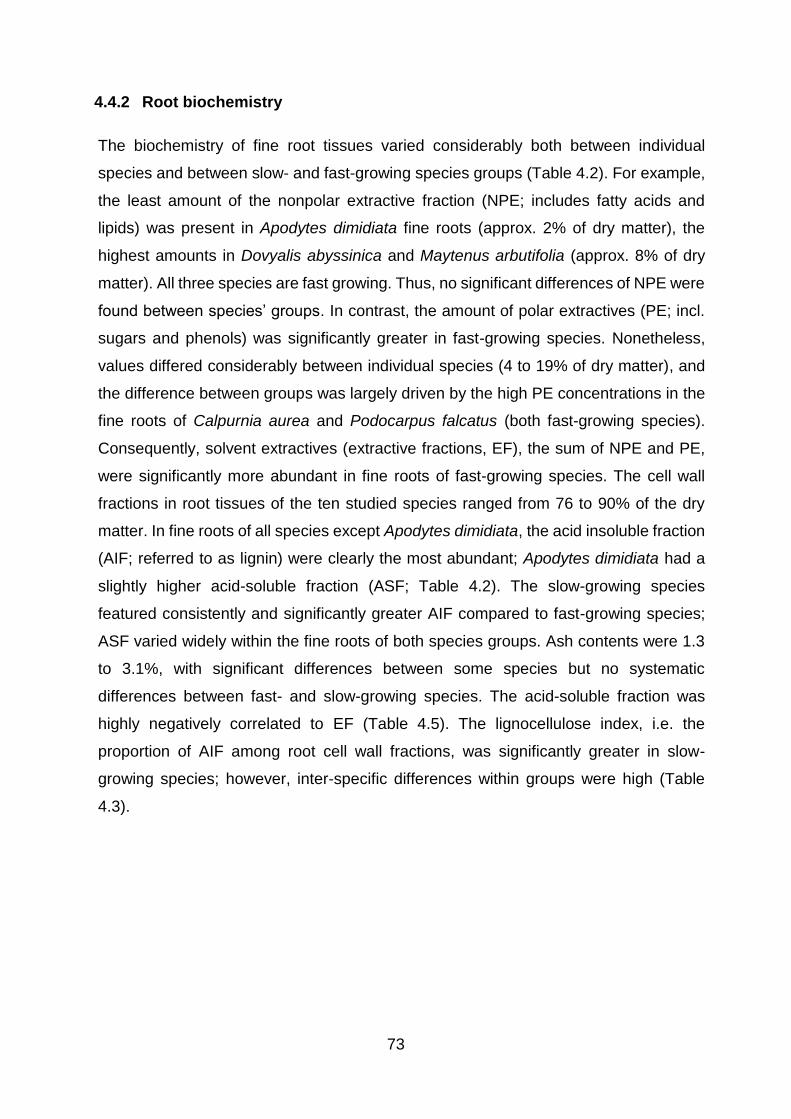
73

4.4.2 Root biochemistry

The biochemistry of fine root tissues varied considerably both between individual

species and between slow- and fast-growing species groups (Table 4.2). For example,

the least amount of the nonpolar extractive fraction (NPE; includes fatty acids and

lipids) was present in Apodytes dimidiata fine roots (approx. 2% of dry matter), the

highest amounts in Dovyalis abyssinica and Maytenus arbutifolia (approx. 8% of dry

matter). All three species are fast growing. Thus, no significant differences of NPE were

found between species’ groups. In contrast, the amount of polar extractives (PE; incl.

sugars and phenols) was significantly greater in fast-growing species. Nonetheless,

values differed considerably between individual species (4 to 19% of dry matter), and

the difference between groups was largely driven by the high PE concentrations in the

fine roots of Calpurnia aurea and Podocarpus falcatus (both fast-growing species).

Consequently, solvent extractives (extractive fractions, EF), the sum of NPE and PE,

were significantly more abundant in fine roots of fast-growing species. The cell wall

fractions in root tissues of the ten studied species ranged from 76 to 90% of the dry

matter. In fine roots of all species except Apodytes dimidiata, the acid insoluble fraction

(AIF; referred to as lignin) were clearly the most abundant; Apodytes dimidiata had a

slightly higher acid-soluble fraction (ASF; Table 4.2). The slow-growing species

featured consistently and significantly greater AIF compared to fast-growing species;

ASF varied widely within the fine roots of both species groups. Ash contents were 1.3

to 3.1%, with significant differences between some species but no systematic

differences between fast- and slow-growing species. The acid-soluble fraction was

highly negatively correlated to EF (Table 4.5). The lignocellulose index, i.e. the

proportion of AIF among root cell wall fractions, was significantly greater in slow-

growing species; however, inter-specific differences within groups were high (Table

4.3).

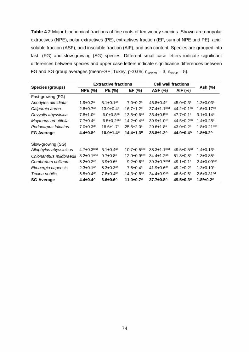
74

Table 4 2 Major biochemical fractions of fine roots of ten woody species. Shown are nonpolar

extractives (NPE), polar extractives (PE), extractives fraction (EF, sum of NPE and PE), acid-

soluble fraction (ASF), acid insoluble fraction (AIF), and ash content. Species are grouped into

fast- (FG) and slow-growing (SG) species. Different small case letters indicate significant

differences between species and upper case letters indicate significance differences between

FG and SG group averages (mean±SE; Tukey, p<0.05; nspecies = 3, ngroup = 5).

Species (groups) Extractive fractions Cell wall fractions

Ash (%) NPE (%) PE (%) EF (%) ASF (%) AIF (%)

Fast-growing (FG)

Apodytes dimidiata 1.9±0.2a 5.1±0.1ab 7.0±0.2a 46.8±0.4e 45.0±0.3b 1.3±0.03a

Calpurnia aurea 2.8±0.7ab 13.9±0.4d 16.7±1.2d 37.4±1.1bcd 44.2±0.1ab 1.6±0.17ab

Dovyalis abyssinica 7.8±1.0e 6.0±0.8ab 13.8±0.6cd 35.4±0.5bc 47.7±0.1c 3.1±0.14d

Maytenus arbutifolia 7.7±0.4e 6.5±0.2abc 14.2±0.4cd 39.9±1.0cd 44.5±0.2ab 1.4±0.28a

Podocarpus falcatus 7.0±0.3de 18.6±1.7e 25.6±2.0e 29.6±1.8a 43.0±0.2a 1.8±0.21abc

FG Average 4.4±0.8A 10.0±1.4B 14.4±1.3B 38.8±1.2A 44.9±0.4A 1.8±0.2A

Slow-growing (SG)

Allophylus abyssinicus 4.7±0.3bcd 6.1±0.4ab 10.7±0.5abc 38.3±1.1bcd 49.5±0.5cd 1.4±0.13a

Chionanthus mildbraedii 3.2±0.1abc 9.7±0.8c 12.9±0.9bcd 34.4±1.2ab 51.3±0.8d 1.3±0.85a

Combretum collinum 5.2±0.2cd 3.9±0.6a 9.2±0.6ab 39.3±0.7bcd 49.1±0.1c 2.4±0.09bcd

Ekebergia capensis 2.3±0.1ab 5.3±0.3ab 7.6±0.4a 41.9±0.6de 49.2±0.2c 1.3±0.10a

Teclea nobilis 6.5±0.4de 7.8±0.4bc 14.3±0.8cd 34.4±0.9ab 48.6±0.6c 2.6±0.31cd

SG Average 4.4±0.4A 6.6±0.6A 11.0±0.7A 37.7±0.8A 49.5±0.3B 1.8a±0.2A

75

Table 4 3 Litter quality indices of ten woody species. Shown are carbon (C) and nitrogen (N)

contents, C/N ratio, acid insoluble fraction (AIF) to N ratio, and lignocellulose index. Species

are grouped into fast- (FG) and slow-growing (SG) species; see Supplementary Information

Table A2.2 for details. Lignocellulose index is the ratio of AIF to cell wall fraction. Small case

letters indicate significant differences between species and upper case letter indicate

differences between FG and SG group averages (mean±SE; Tukey, p<0.05; nspecies = 3, ngroups

= 5).

Species (Groups) C% N% C:N Ratio AIF:N Ratio

Lignocellulose index

Fast-growing (FG) Apodytes dimidiata 44.8±0.40ab 1.38±0.01d 32.6±0.4b 32.7±0.1c 0.49±0.00a Calpurnia aurea 44.5±0.30a 1.21±0.00bc 36.8±0.3d 36.6±0.1d 0.54±0.01bc Dovyalis abyssinica 46.3±0.03bc 1.38±0.01d 33.7±0.1bc 34.7±0.1cd 0.57±0.00cde Maytenus arbutifolia 45.2±0.65ab 1.73±0.01f 26.2±0.5a 25.8±0.2a 0.53±0.01ab Podocarpus falcatus 45.3±0.40ab 1.08±0.02a 42.0±0.5f 39.9±0.6ef 0.56±0.01bcd FG Average 45.2±0.24A 1.35±0.06A 34.3±1.4A 33.9±1.3A 0.54±0.01A Slow-growing (SG) Allophylus abyssinicus 48.2±0.39d 1.26±0.01d 38.3±0.2d 39.4±0.6e 0.56±0.01bcde Chionanthus mildbraedii 49.9±0.22e 1.51±0.01b 33.0±0.3b 33.9±0.7c 0.60±0.01e Combretum collinum 47.1±0.16cd 1.36±0.01c 34.6±0.3c 36.1±0.2d 0.56±0.01bcd Ekebergia capensis 47.5±0.13cd 1.17±0.00e 40.4±0.1e 41.9±0.3f 0.54±0.00bc Teclea nobilis 47.1±0.09cd 1.74±0.01a 27.1±0.1a 28.0±0.5b 0.59±0.01de SG Average 47.9±0.29B 1.41±0.04A 34.7±1.2A 35.9±1.3A 0.57±0.01B

4.4.3 Carbon cost of root production

The calculated amount of glucose needed to produce one gram of fine root biomass

varied significantly among species (Table 4.4). For example, these carbon costs were

highest in Chionanthus mildbraedii (1.5 g glucose g-1 dw) and lowest in Calpurnia aurea

roots (1.2 g glucose g-1 dw). The calculated amount of glucose needed to synthesize

root biomass was significantly and consistently greater in slow-growing versus fast-

growing species (Fig. 4.2, Table 4.4).

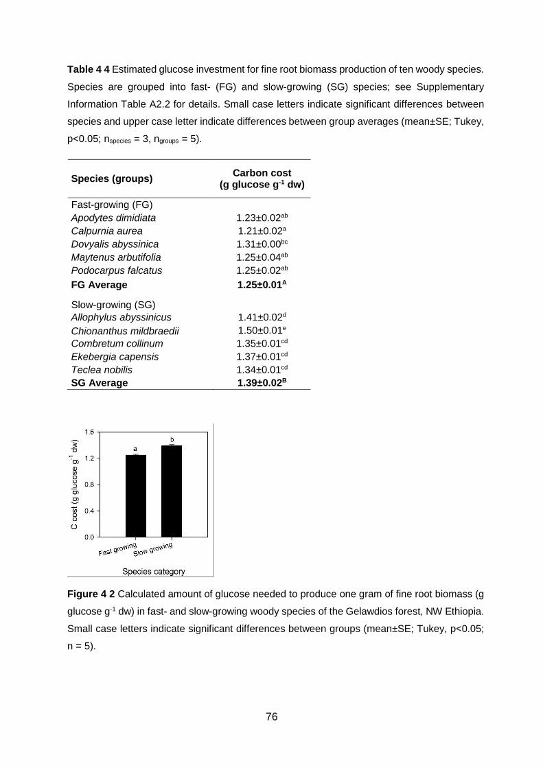
76

Table 4 4 Estimated glucose investment for fine root biomass production of ten woody species.

Species are grouped into fast- (FG) and slow-growing (SG) species; see Supplementary

Information Table A2.2 for details. Small case letters indicate significant differences between

species and upper case letter indicate differences between group averages (mean±SE; Tukey,

p<0.05; nspecies = 3, ngroups = 5).

Species (groups) Carbon cost

(g glucose g-1 dw)

Fast-growing (FG)

Apodytes dimidiata 1.23±0.02ab

Calpurnia aurea 1.21±0.02a

Dovyalis abyssinica 1.31±0.00bc

Maytenus arbutifolia 1.25±0.04ab

Podocarpus falcatus 1.25±0.02ab

FG Average 1.25±0.01A

Slow-growing (SG)

Allophylus abyssinicus 1.41±0.02d

Chionanthus mildbraedii 1.50±0.01e

Combretum collinum 1.35±0.01cd

Ekebergia capensis 1.37±0.01cd

Teclea nobilis 1.34±0.01cd

SG Average 1.39±0.02B

Figure 4 2 Calculated amount of glucose needed to produce one gram of fine root biomass (g

glucose g-1 dw) in fast- and slow-growing woody species of the Gelawdios forest, NW Ethiopia.

Small case letters indicate significant differences between groups (mean±SE; Tukey, p<0.05;

n = 5).

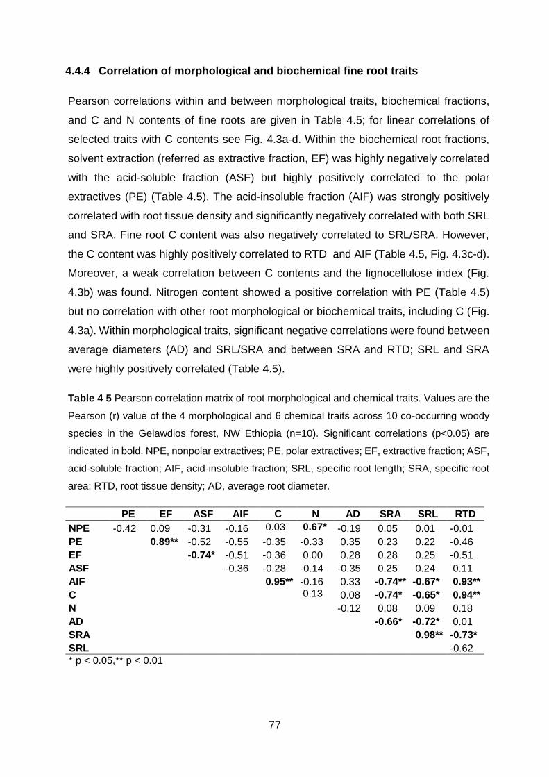
77

4.4.4 Correlation of morphological and biochemical fine root traits

Pearson correlations within and between morphological traits, biochemical fractions,

and C and N contents of fine roots are given in Table 4.5; for linear correlations of

selected traits with C contents see Fig. 4.3a-d. Within the biochemical root fractions,

solvent extraction (referred as extractive fraction, EF) was highly negatively correlated

with the acid-soluble fraction (ASF) but highly positively correlated to the polar

extractives (PE) (Table 4.5). The acid-insoluble fraction (AIF) was strongly positively

correlated with root tissue density and significantly negatively correlated with both SRL

and SRA. Fine root C content was also negatively correlated to SRL/SRA. However,

the C content was highly positively correlated to RTD and AIF (Table 4.5, Fig. 4.3c-d).

Moreover, a weak correlation between C contents and the lignocellulose index (Fig.

4.3b) was found. Nitrogen content showed a positive correlation with PE (Table 4.5)

but no correlation with other root morphological or biochemical traits, including C (Fig.

4.3a). Within morphological traits, significant negative correlations were found between

average diameters (AD) and SRL/SRA and between SRA and RTD; SRL and SRA

were highly positively correlated (Table 4.5).

Table 4 5 Pearson correlation matrix of root morphological and chemical traits. Values are the

Pearson (r) value of the 4 morphological and 6 chemical traits across 10 co-occurring woody

species in the Gelawdios forest, NW Ethiopia (n=10). Significant correlations (p<0.05) are

indicated in bold. NPE, nonpolar extractives; PE, polar extractives; EF, extractive fraction; ASF,

acid-soluble fraction; AIF, acid-insoluble fraction; SRL, specific root length; SRA, specific root

area; RTD, root tissue density; AD, average root diameter.

PE EF ASF AIF C N AD SRA SRL RTD

NPE -0.42 0.09 -0.31 -0.16 0.03 0.67* -0.19 0.05 0.01 -0.01

PE 0.89** -0.52 -0.55 -0.35 -0.33 0.35 0.23 0.22 -0.46

EF -0.74* -0.51 -0.36 0.00 0.28 0.28 0.25 -0.51

ASF -0.36 -0.28 -0.14 -0.35 0.25 0.24 0.11

AIF 0.95** -0.16 0.33 -0.74** -0.67* 0.93**

C 0.13 0.08 -0.74* -0.65* 0.94**

N -0.12 0.08 0.09 0.18

AD -0.66* -0.72* 0.01

SRA 0.98** -0.73*

SRL -0.62

* p < 0.05,** p < 0.01

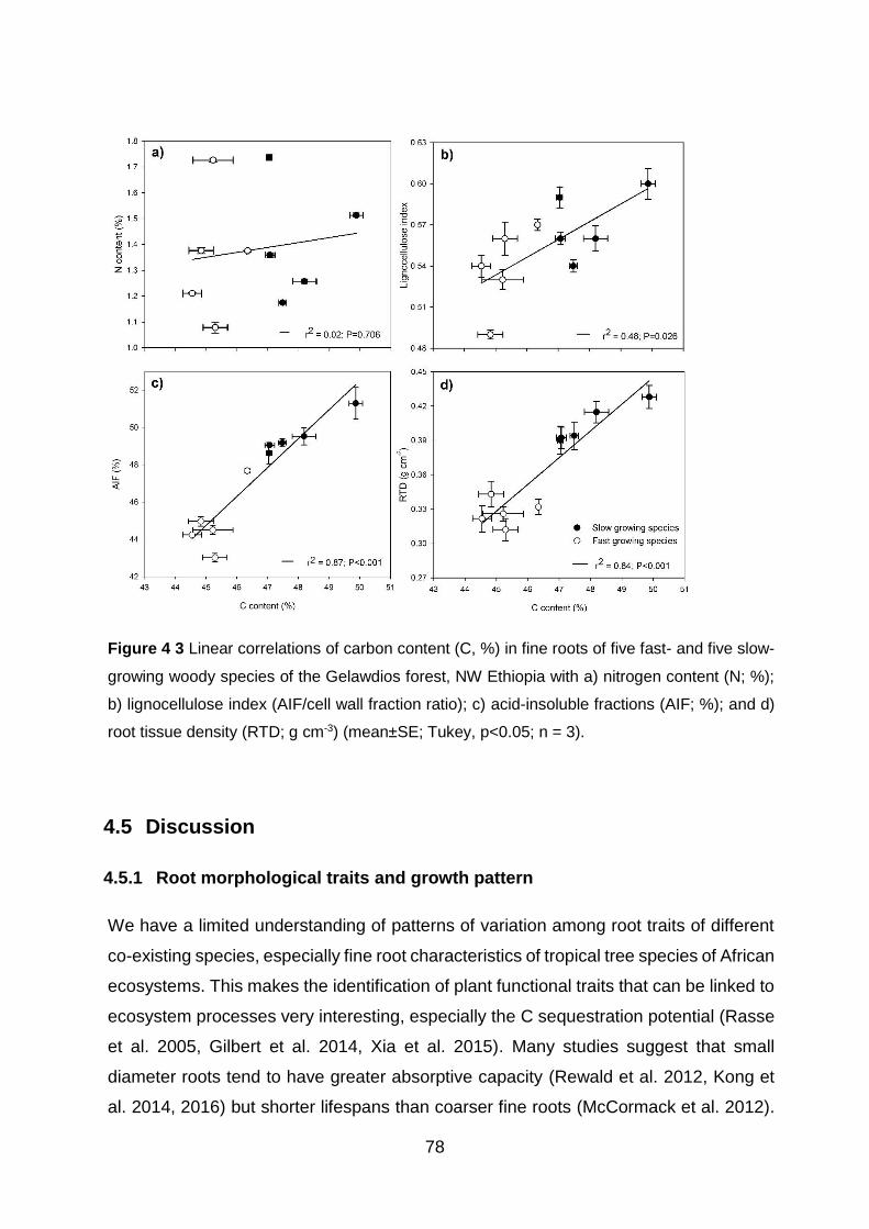
78

Figure 4 3 Linear correlations of carbon content (C, %) in fine roots of five fast- and five slow-

growing woody species of the Gelawdios forest, NW Ethiopia with a) nitrogen content (N; %);

b) lignocellulose index (AIF/cell wall fraction ratio); c) acid-insoluble fractions (AIF; %); and d)

root tissue density (RTD; g cm-3) (mean±SE; Tukey, p<0.05; n = 3).

4.5 Discussion

4.5.1 Root morphological traits and growth pattern

We have a limited understanding of patterns of variation among root traits of different

co-existing species, especially fine root characteristics of tropical tree species of African

ecosystems. This makes the identification of plant functional traits that can be linked to

ecosystem processes very interesting, especially the C sequestration potential (Rasse

et al. 2005, Gilbert et al. 2014, Xia et al. 2015). Many studies suggest that small

diameter roots tend to have greater absorptive capacity (Rewald et al. 2012, Kong et

al. 2014, 2016) but shorter lifespans than coarser fine roots (McCormack et al. 2012).

79

Such roots are also considered to play an important role in soil carbon input and nutrient

cycling. The average diameters of fine roots (0.53-0.76 mm) we recorded in Ethiopia

are in the range reported for tree species of other tropical ecosystems (0.52-1.4 mm;

Collins et al. 2016), but are considerably larger than those frequently reported for trees

in temperate forests (0.24-0.54 mm; Gu et al. 2014) and boreal forests (0.31-0.47;

Ostonen et al. 2013). For example, Pinno et al. (2010) reported – for roots of Populus

tremuloides in boreal forests – that 97% of the total root length is <1 mm diameter.

Other studies yielded similar findings: roots less than 0.5 mm in diameter accounted for

89% of the total root length in Prunus avium (Baddeley and Watson 2005) and 75% for

nine North American tree species (Pregitzer et al. 2002). In our study, about 50% of the

total fine root length was below 0.5 mm, and more than 80% of the total length were

accounted for by root segments <1 mm in diameter (Fig 4.1; Table 4.1). Species such

as Maytenus arbutifolia, Combretum collinum, and Allophylus abyssinicus are the

thinnest (90% of total root length <1 mm diameter), while Podocarpus falcatus,

Ekebergia capensis, and Teclea nobilis had the thickest values (Table 4.1). Overall, the

vast majority of fine root length was below 1 mm in diameter for all species (Fig. 4.1).

It has been shown that coarser fine roots show secondary growth, as evidenced by the

highest root tissue density (RTD), and have a lower specific root area (SRA) than finer

roots (Silver and Miya 2001, Rewald et al. 2014). In our study, fine root diameter was

negatively correlated with SRA (rpearson = -0.66; P<0.05) and SRL (rpearson = -0.72;

P<0.05; Table 4.5). Basile et al. (2007) also reported a similar negative correlation.

Comparing morphological traits with growth rates showed that average RTD is lower in

fast-growing species, whereas SRA and SRL are higher in slow-growing species. Some

of the fast-growing species such as Calpurnia aurea and Maytenus arbutifolia had much

higher SRA and SRL than the slow-growing species Ekebergia capensis and Teclea

nobilis, which exhibited the lowest SRA and SRL values (Table 4.1). Similar results

have been reported for other species, where very fine roots of fast-growing species had

much higher SRL (Pregitzer et al. 1997, Basile et al. 2007). Similarly, the RTD values

(0.31 - 0.41 g cm-3) are in the range reported for tree species of other tropical

ecosystems (0.2 - 0.6 g cm-3; Collins et al. 2016) and for temperate trees (0.32-0.83 g

cm-3; McCormack et al. 2012), but they are greater than values previously found in

other temperate forest ecosystems (Comas and Eissenstat 2004). Several authors

have suggested that a wide variety of climate and soil conditions such as temperature,

80

moisture, nutrient content, pH, and physical disturbance of the soil affect fine root

morphology (Pregitzer et al. 2002, Zobel et al. 2007, Ostonen et al. 2007). In co-existing

species of the same site, however, the morphological differences may reflect the

species’ economic spectrum and ecological strategies for resource capture under

competition (Wang et al. 2006, Collins et al. 2016, Valverde-Barrantes et al. 2016).

High SRA and SRL may facilitate faster growth and more rapid acquisition of soil

resources (Valverde-Barrantes et al. 2016). Given the apparent species-specific

differences in root morphology between co-existing species, many authors have

emphasized root morphological plasticity as an important adaptation mode to variable

growth conditions (Fransen et al. 1999, Sorgoná et al. 2007, Ostonen et al. 2013,

Gratani 2014). Based on the optimal foraging theory, Ostonen et al. (2007) identified

two main strategies of fine root adaptation to different regimes of nutrient supply: higher

C investment to increase the fine root biomass (and root length), or changing root

morphology to increased nutrient uptake efficiency through a higher specific root area.

Similar ideas have been suggested by Meinen et al. (2009) to explain differences in

root morphology between species. In relation to the litter quality index, SRA and SRL

decreased with increasing RTD (Table 4.5). The negative associations of SRA and SRL

with RTD suggest that the fast-growing species increase the total surface area of

absorbing roots for higher nutrient use efficiency and that their roots are less expensive

to construct per unit mass (Table 4.4). Similarly, Pregitzer et al. (2002) reported that

“infinitely fine” roots are the most efficient for nutrient acquisition per gram of C

expended to construct them. In contrast, slow-growing species tended to construct

more C-costly fine roots.

4.5.2 Root biochemistry and carbon cost implications for root litter quality

The fine roots of all ten species differed with respect to concentrations of C and N as

well as of chemical compounds. The C content ranged from 44% (Calpurnia aurea) to

50% (Chionanthus mildbraedii). The average C concentration for fast-growing species

was about 45% (Table 4.4). In 59 Panamanian rainforest species, C content ranged

from 42 to 52% (Martin and Thomas 2011) and 37 to 44% for 24 species in Europe

(Poorter and Bergkotte 1992). Carbon concentrations are often assumed to be about

50% of the dry mass; this value is widely used for below-ground C estimations (Gibbs

et al. 2007, Robinson 2007), but will overestimate total carbon stocks in fine roots.

81

Nitrogen contents also varied significantly in the fine roots of the 10 species. The

highest N content was determined in Teclea nobilis and Maytenus arbutifolia, which in

the former may be due to T. nobilis being a N2-fixing species (Orwa et al. 2009). The

N2-fixing status of Maytenus arbutifolia is unknown but its leaves have been shown to

contain high crude protein levels compared to 18 other species used for fodder

(Shenkute et al. 2012);16% of the crude protein in the leaves is nitrogen (Levey et al.

2000). Interestingly, however, no significance difference in N contents was found

between the fast- and slow-growing species groups (Table 4.3). This contradicts earlier

findings on seedlings (Comas et al. 2002) that N concentrations are higher in fast-

growing species. Root C:N ratios also played an important role in predicting patterns of

root decay, and these ratios are a valuable predictive tool in numerous studies of litter

decomposition at local, regional, and global scales (Silver and Miya 2001, Leppälammi-

Kujansuu et al. 2014, García-Palacios et al. 2016). The C:N ratios of roots in our study

ranged from 26 to 40, with significant differences between individual species but no

difference between growth rates. Theoretically, the optimum C:N ratio for microbial

growth, and thus decomposition, is approximately 25, but fungi and bacteria can

decompose substrates with much higher ratios (Reshi and Tyub 2007). According to

Reshi and Tyub (2007), substrates with C:N ratios of <20 decompose rapidly and NH4

is released through N-mineralization. Plant material with C:N ratios between 25-75 can

be regarded as intermediate values, and our data lie in this range. Litter with such C:N

ratio decompose quickly but N mineralization is often reduced by increased microbial

immobilization as well as protein complexation by polyphenols when the cells lyse

(Silver and Miya 2001). Roots with C:N ratios exceeding 75 are often much more

difficult to break down (Swift et al. 1979) due to greater amounts of structural woody

materials (Silver and Miya 2001).

The biochemical compositions of roots such as AIF, ASF, and EF vary with species,

and these variations determine the root litter quality and the quality of C input into soil

(Xia et al. 2015). In the present study, the AIF ranged from 43-51% (combined mean

of 47%; Table 4.2) and was consistently the highest C fraction. This value is consistent

with other studies, whose AIF averaged 49% (Hendricks et al. 2000) and 50% (Muller

et al. 1989). A recent biochemical study by Xia et al. (2015) also reported that fine roots

contained a 2.9 fold higher AIF content compared to the other fractions. Abiven et al.

(2005) also noticed large lignin-like fractions in roots of crop plants. The AIF is primarily

82

composed of highly reduced compounds such as suberin, cutin, and tannin-protein

complexes associated with lignin (Hendricks et al. 2000, Sun et al. 2013). These

compounds are thought to be highly recalcitrant and resistant to biochemical

degradation (Lorenz et al. 2007, Sun et al. 2013, Xia et al. 2015). Moreover, after

cellulose, lignin alone is one of the most abundant organic polymers in plants; the

content of lignin in wood is 20–40% of dry matter (Chen 2014). Lignin is a highly cross-

linked polymer that is resistance to chemical or biological attack; it provides mechanical

support in wood by reinforcing cell walls of xylem tissue and lignified sclerenchyma

fibres in vascular plants (Kögel-Knabner 2002, Chen 2014). Hydroxyls and many polar

groups are present in the lignin structure, resulting in strong intramolecular and

intermolecular hydrogen bonds and making the intrinsic lignin insoluble in any solvent

(Chen 2014). The presence of phenolic hydroxyl and carboxyl, however, makes the

lignin soluble in alkaline solutions (Goñi and Hedges 1992). The AIF was positively

correlated with C content (r2 = 0.87, P<0.001; Fig. 4.3c) and RTD (r2 = 0.84; P<0.001;

Fig. 4.3d) and, thus, this relationship may provide some insight into carbon investment

to fine roots. In our study, roots with a high lignin content tend to invest more carbon

per unit biomass. This can be explained by the higher glucose investment (Table 4.4)

and the higher C content within lignin compared to cellulose. For example, the

elemental composition of lignin from a red oak and yellow popular wood sample is 62

% C and 1 % N, (Jin et al. 2013). In comparison, cellulose is only 44 % C (Chen 2014).

The lignocellulose index, a ratio of AIF to the cell wall fraction (AIF+ASF), is higher in

slow-growing species, as is the total C content (Table 4.3). This suggests that both

chemical (AIF) and morphological (higher RTD) factors make the fine roots of slow-

growing species more expensive to construct in terms of C per unit mass. These

parameters (AIF, lignocellulose index, RTD) determine the decomposition dynamics

(Sun et al. 2013, Zhang and Wang 2015) and are a good indicators for root substrate

quality (Hendricks et al. 2000, Prieto et al. 2016). Input of recalcitrant materials from

the turnover of fine roots contributes to long-term CO2 sinks in soils (Xia et al. 2015).

In contrast to the AIF, the amounts of polar extractives (PE) and extractive fractions

(EF) were greater in fast-growing species. Solvent extractives are compounds of non-

structural substances, mostly low-molecular-mass compounds consisting of nonpolar

constituents such as alkaloids, fats, oils, waxes, and resins, as well as of polar

constituents such as nonstructural carbohydrates and water-soluble phenolics

83

(Pettersen 1984, Yang and Jaakkola 2011, Sun et al. 2013). Among the individual

species, Podocarpus falcatus had the highest extractive fraction (25%), Apodytes

dimidiata the lowest value (7%). Both Podocarpus falcatus and Apodytes dimidiata are

from the fast-growing species category (Table 4.2). In an investigation of 14 species

from Gelawdios forest for other chemical fractions, Podocarpus falcatus had the

greatest concentration of total phenols and condensed tannins in both roots (Tigabu

2016) and leaves (Habteyohannes 2016). Tannins are classified as hydrolyzable

tannins (esters of a sugar residues (usually D-glucose) with one or more polyphenol

carboxylic acids) and condensed tannins (polymers of flavonoids consisting mainly of

3-8 flavonoid units), and are categorized as extractives (Yang and Jaakkola 2011).

Some tannins, however, form a complex tannin-protein complex associated with the

AIF that cannot be extracted using neutral solvents (Sun et al. 2013). Moreover,

Podocarpus species are known to produce and store terpenoid resin and phenolic

resin, mainly induced by injury (Langenheim 2003). Nonetheless, the family has not

been analyzed chemically in detail and needs further investigation. Pettersen (1984)

suggested that solvent extractive materials constitute 4-10% of the dry weight of wood

of species in temperate climates and that the values may be as much as 20% of the

wood of tropical species. Preston et al. (2000), however, reported that nonpolar

extractives and water-soluble extractives together make up 40-50% of total dry litter

mass in 37 species of trees in Canadian forests. Since extractives are soluble in neutral

solvents and do not contribute to the cell wall structure (Pettersen 1984), they are

considered as labile compounds that degrade easily compared to other fractions. Sun

et al. (2013) confirmed that the extractives disappeared rapidly at the initial stages of

decomposition.

Cellulose is the most abundant organic polymer, usually accounting for 35–50% of dry

weight (Chen 2014). In most conditions, the cellulose is wrapped in hemicellulose,

which itself accounts for 20–35% dry matter (Chen 2014). In our study, the ASF that

contains mainly cellulose and hemicellulose showed no variation between functional

groups, but significant variation existed between individual species. Among the ten

studied species, Podocarpus falcatus showed the least ASF (30%), Apodytes dimidiata

the highest fraction (47%). Tigabu (2016) also found high concentrations of cellulose

and hemicellulose (41%) in fine roots of Apodytes dimidiata. These two polymers are

made of linear chains of β-1,4-linked glucose units, ranging from hundreds to ten

84

thousands of units (Kögel-Knabner 2002), and are insoluble in water, but soluble in

acidic and alkaline solutions at normal temperatures (Li et al. 2014). Due to the

chemical bonding and C content (44% in cellulose), ASF is the second fastest

decomposing fraction after the solvent extractives (Sun et al. 2013).

4.6 Conclusion

The morphological parameters of fine roots are quite variable among ten tropical

species, but reflect the general difference between fast-and slow-growing species.

Generally, fast-growing species have higher SRA and SRL but lower RTD, which are

characteristics assumed to support high rates of nutrient acquisition. Our results

provide evidence that RTD is positively correlated with AIF, C content, and C

construction cost, and is consistently higher in slow-growing species. The extractive

fractions and ASF of fine roots appeared to be unrelated to any root morphological

characteristics.

85

5 Litter production, chemistry, and turnover in a pristine

forest ecosystem in the Ethiopian highland

5.1 Abstract

Amount of plant litter and its decomposition rate determine the rate of carbon deposition

into the soil. The objective of this study is to determine the carbon input through above-

and below-ground litter production and turnover in the Ethiopian highland forests. The

litterfall and fine root production were studied for one year using litter traps and

sequential coring. Four dominant indigenous tree species were selected for chemical

analysis and the decomposition rate experiment using standard litterbag technique

from June 2015 to June 2016. Results showed that annual total litterfall production was

1090 g m-2 y-1 while fine root production was 723 g m-2 yr-1. In the decomposition

analysis, the litter mass in the litterbag declined exponentially with time for all species.

The annual decay constant (k) varied from 1.6 to 3.2 yr-1 for leaves and 1.3 to 1.8 yr-1

for fine roots indicating leaves decompose more rapidly than fine roots. Leaf litter

exhibited higher concentrations of extractive fractions (EF) and acid-soluble fractions

(ASF) that contain mainly labile carbons such as carbohydrates and cellulose than fine

roots. Fine roots contained consistently greater acid-insoluble fraction (AIF) mainly

lignin and lignin-suberin complexes than leaf litters. Thus, fine roots exhibit about 1.5

times higher recalcitrant carbon input into the soil than leaf litters. Decomposition rates

of litters were determined by EF, ASF, and AIF whereas litter quality indices such N,

C:N ratio, AIF:N ratio were poor predictors of decay in this experiment due to N is

affected by N2-fixing symbionts, N resorption, and leaching.

Keywords: litterfall production, fine roots, carbon input, litter chemistry, decomposition

rate, litterbag.

86

5.2 Introduction

Changes in the amount of soil organic carbon in the soil are the result of differences

between additions (litter inputs from above- and below-ground) and losses through

mineralization (Gaudinski et al. 2001, Conant and et.al. 2011) and erosion (Chapter 2;

Mey et al. 2015, Li et al. 2016). Above-ground fine litterfall includes leaves, flowers,

fruits, bark and twigs (Jia et al. 2016). Of the below-ground inputs, fine roots (Freschet

et al. 2013) are the major pathways of organic carbon input in to the soil through the

decomposition cycle (Berg 2000, Freschet et al. 2013, Macinnis-Ng and

Schwendenmann 2015). The quantity and quality of litter materials play an important

role in the formation and accumulation of soil organic matter and are key links in

biogeochemical cycles that connect above- and below-ground processes in terrestrial

ecosystems (Kögel-Knabner 2002, Freschet et al. 2013, Becker et al. 2015).

Previous investigations on litterfall and fine root production and their turnover have

been focused on temperate and Mediterranean climates (Guo and Sims 1999,

Celentano et al. 2011, Salete Capellesso et al. 2016). While some models have been

proposed to predict litter production (Adair et al. 2008, Cotrufo et al. 2010, Hararuk

and Luo 2014), the amount and quality of litterfall and fine root turnover varies

considerably between regions (Macinnis-Ng and Schwendenmann 2015), season

(Zhang et al. 2014), and tree species composition (Becker et al. 2015). Information on

the influence of species richness, litter composition, and the biochemical quality of

litter on carbon cycling of tropical regions remains scarce especially in the Ethiopian

highlands. Given the important role of litter inputs and decomposition to SOC storage

and ecosystem functioning, it is thus important to accurately quantify and characterize

carbon deposition through above- and below-ground litters, litter chemistry, and decay

rates more in a species rich tropical forest ecosystems (Guo and Sims 1999, Freschet

et al. 2013, Salete Capellesso et al. 2016).

The accumulation of organic detritus in the organic layer of forests are controlled by the

rate of decomposition of the plant material which is influenced by variability in litter

quality, soil moisture and temperature, and the kinds of microflora and fauna present

(Salomé et al. 2010, Yeong et al. 2016). The carbon quality of substrates may be the

predominant chemical control over decomposition (Chapin et al. 2011). Quality refers

to chemical characteristics of the litter that influence the susceptibility of litter to

87

decomposition (Karberg et al. 2008). Some studies reported that there is a 5-fold to 10-

fold range in decomposition rate of litter in a given climate, due to differences in

substrate quality (Chapin et al. 2011). Some authors reported that leaves decompose

more rapidly than woody components and deciduous leaves decompose more rapidly

than evergreen leaves and these differences in decomposition rates are a

consequence of their chemical composition (Cornelissen 1996, Chapin et al. 2011,

Prescott et al. 2011). The chemical compounds present can be categorized roughly as

labile compounds (e.g. fats, oils, waxes, nonstructural carbohydrates, and

polyphenols), moderately degradable compounds (cellulose and hemicellulose), and

highly recalcitrant compounds tissues such as lignin, suberin, cutin, and tannin-protein

complexes (Ryan et al. 1990, Sun et al. 2013, Xia et al. 2015). Litter containing high

concentrations of labile compounds (e.g. carbohydrates) tends to decompose rapidly

because these compounds can be readily metabolized by soil microorganisms or are

leached easily (Karberg et al. 2008). Labile structural compounds such as cellulose are

more stable than carbohydrates but are quickly metabolized in contrast to recalcitrant

structural compounds such as lignin because of their aromatic rings and irregular

structure (Karberg et al. 2008, Xia et al. 2015). The C:N ratio, lignin:N ratio, and

lignocellulose index have been frequently used as an index of litter quality and are good

predictors of the decomposition rate – lower values of these indices generally indicate

faster rates of decomposition (Preston et al. 2000, Girisha 2001, Moorhead et al. 2014,

Xia et al. 2015). Therefore, species difference in decomposition rate should depend on

species- and tissue-specific litter chemistry properties (Scherer-Lorenzen et al. 2007).

In this study three hypothesis are proposed to explain how initial litter quality influences

litter decomposition and carbon release. The first hypothesis suggests that leaves

decompose more rapidly than fine roots due to their chemical composition. Hence, we

expect that litter quality indices such as C:N ratio, lignin:N ratio and lignocellulose index

are lower in the leaves than fine roots. The second hypothesis suggests that species

having less acid-insoluble fractions (less lignified tissue) decompose faster than

species containing more labile compounds. The third hypothesis suggest that litter

mixtures of varying species enhance litter decomposition rates – assuming the

occurrence of highly degradable litter favors the breakdown of more recalcitrant litter in

the mixtures. Therefore, the objectives of this study were: (i) to determine the seasonal

and annual litterfall, fine root turnover, and C flux into the soil of a natural mixed forest,

88

and (ii) to investigate the in-situ decomposition rate and residence time of the detritus

material and relate to species- and tissue-specific initial litter chemistry.


5.3.1 Description of the study site

This study was conducted in the remnant Afromontane forest at Gelawdios in the

Amhara National Regional State, north central part of Ethiopia. Gelawdios (11°38’25’’N,

37°48’55’’E) is located east of Lake Tana at an altitude of 2500 m above sea level.

While Ethiopia is located in the tropics, the climate of the study area is temperate with

dry winter and warm summer (Cwb) according to the Köppen-Geiger climate

classification (Peel et al. 2007). The mean annual precipitation in the area is 1200 mm

with the main rainy season from June to September and with low-intensity precipitation

from March to May (Wassie et al. 2009). The annual mean air temperature is 19°C

(Wassie et al. 2009). The soils are classified as Cambisols. The soil physical and

chemical characteristics of the site are shown in Table 4.1. The Afromontane Gelawdios

forest is a small, isolated, but pristine forest fragments (‘church forest’) covering an area

of about 100 ha in the otherwise almost completely deforested Ethiopian Highlands

(Wassie et al. 2009, Aerts et al. 2016). The dominant woody species in the forest are

Allophylus abyssinicus (Hochst.) Radlk., Apodytes dimidiata E. Mey ex. Arn., Calpurnia

aurea (Ait.) Benth., Chionanthus mildbraedii (Gilg & Schellenb.) Stearn, Combretum

collinum Fresen., Dovyalis abyssinica (A. Rich.) Warb., Ekebergia capensis (Sparm.),

Maytenus arbutifolia (A. Rich.) Wilczek, Podocarpus falcatus (Thunb.) Mirb., and

Teclea nobilis (Del.).

Table 5 1 Soil physical and chemical properties at the Gelawdios forest. Values of carbon (C),

nitrogen (N), C:N ratio, and pH are mean±SE.

Soil depth (cm)

Sand-Silt-Clay (%)

C (%) N (%) C:N ratio

pH (CaCl2)

0-10 9-39-52 11.8±0.9 1.09±0.07 10.8±0.3 5.94±0.11

10-20 5-34-61 7.2±0.7 0.70±0.07 10.3±0.2 5.55±0.10

20-30 11-46-43 4.6±0.3 0.42±0.03 11.0±0.3 5.40±0.08

30-50 9-63-28 3.5±0.3 0.30±0.02 11.7±0.4 5.35±0.07

89

5.3.2 Litterfall collection and fine root biomass determination

Litterfall was collected weekly from July 2014 to June 2015. Ten litter traps were

systematically placed in 100 m distance between each other along a transect line.

Samples were collected on a 0.5 m X 0.5 m wooden frame furnished with a 1 mm

polyamide mesh (Franz Eckert GmbH, Waldkirch, Germany); positioned 50 cm above

the ground. At the end of each month, the weekly collected litter were combined and

sorted into leaves, branches and twigs, reproductive organs (flowers, fruits, and seed),

and miscellaneous material (unidentified plant parts, mosses). The collected litter was

dried at 70°C to constant weight before weighing to the nearest 0.01g. Seasonal litter

productivity (g m-2) for the winter, spring, summer, and autumn seasons was calculated.

Winter - December, January and February are the dry months with frost in morning.

Spring - March, April and May are the autumn season in Ethiopia with occasional

showers. May is the hottest month in Ethiopia. Summer - June, July and August are the

heavy rainfall months; autumn - September, October and November are the spring

season in Ethiopia, sometimes known as the harvest season.

Methods for retrieving fine root biomass (live roots) and necromass (dead roots) stock

as well as annual root production and turnover can be found in Chapter 3. The fine

roots stock and production estimated using sequential coring with Decision Matrix

calculation technique (Chapter 3) were used for comparison of C input with leaf litter in

this chapter.

5.3.3 Litter (leaf and root) decomposition using litterbag technique

Based on dominance, four species namely, Allophylus abyssinicus, Chionanthus

mildbraedii, Combretum collinum, and Teclea nobilis were selected for chemical

analysis through sequential extraction and decomposition analysis using litterbag

technique. Since there was not enough material from the collected litter, samples of

litters for decomposition analysis and biochemical fraction analysis were collected from

fallen leaves on the forest floor. Root samples for decomposition analysis were taken

from the selected tree species by strictly tracking coarse roots from the tree base

(Rewald et al. 2012). For comparison purpose, fine roots (<2 mm diameter) and coarse

roots (2-5 mm diameter) were separately included in the litterbag during the

decomposition experiment.

90

Both leaf and root decomposition was studied for a period of 1 year from June 2015 to

June 2016 using standard litter-bag techniques in a time series (Scherer-Lorenzen et

al. 2007, Karberg et al. 2008, Certini et al. 2015). The air dried litter was packed within

litter bags of polyamide mesh (Franz Eckert GmbH, Waldkirch, Germany); 1.0 mm

mesh was used on the bottom to reduce loss of small fragments and 2 mm was used

on top to allow macro-invertebrates to enter the bag (Karberg et al. 2008). The sizes of

the mesh bags were 10 cm X 10 cm for roots and 10 cm X 15 cm for leaves – adjusting

for the entered size of litter.

Four grams of either leaf or root litter materials from the four selected tree species

(Allophylus abyssinicus, Chionanthus mildbraedii, Combretum collinum, and Teclea

nobilis) were placed inside in monospecific litterbags. For leaves, a combination of two

species (2 g per species) was placed inside mixed-species litterbags. The six realized

combinations were Allophylus abyssinicus with either Chionanthus mildbraedii,

Combretum collinum, or Teclea nobilis, and Chionanthus mildbraedii with either

Combretum collinum or Teclea nobilis, and Combretum collinum with Teclea nobilis. In

four species combination (Allophylus abyssinicus, Chionanthus mildbraedii,

Combretum collinum, and Teclea nobilis), 1 g per species or 25% each were placed for

both leaves and roots. The combinations were assembled to test whether the decay of

specific litter is affected by the presence of other species, e.g. due to its palatability or

inhibitory effect on microorganisms. There were not enough materials available to

prepare all two-mixed species combinations for fine and coarse roots. Litterbags of

each treatment were prepared at five replications; retrieval took place at months of 0.5,

1, 2, 3, 6, 12 for leaves (yielding 360 samples) and months of 1, 2, 3, 6, and 12 for roots

(300 samples). Bags were placed at 45° in June 2015 at a soil depth of 3-10 cm (to

prevent their discovery and loss). At the time of retrieval, materials were carefully

brushed and cleaned to remove any attached particles that are not the original material.

The retrieved litter was carefully transferred to clean paper bags, oven-dried until

constant weight, and weighed to the nearest 0.01 g.

5.3.4 Chemical analysis

Leaf samples from forest floor of fallen leaves and root samples from each species

were transported to Vienna, for initial litter chemistry analysis. Both leaf and fine root

litter samples were dried at 70°C until constant weight and ground to powder using a

91

ball mill (Fritsch Pulverisette 5, Idar-Oberstein, Germany). Due to limited availability of

sample materials, three technical replicates per species were analyzed for total carbon

and nitrogen concentration on a CN elemental analyzer (Truspec CNS LECO, St.

Joseph, USA). Three other subsamples per species were analyzed for carbon fractions

using procedures adapted from Ryan et al. (1990), Sun et al. (2013) and Kong et al.

(2016). In brief, root carbon fractions, including non-polar extractives (fats, oil, wax),

polar extractives (carbohydrates, polyphenols), acid-soluble structural components

(cellulose, hemicellulose), acid-insoluble structural components (mainly lignin, suberin),

and ash, were assessed using a series of digestion technique (Ryan et al. 1990). Detail

procedure of chemical analysis for fine roots can be found in Chapter 4. The same

procedure was applied here for leaf litters.

5.3.5 Calculations of decomposition parameters, C and N input into the soil

Rates of litter materials decomposition were simulated by a single negative exponential

decay equation according to Olson, (1963) and Salete Capellesso et al. (2016) as:

Mt = M0*e-kt (1)

where Mt denotes litters mass at time t, M0 the initial mass and k the decomposition

rate. The rate was used to estimate the mean time needed for the litter fraction to

decompose, in days. Olson (1963) also develop a model to predict the time required

from estimated k values to reach half of the organic matter decomposition (T(0.5) =

ln(0.5)/(-k) = 0.693/k), the time required for attaining 95% mass loss (T(95) = 3/K), and

the time needed to reach 99% mass loss of the final level (T(99) = 5/k). Annual potential

C and N input (expressed in g m-2 yr-1) through plant litters were computed by

multiplying annual leaf litter or fine root mass values with its corresponding C and N

concentrations assuming that there was no translocation during leaf or root senescence

(Xia et al. 2015).

5.3.6 Statistical analysis

Statistical differences of litter production, chemical composition, and decomposition

rates between species and treatment differences were analyzed by using a one-way

ANOVA. If significant differences were found, multiple comparisons were carried out

based on Tukey’s HSD test. Assumptions of normality and homogeneous variance

were examined by Shapiro-Wilk’s and Levene’s test respectively before analysis. Data

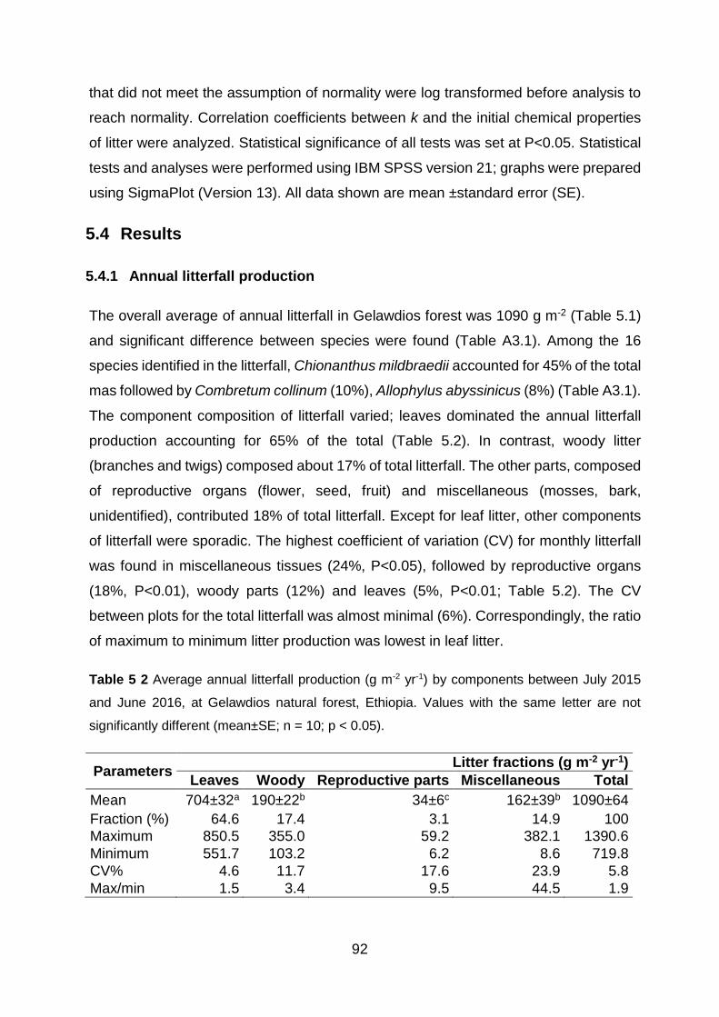
92

that did not meet the assumption of normality were log transformed before analysis to

reach normality. Correlation coefficients between k and the initial chemical properties

of litter were analyzed. Statistical significance of all tests was set at P<0.05. Statistical

tests and analyses were performed using IBM SPSS version 21; graphs were prepared

using SigmaPlot (Version 13). All data shown are mean ±standard error (SE).

5.4 Results

5.4.1 Annual litterfall production

The overall average of annual litterfall in Gelawdios forest was 1090 g m-2 (Table 5.1)

and significant difference between species were found (Table A3.1). Among the 16

species identified in the litterfall, Chionanthus mildbraedii accounted for 45% of the total

mas followed by Combretum collinum (10%), Allophylus abyssinicus (8%) (Table A3.1).

The component composition of litterfall varied; leaves dominated the annual litterfall

production accounting for 65% of the total (Table 5.2). In contrast, woody litter

(branches and twigs) composed about 17% of total litterfall. The other parts, composed

of reproductive organs (flower, seed, fruit) and miscellaneous (mosses, bark,

unidentified), contributed 18% of total litterfall. Except for leaf litter, other components

of litterfall were sporadic. The highest coefficient of variation (CV) for monthly litterfall

was found in miscellaneous tissues (24%, P<0.05), followed by reproductive organs

(18%, P<0.01), woody parts (12%) and leaves (5%, P<0.01; Table 5.2). The CV

between plots for the total litterfall was almost minimal (6%). Correspondingly, the ratio

of maximum to minimum litter production was lowest in leaf litter.

Table 5 2 Average annual litterfall production (g m-2 yr-1) by components between July 2015

and June 2016, at Gelawdios natural forest, Ethiopia. Values with the same letter are not

significantly different (mean±SE; n = 10; p < 0.05).

Parameters Litter fractions (g m-2 yr-1)

Leaves Woody Reproductive parts Miscellaneous Total

Mean 704±32a 190±22b 34±6c 162±39b 1090±64

Fraction (%) 64.6 17.4 3.1 14.9 100

Maximum 850.5 355.0 59.2 382.1 1390.6

Minimum 551.7 103.2 6.2 8.6 719.8

CV% 4.6 11.7 17.6 23.9 5.8

Max/min 1.5 3.4 9.5 44.5 1.9

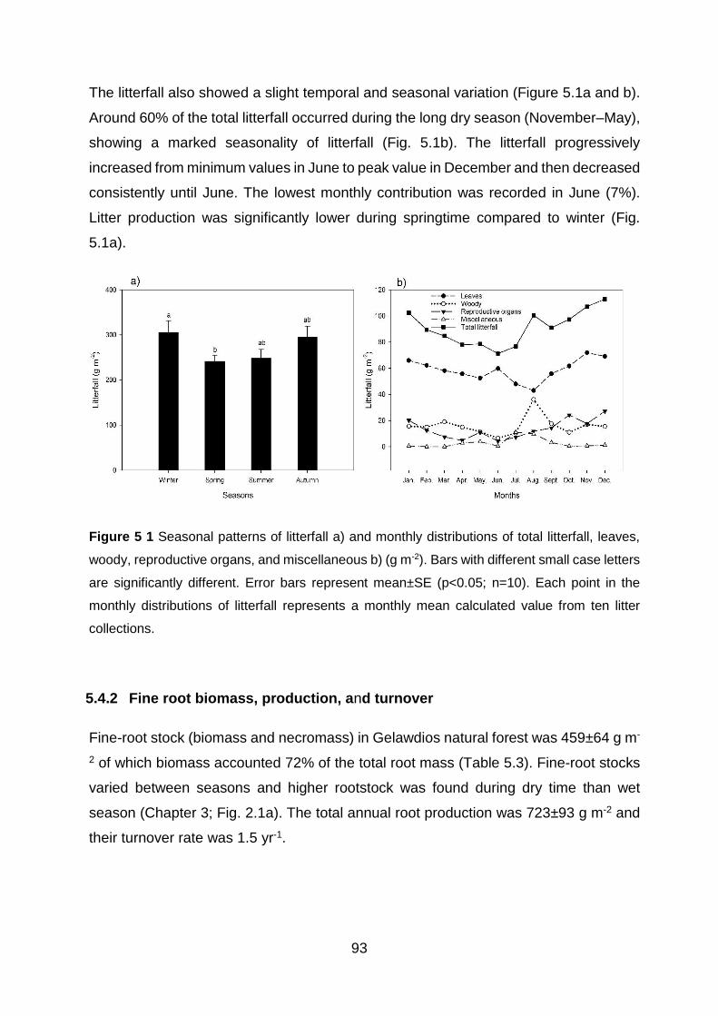
93

The litterfall also showed a slight temporal and seasonal variation (Figure 5.1a and b).

Around 60% of the total litterfall occurred during the long dry season (November–May),

showing a marked seasonality of litterfall (Fig. 5.1b). The litterfall progressively

increased from minimum values in June to peak value in December and then decreased

consistently until June. The lowest monthly contribution was recorded in June (7%).

Litter production was significantly lower during springtime compared to winter (Fig.

5.1a).

Figure 5 1 Seasonal patterns of litterfall a) and monthly distributions of total litterfall, leaves,

woody, reproductive organs, and miscellaneous b) (g m-2). Bars with different small case letters

are significantly different. Error bars represent mean±SE (p<0.05; n=10). Each point in the

monthly distributions of litterfall represents a monthly mean calculated value from ten litter

collections.

5.4.2 Fine root biomass, production, and turnover

Fine-root stock (biomass and necromass) in Gelawdios natural forest was 459±64 g m-

2 of which biomass accounted 72% of the total root mass (Table 5.3). Fine-root stocks

varied between seasons and higher rootstock was found during dry time than wet

season (Chapter 3; Fig. 2.1a). The total annual root production was 723±93 g m-2 and

their turnover rate was 1.5 yr-1.

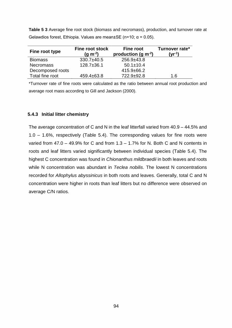
94

Table 5 3 Average fine root stock (biomass and necromass), production, and turnover rate at

Gelawdios forest, Ethiopia. Values are mean±SE (n=10; α = 0.05).

Fine root type Fine root stock

(g m-2) Fine root

production (g m-2) Turnover rate*

(yr-1)

Biomass 330.7±40.5 256.9±43.8 Necromass 128.7±36.1 50.1±10.4 Decomposed roots 415.9±66.2 Total fine root 459.4±63.8 722.9±92.8 1.6

*Turnover rate of fine roots were calculated as the ratio between annual root production and

average root mass according to Gill and Jackson (2000).

5.4.3 Initial litter chemistry

The average concentration of C and N in the leaf litterfall varied from 40.9 – 44.5% and

1.0 – 1.6%, respectively (Table 5.4). The corresponding values for fine roots were

varied from 47.0 – 49.9% for C and from 1.3 – 1.7% for N. Both C and N contents in

roots and leaf litters varied significantly between individual species (Table 5.4). The

highest C concentration was found in Chionanthus mildbraedii in both leaves and roots

while N concentration was abundant in Teclea nobilis. The lowest N concentrations

recorded for Allophylus abyssinicus in both roots and leaves. Generally, total C and N

concentration were higher in roots than leaf litters but no difference were observed on

average C/N ratios.

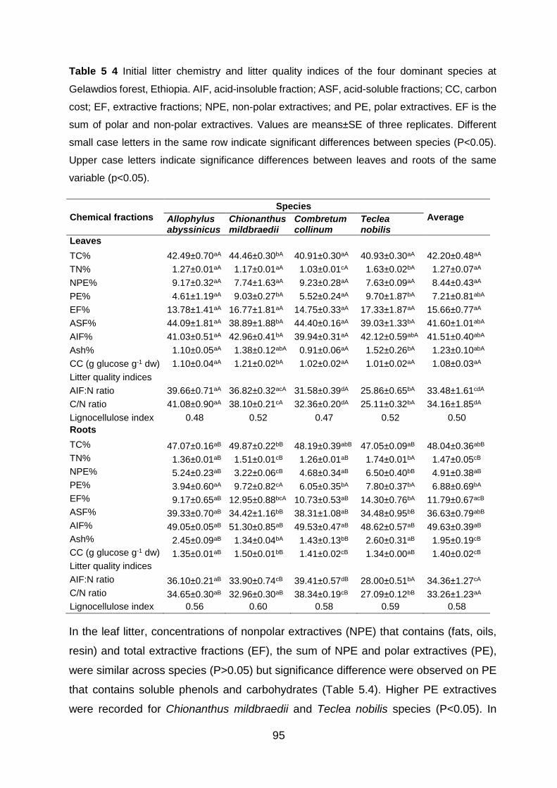
95

Table 5 4 Initial litter chemistry and litter quality indices of the four dominant species at

Gelawdios forest, Ethiopia. AIF, acid-insoluble fraction; ASF, acid-soluble fractions; CC, carbon

cost; EF, extractive fractions; NPE, non-polar extractives; and PE, polar extractives. EF is the

sum of polar and non-polar extractives. Values are means±SE of three replicates. Different

small case letters in the same row indicate significant differences between species (P<0.05).

Upper case letters indicate significance differences between leaves and roots of the same

variable (p<0.05).

Chemical fractions

Species

Average Allophylus abyssinicus

Chionanthus mildbraedii

Combretum collinum

Teclea nobilis

Leaves

TC% 42.49±0.70aA 44.46±0.30bA 40.91±0.30aA 40.93±0.30aA 42.20±0.48aA

TN% 1.27±0.01aA 1.17±0.01aA 1.03±0.01cA 1.63±0.02bA 1.27±0.07aA

NPE% 9.17±0.32aA 7.74±1.63aA 9.23±0.28aA 7.63±0.09aA 8.44±0.43aA

PE% 4.61±1.19aA 9.03±0.27bA 5.52±0.24aA 9.70±1.87bA 7.21±0.81abA

EF% 13.78±1.41aA 16.77±1.81aA 14.75±0.33aA 17.33±1.87aA 15.66±0.77aA

ASF% 44.09±1.81aA 38.89±1.88bA 44.40±0.16aA 39.03±1.33bA 41.60±1.01abA

AIF% 41.03±0.51aA 42.96±0.41bA 39.94±0.31aA 42.12±0.59abA 41.51±0.40abA

Ash% 1.10±0.05aA 1.38±0.12abA 0.91±0.06aA 1.52±0.26bA 1.23±0.10abA

CC (g glucose g-1 dw) 1.10±0.04aA 1.21±0.02bA 1.02±0.02aA 1.01±0.02aA 1.08±0.03aA

Litter quality indices

AIF:N ratio 39.66±0.71aA 36.82±0.32acA 31.58±0.39dA 25.86±0.65bA 33.48±1.61cdA

C/N ratio 41.08±0.90aA 38.10±0.21cA 32.36±0.20dA 25.11±0.32bA 34.16±1.85dA

Lignocellulose index 0.48 0.52 0.47 0.52 0.50

Roots

TC% 47.07±0.16aB 49.87±0.22bB 48.19±0.39abB 47.05±0.09aB 48.04±0.36abB

TN% 1.36±0.01aB 1.51±0.01cB 1.26±0.01aB 1.74±0.01bA 1.47±0.05cB

NPE% 5.24±0.23aB 3.22±0.06cB 4.68±0.34aB 6.50±0.40bB 4.91±0.38aB

PE% 3.94±0.60aA 9.72±0.82cA 6.05±0.35bA 7.80±0.37bA 6.88±0.69bA

EF% 9.17±0.65aB 12.95±0.88bcA 10.73±0.53aB 14.30±0.76bA 11.79±0.67acB

ASF% 39.33±0.70aB 34.42±1.16bB 38.31±1.08aB 34.48±0.95bB 36.63±0.79abB

AIF% 49.05±0.05aB 51.30±0.85aB 49.53±0.47aB 48.62±0.57aB 49.63±0.39aB

Ash% 2.45±0.09aB 1.34±0.04bA 1.43±0.13bB 2.60±0.31aB 1.95±0.19cB

CC (g glucose g-1 dw) 1.35±0.01aB 1.50±0.01bB 1.41±0.02cB 1.34±0.00aB 1.40±0.02cB

Litter quality indices

AIF:N ratio 36.10±0.21aB 33.90±0.74cB 39.41±0.57dB 28.00±0.51bA 34.36±1.27cA

C/N ratio 34.65±0.30aB 32.96±0.30aB 38.34±0.19cB 27.09±0.12bB 33.26±1.23aA

Lignocellulose index 0.56 0.60 0.58 0.59 0.58

In the leaf litter, concentrations of nonpolar extractives (NPE) that contains (fats, oils,

resin) and total extractive fractions (EF), the sum of NPE and polar extractives (PE),

were similar across species (P>0.05) but significance difference were observed on PE

that contains soluble phenols and carbohydrates (Table 5.4). Higher PE extractives

were recorded for Chionanthus mildbraedii and Teclea nobilis species (P<0.05). In

96

roots, Chionanthus mildbraedii species had the lowest NPE (P<0.05) but significantly

higher with PE than other species (P<0.05). Among all species, Combretum collinum

fine roots had the lowest PE (p<0.05). Overall, leaf litter exhibited greater

concentrations of EF and acid-soluble fractions (ASF) than fine roots (Table 5.4). By

contrast, fine roots contained consistently greater acid-insoluble fraction (AIF) than leaf

litters (P<0.001). The cell wall fractions (the sum of ASF and AIF) in root tissues ranged

from 85 to 91% of the dry matter whereas in leaves it ranged from 82 to 86%. Generally,

leaves and roots of the two deciduous species (Combretum collinum and Allophylus

abyssinicus) had higher ASF, and low AIF (lignin content) in leaves only compared to

evergreen species (Teclea nobilis and Chionanthus mildbraedii). Ash contents also

varied between species and were higher in roots than leaves except for Chionanthus

mildbraedii where no difference was found. The lignocellulose index, the proportion of

AIF to cell wall fraction, was greater in roots (58%) than leaves (50%). The AIF:N ratio

had no difference between roots and leaves. Large variation of carbon cost (the amount

of glucoses needed to produce one gram biomass) was found among plant species

and in above- versus below-ground biomass. Among the four species, carbon cost is

significantly higher in Chionanthus mildbraedii species both in leaves and in roots than

other species (P<0.05; Table 5.4). Generally, the carbon investment was significantly

higher in roots than leaves for all species (P<0.05).

5.4.4 Litter decay measurement and turnover rate

The residual litter mass (both roots and leaves) in the bags at each sampling time (in

months) declined exponentially for all species (Fig. 5.3a-d). During the first 3 months,

the weight of remaining litter mass reduced minimal but it was reduced sharply in the

3-6 months time intervals. Between 6-12 months, the weight loss due to microbial

decomposition was minimal again forming nearly a plateau. The mass loss of litter

varied between species (Table A3.2). The decay rate coefficient (k) and residence time

of decomposing materials are presented in Table 5.5. The annual mean decomposition

quotient (k) varied from 1.6±0.1 yr-1 for Chionanthus mildbraedii leaves to 3.1±0.9 yr-1

for Combretum collinum leaves. For example, at 3-months, mass loss of leaf litter was

greater for deciduous species Allophylus abyssinicus (55%) and Combretum collinum

(56%) than for evergreen species (Chionanthus mildbraedii (37%) and Teclea nobilis

(40%)). At the end of the year, more than 90% of the leaf biomass of Combretum

collinum was decomposed (Table 5.5). Generally, mass loss was average when litters

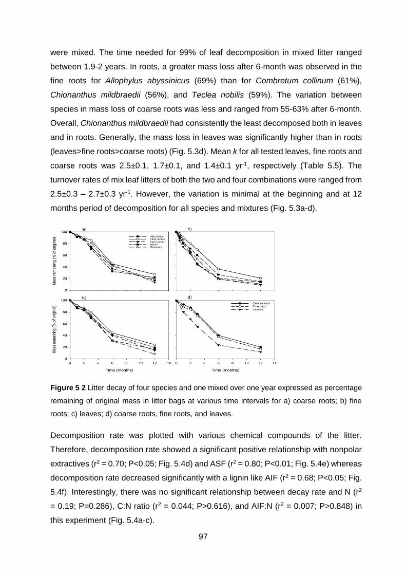
97

were mixed. The time needed for 99% of leaf decomposition in mixed litter ranged

between 1.9-2 years. In roots, a greater mass loss after 6-month was observed in the

fine roots for Allophylus abyssinicus (69%) than for Combretum collinum (61%),

Chionanthus mildbraedii (56%), and Teclea nobilis (59%). The variation between

species in mass loss of coarse roots was less and ranged from 55-63% after 6-month.

Overall, Chionanthus mildbraedii had consistently the least decomposed both in leaves

and in roots. Generally, the mass loss in leaves was significantly higher than in roots

(leaves>fine roots>coarse roots) (Fig. 5.3d). Mean k for all tested leaves, fine roots and

coarse roots was 2.5±0.1, 1.7±0.1, and 1.4±0.1 yr-1, respectively (Table 5.5). The

turnover rates of mix leaf litters of both the two and four combinations were ranged from

2.5±0.3 – 2.7±0.3 yr-1. However, the variation is minimal at the beginning and at 12

months period of decomposition for all species and mixtures (Fig. 5.3a-d).

Figure 5 2 Litter decay of four species and one mixed over one year expressed as percentage

remaining of original mass in litter bags at various time intervals for a) coarse roots; b) fine

roots; c) leaves; d) coarse roots, fine roots, and leaves.

Decomposition rate was plotted with various chemical compounds of the litter.

Therefore, decomposition rate showed a significant positive relationship with nonpolar

extractives (r2 = 0.70; P<0.05; Fig. 5.4d) and ASF (r2 = 0.80; P<0.01; Fig. 5.4e) whereas

decomposition rate decreased significantly with a lignin like AIF (r2 = 0.68; P<0.05; Fig.

5.4f). Interestingly, there was no significant relationship between decay rate and N (r2

= 0.19; P=0.286), C:N ratio (r2 = 0.044; P>0.616), and AIF:N (r2 = 0.007; P>0.848) in

this experiment (Fig. 5.4a-c).

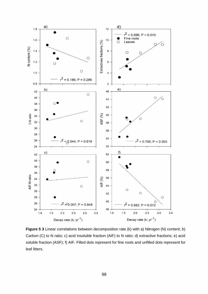
98

Figure 5 3 Linear correlations between decomposition rate (k) with a) Nitrogen (N) content; b)

Carbon (C) to N ratio; c) acid insoluble fraction (AIF) to N ratio; d) extractive fractions; e) acid

soluble fraction (ASF); f) AIF. Filled dots represent for fine roots and unfilled dots represent for

leaf litters.

99

Table 5 5 Litter decay rate coefficients and residence time for leaves, fine roots, and coarse

roots of the four monospecies, two possible combinations for leaves and four species

combinations for all categories. The decomposition rates (k) were estimated using a single

exponential decay model as Mt = M0*e-kt according to Olson, (1963). Where Mt is the litter dry

mass at time t, M0 is the initial litter mass, t is the sampling time interval, and k is the annual

decay constant. Mean residence time (Rt) of litter in each treatment was estimated by the

inverse of k calculated. T(0.5) is a half-life period calculated as 0.693/k, whereas the T(95) and

T(99) are the time needed for 95% and 99% mass loss and calculated as 3/k and 5/k,

respectively. Values in decay rate constant (k) are mean±SE; n=3.

Species Decay rate

constant (k) yr-1 R2

T(0.5) (yr)

T(95) (yr)

T(99) (yr)

Leaves Allophylus abyssinicus 2.9±0.3 0.816 0.24 1.1 1.8 Chionanthus mildbraedii 1.7±0.1 0.942 0.42 1.8 3.0 Combretum collinum 3.2±0.2 0.931 0.22 1.0 1.6 Teclea nobilis 2.2±0.1 0.918 0.31 1.4 2.3 Allophylus abyssinicus, C. mildbraedii 2.5±0.3 0.729 0.28 1.2 2.0 Chionanthus mildbraedii, C. collinum 2.7±0.3 0.802 0.26 1.1 1.8 Chionanthus mildbraedii, Teclea nobilis 2.7±0.3 0.881 0.26 1.1 1.9 Allophylus abyssinicus, C. collinum 2.5±0.2 0.844 0.27 1.2 2.0 Combretum collinum, Teclea nobilis 2.5±0.2 0.943 0.28 1.2 2.0 Allophylus abyssinicus, Teclea nobilis 2.5±0.3 0.822 0.28 1.2 2.0 All four species 2.6±0.2 0.907 0.27 1.2 1.9 Leaves average 2.5±0.1 0.845 0.28 1.2 2.0 Fine roots Allophylus abyssinicus 1.8±0.2 0.847 0.39 1.7 2.8 Chionanthus mildbraedii 1.3±0.1 0.856 0.52 2.3 3.8 Combretum collinum 1.6±0.1 0.869 0.43 1.8 3.1 Teclea nobilis 1.7±0.1 0.841 0.42 1.8 3.0 All four species 1.8±0.2 0.857 0.38 1.7 2.8 Fine root average 1.7±0.1 0.847 0.42 1.8 3.0 Coarse roots Allophylus abyssinicus 1.5±0.1 0.885 0.45 1.9 3.2 Chionanthus mildbraedii 1.2±0.1 0.877 0.58 2.5 4.2 Combretum collinum 1.5±0.1 0.881 0.46 2.0 3.3 Teclea nobilis 1.4±0.1 0.868 0.49 2.1 3.5 All four species 1.6±0.1 0.842 0.43 1.9 3.1 Coarse root average 1.4±0.1 0.866 0.48 2.1 3.5

5.4.5 C and N fluxes into the soil

Using C concentrations and litter production, the total C return to the soils through fine

root was slightly higher (347 g m-2) than that of leaf litter (296 g m-2; Table 5.6). Similarly,

N return to the soil was 8.9 g m-2 through leaves and 10.6 g m-2 through roots. Litter

production (leaves and roots) were plotted against SOC stock. In this relationship, fine

roots exhibit higher carbon input into the soil (r2 = 0.57, P<0.05; Fig. 5.5a) than annual

leaf litter production (r2 = 0.42, P<0.05; Fig. 5.5b).

100

Table 5 6 Mean flux of each biochemical class to soil via leaf litter, fine roots (<2 mm), and the

proportion (%) of the combined flux of leaf litter and fine root flux contributed by fine roots. AIF,

acid-insoluble fraction; RCC, carbon cost; EF, extractive fractions; ASF, acid soluble fractions.

Elemental and chemical fractions

Leaves (g m-2 yr-1)

Fine roots (g m-2 yr-1)

% of roots of total litter

C 29700,4 34732,9 53,9

N 893,8 1062,8 54,3

CC 760,1 1012,2 57,1

EF 11021,5 8524,2 43,6

ASF 29278,1 26490,7 47,5

AIF 29214,7 35882,5 55,1

Figure 5 4 Linear correlation between soil carbon stocks with a) annual fine root production; b)

annual litterfall production; c) total biomass input (litterfall + fine roots).

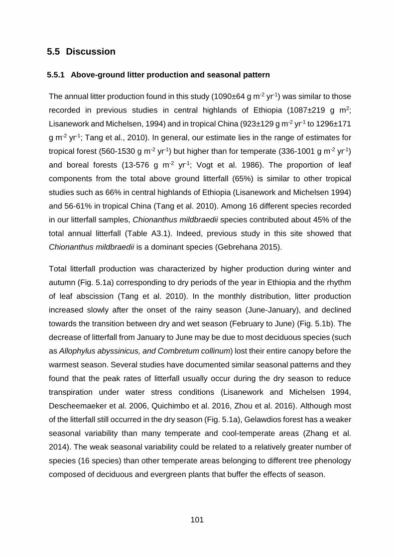
101

5.5 Discussion

5.5.1 Above-ground litter production and seasonal pattern

The annual litter production found in this study (1090±64 g m-2 yr-1) was similar to those

recorded in previous studies in central highlands of Ethiopia (1087±219 g m2;

Lisanework and Michelsen, 1994) and in tropical China (923±129 g m-2 yr-1 to 1296±171

g m-2 yr-1; Tang et al., 2010). In general, our estimate lies in the range of estimates for

tropical forest (560-1530 g m-2 yr-1) but higher than for temperate (336-1001 g m-2 yr-1)

and boreal forests (13-576 g m-2 yr-1; Vogt et al. 1986). The proportion of leaf

components from the total above ground litterfall (65%) is similar to other tropical

studies such as 66% in central highlands of Ethiopia (Lisanework and Michelsen 1994)

and 56-61% in tropical China (Tang et al. 2010). Among 16 different species recorded

in our litterfall samples, Chionanthus mildbraedii species contributed about 45% of the

total annual litterfall (Table A3.1). Indeed, previous study in this site showed that

Chionanthus mildbraedii is a dominant species (Gebrehana 2015).

Total litterfall production was characterized by higher production during winter and

autumn (Fig. 5.1a) corresponding to dry periods of the year in Ethiopia and the rhythm

of leaf abscission (Tang et al. 2010). In the monthly distribution, litter production

increased slowly after the onset of the rainy season (June-January), and declined

towards the transition between dry and wet season (February to June) (Fig. 5.1b). The

decrease of litterfall from January to June may be due to most deciduous species (such

as Allophylus abyssinicus, and Combretum collinum) lost their entire canopy before the

warmest season. Several studies have documented similar seasonal patterns and they

found that the peak rates of litterfall usually occur during the dry season to reduce

transpiration under water stress conditions (Lisanework and Michelsen 1994,

Descheemaeker et al. 2006, Quichimbo et al. 2016, Zhou et al. 2016). Although most

of the litterfall still occurred in the dry season (Fig. 5.1a), Gelawdios forest has a weaker

seasonal variability than many temperate and cool-temperate areas (Zhang et al.

2014). The weak seasonal variability could be related to a relatively greater number of

species (16 species) than other temperate areas belonging to different tree phenology

composed of deciduous and evergreen plants that buffer the effects of season.

102

5.5.2 Factors controlling leaf litter decomposition

Leaf litter mass loss followed a simple exponential decay function (Fig. 5.3a). The

decomposition rates of leaves obtained in our study (1.7 – 3.2 year-1) are within the

range of decomposition rates previously recorded for tropical seasonal rainforests (0.5-

3.7 year-1; Gholz et al., 2000). In the first three months of decomposition, we observed

slower decomposition followed by a rapid decomposition rate between 3-6 months and

generating nearly a plateau after 6 months. This pattern was also observed by Portillo-

Estrada et al., (2016) across European forests and grasslands. Nevertheless, our

decomposition rate is slower with mass loss of 10 – 26% in the first four weeks and 20

– 37% in the first 8 weeks compared to 40 – 50% of the dry weight of litterfall

decomposed in the initial five weeks in an eastern Guatemalan forest (Ewel 1976).

Similarly, Yang et al. (2004) reported from subtropical China that leaves of Castanopsis

kawakamii, and Ormosia xylocarpa lost 91% and 88% of their initial weight in the first

150-day period, respectively. We hypothesize that the initial slower decomposition rate

in our study was generated by the combination of the following factors. First, this period

coincided with the main rainy period in Ethiopia and about 80% of the total rainfall

occurring during these three months only, which starts mid-June and ends early

September (UNECA 1996). Therefore, all airspaces are filled with water at this time

which hampers gas exchange (Karavin et al. 2016) so that microbes couldn’t get

enough air and thus reduce the decomposition rate. Some authors explained that soil

moisture is effective to a certain extent (Demessie et al. 2012), however, excess water

in the soil causes a decrease in decomposition rate because of anaerobic conditions

(Karavin et al. 2016). The second reason could be related to the invasion of

microorganisms. During the initial phase, microorganisms either need some time to

colonize the litter fully (Voříšková and Baldrian 2012) or their fungal mycelia and

microbes itself may contribute to the mass left (Portillo-Estrada et al. 2016). For

example, in a leaf litter decomposition experiment across European forests and

grasslands, Portillo-Estrada et al. (2016) noticed even litter mass increases relative to

the previous sampling during the first month of decomposition due to fungal mycelia.

The relatively sharp decline of remaining mass between 3 – 6 months may be attributed

to sufficient colonization of microbes (Voříšková and Baldrian 2012), optimal soil

temperature, moisture, and air conditions for microbial organisms (Yuste et al. 2007).

After three months of heavy rainfall, the temperature increased slowly and the

103

precipitation decreased sharply (Sisay et al. 2016) but provides sufficient soil moisture

that may explain the sharp decline in weight of the remaining litter mass during these

periods. It is known that decomposition rate is increased exponentially with increasing

temperature (Bradford 2013). According to Bradford (2013), a 10°C increase of

temperature increase decomposition rate by double. In Gelawdios, the temperature is

increased progressively from the lowest (16°C) in July and August to the maximum

24°C in February and March (Wassie et al. 2009). Thus, an 8°C increase of temperature

from the first three months to the next 6 months accelerates the decomposition rate by

1.6 times than the previous decomposition rate. After 6 months of incubation, the litter

mass loss rate decreased and generating nearly a plateau shape as observed in Fig.

5.3a-d. The slow decomposition revealed at this time can be partly explained by the

longer dry period, during which decomposition is almost impeded. In addition, the

relatively slower decay rates at later stages may be due to the decrease of the substrate

quality as a result of the removal of the labile carbon and the accumulation of

recalcitrant matter in the residual litter mass (Sun et al. 2013). The decomposition

usually begins by the most degradable fractions of the litter substrate such as soluble

carbohydrates (Sariyildiz and Anderson 2003, Hättenschwiler and Jørgensen 2010,

Moorhead et al. 2014).

Leaf decay rates varied considerably among species ranging from as little as 8% mass

remaining for Allophylus abyssinicus leaves to over 20% mass remaining for

Chionanthus mildbraedii species after one-year in the litterbag experiment (Table

A3.2). Chionanthus mildbraedii litter is consistently the least decompose species that

los only 30% of the initial weight of leaves in three months and about 21% undecayed

(Table A3.2). The slow decomposition in this species may be associated with the high

leaf toughness (Eissenstat and Yanai 1997, Pan et al. 2015, Yeong et al. 2016). For

example, Habteyohannes (2016) reported that Chionanthus mildbraedii is the toughest

leaf (10 N cm2) whereas other 13 species including Combretum collinum and Teclea

nobilis are below 6 N cm2. In addition, our chemical analysis indicated that the

Chionanthus mildbraedii litter is characterized by strongly lignified leaf tissue (Table

5.4), which could further hamper decomposition of leaf litter. Combretum collinum

decayed very rapidly with over 55% decayed in three months and over 90% decayed

within a year. Allophylus abyssinicus species also decayed faster next to Combretum

collinum. These two species (Combretum collinum and Allophylus abyssinicus) are

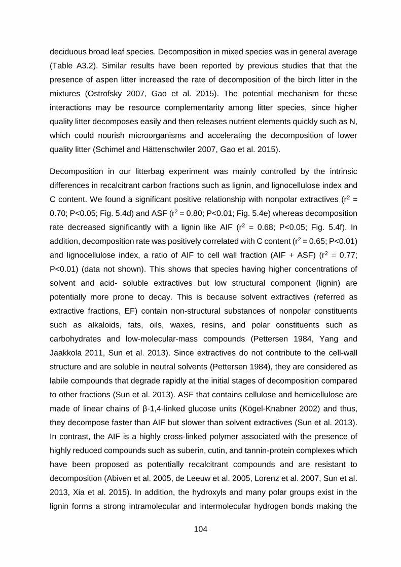
104

deciduous broad leaf species. Decomposition in mixed species was in general average

(Table A3.2). Similar results have been reported by previous studies that that the

presence of aspen litter increased the rate of decomposition of the birch litter in the

mixtures (Ostrofsky 2007, Gao et al. 2015). The potential mechanism for these

interactions may be resource complementarity among litter species, since higher

quality litter decomposes easily and then releases nutrient elements quickly such as N,

which could nourish microorganisms and accelerating the decomposition of lower

quality litter (Schimel and Hättenschwiler 2007, Gao et al. 2015).

Decomposition in our litterbag experiment was mainly controlled by the intrinsic

differences in recalcitrant carbon fractions such as lignin, and lignocellulose index and

C content. We found a significant positive relationship with nonpolar extractives (r2 =

0.70; P<0.05; Fig. 5.4d) and ASF (r2 = 0.80; P<0.01; Fig. 5.4e) whereas decomposition

rate decreased significantly with a lignin like AIF (r2 = 0.68; P<0.05; Fig. 5.4f). In

addition, decomposition rate was positively correlated with C content (r2 = 0.65; P<0.01)

and lignocellulose index, a ratio of AIF to cell wall fraction (AIF + ASF) (r2 = 0.77;

P<0.01) (data not shown). This shows that species having higher concentrations of

solvent and acid- soluble extractives but low structural component (lignin) are

potentially more prone to decay. This is because solvent extractives (referred as

extractive fractions, EF) contain non-structural substances of nonpolar constituents

such as alkaloids, fats, oils, waxes, resins, and polar constituents such as

carbohydrates and low-molecular-mass compounds (Pettersen 1984, Yang and

Jaakkola 2011, Sun et al. 2013). Since extractives do not contribute to the cell-wall

structure and are soluble in neutral solvents (Pettersen 1984), they are considered as

labile compounds that degrade rapidly at the initial stages of decomposition compared

to other fractions (Sun et al. 2013). ASF that contains cellulose and hemicellulose are

made of linear chains of β-1,4-linked glucose units (Kögel-Knabner 2002) and thus,

they decompose faster than AIF but slower than solvent extractives (Sun et al. 2013).

In contrast, the AIF is a highly cross-linked polymer associated with the presence of

highly reduced compounds such as suberin, cutin, and tannin-protein complexes which

have been proposed as potentially recalcitrant compounds and are resistant to

decomposition (Abiven et al. 2005, de Leeuw et al. 2005, Lorenz et al. 2007, Sun et al.

2013, Xia et al. 2015). In addition, the hydroxyls and many polar groups exist in the

lignin forms a strong intramolecular and intermolecular hydrogen bonds making the

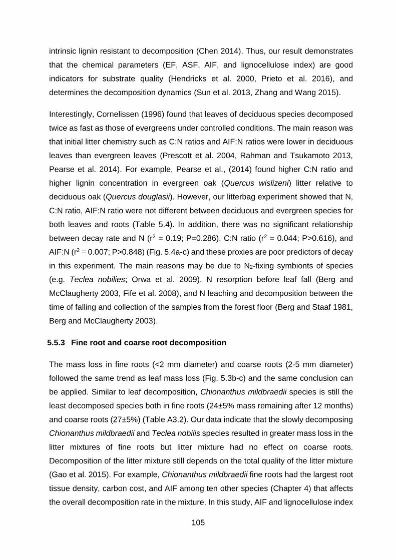
105

intrinsic lignin resistant to decomposition (Chen 2014). Thus, our result demonstrates

that the chemical parameters (EF, ASF, AIF, and lignocellulose index) are good

indicators for substrate quality (Hendricks et al. 2000, Prieto et al. 2016), and

determines the decomposition dynamics (Sun et al. 2013, Zhang and Wang 2015).

Interestingly, Cornelissen (1996) found that leaves of deciduous species decomposed

twice as fast as those of evergreens under controlled conditions. The main reason was

that initial litter chemistry such as C:N ratios and AIF:N ratios were lower in deciduous

leaves than evergreen leaves (Prescott et al. 2004, Rahman and Tsukamoto 2013,

Pearse et al. 2014). For example, Pearse et al., (2014) found higher C:N ratio and

higher lignin concentration in evergreen oak (Quercus wislizeni) litter relative to

deciduous oak (Quercus douglasii). However, our litterbag experiment showed that N,

C:N ratio, AIF:N ratio were not different between deciduous and evergreen species for

both leaves and roots (Table 5.4). In addition, there was no significant relationship

between decay rate and N (r2 = 0.19; P=0.286), C:N ratio (r2 = 0.044; P>0.616), and

AIF:N (r2 = 0.007; P>0.848) (Fig. 5.4a-c) and these proxies are poor predictors of decay

in this experiment. The main reasons may be due to N2-fixing symbionts of species

(e.g. Teclea nobilies; Orwa et al. 2009), N resorption before leaf fall (Berg and

McClaugherty 2003, Fife et al. 2008), and N leaching and decomposition between the

time of falling and collection of the samples from the forest floor (Berg and Staaf 1981,

Berg and McClaugherty 2003).

5.5.3 Fine root and coarse root decomposition

The mass loss in fine roots (<2 mm diameter) and coarse roots (2-5 mm diameter)

followed the same trend as leaf mass loss (Fig. 5.3b-c) and the same conclusion can

be applied. Similar to leaf decomposition, Chionanthus mildbraedii species is still the

least decomposed species both in fine roots (24±5% mass remaining after 12 months)

and coarse roots (27±5%) (Table A3.2). Our data indicate that the slowly decomposing

Chionanthus mildbraedii and Teclea nobilis species resulted in greater mass loss in the

litter mixtures of fine roots but litter mixture had no effect on coarse roots.

Decomposition of the litter mixture still depends on the total quality of the litter mixture

(Gao et al. 2015). For example, Chionanthus mildbraedii fine roots had the largest root

tissue density, carbon cost, and AIF among ten other species (Chapter 4) that affects

the overall decomposition rate in the mixture. In this study, AIF and lignocellulose index

106

in Chionanthus mildbraedii have no difference with other species but root carbon cost

is significantly higher than all other species (P<0.001; Table 5.4). In general, fine roots

decomposed on average significantly slower (17±2% mass remaining after 12 months,

mean ± SD) than leaves (12±1%; p<0.001) but no significant difference with coarse

roots (20±2%) (Fig. 5.3d; Table A3.2). The decomposition rate (k) was in the order of

leaves (2.5±0.1), fine roots (1.6±0.1), and coarse roots (1.4±0.1) (Table 5.5).

5.5.4 Biochemical fluxes from litters into the soil

The total C return to the soils through fine root (347 g m-2) and leaf litter (296 g m-2;

Table 5.6) is lower than other estimates in tropical forests (436 g C m-2 yr-1 for roots or

leaves in China; Chen et al., 2005). Nevertheless, our estimate is higher than that of

boreal forest in Finland (272 g C m-2 yr-1 for fine roots and 235 g C m-2 yr-1 for above-

ground litterfall; Leppälammi-Kujansuu et al., 2014). Using N concentrations and

litterfall data, N return to the soil from leaves (8.9 g m-2) is similar to Ethiopian highland

forest (8.6 g m-2; Lisanework and Michelsen, 1994) but in the lower range of reports

from eucalyptus stand in New Zealand (8.3-13.5 g m-2; Guo and Sims, 1999). The

difference is due to either amount of litterfall or N concentration in the leaf material. Still,

N return to the soil through leaves was lower than that of roots (10.6 g m-2) in this study

(Table 5.6) and this may be due to N2-fixing symbionts in roots or N resorption or

leaching in the leaves.

ASF and AIF were the two largest biochemical fluxes to the soil (47-50%) and extractive

fractions (EF) accounted for <16% of the total litter flux in leaves and <12% in fine roots.

The finding of this study showed that fine roots exhibit higher carbon input into the soil

(r2 = 0.57, P<0.05; Fig. 5.5a) than annual leaf litter production (r2 = 0.42, P<0.05; Fig.

5.5b) and dominated the fluxes of recalcitrant carbon (an 8% difference in AIF) (Table

5.4). Out of the total carbon input, fine roots contributed about 1.5-times higher

recalcitrant carbon into the soil (Table 5.6). Xia et al., (2015) also showed that fine roots

contained 2.9-fold higher AIF and 2.3-fold more condensed tannins than leaf litter; both

are relatively difficult to decompose. By contrast, leaf litter contributed greater quantities

of labile compounds: cellulose, soluble phenolics and carbohydrates (57% in leaves vs

48% in fine roots). Thus, we hypothesized that fine roots are the major source of

recalcitrant carbon fractions entering the soil at our study site.

107

5.6 Conclusion

Litterfall in the studied areas is characterized by weak seasonality mainly attributed to

plant phenology. Fine root production is nearly equal to leaf litterfall. Nevertheless, our

results suggest that fine roots might contribute more recalcitrant SOC than leaves

because of larger amounts of AIF in the fine roots. Species with higher recalcitrant

structural compounds (AIF) are slowly decomposed whereas litter containing high

concentration of labile compounds (e.g. carbohydrates, cellulose) decompose faster.

The presence of deciduous species such as Combretum collinum and Allophylus

abyssinicus stimulate the decomposition of the less decompose Chionanthus

mildbraedii species in the mixtures litter. When it comes to species selection for

regulating global biogeochemical cycle, soil carbon deposition in the long-term, and

ecosystem function, evergreen species such as Chionanthus mildbraedii and Teclea

nobilis are preferable due to higher litter biomass production and lignin content in the

litter biomass than deciduous species.

108

6 The biological origin of soil organic carbon and

response to land use change based on biomarker

analysis

6.1 Abstract

Soil organic carbon accounts for more than four times the amount of carbon in the

atmosphere and is a fundamental part of the carbon cycle and life on Earth. This

material is primarily manufactured by plants but also by animals and microorganisms

which, as part of the food chain, return to the soil when they die and decompose. Once

decomposed and incorporated to the soil, this carbon loses its anatomical

characteristics, making it difficult to characterize and isolate its biological origin and

status of degradation. Therefore, this study aimed to reconstruct the biological origin of

soil organic carbon and to attribute it to its parent materials based on its carbon

skeleton. This effort is also a step forward in characterizing the relative stage of organic

matter degradation in different land use types. Individual biomarkers were identified

and quantified by applying chromatographic and spectrometric techniques after

sequential extraction including solvent extraction, base hydrolysis, and CuO oxidation.

The soil samples stem from four land use systems in the northern highlands of Ethiopia.

Although the identified biomarkers represented only 4% of the total organic matter, they

provided useful information on their origin, tissue type, major taxonomic group, and

stages of organic matter degradation. The overall result generally revealed a major

input of soil organic carbon derived from vascular plants; the microbial and animals

inputs were present as minor components. The relative proportion of suberin was about

2 times that of cutin in natural forest, eucalyptus, and cropland. This emphasized the

importance of below-ground biomass in the distribution of organic carbon in the soil.

The occurrences and concentrations of benzyls and lignin-derived phenols was about

4 times higher in the natural forest soil than in the other land use soils, indicating the

predominant input of recalcitrant organic carbon derived from higher plants into the

forest ecosystem. The ratio of syringyls to vanillyls (S/V) and of cinnamyl to vanillyl

(C/V) monomers – along with the lignin phenol vegetation index – indicated that non-

woody angiosperms plants are the predominant source for lignin. In all land use types,

the carbon source was mainly from C3 plants, not C4 plants. Although the extent of

organic matter degradation depends on microbial activity and biochemistry, the highest

109

suberin/cutin and C16/∑C16 ratios indicate preferential degradation of cutin.

Combining the evidence of the degradation parameters, the degradation of lignin was

enhanced in the forest soil, supported by the elevated acid/aldehyde (Ad/Al) ratios of

vanillyl and syringyl units.

6.2 Introduction

The amount of carbon (C) stored in the soil (3150 Pg C) is more than four times greater

than that in the atmosphere (750 Pg C) and is a fundamental part of the global carbon

cycle (Batjes 1996, Hiederer and Köchy 2011, Fan et al. 2016). Soil is a complex

mixture of organic compounds primarily produced by plants but also by animals and

microorganisms as part of the food chain (Amelung et al. 2008, Feng and Simpson

2011). Soil organic matter (SOM) has a mean residence time in soil ranging from days

to millennia (Amelung et al. 2008). Once organic material is incorporated into the soil,

it loses its anatomical characteristics during degradation, featuring different stages of

biological oxidation (Feng and Simpson 2007). Subsequently, morphological

identification is no longer a viable method to determine the biological origin of carbon

in the soil (Amelung et al. 2008).

Quantitative and qualitative measurements of soil organic carbon (SOC) dynamics

have been of great interest in recent years. This reflects the major significance of SOC

in the environment and its high contribution to soil productivity by improving soil fertility

and soil aggregation and based on its resistance to physical degradation (Strosser

2010, Scharlemann et al. 2014). Nonetheless, unsustainable land use management

practices, commonly by small-scale farmers, accelerate decomposition and carbon

losses through respiration and erosion (Lal 2010a, 2010b). Numerous studies have

quantified carbon dynamics, turnover, distribution, and chemical characterization in

terrestrial ecosystems based on bulk properties and elemental compositions (Schuman

et al. 2002, Jones et al. 2005, Conti et al. 2016). Limited information, however, is

available on the sources and chemical composition of input materials, except for certain

temperate ecosystems (Hedges et al. 1984, Otto et al. 2005, Otto and Simpson 2006a,

2007, Pautler et al. 2010, Li et al. 2015). The overall degradation stages of organic

matter are often unknown (Guo and Sims 1999, Girisha 2001, Otto et al. 2005). This

calls for the determination of biological origin of materials for soil carbon deposition and

110

the degradation status of carbon in various physical and chemical fractions in soils.

This is an important step forward in predicting the behavior of soil carbon and the

retention time of carbon in soils of different land use systems (Otto et al. 2005). This is

the first attempt to study the soil carbon origin of different land use systems based on

biomarker analysis at the molecular level, particularly for African ecosystems.

Structurally unique biochemicals (biomarkers) carry useful information and quantitative

evidence to reconstruct their parent organic materials as well as to determine the stage

of SOM degradation based on their carbon skeleton (Kögel-Knabner 2000, Simoneit

2002, 2005, Amelung et al. 2008, Feng and Simpson 2011, Li et al. 2015). The

composition of uncharacterized SOM is very complex, and some methodological

approaches result in signal overlap. Thus, sequential biomarker extraction with the

application of chromatographic and spectrometric techniques is one of the most

commonly used approaches to detect and quantify the concentration of specific

biomarkers at the molecular level (Poirier et al. 2005, Amelung et al. 2008, Feng and

Simpson 2011). The sequential biomarker extraction techniques include organic

solvent extraction and chemolytic methods such as base hydrolysis and CuO oxidation

because one extraction method may not provide all the required information to trace

SOM sources and processes in the soil (Kögel-Knabner 2000, Otto and Simpson 2007,

Feng 2009). Identification and quantification of individual biomarkers involves gas

chromatography and mass spectrometry (GC-MS) at the molecular level (Kögel-

Knabner 2000, Poirier et al. 2005, Otto and Simpson 2007, Amelung et al. 2008).

Extraction with organic solvents isolates unbound (free) lipids (Feng 2009) such as n-

alkanes, n-alkanols, n-alkanoic acids, steroids, hopanoids, and other terpenoids

(Kögel-Knabner 2000, Otto and Simpson 2006a, Feng and Simpson 2007, Amelung et

al. 2008). Solvent extraction thus provides a general overview of biomarkers from plant

and microbial sources (Goñi et al. 2003, Angst et al. 2016). For example, among the

compounds, even-numbered long-chain (>C20) alkanoic acids and alkanols are

common constituents of plant-derived wax lipids, whereas branched short-chain (<C20)

alkanoic acids, hopanoids, and ergosterol are indicators of microbial-derived SOM

(Feng and Simpson 2011).

As opposed to ‘free’ lipids, ester-bound soil lipids are not extractable with organic

solvents, but can be cleaved from SOM using chemolytic methods such as base

111

hydrolysis (Otto and Simpson 2007, Feng and Simpson 2011). Base hydrolysis is

mainly used to trace root or leaf origin inputs based on suberin- and cutin-derived

markers (Bull et al. 2000, Otto et al. 2005). The predominant long-chain ω-hydroxy-

alkanoic acids and α, ω-alkanedioic acids in bound soil lipids are typical biomarkers for

suberin, primarily used for tracing root or bark inputs into the soil. In turn, C16 and C18

ω-hydroxyalkanoic acids with mid-chain hydroxy or epoxy groups are biomarkers for

cutin or leaf cuticle inputs (Feng and Simpson 2011). According to Feng and Simpson

(2011), suberin- and cutin-derived compounds are recalcitrant and less prone to

microbial attack than solvent-extractable compounds.

The CuO oxidation targets ether bonds to release lignin-derived phenols (Hedges and

Ertel 1982, Otto and Simpson 2006b, Amelung et al. 2008, Feng 2009, Clemente 2012).

Lignin is made up of a polymeric network of phenols. This makes measuring and tracing

lignin directly difficult because of its high molecular weight and low extractability in soils

(Kögel-Knabner 2002, Feng and Simpson 2011). Alternatively, the lignin biopolymer,

namely lignin-derived phenols (vanillyl, syringyl, and cinnamyl) can be released from

SOM with chemolytic methods such as CuO oxidation (Hedges and Mann 1979a, Goñi

and Hedges 1992). Comparison of the abundance of acids to aldehydes (Ad/Al) in this

extract can provide information about the degradation state of lignin in a sample (Otto

and Simpson 2007). The relative abundances of the phenol structural classes can also

provide information about whether lignin is derived from angiosperm vs gymnosperm

sources or from woody vs non-woody tissues (Hedges and Mann 1979a, Goñi et al.

2000) and stages of SOM degradation (Amelung et al. 2008, Feng 2009, Clemente

2012). In addition, biomarkers can provide a general overview of root or above-ground

plant sources based on suberin- and cutin-derived compounds (Otto and Simpson

2006a). Overall, these analyses provide evidence on the origin of SOM (plants, fungi,

bacteria, animals, or anthropogenic origin) by using biomarkers as a screening tool for

bulk SOM composition. Therefore, the objectives of this study are 1) to determine and

quantify the distribution of biomarkers in different land use systems at the molecular

level; 2) to reconstruct the biological origin of soil organic carbon to their parent

materials based on their carbon skeleton; and 3) to characterize the relative stage of

organic matter degradation in the soil.

112

6.3 Methodology

6.3.1 Study area

Four land use systems (natural forest, eucalyptus plantation, cropland and grazing

land) were selected in Gelawdios, north-central Ethiopia. The study area (Gelawdios)

is geographically located at 11°38’25’’ N and 37°48’55’’ E at an elevation of 2500 m

above sea level. The topography is typical of volcanic landscapes, comprising volcanic

rocks with ragged and undulating landforms. The major soil type is classified as

Cambisols with a clay loam texture according to the World Reference Base for soil

resources (Awulachew et al. 2009, Betrie et al. 2011, WRB 2014). The mean annual

rainfall at Gelawdios is 1220 mm with a unimodal rainy season, and the average annual

temperature is 19°C (Wassie et al. 2009). Although Ethiopia is geographically located

in the tropics, the climate of the study area is temperate with a dry winter and a warm,

wet summer (Cwb) according to the Köppen-Geiger climate classification (Peel et al.

2007). The forest is a pristine Afromontane dry forest composed mostly of a mixture of

indigenous tree species; it is almost exclusively confined to sacred groves associated

with a church. The dominant tree species are Albizia schimperiana, Apodytes dimidiata,

Calpurnia aurea, Croton macrostachyus, Ekebergia capensis, Maytenus arbutifolia,

and Schefflera abyssinica. In Gelawdios forest, the number of tree species per hectare

is about 6300 (Chapter 2, Table 2.1). Due to higher tree density, undergrowth of

grasses in the forest is minor. The eucalyptus stand was established on formerly

common grazing land in 1985 and was consecutively thinned to its current density

about 3000 trees per hectare (Chapter 2, Table 2.1). Due to the large space between

trees, the undergrowth is dominated with grasses and indigenous shrub species. The

adjacent grazing land and cropland was converted from natural forest approx. 50 years

ago, although the exact date is not known. The grazing land was used as communal

grazing lands for herds of animals and it consists of highly degraded, nearly bare

ground. The cropland has been cultivated to a depth of ca. 30 cm without fallow periods;

the crop residues are harvested for animal feeding. The principal crops are ‘teff’

(Eragrostis tef), wheat (Triticum aestivum), and barley (Hodeum vulgare).

6.3.2 Soil sampling, C and N analysis

Soil samples were collected at the end of the wet season in September 2015 from all

land use types. Soil samples from the top 10 cm were collected from each land use at

113

10 sampling points marked at 50-100 m along a transect line. At each sampling point,

one sample was taken to the depth of 10 cm with a soil corer (6.6 cm diameter) after

removing the litter layer (if present). The soil samples were sieved in Ethiopia, packed

separately in a plastic bag, and transported to Vienna for laboratory analysis. Sub-

samples of soils weighing approx. 3-5 g from each sample were dried at 105°C for 48

h. From each sample, about 200 mg of soil was taken and total C and N concentrations

were determined on a CN elemental analyser (Truspec CNS LECO, St. Joseph, USA).

6.3.3 Sequential extraction procedures

Sequential chemical extractions (solvent extraction, base hydrolysis, and CuO

oxidation) were conducted on soil samples to determine total solvent extracts, bound

lipids, and lignin-derived phenols, respectively (Otto et al. 2005, Feng and Simpson

2008, Feng 2009, Clemente 2012).

Solvent extraction: Three soil samples (20 g) from each land use were first sonicated

twice for 15 min, each time with 30 ml double deionized water to remove the water-

soluble polar compounds. The water-extracted soil residues (~20 g) were then freeze-

dried and extracted with organic solvents as follows: samples were sonicated for 15

min with 50 ml of methanol, dichloromethane:methanol (1:1; v/v), and dichloromethane,

sequentially. The combined solvent extracts were passed through glass-fiber filters

(Whatman GF/A) into a round bottom flask, concentrated by rotary evaporation, and

then completely dried under nitrogen gas (N2) in 2 ml glass vials. The remaining soil

samples (non-extractable materials) were air-dried for further analysis.

6.3.4 Base hydrolysis

The air-dried soil residues from solvent extraction were then subject to base hydrolysis

to yield ester-linked lipids (Otto and Simpson, 2006a). Briefly, the residues after solvent

extraction were heated at 100°C for 3 h in Teflon-lined bombs with 20 ml of 1 M

methanolic KOH. After cooling, the extracts were acidified to pH 1 with 6 M HCl and

filtered through pre-extracted cellulose filters (Fisher P5, 5-10 µm). Again, the soil

residues were extracted twice by sonication for 15 min with 30 ml

dichloromethane:methanol (1:1 v/v) as described above. The two extracts were

combined and then filtered through glass-fiber filters (Whatman GF/A) into round

bottom flasks. Double-deionized water (50 ml) was added to each extract. Lipids were

114

recovered from the water phase by liquid–liquid extraction in a separation funnel with

50 ml diethyl ether. Anhydrous Na2SO4 was added to the combined ether phases to

remove any water. The ether extracts were concentrated by rotary evaporation,

transferred to 2 ml glass vials, and dried under N2 gas. The remaining soil samples

were air-dried for further analysis.

6.3.5 CuO oxidation

The base hydrolysis residues were air-dried and further oxidized with CuO to release

lignin-derived phenols. Soil residues (~10 g) were extracted with 1 g CuO, 100 mg

ammonium iron (II) sulfate hexahydrate [Fe(NH4)2(SO4)2·6H2O], and 15 ml of 2 M

NaOH in Teflon-lined bombs at 170°C for 2.5 h. After heating, the bombs were cooled

under running water, the liquids were decanted into Teflon centrifuge tubes (50 ml),

and the residues were washed twice each with 10 ml deionized water using a magnetic

stirrer for 10 min. The combined washings and extracts were centrifuged for 30 min at

1050 g force (Heraeus Megafuge 1.0, Hanau, Germany). The supernatant was

decanted into another Teflon centrifuge tube, acidified to pH 1 with 6 M HCl, and kept

for 1 h at room temperature in the dark to prevent reactions of cinnamic acids. After

centrifugation (at 1050 g force for 30 min), the supernatant was transferred to a

separation funnel and liquid–liquid extracted twice with 50 ml diethyl ether. The ether

extracts were concentrated by rotary evaporation, transferred to 2 ml glass vials, and

dried under N2 gas.

6.3.6 Derivatization and GC/MS Analysis

Derivatization was conducted according to Otto et al. (2005) and Feng and Simpson

(2011). In brief, the extracts were re-dissolved, and aliquots (containing ~1 mg extracts)

were derivatized for GC/MS analysis. Solvent extracts and CuO oxidation products

were each re-dissolved in 500 μl dichloromethane:methanol (1:1; v/v). Aliquots of the

extracts (100 μl) were dried in a stream of N2 and then converted to trimethylsilyl (TMS)

derivatives by 90 μl N,O-bis-(trimethylsilyl)trifluoroacetamide (BSTFA) and 10 μl

pyridine for 3 h at 70°C. After cooling, 100 μl hexane was added to dilute the extracts.

The base hydrolysis products were first methylated by reacting with 600 μl of

diazomethane in ether at 37°C for 1 h, evaporated to dryness under N2, and then

silylated with BSTFA and pyridine as described above. Oleic acid (C18:1 alkanoic acid),

tetracosane, and ergosterol were derivatized and used as external standards for

115

solvent extracts. Oleic acid methyl ester and vanillic acid were used as external

standards for base hydrolysis and CuO oxidation products, respectively. To ensure a

linear response, standards ranging from 10-1000 ppm were analyzed using the same

procedure as the biomarker extracts. GC/MS analysis was performed on an Agilent

model 6890N GC coupled to a Hewlett-Packard model 5975 quadrupole mass selective

detector.

Separation was achieved on a HP5-MS fused silica capillary column (30 m × 0.25 mm

internal diameter, 0.25 μm film thickness). The GC operating condition was as follows:

temperature held at 65°C for 2 min, increased from 65 to 300°C at a rate of 6°C min-1

with final isothermal hold at 300°C for 20 min. Helium was used as the carrier gas. The

samples were injected with a 2:1 split ratio and the injector temperature was set at

280°C. The sample (1 μl) was injected with an Agilent 7683B auto sampler. The mass

spectrometer was operated in the electron impact mode (EI) at 70 eV ionization energy

and scanned from 50 to 650 Daltons. Data were acquired and processed with the

Chemstation G1701FA software.

Individual compounds were identified by comparing the mass spectra with the National

Institute of Standards and Technology library (NIST, version 2.0), Wiley MS library data,

and standards. Concentrations of individual compounds were calculated by comparing

the peak area of the compound to that of the standard in the total ion current (TIC) and

were then normalized to the soil carbon contents (Pautler et al. 2010). The C-

normalized biomarker concentrations indicates the relative contribution of the identified

biomarkers with respect to one gram of organic carbon in the soil (Pautler et al. 2010).

All the samples were run in triplicate; values are mean±SE. If a compound was

identified in only one or two of three replicates, SE was not calculated.

6.3.7 Origin and degradation parameters

Several biomarker ratios have been proposed to distinguish between the inputs of

organic matter in the soil. The ratios of C31/(C23+C27) alkanes from solvent extraction

are commonly employed to distinguish between inputs from grasses and trees,

whereby longer chain alkanes such as C31 and C33 are derived from grass tissues (Paul

2016). The relative inputs of C3 and C4 plants can be differentiated by the carboxylic

acid ratio of C24/(n-C22 + n-C26) (Wiesenberg and Schwark 2006). A ratio >0.67

indicates C4 origin, otherwise C3 origin. This is because lipid compounds containing C24

116

alkanoic acids are from C4 plants, whereas C22 and C26 acids are from C3 plants.

Suberin and cutin are used to trace below- and above-ground plant origin, respectively.

Suberin and cutin biomarkers were summarized and calculated according to their

occurrence only in suberin or cutin, based on parameters developed by Otto & Simpson

(2006). Long-chain ω-hydroxyalkanoic acids (≥C20) and α, ω-alkanoic acids (C16-C24)

are typical biomarkers for suberin (ΣS), whereas C16 and C18 ω-hydroxyalkanoic acids

are used as cutin (ΣC) biomarker signatures. Biomarkers derived from both suberin or

cutin (ΣSvC) are ω-hydroxyalkanoic acids C16, C18, C18 di- and trihydroxy acids, and α,

ω-alkanedioic acids C16, C18.

The composition of phenolic lignin compounds obtained after CuO oxidation can be

used to calculate parameters for the origin of lignin. Major plant taxonomic groups

(gymnosperms vs angiosperms) and tissue type (woody vs non-woody tissue) can be

differentiated by the ratios of syringyl to vanillyl (S/V) and cinnamyl- to vanillyl-type

(C/V) monomers (Hedges and Ertel 1982, Goñi and Montgomery 2000). Accordingly,

the S/V ratio of angiosperm tissues has been reported as >0.6. This is because

gymnosperm wood contains only vanillyl derivatives (V: vanillin, acetovanillone, vanillic

acid), while angiosperm wood is composed of approximately equal quantities of

vanillyls and syringyls (S: syringaldehyde, acetosyringone, syringic acid). The lignin-

derived phenol (V, S, C) ratios are also used to estimate the relative contributions of

woody and non-woody angiosperms. Non-woody angiosperm tissues exhibit a V:S:C

ratio of about 1:1:1 (Hedges and Mann 1979a). To improve the detection of lignin

sources as an indicator of vegetation contribution using lignin index-phenols, another

useful parameter (lignin phenol vegetation index – LPVI) was developed by Tareq et

al. (2004). It is calculated according to the following equation.

LPVI = [{S(S+1)/(V+1)+1}*{C(C+1)/(V+1)+1}] in which S=100*S/(S+V+C);

C=100*C/(S+V+C); and V=100*V/(S+V+C).

Based on this parameter, the distinct boundaries of LPVI ranges are <1 for

gymnosperm woods, 3-27 for non-woody gymnosperm tissues, 67-415 for angiosperm

woods, and 176-2782 for non-woody angiosperms.

To assess the degradation of free lipids, bound lipids, and lignin in the soil, degradation

parameters were calculated according to Goñi and Hedges (1990), Otto & Simpson

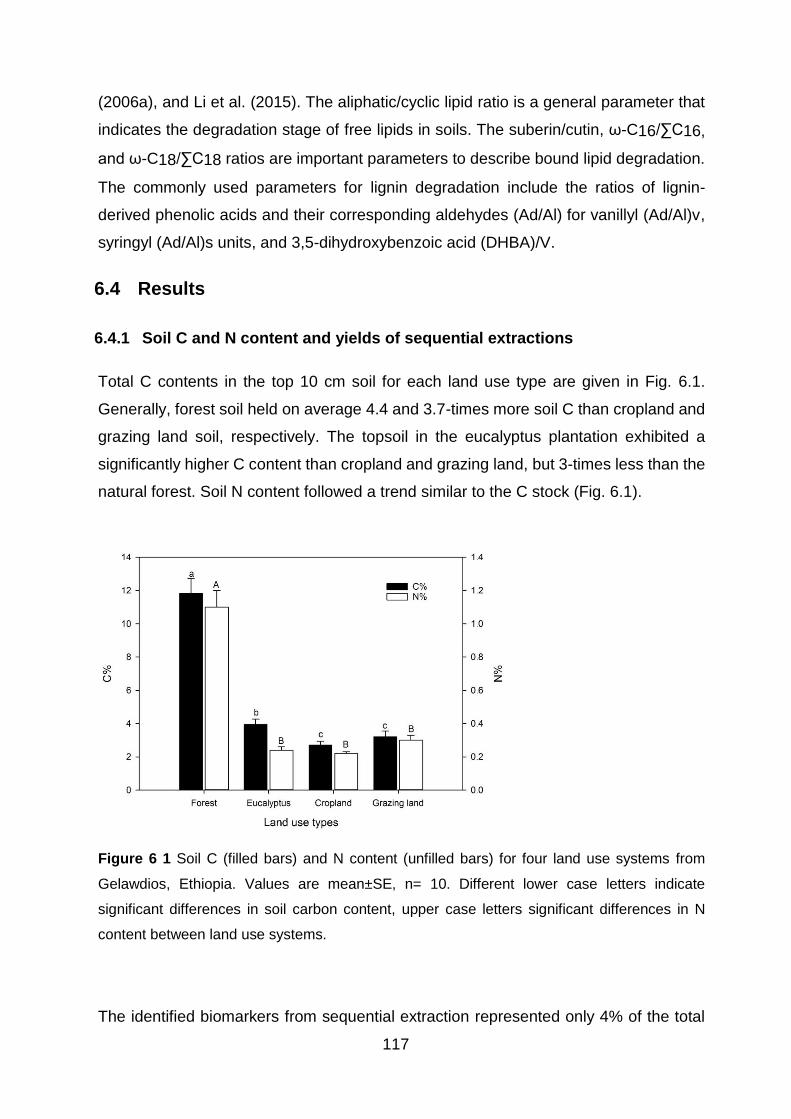
117

(2006a), and Li et al. (2015). The aliphatic/cyclic lipid ratio is a general parameter that

indicates the degradation stage of free lipids in soils. The suberin/cutin, ω-C16/∑C16,

and ω-C18/∑C18 ratios are important parameters to describe bound lipid degradation.

The commonly used parameters for lignin degradation include the ratios of lignin-

derived phenolic acids and their corresponding aldehydes (Ad/Al) for vanillyl (Ad/Al)v,

syringyl (Ad/Al)s units, and 3,5-dihydroxybenzoic acid (DHBA)/V.

6.4 Results

6.4.1 Soil C and N content and yields of sequential extractions

Total C contents in the top 10 cm soil for each land use type are given in Fig. 6.1.

Generally, forest soil held on average 4.4 and 3.7-times more soil C than cropland and

grazing land soil, respectively. The topsoil in the eucalyptus plantation exhibited a

significantly higher C content than cropland and grazing land, but 3-times less than the

natural forest. Soil N content followed a trend similar to the C stock (Fig. 6.1).

Figure 6 1 Soil C (filled bars) and N content (unfilled bars) for four land use systems from

Gelawdios, Ethiopia. Values are mean±SE, n= 10. Different lower case letters indicate

significant differences in soil carbon content, upper case letters significant differences in N

content between land use systems.

The identified biomarkers from sequential extraction represented only 4% of the total

118

organic matter in all land use systems. This means that substantial fractions of SOM

associated with mineral surfaces remain uncharacterized. Although only small fractions

could be obtained by sequential extraction of the soil, these extracts provide useful

information on their biological origin and the degradation status of organic matter based

on characteristic biomarkers. Among the sequential extraction, the highest yield was

obtained from base hydrolysis products (Fig. 6.2).

Figure 6 2 Carbon-normalized extract yields of solvent, base hydrolysis, and CuO oxidation

products of four land use systems from Gelawdios, Ethiopia. Values are mean±SE, n= 3.

6.4.2 Composition and distribution of solvent-extractable free lipids

The major chemical compounds detected in the solvent extract include a series of

aliphatic lipids (n-alkanols, n-alkanes, n-alkanoic acids), carbohydrates,

monoacylglycerides, steroids, and terpenoids (Table 6.1). The GC-MS total ion

chromatogram (TIC) of the major components in the silylated solvent extracts is shown

in Appendix 3 Figure 1 (Figure A4.1). All lists of individual compounds with their

corresponding molecular formula and weight are presented in supplementary data

Table A4.1. The C-normalized yield (mg/1 g C) obtained from solvent extracts was

highest in eucalyptus soil (8.3 mg/g C) followed by forest soil (5.7 mg/g C), cropland

(3.5 mg/g C), and grazing land (3.3 mg/g C) (Table 6.1). Aliphatic lipids accounted for

57-88% of the detected chemicals in the free lipids and were most abundant in natural

forest soil and least abundant in grazing land and cropland (Table 6.1).

119

Table 6 1 Occurrence and quantities of compounds (µg/g C) identified in the solvent extracts

of soil samples of different land use systems in Gelawdios, Ethiopia. Values are mean±SE, n=

3.

Compounda Forest Eucalyptus Cropland Grazing

land

n-Alkanols (C14-C30) 324±171 520±212 250±86 356±103

n-Alkanes (C17-C31) 222±71 391±78 139±66 58±15

n-Alkanoic acids (C9-C26) 448±184 1129±128 207±49 272±31

Iso- Alkanoic acids (C17) 24b nd nd nd

Monoacylglycerides (C19-C21) 52±26 260±19 134±46 84±2 Carbohydrates 3936±703 2429±256 1820±229 1894±192 Steroids and Terpenoids 622±267 3461±341 729±80 616±99 Unknowns 38±3 126±11 238±100 68±b Total aliphatic lipids 5007±746 4729±531 2550±430 2664±300 Identified total solvent extracts 5629±740 8190±857 3279±508 3280±394

nd, not detected

a All polar compounds were identified as their trimethylsilyl (TMS) derivatives.

b Average values detected from two samples only

The concentration of n-alkanols in the range of C14-C30 and n-alkanoic acids in the

range of C9-C26 showed a significant even-over-odd dominance, whereas n-alkanes in

the range of C17-C31 exhibited a preference of odd-numbered molecules (Table A4.1).

The combined concentrations of n-alkanols, alkanes, and alkanoic acids were in the

range of 0.6-2 mg/g C and greatest in eucalyptus soil and least in cropland soil (Table

6.1). Four carbohydrates (glucose, mannose, sucrose, and trehalose) were identified

in the solvent extracts (see details Table A4.1). Monosaccharides were detected only

in minor amounts (1% of total carbohydrates in forest, 13% in eucalyptus, 7% each in

cropland and grazing lands). Trehalose, in contrast, was found in the greatest amounts

(77-99% of total carbohydrates and 26-69% of the identified total solvent extracts). The

solvent extracts also included four monoacylglycerides, three of them being C21

compounds.

Cyclic lipids of steroids and terpenoids were detected in small amounts at

concentrations of 0.6-3.4 mg/g C; the highest concentration was detected in eucalyptus

soil (Table A4.1). The steroid cholesterol was detected in small amounts in all land use

types, whereas ergosterol was detected in minor amounts in the forest and eucalyptus

soil only. The detected phytosterols include campesterol, stigmasterol, β-sitosterol, and

sitosterone; these compounds contributed over 81-96% of total steroids in the forest,

cropland, and grazing land but only 19% in eucalyptus soil. In contrast, sesquiterpense

120

of trans-farnesol and globulol combined contributed 38% of total steroids in the

eucalyptus stand soil. Aromadendrene, γ-elemene, and ledol are also sesquiterpense,

detected in relatively higher concentration in eucalyptus soil and in minor

concentrations in cropland. The detected triterpenoids include ß- amyrin, α- amyrin,

lupeol, erythrodiol, and oleanolic acid. The latter two showed higher concentrations in

eucalyptus soil (29% of the total steroids and terpenoid extractions) but lower values in

other land use type soils (Table A4.1).

6.4.3 Composition and distribution of bound lipids

The major products identified after base hydrolysis included a series of aliphatic lipids

(n-alkanols, n-alkanoic acids, mid-chain substituted and branched acids, ω-

hydroxyalkanoic acids, α-hydroxyalkanoic acids, α,ω-alkanedioic acids, and

glycerides), with a lesser contribution from benzyls and phenols, and one steroid (Table

6.3). Compounds identified in the base hydrolysis are listed in detail in Table A4.2 and

the GC-MS chromatograms Figure A4.2. The C-normalized concentrations of total

bound lipids after base hydrolysis extraction were generally highest in the grazing land

(111.3±8.2 mg/g C), followed by cropland (97.1±4.4 mg/g C), eucalyptus soil (82.0±1.0

mg/g C), and natural forest (29.9±1.2 mg/g C) (Table 6.2). Aliphatic lipids showed a

similar pattern and represented more than 60% of the total base extracts; n-alkanoic

acids in the range of C14-C30 were detected in largest quantity (4.8-12.2 mg/g C), with

a strong even-over-odd preference (Table A4.2). Mostly even-numbered chains of α,

ω-alkanedioic acids in the range of C4-C20 were detected in minor amounts in all

samples (324-678 µg/g C). Mid-chain substituted hydroxyalkanoic acids (C16, C18, and

C19) and other α-alkanoic acids, ω- alkanoic acids, and glycerides combined were

detected in minor concentrations (1.1-2.2 mg/g C). Branched alkanoic acid (iso-C16)

was detected in low amounts (11-37 µg/g C) and was absent in grazing land soil

samples (Table 6.2). Base hydrolysis also cleaved glycerides (C19) in minor

concentrations (238-486 µg/g C) in three land use types but was absent in grazing land.

One organophosphate of C19 was also detected in all soil samples at high

concentrations (1.5-6.7 mg/g C). Benzyls and phenols ranged from 0.4-2.3 mg/g C

(Table 6.2).

Table 6 2 Occurrence and quantities of compounds (µg/g C) identified from base hydrolysis of

soil samples in different land use systems in Gelawdios, Ethiopia. Values are mean±SE, n= 3.

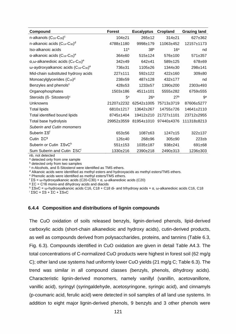
121

Compound Forest Eucalyptus Cropland Grazing land

n-alkanols (C16-C28)c 104±21 265±12 314±21 627±362

n-alkanoic acids (C14-C30)d 4788±1180 9998±179 11063±452 12157±1173

Iso-alkanoic acids 11b 38b 16a nd

α-alkanoic acids (C16-C25)e 364±60 515±124 576±100 571±357

α,ω-alkanedioic acids (C4-C20)e 342±49 642±41 589±125 678±69

ω-aydroxyalkanoic acids (C16-C30)e 736±31 1105±26 1344±30 298±141

Mid-chain substituted hydroxy acids 227±111 592±122 422±160 309±80

Monoacylglycerides (C19)d 238±59 487±128 432±177 nd

Benzyles and phenolsc 428±53 1233±57 1390±200 2303±493

Organophosphates 1503±186 4511±101 5555±282 6759±555

Steroids (ß- Sitosterol)c 5a 26a 27b 9a

Unknowns 21207±2232 62542±1005 75713±3719 87606±5277

Total lipids 6810±1217 13642±267 14755±726 14641±2110

Total identified bound lipids 8745±1404 19412±210 21727±1101 23712±2955

Total base hydrolysis 29952±3559 81954±1010 97440±4376 111318±8213

Suberin and Cutin monomers

Suberin ΣSf 653±56 1087±63 1247±15 322±137

Cutin ΣCg 126±40 268±96 305±90 223±b

Suberin or Cutin ΣSvCh 551±153 1035±187 938±241 691±68

Sum Suberin and Cutin ΣSCi 1330±216 2390±218 2490±313 1236±303 nb, not detected a detected only from one sample b detected only from two samples c n-Alcohols, and ß-Sitosterol were identified as TMS ethers. d Alkanoic acids were identified as methyl esters and hydroxyacids as methyl esters/TMS ethers. e Phenolic acids were identified as methyl esters/TMS ethers. f ΣS = ω-hydroxyalkanoic acids (C20-C30) + α, ω-alkanedioic acids (C20) g ΣC = C16 mono-and dihydroxy acids and diacids h ΣSvC = ω-hydroxyalkanoic acids C16, C18 + C18 di- and trihydroxy acids + α, ω-alkanedioic acids C16, C18 i ΣSC = ΣS + ΣC + ΣSvC

6.4.4 Composition and distributions of lignin compounds

The CuO oxidation of soils released benzyls, lignin-derived phenols, lipid-derived

carboxylic acids (short-chain alkanedioic and hydroxy acids), cutin-derived products,

as well as compounds derived from polysaccharides, proteins, and tannins (Table 6.3,

Fig. 6.3). Compounds identified in CuO oxidation are given in detail Table A4.3. The

total concentrations of C-normalized CuO products were highest in forest soil (62 mg/g

C); other land use systems had uniformly lower CuO yields (21 mg/g C; Table 6.3). The

trend was similar in all compound classes (benzyls, phenols, dihydroxy acids).

Characteristic lignin-derived monomers, namely vanillyl (vanillin, acetovanillone,

vanillic acid), syringyl (syringaldehyde, acetosyringone, syringic acid), and cinnamyls

(p-coumaric acid, ferulic acid) were detected in soil samples of all land use systems. In

addition to eight major lignin-derived phenols, 9 benzyls and 3 other phenols were

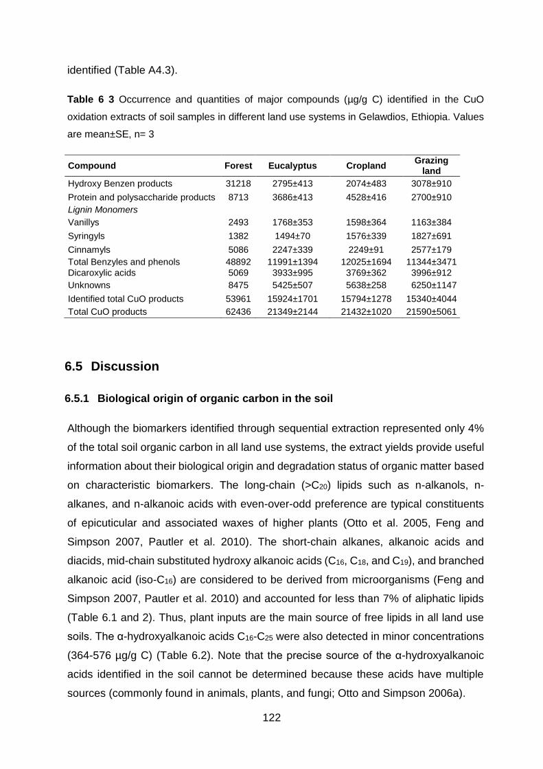
122

identified (Table A4.3).

Table 6 3 Occurrence and quantities of major compounds (µg/g C) identified in the CuO

oxidation extracts of soil samples in different land use systems in Gelawdios, Ethiopia. Values

are mean±SE, n= 3

Compound Forest Eucalyptus Cropland Grazing

land

Hydroxy Benzen products 31218 2795±413 2074±483 3078±910

Protein and polysaccharide products 8713 3686±413 4528±416 2700±910

Lignin Monomers

Vanillys 2493 1768±353 1598±364 1163±384

Syringyls 1382 1494±70 1576±339 1827±691

Cinnamyls 5086 2247±339 2249±91 2577±179

Total Benzyles and phenols 48892 11991±1394 12025±1694 11344±3471

Dicaroxylic acids 5069 3933±995 3769±362 3996±912

Unknowns 8475 5425±507 5638±258 6250±1147

Identified total CuO products 53961 15924±1701 15794±1278 15340±4044

Total CuO products 62436 21349±2144 21432±1020 21590±5061

6.5 Discussion

6.5.1 Biological origin of organic carbon in the soil

Although the biomarkers identified through sequential extraction represented only 4%

of the total soil organic carbon in all land use systems, the extract yields provide useful

information about their biological origin and degradation status of organic matter based

on characteristic biomarkers. The long-chain (>C20) lipids such as n-alkanols, n-

alkanes, and n-alkanoic acids with even-over-odd preference are typical constituents

of epicuticular and associated waxes of higher plants (Otto et al. 2005, Feng and

Simpson 2007, Pautler et al. 2010). The short-chain alkanes, alkanoic acids and

diacids, mid-chain substituted hydroxy alkanoic acids (C16, C18, and C19), and branched

alkanoic acid (iso-C16) are considered to be derived from microorganisms (Feng and

Simpson 2007, Pautler et al. 2010) and accounted for less than 7% of aliphatic lipids

(Table 6.1 and 2). Thus, plant inputs are the main source of free lipids in all land use

soils. The α-hydroxyalkanoic acids C16-C25 were also detected in minor concentrations

(364-576 µg/g C) (Table 6.2). Note that the precise source of the α-hydroxyalkanoic

acids identified in the soil cannot be determined because these acids have multiple

sources (commonly found in animals, plants, and fungi; Otto and Simpson 2006a).

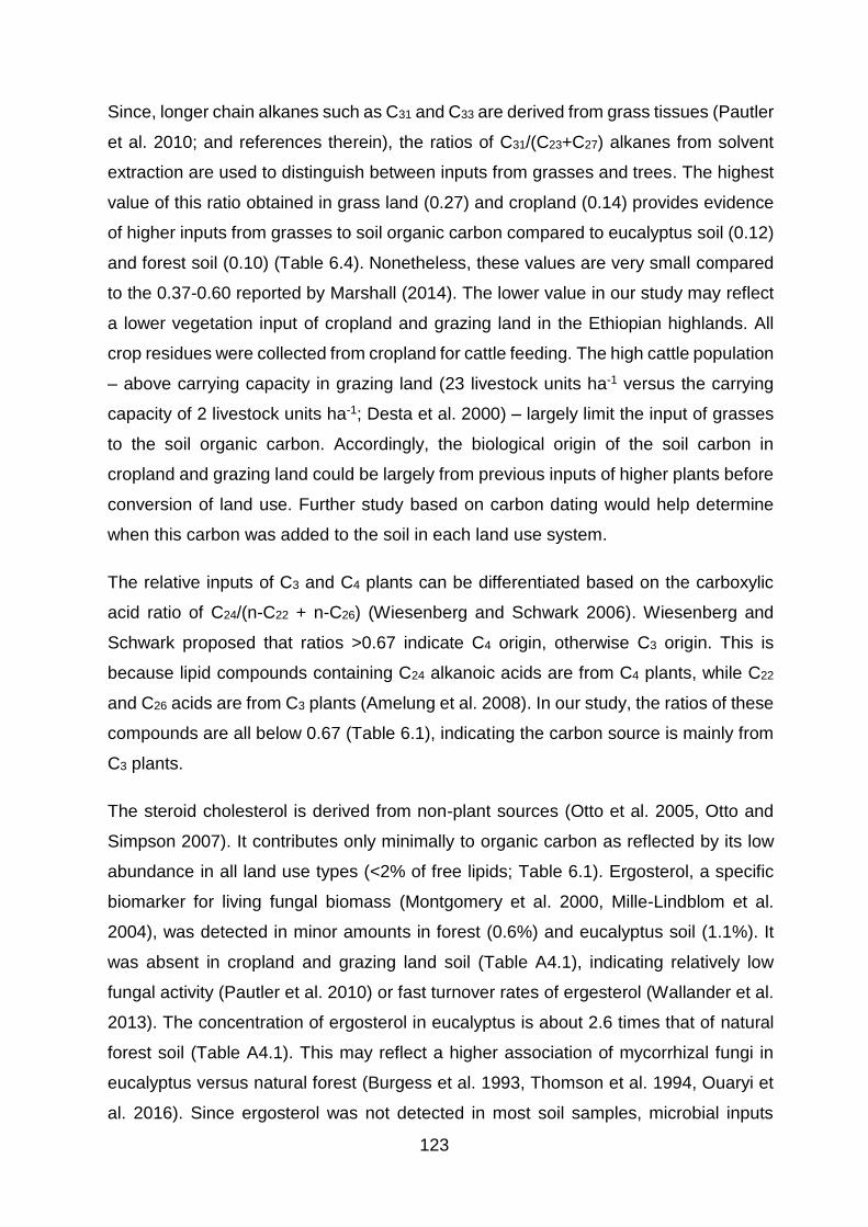
123

Since, longer chain alkanes such as C31 and C33 are derived from grass tissues (Pautler

et al. 2010; and references therein), the ratios of C31/(C23+C27) alkanes from solvent

extraction are used to distinguish between inputs from grasses and trees. The highest

value of this ratio obtained in grass land (0.27) and cropland (0.14) provides evidence

of higher inputs from grasses to soil organic carbon compared to eucalyptus soil (0.12)

and forest soil (0.10) (Table 6.4). Nonetheless, these values are very small compared

to the 0.37-0.60 reported by Marshall (2014). The lower value in our study may reflect

a lower vegetation input of cropland and grazing land in the Ethiopian highlands. All

crop residues were collected from cropland for cattle feeding. The high cattle population

– above carrying capacity in grazing land (23 livestock units ha-1 versus the carrying

capacity of 2 livestock units ha-1; Desta et al. 2000) – largely limit the input of grasses

to the soil organic carbon. Accordingly, the biological origin of the soil carbon in

cropland and grazing land could be largely from previous inputs of higher plants before

conversion of land use. Further study based on carbon dating would help determine

when this carbon was added to the soil in each land use system.

The relative inputs of C3 and C4 plants can be differentiated based on the carboxylic

acid ratio of C24/(n-C22 + n-C26) (Wiesenberg and Schwark 2006). Wiesenberg and

Schwark proposed that ratios >0.67 indicate C4 origin, otherwise C3 origin. This is

because lipid compounds containing C24 alkanoic acids are from C4 plants, while C22

and C26 acids are from C3 plants (Amelung et al. 2008). In our study, the ratios of these

compounds are all below 0.67 (Table 6.1), indicating the carbon source is mainly from

C3 plants.

The steroid cholesterol is derived from non-plant sources (Otto et al. 2005, Otto and

Simpson 2007). It contributes only minimally to organic carbon as reflected by its low

abundance in all land use types (<2% of free lipids; Table 6.1). Ergosterol, a specific

biomarker for living fungal biomass (Montgomery et al. 2000, Mille-Lindblom et al.

2004), was detected in minor amounts in forest (0.6%) and eucalyptus soil (1.1%). It

was absent in cropland and grazing land soil (Table A4.1), indicating relatively low

fungal activity (Pautler et al. 2010) or fast turnover rates of ergesterol (Wallander et al.

2013). The concentration of ergosterol in eucalyptus is about 2.6 times that of natural

forest soil (Table A4.1). This may reflect a higher association of mycorrhizal fungi in

eucalyptus versus natural forest (Burgess et al. 1993, Thomson et al. 1994, Ouaryi et

al. 2016). Since ergosterol was not detected in most soil samples, microbial inputs

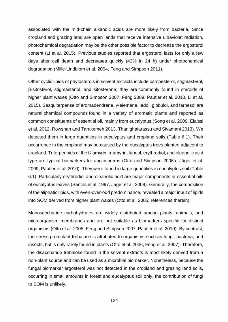
124

associated with the mid-chain alkanoic acids are more likely from bacteria. Since

cropland and grazing land are open lands that receive intensive ultraviolet radiation,

photochemical degradation may be the other possible factor to decrease the ergosterol

content (Li et al. 2015). Previous studies reported that ergosterol lasts for only a few

days after cell death and decreases quickly (43% in 24 h) under photochemical

degradation (Mille-Lindblom et al. 2004, Feng and Simpson 2011).

Other cyclic lipids of phytosterols in solvent extracts include campesterol, stigmasterol,

β-sitosterol, stigmastanol, and sitosterone; they are commonly found in steroids of

higher plant waxes (Otto and Simpson 2007, Feng 2009, Pautler et al. 2010, Li et al.

2015). Sesquiterpense of aromadendrene, γ-elemene, ledol, globulol, and farnesol are

natural chemical compounds found in a variety of aromatic plants and reported as

common constituents of essential oil, mainly from eucalyptus (Song et al. 2009, Elaissi

et al. 2012, Rowshan and Tarakemeh 2013, Thanighaiarassu and Sivamani 2013). We

detected them in large quantities in eucalyptus and cropland soils (Table 6.1). Their

occurrence in the cropland may be caused by the eucalyptus trees planted adjacent to

cropland. Triterpenoids of the ß-amyrin, α-amyrin, lupeol, erythrodiol, and oleanolic acid

type are typical biomarkers for angiosperms (Otto and Simpson 2006a, Jäger et al.

2009, Pautler et al. 2010). They were found in large quantities in eucalyptus soil (Table

6.1). Particularly erythrodiol and oleanolic acid are major components in essential oils

of eucalyptus leaves (Santos et al. 1997, Jäger et al. 2009). Generally, the composition

of the aliphatic lipids, with even-over-odd predominance, revealed a major input of lipids

into SOM derived from higher plant waxes (Otto et al. 2005; references therein).

Monosaccharide carbohydrates are widely distributed among plants, animals, and

microorganism membranes and are not suitable as biomarkers specific for distinct

organisms (Otto et al. 2005, Feng and Simpson 2007, Pautler et al. 2010). By contrast,

the stress protectant trehalose is attributed to organisms such as fungi, bacteria, and

insects, but is only rarely found in plants (Otto et al. 2006, Feng et al. 2007). Therefore,

the disaccharide trehalose found in the solvent extracts is most likely derived from a

non-plant source and can be used as a microbial biomarker. Nonetheless, because the

fungal biomarker ergosterol was not detected in the cropland and grazing land soils,

occurring in small amounts in forest and eucalyptus soil only, the contribution of fungi

to SOM is unlikely.

125

Suberin is a characteristic biomacromolecule of roots and bark of vascular plants (Otto

and Simpson 2007) and is thus used to trace mainly belowground plant origin,

assuming that bark contributes little to soil organic carbon. Cutin is produced in the

epidermal cells to form a protective barrier on leaves, flowers, and fruits of vascular

plants and can be used to estimate the input of organic matter originating from shoot

biomass (Nierop 1998, Nierop et al. 2006). Due to the compositional similarity of

suberin and cutin, the differentiation of characteristic biomarkers for both sources is

difficult. Some compounds derived from plant waxes or the lingo-cellulose complex

show signal overlap (Otto and Simpson 2006a), and they were excluded here as

characteristic suberin or cutin biomarkers. Therefore, from the detected compounds,

typical suberin biomarkers (ΣS) include ω-hydroxyalkanoic acid (≥C20) and α, ω-

alkanoic acids (C16-C24). They represented 1.4% (322 µg/g C) of the identified bound

lipids in grazing land soil to 7.5% (1247 µg/g C) in forest soil (Table 6.2). Compounds

of C16 mono-and dihydroxy acids and diacids represented <1.4% (126-305 µg/g C;

Table 6.2) and are used as cutin biomarker signatures (Otto and Simpson 2006a).

Biomarkers derived from either suberin or cutin (ΣSvC) are ω-hydroxyalkanoic acids

C16, C18, C18 di- and trihydroxy acids, and α, ω-alkanedioic acids C16, C18 and

accounted for 3-6% of identified bound lipids (551-1035 µg/g C; Table 6.2). The

combined suberin and cutin represented 8-19% of aliphatic lipids. The relative

proportion of suberin was about 2 time that of cutin in forest, eucalyptus, and cropland

soils, whereas in grazing land soil, suberin and cutin concentrations were similar (Table

6.4). This shows that below-ground biomass in the forest ecosystem contributed about

twice the organic carbon than above-ground parts. In cropland, all crop residues are

harvested for either cattle fodder or fuel and, thus, the remaining part is crop roots that

may increase the contribution of suberin compared to cutin. Since forest-derived

monomers are preserved in the soil for more than 50 years, the higher suberin content

in cropland seemed to be derived from former forest vegetation (Mendez-Millan et al.

2012). The lower suberin concentration in grazing land may be because grass-derived

monomers degrade rapidly compared with forest-derived monomers of the same

compound classes in tropical soils (Hamer et al. 2012). The ω-hydroxy carboxylic acids

and α, ω-alkanedioic acids of forest origin may have been stabilized in the soils by

bonding to soil minerals. In addition, Hamer and coauthors found a more than five-times

higher concentration of x,16-diOH C16:0 compounds in forest litter than in grass

biomass, potentially explaining the greater proportion of forest-derived monomer. In

126

general, the composition of the bound soil lipids extracted by base hydrolysis such as

aliphatic lipids (6.8-14.8 mg/g C) and phenols (0.4-2.3 mg/g C; Table 6.1, 6.2) mainly

originate from suberin, cutin, and plant surface wax esters (Hedges and Ertel 1982,

Otto et al. 2005, Otto and Simpson 2006a). This reflects major inputs by vascular plants

and minor inputs by microorganisms to soil carbon.

The observed phenols (p-hydroxyacetophenone, 4-hydroxybenzoic acid, vanillyl,

acetovanillone, vanillic acid, isovanillic acid, p-coumaric acid, ferulic acid compounds)

are reported to be characteristic for lignin monomers (Otto and Simpson 2007).

Nonetheless, the phenols identified in the bound lipid fractions are likely derived from

the ester-bound aromatic constituents of suberin and the lignocellulose complex

(Kögel-Knabner 2000, Otto et al. 2005). This is because the applied base hydrolysis

cleaves esters, but not ethers (Otto et al. 2005). According to Pautler et al. (2013), the

observed phenols after alkaline hydrolysis are likely derived from suberin and/or

lignocelluloses as they are connected by ester bonds within these biopolymers (rather

than from the lignin cell wall biopolymers, which are linked by ether bonds).

CuO oxidation released mainly lignin-specific phenols from the lignin polymer. These

refer to the sum of vanillyl, syringyl, and cinnamyl phenols, which are essential

components of the cell walls of vascular plants (Table 6.3; Goñi and Hedges 1992).

These phenols accounted for more than 52% of all CuO products in all land use

systems (Table 6.3). Benzoic acid, p-hydroxybenzaldehyde, 4-hydroxybenzeneacetic

acid, pyrrol-1-carboxylic acid, and short-chain dicarboxylic acids are considered to be

the oxidation products of proteinaceous and polysaccharide material (Goñi and

Montgomery 2000, Otto et al. 2005, Tesi et al. 2014). In contrast, tannins and other

flavonoids have been suggested as the sources for 3,5-dihydroxy benzoic acid (Otto et

al. 2006). According to Otto et al. (2005) the exact source of 2,4,6-trihydroxybenzoic

acid is not known, although similar compounds such as 1,2,4- and 1,3,5-

trihydroxybenzoic acids have been reported as black carbon markers from thermal

alteration of parent structures (Kuo et al. 2008). These compounds may thus indicate

biochar residues remaining after conversion of forest to other land use types using fire

as a tool or during (illegal) charcoal production in the forest. Overall, the occurrences

and concentrations of benzyls and lignin-derived phenols are about 2 times higher in

forest soil than other land use soils. This points to a predominant input of recalcitrant

organic carbon into the forest ecosystem derived from higher plants.

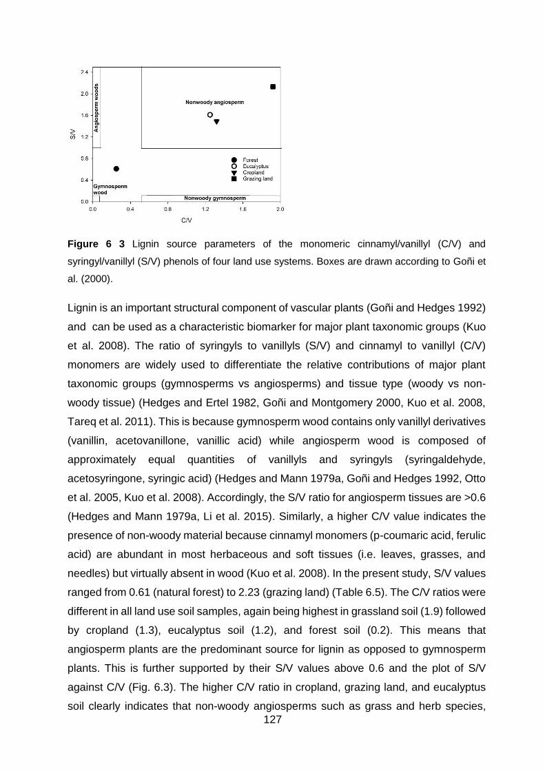
127

Figure 6 3 Lignin source parameters of the monomeric cinnamyl/vanillyl (C/V) and

syringyl/vanillyl (S/V) phenols of four land use systems. Boxes are drawn according to Goñi et

al. (2000).

Lignin is an important structural component of vascular plants (Goñi and Hedges 1992)

and can be used as a characteristic biomarker for major plant taxonomic groups (Kuo

et al. 2008). The ratio of syringyls to vanillyls (S/V) and cinnamyl to vanillyl (C/V)

monomers are widely used to differentiate the relative contributions of major plant

taxonomic groups (gymnosperms vs angiosperms) and tissue type (woody vs non-

woody tissue) (Hedges and Ertel 1982, Goñi and Montgomery 2000, Kuo et al. 2008,

Tareq et al. 2011). This is because gymnosperm wood contains only vanillyl derivatives

(vanillin, acetovanillone, vanillic acid) while angiosperm wood is composed of

approximately equal quantities of vanillyls and syringyls (syringaldehyde,

acetosyringone, syringic acid) (Hedges and Mann 1979a, Goñi and Hedges 1992, Otto

et al. 2005, Kuo et al. 2008). Accordingly, the S/V ratio for angiosperm tissues are >0.6

(Hedges and Mann 1979a, Li et al. 2015). Similarly, a higher C/V value indicates the

presence of non-woody material because cinnamyl monomers (p-coumaric acid, ferulic

acid) are abundant in most herbaceous and soft tissues (i.e. leaves, grasses, and

needles) but virtually absent in wood (Kuo et al. 2008). In the present study, S/V values

ranged from 0.61 (natural forest) to 2.23 (grazing land) (Table 6.5). The C/V ratios were

different in all land use soil samples, again being highest in grassland soil (1.9) followed

by cropland (1.3), eucalyptus soil (1.2), and forest soil (0.2). This means that

angiosperm plants are the predominant source for lignin as opposed to gymnosperm

plants. This is further supported by their S/V values above 0.6 and the plot of S/V

against C/V (Fig. 6.3). The higher C/V ratio in cropland, grazing land, and eucalyptus

soil clearly indicates that non-woody angiosperms such as grass and herb species,

128

which contain abundant cinnamyl phenols, are the predominant sources of lignin.

Although degradation might affect these ratios and can alter the original plant

composition (Tesi et al. 2014), both angiosperm woody and non-woody tissues are

equally important for SOM accumulation in the natural forest ecosystem. These lowest

S/V and C/V values in natural forest soil reflect a mixture of different angiosperm

species and to some extent gymnosperm woody and non-woody (leaves) sources. This

indicates that the forest was probably once covered by an Olive-Juniper-Podocarpus

forest as evidenced by the presence of Podocarpus falcatus species inside the natural

forest and scattered Olea africana and Juniperus procera trees in the surrounding area

and compounds of Gelawdios church. This, however, calls for further study on the

history of the forest. Gymnosperms yield higher amounts of ω-C16/∑C16 acids relative

to angiosperms (Pisani et al. 2013) and this may lower the S/V ratios, as indicated by

more abundant ω-C16 acids in the forest ecosystem (Table 6.4). Other studies also

reported lower S/V values for conifer-dominated species. For example, Li et al. (2015)

reported a low S/V value (0.23) under pine-dominated forests and 0.84 for farmland

soils. The lignin-derived phenols (V:S:C) ratios are also used to estimate the relative

contributions of woody and non-woody angiosperms; the latter exhibit a ratio of about

1:1:1 (Hedges and Mann 1979a, Kögel-Knabner 2000, Otto et al. 2006). The lignin-

derived phenols detected in our samples exhibited a V:S:C ratio of 4:2:1 (forest soil)

and 1:1:1 (eucalyptus, cropland, and grazing land soils) (Table 6.4). The relatively equal

ratio in the latter three soils further confirms that lignin-derived phenols originate mainly

from non-woody angiosperm sources. This is consistent with the S/V and C/V ratios.

The higher V:S:C ratio in the natural forest indicates that woody angiosperms contribute

significantly to soil organic carbon. However, the lignin index-phenols and their ratios

do not give a fine resolution spectrum to distinguish sources among angiosperms,

gymnosperms, and non-woody contributions. This is because of the complex mixture

of different plants as well as the different diagenetic reactivity of cinnamyl, syringyl, and

vanillyl groups (Tareq et al. 2011). To improve the detection of lignin sources, another

useful parameter (lignin phenol vegetation index – LPVI) was developed by Tareq et

al. (2004). LPVI provides a better resolution of the lignin sources based on the relative

abundances of vanillyl, syringyl, and cinnamyl-type phenols. Tareq et al. (2011)

calculated the LPVI values from lignin-phenol data of Hedges and Mann (1979). This

yielded values of 1 for gymnosperm wood, 3-27 for non-woody gymnosperm tissues,

67-415 for angiosperm wood, and 176-2782 for non-woody angiosperms (Tareq et al.

129

2004). In the present study, the LPVI values of the natural forest (92) are in the range

of angiosperm woods. In contrast, soil samples from eucalyptus (880), cropland (901),

and grazing land (2051) show characteristics for non-woody angiosperms, which is

consistent with plots of S/V vs C/V (Fig. 6.4).

6.5.2 Degradation stage of plant organic matter

Soil lipids are highly resistant to biodegradation (Kögel-Knabner 2000), but the extent

of lipid degradation depends on microbial activity and physico-chemical conditions

(Nierop et al. 2005, Otto et al. 2005). The aliphatic/cyclic lipid ratio is a general

parameter to assess the degradation of free lipids in the soil (Otto and Simpson 2006a,

Li et al. 2015). After solvent extraction, the aliphatic/cyclic lipids ratios were 22 (forest),

1.4 (eucalyptus), 3.4 (cropland), and 4.4 (grazing land). The lowest value (1.4) suggests

that cyclic lipids are better preserved in eucalyptus soil. In the natural forest soil, the

highest ratio is due to less accumulation of cyclic lipids and continuous input of aliphatic

lipids into the soil.

The suberin/cutin ratios are important parameters to describe bound lipid degradation.

Suberin is more resistant to degradation than cutin due to its contents of ω-

hydroxyalkanoic acids and phenolic units (Goñi & Hedges 1990; Otto et al. 2005; and

references therein). In this study the suberin/cutin ratios were 1.9 (forest), 1.7

(eucalyptus), 1.9 (cropland), and 1.1 (grazing land) (Table 6.4). The higher ratios in

forest, eucalyptus, and cropland soils compared to grazing land indicate preferential

degradation of cutin over suberin. Mendez-Millan et al. (2012) showed that 58-63% of

the forest-derived suberin monomers such as C18 di- and trihydroxy and epoxy acids

are preserved in the soil for more than 53 years. In contrast, cutin monomers such as

C16 mono-and dihydroxy acids, amounting to a maximum of 37-42%, are preserved

only for 20 years in pastureland. Moreover, grass-derived monomers degrade rapidly

compared with forest-derived monomers of the same compound classes due to their

chemical structure (Hamer et al. 2012). This yields the lowest ratio in grassland soil

(Table 6.4). The ω-hydroxy carboxylic acids and α, ω-alkanedioic acids of forest origin

may have been stabilized by bonding to soil minerals. The higher suberin/cutin ratio in

cropland is mainly due to the removal of above-ground biomass after crop harvest along

with selective degradation of cutin over suberin. Increased ratios of ω-C16/∑C16 and

ω-C18/∑C18 have been reported with progressing cutin degradation in marine

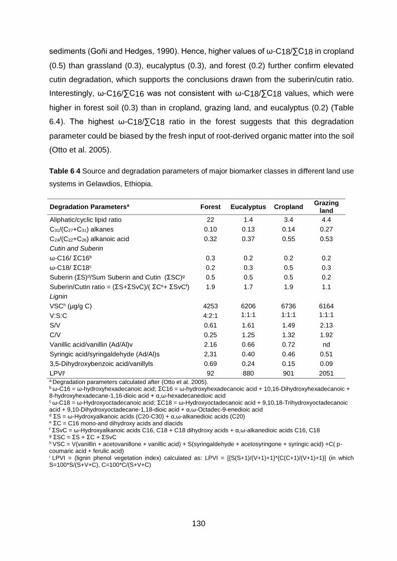
130

sediments (Goñi and Hedges, 1990). Hence, higher values of ω-C18/∑C18 in cropland

(0.5) than grassland (0.3), eucalyptus (0.3), and forest (0.2) further confirm elevated

cutin degradation, which supports the conclusions drawn from the suberin/cutin ratio.

Interestingly, ω-C16/∑C16 was not consistent with ω-C18/∑C18 values, which were

higher in forest soil (0.3) than in cropland, grazing land, and eucalyptus (0.2) (Table

6.4). The highest ω-C18/∑C18 ratio in the forest suggests that this degradation

parameter could be biased by the fresh input of root-derived organic matter into the soil

(Otto et al. 2005).

Table 6 4 Source and degradation parameters of major biomarker classes in different land use

systems in Gelawdios, Ethiopia.

Degradation Parametersa Forest Eucalyptus Cropland Grazing

land

Aliphatic/cyclic lipid ratio 22 1.4 3.4 4.4

C31/(C27+C31) alkanes 0.10 0.13 0.14 0.27

C24/(C22+C26) alkanoic acid 0.32 0.37 0.55 0.53

Cutin and Suberin

ω-C16/ ΣC16b 0.3 0.2 0.2 0.2

ω-C18/ ΣC18c 0.2 0.3 0.5 0.3

Suberin (ΣS)d/Sum Suberin and Cutin (ΣSC)g 0.5 0.5 0.5 0.2

Suberin/Cutin ratio = (ΣS+ΣSvC)/( ΣCe+ ΣSvCf) 1.9 1.7 1.9 1.1

Lignin

VSCh (µg/g C) 4253 6206 6736 6164

V:S:C 4:2:1 1:1:1 1:1:1 1:1:1

S/V 0.61 1.61 1.49 2.13

C/V 0.25 1.25 1.32 1.92

Vanillic acid/vanillin (Ad/Al)v 2.16 0.66 0.72 nd

Syringic acid/syringaldehyde (Ad/Al)s 2,31 0.40 0.46 0.51

3,5-Dihydroxybenzoic acid/vanillyls 0.69 0.24 0.15 0.09

LPVIi 92 880 901 2051 a Degradation parameters calculated after (Otto et al. 2005). b ω-C16 = ω-hydroxyhexadecanoic acid; ΣC16 = ω-hydroxyhexadecanoic acid + 10,16-Dihydroxyhexadecanoic + 8-hydroxyhexadecane-1,16-dioic acid + α,ω-hexadecanedioic acid c ω-C18 = ω-Hydroxyoctadecanoic acid; ΣC18 = ω-Hydroxyoctadecanoic acid + 9,10,18-Trihydroxyoctadecanoic acid + 9,10-Dihydroxyoctadecane-1,18-dioic acid + α,ω-Octadec-9-enedioic acid d ΣS = ω-Hydroxyalkanoic acids (C20-C30) + α,ω-alkanedioic acids (C20) e ΣC = C16 mono-and dihydroxy acids and diacids f ΣSvC = ω-Hydroxyalkanoic acids C16, C18 + C18 dihydroxy acids + α,ω-alkanedioic acids C16, C18 g ΣSC = ΣS + ΣC + ΣSvC h VSC = V(vanillin + acetovanillone + vanillic acid) + S(syringaldehyde + acetosyringone + syringic acid) +C( p-coumaric acid + ferulic acid) i LPVI = (lignin phenol vegetation index) calculated as: LPVI = [{S(S+1)/(V+1)+1}*{C(C+1)/(V+1)+1}] (in which S=100*S/(S+V+C), C=100*C/(S+V+C)

131

Lignin is among the best preserved components in the soil organic matter due to its

greater stability to biodegradation (Kuo et al. 2008). Its recalcitrance plays a significant

role in the biospheric carbon cycle (Colberg, 1988) and has been extensively used in

characterizing the degradation stage of soil organic matter (Tesi et al. 2014).

Biodegradation of lignin is mainly governed by white-rot and brown-rot fungi by

oxidative cleavage (Hedges and Mann 1979a). The yields of VSC and the ratios of

lignin-derived phenolic acids to corresponding aldehydes of vanillyl and syringyl units

(Ad/Al)v, (Ad/Al)s, and 3,5-dihydroxybenzoic acid (DHBA)/V are generally used as

indicators of the level of lignin degradation in the soil (Hedges and Mann 1979a, Goñi

and Montgomery 2000, Otto et al. 2005, Otto and Simpson 2006b). Based on total

lignin-index phenols, the yields of VSC were in the order: cropland (6.7 mg/g C), grazing

land and eucalyptus (6.2 mg/g C), and forest soil (4.2 mg/g C). Accordingly, lignin

compounds are least preserved in forest soils (Table 6.4). Since these values are

normalized to soil carbon contents, the lowest value of lignin in the natural forest can

be biased by the different inputs of organic matter into the soil. The presence of fungi

in this ecosystem, however, as indicated by the ergosterol biomarker, may contribute

to lower VSC yields in the forest but has little effect on the eucalyptus soil. The lowest

S/V (0.6) and C/V (0.2) ratios are in forest, with values in the other land use soils

exceeding 1.2 (Table 6.4). This indicates preferential degradation of syringyls and

cinnamyls monomers. The explanation is that cinnamyls link the carbohydrates and

lignin in the ligno-cellulose complex, making them more accessible to decomposition

than vanillyls (Feng & Simpson 2007, and references therein). Syringyls were also

reported to degrade faster than vanillyls in the environment, while vanillyls accumulate

more than cinnamyls and syringyls (Hedges et al. 1984, Otto et al. 2005)

Previous studies report that fresh angiosperm wood has Ad/Al ratios of 0.1-0.5 for both

syringyl and vanillyl units; higher values of 0.2-1.6 were recorded for fresh non-woody

tissues such as leaves and grasses (Goñi and Hedges 1992, Otto and Simpson 2006b,

Pisani et al. 2013). The Ad/Alv ratios for the samples analyzed in the present study were

highest in forest soil (2.2) followed by cropland and grazing land soil (0.7). In addition,

the (Ad/Al)s ratio was higher (2.3) in the forest soil than eucalyptus soil (0.4), cropland

and grazing land (0.5) (Table 6.4) suggesting the preferential degradation of

syringaldehyde over syringic acid. Finally, forest soils may be more oxidized due to the

optimal soil conditions for lignin-degrading fungi, as indicated by the presence of

132

ergosterol and the soil pH, temperature, moisture values (Pisani et al. 2013). The 3, 5-

dihydroxybenzoic acid to vanillyls ratio was in the order: forest (0.69), eucalyptus (0.24),

cropland (0.15), and grazing land (0.09) (Table 6.4). The highest value in forest soil

shows increased degradation of tannins because 3,5-dihydroxybenzoic acid after CuO

oxidation was derived from tannin oxidation (Li et al. 2015). Combining the evidence of

the degradation parameters, enhanced degradation of lignin occurred in the forest soil

as indicated by elevated acid/aldehyde (Ad/Al) ratios of vanillyl and syringyl units and

3,5-dihydroxybenzoic acid /vanillyls.

6.6 Conclusions

Overall, aliphatic lipids and lignin accounted for 46-84% of the total detected chemicals.

This demonstrated that the major input of soil organic carbon is from higher plants. The

short-chain alkanoic acids, ergosterol, and the disaccharide trehalose accounted for

less than 7% of aliphatic lipids in all land use soils, pointing to minor microbial inputs.

Ergosterol, however, a fungal biomarker, was not detected in the cropland and grazing

land soils, and occurred in only small amounts in forest and eucalyptus soil.

Accordingly, the microbial input more likely originates from bacteria. The high S/V and

C/V ratios (except for the forest ecosystem) indicate that non-woody angiosperm

tissues – mainly from C3 plants – are major contributors among the taxonomic groups.

This is because syringyl and cinnamyl monomers are abundant in most herbaceous

and soft tissues but virtually absent in wood. The lowest S/V and C/V values obtained

in forest soil reflect a mixture of different sources including woody angiosperms and

gymnosperms. A higher VSC ratio and higher LPVI values in the forest soil than in other

land use systems further provide a better resolution of the lignin sources: woody

angiosperms are equally important in contributing to soil organic carbon. The

terpenoids such as the ß-amyrin, α-amyrin, lupeol, and erythrodiol are also typical

biomarker for angiosperms. In the forest, eucalyptus, and cropland soils, root biomass

contributed C input in the soil twice compared to above-ground parts, as revealed by

their relative proportions of suberin and cutin. In addition, the highest suberin to cutin

ratio indicates that suberin is more resistant to degradation than cutin (due to contents

of ω-hydroxyalkanoic acids and high mineral bonding capacity of phenolic units in

suberin). The ratios of lignin-index phenols revealed that syringyls and cinnamyls are

degraded faster than vanillyls. In general, lignin degradation was enhanced in the forest

soil, as indicated by elevated acid/aldehyde (Ad/Al) ratios of vanillyl and syringyl units.

133

7 Microbial soil respiration and its dependency on

substrate availability and temperature in four contrasting

land use systems

7.1 Abstract

Soil organic carbon (SOC) is a fundamental part of the carbon cycle. Soil microorganisms are

the center of the biological activity regulating the breakdown and accumulation of SOC stocks

as well as the CO2 efflux to the atmosphere. Nevertheless, the extent to which substrate

availability and quality affects microbial functioning is largely unknown. This study was therefore

designed to determine the amount of CO2 effluxes from different ecosystems to the atmosphere

along a temperature gradient with or without carbon sources. Glucose, lignin, and starch were

added as proxies for substrate availability. Ammonium nitrate and calcium phosphate were also

included to determine whether microbes are limited by nutrient deficiency. The investigation is

based on the use of the MicroResp method containing a cresol red gel carrying colorimetric

indicator. This enables measuring the amount of CO2 evolved from the soil along the

temperature gradient. We found that basal respiration ranged from 0.4±0.1 to 0.9±0.1 µg CO2-

C g soil-1 h-1, which is consistent with the SOC content. Nonetheless, a strong C use efficiency

was observed at lower C content in the soil, as indicated by elevated specific basal respiration

in cropland and grazing land. Respiration rates were higher in the soils where carbon sources

(glucose, lignin, starch) were added, and microbes showed a preferential degradation of

substrates. In contrast to the conventional belief that aromatic structures are recalcitrant and

stable in soil, lignin was preferentially degraded over starch substrate. Microbial respiration in

the nutrient (N and P) addition soils was significantly lower than in soils supplied with carbon

sources, but did not differ significantly from control soil. The contribution of microbial biomass

carbon (MBc) to soil organic carbon was generally <1% of total organic carbon in the soil for all

land use types, but forest soil had twice-higher levels of MBc than other land use systems. The

ratio of basal respiration to microbial biomass carbon (metabolic quotient; qCO2) ranged from

2.1 (forest soil) to 3.9 (eucalyptus soil), reflecting higher microbial C use efficiency under

eucalyptus. The microbial communities released more CO2 per unit microbial biomass under

acidic soil conditions. Generally, microbial respiration increased with temperature in all land

use systems, but at a decreasing rate above 25°C, and the Q10 values declined at high

temperature and at lower substrate availability.

Keywords: SOC, microbial respiration, temperature sensitivity, substrate, nutrient, microbial

quotient, land use change, CO2 efflux

134

7.2 Introduction

Soil is the largest terrestrial carbon pool (3150 Pg C; Fan et al., 2016), accounting for

more than four times the amount of carbon in the atmosphere, (750 Pg C) and is a

fundamental part of carbon cycle and life on Earth (Batjes 1996, Hiederer and Köchy

2011). This pool is a result of an imbalance between organic matter production and its

decomposition, and is a source of CO2 to the atmosphere (Yuste et al. 2007). Soil

microorganisms regulate the breakdown of organic matter and determine SOC stocks

in the soil as well as the CO2 efflux to the atmosphere (Bradford 2013). These

microorganisms decompose organic matter and assimilate the produced low molecular

weight organic compounds from the soil environment. Thus, microorganisms

themselves account for 1-3% of soil organic C (Martens 1995, Wang and Sainju 2014).

Soil microbial respiration releases about 60 Pg of carbon per year to the atmosphere

as CO2 (Shao et al. 2013). The source of this respiration is microbial decomposition of

soil organic matter (Kalinina et al. 2010) to obtain energy for growth and functioning.

The size of the CO2 flux is determined by temperature (Bradford et al. 2008), moisture

(Meisner et al. 2015), carbon input (Yuste et al. 2007), and nutrients such as N and P

(Gnankambary et al. 2008, Birgander et al. 2014). Respiration rates respond more

positively to increasing temperature than do photosynthetic rates (Frank et al. 2015).

This imbalance due to elevated microbial respiration rates implies that increased

temperature will lead to an increase in the net flux from soil to the atmosphere (Bradford

2013).

The extent to which indirect vs direct temperature effects on SOC dynamics along with

substrate availability and quality in different ecosystems is largely untested (Rousk et

al. 2012). Many studies have shown that soil microbial respiration increases with

temperature (Davidson and Janssens 2006, Allison et al. 2010, Karhu et al. 2014,

Mayer et al. 2016). This information, however, is uncertain because the response of

soil microbial communities to changing temperatures has the potential to either

decrease (Bradford et al. 2008, 2010) or increase (Hartley et al. 2008) soil microbial

respiration. For example, a study conducted from the Arctic to the Amazon along the

climate gradient reported that the strongest enhancing response occurred in soil from

cold climatic regions (Karhu et al. 2014). Similarly, Hartley et al. (2008) reported that

microbial activity acclimates to long-term temperature, greatly reducing the potential for

enhanced respiration in Arctic soils. Moreover, the relationship between soil microbial

135

respiration and substrate availability (C and nutrient sources) with changing

temperature at different land use systems remains uncertain. Many studies have

limitations in that they consider the response of microbial respiration to temperature

change, substrate availability, substrate quality, and anthropogenic effects only in one

particular ecosystem. Incorporating carbon and nutrient sources in different ecosystem

soils – and incubating soils at different temperatures prior to measuring CO2 production

– overcomes this limitation and may provide more realistic outcomes that reflect actual

ecosystem responses to temperature change. This makes it important to measure

biological activity in the soil, because this reflects the capacity of soil to support soil

microorganisms, the level of microbial activity, SOM content and its decomposition.

Conversion of tropical forest to other land use systems reduces soil carbon stocks

either through loss of C input or through C mineralization by microbes (Joergensen

2010). Guillaume et al., (2016) observed up to 70% soil organic carbon (SOC) losses

in the topsoil under oil palm and rubber plantations in Indonesia compared to rainforest.

SOC losses are also associated with a decline of soil quality and functions related to

microbial activity (Guillaume et al. 2016). This calls for determining the sensitivity of

biological indicators to land-use changes as well as to substrate and temperature

fluctuations. Microbial activity depends on SOC availability (Moorhead et al. 2014).

Thus, the basal respiration per unit of SOC can be used as an indicator of C availability

(Guillaume et al. 2016). The production of enzymes requires microbial investment of

energy in the form of C and nutrients, particularly N and P (Schimel and Weintraub

2003, Hernández et al. 2010). Accordingly, their activity may increase with the

increasing availability of labile C and nutrient fertilization. Microbial activity can be

simply regulated by providing C sources and by N or P fertilization (Schlentner and

Cleve 1985, Thirukkumaran and Parkinson 2000, Hernández et al. 2010). However,

the effects of these additions depend on the enzyme of interest (produced by

microorganisms) and on the quality of the substrates (Hernández et al. 2010). Further

indices such as the metabolic quotient (basal respiration to microbial biomass ratio;

qCO2) are the most widely used and reflect the carbon-use efficiency of microbial

communities. They are also suggested to reflect the soil function of supporting microbial

growth (Anderson and Domsch 1990, Joergensen 2010, Guillaume et al. 2016).

Many methods have been developed to measure microbial biomass and microbial

respiration, including the fumigation method (Jenkinson and Powlson 1976, Vance et

136

al. 1987), the substrate-induced respiration method (Anderson and Domsch 1978), and

the adenosine triphosphate (ATP) extraction method (Tate and Jenkinson 1982). In this

study, the microbial activity and biological indices were determined using the

MicroResp method in sieved soils under laboratory incubation. MicroResp is a

microplate-based respiration system which enables analyzing basal respiration and

substrate-induced respiration simultaneously (Campbell et al. 2003, Chapman et al.

2007, Renault et al. 2013). This helps in testing a range of C sources and substrate

qualities at different temperatures. This approach measures and characterizes CO2

production by microbial communities when the microbes feed on soil organic matter

(Campbell et al. 2003). Profiling microbial respiration on various substrates and at

various temperature provides an insight into the effects of rising atmospheric CO2

concentrations and the concomitant projected climate change scenarios, which have

unknown implications for long-term soil C storage (Renault et al. 2013). We

hypothesized that the efficiency of microbes in decomposing soil organic matter, and

the amount of CO2 efflux, are limited by the availability of C substrates and by N & P

deficiencies. The chemical composition of different soil SOM pools varies, being

composed of easily degradable compounds and of compounds more resistant to

microbial attack (Hernández et al. 2010). Which chemical structures are preferentially

consumed by microbes in the field at different temperatures remains unclear. The aim

of this study was therefore to determine fluxes of carbon from the soil to the atmosphere

at different temperatures with or without carbon sources in soils of different land use

systems. We examined the effect of temperature variation with the addition of glucose,

lignin, and starch as proxies for substrate availability of contrasting recalcitrance on

CO2 efflux from soil relative to soils receiving water alone. We also examined the effect

of N and P nutrients to determine whether microbial activity is N or P limited. This was

done on soils from four contrasting land use systems: natural forest, eucalyptus

plantation, grazing land, and cropland. The amount of CO2 evolved from the soil and

its response to temperature change was measured using the MicroResp method on

sieved soils under laboratory incubation.

137


7.3.1 Site description

Four land use systems (natural forest, eucalyptus plantation, cropland, grazing land)

were selected in Gelawdios, north-central Ethiopia. The study area (Gelawdios) is

located at 11°38’25’’ N and 37°48’55’’ E at an elevation of 2500 m above sea level

(a.s.l.). The topography is typical of volcanic landscapes, comprising volcanic rocks

with ragged and undulating landforms. The major soil type is classified as Cambisols

with a clay loam texture according to the World Reference Base for soil resources

(WRB 2014). The mean annual rainfall at Gelawdios is 1220 mm, with a unimodal rainy

season with the main rainfall months between June and September; the average

annual temperature is 19°C (Wassie et al. 2009). Although Ethiopia is geographically

located in the tropics, the climate of the study areas is temperate with dry winters and

warm summers (Cwb) according to the Köppen-Geiger climate classification (Peel et

al. 2007). The forest is a pristine Afromontane dry forest composed mostly of a mixture

of indigenous tree species and is almost exclusively confined to sacred groves

associated with churches. The dominant tree species are Albizia schimperiana,

Apodytes dimidiata, Calpurnia aurea, Croton macrostachyus, Ekebergia capensis,

Maytenus arbutifolia, and Schefflera abyssinica. The eucalyptus stand was established

on formerly common grazing land in 1985 and was successively thinned to its current

density about 3000 trees per hectare. The adjacent grazing land and cropland were

converted from natural forest approximately 50 years ago (exact date unknown). The

grazing land was used as communal grazing lands for herds of animals; it is highly

degraded, nearly bare ground. The cropland has been cultivated without fallow, and all

crop residues are harvested to feed cattle at home.

7.3.2 Soil sampling

Soils were collected in September 2015 from the four land use systems (natural forest,

eucalyptus plantation, grazing land, and cropland). Soils were taken in the first 10 cm

depth from three sampling points along a transect line. The distance between sampling

points was 200 m in the natural forest and 50 m in the other land use types. Soils were

sieved through a 2 mm stainless sieve in Ethiopia and transported to Vienna for further

laboratory analysis. They were stored at 4°C in zipped bags until use in the

138

experiments. All lab analyses were done at University of Natural Resources and Life

Sciences, Vienna (Austria).

7.3.3 Total C, N, and soil pH analysis

A subsample of approximately 3-5 g soil was dried at 105°C for 48 h for total carbon

and nitrogen analysis. Detailed procedures are provided in chapter 2. Total carbon and

nitrogen concentrations were determined on a CN elemental analyser (Truspec CNS

LECO, St. Joseph, USA). The analytical precision and reproducibility of the instrument

were determined based on an analysis of a calibration sample standard (Part No 502-

309 purchased from LECO). Soil pH was determined in 1:3 soil suspensions in 0.01 M

CaCl2 solution using a digital potentiometric pH-meter.

7.3.4 Determination of moisture content and water holding capacity

Soil moisture content was determined using subsamples of about 10 g soil, which were

dried at 105°C for 24 h. Another portion of soil samples (~20 g) was used to determine

water-holding capacity. The soils were soaked in water for 24 h and drained before

weighing. The soils were then dried in the oven at 105°C and re-weighed. We also

conducted preliminary runs to determine the appropriate water content in relation to

water holding capacity for maximum respiration. This prevented restricting the gaseous

exchange due to too wet or dry soil. From the available moisture content, the soils were

supplemented with deionized water to the desired water content of the soil (40, 50, 60,

70, 80, 90, and 100% of water holding capacity). Our pre-test showed that microbial

respiration was highest at 50-70% water holding capacity; below or above these values,

respiration declined. We therefore adjusted our samples to 40% water holding capacity

so that, after a carbon source in solution is added, the moisture content increased to

the required level of 50-70% water holding capacity. The soil without substrate also

received deionized water to reach 50-70% water holding capacity.

7.3.5 Preparation of carbon and nutrient sources

Three carbon sources (glucose, starch, lignin) that are ecologically relevant to soil were

selected based on the previously described studies (Campbell et al. 2003, García-

Palacios et al. 2013, Bao et al. 2015). Two additional nutrient sources (ammonium

nitrate and calcium phosphate) were included to determine whether microbes are

limited by N or P deficiencies. The concentrations of carbon and nutrient sources were

139

prepared so as to deliver 30 mg C, P or N per g of soil water (MicroResp technical

manual).

7.3.6 Preparing agar and indicator solution for the MicroResp

MicroResp detection plates were prepared according to the protocol provided by

MicroResp technical manual. In short, 3% Purified Agar (3 g per 100 ml) was prepared

in deionized water and dissolved by heating in a microwave to 120 °C until the agar

dissolves. Indicator solution was prepared in 1 L (18.25 mg cresol red, 16.77 g KCl,

0.315 g NaHCO3) and dissolved at 50°C, then filled up to end volume. Cresol is a water-

soluble indicator that changes color when it reacts with CO2. Once the temperature of

each solution has equilibrated at 60°C, the indicator solution and agar were transferred

into a beaker and mixed thoroughly with constant stirring. Then, 150 µL aliquots were

dispensed into the microplate using an 8-channel pipette. Precautions were taken

during dispensing to avoid bubbles in the wells. The plates were then stored in the dark

at room temperature in a desiccator with self-indicating soda lime on the base and a

beaker of water to keep the atmosphere CO2 free and moist.

7.3.7 Soil filling and incubation

We used sieved soil because it homogenizes the soils, removes rocks and roots, and

simplifies soil filling in the deep-well plates. The MicroResp consists of a 96-deep well

microplate to hold soil samples with a capacity of 1.2 ml, a 96-well detection plate,

MicroResp seal (silicone rubber gasket), and metal clamp to hold the three parts firmly

together (Campbell et al. 2003). Soil was placed into the deep-well plate by using a

third device made from a 300-µl well microtiter plate from which the bottom had been

removed and replaced with a Perspex sliding base. In each deep well of the microplate,

approx. 0.3 g of soil was filled from either natural forest, eucalyptus plantation, grazing

land, or cropland. Each land use type had 24 wells, six treatments with four replicates

each. After removing the filling device, the deep well plates were covered with Parafilm

for incubation, after adjusting to the desired water holding capacity for normalization.

Incubation was carried out as described by Campbell et al. (2003) and Creamer et al.

(2014) at different temperatures. In summary, microplates holding about 0.3 gm of soil

per deep well plate – at 40% of WHC, corresponding to optimal edaphic conditions for

microbial respiration – were incubated at room temperature (ca. 22°C) for 1 week in the

dark for normalizations (Bérard et al. 2016). This pre-incubation also enables recovery

140

after disturbances induced by sieving and humidity adjustment. During incubation, the

plates were covered with Parafilm to prevent water loss and soil contamination.

7.3.8 Measurement of soil respiration

We quantified microbial respiration by measuring the amounts of CO2 production during

incubation with or without substrates. After one-week normalization, four wells per land

use system were each supplemented with 25 μl of the desired substrate solutions of

glucose, starch, lignin, ammonium, phosphate, or water (control), which set them to 50-

70% water holding capacity. Three replications (plates) for each temperature scale (5,

15, 25, 35°C) were made. The plate containing the agar gel was read colorimetrically

before incubation with an absorbance microplate reader (VMAX; Molecular Devices,

Wokingham, United Kingdom) at 570 nm (t0). The plates were then sealed together with

a silicone rubber gasket with interconnecting holes between the corresponding wells.

The assembly is held together firmly with a purpose-designed clamp. In each closed

well of a 96-well microplate, moist soils with or without C, N and P substrates were

incubated for 6 h (Creamer et al. 2014) at 5, 15, 25, and 35°C in the presence of an

agar gel carrying cresol red as indicator dye. After 6 h of incubation, the plates

containing the gel were immediately re-read (t1).

7.3.9 Quantifying CO2 efflux and biological indices

The absorbance after 6 h (t1) was normalized for any differences recorded at time zero

(t0) and then converted to headspace CO2 concentration. This involved a calibration

curve obtained from a calibration dye color (detection gel) with different CO2

concentrations by using equilibrated solutions (Drage et al. 2012).

The CO2 product rate is calculated by converting the 6 h %CO2 data to µg CO2-C g soil-

1 h-1 using gas constants, constants for incubation temperature in °C (T), headspace

volume (vol) in the well (µl), fresh weight (fwt) of soil per well (g), incubation time in

hours (t), and soil sample% dry weight (dwt) (Bérard et al., 2011; Campbell et al., 2003,

MicroResp technical manual).

R (µg CO2-C) = {[(%CO2/100)*vol*(44/22.4)*(12/44)*(273/(273+T))]/soil fwt*(soil% dwt/100)}/t (1)

Soil carbon loss per annum was estimated by the following equation according to Feng

and Simpson (2008):

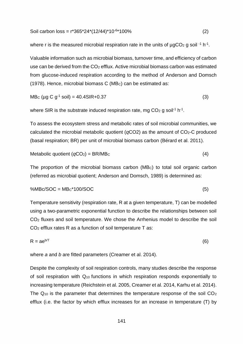
141

Soil carbon loss = r*365*24*(12/44)*10-6*100% (2)

where r is the measured microbial respiration rate in the units of µgCO2 g soil -1 h-1.

Valuable information such as microbial biomass, turnover time, and efficiency of carbon

use can be derived from the CO2 efflux. Active microbial biomass carbon was estimated

from glucose-induced respiration according to the method of Anderson and Domsch

(1978). Hence, microbial biomass C (MBC) can be estimated as:

MBC (µg C g-1 soil) = 40.4SIR+0.37 (3)

where SIR is the substrate induced respiration rate, mg CO2 g soil-1 h-1.

To assess the ecosystem stress and metabolic rates of soil microbial communities, we

calculated the microbial metabolic quotient (qCO2) as the amount of CO2-C produced

(basal respiration; BR) per unit of microbial biomass carbon (Bérard et al. 2011).

Metabolic quotient (qCO2) = BR/MBC (4)

The proportion of the microbial biomass carbon (MBC) to total soil organic carbon

(referred as microbial quotient; Anderson and Domsch, 1989) is determined as:

%MBc/SOC = MBC*100/SOC (5)

Temperature sensitivity (respiration rate, R at a given temperature, T) can be modelled

using a two-parametric exponential function to describe the relationships between soil

CO2 fluxes and soil temperature. We chose the Arrhenius model to describe the soil

CO2 efflux rates R as a function of soil temperature T as:

R = aeb/T (6)

where a and b are fitted parameters (Creamer et al. 2014).

Despite the complexity of soil respiration controls, many studies describe the response

of soil respiration with Q10 functions in which respiration responds exponentially to

increasing temperature (Reichstein et al. 2005, Creamer et al. 2014, Karhu et al. 2014).

The Q10 is the parameter that determines the temperature response of the soil CO2

efflux (i.e. the factor by which efflux increases for an increase in temperature (T) by

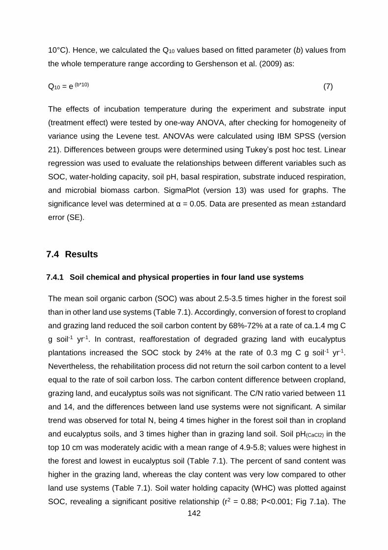
142

10°C). Hence, we calculated the Q10 values based on fitted parameter (b) values from

the whole temperature range according to Gershenson et al. (2009) as:

Q10 = e (b*10) (7)

The effects of incubation temperature during the experiment and substrate input

(treatment effect) were tested by one-way ANOVA, after checking for homogeneity of

variance using the Levene test. ANOVAs were calculated using IBM SPSS (version

21). Differences between groups were determined using Tukey’s post hoc test. Linear

regression was used to evaluate the relationships between different variables such as

SOC, water-holding capacity, soil pH, basal respiration, substrate induced respiration,

and microbial biomass carbon. SigmaPlot (version 13) was used for graphs. The

significance level was determined at α = 0.05. Data are presented as mean ±standard

error (SE).

7.4 Results

7.4.1 Soil chemical and physical properties in four land use systems

The mean soil organic carbon (SOC) was about 2.5-3.5 times higher in the forest soil

than in other land use systems (Table 7.1). Accordingly, conversion of forest to cropland

and grazing land reduced the soil carbon content by 68%-72% at a rate of ca.1.4 mg C

g soil-1 yr-1. In contrast, reafforestation of degraded grazing land with eucalyptus

plantations increased the SOC stock by 24% at the rate of 0.3 mg C g soil-1 yr-1.

Nevertheless, the rehabilitation process did not return the soil carbon content to a level

equal to the rate of soil carbon loss. The carbon content difference between cropland,

grazing land, and eucalyptus soils was not significant. The C/N ratio varied between 11

and 14, and the differences between land use systems were not significant. A similar

trend was observed for total N, being 4 times higher in the forest soil than in cropland

and eucalyptus soils, and 3 times higher than in grazing land soil. Soil pH(CaCl2) in the

top 10 cm was moderately acidic with a mean range of 4.9-5.8; values were highest in

the forest and lowest in eucalyptus soil (Table 7.1). The percent of sand content was

higher in the grazing land, whereas the clay content was very low compared to other

land use systems (Table 7.1). Soil water holding capacity (WHC) was plotted against

SOC, revealing a significant positive relationship (r2 = 0.88; P<0.001; Fig 7.1a). The

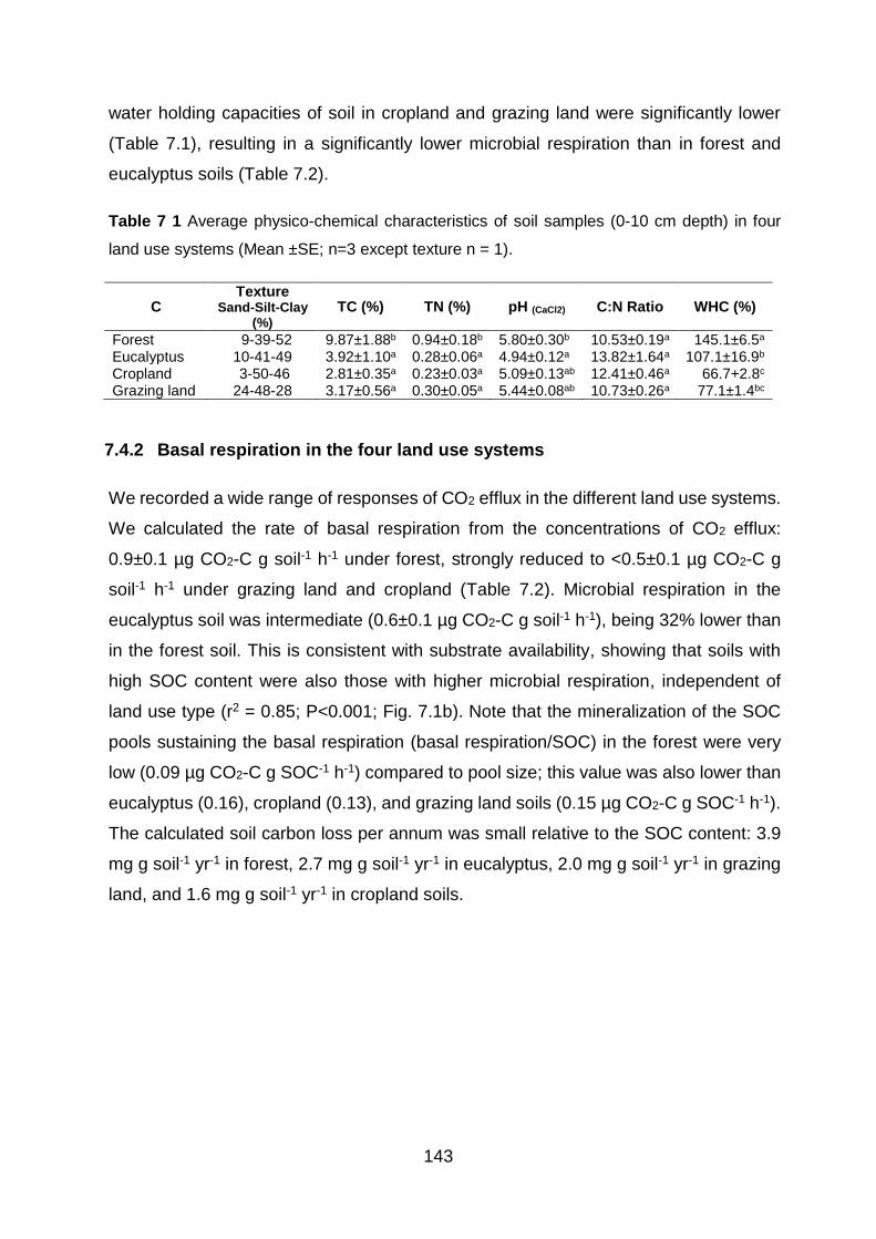
143

water holding capacities of soil in cropland and grazing land were significantly lower

(Table 7.1), resulting in a significantly lower microbial respiration than in forest and

eucalyptus soils (Table 7.2).

Table 7 1 Average physico-chemical characteristics of soil samples (0-10 cm depth) in four

land use systems (Mean ±SE; n=3 except texture n = 1).

C Texture

Sand-Silt-Clay (%)

TC (%) TN (%) pH (CaCl2) C:N Ratio WHC (%)

Forest 9-39-52 9.87±1.88b 0.94±0.18b 5.80±0.30b 10.53±0.19a 145.1±6.5a Eucalyptus 10-41-49 3.92±1.10a 0.28±0.06a 4.94±0.12a 13.82±1.64a 107.1±16.9b Cropland 3-50-46 2.81±0.35a 0.23±0.03a 5.09±0.13ab 12.41±0.46a 66.7+2.8c Grazing land 24-48-28 3.17±0.56a 0.30±0.05a 5.44±0.08ab 10.73±0.26a 77.1±1.4bc

7.4.2 Basal respiration in the four land use systems

We recorded a wide range of responses of CO2 efflux in the different land use systems.

We calculated the rate of basal respiration from the concentrations of CO2 efflux:

0.9±0.1 µg CO2-C g soil-1 h-1 under forest, strongly reduced to <0.5±0.1 µg CO2-C g

soil-1 h-1 under grazing land and cropland (Table 7.2). Microbial respiration in the

eucalyptus soil was intermediate (0.6±0.1 µg CO2-C g soil-1 h-1), being 32% lower than

in the forest soil. This is consistent with substrate availability, showing that soils with

high SOC content were also those with higher microbial respiration, independent of

land use type (r2 = 0.85; P<0.001; Fig. 7.1b). Note that the mineralization of the SOC

pools sustaining the basal respiration (basal respiration/SOC) in the forest were very

low (0.09 µg CO2-C g SOC-1 h-1) compared to pool size; this value was also lower than

eucalyptus (0.16), cropland (0.13), and grazing land soils (0.15 µg CO2-C g SOC-1 h-1).

The calculated soil carbon loss per annum was small relative to the SOC content: 3.9

mg g soil-1 yr-1 in forest, 2.7 mg g soil-1 yr-1 in eucalyptus, 2.0 mg g soil-1 yr-1 in grazing

land, and 1.6 mg g soil-1 yr-1 in cropland soils.

144

Table 7 2 Soil microbial parameters in the sampled soils at 25°C. The amount of glucose added

in the substrate induced respiration (SIR) used a standard concentration designed to deliver 30

mg ml-1 of soil water at 40% of water holding capacity in the MicroResp (Campbell et al. 2003).

Metabolic quotient (qCO2) was calculated as the ratio of soil basal respiration to microbial

biomass carbon (MBc) (Anderson and Domsch 1978). Values denote means and standard

errors of three replicates. Different letters show significant differences between land use

systems following Tukey’s HSD test (p<0.05).

Land use CO2 efflux

(%)

Basal respiration (µg

g soil-1 h-1)

SIR (µg g soil-1 h-1)

MBc (µg C g soil-1)

%MBc/TC qCO2

Forest 0.14±0.005a 0.90±0.07a 10.76±1.73a 435.1±69.7a 0.64±0.10ab 2.1±0.2a Eucalyptus 0.11±0.009a 0.61±0.09ab 4.37±1.12b 177.0±45.4b 0.79±0.20ab 3.9±0.9b Cropland 0.08±0.001b 0.37±0.07b 3.53±0.92b 142.9±37.0b 0.46±0.12a 2.9±0.7bc Grazing land 0.07±0.006b 0.46±0.09b 4.43±1.25b 179.5±50.5b 0.86±0.24bc 2.7±0.4c

Figure 7 1 Linear regression of SOC with panel a) water holding capacity (WHC), panel b)

basal respiration (BR), and panel c) microbial biomass carbon (MBc) for the four land use soils.

7.4.3 Microbial respiration in response to substrate availability

We added substrates with a range of recalcitrance (glucose, starch, lignin) and nutrient

sources (ammonia and phosphate) to determine whether soil microbes are limited by

either C-source or nutrient deficiency. Significant differences occurred for all carbon

substrates but not for fertilizer input. Higher respiration rates were obtained in soils to

which carbon sources were added (Fig. 7.3a-d; Table 7.3). Glucose induced the largest

microbial utilization throughout the temperature range. Surprisingly, adding lignin

substrate yielded the second highest response by the microbial community, followed

by starch. Microbial respirations in the nutrient (N and P) addition soils were significantly

lower than in soils supplied with carbon sources (glucose, lignin, starch). However,

there was no significant change in microbial respiration between the control and soils

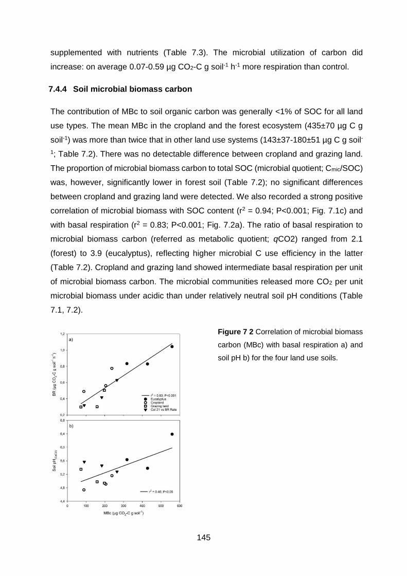
145

supplemented with nutrients (Table 7.3). The microbial utilization of carbon did

increase: on average 0.07-0.59 µg CO2-C g soil-1 h-1 more respiration than control.

7.4.4 Soil microbial biomass carbon

The contribution of MBc to soil organic carbon was generally <1% of SOC for all land

use types. The mean MBc in the cropland and the forest ecosystem (435±70 µg C g

soil-1) was more than twice that in other land use systems (143±37-180±51 µg C g soil-

1; Table 7.2). There was no detectable difference between cropland and grazing land.

The proportion of microbial biomass carbon to total SOC (microbial quotient; Cmic/SOC)

was, however, significantly lower in forest soil (Table 7.2); no significant differences

between cropland and grazing land were detected. We also recorded a strong positive

correlation of microbial biomass with SOC content (r2 = 0.94; P<0.001; Fig. 7.1c) and

with basal respiration (r2 = 0.83; P<0.001; Fig. 7.2a). The ratio of basal respiration to

microbial biomass carbon (referred as metabolic quotient; qCO2) ranged from 2.1

(forest) to 3.9 (eucalyptus), reflecting higher microbial C use efficiency in the latter

(Table 7.2). Cropland and grazing land showed intermediate basal respiration per unit

of microbial biomass carbon. The microbial communities released more CO2 per unit

microbial biomass under acidic than under relatively neutral soil pH conditions (Table

7.1, 7.2).

Figure 7 2 Correlation of microbial biomass

carbon (MBc) with basal respiration a) and

soil pH b) for the four land use soils.

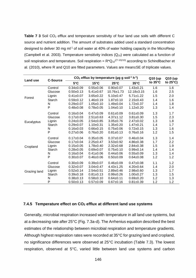
146

Table 7 3 Soil CO2 efflux and temperature sensitivity of four land use soils with different C

source and nutrient addition. The amount of substrates added used a standard concentration

designed to deliver 30 mg ml-1 of soil water at 40% of water holding capacity in the MicroResp

(Campbell et al. 2003). Temperature sensitivity indices (Q10) were calculated as a function of

soil respiration and temperature. Soil respiration = R*Q10((T-10)/10) according to Schindlbacher et

al. (2010), where R and Q10 are fitted parameters. Values are mean±SE of triplicate values.

Land use C-Source CO2 efflux by temperature (µg g soil-1 h-1) Q10 (up

to 35°C Q10 (up to 25°C) 5°C 15°C 25°C 35°C

Forest

Control 0.34±0.09 0.55±0.06 0.90±0.07 1.43±0.21 1.6 1.6 Glucose 0.50±0.13 5.41±0.67 10.76±1.73 12.18±3.15 1.6 2.5

Lignin 0.41±0.07 3.65±0.22 5.10±0.47 5.71±1.22 1.5 2.0

Starch 0.59±0.12 1.46±0.19 1.87±0.10 2.15±0.43 1.4 1.6 N 0.29±0.07 1.05±0.10 1.49±0.04 1.72±0.37 1.4 1.8 P 0.48±0.08 0.78±0.05 1.04±0.10 1.12±0.20 1.3 1.4

Eucalyptus

Control 0.16±0.04 0.47±0.09 0.61±0.09 0.61±0.09 1.3 1.7 Glucose 0.17±0.03 2.51±0.63 4.37±1.12 3.81±0.30 1.5 2.3 Lignin 0.24±0.05 2.54±0.85 3.05±0.76 2.47±0.02 1.3 1.8 Starch 0.29±0.07 1.10±0.31 1.35±0.20 1.47±0.21 1.4 1.7 N 0.16±0.03 0.66±0.15 0.75±0.06 0.72±0.15 1.3 1.6 P 0.27±0.06 0.76±0.20 0.81±0.13 0.76±0.16 1.2 1.5

Cropland


Grazing land


7.4.5 Temperature effect on CO2 efflux at different land use systems

Generally, microbial respiration increased with temperature in all land use systems, but

at a decreasing rate after 25°C (Fig. 7.3a-d). The Arrhenius equation described the best

estimates of the relationship between microbial respiration and temperature gradients.

Although highest respiration rates were recorded at 35°C for grazing land and cropland,

no significance differences were observed at 25°C incubation (Table 7.3). The lowest

respiration, observed at 5°C, varied little between land use systems and carbon

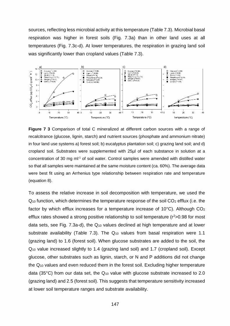
147

sources, reflecting less microbial activity at this temperature (Table 7.3). Microbial basal

respiration was higher in forest soils (Fig. 7.3a) than in other land uses at all

temperatures (Fig. 7.3c-d). At lower temperatures, the respiration in grazing land soil

was significantly lower than cropland values (Table 7.3).

Figure 7 3 Comparison of total C mineralized at different carbon sources with a range of

recalcitrance (glucose, lignin, starch) and nutrient sources (phosphate and ammonium nitrate)

in four land use systems a) forest soil; b) eucalyptus plantation soil; c) grazing land soil; and d)

cropland soil. Substrates were supplemented with 25µl of each substance in solution at a

concentration of 30 mg ml-1 of soil water. Control samples were amended with distilled water

so that all samples were maintained at the same moisture content (ca. 60%). The average data

were best fit using an Arrhenius type relationship between respiration rate and temperature

(equation 8).

To assess the relative increase in soil decomposition with temperature, we used the

Q10 function, which determines the temperature response of the soil CO2 efflux (i.e. the

factor by which efflux increases for a temperature increase of 10°C). Although CO2

efflux rates showed a strong positive relationship to soil temperature (r2>0.98 for most

data sets, see Fig. 7.3a-d), the Q10 values declined at high temperature and at lower

substrate availability (Table 7.3). The Q10 values from basal respiration were 1.1

(grazing land) to 1.6 (forest soil). When glucose substrates are added to the soil, the

Q10 value increased slightly to 1.4 (grazing land soil) and 1.7 (cropland soil). Except

glucose, other substrates such as lignin, starch, or N and P additions did not change

the Q10 values and even reduced them in the forest soil. Excluding higher temperature

data (35°C) from our data set, the Q10 value with glucose substrate increased to 2.0

(grazing land) and 2.5 (forest soil). This suggests that temperature sensitivity increased

at lower soil temperature ranges and substrate availability.

148

7.5 Discussion

7.5.1 Resource availability and carbon use efficiency of microorganisms

Soil respiration is a good indicator of overall soil biological activity and of the carbon

use efficiency by microorganisms. The mean soil respiration rates measured in this

study (0.4-0.9 µg CO2-C g soil-1 h-1) were similar to average tropical soil respiration

rates (0.42-0.83 µg CO2-C g soil-1 h-1; Joergensen, 2010). Our values, however, are

slightly higher than the mean basal respiration rate of 0.46 µg CO2-C g soil-1 h-1

measured in 62 temperate German soils as mentioned by Joergensen (2010).

We observed a clear decreasing pattern in the microbial respiration rate along a

decreasing SOC gradient (Fig. 7.1b-c). This indicates that soil C is the limiting factor

for microorganism activity. The greater soil respiration we recorded in the natural forest

suggests higher rates of soil carbon turnover than in other land use systems. Recently,

Oertel et al. (2016) reported higher soil respiration rates in forest than in other bare land

use types, and they correlated this with higher soil organic carbon contents. The

continuous input of below- and above-ground organic matter is a crucial energy source

for the microbial community in the forest ecosystem. Many studies have shown that

conversion of tropical forest to cropland or grazing land decreases the soil organic

matter content by up to 70% depending on the number of years under cultivation and

land use management (Fearnside et al. 1998, Deng et al. 2016a, Fan et al. 2016). The

lowest CO2 respiration rates recorded for cropland and grazing land soils probably

reflect their low total C content, which apparently provide insufficient food for microbes.

This may reflect the combined effect of complete removal of crop residues and poor

management practices, which remove valuable energy sources for microbial

communities. The eucalyptus soils showed an intermediate respiratory activity, but

significantly higher than that of the cropland and grazing land. This suggests that

restoring degraded sites provides greater benefits in terms of soil organic matter inputs

and microbial activity. Microbial respiration differences among land use systems were

probably also driven by soil moisture differences resulted from soil organic matter

content differences. For example, a 1% rise of SOC increased the water holding

capacity by ca. 9 times (Fig. 7.1a). Therefore, more SOC in the forest soil increased

the water holding capacity proportionally during adjustments to 40% before incubation;

149

this provides better conditions for microorganisms, potentially enhancing soil

respiration.

We supplied microorganisms with carbon sources of contrasting recalcitrance to

determine whether soil organic matter and carbon quality are an important determinant

of soil respiration. In general, soil respiration rates in the glucose-, lignin-, and starch-

supplemented soils were significantly higher than in the control soil (Table 7.3; Fig. 7.3),

further confirming that microbes are limited by carbon availability. In addition to

substrate availability, substrate quality resulted in different soil respiration rates. The

magnitude of effects on microbial respiration depends on the specific composition of

the substrate added. In general, adding labile carbon sources (glucose) stimulates

microbial respiration in all land use soils (Fig. 7.3). Surprisingly, the second highest CO2

efflux was in soils supplied with lignin substrate, indicating preferential degradation of

lignin over starch. Lignin is considered to be more recalcitrant than starch (Hernández

et al. 2010), hence the moderately labile substrate (starch) should have been depleted

faster than the more recalcitrant substrate (lignin). Moreover, starch is easily degraded

by aerobic as well as anaerobic microorganisms (Kögel-Knabner 2002), whereas white-

rot and brown-rot fungi (Goñi et al. 1993) and certain bacteria such as Streptomyces

sp. or Nocarda sp. (Brown and Chang 2014, Duboc et al. 2014) are commonly

responsible for lignin degradation. Therefore, the higher CO2 efflux in the lignin-induced

soils indicates the relative profile structure of microorganisms with lignin-specialized

fungi and bacterial dominance. Previous studies have shown that lignin decomposition

in soil can be as fast or even faster than bulk soil organic matter, and only a small

fraction of lignin (10%) seems to persist on a time scale of decades (Marschner et al.

2008, Duboc et al. 2014). Moreover, Feng et al. (2008) showed that warming can

accelerate lignin decomposition, while soil fungi, the primary decomposers of lignin in

soil, increased in abundance. Bradford (2013) and Steinweg et al. (2008) reported that

substrate limitation might shift enzyme expression toward higher affinity enzymes. That

would reduce maximum catalytic rates, favouring a slower growing microbial biomass

and a lower respiration rate. Further microbial identification and quantification would

help to elucidate microbial community structure and the taxonomy of the species.

Soil respiration in soils supplied with nutrients (N and P) was not significantly different

from control soils, suggesting that microbial activity was less affected by nutrient

deficiencies. In temperate and boreal forests, N and P has usually been found to be the

150

main limiting factor after C (Gnankambary et al. 2008, Giesler et al. 2012). On the

contrary, adding N fertilizer to soils even reduced soil respiration, and this has been

suggested to reflect microbial reallocation of C to biomass or enzyme production

(Schimel and Weintraub 2003, Allison and Vitousek 2005).

7.5.2 Biological indicators for eco-physiological stress

We calculated the microbial metabolic quotient (qCO2) – the amount of CO2 produced

per unit of microbial biomass carbon (Anderson and Domsch 1990) – to assess the

ecosystem stress and metabolic rates of soil microbial communities. This index has

been widely used as a biological indicator of ecosystem soil management practice and

disturbance (Wardle and Ghani 1995, Thirukkumaran and Parkinson 2000, Campbell

et al. 2003, Tosi et al. 2016). Disturbance supposedly increases qCO2, suggesting that

the richness of organic C from different cultures benefits respiration (Bastida et al.

2008). We found a lower metabolic quotient (qCO2) in the forest ecosystem (Table 7.3).

This points to favourable conditions for microbes and less disturbance in this

ecosystem. We also found that the eucalyptus soil had the highest qCO2, which is not

consistent with disturbance. The probable explanation is that eucalyptus species are

known to be inhibitory to soil microorganisms (Louzada et al. 1997, Martins et al. 2013).

These trees are associated with low litter decomposition and reportedly adversely affect

soil attributes (Lemenih et al. 2004). Combined, these factors may induce stress in

microbial communities, which have been shown to have high qCO2. Plant litter

decomposition studies demonstrate that a significant increase in qCO2 can eventually

occur in litter types initially resistant to decomposition (Wardle and Ghani 1995).

Differences in pH probably explain some of the variation in qCO2 because we found a

negative (but not significant) relationship between qCO2 and soil pH (r2 = 0.84; P=0.086;

data not shown). The relationship between the qCO2 and pH means that careful

management of soil pH is required to ensure a healthy and continued soil fertility (Yan

et al. 2003). Our eucalyptus plantation site has been less disturbed during the plantation

period (the last 30 years), but qCO2 was higher in the eucalyptus than at the other 3

sites, indicating that microbial stress is related more to acidity than to disturbance. This

result agrees with Wardle and Ghani (1995), who reported that qCO2 often declines

with increasing pH, which points to an effect of stress rather than disturbance levels.

Other studies by Wolters (1991) reported an increase in qCO2 after acid rain and a

151

reduction after lime treatment in beech forest soils. We can generalize that microbial

communities release more CO2 per unit microbial biomass under acidic than under

relatively neutral soil pH conditions.

7.5.3 Effect of temperature on microbial decomposition

The CO2 efflux increased with temperature but at a decreasing rate above 25°C (Fig.

7.3a-d). This relationship is best represented by the Arrhenius equation by fitting the

measured microbial CO2 efflux as a function of temperature (Lloyd and Taylor 1994).

For C substrate induced respiration, r2 values for all fitted temperature response

functions were >0.98. The Arrhenius model predicted an initial increase in soil

respiration due to the temperature sensitivity of microbial activity, but then approaching

a steady state at higher temperature (Fig. 7.3). This means that this model does not

support the scenarios in which CO2 concentration increases exponentially with

temperature. Despite the wide usage of the exponential model, it can only be valid in a

narrow temperature range because it is unrealistic to expect that biological activity

would increase without limit as a function of temperature (Tuomi et al. 2007). This

growth must cease and ultimately turn into a decrease as temperature increases above

a certain level.

The temperature sensitivity (expressed as Q10) declined at lower substrate availability

and at high temperature (Table 7.3). The metric “Q10” is a commonly used parameter

to estimate temperature sensitivity that computes the relative increase in

decomposition rate per 10°C temperature rise (Bradford 2013). The CO2 effluxes are

less sensitive to temperature change at low organic C content. For example, cropland

and grazing land soils have low Q10 values of 1.1-1.3 (Table 7.3). This may be partly

explained by thermal adaptation due to long exposure to temperature fluctuations in

these open fields. Previous studies also reported that the temperature sensitivity (Q10)

of respiration declines at lower substrate availabilities (Davidson and Janssens 2006,

Allison et al. 2010). Higher temperature sensitivity in forest and eucalyptus plantation

soils suggests the C availability and quality might affect the soil C response to warming.

Our addition of different substrates increased the Q10 value (Table 7.3), further

confirming that the temperature sensitivity of soil organic matter breakdown is also

influenced by substrate availability (Conant and et.al. 2011). The higher Q10 value after

lignin versus starch addition (Table 7.3) supports the Arrhenius kinetic theory that the

152

decomposition of more recalcitrant compounds is more sensitive to temperature

increase compared to more simple compounds (Davidson and Janssens 2006).

Similarly, Feng and Simpson (2008) reported that lignin monomers exhibited higher Q10

values than the solvent-extractable compounds, which is consistent with the above

theory. This is because less reactive and more chemically recalcitrant molecules with

greater activation energies have greater temperature sensitivity (Conant and et.al.

2011).

The temperature sensitivity (Q10) also declined at high temperature (Table 7.3).

Excluding the respiration values recorded at the 35°C incubation from our data set, we

observed a twofold variation (Q10 = 2.0-2.2). Atkin and Tjoelker (2003) reported that

adaptation of microbial respiration to warming is exhibited through a drop in Q10 values.

Empirical studies suggest that warming at high temperatures reduced microbial carbon

use efficiency from 0.31 to 0.23, also reducing the amount of assimilated C allocated

to microbial growth (Allison et al. 2010). Some studies argued that warming at high

temperatures induced a change in microbial physiology and community shifts

(Davidson and Janssens 2006, Bradford et al. 2008). For example, Bérard et al. (2011)

reported that high temperature shifts the soil microbial community from fungi towards

bacteria. One reason for the reduced CO2 efflux at higher temperature may be the

reduction of soil moisture at 35°C during incubation period: only few water droplets

were observed on the surface of the gasket. This is because warming dries the soil,

directly affecting enzyme activity and diffusion rates between microbes and their

immediate environment (Conant and et.al. 2011, Bradford 2013) as well as substrate

availability (Davidson and Janssens 2006). This returns soil respiration to a steady state

(Steinweg et al. 2008, Allison et al. 2010, Bradford et al. 2010). We did not measure

the amount of water loss during incubation and therefore cannot generalize the effect

of drought on microbial respiration. In our previous pre-test measurements, microbial

respiration was highest at 50-70% water holding capacity; below or above these values,

respiration declined.

153

7.6 Conclusion

Our study demonstrates that soil respiration increases with temperature, but that the

rate of this increase drops above 25°C. This indicates that expectations of increasing

biological activity without limit as a function of temperature are erroneous. Low C

contents in soil after land use conversion from forest to cropland and grazing land

restrict soil respiration rates and make the microbial communities in these soils strongly

C limited. Greater soil respiration in the natural forest is evidence for high rates of

biological activity and soil carbon turnover. The MBc was twice as high in the forest soil

as in the other land use systems, which reflects the higher energy supply for

microorganisms. In general, soil respiration rates were significantly higher in substrate-

supplemented soils than the control soil, further confirming that microbes are limited by

C sources. Substrate quality also yielded different soil respiration rates, pointing to

preferential degradation of substrates by microbes. Nonetheless, the response of

microbes to nutrient addition was not significant, meaning that they are not limited by

nutrient deficiency. The carbon use efficiency of microbes is higher under acidic

conditions.

154

8 Summary and conclusions

The study was conducted in the Amhara Regional State located in the northcentral

parts of Ethiopia. Five research sites (Katassi, Gelawdios, Tara Gedam, Ambober, and

Mahibere-Selassie) were selected at an average distance of 120 km between each

other. Elevations range from approximately 800 m a.s.l. at Mahibere-Selassie to 2500

m at Gelawdios. At each site, up to five-land use types (natural forest, eucalyptus

plantation, exclosure (rejuvenated woodland on former grazing land), cropland, and

grazing land) were identified adjacent to each other to give similar topography, edaphic,

and climate conditions for comparison of land uses at each site. However, not all land

use systems were available at each site. The highland forests are Afromontane

remnant pristine forests mostly confined to sacred groves associated with churches.

The lowland semiarid forest around Mahibere-Selassie monastery is a savannah

woodland dominated by grasses with some scattered trees. The eucalyptus plantations

were established around 1985 with Eucalyptus globules at Katassi and Gelawdios on

grazing land and Eucalyptus camaldunesis at Tara Gedam on former cropland. The

exclosure was established at Ambober in 2007 on former grazing land. All studied

croplands and grazing lands were converted from natural forest within the last 50 years.

This thesis has addressed several major aspects of the biogeochemical cycle based

on field and laboratory investigations of different land use systems in NW Ethiopia. The

methodologies and results from experimental studies have been presented and

discussed individually in chapters two to seven. This final chapter serves to summarize,

integrate the data presented, and relate the findings to a wide range of research

questions raised during the inception of this research.

Land use plays a major role in determining the C storage of soils. In Ethiopian highland

ecosystems, greater SOC stocks were found in the natural forest than in any other land

use systems. Following land use conversion from native forest to cropland or grazing

land, SOC stocks were reduced by 88% at site level in <50 years. In contrast,

converting degraded cropland or grazing land into perennial vegetation, e.g.

afforestation with eucalyptus, is found to increase SOC stocks by increasing C input

from plant litter. Surprisingly, the effects of exclosures (natural vegetation restoration)

to increase SOC stocks was not significant over 8 years establishment in subsoils (10-

155

30 cm depth), questioning the suitability of the natural regeneration for quick recovery

of SOC stocks.

Major factors underlying the reduction of carbon stock are erosion and enhanced

mineralization. In the studied areas, the level of SOC stock in topsoil (0-10 cm) of

cropland or grazing land was less than the SOC stock of the adjacent forest soil at the

depth of 30-50 cm. The geochemical markers such as Sr/Ca and Ba/Ca ratio at 30-50

cm depth in the forest soil profiles are comparable to the 0-10 cm depth of cropland

soil. Both factors suggest that the upper soil profile has been lost by erosion in cropland

and grazing land. Concerning mineralization, the possible maximum annual carbon loss

rate through heterotrophic respiration was estimated to be 3.9 mg g soil-1 yr-1 in forests,

2.7 mg g soil-1 yr-1 in eucalyptus stand, 2.0 mg g soil-1 yr-1 in grazing lands, and 1.6 mg

g soil-1 yr-1 in croplands. This is consistent with substrate availability showing that soils

with high SOC content have higher microbial respiration independent of land use type.

However, this estimation was based on the optimum soil moisture content and

temperature throughout the year, while this optimum condition may occur only for few

days a year. The loss of SOC by heterotrophic respiration is smaller than the effect of

erosion (6.5 mg g soil-1 yr-1 on average) and can be compensated by litter input in to

the soil.

Nevertheless, land use conversions from native forest to grazing land or cropland alter

the overall quantity and quality of litter inputs. The annual above litterfall production in

the forest ecosystem was about 1100 g dry weight (dw) m-2 of which leaves comprised

65%. The above-ground C input, mainly through leaves, was estimated about 300 g m-

2. Above-ground litter inputs in eucalyptus, cropland, and grazing land are estimated to

be minor due to leaf litter raking, complete residual harvest, and overgrazing,

respectively. Similarly, the average fine root production was estimated to be about 700

g dw m-2 in natural forest and eucalyptus stands whereas fine root production in grazing

land and cropland was about 50-60 g dw m-2. Therefore, the amount of annual C input

into the soil by fine roots alone was about 340 g m-2 in natural forest and eucalyptus

stands and ca. 30 g m-2 in grazing land and croplands. Overall, the results illustrate that

conversion of native forest to grazing land and cropland resulted in the reduction of C

input into the soil by >90%. Compared to the above leaf litterfall, fine roots contributed

about 15% more C into the soil, emphasizing their importance for SOC accumulation.

156

The litter chemistry analysis revealed that acid soluble fraction (ASF; i.e. mainly

cellulose) and acid insoluble fraction (AIF; i.e. mainly lignin) were the two compound

groups contributing most to C input into the soil. ASF and AIF were equally present in

leaf extracts (ca. 42% each) whereas ASF in roots accounted for 37% and AIF

accounted for 50% of total extracts. Solvent extractives (i.e. extractive fractions mainly

carbohydrates) accounted for <16% of the total fluxes in leaves and <12% in fine roots

and the rest were ash. The AIF from roots contains a highly cross-linked polymer with

highly reduced compounds of suberin and tannin-protein complexes, which are

resistant to degradation. By contrast, leaf litter contributed considerably more labile C

compounds such as cellulose, soluble phenolics and carbohydrates to the soil than fine

roots. Thus, fine root estimated to contribute about 1.5 times more recalcitrant C input

into the soil than leaf litter. Suberin and cutin can be used as markers to estimate the

input of organic matter originating from root biomass and shoot specific contribution

into the soil. The biomarker analysis revealed that the amount of suberin was 2-times

that of cutin – further confirming the greater input of recalcitrant carbon by fine roots.

Based on the biomarker analysis of soils, aliphatic lipids and lignin accounted about 46-

84% of the total detected compounds and revealed a major input of soil organic carbon

derived from higher plants. The short-chain alkanoic acids, ergosterol, and a

disaccharide trehalose accounted only for less than 7% of aliphatic lipids in all soils

indicating the microbial inputs were present as minor components. Cholesterol is

derived from non-plant source such as soil fauna, fungi, and algae and has minor

contribution to soil organic carbon as reflected by its low abundance in all land use

types. From the CuO oxidation yields, the ratio of syringyls to vanillyls (S/V) and

cinnamyls to vanillyls (C/V) monomers are widely used to differentiate the relative

contributions of major plant taxonomic groups (gymnosperms vs angiosperms), tissue

type (woody vs non-woody tissue), and diagenetic state of lignin. Accordingly, S/V

values varied in the range of 0.61 to 2.23 suggesting that angiosperm plants are the

predominant sources for lignin compared to gymnosperm plants because S/V values

above 0.6 are considered as angiosperm origin. Similarly, a higher value of C/V ratio is

indicative of the presence of non-woody material because cinnamyl monomers (p-

coumaric acid, ferulic acid) are abundant in most herbaceous and soft tissues (i.e.

leaves, grasses) but virtually absent from wood. The lignin-derived phenols exhibited a

V:S:C ratio of 4:2:1 (forest soil); 1:1:1 (eucalypt, cropland, and grazing land soils).

157

Relatively equal V:S:C: ratio in eucalyptus, cropland, and grazing land soils further

confirming that lignin-derived phenols originate mainly from non-woody angiosperm

sources, which is consistent with S/V and C/V ratios. The higher V:S:C ratio in the

natural forest indicates that woody angiosperms have significant contributions to SOC.

The ratios of lignin-derived phenolic acids and 3, 5-dihydroxybenzoic acid (DHBA)/V

are generally used as indicators of the level of lignin and tannin degradation in the soil,

respectively. The lowest ratio of S/V (0.6) and C/V (0.2) was in forest, while the other

land use soils show a ratio greater than 1.2, indicating enhanced degradation of lignin

in the forest soil, and preferential degradation of syringyls and cinnamyls from the lignin-

derived phenols. This is because cinnamyls linking carbohydrates and lignin in the

ligno-cellulose complex and are therefore more accessible to decomposition than

vanillyls. The 3, 5-dihydroxybenzoic acid to vanillyls was in the order of forest soil

(0.69), eucalyptus (0.24), cropland soil (0.15), and grazing land soil (0.09). The highest

value in forest soil shows increased degradation of tannins as 3, 5-dihydroxybenzoic

acid in the CuO oxidation was derived from tannin oxidation.

A litterbag experiment revealed that leaf litter decomposed faster than fine root litter

with a decomposition rate constant (k) of 2.5 yr-1 for leaves and 1.7 yr-1 for fine roots.

Fine root morphological traits such as specific root surface area (SRA), specific root

length (SRL), and root tissue density (RTD; g cm–3) are important with regard to plant

growth strategy, roots life span, and root decomposition rate. This study demonstrates

that roots of fast-growing species have low RTD. The calculated amount of glucose

needed to produce a gram of tissue biomass ranged between 1.2 and 1.5 g glucose g-

1 dw and was significantly and consistently greater in slow-growing species compared

to fast-growing species. Fine root C contents were negatively correlated to specific root

length or area (SRL/SRA), but positively correlated to RTD and AIF and were largely

consistent with a range of species. This difference between growth patterns determines

the decomposition dynamics and C deposition in the soil and suggests that species

having lower RTD and low structural components (low lignin) decompose more rapidly

Due to species-specific morphological and litter chemistry differences, decomposition

of litter materials in the litterbag experiment varied largely by species. Among the

studied species, the deciduous species (Allophylus abyssinicus, and Combretum

collinum) decomposed faster than evergreen species (Chionanthus mildbraedii and

Teclea nobilis). Furthermore, the presence of litter from deciduous species in litter

158

mixtures, i.e. the normal situation in mixed forests, increased the rate of decomposition

of other slower decomposing litter types.

Overall, these findings are fundamental to improving our understanding of

biogeochemical cycles under different land use systems and its impact on the global C

balance. This thesis may support decision-making on land use and management of soil

carbon by raising awareness and upgrading existing knowledge on the SOC dynamics

and importance of SOC management as the basis for essential ecosystem functions.

Decisions on soil carbon management requires a better understanding of the spatial

variation in SOC stocks and their C source as well as the potential to use management

approaches to reduce losses and/or increase stocks. In the Amhara region, there is

both a need and an opportunity to influence land use policy and management to

improve soil C quantity and quality. This can be evidenced by mass mobilization of

farmers by the government for soil and water conservation campaign work in the whole

regions since decades. However, this campaign focused only on physical and biological

conservation activities and ignoring soil C management. Therefore, soil conservation

efforts need to emphasize and promote land use practices that focus on the possible

greatest increase or at least stabilization in SOC through afforestation, exclosure or

reduction of losses due to erosion, and above all sustainable management approaches.

Promoting land uses that maintain biomass C input is more beneficial to overall carbon

stocks that improves soil quality resulting in greater productivity and ultimately

increased food security.

159

References

Abiven, S., S. Recous, V. Reyes, and R. Oliver. 2005. Mineralisation of C and N from root, stem and leaf residues in soil and role of their biochemical quality. Biology and Fertility of Soils 42:119–128.

Abiyu, A. 2012. The role of seed dispersal, exclosures, nurse shrubs and trees around churches and farms for restoration of ecosystem diversity and productivity in the Ethiopian highlands. University of Natural Resources and Life Science, Vienna, Austria.

Abu-hashim, M., M. Elsayed, and A.-E. Belal. 2016. Effect of land-use changes and site variables on surface soil organic carbon pool at Mediterranean Region. Journal of African Earth Sciences 114:78–84.

Adair, E., W. Parton, S. del Grosso, W. Silver, M. Harmon, S. Hall, I. Burke, and S. Hart. 2008. Simple three-pool model accurately describes patterns of long-term litter decomposition in diverse climates. Global change biology 14:2636–2660.

Aerts, R., C. Bakker, and H. De Caluwe. 1992. Root turnover as determinant of the cycling of C, N, and P in a dry heathland ecosystem. Biogeochemistry 15:175–190.

Aerts, R., K. Van Overtveld, E. November, A. Wassie, A. Abiyu, S. Demissew, D. D. Daye, K. Giday, M. Haile, and S. TewoldeBerhan. 2016. Conservation of the Ethiopian church forests: Threats, opportunities and implications for their management. Science of the Total Environment 551:404–414.

Ajami, M., A. Heidari, F. Khormali, M. Gorji, and S. Ayoubi. 2016. Environmental factors controlling soil organic carbon storage in loess soils of a subhumid region, northern Iran. Geoderma 281:1–10.

Allison, S. D., and P. M. Vitousek. 2005. Responses of extracellular enzymes to simple and complex nutrient inputs. Soil Biology and Biochemistry 37:937–944.

Allison, S. D., M. D. Wallenstein, and M. A. Bradford. 2010. Soil-carbon response to warming dependent on microbial physiology. Nature Geoscience 3:336–340.

Alvarez, R., and R. S. R. Lavado. 1998. Climate, organic matter and clay content relationships in the Pampa and Chaco soils, Argentina. Geoderma 83:127–141.

Amelung, W., S. Brodowski, A. Sandhage-Hofmann, and R. Bol. 2008. Combining biomarker with stable isotope analyses for assessing the transformation and turnover of soil organic matter. Advances in agronomy 100:155–250.

Anderson, J. P. E., and K. H. Domsch. 1978. A physiological method for the quantitative measurement of microbial biomass in soils. Soil Biology and Biochemistry 10:215–221.

Anderson, T.-H., and K. H. Domsch. 1989. Ratios of microbial biomass carbon to total organic carbon in arable soils. Soil Biology and Biochemistry 21:471–479.

Anderson, T.-H., and K. H. Domsch. 1990. Application of eco-physiological quotients (qCO2 and qD) on microbial biomasses from soils of different cropping histories. Soil Biology and Biochemistry 22:251–255.

Andreasson, F., M. Gonzalez, L. Augusto, and M. R. Bakker. 2015. Comparison of ingrowth cores and ingrowth meshes in root studies: 3 years of data on Pinus pinaster and its understory. Trees:1–16.

Angst, G., S. John, C. W. Mueller, I. Kögel-Knabner, and J. Rethemeyer. 2016. Tracing the sources and spatial distribution of organic carbon in subsoils using a multi-biomarker approach. Nature Publishing Group.

Aragão, L. E. O. C., Y. Malhi, D. B. Metcalfe, J. E. Silva-Espejo, E. Jiménez, D. Navarrete, S. Almeida, A. C. L. Costa, N. Salinas, O. L. Phillips, L. O. Anderson, E. Alvarez, T. R. Baker, P.

160

H. Goncalvez, J. Huamán-Ovalle, M. Mamani-Solórzano, P. Meir, A. Monteagudo, S. Patiño, M. C. Peñuela, A. Prieto, C. A. Quesada, A. Rozas-Dávila, A. Rudas, J. A. Silva Jr., and R. Vásquez. 2009. Above- and below-ground net primary productivity across ten Amazonian forests on contrasting soils. Biogeosciences 6:2759–2778.

Assaye, Y., Y. G. Selassie, and B. Ayele. 2013. A socio-economic contribution of high land bamboo (Yushania Alpina) for household livelihood in Banja District, Northwestern Ethiopia. Journal of Agriculture and Biodiversity Research 2:151–159.

Atkin, O. K., and M. G. Tjoelker. 2003. Thermal acclimation and the dynamic response of plant respiration to temperature. Trends in Plant Science 8:343–351.

Awulachew, S. B., M. McCartney, T. S. Steenhuis, and A. A. Ahmed. 2009. A review of hydrology, sediment and water resource use in the Blue Nile Basin. International Water Management Institute (IWMI), Colombo, Sri Lanka.

Ayalew, D., K. Tesfaye, G. Mamo, B. Yitaferu, and W. Bayu. 2012. Outlook of future climate in northwestern Ethiopia. Agricultural Sciences 3:608–624.

Baddeley, J. A., and C. A. Watson. 2005. Influences of root diameter, tree age, soil depth and season on fine root survivorship in Prunus avium. Plant and Soil 276:15–22.

Balesdent, J., E. Besnard, D. Arrouays, and C. Chenu. 1998. The dynamics of carbon in particle-size fractions of soil in a forest-cultivation sequence. Plant and Soil 201:49–57.

Bane, J., S. Nune, A. Mekonnen, and R. Bluffstone. 2007. Policies to increase forest cover in Ethiopia Contents. Page 239Proceedings of a Policy Workshop organized. Addis Ababa, Ethiopia, Ethiopia.

Bao, X., J. Yu, W. Liang, C. Lu, J. Zhu, and Q. Li. 2015. The interactive effects of elevated ozone and wheat cultivars on soil microbial community composition and metabolic diversity. Applied Soil Ecology 87:11–18.

Bardgett, R. D., L. Mommer, and F. T. De Vries. 2014. Going underground: root traits as drivers of ecosystem processes. Trends in Ecology & Evolution 29:692–699.

Basile, B., D. R. Bryla, M. L. Salsman, J. Marsal, C. Cirillo, R. S. Johnson, and T. M. DeJong. 2007. Growth patterns and morphology of fine roots of size-controlling and invigorating peach rootstocks. Tree physiology 27:231–241.

Bastida, F., A. Zsolnay, T. Hernández, and C. García. 2008. Past, present and future of soil quality indices: A biological perspective. Geoderma 147:159–171.

Batjes, N. H. 1996. Total carbon and nitrogen in the soils of the world. European journal of soil science 47:151–163.

Batjes, N. H., and W. G. Sombroek. 1997. Possibilities for carbon sequestration in tropical and subtropical soils. Global change biology 3:161–173.

Becker, J., H. Pabst, J. Mnyonga, and Y. Kuzyakov. 2015. Annual litterfall dynamics and nutrient deposition depending on elevation and land use at Mt. Kilimanjaro. Biogeosciences 12:5635–5646.

Bekele, M. 2011. Forest plantations and woodlots in Ethiopia. First edition. Regional Soil Conservation Unit, Swedish International Development Authority, Nairobi, Kenya.

Bekele, T. A. 2007. Useful trees and shrubs of Ethiopia: identification, propagation and management for 17 agroclimatic zones. Page (B. Tengnäs, E. Kelbesa, S. Demissew, and P. Maundu, Eds.). RELMA in ICRAF Project, World Agroforestry Centre, Eastern Africa Region, Nairobi, Kenya.

Bérard, A., T. Bouchet, G. Sévenier, A. L. Pablo, and R. Gros. 2011. Resilience of soil microbial communities impacted by severe drought and high temperature in the context of Mediterranean heat waves. European Journal of Soil Biology 47:333–342.

Bérard, A., L. Capowiez, S. Mombo, E. Schreck, C. Dumat, F. Deola, and Y. Capowiez. 2016. Soil

161

microbial respiration and PICT responses to an industrial and historic lead pollution: a field study. Environmental Science and Pollution Research 23:4271–4281.

Berg, B. 2000. Litter decomposition and organic matter turnover in northern forest soils. Forest Ecology and Management 133:13–22.

Berg, B., and C. McClaugherty. 2003. Plant litter : decomposition, humus formation, carbon sequestration. Springer Berlin Heidelberg, Berlin, Heidelberg.

Berg, B., and H. Staaf. 1981. Leaching, accumulation and release of nitrogen in decomposing forest litter. Ecological Bulletins 33:163–178.

Berhongaray, G., I. A. Janssens, J. S. King, and R. Ceulemans. 2013. Fine root biomass and turnover of two fast-growing poplar genotypes in a short-rotation coppice culture. Plant and Soil 373:269–283.

Betrie, G. D., Y. A. Mohamed, A. van Griensven, and R. Srinivasan. 2011. Sediment management modelling in the Blue Nile Basin using SWAT model. Hydrology and Earth System Sciences 15:807–818.

Bewket, W., and D. Conway. 2007. A note on the temporal and spatial variability of rainfall in the

drought‐prone Amhara region of Ethiopia. International Journal of Climatology 27:1467–1477.

Bewket, W., and G. Sterk. 2003. Assessment of soil erosion in cultivated fields using a survey methodology for rills in the Chemoga watershed, Ethiopia. Agriculture, Ecosystems & Environment 97:81–93.

Bewket, W., and G. Sterk. 2005. Dynamics in land cover and its effect on stream flow in the Chemoga watershed, Blue Nile basin, Ethiopia. Hydrological Processes 19:445–458.

Bewket, W., and L. Stroosnijder. 2003. Effects of agroecological land use succession on soil properties in Chemoga watershed, Blue Nile basin, Ethiopia. Geoderma 111:85–98.

Birgander, J., J. Rousk, and P. A. Olsson. 2014. Comparison of fertility and seasonal effects on grassland microbial communities. Soil Biology and Biochemistry 76:80–89.

Birouste, M., E. Zamora-Ledezma, C. Bossard, I. M. Pérez-Ramos, and C. Roumet. 2014. Measurement of fine root tissue density: a comparison of three methods reveals the potential of root dry matter content. Plant and Soil 374:299–313.

Bohm, W. 1979. Methods of studying root systems. Page (D. Vj. D. Billings, A. F. Golley, W. O. L. Lange, and O. R. J. S. Olson, Eds.) Springer-Verlag Berlin Heidelberg. New York.

Bradford, M. A. 2013. Thermal adaptation of decomposer communities in warming soils. Frontiers in microbiology 4.

Bradford, M. A., C. A. Davies, S. D. Frey, T. R. Maddox, J. M. Melillo, J. E. Mohan, J. F. Reynolds, K. K. Treseder, and M. D. Wallenstein. 2008. Thermal adaptation of soil microbial respiration to elevated temperature. Ecology letters 11:1316–1327.

Bradford, M. A., B. W. Watts, and C. A. Davies. 2010. Thermal adaptation of heterotrophic soil respiration in laboratory microcosms. Global change biology 16:1576–1588.

Brando, P. M., D. C. Nepstad, E. A. Davidson, S. E. Trumbore, D. Ray, and P. Camargo. 2008. Drought effects on litterfall, wood production and belowground carbon cycling in an Amazon forest: results of a throughfall reduction experiment. Philosophical transactions of the Royal Society of London. Series B, Biological sciences 363:1839–48.

Brassard, B. W., H. Y. H. Chen, X. Cavard, J. Laganière, P. B. Reich, Y. Bergeron, D. Paré, Z. Yuan, J. Laganiere, P. B. Reich, Y. Bergeron, D. Pare, and Z. Yuan. 2013. Tree species diversity increases fine root productivity through increased soil volume filling. Journal of Ecology 101:210–219.

Brhane, G., and K. Mekonen. 2009. Estimating Soil Loss Using Universal Soil Loss Equation (USLE) for Soil Conservation planning at Medego Watershed, Northern Ethiopia. Marsland Press

162

Journal of American ScienceJournal of American Science 5:58–69.

Brown, M. E., and M. C. Chang. 2014. Exploring bacterial lignin degradation. Current Opinion in Chemical Biology 19:1–7.

Brunner, I., M. R. Bakker, R. G. Björk, Y. Hirano, M. Lukac, X. Aranda, I. Børja, T. D. Eldhuset, H. S. Helmisaari, C. Jourdan, B. Konôpka, B. C. López, C. Miguel Pérez, H. Persson, and I. Ostonen. 2012. Fine-root turnover rates of European forests revisited: an analysis of data from sequential coring and ingrowth cores. Plant and Soil 362:357–372.

Bull, I. D., C. J. Nott, P. F. van Bergen, P. R. Poulton, and R. P. Evershed. 2000. Organic geochemical studies of soils from the Rothamsted classical experiments—VI. The occurrence and source of organic acids in an experimental grassland soil. Soil Biology and Biochemistry 32:1367–1376.

Bullen, T. D., S. W. Bailey, B. Thomas D., B. Scott W., T. D. Bullen, and S. W. Bailey. 2005. Identifying calcium sources at an acid deposition-impacted spruce forest: a strontium isotope, alkaline earth element multi-tracer approach. Biogeochemistry 74:63–99.

Burgess, T. I., N. Malajczuk, and T. S. Grove. 1993. The ability of 16 ectomycorrhizal fungi to increase growth and phosphorus uptake of Eucalyptus globulus Labill. and E. diversicolor F. Muell. Plant and Soil 153:155–164.

Callesen, I., K. Raulund-Rasmussen, and J. Westman. 2007. Nitrogen pools and c:n ratios in well-drained nordic forest soils related to climate and soil texture. Boreal environment research 12:681–692.

Campbell, C. D., S. J. Chapman, C. M. Cameron, M. S. Davidson, and J. M. Potts. 2003. A rapid microtiter plate method to measure carbon dioxide evolved from carbon substrate amendments so as to determine the physiological profiles of soil microbial communities by using whole soil. Applied and environmental microbiology 69:3593–3599.

Canadell, J., R. B. Jackson, J. B. Ehleringer, H. A. Mooney, O. E. Sala, and E.-D. Schulze. 1996. Maximum rooting depth of vegetation types at the global scale. Oecologia 108:583–595.

Capo, R. C., B. W. Stewart, and O. A. Chadwick. 1998. Strontium isotopes as tracers of ecosystem processes: theory and methods. Geoderma 82:197–225.

Carey, J. C., J. Tang, P. H. Templer, K. D. Kroeger, T. W. Crowther, A. J. Burton, J. S. Dukes, B. Emmett, S. D. Frey, M. A. Heskel, L. Jiang, M. B. Machmuller, J. Mohan, A. M. Panetta, P. B. Reich, S. Reinsch, X. Wang, S. D. Allison, C. Bamminger, S. Bridgham, S. L. Collins, G. de Dato, W. C. Eddy, B. J. Enquist, M. Estiarte, J. Harte, A. Henderson, B. R. Johnson, K. S. Larsen, Y. Luo, S. Marhan, J. M. Melillo, J. Peñuelas, L. Pfeifer-Meister, C. Poll, E. Rastetter, A. B. Reinmann, L. L. Reynolds, I. K. Schmidt, G. R. Shaver, A. L. Strong, V. Suseela, and A. Tietema. 2016. Temperature response of soil respiration largely unaltered with experimental warming. Proceedings of the National Academy of Sciences of the United States of America 113:13797–13802.

Celentano, D., R. A. Zahawi, B. Finegan, R. Ostertag, R. J. Cole, and K. D. Holl. 2011. Litterfall Dynamics Under Different Tropical Forest Restoration Strategies in Costa Rica. Biotropica 43:279–287.

Certini, G., L. S. Vestgarden, C. Forte, and L. Tau Strand. 2015. Litter decomposition rate and soil organic matter quality in a patchwork heathland of southern Norway 1:207–216.

Chapin, F. S., P. A. (Pamela A. . Matson, P. M. Vitousek, M. C. Chapin, F. S. Chapin III, P. A. (Pamela A. . Matson, and H. A. Mooney. 2011. Principles of Terrestrial Ecosystem Ecology. Springer, New York Dordrecht Heidelberg London.

Chapman, S. J., C. D. Campbell, and R. R. E. Artz. 2007. Assessing CLPPs Using MicroRespTM A Comparison with Biolog and multi-SIR*. J Soils Sediments 7:406–410.

Chen, G.-S., Y.-S. Yang, J.-S. Xie, J.-F. Guo, R. Gao, and W. Qian. 2005. Conversion of a natural

163

broad-leafed evergreen forest into pure plantation forests in a subtropical area: Effects on carbon storage. Annals of Forest Science 62:659–668.

Chen, H. 2014. Chemical Composition and Structure of Natural Lignocellulose. Pages 25–71Biotechnology of Lignocellulose. Springer Netherlands, Dordrecht.

Chen, S., Y. Huang, J. Zou, and Y. Shi. 2013. Mean residence time of global topsoil organic carbon depends on temperature, precipitation and soil nitrogen. Global and Planetary Change 100:99–108.

Chen, X., D. Eamus, and L. B. Hutley. 2004. Seasonal patterns of fine-root productivity and turnover in a tropical savanna of northern Australia. Journal of Tropical Ecology 20:221–224.

Clark, D. A., S. Brown, D. W. Kicklighter, J. Q. Chambers, J. R. Thomlinson, and J. Ni. 2001. Measuring net primary production in forests: concepts and field methods. Ecological Applications 11:356–370.

Clemente, J. S. 2012. Soil Organic Matter Composition Impacts its Degradability and Association with Soil Minerals. University of Toronto.

Collins, C. G., S. J. Wright, and N. Wurzburger. 2016. Root and leaf traits reflect distinct resource acquisition strategies in tropical lianas and trees. Oecologia 180:1037–1047.

Comas, L., T. Bouma, and D. Eissenstat. 2002. Linking root traits to potential growth rate in six temperate tree species. Oecologia 132:34–43.

Comas, L. H., S. R. Becker, V. M. V Cruz, P. F. Byrne, and D. A. Dierig. 2013. Root traits contributing to plant productivity under drought. Frontiers in plant science 4:442.

Comas, L. H., and D. M. Eissenstat. 2004. Linking fine root traits to maximum potential growth rate among 11 mature temperate tree species. Functional Ecology 18:388–397.

Conant, R. T., K. Paustian, and E. T. Elliott. 2001. Grassland management and conversion into grassland: effects on soil carbon. Ecological Applications 11:343–355.

Conant, T. R., and et.al. 2011. Temperature and soil organic matter decomposition rates – synthesis of current knowledge and a way forward. Global change biology 17:3392–3404.

Contador, M. L., L. H. Comas, S. G. Metcalf, W. L. Stewart, I. Porris Gomez, C. Negron, and B. D. Lampinen. 2015. Root growth dynamics linked to above-ground growth in walnut (Juglans regia). Annals of botany 116:49–60.

Conti, G., E. Kowaljow, F. Baptist, C. Rumpel, A. Cuchietti, N. P. Harguindeguy, and S. Díaz. 2016. Altered soil carbon dynamics under different land-use regimes in subtropical seasonally-dry forests of central Argentina. Plant and Soil:1–13.

Cornelissen, J. H. C. 1996. An Experimental Comparison of Leaf Decomposition Rates in a Wide Range of Temperate Plant Species and Types. The Journal of Ecology 84:573.

Cotrufo, M. F., J. Ngao, F. Marzaioli, and D. Piermatteo. 2010. Inter-comparison of methods for quantifying above-ground leaf litter decomposition rates. Plant and Soil 334:365–376.

Couteaux, M.-M., P. Bottner, and B. Berg. 1995. Litter decomposition, climate and liter quality. Trends in Ecology & Evolution 10:63–66.

Creamer, R. E., R. P. O. Schulte, D. Stone, A. Gal, P. H. Krogh, G. Lo Papa, P. J. Murray, G. Pérès, B. Foerster, M. Rutgers, J. P. Sousa, A. Winding, G. Lo Papa, P. J. Murray, G. Pérès, B. Foerster, M. Rutgers, G. Lo Papa, P. J. Murray, G. Pérès, B. Foerster, M. Rutgers, J. P. Sousa, A. Winding, G. Lo Papa, P. J. Murray, G. Pérès, B. Foerster, and M. Rutgers. 2014. Measuring basal soil respiration across Europe: Do incubation temperature and incubation period matter? Ecological Indicators 36:409–418.

CSA. 2008. Summary and Statistical Report of the 2007 Population and Housing Census. Addis Ababa, Eethiopia, Eethiopia.

164

Dauer, M. J., J. Chorover, A. O. Chadwick, J. Oleksyn, G. M. Tjoelker, E. S. Hobbie, B. P. Reich, and M. D. Eissenstat. 2007. Controls over leaf and litter calcium concentrations among temperate trees. Biogeochemistry:175–187.

Davidson, E. A., and I. A. Janssens. 2006. Temperature sensitivity of soil carbon decomposition and feedbacks to climate change. Nature 440:165–173.

Demessie, A., B. R. Singh, R. Lal, and L. T. Strand. 2012. Leaf litter fall and litter decomposition under Eucalyptus and coniferous plantations in Gambo District, southern Ethiopia. Acta Agriculturae Scandinavica, Section B - Soil & Plant Science 62:467–473.

Deng, L., G. Liu, and Z. Shangguan. 2014. Land-use conversion and changing soil carbon stocks in China’s ‘Grain-for-Green’ Program: a synthesis. Global change biology 20:3544–3556.

Deng, L., G. Wang, G. Liu, and Z. Shangguan. 2016a. Effects of age and land-use changes on soil carbon and nitrogen sequestrations following cropland abandonment on the Loess Plateau, China. Ecological Engineering 90:105–112.

Deng, L., G. Zhu, Z. Tang, and Z. Shangguan. 2016b. Global patterns of the effects of land-use changes on soil carbon stocks. Global Ecology and Conservation 5:127–138.

Derry, L. A., and O. A. Chadwick. 2007. Contributions from Earth’s Atmosphere to Soil. Elements 3.

Descheemaeker, K., B. Muys, J. Nyssen, J. Poesen, D. Raes, M. Haile, and J. Deckers. 2006. Litter production and organic matter accumulation in exclosures of the Tigray highlands, Ethiopia. Forest Ecology and Management 233:21–35.

Desta, L., M. Kassie, S. Beninc, and J. Penderd. 2000. Land degradation in the highlands of Amhara region and strategies for sustainable land management. Page in J. P. and S. K. E. M.A. Jabbar, editor. Policies for sustainable land management in the highlands of Ethiopia. International Livestock Research Institute, Addis Ababa, Eethiopia.

De Deyn, G. B., J. H. C. Cornelissen, and R. D. Bardgett. 2008. Plant functional traits and soil carbon sequestration in contrasting biomes. Ecol Lett 11:516–531.

Don, A., J. Schumacher, and A. Freibauer. 2011. Impact of tropical land‐use change on soil organic carbon stocks–a meta‐analysis. Global change biology 17:1658–1670.

Don, A., J. Schumacher, M. Scherer-Lorenzen, T. Scholten, and E.-D. Schulze. 2007. Spatial and vertical variation of soil carbon at two grassland sites—implications for measuring soil carbon stocks. Geoderma 141:272–282.

Drage, S., D. Engelmeier, G. Bachmann, A. Sessitsch, B. Mitter, and F. Hadacek. 2012. Combining microdilution with MicroRespTM: Microbial substrate utilization, antimicrobial susceptibility and respiration. Journal of Microbiological Methods 88:399–412.

Duboc, O., M.-F. Dignac, I. Djukic, F. Zehetner, M. H. Gerzabek, and C. Rumpel. 2014. Lignin decomposition along an Alpine elevation gradient in relation to physicochemical and soil microbial parameters. Global Change Biology 20:2272–2285.

Eissenstat, D. M. 1991. On the relationship between specific root length and the rate of root proliferation: a field study using citrus rootstocks. New Phytologist 118:63–68.

Eissenstat, D. M., and R. D. Yanai. 1997. The Ecology of Root Lifespan. Advances in Ecological Research 27:1–60.

Elaissi, A., Z. Rouis, N. A. Ben Salem, S. Mabrouk, Y. ben Salem, K. B. H. Salah, M. Aouni, F. Farhat, R. Chemli, F. Harzallah-Skhiri, and M. L. Khouja. 2012. Chemical composition of 8 eucalyptus species’ essential oils and the evaluation of their antibacterial, antifungal and antiviral activities. BMC Complementary and Alternative Medicine 12:81.

Eswaran, H., E. Van Den Berg, and P. Reich. 1993. Organic Carbon in Soils of the World. Soil Science Society of America Journal 57:192.

Ewel, J. J. 1976. Litter Fall and Leaf Decomposition in a Tropical Forest Succession in Eastern

165

Guatemala. The Journal of Ecology 64:293.

Fan, S., F. Guan, X. Xu, D. I. Forrester, W. Ma, and X. Tang. 2016. Ecosystem Carbon Stock Loss after Land Use Change in Subtropical Forests in China. Forests 7.

Fearnside, P. M., R. I. Barbosa, and R. Imbrozio Barbosa. 1998. Soil carbon changes from conversion of forest to pasture in Brazilian Amazonia. Forest Ecology and Management 108:147–166.

Feng, X. 2009. The Molecular Composition of Soil Organic Matter (SOM) and Potential Responses to Global Warming and Elevated CO2. University of Toronto.

Feng, X., L. L. Nielsen, and M. J. Simpson. 2007. Responses of soil organic matter and microorganisms to freeze–thaw cycles. Soil Biology and Biochemistry 39:2027–2037.

Feng, X., E. J. Simpson, K. P. Wilson, D. D. Williams, and M. J. Simpson. 2008. Increased cuticular carbon sequestration and lignin oxidation in response to soil warming. Nature Geoscience 1:836–839.

Feng, X., and M. J. Simpson. 2007. The distribution and degradation of biomarkers in Alberta grassland soil profiles. Organic Geochemistry 38:1558–1570.

Feng, X., and M. J. Simpson. 2008. Temperature responses of individual soil organic matter components. Journal of Geophysical Research: Biogeosciences (2005–2012) 113.

Feng, X., and M. J. Simpson. 2011. Molecular-level methods for monitoring soil organic matter responses to global climate change. Journal of Environmental Monitoring 13:1246–1254.

Fernandez, D. P., J. C. Neff, C. Huang, G. P. Asner, and N. N. Barger. 2013. Twentieth century carbon stock changes related to Piñon-Juniper expansion into a black sagebrush community. Carbon balance and management 8:13.

Fichtl, R., and A. Adi. 1994. Honeybee flora of Ethiopia. Margraf Verlag, Weikersheim, Germany.

Fife, D. N., E. K. S. Nambiar, and E. Saur. 2008. Retranslocation of foliar nutrients in evergreen tree species planted in a Mediterranean environment. Tree physiology 28:187–96.

Finér, L., H.-S. Helmisaari, K. Lõhmus, H. Majdi, I. Brunner, I. Børja, T. Eldhuset, D. Godbold, T. Grebenc, and B. Konôpka. 2007. Variation in fine root biomass of three European tree species: Beech (Fagus sylvatica L.), Norway spruce (Picea abies L. Karst.), and Scots pine (Pinus sylvestris L.). Plant Biosystems 141:394–405.

Finér, L., M. Ohashi, K. Noguchi, and Y. Hirano. 2011. Factors causing variation in fine root biomass in forest ecosystems. Forest Ecology and Management 261:265–277.

Frank, D., M. Reichstein, M. Bahn, K. Thonicke, D. Frank, M. D. Mahecha, P. Smith, M. Velde, S. Vicca, and F. Babst. 2015. Effects of climate extremes on the terrestrial carbon cycle: concepts, processes and potential future impacts. Global change biology 21:2861–2880.

Fransen, B., J. Blijjenberg, and H. De Kroon. 1999. Root morphological and physiological plasticity of perennial grass species and the exploitation of spatial and temporal heterogeneous nutrient patches. Plant and Soil 211:179–189.

Freschet, G. T., W. K. Cornwell, D. A. Wardle, T. G. Elumeeva, W. Liu, B. G. Jackson, V. G. Onipchenko, N. A. Soudzilovskaia, J. Tao, and J. H. C. Cornelissen. 2013. Linking litter decomposition of above- and below-ground organs to plant-soil feedbacks worldwide. Journal of Ecology 101:943–952.

Del Galdo, I., J. Six, A. Peressotti, and M. Francesca Cotrufo. 2003. Assessing the impact of land‐use change on soil C sequestration in agricultural soils by means of organic matter fractionation and stable C isotopes. Global change biology 9:1204–1213.

Gale, M. R., and D. F. Grigal. 1987. Vertical root distributions of northern tree species in relation to successional status. Canadian Journal of Forest Research 17:829–834.

166

Gao, J., F. Kang, T. Li, X. Song, W. Zhao, X. Yu, and H. Han. 2015. Assessing the Effect of Leaf Litter Diversity on the Decomposition and Associated Diversity of Fungal Assemblages. Forests 6:2371–2386.

García-Palacios, P., R. Milla, M. Álvaro-Sánchez, N. Martín-Robles, and M. Maestro. 2013. Application of a high-throughput laboratory method to assess litter decomposition rates in multiple-species experiments. Page Soil Biology and Biochemistry.

García-Palacios, P., I. Prieto, J.-M. Ourcival, and S. Hättenschwiler. 2016. Disentangling the Litter Quality and Soil Microbial Contribution to Leaf and Fine Root Litter Decomposition Responses to Reduced Rainfall. Ecosystems 19:490–503.

Gaudinski, J., S. Trumbore, E. Davidson, A. Cook, D. Markewitz, and D. Richter. 2001. The age of fine-root carbon in three forests of the eastern United States measured by radiocarbon. Oecologia 129:420–429.

Gebrehana, K. 2015. Biodiversity and Growth Rates of Natural Forests in the Amhara Region of Ethiopia. University of Natural Resources and Life Sciences (BOKU), Austria, Vienna.

Gebremariam, M., and F. Kebede. 2010. Land use change effect on soil carbon stock, above-ground biomass, aggregate stability and soil Crust: A case from Tahtay Adyabo, North Western Tigray, Northern Ethiopia. Journal of the drylands 2:220–225.

Gershenson, A., N. E. Bader, and W. Cheng. 2009. Effects of substrate availability on the temperature sensitivity of soil organic matter decomposition. Global Change Biology 15:176–183.

Gholz, H. L., D. A. Wedin, S. M. Smitherman, M. E. Harmon, and W. J. Parton. 2000. Long-term dynamics of pine and hardwood litter in contrasting environments: toward a global model of decomposition. Global Change Biology 6:751–765.

Gibbs, H. K., S. Brown, J. O. Niles, and J. A. Foley. 2007. Monitoring and estimating tropical forest carbon stocks: making REDD a reality. Environmental Research Letters 2:45023.

Giesler, R., C. Esberg, A. Lagerström, and B. J. Graae. 2012. Phosphorus availability and microbial respiration across different tundra vegetation types. Biogeochemistry 108:429–445.

Gilbert, K. J., T. J. Fahey, J. C. Maerz, R. E. Sherman, P. Bohlen, J. J. Dombroskie, P. M. Groffman, and J. B. Yavitt. 2014. Exploring carbon flow through the root channel in a temperate forest soil food web. Soil Biology and Biochemistry 76:45–52.

Gill, R. A., and R. B. Jackson. 2000. Global patterns of root turnover for terrestrial ecosystems. New Phytologist 147:13–31.

Gill, R., I. C. Burke, D. G. Milchunas, and W. K. Lauenroth. 1999. Relationship Between Root Biomass and Soil Organic Matter Pools in the Shortgrass Steppe of Eastern Colorado. Ecosystems 2:226–236.

Girisha, G. K. 2001. Effects of litter and woody debris quality on decomposition and nutrient release in exotic forests in New Zealand. Lincoln University.

Girmay, G., B. R. Singh, H. Mitiku, T. Borresen, and R. Lal. 2008. Carbon stocks in Ethiopian soils in relation to land use and soil management. Land Degradation & Development 19:351–367.

Gnankambary, Z., U. Ilstedt, G. Nyberg, V. Hien, and A. Malmer. 2008. Nitrogen and phosphorus limitation of soil microbial respiration in two tropical agroforestry parklands in the south-Sudanese zone of Burkina Faso: the effects of tree canopy and fertilization. Soil Biology and Biochemistry 40:350–359.

Godbold, D. L., H.-W. Fritz, G. Jentschke, H. Meesenburg, and P. Rademacher. 2003. Root turnover and root necromass accumulation of Norway spruce (Picea abies) are affected by soil acidity. Tree physiology 23:915–921.

Goñi, M. A., and J. I. Hedges. 1990. The diagenetic behavior of cutin acids in buried conifer needles

167

and sediments from a coastal marine environment. Geochimica et Cosmochimica Acta 54:3083–3093.

Goñi, M. A., and J. I. Hedges. 1992. Lignin dimers: Structures, distribution, and potential geochemical applications. Geochimica et Cosmochimica Acta 56:4025–4043.

Goñi, M. A., and S. Montgomery. 2000. Alkaline CuO oxidation with a microwave digestion system: Lignin analyses of geochemical samples. Analytical Chemistry 72:3116–3121.

Goñi, M. A., B. Nelson, R. A. Blanchette, and J. I. Hedges. 1993. Fungal degradation of wood lignins: Geochemical perspectives from CuO-derived phenolic dimers and monomers. Geochimica et Cosmochimica Acta 57:3985–4002.

Goñi, M. A., M. J. Teixeira, and D. W. Perkey. 2003. Sources and distribution of organic matter in a river-dominated estuary (Winyah Bay, SC, USA). Estuarine, Coastal and Shelf Science 57:1023–1048.

Goñi, M. A., M. B. Yunker, R. W. Macdonald, and T. I. Eglinton. 2000. Distribution and sources of organic biomarkers in arctic sediments from the Mackenzie River and Beaufort Shelf. Marine Chemistry 71:23–51.

Gratani, L. 2014. Plant Phenotypic Plasticity in Response to Environmental Factors. Advances in Botany 2104:17.

Gu, J., Y. Xu, X. Dong, H. Wang, and Z. Wang. 2014. Root diameter variations explained by anatomy and phylogeny of 50 tropical and temperate tree species. Tree Physiology 34:415–425.

Guillaume, T., D. Maranguit, K. Murtilaksono, and Y. Kuzyakov. 2016. Sensitivity and resistance of soil fertility indicators to land-use changes: New concept and examples from conversion of Indonesian rainforest to plantations. Ecological Indicators 67:49–57.

Guo, L. B., and R. M. Gifford. 2002. Soil carbon stocks and land use change: a meta analysis. Global change biology 8:345–360.

Guo, L. B., and R. E. H. Sims. 1999. Litter production and nutrient return in New Zealand eucalypt short-rotation forests: implications for land management. Agriculture, Ecosystems & Environment 73:93–100.

Habteyohannes, L. 2016. Leaf Traits of Church Forest Trees in North West Ethiopia. University of Natural Resources and Life Sciences.

Hairiah, K., S. M. Sitompul, M. van Noordwijk, and C. Palm. 2001. Carbon stocks of tropical land use systems as part of the global C balance. Effects of forest conversion and options for clean development activities. International Centre for research in Agroforestry, ICRAF.

Hamer, U., C. Rumpel, and M.-F. Dignac. 2012. Cutin and suberin biomarkers as tracers for the turnover of shoot and root derived organic matter along a chronosequence of Ecuadorian pasture soils. European Journal of Soil Science 63:808–819.

Hansson, K., H.-S. Helmisaari, S. P. Sah, and H. Lange. 2013. Fine root production and turnover of tree and understorey vegetation in Scots pine, silver birch and Norway spruce stands in SW Sweden. Forest Ecology and Management 309:58–65.

Hararuk, O., and Y. Luo. 2014. Improvement of global litter turnover rate predictions using a Bayesian MCMC approach. Ecosphere 5:art163.

Harteveld, M., D. Hertel, M. Wiens, and C. Leuschner. 2007. Spatial and temporal variability fo fine root abundance and growth in tropical moist forests and agroforestry systems (Sulawesi, Indonesia). ECOTROPICA 13:111–120.

Hartley, I. P., D. W. Hopkins, M. H. Garnett, M. Sommerkorn, and P. A. Wookey. 2008. Soil microbial respiration in arctic soil does not acclimate to temperature. Ecology letters 11:1092–1100.

Hashimoto, S., N. Carvalhais, A. Ito, M. Migliavacca, K. Nishina, and M. Reichstein. 2015. Global spatiotemporal distribution of soil respiration Global spatiotemporal distribution of soil

168

respiration modeled using a global database Global spatiotemporal distribution of soil respiration Global spatiotemporal distribution of soil respiration. BGD Biogeosciences Discuss 12:4331–4364.

Hättenschwiler, S., and H. B. Jørgensen. 2010. Carbon quality rather than stoichiometry controls litter decomposition in a tropical rain forest. Journal of Ecology 98:754–763.

Hedberg, I. 2003. Flora of Ethiopia and Eritrea Pt. 1. Apiaceae to Dipsacaceae.

Hedges, J. I., and J. R. Ertel. 1982. Characterization of lignin by gas capillary chromatography of cupric oxide oxidation products. Analytical Chemistry 54:174–178.

Hedges, J. I., and D. C. Mann. 1979a. The characterization of plant tissues by their lignin oxidation products. Geochimica et Cosmochimica Acta 43:1803–1807.

Hedges, J. I., and D. C. Mann. 1979b. The lignin geochemistry of marine sediments from the southern Washington coast. Geochimica et Cosmochimica Acta 43:1809–1818.

Hedges, J. I., H. J. Turin2, and J. R. Ertel. 1984. Sources and distributions of sedimentary organic matter in the Columbia River drainage basin, Washington and Oregon’. Ltmnol. Oceanogr 29:35–46.

Helmisaari, H.-S., and L. Hallbäcken. 1999. Fine-root biomass and necromass in limed and fertilized Norway spruce (Picea abies (L.) Karst.) stands. Forest Ecology and Management 119:99–110.

Hendricks, J. J., J. D. Aber, K. J. Nadelhoffer, and R. D. Hallett. 2000. Nitrogen Controls on Fine Root Substrate Quality in Temperate Forest Ecosystems. Ecosystems 3:57–69.

Hernández, D. L., S. E. Hobbie, T. Richard, C. D. L. Hernández, and S. E. Hobbie. 2010. The effects of substrate composition, quantity, and diversity on microbial activity. Plant Soil 335:397–411.

Hertel, D., M. A. Harteveld, and C. Leuschner. 2008. Conversion of a tropical forest into agroforest alters the fine root-related carbon flux to the soil. Soil Biology and Biochemistry 41:481–490.

Hertel, D., and C. Leuschner. 2002. A comparison of four different fine root production estimates with ecosystem carbon balance data in a Fagus–Quercus mixed forest. Plant and Soil 239:237–251.

Hertel, D., T. Strecker, H. Müller-Haubold, and C. Leuschner. 2013. Fine root biomass and dynamics in beech forests across a precipitation gradient - is optimal resource partitioning theory applicable to water-limited mature trees? Journal of Ecology 101:1183–1200.

Hiederer, R., and M. Köchy. 2011. Global Soil Organic Carbon Estimates and the Harmonized World Soil Database. EUR 25225 EN. Publications Office of the European Union. Citeseer, Joint Research Center. Ispra, Italy.

Houghton, R. A., and C. L. Goodale. 2004. Effects of land-use change on the carbon balance of terrestrial ecosystems. Ecosystems and land use change 153:85–98.

Hurni, H., S. Abate, A. Bantider, B. Debele, E. Ludi, B. Portner, B. Yitaferu, and G. Zeleke. 2010. Land Degradation and Sustainable Land Management in the Highlands of Ethiopia.

Jackson, R., H. A. Mooney, and E.-D. Schulze. 1997. A global budget for fine root biomass, surface area, and nutrient contents. Proceedings of the National Academy of Sciences 94:7362–7366.

Jäger, S., H. Trojan, T. Kopp, M. N. Laszczyk, and A. Scheffler. 2009. Pentacyclic Triterpene Distribution in Various Plants – Rich Sources for a New Group of Multi-Potent Plant Extracts. Molecules 14:2016–2031.

Jenkinson, D. S., and D. S. Powlson. 1976. The effects of biocidal treatments on metabolism in soil—V: A method for measuring soil biomass. Soil Biology and Biochemistry 8:209–213.

Jepsen, R., J. Roberts, and W. Lick. 1997. Effects of bulk density on sediment erosion rates. Water, Air, & Soil Pollution 99:21–31.

Jia, B., G. Zhou, and Z. Xu. 2016. Forest litterfall and its composition: a new data set of observational

169

data from China. Ecology 97:1365–1365.

Jin, W., K. Singh, and J. Zondlo. 2013. Pyrolysis Kinetics of Physical Components of Wood and Wood-Polymers Using Isoconversion Method. Agriculture 3:12–32.

Jobbágy, E. G., and R. B. Jackson. 2000. The vertical distribution of soil organic carbon and its relation to climate and vegetation. Ecological applications 10:423–436.

Joergensen, R. G. 2010. Organic Matter and Micro-Organisms in Tropical Soils. Pages 17–44. Springer Berlin Heidelberg.

Johnson, M. G., D. T. Tingey, D. L. Phillips, and M. J. Storm. 2001. Advancing fine root research with minirhizotrons. Environmental and Experimental Botany 45:263–289.

Jones, C., C. McConnell, K. Coleman, P. Cox, P. Falloon, D. Jenkinson, and D. Powlson. 2005. Global climate change and soil carbon stocks; predictions from two contrasting models for the turnover of organic carbon in soil. Global change biology 11:154–166.

Joslin, J. D., M. H. Wolfe, and P. J. Hanson. 2000. Effects of altered water regimes on forest root systems. New Phytologist 147:117–129.

Joslin, J. D., M. H. Wolfe, and P. J. Hanson. 2001. Factors controlling the timing of root elongation intensity in a mature upland oak stand. Plant and Soil 228:201–212.

Kabata-Pendias, A. 2010. Trace elements in soils and plants. Fourth. CRC press, USA.

Kalinina, O., S. V Goryachkin, N. A. Karavaeva, D. I. Lyuri, and L. Giani. 2010. Dynamics of carbon pools in post-agrogenic sandy soils of southern taiga of Russia. Carbon Balance Manag 5:1.

Karavin, N., E. Yalman, Z. Kizir, A. Kocamaz, and B. Kartal. 2016. Variation in leaf litter decomposition rate according to salinity and water regime in Juglans regia L. Int. J. Adv. Res. Biol. Sci. International Journal of Advanced Research in Biological Sciences 3:158–162.

Karberg, N. J., N. A. Scott, C. P. Giardina, N. J. Karberg, N. A. Scott, C. P. Giardina, and C. M. Hoover. 2008. Methods for Estimating Litter Decomposition. Pages 103–111Field measurements for forest carbon monitoring.

Karhu, K., M. D. Auffret, J. A. J. Dungait, D. W. Hopkins, J. I. Prosser, B. K. Singh, J.-A. Subke, P. A. Wookey, G. I. Ågren, and M.-T. Sebastià. 2014. Temperature sensitivity of soil respiration rates enhanced by microbial community response. Nature 513:81–84.

Katende, A. B., A. Birnie, and B. Tengnas. 1995. Useful trees and shrubs for Uganda : identification, propagation, and management for agricultural and pastoral communities. Regional Soil Conservation Unit, Kampala.

Kätterer, T., A. Fabião, M. Madeira, C. Ribeiro, and E. Steen. 1995. Fine-root dynamics, soil moisture and soil carbon content in a Eucalyptus globulus plantation under different irrigation and fertilisation regimes. Forest Ecology and Management 74:1–12.

Kettler, T. A., J. W. Doran, and T. L. Gilbert. 2001. Simplified method for soil particle-size determination to accompany soil-quality analyses. Soil Science Society of America Journal 65:849–852.

King, J., K. Pregitzer, D. Zak, J. Sober, J. Isebrands, R. Dickson, G. Hendrey, and D. Karnosky. 2001. Fine-root biomass and fluxes of soil carbon in young stands of paper birch and trembling aspen as affected by elevated atmospheric CO2 and tropospheric O3. Oecologia 128:237–250.

Knicker, H. 2007. How does fire affect the nature and stability of soil organic nitrogen and carbon? A review. Biogeochemistry 85:91–118.

Kögel-Knabner, I. 2000. Analytical approaches for characterizing soil organic matter. Organic Geochemistry 31:609–625.

Kögel-Knabner, I. 2002. The macromolecular organic composition of plant and microbial residues as inputs to soil organic matter. Soil Biology and Biochemistry 34:139–162.

170

Kögel-Knabner, I., F. Ziegler, M. Riederer, and W. Zech. 1989. Distribution and decomposition pattern of cutin and suberin in forest soils. Zeitschrift für Pflanzenernährung und Bodenkunde 152:409–413.

Kong, D. L., J. J. Wang, P. Kardol, H. F. Wu, H. Zeng, X. B. Deng, and Y. Deng. 2016. Economic strategies of plant absorptive roots vary with root diameter. Biogeosciences 13:415–424.

Kong, D., C. Ma, Q. Zhang, L. Li, X. Chen, H. Zeng, and D. Guo. 2014. Leading dimensions in absorptive root trait variation across 96 subtropical forest species. New Phytologist 203:863–872.

Kucbel, S., P. Jaloviar, and J. Špišák. 2011. Quantity, vertical distribution and morphology of fine roots in Norway spruce stands with different stem density. Plant Root 5:46–55.

Kuo, L.-J., P. Louchouarn, and B. E. Herbert. 2008. Fate of CuO-derived lignin oxidation products during plant combustion: application to the evaluation of char input to soil organic matter. Organic Geochemistry 39:1522–1536.

Kuzyakov, Y., and G. Domanski. 2000. Carbon input by plants into the soil. Review. Journal of Plant Nutrition and Soil Science 163:421–431.

Lal, R. 1995. Soils and global change. Lewis Publishers.

Lal, R. 2010a. Managing soils for a warming earth in a food-insecure and energy-starved world. Journal of Plant Nutrition and Soil Science 173:4–15.

Lal, R. 2010b. Managing Soils and Ecosystems for Mitigating Anthropogenic Carbon Emissions and Advancing Global Food Security. BioScience 60:708–721.

Langenheim, J. H. 2003. Plant resins : chemistry, evolution, ecology, and ethnobotany. Timber Press, Portland, Cambridge.

de Leeuw, J. W., G. J. M. Versteegh, and P. F. van Bergen. 2005. Biomacromolecules of algae and plants and their fossil analogues. Pages 209–233Plants and Climate Change. Springer Netherlands, Dordrecht.

Lemenih, M., and F. Itanna. 2004. Soil carbon stocks and turnovers in various vegetation types and arable lands along an elevation gradient in southern Ethiopia. Geoderma 123:177–188.

Lemenih, M., E. Karltun, and M. Olsson. 2005. Soil organic matter dynamics after deforestation along a farm field chronosequence in southern highlands of Ethiopia. Agriculture, Ecosystems & Environment 109:9–19.

Lemenih, M., B. Lemma, and D. Teketay. 2006. Changes in soil carbon and total nitrogen following reforestation of previously cultivated land in the highlands of Ethiopia. SINET: Ethiopian Journal of Science 28:99–108.

Lemenih, M., M. Olsson, and E. Karltun. 2004. Comparison of soil attributes under Cupressus lusitanica and Eucalyptus saligna established on abandoned farmlands with continuously cropped farmlands and natural forest in Ethiopia. Forest Ecology and Management 195:57–67.

Leppälammi-Kujansuu, J. 2014. Norway spruce fine root dynamics and carbon input into soil in relation to environmental factors. University of Helsinki.

Leppälammi-Kujansuu, J., L. Aro, M. Salemaa, K. Hansson, D. B. Kleja, and H.-S. Helmisaari. 2014. Fine root longevity and carbon input into soil from below- and aboveground litter in climatically contrasting forests. Forest Ecology and Management 326:79–90.

Lequy, É., S. Conil, and M.-P. Turpault. 2012. Impacts of Aeolian dust deposition on European forest sustainability: A review. Forest Ecology and Management 267:240–252.

Leuschner, C., and D. Hertel. 2003. Fine root biomass of temperate forests in relation to soil acidity and fertility, climate, age and species. Pages 405–438Progress in botany. Springer.

Levey, D. J., H. A. Bissell, and S. F. O’Keefe. 2000. Conversion of Nitrogen to Protein and Amino

171

Acids in Wild Fruits. Journal of Chemical Ecology 26:1749–1763.

Li, F., B. Pan, D. Zhang, X. Yang, H. Li, S. Liao, A. Ghaffar, H. Peng, and B. Xing. 2015. Organic matter source and degradation as revealed by molecular biomarkers in agricultural soils of Yuanyang terrace. Scientific Reports 5:11074.

Li, S., L. Bashline, L. Lei, and Y. Gu. 2014. Cellulose synthesis and its regulation. The Arabidopsis book 12:e0169.

Li, X., J. Zhu, H. Lange, and S. Han. 2013. A modified ingrowth core method for measuring fine root production, mortality and decomposition in forests. Tree physiology 33:18–25.

Li, Y., X. Zhao, Y. Chen, Y. Luo, and S. Wang. 2012. Effects of grazing exclusion on carbon sequestration and the associated vegetation and soil characteristics at a semi-arid desertified sandy site in Inner Mongolia, northern China. Canadian Journal of Soil Science 92:807–819.

Li, Z., X. Nie, X. Chang, L. Liu, L. Sun, and J. Poesen. 2016. Characteristics of Soil and Organic Carbon Loss Induced by Water Erosion on the Loess Plateau in China. PLOS ONE 11:e0154591.

Lima, T. T. S., I. S. Miranda, and S. S. Vasconcelos. 2010. Effects of water and nutrient availability on fine root growth in eastern Amazonian forest regrowth, Brazil. New Phytologist 187:622–630.

Lisanework, N., and A. Michelsen. 1994. Litterfall and nutrient release by decomposition in three plantations compared with a natural forest in the Ethiopian highland. Forest ecology and Management 65:149–164.

Lloyd, J., and J. A. Taylor. 1994. On the temperature dependence of soil respiration. Functional Ecology 8:315–323.

López, B., S. Sabaté, and C. A. Gracia. 2001. Annual and seasonal changes in fine root biomass of a Quercus ilex L. forest. Plant and Soil 230:125–134.

Lorenz, K., R. Lal, C. M. Preston, and K. G. J. Nierop. 2007. Strengthening the soil organic carbon pool by increasing contributions from recalcitrant aliphatic bio(macro)molecules. Geoderma 142:1–10.

Louzada, J. N. C., J. Schoereder, and P. De Marco. 1997. Litter decomposition in semideciduous forest and Eucalyptus spp. crop in Brazil: a comparison. Forest Ecology and Management 94:31–36.

Lukac, M. 2012. Fine root turnover. Pages 363–373Measuring Roots. Springer.

Lukac, M., and D. L. Godbold. 2001. A modification of the ingrowth-core method to determine root production in fast growing tree species. Journal of Plant Nutrition and Soil Science 164:613–614.

Lukac, M., and D. L. Godbold. 2010. Fine root biomass and turnover in southern taiga estimated by root inclusion nets. Plant and Soil 331:505–513.

Macinnis-Ng, C., and L. Schwendenmann. 2015. Litterfall, carbon and nitrogen cycling in a southern hemisphere conifer forest dominated by kauri (Agathis australis) during drought. Plant Ecology 216:247–262.

Maeght, J.-L., B. Rewald, and A. Pierret. 2013. How to study deep roots—and why it matters. Frontiers in plant science 4.

Majdi, H., K. Pregitzer, A.-S. Moren, J.-E. Nylund, and G. I. Ågren. 2005. Measuring fine root turnover in forest ecosystems. Plant and Soil 276:1–8.

Makita, N., Y. Kosugi, M. Dannoura, S. Takanashi, K. Niiyama, A. R. Kassim, and A. R. Nik. 2012. Patterns of root respiration rates and morphological traits in 13 tree species in a tropical forest. Tree Physiology 32:303–312.

172

Makkonen, K., and H.-S. Helmisaari. 1999. Assessing fine-root biomass and production in a Scots pine stand–comparison of soil core and root ingrowth core methods. Plant and Soil 210:43–50.

Malhi, Y., D. D. Baldocchi, and P. G. Jarvis. 1999. The carbon balance of tropical, temperate and boreal forests. Plant, cell & environment 22:715–740.

Malhi, Y., C. Doughty, and D. Galbraith. 2011. The allocation of ecosystem net primary productivity in tropical forests. Philosophical transactions of the Royal Society of London. Series B, Biological sciences 366:3225–3245.

Marschner, B., S. Brodowski, A. Dreves, G. Gleixner, A. Gude, P. M. Grootes, U. Hamer, A. Heim, G. Jandl, R. Ji, K. Kaiser, K. Kalbitz, C. Kramer, P. Leinweber, J. Rethemeyer, A. Schäffer, M. W. I. Schmidt, L. Schwark, and G. L. B. Wiesenberg. 2008. How relevant is recalcitrance for the stabilization of organic matter in soils? Journal of Plant Nutrition and Soil Science 171:91–110.

Marshall, M. H. M. 2014. Characterization of Natural Organic Matter in Bentonite Clays and Clay-rich Sediments. University of Toronto.

Martens, R. 1995. Current methods for measuring microbial biomass C in soil: potentials and limitations. Biology and Fertility of Soils 19:87–99.

Martin, A. R., and S. C. Thomas. 2011. A reassessment of carbon content in tropical trees. PLoS One 6:e23533.

Martins, C., T. Natal-da-Luz, J. P. Sousa, M. J. Gonçalves, L. Salgueiro, and C. Canhoto. 2013. Effects of essential oils from Eucalyptus globulus leaves on soil organisms involved in leaf degradation. PloS one 8:e61233.

Mayer, M., H. Sandén, B. Rewald, D. L. Godbold, and K. Katzensteiner. 2016. Increase in heterotrophic soil respiration by temperature drives decline in soil organic carbon stocks after forest windthrow in a mountainous ecosystem. Functional Ecology.

McClaugherty, C. A., J. D. Aber, and J. M. Melillo. 1982. The role of fine roots in the organic matter and nitrogen budgets of two forested ecosystems. Ecology:1481–1490.

McCormack, M. L., T. S. Adams, E. A. H. Smithwick, and D. M. Eissenstat. 2012. Predicting fine root lifespan from plant functional traits in temperate trees. New Phytologist 195:823–831.

McCormack, M. L., I. A. Dickie, D. M. Eissenstat, T. J. Fahey, C. W. Fernandez, D. Guo, H. H.-S. Helmisaari, E. A. Hobbie, C. M. Iversen, R. B. Jackson, J. Leppälammi-Kujansuu, R. J. Norby, R. P. Phillips, K. S. Pregitzer, S. G. Pritchard, B. Rewald, and M. Zadworny. 2015. Redefining fine roots improves understanding of below-ground contributions to terrestrial biosphere processes. New Phytologist 207:505–518.

Meinen, C., D. Hertel, and C. Leuschner. 2009. Biomass and morphology of fine roots in temperate broad-leaved forests differing in tree species diversity: is there evidence of below-ground overyielding? Oecologia 161:99–111.

Meisner, A., J. Rousk, and E. Bååth. 2015. Prolonged drought changes the bacterial growth response to rewetting. Soil Biology and Biochemistry 88:314–322.

Mekuria, W., E. Veldkamp, and M. Haile. 2009. Carbon stock changes with relation to land use conversion in the lowlands of Tigray, Ethiopia. Page Proceedings of Conference on International Research on Food Security, Natural Resource Management and Rural Development; Proceedings of the 36th Meeting of the Italian Society of Agronomy. Tropentag, University of Hamburg.

Mendez-Millan, M., M.-F. Dignac, C. Rumpel, and S. Derenne. 2011. Can cutin and suberin biomarkers be used to trace shoot and root-derived organic matter? A molecular and isotopic approach. Biogeochemistry 106:23–38.

Mendez-Millan, M., M.-F. Dignac, C. Rumpel, D. P. Rasse, G. Bardoux, and S. Derenne. 2012. Contribution of maize root derived C to soil organic carbon throughout an agricultural soil profile

173

assessed by compound specific 13 C analysis. Organic Geochemistry 42:1502–1511.

Mendez-Millan, M., M.-F. Dignac, C. Rumpel, D. P. Rasse, and S. Derenne. 2010. Molecular dynamics of shoot vs. root biomarkers in an agricultural soil estimated by natural abundance 13 C labelling. Soil Biology and Biochemistry 42:169–177.

Meseret, D. 2016. Land Degradation in Amhara Region of Ethiopia: Review on Extent, Impacts and Rehabilitation Practices. Journal of Environment and Earth Science 6:120–130.

Meshesha, D. T., A. Tsunekawa, M. Tsubo, S. A. Ali, and N. Haregeweyn. 2014. Land-use change and its socio-environmental impact in Eastern Ethiopia’s highland. Regional Environmental Change 14:757–768.

Metcalfe, D. B., P. Meir, L. E. O. C. Aragão, A. C. L. da Costa, A. P. Braga, P. H. L. Gonçalves, J. de Athaydes Silva Junior, S. S. de Almeida, L. A. Dawson, Y. Malhi, and M. Williams. 2008. The effects of water availability on root growth and morphology in an Amazon rainforest. Plant and Soil 311:189–199.

Mey, D., J. Sartohadi, D. Mardiatno, and M. A. Marfai. 2015. Prediction of soil organic carbon loss due to erosion in Girindulu Watersheds. Journal of Degraded and Mining Lands Management 2:327–334.

Mille-Lindblom, C., E. von Wachenfeldt, and L. J. Tranvik. 2004. Ergosterol as a measure of living fungal biomass: persistence in environmental samples after fungal death. Journal of Microbiological Methods 59:253–262.

Milne, E., R. Al Adamat, N. H. Batjes, M. Bernoux, T. Bhattacharyya, C. E. P. C. Cerri, C. E. P. C. Cerri, K. Coleman, M. Easter, and P. Falloon. 2007. National and sub-national assessments of soil organic carbon stocks and changes: The GEFSOC modelling system. Agriculture, Ecosystems & Environment 122:3–12.

Moges, Y., and M. Kindu. 2006. Effects of fencing and ground cultivation on natural regeneration of Boswellia papyrifera in Metema Wereda, Ethiopia. Journal of the drylands 1:45–51.

Molla, T., and B. Sisheber. 2017. Estimating soil erosion risk and evaluating erosion control measures for soil conservation planning at Koga watershed in the highlands of Ethiopia. Solid Earth 8:13–25.

Montgomery, H. J., C. M. Monreal, J. C. Young, and K. A. Seifert. 2000. Determinination of soil fungal biomass from soil ergosterol analyses. Soil Biology and Biochemistry 32:1207–1217.

Moorhead, D., G. Lashermes, S. Recous, and I. Bertrand. 2014. Interacting Microbe and Litter Quality Controls on Litter Decomposition: A Modeling Analysis. PLoS ONE 9:e108769.

Moura, P. M., T. D. Althoff, R. A. Oliveira, J. S. Souto, P. C. Souto, R. S. C. Menezes, and E. V. S. B. Sampaio. 2016. Carbon and nutrient fluxes through litterfall at four succession stages of Caatinga dry forest in Northeastern Brazil. Nutrient Cycling in Agroecosystems 105:25–38.

Mulkey, S. S., K. Kitajima, and S. J. Wright. 1996. Plant physiological ecology of tropical forest canopies. Trends in Ecology & Evolution 11:408–412.

Muller, R. N., P. J. Kalisz, and J. O. Luken. 1989. Fine root production of astringent phenolics. Oecologia 79:563–565.

Nedessa, B., J. Ali, and I. Nyborg. 2005. Exploring Ecological and Socio-Economic Issues for the Improvement of Area Enclosure Management A Case Study from Ethiopia.

Neill, C. 1992. Comparison of Soil Coring and Ingrowth Methods for Measuring Belowground Production. Ecology 73:1918–1921.

Nierop, K. G. J. 1998. Origin of aliphatic compounds in a forest soil. Organic Geochemistry 29:1009–1016.

Nierop, K. G. J., B. Jansen, J. A. Hageman, and J. M. Verstraten. 2006. The Complementarity of Extractable and Ester-Bound Lipids in a Soil Profile Under Pine. Plant and Soil 286:269–285.

174

Nierop, K. G. J., D. F. W. Naafs, and P. F. van Bergen. 2005. Origin, occurrence and fate of extractable lipids in Dutch coastal dune soils along a pH gradient. Organic Geochemistry 36:555–566.

Nkonya, E., J. Koo, E. Kato, and Z. Guo. 2013. Trends and patterns of land use change and international aid in sub-Saharan Africa.

Nyssen, J., J. Poesen, J. Moeyersons, J. Deckers, M. Haile, and A. Lang. 2004. Human impact on the environment in the Ethiopian and Eritrean highlands—a state of the art. Earth-Science Reviews 64:273–320.

Nyssen, J., H. Temesgen, M. Lemenih, A. Zenebe, N. Haregeweyn, and M. Haile. 2008. Spatial and temporal variation of soil organic carbon stocks in a lake retreat area of the Ethiopian Rift Valley. Geoderma 146:261–268.

Oertel, C., J. Matschullat, K. Zurba, F. Zimmermann, and S. Erasmi. 2016. Greenhouse gas emissions from soils—A review. Chemie der Erde - Geochemistry 76:327–352.

Olson, J. S. 1963. Energy Storage and the Balance of Producers and Decomposers in Ecological Systems. Ecology 44:322–331.

Orwa, M. A., J. Kindt, R, and R. S. C. Anthony. 2009. Agroforestry Database: a tree reference and selection guide version 4.0. World Agroforestry Centre, Kenya.

Osawa, A., and R. Aizawa. 2012. A new approach to estimate fine root production, mortality, and decomposition using litter bag experiments and soil core techniques. Plant and Soil 355:167–181.

Ostonen, I., Ü. Püttsepp, C. Biel, O. Alberton, M. R. Bakker, K. Lõhmus, H. Majdi, D. Metcalfe, A. F. M. Olsthoorn, A. Pronk, E. Vanguelova, M. Weih, and I. Brunner. 2007. Specific root length as an indicator of environmental change. Plant Biosystems 141:426–442.

Ostonen, I., K. Rosenvald, H.-S. Helmisaari, D. Godbold, K. Parts, V. Uri, K. Lõhmus, B. Rewald, and C. Nabais. 2013. Morphological plasticity of ectomycorrhizal short roots in Betula sp and Picea abies forests across climate and forest succession gradients: its role in changing environments. Frontiers in microbiology 4:1–10.

Ostrofsky, M. L. 2007. A comment on the use of exponential decay models to test nonadditive processing hypotheses in multispecies mixtures of litter. Journal of the North American Benthological Society 26:23–27.

Otto, A., R. Gondokusumo, and M. J. Simpson. 2006. Characterization and quantification of biomarkers from biomass burning at a recent wildfire site in Northern Alberta, Canada. Applied Geochemistry 21:166–183.

Otto, A., C. Shunthirasingham, and M. J. Simpson. 2005. A comparison of plant and microbial biomarkers in grassland soils from the Prairie Ecozone of Canada. Organic Geochemistry 36:425–448.

Otto, A., and M. J. Simpson. 2006a. Sources and composition of hydrolysable aliphatic lipids and phenols in soils from western Canada. Organic Geochemistry 37:385–407.

Otto, A., and M. J. Simpson. 2006b. Evaluation of CuO oxidation parameters for determining the source and stage of lignin degradation in soil. Biogeochemistry 80:121–142.

Otto, A., and M. J. Simpson. 2007. Analysis of soil organic matter biomarkers by sequential chemical degradation and gas chromatography–mass spectrometry. Journal of separation science 30:272–282.

Ouaryi, A., A. Boularbah, H. Sanguin, M. Hafidi, E. Baudoin, L. Ouahmane, C. Le Roux, A. Galiana, Y. Prin, and R. Duponnois. 2016. High potential of symbiotic interactions between native mycorrhizal fungi and the exotic tree Eucalyptus camaldulensis for phytostabilization of metal-contaminated arid soils. International Journal of Phytoremediation 18:41–47.

175

Pan, X., Y.-B. Song, C. Jiang, G.-F. Liu, X.-H. Ye, X.-F. Xie, Y.-K. Hu, W.-W. Zhao, L. Cui, J. H. C. Cornelissen, M. Dong, and A. Prinzing. 2015. Evolutionary Position and Leaf Toughness Control Chemical Transformation of Litter, and Drought Reinforces This Control: Evidence from a Common Garden Experiment across 48 Species. PLOS ONE 10:e0143140.

Pan, Y., R. A. Birdsey, J. Fang, R. Houghton, P. E. Kauppi, W. A. Kurz, O. L. Phillips, A. Shvidenko, S. L. Lewis, J. G. Canadell, P. Ciais, R. B. Jackson, S. W. Pacala, A. D. McGuire, S. Piao, A. Rautiainen, S. Sitch, and D. Hayes. 2011. A Large and Persistent Carbon Sink in the World’s Forests. Science 333:988–993.

Paul, E. A. 2016. The nature and dynamics of soil organic matter: Plant inputs, microbial transformations, and organic matter stabilization.

Pautler, B. G., J. Austin, A. Otto, K. Stewart, S. F. Lamoureux, and M. J. Simpson. 2010. Biomarker assessment of organic matter sources and degradation in Canadian High Arctic littoral sediments. Biogeochemistry 100:75–87.

Pautler, B. G., P. T. Sanborn, A. J. Simpson, and M. J. Simpson. 2013. Molecular characterization of organic matter in Canadian Arctic paleosols for paleoecological applications. Organic Geochemistry 63:122–138.

Pearse, I. S., R. C. Cobb, and R. Karban. 2014. The phenology-substrate-match hypothesis explains decomposition rates of evergreen and deciduous oak leaves. Journal of Ecology 102:28–35.

Peel, M. C., B. L. Finlayson, and T. A. McMahon. 2007. Updated world map of the Köppen-Geiger climate classification. Hydrology and Earth System Sciences Discussions Discussions 4:439–473.

Pettersen, R. C. 1984. The Chemical Compostition of Wood. Pages 57–126The Chemistry of Solid Wood.

Pinno, B. D., S. D. Wilson, D. F. Steinaker, K. C. J. Van Rees, and S. A. Mcdonald. 2010. Fine root dynamics of trembling aspen in boreal forest and aspen parkland in central Canada. Annals of Forest Science 67:1–6.

Pisani, O., K. M. Hills, D. Courtier-Murias, A. J. Simpson, N. J. Mellor, E. A. Paul, S. J. Morris, and M. J. Simpson. 2013. Molecular level analysis of long term vegetative shifts and relationships to soil organic matter composition. Organic Geochemistry 62:7–16.

Poeplau, C., A. Don, L. Vvesterdal, J. Leifield, B. Van Wesemael, J. Schumacher, A. Gensior, C. Poeplau, L. Vesterdal, J. Leifeld, B. Van Wesemael, J. Schumacher, and A. Gensior. 2011. Temporal dynamics of soil organic carbon after land-use change in the temperate zone - carbon response functions as a model approach. Global Change Biology 17:2415–2427.

Pohjonen, V., and T. Pukkala. 1990. Eucalyptus globulus in Ethiopian forestry. Forest Ecology and Management 36:19–31.

Poirier, N., S. P. Sohi, J. L. Gaunt, N. Mahieu, E. W. Randall, D. S. Powlson, and R. P. Evershed. 2005. The chemical composition of measurable soil organic matter pools. Organic Geochemistry 36:1174–1189.

Poorter, H. 1994. Construction costs and payback time of biomass: a whole plant perspective. Pages 111–127in J. Roy and E. Garnier, editors.A whole plant perspective on carbon-nitrogen interactions.

Poorter, H., and M. Bergkotte. 1992. Chemical composition of 24 wild species differing in relative growth rate. Plant, cell & environment 15:221–229.

Poorter, H., S. Pepin, T. Rijkers, Y. De Jong, J. R. Evans, and C. Körner. 2006. Construction costs, chemical composition and payback time of high-and low-irradiance leaves. Journal of Experimental Botany 57:355–371.

Portillo-Estrada, M., M. Pihlatie, J. F. J. Korhonen, J. Levula, A. K. F. Frumau, A. Ibrom, J. J. Lembrechts, L. Morillas, L. Horváth, S. K. Jones, and Ü. Niinemets. 2016. Climatic controls on

176

leaf litter decomposition across European forests and grasslands revealed by reciprocal litter transplantation experiments. Biogeosciences 13:1621–1633.

Post, W. M., and K. C. Kwon. 2000. Soil carbon sequestration and land‐use change: processes and potential. Global change biology 6:317–327.

Powers, J. S., M. D. Corre, T. E. Twine, and E. Veldkamp. 2011. Geographic bias of field observations of soil carbon stocks with tropical land-use changes precludes spatial extrapolation. Proceedings of the National Academy of Sciences 108:6318–6322.

Pregitzer, K. S., J. L. DeForest, A. J. Burton, M. F. Allen, R. W. Ruess, and R. L. Hendrick. 2002. Fine root architecture of nine North American trees. Ecological Monographs 72:293–309.

Pregitzer, K. S., M. E. Kubiske, C. K. Yu, and R. L. Hendrick. 1997. Relationships among root branch order, carbon, and nitrogen in four temperate species. Oecologia 111:302–308.

Prescott, C. E., L. Vesterdal, C. M. Preston, and S. W. Simard. 2004. Influence of initial chemistry on decomposition of foliar litter in contrasting forest types in British Columbia. Canadian Journal of Forest Research 34:1714–1729.

Prescott, C. E., L. M. Zabek, C. L. Staley, and R. Kabzems. 2011. Decomposition of broadleaf and needle litter in forests of British Columbia : influences of litter type , forest type , and litter mixtures. Canadian Journal of Forest Research 30:1742–1750.

Preston, C. M., J. A. Trofymow, the, and the C. I. D. E. Working Group. 2000. Variability in litter quality and its relationship to litter decay in Canadian forests. Canadian Journal of Botany 78:1269–1287.

Priess, J., C. Then, and H. Fölster. 1999. Litter and fine-root production in three types of tropical premontane rain forest in SE Venezuela. Plant Ecology 143:171–187.

Priestley, C. A., P. B. Catlin, and E. A. Olsson. 1976. The Distribution of 14C-Labelled Assimilates in Young Apple Trees as Influenced by Doses of Supplementary Nitrogen. Annals of Botany 40:1163–1170.

Prieto, I., A. Stokes, and C. Roumet. 2016. Root functional parameters predict fine root decomposability at the community level. Journal of Ecology 104:725–733.

Le Quéré, C., R. M. Andrew, J. G. Canadell, S. Sitch, J. I. Korsbakken, G. P. Peters, A. C. Manning, T. A. Boden, P. P. Tans, R. A. Houghton, R. F. Keeling, S. Alin, O. D. Andrews, P. Anthoni, L. Barbero, L. Bopp, F. Chevallier, L. P. Chini, P. Ciais, K. Currie, C. Delire, S. C. Doney, P. Friedlingstein, T. Gkritzalis, I. Harris, J. Hauck, V. Haverd, M. Hoppema, K. Klein Goldewijk, A. K. Jain, E. Kato, A. Körtzinger, P. Landschützer, N. Lefèvre, A. Lenton, S. Lienert, D. Lombardozzi, J. R. Melton, N. Metzl, F. Millero, P. M. S. Monteiro, D. R. Munro, J. E. M. S. Nabel, S. Nakaoka, K. O'Brien, A. Olsen, A. M. Omar, T. Ono, D. Pierrot, B. Poulter, C. Rödenbeck, J. Salisbury, U. Schuster, J. Schwinger, R. Séférian, I. Skjelvan, B. D. Stocker, A. J. Sutton, T. Takahashi, H. Tian, B. Tilbrook, I. T. van der Laan-Luijkx, G. R. van der Werf, N. Viovy, A. P. Walker, A. J. Wiltshire, and S. Zaehle. 2016. Global Carbon Budget 2016. Earth System Science Data 8:605–649.

Quichimbo, P., D. Veintimilla, Y. Carrión, and L. Jiménez. 2016. Litterfall production under pine plantations in the southern Andes region of Ecuador (Producción de hojarasca bajo plantaciones de pino en los Andes del Sur del Ecuador). Enfoque UTE 33:14–2514.

Rahman, M. M., and J. Tsukamoto. 2013. Leaf traits, litter decomposability and forest floor dynamics in an evergreen- and a deciduous-broadleaved forest in warm temperate Japan. Forestry 86:441–451.

Rasse, D. P., C. Rumpel, and M.-F. Dignac. 2005. Is soil carbon mostly root carbon? Mechanisms for a specific stabilisation. Plant and Soil 269:341–356.

Reichstein, M., J.-A. Subke, A. C. Angeli, and J. D. Tenhunen. 2005. Does the temperature sensitivity of decomposition of soil organic matter depend upon water content, soil horizon, or

177

incubation time? Global Change Biology 11:1754–1767.

Renault, P., M. M Ben-Sassi, and A. Berard. 2013. Improving the MicroRespTM substrate-induced respiration method by a more complete description of CO2 behavior in closed incubation wells. Geoderma 207–208.

Reshi, Z., and S. Tyub. 2007. Detritus and decomposition in ecosystems. New India Pub. Agency, New Delhi, India.

Rewald, B., C. Meinen, M. Trockenbrodt, J. E. Ephrath, and S. Rachmilevitch. 2012. Root taxa identification in plant mixtures–current techniques and future challenges. Plant and Soil 359:165–182.

Rewald, B., A. Rechenmacher, and D. L. Godbold. 2014. It’s complicated: intraroot system variability of respiration and morphological traits in four deciduous tree species. Plant physiology 166:736–745.

Reynolds, L. L., B. R. Johnson, L. Pfeifer-Meister, and S. D. Bridgham. 2015. Soil respiration response to climate change in Pacific Northwest prairies is mediated by a regional Mediterranean climate gradient. Global Change Biology 21:487–500.

Riederer, M., K. Matzke, F. Ziegler, and I. Kögel-Knabner. 1993. Occurence, distribution and fate of the lipid plant biopolymers cutin and suberin in teperate forest soils. Org. Geochem. 20:1063–1076.

Robinson, D. 2007. Implications of a large global root biomass for carbon sink estimates and for soil carbon dynamics. Proceedings of the Royal Society of London B: Biological Sciences 274:2753–2759.

Rochette, P., and G. L. Hutchinson. 2005. Measurement of Soil Respiration in situ: Chamber Techniques. USDA-ARS / UNL Faculty:247–286.

Rousk, J., S. D. Frey, and E. Bååth. 2012. Temperature adaptation of bacterial communities in experimentally warmed forest soils. Global Change Biology 18:3252–3258.

Rowshan, V., and A. Tarakemeh. 2013. Chemical composition of Scaligeria meifolia Boiss. essential oil from Iran. Herla Rolonica 59.

Ruess, R. W., R. L. Hendrick, J. C. Vogel, and B. Sveinbjornsson. 2006. The role of fine roots in the functioning of Alaskan boreal forests. Page in M. W. O. F. Stuart Chapin Keith van Cleve, Leslie A. Viereck, David L. Verbyla, editor. Alaska’s Changing Boreal Forest. Oxford University Press: New York, New York.

Ryan, M. G. 1991. A simple method for estimating gross carbon budgets for vegetation in forest ecosystems. Tree physiology 9:255–266.

Ryan, M. G., and B. E. Law. 2005. Interpreting, measuring, and modeling soil respiration. Biogeochemistry 73:3–27.

Ryan, M. G., J. M. Melillo, and A. Ricca. 1990. A comparison of methods for determining proximate carbon fractions of forest litter. Canadian Journal of Forest Research 20:166–171.

Saiz, G., K. Black, B. Reidy, S. Lopez, and E. P. Farrell. 2007. Assessment of soil CO 2 efflux and its components using a process-based model in a young temperate forest site. Geoderma 139:79–89.

Salete Capellesso, E., K. L. Scrovonski, E. M. Zanin, L. U. Hepp, C. Bayer, and T. L. Sausen. 2016. Effects of forest structure on litter production, soil chemical composition and litter–soil interactions. Acta Botanica Brasilica:1–7.

Salomé, C., N. Nunan, V. Pouteau, T. Z. Lerch, and C. Chenu. 2010. Carbon dynamics in topsoil and in subsoil may be controlled by different regulatory mechanisms. Global change biology 16:416–426.

Santantonio, D., and J. C. Grace. 1987. Estimating fine-root production and turnover from biomass

178

and decomposition data: a compartment–flow model. Canadian Journal of Forest Research 17:900–908.

Santos, G. G., J. C. N. Alves, J. M. L. Rodilla, A. P. Duarte, A. M. Lithgow, and J. G. Urones. 1997. Terpenoids and other constituents of Eucalyptus globulus. Phytochemistry 44:1309–1312.

Sariyildiz, T., and J. M. Anderson. 2003. Interactions between litter quality, decomposition and soil fertility: a laboratory study. Soil Biology and Biochemistry 35:391–399.

Scharlemann, J. P., E. V. Tanner, R. Hiederer, and V. Kapos. 2014. Global soil carbon: understanding and managing the largest terrestrial carbon pool. Carbon Management 5:81–91.

Schenk, H. J., and R. B. Jackson. 2002. The Global Biogeography of Roots. Ecological Monographs 72:311–328.

Scherer-Lorenzen, M., J. L. Bonilla, C. Potvin, M. Scherer-Lorenzen, Á. J. L. Bonilla, and C. Potvin. 2007. Tree species richness affects litter production and decomposition rates in a tropical biodiversity experiment. Oikos 116:2108–2124.

Schimel, J. P., and S. Hättenschwiler. 2007. Nitrogen transfer between decomposing leaves of different N status. Soil Biology and Biochemistry 39:1428–1436.

Schimel, J. P., and M. N. Weintraub. 2003. The implications of exoenzyme activity on microbial carbon and nitrogen limitation in soil: a theoretical model. Soil Biology and Biochemistry 35:549–563.

Schindlbacher, A., C. De Gonzalo, E. Díaz‐pinés, P. Gorría, B. Matthews, R. Inclán, S. Zechmeister‐boltenstern, A. Rubio, and R. Jandl. 2010. Temperature sensitivity of forest soil organic matter decomposition along two elevation gradients. Temperature J. Geophys. Res 115:10.

Schlentner, R. E., and K. Van Cleve. 1985. Relationships between CO2 evolution from soil, substrate temperature, and substrate moisture in four mature forest types in interior Alaska. Canadian Journal of Forest Research 15:97–106.

Schrumpf, M., E. D. Schulze, K. Kaiser, and J. Schumacher. 2011. How accurately can soil organic carbon stocks and stock changes be quantified by soil inventories? Biogeosciences Discussions 8:1193–1212.

Schulp, C. J. E., G.-J. Nabuurs, P. H. Verburg, and R. W. de Waal. 2008. Effect of tree species on carbon stocks in forest floor and mineral soil and implications for soil carbon inventories. Forest Ecology and Management 256:482–490.

Schuman, G. E., H. H. Janzen, and J. E. Herrick. 2002. Soil carbon dynamics and potential carbon sequestration by rangelands. Environmental pollution 116:391–396.

Shao, P., X. Zeng, D. J. P. Moore, and X. Zeng. 2013. Soil microbial respiration from observations and Earth System Models. Environmental Research Letters 8:34034.

Shenkute, B., A. Hassen, T. Assafa, N. Amen, and A. Ebro. 2012. Identification and nutritive value of potential fodder trees and shrubs in the mid rift valley of Ethiopia. Journal of Animal & Plant Sciences 22:1126–1132.

Shiferaw, A. 2011. Estimating soil loss rates for soil conservation planning in the Borena Woreda of South Wollo Highlands, Ethiopia. Journal of Sustainable Development in Africa 13:87–106.

Shiferaw, B., and S. Holden. 1999. Soil erosion and smallholders’ conservation decisions in the highlands of Ethiopia. World development 27:739–752.

Silver, W. L., and R. K. Miya. 2001. Global patterns in root decomposition: comparisons of climate and litter quality effects. Oecologia 129:407–419.

Simoneit, B. R. T. 2002. Molecular Indicators (Biomarkers) of Past Life. The Anatomical Record 268:186–195.

179

Simoneit, B. R. T. 2005. A review of current applications of mass spectrometry for biomarker/molecular tracer elucidations. Mass Spectrometry Reviews 24:719–765.

Simpson, M. J., B. Chefetz, A. P. Deshmukh, P. G. Hatcher, and P. G. Hatcher. 2005. Comparison of polycyclic aromatic hydrocarbon distributions and sedimentary organic matter characteristics in contaminated, coastal sediments from Pensacola Bay, Florida. Marine Chemistry 59:139–163.

Sisay, K., C. Thurnher, and H. Hasenauer. 2016. Daily climate data for the Amhara region in Northwestern Ethiopia. International Journal of Climatology.

Sluiter, A., R. Ruiz, C. Scarlata, J. Sluiter, and D. Templeton. 2005. Determination of extractives in biomass. Page Laboratory Analytical Procedure (LAP). National Renewable Energy Laboratory, 1617 Cole Boulevard, Golden, Colorado.

Smith, P. 2007. Land use change and soil organic carbon dynamics. Nutrient Cycling in Agroecosystems 81:169–178.

Solly, E. F., I. Schöning, S. Boch, E. Kandeler, S. Marhan, B. Michalzik, J. Müller, J. Zscheischler, S. E. Trumbore, and M. Schrumpf. 2014. Factors controlling decomposition rates of fine root litter in temperate forests and grasslands. Plant and Soil 382:203–218.

Solomon, D., F. Fritzsche, M. Tekalign, J. Lehmann, and W. Zech. 2002. Soil organic matter composition in the subhumid Ethiopian highlands as influenced by deforestation and agricultural management. Soil Science Society of America Journal 66:68–82.

Song, A., Y. Wang, and Y. Liu. 2009. Study on the chemical constituents of the essential oil of the leaves of Eucalyptus globulus Labill from China. Asian Journal of Traditional Medicines 4.

Sorgoná, A., M. R. Abenavoli, P. G. Gringeri, and G. Cacco. 2007. Comparing Morphological Plasticity of Root Orders in Slow-and Fast-growing Citrus Rootstocks Supplied with Different Nitrate Levels. Annals of botany 100:1287–1296.

Spielvogel, S., J. Prietzel, J. Leide, M. Riedel, J. Zemke, and I. Kögel-Knabner. 2014. Distribution of cutin and suberin biomarkers under forest trees with different root systems. Plant and Soil 381:95–110.

Steinaker, D. F., and S. D. Wilson. 2008. Phenology of fine roots and leaves in forest and grassland. Journal of Ecology 96:1222–1229.

Steinweg, J. M., A. F. Plante, R. T. Conant, E. A. Paul, and D. L. Tanaka. 2008. Patterns of substrate utilization during long-term incubations at different temperatures. Soil Biology and Biochemistry 40:2722–2728.

Strosser, E. 2010. Methods for determination of labile soil organic matter: an overview. Journal of Agrobiology 27:49–60.

Sun, T., L. Dong, Z. Mao, and Y. Li. 2015. Fine root dynamics of trees and understorey vegetation in a chronosequence of Betula platyphylla stands. Forest Ecology and Management 346.

Sun, T., Z. Mao, and Y. Han. 2013. Slow decomposition of very fine roots and some factors controlling the process: a 4-year experiment in four temperate tree species. Plant and Soil 372:445–458.

Suseela, V., R. T. Conant, M. D. Wallenstein, and J. S. Dukes. 2012. Effects of soil moisture on the temperature sensitivity of heterotrophic respiration vary seasonally in an old-field climate change experiment. Global Change Biology 18:336–348.

Swift, M. J. (Michael J., O. W. Heal, and J. M. (Jonathan M. Anderson. 1979. Decomposition in terrestrial ecosystems. University of California Press, Berkeley and Los Angeles.

Tabouret, H., G. Bareille, F. Claverie, C. Pécheyran, P. Prouzet, and O. F. X. Donard. 2010. Simultaneous use of strontium: calcium and barium: calcium ratios in otoliths as markers of habitat: Application to the European eel (Anguilla anguilla) in the Adour basin, South West

180

France. Marine Environmental Research 70:35–45.

Tang, J.-W., M. Cao, J.-H. Zhang, and M.-H. Li. 2010. Litterfall production, decomposition and nutrient use efficiency varies with tropical forest types in Xishuangbanna, SW China: a 10-year study. Plant and Soil 335:271–288.

Tareq, S. M., H. Kitagawa, and K. Ohta. 2011. Lignin biomarker and isotopic records of paleovegetation and climate changes from Lake Erhai, southwest China, since 18.5kaBP. Quaternary International 229:47–56.

Tareq, S. M., N. Tanaka, and K. Ohta. 2004. Biomarker signature in tropical wetland: lignin phenol vegetation index (LPVI) and its implications for reconstructing the paleoenvironment. Science of The Total Environment 324:91–103.

Tate, K. R., and D. S. Jenkinson. 1982. Adenosine triphosphate measurement in soil: An improved method. Soil Biology and Biochemistry 14:331–335.

Teketay, D., M. Lemenih, T. Bekele, Y. Yemshaw, S. Feleke, W. Tadesse, Y. Moges, T. Hunde, and D. Nigussie. 2010. Forest resources and challenges of sustainable forest management and conservation in Ethiopia. Page in T. T. Frans Bongers, editor. Degraded forests in Eastern Africa: management and restoration. Earthscan, London, Newyork.

Tesfaye, M. A., F. Bravo, R. Ruiz-Peinado, V. Pando, and A. Bravo-Oviedo. 2016. Impact of changes in land use, species and elevation on soil organic carbon and total nitrogen in Ethiopian Central Highlands. Geoderma 261:70–79.

Tesi, T., I. Semiletov, G. Hugelius, O. Dudarev, P. Kuhry, and Ö. Gustafsson. 2014. Composition and fate of terrigenous organic matter along the Arctic land–ocean continuum in East Siberia: Insights from biomarkers and carbon isotopes. Geochimica et Cosmochimica Acta 133:235–256.

Teskey, R. O., and T. M. Hinckley. 1981. Influence of temperature and water potential on root growth of white oak. Physiologia Plantarum 52:363–369.

Thanighaiarassu, R. R., and P. Sivamani. 2013. Analysis of Chemical Composition of Four Essential Oils by GC-MS and its Antibacterial Activity against Human Pathogenic Bacteria. International Journal of Pharmaceutical & Biological Archives 4:195–200.

Thirukkumaran, C. M., and D. Parkinson. 2000. Microbial respiration, biomass, metabolic quotient and litter decomposition in a lodgepole pine forest floor amended with nitrogen and phosphorous fertilizers. Soil Biology and Biochemistry 32:59–66.

Thomson, B. D., T. S. Grove, N. Malajczuk, and G. E. S. J. Hardy. 1994. The effectiveness of ectomycorrhizal fungi in increasing the growth of Eucalyptus globulus Labill. in relation to root colonization and hyphal development in soil. New Phytologist 126:517–524.

Tigabu, Y. 2016. Investigation of fine root trait differences among woody species and between functional types in church forest of Gelawdios, Amhara region, Ethiopia. University of Natural Resources and Life Sciences.

Tosi, M., O. S. Correa, M. A. Soria, J. A. Vogrig, O. Sydorenko, and M. S. Montecchia. 2016. Land-use change affects the functionality of soil microbial communities: A chronosequence approach in the Argentinian Yungas. Applied Soil Ecology 108:118–127.

Trumbore, S. E., E. A. Davidson, P. Barbosa de Camargo, D. C. Nepstad, and L. A. Martinelli. 1995. Belowground cycling of carbon in forests and pastures of Eastern Amazonia. Global biogeochemical cycles 9:515–528.

Tuomi, M., P. Vanhala, K. Karhu, H. Fritze, and J. Liski. 2007. Heterotrophic soil respiration—Comparison of different models describing its temperature dependence. Ecological modelling:182–190.

UNECA. 1996. Sustainable agriculture and environmental rehabilitation programme (SAERP): household level socio-economic survey of the Amhara region. Addis Ababa, Eethiopia,

181

Eethiopia.

Valverde-Barrantes, O. J., C. B. Blackwood, K. R. Kramer-Walter, P. J. Bellingham, T. R. Millar, R. D. Smissen, S. J. Richardson, and D. C. Laughlin. 2016. Root traits are multidimensional: specific root length is independent from root tissue density and the plant economic spectrum: Commentary on Kramer-Walter et al. (2016). Journal of Ecology 104:1311–1313.

Valverde-Barrantes, O. J., J. W. Raich, and A. E. Russell. 2007. Fine-root mass, growth and nitrogen content for six tropical tree species. Plant and Soil:357–370.

Vance, E. D., P. C. Brookes, and D. S. Jenkinson. 1987. An extraction method for measuring soil microbial biomass C. Soil Biology and Biochemistry 19:703–707.

Vertregt, N., and F. W. T. P. De Vries. 1987. A rapid method for determining the efficiency of biosynthesis of plant biomass. Journal of Theoretical Biology 128:109–119.

Vesterdal, L., N. Clarke, B. D. Sigurdsson, and P. Gundersen. 2013. Do tree species influence soil carbon stocks in temperate and boreal forests? Forest Ecology and Management 309:4–18.

Victoria, R., S. Banwart, H. Black, J. Ingram, H. Joosten, E. Milne, E. Noellemeyer, and Y. Baskin. 2012. The benefits of soil carbon. United Nations Environment Programme, Nairobi, Kenya.

Vitousek, P. M. 1984. Litterfall, Nutrient Cycling, and Nutrient Limitation in Tropical Forests. Ecology 65:285–298.

Vivin, P., M. Castelan-Estrada, and J.-P. Gaudillere. 2015. Seasonal changes in chemical composition and construction costs of grapevine tissues. VITIS-Journal of Grapevine Research 42:5.

Vogt, K. A., C. C. Grier, and D. J. Vogt. 1986. Production, Turnover, and Nutrient Dynamics of Above- and Belowground Detritus of World Forests. Pages 303–377in A. Macfadyen and C. D. Ford, editors.Advances in Ecological Research. Volume 15. Academic Press, New York.

Vogt, K. A., D. J. Vogt, and J. Bloomfield. 1998. Analysis of some direct and indirect methods for estimating root biomass and production of forests at an ecosystem level. plant soil 200:71–89.

Vogt, K. A., D. J. Vogt, P. A. Palmiotto, P. Boon, J. O’Hara, and H. Asbjornsen. 1996. Review of root dynamics in forest ecosystems grouped by climate, climatic forest type and species. Plant and Soil 187:159–219.

Voříšková, J., and P. Baldrian. 2012. Fungal community on decomposing leaf litter undergoes rapid successional changes. The ISME Journal 7:477–486.

Waisel, Y., A. Eshel, T. Beeckman, and U. Kafkafi. 2002. Plant roots: the hidden half. CRC Press.

Wallander, H., A. Ekblad, D. L. Godbold, D. Johnson, A. Bahr, P. Baldrian, R. G. Björk, B. Kieliszewska-Rokicka, R. Kjøller, and H. Kraigher. 2013. Evaluation of methods to estimate production, biomass and turnover of ectomycorrhizal mycelium in forests soils–A review. Soil Biology and Biochemistry 57:1034–1047.

Wang, J., and U. M. Sainju. 2014. Soil Carbon and Nitrogen Fractions and Crop Yields Affected by Residue Placement and Crop Types.

Wang, Z., D. Guo, X. Wang, J. Gu, and L. Mei. 2006. Fine root architecture, morphology, and biomass of different branch orders of two Chinese temperate tree species. Plant and Soil 288:155–171.

Wardle, D. A., and A. Ghani. 1995. A critique of the microbial metabolic quotient (qCO2) as a bioindicator of disturbance and ecosystem development. Soil Biology and Biochemistry 27:1601–1610.

Wassie, A., F. J. Sterck, D. Teketay, and F. Bongers. 2009. Tree regeneration in church forests of Ethiopia: effects of microsites and management. Biotropica 41:110–119.

WBISP. 2004. Woody Biomass Inventory and Strategic Planning Terminal report.

182

Weemstra, M., L. Mommer, E. J. W. Visser, J. van Ruijven, T. W. Kuyper, G. M. J. Mohren, and F. J. Sterck. 2016. Towards a multidimensional root trait framework: a tree root review. New Phytologist 211:1159–1169.

Wei, X., M. Shao, W. Gale, and L. Li. 2014. Global pattern of soil carbon losses due to the conversion of forests to agricultural land. Scientific reports 4:4062.

Wiesenberg, G. L. B., and L. Schwark. 2006. Carboxylic acid distribution patterns of temperate C3 and C4 crops. Organic Geochemistry 37:1973–1982.

Wild, B., N. Gentsch, P. Čapek, K. Diáková, R. J. E. Alves, J. Bárta, A. Gittel, G. Hugelius, A. Knoltsch, P. Kuhry, N. Lashchinskiy, R. Mikutta, J. Palmtag, C. Schleper, J. Schnecker, O. Shibistova, M. Takriti, V. L. Torsvik, T. Urich, M. Watzka, H. Šantrůčková, G. Guggenberger, and A. Richter. 2016. Plant-derived compounds stimulate the decomposition of organic matter in arctic permafrost soils. Nature Publishing Group.

Wolters, V. 1991. Biological processes in two beech forest soils treated with simulated acid rain—a laboratory experiment with Isotoma tigrina (insecta, collembola). Soil Biology and Biochemistry 23:381–390.

Workneh, S., and G. Glatzel. 2008. Land use changes and soil organic carbon and soil nitrogen in the Northwestern Highlands of Ethiopia. University of Natural Resources and Applied Life Sciences, Vienna, Vienna.

WRB. 2014. World Reference Base for Soil Resources 2014. Page International soil classification system for naming soils and creating legends for soil maps. Food and Agriculture Organization of the United Nations, Rome, Italy.

Wutzler, T., and M. Reichstein. 2008. Colimitation of decomposition by substrate and decomposers – a comparison of model formulations. Biogeosciences 5:749–759.

Wynn, J. G., M. I. Bird, L. Vellen, E. Grand‐Clement, J. Carter, S. L. Berry, E. Grand-Clement, J. Carter, S. L. Berry, E. Grand‐Clement, J. Carter, S. L. Berry, E. Grand-Clement, J. Carter, and

S. L. Berry. 2006. Continental‐scale measurement of the soil organic carbon pool with climatic, edaphic, and biotic controls. Global biogeochemical cycles 20:1–12.

Xia, M., A. F. Talhelm, and K. S. Pregitzer. 2015. Fine roots are the dominant source of recalcitrant plant litter in sugar maple‐dominated northern hardwood forests. New Phytologist 208:715–726.

Yan, T., L. Yang, and C. D. Campbell. 2003. Microbial biomass and metabolic quotient of soils under different land use in the Three Gorges Reservoir area. Geoderma 115:129–138.

Yang, G., and P. Jaakkola. 2011. Wood chemistry and isolation of extractives from wood. Literature study for BIOTULI project-Saimaa University of Applied Sciences. Saimaa University of Applied Sciences.

Yang, Y.-S., G.-S. Chen, P. Lin, J.-S. Xie, and J.-F. Guo. 2004a. Fine root distribution, seasonal pattern and production in four plantations compared with a natural forest in subtropical China. Annals of Forest Science 61:617–627.

Yang, Y. S., J. F. Guo, G. S. Chen, J. S. Xie, L. P. Cai, and P. Lin. 2004b. Litterfall, nutrient return, and leaf-litter decomposition in four plantations compared with a natural forest in subtropical China. Annals of Forest Science 61:465–476.

Yavitt, J. B., and S. J. Wright. 2001. Drought and Irrigation Effects on Fine Root Dynamics in a Tropical Moist Forest, Panama. Biotropica 33:421–434.

Yeong, K. L., G. Reynolds, and J. K. Hill. 2016. Leaf litter decomposition rates in degraded and fragmented tropical rain forests of Borneo. Biotropica 48:443–452.

Yuan, Z. Y., and H. Y. H. Chen. 2010. Fine root biomass, production, turnover rates, and nutrient contents in boreal forest ecosystems in relation to species, climate, fertility, and stand age: literature review and meta-analyses. Critical Reviews in Plant Sciences 29:204–221.

183

Yuan, Z. Y., and H. Y. H. Chen. 2013. Simplifying the decision matrix for estimating fine root production by the sequential soil coring approach. Acta Oecologica 48:54–61.

Yuste, J. C., D. D. Baldocchi, A. Gershenson, A. Goldstein, L. Misson, and S. Wong. 2007. Microbial soil respiration and its dependency on carbon inputs, soil temperature and moisture. Global change biology 13:2018–2035.

Zeleke, G., and H. Hurni. 2001. Implications of land use and land cover dynamics for mountain resource degradation in the Northwestern Ethiopian highlands. Mountain Research and Development 21:184–191.

Zhang, H., W. Yuan, W. Dong, and S. Liu. 2014. Seasonal patterns of litterfall in forest ecosystem worldwide. Ecological Complexity 20:240–247.

Zhang, X., and W. Wang. 2015. The decomposition of fine and coarse roots: their global patterns and controlling factors. Scientific Reports 5:9940.

Zhou, J., X. Lang, B. Du, H. Zhang, H. Liu, Y. Zhang, and L. Shang. 2016. Litterfall and nutrient return in moist evergreen broad-leaved primary forest and mixed subtropical secondary deciduous broad-leaved forest in China. European Journal of Forest Research 135:77–86.

Zimmermann, M., P. Meir, M. R. Silman, A. Fedders, A. Gibbon, Y. Malhi, D. H. Urrego, M. B. Bush, K. J. Feeley, K. C. Garcia, G. C. Dargie, W. R. Farfan, B. P. Goetz, W. T. Johnson, K. M. Kline, A. T. Modi, N. M. Q. Rurau, B. T. Staudt, and F. Zamora. 2009. No Differences in Soil Carbon Stocks Across the Tree Line in the Peruvian Andes. Ecosystems 13:62–74.

Zobel, R. W., T. B. Kinraide, and V. C. Baligar. 2007. Fine root diameters can change in response to changes in nutrient concentrations. Plant and Soil 297:243–254.

184

Appendices

Appendix 1. Supplementary materials for Chapter 2

Table A1.1 Soil texture, carbon (C) and nitrogen (N) concentrations and stocks, bulk density

(BD) and soil pH at all study plots (labelled as site and land use type) and four soil depths

(mean±SE; n(texture) = 3, n(BD/pH) = 5, n(C/N) = 10).

Soil depth (cm)

Sand-Silt-Clay (%)

C (%) N (%) BD

(g cm-3) pH

(H2O) pH

(CaCl2) C stock (kg m-2)

N stock (kg m-2)

C:N Ratio

Katassi Forest

0-10 10-30-60 13.33±1.3 0.98±0.06 0.76±0.08 6.11±0.11 5.72±0.11 9.97±0.99 0.74±0.05 13.36±0.77

10-20 16-44-40 7.48±0.77 0.64±0.05 0.85±0.07 6.15±0.13 5.68±0.14 6.17±0.63 0.52±0.04 11.63±0.42

20-30 24-48-28 5.93±0.78 0.54±0.06 0.92±0.06 6.15±0.14 5.69±0.15 4.86±0.64 0.44±0.05 10.84±0.67

30-50 9-58-33 3.16±0.29 0.30±0.03 1.03±0.06 6.16±0.23 5.53±0.26 4.84±0.44 0.45±0.04 10.64±0.23

Katassi Eucalyptus

0-10 5-69-26 5.20±0.27 0.38±0.02 1.08±0.04 5.40±0.04 4.49±0.06 5.32±0.28 0.39±0.02 13.64±0.25

10-20 3-62-35 3.87±0.36 0.30±0.03 1.13±0.05 5.34±0.09 4.39±0.04 3.73±0.35 0.29±0.03 13.04±0.26

20-30 6-59-35 3.55±0.38 0.28±0.03 1.19±0.06 5.27±0.06 4.31±0.03 3.43±0.37 0.27±0.03 12.59±0.21

30-50 8-58-34 3.06±0.51 0.25±0.04 1.32±0.06 5.33±0.06 4.34±0.02 4.69±0.94 0.38±0.07 12.02±0.35

Katassi Cropland

0-10 4-30-67 1.12±0.07 0.13±0.01 1.06±0.08 5.88±0.10 5.06±0.10 1.12±0.07 0.13±0.01 8.42±0.31

10-20 10-32-58 0.75±0.05 0.12±0.01 1.09±0.03 5.82±0.09 4.82±0.09 0.78±0.06 0.12±0.01 6.36±0.35

20-30 4-28-68 0.61±0.06 0.10±0.01 1.12±0.02 5.75±0.10 4.81±0.11 0.59±0.06 0.10±0.01 6.21±0.46

30-50 4-28-68 0.43±0.08 0.09±0.01 1.20±0.04 5.81±0.13 4.84±0.14 0.71±0.13 0.16±0.01 4.34±0.63

Gelawdios Forest

0-10 9-39-52 11.83±0.9 1.09±0.07 0.74±0.01 6.26±0.08 5.94±0.11 8.41±0.67 0.77±0.05 10.81±0.26

10-20 4-34-61 7.17±0.74 0.70±0.07 0.89±0.03 5.96±0.08 5.55±0.10 5.72±0.59 0.55±0.06 10.34±0.15

20-30 11-46-43 4.63±0.33 0.42±0.03 1.02±0.05 5.84±0.07 5.40±0.08 3.74±0.27 0.34±0.03 11.03±0.26

30-50 9-63-28 3.49±0.29 0.30±0.02 1.18±0.11 5.84±0.08 5.35±0.07 5.30±0.44 0.45±0.03 11.70±0.42

Gelawdios Eucalyptus

0-10 10-41-49 3.95±0.31 0.24±0.02 1.24±0.03 6.12±0.15 5.08±0.13 4.84±0.38 0.30±0.02 16.33±0.78

10-20 13-50-37 2.22±0.14 0.18±0.01 1.30±0.02 5.94±0.10 4.88±0.10 2.84±0.17 0.24±0.02 12.26±0.46

20-30 9-47-44 1.76±0.18 0.15±0.02 1.34±0.01 5.73±0.17 4.76±0.09 2.27±0.24 0.20±0.02 11.72±0.38

30-50 10-43-47 1.60±0.12 0.15±0.01 1.36±0.03 5.88±0.17 4.83±0.13 3.92±0.29 0.36±0.03 10.90±0.19

Gelawdios Cropland

0-10 3-50-46 2.71±0.12 0.22±0.01 1.23±0.03 5.99±0.05 5.13±0.06 3.07±0.14 0.25±0.01 12.69±0.56

10-20 3-55-42 2.58±0.18 0.21±0.02 1.26±0.05 6.13±0.08 5.31±0.09 2.70±0.19 0.22±0.02 12.36±0.50

20-30 2-52-46 2.35±0.11 0.18±0.01 1.24±0.02 6.26±0.06 5.38±0.08 2.21±0.10 0.17±0.01 13.19±0.44

30-50 6-59-35 2.12±0.16 0.17±0.01 1.33±0.02 6.30±0.09 5.43±0.10 3.67±0.27 0.29±0.02 12.67±0.50

Gelawdios Grazing land

0-10 24-48-28 3.21±0.34 0.30±0.03 1.22±0.06 5.95±0.12 5.37±0.07 3.65±0.38 0.34±0.04 10.78±0.08

10-20 32-45-24 2.47±0.21 0.23±0.02 1.20±0.04 6.16±0.11 5.44±0.07 2.68±0.23 0.25±0.02 10.71±0.18

20-30 25-34-41 2.03±0.21 0.19±0.02 1.28±0.04 6.39±0.08 5.56±0.04 1.95±0.20 0.18±0.02 10.77±0.25

30-50 39-47-14 1.52±0.24 0.14±0.02 1.29±0.04 6.53±0.06 5.65±0.03 2.66±0.42 0.24±0.04 10.96±0.33

Tara Gedam Forest

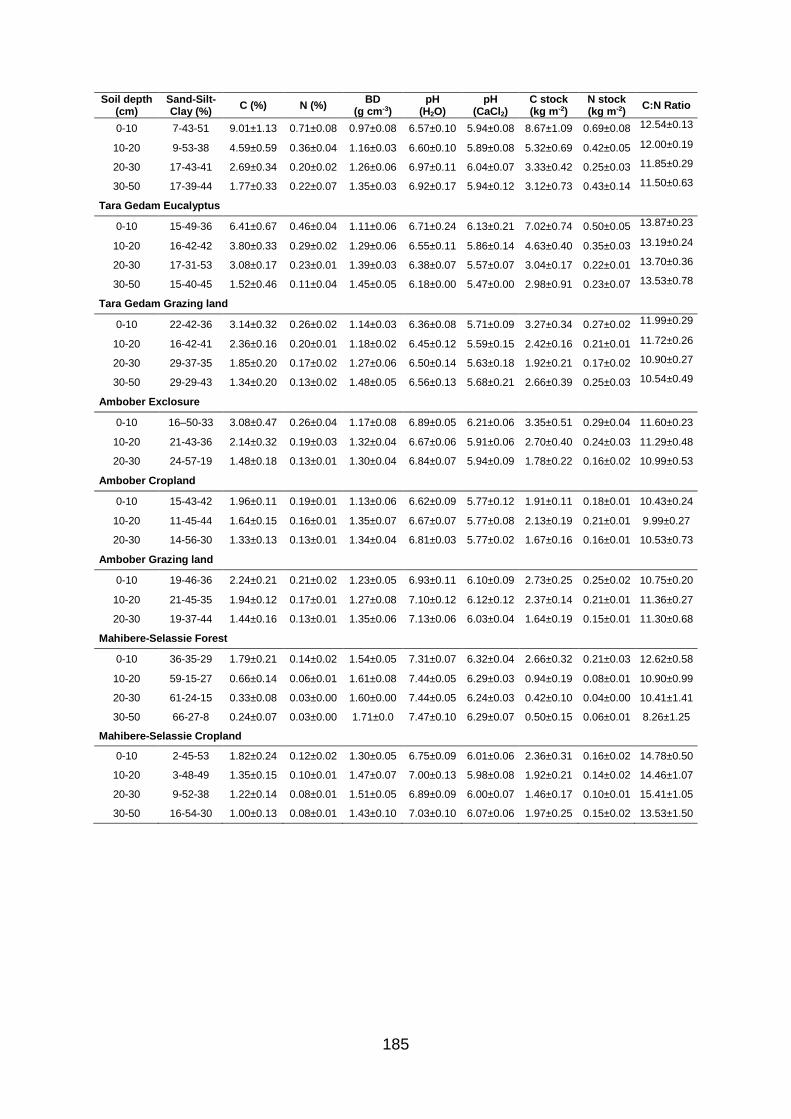
185

Soil depth (cm)

Sand-Silt-Clay (%)

C (%) N (%) BD

(g cm-3) pH

(H2O) pH

(CaCl2) C stock (kg m-2)

N stock (kg m-2)

C:N Ratio

0-10 7-43-51 9.01±1.13 0.71±0.08 0.97±0.08 6.57±0.10 5.94±0.08 8.67±1.09 0.69±0.08 12.54±0.13

10-20 9-53-38 4.59±0.59 0.36±0.04 1.16±0.03 6.60±0.10 5.89±0.08 5.32±0.69 0.42±0.05 12.00±0.19

20-30 17-43-41 2.69±0.34 0.20±0.02 1.26±0.06 6.97±0.11 6.04±0.07 3.33±0.42 0.25±0.03 11.85±0.29

30-50 17-39-44 1.77±0.33 0.22±0.07 1.35±0.03 6.92±0.17 5.94±0.12 3.12±0.73 0.43±0.14 11.50±0.63

Tara Gedam Eucalyptus

0-10 15-49-36 6.41±0.67 0.46±0.04 1.11±0.06 6.71±0.24 6.13±0.21 7.02±0.74 0.50±0.05 13.87±0.23

10-20 16-42-42 3.80±0.33 0.29±0.02 1.29±0.06 6.55±0.11 5.86±0.14 4.63±0.40 0.35±0.03 13.19±0.24

20-30 17-31-53 3.08±0.17 0.23±0.01 1.39±0.03 6.38±0.07 5.57±0.07 3.04±0.17 0.22±0.01 13.70±0.36

30-50 15-40-45 1.52±0.46 0.11±0.04 1.45±0.05 6.18±0.00 5.47±0.00 2.98±0.91 0.23±0.07 13.53±0.78

Tara Gedam Grazing land

0-10 22-42-36 3.14±0.32 0.26±0.02 1.14±0.03 6.36±0.08 5.71±0.09 3.27±0.34 0.27±0.02 11.99±0.29

10-20 16-42-41 2.36±0.16 0.20±0.01 1.18±0.02 6.45±0.12 5.59±0.15 2.42±0.16 0.21±0.01 11.72±0.26

20-30 29-37-35 1.85±0.20 0.17±0.02 1.27±0.06 6.50±0.14 5.63±0.18 1.92±0.21 0.17±0.02 10.90±0.27

30-50 29-29-43 1.34±0.20 0.13±0.02 1.48±0.05 6.56±0.13 5.68±0.21 2.66±0.39 0.25±0.03 10.54±0.49

Ambober Exclosure

0-10 16–50-33 3.08±0.47 0.26±0.04 1.17±0.08 6.89±0.05 6.21±0.06 3.35±0.51 0.29±0.04 11.60±0.23

10-20 21-43-36 2.14±0.32 0.19±0.03 1.32±0.04 6.67±0.06 5.91±0.06 2.70±0.40 0.24±0.03 11.29±0.48

20-30 24-57-19 1.48±0.18 0.13±0.01 1.30±0.04 6.84±0.07 5.94±0.09 1.78±0.22 0.16±0.02 10.99±0.53

Ambober Cropland

0-10 15-43-42 1.96±0.11 0.19±0.01 1.13±0.06 6.62±0.09 5.77±0.12 1.91±0.11 0.18±0.01 10.43±0.24

10-20 11-45-44 1.64±0.15 0.16±0.01 1.35±0.07 6.67±0.07 5.77±0.08 2.13±0.19 0.21±0.01 9.99±0.27

20-30 14-56-30 1.33±0.13 0.13±0.01 1.34±0.04 6.81±0.03 5.77±0.02 1.67±0.16 0.16±0.01 10.53±0.73

Ambober Grazing land

0-10 19-46-36 2.24±0.21 0.21±0.02 1.23±0.05 6.93±0.11 6.10±0.09 2.73±0.25 0.25±0.02 10.75±0.20

10-20 21-45-35 1.94±0.12 0.17±0.01 1.27±0.08 7.10±0.12 6.12±0.12 2.37±0.14 0.21±0.01 11.36±0.27

20-30 19-37-44 1.44±0.16 0.13±0.01 1.35±0.06 7.13±0.06 6.03±0.04 1.64±0.19 0.15±0.01 11.30±0.68

Mahibere-Selassie Forest

0-10 36-35-29 1.79±0.21 0.14±0.02 1.54±0.05 7.31±0.07 6.32±0.04 2.66±0.32 0.21±0.03 12.62±0.58

10-20 59-15-27 0.66±0.14 0.06±0.01 1.61±0.08 7.44±0.05 6.29±0.03 0.94±0.19 0.08±0.01 10.90±0.99

20-30 61-24-15 0.33±0.08 0.03±0.00 1.60±0.00 7.44±0.05 6.24±0.03 0.42±0.10 0.04±0.00 10.41±1.41

30-50 66-27-8 0.24±0.07 0.03±0.00 1.71±0.0 7.47±0.10 6.29±0.07 0.50±0.15 0.06±0.01 8.26±1.25

Mahibere-Selassie Cropland

0-10 2-45-53 1.82±0.24 0.12±0.02 1.30±0.05 6.75±0.09 6.01±0.06 2.36±0.31 0.16±0.02 14.78±0.50

10-20 3-48-49 1.35±0.15 0.10±0.01 1.47±0.07 7.00±0.13 5.98±0.08 1.92±0.21 0.14±0.02 14.46±1.07

20-30 9-52-38 1.22±0.14 0.08±0.01 1.51±0.05 6.89±0.09 6.00±0.07 1.46±0.17 0.10±0.01 15.41±1.05

30-50 16-54-30 1.00±0.13 0.08±0.01 1.43±0.10 7.03±0.10 6.07±0.06 1.97±0.25 0.15±0.02 13.53±1.50

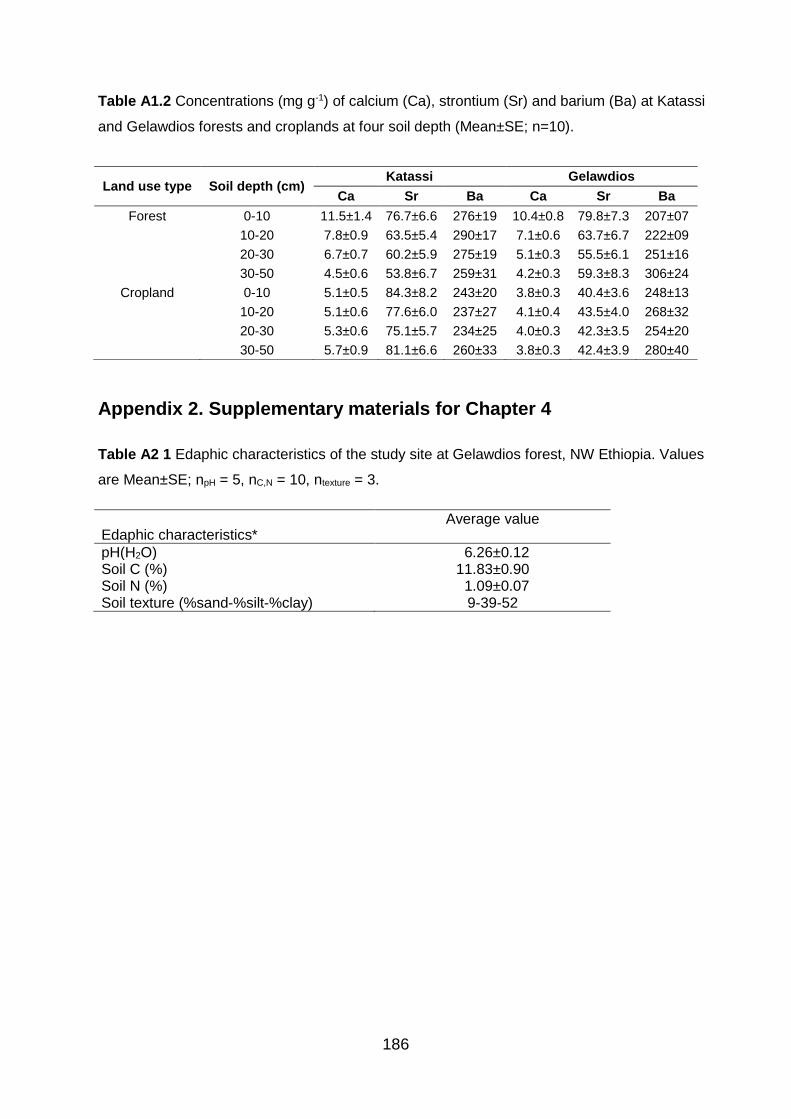
186

Table A1.2 Concentrations (mg g-1) of calcium (Ca), strontium (Sr) and barium (Ba) at Katassi

and Gelawdios forests and croplands at four soil depth (Mean±SE; n=10).


Table A2 1 Edaphic characteristics of the study site at Gelawdios forest, NW Ethiopia. Values

are Mean±SE; npH = 5, nC,N = 10, ntexture = 3.

Edaphic characteristics* Average value

pH(H2O) 6.26±0.12 Soil C (%) 11.83±0.90 Soil N (%) 1.09±0.07 Soil texture (%sand-%silt-%clay) 9-39-52

Land use type Soil depth (cm) Katassi Gelawdios

Ca Sr Ba Ca Sr Ba

Forest 0-10 11.5±1.4 76.7±6.6 276±19 10.4±0.8 79.8±7.3 207±07 10-20 7.8±0.9 63.5±5.4 290±17 7.1±0.6 63.7±6.7 222±09 20-30 6.7±0.7 60.2±5.9 275±19 5.1±0.3 55.5±6.1 251±16 30-50 4.5±0.6 53.8±6.7 259±31 4.2±0.3 59.3±8.3 306±24

Cropland 0-10 5.1±0.5 84.3±8.2 243±20 3.8±0.3 40.4±3.6 248±13 10-20 5.1±0.6 77.6±6.0 237±27 4.1±0.4 43.5±4.0 268±32 20-30 5.3±0.6 75.1±5.7 234±25 4.0±0.3 42.3±3.5 254±20 30-50 5.7±0.9 81.1±6.6 260±33 3.8±0.3 42.4±3.9 280±40

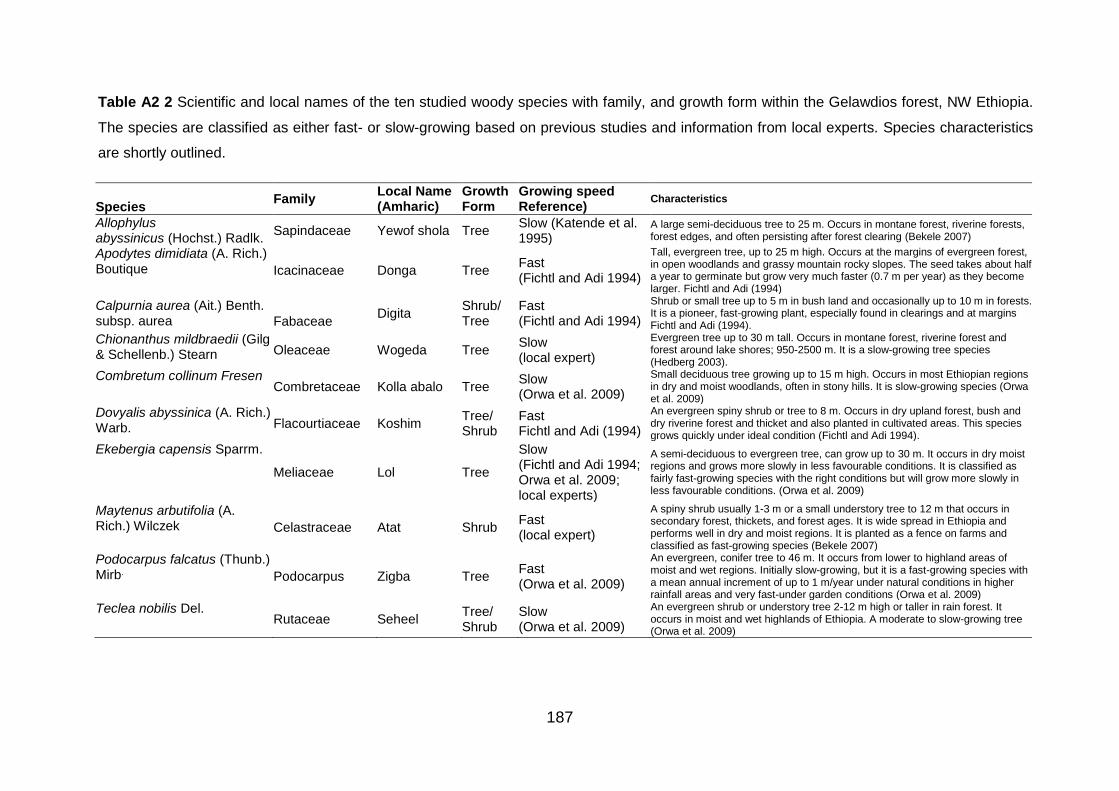
187

Table A2 2 Scientific and local names of the ten studied woody species with family, and growth form within the Gelawdios forest, NW Ethiopia.

The species are classified as either fast- or slow-growing based on previous studies and information from local experts. Species characteristics

are shortly outlined.

Species Family

Local Name (Amharic)

Growth Form

Growing speed Reference)

Characteristics

Allophylus abyssinicus (Hochst.) Radlk.

Sapindaceae Yewof shola Tree Slow (Katende et al. 1995)

A large semi-deciduous tree to 25 m. Occurs in montane forest, riverine forests, forest edges, and often persisting after forest clearing (Bekele 2007)

Apodytes dimidiata (A. Rich.) Boutique Icacinaceae Donga Tree

Fast (Fichtl and Adi 1994)

Tall, evergreen tree, up to 25 m high. Occurs at the margins of evergreen forest, in open woodlands and grassy mountain rocky slopes. The seed takes about half a year to germinate but grow very much faster (0.7 m per year) as they become larger. Fichtl and Adi (1994)

Calpurnia aurea (Ait.) Benth. subsp. aurea Fabaceae

Digita Shrub/ Tree

Fast (Fichtl and Adi 1994)

Shrub or small tree up to 5 m in bush land and occasionally up to 10 m in forests. It is a pioneer, fast-growing plant, especially found in clearings and at margins Fichtl and Adi (1994).

Chionanthus mildbraedii (Gilg & Schellenb.) Stearn Oleaceae Wogeda Tree

Slow (local expert)

Evergreen tree up to 30 m tall. Occurs in montane forest, riverine forest and forest around lake shores; 950-2500 m. It is a slow-growing tree species (Hedberg 2003).

Combretum collinum Fresen Combretaceae Kolla abalo Tree

Slow (Orwa et al. 2009)

Small deciduous tree growing up to 15 m high. Occurs in most Ethiopian regions in dry and moist woodlands, often in stony hills. It is slow-growing species (Orwa et al. 2009)

Dovyalis abyssinica (A. Rich.) Warb. Flacourtiaceae Koshim

Tree/ Shrub

Fast Fichtl and Adi (1994)

An evergreen spiny shrub or tree to 8 m. Occurs in dry upland forest, bush and dry riverine forest and thicket and also planted in cultivated areas. This species grows quickly under ideal condition (Fichtl and Adi 1994).

Ekebergia capensis Sparrm.

Meliaceae Lol Tree

Slow (Fichtl and Adi 1994; Orwa et al. 2009; local experts)

A semi-deciduous to evergreen tree, can grow up to 30 m. It occurs in dry moist regions and grows more slowly in less favourable conditions. It is classified as fairly fast-growing species with the right conditions but will grow more slowly in less favourable conditions. (Orwa et al. 2009)

Maytenus arbutifolia (A. Rich.) Wilczek Celastraceae Atat Shrub

Fast (local expert)

A spiny shrub usually 1-3 m or a small understory tree to 12 m that occurs in secondary forest, thickets, and forest ages. It is wide spread in Ethiopia and performs well in dry and moist regions. It is planted as a fence on farms and classified as fast-growing species (Bekele 2007)

Podocarpus falcatus (Thunb.) Mirb. Podocarpus Zigba Tree

Fast (Orwa et al. 2009)

An evergreen, conifer tree to 46 m. It occurs from lower to highland areas of moist and wet regions. Initially slow-growing, but it is a fast-growing species with a mean annual increment of up to 1 m/year under natural conditions in higher rainfall areas and very fast-under garden conditions (Orwa et al. 2009)

Teclea nobilis Del. Rutaceae Seheel

Tree/ Shrub

Slow (Orwa et al. 2009)

An evergreen shrub or understory tree 2-12 m high or taller in rain forest. It occurs in moist and wet highlands of Ethiopia. A moderate to slow-growing tree (Orwa et al. 2009)

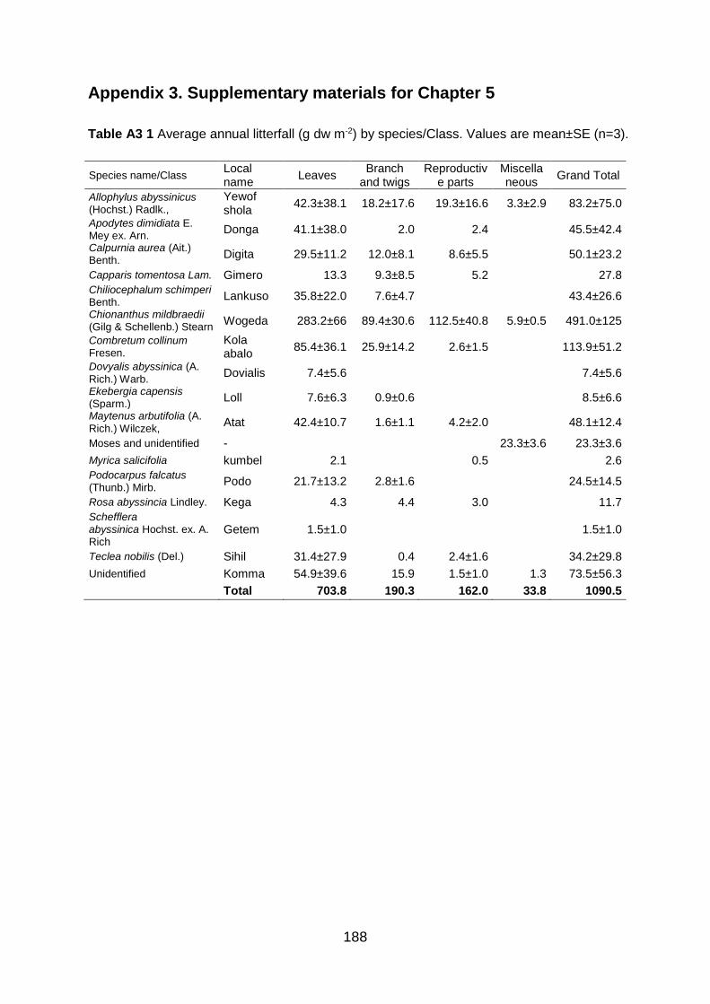
188


Table A3 1 Average annual litterfall (g dw m-2) by species/Class. Values are mean±SE (n=3).

Species name/Class Local name

Leaves Branch

and twigs Reproductiv

e parts Miscellaneous

Grand Total

Allophylus abyssinicus (Hochst.) Radlk.,

Yewof shola

42.3±38.1 18.2±17.6 19.3±16.6 3.3±2.9 83.2±75.0

Apodytes dimidiata E. Mey ex. Arn.

Donga 41.1±38.0 2.0 2.4 45.5±42.4

Calpurnia aurea (Ait.) Benth.

Digita 29.5±11.2 12.0±8.1 8.6±5.5 50.1±23.2

Capparis tomentosa Lam. Gimero 13.3 9.3±8.5 5.2 27.8

Chiliocephalum schimperi Benth.

Lankuso 35.8±22.0 7.6±4.7 43.4±26.6

Chionanthus mildbraedii (Gilg & Schellenb.) Stearn

Wogeda 283.2±66 89.4±30.6 112.5±40.8 5.9±0.5 491.0±125

Combretum collinum Fresen.

Kola abalo

85.4±36.1 25.9±14.2 2.6±1.5 113.9±51.2

Dovyalis abyssinica (A.

Rich.) Warb. Dovialis 7.4±5.6 7.4±5.6

Ekebergia capensis (Sparm.)

Loll 7.6±6.3 0.9±0.6 8.5±6.6

Maytenus arbutifolia (A.

Rich.) Wilczek, Atat 42.4±10.7 1.6±1.1 4.2±2.0 48.1±12.4

Moses and unidentified - 23.3±3.6 23.3±3.6

Myrica salicifolia kumbel 2.1 0.5 2.6

Podocarpus falcatus (Thunb.) Mirb.

Podo 21.7±13.2 2.8±1.6 24.5±14.5

Rosa abyssincia Lindley. Kega 4.3 4.4 3.0 11.7

Schefflera abyssinica Hochst. ex. A. Rich

Getem 1.5±1.0 1.5±1.0

Teclea nobilis (Del.) Sihil 31.4±27.9 0.4 2.4±1.6 34.2±29.8

Unidentified Komma 54.9±39.6 15.9 1.5±1.0 1.3 73.5±56.3

Total 703.8 190.3 162.0 33.8 1090.5

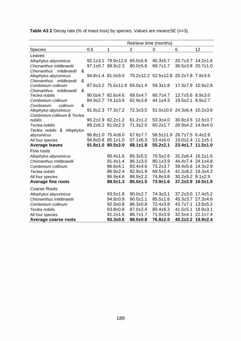
189

Table A3 2 Decay rate (% of mass loss) by species. Values are mean±SE (n=3).

Retrieve time (months)

Species 0.5 1 2 3 6 12

Leaves Allophylus abyssinicus 92.1±3.1 79.9±12.0 65.0±5.6 45.3±5.7 20.7±3.7 14.2±1.6 Chionanthus mildbraedii 97.1±0.7 89.9±2.3 80.0±5.6 69.7±1.7 36.5±3.8 20.7±1.0 Chionanthus mildbraedii & Allophylus abyssinicus 94.8±1.4 81.0±9.0 70.2±12.2 52.5±12.8 25.2±7.8 7.9±3.5 Chionanthus mildbraedii & Combretum collinum 87.6±3.2 75.6±11.9 65.0±1.4 59.3±1.8 17.3±7.9 10.9±2.8 Chionanthus mildbraedii & Teclea nobilis 90.0±4.7 82.6±4.6 69.0±4.7 60.7±4.7 12.7±5.6 8.9±3.0 Combretum collinum 84.9±2.7 74.1±3.9 62.9±3.8 44.1±4.3 19.5±2.1 8.9±2.7 Combretum collinum & Allophylus abyssinicus 91.9±2.3 77.3±7.2 72.3±3.5 51.0±10.0 24.3±6.4 10.2±3.6 Combretum collinum & Teclea nobilis 90.2±2.9 82.2±1.2 61.2±1.2 53.3±4.0 30.8±3.5 12.5±3.7 Teclea nobilis 89.2±6.2 81.0±2.3 71.3±2.0 60.2±1.7 26.9±4.2 14.9±4.0 Teclea nobilis & Allophylus abyssinicus 96.8±1.0 75.4±8.0 67.6±7.7 58.5±11.9 26.7±7.5 6.4±2.8 All four species 94.8±0.8 85.1±1.0 67.1±6.3 53.4±6.0 19.0±2.4 11.1±5.1 Average leaves 91.8±1.0 80.5±2.0 68.1±1.8 55.2±2.1 23.4±1.7 11.5±1.0

Fine roots Allophylus abyssinicus 90.4±1.6 85.3±5.5 70.5±2.6 31.2±6.4 16.2±1.6 Chionanthus mildbraedii 91.4±1.4 86.1±3.0 80.1±3.9 44.4±7.4 24.1±4.8 Combretum collinum 86.6±4.1 83.4±4.6 73.2±3.7 39.4±5.6 14.3±2.9 Teclea nobilis 86.9±2.4 82.9±1.9 69.5±2.4 41.3±8.2 19.3±4.2 All four species 86.9±4.6 86.9±2.2 74.8±3.8 30.2±5.2 8.1±2.9 Average fine roots 88.5±1.3 85.0±1.5 73.9±1.6 37.2±2.9 16.5±1.9

Coarse Roots Allophylus abyssinicus 93.5±1.8 90.0±2.7 74.3±3.1 37.2±3.0 17.4±5.2 Chionanthus mildbraedii 94.8±0.8 90.0±1.1 85.5±1.6 45.3±3.7 27.3±4.6 Combretum collinum 92.9±0.8 86.3±0.8 72.4±3.8 43.7±7.1 13.8±5.2 Teclea nobilis 93.8±0.8 87.0±2.4 80.4±6.3 41.5±5.1 18.9±3.1 All four species 91.2±1.6 86.7±1.7 71.0±3.9 32.5±4.1 22.1±7.4 Average coarse roots 93.3±0.6 88.0±0.8 76.8±2.0 40.2±2.2 19.9±2.4

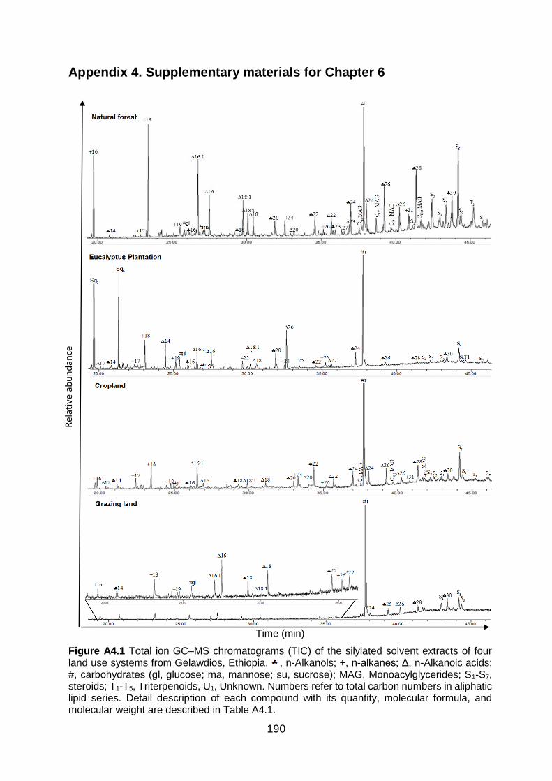
190


Time (min)

Figure A4.1 Total ion GC–MS chromatograms (TIC) of the silylated solvent extracts of four land use systems from Gelawdios, Ethiopia. , n-Alkanols; +, n-alkanes; Δ, n-Alkanoic acids; #, carbohydrates (gl, glucose; ma, mannose; su, sucrose); MAG, Monoacylglycerides; S1-S7, steroids; T1-T5, Triterpenoids, U1, Unknown. Numbers refer to total carbon numbers in aliphatic lipid series. Detail description of each compound with its quantity, molecular formula, and molecular weight are described in Table A4.1.

Rel

ativ

e ab

un

dan

ce

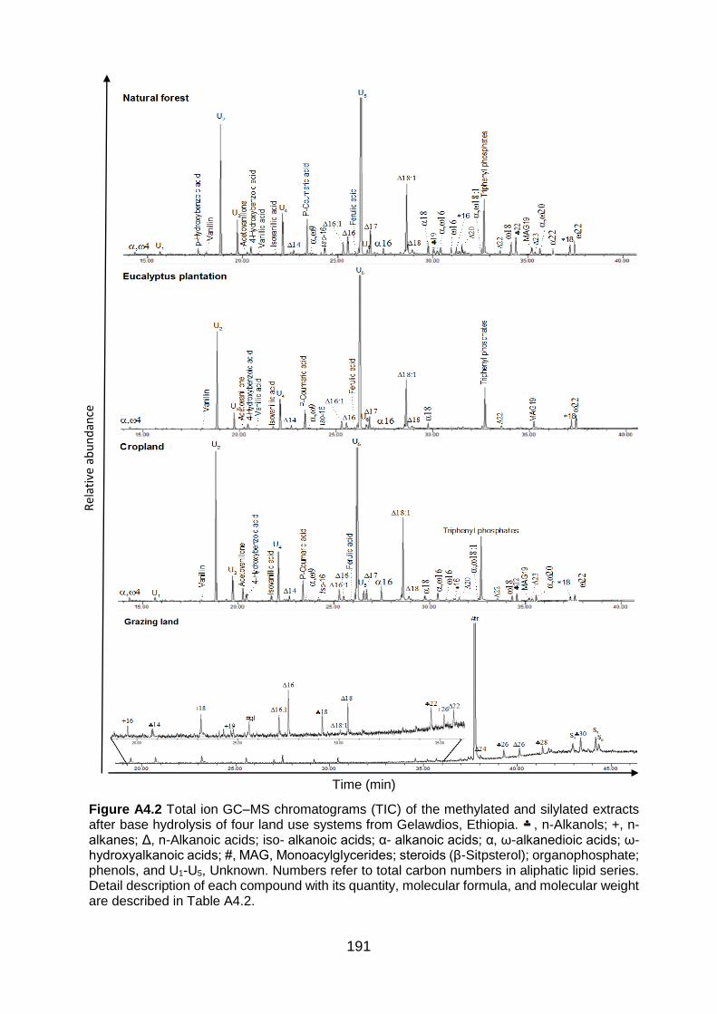
191

Time (min)

Figure A4.2 Total ion GC–MS chromatograms (TIC) of the methylated and silylated extracts after base hydrolysis of four land use systems from Gelawdios, Ethiopia. , n-Alkanols; +, n-alkanes; Δ, n-Alkanoic acids; iso- alkanoic acids; α- alkanoic acids; α, ω-alkanedioic acids; ω-hydroxyalkanoic acids; #, MAG, Monoacylglycerides; steroids (β-Sitpsterol); organophosphate; phenols, and U1-U5, Unknown. Numbers refer to total carbon numbers in aliphatic lipid series. Detail description of each compound with its quantity, molecular formula, and molecular weight are described in Table A4.2.

Rel

ativ

e ab

un

dan

ce

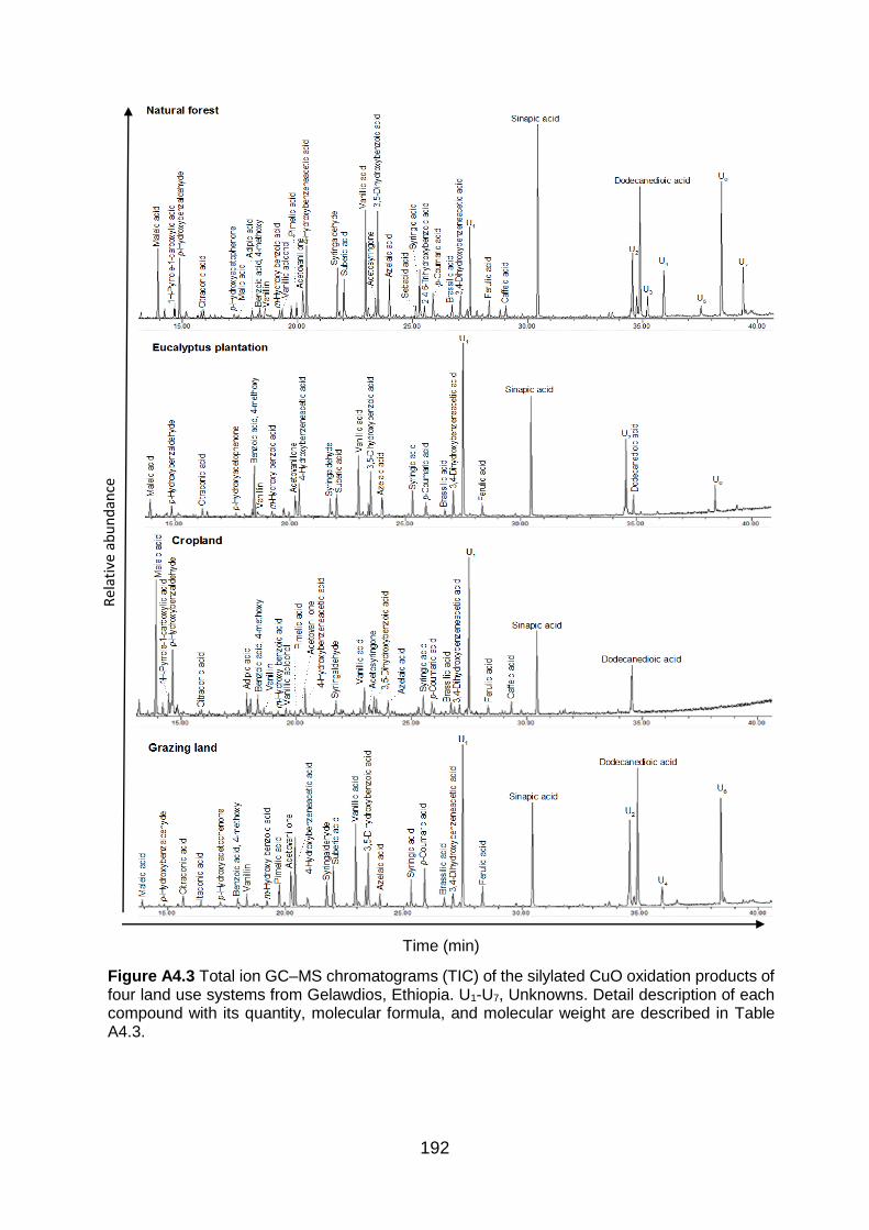
192

Time (min)

Figure A4.3 Total ion GC–MS chromatograms (TIC) of the silylated CuO oxidation products of four land use systems from Gelawdios, Ethiopia. U1-U7, Unknowns. Detail description of each compound with its quantity, molecular formula, and molecular weight are described in Table A4.3.

Rel

ativ

e ab

un

dan

ce

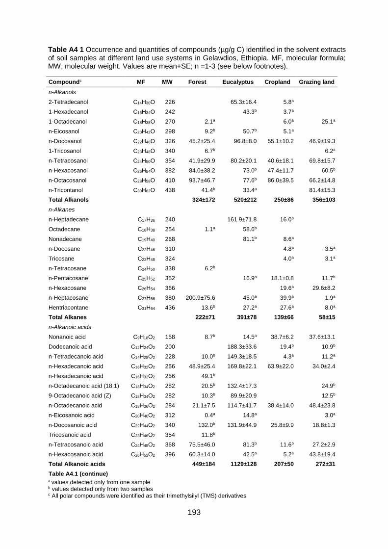
193

Table A4 1 Occurrence and quantities of compounds (µg/g C) identified in the solvent extracts of soil samples at different land use systems in Gelawdios, Ethiopia. MF, molecular formula; MW, molecular weight. Values are mean+SE; n =1-3 (see below footnotes).

Compoundc MF MW Forest Eucalyptus Cropland Grazing land

n-Alkanols

2-Tetradecanol C14H30O 226 65.3±16.4 5.8a

1-Hexadecanol C16H34O 242 43.3b 3.7a

1-Octadecanol C18H38O 270 2.1a 6.0a 25.1a

n-Eicosanol C20H42O 298 9.2b 50.7b 5.1a

n-Docosanol C22H46O 326 45.2±25.4 96.8±8.0 55.1±10.2 46.9±19.3

1-Tricosanol C23H48O 340 6.7b 6.2a

n-Tetracosanol C24H50O 354 41.9±29.9 80.2±20.1 40.6±18.1 69.8±15.7

n-Hexacosanol C26H54O 382 84.0±38.2 73.0b 47.4±11.7 60.5b

n-Octacosanol C28H58O 410 93.7±46.7 77.6b 86.0±39.5 66.2±14.8

n-Tricontanol C30H62O 438 41.4b 33.4a 81.4±15.3

Total Alkanols 324±172 520±212 250±86 356±103

n-Alkanes

n-Heptadecane C17H36 240 161.9±71.8 16.0b

Octadecane C18H38 254 1.1a 58.6b

Nonadecane C19H40 268 81.1b 8.6a

n-Docosane C22H46 310 4.8a 3.5a

Tricosane C23H48 324 4.0a 3.1a

n-Tetracosane C24H50 338 6.2b

n-Pentacosane C25H52 352 16.9a 18.1±0.8 11.7b

n-Hexacosane C26H54 366 19.6a 29.6±8.2

n-Heptacosane C27H56 380 200.9±75.6 45.0a 39.9a 1.9a

Hentriacontane C31H64 436 13.6b 27.2a 27.6a 8.0a

Total Alkanes 222±71 391±78 139±66 58±15

n-Alkanoic acids

Nonanoic acid C9H18O2 158 8.7b 14.5a 38.7±6.2 37.6±13.1

Dodecanoic acid C12H24O2 200 188.3±33.6 19.4b 10.9b

n-Tetradecanoic acid C14H28O2 228 10.0b 149.3±18.5 4.3a 11.2a

n-Hexadecanoic acid C16H32O2 256 48.9±25.4 169.8±22.1 63.9±22.0 34.0±2.4

n-Hexadecanoic acid C16H32O2 256 49.1b

n-Octadecanoic acid (18:1) C18H34O2 282 20.5b 132.4±17.3 24.9b

9-Octadecanoic acid (Z) C18H34O2 282 10.3b 89.9±20.9 12.5b

n-Octadecanoic acid C18H36O2 284 21.1±7.5 114.7±41.7 38.4±14.0 48.4±23.8

n-Eicosanoic acid C20H40O2 312 0.4a 14.8a 3.0a

n-Docosanoic acid C22H44O2 340 132.0b 131.9±44.9 25.8±9.9 18.8±1.3

Tricosanoic acid C23H46O2 354 11.8b

n-Tetracosanoic acid C24H48O2 368 75.5±46.0 81.3b 11.6b 27.2±2.9

n-Hexacosanoic acid C26H52O2 396 60.3±14.0 42.5a 5.2a 43.8±19.4

Total Alkanoic acids 449±184 1129±128 207±50 272±31

Table A4.1 (continue) a values detected only from one sample b values detected only from two samples c All polar compounds were identified as their trimethylsilyl (TMS) derivatives

194

Table A4.1 continued

Compoundc MF MW Forest Eucalyptus Cropland Grazing land

Iso- Alkanoic acids

Iso-Heptadecanoic acid C17H34O2 270 24.5b

Monoacylglycerides

(±)-2,3-Dihydroxypropyl hexadecanoate (C16)

C19H38O4 330 9.2b 19.1a 37.12b

Monostearin (C18:1) C21H42O4 358 16.1b 134.4±26.1 97.0±19.14 64.9±8.9

Linolein, 1-mono (C18:1) C21H38O4 354 20.6±9.5 31.9a 9.3a

2-Monolinolenin (C18:2) C21H36O4 352 6.4a 74.3±16.0 9.7a

Total Monoacylglycerides 52±26 260±19 134±46 84±2

Carbohydrates

D-Glucose C6H12O6 180 16.2b 90.1±32.9 37.8±16.6 46.7±14.7

Mannose C6H12O6 180 16.9±7.0 211.9±78.4 78.4±25.3 46.0±14.0

Sucrose C12H22O11 342 7.7b 19.6a 19.5b 33.0±11.3

Trehalose C12H22O11 342 3895±712.5 2107.4±217.1 1684.1±191 1768.2±157.8

Total Carbohydrates 3936±703 2429±256 18120±229 1894±192

Steroids and Terpenoids

Aromadendrene C15H24 204 0.5a 124.9b 13.8a

γ-Elemene C15H24 204 183.0±81.1 13.5a

Ledol C15H26O 222 157.2±32.9 9.3a

(-)-Globulol C15H26O 222 72.0±7.5 17.1b 11.8a

trans-Farnesol C15H26O 222 752.7±64.9 48.2a

Cholesterol C27H46O 386 11.4b 98.8±33.0 62.2b 23.6b

Ergostrol C28H44O 396 36.8b 94.7a

Campesterol C28H48O 400 32.9b 117.3±28.7 87.9b 104.7±0.3

Stigmasterol C29H48O 412 56.0b 243.1±30.4 110.2±17.4 138.9±18.3

ß-Sitosterol C29H50O 414 232.2±93.8 243.2±6.0 237.9±46.1 142.9±25.7

Stigmastanol C29H52O 416 119.4±34.2

ß- Amyrin C30H50O 426 81.2b 161.8±1.8 98.9±16.3

α- Amyrin C30H50O 426 14.7b 66.1±17.9

Lupeol C30H50O 426 9.7a 87.3b 13.3a 28.0a

Sitosterone C29H48O 412 13.3a 73.6b 17.0a

Erthrodiol C30H50O2 442 47.4b 343.6±100.3

Oleanolic acid C30H48O3 456 85.4±52.5 642.1±132.5 46.9b

Total Steroids and Terpenoids 622±267 3461±341 729±80 616±616

Unknownd 37.6±3.4 126.2±10.8 238.1±99.6 67.7b

Total aliphatic lipids 5007±746 4729±531 2550±430 2664±300

Total solvent extracts 5629±740 8190±857 3279±508 3280±394 a values detected only from one sample b values detected only from two samples c All polar compounds were identified as their trimethylsilyl (TMS) derivatives d Identified as Glycocholic acid (C26H43NO6)

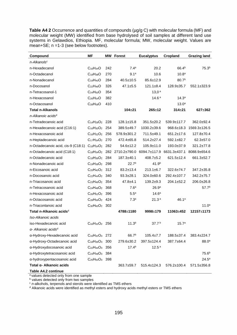
195

Table A4 2 Occurrence and quantities of compounds (µg/g C) with molecular formula (MF) and molecular weight (MW) identified from base hydrolysed of soil samples at different land use systems in Gelawdios, Ethiopia. MF, molecular formula; MW, molecular weight. Values are mean+SE; n =1-3 (see below footnotes).

Compound MF MW Forest Eucalyptus Cropland Grazing land

n-Alkanolsc

n-Hexadecanol C16H34O 242 7.4a 20.2 66.4b 75.3b

n-Octadecanol C18H38O 270 9.1a 10.6 10.8a

n-Nonadecanol C19H40O 284 40.5±10.5 85.6±12.9 80.7b

n-Docosanol C22H46O 326 47.1±5.5 121.1±8.4 128.9±35.7 552.1±323.9

n-Tetracosanol-1 C24H50O 354 13,0 a

n-Hexacosanol C26H54O 382 14.6 a 14.3a

n-Octacosanol C28H58O 410 13.0a

Total n-Alkanols 104±21 265±12 314±21 627±362

n-Alkanoic acidsd

n-Tetradecanoic acid C14H28O2 228 128.1±15.8 351.5±20.2 539.9±117.7 362.0±92.4

n-Hexadecanoic acid (C16:1) C16H30O2 254 389.5±49.7 1030.2±39.6 968.6±18.3 1569.3±126.5

n-Hexacosanoic acid C16H32O2 256 578.9±301.2 711.5±49.1 651.2±17.6 127.8±70.4

n-Heptadecanoic acid C17H34O2 270 472.4±65.8 514.2±27.4 592.1±82.7 62.3±57.0

n-Octadecanoic acid, cis-9 (C18:1) C18H34O2 282 54.6±12.2 105.9±11.0 193.0±37.9 321.2±77.8

n-Octadecanoic acid (C18:1) C18H34O2 282 2710.2±790.0 6094.7±117.9 6631.3±437.1 8088.9±654.6

n-Octadecanoic acid C18H36O2 284 187.3±40.1 408.7±5.2 621.5±12.4 661.3±52.7

n-Nonadecanoic acid C19H38O2 298 22.7b 41.9b

n-Eicosanoic acid C20H40O2 312 83.2±13.4 213.1±6.7 322.6±74.7 347.2±35.8

n-Docosanoic acid C22H44O2 340 93.3±28.1 324.0±60.6 292.4±107.7 342.2±75.7

n-Triacosanoic acid C23H46O2 354 47.8±4.1 139.2±9.3 204.1±52.2 206.0±26.8

n-Tetracosanoic acid C24H48O2 368 7.6a 26.9a 57.7b

n-Hexacosanoic acid C26H52O2 396 5.5a 14.6a

n-Octacosanoic acid C28H56O2 424 7.3a 21.3 a 46.1a

n-Triacontanoic acid C30H60O2 302 11.0a

Total n-Alkanoic acidsd 4788±1180 9998±179 11063±452 12157±1173

Iso-Alkanoic acids

iso-Hexadecanoic acid C16H32O2 256 11.3b 37.7 b 15.7a

α- Alkanoic acidsd

α-Hydroxy-Hexadecanoic acid C16H32O3 272 66.7b 105.4±7.7 188.5±37.4 383.4±224.7

α-Hydroxy-Octadecanoic acid C18H36O3 300 279.6±30.2 397.5±124.4 387.7±64.4 88.0a

α-Hydroxydocosanoic acid C22H44O3 356 17.4b 12.5 a

α-Hydroxytetracosanoic acid C24H48O3 384 75.6b

α-hydroxypentacosanoic acid C25H50O3 398 24.5a

Total α- Alkanoic acids 363.7±59.7 515.4±124.3 576.2±100.4 571.5±356.8

Table A4.2 continue a values detected only from one sample b values detected only from two samples c n-alkohols, terpenols and sterols were identified as TMS ethers d Alkanoic acids were identified as methyl esters and hydroxy acids methyl esters or TMS ethers

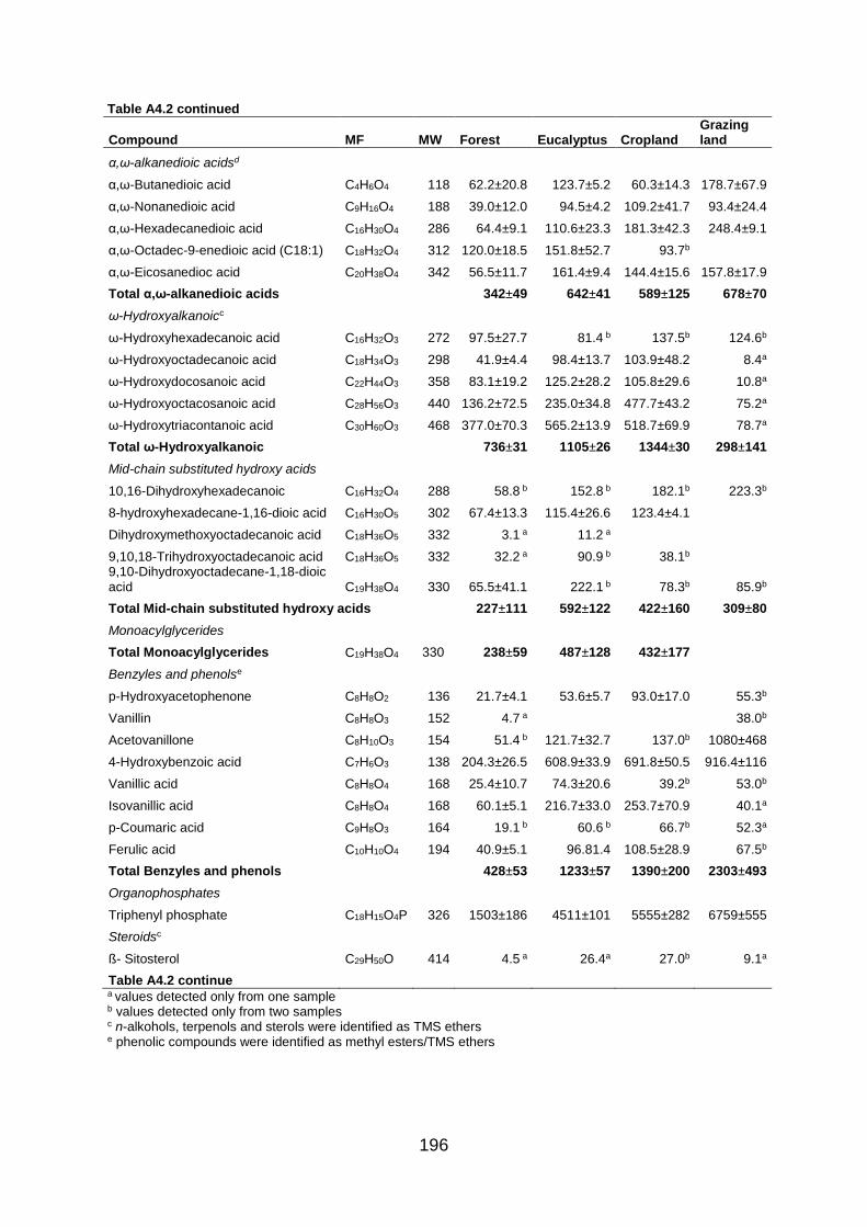
196



α,ω-alkanedioic acidsd

α,ω-Butanedioic acid C4H6O4 118 62.2±20.8 123.7±5.2 60.3±14.3 178.7±67.9

α,ω-Nonanedioic acid C9H16O4 188 39.0±12.0 94.5±4.2 109.2±41.7 93.4±24.4

α,ω-Hexadecanedioic acid C16H30O4 286 64.4±9.1 110.6±23.3 181.3±42.3 248.4±9.1

α,ω-Octadec-9-enedioic acid (C18:1) C18H32O4 312 120.0±18.5 151.8±52.7 93.7b

α,ω-Eicosanedioc acid C20H38O4 342 56.5±11.7 161.4±9.4 144.4±15.6 157.8±17.9

Total α,ω-alkanedioic acids 342±49 642±41 589±125 678±70

ω-Hydroxyalkanoicc

ω-Hydroxyhexadecanoic acid C16H32O3 272 97.5±27.7 81.4 b 137.5b 124.6b

ω-Hydroxyoctadecanoic acid C18H34O3 298 41.9±4.4 98.4±13.7 103.9±48.2 8.4a

ω-Hydroxydocosanoic acid C22H44O3 358 83.1±19.2 125.2±28.2 105.8±29.6 10.8a

ω-Hydroxyoctacosanoic acid C28H56O3 440 136.2±72.5 235.0±34.8 477.7±43.2 75.2a

ω-Hydroxytriacontanoic acid C30H60O3 468 377.0±70.3 565.2±13.9 518.7±69.9 78.7a

Total ω-Hydroxyalkanoic 736±31 1105±26 1344±30 298±141

Mid-chain substituted hydroxy acids

10,16-Dihydroxyhexadecanoic C16H32O4 288 58.8 b 152.8 b 182.1b 223.3b

8-hydroxyhexadecane-1,16-dioic acid C16H30O5 302 67.4±13.3 115.4±26.6 123.4±4.1

Dihydroxymethoxyoctadecanoic acid C18H36O5 332 3.1 a 11.2 a

9,10,18-Trihydroxyoctadecanoic acid C18H36O5 332 32.2 a 90.9 b 38.1b 9,10-Dihydroxyoctadecane-1,18-dioic acid C19H38O4 330 65.5±41.1 222.1 b 78.3b 85.9b

Total Mid-chain substituted hydroxy acids 227±111 592±122 422±160 309±80

Monoacylglycerides

Total Monoacylglycerides C19H38O4 330 238±59 487±128 432±177

Benzyles and phenolse

p-Hydroxyacetophenone C8H8O2 136 21.7±4.1 53.6±5.7 93.0±17.0 55.3b

Vanillin C8H8O3 152 4.7 a 38.0b

Acetovanillone C8H10O3 154 51.4 b 121.7±32.7 137.0b 1080±468

4-Hydroxybenzoic acid C7H6O3 138 204.3±26.5 608.9±33.9 691.8±50.5 916.4±116

Vanillic acid C8H8O4 168 25.4±10.7 74.3±20.6 39.2b 53.0b

Isovanillic acid C8H8O4 168 60.1±5.1 216.7±33.0 253.7±70.9 40.1a

p-Coumaric acid C9H8O3 164 19.1 b 60.6 b 66.7b 52.3a

Ferulic acid C10H10O4 194 40.9±5.1 96.81.4 108.5±28.9 67.5b

Total Benzyles and phenols 428±53 1233±57 1390±200 2303±493

Organophosphates

Triphenyl phosphate C18H15O4P 326 1503±186 4511±101 5555±282 6759±555

Steroidsc

ß- Sitosterol C29H50O 414 4.5 a 26.4a 27.0b 9.1a

Table A4.2 continue a values detected only from one sample b values detected only from two samples c n-alkohols, terpenols and sterols were identified as TMS ethers e phenolic compounds were identified as methyl esters/TMS ethers

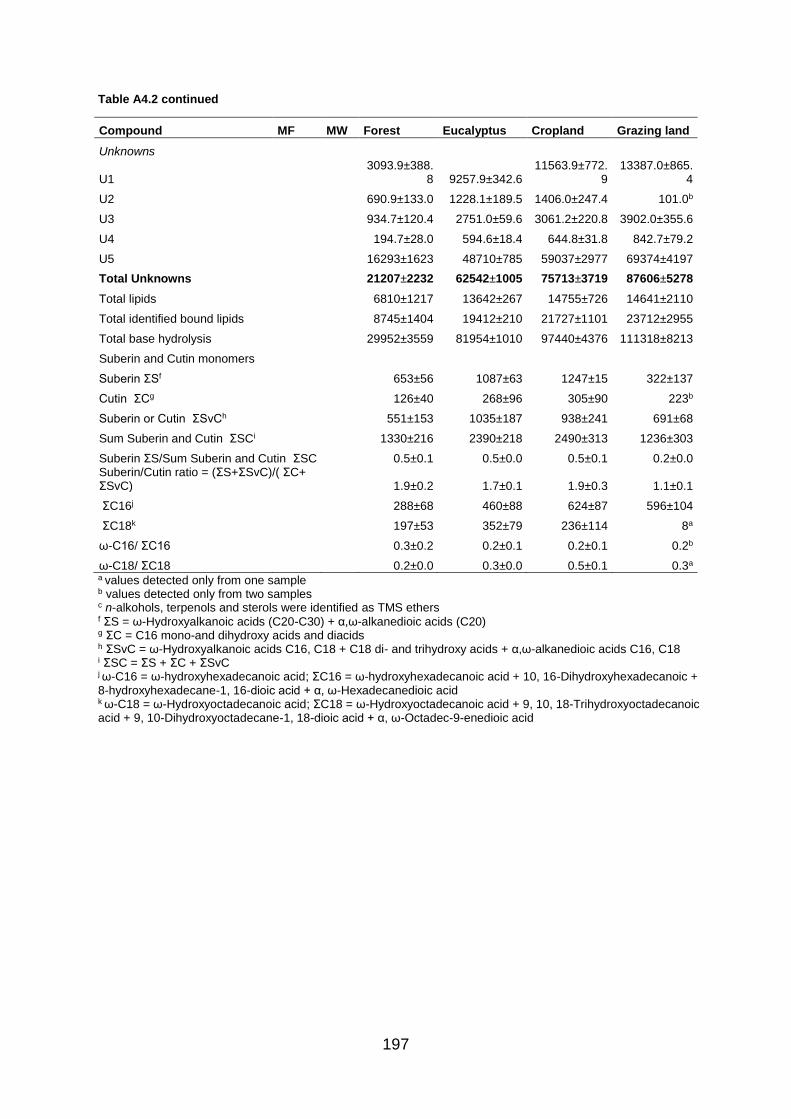
197



Unknowns

U1 3093.9±388.

8 9257.9±342.6 11563.9±772.

9 13387.0±865.

4

U2 690.9±133.0 1228.1±189.5 1406.0±247.4 101.0b

U3 934.7±120.4 2751.0±59.6 3061.2±220.8 3902.0±355.6

U4 194.7±28.0 594.6±18.4 644.8±31.8 842.7±79.2

U5 16293±1623 48710±785 59037±2977 69374±4197

Total Unknowns 21207±2232 62542±1005 75713±3719 87606±5278

Total lipids 6810±1217 13642±267 14755±726 14641±2110

Total identified bound lipids 8745±1404 19412±210 21727±1101 23712±2955

Total base hydrolysis 29952±3559 81954±1010 97440±4376 111318±8213

Suberin and Cutin monomers

Suberin ΣSf 653±56 1087±63 1247±15 322±137

Cutin ΣCg 126±40 268±96 305±90 223b

Suberin or Cutin ΣSvCh 551±153 1035±187 938±241 691±68

Sum Suberin and Cutin ΣSCi 1330±216 2390±218 2490±313 1236±303

Suberin ΣS/Sum Suberin and Cutin ΣSC 0.5±0.1 0.5±0.0 0.5±0.1 0.2±0.0 Suberin/Cutin ratio = (ΣS+ΣSvC)/( ΣC+ ΣSvC) 1.9±0.2 1.7±0.1 1.9±0.3 1.1±0.1

ΣC16j 288±68 460±88 624±87 596±104

ΣC18k 197±53 352±79 236±114 8a

ω-C16/ ΣC16 0.3±0.2 0.2±0.1 0.2±0.1 0.2b

ω-C18/ ΣC18 0.2±0.0 0.3±0.0 0.5±0.1 0.3a a values detected only from one sample b values detected only from two samples c n-alkohols, terpenols and sterols were identified as TMS ethers f ΣS = ω-Hydroxyalkanoic acids (C20-C30) + α,ω-alkanedioic acids (C20) g ΣC = C16 mono-and dihydroxy acids and diacids h ΣSvC = ω-Hydroxyalkanoic acids C16, C18 + C18 di- and trihydroxy acids + α,ω-alkanedioic acids C16, C18 i ΣSC = ΣS + ΣC + ΣSvC j ω-C16 = ω-hydroxyhexadecanoic acid; ΣC16 = ω-hydroxyhexadecanoic acid + 10, 16-Dihydroxyhexadecanoic + 8-hydroxyhexadecane-1, 16-dioic acid + α, ω-Hexadecanedioic acid k ω-C18 = ω-Hydroxyoctadecanoic acid; ΣC18 = ω-Hydroxyoctadecanoic acid + 9, 10, 18-Trihydroxyoctadecanoic acid + 9, 10-Dihydroxyoctadecane-1, 18-dioic acid + α, ω-Octadec-9-enedioic acid

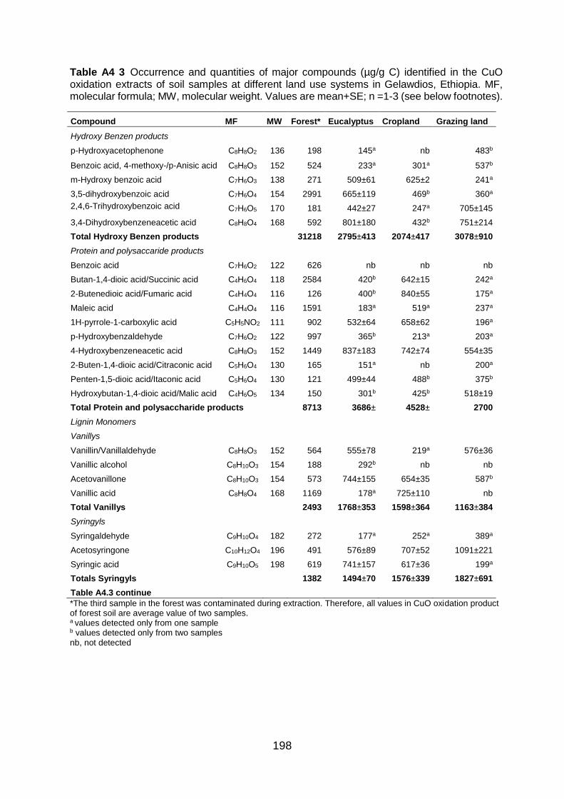
198

Table A4 3 Occurrence and quantities of major compounds (µg/g C) identified in the CuO oxidation extracts of soil samples at different land use systems in Gelawdios, Ethiopia. MF, molecular formula; MW, molecular weight. Values are mean+SE; n =1-3 (see below footnotes).

Compound MF MW Forest* Eucalyptus Cropland Grazing land

Hydroxy Benzen products

p-Hydroxyacetophenone C8H8O2 136 198 145a nb 483b

Benzoic acid, 4-methoxy-/p-Anisic acid C8H8O3 152 524 233a 301a 537b

m-Hydroxy benzoic acid C7H6O3 138 271 509±61 625±2 241a

3,5-dihydroxybenzoic acid C7H6O4 154 2991 665±119 469b 360a

2,4,6-Trihydroxybenzoic acid C7H6O5 170 181 442±27 247a 705±145

3,4-Dihydroxybenzeneacetic acid C8H8O4 168 592 801±180 432b 751±214

Total Hydroxy Benzen products 31218 2795±413 2074±417 3078±910

Protein and polysaccaride products

Benzoic acid C7H6O2 122 626 nb nb nb

Butan-1,4-dioic acid/Succinic acid C4H6O4 118 2584 420b 642±15 242a

2-Butenedioic acid/Fumaric acid C4H4O4 116 126 400b 840±55 175a

Maleic acid C4H4O4 116 1591 183a 519a 237a

1H-pyrrole-1-carboxylic acid C5H5NO2 111 902 532±64 658±62 196a

p-Hydroxybenzaldehyde C7H6O2 122 997 365b 213a 203a

4-Hydroxybenzeneacetic acid C8H8O3 152 1449 837±183 742±74 554±35

2-Buten-1,4-dioic acid/Citraconic acid C5H6O4 130 165 151a nb 200a

Penten-1,5-dioic acid/Itaconic acid C5H6O4 130 121 499±44 488b 375b

Hydroxybutan-1,4-dioic acid/Malic acid C4H6O5 134 150 301b 425b 518±19

Total Protein and polysaccharide products 8713 3686± 4528± 2700

Lignin Monomers

Vanillys

Vanillin/Vanillaldehyde C8H8O3 152 564 555±78 219a 576±36

Vanillic alcohol C8H10O3 154 188 292b nb nb

Acetovanillone C8H10O3 154 573 744±155 654±35 587b

Vanillic acid C8H8O4 168 1169 178a 725±110 nb

Total Vanillys 2493 1768±353 1598±364 1163±384

Syringyls

Syringaldehyde C9H10O4 182 272 177a 252a 389a

Acetosyringone C10H12O4 196 491 576±89 707±52 1091±221

Syringic acid C9H10O5 198 619 741±157 617±36 199a

Totals Syringyls 1382 1494±70 1576±339 1827±691

Table A4.3 continue

*The third sample in the forest was contaminated during extraction. Therefore, all values in CuO oxidation product of forest soil are average value of two samples. a values detected only from one sample b values detected only from two samples nb, not detected

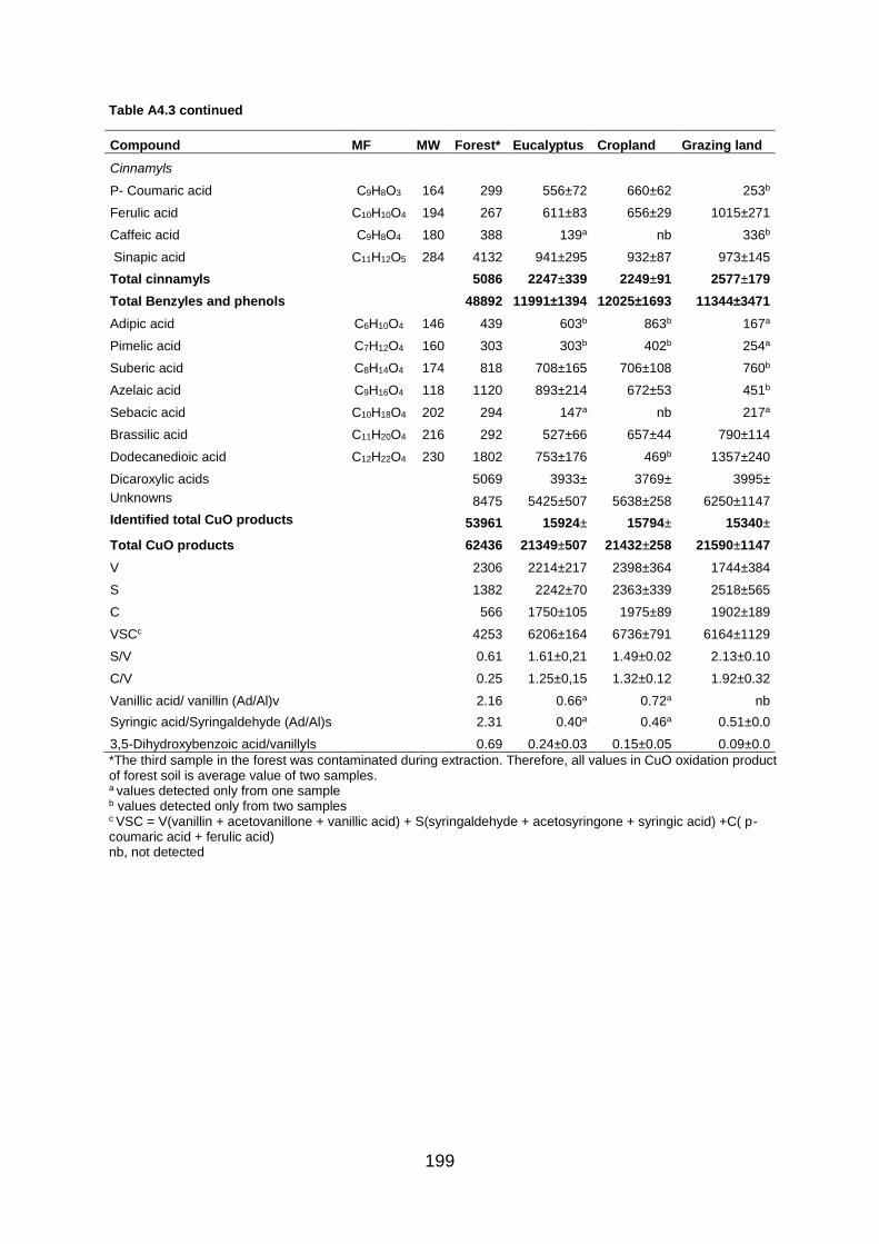
199


Compound MF MW Forest* Eucalyptus Cropland Grazing land

Cinnamyls

P- Coumaric acid C9H8O3 164 299 556±72 660±62 253b

Ferulic acid C10H10O4 194 267 611±83 656±29 1015±271

Caffeic acid C9H8O4 180 388 139a nb 336b

Sinapic acid C11H12O5 284 4132 941±295 932±87 973±145

Total cinnamyls 5086 2247±339 2249±91 2577±179

Total Benzyles and phenols 48892 11991±1394 12025±1693 11344±3471

Adipic acid C6H10O4 146 439 603b 863b 167a

Pimelic acid C7H12O4 160 303 303b 402b 254a

Suberic acid C8H14O4 174 818 708±165 706±108 760b

Azelaic acid C9H16O4 118 1120 893±214 672±53 451b

Sebacic acid C10H18O4 202 294 147a nb 217a

Brassilic acid C11H20O4 216 292 527±66 657±44 790±114

Dodecanedioic acid C12H22O4 230 1802 753±176 469b 1357±240

Dicaroxylic acids 5069 3933± 3769± 3995±

Unknowns 8475 5425±507 5638±258 6250±1147

Identified total CuO products 53961 15924± 15794± 15340±

Total CuO products 62436 21349±507 21432±258 21590±1147

V 2306 2214±217 2398±364 1744±384

S 1382 2242±70 2363±339 2518±565

C 566 1750±105 1975±89 1902±189

VSCc 4253 6206±164 6736±791 6164±1129

S/V 0.61 1.61±0,21 1.49±0.02 2.13±0.10

C/V 0.25 1.25±0,15 1.32±0.12 1.92±0.32

Vanillic acid/ vanillin (Ad/Al)v 2.16 0.66a 0.72a nb

Syringic acid/Syringaldehyde (Ad/Al)s 2.31 0.40a 0.46a 0.51±0.0

3,5-Dihydroxybenzoic acid/vanillyls 0.69 0.24±0.03 0.15±0.05 0.09±0.0

*The third sample in the forest was contaminated during extraction. Therefore, all values in CuO oxidation product of forest soil is average value of two samples. a values detected only from one sample b values detected only from two samples c VSC = V(vanillin + acetovanillone + vanillic acid) + S(syringaldehyde + acetosyringone + syringic acid) +C( p-coumaric acid + ferulic acid) nb, not detected

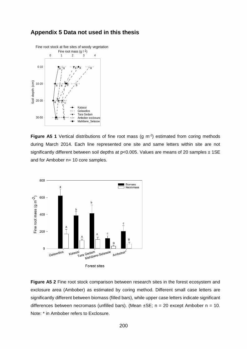
200

Appendix 5 Data not used in this thesis

Figure A5 1 Vertical distributions of fine root mass (g m-2) estimated from coring methods

during March 2014. Each line represented one site and same letters within site are not

significantly different between soil depths at p<0.005. Values are means of 20 samples ± 1SE

and for Ambober n= 10 core samples.

Figure A5 2 Fine root stock comparison between research sites in the forest ecosystem and

exclosure area (Ambober) as estimated by coring method. Different small case letters are

significantly different between biomass (filled bars), while upper case letters indicate significant

differences between necromass (unfilled bars). (Mean ±SE; n = 20 except Ambober n = 10.

Note: * in Ambober refers to Exclosure.

Fine root stock at five sites of woody vegetation Fine root mass (g l-1)

0 1 2 3 4

Soil d

ep

th (

cm

)

0-10

10-20

20-30

30-50

Katassi Gelawdios Tara Gedam Ambober exclosure Mahibere_Selasse

a

b

c

c

a

c

c

b

a

b

c

a

a

a

a

a

a

a

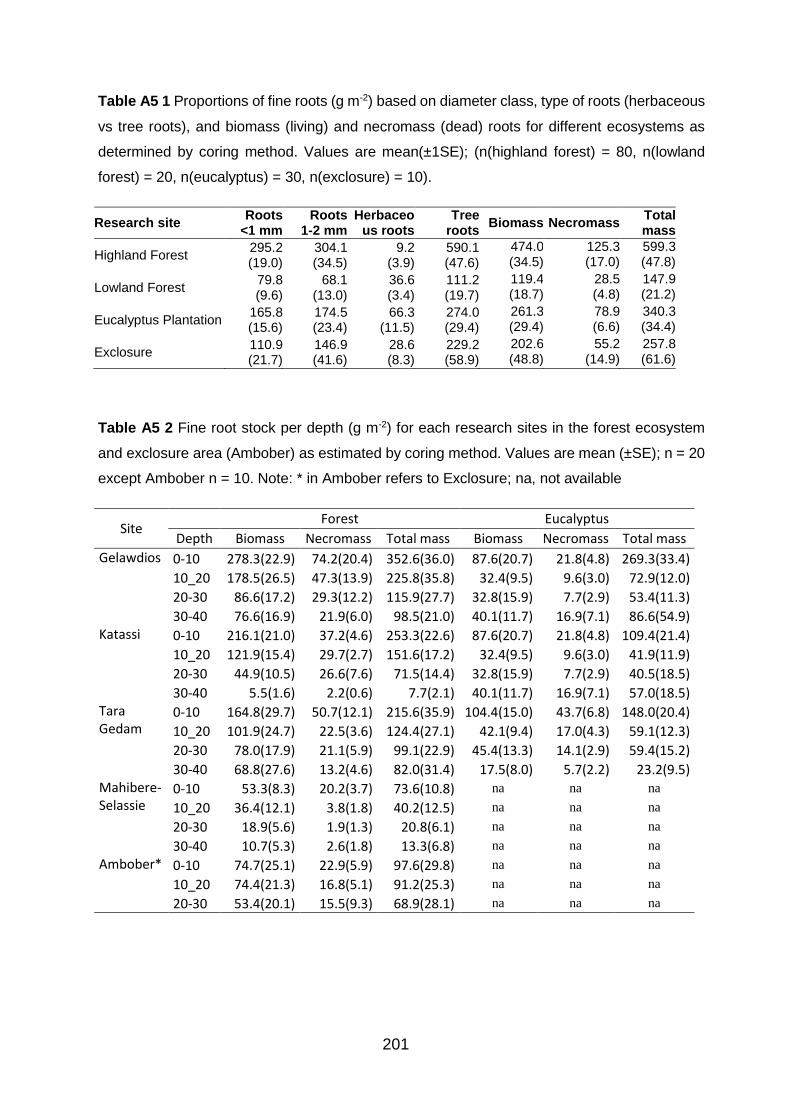
201

Table A5 1 Proportions of fine roots (g m-2) based on diameter class, type of roots (herbaceous

vs tree roots), and biomass (living) and necromass (dead) roots for different ecosystems as

determined by coring method. Values are mean(±1SE); (n(highland forest) = 80, n(lowland

forest) = 20, n(eucalyptus) = 30, n(exclosure) = 10).

Research site Roots

<1 mm Roots

1-2 mm Herbaceo

us roots Tree

roots Biomass Necromass

Total mass

Highland Forest 295.2 (19.0)

304.1 (34.5)

9.2 (3.9)

590.1 (47.6)

474.0 (34.5)

125.3 (17.0)

599.3 (47.8)

Lowland Forest 79.8 (9.6)

68.1 (13.0)

36.6 (3.4)

111.2 (19.7)

119.4 (18.7)

28.5 (4.8)

147.9 (21.2)

Eucalyptus Plantation 165.8 (15.6)

174.5 (23.4)

66.3 (11.5)

274.0 (29.4)

261.3 (29.4)

78.9 (6.6)

340.3 (34.4)

Exclosure 110.9 (21.7)

146.9 (41.6)

28.6 (8.3)

229.2 (58.9)

202.6 (48.8)

55.2 (14.9)

257.8 (61.6)

Table A5 2 Fine root stock per depth (g m-2) for each research sites in the forest ecosystem

and exclosure area (Ambober) as estimated by coring method. Values are mean (±SE); n = 20

except Ambober n = 10. Note: * in Ambober refers to Exclosure; na, not available

Site Forest Eucalyptus

Depth Biomass Necromass Total mass Biomass Necromass Total mass

Gelawdios 0-10 278.3(22.9) 74.2(20.4) 352.6(36.0) 87.6(20.7) 21.8(4.8) 269.3(33.4)

10_20 178.5(26.5) 47.3(13.9) 225.8(35.8) 32.4(9.5) 9.6(3.0) 72.9(12.0)

20-30 86.6(17.2) 29.3(12.2) 115.9(27.7) 32.8(15.9) 7.7(2.9) 53.4(11.3)

30-40 76.6(16.9) 21.9(6.0) 98.5(21.0) 40.1(11.7) 16.9(7.1) 86.6(54.9) Katassi 0-10 216.1(21.0) 37.2(4.6) 253.3(22.6) 87.6(20.7) 21.8(4.8) 109.4(21.4)

10_20 121.9(15.4) 29.7(2.7) 151.6(17.2) 32.4(9.5) 9.6(3.0) 41.9(11.9)

20-30 44.9(10.5) 26.6(7.6) 71.5(14.4) 32.8(15.9) 7.7(2.9) 40.5(18.5)

30-40 5.5(1.6) 2.2(0.6) 7.7(2.1) 40.1(11.7) 16.9(7.1) 57.0(18.5) Tara Gedam

0-10 164.8(29.7) 50.7(12.1) 215.6(35.9) 104.4(15.0) 43.7(6.8) 148.0(20.4)

10_20 101.9(24.7) 22.5(3.6) 124.4(27.1) 42.1(9.4) 17.0(4.3) 59.1(12.3)

20-30 78.0(17.9) 21.1(5.9) 99.1(22.9) 45.4(13.3) 14.1(2.9) 59.4(15.2)

30-40 68.8(27.6) 13.2(4.6) 82.0(31.4) 17.5(8.0) 5.7(2.2) 23.2(9.5) Mahibere-Selassie

0-10 53.3(8.3) 20.2(3.7) 73.6(10.8) na na na

10_20 36.4(12.1) 3.8(1.8) 40.2(12.5) na na na

20-30 18.9(5.6) 1.9(1.3) 20.8(6.1) na na na

30-40 10.7(5.3) 2.6(1.8) 13.3(6.8) na na na

Ambober* 0-10 74.7(25.1) 22.9(5.9) 97.6(29.8) na na na

10_20 74.4(21.3) 16.8(5.1) 91.2(25.3) na na na

20-30 53.4(20.1) 15.5(9.3) 68.9(28.1) na na na

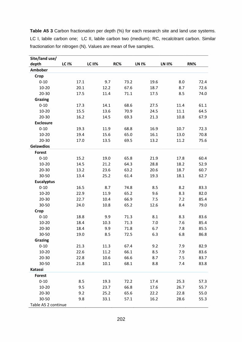
202

Table A5 3 Carbon fractionation per depth (%) for each research site and land use systems.

LC I, labile carbon one; LC II, labile carbon two (medium); RC, recalcitrant carbon. Similar

fractionation for nitrogen (N). Values are mean of five samples.

Site/land use/ depth LC I% LC II% RC% LN I% LN II% RN%

Ambober

Crop

0-10 17.1 9.7 73.2 19.6 8.0 72.4

10-20 20.1 12.2 67.6 18.7 8.7 72.6

20-30 17.5 11.4 71.1 17.5 8.5 74.0

Grazing

0-10 17.3 14.1 68.6 27.5 11.4 61.1

10-20 15.5 13.6 70.9 24.5 11.1 64.5

20-30 16.2 14.5 69.3 21.3 10.8 67.9

Exclosure

0-10 19.3 11.9 68.8 16.9 10.7 72.3

10-20 19.4 15.6 65.0 16.1 13.0 70.8

20-30 17.0 13.5 69.5 13.2 11.2 75.6

Gelawdios

Forest

0-10 15.2 19.0 65.8 21.9 17.8 60.4

10-20 14.5 21.2 64.3 28.8 18.2 52.9

20-30 13.2 23.6 63.2 20.6 18.7 60.7

30-50 13.4 25.2 61.4 19.3 18.1 62.7

Eucalyptus

0-10 16.5 8.7 74.8 8.5 8.2 83.3

10-20 22.9 11.9 65.2 9.6 8.3 82.0

20-30 22.7 10.4 66.9 7.5 7.2 85.4

30-50 24.0 10.8 65.2 12.6 8.4 79.0

Crop

0-10 18.8 9.9 71.3 8.1 8.3 83.6

10-20 18.4 10.3 71.3 7.0 7.6 85.4

20-30 18.4 9.9 71.8 6.7 7.8 85.5

30-50 19.0 8.5 72.5 6.3 6.8 86.8

Grazing

0-10 21.3 11.3 67.4 9.2 7.9 82.9

10-20 22.6 11.2 66.1 8.5 7.9 83.6

20-30 22.8 10.6 66.6 8.7 7.5 83.7

30-50 21.8 10.1 68.1 8.8 7.4 83.8

Katassi

Forest

0-10 8.5 19.3 72.2 17.4 25.3 57.3

10-20 9.5 23.7 66.8 17.6 26.7 55.7

20-30 9.2 25.2 65.6 22.2 22.8 55.0

30-50 9.8 33.1 57.1 16.2 28.6 55.3

Table A5 2 continue

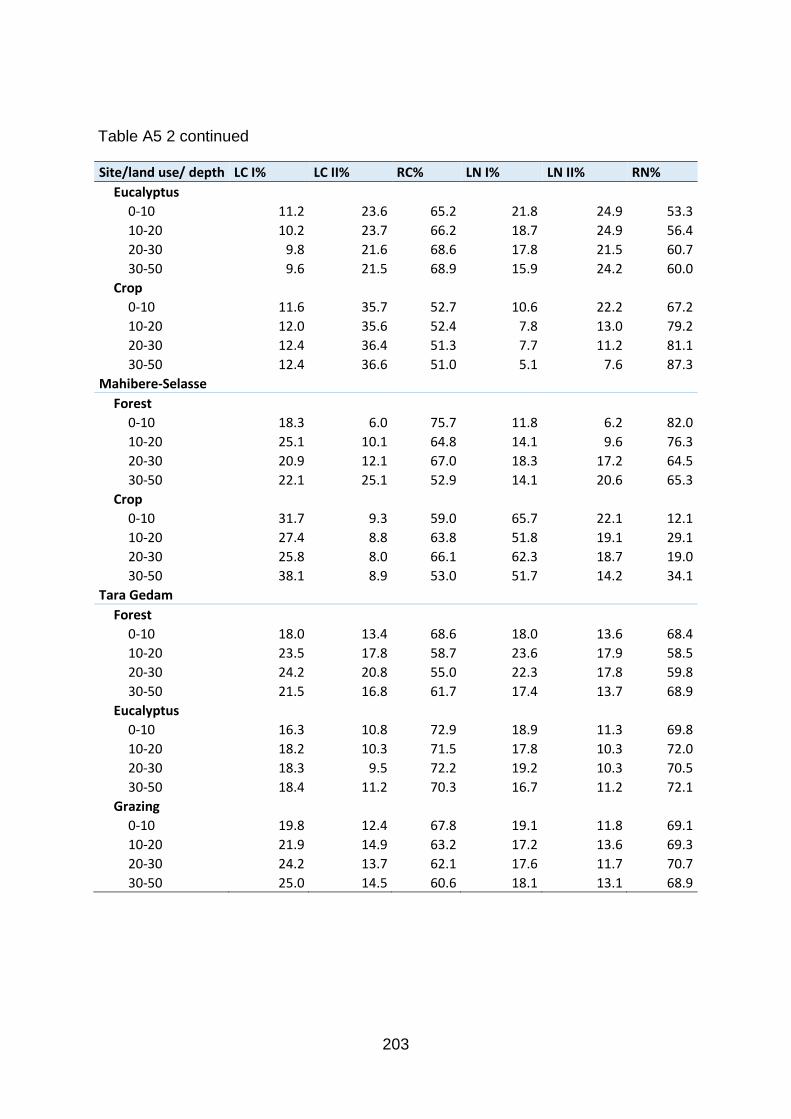
203

Table A5 2 continued

Site/land use/ depth LC I% LC II% RC% LN I% LN II% RN%

Eucalyptus

0-10 11.2 23.6 65.2 21.8 24.9 53.3

10-20 10.2 23.7 66.2 18.7 24.9 56.4

20-30 9.8 21.6 68.6 17.8 21.5 60.7

30-50 9.6 21.5 68.9 15.9 24.2 60.0

Crop

0-10 11.6 35.7 52.7 10.6 22.2 67.2

10-20 12.0 35.6 52.4 7.8 13.0 79.2

20-30 12.4 36.4 51.3 7.7 11.2 81.1

30-50 12.4 36.6 51.0 5.1 7.6 87.3

Mahibere-Selasse

Forest

0-10 18.3 6.0 75.7 11.8 6.2 82.0

10-20 25.1 10.1 64.8 14.1 9.6 76.3

20-30 20.9 12.1 67.0 18.3 17.2 64.5

30-50 22.1 25.1 52.9 14.1 20.6 65.3

Crop

0-10 31.7 9.3 59.0 65.7 22.1 12.1

10-20 27.4 8.8 63.8 51.8 19.1 29.1

20-30 25.8 8.0 66.1 62.3 18.7 19.0

30-50 38.1 8.9 53.0 51.7 14.2 34.1

Tara Gedam

Forest

0-10 18.0 13.4 68.6 18.0 13.6 68.4

10-20 23.5 17.8 58.7 23.6 17.9 58.5

20-30 24.2 20.8 55.0 22.3 17.8 59.8

30-50 21.5 16.8 61.7 17.4 13.7 68.9

Eucalyptus

0-10 16.3 10.8 72.9 18.9 11.3 69.8

10-20 18.2 10.3 71.5 17.8 10.3 72.0

20-30 18.3 9.5 72.2 19.2 10.3 70.5

30-50 18.4 11.2 70.3 16.7 11.2 72.1

Grazing

0-10 19.8 12.4 67.8 19.1 11.8 69.1

10-20 21.9 14.9 63.2 17.2 13.6 69.3

20-30 24.2 13.7 62.1 17.6 11.7 70.7

30-50 25.0 14.5 60.6 18.1 13.1 68.9

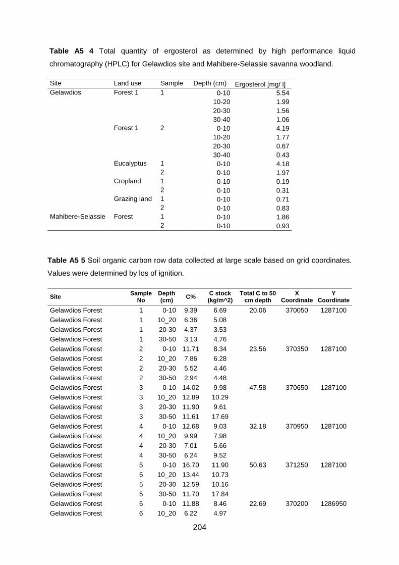
204

Table A5 4 Total quantity of ergosterol as determined by high performance liquid

chromatography (HPLC) for Gelawdios site and Mahibere-Selassie savanna woodland.

Site Land use Sample Depth (cm) Ergosterol [mg/ l]

Gelawdios Forest 1 1 0-10 5.54

10-20 1.99

20-30 1.56

30-40 1.06

Forest 1 2 0-10 4.19

10-20 1.77

20-30 0.67

30-40 0.43

Eucalyptus 1 0-10 4.18

2 0-10 1.97

Cropland 1 0-10 0.19

2 0-10 0.31

Grazing land 1 0-10 0.71

2 0-10 0.83

Mahibere-Selassie Forest 1 0-10 1.86

2 0-10 0.93

Table A5 5 Soil organic carbon row data collected at large scale based on grid coordinates.

Values were determined by los of ignition.

Site Sample

No Depth (cm)

C% C stock (kg/m^2)

Total C to 50 cm depth

X Coordinate

Y Coordinate

Gelawdios Forest 1 0-10 9.39 6.69 20.06 370050 1287100

Gelawdios Forest 1 10_20 6.36 5.08

Gelawdios Forest 1 20-30 4.37 3.53




















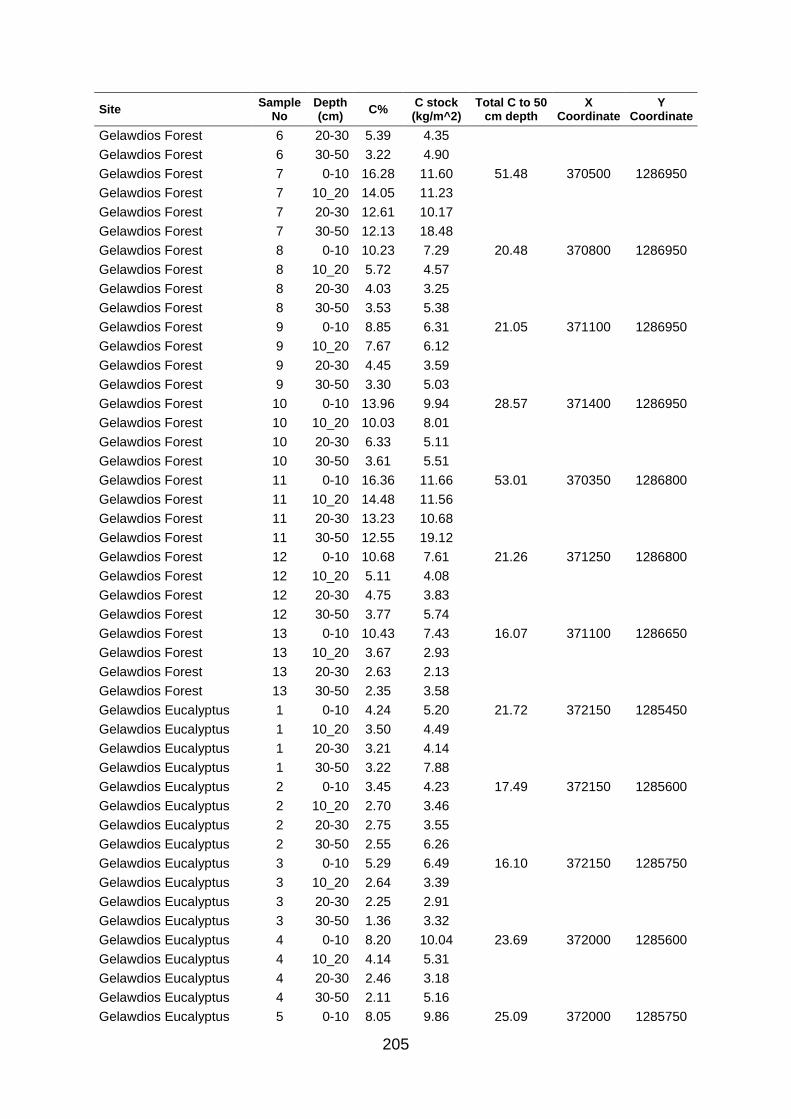
205

Site Sample

No Depth (cm)

C% C stock (kg/m^2)


X Coordinate

Y Coordinate































Gelawdios Eucalyptus 1 0-10 4.24 5.20 21.72 372150 1285450

Gelawdios Eucalyptus 1 10_20 3.50 4.49

Gelawdios Eucalyptus 1 20-30 3.21 4.14















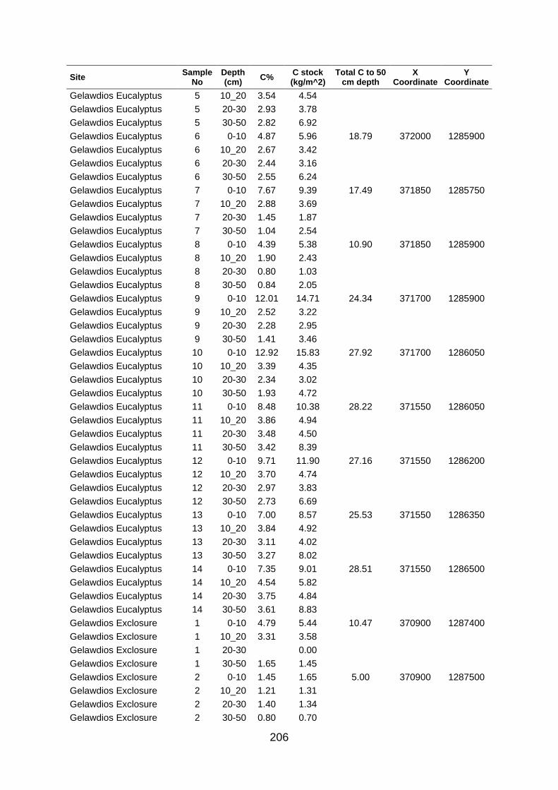
206

Site Sample

No Depth (cm)

C% C stock (kg/m^2)


X Coordinate

Y Coordinate








































Gelawdios Exclosure 1 0-10 4.79 5.44 10.47 370900 1287400

Gelawdios Exclosure 1 10_20 3.31 3.58

Gelawdios Exclosure 1 20-30 0.00

Gelawdios Exclosure 1 30-50 1.65 1.45





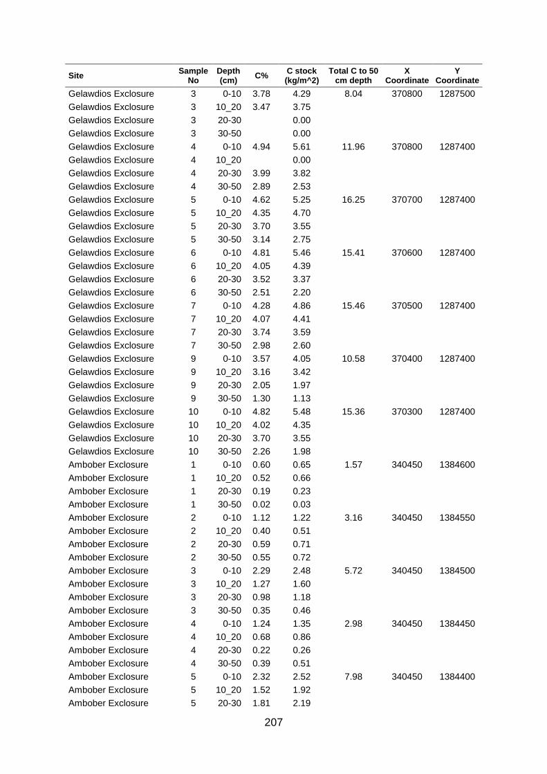
207

Site Sample

No Depth (cm)

C% C stock (kg/m^2)


X Coordinate

Y Coordinate






Gelawdios Exclosure 4 10_20 0.00























Ambober Exclosure 1 0-10 0.60 0.65 1.57 340450 1384600

Ambober Exclosure 1 10_20 0.52 0.66

Ambober Exclosure 1 20-30 0.19 0.23

















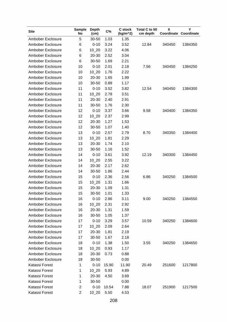
208

Site Sample

No Depth (cm)

C% C stock (kg/m^2)


X Coordinate

Y Coordinate









































Ambober Exclosure 18 30-50 0.00

Katassi Forest 1 0-10 15.90 11.90 20.49 251600 1217800

Katassi Forest 1 10_20 5.93 4.89

Katassi Forest 1 20-30 4.50 3.69

Katassi Forest 1 30-50 0.00

Katassi Forest 2 0-10 10.54 7.88 18.07 251900 1217500


209

Site Sample

No Depth (cm)

C% C stock (kg/m^2)


X Coordinate

Y Coordinate



Katassi Forest 3 0-10 6.75 5.05 13.17 251900 1216900




Katassi Forest 4 0-10 11.32 8.47 29.48 251900 1218100

Katassi Forest 4 10_20 10.34 8.53



Katassi Forest 5 0-10 14.70 11.00 23.94 252200 1217200




Katassi Forest 6 0-10 9.07 6.79 19.04 252500 1218100




Katassi Forest 7 0-10 11.65 8.72 19.17 252500 1217500




Katassi Forest 8 0-10 10.69 8.00 18.84 252500 1216900




Katassi Forest 9 0-10 10.76 8.05 19.90 252800 1217200




Katassi Forest 10 0-10 13.45 10.07 23.22 253100 1217500

Katassi Forest 10 10_20 7.27 6.00

Katassi Forest 10 20-30 4.79 3.93

Katassi Forest 10 30-50 4.23 3.23

Katassi Forest 11 0-10 10.86 8.12 22.73 252800 1217800

Katassi Forest 11 10_20 7.41 6.12

Katassi Forest 11 20-30 5.59 4.59

Katassi Forest 11 30-50 5.11 3.90

Katassi Forest 12 0-10 12.59 9.42 22.91 253100 1218100

Katassi Forest 12 10_20 6.92 5.71

Katassi Forest 12 20-30 5.31 4.36

Katassi Forest 12 30-50 4.48 3.42

Katassi Forest 13 0-10 16.65 12.46 25.28 253400 1217800

Katassi Forest 13 10_20 6.99 5.77

Katassi Forest 13 20-30 4.88 4.00

Katassi Forest 13 30-50 4.00 3.06

Katassi Forest 14 0-10 10.61 7.94 22.05 253400 1217200

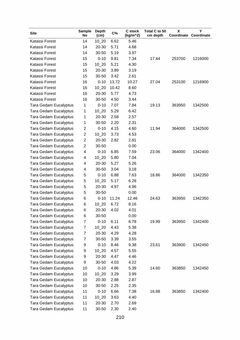
210

Site Sample

No Depth (cm)

C% C stock (kg/m^2)


X Coordinate

Y Coordinate

Katassi Forest 14 10_20 6.62 5.46

Katassi Forest 14 20-30 5.71 4.68

Katassi Forest 14 30-50 5.19 3.97

Katassi Forest 15 0-10 9.81 7.34 17.44 253700 1216000

Katassi Forest 15 10_20 5.21 4.30

Katassi Forest 15 20-30 3.89 3.19

Katassi Forest 15 30-50 3.42 2.61

Katassi Forest 16 0-10 13.72 10.27 27.04 253100 1216900

Katassi Forest 16 10_20 10.42 8.60

Katassi Forest 16 20-30 5.77 4.73

Katassi Forest 16 30-50 4.50 3.44

Tara Gedam Eucalyptus 1 0-10 7.07 7.84 19.13 363950 1342500

Tara Gedam Eucalyptus 1 10_20 5.29 6.42

Tara Gedam Eucalyptus 1 20-30 2.58 2.57





Tara Gedam Eucalyptus 2 30-50 0.00





























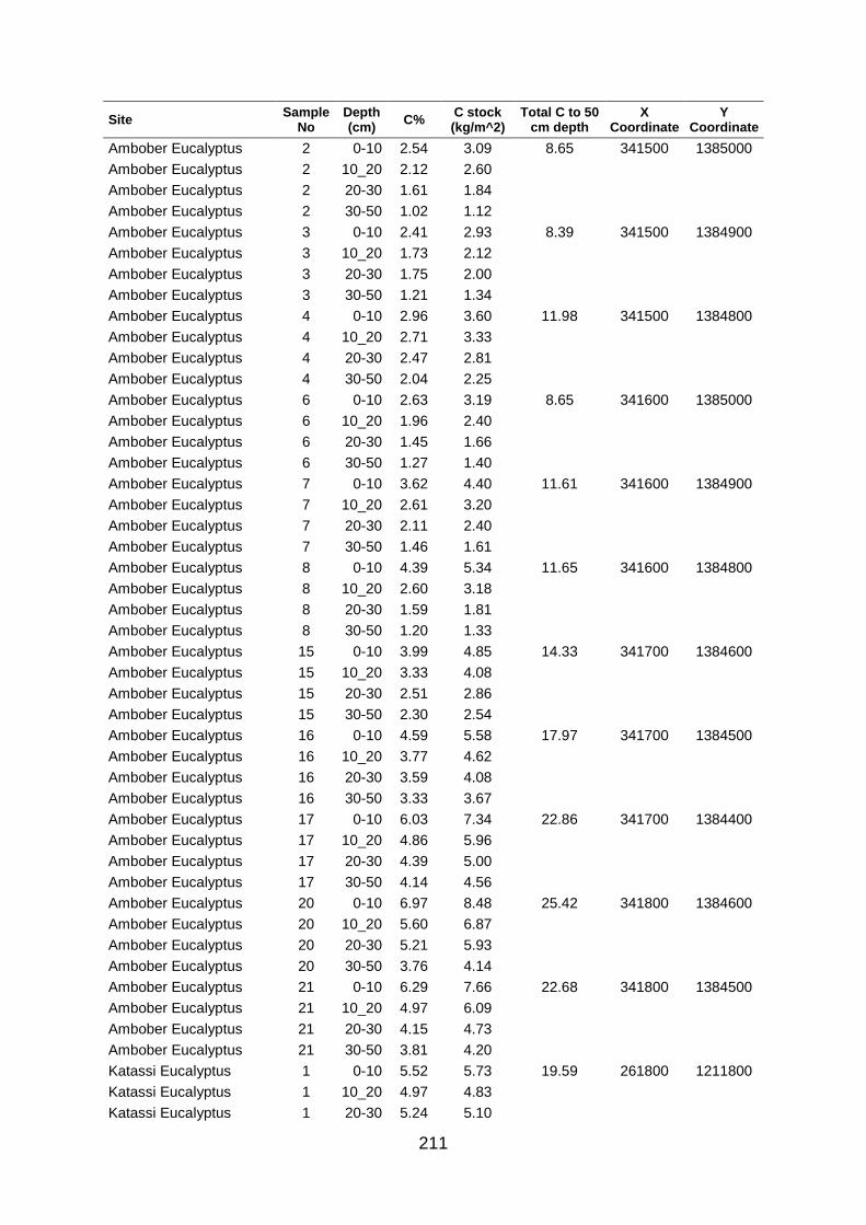
211

Site Sample

No Depth (cm)

C% C stock (kg/m^2)


X Coordinate

Y Coordinate

Ambober Eucalyptus 2 0-10 2.54 3.09 8.65 341500 1385000

Ambober Eucalyptus 2 10_20 2.12 2.60

Ambober Eucalyptus 2 20-30 1.61 1.84










































Katassi Eucalyptus 1 0-10 5.52 5.73 19.59 261800 1211800

Katassi Eucalyptus 1 10_20 4.97 4.83

Katassi Eucalyptus 1 20-30 5.24 5.10

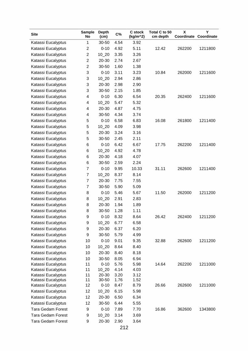
212

Site Sample

No Depth (cm)

C% C stock (kg/m^2)


X Coordinate

Y Coordinate














































Tara Gedam Forest 9 0-10 7.89 7.70 16.86 362600 1343800

Tara Gedam Forest 9 10_20 3.14 3.69

Tara Gedam Forest 9 20-30 2.90 3.64

213

Site Sample

No Depth (cm)

C% C stock (kg/m^2)


X Coordinate

Y Coordinate




















Tara Gedam Forest 24 20-30 0.00






















Mahibere-Selasse Forest 1 0-10 1.96 2.93 3.58 239000 1381000

Mahibere-Selasse Forest 1 10_20 0.30 0.44

Mahibere-Selasse Forest 1 20-30 0.13 0.17










214

Site Sample

No Depth (cm)

C% C stock (kg/m^2)


X Coordinate

Y Coordinate

















































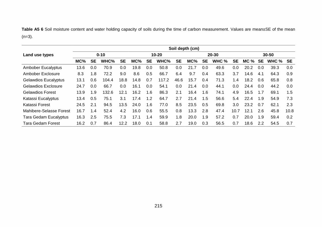
215

Table A5 6 Soil moisture content and water holding capacity of soils during the time of carbon measurement. Values are mean±SE of the mean

(n=3).

Land use types

Soil depth (cm)

0-10 10-20 20-30 30-50

MC% SE WHC% SE MC% SE WHC% SE MC% SE WHC % SE MC % SE WHC % SE

Ambober Eucalyptus 13.6 0.0 70.9 0.0 19.8 0.0 50.8 0.0 21.7 0.0 49.6 0.0 20.2 0.0 39.3 0.0

Ambober Exclosure 8.3 1.8 72.2 9.0 8.6 0.5 66.7 6.4 9.7 0.4 63.3 3.7 14.6 4.1 64.3 0.9

Gelawdios Eucalyptus 13.1 0.6 104.4 18.8 14.8 0.7 117.2 46.6 15.7 0.4 71.3 1.4 18.2 0.6 65.8 0.8

Gelawdios Exclosure 24.7 0.0 66.7 0.0 16.1 0.0 54.1 0.0 21.4 0.0 44.1 0.0 24.4 0.0 44.2 0.0

Gelawdios Forest 13.9 1.9 132.6 12.1 16.2 1.6 86.3 2.1 16.4 1.6 74.1 4.9 16.5 1.7 69.1 1.5

Katassi Eucalyptus 13.4 0.5 75.1 3.1 17.4 1.2 64.7 2.7 21.4 1.5 56.6 5.4 22.4 1.9 54.9 7.3

Katassi Forest 24.5 2.1 94.5 13.5 24.0 1.6 77.0 8.5 23.5 0.5 69.8 3.0 23.2 0.7 62.1 2.3

Mahibere-Selasse Forest 16.7 1.4 52.4 4.2 16.0 0.6 55.5 0.8 13.3 2.8 47.4 10.7 12.1 2.6 45.8 10.8

Tara Gedam Eucalyptus 16.3 2.5 75.5 7.3 17.1 1.4 59.9 1.8 20.0 1.9 57.2 0.7 20.0 1.9 59.4 0.2

Tara Gedam Forest 16.2 0.7 86.4 12.2 18.0 0.1 58.8 2.7 19.0 0.3 56.5 0.7 18.6 2.2 54.5 0.7

Carbon dynamics of different land use systems in NW Ethiopian

Documents

Transcript of Carbon dynamics of different land use systems in NW Ethiopian