CarCarCarCar TravelTravelTravelTravel TimeTimeTimeTime EstimationEstimationEstimationEstimation nearnearnearnear aaaa BusBusBusBus SSSStoptoptoptop withwithwithwith Non-motorizedNon-motorizedNon-motorizedNon-motorized VehiclesVehiclesVehiclesVehicles

YangYangYangYang XiaobaoXiaobaoXiaobaoXiaobao一

School of Traffic and Transportation, Beijing Jiaotong UniversityBeijing 100044, China

HuanHuanHuanHuan MeiMeiMeiMeiSchool of Traffic and Transportation, Beijing Jiaotong University

Beijing 100044, ChinaE-mail: huanmei0125@sohu.com

GuoGuoGuoGuo HongweiHongweiHongweiHongweiDepartment of Transportation Engineering, Beijing Institute of Technology

Beijing 100081, ChinaE-mail: 07114190@bjtu.edu.cn

GaoGaoGaoGao LiangLiangLiangLiangDepartments of Physics, Biology, and Computer Science, Northeastern University

Boston, MA 02115, USAE-mail:lianggao2010@gmail.com

AbstractAbstractAbstractAbstract

Real time system for vehicle travel time and traffic flow is an essential part of Intelligent Transportation Systems.In many Chinese cities, the interactions among buses, bicycles and cars bring difficulty to travel time prediction andtraffic safety management. The aim of this paper is to develop a new model to estimate car travel time near busstops in developing countries by data mining techniques and survival analysis methods. The travel time data undermixed traffic conditions are collected by video camera. Four influential factors including car volume, non-motorized volume, bus departure volume and free ratio of bus stop are chosen by using data mining techniques. Aproportional hazard-based duration model is proposed to analyze the factors related to car travel time. The resultsindicate that mixed traffic flow impacts the car travel time significantly. In addition, various factors can modify thetravel time distribution in different degrees and the model can be used to estimate the travel time under assumedconditions. It is hoped to help improve the planning and designing of proper facilities with mixed traffic flow.

Keywords: time prediction; data mining; survival data; bus stop; mixed traffic flow; traffic safety

一Corresponding author. Tel.: +86-10-51687070. E-mail address: yangxb@bjtu.edu.cn.

International Journal of Computational Intelligence Systems, Vol. 4, No. 6 (December, 2011), 1350-1357

1.1.1.1. IntroductionIntroductionIntroductionIntroduction

In recent decades, many studies have been conducted onthe traffic safety on highways and urban intersections1-3.As a developing country, China has her own trafficcharacteristics. A Mix of non-motorized and motorizedvehicles is an important traffic type in China. Somesurveys show that the non-motorized vehicle, mainlybicycle is one of the most widely used traffic tools inChinese daily travel activity 4. Although someresearchers focused on the car-bicycle conflict andinjury accidents involving cyclists5-7, little informationhas been published concerning the conflict amongmixed traffic streams near bus stops. Meanwhile, withthe development of new technology, Advanced TrafficInformation Systems are widely used in trafficmanagement and control. Real time system for vehicletravel time and traffic flow is an essential part ofAdvanced Traffic Information Systems. In manyChinese bus stops, the interactions among buses,bicycles and cars bring difficulty to travel timeestimation and traffic safety management. Therefore, itis necessary to develop an estimating approach fortravel time near bus stops with mixed traffic flow.

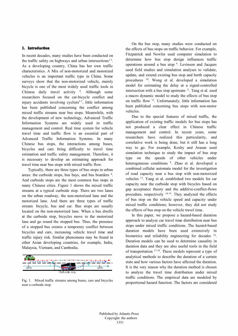
Typically, there are three types of bus stops in urbanareas: the curbside stops, bus bays, and bus boarders 8.And curbside stops are the most common bus stops inmany Chinese cities. Figure 1 shows the mixed trafficstreams at a typical curbside stop. There are two laneson the urban roadway, the non-motorized lane and themotorized lane. And there are three types of trafficstream: bicycle, bus and car. Bus stops are usuallylocated on the non-motorized lane. When a bus dwellsat the curbside stop, bicycles move to the motorizedlane and go round the stopped bus. Thus, the presenceof a stopped bus creates a temporary conflict betweenbicycles and cars, increasing vehicle travel time andtraffic injury risk. Similar phenomena may be found inother Asian developing countries, for example, India,Malaysia, Vietnam, and Cambodia.

Fig. 1. Mixed traffic streams among buses, cars and bicyclesnear a curbside stop.

On the bus stop, many studies were conducted onthe effects of bus stops on traffic behavior. For example,Fitzpatrick and Nowlin used computer simulation todetermine how bus stop design influences trafficoperations around a bus stop 9. Levinson and Jacquesused field studies and simulation analyses to validate,update, and extend existing bus stop and berth capacityprocedures 10. Wong et al. developed a simulationmodel for estimating the delay at a signal-controlledintersection with a bus stop upstream 11. Tang et al. useda macro dynamic model to study the effects of bus stopon traffic flow 12. Unfortunately, little information hasbeen published concerning bus stops with non-motorvehicles.

Due to the special features of mixed traffic, theapplication of existing traffic models for bus stops hasnot produced a clear effect in Chinese trafficmanagement and control. In recent years, someresearchers have realized this particularity, andcorrelative work is being done, but it still has a longway to go. For example, Koshy and Arasan usedsimulation technique to study the impact of bus stoptype on the speeds of other vehicles underheterogeneous conditions 8. Zhao et al. developed acombined cellular automata model for the investigationof road capacity near a bus stop with non-motorizedvehicles 13. Yang et al. established two models for carcapacity near the curbside stop with bicycles based ongap acceptance theory and the additive-conflict-flowsprocedure, respectively 14-15. They analyzed the effectsof bus stop on the vehicle speed and capacity undermixed traffic conditions; however, they did not studythe effects of bus stop on the vehicle travel time.

In this paper, we propose a hazard-based durationapproach to analyze car travel time distribution near busstops under mixed traffic conditions. The hazard-basedduration models have been used extensively inbiometrics and reliability engineering for decades 16.Duration models can be used to determine causality induration data and they are also useful tools in the fieldof transportation 17-19. These models represent a type ofanalytical methods to describe the duration of a certainstate and how various factors have affected the duration.It is the very reason why the duration method is chosento analyze the travel time distribution under mixedtraffic conditions. The empirical data are modeled byproportional hazard function. The factors are considered

Published by Atlantis Press Copyright: the authors 1351

Yang Xiaobao et al.

as influence variables including car volume, non-motorized vehicle volume, bus departure volume, freeratio of bus stop, and so on. With above methods, thedistribution of car travel time under various conditionsis calculated and the influence of the selected variablesis quantified.

2.2.2.2. MethodologyMethodologyMethodologyMethodology

2.1.2.1.2.1.2.1. Hazard-Hazard-Hazard-Hazard-bbbbasedasedasedased ddddurationurationurationurationmmmmodelodelodelodel

Let T be a nonnegative random variable representingthe car travel time in a test road section. Let ( )f tdenote the probability density function of T and let thecumulative distribution function be

0( ) Pr( ) ( )

tF t T t f u du= ≤ = ∫ (1)

Let ( )S t denote the probability that the travelduration does not end prior to t, yield

( ) Pr( ) ( )t

S t T t f u du∞

= > = ∫ (2)

( )S t is usually called “survivor probability” or“endurance probability” in the duration literature. In thispaper, we define ( )S t as continuance probability inorder to represent the probability that a car travelslonger than t (the travel duration still “continues” at t ).

In the hazard-based duration approach, T can becharacterized by a hazard function, ( )tλ . It representsthe instantaneous probability that the travel durationwill end in an infinitesimally small time period, t∆ ,after time t , given that the duration has not ended untiltime t . The mathematical definition for the hazardfunction in terms of probabilities is

0

Pr( )( ) lim

t

t T t t T tt

tλ

∆ →

≤ < + ∆ ≥=

∆(3)

The hazard function gives the conditional failure rate.In this study, the conditional failure rate is theconditional pass rate that cars pass through a bus stop.The hazard function is the instantaneous rate at which acar passes through a bus stop in an infinitesimally smalltime period, t∆ , after time t , given that the car has notpassed the stop until time t .

The result in the hazard function is hazard rate orhazard. Specifically, ( )t tλ ∆ is the approximateprobability of the duration terminating in [ ),t t t+ ∆ ,given continuance up to t . The functions ( )F t , ( )S t ,( )f t and ( )tλ give mathematically equivalent

specifications of the distribution of T . So the hazard

function can also be defined in terms of ( )F t , ( )S t ,and ( )f t , yield

( ) ( ) ln ( )( )1 ( ) ( )

λ−

= = =−f t f t d S ttF t S t dt

(4)

Integrating Eq. (4) from zero to t and using (0) 1S = ,yield

0( ) exp( ( ) )

tS t u duλ= −∫ (5)

Note that car travel time near a bus stop isinfluenced by various factors. A primary objective ofthis paper is to accommodate the effects of theseinfluential factors. The influential factors can be definedas a vector of explanatory variables, xxxx . Then theproportional hazard (PH) form is introduced, whichspecifies the effects of explanatory variables to bemultiplicative on a hazard function, yield

0( ) ( ) ( , )t t gλ λ= xxxx αααα (6)where 0 ( )tλ is the baseline hazard function representingthe hazard when the effects of explanatory variables areneglected [i.e. ( , ) 1g =xxxx αααα ], ( )g i is a known function torepresent the effects of explanatory variables, αααα is avector of parameters for xxxx. In this paper, a typicalspecification with ( , ) exp( )g =xxxx α αxα αxα αxα αx , which wasproposed by Cox 20, is used. This specification isconvenient since it guarantees the positivity of thehazard function without placing constraints on the signsof the elements of αααα . The Cox proportional hazardmodel is

0( ) ( ) exp( )t tλ λ= αxαxαxαx (7)The continuance probability function combining Eq.

(5) and Eq. (7) can be written asexp( )

0( ) [ ( )]S t S t= αxαxαxαx (8)where 0 ( )S t is the baseline continuance probabilityfunction.

2.2.2.2.2.2.2.2.ModelModelModelModel eeeestimationstimationstimationstimation

The model in Eq. (8) has two components, αααα and 0 ( )tλ .Cox 20 introduced an ingenious way of estimating αααα ;this is now known as the partial likelihood method.Because of its simplicity and usefulness, methodologyrelated to this approach is adopted. Suppose that arandom sample consists of k distinct observed durationdata, (1) (2) ( )kt t t< < <⋯ . Let ( )ixxxx be the variableassociated with the sample observed at ( )it . Let ( )( )itRRRRdenote the risk set at ( )it since it consists of allindividuals whose durations are at least ( )it . The log-partial likelihood function for estimating αααα is

Published by Atlantis Press Copyright: the authors 1352

Car Travel Time Estimation

( )

( )1 ( )

( ) log exp( )i

k

i li l t

LL= ∈

=⎧ ⎫⎡ ⎤⎪ ⎪− ⎢ ⎥⎨ ⎬

⎢ ⎥⎪ ⎪⎣ ⎦⎩ ⎭∑ ∑

RRRR

α αx αxα αx αxα αx αxα αx αx (9)

The estimation of 0 ( )tλ can refer to Ref. 18.The overall goodness-of-fit of the model estimation

is determined by the likelihood ratio (LR) statistics,which is specified as

0 ˆ2[ ( ) ( )]LX L L= − −α αα αα αα α (10)where 0( )L αααα is the log-likelihood for null model withall the regression coefficients are set as zero and ˆ( )L ααααis the log-likelihood at convergence with k regressioncoefficients.

3.3.3.3. SurveySurveySurveySurvey andandandand DataDataDataData

3.1.3.1.3.1.3.1. SiteSiteSiteSite ssssurveyurveyurveyurvey ddddesignesignesignesign

Car travel time is the actually observed time for a car topass a bus stop under mixed traffic conditions. Torecord the travel time durations, two videos were placedthe upstream section and the downstream section of thebus stop, respectively. Every car passing the curbsidestop was observed as a data collection unit. The traveltime duration was from the time that a car arrives at theupstream section to the time that it leaves thedownstream section. The study also explored the effectsof mixed traffic flow on the travel time. So the mixedtraffic characteristics at 1 min interval were extractedfrom the videos, such as traffic volumes of variousstreams and the average dwell time of bus stream atevery minute. Meanwhile, the car travel time of selectedsample associated with the mixed traffic characteristicswas matched according to the interval the samplebelonged to.

The observed roadway near the stops contains anon-motorized lane and a motorized lane. The sitesurvey was conducted at the selected curbside stop onXueyuan road in Beijing, China. Data were collected inJanuary of 2008. The survey periods included peak hourand off-peak hour. The length of the test section was67.5 m and the width of the sections was 7.5 m. Inaddition, the test section was not influenced by thetraffic control. The survey was conducted in goodweather. Based on the travel time study, 531 datasamples were observed.

3.2.3.2.3.2.3.2. VariableVariableVariableVariable sssspecificationspecificationspecificationspecifications

The explanatory variables for inclusion in the modelwere chosen by using data mining techniques on thebasis of previous research and intuitive argumentsregarding the effect of mixed traffic flow. In urbantraffic, travel time is determined by driving behavior,traffic conditions, geometric design, and so on. In thispaper, we concern the characteristics of travel timeunder the influence of mixed traffic flow near bus stops.Therefore, the variable specifications used in theduration model should be related to mixed traffic flow.Considering the feasibility of data acquisition, fourexplanatory variables including car volume (Xc), non-motorized vehicle volume (Xn), bus departure volume(Xb), and free ratio of bus stop (Xf) are chosen. The freeratio of bus stop reflects the probability of no bus at thestop at every minute. Although the volume of thecoming bus has an impact on the car travel time, there isa significantly statistical correlation between the volumeof the coming bus and the volume of the departure bus.Additionally, the conflict between the departure bus andthe passing car may occur. The departure bus has agreater impact on the car travel time than the comingbus. Thus, not the volume of the coming bus but thevolume of the departure bus is chosen. Analogously,there is a significantly statistical correlation between thedwell time of stopped bus and free ratio of bus stop.Because the latter has a more direct influence on the cartravel time than the former, the dwell time of stoppedbus is not chosen.

4.4.4.4. EmpiricalEmpiricalEmpiricalEmpirical ResultsResultsResultsResults

4.1.4.1.4.1.4.1. EstimatedEstimatedEstimatedEstimated rrrresultsesultsesultsesults

The estimation of the duration model for car travel timeis shown in Table 1. The LR statistic of the estimatedmodel clearly indicates the overall goodness-of-fit (theLR statistic is 5,471.4, which is greater than the chi-squared statistic with 4 degrees of freedom at anyreasonable level of significance). On the other hand, thestatistical significance of each variable also indicates thesignificant presence of variables in the duration of thetravel time. From the results, all of the includedvariables are statistically significant at the 0.02 level ofsignificance.

Published by Atlantis Press Copyright: the authors 1353

Yang Xiaobao et al.

Table 1. Model estimation.

Variable Coefficient StandardError Z-statistic P Value

Xc -0.041 0.018 -2.362 0.018

Xn -0.030 0.009 -3.211 0.001

Xb -0.431 0.054 -7.916 0.000

Xf 1.059 0.175 6.049 0.000

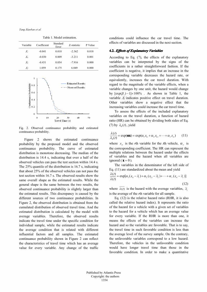
Fig. 2. Observed continuance probability and estimatedcontinuance probability.

Figure 2 shows the estimated continuanceprobability by the proposed model and the observedcontinuance probability. The curve of estimateddistribution is monotone decreasing. The median of thedistribution is 14.4 s, indicating that over a half of theobserved vehicles can pass the test section within 14.4 s.The 25% quantile of the distribution is 16.7 s, indicatingthat about 25% of the observed vehicles can not pass thetest section within 16.7 s. The observed results show thesame overall shape as the estimated results. While thegeneral shape is the same between the two results, theobserved continuance probability is slightly larger thanthe estimated results. This discrepancy is caused by thedifferent sources of two continuance probabilities. InFigure 2, the observed distribution is obtained from thecumulated distribution of observed travel time. And theestimated distribution is calculated by the model withaverage variables. Therefore, the observed resultsindicate the travel time under the specific condition forindividual sample, while the estimated results indicatethe average condition that is related with differentinfluential factors and all samples. The estimatedcontinuance probability shown in Figure 2 can reflectthe characteristics of travel time which has an averagevalue for every variable. Any change of the traffic

conditions could influence the car travel time. Theeffects of variables are discussed in the next section.

4.2.4.2.4.2.4.2. EffectsEffectsEffectsEffects ofofofof ExplanatoryExplanatoryExplanatoryExplanatory VariablesVariablesVariablesVariables

According to Eq. (7), the effects of the explanatoryvariables can be interpreted by the signs of thecoefficients in a rather straightforward fashion. If thecoefficient is negative, it implies that an increase in thecorresponding variable decreases the hazard rate, orequivalently, increases the car travel duration. Withregard to the magnitude of the variable effects, when avariable changes by one unit, the hazard would changeby [exp( ) 1] 100%iβ − × . As shown in Table 1, thevariable Xf indicates positive effect on travel duration.Other variables show a negative effect that theincreasing variables could increase the car travel time.

To assess the effects of the included explanatoryvariables on the travel duration, a function of hazardratio (HR) can be obtained by dividing both sides of Eq.(7) by 0 ( )tλ , yield

1 1 2 20

( ) exp( ) exp( )( ) i i r rit x x xt

λα α α

λ= = + + +αxαxαxαx ⋯ (11)

where rix is the rth variable for the ith vehicle, αr isthe corresponding coefficient. The HR can represent themultiple relations between the hazard under the effectsof variables and the hazard when all variables areignored ( 0=xxxx ).

The variables in the denominator of the left side ofEq. (11) are standardized about the mean and yield

1 1 1 2 2 2( ) exp[ ( ) ( ) ( )]( ) i i r ri rt x x x x x xt

λ α α αλ

= − + − + + −⋯

(12)where ( )tλ is the hazard with the average variables, rxis the average of the rth variable for all sample.

Eq. (12) is the relative hazard ratio (RHR, it is alsocalled the relative hazard index). It represents the ratioof the hazard for a vehicle with a given set of variablesto the hazard for a vehicle which has an average valuefor every variable. If the RHR is more than one, itmeans the effects of the variables can increase thehazard and so the variables are favorable. That is to say,the travel time in such favorable condition is less thanthe average level of the survey sample. On the contrary,the unfavorable variables correspond to a low hazard.Therefore, the vehicles in the unfavorable conditionwould have longer travel time than those in thefavorable condition. In order to make a quantitative

Published by Atlantis Press Copyright: the authors 1354

Car Travel Time Estimation

analysis of the effects of the mixed traffic flow, we canassume that a variable is in the favorable or unfavorablecondition and other variables take their average values.Then the HR or RHR for each variable can be calculated.In addition, the RHR can be used to describe themultiple of the hazard when the observed vehicles are infavorable condition or unfavorable condition comparedwith the average condition. The HR can be used todescribe the multiple of the hazard when the observedvehicles are in favorable condition compared with theunfavorable condition. According to the RHRs and HRsin specific conditions, the influence of mixed trafficflow on the travel time can be analyzed quantitatively.The specific conditions and corresponding HRs andRHRs are shown in Table 2.

Table 2. Analysis of variables related to travel time.

Variable MeanVariables Value Relative Hazard

Ratio HazardRatioUnfavorable Favorable Low

HazardHighHazard

Xc 11.84 30.00 10.00 0.48 1.08 2.25

Xn 13.99 30.00 10.00 0.62 1.13 1.82

Xb 1.84 3.00 1.00 0.61 1.44 2.36

Xf 0.50 0.10 0.90 0.66 1.53 2.32

To illustrate the effects of the selected variables, theRHRs for four variables (Xc, Xn, Xb and Xf) are shown inFigure 3. As shown in Figure 3(a), the variable Xc (carvolume) indicates a negative effect on the hazard. Thisreason is that the increasing car volume could increasethe probability of car queue and then delay the car traveltime. The RHR is 2.25 for the specific conditions. Itmeans that the car pass rate with 10 cars is 2.25 timesthat for a car with 30 cars, when other variables taketheir average values. Compared to the filed survey, theaverage travel time of the vehicles with car volume lessthan 11.84 is 13.85 s; while the average travel time withcar volume more than 11.84 is 15.67 s.

The variable Xn (non-motorized vehicle volume)indicates a negative effect on the hazard, which isshown in Figure 3(b). When a bus dwells at the stop,non-motorized vehicles may change to the motorizedlane. Thus, the increasing volume for non-motorizedvehicles could cause the larger probability of theconflict between cars and non-motorized vehicles,which finally lead to the increase of car travel time. TheRHR is 1.82 for the specific conditions; that is, the pass

Fig. 3. Relative hazard indexes for four variables

rate for a car with 10 non-motor vehicles is 1.82 timesthat for a car with 30 non-motor vehicles.

The volume of bus departure also shows a negativeeffect on travel time. This is the reason that the car-busconflict takes place when a bus departs from the stop tothe motorized lane. The car-bus conflict could delay thecar travel time. The RHR is 2.36 for the specificconditions. It means that the car pass rate with only onedeparture bus is 2.36 times that with 3 departure buses[see Figure 3(c)].

The effect of free ratio of bus stop (Xf) indicates thatthe increasing free ratio of bus stop can increase thehazard, or decrease the continuance probability [seeFigure 3(d)]. It means the probability that the vehiclescan transverse the bus stop longer than time t woulddecrease. This can be explained by the effect of stoppedbus. If no bus dwell at the stop, there is no the conflictbetween cars and non-motorized vehicles, and the non-motorized vehicles have no impact on the car traveltime. Otherwise, one or more stopped buses dwell at thestop, the conflict between cars and non-motorizedvehicles may lead to the increase of the car travel time.Thus, the increasing free ratio of bus stop may increasethe conflict between cars and non-motorized vehiclesand finally lead to the increase of the car travel time.From the results in Table 2, the high free ratio of busstop (90%) is 2.32 times as long as the low free ratio(10%) to make the vehicles have longer travel times.According to the observed data, the average travel timeof the vehicles with free ratio of bus stop less than 50%is 17.35 s; while the average travel time with free ratiomore than 50% is 12.57 s. The observed results alsoverify the estimated results.

Published by Atlantis Press Copyright: the authors 1355

Yang Xiaobao et al.

5.5.5.5. ModelModelModelModel ApplicationApplicationApplicationApplication

The estimated model can be used to predict thedistribution of car travel time under different conditions.By using an assumed variable under a specifiedcondition, a new distribution of the continuanceprobability can be calculated while other variables are attheir mean values respectively. In this paper, the non-motorized vehicle volume is taken as an example topresent the model application. If the non-motorizedvehicle volume ranges from 5 to 35 veh/min, the newdistributions of the continuance probability are shown inFigure 4. The differences between the curves indicatethe strong effect of the non-motorized vehicle volume.While the non-motorized vehicle volume increases from5 to 35 veh/min, the medians are 13.5 s, 14.5 s, and 16.4s; the 25% quartiles are 15.3 s, 17.6 s, and 20.7 s. Here,the 25% quantile is defined as the approximate traveltime. The travel time would have an increase of 17.6%if the non-motorized vehicle volume increases from 20to 35 veh/min. Other variables estimated by the durationmodel can be used to predict the distribution of thecontinuance probability in the same way.

Fig. 4. Distributions of the continuance probability withdifferent non-motorized vehicle volumes

The travel time is typical duration data that is theconcern of the duration model. Most importantly, thehazard-based duration methodology can capture theeffects of mixed traffic flow near bus stops. Therefore,the hazard-based duration approach could be helpful inthe travel time estimation near bus stops with mixedtraffic flow. Before the applications to other sites, themodel should be estimated using the specified field data.Additionally, the explanatory variables can be chosenflexibly according to the research aim and the trafficreality.

6.6.6.6. ConclusionsConclusionsConclusionsConclusions

Real time system is necessary for Advanced TrafficManagement Systems. This paper applies a hazard-based duration model to estimate car travel time nearbus stops under mixed traffic conditions. The conflictamong buses, bicycles and cars are discussed. The traveltime studies are conducted in the tested bus stop withnon-motorized vehicles. Meanwhile, mixed traffic flowand their effects on the car travel time are recorded. Themethodology uses a framework of proportion hazardthat allows different individuals to have various traveltimes according to the traffic conditions.

The paper provides several important insights intothe determinants of the car travel time distribution nearbus stops in developing countries. Firstly, the resultsindicate that car travel time is affected by variousrelated factors near a bus stop. Such influence can bereflected by the distribution of car travel time. Anychange of an influential factor could change the traveltime distribution. Secondly, the free ratio of bus stopshows a negative effect on the car travel time, while thecar volume, the non-motorized vehicle volume and thebus departure volume show positive effects on the cartravel time. Additionally, from the methodologicalstandpoint, this study has provided the empiricalevidence that hazard-based duration approach isappropriate for the travel time analysis under mixedtraffic conditions. The distribution of travel timeestimated by the model would give a quantitativeanalysis of the influence of mixed traffic flow. Finally,the influential factors related mixed trafficcharacteristics should be given full consideration in theplanning and designing of bus stops.

In terms of the future work, research with moredatasets is required. Also other influential factors shouldbe considered, such as the number of passenger loads,and the type of bus stops. In addition, it is necessary tostudy vehicle speed distribution near a bus stop withmixed traffic flow. It is hoped that these findings mayhave a better understanding of bus stops and help toplan and design traffic facilities in developing countries.

AcknowledgementsAcknowledgementsAcknowledgementsAcknowledgements

This work is supported by National Natural ScienceFoundation of China under Grant 70901005, 71131001,Specialized Research Fund for the Doctoral Program ofHigher Education under Grant 20090009120015, and

Published by Atlantis Press Copyright: the authors 1356

Car Travel Time Estimation

Fundamental Research Funds for the CentralUniversities under Grant 2011JBM055.

ReferencesReferencesReferencesReferences

1.W. H. Wang, Q. Cao, K.i Ikeuchi, and H. Bubb, Reliabilityand safety analysis methodology for identification ofdrivers' erroneous actions, Int. J. Automot. Techn. 11111111(6),(2010) 873-881.

2.W. H. Wang, F. G. Hou, H. C. Tan, and H. Bubb, Aframework for function allocation in intelligent driverinterface design for comfort and safety, Int. J. Comput.Int. Sys, 3333(5), (2010) 531-541.

3.W. H. Wang, Y. Mao, J. Jing, X. Wang, H. W. Guo, X. M.Ren, and I. Katsushi, Driver’s various informationprocess and multi-ruled decision-making mechanism: afundamental of intelligent driving shaping model, Int. Nt.J. Comput. Int. Sys. 4444(3), (2011) 297-305.

4.D. H. Wang, T. J. Feng, C. Y. Liang, et al. Research onbicycle conversion factors, Trans Res A, 42424242(8), (2008)1129-1139.

5.I. Walker, Drivers overtaking bicyclists: objective data onthe effects of riding position, helmet use, vehicle type andapparent gender, Accident Analysis and Prevention, 39393939,(2007) 417-425.

6.J. M. Wood, P. F. Lacherez, R. P. Marszalek, and M. J.King, Drivers’ cyclyists’ experiences of sharing the road:incidents, attitudes and perceptions of visibility, AccidentAnalysis and Prevention, 41414141, (2009) 772-776.

7.S. Daniels, T. Brijs, E. Nuyts, and G. Wets, Injury crasheswith bicyclists at roundabouts: influence of some locationcharacteristics and the design of cycle facilities, Journalof Safety Research, 40404040(2), (2009) 141-148.

8.R. Z. Koshy, and V. A. Arasan, Influence of bus stops onflow characteristics of mixed traffic, J. Transp. Eng.131131131131(8) (2005) 640-643.

9.K. Fitzpatrick, and R. L. Nowlin, Effects of bus stop designon suburban arterial operations, Transport. Res. Rec.1571157115711571 (1997) 31-41.

10. H. S. Levinson, K. R. S. Jacques, Bus lane capacityrevisited, Transport. Res. Rec. 1111618618618618 (1998) 189-199.

11. S. C. Wong, H. Yang, W. S. Yeung, et al. Delay atsignal-controlled intersection with bus stop upstream, J.Transp. Eng. 124124124124(3) (1998) 229-234

12. T. Q. Tang, Y. Li, and H. J. Huang, The effects ofbus stop on traffic flow, Int. J. Mod. Phys. C, 20202020(6)(2009) 941-952.

13. X. M. Zhao, B. Jia, Z. Y. Gao, and K. P. Li, Trafficinteractions between motorized vehicles andnonmotorized vehicles near bus stop, Journal ofTransportation Engineering, J. Transp. Eng. 135135135135(11)(2009) 893-905.

14. X. B. Yang, Z. Y. Gao, X. M. Zhao, and B. F. Si,Road capacity at bus stops with mixed traffic flow inChina, Transport. Res. Rec. 2112112112111111 (2009) 18-23.

15. X. B. Yang, Z. Y. Gao, B. F. Si, and L. Gao. Carcapacity near bus stops with mixed traffic derived by

additive-conflict-flows procedure, Sci. China Technol.Sci. 54545454(3) (2011) 737-740.

16. N. M. Kiefer, Economic duration data and hazardfunctions, Journal of Economic Literature, 26262626(2) (1988)646-679.

17. D. A. Hensher, and F. L. Mannering, Hazard-basedduration models and their application to transportanalysis, Transp. Rev. 14141414(1) (1994) 63-82.

18. C. R. Bhat, Duration modeling. Handbook oftransport modelling, in Transport Modeling Annuals(Elsevier Science, 2000), pp. 91–111.

19. H. W. Guo, Z. Y. Gao, X. B. Yang, and X. B. Jiang,Modeling pedestrian violation behavior at signalizedcrosswalks in China: a hazards-based duration approach,Traffic Inj. Prev. 12121212(1) (2011) 96-103.

20. D. R. Cox, Regression models and life tables, J. Roy.Stat. Soc. B, 34343434(2) (1972) 187-220.

Published by Atlantis Press Copyright: the authors 1357