saudi arabia culture minister prince badr visits ... - Arab News
Upload
khangminh22Category
view
1download
0
Cancer incidence in young people in Saudi
Arabia: relation to socioeconomic status and
population mixing
Reem Saeed AlOmar
Submitted in accordance with the requirements for the degree of
Doctor of Philosophy
The University of Leeds
School of Medicine
March 2015


iii
The candidate confirms that the work submitted is her own and that
appropriate credit has been given where reference has been made to the
work of others.
This copy has been supplied on the understanding that it is copyright material and
that no quotation from the thesis may be published without proper
acknowledgement.
© 2015 The University of Leeds and Reem S. AlOmar.

iv
To Mummy and Daddy

v
Acknowledgements
I am very grateful to both my supervisors Drs Graham Law and Roger Parslow for
their patience and invaluable emotional and academic support throughout the past
four years. Their patience was invaluable during my pregnancy and delivery of my
child in the first year, as well as the continued stress in raising a child and studying
full-time. I understand I was not the most straightforward student and for that I will
be indebted to them forever.
This PhD would not have been possible without funding from the University of
Dammam. I acknowledge the head of the Family and Community Medicine
Department Dr. Sameeh Al-Almaei for his help moral support. I also acknowledge
Mr Othaim Al-Othaim from the Central Department for Statistics and Information for
his support in deciphering the census data. I would like to thank Engineer Zaki Farsi
for his generosity in providing me with digitised maps of Saudi Arabia.
I would also like to thank all my colleagues in the office, especially Marlous Van
Laar, Oras Al-Abbas and Arwa Al-Thumairi for allowing me to vent some of my
frustrations and for their continuous support.
Finally, I would like to thank my daddy, for believing in me, supporting me and being
proud of me. I thank him for the so many tearful phone calls and his continuous
questions about my submission date. Thanks to mummy for her everlasting love
and support, and I am very sorry for not being by your side the last five years, I
promise it will not happen again. My thanks are also in order to my husband, who
has kept up with my mood swings for quite some time, as well as to my brothers
and sisters for their sincere love and support. To my son Saeed, I wish to apologise
for not being the best mummy, but I promise I will make it up to you very soon.
.
vi
Abstract
This study describes cancer incidence in under 24 year olds, particularly
leukaemias, lymphomas and central nervous system tumours. It also describes the
socioeconomic status (SES) of the geographically delimited Governorates in Saudi
Arabia, by deriving two indices – the first time this has been done in the country. It
also sought to determine whether SES and Hajj (occurring in Makkah) as a
measure of population mixing has an association with the incidence of these
cancers.
During 1994 to 2008, 17,150 cases were identified from the Saudi Cancer Registry.
Census data were accessed for 2004 and included 29 indicators. A continuous SES
index was constructed using exploratory factor analysis (EFA) and a categorical
index using latent class analysis (LCA). Incidence rate ratios (IRRs) were
calculated for cancers in Makkah compared to other Governorates by year to
assess the effect of Hajj, and for all Governorates to assess the effect of SES.
The Hajj had no significant effect on the incidence for all cancer groups. The
continuous index produced by EFA consisted of scores ranging from 100 to 0, for
affluent to deprived Governorates. The LCA found a four-class model as the best
model fit. Class 1 was termed ‘affluent’, Class 2 ‘upper-middle’, Class 3 ‘lower-
middle’ and Class 4 ‘deprived’. The urbanised Governorates were affluent, whereas
the rural Governorates were on average more deprived. For SES, an elevated risk
was found for acute lymphoblastic leukaemia in the affluent class (IRR=1.38,
95%CI=1.23-1.54), and was reduced in the deprived class (IRR=0.17, 95%CI=0.10-
0.29). Similar associations were observed for all cancer groups.
The findings are not supportive of the PM hypothesis, but give support to the
delayed infection hypothesis, suggesting that delayed exposure to infections may
prevent immune system modulation, although results may be exacerbated by poor
case-ascertainment/under-diagnosis in deprived areas. Similarities between the two
indices suggest validity.
vii
Table of Contents
Acknowledgements ..........................................................................................................v
Abstract ........................................................................................................................... vi
Table of Contents .......................................................................................................... vii
List of Tables ................................................................................................................... xi
List of Figures ............................................................................................................... xiii
List of Abbreviations .................................................................................................... xvi
List of Equations ........................................................................................................... xix
1 Introduction ..................................................................................................................1
1.1 Study rationale ........................................................................................................1
Infectious hypotheses ..........................................................................................2 1.1.1
1.2 Aims and structure of the thesis ...........................................................................5
2 Literature review ..........................................................................................................6
2.1 Cancer ......................................................................................................................6
Haematopoietic cancers ......................................................................................6 2.1.1
2.2 International variations in cancer incidence ..................................................... 10
Childhood and young adult cancers ................................................................. 11 2.2.1
2.3 The Saudi Arabian context .................................................................................. 15
Cancer incidence in Saudi Arabia .................................................................... 15 2.3.1
Childhood cancer incidence in Saudi Arabia.................................................... 16 2.3.2
2.4 Cancer aetiology in children and young adults ................................................ 17
Genetic predisposition and susceptibility ......................................................... 17 2.4.1
Environmental and lifestyle factors .................................................................. 17 2.4.2
Infections .......................................................................................................... 21 2.4.3
2.5 Socioeconomic status ......................................................................................... 50
Socioeconomic status and health .................................................................... 51 2.5.1
Socioeconomic status and childhood cancers ................................................. 52 2.5.2
Socioeconomic trends and patterns ................................................................. 52 2.5.3
Measures of socioeconomic status .................................................................. 53 2.5.4
Socioeconomic status in Saudi Arabia ............................................................. 58 2.5.5
2.6 Research to be conducted .................................................................................. 60
3 Materials and analytical methods ............................................................................ 61
3.1 Administrative geography ................................................................................... 61
3.2 Data sources, collection and manipulation ....................................................... 63
Cancer data ...................................................................................................... 63 3.2.1
viii
Census data ..................................................................................................... 64 3.2.2
Hajj data ........................................................................................................... 67 3.2.3
Geographical information systems ................................................................... 69 3.2.4
3.3 Descriptive analytical methods .......................................................................... 69
Descriptive statistics ......................................................................................... 69 3.3.1
Standardised incidence rates ........................................................................... 69 3.3.2
Cartography ...................................................................................................... 71 3.3.3
Funnel plots ...................................................................................................... 73 3.3.4
Case ascertainment ......................................................................................... 73 3.3.5
3.4 Derivation of area-based measures of socioeconomic status ........................ 75
Standardised index of socioeconomic status ................................................... 75 3.4.1
Classes of socioeconomic status ..................................................................... 81 3.4.2
3.5 Direct Acyclic Graph and regression analyses ................................................ 87
Direct Acyclic Graph ......................................................................................... 87 3.5.1
Poisson regression ........................................................................................... 88 3.5.2
Negative binomial regression ........................................................................... 88 3.5.3
4 Results: Descriptive analyses and mapping .......................................................... 90
4.1 Demographic characteristics, incident cases and incidence rates ................ 90
Demographics .................................................................................................. 90 4.1.1
Incident cases .................................................................................................. 91 4.1.2
Overall age-sex standardised incidence rates ................................................. 94 4.1.3
Age-sex standardised incidence rates and ratios by Governorate .................. 96 4.1.4
Annual increase in Hajj ................................................................................... 124 4.1.5
5 Results: Indices of socioeconomic status ........................................................... 125
5.1 Data cleaning and descriptive statistics ......................................................... 125
Descriptive statistics ....................................................................................... 125 5.1.1
5.2 Standardised index of socioeconomic status ................................................ 128
Data checks .................................................................................................... 128 5.2.1
Factor extraction and factor retention ............................................................ 128 5.2.2
Factor rotation ................................................................................................ 132 5.2.3
Initial index and standardised index ............................................................... 136 5.2.4
5.3 Classes of socioeconomic status .................................................................... 137
Deciding the number of classes ..................................................................... 137 5.3.1
Examining the quality of latent class membership ......................................... 139 5.3.2
Defining and labelling classes ........................................................................ 139 5.3.3
ix
Geographical mapping of both indices ........................................................... 141 5.3.4
Comparing distributions of both indices ......................................................... 143 5.3.5
6 Results: Regression analyses of population mixing and socioeconomic
status, sensitivity analyses and ascertainment of cases ................................... 145
6.1 Regression analyses ......................................................................................... 145
6.2 Sensitivity analyses ........................................................................................... 155
Socioeconomic classes .................................................................................. 155 6.2.1
The effect of the large cities ........................................................................... 157 6.2.2
6.3 Case ascertainment ........................................................................................... 161
Proportion of cases over time......................................................................... 161 6.3.1
Incidence rates by years ................................................................................ 163 6.3.2
Comparison with the US ................................................................................. 164 6.3.3
7 Discussion ............................................................................................................... 168
7.1 Discussion of results ......................................................................................... 168
7.2 Discussion of data sources .............................................................................. 177
Data from the cancer register ......................................................................... 177 7.2.1
The census data and the Hajj data ................................................................ 178 7.2.2
7.3 Discussion of methods ..................................................................................... 179
Disease classification ..................................................................................... 179 7.3.1
Geographical mapping ................................................................................... 179 7.3.2
Possible drawbacks of disease mapping ....................................................... 180 7.3.3
Exploratory factor analysis ............................................................................. 181 7.3.4
Latent class analysis ...................................................................................... 182 7.3.5
Regression analyses ...................................................................................... 184 7.3.6
7.4 Strengths of the study ....................................................................................... 185
7.5 Limitations of the study .................................................................................... 186
7.6 Recommendations and future work ................................................................. 188
7.7 Future planned publications ............................................................................. 189
7.8 Conclusions........................................................................................................ 190
References.................................................................................................................... 192
x
APPENDIX A Extended classification table of the International Classification
of Childhood Cancers 3rd
Edition .......................................................................... 229
APPENDIX B Main classification table of the International Classification of
Childhood Cancers 3rd
Edition............................................................................... 238
APPENDIX C Saudi cancer registry data abstraction form .................................... 243
APPENDIX D Example of phase 1: Converting morphology and topography
codes to ICCC-3 extended classification.............................................................. 245
APPENDIX E Example of phase 2: Converting morphology and topography
codes to ICCC-3 main classification ..................................................................... 248
APPENDIX F Discrepancies found within the total number of households
from each indicator group and the total number of households reported ....... 249
APPENDIX G Commitment letter to Farsi GeoTech Company for use of
Geographical Information System data ................................................................ 251
APPENDIX H Syntax of negative binomial regression analysis in Stata
version 13 ............................................................................................................... 252
APPENDIX I Initial and standardised index of Saudi Governorates .................... 253
APPENDIX J Modal class assignment and the final socioeconomic classes
index of the Saudi Governorates ........................................................................... 256
xi
List of Tables
Table 2.1: Age standardised rates of cancer incidence worldwide in 2008 .................... 10
Table 2.2: Age standardised rates of childhood cancers aged 0-14 between 1960-
1984 ....................................................................................................................... 12
Table 2.3: Age standardised rates of adolescent cancers aged 15-19 between
1980 and 1994 ....................................................................................................... 13
Table 2.4: Comparisons of age standardised incidence rates of all cancers
including Saudi Arabia for 2008 ............................................................................. 16
Table 2.5: Area-based studies on population mixing and childhood leukaemia ............. 32
Table 2.6: Individual-based studies on population mixing and childhood leukaemia ...... 39
Table 2.7: Studies on population mixing and childhood diabetes ................................... 41
Table 2.8: Indicators of the main socioeconomic indices in the UK ................................ 59
Table 3.1: The socioeconomic indicators obtained from the 2004 national census
of Saudi Arabia ...................................................................................................... 66
Table 3.2: Conversion of dates from the Islamic calendar to the Gregorian
calendar ................................................................................................................. 68
Table 3.3: The new World Standard Population for the years 2000-2025 ...................... 70
Table 4.1: Incident cases and incidence rates (per 100,000) of all cancers in Saudi
Arabia by age group and sex, 1994-2008 .............................................................. 90
Table 4.2: Incident cases of main diagnostic groups for males in Saudi Arabia by
age and main diagnostic group, 1994-2008 .......................................................... 92
Table 4.3: Incident cases of main diagnostic groups for females in Saudi Arabia by
age and main diagnostic group, 1994-2008 .......................................................... 93
Table 5.1: Descriptive statistics of the proportions of indicator variables from the
2004 census of Governorates in Saudi Arabia .................................................... 126
Table 5.2: Bartlett’s test of sphericity and the Kaiser-Meyer-Olkin’s test results .......... 128
Table 5.3: Factors extracted from the initial extraction stage ........................................ 130
Table 5.4: The factor loadings of variables on the extracted factors ............................. 131
Table 5.5: The rotated factor loadings of variables on the extracted factors ................ 135
Table 5.6: Proportion of the common variance explained by each factor ..................... 136
Table 5.7: Fit statistics for latent class analysis............................................................. 138
Table 6.1: IRRs and 95% CI for Saudis aged <24 years diagnosed with cancer
(1994 to 2008) associated with socioeconomic status in all Saudi
Governorates using negative binomial regression............................................... 152
Table 6.2: IRRs and 95% CI for Saudis aged <24 years diagnosed with cancer
(1994 to 2008) associated with socioeconomic status using the negative
binomial regression .............................................................................................. 156

xii
Table 6.3: IRRs and 95%CI for Saudis aged <24 years diagnosed with cancer
(1994 to 2008) associated socioeconomic status in all Saudi Governorates
excluding Riyadh, Jeddah and Dammam ............................................................ 158
xiii
List of Figures
Figure 2.1: Diagram of basic haematopoietic stem cell differentiation ...............................7
Figure 2.2: The minimal two-hit model illustrating the natural history for childhood
ALL/AML ................................................................................................................ 45
Figure 3.1: The Provinces of Saudi Arabia ...................................................................... 61
Figure 3.2: The Governorates of Saudi Arabia ................................................................ 62
Figure 3.3: Steps taken to derive the standardised index of socioeconomic status........ 75
Figure 3.4: Steps taken to derive the socioeconomic classes of Saudi Arabia using
latent class analysis ............................................................................................... 81
Figure 3.5: Identification of confounding variables between exposure and outcome...... 87
Figures 4.1: Crude and smoothed age-sex standardised incidence ratios (SIRs) of
acute lymphoblastic leukaemias registered from 1994 to 2008 in young
people under the age of 24 years by Saudi Governorates .................................... 97
Figure 4.2: Crude and smoothed age-sex standardised incidence ratios (SIRs) of
acute myeloid leukaemias registered from 1994 to 2008 in young people
under the age of 24 years by Saudi Governorates ................................................ 98
Figure 4.3: Crude and smoothed age-sex standardised incidence ratios (SIRs) of
chronic myeloid leukaemias registered from 1994 to 2008 in young people
under the age of 24 years by Saudi Governorates .............................................. 100
Figure 4.4: Crude and smoothed age-sex standardised incidence ratios (SIRs) of
‘other leukaemias’ registered from 1994 to 2008 in young people under the
age of 24 years by Saudi Governorates .............................................................. 101
Figure 4.5: Crude and smoothed age-sex standardised incidence ratios (SIRs) of
Hodgkin’s lymphoma registered from 1994 to 2008 in young people under
the age of 24 years by Saudi Governorates ........................................................ 103
Figure 4.6: Crude and smoothed age-sex standardised incidence ratios (SIRs) of
non-Hodgkin’s lymphoma registered from 1994 to 2008 in young people
under the age of 24 years by Saudi Governorates .............................................. 104
Figure 4.7: Crude and smoothed age-sex standardised incidence ratios (SIRs) of
Burkitt’s lymphoma registered from 1994 to 2008 in young people under the
age of 24 years by Saudi Governorates .............................................................. 106
Figure 4.8: Crude and smoothed age-sex standardised incidence ratios (SIRs) of
‘other lymphomas’ registered from 1994 to 2008 in young people under the
age of 24 years by Saudi Governorates .............................................................. 107
Figure 4.9: Crude and smoothed age-sex standardised incidence ratios (SIRs) of
CNS tumours registered from 1994 to 2008 in young people under the age
of 24 years by Saudi Governorates ..................................................................... 109
Figure 4.10: Crude and smoothed age-sex standardised incidence ratios (SIRs) of
‘all other cancers’ registered from 1994 to 2008 in young people under the
age of 24 years by Saudi Governorates .............................................................. 110
xiv
Figure 4.11: Funnel plots of crude and smoothed age-sex standardised incidence
ratios (SIRs) of acute lymphoblastic leukaemia registered from 1994 to 2008
in young people under the age of 24 years by Saudi Governorates ................... 112
Figure 4.12: Funnel plots of crude and smoothed age-sex standardised incidence
ratios (SIRs) of acute myeloid leukaemia registered from 1994 to 2008 in
young people under the age of 24 years by Saudi Governorates ....................... 113
Figure 4.13: Funnel plots of crude and smoothed age-sex standardised incidence
ratios (SIRs) of chronic myeloid leukaemia registered from 1994 to 2008 in
young people under the age of 24 years by Saudi Governorates ....................... 114
Figure 4.14: Funnel plots of crude and smoothed age-sex standardised incidence
ratios (SIRs) of ‘other leukaemias’ registered from 1994 to 2008 in young
people under the age of 24 years by Saudi Governorates .................................. 115
Figure 4.15: Funnel plots of crude and smoothed age-sex standardised incidence
ratios (SIRs) of Hodgkin’s lymphoma registered from 1994 to 2008 in young
people under the age of 24 years by Saudi Governorates .................................. 117
Figure 4.16: Funnel plots of crude and smoothed age-sex standardised incidence
ratios (SIRs) of non-Hodgkin’s lymphoma registered from 1994 to 2008 in
young people under the age of 24 years by Saudi Governorates ....................... 118
Figure 4.17: Funnel plots of crude and smoothed age-sex standardised incidence
ratios (SIRs) of Burkitt’s lymphoma registered from 1994 to 2008 in young
people under the age of 24 years by Saudi Governorates .................................. 119
Figure 4.18: Funnel plots of crude and smoothed age-sex standardised incidence
ratios (SIRs) of ‘other lymphomas’ registered from 1994 to 2008 in young
people under the age of 24 years by Saudi Governorates .................................. 120
Figure 4.19: Funnel plots of crude and smoothed age-sex standardised incidence
ratios (SIRs) of central nervous system tumours registered from 1994 to
2008 in young people under the age of 24 years by Saudi Governorates .......... 122
Figure 4.20: Funnel plots of crude and smoothed age-sex standardised incidence
ratios (SIRs) of ‘all other cancers’ registered from 1994 to 2008 in young
people under the age of 24 years by Saudi Governorates .................................. 123
Figure 4.21: Increase in childhood and young adult population (<24) and Hajj
pilgrims in Saudi Arabia between 1994 and 2008 ............................................... 124
Figure 5.1: Scree plot of eigenvalues of the extracted factors ...................................... 129
Figure 5.2: Factor loadings from the non-rotated factor solution ................................... 133
Figure 5.3: The factor loadings from the rotated factor solution .................................... 134
Figure 5.4: Probability plot of disadvantage in Saudi Arabia ......................................... 140
Figure 5.5: Geographical representation of the standardised index and the class
index for Saudi Governorates .............................................................................. 142
Figure 5.6: Boxplots of the continuous standardised socioeconomic index and the
categorical class socioeconomic index for Saudi Governorates ......................... 143
Figure 6.1: Incidence rate ratios of leukaemias diagnosed in Saudis aged <24
years corresponding to population mixing by year of diagnosis .......................... 146
xv
Figure 6.2: Incidence rate ratios of leukaemias diagnosed in Saudis aged <24
years corresponding to population mixing by year of diagnosis .......................... 148
Figure 6.3: Incidence rate ratios of central nervous system tumours diagnosed in
Saudis aged <24 years corresponding to population mixing by year of
diagnosis .............................................................................................................. 150
Figure 6.4: Incidence rate ratios of other cancers diagnosed in Saudis aged <24
years corresponding to population mixing by year of diagnosis .......................... 150
Figure 6.5: Proportion of cancer cases in Saudi Governorates by socioeconomic
classes over time ................................................................................................. 162
Figure 6.6: Incidence rates of childhood and adolescent cancers by year of
diagnosis .............................................................................................................. 163
Figure 6.7: Incidence rates of childhood and adolescent cancers by three five-year
blocks ................................................................................................................... 164
Figure 6.5: The age-standardised rates of cancers in under and over 14 years of
age for Saudi Arabia (left) and the United States (right) standardised to the
US standard population ....................................................................................... 167
xvi
List of Abbreviations
ABIC Adjusted Bayes information criterion
AIC Akaike information criterion
ASR Age-standardised rate
ALL Acute lymphoblastic leukaemia
AML Acute myeloid leukaemia
BCG Bacillus Calmette-Guérin
BIC Bayes information criterion
BL Burkitt’s lymphoma
BLRT Bootstrap likelihood ratio test
CDSI Central Department of Statistics and Information
CFA Confirmatory factor analysis
CI Confidence interval
COMARE Committee on Medical Aspects of Radiation in the Environment
CML Chronic myeloid leukaemia
CNS Central nervous system
CTHMIHR Custodian of the Two Holy Mosques Institute for Hajj Research
DAG Directed Acyclic Graph
DNA Deoxyribonucleic acid
DM Diabetes Mellitus
E Expected
EBV Epstein-Barr virus
EFA Exploratory factor analysis
GIS Geographical information systems
GLM Generalised linear model
GP General Practitioner
GRO General Register Office
xvii
HBV Hepatitis B virus
HIB Haemophilus influenza B virus
HIV Human immunodeficiency virus
HL Hodgkin’s lymphoma
HPV Human Papillomavirus
HSC Haematopoietic stem cell
HTLV-1 Human T-cell leukaemia/lymphoma virus type 1
ICCC International Classification of Childhood Cancers
ICD-10 International Classification of Disease 10th edition
ICD-O-3 International Classification of Diseases for Oncology 3rd edition
ILC Index of Local Conditions
ILD Index of Local Deprivation
IMD Indices of Multiple Deprivation
JC virus John Cunningham virus
LADs Local authority districts
LCA Latent class analysis
LMR-LRT Lo-Mendell-Rubin likelihood ratio test
KMO Kaiser-Meyer-Olkin
MoH Ministry of Health
NB Negative binomial
NCCLS North California Childhood Leukaemia Study
NHL Non-Hodgkin’s lymphoma
NRCP National Council on Radiation Protection and Measurements
O Observed
ONS Office for National Statistics
OR Odds ratio
PCMR Proportional cancer mortality ratio
PM Population mixing
RNA Ribonucleic acid
xviii
RR Relative risk
RTI Respiratory tract infections
SCR Saudi Cancer Registry
SD Standard deviation
SIR Standardised incidence ratio
SMR Standardised mortality ratio
SES Socioeconomic status
UAE United Arab Emirates
UKCCS United Kingdom Childhood Cancer Study
US United States of America
WHO World Health Organisation
ZIP Zero-inflated Poisson
ZINB Zero-inflated negative binomial model

xix
List of Equations
100Expected
ObservedSIR Equation 3.1
Posterior = Prior x Likelihood Equation 3.2
,;| ii OE
EO
i
vi
Equation 3.3
xZ x
Equation 3.4
UaFaFaFaz jjumjmjjj ...
2211 Equation3.5
UaFaFaFaz
UaFaFaFazUaFaFaFaz
nnumnmnnn
umm
umm
...2211
............................................................................................222
...2221212
111...
2121111
Equation 3.6
aaah jmjjj
2...
2
2
2
1
2 Equation 3.7
n
jjpp aV
1
2 Equation 3.8
WF nnII Equation 3.9

xx
100xIIII
IIIISI
minmax
mini
i
Equation 3.10
ig
G
ggviXp
1
1 Equation 3.11
11
G
gg Equation 3.12
gG|p X viig
1 Equation 3.13
klnAIC Lmax22
Equation 3.14
NlnkBIC Lmax 2 Equation 3.15
24
22
nlnkABIC Lmax Equation 3.16
xbxbxb jj...arln
2211 Equation 3.17
1
1 Introduction
1.1 Study rationale
The global burden of cancer continues to increase as a result of a growing and
aging population, as well as adoption of behaviours believed to cause cancers,
such as tobacco smoking. It is the leading cause of death in developed countries,
and the second leading cause of death in developing countries. Worldwide, an
estimated 12.7 million people with cancer were identified and 7.6 million died of
cancer in 2008 (Jemal et al., 2011, WHO, 2008). In Saudi Arabia, a steady
increase in incidence was observed from the start of reporting to the Saudi Cancer
Registry (SCR) in 1994, and reached a total of 11,946 cases in 2008 (Adler et al.,
1994). The most common causes of death in Saudi relate to heart problems and
road traffic accidents, and although the causes of death are not broken down by
age, congenital anomalies have been reported (Memish et al., 2014). Although
cancers are not within the 10 most commonly occurring diseases causing deaths
within the country, the rapidly changing profile of diseases, as well as the constant
growth of the Saudi population, suggests that cancer may become a major health
issue. Hence, cancer will pose a challenge to the Saudi health care system
(Memish et al., 2014).
Cancer usually takes many years to develop, which is why it predominantly occurs
in adults (Bleyer et al., 2006). However, cancer does develop in children below 14
years of age, and in young adults aged between 15 and 24 years of age. There is a
strong reason to look at cancers within these age groups in Saudi due to the age
structure of the population, where more than 52% of the population is under the age
of 25 (CDSI, 2004a). Furthermore, although incidence in these age groups is
considerably lower than in adults, the level of incidence is disproportionately low
when compared to the net years of disability due to disease occurrence and
treatment, as well as the years of life lost (Yeates et al., 2009, NICE, 2011). Hence,
these age groups are given considerable care and attention and are targeted in
several epidemiological studies worldwide, but not in Saudi Arabia.
Cancer epidemiology remains in its infancy in Saudi Arabia where very few studies
exist, none of which have focused on cancer incidence in children and young
people aged less than 25 years and none have attempted to describe incidence
geographically through mapping within these age groups. This gap in the
knowledge is reflected in the SCR annual reports, where only childhood cases are
reported as a separate age group, and young adults are included with adults cases
2
(Al-Eid et al., 2008). This is not the best practice, as treatments for cancers
occurring in the young adult age group do not follow adult protocols, but usually
follow paediatric protocols (Boissel et al., 2003). Also, geographical epidemiology
assists in discovering disease patterns that may have otherwise been unknown.
The application of disease mapping in Saudi Arabia is very recent, and has only
been aimed at the common types of cancers occurring in the population of all ages,
not at the 0-24 year old age group. Therefore, exploring incidence rates and
geographical distributions of cancers occurring in these age groups helps in
understanding its aetiology.
In childhood, acute lymphoblastic leukaemia (ALL) is the most common cancer with
incidence peaking between two and five years. In young adults the most common
types of cancers are lymphomas (Bleyer et al., 2008). Over the past 30 years, many
research papers have examined the epidemiology of childhood cancers, especially
childhood and young adult leukaemias and lymphomas (Law et al., 2003, Feltbower
et al., 2009, Doll, 1989, Stiller, 2004). In an attempt to understand their aetiology,
three infectious hypotheses have been formulated, namely, the population mixing
(PM) hypothesis, the delayed infection hypothesis and the in utero infection
hypothesis.
Infectious hypotheses 1.1.1
The population mixing (PM) hypothesis suggests that leukaemia is a rare response
to a common infection, and that this infection occurs as a result of PM whereby a
relatively isolated community, which has not yet been exposed to this infection,
receives an influx of people coming mostly from urban backgrounds (Kinlen, 1996).
It has been suggested that the infection, which may be bacterial or viral, may lead
directly to leukaemia. The delayed infection hypothesis, which suggests that the
common childhood ALL occurs as a result of two mutations, the first happens in
utero and the second happens after birth, once the child has been exposed to
several types of infections (Greaves, 1988). The hypothesis has been supported by
both biological and epidemiological studies. The third is the in utero infection
hypothesis which states that childhood ALL may be due to an infection that occurs
in utero during pregnancy (Smith, 1997).
However, it has proven difficult to test these hypotheses directly as there are many
factors to consider, such as the timing of exposure to infections and the subsequent
response to them, as well as assessing exposure to infection in early life (Law et
al., 2008). This is exacerbated by the lack of discovery of the infectious agent in
3
question. Several studies have also examined the incidence of CNS tumours in light
of these hypotheses after emerging evidence of the involvement of infections in
their aetiology.
Relevance of the Hajj 1.1.1.1
Saudi Arabia is home to the holy city of Makkah, as a result it experiences the Hajj
pilgrimage, which is one of the five pillars of Islam. It is an event that has been
going on for more than 1000 years. It is obligatory upon every able Muslim to
perform it at least once in their lifetime, ‘Announce Hajj to mankind. They will come
to you on foot and on every sort of lean animal, coming by every distant road so
that they can be present at what will profit them’ (The Holy Qur’an, 22.27). Annually,
more than two million Muslim pilgrims from over 140 countries gather in Makkah.
The Hajj takes five days to perform, though pilgrims may start to arrive weeks
before the event, and stay several weeks after. During this season, crowd density
can increase to up to seven individuals per square metre (Memish et al., 2009).
Mass migration of this kind increases the risk of contracting communicable
diseases. For example, respiratory tract infections (RTIs) are very common among
pilgrims. In a study during the 1991 and 1992 Hajj seasons, the syncytial virus,
influenza virus A, parainfluenza virus and adenovirus were the more dominant
viruses causing RTIs (El-Sheikh et al., 1998). Also, viruses causing pneumonia
such as mycobacterium tuberculosis, gram-negative bacilli and streptococcus
pneumonia are easily spread during the Hajj (Alzeer et al., 1998). The biggest
outbreak of the W135 serogroup of meningitidis in the world was reported in 2002
(Memish et al., 2003).
The Saudi Ministry of Health (MoH) every year puts forward plans to facilitate the
Hajj, and safeguard pilgrims from such risks. Vaccinations against meningitis are
now obligatory for every pilgrim, and pilgrims coming from countries where yellow
fever is known to be common should present a yellow fever vaccination certificate
upon arrival. However, with such a massive gathering, disease outbreaks still occur.
Although some diseases may be mild in nature, they do however prime the immune
system, thereby increasing protection against potential infections.
The influx of people into Makkah, and its associated infections are similar to that
suggested by Kinlen (1988). Therefore, the Hajj presents itself as an opportunity to
test the PM hypothesis in Saudi in relation to childhood cancers. Although, it should
be stressed that Hajj is an annual event, not a one-off event.
4
Relevance of socioeconomic status 1.1.1.2
Several factors are potentially related to the aetiology of these cancers such as diet
and breastfeeding, but most importantly is socioeconomic status (SES) which is
also related to the first two hypotheses, i.e. the PM and the delayed infection
hypotheses. High affluence is often associated with lower levels of mixing, hence
less exposure to infectious agents. However, none of the Arabian Gulf countries
have an established area-based SES measure that can be used in epidemiological
studies. Such a huge gap in health and social research is frequently reported
(AlGhamdi et al., 2014), and prevents the understanding and examination of any
possible associations. Therefore, utilisation of national Saudi census data has
provided an excellent opportunity to derive two area-based measures that could be
used both in this research and in other future health and social research dealing
with data on a national level.
5
1.2 Aims and structure of the thesis
This thesis focuses on childhood and young adult cancers aged less than 24 years
reported in Saudi Arabia between 1994 and 2008. The aims of this thesis are to:
Describe the pattern of incidence of childhood and young adult cancers
particularly leukaemias, lymphomas and central nervous system (CNS)
tumours across Saudi Arabia, as well as produce international comparisons
with other countries.
Describe the geographical variation in incidence of these cancers.
Construct indices of SES for use in the subsequent analysis, as well as for
use in future research in Saudi.
Examine the effect of SES and Hajj on the incidence of childhood and young
adult cancers in Saudi and interpret the findings in relationship to the PM
hypothesis.
Chapter 2 reviews the literature on cancer and cancer incidence both internationally
and in Saudi Arabia. It focuses on haematopoietic cancers as well as their
incidence in the childhood and young adult population. Furthermore, an overview of
the potential aetiological factors relating to cancers is presented, focusing on SES
and the three infectious hypotheses postulated to play a role in childhood
leukaemia and lymphoma.
Chapter 3 provides an overview of the methods used for handling and analysing
both the cancer data and the census data. The results of these analyses are
presented in Chapters 4, 5 and 6. Chapter 4 presents the results of the descriptive
analyses including direct and indirect standardisations of incidence rates overall
and by geographical region. Chapter 5 presents the results of the two area-based
indices of SES, and Chapter 6 presents the results of the regression analyses of
PM and SES, including sensitivity analysis and an assessment of case-
ascertainment of cancer data.
Chapter 7 discusses in detail the methods used as well as the results of these
analyses, pointing out limitations encountered during the work and putting forward
recommendations for future work.
6
2 Literature review
2.1 Cancer
The word cancer was derived by the father of medicine, Hippocrates, from the
Greek word karkinos; a word used to describe a crab, which Hippocrates (460-370
BC) thought a tumour looked like (Schwab, 2008). It is a group of diseases and
over 100 types have been identified; they differ in their age of onset and rate of
growth. All cancers can be called tumours; however, not all tumours can be called
cancers. Tumours refer to swelling, which may be caused by several other factors
apart from cancer, e.g. inflammation or haemorrhage, or from a growth which is
then classified into either benign or malignant (Renneker, 1988). Unlike malignant
tumours which are cancerous, benign tumours are mainly characterised by their
inability to spread or metastasize to other areas (Knowles and Selby, 2005).
The human body has four groups of tissues: the mesenchyme tissues, the
epithelium tissue, the nervous system and the haematolymphoid tissue. Each has
its own particular types of cells that sustain its structure and functions. In the case
of injury, other surviving cells start to divide to substitute the injured cells and then
stop. This process is known as cell proliferation and is distinguished from cell
growth where the cell increases in size (Knowles and Selby, 2005).
The way in which the numbers of cells increase is known as the cell cycle. The
cycle briefly involves the growth or maturation of all cell components, and then
division to produce two new descendant cells. Almost all cancers are characterised
by dysregulation or disruption of the cell cycle (Weber, 2007, Ruddon, 2007). Thus,
cancer may be defined as an abnormal growth of cells which subsequently leads to
a dysregulated balance of cell proliferation and death of cells, these develop into a
population of cells that may penetrate normal tissues and further metastasize to
other sites (Ruddon, 2007).
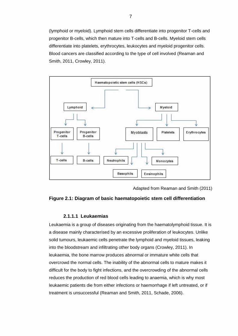
Haematopoietic cancers 2.1.1
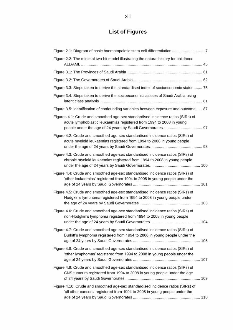
All cells in the body arise from pluripotent stem cells. These cells differentiate into
any of the main germ layers, i.e. the endoderm, the mesoderm or the ectoderm,
and the pluripotent stem cells become multipotent stem cells (Figure 2.1). If they
arise in the blood, then they are known as haematopoietic stem cells (HSCs). HSCs
are one type of multipotent stem cell. HSCs are further classified into either
lymphoid stem cells or myeloid stem cells, depending on the type of targeted cells
7
(lymphoid or myeloid). Lymphoid stem cells differentiate into progenitor T-cells and
progenitor B-cells, which then mature into T-cells and B-cells. Myeloid stem cells
differentiate into platelets, erythrocytes, leukocytes and myeloid progenitor cells.
Blood cancers are classified according to the type of cell involved (Reaman and
Smith, 2011, Crowley, 2011).
Adapted from Reaman and Smith (2011)
Figure 2.1: Diagram of basic haematopoietic stem cell differentiation
Leukaemias 2.1.1.1
Leukaemia is a group of diseases originating from the haematolymphoid tissue. It is
a disease mainly characterised by an excessive proliferation of leukocytes. Unlike
solid tumours, leukaemic cells penetrate the lymphoid and myeloid tissues, leaking
into the bloodstream and infiltrating other body organs (Crowley, 2011). In
leukaemia, the bone marrow produces abnormal or immature white cells that
overcrowd the normal cells. The inability of the abnormal cells to mature makes it
difficult for the body to fight infections, and the overcrowding of the abnormal cells
reduces the production of red blood cells leading to anaemia, which is why most
leukaemic patients die from either infections or haemorrhage if left untreated, or if
treatment is unsuccessful (Reaman and Smith, 2011, Schade, 2006).
8
Leukaemia is classified into several subtypes based on the types of cells and the
level of maturity of the proliferating cells. The main two subtypes are lymphocytic
leukaemia and myelocytic leukaemia. Lymphocytic leukaemia is further
characterised as T lymphocytic leukaemia if it occurs in T cells and B lymphocytic
leukaemia if it occurs in B cells. The maturity of the proliferating cells further
identifies the status of the disease, i.e. if the cells are mature the disease is chronic,
if the cells are primitive then the disease is classified as acute. Acute leukaemia is a
rapid progressive disease, in contrast to chronic leukaemia where the disease
progresses relatively slowly, leading to longer survival rates (Crowley, 2011,
Reaman and Smith, 2011).
Over recent years, it has been possible to understand what occurs at a cellular level
to patients diagnosed with childhood ALL by genetic epidemiological studies and
molecular scrutiny. In childhood leukaemia, chromosomal rearrangements disrupt
the genes that regulate the blood cell formulation (Inaba et al., 2013). Such
rearrangements include chromosomal hyperdiploidy/hypodiploidy and chromosomal
translocations, such as the MLL gene translocation forming the MLL fusion gene in
infant leukaemia with incidence peaks in children younger than one year old, and
the TEL and AML1 translocations to form the TEL-AML1 fusion genes in common
childhood ALL, with incidence peaks between two and five years of age (Inaba et
al., 2013, Greaves, 2002, Lightfoot and Roman, 2004).
Lymphomas 2.1.1.2
Lymphoma is another type of haematopoietic cancer which differs from leukaemia
mainly by the site of origin. In lymphoma the disease develops from lymphocytes
within the lymphatic system, and causes a malignant neoplasm or tumour. The
disease is divided into two major categories: Hodgkin’s lymphoma (HL) and non-
Hodgkin’s lymphoma (NHL). The main difference between the two is the
involvement of Reed-Sternberg cells, which originate from B-cells. In a patient with
HL, the disease develops in an orderly manner, i.e. once one lymph node is
affected then adjacent lymph nodes are expected to be affected as well (Crowley,
2011). In NHL, many subtypes have been identified, and although identification of
these subtypes is complex, the details are crucial to determine the most favourable
therapy. In contrast to HL, NHL may develop from either B-cells or T-cells. The
incidence of HL peaks in childhood in many developing countries, followed by a
steady decline in young adults. However, Burkitt’s lymphoma (BL) is a very
common form of lymphoma in Africa and is linked to Epstein Barr-virus (EBV).

9
During the period between 1968 and 1982, it accounted for almost 68% of all
childhood cancers in Uganda, though it is rare in young adults (Stiller and Parkin,
1996, Stiller, 2007).
10
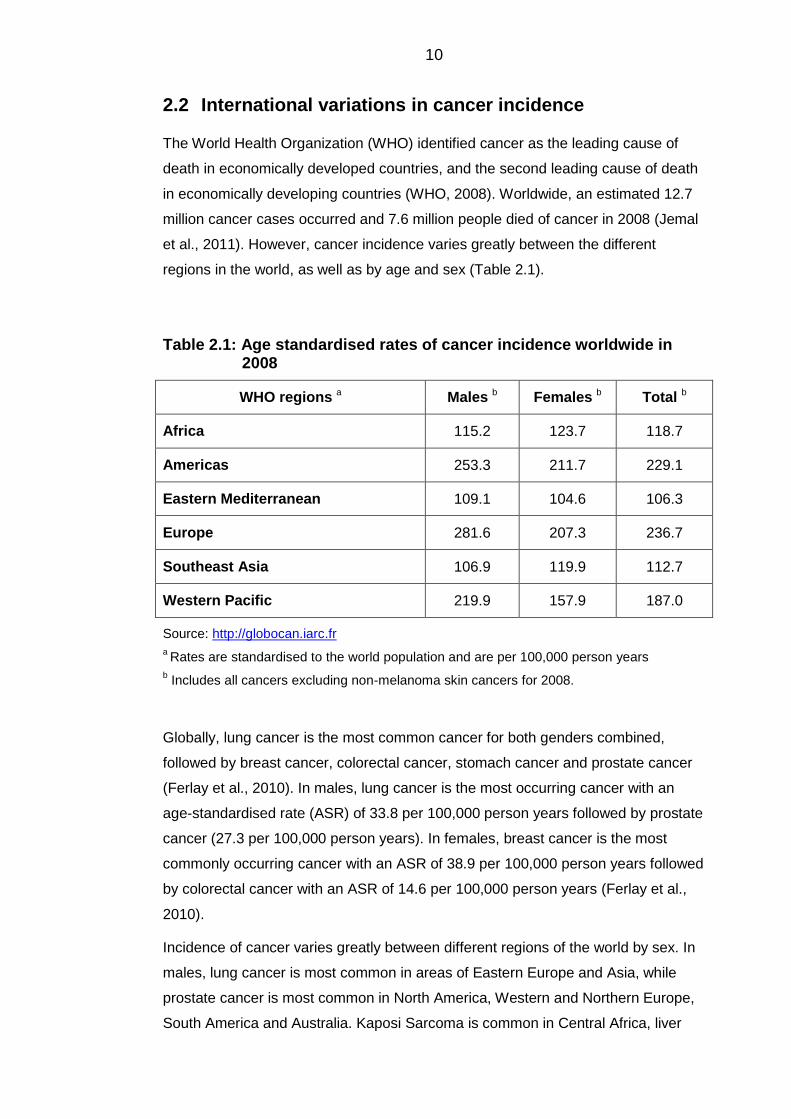
2.2 International variations in cancer incidence
The World Health Organization (WHO) identified cancer as the leading cause of
death in economically developed countries, and the second leading cause of death
in economically developing countries (WHO, 2008). Worldwide, an estimated 12.7
million cancer cases occurred and 7.6 million people died of cancer in 2008 (Jemal
et al., 2011). However, cancer incidence varies greatly between the different
regions in the world, as well as by age and sex (Table 2.1).
Table 2.1: Age standardised rates of cancer incidence worldwide in 2008
WHO regions a Males b Females b Total b
Africa 115.2 123.7 118.7
Americas 253.3 211.7 229.1
Eastern Mediterranean 109.1 104.6 106.3
Europe 281.6 207.3 236.7
Southeast Asia 106.9 119.9 112.7
Western Pacific 219.9 157.9 187.0
Source: http://globocan.iarc.fr
a Rates are standardised to the world population and are per 100,000 person years
b Includes all cancers excluding non-melanoma skin cancers for 2008.
Globally, lung cancer is the most common cancer for both genders combined,
followed by breast cancer, colorectal cancer, stomach cancer and prostate cancer
(Ferlay et al., 2010). In males, lung cancer is the most occurring cancer with an
age-standardised rate (ASR) of 33.8 per 100,000 person years followed by prostate
cancer (27.3 per 100,000 person years). In females, breast cancer is the most
commonly occurring cancer with an ASR of 38.9 per 100,000 person years followed
by colorectal cancer with an ASR of 14.6 per 100,000 person years (Ferlay et al.,
2010).
Incidence of cancer varies greatly between different regions of the world by sex. In
males, lung cancer is most common in areas of Eastern Europe and Asia, while
prostate cancer is most common in North America, Western and Northern Europe,
South America and Australia. Kaposi Sarcoma is common in Central Africa, liver
11
cancer in Western Europe and oesophageal cancer in Eastern Africa. In females,
breast cancer is the most commonly occurring cancer almost everywhere in the
world. Cervical cancer is common in Central America, and in certain parts of South
America (Jemal et al., 2010). Geographical variations in cancer incidence assist in
illustrating aetiological inferences about the different types of cancers (Horner and
Chirikos, 1987). Nonetheless, differences in ASRs between the different regions of
the world may partially be an artefact attributed to the difference in the quality and
nature of the data collection process. Indeed, data from these countries range from
actual numbers of cases and deaths to only estimates derived from samples (Jemal
et al., 2011).
Childhood and young adult cancers 2.2.1
Childhood cancers 2.2.1.1
Childhood cancers are very rare when compared to adult cancers, where the total
incidence rate usually lies between 70-160 per million (Stiller, 2004). They have
been and still are of great interest to scientists, not only because of their target
population, but also because the types of cancers occurring in this age group are
unique in comparison with cancers occurring in older age groups. The carcinomas
mostly occurring in adults, such as lung, colon and breast carcinomas are
extremely rare in children. In the past, childhood cancers have almost always led to
death (Chan and Raney, 2010). In recent years, survival rates have improved
greatly, for example according to the Surveillance, Epidemiology and End Results
(SEER) data, for childhood ALL survival rates increased to 88.5% in the decade
between 2000 and 2010. This is due to the excellent progress in cancer treatment
(Ma et al., 2014, Voute et al., 2005).
Among children aged less than 15 years, the annual ASR of cancer typically lies
between 75 and 40 per million in different parts of the world. Childhood leukaemia
is the most common cancer in children in almost all parts of the world, except in
Africa, where Kaposi Sarcoma and Burkitt’s lymphoma are more common.
Variations are seen within the specific types of cancers (Table 2.2) (Stiller and
Parkin, 1996, Stiller, 2004).
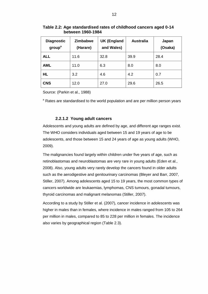
12
Table 2.2: Age standardised rates of childhood cancers aged 0-14 between 1960-1984
Diagnostic
groupa
Zimbabwe
(Harare)
UK (England
and Wales)
Australia Japan
(Osaka)
ALL 11.6 32.8 39.9 28.4
AML 11.0 6.3 8.0 8.0
HL 3.2 4.6 4.2 0.7
CNS 12.0 27.0 29.6 26.5
Source: (Parkin et al., 1988)
a Rates are standardised to the world population and are per million person years
Young adult cancers 2.2.1.2
Adolescents and young adults are defined by age, and different age ranges exist.
The WHO considers individuals aged between 15 and 19 years of age to be
adolescents, and those between 15 and 24 years of age as young adults (WHO,
2009).
The malignancies found largely within children under five years of age, such as
retinoblastomas and neuroblastomas are very rare in young adults (Eden et al.,
2008). Also, young adults very rarely develop the cancers found in older adults
such as the aerodigestive and genitourinary carcinomas (Bleyer and Barr, 2007,
Stiller, 2007). Among adolescents aged 15 to 19 years, the most common types of
cancers worldwide are leukaemias, lymphomas, CNS tumours, gonadal tumours,
thyroid carcinomas and malignant melanomas (Stiller, 2007).
According to a study by Stiller et al. (2007), cancer incidence in adolescents was
higher in males than in females, where incidence in males ranged from 105 to 264
per million in males, compared to 85 to 228 per million in females. The incidence
also varies by geographical region (Table 2.3).
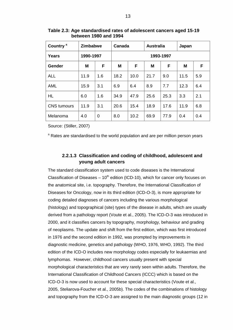
13
Table 2.3: Age standardised rates of adolescent cancers aged 15-19 between 1980 and 1994
Country a Zimbabwe Canada Australia Japan
Years 1990-1997 1993-1997
Gender M F M F M F M F
ALL 11.9 1.6 18.2 10.0 21.7 9.0 11.5 5.9
AML 15.9 3.1 6.9 6.4 8.9 7.7 12.3 6.4
HL 6.0 1.6 34.9 47.9 25.6 25.3 3.3 2.1
CNS tumours 11.9 3.1 20.6 15.4 18.9 17.6 11.9 6.8
Melanoma 4.0 0 8.0 10.2 69.9 77.9 0.4 0.4
Source: (Stiller, 2007)
a Rates are standardised to the world population and are per million person years
Classification and coding of childhood, adolescent and 2.2.1.3
young adult cancers
The standard classification system used to code diseases is the International
Classification of Diseases – 10th edition (ICD-10), which for cancer only focuses on
the anatomical site, i.e. topography. Therefore, the International Classification of
Diseases for Oncology, now in its third edition (ICD-O-3), is more appropriate for
coding detailed diagnoses of cancers including the various morphological
(histology) and topographical (site) types of the disease in adults, which are usually
derived from a pathology report (Voute et al., 2005). The ICD-O-3 was introduced in
2000, and it classifies cancers by topography, morphology, behaviour and grading
of neoplasms. The update and shift from the first edition, which was first introduced
in 1976 and the second edition in 1992, was prompted by improvements in
diagnostic medicine, genetics and pathology (WHO, 1976, WHO, 1992). The third
edition of the ICD-O includes new morphology codes especially for leukaemias and
lymphomas. However, childhood cancers usually present with special
morphological characteristics that are very rarely seen within adults. Therefore, the
International Classification of Childhood Cancers (ICCC) which is based on the
ICD-O-3 is now used to account for these special characteristics (Voute et al.,
2005, Steliarova-Foucher et al., 2005b). The codes of the combinations of histology
and topography from the ICD-O-3 are assigned to the main diagnostic groups (12 in
14
total), which are further subdivided into 47 subgroups (see Appendix A and B)
(Steliarova-Foucher et al., 2005b).
For young adults aged between 15 and 24 years, the Birch et al. (2002)
classification was designed to specifically report the most frequent cancers
occurring within this age group. It is similar to the ICCC classification in that it is
primarily based on morphology. The motivation behind this classification was that
the carcinomas specified in the ICCC are not adequately subdivided to properly
describe the pattern observed in this age group. In addition, the ICD classification –
if used – cannot distinguish carcinomas from non-epithelial tissues. For example,
carcinomas and soft tissue sarcomas occurring in the liver will all be assigned the
code for malignant neoplasm of the liver (Birch et al., 2002). Hence, for studies that
are concerned with cancers occurring in this age group, the Birch et al.
classification is more appropriate. However, in studies that include children and
young adults, the classification used should represent the numerically important
age group in the study (Birch et al., 2002).
15
2.3 The Saudi Arabian context
Officially known as the Kingdom of Saudi Arabia, it is the second largest Arab
country in the Middle East. It is bordered by Iraq, Jordan and Syria in the north,
Kuwait, Bahrain, Qatar and United Arab Emirates (UAE) to the east, Oman and
Yemen to the south and the Red Sea to the west. According to the latest census in
2011, the total population was 28,376,355, with a population density of 14
persons/square km. The capital city is Riyadh and it is also the largest city in the
country. Saudi Arabia a country known for its production of oil and gas from its
natural reserves, but is more prominent in the Muslim world for hosting the two holy
mosques in Makkah and Medinah (CDSI, 2011).
The country is divided into 13 administrative areas, also known as provinces. The
provinces are further divided into 118 Governorates, which are also divided into
sub-Governorates. Each of these divisions differs in terms of the total population,
and population density (CDSI, 2004a). Cancer reporting is relatively new to the
country as it only started in 1994 through the SCR.
Cancer incidence in Saudi Arabia 2.3.1
In Saudi, 11,659 cancer cases were reported to the SCR between the 1st of January
2007 and the 31st of December 2007 with an incidence rate of 82.1 per 100,000
person years. Females had an ASR of 84.2 per 100,000 person years, and males
had an ASR of 80 per 100,000 person years. Rates were highest in females aged
between 45 and 59 years of age, and occurred mostly within males aged between
60 and 74 years (Al-Eid et al., 2008). Table 2.4 gives ASRs for Saudi as well as
other countries. The incidence is higher in the US and the UK where cancer
registration has a long history, however for Saudi Arabia and the UAE, the relatively
low numbers may suggest under-reporting of cases in both countries, in which
cancer registries are relatively new especially for the UAE which commenced
reporting in 1998 (NCR, 2014).
16
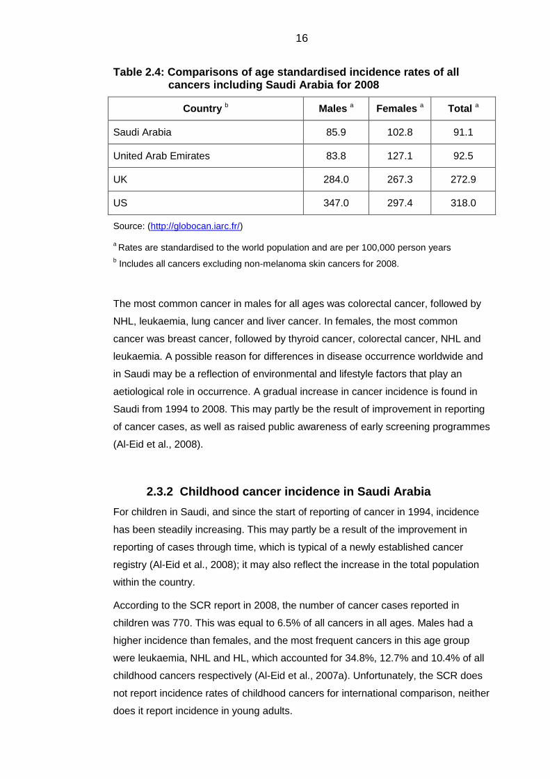
Table 2.4: Comparisons of age standardised incidence rates of all cancers including Saudi Arabia for 2008
Country b Males a Females a Total a
Saudi Arabia 85.9 102.8 91.1
United Arab Emirates 83.8 127.1 92.5
UK 284.0 267.3 272.9
US 347.0 297.4 318.0
Source: (http://globocan.iarc.fr/)
a Rates are standardised to the world population and are per 100,000 person years
b Includes all cancers excluding non-melanoma skin cancers for 2008.
The most common cancer in males for all ages was colorectal cancer, followed by
NHL, leukaemia, lung cancer and liver cancer. In females, the most common
cancer was breast cancer, followed by thyroid cancer, colorectal cancer, NHL and
leukaemia. A possible reason for differences in disease occurrence worldwide and
in Saudi may be a reflection of environmental and lifestyle factors that play an
aetiological role in occurrence. A gradual increase in cancer incidence is found in
Saudi from 1994 to 2008. This may partly be the result of improvement in reporting
of cancer cases, as well as raised public awareness of early screening programmes
(Al-Eid et al., 2008).
Childhood cancer incidence in Saudi Arabia 2.3.2
For children in Saudi, and since the start of reporting of cancer in 1994, incidence
has been steadily increasing. This may partly be a result of the improvement in
reporting of cases through time, which is typical of a newly established cancer
registry (Al-Eid et al., 2008); it may also reflect the increase in the total population
within the country.
According to the SCR report in 2008, the number of cancer cases reported in
children was 770. This was equal to 6.5% of all cancers in all ages. Males had a
higher incidence than females, and the most frequent cancers in this age group
were leukaemia, NHL and HL, which accounted for 34.8%, 12.7% and 10.4% of all
childhood cancers respectively (Al-Eid et al., 2007a). Unfortunately, the SCR does
not report incidence rates of childhood cancers for international comparison, neither
does it report incidence in young adults.
17
2.4 Cancer aetiology in children and young adults
Cancers in young children are thought to be influenced by pre-natal factors, and
cancers in older adults are thought to be influenced by prolonged exposure to
environmental factors. In young adults however, it is thought that cancer is
influenced by a mixture of both factors (Bleyer and Barr, 2007). Causal factors for
cancers fall into two major categories, environmental and lifestyle factors and
genetic predisposition.
Genetic predisposition and susceptibility 2.4.1
Predisposing genes are the genes that can cause a high relative risk of developing
some malignancies within a family, but with low attributable risk to the general
population (Eden, 2010). For example, neurofibromatosis type 1 – a genetic
disorder – is found to be linked to both ALL, chronic myeloid leukaemia (CML) and
lymphoma in families carrying that disorder. Also, children with Down syndrome are
more likely to develop leukaemias especially ALL and AML. In young adults,
leukaemias (including ALL) were found to develop in families with germ-line TP53
mutations (Eden, 2010). On the other hand, the susceptible genes are the genes
that affect how each person responds to the surrounding environmental exposures.
In other words, the risk of acquiring cancer through environmental factors is
modulated by these genes. The types of cancers developed are more common
sporadic cancers and, unlike predisposing genes, individuals carrying these genes
rarely have a family history of cancer (Eden, 2010, Kelloff et al., 2008). An example
is the CHEK2 gene, involved in the DNA damage-repair response pathway which
was identified in non-familial breast cancer patients (Meijers-Heijboer et al., 2002).
However, the underlying mechanisms have only recently started to unfold.
Environmental and lifestyle factors 2.4.2
Ionising radiation 2.4.2.1
People are exposed to ionising radiation on a daily basis, either from natural
sources such as radon gas through inhalation, or from artificial man-made sources
such as x-rays and CT scans. The National Council on Radiation Protection and
Measurements (NRCP) has set an average safe limit of 15 mSv for exposure to
ionising radiation. Exceeding this limit subsequently increases the risk of developing
cancer in both children and adolescents. Evidence is available from the atomic
bomb survivors who were exposed to up to 200 mSv and foetuses that have been
18
exposed to much lower dosages in utero (Doll and Wakeford, 1997). Moreover,
prenatal exposure to ionising radiation through diagnostic radiography was
associated with childhood leukaemia as well as other cancers (Stewart et al., 1958).
It has been generally accepted that children and adolescents are vulnerable to the
effects of ionising radiation with special emphasis on the dose and gestational age
during the time of exposure (Wakeford, 1995). Fortunately, ultrasound has largely
replaced obstetric X-ray in pregnancy, and there is no evidence to date that
connects obstetric ultrasound with any childhood cancer (Wilson and Waterhouse,
1984).
Parental occupational exposure to ionising radiation has also been examined.
Gardner and colleagues (1990) examined the incidence of leukaemia and NHL in
the offspring of workers based in a nuclear plant and reported that exposure of
fathers to radiation was associated with incidence of both diseases in their
offspring, with a dose response effect with the highest relative risk (RR) found for
those exposed to higher cumulative doses of radiation. The estimates for leukaemia
were high with a RR = 8.4 and a confidence interval (CI) of 1.40 - 52.00 and for
NHL the association was very high too (RR = 8.2, 95%CI = 1.36 - 50.56). Both
leukaemia and NHL were found within those with the highest accumulated
exposure of 100 mSv or more before conception (Gardner, 1990). The study only
included 52 cases of leukaemia and 23 cases of HL, hence the wide CIs. It is
unlikely that these findings will ever be corroborated as the radiation doses that the
fathers were exposed to were unusually high. It has been argued however, that if
these cancers occurred as a result of sperm stem cells being exposed to radiation,
then cancer should have been only one of many consequences, such as
spontaneous abortion or other birth defects, as was seen with the victims of the
atomic bomb in Japan and these should have been also examined (Coulter, 1990).
Other case-controls were carried out in other nuclear plants whose workers were
exposed to lower doses than that at Sellafield, but these studies reported
contradictory results (McLaughlin et al., 1993, Draper, 1997). Only one other study
reported a significant increase in risk of childhood leukaemia (RR = 8.0, 95%CI =
1.40 - 54.60) amongst children whose fathers had been exposed to ionising
radiation (Roman et al., 1993a). The study reported that neither the cases nor the
controls were exposed to more than 5 mSv of radiation before child conception,
which is below the safe limit set by the NRCP. Similarly, this study also had a wide
CI and a small sample size of only 54 children suggesting that the findings may be
attributed to chance.
19
In terms of maternal exposure, a case-control study from West Germany examined
the association between maternal exposure to ionising radiation from West German
nuclear plants and childhood leukaemia, lymphoma and solid tumours. The study
reported that maternal exposure significantly increased the odds ratio (OR) for
childhood lymphoma (OR = 3.87, 95%CI = 1.54 - 9.75), but no association was
found for either childhood leukaemia or solid tumours. A non-significant increase in
risk for children of fathers working at nuclear plants was also reported (OR = 1.80,
95%CI = 0.71 - 4.58) (Meinert et al., 1999).
The United Kingdom Childhood Cancer Study (UKCCS) looked into the effects of
household radon, in which the concentrations of radon were measured throughout a
period of six months in the houses of children with leukaemias. The levels of radon
in these houses were compared with those of the controls, and no evidence for
higher levels of radon in houses of cases were found (UKCCS, 2002). Furthermore,
a meta-analysis of five studies found that there was no evidence of association
between childhood leukaemia and radon (Yoshinaga et al., 2005). The same was
found for adults also (Law et al., 2000).
Ionising radiation at high levels can be lethal and long-term effects have been seen
in unusual situations such as that in Japan. However, doses at lower levels, such
as those observed in normal living conditions have not been shown to increase risk.
The preconception paternal irradiation theory proposed by Gardner (1990) is
difficult to substantiate, since there is a lack of comparable data.
Non-ionising radiation 2.4.2.2
Non-ionising radiation from natural sources such as sunlight has been known to
cause melanoma and other skin cancers (Voûte, 2005). Also, electromagnetic
radiation such as that emitted from electrical appliances and high voltage electricity
lines has been extensively examined, but has delivered inconsistent results. For
example, a meta-analysis of a group of nine case control studies found no evidence
of an increase in leukaemia when exposure was below 0.4 μT (Microtesla is the
measurement unit of field intensity for magnetic fields), but exposure higher than
these levels was found to double the risk (Ahlbom et al., 2000). It is thought
however, that some of the observed risk was related to the bias in the selection of
controls, in which most of the controls who volunteer for case-control studies have a
higher SES, this is because 0.4 μT is considered a very weak magnetic field.
The UKCCS also examined the association between childhood cancers and power
lines by measuring the distance between a home and a particular power line in a
20
case-control study, but no association between cancers and field exposures and
between cases and controls was found (Skinner et al., 2002). No underlying
biological mechanism has been agreed upon as to how this might trigger
carcinogenesis (Eden, 2010).
Alcohol consumption and cigarette smoking 2.4.2.3
Information on the relationship between parental alcohol consumption and
childhood cancers, leukaemia in particular, has mainly focused on maternal
consumption throughout pregnancy. For leukaemias, Severson et al. (1993) found a
positive association between maternal alcohol consumption and AML in children
diagnosed before their second birthday (OR = 3.00, 95%CI = 1.23 - 8.35). Although,
the sample size in this study was relatively small, this is reflected in the wide CIs.
(Severson et al., 1993). A second study found a similar association was reported for
AML (OR = 2.64, 95%CI = 1.36 - 5.06), but not for ALL. With regards to paternal
alcohol consumption, no association was found with childhood leukaemias
(Severson et al., 1993, Shu et al., 1996).
Cigarette smoking is one of the most well documented carcinogens. Studies that
examined parental alcohol consumption also examined parental smoking either
independently or together, since both are highly correlated (Eden, 2010). One study
found that paternal smoking was associated with lymphomas and neuroblastomas
(RR = 1.37, 95%CI = 1.02 - 1.83 and RR = 1.48, 95%CI = 1.09 - 2.02, respectively).
The same study also looked at maternal smoking during pregnancy and found that
it had a positive association with childhood ALL (RR = 1.24, 95%CI = 1.01 - 1.52)
(Sorahan, 1997).
The UKCCS case-control study examined the association for smoking by both
parents and found no statistically significant association. Since the study depended
entirely on self-reported behaviour, then any under-reporting within parents of
cases could have revealed significant associations (Pang et al., 2003). It is believed
that germ cell mutations and/or damage occur during spermatogenesis. This belief
is supported by research that has shown a significant increase in oxidative damage
of smokers’ sperm DNA, and that this damage may be linked to childhood cancers
and birth defects in their offspring (Fraga et al., 1996). In order to better understand
any association, examination of biomarkers for genotypes and phenotypes relevant
to tobacco products is essential.
21
Infections 2.4.3
One of the earliest suggestions of infections relating to leukaemia incidence was
made in the late 1930s, in which a cluster of cases of childhood leukaemia was
found in Ashington, Northumberland (Kellet, 1937). It was suggested that the cause
may be due to ‘some unknown specific external infection’ (Kellet, 1937, p.245).
After recognising that leukaemia in itself was not contagious, the idea of an
infectious aetiology somewhat subsided. However, the discovery of the role of the
Human T-cell leukaemia/lymphoma virus (HTLV-I) in causing adult T-cell
leukaemia/lymphoma (Gallo et al., 1984), as well as findings on animal studies in
which it was found that leukaemia in cats, chicken and cattle was viral in origin,
sustained the idea of an infectious aetiology (Schulz, 2002).
Indeed, there is no doubt that specific infections/parasitic agents have been
implicated in cancers. For example, Human Papillomavirus (HPV) infection is
associated with cervical cancer (Schiffman et al., 1993). In Africa, EBV antibodies
were present in most cases of BL, although not all individuals with the virus
developed BL (Brady et al., 2007). Furthermore, the Hepatitis B virus (HBV) is
associated with liver cancer, but patients usually are only diagnosed with acute
hepatitis. Therefore, the development of hepatic cancer may be triggered by
environmental factors after the infection, but HBV increases the risk nonetheless
(Mera, 1997). In addition, viruses that contain reverse transcriptase – an enzyme
that shifts the viral ribonucleic acid (RNA) to deoxyribonucleic acid (DNA) – have
been found to have a role in some cases, whereby the viral DNA is merged with the
host cell, hence causing cell disruption (Mera, 1997). Examples of RNA viruses
include the Human Immunodeficiency virus (HIV), which is an established risk
factor for Kaposi Sarcoma, and NHL as well as the HTLV-I and HTLV-II which
causes hairy cell leukaemia (Engels, 2001, Mera, 1997).
The pathological findings coupled with epidemiological studies are in favour of an
infectious aetiology of childhood leukaemia/lymphoma. The way in which infections
spread is governed by two important concepts in the study of infections: herd
immunity and hygiene hypothesis.
Herd immunity 2.4.3.1
The first concept related to infectious disease transmission is known as herd
immunity, which is based on the theory that the extent of spread of an infectious
disease in a particular community is based on a balance between the number of
susceptibles to that infection and the number of non-susceptibles, i.e. those who
22
are immune either due to a prior exposure, vaccination or who are genetically
immune. Resistance of the susceptibles to that infection occurs when a sufficient
proportion of the community are immune, i.e. herd immunity. The herd effect occurs
for the reason that a high enough proportion of the community is immune, which
makes it less likely that a susceptible individual will acquire that infection (John and
Samuel, 2000, Gordis, 2013).
In order for herd immunity to occur, certain conditions should be met. First, random
mixing, so that the probability that an infected individual is mixing with all other
individuals is the same. Where the infected individual only interacts with the
susceptibles, then it is likely that the infection will spread to them (Gordis, 2013). By
analogy, communities in isolated rural areas are in effect susceptible to new
infections that may be brought in by infected individuals, because they have little or
no herd immunity against this new infection. An example is that of the measles
infection which produced an epidemic in the Faroe Islands when infected
individuals entered the isolated population (Panum, 1847). A good determining
factor of the amount of mixing within populations is population density – the higher
the population density the better the chance for mixing, which in turn increases the
likelihood of producing at least one secondary case of infection from a primary case
(Anderson and May, 1990). The second condition is that the infectious agent should
be restricted to a single host species. Hence, if this condition is not met in that the
infectious agent could be transmitted from outside the human host, then herd
immunity will be compromised as there are other means for transmission (Gordis,
2013).
Herd immunity is very important because it may not be possible to vaccinate 100%
of the population to achieve immunity. However, if a large proportion of the
population is vaccinated, for example by governmental vaccination programmes,
then the rest that are unvaccinated or susceptible to the infection, such as those
who refuse vaccinations due to religious beliefs, or individuals with compromised
immune systems, will be protected as a result of herd immunity. The proportion
needed to achieve herd immunity differs from one infection to another, for example
for measles it is thought that 92% to 95% coverage is sufficient to achieve herd
immunity, whilst for the polio virus 80% to 85% coverage is required (Anderson and
May, 1990). This concept of herd immunity is postulated to play a role in the
aetiology of childhood leukaemia where low herd immunity is assumed to increase
the risk of the disease.
23
Hygiene hypothesis 2.4.3.2
The immune system is programmed to anticipate exposure to infections in utero
and postnatally in early life. Such exposures are necessary to be able to modulate,
and prime its immunological network of interconnected cells for future efficient
responses. Therefore, it is assumed that the absence of such infections in early life
may cause a dysregulated immune response to any later infections. Delayed
exposure to infections may be due to a lack of exposure as a result of social or
geographical isolation, such as that associated with higher socioeconomic positions
(Greaves, 1988).This is related to the second concept which was proposed by
Strachan (1989) and is known as the ‘hygiene hypothesis’. It was initially suggested
in relation to hay fever, but has also been suggested to play a role in the aetiology
of autoimmune diseases such as type 1 diabetes and multiple sclerosis (Bach,
2005, Fleming and Fabry, 2007). It sought to explain the increase in hay fever and
suggested that it was due to the improved hygiene in western industrialised
countries, which decreases exposure to infections in early life due to better hygienic
living conditions, reduced social contact and reduced family size – all
characteristics of higher affluence.
Therefore, close examination of the socioeconomic position of cases is vital in the
understanding of diseases hypothesised to have an infectious aetiology, such as
childhood leukaemia/lymphoma and type 1 diabetes. The behaviours and lifestyle
factors linked to SES matter, such as breastfeeding, overcrowding and hygienic
conditions. Indeed, higher incidence of childhood leukaemia was reported in
populations with higher socioeconomic positions (Doll, 1989). Furthermore, SES
plays a role in the delayed infection hypothesis, which postulates that common
childhood ALL is initiated by a genetic mutational event in utero, and that for overt
leukaemia to occur a second mutation is required. A detailed discussion of SES and
the delayed infection hypothesis is discussed in sections 2.5.
Epidemiological evidence for the role of infections in 2.4.3.3
childhood cancers
Channels for infectious exposure related to herd immunity and the hygiene
hypothesis have been examined in relation to childhood leukaemia in several
studies. For example, breastfeeding is thought to be beneficial as it exposes infants
to foreign antigens and infections through close maternal contact, and hence results
in immunity against these infections. The UKCCS reported a non-significant OR of
0.89 (95%CI = 0.80 - 1.00) if the child has ever been breastfed. The same study
24
reviewed 15 case-control studies and reported a statistically significant reduction of
risk with children who were ever breastfed (OR = 0.86, 95%CI = 0.81 - 0.92) and
the reduction was more pronounced for children who were breastfed for a period of
six months or more. Similar significant reductions were found for HL and all
childhood cancers combined (Beral, 2001). If this association is real, case-control
studies may not be the best method to measure it, since the controls tend to be
from higher socioeconomic groups, whilst breastfeeding is usually higher in these
groups. This serves as an obstacle towards unbiased evidence of any true effect.
It is important to understand the role that PM plays in epidemiological studies that
deal with the spread and distribution of diseases, especially with communicable
infectious diseases which may increase with the increased contact made between
susceptible and infected individuals through migration (Carver, 2003). The PM
hypothesis was suggested by Kinlen (1988) in relation to childhood cancers in an
attempt to explain the higher incidence of childhood leukaemia near the British
nuclear power stations at Sellafield and Dounreay. The 1988 study proposed that
leukaemia may be a rare response to a common infection, and that occurrence of
this infection is facilitated by PM, which occurs when a relatively isolated community
which has not yet been exposed to the infection (susceptibles) receives a rapid
influx of newcomers mostly from urban backgrounds (infecteds) (Kinlen, 1988,
Kinlen et al., 1995). A plethora of research studies exist in the literature using
different proxy measures for PM, these are discussed in more detail in section
2.4.3.4.
The evidence for the association between vaccinations and childhood leukaemia
has been inconsistent. Four studies reported a protective effect for the haemophilus
influenza B (HIB) vaccine, measles and the Bacillus Calmette-Guérin (BCG) virus
which protects against tuberculosis with RR/OR ranging from 0.1 to 0.57 (Groves et
al., 1999, Schuz et al., 1999, Nishi and Miyake, 1989, Hartley et al., 1988). On the
other hand, a border line significant increased risk with the measles vaccine was
reported in another study (OR = 1.9, 95%CI = 1.00 - 3.50), although it may be due
to chance since the ORs for the other vaccines within the study were below 1.00
(Dockerty et al., 1999).
It is important to understand that the idea of mixing in the PM hypothesis is rapid
and sudden, whereas the mixing necessary to maintain herd immunity which exists
prior to any exposure to infection is protective against leukaemia. The most
compelling evidence of a protective effect of PM against cancers with a potential
infectious aetiology was found in studies that examined attendance of children at
25
day care centres. A review of 14 case-control studies showed that almost all
showed a protective effect against childhood leukaemia. The two largest studies
which were the UKCCS and the North California Childhood Leukaemia Study
(NCCLS) both reported similar associations (OR = 0.66, 95%CI = 0.56 - 0.77 and
OR = 0.60, 95%CI = 0.28 - 1.27, respectively) (Gilham et al., 2005, Ma et al., 2005).
The UKCCS reported that a dose-response effect was seen in which the reduction
was substantially pronounced with formal day care attendance with at least four
other children, and the NCCLS found a significant dose-response relationship
between child-hours of exposure and a reduction in risk of childhood ALL for non-
Hispanic white children.
On the other hand, other studies found a link between infections and increased risk
of childhood leukaemia. One such study of maternal infections during pregnancy
occurred in a case-control study based in Finland. It found a significantly increased
risk of EBV infection and ALL, where the odds ratio was 2.9 (Lehtinen et al., 2003).
Also, lower genital tract infection was found to have an elevated OR of 1.8, and
repeated exposure to the infection was associated with a non-significant increase in
risk (Naumburg et al., 2002).
The three hypotheses that attempt to explain the aetiology of childhood leukaemia
are discussed in further detail below.
Population mixing and childhood leukaemia 2.4.3.4
A substantial amount of literature has emerged to try to explain the possible
mechanism behind the clustering of childhood leukaemia and lymphoma during the
last 30 years (Gatrell, 2011). To date, the definition of PM remains elusive, as
researchers disagree on what this term represents (Law et al., 2008). Generally, it
may be described as the ‘movement and interaction of people over time and space’
(Miller et al, 2007, p. 626). There are several ways in which populations do mix,
whether partaking in leisure activities, moving to areas or commuting to work.
Children mix by attending day care centres, schools and playgroups. However, the
concept remains complex, no right or wrong answer exists on how to measure PM,
although certainly some measurements are more robust than others (Law et al.,
2008). These are discussed further below.
A series of studies by Kinlen and others, both within the UK and other countries,
have used different definitions and proxy measures for PM, which partly explains
why they have come up with such equivocal results. The differences have been
mainly due to data availability issues or simply because of prior beliefs of the

26
author, such as occupation as a measure for PM. The studies may be grouped into
several categories based on the level of study, i.e. area or individual level and type
of measurement used in each study. A summary of all studies and their types are
presented in Tables 2.5 and 2.6 for childhood leukaemias, and in Table 2.5 for
childhood diabetes.
2.4.3.4.1 Area based studies
The majority of studies on PM and childhood cancer were carried out at the
population level, i.e. were ecological in nature. These came up with measures of
PM as proxies for the number of circulating infections within a community (Law et
al., 2008). Although ecological studies are often appropriate to use in rare diseases,
such as childhood leukaemias, by increasing the power of the statistical analyses
through aggregating the number of cases, they do suffer from a few disadvantages.
First, ecological study designs suffer from the ecological fallacy, whereby
associations observed on the area level may not hold on the individual level.
Second, they are susceptible to confounding factors that are thought to influence
the outcome, so in the case of childhood leukaemia/lymphoma some confounders
include breastfeeding, vaccinations and attending day care centres. This is mainly
because confounders are extremely difficult to collect and measure on the
community level. Also, ecological studies typically rely on routinely collected data
that tend to provide a crude measure of the exposure of interest at one point in time
(Ebrahim and Bowling, 2005). Several types of PM measures were used in these
studies, as summarised in Table 2.7.
The majority of area-based measures used population growth (Kinlen, 1988, Kinlen
et al., 1990, Dockerty et al., 1996, Alexander et al., 1997) and population change
(Wartenberg et al., 2004, Langford, 1991, Koushik et al., 2001, Clark et al., 2007).
Although all, except for the study in New Zealand (Dockerty et al., 1996), concluded
support for the PM hypothesis, as suggested by Kinlen (1988), there are issues with
the design and methodology of these studies. First, these studies were
retrospective in nature, which poses an important issue in that the areas chosen by
the researcher were only chosen due to an observed excess of cases. This is
related to a methodological term known as boundary shrinkage in the investigations
of possible clusters, such as in the case of the Sellafield childhood leukaemia
cluster (Olsen et al., 1996). Boundary shrinkage can be described as limiting the
investigation to the population from which the cases were identified geographically,
as well as the time period of the suspected cluster. This may be described as the
27
‘Texas sharpshooter who first fires his gun and then draws the target around the
bullet hole’ (Olsen et al., 1996, p. 864). Since the population is involved in the
calculation of the expected number of cases by multiplying the incidence/death
rates in age/sex strata by that population, then limiting that population to a set of
boundaries both in space and time will greatly affect the resulting ratio. Hence, it is
expected to find an excess in such areas, the narrower the area is, the higher the
excess in cases (Olsen et al., 1996). A better practice is to generalise the study to
cover a wider area, so that for example instead of only examining Sellafield, it may
have been better to look at England as a whole. Furthermore, the sole use of crude
measures of incomers has not made it possible to assess the place of origin of
incomers.
Other studies examined PM through occupational moves, i.e. any migration
whether temporary or permanent for occupational reasons (Kinlen et al., 1991,
Kinlen and Stiller, 1993, Kinlen, 1995, Kinlen, 1997, Boutou et al., 2002, Kinlen,
2006, Fear et al., 1999b). All were supportive of the Kinlen’s hypothesis except for
the study by Fear et al. (1999b), which is also the only study that did not suffer from
boundary shrinkage. Fear et al. (1999b) did not limit the study to specific areas, on
the contrary, they utilised routinely collected mortality data from leukaemia from
across England and Wales between the years 1959 to 1963 and 1970 to 1990, and
found a non-significant inverse association with high social contact for overall
leukaemia, and leukaemia in the 0-4 age group and ALL. They concluded that high
social contact is in fact protective against leukaemia. The results are unlikely to be
due to chance since for the low social contact group almost all of the risk estimates
were not significant.
Commuting and residential migration have been used as proxy measures for PM in
the UK (Kinlen et al., 1990), France (Rudant et al., 2006) and Hungary (Nyári et al.,
2006), all of which concluded their support for the PM hypothesis. None of these
studies however, adjusted for SES and all had the same boundary shrinkage
problem. On the other hand, a few studies used a reproducible measure of PM from
routinely collected data as opposed to crude numbers using the Shannon index of
diversity (Shannon, 1948), which takes into account both the volume and diversity
of incomers (Stiller and Boyle, 1996, Dickinson et al., 2002, Dickinson and Parker,
1999, Parslow et al., 2002, Stiller et al., 2008). Some found a significant positive
association between childhood leukaemia/NHL and migration (Dickinson et al.,
2002, Stiller and Boyle, 1996, Dickinson and Parker, 1999, Stiller et al., 2008).
Although results of these studies arrived at the same conclusion, they should be
compared with care as they analysed data on different geographical levels and
28
covered different years. However, one study found contrasting results (Parslow et
al., 2002), noting that incidence of ALL and all leukaemia groups was significantly
low in areas of high childhood PM in terms of migration diversity (IRR = 0.67,
95%CI = 0.47 - 0.94 and IRR = 0.72, 95%CI = 0.54 - 0.97 respectively). Another
found no association between population volume and incidence of ALL, although a
non-statistically significant positive association was found for incidence in rural
areas (IRR = 1.26) and incidence in the 0-4 age group was higher in wards where
incomers were more diverse (Stiller et al., 2008). The study does not exclusively
support the PM hypothesis, but does support an infectious aetiology for ALL in that
immune responses to ordinary infections play a major role in its aetiology.
These groups of studies should not be compared to the earlier studies by Kinlen
mainly because the areas he chose witnessed sudden and rapid population growth
and were examined retrospectively, unlike these studies that examined the effects
of PM in areas that did not necessarily experience rapid influxes of populations
(Parslow et al., 2002). A possible explanation of the findings of Parslow et al. (2002)
and Stiller et al. (2008) is the protection conferred upon those living in areas with
high levels of PM, since these high levels increase the chance of exposure to a
wide range of infections, thereby improving the immune system. This suggestion is
related to the alternative hypothesis suggested by Greaves (1988). The findings
from the study by Parslow et al. (2002) support this hypothesis since areas
witnessing low PM have a higher incidence of ALL.
A few studies on PM have examined the effects of large one-off events, mostly
focusing around war evacuations and refugees. These studies, along with some of
the earlier work on PM, were concerned with threshold effects, i.e. where
considerable movement or migration occurred, such as in war time related
migration studies (Kinlen and John, 1994, Kinlen and Balkwill, 2001), all of these
studies supported the PM hypothesis.
One study examined incidence of leukaemia across 34 countries by gathering
mortality information from the WHO mortality database. It was found that leukaemia
mortality was high in Greece, Denmark, Sweden and Italy. Kinlen offered
explanations for the high incidence in Greece and Italy as being the countries
characterised as being rural, and having experienced significant population
movement and rural-urban movement. However, no explanation was given for
increases in Denmark or Sweden which were, as Kinlen noted himself, urban. A
possible explanation for the high increases in Denmark and Sweden may be the
high SES of these countries. These two countries have been categorised as being
29
within the highest-income by The World Bank (TWB, 2014). Under the hygiene
hypothesis, communities with a high SES have fewer infections in early life as a
result of better hygienic conditions (Strachan, 1989). This is further linked to the
delayed infection hypothesis (Greaves, 1988).
2.4.3.4.2 Individual based studies
The majority of individual-based studies on PM relate to paternally mediated
transmission of infections, due to the availability of paternal occupation information
relating to each case of leukaemia (Roman et al., 1993b, Kinlen and Bramald,
2001, Pearce et al., 2004, Keegan et al., 2012, Law et al., 2003). Some have
supported the PM hypothesis (Kinlen and Bramald, 2001, Pearce et al., 2004,
Kinlen et al., 2002). One found that parents of children with leukaemia did not seem
to have more or less social contact (Roman et al., 1993b). On the other hand, a
recent study found that higher paternal occupational social class was associated
with an increased risk for lymphoid leukaemia (OR = 1.42, 95%CI = 1.03 to 1.94),
with a significant declining trend with lower paternal social class (Keegan et al.,
2012). Although this study did not examine the association with regard to the
urban/rural status of cases, and the resulting reduction in risk with the lower social
class does not support the PM hypothesis per se, it does give credible evidence to
the infectious aetiology of childhood leukaemia, even in urban areas where higher
social class does include some type of social isolation.
Only one case-control study examined the effect of residential mobility – as a proxy
for PM – on childhood leukaemia and NHL in the UK (Law et al., 2003). Again, the
study assessed PM using census-based data to derive both population volume and
population diversity, which was calculated using the Shannon index of diversity
(Shannon, 1948). The population volume for all ages and for children was not
associated with ALL. There was a significant increase in risk of ALL for the lowest
percentile of mixing diversity for all age populations (OR = 1.37, 95%CI = 1.00 to
1.86), However, the study was not supportive of the PM hypothesis, similar to that
of Parslow et al. (2001).
These studies looked into paternal occupational/social contact only, without looking
into maternal contact. The examination of maternal occupational and social contact
especially throughout pregnancy and around the time of diagnosis should be
examined, since usually mothers are closer to their children than fathers, thus it is
more likely that mothers could transmit infections to their children. Also, if mothers
30
have more social contact then they may confer immune protection to the child
through pregnancy and/or breastfeeding.
2.4.3.4.3 Population mixing and childhood diabetes
Research shows that childhood leukaemia particularly ALL, and childhood type 1
diabetes mellitus (DM) share similar geographical characteristics. For example,
Staines (1996) showed that both diseases are more common in affluent areas, in
areas of low population density and within rural areas. Also, countries with high or
low incidence of either disease are likely to have a corresponding rate for the other
disease (Feltbower et al., 2004). Although the two diseases do not seem to be
biologically similar, evidence suggests that environmental exposures probably
influence occurrence of both diseases (Parslow et al., 2005, Staines, 1996).
Several studies on PM and parental occupational contact with childhood type 1
diabetes have been carried out. For example, the case-control study by Fear et al.
(1999) found no association between childhood type 1 DM and high maternal or
paternal contact occupations in Yorkshire and Northern Ireland (Fear et al., 1999a).
Unlike previous studies on PM and childhood leukaemia which mainly focused on
fathers’ occupational contact retrospectively, this study investigated both maternal
and paternal occupational contacts prospectively, thus a more realistic measure of
parental social contact was captured. Also, McKinney et al. (2000) examined social
mixing of children through attendance at day care centres as a proxy for exposure
to infections. The study found that there was a borderline significant negative
association between day care attendance for children under one year of age and
incidence of childhood type 1 DM (OR = 0.71, 95%CI = 0.51 – 1.00). The same
association was found for exclusively breastfeeding for three months and atopy (OR
= 0.63, 95%CI = 0.39 – 1.01 and 0.41, 95%CI = 0.41 – 0.81). Furthermore, the
study results show a significant trend of decreasing risk with increasing numbers of
childhood contacts reflecting a dose-response relationship that strengthens the
association as a causal one (McKinney et al., 2000). Attendance to pre-school day
care centres and breastfeeding are good proxy measures for measuring exposure
to infections in early life, especially as they also cause exposure to sub-clinical or
asymptomatic infections. A similar effect was seen for childhood type 1 DM when
PM was measured using the Shannon Index of Diversity (Parslow et al., 2001).
More recently, the same association was found in New Zealand (Miller et al., 2007).
The study, however, was severely affected by mathematical coupling in the
multivariate model, which occurs if two variables share a common component.

31
Mathematical coupling causes bias to parameter estimates due to violation of the
assumption of lack of collinearity between the variables, thereby giving misleading
results (Tu and Gilthorpe, 2011). In this study, the multivariate model included PM
as an overall measure against individual components of that measure.
These studies on PM and childhood type 1 DM are very relevant to childhood
leukaemia. Firstly, both diseases share common epidemiological and possible
aetiological features (Feltbower et al., 2004). It is now accepted that environmental
triggers, such as delayed exposure to infections play a role in children who are
already genetically susceptible to DM (Miller et al., 2007, Daneman, 2006). This
scenario is closely linked to the ‘delayed infection hypothesis’, although for this
hypothesis to play a role in the aetiology of childhood leukaemia, a pre-malignant
clone developed in utero should occur, as well as some degree of genetic
susceptibility that may be imposed by an inherited allelic variation in the immune
response genes of the offspring (Greaves, 2009). The previous studies, although
relating to a biologically different disease and not in support of the PM hypothesis,
add evidence to support the delayed infection hypothesis where immunological
isolation due to social isolation (whether that be in rural areas that allow for only a
limited scope of infections, or communities in urban areas that are affluent and thus
live a more isolated lifestyle), may lead to childhood type 1 DM and childhood
leukaemia (Parslow et al., 2002, Law et al., 2003).
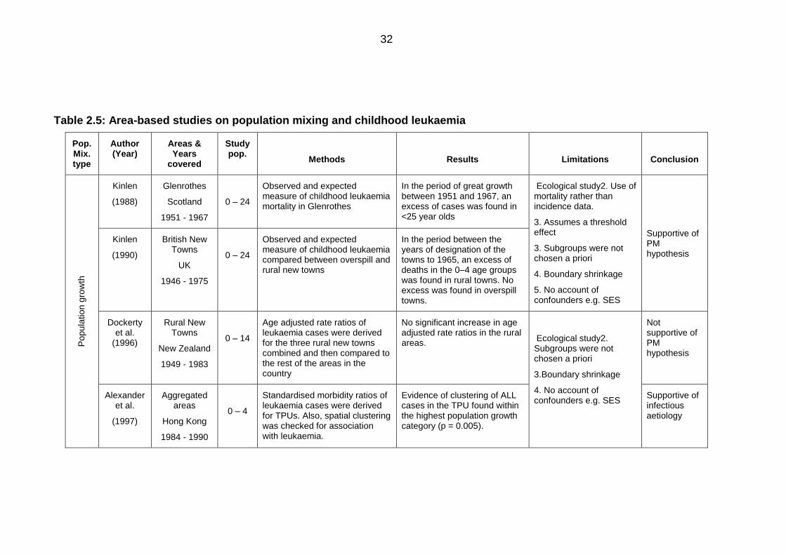
32
Table 2.5: Area-based studies on population mixing and childhood leukaemia
Pop. Mix. type
Author (Year)
Areas & Years
covered
Study pop.
Methods
Results
Limitations
Conclusion
Popula
tion g
row
th
Kinlen
(1988)
Glenrothes
Scotland
1951 - 1967
0 – 24
Observed and expected measure of childhood leukaemia mortality in Glenrothes
In the period of great growth between 1951 and 1967, an excess of cases was found in <25 year olds
Ecological study2. Use of mortality rather than incidence data.
3. Assumes a threshold effect
3. Subgroups were not chosen a priori
4. Boundary shrinkage
5. No account of confounders e.g. SES
Supportive of PM hypothesis
Kinlen
(1990)
British New Towns
UK
1946 - 1975
0 – 24
Observed and expected measure of childhood leukaemia compared between overspill and rural new towns
In the period between the years of designation of the towns to 1965, an excess of deaths in the 0–4 age groups was found in rural towns. No excess was found in overspill towns.
Dockerty et al.
(1996)
Rural New Towns
New Zealand
1949 - 1983
0 – 14
Age adjusted rate ratios of leukaemia cases were derived for the three rural new towns combined and then compared to the rest of the areas in the country
No significant increase in age adjusted rate ratios in the rural areas.
Ecological study2. Subgroups were not chosen a priori
3.Boundary shrinkage
4. No account of confounders e.g. SES
Not supportive of PM hypothesis
Alexander et al.
(1997)
Aggregated areas
Hong Kong
1984 - 1990
0 – 4
Standardised morbidity ratios of leukaemia cases were derived for TPUs. Also, spatial clustering was checked for association with leukaemia.
Evidence of clustering of ALL cases in the TPU found within the highest population growth category (p = 0.005).
Supportive of infectious aetiology
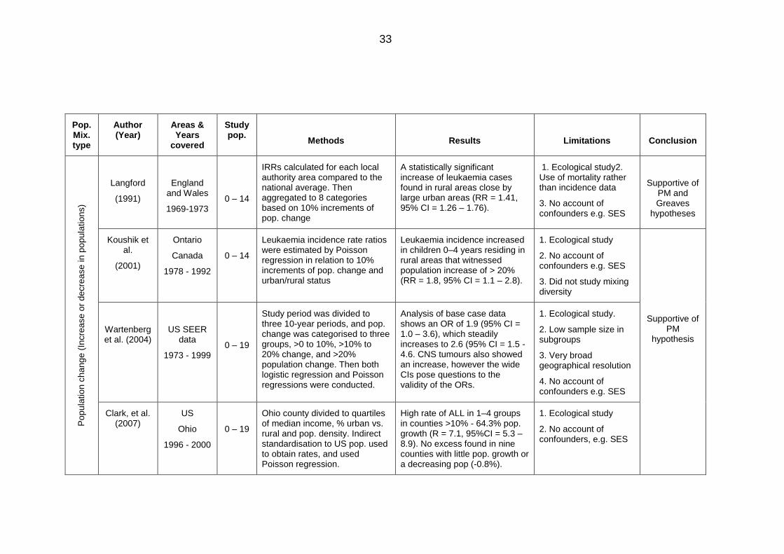
33
Pop. Mix. type
Author (Year)
Areas & Years
covered
Study pop.
Methods
Results
Limitations
Conclusion
Popula
tion c
hang
e (
Incre
ase o
r decre
ase in p
opula
tions)
Langford
(1991)
England and Wales
1969-1973
0 – 14
IRRs calculated for each local authority area compared to the national average. Then aggregated to 8 categories based on 10% increments of pop. change
A statistically significant increase of leukaemia cases found in rural areas close by large urban areas (RR = 1.41, 95% CI = 1.26 – 1.76).
1. Ecological study2. Use of mortality rather than incidence data
3. No account of confounders e.g. SES
Supportive of PM and Greaves
hypotheses
Koushik et al.
(2001)
Ontario
Canada
1978 - 1992
0 – 14
Leukaemia incidence rate ratios were estimated by Poisson regression in relation to 10% increments of pop. change and urban/rural status
Leukaemia incidence increased in children 0–4 years residing in rural areas that witnessed population increase of > 20% (RR = 1.8, 95% CI = 1.1 – 2.8).
1. Ecological study
2. No account of confounders e.g. SES
3. Did not study mixing diversity
Supportive of PM
hypothesis
Wartenberg et al. (2004)
US SEER data
1973 - 1999
0 – 19
Study period was divided to three 10-year periods, and pop. change was categorised to three groups, >0 to 10%, >10% to 20% change, and >20% population change. Then both logistic regression and Poisson regressions were conducted.
Analysis of base case data shows an OR of 1.9 (95% CI = 1.0 – 3.6), which steadily increases to 2.6 (95% CI = 1.5 - 4.6. CNS tumours also showed an increase, however the wide CIs pose questions to the validity of the ORs.
1. Ecological study.
2. Low sample size in subgroups
3. Very broad geographical resolution
4. No account of confounders e.g. SES
Clark, et al. (2007)
US
Ohio
1996 - 2000
0 – 19
Ohio county divided to quartiles of median income, % urban vs. rural and pop. density. Indirect standardisation to US pop. used to obtain rates, and used Poisson regression.
High rate of ALL in 1–4 groups in counties >10% - 64.3% pop. growth (R = 7.1, 95%CI = 5.3 – 8.9). No excess found in nine counties with little pop. growth or a decreasing pop (-0.8%).
1. Ecological study
2. No account of confounders, e.g. SES
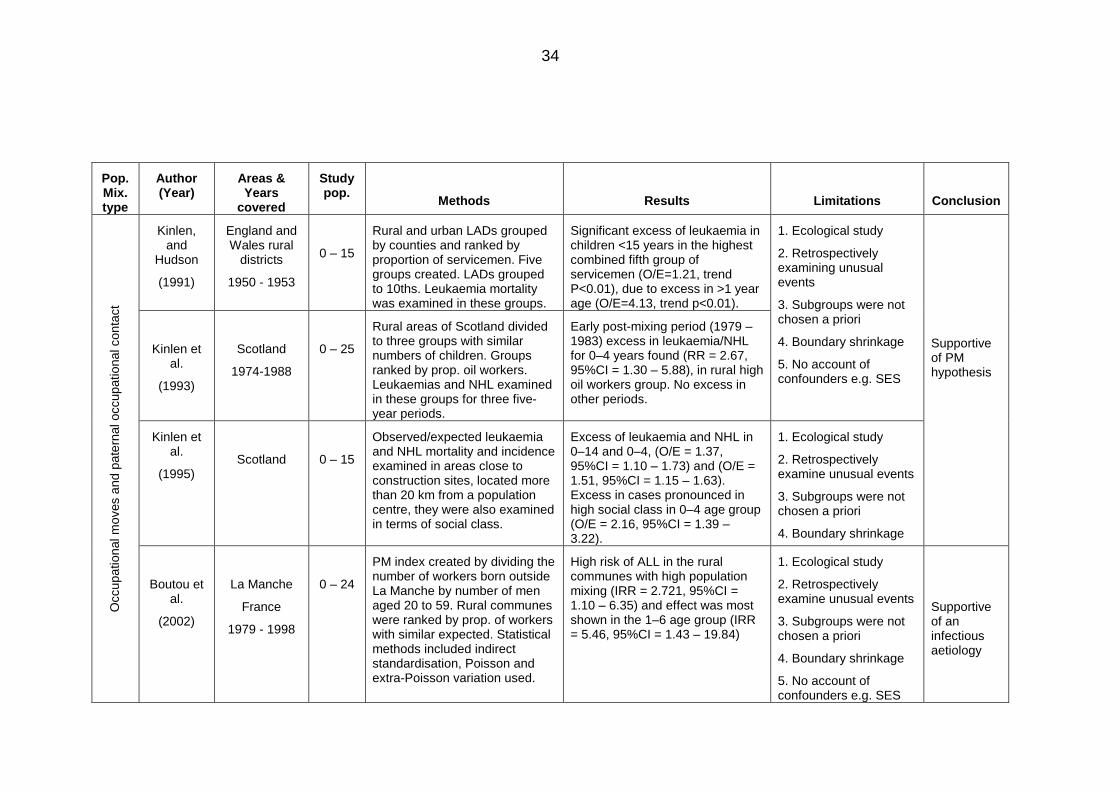
34
Pop. Mix. type
Author (Year)
Areas & Years
covered
Study pop.
Methods
Results
Limitations
Conclusion
Occupational m
oves a
nd
pate
rnal occupational conta
ct
Kinlen, and
Hudson
(1991)
England and Wales rural
districts
1950 - 1953
0 – 15
Rural and urban LADs grouped by counties and ranked by proportion of servicemen. Five groups created. LADs grouped to 10ths. Leukaemia mortality was examined in these groups.
Significant excess of leukaemia in children <15 years in the highest combined fifth group of servicemen (O/E=1.21, trend P<0.01), due to excess in >1 year age (O/E=4.13, trend p<0.01).
1. Ecological study
2. Retrospectively examining unusual events
3. Subgroups were not chosen a priori
4. Boundary shrinkage
5. No account of confounders e.g. SES
Supportive of PM hypothesis
Kinlen et al.
(1993)
Scotland
1974-1988
0 – 25
Rural areas of Scotland divided to three groups with similar numbers of children. Groups ranked by prop. oil workers. Leukaemias and NHL examined in these groups for three five-year periods.
Early post-mixing period (1979 – 1983) excess in leukaemia/NHL for 0–4 years found (RR = 2.67, 95%CI = 1.30 – 5.88), in rural high oil workers group. No excess in other periods.
Kinlen et al.
(1995)
Scotland
0 – 15
Observed/expected leukaemia and NHL mortality and incidence examined in areas close to construction sites, located more than 20 km from a population centre, they were also examined in terms of social class.
Excess of leukaemia and NHL in 0–14 and 0–4, (O/E = 1.37, 95%CI = 1.10 – 1.73) and (O/E = 1.51, 95%CI = 1.15 – 1.63). Excess in cases pronounced in high social class in 0–4 age group (O/E = 2.16, 95%CI = 1.39 – 3.22).
1. Ecological study
2. Retrospectively examine unusual events
3. Subgroups were not chosen a priori
4. Boundary shrinkage
Boutou et al.
(2002)
La Manche
France
1979 - 1998
0 – 24
PM index created by dividing the number of workers born outside La Manche by number of men aged 20 to 59. Rural communes were ranked by prop. of workers with similar expected. Statistical methods included indirect standardisation, Poisson and extra-Poisson variation used.
High risk of ALL in the rural communes with high population mixing (IRR = 2.721, 95%CI = 1.10 – 6.35) and effect was most shown in the 1–6 age group (IRR = 5.46, 95%CI = 1.43 – 19.84)
1. Ecological study
2. Retrospectively examine unusual events
3. Subgroups were not chosen a priori
4. Boundary shrinkage
5. No account of confounders e.g. SES
Supportive of an infectious aetiology
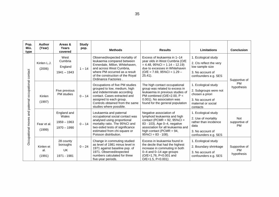
35
Pop. Mix. type
Author (Year)
Areas & Years
covered
Study pop.
Methods
Results
Limitations
Conclusion
Occupational m
oves a
nd
pate
rnal occupational conta
ct
Kinlen L.J.
(2006)
West Cumbria
England
1941 – 1943
1 – 14
Observed/expected mortality of leukaemia compared between Ennerdale, Millon, Whitehaven, and across West Cumbria, where PM occurred as a result of the construction of the Royal Ordinance Factories .
Excess of leukaemia in 1–14 year olds in West Cumbria (O/E = 4.48, 95%CI = 1.14 – 12.19) due to excesses in Whitehaven (O/E = 7.69, 95%CI = 1.29 – 25.41).
1. Ecological study
2. CIs reflect the very low sample size
3. No account of confounders e.g. SES
Supportive of PM
hypothesis
Kinlen
(1997)
Five previous PM studies
0 – 14
Occupations of five PM studies grouped to low, medium, high and indeterminate according contact. Cases extracted and assigned to each group. Controls obtained from the same studies where possible.
The high contact occupational group was related to excess in leukaemia in previous studies of PM combined (O/E=2.00, P < 0.001). No association was found for the general population
1. Ecological study
2. Subgroups were not chosen a priori
3. No account of maternal or social contacts
Fear et al.
(1999)
England and Wales
1959 – 1963
1970 – 1990
0 – 14
Leukaemia and paternal occupational social contact was analysed using proportional mortality ratio. The 95%CI and two-sided tests of significance estimated from chi-square or Poisson distribution.
Negative association of lymphoid leukaemia and high contact (PCMR = 92, 95%CI = 83 - 103). Age 0–4, negative association for all leukaemia and high contact (PCMR = 94, 95%CI = 83 - 108).
1. Ecological study
2. Use of mortality rather than incidence data
3. No account of confounders e.g. SES
Not supportive of
PM
Kinlen et al.
(1991)
28 county boroughs
UK
1971 - 1981
0 – 24
Change in commuting studied as level of 1981 minus level in 1971 against baseline pop. of 1971. Observed/expected numbers calculated for three five-year periods.
Excess in leukaemia found in the decile that had the highest increase in commuting in both 0–4 and 0–14 age groups (O/E=1.76, P<0.001 and O/E=1.5, P<0.001)
1. Ecological study
2. Boundary shrinkage
3. No account of confounders e.g. SES
Supportive of PM
hypothesis
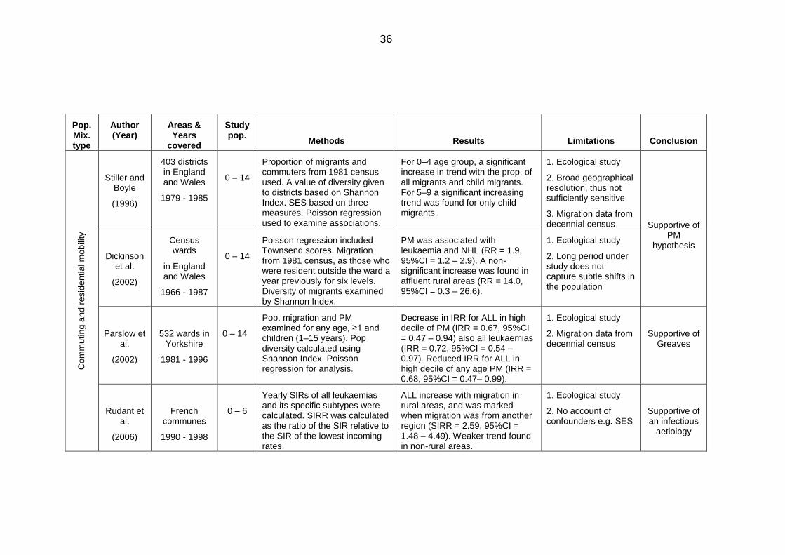
36
Pop. Mix. type
Author (Year)
Areas & Years
covered
Study pop.
Methods
Results
Limitations
Conclusion
Com
muting a
nd r
esid
ential m
obili
ty
Stiller and Boyle
(1996)
403 districts in England and Wales
1979 - 1985
0 – 14
Proportion of migrants and commuters from 1981 census used. A value of diversity given to districts based on Shannon Index. SES based on three measures. Poisson regression used to examine associations.
For 0–4 age group, a significant increase in trend with the prop. of all migrants and child migrants. For 5–9 a significant increasing trend was found for only child migrants.
1. Ecological study
2. Broad geographical resolution, thus not sufficiently sensitive
3. Migration data from decennial census
Supportive of PM
hypothesis
Dickinson et al.
(2002)
Census wards
in England and Wales
1966 - 1987
0 – 14
Poisson regression included Townsend scores. Migration from 1981 census, as those who were resident outside the ward a year previously for six levels. Diversity of migrants examined by Shannon Index.
PM was associated with leukaemia and NHL (RR = 1.9, 95%CI = 1.2 – 2.9). A non-significant increase was found in affluent rural areas (RR = 14.0, 95%CI = 0.3 – 26.6).
1. Ecological study
2. Long period under study does not capture subtle shifts in the population
Parslow et al.
(2002)
532 wards in Yorkshire
1981 - 1996
0 – 14
Pop. migration and PM examined for any age, ≥1 and children (1–15 years). Pop diversity calculated using Shannon Index. Poisson regression for analysis.
Decrease in IRR for ALL in high decile of PM (IRR = 0.67, 95%CI = 0.47 – 0.94) also all leukaemias (IRR = 0.72, 95%CI = 0.54 – 0.97). Reduced IRR for ALL in high decile of any age PM (IRR = 0.68, 95%CI = 0.47– 0.99).
1. Ecological study
2. Migration data from decennial census
Supportive of Greaves
Rudant et al.
(2006)
French communes
1990 - 1998
0 – 6
Yearly SIRs of all leukaemias and its specific subtypes were calculated. SIRR was calculated as the ratio of the SIR relative to the SIR of the lowest incoming rates.
ALL increase with migration in rural areas, and was marked when migration was from another region (SIRR = 2.59, 95%CI = 1.48 – 4.49). Weaker trend found in non-rural areas.
1. Ecological study
2. No account of confounders e.g. SES
Supportive of an infectious
aetiology
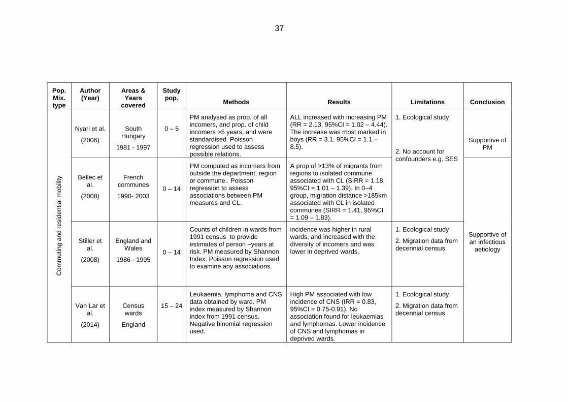
37
Pop. Mix. type
Author (Year)
Areas & Years
covered
Study pop.
Methods
Results
Limitations
Conclusion
Com
muting a
nd r
esid
ential m
obili
ty
Nyari et al.
(2006)
South Hungary
1981 - 1997
0 – 5
PM analysed as prop. of all incomers, and prop. of child incomers >5 years, and were standardised. Poisson regression used to assess possible relations.
ALL increased with increasing PM (RR = 2.13, 95%CI = 1.02 – 4.44). The increase was most marked in boys (RR = 3.1, 95%CI = 1.1 – 8.5).
1. Ecological study
2. No account for confounders e.g. SES
Supportive of PM
Bellec et al.
(2008)
French communes
1990- 2003
0 – 14
PM computed as incomers from outside the department, region or commune.. Poisson regression to assess associations between PM measures and CL.
A prop of >13% of migrants from regions to isolated commune associated with CL (SIRR = 1.18, 95%CI = 1.01 – 1.39). In 0–4 group, migration distance >185km associated with CL in isolated communes (SIRR = 1.41, 95%CI = 1.09 – 1.83).
Supportive of an infectious
aetiology
Stiller et al.
(2008)
England and Wales
1986 - 1995
0 – 14
Counts of children in wards from 1991 census to provide estimates of person –years at risk. PM measured by Shannon Index. Poisson regression used to examine any associations.
incidence was higher in rural wards, and increased with the diversity of incomers and was lower in deprived wards.
1. Ecological study
2. Migration data from decennial census
Van Lar et al.
(2014)
Census wards
England
15 – 24
Leukaemia, lymphoma and CNS data obtained by ward. PM index measured by Shannon index from 1991 census. Negative binomial regression used.
High PM associated with low incidence of CNS (IRR = 0.83, 95%CI = 0.75-0.91). No association found for leukaemias and lymphomas. Lower incidence of CNS and lymphomas in deprived wards.
1. Ecological study
2. Migration data from decennial census
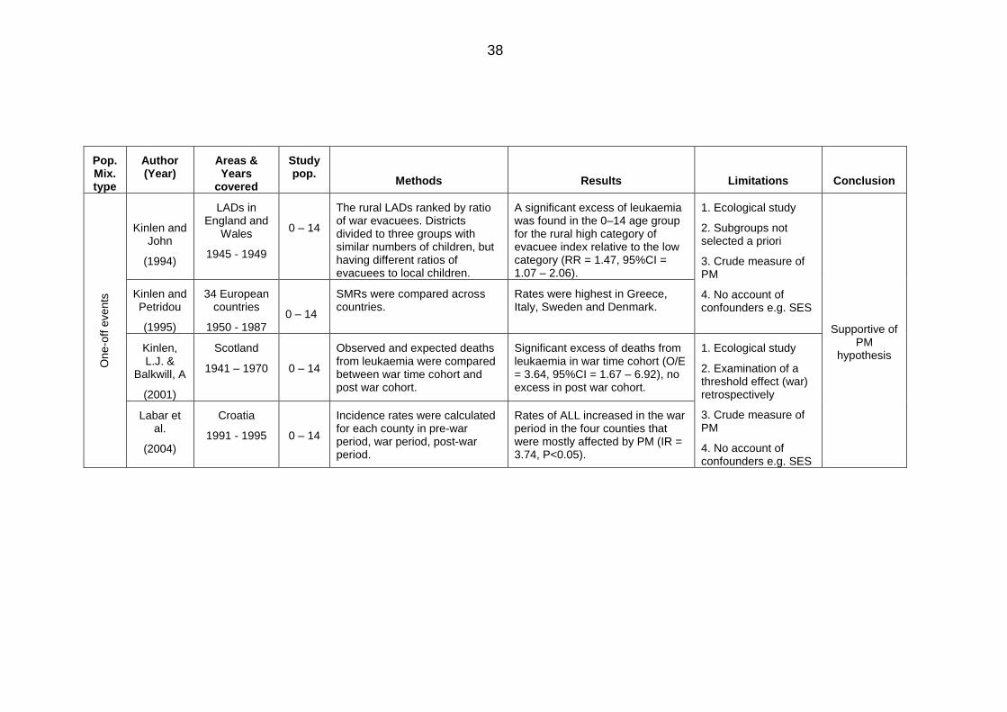
38
Pop. Mix. type
Author (Year)
Areas & Years
covered
Study pop.
Methods
Results
Limitations
Conclusion
One
-off e
vents
Kinlen and John
(1994)
LADs in England and
Wales
1945 - 1949
0 – 14
The rural LADs ranked by ratio of war evacuees. Districts divided to three groups with similar numbers of children, but having different ratios of evacuees to local children.
A significant excess of leukaemia was found in the 0–14 age group for the rural high category of evacuee index relative to the low category (RR = 1.47, 95%CI = 1.07 – 2.06).
1. Ecological study
2. Subgroups not selected a priori
3. Crude measure of PM
4. No account of confounders e.g. SES
Supportive of PM
hypothesis
Kinlen and Petridou
(1995)
34 European countries
1950 - 1987
0 – 14
SMRs were compared across countries.
Rates were highest in Greece, Italy, Sweden and Denmark.
Kinlen, L.J. &
Balkwill, A
(2001)
Scotland
1941 – 1970
0 – 14
Observed and expected deaths from leukaemia were compared between war time cohort and post war cohort.
Significant excess of deaths from leukaemia in war time cohort (O/E = 3.64, 95%CI = 1.67 – 6.92), no excess in post war cohort.
1. Ecological study
2. Examination of a threshold effect (war) retrospectively
3. Crude measure of PM
4. No account of confounders e.g. SES
Labar et al.
(2004)
Croatia
1991 - 1995
0 – 14
Incidence rates were calculated for each county in pre-war period, war period, post-war period.
Rates of ALL increased in the war period in the four counties that were mostly affected by PM (IR = 3.74, P<0.05).
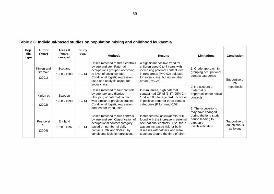
39
Table 2.6: Individual-based studies on population mixing and childhood leukaemia
Pop. Mix. type
Author (Year)
Areas & Years
covered
Study pop.
Methods
Results
Limitations
Conclusion
Kinlen and Bramald
(2001)
Scotland
1950 - 1989
0 – 14
Cases matched to three controls by age and sex. Paternal occupations grouped according to level of social contact. Conditional logistic regression used and analysis adjust for social class.
A significant positive trend for children aged 0 to 4 years with increasing paternal contact level in rural areas (P=0.02) adjusted for social class, but not in urban areas (P=0.26).
1. Crude approach in grouping occupational contact categories
2. No account of maternal or opportunities for social contacts
3. The occupations may have changed during the long study period leading to exposure misclassification
Supportive of PM
hypothesis
Kinlen et al.
(2002)
Sweden
1958 - 1998
0 – 14
Cases matched to four controls by age, sex and district. Grouping of paternal contact was similar to previous studies. Conditional logistic regression and test for trend used.
In rural areas, high paternal contact had OR of (3.47, 95% CI= 1.54 – 7.85) for age 0–4. Increase in positive trend for three contact categories (P for trend 0.02).
Pearce et al.
(2004)
England
1968 - 1997
0 – 14
Cases matched to two controls by age and sex. Classification of occupational contact category based on number of daily contacts. OR and 95% CI by conditional logistic regression.
Increased risk of leukaemia/NHL found with the increase in paternal occupational contacts. Also, there was an increased risk for both diseases with fathers who were teachers around the time of birth.
Supportive of an infectious
aetiology
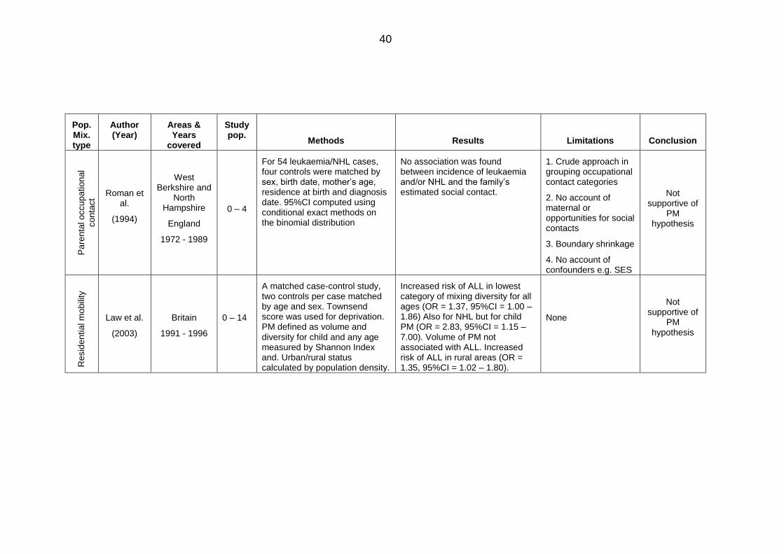
40
Pop. Mix. type
Author (Year)
Areas & Years
covered
Study pop.
Methods
Results
Limitations
Conclusion
Pare
nta
l occupational
conta
ct
Roman et al.
(1994)
West Berkshire and
North Hampshire
England
1972 - 1989
0 – 4
For 54 leukaemia/NHL cases, four controls were matched by sex, birth date, mother’s age, residence at birth and diagnosis date. 95%CI computed using conditional exact methods on the binomial distribution
No association was found between incidence of leukaemia and/or NHL and the family’s estimated social contact.
1. Crude approach in grouping occupational contact categories
2. No account of maternal or opportunities for social contacts
3. Boundary shrinkage
4. No account of confounders e.g. SES
Not supportive of
PM hypothesis
Resid
ential m
obili
ty
Law et al.
(2003)
Britain
1991 - 1996
0 – 14
A matched case-control study, two controls per case matched by age and sex. Townsend score was used for deprivation. PM defined as volume and diversity for child and any age measured by Shannon Index and. Urban/rural status calculated by population density.
Increased risk of ALL in lowest category of mixing diversity for all ages (OR = 1.37, 95%CI = 1.00 – 1.86) Also for NHL but for child PM (OR = 2.83, 95%CI = 1.15 – 7.00). Volume of PM not associated with ALL. Increased risk of ALL in rural areas (OR = 1.35, 95%CI = 1.02 – 1.80).
None
Not supportive of
PM hypothesis
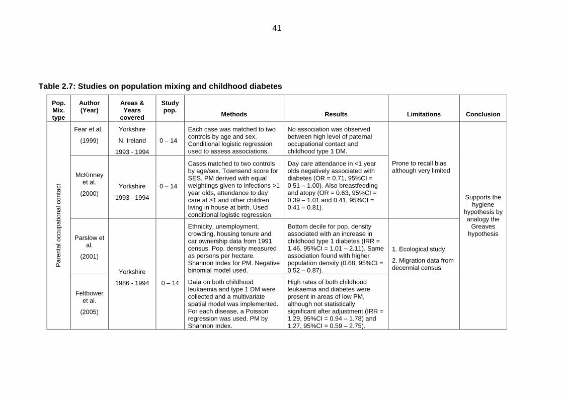
41
Table 2.7: Studies on population mixing and childhood diabetes
Pop. Mix. type
Author (Year)
Areas & Years
covered
Study pop.
Methods
Results
Limitations
Conclusion
Pare
nta
l occupational conta
ct
Fear et al.
(1999)
Yorkshire
N. Ireland
1993 - 1994
0 – 14
Each case was matched to two controls by age and sex. Conditional logistic regression used to assess associations.
No association was observed between high level of paternal occupational contact and childhood type 1 DM.
Prone to recall bias although very limited
Supports the hygiene
hypothesis by analogy the
Greaves hypothesis
McKinney et al.
(2000)
Yorkshire
1993 - 1994
0 – 14
Cases matched to two controls by age/sex. Townsend score for SES. PM derived with equal weightings given to infections >1 year olds, attendance to day care at >1 and other children living in house at birth. Used conditional logistic regression.
Day care attendance in <1 year olds negatively associated with diabetes (OR = 0.71, 95%CI = 0.51 – 1.00). Also breastfeeding and atopy (OR = 0.63, 95%CI = 0.39 – 1.01 and 0.41, 95%CI = 0.41 – 0.81).
Parslow et al.
(2001)
Yorkshire
1986 - 1994
0 – 14
Ethnicity, unemployment, crowding, housing tenure and car ownership data from 1991 census. Pop. density measured as persons per hectare. Shannon Index for PM. Negative binomial model used.
Bottom decile for pop. density associated with an increase in childhood type 1 diabetes (IRR = 1.46, 95%CI = 1.01 – 2.11). Same association found with higher population density (0.68, 95%CI = 0.52 – 0.87).
1. Ecological study
2. Migration data from decennial census
Feltbower et al.
(2005)
Data on both childhood leukaemia and type 1 DM were collected and a multivariate spatial model was implemented. For each disease, a Poisson regression was used. PM by Shannon Index.
High rates of both childhood leukaemia and diabetes were present in areas of low PM, although not statistically significant after adjustment (IRR = 1.29, 95%CI = 0.94 – 1.78) and 1.27, 95%CI = 0.59 – 2.75).
42
Pop. Mix. type
Author (Year)
Areas & Years
covered
Study pop.
Methods
Results
Limitations
Conclusion
Pare
nta
l occupational conta
ct
Miller et al. (2009)
Canterbury
New Zealand
1999- 2004
0 – 14 PM measure from census data, which included migration diversity and migration distance. Adjusted for pop. density and SES. Poisson regression used to examine any associations.
Incidence of childhood diabetes was increased in areas of high PM.
Mathematical coupling Supportive of PM
hypothesis
Hall et al. (2014)
Colorado
USA
1993-2014
0 – 14
Cox proportional hazards regression used to examine associations between incidence of diabetes, day care attendance and breastfeeding.
No associations observed between diabetes and daycare attendance (HR: 0.89; CI: 0.54–1.47). Adjusting for breastfeeding modified the associations and diabetes was increased in non-breastfed children although non-significant (HR: 1.56; CI: 0.77–3.16).
1. Small number of cases
2. No account of confounders e.g. SES
Supportive of an infectious
aetiology
43
2.4.3.4.4 Summary of studies on population mixing
Estimation of the level of infection for each individual is fraught with difficulty. The
indicators for infection rely on biological markers and/or clinically diagnosed
symptoms, and the majority of infections experienced in early life do not require
medical consultation (Law et al., 2008). The measures of PM used in these studies
are merely proxies, and they are not expected to capture an individual’s exposure
to infections completely. Nonetheless, the series of studies on PM and childhood
leukaemia and NHL have generated much controversy and confusion for several
reasons. The first of which is the gradual change of the hypothesis that can be seen
under close examination of these studies. The original hypothesis suggested by
Kinlen in 1988 was based on the idea that PM leads to the mixing of susceptible
and infected children, which subsequently results in an epidemic of a yet
unidentified infection, and that this infection leads to leukaemia (Kinlen, 1988,
Kinlen, 1995). Kinlen further explains in his 1990 study, that the mixing of children
subsequently leads to a child-child transmission of the unknown infective agent,
and draws attention to the high density of children in the British New Towns as a
result of the high proportion of young adults within those towns (Kinlen et al., 1990).
Although the excess was limited to pre-school children, he explained that ‘infected
older siblings and parents are well placed to infect young children, moreover with
large doses of the agent’ (Kinlen et al., 1990, p. 581). The hypothesis then included
an adult-child transmission of the infection by adults commuting to work. Thereby, it
was no longer exclusive to influxes of people to a relatively rural area (Kinlen et al.,
1991). The hypothesis was then further extended to examine whether an excess of
childhood leukaemia was linked to paternal occupational contact only in areas that
had witnessed an excess of the disease (Kinlen, 1997, Kinlen and Bramald, 2001,
Kinlen et al., 2002). Therefore, a close examination of the studies published on PM
(Tables 2.4 and 2.5) shows how the original hypothesis published in the late 1980s
has been refined to only include areas in which an excess of cases was found.
Such an approach is not ideal because limiting the boundaries of an area under
study will almost always result in an excess of the outcome – a problem commonly
referred to as boundary shrinkage. A further problem with such an approach is that
it will also result in a small sample size, especially if the disease in question is rare.
Consequently, a better method is to generalise the study area to cover large parts
chosen a priori, not only to specific areas, such as those adopted in more recent
studies (Fear et al., 1999b, Roman et al., 1994, Parslow et al., 2002, Law et al.,

44
2003). These studies produced different results that were unsupportive of the
hypothesis and some concluded that PM may actually be protective.
Also, PM has been defined in a different way to that seen in most of the traditional
studies. Within these studies, a reproducible measure of PM was used which
included both the volume of the people and their places of origin. The data used in
this measure was collected independently of the study itself, i.e. census data,
ensuring its accuracy and consistency in contrast to crude numbers used in the
majority of the other studies. Further, several traditional studies used leukaemia
mortality instead of leukaemia incidence, which is understandable in the earlier
years where no data on incidence was available. However, in the past few decades,
survival from childhood cancers, particularly lymphoblastic leukaemia has improved
(Ma et al., 2014). The type of the study, i.e. area-based or individual-based plays an
important role in the variation between these studies. The use of individual-based
studies improves the accuracy in the measurement of confounding variables.
Studies on PM carried out in countries other than the UK have tried to use similar
measures of PM. However, the limited availability of the data limits the efforts in
creating a unified definition of PM. The seriousness of childhood cancers should
increase international efforts to construct studies similar to the UKCCS in other
countries, so as to come up with conclusions on the aetiology of not only childhood
leukaemia, but also childhood cancers in general. This will allow for comparison
between these studies and a better understanding of the underlying risk factors will
emerge. Furthermore, it would be useful to test the validity of the different measures
of PM in these studies by assessing the type of infection, incubation period and
reproductive rate (Law et al., 2008)
In conclusion, Kinlen (1988) sought to refine the PM hypothesis, but failed to
provide a biological mechanism for all situations. Furthermore, in almost all studies,
all subtypes of ALL were assumed to have the main underlying cause whether
infant ALL or common childhood ALL. In contrast, Wiemles et al. (1999) provided
evidence of a genetic mutational event occurring neonatally, from blood spots
obtained from 12 children aged between two and five years in Italy and the UK who
had been recently diagnosed with ALL. This finding, along with those from the
studies on PM and diabetes, and some of those on leukaemia are in support of the
alternative hypothesis put forward by Greaves (1988) (Wiemels et al., 1999a).
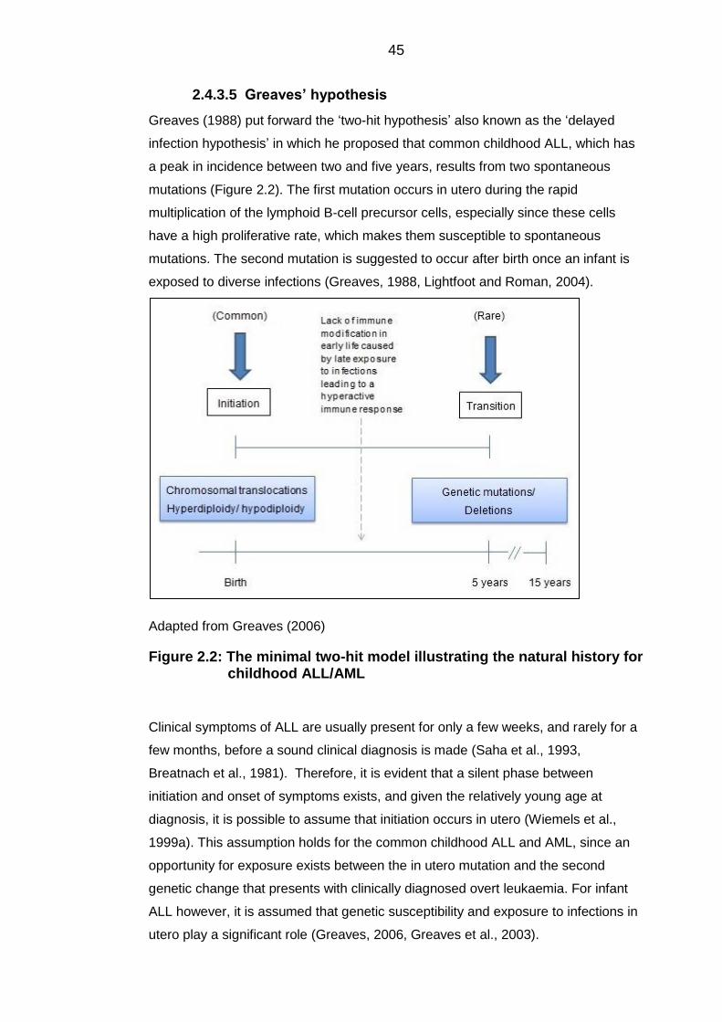
45
Greaves’hypothesis 2.4.3.5
Greaves (1988) put forward the ‘two-hit hypothesis’ also known as the ‘delayed
infection hypothesis’ in which he proposed that common childhood ALL, which has
a peak in incidence between two and five years, results from two spontaneous
mutations (Figure 2.2). The first mutation occurs in utero during the rapid
multiplication of the lymphoid B-cell precursor cells, especially since these cells
have a high proliferative rate, which makes them susceptible to spontaneous
mutations. The second mutation is suggested to occur after birth once an infant is
exposed to diverse infections (Greaves, 1988, Lightfoot and Roman, 2004).
Adapted from Greaves (2006)
Figure 2.2: The minimal two-hit model illustrating the natural history for childhood ALL/AML
Clinical symptoms of ALL are usually present for only a few weeks, and rarely for a
few months, before a sound clinical diagnosis is made (Saha et al., 1993,
Breatnach et al., 1981). Therefore, it is evident that a silent phase between
initiation and onset of symptoms exists, and given the relatively young age at
diagnosis, it is possible to assume that initiation occurs in utero (Wiemels et al.,
1999a). This assumption holds for the common childhood ALL and AML, since an
opportunity for exposure exists between the in utero mutation and the second
genetic change that presents with clinically diagnosed overt leukaemia. For infant
ALL however, it is assumed that genetic susceptibility and exposure to infections in
utero play a significant role (Greaves, 2006, Greaves et al., 2003).
46
2.4.3.5.1 Biological evidence
At the time when the hypothesis was first suggested in 1988, it was merely
speculative, however by the end of the 1990s and with advances in molecular
biology the hypothesis has become substantiated (Greaves, 2006). Evidence for
the first hit came from molecular inspection of several pairs of identical twins (i.e.
monozygotic twins formed from a single fertilised egg and split into two embryos),
aged between 2 and 14 years when diagnosed with ALL or infant ALL. These
studies provided evidence that the TEL-AML1 breakpoints for childhood ALL, as
well as the MLL gene breakpoints in infant ALL, are exactly the same. This means
that such mutations occur in one cell in one foetus in utero, and then passed to the
second twin via the shared placental circulation (Ford et al., 1997, Ford et al., 1998,
Wiemels et al., 1999b). Furthermore, with several pairs of twins, asynchronous
diagnosis was made in where there was a gap of a few years between the
diagnoses of each twin, indicating the need for a second postnatal event whether
genetic or involving infectious exposure (Greaves et al., 2003). Studies on twins
also revealed that in one set of twins, one twin was diagnosed with T-cell ALL and
the other with T-cell NHL, which supports the idea that these two diseases are
biologically similar (Ford et al., 1997, Greaves et al., 2003).
Furthermore, Guthrie cards, which contain neonatal blood spots that are typically
retained for several years, have been retrospectively examined in several studies
(Wiemels et al., 1999a, Gale et al., 1997). These cards are a good source of intact
DNA that can be easily amplified by the polymerase chain reaction (PCR)
technology to look for any genetic mutations (Jinks et al., 1989). These studies
showed that the TEL-AML1 fusion genes that are frequently seen in the common
form of ALL were present in these blood spots, providing strong unequivocal
support for the first mutation originating in utero.
2.4.3.5.2 Epidemiological evidence
A substantial body of epidemiological studies have sought to address the infectious
aetiology of childhood ALL (Table 2.7). Although they mainly addressed the PM
hypothesis, several of these studies also supported the delayed infection
hypothesis. For example, an assumption may be made that the cases within the
studies dealing with clusters of leukaemia had the common prenatal genetic
mutation, i.e. the first hit. Consequently, delayed exposure to infection through
isolation or high socioeconomic conditions may have initiated the second postnatal
promotional event (Greaves, 2006). It is necessary to point out that these studies
47
did not examine both infant and common childhood ALL, and did not look at these
subtypes separately.
In addition, the likelihood of acquiring infections is highly dependent on social
contact as well as the frequency of such contact. In children, attendance to day
care centres or playgroups may be used as a proxy measure for social contact. It
was found that such attendance increases the chances of acquiring viruses such as
the HIB and common upper respiratory tract infections (Istre et al., 1985, Greaves,
2006). Also, the frequency of attendance, as well as the number of children within a
social group, increases the chances of acquiring infections even further (Greaves,
2006). Studies on attendance to day care centres have shown that attendance
confers protection against autoimmune diseases (Krämer et al., 1999, McKinney et
al., 2000). Similar associations have been reported for common childhood ALL from
the UKCCS and the NCCLS (estimates previously reported) (Gilham et al., 2005,
Ma et al., 2005). These studies are supportive of the delayed infection hypothesis.
The UKCCS further investigated clinically diagnosed infections in the first year of
life, abstracted from general practitioner (GP) records for both cases and controls.
According to the delayed infection hypothesis, the cases would have a deficit of
infections compared to the controls (Roman et al., 2007). However, the results
showed that only 18% of controls compared to 24% of cases were diagnosed with
at least one infection in the first month of life (OR = 1.4, 95%CI = 1.1 – 1.9), and by
the end of the first year of life the numbers increased to 85% in controls and 88% in
cases (OR = 1.3 – 1.8) (Roman et al., 2007). A similar association was reported in
another study (Cardwell et al., 2008). Although the results were contrary to the
original hypothesis, they do not refute it for two reasons. The first is that the
hypothesis does not specify that the underlying infection is overt and clear in a way
that necessitates a visit to the GP. It may be an innocuous infection with minimal
symptoms, hence these studies do mask such infections. The second is that
assuming all cases had the first mutation in utero, then an abnormal response to
infections may precipitate the second mutation that develops the leukaemic cells
into full blown leukaemia. Such an abnormal response may be reflected in the high
level of reported infections within GP records.
2.4.3.5.3 Contrasts with PM
It is important to note that the PM hypothesis and the delayed infection hypothesis
are not mutually exclusive. The two hypotheses share common grounds in that they
postulate that childhood leukaemia is a rare response to a common infection that
48
may be acquired by a delayed exposure to that infection, whether due to isolation or
modern living conditions. High levels of mixing to a previously isolated area
introduce novel infections to the host community, thereby providing an opportunity
for the second hit necessary to develop overt leukaemia (Greaves, 2006).
Furthermore, unlike the PM hypothesis which depends solely on epidemiological
theories, the delayed infection hypothesis considers the natural history of ALL in
terms of the actual biological and immunological nature of the disease. Also,
although the epidemiological studies concerned with PM are based on data of
patients who mostly had the common form of ALL, the interpretation of the data
indicated that all subtypes of ALL as well as NHL shared a common aetiology.
However, the delayed infection hypothesis was only concerned with common types
of ALL in children with incidence peaking between two and five years of age.
Smith’shypothesis 2.4.3.6
Smith (1997) proposed an alternative model to explain the peak in common
childhood ALL, that aetiological agents causing an infection during pregnancy are
transmitted to the foetus, thereby resulting in an in utero infection, consequently
increasing the risk of ALL. This hypothesis attributes the latency period between the
in utero infection and the clinical presentation of ALL to a second post-natal event
or to a true latency period related to the growth rate of leukaemia cells. Certain
characteristics of the aetiological agent have been identified to allow for the broad
range of suspected agents to be narrowed. First, since hyperdiploidy is the most
common cytogenetic abnormality in ALL, and since the median age at diagnosis of
ALL with hyperdiploidy coincides with the peak in ALL incidence found in
epidemiological studies, the aetiological agent should therefore be able to cause
genomic instability. Secondly, since hyperdiploidy is mostly associated with B-cell
ALL, and rarely with T-cell ALL, and since the elevated risk of ALL related to
socioeconomic status is specific to B-cell ALL, the agent should consequently affect
B lymphocytes. Also, the agent should have minimal symptoms otherwise any
obvious symptoms caused by the infectious agent would have been reported.
Additionally, the agent must be capable of passing to the foetus through the
placenta without causing any foetal abnormalities otherwise these abnormalities
would have been seen among ALL cases. Equally important is that this agent
should have a limited cancer causing potential. One potential candidate suggested
was the John Cunningham (JC) virus from the polymavirus family, which meets
most of these conditions (Smith, 1997).

49
Some studies attempted to detect the JC virus as well as the polymavirus hominis
1, also known as the BK virus, from the polymavirus family using specimens from
children diagnosed with common childhood ALL (Smith et al., 1999, MacKenzie et
al., 1999). However, not one was able to detect these viruses, concluding that these
were unlikely to be implicated in the aetiology of the disease.
50
2.5 Socioeconomic status
Throughout the years, studies of populations have documented an association
between SES and health. Since the 19th century, the link between SES and ill
health has been extensively examined, from the time when researchers examined
the health outcome differences between the working class in Europe, the royalty
and the elite (Antonovsky, 1967). Ever since, the examination of the relationship
between SES and health has been of much interest. The relationship is better
described as a gradient, because the differences in incidence and mortality in
health are found at every level of the hierarchy of SES regardless of a cut-off point
(Adler et al., 1994).
It is very important to understand that SES does not refer to a single measure – it is
in fact multi-dimensional. Measures typically include social status which may be
measured by education, economic status which may be measured by income
and/or ownership of several other items such as a home or a car, and also work
status which may be measured by occupation (Dutton and Levine, 1989).
Confusion may arise as a result of the different terms used to name this field of
research. Such terms may include SES, deprivation or poverty, all of which are
sometimes mistakenly used interchangeably, despite the fact that different concepts
lie beneath these terms.
Poverty refers to living below a certain threshold of income, this term must not be
mistaken with relative poverty, as relative poverty refers to the lack of resources
regarded as necessary in a community (Shaw et al., 2007). Several definitions of
poverty exist, Townsend (1979) defined it as ‘the absence or inadequacy of those
diets, amenities, standards, services and activities which are common or customary
in society’, the European Union (1985) defines it as ‘persons whose resources
(material, cultural and social) are so limited as to exclude them from the minimum
acceptable way of life in the Member State to which they belong’. It is the socially
defined concept of relative poverty, i.e. of what others regard as necessary for an
acceptable standard of living, which differs from poverty alone, i.e. income.
On the other hand, deprivation is a concept that overlaps, but is not equal to the
meaning of poverty. Deprivation is a wider concept, which includes material
deprivation, social deprivation and multiple deprivation (Shaw et al., 2007). Material
deprivation reflects access to the different resources and goods which allow
individuals ‘to play the roles, participate in relationships and follow the customary
behaviour which is expected of them by virtue of their membership in society’
(Townsend, 1993). Social deprivation, however, relates to the social contacts, roles

51
and membership of people within their community. Multiple deprivation, which is
widely used within health research, reflects the deprivation of several factors at the
same time, these factors may include income, employment and housing
environment, for example availability of televisions, phones or even cars (CLIP,
2002). The main difference between the concepts of deprivation and SES is that the
former examines the unavailability of living conditions whereas the latter examines
the status of people within an area. However, indices measuring deprivation such
as the IMD are able to identify both the disadvantaged and the affluent. In this body
of work, the term SES will be used.
Socioeconomic status and health 2.5.1
For all people, the opportunity to live a healthy long life is unequal. It has been
found that those who are more deprived have a higher risk of disease, disability and
death (Graham, 2009). This association is part of the socioeconomic gradient,
where people in the middle levels of the social hierarchy tend to enjoy a healthier
longer life. Indeed, it is evident that in low income societies infections spread and
morality rates are high, and in rich societies where death rates are low, chronic
disease rates are high (Graham, 2009, Adler et al., 1994). Acknowledging that an
association exists between SES and health is not the same as explaining how it
operates. The general consensus is that such a health gradient persists because a
person’s access to health resources is determined by his/her socioeconomic
position, regardless of the changes in causes of death over time. Consequently, the
more advantaged people have better access to health resources and thereby have
a better chance in health enhancement, whereby the most disadvantaged have
limited access to health resources and thus may be more exposed to health risks
(Power and Matthews, 1997, Graham, 2009). A further explanation is that the
lifestyle behaviours associated with the socioeconomic position of individuals may
be considered risk factors for specific diseases such as smoking and physical
inactivity. Therefore, epidemiological research investigating possible risk factors
associated with a disease are considered suspect unless SES is controlled for, i.e.
SES must almost always be included in the analyses of health research as a
potential confounding factor (Liberatos et al., 1988, Adler et al., 1994).
Similarly, children living in poor conditions are more likely to be exposed to health-
related risks. For example, cerebral palsy is more common in families with a low
SES (Dolk et al., 2001), a similar association is found for emotional and behavioural
problems (Meltzer et al., 2003), as well as obesity (Shrewsbury and Wardle, 2008).
52
Even as early as infancy, such an association is found, for example poorer mothers
are more likely to deliver pre-term or give birth to smaller babies (Spencer, 2003).
Socioeconomic status and childhood cancers 2.5.2
The notion that SES is in some way related to the development of childhood ALL is
not new. The National Cancer Institute published a report in 1999 which included
high SES as a ‘known risk factor’ for ALL (Ries, 1999, p. 29). Although others may
correctly argue that high SES in itself is not the cause, behaviours and lifestyles
associated with high SES are. Such behaviours include better hygienic living
conditions, more breastfeeding and reduced family size (Eden, 2010). Measures of
SES are of particular interest to the PM and delayed infection hypothesis suggested
for the aetiology of ALL (Greaves, 2006). It is hypothesised that the second hit that
leads to full blown leukaemia is mediated by delayed exposure to infections, seen in
circumstances such as those found in affluent societies.
A systematic review identified 47 studies that examined SES and childhood
leukaemia between 1945 and 2002, and reported that the association was
heterogeneous (Poole et al., 2006). Possible explanations for the inconsistent
results may be due to the different study designs, which included ecological and
case-controls. With individual based case-control studies, a methodological issue is
often encountered in the selection of the controls which affects the resulting
outcome. Usually, the controls come from individuals with high SES, which creates
participation bias (Law et al., 2002). A further review found that incidence of
childhood ALL was persistently higher in affluent societies (Kroll et al., 2011b), and
although this finding is in support of the delayed infection hypothesis, another
possible explanation reported in the review was the potential under-reporting/under-
diagnosis of cases. Although, under-diagnosis may be more likely, since it would be
expected that there would be some improvement, hence attenuation of the
association in recent years, which is not the case (Kroll et al., 2011b).
Socioeconomic trends and patterns 2.5.3
The distribution of people who are in poor health is not random in the population.
Instead, they are more likely to concentrate amongst those with fewer resources
that enable them to live an economically secure and prosperous life (Graham,
2009). Differences persist between countries as they do within countries. Globally,
a 20-year difference in life expectancy was found between the 60% of the world’s
population living in low income countries and the one-sixth of people living in high-
income countries (UNDP, 2007). Furthermore, socioeconomic inequalities continue
53
to persist across time, a prominent example was in 19th century Britain where
infectious diseases were associated with overcrowding and poor sanitation. Then,
mortality from infectious diseases dropped and by the 20th century, chronic
diseases such as heart disease and cancer were high (Graham, 2009). The
socioeconomic conditions of overcrowding and poor sanitation play an insignificant
role in these chronic conditions, instead a constellation of behaviours such as
physical inactivity, smoking and high fat diets are the major risk factors (Graham,
2009, Lopez, 2006).
Measures of socioeconomic status 2.5.4
The UK has given careful attention to the measurement of SES. The creation of a
measure of deprivation has been one of the governments’ priorities, to help identify
people who are in more need (Smith, 2002). Indeed, it has been a function of the
General Register Office (GRO) to measure the differences in mortality and other
health inequalities since 1837 and now the tradition is carried out by the Office for
National Statistics (ONS). The main focus of the literature is aimed at measurement
of SES in the UK, as it has a long experience in this particular area. The indices of
SES developed in the UK do not only include income as an indicator, but rather a
variety of indicators (Table 2.8). Different methods of obtaining measures or scores
of deprivation exist and may be generally categorised as either weighted or un-
weighted depending on the method used.
Measures of SES include individual characteristics that may be collected from
actual patients, such as measures used in case-control studies of ALL, or
ecological measures using routinely collected census data. These typically include
matching individuals’ residential information, such as postcodes, to a spatial
location, thus creating area-profiles that are easy to use in research (Denny and
Davidson, 2012).
A variety of area-based indices have been developed in the UK since the 1981
census. The function of an index is to come up with one single value that would
represent the different measures of deprivation. It may be that the value is
meaningful, for example the proportion of households in an area that are
considered deprived, or that the number in itself is meaningless, but provides an
abstract measure of deprivation, i.e. the figure may be used to rank areas. These
indices include the Indices of Local Conditions (ILCs) and Local Deprivation, the
Carstairs index, the Townsend index and the Indices of Multiple Deprivation (IMD).
The indices were developed to aid in the identification of highly deprived areas,
54
which in turn supports proper resource allocation (Shaw et al., 2007, CLIP, 2002).
The majority of these measures are frequently updated to take into account
changes in the census data and community characteristics.
The Townsend index 2.5.4.1
The Townsend index, developed by Peter Townsend in the late 1980s aimed to
explain the inequalities between the populations of the 678 wards in the northern
region of England (Townsend et al., 1988). The measure makes use of indicators of
deprivation derived from the 1981 census data, but which can also be derived using
subsequent census data from 1991 and 2001 (Table 2.8). The indicators used are
unemployment, car ownership, home ownership and overcrowding. Unemployment
and overcrowding are log transformed to normalise their distributions. The final
score for a specific area is the sum of the z scores for all indicators. The resulting
score provides a convenient method of ranking areas according to the SES.
Therefore, areas that are more deprived have high positive scores and areas that
are less deprived have high negative scores (Townsend et al., 1988).
The Carstairs index 2.5.4.2
The Carstairs index is another type of area based deprivation index developed by
Vera Carstairs and Russell Morris in 1991. It was aimed at measuring the level of
deprivation using data derived from decennial censuses in Scotland. It was
designed to measure access ‘to those goods and services, resources and
amenities and characteristics of a physical environment which are customary to a
society’ (Carstairs and Morris, 1991). The index is made up of four indicators, two
of these indicators are the same as those used in the Townsend index, namely,
overcrowding and car ownership. However, the other two indicators include low
social class and unemployment in the male population only (Table 2.8). Given that
the index focuses on material resources, it emphasises wealth and income as
important determinants of deprivation. Therefore, the use of the car ownership
indicator was intended as a surrogate for income, since no information on income is
included in census data. The method of calculation is similar to the Townsend
index. Equal weights are given to all indicators, and the final score is the sum of the
standardised indicators which are divided into seven categories ranging from very
high to very low deprivation (Carstairs and Morris, 1991).
55
Strengths and limitations of the Carstairs and Townsend 2.5.4.3
indices
Given that both of these indices are area based, this has the advantage of
assigning individuals to an area by means of a postcode. This allows for linking of
other SES characteristics from that area to individuals whose records do not
contain individual level socioeconomic data. Also, these indices have the advantage
of simplicity in the method of construction; the indices can be easily constructed
consistently over time using the same indicators from decennial census data.
Furthermore, researchers are able to construct these indices across the UK for
comparison, whereas a different IMD was constructed for each of the four
countries.
Nonetheless, the two indices suffer from a few limitations. First, because the indices
employ indicators derived from the UK census data, they can only be produced
every 10 years and are restricted by any policy changes made to the way the data
are collected. Secondly, changes in the scores from the 1981 census and the 1991
census for a given ward or area do not necessarily reflect changes in that area’s
level of SES, any changes may well be a reflection of the social characteristics in
home and car ownership, e.g. car ownership once was an indication of affluence,
but is now the norm. Furthermore, the fact that the Carstairs index measures
unemployment in men alone is a strong drawback, given the currently high
participation of women in the labour force. The fact that the indices are area-based
puts them at risk for the ecological fallacy. Also, there are vast urban and rural
differences where the rural wards are usually much larger then urban wards, and
the populations are much smaller. Therefore, it has been argued that deprivation in
rural wards is almost invisible, where high and low deprivation scores are likely to
be in wards which are internally similar (Morgan and Baker, 2006).
The Indices of Local Conditions and Local Deprivation 2.5.4.4
The ILC is an area-based measure of deprivation, developed around the mid-1990s
by the then Department of the Environment. The index included 12 indicators taken
from census and non-census variables (Table 2.8). Therefore, it was intended for
use on the local authority level, but it may be used on the electoral ward level if only
census indicators are included (Shaw et al., 2007). An update to this index is known
as the Index of Local Deprivation (ILD) produced in 1998 by the then Department
for the Environment, Transport and the Regions. There are two main differences
between both indices. First, when calculating the ILD only positive values of the log
56
transformed signed chi-square values are summed, whereas for the ILC all the
transformed values are summed to come up with the overall score. The use of the
signed chi-square method aimed to reduce the problem of the small denominators
found in some areas (DoE, 1995). Secondly, two of the ILD indicators are multiplied
by two, namely, the SMR and the home insurance premium. However, no weights
are given to the ILC indicators (Shaw et al., 2007, Simpson, 1995).
The main purpose of the indices was to assist the government in targeting
resources to local organisations. They are not appropriate for health research
because they include SMR within their calculations, especially when examining
mortality, as mathematical coupling may be introduced. Furthermore, since the ILC
uses raw numbers as opposed to percentages, lower weights are given to areas
that have a lower count, e.g. an area with 3 out of 10 people unemployed will
therefore have a lower score than an area that has 30 out of 100 people
unemployed, hence producing spurious results (Simpson, 1995, CLIP, 2002).
The indices of multiple deprivation 2.5.4.5
The IMD is another type of area-based measure of deprivation. The first version
was produced in 2000 after a review of the ILC by the University of Oxford. The
idea of the index of multiple deprivation is that the term ‘deprivation’ is multi-
dimensional, therefore, a number of indicators were chosen to represent a separate
dimension, where multiple deprivation is the combination of these domains or
dimensions. Indicators within the domains were carefully selected so as to
comprehensively represent the deprivation within those domains using the available
data. The IMD produced for England is discussed as an example below.
The construction of the IMD 2000 was innovative in the selection of indicators and
the underlying methodology. As opposed to the 12 indicators used in the ILD, 33
separate indicators were chosen to describe the six domains of the index (Table
2.8). Furthermore, shrunken estimates of the ward to the local authority district
mean were adopted to account for the small number problems that may arise from
rural or small areas. The method through which indicators were summed to form
domains involved factor analysis for those domains that included indicators
measured on different scales. These domains allowed ranking the wards according
to deprivation relative to all other wards for each domain. However, to obtain an
overall index for deprivation, the domains were first transformed to an exponential
distribution, and after giving higher weights to the income and employment domains
they were then summed (SDRG, 2000).
57
The major advantage of this index is the inclusion of the six domains of deprivation,
which means that each ward in England can be ranked relative to other wards for
each separate domain. Also, when including the index in research, an author has
the choice of including the overall IMD score for all domains, or conducting
research with the domains themselves. Furthermore, the IMD 2000 demonstrates
an evolution in the measures of SES, where methods used are continuously
refined, an example is the use of factor analysis rather than the signed chi-square
method which was used in the previous index. Nonetheless, the overall IMD 2000
score has two main drawbacks. First, since the IMD 2000 includes a domain for
health deprivation and disability, it is not suitable for inclusion in health related
research, an alternative is to use other domains of the IMD as opposed to the
overall score. Secondly, an issue with the ‘geographical access to services’ arises
because this domain was found to behave in a different way to other domains, in
the sense that all other domains are positively associated with each other, i.e. if one
area is housing deprived then it is mostly like to be employment deprived. However,
for this particular domain this is not the case. This is understandable considering
that the areas that are income deprived are usually in the highly populated areas
where GP surgeries and hospitals are a short distance away, whilst the rural areas
are relatively more affluent, but are found to be far from such health facilities. This
issue should be considered in certain health applications where distance to health
facilities is considered important (Shaw et al., 2007). Furthermore, the IMD
discussed here is for England alone. Other IMDs have been constructed for
Scotland, Northern Ireland and Wales, but are not comparable. Discussions on the
feasibility of producing an IMD for the UK are now in the process (UKSA, 2011).
The development of the IMD 2000 served as a basis for more up-to-date versions.
The IMD 2004, 2007 and 2010 followed, all of which were very similar to each
other, although there are two key differences between them and the IMD 2000.
First, the later indices included a seventh domain defined as ‘crime’, and secondly,
they measured each of these domains on the Lower Super Output Area (LSOA)
which allows for examining deprivation on a finer geographical spatial scale (DCLG,
2011). Since the methodology and the measured domains are similar in these
subsequent indices, they are comparable. These indices suffer from the same
drawbacks as the IMD 2000 (Shaw et al., 2007). Furthermore, the use of these
indices in health research can cause mathematical coupling as health and disability
are one of the indicators used (Table 2.8), unless the researcher chooses to select
individual domains rather than the overall score.
58
Socioeconomic status in Saudi Arabia 2.5.5
Measures of SES in the Gulf countries and particularly in Saudi Arabia have not
been developed. The typical measures of SES used in health research in these
countries rely solely on individuals, such as income or educational status of the
individual or the individual’s parents, and these measures fail to account for the
social and health context (Al-Baghli et al., 2010, Shah et al., 1999). To our
knowledge, no study has yet examined the relationship between any health
outcome and SES on an area-based level in the Gulf region, because no area-
based measure exists for any of these countries. In Saudi, the problem is more
pronounced, because it is the largest country in the Gulf (WHO, 2011). Unlike the
UK and other developed countries, it is a common perception that rural areas are
more deprived than urban areas, particularly in education, income and health
outcomes. Inequalities in health outcomes are inevitable due to the larger transport
distances to specialised health institutions for those living within the highly isolated
and rural areas.
Saudi researchers and planners who seek to describe and take action on health
disparities caused by SES face a major challenge in the lack of any measure of
SES within the country. Such a gap prevents researchers from accounting for
socioeconomic inequalities that inevitably influence any health outcome, especially
in studies utilising data from national disease registries (AlGhamdi et al., 2014). The
examination of area-based SES will encourage the study of health inequalities in
Saudi Arabia, and provide a valid measure to be used in future research, as well as
provide disease registries in Saudi Arabia with the opportunity of including these
measures within the patient information to facilitate their use among researchers.
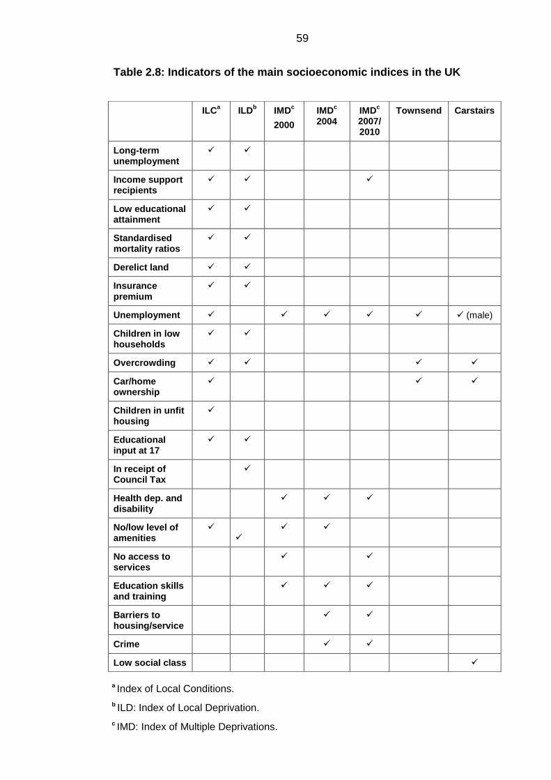
59
Table 2.8: Indicators of the main socioeconomic indices in the UK
ILCa ILD
b IMD
c
2000
IMDc
2004 IMD
c
2007/ 2010
Townsend Carstairs
Long-term unemployment
Income support recipients
Low educational attainment
Standardised mortality ratios
Derelict land
Insurance premium
Unemployment (male)
Children in low households
Overcrowding
Car/home ownership
Children in unfit housing
Educational input at 17
In receipt of Council Tax
Health dep. and disability
No/low level of amenities
No access to services
Education skills and training
Barriers to housing/service
Crime
Low social class
a Index of Local Conditions.
b ILD: Index of Local Deprivation.
c IMD: Index of Multiple Deprivations.
60
2.6 Research to be conducted
Based on the evidence reviewed in this chapter, the following research areas have
been identified:
There is a paucity of research on childhood cancers in Saudi Arabia, and
none for young adult cancers, although data on cancer cases have been
reported since 1994. Therefore, there is no understanding of the pattern of
incidence in these age groups.
There is a lack of an established area-based SES measure for Saudi
Arabia, which poses a challenge for health researchers dealing with Saudi
data. Several studies on Saudi Arabia have mentioned this as a limitation.
Saudi Arabia provides an excellent opportunity to examine how PM in terms
of the Hajj affects the incidence of childhood and young adult cancers,
particularly leukaemia and lymphoma.
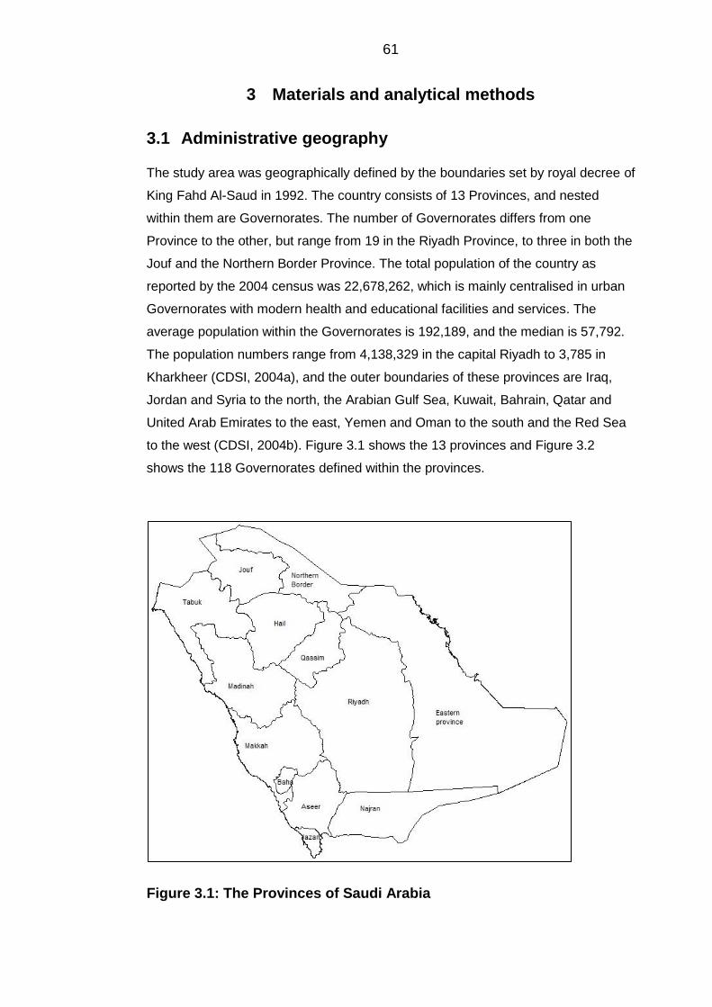
61
3 Materials and analytical methods
3.1 Administrative geography
The study area was geographically defined by the boundaries set by royal decree of
King Fahd Al-Saud in 1992. The country consists of 13 Provinces, and nested
within them are Governorates. The number of Governorates differs from one
Province to the other, but range from 19 in the Riyadh Province, to three in both the
Jouf and the Northern Border Province. The total population of the country as
reported by the 2004 census was 22,678,262, which is mainly centralised in urban
Governorates with modern health and educational facilities and services. The
average population within the Governorates is 192,189, and the median is 57,792.
The population numbers range from 4,138,329 in the capital Riyadh to 3,785 in
Kharkheer (CDSI, 2004a), and the outer boundaries of these provinces are Iraq,
Jordan and Syria to the north, the Arabian Gulf Sea, Kuwait, Bahrain, Qatar and
United Arab Emirates to the east, Yemen and Oman to the south and the Red Sea
to the west (CDSI, 2004b). Figure 3.1 shows the 13 provinces and Figure 3.2
shows the 118 Governorates defined within the provinces.
Figure 3.1: The Provinces of Saudi Arabia
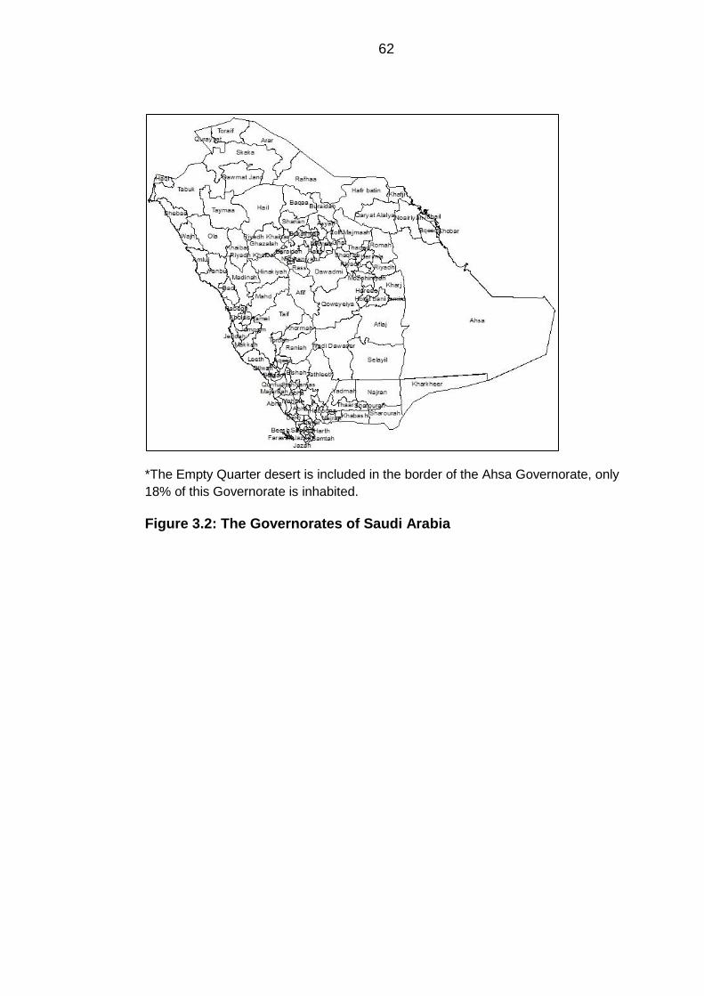
62
*The Empty Quarter desert is included in the border of the Ahsa Governorate, only
18% of this Governorate is inhabited.
Figure 3.2: The Governorates of Saudi Arabia
63
3.2 Data sources, collection and manipulation
Cancer data 3.2.1
The Saudi Cancer Registry 3.2.1.1
The Saudi Cancer Registry (SCR) was established in 1992, under the authority of
the MoH and began reporting cases of cancers in Saudi Arabia from the 1st of
January 1994 (Al-Eid et al., 2007b). The objective of the SCR was to describe the
incidence of cancer in the population of Saudi, as well as to provide valid data for
medical research. The SCR is based in the capital city of Riyadh, and has set up
five regional branches as well as four offices based at different hospitals to ensure
the ongoing reporting of cases. Data abstraction is performed by SCR trained
cancer registrars, who use medical records as the main source of information, as
well as histopathological reports and death certificates. The data abstraction form
includes personal and demographic information as well as cancer morphology and
topography (Appendix C) (Al-Eid et al., 2007b). The SCR uses the International
Classification of Diseases for Oncology – 3rd edition (ICD-O-3) to code cancers.
Although the exact procedure is not known, quality assurance of all collected data is
done by verification of topography, morphology and staging information, as well as
data consolidation from multiple sources. It is not made clear whether there is a
standard for the SCR for cross-checking the quality of the acquired data, and the
level of case ascertainment (Al-Eid et al., 2007b).
Patients suspected of cancer of all ages are referred from primary health care
centres to secondary hospitals for further care, and if required are further referred to
specialist hospitals.
Data collection 3.2.1.2
The request for cancer data was facilitated by on-site visits to the cancer registry,
and the data were finally received on 27/07/2012. For this research, the target
population consisted of young people in Saudi Arabia (0 to 24 years). This
population was the focal point to enable comparison with other studies from
different countries, as well as to be able to study the effect of population mixing
(PM) on this specific age group based on the discussed hypotheses. Hence, the
obtained data included all Saudis and non-Saudis aged between 0 and 24 years
with a newly diagnosed malignancy. The addresses of patients were not given,
although in any case, the P.O. box traditionally identified a central post office for
mail collection and not a residential address. However, the province and
Governorate of each individual patient was provided. The data also included the
topography and morphology of each patient.
64
Data manipulation 3.2.1.3
As the target population involved patients aged <24 years, the malignancies had to
be coded using the International Classification of Childhood Cancers (ICCC-3) to
identify disease patterns. The conversion was performed using statistical coding in
Stata Software version 12 (StataCorp, 2011a), using the extended classification
table (Appendix A), then the main classification table (Appendix B), to enable
arrangement of diseases into main diagnostic groups (Steliarova-Foucher et al.,
2005a). The procedure was performed in 2 phases:
Phase 1: This phase involved combining the morphology and topography of
each patient from the cancer data to assign a diagnosis to each patient, with
guidance from the extended classification table (example given in Appendix
D).
Phase 2: This phase involved summarising the extended classification table
of disease groups to the main classification table, and labelling each cancer
type for use in subsequent analyses (example given in Appendix E).
The location of each patient was not logged in the same geographical manner, as
some patients recorded Governorates and some recorded neighbourhoods or
districts. For the purpose of unifying the geographical level of patient allocation, and
for linkage with census data, each location was cross-referenced to ensure
accuracy of patient address. In the case where neighbourhoods or districts were
recorded instead of Governorates, these were substituted by the Governorate to
which that centre or district belonged. From the total number of patients, 4.36%
(782) had unknown locations. This group had to be excluded from some of the
analyses concerned with patient location.
Census data 3.2.2
The Central Department of Statistics and Information 3.2.2.1
The Central Department of Statistics and Information (CDSI) is the organisation
responsible for organising, monitoring and producing reliable population data. The
first census was carried out in 1974, followed by other censuses in the years 1992,
2004 and results are yet to be published for the 2010 census. Prior to the 2004
census, fieldwork preparation started in September 2001 and continued until
October 2003. This preparation included producing a directory to clarify the names
65
of all areas such as cities, villages, farms and Bedouin gatherings and how they
relate to the main administrative area. It also included estimating the number of
households in each of these areas, so as to be able to divide them into small
census units and assign a worker to each unit. The data collection method of the
census consisted of a questionnaire that included 62 questions covering
geographic, educational, economic and migration information of each member
within a household (CDSI, 2004b).
Data collection 3.2.2.2
Population data used to calculate standardised incidence rates were obtained from
the CDSI using the 2004 national census on 04/09/2012. The CDSI webpage
(www.cdsi.gov.sa) only publishes data per province. Therefore, population data
containing counts for five-year age groups for males and females per Governorate,
as well as socioeconomic indicators collected from the census questionnaire per
Governorate were requested. The data on socioeconomic indicators were received
as whole numbers for each Governorate, for use in constructing the measures of
socioeconomic status (SES). The indicators included educational status,
employment status, type of housing, housing tenure and the availability of several
household items (Table 3.1).
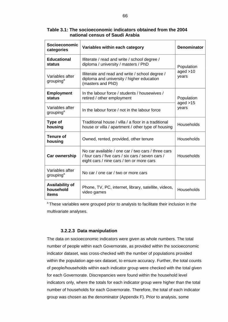
66
Table 3.1: The socioeconomic indicators obtained from the 2004 national census of Saudi Arabia
Socioeconomic categories
Variables within each category Denominator
Educational status
Illiterate / read and write / school degree / diploma / university / masters / PhD
Population aged >10 years Variables after
groupinga
Illiterate and read and write / school degree / diploma and university / higher education (masters and PhD)
Employment status
In the labour force / students / housewives / retired / other employment Population
aged >15 years Variables after
groupinga In the labour force / not in the labour force
Type of housing
Traditional house / villa / a floor in a traditional house or villa / apartment / other type of housing
Households
Tenure of housing
Owned, rented, provided, other tenure Households
Car ownership No car available / one car / two cars / three cars / four cars / five cars / six cars / seven cars / eight cars / nine cars / ten or more cars
Households
Variables after groupinga
No car / one car / two or more cars
Availability of household items
Phone, TV, PC, internet, library, satellite, videos, video games
Households
a These variables were grouped prior to analysis to facilitate their inclusion in the
multivariate analyses.
Data manipulation 3.2.2.3
The data on socioeconomic indicators were given as whole numbers. The total
number of people within each Governorate, as provided within the socioeconomic
indicator dataset, was cross-checked with the number of populations provided
within the population age-sex dataset, to ensure accuracy. Further, the total counts
of people/households within each indicator group were checked with the total given
for each Governorate. Discrepancies were found within the household level
indicators only, where the totals for each indicator group were higher than the total
number of households for each Governorate. Therefore, the total of each indicator
group was chosen as the denominator (Appendix F). Prior to analysis, some
67
variables had to be aggregated for example, the illiterate and the read and write
variables were aggregated into one variable. The aggregation allowed the variables
to be more normally distributed, as well as being easier to include in the analysis.
Then, all indicators were expressed as proportions to be able to measure the actual
effect of each indicator. Proportions were calculated using indicator specific
denominators for both the education and employment indicators. The counts of
people regarding the educational indicators only included those above 10 years of
age, and within the employment status indicators included those above 15 years of
age (CDSI, 2004b). Therefore, the population denominator only included the
number of people aged above 10 years and 15 years, respectively (Table 3.1).
Since the age and sex data for each Governorate was only available for 2004,
populations for the years from 1994 to 2008 were estimated based on the 2.5%
annual increase reported by the annual census reports available online
(www.cdsi.gov.sa). The estimated population of 1994 was divided by the actual
population reported from the 1992 census which produced a value to be used as a
multiplier. This value was then multiplied by the actual population of 2004 in each
stratum to produce an estimated value of the population for 1994. The same
process was done for all years except 2004, since the actual number was available.
Hajj data 3.2.3
Custodian of the Two Holy Mosques Institute for Hajj 3.2.3.1
Research
The Custodian of the Two Holy Mosques Institute for Hajj Research (CTHMIHR),
formerly known as the Hajj Research Centre, was established in 1975, as a group
of researchers based at King Abdulaziz University in Jeddah, with the aim of
establishing an information bank about the Hajj. CTHMIHR has now moved to Um-
AlQuraa University in Makkah and currently aims to become the primary source of
Hajj-related scientific information, where relevant statistics may be provided for
research and policy making services (UQU, 2014).
Data collection 3.2.3.2
A data request was made, and the data were received on 21/11/2011. The data
included the number of pilgrims arriving into Makkah by the Islamic calendar (also
known as the Um-AlQuraa calendar) year. The original data requested included a
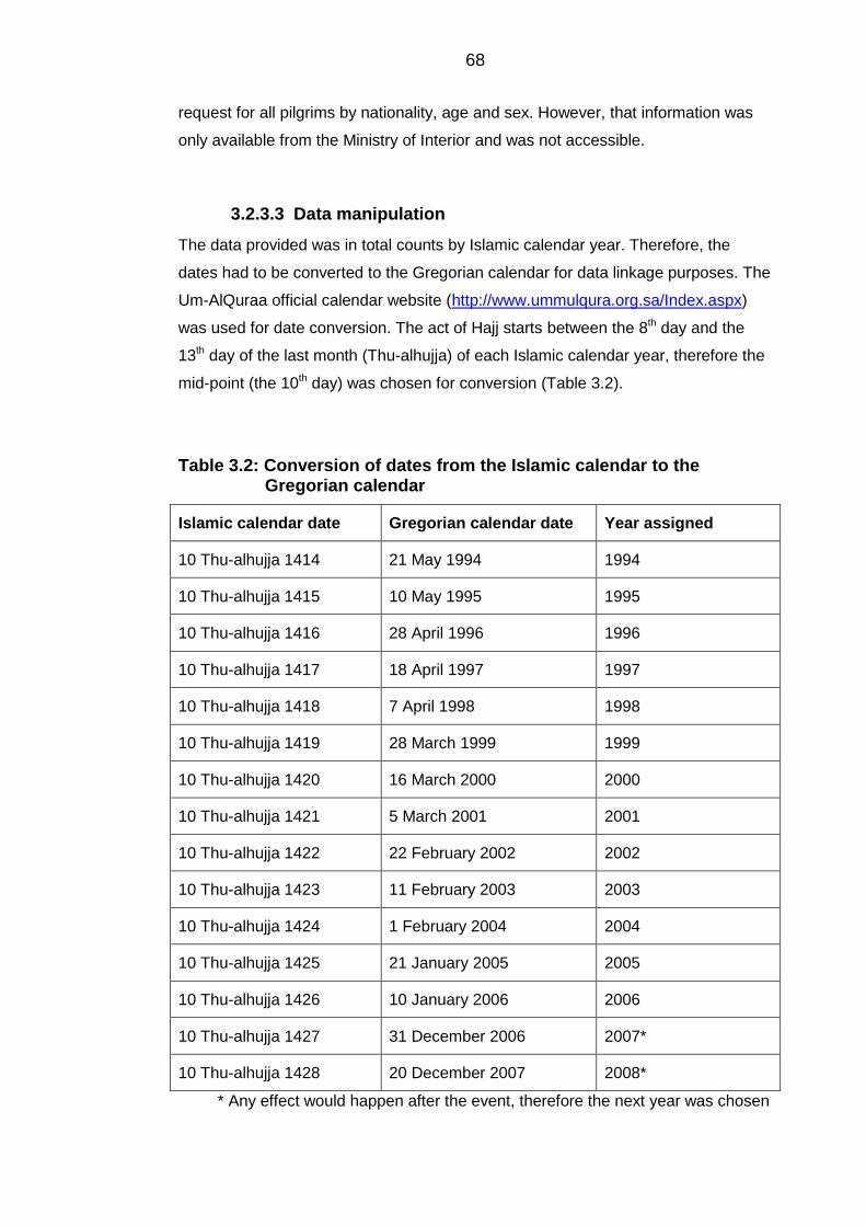
68
request for all pilgrims by nationality, age and sex. However, that information was
only available from the Ministry of Interior and was not accessible.
Data manipulation 3.2.3.3
The data provided was in total counts by Islamic calendar year. Therefore, the
dates had to be converted to the Gregorian calendar for data linkage purposes. The
Um-AlQuraa official calendar website (http://www.ummulqura.org.sa/Index.aspx)
was used for date conversion. The act of Hajj starts between the 8th day and the
13th day of the last month (Thu-alhujja) of each Islamic calendar year, therefore the
mid-point (the 10th day) was chosen for conversion (Table 3.2).
Table 3.2: Conversion of dates from the Islamic calendar to the Gregorian calendar
Islamic calendar date Gregorian calendar date Year assigned
10 Thu-alhujja 1414 21 May 1994 1994
10 Thu-alhujja 1415 10 May 1995 1995
10 Thu-alhujja 1416 28 April 1996 1996
10 Thu-alhujja 1417 18 April 1997 1997
10 Thu-alhujja 1418 7 April 1998 1998
10 Thu-alhujja 1419 28 March 1999 1999
10 Thu-alhujja 1420 16 March 2000 2000
10 Thu-alhujja 1421 5 March 2001 2001
10 Thu-alhujja 1422 22 February 2002
2002
10 Thu-alhujja 1423 11 February 2003 2003
10 Thu-alhujja 1424 1 February 2004 2004
10 Thu-alhujja 1425 21 January 2005 2005
10 Thu-alhujja 1426 10 January 2006 2006
10 Thu-alhujja 1427 31 December 2006 2007*
10 Thu-alhujja 1428 20 December 2007 2008*
* Any effect would happen after the event, therefore the next year was chosen
69
Geographical information systems 3.2.4
Data collection 3.2.4.1
Geographical information systems (GIS) boundary data of the Saudi Arabian
Governorates were requested and received from the Farsi GeoTech Company on
05/05/2012. This company is renowned for its work and has an index of
governmental services (Appendix G).
Data manipulation 3.2.4.2
The GIS data included digital boundaries of provinces and Governorates, each on a
separate layer, accessible through ArcMap software version 10 (ESRI, 2010). The
Governorate level layer included 142 polygons rather than 118 (each polygon
should represent a Governorate). This was due to the fact that some Governorates
were divided into smaller districts. Therefore, the dissolve tool within the ArcMap
software was used to re-group and merge divided Governorates. This tool then
generated a new layer that contained 118 polygons. This layer was used for the
cartography.
3.3 Descriptive analytical methods
Descriptive statistics 3.3.1
Summary descriptive statistics were used to examine the census data. Statistics
included the mean, so as to provide a number to represent the centre or average of
the data, as well as the standard deviation (SD) to measure the spread of the data
from the mean. Also, skewness and kurtosis were inspected – these are measures
to check for the normality of the data, where skewness indicates whether the data
are asymmetrical or positively/negatively skewed, and the kurtosis checks the
peakedness of the data.
Standardised incidence rates 3.3.2
Incident cases were defined as the occurrence of new cases over a specific time
period within a specific population. An incidence rate is defined as the number of
new cases of a disease divided by the population at risk within a specified time
period. Direct standardisation was used to account for the different population
structures upon comparing the incidence in Saudi with other countries and indirect
standardisation was used to account for the different population structure between
the different Governorates, thereby facilitating internal comparisons, as opposed to
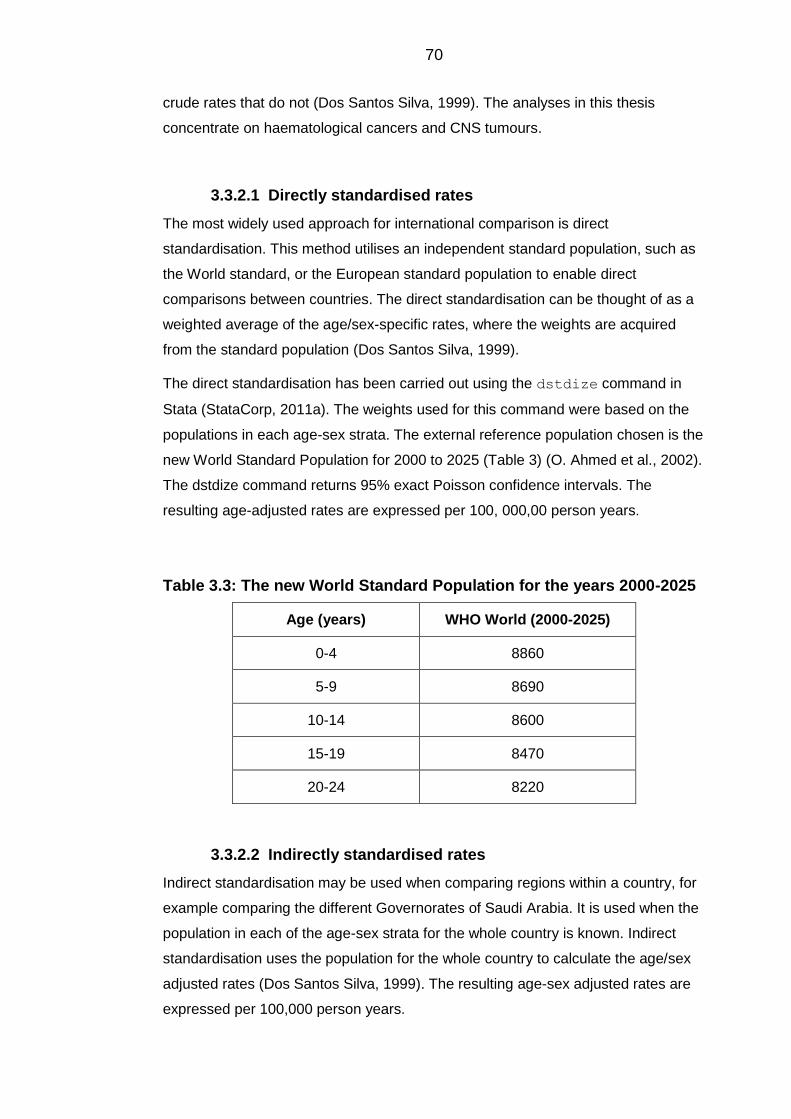
70
crude rates that do not (Dos Santos Silva, 1999). The analyses in this thesis
concentrate on haematological cancers and CNS tumours.
Directly standardised rates 3.3.2.1
The most widely used approach for international comparison is direct
standardisation. This method utilises an independent standard population, such as
the World standard, or the European standard population to enable direct
comparisons between countries. The direct standardisation can be thought of as a
weighted average of the age/sex-specific rates, where the weights are acquired
from the standard population (Dos Santos Silva, 1999).
The direct standardisation has been carried out using the dstdize command in
Stata (StataCorp, 2011a). The weights used for this command were based on the
populations in each age-sex strata. The external reference population chosen is the
new World Standard Population for 2000 to 2025 (Table 3) (O. Ahmed et al., 2002).
The dstdize command returns 95% exact Poisson confidence intervals. The
resulting age-adjusted rates are expressed per 100, 000,00 person years.
Table 3.3: The new World Standard Population for the years 2000-2025
Age (years) WHO World (2000-2025)
0-4 8860
5-9 8690
10-14 8600
15-19 8470
20-24 8220
Indirectly standardised rates 3.3.2.2
Indirect standardisation may be used when comparing regions within a country, for
example comparing the different Governorates of Saudi Arabia. It is used when the
population in each of the age-sex strata for the whole country is known. Indirect
standardisation uses the population for the whole country to calculate the age/sex
adjusted rates (Dos Santos Silva, 1999). The resulting age-sex adjusted rates are
expressed per 100,000 person years.
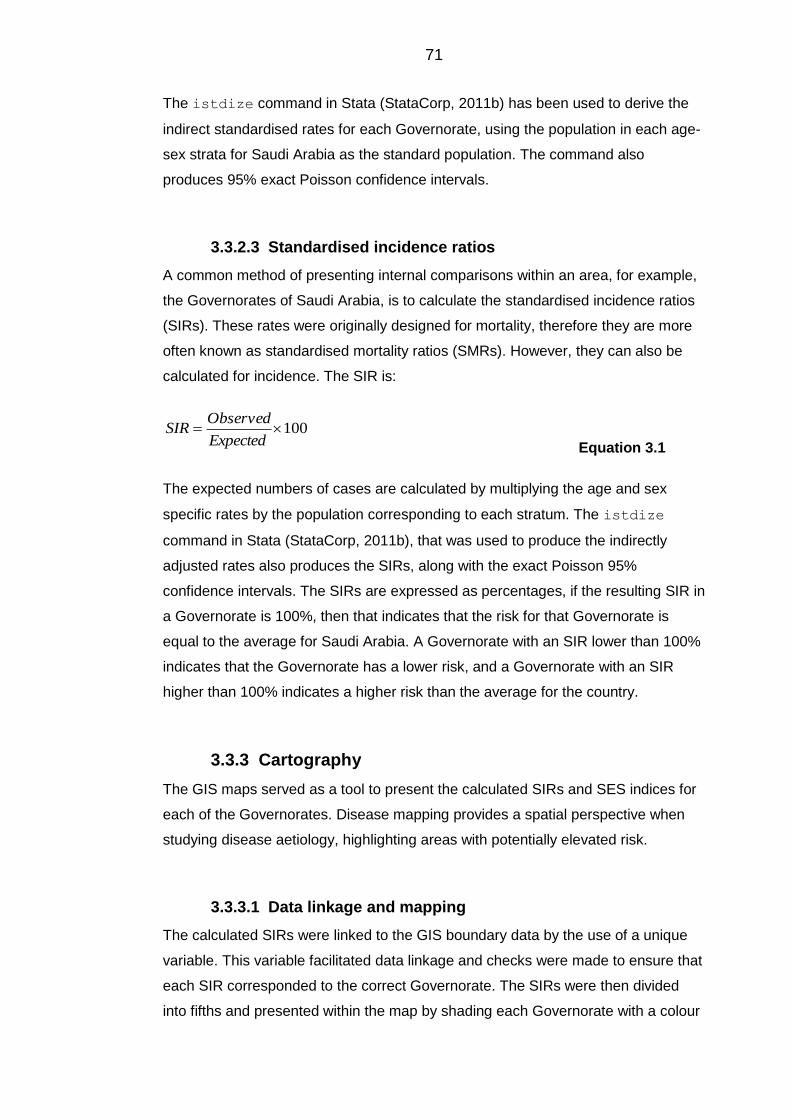
71
The istdize command in Stata (StataCorp, 2011b) has been used to derive the
indirect standardised rates for each Governorate, using the population in each age-
sex strata for Saudi Arabia as the standard population. The command also
produces 95% exact Poisson confidence intervals.
Standardised incidence ratios 3.3.2.3
A common method of presenting internal comparisons within an area, for example,
the Governorates of Saudi Arabia, is to calculate the standardised incidence ratios
(SIRs). These rates were originally designed for mortality, therefore they are more
often known as standardised mortality ratios (SMRs). However, they can also be
calculated for incidence. The SIR is:
100Expected
ObservedSIR
Equation 3.1
The expected numbers of cases are calculated by multiplying the age and sex
specific rates by the population corresponding to each stratum. The istdize
command in Stata (StataCorp, 2011b), that was used to produce the indirectly
adjusted rates also produces the SIRs, along with the exact Poisson 95%
confidence intervals. The SIRs are expressed as percentages, if the resulting SIR in
a Governorate is 100%, then that indicates that the risk for that Governorate is
equal to the average for Saudi Arabia. A Governorate with an SIR lower than 100%
indicates that the Governorate has a lower risk, and a Governorate with an SIR
higher than 100% indicates a higher risk than the average for the country.
Cartography 3.3.3
The GIS maps served as a tool to present the calculated SIRs and SES indices for
each of the Governorates. Disease mapping provides a spatial perspective when
studying disease aetiology, highlighting areas with potentially elevated risk.
Data linkage and mapping 3.3.3.1
The calculated SIRs were linked to the GIS boundary data by the use of a unique
variable. This variable facilitated data linkage and checks were made to ensure that
each SIR corresponded to the correct Governorate. The SIRs were then divided
into fifths and presented within the map by shading each Governorate with a colour

72
corresponding to the SIR: Governorates with the lowest quintile of SIRs are
coloured white, and Governorates with the highest quintile are coloured a darker
shade of blue.
3.3.3.1.1 Smoothing the standardised incidence ratios
The raw SIRs calculated for each Governorate may misrepresent the geographical
distribution of the disease risk, since it does not take into account the differing
population sizes of the Governorates. Clayton and Kaldor (1987) proposed
Empirical Bayes smoothing to account for the small population sizes, and stabilise
rates. The basic underlying theory is to compute the posterior distribution where:
Posterior = Prior x Likelihood Equation 3.2
The likelihood relates to the Poisson distributed observed cases, and the prior is
based on prior belief from the distribution of cases, for example, the rates are more
likely to be reliable in areas with large population sizes than those with smaller
population sizes.
From a Gamma distribution, where is the shape parameter, is the scale
parameter and
v is the mean, then the posterior expectation conditional on iO
,;| ii OE of the ith area is:
EO
i
vi
Equation 3.3
Oi is the observed number of cases in area i
E iis the expected number of cases in area i
Equation 3.3 shows how the SIR is smoothed or shrunk towards the overall mean
(Clayton and Kaldor, 1987). Therefore, if the ith area has a small population, the
values of Oi and E i
will be small compared to the mean, thus the empirical
Bayes estimate will shrink towards the mean. Conversely, if the ith area has a large
population size, the values of Oi and E i
will be large compared to the mean,
and the empirical Bayes estimate will be very close to the actual SIR.
Spatial empirical Bayes (SEB) however, defines a neighbourhood around which
each area is smoothed. A neighbourhood may be defined as all the contiguous
73
areas plus the ith area itself. Contiguity may be defined as ‘a measure to check for
continuity between areas’ (Lai et al. 2008, p. 79). There are two types of contiguity:
the queen and the rook contiguity. The queen contiguity accepts an adjacent area
that has a meeting point with the ith area, whilst the rook contiguity only accepts the
neighbourhoods with a considerable amount of adjacency (Lai et al., 2008). First
order contiguity is chosen if it is only desired to include the adjacent areas to the
centre cell, and higher orders may be chosen if areas that share a border with the
adjacent areas are included. For this study, the queen contiguity with first and
second order was mapped, because disease risk is not restricted to one direction,
and also because some Governorates have very low population sizes. It has also
been noted that patients travel across Governorate borders for further diagnostic
and treatment purposes. The SEB smoothing was performed in GeoDa software
(Anselin et al., 2006).
Funnel plots 3.3.4
Originally, funnel plots were used in meta-analysis to examine any possible bias.
They are also used to make institutional comparisons on the basis of outcome
measures, so whether these institutions were hospitals, hospital departments, or in
this case, Governorates. The plots get the name from the funnel shape formed by
upper and lower 95% and 99.8% control limits around the central line that is equal
to an incidence ratio of 1, the limits become narrower when the sample size
becomes larger. The observed indicator variable is plotted against a measure of its
precision (Spiegelhalter, 2005, Spiegelhalter, 2002).The plots show the SIRs for
each Governorate before and after empirical Bayes smoothing against the expected
number of cases. Funnel plots have been constructed in Stata (StataCorp, 2011b)
using the funnelcompar command.
Case ascertainment 3.3.5
Since the data were acquired from a relatively new cancer registry, it is reasonable
to check for case ascertainment of the data. The usual method of capture-recapture
could not be used in this data since this method requires examining records from
the different sources of data, and this is not feasible for reasons of confidentiality
and time limitations. Therefore, age-sex standardised incidence rates between the
US and Saudi Arabia were examined and compared by the year of diagnosis for all
disease categories. Also, incidence rates in both countries were compared by the
method of direct standardisation to the US standard population. This made it

74
possible to look for any signs of under ascertainment of cases by identifying
unusually low rates, although, rates may well be different between the US and
Saudi Arabia.
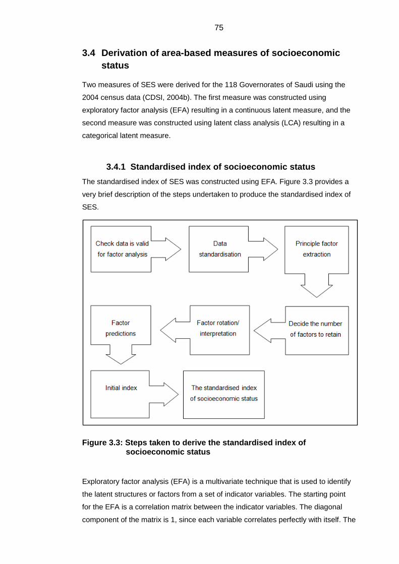
75
3.4 Derivation of area-based measures of socioeconomic
status
Two measures of SES were derived for the 118 Governorates of Saudi using the
2004 census data (CDSI, 2004b). The first measure was constructed using
exploratory factor analysis (EFA) resulting in a continuous latent measure, and the
second measure was constructed using latent class analysis (LCA) resulting in a
categorical latent measure.
Standardised index of socioeconomic status 3.4.1
The standardised index of SES was constructed using EFA. Figure 3.3 provides a
very brief description of the steps undertaken to produce the standardised index of
SES.
Figure 3.3: Steps taken to derive the standardised index of socioeconomic status
Exploratory factor analysis (EFA) is a multivariate technique that is used to identify
the latent structures or factors from a set of indicator variables. The starting point
for the EFA is a correlation matrix between the indicator variables. The diagonal
component of the matrix is 1, since each variable correlates perfectly with itself. The
76
off-diagonal components are the correlation coefficients between each pair of
variables. In the event that there are clusters of high correlation coefficients, then
this may mean that a number of latent structures or factors exist. EFA is a
multivariate analysis that uncovers these latent structures by explaining the
maximum amount of common variance within the interrelated factors (Field, 2000).
Data checks 3.4.1.1
The data within the analysis included the grouped variables from Table 3.1, except
for the ‘employment category’ variable, where the ungrouped original variables
were used. The first step was to check whether the data were appropriate for an
EFA by conducting two tests. The first is the Bartlett’s test of sphericity, which is a
statistic that tests whether the correlation matrix is an identity matrix, i.e., that the
diagonal components are equal to one, and the off-diagonal components are equal
to zero, which means the variables are not correlated (Bartlett, 1951). The statistic
produces a P-value, if the value is significant (P < 0.05) then the null hypothesis is
rejected, and it is concluded that the variables are highly correlated suggesting
factorability. The second test is the Kaiser-Meyer-Olkin (KMO) test, which is a
measure of sampling adequacy. It is a test that compares the observed correlation
coefficient to the partial correlation coefficient (Kaiser and Rice, 1974). The partial
correlation coefficients are the correlations between a pair of variables after the
common variance has been removed. If the ratio is close to one, then this indicates
that the partial correlations are small and therefore the variables are highly
correlated, but if the ratio is small then this indicates that the partial correlation is
high and the variables are not sufficiently correlated for an EFA. Kaiser and Rice
(1974) labelled the possible outcomes as ‘marvellous’ if the value is in the 0.90s,
‘meritorious’ in the 0.80s, ‘middling’ in the 0.70s, ‘mediocre’ in the 0.60s, ‘miserable’
in the 0.50s and unacceptable <0.50. The command factortest in Stata
(StataCorp, 2011b) was used to compute both test statistics.
Factor extraction method 3.4.1.2
Prior to factor extraction, the indicator variables were standardised to have a mean
of zero and a standard deviation of one, so that the standardised Z score for an
observation x ( xZ ) is given by
xZ x
Equation 3.4
77
Where, is the mean of the variable x and is the standard deviation. This
step is crucial before an aggregation process, not only to account for the different
scales of the indicator variables, but also to prevent variables with disproportionate
ranges unnecessary prominence at the expense of others (Gilthorpe, 1995).
The basic factor analysis formula for a variable j ( Z j) is given by:
UaFaFaFaz jjumjmjjj ...
2211 Equation 3.5
(j = 1, 2, …, n)
Where each of the n observed variables are linearly described in terms of m
common factors that are usually much smaller than n. The a jare the factor
loadings, for example a j1 is the loading of variable z1
on factor F1. The
Ua jjuis the unique factor that accounts for the remaining variance (including
residual error) for the observed variable Z j (Harman, 1967).
The procedure starts with estimating the first principal factor that explains the
maximum amount of common variance possible, then the second principal factor is
estimated that accounts for the maximum amount of common variance from the
remaining residual space after the first factor is removed, until the nth factor has
been extracted, so that the factor analysis models for variable 1 to n are given by
UaFaFaFaz
UaFaFaFazUaFaFaFaz
nnumnmnnn
umm
umm
...2211
............................................................................................222
...2221212
111...
2121111
Equation 3.6
The principal factor was chosen as the factor extraction method. Although previous
papers have chosen principal-component factoring, this method has an assumption
that the communality is equal to one for all variables (StataCorp, 2012). The
communality is the variance of the variable accounted for by the factors. It is
calculated by taking the squared sum of a variable’s loadings across the extracted
factors (Harman, 1967).
From the basic factor analysis formula in Equation 3.5, the communality (h j
2) may
be expressed as:
78
aaah jmjjj
2...
2
2
2
1
2 Equation 3.7
Stata does not report the communality, but it reports the uniqueness. The
uniqueness is the variance that is unique to each variable, so it is simply one minus
the communality. Therefore, since the principal-component factor extraction method
assumes that the communalities are equal to one, the uniqueness should then be
equal to zero. This method was first used, and the uniquenesses were examined
and were found to be more than zero. Therefore, the data violates this assumption,
and the principal factoring extraction method was used.
The factor command in Stata (StataCorp, 2011b) performs the factor analysis
with the principal factoring extraction method as the default.
Factor retention 3.4.1.3
The EFA produces the same amount of factors as there are variables. Each factor
is assigned an eigenvalue (V m) which is a value that describes the contribution of
each factor to the overall factor solution. It is calculated as the sum of the loadings
for a factor across all observations (Harman, 1967). The eigenvalue of a factor may
also be expressed in terms of its proportion in explaining the overall common
variance, and so the higher the proportion the more important that factor is.
Eigenvalues are mathematically represented as:
n
jjmm aV
1
2
Equation 3.8
Where n are the observed variables and a jmare the factor loadings for a variable j
on factor m .
The decision on the number of factors to retain was based upon three criteria. First,
the Guttman-Kaiser rule, which describes the truly existing factors as the factors
with eigenvalues above one (Kaiser, 1960, Guttman, 1954). The second criterion is
the scree-plot, which is a plot of the eigenvalues and the factors and is determined
by the point at which the plotted values start to level off (Cattell, 1966). The third
and final criterion is the ability to interpret all potentially retained factors (Bandalos,
2009).
Less common methods are used for factor retention and include parallel analysis
and minimum average partial procedures. The parallel analysis includes simulation
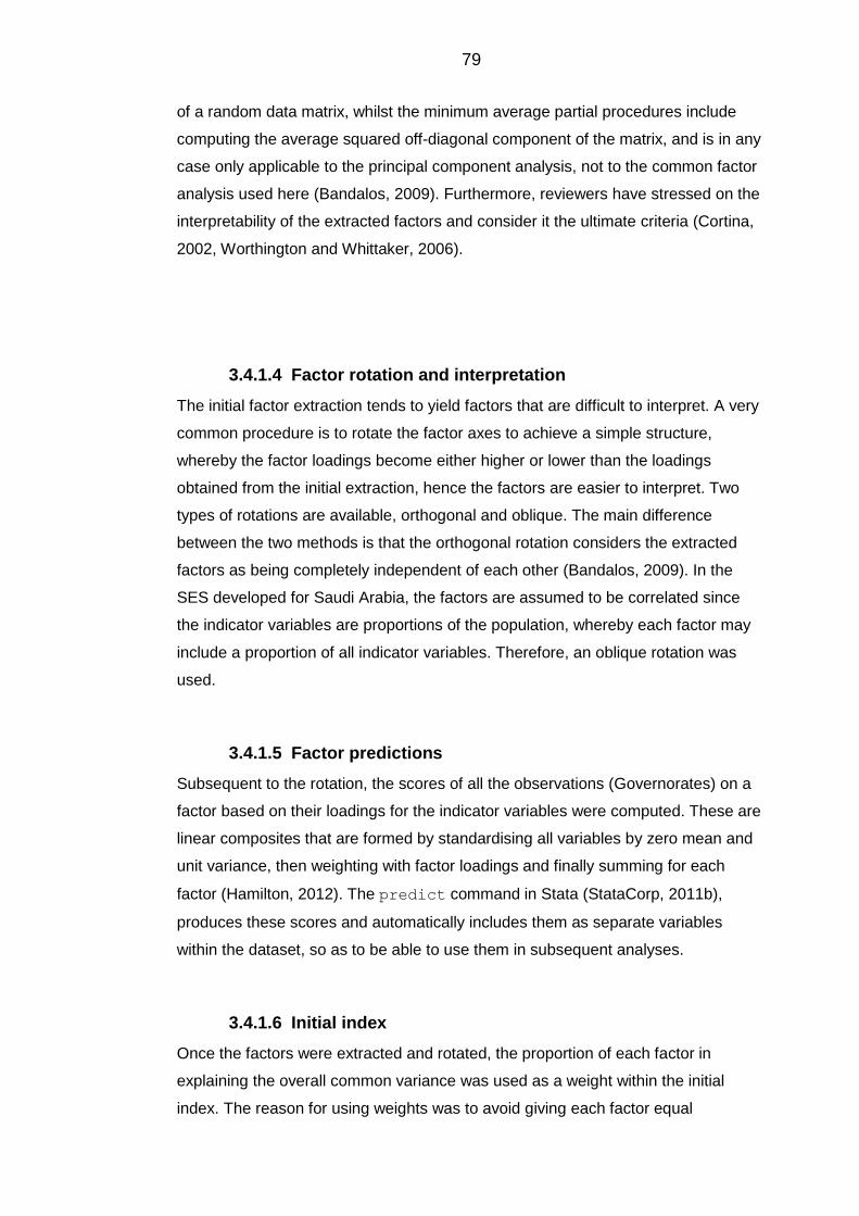
79
of a random data matrix, whilst the minimum average partial procedures include
computing the average squared off-diagonal component of the matrix, and is in any
case only applicable to the principal component analysis, not to the common factor
analysis used here (Bandalos, 2009). Furthermore, reviewers have stressed on the
interpretability of the extracted factors and consider it the ultimate criteria (Cortina,
2002, Worthington and Whittaker, 2006).
Factor rotation and interpretation 3.4.1.4
The initial factor extraction tends to yield factors that are difficult to interpret. A very
common procedure is to rotate the factor axes to achieve a simple structure,
whereby the factor loadings become either higher or lower than the loadings
obtained from the initial extraction, hence the factors are easier to interpret. Two
types of rotations are available, orthogonal and oblique. The main difference
between the two methods is that the orthogonal rotation considers the extracted
factors as being completely independent of each other (Bandalos, 2009). In the
SES developed for Saudi Arabia, the factors are assumed to be correlated since
the indicator variables are proportions of the population, whereby each factor may
include a proportion of all indicator variables. Therefore, an oblique rotation was
used.
Factor predictions 3.4.1.5
Subsequent to the rotation, the scores of all the observations (Governorates) on a
factor based on their loadings for the indicator variables were computed. These are
linear composites that are formed by standardising all variables by zero mean and
unit variance, then weighting with factor loadings and finally summing for each
factor (Hamilton, 2012). The predict command in Stata (StataCorp, 2011b),
produces these scores and automatically includes them as separate variables
within the dataset, so as to be able to use them in subsequent analyses.
Initial index 3.4.1.6
Once the factors were extracted and rotated, the proportion of each factor in
explaining the overall common variance was used as a weight within the initial
index. The reason for using weights was to avoid giving each factor equal
80
importance, and to account for factors that could be more important in explaining
the SES than others within the population (Kishnan, 2010). The formula for the
initial index II is straightforward and is given by:
WF nnII Equation 3.9
Where F n is the score for each factor and W n
is the weight of each factor or the
proportion of common variance explained for that factor.
This initial index then produced a score for each of the 118 Governorates of Saudi
Arabia, and the values ranged from positive to negative numbers, where the highest
positive number indicated the corresponding Governorate to be the most affluent
and the lowest negative number indicated the corresponding Governorate to be the
most deprived.
Final standardised index 3.4.1.7
The initial index produces values that are both positive and negative. For easier
interpretation, the index is calibrated on a scale from 100 to 0, whereby 100
corresponds to the affluent Governorate and 0 to the most deprived. The formula
for the i th Governorate is given as follows:
100xIIII
IIIISI
minmax
mini
i
Equation 3.10
Where II iis the initial index for i th Governorate, and II min
is the lowest value of
any Governorate from the initial index, and II maxis the highest value of any
Governorate from the initial index.
This formula enables the measuring of SES of a Governorate relative to the
difference between the best and the worst Governorate. It also provides a clearer
means of comparison compared to the initial index. This method has been used in
previous measures of SES in other countries (Hightower, 1978, Kishnan, 2010,
Sekhar et al., 1991, Fukuda et al., 2007).
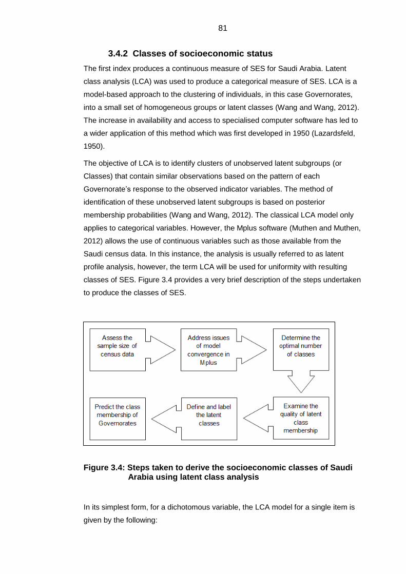
81
Classes of socioeconomic status 3.4.2
The first index produces a continuous measure of SES for Saudi Arabia. Latent
class analysis (LCA) was used to produce a categorical measure of SES. LCA is a
model-based approach to the clustering of individuals, in this case Governorates,
into a small set of homogeneous groups or latent classes (Wang and Wang, 2012).
The increase in availability and access to specialised computer software has led to
a wider application of this method which was first developed in 1950 (Lazardsfeld,
1950).
The objective of LCA is to identify clusters of unobserved latent subgroups (or
Classes) that contain similar observations based on the pattern of each
Governorate’s response to the observed indicator variables. The method of
identification of these unobserved latent subgroups is based on posterior
membership probabilities (Wang and Wang, 2012). The classical LCA model only
applies to categorical variables. However, the Mplus software (Muthen and Muthen,
2012) allows the use of continuous variables such as those available from the
Saudi census data. In this instance, the analysis is usually referred to as latent
profile analysis, however, the term LCA will be used for uniformity with resulting
classes of SES. Figure 3.4 provides a very brief description of the steps undertaken
to produce the classes of SES.
Figure 3.4: Steps taken to derive the socioeconomic classes of Saudi Arabia using latent class analysis
In its simplest form, for a dichotomous variable, the LCA model for a single item is
given by the following:
82
ig
G
ggviXp
1
1 Equation 3.11
Where, 1X vip indicates the unconditional probability that a random individual v
achieves a score of 1X (which is the highest score possible) on the item i ,
where I..,,i 21 . The gis the class size parameter that indicates the
unconditional probability of the observation v belonging to the latent class g , where
G..,,g 21 (Geiser, 2010). One important assumption is that each observation v
belongs to only one latent class, in other words the latent classes are independent
of each other. Therefore, the summation of probabilities of all the classes is equal to
one:
11
G
gg Equation 3.12
The conditional probability of a score of one on item i given membership in class g
is given by the following:
gG|p X viig
1 Equation 3.13
Similar to EFA, the decision on the optimal number of classes is made by the
researcher by means of certain criteria. The parameter estimates and model fit
statistics such as the Akaike Information Criterion (AIC) and the Bayes Information
Criterion (BIC) are determined by an iterative estimation procedure based on the
maximum likelihood estimation, which is the default in Mplus (Geiser, 2010, Muthen
and Muthen, 2012). The objective is to maximise the likelihood function in order to
find the model with the largest possible log likelihood value. This log likelihood is a
measure of the probability of the observed indicator variables given the model, and
is the measure used as the basis for the calculation of the model fit statistics
(Geiser, 2010).
83
Overcoming issues with sample size 3.4.2.1
The analysis was started in Mplus and included the same variables used within the
EFA. However, the model would not converge. It was then found that the problem
persisted because of the small sample size relative to the number of indicator
variables used. Wang and Wang (2012) noted, ‘It is widely recognized that small
sample size could cause a series of problems, including, but not limited to, failure of
estimation convergence, improper solutions ...’ (p.391). There is no consensus in
the literature with regards to the sample size required for LCA and structural
equation modelling (SEM) in general. For example, some find that N=100-150 is the
minimum sample required (Tabachnick and Fidell, 2001, Ding et al., 1995), while
some researchers consider that N=200 is the minimum required (Boomsma and
Hoogland, 2001, Kline, 2005).
It is often necessary to consider the sample size in relation to the number of
indicator variables used. One accepted rule of thumb is to have ten observations for
every one indicator variable (Nunnally, 1967). A much lower ratio was suggested
that allows for five observations per indicator variable (Bentler and Chou, 1987).
Considering the 29 variables available after the necessary grouping from Table 3.1,
this would mean that for the first rule of thumb, at least 290 observations would be
required, and with the second at least 145. However, since the observations are
Governorates and they are only 118, it is impossible to increase the sample size.
Therefore, a decision was made to reduce the number of indicator variables to
achieve the widely accepted ratio of 10:1. The variables chosen include only the
disadvantage indicators: not in the labour force, illiterate or can read and write, no
car, living in a traditional house, living in a floor of a villa or a traditional house,
house not owned, no phone, no television, no internet, no library and no satellite.
Consequently, there are 11 variables for 118 Governorates, thereby achieving the
10:1 accepted ratio.
Issues of model convergence 3.4.2.2
A common problem with iterative estimation procedures, such as those underlying
LCA, is that the default set of starting values (e.g. in Mplus the default is 10) for the
parameter does not allow the model to converge with the best possible log
likelihood value. Because the estimation method is iterative, many solutions are
obtained for these iterations. The solution with the highest log likelihood value
indicates that the model converged on what is known as the global maximum.
Consequently, if the model does not find the global maximum, it then terminates on

84
the local maximum, which is associated with inaccurate parameter estimates
(Geiser, 2010, Wang and Wang, 2012).
In the event that only a few starting values are used in Mplus (or in any other
structural equation modelling software), then it is likely that the estimation will
terminate on a local maximum. Therefore, in order to increase the chances of
obtaining the global maximum solution, a sufficient number of starting values should
be used. A set of different numbers of starting values were tried, and a global
maximum was obtained when the number of starts was increased to 1000.
Deciding the number of classes 3.4.2.3
The number of latent classes is unobserved, and therefore it cannot be directly
estimated from the dataset. To determine the optimal number of classes in LCA, a
series of LCA models were run starting with a one-class model and increasing the
number of classes with each run. Then, the optimal number of classes was chosen
based on a comparison of the model fit indices of the k-class model and the (k-1)-
class model. The (k-1)-class model is the same as the k-class model, but with one
latent class set to zero (Wang and Wang, 2012, Geiser, 2010).
The first model fit index to examine is the AIC (Akaike, 1987). The idea underlying
the AIC is to select the best model that minimises the difference between the
unknown true data and the estimated model. This difference is known as the
Kullback-Leibler difference. It is widely used for its simplicity, as it only requires the
maximum likelihood achieved by the model, and is calculated by:
klnAIC Lmax22
Equation 3.14
Where Lmaxis the maximum likelihood value from the model, and k is the number
of parameters reported for the model, and is the penalty term that is used to
combine absolute model fit and model parsimony. The lower the AIC the better the
model fit (Wang and Wang, 2012). The second model fit index is the BIC (Schwarz,
1978). Similar to the AIC, the BIC adds a stronger penalty term by adding more
parameters to the model and is estimated by:
NlnkBIC Lmax 2 Equation 3.15
Where N is the sample size used for the model. The lower the value of the BIC the
better the model fit. A further model fit index reported by Mplus is the Adjusted
85
Bayes Information Criterion (ABIC) (Wang and Wang, 2012), which reduces the
penalty of the BIC for smaller sample sizes by:
24
22
nlnkABIC Lmax
Equation 3.16
Other model fit indices reported in Mplus include the Lo-Mendell-Rubin likelihood
ratio test (LMR-LRT), this examines the model fit and looks for any improvement
between a k-class and a (k-1)-class model. A significant P-value (P<0.05) indicates
that the k-class model fit is significantly better than a (k-1)-class model. If however,
the P-value is non-significant (P≥0.05), then the (k-1)-class model is preferred (Lo
et al., 2001). The final model fit index is the Bootstrap Likelihood Difference test
(BLRT), which also compares a k-class model with a (k-1)-class model. Using a
parametric bootstrapping procedure, P-values for the likelihood difference are
estimated by fitting the k-class and (k-1)-class model to every bootstrap sample and
calculating the likelihood ratio for each bootstrap sample. A significant P-value
(P<0.05) indicates that the k-class model is a better fit than the (k-1)-class model
(Geiser, 2010, Wang and Wang, 2012).
All these model fit indices were taken into account during the model fit selection
process, and they all usually led to the same conclusion, although, some
discrepancies were found. The evidence suggests that the BIC along with the BLRT
fit indices are the most reliable (Nylund et al., 2007).
Examining the quality of latent class membership 3.4.2.4
Upon deciding on the optimal number of classes for the model, the observations or
Governorates were then classified into the latent classes. The way in which each
Governorate was assigned to a class was through the conditional probability from
Equation 3.13. The latent class membership of the Governorates was identified
based on the estimated probability. The sum of the probabilities is equal to one
(Equation 3.12). Therefore, the closer the value is to one the more likely it belongs
to that latent class (modal assignment) (Wang and Wang, 2012). A rule of thumb for
a good classification is when the modal assignment probability is higher than 0.70
(Nagin, 2005). Another common criterion used was the entropy, which measures
the accuracy of classification of Governorates into latent classes. The value ranges
from zero to one, the closer the value to one the more accurate the classification is.
It is suggested that an entropy of more than 0.80 is high, 0.60 is medium and 0.40
is low (Clark, 2010).
86
Defining and labelling the latent classes 3.4.2.5
Similar to examining the factor loadings and labelling the factors in the EFA, the
probabilities are examined and the latent classes are labelled in the LCA. The
higher the probability for a given Governorate on a given class the more likely it is
that it belongs to it. This is also aided by a probability plot that is provided within
Mplus. The plot provides a visual representation of how each indicator variable
relates to each class in terms of the probability. It is crucial and a sign that the LCA
model has succeeded if the resulting classes are clearly interpretable. The main
objective of the LCA is to group homogenous observations or, in this case,
Governorates together in separate classes. Consequently, the researcher should
be able to define each class by the pattern of item-response probability in that class
(Wang and Wang, 2012). If one class is not interpretable or does not make sense,
the LCA model then should be discarded despite a good model fit.
Predicting the class membership of Governorates 3.4.2.6
The final step in LCA is to predict the resulting latent classes, similarly to predicting
the factors in an EFA. This is readily done in Mplus by specifying save =
cprobabilities under the save section of the command lines. A new file is
generated that contains the probability of each Governorate belonging to each
class, with a column for every class, and finally a categorical latent class variable
that specifies to which class each Governorate belongs (based on the probabilities)
(Geiser, 2010).
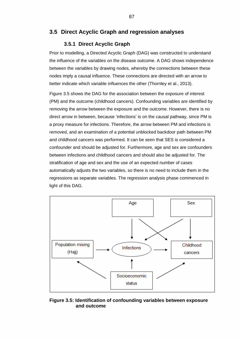
87
3.5 Direct Acyclic Graph and regression analyses
Direct Acyclic Graph 3.5.1
Prior to modelling, a Directed Acyclic Graph (DAG) was constructed to understand
the influence of the variables on the disease outcome. A DAG shows independence
between the variables by drawing nodes, whereby the connections between these
nodes imply a causal influence. These connections are directed with an arrow to
better indicate which variable influences the other (Thornley et al., 2013).
Figure 3.5 shows the DAG for the association between the exposure of interest
(PM) and the outcome (childhood cancers). Confounding variables are identified by
removing the arrow between the exposure and the outcome. However, there is no
direct arrow in between, because ‘infections’ is on the causal pathway, since PM is
a proxy measure for infections. Therefore, the arrow between PM and infections is
removed, and an examination of a potential unblocked backdoor path between PM
and childhood cancers was performed. It can be seen that SES is considered a
confounder and should be adjusted for. Furthermore, age and sex are confounders
between infections and childhood cancers and should also be adjusted for. The
stratification of age and sex and the use of an expected number of cases
automatically adjusts the two variables, so there is no need to include them in the
regressions as separate variables. The regression analysis phase commenced in
light of this DAG.
Figure 3.5: Identification of confounding variables between exposure and outcome
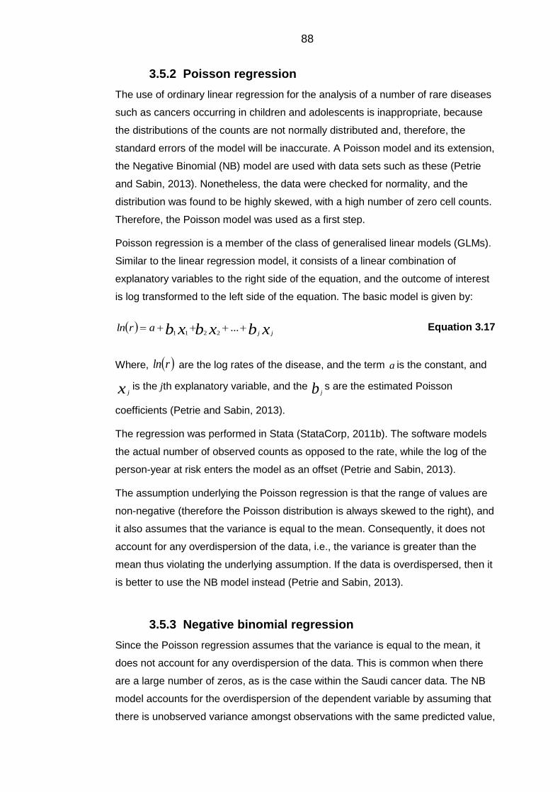
88
Poisson regression 3.5.2
The use of ordinary linear regression for the analysis of a number of rare diseases
such as cancers occurring in children and adolescents is inappropriate, because
the distributions of the counts are not normally distributed and, therefore, the
standard errors of the model will be inaccurate. A Poisson model and its extension,
the Negative Binomial (NB) model are used with data sets such as these (Petrie
and Sabin, 2013). Nonetheless, the data were checked for normality, and the
distribution was found to be highly skewed, with a high number of zero cell counts.
Therefore, the Poisson model was used as a first step.
Poisson regression is a member of the class of generalised linear models (GLMs).
Similar to the linear regression model, it consists of a linear combination of
explanatory variables to the right side of the equation, and the outcome of interest
is log transformed to the left side of the equation. The basic model is given by:
xbxbxb jj...arln
2211 Equation 3.17
Where, rln are the log rates of the disease, and the term a is the constant, and
x jis the jth explanatory variable, and the b j
s are the estimated Poisson
coefficients (Petrie and Sabin, 2013).
The regression was performed in Stata (StataCorp, 2011b). The software models
the actual number of observed counts as opposed to the rate, while the log of the
person-year at risk enters the model as an offset (Petrie and Sabin, 2013).
The assumption underlying the Poisson regression is that the range of values are
non-negative (therefore the Poisson distribution is always skewed to the right), and
it also assumes that the variance is equal to the mean. Consequently, it does not
account for any overdispersion of the data, i.e., the variance is greater than the
mean thus violating the underlying assumption. If the data is overdispersed, then it
is better to use the NB model instead (Petrie and Sabin, 2013).
Negative binomial regression 3.5.3
Since the Poisson regression assumes that the variance is equal to the mean, it
does not account for any overdispersion of the data. This is common when there
are a large number of zeros, as is the case within the Saudi cancer data. The NB
model accounts for the overdispersion of the dependent variable by assuming that
there is unobserved variance amongst observations with the same predicted value,
89
which leads to a larger variance of the distribution of the outcome, more than can
be accounted for by a simple Poisson, though the mean is not affected (Little,
2013).
A useful feature of the NB model is that the Poisson model is nested within it. The
main differences between the Poisson and the NB is that the NB model has an α
parameter that is estimated along with the other model parameters and which
measures the overdispersion numerically. If the α is equal to zero then there is no
overdispersion and the model reduces to the simpler Poisson model. If however, α
> 0, then this indicates that overdispersion does exist and is accounted for. The
interpretation of the model coefficients are the same as the Poisson model. Also,
the variance in the NB model is larger than the variance of the Poisson, though the
means are the same (Little, 2013).
Inspection of the data both visually by a histogram and statistically showed there is
overdispersion. Therefore, the NB model was used, in which the alpha parameter
that is estimated alongside the models’ parameters all showed a value of > 0,
thereby confirming the overdispersion in the outcome.
The data were arranged in strata of years, age and sex by Governorates.
Univariable analysis was performed on each of the PM, SES and year variables to
assess which to include in the multivariable analyses (Appendix H). The PM was
modelled as a binary variable to be able to distinguish the effect of the exposure to
Hajj, which happens in Makkah, on the incidence of cancers when compared to the
rest of the Saudi Governorates each year. This was the only feasible method for
assessing the effect of Hajj given the limited availability of the data. Further, three
sets of regressions were performed for every disease category using SES as the
main independent variable. The first included the standardised index of SES as a
continuous variable, as derived by the EFA from this study. The second set
included the use of the same standardised index, but using quintiles of the SES
variable and model as a categorical variable. The third set included the use of the
categorical classes of SES as derived by the LCA approach. These three sets were
utilised to look for the effect of SES on the incidence of each cancer group. The
second class ‘upper middle class’ category was chosen as the reference group for
the SES, since it included the majority of Governorates, whereas for the quintiles of
SES, the reference group was chosen as the most affluent category, since all
quintiles had similar numbers of Governorates, thus by choosing the most affluent it
is easier to compare. The model diagnostics included inspection of likelihood ratio
tests, AICs and BICs.
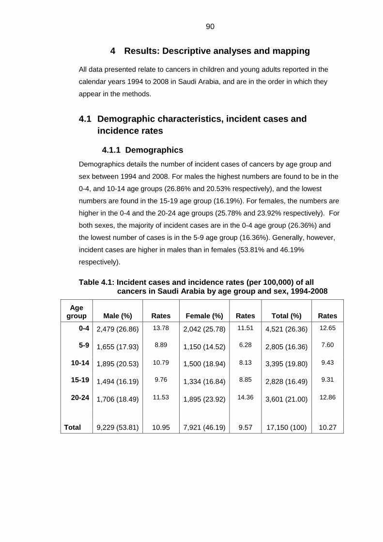
90
4 Results: Descriptive analyses and mapping
All data presented relate to cancers in children and young adults reported in the
calendar years 1994 to 2008 in Saudi Arabia, and are in the order in which they
appear in the methods.
4.1 Demographic characteristics, incident cases and
incidence rates
Demographics 4.1.1
Demographics details the number of incident cases of cancers by age group and
sex between 1994 and 2008. For males the highest numbers are found to be in the
0-4, and 10-14 age groups (26.86% and 20.53% respectively), and the lowest
numbers are found in the 15-19 age group (16.19%). For females, the numbers are
higher in the 0-4 and the 20-24 age groups (25.78% and 23.92% respectively). For
both sexes, the majority of incident cases are in the 0-4 age group (26.36%) and
the lowest number of cases is in the 5-9 age group (16.36%). Generally, however,
incident cases are higher in males than in females (53.81% and 46.19%
respectively).
Table 4.1: Incident cases and incidence rates (per 100,000) of all cancers in Saudi Arabia by age group and sex, 1994-2008
Age group Male (%)
Rates Female (%)
Rates Total (%)
Rates
0-4 2,479 (26.86) 13.78 2,042 (25.78) 11.51 4,521 (26.36) 12.65
5-9 1,655 (17.93) 8.89 1,150 (14.52) 6.28 2,805 (16.36) 7.60
10-14 1,895 (20.53) 10.79 1,500 (18.94) 8.13 3,395 (19.80) 9.43
15-19 1,494 (16.19) 9.76 1,334 (16.84) 8.85 2,828 (16.49) 9.31
20-24 1,706 (18.49) 11.53 1,895 (23.92) 14.36 3,601 (21.00) 12.86
Total 9,229 (53.81) 10.95 7,921 (46.19) 9.57 17,150 (100) 10.27
91
Incident cases 4.1.2
Tables 4.2 and 4.3 detail the incident cases of cancers for males and females by
age groups between 1994 and 2008 for the main diagnostic groups according to the
ICCC-3. For males, in the 0-4 age group, the most commonly occurring types of
cancers were leukaemias, CNS tumours and lymphomas (38.60%, 11.86% and
11.62% respectively). However for females within the same age group, the highest
numbers of incident cases were for leukaemias, neuroblastomas and CNS tumours
(37.86%, 11.61% and 10.87% respectively). For the 5-9 age group, the most
common types of cancers were leukaemia, lymphomas and CNS tumours (34.50%,
29.00% and 15.89% respectively) for males, and leukaemias, CNS tumours and
lymphomas (36.96%, 19.48% and 14.96% respectively) for females. Lymphomas
were the most commonly occurring cancers in the 10-14 age group (30.61%),
followed by leukaemias and malignant bone tumours (26.28% and 12.19%
respectively) in males, which were also the most common types in females
(26.40%, 24.27% and 13.13% respectively). Similarly, lymphomas, leukaemias and
malignant bone tumours in males were the most occurring for the 15-19 age group
(33.47%, 23.43% and 12.45% respectively). However, for females the most
common cancers were lymphomas, followed by epithelial tumours, and leukaemias
(28.64%, 26.39% and 14.24% respectively). For males in the 20-24 age group,
lymphomas were the most occurring cancer (30.30%) followed by epithelial tumours
(19.81%) and leukaemias (17.76%). For females, the most common cancers were
epithelial tumours (44.17%) followed by lymphomas and leukaemias (22.37% and
10.61% respectively). No cases were reported for retinoblastomas in either gender
for the 15-19 and 20-24 age groups.
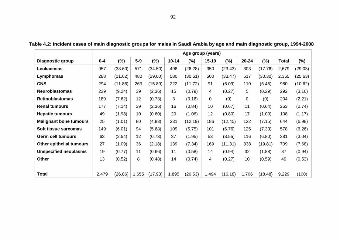
92
Table 4.2: Incident cases of main diagnostic groups for males in Saudi Arabia by age and main diagnostic group, 1994-2008
Age group (years)
Diagnostic group 0-4 (%) 5-9 (%) 10-14 (%) 15-19 (%) 20-24 (%) Total (%)
Leukaemias 957 (38.60) 571 (34.50) 498 (26.28) 350 (23.43) 303 (17.76) 2,679 (29.03)
Lymphomas 288 (11.62) 480 (29.00) 580 (30.61) 500 (33.47) 517 (30.30) 2,365 (25.63)
CNS 294 (11.86) 263 (15.89) 222 (11.72) 91 (6.09) 110 (6.45) 980 (10.62)
Neuroblastomas 229 (9.24) 39 (2.36) 15 (0.79) 4 (0.27) 5 (0.29) 292 (3.16)
Retinoblastomas 189 (7.62) 12 (0.73) 3 (0.16) 0 (0) 0 (0) 204 (2.21)
Renal tumours 177 (7.14) 39 (2.36) 16 (0.84) 10 (0.67) 11 (0.64) 253 (2.74)
Hepatic tumours 49 (1.98) 10 (0.60) 20 (1.06) 12 (0.80) 17 (1.00) 108 (1.17)
Malignant bone tumours 25 (1.01) 80 (4.83) 231 (12.19) 186 (12.45) 122 (7.15) 644 (6.98)
Soft tissue sarcomas 149 (6.01) 94 (5.68) 109 (5.75) 101 (6.76) 125 (7.33) 578 (6.26)
Germ cell tumours 63 (2.54) 12 (0.73) 37 (1.95) 53 (3.55) 116 (6.80) 281 (3.04)
Other epithelial tumours 27 (1.09) 36 (2.18) 139 (7.34) 169 (11.31) 338 (19.81) 709 (7.68)
Unspecified neoplasms 19 (0.77) 11 (0.66) 11 (0.58) 14 (0.94) 32 (1.88) 87 (0.94)
Other 13 (0.52) 8 (0.48) 14 (0.74) 4 (0.27) 10 (0.59) 49 (0.53)
Total 2,479 (26.86) 1,655 (17.93) 1,895 (20.53) 1,494 (16.18) 1,706 (18.48) 9,229 (100)
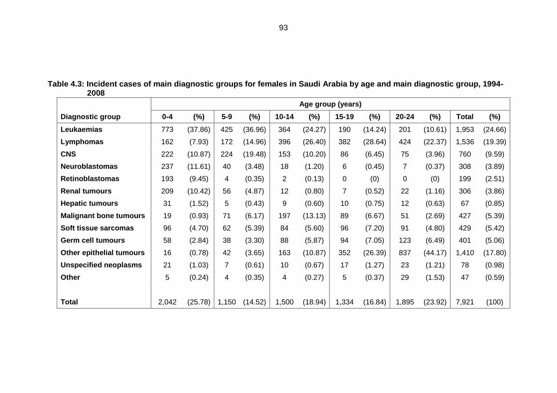
93
Table 4.3: Incident cases of main diagnostic groups for females in Saudi Arabia by age and main diagnostic group, 1994-2008
Age group (years)
Diagnostic group 0-4 (%) 5-9 (%) 10-14 (%) 15-19 (%) 20-24 (%) Total (%)
Leukaemias 773 (37.86) 425 (36.96) 364 (24.27) 190 (14.24) 201 (10.61) 1,953 (24.66)
Lymphomas 162 (7.93) 172 (14.96) 396 (26.40) 382 (28.64) 424 (22.37) 1,536 (19.39)
CNS 222 (10.87) 224 (19.48) 153 (10.20) 86 (6.45) 75 (3.96) 760 (9.59)
Neuroblastomas 237 (11.61) 40 (3.48) 18 (1.20) 6 (0.45) 7 (0.37) 308 (3.89)
Retinoblastomas 193 (9.45) 4 (0.35) 2 (0.13) 0 (0) 0 (0) 199 (2.51)
Renal tumours 209 (10.42) 56 (4.87) 12 (0.80) 7 (0.52) 22 (1.16) 306 (3.86)
Hepatic tumours 31 (1.52) 5 (0.43) 9 (0.60) 10 (0.75) 12 (0.63) 67 (0.85)
Malignant bone tumours 19 (0.93) 71 (6.17) 197 (13.13) 89 (6.67) 51 (2.69) 427 (5.39)
Soft tissue sarcomas 96 (4.70) 62 (5.39) 84 (5.60) 96 (7.20) 91 (4.80) 429 (5.42)
Germ cell tumours 58 (2.84) 38 (3.30) 88 (5.87) 94 (7.05) 123 (6.49) 401 (5.06)
Other epithelial tumours 16 (0.78) 42 (3.65) 163 (10.87) 352 (26.39) 837 (44.17) 1,410 (17.80)
Unspecified neoplasms 21 (1.03) 7 (0.61) 10 (0.67) 17 (1.27) 23 (1.21) 78 (0.98)
Other 5 (0.24) 4 (0.35) 4 (0.27) 5 (0.37) 29 (1.53) 47 (0.59)
Total 2,042 (25.78) 1,150 (14.52) 1,500 (18.94) 1,334 (16.84) 1,895 (23.92) 7,921 (100)
94
Overall age-sex standardised incidence rates 4.1.3
The indirect and direct age-sex standardised rates for leukaemias, lymphomas,
CNS tumours and other cancers are presented in Table 4.4. The rates are given as
per 1,000,000 person years. The rate for ALL in Saudi Arabia was 18.50 per
1,000,000 person years (Table 4.4). In direct standardisation for the World,
European or US standard population the incidence rate dropped slightly to 17.86
per 1,000,000, 18.15 per 1,000,000 and 17.62 per 1,000,000 person years,
respectively. The age-sex standardised rates also dropped for BL and CNS
tumours. However, for CML, NHL and the ‘other cancers’ group, the incidence was
raised when standardising to the World, European or US population. The increased
incidence is more marked for the ‘other cancers’ group, where the indirect rate was
41.17 per 1,000,000 person years (95%CI=40.20-42.14), and the direct rates for
the World, European and US standard population were 42.25, 42.72 and 41.92 per
1,000,000 person years. The differences are more marked when the age-sex
adjusted incidence rates are standardised to the US standard population, this may
be due to differences in the age structure between the US and Saudi Arabia in the
0-24 age group.
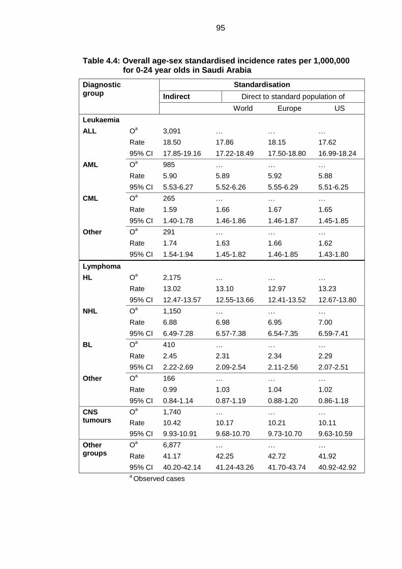
95
Table 4.4: Overall age-sex standardised incidence rates per 1,000,000 for 0-24 year olds in Saudi Arabia
Diagnostic group
Standardisation
Indirect Direct to standard population of
World Europe US
Leukaemia
ALL Oa 3,091 … … …
Rate 18.50 17.86 18.15 17.62
95% CI 17.85-19.16 17.22-18.49 17.50-18.80 16.99-18.24
AML Oa 985 … … …
Rate 5.90 5.89 5.92 5.88
95% CI 5.53-6.27 5.52-6.26 5.55-6.29 5.51-6.25
CML Oa 265 … … …
Rate 1.59 1.66 1.67 1.65
95% CI 1.40-1.78 1.46-1.86 1.46-1.87 1.45-1.85
Other Oa 291 … … …
Rate 1.74 1.63 1.66 1.62
95% CI 1.54-1.94 1.45-1.82 1.46-1.85 1.43-1.80
Lymphoma
HL Oa 2,175 … … …
Rate 13.02 13.10 12.97 13.23
95% CI 12.47-13.57 12.55-13.66 12.41-13.52 12.67-13.80
NHL Oa 1,150 … … …
Rate 6.88 6.98 6.95 7.00
95% CI 6.49-7.28 6.57-7.38 6.54-7.35 6.59-7.41
BL Oa 410 … … …
Rate 2.45 2.31 2.34 2.29
95% CI 2.22-2.69 2.09-2.54 2.11-2.56 2.07-2.51
Other Oa 166 … … …
Rate 0.99 1.03 1.04 1.02
95% CI 0.84-1.14 0.87-1.19 0.88-1.20 0.86-1.18
CNS tumours
Oa 1,740 … … …
Rate 10.42 10.17 10.21 10.11
95% CI 9.93-10.91 9.68-10.70 9.73-10.70 9.63-10.59
Other groups
Oa 6,877 … … …
Rate 41.17 42.25 42.72 41.92
95% CI 40.20-42.14 41.24-43.26 41.70-43.74 40.92-42.92 a Observed cases
96
Age-sex standardised incidence rates and ratios by 4.1.4
Governorate
The age-sex standardised incidence rates and the SIRs along with the 95%
confidence intervals for each disease category were computed in young people
aged under 24 years in Saudi Arabian Governorates, but have not been given. The
SIRs have been used in disease mapping and funnel plots.
Disease mapping 4.1.4.1
Figure 4.1 shows the crude and SEB smoothed SIRs for ALL. For the crude SIRs,
the number of expected cases in the three large Governorates of Riyadh, Jeddah
and Dammam were lower than the observed, which is reflected in the high SIRs of
these Governorates. There were 23 Governorates with no cases present, providing
an SIR of zero. For the SEB smoothed rates, the SIR of one Governorate shrunk
towards the mean of its neighbouring Governorates. For example, Badr in the
western coast had an estimated SIR of zero due to having no observed cases of
ALL. However, after the SEB smoothing, the estimated smoothed SIR became
0.55. The smoothed map shows a pattern of high incidence in the central region of
Riyadh, as well as in the Eastern province, Jeddah, Medinah and in the Northern
Border region of Toraif and Qurayyat.
Figure 4.2 shows the crude and smoothed SIRs for AML. For the crude SIRs, a
total of 47 Governorates had no observed cases reported. However, the
Governorate with the highest SIR of 2.95 was Toraif (95%CI = 1.08 - 6.41), located
in the Northern Border province, due to having 6 observed cases compared to the
2.04 expected, which are small numbers. After smoothing, the SIR for Toraif shrank
to 1.47. The smoothed map in general, shows a clearer pattern of AML incidence,
in which incidence remains high in the north eastern, central and south eastern
regions of the country. In the south, Baha, Abha and Jazan Governorates have a
persistent high incidence of AML after smoothing.
97
a) Crude SIRs b) Smoothed SIRs
Figures 4.1: Crude and smoothed age-sex standardised incidence ratios (SIRs) of acute lymphoblastic leukaemias registered from 1994 to 2008 in young people under the age of 24 years by Saudi Governorates
98
a) Crude SIRs b) Smoothed SIRs
Figure 4.2: Crude and smoothed age-sex standardised incidence ratios (SIRs) of acute myeloid leukaemias registered from 1994 to 2008 in young people under the age of 24 years by Saudi Governorates
99
Figure 4.3 shows the crude and SEB smoothed SIRs for CML. For the crude SIR,
no clear pattern of incidence can be seen. The Governorates with the highest SIRs
were found in Herimla, Rayth and Kamel, these are characterised as small sparsely
populated Governorates. The high SIRs were due to having one observed case of
CML within the 15-year study period, compared to an expected number of cases of
below 0.25 in each of these Governorates. Other Governorates with a high SIR
included Qurayyat and Abha. The SEB smoothed map has imposed a much clearer
pattern of incidence, in which only Qurayyat and Abha Governorates retain a high
SIR. The majority of the other Governorates have an estimated smoothed SIR
between 0.72 and 1.30.
Figure 4.4 gives the crude and smoothed SIRs of the ‘other leukaemias’ group.
Many Governorates had no cases (n=74). Those with a high SIR are scattered in
the country, in the north in Toraif and Skaka, in the west in Medinah and Jeddah
and in the south in Baha and Bishah, and some of the neighbouring areas of these
Governorates had zero cases, hence no discernible pattern can be deduced.
However, the SEB smoothed map shrunk the high SIRs towards the mean of the
neighbouring Governorates, which resulted in a much clearer pattern of incidence.
Only the Zolfi and Ola Governorates keep their SIR of zero, since all their
neighbouring Governorates also had an SIR of zero in the crude SIR map.
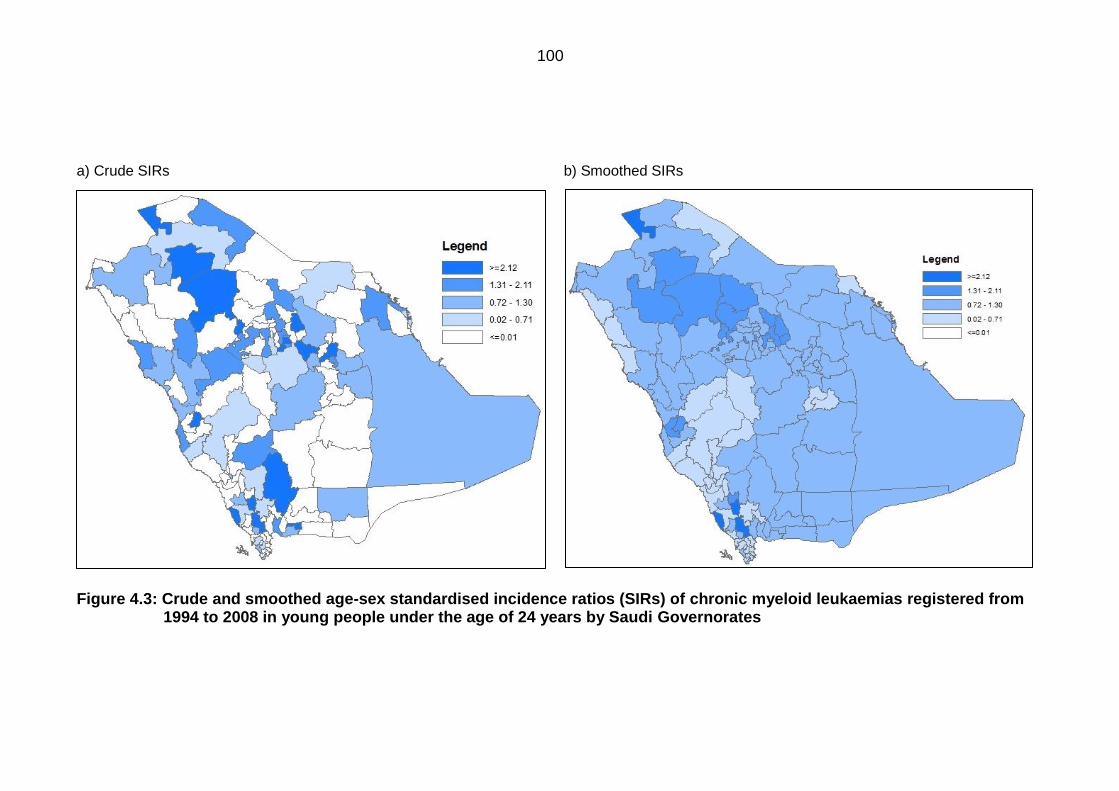
100
a) Crude SIRs b) Smoothed SIRs
Figure 4.3: Crude and smoothed age-sex standardised incidence ratios (SIRs) of chronic myeloid leukaemias registered from 1994 to 2008 in young people under the age of 24 years by Saudi Governorates
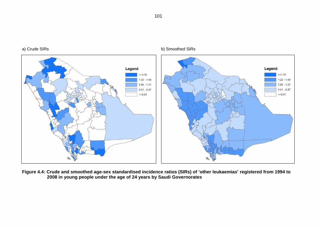
101
a) Crude SIRs b) Smoothed SIRs
Figure 4.4: Crude and smoothed age-sex standardised incidence ratios (SIRs) of ‘other leukaemias’ registered from 1994 to 2008 in young people under the age of 24 years by Saudi Governorates
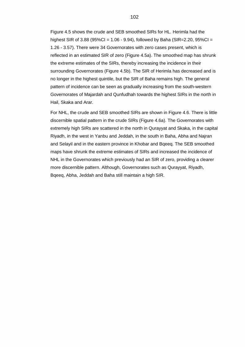
102
Figure 4.5 shows the crude and SEB smoothed SIRs for HL. Herimla had the
highest SIR of 3.88 (95%CI = 1.06 - 9.94), followed by Baha (SIR=2.20, 95%CI =
1.26 - 3.57). There were 34 Governorates with zero cases present, which is
reflected in an estimated SIR of zero (Figure 4.5a). The smoothed map has shrunk
the extreme estimates of the SIRs, thereby increasing the incidence in their
surrounding Governorates (Figure 4.5b). The SIR of Herimla has decreased and is
no longer in the highest quintile, but the SIR of Baha remains high. The general
pattern of incidence can be seen as gradually increasing from the south-western
Governorates of Majardah and Qunfudhah towards the highest SIRs in the north in
Hail, Skaka and Arar.
For NHL, the crude and SEB smoothed SIRs are shown in Figure 4.6. There is little
discernible spatial pattern in the crude SIRs (Figure 4.6a). The Governorates with
extremely high SIRs are scattered in the north in Qurayyat and Skaka, in the capital
Riyadh, in the west in Yanbu and Jeddah, in the south in Baha, Abha and Najran
and Selayil and in the eastern province in Khobar and Bqeeq. The SEB smoothed
maps have shrunk the extreme estimates of SIRs and increased the incidence of
NHL in the Governorates which previously had an SIR of zero, providing a clearer
more discernible pattern. Although, Governorates such as Qurayyat, Riyadh,
Bqeeq, Abha, Jeddah and Baha still maintain a high SIR.
103
a) Crude SIRs b) Smoothed SIRs
Figure 4.5: Crude and smoothed age-sex standardised incidence ratios (SIRs) of Hodgkin’slymphoma registered from 1994 to 2008 in young people under the age of 24 years by Saudi Governorates
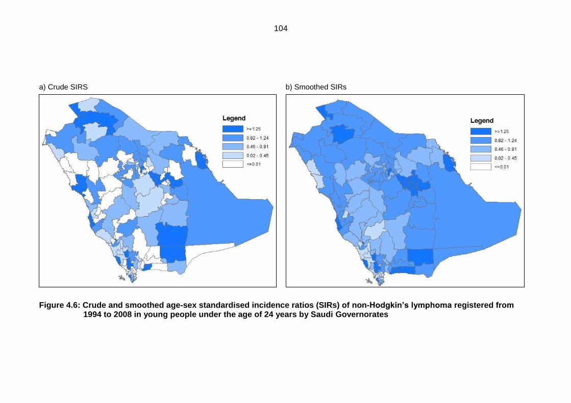
104
a) Crude SIRS b) Smoothed SIRs
Figure 4.6: Crude and smoothed age-sex standardised incidence ratios (SIRs) of non-Hodgkin’slymphoma registered from 1994 to 2008 in young people under the age of 24 years by Saudi Governorates
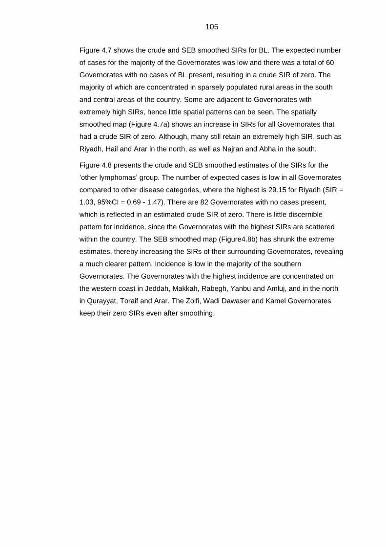
105
Figure 4.7 shows the crude and SEB smoothed SIRs for BL. The expected number
of cases for the majority of the Governorates was low and there was a total of 60
Governorates with no cases of BL present, resulting in a crude SIR of zero. The
majority of which are concentrated in sparsely populated rural areas in the south
and central areas of the country. Some are adjacent to Governorates with
extremely high SIRs, hence little spatial patterns can be seen. The spatially
smoothed map (Figure 4.7a) shows an increase in SIRs for all Governorates that
had a crude SIR of zero. Although, many still retain an extremely high SIR, such as
Riyadh, Hail and Arar in the north, as well as Najran and Abha in the south.
Figure 4.8 presents the crude and SEB smoothed estimates of the SIRs for the
‘other lymphomas’ group. The number of expected cases is low in all Governorates
compared to other disease categories, where the highest is 29.15 for Riyadh (SIR =
1.03, 95%CI = 0.69 - 1.47). There are 82 Governorates with no cases present,
which is reflected in an estimated crude SIR of zero. There is little discernible
pattern for incidence, since the Governorates with the highest SIRs are scattered
within the country. The SEB smoothed map (Figure4.8b) has shrunk the extreme
estimates, thereby increasing the SIRs of their surrounding Governorates, revealing
a much clearer pattern. Incidence is low in the majority of the southern
Governorates. The Governorates with the highest incidence are concentrated on
the western coast in Jeddah, Makkah, Rabegh, Yanbu and Amluj, and in the north
in Qurayyat, Toraif and Arar. The Zolfi, Wadi Dawaser and Kamel Governorates
keep their zero SIRs even after smoothing.
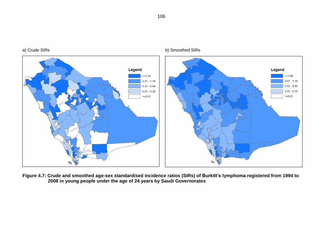
106
a) Crude SIRs b) Smoothed SIRs
Figure 4.7: Crude and smoothed age-sex standardised incidence ratios (SIRs) of Burkitt’slymphoma registered from 1994 to 2008 in young people under the age of 24 years by Saudi Governorates
107
a) Crude SIRs b) Smoothed SIRs
Figure 4.8: Crude and smoothed age-sex standardised incidence ratios (SIRs) of ‘other lymphomas’ registered from 1994 to 2008 in young people under the age of 24 years by Saudi Governorates

108
Figure 4.9 presents the crude and smoothed estimates for CNS tumours. The
highest quintile of SIRs was found in the highly populated Governorates of Riyadh,
Jeddah, Dammam, Hail, Buraidah, Madinah and Baha, as well as in the sparsely
populated Governorates such as Qurayyat and Riyadh Khobaraa. Both high and
low populated Governorates are adjacent to others with SIRs of zero due to no
cases being present, hence no spatial pattern can be seen. However, the SEB
smoothed map (Figure 4.9b), has shrunk the extreme estimates, and therefore a
concentration of Governorates with high SIRs can be seen in the central region, as
well as in the west in Yanbu, Badr and Madinah. Governorates with low SIRs are
mostly seen in the south western region in Qunfudhah, Qilwah and Sarat Abaida.
For the ‘all other cancers’ group, the crude and SEB smoothed SIRs are presented
in Figure 4.10. Only 15 Governorates have an SIR of zero due to no cases present,
and all of these are surrounded by Governorates with an SIR in the highest quintile.
The highest SIR was found in Shaqraa, which is located in the central province of
Riyadh (SIR = 4.30, 95%CI = 3.05 - 5.87), followed by Baha (SIR = 2.20, 95%CI =
1.70 - 2.81). The SEB smoothed map (Figure 4.10b), presents a clearer pattern of
incidence, in which the high SIRs have shrunk towards the mean of the
neighbouring areas, thereby increasing the SIRs for those areas. The entire eastern
provinces, along with Governorates from the Riyadh province, maintain a high SIR
after smoothing. A slightly lower incidence is seen in the north and in Governorates
in the south. Though, Baha and Shaqraa have a persistently high SIR.
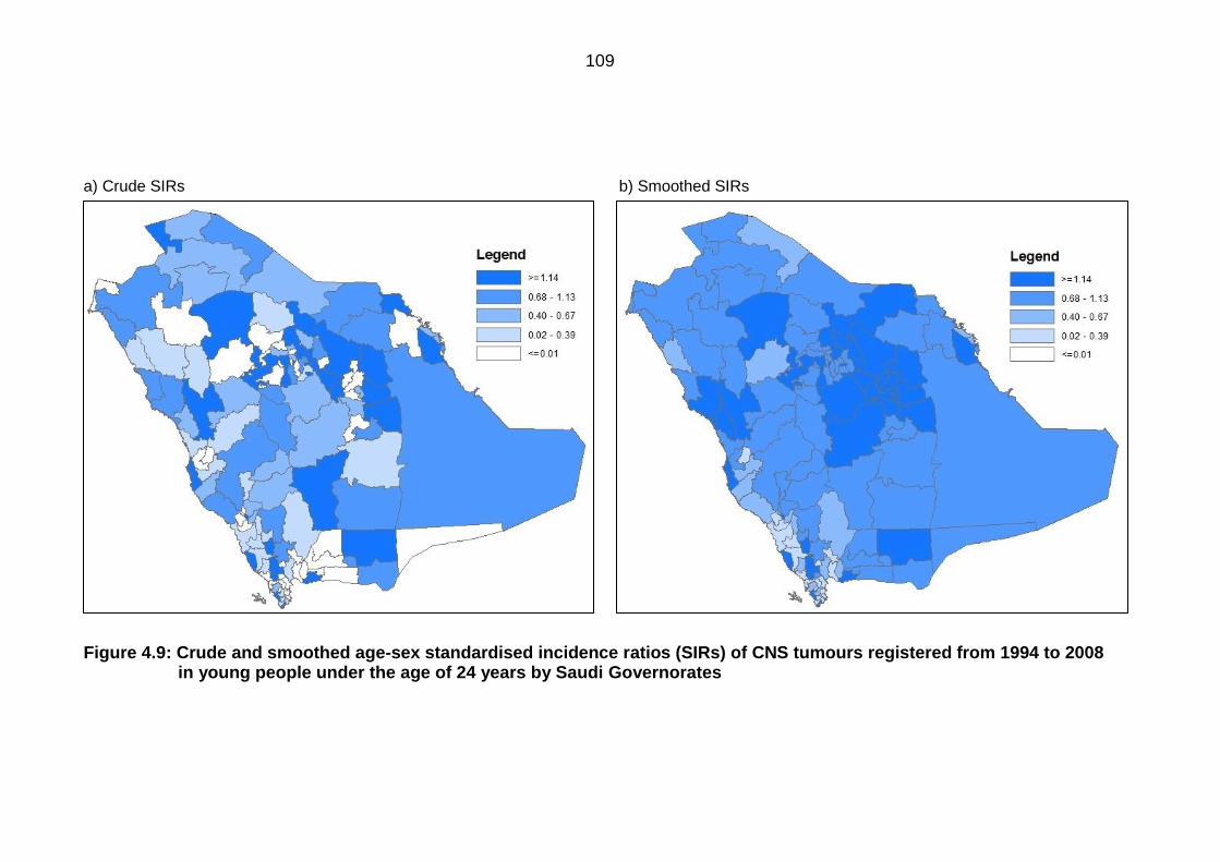
109
a) Crude SIRs b) Smoothed SIRs
Figure 4.9: Crude and smoothed age-sex standardised incidence ratios (SIRs) of CNS tumours registered from 1994 to 2008 in young people under the age of 24 years by Saudi Governorates
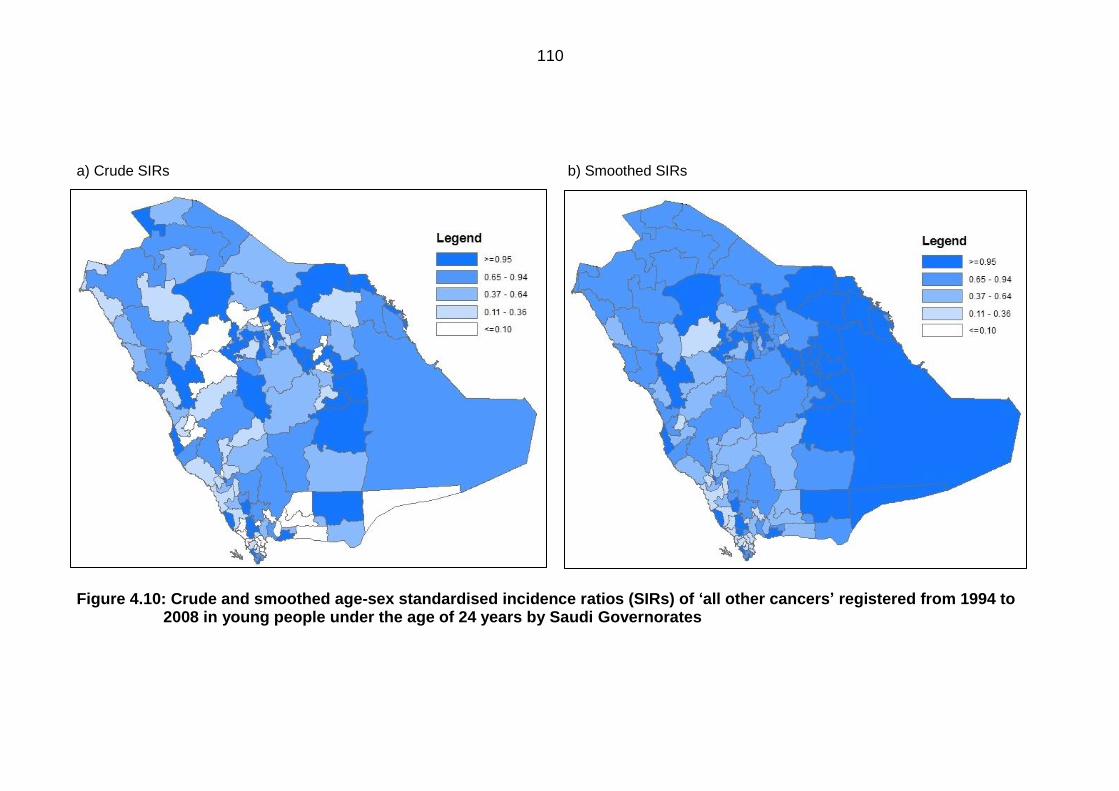
110
a) Crude SIRs b) Smoothed SIRs
Figure 4.10: Crude and smoothed age-sex standardised incidence ratios (SIRs) of ‘all other cancers’ registered from 1994 to 2008 in young people under the age of 24 years by Saudi Governorates

111
Funnel plots 4.1.4.2
Figure 4.11 gives the crude and smoothed funnel plots for SIRs for ALL. The plot
reflects the SIRs mapped in Figure 4.1 (Figure 4.1a), where Baha, Jazan, Buraidah,
Jeddah and Riyadh had extremely high SIRs placing them outside the upper 99.8%
control limit. The majority of Governorates however, were within both control limits.
The smoothed SIRs were also given (Figure 4.1b), which show a slight reduction in
the extreme SIRs, for example the SIRs of Baha and Jazan have been smoothed
from 2.58 and 2.07 to 2.48 and 2.01 respectively. Also, the smoothing has raised
the SIRs in the Governorates with low values.
Funnel plots for AML are given in Figure 4.12. The SEB smoothed plot (Figure
4.12), clearly shows a reduction in SIRs, such as the SIRs for Toraif and Aflaj which
have been reduced from 2.95 and 2.67 to 1.47 and 1.28 respectively, thus these
Governorates are no longer above the 99.8% control limit. Similarly, for CML and
the ‘other leukaemias’ group, the number of Governorates with zero cases
decreased in the smoothed plots in Figures 4.13 and 4.14. Several Governorates
with extremely high SIRs such as Herimla and Rayth for CMLs and Toraif and
Bishah for the ‘other leukaemias’ group decreased within the control limits. Of
importance is the Makkah Governorate, which was found to have an SIR below one
for all types of leukaemia before and after smoothing. In fact, for ALL, both the
crude and smoothed SIRs were below the lower 99.8% control limit.
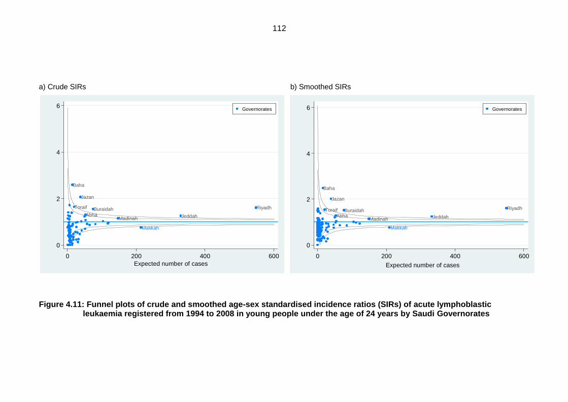
112
Makkah
Madinah
Toraif
Baha
Riyadh
Abha
Jazan
Buraidah
Jeddah
0
2
4
6
sta
nd
ard
ise
d in
cid
en
ce
ra
tios
0 200 400 600
Expected number of cases
Governorates
Makkah
Madinah
Toraif
Baha
Riyadh
Abha
Jazan
Buraidah
Jeddah
0
2
4
6
sta
nd
ard
ise
d in
cid
en
ce
ra
tios
0 200 400 600
Expected number of cases
Governorates
a) Crude SIRs b) Smoothed SIRs
Figure 4.11: Funnel plots of crude and smoothed age-sex standardised incidence ratios (SIRs) of acute lymphoblastic leukaemia registered from 1994 to 2008 in young people under the age of 24 years by Saudi Governorates
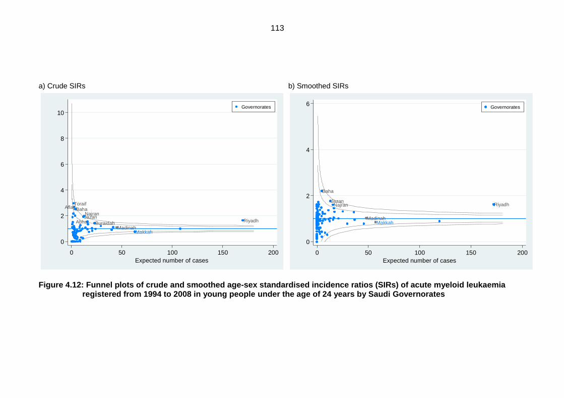
113
MakkahMadinah
Aflaj Baha
RiyadhAbhaJazanNajran
Buraidah
Toraif
0
2
4
6
8
10
sta
nd
ard
ise
d in
cid
en
ce
ra
tios
0 50 100 150 200
Expected number of cases
Governorates
MakkahMadinah
Baha
RiyadhJazan
Najran
0
2
4
6
sta
nd
ard
ise
d in
cid
en
ce
ra
tios
0 50 100 150 200
Expected number of cases
Governorates
a) Crude SIRs b) Smoothed SIRs
Figure 4.12: Funnel plots of crude and smoothed age-sex standardised incidence ratios (SIRs) of acute myeloid leukaemia registered from 1994 to 2008 in young people under the age of 24 years by Saudi Governorates
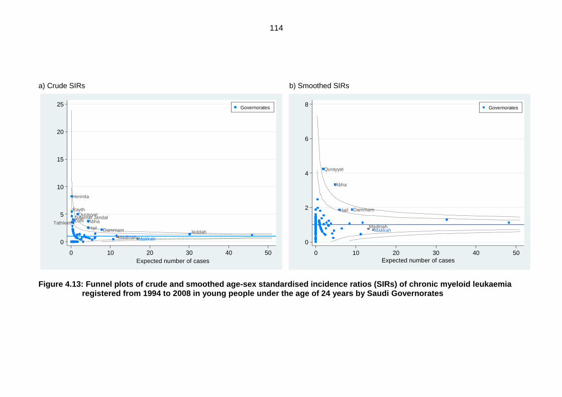
114
MakkahMadinah
QurayyatRayth
ZolfiDawmat Jandal
Herimla
Abha
DammamHailJeddah
Tathleeth
0
5
10
15
20
25
sta
nd
ard
ise
d in
cid
en
ce
ra
tios
0 10 20 30 40 50
Expected number of cases
Governorates
MakkahMadinah
Qurayyat
Abha
DammamHail
0
2
4
6
8
sta
nd
ard
ise
d in
cid
en
ce
ra
tios
0 10 20 30 40 50
Expected number of cases
Governorates
a) Crude SIRs b) Smoothed SIRs
Figure 4.13: Funnel plots of crude and smoothed age-sex standardised incidence ratios (SIRs) of chronic myeloid leukaemia registered from 1994 to 2008 in young people under the age of 24 years by Saudi Governorates
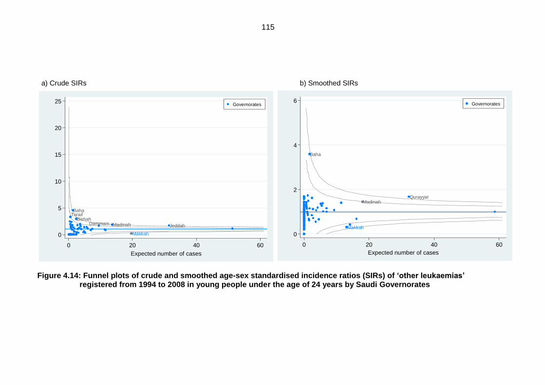
115
Makkah
Madinah
Baha
Qurayyat
0
2
4
6
sta
nd
ard
ise
d in
cid
en
ce
ra
tios
0 20 40 60
Expected number of cases
Governorates
Makkah
Bishah
Baha
MadinahDammam Jeddah
Toraif
0
5
10
15
20
25
sta
nd
ard
ise
d in
cid
en
ce
ra
tios
0 20 40 60
Expected number of cases
Governorates
a) Crude SIRs b) Smoothed SIRs
Figure 4.14: Funnel plots of crude and smoothed age-sex standardised incidence ratios (SIRs) of ‘otherleukaemias’ registered from 1994 to 2008 in young people under the age of 24 years by Saudi Governorates
116
Figure 4.15 and 4.16 plot the crude and SEB smoothed SIRs for HL and NHL
respectively. The expected cases for HL are highest amongst all types of
lymphomas. The plot clearly shows that Herimla had the highest incidence rate
(SIR=3.80), followed by Baha (SIR=2.19). Following smoothing, the extremely high
SIRs decreased, but the highest reduction was for the Herimla Governorate
(smoothed SIR=1.51), which decreased to below the upper control limit, due to
having a low population compared to other Governorates. Similarly for NHL, Bqeeq
had the highest reduction in SIR after SEB smoothing.
Figure 4.17 plots the crude and SEB smoothed SIRs for BL. The Raas Tanourah,
Uhd Masarha, Baha, Sarat Abaida and Abha Governorates had SIRs above the
95% control limit. After SEB smoothing (Figure 4.17b), the Governorates with the
lower populations, such as Raas Tanourah, Uhd Masarha, Shaqraa and Sarat
Abaida had the highest reduction in SIRs. Furthermore, the number of Governorates
with zero SIRs was reduced. For the ‘other lymphomas’ group (Figure 4.18), the
number of expected cases was relatively low. The SEB smoothing reduced the
number of Governorates with zero cases.
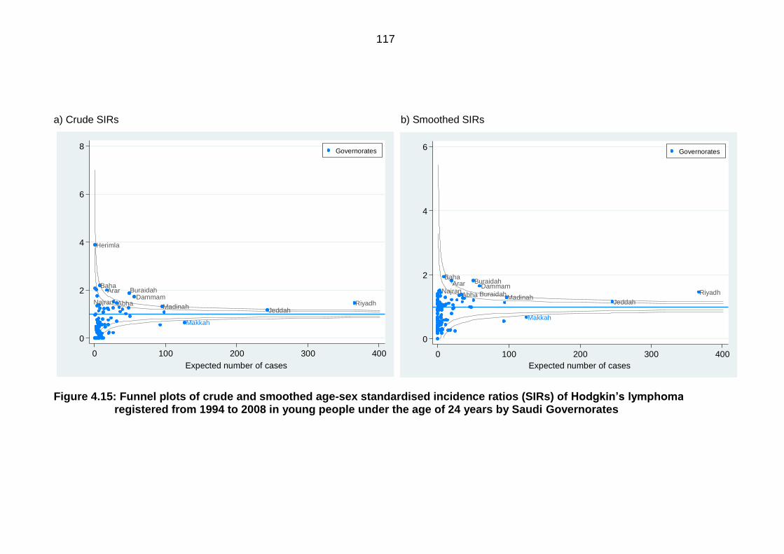
117
Makkah
Herimla
Baha
MadinahRiyadhAbha
DammamNajran
Arar Buraidah
Jeddah
0
2
4
6
8
sta
nd
ard
ise
d in
cid
en
ce
ra
tios
0 100 200 300 400
Expected number of cases
Governorates
Makkah
Madinah
Baha
Buraidah RiyadhAbha
DammamNajran
Arar Buraidah
Jeddah
0
2
4
6
sta
nd
ard
ise
d in
cid
en
ce
ra
tios
0 100 200 300 400
Expected number of cases
Governorates
a) Crude SIRs b) Smoothed SIRs
Figure 4.15: Funnel plots of crude and smoothed age-sex standardised incidence ratios (SIRs) of Hodgkin’slymphoma registered from 1994 to 2008 in young people under the age of 24 years by Saudi Governorates
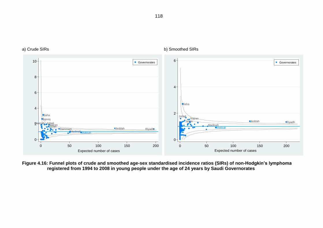
118
MakkahMadinah
Jubail
Bqeeq
Baha
RiyadhDammamJazanNajran
Jeddah
Onaizah
0
2
4
6
8
10
sta
nd
ard
ise
d in
cid
en
ce
ra
tios
0 50 100 150 200
Expected number of cases
Governorates
MakkahMadinah
Jubail
Baha
RiyadhJazanNajran
Jeddah
0
2
4
6
sta
nd
ard
ise
d in
cid
en
ce
ra
tios
0 50 100 150 200
Expected number of cases
Governorates
a) Crude SIRs b) Smoothed SIRs
Figure 4.16: Funnel plots of crude and smoothed age-sex standardised incidence ratios (SIRs) of non-Hodgkin’slymphomaregistered from 1994 to 2008 in young people under the age of 24 years by Saudi Governorates
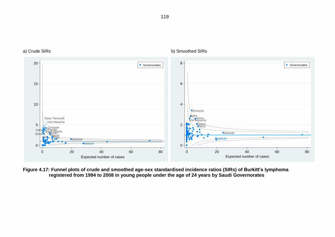
119
Makkah
Uhd Masarha
QurayyatBaha
MadinahAbha
JazanNajran
ArarQilwah
Raas Tanourah
Sarat AbaidaShaqraa
0
5
10
15
20
sta
nd
ard
ise
d in
cid
en
ce
ra
tios
0 20 40 60 80
Expected number of cases
Governorates
Makkah
Madinah
Uhd Masarha
Qurayyat
Baha
Abha
Jazan
Najran
0
2
4
6
8
sta
nd
ard
ise
d in
cid
en
ce
ra
tios
0 20 40 60 80
Expected number of cases
Governorates
a) Crude SIRs b) Smoothed SIRs
Figure 4.17: Funnel plots of crude and smoothed age-sex standardised incidence ratios (SIRs) of Burkitt’slymphoma registered from 1994 to 2008 in young people under the age of 24 years by Saudi Governorates
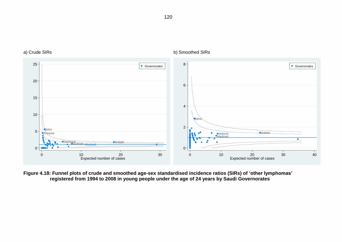
120
MakkahMadinah
Baha
Dammam Jeddah
Shaqraa
0
5
10
15
20
25
sta
nd
ard
ise
d in
cid
en
ce
ra
tios
0 10 20 30Expected number of cases
Governorates
MakkahMadinah
Baha
Jeddah
0
2
4
6
8
sta
nd
ard
ise
d in
cid
en
ce
ra
tios
0 10 20 30 40Expected number of cases
Governorates
a) Crude SIRs b) Smoothed SIRs
Figure 4.18: Funnel plots of crude and smoothed age-sex standardised incidence ratios (SIRs) of ‘otherlymphomas’ registered from 1994 to 2008 in young people under the age of 24 years by Saudi Governorates
121
Figure 4.19 plots the crude and SEB smoothed SIRs for CNS tumours. The SEB
smoothing shrunk the SIRs of the Governorates with extreme SIRs. However, those
with high population numbers such as Riyadh, Jeddah and Madinah still maintain
high SIRs above the upper 99.8% control limit. The number of Governorates with
zero SIRs, due to no cases present, decreased. Although, the Makkah Governorate
maintains a low SIR below the lower control limits, even after smoothing.
For the ‘all other cancers’ group, Figure 4.20 shows the crude and SEB smoothed
SIRs on funnel plots. The number of expected cases is high and exceeds 1000
cases for Riyadh. The SEB smoothing reduced the Shaqraa Governorate from 4.30
to 2.70. Additionally, Raas Tanourah was reduced to below the upper control limit.
Furthermore, Makkah keeps a low SIR that is below the lower control limits, both
before and after smoothing.
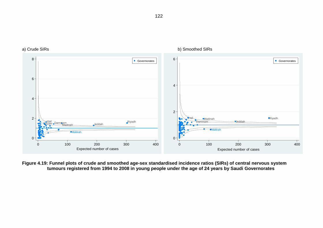
122
Makkah
MadinahRiyadhDammam
HailJazan Jeddah
0
2
4
6
8
sta
nd
ard
ise
d in
cid
en
ce
ra
tios
0 100 200 300 400
Expected number of cases
Governorates
Makkah
Madinah Riyadh
Dammam
Hail
Jeddah
0
2
4
6
sta
nd
ard
ise
d in
cid
en
ce
ra
tios
0 100 200 300 400
Expected number of cases
Governorates
a) Crude SIRs b) Smoothed SIRs
Figure 4.19: Funnel plots of crude and smoothed age-sex standardised incidence ratios (SIRs) of central nervous system tumours registered from 1994 to 2008 in young people under the age of 24 years by Saudi Governorates
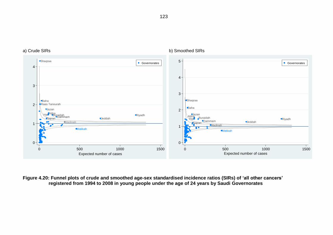
123
Makkah
Madinah
Baha
RiyadhAbha
DammamHail
Jazan
Najran
Buraidah
Jeddah
Raas Tanourah
Shaqraa
0
1
2
3
4
sta
nd
ard
ise
d in
cid
en
ce
ra
tios
0 500 1000 1500
Expected number of cases
Governorates
Makkah
Madinah
Baha
RiyadhAbha
DammamHail
Jazan
Najran
Buraidah
Jeddah
Shaqraa
0
1
2
3
4
5
sta
nd
ard
ise
d in
cid
en
ce
ra
tios
0 500 1000 1500
Expected number of cases
Governorates
a) Crude SIRs b) Smoothed SIRs
Figure 4.20: Funnel plots of crude and smoothed age-sex standardised incidence ratios (SIRs) of ‘allothercancers’ registered from 1994 to 2008 in young people under the age of 24 years by Saudi Governorates
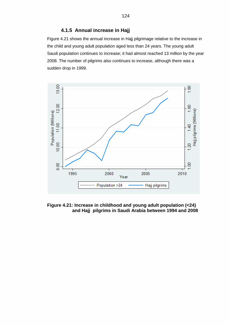
124
Annual increase in Hajj 4.1.5
Figure 4.21 shows the annual increase in Hajj pilgrimage relative to the increase in
the child and young adult population aged less than 24 years. The young adult
Saudi population continues to increase; it had almost reached 13 million by the year
2008. The number of pilgrims also continues to increase, although there was a
sudden drop in 1999.
Figure 4.21: Increase in childhood and young adult population (<24) and Hajj pilgrims in Saudi Arabia between 1994 and 2008
125
5 Results: Indices of socioeconomic status
The data presented here is from the 2004 national census data. Details of all
analytical methods were given in Chapter 3.
5.1 Data cleaning and descriptive statistics
Descriptive statistics 5.1.1
Table 5.1 details the descriptive statistics on the available variables from the 2004
national census of Saudi Arabia. Aggregating variables such as the ‘two or more
cars’ variable has led to the distribution being more normally distributed. For the
educational status category, the lowest mean was found for those with a higher
education, i.e. a masters and a PhD (0.003). This variable is also positively skewed
(skewness= 2.56) and its kurtosis is high (12.47), indicating a high peaked non-
normal distribution. Further, the maximum proportion for a Governorate with higher
education was only 0.019. For employment status, the average number of people in
the labour force was 0.485 (SD=0.08), where the minimum number in a
Governorate was high (0.32). For the type of housing and housing tenure
categories, both the ‘other type of housing’, which indicated people living in tents or
slums, and ‘other tenure’, which indicated whether the home is provided by a
charity, are very small, in which the mean and SD for these variables were only
0.10 (SD=0.07) and 0.01 (SD=0.01), respectively. No Governorate had a minimum
value of 0.00 for the household amenities category. The lowest minimum value was
0.03 for the ‘no TV available’ variable.
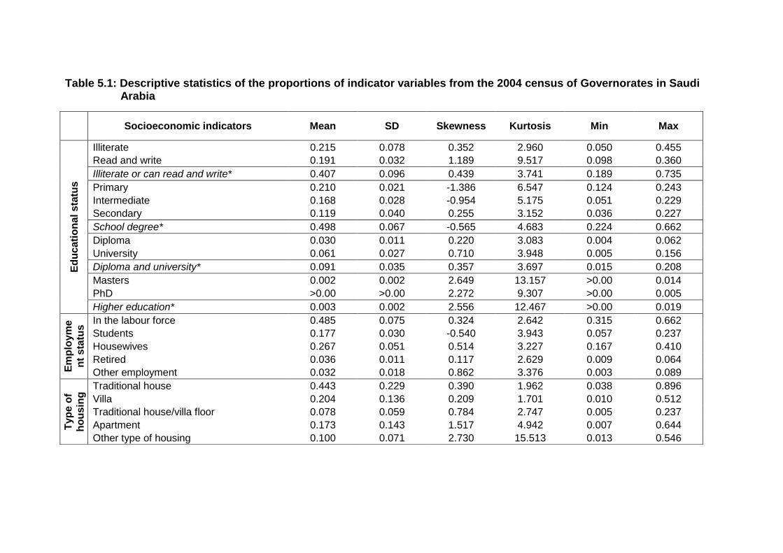
Table 5.1: Descriptive statistics of the proportions of indicator variables from the 2004 census of Governorates in Saudi Arabia
Socioeconomic indicators Mean SD Skewness Kurtosis Min Max
Ed
uc
ati
on
al s
tatu
s
Illiterate 0.215 0.078 0.352 2.960 0.050 0.455
Read and write 0.191 0.032 1.189 9.517 0.098 0.360
Illiterate or can read and write* 0.407 0.096 0.439 3.741 0.189 0.735
Primary 0.210 0.021 -1.386 6.547 0.124 0.243
Intermediate 0.168 0.028 -0.954 5.175 0.051 0.229
Secondary 0.119 0.040 0.255 3.152 0.036 0.227
School degree* 0.498 0.067 -0.565 4.683 0.224 0.662
Diploma 0.030 0.011 0.220 3.083 0.004 0.062
University 0.061 0.027 0.710 3.948 0.005 0.156
Diploma and university* 0.091 0.035 0.357 3.697 0.015 0.208
Masters 0.002 0.002 2.649 13.157 >0.00 0.014
PhD >0.00 >0.00 2.272 9.307 >0.00 0.005
Higher education* 0.003 0.002 2.556 12.467 >0.00 0.019
Em
plo
ym
e
nt
sta
tus In the labour force 0.485 0.075 0.324 2.642 0.315 0.662
Students 0.177 0.030 -0.540 3.943 0.057 0.237
Housewives 0.267 0.051 0.514 3.227 0.167 0.410
Retired 0.036 0.011 0.117 2.629 0.009 0.064
Other employment 0.032 0.018 0.862 3.376 0.003 0.089
Typ
e o
f
ho
usin
g Traditional house 0.443 0.229 0.390 1.962 0.038 0.896
Villa 0.204 0.136 0.209 1.701 0.010 0.512
Traditional house/villa floor 0.078 0.059 0.784 2.747 0.005 0.237
Apartment 0.173 0.143 1.517 4.942 0.007 0.644
Other type of housing 0.100 0.071 2.730 15.513 0.013 0.546
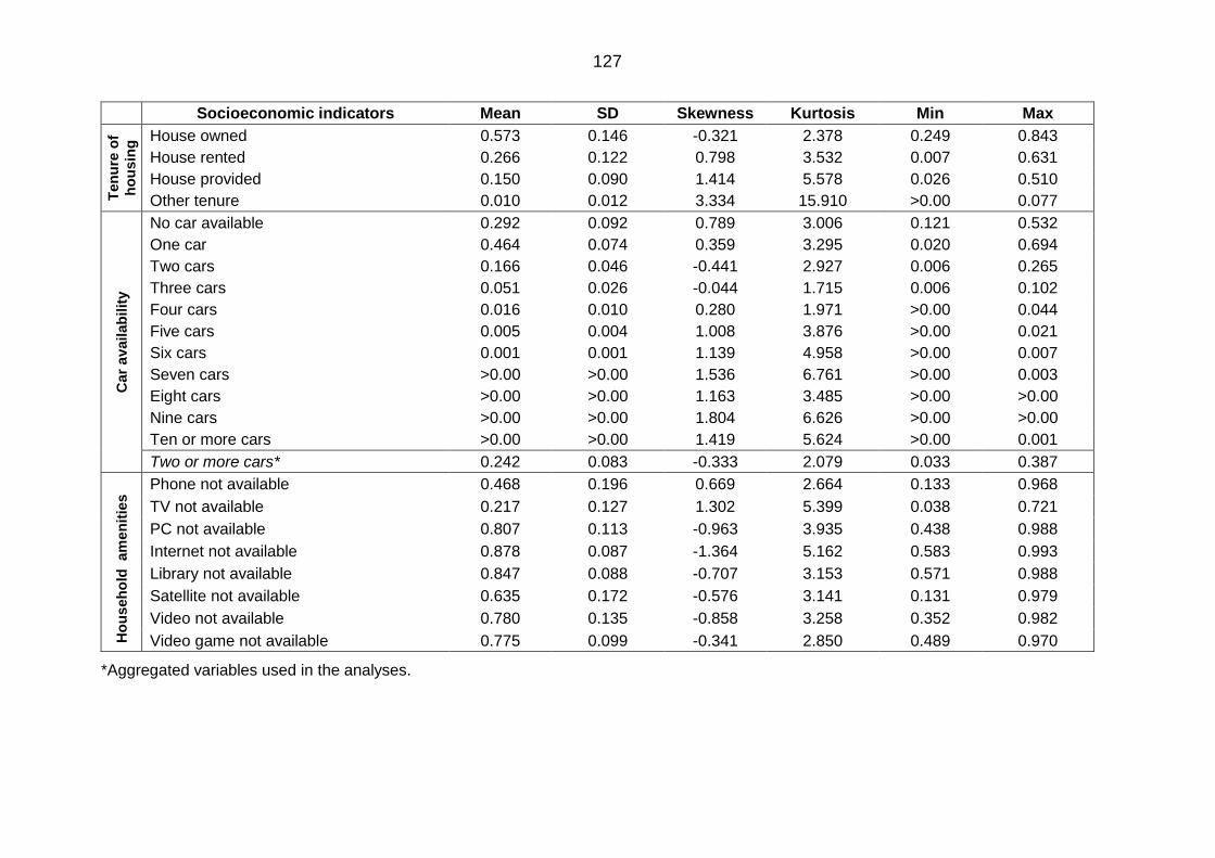
127
Socioeconomic indicators Mean SD Skewness Kurtosis Min Max T
en
ure
of
ho
usin
g House owned 0.573 0.146 -0.321 2.378 0.249 0.843
House rented 0.266 0.122 0.798 3.532 0.007 0.631
House provided 0.150 0.090 1.414 5.578 0.026 0.510
Other tenure 0.010 0.012 3.334 15.910 >0.00 0.077
Car
avail
ab
ilit
y
No car available 0.292 0.092 0.789 3.006 0.121 0.532
One car 0.464 0.074 0.359 3.295 0.020 0.694
Two cars 0.166 0.046 -0.441 2.927 0.006 0.265
Three cars 0.051 0.026 -0.044 1.715 0.006 0.102
Four cars 0.016 0.010 0.280 1.971 >0.00 0.044
Five cars 0.005 0.004 1.008 3.876 >0.00 0.021
Six cars 0.001 0.001 1.139 4.958 >0.00 0.007
Seven cars >0.00 >0.00 1.536 6.761 >0.00 0.003
Eight cars >0.00 >0.00 1.163 3.485 >0.00 >0.00
Nine cars >0.00 >0.00 1.804 6.626 >0.00 >0.00
Ten or more cars >0.00 >0.00 1.419 5.624 >0.00 0.001
Two or more cars* 0.242 0.083 -0.333 2.079 0.033 0.387
Ho
useh
old
am
en
itie
s Phone not available 0.468 0.196 0.669 2.664 0.133 0.968
TV not available 0.217 0.127 1.302 5.399 0.038 0.721
PC not available 0.807 0.113 -0.963 3.935 0.438 0.988
Internet not available 0.878 0.087 -1.364 5.162 0.583 0.993
Library not available 0.847 0.088 -0.707 3.153 0.571 0.988
Satellite not available 0.635 0.172 -0.576 3.141 0.131 0.979
Video not available 0.780 0.135 -0.858 3.258 0.352 0.982
Video game not available 0.775 0.099 -0.341 2.850 0.489 0.970
*Aggregated variables used in the analyses.

5.2 Standardised index of socioeconomic status
The EFA method was used to formulate the index. The results are presented in the
same order as they were explained in Chapter 3.
Data checks 5.2.1
The Bartlett’s test of sphericity and the Kaiser-Meyer-Olkin (KMO) test results are
presented in Table 5.2. The KMO test result is above 0.70 indicating that the results
are in the middling area and are suitable for EFA. Also, the Bartlett’s test is
significant, also showing that the data is suitable for EFA.
Table 5.2: Bartlett’stestofsphericityandtheKaiser-Meyer-Olkin’stestresults
Factor extraction and factor retention 5.2.2
The principal factor method was used to extract the factors. The initial factors
extracted are available in Table 5.3. The initial extraction produced the same
number of factors as there were indicator variables. Since 29 indicator variables
were used, then 29 factors were extracted, each explaining a certain proportion of
the common variance. The eigenvalue is highest for the first factor, because it is the
factor that contributes more to the overall factor solution, i.e. explains the common
variance more than the other factors. The eigenvalue then starts to diminish. The
decision on the number of factors to retain was made based on three criteria. First,
the scree plot in Figure 5.1, which plotted all 29 factors that were extracted. From
the plot, the four factors on the steep slope are the meaningful factors. This is
because after the fourth factor, the eigenvalues start to level off. Therefore, the
remaining extracted factors may be discarded.
Test statistic Result
Kaiser-Meyer-Olkin test 0.727
Bartlett’s test of sphericity P value > 0.01
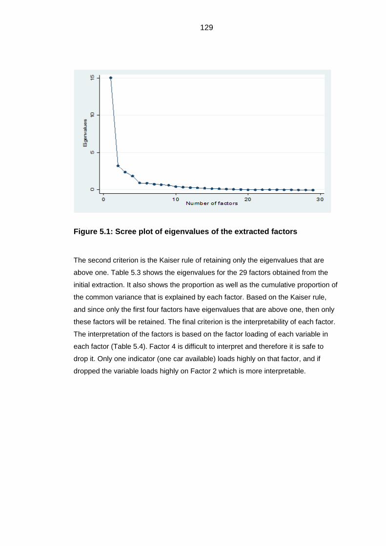
129
Figure 5.1: Scree plot of eigenvalues of the extracted factors
The second criterion is the Kaiser rule of retaining only the eigenvalues that are
above one. Table 5.3 shows the eigenvalues for the 29 factors obtained from the
initial extraction. It also shows the proportion as well as the cumulative proportion of
the common variance that is explained by each factor. Based on the Kaiser rule,
and since only the first four factors have eigenvalues that are above one, then only
these factors will be retained. The final criterion is the interpretability of each factor.
The interpretation of the factors is based on the factor loading of each variable in
each factor (Table 5.4). Factor 4 is difficult to interpret and therefore it is safe to
drop it. Only one indicator (one car available) loads highly on that factor, and if
dropped the variable loads highly on Factor 2 which is more interpretable.
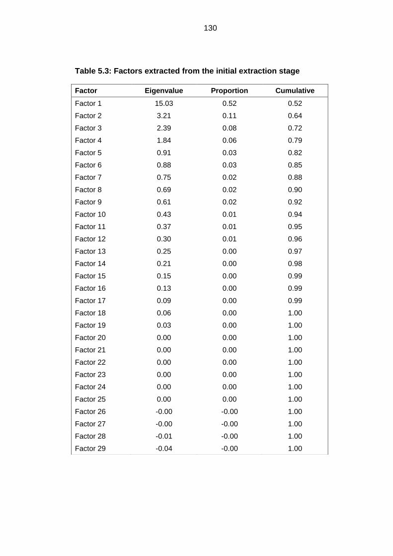
130
Table 5.3: Factors extracted from the initial extraction stage
Factor Eigenvalue Proportion Cumulative
Factor 1 15.03 0.52 0.52
Factor 2 3.21 0.11 0.64
Factor 3 2.39 0.08 0.72
Factor 4 1.84 0.06 0.79
Factor 5 0.91 0.03 0.82
Factor 6 0.88 0.03 0.85
Factor 7 0.75 0.02 0.88
Factor 8 0.69 0.02 0.90
Factor 9 0.61 0.02 0.92
Factor 10 0.43 0.01 0.94
Factor 11 0.37 0.01 0.95
Factor 12 0.30 0.01 0.96
Factor 13 0.25 0.00 0.97
Factor 14 0.21 0.00 0.98
Factor 15 0.15 0.00 0.99
Factor 16 0.13 0.00 0.99
Factor 17 0.09 0.00 0.99
Factor 18 0.06 0.00 1.00
Factor 19 0.03 0.00 1.00
Factor 20 0.00 0.00 1.00
Factor 21 0.00 0.00 1.00
Factor 22 0.00 0.00 1.00
Factor 23 0.00 0.00 1.00
Factor 24 0.00 0.00 1.00
Factor 25 0.00 0.00 1.00
Factor 26 -0.00 -0.00 1.00
Factor 27 -0.00 -0.00 1.00
Factor 28 -0.01 -0.00 1.00
Factor 29 -0.04 -0.00 1.00
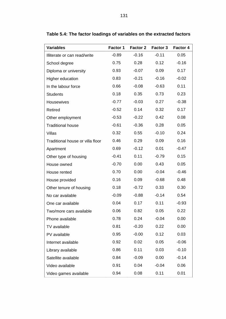
131
Table 5.4: The factor loadings of variables on the extracted factors
Variables Factor 1 Factor 2 Factor 3 Factor 4
Illiterate or can read/write -0.89 -0.16 -0.11 0.05
School degree 0.75 0.28 0.12 -0.16
Diploma or university 0.93 -0.07 0.09 0.17
Higher education 0.83 -0.21 -0.16 -0.02
In the labour force 0.66 -0.08 -0.63 0.11
Students 0.18 0.35 0.73 0.23
Housewives -0.77 -0.03 0.27 -0.38
Retired -0.52 0.14 0.32 0.17
Other employment -0.53 -0.22 0.42 0.08
Traditional house -0.61 -0.36 0.28 0.05
Villas 0.32 0.55 -0.10 0.24
Traditional house or villa floor 0.46 0.29 0.09 0.16
Apartment 0.69 -0.12 0.01 -0.47
Other type of housing -0.41 0.11 -0.79 0.15
House owned -0.70 0.00 0.43 0.05
House rented 0.70 0.00 -0.04 -0.46
House provided 0.16 0.09 -0.68 0.48
Other tenure of housing 0.18 -0.72 0.33 0.30
No car available -0.09 -0.88 -0.14 0.54
One car available 0.04 0.17 0.11 -0.93
Two/more cars available 0.06 0.82 0.05 0.22
Phone available 0.78 0.24 -0.04 0.00
TV available 0.81 -0.20 0.22 0.00
PV available 0.95 -0.00 0.12 0.03
Internet available 0.92 0.02 0.05 -0.06
Library available 0.86 0.11 0.03 -0.10
Satellite available 0.84 -0.09 0.00 -0.14
Video available 0.91 0.04 -0.04 0.06
Video games available 0.94 0.08 0.11 0.01
132
Factor rotation 5.2.3
Figure 5.2 presents the non-rotated factor solution for the three factors. Factor
loading plots help in visually identifying variables with high loadings on specific
variables. The non-rotated factor solution does not present a distinguishable pattern
of loadings of the indicator variables. Interpretation of these factors proved to be
difficult as some factors had high loadings on two factors, for example the ‘rented
home’ and ‘living in apartment’ variables had a high loading on both Factor 1 and
Factor 2. Therefore, these factors were rotated using the oblique factor rotation
method.
Figure 5.3 presents the rotated factor solution. The rotation made it possible to
distinguish between the high and low loadings of factors. For example, in the first
plot of Factor 1 against Factor 2, high loadings for Factor 1 were seen for the
availability of household items, such as a PC, TV and satellite, also, a high loading
was found for the ‘living in apartments’ and ‘in the labour force’ variables.
Furthermore, high loadings on Factor 2 were seen for ‘having two or more cars’ and
living in ‘villas’. In the plot of Factor 2 against Factor 3, a clear distinction can be
made for the variables with high loadings on Factor 3, these were for ‘other
employment’, ‘traditional house’ and the house tenure is ‘owned’. The ‘students’
variable happened to have a high loading on both Factor 2 and Factor 3.
This plot is a reflection of the table of loadings available in Table 5.5. Inspection of
the factor loadings from this table, and from the loading plots made it possible to
label the factors. Factor 1 was labelled ‘middle class’, Factor 2 ‘affluent class’ and
Factor 3 ‘deprived class’.
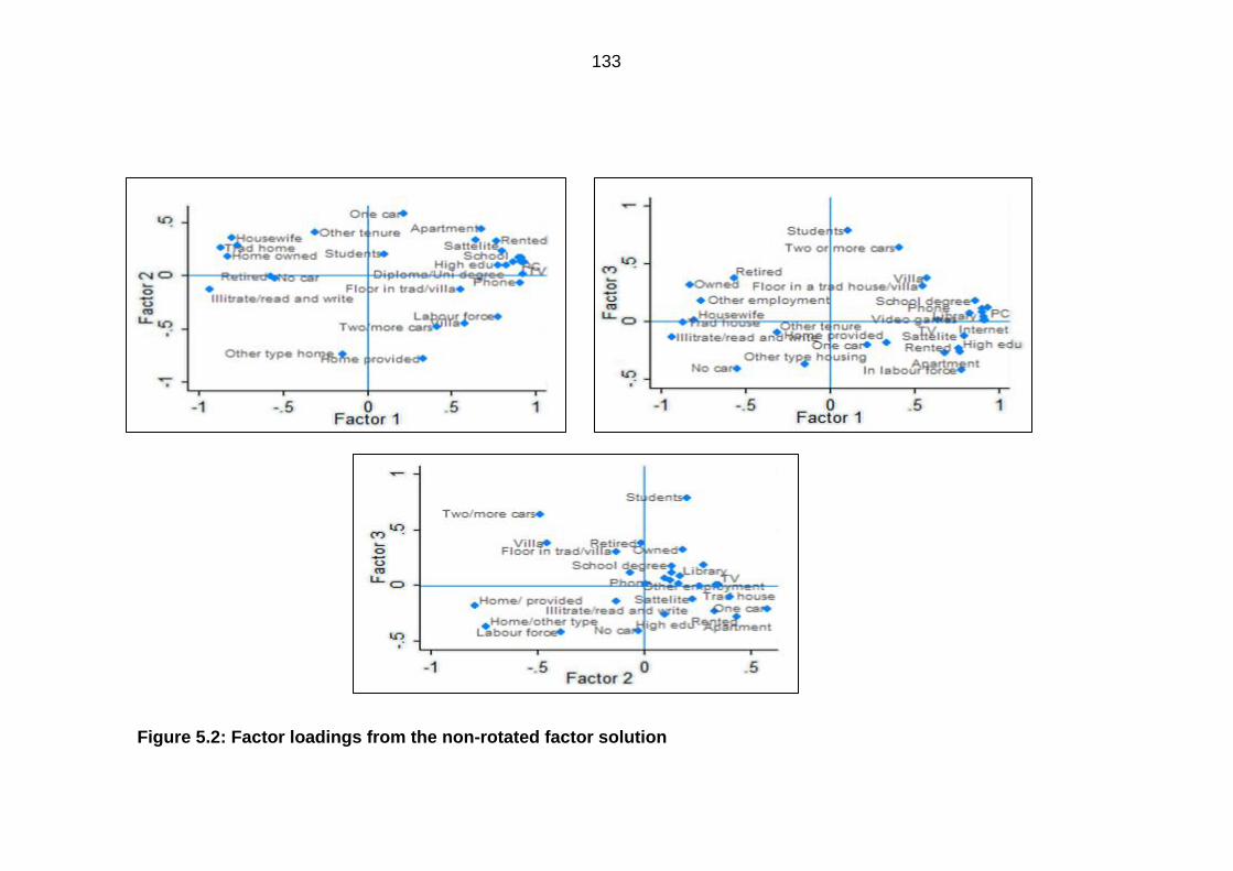
133
Figure 5.2: Factor loadings from the non-rotated factor solution
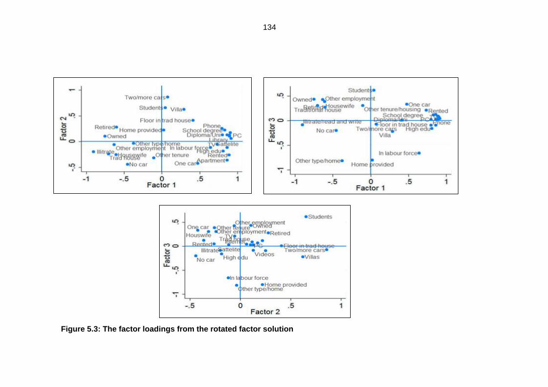
134
Figure 5.3: The factor loadings from the rotated factor solution
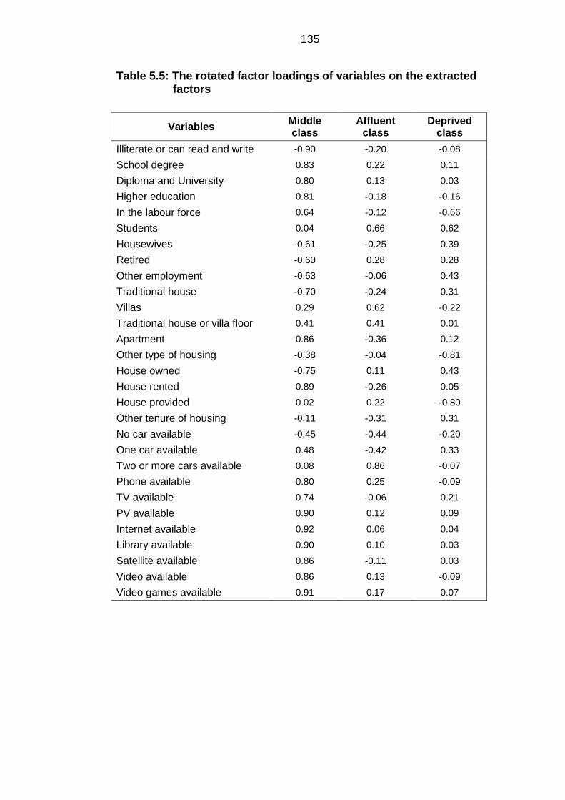
135
Table 5.5: The rotated factor loadings of variables on the extracted factors
Variables Middle class
Affluent class
Deprived class
Illiterate or can read and write -0.90 -0.20 -0.08
School degree 0.83 0.22 0.11
Diploma and University 0.80 0.13 0.03
Higher education 0.81 -0.18 -0.16
In the labour force 0.64 -0.12 -0.66
Students 0.04 0.66 0.62
Housewives -0.61 -0.25 0.39
Retired -0.60 0.28 0.28
Other employment -0.63 -0.06 0.43
Traditional house -0.70 -0.24 0.31
Villas 0.29 0.62 -0.22
Traditional house or villa floor 0.41 0.41 0.01
Apartment 0.86 -0.36 0.12
Other type of housing -0.38 -0.04 -0.81
House owned -0.75 0.11 0.43
House rented 0.89 -0.26 0.05
House provided 0.02 0.22 -0.80
Other tenure of housing -0.11 -0.31 0.31
No car available -0.45 -0.44 -0.20
One car available 0.48 -0.42 0.33
Two or more cars available 0.08 0.86 -0.07
Phone available 0.80 0.25 -0.09
TV available 0.74 -0.06 0.21
PV available 0.90 0.12 0.09
Internet available 0.92 0.06 0.04
Library available 0.90 0.10 0.03
Satellite available 0.86 -0.11 0.03
Video available 0.86 0.13 -0.09
Video games available 0.91 0.17 0.07
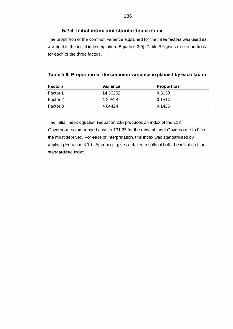
136
Initial index and standardised index 5.2.4
The proportion of the common variance explained for the three factors was used as
a weight in the initial index equation (Equation 3.9). Table 5.6 gives the proportions
for each of the three factors.
Table 5.6: Proportion of the common variance explained by each factor
The initial index equation (Equation 3.9) produces an index of the 118
Governorates that range between 131.25 for the most affluent Governorate to 0 for
the most deprived. For ease of interpretation, this index was standardised by
applying Equation 3.10. Appendix I gives detailed results of both the initial and the
standardised index.
Factors Variance Proportion
Factor 1 14.63252 0.5158
Factor 2 4.29528 0.1514
Factor 3 4.04424 0.1426

137
5.3 Classes of socioeconomic status
The LCA method was used to formulate the index. The results are presented in the
same order as they were explained in Chapter 3.
Deciding the number of classes 5.3.1
The model fit indices for the one- to four-class models are presented in Table 5.7.
Both the two- and four-class solutions have entropy very close to one (0.98),
indicating that the accuracy of classification is excellent. Also, the LMR-LRT and
BLRT tests resulted in a significant P-value, indicating that these two class models
are better than a k-1 class model. However, the AIC, BIC and ABIC were lower in
the four-class solution, hence giving it more preference than a two-class model.
Also, the four-class solution is more interpretable, as it groups the Governorates
into four clear homogenous groups, rather than two groups. Hence, the four-class
model was chosen. Specifying a five-class model would not allow the model to
converge.
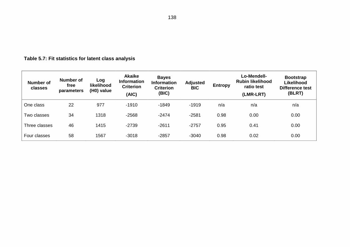
138
Table 5.7: Fit statistics for latent class analysis
Number of classes
Number of free
parameters
Log likelihood (H0) value
Akaike Information
Criterion
(AIC)
Bayes Information
Criterion (BIC)
Adjusted BIC
Entropy
Lo-Mendell-Rubin likelihood
ratio test
(LMR-LRT)
Bootstrap Likelihood
Difference test (BLRT)
One class 22 977 -1910 -1849 -1919 n/a n/a n/a
Two classes 34 1318 -2568 -2474 -2581 0.98 0.00 0.00
Three classes 46 1415 -2739 -2611 -2757 0.95 0.41 0.00
Four classes 58 1567 -3018 -2857 -3040 0.98 0.02 0.00

139
Examining the quality of latent class membership 5.3.2
The class membership of each Governorate is decided by means of modal
assignment probability. If the probability is very high and the class separation is
large, then the class membership is of high quality. Appendix J provides the final
class four-class solution, as well as the modal assignment probability. It can be
seen that the class separation is large. Therefore, the quality of modal assignment
is very good. A further measure of the quality of class membership is the entropy
(Table 5.7). The entropy is very high for the four-class solution (0.98) indicating that
the classification of the classes is very much accurate.
Defining and labelling classes 5.3.3
Figure 5.4 gives the probability plot for the four-class solution. This plot is used to
define and label each class. Since the indicator variables chosen are the
disadvantage variables, the lower the probability of each variable the greater the
affluence indicated. Class 1 shows a low probability in all indicators except for the
‘living in a floor of the traditional or villa’ variable and the ‘house not owned’
variable, indicating that Class 1 represents the most affluent Governorates and has
been labelled ‘the affluent class’; this includes 11.1% of the Governorates. Class 4
is shown to have the highest probability of all variables except for ‘living in a floor of
a traditional house or villa’ and ‘house not owned’ variables, thereby indicating that
this variable represents the most deprived Governorates, and includes 11.01% of
Governorates. Class 2 is labelled ‘upper middle class’ and includes 44.91% of
Governorates. Class 3 is labelled ‘lower middle class’ and includes 33.05% of
Governorates and finally Class 4 is labelled ‘the deprived class’ and includes
11.01% of Governorates.
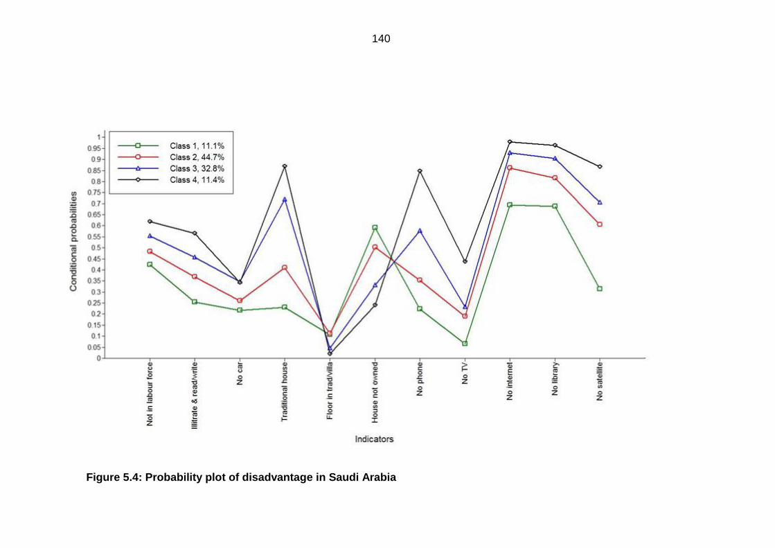
140
Figure 5.4: Probability plot of disadvantage in Saudi Arabia
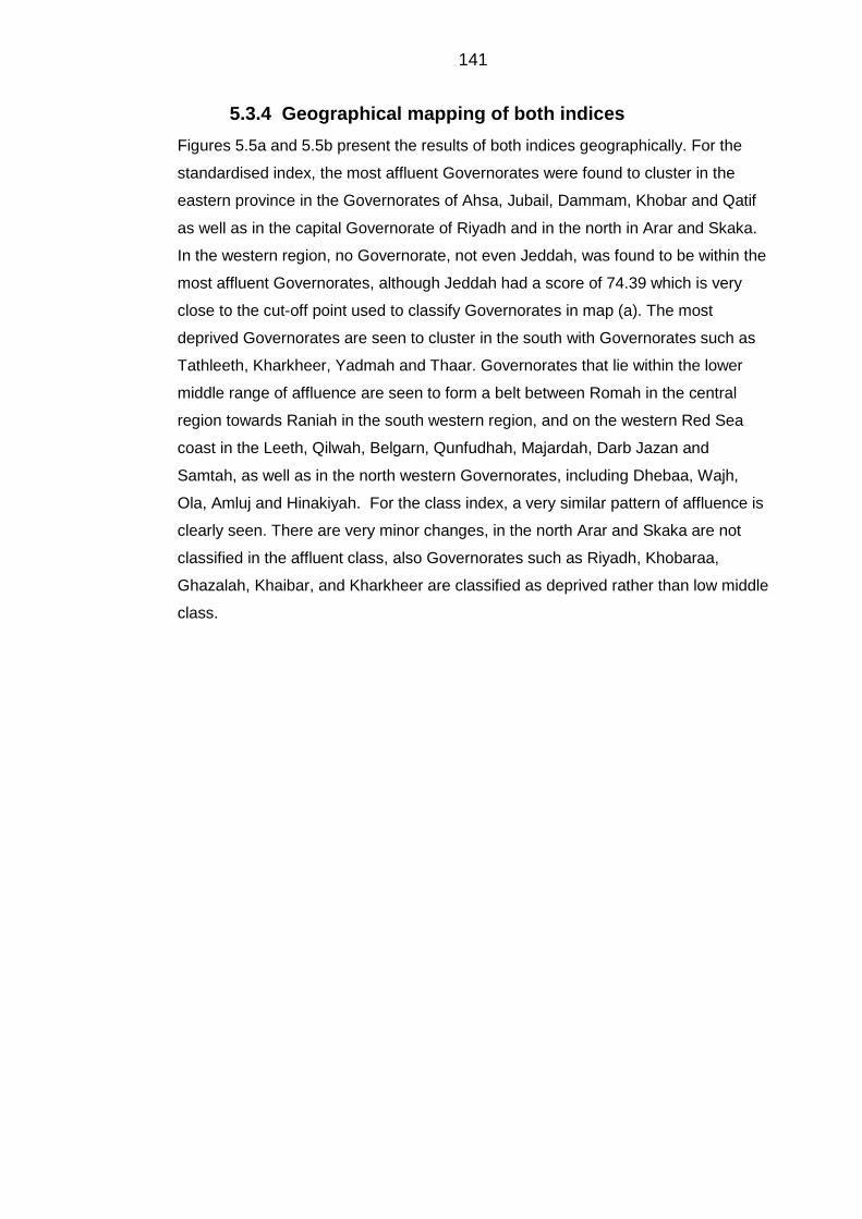
141
Geographical mapping of both indices 5.3.4
Figures 5.5a and 5.5b present the results of both indices geographically. For the
standardised index, the most affluent Governorates were found to cluster in the
eastern province in the Governorates of Ahsa, Jubail, Dammam, Khobar and Qatif
as well as in the capital Governorate of Riyadh and in the north in Arar and Skaka.
In the western region, no Governorate, not even Jeddah, was found to be within the
most affluent Governorates, although Jeddah had a score of 74.39 which is very
close to the cut-off point used to classify Governorates in map (a). The most
deprived Governorates are seen to cluster in the south with Governorates such as
Tathleeth, Kharkheer, Yadmah and Thaar. Governorates that lie within the lower
middle range of affluence are seen to form a belt between Romah in the central
region towards Raniah in the south western region, and on the western Red Sea
coast in the Leeth, Qilwah, Belgarn, Qunfudhah, Majardah, Darb Jazan and
Samtah, as well as in the north western Governorates, including Dhebaa, Wajh,
Ola, Amluj and Hinakiyah. For the class index, a very similar pattern of affluence is
clearly seen. There are very minor changes, in the north Arar and Skaka are not
classified in the affluent class, also Governorates such as Riyadh, Khobaraa,
Ghazalah, Khaibar, and Kharkheer are classified as deprived rather than low middle
class.
142
a) Standardised index b) Class index
Figure 5.5: Geographical representation of the standardised index and the class index for Saudi Governorates
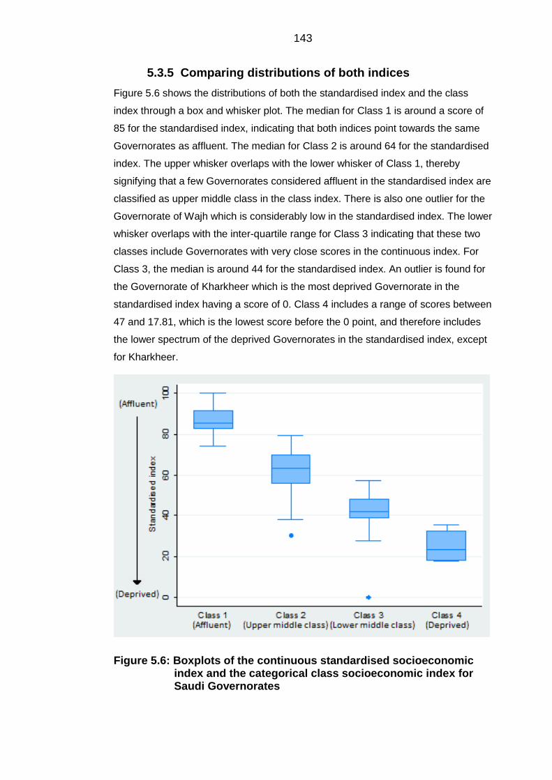
143
Comparing distributions of both indices 5.3.5
Figure 5.6 shows the distributions of both the standardised index and the class
index through a box and whisker plot. The median for Class 1 is around a score of
85 for the standardised index, indicating that both indices point towards the same
Governorates as affluent. The median for Class 2 is around 64 for the standardised
index. The upper whisker overlaps with the lower whisker of Class 1, thereby
signifying that a few Governorates considered affluent in the standardised index are
classified as upper middle class in the class index. There is also one outlier for the
Governorate of Wajh which is considerably low in the standardised index. The lower
whisker overlaps with the inter-quartile range for Class 3 indicating that these two
classes include Governorates with very close scores in the continuous index. For
Class 3, the median is around 44 for the standardised index. An outlier is found for
the Governorate of Kharkheer which is the most deprived Governorate in the
standardised index having a score of 0. Class 4 includes a range of scores between
47 and 17.81, which is the lowest score before the 0 point, and therefore includes
the lower spectrum of the deprived Governorates in the standardised index, except
for Kharkheer.
Figure 5.6: Boxplots of the continuous standardised socioeconomic index and the categorical class socioeconomic index for Saudi Governorates

144
The linear pattern in the distribution of the box plots shows that the two indices
point towards the same Governorates as either affluent or deprived, except for
minor differences expressed in the whiskers and outliers.
145
6 Results: Regression analyses of population mixing and
socioeconomic status, sensitivity analyses and
ascertainment of cases
All data presented are for the calendar years from 1994 to 2008 and are presented
in the order in which they appear in the methods. Analytical methods were dealt
with in Chapter 4.
6.1 Regression analyses
The first attempt at regression involved a Poisson regression. However, the data
exhibited a large overdispersion that the Poisson model was simply not able to
account for, as well as a large number of zero cells. It was also found that α > 0,
indicating that Poisson was not an ideal method and therefore the negative binomial
model was used instead.
The univariable analysis showed that only the SES variables were statistically
significant (P<0.00). Nevertheless, the PM variable was modelled by year of
diagnosis to check for any variation in incidence. The IRR for PM and its relative
95%CI for all diagnostic groups were plotted in Figures 6.1-6.4. The IRRs have
been log transformed to show a clearer picture, hence the point of no effect is zero.
The figures clearly showed that PM in Makkah compared to the rest of the
Governorates has no significant effect on the incidence of all diagnostic groups.
Only for CNS in the year 1997 is there a borderline significant elevated risk (Non-
logged IRR = 2.43, 95%CI = 0.99 - 5.98, logged IRR = 0.88, 95%CI = -0.01 - 1.78).
For CML, other leukaemias group, BL and other lymphomas group, some years had
no cases reported in Makkah.
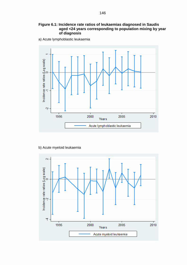
146
Figure 6.1: Incidence rate ratios of leukaemias diagnosed in Saudis aged <24 years corresponding to population mixing by year of diagnosis
a) Acute lymphoblastic leukaemia
b) Acute myeloid leukaemia
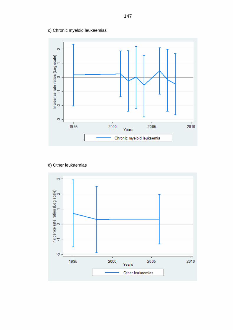
147
c) Chronic myeloid leukaemias
d) Other leukaemias
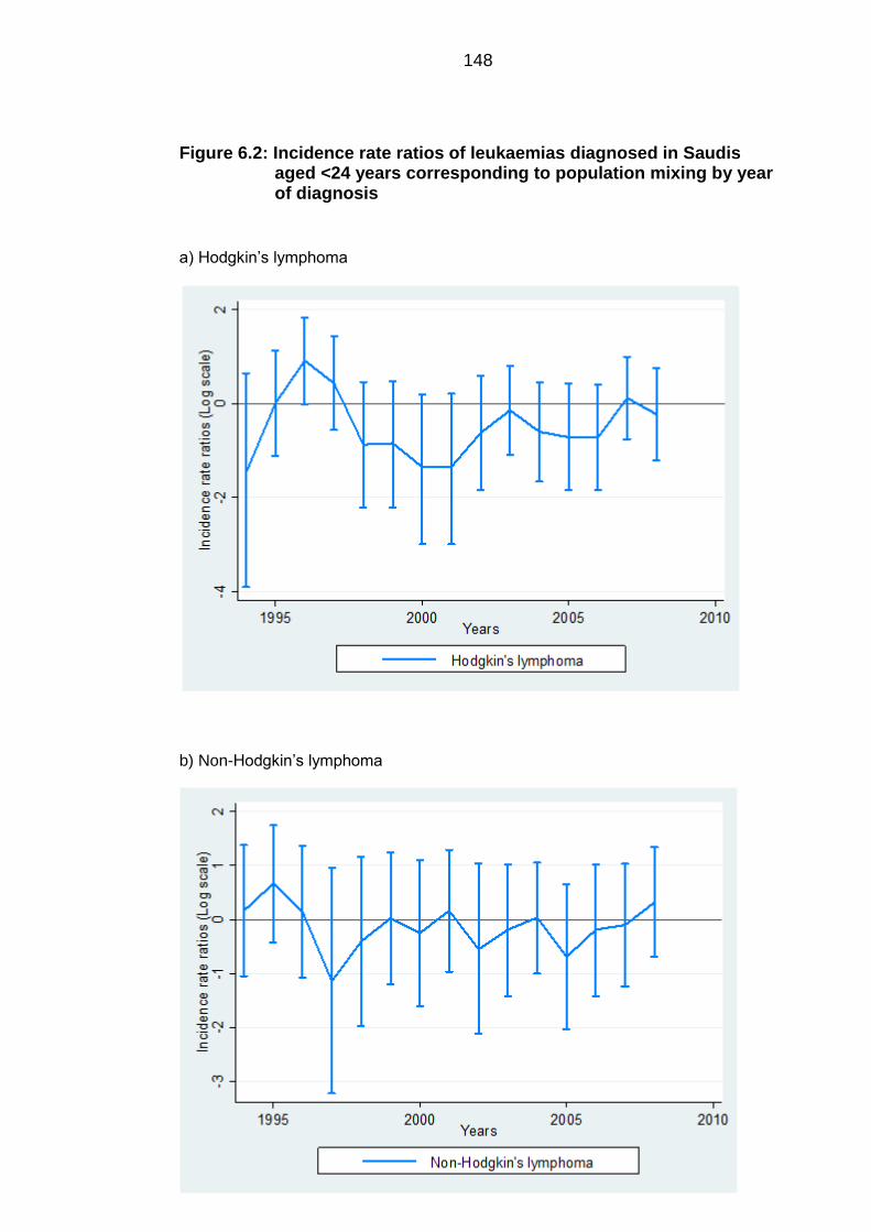
148
Figure 6.2: Incidence rate ratios of leukaemias diagnosed in Saudis aged <24 years corresponding to population mixing by year of diagnosis
a) Hodgkin’s lymphoma
b) Non-Hodgkin’s lymphoma
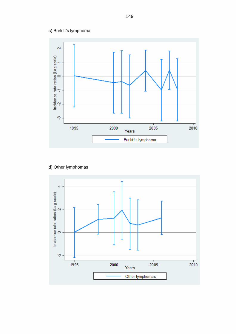
149
c) Burkitt’s lymphoma
d) Other lymphomas
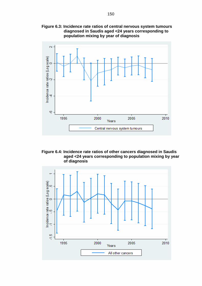
150
Figure 6.3: Incidence rate ratios of central nervous system tumours diagnosed in Saudis aged <24 years corresponding to population mixing by year of diagnosis
Figure 6.4: Incidence rate ratios of other cancers diagnosed in Saudis aged <24 years corresponding to population mixing by year of diagnosis
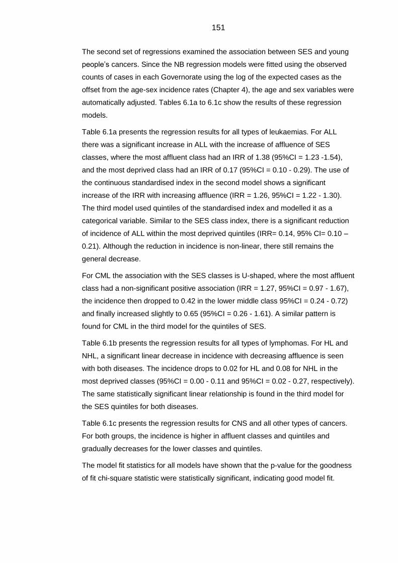
151
The second set of regressions examined the association between SES and young
people’s cancers. Since the NB regression models were fitted using the observed
counts of cases in each Governorate using the log of the expected cases as the
offset from the age-sex incidence rates (Chapter 4), the age and sex variables were
automatically adjusted. Tables 6.1a to 6.1c show the results of these regression
models.
Table 6.1a presents the regression results for all types of leukaemias. For ALL
there was a significant increase in ALL with the increase of affluence of SES
classes, where the most affluent class had an IRR of 1.38 (95%CI = 1.23 -1.54),
and the most deprived class had an IRR of 0.17 (95%CI = 0.10 - 0.29). The use of
the continuous standardised index in the second model shows a significant
increase of the IRR with increasing affluence (IRR = 1.26, 95%CI = 1.22 - 1.30).
The third model used quintiles of the standardised index and modelled it as a
categorical variable. Similar to the SES class index, there is a significant reduction
of incidence of ALL within the most deprived quintiles (IRR= 0.14, 95% CI= 0.10 –
0.21). Although the reduction in incidence is non-linear, there still remains the
general decrease.
For CML the association with the SES classes is U-shaped, where the most affluent
class had a non-significant positive association (IRR = 1.27, 95%CI = 0.97 - 1.67),
the incidence then dropped to 0.42 in the lower middle class 95%CI = 0.24 - 0.72)
and finally increased slightly to 0.65 (95%CI = 0.26 - 1.61). A similar pattern is
found for CML in the third model for the quintiles of SES.
Table 6.1b presents the regression results for all types of lymphomas. For HL and
NHL, a significant linear decrease in incidence with decreasing affluence is seen
with both diseases. The incidence drops to 0.02 for HL and 0.08 for NHL in the
most deprived classes (95%CI = 0.00 - 0.11 and 95%CI = 0.02 - 0.27, respectively).
The same statistically significant linear relationship is found in the third model for
the SES quintiles for both diseases.
Table 6.1c presents the regression results for CNS and all other types of cancers.
For both groups, the incidence is higher in affluent classes and quintiles and
gradually decreases for the lower classes and quintiles.
The model fit statistics for all models have shown that the p-value for the goodness
of fit chi-square statistic were statistically significant, indicating good model fit.
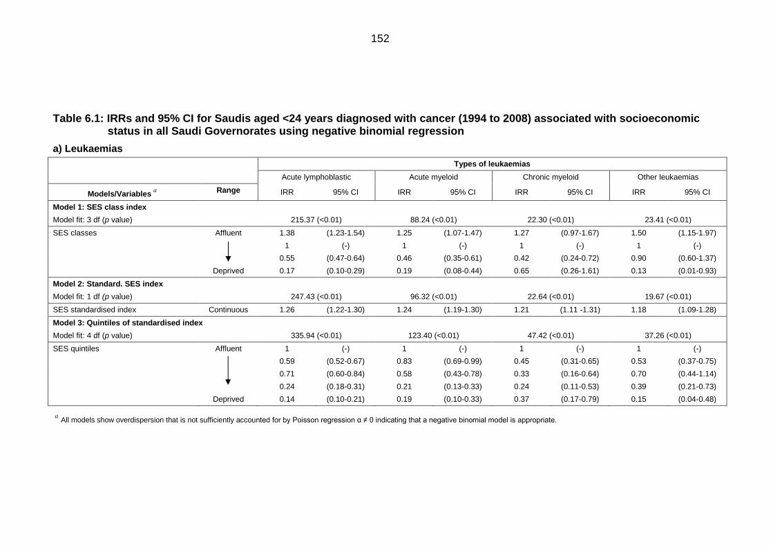
152
Table 6.1: IRRs and 95% CI for Saudis aged <24 years diagnosed with cancer (1994 to 2008) associated with socioeconomic status in all Saudi Governorates using negative binomial regression
a) Leukaemias
aAll models show overdispersion that is not sufficiently accounted for by Poisson regression α ≠ 0 indicating that a negative binomial model is appropriate.
Types of leukaemias
Acute lymphoblastic Acute myeloid Chronic myeloid Other leukaemias
Models/Variablesa
Range IRR 95% CI IRR 95% CI IRR 95% CI IRR 95% CI
Model 1: SES class index
Model fit: 3 df (p value) 215.37 (<0.01) 88.24 (<0.01) 22.30 (<0.01) 23.41 (<0.01)
SES classes Affluent 1.38 (1.23-1.54) 1.25 (1.07-1.47) 1.27 (0.97-1.67) 1.50 (1.15-1.97)
1 (-) 1 (-) 1 (-) 1 (-)
0.55 (0.47-0.64) 0.46 (0.35-0.61) 0.42 (0.24-0.72) 0.90 (0.60-1.37)
Deprived 0.17 (0.10-0.29) 0.19 (0.08-0.44) 0.65 (0.26-1.61) 0.13 (0.01-0.93)
Model 2: Standard. SES index
Model fit: 1 df (p value) 247.43 (<0.01) 96.32 (<0.01) 22.64 (<0.01) 19.67 (<0.01)
SES standardised index Continuous 1.26 (1.22-1.30) 1.24 (1.19-1.30) 1.21 (1.11 -1.31) 1.18 (1.09-1.28)
Model 3: Quintiles of standardised index
Model fit: 4 df (p value) 335.94 (<0.01) 123.40 (<0.01) 47.42 (<0.01) 37.26 (<0.01)
SES quintiles Affluent 1 (-) 1 (-) 1 (-) 1 (-)
0.59 (0.52-0.67) 0.83 (0.69-0.99) 0.45 (0.31-0.65) 0.53 (0.37-0.75)
0.71 (0.60-0.84) 0.58 (0.43-0.78) 0.33 (0.16-0.64) 0.70 (0.44-1.14)
0.24 (0.18-0.31) 0.21 (0.13-0.33) 0.24 (0.11-0.53) 0.39 (0.21-0.73)
Deprived 0.14 (0.10-0.21) 0.19 (0.10-0.33) 0.37 (0.17-0.79) 0.15 (0.04-0.48)
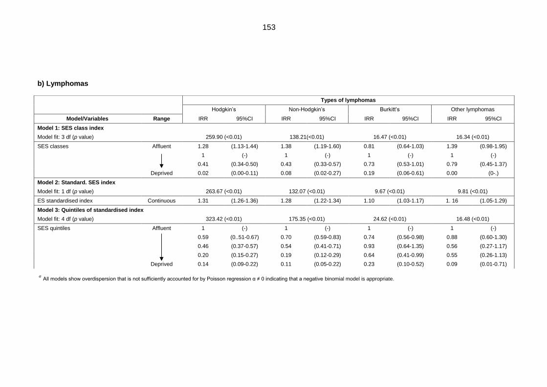
153
b) Lymphomas
aAll models show overdispersion that is not sufficiently accounted for by Poisson regression α ≠ 0 indicating that a negative binomial model is appropriate.
Types of lymphomas
Hodgkin’s Non-Hodgkin’s Burkitt’s Other lymphomas
Model/Variables Range IRR 95%CI IRR 95%CI IRR 95%CI IRR 95%CI
Model 1: SES class index
Model fit: 3 df (p value) 259.90 (<0.01) 138.21(<0.01) 16.47 (<0.01) 16.34 (<0.01)
SES classes Affluent 1.28 (1.13-1.44) 1.38 (1.19-1.60) 0.81 (0.64-1.03) 1.39 (0.98-1.95)
1 (-) 1 (-) 1 (-) 1 (-)
0.41 (0.34-0.50) 0.43 (0.33-0.57) 0.73 (0.53-1.01) 0.79 (0.45-1.37)
Deprived 0.02 (0.00-0.11) 0.08 (0.02-0.27) 0.19 (0.06-0.61) 0.00 (0-.)
Model 2: Standard. SES index
Model fit: 1 df (p value) 263.67 (<0.01) 132.07 (<0.01) 9.67 (<0.01) 9.81 (<0.01)
ES standardised index Continuous 1.31 (1.26-1.36) 1.28 (1.22-1.34) 1.10 (1.03-1.17) 1. 16 (1.05-1.29)
Model 3: Quintiles of standardised index
Model fit: 4 df (p value) 323.42 (<0.01) 175.35 (<0.01) 24.62 (<0.01) 16.48 (<0.01)
SES quintiles Affluent 1 (-) 1 (-) 1 (-) 1 (-)
0.59 (0..51-0.67) 0.70 (0.59-0.83) 0.74 (0.56-0.98) 0.88 (0.60-1.30)
0.46 (0.37-0.57) 0.54 (0.41-0.71) 0.93 (0.64-1.35) 0.56 (0.27-1.17)
0.20 (0.15-0.27) 0.19 (0.12-0.29) 0.64 (0.41-0.99) 0.55 (0.26-1.13)
Deprived 0.14 (0.09-0.22) 0.11 (0.05-0.22) 0.23 (0.10-0.52) 0.09 (0.01-0.71)
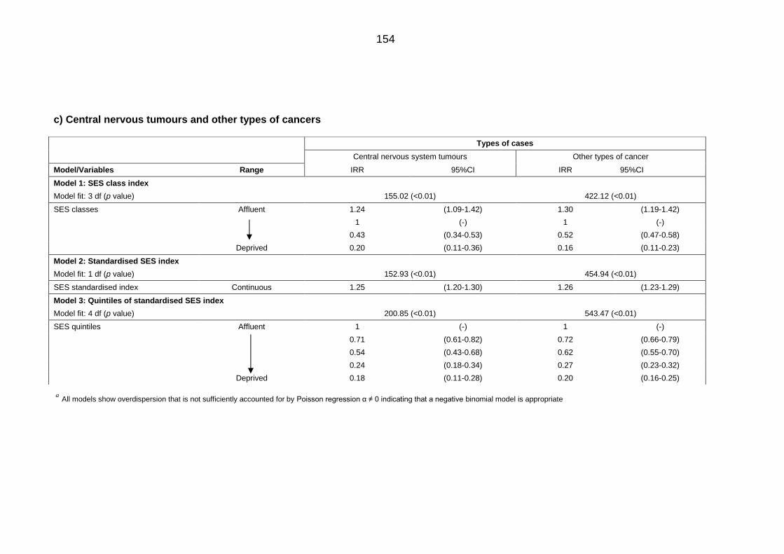
154
c) Central nervous tumours and other types of cancers
aAll models show overdispersion that is not sufficiently accounted for by Poisson regression α ≠ 0 indicating that a negative binomial model is appropriate
Types of cases
Central nervous system tumours Other types of cancer
Model/Variables Range IRR 95%CI IRR 95%CI
Model 1: SES class index
Model fit: 3 df (p value) 155.02 (<0.01) 422.12 (<0.01)
SES classes Affluent 1.24 (1.09-1.42) 1.30 (1.19-1.42)
1 (-) 1 (-)
0.43 (0.34-0.53) 0.52 (0.47-0.58)
Deprived 0.20 (0.11-0.36) 0.16 (0.11-0.23)
Model 2: Standardised SES index
Model fit: 1 df (p value) 152.93 (<0.01) 454.94 (<0.01)
SES standardised index Continuous 1.25 (1.20-1.30) 1.26 (1.23-1.29)
Model 3: Quintiles of standardised SES index
Model fit: 4 df (p value) 200.85 (<0.01) 543.47 (<0.01)
SES quintiles Affluent 1 (-) 1 (-)
0.71 (0.61-0.82) 0.72 (0.66-0.79)
0.54 (0.43-0.68) 0.62 (0.55-0.70)
0.24 (0.18-0.34) 0.27 (0.23-0.32)
Deprived 0.18 (0.11-0.28) 0.20 (0.16-0.25)
155
6.2 Sensitivity analyses
Socioeconomic classes 6.2.1
Sensitivity analyses were conducted in order to understand how the SES classes
variable and the year variable affects the resulting IRR. Therefore, the modal
probabilities that were used to assign Governorates into their respective classes
were introduced into the model in place of the SES classes. Table 6.2 presents the
regression results.
It was found that modelling the modal probabilities for the SES classes had little to
no effect on the resulting incidence of all cancers. The direction and significance of
the associations in all groups have not changed.
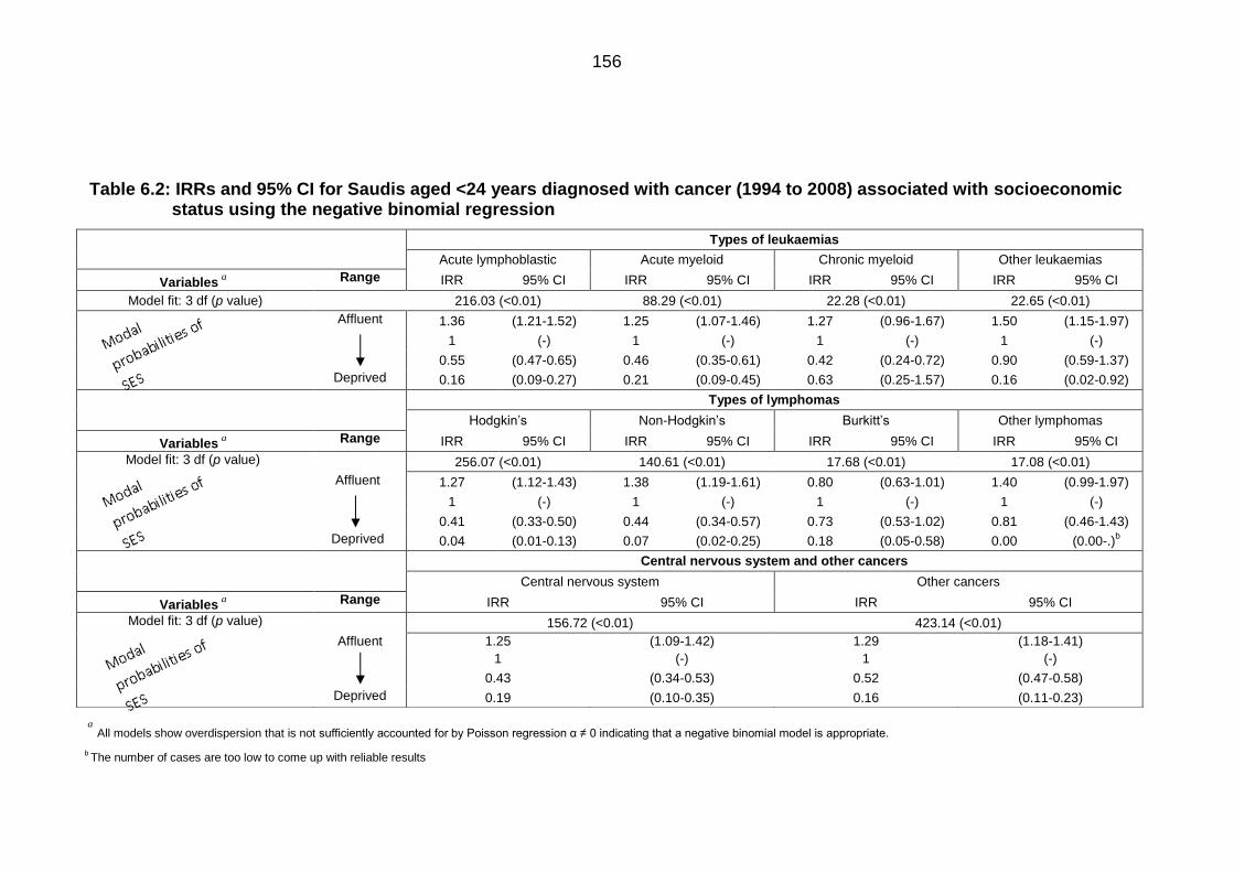
156
Table 6.2: IRRs and 95% CI for Saudis aged <24 years diagnosed with cancer (1994 to 2008) associated with socioeconomic status using the negative binomial regression
aAll models show overdispersion that is not sufficiently accounted for by Poisson regression α ≠ 0 indicating that a negative binomial model is appropriate.
b The number of cases are too low to come up with reliable results
Types of leukaemias
Acute lymphoblastic Acute myeloid Chronic myeloid Other leukaemias
Variablesa
Range IRR 95% CI IRR 95% CI IRR 95% CI IRR 95% CI
Model fit: 3 df (p value) 216.03 (<0.01) 88.29 (<0.01) 22.28 (<0.01) 22.65 (<0.01)
Affluent 1.36 (1.21-1.52) 1.25 (1.07-1.46) 1.27 (0.96-1.67) 1.50 (1.15-1.97)
1 (-) 1 (-) 1 (-) 1 (-)
0.55 (0.47-0.65) 0.46 (0.35-0.61) 0.42 (0.24-0.72) 0.90 (0.59-1.37)
Deprived 0.16 (0.09-0.27) 0.21 (0.09-0.45) 0.63 (0.25-1.57) 0.16 (0.02-0.92)
Types of lymphomas
Hodgkin’s Non-Hodgkin’s Burkitt’s Other lymphomas
Variablesa
Range IRR 95% CI IRR 95% CI IRR 95% CI IRR 95% CI
Model fit: 3 df (p value) 256.07 (<0.01) 140.61 (<0.01) 17.68 (<0.01) 17.08 (<0.01)
Affluent 1.27 (1.12-1.43) 1.38 (1.19-1.61) 0.80 (0.63-1.01) 1.40 (0.99-1.97)
1 (-) 1 (-) 1 (-) 1 (-)
0.41 (0.33-0.50) 0.44 (0.34-0.57) 0.73 (0.53-1.02) 0.81 (0.46-1.43)
Deprived 0.04 (0.01-0.13) 0.07 (0.02-0.25) 0.18 (0.05-0.58) 0.00 (0.00-.)b
Central nervous system and other cancers
Central nervous system Other cancers
Variablesa
Range IRR 95% CI IRR 95% CI
Model fit: 3 df (p value) 156.72 (<0.01) 423.14 (<0.01)
Affluent 1.25 (1.09-1.42) 1.29 (1.18-1.41)
1 (-) 1 (-)
0.43 (0.34-0.53) 0.52 (0.47-0.58)
Deprived 0.19 (0.10-0.35) 0.16 (0.11-0.23)
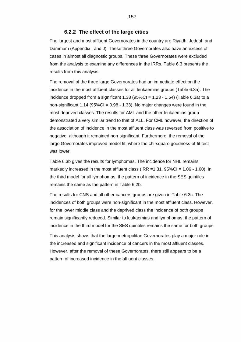
157
The effect of the large cities 6.2.2
The largest and most affluent Governorates in the country are Riyadh, Jeddah and
Dammam (Appendix I and J). These three Governorates also have an excess of
cases in almost all diagnostic groups. These three Governorates were excluded
from the analysis to examine any differences in the IRRs. Table 6.3 presents the
results from this analysis.
The removal of the three large Governorates had an immediate effect on the
incidence in the most affluent classes for all leukaemias groups (Table 6.3a). The
incidence dropped from a significant 1.38 (95%CI = 1.23 - 1.54) (Table 6.3a) to a
non-significant 1.14 (95%CI = 0.98 - 1.33). No major changes were found in the
most deprived classes. The results for AML and the other leukaemias group
demonstrated a very similar trend to that of ALL. For CML however, the direction of
the association of incidence in the most affluent class was reversed from positive to
negative, although it remained non-significant. Furthermore, the removal of the
large Governorates improved model fit, where the chi-square goodness-of-fit test
was lower.
Table 6.3b gives the results for lymphomas. The incidence for NHL remains
markedly increased in the most affluent class (IRR =1.31, 95%CI = 1.06 - 1.60). In
the third model for all lymphomas, the pattern of incidence in the SES quintiles
remains the same as the pattern in Table 6.2b.
The results for CNS and all other cancers groups are given in Table 6.3c. The
incidences of both groups were non-significant in the most affluent class. However,
for the lower middle class and the deprived class the incidence of both groups
remain significantly reduced. Similar to leukaemias and lymphomas, the pattern of
incidence in the third model for the SES quintiles remains the same for both groups.
This analysis shows that the large metropolitan Governorates play a major role in
the increased and significant incidence of cancers in the most affluent classes.
However, after the removal of these Governorates, there still appears to be a
pattern of increased incidence in the affluent classes.
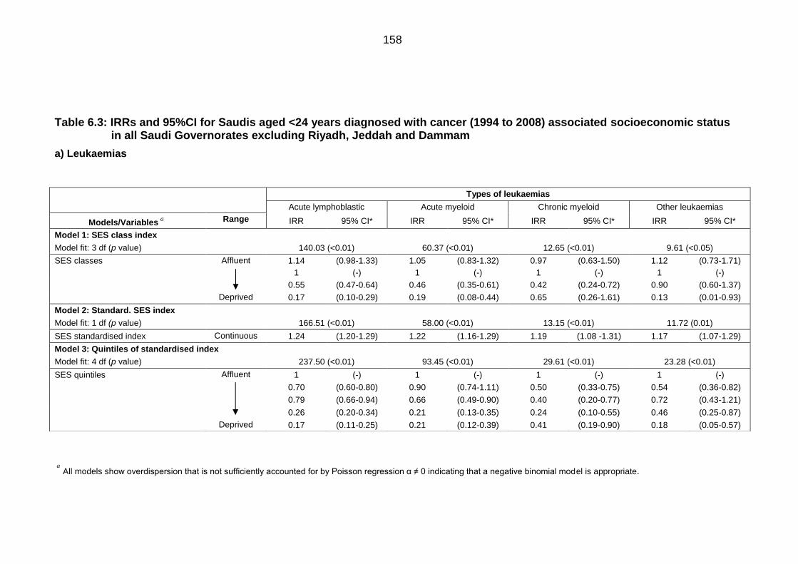
158
Table 6.3: IRRs and 95%CI for Saudis aged <24 years diagnosed with cancer (1994 to 2008) associated socioeconomic status in all Saudi Governorates excluding Riyadh, Jeddah and Dammam
a) Leukaemias
aAll models show overdispersion that is not sufficiently accounted for by Poisson regression α ≠ 0 indicating that a negative binomial model is appropriate.
Types of leukaemias
Acute lymphoblastic Acute myeloid Chronic myeloid Other leukaemias
Models/Variablesa
Range IRR 95% CI* IRR 95% CI* IRR 95% CI* IRR 95% CI*
Model 1: SES class index
Model fit: 3 df (p value) 140.03 (<0.01) 60.37 (<0.01) 12.65 (<0.01) 9.61 (<0.05)
SES classes Affluent 1.14 (0.98-1.33) 1.05 (0.83-1.32) 0.97 (0.63-1.50) 1.12 (0.73-1.71)
1 (-) 1 (-) 1 (-) 1 (-)
0.55 (0.47-0.64) 0.46 (0.35-0.61) 0.42 (0.24-0.72) 0.90 (0.60-1.37)
Deprived 0.17 (0.10-0.29) 0.19 (0.08-0.44) 0.65 (0.26-1.61) 0.13 (0.01-0.93)
Model 2: Standard. SES index
Model fit: 1 df (p value) 166.51 (<0.01) 58.00 (<0.01) 13.15 (<0.01) 11.72 (0.01)
SES standardised index Continuous 1.24 (1.20-1.29) 1.22 (1.16-1.29) 1.19 (1.08 -1.31) 1.17 (1.07-1.29)
Model 3: Quintiles of standardised index
Model fit: 4 df (p value) 237.50 (<0.01) 93.45 (<0.01) 29.61 (<0.01) 23.28 (<0.01)
SES quintiles Affluent 1 (-) 1 (-) 1 (-) 1 (-)
0.70 (0.60-0.80) 0.90 (0.74-1.11) 0.50 (0.33-0.75) 0.54 (0.36-0.82)
0.79 (0.66-0.94) 0.66 (0.49-0.90) 0.40 (0.20-0.77) 0.72 (0.43-1.21)
0.26 (0.20-0.34) 0.21 (0.13-0.35) 0.24 (0.10-0.55) 0.46 (0.25-0.87)
Deprived 0.17 (0.11-0.25) 0.21 (0.12-0.39) 0.41 (0.19-0.90) 0.18 (0.05-0.57)
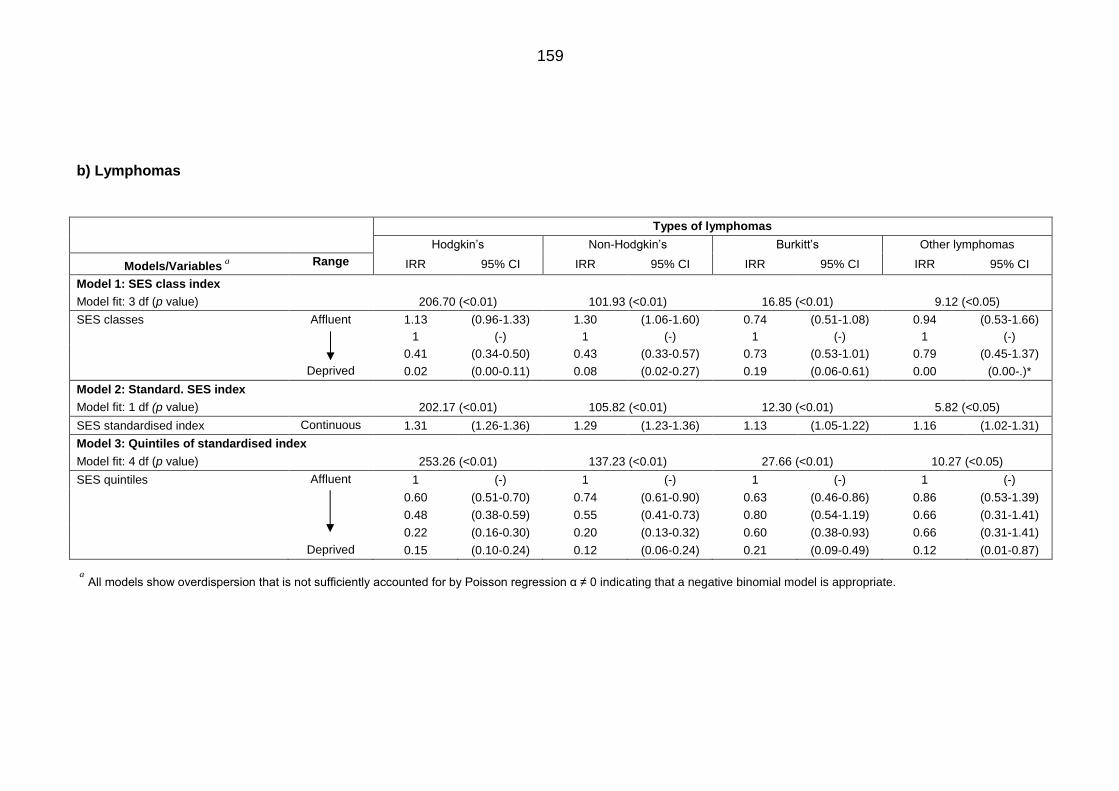
159
b) Lymphomas
aAll models show overdispersion that is not sufficiently accounted for by Poisson regression α ≠ 0 indicating that a negative binomial model is appropriate.
Types of lymphomas
Hodgkin’s Non-Hodgkin’s Burkitt’s Other lymphomas
Models/Variablesa
Range IRR 95% CI IRR 95% CI IRR 95% CI IRR 95% CI
Model 1: SES class index
Model fit: 3 df (p value) 206.70 (<0.01) 101.93 (<0.01) 16.85 (<0.01) 9.12 (<0.05)
SES classes Affluent 1.13 (0.96-1.33) 1.30 (1.06-1.60) 0.74 (0.51-1.08) 0.94 (0.53-1.66)
1 (-) 1 (-) 1 (-) 1 (-)
0.41 (0.34-0.50) 0.43 (0.33-0.57) 0.73 (0.53-1.01) 0.79 (0.45-1.37)
Deprived 0.02 (0.00-0.11) 0.08 (0.02-0.27) 0.19 (0.06-0.61) 0.00 (0.00-.)*
Model 2: Standard. SES index
Model fit: 1 df (p value) 202.17 (<0.01) 105.82 (<0.01) 12.30 (<0.01) 5.82 (<0.05)
SES standardised index Continuous 1.31 (1.26-1.36) 1.29 (1.23-1.36) 1.13 (1.05-1.22) 1.16 (1.02-1.31)
Model 3: Quintiles of standardised index
Model fit: 4 df (p value) 253.26 (<0.01) 137.23 (<0.01) 27.66 (<0.01) 10.27 (<0.05)
SES quintiles Affluent 1 (-) 1 (-) 1 (-) 1 (-)
0.60 (0.51-0.70) 0.74 (0.61-0.90) 0.63 (0.46-0.86) 0.86 (0.53-1.39)
0.48 (0.38-0.59) 0.55 (0.41-0.73) 0.80 (0.54-1.19) 0.66 (0.31-1.41)
0.22 (0.16-0.30) 0.20 (0.13-0.32) 0.60 (0.38-0.93) 0.66 (0.31-1.41)
Deprived 0.15 (0.10-0.24) 0.12 (0.06-0.24) 0.21 (0.09-0.49) 0.12 (0.01-0.87)
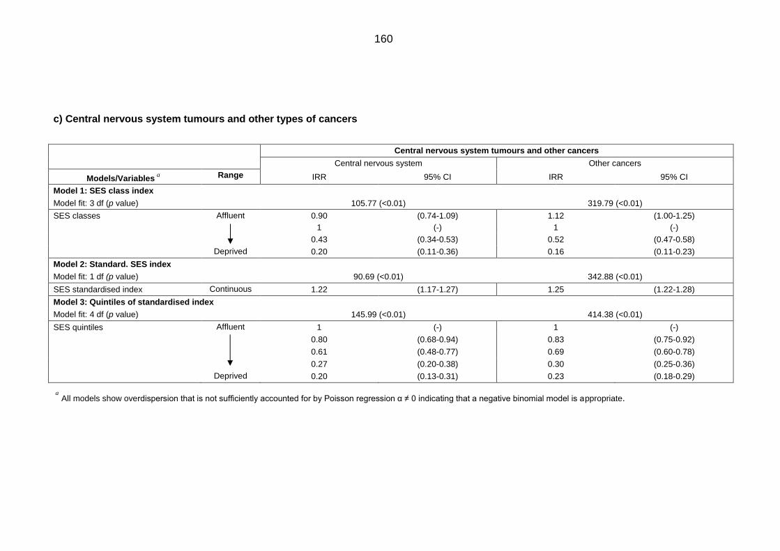
160
c) Central nervous system tumours and other types of cancers
aAll models show overdispersion that is not sufficiently accounted for by Poisson regression α ≠ 0 indicating that a negative binomial model is appropriate.
Central nervous system tumours and other cancers
Central nervous system Other cancers
Models/Variablesa
Range IRR 95% CI IRR 95% CI
Model 1: SES class index
Model fit: 3 df (p value) 105.77 (<0.01) 319.79 (<0.01)
SES classes Affluent 0.90 (0.74-1.09) 1.12 (1.00-1.25)
1 (-) 1 (-)
0.43 (0.34-0.53) 0.52 (0.47-0.58)
Deprived 0.20 (0.11-0.36) 0.16 (0.11-0.23)
Model 2: Standard. SES index
Model fit: 1 df (p value) 90.69 (<0.01) 342.88 (<0.01)
SES standardised index Continuous 1.22 (1.17-1.27) 1.25 (1.22-1.28)
Model 3: Quintiles of standardised index
Model fit: 4 df (p value) 145.99 (<0.01) 414.38 (<0.01)
SES quintiles Affluent 1 (-) 1 (-)
0.80 (0.68-0.94) 0.83 (0.75-0.92)
0.61 (0.48-0.77) 0.69 (0.60-0.78)
0.27 (0.20-0.38) 0.30 (0.25-0.36)
Deprived 0.20 (0.13-0.31) 0.23 (0.18-0.29)
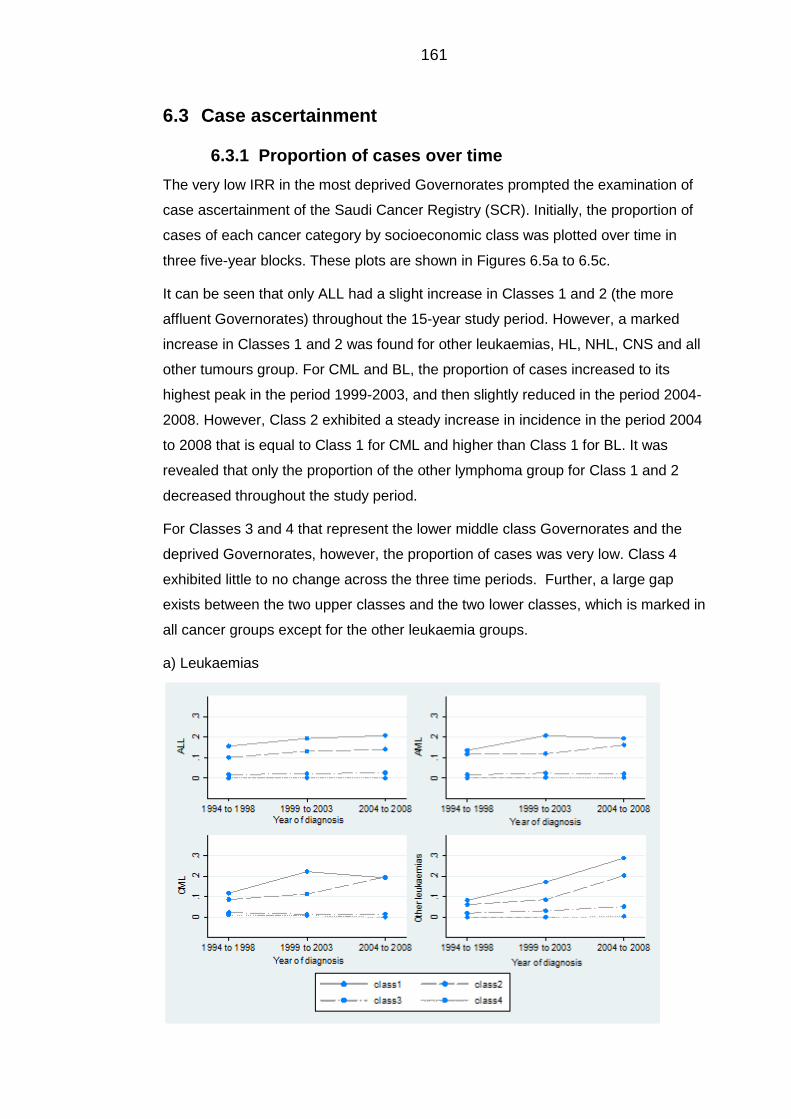
161
6.3 Case ascertainment
Proportion of cases over time 6.3.1
The very low IRR in the most deprived Governorates prompted the examination of
case ascertainment of the Saudi Cancer Registry (SCR). Initially, the proportion of
cases of each cancer category by socioeconomic class was plotted over time in
three five-year blocks. These plots are shown in Figures 6.5a to 6.5c.
It can be seen that only ALL had a slight increase in Classes 1 and 2 (the more
affluent Governorates) throughout the 15-year study period. However, a marked
increase in Classes 1 and 2 was found for other leukaemias, HL, NHL, CNS and all
other tumours group. For CML and BL, the proportion of cases increased to its
highest peak in the period 1999-2003, and then slightly reduced in the period 2004-
2008. However, Class 2 exhibited a steady increase in incidence in the period 2004
to 2008 that is equal to Class 1 for CML and higher than Class 1 for BL. It was
revealed that only the proportion of the other lymphoma group for Class 1 and 2
decreased throughout the study period.
For Classes 3 and 4 that represent the lower middle class Governorates and the
deprived Governorates, however, the proportion of cases was very low. Class 4
exhibited little to no change across the three time periods. Further, a large gap
exists between the two upper classes and the two lower classes, which is marked in
all cancer groups except for the other leukaemia groups.
a) Leukaemias
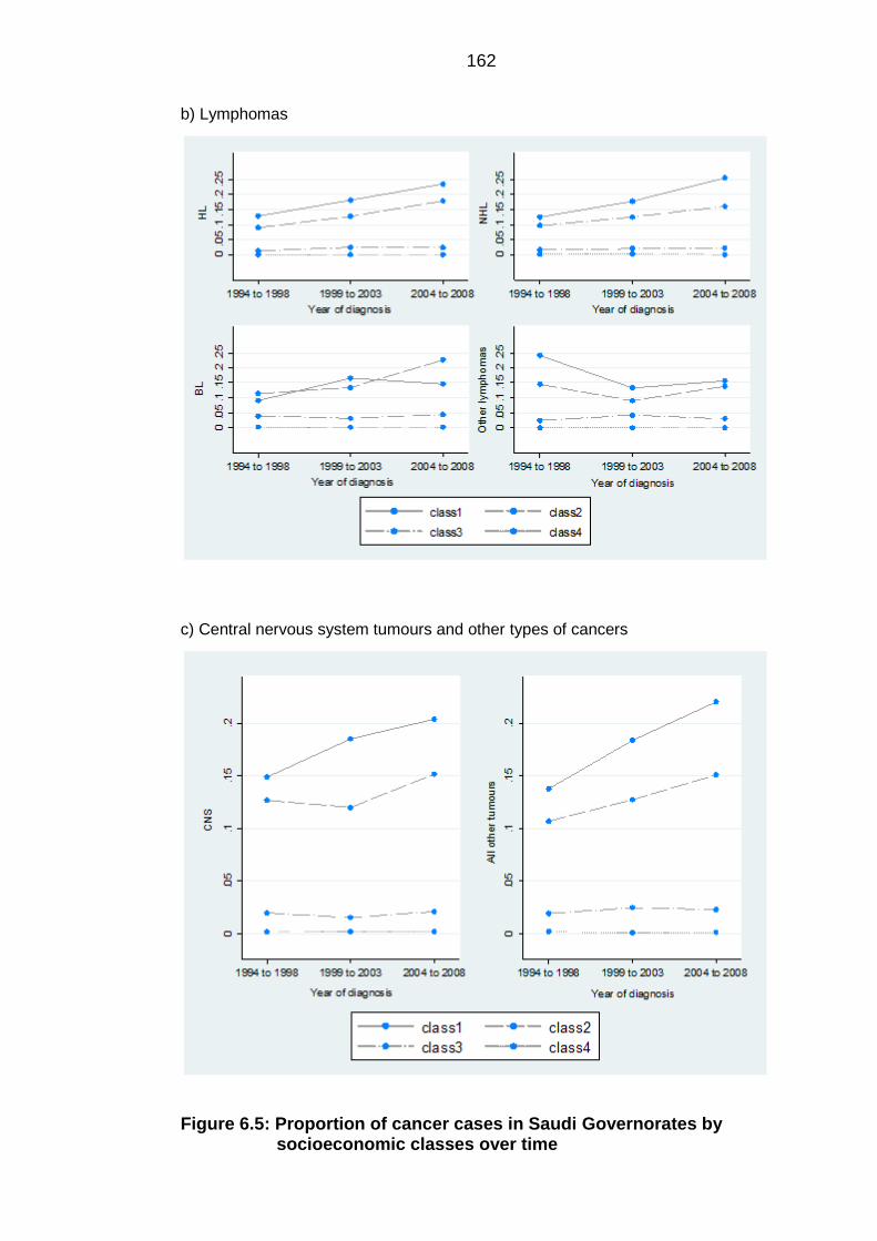
162
b) Lymphomas
c) Central nervous system tumours and other types of cancers
Figure 6.5: Proportion of cancer cases in Saudi Governorates by socioeconomic classes over time
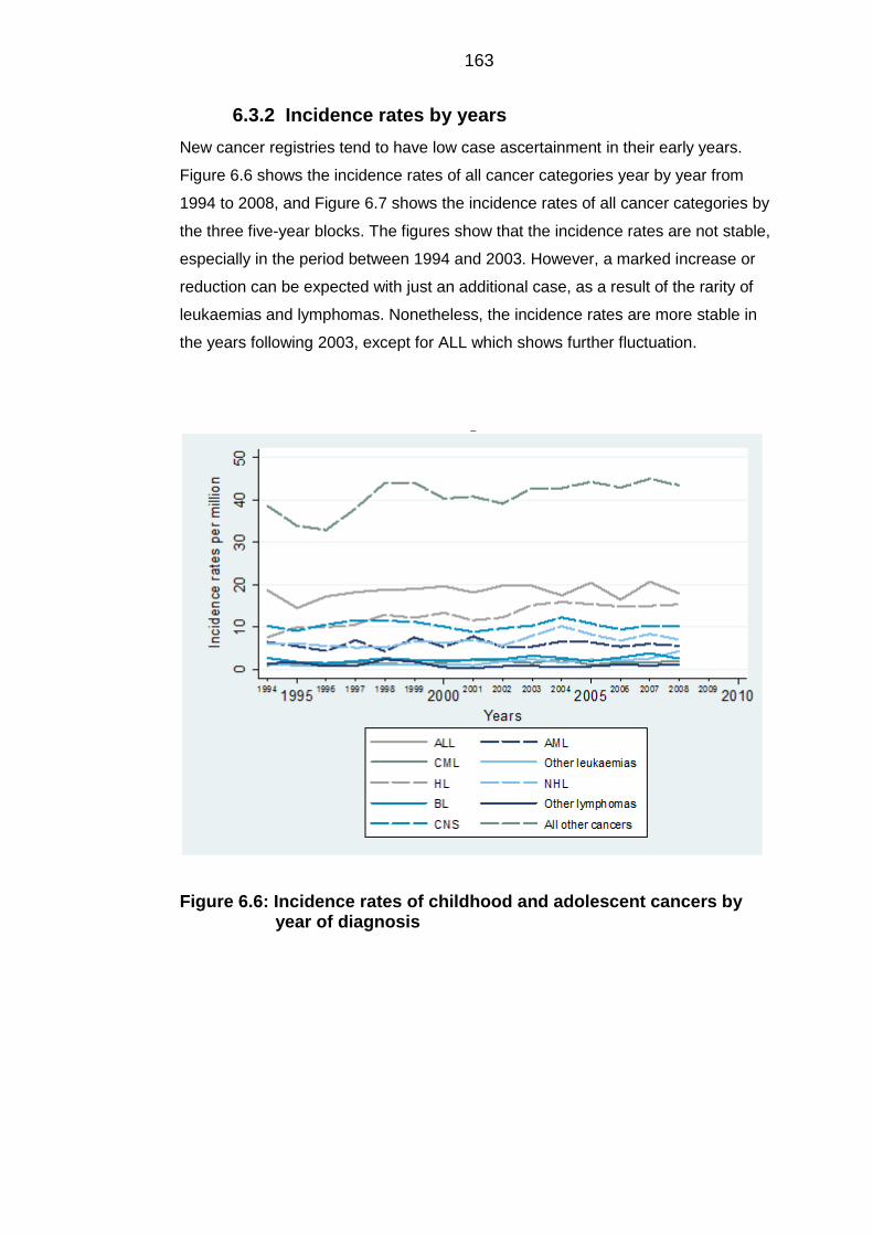
163
Incidence rates by years 6.3.2
New cancer registries tend to have low case ascertainment in their early years.
Figure 6.6 shows the incidence rates of all cancer categories year by year from
1994 to 2008, and Figure 6.7 shows the incidence rates of all cancer categories by
the three five-year blocks. The figures show that the incidence rates are not stable,
especially in the period between 1994 and 2003. However, a marked increase or
reduction can be expected with just an additional case, as a result of the rarity of
leukaemias and lymphomas. Nonetheless, the incidence rates are more stable in
the years following 2003, except for ALL which shows further fluctuation.
Figure 6.6: Incidence rates of childhood and adolescent cancers by year of diagnosis
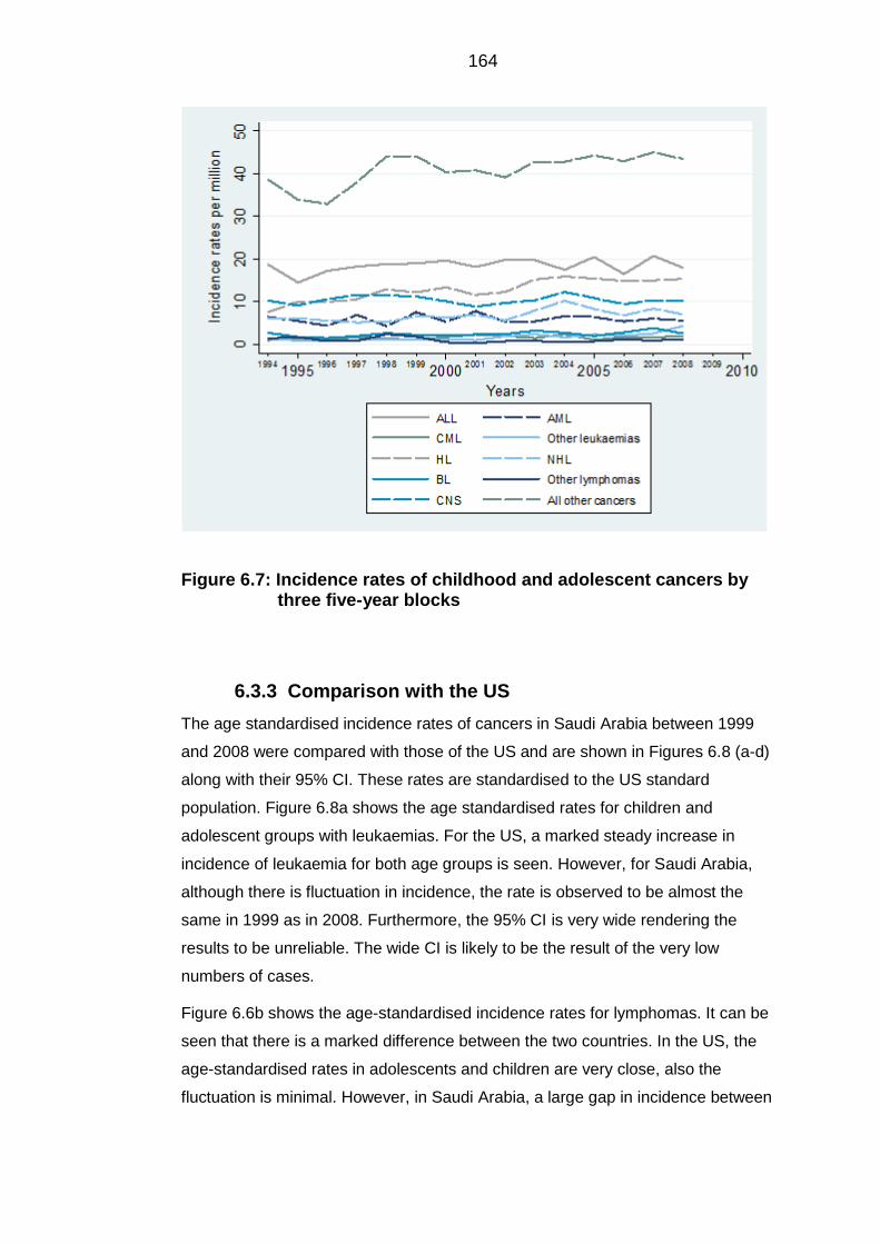
164
Figure 6.7: Incidence rates of childhood and adolescent cancers by three five-year blocks
Comparison with the US 6.3.3
The age standardised incidence rates of cancers in Saudi Arabia between 1999
and 2008 were compared with those of the US and are shown in Figures 6.8 (a-d)
along with their 95% CI. These rates are standardised to the US standard
population. Figure 6.8a shows the age standardised rates for children and
adolescent groups with leukaemias. For the US, a marked steady increase in
incidence of leukaemia for both age groups is seen. However, for Saudi Arabia,
although there is fluctuation in incidence, the rate is observed to be almost the
same in 1999 as in 2008. Furthermore, the 95% CI is very wide rendering the
results to be unreliable. The wide CI is likely to be the result of the very low
numbers of cases.
Figure 6.6b shows the age-standardised incidence rates for lymphomas. It can be
seen that there is a marked difference between the two countries. In the US, the
age-standardised rates in adolescents and children are very close, also the
fluctuation is minimal. However, in Saudi Arabia, a large gap in incidence between
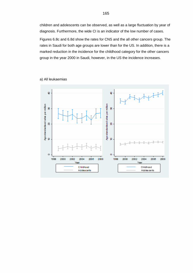
165
children and adolescents can be observed, as well as a large fluctuation by year of
diagnosis. Furthermore, the wide CI is an indicator of the low number of cases.
Figures 6.8c and 6.8d show the rates for CNS and the all other cancers group. The
rates in Saudi for both age groups are lower than for the US. In addition, there is a
marked reduction in the incidence for the childhood category for the other cancers
group in the year 2000 in Saudi, however, in the US the incidence increases.
a) All leukaemias
166
b) All lymphomas
c) Central nervous system tumours
167
d) All other types of cancers
Figure 6.5: The age-standardised rates of cancers in under and over 14 years of age for Saudi Arabia (left) and the United States (right) standardised to the US standard population
168
7 Discussion
7.1 Discussion of results
This study is the first to quantify childhood and young adult cancers in Saudi Arabia
as a separate group. It is novel in that it analysed incidence in these groups over a
period of 15 years from 1994 to 2008, as well as derived two area-based measures
of SES for Saudi Arabia that were used in the subsequent analysis to address the
effects of SES and PM in terms of Hajj. These indices may also be used in other
health and social research studies. The results from this thesis address the aims
set out in Chapter 1.
Describe the pattern of incidence of childhood and young adult
cancers particularly leukaemias, lymphomas and central nervous
system (CNS) tumours across Saudi Arabia, as well as produce
international comparisons.
This study has successfully quantified the incidence of cancers in these age groups
for all diagnostic groups defined by the ICCC-3, as reported to the SCR between
the years 1994 and 2008. Incident cases and incidence rates reported revealed that
incidence of cancers was more pronounced in males specifically for leukaemias,
lymphomas and CNS tumours in the 0-4 age group. The most common diagnostic
group reported for both genders was leukaemias, with higher cases found in the 0-4
age group, which is similar to international patterns of incidence (Stiller, 2007,
Valery et al., 2014, Stiller and Parkin, 1996).
This study has also been successful in producing international comparisons for the
three main diagnostic groups through direct age-sex standardisation using three
different standard populations, i.e. World standard, European standard and the US
standard. The rates for ALL were higher when standardising to the Saudi
population. This may be a result of the relatively younger population of Saudi
Arabia, where cancer incidence is mostly accounted for by ALL. There are slight
differences in rates when using different standard populations, due to the different
age structures. For example, the European standard gives equal weights for ages 5
to 54 and the US standard gives more weight to older age groups. This explains the
larger differences found when standardising to the US standard population,
especially for the leukaemias group.
169
It has been possible to compare these findings with a previous study that computed
age-sex standardised rates for children and young adults aged less than 24 years
in Northern England, and also standardised to the world standard population
(Feltbower et al., 2009). For ALL, AML, HL and NHL the age-sex standardised rate
in Northern England was markedly higher than in Saudi (26.9, 7.6, 14.7 and 9.5 per
million compared to 17.86, 5.89, 13.10 and 6.98 per million, respectively). These
differences are likely to be due to comparing an economically developed country
with an economically developing country, where incidence is higher in developed
countries, where higher levels of hygiene and social isolation are found due to
higher levels of affluence (Jemal et al., 2011). It should be stressed that underlying
factors associated with behavioural factors and social lifestyle may have also
contributed to the difference, although this is less likely in younger cancer sufferers.
Under reporting due to poor case-ascertainment or under-diagnosis could have
played a role in these low rates.
Aim 2: Describe the geographical variation in incidence of these
cancers.
This study aimed to describe the variation in incidence of leukaemias, lymphomas
and CNS tumours in children and young people within the first 15 years of reporting
by the SCR, and has successfully achieved this aim. For each diagnostic group the
SIRs were calculated and mapped for all of the 118 Governorates of Saudi Arabia.
The maps showed little discernible pattern prior to smoothing, whereby 14
Governorates had an SIR of zero due to no observed cases being reported within
them for all diagnostic groups. These Governorates are Badae, Dayer, Dhurma,
Ghazalah, Harth, Kamel, Khabash, Kharkheer, Oyoon Jawaa, Quraa, Rejal Almaa,
Thaar, Thadeq and Yadmah. All have one common attribute in that they are
geographically small rural areas with small population sizes. This suggests that
under-reporting and/or under-diagnosis may have played role. In general, one might
assume that Governorates in close proximity to each other will have similar SIRs
thereby revealing a pattern of incidence. However, the maps of crude SIRs did not
reveal any discernible pattern which necessitated spatial smoothing.
Furthermore, for all diagnostic groups Governorates with larger population sizes
such as Riyadh, Jeddah and Dammam showed constantly high SIRs. This is more
likely to be due to statistical rather than biological phenomena. The extremely high
numbers of observed cases compared to the expected cases in these three
Governorates is likely to be due to the availability of referral centres that offer
170
patients from outside these Governorates cancer-related care, especially for the
Riyadh Governorate. Consequently, these patients provide a temporary address as
being one of the three Governorates rather than their permanent address, hence
leading to misclassification bias. This could potentially cause an overestimate of the
IRRs in these Governorates, and an underestimate in the rural Governorates.
This observation is further supported by the fact that other Governorates with high
SIRs are the capital Governorates of their relative Provinces. Each of the 13
provinces in Saudi Arabia is made up of several Governorates, one of which is
named the “Amarah” or the capital of that province. This capital Governorate is
highly populated compared to the rest of the Governorates within that province, and
provides secondary health care services. It is not uncommon for patients to report
the capital Governorate as their place of residence rather than the actual ‘rural’
Governorate. These capital Governorates include Baha, Arar, Hail, Jazan, Najran,
Abha, Buraidah, Skaka, Tabuk and Makkah. All were found to have moderate to
high SIRs for all diagnostic groups.
Furthermore, it can be demonstrated that there are considerable differences in
incidence across Governorates, which may reflect under-ascertainment or under-
diagnosis, especially in rural areas, which may be due to limited geographical
access to health services.
There have been no comparable studies in the mapping of childhood and young
adult cancers in Saudi Arabia. Only two studies have examined the geographical
distribution of cancer incidence in Saudi Arabia by utilising data from the web-based
atlas developed in 2013 (Al-Ahmadi and Al-Zahrani, 2013a, Al-Ahmadi, 2013, Al-
Ahmadi and Al-Zahrani, 2013b). However, both looked at only the most common
types of cancers reported between 1998 and 2004, and did not make it clear which
age groups were represented. Most importantly, the rates were computed in cities
only, not in all 118 Governorates and these rates were only crude, thus no indirect
age-sex standardisation was performed. Consequently, these studies are not
comparable to this work which has mapped indirectly estimated age-sex
standardised rates of childhood and young adult cancers. Indirect rates should be
used when making internal comparisons, for example when comparing the
Governorates to each other.
171
Construct indices of SES, to be used in future research as well as in
the subsequent analyses in this study, to adjust for the socioeconomic
position of the Governorates under examination.
This project has succeeded in producing two area-based measures of SES for the
118 Governorates of Saudi Arabia, which have been mapped for comparison. The
two replicable indices of SES have been formulated using multiple socioeconomic
indicators available from the 2004 national census data. These have shown that 8
out of 11 Governorates within the Eastern province are within the most affluent
Governorates of the country. These are Qatif, Khobar, Rass Tanourah, Jubail,
Dammam, Bqeeq, Ahsa and Khafji. The Eastern province hosts five major
universities within the country, as well as ARAMCO, one of the world’s largest oil
companies. The Jubail Governorate in the northern part of the Eastern province is
the largest industrial city in the Middle East. Therefore, it is logical to find these
Governorates to be within the most affluent, especially when the Eastern provinces
are the gateway to the rest of the Gulf countries. The major cities in the country,
such as the capital Riyadh and Jeddah, as well as some of the capital
Governorates of provinces such as Arar, Skaka and Buraidah, were also within the
affluent ranking in the two indices.
The selection of indicators was extremely important. The analysis began with a
close examination of what had been chosen to formulate indices in other countries.
For example, the Townsend and Carstairs indices in the UK (Townsend et al.,
1988, Carstairs and Morris, 1991), as well as the index in Italy (Tello et al., 2005) all
utilised indicators available from national censuses. In contrast to the Saudi census,
the censuses used in formulating these indices included indicators such as
unemployment and overcrowding. Although the Saudi census does have a variable
for employment status, this variable only shows the proportion in the labour force,
and this includes the proportion of the population who are available for work, hence
both employed and unemployed are included in that variable. Furthermore, the
Saudi census collects information on the number of rooms per household, therefore
the information necessary to create an overcrowding variable was available, but
was not used to derive it. Thus, a decision was made that balanced what had to be
included and what was available and accessible from the census.
Interestingly, the loadings of the variables on each factor show that the first factor
labelled as ‘Middle class’ has better qualified constituents than Factor 2 ‘Affluent
class’ in terms of education. This is culturally justified where the highly educated are
not usually wealthy, and the wealthy are not highly educated. Furthermore, the
172
student indicator had a dichotomy on two factors: Factor 2 labelled as ‘Affluent
class’ and Factor 3 labelled as ‘Deprived class’. A Governorate that has a high
proportion of students may indicate that it is either affluent or poor. This indicator
covers the population aged greater than 15 years. Therefore, it includes both
university students and mature students (over 21 years old) returning to schools to
gain better jobs. Both of which may explain why the indicator loads highly onto the
two factors.
Similar to the Townsend index (Townsend et al., 1988), the final numerical value
assigned to each Governorate in the standardised index does not measure a
specific object. The value provides an abstract measure of deprivation that is used
to rank these Governorates. The standardised index method has been used to
develop an index for Canada (Kishnan, 2010), India (Sekhar et al., 1991, Antony
and Visweswara Rao, 2007), Japan (Fukuda et al., 2007) and the State of
Mississippi in the USA (Hightower, 1978). However, none of these studies
attempted to reconstruct the index using another statistical method for extra validity.
The LCA approach was chosen to construct categorical classes of SES to be used
in future analyses; hence, Saudi researchers have the choice between a continuous
or a categorical index.
The study further explored the distribution of the two indices numerically and
geographically, and showed very minor differences between them, adding further
support to the pattern of affluence in the country. These indices can be added to
Saudi disease registries such as the SCR, as well as for administrative purposes.
Since this is the first project to derive indices of SES, there are no comparable
studies in Saudi Arabia or in the Gulf region, an area which is known for its wealth
and high income per capita. In Kuwait, it was suggested that a person’s
connectedness may be used as a surrogate for social class, rather than deriving a
measure for SES, since it is considered a city state with very few areas that may be
defined as truly rural or poor (Shah et al., 1999). This is not the case for Saudi
Arabia, as it is a vast country with several Governorates considered extremely rural,
and which lack higher educational institutions and specialised health organisations.
It is a common perception that these rural areas are considered more deprived,
whilst urban areas are the most affluent. This perception has been verified by these
newly developed indices.
Comparing the results of these indices with those of Townsend and Carstairs
(Townsend et al., 1988, Carstairs and Morris, 1991), which are usually calculated
on the census ward level, it is seen that rural wards had lower scores indicating less
173
deprivation and urban areas had higher scores indicating more deprivation. In
Saudi Arabia, however, rural areas had lower scores in the standardised index and
were categorised as either the ‘lower middle class’ or ‘most deprived class’ in the
categorical class index. Although it is important to remember that these indices are
methodologically different and there were differences in the indicators chosen for
analysis. It is one of the social characteristics of Saudi Arabia to centralise in one
specific area that includes higher educational and specialised health services.
These areas are often associated with more job opportunities for the unemployed,
and usually have more economical and financial opportunities for those interested
in business. Therefore, these areas are usually characterised by affluence.
The Saudi government has aimed to address centralisation in the large cities of the
country. For example, very recently in 2013 work was done to develop the ‘Waad
Alshamal’ industrial complex costing over £360 million, 25 kilometres from the rural
Governorate of Toraif in the North. The complex will include seven world-scale
phosphate processing plants and will create no less than 22,000 jobs (Bechtel,
2013). Also, the King Abdullah University of Science and Technology was
developed in 2010 close to the non-urban Governorate of Rabegh on the west
coast (KAUST, 2015). Such initiatives may alter the pattern of affluence, therefore,
an update of the indices with the next published census may show changes,
especially in these two areas.
Examine the effect of SES and Hajj on the incidence of childhood and
young adult cancers in Saudi Arabia and interpret the findings in
relationship to the PM hypothesis.
After describing the variation in incidence and deriving measures of SES, this
project then attempted to determine the effect that SES and Hajj might have on the
incidence of these cancers. The main findings of this work are that Hajj as a
measure of PM had no significant effect on any of the diagnostic groups,
particularly ALL, NHL and CNS tumours, and that incidence was higher in affluent
Governorates.
These findings are not supportive of the PM hypothesis as suggested by Kinlen
(1988); they do however support the concept of herd immunity (Anderson and May,
1990), in which continuous mixing prior to the exposure of infection confers
protection against leukaemia. The Hajj is a unique measure of PM, as it is an event
that has been going on for over 1,400 years. Hence, people residing within Makkah
are likely to have established herd immunity and have a primed immune system
174
due to continuous exposure to infections brought by pilgrims, in particular children
who are continuously exposed to these infections in their early life.
For the ALL subtype, NHL and CNS tumours a linear association with SES was
found where incidence was highest in the most affluent areas, compared to the
most deprived. In comparing these results with those of others in the UK, it should
be stressed that the rural areas in the UK are the most affluent, whilst in Saudi
these areas are deprived. In light of this, this study is in agreement with that of
others in England for children and young adults (Dickinson et al., 2002, Van Laar et
al., 2014, Law et al., 2003) and in Yorkshire (Parslow et al., 2002). Furthermore,
this association was observed in studies dealing with childhood DM, which is a
disease thought to be parallel to ALL in terms of underlying aetiology and
geographical distribution (McKinney et al., 2000, Feltbower et al., 2005). This
association was found even after eliminating the three major Governorates of
Riyadh, Dammam and Jeddah which were within the most affluent Governorates
and had high SIRs.
These findings are supportive of the hygiene hypothesis (Strachan, 1989). If this
hypothesis was operating, then affluent areas would have higher rates of cancers,
particularly ALL which was demonstrated to be the case even after eliminating the
most highly affluent areas. Also, the delayed infection hypothesis put forward by
Greaves (1988) specifically relates to the childhood ALL subtype (but similar
associations were found for NHL). These findings do not suggest an in utero event
for ALL, however, the negative association between ALL and PM is consistent with
the delayed infection hypothesis, where exposure to infections in early life is
necessary to prime the immune system against abnormal responses to infections,
whether symptomatic or asymptomatic (Wiemels et al., 1999a, Greaves, 1997). On
the other hand, it is unlikely that this is the only explanation for the marked
association between ALL and NHL incidence and affluence. Factors such as poor
case-ascertainment and/or limited access to health organisations are believed to
have played a role in the highly rural areas. However, these findings warrant further
investigation.
It should be noted that these findings were not able to clearly distinguish whether
deprivation or the rurality of these deprived Governorates played a role in the
observed association. According to both the PM (Kinlen, 1988, Kinlen, 1995) and
delayed infection hypotheses (Greaves, 1997), susceptibility is conferred upon
individuals who are isolated either geographically, i.e. residing in rural areas, or
socially due to higher affluence. It should be noted that no Governorate is truly
175
isolated as there is a massive network of modern roads linking all parts of the
country. The present study did not identify rural and deprived areas with a higher
incidence of cancers, only affluent urban areas. This is in contrast to previous
studies, such as that of Law et al. (2003) and Dickinson et al. (2002) in England,
who found a non-significant elevated risk of both childhood ALL and NHL in rural
areas. It is more likely however, that affluence has contributed more to these
results, as it is the only common denominator between the urban areas in Saudi
and the rural areas in the UK studies. Unfortunately, this study lacked data on the
level of urbanicity of Governorates. Population-weighted population density was not
available (Dorling and Atkins, 1995), and the use of normal population density was
not appropriate for the purposes of this work, since populations are often
centralised in one area of a Governorate, thus that data would not appropriately
measure the density at which individuals live. Other unmeasured confounders may
have also contributed to these results.
This work should be compared to previous studies with caution. Although the
results were similar, it should be taken into account that the measure of PM used
here is different in a few aspects. First, Hajj is an annual event that is confined in
both time and space, as it takes place in a small geographical area and takes only
five days to perform. Therefore, it is different to previous measures of PM, which
measure migrants or commuting, as these are more permanent in nature.
Furthermore, this work should not be compared to studies by Kinlen that
retrospectively examined crude measures of PM in relatively isolated populations,
since Makkah is a highly urbanised Governorate and the study included all 118
Governorates of Saudi Arabia, thus did not focus on clusters of leukaemia. This
study provides support to the debate that the variation observed in the incidence of
ALL and NHL may be attributed to early exposure to infection, for which Hajj may
play a major role.
The pattern of incidence of AML, HL and CNS tumours does not follow that of ALL
and NHL. Although incidence was highest in the most affluent Governorates, the
association was not linear across the rest of the SES categories. There is no
plausible explanation for these findings, although they do warrant further
investigation on a more refined geographical scale. The estimates for CML, other
leukaemias group, BL and other lymphomas group give little information due to
small numbers.
The marked association with SES has raised suspicions about case-ascertainment
especially in the rural/deprived Governorates. Hence, case-ascertainment was
176
explored to the extent available by the cancer data by plotting the proportion of
each diagnostic group by SES by year. The findings further point towards poor
case-ascertainment in these areas where the proportion was very low regardless of
the year of diagnosis. Plotting incidence rates by year, the rates were found to be
more stable following the year 2003, which may indicate improvement in reporting
of cases. Furthermore, age standardised rates for the two groups of children aged
0-14 and young adults aged 15-24 in both Saudi Arabia and the US standardised to
the US standard population showed marked differences. First, the rates in Saudi,
especially for lymphomas and other types of cancer, were unstable and were
accompanied by relatively wide CIs particularly for lymphomas, which may reflect
the low number of cases for that group. For these two groups of cancers, there was
a drop in incidence in 2001 and 2002 that could only be explained by issues of poor
reporting or under-diagnosis. Although, there may well be true differences in
incidence between the two countries, where one is developed and the other is
developing. Only one study explored case-ascertainment in one major hospital in
Riyadh during the first year of reporting, using the capture re-capture method, and
found that the overall rate of case-ascertainment was only 68% (Al-Zahrani et al.,
2003). This rate is very low compared to international cancer registries, for example
in the Netherlands case-ascertainment of three major registries found an overall
rate of 98.3% (Schouten et al., 1994), and in the UK case-ascertainment was higher
than 99% (Kroll et al., 2011a). However, these are relatively old registries, whilst the
study on the SCR ascertainment only focused on the first year of reporting. No
other data study has explored case-ascertainment in later years to check for
possible improvement. The established methods for case-ascertainment such as
capture-recapture and independent case-ascertainment were beyond the scope of
this work.
177
7.2 Discussion of data sources
Data from the cancer register 7.2.1
The (Saudi Cancer Registry) SCR is the only source of data that has been used to
investigate environmental risk factors proposed in the aetiology of cancers. The
registry collects data on cases of all ages diagnosed with cancer while resident
within Saudi Arabia. The process of data collection continues prospectively, and the
registry has reported more than 135,000 cases throughout the period 1994 to 2008.
The topography, morphology and other diagnostic details of cases are collected
from hospital medical records, histopathological reports and death records by
trained registrars. The quality of population-based registries depends on both the
completeness and validity of the data. The major challenge the registry is facing
concerns incompleteness of medical records, completeness of ascertainment and
acquiring qualified oncology registrars. A further challenge is that many patients
seek medical treatment in the larger cities such as Riyadh, Jeddah and Dammam
where there are more specialised hospitals, thereby only reporting their temporary
address. This greatly increases the rates in these Governorates which do not
reflect the underlying rates of disease at a geographical level (Al-Eid et al., 2007a).
A population-based registry such as the SCR should aim to report every single case
occurring within its catchment area, i.e. within the borders of Saudi Arabia 100%
case ascertainment should be achieved. For Saudi Arabia, the level of case
ascertainment for the cases reported from all regions of the country is yet to be
examined. There has been only one attempt at examining case ascertainment of
cancers reported to the SCR for the year 1994, and this used the capture-recapture
method for one major referral hospital in Riyadh. The study concluded that the
ascertainment rate from medical records was 51%, from pathology reports the rate
was 53% and from death certificates the rate was 17%. The study also concluded
that the overall rate from all sources was 68%. These results are not surprising
considering these rates were taken for the first year of actual reporting (Al-Zahrani
et al., 2003).
There are several methods to check for the validity or quality of the collected data,
such as re-abstracting and re-coding a sample of the data to ensure that none are
invalid. In any case, each registry should develop its own internal checks for
ensuring the validity of their data. For the SCR, these checks include verification of
site and morphology data, as well as case linkage between a tumour and a patient
(Al-Eid et al., 2007a).
178
Relevant to this work is patient addresses. The addresses obtained from patients
are largely P.O. boxes that are centralised which do not indicate the actual
geographical location of patients; this data is not disclosed for patient confidentiality
reasons. The location of patients, however, in the majority of cases was given at a
Governorate level, or sometimes at a district level. It is not likely that during the data
collection process there was a requirement to give the exact location of patients.
Therefore, it was structurally impossible to obtain data on a finer geographical
scale. This is very different to data from the UK cancer registry which provides data
on several geographical levels.
The census data and the Hajj data 7.2.2
To date, five censuses have been conducted in Saudi Arabia by the Central
Department for Statistics and Information (CDSI), these were in 1962, 1974, 1992,
2004 and 2010. The first census of 1962 is rarely used officially as it did not cover
the entire population, but the second census of 1974 is considered the first
comprehensive census in Saudi history (CDSI, 2004a). There are no official
statements about the coverage of the censuses conducted in the later years.
Although, the population figures between 2004 and 2010 are consistent with natural
increase figures, indicating that the population figures for 2004 are valid (Bel-Air,
2014).
For the Hajj data, the number of foreign pilgrims entering the country is assumed to
be 100% accurate, since Saudi customs require a Hajj visa. However, the validity of
the number of pilgrims from within the country has not been officially reported.
179
7.3 Discussion of methods
Disease classification 7.3.1
The published reports of cancer incidence from the SCR are only based on the
ICD-10 classification, rather than on the ICCC-3 classification for the childhood
category. This is not best practice, because for the childhood population (less than
15 years of age) classification of cancers should be based on histology rather than
topography, therefore the ICCC-3 classification is more suitable for that age group
as it also permits international comparisons to be made. For the adolescents and
young adults group (aged between 15 and 24 years), the Birch et al. (2002) disease
classification was produced; this takes into account the most frequent cancers
occurring within this age group and those that are rare in children, such as
carcinomas (Birch et al., 2002).
Although the current study targeted patients of less than 25 years of age, which
includes both children and young adults, it used the ICCC-3 classification, primarily
for two reasons. First, any classification system should represent the most
important age groups numerically, and that was the childhood population. Secondly,
the use of one rather than two classifications ensures consistency in analyses and
interpretation.
Geographical mapping 7.3.2
Examination of geographical patterns of disease incidence is one element of the
classic triad in descriptive epidemiology of time, person and place. Place is a
surrogate for environmental, lifestyle and possibly genetic factors that may underlie
patterns of occurrence of a disease across populations. Geographical mapping
conveys direct visual information on the spatial distribution of a disease and can
easily identify subtle patterns that may be missed if the same data is presented in a
tabular form.
Of importance is selection of the appropriate administrative unit for mapping. This
study used Governorates as the administrative unit for mapping, which was mainly
due to the fact that measures of PM are by definition on an area level. Also, there
were data limitations of the SCR on smaller geographical levels and data
accessibility of the census data. In addition, the selection of appropriate data
classifications within the maps is extremely important. The ArcGIS mapping
software offers several types of classification schemes such as equal interval and
quantiles. The classification method used in this work was the quantile method,
180
which placed equal numbers of Governorates into each of five classes i.e. fifths.
Therefore, each class contained 20% of Governorates. Quantiles are often
preferred over other methods in the mapping of epidemiological and disease data
for the simplicity and intuitiveness in map reading (Brewer and Pickle, 2002). The
spatially smoothed maps share the same legend as the non-smoothed to aid in
map comparisons and interpretation.
Disease mapping in Saudi Arabia is a relatively new field. Interest has recently
been sparked with the development of a web-based cancer atlas for Saudi Arabia in
2013, which is yet to be made available for public use (Al-Ahmadi, 2013). The atlas
however, is limited to cancer data between 1998 and 2004, and only includes
incidence rates and age-standardised rates to the world standard population. Also,
the atlas is limited by only including the most common types of cancer reported by
the SCR. This study is the first to geographically map SIRs of all major ICCC
subgroups of disease categories that were reported to the SCR, from the first year
of cancer reporting in 1994 to 2008, for a well-defined young adult population, as
well as the first to ever apply spatial smoothing to these rates.
Possible drawbacks of disease mapping 7.3.3
Although the SIR was chosen as a risk estimate for disease occurrence in the
Choropleth maps, it must be noted that it does not imply absolute risk. It merely
compares the number of observed cases to the number of expected cases
calculated from the age-sex specific incidence for a specified area. The SIRs are
easily understandable and more precise than crude incidence rates (Esteve, 1994).
However, similar to other risk estimates, this method may suffer from chance
variations in incidence, especially in Governorates with very low numbers of
observed cases. This is a particular problem when dealing with rare diseases,
where thousands of individuals are required before one single case is expected
occur (Bruce et al., 2013). This leads to spuriously highlighted high or low areas of
risk. In this study, despite the fact that the geographical unit is relatively broad, i.e.
Governorates, and the study spanned a period of 15 years between 1994 and
2008, some Governorates have extremely low numbers of cases, and 23 had no
cases at all. Also, some Governorates have very low population numbers.
Therefore, some degree of chance variation may be found. In fact, the CIs of some
SIRs include unity, hence a chance variation does exist.
Therefore, the standard statistical method of spatial empirical Bayes smoothing was
used, as that takes into account the very low population numbers, thus adjusting

181
the SIRs by shrinking them to the means of the neighbouring Governorates. This
decreases the likelihood of presenting unusually high or low risks and reveals
patterns that would have been otherwise missed (Clayton and Kaldor, 1987).
Therefore, with the use of smoothing to correct for small population numbers, the
advantages of the SIRs as a comparative method outweigh its potential limitations.
Exploratory factor analysis 7.3.4
In the process of deriving indices of SES, EFA was chosen because it does not
require a priori hypothesis about the data, in fact it is used to formulate hypotheses
(Fabrigar and Wegener, 2012). Since this is the first attempt at measuring SES for
Saudi Arabia it seemed reasonable to explore the data using this technique.
Furthermore, this method, as well as the formulas used to calculate the scores, has
been used in Canada (Kishnan, 2010), India (Sekhar et al., 1991, Antony and
Visweswara Rao, 2007), Japan (Fukuda et al., 2007) and in construction of an
index for the state of Mississippi in the United States of America (Hightower, 1978),
and the methods are well documented within the literature. Some have used
principal component analysis (Kishnan, 2010, Vyas and Kumaranayake, 2006),
however the principal component analysis is used as a data reduction technique
only.
There are three common criteria to consider upon deciding the number of factors to
retain after the initial extraction of the factors. First, the Guttman-Kaiser rule which
describes the truly existing factors as the factors with eigenvalues above one
(Kaiser, 1960, Guttman, 1954). This is the most commonly used method within the
literature; but is mistakenly used on its own. A scree-plot is also used, it plots the
eigenvalues and the number of factors and is determined by the point at which the
plotted values start to level off (Cattell, 1966). The most important criterion is the
interpretability. In this study, the scree plot and eigenvalues found four factors to
retain, but the fourth factor was not interpretable. In this situation it is reasonable to
drop the fourth factor and keep the first three factors that are interpretable
(Bandalos, 2009). As stated by Worthington and Whittaker (2006), “In the end,
researchers should only retain a factor if they can interpret it in a meaningful way,
no matter how solid the evidence for its retention based on the empirical criteria”
(p.822). Therefore, although the fourth factor satisfied the first two conditions, it was
not interpretable even after rotation and was dropped.
The initial factor extraction usually yields factors that are difficult to interpret. A very
common procedure is to rotate the factor axes to achieve a simple structure,
182
whereby the factor loadings will become either higher or lower than the loadings
obtained from the initial extraction, hence the factors will be easier to interpret. Two
types of rotations are available, orthogonal and oblique. It is a common
misconception amongst researchers to regard orthogonal rotation as the “best”
method (Bandalos, 2009). Indeed, most of the previous methodological papers on
SES using EFA employed an orthogonal rotation without commenting on the
assumptions of the factors or the rationale behind that choice (Fukuda et al., 2007,
Kishnan, 2010, Hightower, 1978). It is always safer to consider the factors as not
being perfectly independent, hence using an oblique rotation rather than an
orthogonal one (Preacher and MacCallum, 2003). In any case, an oblique rotation
will default to an orthogonal if the factors are truly uncorrelated, but the factors will
be allowed to correlate if it is necessary to achieve the simple structure, therefore
an oblique rotation was used in this study.
Possible drawbacks of EFA 7.3.4.1
A commonly reported limitation of EFA is the high level of subjectivity that arises
from the several methodological decisions the researcher makes in a single
analysis. Thus, the accuracy of the results depends on the quality of these
decisions (Beavers et al., 2013). Therefore, ideally EFA should not be used on its
own unless for exploratory reasons.
There is no consensus on the minimum sample size required. However, normality
checks are necessary in small samples, because non-normal distributions produce
an underestimate of the variance of a variable. Though, in large samples, i.e. a
sample of greater than 100, the underestimates of variances disappears if the
variables are positively skewed. If the variables are negatively skewed, then a
sample size of greater than 200 is required (Tabachnick and Fidell, 2007).
Therefore, since the variables obtained from the CDSI are either normally
distributed, or positively skewed, and since the sample size is greater than 100
(N=118), no transformations were performed on the skewed data.
Latent class analysis 7.3.5
The LCA statistical method was chosen to classify the Governorates into
homogenous groups. Unlike EFA, it is not only used for exploratory purposes, but is
also used as a confirmatory statistical technique, i.e. results from an LCA model
should confirm that of previous latent analysis (Geiser, 2010). In this work, LCA was
183
used to confirm and validate the results from the EFA. Although confirmatory factor
analysis (CFA) could have been used, LCA was chosen due to the resulting
categorical variables. Therefore, two indices of SES have been derived, one
continuous and the other categorical. The use of LCA in relation to SES is not new
since previous studies have utilised LCA to derive indices of SES, such as the
index derived from a cross-sectional survey in the Philippines (Dahly, 2010), as well
as the derivation of three socioeconomic classes on the neighbourhood level in
Portugal (Alves et al., 2013).
The LCA is aimed at grouping observations or Governorates based on the pattern
of item responses, therefore it is a person-centred approach to latent analysis. The
main assumption underlying LCA is conditional independence, i.e. the indicator
variables are mutually independent once the categorical variable, i.e. SES class
variable is conditioned out. Furthermore, LCA may be used when indicator
variables are non-normal. In fact, LCA captures non-normal outcomes, especially if
there is a sound theory underlying the non-normality of the variables, for example if
the variable is non-normal due to different response patterns from the observations.
Hence, skewness is a result of the variable belonging to two or more classes.
Therefore, log transforming the variables may lead to loss of information (Beng,
2003).
Possible drawbacks of LCA 7.3.5.1
The first issue encountered in this work was model convergence in Mplus. This is a
complication that is encountered in iterative estimation procedures such as that
found in LCA. It is often found that one set of parameter starting values does not
make it possible to find the solution with the best log likelihood, and thus the model
converges on the local likelihood maximum which results in inaccurate parameter
estimates. Furthermore, the local maximum problem is more frequent in models
with four or more extracted classes (Geiser, 2010). In this work, the problem of local
maximum was encountered and the starting values had to be increased to 1000.
Also, the highest number of classes extracted was four classes, because when five
classes were set to be extracted, the model only converged on the local maximum,
regardless of the number of starting values.
Also, sample size was a further limitation. The data set used here contained a small
number of observations (N=118) relative to the number of indicator variables
(n=29). Therefore, the number of variables had to be reduced to allow for the rule of
thumb of 10 observations per indicator. Thus, the indicator variables were reduced
184
to only 11. The choice of variables was based on the disadvantaged variables only.
This is similar to the variable selection used in UK indices such as the Carstairs and
Townsend indices, in which the disadvantaged variables, such as low social class
and overcrowding were used. This allowed proper model convergence and
derivation of sensible and interpretable results comparable with the results of the
EFA.
Regression analyses 7.3.6
The NB regression was chosen because a useful feature of the NB model is that
the Poisson model is nested within it. The main differences between the Poisson
and the NB is that the NB model has an α parameter that is estimated along with
the other model parameters, and which measures the overdispersion numerically. If
the α is equal to zero then there is no overdispersion and the model reduces to the
simpler Poisson model. If however, the α > 0, then this indicates that overdispersion
does exist and is accounted for. The interpretation of the model coefficients are the
same as the Poisson model. Also, the variance in the NB model is larger than the
variance of the Poisson, though the means are the same (Little, 2013).
Other models considered for use 7.3.6.1
A further type of model that was considered for use was the zero-inflated Poisson
(ZIP) and the zero-inflated NB model (ZINB). These models account for excessive
zeros within the data. This is done by modelling the data as having a mixture of two
distributions, the first has a central location of zero (also known as structured zeros)
and the other has a central location of none-zeros. The first distribution is modelled
using logistic regression and the second is modelled using a Poisson model in the
ZIP model or the NB in the ZINB (He et al., 2014).
Prior to using these models, it was important to consider their underlying
assumptions. These models assume that the data is generated from two different
populations, the first are those who have no probability of acquiring the outcome of
interest, and therefore will always have a value of zero, and the second population
produces a value of zero but with some probability. This assumption does not apply
to the cancer data, since the data is generated from one population all with a
probability of acquiring cancer. Therefore, these models were not appropriate for
use with this data.
185
7.4 Strengths of the study
A major strength for this study is that it is the first to address cancers in the
childhood and young adult groups in Saudi Arabia, no research has previously
explored incidence in these age groups. It also addressed major gaps in knowledge
related to Saudi health and social research. First, it has succeeded in producing two
area-based measures of SES for the 118 Governorates of Saudi Arabia for the first
time, and has set the basis for future research in this field. The fact that the two
indices were derived from routinely collected independent census data makes it
possible to replicate and update with the next published census. Previous
researches on Saudi health data have not been able to adjust for area-based SES
as none were available, and this has been a cited limitation (AlGhamdi et al., 2014).
Secondly, it has used a nation-wide population-based cancer registry to identify
cases from a well-defined age group. Therefore, it has the largest statistical power
possible. Both the cancer data and the census data were used to come up with
indirect age-sex standardised rates, hence it was possible to make comparisons in
incidence between the Saudi Governorates for the first time, by mapping these
rates and applying necessary spatial smoothing to identify patterns. Furthermore, it
made use of the Hajj data in a novel way by considering it as a natural experiment,
thereby studying any effect it may have on the incidence of childhood and young
adult cancers.

186
7.5 Limitations of the study
This study design was an aggregation of cancer counts in childhood and young
adults that have occurred at the Governorate level.
Such ecological studies that attempt to describe areas through a snapshot of data
are subject to the ecological fallacy (Piantadosi et al., 1988). This occurs when
conclusions on individuals are based on analysis of aggregated data. This may be
exacerbated by the fact that areas under analysis are not small. However, the SCR
does not give data on addresses as they are usually centralised P.O. Boxes that do
not indicate an individual’s address. The only possible location provided was the
Governorate. One consequence of ecological studies is the inability to adjust for
potential confounders such as breastfeeding, attendance to day care centres, etc.
which can only be collected on an individual level.
One confounder that may have been used in this study design was population
density, which has been previously used to measure urbanisation. The use of the
normal population density measured by persons/square miles is not appropriate for
use in this situation. This is because Governorates are extremely wide, and
populations centralised in only one small area. One clear example is the Ahsa
Governorate (Figure 3.2), which administratively includes the entire Empty Quarter
desert, where only 18% of that Governorate is populated. The best possible
approach to this problem was to obtain data on population-weighted population
density, as suggested by Dorling and Atkins (1995). This measure of density, unlike
the normal population density which is area weighted, is population weighted by
measuring the density of where an average person lives. However, no such data
has been derived for the Saudi Governorates.
With regards to the socioeconomic indices, one methodological issue is the
modifiable aerial unit problem, whereby the choice of the geographical level of
analysis is made solely on the basis of administrative and/or political convenience,
rather than being based on sound empirical evidence (Schuurman et al., 2007). A
further problem, especially with the socioeconomic class index, is misclassification
bias. It is a problem that occurs with categorical variables by assigning each
Governorate to a class, for example, assigning Riyadh to the affluent class, thereby
assuming that all of the population of Riyadh are affluent, which is not true. One
way to overcome these issues is to reproduce these indices on a smaller
geographical scale.
There have also been some issues with data availability and data accessibility.
Saudi census data for the Governorate level are not readily available to download
187
from the CDSI webpage. Only aggregated data for the province level is made
available for use. On-site visits to the CDSI were made and formal letters by
Ministry officials had to be written in order to access this data, which delayed the
process of data analysis. Furthermore, the level of coverage was not publically
published, therefore there is a level of uncertainty for 100% coverage, especially in
the most rural areas. Similarly, the only figure of case-ascertainment published for
the SCR was 68%, which only covered one referral hospital in Riyadh during the
first year of reporting. This figure does not inspire confidence, especially as it is
drawn from an area where incidence is already high. Rural areas with extremely low
numbers of cases, or which have no cases at all, are likely to have a result of poor
case-ascertainment. Cancer registries provide data on which epidemiologic
research and health policies rely. Therefore, complete and high quality data is vital.
Low case-ascertainment in research may give misleading results. Furthermore, this
project did not examine the subgroups of childhood and young adults separately,
and did not examine subgroups of CNS tumours due to time limitations.
In relation to the Hajj, the project originally aimed at creating a measure of PM
through the Shannon Index of Diversity (Shannon, 1948), since high diversity of
mixing was found to be associated with increased incidence of ALL in previous
studies (Parslow et al., 2002, Law et al., 2003, Feltbower et al., 2005). However,
data on the place of origin of pilgrims was kept by the Ministry of Interior and could
not be released. Therefore, only the total numbers of pilgrims by year were used.
188
7.6 Recommendations and future work
This project has the set basis for work in the field of SES. For the purposes of this
study and to facilitate data linkage with cancer cases, Governorates were chosen
as the geographical unit of analysis. Although these newly developed indices are
replicable with the next national census, further work should be done to analyse
residential zip codes or districts, which will reveal a clearer pattern of affluence.
Additionally, disease registries should incorporate these new developed
socioeconomic indices into their data to be included into future analyses.
An excellent opportunity has risen with the introduction of the new postal system in
2011. The new system should facilitate the process of selecting smaller boundaries,
for example, a residential zip code or district will enable assigning individuals to
spatial locations. The smaller boundaries will ensure that the populations within
these areas are less heterogeneous, which will increase the reliability of these
analyses, and reduce the effects of the modifiable area unit problem and
misclassification bias. Disease registries wishing to use area-based measures of
SES should integrate these newly developed residential addresses into their
databases for data linkage.
Moreover, data to create measures such as overcrowding and unemployment have
been collected, but are not given. The inclusion of these variables in future indices
will help to derive more precise indices. In addition, the CDSI will most likely be able
to publish population-weighted population density data. This data has been used
previously to adjust for its potential confounding effects, and should be included in
future ecological analyses.
However, such work will be challenging to perform in light of the difficulties faced in
data access during the data collection phase of the work. The CDSI should
encourage the use of census data by publishing data online, on different
geographical levels, as is the case with census data in other countries. For
example, in the UK, census data are published by the Office of National Statistics in
geographical levels as well as small output areas.
With regards to the cancer data, it is believed that registrars collect data given by
patients in hospitals. Hospitals should encourage patients to provide a more precise
location of patient residence, such as residential districts. This information will help
with future analyses that aim to look for any associations with potential aetiological
factors. It is recommended that the SCR examine case-ascertainment on a
continuous basis, especially in the more rural Governorates, either through capture-
189
recapture methods or by independent case-ascertainment, although the latter was
reported to be more accurate (Schouten et al., 1994).
This is the first project that has analysed age-sex standardised rates of cases
reported between 1994 and 2008 in the 0-24 age group, and thus has set the basis
for future studies surrounding incidence for this group. Future work should include
analysis of smaller subgroups for example 0-4, 5-9, 10-14 and 15-24 year groups
for better comparison with previous studies and to ascertain whether associations
observed still hold on these subgroups.
7.7 Future planned publications
The results from Chapter 5 are already under review in the Journal of Public Health.
In addition, work is ongoing for the preparation of a scientific paper from Chapter 6
to the British Journal of Cancer.
190
7.8 Conclusions
This study has set the basis for work on the incidence of childhood and young adult
cancers, an age group which has received no attention in previous Saudi studies.
Results showed that cancers were mostly accounted for by ALL in the 0-4 age
range, which is similar to international patterns. Standardising leukaemias,
lymphomas and CNS tumours to the world standard population demonstrated that
Saudi had lower rates compared to the UK (Feltbower et al., 2009). The study has
also shown that there is a difference in the incidence of all diagnostic groups across
the Saudi Governorates. The very low incidences in the most deprived
Governorates suggest that case-ascertainment and/or under-diagnosis may be
attributed to limited access to health organisations.
In Saudi Arabia, no area-based measure of SES has been derived, and this has
been set as a limitation in previous nation-wide studies (AlGhamdi et al., 2014).
Therefore, this work aimed to derive two area-based measures of SES for the 118
Governorates that could be used to assess its effect upon the incidence of
childhood and young adult cancers and interpret the results in light of the PM
hypothesis. The two indices were developed with already established
methodologies used to derive indices in other countries. The first was continuous
and the second was categorical; they showed very similar patterns of affluence in
which the large urban Governorates were more affluent and the smaller rural areas
were more deprived. These indices were then used in the regression analyses to
assess whether SES and PM in terms of Hajj had any associations with the
incidence of leukaemias, lymphomas and CNS tumours.
The main findings from the regression analyses indicated that PM had no significant
effect on ALL and all other diagnostic groups. Furthermore, incidence was higher
with increasing affluence, which is in line with previous studies that adjusted for
SES (Dickinson et al., 2002, Law et al., 2003, Van Laar et al., 2014, Parslow et al.,
2002). It should be noted, however, that in these studies the affluent areas were
rural, while in Saudi the affluent areas were urban. Therefore, although the findings
were unable to distinguish whether rurality or affluence contributed to the findings,
the fact that affluence is the only common factor gives more weight to its effect.
The findings from this study are not supportive of the PM hypothesis, but give
support to the delayed infection hypothesis for two main reasons. The first is that
incidence was higher in affluent Governorates where social isolation due to
affluence may have delayed exposure to infections in early life. Secondly, in
Makkah, the Hajj is an annual event where infections are one major side-effect. The

191
annual exposure of the residents of Makkah to these infections, especially for
infants in early life, may have primed their immune system thereby reducing the risk
of the second mutational event required for the development of overt leukaemia.
However, case-ascertainment and under-diagnosis may have exacerbated these
findings.
Future research is needed to confirm these results, especially in the childhood age
group aged 0-14. However, careful consideration should be given to issues with
case-ascertainment prior to any investigation to ensure valid conclusions.
192
References
ADLER, N. E., BOYCE, T., CHESNEY, M. A., COHEN, S., FOLKMAN, S., KAHN, R. L. & SYME, S. L. 1994. Socioeconomic status and health: The challange of the gradient. American Psychologist, 49, 15-24.
AHLBOM, A., DAY, N., FEYCHTING, M., ROMAN, E., SKINNER, J., DOCKERTY, J., LINET, M., MCBRIDE, M., MICHAELIS, J., OLSEN, J. H., TYNES, T. & VERKASALO, P. K. 2000. A pooled analysis of magnetic fields and childhood leukaemia. Br J Cancer, 83, 692-698.
AHMED, O., BOSCHI-PINTO, C., LOPEZ, A., MURRAY, C., LOZANO R. & INOUE, M. 2002. Age standardisation of Rates: A new WHO standard. Geneva: World Health Organisation.
AKAIKE, H. 1987. Factor analysis and AIC. Psychometrika, 52, 317-332.
AL-AHMADI, K. & AL-ZAHRANI, A. 2013a. NO2 and Cancer Incidence in Saudi Arabia. International Journal of Enviromental Research and Public Health, 10, 5844-5862.
AL-AHMADI, K. & AL-ZAHRANI, A. 2013b. Spatial autocorrelation of cancer incidence in Saudi Arabia. International Journal of Enviromental Research and Public Health, 10, 7207-7228.
AL-AHMADI, K., AL-ZAHRANI, A., AL-DOSSARI, A. 2013. A Web-Based Cancer Atlas of Saudi Arabia. Journal of Geographic Information System, 5, 471-485.
AL-BAGHLI, N. A., AL-GHAMDI, A. J., AL-TURKI, K. A., EL-ZUBAIER, A. G., AL-MOSTAFA, B. A., AL-BAGHLI, F. A. & AL-AMEER, M. M. 2010. Awareness of cardiovascular disease in eastern Saudi Arabia Journal of Family and Community Medicine, 17, 15-21.
AL-EID, H. S., MANALO, M. S., BAZARBASHI, S. & AL-ZAHRANI, A. 2007. Cancer incidence and survival report Riyadh: Saudi Cancer Registry.
AL-EID, H. S., MANALO, M. S., BAZARBASHI, S. & AL-ZAHRANI, A. 2008. Cancer incidence and survival report Riyadh. Saudi Cancer Registry.
AL-ZAHRANI, A., BAOMER, A., AL-HAMDAN, N. & MOHAMED, G. 2003. Completeness and validity of cancer registration in a major public referral hospital in Saudi Arabia. Annals of Saudi Medicine, 23, 6-9.
ALEXANDER, F. E., CHAN, L. C., LAM, T. H., YUEN, P., LEUNG, N. K., HA, S. Y., YUEN, H. L., LI, C. K., LAU, Y. L. & GREAVES, M. F. 1997. Clustering of childhood leukaemia in Hong Kong: association with the childhood peak and common acute lymphoblastic leukaemia and with population mixing. Br J Cancer, 75, 457-463.
ALGHAMDI, I. G., HUSSAIN, I. I., ALGHAMDI, M. S. & EL-SHEEMY, M. A. 2014. The incidence rate of corpus uteri cancer among females in Saudi Arabia: an observational descriptive epidemiological analysis of data from Saudi Cancer Registry 2001-2008. International Journal of Womens Health, 29, 141-147.
ALVES, L., SILVA, S., SEVERO, M., COSTA, D., PINA, M., BARROS, H. & AZEVEDO, A. 2013. Association between neighborhood deprivation
193
and fruits and vegetables consumption and leisure-time physical activity: A cross-sectional multilevel analysis. Biomedical Central of Public Health, 13.
ALZEER, A., MASHLAH, A., FAKIM, N., AL-SUGAIR, N., AL-HEDAITHY, M., AL-MAJED, S. & JAMJOOM, G. 1998. Tuberculosis is the commonest cause of pneumonia requiring hospitalization during Hajj (pilgrimage to Makkah). The Journal of Infection, 36, 303-6.
ANDERSON, R. M. & MAY, R. M. 1990. Immunisation and herd immunity. The Lancet, 335, 641-645.
ANSELIN, L., SYABRI, I. & KHO, Y. 2006. An Introduction to spatial data analysis. Geographical analysis. 38 (1), 2006: 5-22
ANTONIO ORTEGA-GARCIA, J., MARTIN, M., NAVARRO-CAMBA, E., GARCIA-CASTELL, J., P. SOLDIN, O. & FERRIS-TORTAJADA, J. 2009. Pediatric Health Effects of Chronic Exposure to Extremely Low Frequency Electromagnetic Fields. Current Pediatric Reviews, 5, 234-240.
ANTONOVSKY, A. 1967. Social Class, Life Expectancy and Overall Mortality, Milbank Memorial Fund.
ANTONY, G. M. & VISWESWARA RAO, K. 2007. A composite index to explain variations in poverty, health, nutritional status and standard of living: Use of multivariate statistical methods. Public Health, 121, 578-587.
BACH, J.-F. 2005. Infections and autoimmune diseases. Journal of Autoimmunity, 25, Supplement, 74-80.
BANDALOS, D. L. 2009. Four common misconceptions in exploratory factor analysis. In: LANCE, C. E. & VANDENBERG, R. J. (eds.). Statistical and Methodological Myths and Urban Legends. Hove: Taylor & Francis.
BEAVERS, A. S., LOUNSBURY, J. W., RICHARDS, J. K., HUCK, S. W., SKOLITS, G. J. & ESQUIVEL, S. L. 2013. Practical considerations for using exploratory factor analysis in educational research Practical Assessment, Research and Evaluation, 18.
BECHTEL. 2013. Bechtel to oversee development of new phosphate complex and industrial city [Online]. Bechtel. [Accessed 10/01/2015].
BEL-AIR, F. D. 2014. Demography, migration and labour market in Saudi Arabia. Gulf Research Centre.
BENG, M. 2003. Statistical and Substantive Checking in Growth Mixture Modeling: Comment on Bauer and Curran (2003). Psychological Methods, 8, 369-377.
BENTLER, P. M. & CHOU, C. 1987. Practical issues in structural modeling. Sociological Methods and Research, 16, 78-117.
BERAL, V., FEAR, N.T., ALEXANDER, F., APPLEBY, P. 2001. Breastfeeding and childhood cancer. British Journal of Cancer, 85, 1685-1694.
194
BIRCH, J. M., ALSTON, R. D., KELSEY, A. M., QUINN, M. J., BABB, P. & MCNALLY, R. J. Q. 2002. Classification and incidence of cancers in adolescents and young adults in England 1979-1997. Br J Cancer, 87, 1267-1274.
BLEYER, A., BARR, R., HAYES-LATTIN, B., THOMAS, D., ELLIS, C. & ANDERSON, B. 2008. The distinctive biology of cancer in adolescents and young adults. Nat Rev Cancer, 8, 288-298.
BLEYER, A., O’LEARY, M., BARR, R. & RIES, L. A. G. 2006. Cancer Epidemiology in Older Adolescents and Young Adults 15 to 29 Years of Age, Including SEER Incidence and Survival: 1975-2000. Bethesda: National Cancer Institute.
BLEYER, A. W. & BARR, R. D. 2007. Cancer in Adolescents and Young Adults, Springer.
BOISSEL, N., AUCLERC, M.-F., LHÉRITIER, V., PEREL, Y., THOMAS, X., LEBLANC, T., ROUSSELOT, P., CAYUELA, J.-M., GABERT, J., FEGUEUX, N., PIGUET, C., HUGUET-RIGAL, F., BERTHOU, C., BOIRON, J.-M., PAUTAS, C., MICHEL, G., FIÈRE, D., LEVERGER, G., DOMBRET, H. & BARUCHEL, A. 2003. Should Adolescents With Acute Lymphoblastic Leukemia Be Treated as Old Children or Young Adults? Comparison of the French FRALLE-93 and LALA-94 Trials. Journal of Clinical Oncology, 21, 774-780.
BOOMSMA, A. & HOOGLAND, J. J. 2001. The robustness of LISREL modeling revisited. In: CUDECK, R., DU TOIT, S. & SORBUM, D. (eds.) Structural equation models: Present and future. A A festchrift in Honor of Karl Joreskog. Chicago, IL: Scientific Software International.
BOUTOU, O., GUIZARD, A. V., SLAMA, R., POTTIER, D. & SPIRA, A. 2002. Population mixing and leukaemia in young people around the La Hague nuclear waste reprocessing plant. Br J Cancer, 87, 740-745.
BRADY, G., MACARTHUR, G. J. & FARRELL, P. J. 2007. Epstein–Barr virus and Burkitt lymphoma. Journal of Clinical Pathology, 60, 1397-1402.
BREATNACH, F., CHESSELLS, J. M. & GREAVES, M. F. 1981. The Aplastic Presentation of Childhood Leukaemia: a Feature of Common-ALL. British Journal of Haematology, 49, 387-393.
BREWER, C. A. & PICKLE, L. 2002. Evaluation of methods for classifying epidemiological data on choropleth maps in series. Annals of the Association of American Geographers, 92, 662-681.
BRUCE, N., POPE, D. & STANISTREET, D. 2013. Quantitative Methods for Health Research: A Practical Interactive Guide to Epidemiology and Statistics, Wiley.
CARDWELL, C. R., MCKINNEY, P. A., PATTERSON, C. C. & MURRAY, L. J. 2008. Infections in early life and childhood leukaemia risk: a UK case-control study of general practitioner records. Br J Cancer, 99, 1529-1533.
195
CARSTAIRS, V. D. L. & MORRIS, R. 1991. Deprivation and Health in Scotland, Aberdeen University Press.
CARVER, S. 2003. Innovations In GIS 5: Selected Papers From The Fifth National Conference On GIS Research UK, Taylor & Francis.
CATTELL, R. 1966. The scree test for the number of factors. Multivariate Behavioral Research, 1, 245-276.
CDSI 2004. Demographic research bulletin. Riyadh: Central Department for Statistics and Information.
CDSI. 2011. Key indicators of 2011 census in Saudi Arabia [Online]. Riyadh: Central Department for Statistics and Information. Available: http://www.cdsi.gov.sa/english/ [Accessed 01/05/2012.
CLARK, B. R., FERKETICH, A. K., FISHER, J. L., RUYMANN, F. B., HARRIS, R. E. & WILKINS, J. R. 2007. Evidence of population mixing based on the geographical distribution of childhood leukemia in Ohio. Pediatric Blood & Cancer, 49, 797-802.
CLARK, S. L. 2010. Mixture modeling with behavioural data, Los Angeles, C.A., University of California.
CLAYTON, D. & KALDOR, J. 1987. Empirical Bayes Estimates of Age-Standardized Relative Risks for Use in Disease Mapping. Biometrics, 43, 671-681.
CLIP. 2002. Measuring deprivation [Online]. Central and Local Information Partnership. Available: http://www.clip.local.gov.uk/lgv/aio/39171 [Accessed 04/09/2013.
CORTINA, J. M. 2002. Big things have small beginnings: An assortment of ‘minor’ methological misunderstandings Journal of management 28, 339-362.
COULTER, J. 1990. Leukaemia and lymphoma among young people near Sellafield.
CROWLEY, L. 2011. Essentials of Human Disease, Jones & Bartlett Learning.
DAHLY, D. 2010. Socioeconomic determinants of obesity in Cebu, Philippines: A latent class analysis using Mplus. Centre for Epidemiology and Biostatistics, University of Leeds.
DANEMAN, D. 2006. Type 1 diabetes. Lancet, 367, 847-858.
DCLG 2011. The English Indices of Deprivation 2010. Department for Communities and Local Government.
DENNY, K. & DAVIDSON, M. J. 2012. Area-based socioeconomic measures as tools for health disparities research, policy and planning. Canadian Journal of Publish Health, 5, S4-6.
DICKINSON, H. O., HAMMAL, D. M., BITHELL, J. F. & PARKER, L. 2002. Population mixing and childhood leukaemia and non-Hodgkin's lymphoma in census wards in England and Wales, 1966-87. Br J Cancer, 86, 1411-1413.
196
DICKINSON, H. O. & PARKER, L. 1999. Quantifying the effect of population mixing on childhood leukaemia risk: the Seascale cluster. Br J Cancer, 81, 144-151.
DING, L., VELICER, W. F. & HARLOW, L. L. 1995. Effects of estimation methods, number of indicators per factor, and improper solutions on structural equation modeling fit indices. Structural Equation Modeling: A Multidisciplinary Journal, 2, 119-143.
DOCKERTY, J. D., COX, B., BORMAN, B. & SHARPLES, K. 1996. Population mixing and the incidence of childhood leukaemias: retrospective comparison in rural areas of New Zealand. BMJ, 312, 1203-1204.
DOCKERTY, J. D., SKEGG, D. C. G., ELWOOD, J. M., HERBISON, G. P., BECROFT, D. M. O. & LEWIS, M. E. 1999. Infections, vaccinations, and the risk of childhood leukaemia. Br J Cancer, 80, 1483-1489.
DOE 1995. 1991 Deprivation index: a review of approaches and a matrix of results, London, HMSO.
DOLK, H., PATTENDEN, S. & JOHNSON, A. 2001. Cerebral palsy, low birthweight and socio-economic deprivation: inequalities in a major cause of childhood disability. Paediatric and Perinatal Epidemiology, 15, 359-363.
DOLL, R. 1989. The Epidemiology of Childhood Leukaemia. Journal of the Royal Statistical Society. Series A (Statistics in Society), 152, 341-351.
DOLL, R. & WAKEFORD, R. 1997. Risk of childhood cancer from fetal irradiation. The British Journal of Radiology, 70, 130-139.
DORLING, D. & ATKINS, D. 1995. Population density, change and concentration in Great Britain 1971, 1981 and 1991. OPCS Series SMPS no 58. London: HMSO.
DOS SANTOS SILVA, I. 1999. Cancer Epidemiology: Principles and Methods, International Agency for Research on Cancer.
DRAPER, G. J., LITTLE, M.P., SORAHAN, T., KINLEN, L.J., BUNCH, K.J., CONQUEST, A.J., KENDALL, G.M., KNEALE, G.W., LANCASHIRE, R.J., MUIRHEAD, C.R., O'CONNOR, C.M., VINCENT, T.J. 1997. Cancer in the offspring of radiation workers: a record linkage study British Medical Journal, 315, 1181-1188.
DUTTON, D. B. & LEVINE, S. (eds.) 1989. Socioeconomic status and health: Overview, methodological critique, and reformulation, Menlo Park, CA: The Henry J. Kaiser Family Foundation.
EBRAHIM, S. & BOWLING, A. 2005. Handbook of Health Research Methods: Investigation, Measurement and Analysis, McGraw-Hill Education.
EDEN, T. 2010. Aetiology of childhood leukaemia. Cancer treatment reviews, 36, 286-297.
EDEN, T., BARR, R., BLEYER, A. & WHITESON, M. 2008. Cancer and the Adolescent, Wiley.
197
EL-SHEIKH, S. M., EL-ASSOULI, S. M., MOHAMMED, K. A. & ALBAR, M. 1998. Bacteria and viruses that cause respiratory tract infections during the pilgrimage (Haj) season in Makkah, Saudi Arabia. Tropical Medicine & International Health, 3, 205-209.
ENGELS, E. A. 2001. Human immunodeficiency virus infection, aging, and cancer. Journal of clinical epidemiology, 54, S29-S34.
ESRI 2010. ArcMap 10. Redlands, California: ESRI.
ESTEVE, J., BENHAMOU, E., RAYMOND, L. 1994. Statistical method in cancer research, Volume IV: Descriptive epidemiology Lyon, International Agency for Research on Cancer.
FABRIGAR, L. R. & WEGENER, D. T. 2012. Exploratory Factor Analysis, OUP USA.
FEAR, N. T., MCKINNEY, P. A., PATTERSON, C. C., PARSLOW, R. C. & BODANSKY, H. J. 1999a. Childhood Type 1 diabetes mellitus and parental occupations involving social mixing and infectious contacts: two population-based case–control studies. Diabetic Medicine, 16, 1025-1029.
FEAR, N. T., ROMAN, E., REEVES, G. & PANNETT, B. 1999b. Are the Children of Fathers Whose Jobs Involve Contact with Many People at an Increased Risk of Leukaemia? Occupational and Environmental Medicine, 56, 438-442.
FELTBOWER, R. G., MCKINNEY, P. A., GREAVES, M. F., PARSLOW, R. C. & BODANSKY, H. J. 2004. International parallels in leukaemia and diabetes epidemiology. Archives of Disease in Childhood, 89, 54-56.
FELTBOWER, R. G., MANDA, S. O. M., GILTHORPE, M. S., GREAVES, M. F., PARSLOW, R. C., KINSEY, S. E., BODANSKY, H. J. & MCKINNEY, P. A. 2005. Detecting Small-Area Similarities in the Epidemiology of Childhood Acute Lymphoblastic Leukemia and Diabetes Mellitus, Type 1: A Bayesian Approach. American Journal of Epidemiology, 161, 1168-1180.
FELTBOWER, R. G., MCNALLY, R. J. Q., KINSEY, S. E., LEWIS, I. J., PICTON, S. V., PROCTOR, S. J., RICHARDS, M., SHENTON, G., SKINNER, R., STARK, D. P., VORMOOR, J., WINDEBANK, K. P. & MCKINNEY, P. A. 2009. Epidemiology of leukaemia and lymphoma in children and young adults from the north of England, 1990–2002. European Journal of Cancer, 45, 420-427.
FERLAY, J., SHIN, H. R., BRAY, F., FORMAN, D., MATHERS, C. & PARKIN, D. M. 2010. GLOBOCAN 2008 v2.0, Cancer Incidence and Mortality Worldwide: IARC CancerBase No. 10 [Online]. Lyon, France: International Agency for Research on Cancer. Available: http://globocan.iarc.fr/ [Accessed 28/12/2011.
FIELD, A. P. 2000. Discovering Statistics Using SPSS for Windows: Advanced Techniques for the Beginner, Sage Publications.
FLEMING, J. & FABRY, Z. 2007. The hygiene hypothesis and multiple sclerosis. Annals of Neurology, 61, 85-89.
198
FORD, A. M., BENNETT, C. A., PRICE, C. M., BRUIN, M. C. A., VAN WERING, E. R. & GREAVES, M. 1998. Fetal origins of the TEL-AML1 fusion gene in identical twins with leukemia. Proceedings of the National Academy of Sciences, 95, 4584-4588.
FORD, A. M., POMBO-DE-OLIVEIRA, M. S., MCCARTHY, K. P., MACLEAN, J. M., CARRICO, K. C., VINCENT, R. F. & GREAVES, M. 1997. Monoclonal Origin of Concordant T-Cell Malignancy in Identical Twins.
FRAGA, C. G., MOTCHNIK, P. A., WYROBEK, A. J., REMPEL, D. M. & AMES, B. N. 1996. Smoking and low antioxidant levels increase oxidative damage to sperm DNA. Mutation Research/Fundamental and Molecular Mechanisms of Mutagenesis, 351, 199-203.
FUKUDA, Y., NAKAMURA, K. & TAKANO, T. 2007. Higher mortality in areas of lower socioeconomic position measured by a single index of deprivation in Japan. Public Health, 121, 163-173.
GALE, K. B., FORD, A. M., REPP, R., BORKHARDT, A., KELLER, C., EDEN, O. B. & GREAVES, M. F. 1997. Backtracking leukemia to birth: Identification of clonotypic gene fusion sequences in neonatal blood spots. Proceedings of the National Academy of Sciences, 94, 13950-13954.
GALLO, R. C., ESSEX, M., GROSS, L. & LABORATORY, C. S. H. 1984. Human T-cell leukemia/lymphoma virus: the family of human T-lymphotropic retroviruses, their role in malignancies and association with AIDS, Cold Spring Harbor Laboratory.
GARDNER, M. J., SNEE, M.P., HALL, A.J., POWELL, C.A., DOWNES, S., TERRELL, J.D. 1990. Results of case-control study of leukaemia and lymphoma among young people near Sellafield nuclear plant in West Cumbria. British Medical Journal, 300, 423-429.
GATRELL, A. C. 2011. Mobilities and Health, Ashgate.
GEISER, C. 2010. Data analysis with Mplus New York, NY, The Guilford Press.
GILHAM, C., PETO, J., SIMPSON, J., ROMAN, E., EDEN, T. O. B., GREAVES, M. F. & ALEXANDER, F. E. 2005. Day care in infancy and risk of childhood acute lymphoblastic leukaemia: findings from UK case-control study.
GILTHORPE, M. S. 1995. The importance of normalisation in the construction of deprivation indices. Journal of Epidemiology and Community Health, 49, S45-S50.
GORDIS, L. 2013. Epidemiology: with STUDENT CONSULT Online Access, Elsevier Health Sciences.
GRAHAM, H. 2009. Understanding Health Inequalities, McGraw-Hill Education.
GREAVES, M. 2002. Childhood leukaemia.
GREAVES, M. 2006. Infection, immune responses and the aetiology of childhood leukaemia. Nat Rev Cancer, 6, 193-203.
199
GREAVES, M. F. 1988. Spectulations on the cause of childhood acute lymphoblastic leukaemia. Leukaemia, 2, 120-5.
GREAVES, M. F. 1997. Aetiology of acute leukaemia. The Lancet, 349, 344-349.
GREAVES, M. F., MAIA, A. T., WIEMELS, J. L. & FORD, A. M. 2003. Leukemia in twins: lessons in natural history.
GROVES, F. D., GRIDLEY, G., WACHOLDER, S., SHU, X. O., ROBISON, L. L., NEGLIA, J. P. & LINET, M. S. 1999. Infant vaccinations and risk of childhood acute lymphoblastic leukaemia in the USA. Br J Cancer, 81, 175-178.
GUTTMAN, L. 1954. Some necessary conditions for common factor analysis. Psychometrika, 19, 149-161.
HARTLEY, A. L., BIRCH, J. M., MCKINNEY, P. A., BLAIR, V., TEARE, M. D., J., C., MANN, J. R., STILLER, C., DRAPER, G. J. & JOHNSTON, H. E. 1988. The Inter-Regional Epidemiological Study of Childhood Cancer (IRESCC): past medical history in children with cancer. Journal of Epidemiology and Community Health, 42, 235-242.
HAMILTON, L. 2012. Statistics with STATA: Version 12, Cengage Learning.
HARMAN, H. A. 1967. Modern Factor Analysis, University of Chicago Press.
HIGHTOWER, W. L. 1978. Development of an Index of Health Utilizing Factor Analysis. Medical Care, 16, 245-255.
HORNER, R. D. & CHIRIKOS, T. N. 1987. Survivorship Differences in Geographical Comparisons of Cancer Mortality: An Urban-Rural Analysis. International Journal of Epidemiology, 16, 184-189.
INABA, H., GREAVES, M. & MULLIGHAN, C. G. 2013. Acute lymphoblastic leukaemia. The Lancet, 381, 1943-1955.
ISTRE, G. R., CONNER, J. S., BROOME, C., HIGHTOWER, A. & HOPKINS, R. S. 1985. Risk factors for primary invasive Haemophilus influenzae disease: increased risk from day care attendance and school-aged household members. Journal of Pediatrics, 106, 190-5.
JEMAL, A., BRAY, F., CENTER, M. M., FERLAY, J., WARD, E. & FORMAN, D. 2011. Global cancer statistics. CA: A Cancer Journal for Clinicians, 61, 69-90.
JEMAL, A., CENTER, M. M., DESANTIS, C. & WARD, E. M. 2010. Global Patterns of Cancer Incidence and Mortality Rates and Trends.
JINKS, D. C., MINTER, M., TARVER, D. A., VANDERFORD, M., HEJTMANCIK, J. F. & MCCABE, E. R. B. 1989. Molecular genetic diagnosis or sickle-cell disease using dried blood specimens on blotters used for newborn screening. Human Genetics, 81, 363-366.
JOHN, T. J. & SAMUEL, R. 2000. Herd immunity and herd effect: new insights and definitions. European Journal of Epidemiology, 16, 601-606.
KAISER, H. F. 1960. The application of electronic computers to factor analysis. Educational and Psychological Measurement, 20, 141-151.
200
KAISER, H. F. & RICE, J. 1974. Little Jiffy, Mark IV. Educational and Psychological Measurement, 34, 111-117.
KAUST. 2015. The history of KAUST [Online]. King Abdullah University of Science and Technology. [Accessed 10/01/2015].
KEEGAN, T. J., BUNCH, K. J., VINCENT, T. J., KING, J. C., O'NEILL, K. A., KENDALL, G. M., MACCARTHY, A., FEAR, N. T. & MFG, M. 2012. Case-control study of paternal occupation and childhood leukaemia in Great Britain, 1962-2006. Br J Cancer, 107, 1652-1659.
KELLET, C. E. 1937. Acute myeloid leukaemia in one of identical twins. Archives of Disease in Childhood, 12, 239-252.
KELLOFF, G. J., HAWK, E. T. & SIGMAN, C. C. 2008. Cancer Chemoprevention: Volume 2: Strategies for Cancer Chemoprevention, Humana Press.
KINLEN, L. 2006. Childhood leukaemia and ordnance factories in west Cumbria during the Second World War. Br J Cancer, 95, 102-106.
KINLEN, L., JIANG, J. & HEMMINKI, K. 2002. A case-control study of childhood leukaemia and paternal occupational contact level in rural Sweden. Br J Cancer, 86, 732-737.
KINLEN, L. & PETRIDOU, E. 1995. Childhood leukemia and rural population movements: Greece, Italy, and other countries. Cancer Causes & Control, 6, 445-450.
KINLEN, L. J. 1988. Evidence for an infective cause of childhood leukaemia comparison of a Scottish new town with nuclear reprocessing sites in Britain. The Lancet, 2, 1323-1327.
KINLEN, L. J. 1995. Epidemiological evidence for an infective basis in childhood leukaemia. Br J Cancer, 71, 1-5.
KINLEN, L. J. 1996. Epidemiological evidence for an infective basis in childhood leukaemia. The Journal of the Royal Society for the Promotion of Health, 116, 393-399.
KINLEN, L. J. 1997. High-contact paternal occupations, infection and childhood leukaemia: five studies of unusual population-mixing of adults. Br J Cancer, 76, 1539-45.
KINLEN, L. J. & BALKWILL, A. 2001. Infective cause of childhood leukaemia and wartime population mixing in Orkney and Shetland, UK. The Lancet, 357, 858.
KINLEN, L. J. & BRAMALD, S. 2001. Paternal occupational contact level and childhood leukaemia in rural Scotland: a case-control study. Br J Cancer, 84, 1002-1007.
KINLEN, L. J., CLARKE, K. & HUDSON, C. 1990. Evidence from population mixing in British New Towns 1946-85 of an infective basis for childhood leukaemia. The Lancet, 336, 577-582.
KINLEN, L. J., DICKSON, M. & STILLER, C. A. 1995. Childhood leukaemia and non-Hodgkin's lymphoma near large rural construction sites, with a comparison with Sellafield nuclear site.[Erratum appears in BMJ 1995 Apr 8;310(6984):911]. British Medical Journal, 310, 763-8.
201
KINLEN, L. J., HUDSON, C. M. & STILLER, C. A. 1991. Contacts between adults as evidence for an infective origin of childhood leukaemia: an explanation for the excess near nuclear establishments in west Berkshire? Br J Cancer, 64, 549-554.
KINLEN, L. J. & JOHN, S. M. 1994. Wartime evacuation and mortality from childhood leukaemia in England and Wales in 1945-9. BMJ, 309, 1197-1202.
KINLEN, L. J. & STILLER, C. 1993. Population mixing and excess of childhood leukemia. BMJ, 306, 930-930.
KISHNAN, V. 2010. Constructing an area-based socioeconomic status index: A principle components analysis approach. Early Childhood Intervention Australia. Canberra, Australia.
KLINE, R. B. 2005. Principle and practices of structural equation modeling, New York, NY, Guilford.
KNOWLES, M. & SELBY, P. 2005. Introduction to the Cellular and Molecular Biology of Cancer, OUP Oxford.
KOUSHIK, A., KING, W. D. & MCLAUGHLIN, J. R. 2001. An ecologic study of childhood leukemia and population mixing in Ontario, Canada. Cancer Causes Control, 12, 483-90.
KRÄMER, U., HEINRICH, J., WJST, M. & WICHMANN, H. E. 1999. Age of entry to day nursery and allergy in later childhood. The Lancet, 353, 450-454.
KRIEGER, N. & FEE, E. 1996. Measuring social inequalities in health in the United States: A historical review, 1900-1950. International journal of health services, 26, 391-418.
KROLL, M. E., STILLER, C. A., MURPHY, M. F. G. & CARPENTER, L. M. 2011. Childhood leukaemia and socioeconomic status in England and Wales 1976-2005: evidence of higher incidence in relatively affluent communities persists over time. Br J Cancer, 105, 1783-1787.
KROLL, M. E., MURPHY, M. F. G., CARPENTER, L. M. & STILLER, C. A. 2011. Childhood cancer registration in Britain: capture-recapture estimates of completeness of ascertainment. British Journal of Cancer, 104, 1227-1233.
KUH, D. & SHLOMO, Y. B. 2004. A Life Course Approach to Chronic Disease Epidemiology, OUP Oxford.
LANGFORD, I. 1991. Childhood leukaemia mortality and population change in England and Wales 1969-73. Soc Sci Med, 33, 435-40.
LAW, G. R., FELTBOWER, R. G., TAYLOR, J. C., PARSLOW, R. C., GILTHORPE, M. S., BOYLE, P. & MCKINNEY, P. A. 2008. What do epidemiologists mean by ‘population mixing’? Pediatric Blood & Cancer, 51, 155-160.
LAW, G. R., KANE, E. V., ROMAN, E., SMITH, A. & CARTWRIGHT, R. 2000. Residential radon exposure and adult acute leukaemia. The Lancet, 355, 1888.
202
LAW, G. R., PARSLOW, R. C., ROMAN, E. & INVESTIGATORS, O. B. O. T. U. K. C. C. S. 2003. Childhood Cancer and Population Mixing. American Journal of Epidemiology, 158, 328-336.
LAZARDSFELD, P. F. 1950. The logical and mathematical foundations of latent structure analysis. In: STOUFFER, S. A. (ed.) Measurement and Predicition. Princeton, NJ: Princeton University Press.
LEHTINEN, M., KOSKELA, P., ÖGMUNDSDOTTIR, H. M., BLOIGU, A., DILLNER, J., GUDNADOTTIR, M., HAKULINEN, T., KJARTANSDOTTIR, A., KVARNUNG, M., PUKKALA, E., TULINIUS, H. & LEHTINEN, T. 2003. Maternal Herpesvirus Infections and Risk of Acute Lymphoblastic Leukemia in the Offspring. American Journal of Epidemiology, 158, 207-213.
LIBERATOS, P., LINK, B. G. & KELSEY, J. L. 1988. The measurement of social class in epidemiology. Epidemiologic Reviews, 10, 87-121.
LIGHTFOOT, T. J. & ROMAN, E. 2004. Causes of childhood leukaemia and lymphoma. Toxicology and Applied Pharmacology, 199, 104-117.
LITTLE, T. D. 2013. The Oxford Handbook of Quantitative Methods in Psychology: Vol. 2: Statistical Analysis, OUP USA.
LO, Y., MENDELL, N. & RUBIN, D. 2001. Testing the number of components in a normal mixture Biometrika, 88, 767-778.
LOPEZ, A. D. 2006. Global Burden of Disease and Risk Factors, World Bank Publications.
MA, H., SUN, H. & SUN, X. 2014. Survival improvement by decade of patients aged 0-14 years with acute lymphoblastic leukemia: a SEER analysis. Sci. Rep., 4.
MA, X., BUFFLER, P. A., WIEMELS, J. L., SELVIN, S., METAYER, C., LOH, M., DOES, M. B. & WIENCKE, J. K. 2005. Ethnic Difference in Daycare Attendance, Early Infections, and Risk of Childhood Acute Lymphoblastic Leukemia. Cancer Epidemiology Biomarkers & Prevention, 14, 1928-1934.
MACKENZIE, J., PERRY, J., FORD, A. M., JARRETT, R. F. & GREAVES, M. 1999. JC and BK virus sequences are not detectable in leukaemic samples from children with common acute lymphoblastic leukaemia. Br J Cancer, 81, 898-899.
MANDA, S. O. M., FELTBOWER, R. G. & GILTHORPE, M. S. 2009. Investigating spatio-temporal similarities in the epidemiology of childhood leukaemia and diabetes. European Journal of Epidemiology, 24, 743-52.
MCKINNEY, P. A., OKASHA, M., PARSLOW, R. C., LAW, G. R., GURNEY, K. A., WILLIAMS, R. & BODANSKY, H. J. 2000. Early social mixing and childhood Type 1 diabetes mellitus: a case–control study in Yorkshire, UK. Diabetic Medicine, 17, 236-242.
MCLAUGHLIN, J. R., KING, W. D., ANDERSON, T. W., CLARKE, E. A. & ASHMORE, J. P. 1993. Paternal radiation exposure and leukaemia in offspring: the Ontario case-control study.
203
MEIJERS-HEIJBOER, H., OUWELAND, A., KLIJN, J., WASIELEWSKI, M., SNOO, A., OLDENBURG, R., HOLLESTELLE, A., HOUBEN, M., CREPIN, E., VEGHEL-PLANDSOEN, M., ELSTRODT, F., DUIJN, C., BARTELS, C., MEIJERS, C., SCHUTTE, M., MCGUFFOG, L., THOMPSON, D., D.F., F. E., SODHA, N., SEAL, S., BARFOOT, R., MANGION, J., CHANG-CLAUDE, J., ECCLES, D., EELES, R., EVANS, D. G., HOULSTON, R., MURDAY, V., NAROD, S., PERETZ, T., JULIAN PETO, J., PHELAN, C., ZHANG, H. X., SZABO, C., DEVILEE, P., GOLDGAR, D., P.A., F., NATHANSON, K. L., WEBER, B. L., RAHMAN, N. & STRATTON, M. R. 2002. Low-penetrance susceptibility to breast cancer due to CHEK2[ast]1100delC in noncarriers of BRCA1 or BRCA2 mutations. Nat Genet, 31, 55-59.
MEINERT, R., KALETSCH, U., KAATSCH, P., SCHÜZ, J. & MICHAELIS, J. 1999. Associations between Childhood Cancer and Ionizing Radiation: Results of a Population-based Case-Control Study in Germany. Cancer Epidemiology Biomarkers & Prevention, 8, 793-799.
MELTZER, H., GATWARD, R., GOODMAN, R. & FORD, T. 2003. Mental health of children and adolescents in Great Britain. International Review of Psychiatry, 15, 185-187.
MEMISH, Z. A., JABER, S., MOKDAD, A. H., ALMAZROA, M. A., MURRAY, C. J. L. & AL RABEEAH, A. A. 2014. Burden of Disease, Injuries, and Risk Factors in the Kingdom of Saudi Arabia, 1990-2010. Preventing Chronic Disease, 11, E169.
MEMISH, Z. A., MCNABB, S. J. N., MAHONEY, F., ALRABIAH, F., MARANO, N., AHMED, Q. A., MAHJOUR, J., HAJJEH, R. A., FORMENTY, P., HARMANCI, F. H., EL BUSHRA, H., UYEKI, T. M., NUNN, M., ISLA, N. & BARBESCHI, M. 2009. Establishment of public health security in Saudi Arabia for the 2009 Hajj in response to pandemic influenza A H1N1. The Lancet, 374, 1786-1791.
MEMISH, Z. A., VENKATESH, S. & AHMED, Q. A. 2003. Travel epidemiology: the Saudi perspective. International journal of antimicrobial agents, 21, 96-101.
MERA, S. L. 1997. Understanding Disease: Pathology and Prevention, Stanley Thornes.
MILLER, L. J., PEARCE, J., BARNETT, R., WILLIS, J. A., DARLOW, B. A. & SCOTT, R. S. 2007. Is population mixing associated with childhood type 1 diabetes in Canterbury, New Zealand? Social Science & Medicine, 68, 625-630.
MUTHEN, L. K. & MUTHEN, B. O. 2012. Mplus: statistical analysis with latent variables. A user's guide. 7th Edition. ed. Los Angeles, CA.
NAGIN, D. S. 2005. Group-based modeling of development, London, Harvard University Press.
NAUMBURG, E., BELLOCCO, R., CNATTINGIUS, S., JONZON, A. & EKBOM, A. 2002. Perinatal exposure to infection and risk of childhood leukemia. Medical and Pediatric Oncology, 38, 391-397.
204
NCR. 2014. National Cancer Registry [Online]. Tawam Hospital Available: http://www.tawamhospital.ae/NCR/NCR.htm [Accessed 15/10/2014.
NICE 2011. Colorectal Cancer: The Diagnosis and Management of Colorectal Cancer. Cardiff: National Collaborating Centre for Cancer
NISHI, M. & MIYAKE, H. 1989. A case-control study of non-T cell acute lymphoblastic leukaemia of children in Hokkaido, Japan. Journal of Epidemiology and Community Health, 43, 352-355.
NUNNALLY, J. C. 1967. Psychomteric Theory, New York, NY, McGraw-Hill.
NYÁRI, T. A., KAJTÁR, P., BARTYIK, K., THURZÓ, L. & PARKER, L. 2006. Childhood acute lymphoblastic leukaemia in relation to population mixing around the time of birth in South Hungary. Pediatric Blood & Cancer, 47, 944-948.
NYLUND, K. L., ASPAROUHOV, T. & MUTHÉN, B. O. 2007. Deciding on the number of classes in latent class analysis and growth mixture modelling: A Monte Carlo simulation study. Structural Equation Modelling, 14, 535-69.
OLSEN, S. F., MARTUZZI, M. & ELLIOTT, P. 1996. Cluster analysis and disease mapping—why, when, and how? A step by step guide.
PANG, D., MCNALLY, R. & BIRCH, J. M. 2003. Parental smoking and childhood cancer: results from the United Kingdom Childhood Cancer Study. Br J Cancer, 88, 373-381.
PANUM, P. L. 1847. Observations made during the epidemic of measles on the Faroe Islands in the year 1846, New York.
PARSLOW, R., MCKINNEY, P., LAW, G. & BODANSKY, H. 2001. Population mixing and childhood diabetes. International Journal of Epidemiology, 30, 533-538.
PARSLOW, R. C., LAW, G. R., FELTBOWER, R., KINSEY, S. E. & MCKINNEY, P. A. 2002. Population mixing, childhood leukaemia, CNS tumours and other childhood cancers in Yorkshire. European journal of cancer (Oxford, England : 1990), 38, 2033-2040.
PARSLOW, R. C., LAW, G. R., FELTBOWER, R. G. & MCKINNEY, P. A. 2005. Childhood leukaemia incidence and the population mixing hypothesis in US SEER data. Br J Cancer, 92, 978-978.
PEARCE, M. S., COTTERILL, S. J. & PARKER, L. 2004. Fathers' Occupational Contacts and Risk of Childhood Leukemia and Non-Hodgkin Lymphoma. Epidemiology, 15, 352-356 10.1097/01.ede.0000120883.24664.26.
PETRIE, A. & SABIN, C. 2013. Medical Statistics at a Glance, Wiley.
POOLE, C., GREENLAND, S., LUETTERS, C., KELSEY, J. L. & MEZEI, G. 2006. Socioeconomic status and childhood leukaemia: a review. International Journal of Epidemiology, 35, 370-384.
POWER, C. & MATTHEWS, S. 1997. Origins of health inequalities in a national population sample. The Lancet, 350, 1584-1589.
205
PIANTADOSI, S., BYAR, D. P. & GREEN, S. B. 1988. The ecological fallacy. Americal Journal of Epidemiology, 127, 893-904.
PREACHER, K. J. & MACCALLUM, R. C. 2003. Reparing Tom Swift's electric factor analysis machine. Understanding Statistics, 2, 13-43.
REAMAN, G. H. & SMITH, F. O. 2011. Childhood Leukemia: A Practical Handbook, Springer.
RENNEKER, M. 1988. Understanding Cancer, Palo Alto, Bull Publishing Company
ROMAN, E., SIMPSON, J., ANSELL, P., KINSEY, S., MITCHELL, C., MCKINNEY, P., BIRCH, J., GREAVES, M. & EDEN, T. 2007. Childhood Acute Lymphoblastic Leukemia and Infections in the First Year of Life: A Report from the United Kingdom Childhood Cancer Study. American Journal of Epidemiology, 165, 496-504.
ROMAN, E., WATSON, A., BERAL, V., BUCKLE, S., BULL, D., BAKER, K., RYDER, H. & BARTON, C. 1993a. Case-control study of leukaemia and non-Hodgkin's lymphoma among children aged 0-4 years living in west Berkshire and north Hampshire health districts.
ROMAN, E., WATSON, A., BERAL, V., BUCKLE, S., BULL, D., BAKER, K., RYDER, H. & BARTON, C. 1993b. Case-control study of leukaemia and non-Hodgkin's lymphoma among children aged 0-4 years living in west Berkshire and north Hampshire health districts. British Medical Journal, 306, 615-621.
ROMAN, E., WATSON, A., BULL, D. & BAKER, K. 1994. Leukaemia risk and social contact in children aged 0-4 years in southern England. J Epidemiol Community Health., 48, 601-2.
RUDANT, J., BACCAINI, B., RIPERT, M., GOUBIN, A., BELLEC, S., HEMON, D. & CLAVEL, J. 2006. Population Mixing at the Place of Residence at the Time of Birth and Incidence of Childhood Leukemia in France. Epidemiology, 17, S115-S116.
RUDDON, R. W. 2007. Cancer Biology, Oxford University Press, USA.
SAHA, V., LOVE, S., EDEN, T., MICALLEF-EYNAUD, P. & MACKINLAY, G. 1993. Determinants of symptom interval in childhood cancer. Archives of Disease in Childhood, 68, 771-774.
SCHADE, J. P. 2006. The Complete Encyclopedia of Medicine & Health, Foreign Media Books.
SCHIFFMAN, M. H., BAUER, H. M., HOOVER, R. N., GLASS, A. G., CADELL, D. M., RUSH, B. B., SCOTT, D. R., SHERMAN, M. E., KURMAN, R. J., WACHOLDER, S., STANTON, C. K. & MANOS, M. M. 1993. Epidemiologic Evidence Showing That Human Papillomavirus Infection Causes Most Cervical Intraepithelial Neoplasia. Journal of the National Cancer Institute, 85, 958-964.
SCHOUTEN, L. J., STRAATMEN, H., KIEMENEY, L. A. L. M., GIMBRERE, C. H. F. & VERBEEK, A. L. M. 1994. The Capture-Recapture Method for Estimation of Cancer Registry Completeness: A Useful Tool? International Journal of Epidemiology, 23, 1111-1116.
206
SCHULZ, T. F., NEIL, J.C. 2002. In: HERNDERSON, E. S., LISTER, T.A., GREAVES, M.F. (ed.) Leukaemia. Philadelphia Saunders.
SCHUURMAN, N., BELL, N., DUNN, J. & OLIVER, L. 2007. Deprivation Indices, Population Health and Geography: An Evaluation of the Spatial Effectiveness of Indices at Multiple Scales. Journal of Urban Health, 84, 591-603.
SCHUZ, J., KALETSCH, U., MEINERT, R., KAATSCH, P. & MICHAELIS, J. 1999. Association of childhood leukaemia with factors related to the immune system. Br J Cancer, 80, 585-590.
SCHWAB, M. 2008. Encyclopedia of Cancer, Springer.
SCHWARZ, G. 1978. Estimating the Dimension of a Model. 461-464.
SDRG. 2000. Stage 2: Methodology for an Index of Multiple Deprivation [Online]. University of Oxford. Available: http://webarchive.nationalarchives.gov.uk/20120919132719/http://www.communities.gov.uk/documents/communities/pdf/131212.pdf [Accessed 30/08/2013.
SE 2004. Scottish Index of Multiple Deprivation 2004: Summary Technical Report, Scotland, Scottish Executive.
SEKHAR, C. C., INDRAYAN, A. & GUPTA, S. M. 1991. Development of an Index of Need for Health Resources for Indian States Using Factor Analysis. International Journal of Epidemiology, 20, 246-250.
SEVERSON, R. K., BUCKLEY, J. D., WOODS, W. G., BENJAMIN, D. & ROBISON, L. L. 1993. Cigarette smoking and alcohol consumption by parents of children with acute myeloid leukemia: an analysis within morphological subgroups--a report from the Childrens Cancer Group. Cancer Epidemiology Biomarkers & Prevention, 2, 433-439.
SHAH, N. M., SHAH, M. A. & RADOVANOVIC, Z. 1999. Social class and morbidity differences among Kuwaiti children. Journal of Health and Population in Developing Countries, 2, 58-69.
SHANNON, C. E. 1948. A mathematical theory of communication. Bell System Technical Journal, The, 27, 379-423.
SHAW, M., GALOBARDES, B., LAWLOR, D., LYNCH, J., WHEELER, B. & SMITH, G. S. 2007. The Handbook of Inequality and Socioeconomic Position, Policy Press.
SHREWSBURY, V. & WARDLE, J. 2008. Socioeconomic Status and Adiposity in Childhood: A Systematic Review of Cross-sectional Studies 1990–2005. Obesity, 16, 275-284.
SHU, X.-O., ROSS, J. A., PENDERGRASS, T. W., REAMAN, G. H., LAMPKIN, B. & ROBISON, L. L. 1996. Parental Alcohol Consumption, Cigarette Smoking, and Risk of Infant Leukemia: a Childrens Cancer Group Study. Journal of the National Cancer Institute, 88, 24-31.
SIMPSON, L. 1995. The Department of the Enviroment's Index of Local Conditions: Don't touch it. Radical Statistics, 61, 13-25.
207
SKINNER, J., MEE, T. J., BLACKWELL, R. P., MASLANYJ, M. P., SIMPSON, J., ALLEN, S. G. & DAY, N. E. 2002. Exposure to power frequency electric fields and the risk of childhood cancer in the UK. Br J Cancer, 87, 1257-1266.
SMITH, M. 1997. Considerations on a Possible Viral Etiology for B-Precursor Acute Lymphoblastic Leukemia of Childhood. Journal of Immunotherapy, 20, 89-100.
SMITH, M. A., STRICKLER, H. D., GRANOVSKY, M., REAMAN, G., LINET, M., DANIEL, R. & SHAH, K. V. 1999. Investigation of leukemia cells from children with common acute lymphoblastic leukemia for genomic sequences of the primate polyomaviruses JC virus, BK virus, and Simian virus 40. Medical and Pediatric Oncology, 33, 441-443.
SORAHAN, T., PRIOR, P., LANCASHIRE, R.J., FAUX, S.P., HULTEN, M.A., PECK, I.M., STEWART, A.M. 1997. Childhood cancer and parental use of tobacco: deaths from 1953 to 1955. British Journal of Cancer, 76, 1525-31.
SPENCER, N. 2003. Weighing the Evidence: How is Birthweight Determined?, Radcliffe Medical Press.
SPIEGELHALTER, D. 2002. Funnel plots for institutional comparison. Quality and Safety in Health Care, 11, 390-391.
SPIEGELHALTER, D. J. 2005. Funnel plots for comparing institutional performance. Statistics in Medicine, 24, 1185-1202.
STAINES, A. 1996. The geographical epidemiology of childhood insulin dependent diabetes and childhood acute lymphoblastic leukaemia in Yorkshire. PhD, University of Leeds.
STATACORP 2011a. Stata: Release 12. Texas: College Station.
STATACORP 2011b. Stata: Release 12. Statistical Software. Texas: College Station.
STATACORP 2012. Stata multivariate statistics reference manual. Texas: College Station.
STELIAROVA-FOUCHER, E., STILLER, C., LACOUR, B. & KAATSCH, P. 2005a. International Classification of Childhood Cancer, 3rd ed. American Cancer Society, 103, 1457-1467.
STEWART, A., WEBB, J. & HEWITT, D. 1958. A Survey of Childhood Malignancies.
STILLER, C. A. 2004. Epidemiology and genetics of childhood cancer. Oncogene, 23, 6429-6444.
STILLER, C. A. 2007. International patterns of cancer incidence in adolescents. Cancer treatment reviews, 33, 631-645.
STILLER, C. A. & BOYLE, P. J. 1996. Effect of population mixing and socioeconomic status in England and Wales, 1979–85, on lymphoblastic leukaemia in children. BMJ, 313, 1297-1300.
STILLER, C. A., KROLL, M. E., BOYLE, P. J. & FENG, Z. 2008. Population mixing, socioeconomic status and incidence of childhood acute
208
lymphoblastic leukaemia in England and Wales: analysis by census ward. Br J Cancer, 98, 1006-1011.
STILLER, C. A. & PARKIN, D. M. 1996. Geographic and ethnic variations in the incidence of childhood cancer. British Medical Bulletin, 52, 682-703.
STRACHAN, D. P. 1989. Hay fever, hygiene, and household size. BMJ, 299, 1259-1260.
TABACHNICK, B. G. & FIDELL, L. S. 2001. Using multivariate statistics, Boston, MA, Allyn & Bacon.
TABACHNICK, B. G. & FIDELL, L. S. 2007. Using Multivariate Statistics, Pearson.
TABACHNICK, B. G. & FIDELL, L. S. 2013. Using Multivariate Statistics, Pearson Education.
TELLO, J. E., JONES, J., BONIZZATO, P., MAZZI, M., AMADDEO, F. & TANSELLA, M. 2005. A census-based socio-economic status (SES) index as a tool to examine the relationship between mental health services use and deprivation. Social Science & Medicine, 61, 2096-2105.
THORNLEY, S., MARSHALL, R. J., WELLS, S. & JACKSON, R. 2013. Using directed acyclic graphs for investigating causal paths for cardiovascular disease. Journal of Biometrics and Biostatistics, 4.
TOWNSEND, P. 1993. The international analysis of poverty, Harvester Wheatsheaf.
TOWNSEND, P., PHILLIMORE, P. & BEATTIE, A. 1988. Health and Deprivation: Inequality and the North, Croom Helm.
TWB. 2014. Country and Lending Groups [Online]. The World Bank. [Accessed 17/10/2014.
UKCCS 2002. The United Kingdom Childhood Cancer Study of exposure to domestic sources of ionising radiation: 1: radon gas. Br J Cancer, 86, 1721-1726.
UKSA. 2011. The demand for, and feasibility of, a UK-wide index of multiple deprivation [Online]. UK Statistics Authority. Available: http://www.statisticsauthority.gov.uk/assessment/monitoring/monitoring-reviews/monitoring-brief-6-2011---indices-of-multiple-depravation.pdf [Accessed 30/09/2013.
UNDP 2007. Human Development Report 2007/2008. New York: United Nations Development Programme (UNDP).
UQU. 2014. Custodian of the Two Holy Mosques Institute for Hajj Research [Online]. Makkah: Umm Al-Qura University. Available: https://uqu.edu.sa/page/en/4249 [Accessed 06/04/2014.
VALERY, P. C., MOORE, S. P., MEIKLEJOHN, J. & BRAY, F. 2014. International variations in childhood cancer in indigenous populations: a systematic review. The Lancet Oncology, 15, e90-e103.

209
VAN LAAR, M., STARK, P. D., MCKINNEY, P., PARSLOW, R. C., KINSEY, S. E., PICTON, S. V. & FELTBOWER, R. G. 2014. Population mixing for leukaemia, lymphoma and CNS tumours in teenagers and young adults in England, 1996–2005. Biomed Central Journal of Cancer, 14, 698.
VOÛTE, P. A. 2005. Cancer in Children: Clinical Management, Oxford University Press.
VOUTE, P. A., BARRETT, A., STEVENS, M. C. G. & CARON, H. N. 2005. Cancer in Children: Clinical Management, Oxford University Press, USA.
VYAS, S. & KUMARANAYAKE, L. 2006. Constructing socio-economic status indices: how to use principal components analysis. Health Policy and Planning, 21, 459-468.
WAKEFORD, R. 1995. The risk of childhood cancer from intrauterine and preconceptional exposure to ionizing radiation. Environmental Health Perspectives, 103, 1018-1025.
WANG, J. & WANG, X. 2012. Structural equation modeling: Applications using Mplus, West Sussex, UK Wiley
WARTENBERG, D., SCHNEIDER, D. & BROWN, S. 2004. Childhood leukaemia incidence and the population mixing hypothesis in US SEER data. Br J Cancer, 90, 1771-1776.
WEBER, G. F. 2007. Molecular Mechanisms of Cancer, Springer.
WHO 1976. International Classification of Diseases for Oncology (ICD-O). Geneva: World Health Organisation.
WHO 1992. International Classification of Diseases for Oncology, 2nd ed. Geneva: World Health Organisation.
WHO 2008. The Global Burden of Disease: 2004 Update. Geneva: World Health Organization.
WHO. 2009. Child and adolescent health [Online]. New Delhi. Available: http://www.searo.who.int/en/Section13/Section1245_4980.htm.
WHO 2011. Country cooperation strategy for WHO and Saudi Arabia 2006-2011. Cairo: World Health Organisation.
WIEMELS, J. L., CAZZANIGA, G., DANIOTTI, M., EDEN, O. B., ADDISON, G. M., MASERA, G., SAHA, V., BIONDI, A. & GREAVES, M. F. 1999a. Prenatal origin of acute lymphoblastic leukaemia in children. The Lancet, 354, 1499-1503.
WIEMELS, J. L., FORD, A. M., VAN WERING, E. R., POSTMA, A. & GREAVES, M. 1999b. Protracted and Variable Latency of Acute Lymphoblastic Leukemia AfterTEL-AML1 Gene Fusion In Utero.
WILSON, L. M. K. & WATERHOUSE, J. A. H. 1984. Obstetric ultrasound and childhood malignancies. The Lancet, 324, 997-999.
WORTHINGTON, R. L. & WHITTAKER, T. A. 2006. Scale development research: A content analysis and recommendations for best practice. The Counseling Psychologist, 34, 806-838.
210
YEATES, K. O., RIS, D., TAYLOR, H. G. & PENNINGTON, B. F. 2009. Pediatric Neuropsychology, Second Edition: Research, Theory, and Practice, Guilford Publications.
YOSHINAGA, S., TOKONAMI, S. & AKIBA, S. 2005. Residential radon and childhood leukemia: a metaanalysis of published studies. International Congress Series, 1276, 430-431.
ADLER, N. E., BOYCE, T., CHESNEY, M. A., COHEN, S., FOLKMAN, S., KAHN, R. L. & SYME, S. L. 1994. Socioeconomic status and health: The challange of the gradient. American Psychologist, 49, 15-24.
AHLBOM, A., DAY, N., FEYCHTING, M., ROMAN, E., SKINNER, J., DOCKERTY, J., LINET, M., MCBRIDE, M., MICHAELIS, J., OLSEN, J. H., TYNES, T. & VERKASALO, P. K. 2000. A pooled analysis of magnetic fields and childhood leukaemia. Br J Cancer, 83, 692-698.
AKAIKE, H. 1987. Factor analysis and AIC. Psychometrika, 52, 317-332.
AL-AHMADI, K. & AL-ZAHRANI, A. 2013a. NO2 and Cancer Incidence in Saudi Arabia. International Journal of Enviromental Research and Public Health, 10, 5844-5862.
AL-AHMADI, K. & AL-ZAHRANI, A. 2013b. Spatial autocorrelation of cancer incidence in Saudi Arabia. International Journal of Enviromental Research and Public Health, 10, 7207-7228.
AL-AHMADI, K., AL-ZAHRANI, A., AL-DOSSARI, A. 2013. A Web-Based Cancer Atlas of Saudi Arabia. Journal of Geographic Information System, 5, 471-485.
AL-BAGHLI, N. A., AL-GHAMDI, A. J., AL-TURKI, K. A., EL-ZUBAIER, A. G., AL-MOSTAFA, B. A., AL-BAGHLI, F. A. & AL-AMEER, M. M. 2010. Awareness of cardiovascular disease in eastern Saudi Arabia Journal of Family and Community Medicine, 17, 15-21.
AL-EID, H. S., MANALO, M. S., BAZARBASHI, S. & AL-ZAHRANI, A. 2007a. Cancer incidence and survival report Riyadh: Saudi Cancer Registry.
AL-EID, H. S., MANALO, M. S., BAZARBASHI, S. & AL-ZAHRANI, A. 2008. Cancer incidence and survival report Riyadh.
AL-EID, H. S., MANOLO, M. S., BAZARBASHI, S. & AL-ZAHRANI, A. 2007b. Cancer incidence and survival report. Riyadh: Saudi Cancer Registry.
AL-ZAHRANI, A., BAOMER, A., AL-HAMDAN, N. & MOHAMED, G. 2003. Completeness and validity of cancer registration in a major public referral hospital in Saudi Arabia. Annals of Saudi Medicine, 23, 6-9.
ALEXANDER, F. E., CHAN, L. C., LAM, T. H., YUEN, P., LEUNG, N. K., HA, S. Y., YUEN, H. L., LI, C. K., LAU, Y. L. & GREAVES, M. F. 1997. Clustering of childhood leukaemia in Hong Kong: association with the childhood peak and common acute lymphoblastic leukaemia and with population mixing. Br J Cancer, 75, 457-463.
211
ALGHAMDI, I. G., HUSSAIN, I. I., ALGHAMDI, M. S., DOHAL, A. A., ALGHAMDI, M. M. & EL-SHEEMY, M. A. 2014. Incidence rate of non-Hodgkin’s lymphomas among males in Saudi Arabia: an observational descriptive epidemiological analysis of data from the Saudi Cancer Registry, 2001–2008. International Journal of General Medicine, 7, 311-317.
ALVES, L., SILVA, S., SEVERO, M., COSTA, D., PINA, M., BARROS, H. & AZEVEDO, A. 2013. Association between neighborhood deprivation and fruits and vegetables consumption and leisure-time physical activity: A cross-sectional multilevel analysis. Biomedical Central of Public Health, 13.
ALZEER, A., MASHLAH, A., FAKIM, N., AL-SUGAIR, N., AL-HEDAITHY, M., AL-MAJED, S. & JAMJOOM, G. 1998. Tuberculosis is the commonest cause of pneumonia requiring hospitalization during Hajj (pilgrimage to Makkah). The Journal of Infection, 36, 303-6.
ANDERSON, R. M. & MAY, R. M. 1990. Immunisation and herd immunity. The Lancet, 335, 641-645.
ANSELIN, L., SYABRI, I. & KHO, Y. 2006. An Introduction to spatial data analysis. Geographical analysis.
ANTONOVSKY, A. 1967. Social Class, Life Expectancy and Overall Mortality, Milbank Memorial Fund.
ANTONY, G. M. & VISWESWARA RAO, K. 2007. A composite index to explain variations in poverty, health, nutritional status and standard of living: Use of multivariate statistical methods. Public Health, 121, 578-587.
BACH, J.-F. 2005. Infections and autoimmune diseases. Journal of Autoimmunity, 25, Supplement, 74-80.
BANDALOS, D. L. 2009. Four common misconceptions in exploratory factor analysis. In: LANCE, C. E. & VANDENBERG, R. J. (eds.). Hove: Taylor & Francis.
BARTLETT, M. S. 1951. The effect of standardisation on a chi square approximation in factor analysis. Biometrika, 38, 337-344.
BEAVERS, A. S., LOUNSBURY, J. W., RICHARDS, J. K., HUCK, S. W., SKOLITS, G. J. & ESQUIVEL, S. L. 2013. Practical considerations for using exploratory factor analysis in educational research Practical Assessment, Research and Evaluation, 18.
BECHTEL. 2013. Bechtel to oversee development of new phosphate complex and industrial city [Online]. Bechtel. [Accessed 10/01/2015.
BEL-AIR, F. D. 2014. Demography, migration and labour market in Saudi Arabia. Gulf Research Centre.
BENG, M. 2003. Statistical and Substantive Checking in Growth
Mixture Modeling: Comment on Bauer and Curran (2003). Psychological Methods, 8, 369-377.
BENTLER, P. M. & CHOU, C. 1987. Practical issues in structural modeling. Sociological Methods and Research, 16, 78-117.
212
BERAL, V., FEAR, N.T., ALEXANDER, F., APPLEBY, P. 2001. Breastfeeding and childhood cancer. British Journal of Cancer, 85, 1685-1694.
BIRCH, J. M., ALSTON, R. D., KELSEY, A. M., QUINN, M. J., BABB, P. & MCNALLY, R. J. Q. 2002. Classification and incidence of cancers in adolescents and young adults in England 1979-1997. Br J Cancer, 87, 1267-1274.
BLEYER, A., BARR, R., HAYES-LATTIN, B., THOMAS, D., ELLIS, C. & ANDERSON, B. 2008. The distinctive biology of cancer in adolescents and young adults. Nat Rev Cancer, 8, 288-298.
BLEYER, A., O’LEARY, M., BARR, R. & RIES, L. A. G. 2006. Cancer Epidemiology in Older Adolescents and
Young Adults 15 to 29 Years of Age, Including SEER Incidence and Survival: 1975-2000. Bethesda: National Cancer Institute.
BLEYER, A. W. & BARR, R. D. 2007. Cancer in Adolescents and Young Adults, Springer.
BOISSEL, N., AUCLERC, M.-F., LHÉRITIER, V., PEREL, Y., THOMAS, X., LEBLANC, T., ROUSSELOT, P., CAYUELA, J.-M., GABERT, J., FEGUEUX, N., PIGUET, C., HUGUET-RIGAL, F., BERTHOU, C., BOIRON, J.-M., PAUTAS, C., MICHEL, G., FIÈRE, D., LEVERGER, G., DOMBRET, H. & BARUCHEL, A. 2003. Should Adolescents With Acute Lymphoblastic Leukemia Be Treated as Old Children or Young Adults? Comparison of the French FRALLE-93 and LALA-94 Trials. Journal of Clinical Oncology, 21, 774-780.
BOOMSMA, A. & HOOGLAND, J. J. 2001. The robustness of LISREL modeling revisited. In: CUDECK, R., DU TOIT, S. & SORBUM, D. (eds.) Structural equation models: Present and future. A A festchrift in Honor of Karl Joreskog. Chicago, IL: Scientific Software International.
BOUTOU, O., GUIZARD, A. V., SLAMA, R., POTTIER, D. & SPIRA, A. 2002. Population mixing and leukaemia in young people around the La Hague nuclear waste reprocessing plant. Br J Cancer, 87, 740-745.
BRADY, G., MACARTHUR, G. J. & FARRELL, P. J. 2007. Epstein–Barr virus and Burkitt lymphoma. Journal of Clinical Pathology, 60, 1397-1402.
BREATNACH, F., CHESSELLS, J. M. & GREAVES, M. F. 1981. The Aplastic Presentation of Childhood Leukaemia: a Feature of Common-ALL. British Journal of Haematology, 49, 387-393.
BREWER, C. A. & PICKLE, L. 2002. Evaluation of methods for classifying epidemiological data on choropleth maps in series. Annals of the Association of American Geographers, 92, 662-681.
BRUCE, N., POPE, D. & STANISTREET, D. 2013. Quantitative Methods for Health Research: A Practical Interactive Guide to Epidemiology and Statistics, Wiley.
213
CARDWELL, C. R., MCKINNEY, P. A., PATTERSON, C. C. & MURRAY, L. J. 2008. Infections in early life and childhood leukaemia risk: a UK case-control study of general practitioner records. Br J Cancer, 99, 1529-1533.
CARSTAIRS, V. D. L. & MORRIS, R. 1991. Deprivation and Health in Scotland, Aberdeen University Press.
CARVER, S. 2003. Innovations In GIS 5: Selected Papers From The Fifth National Conference On GIS Research UK, Taylor & Francis.
CATTELL, R. 1966. The scree test for the number of factors. Multivariate Behavioral Research, 1, 245-276.
CDSI 2004a. Demographic research bulletin. Riyadh: Central Department for Statistics and Information.
CDSI 2004b. Detailed results: Population and housing census 1425H [2004]. Riyadh: Ministry of Economy and Planning.
CDSI. 2011. Key indicators of 2011 census in Saudi Arabia [Online]. Riyadh: Central Department for Statistics and Information. Available: http://www.cdsi.gov.sa/english/ [Accessed 01/05/2012.
CHAN, K. W. & RANEY, R. B. 2010. Pediatric Oncology, Springer.
CLARK, B. R., FERKETICH, A. K., FISHER, J. L., RUYMANN, F. B., HARRIS, R. E. & WILKINS, J. R. 2007. Evidence of population mixing based on the geographical distribution of childhood leukemia in Ohio. Pediatric Blood & Cancer, 49, 797-802.
CLARK, S. L. 2010. Mixture modeling with behavioural data, Los Angeles, C.A., University of California.
CLAYTON, D. & KALDOR, J. 1987. Empirical Bayes Estimates of Age-Standardized Relative Risks for Use in Disease Mapping. Biometrics, 43, 671-681.
CLIP. 2002. Measuring deprivation [Online]. Central and Local Information Partnership. Available: http://www.clip.local.gov.uk/lgv/aio/39171 [Accessed 04/09/2013.
CORTINA, J. M. 2002. Big things have small beginnings: An assortment of "minor" methological misunderstandings Journal of management 28, 339-362.
COULTER, J. 1990. Leukaemia and lymphoma among young people near Sellafield.
CROWLEY, L. 2011. Essentials of Human Disease, Jones & Bartlett Learning.
DAHLY, D. 2010. Socioeconomic determinants of obesity in Cebu, Philippines: A latent class analysis using Mplus.
DANEMAN, D. 2006. Type 1 diabetes. Lancet, 367, 847-858.
DCLG 2011. The English Indices of Deprivation 2010. Department for Communities and Local Government.
214
DENNY, K. & DAVIDSON, M. J. 2012. Area-based socioeconomic measures as tools for health disparities research, policy and planning. Canadian Journal of Publish Health, 5, S4-6.
DICKINSON, H. O., HAMMAL, D. M., BITHELL, J. F. & PARKER, L. 2002. Population mixing and childhood leukaemia and non-Hodgkin's lymphoma in census wards in England and Wales, 1966-87. Br J Cancer, 86, 1411-1413.
DICKINSON, H. O. & PARKER, L. 1999. Quantifying the effect of population mixing on childhood leukaemia risk: the Seascale cluster. Br J Cancer, 81, 144-151.
DING, L., VELICER, W. F. & HARLOW, L. L. 1995. Effects of estimation methods, number of indicators per factor, and improper solutions on structural equation modeling fit indices. Structural Equation Modeling: A Multidisciplinary Journal, 2, 119-143.
DOCKERTY, J. D., COX, B., BORMAN, B. & SHARPLES, K. 1996. Population mixing and the incidence of childhood leukaemias: retrospective comparison in rural areas of New Zealand. BMJ, 312, 1203-1204.
DOCKERTY, J. D., SKEGG, D. C. G., ELWOOD, J. M., HERBISON, G. P., BECROFT, D. M. O. & LEWIS, M. E. 1999. Infections, vaccinations, and the risk of childhood leukaemia. Br J Cancer, 80, 1483-1489.
DOE 1995. 1991 Deprivation index: a review of approaches and a matrix of results, London, HMSO.
DOLK, H., PATTENDEN, S. & JOHNSON, A. 2001. Cerebral palsy, low birthweight and socio-economic deprivation: inequalities in a major cause of childhood disability. Paediatric and Perinatal Epidemiology, 15, 359-363.
DOLL, R. 1989. The Epidemiology of Childhood Leukaemia. Journal of the Royal Statistical Society. Series A (Statistics in Society), 152, 341-351.
DOLL, R. & WAKEFORD, R. 1997. Risk of childhood cancer from fetal irradiation. The British Journal of Radiology, 70, 130-139.
DORLING, D. & ATKINS, D. 1995. Population density, change and concentration in Great Britain 1971, 1981 and 1991. OPCS Series SMPS no 58. London: HMSO.
DOS SANTOS SILVA, I. 1999. Cancer Epidemiology: Principles and Methods, International Agency for Research on Cancer.
DRAPER, G. J., LITTLE, M.P., SORAHAN, T., KINLEN, L.J., BUNCH, K.J., CONQUEST, A.J., KENDALL, G.M., KNEALE, G.W., LANCASHIRE, R.J., MUIRHEAD, C.R., O'CONNOR, C.M., VINCENT, T.J. 1997. Cancer in the offspring of radiation workers: a record linkage study British Medical Journal, 315, 1181-1188.
DUTTON, D. B. & LEVINE, S. (eds.) 1989. Socioeconomic status and health: Overview, methodological critique, and reformulation, Menlo Park, CA: The Henry J. Kaiser Family Foundation.
215
EBRAHIM, S. & BOWLING, A. 2005. Handbook of Health Research Methods: Investigation, Measurement and Analysis, McGraw-Hill Education.
EDEN, T. 2010. Aetiology of childhood leukaemia. Cancer Treatment Reviews, 36, 286-297.
EDEN, T., BARR, R., BLEYER, A. & WHITESON, M. 2008. Cancer and the Adolescent, Wiley.
EL-SHEIKH, S. M., EL-ASSOULI, S. M., MOHAMMED, K. A. & ALBAR, M. 1998. Bacteria and viruses that cause respiratory tract infections during the pilgrimage (Haj) season in Makkah, Saudi Arabia. Tropical Medicine & International Health, 3, 205-209.
ENGELS, E. A. 2001. Human immunodeficiency virus infection, aging, and cancer. Journal of clinical epidemiology, 54, S29-S34.
ESRI 2010. ArcMap 10. Redlands, California: ESRI.
ESTEVE, J., BENHAMOU, E., RAYMOND, L. 1994. Statistical method in cancer research, Volume IV: Descriptive epidemiology Lyon, International Agency for Research on Cancer.
FABRIGAR, L. R. & WEGENER, D. T. 2012. Exploratory Factor Analysis, OUP USA.
FEAR, N. T., MCKINNEY, P. A., PATTERSON, C. C., PARSLOW, R. C. & BODANSKY, H. J. 1999a. Childhood Type 1 diabetes mellitus and parental occupations involving social mixing and infectious contacts: two population-based case–control studies. Diabetic Medicine, 16, 1025-1029.
FEAR, N. T., ROMAN, E., REEVES, G. & PANNETT, B. 1999b. Are the Children of Fathers Whose Jobs Involve Contact with Many People at an Increased Risk of Leukaemia? Occupational and Environmental Medicine, 56, 438-442.
FELTBOWER, R. G., MANDA, S. O. M., GILTHORPE, M. S., GREAVES, M. F., PARSLOW, R. C., KINSEY, S. E., BODANSKY, H. J. & MCKINNEY, P. A. 2005. Detecting Small-Area Similarities in the Epidemiology of Childhood Acute Lymphoblastic Leukemia and Diabetes Mellitus, Type 1: A Bayesian Approach. American Journal of Epidemiology, 161, 1168-1180.
FELTBOWER, R. G., MCKINNEY, P. A., GREAVES, M. F., PARSLOW, R. C. & BODANSKY, H. J. 2004. International parallels in leukaemia and diabetes epidemiology. Archives of Disease in Childhood, 89, 54-56.
FELTBOWER, R. G., MCNALLY, R. J. Q., KINSEY, S. E., LEWIS, I. J., PICTON, S. V., PROCTOR, S. J., RICHARDS, M., SHENTON, G., SKINNER, R., STARK, D. P., VORMOOR, J., WINDEBANK, K. P. & MCKINNEY, P. A. 2009. Epidemiology of leukaemia and lymphoma in children and young adults from the north of England, 1990–2002. European Journal of Cancer, 45, 420-427.
FERLAY, J., SHIN, H. R., BRAY, F., FORMAN, D., MATHERS, C. & PARKIN, D. M. 2010. GLOBOCAN 2008 v2.0, Cancer Incidence and
216
Mortality Worldwide: IARC CancerBase No. 10 [Online]. Lyon, France: International Agency for Research on Cancer. Available: http://globocan.iarc.fr/ [Accessed 28/12/2011.
FIELD, A. P. 2000. Discovering Statistics Using SPSS for Windows: Advanced Techniques for the Beginner, Sage Publications.
FLEMING, J. & FABRY, Z. 2007. The hygiene hypothesis and multiple sclerosis. Annals of Neurology, 61, 85-89.
FORD, A. M., BENNETT, C. A., PRICE, C. M., BRUIN, M. C. A., VAN WERING, E. R. & GREAVES, M. 1998. Fetal origins of the TEL-AML1 fusion gene in identical twins with leukemia. Proceedings of the National Academy of Sciences, 95, 4584-4588.
FORD, A. M., POMBO-DE-OLIVEIRA, M. S., MCCARTHY, K. P., MACLEAN, J. M., CARRICO, K. C., VINCENT, R. F. & GREAVES, M. 1997. Monoclonal Origin of Concordant T-Cell Malignancy in Identical Twins.
FRAGA, C. G., MOTCHNIK, P. A., WYROBEK, A. J., REMPEL, D. M. & AMES, B. N. 1996. Smoking and low antioxidant levels increase oxidative damage to sperm DNA. Mutation Research/Fundamental and Molecular Mechanisms of Mutagenesis, 351, 199-203.
FUKUDA, Y., NAKAMURA, K. & TAKANO, T. 2007. Higher mortality in areas of lower socioeconomic position measured by a single index of deprivation in Japan. Public Health, 121, 163-173.
GALE, K. B., FORD, A. M., REPP, R., BORKHARDT, A., KELLER, C., EDEN, O. B. & GREAVES, M. F. 1997. Backtracking leukemia to birth: Identification of clonotypic gene fusion sequences in neonatal blood spots. Proceedings of the National Academy of Sciences, 94, 13950-13954.
GALLO, R. C., ESSEX, M., GROSS, L. & LABORATORY, C. S. H. 1984. Human T-cell leukemia/lymphoma virus: the family of human T-lymphotropic retroviruses, their role in malignancies and association with AIDS, Cold Spring Harbor Laboratory.
GARDNER, M. J., SNEE, M.P., HALL, A.J., POWELL, C.A., DOWNES, S., TERRELL, J.D. 1990. Results of case-control study of leukaemia and lymphoma among young people near Sellafield nuclear plant in West Cumbria. British Medical Journal, 300, 423-429.
GATRELL, A. C. 2011. Mobilities and Health, Ashgate.
GEISER, C. 2010. Data analysis with Mplus New York, NY, The Guilford Press.
GILHAM, C., PETO, J., SIMPSON, J., ROMAN, E., EDEN, T. O. B., GREAVES, M. F. & ALEXANDER, F. E. 2005. Day care in infancy and risk of childhood acute lymphoblastic leukaemia: findings from UK case-control study.
GILTHORPE, M. S. 1995. The importance of normalisation in the construction of deprivation indices. Journal of Epidemiology and Community Health, 49, S45-S50.
217
GORDIS, L. 2013. Epidemiology: with STUDENT CONSULT Online Access, Elsevier Health Sciences.
GRAHAM, H. 2009. Understanding Health Inequalities, McGraw-Hill Education.
GREAVES, M. 2002. Childhood leukaemia.
GREAVES, M. 2006. Infection, immune responses and the aetiology of childhood leukaemia. Nat Rev Cancer, 6, 193-203.
GREAVES, M. F. 1988. Spectulations on the cause of childhood acute lymphoblastic leukaemia. Leukaemia, 2, 120-5.
GREAVES, M. F. 1997. Aetiology of acute leukaemia. The Lancet, 349, 344-349.
GREAVES, M. F., MAIA, A. T., WIEMELS, J. L. & FORD, A. M. 2003. Leukemia in twins: lessons in natural history.
GROVES, F. D., GRIDLEY, G., WACHOLDER, S., SHU, X. O., ROBISON, L. L., NEGLIA, J. P. & LINET, M. S. 1999. Infant vaccinations and risk of childhood acute lymphoblastic leukaemia in the USA. Br J Cancer, 81, 175-178.
GUTTMAN, L. 1954. Some necessary conditions for common factor analysis. Psychometrika, 19, 149-161.
HAMILTON, L. 2012. Statistics with STATA: Version 12, Cengage Learning.
HARMAN, H. A. 1967. Modern Factor Analysis, University of Chicago Press.
HARTLEY, A. L., BIRCH, J. M., MCKINNEY, P. A., BLAIR, V., TEARE, M. D., J., C., MANN, J. R., STILLER, C., DRAPER, G. J. & JOHNSTON, H. E. 1988. The Inter-Regional Epidemiological Study of Childhood Cancer (IRESCC): past medical history in children with cancer. Journal of Epidemiology and Community Health, 42, 235-242.
HE, H., TANG, W., WANG, W. & CRITS-CHRISTOPH, P. 2014. Structural zeroes and zero-inflated models. Shanghai Archives of Psychiatry, 26, 236-242.
HIGHTOWER, W. L. 1978. Development of an Index of Health Utilizing Factor Analysis. Medical Care, 16, 245-255.
HORNER, R. D. & CHIRIKOS, T. N. 1987. Survivorship Differences in Geographical Comparisons of Cancer Mortality: An Urban-Rural Analysis. International Journal of Epidemiology, 16, 184-189.
INABA, H., GREAVES, M. & MULLIGHAN, C. G. 2013. Acute lymphoblastic leukaemia. The Lancet, 381, 1943-1955.
ISTRE, G. R., CONNER, J. S., BROOME, C., HIGHTOWER, A. & HOPKINS, R. S. 1985. Risk factors for primary invasive Haemophilus influenzae disease: increased risk from day care attendance and school-aged household members. Journal of Pediatrics, 106, 190-5.
JEMAL, A., BRAY, F., CENTER, M. M., FERLAY, J., WARD, E. & FORMAN, D. 2011. Global cancer statistics. CA: A Cancer Journal for Clinicians, 61, 69-90.
218
JEMAL, A., CENTER, M. M., DESANTIS, C. & WARD, E. M. 2010. Global Patterns of Cancer Incidence and Mortality Rates and Trends.
JINKS, D. C., MINTER, M., TARVER, D. A., VANDERFORD, M., HEJTMANCIK, J. F. & MCCABE, E. R. B. 1989. Molecular genetic diagnosis or sickle-cell disease using dried blood specimens on blotters used for newborn screening. Human Genetics, 81, 363-366.
JOHN, T. J. & SAMUEL, R. 2000. Herd immunity and herd effect: new insights and definitions. European Journal of Epidemiology, 16, 601-606.
KAISER, H. F. 1960. The application of electronic computers to factor analysis. Educational and Psychological Measurement, 20, 141-151.
KAISER, H. F. & RICE, J. 1974. Little Jiffy, Mark IV. Educational and Psychological Measurement, 34, 111-117.
KAUST. 2015. The history of KAUST [Online]. King Abdullah University of Science and Technology. [Accessed 10/01/2015.
KEEGAN, T. J., BUNCH, K. J., VINCENT, T. J., KING, J. C., O'NEILL, K. A., KENDALL, G. M., MACCARTHY, A., FEAR, N. T. & MFG, M. 2012. Case-control study of paternal occupation and childhood leukaemia in Great Britain, 1962-2006. Br J Cancer, 107, 1652-1659.
KELLET, C. E. 1937. Acute myeloid leukaemia in one of identical twins. Archives of Disease in Childhood, 12, 239-252.
KELLOFF, G. J., HAWK, E. T. & SIGMAN, C. C. 2008. Cancer Chemoprevention: Volume 2: Strategies for Cancer Chemoprevention, Humana Press.
KINLEN, L. 2006. Childhood leukaemia and ordnance factories in west Cumbria during the Second World War. Br J Cancer, 95, 102-106.
KINLEN, L., JIANG, J. & HEMMINKI, K. 2002. A case-control study of childhood leukaemia and paternal occupational contact level in rural Sweden. Br J Cancer, 86, 732-737.
KINLEN, L. J. 1988. Evidence for an infective cause of childhood leukaemia comparison of a Scottish new town with nuclear reprocessing sites in Britain. The Lancet, 2, 1323-1327.
KINLEN, L. J. 1995. Epidemiological evidence for an infective basis in childhood leukaemia. Br J Cancer, 71, 1-5.
KINLEN, L. J. 1996. Epidemiological evidence for an infective basis in childhood leukaemia. The Journal of the Royal Society for the Promotion of Health, 116, 393-399.
KINLEN, L. J. 1997. High-contact paternal occupations, infection and childhood leukaemia: five studies of unusual population-mixing of adults. Br J Cancer, 76, 1539-45.
KINLEN, L. J. & BALKWILL, A. 2001. Infective cause of childhood leukaemia and wartime population mixing in Orkney and Shetland, UK. The Lancet, 357, 858.
219
KINLEN, L. J. & BRAMALD, S. 2001. Paternal occupational contact level and childhood leukaemia in rural Scotland: a case-control study. Br J Cancer, 84, 1002-1007.
KINLEN, L. J., CLARKE, K. & HUDSON, C. 1990. Evidence from population mixing in British New Towns 1946-85 of an infective basis for childhood leukaemia. The Lancet, 336, 577-582.
KINLEN, L. J., DICKSON, M. & STILLER, C. A. 1995. Childhood leukaemia and non-Hodgkin's lymphoma near large rural construction sites, with a comparison with Sellafield nuclear site.[Erratum appears in BMJ 1995 Apr 8;310(6984):911]. British Medical Journal, 310, 763-8.
KINLEN, L. J., HUDSON, C. M. & STILLER, C. A. 1991. Contacts between adults as evidence for an infective origin of childhood leukaemia: an explanation for the excess near nuclear establishments in west Berkshire? Br J Cancer, 64, 549-554.
KINLEN, L. J. & JOHN, S. M. 1994. Wartime evacuation and mortality from childhood leukaemia in England and Wales in 1945-9. BMJ, 309, 1197-1202.
KINLEN, L. J. & STILLER, C. 1993. Population mixing and excess of childhood leukemia. BMJ, 306, 930-930.
KISHNAN, V. 2010. Constructing an area-based socioeconomic status index: A principle components analysis approach. Early Childhood Intervention Australia. Canberra, Australia.
KLINE, R. B. 2005. Principle and practices of structural equation modeling, New York, NY, Guilford.
KNOWLES, M. & SELBY, P. 2005. Introduction to the Cellular and Molecular Biology of Cancer, OUP Oxford.
KOUSHIK, A., KING, W. D. & MCLAUGHLIN, J. R. 2001. An ecologic study of childhood leukemia and population mixing in Ontario, Canada. Cancer Causes Control, 12, 483-90.
KRÄMER, U., HEINRICH, J., WJST, M. & WICHMANN, H. E. 1999. Age of entry to day nursery and allergy in later childhood. The Lancet, 353, 450-454.
KROLL, M. E., MURPHY, M. F. G., CARPENTER, L. M. & STILLER, C. A. 2011a. Childhood cancer registration in Britain: capture-recapture estimates of completeness of ascertainment. British Journal of Cancer, 104, 1227-1233.
KROLL, M. E., STILLER, C. A., MURPHY, M. F. G. & CARPENTER, L. M. 2011b. Childhood leukaemia and socioeconomic status in England and Wales 1976-2005: evidence of higher incidence in relatively affluent communities persists over time. Br J Cancer, 105, 1783-1787.
LAI, P. C., SO, F. M. & CHAN, K. W. 2008. Spatial Epidemiological Approaches in Disease Mapping and Analysis, Taylor & Francis.
LANGFORD, I. 1991. Childhood leukaemia mortality and population change in England and Wales 1969-73. Soc Sci Med, 33, 435-40.
220
LAW, G. R., FELTBOWER, R. G., TAYLOR, J. C., PARSLOW, R. C., GILTHORPE, M. S., BOYLE, P. & MCKINNEY, P. A. 2008. What do epidemiologists mean by ‘population mixing’? Pediatric Blood & Cancer, 51, 155-160.
LAW, G. R., KANE, E. V., ROMAN, E., SMITH, A. & CARTWRIGHT, R. 2000. Residential radon exposure and adult acute leukaemia. The Lancet, 355, 1888.
LAW, G. R., PARSLOW, R. C., ROMAN, E. & INVESTIGATORS, O. B. O. T. U. K. C. C. S. 2003. Childhood Cancer and Population Mixing. American Journal of Epidemiology, 158, 328-336.
LAW, G. R., SMITH, A. G. & ROMAN, E. 2002. The importance of full participation: lessons from a national case-control study. Br J Cancer, 86, 350-355.
LAZARDSFELD, P. F. 1950. The logical and mathematical foundations of latent structure analysis. In: STOUFFER, S. A. (ed.) Measurement and Predicition. Princeton, NJ: Princeton University Press.
LEHTINEN, M., KOSKELA, P., ÖGMUNDSDOTTIR, H. M., BLOIGU, A., DILLNER, J., GUDNADOTTIR, M., HAKULINEN, T., KJARTANSDOTTIR, A., KVARNUNG, M., PUKKALA, E., TULINIUS, H. & LEHTINEN, T. 2003. Maternal Herpesvirus Infections and Risk of Acute Lymphoblastic Leukemia in the Offspring. American Journal of Epidemiology, 158, 207-213.
LIBERATOS, P., LINK, B. G. & KELSEY, J. L. 1988. The measurement of social class in epidemiology. Epidemiologic Reviews, 10, 87-121.
LIGHTFOOT, T. J. & ROMAN, E. 2004. Causes of childhood leukaemia and lymphoma. Toxicology and Applied Pharmacology, 199, 104-117.
LITTLE, T. D. 2013. The Oxford Handbook of Quantitative Methods in Psychology: Vol. 2: Statistical Analysis, OUP USA.
LO, Y., MENDELL, N. & RUBIN, D. 2001. Testing the number of components in a normal mixture Biometrika, 88, 767-778.
LOPEZ, A. D. 2006. Global Burden of Disease and Risk Factors, World Bank Publications.
MA, H., SUN, H. & SUN, X. 2014. Survival improvement by decade of patients aged 0-14 years with acute lymphoblastic leukemia: a SEER analysis. Sci. Rep., 4.
MA, X., BUFFLER, P. A., WIEMELS, J. L., SELVIN, S., METAYER, C., LOH, M., DOES, M. B. & WIENCKE, J. K. 2005. Ethnic Difference in Daycare Attendance, Early Infections, and Risk of Childhood Acute Lymphoblastic Leukemia. Cancer Epidemiology Biomarkers & Prevention, 14, 1928-1934.
MACKENZIE, J., PERRY, J., FORD, A. M., JARRETT, R. F. & GREAVES, M. 1999. JC and BK virus sequences are not detectable in leukaemic samples from children with common acute lymphoblastic leukaemia. Br J Cancer, 81, 898-899.
221
MCKINNEY, P. A., OKASHA, M., PARSLOW, R. C., LAW, G. R., GURNEY, K. A., WILLIAMS, R. & BODANSKY, H. J. 2000. Early social mixing and childhood Type 1 diabetes mellitus: a case–control study in Yorkshire, UK. Diabetic Medicine, 17, 236-242.
MCLAUGHLIN, J. R., KING, W. D., ANDERSON, T. W., CLARKE, E. A. & ASHMORE, J. P. 1993. Paternal radiation exposure and leukaemia in offspring: the Ontario case-control study.
MEIJERS-HEIJBOER, H., OUWELAND, A., KLIJN, J., WASIELEWSKI, M., SNOO, A., OLDENBURG, R., HOLLESTELLE, A., HOUBEN, M., CREPIN, E., VEGHEL-PLANDSOEN, M., ELSTRODT, F., DUIJN, C., BARTELS, C., MEIJERS, C., SCHUTTE, M., MCGUFFOG, L., THOMPSON, D., D.F., F. E., SODHA, N., SEAL, S., BARFOOT, R., MANGION, J., CHANG-CLAUDE, J., ECCLES, D., EELES, R., EVANS, D. G., HOULSTON, R., MURDAY, V., NAROD, S., PERETZ, T., JULIAN PETO, J., PHELAN, C., ZHANG, H. X., SZABO, C., DEVILEE, P., GOLDGAR, D., P.A., F., NATHANSON, K. L., WEBER, B. L., RAHMAN, N. & STRATTON, M. R. 2002. Low-penetrance susceptibility to breast cancer due to CHEK2[ast]1100delC in noncarriers of BRCA1 or BRCA2 mutations. Nat Genet, 31, 55-59.
MEINERT, R., KALETSCH, U., KAATSCH, P., SCHÜZ, J. & MICHAELIS, J. 1999. Associations between Childhood Cancer and Ionizing Radiation: Results of a Population-based Case-Control Study in Germany. Cancer Epidemiology Biomarkers & Prevention, 8, 793-799.
MELTZER, H., GATWARD, R., GOODMAN, R. & FORD, T. 2003. Mental health of children and adolescents in Great Britain. International Review of Psychiatry, 15, 185-187.
MEMISH, Z. A., JABER, S., MOKDAD, A. H., ALMAZROA, M. A., MURRAY, C. J. L. & AL RABEEAH, A. A. 2014. Burden of Disease, Injuries, and Risk Factors in the Kingdom of Saudi Arabia, 1990-2010. Preventing Chronic Disease, 11, E169.
MEMISH, Z. A., MCNABB, S. J. N., MAHONEY, F., ALRABIAH, F., MARANO, N., AHMED, Q. A., MAHJOUR, J., HAJJEH, R. A., FORMENTY, P., HARMANCI, F. H., EL BUSHRA, H., UYEKI, T. M., NUNN, M., ISLA, N. & BARBESCHI, M. 2009. Establishment of public health security in Saudi Arabia for the 2009 Hajj in response to pandemic influenza A H1N1. The Lancet, 374, 1786-1791.
MEMISH, Z. A., VENKATESH, S. & AHMED, Q. A. 2003. Travel epidemiology: the Saudi perspective. International journal of antimicrobial agents, 21, 96-101.
MERA, S. L. 1997. Understanding Disease: Pathology and Prevention, Stanley Thornes.
MILLER, L. J., PEARCE, J., BARNETT, R., WILLIS, J. A., DARLOW, B. A. & SCOTT, R. S. 2007. Is population mixing associated with childhood type 1 diabetes in Canterbury, New Zealand? Social Science & Medicine, 68, 625-630.
222
MORGAN, O. & BAKER, A. 2006. Measuring deprivation in England and Wales using 2001 Carstairs scores Health Statistics Quarterly. London: Office for National Statistics.
MUTHEN, L. K. & MUTHEN, B. O. 2012. Mplus: statistical analysis with latent variables. A user's guide 7th Edition. Seventh Edition ed. Los Angeles, CA.
NAGIN, D. S. 2005. Group-based modeling of development, London, Harvard University Press.
NAUMBURG, E., BELLOCCO, R., CNATTINGIUS, S., JONZON, A. & EKBOM, A. 2002. Perinatal exposure to infection and risk of childhood leukemia. Medical and Pediatric Oncology, 38, 391-397.
NCR. 2014. National Cancer Registry [Online]. Tawam Hospital Available: http://www.tawamhospital.ae/NCR/NCR.htm [Accessed 15/10/2014.
NICE 2011. Colorectal Cancer: The Diagnosis and Management of Colorectal Cancer. Cardiff: National Collaborating Centre for Cancer
NISHI, M. & MIYAKE, H. 1989. A case-control study of non-T cell acute lymphoblastic leukaemia of children in Hokkaido, Japan. Journal of Epidemiology and Community Health, 43, 352-355.
NUNNALLY, J. C. 1967. Psychomteric Theory, New York, NY, McGraw-Hill.
NYÁRI, T. A., KAJTÁR, P., BARTYIK, K., THURZÓ, L. & PARKER, L. 2006. Childhood acute lymphoblastic leukaemia in relation to population mixing around the time of birth in South Hungary. Pediatric Blood & Cancer, 47, 944-948.
NYLUND, K. L., ASPAROUHOV, T. & MUTHÉN, B. O. 2007. Deciding on the number of classes in latent class analysis and growth mixture modelling: A Monte Carlo simulation study. Structural Equation Modelling, 14, 535-69.
O. AHMED, C. BOSCHI-PINTO, A. LOPEZ, C. MURRAY, R. LOZANO & M. INOUE 2002. Age standardisation of Rates: A new WHO standard. Geneva: World Health Organisation.
OLSEN, S. F., MARTUZZI, M. & ELLIOTT, P. 1996. Cluster analysis and disease mapping—why, when, and how? A step by step guide.
PANG, D., MCNALLY, R. & BIRCH, J. M. 2003. Parental smoking and childhood cancer: results from the United Kingdom Childhood Cancer Study. Br J Cancer, 88, 373-381.
PANUM, P. L. 1847. Observations made during the epidemic of measles on the Faroe Islands in the year 1846, New York.
PARKIN, D. M., STILLER, C., DRAPER, G. J., BIEBER, C. A., TERRACINI, B. & YOUNG, J. L. 1988. International incidence of childhood cancers (IARC Scientific Publications No. 87). Lyon: International Agency for Research on Cancer.
PARSLOW, R., MCKINNEY, P., LAW, G. & BODANSKY, H. 2001. Population mixing and childhood diabetes. International Journal of Epidemiology, 30, 533-538.
223
PARSLOW, R. C., LAW, G. R., FELTBOWER, R., KINSEY, S. E. & MCKINNEY, P. A. 2002. Population mixing, childhood leukaemia, CNS tumours and other childhood cancers in Yorkshire. European journal of cancer (Oxford, England : 1990), 38, 2033-2040.
PARSLOW, R. C., LAW, G. R., FELTBOWER, R. G. & MCKINNEY, P. A. 2005. Childhood leukaemia incidence and the population mixing hypothesis in US SEER data. Br J Cancer, 92, 978-978.
PEARCE, M. S., COTTERILL, S. J. & PARKER, L. 2004. Fathers' Occupational Contacts and Risk of Childhood Leukemia and Non-Hodgkin Lymphoma. Epidemiology, 15, 352-356 10.1097/01.ede.0000120883.24664.26.
PETRIE, A. & SABIN, C. 2013. Medical Statistics at a Glance, Wiley.
PIANTADOSI, S., BYAR, D. P. & GREEN, S. B. 1988. The ecological fallacy. Americal Journal of Epidemiology, 127, 893-904.
POOLE, C., GREENLAND, S., LUETTERS, C., KELSEY, J. L. & MEZEI, G. 2006. Socioeconomic status and childhood leukaemia: a review. International Journal of Epidemiology, 35, 370-384.
POWER, C. & MATTHEWS, S. 1997. Origins of health inequalities in a national population sample. The Lancet, 350, 1584-1589.
PREACHER, K. J. & MACCALLUM, R. C. 2003. Reparing Tom Swift's electric factor analysis machine. Understanding Statistics, 2, 13-43.
REAMAN, G. H. & SMITH, F. O. 2011. Childhood Leukemia: A Practical Handbook, Springer.
RENNEKER, M. 1988. Understanding Cancer, Palo Alto, Bull Publishing Company
ROMAN, E., SIMPSON, J., ANSELL, P., KINSEY, S., MITCHELL, C., MCKINNEY, P., BIRCH, J., GREAVES, M. & EDEN, T. 2007. Childhood Acute Lymphoblastic Leukemia and Infections in the First Year of Life: A Report from the United Kingdom Childhood Cancer Study. American Journal of Epidemiology, 165, 496-504.
ROMAN, E., WATSON, A., BERAL, V., BUCKLE, S., BULL, D., BAKER, K., RYDER, H. & BARTON, C. 1993a. Case-control study of leukaemia and non-Hodgkin's lymphoma among children aged 0-4 years living in west Berkshire and north Hampshire health districts. British Medical Journal, 306, 615-621.
ROMAN, E., WATSON, A., BERAL, V., BUCKLE, S., BULL, D., BAKER, K., RYDER, H. & BARTON, C. 1993b. Case-control study of leukaemia and non-Hodgkin's lymphoma among children aged 0-4 years living in west Berkshire and north Hampshire health districts.
ROMAN, E., WATSON, A., BULL, D. & BAKER, K. 1994. Leukaemia risk and social contact in children aged 0-4 years in southern England. J Epidemiol Community Health., 48, 601-2.
RUDANT, J., BACCAINI, B., RIPERT, M., GOUBIN, A., BELLEC, S., HEMON, D. & CLAVEL, J. 2006. Population Mixing at the Place of
224
Residence at the Time of Birth and Incidence of Childhood Leukemia in France. Epidemiology, 17, S115-S116.
RUDDON, R. W. 2007. Cancer Biology, Oxford University Press, USA.
SAHA, V., LOVE, S., EDEN, T., MICALLEF-EYNAUD, P. & MACKINLAY, G. 1993. Determinants of symptom interval in childhood cancer. Archives of Disease in Childhood, 68, 771-774.
SCHADE, J. P. 2006. The Complete Encyclopedia of Medicine & Health, Foreign Media Books.
SCHIFFMAN, M. H., BAUER, H. M., HOOVER, R. N., GLASS, A. G., CADELL, D. M., RUSH, B. B., SCOTT, D. R., SHERMAN, M. E., KURMAN, R. J., WACHOLDER, S., STANTON, C. K. & MANOS, M. M. 1993. Epidemiologic Evidence Showing That Human Papillomavirus Infection Causes Most Cervical Intraepithelial Neoplasia. Journal of the National Cancer Institute, 85, 958-964.
SCHOUTEN, L. J., STRAATMEN, H., KIEMENEY, L. A. L. M., GIMBRERE, C. H. F. & VERBEEK, A. L. M. 1994. The Capture-Recapture Method for Estimation of Cancer Registry Completeness: A Useful Tool? International Journal of Epidemiology, 23, 1111-1116.
SCHULZ, T. F., NEIL, J.C. 2002. In: HERNDERSON, E. S., LISTER, T.A., GREAVES, M.F. (ed.) Leukaemia. Philadelphia Saunders.
SCHUURMAN, N., BELL, N., DUNN, J. & OLIVER, L. 2007. Deprivation Indices, Population Health and Geography: An Evaluation of the Spatial Effectiveness of Indices at Multiple Scales. Journal of Urban Health, 84, 591-603.
SCHUZ, J., KALETSCH, U., MEINERT, R., KAATSCH, P. & MICHAELIS, J. 1999. Association of childhood leukaemia with factors related to the immune system. Br J Cancer, 80, 585-590.
SCHWAB, M. 2008. Encyclopedia of Cancer, Springer.
SCHWARZ, G. 1978. Estimating the Dimension of a Model. 461-464.
SDRG. 2000. Stage 2: Methodology for an Index of Multiple Deprivation [Online]. University of Oxford. Available: http://webarchive.nationalarchives.gov.uk/20120919132719/http://www.communities.gov.uk/documents/communities/pdf/131212.pdf [Accessed 30/08/2013.
SEKHAR, C. C., INDRAYAN, A. & GUPTA, S. M. 1991. Development of an Index of Need for Health Resources for Indian States Using Factor Analysis. International Journal of Epidemiology, 20, 246-250.
SEVERSON, R. K., BUCKLEY, J. D., WOODS, W. G., BENJAMIN, D. & ROBISON, L. L. 1993. Cigarette smoking and alcohol consumption by parents of children with acute myeloid leukemia: an analysis within morphological subgroups--a report from the Childrens Cancer Group. Cancer Epidemiology Biomarkers & Prevention, 2, 433-439.
SHAH, N. M., SHAH, M. A. & RADOVANOVIC, Z. 1999. Social class and morbidity differences among Kuwaiti children. Journal of Health and Population in Developing Countries, 2, 58-69.
225
SHANNON, C. E. 1948. A mathematical theory of communication. Bell System Technical Journal, The, 27, 379-423.
SHAW, M., GALOBARDES, B., LAWLOR, D., LYNCH, J., WHEELER, B. & SMITH, G. S. 2007. The Handbook of Inequality and Socioeconomic Position, Policy Press.
SHREWSBURY, V. & WARDLE, J. 2008. Socioeconomic Status and Adiposity in Childhood: A Systematic Review of Cross-sectional Studies 1990–2005. Obesity, 16, 275-284.
SHU, X.-O., ROSS, J. A., PENDERGRASS, T. W., REAMAN, G. H., LAMPKIN, B. & ROBISON, L. L. 1996. Parental Alcohol Consumption, Cigarette Smoking, and Risk of Infant Leukemia: a Childrens Cancer Group Study. Journal of the National Cancer Institute, 88, 24-31.
SIMPSON, L. 1995. The Department of the Enviroment's Index of Local Conditions: Don't touch it. Radical Statistics, 61, 13-25.
SKINNER, J., MEE, T. J., BLACKWELL, R. P., MASLANYJ, M. P., SIMPSON, J., ALLEN, S. G. & DAY, N. E. 2002. Exposure to power frequency electric fields and the risk of childhood cancer in the UK. Br J Cancer, 87, 1257-1266.
SMITH, L. K. 2002. Measuring deprivation in health services research, with particular reference to analyses of cancer incidence, mortality and survival. University of Leicester.
SMITH, M. 1997. Considerations on a Possible Viral Etiology for B-Precursor Acute Lymphoblastic Leukemia of Childhood. Journal of Immunotherapy, 20, 89-100.
SMITH, M. A., STRICKLER, H. D., GRANOVSKY, M., REAMAN, G., LINET, M., DANIEL, R. & SHAH, K. V. 1999. Investigation of leukemia cells from children with common acute lymphoblastic leukemia for genomic sequences of the primate polyomaviruses JC virus, BK virus, and Simian virus 40. Medical and Pediatric Oncology, 33, 441-443.
SORAHAN, T., PRIOR, P., LANCASHIRE, R.J., FAUX, S.P., HULTEN, M.A., PECK, I.M., STEWART, A.M. 1997. Childhood cancer and parental use of tobacco: deaths from 1953 to 1955. British Journal of Cancer, 76, 1525-31.
SPENCER, N. 2003. Weighing the Evidence: How is Birthweight Determined?, Radcliffe Medical Press.
SPIEGELHALTER, D. 2002. Funnel plots for institutional comparison. Quality and Safety in Health Care, 11, 390-391.
SPIEGELHALTER, D. J. 2005. Funnel plots for comparing institutional performance. Statistics in Medicine, 24, 1185-1202.
STAINES, A. 1996. The geographical epidemiology of childhood insulin dependent diabetes and childhood acute lymphoblastic leukaemia in Yorkshire. PhD, University of Leeds.
STATACORP 2011a. Stata: Release 12. TX: College Station.

226
STATACORP 2011b. Stata: Release 12. Statistical Software. TX: College Station.
STATACORP 2012. Stata multivariate statistics reference manual. Texas: College Station.
STELIAROVA-FOUCHER, E., STILLER, C., LACOUR, B. & KAATSCH, P. 2005a. Internation classification of childhood cancer, third edition. Cancer, 103, 1457-67.
STELIAROVA-FOUCHER, E., STILLER, C., LACOUR, B. & KAATSCH, P. 2005b. International classification of childhood cancers, third edition. Cancer, 103, 1457-1467.
STEWART, A., WEBB, J. & HEWITT, D. 1958. A Survey of Childhood Malignancies.
STILLER, C. A. 2004. Epidemiology and genetics of childhood cancer. Oncogene, 23, 6429-6444.
STILLER, C. A. 2007. International patterns of cancer incidence in adolescents. Cancer treatment reviews, 33, 631-645.
STILLER, C. A. & BOYLE, P. J. 1996. Effect of population mixing and socioeconomic status in England and Wales, 1979–85, on lymphoblastic leukaemia in children. BMJ, 313, 1297-1300.
STILLER, C. A., KROLL, M. E., BOYLE, P. J. & FENG, Z. 2008. Population mixing, socioeconomic status and incidence of childhood acute lymphoblastic leukaemia in England and Wales: analysis by census ward. Br J Cancer, 98, 1006-1011.
STILLER, C. A. & PARKIN, D. M. 1996. Geographic and ethnic variations in the incidence of childhood cancer. British Medical Bulletin, 52, 682-703.
STRACHAN, D. P. 1989. Hay fever, hygiene, and household size. BMJ, 299, 1259-1260.
TABACHNICK, B. G. & FIDELL, L. S. 2001. Using multivariate statistics, Boston, MA, Allyn & Bacon.
TABACHNICK, B. G. & FIDELL, L. S. 2007. Using Multivariate Statistics, Pearson.
TELLO, J. E., JONES, J., BONIZZATO, P., MAZZI, M., AMADDEO, F. & TANSELLA, M. 2005. A census-based socio-economic status (SES) index as a tool to examine the relationship between mental health services use and deprivation. Social Science & Medicine, 61, 2096-2105.
THORNLEY, S., MARSHALL, R. J., WELLS, S. & JACKSON, R. 2013. Using directed acyclic graphs for investigating causal paths for cardiovascular disease. Journal of Biometrics and Biostatistics, 4.
TOWNSEND, P. 1993. The international analysis of poverty, Harvester Wheatsheaf.
TOWNSEND, P., PHILLIMORE, P. & BEATTIE, A. 1988. Health and Deprivation: Inequality and the North, Croom Helm.
227
TU, Y. K. & GILTHORPE, M. S. 2011. Statistical Thinking in Epidemiology, CRC Press.
TWB. 2014. Country and Lending Groups [Online]. The World Bank. [Accessed 17/10/2014.
UKCCS 2002. The United Kingdom Childhood Cancer Study of exposure to domestic sources of ionising radiation: 1: radon gas. Br J Cancer, 86, 1721-1726.
UKSA. 2011. The demand for, and feasibility of, a UK-wide index of multiple deprivation [Online]. UK Statistics Authority. Available: http://www.statisticsauthority.gov.uk/assessment/monitoring/monitoring-reviews/monitoring-brief-6-2011---indices-of-multiple-depravation.pdf [Accessed 30/09/2013.
UNDP 2007. Human Development Report 2007/2008. New York: United Nations Development Programme (UNDP).
UQU. 2014. Custodian of the Two Holy Mosques Institute for Hajj Research [Online]. Makkah: Umm Al-Qura University. Available: https://uqu.edu.sa/page/en/4249 [Accessed 06/04/2014.
VALERY, P. C., MOORE, S. P., MEIKLEJOHN, J. & BRAY, F. 2014. International variations in childhood cancer in indigenous populations: a systematic review. The Lancet Oncology, 15, e90-e103.
VAN LAAR, M., STARK, P. D., MCKINNEY, P., PARSLOW, R. C., KINSEY, S. E., PICTON, S. V. & FELTBOWER, R. G. 2014. Population mixing for leukaemia, lymphoma and CNS tumours in teenagers and young adults in England, 1996–2005. Biomed Central Journal of Cancer, 14, 698.
VOÛTE, P. A. 2005. Cancer in Children: Clinical Management, Oxford University Press.
VOUTE, P. A., BARRETT, A., STEVENS, M. C. G. & CARON, H. N. 2005. Cancer in Children: Clinical Management, Oxford University Press, USA.
VYAS, S. & KUMARANAYAKE, L. 2006. Constructing socio-economic status indices: how to use principal components analysis. Health Policy and Planning, 21, 459-468.
WAKEFORD, R. 1995. The risk of childhood cancer from intrauterine and preconceptional exposure to ionizing radiation. Environmental Health Perspectives, 103, 1018-1025.
WANG, J. & WANG, X. 2012. Structural equation modeling: Applications using Mplus, West Sussex, UK Wiley
WARTENBERG, D., SCHNEIDER, D. & BROWN, S. 2004. Childhood leukaemia incidence and the population mixing hypothesis in US SEER data. Br J Cancer, 90, 1771-1776.
WEBER, G. F. 2007. Molecular Mechanisms of Cancer, Springer.
WHO 1976. International Classification of Diseases for Oncology (ICD-O). Geneva: World Health Organisation.
228
WHO 1992. International Classification of Diseases for Oncology, 2nd ed. Geneva: World Health Organisation.
WHO 2008. The Global Burden of Disease: 2004 Update. Geneva: World Health Organization.
WHO. 2009. Child and adolescent health [Online]. New Delhi. Available: http://www.searo.who.int/en/Section13/Section1245_4980.htm.
WHO 2011. Country cooperation strategy for WHO and Saudi Arabia 2006-2011. Cairo: World Health Organisation.
WIEMELS, J. L., CAZZANIGA, G., DANIOTTI, M., EDEN, O. B., ADDISON, G. M., MASERA, G., SAHA, V., BIONDI, A. & GREAVES, M. F. 1999a. Prenatal origin of acute lymphoblastic leukaemia in children. The Lancet, 354, 1499-1503.
WIEMELS, J. L., FORD, A. M., VAN WERING, E. R., POSTMA, A. & GREAVES, M. 1999b. Protracted and Variable Latency of Acute Lymphoblastic Leukemia AfterTEL-AML1 Gene Fusion In Utero.
WILSON, L. M. K. & WATERHOUSE, J. A. H. 1984. Obstetric ultrasound and childhood malignancies. The Lancet, 324, 997-999.
WORTHINGTON, R. L. & WHITTAKER, T. A. 2006. Scale development research: A content analysis and recommendations for best practice. The Counseling Psychologist, 34, 806-838.
YEATES, K. O., RIS, D., TAYLOR, H. G. & PENNINGTON, B. F. 2009. Pediatric Neuropsychology, Second Edition: Research, Theory, and Practice, Guilford Publications.
YOSHINAGA, S., TOKONAMI, S. & AKIBA, S. 2005. Residential radon and childhood leukemia: a metaanalysis of published studies. International Congress Series, 1276, 430-431.
229
APPENDIX A Extended classification table of the
International Classification of Childhood Cancers 3rd
Edition
Site Group ICD-O-3 Histology (Type) ICD-O-2/3 Site Recode for Extended
Classification
I Leukemias, myeloproliferative diseases, and myelodysplastic diseases
(a) Lymphoid leukemias
(a.1) Precursor cell leukemias
9835, 9836, 9837 C000-C809 001
(a.2) Mature B-cell leukemias
9823, 9826, 9832, 9833, 9940
C000-C809 002
(a.3) Mature T-cell and NK cell leukemias
9827, 9831, 9834, 9948 C000-C809 003
(a.4) Lymphoid leukemia, NOS
9820 C000-C809 004
(b) Acute myeloid leukemias 9840, 9861, 9866, 9867, 9870-9874, 9891, 9895-9897, 9910, 9920, 9931
C000-C809 005
(c) Chronic myeloproliferative diseases
9863, 9875, 9876, 9950, 9960-9964
C000-C809 006
(d) Myelodysplastic syndrome and other myeloproliferative diseases
9945, 9946, 9975, 9980, 9982-9987, 9989
C000-C809 007
(e) Unspecified and other specified leukemias
9800, 9801, 9805, 9860, 9930
C000-C809 008
II Lymphomas and reticuloendothelial neoplasms
(a) Hodgkin lymphomas 9650-9655, 9659, 9661-9665, 9667
C000-C809 009
(b) Non-Hodgkin lymphomas (except Burkitt lymphoma)
(b.1) Precursor cell lymphomas
9727-9729 C000-C809 010
(b.2) Mature B-cell lymphomas (except Burkitt lymphoma)
9670, 9671, 9673, 9675, 9678-9680, 9684, 9689-9691, 9695, 9698, 9699, 9731-9734, 9761, 9762, 9764-9766, 9769, 9970
C000-C809 011
(b.3) Mature T-cell and NK-cell lymphomas
9700-9702, 9705, 9708, 9709, 9714, 9716-9719, 9767, 9768
C000-C809 012
(b.4) Non-Hodgkin lymphomas, NOS
9591, 9760 C000-C809 013

230
(c) Burkitt lymphoma 9687 C000-C809 014
(d) Miscellaneous lymphoreticular neoplasms
9740-9742, 9750, 9754-9758
C000-C809 015
(e) Unspecified lymphomas 9590, 9596 C000-C809 016
III CNS and miscellaneous intracranial and intraspinal neoplasms
(a) Ependymomas and choroid plexus tumor
(a.1) Ependymomas 9383, 9391-9394 C000-C809 017
(a.2) Choroid plexus tumor 9390 C000-C809 018
(b) Astrocytomas 9380 C723 019
9384, 9400-9411, 9420, 9421-9424, 9440-9442
C000-C809 019
(c) Intracranial and intraspinal embryonal tumors
(c.1) Medulloblastomas 9470-9472, 9474, 9480 C000-C809 020
(c.2) PNET 9473 C000-C809 021
(c.3) Medulloepithelioma 9501-9504 C700-C729 022
(c.4) Atypical teratoid/rhabdoid tumor
9508 C000-C809 023
(d) Other gliomas
(d.1) Oligodendrogliomas 9450, 9451, 9460 C000-C809 024
(d.2) Mixed and unspecified gliomas
9380 C700-C722, C724-C729, C751, C753
025
9382 C000-C809 025
(d.3) Neuroepithelial glial tumors of uncertain origin
9381, 9430, 9444 C000-C809 026
(e) Other specified intracranial and intraspinal neoplasms
(e.1) Pituitary adenomas and carcinomas
8270-8281, 8300 C000-C809 027
(e.2) Tumors of the sellar region (craniopharyngiomas)
9350-9352, 9582 C000-C809 028
(e.3) Pineal parenchymal tumors
9360-9362 C000-C809 029
(e.4) Neuronal and mixed neuronal-glial tumors
9412, 9413, 9492, 9493, 9505-9507
C000-C809 030
(e.5) Meningiomas 9530-9539 C000-C809 031
(f) Unspecified intracranial and intraspinal neoplasms
8000-8005 C700-C729, C751-C753
032
IV Neuroblastoma and other peripheral nervous cell tumors
(a) Neuroblastoma and ganglioneuroblastoma
9490, 9500 C000-C809 033
231
(b) Other peripheral nervous cell tumors
8680-8683, 8690-8693, 8700, 9520-9523
C000-C809 034
9501-9504 C000-C699, C739-C768, C809
034
V Retinoblastoma 9510-9514 C000-C809 035
VI Renal tumors
(a) Nephroblastoma and other nonepithelial renal tumors
(a.1) Nephroblastoma 8959, 8960 C000-C809 036
(a.2) Rhabdoid renal tumor 8963 C649 037
(a.3) Kidney sarcomas 8964-8967 C000-C809 038
(a.4) pPNET of kidney 9364 C649 039
(b) Renal carcinomas 8010-8041, 8050-8075, 8082, 8120-8122, 8130-8141, 8143, 8155, 8190-8201, 8210, 8211, 8221-8231, 8240, 8241, 8244-8246, 8260-8263, 8290, 8310, 8320, 8323, 8401, 8430, 8440, 8480-8490, 8504, 8510, 8550, 8560-8576
C649 040
8311, 8312, 8316-8319, 8361
C000-C809 040
(c) Unspecified malignant renal tumors
8000-8005 C649 041
VII Hepatic tumors
(a) Hepatoblastoma 8970 C000-C809 042
(b) Hepatic carcinomas 8010-8041, 8050-8075, 8082, 8120-8122, 8140, 8141, 8143, 8155, 8190-8201, 8210, 8211, 8230, 8231, 8240, 8241, 8244-8246, 8260-8264, 8310, 8320, 8323, 8401, 8430, 8440, 8480-8490, 8504, 8510, 8550, 8560-8576
C220, C221 043
8160-8180 C000-C809 043
(c) Unspecified malignant hepatic tumors
8000-8005 C220-C221 044
VIII Malignant bone tumors
(a) Osteosarcomas 9180-9187, 9191-9195, 9200
C400-C419, C760-C768, C809
045
(b) Chondrosarcomas 9210, 9220, 9240 C400-C419, C760-C768, C809
046
9221, 9230, 9241-9243 C000-C809 046
(c) Ewing tumor and related sarcomas of bone
(c.1) Ewing tumor and Askin tumor of bone
9260 C400-C419, C760-C768, C809
047
232
9365 C400-C419 047
(c.2) pPNET of bone 9363, 9364 C400-C419 048
(d) Other specified malignant bone tumors
(d.1) Malignant fibrous neoplasms of bone
8810, 8811, 8823, 8830 C400-C419 049
8812, 9262 C000-C809 049
(d.2) Malignant chordomas 9370-9372 C000-C809 050
(d.3) Odontogenic malignant tumors
9270-9275, 9280-9282, 9290, 9300-9302, 9310-9312, 9320-9322, 9330, 9340-9342
C000-C809 051
(d.4) Miscellaneous malignant bone tumors
9250, 9261 C000-C809 052
(e) Unspecified malignant bone tumors
8000-8005, 8800, 8801, 8803-8805
C400-C419 053
IX Soft tissue and other extraosseous sarcomas
(a) Rhabdomyosarcomas 8900-8905, 8910, 8912, 8920, 8991
C000-C809 054
(b) Fibrosarcomas, peripheral nerve sheath tumors, and other fibrous neoplasms
(b.1) Fibroblastic and myofibroblastic tumors
8810, 8811, 8813-8815, 8821, 8823, 8834-8835
C000-C399, C440-C768, C809
055
8820, 8822, 8824-8827, 9150, 9160
C000-C809 055
(b.2) Nerve sheath tumors 9540-9571 C000-C809 056
(b.3) Other fibromatous neoplasms
9491, 9580 C000-C809 057
(c) Kaposi sarcoma 9140 C000-C809 058
(d) Other specified soft tissue sarcomas
(d.1) Ewing tumor and Askin tumor of soft tissue
9260 C000-C399, C470-C759
059
9365 C000-C399, C470-C639, C659-C768, C809
059
(d.2) pPNET of soft tissue 9364 C000-C399, C470-C639, C659-C699, C739-C768, C809
060
(d.3) Extrarenal rhabdoid tumor
8963 C000-C639, C659-C699, C739-C768, C809
061
(d.4) Liposarcomas 8850-8858, 8860-8862, 8870, 8880, 8881
C000-C809 062
(d.5) Fibrohistiocytic tumors 8830 C000-C399, C440-C768, C809
063
8831-8833, 8836, 9251, 9252
C000-C809 063
233
(d.6) Leiomyosarcomas 8890-8898 C000-C809 064
(d.7) Synovial sarcomas 9040-9044 C000-C809 065
(d.8) Blood vessel tumors 9120-9125, 9130-9133, 9135, 9136, 9141, 9142, 9161, 9170-9175
C000-C809 066
(d.9) Osseous and chondromatous neoplasms of soft tissue
9180, 9210, 9220, 9240 C490-C499 067
9231 C000-C809 067
(d.10) Alveolar soft parts sarcoma
9581 C000-C809 068
(d.11) Miscellaneous soft tissue sarcomas
8587, 8710-8713, 8806, 8840-8842, 8921, 8982, 8990, 9373
C000-C809 069
(e) Unspecified soft tissue sarcomas
8800-8805 C000-C399, C440-C768, C809
070
X Germ cell tumors, trophoblastic tumors, and neoplasms of gonads
(a) Intracranial and intraspinal germ cell tumors
(a.1) Intracranial and intraspinal germinomas
9060-9065 C700-C729, C751-C753
071
(a.2) Intracranial and intraspinal teratomas
9080-9084 C700-C729, C751-C753
072
(a.3) Intracranial and intraspinal embryonal carcinomas
9070, 9072 C700-C729, C751-C753
073
(a.4) Intracranial and intraspinal yolk sac tumor
9071 C700-C729, C751-C753
074
(a.5) Intracranial and intraspinal choriocarcinoma
9100 C700-C729, C751-C753
075
(a.6) Intracranial and intraspinal tumors of mixed forms
9085, 9101 C700-C729, C751-C753
076
(b) Malignant extracranial and extragonadal germ cell tumors
(b.1) Malignant germinomas of extracranial and extragonadal sites
9060-9065 C000-C559, C570-C619, C630-C699, C739-C750, C754-C768, C809
077
(b.2) Malignant teratomas of extracranial and extragonadal sites
9080-9084 C000-C559, C570-C619, C630-C699, C739-C750, C754-C768, C809
078
(b.3) Embryonal carcinomas of extracranial and extragonadal sites
9070, 9072 C000-C559, C570-C619, C630-C699, C739-C750, C754-C768, C809
079
(b.4) Yolk sac tumor of extracranial and extragonadal sites
9071 C000-C559, C570-C619, C630-C699, C739-C750, C754-C768, C809
080
234
(b.5) Choriocarcinomas of extracranial and extragonadal sites
9100, 9103, 9104 C000-C559, C570-C619, C630-C699, C739-C750, C754-C768, C809
081
(b.6) Other and unspecified malignant mixed germ cell tumors of extracranial and extragonadal sites
9085, 9101, 9102, 9105 C000-C559, C570-C619, C630-C699, C739-C750, C754-C768, C809
082
(c) Malignant gonadal germ cell tumors
(c.1) Malignant gonadal germinomas
9060-9065 C569, C620-C629 083
(c.2) Malignant gonadal teratomas
9080-9084, 9090, 9091 C569, C620-C629 084
(c.3) Gonadal embryonal carcinomas
9070, 9072 C569, C620-C629 085
(c.4) Gonadal yolk sac tumor
9071 C569, C620-C629 086
(c.5) Gonadal choriocarcinoma
9100 C569, C620-C629 087
(c.6) Malignant gonadal tumors of mixed forms
9085, 9101 C569, C620-C629 088
(c.7) Malignant gonadal gonadoblastoma
9073 C569, C620-C629 089
(d) Gonadal carcinomas 8010-8041, 8050-8075, 8082, 8120-8122, 8130-8141, 8143, 8190-8201, 8210, 8211, 8221-8241, 8244-8246, 8260-8263, 8290, 8310, 8313, 8320, 8323, 8380-8384, 8430, 8440, 8480-8490, 8504, 8510, 8550, 8560-8573, 9000, 9014, 9015
C569, C620-C629 090
8441-8444, 8450, 8451, 8460-8473
C000-C809 090
(e) Other and unspecified malignant gonadal tumors
8590-8671 C000-C809 091
8000-8005 C569, C620-C629 091
XI Other malignant epithelial neoplasms and malignant melanomas
(a) Adrenocortical carcinomas 8370-8375 C000-C809 092
(b) Thyroid carcinomas 8010-8041, 8050-8075, 8082, 8120-8122, 8130-8141, 8190, 8200, 8201, 8211, 8230, 8231, 8244-8246, 8260-8263, 8290, 8310, 8320, 8323, 8430, 8440, 8480, 8481, 8510, 8560-8573
C739 093
8330-8337, 8340-8347, 8350
C000-C809 093
(c) Nasopharyngeal carcinomas
8010-8041, 8050-8075, 8082, 8083, 8120-8122,
C110-C119 094
235
8130-8141, 8190, 8200, 8201, 8211, 8230, 8231, 8244-8246, 8260-8263, 8290, 8310, 8320, 8323, 8430, 8440, 8480, 8481, 8500-8576
(d) Malignant melanomas 8720-8780, 8790 C000-C809 095
(e) Skin carcinomas 8010-8041, 8050-8075, 8078, 8082, 8090-8110, 8140, 8143, 8147, 8190, 8200, 8240, 8246, 8247, 8260, 8310, 8320, 8323, 8390-8420, 8430, 8480, 8542, 8560, 8570-8573, 8940, 8941
C440-C449 096
(f) Other and unspecified carcinomas
(f.1) Carcinomas of salivary glands
8010-8084, 8120-8157, 8190-8264, 8290, 8310, 8313-8315, 8320-8325, 8360, 8380-8384, 8430-8440, 8452-8454, 8480-8586, 8588-8589, 8940, 8941, 8983, 9000, 9010-9016, 9020, 9030
C079-C089 097
(f.2) Carcinomas of colon and rectum
8010-8084, 8120-8157, 8190-8264, 8290, 8310, 8313-8315, 8320-8325, 8360, 8380-8384, 8430-8440, 8452-8454, 8480-8586, 8588-8589, 8940, 8941, 8983, 9000, 9010-9016, 9020, 9030
C180, C182-C189, C199, C209, C210-C218
098
(f.3) Carcinomas of appendix
8010-8084, 8120-8157, 8190-8264, 8290, 8310, 8313-8315, 8320-8325, 8360, 8380-8384, 8430-8440, 8452-8454, 8480-8586, 8588-8589, 8940, 8941, 8983, 9000, 9010-9016, 9020, 9030
C181 099
(f.4) Carcinomas of lung 8010-8084, 8120-8157, 8190-8264, 8290, 8310, 8313-8315, 8320-8325, 8360, 8380-8384, 8430-8440, 8452-8454, 8480-8586, 8588-8589, 8940, 8941, 8983, 9000, 9010-9016, 9020, 9030
C340-C349 100
(f.5) Carcinomas of thymus 8010-8084, 8120-8157, 8190-8264, 8290, 8310, 8313-8315, 8320-8325, 8360, 8380-8384, 8430-8440, 8452-8454, 8480-8586, 8588-8589, 8940, 8941, 8983, 9000, 9010-9016, 9020, 9030
C379 101
(f.6) Carcinomas of breast 8010-8084, 8120-8157, 8190-8264, 8290, 8310, 8313-8315, 8320-8325, 8360, 8380-8384, 8430-
C500-C509 102
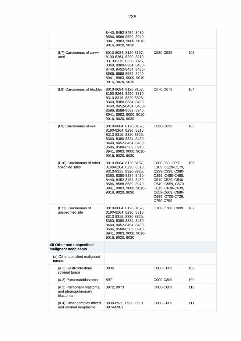
236
8440, 8452-8454, 8480-8586, 8588-8589, 8940, 8941, 8983, 9000, 9010-9016, 9020, 9030
(f.7) Carcinomas of cervix uteri
8010-8084, 8120-8157, 8190-8264, 8290, 8310, 8313-8315, 8320-8325, 8360, 8380-8384, 8430-8440, 8452-8454, 8480-8586, 8588-8589, 8940, 8941, 8983, 9000, 9010-9016, 9020, 9030
C530-C539 103
(f.8) Carcinomas of bladder 8010-8084, 8120-8157, 8190-8264, 8290, 8310, 8313-8315, 8320-8325, 8360, 8380-8384, 8430-8440, 8452-8454, 8480-8586, 8588-8589, 8940, 8941, 8983, 9000, 9010-9016, 9020, 9030
C670-C679 104
(f.9) Carcinomas of eye 8010-8084, 8120-8157, 8190-8264, 8290, 8310, 8313-8315, 8320-8325, 8360, 8380-8384, 8430-8440, 8452-8454, 8480-8586, 8588-8589, 8940, 8941, 8983, 9000, 9010-9016, 9020, 9030
C690-C699 105
(f.10) Carcinomas of other specified sites
8010-8084, 8120-8157, 8190-8264, 8290, 8310, 8313-8315, 8320-8325, 8360, 8380-8384, 8430-8440, 8452-8454, 8480-8586, 8588-8589, 8940, 8941, 8983, 9000, 9010-9016, 9020, 9030
C000-069, C090-C109, C129-C179, C239-C339, C380-C399, C480-C488, C510-C529, C540-C549, C559, C570-C619, C630-C639, C659-C669, C680-C689, C700-C729, C750-C759
106
(f.11) Carcinomas of unspecified site
8010-8084, 8120-8157, 8190-8264, 8290, 8310, 8313-8315, 8320-8325, 8360, 8380-8384, 8430-8440, 8452-8454, 8480-8586, 8588-8589, 8940, 8941, 8983, 9000, 9010-9016, 9020, 9030
C760-C768, C809 107
XII Other and unspecified malignant neoplasms
(a) Other specified malignant tumors
(a.1) Gastrointestinal stromal tumor
8936 C000-C809 108
(a.2) Pancreatoblastoma 8971 C000-C809 109
(a.3) Pulmonary blastoma and pleuropulmonary blastoma
8972, 8973 C000-C809 110
(a.4) Other complex mixed and stromal neoplasms
8930-8935, 8950, 8951, 8974-8981
C000-C809 111

237
(a.5) Mesothelioma 9050-9055 C000-C809 112
(a.6) Other specified malignant tumors
9110 C000-C809 113
9363 C000-C399, C470-C759
113
(b) Other unspecified malignant tumors
8000-8005 C000-C218, C239-C399, C420-C559, C570-C619, C630-C639, C659-C699, C739-C750, C754-809
114
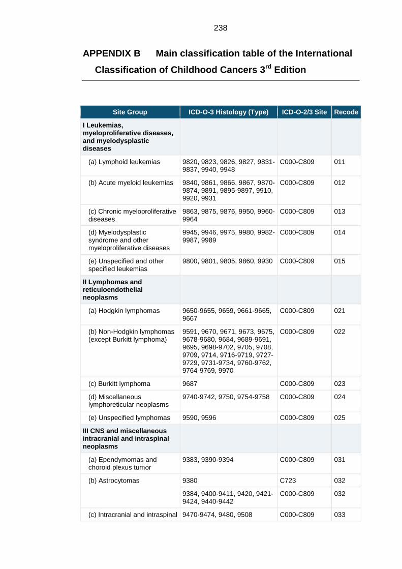
238
APPENDIX B Main classification table of the International
Classification of Childhood Cancers 3rd Edition
Site Group ICD-O-3 Histology (Type) ICD-O-2/3 Site Recode
I Leukemias, myeloproliferative diseases, and myelodysplastic diseases
(a) Lymphoid leukemias 9820, 9823, 9826, 9827, 9831-9837, 9940, 9948
C000-C809 011
(b) Acute myeloid leukemias 9840, 9861, 9866, 9867, 9870-9874, 9891, 9895-9897, 9910, 9920, 9931
C000-C809 012
(c) Chronic myeloproliferative diseases
9863, 9875, 9876, 9950, 9960-9964
C000-C809 013
(d) Myelodysplastic syndrome and other myeloproliferative diseases
9945, 9946, 9975, 9980, 9982-9987, 9989
C000-C809 014
(e) Unspecified and other specified leukemias
9800, 9801, 9805, 9860, 9930 C000-C809 015
II Lymphomas and reticuloendothelial neoplasms
(a) Hodgkin lymphomas 9650-9655, 9659, 9661-9665, 9667
C000-C809 021
(b) Non-Hodgkin lymphomas (except Burkitt lymphoma)
9591, 9670, 9671, 9673, 9675, 9678-9680, 9684, 9689-9691, 9695, 9698-9702, 9705, 9708, 9709, 9714, 9716-9719, 9727-9729, 9731-9734, 9760-9762, 9764-9769, 9970
C000-C809 022
(c) Burkitt lymphoma 9687 C000-C809 023
(d) Miscellaneous lymphoreticular neoplasms
9740-9742, 9750, 9754-9758 C000-C809 024
(e) Unspecified lymphomas 9590, 9596 C000-C809 025
III CNS and miscellaneous intracranial and intraspinal neoplasms
(a) Ependymomas and choroid plexus tumor
9383, 9390-9394 C000-C809 031
(b) Astrocytomas 9380 C723 032
9384, 9400-9411, 9420, 9421-9424, 9440-9442
C000-C809 032
(c) Intracranial and intraspinal 9470-9474, 9480, 9508 C000-C809 033
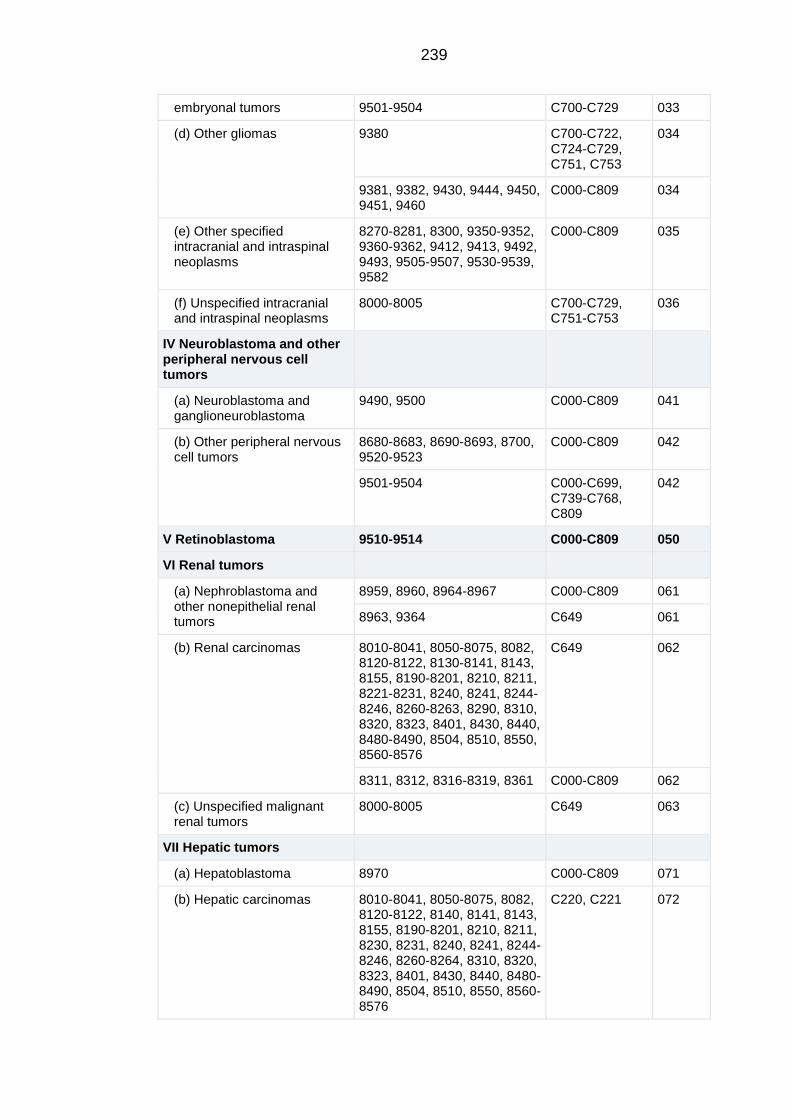
239
embryonal tumors 9501-9504 C700-C729 033
(d) Other gliomas 9380 C700-C722, C724-C729, C751, C753
034
9381, 9382, 9430, 9444, 9450, 9451, 9460
C000-C809 034
(e) Other specified intracranial and intraspinal neoplasms
8270-8281, 8300, 9350-9352, 9360-9362, 9412, 9413, 9492, 9493, 9505-9507, 9530-9539, 9582
C000-C809 035
(f) Unspecified intracranial and intraspinal neoplasms
8000-8005 C700-C729, C751-C753
036
IV Neuroblastoma and other peripheral nervous cell tumors
(a) Neuroblastoma and ganglioneuroblastoma
9490, 9500 C000-C809 041
(b) Other peripheral nervous cell tumors
8680-8683, 8690-8693, 8700, 9520-9523
C000-C809 042
9501-9504 C000-C699, C739-C768, C809
042
V Retinoblastoma 9510-9514 C000-C809 050
VI Renal tumors
(a) Nephroblastoma and other nonepithelial renal tumors
8959, 8960, 8964-8967 C000-C809 061
8963, 9364 C649 061
(b) Renal carcinomas 8010-8041, 8050-8075, 8082, 8120-8122, 8130-8141, 8143, 8155, 8190-8201, 8210, 8211, 8221-8231, 8240, 8241, 8244-8246, 8260-8263, 8290, 8310, 8320, 8323, 8401, 8430, 8440, 8480-8490, 8504, 8510, 8550, 8560-8576
C649 062
8311, 8312, 8316-8319, 8361 C000-C809 062
(c) Unspecified malignant renal tumors
8000-8005 C649 063
VII Hepatic tumors
(a) Hepatoblastoma 8970 C000-C809 071
(b) Hepatic carcinomas 8010-8041, 8050-8075, 8082, 8120-8122, 8140, 8141, 8143, 8155, 8190-8201, 8210, 8211, 8230, 8231, 8240, 8241, 8244-8246, 8260-8264, 8310, 8320, 8323, 8401, 8430, 8440, 8480-8490, 8504, 8510, 8550, 8560-8576
C220, C221 072
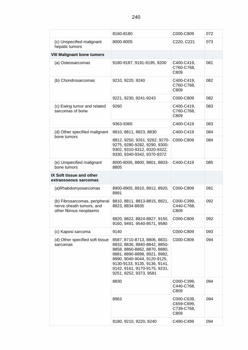
240
8160-8180 C000-C809 072
(c) Unspecified malignant hepatic tumors
8000-8005 C220, C221 073
VIII Malignant bone tumors
(a) Osteosarcomas 9180-9187, 9191-9195, 9200 C400-C419, C760-C768, C809
081
(b) Chondrosarcomas 9210, 9220, 9240 C400-C419, C760-C768, C809
082
9221, 9230, 9241-9243 C000-C809 082
(c) Ewing tumor and related sarcomas of bone
9260 C400-C419, C760-C768, C809
083
9363-9365 C400-C419 083
(d) Other specified malignant bone tumors
8810, 8811, 8823, 8830 C400-C419 084
8812, 9250, 9261, 9262, 9270-9275, 9280-9282, 9290, 9300-9302, 9310-9312, 9320-9322, 9330, 9340-9342, 9370-9372
C000-C809 084
(e) Unspecified malignant bone tumors
8000-8005, 8800, 8801, 8803-8805
C400-C419 085
IX Soft tissue and other extraosseous sarcomas
(a)Rhabdomyosarcomas 8900-8905, 8910, 8912, 8920, 8991
C000-C809 091
(b) Fibrosarcomas, peripheral nerve sheath tumors, and other fibrous neoplasms
8810, 8811, 8813-8815, 8821, 8823, 8834-8835
C000-C399, C440-C768, C809
092
8820, 8822, 8824-8827, 9150, 9160, 9491, 9540-9571, 9580
C000-C809 092
(c) Kaposi sarcoma 9140 C000-C809 093
(d) Other specified soft tissue sarcomas
8587, 8710-8713, 8806, 8831-8833, 8836, 8840-8842, 8850-8858, 8860-8862, 8870, 8880, 8881, 8890-8898, 8921, 8982, 8990, 9040-9044, 9120-9125, 9130-9133, 9135, 9136, 9141, 9142, 9161, 9170-9175, 9231, 9251, 9252, 9373, 9581
C000-C809 094
8830 C000-C399, C440-C768, C809
094
8963 C000-C639, C659-C699, C739-C768, C809
094
9180, 9210, 9220, 9240 C490-C499 094
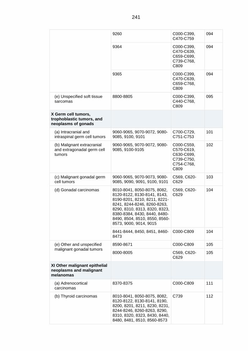
241
9260 C000-C399, C470-C759
094
9364 C000-C399, C470-C639, C659-C699, C739-C768, C809
094
9365 C000-C399, C470-C639, C659-C768, C809
094
(e) Unspecified soft tissue sarcomas
8800-8805 C000-C399, C440-C768, C809
095
X Germ cell tumors, trophoblastic tumors, and neoplasms of gonads
(a) Intracranial and intraspinal germ cell tumors
9060-9065, 9070-9072, 9080-9085, 9100, 9101
C700-C729, C751-C753
101
(b) Malignant extracranial and extragonadal germ cell tumors
9060-9065, 9070-9072, 9080-9085, 9100-9105
C000-C559, C570-C619, C630-C699, C739-C750, C754-C768, C809
102
(c) Malignant gonadal germ cell tumors
9060-9065, 9070-9073, 9080-9085, 9090, 9091, 9100, 9101
C569, C620-C629
103
(d) Gonadal carcinomas 8010-8041, 8050-8075, 8082, 8120-8122, 8130-8141, 8143, 8190-8201, 8210, 8211, 8221-8241, 8244-8246, 8260-8263, 8290, 8310, 8313, 8320, 8323, 8380-8384, 8430, 8440, 8480-8490, 8504, 8510, 8550, 8560-8573, 9000, 9014, 9015
C569, C620-C629
104
8441-8444, 8450, 8451, 8460-8473
C000-C809 104
(e) Other and unspecified malignant gonadal tumors
8590-8671 C000-C809 105
8000-8005 C569, C620-C629
105
XI Other malignant epithelial neoplasms and malignant melanomas
(a) Adrenocortical carcinomas
8370-8375 C000-C809 111
(b) Thyroid carcinomas 8010-8041, 8050-8075, 8082, 8120-8122, 8130-8141, 8190, 8200, 8201, 8211, 8230, 8231, 8244-8246, 8260-8263, 8290, 8310, 8320, 8323, 8430, 8440, 8480, 8481, 8510, 8560-8573
C739 112
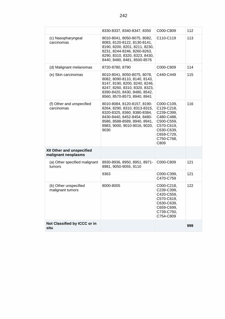
242
8330-8337, 8340-8347, 8350 C000-C809 112
(c) Nasopharyngeal carcinomas
8010-8041, 8050-8075, 8082, 8083, 8120-8122, 8130-8141, 8190, 8200, 8201, 8211, 8230, 8231, 8244-8246, 8260-8263, 8290, 8310, 8320, 8323, 8430, 8440, 8480, 8481, 8500-8576
C110-C119 113
(d) Malignant melanomas 8720-8780, 8790 C000-C809 114
(e) Skin carcinomas 8010-8041, 8050-8075, 8078, 8082, 8090-8110, 8140, 8143, 8147, 8190, 8200, 8240, 8246, 8247, 8260, 8310, 8320, 8323, 8390-8420, 8430, 8480, 8542, 8560, 8570-8573, 8940, 8941
C440-C449 115
(f) Other and unspecified carcinomas
8010-8084, 8120-8157, 8190-8264, 8290, 8310, 8313-8315, 8320-8325, 8360, 8380-8384, 8430-8440, 8452-8454, 8480-8586, 8588-8589, 8940, 8941, 8983, 9000, 9010-9016, 9020, 9030
C000-C109, C129-C218, C239-C399, C480-C488, C500-C559, C570-C619, C630-C639, C659-C729, C750-C768, C809
116
XII Other and unspecified malignant neoplasms
(a) Other specified malignant tumors
8930-8936, 8950, 8951, 8971-8981, 9050-9055, 9110
C000-C809 121
9363 C000-C399, C470-C759
121
(b) Other unspecified malignant tumors
8000-8005 C000-C218, C239-C399, C420-C559, C570-C619, C630-C639, C659-C699, C739-C750, C754-C809
122
Not Classified by ICCC or in situ
999
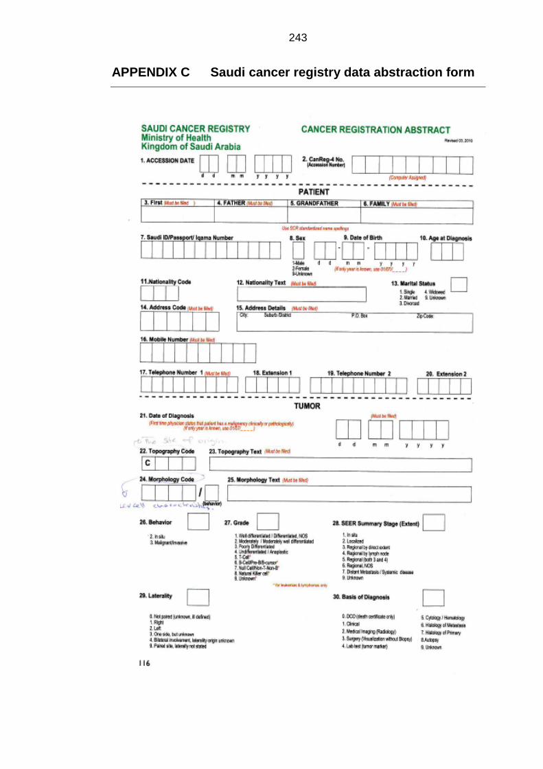
243
APPENDIX C Saudi cancer registry data abstraction form
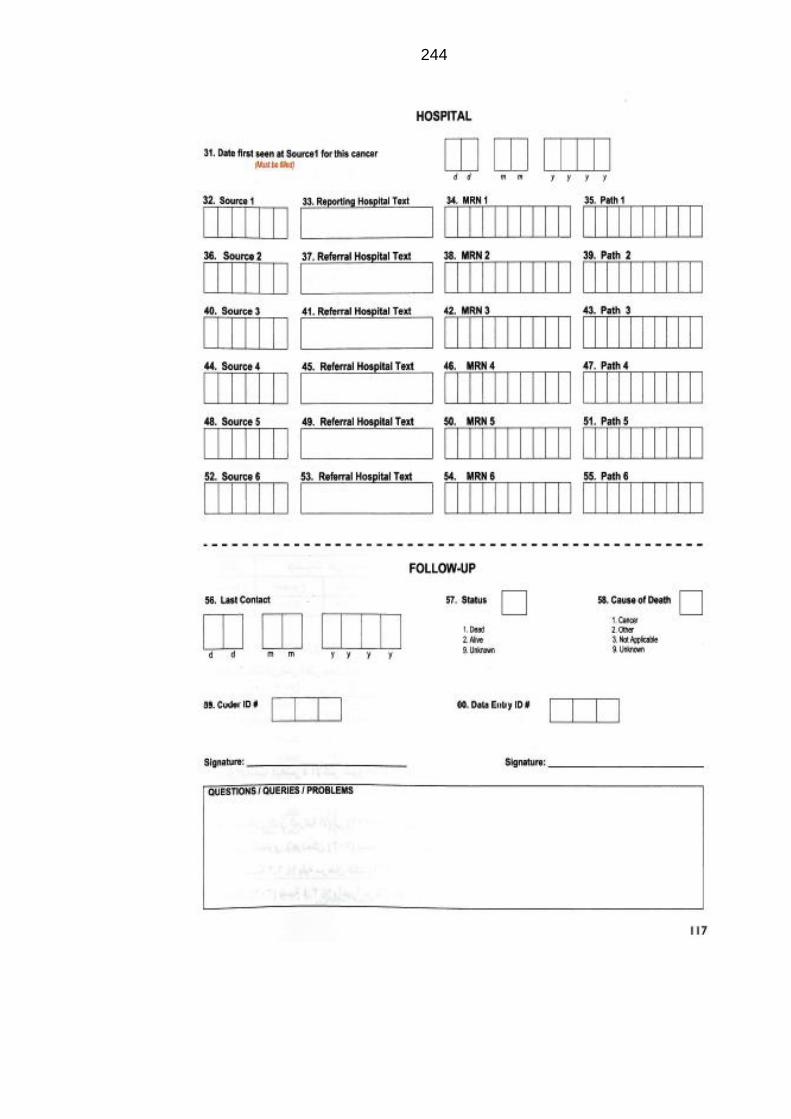
244
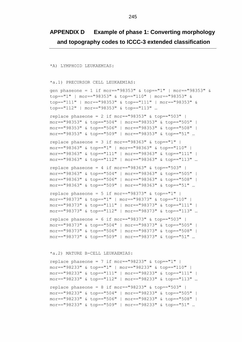
245
APPENDIX D Example of phase 1: Converting morphology
and topography codes to ICCC-3 extended classification
*A) LYMPHOID LEUKAEMIAS:
*a.1) PRECURSOR CELL LEUKAEMIAS:
gen phaseone = 1 if mor=="98353" & top=="1" | mor=="98353" &
top=="1" | mor=="98353" & top=="110" | mor=="98353" &
top=="111" | mor=="98353" & top=="111" | mor=="98353" &
top=="112" | mor=="98353" & top=="113" …
replace phaseone = 2 if mor=="98353" & top=="503" |
mor=="98353" & top=="504" | mor=="98353" & top=="505" |
mor=="98353" & top=="506" | mor=="98353" & top=="508" |
mor=="98353" & top=="509" | mor=="98353" & top=="51" …
replace phaseone = 3 if mor=="98363" & top=="1" |
mor=="98363" & top=="1" | mor=="98363" & top=="110" |
mor=="98363" & top=="111" | mor=="98363" & top=="111" |
mor=="98363" & top=="112" | mor=="98363" & top=="113" …
replace phaseone = 4 if mor=="98363" & top=="503" |
mor=="98363" & top=="504" | mor=="98363" & top=="505" |
mor=="98363" & top=="506" | mor=="98363" & top=="508" |
mor=="98363" & top=="509" | mor=="98363" & top=="51" …
replace phaseone = 5 if mor=="98373" & top=="1" |
mor=="98373" & top=="1" | mor=="98373" & top=="110" |
mor=="98373" & top=="111" | mor=="98373" & top=="111" |
mor=="98373" & top=="112" | mor=="98373" & top=="113" …
replace phaseone = 6 if mor=="98373" & top=="503" |
mor=="98373" & top=="504" | mor=="98373" & top=="505" |
mor=="98373" & top=="506" | mor=="98373" & top=="508" |
mor=="98373" & top=="509" | mor=="98373" & top=="51" …
*a.2) MATURE B-CELL LEUKAEMIAS:
replace phaseone = 7 if mor=="98233" & top=="1" |
mor=="98233" & top=="1" | mor=="98233" & top=="110" |
mor=="98233" & top=="111" | mor=="98233" & top=="111" |
mor=="98233" & top=="112" | mor=="98233" & top=="113" …
replace phaseone = 8 if mor=="98233" & top=="503" |
mor=="98233" & top=="504" | mor=="98233" & top=="505" |
mor=="98233" & top=="506" | mor=="98233" & top=="508" |
mor=="98233" & top=="509" | mor=="98233" & top=="51" …
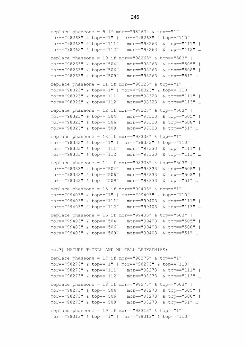
246
replace phaseone = 9 if mor=="98263" & top=="1" |
mor=="98263" & top=="1" | mor=="98263" & top=="110" |
mor=="98263" & top=="111" | mor=="98263" & top=="111" |
mor=="98263" & top=="112" | mor=="98263" & top=="113" …
replace phaseone = 10 if mor=="98263" & top=="503" |
mor=="98263" & top=="504" | mor=="98263" & top=="505" |
mor=="98263" & top=="506" | mor=="98263" & top=="508" |
mor=="98263" & top=="509" | mor=="98263" & top=="51" …
replace phaseone = 11 if mor=="98323" & top=="1" |
mor=="98323" & top=="1" | mor=="98323" & top=="110" |
mor=="98323" & top=="111" | mor=="98323" & top=="111" |
mor=="98323" & top=="112" | mor=="98323" & top=="113" …
replace phaseone = 12 if mor=="98323" & top=="503" |
mor=="98323" & top=="504" | mor=="98323" & top=="505" |
mor=="98323" & top=="506" | mor=="98323" & top=="508" |
mor=="98323" & top=="509" | mor=="98323" & top=="51" …
replace phaseone = 13 if mor=="98333" & top=="1" |
mor=="98333" & top=="1" | mor=="98333" & top=="110" |
mor=="98333" & top=="111" | mor=="98333" & top=="111" |
mor=="98333" & top=="112" | mor=="98333" & top=="113" …
replace phaseone = 14 if mor=="98333" & top=="503" |
mor=="98333" & top=="504" | mor=="98333" & top=="505" |
mor=="98333" & top=="506" | mor=="98333" & top=="508" |
mor=="98333" & top=="509" | mor=="98333" & top=="51" …
replace phaseone = 15 if mor=="99403" & top=="1" |
mor=="99403" & top=="1" | mor=="99403" & top=="110" |
mor=="99403" & top=="111" | mor=="99403" & top=="111" |
mor=="99403" & top=="112" | mor=="99403" & top=="113" …
replace phaseone = 16 if mor=="99403" & top=="503" |
mor=="99403" & top=="504" | mor=="99403" & top=="505" |
mor=="99403" & top=="506" | mor=="99403" & top=="508" |
mor=="99403" & top=="509" | mor=="99403" & top=="51" …
*a.3) MATURE T-CELL AND NK CELL LEUKAEMIAS:
replace phaseone = 17 if mor=="98273" & top=="1" |
mor=="98273" & top=="1" | mor=="98273" & top=="110" |
mor=="98273" & top=="111" | mor=="98273" & top=="111" |
mor=="98273" & top=="112" | mor=="98273" & top=="113" …
replace phaseone = 18 if mor=="98273" & top=="503" |
mor=="98273" & top=="504" | mor=="98273" & top=="505" |
mor=="98273" & top=="506" | mor=="98273" & top=="508" |
mor=="98273" & top=="509" | mor=="98273" & top=="51" …
replace phaseone = 19 if mor=="98313" & top=="1" |
mor=="98313" & top=="1" | mor=="98313" & top=="110" |
247
mor=="98313" & top=="111" | mor=="98313" & top=="111" |
mor=="98313" & top=="112" | mor=="98313" & top=="113" …
replace phaseone = 20 if mor=="98313" & top=="503" |
mor=="98313" & top=="504" | mor=="98313" & top=="505" |
mor=="98313" & top=="506" | mor=="98313" & top=="508" |
mor=="98313" & top=="509" | mor=="98313" & top=="51" …
replace phaseone = 21 if mor=="98343" & top=="1" |
mor=="98343" & top=="1" | mor=="98343" & top=="110" |
mor=="98343" & top=="111" | mor=="98343" & top=="111" |
mor=="98343" & top=="112" | mor=="98343" & top=="113" …
replace phaseone = 22 if mor=="98343" & top=="503" |
mor=="98343" & top=="504" | mor=="98343" & top=="505" |
mor=="98343" & top=="506" | mor=="98343" & top=="508" |
mor=="98343" & top=="509" | mor=="98343" & top=="51" …
replace phaseone = 23 if mor=="99483" & top=="1" |
mor=="99483" & top=="1" | mor=="99483" & top=="110" |
mor=="99483" & top=="111" | mor=="99483" & top=="111" |
mor=="99483" & top=="112" | mor=="99483" & top=="113" …
replace phaseone = 24 if mor=="99483" & top=="503" |
mor=="99483" & top=="504" | mor=="99483" & top=="505" |
mor=="99483" & top=="506" | mor=="99483" & top=="508" |
mor=="99483" & top=="509" | mor=="99483" & top=="51" …
*a.4) LYMPHOID LEUKAEMIAS, NOS:
replace phaseone = 27 if mor=="98203" & top=="1" |
mor=="98203" & top=="1" | mor=="98203" & top=="110" |
mor=="98203" & top=="111" | mor=="98203" & top=="111" |
mor=="98203" & top=="112" | mor=="98203" & top=="113" …
replace phaseone = 28 if mor=="98203" & top=="503" |
mor=="98203" & top=="504" | mor=="98203" & top=="505" |
mor=="98203" & top=="506" | mor=="98203" & top=="508" |
mor=="98203" & top=="509" | mor=="98203" & top=="51" …
*---------------------------------*
*---------------------------------*
*GENERATE ICCC-E:
gen ICCCE = 001 if phaseone ==1 | phaseone==2 | phaseone==3 |
phaseone==4 | phaseone==5 | phaseone==6
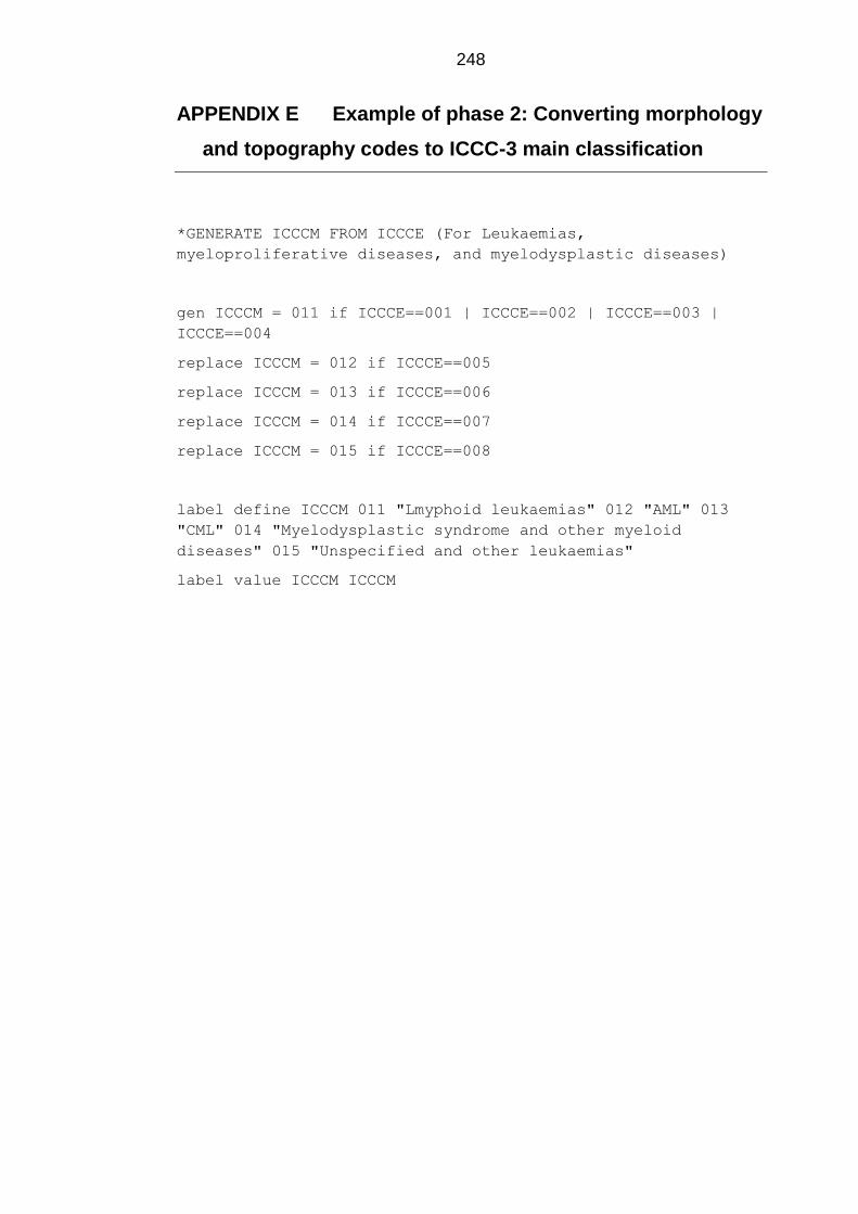
248
APPENDIX E Example of phase 2: Converting morphology
and topography codes to ICCC-3 main classification
*GENERATE ICCCM FROM ICCCE (For Leukaemias,
myeloproliferative diseases, and myelodysplastic diseases)
gen ICCCM = 011 if ICCCE==001 | ICCCE==002 | ICCCE==003 |
ICCCE==004
replace ICCCM = 012 if ICCCE==005
replace ICCCM = 013 if ICCCE==006
replace ICCCM = 014 if ICCCE==007
replace ICCCM = 015 if ICCCE==008
label define ICCCM 011 "Lmyphoid leukaemias" 012 "AML" 013
"CML" 014 "Myelodysplastic syndrome and other myeloid
diseases" 015 "Unspecified and other leukaemias"
label value ICCCM ICCCM
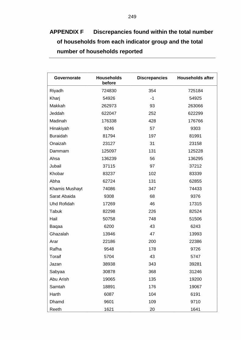
249
APPENDIX F Discrepancies found within the total number
of households from each indicator group and the total
number of households reported
Governorate Households before
Discrepancies Households after
Riyadh 724830 354 725184
Kharj 54926 -1 54925
Makkah 262973 93 263066
Jeddah 622047 252 622299
Madinah 176338 428 176766
Hinakiyah 9246 57 9303
Buraidah 81794 197 81991
Onaizah 23127 31 23158
Dammam 125097 131 125228
Ahsa 136239 56 136295
Jubail 37115 97 37212
Khobar 83237 102 83339
Abha 62724 131 62855
Khamis Mushayt 74086 347 74433
Sarat Abaida 9308 68 9376
Uhd Rofidah 17269 46 17315
Tabuk 82298 226 82524
Hail 50758 748 51506
Baqaa 6200 43 6243
Ghazalah 13946 47 13993
Arar 22186 200 22386
Rafha 9548 178 9726
Toraif 5704 43 5747
Jazan 38938 343 39281
Sabyaa 30878 368 31246
Abu Arish 19065 135 19200
Samtah 18891 176 19067
Harth 6087 104 6191
Dhamd 9601 109 9710
Reeth 1621 20 1641
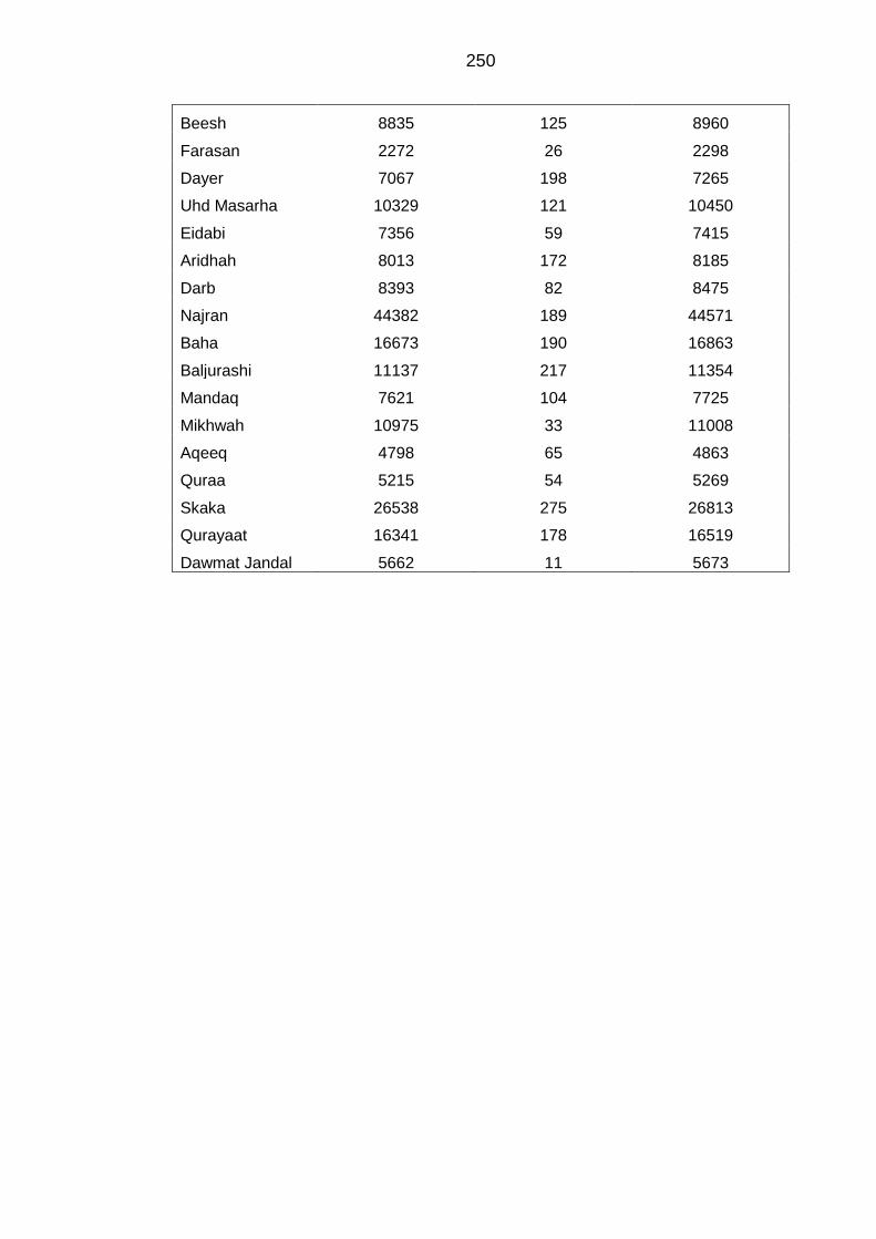
250
Beesh 8835 125 8960
Farasan 2272 26 2298
Dayer 7067 198 7265
Uhd Masarha 10329 121 10450
Eidabi 7356 59 7415
Aridhah 8013 172 8185
Darb 8393 82 8475
Najran 44382 189 44571
Baha 16673 190 16863
Baljurashi 11137 217 11354
Mandaq 7621 104 7725
Mikhwah 10975 33 11008
Aqeeq 4798 65 4863
Quraa 5215 54 5269
Skaka 26538 275 26813
Qurayaat 16341 178 16519
Dawmat Jandal 5662 11 5673
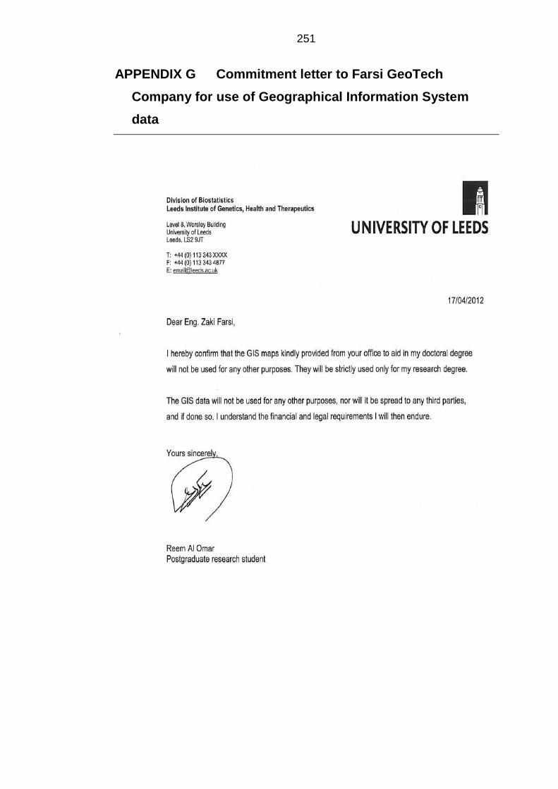
251
APPENDIX G Commitment letter to Farsi GeoTech
Company for use of Geographical Information System
data
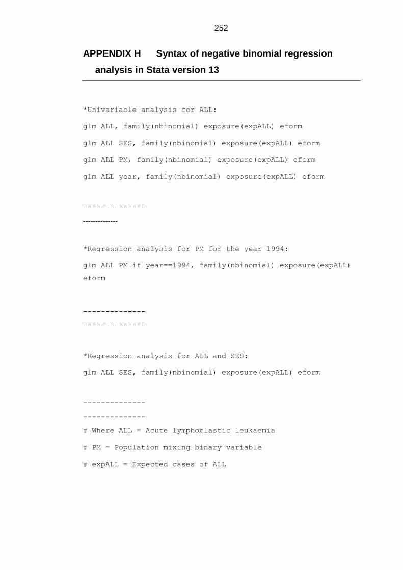
252
APPENDIX H Syntax of negative binomial regression
analysis in Stata version 13
*Univariable analysis for ALL:
glm ALL, family(nbinomial) exposure(expALL) eform
glm ALL SES, family(nbinomial) exposure(expALL) eform
glm ALL PM, family(nbinomial) exposure(expALL) eform
glm ALL year, family(nbinomial) exposure(expALL) eform
--------------
--------------
*Regression analysis for PM for the year 1994:
glm ALL PM if year==1994, family(nbinomial) exposure(expALL)
eform
--------------
--------------
*Regression analysis for ALL and SES:
glm ALL SES, family(nbinomial) exposure(expALL) eform
--------------
--------------
# Where ALL = Acute lymphoblastic leukaemia
# PM = Population mixing binary variable
# expALL = Expected cases of ALL
253
APPENDIX I Initial and standardised index of Saudi
Governorates
Province Governorate Initial index Standardised index
Eastern Region Qatif 131.25 100.00
Eastern Region Khobar 122.70 97.02
Eastern Region Rass Tanourah 113.03 93.64
Eastern Region Jubail 106.89 91.50
Riyadh Riyadh 104.71 90.74
Eastern Region Dammam 104.08 90.52
Eastern Region Bqeeq 89.92 85.59
Eastern Region Ahsa 86.56 84.41
Eastern Region Khafji 84.11 83.56
Qassim Onaizah 82.63 83.04
Baha Baha 80.88 82.43
Northern border Arar 72.58 79.53
Jouf Skaka 62.74 76.10
Riyadh Dareiyah 60.72 75.40
Qassim Buraidah 62.27 75.94
Jouf Qurayaat 57.65 74.33
Makkah Jeddah 57.83 74.39
Hail Hail 58.07 74.48
Madinah Madinah 56.78 74.02
Tabuk Tabuk 57.32 74.21
Qassim Rass 55.87 73.71
Aseer Abha 55.92 73.72
Jouf Dawmat Jandal 53.19 72.77
Qassim Badae 50.97 72.00
Aseer Khamis Mushayt 48.86 71.26
Madinah Yanbu 47.68 70.85
Northern border Toraif 45.62 70.13
Riyadh Zolfi 42.84 69.16
Baha Mandaq 40.32 68.28
Riyadh Shaqraa 41.28 68.62
Makkah Taif 38.50 67.65
Eastern Region Hafr batin 38.80 67.76
Riyadh Kharj 37.91 67.44
Baha Baljurashi 36.02 66.78
Makkah Makkah 36.65 67.01
Northern border Rafha 29.70 64.58
254
Qassim Asyah 30.24 64.77
Qassim Midnab 28.53 64.17
Riyadh Majmaah 27.64 63.86
Qassim Shamssiyah 26.13 63.33
Aseer Namas 20.62 61.41
Qassim Bikairiah 20.17 61.26
Riyadh Hotat bani tamim 19.64 61.07
Tabuk Haql 21.86 61.84
Qassim Riyadh Khobaraa 18.08 60.53
Aseer Uhd Rofidah 17.03 60.16
Najran Najran 13.95 59.09
Najran Sharourah 10.69 57.95
Riyadh Selayil 11.77 58.33
Baha Quraa 6.25 56.40
Eastern Region Noariyah 8.15 57.06
Jazan Jazan 9.25 57.45
Riyadh Afeef 11.28 58.15
Eastern Region Qaryat Alya 3.06 55.29
Aseer Belgarn 6.47 56.48
Riyadh Dawadmi 4.79 55.89
Qassim Oyoon Jawaa 4.80 55.90
Riyadh Hareeq -1.41 53.73
Riyadh Aflaj 0.11 54.26
Jazan Farasan -2.01 53.52
Aseer Dhahran Janoub -2.21 53.45
Riyadh Wadi Dawaser -4.86 52.53
Tabuk Tayma -5.26 52.39
Makkah Rabegh -8.69 51.19
Aseer Bishah -11.21 50.31
Riyadh Ghat -8.80 51.15
Madinah Badr -12.09 50.00
Tabuk Wajh -12.38 49.90
Jazan Abu Arish -15.04 48.98
Baha Mikhwah -16.21 48.57
Tabuk Amluj -16.22 48.56
Makkah Kholais -18.29 47.84
Aseer Sarat Abaida -18.36 47.82
Riyadh Romah -24.33 45.73
Makkah Jomoom -26.44 45.00
Tabuk Dhebaa -25.71 45.25
Makkah Khormah -27.93 44.48
Jazan Uhd Masarha -31.48 43.24
255
Riyadh Thadeq -28.73 44.20
Aseer Rejal Almaa -31.72 43.16
Makkah Raniah -34.29 42.26
Aseer Mahail -32.13 43.02
Jazan Beesh -34.73 42.11
Jazan Dhamd -32.40 42.92
Baha Qilwah -34.97 42.03
Jazan Sabyaa -33.87 42.41
Makkah Qunfudhah -35.41 41.87
Madinah Khaibar -35.45 41.86
Madinah Ola -35.41 41.87
Hail Baqaa -39.79 40.34
Aseer Majardah -40.53 40.08
Riyadh Mozahimyah -40.18 40.21
Najran Haboona -46.51 38.00
Baha Aqeeq -44.39 38.74
Makkah Torbah -43.16 39.17
Jazan Samtah -45.51 38.35
Riyadh Herimla -46.16 38.12
Riyadh Qowaiyah -48.83 37.19
Hail Shanan -51.53 36.25
Najran Badr Janoub -56.75 34.43
Madinah Hinakiyah -54.67 35.15
Jazan Darb -56.06 34.67
Makkah Leeth -55.07 35.01
Qassim Nabhanyah -59.14 33.59
Hail Ghazalah -62.56 32.40
Madinah Mahd -66.19 31.13
Riyadh Dhurma -68.99 30.16
Najran Khabash -76.20 27.64
Jazan Dayer -77.09 27.33
Najran Thaar -85.75 24.31
Aseer Tathleeth -88.30 23.42
Makkah Kamel -90.79 22.55
Jazan Harth -103.39 18.16
Jazan Aridhah -103.08 18.27
Jazan Eidabi -103.60 18.09
Najran Yadmah -101.28 18.90
Jazan Reeth -104.40 17.81
Najran Kharkheer -155.46 0.00
256
APPENDIX J Modal class assignment and the final
socioeconomic classes index of the Saudi Governorates
Region Governorate p1* p2* p3* p4* class
Eastern region Khobar 1 0 0 0 1
Eastern region Jubail 1 0 0 0 1
Eastern region Dammam 1 0 0 0 1
Riyadh Riyadh 1 0 0 0 1
Eastern region Rass Tanourah 1 0 0 0 1
Eastern region Qatif 1 0 0 0 1
Makkah Jeddah 1 0 0 0 1
Qassim Onaizah 0.999 0.001 0 0 1
Eastern region Bqeeq 1 0 0 0 1
Riyadh Dareiyah 0.998 0.002 0 0 1
Eastern region Khafji 1 0 0 0 1
Eastern region Ahsa 1 0 0 0 1
Baha Baha 0.919 0.081 0 0 1
Tabuk Tabuk 0 1 0 0 2
Madinah Madinah 0.001 0.999 0 0 2
Madinah Yanbu 0.234 0.766 0 0 2
Northern border Arar 0.002 0.998 0 0 2
Riyadh Kharj 0 1 0 0 2
Qassim Buraidah 0 1 0 0 2
Riyadh Shaqraa 0 1 0 0 2
Aseer Khamis Mushayt 0 1 0 0 2
Aseer Abha 0 1 0 0 2
Qassim Rass 0 1 0 0 2
Makkah Makkah 0 1 0 0 2
Jouf Skaka 0 1 0 0 2
Qassim Badae 0 1 0 0 2
Eastern region Hafr batin 0 1 0 0 2
Hail Hail 0 1 0 0 2
Jouf Dawmat Jandal 0 1 0 0 2
Northern border Toraif 0 1 0 0 2
Riyadh Zolfi 0 1 0 0 2
Makkah Taif 0 1 0 0 2
Jouf Qurayyat 0 1 0 0 2
Qassim Midnab 0 1 0 0 2
Riyadh Majmaah 0 1 0 0 2
Baha Baljurashi 0 1 0 0 2
257
Najran Sharourah 0 1 0 0 2
Riyadh Hareeq 0 1 0 0 2
Riyadh Selayil 0 1 0 0 2
Riyadh Hotat bani tamim 0 1 0 0 2
Tabuk Haql 0 1 0 0 2
Qassim Bikairiah 0 1 0 0 2
Najran Najran 0 1 0 0 2
Qassim Asyah 0 1 0 0 2
Riyadh Ghat 0 1 0 0 2
Northern border Rafha 0 1 0 0 2
Baha Mandaq 0 1 0 0 2
Qassim Oyoon Jawaa 0 1 0 0 2
Aseer Uhd Rofidah 0 1 0 0 2
Aseer Namas 0 1 0 0 2
Qassim Shamssiyah 0 0.999 0.001 0 2
Eastern region Noariyah 0 0.998 0.002 0 2
Riyadh Herimla 0 1 0 0 2
Qassim Riyadh Khobaraa 0 0.994 0.006 0 2
Riyadh Aflaj 0 1 0 0 2
Riyadh Mozahimyah 0 1 0 0 2
Riyadh Wadi Dawaser 0 0.999 0.001 0 2
Eastern region Qaryat Alya 0 0.998 0.002 0 2
Riyadh Romah 0 1 0 0 2
Riyadh Dawadmi 0 0.974 0.026 0 2
Riyadh Afeef 0 0.986 0.014 0 2
Tabuk Wajh 0 0.959 0.041 0 2
Tabuk Tayma 0 1 0 0 2
Baha Quraa 0 0.997 0.003 0 2
Riyadh Thadeq 0 0.961 0.039 0 2
Riyadh Dhurma 0 0.992 0.008 0 2
Jazan Jazan 0 0.011 0.989 0 3
Makkah Rabegh 0 0.018 0.982 0 3
Aseer Belgarn 0 0 1 0 3
Tabuk Dhebaa 0 0.001 0.999 0 3
Tabuk Amluj 0 0.005 0.995 0 3
Jazan Farasan 0 0 1 0 3
Aseer Bishah 0 0 1 0 3
Aseer Dhahran Janoub 0 0 1 0 3
Madinah Ola 0 0 1 0 3
Madinah Badr 0 0 1 0 3
Makkah Khormah 0 0 1 0 3
Jazan Abu Arish 0 0 1 0 3
258
Makkah Raniah 0 0 1 0 3
Hail Baqaa 0 0 1 0 3
Riyadh Qowaiyah 0 0 1 0 3
Makkah Kholais 0 0 1 0 3
Baha Mikhwah 0 0 1 0 3
Aseer Sarat Abaida 0 0 1 0 3
Makkah Jomoom 0 0 1 0 3
Najran Haboona 0 0 1 0 3
Makkah Torbah 0 0 1 0 3
Hail Shanan 0 0 1 0 3
Aseer Rejal Almaa 0 0 1 0 3
Jazan Sabyaa 0 0 1 0 3
Madinah Khaibar 0 0 1 0 3
Baha Aqeeq 0 0 1 0 3
Aseer Mahail 0 0 1 0 3
Jazan Beesh 0 0 1 0 3
Jazan Uhd Masarha 0 0 1 0 3
Jazan Dhamd 0 0 1 0 3
Makkah Qunfudhah 0 0 0.982 0.018 3
Aseer Majardah 0 0 0.999 0.001 3
Baha Qilwah 0 0 0.973 0.027 3
Jazan Darb 0 0 1 0 3
Najran Badr Janoub 0 0 1 0 3
Madinah Mahd 0 0 0.595 0.405 3
Jazan Samtah 0 0 0.998 0.002 3
Najran Khabash 0 0 1 0 3
Najran Kharkheer 0 0 1 0 3
Madinah Hinakiyah 0 0 0.003 0.997 4
Qassim Nabhanyah 0 0 0 1 4
Makkah Leeth 0 0 0 1 4
Hail Ghazalah 0 0 0 1 4
Aseer Tathleeth 0 0 0 1 4
Jazan Dayer 0 0 0 1 4
Najran Thaar 0 0 0 1 4
Makkah Kamel 0 0 0 1 4
Najran Yadmah 0 0 0 1 4
Jazan Harth 0 0 0 1 4
Jazan Eidabi 0 0 0 1 4
Jazan Aridhah 0 0 0 1 4
Jazan Reeth 0 0 0 1 4
*The probability of each Governorate belonging to a class.1
Copyright © 2022 FDOKUMEN