IIIS Discussion Paper

No.159/June 2006

Can the Benefits of Developed Country Agricultural TradeReforms Trickle Down to the Rural Agricultural Householdsin Least Developed Countries: Analysis via PriceTransmission in Selected Agricultural Markets in Uganda

Michael Atingi-EgoResearch DepartmentBank of Uganda

Jacob OpolotResearch DepartmentBank of Uganda

Anna Santa DraleResearch DepartmentBank of Uganda

IIIS Discussion Paper No. 159

Can the Benefits of Developed Country Agricultural Trade Reforms Trickle Down to the Rural Agricultural Households in Least Developed Countries: Analysis via Price Transmission in Selected Agricultural Markets in Uganda Michael Atingi-Ego Jacob Opolot Anna Santa Drale June 2006

Disclaimer Any opinions expressed here are those of the author(s) and not those of the IIIS. All works posted here are owned and copyrighted by the author(s). Papers may only be downloaded for personal use only.

i

Can the Benefits of Developed Country Agricultural Trade Reforms Trickle Down to the Rural Agricultural Households in Least

Developed Countries: Analysis via Price Transmission in Selected Agricultural Markets in Uganda

Michael Atingi-Ego, Jacob Opolot and Anna Santa Drale Research Department

Bank of Uganda

Abstract. This paper investigates the extent of price transmission from international to domestic markets for selected agricultural products in Uganda, so as to assess the likely impact of increased market access on agricultural household poverty in rural Uganda. The study applies a variety of econometric techniques to assess the various components of market integration using monthly data over the period 2000 through 2004. The results indicate that there is price transmission from world market prices to border prices in the case of cotton, tea and tobacco. However, there is insufficient evidence of price transmission from border prices to producer prices. We also found evidence to support the null of no price transmission from border to producer prices for the non-traditional exports of beans, maize and banana, which are mostly exported to the regional market. We recommend that Government should strengthen the information network on agricultural marketing and distribution so as to reduce exploitation of smallholder farmers by well-informed middlemen. Government should also strive to increase investment in the agricultural sector so as to improve marketing and transport infrastructure.

Keywords. Agricultural trade, price transmission, developing countries JEL classification. Q13, Q17 Acknowledgements. This paper is an output of the Policy Coherence project based in the Institute for International Integration Studies and supported by a research grant from the Advisory Board for Irish Aid. The views expressed in this paper are those of the authors and do not in anyway represent the official position of the Bank of Uganda, the Institute for International Integration Studies or the Advisory Board

ii

for Irish Aid. Further details can be found on the project website, available at www.tcd.ie/iiis/policycoherence.

iii

Table of Contents

Table of Contents ............................................................................................................iii List of Tables ................................................................................................................... iv List of Figures .................................................................................................................. iv 1 Introduction.............................................................................................................. 5 2. Market access initiatives for Uganda......................................................................... 6

2.1 Europe and the Africa, Caribbean and Pacific (ACP) countries ....................... 7 2.2 The African Growth and Opportunity Act (AGOA) ...................................... 8 2.3 Multilateral initiatives ....................................................................................... 9

3. Review of theoretical and empirical literature on price transmission..................... 10 3.1 Theoretical framework ................................................................................... 10 3.2 Empirical literature on price transmission ...................................................... 14

3.2.1 Analytical frameworks ................................................................................ 14 3.2.2 Empirical investigations on price transmission in Uganda.......................... 15

4. Methodology........................................................................................................... 17 4.1 Analytical framework ..................................................................................... 17

4.1.1 Cointegration .............................................................................................. 17 4.1.2 Granger causality and error correction models ........................................... 18

4.2 Estimation procedure ...................................................................................... 20 4.3 Data................................................................................................................. 21 4.4 Limitations of the study .................................................................................. 22

5 Importance, production and marketing characteristics of the commodity sub-sectors ............................................................................................................................. 22

5.1 Cotton............................................................................................................. 22 5.2 Tea................................................................................................................... 24 5.3 Tobacco........................................................................................................... 24 5.4 Bananas............................................................................................................ 25

6 Empirical Results .................................................................................................... 27 6.1 Cotton............................................................................................................. 28 6.2 Tea................................................................................................................... 29 6.3 Tobacco........................................................................................................... 30 6.4 Bananas............................................................................................................ 31 6.5 Beans ............................................................................................................... 32 6.6 Maize............................................................................................................... 33

7. Conclusions and Policy Recommendations............................................................ 34 Appendix A. Dynamic regression models ................................................................. 48 References....................................................................................................................... 50

iv

List of Tables

Table 1: Description of variables used in the study……………………………………27 Table 2: Results for the cotton market integration analysis…………………………….28 Table 3: Results for the Tea market integration analysis………………………….….....29 Table 4: Results for the Tobacco market integration analysis…………………….……30 Table 5: Results for the Banana market integration analysis……………………... ……31 Table 6: Results for the Beans market integration analysis……………..…………..…..32 Table 7: Results for the Maize market integration analysis…………..……………....…33 List of Figures Figure 1: World and domestic price developments…………………………………….34

5

1 Introduction

After a prolonged period of isolation from the global development process, various initiatives are underway to integrate Least Developed Countries (LDCs) into the global development agenda. One such initiative seeks to integrate LDCs into the international trade community. To date, various schemes, both bilateral and multilateral, aimed at increasing LDCs’ access to developed country markets have been instituted with the hope that this will contribute positively towards poverty reduction and enhance sustainable development in LDCs. The Cotonou Agreement, which succeeded the Lomé Convention, for example, aims in part at reducing poverty through a gradual integration of ACP economies into the global trade arena. Other initiatives, such as the EU’s Everything But Arms (EBA) scheme and the US African Growth and Opportunity Act (AGOA), also grant LDCs preferential market access to developed country markets. However, for these initiatives to have a desirable impact on poverty, LDCs must ensure that all economic agents are integrated into the global market process. Price transmission from international to domestic markets is thus an essential element in understanding the dynamics of integration of economic agents into the world economy. Trade policy reforms in global agricultural markets can only have an impact on the welfare of agricultural producers in LDCs if domestic commodity markets respond to changes in international prices. The absence of market integration or even an incomplete pass-through effect from one market to another has potential adverse implications for agricultural households in developing countries. The objective of this paper is to investigate the extent of short-run price transmission from international to domestic markets for a number of agricultural commodities produced in Uganda. Its aim is to assess the likely impact of increased world market access on agricultural household poverty in rural Uganda; and to make policy recommendations that would mitigate the structural and policy-induced impediments to the price transmission mechanism. In particular, we investigate the extent of price transmission and market integration in six commodity markets: cotton, tea, tobacco, fruits (bananas), maize and beans. This choice was largely dictated by four factors: the importance of trade flows to the European Union given the ongoing reforms in its Common Agricultural Policy;

6

the current importance and potential future impact of these commodities on rural livelihoods; the scanty empirical evidence on the extent of price transmission in these commodity markets;1 and the availability of data. We deliberately do not include coffee in the analysis because it is well covered by a number of previous studies. The rest of the paper is structured as follows. Section 2 presents a brief overview of initiatives that grant Uganda increased market access to developed country markets. Section 3 reviews the theoretical and empirical literature on price transmission while section 4 presents the analytical framework and discusses the data used for investigating price transmission in the selected agricultural markets. The importance, production and marketing characteristics of the specific commodity sub-sectors are discussed in section 5, while the empirical findings are presented in section 6. Finally, the conclusions and policy recommendations are presented in section 7. 2. Market access initiatives for Uganda

Since the late 1980s, Uganda has implemented wide-ranging trade and structural reforms aimed at diversifying the export sector and increasing Uganda’s integration into the global economy. Substantial success has been registered in diversifying exports, which were highly concentrated in coffee. In 2005, coffee exports accounted for only 19% of total export earnings compared to about 80% in 1990. Non-traditional exports2 now contribute a significant portion of total export earnings. Notwithstanding this success, Uganda’s participation in international trade remains quite low. Exports as a share of GDP have risen only marginally to about 10% to date from about 5% of GDP in 1990, while imports have stagnated at around 20% of GDP. Uganda is currently a beneficiary of, and has further potential to benefit from, a series of trade policy reforms by third countries which could affects its terms of access and the prices received or paid for its major export and import commodities. These third country trade policy reforms affecting Uganda are briefly reviewed in this section.

1 Notwithstanding the importance of these commodities on the livelihood of many rural communities, little if any research has focused on establishing the extent of price transmission from international to domestic markets, as most research in Uganda has focused on the coffee sector (see Section 3.2.2). 2 Non-traditional exports are exports other than coffee, cotton, tea, and tobacco.

7

2.1 Europe and the Africa, Caribbean and Pacific (ACP) countries

When Great Britain joined the EEC (now the EU) in 1973, it brought with it preferential agreements with the Commonwealth countries. The EEC and the ACP created what came to be known as the Lomé Convention I. The Lomé Convention regulated trade and co-operation between the two blocks, the EEC and the ACP. Revisions to the Lomé Convention were made every 5 years.3 The association provided for preferential non-reciprocal tariffs for ACP exports to EEC countries; a system of compensation for the loss of income of exports due to fluctuations in world market prices; special considerations for exports of sugar, beef and bananas from ACP countries; and the financing of infrastructure, agricultural, and mining programmes. Following the creation of the World Trade Organisation (WTO) in 1995, a new co-operation agreement, the Cotonou Agreement, replaced the Lomé Convention and came into effect in June 2000. This Agreement provided for new commercial agreements between the EU and the ACP countries, which are compatible with WTO rules on preferential trade arrangements. The Cotonou Agreement seeks to bridge the legal gap to bring the EU/ACP accords into conformity with WTO rules. The agreement outlines the steps to be taken, beginning in 2002, towards the possibility of signing WTO- compatible free trade agreements (FTAs) to replace the non-reciprocal trade preferences under the Lomé Convention

The East and Southern African (ESA) countries from the ACP group of states launched bilateral trade negotiations with the EU towards WTO-compliant 'Economic Partnership Agreements' or EPAs in February 2004 as part of this process. The ESA configuration includes members of the Common Market For East and Southern Africa (COMESA). Uganda is part of the COMESA for this purpose. Negotiations towards the new reciprocal EPAs (or other alternative trade arrangements) are scheduled to conclude at the end of 2007. The EPAs are mandated to enter into force from 2008 until 2020. If the ESA negotiations with the EU lead to an EPA, then Uganda would be expected to eliminate tariffs on substantially all imports from the EU over this period.

3 The Lomé Convention was revised four times, thus Lomé I to IV.

8

Uganda has benefited from the EU’s ‘Everything But Arms’ (EBA) scheme since 5 March 2001. The EBA grants all goods (with the exception of arms) originating from LDCs duty-free and quota-free access to the EU market. It reduces to zero all tariffs on imports from LDCs except arms and frees such imports from any quantitative restriction. The special arrangements provided for in the EBA initiative with regard to market access for LDCs will be maintained for an unlimited period of time. Three products were not liberalised immediately: bananas, rice and sugar. Duties on bananas were eliminated at the beginning of 2006; duties on rice and sugar will be eliminated in 2008 and 2009, respectively. Enacting the EBA initiative ended the non-discrimination among ACP states under the Cotonou Agreement. The European Union can now offer better market access to LDC ACP countries without extending it to non-LDC ACP countries, as the Cotonou Agreement would have required. The EBA initiative thus grants more preferential market access to ACP LDCs, including Uganda, than to ACP non-LDCs. Of particular relevance to agricultural trade is the ongoing reform of the EU’s Common Agricultural Policy (CAP). The main elements of the CAP reform are a single-farm-payment-system, which will no longer be linked to the volume of production; maintaining a limited link only under well defined conditions between subsidies and production; linking subsidies to the respect of environment, food safety and animal welfare standards; and reduction of direct payments ("modulation") for bigger farms to finance the new rural development policy. The single farm payment came in force in 2004, but member states are allowed to delay this until 2007. There have also been several other modifications of the market policies of the CAP in the areas of milk, sugar, cereals, rice, durum wheat, nuts, starch potatoes and dried fodder. Uganda trades in some of these products, so CAP reform can affect its terms of trade. 2.2 The African Growth and Opportunity Act (AGOA)

The African Growth Opportunity Act (AGOA) was enacted into law by the United States Congress in May 2000. This is the most important trade legislation in the US since ratification of the Uruguay Round by Congress in 1994. Under the Act, African countries meeting certain human rights and labour standards enjoy:

9

(i) Duty-free and quota-free access to the US markets for finished textiles made from the US fabric, yarn, and thread;

(ii) Duty free access for clothing made from African fabrics (the amount allowable is able to rise from 1.5% of American imports to 3.5% over eight years); and

(iii) Four years of quota-free market access for apparel made from third-country fabric in countries with a GDP per capita of less than US$1500.

It is estimated that the second provision of the Act alone, the most important, will boost African export revenues from the current US$250 million to US$4.2 billion by 2008. The value of all clothing exports from Africa in 1999 amounted to US$584 million, or about 1% of the US$50.8 billion worth of clothing imported by the US last year. Uganda acceded to the AGOA trade initiative on 26th October 2001. Before then, Uganda’s trade with the United States took place under the Generalised System of Preferences (GSP) for Least Developed Countries. Under the AGOA initiative, Uganda can export the following manufactures into the US market: textiles and apparel; leather and leather products; handicrafts, curving and boutiques, beverages; fish products, processed foods; and timber products. Thus, there are a number of unilateral preference offers which Uganda as an LDC can exploit and the number of these unilateral offers is likely to increase as global competition increases. 2.3 Multilateral initiatives

Uganda as a member of the World Trade Organization will be affected by the multilateral trade reforms aimed at increasing LDC’s access to developed country markets. During the Doha round which began in 2001, further initiatives aimed at addressing the high level of economic distortions in developed country agricultural sectors have been proposed. The Doha declaration aimed at substantial improvements in market access; reductions of all forms of export subsidies, with a view to substantial reductions and eventual phasing out of trade-distorting domestic support. Various deadlines set for these negotiations since they began in 2001 have been missed, and at the time of writing (June 2006) the eventual outcome remains uncertain.

10

A number of conditional offers have been put on the table by the major negotiating groups. For example, the EU offer made in October 2005 provides for 60% cuts in the EU’s highest agricultural tariffs (those over 90%), a 70% reduction in the ceilings for trade-distorting domestic support, and following the Hong Kong Ministerial Conference in December 2005, the elimination of export subsidies by 2013. At the Hong Kong Conference, WTO members also agreed that developed country members, and developing countries in a position to do so, would eliminate all tariffs and quotas on imports from the least developed countries. Initially, up to 3% of tariff lines can be withheld from this offer (which is likely to considerably dilute its value), but the hope is expressed that countries can move towards full duty-free access over time. If these elements are included in a final agreement, even if they fall short of the ambitions of some of the negotiating partners, then market access for Ugandan exports particularly to non-EU markets should improve. These initiative have in common that they alter the relative prices facing Uganda in international trade. If Uganda is to take advantage of improved export prices, or mitigate the negative impact of higher import prices, then these changes in international prices must be reflected in the prices paid to producers, or paid by consumers, within the country. The remainder of this paper examines the extent to which, historically, changes in international prices have been passed through to border and eventually producer prices for a number of traded commodities. 3. Review of theoretical and empirical literature on price transmission

This section describes the basis of the analytical framework used in the paper and discusses the theoretical and empirical literature on price transmission. It first presents the theoretical framework, followed by a brief discussion of the empirical methodologies used in investigating the extent of price transmission and market integration in agricultural commodity markets. Finally, a review of empirical work on price transmission in Uganda is presented. 3.1 Theoretical framework

Given two spatially separated markets, the Law of One Price (LOP) postulates that allowing for costs of transporting a commodity from market 1 to market 2, the relationship between prices in the two markets is given by:

11

(3.1)

Where p1t and p2t are the prices of the commodity in market 1 and market 2 in period t respectively, and c is the cost of transporting the commodity from market 1 to market 2. If condition (3.1) holds, then the two markets are said to be perfectly integrated. On the other hand, if the joint distribution of the two prices is found to be non-existent, that is, the two prices are found to be independent of each other, then the two markets are not integrated and there is no price transmission from one market to another. The perfect integration condition is unlikely, especially in the short-run. In general, however, spatial arbitrage is expected to ensure that prices of a commodity will differ by an amount that is at most equal to the cost of transferring a commodity from one market to another, thus:

(3.2) Equation (3.2) is the spatial arbitrage condition that identifies a weak version of the LOP, the strong form is characterised by equality (3.1). Fackler and Goodwin (2001) emphasize that condition (3.2) is an equilibrium condition because prices may diverge from relationship (3.1), but spatial arbitrage will ensure that the difference between the two prices moves towards the transfer cost. The spatial arbitrage condition also implies that if price changes are not passed-through instantaneously, but with a lag, price transmission is incomplete in the short run, but complete in the long run. The premise of spatial price determination models is that, if two markets are linked by trade in a fair market system, excess demand or supply in one market will have an equal impact on price in both markets. Thus, if the world and domestic markets are linked, price changes in one market should have a bearing on the other. The extent of transmission may be limited by a number of factors including international trade restrictions and regulations, transport and other distribution costs, the extent of competition among traders, and the functioning of markets. It is thus convenient to represent the domestic price of an exportable good as:

xxwxd ctepp −−= )1( (3.3)

cpp tt += 12

cpp tt ≤− 12

12

and that of an importable good by:

mmwmd ctepp ++= )1( (3.4)

Where x

dp and mdp are the domestic prices of exportables and importables

respectively, pw is the world market price, e is the nominal exchange rate, ti (i = x, m) is the proportional tariff or tax on exports (x) and imports (m) respectively, and c represents transaction costs. Thus, as argued by Krueger (1992), correcting exchange rate distortions can have a major impact on prices received by the poor agricultural households. From equations (3.3) and (3.4), it is also evident that changes in border taxes (ti) can be offset or exacerbated by changes in transaction costs. Hertel and Winters (2004) argue that these may be exogenous (that is, due to domestic policy changes, such as when trade liberalization is accompanied by market reforms) or endogenous (when an imperfectly competitive distribution sector absorbs some of the border price change into its own margins). Thus, the implementation of tariff cuts, in general, should allow international prices to be transmitted to domestic markets in relative terms. If, however, the tariff is exclusionary or prohibitively high, then changes in international prices would be only marginally transmitted to the domestic market if at all. Domestic prices will be close to autarkic levels, eliminating opportunities for spatial arbitrage and resulting in the two prices moving independently of each other, as if an import ban was in place (Rapsomanikis, Hallam and Conforti, 2004). Price support policies, such as intervention mechanisms and price floors, may also isolate domestic prices from international price movements or at best result in a non-linear relationship, depending on the level of intervention or floor price relative to the international price. At the extreme, changes in international prices will have no effect on domestic prices if the international price is below the floor level. Price floor policies may therefore result in the domestic and international prices being completely unrelated below a certain threshold determined by the floor price, or in the two prices having a non-linear relationship, with increases in the international price fully transmitted to the domestic level, while decreases are incompletely passed-through. In addition to policies, large marketing margins that arise due to high transfer costs may also insulate the domestic markets from international price developments. Sexton, Kling and Carman (1991) argue that high transfer costs and marketing

13

margins hinder the transmission of price signals as they may prohibit arbitrage. Changes in world prices are therefore not fully transmitted to domestic prices. Krugman (1986), Dornbush (1987), and Froot and Klempeter (1989) also argue that non-competitive behaviour, such as that considered in pricing-to-market models, can hinder market integration. Incomplete pass-through may arise either due to trade and other related policy distortions or due to high transactions costs, such as poor transport and communications infrastructure. Price information asymmetry on the part of economic agents may also lead to decisions that contribute to inefficient outcomes. Hertel et al (2004) argue that price transmission is likely to be partially ineffective for the poor people living in remote rural areas (where transaction costs are high), in the absence of specific policy interventions aimed at improving the price transmission mechanism. Goetz (1992) reports that high fixed transport costs prevent some households from trading in many parts of Sub-Saharan Africa. Market characteristics and distortions inherent in markets may make prices adjust slowly rather than instantaneously, or less than completely, or yield a non-linear relationship between the prices. The spatial arbitrage condition includes cases that lie between the two polar cases of the strong form of the LOP and the absence of market integration. Prakash (1998) and Balcombe and Morisson (2002) argue that, given the diverse range of ways by which prices may be related, the concept of price transmission can be thought of as being based on three notions, that is:

(i) co-movement and completeness of adjustment, which implies that changes in prices in one market are fully transmitted to the other habitually;

(ii) dynamics and speed of adjustment, which has implications for the process by which, and the rate at which, changes in prices in one market filter into the other market; and

(iii) asymmetry of responses, which has implications for the co-movement of prices. Upward and downward movement of prices in one market may be symmetrically or asymmetrically transmitted to the other. The extent of completeness and the speed of adjustment can both be asymmetric.

Spatial asymmetric price response implies a non-linear adjustment. It may be due to policies or market power in the long run, or in the short run due to inventory holding behaviour in domestic markets, which may lead to asymmetries as high international price expectations lead to stock accumulation. Maccini (1978) and Blinder (1982) argue that the subsequent release of stocks after the realization of

14

high international price expectations may exert downward pressure on the domestic market and cause the domestic price to rise by less than it would have done in the presence of inventories. Bailey and Brorsen (1989) also argue that asymmetric price response may, in addition, be due to different reactions to increases and decreases of input costs, depending on whether prices are falling or rising, as competition between wholesalers with excess capacity and high fixed costs may result in prices that rise swiftly when the demand for the product is high, but decrease at a sluggish rate when demand plummets. 3.2 Empirical literature on price transmission

3.2.1 Analytical frameworks

Earlier empirical work examining the relationship between sets of prices used either correlation coefficients (e.g. Mohendru (1937), Gupta (1973), and Stigler and Sherwin (1985)) or regression models (e.g. Richardson (1978) and Mundlak and Larson (1992)) of the form:

tf

tdt pp µβα ++= , (3.5)

where dtp and f

tp (usually expressed in logarithms) denote the domestic and

foreign prices of the commodity under consideration, respectively; � and � are parameters to be estimated; and µt is the error term. The null hypothesis that the slope coefficient (�) equals unity and possibly the intercept (�) equals zero are usually tested. The reliability of the results obtaining from the estimation of equation (3.5) is limited for two fundamental reasons. First, it is very unlikely that domestic and international market prices will differ only by a white noise, given the extensive nature of market interventions that primary commodity markets are subjected to in developing countries. Therefore, a priori, one can expect the null to be rejected without necessarily ruling out some degree of co-movement between domestic and world market prices. Second, the statistical properties of the series involved in the regression, most importantly non-stationarity, may invalidate standard econometric tests and thus give misleading results regarding the degree to which world price signals are being transmitted to domestic markets.

15

In order to circumvent the restrictive nature of equation (3.5), recent studies have tended to use dynamic regression models4, whose inspiration stems from the dynamic nature of interregional commodity trade and arbitrage activities that may involve significant delivery lags and other impediments to adjustment (Fackler and Goodwin, 2001). In particular, they employ cointegration analysis, error correction models, Granger causality tests and symmetry for testing each of the components of price transmission, and thus provide particular insights into the nature of price transmission. Rapsomanikis et al (2004) argue that, collectively, these techniques offer a framework for the assessment of price transmission and market integration. Cointegration can be thought of as the empirical counterpart to the theoretical notion of a long run equilibrium relationship. If two spatially separated price series are cointegrated, there is a tendency for them to co-move in the long run, according to a linear relationship. In the short run the prices may drift apart, as shocks in one market may not be instantaneously transmitted to other markets. These could be proxied by short run developments in Error Correction Models. Arbitrage opportunities however ensure that the divergences from the underlying long run (equilibrium) relationship are transitory (Rapsomanikis et al, 2004). The theoretical underpinnings of cointegration suggest that the weak exogeneity assumption could represent the weak form of the LOP while the strong exogeneity assumption in Error Correction Models would pass for the strong form. 3.2.2 Empirical investigations on price transmission in Uganda

In Uganda, most of the empirical work on price transmission has concentrated on the coffee sub-sector. This is because, for quite some time, coffee was the major export commodity, accounting for more than 50 percent of Uganda’s export earnings. It was thus seen as a major vehicle for poverty reduction, hence the concentration of empirical analysis on the coffee sector. In what follows, the few studies that have applied the above methodologies to analyse price transmission in selected agricultural markets in Uganda are discussed. Fafchamps M. et al (2003) using primary data collected from four coffee growing districts in 2002 and 2003 found that, with the liberalization of coffee marketing in Uganda, international market prices were largely reflected in prices paid by exporters and traders. However, combining producer surveys with trader surveys

4 See appendix A for an exposition of dynamic regression models.

16

produces a picture that is quite different from previous studies as it shows that prices paid at the market level need not reflect prices actually received by farmers. During the study period, fluctuations in international prices were not fully reflected in producer prices. They attributed this to the fact that producers were more likely to sell at the farm-gate when prices went up, thereby lowering the price they actually received. They also found evidence that the number of itinerant traders purchasing coffee from farmers’ gates increased when coffee prices increased. The study also found that domestic price margins appear to be relatively stable in absolute levels. The gap between the purchase price paid by exporters and that paid by large traders is fairly small and constant over time. In contrast, they find a large difference between the price paid by exporters and the international coffee price. Notwithstanding data limitations, they conclude that the price received by coffee producers could be increased by reducing transport and handling charges in the domestic and international market chain. Rapsomanikis et al (2004) used cointegration analysis together with Granger Causality tests and Vector Error Correction Models (VECM) to determine the extent of price transmission in the Ugandan coffee sector using monthly data on producer and international prices for the period January 1990 to December 2001. Using the Johansen (1988; 1991) test, they found sufficient evidence for the alternative of one cointegrating relationship, indicating that the domestic and international markets are integrated. The Granger causality tests also suggest that world market prices Granger-cause domestic producer prices. In the VECM, the error correction coefficient of -0.18 suggests that the adjustment to the long run relationship was relatively fast, with the producer price adjusting fully to changes in world market prices after approximately five months. They also found that shocks in the international price were instantaneously, although not fully, passed through to the domestic market. The VECM tests also indicate that, in the long run, the world market price Granger-causes the producer price, but not vice versa, confirming that Uganda is a price taker in the world market. Finally, they also found sufficient evidence to conclude that adjustment to the long run equilibrium is not asymmetric. Overall, the tests suggest that the Ugandan coffee market is integrated with the international market and adjustment to long run equilibrium is fairly fast. Krivonos (2004) explored the extent to which the reforms in the coffee sub sector were successful in raising the share of the world market price received by producers

17

and in improving the transmission of price signals from the world market to domestic markets in coffee producing countries, including Uganda. Short-run price transmission, the speed of adjustment and the equilibrium producer price shares were estimated prior and after the reforms. Asymmetric price transmission was tested in both periods to check whether price increases were passed through to producers as fast as price decreases and whether the nature of the asymmetry had changed after the reforms. The results suggest that the long-run shares of producer prices in the world price increased. For Uganda the target share in the world market price increased from 0.32 to 0.91. The short-run transmission and speed of adjustment of domestic prices also improved, meaning that producer prices react faster to changes in the world market price than they did before the reforms, especially in Uganda, where prior to the reforms the transmission was close to zero. The extent of the reforms seems to have had an impact on how much price transmission has changed: the countries that have liberalized fully like Uganda experience almost instant pass through of prices today. 4. Methodology

This section deals with the methodological issues of the study. It discusses the analytical framework and the estimation procedure used in the study. It also discusses the data used and the rationale for the choice of commodities used in the analysis.

4.1 Analytical framework

Following Rapsomanikis et al (2004), we use cointegration analysis together with Granger causality tests and Vector Error Correction Models (VECM) to determine the extent of market integration in the selected agricultural markets. In what follows, the theoretical underpinnings of the analytical framework are presented. 4.1.1 Cointegration

Prices p1 and p2 in spatially or vertically separated markets with stochastic trends and of the same order of integration are said to be cointegrated if P1t – �p2t = �t is I(0). In this specification, � is the cointegrating vector. Specifically, the two prices are cointegrated if there exists a linear combination between them that does not have a stochastic trend, even though the individual time series may contain stochastic trends. The stationarity of the residual implies that, although p1 and p2 move extensively on their own, they are linked in a long run stable equilibrium.

18

Cointegration thus implies that the two prices trend together in the long run, although they may drift apart in the short run.5 In the multivariate version, a group of n prices are cointegrated if they have (n-1) cointegrating vectors, which implies that any one of the prices can be solved for in terms of any other single price. This means that any single price is representative of the group. Multivariate cointegration tests are conducted in the context of the reduced VAR model, which is specified as:

tntntt ppp εββ +++= −− ...11 (4.1)

4.1.2 Granger causality and error correction models

The concept of cointegration has important implications, embodied in the Granger Representation Theorem (Engle and Granger, 1987). This states that if two trending, say I(1), variables are cointegrated, their relationship may be perfectly described by an Error Correction Model (ECM), and vice versa. In the case of two spatially separated markets, with cointegrated prices, p1t and p2t, the Vector Error Correction Model (VECM) is given by:

[ ] ⎥⎦

⎤⎢⎣

⎡+⎥

⎦

⎤⎢⎣

⎡∆∆

++⎥⎦

⎤⎢⎣

⎡∆∆

+−⎥⎦

⎤⎢⎣

⎡+⎥

⎦

⎤⎢⎣

⎡=⎥

⎦

⎤⎢⎣

⎡∆∆

−

−

−

−−−

t

t

kt

ktk

t

ttt

t

t

pp

App

Apppp

2

1

2

1

12

1121211

2

1

2

1

2

1 ...νν

βαα

µµ

(4.2)

where the operator ∆, denotes that the I(1) variables have been differenced in order to achieve stationarity, �1tand �2t are iid disturbances with zero mean and constant finite variance, and � is the cointegrating parameter that characterizes the long run equilibrium relationship between the two prices. The parameters contained in matrices A2...Ak, measure the short run effects. The levels of the variables enter the error correction model combined as the single entity, that is, )( 1211 −− − tt pp β . This not only reflects the errors or any divergence

from the equilibrium, but also corresponds to the lagged error term of the equation. The vector of �’s ,10( << iα )2,1=i contains the error correction

coefficients. These coefficients measure the extent of corrections of the errors that the market initiates by adjusting p1t and p2t towards restoring the long run equilibrium relationship.

5 The concept of cointegration is thus consistent with the notion of market integration

19

The speed with which the market returns to its equilibrium depends on the proximity of the parameter �i to one, and the short run adjustments are directed by, and consistent with, the long run equilibrium relationship. This allows the relationship between the two prices to be consistent with the speed of adjustment. The ECM provides a structure within which gradual, rather than instantaneous, price transmission can be tested, thus taking into account discontinuities in trade and other factors that may impede market integration over time. Rapsomanikis et al (2004) argue that the proximity of the error correction coefficient to minus one (-1) can be used to assess the extent to which policies, transaction costs and other distortions delay full adjustment to the long run equilibrium. Granger (1988) and subsequent analysts have also argued that cointegration between two variables implies the existence of causality (in the Granger sense) between them in at least one direction.6 However, this notwithstanding, cointegration itself cannot be used to make inferences about the direction of causation between the variables, and thus causality tests are necessary. The evidence of whether, and in which direction, price transmission is occurring between two series is further provided by the Granger causality tests. The hypothesis that p1 Granger-causes p2 and vice versa can be assessed within a Vector Autoregression (VAR) framework by testing the null that the coefficients of a subset of these jointly determined variables, the lagged p1 terms, are equal to zero. Granger (1988) further proposed a test for long run Granger causality within the context of the error correction representation of a cointegrated system of variables. The presence and direction of Granger causality in the long run can be assessed by testing the null that the error correction coefficients α1 and 2α in the VECM presented by (4.2) are equal to zero, a test that also reveals weak exogeneity in the econometric sense. In more detail, under α1 = 0, 02 ≠α , p2 Granger-causes p1 in the

long run, under α2 = 0, 01 ≠α , p1 Granger-causes p2 in the long run, while under

01 ≠α and 02 ≠α , both series Granger-cause each other in the long run. The ECM also provides a framework for testing for asymmetric and non-linear adjustment to long run equilibrium. Following Granger and Lee (1989), we use an asymmetric ECM (AECM) where the speed of adjustment of endogenous variables

6 Although cointegration between two price series implies Granger causality in at least one direction, the opposite is not necessarily true, that is, causality in at least one direction does not imply the existence of a cointegrating relationship.

20

depends on whether the deviation from the long run equilibrium is positive or negative. The single asymmetric ECM is thus specified as:

tit

n

iiit

k

iittttt ppppppp 11

12

0121111211111 )()( νγδβαβαµ +∆+∆+−+−+=∆ −

=−

=

−−−

−+−−

+ ∑∑ (4.3)

The errors from this equilibrium are decomposed in two components, that is:

+−− − )( 1211 tt pp β and −

−− − )( 1211 tt pp β . The two components reflect positive and

negative disequilibria respectively. Asymmetry therefore occurs when positive and negative divergences from the long run equilibrium between p1t and p2t result in changes in p1t that have different magnitudes. Consequently, asymmetry in transmission implies that −+ ≠ 11 αα . Thus, the null of symmetry against the alternative of asymmetry in price transmission is tested by imposing the equality restriction, −+ = 11 αα . 4.2 Estimation procedure

Following Dickey and Fuller (1979) and Phillips and Perron (1988), the order of integration for each commodity price is tested using the Augmented Dickey-Fuller and the Phillips Perron tests.7 The Akaike Information criterion (AIC) is used to determine the appropriate lag length. Two markets are said to be integrated if the prices associated with them are of the same order of integration. If the series are found to be I(0), then the dynamics of the relationship are assessed by means of an Autoregressive Distributed Lag (ADL) model. Granger Causality is tested within a Vector Autoregression (VAR) framework, to assess price transmission between the markets. If, however, it is found that the series are of the same order of integration, other than I(0), (say I(1)), then the null of non cointegration is tested against the alternative hypothesis of one cointegrating vector using the Johansen procedure (Johansen 1988, 1991). Evidence against the null of no cointegration implies that prices co-move and that markets are integrated. No restrictions are imposed, nor

tested for, on the cointegrating parameter estimate,∧

β . Inference on the degree of

7 We apply both tests to increase our level of comfort, since the commonly used ADF test sometimes behaves poorly, especially in the presence of serial correlation. Although Dickey and Fuller correct for serial correlation by including lagged differenced terms in the regression, the size and strength of the ADF test has been found to be sensitive to the number of lagged differenced terms in the regression. The Phillips and Perron test on the other hand are found to be more reliable since they use consistent estimators of the variance.

21

price transmission based on the size of the parameter may be misleading, and is thus not recommended. On the other hand, if the null of non-cointegration is not rejected, it will be concluded that the markets are not integrated, and /or that it is not possible to conclude whether or not price transmission along the supply chain is complete (Rapsomanikis G. et al, 2004). If the test above indicates that the price series are cointegrated, then the next step will be to focus on the error correction representation in the form of a (V)ECM and to examine the short run dynamics, the speed of adjustment and the direction of Granger causality in the short or the long run following Granger (1969, 1988). Finally, based on the results on the direction of causality, a AECM is specified to test for the null of symmetry following Granger and Lee (1989) or Prakash, Oliver and Balcombe (2001). 4.3 Data

Logarithmic transformation of the monthly price series for the period January 2000 to December 2004 all expressed in US$ per kilogram were used in the analysis. The use of monthly prices to measure the extent of price transmission is advantageous in that they reflect actual price movements as opposed to annual prices, which are averages over a longer period of time.8 In agricultural markets in Uganda, prices fall dramatically during the harvest season. These price changes are hardly reflected in annual prices. This period of study is largely dictated by the availability of data. Data on producer prices were obtained from the Bank of Uganda database, Foodnet-Uganda and other sector specific sources. For maize, bananas and beans producer prices are proxied by off-lorry prices. For cotton, tea and tobacco, the average monthly prices are used. The realized unit export prices (obtained from the balance of payments statistics) expressed in US$ were used as border prices. Difference in the quality of the commodity from one month to another can cause fluctuations in the movement of realized unit export prices. This however does not invalidate our findings since there are very insignificant monthly changes in quality for the commodities under investigation. The international prices for all commodities were obtained from the

8 Annual prices can give a different picture of the extent of price transmission in the same commodity markets.

22

IMF International Financial Statistics commodity price database (see table 1 for details). All prices were converted to US dollars per kg.

4.4 Limitations of the study

Notwithstanding the appealing nature of the above diagnostic framework, it does not identify the specific factors that affect market integration and price transmission. Used in isolation, it cannot distinguish whether incomplete price transmission and market integration is shaped by transaction costs, policy intervention that insulates the domestic markets, or by the degree of market power exerted by agents in the supply chain. For completeness therefore, the results are complemented with some qualitative information on the major factors that determine the extent of transmission. The production and marketing characteristics of the commodity sub-sectors are discussed in section 5 below. 5 Importance, production and marketing characteristics of the commodity

sub-sectors

This section discusses the production and marketing characteristics of the commodity markets examined. This discussion will enhance our understanding of the price formation mechanisms. In particular, it will help identify the factors that affect market integration and price transmission in the commodity markets studied. 5.1 Cotton

Cotton has traditionally been one of Uganda’s most important export commodities. It is grown by small-scale farmers on average land holdings of about one acre, scattered all over cotton growing areas.9 The Ugandan cotton fibre is of high-grade medium staple, while most of the cotton produced worldwide is of a shorter staple length.10 Although cotton earnings have dropped from peak levels of about 40% of total foreign exchange earnings in the 1960s to only 5.5%, it is nonetheless estimated to contribute directly to the incomes of 10% of the rural population in the cotton growing areas of the eastern, northern and western parts of the country. 9 Cotton production is characterized by low productivity, insufficient research and training, insufficient availability of inputs, and limited access to credit facilities. The cotton sector is also characterized by institutional and policy-induced constraints such as inadequate information, inadequate government support, and poor transport and communications infrastructure. 10 This gives Ugandan cotton exporters a market advantage over other cotton exporters.

23

Prior to the liberalization of the cotton sector in 1993, the Lint Marketing Board (LMB) through a network of co-operative unions controlled all production and marketing chains.11 With liberalization, private players entered the industry, and the regulatory and administrative functions of the LMB were transferred to the Cotton Development Organization (CDO). The CDO advises on indicative farm-gate prices, on average only once per season, thus indicative farm gate prices often remain unchanged for long periods and changes in world prices are absorbed by marketing agents or traders. In addition, although the production, ginning and marketing of cotton is liberalized, the limited number of players in the ginning and marketing chains has given some participants undue advantage in the industry.12 Thus, notwithstanding the liberalization of the cotton sector, cotton producers are still confronted with a number of production and institutional constraints that not only impede productivity, but also reduce the profitability of the production enterprise.

11 Co-operative unions were in charge of ginning and internal marketing and LMB was in charge of external marketing. 12 In most areas, one ginner controls the ginning and marketing channels of the entire cotton industry in a given locality.

24

5.2 Tea

Since colonial times, tea has been one of Uganda’s most important foreign exchange earners. Tea contributes not only to foreign exchange earnings but also to sustainable livelihoods of the rural poor by providing employment.13 It is thus an important vehicle for poverty eradication and family income stabilization. Before 1972, the management of the tea industry was under the Uganda Tea Association, a voluntary association of tea producers. In 1972, the Uganda Tea Authority was formed to manage the tea industry. This effectively brought tea production and marketing under government control. During this time, tea production collapsed substantially. In 1983, the tea industry was liberalised and the Uganda Tea Association revived. Since then, there has been a gradual recovery in the industry, which today accounts for about 9% of agricultural export earnings. Although tea has traditionally been grown in large estates, tea out-growers are increasingly playing an important role in the expansion of industry. In 2001, smallholder production was estimated to have contributed about 32% of total tea output. Out-growers tend to be concentrated around large tea estates and private factories. This tends to give large estate owners and private factories an advantage in setting farm-gate prices. There are, however, arrangements for smallholders to form co-operatives to enhance their bargaining power and thus reduce their exploitation. Uganda sells 90% of its tea through the Mombasa Tea Auction, while the rest is exported directly to Poland, Ireland, Ethiopia and Britain. Following the closure of the London Tea Auction in June 1998, the Mombasa auction is the second largest auction in the world. 5.3 Tobacco

Tobacco, which was introduced into Uganda in the early 1920s, is the second largest commodity export after coffee, contributing over 12% of agricultural export earnings. It is estimated that close to one million people derive their livelihood directly or indirectly from the tobacco industry. This includes an estimated 50,000 families who subsist exclusively from incomes derived from the sale of tobacco.

13 Tea production is labour intensive and as such provides employment to a large number of people.

25

After registering peak production in the early 1970s, production collapsed during the mid 1970s, when the tobacco industry was nationalised and the management brought under the monopoly of the National Tobacco Corporation. Production recovered in the mid 1980s after the divestiture of the industry to British American Tobacco (BAT) Uganda Limited, which now controls up to 93% of the market. BAT, which enjoys a monopoly in the industry, engages farmers on contract farming.14 Under the contract arrangement, all tobacco farmers have accounts with BAT. The inputs at to a greater extent provided by BAT, which subsequently debits the farmer’s account. Likewise, when the crop is harvested, the account is credited until the loan is paid off, thereafter farmers receive cash for the additional tobacco sold. Each year the company announces pre-season prices for the different grades of tobacco leaf. Interested farmers enter into a one-year agreement with BAT, under which BAT provides inputs and the farmer sells his or her tobacco to BAT. The amount of inputs supplied is restricted in value to roughly 30% of the farmer's expected crop income. 5.4 Bananas

Uganda is one of the leading producers of bananas, producing both the cooking banana15 and the dessert type. Bananas are mainly grown in central, eastern and western parts of the country. Within the East African region, Uganda produces the highest quality bananas, with annual growth rates of about 5.1% (Agona et al, 2002). Like most agricultural output, bananas are mainly produced by smallholder agricultural households, with limited scientific agricultural practices.16 The banana export market is dominated by the Cavendish banana, which is hardly grown in Uganda. However, the small apple banana17 (locally known as Ndiizi) is attractive as an exotic banana to an increasing number of consumers. IDEA (2001a) reports that surveys have shown that European consumers would prefer to buy 14 Tobacco is the only crop produced under contract farming in Uganda. BAT provides farmers with the necessary inputs and, after harvest, the crop is sold to BAT at the contract price. 15 The local name for the cooking banana is matooke. There is limited export of these varieties to the European market, mainly to serve the ethnic tastes of the migrant African and Asian population. 16 There is limited application of improved agricultural inputs and scientific methods of production.

26

smaller bananas if they were readily available. The Gros mitchel banana, locally known as bogoya, is also another substitute for the Cavendish banana. Both the apple banana and the Gros mitchel banana are superior in terms of sweetness and flavour. This gives them a competitive edge over the Cavendish banana in the world market (IDEA; 2001a, 2001b). This notwithstanding, there is limited export of these varieties to the European market. In terms of marketing, like most food crops in Uganda, farmers are the first link in the marketing chain, since they are both producers and consumers. A sizeable portion of output is consumed by the household from their own production, and by purchasing from neighbours and village markets. The second actor in the marketing chain is the village trader/broker. Individual farmers or group of farmers rarely transport and wholesale their own output. The broker ultimately sells to the wholesaler/exporter. Thus, there is limited contact, if any, between the farmer and the exporter. Like all agricultural markets in Uganda, limited market infrastructure and complete absence of registration facilities at the farm level has resulted in high post-harvest losses and quality problems. 5.5 Maize and beans

Since the mid 1980s, maize and beans, which are mainly produced by smallholder agricultural households, have played an increasingly important role in regional trade. Today, maize and beans account for more than 5% of total agricultural exports.18 In terms of livelihood, they are not only a source of income for the smallholder rural agricultural households, but also form part of a typical consumption basket of the poor and middle-income groups. Prior to the liberalization of the food crop sub-sector in the early 1990s19, the Produce Marketing Board (PMB) was mandated to procure, process store and market all food crops, mainly for domestic consumption. Today, production and marketing (at farm level) of traditional food crops such as maize and beans is almost

17 Uganda is the leading producer of apple bananas in the world. 18 The local price of maize and beans is mainly driven by food shortages in neighboring countries and demand by international agencies like the United Nations High Commission for Refugees and the World Food Programme. 19 Liberalization also involved the lifting of restrictions on the movement of food crops across districts.

27

exclusively the responsibility of smallholder farmers and yet no adequate infrastructure is in place.20 Like all rural smallholder agricultural households, the producers do not have access to credit, which further inhibits output and productivity. Private traders buy directly from farmers, who because of information asymmetry and inaccessibility to urban markets are offered very low prices. 6 Empirical Results

This section presents the empirical findings of the study. The econometric results are complemented with the qualitative information on production and marketing characteristics to determine the extent of market integration and the factors that impede price transmission from one market to another.

20 Lack of production and marketing infrastructure has resulted in high post-harvest losses and quality problems.

28

6.1 Cotton

The results for cotton are summarized in table 2. Using both the ADF and PP tests, both with and without a deterministic trend, there is insufficient evidence to reject the null of a unit root save for the producer price of cotton, which is found to be I(0). The other price series were found to be stationary in first differences. Since the producer price is I(0) and the border price is I(1), we conclude that the two markets are not integrated. With liberalization of the cotton industry, one would have expected an instantaneous transmission from border to producer prices. However, notwithstanding this liberalization, the limited number of market players in a particular locality gives them undue influence over the market, which reduces competition, thus inhibiting competitive pricing. As already discussed, some ginners control the entire marketing chain in some areas, which reduces the need for competitive pricing. In addition, the indicative prices announced by CDO are treated as price ceilings by ginneries, ensuring additional margins due to changes in world prices accrue solely to agents or traders. The Granger-causality test indicates that there is some evidence of Granger causality from the border price to farm prices. It appears that, over time, shocks or changes in the border price pass through to the producer level, but these changes are not adequate to drive producer prices. The ADL model indicates that producer prices to some extent follow an autoregressive pattern. The border prices, however, have no impact on producer prices. Overall, the results seem to indicate that Ugandan cotton producers are not integrated into the world market process. For border and world market prices which are both I(1), we proceed by testing the null of non cointegration against the alternative of one cointegrating vector using the Johansen procedure (Johansen 1988, 1991). From the results, there is strong evidence that the border price and the world market price of cotton are cointegrated, with the Johansen test rejecting the null of no cointegration at 5% level of significance, but failing to reject the null of one cointegrating vector. Granger causality tests also indicate that cotton exporters in Uganda are integrated into the world market process and that there is Granger Causality in at least one direction, as the Granger-causality tests indicate that “world market prices Granger-causes border prices of cotton”.

29

The error correction model suggests that the adjustment process is relatively fast with 37% of the divergence from notional long run equilibrium being corrected each month. The short-run dynamics indicate that changes in the world market price are transmitted to the exporters contemporaneously, although not fully. This suggests that markets are integrated in the short run, with changes in international prices being partly transmitted to the exporters. Tests for long run Granger causality indicate that world market prices affect border prices in the long-run. With respect to symmetry of adjustment, there is sufficient evidence to the effect that adjustment to long run equilibrium is not asymmetric, as the F-test fails to reject the null hypothesis of symmetry. Overall, there is sufficient evidence that Ugandan cotton exporters are integrated into the international market process, and adjustment to the long run equilibrium is fast. 6.2 Tea

The results for the tea analysis are summarized in table 3. Using both the ADF and PP tests, both with and without a deterministic trend, there is insufficient evidence to reject the null of a unit root in all price series. When applied to first differences, all the three series reject the null of a unit root, indicating that all the price series are I(1). Since all the price series are found to be I(1), we test for the null of non-cointegration against the alternative hypothesis of one cointegrating vector for farm level and border prices; and border and world market prices using the Johansen procedure (Johansen 1988, 1991). From the cointegration tests, there is strong evidence that producer and border prices are not cointegrated, with the Johansen test failing to reject the null of no cointegration at 5% level of significance. The causality results indicate absence of causality from border to producer prices, as there is insufficient evidence to reject the null of “border prices do not Granger cause producer prices”. The results of the ADL model also help corroborate the Granger causality results, and further indicate that the producer price does not follow an autoregressive pattern. There is thus sufficient evidence to conclude that the domestic producers are not integrated into the world market process. Indeed, this is not surprising given the nature of the tea sub-sector in Uganda. The tea out-growers generally have no market power and in most cases sell the tealeaf to large estates, which in most cases have monopoly power within a given locality.

30

The border price and the world market price on the other hand are cointegrated, with the Johansen test rejecting the null of no cointegration in favour of the alternative of one cointegrating vector. This suggests that Ugandan tea exporters are integrated into the world market process. The Granger causality tests also indicate that there is Granger causality from world market prices to border prices. The error correction model suggests that the adjustment process is relatively fast with 45% of the divergence from notional long run equilibrium being corrected each month. The short-run dynamics indicate that changes in the world market prices are transmitted to the exporters contemporaneously, although not fully. This suggests that markets are integrated in the short run, with changes in international prices being partly transmitted to the exporters. Tests for long run Granger causality indicate that “world market prices Granger cause Ugandan border prices”, but not vice versa. Tests for symmetry of adjustment indicate that adjustment to long run equilibrium is not asymmetric, as the F-test fails to reject the null hypothesis of symmetry. Overall, there is sufficient evidence that Ugandan tea exporters are integrated into the international market process, and adjustment to the long run equilibrium is fast. This is not surprising given that Uganda tea exporters participate directly at the Mombasa Tea Auction. 6.3 Tobacco

The results for the tobacco analysis are summarized in table 4. Using both the ADF and PP tests, both with and without a deterministic trend, there is insufficient evidence to reject the null of a unit root in producer prices.21 Producer prices were found to be stationary in first differences. On the other hand, the border price was found to be stationary in levels, whereas world market prices were only found to be trend stationary in levels. Given that the producer prices are I(1), and the border prices are I(0), we conclude that the two markets are not integrated. These results are further supported by the Granger Causality results, which suggest that there is no evidence of Granger causality from border prices to producer prices. The results of the ADL model suggest that the producer prices to some extent follow an autoregressive pattern. As expected, however, the lagged terms of the border price seem not to influence the producer prices.

21 The producer price for tobacco means the producer price for both fire cured and flue cured tobacco.

31

The Granger causality tests for border and world market prices indicate strong causality from world market prices to border prices. It thus appears that changes or shocks to world market prices are passed on to tobacco exporters within two months. The results of the ADL model also suggest that, to some extent, the border prices follow an autoregressive pattern, with the first lag of the border price being highly significant. The coefficient of the world market price is also positive and highly significant, indicating a contemporaneous relationship between the two sets of prices. The lagged terms of the world prices send mixed signals, with the coefficient of the first lag being positive and the coefficient of the second lag negative. This makes it difficult to assess the relationship between border prices and the world price. Overall, there is strong evidence in support of a positive relationship between border and world market prices and no integration between border and producer prices. Thus, the tobacco exporters absorb all the benefits (and risks) of world market price movements. This is indeed expected given the nature of the tobacco industry in Uganda. British American Tobacco (Uganda) Limited (BAT), the main player in the tobacco industry, controlling up to 93% of the market, practices contract farming. Since farmers are provided with inputs and prices are set a priori at the beginning of the season, any changes in world market prices do not affect the contract price. Thus changes in world market prices do not trickle down to producers in the short-term. 6.4 Bananas

As shown in table 5, using both the ADF and PP tests, both with and without a deterministic trend, there is insufficient evidence to reject the null of a unit root in all the price series. When applied to first differences, all the three series reject the null of a unit root, indicating that all the price series are I(1). Since all the price series are found to be I(1), we test for the null of no cointegration against the alternative of one cointegrating vector for each pair of prices, using the Johansen procedure (Johansen 1988, 1991). From the cointegration tests, there is insufficient evidence to reject the null of no cointegrating vector in both tests. This suggests absence of market integration. This is not surprising for a number of reasons. First, the world market price for bananas represents the Cavendish type of dessert banana, which is very different from the

32

cooking banana grown in Uganda. Of course, if the two markets were integrated, then product substitution would ensure the co-movement of border and world market prices even if the Ugandan banana exports are not of the Cavendish type which is mainly traded in the world market. Second, at the producer level, farmers are generally price takers who are not market oriented. In most cases, it is surplus output that is marketed. At the same time, there are no organized rural markets. This makes them highly vulnerable to exploitation as they are willing to take whatever price is offered by middlemen. Third, bananas are mostly exported to the regional market, and there may be limited co-movement between the regional and world prices in the short-run. Given the absence of cointegration, we proceed to Granger causality tests and the specification of an ADL model. The Granger causality results indicate that there is insufficient evidence to reject the null that “border prices do not Granger-cause producer prices”. Similarly, there is insufficient evidence to reject the null that “world market prices do not Granger-cause border prices”. The Granger causality results further support the finding of the absence of market integration. The results of the ADL model indicate that to some extent producer prices in Uganda follow an autoregressive pattern. On the other hand, the border prices do not appear to influence producer prices, which is consistent with the above findings. The border prices are also to some extent found to follow an autoregressive pattern. However, it is difficult to assess the impact of world market prices on border price. Overall, the results seem to indicate absence of integration in the banana industry in Uganda. 6.5 Beans

The results for the beans analysis are summarized in table 6. The soybean price in the world market was used a proxy for the world market price of beans. This choice was largely driven by the fact that since the two are to a large extent substitutes, substitutability would ensure the co-movement of the two prices. As shown in the table, using both the ADF and PP tests, both with and without a deterministic trend, there is sufficient evidence to reject the null of a unit root in producer and border prices. However, world market prices are found to be non-stationary in levels, but stationary in first differences. Thus, producer and border prices are I(0), whereas world market prices are I(1). Consequently, we conclude that the two markets are not integrated. Indeed, this is true given that beans are only exported to regional markets, and sometimes through informal border trade.

33

On the other hand, since both producer and border prices are I(0), we proceed to test for Granger causality and specify an ADL model. The causality results indicate complete absence of Granger-causality from border to producer prices. The results of the ADL model indicate that producer prices follow an autoregressive pattern. The border price and its lagged terms are however found to be insignificant. The border prices are also found to follow an autoregressive pattern to a lesser extent, and as expected, the world market prices and its lagged terms play no role in the determination of the border price. Overall, the results seem to indicate absence of market integration in the beans sub-sector in Uganda. 6.6 Maize

The results for the maize analysis are summarized in table 7. As seen from table 7, using both the ADF and PP tests, both with and without a deterministic trend, there is insufficient evidence to reject the null of a unit root in producer and world market prices for maize. However, these prices are found to be stationary in first differences. Border prices on the other hand are found to be stationary in levels. Since producer prices are I(1) and border prices are I(0) we conclude that the two markets are not integrated. In the same vein, since the border prices are I(0) and world market prices are I(1), the two markets are not integrated. We thus proceed to test Granger-causality, and specify an ADL model to determine the autoregressive nature of prices. As seen from the table, the null that “border prices do not Granger-cause producer prices” can only be rejected in the first lag of border prices. In the subsequent lags, the null cannot be rejected. The ADL model for producer prices also shows that the border prices and its lagged terms do not play any role in the determination of the producer prices. The only significant term is the first lag of producer prices. In border prices, the null of “world market prices do not Granger-cause border prices” is completely rejected. In the ADL model, the only significant term is the first lag of border prices. The world market prices have no impact in the ADL model. Overall, the results seem to indicate absence of market integration in the Maize sub-sector in Uganda. These results are consistent with what is expected, given that the food crop sub sector is characterized by the absence of organized marketing channels at the producer level. The small-scale producers sell to the

34

middlemen/agents at any price, especially after the harvest season. The middlemen in turn sell to the regional market. 7. Conclusions and policy recommendations

Since the late 1980s, Uganda has implemented wide-ranging trade and structural reforms aimed at diversifying the export sector and increasing Uganda’s integration into the global economy. Although substantial success has been registered in diversifying exports, Uganda’s participation in international trade remains quite low despite various schemes, both bilateral and multilateral, aimed at increasing LDCs’ access to developed country markets. At the same time, for these initiatives to have a desirable impact on poverty, Uganda must ensure that all economic agents are integrated into the global market process. Trade policy reforms in global agricultural markets can only have an impact on the welfare of agricultural producers in LDCs if domestic commodity markets respond to changes in international prices. Notwithstanding the agricultural trade and marketing reforms that have been undertaken by the Government, price transmission from world market prices to the producer level in Uganda still remains a mystery. Previous empirical work in Uganda has concentrated on coffee, and broadly found that, since liberalization, coffee farmers and exporters are well integrated into the world market. This study concentrates on other export crops including non-traditional exports and comes to a different conclusion. The empirical findings reveal that cotton, tea and tobacco exporters are integrated into the global market process. Moreover, transmission was found to be symmetric. However, the exporters absorb all the benefits (and risks) of world price shocks, as no evidence of price transmission from border price to producer price was found in the short term. The empirical findings also reveal that the exporters of non-traditional exports such as maize, beans and bananas are not integrated into the global market place. These commodities largely serve the regional market. In these cases, transmission from international to border as well as from border to producer prices was found to be non-existent.

35

If the benefits of agricultural trade reforms in developed countries are to trickle down to rural agricultural households in Uganda, further agricultural sector and agricultural trade-related reforms need to be undertaken. We recommend that:

(i) Government should strengthen the information network on agricultural marketing and distribution so as to reduce the exploitation of rural smallholder farmers by well-informed middlemen.

(ii) Government should increase its investment in the agricultural sector so as to

improve marketing and transport infrastructure. This will help reduce transaction costs. The reduction in transaction cost will help farmers realize higher prices for their produce.

36

Table 1 Description of variables used in the study Variable name Description Source

COTFARM Producer price of cotton. Bank of Uganda COTFOB Border price of cotton proxied by realized unit

export prices for cotton expressed in US dollars per kilogram.

Bank of Uganda

COTINT World market price for cotton. International Financial Statistics commodity prices database

TEAFARM Producer price for tea. Bank of Uganda TEAFOB Border price of tea proxied by realized unit

export price for tea expressed in US dollars per kilogram

Bank of Uganda

TEAINT World market price for tea. International Financial Statistics commodity prices database

TOBFLUE Producer price for flue cured tobacco. Bank of Uganda TOBFIRE Producer price for fire cured tobacco. Bank of Uganda TOBFOB Border price of tobacco proxied by realized unit

export price for tobacco expressed in US dollars per kilogram.

Bank of Uganda

TOBINT World market price for tobacco. International Financial Statistics commodity prices database

FFARM Producer price for banana proxied by off-lorry prices

Foodnet-Uganda

FFOB Border price of bananas proxied by realized unit export price for bananas expressed in US dollars per kilogram.

Bank of Uganda

FINT World market price of bananas. International Financial Statistics commodity prices database

BEFARM Producer price for beans proxied by off-lorry prices

Foodnet-Uganda

BEFOB Border price of beans proxied by realized unit export price for beans expressed in US dollars per kilogram

Bank of Uganda

BEINT World market price for beans proxied by the world market price of soybeans.

International Financial Statistics commodity prices database

MAFARM Producer price for maize proxied by off-lorry prices

Foodnet-Uganda

MAFOB Border price of maize proxied by realized unit export price for maize expressed in US dollars per kilogram

Bank of Uganda

MAINT World market price for maize. International Financial Statistics commodity prices database

37

Source: Authors’ descriptions

38

Table 2 Results for the cotton market integration analysis Levels First differences With drift With drift

and trend With drift With drift

and trend

Order of Integration

Unit Root Tests Producer price (COTFARM) ADF Test Philips Perron test Border price (COTFOB) ADF Test Philips Perron test World Market Price(COTINT) ADF Test Philips Perron test

-3.6182*** -7.8307*** -2.0448 -2.2039 -2.2403 -1.6512

-3.6384** -7.8859*** -2.6629 -2.6051 -2.1012 -1.7385

-5.8849*** -7.7878*** -3.4392** -3.6847***

-5.7378*** -7.7583*** -3.3558* -3.6093**

I(0) I(1) I(1)

Critical values: with trend -3.55(1%), -2.91(5%), -2.59(10%); with trend and drift:-4.12(1%), -3.49(5%), -3.17 (10%) A. Producer level and Border Prices 1) Granger Causality tests 2) Autoregressive Distributed Lag model No. of lagged TEAFOB terms F-Statistic Probability coefficient t-statistic 1 2.999 0.089 CONSTANT -0.718 -2.143 2 2.180 0.123 COTFARM(-1) 0.125 0.922 3 2.638 0.051 COTFARM(-2) 0.369 2.681 4 3.375 0.017 COTFARM(-3) 0.302 2.278 5 3.829 0.120 COTFOB 0.203 1.855 6 2.902 0.019 COTFOB(-1) -0.279 -1.655 COTFOB(-2) -0.127 -0.922 COTFOB(-3) 0.114 1.012 B. Border and World Market Prices 1.Cointegration tests (Border and World Market Prices) Likelihood 5 Percent 1 Percent Hypothesized Eigenvalue Ratio Critical Value Critical Value No. of CE(s) 0.3079 28.556 15.41 20.04 None ** 0.0633 3.469 3.76 6.65 At most 1 *(**) denotes rejection of the hypothesis at 5%(1%) significance level 2) Granger Causality tests a) Border price No. of lagged COTINT terms. F-Statistic Probability 1 14.202 0.000 2 8.292 0.000 3 4.608 0.006 4 3.736 0.010 5 2.829 0.030 6 2.023 0.084 3) Error Correction models Symmetric Asymmetric Variable Coefficient t-ratio Variable Coefficient t-ratio CONSTANT 0.001 0.146 CONSTANT 0.003 1.689 ECM(-1) -0.370 -4.298 ECM(-1)+ -0.517 -2.549 �COTINT 0.219 2.409 �COTINT 0.054 0.191 ECM(-1)- -0.521 -3.680 �COTINT 0.002 0.101

39

4) Tests for long run Granger Causality 5) Tests for symmetry versus asymmetry Parameter t-ratio F-Value Probability ECM(-1) 0.139 3.181 1.273 0.237 Wald test Probability 0.186 0.576

Source: Authors’ computations from the price data

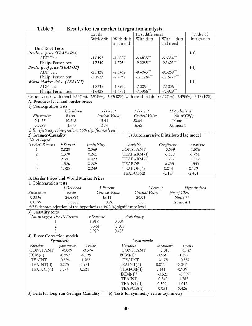
40

Table 3 Results for tea market integration analysis Levels First differences With drift With drift

and trend With drift With drift

and trend

Order of Integration

Unit Root Tests Producer price (TEAFARM) ADF Test Philips Perron test Border (fob) price (TEAFOB) ADF Test Philips Perron test World Market Price (TEAINT) ADF Test Philips Perron test

-1.6193 -1.7340 -2.5128 -2.1927 -1.8335 -1.6428

-1.6307 -1.7054 -2.3432 -2.4932 -1.7922 -1.6791

-6.4835*** -9.2285*** -8.4043*** -12.1284*** -7.0064*** -7.5966***

-6.6354*** -9.3603*** -8.5268*** -12.5779*** -7.1006*** -7.5929***

I(1) I(1) I(1)

Critical values: with trend -3.55(1%), -2.91(5%), -2.59(10%); with trend and drift:-4.12(1%), -3.49(5%), -3.17 (10%) A. Producer level and border prices 1) Cointegration tests Likelihood 5 Percent 1 Percent Hypothesized Eigenvalue Ratio Critical Value Critical Value No. of CE(s) 0.1437 10.518 15.41 20.04 None 0.0289 1.677 3.76 6.65 At most 1 L.R. rejects any cointegration at 5% significance level 2) Granger-Causality 3) Autoregressive Distributed lag model No. of lagged TEAFOB terms F-Statisti Probability Variable Coefficient t-statistic 1 0.820 0.369 CONSTANT -0.039 -1.586 2 1.378 0.261 TEAFARM(-1) -0.188 -0.761 3 2.391 0.079 TEAFARM(-2) 0.277 1.142 4 1.526 0.209 TEAFOB 0.035 1.543 5 1.385 0.249 TEAFOB(-1) -0.014 -0.179 TEAFOB(-2) -0.157 -2.404 B. Border Prices and World Market Prices 1. Cointegration tests Likelihood 5 Percent 1 Percent Hypothesized Eigenvalue Ratio Critical Value Critical Value No. of CE(s) 0.3336 26.6588 15.41 20.04 None ** 0.0599 3.5266 3.76 6.65 At most 1 *(**) denotes rejection of the hypothesis at 5%(1%) significance level 3) Causality tests No. of lagged TEAINT terms. F-Statistic Probability 1 8.918 0.004 2 3.468 0.038 3 0.929 0.433 4) Error Correction models Symmetric Asymmetric Variable parameter t-ratio Variable parameter t-ratio CONSTANT -0.009 -0.574 CONSTANT 0.018 0.783 ECM(-1) -0.597 -4.195 ECM(-1)+ -0.568 -1.897 �TEAINT 0.596 1.967 �TEAINT 0.175 0.559 �TEAINT(-1) -0.275 -0.971 �TEAINT(-1) 0.011 0.037 �TEAFOB(-1) 0.074 0.521 �TEAFOB(-1) 0.141 -0.939

ECM(-1)+ -0.521 -3.997 �TEAINT 0.540 1.785 �TEAINT(-1) -0.302 -1.042 �TEAFOB(-1) -0.054 -0.426 5) Tests for long run Granger Causality 6) Tests for symmetry versus asymmetry

41

Parameter t-ratio F-Value Probability ECM(-1) 0.157 2.967 1.247 0.316 Wald test Probability 1.261 0.473

Source: Authors’ computations from the price data

42

Table 4 Results for tobacco market integration analysis Levels First differences With drift With drift

and trend With drift With drift

and trend

Order of integration

Unit Root tests Producer level price Flue cured (TOBFLUE) ADF Test Philips Perron test Fire cured (TOBFIRE) ADF Test Philips Perron test Border price (TOBFOB) ADF Test Philips Perron test World Market Prices (TOBINT) ADF Test Philips Perron test

-2.578 -2.411 -2.639* -2.443 -3.451** -3.699*** -1.274 -1.371

-1.528 -1.458 -1.767 -1.563 -4.579*** -4.791*** -3.146* -3.636**

-3.818*** -6.663*** -3.944*** -6.234*** - - -6.3474*** -9.8778***

-4.2926*** -7.1134*** -4.3648*** -6.6039*** - - -6.2952*** -9.7943***

I(1) I(1) I(0) I(0)

Critical values: with trend -3.55(1%), -2.91(5%), -2.59(10%); with trend and drift:-4.12(1%), -3.49(5%), -3.17 (10%) 2) Granger causality tests a) Flue cured b) Fire cured c)Border price No. of lagged No. of lagged No. of lagged TOBFOB terms F-Test Prob TOBFOB terms F-Test Prob TOBINT terms F-Test Prob 1 0.072 0.789 1 0.000 0.986 1 3.306 0.074 2 0.436 0.648 2 0.001 0.990 2 2.701 0.076 3 0.434 0.729 3 0.114 0.950 3 2.049 0.119 4 0.715 0.586 4 0.199 0.937 4 1.425 0.241 5 0.549 0.738 5 0.185 0.967 3) Autoregressive Distributed Lag Models a) Flue cured b) Fire cured Coefficient t-stat Coefficient t-stat CONSTANT 0.059 -1.996 CONSTANT -0.065 -2.087 TOBFLUE(-1) 0.999 7.240 TOBFIRE(-1) 1.073 7.739 TOBFLUE(-2) -0.092 -0.702 TOBFIRE(-2) -1.167 -1.264 TOBFOB 0.008 0.709 TOBFOB 0.001 0.108 TOBFOB(-1) 0.003 0.247 TOBFOB(-1) 0.000 0.060 TOBFOB(-2) -0.009 -0.835 TOBFOB(-2) 0.000 -0.081

c) Border price Coefficient t-stat CONSTANT -0.016 -0.211 TOBFOB(-1) 0.620 4.613 TOBFOB(-2) -0.212 -1.576 TOBINT 0.907 5.952 TOBINT(-1) -0.659 -2.949

TOBINT(-2) 0.129 0.653 Source: Authors computations from the price data

43

Table 5 Results for Fruits (Bananas) market integration analysis Levels First differences With drift With drift

and trend With drift With drift

and trend

Order of integration

Unit Root Tests Producer price (FFARM) ADF Test Philips Perron test Border (fob) price (FFOB) ADF Test Philips Perron test World Market Price (FINT) ADF Test Philips Perron test

-2.2864 -1.8975 -2.1084 -2.3790 -2.4689 -2.8735*

-2.1071 -1.7299 -2.4304 -2.9278 -2.4318 -2.8527

-5.0471*** -5.6518*** -6.7609*** -9.3444*** -6.4515*** -9.1529***

-5.1079*** -5.6926*** -6.7379*** -9.2573*** -6.3847*** -9.0799***

I(1) I(1) I(1)

Critical values: with trend –3.55(1%), -2.91(5%), -2.59(10%); with trend and drift:-4.12(1%), -3.49(5%), -3.17 (10%) Cointegration tests a) Producer level (FFARM) and border prices (FFOB) Likelihood 5 Percent 1 Percent Hypothesized Eigenvalue Ratio Critical Value Critical Value No. of CE(s) 0.13636 11.84202 15.41 20.04 None 0.05593 3.33869 3.76 6.65 At most 1 L.R. rejects any cointegration at 5% significance level b) Border Prices (FFOB) and World Market Prices (FINT) Likelihood 5 Percent 1 Percent Hypothesized Eigenvalue Ratio Critical Value Critical Value No. of CE(s) 0.101399 6.2014 15.41 20.04 None 0.000001 0.00019 3.76 6.65 At most 1 L.R. rejects any cointegration at 5% significance level Granger Causality a) From FFOB to FFARM b) From FINT to FFOB No. of lagged No. of lagged TEAFOB terms F-Statistic Probability TEAINT terms. F-Statistic Probability 1 2.447 0.123 1 0.948 0.330 2 1.254 0.294 2 0.370 0.692 3 0.958 0.419 3 0.339 0.797 4 1.091 0.372 4 0.345 0.845 4) Autoregressive Distributed Lag Model a) Producer Level Prices b) Border Prices Coefficient t-ratio Coefficient t-ratio CONSTANT -0.5753 -2.357 CONSTANT -0.0071 0.1969 FFARM(-1) 1.1934 9.142 FFOB(-1) 1.1845 8.5907 FFARM(-2) -0.3515 -2.713 FFOB(-2) -0.1777 -1.2229 FFOB 0.0016 0.009 FINT 0.9668 24.7163 FFOB(-1) 0.1709 0.821 FINT(-1) -1.1436 -7.9895 FFOB(-2) 0.0054 0.0316 FINT(-2) 0.1823 -1.2694

Source: Authors computations from the price data

44

Table 6 Results for Beans market integration analysis Levels First differences With drift With drift

and trend With drift With drift

and trend

Order of integration

Unit Root tests Producer level price (BEFARM) ADF Test Philips Perron test Border price(BEFOB) ADF Test Philips Perron test World Market Price(BEINT) ADF Test Philips Perron test

-4.6364*** -3.9054*** -5.1835*** -5.3541*** -2.4879 -2.0229

-4.8699*** -4.0161** -5.2573*** -5.3138*** -2.9106 -2.0231

-3.9280*** -4.4658***

-3.8841** -4.4294***

I(0) I(0) I(1)

Critical values: with trend –3.55(1%), -2.91(5%), -2.59(10%); with trend and drift:-4.12(1%), -3.49(5%), -3.17 (10%) Granger Causality tests a) From border to producer price b) From world market price to producer price No. of lagged No. of lagged TEAFOB terms F-Statistic Probability TEAINT terms F-Statistic Probability 1 0.053 0.819 1 0.000 0.978 2 0.222 0.801 2 0.103 0.903 3 0.653 0.585 3 0.551 0.649 4 0.567 0.688 4 0.399 0.807 5 0.708 0.621 5 0.283 0.919 Auto Regressive Distributed Lag Model a) Producer Level (producer) Prices b) Border Prices Variable Coefficient t-ratio Variable Coefficient t-ratio CONSTANT -0.536 -3.854 CONSTANT -0.466 0.660 BEFARM(-1) 0.784 6.027 BEFOB(-1) 0.407 2.979 BEFARM(-2) 0.266 2.194 BEFOB(-2) -0.025 -0.187 BEFOB 0.044 1.216 BEINT 0.345 1.065 BEFOB(-1) -0.028 -0.711 BEINT(-1) -0.244 -1.085 BEFOB(-2) -0.014 -0.387 BEINT(-2) 0.142 0.904

Source: Authors computations from the price data

45

Table 7 Results for Maize market integration analysis Levels First differences With drift With drift

and trend With drift With drift

and trend

Order of integration

Unit Root tests

Producer level price (MAFARM) ADF Test Philips Perron test Border price (MAFOB) ADF Test Philips Perron test World Market Price (MAINT) ADF Test Philips Perron test

-2.2384 -1.8949 -3.2989** -4.7122*** -2.3762 -1.9710

-2.5933 -2.2729 -3.2641* -4.6799*** -3.4606 -2.4475

-6.0135*** -6.3183*** - - -4.2856*** -4.8320***

-6.0265*** -6.2473*** - - -4.2503*** -4.7871***

I(1) I(0) I(1)

Critical values: with trend -3.55(1%), -2.91(5%), -2.59(10%); with trend and drift:-4.12(1%), -3.49(5%), -3.17 (10%) Granger causality tests a) Producer price b) Border Price No. of lagged No. of lagged MAFOB terms F-Test Prob MAINT terms F-Test Prob 1 2.883 0.001 1 0.445 0.507 2 0.665 0.518 2 0.444 0.643 3 0.591 0.624 3 0.564 0.641 4 0.553 0.698 4 0.903 0.469 5 0.478 0.791 5 0.974 0.409 Autoregressive Distributed Lag Models a) Producer Price b) Border price Coefficient t-Statistic Coefficient t-Statistic CONSTANT 0.296 2.006 CONSTANT -0.225 -0.368 MAFARM(-1) 0.957 7.808 MAFOB(-1) 0.526 3.819 MAFARM(-2) -0.155 -1.029 MAFOB(-2) 0.089 0.650 MAFOB -0.061 -0.624 MAINT -0.275 -0.382 MAFARM(-1) -0.077 -0.726 MAINT(-1) 0.107 0.122 MAFARM(-2) -0.018 0.194 MAINT(-2) 0.320 0.446

Source: Authors computations from the price data

46

Figure 1. World and domestic price developments Tea Maize Cotton Bananas Beans Tobacco

0.00 0.50 1.00 1.50 2.00 2.50 3.00

Period

0.00

0.01

0.020.03

0.04

0.05

0.060.07

0.08

0.09

World price fob price producer price

0.00

0.05

0.10

0.15

0.20

0.25

0.30

0.35

0.40

0.45

Period

0.00

0.05

0.10

0.15

0.20

0.25

0.30

World price fob price producer price

0.00 0.20 0.40 0.60 0.80 1.00 1.20 1.40 1.60 1.80 2.00

Period

0.00

0.05

0.10

0.15

0.20

0.25

0.30

0.35

World price fob price producer price

0.00

0.10

0.20

0.30

0.40

0.50

0.60

0.70

0.80

Period

0.00

0.05

0.10

0.15

0.20

0.25

World price fob price producer price

0.00 0.10 0.20 0.30 0.40 0.50 0.60 0.70 0.80 0.90

Period

World price fob price producer price

0.00

0.50

1.00

1.50

2.00

2.50

3.00

3.50

4.00

Period

0.00

0.10

0.20

0.30

0.40

0.50

0.60

0.70

Farm level price (US$/Kg

World price fob price producer price (flue) Producer price (fire)

47

48

Appendix A. Dynamic regression models Dynamic regression models usually use a VAR model of the form:

ttkt

n

kkt DXPP εββ ++= −

=∑

10 (A.1)

Where Pt and Xt are vectors of prices and exogenous factor affecting prices respectively; Bi is a matrix of coefficients; and εt is a vector of error terms, representing exogenous, serially independent but unobservable market shocks. The equilibrium condition for a dynamic regression model based on a two-point location model, in which location 1 always exports to location 2, can be written in matrix form as:

⎥⎦

⎤⎢⎣

⎡ +=⎥

⎦

⎤⎢⎣

⎡⎥⎦

⎤⎢⎣

⎡− t

tt

t

t

rabab

ppbb 2211

2

121

11 (A.2)

Equation (A.2), usually expressed in price levels assumes that transport costs are absolute, i.e. not dependent on the price of the commodity (see Fackler and Goodwin, 2001). Log specifications are however, justified if transport costs are expressed in percentage terms. In equation (A.2), the three forcing variables are a1t, a2t, and rt, two of which always appear together. Writing the forcing variables as a VAR yields:

tkt

m

kkt vzz += −

=∑

1

β (A.3)

where z1t = b1a1t + b2a2 and z2t = rt. Elimination of the forcing variables results in a VAR in prices, thus:

tkt

m

k kk

kkt vp

bbp

bb+⎥

⎦

⎤⎢⎣

⎡−⎥

⎦

⎤⎢⎣

⎡=⎥

⎦

⎤⎢⎣

⎡− −

=∑ 1111

21

1 2221

121121

ββββ

= tkt

m

k kkkk

kkkk vpbbbb

+⎥⎦

⎤⎢⎣

⎡+−+−

−=∑

1 2222122121

1221112111

ββββββββ

(A.4)

49

50

References Agona, J. A. et al, (2002), A market overview of the dried fruits sector in Uganda,

National post harvest programme/KARI.

Baffes, J., and Gardner, B., (2003), “The Transmission of World Commodity Prices to

Domestic Markets Under Policy Reforms in Developing Countries”, Policy Reforms in Developing Countries.

Bailey, D. V. & Brorsen, B.W. (1989), Price asymmetry in spatial fed cattle markets,

Western Journal of Agricultural Economics, 14.

Balcombe, K. & Morrison, J. (2002), Commodity price transmission: A critical review of

techniques and an application to selected tropical export commodities. A study for FAO – ESCR.

Blinder, A.S. (1982), Inventories and Sticky prices: more on the microfoundations of

macroeconomics. American Economic Review, 72.

Confort, P. (2004), “Price Transmission in Selected Agricultural Markets”, FAO Commodities and Trade Policy Research Working Paper No. 7.

Dickey, D. & Fuller, W. (1979), Distribution of the Estimators for autoregressive time

series with a unit root. Journal of the American Statistical Association, 74.

Dornbusch, R.. (1987), Exchange rates and prices. American Economic Review, March

Engle, R.F. & Granger C.W.J., 1987. Cointegration and error correction: representation, estimation and testing. Econometrica, 55.

Fackler, P. L. and Goodwin, B. K., (2001), “Spatial Price Analysis” In B. L Gardner and G. C. Rausser. Eds. Handbook of Agricultural Economics. Amsterdam: Elservier Science.

Fafchamps M., et al, (2003), “The Transmission of International Commodity Prices to

Domestic Prices”, CSAE WP2003-14.

Froot, A.K. & Klemperer, P.D., (1989), Exchange rates pass-through when market share

51

matters. American Economic Review, vol 79.

Goetz, E.G. (1992), Landuse and Homeless Policy in Los Angeles, International Journal of Urban and Regional Research, 16 (4).

Government of Uganda, (2000). ‘Plan for Modernisation of Agriculture: Eradicating

poverty in Uganda, Government Strategy and Operational Framework. Granger, C.W.J. (1988), Some recent developments in the concept of causality." Journal

of Econometrics, 39.

Granger, C.W.J. & Lee, T. H.,(1989), Investigation of Production, sales and inventory

relationships using multicointegration and non-symmetric error correction models, Journal of Applied Econometrics, 4.

Granger, C.W.J., (1969), Investigating Causal Relationships by Econometric Models and

Cross Spectral Methods, Econometrica, 37. Gupta, R.D. (1973), On Testing Latent Vectors of a Normal Co-variance Matrix,

Canada. Journal of Statistics, Vol. 1, No. 2.

Hertel, T., and A. Winters., (2005). Poverty and the WTO: Impacts of the Doha Development Agenda. New York: Palgrave Macmillan and Washington D.C.: World Bank.

Hertel, T. W., et al (2004). The earnings effects of multilateral trade liberalization: Implications for poverty. World Bank Economic Review.

IDEA (2001a), Apple banana, Agribusiness Development Centre commercialization

bulletin No.8.

IDEA (2001b), Fresh produce exports from Uganda, Agribusiness Development Centre.

IMF/IDA (2003). ‘Joint Staff Assessment of Poverty Reduction Strategy Paper, Annual

Progress Report’.

Johansen S., (1991). Estimation and hypothesis testing of cointegration vectors in Gaussian vector autoregressive models." Econometrica, 59.

52

Krivonos, E (2004), “The impact of coffee market reforms on producer prices and price

transmission”. World Bank policy Research working paper 3358

Krueger, A., (1992). Economic Policy Reform in Developing Countries, The MIT Press.

Krugman, P., (1986), Pricing to market when exchange rate changes. NBER Working

Paper No. 1926.

Maccini, L.J., (1978). The Impact of demand and price expectations on the behaviour of

Prices, American Economic Review, 68.

Mohendru, I. D, (1937),“Some factor affecting the price of wheat in Punjab”, Publication No. 49, Board of Economic Inquiry, Punjab Government.

Morrissey, O., et al, (2003), “Trade Policies, Performance and Poverty in Uganda”, Uganda Trade and Poverty Project (UTPP)

Mundlak, Y. & Larson, D.F., (1992). On the transmission of world agricultural prices.

World Bank Economic Review, 6.

Phillips, P.C.B. & Perron, P. 1988. Testing for a unit root in time series regression. Biometrica, 75.

Prakash, A.B., (1999). The Transmission of Signals in a decentralised commodity marketing system. The case of the UK Pork Market, PhD. Thesis, Wye College, University of London.

Rapsomanikis, G., et al, (2004), “Market Integration and Price Transmission in Selected

Food and Cash Crop Markets of Developing Countries: Review and Applications” Commodity Market Review 2003 – 2004, FAO, Rome Italy.

Richardson, W. S., (1978): Forecasting extratropical storm-related beach erosion along

the U.S. east coast. TDL Office Note 78-13, National Weather Service, NOAA, U.S. Department of Commerce.

Sexton, et al (1991), “Market Integration, Efficiency of Arbitrage and Imperfect Competition: Methodology and Application to the US Celery”, American Journal of Agricultural Economics, Vol.73.

Shahidur, R.., (2004), “Spatial Integration of Maize Markets in Post-Liberalized

53

Uganda”, International Food Policy Research Institute; Markets, Trade and Institutions Division; MTID Discussion Paper No. 71.

Stigler, G. and Sherwin, R.., (1985), The extent of the market. Journal of Law and Economics, 28.

Institute for International Integration StudiesThe Sutherland Centre, Trinity College Dublin, Dublin 2, Ireland