Can molecular dynamics simulations help in discriminating correct from erroneous protein 3D models

BioMed CentralBMC Bioinformatics

ss
Open AcceResearch articleCan molecular dynamics simulations help in discriminating correct from erroneous protein 3D models?Jean-François Taly, Antoine Marin and Jean-François Gibrat*
Address: INRA, Unité Mathématique Informatique et Génome UR1077, F-78350 Jouy-en-Josas, France

Email: Jean-François Taly - [email protected]; Antoine Marin - [email protected]; Jean-François Gibrat* - [email protected]

* Corresponding author

AbstractBackground: Recent approaches for predicting the three-dimensional (3D) structure of proteinssuch as de novo or fold recognition methods mostly rely on simplified energy potential functionsand a reduced representation of the polypeptide chain. These simplifications facilitate theexploration of the protein conformational space but do not permit to capture entirely the subtlerelationship that exists between the amino acid sequence and its native structure. It has beenproposed that physics-based energy functions together with techniques for sampling theconformational space, e.g., Monte Carlo or molecular dynamics (MD) simulations, are better suitedto the task of modelling proteins at higher resolutions than those of models obtained with theformer type of methods. In this study we monitor different protein structural properties along MDtrajectories to discriminate correct from erroneous models. These models are based on thesequence-structure alignments provided by our fold recognition method, FROST. We definecorrect models as being built from alignments of sequences with structures similar to their nativestructures and erroneous models from alignments of sequences with structures unrelated to theirnative structures.

Results: For three test sequences whose native structures belong to the all-α, all-β and αβ classeswe built a set of models intended to cover the whole spectrum: from a perfect model, i.e., thenative structure, to a very poor model, i.e., a random alignment of the test sequence with astructure belonging to another structural class, including several intermediate models based on foldrecognition alignments. We submitted these models to 11 ns of MD simulations at three differenttemperatures. We monitored along the corresponding trajectories the mean of the Root-Mean-Square deviations (RMSd) with respect to the initial conformation, the RMSd fluctuations, thenumber of conformation clusters, the evolution of secondary structures and the surface area ofresidues. None of these criteria alone is 100% efficient in discriminating correct from erroneousmodels. The mean RMSd, RMSd fluctuations, secondary structure and clustering of conformationsshow some false positives whereas the residue surface area criterion shows false negatives.However if we consider these criteria in combination it is straightforward to discriminate the twotypes of models.

Conclusion: The ability of discriminating correct from erroneous models allows us to improvethe specificity and sensitivity of our fold recognition method for a number of ambiguous cases.

Published: 7 January 2008

BMC Bioinformatics 2008, 9:6 doi:10.1186/1471-2105-9-6

Received: 18 July 2007Accepted: 7 January 2008

This article is available from: http://www.biomedcentral.com/1471-2105/9/6

© 2008 Taly et al; licensee BioMed Central Ltd. This is an Open Access article distributed under the terms of the Creative Commons Attribution License (http://creativecommons.org/licenses/by/2.0), which permits unrestricted use, distribution, and reproduction in any medium, provided the original work is properly cited.

of 24(page number not for citation purposes)

http://www.biomedcentral.com/1471-2105/9/6

http://creativecommons.org/licenses/by/2.0

http://www.ncbi.nlm.nih.gov/entrez/query.fcgi?cmd=Retrieve&db=PubMed&dopt=Abstract&list_uids=18179702

http://www.biomedcentral.com/

http://www.biomedcentral.com/info/about/charter/

BMC Bioinformatics 2008, 9:6 http://www.biomedcentral.com/1471-2105/9/6

BackgroundThe last 10 years have witnessed steady progress in theprediction of the three-dimensional (3D) structure of pro-teins from their amino acid sequence [1]. Most currentapproaches, ranging from de novo to fold recognition(threading) techniques, are based on simplified "energy"potentials (with a few exceptions such as the UNRES forcefield [2]). These empirical potentials, often more appro-priately referred to as score functions, are derived fromstatistical analyses of structural features observed inknown 3D structures: residue-wise interactions, secondarystructure propensities, residue surface, etc. They are usedwith a reduced representation of the polypeptide chain(for instance, in many threading methods residues arerepresented by a single site, the Cβ or the Cα atom). Suchcoarse-grained potentials cannot capture wholly the sub-tle relationship that exists between the amino acidsequence and the 3D structure of proteins. However theirsimplicity is an asset for exploring the conformationalspace, they permit to filter out improbable or unrealisticstructures and, hopefully, to propose structures that areclose to the native structure. De novo techniques, such asthose developed by the Baker's group [3], generate hun-dreds of structures some close to the native structure butalso many far from it. Threading methods are more con-strained since they only consider known 3D structuresand seek whether a particular query sequence might becompatible with some of these structures. Typically, theyprovide a list of template structures that are ranked byscores. All these methods have developed their ownmeans to judge whether a de novo structure is close to thenative structure or whether a particular template structureis compatible with a given sequence. However, in somecases this judgement is not clear-cut and it has been sug-gested that these techniques could benefit from the use ofan atomic representation of the polypeptide chaintogether with detailed energy functions based on chemi-cal-physical principles [4]. One would thus adopt a hier-archical approach, simplified potentials would permit tofocus on a limited number of plausible candidates anddetailed potentials would help in discriminating betweennative and misfolded structures. Since the pioneeringwork of Novotny et al.[5] a number of groups have soughtto analyse whether usual molecular mechanics forcefields, such as those employed for molecular dynamics(MD) simulations complemented with different ways ofcomputing solvation effects, could indeed discriminatethe native structure from misfolded conformations [6-13].All these works, except [7] that uses a limited sampling,are based on minimised conformations, hence the need tointroduce different terms to represent solvation freeenergy. It appears that such empirical free energy calcula-tions are able to make a distinction, in many cases,between native structures and decoys. These works alsoanalysed the role of the different terms involved in the free

energy computation: internal, van der Waals and electro-static energies, solvation contributions, etc. arriving atsomewhat different conclusions as to which terms werepreponderant for the discrimination.

Other groups [14-16] tackled a related question: can phys-ics-based potentials together with an extensive samplingof the protein conformational space using MD simula-tions refine, i.e., bring closer to the native structure, an ini-tial model resulting from a previous stage employingcoarse-grained potentials?

In this work we wish to answer a very pragmatic question.We have developed a fold recognition method calledFROST [17]. In this method we perform a statistical anal-ysis of the scores to decide whether a sequence is compat-ible with a template structure. This permits us to recover60% of the related sequence-structure pairs while keepingan error rate of 1%. Unfortunately 40% of the pairs do notsatisfy this statistical criterion although, for an importantfraction of them, a compatible template structure can befound amongst the top templates of the list ordered bynormalised scores. Hereafter, we will refer to the zonewhere scores are not statistically significant as the "twi-light zone" of the method. The question we would like toanswer is thus the following: can physics-based potentialsand MD simulations help us in discriminating "correct"from "erroneous" templates in such borderline cases. Ourmotivation is similar to the one of Kinjo and colleagues[11] although, as described below, we employ a differentapproach.

We define a correct template as a structure that is similarto the query sequence native structure and an erroneoustemplate as any other structure of the database. Let us notethat these erroneous templates, because they appear in thetop of the list, constitute difficult cases compared to whathas been done by Novotny et al.[5]. They just swapped thesequences between an all-α protein and an all-β proteinwithout paying attention whether this procedure buriedcharged residues or exposed non polar residues. Thethreading method will find the best location for the queryresidues in the 3D structure according to its empiricalscore function (the current version of the method insuresthat the best alignment score between the query sequenceand the template structures is found). Therefore many ofthe top erroneous templates are likely to exhibit somecommon features with the correct templates making themdifficult to distinguish.

To answer the above question, for the borderline cases, webuild 3D models based on the sequence-structure align-ments provided by our fold recognition method and wesubmit them to MD simulations. We monitor differentstructural features: RMSd, radius of gyration, secondary



structures, side chain surface, etc. along the trajectories todiscriminate correct from erroneous models. There aremany ways in which a 3D model can be erroneous. In thisstudy, to be consistent with the question we want toanswer, an erroneous model is defined as a model forwhich the sequence has been aligned with a templatestructure that has no relationship with its native structure.

Notice that, in real cases, one cannot use approaches sim-ilar to those described in [6-13] since they require theknowledge of the native structure. In these studies, thevalue of the free energy for the native structure is usuallysmaller than the value of the free energy for the decoys butthe difference is often quite small relative to the magni-tude of the figures involved (a few percents at best). Freeenergy values are very different according to the proteinstudied and there is no absolute scale on which one couldrely. Therefore instead of trying to compute the free energyof the models we choose to rely on the analysis of thebehaviour of different structural features along the MDtrajectories.

ResultsWe selected 3 query domains representative of the princi-pal SCOP [18] classes: all-α, all-β and αβ. For each querydomain we built 6 models as described in the Method sec-tion (listed in Table 1). These models correspond to thesame sequence (the query sequence) aligned with differenttemplate structures. They cover the whole spectrum ofmodels that can be generated for a query sequence: froma perfect model corresponding to the native structure(NS0) to a very poor model where the query sequence hasbeen aligned with a template structure completely differ-ent from its native structure (DT2).

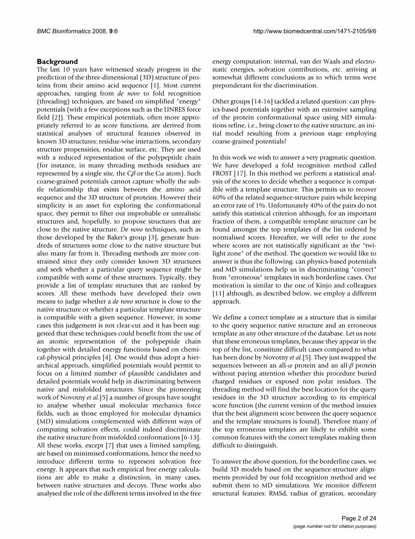
Between these two extremes, that are used as controls, wewish to focus on intermediate models that are typical ofwhat can be expected after a fold recognition analysis (seeFig. 1). For the first three intermediate models, ST1, ST2,

ST3, the query sequence has been aligned with a templatestructure that is similar to the native structure. For ST1 andST2 the alignment is good or fair (see Additional file 1,Tables S1 and S2 for a precise definition of these terms).These two models are mainly distinguished by the per-centage of sequence identity between the query sequenceand the sequence of the template structure: ST1 is in therange 20–30 approaching the generally recognised limitof 30% for homology modelling [19]. ST2 has been cho-

Schematic representation of the ranking, according to the FROST score, of the template structures that are used to build the 6 models for a given query sequence (template structures are designated by the corresponding model name)Figure 1Schematic representation of the ranking, according to the FROST score, of the template structures that are used to build the 6 models for a given query sequence (template structures are desig-nated by the corresponding model name). Ssig represents the score above which there is less than 1% chance to find a false pos-itive [17]. Below this score we define the "twilight zone" of the method. In this zone the score does not allow us to predict with enough confidence whether the template structure is similar to the query sequence structure or not. DT1 is the first false posi-tive, i.e., the template structure, not similar with the query struc-ture, which has the highest FROST score. In this work the template structures we chose for ST2, DT1 and ST3 have compa-rable scores and they are found in the twilight zone. The template structure for ST1 has a score that is usually above Ssig. The order-ing of the template structures for ST2, DT1 and ST3 can change from what is depicted on the figure depending on the query sequence.

Table 1: Summary of the characteristics of the 6 models built for each query structure

Model CharacteristicsTemplate Alignment % seq. Id.

NS0 Native struct. Exact 100ST1 Similar Good 20 – 30ST2 Similar Fair 0 – 20ST3 Similar Poor 0 – 15DT1 Different - 0 – 15DT2 Different - 0 – 15

As a mnemonic, the first letter indicates whether the query sequence has been aligned with the right template (S) or not (D) and the last digit indicates the proximity of the model with the true structure. (See method section for further detail).



sen, on purpose, to lie within the twilight zone. Usuallythis implies that the percentage of sequence identity isbelow 20%, typical of fold recognition targets. ST3 has thesame characteristics as ST2 except that we selected a tem-plate structure on which the fold recognition method wasnot able to align correctly the query sequence. This is oftenthe case when the template structure, although globallysimilar to the query native structure, possesses additionalsecondary structure elements or when secondary structureelements of the "core" have undergone substantialmotions relative to each other. These two characteristicsperturb the fold recognition alignment. The last model,DT1, has been obtained by aligning the query sequencewith a template structure that is different from its nativestructure. It must be noticed that we chose the templatestructure that corresponds to the first false positiveappearing in the fold recognition list of structures rankedby score. Therefore, according to the FROST score func-tion, this template structure possesses some features simi-lar to the query native structure. Indeed we often observethat such template structures share motifs with the querynative structure that tend to confuse the fold recognitionmethod.

Let us emphasise that all models, as far as the backbone isconcerned, are based on known 3D structures. Structuralfeatures such as the network of hydrogen bonds, the Ram-achandran zones for the φ and ψ angles, etc. are realistic(with the possible exception of regions corresponding tothe loops built by Modeller). The only unrealistic struc-tural feature concerns the location and interactions of sidechains in some of the models.

In the following, we try, by monitoring various structuralcharacteristics along MD trajectories at different tempera-tures, to answer two questions. First, is it possible to dis-tinguish, quantitatively or qualitatively, models for whichthe query sequence has been aligned with a templatestructure similar to its native structure from models forwhich the query sequence has been aligned with templatestructures without relation with its native structure? If thequery sequence has been aligned with the correct templatestructure but with a poor alignment can we pinpoint partsof the model that correspond to misaligned regions?

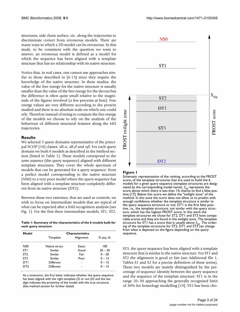
Analysis of the modelsAll-α modelsFig. 2 shows the query protein for the all-α class and thetemplate structures that are used to build the models. InAdditional file 1, Table S1 gives details about the structurecomparisons, Figure S1 displays the relationship thatexists between these structures according to the SCOPhierarchy, Table S2 shows comparisons of the modelswith the query native structure and Figure S2 shows thestructural superimposition of the models with the query

native structure. Notice that not all models have a lengthequal to the query sequence length (105 residues). Mod-eller does not know how to handle properly residues that,according to the alignment, are located before the N-ter-minus, or after the C-terminus of the template structure.In such cases it generates extended conformations. Wethus decided to chop these residues in the alignment.

Fig. 2 shows the FROST score (the twilight zone lies belowSsig = 15), the VAST score (a score above 2 is indicative ofa clear structural relationship between the proteins), theTM-score (a score larger than 0.4 implies a structural rela-tionship between the proteins) and the RMSd of the modelwith respect to the query native structure.

The FROST score is very high for model ST1 since thismodel is in the range of homology modelling. Scores forother models are in the FROST twilight zone with a smalldifference between scores for ST2, ST3 and DT1. This isprecisely to help us resolving such ambiguous situationsthat we would like to employ MD simulations.

All indicators show that ST1 is related to the query nativestructure. For ST2 the VAST score is negative but the TM-score is significant. ST3 and DT1 appear to have about thesame weak similarity with the query structure. The TM-score is slightly above the significant threshold of 0.4. Infact, according to SCOP, ST3 belongs to the same fold asthe query protein (4-helical up-and-down bundle)whereas DT1 belongs to a different fold (DNA/RNA-bind-ing 3-helical bundle). These two folds obviously share acommon helical motif that confuses the fold recognitionprogram.

Model ST2 is marginally similar to the query native struc-ture with an RMSd of 5.7 Å

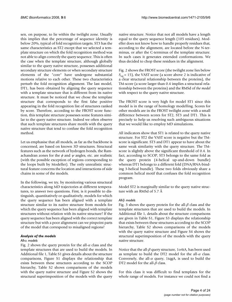
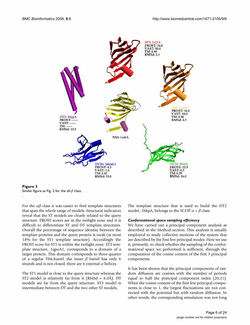
All-β modelsFig. 3 shows the query protein for the all-β class and thetemplate structures that are used to build the models. InAdditional file 1, details about the structure comparisonsare given in Table S1, Figure S3 displays the relationshipthat exists between these structures according to the SCOPhierarchy, Table S2 shows comparisons of the modelswith the query native structure and Figure S4 shows thestructural superimposition of the models with the querynative structure.

Notice that the all-β query structure, 1o4tA, has been usedas template to build the DT2 model for the all-α class.Conversely, the all-α query, 1tqgA, is used to build theDT2 model for the all-β class.

For this class it was difficult to find templates for thewhole range of models. For instance we could not find a



template for model ST1. Therefore we decided that thetemplate for ST2 would also be used as template for ST1.The two models just differ by the type of alignment that isused: ST1 is based on the structural alignment whereasST2 is based on the fold recognition alignment. We couldnot find either a template for the ST3 model. Instead webuilt two DT1 models, named DT1a and DT1b. The tem-plates used for DT1a and DT1b belongs to the same SCOPfold (Immunoglobulin-like β sandwich) but to differentsuper-families.

The template used for models ST1 and ST2 is clearly sim-ilar to the query structure. Both this template and thequery structure belong to the same SCOP family of thedouble-stranded β helix SCOP fold. The query protein,1o4tA, whose length is 115 residues, is a homodimer inthe PDB file. At its N-terminus there exists a small strandthat pairs with its counterpart in the other monomer.

When using only the monomer this strand is floating inthe solvent. We thus decided to remove this portion of thesequence (9 residues) from the NS0 model to obtain amore compact 3D structure. However alignments withtemplate structures where performed with the completesequence. This explains why the DT1b model is 112 resi-dues long.

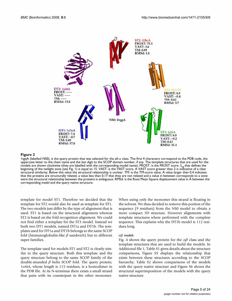
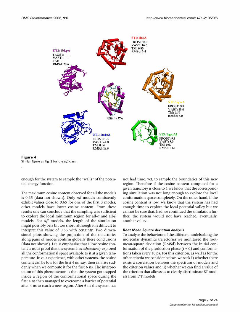
αβ modelsFig. 4 shows the query protein for the αβ class and thetemplate structures that are used to build the models. InAdditional file 1, Table S1 gives details about the structurecomparisons, Figure S5 displays the relationship thatexists between these structures according to the SCOPhierarchy, Table S2 shows comparisons of the modelswith the query native structure and Figure S6 shows thestructural superimposition of the models with the querynative structure.

1tgqA (labelled NS0), is the query protein that was selected for the all-α classFigure 21tgqA (labelled NS0), is the query protein that was selected for the all-α class. The first 4 characters correspond to the PDB code, the uppercase letter to the chain name and the last digit to the SCOP domain number, if any. The template structures that are used for the models are shown clockwise (they are labelled with the corresponding model name). FROST: is the FROST score. Ssig that defines the beginning of the twilight zone (see Fig. 1) is equal to 15. VAST: is the VAST score. A VAST score greater than 2 is indicative of a clear structural similarity. Below this value the structural relationship is unclear. TM: is the TM-score value. A value larger than 0.4 indicates that the proteins are structurally related, a value less than 0.17 that they are not related and a value in between corresponds to a zone were the structural relationship between the proteins is ambiguous. RMSd: is the Root Mean Square displacement value in Å between the corresponding model and the query native structure.



For the αβ class it was easier to find template structuresthat span the whole range of models. Structural indicatorsreveal that the ST models are clearly related to the querystructure. FROST scores are in the twilight zone and it isdifficult to differentiate ST and DT template structures.Overall the percentage of sequence identity between thetemplate proteins and the query protein is weak (at most18% for the ST1 template structure). Accordingly theFROST score for ST1 is within the twilight zone. ST3 tem-plate structure, 1qpoA1, corresponds to a domain of alarger protein. This domain corresponds to three-quarterof a regular TIM-barrel: the inner β barrel has only 6strands and is not closed; there are 6 external α helices.

The ST1 model is close to the query structure whereas theST2 model is relatively far from it (RMSd = 8.0Å). DTmodels are far from the query structure. ST3 model isintermediate between DT and the two other ST models.

The template structure that is used to build the DT2model, 1bkpA, belongs to the SCOP α + β class.

Conformational space sampling efficiencyWe have carried out a principal component analysis asdescribed in the Method section. This analysis is usuallyemployed to study collective motions of the system thatare described by the first few principal modes. Here we useit, primarily, to check whether the sampling of the confor-mational space we performed is sufficient, through thecomputation of the cosine content of the first 3 principalcomponents.

It has been shown that the principal components of ran-dom diffusion are cosines with the number of periodsequal to half the principal component index [20,21].When the cosine content of the first few principal compo-nents is close to 1, the largest fluctuations are not con-nected with the potential but with random diffusion. Inother words, the corresponding simulation was not long

Similar figure as Fig. 2 for the all-β classFigure 3Similar figure as Fig. 2 for the all-β class.



enough for the system to sample the "walls" of the poten-tial energy function.

The maximum cosine content observed for all the modelsis 0.65 (data not shown). Only αβ models consistentlyexhibit values close to 0.65 for one of the first 3 modes,other models have lower cosine content. From theseresults one can conclude that the sampling was sufficientto explore the local minimum region for all-α and all-βmodels. For αβ models, the length of the simulationmight possibly be a bit too short, although it is difficult tointerpret this value of 0.65 with certainty. Two dimen-sional plots showing the projection of the trajectoriesalong pairs of modes confirm globally these conclusions(data not shown). Let us emphasise that a low cosine con-tent is not a proof that the system has exhaustively exploredall the conformational space available to it at a given tem-perature. In our experience, with other systems, the cosinecontent can be low for the first 4 ns, say, then can rise sud-denly when we compute it for the first 6 ns. The interpre-tation of this phenomenon is that the system got trappedinside a region of the conformational space during thefirst 4 ns then managed to overcome a barrier of potentialafter 4 ns to reach a new region. After 6 ns the system has

not had time, yet, to sample the boundaries of this newregion. Therefore if the cosine content computed for agiven trajectory is close to 1 we know that the correspond-ing simulation was not long enough to explore the localconformation space completely. On the other hand, if thecosine content is low, we know that the system has hadenough time to explore the local potential valley but wecannot be sure that, had we continued the simulation fur-ther, the system would not have reached, eventually,another valley.

Root Mean Square deviation analysisTo analyse the behaviour of the different models along themolecular dynamics trajectories we monitored the root-mean-square deviation (RMSd) between the initial con-formation of the production phase (t = 0) and conforma-tions taken every 10 ps. For this criterion, as well as for theother criteria we consider below, we seek i) whether thereexists a correlation between the spectrum of models andthe criterion values and ii) whether we can find a value ofthe criterion that allows us to clearly discriminate ST mod-els from DT models.

Similar figure as Fig. 2 for the αβ classFigure 4Similar figure as Fig. 2 for the αβ class.



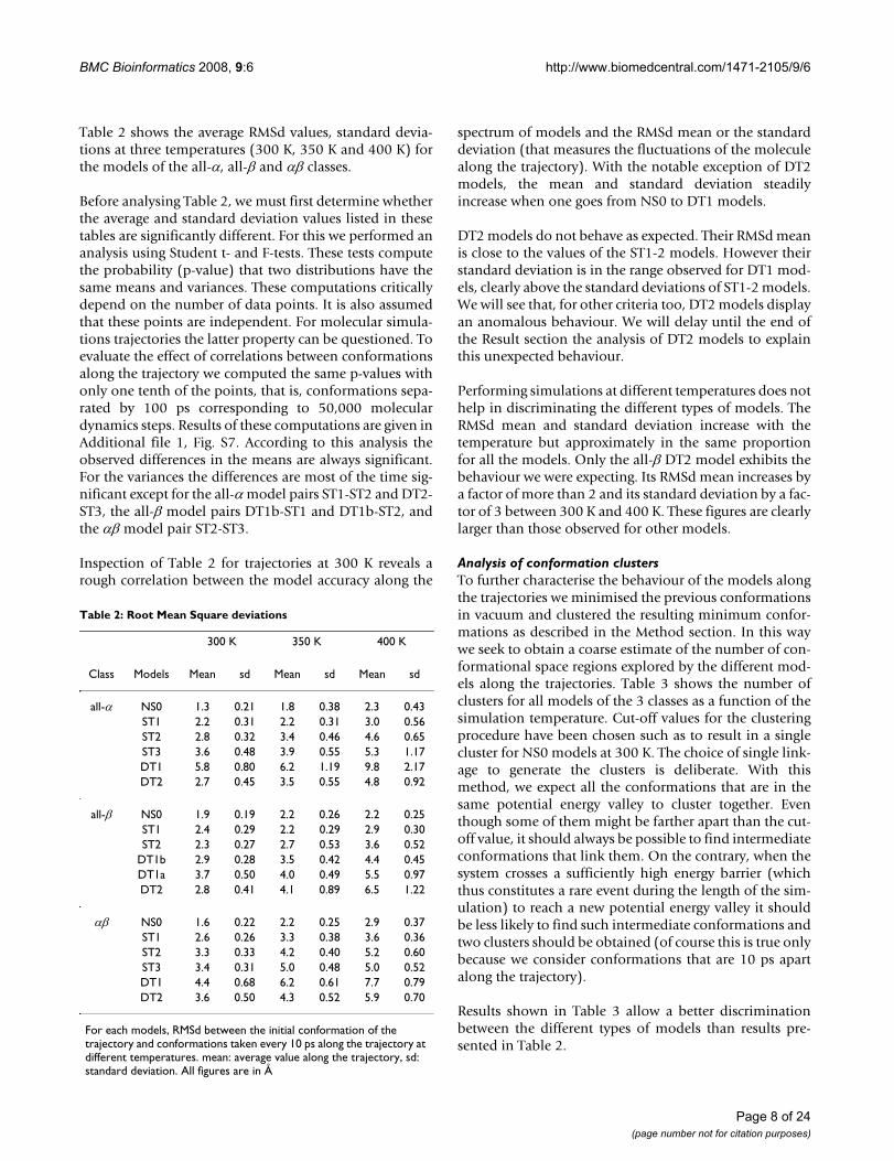
Table 2 shows the average RMSd values, standard devia-tions at three temperatures (300 K, 350 K and 400 K) forthe models of the all-α, all-β and αβ classes.

Before analysing Table 2, we must first determine whetherthe average and standard deviation values listed in thesetables are significantly different. For this we performed ananalysis using Student t- and F-tests. These tests computethe probability (p-value) that two distributions have thesame means and variances. These computations criticallydepend on the number of data points. It is also assumedthat these points are independent. For molecular simula-tions trajectories the latter property can be questioned. Toevaluate the effect of correlations between conformationsalong the trajectory we computed the same p-values withonly one tenth of the points, that is, conformations sepa-rated by 100 ps corresponding to 50,000 moleculardynamics steps. Results of these computations are given inAdditional file 1, Fig. S7. According to this analysis theobserved differences in the means are always significant.For the variances the differences are most of the time sig-nificant except for the all-α model pairs ST1-ST2 and DT2-ST3, the all-β model pairs DT1b-ST1 and DT1b-ST2, andthe αβ model pair ST2-ST3.

Inspection of Table 2 for trajectories at 300 K reveals arough correlation between the model accuracy along the

spectrum of models and the RMSd mean or the standarddeviation (that measures the fluctuations of the moleculealong the trajectory). With the notable exception of DT2models, the mean and standard deviation steadilyincrease when one goes from NS0 to DT1 models.

DT2 models do not behave as expected. Their RMSd meanis close to the values of the ST1-2 models. However theirstandard deviation is in the range observed for DT1 mod-els, clearly above the standard deviations of ST1-2 models.We will see that, for other criteria too, DT2 models displayan anomalous behaviour. We will delay until the end ofthe Result section the analysis of DT2 models to explainthis unexpected behaviour.

Performing simulations at different temperatures does nothelp in discriminating the different types of models. TheRMSd mean and standard deviation increase with thetemperature but approximately in the same proportionfor all the models. Only the all-β DT2 model exhibits thebehaviour we were expecting. Its RMSd mean increases bya factor of more than 2 and its standard deviation by a fac-tor of 3 between 300 K and 400 K. These figures are clearlylarger than those observed for other models.

Analysis of conformation clustersTo further characterise the behaviour of the models alongthe trajectories we minimised the previous conformationsin vacuum and clustered the resulting minimum confor-mations as described in the Method section. In this waywe seek to obtain a coarse estimate of the number of con-formational space regions explored by the different mod-els along the trajectories. Table 3 shows the number ofclusters for all models of the 3 classes as a function of thesimulation temperature. Cut-off values for the clusteringprocedure have been chosen such as to result in a singlecluster for NS0 models at 300 K. The choice of single link-age to generate the clusters is deliberate. With thismethod, we expect all the conformations that are in thesame potential energy valley to cluster together. Eventhough some of them might be farther apart than the cut-off value, it should always be possible to find intermediateconformations that link them. On the contrary, when thesystem crosses a sufficiently high energy barrier (whichthus constitutes a rare event during the length of the sim-ulation) to reach a new potential energy valley it shouldbe less likely to find such intermediate conformations andtwo clusters should be obtained (of course this is true onlybecause we consider conformations that are 10 ps apartalong the trajectory).

Results shown in Table 3 allow a better discriminationbetween the different types of models than results pre-sented in Table 2.

Table 2: Root Mean Square deviations

300 K 350 K 400 K

Class Models Mean sd Mean sd Mean sd

all-α NS0 1.3 0.21 1.8 0.38 2.3 0.43ST1 2.2 0.31 2.2 0.31 3.0 0.56ST2 2.8 0.32 3.4 0.46 4.6 0.65ST3 3.6 0.48 3.9 0.55 5.3 1.17DT1 5.8 0.80 6.2 1.19 9.8 2.17DT2 2.7 0.45 3.5 0.55 4.8 0.92

all-β NS0 1.9 0.19 2.2 0.26 2.2 0.25ST1 2.4 0.29 2.2 0.29 2.9 0.30ST2 2.3 0.27 2.7 0.53 3.6 0.52

DT1b 2.9 0.28 3.5 0.42 4.4 0.45DT1a 3.7 0.50 4.0 0.49 5.5 0.97DT2 2.8 0.41 4.1 0.89 6.5 1.22

αβ NS0 1.6 0.22 2.2 0.25 2.9 0.37ST1 2.6 0.26 3.3 0.38 3.6 0.36ST2 3.3 0.33 4.2 0.40 5.2 0.60ST3 3.4 0.31 5.0 0.48 5.0 0.52DT1 4.4 0.68 6.2 0.61 7.7 0.79DT2 3.6 0.50 4.3 0.52 5.9 0.70

For each models, RMSd between the initial conformation of the trajectory and conformations taken every 10 ps along the trajectory at different temperatures. mean: average value along the trajectory, sd: standard deviation. All figures are in Å



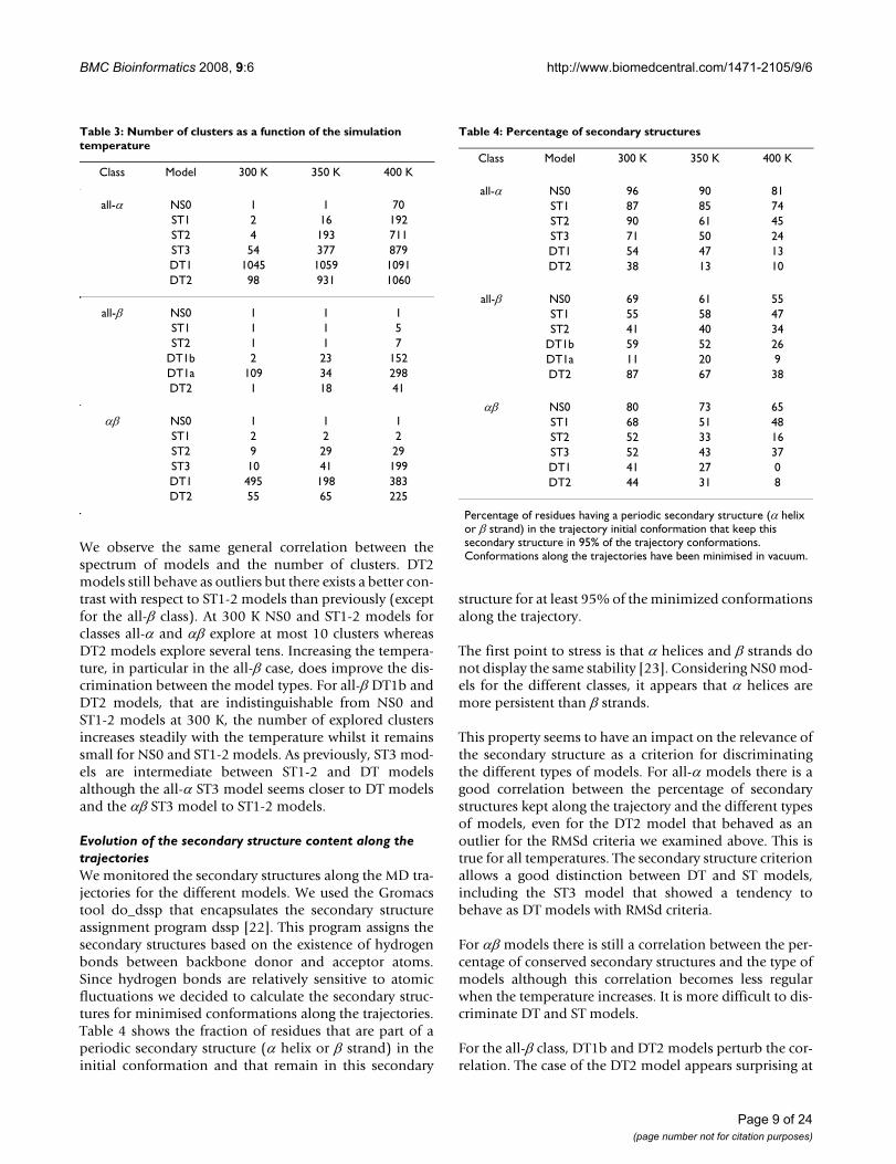
We observe the same general correlation between thespectrum of models and the number of clusters. DT2models still behave as outliers but there exists a better con-trast with respect to ST1-2 models than previously (exceptfor the all-β class). At 300 K NS0 and ST1-2 models forclasses all-α and αβ explore at most 10 clusters whereasDT2 models explore several tens. Increasing the tempera-ture, in particular in the all-β case, does improve the dis-crimination between the model types. For all-β DT1b andDT2 models, that are indistinguishable from NS0 andST1-2 models at 300 K, the number of explored clustersincreases steadily with the temperature whilst it remainssmall for NS0 and ST1-2 models. As previously, ST3 mod-els are intermediate between ST1-2 and DT modelsalthough the all-α ST3 model seems closer to DT modelsand the αβ ST3 model to ST1-2 models.

Evolution of the secondary structure content along the trajectoriesWe monitored the secondary structures along the MD tra-jectories for the different models. We used the Gromacstool do_dssp that encapsulates the secondary structureassignment program dssp [22]. This program assigns thesecondary structures based on the existence of hydrogenbonds between backbone donor and acceptor atoms.Since hydrogen bonds are relatively sensitive to atomicfluctuations we decided to calculate the secondary struc-tures for minimised conformations along the trajectories.Table 4 shows the fraction of residues that are part of aperiodic secondary structure (α helix or β strand) in theinitial conformation and that remain in this secondary

structure for at least 95% of the minimized conformationsalong the trajectory.

The first point to stress is that α helices and β strands donot display the same stability [23]. Considering NS0 mod-els for the different classes, it appears that α helices aremore persistent than β strands.

This property seems to have an impact on the relevance ofthe secondary structure as a criterion for discriminatingthe different types of models. For all-α models there is agood correlation between the percentage of secondarystructures kept along the trajectory and the different typesof models, even for the DT2 model that behaved as anoutlier for the RMSd criteria we examined above. This istrue for all temperatures. The secondary structure criterionallows a good distinction between DT and ST models,including the ST3 model that showed a tendency tobehave as DT models with RMSd criteria.

For αβ models there is still a correlation between the per-centage of conserved secondary structures and the type ofmodels although this correlation becomes less regularwhen the temperature increases. It is more difficult to dis-criminate DT and ST models.

For the all-β class, DT1b and DT2 models perturb the cor-relation. The case of the DT2 model appears surprising at

Table 4: Percentage of secondary structures

Class Model 300 K 350 K 400 K

all-α NS0 96 90 81ST1 87 85 74ST2 90 61 45ST3 71 50 24DT1 54 47 13DT2 38 13 10

all-β NS0 69 61 55ST1 55 58 47ST2 41 40 34

DT1b 59 52 26DT1a 11 20 9DT2 87 67 38

αβ NS0 80 73 65ST1 68 51 48ST2 52 33 16ST3 52 43 37DT1 41 27 0DT2 44 31 8

Percentage of residues having a periodic secondary structure (α helix or β strand) in the trajectory initial conformation that keep this secondary structure in 95% of the trajectory conformations. Conformations along the trajectories have been minimised in vacuum.

Table 3: Number of clusters as a function of the simulation temperature

Class Model 300 K 350 K 400 K

all-α NS0 1 1 70ST1 2 16 192ST2 4 193 711ST3 54 377 879DT1 1045 1059 1091DT2 98 931 1060

all-β NS0 1 1 1ST1 1 1 5ST2 1 1 7

DT1b 2 23 152DT1a 109 34 298DT2 1 18 41

αβ NS0 1 1 1ST1 2 2 2ST2 9 29 29ST3 10 41 199DT1 495 198 383DT2 55 65 225



first sight since it exhibits a higher fraction of conservedsecondary structures than the native structure itself at 300K. In this model the native sequence has been alignedwith the all-α query structure. This confirms our previousobservation that α helices appear to be more stable than βstrands. Let us note, however, that the NS0 model loosesfew secondary structures when the temperature increasesunlike the DT2 model whose fraction of secondary struc-tures is halved when the temperature is raised from 300 Kto 400 K. For this class the secondary structure criterion isineffective in discriminating the different types of models.

Statistical score based on residue surface areasThe accessible surface area of the residues is an importantparameter to characterise protein 3D structures. To quan-tify this parameter we defined an empirical score functionbased on the residue surface areas. This score functiontakes into consideration the so-called "polar satisfaction"of the polar residues and the "hydrophobic satisfaction"of hydrophobic residues. These two criteria are intendedto account for the observed tendency of hydrophobic res-idues to be buried and polar residues to be in contact withthe solvent or other polar residues. The method sectionbriefly describes how this score function is calculated. Wecompute 2 types of scores. The first one is a global scorefor the whole protein, the second is a window score that isthe mean of the scores in an 11-residue window centredon a residue of interest (each residue in the sequence isthus characterised by a particular window score).

Table 5 shows the global score at the beginning of the MDsimulations and the mean global scores along trajectoriesat 300, 350 and 400 K for the different models of the threeabove classes. The scores are computed on the minimisedconformations along the trajectories. The initial confor-mation at t = 0 is also minimised before computing itsscore. In Table 5 figures in italic are beyond the value char-acteristic of the 1% confidence threshold. For instance, forreal 3D structures of the all-α class only 1% of the proteinsare expected to have a global score less than -1.29 (seeAdditional file 1, Table S3). All-α models whose globalscore is less than this value are considered to differ signif-icantly (with a 1% confidence level) from a real 3D struc-ture.

It is interesting to notice that MD simulations, althoughthe physics-based function they employ does not take intoaccount the residue surface areas, systematically improvethe global score for all the models with respect to the staticmodels at t = 0. In particular this allows the all-α and all-β ST2 models and the αβ ST1 model, that appear signifi-cantly different from a true structure when only the staticinitial conformation at t = 0 is considered, to be broughtwithin the range of scores characteristic of real 3D struc-tures. The improvement for NS0 models is, in general, less

than the improvement observed for other models. Theworst models show a tendency to exhibit the largest scoreimprovements, although this is not systematic.

The global score allows the discrimination of the ST1-2models (except for the αβ class). ST3 models behave asthe DT models with this criterion. The scores of DT mod-els are usually far below the 1% confidence thresholdvalue (several standard deviations). DT models are thuseasy to detect.

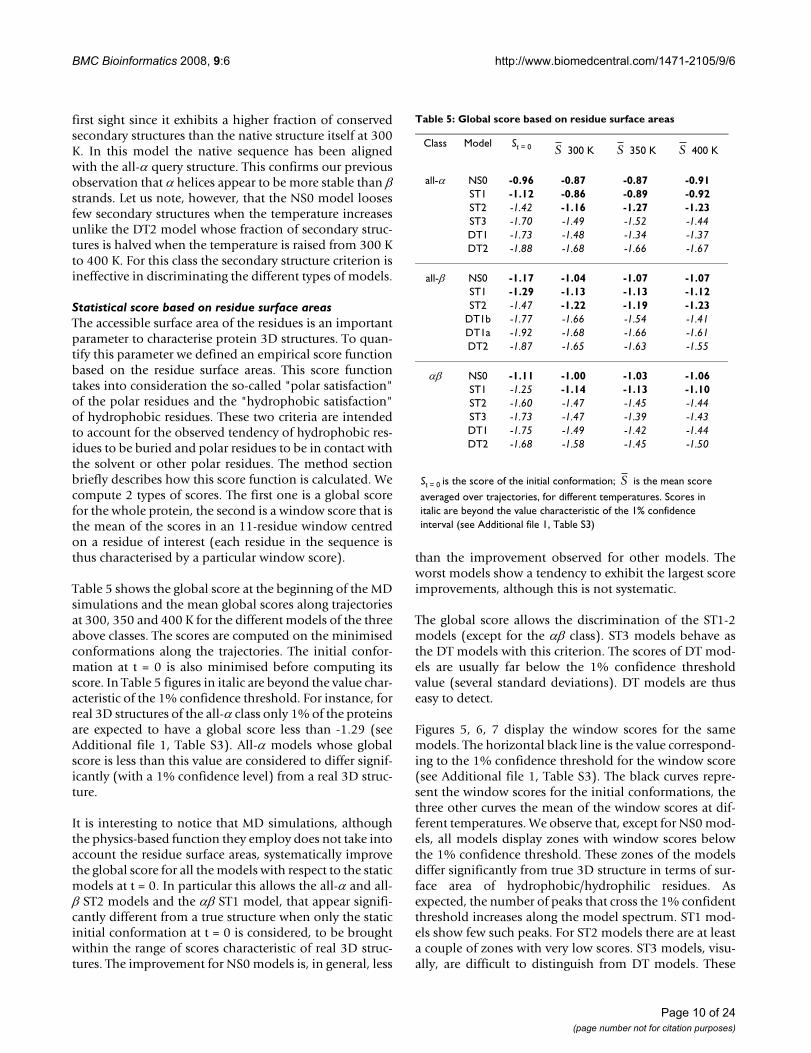
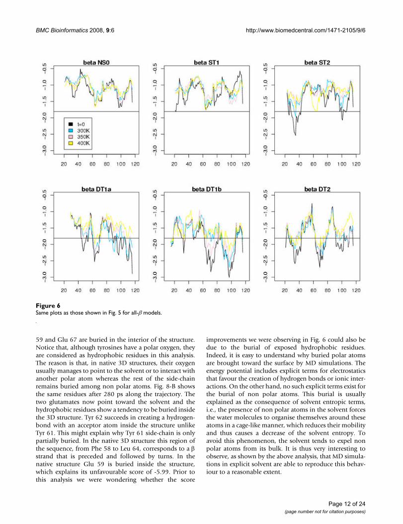
Figures 5, 6, 7 display the window scores for the samemodels. The horizontal black line is the value correspond-ing to the 1% confidence threshold for the window score(see Additional file 1, Table S3). The black curves repre-sent the window scores for the initial conformations, thethree other curves the mean of the window scores at dif-ferent temperatures. We observe that, except for NS0 mod-els, all models display zones with window scores belowthe 1% confidence threshold. These zones of the modelsdiffer significantly from true 3D structure in terms of sur-face area of hydrophobic/hydrophilic residues. Asexpected, the number of peaks that cross the 1% confidentthreshold increases along the model spectrum. ST1 mod-els show few such peaks. For ST2 models there are at leasta couple of zones with very low scores. ST3 models, visu-ally, are difficult to distinguish from DT models. These

Table 5: Global score based on residue surface areas

Class Model St = 0 300 K 350 K 400 K

all-α NS0 -0.96 -0.87 -0.87 -0.91ST1 -1.12 -0.86 -0.89 -0.92ST2 -1.42 -1.16 -1.27 -1.23ST3 -1.70 -1.49 -1.52 -1.44DT1 -1.73 -1.48 -1.34 -1.37DT2 -1.88 -1.68 -1.66 -1.67

all-β NS0 -1.17 -1.04 -1.07 -1.07ST1 -1.29 -1.13 -1.13 -1.12ST2 -1.47 -1.22 -1.19 -1.23

DT1b -1.77 -1.66 -1.54 -1.41DT1a -1.92 -1.68 -1.66 -1.61DT2 -1.87 -1.65 -1.63 -1.55

αβ NS0 -1.11 -1.00 -1.03 -1.06ST1 -1.25 -1.14 -1.13 -1.10ST2 -1.60 -1.47 -1.45 -1.44ST3 -1.73 -1.47 -1.39 -1.43DT1 -1.75 -1.49 -1.42 -1.44DT2 -1.68 -1.58 -1.45 -1.50

St = 0 is the score of the initial conformation; is the mean score

averaged over trajectories, for different temperatures. Scores in italic are beyond the value characteristic of the 1% confidence interval (see Additional file 1, Table S3)

S S S

S



observations, of course, are consistent with results shownin Table 5. The principal benefit of the window score overthe global score is that it allows us to single out regions ofthe models that are likely wrong. We thus investigated fur-ther, for different models, those peaks that show a clearimprovement of the initial conformation at t = 0 duringthe MD trajectory.

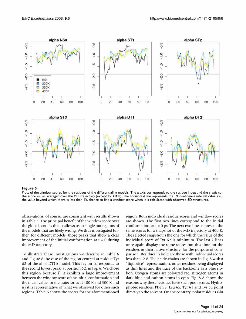
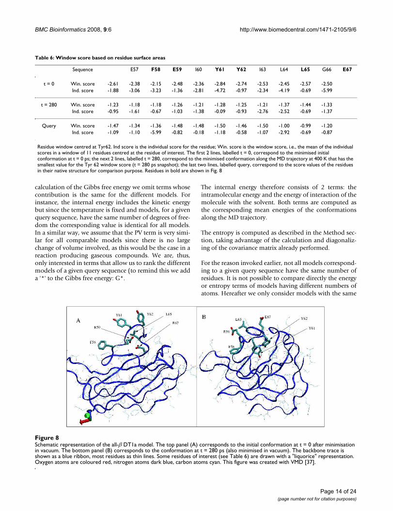
To illustrate these investigations we describe in Table 6and Figure 8 the case of the region centred at residue Tyr62 of the all-β DT1b model. This region corresponds tothe second lowest peak, at position 62, in Fig. 6. We chosethis region because i) it exhibits a large improvementbetween the window score of the initial conformation andthe mean value for the trajectories at 400 K and 300 K andii) it is representative of what we observed for other suchregions. Table 6 shows the scores for the aforementioned

region. Both individual residue scores and window scoresare shown. The first two lines correspond to the initialconformation, at t = 0 ps. The next two lines represent thesame scores for a snapshot of the MD trajectory at 400 K.The selected snapshot is the one for which the value of theindividual score of Tyr 62 is minimum. The last 2 linesonce again display the same scores but this time for theresidues in their native structure, for the purpose of com-parison. Residues in bold are those with individual scoresless than -2.8. Their side-chains are shown in Fig. 8 with a"liquorice" representation, other residues being displayedas thin lines and the trace of the backbone as a blue rib-bon. Oxygen atoms are coloured red, nitrogen atoms indark blue and carbon atoms in cyan. Fig. 8-A shows thereasons why these residues have such poor scores. Hydro-phobic residues: Phe 58, Leu 65, Tyr 61 and Tyr 62 pointdirectly to the solvent. On the contrary, polar residues Glu

Plots of the window scores for the residues of the different all-α modelsFigure 5Plots of the window scores for the residues of the different all-α models. The x-axis corresponds to the residue index and the y-axis to the score values averaged over the MD trajectory (except for t = 0). The horizontal line represents the 1% confidence interval value, i.e., the value beyond which there is less than 1% chance to find a window score when it is calculated with observed 3D structures.



59 and Glu 67 are buried in the interior of the structure.Notice that, although tyrosines have a polar oxygen, theyare considered as hydrophobic residues in this analysis.The reason is that, in native 3D structures, their oxygenusually manages to point to the solvent or to interact withanother polar atom whereas the rest of the side-chainremains buried among non polar atoms. Fig. 8-B showsthe same residues after 280 ps along the trajectory. Thetwo glutamates now point toward the solvent and thehydrophobic residues show a tendency to be buried insidethe 3D structure. Tyr 62 succeeds in creating a hydrogen-bond with an acceptor atom inside the structure unlikeTyr 61. This might explain why Tyr 61 side-chain is onlypartially buried. In the native 3D structure this region ofthe sequence, from Phe 58 to Leu 64, corresponds to a βstrand that is preceded and followed by turns. In thenative structure Glu 59 is buried inside the structure,which explains its unfavourable score of -5.99. Prior tothis analysis we were wondering whether the score

improvements we were observing in Fig. 6 could also bedue to the burial of exposed hydrophobic residues.Indeed, it is easy to understand why buried polar atomsare brought toward the surface by MD simulations. Theenergy potential includes explicit terms for electrostaticsthat favour the creation of hydrogen bonds or ionic inter-actions. On the other hand, no such explicit terms exist forthe burial of non polar atoms. This burial is usuallyexplained as the consequence of solvent entropic terms,i.e., the presence of non polar atoms in the solvent forcesthe water molecules to organise themselves around theseatoms in a cage-like manner, which reduces their mobilityand thus causes a decrease of the solvent entropy. Toavoid this phenomenon, the solvent tends to expel nonpolar atoms from its bulk. It is thus very interesting toobserve, as shown by the above analysis, that MD simula-tions in explicit solvent are able to reproduce this behav-iour to a reasonable extent.

Same plots as those shown in Fig. 5 for all-β modelsFigure 6Same plots as those shown in Fig. 5 for all-β models.



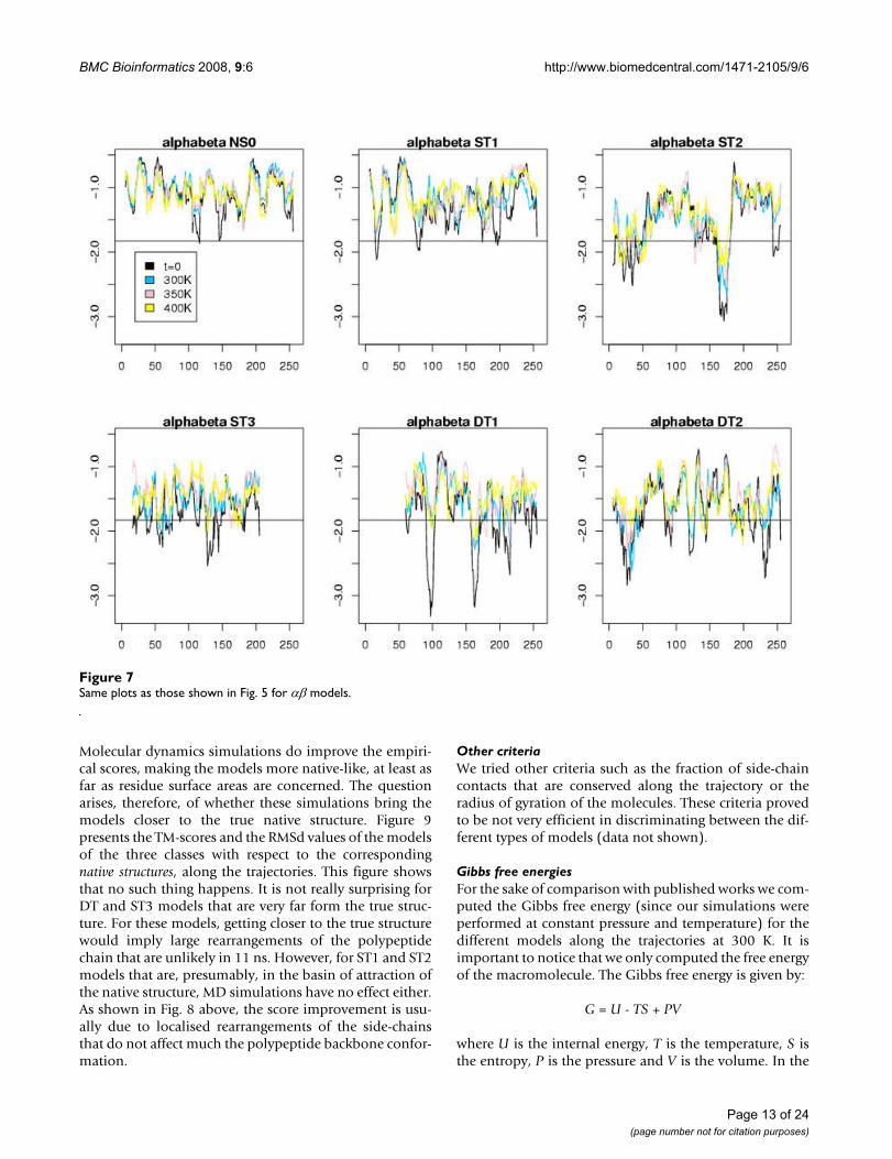
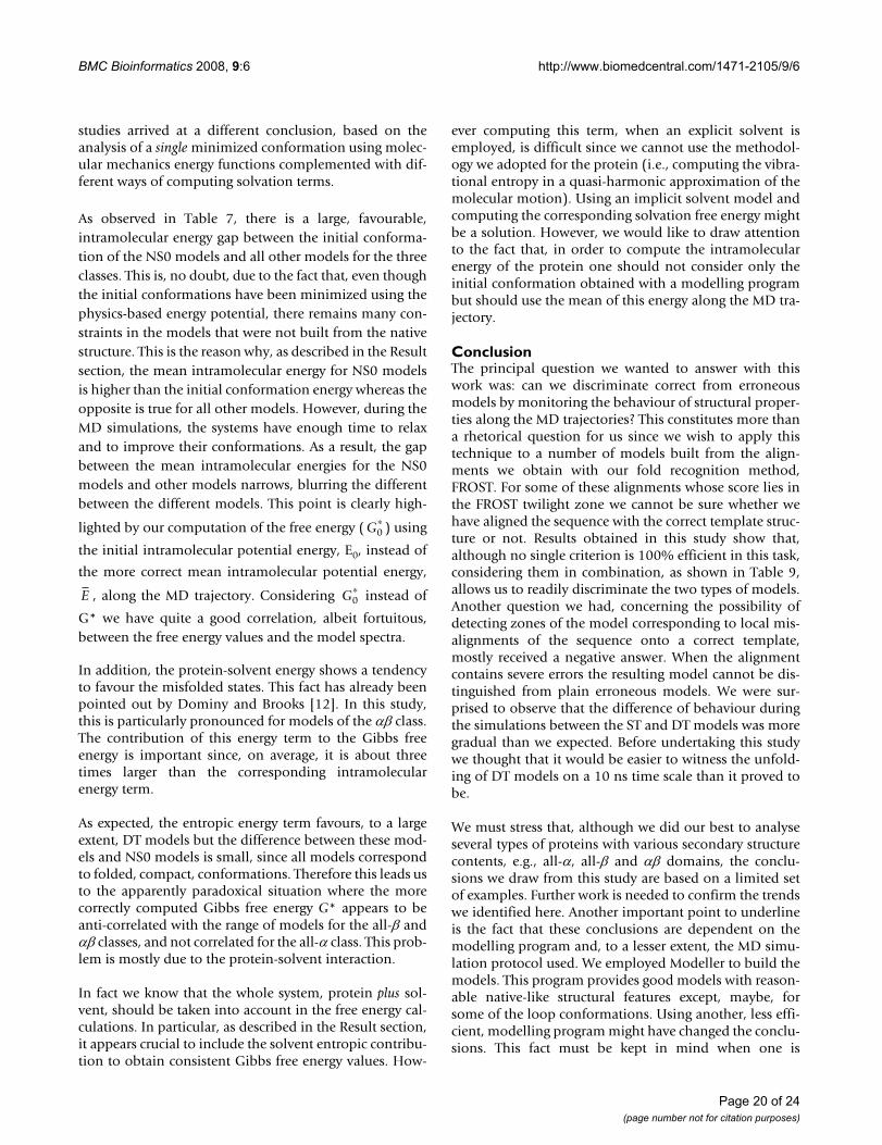
Molecular dynamics simulations do improve the empiri-cal scores, making the models more native-like, at least asfar as residue surface areas are concerned. The questionarises, therefore, of whether these simulations bring themodels closer to the true native structure. Figure 9presents the TM-scores and the RMSd values of the modelsof the three classes with respect to the correspondingnative structures, along the trajectories. This figure showsthat no such thing happens. It is not really surprising forDT and ST3 models that are very far form the true struc-ture. For these models, getting closer to the true structurewould imply large rearrangements of the polypeptidechain that are unlikely in 11 ns. However, for ST1 and ST2models that are, presumably, in the basin of attraction ofthe native structure, MD simulations have no effect either.As shown in Fig. 8 above, the score improvement is usu-ally due to localised rearrangements of the side-chainsthat do not affect much the polypeptide backbone confor-mation.

Other criteriaWe tried other criteria such as the fraction of side-chaincontacts that are conserved along the trajectory or theradius of gyration of the molecules. These criteria provedto be not very efficient in discriminating between the dif-ferent types of models (data not shown).

Gibbs free energiesFor the sake of comparison with published works we com-puted the Gibbs free energy (since our simulations wereperformed at constant pressure and temperature) for thedifferent models along the trajectories at 300 K. It isimportant to notice that we only computed the free energyof the macromolecule. The Gibbs free energy is given by:

G = U - TS + PV

where U is the internal energy, T is the temperature, S isthe entropy, P is the pressure and V is the volume. In the

Same plots as those shown in Fig. 5 for αβ modelsFigure 7Same plots as those shown in Fig. 5 for αβ models.



calculation of the Gibbs free energy we omit terms whosecontribution is the same for the different models. Forinstance, the internal energy includes the kinetic energybut since the temperature is fixed and models, for a givenquery sequence, have the same number of degrees of free-dom the corresponding value is identical for all models.In a similar way, we assume that the PV term is very simi-lar for all comparable models since there is no largechange of volume involved, as this would be the case in areaction producing gaseous compounds. We are, thus,only interested in terms that allow us to rank the differentmodels of a given query sequence (to remind this we adda '*' to the Gibbs free energy: G*.

The internal energy therefore consists of 2 terms: theintramolecular energy and the energy of interaction of themolecule with the solvent. Both terms are computed asthe corresponding mean energies of the conformationsalong the MD trajectory.

The entropy is computed as described in the Method sec-tion, taking advantage of the calculation and diagonaliz-ing of the covariance matrix already performed.

For the reason invoked earlier, not all models correspond-ing to a given query sequence have the same number ofresidues. It is not possible to compare directly the energyor entropy terms of models having different numbers ofatoms. Hereafter we only consider models with the same

Schematic representation of the all-β DT1a modelFigure 8Schematic representation of the all-β DT1a model. The top panel (A) corresponds to the initial conformation at t = 0 after minimisation in vacuum. The bottom panel (B) corresponds to the conformation at t = 280 ps (also minimised in vacuum). The backbone trace is shown as a blue ribbon, most residues as thin lines. Some residues of interest (see Table 6) are drawn with a "liquorice" representation. Oxygen atoms are coloured red, nitrogen atoms dark blue, carbon atoms cyan. This figure was created with VMD [37].

Table 6: Window score based on residue surface areas

Sequence E57 F58 E59 I60 Y61 Y62 I63 L64 L65 G66 E67

t = 0 Win. score -2.61 -2.38 -2.15 -2.48 -2.36 -2.84 -2.74 -2.53 -2.45 -2.57 -2.50Ind. score -1.88 -3.06 -3.23 -1.36 -2.81 -4.72 -0.97 -2.34 -4.19 -0.69 -5.99

t = 280 Win. score -1.23 -1.18 -1.18 -1.26 -1.21 -1.28 -1.25 -1.21 -1.37 -1.44 -1.33Ind. score -0.95 -1.61 -0.67 -1.03 -1.38 -0.09 -0.93 -2.76 -2.52 -0.69 -1.37

Query Win. score -1.47 -1.34 -1.36 -1.48 -1.48 -1.50 -1.46 -1.50 -1.00 -0.99 -1.20Ind. score -1.09 -1.10 -5.99 -0.82 -0.18 -1.18 -0.58 -1.07 -2.92 -0.69 -0.87

Residue window centred at Tyr62. Ind score is the individual score for the residue; Win. score is the window score, i.e., the mean of the individual scores in a window of 11 residues centred at the residue of interest. The first 2 lines, labelled t = 0, correspond to the minimised initial conformation at t = 0 ps; the next 2 lines, labelled t = 280, correspond to the minimised conformation along the MD trajectory at 400 K that has the smallest value for the Tyr 62 window score (t = 280 ps snapshot); the last two lines, labelled query, correspond to the score values of the residues in their native structure for comparison purpose. Residues in bold are shown in Fig. 8




TM scores (left panel) and RMSd values (right panel) for the models of the all-α class (top), all-β class (middle) and αβ class (bottom)Figure 9TM scores (left panel) and RMSd values (right panel) for the models of the all-α class (top), all-β class (middle) and αβ class (bottom). The colour code for the models is: NS0 = black, ST1 = red, ST2 = orange, ST3 = green, DT1 = blue, DT2 = purple. Horizontal lines in the TM score panel correspond to the limit above which two structures are clearly related in terms of 3D structures (0.4), and the limit below which they are clearly different (0.17).


number of residues. Table 7 shows the results that wereobtained.

For the intramolecular energy term, NS0 models are theonly models to have an initial energy lower than the meanenergy at 300 K. NS0 models are close to the native struc-ture and thus they are supposed to have many favourableinteractions. When we consider the energy of conforma-tions along the trajectory we expect less favourable inter-actions to be generated due to the thermal fluctuations,thus leading to an energy value that is higher on average.However, other models show an opposite behaviour, theinitial conformation has an energy higher than the meanenergy. The initial conformation for these models is thusclearly not optimal in terms of the physics-based poten-tial. NS0 models do not always have the lowest intramo-lecular energy, for instance the DT2 model for the all-αclass and the DT1a model for the all-β class have a lowerintramolecular energy.

On the other hand, for the solvent – protein interactionenergy, all models, except the NS0 model of the αβ class,exhibit a lower energy for the initial conformation than

for the mean energy along the trajectory, as expected. Itmust be noted that this term strongly favours the ST2 andDT models over the NS0 model for the αβ class. For otherclasses this trend exists but is less pronounced. Dominyand Brooks [12] using the CHARMM force field and a gen-eralized Born implicit solvation term found that mis-folded states were favoured by the solvation term. Theyattributed this fact to the mispairing of favourableintramolecular ionic contacts.

The entropic term is proportional to the number of con-formational states available to the system at a given tem-perature. We thus expect NS0 models to exhibit a smallervalue for this term than DT2 models. We observe a reason-able correlation between the entropic term values and therange of models (except for the all-β DT2 models whichhas the smallest entropic value).

We computed two values of the Gibbs free energy: G* forz

which we use the mean intramolecular energy ( ) along

the trajectory and for which we use the initial value of

the intramolecular energy E0. Considering these two

E

G0∗

Table 7: Gibbs free energies

Energy of the protein Energy protein-solventClass Model Nres E0 σE E0 σE TS G*

all-α NS0 105 -5 739 -5 316 345 -18 266 -17 123 672 1 157 -23 596 -24 019ST1 105 -4 002 -4 536 424 -20 587 -18 616 827 1 245 -24 397 -23 863ST2 91 -4 719 -4 892 335 -15 330 -15 354 636 1 119 - -ST3 104 -3 041 -4 745 543 -21 442 -17 646 1 026 1 325 -23 716 -22 012DT1 105 -2 379 -4 627 400 -23 278 -17 894 798 1 483 -24 004 -21 756DT2 105 -5 018 -5 755 289 -16 742 -15 625 509 1 337 -22 717 -21 980

all-β NS0 106 -6 018 -5 159 383 -15 237 -15 023 757 1 193 -21 375 -22 448ST1 106 -3 932 -4 836 333 -18 562 -15 585 657 1 274 -21 695 -23 768ST2 104 -2 828 -3 651 404 -18 910 -16 835 779 1 315 -21 801 -23 053

DT1b 98 -3 068 -3 621 355 -17 127 -15 244 681 1 368 - -DT1a 112 -3 301 -5 385 468 -19 417 -15 484 843 1 304 - -DT2 106 -3 483 -4 426 374 -18 988 -16 233 704 1 185 -21 844 -23 656

αβ NS0 260 -16 963 -13 912 452 -28 307 -30 284 826 2 339 -46 535 -49 586ST1 260 -11 223 -11 888 503 -36 671 -33 328 991 2 534 -47 750 -47 085ST2 260 -6 735 -9 817 911 -42 134 -36 954 1 625 2 731 -49 502 -46 420ST3 200 -6 774 -8 629 445 -28 844 -25 728 790 2 104 - -DT1 196 -2 578 -5 515 907 -40 953 -34 756 1 653 2 382 - -DT2 260 -8 369 -10 391 655 -40 331 -35 703 1 145 2 716 -48 810 -46 788

E0 is the energy for the initial conformation at t = 0; is the mean energy along the trajectory at T = 300 K;σE is the corresponding standard deviation. Column 3 is the number of residues in the model. Columns 4–6 correspond to the intramolecular protein energy, columns 7–9 correspond to the interaction energy of the protein with the solvent. Column 10 is the entropic contribution. Column 11, G* is the approximation

of the Gibbs free energy (see text). Column 12, is similar to G* except that it is computed using the protein is similar to G term E0 instead of

. The Gibbs free energy is not computed for models for which the number of residues differs by more than a couple of residues from the query

sequence length. All figures are in kJ/mol.

E E G0∗

E

E

G0∗



terms, we obtain very different pictures. For , there is a

perfect correlation between the model spectrum and the

free energy values for the all-α class and a reasonable cor-relation for the two other classes (once again the DT2models depart from the expected behaviour, they have aslightly lower free energy value than the correspondingST2 models). On the contrary, for G* there is an anti-cor-

relation for the all-β class, and to a lesser extent for the αβclass and no clear correlation for the all-α class. We notethat G* provides a better approximation of the true free

energy value than since the intramolecular energy,

and thus the internal energy, U, is much better estimatedby the mean intramolecular potential energy along thetrajectory than by a single minimised conformation. The

good correlation observed between and the spectrum

of models for the three classes is accidental. It is essentiallydue to the fact that the initial conformation for the mod-els, as described above, contains many constraints com-pared to the native structure. These constraints are relaxedduring the MD simulation. Therefore the Gibbs freeenergy, G*, computed for the macromolecule alone, does notappear to be an efficient criterion to discriminate the dif-ferent types of models. Since, in this calculation, we omita very important term, the entropic contribution of thesolvent, this is not very surprising (see Discussion below).

Analysis of the DT2 modelsThe unexpected behaviour of DT2 models that were sup-posed to act as controls at one extremity of the modelspectrum (the opposite extremity being the NS0 models)prompted us to analyse in detail these models for the all-α and all-β classes.

DT2 models are supposed to be worst than DT1 modelsbecause we just swapped the sequences without payingattention to the burial of charged residues or the exposureof non polar residues to the solvent. DT1 models, on theother hand, correspond to the first false positive in theranked list of scores. The fold recognition algorithm pro-vides the best score it can find and thus tends to avoid, asmuch as possible, such very unfavourable side-chainassignment. However, DT2 models unlike DT1 and STmodels, were aligned with 100% of the selected templatestructure. We did not need to model loop conformationswith Modeller. To analyse whether this point was crucialwe built new DT2 models for the all-α and all-β classeswith the same template structure except that, this time, thecoverage was 86% (slightly above the lowest coverageused for models of these classes, 83% for the all-α ST2model, see Additional file 1, Table S1). In practice we ran-domly chose 15 residues in the template structure loops

and we left to Modeller the task of building the conforma-tion of these residues. These new models were then sub-mitted to MD simulations at different temperatures aspreviously described.

Table 8 presents the same data as in Table 2 for the newDT2 models. It shows that the new models behave morelike the DT1 model than the ST models, as the initial DT2models did previously. To better understand the reasonsof these changes, we analysed the molecular dynamics tra-jectories for the initial and new DT2 models. The struc-tural differences between these models are relativelyslight.

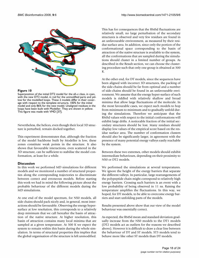
For example, Fig. 10 shows the differences in terms of the3D structure between the initial all-α DT2 model (incyan) and the corresponding new model (in red for thealigned part and yellow for the modelled loops). The larg-est difference corresponds to the loop between the first 2strands that is shown in the foreground of Fig. 10. In thetemplate structure the loop is tight and there is a helix turn(represented by the cylinder in cyan) that packs againstthe rest of the structure. In the new model the loop con-formation provided by Modeller is more extended andthus does not interact as closely with its counterpart in thetemplate structure. When we monitor the trajectory forthe new DT2 model we observe that the structure starts tounfold precisely at this point. The two first strands moveapart from the other strands; they gradually unzip. Thisbehaviour is not observed with the initial DT2 model, thehelical turn remains firmly docked with the rest of thestructure. A close inspection of the residues involved inthe interface between these two portions of the 3D struc-ture reveals that, just by chance, the interface consists ofhydrophobic residues that are packed together.

For the all-β models the case is less striking. We let Mod-eller generate the conformation of 5 residues in each ofthe 3 inner loops, i.e., the loops between 2 helices. Theconformation of the modelled loops appears to be morefloppy than the one of the real loops. This is confirmedduring the MD simulation since the modelled loopsundergo large motions that lead, for one of the helices, toa tendency to unfold at both extremities (only the centralpart remains helical throughout the whole trajectory).

G0∗

G0∗

G0∗

Table 8: Root Mean Square deviations

300 K 350 K 400 K

New DT2 models mean sd Mean sd Mean sd

all-α 4.7 1.29 3.8 0.98 5.8 0.83all-β 4.2 0.70 5.0 0.70 6.6 1.10

Same data as in Table 2 for new DT2 models.



Nevertheless, the helices, even though their local 3D struc-ture is perturbed, remain docked together.

This experiment demonstrates that, although the fractionof the model backbone built by Modeller is low, thesezones constitute weak points in the structure. It alsoshows that favourable interactions, even scattered in the3D structure, can be sufficient to stabilise the model con-formation, at least for a while.

DiscussionIn this work we performed MD simulations for differentmodels and we monitored a number of structural proper-ties along the corresponding trajectories to discriminatebetween correct and erroneous models. Before startingthis work we had in mind the following picture about theprobable behaviour of the different models during theMD simulations.

At one end of the model spectrum, for NS0 models, allside chains should pack nicely and, in general, most inter-actions should be favourable. Observing the energy hyper-surface at low resolution, this corresponds to a relativelydeep minimum that we call hereafter the basin of attrac-tion of the native structure. At higher resolution, thisbasin of attraction contains many local minima that aresampled at a given temperature. At 300 K we expect thesystem to remain within this basin during the whole sim-ulation. In terms of structural properties this implies thatthe global organisation of the structure is left unmodified.

This has for consequences that the RMSd fluctuations arerelatively small, no large perturbation of the secondarystructures is observed and very few residues are found inan unfavourable environment, as measured by their resi-due surface area. In addition, since only the portion of theconformational space corresponding to the basin ofattraction of the native structure is available to the system,all the conformations that are sampled during the simula-tions should cluster in a limited number of groups. Asdescribed in the Result section, we can choose the cluster-ing procedure such that only one group is obtained at 300K.

At the other end, for DT models, since the sequences havebeen aligned with incorrect 3D structures, the packing ofthe side-chains should be far from optimal and a numberof side-chains should be found in an unfavourable envi-ronment. We assume that the energy hyper-surface of suchmodels is riddled with relatively shallow and broadminima that allow large fluctuations of the molecule. Inthe most favourable cases, we expect such models to hopfrom minimum to minimum and to gradually unfold dur-ing the simulations. Therefore we anticipate that theRMSd values with respect to the initial conformations willexhibit large drifts. A noticeable fraction of the initial sec-ondary structures should be lost. Many residues shoulddisplay low values of the empirical score based on the res-idue surface area. The number of conformation clustersshould also be significantly larger, in agreement with thepresence of many potential energy valleys easily reachableby the system.

Between these two extremes, other models should exhibitintermediate behaviours, depending on their proximity toNS0 or DT2 models.

We performed the simulations at several temperatures.We ignore the height of the energy barriers that separatethe different valleys. In particular, large rearrangements ofthe polypeptide chain might correspond to relatively highenergy barriers. Crossing such barriers is an event with alow probability of being observed in 11 ns. Raising thetemperature amplifies the fluctuations. In this way, wehoped, for DT models, to be able to overcome energy bar-riers and start unfolding parts of the models.

Results presented above show that our view of the modelbehaviour was essentially correct.

As expected, the RMSd mean and standard deviation grad-ually increase from the NS0 models to the DT1 models(DT2 models act as outliers for the reasons we describedabove). However it is difficult to draw a clear line betweenthe behaviour of DT and ST models. ST3 models tend tobehave more like other ST models than DT models.

Superposition of the initial DT2 model for the all-α class, in cyan, with the new DT2 model, in red for the unmodified parts and yellow for the modelled loopsFigure 10Superposition of the initial DT2 model for the all-α class, in cyan, with the new DT2 model, in red for the unmodified parts and yel-low for the modelled loops. These 2 models differ in their cover-age with respect to the template structure, 100% for the initial model and only 86% for the new model. Unaligned residues in the loops have been built with Modeller. They are shown in yellow. This figure was made with VMD [37].



The number of clusters at 300 K would provide an excel-lent mean of discriminating ST from DT models but forthe all-β DT1a and DT2 models that exhibit an anoma-lous behaviour. Raising the temperature at 350 K or 400 Ksolves this problem. This is one of the few cases whereincreasing the temperature is useful in these analyses. At300 K ST1-2 models have less than 10 clusters, DT modelsseveral tens or hundreds. ST3 models are more difficult toclassify, the all-α class ST3 model behaving like a DTmodel and the one of the αβ class rather like a ST model.

The usefulness of the secondary structure criterion to dis-criminate the models depends on the type of secondarystructure. For models containing α helices there is a goodcorrelation between the mean content in secondary struc-ture and the spectrum of models. This is less clear formodels containing β strands, in particular those of the all-β class. For this class the DT1a model and, once again, theDT2 model depart from the expected behaviour. Herealso, performing the simulations at 350 or 400 K clarifiesthe situation. The surface area of hydrophobic/hydrophilic residues, implemented as a satisfaction score,provides the most quantitative criterion for the discrimi-nation of the models. Using the threshold for the 1% con-fidence interval we are able to clearly distinguish ST1-2models (except the ST2 model of the αβ class but asshown on Fig. 4 this model is far from the native structurewith an RMSd of 8 Å) from DT models. With this criterionST3 models behave like DT models.

To summarise the above points, no single criterion is suf-ficient to distinguish ST1-2 models from DT models in allcases. Criteria such as the RMSd mean, RMSd standarddeviation and clustering are subject to a few false posi-tives, i.e., DT models behave like ST models. The satisfac-tion score generates one false negative, e.g., the αβ ST2model is indistinguishable from DT models with this cri-terion. The clustering and satisfaction score provide morequantitative criteria than other structural features we con-sidered in this study. If we consider conjointly all the cri-teria it is relatively straightforward to discriminate ST1-2from DT models, as shown in Table 9. Most of the time,ST3 models behave like DT models. Therefore grossly mis-aligning a sequence with the correct template structureresults in a model that is no better than models for whichthe sequence has been aligned with erroneous structures.

Running simulations at different temperatures did notprove very helpful, except possibly for the models of theall-β class for which, in a couple of occasions concerningthe clustering and secondary structure criteria, it contrib-uted to a better discrimination of the DT and ST models.Moreover, it is likely that 400 K is too high a temperaturefor running meaningful MD simulations.

Although the simulations were able to improve the sur-face area of hydrophobic/hydrophilic residues, makingthe side chains more native-like, we did not observe anyimprovement of the ST1-2 model backbones in terms ofRMSd values, that is, the model main chains did notbecome any closer to the native structure main chains.MD simulations in explicit solvent using Rosetta decoys asmodels [15] showed that such improvements can some-times be observed on a 10–100 ns time scale. In this studythe simulation time corresponds to the lower end of thisinterval which might explain, in part, why we do not wit-ness any backbone improvement. Other works, usingMonte Carlo simulations [24] or just simple minimisa-tions [25], did succeed in improving the ranking of goodmodels and, sometimes, in refining the conformation of"low" resolution 3D structures [24,26]. In our case our"good" models are relatively far from the native structures(the ST2 model for the all-α class is 5.7 Å and the ST2model for the αβ class is 8 Å from the correspondingnative structures). It is likely that this sort of "low" resolu-tion models need more than 11 ns to be significantlyameliorated.

Computations of the Gibbs free energy did not help us indiscriminating correct from erroneous models. Other

Table 9: Criteria used to discriminate the models at 300 K

Class Model RMSd mean

RMSd fluct.

Clusters SSEs Satisfaction score

all-α NS0 + + ++ ++ +++ST1 + + ++ ++ +++ST2 + + ++ ++ +++ST3 + + - + - -DT1 + ++ ++ ++ +++DT2 - - - ++ ++ +++

all-β NS0 + + ++ + +++ST1 + + ++ + +++ST2 + + ++ - +++

DT1b - - - - - - +++DT1a + + ++ + +++DT2 - + - - - - +++

αβ NS0 + + ++ ++ +++ST1 + + ++ ++ +++ST2 + + + + - -ST3 + + + + - -DT1 + + ++ - +++DT2 - - + + - +++

RMSd mean, RMSd uctuations, number of clusters along the trajectory, evolution of the secondary structures, hydrophobic and polar satisfaction score. The number of '+' symbolises the confidence in the criterion result. For instance the hydrophobic/polar satisfaction score provides a quantitative answer that is easy to interpret whereas results provided by the RMSd mean are more difficult to judge. The '-' indicates false positives or negatives.



studies arrived at a different conclusion, based on theanalysis of a single minimized conformation using molec-ular mechanics energy functions complemented with dif-ferent ways of computing solvation terms.

As observed in Table 7, there is a large, favourable,intramolecular energy gap between the initial conforma-tion of the NS0 models and all other models for the threeclasses. This is, no doubt, due to the fact that, even thoughthe initial conformations have been minimized using thephysics-based energy potential, there remains many con-straints in the models that were not built from the nativestructure. This is the reason why, as described in the Resultsection, the mean intramolecular energy for NS0 modelsis higher than the initial conformation energy whereas theopposite is true for all other models. However, during theMD simulations, the systems have enough time to relaxand to improve their conformations. As a result, the gapbetween the mean intramolecular energies for the NS0models and other models narrows, blurring the differentbetween the different models. This point is clearly high-

lighted by our computation of the free energy ( ) using

the initial intramolecular potential energy, E0, instead of

the more correct mean intramolecular potential energy,

, along the MD trajectory. Considering instead of

G* we have quite a good correlation, albeit fortuitous,between the free energy values and the model spectra.

In addition, the protein-solvent energy shows a tendencyto favour the misfolded states. This fact has already beenpointed out by Dominy and Brooks [12]. In this study,this is particularly pronounced for models of the αβ class.The contribution of this energy term to the Gibbs freeenergy is important since, on average, it is about threetimes larger than the corresponding intramolecularenergy term.

As expected, the entropic energy term favours, to a largeextent, DT models but the difference between these mod-els and NS0 models is small, since all models correspondto folded, compact, conformations. Therefore this leads usto the apparently paradoxical situation where the morecorrectly computed Gibbs free energy G* appears to beanti-correlated with the range of models for the all-β andαβ classes, and not correlated for the all-α class. This prob-lem is mostly due to the protein-solvent interaction.

In fact we know that the whole system, protein plus sol-vent, should be taken into account in the free energy cal-culations. In particular, as described in the Result section,it appears crucial to include the solvent entropic contribu-tion to obtain consistent Gibbs free energy values. How-

ever computing this term, when an explicit solvent isemployed, is difficult since we cannot use the methodol-ogy we adopted for the protein (i.e., computing the vibra-tional entropy in a quasi-harmonic approximation of themolecular motion). Using an implicit solvent model andcomputing the corresponding solvation free energy mightbe a solution. However, we would like to draw attentionto the fact that, in order to compute the intramolecularenergy of the protein one should not consider only theinitial conformation obtained with a modelling programbut should use the mean of this energy along the MD tra-jectory.

ConclusionThe principal question we wanted to answer with thiswork was: can we discriminate correct from erroneousmodels by monitoring the behaviour of structural proper-ties along the MD trajectories? This constitutes more thana rhetorical question for us since we wish to apply thistechnique to a number of models built from the align-ments we obtain with our fold recognition method,FROST. For some of these alignments whose score lies inthe FROST twilight zone we cannot be sure whether wehave aligned the sequence with the correct template struc-ture or not. Results obtained in this study show that,although no single criterion is 100% efficient in this task,considering them in combination, as shown in Table 9,allows us to readily discriminate the two types of models.Another question we had, concerning the possibility ofdetecting zones of the model corresponding to local mis-alignments of the sequence onto a correct template,mostly received a negative answer. When the alignmentcontains severe errors the resulting model cannot be dis-tinguished from plain erroneous models. We were sur-prised to observe that the difference of behaviour duringthe simulations between the ST and DT models was moregradual than we expected. Before undertaking this studywe thought that it would be easier to witness the unfold-ing of DT models on a 10 ns time scale than it proved tobe.

We must stress that, although we did our best to analyseseveral types of proteins with various secondary structurecontents, e.g., all-α, all-β and αβ domains, the conclu-sions we draw from this study are based on a limited setof examples. Further work is needed to confirm the trendswe identified here. Another important point to underlineis the fact that these conclusions are dependent on themodelling program and, to a lesser extent, the MD simu-lation protocol used. We employed Modeller to build themodels. This program provides good models with reason-able native-like structural features except, maybe, forsome of the loop conformations. Using another, less effi-cient, modelling program might have changed the conclu-sions. This fact must be kept in mind when one is

G0∗

E G0∗



comparing different studies about the stability, or theenergy, of models.

Our aim, when performing these simulations on models,is not so much to verify that the models are reasonable interms of structural properties as to check whether our foldrecognition method has been able to identify correctly thetemplate structure. We are interested in microbial genomeannotation [27]. Homology search methods constitutethe cornerstone of the annotation process. Unfortunately,methods based on sequence comparison are no longerefficient when the similarity is below 20% sequence iden-tity, leaving between 25 to 50% "orphan" codingsequences (CDSs), depending on the organism analysed.Fold recognition techniques can detect remote homologs,having less than 20% sequence identity, allowing us toobtain a crucial piece of information about these orphanCDSs. Therefore the MD simulations we described in thisstudy are a means for us to improve the sensitivity andspecificity of our fold recognition method for ambiguouscases, i.e., when the corresponding scores are within thetwilight zone.

To conclude with a practical consideration, we give anorder of magnitude of the amount of time required fortesting one model. For an all-α model, the system, proteinplus solvent, is made of about 15,000 atoms. We haveavailable a cluster of 10 bi-processors dual core x86 64 at2.33 GHz (10 blades). Using the 4 CPUs of a blade in par-allel we are able to simulate 8 ns a day (2.6 ns a day perCPU). Although not exactly a routine calculation, thisallows us, to run an 11 ns MD simulation for a model ofthis size, overnight, employing 3 blades. The analysis ofthe trajectories, due to the minimisation of the conforma-tions, requires about the same amount of time. A way ofspeeding up the simulations would be to use an implicitrepresentation of the solvent instead of the explicit repre-sentation we used in this study. This would have the addi-tional merit of allowing us to compute the solvation freeenergy.

MethodsSelection of query and template structuresFor the selection of the query domains we started with twofolds belonging to three SCOP classes : DNA/RNA bind-ing 3 helical bundle (81 families) and 4 helical up anddown bundle (12 families) for the α class; immunoglob-ulin-like beta sandwich (49 families) and double strandedβ helix (29 families) for the β class; TIM barrel (84 fami-lies) and NADP binding Rossmann (29 families) for theαβ class.

Representatives of the different families of these foldswere selected with the help of the AEROSPACIE scorecomputed for the ASTRAL database [28]. As far as possi-

ble, we disregarded domains with prosthetic groups,disulfide bridges, co-factors and those belonging to oli-gomers.

A cross-comparison of all these representatives was carriedout using the 3D structure comparison method VAST[29,30] to measure their degree of structural relatednessand to obtain 3D structural alignments. To complementthe results provided by VAST we also employed anotherstructural measure: the TM-score [31].

We then used the fold recognition program FROST [17] toobtain, for each representative domain, a list of templatestructures ranked by score. Representative domains weretagged as potential queries if we could find, in the top ofthe corresponding lists, three structures similar to the rep-resentative domain fold and with the following proper-ties. The first similar structure (called Similar Template 1,ST1) had to be close to the representative domain with ahigh percentage of identical residues (for fold recognitiontechniques this corresponds to a range of 20–30%sequence identity) and an alignment close to the struc-tural alignment found by VAST between the pair of struc-tures. The second similar structure (ST2) had the samecharacteristics as ST1 except for the percentage ofsequence identity that had to be low (typically less than20% identity). Finally for the third similar structure (ST3)the alignment provided by FROST had to contain errorswith respect to the structural alignment found by VAST.

For each of the three query structures selected in such away (one for each class of secondary structure: α, β, αβ)we built six models (as described in the next section). Thefirst one corresponded to the native structure (calledNS0), the next three to the similar structures (ST1, ST2,ST3). The fifth one corresponded to the first false positivein the list of template (see Fig. 1), i.e., a structure havingno relation with the query structure (called Different Tem-plate 1, DT1). The last one (called DT2), used as a control,was similar to the experiment of Novotny et al.[5]: we justaligned, without insertion/deletion, the query domainsequence with a fold having a similar size and belongingto a different secondary structure class. Table 1 summa-rises the characteristics of the different models that werebuilt.

3D structure modellingThree-dimensional models were built with Modeller 6v1[32] starting from the alignments provided by the fold rec-ognition method FROST (except for DT2 models and theST1 models as discussed in the Result section). For eachtype of model, five models were generated using Modellerdefault parameters and the one having the best objectivefunction was kept. For the query sequence we did not usethe PDB structure directly. We created a 3D model using



the same modelling protocol starting from a (perfect)alignment of the sequence with itself. For DT2 models wealigned the query sequence with the sequence of the tem-plate structure without insertion/deletion since bothsequences have approximately the same number of resi-dues. For ST1 models, to be sure to obtain good align-ments, we used the more accurate VAST structuralalignment instead of the FROST alignment.

Molecular dynamics simulationsAll simulations were performed in explicit water using theversion 3.3.1 of the Gromacs package [33] in conjunctionwith the Gromos96 43a1 force field for condensed phase.The Simple Point Charge (SPC) model was used to repre-sent water. The protonation state of ionizable groups inthe proteins was chosen appropriate for pH 7.0. Counte-rions were added to neutralise the system. Moleculardynamics simulations were performed at constant tem-perature and pressure in a periodic rhombic dodecahe-dron box. The minimum distance between an atom of theprotein and a box wall was 0.8 nm. Simulations at 300,350 and 400 K were carried out. During these simulationsa pressure of 1 bar was maintained. Temperature and pres-sure were kept constant by coupling to an external heatbath (Berensen thermostat) and an isotropic pressurebath (Berensen barostat). Corresponding relaxation timeswere set to 0.5 ps (separately for the protein, the solventand the counterions) and 1.0 ps. Electrostatic interactionswere calculated with the fast Particle-Mesh Ewald method(PME) and a distance cut-off of 0.9 nm. When using PME,other relevant parameters such as FFT grid spacing, inter-polation order, geometry of the Ewald summations, etc.were left to their default values. Van der Waals (VdW)interactions were evaluated using twin range cut-offs of1.4 nm for VdW cut-off and 0.9 nm for the short-rangeneighbour list. Non-bonded interactions were evaluatedwith a grid using periodic boundary conditions in alldirections. Neighbour pair list was updated every 10 steps.Covalent bonds with H-atoms were constrained using theLINCS algorithm. An integration step of 2 fs was used. Togenerate the starting conformation the following protocolwas employed. First an energy minimisation was per-formed using steepest descent followed by a quasi-newtonmethod (Broyden-Fletcher-Goldfarb-Shanno algorithm).This phase was followed by 200 ps of equilibration withposition restraints of the protein using a simulatedannealing procedure that, starting at a temperature of 250K, raised it to 300 K in 10 ps and maintained it to thisvalue for the 190 remaining ps, allowing the system torelax. Production phase data were obtained by first carry-ing out a 1 ns simulation run then performing ten 1 nssimulation runs branching off this first trajectory every100 ps. This procedure was used to improve the samplingof the conformational space [34]. The total length of theproduction phase trajectory was thus 11 ns.

Principal component analysisPrincipal component analysis, or covariance analysis,consists in calculating the mass-weighted covariancematrix of the atomic coordinates along the MD trajectorythen diagonalising it. The eigenvectors are the essentialmodes that describe collective motions in the protein. Thecorresponding eigenvalues are the mean square fluctua-tions along these modes. The main advantage of this tech-nique is that only a very limited number of modes (atmost a dozen) are required to describe most of the proteindynamics. Using these data different analyses can be car-ried out: projection of the trajectory along the differentmodes, atomic mean square fluctuations along themodes, subspace overlap, etc. A very useful analysis is thecalculation of the cosine content of the first principalcomponents that gives an indication of the efficiency ofthe conformational space sampling. To perform the anal-ysis described in the text we used the relevant Gromacstools, in particular g_covar to calculate and diagonalisethe covariance matrix and g_anaeig to analyses eigenvec-tors and eigenvalues.

Computation of the vibrational entropyThe mass-weighted covariance matrix can be used to com-pute the vibrational entropy of the molecule. The molec-ular motion along the MD trajectory is approximated asquasi-harmonic. Covariance matrix eigenvalues, λi, definethe corresponding frequencies:

the entropy S of the macroscopic state is given by [35]:

kB is the Boltzmann's constant, h the Planck's constant, Tthe temperature and NA the Avogadro's number.

Clustering of conformationsConformations every 10 ps along the trajectories wereminimised in vacuum. The resulting minimum conforma-tions were clustered using the Gromacs tool g cluster thatprovides several clustering methods. Here we build clus-ters with a single linkage method using, for each class, acut-off value corresponding to the RMSd mean value at300 K for NS0 models: 1.2 Å, 1.86 Å and 1.98 Å for the all-α, all-β and αβ classes respectively. The RMSd mean val-ues used are those obtained with the minimised confor-mations. In a real situation, since we do not know thenative structure of the query sequence, we would useRMSd cut-off values of 1.5 Å for all-α proteins and 2.0 Åfor all-β and αβ proteins.

( )2 2πνλi

kBT

i=

S N k ii

h ikBTA B

i

i i=−

− − − =∑ θθ

θ θ νexp( )

log( exp( ))1

1 where



Statistical score based on the residue surface areaTo analyse the quality of models we developed an all-atom statistical score based on the residue surface area(unpublished work), inspired by the work of Eisenbergand colleagues in [36]. Here, for completeness, we give abrief description of this statistical score.

For each type of residue we compute the fraction of thepolar atom surface in contact with other polar atoms,dubbed "polar satisfaction" and the fraction of non polaratom surface in contact with non polar atoms, called"hydrophobic satisfaction". We consider oxygen andnitrogen as polar and all other atoms as non polar. Hydro-gen atoms are ignored in this analysis. These two termsmeasure the tendency of non polar atoms to form ahydrophobic core and of polar atoms to avoid being bur-ied among non polar atoms. We compiled these fractionsfor residues belonging to three sets of proteins (all-α, all-β and αβ) as shown in Table S4 in Additional file 1. Themean environment for residues in a protein depends onthe size of the protein thus we only selected proteinswhose length was ± 30 residue long with respect to thelength of the three query proteins. The proteins are sur-rounded by water molecules, i.e., polar atoms.

In Additional file 1, Fig. S8 shows the calculated densityand cumulative probabilities for the tryptophan hydro-phobic satisfaction in proteins belonging to the all-αclass. Let us assume that, for a tryptophan in a model, wemeasure a hydrophobic satisfaction value of 0.706 asshown on Fig. 8. The corresponding score is the logarithmof the cumulative probability for the hydrophobic satis-faction (HS) up to the measured value, i.e., S = ln(p(HS <0.706)) = ln(0.57) = -0.56. With this definition, if a hydro-phobic residue is completely buried among hydrophobicatoms, its hydrophobic satisfaction is 1 and hence itsscore is maximum (zero). The lower the hydrophobic sat-isfaction is the lower the score. The same score definition,only based on the polar satisfaction, apply for polar resi-dues. In our analysis we considered {A, V, C, I, L, F, M, Y,W, P} as hydrophobic residues and {S, T, H, K, D, N, Q,E, R} as polar residues. Notice that polar residues consistof polar and non polar atoms. In this analysis we did nottake into consideration non polar atoms of polar residues.Tryptophan and tyrosine, in spite of having one polaratom, are considered as hydrophobic due to the largenumber of non polar atoms that compose their side chain.

For proteins of the three sets we computed the distribu-tions of scores for the whole protein (global score) as wellas the distributions of scores for windows of width 11 res-idues along the sequence. The latter is intended to pin-point zones in the model for which residues significantlydepart from the behaviour observed in protein 3D struc-tures. In Additional file 1, Table S3 shows the mean,

standard deviation and the value corresponding to 1%confidence threshold for the global score and windowscore. The Shapiro-Wilk statistical test computes the p-value that the distribution is normal (null hypothesis).For the all-α and αβ protein global score distributions onecannot reject the null hypothesis at a confidence thresh-old of 10%. This is not true for the all-β proteins. For themwe computed empirically the 1% confidence interval. Forthe window score distributions, there is a strong correla-tion between overlapping windows and it is likely that theShapiro-Wilk test is meaningless in such a case. We alsocomputed empirically the corresponding 1% confidencelevel. It is interesting to notice that the means are all verysimilar for the global or the window scores. The windowscore distributions have all the same standard deviations.For the global score distributions the standard deviationsdecrease from the all-α class to the αβ class. This is due tothe number of proteins involved in the computation thatgoes from 79 to 167 and also to the size of the proteinsthat varies from 106 to 230 residues. In Additional file 1,Table S3 indicates that residues, on average, have similarenvironments whatever the structural class considered.

Authors' contributionsJFT participated in the conception of the study, carried outthe analyses and participated in the writing of the manu-script. AM provided assistance with the FROST program.JFG conceived of the study, supervised and coordinatedthe whole project and wrote the manuscript. All authorsread and approved the manuscript.

Additional material

AcknowledgementsWe are grateful to the INRA MIGALE bioinformatics platform for providing computational resources. Part of this research was supported by a grant from the Agence Nationale de la Recherche (ANR-06-CIS6-008). JFT is grateful to the Ministère de l'Education Nationale, de l'Enseignement Supérieur et de la Recherche for the award of a doctoral fellowship.

References1. Kryshtafovych A, Venclovas C, Fidelis K, Moult J: Progress over the

first decade of CASP experiments. Proteins 2005, 61(Suppl7):225-36.

2. Oldziej S, Czaplewski C, Liwo A, Chinchio M, Nanias M, Vila JA, KhaliliM, Arnautova YA, Jagielska A, Makowski M, Schafroth HD, Kazmierk-iewicz R, Ripoll DR, Pillardy J, Saunders JA, Kang YK, Gibson KD,Scheraga HA: Physics-based protein-structure predictionusing a hierarchical protocol based on the UNRES force

Additional file 1Supplementary tables and figures. This file contains the 8 supplementary figures and 4 supplementary tables listed in the text.Click here for file[http://www.biomedcentral.com/content/supplementary/1471-2105-9-6-S1.pdf]


http://www.biomedcentral.com/content/supplementary/1471-2105-9-6-S1.pdf






Publish with BioMed Central and every scientist can read your work free of charge

"BioMed Central will be the most significant development for disseminating the results of biomedical research in our lifetime."

Sir Paul Nurse, Cancer Research UK

Your research papers will be:

available free of charge to the entire biomedical community

peer reviewed and published immediately upon acceptance

cited in PubMed and archived on PubMed Central

yours — you keep the copyright

Submit your manuscript here:http://www.biomedcentral.com/info/publishing_adv.asp

BioMedcentral

field: assessment in two blind tests. Proc Natl Acad Sci USA 2005,102:7547-52.

3. Schueler-Furman O, Wang C, Bradley P, Misura K, Baker D:Progress in modeling of protein structures and interactions.Science 2005, 310:638-42.

4. Lazaridis T, Karplus M: Effective energy functions for proteinstructure prediction. Curr Opin Struct Biol 2000, 10:139-45.

5. Novotny J, Bruccoleri R, Karplus M: An analysis of incorrectlyfolded protein models. Implications for structure predic-tions. J Mol Biol 1984, 177:787-818.

6. Novotny J, Rashin AA, Bruccoleri RE: Criteria that discriminatebetween native proteins and incorrectly folded models. Pro-teins 1988, 4:19-30.

7. Vorobjev YN, Almagro JC, Hermans J: Discrimination betweennative and intentionally misfolded conformations of pro-teins: ES/IS, a new method for calculating conformationalfree energy that uses both dynamics simulations with anexplicit solvent and an implicit solvent continuum model.Proteins 1998, 32:399-413.

8. Janardhan A, Vajda S: Selecting near-native conformations inhomology modeling: the role of molecular mechanics andsolvation terms. Protein Sci 1998, 7:1772-80.

9. Lazaridis T, Karplus M: Discrimination of the native from mis-folded protein models with an energy function includingimplicit solvation. J Mol Biol 1999, 288:477-87.

10. Gatchell DW, Dennis S, Vajda S: Discrimination of near-nativeprotein structures from misfolded models by empirical freeenergy functions. Proteins 2000, 41:518-34.

11. Kinjo AR, Kidera A, Nakamura H, Nishikawa K: Physicochemicalevaluation of protein folds predicted by threading. Eur BiophysJ 2001, 30:1-10.

12. Dominy BN, Brooks CL III: Identifying native-like protein struc-tures using physics-based potentials. J Comput Chem 2002,23:147-60.

13. Felts AK, Gallicchio E, Wallqvist A, Levy RM: Distinguishing nativeconformations of proteins from decoys with an effective freeenergy estimator based on the OPLS all-atom force field andthe Surface Generalized Born solvent model. Proteins 2002,48:404-22.

14. Lee MR, Tsai J, Baker D, Kollman PA: Molecular dynamics in theendgame of protein structure prediction. J Mol Biol 2001,313:417-30.

15. Fan H, Mark AE: Refinement of homology-based protein struc-tures by molecular dynamics simulation techniques. ProteinSci 2004, 13:211-20.

16. Chen J, Brooks CL 3rd: Can molecular dynamics simulationsprovide high-resolution refinement of protein structure? Pro-teins 2007, 67(4):922-930.

17. Marin A, Pothier J, Zimmermann K, Gibrat JF: FROST: a filter-based fold recognition method. Proteins 2002, 49:493-509.

18. Andreeva A, Howorth D, Brenner SE, Hubbard TJ, Chothia C, MurzinAG: SCOP database in 2004: refinements integrate structureand sequence family data. Nucleic Acids Res 2004, 32:D226-9.

19. Melo F, Sanchez R, Sali A: Statistical potentials for fold assess-ment. Protein Sci 2002, 11:430-48.

20. Hess B: Similarities between principal components of proteindynamics and random diffusion. Phys Rev E 2000, 62:8438-48.

21. Hess B: Convergence of sampling in protein simulations. PhysRev E 2002, 65:031910,1-031910,10.

22. Kabsch W, Sander C: Dictionary of protein secondary struc-ture: pattern recognition of hydrogen-bonded and geometri-cal features. Biopolymers 1983, 22(12):2577-637.

23. Gilquin B, Guilbert C, Perahia D: Unfolding of hen egg lysozymeby molecular dynamics simulations at 300 K: insight into therole of the interdomain interface. Proteins 2000, 41:58-74.

24. Bradley P, Misura KM, Baker D: Toward high-resolution de novostructure prediction for small proteins. Science 2005,309:1868-71.

25. Kmiecik S, Gront D, Kolinski A: Towards the high-resolutionprotein structure prediction. Fast refinement of reducedmodels with all-atom force field. BMC Struct Biol 2007, 7:43.

26. Simmerling C, Lee MR, Ortiz AR, Kolinski A, Skolnick J, Kollman PA:Combining MONSSTER and LES/PME to predict proteinstructure from amino acid sequence: application to the smallprotein CMTI-1. J Am Chem Soc 2000, 122:8392-8402.

27. Bryson K, Loux V, Bossy R, Nicolas P, Chaillou S, van de Guchte M,Penaud S, Maguin E, Hoebeke M, Bessieres P, Gibrat JF: AGMIAL:implementing an annotation strategy for prokaryotegenomes as a distributed system. Nucleic Acids Res 2006,34:3533-45.

28. Chandonia JM, Walker NS, Lo Conte L, Koehl P, Levitt M, BrennerSE: ASTRAL compendium enhancements. Nucleic Acids Res2002, 30:260-3.

29. Madej T, Gibrat JF, Bryant SH: Threading a database of proteincores. Proteins 1995, 23:356-69.

30. Gibrat JF, Madej T, Bryant SH: Surprising similarities in structurecomparison. Curr Opin Struct Biol 1996, 6:377-85.

31. Zhang Y, Skolnick J: Scoring function for automated assess-ment of protein structure template quality. Proteins 2004,57:702-10.

32. Sali A, Blundell TL: Comparative protein modelling by satisfac-tion of spatial restraints. J Mol Biol 1993, 234:779-815.

33. Van Der Spoel D, Lindahl E, Hess B, Groenhof G, Mark AE, BerendsenHJ: GROMACS: fast, flexible, and free. J Comput Chem 2005,26:1701-18.

34. Caves L, Evanseck J, Karplus M: Locally accessible conformationsof proteins: multiple molecular dynamics simulations ofcrambin. Protein Sci 1998, 7:649-66.

35. McQuarrie DA: Statistical Mechanics New-York: HarperCollins; 1976. 36. Eisenberg D, Luthy R, Bowie JU: VERIFY3D: assessment of pro-

tein models with three-dimensional profiles. Methods Enzymol1997, 277:396-404.

37. Humphrey W, Dalke A, Schulten K: VMD – Visual MolecularDynamics. J Molec Graphics 1996, 14:33-38.








































































http://www.biomedcentral.com/info/publishing_adv.asp


Can molecular dynamics simulations help in discriminating correct from erroneous protein 3D models

Documents

Transcript of Can molecular dynamics simulations help in discriminating correct from erroneous protein 3D models