Munich Personal RePEc Archive

Stochastic Choice: Rational or

Erroneous?

Dong, Xueqi and Liu, Shuo Li

Newcastle University, Harvard University

December 2019

Online at https://mpra.ub.uni-muenchen.de/107678/

MPRA Paper No. 107678, posted 14 May 2021 20:44 UTC

Abstract

Likelihood functions have been the central pieces of statistical inference. For dis-

crete choice data, conventional likelihood functions are specified by random utility

(RU) models, such as logit and tremble, which generate choice stochasticity through

an ”error”, or, equivalently, random preference.

For risky discrete choice, this paper explores an alternative method to construct

the likelihood function: Rational Expectation Stochastic Choice (RESC). In line with

Machina (1985), the subject optimally and deterministically chooses a stochastic choice

function among all possible stochastic choice functions; the choice stochasticity can

be explained by risk aversion and the relaxation of the reduction of compound lot-

tery. The model maximizes a simple two-layer expectation that disentangles risk and

randomization, in the similar spirit of Klibanoff et al. (2005) where ambiguity and

risk are disentangled.

The model is applied to an experiment, where we do not commit to a particular

stochastic choice function but let the data speak. In RESC, well-developed decision

analysis methods to measure risk attitude toward objective probability can also be ap-

plied to measure the attitude toward the implied choice probability. Stochastic choice

functions are structurally estimated to estimate the stochastic choice functions, and

use standard discrimination test to compare the goodness of fit of RESC and different

RUs. The RUs are Expected Utility+logit and other leading contenders for describing

decision under risk. The results suggest the statistical superiority of RESC over ”er-

ror” rules. With weakly fewer parameters, RESC outperforms different benchmark

RU models for 30% − 89% of subjects. RU models outperform RESC for 0% − 2% of

subjects. Similar statistical superiority is replicated in a second set of experimental

data.

Key Words Experiment; Likelihood Function; Maximum Likelihood Identification;

Risk Aversion Parameter; Clarke Test; Discrimination of Stochastic Choice Functions

1 Introduction

In 1912, a college student, Fisher fitted the probability mass function of a discrete data

set through his maximum likelihood procedure, trying to challenge the ”error theory”

and OLS popular at that time. He might not expect that his model later becomes the

dominating method in modeling discrete choice data. In the setting of discrete choice,

both theorists and experimentalists in economics confirmed that, even if ”the circum-

stances of choice seem in all relevant respects to be the same”, an individual does not

1

always choose deterministically in the same choice tasks1, especially when the alterna-

tives are complicated prospects (Debreu 1959 page 3). The stochasticity in choice data

makes it difficult to explain the data with deterministic preference over the primitive.

Marschak, Debreu, Luce and others assumed that an individual always chooses a proba-

bility mass function (a.k.a. stochastic choice function) of the discrete alternatives, even

if the individual is forced to choose only one alternative.

It is, therefore, a standard practice since Marschak and Luce to model the choice

data with a stochastic choice function; the value of the stochastic choice function equals

the value of the likelihood function, which can be estimated through a maximum likeli-

hood procedure and discriminated by Likelihood Ratio Test (LRT) or its generalizations.

The recent applications of aforementioned procedure include but do not limit to medi-

cal decision (de Bekker-Grob, Ryan and Gerard 2012), policy evaluation, school choice

(Chen and Sonmez 2006), online rating system (Harper et al. 2005), job choice, food

choice (Allen and Rehbeck 2019a), location choice, urban planning, informetrics (Liu et

al. 2018), and decision under risk and uncertainty (Conte, Hey and and Moffatt 2011;

Georgalos 2018). It is broadly applied everywhere.

To derive the stochastic choice function, Valavanis-Vail (1957), Block and Marschak

(1957), and Marschak (1959) suggest ”stochastic utility”, ”random ordering”, or ”ran-

dom utility” (RU) based on Thurstone (1927). The RU model is equivalent to the so-call

”discrete choice” (DC) model2, that uses a deterministic preference functionals to predict

deterministic choices and an extra error component to capture the discrepancy between

the predicted choices and actual choices: the agent evaluates the utility of alternative f

as u(f ) + ǫ(f ). The error component ǫ(f ) is thus attributed to the randomness of pref-

erence, where the decision-makers are assumed to have randomly variating tastes or

make errors. Two typical examples of this class are probit (Thurstone 1927), which is

a DC model with normally distributed i.i.d. error, and logit (Luce 1958), a DC model

with i.i.d. extreme-value type II error. RU has been one of the most widely adopted

econometric model.

RU is a natural explanation of choice variation. For example, if a subject chose an

alternative for a portion of time, it seems natural to assume that she prefers this alter-

native only in this portion of time (Machina 1985). However, evidence in experimental

1Psychologists accepted ”stochastic choice” a bit earlier (Thurstone 1927); Davidson and Marshack (1957)

tried to advocate the stochasticity of choice to economists, who have been assuming that the preference is

deterministic and transitive.2For example, see Straklescki (2019).

2

studies suggest that fluctuating taste is not the sole source of stochasticity: when asked

to repeatedly choose from the same menu of alternatives, subjects usually make differ-

ent choices, even if the repetitive tasks are presented simultaneously3. Besides the taste

shocks, RU and DC might originate from noise or ”error-making” (tremble). In addi-

tion to the error term, RU and DC assume a deterministic ranking among the discrete

alternatives in the menu. However, both recent theoretical and experimental works re-

affirmed that in some decision tasks, there could be no alternative that is “clearly” better

than the others (for example Fudenberg et al. 2015 and Agranov and Ortoleva 2017).

Furthermore, in an experimental setting, the subjects’ choices are usually inconsistent

with the prediction of the deterministic utility for more than twenty percent of times

(for example Marschak 1959). It makes sense to attribute the small discrepancy to the

error-making, but does the consistently high ”error rate” solely due to error?

In an RU, choosing the error distribution is important: any deterministic utility plus

error can be represented with any other arbitrary deterministic utility plus some other

error distribution4. A straightforward implication is that a utility function with a risk

aversion parameter of 0.1 plus error is equivalent to the same utility function with a

risk aversion parameter of 100 plus another error distribution. Thurstone himself ad-

mitted the arbitrariness in picking error distribution. This is unsatisfactory (Cosslett

1983; Manski 1975; Chiong and Shum 2018) because arbitrarily choosing the error dis-

tribution will lead to the misspecification of the choice probability model. Additionally,

the analysts usually have no a priori knowledge about the distribution (Cosslet 1983;

Chiong and Shum 2018). So one might ask: what distributions fit the best and why?

Does ”explaining” choice randomness with preference randomness really explains the

ultimate source of randomness (Machina 1985)5?

In contrast to the fundamental assumptions of RU, most economists use a determin-

istic and transitive preference in their models despite of the stochasticity in the data.

3Tversky (1969), Camerer (1989), Starmer and Sugden (1989), Hey and Orme (1994), Carbone and Hey

(1995), Ballinger and Wilcox (1997), Hey (2001), Dwenger, Kubler and Weizsacker (2018), Agranov and Or-

toleva (2017).4This is a simple corollary to the fact that discrete choice rule is equivalent to a random utility model. For

any utility functions u,v and error distribution ǫ, there exists an error distribution ǫ′ such that u + ǫ = v + ǫ′ .

However, for any error distributions ǫ,ǫ′ , and any function u, there does not necessarily exist a utility function

v such that the equity holds (for example, see Strzalecki 2019).5RU also limits the dependence of error distribution on the menu, history, or choice frequency (Machina

1985; Brady and Rehbeck 2016; Manzini and Mariotti 2014). Other important limits of RU can be found, for

example, in Bajari and Benkard (2003) and Echenique and Saito (2018).

3

This dilemma was resolved by Machina (1985), who first suggested an alternative ap-

proach, Stochastic Choice Generated by Deterministic Preference (SCGDP), in which the

stochasticity originates from stable preference rather than unstable (i.e. random) pref-

erence over the lottery. Assume the choice functional assign the respective probabilities

(ρf ,ρg ) to the alternatives {f ,g}, then the individual must weakly prefer the generated

lottery (with {f ,g} as outcomes and (ρf ,ρg ) as probability) over any other generated lot-

teries (stochastic choices) or deterministic choices. This approach is more satisfying than

the random utility rules from a theoretical perspective (Carbone and Hey 1995; Cerreia-

Vioglio et al 2019). The first experimental evidence could be Sopher and Narramore

(2000).

There are several influential stories for SCGDP. Chew et al. (1991) propose a stochas-

tic choice model generated by deterministic preference relaxing betweenness. It allows

the discrimination of randomizing risk and objective risk. Fudenberg et al. (2015) first

axiomatize the stochastic choice generated by additive perturbed utility (APU) using

acyclicity; the stochasticity originates from a cost function. Another source could be

regret-minimizing, which is first suggested by Dwenger, Kubler and Weizsacker (2018)

using field data of school choice. Cerreia-Vioglio et al (2019) propose ”deliberately”

stochastic choice, the SCGDP defining on lottery primitives and assuming the reduction

of compound lottery. In general, the stochastic choice can originate from the determin-

istic preferences for convexity (Machina 1985). As an inspirational example (Machina

1989), suppose a mum is to give an indivisible treat to one of her two children; in this

case, the mum prefers hedging, or ”balancing”, in the sense that the mum prefers to give

some expected reward to both of the two ”attributes” - her two children. Therefore, she

strictly prefers a coin-flip over the decisive allocation to one child6. Several studies have

used randomization devices to elicit similar ”mental coins”7.

Based on these pieces of evidence, this paper proposes an easily estimatable model,

namely Rational Expectation Stochastic Choice (RESC) model for decision under risk.

RESC is a parameterizable special case of SCGDP. The stochastic choice function is

6This relaxes consequentialism. We confine our modest effort within the scope of individual decision mak-

ing under risk, in-line with Machina (1989).7Carbone and Hey (1995) was the first to discriminate SCGDP and RU. Sopher and Narramore (2000) first

suggest the consistency of mixing across permutations as the empirical evidence favoring SCGDP. Dwenger,

Kubler andWeizsacker (2018) find extensive evidence in favor of SCGDP in both the field and the lab; Agranov

and Ortoleva (2017) find that subjects would switch their choice when the same task is repeated and even pay

for a physical randomizing device to randomize their choice.

4

distribution-free and the decision rule is ”rational”8: the stochasticity in choices arises

from maximizing a well-defined preference functional - a simple expectation. RESC

postulates that an agent chooses probabilities to randomize her choice for lotteries. This

results in a new (compound) lottery for which its payoff in each state is the expected

payoff of those lotteries in that state, calculated based on the chosen probability for ran-

domization. The agent’s objective is to maximize the expected utility of the resulting

lottery. We discuss this potential thinking process of the agent in Section 2.1. In short,

the stochasticity in RESC arises from the hedging of negatively correlated acts and bal-

ancing the expected reward in each state:

ρ∗ = argmaxρ

EPu(ρf f + ρgg),

Where P is a probability measure of the states of nature. f and g are state-dependent

lotteries that match each state of nature to a payoff.

A more general formulation allows the discrimination of the risk attitude towards

objective probability and the attitude toward implied choice ”probability” (Appendix

D). Many seminal studies suggest that the relaxation of the reduction of compound lot-

tery is both normatively and empirically appealing (For example, Segal 1990). In our

analysis, there are two sources of uncertainty: the objective probability exogenously

given by the experimenter, and the random choice ”probability” endogenously ”given”

by the subject herself (flip a mental coin) or the nature (flip a physical coin). The choice

”probability” needs not to be an exact probability in the sense of Chipman (1963). It

is well-known that the attitudes towards risk and uncertainty is associated with pes-

simism, source, and trust9. So it is not too unnatural to hypothesize that the subject

is pessimistic when facing the probability set by someone else, but not so pessimistic

when dealing with the random choice probability ”set” by the subject herself or the na-

ture, because she trusts herself or the nature more than trusts others. In game theory,

for instance, mixed strategies are based on the expected value of the payoff calculated

based on the assigned probabilities: the agents are assumed to be risk-neutral when

8It is said to be ”rational” in three senses. First, in the sense of classical economics, the preference is rational

then it must be transitive and complete; a choice function c is rational if it can be written as c ∈ argmaxcU(c)

where U is a deterministic utility function (for example, see Mascolell et al. 1995; Firsch 1927). Second,

the maximization of expectation is considered the ”rational behavior” (von Neumann and Morgenstern 1944)

in decision analysis, game theory, artificial intelligence, finance, cognitive science and behavioral economics

(Tversky and Kahneman 1989). Third, the choice rule cannot be explained by ”error”.9For example, see Abdellaoui et al (2011); Dimmock et al (2016). Bohnet et al (2008) find that people are

more risk averse when dealing with other people than when dealing with nature.

5

evaluating the random choice ”probability”. Indeed, using the second-order model, the

empirical finding in Appendix D suggests that most subjects are risk-averse if the prob-

ability is exogenous, but they are not risk-averse if it is endogenous. Suppose that the

attitudes are the same, then the reduction axiom still holds, the indifference curves in

the Marschak-Machina triangle become linear and RESC degenerates to the determinis-

tic EU (Machina 1985). This might give a modest insight into the quest for the source of

choice stochasticity.

RESC have several advantages, for example, the source of data stochasticity has an

explanation, the analysts do not need to worry about choosing error distributions, tra-

ditional functional forms for EU can still be used, and the model can be estimated with

the similar methods.

The purpose of constructing a likelihood function is to fit it with the data. This

paper uses two sets of binary choice data to investigate the empirical performance of

RESC and RUs through a maximum-likelihood procedure and discrimination tests. The

experimental task (section 3) is completing several problems where each problem asks

one to choose one lottery from a menu of two lotteries. The outcomes of the lotteries are

monetary prizes and depend on the realization of equally-likely-occurring states. The

subject is presented with a pair of alternatives and asked to choose one; she is assumed

to choose the first alternative (f ) with probability ρf and the other one with probability

ρg = 1−ρf (Markschak 1957; Debreu 1959). One might still be in doubt that why do we

use the stochastic choice function to model the deterministic choice data. In fact, this

has long been the standard: although stochasticity was not introduced in the objects of

choice, the subject can ”introduce it in the act of choice” (Debreu 1959)10.

At individual choices level, we useMaximum Likelihood procedures to estimate RESC

and RUs. The deterministic component for RU we have considered are Expected Util-

ity(EU), Quiggin’s (1982) RankDependent Expected Utility (RDEU), Regret Theory (RT)11

and Salience Theory under Risk (ST) (Bordalo et al 2012).

Among known generalizations, RDEU and EU (both with RU) have long been the

”leading” benchmark RUs in measuring risk, not only because of their mathematical

tractability, but also because of their statistical superiority and empirical robustness12

(Conte, Hey and and Moffatt 2011). Despite shortfalls in explaining some named para-

10See also Markschak 1957. Harless and Cameron 1994 also argue that randomness occurs during the act of

choice11Bell (1980, 1982, 1983, 1985). Loomes and Sugden (1982)12As Machina suggested, this is possibly due to many non-EUs relaxing independence are in fact locally EU

6

doxes, EU proves its statistical superiority over most of its generalization through stan-

dard discrimination tests (for example, see Hey and Orme, 1994).

The payoffs of the lotteries are state-dependent. Thus non-Probability Sophistication

(PS)13 models are also considered. PS models include EU, Subjective EU, Choquet EU,

Prospect Theory, and RDEU. There are two notable non-PS models under risk: Regret

Theory and Salience Theory14. Non-PS preference can be normative even if the lotteries

are the vNM simple lotteries without correlation specified (Epstein and Halevy 2019).

SinceMarschak and Luce, it has been the standard to structurally estimate the stochas-

tic choice function by maximum likelihood procedure and compare the models by dis-

crimination tests15. To our surprise, only one work has implemented this process to

compare a non-RU SCGDP model with RU. Carbone and Hey (1995) might be the first

to structurally estimate a non-RU SCGDP model – Chew et al (1991)’s Quadratic Utility

– but it fits well for only one out of forty-four subjects. To our knowledge, all other im-

portant experimental works on differentiating SCGDP and RU did not implement like-

lihood discrimination; they were unable to quantitatively conclude on the goodness of

fit of a stochastic choice function. Utilizing maximum likelihood estimation and sophis-

ticated discrimination process, Section 4 manages to differentiate SCGDP and RU and

suggests an alternative method of measuring risk under the classical setting of discrete

choices. Section 5 repeats the analysis using data from another experiment.

2 The Model and Method

We layout the choice problem in a simple three-equally-likely states case. The model can

be extended to the problem of different states with differing probabilities with trivial

effort. A problem is to choose an alternative from a menu of two lotteries {f ,g}. We

use the notation f to indicate a typical alternative on the menu. The prizes (monetary

payoffs) of the lotteries depend on three states of the world s ∈ S = {s1, s2, s3} eventuates.

Each lottery is a probability distribution that generates from the mapping from S to

a prize space X ⊂ R, that is f (si ) = fi , si ∈ S and fi ∈ X. In the experimental setting of this

paper, the states are equally likely to occur, therefore p(s1) = p(s2) = p(s3) =13 . Table 1

13PS means the preferences over lotteries depend exclusively on the independent probability distributions

of the outcomes.14Refer to Appendix C for details.15Such as LRT for nested models and Vuong/Clarke test for non-nested models

7

illustrates the problem.

Table 1: Menu 1

s1(p1 =13 ) s2(p2 =

13 ) s3 (p3 =

13 )

f f1 f2 f3

g g1 g2 g3

2.1 Rational Expectation Stochastic Choice (RESC)

We emphasize that the optimizing object of RESC is a probability vector specifying how

to randomize between two lotteries. The purpose of this intentional randomization16

is to obtain a two-stage lottery that gives a higher expectation of utility than the two

individual lotteries. The key idea of RESC is the preference for convexity (Marchina 1985):

a probabilistic (hence convex) combination of f and g is preferred to the two individual

alternatives 17.

Our model implies that the decision makers’ evaluation of a simple lottery with ob-

jective probability can be different from the evaluation of a simple lottery with ran-

domizing probability; this is supported by recent evidence that the subjects evaluate an

objective coin differently in comparing to a mental coin (Agranov and Ortoleva 2017).

We now discuss the potential thinking process underpinning RESC. Figure 1(a)18

illustrates what we usually assume for an agent ascribes to make the discrete choice.

The agent is determined to choose either f and g , doing so she would end up with a

lottery with three possible outcomes.

In RU, the observed stochasticity in choices is captured by error. However, classical

RU might not be able to explain the subject when she relaxes consequentialism: the

utility of choosing f might depend on the stochastic choice probability she has assigned

to g (Machina 1989).

The alternative evaluation process can also be demonstrated in Figure 1(b), the agent

16The subject could be either conscious or subconscious.17The first experimental evidence can be found in Sopher and Narramore (2000). The experimental task

here explicitly allows the subject to choose a convex combination over two lotteries. The authors find that

preference for mixtures is common.18We borrow these figures from Ke and Zhang (2019), where they use them for preferences over Anscombe-

Aumann acts.

8

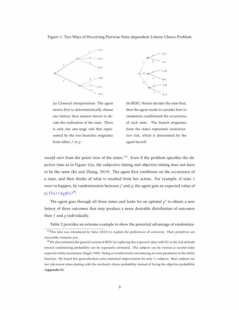
Figure 1: Two Ways of Perceiving Pairwise State-dependent Lottery Choice Problem

(a) Classical interpretation: The agent

moves first to deterministically choose

one lottery, then natures moves to de-

cide the realization of the state. There

is only one one-stage risk that repre-

sented by the tree branches originates

from either f or g .

(b) RESC: Nature decides the state first,

then the agent needs to consider how to

randomize conditioned the occurrence

of each state. The branch originates

from the states represents randomiza-

tion risk, which is determined by the

agent herself.

would start from the point view of the states 19. Even if the problem specifies the ob-

jective time as in Figure 1(a), the subjective timing and objective timing does not have

to be the same (Ke and Zhang, 2019). The agent first conditions on the occurrence of

a state, and then thinks of what is resulted from her action. For example, if state 1

were to happen, by randomization between f and g , the agent gets an expected value of

ρf f (s1) + ρgg(s1)20.

The agent goes through all three states and looks for an optimal ρ∗ to obtain a new

lottery of three outcomes that may produce a more desirable distribution of outcomes

than f and g individually.

Table 2 provides an extreme example to show the potential advantage of randomiza-

19This idea was introduced by Saito (2015) to explain the preferences of convexity. Their primitives are

Anscombe-Aumann acts.20We also estimated the general version of RESC by replacing this expected value with EU so the risk attitude

toward randomizing probability can be separately estimated. The subjects can be viewed as second-order

expected utility maximizers (Segal 1990). Doing so would involve introducing an extra parameter in the utility

function. We found this generalization extra statistical improvement for only 11 subjects. Most subjects are

not risk-averse when dealing with the stochastic choice probability instead of facing the objective probability

(Appendix D)

9

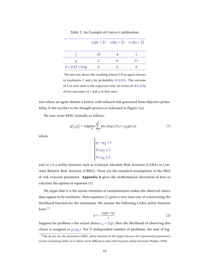
Table 2: An Example of Convex Combination

s1(p1 =13 ) s2(p2 =

13 ) s3 (p3 =

13 )

f 10 4 1

g 2 8 11

k = 0.5f +0.5g 6 6 6

The last row shows the resulting lottery k if an agent chooses

to randomize f and g by probability (0.5,0.5). The outcome

of k in each state is the expected value (in terms of (0.5,0.5))

of two outcomes of f and g in that state.

tion where an agent obtains a lottery with reduced risk generated from objective proba-

bility, if she ascribes to the thought process as indicated in Figure 1(a).

We now write RESC formally as follows:

(ρ∗f ,ρ∗g ) = argmax

ρ

3∑

1

p(si )u(ρf f (si ) + ρgg(si )), (1)

where

ρf + ρg = 1

0 ≤ ρf ≤ 1

0 ≤ ρg ≤ 1

and u(·) is a utility function such as Constant Absolute Risk Aversion (CARA) or Con-

stant Relative Risk Aversion (CRRA). These are the standard assumptions in the MLE

of risk aversion parameter. Appendix A gives the mathematical derivation of how to

calculate the optima in equation (1).

We argue that it is the innate intention of randomization makes the observed choice

data appear to be stochastic. Note equation (1) gives a very neat way of constructing the

likelihood function for the estimation. We assume the following CARA utility function

form 21

u = −exp(−rx)

r. (2)

Suppose for problem n the actual choice cn = f (g), then the likelihood of observing this

choice is assigned as ρf (ρg ). For N independent number of problems, the sum of log-

21We do not use the alternative CRRA utility function in this paper because the experimental parameters

involve evaluating utility at 0, which can be difficult to deal with in power utility functions (Wakker 2008).

10

likelihood is

L(r) =N∑

i

log((ρ∗f ,ρ∗g ) ◦ I ) (3)

where I is an identification vector, that is

I =

[1 0] if cn = f

[0 1] if cn = g,

and ◦ denotes operation for Hadmard product.

The advantage of RESC is that it deals with preferences and stochasticity simultane-

ously. RESC allows a more accurate way of predicting people’s choices in the case when

choices have to be made deterministically in a one-shot fashion, which is the nature of

many real-life choices.

2.2 Model of Deterministic Choice plus Error

Under RU model, the utility of an alternative U(f ) consists of the evaluation of an alter-

native v(f ) that is determined by a preference functional and an error part ǫ(f ):

Uω(f ) = v(f ) + ǫ(f ) (4)

The error ǫ could possibly depend on the whole menu but it is assumed to be only

dependent on f in the mainstream theoretical and empirical literature of random util-

ity or discrete choice. Because it is well-known that the menu-dependent error model

trivially explains everything. For empirical analysis, we choose the most popular and

standard RU model, Logit (Luce 1958), which assumes ǫ to be i.i.d. extreme value. The

Logit choice probability is as follows22.

ρf =ev(f )

ev(f ) + ev(g). (5)

22Note this equation implies the variance of the ǫ is π2

6 . In general one can add an extra scale parameter σ

such that the variance becomes σ2 π2

6 . Then equation (5) becomes

ρf =ev(f )/σ

ev(f )/σ + ev(g)/σ.

If v(·) takes a linear form then scale parameter does not affect the ratio of the parameters in v(·) (Chapter 3,

Train 2009).

11

The interpretation is the likelihood of choosing an alternative is proportional to its eval-

uation compared to the sum of the two evaluations and the error is decreasing with the

advantage in evaluation.

The sum log-likelihood for a dataset of N problems is

L(·) =

N∑

i

log((ρf ,1− ρf ) ◦ I ) (6)

where the arguments of L are the parameters in the preference functionals. For example,

in EU, the argument can be the risk aversion parameter in a CARA utility function.

We consider the following most relevant deterministic theories for our problem: Ex-

pected Utility (EU), Rank Dependent Expected Utility (Quiggin 1982), hereafter RDEU,

and two non-PSmodels: Salience Theory under Risk (ST) and Regret Theory (RT). For all

these theories we assume CARA. The preference functional v(·) for these deterministic

theories are defined in Appendix C.

2.3 Comparison of RESC and RU: An Illustration

In this subsection, we point out the major difference between RU models and RESC.

Consider the choice task 1 and 2 with different menus: {f ,g} and {f ,h}. There are

two states of nature, s1 and s2. f pays zero dollar in s1 and one dollar in s2. g pays zero

dollar in s1 and 1.01 dollars in s2. h pays 1.01 dollars in s1 and zero dollar in s2. The

probability of s1 and s2 are equal. The setting is summarized in the following Table 3.

The choice probability predicted by i.i.d. RU (EU+logit) and Random Expected Util-

ity (Gul and Pesendorfer 2006) is obvious. The error in an RU model only depends on

the specific alternative. Therefore the choice probability in Tasks 1 and 2 would not

change in an RUmodel. It is well known that if the error depends on the menu, then the

RU model just trivially explains everything.

In reality, many subjects would not regard Tasks 1 and 2 as the same task. RESC is

one approach to rectifies this limit of the RU model.

The prediction of RESC in Task 1 and Task 2’ is obvious. In Task 2’, the subject

chooses to equally split her choice probability not because of ”error”, but because of a

desire of balancing the expected payoff in two ”attributes”: the two states23. If we fur-

ther assume ”continuity” which is assumed in most of the mainstream stochastic choice

23This is suggested in the spirit of Machina (1989)’s mum example of normative decision under risk.

12

Table 3: Choice Probability under Different Theories

Choice Probability

RU (iid) REU RESC

s1 s2

Task 1 Lottery f 0 1 ∼40% 0% 0%

Lottery g 0 1.01 ∼60% 100% 100%

Task 2 Lottery f 0 1 ∼40% 0% ∼40%

Lottery h 1.01 0 ∼60% 100% ∼60%

Task 2’ Lottery f 0 1 50% 50% 50%

Lottery h′ 1 0 50% 50% 50%

theories, then the stochastic choice ρ is a continuous function (or correspondence). In

task 2, intuitively, where h′ is altered a little bit to become h, the choice probability

should also be only altered a little bit. Therefore, in task 2, the subject would still assign

some probability to lottery f , otherwise continuity is violated. The experimental setting

is similar to but more complicated than this example.

3 Experiment and Data

The data used in this study was obtained in a research university’s decision lab from 89

subjects drawn from both graduate and undergraduate students. There were 28 pair-

wise choice tasks over two state-dependent lotteries as in Table 1. Appendix B presents

a screenshot of the sample choice task and the list of all tasks. The subjects were told at

the beginning that the computer would randomly draw a choice task (Random-Lottery

Incentive System) and draw a state of that choice task to decide their payments after

they finish all tasks. The sequence of the tasks was randomized. Each subject’s choice of

the lotteries (lottery 1 or lottery 2) in each task was recorded. Therefore, the dataset is a

matrix of size 28 by 89 with the element of the binary number 1 or 2. Average reward is

∼ 13 dollars. Completing time was about 30 min. Four sessions were run. A subject can

only participate in one session. No data were excluded from the analysis.

All subjects signed relevant consent forms and all experimenters took relevant train-

13

ing. The experiment was approved by the ethical approval committee.

4 Estimation Strategy and Discrimination Results

This paper uses Maximum Likelihood procedures to estimate the parameters in stochas-

tic choice functions (RESC and RU) at an individual subject level24. The sum of log-

likelihood for RESC and RU models are defined in equation (3) and equation (6) respec-

tively. In terms of RUmodels, we stick with the standard logit form (5) in Luce’s original

work25.

Figure 2 shows the histogram of the estimated risk aversion parameter from RESC

and EU. In the estimation we constraint r between −0.3 and 0.3. Values outside these

bounds imply extremely risk-seeking or risk aversion and they are unidentifiable given

the experimental parameters. To set a constraint for r is standard in structural estima-

tion literature 26

24There are no analytical solutions for the optimizing of the choice problem, therefore there are no explicit

solutions to maximize the sum of log-likelihood functions either. We write the algorithms for optimization in

MatLab.25The main result remains similar when using other RUs such as more general forms of logit, probit, and

tremble.26For example, see Georgalos (2019). Some intuition of these numbers: under r = −0.3, the Certainty Equiv-

alent of the lottery (22,0.5;0,0.5) is 21; under r = 0.3 it is 2. A detailed description of the intuition of the

boundaries of risk aversion parameters and the unidentifiability beyond the bound can be found in Holt and

Laury (2002). The main result remains robust when the boundary is shifted.

14

Figure 2: Estimated Risk Aversion Parameter r

y axis is the number of subjects. x axis is the ML estimated risk aversion parameter

r as in equation (2). ”0.3+” means 0.3 or higher. ”-0.3-” means -0.3 or lower. A

higher r indicates higher risk aversion. Values less (more) than −0.3 (0.3) suggest

extreme risk seeking (aversion) and are unidentifiable in the dataset. Consistent

with previous experimental studies, the majority of the subjects are risk averse. On

average, r is higher in RESC than in EU + Logit.

We can see under RESC risk aversion is higher than EU. This is probably due to the

choice of a riskier lottery is considered to be hedging in RESC but is considered to be an

error in EU.

RESC does not nest any of the RU models; therefore it is standard to use the Clarke

test (2003) to compare the goodness of fit of two non-nested competing likelihood func-

tions (Imai and Tingley 2012). Vuong (1989) is the other canonical test to compare

non-nested models. However, Clarke (2003, 2007) demonstrate the former test is more

suitable with small sample size and likelihood ratios exhibiting sharp peaks than a nor-

mal distribution, which is our case as shown in Figure 3.

In recent literature, Clarke test is generally considered appropriate and sufficient

to discriminate stochastic choice rules, especially under risk and uncertainty (Among

many others, see Hey and Panaccione 2011; Panagiotelis and Czado and Joe 2012; Hey

15

and Pace 2014; Wilcox 2015); no more robustness check is usually performed.

Figure 3: Histogram of the Log of the Likelihood Ratios

x axis the individual likelihood ratio of EU+logit to RESC under each

problem. It is calculated based on the estimated parameter from MLE.

y axis is the number of problems. All subjects’ data in all problems

were pooled to get this histogram. The red line was the fitted normal

distribution curve. It is clear the distribution has a higher peak than the

normal distribution.

In the Clarke test, the null hypothesis is that the two competing models are equally

good, hence on a particular problem the probability of the log-likelihood for one model

being larger than the probability of the other model is 12 .

Let L1 and L2 denote the individual log-likelihoods of the 28 problems, which are

calculated using the estimated parameters. When the twomodels have the same number

of parameter, the test statistic is

T =

28∑

1

I(L2 −L1)

where

I(L2 −L1) =

1 if L2 > L1

0 if L2 ≤ L1

Under the null hypothesis T has a binomial distribution with parameters n = 28

16

and p = 0.5. Thus an observation greater than 19 rejects the null hypothesis at the 5%

significance level.

Figure 4: Clarke Test Between EU and RESC

On the left panel, x axis is the number of problems that EU+logit has a higher

likelihood than RESC for each subject. If the number was more than 19, then

we rejected the null that the two models perform the same at 5% and concluded

that EU+Logit was better for this subject. There was only 2 out of 89 subjects

that EU+logit was significantly better. The right panel reversed the comparison

by counting the numbers that RESC has a higher likelihood than the EU. It shows

27/89 subjects’ data fitted better in RESC.

Both RSEC and EU have one parameter to estimate, therefore individual likelihoods

can be directly compared. In general, the individual likelihood of models with more

parameters is penalized by log(N )/N , where N is the number of the extra parameters.

Therefore, when we compare RESC with ST, the individual likelihoods of ST is sub-

tracted by log(28)/28 since ST has one more parameter. The results of all comparisons

between models using the Clarke test are summarized in the following Table 4. It shows

the advantage of RESC, compared to both PS theories (EU and RDEU) and non-PS theo-

ries (ST and RT).

17

Table 4: Clarke Test Results

(a) RESC vs EU+error

EU better RESC better neither better

2% 30% 68%

(b) RESC vs RDEU+error

RDEU better RESC better neither better

0% 89% 11%

(c) RESC vs ST+error

ST better RESC better neither better

0 55% 45%

(d) RESC vs RT+error

RT better RESC better neither better

0% 57% 43%

5 Replication

As a robustness check, we replicate the analysis using another set of data first analyzed

in Agranov and Ortoleva (2017). This experiment consisted of four parts of different

settings. We use the data from the part that the experimental task wasmaking a pairwise

state-dependent lottery choice. The randomization device was the same. There were

four possible states for the lottery and subjects were told the realization of the state

would be determined by a computerized four-sided dice. There were 7 choice problems

and each problem was repeated three times in a row, which the subjects were informed.

The figure in Appendix B shows the 7 problems. Random lottery incentive system was

also adopted. The subjects were 80 university students. Therefore the dataset is a matrix

of row 21 by 80 with binary number 1 or 2.

The original analysis follows a simple descriptive fashion: if a subject did not switch

preference in all repetitions, then it is concluded that the individual makes deterministic

choice. If the subject did switch, then it is concluded that the individual makes stochas-

tic choice. However, since deterministic choice is a special case of stochastic choice, even

if the subject makes deterministic choice in all three repetitions, we cannot make sure

that the subject will always choose deterministically if the task is changed or more repe-

tition is administrated. This paper discriminates the deterministic plus error model and

SCGDP using sophisticated discrimination tests.

We fit the data into the same RESC and EU+logit as defined in Section 2. For both, the

same CARA utility function, as in equation (2), is adopted. The same standard Clarke

test was adopted: since there are 21 problems, a model giving more than 14 higher

likelihood fits better than the other at a significance of 5% level. Figure 5 indicates that

18

RESC strikingly outperforms EU+logit. The null hypotheses that RESC is not superior

than EU+logit are rejected for all subjects. The null hypotheses that EU+logit is not

better than RESC cannot be rejected for any of the subjects. This is consistent with the

message from the original paper - a large majority of subjects exhibit ”stochastic choice”

and this choice inconsistency in repetitions is difficult to be explained by deterministic

preference theories and RUs.

Many have been questioning the original 2017 experimental results. For example,

some of them believe the subjects are ”framed” to randomize, because of the repetitive

setting of the experiment.

However, it is worth noting that, even if the subject does not seem to ”choose stochas-

tically” in the repetitions27, her preference is sometimes still incompatible with deter-

ministic EU or EU+error. The reasoning is as follows. A subject’s choice over two dif-

ferent lotteries gives us information about her risk attitudes under EU (curvature of a

utility function). If we fix a particular form of the utility function, then we can use that

choice to calculate a one-sided range of risk parameter in the utility function28. For ex-

ample, suppose a subject consistently chooses one lottery in one set of the three, which

implies risk-averse. Meanwhile, the same subject’s consistent choices in another set can

indicate risk-seeking. One can always trivially argue this is due to ”error”, but it is dif-

ficult to imagine a subject would make the same ”error” three times in a row. We have

identified 25 subjects who ”did not make stochastic choices” based on simple descrip-

tive statistics; however, among them, there are 10 subjects are of the type of that cannot

be explained by EU well while RESC predicts their choice much more nicely. The other

subjects might be explained by EU, but RESC still fits significantly better.

27i.e. they always choose the same object in repetition. This is determined by using simple descriptive

statistics.28For example, consider the choice task of Hard3 as the figure in Appendix B. If a subject had chosen the

lottery in the second row, then we know her risk aversion r > 0.0042 as in the CARA utility function (2).

19

Figure 5: Clarke Test Between EU+error and RESC

The x-axis is the total number that one model has a higher likelihood than the

other among one subject’s all 21 problems. By Clarke test of non-nested models, a

number of more than 14 indicates the former model fits better at 5% confidence in-

terval. There were 80 subjects in total. RESC fits significantly better than EU+error

for all subjects. EU+error fits significantly better than EU+error for no subjects.

6 Discussion

The results seem surprising are not surprising because it is known that explaining ran-

domness in data with randomness of preference still does not explain the source of ran-

domness (Machina 1985). Estimating utility function from binary choice data can often

be not very successful due to the randomness. When the utility function suggests the

subject prefers one alternative to the other, it might make sense to attribute the small

discrepancy in choice probability to errors. However, suppose one subject consistently

chooses an alternative for 55% of the time, can we claim that she strictly prefers one

alternative to the other? When the deterministic utility function suggests she should be

choosing it for sure, can we claim this choice probability of 55% instead of 100% is due

to error? How could we refute the hypothesis that she chooses the randomizing proba-

bility by an instinctive optimization process? Of course, future theoretical investigation

20

and empirical evidence is needed to thoroughly understand the rationale behind.

Similar evidence can be found in the psychology and evolutionary dynamics lit-

erature. For example, the well-documented phenomena of ”probability weighting” is

widely observed in human and animals.

s1(p1 =13 ) s2(p2 =

13 ) s3 (p3 =

13 )

f 10 4 1

g 2 8 11

k = 0.5f +0.5g 6 6 6

The last row shows the resulting lottery k if an agent chooses

to randomize f and g by probability (0.5,0.5). The outcome

of k in each state is the expected value (in terms of (0.5,0.5))

of two outcomes of f and g in that state.

Expected utility maximizer will always not to perform probability weighting.

The theory can be applied in building more efficient machine intelligence (AI). There

are two primary goals of building AI: first, build AI that makes better decisions; second,

build the AI that makes decisions just like a human. All decisions in real world are to

some extend risky. For an abstract example (1.1,0) and (0,1), with the probability P(s1) =

s2 There are three way of designing AI: 1) Each AI program optimize a deterministic

expected utility. 2) Each AI optimize a deterministic expected utility plus some error. 3)

More recently, Zhang et al (2014 PNAS) have proposed a binary-choice model that

provides an evolutionary framework for generating a variety of behaviors that are con-

sidered anomalous from the perspective of traditional economic models (i.e., loss aver-

sion, probability matching, and bounded rationality). In this framework, natural selec-

tion yields standard risk-neutral optimizing economic behavior when reproductive risk

is idiosyncratic (i.e., uncorrelated across individuals within a given generation). How-

ever, when reproductive risk is systematic (i.e., correlated among individuals within a

given generation), some seemingly irrational behaviors, such as probability matching

and loss aversion, become evolutionarily dominant.

2019 ( PNAS)

The example of AI is more suitable for a ”Rational” Stochastic Choice rather than a

RU-based stochastic choice because unlike human, AI does not necessarily need to have

variating taste or ”make errors”.

21

In sum, the EU maximizer appears to be a RESC decision maker in a single choice

if one of the following conditions hold: 1) the agents are sufficiently altruistic: they

maximize the EU of the whole group; 2) the agent is an individual EU maximizer and is

expected to make the same or similar decisions for multiple time in its whole lifespan.

Future Perspectives

Future improvements include replicating with health discrete choice data, applying the

same technique into multi-attribute binary choices, applying the model into decision

under ambiguity, further theoretically axiomatization of this model, and comparing this

model with other nascent stochastic choice models such as REU. Additionally, this pa-

per primarily focuses on lotteries with determined correlations. To apply the model to

simple lotteries with non-deterministic but ambiguous correlation, one might adopt the

thoughts in Epstein and Halevy (2019): the subjects might have a subjective belief of the

unknown correlation.

7 Concluding Remarks

This paper introduces a distribution-free approach tomodeling discrete choice andmea-

suring risk. Without assuming any error distribution, the functional form of RESC is

even simpler thanmany of the conventional tractable models such as the EU+error mod-

els. Many commonly used features and methods in the EU, such as estimating the risk-

averse parameter with CRRA or CARA utility function, are applicable in the same way

in RESC. In this case, RESC’s statistical superiority might because the subjects strategi-

cally choose a probability mass function to optimize their expectation, rather than the

randomization due to an ”error”. The second reason for statistical superiority might

be directly fitting the stochastic choice with one parameter. This was done in spirit of

Alpha Go Zero’ improvement, in which the policy function and value function are com-

bined to one, contrary to the separately estimated functions in Alpha Go (Silver et al.

2017 Nature). In classic RU, people often fit the deterministic component with many

parameters, when fitting the stochastic component - error distribution - with zero or

one parameter. As discussed in the introduction, in an RU model, the error distribu-

tion could be more important than the deterministic component. Therefore, the classic

application of RU models might involve an over-fitting and over-modeling of the deter-

ministic component, while under-fitting and under-modeling the stochastic component.

22

In contrast, RESC models both components with one variable, reaching a natural bal-

ance. RESC ranks the stochastic choice functions but does not rank the primitives –

everything has its place; no one is superior to the others.

Appendix - Literature Relations on Stochastic Choice Gen-

erated by Deterministic Preferences

The strain of literature initiated by Machina (1985) does provide richer information

about the origin of choice stochasticity. The most influential examples are Fudenberg

et al’s (2015) Additive Perturbed Utility (APU), Ortoleva et al’s (2017, 2019) ”delib-

erate stochastic” (DS) and cautious stochastic choice (CSC), and Dwenger, Kubler and

Weizsacker (2018)’s regret minimization. The first one generates stochastic choice be-

cause of a cost function, which could be meaningfully interpreted as the cost of learning

or the cost of attention. The second one introduces a max-min structure, which can be

interpreted as being cautious or pessimistic. The third one suggests that deterministic

choice generates more aftermath regret. RESC generates stochastic choice by balancing

the expected payoff between different states.

The intersect between SCGDP and RU model is not an empty-set. APU is neither a

special case nor a generalization RU model, though both logit and probit, due to their

stringent functional form, are special cases of both RU and APU. There are several differ-

ent characteristics of SCGDP and RU. As the first effort to axiomatize stochastic choice

function with acyclicity, APU assumes an elegant and estimable functional form. APU

inherited both the advantages of SCGDP - generated by deterministic preference - and

the advantages of RU - the separation of the deterministic component and the stochastic

component. An important generalization of APU into multi-attribute alternatives can

be found in Allen and Rehbeck (2019ab). RESC cannot be expressed as APU or RU be-

cause it can violate regularity. Additionally, APU and RU usually consider the discrete

set as the menu, while RESC considers the acts or state-dependent lottery as primitive.

Both APU and RESC can violate stochastic transitivity. Both models cannot be repre-

sented with a utility plus error. Both models have well-defined parameters ready to

be estimated. RESC is similar to DS and CSC, in the sense that both relax regularity

and both may be considered the relaxing of consequentialism. RESC is different from

RU and CSC as RESC is a simple maximization of expectation, considers the space of

acts, relaxes probability sophistication, and most importantly, relaxes the reduction of

23

compound lottery to allow the discrimination of the objective probability and stochastic

choice probability.

There are several other lines of literature try to rationalize the stochastic component

in choices. Motivated by neurophysiological evidence, one possible source of stochastic

choice is considered to be the noise in signal and signal-processing (Woodford 2014);

in this line of research the preference is not necessarily fluctuating but the cognitive

processes can. Bounded rationality is sufficient to generate the stochastic choice in a de-

terministic setting, even if the indifference curves in the Marschak-Machina triangle are

linear (Stoye 2015). Another approach is based on the bounded rationality of decision-

maker who optimally acquires costly information (among others, see Sims 2003; Caplin,

Dean, and Leahy 2019). The rational inattention models maximize a generalized expec-

tation minus attention cost. It explains better than random utility models in decision

with time variation (Webb 2019) and decisions with information acquisition. The earli-

est dynamic stochastic choice model generated by optimizing long-term rewards might

be credited to Thompson (1933); it is plausible that stochastic choice is a result of sam-

pling and learning (Natenzon 2017). Our experimental set-ups control the uncertainty-

learning factor of randomizing choices, because only the single-period choice under risk

is considered: there is no ambiguity involved.

24

References

Abdellaoui, Mohammed et al. (2011). “The rich domain of uncertainty: Source func-

tions and their experimental implementation”. In: American Economic Review 101.2,

pp. 695–723.

Agranov, Marina and Pietro Ortoleva (2017). “Stochastic choice and preferences for ran-

domization”. In: Journal of Political Economy 125.1, pp. 40–68.

Allen, Roy and John Rehbeck (2019a). “Identification with additively separable hetero-

geneity”. In: Econometrica 87.3, pp. 1021–1054.

— (2019b). “Revealed Stochastic Choice with Attributes”. In:Available at SSRN 2818041.

Ballinger, T Parker and Nathaniel TWilcox (1997). “Decisions, error and heterogeneity”.

In: The Economic Journal 107.443, pp. 1090–1105.

Bekker-Grob, Esther W de, Mandy Ryan, and Karen Gerard (2012). “Discrete choice

experiments in health economics: a review of the literature”. In: Health economics

21.2, pp. 145–172.

Bell, David E (1982). “Regret in decision making under uncertainty”. In: Operations re-

search 30.5, pp. 961–981.

— (1983). “Risk premiums for decision regret”. In:Management Science 29.10, pp. 1156–

1166.

— (1985). “Reply—Putting a premium on regret”. In:Management Science 31.1, pp. 117–

122.

Bell, David E and Howard Raiffa (1980). “Decision regret: A component of risk aver-

sion”. In: WP HBS, pp. 80–56.

Block, HD, Jacob Marschak, et al. (1957). Random orderings. Tech. rep. Cowles Founda-

tion for Research in Economics, Yale University.

Bohnet, Iris et al. (2008). “Betrayal aversion: Evidence from brazil, china, oman, switzer-

land, turkey, and the united states”. In: American Economic Review 98.1, pp. 294–310.

Bordalo, Pedro, Nicola Gennaioli, and Andrei Shleifer (2012). “Salience theory of choice

under risk”. In: The Quarterly journal of economics 127.3, pp. 1243–1285.

Caplin, Andrew, Mark Dean, and John Leahy (2018). “Rational inattention, optimal

consideration sets, and stochastic choice”. In: The Review of Economic Studies 86.3,

pp. 1061–1094.

Cerreia-Vioglio, Simone et al. (2019). “Deliberately stochastic”. In: American Economic

Review 109.7, pp. 2425–45.

25

Charness, Gary, Uri Gneezy, and Alex Imas (2013). “Experimental methods: Eliciting

risk preferences”. In: Journal of Economic Behavior & Organization 87, pp. 43–51.

Chen, Yan and Tayfun Sonmez (2006). “School choice: an experimental study”. In: Jour-

nal of Economic theory 127.1, pp. 202–231.

Chew, Soo Hong, Larry G Epstein, Uzi Segal, et al. (1991). “Mixture symmetry and

quadratic utility”. In: Econometrica 59.1, pp. 139–63.

Chiong, Khai Xiang andMatthew Shum (2018). “Randomprojection estimation of discrete-

choice models with large choice sets”. In: Management Science 65.1, pp. 256–271.

Chipman, John S (1963). “Stochastic choice and subjective probability”. In: Decisions,

values and groups 1, pp. 70–95.

Clarke, Kevin A (2003). “Nonparametric model discrimination in international rela-

tions”. In: Journal of Conflict Resolution 47.1, pp. 72–93.

— (2007). “A simple distribution-free test for nonnested model selection”. In: Political

Analysis 15.3, pp. 347–363.

Conte, Anna, John D Hey, and Peter G Moffatt (2011). “Mixture models of choice under

risk”. In: Journal of Econometrics 162.1, pp. 79–88.

Cosslett, Stephen R (1983). “Distribution-free maximum likelihood estimator of the bi-

nary choice model”. In: Econometrica: Journal of the Econometric Society, pp. 765–782.

Davidson, Donald, John Charles ChenowethMcKinsey, and Patrick Suppes (1955). “Out-

lines of a formal theory of value, I”. In: Philosophy of science 22.2, pp. 140–160.

Debreu, Gerard (1958). “Stochastic choice and cardinal utility”. In: Econometrica: Journal

of the Econometric Society, pp. 440–444.

— (1959). Topological methods in cardinal utility theory. Tech. rep. Cowles Foundation for

Research in Economics, Yale University.

Dimmock, Stephen G, Roy Kouwenberg, and Peter P Wakker (2015). “Ambiguity atti-

tudes in a large representative sample”. In:Management Science 62.5, pp. 1363–1380.

Dwenger, Nadja, Dorothea Kubler, and Georg Weizsacker (2018). “Flipping a coin: Ev-

idence from university applications”. In: Journal of Public Economics 167, pp. 240–

250.

Epstein, Larry G and Yoram Halevy (2019). “Ambiguous correlation”. In: The Review of

Economic Studies 86.2, pp. 668–693.

Fernando Branco Monic Sun, J. Miguel Villas-Boas (2012). “Optimal Search for Product

Information”. In: Management Science 58.11, pp. 2037–2056.

Fisher, Ronald A (1912). “On an absolute criterion for fitting frequency curves”. In:Mes-

senger of Mathmatics.

26

Fisher, Ronald Aylmer (1925). “Theory of statistical estimation”. In: Mathematical Pro-

ceedings of the Cambridge Philosophical Society. Vol. 22. 5. Cambridge University Press,

pp. 700–725.

Fudenberg, Drew, Ryota Iijima, and Tomasz Strzalecki (2015). “Stochastic choice and

revealed perturbed utility”. In: Econometrica 83.6, pp. 2371–2409.

Georgalos, Konstantinos, Ivan Paya, and David A Peel (2018). “On the contribution of

the Markowitz model of utility to explain risky choice in experimental research”. In:

Journal of Economic Behavior & Organization.

Georgescu-Roegen, Nicholas (1958). “Threshold in Choice and the Theory of Demand”.

In: Econometrica: Journal of the Econometric Society, pp. 157–168.

Gul, Faruk and Wolfgang Pesendorfer (2006). “Random expected utility”. In: Economet-

rica 74.1, pp. 121–146.

Harless, David W and Colin F Camerer (1994). “The predictive utility of generalized ex-

pected utility theories”. In: Econometrica: Journal of the Econometric Society, pp. 1251–

1289.

Harper, F Maxwell et al. (2005). “An economic model of user rating in an online rec-

ommender system”. In: International Conference on User Modeling. Springer, pp. 307–

316.

Hart, Oliver D (1975). “Some negative results on the existence of comparative statics

results in portfolio theory”. In: The Review of Economic Studies 42.4, pp. 615–621.

Hey, John D (2001). “Does repetition improve consistency?” In: Experimental economics

4.1, pp. 5–54.

Hey, John D and Enrica Carbone (1995). “Stochastic choice with deterministic prefer-

ences: An experimental investigation”. In: Economics Letters 47.2, pp. 161–167.

Hey, John D and Chris Orme (1994). “Investigating generalizations of expected utility

theory using experimental data”. In: Econometrica: Journal of the Econometric Society,

pp. 1291–1326.

Hey, John D and Noemi Pace (2014). “The explanatory and predictive power of non two-

stage-probability theories of decision making under ambiguity”. In: Journal of Risk

and Uncertainty 49.1, pp. 1–29.

Hey, John D and Luca Panaccione (2011). “Dynamic decision making: what do people

do?” In: Journal of Risk and Uncertainty 42.2, pp. 85–123.

Holt, Charles A and Susan K Laury (2002). “Risk aversion and incentive effects”. In:

American economic review 92.5, pp. 1644–1655.

27

Imai, Kosuke and Dustin Tingley (2012). “A statistical method for empirical testing of

competing theories”. In: American Journal of Political Science 56.1, pp. 218–236.

Ke, Shaowei and Qi Zhang (2019). Randomization and ambiguity aversion. Tech. rep. con-

ditionally accepted at Econometrica.

Ke, T Tony, Zuo-Jun Max Shen, and J Miguel Villas-Boas (2016). “Search for information

on multiple products”. In: Management Science 62.12, pp. 3576–3603.

Lee, Frederic S and Sandra Harley (1998). “Peer review, the research assessment exercise

and the demise of non-mainstream economics”. In: Capital & Class 22.3, pp. 23–51.

List, John A (2002). “Preference reversals of a different kind: The” More is less” Phe-

nomenon”. In: American Economic Review 92.5, pp. 1636–1643.

Liu, Meijun et al. (2018). “Survive or perish: Investigating the life cycle of academic jour-

nals from 1950 to 2013 using survival analysis methods”. In: Journal of Informetrics

12.1, pp. 344–364.

Loomes, Graham and Robert Sugden (1982). “Regret theory: An alternative theory of

rational choice under uncertainty”. In: The economic journal 92.368, pp. 805–824.

Luce, R Duncan (1958). “A probabilistic theory of utility”. In: Econometrica: Journal of

the Econometric Society, pp. 193–224.

Machina, Mark J (1985). “Stochastic choice functions generated from deterministic pref-

erences over lotteries”. In: The economic journal 95.379, pp. 575–594.

— (1989). “Dynamic consistency and non-expected utility models of choice under un-

certainty”. In: Journal of Economic Literature 27.4, pp. 1622–1668.

Manski, Charles F (1975). “Maximum score estimation of the stochastic utility model of

choice”. In: Journal of econometrics 3.3, pp. 205–228.

Marschak, Jacob (1959). Binary choice constraints and random utility indicators. Tech. rep.

Cowles Foundation for Research in Economics, Yale University.

Marschak, Jacob and Donald Davidson (1957). Experimental Tests of Stochastic Decision

Theory. Cowles Foundation Discussion Papers 22. Cowles Foundation for Research

in Economics, Yale University. url: https://EconPapers.repec.org/RePEc:cwl:

cwldpp:22.

Marschak, Jacob, Donald Davidson, et al. (1957). Experimental tests of stochastic deci-

sion theory. Tech. rep. Discussion Papers 22, Cowles Foundation for Research in Eco-

nomics, Yale University.

Mas-Colell, Andreu, Michael Dennis Whinston, Jerry R Green, et al. (1995). Microeco-

nomic theory. Vol. 1. Oxford university press New York.

28

Moffatt, Peter G and Simon A Peters (2001). “Testing for the presence of a tremble in

economic experiments”. In: Experimental Economics 4.3, pp. 221–228.

Natenzon, Paulo (2019). “Random choice and learning”. In: Journal of Political Economy

127.1, pp. 419–457.

Panagiotelis, Anastasios, Claudia Czado, and Harry Joe (2012). “Pair copula construc-

tions for multivariate discrete data”. In: Journal of the American Statistical Association

107.499, pp. 1063–1072.

Roth, Alvin E (1995). “Introduction to experimental economics”. In: The handbook of

experimental economics 1, pp. 3–109.

Segal, Uzi (1990). “Two-stage lotteries without the reduction axiom”. In: Econometrica:

Journal of the Econometric Society, pp. 349–377.

Sims, Christopher A (2003). “Implications of rational inattention”. In: Journal of mone-

tary Economics 50.3, pp. 665–690.

Sopher, Barry and J Mattison Narramore (2000). “Stochastic choice and consistency in

decision making under risk: An experimental study”. In: Theory and Decision 48.4,

pp. 323–350.

Starmer, Chris and Robert Sugden (1989). “Probability and juxtaposition effects: An ex-

perimental investigation of the common ratio effect”. In: Journal of Risk and Uncer-

tainty 2.2, pp. 159–178.

Strzalecki, Tomasz (2019). Lecture Notes on Stochastic Choice. url: https://scholar.

harvard.edu/files/tomasz/files/scslides34.pdf.

Thompson, William R (1933). “On the likelihood that one unknown probability exceeds

another in view of the evidence of two samples”. In: Biometrika 25.3/4, pp. 285–294.

Thurstone, Louis Leon (1927). “A law of comparative judgement”. In: Psychological Re-

view 34.July, pp. 273–286.

Train, Kenneth E (2009). Discrete choice methods with simulation. Cambridge university

press.

Tversky, Amos (1969). “Intransitivity of preferences.” In: Psychological review 76.1, p. 31.

Tversky, Amos and Daniel Kahneman (1989). “Rational choice and the framing of de-

cisions”. In: Multiple criteria decision making and risk analysis using microcomputers.

Springer, pp. 81–126.

Valavanis-Vail, S (1957). “A Stochastic Model for Utilities”. In: seminar on the application

of mathematics to social sciences, University of Michigan.

Von Neumann, J and O Morgenstern (1944). Theory of games and economic behavior.

Princeton University Press.

29

Vuong, Quang H (1989). “Likelihood ratio tests for model selection and non-nested hy-

potheses”. In: Econometrica: Journal of the Econometric Society, pp. 307–333.

Wakker, Peter P (2008). “Explaining the characteristics of the power (CRRA) utility fam-

ily”. In: Health economics 17.12, pp. 1329–1344.

Webb, Ryan (2018). “The (neural) dynamics of stochastic choice”. In: Management Sci-

ence 65.1, pp. 230–255.

Wilcox, Nathaniel T (2015). Error and generalization in discrete choice under risk. Tech.

rep.

Woodford, Michael (2014). “Stochastic choice: An optimizing neuroeconomic model”.

In: American Economic Review 104.5, pp. 495–500.

30

AppendixA - Rational Expectation Stochastic Choice (RESC)

Optima

A problem is a choice from a menu of two state-dependent lotteries {f ,g}. The prizes

(monetary payoffs) of the lottery depend on three states of the world s ∈ S{s1, s2, s3} even-

tuates. We assume that p(s1) = p(s2) = p(s3) =13 . Table 5 illus the problem.

Table 5: Menu 1

s1(p1 =13 ) s2(p2 =

13 ) s3 (p3 =

13 )

f f1 f2 f3

g g1 g2 g3

The RESC theory postulates the subject randomizes her choice over f and g . The

objective of choice is the probability of choosing f , denoted by ρ ( the probability of

choosing g then is 1ρ.) If state i occurred, the expected (expectation over the random-

ization between f and g) payoff in state i then is

xi =i +(1− ρ)gi = ρ(fi − gi ) + gi

RESC theory further postulates the subject wants tomaximize the following expected

utility :

U(ρ) = u(x1) +u(x2+u(x3)

where

xi = ρfi + (1− ρ)gi , , i = 1,2,3.

The first order condition is

U ′(ρ) = u′(x1)(f1 − g1) +u′(x2)(f2 − g2) +u′(x3)(f3 − g3) (7)

CARA utility function

Suppose u(x) takes the following CARA utility function, that is

u(x) = −e−rx

r.

31

Note that u′(x) = e−rx. The first order condition (7)becomes

e−x1(f1 − g1) + e−x2(f2 − g2) + e−x3(f3 − g3) = 0.

which has the following explicit form

e−(ρf1+(1−ρ)g1)(f1 − g1) + e−(ρf2+(1−ρ)g2)(f2 − g2) + e−(ρf3+(1−ρ)g3)(f3 − g3).

There is no explicit solution for the equation above. Figure 6 gives the plot of U(ρ) and

its first derivative U ′(ρ) = ∂U∂ρ

against ρ. It shows U(ρ) is nicely concave and U ′(ρ) is

monotone with one unique root. The parameters used for the plot are f1 = 15, f2 = 0, f3 =

3, g1 = 0, g2 = 6, g3 = 10, r = 0.3.

Figure 6: RESC Objective Function and its First Derivative

CRRA utility function

Suppose that u(x) takes the following CRRA utility function form

u(x) =

x(1−r)1−r r , 1

log(x) r = 1

Noting u′(x) = x−r , then first order condition (7) becomes

x−r1 (f1 − g1) + x−r2 (f2 − g2) + x−r3 (f3 − g3) = 0,

32

which also does not have an explicit solution and will need to be solved numerically.

33

Appendix B - Experiment

Figure 7: Screenshot of the Experiment Interface

Figure 8: The 28 Experiment Tasks

34

Figure 9: The Seven Problems in Agranov and Ortoleva (2017

In the experiment, the two lotteries were not presented in this tabular format. However

the implementation of the experiment implicitly set the outcomes of lotteries to be

state-dependent. Interested readers can find the procedural details of the experiment

in the paper and its online supplemental material.

35

Appendix C- Deterministic Choice Rules

Expected Utility(EU)

Under EU, an individual behaves as if compares the two expected utilities EU(f ) =∑3

1 pif (si ) and EU(g) =∑3

1 pif (si ) and choose the act that has a higher expected util-

ity.

Rank Dependent Expected Utility (RDEU)

RDEU differs from EU only in that an individual does not use the given objective proba-

bilities to calculate the expected utility. Instead, probabilities are distorted according to

the rank of the three payoffs. Let f1 ≤ f2 ≤ f3 such the three payoffs that is ranked in an

ascending order and denote the corresponding states s′1, s′2, s′3. Then the RESC of act f is

calculated as

u(f1)(1−w(p(s′2 ∩ s

′3)) +u(f2)(w(p(s

′2 ∩ s

′3)−w(p(s

′3)) +u(f3)w(p(s3)) (8)

where w(.) is a probability weighting function weakly increasing in [0,1] and w(0) =

0,w(1) = 1. Note that if w(.) is linear RDEU reduces to EU. A convex w(.) leads to over-

weight of bad outcomes and therefore represents a pessimistic attitude. Similarly a con-

cave w(.) represents an optimistic attitude.

In our problem there are three states and the probabilities are kept as the same across

all problems. Therefore, for each subject we only need to estimate two distorted proba-

bilities, which are assumed to be used for all problems. We write the evaluation of the

two alternatives as follows.

RDEU(f ) = p1u(f1) + p2u(f2) + (1− p1 − p2)u(f3)

RDEU(g) = p1u(g1) + p2u(g2) + (1− p1 − p2)u(g3)

where we have either p1 ≤ p2 ≤ 1 − p1 − p2 or p1 ≥ p2 ≥ 1 − p1 − p2. In the special case

when p1 = p2 =13 , RDEU reduces to EU.

36

Salience Theory under Risk (ST)

ST postulates that probability distortion is state-dependent. In RDEU, the evaluation

of a lottery would not depend on how the state-contingent payoffs of one alternative

correlate with of the other lottery. But in ST, how probabilities are distorted exactly

by contrasting the the two payoffs of the two lotteries in each state. It postulates that

individuals over weights the probability of the the most salient states. The salience of

state i is defined as

σi =

|f (si )−g(si )||f (si )|+|g(si )|

if |f (si )|+ |g(si )| , 0

0 if |f (si )|+ |g(si )| = 0.

Without loss of generality, let σ(s1) > σ(s2) > σ(s3). Then the probabilities are distorted

as followsp2p1

= δp2p1

,p3p2

= δp3p2

, p1 + p2 + p2 = 1

where 0 < δ ≤ 1. When δ = 1, ST reduces to EU. Sine we use equal probabilities for all

problems, there is

p1 =1

1+δ+δ2

p2 =δ

1+δ+δ2

p3 =δ2

1+δ+δ2

(9)

.

Therefore, the Salience adjusted Expected Utility is calculated as follows.

ST (f ) = 11+δ+δ2

u(f1) +δ

1+δ+δ2u(f2) +

δ2

1+δ+δ2u(f3) (10)

ST (g) = 11+δ+δ2

u(g1) +δ

1+δ+δ2u(f2)u(g2) +

δ2

1+δ+δ2u(g3). (11)

Regret Theory (RT)

RT postulates that when an individual evaluates an alternative, she would take into

account what she can obtain if she had chosen otherwise. Different functions forms had

been given by Fishburn (1982), Bell (1982) and Loomes and Sugden (1982), which is the

one this paper adopt.

37

Denote a preference relation as �. We use the tractable Loomes and Sugden (1982),

RT preference is written in the following way.

f � g⇔3

∑

i

piQ(u(fsi )−u(gsi )) ≥ 0. (12)

whereQ(.) is a strictly increasing, skew-symmetric and convex function. Here we further

assume it has the function form that Q(x) = xα . When α = 1 RT reduces to EU. α > 1

repRESCnts regret aversion.

Based on equation (12), we can write the evaluation of the two acts as follows

RTEU(f ) =∑3

i IipiQ(u(fsi )−u(gsi )) (13)

RTEU(g) =∑3

i IipiQ(u(fsi )−u(gsi )) (14)

where

Ii =

1, if fsi ≥ gsi

0, if fsi < gsi

.

38

Appendix D - Empirical Performance of a General Version

of RESC

We also estimated the following general version of RESC by replacing this expected

value with expected utility. Therefore we assume an agent choose a stochastic choice

function that maximizes the following objective function

U(ρ) = u(x1) +u(x2) +u(x3)

where

xi = ρv(fi ) + (1− ρ)v(gi ), , i = 1,2,3 (15)

where v(x) = −exp(−rx)

r , which is a CARA utility function. The risk attitude toward ran-

domizing probability can be separately estimated as the r parameter in v(·). The subjects

can be viewed as second-order expected utility maximizer (Segal 1990). Doing so would

involve introducing an extra parameter. By LRT, the generalization of RESC generates

extra statistical improvement for only 11 subjects comparing to the the RESC studied in

section 4 and 5. Additionally, most subjects are not risk averse when dealing with the

stochastic choice probability (Fig 10).

39

Figure 10: Estimated Randomization Risk Aversion

We fit each subject’s data into the general version of RSEC to obtain the Maximum

Likelihood estimates for r in equation 15t). It represents an subject’s aversion to

randomization risk. Most of the values are closes to 0. This indicates the majority

of subjects are neutral to this type of risk.

Appendix E- Stochastic ChoiceGenerated byDeterministic

Preferences

The strain of literature initiated by Machina (1985) does provide richer information

about the origin of choice stochasticity. The two most influential examples are Fuden-

berg et al’s (2015) Additive Perturbed Utility (APU) and Ortoleva et al’s (2017, 2019)

”deliberate stochastic” (DS) and cautious stochastic choice (CSC). The former generates

stochastic choice because of a cost function, which could be meaningfully interpreted as

the cost of learning or the cost of attention. The latter introduces a max-min structure,

which can be interpreted as being cautious or pessimistic. RESC generates stochastic

choice by balancing the expected payoff between different states.

The intersect between SCGDP and RU model is not an empty-set. APU is neither a

special case nor a generalization RU model, though both logit and probit, due to their

stringent functional form, are special cases of both RU and APU. There are several differ-

40

ent characteristics of SCGDP and RU. As the first effort to axiomatize stochastic choice

function with acyclicity, APU assumes an elegant and estimable functional form. APU

inherited both the advantages of SCGDP - generated by deterministic preference - and

the advantages of RU - the separation of the deterministic component and the stochastic

component. An important generalization of APU into multi-attribute alternatives can

be found in Allen and Rehbeck (2019ab). RESC cannot be expressed as APU or RU be-

cause it can violate regularity. Additionally, APU and RU usually consider the discrete

set as the menu, while RESC considers the acts or state-dependent lottery as primitive.

Both APU and RESC can violate stochastic transitivity. Both models cannot be repre-

sented with a utility plus error. Both models have well-defined parameters ready to

be estimated. RESC is similar to DS and CSC, in the sense that both relax regularity

and both may be considered the relaxing of consequentialism. RESC is different from

DS and CSC as RESC is a simple maximization of expectation, considers the space of

acts, relaxes probability sophistication, and most importantly, relaxes the reduction of

compound lottery to enable the discrimination of risk probability and stochastic choice

probability.

There are several other lines of literature try to rationalize the stochastic component

in choices. Motivated by neurophysiological evidence, one possible source of stochastic

choice is considered to be the noise in signal and signal-processing (Woodford 2014);

in this line of research the preference is not necessarily fluctuating but the cognitive

processes can. Bounded rationality is sufficient to generate the stochastic choice in a de-

terministic setting, even if the indifference curves in the Marschak-Machina triangle are

linear (Stoye 2015). Another approach is based on the bounded rationality of decision-

maker who optimally acquires costly information (among others, see Sims 2003; Caplin,

Dean, and Leahy 2019). The rational inattention models maximize a generalized expec-

tation minus attention cost. It explains better than random utility models in decision

with time variation (Webb 2019) and decisions with information acquisition. The earli-

est dynamic stochastic choice model generated by optimizing long-term rewards might

be credited to Thompson (1933); it is plausible that stochastic choice is a result of sam-

pling and learning (Natenzon 2017).

41

References

Abdellaoui, Mohammed et al. (2011). “The rich domain of uncertainty: Source func-

tions and their experimental implementation”. In: American Economic Review 101.2,

pp. 695–723.

Agranov, Marina and Pietro Ortoleva (2017). “Stochastic choice and preferences for ran-

domization”. In: Journal of Political Economy 125.1, pp. 40–68.

Allen, Roy and John Rehbeck (2019a). “Identification with additively separable hetero-

geneity”. In: Econometrica 87.3, pp. 1021–1054.

— (2019b). “Revealed Stochastic Choice with Attributes”. In:Available at SSRN 2818041.

Ballinger, T Parker and Nathaniel TWilcox (1997). “Decisions, error and heterogeneity”.

In: The Economic Journal 107.443, pp. 1090–1105.

Bekker-Grob, Esther W de, Mandy Ryan, and Karen Gerard (2012). “Discrete choice

experiments in health economics: a review of the literature”. In: Health economics

21.2, pp. 145–172.

Bell, David E (1982). “Regret in decision making under uncertainty”. In: Operations re-

search 30.5, pp. 961–981.

— (1983). “Risk premiums for decision regret”. In:Management Science 29.10, pp. 1156–

1166.

— (1985). “Reply—Putting a premium on regret”. In:Management Science 31.1, pp. 117–

122.

Bell, David E and Howard Raiffa (1980). “Decision regret: A component of risk aver-

sion”. In: WP HBS, pp. 80–56.

Block, HD, Jacob Marschak, et al. (1957). Random orderings. Tech. rep. Cowles Founda-

tion for Research in Economics, Yale University.

Bohnet, Iris et al. (2008). “Betrayal aversion: Evidence from brazil, china, oman, switzer-

land, turkey, and the united states”. In: American Economic Review 98.1, pp. 294–310.

Bordalo, Pedro, Nicola Gennaioli, and Andrei Shleifer (2012). “Salience theory of choice

under risk”. In: The Quarterly journal of economics 127.3, pp. 1243–1285.

Caplin, Andrew, Mark Dean, and John Leahy (2018). “Rational inattention, optimal

consideration sets, and stochastic choice”. In: The Review of Economic Studies 86.3,

pp. 1061–1094.

Cerreia-Vioglio, Simone et al. (2019). “Deliberately stochastic”. In: American Economic

Review 109.7, pp. 2425–45.

42

Charness, Gary, Uri Gneezy, and Alex Imas (2013). “Experimental methods: Eliciting

risk preferences”. In: Journal of Economic Behavior & Organization 87, pp. 43–51.

Chen, Yan and Tayfun Sonmez (2006). “School choice: an experimental study”. In: Jour-

nal of Economic theory 127.1, pp. 202–231.

Chew, Soo Hong, Larry G Epstein, Uzi Segal, et al. (1991). “Mixture symmetry and

quadratic utility”. In: Econometrica 59.1, pp. 139–63.

Chiong, Khai Xiang andMatthew Shum (2018). “Randomprojection estimation of discrete-

choice models with large choice sets”. In: Management Science 65.1, pp. 256–271.

Chipman, John S (1963). “Stochastic choice and subjective probability”. In: Decisions,

values and groups 1, pp. 70–95.

Clarke, Kevin A (2003). “Nonparametric model discrimination in international rela-

tions”. In: Journal of Conflict Resolution 47.1, pp. 72–93.

— (2007). “A simple distribution-free test for nonnested model selection”. In: Political

Analysis 15.3, pp. 347–363.

Conte, Anna, John D Hey, and Peter G Moffatt (2011). “Mixture models of choice under

risk”. In: Journal of Econometrics 162.1, pp. 79–88.

Cosslett, Stephen R (1983). “Distribution-free maximum likelihood estimator of the bi-

nary choice model”. In: Econometrica: Journal of the Econometric Society, pp. 765–782.

Davidson, Donald, John Charles ChenowethMcKinsey, and Patrick Suppes (1955). “Out-

lines of a formal theory of value, I”. In: Philosophy of science 22.2, pp. 140–160.

Debreu, Gerard (1958). “Stochastic choice and cardinal utility”. In: Econometrica: Journal

of the Econometric Society, pp. 440–444.

— (1959). Topological methods in cardinal utility theory. Tech. rep. Cowles Foundation for

Research in Economics, Yale University.

Dimmock, Stephen G, Roy Kouwenberg, and Peter P Wakker (2015). “Ambiguity atti-

tudes in a large representative sample”. In:Management Science 62.5, pp. 1363–1380.

Dwenger, Nadja, Dorothea Kubler, and Georg Weizsacker (2018). “Flipping a coin: Ev-

idence from university applications”. In: Journal of Public Economics 167, pp. 240–

250.

Epstein, Larry G and Yoram Halevy (2019). “Ambiguous correlation”. In: The Review of

Economic Studies 86.2, pp. 668–693.

Fernando Branco Monic Sun, J. Miguel Villas-Boas (2012). “Optimal Search for Product

Information”. In: Management Science 58.11, pp. 2037–2056.

Fisher, Ronald A (1912). “On an absolute criterion for fitting frequency curves”. In:Mes-

senger of Mathmatics.

43

Fisher, Ronald Aylmer (1925). “Theory of statistical estimation”. In: Mathematical Pro-

ceedings of the Cambridge Philosophical Society. Vol. 22. 5. Cambridge University Press,

pp. 700–725.

Fudenberg, Drew, Ryota Iijima, and Tomasz Strzalecki (2015). “Stochastic choice and

revealed perturbed utility”. In: Econometrica 83.6, pp. 2371–2409.

Georgalos, Konstantinos, Ivan Paya, and David A Peel (2018). “On the contribution of

the Markowitz model of utility to explain risky choice in experimental research”. In:

Journal of Economic Behavior & Organization.

Georgescu-Roegen, Nicholas (1958). “Threshold in Choice and the Theory of Demand”.

In: Econometrica: Journal of the Econometric Society, pp. 157–168.

Gul, Faruk and Wolfgang Pesendorfer (2006). “Random expected utility”. In: Economet-

rica 74.1, pp. 121–146.

Harless, David W and Colin F Camerer (1994). “The predictive utility of generalized ex-

pected utility theories”. In: Econometrica: Journal of the Econometric Society, pp. 1251–

1289.

Harper, F Maxwell et al. (2005). “An economic model of user rating in an online rec-

ommender system”. In: International Conference on User Modeling. Springer, pp. 307–

316.

Hart, Oliver D (1975). “Some negative results on the existence of comparative statics

results in portfolio theory”. In: The Review of Economic Studies 42.4, pp. 615–621.

Hey, John D (2001). “Does repetition improve consistency?” In: Experimental economics

4.1, pp. 5–54.

Hey, John D and Enrica Carbone (1995). “Stochastic choice with deterministic prefer-

ences: An experimental investigation”. In: Economics Letters 47.2, pp. 161–167.

Hey, John D and Chris Orme (1994). “Investigating generalizations of expected utility

theory using experimental data”. In: Econometrica: Journal of the Econometric Society,

pp. 1291–1326.

Hey, John D and Noemi Pace (2014). “The explanatory and predictive power of non two-

stage-probability theories of decision making under ambiguity”. In: Journal of Risk

and Uncertainty 49.1, pp. 1–29.

Hey, John D and Luca Panaccione (2011). “Dynamic decision making: what do people

do?” In: Journal of Risk and Uncertainty 42.2, pp. 85–123.

Holt, Charles A and Susan K Laury (2002). “Risk aversion and incentive effects”. In:

American economic review 92.5, pp. 1644–1655.

44

Imai, Kosuke and Dustin Tingley (2012). “A statistical method for empirical testing of

competing theories”. In: American Journal of Political Science 56.1, pp. 218–236.

Ke, Shaowei and Qi Zhang (2019). Randomization and ambiguity aversion. Tech. rep. con-

ditionally accepted at Econometrica.

Ke, T Tony, Zuo-Jun Max Shen, and J Miguel Villas-Boas (2016). “Search for information

on multiple products”. In: Management Science 62.12, pp. 3576–3603.

Lee, Frederic S and Sandra Harley (1998). “Peer review, the research assessment exercise

and the demise of non-mainstream economics”. In: Capital & Class 22.3, pp. 23–51.

List, John A (2002). “Preference reversals of a different kind: The” More is less” Phe-

nomenon”. In: American Economic Review 92.5, pp. 1636–1643.

Liu, Meijun et al. (2018). “Survive or perish: Investigating the life cycle of academic jour-

nals from 1950 to 2013 using survival analysis methods”. In: Journal of Informetrics

12.1, pp. 344–364.

Loomes, Graham and Robert Sugden (1982). “Regret theory: An alternative theory of

rational choice under uncertainty”. In: The economic journal 92.368, pp. 805–824.

Luce, R Duncan (1958). “A probabilistic theory of utility”. In: Econometrica: Journal of

the Econometric Society, pp. 193–224.

Machina, Mark J (1985). “Stochastic choice functions generated from deterministic pref-

erences over lotteries”. In: The economic journal 95.379, pp. 575–594.

— (1989). “Dynamic consistency and non-expected utility models of choice under un-

certainty”. In: Journal of Economic Literature 27.4, pp. 1622–1668.

Manski, Charles F (1975). “Maximum score estimation of the stochastic utility model of

choice”. In: Journal of econometrics 3.3, pp. 205–228.

Marschak, Jacob (1959). Binary choice constraints and random utility indicators. Tech. rep.

Cowles Foundation for Research in Economics, Yale University.

Marschak, Jacob and Donald Davidson (1957). Experimental Tests of Stochastic Decision

Theory. Cowles Foundation Discussion Papers 22. Cowles Foundation for Research

in Economics, Yale University. url: https://EconPapers.repec.org/RePEc:cwl:

cwldpp:22.

Marschak, Jacob, Donald Davidson, et al. (1957). Experimental tests of stochastic deci-

sion theory. Tech. rep. Discussion Papers 22, Cowles Foundation for Research in Eco-

nomics, Yale University.

Mas-Colell, Andreu, Michael Dennis Whinston, Jerry R Green, et al. (1995). Microeco-

nomic theory. Vol. 1. Oxford university press New York.

45

Moffatt, Peter G and Simon A Peters (2001). “Testing for the presence of a tremble in

economic experiments”. In: Experimental Economics 4.3, pp. 221–228.

Natenzon, Paulo (2019). “Random choice and learning”. In: Journal of Political Economy

127.1, pp. 419–457.

Panagiotelis, Anastasios, Claudia Czado, and Harry Joe (2012). “Pair copula construc-

tions for multivariate discrete data”. In: Journal of the American Statistical Association

107.499, pp. 1063–1072.

Roth, Alvin E (1995). “Introduction to experimental economics”. In: The handbook of

experimental economics 1, pp. 3–109.

Segal, Uzi (1990). “Two-stage lotteries without the reduction axiom”. In: Econometrica:

Journal of the Econometric Society, pp. 349–377.

Sims, Christopher A (2003). “Implications of rational inattention”. In: Journal of mone-

tary Economics 50.3, pp. 665–690.

Sopher, Barry and J Mattison Narramore (2000). “Stochastic choice and consistency in

decision making under risk: An experimental study”. In: Theory and Decision 48.4,

pp. 323–350.

Starmer, Chris and Robert Sugden (1989). “Probability and juxtaposition effects: An ex-

perimental investigation of the common ratio effect”. In: Journal of Risk and Uncer-

tainty 2.2, pp. 159–178.

Strzalecki, Tomasz (2019). Lecture Notes on Stochastic Choice. url: https://scholar.

harvard.edu/files/tomasz/files/scslides34.pdf.

Thompson, William R (1933). “On the likelihood that one unknown probability exceeds

another in view of the evidence of two samples”. In: Biometrika 25.3/4, pp. 285–294.

Thurstone, Louis Leon (1927). “A law of comparative judgement”. In: Psychological Re-

view 34.July, pp. 273–286.

Train, Kenneth E (2009). Discrete choice methods with simulation. Cambridge university

press.

Tversky, Amos (1969). “Intransitivity of preferences.” In: Psychological review 76.1, p. 31.

Tversky, Amos and Daniel Kahneman (1989). “Rational choice and the framing of de-

cisions”. In: Multiple criteria decision making and risk analysis using microcomputers.

Springer, pp. 81–126.

Valavanis-Vail, S (1957). “A Stochastic Model for Utilities”. In: seminar on the application

of mathematics to social sciences, University of Michigan.

Von Neumann, J and O Morgenstern (1944). Theory of games and economic behavior.

Princeton University Press.

46

Vuong, Quang H (1989). “Likelihood ratio tests for model selection and non-nested hy-

potheses”. In: Econometrica: Journal of the Econometric Society, pp. 307–333.

Wakker, Peter P (2008). “Explaining the characteristics of the power (CRRA) utility fam-

ily”. In: Health economics 17.12, pp. 1329–1344.

Webb, Ryan (2018). “The (neural) dynamics of stochastic choice”. In: Management Sci-

ence 65.1, pp. 230–255.

Wilcox, Nathaniel T (2015). Error and generalization in discrete choice under risk. Tech.

rep.

Woodford, Michael (2014). “Stochastic choice: An optimizing neuroeconomic model”.

In: American Economic Review 104.5, pp. 495–500.

47