Munich Personal RePEc Archive

Physician Response to Prices of Other

Physicians: Evidence from a Field

Experiment

Barkowski, Scott

Clemson University

30 July 2021

Online at https://mpra.ub.uni-muenchen.de/108966/

MPRA Paper No. 108966, posted 03 Aug 2021 00:45 UTC

Physician Response to Prices of Other Physicians:

Evidence from a Field Experiment

Scott Barkowski∗†

July 2021

Abstract

Recent efforts to increase price transparency for American consumers of healthcare have largely failed to produce savings. Medical-field research on physician-sideprice transparency, however, has shown promise for savings but suffers from pervasivemethodological problems. I perform a field experiment that addresses these measure-ment difficulties while studying an area that has received little attention: physicianreferrals. Working with a group of medical practices linked as an Independent PracticeAssociation (IPA), I randomly selected primary care practices to receive a list of averagecosts – that is, prices – for new referrals to six ophthalmology practices that were partof the IPA’s provider network. These practices handled the bulk of the IPA’s ophthal-mology patients and represented substitute providers. Using the IPA’s administrativedata on referrals, I find that during the first two months following the distribution ofthe price list, the treatment group primary care physicians (PCPs) increased referralshare towards the least expensive ophthalmology practice by 147 percent. These re-ferrals were allocated away from the most expensive practice and those not listed onthe report. These effects were only found, however, for patients for whom the PCPshad a cost reduction incentive. The large initial effect dissipated over the followingfour months. For patients with a limited financial interest for the PCPs, I find littleevidence of a treatment response. These contrasting results suggest the PCPs wereinfluenced by cost reduction motives and provide more evidence of the potential forsavings from physician-side price transparency.

Keywords: Physician price transparency, referrals, informationJEL categories: I11, D83

∗The John E. Walker Department of Economics, Clemson University, sbarkow@clemson.edu.†I thank the IPA and a number of its employees for working with me on this project and making it

possible. Helpful comments on this draft were provided by: Marianne Bitler, W. David Bradford, LindaCohen, Sean Fahle, Jeffrey McCullough, David Neumark, R. Vincent Pohl, Joanne Song McLaughlin, NeerajSood, and Nicolas Ziebarth; workshop participants at Clemson, Georgia State, Kentucky, and SUNY-Buffalo;and conference participants at 2015 and 2017 South Carolina Applied Micro Day, 2015 SEA Annual Meeting,2015 Georgia Health Economics Research Day, 2016 ASHEcon Conference, 2016 Midwest Health EconomicsConference, 2016 NBER-SI Health Care Session, 2017 iHEA World Congress, 2017 Advances with FieldExperiments Conference, and the 2019 AEA/ASSA Annual Meeting. c©2021 by Scott Barkowski.

1 Introduction

A well-known stylized fact of the American health care industry is that prices of medical

services are not known by consumers and providers in the market. As the field has struggled

with cost containment in recent decades, this lack of transparency has increasingly become

a point of focus for members of the industry, policy makers, and researchers. Much of

this focus has manifest itself in pushes for price transparency on the consumer side. Many

states have pursued or passed legislation to increase such price transparency, while at the

federal level multiple unpassed bills have been introduced in Congress to that end (Sinaiko

and Rosenthal, 2011). Most recently, Donald Trump issued an executive order requiring

hospitals to post price lists, which, after some legal challenges, went into effect at the start

of 2021 (Luhby, 2019, 2021). In the private sector, employers and insurers have begun

providing access for employees and plan members to price transparency tools in the hopes

that these would help consumers engage in price shopping for medical services.1 Despite

high hopes, results of these efforts thus far have been discouraging. A report by the U.S.

Government Accountability Office (2011) reviewing early transparency efforts noted that

relevant information on prices was still difficult to find. Additionally, while some researchers

have found evidence that consumers who use price transparency tools end up consuming

lower cost services (Whaley et al., 2014; Desai et al., 2017), overall these tools have been

found not to affect overall spending or prices because their use by consumers has been low

(Tu and Lauer, 2009; Sinaiko and Rosenthal, 2016; Desai et al., 2016, 2017; Gourevitch et

al., 2017).

Beyond consumers, the lack of information on prices in health care also extends to physi-

cians. Surveys of doctors consistently suggest that they have low awareness of, and low access

to, the prices for services they provide, recommend, or prescribe (Shulkin, 1988; Tierney et

al., 1990; Reichert et al., 2000; Allan and Innes, 2004; Allan et al., 2007; Allan and Lexchin,

2008; Okike et al., 2014). Despite this, there has not been large scale public or private effort

put into providing information on prices to physicians as there has been for consumers – an

asymmetry that is surprising for two reasons. First, acting as agents on behalf of consumers,

physicians heavily influence the choice of health care goods and services that are consumed.

Second, there has been significant interest in physician responses to price transparency in

the medical literature, and studies there have shown some promise towards achieving cost

savings (Varkey et al., 2010; Goetz et al., 2015; Silvestri et al., 2016; Mummadi and Mishra,

2018). Part of the explanation for tepid interest could be the ethical tension physicians face

1Though price transparency is generally pursued in the hopes that it would result in lower prices, Kyleand Ridley (2007) provide one argument that transparency might not lower prices for all consumers andcould have other, undesirable effects.

1

when they are asked to balance medical quality and cost considerations (Riggs and DeCamp,

2014; Galen, 2014), but given the potential for spending reduction, it would seem to be an

idea meriting further pursuit.

In this paper, I consider the effects of price transparency for primary care physicians

(PCPs) on their referrals to specialist physicians. I partnered with a group of medical prac-

tices located in a western American state – an Independent Practice Association (IPA) – to

perform a field experiment where we distributed a report on prices for several ophthalmology

practices to randomly selected PCP groups and measured the effect on the PCPs’ referrals to

those specialty practices. Measurement is based on IPA administrative data that specifically

identifies when a referral is made, who sent it, and to whom it was made. I estimate effects

for two different types of patients. For the first type, the PCPs have a financial incentive to

refer patients to less costly specialists. For these patients, I find that the treatment group

PCPs reallocated referrals towards the least expensive ophthalmology practice by 147% dur-

ing the first two months after treatment, an effect that dissipated over the following four

months. In contrast, I find little evidence of a response to the treatment for the second

type of patients. For these, the PCPs’ financial incentive to refer to cheaper specialists

is largely muted because payment for their treatment by ophthalmologists is primarily on

a flat-rate basis. This asymmetric result is consistent with cost reduction motivating the

PCPs’ responses.

The results of this study add to the body of knowledge in two related literatures. The

first, pursued in the medical field, is on effects of physician-level price transparency, and

includes Cummings et al. (1982), Marton et al. (1985), Tierney et al. (1990), Frazier et al.

(1991), Bates et al. (1997), Hampers et al. (1999), Feldman et al. (2013), Durand et al.

(2013), Horn et al. (2014), Brotman et al. (2017), Chien et al. (2017), Melendez-Rosado et

al. (2017), Schiavoni et al. (2017), Schmidt et al. (2017), Sedrak et al. (2017), Riley et al.

(2018), Silvestri et al. (2018), Kozak et al. (2019), and Monsen et al. (2019). Reviews are

provided by Varkey et al. (2010), Goetz et al. (2015), Silvestri et al. (2016), and Mummadi

and Mishra (2018). The second one, in the economics field, studies the effect of prices on

physician referrals and includes only Ho and Pakes (2014).

The medical price-transparency literature has tended to find that doctors respond to

prices by recommending lower cost services, but interpretation is not straightforward since

these studies usually suffer from at least one of three problems. First, though researchers have

often used rising health care costs to motivate price transparency investigations, they seldom

discuss why price information might affect costs or whether there are relevant incentives.

This leaves ambiguous the underlying process these interventions are supposed to be testing.

When effects are found, it is unclear whether they could be extrapolated or further built

2

upon. When not, there is little understanding as to why. Second, the prices made available to

physicians are almost always not for sets of services that are substitutes. Typically physicians

are provided prices for a set of commonly ordered services or tests, but the most common

services tend to be so frequently used because they are hard to substitute for, at least in

part. Once physicians learn prices in these studies, they might not have price information

for available alternatives or even have alternative treatments from which to choose.2

Third, among randomized price-transparency trials, in most cases randomization has

not been applied along the appropriate dimension. It is usually implemented at the service

level, and in one case at the patient level. In service-level randomization, physicians are

provided prices for one set of treatment-arm services but not for a set of control-arm ones.

An immediate problem is that the control services might not be good comparisons for the

treatment ones, particularly if the treatment-arm is comprised of the most commonly ordered

services. More subtly, though, is there may be cross-price effects across different services. If a

service in the treatment arm has a substitute or complement in the control arm, any changes

induced by prices for the treatment group service would also cause corresponding changes in

the control group. With patient-level randomization, as in Bates et al. (1997), control-group

contamination is likely since doctors could remember prices they see for treatment group

patients when making care decisions for control group ones.

In this study, each of the above issues is addressed in the research design. The physician

subjects have a financial incentive to reduce costs with respect to referrals that is stronger

for some patients and not others, and the intervention is designed to test the response to

those incentives. Additionally, the prices that the IPA provided the treated PCPs with were

for a set of ophthalmology practices that provide largely similar services, giving the PCPs a

set of substitute choices with different prices from which to choose. Finally, I randomized the

treatment at the PCP-practice level, so that the treatment and control groups are comparable

on average and there is less danger of cross-group contamination than in many previous

studies.

Aside from addressing the methodological issues above, this paper’s focus on referrals

to specialists fills a gap in the medical price-transparency literature, which has exclusively

studied effects for laboratory tests, imaging, procedures, or prescriptions. Moreover, it is

referrals that also links this paper to the work of Ho and Pakes (2014), which retrospectively

studied how prices of hospitals affected the allocation of women giving birth across those

hospitals. Ho and Pakes estimated a negative effect for price on the likelihood a woman

2One type of study that usually avoids this critique is of price transparency for drugs (e.g., Frazier et al.,1991; Monsen et al., 2019). Generic and name-brand drugs provide direct substitutes with different costsand serve as a natural strategy for a price transparency intervention.

3

would deliver her baby at a given hospital, and that this negative effect grew in magnitude

with the probability that the women’s physicians’ compensation was affected by hospital

prices. This implied that doctors responded to prices in referring their patients to hospitals.

While Ho and Pakes (2014) does not suffer from the problems described above that

affect the medical literature, it does have three weaknesses relative to price-transparency

studies: they did not directly observe distribution of price information to physicians nor

their actions in response (that is, their referrals). Both are features that are characteristic of

the medical-field studies. Further, unlike some of the medical literature, Ho and Pakes did

not randomly assign prices across doctors. In advancing their work, I address each of these

issues: working with the IPA I observe the distribution of price information to randomly

assigned PCPs and use the IPA’s administrative data to directly observe their referrals in

response. Observing the distribution of prices is a particularly important improvement in

the face of the physician surveys I noted above that report doctors being unaware of prices.

Their study does not provide a clear answer as to how physicians would obtain a detailed

understanding of hospital prices at the patient insurance-plan level. Nevertheless, despite

these differences, I report results that are quite consistent with theirs. The combined findings

of both studies, therefore, provide strong evidence that physicians will respond to prices in

making referrals when they know them and incentives align for them to do so.

I organize the rest of this paper as follows. In the next section I present relevant back-

ground and the context of the experiment. In Section 3 I describe the experiment procedures

and the treatment, and then discuss econometric methods and my referrals data in Section

4. I present results and then conclude in Sections 5 and 6, respectively.

2 Background

The association of medical practices as an IPA happens for several reasons, but for this study

the most important is that it creates a network of medical resources that can provide HMO

services. The associated physicians can then market their network to insurance companies

that offer HMO health insurance plans, but do not have vertically integrated medical facili-

ties.3 The IPA contracts with such insurance companies, whose customers that have HMO

plans can choose the IPA to be their provider.4 The IPA’s key selling point to these customers

3Other important reasons for the existence of the IPA include the facilitation of contracting with healthinsurance companies, which can be time and resource consuming for individual practices, and the improve-ment of those practices’ bargaining positions within the contracting process, helping to increase negotiatedrates they receive.

4The IPA does have a small population of patients that do not have HMO insurance (and who are mainlycovered under Point-of-Service plans), but since more than 91% of the IPA’s claims are generated by patientswith HMO coverage, I focus on those patients, and all analyses herein are limited to those with HMO plans.

4

is its network of services, which patients know will be covered by their health plans with

relatively little out-of-pocket cost. The IPA has been successful in pursuing this strategy,

and at the time this experiment was taking place, it had attracted roughly eighty-thousand

patient members.

To manage these patients, the IPA had relationships with approximately 150 PCPs and

350 specialists. Physician associates are not employees of the IPA (they are employees of

their respective medical practices), but they are contracted with the IPA to provide services

to the patients of the IPA. Informally speaking, the IPA serves as a middleman, receiving

payment from patient insurance companies for providing health care services to the patients,

then turning around and paying the physicians, who are the ones actually providing the

medical services.

As a provider of HMO services, the IPA assigns each patient to a PCP who is responsible

for the patient’s overall health and who manages the care the patient receives through the

IPA. The PCPs’ roles as care managers are key to the financial success of the IPA, since

they potentially keep costs down by limiting the use of unnecessary services. Most impor-

tantly for the purposes of this project, this role includes managing the services of specialist

physicians (including those of ophthalmologists) which are almost always only covered under

patient insurance when patients are referred by their PCP.5 The PCPs have a direct finan-

cial incentive to perform their role as gatekeepers to costly services, as bonuses paid to the

PCPs are based in part on the financial results of the IPA. So if PCPs reduce the cost of

their patients’ care by, for example, referring to less expensive specialists, then they could

see larger bonuses.

While it is clear that the PCPs indeed had a financial interest in helping to keep costs

down, it is less clear how strong that interest is, and what their awareness of it was. Since

the IPA was associated with many PCPs, the relative impact of any single PCP’s actions on

costs are certain to be small relative to the overall costs of the IPA, and so an individual who

works to save money for the IPA may go unrewarded if the rest of the group’s actions end

up negating those savings. Moreover, IPA management believed that PCP awareness of the

potential for cost savings to affect bonuses was not high, since bonuses were also affected by

several types of care quality measures that were the primary focus of the PCPs’ attention.

On the other hand, in recent years, the IPA had been making efforts to communicate to the

PCPs the importance of being mindful of costs. For example, in 2011, the IPA had provided

the PCPs a list of the per patient average costs for gastroenterologists, and a report of each

PCP’s own patient costs. This report of PCP costs included a breakdown by specialty,

5Referrals from one specialist to another were possible, but the IPA is designed so that access to thespecialist network in the first place goes through the PCP.

5

making clear what share each contributed. Moreover, in July 2013, the IPA provided all

PCPs a report on PCP costs that listed each physician’s name and per-patient cost, rather

than ID numbers that kept true identities private, hence making each PCP’s cost known to

all other PCPs. Thus, while the financial incentive’s salience is not clear, it is certain that

the PCPs were being encouraged by the IPA to be mindful of costs.

Physicians associated with the IPA receive compensation through two different payment

systems: capitation and fee-for-service (FFS). Under the capitation system, physicians re-

ceive a fixed payment per-patient, per-month that covers a set of agreed-upon services. For

example, for a PCP, standard office visits are capitated, meaning they are not reimbursed

by the IPA as they occur, but are included under the regular capitation payment the PCP

practice receives. This is true for a number of common services provided by PCPs. More

generally, the extent of services which are paid via capitation vary by specialty and patient

insurance. For services that are not capitated, physicians are paid FFS, meaning on a per-

service basis. The FFS payments, therefore, represent true marginal costs for these services

for the IPA.

Both PCPs and specialists can have services that are paid on a capitated basis, but

within this paper, except for the paragraph above, any time capitation is discussed, it is in

reference to services provided by ophthalmologists. That is, any time I reference services

being capitated, or physicians being paid on a capitated basis, I am referring to payments

by the IPA to ophthalmology practices – not PCPs.

The IPA categorizes its patients into two broad categories for operational reasons. About

three-quarters are standard, non-Medicare patients, which I call “HMO patients”, or “HMOs”,

while the remaining quarter is comprised of Medicare Advantage patients, which I refer to as

“SrHMO patients”, or “SrHMOs”.6 Despite that HMO patients outnumber SrHMO ones by

approximately three-to-one, SrHMO patients are responsible for more than 45% of all IPA

claims. In ophthalmology, the distinction between these two types is particularly important:

HMO patients are all paid on a FFS basis, but for SrHMOs, about three-quarters of services

are capitated.7 For example, when an HMO patient is referred to ophthalmology, the IPA

pays for every service performed. In contrast, for SrHMO patients, the IPA makes a monthly

flat payment to the ophthalmologist to cover the cost of a number of common services. If

the ophthalmologist increases the intensity of treatment by increasing the use of capitated

6Medicare Advantage is a special program within Medicare that allows members to join HMOs thatprovide coverage for a broader array of services, but with less freedom of choice, than standard Medicare.

7The claims that are capitated also tend to be relatively expensive services. In 2013, the average cost ofeach claim for capitated services was more than twice that of FFS claims, and capitated claims representedabout 88% of the total value of claims (where the Medicare “allowed amount” is taken as the cost of capitatedservices).

6

services, then the IPA does not incur additional costs. Thus for ophthalmology, increases in

treatment intensity have more impact on IPA costs when it happens for HMO patients. For

SrHMOs, the IPA’s exposure is limited due to the capitation arrangement.

Under the assumption that financial incentives are indeed salient to the PCPs, the above

differences in capitation between patient types mean the incentives vary along the same di-

mension. Since treatment for all HMO patients directly affects IPA costs (and the PCPs’

potential bonus pool), PCPs can potentially affect their bonuses by their choice of ophthal-

mologists for referrals. But for SrHMO patients, the high level of capitation means PCP

bonuses would be much less likely to be affected by specialist choice. So, if PCPs respond

to the price information they receive in this study in a way consistent with their financial

incentives, they would send more of their HMO patients to cheaper ophthalmologists than

if they did not have the prices.8 However, for SrHMO patients, since there is no financial

incentive (or a much smaller one), they are less likely to respond to the prices (or at least it

would be a smaller effect). Thus, to the extent effects induced by this study are driven by

financial incentives on the part of the physicians, the effect should be seen for HMO patient

referrals but not (or should be much smaller) for SrHMO patients.

Despite the clear predictions implied by the PCPs’ financial incentives, prices are only

one of several considerations for PCPs in the referral process. First, a PCP must decide

to make a referral and to which specialty to make it. Surveys of physicians have indicated

that, at this stage, referrals are most often made for advice on diagnosis or treatment, they

depend on patient symptoms or conditions, and they are more likely for uncommon medical

conditions (Donohoe et al., 1999; Forrest et al., 1999; Forrest and Reid, 2001; Forrest et

al., 2002, 2006). Second, having decided to make a referral, when choosing the particular

specialist, PCPs weigh their previous experiences with specialists, appointment availability,

specialist communication quality and relevant skills, previous patient experiences, and PCPs’

own pre-dispositions towards particular specialists (Forrest et al., 2002; Starfield et al., 2002;

Anthony, 2003; Kinchen et al., 2004; Barnett et al., 2012; Hackl et al., 2015). Thus, prices

are only one of many possible factors that could influence referral choices, so my ability to

identify an effect in this study depends on whether the financial incentives play an important

enough role to avoid being lost among all these other factors.

8If PCPs fully optimize along financial grounds, then they would send all HMO patient referrals to thecheapest ophthalmology provider.

7

3 Experiment Description

The subjects of the experiment were all PCPs associated with the IPA and practiced in either

the family practice or internal medicine specialties in an outpatient (ambulatory) setting.9

Subjects assigned to the treatment group all received an informational treatment: a letter

containing historical average costs of six ophthalmology practices affiliated with the IPA,

the “treatment,” “prices,” or “cost report,” which is described below. The control group

subjects did not receive anything. In order to maximize the experiment sample size, all of

the IPA’s PCPs who were active at the time of the treatment distribution were included if

they satisfied minimal criteria: they must have had at least ten claims during each calendar

month from August 2013 through January 2014, and made at least one patient referral to

ophthalmology during that period.10 In the end, a total of 93 PCPs – 35 internists and

58 family practitioners – were included in the experiment. These physicians were typically

organized into group practices, which I measure using the office addresses of the PCPs. Thus,

a PCP practice in the context of this project is either one PCP or multiple ones that have

the same office address listed with the IPA. In total, there were 55 included practices, with

24 of them being internal medicine, 30 family practice, and one mixed specialty group.

To account for the organization of PCPs into practices, assignment into treatment and

control groups took place at the practice level, so that either all PCPs in a practice were

assigned to the treatment group, or none were. This feature of the experimental procedure

was intended to minimize control group contamination via discussion between PCPs, since if

the subjects were going to discuss the information received in the treatment, it seemed likely

that it would take place within the practice. To the extent, however, that discussion outside

the practice indeed took place and resulted in control group contamination, the results of

the experiment may understate the effects of the treatment.

I focused on ophthalmology in this project for three main reasons. First, ophthalmol-

ogists receive a large number of referrals from the IPA’s PCPs. During the twelve month

period from March 2012 through February 2013, the ophthalmology specialty received 3,467

referrals from Family Practitioners and 2,461 from Internists. For both types of PCPs, these

figures made ophthalmology the fourth most often referred to specialty in the IPA. Second,

before this experiment, the IPA PCPs had never previously received any information about

ophthalmologist costs, allowing for the measurement of the effect of completely new infor-

9This project was reviewed by the staffs of UCI’s Office of Research and Clemson’s Office of ResearchCompliance and both confirmed that this study does not qualify as human subjects research since onlyde-identified data (which could be re-identified by the IPA) was available to the author.

10Three PCPs who were social contacts of me were also excluded. August 2013 to January 2014 was usedsince it was the most current data available when the distribution list was finalized.

8

mation. Third, as the medical specialty of physicians who treat and study diseases and

functions of the eye, ophthalmology is a particularly highly specialized area of medicine, and

PCPs typically cannot substitute their own services, or those of other specialists, for those

of ophthalmologists. Ideally, the introduction of cost information to the PCPs would not

affect the likelihood of a referral to the specialty of interest. That is, for a given patient, the

probability he will be referred to ophthalmology will be the same both before and after the

introduction of cost information. Since ophthalmology is so specialized, it is likely that the

only margin of response available to PCPs would be to which ophthalmologist the referral

is made, not whether or not to refer to ophthalmology at all.

During the experiment, the IPA collected data on PCP referrals as part of its normal

operations. This data was generated by the PCPs’ activities of seeing and treating patients

as part of their usual medical practices in their regular offices. The IPA regularly collects

all of this data, and all of the physicians are aware of this data collection. Moreover, none

of the physicians were made aware that the distribution of the price information was related

to an experiment, thereby minimizing any possible influence of the “Hawthorne effect.”

3.1 Experimental Treatment: the Cost Report

The experimental treatment for this study was a report listing two numbers for each of six

busy ophthalmology practices. The numbers were risk-adjusted, 180-day cost averages for

newly referred patients to ophthalmology for both HMO and SrHMO patients. Together

with the cost report, the treatment group PCPs also received a cover letter from the CEO

of the IPA, briefly explaining the reason for receiving the report and a description of how

the costs were calculated. Anonymous facsimiles of the report and cover letter are attached

as Figures 1 and 2.

The cover letter was included to explain to the PCPs what the report contained and why,

but its contents were crafted with several additional goals in mind. First, it was designed to

convey to the PCPs that their receipt of the cost report was not out-of-the-ordinary. Hence,

its first sentence stated that the report was “requested by” the PCPs of the IPA and that

it was part of a “continuing” effort to “share information on specialty costs.” Second, it

sought to support the credibility of the cost figures. To create a sense of authority, the cover

letter bore the signature of the organization CEO and was printed on IPA letterhead.11 To

emphasize accuracy, it mentioned that the figures were based on claims from recent patient

encounters. To underscore that the figures were comparable across ophthalmologists, the

11The letterhead included a large IPA logo at the top left, and the IPA’s mailing address and contactnumbers running along the bottom of the page. These features of the letter, along with the CEO’s signatureand name, are omitted from the included copy to keep the IPA’s identity private.

9

letter briefly described how the figures were risk-adjusted. The process was explained as

having used only patient conditions that were “common across practices” and that the

figures reflected “IPA-wide prevalence instead of individual practice level prevalence.” The

emphasis on comparability was important since the PCPs were aware of the potential for

underlying patient populations to affect costs.

Third, to limit the chance that the cost report could send an unintended signal about

the quality of the included ophthalmologists, the letter implied they were all of comparable

quality. It mentions that the included practices were those who served many IPA patients

and did so with good patient satisfaction scores. Lastly, the first sentence mentioning the

continuing efforts on costs also serves as a reminder that the IPA had been emphasizing cost

control and had asked the PCPs to be mindful of the cost implications of their actions. This

was intended to help induce action in response to the treatment.

The actual cost report was comprised of two parts: the cost table and a set of foot-

notes with additional information.12 On the left side of the table were the names of six

ophthalmology practices. Below each practice name were the names of the IPA network

ophthalmologists associated with each of those practices in smaller, italicized print. For the

facsimile included here, these names (which are confidential) are replaced by identification

numbers that reflect the ranking of the practices in terms of the cost figures contained on

the report. The first digit of the ID indicates the practice’s ranking in cost, from least (1)

to most (6), for HMO patients. The second digit is a placeholder – a zero – for all practices.

The third and last digit indicates the ranking in terms of SrHMO patients. So practice 101

is the least expensive for both types of patients, but practice 603 is the most costly in terms

of HMOs and the third least expensive for SrHMOs.

In presenting cost figures, the table was designed to be simple so as to efficiently convey

the information. This is why only two costs, one for each type of patient, were included for

each practice. The costs were intended to estimate the average charges to the IPA over a

180-day period for a given patient generated by the ophthalmologist receiving a referral for

a new ophthalmologic condition.13 In other words, they represented the marginal cost – or,

price – to the IPA of a new referral.14 Once the costs were produced, the list was sorted in

ascending fashion by HMO patient cost. The SrHMO cost did not play a role in this sorting,

so the ordering of the practices on the report does not reflect any information contained in

12Unlike the cover letter, the cost report did not appear on IPA letterhead, but it did have a large IPAlogo on the top.

13The 180-day period began the date of the first claim made by the ophthalmologist. A “new” conditionmeant that the set of visits used in the calculation had to be preceeded by a period of at least 180 days inwhich no ophthalmology claims were observed for the patient.

14HMO and SrHMO figures were calculated completely independently of each other.

10

the SrHMO figures.

As shown in the table, the variation in costs between the ophthalmologists is quite high.

For HMO patients, practice 101’s $147 figure is less than half of practice 603’s $333 number.

There is less variation for SrHMO patients, but the cost of the most expensive practice,

406, is more than 25% higher than the least expensive, practice 101. Variation in ophthal-

mologist cost does not come from the per-procedure price varying across physicians. For

a given patient, these are the same across IPA ophthalmologists. Moreover, given the risk

adjustment, the influence of differences in patient populations is likely small. Instead, the

variation in costs primarily comes from differences in intensity-of-treatment. For example, a

more costly ophthalmologist might take patients more quickly to surgery than less expensive

ones. Thus, one way to think about the risk-adjusted cost estimates is to think of them

as weighted measures of treatment intensity where the procedure price is the weight. In

fact, for the SrHMO costs, this interpretation is particularly appropriate since the procedure

price is never actually paid on capitated services – it merely represents a measure of what

the procedure would cost if it were paid on a per-procedure basis.

The footnotes under the table provide brief descriptions of the calculation, including reit-

erating that the numbers were risk-adjusted and that they were based on new ophthalmologic

conditions, and also mentioning the criteria for a practice to be included. These notes served

to buttress the credibility of the figures provided by providing additional details suggesting

the costs were calculated carefully and reasonably. Additionally, the first footnote served as

an explicit reminder for the PCPs of the difference between HMO and SrHMO patients by

noting that SrHMO services are highly capitated in ophthalmology.

Distribution of the experimental treatment took place on May 5th, 2014, when the IPA

mailed the ophthalmologist cost report and cover letter to the treatment group subjects via

the U.S. Postal Service. Regular mail was used to distribute the treatment for three main

reasons. First, in its normal operations, IPA management often used mail for communication

with its physicians – especially for important information. Sending the treatment in this

manner, therefore, made it likely to be read by the PCPs and also unlikely to seem unusual

to them or to suggest outside involvement. Second, I wanted to implement a real-world

type method that would be feasible for the IPA or other groups to replicate outside of an

experimental setting. Lastly, this method put little burden on IPA staff. This approach,

though, has the important weakness that it is not possible to observe which PCPs actually

received and opened the cost report letter.

11

4 Econometric Evaluation

The basis of evaluation for all the following analyses is the intention-to-treat approach since

the cost reports were delivered by mail and I did not observe their receipt, nor did I take any

steps to survey the PCPs to confirm their knowledge of the cost information.15 The major

disadvantage to this is that my analyses may understate the true treatment effects if some

treated PCPs did not receive, understand, or retain, the cost information.

To measure the impact of the treatment on referrals to ophthalmology, I use data from the

six-month period beginning May 16th and ending November 15th, 2014 (the “post-period”).

For regressions that adjust for pre-treatment differences between the groups, I use the six

complete months from November 2013 through April 2014 (the “pre-period”). Referrals from

the fifteen days between these periods (May 1st through 15th, 2014) are excluded so that

the pre-period could be based on six complete calendar months and to allow time for the

reports to be delivered, opened, and read by the PCPs.

My primary outcome of interest is the share of a PCP practice’s ophthalmology referrals

that an ophthalmology practice receives. Let p ∈ {1, 2, ..., P} and s ∈ {1, 2, ..., S} index the

PCP and specialist practices, respectively, and t ∈ {1, ..., 6} index bimonthly time periods of

which the first three are in the before the treatment and the last three are after.16 I notate the

referral share using θpst ≡ OPHREFSpst/TOTOPHREFSpt, where OPHREFSpst is the

number of ophthalmology referrals between p and s during period t, and TOTOPHREFSpt

is the total ophthalmology referrals made by p during t.17 The use of referral share makes

the dependent variable more comparable between practices that may have different numbers

of physicians and patients.

Referral share is measured at the PCP-practice level, the natural level of analysis given

the study’s cluster randomization design, which addresses, in a conservative fashion, the

possibility of within practice correlation. Additionally, the alternative approach of measure-

ment at the PCP-level is more prone to missing data because some PCPs may not have

patients needing referral to ophthalmology during a given time period (making a referral

15One reason I did not administer a survey was that it did not seem feasible in the context of my relationshipwith the IPA. Another was that I wanted to keep the intervention as close to normal business activity aspossible, and pursuing a survey or other intervention would have sacrificed (at least to some extent) thatfeature of this project.

16Precisely, the pre-period is divided into three periods, t = 1 for November and December 2013, t = 2for January and February 2014, and t = 3 for March and April 2014. During the post-period, t = 4 for May16th to July 15th, t = 5 for July 16th to September 15th, and t = 6 for September 16th to November 15th(all in 2014).

17Bimonthly periods were chosen to allow effects to vary over time but maintain a large enough samplethat there were few PCP-by-period observations with no ophthalmology referrals, which would cause thiscalculation of θ to be undefined.

12

share calculation undefined). Practices, which often include more than one physician and

typically have more patients, are naturally more likely to have at least one ophthalmology

referral, thereby reducing the frequency of missing data.

My first method of evaluating the treatment effect is comparison of post-treatment mean

referral share across groups by ophthalmology practice, focusing on the practices that were

listed on the cost report.18 That is, I take the difference of sample averages across the

treatment and control groups separately for each period and each ophthalmology practice

on the cost report.19 Comparison of sample averages is straightforward to interpret and

valid given the randomized assignment and the fact that, as I show below, the pre-treatment

measures do not show any statistically significant differences between the groups.

In a second estimation method, I use regression to address two issues not handled by the

comparison of means. The first arises because random assignment was done within strata to

increase the likelihood of balanced groups. The assignment of practices to treatment status

is, therefore, not independent of the randomization strata, so my confidence intervals may

be incorrect. The strata controls, however, allow me to recover independent assignment

conditional on the strata. The second issue is the possibility of pre-treatment differences

in referral share between treatment and control groups. Though assignment was random,

the relatively small number of PCP-practice subjects means that differences between the

groups may not average out completely in practice. Further, the estimators would not be

very precise. Non-significant pre-period differences, therefore, could still have meaningful

implications on estimates if one controls for them. Thus, I take a conservative approach

and include controls for pre-treatment differences for each ophthalmology practice in my

regression model in addition to the strata controls.

To implement the second estimation method, I pool the data for all ophthalmologists and

employ an econometric model that combines six separate event-study models – one for each

ophthalmology practice. It allows for separate treatment effects for each practice that all

vary over the three periods following treatment. It also includes controls for randomization

strata, pre-period differences for each ophthalmology group, and time. It takes the following

18For a given PCP, referral shares must sum to one across all possible ophthalmologists, so the change inthe distribution of share across all possible ophthalmology practices in response to the treatment must sumto zero. By focusing only on the practices listed on the cost report, there is no restriction on the sum of theestimators.

19These sample averages and standard errors do not adjust for the randomization strata.

13

form:

θpst =6∑

j=1

(

6∑

k=4

(

β1jkIpO{s=j}T{t=k} + β2jkO{s=j}T{t=k}

)

+ β3jIpO{s=j} + β4jO{s=j}

)

+23∑

m=1

αmR{b=m} +6∑

h=2

γhT{t=h} + upst.

(4.1)

Here the indicator Ip identifies treatment group members and the set of indicator dummies,

{O{s=j}|1 ≤ j ≤ 6}, separately identifies the six ophthalmology practices listed on the cost

report treatment. Similarly, {T{t=h}|1 ≤ h ≤ 6} and {R{b=m}|1 ≤ m ≤ 23} are sets of

indicators for the six time periods and the strata – or blocks – used for randomization,

respectively, with b ∈ {1, ..., 23} indexing the blocks. The unobserved error term is given by

upst.20

This model includes three coefficients of interest, indicated by the β1jk parameters, for

each ophthalmology practice: one for each two-month span following the treatment distri-

bution (eighteen in total). Given the controls for pre-period differences, each β1jk has a

difference-in-differences-style interpretation:

β1jk = E[θpst|Ip = 1, s = j, t > 3, t = k]− E[θpst|Ip = 0, s = j, t > 3, t = k]

− (E[θpst|Ip = 1, s = j, t ≤ 3]− E[θpst|Ip = 0, s = j, t ≤ 3]) .(4.2)

All model parameters are estimated using ordinary least squares via Stata/MP 13.1 software

for Windows StataCorp (2013), and all standard errors account for clustering at the PCP

practice level. This is necessary for two reasons. First, it addresses potential serial correlation

in PCP referral practices, which could arise if PCPs base referral decisions on habit or

past experiences with specialists. Second, since a PCP-practice’s referral shares across all

ophthalmologists in the network must sum to one, when an ophthalmologist’s share increases,

another’s must decrease. Since the ophthalmologists on the cost report accounted for the

bulk of the referrals, it is therefore likely this correlation will be reflected among them.

In addition to my primary analysis, I also perform several supplemental analyses. Con-

sidering the question of capacity constraints, I focus on ophthalmology practice 101, the least

expensive practice for HMOs, and the rate at which their referrals end up seeing a specialist

there within 45 days. Additionally, I examine whether PCPs responded to the treatment

by adjusting their overall referrals sent to any ophthalmology practice and whether periods

20In implementation, several dummy variables listed in equation (4.1) are dropped to avoid the dummyvariable trap and allow estimation: three from the post period control group (one for each period, all comingfrom one opthalmology practice), one from the pre-period control group (only one since there are not separateparameters for each period in the pre-period), and one time dummy.

14

without any referral at all to ophthalmology became more common. To investigate the ex-

tent to which my estimates are driven by particular sub-groups, I then provide treatment

effect estimates by gender and age groups, and for the three most common referral diag-

noses. Finally, I also examine the effects of the treatment from an alternative perspective

by estimating a simplified version of equation (4.1) on referrals sent by ophthalmology prac-

tices that were not included on the cost report (where all non-report practices are grouped

together). I include gender and age breakdowns in this analysis, as well. Additional details

are provided when I discuss the results of these analyses, below.

4.1 Referrals Data

The IPA operates on a system in which the PCP serves as a gatekeeper for access to special-

ists. Each patient is, at all times, assigned to a PCP who decides when specialists are needed.

When such a decision is made, the PCP submits the referral to the IPA for approval. This

allows the IPA to confirm that the service will be covered by the patient’s insurance, thereby

keeping costs down. This structure provides several advantages for the study of referrals.

First, the approval process provides a direct manner of tracking physician referrals, implying

less error in referral measurement than if they had to be inferred from claims data or other

methods. Second, the approval process also implies a strong financial incentive for referrals

to be reported to the IPA, since services would not be covered without approval. This im-

proves the representativeness of the referrals observed in the data. Third, the gatekeeper

aspect of the IPA increases the frequency that PCPs make referral decisions, since patients

have a financial incentive to obtain referrals through their PCPs instead of self-referring.

These advantages aside, though, some PCP referral decisions are not observable using the

IPA data. These include referrals that are not approved because they are not covered by

patient insurance, and those that are never sent for approval through the IPA system. One

possible reason a referral might not be sent for approval is that the PCP or patient feels

certain that the service would not be covered, and so the referral is made informally.

To implement the econometric strategy discussed above, I calculate referral shares, θ

using all of the IPA’s submitted and approved referrals for patients 18 years and older. Since

the cost report listed costs for HMO and SrHMO patients separately, I calculate referral

shares for both groups. Specifically, for HMOs, θ is calculated as the number of HMO

referrals to a given specialist divided by the total number of HMO referrals, and SrHMO

shares are calculated analogously. Mean differences and regression models are then estimated

separately for both types of patients. An analogous approach of calculating θ by limiting the

referrals to particular types of patients is used for my results by age, gender, and diagnosis

15

code.

Table 1 presents a breakdown of the number of referrals received by ophthalmology prac-

tice during the six-month pre-period (and includes the average costs reported to PCPs in the

cost report for reference). The 93 subject PCPs made 3,147 referrals to the ophthalmology

specialty, with 86.5 percent of those being directed to the practices listed on the cost report.

Among these, there was fairly wide variation in the number of referrals received, ranging

from 7.7 to 20.5 percent. On average, each cost report practice received about 14 percent

and had similar referral shares for both types of patients, except for 603, which had a much

larger share for HMOs than SrHMOs.

5 Experiment Results

5.1 Randomization

Stratified randomization was used to assign PCP practices to treatment or control groups.

Practices were stratified on the basis of five pre-treatment dummy variables: whether the

practice was an Internal Medicine practice; whether the per-physician count of SrHMO

referrals to Ophthalmology exceeded the pre-period median of all the PCP practices, and the

same for HMO referrals; and whether the per-physician count of SrHMO claims exceeded

the pre-period median of all the PCP practices, and the same for HMO claims.21 These

practice-level measures were created using all IPA claims and referrals data for the six-

month period from August 2013 through January 2014. This time frame does not coincide

with the six-month pre-period of November 2013 to April 2014 because January was the

latest month of data available to me before the distribution of the treatment.22 The strata

were created by the full interaction of the five binary control variables, of which twenty-three

were non-empty.

The underlying assumption of the analyses herein is that the randomization process was

successful in producing a control group that can credibility serve to estimate the counterfac-

tual outcome of what would have happened had the treatment group not received the cost

report. This assumption cannot be verified with data, but suggestive evidence can be offered

21Stratification by pre-period referral shares to each ophthalmology practice would have been an idealstrategy, but since this would have meant six stratification variables, each with (at least) two values, thisapproach did not seem feasible with only 55 subjects. Using the minimum of two values (i.e. low and highreferrals) for each variable, then there would have been 36 mutually exclusive groups to split the 55 practicesbetween, implying fewer than two subjects per strata on average.

22Re-randomization was not performed. The seed for the random number generator used to produce theassignment was set to 20140430, the date the randomization was implemented. The function runiform() inStata/SE 12.1 for Windows was used for random number generation (StataCorp, 2011).

16

by comparison of the groups during the pre-period. To this end, Table 2 presents practice-

level, pre-period sample averages by treatment status, which are measured for the whole

six-month period. The first five rows contain the averages for the stratification variables,

while the following nine contain referral counts, and the rest provide averages of referral

shares. None of the observables reported had means that were statistically significantly dif-

ferent across the two groups at conventional significance levels. Importantly, this includes

the bottom fourteen rows, which contain averages for the main outcome variable of my study

– θ, the ophthalmology group referral share – for each specialist practice. In the next sub-

section I also present pre-period, practice-level averages for θ over time, which are all also

not statistically significant. Additionally, Table 3 presents the pre-period distribution of

PCP practice size (in terms of the number of physicians), which is similar across groups. A

chi-squared test for distribution differences failed to reject at conventional significance levels.

5.2 Comparison of Sample Means

The simplest evaluation of the treatment is the post-period difference between groups, which

can be justified by the lack of statistically significant differences in the pre-period. Figure 3

presents plots of the differences in average referral share between the treatment and control

groups by ophthalmology practice for each two-month period, both before and after treat-

ment. These plots allow for evaluation of the post-treatment effects and the pre-existing

outcome differences in a more detailed manner than in Table 2. Results for practices are

presented in the same order as they appeared on the cost report: from least expensive for

HMO patients (top-left) to most costly (bottom-right) moving across the top row and down

to the second row from left to right. Within each plot, the orange dividing lines divide

the pre- and post-periods, and 95% confidence intervals are indicated by purple lines. The

underlying numeric estimates for these plots are presented in Appendix Tables 1 and 2.

The top panel Figure 3 contains results for HMO patients. We see that for these referrals

the least expensive group, practice 101, received a large spike in referrals coming from the

treatment group, relative to the control group, immediately after the distribution of the cost

report. This increase in referral share then dissipates partially over the next two periods.

The period four difference between groups of 0.1485 is statistically significant at the 5%-level

(p-value = 0.012) and is very large in magnitude, suggesting an effect of more than 310%

when compared to the 0.04775 average share of referrals sent to practice 101 by the control

group. Periods five and six are not statistically significant at conventional levels, but their

point estimates are still relatively large at 0.08155 (143% of the 0.05706 value of the control

group) and 0.05873 (88% of the control group’s 0.06666), respectively.

17

Practice 204 also shows a large positive difference during period four at 0.06287, which

is statistically significant at the 10%-level (p-value = 0.088) and is almost four times the

0.01595 value for the control group in that period. For the other practices during the fourth

time interval, practice 302 has a smaller, but positive, estimate, while the other practices have

negative estimates that increase in magnitude with their ranking in terms of cost. Thus, the

relationship between cost and referral share difference during period four is strictly negative.

However, other than the cases already mentioned (practices 101 and 204 in period four), only

one other estimate for the HMO patients is statistically significant at a conventional level:

-0.08572 for practice 302 in period six (10%-level, p-value = 0.089). Aside from the negative

relationship with price in period four, it is also worth noticing that practice 603’s pattern of

differences is approximately the mirror image of 101’s. Even though 603’s differences are not

statistically significant, the pattern suggests there could be some re-allocation from practice

603 (the most expensive) to 101 (the least).

The bottom panel of Figure 3 presents the same, bi-monthly mean differences for SrHMO

patients. Here we do not see any drastic spikes during the post-period for practice 101, as

we do for the HMOs. For the fourth period, all the estimated differences are close to zero,

and this is also true for several other periods. Only one estimate is statistically significant

at a conventional significance level: practice 505 has a referral-share difference of -0.1051

(10%-level, p-value = 0.086) during period six. The most notable feature of the results for

the SrHMOs is that the estimates that aren’t close to zero tend to be negative, particularly

in periods five and six for the bottom three practices, 406, 505, and 603. That said, the

differences do not align with the practice ranking in terms of costs or order on the cost

report. Thus, unlike the case for the HMO patients, there does not seem to be a pattern

consistent with a price response for SrHMO patients.

Overall we see that for HMOs, practice 101, the least expensive in terms of HMO patients

on the cost report, received a disproportionately large shares of referrals from the treatment

group immediately after the cost report was distributed. More generally, during the first two

months of the post-period, the referral share difference was negatively related to ophthal-

mology practice price. Over the following four months, however, these patterns dissipated.

Referral share differences for SrHMOs, on the other hand, seemingly had no correlation with

the information on the cost report.

At this point, it is worth recalling the primary differences between the SrHMO and HMO

patients: SrHMOs all have Medicare Advantage insurance, and so ophthalmology services for

them are largely capitated. This implies that intensity of treatment does not affect the IPA

costs nearly as much as it does for HMOs. Knowing this, one way to interpret the combined

results for both patient types is that the PCPs understand the difference in financial impact

18

between HMO and SrHMO referrals, and incorporate that knowledge into their decisions.

For patients where the intensity of medical treatment affects costs, they respond by shifting

patients towards the practices they believe are more cost effective, but for patients where

intensity does not have an impact, they seemingly make their decisions without concern for

the relative cost of the specialist. One caveat to this, however, is the fact that, as Medicare

members, SrHMO patients are also older on average than HMO ones, so age could be an

alternative explanation for the differences between HMO and SrHMO referrals. Later in my

analysis I explore this possibility more.

One of the interesting features of the results so far is the dissipation over time of the

estimates for practice 101. There are (at least) three possible explanations. The first is that

since the treatment is informational, over time the information spreads from the treatment

group PCPs to those in the control group, and the difference is reduced because both groups’

referral shares reflect the treatment effect. The second is that the treatment effect itself fades

over time, possibly due to a capacity constraint issue. If PCP patients have trouble getting

appointments with ophthalmologists after the initial surge of referrals in the post-period,

PCPs may re-allocate again to account for appointment availability. The third explanation

is also that the effect itself fades, but in this case due to the salience of the prices in the

minds of the PCPs dissipating over time.

Based on the sample averages reported for the groups separately in Appendix Table 1,

the first explanation above seems to be the least likely. After the distribution of the prices,

the control group referral shares stayed relatively stable over time, while the treatment group

shares spiked in period four, then fell over the next two periods. One would have expected

the control group to increase like the treatment group did if contamination were the source

of the fading estimates.

To investigate the possibility of a capacity constraint issue, in Figure 6 I plot the 45-day

referral-follow-up rate for practice 101 by referral date and patient type.23 That is, the share

of referrals that were followed up by visits (as indicated by payment claims) within 45 days

with the ophthalmology practices to which the patients were referred.24 Here I combine

referrals from the treatment and control groups since a capacity constraint would affect all

patients, not only those from treatment group PCPs. The figure shows that, for HMOs,

follow-up rates were below the pre-period average in each post-period for HMO patients

23The 45-day follow-up period was chosen to maximize the available claims data, which extended 45 dayspast the end of my six-month post-period.

24Payment claims do not identify particular referrals as being the sources from which the claims weregenerated, so I match referrals to claims using the patient ID (the IPA’s identifier for a patient), the plantype (HMO or SrHMO), and the ophthalmology practice. A 45-day follow up is counted if I observe a claimoccurring on or after the referral date but within 45 days.

19

(and also below the lowest of the pre-treatment periods). While this is suggestive, the same

issue is not reflected in the results for SrHMO patients,25 and the pre-period average follow-

up rate lies within the 95% confidence intervals of all the post-period rate estimates for both

HMOs and SrHMOs. Thus, the evidence for a capacity constraint is not strong.

Regarding the third possibility that the price information lost salience in the minds of the

PCPs, given that (as noted above) I did not administer a survey to the PCPs, I am unable

to formally evaluate this hypothesis. I can only note that such an explanation would be

consistent with the findings of Tierney et al. (1990), where the effects of a price-transparency

intervention faded after the treatment period ended and, as shown via survey, physicians were

as inaccurate in their knowledge of service prices after the end of the treatment period as

they were before. Additionally, a fading-memory explanation is also anecdotally consistent

with my experience working with the IPA, as it was clear that the PCPs constantly dealt

with a large amount of information and paperwork. Future price-transparency research that

includes reminders or attempts to measure recollection could be helpful.

The results so far have suggested a sizable effect for the cost report on the referral share

of practice 101, but as I noted above in Section 4, comparison of the sample means does not

address the stratification in the randomization process nor pre-existing differences between

the groups left after randomization. As Figure 3 shows, there are no statistically-significant

pre-period differences for any period or patient type, and, in most cases, the differences in the

pre-period are relatively small. Still, some of the non-significant differences have magnitudes

that are not trivial. For example, during period one, practice 406’s average share of the

control group’s HMO referrals was 0.284, which is 72% larger than its 0.165 share of the

treatment group’s referrals. This suggests a role for the pre-period controls in my regression

analysis to ensure the robustness of the simple mean difference results.

5.3 Regression Model Estimates

Figure 5 presents estimates for the post-period differences – the β1jk coefficients of equation

(4.1) – with numeric values presented in Appendix Table 3.26 It shows that the addition

of controls leads to relatively minor differences from the results in Figure 3 for the sample

means. Across all the estimates for both types of patients, effects are usually slightly smaller

25Anecdotally, the IPA viewed SrHMO patients as more profitable on average than HMO ones, but itis unclear if this was also true for the specialist practices and I have no information as to whether theophthalmologists might have had an incentive to prioritize giving limited appointment slots to either patienttype.

26In Appendix Table 3, each regression is presented across three different columns, with all the coefficientsfor a given period appearing in the same column, and all results for a given ophthalmology practice overtime appearing in the same row.

20

and estimated with higher precision. For HMO patients, like before, the plots in the top

panel show that practice 101 experienced a large spike in referral share during the first period

after the treatment distribution. The point estimate of 0.1269 for period four is statistically

significant at the 5%-level (p-value = 0.026), and represents an effect of 147%.27 As before,

the effect partially dissipates over the following two periods, where the point estimates have

sizable magnitudes but are not statistically significant.

None of the other estimates for the other practices are statistically significant at conven-

tional levels, and this includes practice 204’s estimate for period four, which falls to about

half its previous value at 0.0339. However, two features from the sample average results are

preserved with the added controls – at least approximately. In the simple means results,

the referral share differences were negatively related with the cost report prices for HMO

patients in period four. Here that relationship continues to be seen for all but one practice

(group 406’s estimate is greater than that for 302). Additionally, in the previous results,

those for practice 603 in the post-period approximately mirrored those for 101, a pattern

that also holds in these regression-adjusted estimates.

For SrHMO patients, in the bottom panel, most estimates are fairly close to zero and

are typically smaller in magnitude than the corresponding ones for the HMOs. Moreover,

none are statistically significant at conventional levels. This differs from the previous results

where one estimate, period six for practice 505, was significant at the 10% level. Here that

estimate fell by almost half. Other than that, the estimates seen here are similar to those

obtained previously via sample averages, and, like before, there are no patterns that seem to

correlate with the cost report prices. Overall, the major qualitative findings of the previous

results are not changed for both the HMO and SrHMO patients when the additional controls

are added to the analysis.

The results in Figure 5 also help shed some insight on two important issues. The first

is whether there could be differences in perceived quality of the ophthalmologists, and what

impact they could have. To a large extent, the issue is likely to be addressed by the exper-

imental design or the event-study model. If quality differences are known and result in the

same quality beliefs for all PCPs, then the control group addresses the issue. If, instead,

the PCPs have different perceptions about the quality of the specialists, then the pre-period

controls of the event-study model subtract out the effects of the differing beliefs. A problem

would arise, however, if the PCPs perceived the cost report itself as sending a signal about

quality, as it would only be observed by the treatment group physicians and could not be

27This is based on the estimated counterfactual of 0.08648, which is obtained by taking the control group’speriod four sample average referral share to practice 101 of 0.04775 (from column 4 of Appendix Table 1)and adding the pre-period difference between the groups of 0.03873 (from column 4 of Table 2).

21

accounted for by pre-period data. If that were true, though, we would expect the effect to

be observed for both HMO and SrHMO patients. The lack of effect for SrHMOs suggests

the issue of quality is not a problem for my analysis.

A similar reasoning applies to the second issue. In mid-September of 2014 – four months

into the post-period and the end of period five – one of practice 302’s ophthalmologists left the

practice and the IPA specialist network. This physician was not the only ophthalmologist

in the practice, but he or she handled the bulk of its IPA patients and received the vast

majority of IPA referrals (more than 78% of the practice’s referrals during the pre-period).

This departure, therefore, represented a significant change in the ability of practice 302 to

service the IPA’s patients during the last two months of the post-period. Like the first issue,

the control group addresses many concerns that might arise from this since all PCPs in

the network lost access to this specialist simultaneously. Nevertheless, if information about

the exit disseminated differently between the treatment and control groups, my estimates

could be affected. Thus, one wonders if the specialist’s exit could have been a cause of the

negative estimates for practice 302 HMOs seen in Figures 3 and 5 in the last two periods?

This seems unlikely for two reasons. First, the negative estimates started in period five before

the specialist left. Second, there are no large, negative estimates for the SrHMO patients.

If the departure mattered for PCP referrals, it is hard to see why they would only matter

for one type of patient. So, while one could argue that an early effect could have been a

reflection of PCPs becoming aware of the specialist’s impending exit, the combination of the

early effect and lack of one for SrHMOs does not seem consistent with the pattern one might

expect when a physician leaves the network.

5.3.1 The decision to refer to ophthalmology

Having seen that the treatment group physicians reacted to the price information by reallo-

cating some of their referrals, Figure 6 addresses two related questions. The first is whether

the treatment might have also affected the decision to refer to ophthalmology or not. As

I noted in my discussion of the experiment design, the desire to avoid this possibility was

one of the reasons I focused on ophthalmology, since PCPs seemed unlikely to substitute

their own services, or those of other specialists, for ophthalmologists. The second question

is whether the treatment affected the likelihood that a PCP does not refer to ophthalmology

at all in a period. Since my main outcome of interest is calculated with total ophthalmology

referrals in the denominator, observations with zero ophthalmology referrals are omitted. If

periods with no referral become more common because of the treatment, my estimates might

be misleading.

To address these questions, Figure 6 plots two new outcome variables. In the top panel

22

it is TOTOPHREFSpt/TOTREFSpt, the share of PCP practices’ total referrals sent to

ophthalmology. Here TOTOPHREFSpt is as defined above and TOTREFSpt is the total

referrals for a PCP in a period to any specialty.28 In the bottom panel, a dummy variable

for no referral to ophthalmology at all, ✶(TOTOPHREFSpt = 0), is plotted. Notice that

for both outcomes the question of which practice a referral is sent to plays no role – the only

concern is whether a referral is to ophthalmology generally. Thus, for both cases, a simplified

version of equation (4.1) is used for the econometric model, where all the interactions needed

to account for separate ophthalmology practices are eliminated.

The results in the top panel suggest there was no change in the share of total referrals

sent to ophthalmology. None of the estimates are statistically significant and are relatively

small, particularly for HMOs in the first two post-periods, when there is almost no difference

between the treatment and control groups. The bottom panel shows that there are no group

differences in the likelihood of having no ophthalmology referral that is significant at the 5%

level. However, the fourth period result for SrHMOs is significant at 10% (p-value = 0.072),

with the estimate suggesting that the treatment group was almost 10 percentage points less

likely to have no referral to ophthalmology that period. Thus, Figure 6 as a whole suggests

the treatment had no effect on the decision to refer to ophthalmology, and it did not cause

observations to be more likely to be omitted from the analysis.

5.3.2 Heterogeneity

Estimates of equation (4.1) where the outcome is limited to referrals of male or female

patients are presented in Figure 7. Among HMOs, in the top row, the results for male

patients clearly demonstrate the patterns that were seen in my main estimates. This is

especially true for practices 101 and 603, where the estimates are all larger in magnitude

than in my main results. For female patients, the estimates obtained are smaller in most cases

compared to the main results and none are statistically significant, though some patterns are

still observable. In particular, there is still a spike – though less extreme – for practice 101

in period four, and referral shares are approximately negatively related to prices in period

four, as they had been before (this is also true for males). Thus, the main results appear

to be driven more by male patients, but female ones seem to have contributed, as well. For

SrHMOs, the most notable difference across men and women is there is more variation in

the results for men and two practice-period estimates are statistically significant: period two

for practice 204 (5%) and period six for 505 (10%). Nevertheless, the breakdown by gender

does not reveal any correlations between referral patterns and prices that were hidden by

the aggregation in the main results.

28Every PCP has at least one referral to a specialist in every period.

23

In the next set of plots in Figure 8, estimates are split into two age subgroups per

patient type. Ages were chosen to create an approximately equal division of referrals between

groups.29 The results for HMOs, in the top row, show that both age groups saw a spike of

referrals in period four sent to practice 101, though it is larger and statistically significant for

the younger group (5%-level, p-value = 0.029). But while the spike estimates for both age

groups are similar to the main results (0.1269, 0.1609, and 0.1096, for the main, younger-,

and older-group estimates, respectively), the older group more closely reflects two patterns

seen in the main estimates: the dissipation of the effect over time for practice 101 and the

mirroring of 101’s results by practice 603. Thus, while both groups contributed to the results,

the older HMOs would seem to be driving the main estimates more than the younger ones.

In contrast, for the SrHMOs, while the older and younger groups each reflect some

features of the main SrHMO results, neither seems to be driving the overall main estimates

more than the other. Thus, for SrHMOs, the lack of a relationship to prices in reflected in

both the young and older groups, while for HMOs, the older group appears to drive more of

the results. This provides evidence against the possibility mentioned above that PCPs only

responded to the treatment for HMOs because HMOs are younger patients, and not because

there was a cost saving incentive for them that was not there for SrHMOs.

A final heterogeneity breakdown is provided in Appendix Figures 1 and 2, where re-

ferral effects by broad diagnosis code category are estimated.30 Results for the top three

ophthalmology diagnoses are presented: cataracts, glaucoma, and diabetes.31 Overall, there

is little evidence that referrals of these patients are driven by the cost report prices, nor

do patterns seen in the main results manifest themselves here for either patient type. For

example, among period four HMO patients, the estimates for practice 101 are negative for

cataracts and diabetes, and very close to zero for glaucoma. Thus, no surge in referral share

is present immediately after the treatment as is seen in the main results. This suggests that

the marginal patients affected by the treatment were not those suffering with one of these

top diagnoses.

29More precisely, using adult ophthalmology referrals from the pre-period, the median ages for referredHMOs and SrHMOs are 54 and 74, respectively. However, due to repeated occurrences of 74, using 75 splitsthe SrHMO sample more equally than 74.

30Diagnoses codes are not included on my referral data, so I used the ICD-9 diagnosis codes assigned bythe ophthalmologist to which the patient was referred in the first follow-up claim observed after the referral.ICD-9 codes are highly detailed, so I grouped the codes by their main part (the first three or four digits).The process of matching the referrals and claims was the same as used for the data underlying Figure 6, butthe follow-up period was not limited to 45 days; it included whatever follow ups occurred through the endof 2014, when my claims data ends. An important weakness here is not all referrals result in an visit withthe specialist (and, hence, a claim): for my post-period, almost a quarter of referrals have no observablefollow-up claim.

31Cataracts is almost two-and-a-half more likely than the next most common diagnosis, glaucoma.

24

5.3.3 Non-Cost Report Ophthalmologists

A final set of estimates plotted in Figure 9 presents my results from an alternative perspective

by focusing on the ophthalmology practices that were not included on the cost report. Here

all these practices are grouped together, and effects are estimated using a simplified version

of equation (4.1) where the interaction terms needed to account for separate ophthalmology

practices are removed.32 The top panel shows the overall results for HMO and SrHMO

patients along with separate estimates by gender. The bottom panel provides the estimates

by age groups. Since the cost-report- and non-cost-report practices represent the universe of

in-network ophthalmologists to which the PCPs could refer, positive estimates here imply a

reallocation by treatment group PCPs from cost-report ophthalmologists to those not listed

on it. Conversely, negative estimates imply a reallocation to the cost-report ophthalmologists

(regardless which practices to or from the referrals flow).

Focusing on HMOs, Figure 9 shows a statistically significant decrease in referral share

to non-report practices during period four of -0.1269 (5%-level, p-value = 0.042), implying

that the non-report practices lost almost the same number of referrals from the treatment

group as practice 101 gained in period four (recall the estimate for 101 was 0.1269).33 This

trough in referral share is driven exclusively by referrals of females, as the estimates by

gender show, but seems to reflect both older and younger patients approximately equally, as

the age breakdown shows in the bottom panel. When considered in concert with the main

results by gender in Figure 7, there is strong evidence that both male and female HMOs

were affected by the treatment. They suggest that the marginal male patients that were

reallocated to practice 101 in period four tended to come from practice 603, while female

ones came from non-cost report ophthalmologists. This is evident from the facts that, in

period four, positive estimates for practice 101 are found for both male and female patients,

while the only large, negative estimate for that period for male patients was from 603 and

the only one for females came from the non-report practices.34 In the bottom panel, the

similar estimates for HMOs by age groups also suggest that the differences between HMO

and SrHMO patients may not be due to age differences between the groups.

For SrHMOs, the non-report estimates uncover some surprising findings. They show that

the non-cost-report practices received an influx of referrals from the treatment group later

in the post-period. For the pooled patients, the period six estimate of 0.1529 is statistically

significant at the 5%-level (p-value = 0.006), and appears to be driven by younger females.

32This is the same version of the model used in Figure 6.33The estimates are not exact opposites, but more than four decimal places are needed to see this.34Given the positive estimates for female referrals to practices 204, 302, and 406, there might also have

been some reallocation of female patients from the non-report ophthalmologists to these practices.

25

The results for the younger age group are particularly of note since both periods five and six

are large and significant. Comparing with the main results by age in Figure 8, one can see

there are corresponding large, negative estimates in at least one of the last two periods for

practices 406, 505, and 603. This raises the question of how these practices could be affected

by the treatment, and why it seems to be only for younger SrHMOs? One may notice that

these three practices, 406, 505, and 603, are all either the most, or second most, expensive

practices on the cost report for at least one of the two patient types. Could the PCPs be

diverting referrals away from these practices to the non-cost-report ones, despite the high

level of capitation, because they are viewed as too expensive?

Given the data available, the above scenario is one that I cannot rule out completely.

However, in my evaluation of the evidence, I do not weigh this possibility heavily for two

reasons. First, there is almost no response for SrHMOs during period four. Across all

practices and the various sub-groups, the estimates for SrHMOs in period four are almost

uniformly small. If financial concerns are driving the late-post-period results seen in Figure

9, why did the PCPs not respond earlier? Second, it is hard to see why, if the response is

financial, the referrals were not reallocated to the cheaper practices instead of the non-report

ones. Alternative explanations include the possibilities that these were just random changes

not caused by the treatment, or that some other signal I did not anticipate was sent by the

cost report. Though a result by chance is always possible, it is still a fact that the estimate

reported here is quite large, making the probability it occurred by chance quite small (as

the small p-value indicates). Moreover, if it was a non-financial signal that was sent by the

treatment, there is still the question of why the response was delayed. Thus, I am currently

unable to provide a fully satisfying explanation of this result, but it suggests there may have

been more response by the treatment group in SrHMO referrals than the main results reveal.

Future research on whether there are non-financial signals sent when prices for one set of

doctors are made known to other physicians could provide further insight.

6 Conclusion

This study reports the results of a field experiment that took place during 2014 in the

medical offices of 55 primary care practices associated with an IPA. Subject PCPs, who

were all internists or family practitioners, received a report listing the per-patient average

cost for six busy ophthalmology practices that were part of the IPA network of specialist

physicians. These costs varied not because of differences in per-procedure prices, but because

of different treatment approaches used by the ophthalmologists. The costs were listed for two

separate types of patients: HMO patients, who had HMO insurance coverage through private

26

insurers, and SrHMO patients, who were part of the Medicare Advantage program. Since

ophthalmologists were paid by the IPA for each procedure performed for HMO patients, but

were paid flat rates that covered most services for SrHMOs, there were asymmetric financial

incentives for the two patient types with respect to referrals. An HMO patient sent to a less

expensive ophthalmologist translates to lower costs for the IPA, but the same for a SrHMO

is likely to have little impact on IPA costs. This project, therefore, inspects the effect on

both types of patients separately, allowing for differential responses by the PCPs.

Analyses of IPA referral data suggests that the treatment-group PCPs responded to the

prices on the cost report by increasing the share of their HMO patient ophthalmology referrals

they sent to the least expensive ophthalmology practice by almost 150 percent during the

first two months after the distribution of the price information. This increase faded over

the following four months. While there is some indication that the second least expensive

practice received more HMO patient referrals initially, the other, more expensive practices

all generally received fewer or a similar amount of referrals after treatment. For SrHMO

patients, on the other hand, there was little change in referral patterns in most cases. For

those differences that are seen, there is little evidence of a relationship with the ranking of

ophthalmology practices by price on the cost report. Given the different financial incentives

facing the PCPs by patient type, this differential response is consistent with a behavioral

model for the PCPs in which they were cognizant of, and concerned with, the cost impacts

of their referral choices. Though the medical literature on price transparency has not had

uniform results, my findings are consistent with those that are more carefully done, such as

Tierney et al. (1990) and Monsen et al. (2019), and are also largely in line with those of the

most closely related work on referrals by Ho and Pakes (2014).

In one sense, this result is surprising given that it suggests that a large change in be-

havioral patterns was induced by a relatively low cost intervention. On the other hand, the

PCPs’ financial advantage to reallocating referrals is definitely greater than zero, even if it

is small, and the IPA had been encouraging the doctors to be mindful of costs during the

time period in which the experiment took place. Moreover, the costs to PCPs of changing

who they referred to among network ophthalmologists is likely zero, so the PCPs only stood

to gain by rearranging their referral patterns. In light of this reasoning, maybe the large

response is not so surprising.

Another reason one might find the size of the results surprising is the nature of the

delivery of the treatment via mail. In order for a treatment to be observed, the PCPs

had to receive, open, read, understand, and remember the contents of the cost report –

and any one of those steps could have failed, resulting in no treatment and, hence, no

response. On the other hand, the delivery of the treatment directly to the subjects in this

27

case is much more convenient than occurs in typical consumer-level price transparency efforts.

In those scenarios, consumers have to seek out the price information of their own accord,

something few of them end up doing. Thus, along the convenience margin, my intervention

was relatively strong. Additionally, for several years before the intervention, the IPA had

been emphasizing the importance of costs and the PCPs influence over them. So the subjects

interest in the price information may have been higher than it would have been without such

preparation.

Whether one regards these findings as surprising or not, with regard to health care price

transparency, they provide hope and some direction for further research. Consumer-side

price transparency has, so far, failed to generate much evidence of a potential to produce

cost savings in health care. Additional efforts continue to be made on the consumer side,

such as the recent hospital-price-posting rule implemented by the Trump administration.

However, this study, and the previous literature discussed above, suggest that physician-side

price transparency has cost savings potential and deserves more attention from researchers

and policymakers.

In terms of future research, the dissipation over time of the effects found in this study

suggest that the issue of salience should receive particular attention. Moreover, the large

estimates I obtained belie the fact that they were relatively imprecise. Given the size of the

IPA, the sample size for this project was as large as it could be, but a goal for future research

could be to work with larger organizations, allowing for larger samples that could improve the

precision of estimates, and allow for more examination of heterogeneity. Stronger statements

could then be made about the extent and persistence of responses, and the types of subjects

most responsive to the treatment.

28

References

Allan, G. Michael and Grant D. Innes, “Do family physicians know the costs of medical care? Surveyin British Columbia.,” Canadian Family Physician, 2004, 50 (2), 263–270. 1

and Joel Lexchin, “Physician awareness of diagnostic and nondrug therapeutic costs: A systematicreview,” International Journal of Technology Assessment in Health Care, April 2008, 24 (02), 158–165. 1

, , and Natasha Wiebe, “Physician awareness of drug cost: a systematic review,” PLoS medicine,2007, 4 (9). 1

Anthony, Denise, “Changing the nature of physician referral relationships in the US: the impact of managedcare,” Social Science & Medicine, 2003, 56 (10), 2033–2044. 7

Barnett, Michael L., Nancy L. Keating, Nicholas A. Christakis, A. James O’Malley, and

Bruce E. Landon, “Reasons for Choice of Referral Physician Among Primary Care and SpecialistPhysicians,” Journal of General Internal Medicine, May 2012, 27 (5), 506–512. 7

Bates, David W., Gilad J. Kuperman, Ashish Jha, Jonathan M. Teich, E. John Orav,

Nell Ma’luf, Andrew Onderdonk, Robert Pugatch, Donald Wybenga, James Winkelman,

Troyen A. Brennan, Anthony L. Komaroff, and Milenko J. Tanasijevic, “Does the computerizeddisplay of charges affect impatient ancillary test utilization?,” Archives of Internal Medicine, November1997, 157 (21), 2501 – 2508. 2, 3

Brotman, Daniel J., Leonard S. Feldman, and Kenneth M. Shermock, “Impact of DisplayingInpatient Pharmaceutical Costs at the Time of Order Entry: Lessons From a Tertiary Care Center,”Journal of Hospital Medicine, August 2017, 12 (8), 639–645. 2

Chien, Alyna T., Lisa Soleymani Lehmann, Laura A. Hatfield, Kate E. Koplan, Carter R.

Petty, Anna D. Sinaiko, Meredith B. Rosenthal, and Thomas D. Sequist, “A RandomizedTrial of Displaying Paid Price Information on Imaging Study and Procedure Ordering Rates,” Journal of

General Internal Medicine, April 2017, 32 (4), 434–448. 2

Cummings, K. Michael, Kenneth B. Frisof, Michael J. Long, and George Hrynkiewich, “The Ef-fects of Price Information on Physicians’ Test-Ordering Behavior: Ordering of Diagnostic Tests,” Medical

Care, 1982, 20 (3), 293–301. 2

Desai, Sunita, Laura A. Hatfield, Andrew L. Hicks, Anna D. Sinaiko, Michael E. Chernew,

David Cowling, Santosh Gautam, Sze jung Wu, and Ateev Mehrotra, “Offering A Price Trans-parency Tool Did Not Reduce Overall Spending Among California Public Employees And Retirees,” Health

Affairs, August 2017, 36 (8), 1401–1407. 1

, , , Michael E. Chernew, and Ateev Mehrotra, “Association Between Availability of a PriceTransparency Tool and Outpatient Spending,” JAMA, May 2016, 315 (17), 1874. 1

Donohoe, Martin T., Richard L. Kravitz, David B. Wheeler, Ravi Chandra, Alice Chen,

and Natasha Humphries, “Reasons for outpatient referrals from generalists to specialists,” Journal of

General Internal Medicine, May 1999, 14 (5), 281–286. 7

Durand, Daniel J., Leonard S. Feldman, Jonathan S. Lewin, and Daniel J. Brotman, “ProviderCost Transparency Alone Has No Impact on Inpatient Imaging Utilization,” JOURNAL OF THE AMER-

ICAN COLLEGE OF RADIOLOGY, 2013, 10 (2), 108–113. 2

Feldman, Leonard S., Hasan M. Shihab, David Thiemann, Hsin-Chieh Yeh, Margaret Ardolino,

Steven Mandell, and Daniel J. Brotman, “Impact of providing fee data on laboratory test ordering:A controlled clinical trial,” JAMA Internal Medicine, April 2013, pp. 1–6. 2

29

Forrest, Christopher B. and Robert J. Reid, “Prevalence of health problems and primary care physi-cians’ specialty referral decisions,” Journal of family practice, 2001, 50 (5), 427–427. 7

, Gordon B. Glade, Alison E. Baker, Alison B. Bocian, Myungsa Kang, and Barbara

Starfield, “The pediatric primary-specialty care interface: How pediatricians refer children and ado-lescents to specialty care,” Archives of Pediatrics & Adolescent Medicine, July 1999, 153 (7), 705–714.7

, Paul A. Nutting, Barbara Starfield, and Sarah Von Schrader, “Family physicians’ referraldecisions: results from the ASPN referral study.,” Journal of Family Practice, 2002, 51 (3), 215–223. 7

, , Sarah von Schrader, Charles Rohde, and Barbara Starfield, “Primary care physicianspecialty referral decision making: patient, physician, and health care system determinants,” Medical

decision making: an international journal of the Society for Medical Decision Making, February 2006, 26(1), 76–85. 7

Frazier, Linda M., J. Trig Brown, George W. Divine, Gayle R. Fleming, Nancy M. Philips,

William C. Siegal, and Moise A. Khayrallah, “Can Physician Education Lower the Cost of Pre-scription Drugs?,” Annals of Internal Medicine, July 1991, 115 (2), 116. 2, 3

Galen, Benjamin T., “The Impact of Cost Displays on Ordering,” Journal of General Internal Medicine,October 2014, 29 (10), 1331–1331. 2

Goetz, Celine, Stephen R. Rotman, George Hartoularos, and Tara F. Bishop, “The Effect ofCharge Display on Cost of Care and Physician Practice Behaviors: A Systematic Review,” Journal of

General Internal Medicine, June 2015, 30 (6), 835–842. 1, 2

Gourevitch, Rebecca A., Sunita Desai, Andrew L. Hicks, Laura A. Hatfield, Michael E.

Chernew, and Ateev Mehrotra, “Who Uses a Price Transparency Tool? Implications for IncreasingConsumer Engagement,” INQUIRY: The Journal of Health Care Organization, Provision, and Financing,2017, 54, 1–5. 1

Hackl, Franz, Michael Hummer, and Gerald J. Pruckner, “Old boys’ network in general practitioners’referral behavior?,” Journal of Health Economics, September 2015, 43, 56–73. 7

Hampers, Louis C., Susie Cha, David J. Gutglass, Steven E. Krug, and Helen J. Binns, “TheEffect of Price Information on Test-ordering Behavior and Patient Outcomes in a Pediatric EmergencyDepartment,” Pediatrics, April 1999, 103 (Supplement 1), 877. 2

Ho, Kate and Ariel Pakes, “Hospital Choices, Hospital Prices, and Financial Incentives to Physicians,”American Economic Review, December 2014, 104 (12), 3841–3884. 2, 3, 4, 27

Horn, Daniel M., Kate E. Koplan, Margaret D. Senese, E. John Orav, and Thomas D. Sequist,“The Impact of Cost Displays on Primary Care Physician Laboratory Test Ordering,” Journal of General

Internal Medicine, May 2014, 29 (5), 708–714. 2

Kinchen, Kraig S., Lisa A. Cooper, David Levine, Nae Yuh Wang, and Neil R. Powe, “Referralof Patients to Specialists: Factors Affecting Choice of Specialist by Primary Care Physicians,” Annals of

Family Medicine, May 2004, 2 (3), 245–252. 7

Kozak, Patrick M., Silas P. Trumbo, Bradley W. Christensen, David L. Leverenz, Matthew S.

Shotwell, and Adam J. Kingeter, “Addition of price transparency to an education and feedbackintervention reduces utilization of inpatient echocardiography by resident physicians,” The International

Journal of Cardiovascular Imaging, July 2019, 35 (7), 1259–1263. 2

Kyle, Margaret K. and David B. Ridley, “Would Greater Transparency And Uniformity Of HealthCare Prices Benefit Poor Patients?,” Health Affairs, September 2007, 26 (5), 1384–1391. 1

30

Luhby, Tami, “Trump signs executive order requiring hospitals to disclose prices to patients | CNN Politics,”June 2019. 1

, “Trump’s hospital price transparency rule now in effect. Here’s what that means.,” January 2021. 1

Marton, Keith I., Viviana Tul, and Harold C. Sox Jr., “Modifying test-ordering behavior in the out-patient medical clinic: A controlled trial of two educational interventions,” Archives of Internal Medicine,May 1985, 145 (5), 816–821. 2

Melendez-Rosado, Jose, Kristine M. Thompson, Jed C. Cowdell, Catalina Sanchez Alvarez,

Ryan L. Ung, Armando Villanueva, Kayin B. Jeffers, Jaafer S. Imam, Mario V. Mitkov,

Tasneem A. Kaleem, Lewis Jacob, and Nancy L. Dawson, “Reducing unnecessary testing: anintervention to improve resident ordering practices,” Postgraduate Medical Journal, August 2017, 93

(1102), 476–479. Publisher: The Fellowship of Postgraduate Medicine Section: Original article. 2

Monsen, Craig B., Joshua M. Liao, Barak Gaster, Kevin J. Flynn, and Thomas H. Payne, “Theeffect of medication cost transparency alerts on prescriber behavior,” Journal of the American Medical

Informatics Association, October 2019, 26 (10), 920–927. 2, 3, 27

Mummadi, Srinivas R. and Raghavendra Mishra, “Effectiveness of provider price display in comput-erized physician order entry (CPOE) on healthcare quality: a systematic review,” Journal of the American

Medical Informatics Association, September 2018, 25 (9), 1228–1239. 1, 2

Okike, Kanu, Robert V. O’Toole, Andrew N. Pollak, Julius A. Bishop, Christopher M. McAn-

drew, Samir Mehta, William W. Cross, Grant E. Garrigues, Mitchel B. Harris, and Christo-

pher T. Lebrun, “Survey Finds Few Orthopedic Surgeons Know The Costs Of The Devices They Im-plant,” Health Affairs, January 2014, 33 (1), 103–109. 1

Reichert, Steven, Todd Simon, and Ethan A. Halm, “Physicians’ attitudes about prescribing andknowledge of the costs of common medications,” Archives of Internal Medicine, October 2000, 160 (18),2799–2803. 1

Riggs, Kevin R. and Matthew DeCamp, “Providing Price Displays for Physicians: Which Price IsRight?,” JAMA, October 2014, 312 (16), 1631. 2

Riley, Jacquelyn D., Glenn Stanley, Robert Wyllie, Kandice Kottke-Marchant, and Gary W.

Procop, “The Impact of an Electronic Expensive Test Notification,” American Journal of Clinical Pathol-

ogy, April 2018, 149 (6), 530–535. 2

Satterthwaite, F. E., “An Approximate Distribution of Estimates of Variance Components,” Biometrics

Bulletin, 1946, 2 (6), 110–114. Publisher: [International Biometric Society, Wiley]. 36, 46, 47

Schiavoni, Katherine H., Lisa Soleymani Lehmann, Wendy Guan, Meredith Rosenthal,

Thomas D. Sequist, and Alyna T. Chien, “How Primary Care Physicians Integrate Price Informa-tion into Clinical Decision-Making,” Journal of General Internal Medicine, January 2017, 32 (1), 81–87.2

Schmidt, Robert L., Jorie M. Colbert-Getz, Caroline K. Milne, Daniel J. Vargo, Jerry W

Hussong, John R. Hoidal, Boaz A. Markewitz, Brandon S. Walker, and Kensaku Kawamoto,“Impact of Laboratory Charge Display Within the Electronic Health Record Across an Entire AcademicMedical Center: Results of a Randomized Controlled Trial,” American Journal of Clinical Pathology,November 2017, 148 (6), 513–522. 2

Sedrak, Mina S., Jennifer S. Myers, Dylan S. Small, Irving Nachamkin, Justin B. Ziemba, Dana

Murray, Gregory W. Kurtzman, Jingsan Zhu, Wenli Wang, Deborah Mincarelli, Daniel

Danoski, Brian P. Wells, Jeffrey S. Berns, Patrick J. Brennan, C. William Hanson, C. Jessica

31

Dine, and Mitesh S. Patel, “Effect of a Price Transparency Intervention in the Electronic HealthRecord on Clinician Ordering of Inpatient Laboratory Tests: The PRICE Randomized Clinical Trial,”JAMA Internal Medicine, July 2017, 177 (7), 939. 2

Shulkin, David J., “Cost Estimates of Diagnostic Procedures,” New England Journal of Medicine, Novem-ber 1988, 319 (19), 1291–1291. 1

Silvestri, Mark T., Tasce R. Bongiovanni, Janis G. Glover, and Cary P. Gross, “Impact of pricedisplay on provider ordering: A systematic review: Price Display Systematic Review,” Journal of Hospital

Medicine, January 2016, 11 (1), 65–76. 1, 2

, Xiao Xu, Theodore Long, Tasce Bongiovanni, Steven L. Bernstein, Sarwat I. Chaudhry,

Julia I. Silvestri, Marilyn Stolar, Erich J. Greene, James D. Dziura, Cary P. Gross, and

Harlan M. Krumholz, “Impact of Cost Display on Ordering Patterns for Hospital Laboratory andImaging Services,” Journal of General Internal Medicine, August 2018, 33 (8), 1268–1275. 2

Sinaiko, Anna D. and Meredith B. Rosenthal, “Increased Price Transparency in Health Care —Challenges and Potential Effects,” New England Journal of Medicine, March 2011, 364 (10), 891–894. 1

and , “Examining a health care price transparency tool: who uses it, and how they shop for care,”Health Affairs, 2016, 35 (4), 662–670. 1

Starfield, Barbara, Christopher B. Forrest, Paul A. Nutting, and Sarah von Schrader, “Vari-ability in physician referral decisions.,” The Journal of the American Board of Family Practice, November2002, 15 (6), 473–480. 7

StataCorp, “Stata Statistical Software: Release 12,” 2011. 16

, “Stata Statistical Software: Release 13.1,” 2013. 14

Tierney, William M., Michael E. Miller, and Clement J. McDonald, “The Effect on Test Ordering ofInforming Physicians of the Charges for Outpatient Diagnostic Tests,” New England Journal of Medicine,May 1990, 322 (21), 1499–1504. 1, 2, 20, 27

Tu, Ha T. and Johanna R. Lauer, “Impact of health care price transparency on price variation: the NewHampshire experience,” Technical Report 128, Center for Studying Health System Change, Washington,DC November 2009. 1

U.S. Government Accountability Office, “Health Care Price Transparency: Meaningful Price Informa-tion Is Difficult for Consumers to Obtain Prior to Receiving Care,” Report to Congressional RequestersGAO-11-791 September 2011. 1

Varkey, Prathibha, Mohammad H. Murad, Chad Braun, Kristi J.H. Grall, and Vivek Saoji,“A review of cost-effectiveness, cost-containment and economics curricula in graduate medical education:Teaching cost-effectiveness,” Journal of Evaluation in Clinical Practice, December 2010, 16 (6), 1055–1062. 1, 2

Whaley, Christopher, Jennifer Schneider Chafen, Sophie Pinkard, Gabriella Kellerman, Dena

Bravata, Robert Kocher, and Neeraj Sood, “Association Between Availability of Health ServicePrices and Payments for These Services,” JAMA, October 2014, 312 (16), 1670. 1

32

May 1, 2014

Dear Doctor,

As requested by our primary care physicians, we are continuing our efforts to share

information on specialty costs by rendering physician. To that end, please find the

included report on average costs per patient for IPA Ophthalmology practices. These

costs are based on actual claims from encounters with patients who were newly

referred to Ophthalmology, and who had their first encounters with Ophthalmologists

during the twelve-month period from July 2012 through June 2013. All claims over the

180-day period following the first encounter were used in the calculations.

Since our goal was to produce a broad measure of cost, we calculated the averages

using claims for patients across a range of diagnoses. However, in order to increase the

comparability of the averages, we only used diagnoses that were common across

practices, and adjusted diagnosis proportions to reflect IPA-wide prevalence instead of

individual practice level prevalence. As a result, for the patients included in this

analysis, cataract diagnoses were the most common, occurring roughly 50% of the time.

Since cataract conditions are relatively costly to treat, these patients accounted for

almost 71% of the average costs reported.

Lastly, to further improve comparability, only practices that saw more than 300 newly

referred patients and had patient satisfaction scores above 80% were included.

Sincerely,

Chief Executive Officer

Figure 1: Cover Letter for Ophthalmologist Cost Report

33

This document is private and confidential. It is for the use only by the persons to whom it was distributed by the IPA or to persons who have received

written authorization by the IPA

Average 180-Day Cost for Newly Referred Patients to Ophthalmology For patients with first encounters with Ophthalmology during the twelve-month period

from July 2012 through June 2013

Practice / Physician Name HMO Patients SrHMO Patients

101

$147 $450

204

$215 $502

302

$230 $456

406 $270 $575

505

$292 $561

603 $333 $470

Notes:

(1) Ophthalmology is paid fee-for-service for HMO patients. For SrHMO patients,

approximately 75% of procedure codes are capitated, with the rest being fee-for-

service. Costs for capitated codes are based on the Medicare fee schedule for

claims submitted.

(2) Averages have been adjusted for observable differences in the underlying health

of specialist patient populations, and rounded to the nearest dollar.

(3) Newly referred patients are those that had not had a claim in Ophthalmology for

the previous 180-days and were referred to Ophthalmology by an internist or FP

during the previous 180-days.

(4) Ophthalmology practices included on this report all had at least 300 newly

referred patients, had patient satisfaction scores for all practice ophthalmologists

exceeding 80%.

Figure 2: Ophthalmologist Cost Report

34

Table 1: Characteristics of ophthalmology practices

Average Cost ($)

Pre-Period Referrals Received Reported to PCPs

Ophthalmology All HMO Patients SrHMO Patients HMO SrHMO

Practice ID Count Share Count Share Count Share Patients Patients

101 341 10.8% 102 9.3% 239 11.7% 147 450

204 241 7.7% 80 7.3% 161 7.9% 215 502

302 459 14.6% 140 12.7% 319 15.6% 230 456

406 636 20.2% 242 22.0% 394 19.2% 270 575

505 646 20.5% 191 17.4% 455 22.2% 292 561

603 400 12.7% 197 17.9% 203 9.9% 333 470

Cost report practices 2,723 86.5% 952 86.6% 1,771 86.5% – –

All others 424 13.5% 147 13.4% 277 13.5% – –

All ophthamologists 3,147 100% 1,099 100% 2,048 100% – –

35

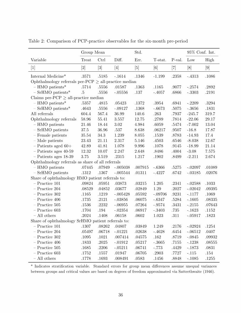
Table 2: Comparison of PCP-practice observables for the six-month pre-period

Group Mean Std. 95% Conf. Int.

Variable Treat Ctrl Diff. Err. T-stat. P-val. Low High

[1] [2] [3] [4] [5] [6] [7] [8] [9]

Internal Medicine* .3571 .5185 -.1614 .1346 -1.199 .2358 -.4313 .1086Ophthalmology referrals per-PCP ≥ all-practice median– HMO patients* .5714 .5556 .01587 .1363 .1165 .9077 -.2574 .2892– SrHMO patients* .5 .5556 -.05556 .137 -.4057 .6866 -.3303 .2191

Claims per-PCP ≥ all-practice median– HMO patients* .5357 .4815 .05423 .1372 .3954 .6941 -.2209 .3294– SrHMO patients* .4643 .5556 -.09127 .1368 -.6673 .5075 -.3656 .1831

All referrals 604.4 567.4 36.99 140.6 .263 .7937 -245.7 319.7Ophthalmology referrals 58.96 55.41 3.557 12.75 .2789 .7814 -22.06 29.17– HMO patients 21.46 18.44 3.02 4.984 .6059 .5474 -7.002 13.04– SrHMO patients 37.5 36.96 .537 8.638 .06217 .9507 -16.8 17.87– Female patients 35.54 34.3 1.239 8.055 .1539 .8783 -14.93 17.4– Male patients 23.43 21.11 2.317 5.146 .4503 .6546 -8.038 12.67– Patients aged 60+ 42.89 41.81 1.078 9.996 .1078 .9145 -18.99 21.14– Patients ages 40-59 12.32 10.07 2.247 2.648 .8486 .4004 -3.08 7.575– Patients ages 18-39 3.75 3.519 .2315 1.217 .1902 .8499 -2.211 2.674

Ophthalmology referrals as share of all referrals– HMO patients .07445 .07949 -.005038 .007915 -.6366 .5275 -.02097 .01089– SrHMO patients .1312 .1367 -.005544 .01311 -.4227 .6742 -.03185 .02076

Share of ophthalmology HMO patient referrals to:– Practice 101 .09824 .05951 .03873 .03215 1.205 .2341 -.02588 .1033– Practice 204 .08529 .04852 .03677 .02849 1.29 .2027 -.02042 .09395– Practice 302 .1165 .1219 -.005428 .05592 -.09706 .9231 -.1177 .1069– Practice 406 .1735 .2121 -.03856 .06075 -.6347 .5284 -.1605 .08335– Practice 505 .1536 .2232 -.06955 .07264 -.9574 .3431 -.2155 .07643– Practice 603 .1704 .194 -.02354 .06917 -.3403 .735 -.1623 .1152– All others .2024 .1408 .06158 .0602 1.023 .311 -.05917 .1823

Share of ophthalmology SrHMO patient referrals to:– Practice 101 .1307 .08262 .04807 .03849 1.249 .2176 -.02924 .1254– Practice 204 .05497 .06718 -.01221 .02638 -.4628 .6454 -.06512 .0407– Practice 302 .1095 .1021 .007414 .04575 .162 .8719 -.0845 .09932– Practice 406 .1833 .2025 -.01912 .05217 -.3665 .7155 -.1238 .08555– Practice 505 .1685 .2206 -.05211 .06741 -.773 .4429 -.1873 .0831– Practice 603 .1752 .1557 .01947 .06705 .2903 .7727 -.115 .154– All others .1778 .1693 .008491 .0583 .1456 .8848 -.1085 .1255

* Indicates stratification variable. Standard errors for group mean differences assume unequal variances

between groups and critical values are based on degrees of freedom approximated via Satterthwaite (1946).

36

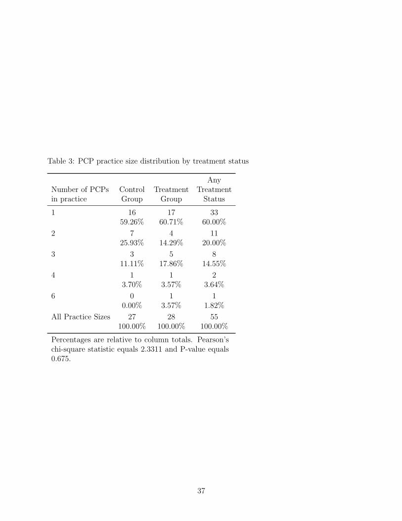
Table 3: PCP practice size distribution by treatment status

AnyNumber of PCPs Control Treatment Treatmentin practice Group Group Status

1 16 17 3359.26% 60.71% 60.00%

2 7 4 1125.93% 14.29% 20.00%

3 3 5 811.11% 17.86% 14.55%

4 1 1 23.70% 3.57% 3.64%

6 0 1 10.00% 3.57% 1.82%

All Practice Sizes 27 28 55100.00% 100.00% 100.00%

Percentages are relative to column totals. Pearson’schi-square statistic equals 2.3311 and P-value equals0.675.

37

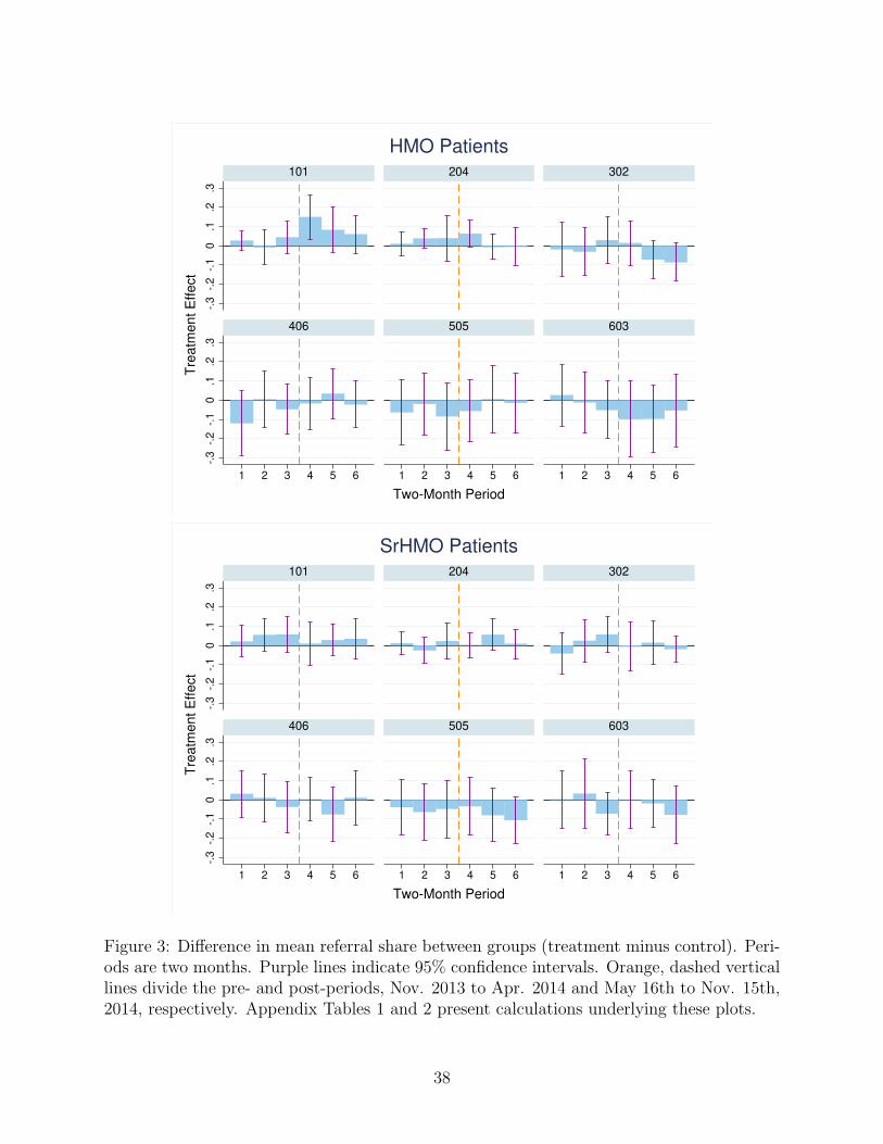
-.3

-.2

-.1

0.1

.2.3

-.3

-.2

-.1

0.1

.2.3

1 2 3 4 5 6 1 2 3 4 5 6 1 2 3 4 5 6

101 204 302

406 505 603

Tre

atm

ent E

ffect

Two-Month Period

HMO Patients

-.3

-.2

-.1

0.1

.2.3

-.3

-.2

-.1

0.1

.2.3

1 2 3 4 5 6 1 2 3 4 5 6 1 2 3 4 5 6

101 204 302

406 505 603

Tre

atm

ent E

ffect

Two-Month Period

SrHMO Patients

Figure 3: Difference in mean referral share between groups (treatment minus control). Peri-ods are two months. Purple lines indicate 95% confidence intervals. Orange, dashed verticallines divide the pre- and post-periods, Nov. 2013 to Apr. 2014 and May 16th to Nov. 15th,2014, respectively. Appendix Tables 1 and 2 present calculations underlying these plots.

38

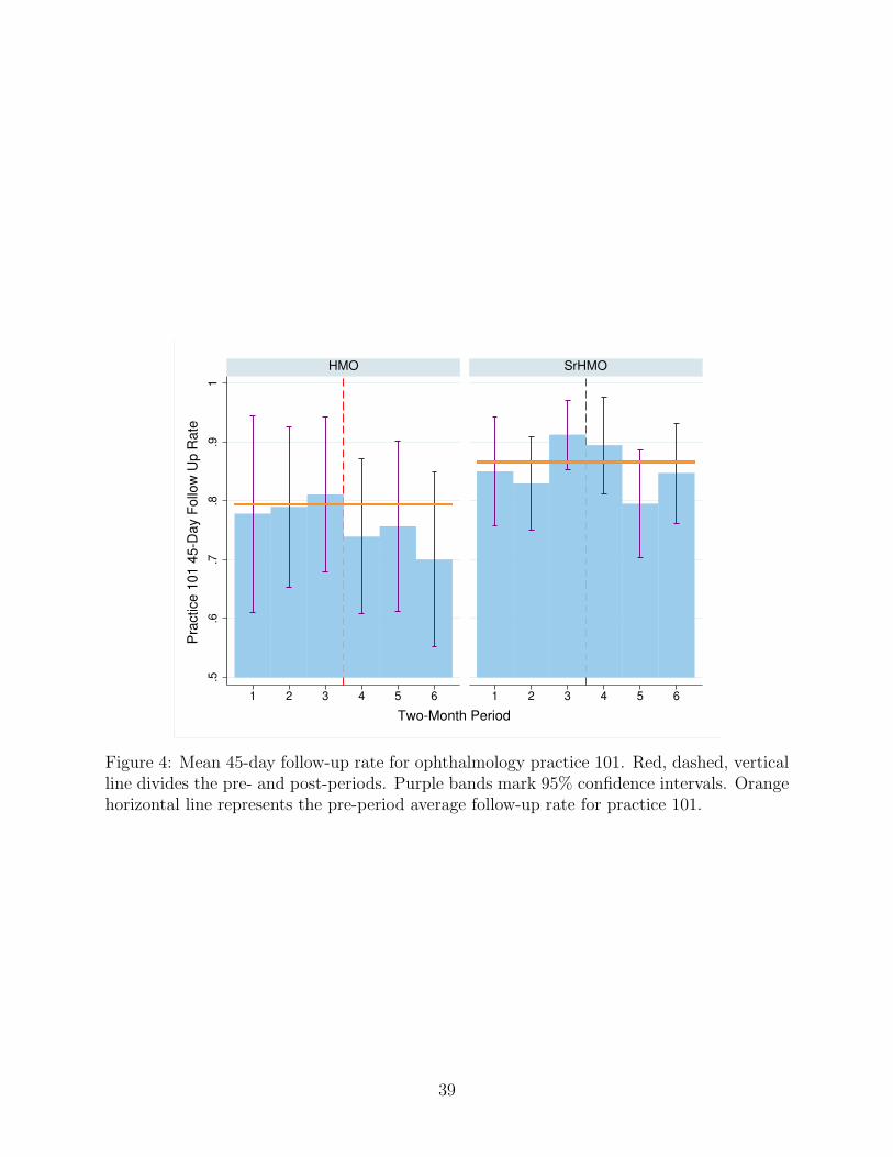
.5.6

.7.8

.91

1 2 3 4 5 6 1 2 3 4 5 6

HMO SrHMO

Pra

ctice 1

01 4

5-D

ay F

ollo

w U

p R

ate

Two-Month Period

Figure 4: Mean 45-day follow-up rate for ophthalmology practice 101. Red, dashed, verticalline divides the pre- and post-periods. Purple bands mark 95% confidence intervals. Orangehorizontal line represents the pre-period average follow-up rate for practice 101.

39

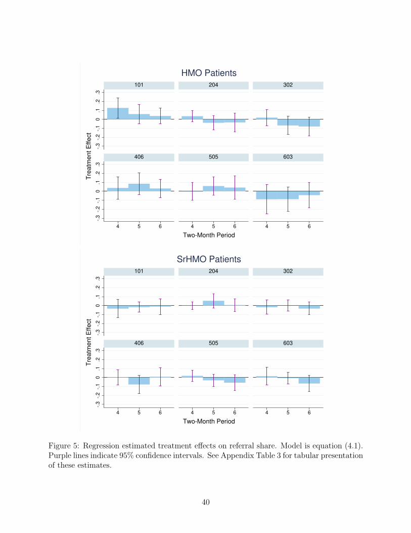
-.3

-.2

-.1

0.1

.2.3

-.3

-.2

-.1

0.1

.2.3

4 5 6 4 5 6 4 5 6

101 204 302

406 505 603

Tre

atm

ent E

ffect

Two-Month Period

HMO Patients

-.3

-.2

-.1

0.1

.2.3

-.3

-.2

-.1

0.1

.2.3

4 5 6 4 5 6 4 5 6

101 204 302

406 505 603

Tre

atm

ent E

ffect

Two-Month Period

SrHMO Patients

Figure 5: Regression estimated treatment effects on referral share. Model is equation (4.1).Purple lines indicate 95% confidence intervals. See Appendix Table 3 for tabular presentationof these estimates.

40

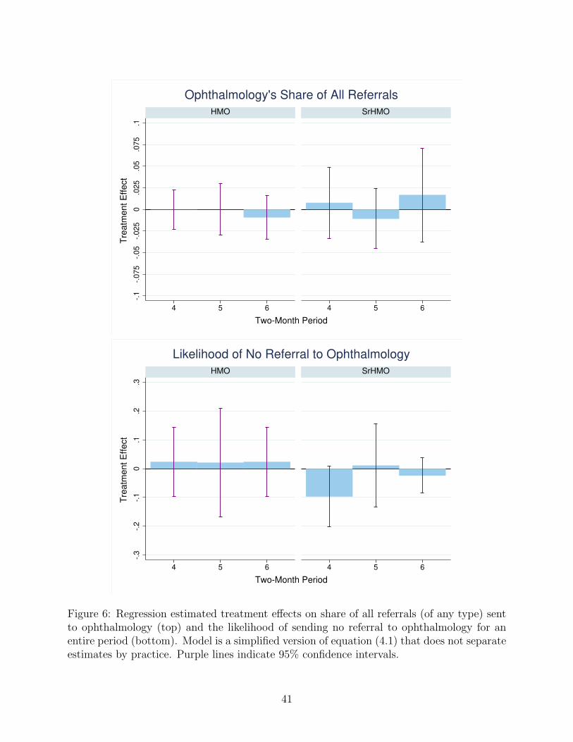
-.1

-.0

75

-.0

5-.

02

50

.02

5.0

5.0

75

.1

4 5 6 4 5 6

HMO SrHMO

Tre

atm

ent E

ffect

Two-Month Period

Ophthalmology's Share of All Referrals

-.3

-.2

-.1

0.1

.2.3

4 5 6 4 5 6

HMO SrHMO

Tre

atm

ent E

ffect

Two-Month Period

Likelihood of No Referral to Ophthalmology

Figure 6: Regression estimated treatment effects on share of all referrals (of any type) sentto ophthalmology (top) and the likelihood of sending no referral to ophthalmology for anentire period (bottom). Model is a simplified version of equation (4.1) that does not separateestimates by practice. Purple lines indicate 95% confidence intervals.

41

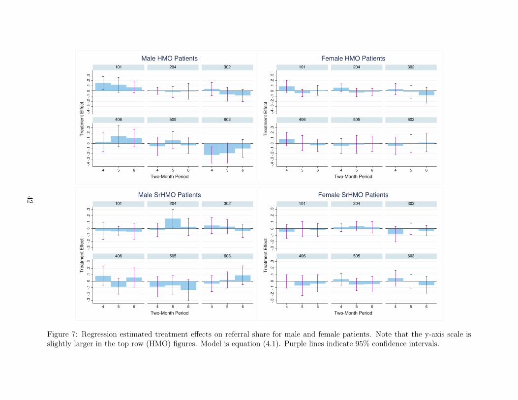
-.4

-.3

-.2

-.1

0.1

.2.3

-.4

-.3

-.2

-.1

0.1

.2.3

4 5 6 4 5 6 4 5 6

101 204 302

406 505 603

Tre

atm

ent E

ffect

Two-Month Period

Male HMO Patients

-.4

-.3

-.2

-.1

0.1

.2.3

-.4

-.3

-.2

-.1

0.1

.2.3

4 5 6 4 5 6 4 5 6

101 204 302

406 505 603

Tre

atm

ent E

ffect

Two-Month Period

Female HMO Patients

-.3

-.2

-.1

0.1

.2.3

-.3

-.2

-.1

0.1

.2.3

4 5 6 4 5 6 4 5 6

101 204 302

406 505 603

Tre

atm

ent E

ffect

Two-Month Period

Male SrHMO Patients

-.3

-.2

-.1

0.1

.2.3

-.3

-.2

-.1

0.1

.2.3

4 5 6 4 5 6 4 5 6

101 204 302

406 505 603

Tre

atm

ent E

ffect

Two-Month Period

Female SrHMO Patients

Figure 7: Regression estimated treatment effects on referral share for male and female patients. Note that the y-axis scale isslightly larger in the top row (HMO) figures. Model is equation (4.1). Purple lines indicate 95% confidence intervals.

42

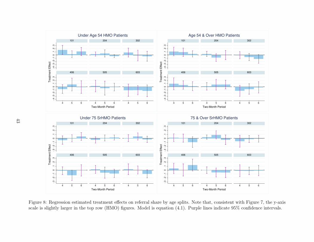
-.4

-.3

-.2

-.1

0.1

.2.3

-.4

-.3

-.2

-.1

0.1

.2.3

4 5 6 4 5 6 4 5 6

101 204 302

406 505 603

Tre

atm

ent E

ffect

Two-Month Period

Under Age 54 HMO Patients

-.4

-.3

-.2

-.1

0.1

.2.3

-.4

-.3

-.2

-.1

0.1

.2.3

4 5 6 4 5 6 4 5 6

101 204 302

406 505 603

Tre

atm

ent E

ffect

Two-Month Period

Age 54 & Over HMO Patients

-.3

-.2

-.1

0.1

.2.3

-.3

-.2

-.1

0.1

.2.3

4 5 6 4 5 6 4 5 6

101 204 302

406 505 603

Tre

atm

ent E

ffect

Two-Month Period

Under 75 SrHMO Patients

-.3

-.2

-.1

0.1

.2.3

-.3

-.2

-.1

0.1

.2.3

4 5 6 4 5 6 4 5 6

101 204 302

406 505 603

Tre

atm

ent E

ffect

Two-Month Period

75 & Over SrHMO Patients

Figure 8: Regression estimated treatment effects on referral share by age splits. Note that, consistent with Figure 7, the y-axisscale is slightly larger in the top row (HMO) figures. Model is equation (4.1). Purple lines indicate 95% confidence intervals.

43

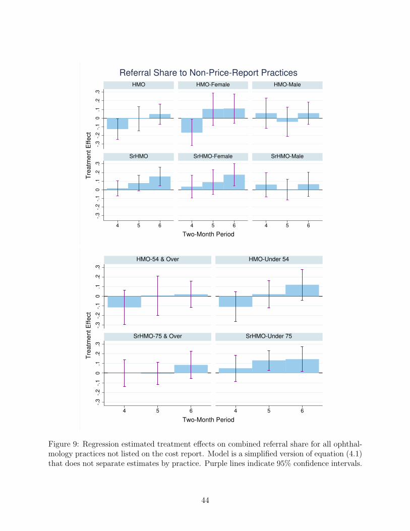
-.3

-.2

-.1

0.1

.2.3

-.3

-.2

-.1

0.1

.2.3

4 5 6 4 5 6 4 5 6

HMO HMO-Female HMO-Male

SrHMO SrHMO-Female SrHMO-Male

Tre

atm

ent E

ffect

Two-Month Period

Referral Share to Non-Price-Report Practices

-.3

-.2

-.1

0.1

.2.3

-.3

-.2

-.1

0.1

.2.3

4 5 6 4 5 6

HMO-54 & Over HMO-Under 54

SrHMO-75 & Over SrHMO-Under 75

Tre

atm

ent E

ffect

Two-Month Period

Figure 9: Regression estimated treatment effects on combined referral share for all ophthal-mology practices not listed on the cost report. Model is a simplified version of equation (4.1)that does not separate estimates by practice. Purple lines indicate 95% confidence intervals.

44

Appendix

45

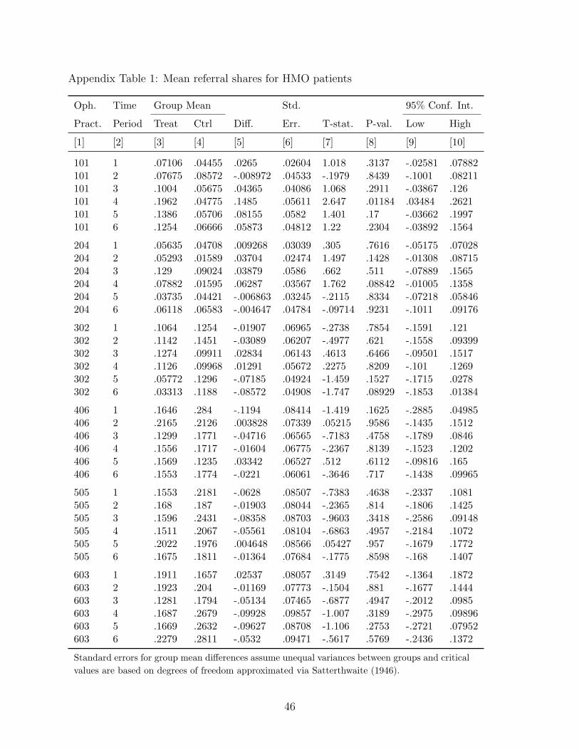
Appendix Table 1: Mean referral shares for HMO patients

Oph. Time Group Mean Std. 95% Conf. Int.

Pract. Period Treat Ctrl Diff. Err. T-stat. P-val. Low High

[1] [2] [3] [4] [5] [6] [7] [8] [9] [10]

101 1 .07106 .04455 .0265 .02604 1.018 .3137 -.02581 .07882101 2 .07675 .08572 -.008972 .04533 -.1979 .8439 -.1001 .08211101 3 .1004 .05675 .04365 .04086 1.068 .2911 -.03867 .126101 4 .1962 .04775 .1485 .05611 2.647 .01184 .03484 .2621101 5 .1386 .05706 .08155 .0582 1.401 .17 -.03662 .1997101 6 .1254 .06666 .05873 .04812 1.22 .2304 -.03892 .1564

204 1 .05635 .04708 .009268 .03039 .305 .7616 -.05175 .07028204 2 .05293 .01589 .03704 .02474 1.497 .1428 -.01308 .08715204 3 .129 .09024 .03879 .0586 .662 .511 -.07889 .1565204 4 .07882 .01595 .06287 .03567 1.762 .08842 -.01005 .1358204 5 .03735 .04421 -.006863 .03245 -.2115 .8334 -.07218 .05846204 6 .06118 .06583 -.004647 .04784 -.09714 .9231 -.1011 .09176

302 1 .1064 .1254 -.01907 .06965 -.2738 .7854 -.1591 .121302 2 .1142 .1451 -.03089 .06207 -.4977 .621 -.1558 .09399302 3 .1274 .09911 .02834 .06143 .4613 .6466 -.09501 .1517302 4 .1126 .09968 .01291 .05672 .2275 .8209 -.101 .1269302 5 .05772 .1296 -.07185 .04924 -1.459 .1527 -.1715 .0278302 6 .03313 .1188 -.08572 .04908 -1.747 .08929 -.1853 .01384

406 1 .1646 .284 -.1194 .08414 -1.419 .1625 -.2885 .04985406 2 .2165 .2126 .003828 .07339 .05215 .9586 -.1435 .1512406 3 .1299 .1771 -.04716 .06565 -.7183 .4758 -.1789 .0846406 4 .1556 .1717 -.01604 .06775 -.2367 .8139 -.1523 .1202406 5 .1569 .1235 .03342 .06527 .512 .6112 -.09816 .165406 6 .1553 .1774 -.0221 .06061 -.3646 .717 -.1438 .09965

505 1 .1553 .2181 -.0628 .08507 -.7383 .4638 -.2337 .1081505 2 .168 .187 -.01903 .08044 -.2365 .814 -.1806 .1425505 3 .1596 .2431 -.08358 .08703 -.9603 .3418 -.2586 .09148505 4 .1511 .2067 -.05561 .08104 -.6863 .4957 -.2184 .1072505 5 .2022 .1976 .004648 .08566 .05427 .957 -.1679 .1772505 6 .1675 .1811 -.01364 .07684 -.1775 .8598 -.168 .1407

603 1 .1911 .1657 .02537 .08057 .3149 .7542 -.1364 .1872603 2 .1923 .204 -.01169 .07773 -.1504 .881 -.1677 .1444603 3 .1281 .1794 -.05134 .07465 -.6877 .4947 -.2012 .0985603 4 .1687 .2679 -.09928 .09857 -1.007 .3189 -.2975 .09896603 5 .1669 .2632 -.09627 .08708 -1.106 .2753 -.2721 .07952603 6 .2279 .2811 -.0532 .09471 -.5617 .5769 -.2436 .1372

Standard errors for group mean differences assume unequal variances between groups and critical

values are based on degrees of freedom approximated via Satterthwaite (1946).

46

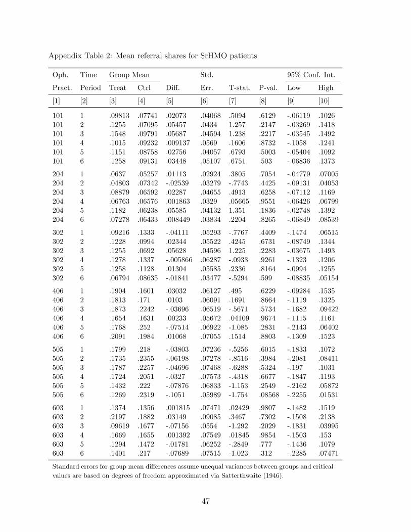
Appendix Table 2: Mean referral shares for SrHMO patients

Oph. Time Group Mean Std. 95% Conf. Int.

Pract. Period Treat Ctrl Diff. Err. T-stat. P-val. Low High

[1] [2] [3] [4] [5] [6] [7] [8] [9] [10]

101 1 .09813 .07741 .02073 .04068 .5094 .6129 -.06119 .1026101 2 .1255 .07095 .05457 .0434 1.257 .2147 -.03269 .1418101 3 .1548 .09791 .05687 .04594 1.238 .2217 -.03545 .1492101 4 .1015 .09232 .009137 .0569 .1606 .8732 -.1058 .1241101 5 .1151 .08758 .02756 .04057 .6793 .5003 -.05404 .1092101 6 .1258 .09131 .03448 .05107 .6751 .503 -.06836 .1373

204 1 .0637 .05257 .01113 .02924 .3805 .7054 -.04779 .07005204 2 .04803 .07342 -.02539 .03279 -.7743 .4425 -.09131 .04053204 3 .08879 .06592 .02287 .04655 .4913 .6258 -.07112 .1169204 4 .06763 .06576 .001863 .0329 .05665 .9551 -.06426 .06799204 5 .1182 .06238 .05585 .04132 1.351 .1836 -.02748 .1392204 6 .07278 .06433 .008449 .03834 .2204 .8265 -.06849 .08539

302 1 .09216 .1333 -.04111 .05293 -.7767 .4409 -.1474 .06515302 2 .1228 .0994 .02344 .05522 .4245 .6731 -.08749 .1344302 3 .1255 .0692 .05628 .04596 1.225 .2283 -.03675 .1493302 4 .1278 .1337 -.005866 .06287 -.0933 .9261 -.1323 .1206302 5 .1258 .1128 .01304 .05585 .2336 .8164 -.0994 .1255302 6 .06794 .08635 -.01841 .03477 -.5294 .599 -.08835 .05154

406 1 .1904 .1601 .03032 .06127 .495 .6229 -.09284 .1535406 2 .1813 .171 .0103 .06091 .1691 .8664 -.1119 .1325406 3 .1873 .2242 -.03696 .06519 -.5671 .5734 -.1682 .09422406 4 .1654 .1631 .00233 .05672 .04109 .9674 -.1115 .1161406 5 .1768 .252 -.07514 .06922 -1.085 .2831 -.2143 .06402406 6 .2091 .1984 .01068 .07055 .1514 .8803 -.1309 .1523

505 1 .1799 .218 -.03803 .07236 -.5256 .6015 -.1833 .1072505 2 .1735 .2355 -.06198 .07278 -.8516 .3984 -.2081 .08411505 3 .1787 .2257 -.04696 .07468 -.6288 .5324 -.197 .1031505 4 .1724 .2051 -.0327 .07573 -.4318 .6677 -.1847 .1193505 5 .1432 .222 -.07876 .06833 -1.153 .2549 -.2162 .05872505 6 .1269 .2319 -.1051 .05989 -1.754 .08568 -.2255 .01531

603 1 .1374 .1356 .001815 .07471 .02429 .9807 -.1482 .1519603 2 .2197 .1882 .03149 .09085 .3467 .7302 -.1508 .2138603 3 .09619 .1677 -.07156 .0554 -1.292 .2029 -.1831 .03995603 4 .1669 .1655 .001392 .07549 .01845 .9854 -.1503 .153603 5 .1294 .1472 -.01781 .06252 -.2849 .777 -.1436 .1079603 6 .1401 .217 -.07689 .07515 -1.023 .312 -.2285 .07471

Standard errors for group mean differences assume unequal variances between groups and critical

values are based on degrees of freedom approximated via Satterthwaite (1946).

47

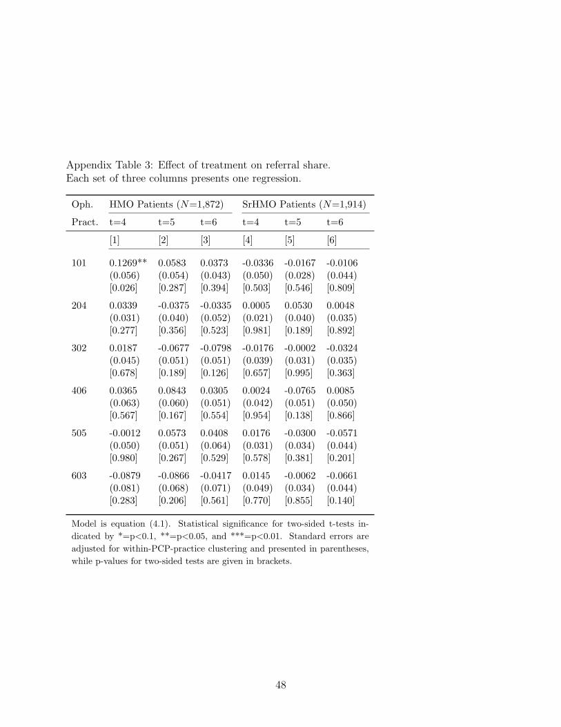
Appendix Table 3: Effect of treatment on referral share.Each set of three columns presents one regression.

Oph. HMO Patients (N=1,872) SrHMO Patients (N=1,914)

Pract. t=4 t=5 t=6 t=4 t=5 t=6

[1] [2] [3] [4] [5] [6]

101 0.1269** 0.0583 0.0373 -0.0336 -0.0167 -0.0106(0.056) (0.054) (0.043) (0.050) (0.028) (0.044)[0.026] [0.287] [0.394] [0.503] [0.546] [0.809]

204 0.0339 -0.0375 -0.0335 0.0005 0.0530 0.0048(0.031) (0.040) (0.052) (0.021) (0.040) (0.035)[0.277] [0.356] [0.523] [0.981] [0.189] [0.892]

302 0.0187 -0.0677 -0.0798 -0.0176 -0.0002 -0.0324(0.045) (0.051) (0.051) (0.039) (0.031) (0.035)[0.678] [0.189] [0.126] [0.657] [0.995] [0.363]

406 0.0365 0.0843 0.0305 0.0024 -0.0765 0.0085(0.063) (0.060) (0.051) (0.042) (0.051) (0.050)[0.567] [0.167] [0.554] [0.954] [0.138] [0.866]

505 -0.0012 0.0573 0.0408 0.0176 -0.0300 -0.0571(0.050) (0.051) (0.064) (0.031) (0.034) (0.044)[0.980] [0.267] [0.529] [0.578] [0.381] [0.201]

603 -0.0879 -0.0866 -0.0417 0.0145 -0.0062 -0.0661(0.081) (0.068) (0.071) (0.049) (0.034) (0.044)[0.283] [0.206] [0.561] [0.770] [0.855] [0.140]

Model is equation (4.1). Statistical significance for two-sided t-tests in-

dicated by *=p<0.1, **=p<0.05, and ***=p<0.01. Standard errors are

adjusted for within-PCP-practice clustering and presented in parentheses,

while p-values for two-sided tests are given in brackets.

48

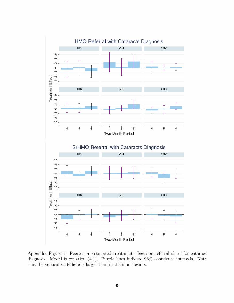
-.9

-.6

-.3

0.3

.6.9

-.9

-.6

-.3

0.3

.6.9

4 5 6 4 5 6 4 5 6

101 204 302

406 505 603

Tre

atm

ent E

ffect

Two-Month Period

HMO Referral with Cataracts Diagnosis

-.9

-.6

-.3

0.3

.6.9

-.9

-.6

-.3

0.3

.6.9

4 5 6 4 5 6 4 5 6

101 204 302

406 505 603

Tre

atm

ent E

ffect

Two-Month Period

SrHMO Referral with Cataracts Diagnosis

Appendix Figure 1: Regression estimated treatment effects on referral share for cataractdiagnosis. Model is equation (4.1). Purple lines indicate 95% confidence intervals. Notethat the vertical scale here is larger than in the main results.

49

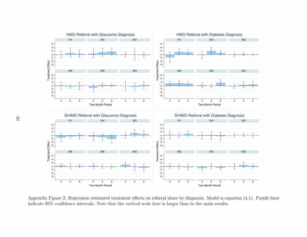
-.9

-.6

-.3

0.3

.6.9

-.9

-.6

-.3

0.3

.6.9

4 5 6 4 5 6 4 5 6

101 204 302

406 505 603

Tre

atm

ent E

ffect

Two-Month Period

HMO Referral with Glaucoma Diagnosis

-.9

-.6

-.3

0.3

.6.9

-.9

-.6

-.3

0.3

.6.9

4 5 6 4 5 6 4 5 6

101 204 302

406 505 603

Tre

atm

ent E

ffect

Two-Month Period

HMO Referral with Diabetes Diagnosis

-.9

-.6

-.3

0.3

.6.9

-.9

-.6

-.3

0.3

.6.9

4 5 6 4 5 6 4 5 6

101 204 302

406 505 603

Tre

atm

ent E

ffect

Two-Month Period

SrHMO Referral with Glaucoma Diagnosis

-.9

-.6

-.3

0.3

.6.9

-.9

-.6

-.3

0.3

.6.9

4 5 6 4 5 6 4 5 6

101 204 302

406 505 603

Tre

atm

ent E

ffect

Two-Month Period

SrHMO Referral with Diabetes Diagnosis

Appendix Figure 2: Regression estimated treatment effects on referral share by diagnosis. Model is equation (4.1). Purple linesindicate 95% confidence intervals. Note that the vertical scale here is larger than in the main results.

50