Correct boundary conditions for DNS models of nonlinear ...

1

Correct boundary conditions for DNS models of 1

nonlinear acoustic-gravity waves forced by 2

atmospheric pressure variations. 3

4

Yuliya Kurdyaeva1, Sergey Kshevetskii1, Nikolai Gavrilov2, Sergey Kulichkov3 5

6

[1]{ Baltic Federal University, Institute of Physical-Mathematical Sciences and Information 7

Technologies, Kaliningrad, Russia } 8

[2]{Saint-Petersburg State University, Atmospheric Physics Department, Russia} 9

[3]{ Obukhov Institute of Atmospheric Physics, Russian Academy of Science, Moscow, Russia} 10

Correspondence to S. P. Kshevetskii ([email protected]) 11

12

Abstract 13

Currently, international networks exist for high-resolution microbarograph recording wave 14

pressure variations at the surface of the Earth. This increases interest in simulating propagation 15

of waves caused by variations of atmospheric pressure. Such mathematical problem involves a 16

set of primitive nonlinear hydrodynamic equations with lower boundary conditions in the form 17

of wavelike pressure variations at the Earth’s surface. To analyze the correctness of the problem, 18

the linearized equations are used near the ground for small amplitudes of surface wave 19

excitation. The method of wave energy functional shows that in nondissipative approximation 20

the solution of the boundary problem is uniquely determined by the variable pressure field at the 21

Earth’s surface. Respective dissipative problem has also unique solution with the appropriate 22

choice of lower boundary conditions for temperature and velocity components. To test the 23

numerical algorithm, analytical solutions of the linearized equations for acoustic and gravity 24

wave modes are used. Reasonable agreements of numerical and analytical solutions are obtained. 25

Analytical studies show possibilities of sharp changes of temperature and density near the 26

ground. Numerical simulations confirm these analytical results. Obtained algorithms and 27

computer codes can be used for simulations of atmospheric wave propagation from the pressure 28

variations at the Earth’s surface. 29

1 Introduction 30

Acoustic-gravity waves (AGWs) are observed in the atmosphere almost permanently. 31

According to recent knowledge, atmospheric AGWs propagating in the middle and upper 32

atmosphere can be excited at tropospheric heights. These waves can be generated by mesoscale 33

Geosci. Model Dev. Discuss., doi:10.5194/gmd-2017-76, 2017Manuscript under review for journal Geosci. Model Dev.Discussion started: 23 May 2017c© Author(s) 2017. CC-BY 3.0 License.

2

turbulence and convection (Fritts and Alexander, 2003; Fritts et al., 2006), atmospheric fronts 1

and jet streams (e.g., Gavrilov and Fukao, 1999; Plougonven and Snyder, 2007; Plougonven and 2

Zhang, 2014;) with maximum wave excitation efficiency at altitudes 9-12 km (e.g., Medvedev 3

and Gavrilov, 1995; Dalin et al., 2016). Generated waves can propagate from tropospheric 4

heights to the middle and upper atmosphere, where they can break and produce turbulence, or 5

other instability events (e.g., Fritts and Alexander, 2003; Gavrilov and Yudin, 1992; Gavrilov 6

and Fukao, 1999). AGW appearance is often associated with meteorological phenomena (Blanc 7

et al., 2014). During the origin and evolution of Cumulus clouds, water phase transitions and 8

respective heating/cooling occur, which can produce substantial generation of wave processes in 9

the atmosphere (e.g., Pierce and Coroniti, 1966; Balachandran, 1980; Fovell et al., 1992; Miller, 10

1999; Alexander et al., 2004; Blanc et al., 2014). 11

To simulate atmospheric AGWs and turbulence, numerical models based on non-12

hydrostatic primitive hydrodynamic equations are recently used. Baker and Schubert (2000) 13

simulated distribution of nonlinear waves in the atmosphere of Venus, using the localized area 14

with horizontal and vertical dimensions of 120 km and 48 km, respectively. Fritts and Garten 15

(1996) and Andreassen et al. (1998) simulated Kelvin-Helmholtz instability and turbulence 16

generation by breaking waves. They used atmospheric areas with relatively small vertical and 17

horizontal dimensions, and applied Halerkin-type algorithms, based on the conversion of initial 18

hydrodynamic equations into sets of equations for spectral components. Yu et al. (2009) and Liu 19

et al. (2008) developed two-dimensional numerical models for propagating atmospheric AGWs. 20

Gavrilov and Kshevetskii (2013, 2015) developed two-dimensional numerical methods 21

for high-resolution wave simulation based on hydrodynamic conservation laws. Such numerical 22

methods ensuring precise execution of basic conservation laws are called as conservative. These 23

methods allow simulating even processes, in which solutions of nonlinear hydrodynamic 24

equations can be non-smooth. Such solutions are called as generalized or weak solutions of 25

hydrodynamic equations. Requirements of accurate holding fundamental conservation laws are 26

important for these methods, because they allow obtaining physically reasonable generalized 27

solutions to the equations. The basic ideas of the generalized solution theory and respective 28

numerical techniques were formulated by Lax (1957) and Lax and Wendroff (1960). Kshevetskii 29

(2001b, c), also Kshevetskii and Gavrilov (2003) developed stable two-dimentional AGW 30

algorithms and models. Gavrilov and Kshevetskii (2014a) extended their two-dimensional model 31

to the three-dimensional version. They used this 3D model to simulate AGW propagation from 32

the harmonic forcing at the Earth's surface. 33


3

Kshevetskii and Kulichkov (2015) used a three-dimensional nonlinear model for 1

description of the AGW generation by heating/cooling atmospheric gas in water phase 2

transitions during evolutions of thunderstorm clouds. Particularly, they studied connections of 3

local atmospheric pressure with the formation and development of thundercloud, and simulated 4

AGW propagation to the middle and upper atmosphere. Karpov and Kshevetskii (2014) modeled 5

AGW propagation from the local non-stationary source located at the Earth's surface. They 6

showed that infrasound waves propagating from tropospheric heights could significantly heat the 7

upper atmosphere. In addition, decaying waves can create jet streams currents in the upper 8

atmosphere. These effects require further detailed studies because of great diversity of their 9

characteristics. Processes of Cumulus cloud evolution lead to AGW generation (e.g., Blanc et al., 10

2014; Alexander et al., 2004). These waves can reach the Earth’s surface and can change the 11

surface pressure (Blanc et al., 2014; Kshevetskii and Kulichkov, 2015). 12

Regardless the reasons leading to wave variations of the surface pressure, one can use 13

these variations the lower boundary conditions for AGW simulations in the atmosphere. Wave 14

variations of the atmospheric surface pressure are recorded with microbarographs. Networks of 15

microbarographs exist and actively expanded currently in Europe and Africa (Blanc et al., 2014). 16

It is tempting to use this experimental data for AGW simulating in the atmosphere. However, the 17

specifying the surface pressure as lower boundary conditions in the nonlinear numerical AGW 18

models raise some problems not adequately studied in the past. In the present paper, we are 19

going to discuss these problems and consider methods for their solutions. 20

First, we perform a mathematical analysis of a set of primitive hydrodynamic equations 21

in order to offer the correct formulating the mathematical problem about propagation of AGWs 22

forced by pressure variations at the lower boundary of the atmosphere. Nonlinear equations are 23

difficult for strict mathematical analysis. However, wave amplitudes at the Earth’s surface are 24

usually small. This allows starting the correctness study from the analysis of linearized 25

equations. Hydrodynamic equations contain atmospheric density and temperature. For zero 26

vertical speed of the Earth's surface, numerical methods require setting the temperature and 27

density at the lower boundary of the atmosphere. However, we found below that the solution of 28

the boundary problem is uniquely identified by specifying a variable pressure field at the lower 29

boundary. This fact is not trivial and allows us correct simulating AGW propagation forced by 30

surface pressure variations. 31

We modified the high-resolution numerical AGW model described by Gavrilov and 32

Kshevetskii (2014a,b) and Gavrilov et al. (2015), and available online (ATMOSYM, 2016). The 33

model was adapted for simulating AGW propagation from varying surface pressure. We 34


4

performed test simulations and compared numerical results with exact analytical solutions 1

obtained for respective linearized hydrodynamic equations. In addition, we made three-2

dimensional nonlinear simulation of AGWs caused by experimentally observed variations of 3

atmospheric pressure at the Earth's surface. 4

2 Numerical model 5

In the present paper, we mainly consider the three-dimentional high-resolution numerical 6

model ATMOSYM simulating atmospheric AGWs, which was developed by Gavrilov and 7

Kshevetskii (2014a,b) and Gavrilov et al. (2015). Recently this model becomes available for all 8

users online (see ATMOSYM, 2016) 9

2.1 Nonlinear hydrodynamic equations. 10

The ATMOSYM numerical model uses the following set of primitive hydrodynamic 11

equations for the atmosphere considered as the ideal gas: 12

the continuity equation 13

;=z

ρw+

y

ρv+

x

ρu+

t

ρ0

(1) 14

the motion equations 15

;z

uς(z)

z+ς(z)u

y+

x+

x

p=vρω+

z

ρuw+

y

ρuv+

x

ρu+

t

ρuz

2

2

2

2

2

2 16

;z

vς(z)

z+ς(z)v

y+

x+

y

p=uρω

z

ρvw+

y

ρv+

x

ρuv+

t

ρvz

2

2

2

2

2

2 (2) 17

;z

wς(z)

z+ς(z)w

y+

x+ρg

z

p=

z

ρw+

y

ρvw+

x

ρuw+

t

ρw 2

2

2

2

2

18

the heat balance equation 19

;z

w+

y

w+

x

w+

z

v+

y

v+

x

v+

z

u+

y

u+

x

uς(z)=Q

;Q+z

)(T'κ(z)

z+κ(z)T

y+

x+

z

w+

y

v+

x

up=

z

pw+

y

pv+

x

pu+

t

p

γ

visc

visc

222222222

2

2

2

2

1

1

20

(3) 21

the ideal gas state equation 22

μTρR=p g / (4) 23


5

In Eq. (1) – (4) t is time; x, y, z and u, v, w are coordinates and velocity components 1

directed, respectively, eastwards, northwards and upwards; p, ρ, T are pressure, density and 2

temperature; Rg is the universal gas constant; µ is the air molecular weight; g is the acceleration 3

of gravity; γ is the heat capacity ratio; ς and κ are the dynamic viscosity and thermal conductivity 4

coefficients; ωz is the vertical component of the angular velocity of the Earth’s rotation. 5

Eq. (1) – (4) take into account non-linear and dissipative processes accompanying wave 6

propagation. They can describe, in particular, such complex phenomena as the formation of 7

shock waves, the wave breaking and turbulence generation. The AGWSYM numerical model 8

provides a self-consistent description of wave processes and takes into account the changes in 9

atmospheric parameters due to energy transfer from dissipating waves to the atmosphere. 10

Vertical profiles of the background temperature T0 (z) are taken from the semi-empirical 11

atmospheric models NRL-MSISE-00 (Picone et al., 2002). Molecular kinematic viscosity is 12

approximated with the formula by Banks and Kokarts (1973): 13

14

(z)ρ(z)T=(z)ρ(z)ζ=(z)ν 0 00

7

00 /103.4/ (5) 15

16

The molecular thermal conductivity coefficient is obtained with dividing the coefficient of 17

viscosity by the Prandtl number. Similar expressions for molecular viscosity and thermal 18

conductivity were used by Yu et al. (2009) and Liu et al. (2010). The ATMOSYM model also 19

takes into account vertical profiles of the background turbulent viscosity and thermal 20

conductivity with maxima about 10 m2s

−1 near the ground and at altitude of 100 km, and a 21

minimum of 0.1 m2s

1 in the stratosphere (see Gavrilov, 2013). Model does not take into account 22

some effects (e.g., the dissipation due to ion friction and radiative heat exchange), which are less 23

important for high frequency AGV. 24

2.2 Boundary conditions 25

The ATMOSYM model simulates waves in a limited atmospheric region. For analyzing 26

spectral AGW components, periodical conditions at horizontal boundaries are frequently 27

appropriate. Let Lx and Ly are dimensions of the model area along axes x and y, respectively. 28

Then periodical horizontal boundary conditions have the following form: 29


6

).,,0,(),,,(),,,,0(),,,(

),,,0,(),,,(),,,,0(),,,(

),,,0,(),,,(),,,,0(),,,(

),,,0,(),,,(),,,,0(),,,(

),,,0,(),,,(),,,,0(),,,(

),,,0,(),,,(),,,,0(),,,(

tzyxTtzLyxTtzyxTtzyLxT

tzyxtzLyxtzyxtzyLx

tzyxptzLyxptzyxptzyLxp

tzyxwtzLyxwtzyxwtzyLxw

tzyxvtzLyxvtzyxvtzyLxv

tzyxutzLyxutzyxutzyLxu

yx

yx

yx

yx

yx

yx

(6) 1

At the top, standard upper boundary conditions for wave propagation problems in 2

the thermosphere are used: 3

.0,0,0,0

hzhzhzhz

wz

v

z

u

z

T (7) 4

These boundary conditions are usually valid at high molecular viscosity and thermal conduction 5

at high altitudes ( h 500 km). The equation set (1) – (4) is difficult for strict analysis and most 6

boundary conditions are obtained empirically from simulation practice. At the Earth’s surface, 7

one can specify conditions for velocity components. Most frequently, the air non-flow through 8

the surface is supposed, when w(x,y,z=0,t) = 0. However, for studies of waves from earthquakes 9

or tsunami (Matsamura et al., 2011; Kherani et. al., 2012; Shinagawa et al., 2007) or vertical 10

vibrations of gas caused by convection (Fovell et al., 1992; Snively and Pasko, 2003), and in 11

some other cases, w(x,y,z=0,t) is specified on the basis of experimental data or using general 12

assumptions about considered phenomena. The condition of the air adhesion at the Earth’s 13

surface is natural in the viscous model, when u(x,y,z=0,t) = 0 and v(x,y,,z=0,t) = 0. In addition, 14

one should specify the lower boundary conditions for relative variations of pressure, density and 15

temperature 16

,T)T(T=TT=Θ,ρ)ρ(ρ=ρρ=R,p)p(p=pp=Ρ 000000000 //'//'//' (8) 17

where primes denote inclinations of hydrodynamic fields from respective background values 18

denoted with zero subscripts. In the present study, we consider the usage of the surface pressure 19

measurements as the lower boundary condition, when 20

t),y,(x,f=t),=zy,P(x, p0 (9) 21

where fp(x,y,t) is an approximation function to the surface measurement data. Changes in the 22

boundary condition for the other hydrodynamic variables may lead to non-correct mathematical 23

problems. Therefore, the proper options for getting correct mathematical boundary problems 24

require consideration. 25

3 Correctness of the boundary problem 26

System of nonlinear equations (1) – (4) is complex and difficult for analysis. However, 27


7

near the Earth's surface wave amplitudes are usually very small. Nonlinear components have the 1

second order in the solution expansion versus the small amplitude, while the linear terms have 2

the first order. Therefore, one can simplify the equation by removing nonlinear terms (see 3

Gossard and Hook, 1975). 4

5

3.1 Correctness of linearized non-dissipative problem. 6

The linearized equation set obtained from Eqs. (1) – (4) for the case of two spatial 7

variables neglecting viscous and heat conduction terms can be represented in the following form 8

(Kshevetskii, 2001a, 2002): 9

Θ;+R=Ρ;=w)(ρ+u)(ρ+R)(ρ zxt 0000 10

;0)()( 00 xt Ppu ;=gRρ+P)(p+w)(ρ 0zt 000 (10) 11

,=gwNρ+γP))(p(γΘ)(ρ 2

0tt 0//1 00 12

where N is the Brunt-Vaisala frequency; subscripts t, x and z denote respective differentiation. 13

Eq. (10) is obtained for zero background wind, because the wind is usually small near the 14

ground. The case of inclusion of viscosity and thermal conductivity is discussed in the next 15

section. Two-dimension equations are considered here for simplicity. The three-dimensional 16

analysis is similar, but formulae are more bulky. In the two-dimension case, the Coriolis forces 17

are omitted. The initial conditions correspond to the lack of motions at t = 0: 18

.0)0,,(,0)0,,(,0)0,,(,0)0,,( tzxtzxRtzxwtzxu (11) 19

At horizontal boundaries, the two-dimension version of periodical conditions (6) is used. The 20

upper boundary condition 21

w(x,z=h,t) = 0 (12) 22

corresponds to Eq. (7). At the lower boundary we impose the condition (10), which can be 23

rewritten as 24

.000 t)(x,f=t)],=zΘ(x,+t),=z[R(x,=t),=zP(x, p (13) 25

The most important property of the correct solution is its uniqueness. I this respect, the following 26

theorem can be formulated: 27

Theorem 1. If a continuous solution of equations (10) with initial conditions (11) and 28

boundary conditions (6), (12) and (13) exists, then it is unique. 29


8

The proof of this theorem is given in the Appendix A. This theorem has a consequence. 1

Consequence. The Theorem 1 states that in non-dissipative case the solution is uniquely 2

determined by the pressure variations (13) at the lower boundary, but not the surface 3

distributions of relative variations of density R and temperature Θ. This means that arbitrary 4

functions can be added to and subtracted from the surface distributions of R and Θ, but the 5

solution will be the same as far as the sum R + Θ = P is the same at the surface. 6

This allows constructing solutions of linearized non-dissipative equations having jumps 7

in R and Θ near the lower boundary z = 0. In nonlinear models, such jumps can produce 8

instabilities and generate mathematical wave modes non-existing in the nature. Therefore, 9

nonlinear models require specifying correct self-consistent lower boundary conditions for R and 10

Θ in addition to the condition (13) to minimize influence of mathematical wave modes. 11

3.2 Correctness of linearized dissipative problem 12

Linearized set of hydrodynamic equations for the case of two spatial dimensions, taking into account the 13

dissipative terms is as follows: 14

Θ;+R=Ρ;=w)(ρ+u)(ρ+R)(ρ zxt 0000 15

;][ςς(z)(w+[ςς(z)u=Ρ)(p+u)(ρ zzxxxt 00 (14) 16

;][ςς(z)(w+[ςς(z)w=gRρ+Ρ)(p+w)(ρ zzxx0zt 00 17

],)Θ)(κκ(z)(+Θ))[(κ[(κ((γ=gwNρ+γP))(p(γΘ)(ρ zzxx

2

0tt 0000 1//1 18

Compliment the equations (15) with the initial conditions (12). According to (7), the upper 19

boundary have the form of 20

0.0,0, =h)=w(z=|u=|Θ)(T h=zzh=zzo (15) 21

Analogous to the Appendix A, one can proof the following uniqueness theorem: 22

Theorem 2. If a continuous solution exits for the equations (14) with initial conditions 23

(11) and boundary conditions (6), (13), (15) and 24

,0,0,0000

zzzzwu (16) 25

then it is unique. 26

This theorem is proved in the Appendix B. The last boundary condition in (16) leads to 27

the following lower boundary condition for density variations: 28

.00 t),=zΘ(x,t)(x,f=t),=zR(x, p (17) 29


9

This condition should be added to the lower boundary conditions (13) and (16), when one is 1

going to specify nonzero variations of pressure at the Earth’s boundary for studies of AGW 2

propagation. 3

As far as AGW amplitudes are usually small near the ground, one should expect that the 4

solutions of nonlinear and linearized equations should be close near the lower boundary. 5

Therefore, in the present study we solve the following nonlinear AGW boundary problem: a) the 6

equation set is (1) – (4); b) zero initial conditions like (11); c) the horizontal boundary conditions 7

(6); d) the lower boundary conditions (9), (16) and (17). 8

4 Comparisons of nonlinear and linearized models. 9

To study the influence of the lower boundary condition, we made comparisons of 10

simulations using the nonlinear equations (1) – (4) and boundary conditions listed at the end of 11

section 2.1 with analytical solution of the respective linearized equations. 12

4.1 Analytical solution of linearized equations. 13

For the set of linearized equations (10) in isothermal (T0 = const) background conditions 14

the following stationary solution can be obtained using standard methods described by Gossard 15

and Hook (1975) and Beer (1974): 16

,Θ+Rz

B+Θ+RA=tz,x,w

,SωH

B+A+BHmS

ω

mA

ω

kgHCe=tz,x,Θ

,SωH

B+A+BHm+S

ω

mA+

ω

kgHCe=tz,x,R

ωt,mz+kx=S,ω

SkegHC=tz,x,u

0αz

0αz

αz

0

cos4

24sin

1

cos4

24sin

cos

0

0

2

2

2

0

0

2

2

2

(18) 17

where k and m are the horizontal and vertical wave numbers, respectively; ω is the wave 18

frequency; α = (2H0 )-2

, A and B are coefficients having the forms of 19

2

0

22

22

2

0

22

222

0

444

22

444

22-

Hmγ+γ+γmω

ωkγgHγ=B,

Hmγ+γ+γmω

ωkγgHHγmγ=A

2

0

2

0

2

(19) 20

Wave numbers k, m and frequency ω are connected by the dispersion equation 21

22

22

0α+k+mHγ

γk±α+k+mγgH=ω

22

0

2

222 14

112

1 (20) 22


10

Here the signs + and - before the square root correspond to acoustic and internal gravity waves 1

(IGWs), respectively. In Eq. (18) – (20) upward directions of group velocity correspond to m > 0 2

for acoustic and m < 0 for internal gravity waves. 3

4.2 Test simulations. 4

Numerical simulations for comparisons with analytical solutions (18) – (20) are made 5

with the AGWSYM model using the three-dimension algorithms for solving Eq. (1) – (4) 6

developed by Gavrilov and Kshevetskii (2015). We use the initial conditions (11), conditions at 7

the horizontal boundaries (6) and at the upper boundary (7) . At the lower boundary z = 0, we use 8

conditions (16) and specify the plane wave pressure variation: 9

ωt),mz+(kxD=t),=zy,P(x, sin0 (21) 10

where D is the surface amplitude. Relative density variations at the lower boundary are 11

calculated using Eq. (17). Previous simulations with the model (e.g., Gavrilov and Kshevetskii, 12

2015) showed the existence of a transition interval after initiating the boundary forcing at t = 0 13

before the solution comes to a quasi-stationary regime. In this regime, we can expect good 14

agreement between the numerical results and the analytical solution (18) - (20) with C = Dω2 at 15

low altitudes, where AGW amplitudes and molecular viscosity and heat conductivity are small. 16

Numerical results are obtained using the AGWSYM (2016) model for solving the 17

equation set (1) – (4) with initial conditions (11) and conditions (6) at the horizontal boundaries, 18

(7) at the upper boundary, also (16), (17), (21) at the lower boundary. In test runs the atmosphere 19

is isothermal with H0 = 8 km. The wave forcing (21) is activated at t = 0. One should expect that 20

at low altitudes, where wave amplitudes and dissipation are small, numerical solutions would 21

tend to linear analytical solution (18) – (20) with increasing t. 22

Test simulations were made for isothermal atmosphere with H0 = 8 km, Lx = 103 km, k = 23

40π/Lx . Frequencies are ω = π/60 s-1

for the acoustic wave mode and ω = π/1800 s-1

for the IGW 24

mode. To prevent substantial initial AGW pulse at the surface forcing activation, the lower 25

boundary condition (21) was multiplied by factor q = 1-exp(-t/t0) with t0=2 min. This factor 26

gradually increases in time from o to 1 and the intensity of initial AGW pulse become smaller. 27

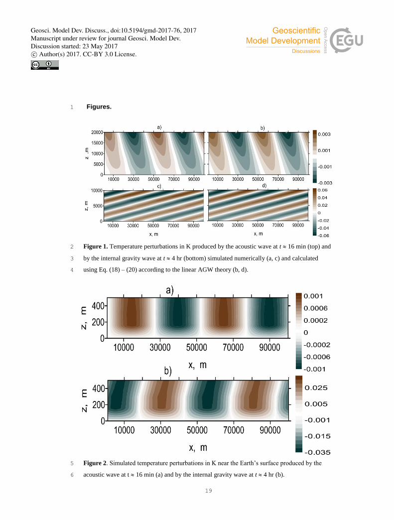
Figure 1 shows numerical and analytical temperature wave fields in the lower atmosphere 28

at different t for the acoustic and IGW modes. Similarities of the left and right panels in Figure 1 29

mean good agreement between nonlinear numerical and linear analytical solutions for small 30

amplitude non-dissipative AGWs. Figure 2 represents numerical solutions with better resolution near 31

the lower boundary. One can see transitions from zero boundary condition for temperature (16) to wave 32


11

fields corresponding simulated AGW. The transition is sharp within a few vertical grid spacing near the 1

ground. 2

4.4 Simulation for observed local pressure variations. 3

To test the numerical model for real data, we used a sample of the surface pressure 4

variations in time, f(t), recorded with microbarograph at the Obukhov Institude of Atmospheric 5

Physics near Moscow (55.7 N, 37,6 E) on April 9, 2016 and shown in Figure 3. Assuming 6

localized near the measurement location (x0,y0) wave source, the lower boundary condition (13) 7

for surface pressure are taken in the following form: 8

]f(t),d))y(y+)x[((x=t),=zy,P(x, 22

0

2

0 /exp0 (22) 9

where d is the half-width of the wave source region. For present simulations we set d = 2 km. 10

Other initial and boundary conditions are the same as in section 4.3. Simulated temperature 11

fields for t 3 min after the wave source activation are shown in the left panel of Figure 4. One 12

can see acoustic waves propagating from the source with amplitudes increasing with height. 13

These acoustic waves have not so high amplitudes because the pressure measurements of Figure 14

3 correspond to quiet meteorological conditions near the observation site. In addition, observed 15

variations of the surface pressure are relatively slow and generate mainly IGWs. Group speed of 16

IGWs is much smaller than the sound speed. Therefore, IGWs in Figure 4 are noticeable near the 17

wave source region. The right panel of Figure 4 is for t 13 min and demonstrates inclined 18

petals. This is characteristic for IGWs propagating in the atmosphere from localized wave 19

sources. 20

5 Conclusion 21

In this study, we set up and mathematically investigated the problem of propagating 22

nonlinear acoustic-gravity waves produced by variable pressure at the surface of the Earth. We 23

also compared the results with analytical solutions of linear AGW theory. 24

Mathematical study showed that solutions of problem of AGW propagation from variable 25

density and temperature specified on the Earth's surface are uniquely identified by the pressure 26

on the Earth's surface, but do not depend on details of individual temperature and density 27

distributions. Numerically simulated acoustic and IGW modes excited by harmonic variations of 28

pressure at the Earth's surface confirmed the theoretical results. 29

The problem of waves propagating from a harmonic source specified at the lower boundary 30

border can be solved analytically in the case of isothermal atmosphere. We compared analytical 31


12

and numerical solutions and demonstrated good agreement between them. Such comparisons can 1

be used for validating numerical models of atmospheric AGWs. 2

Reasonable agreement of wave parameters calculated using numerical simulation and 3

analytical formulae can be considered as an indication of adequate description of wave processes 4

by the nonlinear numerical model. An example is shown of numerical solution of AGW 5

propagation from local variations in the surface atmospheric pressure. Model of direct numerical 6

simulation can be effective for simulating AGWs produced by variations of atmospheric pressure 7

and for testing and validation of simplified parameterizations of wave effects in the atmosphere. 8

9

Computer code availability 10

The computer code is available for free online simulations for all users (see ATMOSYM, 11

2016). The code can be distributed and used with the permission from the Immanuel Kant Baltic 12

Federal (the official owner of the code). Access to the fully functional demo-version of the 13

ATMOSYM computer code, which calculates the experiments described in the present paper, 14

can be granted on demand by request to Sergej Kshevtskii ([email protected]) or Yulia 15

Kurdyaeva ([email protected]). Any questions should be directed to the authors. 16

17

Acknowledgements. This work was partly supported by the Russian Basic Research Foundation 18

(grant 17-05-00574), by the Russian Scientific Foundation (grant 14-17-00685). 19

20

References. 21

Alexander, M., May, P. and Beres, J.: Gravity waves generated by convection in the Darwin area 22

during the Darwin Area Wave Experiment, J. Geophys. Res., 109, D20S04, 1-11, 2004. 23

Andreassen, O., Hvidsten, O., Fritts, D., and Arendt, S.: Vorticity dynamics in a breaking internal 24

gravity wave, Part 1 Initial instability evolution, J. Fluid. Mech., 367, 27-46, 1998. 25

ATMOSYM: A multi-scale atmosphere model from the Earth’s surface up to 500 km, 26

http://atmos.dev.awsmtek.com , 2016 (last access 10.02.2017). 27

Baker, D. and Schubert, G.: Convectively generated internal gravity waves in the lower atmosphere 28

of Venus, Part II mean wind shear and wave-mean flow interaction, J. Atmos. Sci., 57, 200-215, 29

2000. 30


13

Balachandran, N. K.: Gravity waves from thunderstorms, Monthly weather rev., 108, 804-816, 1

1980. 2

Banks, P. M. and Kockarts, G.: Aeronomy, Part B, Elsevier, New York, 1973. 3

Beer, T.: Atmospheric waves, Adam Hilder, London, 1974. 4

Blanc, E., Farges, T., Le Pichon, A., and Heinrich, P.: Ten year observations of gravity waves from 5

thunderstorms in western Africa, J. Geophys. Res. Atmos., 119, 6409-6418, 6

doi:10.1002/2013JD020499, 2014. 7

Dalin, P., Gavrilov, N., Pertsev, N., Perminov, V.,Pogoreltsev, A.,Shevchuk, N., Dubietis, A., 8

Volger, P., Zalcik, M., Ling, A., Kulikov, S., Zadorozhny, A., Salakhutdinov and Grigorieva, I.: 9

A case study of long gravity wave crests in noctilucent clouds and their origin in the upper 10

tropospheric jet stream, J. Geophys. Res. Atmos., 121, 14,102 –14,116, 11

doi:10.1002/2016JD025422, 2016. 12

Fritts, D. C. and Alexander, M. J.: Gravity wave dynamics and effects in the middle atmosphere, 13

Rev. Geophys., 41, 1003, doi:10.1029/2001RG000106, 2003. 14

Fritts, D. C. and Garten, J. F.: Wave breaking and transition to turbulence in stratified shear flows, 15

J. Atmos. Sci., 53, 1057-1085, 1996. 16

Fritts, D. C., Vadas, S. L., Wan, K., and Werne, J. A.: Mean and variable forcing of the middle 17

atmosphere by gravity waves, J. Atmos. Sol.-Terr. Phys., 68, 247-265, 2006 18

Fovell, R., Durran, D., Holton, J.R.: Numerical simulation of convectively generated stratospheric 19

gravity waves, J. Atmos. Sci, v. 47, 1427-1442, 1992. 20

Gavrilov, N. M.: Estimates of turbulent diffusivities and energy dissipation rates from satellite 21

measurements of spectra of stratospheric refractivity perturbations, Atmos. Chem. Phys., 13, 22

12107-12116, doi:10.5194/acp-13-12107-2013, 2013. 23

Gavrilov, N. M. and Fukao, S.: A comparison of seasonal variations of gravity wave intensity 24

observed by the MU radar with a theoretical model, J. Atmos. Sci., 56, 3485-3494, 25

doi:10.1175/1520-0469(1999)056<3485:ACOSVO>2.0.CO;2, 1999. 26

Gavrilov, N. M. and Kshevetskii, S. P.: Numerical modeling of propagation of breaking nonlinear 27

acoustic-gravity waves from the lower to the upper atmosphere, Adv. Space Res., 51, 1168-1174, 28

doi:10.1016/j.asr.2012.10.023, 2013. 29


14

Gavrilov, N. M. and Kshevetskii, S. P.: Numerical modeling of the propagation of nonlinear 1

acoustic-gravity waves in the middle and upper atmosphere. Izvestiya, Atmos. Ocean. Phys., 50, 2

66-72, doi:10.1134/S0001433813050046, 2014a. 3

Gavrilov, N. M. and Kshevetskii, S. P.: Three-dimensional numerical simulation of nonlinear 4

acoustic-gravity wave propagation from the troposphere to the thermosphere, Earth Planets 5

Space, 66, 88, doi:10.1186/1880-5981-66-88, 2014b. 6

Gavrilov, N. M. and Kshevetskii, S. P.: Dynamical and thermal effects of nonsteady nonlinear 7

acoustic-gravity waves propagating from tropospheric sources to the upper atmosphere, Adv. 8

Space Res., 55, doi:10.1016/j.asr.2015.01.033, 2015. 9

Gavrilov, N. M. and Yudin, V. A.: Model for coefficients of turbulence and effective Prandtl 10

number produced by breaking gravity waves in the upper atmosphere, J. Geophys. Res., 97, 11

7619в-7624, doi:10.1029/92JD00185, 1992. 12

Gossard, E. E. and Hooke, W. H.: Waves in the atmosphere, Elsevier Sci. Publ. Co., Amsterdam-13

Oxford-New York, 1975. 14

Karpov, I. V. and Kshevetskii, S. P.: Formation of large-scale disturbances in the upper atmosphere 15

caused by acoustic-gravity wave sources on the Earth’s surface, Geomag. Aeronomy, 54(4), 553-16

562, doi:10.1134/S0016793214040173, 2014. 17

Kherani, E.A., Lognonne P., Hebert H, Rolland, L., Astafyeva , E., Occhipinti, G., Coisson P., 18

Walwer D. and de Paula, E.R.: Modelling of the total electronic content and magnetic field 19

anomalies generated by the 2011 Tohoku-Oki tsunami and associated acoustic-gravity waves, 20

Geophys. J. Int., 191, 1049-1066, DOI: 10.1111/j.1365-246X.2012.05617.x, 2012. 21

Kshevetskii, S. P.: Modelling of propagation of internal gravity waves in gases, Comp. Math. 22

Mathematic. Phys., 41, 295-310, 2001a. 23

Kshevetskii, S. P.: Analytical and numerical investigation of non-linear internal gravity waves, 24

Nonlin. Proc. Geoph., 8, 37-53, 2001b. 25

Kshevetskii, S. P.: Numerical simulation of nonlinear internal gravity waves, Comp. Math. Math. 26

Phys., 41, 1777-1791, 2001c. 27

Kshevetskii, S.P.: Internal gravity waves in non-exponentially density-stratified fluids. Comput. 28

Math. Mathematic. Phys.. 42(10), 1510-1521, 2002. 29

Kshevetskii, S. P. and Gavrilov, N. M.: Vertical propagation of nonlinear gravity waves and their 30

breaking in the atmosphere, Geomagn. Aeronomy, 43(1), 69–76, 2003. 31


15

Kshevetskii, S. P. and Gavrilov, N. M.: Vertical propagation, break ing and effects of nonlinear 1

gravity waves in the atmosphere, J. Atmos. Sol.-Terr. Phys., 67, 1014-1030, 2005. 2

Kshevetskii, S. P. and Kulichkov, S. N.: Effects that Internal Gravity Waves from Convective 3

Clouds Have on Atmospheric Pressure and Spatial Temperature-Disturbance Distribution, 4

Atmospheric and Oceanic Physics, 51(1), 42-48, doi:10.1134/S0001433815010065, 2015. 5

Lax, P. D.: Hyperbolic systems of conservation laws, Comm. Pure Appl. Math., 10, 537-566, 1957. 6

Lax, P. D. and Wendroff, B.: Hyperbolic systems of conservation laws, Comm. Pure Appl. Math., 7

13, 217-237, 1960. 8

Liu, H.-L., Foster, B. T., Hagan, M. E., McInerney, J. M., Maute, A., Qian, L., Richmond, A. D., 9

Roble, R. G., Solomon, S. C., Garcia, R. R., Kinnison, D., Marsh, D. R., Smith, A. K., Richter, 10

J., Sassi, F., and Oberheide, J.: Thermosphere extension of the whole atmosphere community 11

climate model, J. Geophys. Res., 115, A12302, doi:10.1029/2010JA015586, 2010. 12

Liu, X., Xu, J., Liu, H.-L., and Ma, R.: Nonlinear interactions between gravity waves with different 13

wavelengths and diurnal tide, J. Geophys. Res., 113, D08112, doi:10.1029/2007JD009136, 2008. 14

Matsumura, M., Saito, A., Iyemori, T.; Shinagawa, H.; Tsugawa, T.; Otsuka, Y.; Nishioka, M.; 15

Chen, C. H.: Numerical simulations of atmospheric waves excited by the 2011 off the Pacific 16

coast of Tohoku Earthquake. Earth, Planets and Space. 63:68. doi:10.5047/eps.2011.07.015, 17

2011. 18

Medvedev, A. S. and Gavrilov, N. M.: The nonlinear mechanism of gravity wave generation by 19

meteorological motions in the atmosphere, J. Atmos. Terr. Phys., 57, 1221-1231, 1995. 20

Miller, D.V.: Thunderstorm induced gravity waves as a potential hazard to commercial aircraft. 21

American Meteorological Society 79th Annual conference, Windham Anatole Hotel, Dallas,TX, 22

January 10-15. Dallas: American Meteorological Society. 1999. 23

Picone, J.M., Hedin, A.E., Drob, D.P. and Aikin, A.C. : NRL-MSISE-00 Empirical Model of the 24

Atmosphere: Statistical Comparisons and Scientific Issues, J. Geophys. Res., 107(A12), 25

doi:10.1029/2002JA009430, 2002. 26

Pierce, A. D. and Coroniti, S. C.: A mechanism for the generation of acoustic-gravity waves during 27

thunder-storm formation, Nature, 210, 1209-1210, doi 10.1038/2101209a0,1966. 28

Plougonven, R. and Snyder, Ch.: Inertia-gravity waves spontaneously generated by jets and fronts. 29

Part I: Different baroclinic life cycles, J. Atmos. Sci., 64, 2502-2520, 2007. 30


16

Plougonven, R. and Zhang, F. : Internal gravity waves from atmospheric jets and fronts, Rev. 1

Geophys., 52, doi:10.1002/2012RG000419, 2014. 2

Shinagawa, H., Iyemori, T„ Saito, S. and and Maruyama, T. : A numerical simulation of 3

ionospheric and atmospheric variations associated with the Sumatra earthquake on December 26, 4

2004, Earth Planets Space, 59, 1015?1026, 2007. 5

Snively, J..B. and Pasko, V.B.: Breaking of thunderstorm generated gravity waves as a source of 6

short period ducted waves at mesopause altitudes, Geophys. Res. Lett, v. 30, No 24, 2254, 7

doi:10.1029/2003GL018436.,2003. 8

Yu, Y., Hickey, M. P., and Liu, Y.: A numerical model characterizing internal gravity wave 9

propagation into the upper atmosphere, Adv. Space Res., 44, 836-846, 10

doi:10.1016/j.asr.2009.05.014, 2009. 11

12

Appendix A. Proof of the Theorem 1. 13

The Theorem 1 formulated in section 3.1 for the linearized non-dissipative problem states 14

that if a continuous solution of equations (10) with initial conditions (11) and boundary 15

conditions (6), (12), (13) exists, then it is unique. 16

To proof of this uniqueness theorem one can use the indirect (“the proof by 17

contradiction”) method. Suppose that two different solutions χ1 = (u1, w1, Ρ1, Π1, Θ1) and χ2 18

=(u2, w2, Ρ2, Π2, Θ2) exist. Consider the difference of these solutions: )Θ,Π,Ρ,w,u(=Δχ~~~~~ , where 19

2~ uu=u 1 , 2

~ ww=w 1 , 2

~ΡΡ=Ρ 1 , 2

~ΠΠ=Π 1 , 2

~ΘΘ=Θ 1 . If the function fp(x,t) in 20

Eq. (13) is the same for both P1 and P2, the difference Δχ satisfies to Eq. (10) with the initial 21

conditions (11) and boundary conditions (6) and (12). The standard wave energy, e, balance for 22

the Eq. (11) has the following differential form (Gossard and Hooke, 1975): 23

24

.))1((

)(2

1

);,(;0/

2222

0

00

gHwue

wpupjjdivte

(A1.1) 25

26

This equation should be valid for the solution Δχ also. Put this solution to (A1.1) and integrate 27

the obtained equation over the time-spatial domain t],[Ω 0 , where h],[]L,[=Ω x 00 is the 28

considered atmospheric area. Then one can apply the Gauss’s flux theorem, use the zero initial 29


17

conditions (11) and obtain the following relation: 1

2

).~,~(~,~~

)~

)1(~

(~

~~

2

1

0

0

2222

0

vuvdtSdvPp

dgHgHwu

t

S

(A1.2) 3

4

Here S is the boundary of the Ω region, dSnSd

, n

is the external vector, which is normal to 5

the region boundary S. Integration circuit of S includes upper, horizontal and lower boundaries. 6

Consider the right side integral in Eq. (A1.2). Its part along the upper boundary z = h is equal to 7

zero due to the condition (12). Because of periodical conditions (6), the parts of the integral 8

along the left and right boundaries (x = 0 and x = Lx) compensate each other, because they have 9

the same absolute values, but opposite signs. For the lower boundary condition (13) with fixed 10

fp(x,t) the difference 0),0,(~

tzxP and the part of considered integral along the lower surface z 11

= 0 is equal to zero. 12

Summarizing, one can see that the surface integral in the right part of Eq. (A1.2) is equal 13

to zero for considered initial and boundary conditions. This means that all quantities marked with 14

waves in the left part integral of Eq. (A1.2) should be zero, or that χ1 ≡ χ2. 15

Appendix B. Proof of the Theorem 2. 16

The Theorem 2 formulated in section 3.2 for linearized dissipative problem states that if a 17

continuous solution of equations (14) with initial conditions (11) and boundary conditions (6), 18

(13), (15) and (16) exists, then it is unique. 19

To proof this uniqueness theorem the standard indirect (“the proof by contradiction”) 20

method similar to Appendix A can be used. Suppose again that two different solutions χ1 = (u1, 21

w1, Ρ1, Π1, Θ1) and χ2 =(u2, w2, Ρ2, Π2, Θ2) exist. Consider the difference of these solutions: 22

)Θ,Π,Ρ,w,u(=Δχ~~~~~ , where 2

~ uu=u 1 , 2~ ww=w 1 , 2

~ΡΡ=Ρ 1 , 2

~ΠΠ=Π 1 , 23

2

~ΘΘ=Θ 1 . Function Δχ satisfies Eq. (14) with initial conditions (11) and boundary conditions 24

(6), (13), (15) and (16). Getting the wave energy equation for Eq. (14) and applying the Gauss’s 25

flux theorem one can get the following equation similar to (A1.2): 26

27


18

.]~~

)~~~~(~~[

))()(())~()~()~()~((

)~

)1(~

(~

~~

2

1

00 0

00

0

22

0

2222

2222

0

dxdtTwwuuwPp

dtdTwwuu

dgHgHwu

z

t L

zzz

t

zxzxzx

x

(A2.1) 1

2

For the conditions (13) with the same fp(x,t) for both P1 and P2, the difference 0~

=P along the 3

lower boundary z = 0. Then, for conditions (16), the right side integral in (A2.1) is equal to zero, 4

hence solutions χ1 ≡ χ2 (similar to the Appendix A). 5

6

7


19

Figures. 1

Figure 1. Temperature perturbations in K produced by the acoustic wave at t 16 min (top) and 2

by the internal gravity wave at t 4 hr (bottom) simulated numerically (a, c) and calculated 3

using Eq. (18) – (20) according to the linear AGW theory (b, d). 4

Figure 2. Simulated temperature perturbations in K near the Earth’s surface produced by the 5

acoustic wave at t 16 min (a) and by the internal gravity wave at t 4 hr (b). 6


20

Figure 3. Surface pressure variations near Moscow on April 9, 2016. 1

2

3

Figure 4. Simulated temperature perturbations (in °K) due to AGWs excited by the observed 4

surface pressure variations shown in Figure 3 at t = 3 min (left) and t = 13 min (right). Thick 5

lines correspond to zero contours. 6


Correct boundary conditions for DNS models of nonlinear ...

Documents

Transcript of Correct boundary conditions for DNS models of nonlinear ...