Camera Position Estimation for Detecting 3D Scene Change

Yuji Ueno∗

Baowei Lin∗

Kouhei Sakai∗

Toru Tamaki∗

Bisser Raytchev∗

Kazufumi Kaneda∗

Our goal is to detect temporal change/changes between a 3D scene at time A (past) and a query image attime B (now), and to display results in real time with estimated camera positions. In this paper, we proposea method for estimating camera positions for the purpose, which first extract SIFT features from image, andestimate the nearest neighbors between features in the query image and the 3D scene. Then, we estimatecamera positions with RANSAC base on the image-scene correspondences. The proposed method is appliedto real and simulated dataset evaluated by known camera positions.

Keywords: Cameras pose estimation, 3D scene, Change detection, ANN, RANSAC

1. Introduction

Recently surveillance technology developments moti-vate a regular observation of places such as coast, s-lopes, and highways, where disasters and accidents hap-pen with in high probability. At coast, a lot of wavedissipating blocks are settled to decrease the power ofwaves. If the configuration of the blocks is altered whenthere is erosion or earthquakes, the blocks might be col-lapsed and the waves would not be dissipated. A moun-tain slope with a face exposed after a heavy rain mightcause a landslide. Hence, any small changes of the facemust be alerted. The fill beneath a highway is usedto be collapsed due to earthquakes or aging, which re-sults in cracks and subsidence. These places should beobserved all the time, however, it is not practical for awide area. Therefore, an automatic detection of unusualchange seems to be useful and important.

The cases above lead to the common problem that 3Dscene changes in shape. The changes are categorized in-to two types: rigid and non-rigid. Rigid cases are themovement of a rigid body such as a block changes in po-sition. Non-rigid cases are the transformation of a non-rigid object such as a face of a mountain slope slides.Therefore, the problem is stated as the detection of atemporal change over a period between time A (past)and time B (now). Here, time A means before changesand time B means after changes.

In this paper, we describe a method to detect the tem-poral change of the period by using a 3D scene geometryat time A and the image of the same scene at time B.

∗ University of HiroshimaGraduate School of Engineering, Department of Informa-tion.lin-bao-wei@hotmail.com

Computing two 3D scenes or two images are not suitableto detect changes because of several reasons. It is notpractical to use a number of cameras to take images of awide range of the scene. However, a few cameras cannotcapture the change in reasonable resolution. 3D recon-struction at time B is not useful because it takes muchmore time than a reasonable response required by theinteraction with the operator. In contrast, the proposedmethod takes a different approach. Our approach doesnot require fixed cameras because a 3D-2D matching isapplied. 3D reconstruction is used for the 3D scene on-ly at time A; at time B just one image is used. Theprojection matrix of the image at time B is estimatedwith RANSAC in addition to a novel method to outliersrejection of 3D-2D correspondence. Then, the temporalchange is detected and visualized to inform an observerof a potential danger of the scene.

The rest of the paper is organized as follows. Relat-ed work on 3D-2D matching and scene change detec-tion is reviewed in section 2. In section 3, we explaina method for 3D-2D matching with SIFT features be-tween a 3D scene and an image. The matching is thenrefined by reducing outliers with a proposed thresholdof SIFT feature distances described in section 4. Us-ing the matching, the projection matrix of the camerais computed with RANSAC based method explained insection 5. Detection of the change of 3D scene geometryis explained in section 6. In section 7, we show an exper-imental result of estimating a camera pose and detectingthe change of the scene.

2. Related work

Our method requires 3D-2D matching for localization,estimating one camera pose and location, which can becategorized in to following groups.

FCV2012 1

First category is based on image retrieval (1), whichsearches the nearest image to a given image among ahuge number of images with information of camera poseand location stored in a database. This method does notneed 3D scene reconstruction and hence is fast, while theretrieved camera poses and location is discrete ratherthan continuous, even if when a movie was stored in adatabase instead of images.

Second category is landmark-based or maker-basedcamera localization (8) (9). This method is relatively fastbecause only a sparse set of 3D coordinates of landmarksin a 3D scene is required and a dense 3D reconstructionis not needed. However, this does not work when there isno as remarkable objects as for landmarks in the scene.

Third category stores 3D geometry of the scene as wellas image features of images used for the 3D reconstruc-tion (2). A camera can be localized quickly by matchinga given 2D image of the camera and 3D scene in thedatabase. Our approach extends this method because itis applicable to a variety of scenes with few remarkableobjects suitable for landmarks.

An alternative is a markerless AR (3)∼(5) such as P-TAM (6), which is very close to our work because a cam-era pose and location is estimated in real-time and 3Dscene geometry is reconstructed at the same time. How-ever, it may require a registration 3D scene geometries,one is obtained currently (at time B) and the other isbefore (at time A). It is computationally burden evenwhen a GPU based registration (7) is used.

The last category is simultaneous 3D reconstructionand scene change detection (11) which detects buildingsand estimates when the buildings were build using anumber of images taken over time. The images are s-tochastically classified in to groups, and used for recon-struction for each group to find changes of the scenebetween groups. This method might be promising whileit is not for a real-time application.

Our proposed method estimates a camera pose basedon 3D-2D matching to robustly find a projection matrixof the camera in real time, which is explained in thefollowing sections.

3. Camera pose estimation of image using3D scene features

In this section, we explain a method for constructing a3D scene at time A and an estimating a camera positionat time B. First, in section 3.1 we explain the methodfor constructing 3D scene with local features of imagesat time A. Then, in section 3.2 we explain the methodfor estimating a projection matrix for an image at timeB using 3D-2D matching.

3.1 3D scene reconstruction with local fea-tures Feature points xij and features at the points

S(xij) are detected from images at time A where j =(1, 2, . . . , J). As the description of features, we use SIFTfeatures (12) which is invariant to illumination, rotationand scale. A SIFT at xij is denoted as S(xij). Then,a camera position and 3D scene are estimated by usingthe bundle adjustment (18). For features of image xij , 3D

scene Xi and camera positions Pj , we minimize follow-ing expression using a non-linear optimization method:∑

i

∑j

||xij − PjXi||, (1)

where i is the number of 3D points, j is the number ofimages. But, this 3D scene reconstructed by this methodis not dense because the 3D scene is only the points cor-responding to features of images. Therefore, we obtaina dense 3D scene Xi and normal vectors n(Xi) using aMulti-view Stereo (14).

Next, 3D scene Xi is projected to an image by Pj .

But, when the angle of normal vector n(Xi) to the view-ing vector of a camera c is less than 60 degree, that is

n(Xi) · (−c) < cos 60. (2)

Xi is not project because those points do not appear.Then, we compute again SIFT features at 2D pointsPjX

i, which is Xi projected to image j by Pj , and

then S(PjXi) and Xi are stored to database. In this

process, some SIFT features S(P1Xi), S(P2X

i), . . . ,would be the same point Xi from different images, butstored.3.2 Camera pose estimation using 3D-2D

matching Using SIFT feature S(xi) at time B,SIFT feature S(PjX

i) in the database is searched to es-timate correspondence between image xij and 3D scene

Xi.For the search we use nearest neighbor distance. If the

second neighbor distance is more than 0.7 times of themost nearest neighbor distance, these points are corre-sponded. We use ANN (Approximated nearest Neigh-bors) (15) to accelerate the nearest neighbor computa-tion.

A feature of image xij = (xij , yij)T and a 3D scene Xi

have the following relation:

xij = PjXi, (3)

where Pj is a projection matrix. From equation(3),

xij × PjXi = 0, (4)

could hold. Then,

Pj =

p11 p12 p13 p14p21 p22 p23 p24p31 p32 p33 p34

, (5)

is rearranged as a vector pj = (p11, p12, . . . , p34)T tomake the equation Bipj = 0. Here B is

B =

(0T XiT −yiXiT

XiT 0T −xiXiT

). (6)

The system of these equations for x1j ,x

2j , . . . ,x

Nj is

B =

B1

B2

...BN

. (7)

2 FCV2012

Camera Position Estimation for Detecting 3D Scene Change

A solution of these simultaneous equations is the projec-tion matrix. When minimum 8 points correspondencesare given, the simultaneous equation can be solved bythe following steps. When we set

C =(B1 B2 . . . BN

)B1

B2

...BN

. (8)

The vector pj , which shows projection matrix, isgiven by the eigenvector corresponding to the smallesteigenvalue of C. But if outlier exists, it fails. Thereforewe describe a method to deal with outliers in section 4and 5.

Next, R and t are estimated by decomposition of theprojection matrix. Projection matrix P , camera intrin-sic matrix A, rotation matrix R and translation vectort have the relation that P = A[R|t]. Let the left 3 × 3submatrix of P be

M =

p11 p12 p13p21 p22 p23p31 p32 p33

. (9)

This matrix is decomposed by QR-decomposition asM = AR, A is an upper triangular matrix and R is anorthogonal matrix, then intrinsic matrix A and rotationmatrix R are obtained. Translation vector t is given bythe following equation:

t = A−1(p14 p24 p34

)T. (10)

The determinant of rotation matrix R is |R| = 1, sothe determinant of rotation matrix estimated by thismethod becomes |R| = 1. Since this matrix has re-flection, we should estimate a projection matrix to be|R| = 1. When the determinant becomes |R| = −1, thecorrespondences in equation (8) are charged to estimatea projection matrix of |R| = 1.

4. Outlier reduction

In this section, we explain how to reducing outlierswith a threshold.

There is a SIFT feature S(x) at points x in imageand SIFT features S(PnX

i) at 3D scene Xi. Gen-erally, we search the matching from two points Xi1,Xi2 which minimize ‖ S(x) − S(PnX

i) ‖, where ‖S(x) − S(PnX

i1) ‖<‖ S(x) − S(PmXi2) ‖. When‖ S(x) − S(PnX

i1) ‖> 0.7 ‖ S(x) − S(PmXi2) ‖, theyare the outliers.

However in this case, the database has SIFT fea-tures S(P1X

i), S(P2Xi), . . . , S(PnX

i) correspondingthe same Xi. In addition, even if Xi and Xj are d-ifferent, but when ‖ Xi −Xj ‖ is too short, they aretoo close.

Our method reduces outliers by using following twoprocesses. First process explained in section 4.1 is tofind threshold by the nearest neighbor distance of SIFTfeatures. Second process explained in section 4.2 is toreduce one-to-many correspondence.

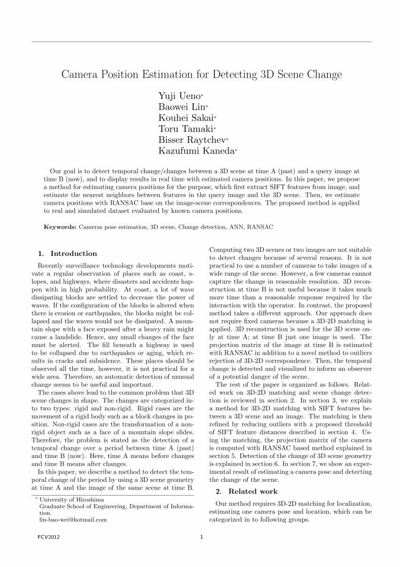
Fig. 1. 3D scene distances and SIFT featuredistances.

4.1 Thresholding SIFT distances Our methodconfirms correspondence when the nearest neighbor dis-tance between SIFTs is smaller than a threshold. 3Dscene distances and SIFT feature distances are shown inFigure 1. Figure 1(a) shows that Xi and Xj are twopoints in the 3D scene, if the distance ‖ Xi −Xj ‖ issmall, then the distance ‖ PnXi − PnXj ‖ in the pro-jected image should be small too. If ‖ PnXi − PnXj ‖is less than 1[pixel], both Xi and Xj may correspondto the same point.

Figure 1(b) shows that the vertical axis denotes thedistances of points in 3D scene which is ‖ Xi −Xj ‖and the horizontal axis denotes the SIFT feature dis-tances of points in projected image which is ‖ S(PnX

i)−S(PnX

j) ‖. In Figure 1(b), although the 3D scene dis-tance ‖ Xi − Xj ‖ is small, SIFT feature distances‖ S(PnX

i) − S(PnXj) ‖ could not be small. Howev-

er, if ‖ S(PnXi)− S(PnX

j) ‖ is small, ‖ Xi −Xj ‖ isalso small.

The maximum distance between 3D scene points ofthis data set is about 50 millimeters. If we set the SIFTfeature distances less than 200, we can get the changerange of 3D scene distance within 10 millimeters. Sothe outliers should be the case that distance of SIFT

FCV2012 3

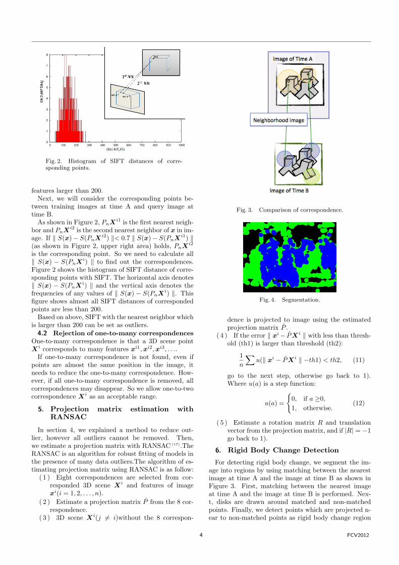
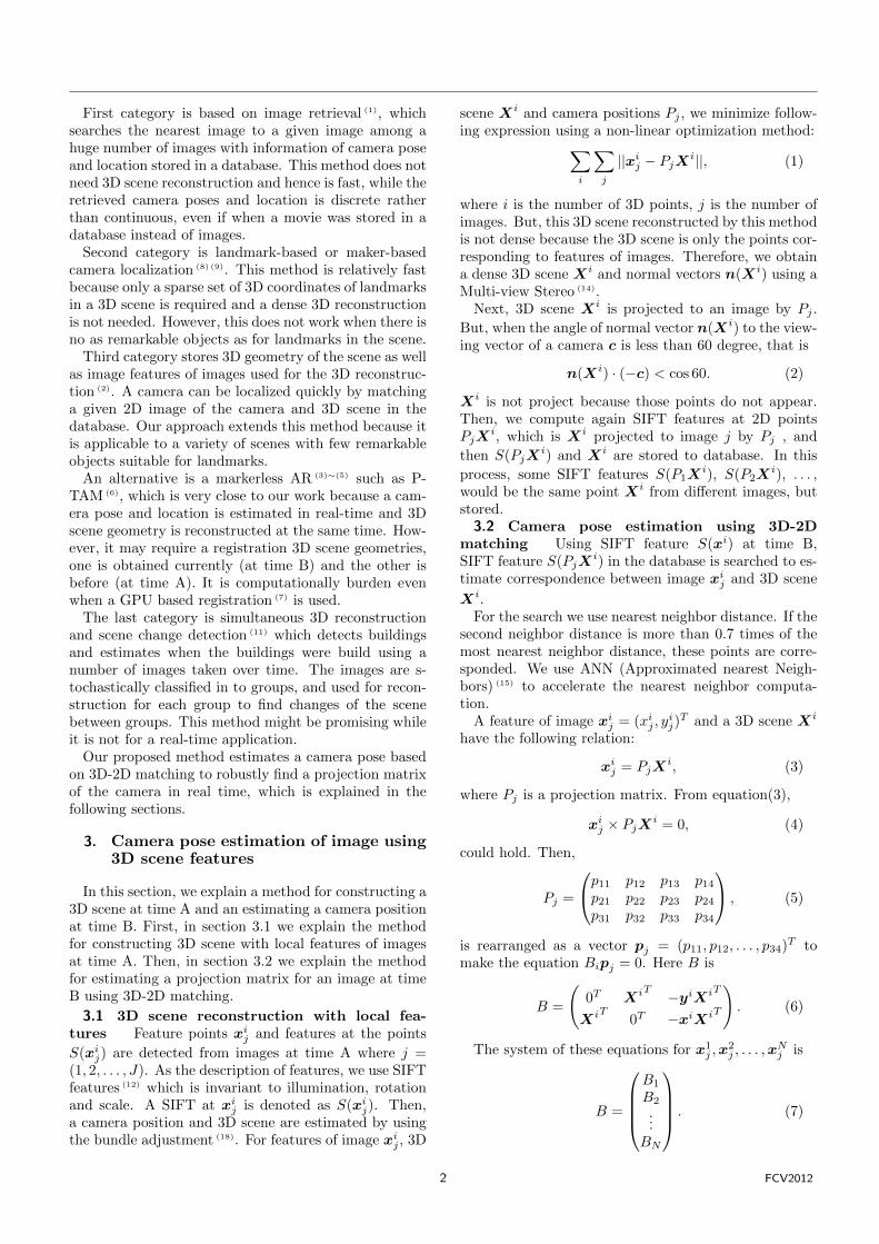
Fig. 2. Histogram of SIFT distances of corre-sponding points.

features larger than 200.Next, we will consider the corresponding points be-

tween training images at time A and query image attime B.

As shown in Figure 2, PnXi1 is the first nearest neigh-

bor and PnXi2 is the second nearest neighbor of x in im-

age. If ‖ S(x)− S(PnXi2) ‖< 0.7 ‖ S(x)− S(PnX

i1) ‖(as shown in Figure 2, upper right area) holds, PnX

i2

is the corresponding point. So we need to calculate all‖ S(x) − S(PnX

i) ‖ to find out the correspondences.Figure 2 shows the histogram of SIFT distance of corre-sponding points with SIFT. The horizontal axis denotes‖ S(x) − S(PnX

i) ‖ and the vertical axis denotes thefrequencies of any values of ‖ S(x) − S(PnX

i) ‖. Thisfigure shows almost all SIFT distances of correspondedpoints are less than 200.

Based on above, SIFT with the nearest neighbor whichis larger than 200 can be set as outliers.4.2 Rejection of one-to-many correspondences

One-to-many correspondence is that a 3D scene pointXi corresponds to many features xi1,xi2,xi3, . . ..

If one-to-many correspondence is not found, even ifpoints are almost the same position in the image, itneeds to reduce the one-to-many correspondence. How-ever, if all one-to-many correspondence is removed, allcorrespondences may disappear. So we allow one-to-twocorrespondence Xi as an acceptable range.

5. Projection matrix estimation withRANSAC

In section 4, we explained a method to reduce out-lier, however all outliers cannot be removed. Then,we estimate a projection matrix with RANSAC (17).TheRANSAC is an algorithm for robust fitting of models inthe presence of many data outliers.The algorithm of es-timating projection matrix using RANSAC is as follow:

( 1 ) Eight correspondences are selected from cor-responded 3D scene Xi and features of imagexi(i = 1, 2, . . . , n).

( 2 ) Estimate a projection matrix P̂ from the 8 cor-respondence.

( 3 ) 3D scene Xi(j 6= i)without the 8 correspon-

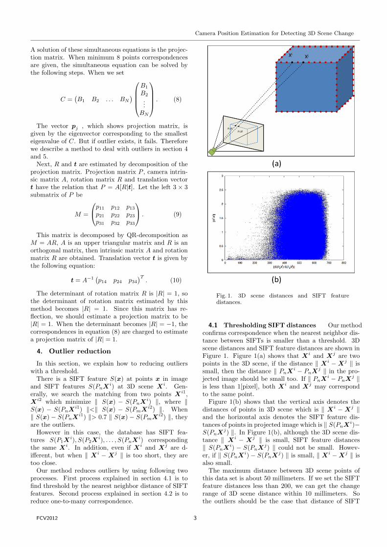
Fig. 3. Comparison of correspondence.

Fig. 4. Segmentation.

dence is projected to image using the estimatedprojection matrix P̂ .

( 4 ) If the error ‖ xi− P̂Xi ‖ with less than thresh-old (th1) is larger than threshold (th2):

1

n

∑u(‖ xi − P̂Xi ‖ −th1) < th2, (11)

go to the next step, otherwise go back to 1).Where u(a) is a step function:

u(a) =

{0, if a ≥0,

1, otherwise.(12)

( 5 ) Estimate a rotation matrix R and translationvector from the projection matrix, and if |R| = −1go back to 1).

6. Rigid Body Change Detection

For detecting rigid body change, we segment the im-age into regions by using matching between the nearestimage at time A and the image at time B as shown inFigure 3. First, matching between the nearest imageat time A and the image at time B is performed. Nex-t, disks are drawn around matched and non-matchedpoints. Finally, we detect points which are projected n-ear to non-matched points as rigid body change region

4 FCV2012

Camera Position Estimation for Detecting 3D Scene Change

Fig. 5. Images at time A.

Fig. 6. Images at time B.

Table 1. Estimation error of images at time A.

dF (Rt, R̂)[deg] e(tt, t̂)

image1 2.14 0.61

image3 2.70 0.31

image5 3.52 0.70

when 3D scene is projected on the image at time B. InFigure 4, we show a segmentation result. Green pointsare non-matching regions and blue points are matchingregions. Since this image is rendered in order of greenand blue, the matched regions (blue) are not overdrawn.

7. Experimental results

7.1 Experimental setup of a cup scene Weused five images of a cup with known projection matri-ces: three for time A (Figure 5), and two for time B(Figure 6). First, the method explained section 3.1 isapplied to three images at time A and make a database.Then the method explained in sections 3.2, 4 and 5 isapplied two images at time B and estimated camera posi-tions. For accuracy evaluation, we also estimate camerapositions for images at time A.

All images are calibrated. Intrinsic matrices A1, A3

and A5 are obtained from projection matrices at timeA. Because all images were taken by the same camera,we use the average of these intrinsic matrices Aave =13 (A1 +A2 +A3) to make points x calibrated as A−1

avex.

Estimated projection matrix P̂ and true projectionmatrix Pt are decomposed into rotation matrices R̂ andRt translation vectors t̂, tt for error evaluation. Trans-lation error is evaluated as relative error of Euclideandistance:

e(tt, t̂) =‖ tt − t̂ ‖‖ t̂ ‖

. (13)

Rotation error is evaluated with distance of rotationmatrix(16):

dF (Rt, R̂) =1√2‖ logRtR̂

T ‖F (14)

logR =

{0, if θ =0,θ

2 sin θ (R−RT ), otherwise.(15)

Table 2. Estimation error of images at time B.

dF (Rt, R̂)[deg] e(tt, t̂)

image2 6.77 1.16

image4 3.64 0.38

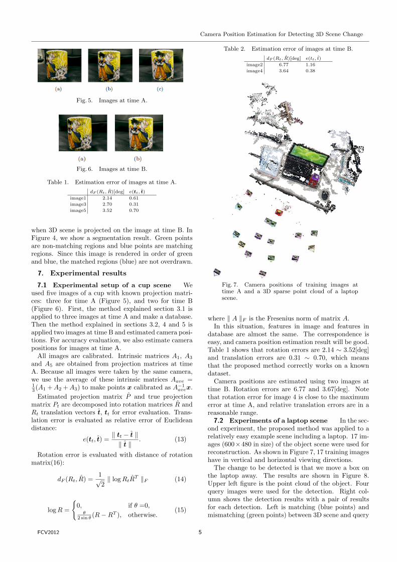
Fig. 7. Camera positions of training images attime A and a 3D sparse point cloud of a laptopscene.

where ‖ A ‖F is the Fresenius norm of matrix A.In this situation, features in image and features in

database are almost the same. The correspondence iseasy, and camera position estimation result will be good.Table 1 shows that rotation errors are 2.14 ∼ 3.52[deg]and translation errors are 0.31 ∼ 0.70, which meansthat the proposed method correctly works on a knowndataset.

Camera positions are estimated using two images attime B. Rotation errors are 6.77 and 3.67[deg]. Notethat rotation error for image 4 is close to the maximumerror at time A, and relative translation errors are in areasonable range.7.2 Experiments of a laptop scene In the sec-

ond experiment, the proposed method was applied to arelatively easy example scene including a laptop. 17 im-ages (600×480 in size) of the object scene were used forreconstruction. As shown in Figure 7, 17 training imageshave in vertical and horizontal viewing directions.

The change to be detected is that we move a box onthe laptop away. The results are shown in Figure 8.Upper left figure is the point cloud of the object. Fourquery images were used for the detection. Right col-umn shows the detection results with a pair of resultsfor each detection. Left is matching (blue points) andmismatching (green points) between 3D scene and query

FCV2012 5

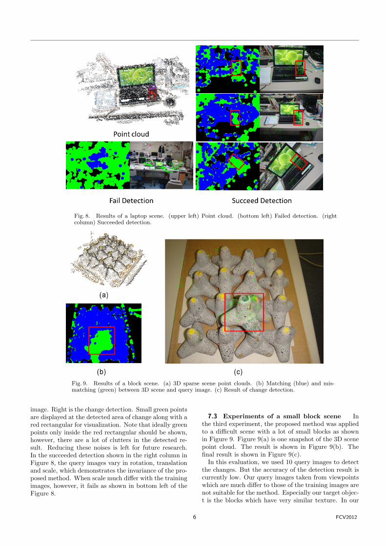
Fig. 8. Results of a laptop scene. (upper left) Point cloud. (bottom left) Failed detection. (rightcolumn) Succeeded detection.

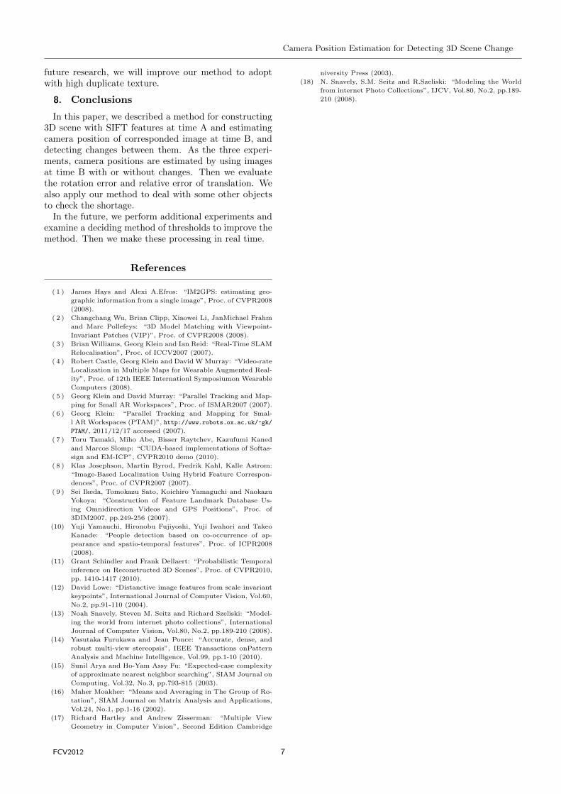
Fig. 9. Results of a block scene. (a) 3D sparse scene point clouds. (b) Matching (blue) and mis-matching (green) between 3D scene and query image. (c) Result of change detection.

image. Right is the change detection. Small green pointsare displayed at the detected area of change along with ared rectangular for visualization. Note that ideally greenpoints only inside the red rectangular should be shown,however, there are a lot of clutters in the detected re-sult. Reducing these noises is left for future research.In the succeeded detection shown in the right column inFigure 8, the query images vary in rotation, translationand scale, which demonstrates the invariance of the pro-posed method. When scale much differ with the trainingimages, however, it fails as shown in bottom left of theFigure 8.

7.3 Experiments of a small block scene Inthe third experiment, the proposed method was appliedto a difficult scene with a lot of small blocks as shownin Figure 9. Figure 9(a) is one snapshot of the 3D scenepoint cloud. The result is shown in Figure 9(b). Thefinal result is shown in Figure 9(c).

In this evaluation, we used 10 query images to detectthe changes. But the accuracy of the detection result iscurrently low. Our query images taken from viewpointswhich are much differ to those of the training images arenot suitable for the method. Especially our target objec-t is the blocks which have very similar texture. In our

6 FCV2012

Camera Position Estimation for Detecting 3D Scene Change

future research, we will improve our method to adoptwith high duplicate texture.

8. Conclusions

In this paper, we described a method for constructing3D scene with SIFT features at time A and estimatingcamera position of corresponded image at time B, anddetecting changes between them. As the three experi-ments, camera positions are estimated by using imagesat time B with or without changes. Then we evaluatethe rotation error and relative error of translation. Wealso apply our method to deal with some other objectsto check the shortage.

In the future, we perform additional experiments andexamine a deciding method of thresholds to improve themethod. Then we make these processing in real time.

References

( 1 ) James Hays and Alexi A.Efros: “IM2GPS: estimating geo-

graphic information from a single image”, Proc. of CVPR2008

(2008).

( 2 ) Changchang Wu, Brian Clipp, Xiaowei Li, JanMichael Frahm

and Marc Pollefeys: “3D Model Matching with Viewpoint-

Invariant Patches (VIP)”, Proc. of CVPR2008 (2008).

( 3 ) Brian Williams, Georg Klein and Ian Reid: “Real-Time SLAM

Relocalisation”, Proc. of ICCV2007 (2007).

( 4 ) Robert Castle, Georg Klein and David W Murray: “Video-rate

Localization in Multiple Maps for Wearable Augmented Real-

ity”, Proc. of 12th IEEE Internationl Symposiumon Wearable

Computers (2008).

( 5 ) Georg Klein and David Murray: “Parallel Tracking and Map-

ping for Small AR Workspaces”, Proc. of ISMAR2007 (2007).

( 6 ) Georg Klein: “Parallel Tracking and Mapping for Smal-

l AR Workspaces (PTAM)”, http://www.robots.ox.ac.uk/~gk/

PTAM/, 2011/12/17 accessed (2007).

( 7 ) Toru Tamaki, Miho Abe, Bisser Raytchev, Kazufumi Kaned

and Marcos Slomp: “CUDA-based implementations of Softas-

sign and EM-ICP”, CVPR2010 demo (2010).

( 8 ) Klas Josephson, Martin Byrod, Fredrik Kahl, Kalle Astrom:

“Image-Based Localization Using Hybrid Feature Correspon-

dences”, Proc. of CVPR2007 (2007).

( 9 ) Sei Ikeda, Tomokazu Sato, Koichiro Yamaguchi and Naokazu

Yokoya: “Construction of Feature Landmark Database Us-

ing Omnidirection Videos and GPS Positions”, Proc. of

3DIM2007, pp.249-256 (2007).

(10) Yuji Yamauchi, Hironobu Fujiyoshi, Yuji Iwahori and Takeo

Kanade: “People detection based on co-occurrence of ap-

pearance and spatio-temporal features”, Proc. of ICPR2008

(2008).

(11) Grant Schindler and Frank Dellaert: “Probabilistic Temporal

inference on Reconstructed 3D Scenes”, Proc. of CVPR2010,

pp. 1410-1417 (2010).

(12) David Lowe: “Distanctive image features from scale invariant

keypoints”, International Journal of Computer Vision, Vol.60,

No.2, pp.91-110 (2004).

(13) Noah Snavely, Steven M. Seitz and Richard Szeliski: “Model-

ing the world from internet photo collections”, International

Journal of Computer Vision, Vol.80, No.2, pp.189-210 (2008).

(14) Yasutaka Furukawa and Jean Ponce: “Accurate, dense, and

robust multi-view stereopsis”, IEEE Transactions onPattern

Analysis and Machine Intelligence, Vol.99, pp.1-10 (2010).

(15) Sunil Arya and Ho-Yam Assy Fu: “Expected-case complexity

of approximate nearest neighbor searching”, SIAM Journal on

Computing, Vol.32, No.3, pp.793-815 (2003).

(16) Maher Moakher: “Means and Averaging in The Group of Ro-

tation”, SIAM Journal on Matrix Analysis and Applications,

Vol.24, No.1, pp.1-16 (2002).

(17) Richard Hartley and Andrew Zisserman: “Multiple View

Geometry in Computer Vision”, Second Edition Cambridge

niversity Press (2003).

(18) N. Snavely, S.M. Seitz and R.Szeliski: “Modeling the World

from internet Photo Collections”, IJCV, Vol.80, No.2, pp.189-

210 (2008).

FCV2012 7