Calculation of conjugate heat transfer problem with volumetric heat generation using the Galerkin...

www.elsevier.com/locate/apm

Applied Mathematical Modelling 29 (2005) 477–495

Calculation of conjugate heat transfer problemwith volumetric heat generation using the Galerkin method

Andrej Horvat *, Borut Mavko 1

Jozef Stefan Institute, Reactor Engineering Division, Jamova 39, SI 1001 Ljubljana, Slovenia

Received 1 September 2003; received in revised form 1 August 2004; accepted 6 September 2004Available online 10 December 2004

Abstract

A mathematical model of fluid flow across a rod bundle with volumetric heat generation has been built.The rods are heated with volumetric internal heat generation. To construct the model, a volume averagetechnique (VAT) has been applied to momentum and energy transport equations for a fluid and a solidphase to develop a specific form of porous media flow equations. The model equations have been solvedwith a semi-analytical Galerkin method. The detailed velocity and temperature fields in the fluid flowand the solid structure have been obtained. Using the solution fields, a whole-section drag coefficient Cdand a whole-section Nusselt number Nu have also been calculated. To validate the developed solution pro-cedure, the results have been compared to the results of a finite volume method. The comparison shows anexcellent agreement. The present results demonstrate that the selected Galerkin approach is capable of per-forming calculations of heat transfer in a cross-flow where thermal conductivity and internal heat genera-tion in a solid structure has to be taken into account. Although the Galerkin method has limitedapplicability in complex geometries, its highly accurate solutions are an important benchmark on whichother numerical results can be tested.� 2004 Elsevier Inc. All rights reserved.

0307-904X/$ - see front matter � 2004 Elsevier Inc. All rights reserved.doi:10.1016/j.apm.2004.09.012

* Corresponding author. Address: ANSYS Europe Ltd., The Gemini Building, Fermi Avenue, Harwell Int. BusinessCentre, Didcot OX11 0QR, UK. Tel.: +44 1235 44 8067/+386 1 58 85 450; fax: +44 1235 44 8001/+386 1 56 12 335/258.E-mail addresses: [email protected], [email protected] (A. Horvat), [email protected] (B. Mavko).1 Tel.: +386 1 58 85 450; fax: +386 1 56 12 335/258.

mailto:[email protected]

mailto:[email protected]

Nomenclature

Ajk matrix of eigenvectorsA0 interface area between the fluid and the solid phase in REVA? W Æ H, channel flow areaB1 (S3/S1 � 2B5)(1 + n2exp(2n))B2 B1exp(2n)B3 �B1 � B2B4 �2B5 � B1nexp(n) + B2nexp(� n)B5 D5/(2D3)c specific heatCd whole-section drag coefficientCh local drag coefficientd rod diameterdh 4Vf/A0, hydraulic diameterD1 F1D2 F4S1/S2D3 F5S1/S2 + F4D4 F1S1/S2D5 F5S3/S1F1 ðafcfqfUd2hÞ=ðkfLÞF4 ðafd2hÞ=H2F5 ðhd2hSÞ=kfG1 �M4/(K(1 + exp(e)))G2 �G1 �M4/KG3 M4/Kh heat transfer coefficientH simulation domain heightI specific internal heat generation rateJ matrix of integralsK M3u, linearized drag coefficientL simulation domain lengthM2 (aflfdh)/(pfUH

2)M3 (ChdhS)/2M4 dh/Ln number of used orthogonal functionsNu Nusselt numberp pressure, pitch between rodsDp whole-section pressure dropQ heat flowReh qfudh/lf, Reynolds numberRHS right-hand side of an equation

478 A. Horvat, B. Mavko / Applied Mathematical Modelling 29 (2005) 477–495

S A0/V, specific surfaceS1 ðasd2hÞ=H2S2 ðhd2hSÞ=ksS3 ðasd2hIÞ=ðksðT g � T inÞÞts Ts � Tb, solid-phase temperature residueT temperatureTb solid phase temperature in absence of convectionTg temperature at the bottom, z = 0 positionTin temperature at the inflow, x = 0 positionu velocity in the streamwise directionU velocity scaleV representative elementary volume (REV)W simulation domain widthx streamwise coordinateX x-dependent part of the tsy horizontal spanwise coordinatez vertical spanwise coordinateZ z-dependent part of the ts

Greek lettersa volume fractionb eigenvaluesc p(2n � 1)/2e

ffiffiffiffiffiffiffiffiffiffiffiffiffiK=M2

pn

ffiffiffiffiffiffiffiffiffiffiffiffiffiffiD3=D2

pk thermal diffusivityl dynamic viscositym kinematic viscosityq density

Subscripts/superscriptsf fluid phasei, j, k, m indecess solid phasex in the streamwise x-directiony in the horizontal spanwise y-directionz in the vertical spanwise z-direction

Symbols^ dimensional variables[ ] values averaged over the whole simulation domain

A. Horvat, B. Mavko / Applied Mathematical Modelling 29 (2005) 477–495 479


1. Introduction

Flows across a solid structure are found in a number of different industrial installations. Mostoften, the subject has been extensively studied for various heat transfer applications. In heatexchangers that are usually used in power generation and chemical industries, heat is transportedfrom one fluid to the another. Due to a phase change or other chemical processes in working flu-ids, walls of an internal heat exchanger�s structure can be considered as isothermal (see [1–8]).In the electronics industry, heat sinks submerged in air or water flow are used to cool electronic

components (see, for example [9–14]). These heat exchangers consist mostly of a high conductingmaterial. The conjugate nature of heat transfer between the flow and the structure complicatesnumerical calculations as well as experimental work [15].In nuclear applications, an internal heat generation due to radioactive decay can be present.

When nuclear fuel rods are cooled with gas or water flow, conjugate heat transfer is coupled withthe volumetric heat generation [16–18]. In this work, our attention is focused on the last case,where high heat conductive rods with internal heat generation are cooled with water cross-flow.To model mass, momentum and energy flow, a volumetric averaging technique (VAT) has been

applied to the transport equations. The technique had been utilised for heat transfer applicationsby Travkin and Catton [19], and further applied to heat exchanger applications by Horvat [15],and Horvat and Catton [20]. In the present work, the volumetrically averaged transport equationswith related boundary conditions have been solved with the Galerkin method.The aim of the present work is to find a close-form solution of the conjugate heat transfer prob-

lem with volumetric heat generation. The applied Galerkin method is a semi-analytical methodwhere a solution field is anticipated to be a series of orthogonal functions. As it does not relyon a discretisation procedure, their results are therefore grid independent. In the past the Galerkinsolution technique was widely used for other transport phenomena related problems [21–24].Although the Galerkin method is a well-established technique, it has not been used for conjugateheat transfer problems with volumetric heat generation. Nevertheless, it should be mentioned thatthe Galerkin approach is not the optimal method for this kind of calculation due to seriouslimitations in the method�s applicability to more realistic geometries and boundary conditions.Nevertheless, it can predict gross flow features very quickly using only a few eigenmodes [25].

2. Simulation domain

Example calculations have been performed for a geometry arrangement that is similar to anexperimental test section used in the Morrin–Martinelli–Gier Memorial Heat Transfer Labora-tory at University of California, Los Angeles to study fluid–structure interactions [26]. A generalarrangement of the simulation domain is given in Fig. 1b.Circular rods with a diameter d ¼ 0:9525cm are attached to an isothermal plate that is 60.96cm

long and 30.48cm wide. Their height is 20cm and they are arranged in 64 rows in the streamwisedirection and in 16 rows in the transverse direction. A pitch-to-diameter ratio in the streamwisedirection is set to px=d ¼ 1:0 and in the transverse direction to py=d ¼ 2:0. The rods are manufac-tured from a cast aluminium alloy 195 and they are exposed to water cross-flow. The entry flowprofile is assumed to be fully developed.


3. Governing equations

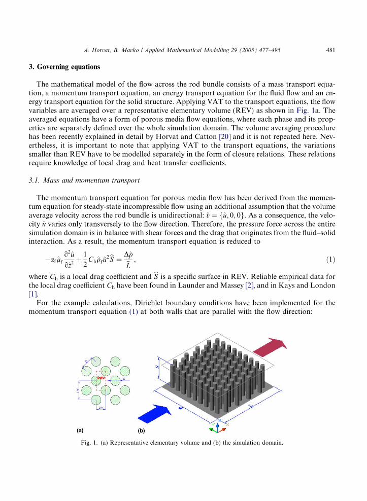
The mathematical model of the flow across the rod bundle consists of a mass transport equa-tion, a momentum transport equation, an energy transport equation for the fluid flow and an en-ergy transport equation for the solid structure. Applying VAT to the transport equations, the flowvariables are averaged over a representative elementary volume (REV) as shown in Fig. 1a. Theaveraged equations have a form of porous media flow equations, where each phase and its prop-erties are separately defined over the whole simulation domain. The volume averaging procedurehas been recently explained in detail by Horvat and Catton [20] and it is not repeated here. Nev-ertheless, it is important to note that applying VAT to the transport equations, the variationssmaller than REV have to be modelled separately in the form of closure relations. These relationsrequire knowledge of local drag and heat transfer coefficients.

3.1. Mass and momentum transport

The momentum transport equation for porous media flow has been derived from the momen-tum equation for steady-state incompressible flow using an additional assumption that the volumeaverage velocity across the rod bundle is unidirectional: v ¼ fu; 0; 0g. As a consequence, the velo-city u varies only transversely to the flow direction. Therefore, the pressure force across the entiresimulation domain is in balance with shear forces and the drag that originates from the fluid–solidinteraction. As a result, the momentum transport equation is reduced to

�af lfo2u

oz2þ 12Chqf u

2bS ¼ DpbL ; ð1Þ

where Ch is a local drag coefficient and bS is a specific surface in REV. Reliable empirical data forthe local drag coefficient Ch have been found in Launder and Massey [2], and in Kays and London[1].For the example calculations, Dirichlet boundary conditions have been implemented for the

momentum transport equation (1) at both walls that are parallel with the flow direction:

Fig. 1. (a) Representative elementary volume and (b) the simulation domain.


z ¼ 0: u ¼ 0;

z ¼ bH : u ¼ 0:ð2Þ

3.2. Heat transport in the fluid flow and the solid structure

The energy transport equation for the fluid flow has also been developed using the unidirec-tional velocity assumption. A temperature field in the fluid results from the balance between ther-mal convection in the streamwise direction, thermal diffusion and the heat transferred from thesolid structure to the fluid flow. Thermal diffusion in the streamwise direction is neglected. Thus,a differential form of the energy equation for the fluid is:

af qf cf uobT fox

¼ af kfo2bT foz2

� hðbT f � bT sÞbS ; ð3Þ

where h is a heat transfer coefficient between the fluid and the solid phase. The data for thelocal heat transfer coefficient h have been taken from Zukauskas and Ulinskas [8], and Kaysand London [1].The rod bundle structure in each REV is only loosely connected in the horizontal directions (see

Fig. 1). As a consequence, only the thermal diffusion in the vertical direction is in balance with theheat leaving the structure through the fluid–solid interface, whereas the thermal diffusion in thehorizontal directions can be neglected. This simplifies the energy equation for the solid structureto:

0 ¼ askso2bT soz2

þ hðbT f � bT sÞbS þ asbI ; ð4Þ

where as = 1 � af.Dirichlet boundary conditions have been imposed at the inflow and at the bottom, and Neu-

mann boundary conditions at the top:

x ¼ 0: bT f ¼ bT in;z ¼ 0: bT f ¼ bT g; bT s ¼ bT g;z ¼ bH :

obT foz

¼ 0; obT soz

¼ 0:

ð5Þ

Inserting the boundary conditions (5) in Eqs. (3) and (4), two additional boundary requirementscan be derived:

z ¼ 0: o2bT foz2

¼ 0; o2bT soz2

¼bIks;

z ¼ bH :o3bT foz3

¼ 0; o3bT soz3

¼ 0:

ð6Þ


4. Scaling procedure

In order to simplify further treatment and solution of the transport equations (1), (3) and (4),they are transformed into a dimensionless form. The dimensionless form of the equations enablesus to use more general algorithms that are already developed and are publicly accessible. Thetransformation has been carried out with a help of scaling factors that are presented in Eq. (7);the variables in the dimensional form are marked with a caret symbol ^ to be distinguish fromthe dimensionless variables.

x ¼ bLx; z ¼ bHz;u ¼ bUu; p ¼ qf bU 2

p; bU ¼ffiffiffiffiffiffiDpqf

s;

bT g � bT f ¼ ðbT g � bT inÞT f ; bT g � bT s ¼ ðbT g � bT inÞT s:ð7Þ

4.1. Mass and momentum transport

Inserting the scaling laws (7) in the momentum transport equation (1) the following form isderived:

�M2

o2uoz2

þM3u2 ¼ M4; ð8Þ

where M2 ¼ ðaflf dhÞ=ðpfUH 2Þ, M3 ¼ ðChdhbSÞ=2 and M4 ¼ dh=bL. These coefficients depend onthe geometry and the flow conditions, and they have been taken constant across the simulationdomain. Further, the momentum transport equation (8) has been linearized to

�M2

o2uoz2

þ Ku ¼ M4; ð9Þ

where K =M3u. Based on the scaling laws (7), the boundary conditions (2) are changed:

z ¼ 0: u ¼ 0;z ¼ 1: u ¼ 0:

ð10Þ

4.2. Heat transport in the fluid flow and the solid structure

The scaling laws (7) are introduced in the fluid-phase energy transport equation (3) that ischanged to

F 1uoT fox

¼ F 4o2T foz2

� F 5ðT f � T sÞ; ð11Þ

where F 1 ¼ ðaf cf qf bU d2hÞ=ðkfbLÞ, F 4 ¼ ðaf d2

hÞ= bH 2and F 5 ¼ ðhd2hbSÞ=kf are coefficients that have

been taken constant over the whole simulation domain.


As in the previous case, inserting the scaling laws (7) in the solid-phase energy transport equa-tion (4) gives the following form:

0 ¼ S1o2T soz2

þ S2ðT f � T sÞ � S3; ð12Þ

where S1 ¼ ðasd2

hÞ= bH 2, S2 ¼ ðhd2hbSÞ=ks and S3 ¼ ðasd

2

hbI Þ=ðksðbT g � bT inÞÞ are again coefficients that

have been taken constant over the whole simulation domain.Together with the transport equations, the boundary conditions (5) and the related boundary

requirements (6) are transformed into the dimensionless form:

x ¼ 0: T f ¼ 1;z ¼ 0: T f ¼ 0; T s ¼ 0;

z ¼ 1: oT foz

¼ 0; oT soz

¼ 0;ð13Þ

and

z ¼ 0: o2T foz2

¼ 0; o2T soz2

¼ S3S1

;

z ¼ 1: o3T foz3

¼ 0; o3T soz3

¼ 0:ð14Þ

5. Solution procedure

A solution of the linearized momentum transport equation (9) is expected to be of the formu exp(ez), where e is a constant. Taking into account the boundary conditions given byEq. (10), the fluid velocity is:

u ¼ G1 expðezÞ þ G2 expð�ezÞ þ G3; ð15Þ
where e ¼
ffiffiffiffiffiffiffiffiffiffiffiffiffiK=M2

p, G1 = �M4/(K(1 + exp(e))), G2 = �G1 �M4/K and G3 =M4/K are constants

that are defined from the boundary conditions.To find a solution to the energy transport equations (11) and (12), both equations are combined

into the single expression:

F 1uoT sox

þ F 4S1S2

o4T soz4

� F 5S1S2

þ F 4

� �o2T soz2

� F 1S1S2uo3T soxoz2

þ F 5S3S1

¼ 0: ð16Þ

Eq. (16) can be written in a more compact form as

D1uoT sox

þ D2o4T soz4

� D3o2T soz2

� D4uo3T soxoz2

þ D5 ¼ 0; ð17Þ

where D1 = F1, D2 = F4S1/S2, D3 = F5S1/S2 + F4, D4 = F1S1/S2 and D5 = F5S3/S1 are constants.Next, the solid-phase temperature field Ts is separated as

T sðx; zÞ ¼ T bðzÞ þ tsðx; zÞ; ð18Þ


where Tb is a temperature field in the absence of force convection across the rod bundle (u = 0)and ts is a solid-phase temperature residue. Inserting the decomposition (18) into Eq. (17), sepa-rate equations are written for the temperature Tb:

D2o4T boz4

� D3o2T boz2

þ D5 ¼ 0 ð19Þ

and for the temperature ts:

D1uotsox

þ D2o4tsoz4

� D3o2tsoz2

� D4uo3ts

oxoz2¼ 0: ð20Þ

The boundary conditions (13) are transformed to

x ¼ 0 : ts ¼ 1;

z ¼ 0 : ts ¼ 0; T b ¼ 0;

z ¼ 1 : otsoz

¼ 0; oT boz

¼ 0;

ð21Þ

and the additional relations (14) to

z ¼ 0 : o2tsoz2

¼ 0; o2T boz2

¼ S3S1

;

z ¼ 1 : o3tsoz3

¼ 0; o3T boz3

¼ 0:

ð22Þ

A solution of Eq. (19) can be found in the following form:

T b ¼ B1 expðnzÞ þ B2 expð�nzÞ þ B3 þ B4zþ B5z2; ð23Þ
where n ¼
ffiffiffiffiffiffiffiffiffiffiffiffiffiD3=D2

p, B1 = (S3/S1 � 2B5)/(1 + n2exp(2n)), B2 = B1exp(2n), B3 = �B1 � B2,

B4 = � 2B5 � B1nexp(n) + B2nexp(� n) and B5 = D5/(2D3) are constants that have to be deter-mined from the boundary conditions (21) and (22).To find the temperature field ts as a solution of Eq. (20), separation of variables is used

ts ¼ X ðxÞZðzÞ: ð24Þ
The solution of Eq. (20) in the z-direction is anticipated to be a finite set of n orthogonalfunctions:
Z ¼ AkZk; Zk ¼ sinðckzÞ; ck ¼2k � 12

p; k ¼ 1; n; ð25Þ

which satisfy the boundary conditions (21) and the addition relations (22). Introducing Eq. (25)into Eq. (20) brings us to

D1uX 0ðAkZkÞ þ D2X ðAkc4kZkÞ þ D3X ðAkc2kZkÞ þ D4uX 0ðAkc2kZkÞ ¼ error; ð26Þ
and in a more compact form to
X 0AkufD1 þ c2kD4gZk þ XAkfc4kD2 þ c2kD3gZk ¼ error: ð27Þ


As the series is finite, there is a certain discrepancy associated with the series expansion (25). Thiserror is orthogonal to the set of functions used for the expansion and can be reduced by multipli-cation with Zj (j = 1,n) and further integration from 0 to 1:

X 0Ak

Z 1

0

ufD1 þ c2kD4gZkZjdzþ XAk

Z 1

0

fc4kD2 þ c2kD3gZkZjdz ¼ 0: ð28Þ

In a matrix form, Eq. (28) is written as

X 0AkJð1Þkj þ XAkJ

ð2Þkj ¼ 0; ð29Þ

where J ð1Þkj and Jð2Þkj are integrals that have been calculated analytically. As the x and z dependent

parts of Eq. (29) can be separated:

b ¼ �X0

X¼AkJ

ð2Þkj

AkJð1Þkj

; ð30Þ

separate equations are written for the x-direction:

X 0 þ bX ¼ 0; ð31Þ
and for the z-direction:
AkJð2Þkj � bAkJ

ð1Þkj ¼ 0: ð32Þ

The solution of Eq. (31) is obtained by integration:

X ¼ C expð�bxÞ; ð33Þ
where C and b are arbitrary constants.Rearranging Eq. (32), an extended eigenvalue problem can be formed as
ðJ ð2Þkj � bJ ð1Þkj ÞAk ¼ 0: ð34Þ

The system of Eq. (34) has a non-trivial solution if

DetðJ ð2Þkj � bJ ð1Þkj Þ ¼ 0: ð35Þ

From this condition, a set of n eigenvalues b have been determined. Furthermore, each eigenvaluebj (j = 1,n) corresponds to a specific j eigenvector Ak that has also been calculated.Using the solutions of Eq. (31) and of the matrix system (35), one can construct the temperature

field:

ts ¼ CjX jAjkZk; ð36Þ
where Cj is a vector of coefficients that has to be determined. Adding the temperature fields Tb(Eq. (23)) and ts (Eq. (36)), the expression for the dimensionless solid-phase temperature Ts iswritten as
T s ¼ ðB1 expðnzÞ þ B2 expð�nzÞ þ B3 þ B4zþ B5z2Þ þ CjX jAjkZk: ð37Þ


Recalling Eq. (12):

T f ¼ � S1S2

o2T soz2

þ T s þS3S2

; ð38Þ

and inserting the expression for the solid-structure temperature Ts (Eq. (37)), the dimensionlessfluid temperature is given by

T f ¼ CjAjk 1þ S1S2

c2k

� �Zk þ B1 1� S1

S2n2

� �expðnzÞ þ B2 1� S1

S2n2

� �expð�nzÞ

þ B3 � 2B5S1S2

þ S3S2

� �þ B4zþ B5z2: ð39Þ

The coefficients Cj have been found from the boundary condition Tf(0,z) = 1. Applying it toEq. (39), one can write:

CjAjk 1þ S1S2

c2k

� �Zk ¼ B1

S1S2

n2 � 1� �

expðnzÞ þ B2S1S2

n2 � 1� �

expð�nzÞ

þ 1� B3 þ 2B5S1S2

� S3S2

� �� B4z� B5z2: ð40Þ

Again, multiplying Eq. (40) by Zi (i = 1,n) and integrating it from 0 to 1:

CjAjk 1þ S1S2

c2k

� �Z 1

0

ZkZidz

¼ B1S1S2

n2 � 1� �Z 1

0

expðnzÞZidzþ B2S1S2

n2 � 1� �Z 1

0

expð�nzÞZidz

þ 1� B3 þ 2B5S1S2

� S3S2

� �Z 1

0

Zidz� B4

Z 1

0

zZidz� B5

Z 1

0

z2Zi dz; ð41Þ

the orthogonality condition reduces Eq. (41) to

CjAji 1þS1S2

c2i

� �J ð1Þi ¼ B1

S1S2

n2 � 1� �

J ð2Þi þ B2S1S2

n2 � 1� �

J ð3Þi þ 1� B3 þ 2B5S1S2

� S3S2

� �J ð4Þi

� B4Jð5Þi � B5J

ð6Þi ; ð42Þ

where J ð1Þi , Jð2Þi , J

ð3Þi , J

ð4Þi , J

ð5Þi and J ð6Þi are analytically calculated integrals. Writing Eq. (42) in a

matrix form:

CjAji ¼RHS

1þ S1S2

c2i�

J ð1Þi; ð43Þ

the unknown coefficients Cj have been calculated by inversion of the matrix system (43).Introducing the calculated coefficients Cj in the relations (37) and (39), the dimensional values

of the solid-structure temperature field bT s and the fluid flow temperature field bT f have beenobtained from the scaling relations:

TableThe wvolum

Dp [PbT in [�bT g [�C


bT s ¼ bT g � ðbT g � bT inÞT s; ð44Þ
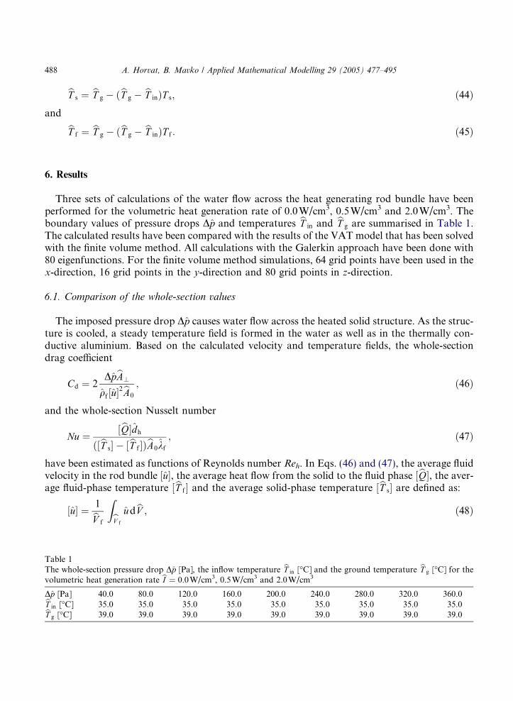
and bT f ¼ bT g � ðbT g � bT inÞT f : ð45Þ
6. Results

Three sets of calculations of the water flow across the heat generating rod bundle have beenperformed for the volumetric heat generation rate of 0.0W/cm3, 0.5W/cm3 and 2.0W/cm3. Theboundary values of pressure drops Dp and temperatures bT in and bT g are summarised in Table 1.The calculated results have been compared with the results of the VAT model that has been solvedwith the finite volume method. All calculations with the Galerkin approach have been done with80 eigenfunctions. For the finite volume method simulations, 64 grid points have been used in thex-direction, 16 grid points in the y-direction and 80 grid points in z-direction.

6.1. Comparison of the whole-section values

The imposed pressure drop Dp causes water flow across the heated solid structure. As the struc-ture is cooled, a steady temperature field is formed in the water as well as in the thermally con-ductive aluminium. Based on the calculated velocity and temperature fields, the whole-sectiondrag coefficient

Cd ¼ 2DpbA?

qf ½u 2bA0 ; ð46Þ

and the whole-section Nusselt number

Nu ¼ ½bQ dhð½bT s � ½bT f ÞbA0kf ; ð47Þ

have been estimated as functions of Reynolds number Reh. In Eqs. (46) and (47), the average fluidvelocity in the rod bundle ½u , the average heat flow from the solid to the fluid phase ½bQ , the aver-age fluid-phase temperature ½bT f and the average solid-phase temperature ½bT s are defined as:

½u ¼ 1bV fZbV f udbV ; ð48Þ

1hole-section pressure drop Dp [Pa], the inflow temperature bT in [�C] and the ground temperature bT g [�C] for theetric heat generation rate bI ¼ 0:0W/cm3, 0.5W/cm3 and 2.0W/cm3a] 40.0 80.0 120.0 160.0 200.0 240.0 280.0 320.0 360.0C] 35.0 35.0 35.0 35.0 35.0 35.0 35.0 35.0 35.0] 39.0 39.0 39.0 39.0 39.0 39.0 39.0 39.0 39.0


b Z b b Z b b� �
½Q ¼ af cf qf bAout uT f dA � bA in uT f dA ;
1Z

½bT f ¼ ½u bV f bV f ubT f dbV ;
1
Z� �
ðbAg þ bA0Þ½bT s ¼ bAgbT g þ bA0 bV s bV s bT s dbV :
The whole-section values of the drag coefficient Cd and the Nusselt number Nu calculated with theGalerkin method have been compared with the results of the finite volume method to validate thedeveloped semi-analytical algorithm.Fig. 2 shows the whole-section drag coefficient Cd (Eq. (46)) as a function of Reynolds number

Reh. As the material properties have been set as constant, the drag coefficient does not changewith the volumetric heat generation rate bI . The results calculated with the Galerkin method arepractically identical to the results obtained by the finite volume method. Table 2 gives numericalvalues of the calculated Reynolds number Reh and the whole-section drag coefficient Cd.Fig. 3 presents the whole-section Nusselt number Nu (Eq. (47)) as a function of Reynolds num-

ber Reh for the volumetric heat generation rate bI ¼ 0:0W/cm3, 0.5W/cm3 and 2.0W/cm3. Again,the comparison with the finite volume results reveal an excellent agreement for the all three vol-umetric generation rates bI . There are slight differences in the case without heat generation(bI ¼ 0:0W/cm3). Namely, due to the absence of the volumetric heat generation, heat transfer

500 1000 1500 2000

Reh

45

50

55

Cd

Galerkin methodFinite volume method

Fig. 2. Whole-section drag coefficient Cd as a function of Reynolds number Reh.

Table 3Reynolds number Reh and the whole-section Nusselt number Nu calculated with the Galerkin method (GM) and withthe finite volume method (FVM) for the volumetric heat generation rate bI ¼ 0:0W/cm3 (Nu 1), 0.5W/cm3 (Nu 2) and2.0W/cm3 (Nu 3)

Reh (GM) 643 942 1177 1378 1558 1722 1875 2017 2152Nu 1 (GM) 34.54 42.71 48.31 52.70 56.36 59.53 62.34 64.86 67.15Nu 2 (GM) 44.19 54.45 61.48 66.98 71.56 75.52 79.03 82.19 85.06Nu 3 (GM) 47.25 58.77 66.75 73.04 78.32 82.91 86.99 90.68 94.06Reh (FVM) 643 941 1176 1378 1557 1722 1874 2017 2152Nu 1 (FVM) 34.50 42.43 47.85 52.08 55.60 58.65 61.34 63.77 65.98Nu 2 (FVM) 44.30 54.50 61.47 66.90 71.43 75.33 78.79 81.90 84.73Nu 3 (FVM) 47.42 58.97 66.95 73.25 78.53 83.11 87.19 90.87 94.25

Reh

30

40

50

60

70

80

90

100

110

Nu

Galerkin method I=2.0W/cm3

Finite volume method I=2.0W/cm3





1000 20001500

Fig. 3. Whole-section Nusselt number Nu as a function of Reynolds number Reh.

Table 2Reynolds number Reh and the whole-section drag coefficient Cd calculated with the Galerkin method (GM) and withthe finite volume method (FVM)

Reh (GM) 643 942 1177 1378 1558 1722 1875 2017 2152Cd (GM) 52.22 48.73 46.80 45.48 44.48 43.68 43.02 42.45 41.96Reh (FVM) 643 941 1176 1378 1557 1722 1874 2017 2152Cd (FVM) 52.22 48.74 46.81 45.49 44.50 43.70 43.03 42.47 41.98


in the rod bundle is dominated by diffusion processes close to the bottom wall, which producesteep gradients in velocity and temperature fields. These gradients are hard to model accurately,therefore both methods produce slightly different results (Table 3).

0.02 0.03 0.04 0.05 0.06 0.07 0.08 0.09 0.1 0.11

u[m/s]

0

0.05

0.1

0.15

0.2

z[m

]

GM, Reh=643FVM, Reh=643GM, Reh=942FVM, Reh=942GM, Reh=1177FVM, Reh=1177GM, Reh=1378FVM, Reh=1378GM, Reh=1558FVM, Reh=1558GM, Reh=1722FVM, Reh=1722GM, Reh=1875FVM, Reh=1875GM, Reh=2017FVM, Reh=2017GM, Reh=2152FVM, Reh=2152

Fig. 4. Velocity distribution for different Reynolds numbers Reh.

0

0.05

0.1

0.15

0.2

z[m

]

0 0.1 0.2 0.3 0.4 0.5 0.6

x [m]

111111

23 45 5 6 66 6

LevelT:

135.5

236.0

336.5

437.0

537.5

638.0

738.5

0

0.05

0.1

0.15

0.2

z[m

]

0 0.1 0.2 0.3 0.4 0.5 0.6

x [m]

111

23 3

4 44

LevelT:

135.5

236.0

336.5

437.0

537.5

638.0

Galerkin method

finite volume method

(a)

(b)

Fig. 5. Temperature field (a) in the solid structure and (b) in the water flow; bI ¼ 0:0W/cm3, Reh = 643.



6.2. Velocity and temperature distribution in the rod bundle

Velocity and temperature fields calculated with the Galerkin method have been compared withthe finite volume method results. Namely, the comparison of detailed velocity and temperaturefields at different Reynolds numbers ease identification of calculation problems and errors.Fig. 4 shows the velocity distributions obtained with the Galerkin method (marked as GM) and

the finite volume method (marked as FVM). The core of the simulation domain has a flat velocityprofile due to the drag associated with the submerged rods. The comparison reveals an excellentagreement between both methods, although the VAT momentum equation in the present Galer-kin solver (Eq. (9)) is simply linearized.The calculations have been performed for all the cases listed in Table 1. Nevertheless, only some

representative examples of the calculated temperature fields in the fluid flow and the solid struc-ture are shown here.Fig. 5 gives a temperature field cross-section for the Reynolds number Reh = 643. The internal

heat generation in the rods is set to bI ¼ 0:0W/cm3. Temperatures are presented in the Celsiusscale. Black isotherms denote the results obtained with the Galerkin method and gray (halftone)

0

0.05

0.1

0.15

0.2

z[m

]

0 0.1 0.2 0.3 0.4 0.5 0.6

x [m]

1

1

2

2

2

2

2

2

345

56

8 1011 12

LevelT:

135.6

235.8

336.0

436.2

536.4

636.6

736.8

837.0

937.2

1037.4

1137.6

1237.8

1338.0

1438.2

0

0.05

0.1

0.15

0.2

z[m

]

0 0.1 0.2 0.3 0.4 0.5 0.6

x [m]

1

1

1

2

2

22

3

3

3

33

3 445

55

66666

7 8910 10 13

LevelT:

135.2

235.4

335.6

435.8

536.0

636.2

736.4

836.6

936.8

1037.0

1137.2

1237.4

1337.6

1437.8

Galerkin method


(a)

(b)



isotherms denote temperatures obtained with the finite-volume method. Isotherms show that heatis being solely transported to the flow from the isothermal bottom wall. As the thermal conduc-tivity of the aluminium rods is higher than of the water flow, the temperature field is more devel-oped in the solid structure (Fig. 5a) than in the flow (Fig. 5b). The comparison of the temperaturefields calculated with the Galerkin and the finite volume method shows an excellent agreement.Fig. 6 presents a temperature field cross-section for the Reynolds number Reh = 1559 at the

internal heat generation rate bI ¼ 0:5W/cm3. Besides a clearly visible heating effect from the bot-tom, the isotherms also reveal gradual heating of the flow due to the internal heat generation inthe solid structure; the isotherms are equally spaced and vertically oriented. A comparison of theisotherms shows only slight discrepancy between the results of the Galerkin and the finite volumemethod. It is believed that discrepancies arose from linearization of the momentum equation (1)and taking a single value for Ch, whereas in the VAT model solved by the finite volume methodthese simplifications were not implemented.In Fig. 7, the internal heat generation rate in the solid structure is increased to bI ¼ 2:0W/cm3.

The Reynolds number for the present case is Reh = 2152. Due to the increase in the volumetric

0

0.05

0.1

0.15

0.2

z[m

]

0 0.1 0.2 0.3 0.4 0.5 0.6

x [m]

1

1

2

23

33

33

44

4

4

55

6

6

66

6

6

6

6

77

77 8

8

8

9 9

99

9

9

9

10

1010

LevelT:

136.2

236.4

336.6

436.8

537.0

637.2

737.4

837.6

937.8

1038.0

1138.2

1238.4

1338.6

1438.8

0

0.05

0.1

0.15

0.2

z[m

]

0 0.1 0.2 0.3 0.4 0.5 0.6

x [m]

22

2

3

3

44

5

5

5

5

5

66

777

8

8

8

9

8 11 10 10 1113

LevelT:

135.2

235.4

335.6

435.8

536.0

636.2

736.4

836.6

936.8

1037.0

1137.2

1237.4

1337.6

1437.8

Galerkin method


(a)

(b)



heat generation rate bI , the temperature dominantly increases in the horizontal direction, from theinflow to the outflow. Heating from the bottom becomes a secondary heat transport mechanism.The water flow leaves the simulated section at temperatures above 36.8�C. Again, the comparisonof the plotted isotherms reveals only negligible difference between the results of the Galerkin andthe finite volume method.

7. Conclusions

The paper presents an effort to utilize the Galerkin method for solving the conjugate heat trans-fer problems where a volumetric heat generation is present in a solid phase.In the scope of this work the volume averaging technique (VAT) was applied to the simulation

of water flow across the aluminium rods with the internal heat generation. The VAT basic ruleswere used to develop a specific form of the porous media flow model. To close the system ofthe transport equations, reliable data for the drag and the heat transfer coefficients werefound in [1,2,8]. The advantage of using VAT is that the computational algorithm is fast, but stillable to present a detailed picture of temperature fields in the fluid flow as well as in the solidstructure.The geometry of the simulation domain and the boundary conditions were similar to the experi-

mental test section used in the Morrin–Martinelli–Gier Memorial Heat Transfer Laboratory atthe University of California, Los Angeles [26]. The calculations were performed for three differentvolumetric heat generation rates bI ¼ 0:0W/cm3, 0.5W/cm3 and 2.0W/cm3 and nine different pres-sure drops Dp. The imposed pressure drops achieved coolant flow of the Reynolds number Rehfrom 643 to 2152.The semi-analytical Galerkin procedure was developed to solve the system of equations. The

calculated whole-section drag coefficient Cd and the Nusselt number Nu were compared withthe results of the finite volume method to validate the developed semi-analytical algorithm.The comparisons show an excellent agreement. The small differences appear only in the case with-out volumetric heat generation (bI ¼ 0:0W/cm3), when the steepest temperature gradients occurclose to the simulation domain�s bottom wall. The detailed velocity and temperature fields inthe coolant flow as well as in the heat conducting structure were also calculated and comparedwith the results of the finite volume method. The comparison shows negligible differences betweenthe results of both methods.The results demonstrate that the selected Galerkin approach is an appropriate method to ob-

tain a close-form solution of the cross-flow problem with heat transfer when the thermal conduc-tivity and the volumetric heat generation in the solid structure significantly influence the heattransfer and therefore have to be taken into account.

Acknowledgment

A. Horvat gratefully acknowledges the financial support received from the Ministry of Educa-tion, Science and Sport of Republic of Slovenia under the project ‘‘Determination of morpholog-ical parameters for optimisation of heat exchanger surfaces’’.


References

[1] W.S. Kays, A.L. London, Compact Heat Exchangers, third ed., Krieger Publishing Company, Malabar, FL, 1998,pp. 152–155.

[2] B.E. Launder, T.H. Massey, The numerical prediction of viscous flow and heat transfer in tube banks, J. HeatTransfer 100 (1978) 565–571.

[3] A.A. Johnson, T.E. Tezduyar, J. Lion, Numerical simulations of flows past periodic arrays of cylinders, Comput.Mech. 11 (1983) 371–383.

[4] M. Fujii, T. Fujii, T. Nagata, A numerical analysis of laminar flow and heat transfer of air in an in-line tube bank,Numer. Heat Transfer 7 (1984) 89–102.

[5] G.R. Noghrehkar, M. Kawaji, A.M.C. Chan, Investigation of two-phase flow regimes in tube bundles under cross-flow conditions, Int. J. Multiphase Flow 25 (1999) 857–874.

[6] A. Zukauskas, Heat transfer from tubes in crossflow, Adv. Heat Transfer 8 (1972) 93–160.[7] A. Zukauskas, Convective Heat Transfer in Cross Flow, Handbook of Single-Phase Convective, Wiley & Sons,New York, 1987.

[8] Zukauskas, A. Ulinskas, Efficiency parameters for heat transfer in tube banks, J. Heat Transfer Eng. 5 (1) (1985)19–25.

[9] K. Al-Jamal, H. Khashashneh, Experimental investigation in heat transfer of triangular and pin fins arrays, Int. J.Heat Mass Transfer 34 (1998) 159–162.

[10] A. Bejan, The optimal spacing for cylinders in crossflow forced convection, J. Heat Transfer 117 (1995) 767–770.[11] A. Bejan, E. Sciubba, The optimal spacing of parallel plates cooled by forced convection, Int. J. Heat Mass

Transfer 35 (12) (1992) 3264–3529.[12] G. Fabbri, Optimum performances of longitudinal convective fins with symmetrical and asymmetrical profiles, Int.

J. Heat Fluid Flow 20 (1999) 634–641.[13] G. Ledezma, A. Bejan, Heat sinks with sloped plate fins in natural and forced convection, Int. J. Heat Mass

Transfer 39 (9) (1996) 1773–1783.[14] H. Yuncu, G. Anbar, An experimental investigation on performance of rectangular fins on a horizontal base in free

convection heat transfer, Heat Mass Transfer 33 (1998) 507–514.[15] A. Horvat, Calculation of Conjugate Heat Transfer in a Heat Sink Using Volume Averaging Technique (VAT),

M.Sc. Thesis, University of California, Los Angeles, CA, 2002.[16] P.Y.P. Chen, J.J. Thompson, Conjugate heat transfer problem with nuclear heating, 2nd Conf. on Struct. Mech. in

Reactor Tech., Berlin, 1973, Proceedings, L1/3.[17] G. Lebon, P. Mathieu, A numerical calculation of nonlinear transient heat conduction in the fuel elements of a

nuclear reactor, Int. J. Heat Mass Transfer 22 (8) (1979) 1187–1198.[18] S.Y. Lee, R.L. Sindelar, D.C. Losey, Thermal modeling and performance analysis of interim dry storage and

geologic disposal facilities for spent nuclear fuel, Radioactive Waste Manage. Disposal 131 (1) (2000) 124–151.[19] V.S. Travkin, I. Catton, Transport phenomena in heterogeneous media based on volume averaging theory, Adv.

Heat Transfer 34 (1999) 1–143.[20] A. Horvat, I. Catton, Numerical technique for modeling conjugate heat transfer in an electronic device heat sink,

Int. J. Heat Mass Transfer 46 (2003) 2155–2168.[21] I. Catton, Convection in a closed rectangular region: the onset of motion, Trans. ASME 1 (1970) 186–188.[22] I. Catton, Effect of wall conduction on the stability of a fluid in a rectangular region heated from below, Trans.

ASME 1 (1972) 446–452.[23] J.M. McDonough, I. Catton, A mixed finite difference-Galerkin procedure for 2D convection in a square box, Int.

J. Heat Mass Transfer 25 (1982) 1137–1146.[24] L.A. Howle, A comparison of the reduced Galerkin and pseudo-spectral methods for simulation of steady

Rayleigh–Benard convection, Int. J. Heat Mass Transfer 39 (12) (1996) 2401–2407.[25] A. Horvat, I. Catton, Application of Galerkin method to conjugate heat transfer calculation, Numerical Heat

Transfer B: Fundamentals 44 (2003) 509–531.[26] I. Catton, P. Adinolfi, O. Alquaddoomi, Fluid-elastic instability in tube arrays, Trans. of the American Nuclear

Society: Winter Annual Meeting 2002, Washington DC, November 2002.

Calculation of conjugate heat transfer problem with volumetric heat generation using the Galerkin...

Documents

Transcript of Calculation of conjugate heat transfer problem with volumetric heat generation using the Galerkin...