c© 2018 Cara Monical

brought to you by COREView metadata, citation and similar papers at core.ac.uk

provided by Illinois Digital Environment for Access to Learning and Scholarship Repository

POLYNOMIALS IN ALGEBRAIC COMBINATORICS

BY

CARA MONICAL

DISSERTATION

Submitted in partial fulfillment of the requirementsfor the degree of Doctor of Philosophy in Mathematics

in the Graduate College of theUniversity of Illinois at Urbana-Champaign, 2018

Urbana, Illinois

Doctoral Committee:

Professor Rinat Kedem, ChairProfessor Alexander Yong, Director of ResearchProfessor Philippe di FrancescoProfessor Susan Tolman

Abstract

A long-standing theme in algebraic combinatorics is to study bases of the rings of symmetric

functions, quasisymmetric functions, and polynomials. Classically, these bases are homoge-

neous functions, however, the introduction of K-theoretic combinatorics has led to increased

interest in finding inhomogeneous deformations of classical bases.

Joint with A. Yong and N. Tokcan, we introduce the notion of saturated Newton polytope

(SNP), a property of polynomials, and study its prevalence in algebraic combinatorics. We

find that many, but not all, of the families that arise in other contexts of algebraic combi-

natorics are SNP. We introduce a family of polytopes called the Schubitopes and connect it

to the Newton polytopes of the Schubert polynomials and the key polynomials.

Semistandard skyline fillings are a combinatorial model that arises from specializing the

combinatorics of Macdonald polynomials. We define a set-valued extension which allows

us to define inhomogeneous deformations of the Demazure atoms, key polynomials, and

quasisymmetric Schur functions. We prove that these deformations act in many ways like

their homogeneous counterparts.

We then continue the work on set-valued skyline fillings. Joint with O. Pechenik and

D. Searles, we provide deformations of the quasikey polynomials and the fundamental par-

ticles. This allows us to lift the quasisymmetric Grothendieck polynomials from the ring

of quasisymmetric polynomials to the ring of polynomials and give expansions between the

different bases under consideration that are analogous to the homogeneous case.

We end with some conjectures on the structure constants of equivariant Schubert calculus

in Type B and C, including a generalization of the Horn inequalities to this setting.

ii

Dedicated to all my friends and family who never stopped believing in me.

iii

Acknowledgments

My first thanks go to my advisor, Alexander Yong, for his dedicated guidance and support.

Over the last few years, he has greatly improved my mathematical depth and writing, and

I am grateful for the time and energy he has invested in my success. I would not be the

mathematician I am now without his mentorship. I would like to thank the other members

of my committee: Philippe Di Francesco, Rinat Kedem, and Susan Tolman.

I am extremely grateful for the algebraic combinatorics community at large who has wel-

comed me at conferences and encouraged my work. I have been inspired by your passion

for the field and your open and friendly community. Specifically, I am much in debt to

my academic siblings Dominic Searles, Oliver Pechenik, and especially my conference buddy

Anna Weigandt for all our conversations and companionship.

Finally, I want to thank everyone who has supported me on this journey – in ways both

big and small. My parents for their faith that I would succeed and practical advice when I

was stuck; Simone Sisneros-Thiry for so many evenings at home and mornings at Le Peep

of emotional support; Jennifer McNeilly for support in her office in all kinds of matters;

my college friends Kara Beer, Hillary Dawe, Katie Smalley, and Elizabeth Wakefield for not

giving up on me; my undergrad professors, particularly Ellen Swanson and Alex McAllister,

for inspiring me in mathematics and encouraging me; and most especially Cole Johnson

whose unwavering support can always be counted on.

This research has been partially funded by a GAANN fellowship from the Mathematics

Department at the University of Illinois and the Diffenbaugh Fellowship from the University

of Illinois.

iv

TABLE OF CONTENTS

LIST OF SYMBOLS . . . . . . . . . . . . . . . . . . . . . . . . . . . . . . . . . . . . vii

CHAPTER 1 INTRODUCTION . . . . . . . . . . . . . . . . . . . . . . . . . . . . 11.1 Partitions, Compositions, and Permutations . . . . . . . . . . . . . . . . . . 21.2 Symmetric Functions . . . . . . . . . . . . . . . . . . . . . . . . . . . . . . . 51.3 Quasisymmetric Functions . . . . . . . . . . . . . . . . . . . . . . . . . . . . 111.4 Polynomials . . . . . . . . . . . . . . . . . . . . . . . . . . . . . . . . . . . . 131.5 Combinatorics of Macdonald Polynomials . . . . . . . . . . . . . . . . . . . . 161.6 K-Theoretic Combinatorics . . . . . . . . . . . . . . . . . . . . . . . . . . . 281.7 Organization . . . . . . . . . . . . . . . . . . . . . . . . . . . . . . . . . . . 32

CHAPTER 2 SATURATED NEWTON POLYTOPES . . . . . . . . . . . . . . . . 332.1 Introduction . . . . . . . . . . . . . . . . . . . . . . . . . . . . . . . . . . . . 332.2 Symmetric functions . . . . . . . . . . . . . . . . . . . . . . . . . . . . . . . 372.3 Macdonald polynomials . . . . . . . . . . . . . . . . . . . . . . . . . . . . . . 512.4 Quasisymmetric functions . . . . . . . . . . . . . . . . . . . . . . . . . . . . 582.5 Schubert polynomials and variations . . . . . . . . . . . . . . . . . . . . . . 61

CHAPTER 3 SET-VALUED SKYLINE FILLINGS . . . . . . . . . . . . . . . . . . 723.1 Introduction . . . . . . . . . . . . . . . . . . . . . . . . . . . . . . . . . . . . 723.2 Combinatorial Lascoux Atoms . . . . . . . . . . . . . . . . . . . . . . . . . . 773.3 Quasisymmetric Grothendieck Functions . . . . . . . . . . . . . . . . . . . . 813.4 Conjectures . . . . . . . . . . . . . . . . . . . . . . . . . . . . . . . . . . . . 85

CHAPTER 4 KAONS AND QUASILASCOUX POLYNOMIALS . . . . . . . . . . 894.1 Introduction and Background . . . . . . . . . . . . . . . . . . . . . . . . . . 894.2 Kaons . . . . . . . . . . . . . . . . . . . . . . . . . . . . . . . . . . . . . . . 1024.3 QuasiLascoux polynomials . . . . . . . . . . . . . . . . . . . . . . . . . . . . 1104.4 Lascoux Polynomials . . . . . . . . . . . . . . . . . . . . . . . . . . . . . . . 115

v

CHAPTER 5 CONJECTURES ABOUT SCHUBERT CALCULUS . . . . . . . . . 1185.1 Introduction . . . . . . . . . . . . . . . . . . . . . . . . . . . . . . . . . . . . 1185.2 The Horn Inequalities . . . . . . . . . . . . . . . . . . . . . . . . . . . . . . . 123

REFERENCES . . . . . . . . . . . . . . . . . . . . . . . . . . . . . . . . . . . . . . . 129

vi

LIST OF SYMBOLS

Partitions, Compositions, and Permutations

λ A partition.

α A composition.

γ A weak composition.

`(γ) The length of γ.

|γ| The size of γ.

xγ The monomial xγ11 xγ22 · · ·x

γ`` .

λ ` n λ is a partition of n.

Par(n) The set of partitions of n.

Comp(n) The set of compositions of n.

WC(n) The set of weak compositions of n.

Par The set of all partitions.

Comp The set of all compositions.

WC The set of all weak compositions.

λ′ The conjugate of λ.

⊆ Partition containment.

≤D Dominance order on partitions, compositions, or permutations.

α � β α is a refinement of β.

vii

γ∗ The weak composition formed by reversing the order of the parts of γ.

γ+ The composition formed by dropping zeros from γ.

λ(γ) The partition formed by sorting the parts of γ in weakly decreasing order.

PermutWC(λ) The set of all weak compositions γ such that λ(γ+) = λ.

PermutC(λ) The set of all compositions α such that λ(α) = λ.

Expand(α) The set of all weak compositions γ such that γ+ = α.

Sm The group of permutations on m letters.

S∞ The group of permutations of Z>0 that fix all but finitely many elements.

w A permutation.

si The elementary transposition swapping i and i+ 1.

D(w) The Rothe diagram of w.

c(w) The Lehmer code of w.

w0 The longest permutation in Sn.

≤B (Strong) Bruhat order on permutations.

Koh(w) The set of all Kohnert diagrams of w.

w(γ) The result of applying the permutation w to γ.

wγ The permutation such that wγ(λγ) = γ.

� The order λ(γ) = λ(δ) and wγ ≤B wδ.

6 Lexicographic order on weak compositions.

Polynomial Families and Polynomial Rings

mλ Monomial symmetric function.

eλ Elementary symmetric function.

hλ Homogeneous symmetric function.

pλ Power sum symmetric function.

viii

sλ Schur function.

sλ Dual Schur function.

Mα Monomial quasisymmetric function.

Fα Fundamental quasisymmetric function.

Sα Quasisymmetric Schur function.

mγ Monomial function.

Sw Schubert polynomial.

Atomγ Demazure atom.

Keyγ Key polynomial.

Slideγ Slide polynomial.

QKeyγ Quasikey polynomial.

Parγ Fundamental particle.

Ksλ Symmetric Grothendieck function.

KFα Multifundamental quasisymmetric function.

KSα Quasisymmetric Grothendieck function.

KSw Grothendieck function.

KAtomγ Lascoux atom.

KKeyγ Lascoux polynomial.

KSlideγ Glide polynomial.

KQKeyγ QuasiLascoux polynomial.

KParγ Kaon.

Pλ Symmetric Macdonald polynomial.

Jλ Integral form of the Macdonald polynomial.

Hλ Modified Macdonald polynomial.

Hλ Transformed, modified Macdonald polynomial.

Eγ Nonsymmetric Macdonald polynomial.

ix

Sym The ring of symmetric functions.

QSym The ring of quasisymmetric functions.

Pol The ring of polynomials in arbitrarily many variables.

Polynomial Operators, Coefficients, and Polytopes

[fα]gβ The coefficient of fα in gβ.

Kλ,µ Kostka coefficient.

LRνλ,µ Littlewood-Richardson coefficient.

∂i1− si

xi − xi+1

.

πi ∂ixi.

πi πi − 1.

∂i ∂i(1 + βxi+1).

τi πi(1 + βxi+1).

τi τi − 1.

Newton(f) The Newton polytope of f .

Pλ The permutahedron of λ.

SD The Schubitope associated to D.

Tableaux and Fillings

T A tableau.

F A filling.

c(T ) The content of T .

xT The monomial of T .

x

read(T ) The reading word of T .

ex(T ) The excess of T .

SSYT(λ) Semistandard Young tableaux of shape λ.

RT(λ) Reverse tableaux of shape λ.

SSCT(α) Semistandard composition tableaux of shape α.

SkyFill(γ,b) Semistandard skyline fillings of shape γ and basement b.

SetSSYT(λ) Semistandard set-valued Young tableaux of shape λ.

SetRT(λ) Set-valued reverse tableaux of shape λ.

SetSSCT(λ) Semistandard set-valued composition tableaux of shape α.

SetSkyFill(γ,b) Semistandard set-valued skyline fillings of shape γ and basement b.

bi The basement b = (1, 2, . . . , n).

xi

CHAPTER 1

Introduction

We are interested in three nested rings:

Symm ⊆ QSymm ⊆ Polm

where Symm (resp. QSymm and Polm) is the ring of symmetric polynomials (resp. quasisym-

metric polynomials and polynomials) in m variables. A common theme in algebraic combi-

natorics is to study different bases of these rings and the relationships between those bases.

In this dissertation, there are three types of relationships of interest:

Definition 1.1 (Inhomogeneous deformation). A family of polynomials {Fα}α∈A for some

indexing set A is an inhomogeneous deformation of a homogeneous family {fα}α∈A if

Fα = fα + higher order terms.

Definition 1.2 (Lift). A family of polynomials {gβ}β∈B is a lift of a family of polynomials

{fα}α∈A if there exists an inclusion ι : A ↪→ B and for all α, we have gι(α) = fα.

Definition 1.3 (Combinatorial expansion). A family of polynomials {gβ}β∈B expands com-

binatorially in a basis {fα}α∈A if for all gβ,

gβ =∑α∈A

cβ,αfα

with cβ,α ∈ Z≥0.

The coefficient of fα in gβ, cβ,α in the definition above, is denoted [fα]gβ. When there is a

combinatorial expansion, we are interested in a combinatorial rule to describe the coefficients

1

cβ,α. Specifically, we seek a counting rule that describes cβ,α as the number of an explicit

set of objects thereby giving a manifestly nonnegative description of the coefficients. A

particular type of combinatorial expansion is called a refinement.

Definition 1.4 (Refinement). A family of polynomials {gβ}β∈B is a refinement of {fα}α∈Aif for each α,

fα =∑β∈B

cα,βgβ

with the following conditions on cα,β:

1. cα,β ∈ {0, 1} and

2. for fixed β0, cα,β0 = 1 for exactly one α.

In other words, {gβ}β∈B is a refinement of {fα}α∈A if we can partition B such that each

fα is the sum of the gβ’s in some block of the partition.

This chapter first defines the objects that will serve as indexing sets to the families of

polynomials under consideration (Section 1.1). We then introduce the bases of Symm (Section

1.2), QSymm (Section 1.3), and Polm (Section 1.4) that will be needed throughout this

dissertation. Section 1.5 discusses the combinatorics of Macdonald polynomials and its use

in different bases of Polm whereas Section 1.6 introduces K-theoretic combinatorics.

1.1 Partitions, Compositions, and Permutations

Our main sources for the next two sections are [Man01, Sta99a].

A partition is a sequence of positive integers λ = (λ1, . . . , λ`) with

λ1 ≥ λ2 ≥ . . . ≥ λ` > 0.

The λi are the parts of λ and the number of parts is the length, `(λ). The size of λ is

|λ| =`(λ)∑i=1

λi.

If |λ| = n, we say that λ is a partition of n, denoted λ ` n. We also denote λ by

1m1(λ)2m2(λ) · · · where mi(λ) is the number of times i appears as a part of λ. For exam-

ple, λ = (4, 2, 2, 1) = 412211 is a partition of 9 with 4 parts.

2

The set of all partitions of n is denoted Par(n) while the set of all partitions (of any size)

is denoted Par. The set Par(n) is a lattice under the partial order dominance order:

Definition 1.5 (Dominance Order). For partitions λ, µ ∈ Par(n), we say λ dominates µ,

denoted λ ≥D µ, if for all k,k∑i=1

λi ≥k∑i=1

µi.

For a partition λ, we define its Young diagram as the diagram with λi boxes in row i,

reading the rows from top to bottom. Thus for λ = (4, 2, 2, 1), the Young diagram is

.

Given a partition λ, the conjugate of λ, denoted λ′, is the partition formed by transposing

a Young diagram. Formally λ′i = #{k : λk ≥ i}. For example, for λ = (4, 2, 2, 1) depicted

above, λ′ = (4, 3, 1, 1) pictured below:

.

A composition (resp. weak composition) is a sequence of positive (resp. nonnegative)

integers, and the parts, size and length of a composition are defined as above. We denote

the set of all compositions of n by Comp(n) and of any size by Comp. Likewise WC(n) is the

set of all weak compositions of n and WC is the set of all weak compositions.

For a weak composition γ, we define γ∗ to be the weak composition formed by reversing

the order of the parts of γ and γ+ to be the composition formed by removing parts of size

0 from γ. Likewise, we define λ(γ) to be the partition formed by sorting the parts of γ in

weakly decreasing order and removing any parts of size 0. Thus, we define PermutWC(λ) to

be the set of all weak compositions γ such that λ(γ) = λ and PermutC(λ) to be the set of

all compositions α such that λ(α) = λ. Furthermore, we define Expand(α) to be the set of

all weak compositions γ such that γ+ = α. For example, for γ = (4, 1, 0, 2), γ∗ = (2, 0, 1, 4),

3

γ+ = (4, 1, 2), and λ(γ) = (4, 2, 1). Finally, let x = {x1, x2, . . .} and then

xγ = xγ11 xγ22 · · ·x

γ`` .

Let Sn be the group of permutations of {1, 2, . . . , n} and S∞ be the group of permutations

of N that fix all but finitely many elements. Generally, we will write permutations in one-

line notation. For example w = 51432 is the permutation where w(1) = 5, w(2) = 1, w(3) =

4, w(4) = 3, and w(5) = 2. An inversion of a permutation w is a pair (i, j) with i < j and

w(i) > w(j) and the length of w, `(w), is the number of inversions. Thus for w = 51432,

the inversions are

{(1, 2), (1, 3), (1, 4), (1, 5), (3, 4), (3, 5), (4, 5)}

and `(w) = 7.

The simple transposition si is the permutation that switches the numbers in positions

i and i + 1 while fixing the remaining letters, and it is well-known that the set {si}n−1i=1

generates Sn. Therefore, every permutation in Sn can be written as a product si1si2 · · · si` .Such a product, read left to right, is called a decomposition of w. The minimum number

of factors in a decomposition of w is `(w) and a decomposition that uses `(w) factors is

reduced. A reduced word records a reduced decomposition by including just the indices

of the transpositions. For example, for w = 51432, s4s3s2s1s4s3s4 is a reduced decomposition,

while 4321434 is a reduced word as seen by the following transformations

12345s4=⇒ 12354

s3=⇒ 12534s2=⇒ 15234

s1=⇒ 51234s4=⇒ 51243

s3=⇒ 51423s4=⇒ 51432.

The following two relations hold for the simple transpositions:

sisj = sjsi |i− j| ≥ 2 (commutation relation)

sisi+1si = si+1sisi+1 (braid relation).

Furthermore, given any two reduced decompositions d1 and d2 of a permutation w, there is

a sequence of these moves that transforms d1 into d2. (Strong) Bruhat order u ≤B w is

the ordering on permutations obtained as the closure of the relation w ≤B wtij if `(wtij) =

`(w) + 1 where tij is the transposition interchanging i and j.

Given a permutation w ∈ Sn, we form the Rothe diagram of w, denoted D(w), as follows.

We use matrix coordinates to describe the position of squares on a n×n grid. Mark dots on

the squares (i, w(i)) and cross off all squares to the right and below these dots. Then, D(w)

4

is the remaining squares. For example, for w = 51432, the diagram D(w) is

.

The number of boxes in D(w) is `(w), and from D(w), we can recover a reduced word of w

as follows. Number the boxes of D(w) from left to right where the numbers in row i start at

i. Continuing our example, we have

1 2 3 4

3 44

.

Then read the reduced word by reading top to bottom, right to left: 4321434. We call this

word the canonical reduced word of w.

The Lehmer code of w, denoted c(w), is the weak composition where the ith position

is the number of boxes in row i of D(w). In the example above, c(w) = (4, 0, 2, 1, 0). It

is a simple exercise to show that a permutation is uniquely identified by its code [Man01,

Proposition 2.1.2].

Given a permutation w and weak composition γ, let w(γ) = (γw−1(1), γw−1(2), . . . , γw−1(`)).

For example, if w = 3142 and γ = (4, 2, 2, 1), then w(γ) = (2, 1, 4, 2). If λ(γ) = λ, let wγ be

the shortest (in terms of length) permutation such that wγ(λ) = γ.

1.2 Symmetric Functions

The group Sm acts on a polynomial in m variables f(x1, x2, . . . , xm) by

w · f(x1, x2, . . . , xm) = f(xw(1), xw(2), . . . , xw(m)).

The polynomial f is symmetric if w · f = f for all w ∈ Sm, or equivalently f is symmetric

if it is invariant under permuting xi and xi+1 for all i. Then, Symnm is the vector space of

5

homogeneous symmetric polynomials of degree n in m variables. For example,

f(x1, x2, x3) = x21x2 + x21x3 + x1x22 + 2x1x2x3 + x1x

23 + x22x3 + x2x

23 ∈ Sym3

3.

The ring of symmetric polynomials in m variables is

Symm =∞⊕n=0

Symnm.

For each m ≥ 0, the map

rm : Symnm+1 → Symn

m

that sets xn+1 = 0 is a surjective homomorphism. Then, we define

Symn = lim←−m

Symnm,

the vector space of homogeneous symmetric functions of degree n. Finally, the ring of

symmetric functions is

Sym =∞⊕n=0

Symn,

or symmetric formal power series of bounded degree.

1.2.1 Bases of Symmetric Functions

In this section we introduce four bases of Symn, indexed by {λ ∈ Par(n)}.

Definition 1.6. The monomial symmetric function mλ is

mλ =∑

γ∈PermutWC(λ)

xγ.

For example,

m(1) = x1 + x2 + x3 + . . .

m(1,1) = x1x2 + x1x3 + x2x3 + . . .

m(3,1) = x31x2 + x1x32 + x31x3 + x1x

33 + x32x3 + x2x

33 + . . . .

6

By definition, if f is a symmetric function,

[xw(λ)]f = [xλ]f

for all w ∈ S∞. Thus f can be expressed as a finite sum of the monomial symmetric functions.

Furthermore, since each monomial appears in exactly one mλ, {mλ : λ ∈ Par(n)} is a basis

of Symn.

Definition 1.7. The elementary symmetric function eλ is defined

ek = m1k =∑

(i1,...,ik)∈Zk>0i1<i2<...<ik

xi1xi2 · · ·xik

and then

eλ = eλ1eλ2 · · · eλ` .

For example,

e(1) = x1 + x2 + x3 + . . . = m(1)

e(1,1) = (x1 + x2 + x3 + . . . )2 = m(2) + 2m(1,1)

e(3) = x1x2x3 + . . . = m(1,1,1)

e(3,1) = (x1x2x3 + x1x2x4 + x1x3x4 + . . .)(x1 + x2 + x3 + . . .) = m(2,1,1) + 4m(1,1,1,1).

The fundamental theorem of symmetric functions states that {eλ : λ ` n} is a basis of Symn

[Sta99a, Theorem 7.4.4].

Definition 1.8. The homogeneous symmetric function hλ is defined

hk =∑

(i1,...,ik)∈Zk>0i1≤i2≤...≤ik

xi1xi2 · · · xik =∑

λ∈Par(k)

mλ

and then

hλ = hλ1hλ2 · · ·hλ` .

7

For example,

h(1) = x1 + x2 + x3 + . . . = m(1)

h(1,1) = (x1 + x2 + x3 + . . . )2 = m(2) + 2m(1,1)

h(3) = x31 + x21x2 + x1x22 + x1x2x3 + . . . = m(3) +m(2,1) +m(1,1,1)

h(3,1) = h(3)h(1) = m(4) + 2m(3,1) + 2m(2,2) + 3m(2,1,1) + 4m(1,1,1,1).

Definition 1.9. The power sum symmetric function pλ is defined

pk = mk =∞∑i=1

xki

and then

pλ = pλ1pλ2 · · · pλ` .

For example,

p(1) = x1 + x2 + x3 + . . . = m(1)

p(1,1) = (x1 + x2 + x3 + . . . )2 = m(2) + 2m(1,1)

p(3) = x31 + x32 + x33 + . . . = m(3)

p(3,1) = (x31 + x32 + x33 + . . .)(x1 + x2 + x3 + . . .) = m(4) +m(3,1).

1.2.2 The Schur Basis

The Schur basis of symmetric functions provides a critical link between symmetric functions

and other branches of mathematics such as Schubert calculus and representation theory of

GLn and Sn; see, e.g., the textbook [Ful97]. We will describe the connection between Schur

functions and Schubert calculus in Chapter 5 where we include some new conjectures on

Schubert calculus.

A Young tableau is a filling of each box of the Young diagram with positive integers.

8

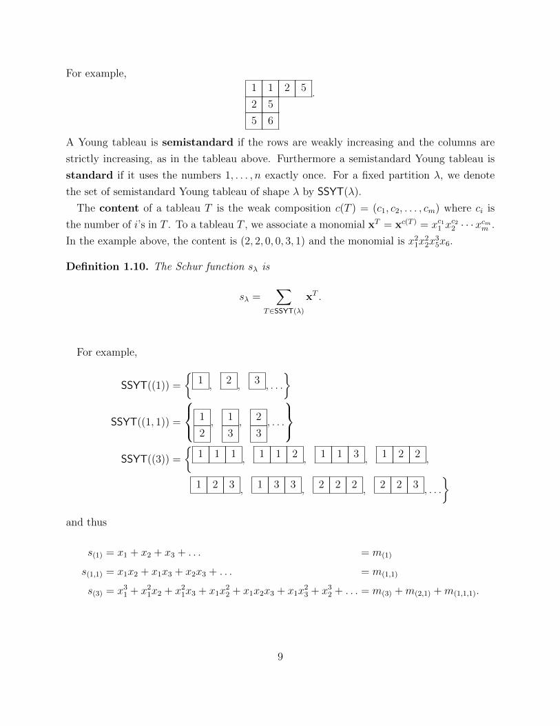
For example,

1 1 2 5

2 5

5 6

.

A Young tableau is semistandard if the rows are weakly increasing and the columns are

strictly increasing, as in the tableau above. Furthermore a semistandard Young tableau is

standard if it uses the numbers 1, . . . , n exactly once. For a fixed partition λ, we denote

the set of semistandard Young tableau of shape λ by SSYT(λ).

The content of a tableau T is the weak composition c(T ) = (c1, c2, . . . , cm) where ci is

the number of i’s in T . To a tableau T , we associate a monomial xT = xc(T ) = xc11 xc22 · · ·xcmm .

In the example above, the content is (2, 2, 0, 0, 3, 1) and the monomial is x21x22x

35x6.

Definition 1.10. The Schur function sλ is

sλ =∑

T∈SSYT(λ)

xT .

For example,

SSYT((1)) =

{1 , 2 , 3 , . . .

}

SSYT((1, 1)) =

1

2, 1

3, 2

3, . . .

SSYT((3)) =

{1 1 1 , 1 1 2 , 1 1 3 , 1 2 2 ,

1 2 3 , 1 3 3 , 2 2 2 , 2 2 3 , . . .

}and thus

s(1) = x1 + x2 + x3 + . . . = m(1)

s(1,1) = x1x2 + x1x3 + x2x3 + . . . = m(1,1)

s(3) = x31 + x21x2 + x21x3 + x1x22 + x1x2x3 + x1x

23 + x32 + . . . = m(3) +m(2,1) +m(1,1,1).

9

The Schur functions expand combinatorially in the monomial basis

sλ =∑µ

Kλ,µmµ (1.1)

where Kλ,µ is the number of semistandard Young tableaux of shape λ and content µ. The

numbers Kλ,µ are called the Kostka coefficients. The vanishing of Kλ,µ is governed by

dominance order [Man01, Exercise 1.2.11] as

Kλ,µ 6= 0 if and only if µ ≤D λ.

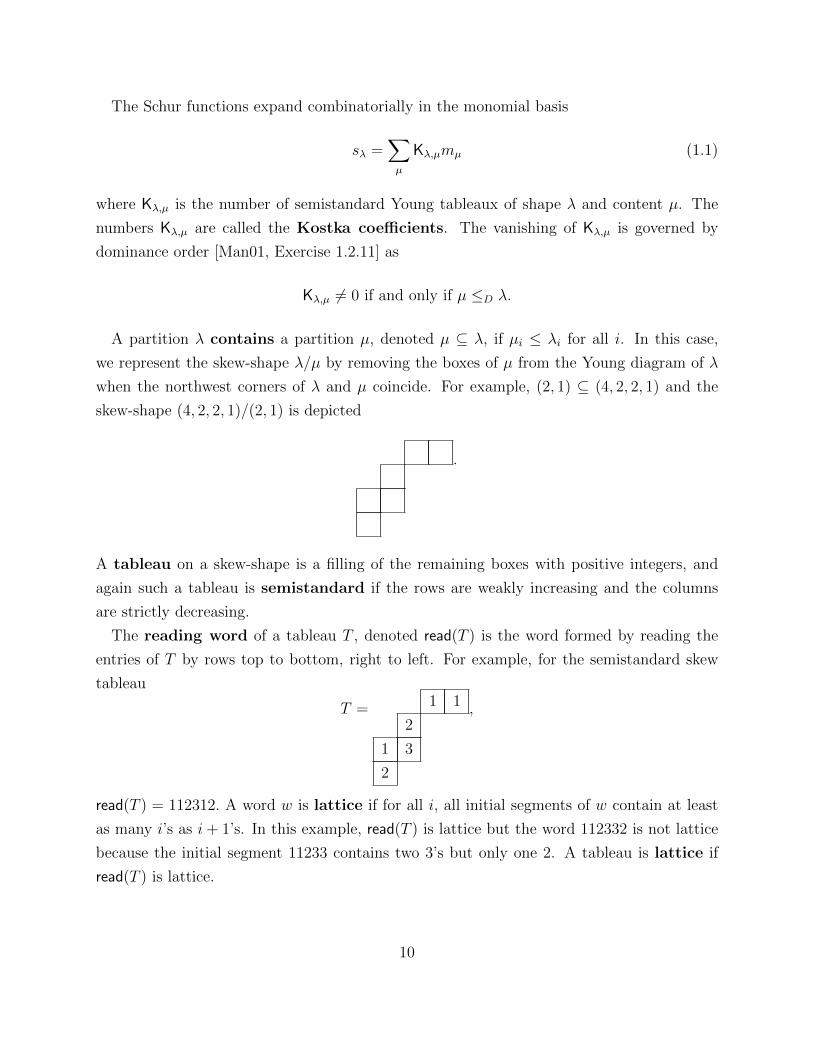
A partition λ contains a partition µ, denoted µ ⊆ λ, if µi ≤ λi for all i. In this case,

we represent the skew-shape λ/µ by removing the boxes of µ from the Young diagram of λ

when the northwest corners of λ and µ coincide. For example, (2, 1) ⊆ (4, 2, 2, 1) and the

skew-shape (4, 2, 2, 1)/(2, 1) is depicted

.

A tableau on a skew-shape is a filling of the remaining boxes with positive integers, and

again such a tableau is semistandard if the rows are weakly increasing and the columns

are strictly decreasing.

The reading word of a tableau T , denoted read(T ) is the word formed by reading the

entries of T by rows top to bottom, right to left. For example, for the semistandard skew

tableau

T = 1 1

2

1 3

2

,

read(T ) = 112312. A word w is lattice if for all i, all initial segments of w contain at least

as many i’s as i+ 1’s. In this example, read(T ) is lattice but the word 112332 is not lattice

because the initial segment 11233 contains two 3’s but only one 2. A tableau is lattice if

read(T ) is lattice.

10

The Schur functions have nonnegative structure constants, i.e.

sλsµ =∑

ν∈Par(|λ|+|µ|)

LRνλ,µsν

with LRνλ,µ ∈ Z≥0.

Theorem 1.11. The Littlewood-Richardson coefficient LRνλ,µ is equal to the number of

lattice, semistandard Young tableaux of skew-shape ν/λ and content µ.

Theorem 1.11 is known as the Littlewood-Richardson rule for the Schur functions sλ.

For example, let λ = (3, 1), µ = (4, 2, 1), and ν = (6, 3, 1, 1). Then LRνλ,µ = 2 and the two

witnessing fillings are

1 1 1

1 2

2

3

and 1 1 1

2 2

1

3

.

1.3 Quasisymmetric Functions

The ring of symmetric polynomials in m variables Symm embeds inside the ring of quasisym-

metric polynomials in m variables, denoted QSymm. A polynomial f(x1, x2, . . . , xm) is qua-

sisymmetric if for all increasing sequences of positive integers 1 ≤ i1 < i2 < . . . < ik ≤ m

and for all compositions with k parts (α1, α2, . . . , αk),

[xα1i1xα2i2· · ·xαkik ]f = [xα1

1 xα22 · · ·x

αkk ]f.

Equivalently, consider the following action of si on a monomial:

si y xγ =

{xsi(γ) if γi = 0 or γi+1 = 0

xγ if γi 6= 0 and γi+1 6= 0. (1.2)

This extends to an action on polynomials and f(x1, . . . , xm) is quasisymmetric if and only if

it is invariant under the action of si for i = 1, . . . ,m− 1. We define QSymnm to be the vector

space of homogeneous quasisymmetric polynomials of degree n in m variables. For example,

f(x1, x2, x3) = x1x22 + x1x

23 + x2x

23 ∈ QSym3

3.

11

The ring of quasisymmetric polynomials in m variables is

QSymm =∞⊕n=0

QSymnm.

For each m ≥ 0, the map

rm : QSymnm+1 → QSymn

m

that sets xn+1 = 0 is a surjective homomorphism. Thus, we can define

QSymn = lim←−m

QSymnm,

the vector space of homogeneous quasisymmetric functions of degree n. Finally, the ring of

quasisymmetric functions is

QSym =∞⊕n=0

QSymn,

or quasisymmetric formal power series of bounded degree.

The study of quasisymmetric functions dates back to the thesis of R. P. Stanley [Sta71]

and subsequent work by I. Gessel in [Ges84]. We define two bases of QSymn, both indexed

by the set of compositions of n.

Definition 1.12. The monomial quasisymmetric function Mα is

Mα =∑

γ∈Expand(α)

xγ.

For example,

M(1) = x1 + x2 + x3 + . . .

M(1,1) = x1x2 + x1x3 + x2x3 + . . .

M(3) = x31 + x32 + x33 + . . .

M(3,1) = x31x2 + x31x3 + x32x3 + . . .

M(1,3) = x1x32 + x1x

33 + x2x

33 + . . . .

Recall from Section 1.1 that given a composition α, the partition λ(α) is the partition

formed by sorting the parts of α in weakly decreasing order and PermutC(λ) is the set of all

12

α such that λ(α) = λ. Since by the definitions of both,

mλ =∑

α∈PermutC(λ)

Mα,

{Mα} is a quasisymmetric refinement of {mλ}.Compositions of n are in bijection with subsets of [n− 1] = {1, 2, . . . , n− 1} where

set((α1, α2, . . . , α`)) = {α1, α1 + α2, . . . , α1 + . . .+ α`−1}.

For example set((1, 2, 2, 1)) = {1, 3, 5}.

Definition 1.13 (Gessel, pg. 291 [Ges84]). For |α| = n, Gessel’s fundamental quasisymmet-

ric function Fα is

Fα =∑

(i1,...,in)∈Zn>0i1≤i2≤...≤in

ij<ij+1 if j∈set(α)

xi1xi2 · · ·xin .

For example,

F(1) = x1 + x2 + x3 + . . . = M(1)

F(1,1) = x1x2 + x1x3 + x2x3 + . . . = M(1,1)

F(3) = x31 + x21x2 + x1x22 + x32 + x21x3 + . . . = M(3) +M(2,1) +M(1,2) +M(1,1,1)

F(1,1,2) = x1x2x23 + x1x2x3x4 + x1x3x

24 + x1x3x4x5 + . . . = M(1,1,2) +M(1,1,1,1).

The composition β is a refinement of the composition α, denoted α � β, if α can be ob-

tained by summing consecutive parts of β. For example, (4, 1, 3, 2) � (3, 1, 1, 1, 2, 1, 1). The

fundamental quasisymmetric basis expands combinatorially in the monomial quasisymmetric

basis [Ges84, Equation 2]:

Fα =∑

β∈Comp(|α|)α�β

Mβ. (1.3)

1.4 Polynomials

Finally, the ring of quasisymmetric polynomials in m variables QSymm embeds inside of Polm,

the ring of polynomials in m variables. We denote the ring of polynomials in arbitrarily many

13

variables as Pol. Bases of Pol are typically indexed by weak compositions.

Definition 1.14. The monomial basis of Pol is

mγ = xγ = xγ11 xγ22 · · ·x

γ`` .

Recall that for a weak composition γ, the composition γ+ is formed by removing the parts

of size 0 from γ. It is clear {mγ} is a polynomial refinement of {Mα} (and therefore {mλ})as

Mα =∑

γ∈Expand(α)

mγ.

The Schubert polynomials are a basis of Pol that generalize the Schur functions and

were introduced by A. Lascoux and M.-P. Schutzenberger [LS82a]. As seen in Chapter 5,

each Schur function represents the cohomology of a Schubert variety in the Grassmannian.

Analogously, each Schubert polynomial represents the cohomology of a Schubert variety in

the flag manifold. Recall from Section 1.1 that permutations are uniquely determined by

their Lehmer code and thus Schubert polynomials are often indexed by permutations.

A. Lascoux and M.-P. Schutzenberger define the Schubert polynomials recursively using

divided difference operators. Let

∂i =1− si

xi − xi+1

and let w0 ∈ Sn be the longest permutation in Sn, i.e. w0 = n . . . 21.

Definition 1.15 (Lascoux-Schutzenberger [LS82a]). The Schubert polynomial Sw0 is

Sw0 = xn−11 xn−22 · · ·xn−1.

For w 6= w0, there exists i such that w(i) < w(i+ 1), and the Schubert polynomial Sw is

Sw = ∂iSwsi .

14

For example,

S54321 = x41x32x

23x4

∂4S54321 =S54312 = x41x32x

23

∂3S54312 =S54132 = x41x32x3 + x41x

32x4

∂2S54132 =S51432 = x41x22x3 + x41x2x

23 + x41x

22x4 + x41x2x3x4 + x41x

23x4.

It is straightforward to check that the divided difference operators satisfy the commutation

and braid relations of the simple transpositions. We can therefore define ∂w = ∂i1∂i2 · · · ∂i`where i1i2 · · · i` is any reduced word of w. The Schubert polynomial is then

Sw = ∂w−1w0xn−11 xn−22 · · ·xn−1.

For more details see [Man01, Definition 2.3.4] and the discussion immediately preceding it.

We now discuss some properties of the Schubert polynomials. The Schubert polynomials

are stable, i.e. for w ∈ Sn and ι : Sn ↪→ Sn+1, Sw = Sι(w), and thus we can consider w

as a member of S∞. Furthermore, the Schubert polynomials expand combinatorially in the

monomial basis.

Moreover, the Schubert polynomials are a lift of the Schur functions from Sym to Pol.

A descent of a permutation is i such that w(i) > w(i + 1). A permutation is said to be

Grassmannian if it has at most one descent. For example, w = 51432 has descents at

1,3, and 4 and so is not Grassmannian, but w = 1347256 is Grassmannian because the only

descent is at 4. Equivalently, a permutation w is Grassmannian if and only if c(w)∗ is a

partition. In this case,

Sw = sc(w)∗(x1, . . . , xk) (1.4)

where k is the position of the descent of w.

Finally, products of Schubert polynomials expand combinatorially in the Schubert basis.

For u ∈ Sm and v ∈ Sn,

SuSv =∑

w∈Sm+n

cwu,vSw.

While {cwu,v} are known to be nonnegative for geometric reasons, giving a counting rule for

{cwu,v} is a well-known open problem [Sta99b, Problem 11].

There are many combinatorial rules that describe the monomial expansion of the Schubert

15

polynomials, including reduced words and compatible sequences [BJS93], RC graphs [BB93],

strand diagrams [FK96], and many others. The first combinatorial rule was conjectured by

A. Kohnert [Koh91]. A proof was given by R. Winkel [Win03] and a new proof has been

given by S. Assaf [Ass17].

A diagram is a subset of boxes in the n×n grid, and a Kohnert move in a diagram moves

the rightmost box of any row up to the next available row (jumping boxes if necessary). Let

Koh(w) be the set of all diagrams generated by Kohnert moves from D(w) where diagrams

are not included with multiplicity even though there might be multiple sequences of moves

to a particular diagram. The content of a diagram is c(D) = (c1, c2, . . . , cn) where ci is the

number of boxes in row i of D. We then have

Sw =∑

D∈Koh(w)

xc(D) (1.5)

where (1.5) is [Win03, Theorem 2] and [Ass17, Corollary 6.8]. Continuing our example with

w = 51432, we have the following diagrams giving us the Schubert polynomial above:

.

None of our results will rely on Kohnert’s rule, however, we include it here due to its

connection to the combinatorics of Chapter 2.

1.5 Combinatorics of Macdonald Polynomials

The Macdonald polynomials are families of symmetric polynomials introduced by I. G. Mac-

donald [Mac88]. For a more detailed reference, see the book [Mac95b].

Recall from Section 1.1 that for a partition λ, the number of parts of size i of λ is mi(λ).

Then define

zλ =∞∏i=1

imi(λ)mi(λ)!.

16

The standard inner product on symmetric functions is

〈pλ, pµ〉 = δλ,µzλ

where

δλ,µ =

{1 λ = µ

0 λ 6= µ.

The Schur functions are the unique family that satisfy

1. Upper triangular with respect to the monomial basis, i.e. fλ = mλ +∑

µ∈Par(|λ|)µ<Dλ

cλ,µmµ

and

2. Orthogonal with respect to the inner product, i.e. 〈fλ, fµ〉 = 0 if λ 6= µ.

I. G. Macdonald defined a q, t-analogue of this inner product:

〈pλ, pµ〉q,t = δλ,µzλ

`(λ)∏i=1

1− qλi1− tλi

.

Definition 1.16 (Macdonald, Equation 4.7 [Mac95b]). The Macdonald polynomials Pλ are

the the unique family satisfying

1. Upper triangular with respect to the monomial basis, i.e. fλ = mλ+∑

µ∈Par(|λ|)µ<Dλ

cλ,µmµ and

2. Orthogonal with respect to the q, t-inner product, i.e. 〈fλ, fµ〉q,t = 0 if λ 6= µ.

I. G. Macdonald proved such a family exists [Mac88, Theorem 2.3]. From this definition

it is clear that the Macdonald polynomials are a q, t-generalization of the Schur functions

since when q = t, we recover them.

In addition to the original Macdonald polynomials {Pλ}, a few transformations of the

Macdonald polynomials are often studied. For a partition λ, suppose b = (i, j) is a box of

its Young diagram. Then, arm(b) = #{k > i : λk ≥ j}, or the number strictly boxes below b

and leg(b) = λi − j, or the number of boxes strictly right of b. For example, in the diagram

below, the box b is in position (1,2). The arm of b is depicted in red and thus arm(b) = 2,

while the leg of b is depicted in yellow and leg(b) = 3.

17

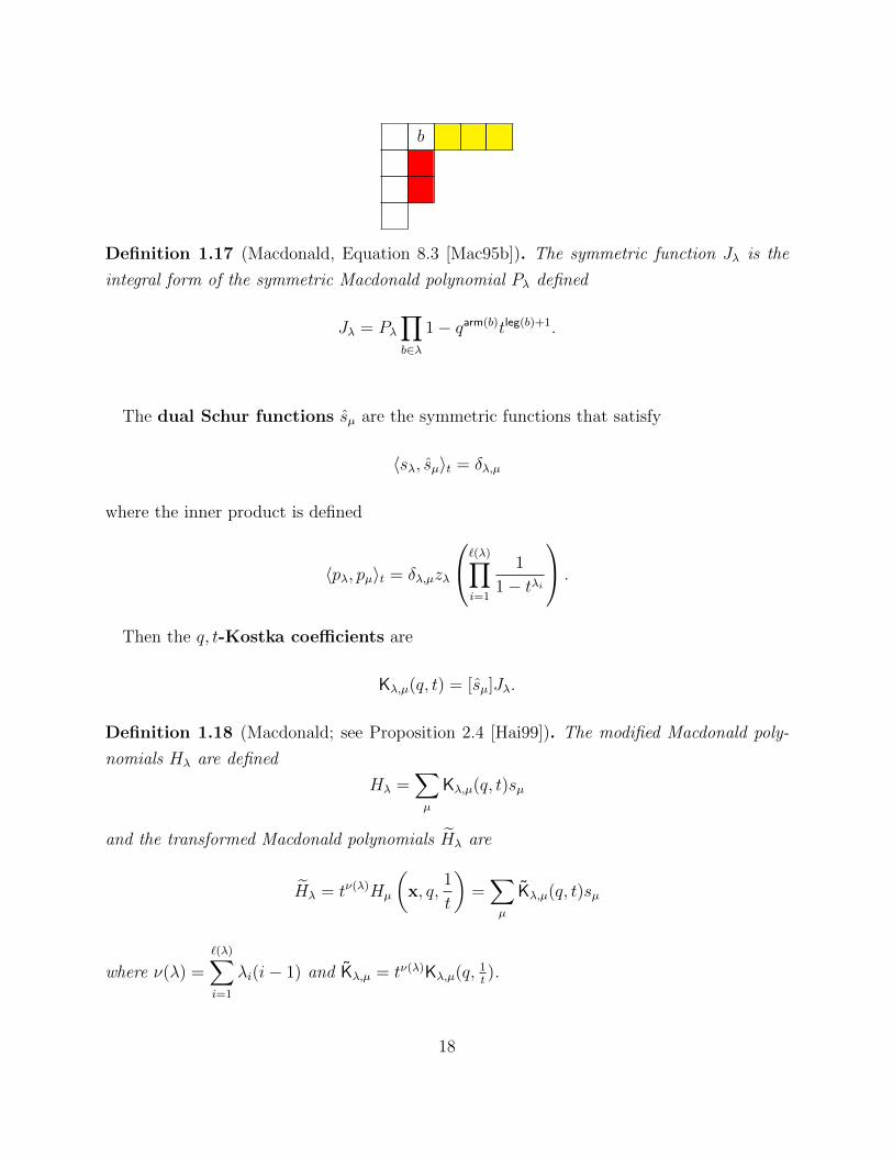
b

Definition 1.17 (Macdonald, Equation 8.3 [Mac95b]). The symmetric function Jλ is the

integral form of the symmetric Macdonald polynomial Pλ defined

Jλ = Pλ∏b∈λ

1− qarm(b)tleg(b)+1.

The dual Schur functions sµ are the symmetric functions that satisfy

〈sλ, sµ〉t = δλ,µ

where the inner product is defined

〈pλ, pµ〉t = δλ,µzλ

`(λ)∏i=1

1

1− tλi

.

Then the q, t-Kostka coefficients are

Kλ,µ(q, t) = [sµ]Jλ.

Definition 1.18 (Macdonald; see Proposition 2.4 [Hai99]). The modified Macdonald poly-

nomials Hλ are defined

Hλ =∑µ

Kλ,µ(q, t)sµ

and the transformed Macdonald polynomials Hλ are

Hλ = tν(λ)Hµ

(x, q,

1

t

)=∑µ

Kλ,µ(q, t)sµ

where ν(λ) =

`(λ)∑i=1

λi(i− 1) and Kλ,µ = tν(λ)Kλ,µ(q, 1t).

18

J. Haglund, M. Haiman, and N. Loehr [HHL05] define a filling F as an assignment of the

boxes of λ with positive integers. The content of F , denoted c(F ) is the weak composition

counting the number of i’s in F and xF = xc(F ). A descent of F is a box that is filled with

an integer strictly greater than the integer immediately to its left. Let Des(F ) be the set of

descents of F .

Two cells are said to be attacking if they are in the same column, or if they are in adjacent

columns and the left box is strictly above the right box. The two kinds of attacking cells are

a

b

b

a

.

A pair of attacking cells is an inversion if a > b and let Inv(F ) be the set of inversions of

F . Then, given the definitions of arm(b) and leg(b) above

maj(F ) =∑

b∈Des(F )

(leg(b) + 1)

and

inv(F ) = |Inv(F )| −∑

b∈Des(F )

arm(b).

For example, for the filling

4 4 2 6

2 3 2 1

6 4 4

6 3

there are two descents: the 6 in the first row and the 3 in the second. Therefore

maj(F ) = (1 + 0) + (1 + 2) = 4.

There are 8 inversions: (1) the 4 and 2 in column one, (2-3) the first 4 in column 2 with

both 3’s in column two, (4) the second 4 in column 2 with the second 3 in column 2, (5) the

6 and 1 in column four, (6-7) the 2 in column 1 with the second 4 and 3 in column 2, and

19

(8) the 3 in column 2 and the 4 in column 3. Thus

inv(F ) = 8− (1 + 2) = 5.

Theorem 1.19 (Haglund-Haiman-Loehr, Theorem 2.2 [HHL05]).

Hλ =∑F

qinv(F )tmaj(F )xF

where the sum is over all fillings F of λ.

In addition to the symmetric Macdonald polynomials, the nonsymmetric Macdonald

polyomials, introduced and studied by I. Cherednik [Che95], I. G. Macdonald [Mac95a],

and E. Opdam [Opd95], provide a refinement of the symmetric Macdonald polynomials;

see [HHL08, Proposition 5.3.1]. The nonsymmetric Macdonald polynomials Eγ(x; q, t) are

indexed by weak compositions and are elements of Q[x1, . . .](q, t). In [HHL08], J. Haglund,

M. Haiman, and N. Loehr give a combinatorial rule for the nonsymmetric Macdonald poly-

nomials involving skyline fillings that has similarities to their rule in the symmetric case.

The skyline diagram for γ with basement b = (b1, . . . , bk) consists of k left-justified

rows with γi boxes in row i, plus an additional column 0 containing the value bi in row i. Let

bi = (1, 2, . . . , `(γ)) and b∗i = (`(γ), `(γ)−1, . . . , 1). Then the skyline diagram γ = (1, 0, 2, 1)

and basements bi (left) and b∗i (right) are shown below.

1

2

3

4

4

3

2

1

A skyline filling is an assignment of positive integers to the boxes of the skyline diagram.

Given a filling F , the content of F is the weak composition c(F ) = (c1, c2, . . . , c`) where

ci is the number of i’s in F , excluding any i’s in the basement. Then, the monomial

xF = xc(F ) = xc11 xc22 · · ·x

c`` , and the size of F , denoted |F |, is |c(F )|. A descent of a filling

F is a box filled with a number strictly greater than the number to its left and Des(F ) is

the set of descents of F .

The leg of a box b, denoted leg(b), is the number of boxes strictly right of b. For b = (i, j),

arm(b) is the number of boxes that are either

• (i′, j) with i′ < i and γi′ ≤ γi, or

20

• (i′, j − 1) with i′ > i and γi′ < γi.

When j = 1, it is possible for boxes in the arm of b to be in the basement of the skyline

diagram. For example, the arm of the box b below is denoted in red:

b

.

The two types of attacking cells in the nonsymmetric case are

1 b

2

3

4 a

1

2

3 a

4 b

.

Attacking cells can include cells in the basement. A filling is non-attacking if a 6= b for all

pairs of attacking cells. Furthermore, a pair of attacking cells is an inversion if a > b and

we denote the set of inversions of F by Inv(F ). For example, the filling below on the left

is attacking because the 2’s attack each other but the filling on the right is non-attacking.

On the right hand filling, every pair of numbers in the basement and the first column is an

inversion. Likewise the 2 in the third column and the 1 in the second is an inversion.

1 1

2

3 3 3 2

4 4 2

1 1

2

3 3 3 2

4 4 1

21

Finally, maj, inv, and coinv are defined:

maj(F ) =∑

b∈Des(F )

(leg(b) + 1)

inv(F ) = |Inv(F )| − |{i < j : γi ≤ γj}| −∑

b∈Des(F )

arm(b)

coinv(F ) =

(∑b∈F

arm(b)

)− inv(F ).

Theorem 1.20 (Haglund-Haiman-Loehr; Theorem 3.5.1 [HHL08]).

Eγ(x; q, t) =∑F

xF qmaj(F )tcoinv(F )∏b∈F

F (b)6=F (d(b))

1− t1− qleg(b)+1tarm(b)+1

where the sum is over non-attacking fillings F of γ and d(b) is the box immediately left of b.

We will take this combinatorial description as our definition. An alternate description of

Eγ (Corollary 3.6.4 [HHL08]) involves triples. Triples consist of three boxes on two rows

i < j. As pictured, there are two types of triples depending on the relative lengths of the

rows.

c a...

b

Type A

γi ≥ γj

b...

c a

Type B

γi < γj

A triple is a inversion triple if c < b < a, a ≤ c < b, or b < a ≤ c, and otherwise is

a coinversion triple. For example, in the filling below, the boxes (3, 0), (3, 1), and (4, 1)

form a coinversion triple:

1 1

2

3 2 4

4 3

In this formulation, the t-statistic provides a weight on the coinversion triples instead of a

weight on the inversions.

22

1.5.1 Specializations of Macdonald Polynomials

Many polynomial families of interest are specializations of either the symmetric or nonsym-

metric Macdonald polynomials. We have already seen that the Schur functions are the q = t

specializations of Pλ. Furthermore, the Hall-Littlewood polynomials [LS78a] are the

q = 0 specialization of Pλ whereas the Jack polynomials [KS96] are the specialization

formed by setting t = qα and letting q → 1.

Of particular interest for us are two specializations of the nonsymmetric Macdonald poly-

nomials: the Demazure atoms at q = t = 0 and the key polynomials at q = t =∞. Just

as the Schur polynomials are the characters of the irreducible polynomial representations

of GLn, the key polynomials are the characters of Demazure modules of type A [Dem74].

These polynomials inherit their combinatorics from the Macdonald polynomials; however,

they were originally studied by A. Lascoux and M.-P. Schutzenberger [LS90] and V. Reiner

and M. Shimozono [RS95] using their definition in terms of divided difference operators. Let

πi = ∂ixi and πi = πi − 1.

Since πi and πi satisfy the braid and commutation relations, for a permutation w we can

define πw (resp. πw) as πi1πi2 · · · πi` (resp. πi1 πi2 · · · πi`) where i1i2 · · · i` is any reduced word

of w.

Definition 1.21 (Lascoux-Schutzenberger, [LS90]). The Demazure atom Atomγ and the key

polynomial Keyγ are

Atomγ = πwγxλ(γ) Keyγ = πwγx

λ(γ).

In [LS89], A. Lascoux and M.-P. Schutzenberger prove that the Schubert polynomials

combinatorially expand in the key polynomials.

Theorem 1.22 (Lascoux-Schutzenberger, Theorem 5 [LS89]).

Sw =∑T

Keyc(T )

where the sum is over a particular tableaux T , the specifics we do not need here.

Combinatorially, the Demazure atoms and key polynomials are the generating functions

for semistandard skyline fillings.

23

Definition 1.23 (Mason, Section 3 [Mas09]). A skyline filling is semistandard if

(M1) entries do not repeat in a column,

(M2) rows are weakly decreasing (including the basement), and

(M3) every triple (including those with basement boxes) is an inversion triple.

Let SkyFill(γ,b) be the set of semistandard skyline fillings of shape γ and basement b.

Theorem 1.24 (Mason, Theorem 1.1 [Mas09]). The Demazure atom Atomγ is

Atomγ = Eγ(x; 0, 0) =∑

F∈SkyFill(γ,bi)

xF .

As an example, the semistandard skyline fillings with basement bi and the Demazure atom

for the rearrangements of (2, 1, 0) are in Figure 1.1.

Theorem 1.25 (Mason, Theorem 1.2 [Mas09]). The key polynomial is

Keyγ =∑

F∈SkyFill(γ∗,b∗i )

xF .

For example,

SkyFill((2, 0, 1),b∗i ) =

3 3 3

2

1 1

, 3 3 2

2

1 1

, 3 3 1

2

1 1

, 3 2 2

2

1 1

, 3 2 1

2

1 1

Key(1,0,2) = x1x

23 + x1x2x3 + x21x3 + x1x

22 + x21x2.

For two compositions γ and δ we write

γ � δ if λ(γ) = λ(δ) and wγ ≤B wδ

where λ(γ), wγ, and ≤B are defined in Section 1.1.

24

SkyFill((2, 1, 0),bi) =

1 1 1

2 2

3

SkyFill((0, 2, 1),bi) =

1

2 2 2

3 3

, 1

2 2 1

3 3

SkyFill((2, 0, 1),bi) =

1 1 1

2

3 3

SkyFill((1, 0, 2),bi) =

1 1

2

3 3 3

, 1 1

2

3 3 2

SkyFill((1, 2, 0),bi) =

1 1

2 2 2

3

SkyFill((0, 1, 2),bi) =

1

2 2

3 3 3

and thus

Atom(2,1,0) = x21x2 Atom(0,2,1) = x22x3 + x1x2x3

Atom(2,0,1) = x21x3 Atom(1,0,2) = x1x23 + x1x2x3

Atom(1,2,0) = x1x22 Atom(0,1,2) = x2x

23

Figure 1.1: The set SkyFill(γ,bi) and the Demazure atom Atomγ for γ a rearrangement of(2, 1, 0).

25

Theorem 1.26.

Keyγ =∑

δ∈WC(|γ|)δ�γ

Atomδ.

In the literature, this decomposition can be found in Section 1 of [Mas09] and a proof is

given [Pun16, Lemma 3.5].

In [Mas08], S. Mason gives a combinatorial proof that the Demazure atoms are a polyno-

mial refinement of the Schur functions sλ:

Theorem 1.27 (Mason, (1.1) [Mas08]).

sλ =∑

γ∈PermutWC(λ)

Atomγ.

Theorems 1.26 and 1.27 together show that the key polynomials are a lift of the Schur

functions from Symm to Polm where Symm is symmetric polynomials in m variables. That

is, when γ is weakly increasing with m parts, then

Keyγ = sγ∗(x1, x2, . . . , xm). (1.6)

This is because when γ is weakly increasing, wγ = w0, and so we have δ � γ for all weak

compositions δ such that λ(δ) = λ(γ) and `(δ) ≤ m. Thus, the decompositions in Theorems

1.26 and 1.27 are identical.

Recall that a function is quasisymmetric if for all i, it is invariant under the action of

si defined in (1.2). Suppose F is a filling that contains i’s but no i + 1’s. Let Fi be the

filling formed by replacing all i’s with i+1’s. A model for fillings produces a quasisymmetric

function if for every F above, Fi is a valid filling. This will hold if the rules for determining

a valid filling consist only of inequalities between the chosen entries in the boxes.

Thus, the Schur function is quasisymmetric (as it is in fact symmetric) since the rules

only require the rows to be weakly increasing and the columns to be strictly increasing. The

Demazure atom is not quasisymmetric as the basement is fixed at bi = i and thus is a rule

that is not an inequality on the chosen entries.

The quasisymmetric Schur functions were introduced by J. Haglund, K. Luoto, S. Ma-

son, and S. van Willigenburg in [HLMvW11a]. Combinatorially, Sα is generated by semi-

standard composition tableaux of shape α which are fillings of α (with no basement)

26

such that

1. entries do not repeat in a column,

2. rows are weakly decreasing,

3. every triple is an inversion triple, and

4. the leftmost column is weakly increasing from top-to-bottom.

Let SSCT(α) be the set of all semistandard composition tableau of shape α.

Definition 1.28 (Haglund et al., Definitions 4.3 and 5.1 [HLMvW11a]). The quasisymmetric

Schur function Sα is

Sα =∑

T∈SSCT(α)

xT .

For example,

SSCT((1, 2)) =

1

2 2, 1

3 3, 1

3 2, 2

3 3, . . .

S(1,2) = x1x

22 + x1x

23 + x1x2x3 + x2x

23 + . . . .

In essence, semistandard composition tableau are semistandard skyline fillings with the base-

ment omitted and the first column weakly increasing to account for being able to insert rows

of length 0 into a skyline filling. Then, it is clear from the combinatorics that

Sα =∑

γ∈Expand(α)

Atomγ, (1.7)

and thus the Demazure atoms provide a polynomial refinement of the quasisymmetric Schur

functions. (In fact, this decomposition was the original definition of Sα [HLMvW11a, Defi-

nition 5.1].) Likewise, just as {Mα} is a quasisymmetric refinement of {mλ}, we have that

{Sα} is a quasisymmetric refinement of {sλ}:

sλ =∑

α∈PermutC(λ)

Sα =∑

γ∈PermutWC(λ)

Atomγ. (1.8)

Finally, the quasisymmetric Schur functions combinatorially expand in the fundamental

quasisymmetric functions.

27

Proposition 1.29 (Haglund et al., Proposition 5.2, [HLMvW11a]).

Sα =∑T

Fd(T )

where the sum is over a specific set of standard reverse tableaux and d(T ) is the composition

corresponding to the set {i : i+ 1 does not appear strictly left of i in T}.

1.6 K-Theoretic Combinatorics

In [LS82b], A. Lascoux and M.-P. Schutzenberger defined the Grothendieck polynomials.

These polynomials are K-theoretic analogues of the Schubert polynomials in that they repre-

sent the K-theory classes of Schubert varieties of the flag variety the same way the Schubert

polynomials represent the cohomology classes of Schubert varieties. To help the reader keep

track of the relations between all the families of polynomials under consideration, we denote

the K-analogue of each basis by merely prepending a ‘K’ to the notation for that family.

Let

∂i = ∂i(1 + βxi+1).

Definition 1.30 (Lascoux-Schutzenberger [LS82b]). The Grothendieck polynomial KSw0 is

KSw0 = xn−11 xn−22 · · ·xn−1.

For w 6= w0, there exists i such that w(i) < w(i+ 1), and then the Grothendieck polynomial

KSw is

KSw = ∂iKSwsi .

In the original definition of A. Lascoux and M.-P. Schutzenberger, β = −1. The β notation

was introduced by S. Fomin and A. Kirillov who gave formulas for KSw that are analogous

to those for the Schubert polynomials [FK96].

The Schubert polynomial Sw is a homogeneous polynomial of degree `(w). It is clear from

the definition of ∂i that a term of degree `(w) + k in the x variables in KSw will have a

coefficient of βk. Then, setting β = 0 recovers the lowest degree terms of KSw, which equal

Sw. Thus KSw is an inhomogeneous deformation of Sw.

28

The Grothendieck polynomials corresponding to Grassmannian permutations are the sym-

metric Grothendieck polynomials Ksλ and are the K-analogue of the Schur functions.

C. Lenart made important contributions to the combinatorics of Ksλ, including the ex-

pansion of Ksλ into the Schur functions [Len00]. Building on this work, A. Buch opened up

the possibility of set-valued combinatorics with a set-valued tableau rule for Ksλ [Buc02].

A set-valued tableau is a filling of the Young diagram with sets of positive integers. We

compare sets with A ≤ B (resp. A < B) if for every a ∈ A, b ∈ B, a ≤ b (resp. a < b). Then,

a set-valued tableau is semistandard if the rows are weakly increasing and the columns are

strictly increasing, where we compare sets. Equivalently, a set-valued tableau is semistandard

if for any selection of one entry in each box, the resulting tableau is semistandard.

The content, size, and monomial of a set-valued tableau are unchanged from a single-valued

tableau. If T is a set-valued tableau of shape λ, then the excess of T is ex(T ) = |T | − |λ|.Let SetSSYT(λ) be the set of all semistandard set-valued tableaux of shape λ.

Theorem 1.31 (Buch, Theorem 3.1 [Buc02]).

Ksλ =∑

T∈SetSSYT(λ)

βex(T )xT .

For example,

SetSSYT((2, 1)) =

1 1

2, 1 2

2, 1 12

2, 1 3

2, 1 3

3, 1 3

23, 1 13

23, . . .

Ks(2,1) = x21x2 + x1x

22 + βx21x

22 + x1x2x3 + x1x

23 + βx1x2x

23 + β2x21x2x

23 + . . . .

Since a semistandard set-valued tableau with zero excess is just an ordinary semistan-

dard tableau, setting β = 0 in Ksλ yields sλ. In other words, Ksλ is an inhomogeneous

deformation of sλ.

In recent years, there has been interest in finding “K-theoretic” analogues of many ob-

jects within algebraic combinatorics. For example, a (partial) list as follows was given

by O. Pechenik and A. Yong in [PY16]. This interest includes elements of the theory

of Young tableaux motivated by the symmetric Grothendieck polynomials [Len00, Buc02,

BKS+07, TY09b, BS16, GMP+16, HKP+17, LMS16], but this combinatorics is only part

of a broader conversation. For example, K-analogues have been studied for Hopf algebras

[LP07, PP16, Pat16], cyclic sieving [Pec14, Rho17, PSV16], homomesy [BPS16], longest

29

increasing sequences of random words [TY11], poset edge densities [RTY16], and plane par-

titions [DPS17, HPPW16].

Of particular interest later in this thesis is the notion of a genomic tableau due to

O. Pechenik and A. Yong [PY16]. A genomic tableau is a tableau is a tableau T such that

each box is filled with a label ij and for each i, {j|ij appears in T} = {1, 2, . . . , ki} for some

ki. A family i of labels is the collection {ij}kij=1, and the gene ij is the set of all labels

for fixed i and j. Furthermore, the genes must partition the labels of a particular family

as the entries of T are read from left to right, and no gene can contain two boxes in the

same row. The content of T is the number of genes of each family. Then, a genomic

tableau is semistandard if it is semistandard when considering only the families of the

labels. For example, the genomic tableau below, where each color corresponds to a gene, is

semistandard:11 12 22 32

21 22 31

31

.

A genomic tableau is lattice if every tableau formed by selecting one element of each gene

is lattice.

The Littlewood-Richardson rule for Ksλ gives a combinatorial rule for the structure con-

stants KLRνλ,µ:

KsλKsµ =∑ν

KLRν∈Parλ,µ Ksν .

While the first Littlewood-Richardson rule for Ksλ was given by A. Buch [Buc02], genomic

tableaux were introduced to give an equivariant K-theoretic Littlewood-Richardson rule

[PY15], which specializes to the K-theoretic case.

Theorem 1.32 (Pechenik-Yong, Theorem 1.4 [PY16]). The coefficient KLRνλ,µ is the number

of lattice, semistandard genomic tableaux of shape ν/λ and content µ.

Another example of a K-analogue is the multi-fundamental functions of T. Lam and

P. Pylyavskyy [LP07]. These are the K-analogues of Gessel’s fundamental quasisymmetric

functions. Recall from Definition 1.13,

Fα =∑

(i1,...,in)∈Zn>0i1≤i2≤...≤in

ij<ij+1 if j∈set(α)

xi1xi2 · · ·xin .

T. Lam and P. Pylyavskyy’s definition of the multi-fundamental KFα replaces the single

30

integer ij with a subset of integers Sij .

Definition 1.33 (Lam-Pylyavskyy, Definition 5.4 [LP07]). The multi-fundamental function

KFα for |α| = n is defined

KFα =∑

Si1≤Si2≤...≤SinSij<Sij+1

if j∈set(α)

βex(Si1 ,...,Sin )xSi1xSi2 · · ·xSin

where each Si is a finite, nonempty subset of Z>0, xS =∏i∈S

xi and ex(Si1 , . . . , Sin) =

n∑j=1

(|Sij | − 1

).

For example, for α = (1, 2), set(α) = {1} and thus admissible sequences of sets are of the

form (S1, S2, S3) where S1 < S2 ≤ S3. Some possible examples are

{(1, 2, 2), (1, 2, 3), (1, 23, 3), (12, 3, 34), . . .}.

Again, the lowest degree terms occur when |Si| = 1 for all i. In this case, we recover the

definition of Fα and thus KFα is an inhomogeneous deformation of Fα.

In [Las01], A. Lascoux modifies the divided difference operators used to define the De-

mazure atoms and key polynomials in order to define the Lascoux atoms and Lascoux poly-

nomials. Let

τi = πi(1 + βxi+1) and τi = τi − 1.

Definition 1.34 (Lascoux [Las01]). The Lascoux polynomial KKeyγ is

KKeyγ = τwγxλ(γ)

while the Lascoux atom KAtomγ is

KAtomγ = τwγxλ(γ).

Like with the Grothendieck functions KSw, we can see from the operator definition that

β is merely tracking the excess degree of each term and thus KAtomγ is an inhomogeneous

deformation of Atomγ and KKeyγ is an inhomogeneous deformation of Keyγ. It is open to

31

prove a combinatorial rule describing these polynomials. A conjectural description for KKeyγ

using a generalization of Kohnert’s rule was given by C. Ross and A. Yong [RY15].

1.7 Organization

In Chapter 2, we introduce the notion of saturated Newton polytope (SNP), a property

describing polynomials. We discuss its prevalence in algebraic combinatorics by evaluating

whether the families of polynomials discussed in this chapter, among others, are SNP. We

also describe the Newton polytopes of several families in algebraic combinatorics. In Chap-

ter 3, we will give another conjectural description of the Lascoux atoms and polynomials by

generalizing the skyline fillings of Section 1.5. We will then use this combinatorial model to

define K-analogues of the quasisymmetric Schur functions, and show that these inhomoge-

neous deformations behave in many ways like their homogeneous counterparts. In Chapter

4, we continue this work on set-valued skyline fillings and inhomogeneous deformations and

introduce two new bases of polynomials. We show how these new bases fit into the existing

relationships between K-analogues. Finally, in chapter 5, we give some new conjectures on

Schubert calculus.

32

CHAPTER 2

Saturated Newton Polytopes

This chapter is derived from joint work with N. Tokcan and A. Yong that appears on the

arXiv [MTY17].

2.1 Introduction

The Newton polytope of a polynomial f =∑γ∈Zn≥0

cγxγ ∈ C[x1, . . . , xn] is the convex hull

of its exponent vectors, i.e.,

Newton(f) = conv({γ : cγ 6= 0}) ⊆ Rn.

Definition 2.1. The polynomial f has saturated Newton polytope (SNP) if cγ 6= 0 whenever

γ ∈ Newton(f).

Example 2.2. Let f be the determinant of a generic n × n matrix. The exponent vectors

correspond to permutation matrices. Then, Newton(f) is the Birkhoff polytope of n× ndoubly stochastic matrices. SNPness says there are no additional lattice points, which is

obvious here. (The Birkhoff-von Neumann theorem states all lattice points are vertices.)

Generally, polynomials are not SNP. Worse still, SNP is not preserved by basic polynomial

operations. For example, f = x21+x2x3+x2x4+x3x4 is SNP but f 2 is not (it misses x1x2x3x4).

Nevertheless, there are a number of families of polynomials in algebraic combinatorics where

every member is (conjecturally) SNP. Examples motivating our investigation include:

• The Schur polynomials are SNP. This rephrases R. Rado’s theorem [Rad52] about

permutahedra and dominance order on partitions (cf. Proposition 2.7).

33

• Classical resultants are SNP (Theorem 2.23). Their Newton polytopes were studied by

I. M. Gelfand-M. Kapranov-A. Zelevinsky [GKZ90]. Classical discriminants are SNP

up to quartics — but not quintics (Proposition 2.26).

• Cycle index polynomials from Redfield–Polya theory (Theorem 2.33)

• C. Reutenauer’s symmetric polynomials [Reu95] linked to the free Lie algebra and to

Witt vectors (Theorem 2.35)

• J. R. Stembridge’s symmetric polynomials [Ste91] associated to totally nonnegative

matrices (Theorem 2.31)

• R. P. Stanley’s symmetric polynomials [Sta84], introduced to enumerate reduced words

of permutations (Theorem 2.71)

• Generic (q, t)-evaluation of symmetric Macdonald polynomials (Theorem 2.40, Propo-

sition 2.45)

• Key polynomials (Conjecture 2.49). We give two conjectural descriptions of the Newton

polytopes (Conjectures 2.48 and 2.50). We determine a list of vertices of the Newton

polytopes (Theorem 2.51) and conjecture this list is complete (Conjecture 2.52).

• Schubert polynomials (Conjecture 2.63). We conjectured (Conjecture 2.76) a descrip-

tion of the Newton polytopes in terms of the Schubitope, which we introduce below.

• Grothendieck and Lascoux polynomials are also conjecturally SNP (Conjectures 2.66

and 2.69).

In more recent developments, some of these conjectures have been fully or partially re-

solved. In [FMS17], A. Fink, K. Meszaros, and A. St. Dizier prove that the keys and the

Schuberts are SNP (Corollary 8). They also prove our conjectural descriptions of their New-

ton polytopes (Theorem 10). Additionally, the Grothendieck polynomials have been proven

to be SNP in two cases: in the symmetric case by L. Escobar and A. Yong [EY17] and in

the case that w = 1π where π is a dominant permutation by K. Meszaros and A. St. Dizier

(Theorem C [MS17]).

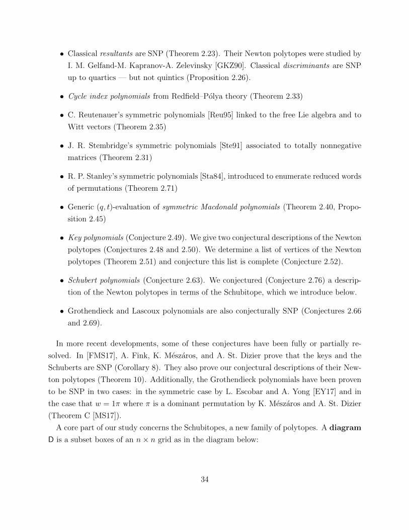
A core part of our study concerns the Schubitopes, a new family of polytopes. A diagram

D is a subset boxes of an n× n grid as in the diagram below:

34

Fix S ⊆ [n] = {1, 2, . . . , n} and a column c ∈ [n]. Let wordc,S(D) be formed by reading c

from top to bottom and recording

• ( if (r, c) /∈ D and r ∈ S,

• ) if (r, c) ∈ D and r /∈ S, and

• ? if (r, c) ∈ D and r ∈ S.

Let

θcD(S) = #paired ( )’s in wordc,S(D) + #?’s in wordc,S(D).

Set θD(S) =∑c∈[n]

θcD(S). For instance, for D above

θD({1}) = 4 θD({1, 2}) = 6 θD({1, 2, 3}) = 6

θD({2}) = 4 θD({1, 3}) = 6 θD({1, 2, 4}) = 6

θD({3}) = 4 θD({1, 4}) = 5 θD({1, 3, 4}) = 6

θD({4}) = 1 θD({2, 3}) = 5 θD({2, 3, 4}) = 5.

θD({2, 4}) = 4

θD({3, 4}) = 4

Define the Schubitope of D as

SD =

{(α1, . . . , αn) ∈ Rn

≥0 :n∑i=1

αi = #D and∑i∈S

αi ≤ θD(S) for all S ⊂ [n]

}.

As we conjectured in Conjectures 2.48 and 2.76, the Schubitope for a skyline diagram and

for a Rothe diagram respectively are the Newton polytopes of a key and Schubert polyno-

mial [FMS17, Theorem 10]. Fix a partition λ = (λ1, λ2, . . . , λn). The λ-permutahedron,

denoted Pλ, is the convex hull of the Sn-orbit of λ in Rn. The Schubitope is a generalization

of the permutahedron (Proposition 2.86). Figure 2.1 depicts SD(21543), which is a three-

dimensional convex polytope in R4. Conjecture 2.82 asserts that Ehrhart polynomials of

35

(3, 1, 0, 0) (2, 0, 2, 0)

(2, 2, 0, 0)

(1, 1, 1, 1)

(3, 0, 1, 0)

(2, 1, 1, 0)

(1, 0, 2, 1)

(1, 2, 1, 0)

(1, 1, 2, 0)

(1, 2, 0, 1)(2, 0, 1, 1)

(2, 1, 0, 1)

(3, 0, 0, 1)

Figure 2.1: The Schubitope SD(21543).

Schubitopes SD(w) have positive coefficients; cf. [CL17, Conjecture 1.2].

A cornerstone of the theory of symmetric polynomials is the combinatorics of Littlewood-

Richardson coefficients. An important special case of these numbers are the Kostka coeffi-

cients Kλ,µ, see Equation 1.1. Recall that the nonzeroness of Kλ,µ is governed by dominance

order which is defined by the linear inequalities (see Definition 1.5). Alternatively, Rado’s

theorem [Rad52, Theorem 1] states this order characterizes when Pµ ⊆ Pλ. These two

viewpoints on dominance order are connected since Pλ is the Newton polytope of the Schur

polynomial sλ(x1, x2, . . . , xn).

For Schubert polynomials, there is no analogous Littlewood-Richardson rule. However,

with a parallel in mind, we propose a “dominance order for permutations” via Newton poly-

topes. The inequalities of the Schubitope generalize dominance order; see Proposition 2.86.

2.1.1 Organization

Section 2.2 develops and applies basic results about SNP symmetric polynomials. Section 2.3

turns to flavors of Macdonald polynomials and their specializations, including the key poly-

nomials and Demazure atoms. Section 2.4 concerns quasisymmetric functions. Monomial

quasisymmetric and Gessel’s fundamental quasisymmetric polynomials are not SNP, but have

equal Newton polytopes. The quasisymmetric Schur polynomials are also not SNP, which

36

demonstrates a qualitative difference with Schur polynomials. Section 2.5 discusses Schu-

bert polynomials and a number of variations. We define dominance order for permutations

and study its poset-theoretic properties. We connect the Schubitope to work of A. Kohnert

[Koh91] and explain a salient contrast (Remark 2.84).

2.2 Symmetric functions

2.2.1 Basic facts about SNP

Recall from Section 1.2 that Sym is the ring of symmetric functions (of finite degree) and

Symn is the ring of symmetric polynomials in n variables. Then, given f ∈ Sym, let

fn = f(x1, . . . , xn) ∈ Symn

be the specialization that sets xi = 0 for i ≥ n + 1. Whether fn is SNP depends on n. For

example, if f = p(2) =∑

i x2i , f1 = x21 is SNP while f2 = x21 + x22 is not.

Definition 2.3. The symmetric function f ∈ Sym is SNP if fm(x1, . . . , xm) is SNP for all

m ≥ 1.

Proposition 2.4 (Stability of SNP). Let f ∈ Sym. Then f is SNP if there exists m ≥ deg(f)

such that fm is SNP.

Proof. We first show that if fm is SNP, fn is SNP for any n ≤ m. Suppose

γ ∈ Newton(fn) ⊆ Newton(fm).

Since fm is SNP, xγ is a monomial of fm. However, since

γ ∈ Newton(fn) ∈ Rn,

the nonzero positions of γ must be in positions 1, . . . , n, and thus xγ is a monomial of

fn = fm(x1, . . . , xn, 0, . . . , 0).

To complete the proof, we now show if fm for m ≥ deg(f) is SNP, then fn is SNP for all

37

n ≥ m. Suppose γ ∈ Newton(fn) and thus

γ =∑i

ciβi (2.1)

where xβi

is a monomial of f . Since n ≥ m ≥ deg(f), there are at most m coordinates

where γj > 0, say j1, . . . , jm. Furthermore, since each βi ∈ Zn>0, if ci > 0, then βij = 0 for

j 6= j1, . . . , jm. Choose w ∈ Sn such that w(jc) = c for c = 1, . . . ,m. Applying w to (2.1)

gives

w(γ) =∑i

ciw(βi).

Since the nonzero coordinates of w(βi) occur in positions 1, . . . ,m, the nonzero coordinates

of w(γ) only occur in these positions as well. Since f ∈ Sym and each xβi

is a monomial of

f , then each xw(βi) is a monomial of fm as well. Consequently, w(γ) ∈ Newton(fm). Since

fm is SNP, [xw(γ)]f 6= 0. Again, f ∈ Sym implies [xγ]f 6= 0. Hence, fn is SNP.

Remark 2.5. In the proof of Proposition 2.4, w is chosen so that the nonzero components

of the vectors γ and w(γ) are in the same relative order. Thus the result extends to the

quasisymmetric case of Section 2.4.

Remark 2.6. The stabilization constant deg(f) is tight. Let fλ = [m1|λ| ]sλ, or equivalently the

number of standard Young tableaux of shape λ. Then, let f = sλ − fλm1|λ|. The polynomial

fn is SNP for n < |λ| = deg(f) but not SNP for n ≥ |λ|.

Proposition 2.7. Suppose f ∈ Symn is homogeneous of degree d and thus

f =∑

µ∈Par(d)

cµsµ.

Suppose there exists λ with cλ 6= 0 such that cµ 6= 0 only if µ ≤D λ. If n < `(λ), we have

f = 0. Otherwise:

(I) Newton(f) = Pλ ⊂ Rn.

(II) The vertices of Newton(f) are rearrangements of λ.

(III) If moreover cµ ≥ 0 for all µ, then f has SNP.

Proof. If µ ≤D λ, then `(µ) ≥ `(λ). Thus if n < `(λ), we have sµ(x1, . . . , xn) ≡ 0 for all µ

such that cµ 6= 0. Otherwise, suppose n ≥ `(λ).

38

(I): Recall from (1.1) that sλ =∑

µ∈Par(d)µ≤Dλ

Kλ,µmµ. Then since f =∑

µ∈Par(d)µ≤Dλ

cµsµ, we have

f =∑

µ∈Par(d)µ≤Dλ

dµmµ.

By the definitions of both,

Newton(mµ(x1, . . . , xn)) = Pµ ⊂ Rn. (2.2)

Also,

Newton(f + g) = conv(Newton(f) ∪ Newton(g)).

Hence,

Newton(f) = conv

⋃µ∈Par(d)µ≤Dλ

Newton(mµ)

= conv

⋃µ∈Par(d)µ≤Dλ

Pµ

.

R. Rado’s theorem [Rad52, Theorem 1] states:

Pµ ⊆ Pλ ⇐⇒ µ ≤D λ. (2.3)

Thus by (2.3),

Newton(f) = conv

( ⋃µ≤Dλ

Pµ

)= Pλ,

proving (I).

(II): In view of (I), it suffices to know this claim for Pλ. This is well-known, but we include

a proof for completeness.

Since Pλ is the convex hull of the Sn-orbit of λ, any vertex of Pλ is a rearrangement of λ.

It remains to show that every such rearrangement β is in fact a vertex. Thus it suffices to

show there is no nontrivial convex combination

β =∑

γ∈PermutWC(λ)γ 6=β

cγγ. (2.4)

Let λ = Λk11 · · ·Λkm

m with Λ1 > Λ2 > . . . > Λm. Since β is a rearrangement of λ, let

39

i11, . . . , i1k1

be the positions in β of the k1 parts of size Λ1. Since γi1j ≤ Λ1 for all γ we have

that cγ = 0 whenever γ satisfies γi1j 6= Λ1 for any 1 ≤ j ≤ k1.

Let i21, . . . , i2k2

be the positions in β of the k2 parts of size Λ2. Similarly, cγ = 0 whenever

γ satisfies γi2j 6= Λ2 for any 1 ≤ j ≤ k2. Continuing, we see that cγ = 0 for all γ 6= β. That

is, there is no convex combination (2.4), as desired.

(III): Suppose γ is a lattice point in Newton(f) = Pλ ⊂ Rn. By symmetry, Pλ(γ) ⊆ Pλ.Then by (2.3), we have λ(γ) ≤D λ and so by (1.1), Kλ,λ(γ) 6= 0. Since xγ appears in

mλ(γ)(x1, . . . , xn), then xγ appears in f(x1, . . . , xn) (here we are using the Schur positivity

of f and the fact `(λ(γ)) ≤ n). Thus f is SNP.

Example 2.8 (Schur positivity does not imply SNP). Let

f = s(8,2,2) + s(6,6).

It is enough to show f3 = f(x1, x2, x3) is not SNP. Now, in 3 variables, m(8,2,2) and m(6,6)

appear in the monomial expansion of f3. However, [m(7,4,1)]f3 = 0 since (7, 4, 1) is not

≤D-comparable with (8, 2, 2) nor (6, 6, 0). Yet,

(7, 4, 1) =1

2(8, 2, 2) +

1

2(6, 6, 0) ∈ Newton(f3).

Hence f is not SNP.

Example 2.9 (The Schur positivity assumption in Proposition 2.7(III) is necessary). The

function

f = s(3,1)(x1, x2)− s(2,2)(x1, x2) = x31x2 + x1x32

is not SNP.

Example 2.10 (SNP does not require a unique ≤D-maximal term). The function

f = s(2,2,2) + s(3,1,1,1)

is SNP but (2, 2, 2) and (3, 1, 1, 1) are ≤D-incomparable. An instance of this from the liter-

ature of algebraic combinatorics is found in Example 2.38.

Proposition 2.11 (Products of Schur polynomials are SNP). The product

sλ(1)sλ(2) · · · sλ(N) ∈ Sym

40

is SNP for any partitions λ(1), . . . , λ(N).

Proof. We have

sλsµ =∑ν

LRν∈Par(|λ|+|µ|)λ,µ sν ∈ Sym,

where LRνλ,µ ∈ Z≥0 is the Littlewood-Richardson coefficient (see Theorem 1.11). By ho-

mogeneity, LRνλ,µ = 0 unless |ν| = |λ| + |µ|. Let λ + µ = (λ1 + µ1, λ2 + µ2, . . .). It

suffices to show LRλ+µλ,µ 6= 0 and ν ≤D λ + µ whenever LRνλ,µ ≥ 0. Actually, we show

sλ+µ is the unique ≤D-maximal term in the Schur expansion of sλeµ′ . Since eµ′ = sµ +

(positive sum of Schur functions), this will suffice. The strengthening holds by an easy in-

duction on the number of nonzero parts of µ and the Pieri rule in the form of [Sta99a,

Example 7.15.8]. Iterating this argument shows that sλ(1) · · · sλ(N) has unique ≤D maximal

term sλ(1)+···+λ(N) and hence is SNP.

A polytope P possesses the integer decomposition property if for all k ∈ Z>0 and for

all lattice points α of kP , there exists lattice points α1, . . . , αk of P such that

α = α1 + · · ·+ αk,

where kP = {kα : α ∈ P}; see, e. g., [CHHH14].

Example 2.12. The permutahedron Pλ has the integer decomposition property.

Proof. The Minkowski sum of two polytopes P and Q is

P +Q = {p+ q : p ∈ P , q ∈ Q}.

Thus,

Newton(f · g) = Newton(f) + Newton(g).

Furthermore, it is clear

kP = P + · · ·+ P︸ ︷︷ ︸k times

.

Now consider kPλ = Newton(skλ). By Proposition 2.11, we have skλ is SNP. Thus, for α ∈ kPλ,we know xα is a monomial of skλ. We then have monomials xα1 , . . . ,xαk of sλ such that

xα = xα1 · · ·xαk .

41

Since Newton(sλ) = Pλ, each αi is a lattice point of Pλ and thus, Pλ has the integer decom-

position property.

We thank J. Hofscheier for pointing out the connection to the integer decomposition

property. Recall the power sum symmetric polynomial from Definition 1.9:

pk =n∑i=1

xki and pλ = pλ1pλ2 · · · .

Proposition 2.13. Let

f =∑

λ∈Par(n)

cλpλ ∈ Sym

be not identically zero. Assume cλ ≥ 0 for all λ, and that f is Schur positive. Then f is

SNP.

Proof. Recall, (n) indexes the trivial representation of Sn that sends each π ∈ Sn to the 1×1

identity matrix. As χ(n) is the trace of this matrix, we have χ(n)(µ) = 1 for all conjugacy

classes µ ∈ Par(n).

We have

pµ =∑

λ∈Par(n)

χλ(µ)sλ.

Therefore,

f =∑

λ∈Par(n)

cλpλ =

∑λ∈Par(n)

cλ

s(n) +∑

λ∈Par(n)λ 6=(n)

dλsλ.

By hypothesis, each cλ ≥ 0. Since f 6≡ 0, some cλ > 0 and hence s(n) appears. Now, (n) is

the (unique) maximum in (Par(n),≤D). Also, since f is Schur positive, each dλ ≥ 0. Hence

the result follows from Proposition 2.7(III).

2.2.2 Examples and counterexamples

Recall from Section 1.1 that λ′ is the conjugate of λ, i.e. the shape obtained by transposing

the Young diagram of λ. Then, let

ω : Sym→ Sym

42

be the involutive automorphism defined by

ω(sλ) = sλ′ .

Example 2.14 (The map ω does not preserve SNP). Example 2.8 shows f = s(8,2,2) + s(6,6) ∈Sym is not SNP. Now

ω(f) = s(3,3,1,1,1,1,1,1) + s(2,2,2,2,2,2) ∈ Sym.

To see that ω(f) is SNP, it suffices to show that any partition ν that is is a linear combination

of rearrangements of λ = (3, 3, 1, 1, 1, 1, 1, 1) and µ = (2, 2, 2, 2, 2, 2) satisfies ν ≤D λ or

ν ≤D µ. We leave the details to the reader.

Example 2.15 (Monomial symmetric and forgotten symmetric polynomials). It is immediate

from (2.2) and (2.3) that

mλ ∈ Sym is SNP ⇐⇒ λ = 1n.

The forgotten symmetric functions are defined by

fλ = (−1)|λ|−`(λ)ω(mλ).

Proposition 2.16. The forgotten symmetric function fλ ∈ Sym is SNP if and only if λ = 1n.

Proof. (⇐) If λ = 1n then mλ = s1n and fλ = s(n,0,0,...,0) which is SNP.

(⇒) We use the following formula [Sta99a, Exercise 7.9]:

fλ =∑µ

aλµmµ

where aλµ is the number of distinct rearrangements (γ1, . . . , γ`) of λ = (λ1, . . . , λ`) such that{i∑

s=1

γs : 1 ≤ i ≤ `(λ)

}⊇

{j∑t=1

µt : 1 ≤ j ≤ `(µ)

}. (2.5)

Suppose λ 6= 1n. If µ = 1n then{j∑t=1

µt : 1 ≤ j ≤ `(µ)

}= {1, 2, 3, . . . , n}.

43

On the other hand, `(λ) < n and hence the set on the lefthand side of (2.5) has size strictly

smaller than n. Thus aλ,1n = 0.

Now, 1n ∈ Pµ for all µ = (µ1, . . . , µn) ` n. Then since fλ is m-positive, 1n ∈ Newton(fλ)

so long as we are working in at least deg(fλ) many variables. If λ 6= 1n then aλ,1n = 0 means

1n is not an exponent vector of fλ. Thus, if λ 6= 1n, then fλ is not SNP, the contrapositive

of (⇒).

Example 2.17 (Elementary and complete homogeneous symmetric polynomials). Recall from

Definitions 1.7 and 1.8, the elementary symmetric polynomial ek is the sum of all degree k

monomials with distinct variables whereas the complete homogeneous symmetric polynomial

hk is the sum of all degree k monomials. Then,

eλ = eλ1eλ2 · · · and hλ = hλ1hλ2 · · · .

Proposition 2.18. Each eλ and hλ is SNP.

Proof. Since ek = s1k and hk = s(k) the claim holds by Proposition 2.11.

By the Pieri rule,

e(1)(x1, . . . , xn)k =∑λ

fλsλ(x1, . . . , xn).

In particular s(k,0,...,0) appears on the right hand side. Since λ ≤D (k) for all λ ` k, by

Proposition 2.7(I) one recovers that the Minkowski sum of k regular simplices in Rn is

P(k,0,...,0). Similarly, by the argument of Proposition 2.11, Pλ = Newton(eλ′) and hence

one recovers that Pλ is a Minkowski sum of hypersimplices. For earlier work see, e.g.,

[Pos09, Cro10, AM09].

Example 2.19 (e-positivity does not imply SNP). A symmetric function f ∈ Sym is e-

positive if f =∑

λ aλeλ where aλ ≥ 0 for every λ. Since

eλ =∑µ

Kµ′,λsµ,

e-positivity implies Schur positivity. Consider

f = e(3,3,1,1,1,1,1,1) + e(2,2,2,2,2,2) ∈ Sym.

In the monomial expansion, m(8,2,2) and m(6,6) appear. However, m(7,4,1) does not appear.

This implies f is not SNP.

44

Example 2.20 (More on power sum symmetric polynomials). Recall the power sum symmetric

polynomials defined in Definition 1.9 and immediately before Proposition 2.13. Clearly pk is

not SNP if k > 1 and n > 1. Also, pλ is not SNP for n > 1 whenever λi ≥ 2 for all i. This

is since x|λ|1 and x

|λ|2 both appear as monomials in pλ but x

|λ|−11 x2 does not. Furthermore:

Proposition 2.21. The power sum symmetric polynomial pλ ∈ Symn for n > `(λ) is SNP

if and only if λ = 1k.

Proof. (⇐) If λ = 1k, then pλ = eλ which is SNP by Proposition 2.18.

(⇒) Suppose λ1 ≥ 2 and let ` = `(λ). Then since n > `, the monomials xλ11 xλ22 · · ·x

λ`` and

xλ22 · · ·xλ`` x

λ1`+1 appear in pλ. Thus,

(λ1 − 1, λ2, . . . , λ`, 1) =λ1 − 1

λ1(λ1, λ2, . . . , λ`, 0) +

1

λ1(0, λ2, . . . , λ`, λ1) ∈ Newton(pλ).

However, this point cannot be an exponent vector since it has ` + 1 nonzero components

whereas every monomial of pλ uses at most ` distinct variables.

By Proposition 2.4, this shows that pλ ∈ Sym is SNP if and only if λ = 1k.

Example 2.22 (The resultant, the Gale-Ryser theorem and (0, 1)-matrices). Let

f =m∑i=0

aizi and g =

n∑i=1

bizi

be two polynomials of degree m and n respectively and with roots

{x1, . . . , xm} and {y1, . . . , yn}

respectively (not necessarily distinct). The resultant is

R(f, g) = anmbmn

m∏i=1

n∏j=1

(xi − yj).

This polynomial is separately symmetric in the x and y variables. In [GKZ90] the Newton

polytope of R(f, g) is determined; see also the book [GKZ94]. However, we are not aware of

the following result appearing explicitly in the literature.

Theorem 2.23. The resultant R(f, g) is SNP.

45

Proof. Consider

F =m∏i=1

n∏j=1

(1 + xiyj).

In fact, [xαyβ]F equals the number of (0, 1)-matrices of dimension m × n whose row sums

are given by α and column sums are given by β; see, e.g., [Sta99a, Proposition 7.4.3]. Let

M(α, β) equal the number of these matrices. The Gale-Ryser theorem states

M(α, β) > 0 ⇐⇒ λ(β) ≤D λ(α)′. (2.6)

Call a pair of vectors (α, β) ∈ Zm+n≥0 a GR pair if it satisfies either of the equivalent

conditions in (2.6).

In fact F is SNP. Suppose

(α(1), β(1)), (α(2), β(2)), . . . , (α(N), β(N))

are GR pairs and

(α, β) =N∑t=1

di(α(t), β(t))

with di ≥ 0 and∑N

t=1 di = 1 be a convex combination. The SNPness of F is equivalent to

the claim (α, β) is a GR pair whenever (α, β) ∈ Zm+n≥0 . The latter claim is immediate from

[Bar12, Theorem 3, part 1] which establishes the “approximate log-concavity” of M(α, β).

We thank A. Barvinok for pointing out this reference to us.

Now notice that

F is SNP⇐⇒m∏i=1

n∏j=1

(1 + xiy−1j ) is SNP

⇐⇒ ym1 ym2 · · · ymn

m∏i=1

n∏j=1

(1 + xiy−1j ) is SNP

⇐⇒m∏i=1

n∏j=1

(xi + yj) is SNP

⇐⇒m∏i=1

n∏j=1

(xi − yj) is SNP

⇐⇒ R(f, g) is SNP.

46

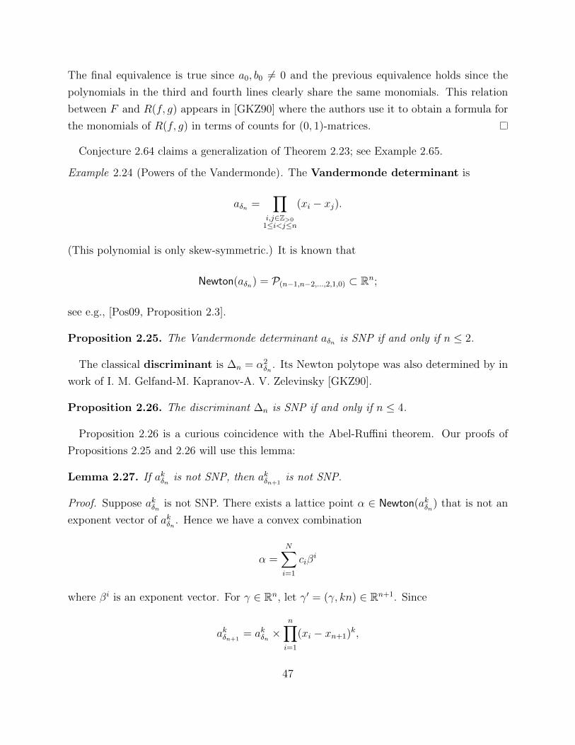
The final equivalence is true since a0, b0 6= 0 and the previous equivalence holds since the

polynomials in the third and fourth lines clearly share the same monomials. This relation

between F and R(f, g) appears in [GKZ90] where the authors use it to obtain a formula for

the monomials of R(f, g) in terms of counts for (0, 1)-matrices.

Conjecture 2.64 claims a generalization of Theorem 2.23; see Example 2.65.

Example 2.24 (Powers of the Vandermonde). The Vandermonde determinant is

aδn =∏

i,j∈Z>01≤i<j≤n

(xi − xj).

(This polynomial is only skew-symmetric.) It is known that

Newton(aδn) = P(n−1,n−2,...,2,1,0) ⊂ Rn;

see e.g., [Pos09, Proposition 2.3].

Proposition 2.25. The Vandermonde determinant aδn is SNP if and only if n ≤ 2.

The classical discriminant is ∆n = α2δn

. Its Newton polytope was also determined by in

work of I. M. Gelfand-M. Kapranov-A. V. Zelevinsky [GKZ90].

Proposition 2.26. The discriminant ∆n is SNP if and only if n ≤ 4.

Proposition 2.26 is a curious coincidence with the Abel-Ruffini theorem. Our proofs of

Propositions 2.25 and 2.26 will use this lemma:

Lemma 2.27. If akδn is not SNP, then akδn+1is not SNP.

Proof. Suppose akδn is not SNP. There exists a lattice point α ∈ Newton(akδn) that is not an

exponent vector of akδn . Hence we have a convex combination

α =N∑i=1

ciβi

where βi is an exponent vector. For γ ∈ Rn, let γ′ = (γ, kn) ∈ Rn+1. Since

akδn+1= akδn ×

n∏i=1

(xi − xn+1)k,

47

each (βi)′ is an exponent vector of akδn+1and hence α′ is a lattice point of Newton(akδn+1

).

Since xα′

= xαxknn+1 and xn+1 does not appear in akδn , if α′ is an exponent vector of akδn+1,

then α is an exponent vector of akδn , a contradiction. Thus akδn+1is not SNP.

Proof of Propositions 2.25 and 2.26: Clearly, aδn is SNP for n = 1, 2. One checks that

(1, 1, 1) ∈ Newton(aδ3) but is not an exponent vector of aδ3 .

Separately, one checks ∆n is SNP for n ≤ 4. Also ∆5 is not SNP. In fact, the only lattice

points that are not exponent vectors are all 5! rearrangements of (1, 3, 4, 5, 7).

Now apply Lemma 2.27 to complete an induction argument for each of the two propositions

being proved.

Conjecture 2.28. For all k, there exists Nk such that akδn is not SNP for any n ≥ Nk.

More precisely, for 1 ≤ j ≤ 4 we computed N2j−1 = 3 and moreover that (1, 3j−2, 3j−2)

is a lattice point that is not an exponent vector. Moreover, N2 = 5, N4 = 4, N6 = 4, N8 = 3.

For more on (higher) powers of the Vandermonde, see, e.g., [STW94, Bal11].

Example 2.29 (q-discriminant). The q-discriminant is∏

1≤i<j≤n

(xi − qxj). At q = −1,

fn =∏

1≤i<j≤n

(xi + xj) ∈ Symn.

It is known that

fn = sρn(x1, x2, . . . , xn) where ρn = (n− 1, n− 2, . . . , 3, 2, 1, 0).

Hence fn is SNP and Newton(fn) = Pρn ⊂ Rn.

Example 2.30 (Totally nonnegative matrices). Let

M = (mij)1≤i,j≤n

be an n × n totally nonnegative real matrix. That is, the determinant of every square

submatrix of M is nonnegative. Define

FM =∑w∈Sn

(n∏i=1

mi,w(i)

)pλ(w),

where λ(w) is the cycle type of w.

48

Theorem 2.31. The symmetric function FM is SNP.

Proof. By assumption, mij ≥ 0. A theorem of J. R. Stembridge [Ste91] (cf. [Sta99a, Exer-

cise 7.92]) states that FM is also Schur positive. Now apply Proposition 2.13.

Example 2.32 (Redfield–Polya theory). Let G be a subgroup of Sn. The cycle index poly-

nomial is

ZG =1

|G|∑g∈G

pλ(g),

where λ(g) is the cycle type of g.

Theorem 2.33. The cycle index polynomial ZG has SNP.

Proof. It is true that

ZG =∑

λ∈Par(n)

cλsλ,

where each cλ ∈ Z≥0; see [Sta99a, pg. 396]. This positivity is known for representation-

theoretic reasons (no combinatorial proof is available). Now use Proposition 2.13.

Example 2.34 (C. Reutenauer’s qλ basis). C. Reutenauer [Reu95] introduced a new basis

{qλ} of symmetric polynomials, recursively defined by setting∑λ∈Par(n)

qλ = s(n),

where qλ = qλ1qλ2 · · · .

Theorem 2.35. The symmetric function qλ has SNP.

Proof. C. Reutenauer in loc. cit. conjectured that −q(n) is Schur positive for n ≥ 2. Indeed,

q(1) = s(1), q(2) = −s(1,1), q(3) = −s(2,1).

Reutenauer’s conjecture was later established by W. M. Doran IV [IV96]. The proof sets

f(n, k) =∑

λ∈Par(n)min(λi)≥k

qλa.

49

The argument inducts on n and proceeds by showing that

−f(n, k) = s(n−1,1) +∑i∈Z>02≤i<k

(−f(i, i))(−f(n− i, i)).

His induction claim is that −f(n, k) is Schur positive for k ≥ 2. Let us strengthen his

induction hypothesis, and assume −f(n, k) is Schur positive with s(n−1,1) as the unique ≤Dmaximal term. In the induction step, note each sα appearing in −f(i, i) has α1 ≤ i− 1 and

each sβ in −f(n− i, i) has β1 ≤ n− i− 1. Thus, by the argument of Proposition 2.11, if sγ

appears in sαsβ then γ1 ≤ n− 2, implying the strengthening we need.

It follows from the above argument and the Littlewood-Richardson rule that if λ =

(λ1, . . . , λ`, 1r) where each λi ≥ 2 then qλ has a unique≤D-leading term s(a,b) where a = |λ|−`

and b = `. Thus, qλ has SNP by Proposition 2.7(III).

Example 2.36 (Stanley’s chromatic symmetric polynomial). For a graph G, let cG be Stan-

ley’s chromatic symmetric polynomial [Sta95]. If G = K1,3,

cG(x1, x2, . . .) = m(3,1) + 6m(2,1,1) + 24m(1,1,1,1)

is not SNP as it is missing (2, 2).

It is an open problem to determine for which graphs G is cG Schur positive. Likewise, we

can ask for which graphs is cG SNP.

Conjecture 2.37. Let G be a graph where cG is Schur positive. Then cG is SNP.

This conjecture has exhaustively checked for all graphs with at most 7 vertices and many

graphs on 8 vertices. For graphs with 7 vertices, there are 771 graphs such that cG is both

Schur positive and SNP. Of the 145 graphs such that cG is not Schur positive, 64 have SNP

and 81 do not.

Example 2.38 (Kronecker product of Schur polynomials). The Kronecker product is

sλ ∗ sµ =∑

ν∈Par(|λ|)

Kronνλ,µsν ∈ Sym.

Kronνλ,µ is the Kronecker coefficient, the multiplicity of the Sn-character χν appearing in

χλ ⊗ χµ. We conjecture that sλ ∗ sµ is SNP. We have verified this for all λ, µ ∈ Par(n) for

50

1 ≤ n ≤ 7. Consider

s(4,2) ∗ s(2,2,1,1) = s(1,1,1,1,1,1) + s(2,1,1,1,1) + 2s(2,2,1,1) + s(3,1,1,1) + 2s(3,2,1) + s(3,3) + s(4,1,1).

Notice (3, 3) and (4, 1, 1) are both ≤D-maximal. Hence in this case, SNPness cannot be

blamed on Proposition 2.7(III); cf. [AAV12, Lemma 3.2] and [Val00].

Example 2.39 (Lascoux-Leclerc-Thibon (LLT) polynomials). A. Lascoux, B. Leclerc, and

J. Y. Thibon [LLT97] introduced G(m)λ (x; q). Then, G

(m)λ (x; 1) is a product of Schur polyno-

mials. Hence G(m)λ (x; 1) is SNP by Proposition 2.11. However, G

(m)λ (x; q) ∈ Symn[q] is not

always SNP. One example is

G(2)(3,3)(x1, x2; q) = q3(x31 + x21x2 + x1x

22 + x32) + q(x21x2 + x22x1).

LLT polynomials arise in the study of Macdonald polynomials, the topic of Section 2.3.

(Another related topic is affine Schubert calculus; see the book [LLM+14].)

2.3 Macdonald polynomials

2.3.1 Symmetric and nonsymmetric Macdonald polynomials

The definitions of the Macdonald polynomials used in this section can be found in Section

1.5. Recall that the symmetric Macdonald polynomial Pλ has the form

Pλ(x; q, t) = mλ(x) +∑

µ∈Par(|λ|)µ<Dλ

cλ,µ(q, t)mµ(x) (2.7)

where cλ,µ(q, t) ∈ Q(q, t).

Theorem 2.40. For any (q0, t0) in a Zariski open subset of C2, the specialization Pλ(x; q0, t0)

is SNP, and Newton(Pλ(x; q0, t0)) = Pλ ⊂ Rn whenever n ≥ `(λ).

Lemma 2.41. For any (q0, t0) ∈ C2, we have Newton(Pλ(x; q0, t0)) = Pλ ⊂ Rn whenever

n ≥ `(λ).

Proof. This is by (2.7) and Proposition 2.7(I). Since n ≥ `(λ), we have sλ(x1, . . . , xn) 6≡0.

51

Lemma 2.42. Fix q0, t0 ∈ C. Then, Pλ(x; q0, t0) is SNP if and only if cλ,µ(q0, t0) 6= 0 for

all µ <D λ.

Proof. (⇒) By Lemma 2.41, Newton(Pλ(x; q0, t0)) = Pλ. Thus each µ <D λ appears as a

lattice point of Newton(Pλ(x; q0, t0)). Since we assume Pλ(x; q0, t0) is SNP, we know

[xµ]Pλ(x; q0, t0) 6= 0.

Among the monomial symmetric functions, xµ only appears in mµ. Hence cλ,µ(q0, t0) 6= 0,

as desired.

The proof of (⇐) just reverses the above argument, using the fact that

µ ∈ Newton(Pλ(x; q0, t0)) = Pλ ⇐⇒ γ ∈ Newton(Pλ(x; q0, t0)) = Pλ

for any rearrangement γ of µ ∈ Rn.

Proof of Theorem 2.40: The Newton polytope assertion is by Lemma 2.41. Now

Pλ(x; 0, 0) = sλ(x)

and mµ appears in sλ for every µ <D λ. Hence cλ,µ(q, t) 6≡ 0. Now choose q, t that is neither

a pole nor a root of any of these rational functions (for µ <D λ). Therefore the SNP assertion

follows from Lemma 2.42.

The Hall-Littlewood polynomial is Pλ(x; t) = Pλ(x, 0, t). One has

Pλ(x; t) =∑µ

Kλ,µ(t)sµ(x)

where Kλ,µ(t) is the Kostka-Foulkes polynomial. It is known that

Kλ,µ(t) =∑

T∈SSYT(λ)c(T )=µ

tcharge(T )

where charge(T ) ∈ Z≥0 [LS78b, Theorem 1’]. Since these tableaux can only occur if µ ≤D λ,

we have Kλ,µ(t) 6≡ 0 if and only if µ ≤D λ. Hence we immediately obtain:

Proposition 2.43. If t0 > 0 then Pλ(x; t0) ∈ Sym is SNP and whenever n ≥ `(λ)

Newton(Pλ(x; t0)) = Pλ ⊂ Rn.

52

When λ is a partition with distinct parts, we can represent its shifted diagram as the

diagram where the ith row begins in column i. For example, for λ = (4, 3, 1), the shifted

diagram of λ is

.

Then shifted semistandard tableaux of λ are fillings of the shifted diagram with numbers

from the alphabet

1′ < 1 < 2′ < 2 < . . .

such that rows and columns are weakly increasing, primed entries repeat only in columns,

and unprimed entries repeat only in rows. Then the content of a shifted tableaux T is the

weak composition c(T ) where c(T )i is the number of i and i′ entries in T . The theory of

shifted tableaux can be found in D. Worley’s thesis [Wor84].

The Schur P−polynomial is

SPλ(x) =∑T

xT

where the sum is over shifted semistandard Young tableaux T of a partition λ with distinct

parts. The Schur Q−polynomial is

SQλ(x) = 2`(λ)SPλ. (2.8)

Proposition 2.44. The symmetric functions SPλ(x) and SQλ(S) are SNP and

Newton(SPλ(x)) = Newton(SQλ(x)) = Pλ.

Proof. In fact,

SPλ(x) = Pλ(x; t = −1);

see [Ste89], and Kλ,λ(t) = 1. Furthermore, SPλ is Schur positive; see, e.g., [Ste89, p. 131–

132]. Thus the result follows from Proposition 2.7(III).

The modified Macdonald polynomial Hλ(x; q, t) is a certain transformation of Pλ(x; q, t); see

Definition 1.18.

53

Proposition 2.45. For any q0, t0 > 0, we have Hλ(x; q0, t0) is SNP and whenever n ≥ |λ|,

Newton(Hλ(x; q0, t0)) = P|λ| ⊂ Rn.

Proof. The formula of J. Hagland-M. Haiman-N. Loehr [HHL05] (see Theorem 1.19) states

that

Hλ(x; q0, t0) =∑F

xF qinv(F )0 t

maj(F )0 ,

where the sum is over all fillings F of λ. Thus, for q0, t0 > 0, every monomial of degree |λ|appears.

However, H(3,1,1)(x1, x2, x3, x4, x5; q, t) is not SNP as it misses the monomial qtx3x44.

Example 2.46 (Modified q, t-Kostka polynomials are not SNP). Consider the expansion

Hλ(x; q, t) =∑

µ∈Par(|λ|)

Kλ,µ(q, t)sµ(x)

from Definition 1.18. The coefficients Kλ,µ(q, t) are the (modified) q, t-Kostka coefficients.

Now,

K(2,2,2),(3,3)(q, t) = qt4 + qt3 + q3 + qt2 + t3

is not SNP as it is missing q2t. Hence, Kλ,µ(q, t) need not be SNP.

Let γ be a weak composition and let tij(γ) swap positions i and j of γ. Furthermore, let

mij(γ) = γ + ei − ej

where ei is the vector with a 1 in position i and 0’s elsewhere. S. Sahi [Sah00] defined a

partial order on weak compositions <S whose covering relations are

• if i < j and γj > γi then tij(γ) <S γ, and

• if i < j and γj − γi > 1 then mij(γ) <S tij(γ);

see [HHL08, Section 2.1]. It is part of a definition of the nonsymmetric Macdonald polynomial

Eγ(x; q, t) that

Eγ(x; q, t) = xγ +∑

δ∈WC(|γ|)δ<Sγ

dγ,δ(q, t)xδ

54

where dγ,δ(q, t) ∈ Q(q, t) [HHL08]. S. Sahi [Sah00] proved each dγ,δ(q, t) 6≡ 0. Let Pγ be the

convex hull of all weak compositions δ such that δ ≤S γ. Thus Pγ is the Newton polytope

of Eγ(x; q0, t0) for any generic choice of (q0, t0) ∈ C2. The conjecture below says Eγ(x; q, t)

is “generically SNP”.

Conjecture 2.47. If δ ∈ Pγ and δ ∈ Zn≥0 then δ ≤S γ.

Conjecture 2.47 has been checked for n ≤ 7 and whenever |γ| ≤ 7.

2.3.2 Keys and Demazure atoms

We now investigate SNP for two specializations of Eγ(x; q, t): the key polynomials Keyγ =

Eγ(x;∞,∞) and the Demazure atoms Atomγ = Eγ(x; 0, 0) defined in Definition 1.21. As in

Section 1.5, define Dγ to be the skyline diagram with a left-justified row of γi boxes in row i.

Conjecture 2.48. SDγ = Newton(Keyγ).

We have a combinatorial proof (omitted here) of the “⊇” part of Conjecture 2.48; see

Remark 2.85. This conjecture has been resolved to be true by A. Fink, K. Meszaros, and

A. St. Dizier (Theorem 10, [FMS17]).

Conjecture 2.49. The key polynomial Keyγ has SNP.

This conjecture has also been resolved as true by A. Fink, K. Meszaros, and A. St. Dizier

(Corollary 8, [FMS17]). We have a second conjectural description of Newton(Keyγ). For any

(weak) composition γ, let δ <Key γ be the partial order with covering relations

• if i < j and γj > γi then tij(γ) <Key γ, and

• if i < j and γj − γi > 1 then mij(γ) <Key γ.

Observe that δ <Key γ, then δ <S γ. However, the converse fails as

m12((0, 2)) = (1, 1) <S (2, 0) = t12((0, 2))

but one does not have (1, 1) <Key (2, 0).

Conjecture 2.50.

Keyγ = xγ +∑

δ∈WC(|γ|)δ<Keyγ

kγ,δxδ

55

with kγ,δ > 0 for all δ <Key γ, and thus

Newton(Keyγ) = {δ|δ ≤Key γ}.

Recall from Section 1.5, that for two weak compositions γ and δ we write

γ � δ if λ(γ) = λ(δ) and wγ ≤B wδ.

Theorem 2.51. If δ � γ then δ is a vertex of Newton(Keyγ).

Conjecture 2.52. The converse of Theorem 2.51 holds.

Our proof of Theorem 2.51 uses the decomposition of Keyγ into Demazure atoms given in

Theorem 1.26:

Keyγ =∑

δ∈PermutWC(λ(γ))δ�γ

Atomδ. (2.9)

By the way,

Conjecture 2.53. The Demazure atom Atomγ has SNP.

Conjectures 2.50, 2.52 and 2.53 have been checked for |α| ≤ 7 where α has at most three

parts of size zero.

Proposition 2.54. Suppose δ � γ. Let λ = λ(δ) = λ(γ). Then

{λ} ⊆ Newton(Keyδ) ⊆ Newton(Keyγ) ⊆ Pλ ⊆ Rn,

where n is the position of the last nonzero part of γ.

Proof. Using (2.9) twice, we have

Keyγ =∑

κ∈PermutWC(λ)κ�γ

Atomκ

=∑

κ∈PermutWC(λ)κ�δ

Atomκ +∑

κ∈PermutWC(λ)κ�γκ6�δ

Atomκ

= Keyδ +∑

κ∈PermutWC(λ)κ�γκ6�δ

Atomκ.

56

(1, 0, 2)

(2, 0, 1)

(2, 1, 0) (1, 2, 0)

(0, 2, 1)

(0, 1, 2)

(1, 1, 1)

Figure 2.2: The permutahedron for λ = (2, 1, 0). The shaded region is Newton(Key1,0,2).See Proposition 2.54.

Since each Atomκ is monomial positive [Mas09, Theorem 1.1],

Newton(Keyδ) ⊆ Newton(Keyγ).

Now, λ is�-minimum among rearrangements of λ. By definition Keyλ = xλ. This explains

the leftmost containment.

Similarly, λ∗ is the �-maximum among rearrangements of λ in Zn and Keyλ∗ = sλ (see

Equation (1.6)). However we know Newton(sλ) = Pλ.

Figure 2.2 provides an example of this nesting property for the Newton polytopes of Keyγ.

Lemma 2.55. Suppose P and Q are polytopes such that P ⊆ Q. If v is a vertex of Q and

v ∈ P, then v is a vertex of P.

Proof. The point v is a vertex of Q if and only if there is a separating hyperplane H, i.e.,

there exists a vector c such that cTv ≤ cTy for all y ∈ Q. Since P ⊆ Q, H works for Palso.

Proof of Theorem 2.51: Now,

Keyγ = xγ + (positive sum of monomials);

57

see, e.g., [RS95, Corollary 7]. Hence, γ is in Newton(Keyγ). By Proposition 2.54,

δ ∈ Newton(Keyδ) ⊆ Newton(Keyγ) if δ � γ.

Again applying Proposition 2.54 we have that Newton(Keyγ) ⊆ Pλ(γ). Now we are done

by combining Proposition 2.7(II) and Lemma 2.55.

2.4 Quasisymmetric functions

Recall from Section 1.3 that QSym is the ring of quasisymmetric functions, Mα is the mono-

mial quasisymmetric basis (Definition 1.12), and Fα is Gessel’s fundamental basis (Definition

1.13).

Example 2.56 (The monomial quasisymmetric function Mα need not be SNP). For example,

M(2) = p2 = x21 + x22 + · · · does not have SNP.

Theorem 2.57. We have Newton(Fα(x1, . . . , xn)) = Newton(Mα(x1, . . . , xn)) ⊂ Rn. The

vertices of this polytope are {γ ∈ Zn≥0 : γ+ = α}.

Proof. Recall from (1.3),

Fα =∑

β∈Comp(|α|)β�α

Mβ.

Then, each Mβ is a positive sum of monomials and Mα appears in the expansion (1.3). Thus,

Newton(Fα(x1, . . . , xn)) ⊇ Newton(Mα(x1, . . . , xn)).

Now suppose β = (β1, β2, . . . , βk) ∈ Zk>0 and β � β where

β = (β1, β2, . . . , β′i, β′′i , . . . , βk) ∈ Zk+1

>0

and βi = β′i + β′′i .

We wish to show

Newton(Mβ(x1, . . . , xn)) ⊆ Newton(Mβ(x1, . . . , xn)). (2.10)

58

By induction, this implies the remaining containment

Newton(Fα(x1, . . . , xn)) ⊆ Newton(Mα(x1, . . . , xn)).

Suppose xβ is a monomial of Mβ and thus

β = (β1, . . . , βn) ∈ Zn≥0

where (β)+ = β. Then,

β = (0, . . . , 0, β1, 0, . . . , 0, β2, . . . , β′i, 0, . . . , 0, β

′′i , . . . , βk, 0, . . . , 0)

where we are depicting the 0’s inserted between components of β to obtain β.

Now let

β◦ = (0, . . . , 0, β1, 0, . . . , 0, β2, . . . , βi, 0, . . . , 0, 0, . . . , βk, 0, . . . , 0)

and

β• = (0, . . . , 0, β1, 0, . . . , 0, β2, . . . , 0, 0, . . . , 0, βi, . . . , βk, 0, . . . , 0).

That is β◦ and β• differ from β only by replacing β′i and β′′i by βi, respectively.

Since β′i, β′′i ≥ 0, we have that

β =β′iβiβ◦ +

β′′i

βiβ•

is a convex combination. This proves (2.10) and hence the asserted equality of Newton

polytopes.

Every monomial of Mα(x1, . . . , xn) is a monomial of mα(x1, . . . , xn). Therefore,

Newton(Mα(x1, . . . , xn)) ⊆ Newton(mα(x1, . . . , xn)).

Recall,

Newton(mα(x1, . . . , xn)) = Pλ(α) ⊆ Rn.

The vertices of Pλ(α) are all rearrangements of α; cf. Proposition 2.7(II). Thus, every exponent

vector of mα(x1, . . . , xn) is a vertex of Pλ(α). Furthermore, the containment argument above

shows that every lattice point γ of Newton(Fα) (coming from a monomial) such that γ 6= α

is a convex combination of {γ|λ(γ) = λ(α)}, and thus cannot be a vertex of Newton(Fα).

59

Since all vertices of Newton(Fα) come from a monomial of Fα, to obtain the final claim of

the theorem we may appeal to Lemma 2.55.

Example 2.58 (The fundamental quasisymmetric function Fα need not be SNP). One can

check that

F(2,2) = M(2,2) +M(2,1,1) +M(1,1,2) +M(1,1,1,1).

Thus, (0, 1, 2, 1) = 12(0, 2, 2, 0) + 1

2(0, 0, 2, 2) ∈ Newton(F(2,2)). However, (0, 1, 2, 1) is not an

exponent vector of F(2,2). Hence F(2,2) is not SNP.

The quasisymmetric Schur function (Definition 1.28) has the form

Sα =∑

γ∈Expand(α)

Atomγ.

Many aspects of quasi-Schur theory are parallel to Schur theory [HLMvW11a]. For instance,

consider the transition between the S and M bases of QSym:

Sα =∑

β∈Comp(|α|)

Kα,βMβ

where Kα,β is the number of semistandard composition tableaux of shape α and content β.

Hence Kα,β is an analogue of the Kostka coefficient. However, there are divergences from the

perspective of Newton polytopes as seen in the next three examples:

Example 2.59 (The quasisymmetric Schur function Sα need not be SNP). An example is

S(2,1,3). In at least four variables, x1x22x

23x4 does not appear but x21x

22x

23 and x22x

23x

24 both do.

Nonetheless, it should be interesting to describe the Newton polytope, and to characterize

when Sα is SNP.

Example 2.60. In the symmetric function case,

Newton(sλ(x1, . . . , xn)) = Newton(mλ(x1, . . . , xn)) = Pλ ⊂ Rn.

However,

(0, 0, 2, 2) ∈ Newton(S(1,3)(x1, x2, x3, x4)) but (0, 0, 2, 2) 6∈ Newton(M(1,3)(x1, x2, x3, x4)).

Hence Newton(Sα(x1, . . . , xn)) 6= Newton(Mα(x1, . . . , xn)) in general.

60

Example 2.61. We may define a dominance order �′D on strict compositions by α �′D β if

Newton(Mα) ⊆ Newton(Mβ). The above example shows that Kα,β > 0 if and only if β �′D α

is not generally true. This is in contrast with (2.3).

2.5 Schubert polynomials and variations

2.5.1 The Schubert SNP conjectures

A. Lascoux and M.-P. Schutzenberger introduced the Schubert polynomials [LS82a], which

are defined in Section 1.4 (see Definition 1.15).

Example 2.62 (The operators ∂i and πi do not preserve SNP). This polynomial is SNP:

f = x41 + x31x2 + x21x22 + 2x1x

32.

However

∂1(f) = x31 + x32

is not SNP.

Since πi(g) = ∂i(xi · g), if we set

g = x31 + x21x2 + x1x22 + 2x32

we have π1(g) = ∂1(f). Hence, πi does not preserve SNP.

However, despite this:

Conjecture 2.63. The Schubert polynomial Sw has SNP.

This conjecture has since been confirmed by A. Fink, K. Meszaros, and A. St. Dizier

(Corollary 8, [FMS17]).

The double Schubert polynomial Sw(x; y) is defined by setting

Sw0(x; y) =∏

i,j∈mathbbZ>0i+j≤n

(xi − yj)

and recursively determining Sw(x; y) for w 6= w0 precisely as for Sw(x).

Conjecture 2.64. The double Schubert polynomial Sw(x; y) is SNP.

61

We have checked Conjecture 2.64 for n ≤ 5 (and many other cases). Since Sw(x; 0) =

Sw(x), Conjecture 2.64 generalizes Conjecture 2.63.

Example 2.65 (Double Schubert polynomials are generalized resultants). A permutation is

dominant if its diagram is a partition. Then for w equal to the dominant permutation

w(i) =

{n+ i i = 1, . . . ,m

i−m i = m+ 1, . . . ,m+ n,

Sw(x; y) =n∏i=1

m∏j=1

(xi − yj).

One reference is [Man01, Proposition 2.6.7]. This has the same Newton polytope as R(f, g).

Thus Conjecture 2.64 is a generalization of Theorem 2.23.

A. Lascoux and M.-P. Schutzenberger also introduced the family of Grothendieck poly-

nomials [LS82b]; see Definition 1.30.

Conjecture 2.66. The Grothendieck polynomial Gw has SNP.

Conjecture 2.66 has been exhaustively checked for n ≤ 7. Conjecture 2.66 generalizes

Conjecture 2.63 since

Newton(Sw) = Newton(Gw) ∩

{(α1, . . . , αn) ∈ Rn :

n∑i=1

αi = #Dw

}.

This conjecture has been proven in the two special cases below.

Theorem 2.67 (Escobar-Yong [EY17]). The symmetric Grothendieck function Ksλ is SNP.

Theorem 2.68 (Meszaros-St. Dizier, Theorem C [MS17]). For π a dominant permutation,

KS1π has SNP.

The Lascoux polynomials KKeyγ and Lascoux atoms KAtomγ (see Definition 1.34) that

arise in combinatorial K-theory also seem to be SNP.

Conjecture 2.69. The Lascoux polynomial KKeyγ has SNP.

Conjecture 2.70. The Lascoux atom KAtomγ has SNP.

Conjectures 2.69 and 2.70 have been verified for |α| ≤ 7 where α has at most three parts

of size zero.

62

2.5.2 Stanley polynomials and the stable limit of Conjecture 2.63

For w ∈ Sn, let 1t × w ∈ St+n be the permutation defined

1t × w(i) =

{i 1 ≤ i ≤ t

n+ i t+ 1 ≤ i ≤ t+ n.

The Stanley symmetric polynomial (also known as the stable Schubert polynomial)

is defined by

Fw = limt→∞

S1t×w ∈ Sym.

The power series Fw is well-defined and was originally introduced by R. P. Stanley in

[Sta84]. The next result is a “stable limit” version of Conjecture 2.76.

Theorem 2.71. The Stanley symmetric function Fw ∈ Sym is SNP.

Our proof rests on:

Theorem 2.72 (Theorems 3.2, 4.1, [Sta84]). For

Fw =∑

λ∈Par(`(w))

aw,λsλ,

aw,λ ≥ 0 and there exists λ(w) and µ(w) such that if aw,λ 6= 0, then λ(w) ≤D λ ≤D µ(w).

Proof of Theorem 2.71: Combine Theorem 2.72 and Proposition 2.7(III).

Corollary 2.73. Any skew-Schur polynomial sλ/µ(x) has SNP.

Proof. To every skew shape λ/µ there is a 321-avoiding permutation wλ/µ with the property

that Fwλ/µ(x) = sλ/µ [BJS93]. Now apply Theorem 2.71.

Let

S∞,` = {w ∈ S∞ : `(w) = `}.

Declare

u ≤D v for u, v ∈ S∞,` if Newton(Su) ⊆ Newton(Sv).

Given a partition λ = (λ1 ≥ λ2 ≥ . . . ≥ λk > 0), define wλ,k ∈ Sλ1+k to be the unique

permutation that satisfies

wλ,k(i) = λk−i+1 + i for 1 ≤ i ≤ k

63

and is Grassmannian, i.e., it has at most one descent, at position k. Then one has

Swλ,k = sλ(x1, . . . , xk).

We now show that (S∞,≤D) extends (Par(n),≤D):

Proposition 2.74. Suppose λ, µ ∈ Par(n) and let k = max{`(λ), `(µ)}. Then λ ≤D µ if

and only if wλ,k ≤D wµ,k.

Proof. Since Swλ,k(x1, . . . , xk) = sλ(x1, . . . , xk) and Swµ,k(x1, . . . , xk) = sµ(x1, . . . , xk),

Pλ = Newton(sλ(x1, . . . , xk)) = Newton(Sw,λ(x1, . . . , xk)) ⊆ Rk.

The same statement holds where we replace λ by µ. Now apply Rado’s theorem (2.3).

Figure 2.3 shows part of (S∞,2,≤D). From this one can see that the poset is not graded,

just like dominance order ≤D on partitions is not graded. Unlike ≤D, it is not a lattice:

in Figure 2.3, the elements 231456 and 312456 do not have a unique least upper bound as

142356 and 214356 are incomparable minimal upper bounds.

Theorem 2.75. Every two elements u, v ∈ S∞,` have an upper bound under ≤D.

Proof. Suppose {αi} and {βj} are the exponent vectors of Su and Sv, respectively. It suffices

to show there exists w ∈ S∞,` such that

Sw =∑i

xαi +∑j

xβj + (positive sum of monomials).

We first show that there is a Fw such that each sλ(αi) and sλ(βj) appear (possibly with

multiplicity). A theorem of S. Fomin-C. Greene [FG98] states that

Fw =∑

ν∈Par(`(w))

aw,νsν

where aw,ν is the number of semistandard tableaux of shape ν such that the top-down,

right-to-left reading word is a reduced word for w. Let

w = s1s3s5 · · · s2`−1.

Clearly this decomposition is reduced. All reduced words of w are obtained by permuting

the simple transpositions.

64

312456 231456

142356 214356 134256

213546

132546 213465

125346 132465 124536

123645 124365 123564

Figure 2.3: The S6 part of the Hasse diagram of (S∞,2,≤D)

Filling any shape of size ` by successively placing 1, 3, 5, . . . , 2` − 1 along rows in left to

right order gives a semistandard tableaux. Thus every sµ where µ ` ` appears in Fw. In

particular each sλ(αi) and each sλ(βj) appears. Since xλ(αi) appears in sλ(αi), by symmetry of

sλ(αi), xαi appears as well. That is, xαi appears in Fw. Similarly xβj appears in Fw.

By definition, for any monomial xγ appearing in Fw, there is a finite Nγ such that xγ

appears in S1Nγ×w. It suffices to pick N larger than all Nαi and Nβj .

2.5.3 Inequalities for Newton(Sw)

Let

Dw = {(i, j) : 1 ≤ i, j ≤ n,w(i) > j and w−1(j) > i}

65

be the Rothe diagram of a permutation w ∈ Sn (see Section 1.1).

Conjecture 2.76. SDw = Newton(Sw).

This has been confirmed by A. Fink, K. Meszaros, and A. St. Dizier (Theorem 10,

[FMS17]). Notice that Conjecture 2.76 is equivalent to the assertion that w ≤D v if and only

if θDw(S) ≤ θDv(S) for all S ⊆ [n].

Example 2.77. Suppose w = 21543, the Rothe diagram Dw is given by

One can check that the defining inequalities are

α1 + α2 + α3 + α4 = 4

α1 ≤ 3, α2 ≤ 2, α3 ≤ 2, α4 ≤ 1

α1 + α2 ≤ 4, α1 + α3 ≤ 4, α1 + α4 ≤ 4, α2 + α3 ≤ 3, α2 + α4 ≤ 3, α3 + α4 ≤ 3

α1 + α2 + α3 ≤ 4, α1 + α2 + α4 ≤ 4, α2 + α3 + α4 ≤ 3

α1 + α2 + α3 + α4 ≤ 4.

together with αi ≥ 0 for each i. The polytope is depicted in Section 2.1.

One can uniquely reconstruct u ∈ S∞ with the defining inequalities.

Proposition 2.78. If u, v ∈ Sn are of the same length and θDu(S) = θDv(S) for all S =

{i, i+ 1, . . . , n} where 1 ≤ i ≤ n, then u = v.

Proof. Let

ci(π) = #{j : (i, j) ∈ Dπ}.

Thus (c1(π), c2(π), . . .) is the Lehmer code of π. The Lehmer code uniquely determines

π ∈ S∞; see, e.g., [Man01, Proposition 2.1.2]. Hence it suffices to show the codes of u and v

are the same. This follows from:

i∑j=1

cj(u) = `− θDu({i+ 1, i+ 2, . . . , n}) = `− θDv({i+ 1, i+ 2, . . . , n}) =i∑

j=1

cj(v),

66

for i = 1, 2, . . . n− 1.

The inequalities of SD are in general redundant. If

θD(S) = θD(T ) and S ⊇ T (2.11)

then the inequality ∑i∈T

αi ≤ θD(T )

is unnecessary. Similarly, if

S =⊔i

si and θD(S) =∑i

θD(si) (2.12)

then the S-inequality is implied by the si inequalities.

Problem 2.79. Give the minimal set of inequalities associated to Dw (or more generally,

any D).

Example 2.80. Continuing Example 2.77, minimal inequalities are

α1 + α2 + α3 + α4 = 4

α1 ≤ 3, α2 ≤ 2, α3 ≤ 2, α4 ≤ 1

α1 + α2 ≤ 4, α1 + α3 ≤ 4, α2 + α3 ≤ 3,

α2 + α3 + α4 ≤ 3,

combined with positivity. This minimization is obtained using reductions (2.11) and (2.12).

Example 2.81. If w = 23154 then using the reductions (2.11) and (2.12) leaves:

α1 + α2 + α3 + α4 = 3, α3 + α4 ≤ 1, α1 + α3 + α4 ≤ 2, α2 + α3 + α4 ≤ 2.

However, α3 + α4 ≤ 1 is actually not necessary. Thus reductions (2.11) and (2.12) are not

sufficient for determining minimal inequalities.

Given a polytope P , its Ehrhart polynomial, denoted LP (t), is the polynomial such

that for t ∈ Z≥1, LP (t) equals the number of lattice points in the polytope tP . E. Ehrhart

[Ehr62] showed that for a polytope of dimension d in Rn, LP (t) is in fact a polynomial of

degree d. For more see, e.g., [BR07].

67

w Sw dimSDw vertices of SDw LSDw (t)

1243 x1 + x2 + x3 2 (1, 0, 0), (0, 1, 0), (0, 0, 1) 12t2 + 3

2t+ 1

1324 x1 + x2 1 (1, 0), (0, 1) t+ 11342 x1x2 + x1x3 + x2x3 2 (1, 1, 0), (1, 0, 1), (0, 1, 1) 1

2t2 + 3

2t+ 1

1423 x21 + x1x2 + x22 1 (2, 0), (0, 2) 2t+ 1

1432x21x2 + x1x

22 + x21x3 2

(2, 0, 1), (1, 2, 0), 32t2 + 5

2t+ 1

+x1x2x3 + x22x3 (2, 1, 0), (0, 2, 1)2143 x21 + x1x2 + x1x3 2 (2, 0, 0), (1, 1, 0), (1, 0, 1) 1

2t2 + 3

2t+ 1

2413 x21x2 + x1x22 1 (2, 1), (1, 2) t+ 1

2431 x21x2x3 + x1x22x3 1 (2, 1, 1), (1, 2, 1) t+ 1

3142 x21x2 + x21x3 1 (2, 1, 0), (2, 0, 1) t+ 14132 x31x2 + x31x3 1 (3, 1, 0), (3, 0, 1) t+ 1

Table 2.1: Additional data about positive dimensional Schubitopes SDw for w ∈ S4.

Conjecture 2.82. If LN (SDw )(t) = cdtd + · · ·+ c0, then ci > 0 for i = 0, . . . , d.

Conjecture 2.82 also seems true for SD where D is arbitrary. We have exhaustively checked

this for n = 4 and many random cases for n = 5.

Table 2.1 gives some data about the positive dimensional Schubitopes SDw for w ∈ S4.

2.5.4 Relationship of the Schubitope to Kohnert’s rule

In Section 1.4, we described Kohnert’s combinatorial rule for Sw [Koh91]. With this rule

in hand, one obtains part of Conjecture 2.63, see Proposition 2.83 below. Even though

Conjecture 2.63 has been confirmed, it is open to give a combinatorial proof of the inequalities

and so we give one for one direction of the containment below.

Proposition 2.83. SDw ⊇ Newton(Kw).

Proof. Consider a diagram D ∈ Koh(w) such that c(D) = α. Each Kohnert move preserves

the number of boxes. Hence∑n

i=1 αi = #Dw holds.

Now fix a column c and S ⊆ [n]. Compare the positions of the boxes of D to the boxes of

Dw. Let

TD,S,c = #boxes of D in the rows of S and column c.

Also, let UD,S,c be the number of pairs (r, r′), with no coordinate repeated, such that

r ∈ S, r′ 6∈ S, r < r′, (r, c) 6∈ Dw but (r′, c) ∈ Dw.

68

Since Kohnert moves only bring boxes in from lower rows into higher rows (i.e., boxes migrate

from the south),

TD,S,c ≤ TDw,S,c + UDw,S,c.

Now it is easy to check that

θcD(S) = TDw,S,c + UDw,S,c.

Since αi counts the number of boxes in row i of D, we have

∑i∈S

αi =n∑c=1

TD,S,c ≤n∑c=1

TDw,S,c + UDw,S,c =n∑c=1

θD(S) = θD(S),

as required.

Remark 2.84. Unlike the computation of each θcD(s), the Kohnert moves are not column

independent. Perhaps surprisingly, Conjecture 2.63 says that the a priori coarse upper bound

on∑

i∈s αi captures all monomials appearing in the Schubert polynomial.

Remark 2.85. Kohnert’s rule extends to key polynomials (with proof). Hence the same ar-

gument (which we omit) establishes the “⊇” containment of Conjecture 2.48.

Fix a partition λ = (λ1, λ2, . . . , λn). Let Dλ be the Young diagram for λ (in French

notation) placed flush left in n× n (hence row n has λ1 boxes).

Proposition 2.86 (The Schubitope is a generalized permutahedron). SDλ = Pλ ⊂ Rn.

Lemma 2.87. If w(i) < w(i+ 1), then SDw is symmetric about i and i+ 1. That is,

(α1, α2, . . . , αi, αi+1, . . . , αn) ∈ SDw ⇐⇒ (α1, α2, . . . , αi+1, αi, . . . , αn) ∈ SDw .

Proof. Suppose S ⊆ [n] such that i ∈ S, i + 1 /∈ S. Let S ′ be the set formed from S by

replacing i with i+ 1. Then it suffices to show for any column c,

θcDw(S) = θcDw(S ′).

Since w(i) < w(i+ 1), if (i, c) ∈ Dw, then (i+ 1, c) ∈ Dw as well. There are three cases:

Case 1: ((i, c), (i + 1, c) ∈ Dw). In wordc,S(Dw), rows i and i + 1 contribute ?) whereas in

wordc,S′(Dw) the contribution is )?. The ) does not change whether or not it is paired and

thus θcDw(S) = θcDw(S ′).

69

Case 2: ((i, c) /∈ Dw, (i + 1, c) ∈ Dw). In wordc,S(Dw), rows i and i + 1 contribute (). In

wordc,S′(Dw), the contribution is ?. Both contribute 1 to θcDw(S) and θcDw(S ′) respectively.

Hence θcDw(S) = θcDw(S ′).

Case 3: ((i, c), (i + 1, c) /∈ Dw). In both wordc,S(Dw) and wordc,S′(Dw), rows i and i + 1

contribute (. The ( does not change whether or not it is paired and so θcDw(S) = θcDw(S ′).

Proof of Proposition 2.86: By Proposition 2.7(I),

Newton(sλ(x1, . . . , xn)) = Pλ ⊆ Rn (2.13)

Let wλ,n be the Grassmannian permutation associated to λ. This permutation only has

descent at position n. Then

Swλ,n = sλ(x1, . . . , xn). (2.14)

We next show that

SDwλ,n = Newton(Swλ,n). (2.15)

The “⊇” containment of (2.15) is given by Proposition 2.83. In the case at hand, this

proposition can be deduced from A. Kohnert’s work [Koh91] who proved his conjecture for

Grassmannian permutations. Below we will use that in loc cit., A. Kohnert proved the Grass-

mannian case by giving a weight-preserving bijection φ : SSYT(λ, [n]) → Koh(wλ,n), where

SSYT(λ, [n]) is the set of semistandard tableaux of shape λ with fillings using 1, 2, . . . , n.

We now obtain the other containment of (2.15). Let (α1, α2, . . . , αn) ∈ SDwλ,n . In fact,

Dwλ,n differs from Dλ by removing empty columns and left justifying. Hence it is clear from

the definition of θDλ(S) that

t∑i=1

αi ≤t∑i=1

λi for t = 1, . . . , n. (2.16)

Lemma 2.87 implies that Dwλ,n has an Sn-action by permutation of the coordinates. Hence

if β = λ(α) is the decreasing rearrangement of α, then β also satisfies (2.16), where β replaces

α. That is, β ≤D λ.

Therefore by (1.1), Kλ,β 6= 0 and there exists a semistandard tableau of shape λ and

content β. By the symmetry of sλ(x1, . . . , xn) and the fact it is the weight-generating series

for SSYT(λ, [n]), there is a semistandard tableau U of shape λ and content α.

Now apply Kohnert’s bijection φ to contain D ∈ Koh(wλ,n) with c(D) = α, as desired.

This completes the proof of (2.15).

70

Since Dw and Dλ only differ by a column permutation SDλ = SDwλ,n . Now combine this

with (2.15), (2.14) and (2.13).

The above result can be also deduced by comparing the inequalities of SDλ with those for

Pλ. However, the above argument has elements that might apply more generally.

71

CHAPTER 3

Set-Valued Skyline Fillings

This chapter derives from work previously appearing on the arXiv [Mon16] and a condensed

version was presented at FPSAC [Mon17].

3.1 Introduction

In this chapter we will introduce set-valued skyline fillings and use them to define inho-

mogeneous deformations of the Demazure atoms and key polynomials (Definition 1.21), as

well as the quasisymmetric Schur functions (Definition 1.28). We then give generalizations

of results about ordinary skyline fillings to show how our definition provides a K-analogue

to Demazure atoms. The combinatorial Lascoux atoms defined here (Definition 3.2) are

conjecturally the same as those defined by divided difference operators (Conjecture 3.18).

3.1.1 Definition of Set-Valued Skyline Fillings

Recall from Definition 1.23, a skyline filling is semistandard if

(M1) entries do not repeat in a column,

(M2) rows are weakly decreasing (including the basement), and

(M3) every triple (including those with basement boxes) is an inversion triple.

72

Furthermore, SkyFill(γ,b) is the set of semistandard skyline fillings of shape γ and basement

b and we denote the basement bi = i as bi. The Demazure atom Atomγ is

Atomγ =∑

F∈SkyFill(γ,bi)

xF ;

see Theorem 1.24.

A set-valued filling is an assignment of non-empty subsets of positive integers to the

boxes of the skyline diagram. The maximum entry in each box is the anchor entry and all

other entries are free entries. For a filling F and a box (r, c) of F , we denote the anchor

entry of (r, c) by ancF (r, c) and the set of free entries of (r, c) by freeF (r, c). The content

of F is c(F ) = (c1, . . . , c`) where ci is the number of i entries (anchor or free) not in the

basement of F . The size of F , denoted |F |, is |c(F )| and for γ the shape of F , the excess

of F is ex(F ) = |F | − |γ|. Finally, the monomial of F is xF = xc(F ).

Definition 3.1. A set-valued filling F is semistandard if

(S1) entries do not repeat in a column,

(S2) rows are weakly decreasing where sets A ≥ B if minA ≥ maxB,

(S3) every triple of anchor entries is an inversion triple, and

(S4) if a ∈ freeF (r, c) then for all r′ 6= r, either a > ancF (r′, c), a < ancF (r′, c + 1), or

ancF (r′, c) > ancF (r, c).

Let SetSkyFill(γ,b) be the set of semistandard set-valued skyline diagrams of shape γ and

basement b. The concept of anchor entries is a key part of this definition, see Remark 3.13.

Examples of semistandard set-valued skyline fillings, with their corresponding monomials,

are given below where anchor entries are written in bold.

1 1

2

3 32 2 21

4 4 431

β4x31x32x

23x

24

5 4 3

4

3 32 2 21

2 1

β2x21x32x

23x4

73

Definition 3.2. The combinatorial Lascoux atom KAtomγ is

KAtomγ(x1, . . . , x`; β) =∑

F∈SetSkyFill(γ,bi)

βex(F )xF .

Note that the definition of semistandard set-valued skyline fillings is different from the one

stated previously in [Mon16] and [Mon17]. There are several ways to define (S4) such that

the combinatorial Lascoux atom is unchanged. As seen in the proof of Theorem 3.4, the

key feature of (S4) is guaranteeing there is only one semistandard skyline filling with fixed

anchor and free entries in each column. In this work, we choose the definition given in light

of the results of Chapter 4.

Figure 3.1 gives the semistandard skyline fillings for basement bi for weak compositions

that are rearrangements of (2, 1, 0). Clearly, setting β = 0 yields Atomγ, and thus KAtomγ

is a inhomogeneous deformation of Atomγ. This mostly shows combinatorial Lascoux atoms

form a new (finite) basis of Pol = Z[x1, x2, . . .] – this is Proposition 3.10.

Definition 3.3. The combinatorial Lascoux polynomial KKeyγ is

KKeyγ(x1, . . . , x`; β) =∑

F∈SetSkyFill(γ∗,b∗i )

βex(F )xF .

Again it is clear that setting β = 0 yields Keyγ and thus KKeyγ is an inhomogeneous

deformation of Keyγ. The same argument as the proof of Proposition 3.10 completes the

proof that the combinatorial Lascoux polynomials are a (finite) basis of Pol.

Definition 3.2 is our K-analogue of the Demazure atom. We give generalizations of earlier

results supporting this view, and the combinatorial Lascoux atoms conjecturally satisfy the

natural recurrence for K-theoretic Demazure atoms (see Conjecture 3.18).

3.1.2 Main Results

Recall from Theorem 1.27,

sλ =∑

γ∈PermutWC(λ)

Atomγ,

and thus the Demazure atoms are a polynomial refinement of the Schur functions. We

generalize this to Ksλ and KAtomγ, the K-analogues of sλ and Atomγ, respectively.

74

γ SetSkyFill(γ,bi)

(2, 1, 0) 1 1 1

2 2

3

(2, 0, 1) 1 1 1

2

3 3

1 1 1

2

3 32

(1, 2, 0) 1 1

2 2 2

3

1 1

2 2 21

3

(0, 2, 1) 1

2 2 1

3 3

1

2 2 2

3 3

1

2 2 2

3 31

1

2 2 21

3 3

1

2 21 1

3 3

1

2 2 21

3 31

(1, 0, 2) 1 1

2

3 3 2

1 1

2

3 3 3

1 1

2

3 3 21

1 1

2

3 3 31

1 1

2

3 3 32

1 1

2

3 32 2

1 1

2

3 3 321

1 1

2

3 32 21

(0, 1, 2) 1

2 2

3 3 3

1

2 2

3 3 31

1

2 21

3 3 3

1

2 2

3 3 32

1

2 2

3 3 321

1

2 21

3 3 31

1

2 21

3 3 32

1

2 21

3 3 321

Figure 3.1: SetSkyFill(γ,bi) for γ ∈ PermutWC((2, 1)) and `(γ) = 3.

75

Theorem 3.4.

Ksλ =∑

γ∈PermutWC(γ)

KAtomγ.

Equation (1.7) gives the decomposition of the quasisymmetric Schur functions into De-

mazure atoms. The analogous decomposition is:

Definition 3.5. The quasisymmetric Grothendieck function KSα is

KSα =∑

γ∈Expand(α)

KAtomγ.

By combining Theorem 3.4 and Definition 3.5, we decompose Ksλ into quasisymmetric

Grothendieck functions which generalizes the decomposition in (1.7).

Corollary 3.6.

Ksλ =∑

α∈PermutC(λ)

KSα.

Theorem 3.7. As α runs over all compositions, the functions {KSα} form a basis for QSym.

Theorem 3.7 generalizes [HLMvW11a, Proposition 5.5]. As seen below, the expansion

of a power series f into Lascoux atoms allows us to determine if f is quasisymmetric or

symmetric. If it is, the expansion allows us to determine if f is KSα- or Ksλ-positive, which

is often of interest, cf. [LMvW13, Section 1.1].

Proposition 3.8. Suppose f =∑γ∈WC

cγKAtomγ. Then

1. f is quasisymmetric if and only if for all γ ∈ WC, cγ = cδ for all δ ∈ Expand(γ+), and

2. f is symmetric if and only if for all γ ∈ WC, cγ = cδ for all δ ∈ PermutWC(λ(γ)).

Furthermore, if f is quasisymmetric, f is KSα-positive if and only if f is KAtomγ-positive.

If f is symmetric, f is Ksλ-positive if and only if f is KAtomγ-positive.

Section 3.2 further investigates Lascoux atoms while Section 3.3 focuses on quasisymmetric

Grothendieck functions. Finally, in Section 3.4, we state further conjectures about Lascoux

atoms that continue the analogy with Demazure atoms.

76

3.2 Combinatorial Lascoux Atoms

We first show that combinatorial Lascoux atoms form a finite basis of Pol = Z[x1, .x2, . . .].

Let 6 be the lexicographic order on monomials and for γ, define

S(γ) = {δ ∈ WC : `(δ) ≤ `(γ) and max(δ) ≤ max(γ)}.

Lemma 3.9. For a weak composition γ,

KAtomγ = xγ +∑δ∈S(γ)δ>γ

cγ,δβ|δ|−|γ|xδ.

Proof. We first show there is exactly one semistandard set-valued skyline filling with base-

ment bi of shape and content γ, namely the filling where row i is filled with γi i entries.

First, we observe that since we have exactly as many entries as we have boxes, there can be

no free entries.

Since the rows are weakly decreasing (S2) and bi = i, for any i0, the boxes in the first

i0 rows can only have the values 1, . . . , i0. Since the first row can only contain 1’s and we

have γ1 boxes in the first row and γ1 entries with value 1, all 1’s must be placed in the first

row. Likewise, the second row can only contain 1’s and 2’s. However all 1’s were placed in

row 1, and so we have γ2 boxes in row 2 and exactly γ2 2’s that can be placed in the second

row. Thus all the 2’s must be placed in the second row. Proceeding in this manner, we see

row i must contain all i’s. Thus, xγ appears in KAtomγ with coefficient 1 because the filling

formed by filling row i with all i’s for anchor entries and no free entries is the unique element

of SetSkyFill(γ,bi) with content γ.

Now suppose δ 6 γ and we will show there is no element of SetSkyFill(γ,bi) with content

δ. Since δ 6 γ, there exists i0 such that δj = γj for j < i0 and δi0 < γi0 . Thus,

i0∑i=1

γi >

i0∑i=1

δi.

However,

i0∑i=1

γi is the number of boxes in the first i0 rows and

i0∑i=1

δi is the number of instances

of the numbers 1, . . . , i0. Thus there are more boxes in rows 1, . . . , i0 than instances of the

numbers 1, . . . , i0, and so at least one box in rows 1, . . . , i0 must be empty. Then no element

77

of SetSkyFill(γ,bi) has content δ.

Finally consider F ∈ SetSkyFill(γ,bi) of content δ and we will show δ ∈ S(γ). Since F has

m columns, excluding the basement, and numbers cannot repeat in a column by (S1), each i

can appear at most m times in F . Thus max(δ) ≤ max(γ). Furthermore, since the rows are

weakly decreasing by (S2) and thus the entries in row i are bounded by i, F cannot contain

an entry larger than `(γ) and so `(δ) ≤ `(γ).

Proposition 3.10. For all f ∈ Pol, there is a unique expansion f =∑

γ cγKAtomγ, where

all but finitely many cγ = 0, i.e. {KAtomγ} forms a finite basis of Pol.

Proof. We first establish some properties of the set S(γ). Observe |S(γ)| = (max(γ) + 1)`(γ)

and thus is finite. Furthermore, if δ ∈ S(γ), then S(δ) ⊆ S(γ) as max(δ) ≤ max(γ) and

`(δ) ≤ `(γ).

We now consider the expansion of xγ into Lascoux atoms. By Lemma 3.9,

xγ = KAtomγ −∑δ∈S(γ)δ>γ

cγ,δβ|δ|−|γ|xδ.

Let δ1 be the lexicographically smallest term such that cγ,δ1 6= 0. Then since S(δ1) ⊆ S(γ),

xγ = KAtomγ − cγ,δ1β|δ1|−|γ|KAtomδ1 +∑δ∈S(γ)δ>δ1

(cγ,δ1cδ1,δ − cγ,δ)β|δ|−|γ|xδ.

We then iterate this process with the lexicographically smallest term remaining in the sum,

and thus after the ith step,

xγ = KAtomγ +i∑

j=1

aγ,δjβ|δj |−|γ|KAtomδj +

∑δ∈S(γ)δ>δi

bγ,δβ|δ|−|γ|xδ.

Since we take the lexicographically smallest term remaining at each step, for all i, δi ∈ S(γ)

and γ 6 δ1 6 δ2 6 . . . 6 δi. Since there are finitely many weak compositions in S(γ), this

process must terminate and we have a finite expansion of xγ into Lascoux atoms.

Since any monomial xγ has a finite expansion in Lascoux atoms, any f ∈ Pol does as well.

Finally, suppose

0 =∑γ∈WC

cγKAtomγ

78

and by setting β = 0,

0 =∑γ∈WC

cγAtomγ.

Since Demazure atoms form a basis of polynomials, cγ = 0 for all γ, and {KAtomγ} is a

linearly independent set.

A set-valued reverse tableau is a filling of the shape λ with non-empty sets of positive

integers with weakly decreasing rows and strictly decreasing columns. Let SetRT(λ) be the

collection of set-valued reverse tableaux of shape λ. Since Ksλ is symmetric, it is equivalent

to consider Ksλ as the sum over set-valued reverse tableaux. Then, we define the map

ρ :⊔

γ∈PermutWC(λ)

SetSkyFill(γ,bi)→ SetRT(λ)

as follows. First, sort the anchor entries of each column into decreasing order and then place

the free entries in the unique box in their column such that the columns remain strictly

decreasing and the free entries remain free.

For the inverse ρ−1, start with an empty skyline diagram with basement bi. Work by

columns left to right, top to bottom and place each anchor entry in the highest row such

that weakly decreasing rows is preserved. When all anchor entries have been placed, place

the free entries with the smallest anchor entry in their column such that the rows are weakly

decreasing and the free entries remain free. In the special case where there are no free entries,

ρ and ρ−1 are precisely the bijections ρ and ρ−1 given by Mason in [Mas08].

Example 3.11. Given the filling F = 1 1

2

3 32 2 21

4 4 431

5 5

we calculate ρ(F ) = 5 43 21

4 21

32

1

.

Theorem 3.12. The map ρ is a bijection and ρ−1 is its inverse.

Proof. The anchor entries of a semistandard set-valued skyline filling form an ordinary semi-

standard skyline filling, and likewise the anchor entries of a set-valued reverse tableau form

an ordinary reverse tableau. Since ρ and ρ−1 act exactly on the anchor entries by ρ and ρ−1

which are well-defined and mutual inverses [Mas08], ρ and ρ−1 are well-defined and mutual

inverses on the anchor entries. Thus, since the anchor entries determine the shape of the

79

resulting filling or tableau, ρ and ρ−1 produce fillings and tableaux of the correct shapes.

Thus we only need to show ρ and ρ−1 are well-defined and mutual inverses on the free entries.

The map ρ is well-defined on the free entries. Let F ∈ SetSkyFill(γ,bi) and we want to

show that T = ρ(F ) ∈ SetRT(λ(γ)). By construction the columns of T are strictly decreasing

and so we only need to show that the rows of T are weakly decreasing. Suppose to the

contrary that row i is not and then there must exist α ∈ freeT (i, j) for some j such that

α < ancT (i, j + 1). Since α ∈ freeT (i, j), there are exactly i anchor entries of column j

bigger than α:

ancT (1, j) > ancT (2, j) > . . . > ancT (i, j) > α > ancT (i+ 1, j) > . . . > ancT (k, j).

Since the anchor entries of column j of T are the anchor entries of column j of F , there are

exactly i anchor entries bigger than α in column j of F . However, since α < ancT (i, j + 1),

there are at least i anchor entries in column j + 1 of F bigger than α:

α < ancT (i, j + 1) < ancT (i− 1, j + 1) < . . . < ancT (1, j + 1).

Since α is a free entry of F , it must be in the box of one of the i anchor entries ancT (k, j)

for k = 1, . . . , i. However, since the rows of F are weakly decreasing (S2), none of the i

anchor entries ancT (k, j + 1) for k = 1, . . . , i can appear to the right of the box of α. Thus

there are at most i − 1 anchor entries in column j that can appear to the left of i anchor

entries in column j + 1 that are bigger than α, contradicting that F ∈ SetSkyFill(γ,bi).

The map ρ−1 is well-defined on the free entries. Let T ∈ SetRT(λ) and we want to show

ρ−1(T ) = F ∈ SetSkyFill(γ,bi). Since by definition ρ−1 places free entries with the smallest

anchor entry such that rows are weakly decreasing, we only need to show that such a row

exists. Thus suppose α ∈ freeT (i, j). Since

ancT (1, j) > ancT (2, j) > . . . > ancT (i, j) > α

there are i anchor entries in column j of F that are bigger than α, and so α can be placed

in any of these i boxes and remain free.

Since the rows of T are weakly decreasing, there are at most i−1 anchor entries of column

j + 1 that are bigger than α:

α ≥ ancT (i, j + 1) > ancT (i+ 1, j + 1) > . . . .

80

Since these at most i−1 entries in column j+1 cannot appear to the right of all i possibilities

in column j, α can be placed in one of the i boxes in column j where the anchor entry is

larger than α.

The maps ρ and ρ−1 are mutual inverses. Since the columns of T are strictly decreasing,

there is at most one set-valued reverse tableau of fixed anchor and free entries in each column.

Thus ρρ−1(T ) = T as both ρ and ρ−1 preserve the anchor and free entries of each column of

T .

For the same reason, ρ−1ρ(F ) = F . In [Mas08], Mason showed there is at most one semi-

standard skyline filling (of any shape) with basement bi with given entries in each column.

Since the anchor entries form a semistandard skyline filling and free entries are required to

be with the smallest possible anchor entry, there is at most one set-valued semistandard

skyline filling (of any shape) with basement bi with given anchor and free entries in each

column.

This proves the decomposition of Ksλ into Lascoux atoms.

Theorem 3.4.

Ksλ =∑

γ∈PermutWC(γ)

KAtomγ.

Remark 3.13. One might expect a semistandard set-valued skyline filling to be a filling such

that any selection of one number from each box is a semistandard skyline filling. However,

then the left tableau below would not be semistandard as the right tableau violates the (M3)

condition in rows 2 and 3:

1 1 1

2

3 32

1 1 1

2

3 2

.

Compare this with [KMY08, Section 1.2].

3.3 Quasisymmetric Grothendieck Functions

Recall from Section 1.3 that a function f is quasisymmetric if for any positive integers

α1, . . . , αk and strictly increasing sequence of positive integers i1 < i2 < . . . < ik,

[xα1i1. . . xαkik ]f = [xα1

1 . . . xαkk ]f.

81

In [HLMvW11a], the quasisymmetric Schur function was originally defined

Sα =∑

γ∈Expand(α)

Atomγ.

Combinatorially, however, recall from Section 1.5.1 that a semistandard composition tableau

is a skyline filling of a composition α with no basement and strictly increasing entries from

top to bottom along the first column. Recall from Definition 1.28,

Sα =∑

T∈SSCT(α)

xT

where SSCT(α) is the collection of all semistandard composition tableaux of shape α.

Definition 3.14. A semistandard set-valued composition tableau is a filling T of a compo-

sition shape α with non-empty subsets of positive integers such that

(Q1) entries weakly decrease along rows,

(Q2) anchor entries form a semistandard composition tableau, and

(Q3) if a ∈ freeT (r, c) then for all r′ 6= r, a > ancT (r′, c), a < ancT (r′, c + 1), or

ancT (r′, c) > ancT (r, c).

Let SetSSCT(α) be the collection of semistandard set-valued composition tableaux of shape

α. Inserting rows of size 0 allows the anchor entries of the first column to be any increasing

sequence, and thus

KSα =∑

γ∈Expand(α)

KAtomγ =∑

T∈SetSSCT(α)

βex(T )xT . (3.1)

Proposition 3.15. The function KSα is quasisymmetric.

Proof. Fix a composition α and fix i. It suffices to show

#{T ∈ SetSSCT(α) : T has content β = (β1, . . . , βi−1, βi, 0, βi+2, . . . , βn)}

equals

#{T ∈ SetSSCT(α) : T has content β = (β1, . . . , βi−1, 0, βi, βi+2, . . . , βn)}.

82

Suppose T ∈ SetSSCT(α) has no i + 1’s and let Ti be the tableau formed from T by

replacing all i’s replaced with i + 1’s. We will show that Ti ∈ SetSSCT(α). To show Ti is

semistandard we need to show that entries weakly decrease along rows (Q1), anchor entries

form a semistandard composition tableau (Q2), and free entries are with the smallest possible

anchor entry (Q3).

Free entries stay free and anchor entries stay anchor: If ancT (r, c) = i, then i > x for

all x ∈ freeT (r, c). Thus freeTi(r, c) = freeT (r, c) and so i + 1 > i > freeTi(r, c) and so

i + 1 = ancTi(r, c) Furthermore, if i ∈ freeT (r, c), then ancT (r, c) ≥ i + 2 because T has no

i+ 1’s. Thus i+ 1 < ancTi(r, c) = ancT (r, c) and so i+ 1 ∈ freeTi(r, c).

(Q1) is still valid: Since the rows of T are weakly decreasing and T has no i+1’s, replacing

the i’s with i+ 1’s does not break weakly decreasing.

(Q2) is still valid: For the same reason as above, the anchor entries of the first column

of Ti are still strictly increasing and entries still do not repeat in a column. We now show

replacing an i with i+ 1 does not turn an inversion triple into a coinversion triple. Suppose

we have b < a ≤ c with b = i. Since T has no i+ 1’s, a ≥ i+ 2 and when we replace b with

i + 1, we still have b < a ≤ c. Furthermore suppose we have a ≤ c < b with b = i. Then

clearly we still have a ≤ c < b when b is replaced by i + 1. Similar arguments work when a

or c (or both) is i.

(Q3) is still valid: Finally suppose i ∈ freeT (r, c) and thus i + 1 ∈ freeTi(r, c). We want to

show that for all r′ 6= r, i+1 > ancTi(r′, c), i+1 < ancTi(r

′, c+1), or ancTi(r′, c) > ancTi(r, c).

Thus consider r′ 6= r. Since i ∈ freeT (r, c), we have i > ancT (r′, c), i < ancT (r′, c + 1), or

ancT (r′, c) > ancTi(r, c). In the first case, i+ 1 > i > ancT (r′, c) = ancTi(r′, c). In the second,

since T has no i+1’s and i < ancT (r′, c+1), we have i+1 < ancT (r′, c+1) = ancTi(r′, c+1).

In the last, since T has no i+ 1’s and ancT (r′, c) > ancT (r, c) > i,

ancTi(r′c) = ancT (r′, c) > ancT (r, c) = ancTi(r

′, c).

If an anchor i becomes an i+1, no free entry will move to its box since if i was the smallest

anchor entry possible for a given free entry, replacing all i’s with i+ 1’s guarantees i+ 1 will

be the smallest anchor entry possible for a given free entry.

A very similar argument can be applied to a tableau with no i’s and replacing all i + 1’s

with i’s, and thus KSα is in fact quasisymmetric.

We now complete the proof of Theorem 3.7 and Proposition 3.8. Recall QSymn is the ring

of quasisymmetric polynomials in n variables.

83

Proposition 3.16. The set

{KSα(x1, . . . , xn, 0, . . .) : α ∈ Comp, `(α) ≤ n}

forms a basis of QSymn.

Proof. By definition,

KSα(x1, . . . , xn, 0, . . .) =∑

γ∈Expand(α)`(γ)≤n

KAtomγ.

The lexicographically smallest γ that appears in this sum is α′ where α′ is the weak com-

position formed by prepending 0’s to α until α′ has n parts. Thus by Lemma 3.9, the

lexicographically smallest monomial of KSα is xα′

and every monomial that appears in KSα

is in S(α′).

Then, by the same argument as the proof of Theorem 3.10, for each α′, there are finitely

many possible terms that can be introduced by subtracting [xα′]f · KSα(x1, . . . , xn, 0, . . .)

as only lexicographically larger terms in S(α′). Thus the process of subtracting KSα with

appropriate coefficient for xα′

the lexicographically largest term appearing will terminate

and any quasisymmetric polynomial in n variables can be expanded in {KSα}.Finally, the same argument as with the Lascoux atoms specializing β = 0 shows that the

quasisymmetric Grothendieck functions are linearly independent and thus {KSα} as α runs

over compositions with at most n parts is a basis for QSymn.

Theorem 3.7. As α runs over all compositions, the functions {KSα} form a basis for QSym.

Proof. Let f be a quasisymmetric function. By Proposition 3.16, for any n,

f(x1, . . . , xn, 0, . . .) =∑

α∈Comp

cαKSα(x1, . . . , xn, 0, . . .).

The expansion of the terms of f of degree at most n is determined by f(x1, . . . , xn, 0, . . .).

Thus as n→∞, the expansion of f into KSα stabilizes and {KSα} is a basis for QSym.

These new bases provide a method for determining when a function is quasisymmetric

(resp. symmetric), and then furthermore KSα-positive (resp. Ksλ-positive) .

Proposition 3.8. Suppose f =∑γ∈WC

cγKAtomγ. Then

84

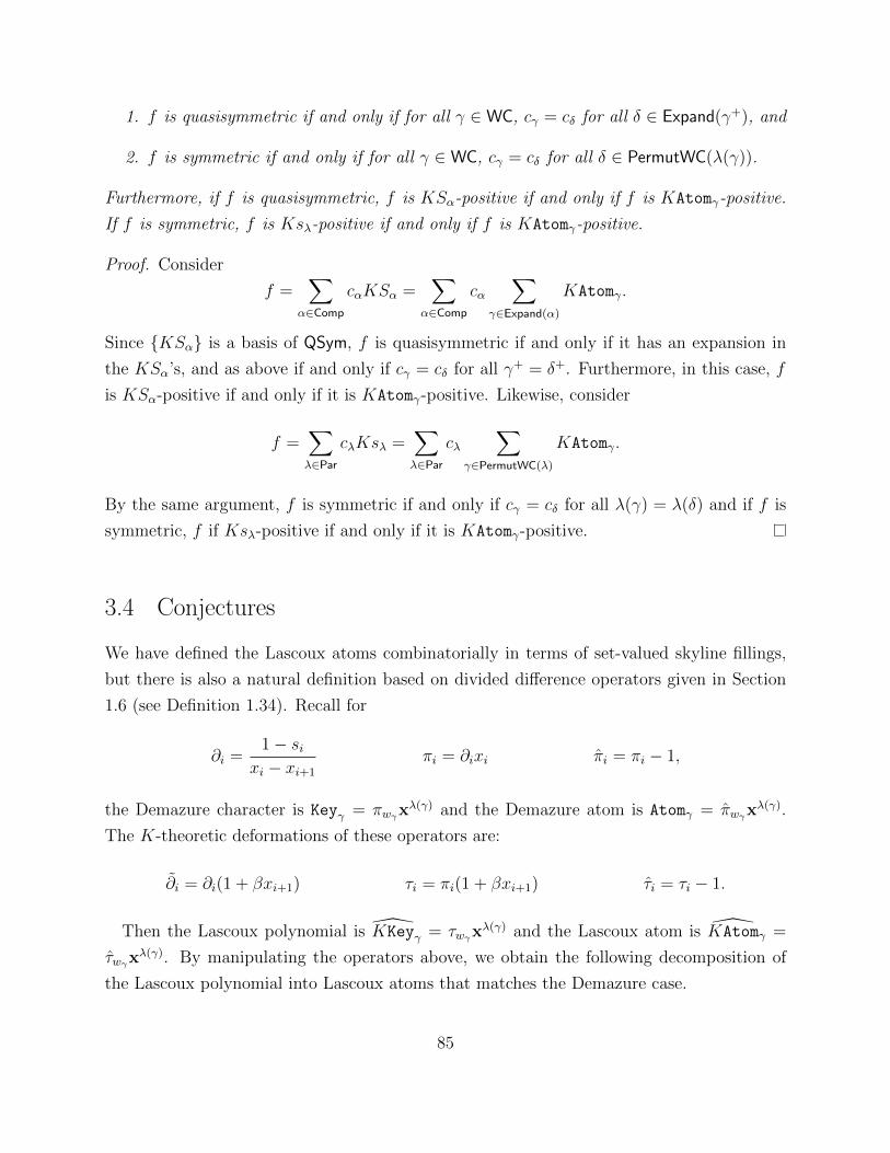
1. f is quasisymmetric if and only if for all γ ∈ WC, cγ = cδ for all δ ∈ Expand(γ+), and

2. f is symmetric if and only if for all γ ∈ WC, cγ = cδ for all δ ∈ PermutWC(λ(γ)).

Furthermore, if f is quasisymmetric, f is KSα-positive if and only if f is KAtomγ-positive.

If f is symmetric, f is Ksλ-positive if and only if f is KAtomγ-positive.

Proof. Consider

f =∑

α∈Comp

cαKSα =∑

α∈Comp

cα∑

γ∈Expand(α)

KAtomγ.

Since {KSα} is a basis of QSym, f is quasisymmetric if and only if it has an expansion in

the KSα’s, and as above if and only if cγ = cδ for all γ+ = δ+. Furthermore, in this case, f

is KSα-positive if and only if it is KAtomγ-positive. Likewise, consider

f =∑λ∈Par

cλKsλ =∑λ∈Par

cλ∑

γ∈PermutWC(λ)

KAtomγ.

By the same argument, f is symmetric if and only if cγ = cδ for all λ(γ) = λ(δ) and if f is

symmetric, f if Ksλ-positive if and only if it is KAtomγ-positive.

3.4 Conjectures

We have defined the Lascoux atoms combinatorially in terms of set-valued skyline fillings,

but there is also a natural definition based on divided difference operators given in Section

1.6 (see Definition 1.34). Recall for

∂i =1− si

xi − xi+1

πi = ∂ixi πi = πi − 1,

the Demazure character is Keyγ = πwγxλ(γ) and the Demazure atom is Atomγ = πwγx

λ(γ).

The K-theoretic deformations of these operators are:

∂i = ∂i(1 + βxi+1) τi = πi(1 + βxi+1) τi = τi − 1.

Then the Lascoux polynomial is KKeyγ = τwγxλ(γ) and the Lascoux atom is KAtomγ =

τwγxλ(γ). By manipulating the operators above, we obtain the following decomposition of

the Lascoux polynomial into Lascoux atoms that matches the Demazure case.

85

Theorem 3.17.

KKeyγ =∑

δ∈PermutWC(λ(γ))δ�γ

KAtomδ

where recall δ � γ if λ(δ) = λ(γ) and wδ ≤B wγ in (strong) Bruhat order.

Proof. In sections 2 and 3 of [Pun16], A. Pun gives a proof in the case that β = 0 using

relations derived between ∂i, πi, and πi. To extend this proof line by line to the Lascoux

case, we only need to show τiτi = −τi.We first show that τiτi = τi. To do this, consider πixi+1f = ∂i(xixi+1f). Since xixi+1 is

symmetric in i and i+ 1,

πixi+1f = ∂i(xixi+1f) = xixi+1∂if.

Now, from Proposition 3.1 of [Pun16], π2i = π and ∂iπi = 0. Then

τ 2i = (πi(1 + βxi+1))(πi(1 + βxi+1))

= π2i (1 + βxi+1) + πiβxi+1πi(1 + βxi+1)

= πi(1 + βxi+1) + βxixi+1∂iπi(1 + βxi+1)

= τi + 0.

Since τi = 1 + τi and τ 2i = τi,

1 + τi = (1 + τi)2 = 1 + 2τi + τ 2i .

Thus

τ 2i = −τi.

A conjectural combinatorial model for KKeyγ using K-Kohnert diagrams was given by

C. Ross and A. Yong in [RY15], but there are no proven combinatorial rules for KKeyγ or

KAtomγ. However, we have checked the following conjectures for all weak compositions γ

with at most 8 boxes and at most 8 rows.

Conjecture 3.18.

KAtomγ = KAtomγ =∑

F∈SetSkyFill(γ,bi)

β|F |−|γ|xF .

86

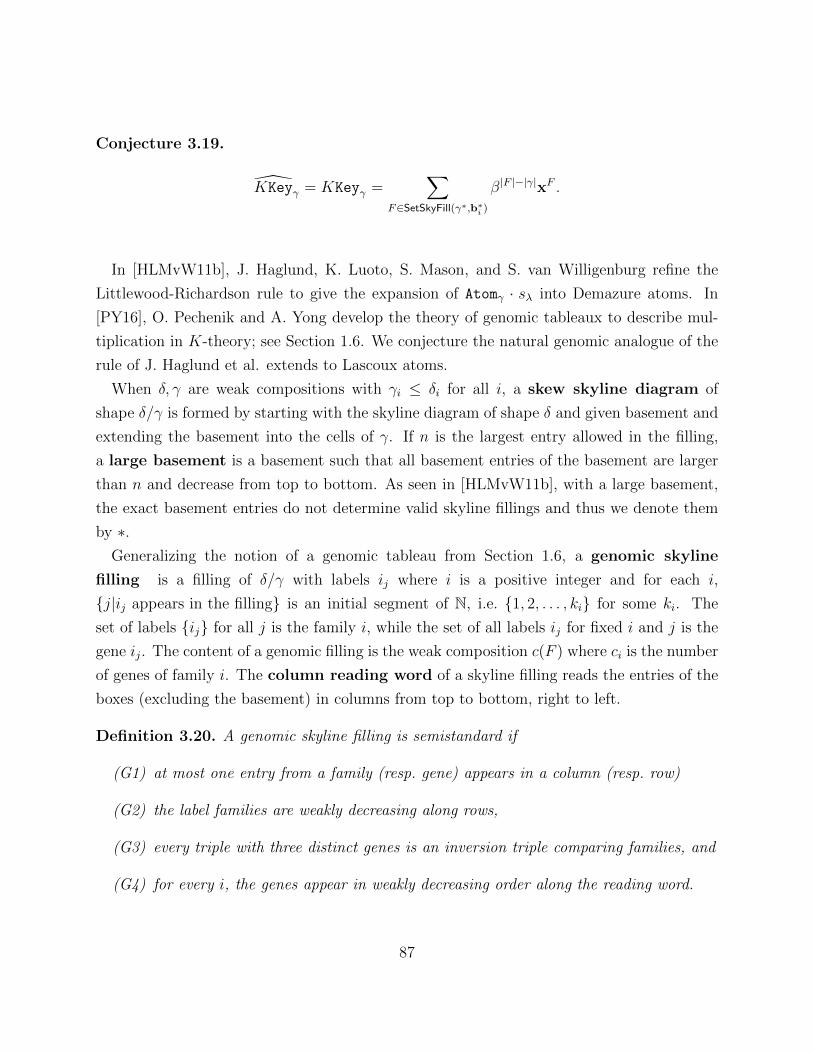
Conjecture 3.19.

KKeyγ = KKeyγ =∑

F∈SetSkyFill(γ∗,b∗i )

β|F |−|γ|xF .

In [HLMvW11b], J. Haglund, K. Luoto, S. Mason, and S. van Willigenburg refine the

Littlewood-Richardson rule to give the expansion of Atomγ · sλ into Demazure atoms. In

[PY16], O. Pechenik and A. Yong develop the theory of genomic tableaux to describe mul-

tiplication in K-theory; see Section 1.6. We conjecture the natural genomic analogue of the

rule of J. Haglund et al. extends to Lascoux atoms.

When δ, γ are weak compositions with γi ≤ δi for all i, a skew skyline diagram of

shape δ/γ is formed by starting with the skyline diagram of shape δ and given basement and

extending the basement into the cells of γ. If n is the largest entry allowed in the filling,

a large basement is a basement such that all basement entries of the basement are larger

than n and decrease from top to bottom. As seen in [HLMvW11b], with a large basement,

the exact basement entries do not determine valid skyline fillings and thus we denote them

by ∗.Generalizing the notion of a genomic tableau from Section 1.6, a genomic skyline

filling is a filling of δ/γ with labels ij where i is a positive integer and for each i,

{j|ij appears in the filling} is an initial segment of N, i.e. {1, 2, . . . , ki} for some ki. The

set of labels {ij} for all j is the family i, while the set of all labels ij for fixed i and j is the

gene ij. The content of a genomic filling is the weak composition c(F ) where ci is the number

of genes of family i. The column reading word of a skyline filling reads the entries of the

boxes (excluding the basement) in columns from top to bottom, right to left.

Definition 3.20. A genomic skyline filling is semistandard if

(G1) at most one entry from a family (resp. gene) appears in a column (resp. row)

(G2) the label families are weakly decreasing along rows,

(G3) every triple with three distinct genes is an inversion triple comparing families, and

(G4) for every i, the genes appear in weakly decreasing order along the reading word.

87

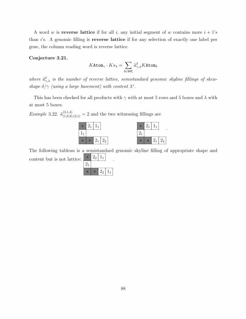
A word w is reverse lattice if for all i, any initial segment of w contains more i + 1’s

than i’s. A genomic filling is reverse lattice if for any selection of exactly one label per

gene, the column reading word is reverse lattice.

Conjecture 3.21.

KAtomγ ·Ksλ =∑δ∈WC

aδγ,λKAtomδ

where aδγ,λ is the number of reverse lattice, semistandard genomic skyline fillings of skew-

shape δ/γ (using a large basement) with content λ∗.

This has been checked for all products with γ with at most 5 rows and 5 boxes and λ with

at most 5 boxes.

Example 3.22. a(3,1,4)(1,0,2),(2,1) = 2 and the two witnessing fillings are

∗ 21 11

11

∗ ∗ 21 22

∗ 21 11

21

∗ ∗ 21 22

.

The following tableau is a semistandard genomic skyline filling of appropriate shape and

content but is not lattice: ∗ 22 11

21

∗ ∗ 22 11

.

88

CHAPTER 4

Kaons and QuasiLascoux Polynomials

This chapter derives from joint work with O. Pechenik and D. Searles that is in preparation.

4.1 Introduction and Background

In this chapter, we will introduce two new bases of Pol and study their relationships to

• the combinatorial Lascoux polynomials and atoms (see Chapter 3),

• the multi-fundamental quasisymmetric functions (see Section 1.3),

• the quasisymmetric Grothendieck functions (see Section 3.3),

• the glide polynomials introduced in [PS17],

• the quasikey polynomials introduced in [AS16], and

• the fundamental particles introduced in [Sea17].

We will use set-valued skyline fillings in order to give combinatorial expansions between the

different bases.

4.1.1 Homogeneous Bases

In this section, we will introduce a number of bases where each member is a homogeneous

polynomial; see Table 4.1 for a summary. We will explain the known lifts (see Table 4.2)

89

and combinatorial expansions (see Table 4.3) between these bases. Figure 4.1 contains all

of the relationships of interest to this chapter. Later in this chapter, we will extend these

relations to their inhomogeneous deformations.

The fundamental slide polynomials were introduced by S. Assaf and D. Searles [AS17].

A weak composition δ is a slide of the weak composition γ if it can be obtained from γ by

a finite sequence of the following local moves:

(m1) 0p⇒ p0, (for p ∈ Z>0);

(m2) 0p⇒ qr (for p, q, r ∈ Z>0 with q + r = p).

Definition 4.1 (Assaf-Searles, Definition 3.6 [AS17]). The fundamental slide polynomial

Slideγ is

Slideγ =∑δ

xδ,

where the sum is all slides δ of γ.

For example,

Slide(0,1,0,2) = x(0,1,0,2) + x(1,0,0,2) + x(0,1,2,0) + x(1,0,2,0) + x(1,2,0,0) + x(0,1,1,1)+

x(1,0,1,1) + x(1,1,0,1) + x(1,1,1,0).

The fundamental particles were introduced by D. Searles [Sea17] as the generating

function for a subset of the slides called mesonic slides.

Definition 4.2. Let γ be a weak composition with nonzero entries in positions n1 < . . . n`.

The weak composition δ is a mesonic slide of γ if it can be obtained from γ by a finite

sequence of the local moves (m1) and (m2) that never applies (m1) at positions nj − 1 and

nj for any j.

Definition 4.3 (Searles, Definition 4.1 [Sea17]). The fundamental particle Parγ is

Parγ =∑δ

xδ,

where the sum is over all mesonic slides of γ.

For example,

Par(0,1,0,2) = x(0,1,0,2) + x(0,1,1,1).

90

Name Symbol Ring Definition

Schur function sλ Sym 1.10Fundamental quasisymmetric function Fα QSym 1.13

Quasisymmetric Schur function Sα QSym 1.28Schubert polynomial Sw Pol 1.15

Key polynomial Keyγ Pol 1.21Demazure atom Atomγ Pol 1.21Slide polynomial Slideγ Pol 4.1

Fundamental particle Parγ Pol 4.3Quasikey polynomial QKeyγ Pol 4.5

Table 4.1: The homogeneous bases we will consider in this chapter.

The quasikey polynomials were introduced in [AS16] and defined in terms of their

positive expansion in fundamental slide polynomials. In [Sea17], it was proved that quasikey

polynomials expand combinatorially in Demazure atoms, and we take this expansion as our

definition.

Definition 4.4. Given weak compositions γ and δ of n we say that δ dominates γ, denoted

by δ ≥D γ, if for all i = 1, . . . , `,

δ1 + · · ·+ δi ≥D γ1 + · · ·+ γi.

Definition 4.5 (Assaf-Searles, Theorem 3.4 [Sea17]). The quasikey polynomial QKeyγ is

QKeyγ =∑

δ∈Expand(γ+)δ≥Dγ

Atomδ.

For example,

QKey(0,1,0,3) = Atom(0,1,0,3) + Atom(1,0,0,3) + Atom(0,1,3,0) + Atom(1,0,3,0) + Atom(1,3,0,0).

Table 4.1 summarizes the homogeneous bases we will use in this chapter. We now ask how

each basis of Sym or QSym lifts to a basis of Pol. This is summarized in Table 4.2.

Sections 1.4 and 1.5 show that the Schubert polynomials and the key polynomials are a

lift of the Schur functions from Sym to Pol; see (1.4) and (1.6).

Then, for a weak composition γ, let 0k × γ be the composition formed by prepending k

zeros to the front of γ.

91

Basis of Pol Lifts Reference

Sw sλ Equation 1.4Keyγ sλ Equation 1.6

Slideγ Fα Proposition 4.6QKeyγ Sα Proposition 4.7

Table 4.2: The lifts of the homogeneous bases from Sym and QSym to Pol.

Proposition 4.6 (Assaf-Searles, Lemma 3.8 [AS17]). For a composition α with `(α) = `,

Slide0n×α(x1, x2, . . . , xn+`) = Fα(x1, x2, . . . , xn+`).

Thus, the fundamental slide polynomials lift the fundamental quasisymmetric polynomials

from QSym to Pol.

Proposition 4.7 (Assaf-Searles, Proposition 4.10 [AS16]). For a composition α with `(α) =

`,

QKeyα(x1, x2, . . . , xn+`) = S0n×α(x1, x2, . . . , xn+`).

Thus, the quasikey polynomials lift the quasisymmetric Schur functions from QSym to Pol.

Finally, we consider the different combinatorial expansions between these different homo-

geneous families. These expansions are summarized in Table 4.3.

Equation (1.8) gives the combinatorial expansion of the Schur function into quasisym-

metric Schur functions, while Proposition 1.29 gives the expansion of quasisymmetric Schur

functions into fundamental quasisymmetric functions. Furthermore, Theorem 1.22 gives the

combinatorial expansion of the Schubert polynomial into key polynomials.

Now, given a composition γ, define a left swap to be the exchange of two parts γi ≤ γj

where i < j.

Definition 4.8 (Assaf-Searles, Section 3 [AS16]). Let lswap(γ) be the set of weak composi-

tions δ that can be obtained from γ by a (possibly empty) sequence of left swaps starting with

γ.

92

For example,

lswap((0, 1, 0, 3)) = {(0, 1, 0, 3), (0, 1, 3, 0), (1, 0, 0, 3), (1, 0, 3, 0), (1, 3, 0, 0),

(0, 3, 0, 1), (0, 3, 1, 0), (3, 0, 0, 1), (3, 0, 1, 0), (3, 1, 0, 0)}.

Following (3.3) in [AS16], define Qlswap(γ) to be all δ ∈ lswap(γ) such that among all

elements ε ∈ lswap(γ) such that ε+ = δ+, then δ is ≥D-minimal. Continuing our example

above,

Qlswap((0, 1, 0, 3)) = {(0, 1, 0, 3), (0, 3, 0, 1)}.

Theorem 4.9 (Assaf-Searles, Theorem 3.7, [AS16]).

Keyγ =∑

δ∈Qlswap(γ)

QKeyδ.

Thus, the key polynomials combinatorially expand in the quasikey polynomials. Decom-

posing further, each quasikey polynomial combinatorially expands in the fundamental slides.

Theorem 4.10 (Assaf-Searles, Theorem 3.4 [AS16]).

QKeyγ =∑

δ∈WC(|γ|)

Cγ,δSlideδ

where Cγ,δ are particular nonnegative integers.

The formula of S. Assaf and D. Searles uses combinatorial objects not needed here, how-

ever, we will give a different explicit formula for Cγ,δ in Theorem 4.38.

As seen in chapters 2 and 3, another approach to the study of key polynomials is to consider

their expansion, not into slides, but rather into Demazure atoms. The same expansion we

have seen with Bruhat order (Theorem 1.26) can also be written in terms of left swaps.

Lemma 4.11 (Searles, Lemma 3.1 [Sea17]).

Keyγ =∑

δ∈lswap(γ)

Atomδ.

We have defined the quasikey polynomials in terms of their Demazure atom expansion and

have seen that the quasikey polynomials expand combinatorially in the slide basis as well.

However, neither the Demazure atoms nor the fundamental slides expand combinatorially

93

Basis Combinatorially Expands In Reference

sλ Sα Equation 1.8Sα Fα Proposition 1.29Sw Keyγ Theorem 1.22Keyγ QKeyγ Theorem 4.9QKeyγ Atomγ Definition 4.5QKeyγ Slideγ Theorem 4.10Slideγ Parγ Proposition 4.12Atomγ Parγ Theorem 4.13

Table 4.3: The combinatorial expansions between the homogeneous bases.

in each other [Sea17, Proposition 4.6]. A common expansion of the Demazure atoms and

fundamental slides is provided by the fundamental particle basis.

Proposition 4.12 (Searles, Proposition 4.4 [Sea17]).

Slideγ =∑

δ∈Expand(γ+)δ≥Dγ

Parδ.

Theorem 4.13 (Searles, Theorem 4.11 [Sea17]).

Atomγ =∑

δ∈WC(|γ|)

Dγ,δParδ

where Dγ,δ are nonnegative integers.

We will describe a set of combinatorial objects counted by Dγ,δ in Theorem 4.29. This

theorem generalizes the expansion of D. Searles for a Demazure atom into fundamental

particles. The relations among these nine families of polynomials are illustrated in Figure 4.1.

4.1.2 K-theoretic Analogues

We are interested in K-theoretic analogues of the nine homogeneous families described in

Section 4.1.1, i.e. we seek inhomogeneous deformations of these polynomials where the rela-

tionships between the deformations mirror their homogeneous counterparts.

94

Sw Keyγ QKeyγ

Atomγ

Slideγ

Parγ

sλ Sα Fα

Figure 4.1: The nine homogeneous families of polynomials considered here. Familiesdepicted in orange are bases of Sym, those in purple are bases of QSym, and those in greenare bases of Pol. The thinner hooked arrows pointing up denote that the basis at the taillifts to the basis at the head. The thicker arrows pointing to the right denote that the basisat the tail combinatorially expands in the basis at the head.

The glide polynomials were defined by O. Pechenik and D. Searles [PS17] and provide an

inhomogeneous deformation of the slide polynomials. In [PS17], a weak komposition is a

weak composition where the positive integers may be colored arbitrarily black or red. For a

weak komposition b, the excess ex(b) is the number of red entries in b.

Definition 4.14 (Pechenik-Searles, Definition 2.2, [PS17]). Let γ be a weak composition

with nonzero entries in positions n1 < · · · < n`. The weak komposition b is a glide of γ if

there exist integers 0 = i0 < i1 < · · · < i` such that, for each 1 ≤ j ≤ `, we have

(G1) γnj = bij−1+1 + · · ·+ bij − ex(bij−1+1, . . . , bij),

(G2) ij ≤ nj, and

(G3) the leftmost nonzero entry among bij−1+1, . . . , bij is black.

Alternatively, b is a glide of γ if it can be obtained from γ by a finite sequence of the

following local moves:

(m1) 0p⇒ p0, (for p ∈ Z>0);

(m2) 0p⇒ qr (for p, q, r ∈ Z>0 with q + r = p);

95

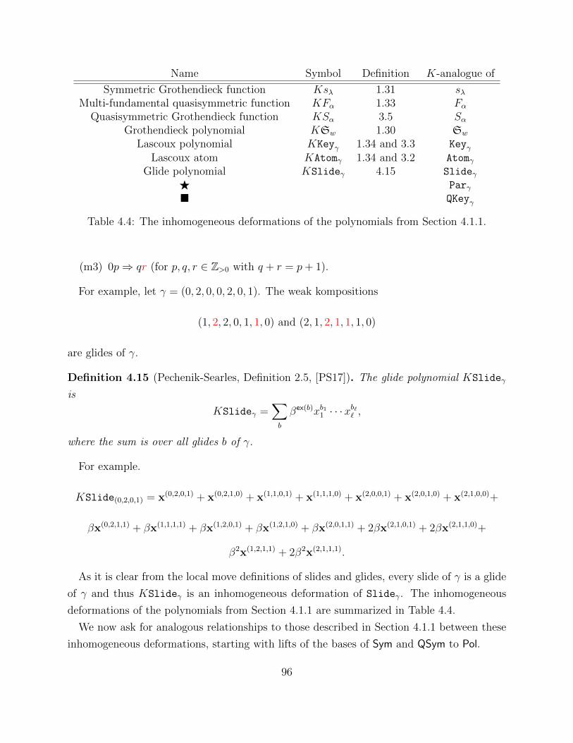
Name Symbol Definition K-analogue of

Symmetric Grothendieck function Ksλ 1.31 sλMulti-fundamental quasisymmetric function KFα 1.33 Fα

Quasisymmetric Grothendieck function KSα 3.5 SαGrothendieck polynomial KSw 1.30 Sw

Lascoux polynomial KKeyγ 1.34 and 3.3 KeyγLascoux atom KAtomγ 1.34 and 3.2 Atomγ

Glide polynomial KSlideγ 4.15 SlideγF Parγ� QKeyγ

Table 4.4: The inhomogeneous deformations of the polynomials from Section 4.1.1.

(m3) 0p⇒ qr (for p, q, r ∈ Z>0 with q + r = p+ 1).

For example, let γ = (0, 2, 0, 0, 2, 0, 1). The weak kompositions

(1, 2, 2, 0, 1, 1, 0) and (2, 1, 2, 1, 1, 1, 0)

are glides of γ.

Definition 4.15 (Pechenik-Searles, Definition 2.5, [PS17]). The glide polynomial KSlideγ

is

KSlideγ =∑b

βex(b)xb11 · · ·xb`` ,

where the sum is over all glides b of γ.

For example.

KSlide(0,2,0,1) = x(0,2,0,1) + x(0,2,1,0) + x(1,1,0,1) + x(1,1,1,0) + x(2,0,0,1) + x(2,0,1,0) + x(2,1,0,0)+

βx(0,2,1,1) + βx(1,1,1,1) + βx(1,2,0,1) + βx(1,2,1,0) + βx(2,0,1,1) + 2βx(2,1,0,1) + 2βx(2,1,1,0)+

β2x(1,2,1,1) + 2β2x(2,1,1,1).

As it is clear from the local move definitions of slides and glides, every slide of γ is a glide

of γ and thus KSlideγ is an inhomogeneous deformation of Slideγ. The inhomogeneous

deformations of the polynomials from Section 4.1.1 are summarized in Table 4.4.

We now ask for analogous relationships to those described in Section 4.1.1 between these

inhomogeneous deformations, starting with lifts of the bases of Sym and QSym to Pol.

96

Basis of Pol Lifts Reference

KSw Ksλ Definition 1.30KKeyγ Ksλ Theorems 1.26 and 1.27KSlideγ KFα Proposition 4.6� KSα

Table 4.5: The lifts of the inhomogeneous bases from Sym and QSym to Pol.

Basis Combinatorially Expands In Reference

Ksλ KSα Corollary 3.6KSα KFαKSw KKeyγ openKKeyγ �� KAtomγ� KSlideγ

KSlideγ FKAtomγ F

Table 4.6: The combinatorial expansions between the inhomogeneous bases.

Recall from Section 1.6, the Grothendieck polynomials lift the symmetric Grothendieck

polynomials, which correspond to Grassmannian permutations. Furthermore, as in the De-

mazure case, combining Theorems 3.4 and 3.17 gives that the Lascoux polynomials are a lift

of the symmetric Grothendieck polynomials.

O. Pechenik and D. Searles show that the glide polynomials are a lift of the multi-

fundamental quasisymmetric polynomials.

Theorem 4.16 (Pechenik-Searles, Theorem 3.5 [PS17]). For a composition α with `(α) = `,

KSlide0n×α(x1, x2, . . . , xn+`) = KFα(x1, x2, . . . , xn+`).

In terms of combinatorial expansions between the K-theoretic analogues, Corollary 3.6

gave the expansion of Ksλ in terms of KSα. The expansion of the Grothendieck polynomials

expand in the Lascoux polynomials is still an open problem, and we will establish the other

relationships in Table 4.6 in this chapter.

97

4.1.3 Statement of Results

The main goal of this chapter is to define the bases that play the role of F and � in

Section 4.1.2. We start with F, a basis that should be an inhomogeneous deformation of

the fundamental particles and should simultaneously combinatorially expand the Lascoux

atoms and the glide polynomials.

Definition 4.17. Let γ be a weak composition with nonzero entries in positions n1 < · · · <n`. The weak komposition b is a mesonic glide of γ if, for each 1 ≤ j ≤ `, we have

(G1′) γnj = bnj−1+1 + · · ·+ bnj − ex(bnj−1+1, . . . , bnj),

(G3′) the leftmost nonzero entry among bnj−1+1, . . . , bnj is black, and

(G4′) bnj 6= 0.

Equivalently, a weak komposition b is a mesonic glide of γ if b can be obtained from γ by a

finite sequence of the local moves (m1), (m2), and (m3) that never applies (m1) at positions

nj − 1 and nj for any j.

Observe that, in particular, a mesonic glide is a glide that happens to satisfy additional

conditions. For example, let γ = (0, 3, 0, 2). Then b = (2, 1, 1, 2) is a mesonic glide of γ. On

the other hand, while b′ = (3, 1, 0, 2) is also a glide of γ, it is not mesonic. To see this fact,

observe that γ has nonzero entries in positions n1 = 2 and n2 = 4, while the only (i1, i2)

satisfying conditions (G1), (G2), and (G3) of Definition 4.14 for b′ is (1, 4). Since i1 < n1, b′

is not mesonic. The reader may check that both b and b′ can be obtained from γ by a finite

sequence of the local moves (m1), (m2), and (m3). However, the reader may also check that

b′ cannot be obtained without applying (m1) at positions 1 and 2.

Definition 4.18. The kaon KParγ is

KParγ =∑b

βex(b)xb,

where the sum is over all mesonic glides of γ.

98

For example,

KPar(0,3,0,2) = x(0,3,0,2) + x(0,3,1,1) + x(1,2,0,2) + x(1,2,1,1) + x(2,1,0,2) + x(2,1,1,1)

+ βx(0,3,1,2) + βx(0,3,2,1) + βx(1,2,1,2) + βx(1,2,2,1) + βx(1,3,0,2) + βx(1,3,1,1)

+ βx(2,1,1,2) + βx(2,1,2,1) + βx(2,2,0,2) + βx(2,2,1,1) + βx(3,1,0,2) + βx(3,1,1,1)

+ β2x(1,3,1,2) + β2x(1,3,2,1) + β2x(2,2,1,2) + β2x(2,2,2,1) + β2x(3,1,1,2) + β2x(3,1,2,1).

Theorem 4.19. The kaons satisfy the properties of F, i.e. are

1. a basis of Pol,

2. inhomogeneous deformations of the fundamental particles,

3. provide a combinatorial expansion of the Lascoux atoms, and

4. provide a combinatorial expansion of the glide polynomials.

This theorem will be proved in Section 4.2; see Theorem 4.26, Proposition 4.24, Theo-

rem 4.29, and Proposition 4.25.

Recall that � is a basis of Pol that is an inhomogeneous deformation of the quasikey

polynomials, lifts the quasisymmetric Grothendieck polynomials from QSym to Pol, provides

a combinatorial expansion for the Lascoux polynomials, and combinatorially expands in the

Lascoux atoms and glide polynomials. We mimic the Demazure atom expansion of the

quasikey polynomials to define the quasiLascoux polynomials.

Definition 4.20. The quasiLascoux polynomial KQKeyγ is

KQKeyγ =∑

δ∈Expand(γ+)δ≥Dγ

KAtomδ.

Theorem 4.21. The quasiLascoux polynomials satisfy the properties of �, i.e. are

1. a basis of Pol,

2. inhomogeneous deformations of the quasikey polynomials,

3. a lift of the quasisymmetric Grothendieck functions,

4. provide a combinatorial expansion of the Lascoux polynomials,

99

5. combinatorially expand in the glide polynomials, and

6. combinatorially expand in the Lascoux atoms.

This theorem will be proved in Sections 4.3 and 4.4; see Theorem 4.35, Equation 4.1, Equa-

tion 4.2, Theorem 4.44, and Theorem 4.38. The last claim is our definition of the quasiLas-

coux polynomials. A consequence of Theorem 4.21 is that the quasisymmetric Grothendieck

basis expands combinatorially into the basis of multifundamental quasisymmetric polyno-

mials; see Corollary 4.41. The relations among the nine families of K-theoretic polynomials

and their nine families of β = 0 specializations are illustrated in Figure 4.2.

Except for the Grothendieck polynomials {KSw} and their symmetric subset {Ksλ},the geometric significance of these deformed polynomials is currently mysterious. While,

for example, the glide polynomials seem useful in the study of Grothendieck polynomials

[PS17], it is unknown how to interpret any single glide polynomial KSlideγ as representing

a geometric object or datum. We conclude with two conjectures that appear, to us, to

suggest some deeper mathematical structure.

Conjecture 4.22. For weak compositions γ and δ, let

Mγ,δ(β) = [KSlideδ]KQKeyγ.

Then for fixed γ, we have ∑δ∈WC

Mγ,δ(−1) ∈ {0, 1}.

For example, for γ = (0, 6, 6, 2),∑δ∈WC

M δγ = 16β3 + 75β2 + 94β + 36.

Substituting in β = −1 gives us 1. This has been checked for all γ with at most 3 zeros and

|γ| ≤ 7.

Conjecture 4.23. For weak compositions γ and δ, let

Nγ,δ(β) = [KParδ]KAtomγ.

Then for fixed γ, we have ∑δ∈WC

Nγ,δ(−1) ∈ {0, 1}.

100

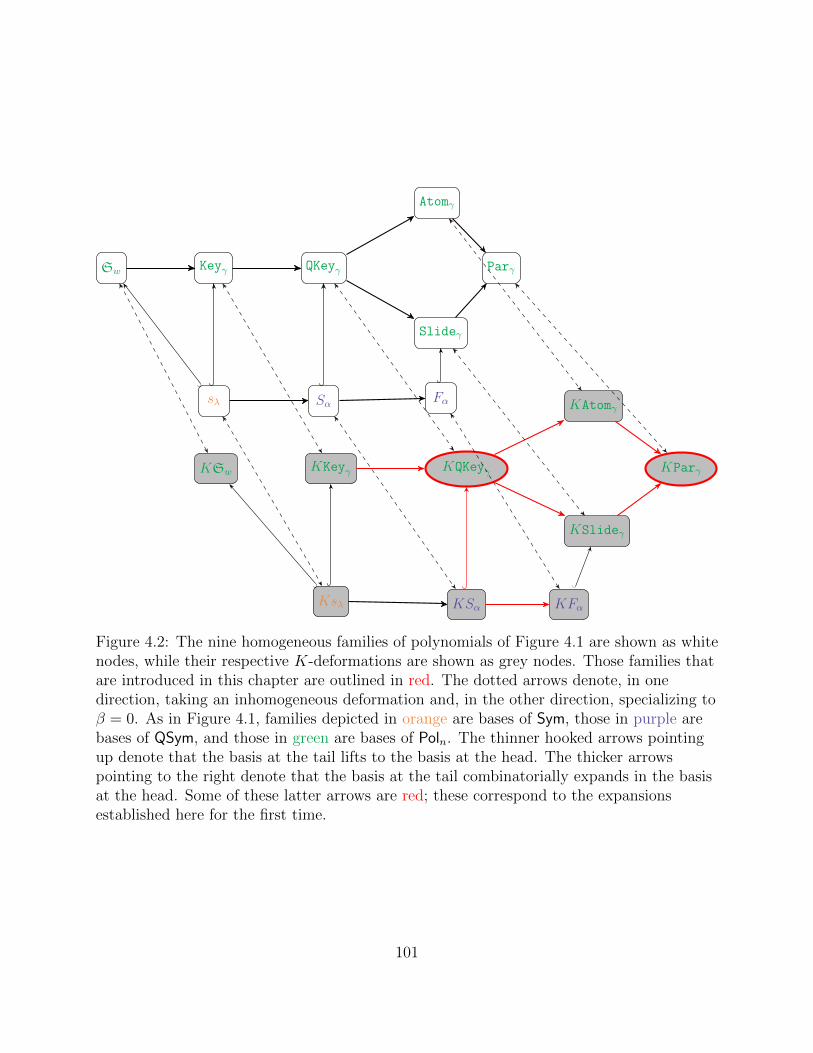
Sw Keyγ QKeyγ

Atomγ

Slideγ

Parγ

sλ Sα Fα

KSw KKeyγ KQKeyγ

KAtomγ

KSlideγ

KParγ

Ksλ KSα KFα

Figure 4.2: The nine homogeneous families of polynomials of Figure 4.1 are shown as whitenodes, while their respective K-deformations are shown as grey nodes. Those families thatare introduced in this chapter are outlined in red. The dotted arrows denote, in onedirection, taking an inhomogeneous deformation and, in the other direction, specializing toβ = 0. As in Figure 4.1, families depicted in orange are bases of Sym, those in purple arebases of QSym, and those in green are bases of Poln. The thinner hooked arrows pointingup denote that the basis at the tail lifts to the basis at the head. The thicker arrowspointing to the right denote that the basis at the tail combinatorially expands in the basisat the head. Some of these latter arrows are red; these correspond to the expansionsestablished here for the first time.

101

For example, for γ = (0, 6, 6, 2),∑δ∈WC

M δγ = 16β3 + 66β2 + 80β + 31.

Again substituting in β = −1 gives us 1. This has also been checked for all γ with at most

3 zeros and |γ| ≤ 7.

4.2 Kaons

In this section, we prove that the kaons have the properties of the basis F in Section 4.1.2,

namely those listed in Theorem 4.19.

Proposition 4.24. The fundamental particles are the β = 0 specialization of kaons, i.e. the

kaons are an inhomogeneous deformation of the fundamental particles.

Proof. Since any mesonic slide of γ is a mesonic glide of γ, this is clear from the definitions

of the two families of polynomials.

4.2.1 Kaons and glide polynomials

Proposition 4.25.

KSlideγ =∑

δ∈Expand(γ+)δ≥Dγ

KParδ.

In particular, every glide polynomial combinatorially expands in the kaons.

Proof. Let γ be a weak composition with nonzero entries in positions n1 < · · · < n`. Suppose

g is a glide of γ. Then there are 0 = i0 < i1 < · · · < i` satisfying conditions (G1), (G2),

and (G3) of Definition 4.14. We obtain g from γ via a 2-step process. First, apply (m1)

repeatedly to move each nonzero entry of γ from position nj to position ij. Call the resulting

weak composition δ. Note that δ satisfies δ ≥D γ and δ+ = γ+. Second, apply some sequence

of (m1), (m2) and (m3) to obtain the weak komposition g from δ. In this second step, note

that we never apply (m1) at positions ij − 1 and ij for any j.

Hence every glide g of γ is a mesonic glide of a δ with δ ≥D γ and δ+ = γ+. Conversely,

every mesonic glide of such a weak composition δ is clearly a glide of γ.

102

Thus to complete the proof, we only need to show that there is at most one δ with δ+ = γ+

such that b is a mesonic glide of δ. Let α = δ+ = (α1, . . . , α`). By the definition of mesonic

glide, we know that

αj = δnj = bnj−1+1 + . . .+ bnj − ex(bnj−1+1, . . . , bnj),

the leftmost nonzero entry among bnj−1+1, . . . , bnj is black, and bnj 6= 0. We claim there is

only one sequence n1, . . . , n` that satisfies these conditions. Suppose to the contrary that

there are two m1, . . . ,m` and n1, . . . , n` and let i be the lowest index such that mi 6= ni.

Without loss of generality, assume mi > ni. Then,

αi = bmi−1+1 + . . .+ bmi − ex(bmi−1+1, . . . , bmi)

= bmi−1+1 + . . .+ bni + bni+1 + . . .+ bmi − ex(bmi−1+1, . . . , bni)− ex(bni+1, . . . , bmi)

= αi + bni+1 + . . .+ bmi − ex(bni+1, . . . , bmi),

and so we have

0 = bni+1 + . . .+ bmi − ex(bni+1, . . . , bmi).

This is only possible if each of bni+1, . . . , bmi is either 0 or a red 1. Since bmi 6= 0, there is

at least one red 1 in this set of entries. However, the first nonzero entry of bni+1, . . . , bni+1is

required to be black, a contradiction.

In light of Proposition 4.24, setting β = 0 in Proposition 4.25 recovers [Sea17, Propo-

sition 4.4] on the expansion of fundamental slides into fundamental particles. Note that

although our K-theoretic deformations of those polynomials are significantly larger, the ma-

trix of basis change is exactly the same as for fundamental slides into fundamental particles.

Theorem 4.26. The set

{βkKParγ : k ∈ Z≥0 and γ is a weak composition of length n}

is an additive basis of the free Z-module Z[x1, x2, . . . , xn; β].

Proof. By Proposition 4.25, every glide polynomial can be written as a positive sum of kaons,

and indeed the transition matrix is unitriangular with respect to the lexicographic total order

on weak compositions. Furthermore, the expansion of a glide polynomial into kaons is finite

as there are finitely many compositions with γ+ = δ+ and δ ≥D γ. Hence, the transition

103

matrix is invertible over Z, and the theorem follows from the fact that glide polynomials are

an additive basis of Z[x1, x2, . . . , xn; β] [PS17, Theorem 2.6].

We can also see that the expansion of any polynomial into kaons is finite by a similar

argument to the proof of Theorem 3.10. If δ is a mesonic glide of γ, then max(δ) ≤ max(γ).

Thus, for any monomial xγ, there are finitely many terms (determined solely by γ) that can

be introduced in the process of expanding xγ in the kaons.

The kaon basis does not have positive structure coefficients. Nonetheless, we conjecture

the following:

Conjecture 4.27. For any weak compositions γ and δ, the product

KParγ ·KSlideδ

expands combinatorially in the kaon basis.

For example,

KPar(2,0,1)KSlide(1,0,2) = KPar(3,0,3)+βKPar(3,1,3)+βKPar(3,2,2)+β2KPar(3,2,3)+β

2KPar(3,3,2).

This has been checked for all γ, δ with at most 3 zeros and |γ|, |δ| ≤ 5.

4.2.2 Kaons and Lascoux atoms

Recall from Definition 3.1 that SetSkyFill(γ,b) is the set of all semistandard set-valued skyline

fillings of shape γ and basement b and that a set-valued skyline filling is semistandard if

(S1) entries do not repeat in a column,

(S2) rows are weakly decreasing where sets A ≥ B if minA ≥ maxB,

(S3) every triple of anchor entries is an inversion triple, and

(S4) free entries are with the smallest possible anchor entry such that (S2) is not broken.

Let T ∈ SetSkyFill(γ,bi). Then for every i appearing in T , let i+ be the smallest non-

basement entry greater than i appearing in T . If k is the greatest entry in T , we set

k+ = k + 1.

104

Definition 4.28. Let γ be a weak composition and T ∈ SetSkyFill(γ,bi). We say T is

meson-highest if, for every i appearing in T , either

• the leftmost i is in the leftmost column and is an anchor, or

• there is a i+ weakly right of the leftmost i and in a different box.

Let MesonSetSkyFill(γ,bi) be the set of all meson-highest T ∈ SetSkyFill(γ,bi). Two

examples of meson-highest fillings are below. The filling on the left is meson-highest as the

leftmost 1, 3, 4 are anchor in the left-most column and the leftmost 2 (in column 1) has a 3

in column 2. The filling on the right is not meson-highest since there is a free 2 in column 1

and no 3 weakly to the right.

1 1

2

3 32 2 21

4 4 431

1 1

2

3 32 2 21

4 4 41

Theorem 4.29.

KAtomγ =∑

T∈MesonSetSkyFill(γ,bi)

β|T |−|γ|KParc(T ).

In particular, the Lascoux atoms expand combinatorially in the kaons.

Setting β = 0 in Theorem 4.29 recovers [Sea17, Theorem 4.11].

To prove Theorem 4.29, we must first develop properties of a destandardization map,

denoted dst, on SetSkyFill(γ,bi). Fix T ∈ SetSkyFill(γ,bi). Consider the least integer i with

the property that the leftmost i in T is

• not an anchor in the leftmost column and

• has no i+ weakly to its right in a different box;

replace every i in T with an i + 1. If this results in two instances of i + 1 in a single box,

delete one. Repeat this replacement process until no further replacements can be made: the

final result is dst(T ). In fact, the order in which we perform replacements does not affect

the resulting destandardization. Nonetheless, it is convenient to fix the explicit replacement

order chosen here. This algorithm necessarily terminates, as we only perform replacement on

entries i that are strictly less than the maximum entry k of T ; this is because k is guaranteed

to appear as an anchor in the leftmost column of T .

105

Example 4.30. On the filling above that is not meson-highest, the following is the result of

the destandardization map:

T = 1 1

2

3 32 2 21

4 4 41

dst=⇒ 1 1

2

3 3 3 31

4 4 41

= S

Lemma 4.31. If T ∈ SetSkyFill(γ,bi), then

dst(T ) ∈ MesonSetSkyFill(γ,bi).

Moreover,

dst(T ) = T if and only if T ∈ MesonSetSkyFill(γ,bi) ⊆ SetSkyFill(γ,bi).

Proof. Fix the weak composition γ. By definition, if T ∈ MesonSetSkyFill(γ,bi), then

dst(T ) = T as dst changes exactly the entries that don’t exist when T is meson-highest.

Moreover, if T /∈ MesonSetSkyFill(γ,bi), then by definition dst(T ) 6= T . Hence, the second

claim of the lemma is clear.

It remains to establish the first claim of the lemma, so fix T ∈ SetSkyFill(γ,bi). It

is enough to show that dst(T ) ∈ SetSkyFill(γ,bi), for then by definition we must have

dst(T ) ∈ MesonSetSkyFill(γ,bi), as the destandardization algorithm does not terminate until

the extra conditions defining MesonSetSkyFill(γ,bi) are satisfied. Since destandardization is

defined as a sequence of replacements, it is enough by induction to show that any single such

replacement produces an element of SetSkyFill(γ,bi).

Suppose we replace the letters i in T and the result is T ′. Then, by assumption, the

leftmost i ∈ T

• is not an anchor in the leftmost column of T , and

• does not have an i+ weakly to its right in T and in a different box.

We want to show that T ′ satisfies the conditions (S.1)–(S.4).

(S1): If there is no column of T containing both i and i+ 1, then it is clear that T ′ satisfies

(S1). Hence, suppose column c of T contains both i and i + 1. Then, i+ = i + 1. Since T

106

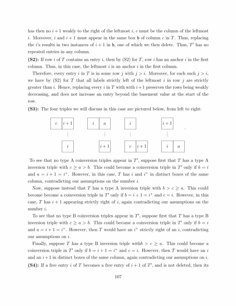
has then no i+ 1 weakly to the right of the leftmost i, c must be the column of the leftmost

i. Moreover, i and i + 1 must appear in the same box b of column c in T . Thus, replacing

the i’s results in two instances of i + 1 in b, one of which we then delete. Thus, T ′ has no

repeated entries in any column.

(S2): If row i of T contains an entry i, then by (S2) for T , row i has an anchor i in the first

column. Thus, in this case, the leftmost i is an anchor i in the first column.

Therefore, every entry i in T is in some row j with j > i. Moreover, for each such j > i,

we have by (S2) for T that all labels strictly left of the leftmost i in row j are strictly

greater than i. Hence, replacing every i in T with with i+ 1 preserves the rows being weakly

decreasing, and does not increase an entry beyond the basement value at the start of the

row.

(S3): The four triples we will discuss in this case are pictured below, from left to right:

c i+ 1

...

i

i a

...

i+ 1

i

...

c i+ 1

i+ 1

...

i a

.

To see that no type A coinversion triples appear in T ′, suppose first that T has a type A

inversion triple with c ≥ a > b. This could become a coinversion triple in T ′ only if b = i

and a = i + 1 = i+. However, in this case, T has i and i+ in distinct boxes of the same

column, contradicting our assumptions on the number i.

Now, suppose instead that T has a type A inversion triple with b > c ≥ a. This could

become become a coinversion triple in T ′ only if b = i + 1 = i+ and c = i. However, in this

case, T has i + 1 appearing strictly right of i, again contradicting our assumptions on the

number i.

To see that no type B coinversion triples appear in T ′, suppose first that T has a type B

inversion triple with c ≥ a > b. This could become a coinversion triple in T ′ only if b = i

and a = i + 1 = i+. However, then T would have an i+ strictly right of an i, contradicting

our assumptions on i.

Finally, suppose T has a type B inversion triple withb > c ≥ a. This could become a

coinversion triple in T ′ only if b = i + 1 = i+ and c = i. However, then T would have an i

and an i+ 1 in distinct boxes of the same column, again contradicting our assumptions on i.

(S4): If a free entry i of T becomes a free entry of i + 1 of T ′, and is not deleted, then its

107

anchor entry j is larger than i+ 1 in both T and T ′. In particular, since j was the smallest

anchor entry in this column accept a free entry i in T (by (S4)), j is still the smallest anchor

entry accepting a free entry i+ 1 in T ′.

If an anchor entry i of T becomes the anchor entry i+1 of T ′, then since any other anchor

entry in this column is either greater than i + 1 or smaller than i, any free entries in the

cell of this anchor entry are still with the smallest possible anchor entry. Any other free

entries in a column where an anchor entry i becomes an anchor entry i+ 1 are also still with

the smallest possible anchor entry, again since other anchor entries in this column are either

greater than i+ 1 or smaller than i.

Lemma 4.32. Let S ∈ MesonSetSkyFill(γ,bi). Then

KParc(S) =∑

T∈dst−1(S)

β|T |−|S|xT .

Proof. We must establish a weight-preserving bijection between mesonic glides of c(S) and

fillings T ∈ dst−1(S).

Fix T ∈ dst−1(S) with c(T ) = (c1, . . . , c`). Define the colored weight kwt(T ) of T to

be the weak komposition obtained from c(T ) by coloring ci+1 red if an i+ 1 is deleted after

replacing every i with i + 1 during a step of destandardization. For example, for the filling

in Example 4.30, c(S) = (3, 0, 3, 2) and kwt(T ) = (3, 3, 1, 2) since a 3 is deleted when the 2’s

are changed to 3’s. We observe that (3, 3, 1, 2) is a mesonic glide of (3, 0, 3, 2).

We claim that in general kwt(T ) is a mesonic glide of c(S). Consider the process of

destandardization of T to produce S. Each time we replace every i in T ′ by i+ 1 to produce

T ′′, we change the ith and (i+ 1)st entries of the colored weight by

(q, r) 7→ (0, q + r − 1),

if a duplicate i+ 1 is deleted, or

(q, r) 7→ (0, q + r),

if not. Note that when we replace the i’s with i + 1’s, we can remove at most one i + 1.

If there were two boxes containing two i + 1’s after replacing the i’s, then T had an i + 1

weakly to the right of an i and in a different box and so we would not have replaced the i’s.

Since these are the inverses of the local move (m3) in the first case and either (m1) or (m2)

in the second case, it follows then that kwt(T ) is a glide of the weak composition c(S).

108

Let c(S) have nonzero entries in positions n1 < · · · < n`. A local change to the colored

weight

(q, 0) 7→ (0, q)

in positions nj−1 and nj for some j would correspond to a step of destandardization replacing

every instance of nj − 1 with nj in a T ′ that contains no label nj. Since S is meson-highest,

the entries nj of S satisfy the meson-highest condition. Since T ′ destandardizes to S and all

entries nj − 1 change to nj, the entries nj − 1 of T ′ therefore also satisfy the meson-highest

condition. This contradicts the application of such a destandardization step to T ′. Hence,

kwt(T ) is a mesonic glide of c(S).

For the other direction, let b be a mesonic glide of the weak composition c(S). We construct

(the unique) T ∈ dst−1(S) such that kwt(T ) = b as follows. Suppose c(S) has nonzero entries

in positions n1 < · · · < n`.

For i = 1, . . . , ` carry out the following process. Construct the string stri as follows. For

each nonzero bnj−1+1, . . . , bnj if bi is black, record bi black i’s and if bi is red, record one red

i followed by bi − 1 black i’s. Now we will replace the instances of n1 in S with the entries

of str1 as follows.

In the rightmost box of S containing an n1, replace that n1 with the first entry of str1.

If the next entry of str1 is red, place it in the same box the previous entry was placed in,

otherwise, place it in the next box of S to the left that contains an n1, replacing that n1.

Continue in this manner until all entries of str1 have been placed in S. This procedure is

well-defined since by (S1) no more than one entry n1 appears in any column of S; and since

the number c(S)n1 of n1’s in S is exactly the length of the string str1 minus the number of

red entries (by (G1)), each black entry goes in a different box of S, and each red entry goes

in a box along with a black entry. Repeat this process with n2, . . . , n` in order.

For example, consider the following meson-highest filling S below. We have c(S) =

(0, 3, 0, 2) and (2, 1, 1, 2) is a mesonic glide of c(S). Thus, str1 = 112 and str2 = 344 and we

make the following replacements in S

S = 1

2 2 2 2

3

4 4 4

⇒ 1

2 2 1 1

3

4 4 4

. ⇒ 1

2 2 1 1

3

4 4 43

= T.

If the resulting filling T is a valid semistandard skyline filling, it is unique as there was

109

no choice at any step of the process. Furthermore, by construction, the resulting filling

T has colored weight b and destandardizes to S. Thus, we only need to show that T ∈SetSkyFill(γ,bi).

To see this, notice that the entries of strj (which replace the entries nj in S) are all strictly

larger than nj−1 and weakly smaller than nj. This fact implies that all the inequalities

between entries of boxes in S are preserved, and thus all of (S1), (S2), (S3) and (S4) are

preserved. Since bnj 6= 0, the leftmost nj in S is still a nj. This guarantees that the

anchor entry of the leftmost column remains equal to its row index, and thus (S3) is satisfied

including the basement boxes.

Proof of Theorem 4.29. We have∑S∈MesonSetSkyFill(γ,bi)

β|S|−|γ|KParc(S) =∑

S∈MesonSetSkyFill(γ,bi)

β|S|−|γ|∑

T∈dst−1(S)

β|T |−|S|xT

=∑

U∈SetSkyFill(γ,bi)

β|U |−|γ|xU

= KAtomγ,

where the first inequality is Lemma 4.32, the second is Lemma 4.31, and the third is Defini-

tion 3.2.

4.3 QuasiLascoux polynomials

In this section, we describe a combinatorial model for the quasiLascoux polynomial, giving

the monomial expansion directly. We also prove that the quasiLascoux polynomials satisfy

the properties of �, i.e. the properties listed in Theorem 4.21.

Definition 4.33. A quasistandard set-valued skyline filling is a filling of a skyline diagram

such that

(S1) entries do not repeat in a column,

(S2) rows are weakly decreasing including the basement,

(S3’) every triple of anchor entries is an inversion triple, excluding triples with any entry

in the basement,

110

(S4) free entries are with the smallest possible anchor entry that does not violate (S2),

(S5) and the anchor entries of the leftmost column (strictly) increase from top to bottom.

LetQSetSkyFill(γ,b) to be the collection of quasistandard set-valued skyline fillings of

shape γ and basement b.

Proposition 4.34.

KQKeyγ =∑

S∈QSetSkyFill(γ,bi)

βex(S)xS.

Proof. There is a weight-preserving bijection

QSetSkyFill(γ,bi) ←→⋃

δ∈Expand(γ+)δ≥Dγ

SetSkyFill(δ,bi)

where the image of T ∈ QSetSkyFill(γ,b) is obtained by moving each row of T upwards

so that each entry in the first column is equal to its row index. This is well-defined since

moving rows does not affect the status of any triple, as long at the rows retain their relative

order. The triple condition applying to entries in the basement merely forces the anchor

entries of the first column be equal to their basement value. The statement then follows

from Definitions 3.2 and 4.20.

For example, the set QSetSkyFill((1, 0, 2),bi) consists of the ten diagrams in Figure 4.3.

Therefore, we have

KQKey(1,0,2) = x(1,0,2) + x(1,1,1) + x(1,2,0) + βx(1,1,2) + βx(2,0,2) + βx(1,2,1)+

βx(2,1,1) + βx(2,2,0) + β2x(2,1,2) + β2x(2,2,1).

Theorem 4.35. The set

{βkKQKeyγ : k ∈ Z≥0 and γ is a weak composition of length n}

is an additive basis of the free Z-module Z[x1, x2, . . . , xn; β].

Proof. Since the proof of Lemma 3.9 depends only on (S1) and (S2) which hold for the

111

1 1

2

3 3 3

1 1

2

3 3 32

1 1

2

3 3 31

1 1

2

3 3 321

1 1

2

3 3 2

1 1

2

3 3 21

1 1

2

3 32 2

1 1

2

3 32 21

1 1

2

3 2 2

1 1

2

3 2 21

Figure 4.3: The ten elements of QSetSkyFill((1, 0, 2),bi).

quasistandard fillings, we have

KQKeyγ = xγ +∑δ∈S(γ)δ>γ

bγ,δβ|δ|−|γ|xδ.

Then replacing KAtomγ with KQKeyγ in the proof of Proposition 3.10 completes the proof

that the quasiLascoux polynomials form a basis.

The quasiLascoux polynomials simultaneously generalize the quasikey polynomials of

[AS16] and the quasisymmetric Grothendieck polynomials defined in Chapter 3. Clearly

KQKeyγ(x; 0) = QKeyγ(x), (4.1)

and if all nonzero entries of γ occur in an interval with γk the last nonzero entry of γ, then

KQKeyγ = KSγ+(x1, . . . , xk). (4.2)

Moreover, we have

Proposition 4.36. Let γ be a weak composition. Then the stable limit of the quasiLascoux

polynomial KQKeyγ is the quasisymmetric Grothendieck function KSγ+(x1, x2, . . .).

Proof. Let m > 0 and consider the polynomial KQKey0m×γ(x1, . . . , xm). For any weak com-

position δ, the Lascoux atom KAtomδ is divisible by xbi whenever bi > 0, so if KAtomδ

appears in the Lascoux atom expansion of KQKey0m×γ, it is annihilated on restriction to m

variables. Thus by definition

112

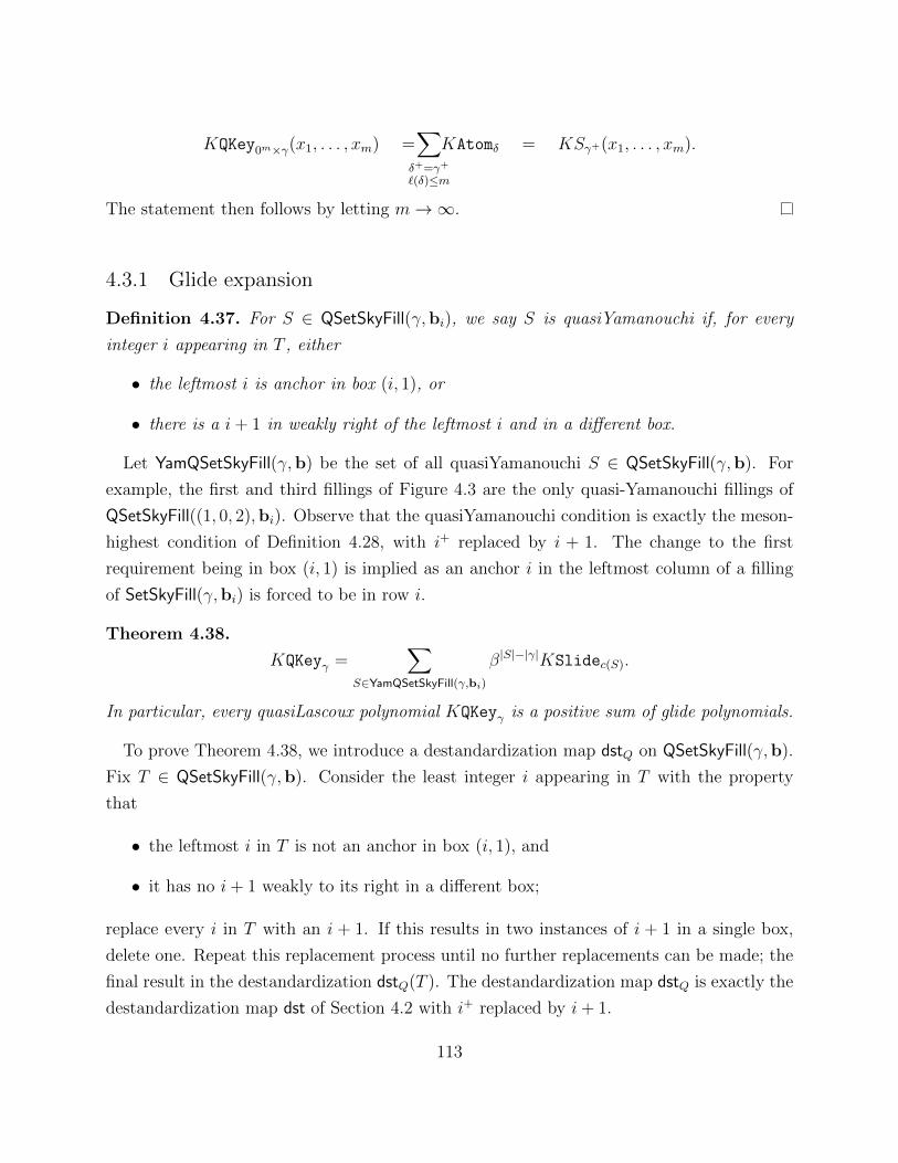
KQKey0m×γ(x1, . . . , xm) =∑δ+=γ+

`(δ)≤m

KAtomδ = KSγ+(x1, . . . , xm).

The statement then follows by letting m→∞.

4.3.1 Glide expansion

Definition 4.37. For S ∈ QSetSkyFill(γ,bi), we say S is quasiYamanouchi if, for every

integer i appearing in T , either

• the leftmost i is anchor in box (i, 1), or

• there is a i+ 1 in weakly right of the leftmost i and in a different box.

Let YamQSetSkyFill(γ,b) be the set of all quasiYamanouchi S ∈ QSetSkyFill(γ,b). For

example, the first and third fillings of Figure 4.3 are the only quasi-Yamanouchi fillings of

QSetSkyFill((1, 0, 2),bi). Observe that the quasiYamanouchi condition is exactly the meson-

highest condition of Definition 4.28, with i+ replaced by i + 1. The change to the first

requirement being in box (i, 1) is implied as an anchor i in the leftmost column of a filling

of SetSkyFill(γ,bi) is forced to be in row i.

Theorem 4.38.

KQKeyγ =∑

S∈YamQSetSkyFill(γ,bi)

β|S|−|γ|KSlidec(S).

In particular, every quasiLascoux polynomial KQKeyγ is a positive sum of glide polynomials.

To prove Theorem 4.38, we introduce a destandardization map dstQ on QSetSkyFill(γ,b).

Fix T ∈ QSetSkyFill(γ,b). Consider the least integer i appearing in T with the property

that

• the leftmost i in T is not an anchor in box (i, 1), and

• it has no i+ 1 weakly to its right in a different box;

replace every i in T with an i + 1. If this results in two instances of i + 1 in a single box,

delete one. Repeat this replacement process until no further replacements can be made; the

final result in the destandardization dstQ(T ). The destandardization map dstQ is exactly the

destandardization map dst of Section 4.2 with i+ replaced by i+ 1.

113

Continuing our example, the first, second, fifth, seventh and ninth fillings of Figure 4.3

destandardize to the first filling; the remaining fillings destandardize to the third filling.

Lemma 4.39. If T ∈ QSetSkyFill(γ,bi) then

dstQ(T ) ∈ YamQSetSkyFill(γ,bi).

Moreover,

dstQ(T ) = T if and only if T ∈ YamQSetSkyFill(γ,bi) ⊂ QSetSkyFill(γ,bi).

Proof. Identical to the proof of Lemma 4.31, with i+ replaced by i+ 1.

Lemma 4.40. Let S ∈ YamQSetSkyFill(γ,bi). Then

KSlidec(S) =∑

T∈dst−1Q (S)

β|T |−|S|xT .

Proof. Nearly identical to the proof of Lemma 4.32. The only difference is that the anchor

entries of the leftmost column no longer have to be equal to their row index, which cor-

responds to the fact that the glide is not necessarily mesonic, and therefore it is possible

bnj = 0.

Proof of Theorem 4.38. We have∑S∈YamQSetSkyFill(γ,bi)

β|S|−|γ|KSlidec(S) =∑

S∈YamQSetSkyFill(γ,bi)

β|S|−|γ|∑

T∈dst−1Q (S)

β|T |−|S|xT

=∑

U∈QSetSkyFill(γ,bi)

β|U |−|γ|xc(U)

= KQKeyγ,

where the first equality is Lemma 4.40, the second is Lemma 4.39, and the third is Proposi-

tion 4.34.

Setting β = 0 in the statement of Theorem 4.38 yields a positive formula for the funda-

mental slide expansion of a quasikey polynomial in terms of quasiYamanouchi quasistandard

skyline fillings. A formula in terms of these objects was alluded to in [Sea17] but not stated

explicitly.

114

Corollary 4.41. The quasisymmetric Grothendieck functions expand combinatorially in the

multi-fundamental quasisymmetric functions.

Proof. By Theorem 4.38, any quasiLascoux (and thus quasisymmetric Grothendieck) polyno-

mial expands positively in the glide basis. The statement then follows from Proposition 4.36

and the fact [PS17] that the stable limits of glide polynomials are the multi-fundamental

quasisymmetric functions.

4.4 Lascoux Polynomials

Recall from Theorem 1.26,

Keyγ =∑

δ∈PermutWC(λ(γ))δ�γ

Atomγ.

We have seen several different ways to define the Lascoux polynomials:

• The original operator definition of A. Lascoux (see Definition 1.34),

• Using the ghostly Kohnert diagrams of C. Ross and A. Yong [RY15], and

• Using set-valued skyline diagrams (see Definition 3.3).

Conjecturally, these definitions are all equivalent, however, there are no known proofs of the

equivalence of any of these definitions. While Theorem 3.17 shows

KKeyγ =∑

δ∈PermutWC(λ(γ))δ�γ

KAtomδ

for the Lascoux polynomials defined by divided difference operators, this decomposition has

not been shown for the other definitions of the Lascoux polynomials or Lascoux atoms.

However, for this chapter, we take this decomposition using combinatorial Lascoux atoms

as the definition of the Lascoux polynomials. Conjecture 3.18 combined with Theorem 3.17

would imply this definition is equivalent to the others.

Definition 4.42. The combinatorial Lascoux polynomial KKeyγ is

KKeyγ =∑

δ∈PermutWC(λ(γ))δ�γ

KAtomδ.

115

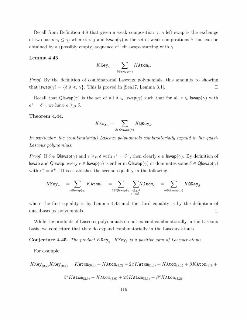
Recall from Definition 4.8 that given a weak composition γ, a left swap is the exchange

of two parts γi ≤ γj where i < j and lswap(γ) is the set of weak compositions δ that can be

obtained by a (possibly empty) sequence of left swaps starting with γ.

Lemma 4.43.

KKeyγ =∑

δ∈lswap(γ)

KAtomδ.

Proof. By the definition of combinatorial Lascoux polynomials, this amounts to showing

that lswap(γ) = {δ|δ � γ}. This is proved in [Sea17, Lemma 3.1].

Recall that Qlswap(γ) is the set of all δ ∈ lswap(γ) such that for all ε ∈ lswap(γ) with

ε+ = δ+, we have ε ≥D δ.

Theorem 4.44.

KKeyγ =∑

δ∈Qlswap(γ)

KQKeyδ.

In particular, the (combinatorial) Lascoux polynomials combinatorially expand in the quasi-

Lascoux polynomials.

Proof. If δ ∈ Qlswap(γ) and ε ≥D δ with ε+ = δ+, then clearly ε ∈ lswap(γ). By definition of

lswap and Qlswap, every ε ∈ lswap(γ) is either in Qlswap(γ) or dominates some δ ∈ Qlswap(γ)

with ε+ = δ+. This establishes the second equality in the following:

KKeyγ =∑

ε∈lswap(γ)

KAtomε =∑

δ∈Qlswap(γ)

∑ε≥Dδε+=δ+

KAtomε =∑

δ∈Qlswap(γ)

KQKeyδ,

where the first equality is by Lemma 4.43 and the third equality is by the definition of

quasiLascoux polynomials.

While the products of Lascoux polynomials do not expand combinatorially in the Lascoux

basis, we conjecture that they do expand combinatorially in the Lascoux atoms.

Conjecture 4.45. The product KKeyγ ·KKeyδ is a positive sum of Lascoux atoms.

For example,

KKey(0,2)KKey(0,1) = KAtom(0,3) +KAtom(1,2) + 2βKAtom(1,3) +KAtom(2,1) + βKAtom(2,2)+

β2KAtom(2,3) +KAtom(3,0) + 2βKAtom(3,1) + β2KAtom(3,2).

116

This has been checked for all γ, δ with at most 3 zeros such that |γ|, |δ| ≤ 5. Specializing

Conjecture 4.45 at β = 0 recovers a conjecture of V. Reiner–M. Shimozono on products of

key polynomials (see [Pun16] for discussion and partial results).

117

CHAPTER 5

Conjectures about Schubert Calculus

5.1 Introduction

We take this opportunity to include some conjectures about (equivariant) Schubert calculus.

Let us begin with a brief history of the subject, culminating with the connection to Schur

polynomials, which we alluded to in Chapter 1. Our reference is S. Kleiman’s [Kle76].

Schubert calculus dates back to the nineteenth century when H. Schubert, among others,

was trying to answer questions in enumerative geometry. A well-known introductory question

of this type is the “four lines problem” that asks given four random lines in 3-space, how

many lines intersect these 4 lines? The calculations of Schubert would conclude there are 2

in the following manner: first we deform our four arbitrary lines so that we have two pairs

of intersecting lines. Then there is one line in between the two points of intersection and for

the other line, each pair of intersecting lines spans a plane and the two planes intersect in a

second line. Since deforming the lines was a continuous function, the number of lines must

be a continuous function as well. Thus it is a constant function and so there are always two

such lines.

It should be noted that the above problem should really be formulated in CP3, and the

notion of “random” is not defined. Indeed, Hilbert’s fifteenth problem was to put a rigorous

foundation for Schubert’s problems and methods, such as the “principle of conservation

of number” utilized above. The modern formulation and solution to Schubert’s four line

problem involves the Grassmannian and its cohomology ring; this is part of intersection

theory [Ful98]. Our reference for the cohomology ring of the Grassmannian and its basis in

Schubert cycles is [Man01].

118

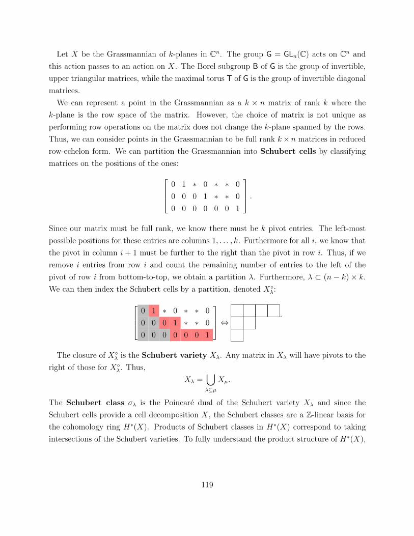
Let X be the Grassmannian of k-planes in Cn. The group G = GLn(C) acts on Cn and

this action passes to an action on X. The Borel subgroup B of G is the group of invertible,

upper triangular matrices, while the maximal torus T of G is the group of invertible diagonal

matrices.

We can represent a point in the Grassmannian as a k × n matrix of rank k where the

k-plane is the row space of the matrix. However, the choice of matrix is not unique as

performing row operations on the matrix does not change the k-plane spanned by the rows.

Thus, we can consider points in the Grassmannian to be full rank k× n matrices in reduced

row-echelon form. We can partition the Grassmannian into Schubert cells by classifying

matrices on the positions of the ones: 0 1 ∗ 0 ∗ ∗ 0

0 0 0 1 ∗ ∗ 0

0 0 0 0 0 0 1

.Since our matrix must be full rank, we know there must be k pivot entries. The left-most

possible positions for these entries are columns 1, . . . , k. Furthermore for all i, we know that

the pivot in column i + 1 must be further to the right than the pivot in row i. Thus, if we

remove i entries from row i and count the remaining number of entries to the left of the

pivot of row i from bottom-to-top, we obtain a partition λ. Furthermore, λ ⊂ (n − k) × k.

We can then index the Schubert cells by a partition, denoted X◦λ: 0 1 ∗ 0 ∗ ∗ 0

0 0 0 1 ∗ ∗ 0

0 0 0 0 0 0 1

⇔ .

The closure of X◦λ is the Schubert variety Xλ. Any matrix in Xλ will have pivots to the

right of those for X◦λ. Thus,

Xλ =⋃λ⊆µ

Xµ.

The Schubert class σλ is the Poincare dual of the Schubert variety Xλ and since the

Schubert cells provide a cell decomposition X, the Schubert classes are a Z-linear basis for

the cohomology ring H∗(X). Products of Schubert classes in H∗(X) correspond to taking

intersections of the Schubert varieties. To fully understand the product structure of H∗(X),

119

it suffices to understand the product

σλ ^ σµ =∑ν

cνλ,µσν .

Remarkably, the coefficients cνλ,µ are the exact Littlewood-Richardson coefficients as in the

product of Schur functions (see Section 1.2.2):

sλsµ =∑ν

cνλ,µsν .

Returning to the four lines problem, let X be the Grassmannian of 2-planes in C4. Since

our four lines are in projective 3-space, they can be considered as points of X. If we fix a

point in X, the Schubert variety X(1) is the collection of all points of X that intersect our

fixed point in at least a line. Thus to find the number of lines that meet 4 random lines, we

merely need to calculate σ4(1). Then using the Littlewood-Richardson rule and the fact that

the Schubert cells of X are indexed by partitions that fit inside a 2 × 2 box, we have the

following calculations:

σ2(1) = σ(1,1) + σ(2)

with the witnessing fillings

1

1.

Then

σ2(1,1) = σ(2,2) due to 1

2,

and

σ2(2) = σ(2,2) due to

1 1.

Finally, σ(1,1)σ(2) = 0 and thus

σ4(1) = 2σ(2,2).

Therefore, there are 2 lines that meet any 4 random lines, as calculated before.

We now generalize this discussion to the equivariant cohomology ring of X; see [TY13] and

the references therein. Since each Xλ is stable with respect to the T action, they also admit

classes σTλ in the T-equivariant cohomology ring of X. The equivariant Schubert classes

form a basis of HT(X,Q) as a module over HT(pt) ∼= Z(β1, ..., βn−1). Thus the equivariant

120

structure constants are defined

σTλ · σT

µ =∑ν

Cνλ,µ(β1, . . . , βn−1)σTν .

In [Gra01, Corollary 4.1], W. Graham proved that Cνλ,µ is a polynomial with positive

coefficients in the βi. The first [Gra01]-positive combinatorial rule for the Grassmannian

was given by A. Knutson and T. Tao [KT03, Theorem 1] using puzzles. Tableau rules

were given by V. Kreiman [Kre10] and A. Molev [Mol09], however H. Thomas and A. Yong

[TY13, Theorem 1.2] give a rule in terms of edge-labeled tableaux and jeu de taquin ,

a tableaux operation.

While the equivariant cohomology of the Grassmannian is well understood, there are

other spaces of interest where this problem is still open, most particularly the miniscule flag

varieties; see [TY09a] and [BL11, Chapter 9]. More generally, let G be a complex, connected,

semisimple Lie group with Weyl group W and fix a Borel subgroup B ⊆ G. Let B− denote

the opposite subgroup and T = B∩ B− the maximal torus. A subgroup P is parabolic when

B ⊆ P ⊆ G and associated to P we have WP ⊆ W. Then X = G/P is a generalized flag

variety.

The Bruhat decomposition of X is the decomposition of X into B−-orbits as follows.

Each coset of WP has a unique minimal length representative w. For wWP ∈ W/WP , the

Schubert cell is defined X◦w = B−wP/P and the Schubert variety Xw is the closure of

X◦w. Finally, the Schubert class σw is the Poincare dual of the Schubert variety Xw and

the set of Schubert classes {σw} where w is a minimal coset representative forms a basis of

the cohomology ring H∗(G/P,Q).

The Schubert structure problem in the cohomology ring H∗(G/P,Q) is to give a combina-

torial rule for the structure coefficients Cwu,v in

σu · σv =∑w

Cwu,vσw.

Miniscule flag varieties correspond to certain maximal parabolic subgroups, and a root-

system uniform combinatorial rule for the Schubert structure problem was given for the

these flag varieties by H. Thomas and A. Yong [TY09a].

Since each Xw is stable with respect to the T-action, they admit classes σTw in the T-

121

equivariant cohomology ring of G/P, denoted HT(G/P;Q). It is a fact [KT03] that

Cwu,v(β1, . . . , βr) =

{0 `(u) + `(v) < `(w)

cwu,v `(u) + `(v) = `(w).

Moreover, W. Graham’s positivity result that Cwu,v as an element of Z[β1, ..., βr] is a poly-

nomial with nonnegative integer coefficients applies in this more general setting [Gra01,

Corollary 4.1].

The cominiscule flag varieties are (see [TY09a, Table 1])

• Type An, the Grassmannian Gr(k, n),

• Type Bn, the odd orthogonal Grassmannian OG(n, 2n+ 1),

• Type Cn, the Lagrangian Grassmannian LG(n, 2n),

• Type Dn, the orthogonal Grassmannian OG(n, 2n),

• Type E6, the Cayley plane OP2, and

• Type E7, the Freudenthal variety, Gω(O3,O6).

Giving a root-system uniform and [Gra01]-positive combinatorial rule for Cwu,v when G/P

is miniscule is an open problem. As far as we are aware, there are no rules known for any

of the nontrivial minuscule cases outside of the Grassmannian. Indeed the main interesting

step towards a root-system uniform rule is to give a [Gra01]-positive combinatorial rule for

Cwu,v when G/P is a maximal orthogonal Grassmannian (type B) or Lagrangian Grassman-

nian (type C). In these two cases, the Schubert classes are indexed by shifted partitions as

described in Section 2.3.

While a precise conjectural rule has eluded us, there are some computational conjec-

tures that shed light on some constraints any rule must adhere to. First, there is a well-

known relationship between the ordinary structure constants of odd orthogonal Grassman-

nian OG(n, 2n + 1) (Type B) and Lagrangian Grassmannian LG(n, 2n) (Type C). Let

cνλ,µ be the structure coefficient of the odd orthogonal Grassmannian and dνλ,µ the structure

coefficient of the Lagrangian Grassmannian. Then,

cνλ,µ = 2`(ν)−`(λ)−`(µ)dνλ,µ.

122

λ µ ν Cνλ,µ Dν

λ,µ

(1) (1) (1) β1 β1(1) (1) (2) 1 2(1) (2) (2) β1 + β2 β1 + 2β2(1) (2) (2, 1) 1 1(1) (2, 1) (2, 1) 2β1 + β2 2β1 + 2β2(2) (2) (2) β1β2 + β2

2 β1β2 + 2β22

(2) (2) (2, 1) 2β1 + 2β2 β1 + 2β2(2) (2, 1) (2, 1) 2β2

1 + 3β1β2 + β22 β2

1 + 3β1β2 + 2β22

(2, 1) (2, 1) (2, 1) 2β31 + 3β2

1β2 + β1β22 β3

1 + 3β21β2 + 2β1β

22

Table 5.1: The nonzero calculations of Cνλ,µ and Dν

λ,µ for λ, µ, ν ⊆ (2, 1).

This can be derived from the fact that Qλ = 2`(λ)Pλ (see Equation (2.8)) where Pλ is

the Schur P -function, representing classes of the orthogonal Grassmannian and Qλ is the

Schur Q-function, representing classes of the Lagrangian Grassmannian. We generalize this

relationship to the equivariant structure constants.

Conjecture 5.1. Let Cνλ,µ be the equivariant structure constant of the odd orthogonal Grass-

mannian and Dνλ,µ the equivariant structure coefficient of the Lagrangian Grassmannian.

Then Cνλ,µ and Dν

λ,µ are polynomials in the simple roots with the same support and for each

βα that appears, there exists a (possibly negative) integer kα such that

[βα]Dνλ,µ = 2kα [βα]Cν

λ,µ.

This has been checked exhaustively for all λ, µ, ν ⊆ (5, 4, 3, 2, 1). The nonzero calculations

for λ, µ, ν ⊆ (2, 1) are listed in Table 5.1, given Cνλ,µ = Cν

µ,λ and Dνλ,µ = Dν

µ,λ .

5.2 The Horn Inequalities

We first briefly recall the history of the Horn inequalities and their connection to Schubert

calculus. Our references for this material are [Ful99, ARY13] and the references within.

The question of the Horn inequalities dates back to the nineteeth century and it asks when

A and B are Hermitian matrices, what are the possible eigenvalues for

A+B = C?

123

Hermitian matrices have real eigenvalues and we consider these eigenvalues in weakly de-

creasing order. Suppose A has eigenvalues λ = λ1 ≥ λ2 ≥ . . . λ2, B has eigenvalues

µ = µ1 ≥ µ2 ≥ . . . ≥ µn, and C has eigenvalues ν = ν1 ≥ ν2 ≥ . . . ≥ νn. We note

here that these values are arbitrarily real values, not necessarily nonnegative integers. The

only obvious relation between λ, µ, and ν concerns the trace of A, B, and C:∑i

λi +∑j

µj =∑k

νk.

We will call (λ, µ, ν) a Hermitian triple if there exists A,B,C with the specified eigenvalues

such that C = A+B.

In 1912, H. Weyl gave a list of necessary inequalities on λ, µ, and ν for A + B = C. For

the next fifty years, various mathematians proved certain inequalities are necessary but a

complete list was not provided until 1962. A. Horn defined a system of inequalities of the

form

νk1 + . . . νkr ≤ λi1 + . . . λir + µj1 + . . .+ µjr

where the triples are in a finite set Tr,n. He computed Tr,n for n ≤ 8 and gave a highly

recursive procedure for defining it in general. He proved that these inequalities were necessary

and conjectured that they were also sufficient, i.e. that (λ, µ, ν) satisfied the inequalities

defined with Tr,n and the trace equality if and only if (λ, µ, ν) was a Hermitian triple.

In 1982, G. J. Heckman showed if the Littlewood-Richardson coefficient cνλ,µ 6= 0 then

(λ, µ, ν) is a Hermitian triple. Then in 1998, A. Kylachko

• defined a different set of inequalities on (λ, µ, ν),

• proved that (λ, µ, ν) is a Hermitian triple if and only if they satisfy his inequalities

(thus giving the first complete solution to the eigenvalue problem).

• Furthermore, he proved if cνλ,µ 6= 0 then (λ, µ, ν) satisfies his inequalities, and

• if (λ, µ, ν) satisfies his inequalities then there exists an integer N such that cNνNλ,Nµ 6= 0

where Nλ = Nλ1 ≥ Nλ2 ≥ . . . Nλn.

A consequence of this result with some previous work reduces the problem of the Horn

inequalities down to the saturation conjecture

cνλ,µ 6= 0⇐⇒ cNνNλ,Nµ for all N.

124

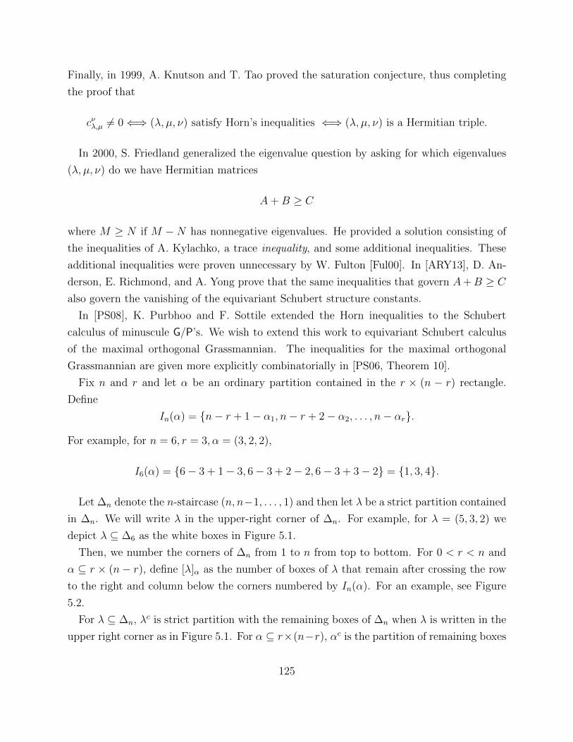
Finally, in 1999, A. Knutson and T. Tao proved the saturation conjecture, thus completing

the proof that

cνλ,µ 6= 0⇐⇒ (λ, µ, ν) satisfy Horn’s inequalities ⇐⇒ (λ, µ, ν) is a Hermitian triple.

In 2000, S. Friedland generalized the eigenvalue question by asking for which eigenvalues

(λ, µ, ν) do we have Hermitian matrices

A+B ≥ C

where M ≥ N if M −N has nonnegative eigenvalues. He provided a solution consisting of

the inequalities of A. Kylachko, a trace inequality, and some additional inequalities. These

additional inequalities were proven unnecessary by W. Fulton [Ful00]. In [ARY13], D. An-

derson, E. Richmond, and A. Yong prove that the same inequalities that govern A+B ≥ C

also govern the vanishing of the equivariant Schubert structure constants.

In [PS08], K. Purbhoo and F. Sottile extended the Horn inequalities to the Schubert

calculus of minuscule G/P’s. We wish to extend this work to equivariant Schubert calculus

of the maximal orthogonal Grassmannian. The inequalities for the maximal orthogonal

Grassmannian are given more explicitly combinatorially in [PS06, Theorem 10].

Fix n and r and let α be an ordinary partition contained in the r × (n − r) rectangle.

Define

In(α) = {n− r + 1− α1, n− r + 2− α2, . . . , n− αr}.

For example, for n = 6, r = 3, α = (3, 2, 2),

I6(α) = {6− 3 + 1− 3, 6− 3 + 2− 2, 6− 3 + 3− 2} = {1, 3, 4}.

Let ∆n denote the n-staircase (n, n−1, . . . , 1) and then let λ be a strict partition contained

in ∆n. We will write λ in the upper-right corner of ∆n. For example, for λ = (5, 3, 2) we

depict λ ⊆ ∆6 as the white boxes in Figure 5.1.

Then, we number the corners of ∆n from 1 to n from top to bottom. For 0 < r < n and

α ⊆ r × (n− r), define [λ]α as the number of boxes of λ that remain after crossing the row

to the right and column below the corners numbered by In(α). For an example, see Figure

5.2.

For λ ⊆ ∆n, λc is strict partition with the remaining boxes of ∆n when λ is written in the

upper right corner as in Figure 5.1. For α ⊆ r×(n−r), αc is the partition of remaining boxes

125

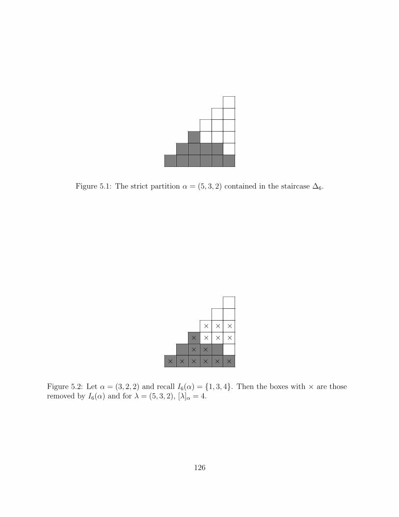
Figure 5.1: The strict partition α = (5, 3, 2) contained in the staircase ∆6.

× × ×× × × ×× ×

× × × × × ×

Figure 5.2: Let α = (3, 2, 2) and recall I6(α) = {1, 3, 4}. Then the boxes with × are thoseremoved by I6(α) and for λ = (5, 3, 2), [λ]α = 4.

126

of r × (n − r) when α is written in the upper right corner. A triple of ordinary partitions

α, β, γ is feasible if the Littlewood-Richardson coefficient cαc

β,γ 6= 0 and a triple of strict

partitions λ, µ, ν is feasible if aλc

µ,ν 6= 0 where aλc

µ,ν is the structure constant of the orthogonal

Grassmannian.

Theorem 5.2 (Purbhoo-Sottile, Theorem 10 [PS06]). The triple λ, µ, ν contained in the

n-staircase is a feasible triple if and only if the

• homogeneity equality |λ|+ |µ|+ |ν| =(n+12

)holds and

• for all 0 < r < n and all feasible α, β, γ ⊆ r × (n− r), [λ]α + [µ]β + [ν]γ ≤(n+1−r

2

).

A triple of strict partitions λ, µ, ν is equivariant feasible if Cλc

µ,ν 6= 0 where Cλc

µ,ν is the

equivariant structure constant of the orthogonal Grassmannian.

Conjecture 5.3. For the maximal Orthogonal Grassmannian, λ, µ, ν contained in the n-

staircase (and not a smaller staircase) is an equivariant feasible triple if and only if for

k = |λ|+ |µ|+ |ν| −(n+12

),

• the homogeneity inequality holds, i.e. k ≥ 0, and

• for all 0 < r < n and all feasible α, β, γ ⊆ r× (n− r), [λ]α + [µ]β + [ν]γ − k ≤(n+1−r

2

).

We have checked this for all λ, µ, ν ⊆ (5, 4, 3, 2, 1).

For example,

C(4,3,2)(3,1),(4,3) = 8β2

1 + 16β1β2 + 8β22 + 16β1β3 + 16β2β3 + 8β2

3 + 8β1β4 + 8β2β4 + 8β3β4 + 2β24 6= 0.

Thus (1), (3, 1), (4, 3) is an equivariant feasible triple with k = 1 + 4 + 7 − 10 = 2. Clearly,

k ≥ 1 and the smallest staircase containing (1), (3, 1), (4, 3) is ∆4. Thus the second condition

states we need to consider 0 < r < 4 and thus let r = 1. For r = 1, there is only one feasible

triple (1), (1), (1). Then we have I4 = {3} and [(1)](1) = 1, [(3, 1)](1) = 2 and [(4, 3)](1) = 3

as

× ×××

× ×××

× ×××

.

Then as desired 4 = 1 + 2 + 3− 2 ≤(4+1−1

2

)= 6. We repeat this for the six feasible triples

for r = 2 and the single feasible triple for r = 3.

127

While the proof of the saturation conjecture was essential to the story of the Type A

Horn inequalities, saturation does not hold in the maximal orthogonal Grassmannian, even

nonequivariantly. The Littlewood-Richardson coefficient c(3,2,1)(2,1),(2,1) = 0 but c

(6,4,2)(4,2),(4,2) = 8.

128

REFERENCES

[AAV12] D. Avella-Alaminos and E. Vallejo, Kronecker products and the RSK corre-spondence, Discrete Math. 312 (2012), no. 8, 1476 – 1486.

[AM09] G. Agnarsson and W. D. Morris, On Minkowski sums of simplices, Ann.Comb. 13 (2009), no. 271.

[ARY13] D. Anderson, E. Richmond, and A. Yong, Eigenvalues of Hermitian matricesand equivariant cohomology of Grassmannians, Composito Math. 149 (2013),1569–1582.

[AS16] S. Assaf and D. Searles, Kohnert tableaux and a lifting of quasi-Schur func-tions, preprint arXiv:1609.03507.

[AS17] , Schubert polynomials, slide polynomials, Stanley symmetric functionsand quasi-Yamanouchi pipe dreams, Adv. Math. 306 (2017), 89–122.

[Ass17] S. Assaf, Combinatorial models for Schubert polynomials, preprintarXiv:1703.00088.

[Bal11] C. Ballantine, Powers of the Vandermonde determinant, Schur functions, andrecursive formulas,, Proceedings of FPSAC 2011, 2011.

[Bar12] A. Barvinok, Matrices with prescribed row and column sums, Linear AlgebraAppl. 436 (2012), no. 4, 820 – 844, Coimbra Meeting on 0-1 Matrix Theoryand Related Topics June 17-19, 2010.

[BB93] N. Bergeron and S. Billey, RC-graphs and Schubert polynomials, Experiment.Math. 2 (1993), no. 4, 257–269.

[BJS93] S. Billey, W. Jockusch, and R. Stanley, Some combinatorial properties ofSchubert polynomials, J. Algebraic Combin. 2 (1993), no. 4, 345–374.

[BKS+07] A. Buch, A. Kresch, M. Shimozono, H. Tamvakis, and A. Yong, StableGrothendieck polynomials and K-theoretic factor sequences, Math. Ann. 340(2007), no. 2, 359–382.

129

[BL11] S. Billey and V. Lakshmibai, Singular loci of Schubert varieties, Progress inMathematics, vol. 182, Birkauser, 2011.

[BPS16] J. Bloom, O. Pechenik, and D. Saracino, Proofs and generalizations of a ho-momesy conjecture of Propp and Roby, Discrete Math. 339 (2016), no. 1, 194– 206.

[BR07] M. Beck and S. Robins, Computing the continuous discretely, Springer-Verlag,New York, 2007.

[BS16] A. Buch and M. Samuel, K-theory of miniscule varieties, J. Reine Angew.Math. 2016 (2016), no. 719, 133–171.

[Buc02] A. Buch, A Littlewood-Richardson rule for the K-theory of Grassmannians,Acta Math. 189 (2002), no. 1, 37–78.

[Che95] I. Cherednik, Nonsymmetric Macdonald polynomials, Int. Math. Res. Not.IMRN (1995), no. 10, 483–515.

[CHHH14] D. Cox, C. Haase, T. Hibi, and A. Higashitani, Integer decomposition propertyof dilated polytopes, Electron. J. Combin. 21 (2014), no. 4, #P4.28.

[CL17] F. Castillo and F. Liu, Berlinevergne valuation and generalized permutohedra,Discrete Comput. Geom. (2017).

[Cro10] D. Croitoru, Mixed volumes of hypersimplices, root systems and shifted youngtableaux, Ph.D. thesis, MIT, Cambridge, MA, 2010.

[Dem74] M. Demazure, Desingularisation des varietes de Schubert, Ann. E. N. S. 4(1974), no. 7, 53–88.

[DPS17] K. Dilks, O. Pechenik, and J. Striker, Resonance in orbits of plane partitionsand increasing tableaux, J. Combin. Theory Ser. A 148 (2017), 244 – 274.

[Ehr62] E. Ehrhart, Sur les polyedres rationnels homothetiques a n dimensions, C. R.Acad. Sci. Paris 254 (1962), 616–618.

[EY17] L. Escobar and A. Yong, Newton polytopes and symmetric Grothendieck poly-nomials, preprint arXiv:1705.07876.

[FG98] S. Fomin and C. Greene, Noncommutative Schur functions and their applica-tions, Discrete Math. 193 (1998), no. 1, 179 – 200.

[FK96] S. Fomin and A. N. Kirillov, The Yang-Baxter equation, symmetric func-tions, and Schubert polynomials, Discrete Math. 153 (1996), no. 1, 123 – 143,Proceedings of the 5th Conference on Formal Power Series and AlgebraicCombinatorics.

130

[FMS17] A. Fink, K. Meszaros, and A. St. Dizier, Schubert polynomials as integer pointtransforms of generalized permutahedra, preprint arXiv:1706.04935.

[Ful97] W. Fulton, Young tableaux : with applications to representation theory andgeometry, London Mathematical Society student texts, Cambridge UniversityPress, Cambridge, New York, 1997.

[Ful98] , Intersection theory, Springer-Verlag, New York, 1998.

[Ful99] , Eigenvalues, invariant factors, highest weights, and Schubert calculus.

[Ful00] William Fulton, Eigenvalues of majorized Hermitian matrices and Little-woodRichardson coefficients, Linear Algebra Appl. 319 (2000), no. 1, 23 –36.

[Ges84] I. M. Gessel, Multipartite P -partitions and inner products of skew Schur func-tions, Combinatorics and Algebra, Contemp. Math., Vol. 34, Amer. Math.Soc., 1984, pp. 289–301.

[GKZ90] I.M Gelfand, M.M Kapranov, and A.V Zelevinsky, Newton polytopes of theclassical resultant and discriminant, Adv. Math. 84 (1990), no. 2, 237 – 254.

[GKZ94] , Discriminants, resultants, and multidimensional determinants, Mod-ern Birkhauser Classics, Birkhauser Basel, 1994.

[GMP+16] C. Gaetz, M. Mastrianni, R. Patrias, H. Peck, C. Robichaux, D. Schwein, andK. Y. Tam, K-Knuth equivalence for increasing tableaux, Electr. J. Comb. 23(2016), no. 1, P1.40.

[Gra01] W. Graham, Positivity in equivariant Schubert calculus, Duke Math. J. 109(2001), no. 3, 599–614.

[Hai99] Mark Haiman, Macdonald polynomials and geometry, New Perspectives inAlgebraic Combinatorics, University Press, 1999, pp. 207–254.

[HHL05] J. Haglund, M. Haiman, and N. Loehr, A combinatorial formula for Macdon-ald polynomials, Jour. Amer. Math. Soc. 18 (2005), no. 3, 735–761.

[HHL08] , A combinatorial formula for nonsymmetric Macdonald polynomials,Amer. J. of Math. 103 (2008), no. 2, 359–383.

[HKP+17] Z. Hamaker, A. Keilthy, R. Patrias, L. Webster, Y. Zhang, and S. Zhou,Shifted hecke insertion and the K-theory of OG(n, 2n + 1), J. of Combin.Theory Ser. A 151 (2017), 207 – 240.

[HLMvW11a] J. Haglund, K. Luoto, S. Mason, and S. van Willigenberg, QuasisymmetricSchur functions, J. Combin. Theory Ser. A 118 (2011), no. 2, 463–490.

131

[HLMvW11b] , Refinements of the Littlewood-Ricardson rule, Trans. Amer. Math.Soc. 363 (2011), no. 3, 1665–1686.

[HPPW16] Z. Hamaker, R. Patrias, O. Pechenik, and N. Williams, Doppelg\“angers:Bijections of Plane Partitions, preprint arXiv:1602.05535.

[IV96] W. F. Doran IV, A proof of Reutenauer’s −qn conjecture, J. Comb. TheorySer. A 74 (1996), no. 2, 342–344.

[Kle76] S. Kleiman, Problem 15. Rigorous foundation of Schubert’s enumerative calcu-lus, Proceedings of Symposia in Pure Mathematics (F. Browder, ed.), vol. 28,Amer. Math. Soc., Providence, RI, 1976, pp. 445–482.

[KMY08] A. Knutson, E. Miller, and A. Yong, Tableau complexes, Isr. J. Math. 163(2008), no. 1, 317–343.

[Koh91] A. Kohnert, Weintrauben, polynome, tableaux, Bayreuth. Math. Schr. 38(1991), 1–97.

[Kre10] V. Kreiman, Equivariant Littlewood-Richardson skew tableaux, Trans. Amer.Math. Soc 362 (2010), no. 5, 2589–3468.

[KS96] F. Knop and S. Sahi, A recursion and a combinatorial formula for Jack poly-nomials.

[KT03] A. Knutson and T. Tao, Puzzles and (equivariant) cohomology of Grassman-nians, Duke Math. J. 119 (2003), no. 2, 221–260.

[Las01] A. Lascoux, Transition on Grothendieck polynomials, ch. 7, pp. 164–179, 2001.

[Len00] C. Lenart, Combinatorial aspects of the K-theory of Grassmannians, Ann.Comb. 4 (2000), no. 1, 67.

[LLM+14] T. Lam, L. Lapointe, J. Morse, A. Schilling, M. Shimozono, and M. Zabrocki,k-Schur functions and affine Schubert calculus, Fields Institute Monographs,Springer-Verlag, 2014.

[LLT97] A. Lascoux, B. Leclerc, and J.-Y. Thibon, Ribbon tableaux, HallLittlewoodfunctions, quantum affine algebras, and unipotent varieties, J. of Math. Phys.38 (1997), no. 2, 1041–1068.

[LMS16] H. Li, J. Morse, and P. Shields, Structure constants for K-theory of Grass-mannians, revisited, J. of Combin. Theory Ser. A 144 (2016), 306 – 325, FiftyYears of the Journal of Combinatorial Theory.

[LMvW13] K. Luoto, S. Mykytiuk, and S. van Willigenburg, An introduction to qua-sisymmetric Schur functions, Springer, New York, 2013.

132

[LP07] T. Lam and P. Pylyavskyy, Combinatorial Hopf algebras and K-homology ofGrassmanians, Int. Math. Res. Not. (2007), 1–48.

[LS78a] A. Lascoux and M.-P. Schutzenberger, Sur une conjecture de H. O. Foulkes,C. R. Acad. Sci. Paris A-B (1978), no. 286, A323–A324.

[LS78b] , Sur une conjecture de H. O. Foulkes, C. R. Acad. Soc. Paris 26A(1978), 323–324.

[LS82a] , Polynomes de Schubert, C. R. Acad. Sci. Paris 294 (1982), no. 13,447–450.

[LS82b] , Structure de Hopf de l’anneau de cohomologie et de l’anneau deGrothendieck d’une variete de drapeaux, C. R. Acad. Sci. Paris 295 (1982),629–633.

[LS89] , Tableaux and noncommutative Schubert polynomials, Funct. Anal.Appl. 23 (1989), no. 3, 223–225.

[LS90] , Keys & standard bases, Invariant theory and tableaux (Minneapolis,MN, 1988), IMA Vol. Math. Appl., vol. 19, Springer, New York, 1990, pp. 125–144.

[Mac88] I. G. Macdonald, A new class of symmetric functions, Publ. I.R.M.A. Stras-bourg, 372/S20, Actes 20 S’eminaire Lotharingien, 1988, pp. 131–171.

[Mac95a] , Affine Hecke algebras and orthogonal polynomials, Semin. Bourbaki37 (1994-1995), 189–207 (eng).

[Mac95b] , Symmetric functions and Hall polynomials, 01 1995.

[Man01] L. Manivel, Symmetric functions, Schubert polynomials, and degeneracy loci,Amer. Math. Soc., 2001.

[Mas08] S. Mason, A decomposition of Schur functions and an analogue of theRobinson-Schensted-Knuth algorithm, Sem. Lothar. Combin. 57 (2008).

[Mas09] , An explicit construction of type A Demazure atoms, J. AlgebraicCombin. 29 (2009), no. 3, 295–313.

[Mol09] A.I. Molev, Littlewoodrichardson polynomials, J. Algebra 321 (2009), no. 11,3450 – 3468, Special Issue in Honor of Gus Lehrer.

[Mon16] C. Monical, Set-Valued Skyline Fillings, preprint arXiv:1611.08777.

[Mon17] C. Monical, Set-valued skyline fillings, Proceedings of FPSAC 2017, 2017.

133

[MS17] K. Meszaros and A. St. Dizier, From generalized permutahedra to Grothendieckpolynomials via flow polytopes, preprint arXiv:1705.02418.

[MTY17] C. Monical, N. Tokcan, and A. Yong, Newton Polytopes in Algebraic Combi-natorics, preprint arXiv:1703.02583.

[Opd95] E. Opdam, Harmonic analysis for certain representations of graded Heckealgebras, Acta Math. 175 (1995), no. 1, 75–121.

[Pat16] R. Patrias, Antipode formulas for some combinatorial Hopf algebras, Electr.J. Comb. 23 (2016), no. 4, P4.30.

[Pec14] O. Pechenik, Cyclic sieving of increasing tableaux and small Schroder paths,J. Combin. Theory Ser. A 125 (2014), 357 – 378.

[Pos09] A. Postnikov, Permutohedra, associahedra, and beyond, Int. Math. Res. Not.2009 (2009), no. 6, 1026–1106.

[PP16] R. Patrias and P. Pylyavskyy, Combinatorics of K-theory via a K-theoreticPoirierReutenauer bialgebra, Discrete Math. 339 (2016), no. 3, 1095 – 1115.

[PS06] K. Purbhoo and F. Sottile, The Horn recursion for Schur P - and Q-functions,2006.

[PS08] , The recursive nature of cominiscule Schubert calculus, Adv. Math.217 (2008), 1962–2004.

[PS17] O. Pechenik and D. Searles, Decompositions of Grothendieck polynomials, Int.Math. Res. Not., to appear (2017), 28 pages, arXiv:1611.02545.

[PSV16] T. Pressey, A. Stokke, and T. Visentin, Increasing tableaux, Narayana num-bers and an instance of the cyclic sieving phenomenon, Ann. Combin. 20(2016), no. 3, 609–621.

[Pun16] A. Pun, On deposition of the product of Demazure atoms and Demazure char-acters, preprint arXiv:1606.02291.

[PY15] O. Pechenik and A. Yong, Equivariant K-theory of Grassmannians, preprintarXiv:1506.01992.

[PY16] , Genomic tableaux, J. of Algebraic Combin. (2016), 1–37.

[Rad52] R. Rado, An inequality, J. Lond. Math. Soc. s1-27 (1952), no. 1, 1–6.

[Reu95] C. Reutenauer, On symmetric functions related to Witt vectors and the freeLie algebra, Adv. Math. 110 (1995), no. 2, 234 – 246.

134

[Rho17] B. Rhoades, A skein action of the symmetric group on noncrossing partitions,J. of Algebraic Combin. 45 (2017), no. 1, 81–127.

[RS95] V. Reiner and M. Shimozono, Key polynomials and a flagged Littlewood-Richardson rule, J. Combin. Theory Ser. A 70 (1995), no. 1, 107 – 143.

[RTY16] V. Reiner, B. Tenner, and A. Yong, Poset edge densities, nearly reduced words,and barely set-valued tableaux, preprint arXiv:1603.09589.

[RY15] C. Ross and A. Yong, Combinatorial rules for three bases of polynomials, Sem.Lothar. Combin. 74 (2015), B74a.

[Sah00] S. Sahi, Some properties of Koornwinder polynomials, Contemp. Math. 254(2000), 395–411.

[Sea17] D. Searles, Polynomial bases: positivity and Schur multiplication, preprintarXiv:1707.01172.

[Sta71] R. Stanley, Ordered structures and partitions, Ph.D. thesis, Harvard Univer-sity, Cambridge, MA, 1971.

[Sta84] , On the number of reduced decompositions of elements of Coxetergroups, Eur. J. of Combin. 5 (1984), no. 4, 359 – 372.

[Sta95] , A symmetric function generalization of the chromatic polynomial ofa graph, Adv. Math. 111 (1995), no. 1, 166 – 194.

[Sta99a] , Enumerative combinatorics, volume 2, Cambridge University Press,1999.

[Sta99b] , Positivity problems and conjectures in algebraic combinatorics, inMathematics: Frontiers and Perspectives, American Mathematical Society,1999, pp. 295–319.

[Ste89] J. Stembridge, Shifted tableaux and the projective representations of symmet-ric groups, Adv. Math. 74 (1989), no. 1, 87 – 134.

[Ste91] , Immanants of totally positive matrices are nonnegative, Bull. Lond.Math. Soc. 23 (1991), no. 5, 422–428.

[STW94] T. Scharf, J. Thibon, and B. G. Wybourne, Powers of the Vandermondedeterminant and the quantum Hall effect, J. Phys. A 27 (1994), no. 12, 4211.

[TY09a] H. Thomas and A. Yong, A combinatorial rule for (co)minuscule Schubertcalculus, Adv. Math. 222 (2009), no. 2, 596 – 620.

[TY09b] , A jeu de taquin theory for increasing tableau, with applications to K-theoretic Schubert calculus, Algebra Number Theory 3 (2009), no. 2, 121–148.

135

[TY11] , Longest increasing subsequences, Plancherel-type measure and theHecke insertion algorithm, Adv. in Appl. Math. 46 (2011), no. 1, 610 – 642,Special issue in honor of Dennis Stanton.

[TY13] , Equivariant Schubert calculus and jeu de taquin, Ann. Inst. Fourierto appear (2013).

[Val00] E. Vallejo, Plane partitions and characters of the symmetric group, J. Alge-braic Combin. 11 (2000), no. 79, 79–88.

[Win03] R. Winkel, A derivation of Kohnert’s algorithm from Monk’s rule., Sem. Loth.Comb. 48 (2003), B48f.

[Wor84] D. Worley, A theory of shifted Young tableaux, Ph.D. thesis, MassachusettsInstitute of Technology, Cambridge, MA, 1984.

136