Department of Aeronautics, Naval Architecture and Railway Vehicles

VIRTUAL PROTOTYPING OF GAS TURBINE COMPONENTS –

AERODYNAMIC REDESIGN AND ANALYSIS OF ACADEMIC JET

ENGINE

PhD thesis

by Mrs. Foroozan Zare

Dr. Árpád Veress

Supervisor

Budapest, 2020

To

My parents

1

Table of Contents

Acknowledgments .............................................................................................................................................. 5

Declaration ......................................................................................................................................................... 6

Nomenclature .................................................................................................................................................... 7

Abstract ............................................................................................................................................................ 13

1. Introduction ............................................................................................................................................. 15

1.1. Aims and Outline of the Thesis ........................................................................................................ 15

1.2. Organization of the Thesis ............................................................................................................... 16

1.3. Introduction of Gas Turbines ........................................................................................................... 17

2. Mathematical Model Development for Thermo-Dynamic Cycle Analysis and Optimization of Turbojet

Engines ............................................................................................................................................................. 21

2.1. Introduction ..................................................................................................................................... 21

2.2. Novel Closed-Form Expression for Critical Pressure and Optimum Pressure Ratios of Turbojet

Engines ......................................................................................................................................................... 23

2.3. Modell Development for Thermo-Dynamic Cycle Analysis of Turbojet Engines with Verification

and Plausibility Check .................................................................................................................................. 30

2.3.1. Triple-Spool Mixed Turbofan Jet Engine ..................................................................................... 30

2.3.2. Dual-Spool Mixed Turbofan Engine ............................................................................................. 41

2.3.3. Single-Spool Turbojet Engine without Afterburner ..................................................................... 44

2.4. Verification and Plausibility Check of the New Equation for the Optimum Compressor Total

Pressure Ratio .............................................................................................................................................. 47

2.4.1. Analysis of Single-Spool Turbojet Engines with Afterburning ..................................................... 47

2.4.2. Numerical Representation – Verification of the New Equation for Optimum Total Pressure

Ratio of the Compressor .......................................................................................................................... 49

2.5. Conclusions ...................................................................................................................................... 53

3. Redesign of the Academic Turbojet Engine ............................................................................................. 55

3.1. Introduction ..................................................................................................................................... 55

3.2. Design Process of the Gas Turbine ................................................................................................... 57

3.3. General Concerns and Design Aspects ............................................................................................. 58

3.4. Redesign Procedure of the Turbojet Engine .................................................................................... 59

3.5. Conclusions ...................................................................................................................................... 62

4. CFD Analysis of the Redesigned Academic Jet Engine ............................................................................. 63

4.1. Flow Modelling of the Separated Engine Components ....................................................................... 64

4.1.1. CFD analysis of the centrifugal compressor ................................................................................ 64

2

4.1.2. CFD analysis of the combustion chamber ................................................................................... 67

4.1.3. CFD analysis of the axial turbine ................................................................................................. 71

4.1.4. CFD analysis of the exhaust nozzle .............................................................................................. 74

4.2. CFD Analysis of the Full Model ......................................................................................................... 76

4.3. Conclusions ...................................................................................................................................... 80

5. Discussion, Conclusion and Verification of the Results ........................................................................... 81

5.1. Verification of the results................................................................................................................. 81

5.2. Conclusions ...................................................................................................................................... 85

6. Novel Application of Inverse Design Method by Means of Redesigning Compressor Stator Vanes in the

Redesigned Jet Engine ..................................................................................................................................... 86

6.1. Introduction of Optimization Methods for CFD in General ............................................................. 86

6.2. Inverse Design Based Optimization ................................................................................................. 90

6.3. Redesign and Optimization of the Compressor Vanned Diffuser for the Academic Jet Engine ...... 91

6.4. Verification of the Results by ANSYS CFX ......................................................................................... 99

6.4.1. Inviscid analysis of the optimized vane (at Rooftop Cp=-1.8) by CFX ......................................... 99

6.4.2. Viscous analysis of the optimized (at Rooftop Cp=-1.8) vane by CFX ....................................... 101

6.5. Conclusions .................................................................................................................................... 105

7. Conclusions ............................................................................................................................................ 107

8. List and Summary of the Thesis ............................................................................................................. 111

Bibliography ................................................................................................................................................... 115

Author’s Publications ..................................................................................................................................... 122

APPENDIX A – Aerodynamic Redesign of the Academic Jet Engine’s Components ................................. 124

A.1 Compressor Design and Analysis ..................................................................................................... 125

A.2 Inlet Channel .................................................................................................................................... 137

A.3 Design Aspects of the Combustion Chamber .................................................................................. 138

A.4 Turbine Design ................................................................................................................................. 140

A.5 Aspects and Design of Exhaust Nozzle............................................................................................. 156

APPENDIX B - Introduction of the Used CFD Methodology by Means of ANSYS CFX ........................... 157

B.1 Governing Equation ......................................................................................................................... 158

B.2 Turbulence Modelling [48]............................................................................................................... 158

B.3 Spray Breakup Models for Combustion ........................................................................................... 159

B.4 Combustion ...................................................................................................................................... 163

B.5 Numerical Method ........................................................................................................................... 164

3

APPENDIX C - Numerical Algorithm of 2D Inhouse Inviscid Flow Solver [54] ........................................ 166

C.1 Governing Equations ........................................................................................................................ 167

C.2 Finite Volume Discretization Method .............................................................................................. 167

C.3 Boundary Conditions........................................................................................................................ 169

C.4 Wall Modification Algorithm............................................................................................................ 170

APPENDIX D - Constrained Optimization [54] ............................................................................................ 172

D.1 Introduction ..................................................................................................................................... 173

D.2 Stratford’s Separation Prediction Method ...................................................................................... 173

D.3 Constrained Optimization of Stratford’s Limiting Pressure Distribution ........................................ 174

4

5

Acknowledgments

First, I am deeply grateful to my supervisor Dr. Árpád Veress for his guidance, support and encouragement.

The completion of this dissertation would not have been possible without the support of my supervisor. I

consider myself very fortunate for having conducted this research under his supervision.

I would like to show appreciation to my colleague Mr. László Sábitz and Mr. Attila Gubovits for the valuable

support, guidance and suggestions throughout my work and improving my knowledge.

I would like to express my special thanks to Dr. Dániel Rohács, head of Department, who provided me

consultation for the present dissertation.

I am thankful to Dr. Abbas Talimian, my colleague, for the useful remarks during our frequent discussions

and his guidance. This thesis has been done with his kind support on my work.

I also would like to express thanks to the members of the Department of Aeronautics, Naval Architecture and

Railway Vehicle for their endless support in improving my knowledge about aircraft engines and providing

friendly atmosphere as well.

Finally, I would like to offer my heartfelt thanks to Mr. Gábor Rácz and Mr. Roland Rákos in the Engineering

Calculations Team at Knorr-Bremse R&D Center Budapest for their endless and kind guidance and support in

the field of CFD modelling and analysis.

The present work has been supported by the Hungarian national EFOP-3.6.1-16-2016-00014 project, titled

"Investigation and development of the disruptive technologies for e-mobility and their integration into the

engineering education” (IDEA-E).

6

Declaration

Undersigned, Zare Foroozan, I hereby state that this PhD thesis is my original own work, which has been

done after registration for the degree of PhD at Budapest University of Technology and Economics,

Faculty of Transportation Engineering and Vehicle Engineering, Kálmán Kandó Doctoral School of

Transportation and Vehicle Engineering and has not been previously included in a thesis or dissertation

submitted to this or any other institution for a degree, diploma or other qualifications. I have used only

the sources listed in the Bibliography in the thesis. All parts taken from other works, either in a word for

word citation or rewritten keeping the original contents, have been unambiguously marked by a reference

to the source.

Berlin, 31.12.2020.

………………………………………..

Foroozan Zare

7

Nomenclature

Variables (Latin)

A Cross sectional area [m2]

a Speed of sound [m/s]

B Boundary layer blockage [-]

b Meridional depth of passage [m]

𝐶𝑓 Specific heat of the fuel [J/kg/K]

𝐶𝑝 Specific heat at constant pressure [J/kg/K], Pressure coefficient [-]

𝐶𝑝𝐷 Pressure recovery coefficient [-]

𝐶�� Mean (between Ti and Ti+1) specific heat at constant pressure [J/kg/K], Canonical

pressure distribution [-]

c Absolute velocity [m/s], Chord length [m]

D Diameter [m], Jacobian [variable]

𝐷𝑁𝑜𝑧𝑧𝑙𝑒 Injector nozzle diameter [m]

𝐷𝑃 Droplet diameter [m]

E Specific total energy [J/kg]

𝑒𝑥 , 𝑒𝑦 Signs of vector components in x and y directions in Cartesian coordinate system

F(U), G(U) Inviscid flux vectors [variable]

f Fuel to air mass flow rates ratio [-]

H Altitude [m], Vector of numerical flux function [variable]

h Specific enthalpy [J/kg],

htot Specific total enthalpy [J/kg]

K Loss coefficient [-]

k Turbulence kinetic energy per unit mass [J/kg], Boltzmann constant [J/K]

𝐿0 Theoretical air mass required to burn 1 kg fuel at stoichiometry condition [kg/kg]

l Blade length [m]

M Mach number [-], Moment [Nm]

�� Mass of flow rate [kg/s]

��𝑎𝑖𝑟 Air mass flow rate enters in the engine [kg/s]

��𝑛𝑜𝑧𝑧𝑙𝑒 Mass flow rate of injector nozzle [kg/s]

N Rotational speed [rev/min]

Nb Number of boundaries

nx, ny Components of local outward pointing unit normal vector [-]

P Power [W]

p Pressure [Pa]

𝑝𝑟_𝑠𝑡𝑎𝑔𝑒 Pressure ratio (static/total) [-]

𝑄 Heat [J/s]

8

𝑄𝑅 Lower heating value of the fuel [J/kg]

𝑞(𝜆) Dimensionless mass flow rate – gas dynamic function [-]

R Specific gas constant [J/kg/K], Relative radius [-]

R Set of real numbers

ℜ Residual [variable]

R+ Set of positive real numbers

Re Reynolds number [-]

RPM Revolution per Minute [1/min]

r Total pressure recovery factor [-], Radius [m], Degree of reaction [-]

S Entropy [J/s]

𝑺𝑴 Momentum source [kg/m2/s2]

𝑺𝑬 Energy source [kg/m/s3]

s Specific entropy [J/kg]

T Temperature [K], Thrust [N]

TSFC Thrust Specific Fuel Consumption [kg/kN/h]

t Time [s], Blade pitch [m]

U Vector of conservative variables [variable], Velocity vector [m/s]

𝑈𝑃,𝑖𝑛𝑖𝑡𝑖𝑎𝑙 Initial velocity of droplet [m/s]

u Component of velocity vector in x direction [m/s], Tangential (blade or frame) velocity

[m/s]

V Velocity [m/s]

Vn Normal velocity to the interface [m/s]

v Component of velocity vector in y direction [m/s], Courant number

W Power [W], Vector of characteristic variables [variable]

𝑊𝑥 Total shaft power per unit mass flow rate [J/kg]

w Component of velocity vector in z direction [m/s], Relative velocity [m/s]

x Cartesian coordinate in space [m]

y Cartesian coordinate in space [m]

y+ Dimensionless wall distance [-]

z Number of blades [-]

Variables (Greek Symbols)

𝛼 Absolute direction (angle) [degree], Inlet flow angle [degree]

αk Constant for the Runge-Kutta time iteration [-]

𝛽 By-pass ratio [-], Relative direction (angle) [degree], Gas dynamic constant [-]

Γ Boundary of the control volume (domain, face in 2D) and cell face (edge in 2D) length

[m]

𝛾 Ratio of specific heats [-]

Δ Difference [-]

9

𝛿 Boundary layer thickness [m]

𝛿𝑏𝑐 Air income ratio due to the turbine blade cooling [-]

𝛿𝑡𝑒𝑐ℎ Bleed air ratio for technological reasons [-]

휀 Reduction rate of cross section due to the blades [-]

휂 Efficiency [-]

𝛬 (x,y) Domain in x, y space

𝜆 Thermal conductivity [W/m/K], Swirl factor [-], Dimensionless velocity [-]

𝜇 Dynamic viscosity [kg/s/m]

𝜈 Kinematic viscosity [m2/s]

𝜉 Power reduction rate of the auxiliary systems [-]

𝜋 Total pressure ratio [-]

𝜋(𝜆) Dimensionless pressure – gas dynamic function [-]

𝜌 Density [kg/m3]

𝜎 Slip factor [-]

𝜏 Elements of the stress tensor [N/m2], Shear stress [N/m2]

𝝉 Stress tensor

𝜏(𝜆) Dimensionless temperature – gas dynamic function [-]

𝜑 Speed coefficient [-]

Ω Area of the control volume (domain, face in 2D) and finite volume (domain, face in 2D) [m2]

𝜔 Specific turbulence dissipation rate [1/s], Angular velocity [1/s]

Subscripts and Superscripts

A Afterburner

a Axial component

al Afterburner liner

b Burning

bc Blade cooling

C Compressor

c Compressor, Critical

crit Critical

cc Combustion chamber

d Diffuser, derivative

f Fuel, Fan, Flow

h Hub

hp High pressure

i,j,k Variables for spatial and sum indexing

id Ideal

in Inlet

10

init Initial

ip Intermediate pressure

L Left side of the cell interface

Le Leading edge

lp Low pressure

m Mechanical, Meridional, Mean

mix Mass flow weighted parameter for air-gas mixture

n Nozzle, Variables normal to the surface

n+1 Parameter at the boundary (next time step)

opt Optimum

out Outlet

p Particle

R Right side of the cell interface

r Rotor

req Required

rotor Impeller of the compressor

s Isentropic, Specific, Stator

st Stoichiometric condition

stage Compressor stage

stat Static

T Turbine

TE Trailing edge

t Tip

tech Bleed air mass flow rate or ratio removal for technological reason

th Thermal, Theoretical

tot, to Total

u Tangential component

w Tangential (whirl) component

w1 Parameters at the relative flow velocity at segment 1

w2 Parameters at the relative flow velocity at segment 2

wm Parameters at the mean relative flow velocity between segment 1 and 2

휃 Tangential (component)

o Degree, Parameters at maximum velocity (minimum pressure) at Stratford’s method

0 Stagnation or total condition (e. g.: enthalpy, pressure, temperature)

1 Impeller inlet or eye, Upstream condition

2 Impeller outlet or tip

3 Inlet section of the vanned diffuser

4 Diffuser exit

11

1, 2, 3 Number of turbine and compressor spool

0-9 Engine cross sections

∞ Parameters at far upstream condition, Infinite

Accents and Operators

¯ Average, Vector

Vector

ˆ Roe’s average state space

𝜵 Nabla operator

T Transpose of a vector or matrix

𝜕 Symbol of derivative

δ Identity matrix or Kronecker Delta function

Abbreviations

ACO Ant Colony Optimization

APU Auxiliary Power Unit

BVM Burning Velocity Model

CAB Cascade Atomization Breakup

CAD Computer Aided Design

CFD Computational Fluid Dynamics

CMC Ceramic Matrix Composite

D Dimension

DNS Direct Numerical Simulation

DS Directional Solidification

EA Evolutionary Algorithms

ECFM Extended Coherent Flame Model

EDM Eddy Dissipation Model

ES Evolutionary Strategy

ETAB Enhanced Taylor Analogy Breakup

FEM Finite Element Method

FDM Finite Different Method

FRC Finite Rate Chemistry

GA Genetic Algorithm

GP Genetic Programming

GUI Graphical User Interface

HP Horsepower, High Pressure

ILU Incomplete Lower Upper

ISRE Isentropic Radial Equilibrium Equation

12

LCS Learning Classifier System

LP Low Pressure

MUSCL Monotone Upstream Schemes for Conservation Laws

NBC Numerical Boundary Condition

PBC Physical Boundary Condition

PDF Probability Density Function

PSD Power Spectral Density

ps Pressure side

R&D Research and Development

RANS Reynolds Averaged Navier-Stokes

Re Reynolds number

RK Runge-Kutta

RPM Revolution per Minute

SA Simulated Annealing

SQP Sequential Quadratic Programming

SST Shear Stress Transport

ST Specific Thrust

SX Single Crystal Alloy

ss Suction side

TAB Taylor Analogy Breakup

TBC Thermal Barrier Coating

TFC Turbulent Flame Closure

TSFC Thrust Specific Fuel Consumption

TMB-C9H12 1,2,4 Trimethylbenzene

UAV Unmanned Aerial Vehicle

vs. versus

13

Abstract

Today, beside many known applications of the gas turbine engines as in the energy sector for example, the

turbojet engines – as the specific type of the gas turbines – are the most relevant propulsion systems for

aeronautical applications at low-speed supersonic flow regime between the low by-pass and ramjet engines.

Moreover, they can be an essential platform amongst the gas turbine engines for establishing new contributions

in development processes. Hence, the main goal of the present thesis is

i. to determine, verify and validate calculation processes, which can be used for modelling, design

and analysing jet engines in aerodynamic point of view with especial care for an academic jet

engine under investigation,

ii. to introduce new calculation approaches for improving accuracy and advancing/optimising

technical characteristics of the investigated propulsion system and

iii. to provide information about the actual status, application range, advantages, challenges of the

applied mathematical models and tools in the R&D environment.

The aerodynamic design process consists of five main steps.

1. The first step is the thermodynamic cycle analyses to determine the desired operational point with the

outcomes of the thermodynamic state variables at each cross section of the engine, which satisfies the

expected goal functions. Although the subject of the present thesis is a single spool academic turbojet

engine, the thermodynamic model developments are introduced for other single-, dual- and triple-

spool jet engines for the sake of complexity. The T-s diagram and the main characteristics of the

engines are determined by concentrated parameter-distribution type methods implemented in

MATLAB environment. The governing equations are based on mass, energy balance and thermo-

dynamical processes with viscous flow assumption. As many information are available in the open

literature about single-, dual- and triple-spool engines are considered, nonlinear constraint

optimization method is used for identifying the unknown parameters as losses, efficiencies and

technical data in case of they are not available and in case of need. The temperature and component

mass fraction dependent gas properties are calculated by iteration cycles in case of functional

dependencies. A new closed-form expression (the unknown parameter is calculated by an analytical

equation directly/explicitly) is derived for determining the critical pressure in choked flow condition

at converging nozzle with considering losses and process-dependent gas properties. New explicit

equation is derived also and verified for calculating the optimum total pressure ratio of the compressor

pertaining at maximum specific thrust at chocked and unchoked nozzle flow conditions for single-

spool turbojet engines.

2. The second step of the design process, in general, is the determination of the RPM and main

geometrical sizes of the engine [1] following the cycle analyses and making decision about the

operational point of the jet engine by using the TSFC-ST (Thrust Specific Fuel Consumption –

Specific Thrust) map in the function of turbine inlet total temperature and total pressure ratio of the

compressor. However, in the present case, as centrifugal compressor is selected for pressurizing the

ambient air, the RPM and main geometrical sizes of the engine are determined by the mean line design

of the centrifugal compressor assembly and turbine.

3. The third step of the design process is the mean line and the 3D design of the engine components as

intake channel, compressor, combustion chamber, turbine and nozzle. The outcomes of the design are

the all necessary dimensions for creating the 3D geometry of the jet engine. Based on the known or

established dimensions, the 3D model of the gas turbine is created in a CAD software.

14

4. Following the model verification in the fourth step, Computational Fluid Dynamics (CFD) analyses

are completed to crosscheck the differences between the designed and the analysed characteristics.

The results of the CFD simulations are compared with the available measured data and conclusions

are drawn about the efficiency of the used analytical and numerical methods.

5. Finally, in the fifth step, inviscid inverse design method has been implemented and applied for

redesigning compressor vanned diffuser of the academic jet engine. The fluid dynamic results of the

redesigned vane structure are verified by a commercial CFD software by means of inviscid and viscous

flow assumptions. The effect of the new geometry is compared also with the baseline one.

The above mentioned 5 steps design process focuses on the aerodynamic design only. The other contributions

as mechanical (both static and dynamic (e.g.: collision)), vibration (e.g.: eigenfrequencies, harmonic response,

PSD (Power Spectral Density)), thermal, fatigue, creep, wearing, durability and ageing aspects of the solid

components and joints including design loops together with the already mentioned aerodynamic design

scenarios and extending that with control, electronics, tests, production related topics and investigating off-

design performances for instance are indispensable part of the design process but they are excluded from the

present study.

15

1. Introduction

1.1. Aims and Outline of the Thesis

The goal of the present thesis is to determine, verify and validate calculation processes, which can be used for

modelling, design and analysing jet engines in aerodynamic point of view with especial care for a specific

single spool academic jet engine under consideration. The introduction of new calculation approaches for

improving accuracy and technical characteristics of the investigated propulsion systems with providing

information about the actual status, application range, advantages and challenges of the considered

mathematical models and tools in the R&D environment are also the part of the present work. Beside the

available triple-, dual- and single-spool turbojet engines with their characteristics found in the international

open literature due to the highest technical coverage with respect to the thermodynamic analysis, a single spool

academic turbojet engine is considered in the redesign process. The basis of the applied single spool engine is

the TSz-21 starter gas turbine, which was used originally for MiG-23 and Szu-22 Russian fighters. This engine

has been reconstructed to be an academic jet propulsion system by Dr. Beneda and Dr. Pásztor from 2005-

2008 and it is still under development with especial care for control systems [2].

The presented aerodynamic design process has four main steps as

1. Thermo-dynamic cycle analysis for determining the design (operational) point,

2. Mean line and 3D design of the engine for having geometrical sizes and CAD models,

3. Computational Fluid Dynamics (CFD) analysis for verification of the design and plausibility check by

the available data and

4. Inverse design of the solid walls, vanned diffuser in the present case.

Following the market research, the determination of the customer requirements, the specifications and the

selection of the cycle type of the turbomachinery layout, the first step of the engine design is the

thermodynamic cycle analysis for determining the design point. A concentrated parameter distribution-type

method has been developed, implemented and verified for analysing the characteristics of jet propulsion

engines by means of a) available or b) expected specifications as follows.

a) Regarding the scenario about the available specifications due to the extended technical coverage, the

following triple-, dual- and single-spool turbojet engines are considered in the analyses [3]:

i. НК-32 and НК-25 triple spool mixed turbofan engines at take-off condition with afterburner,

ii. НК-22 and НК-144A dual spool mixed turbofan engines at take-off and at flight conditions with

and without afterburning respectively, НК-8-4 and НК-86A dual spool mixed turbofan engines at

take-off condition without afterburning and

iii. ВД-7 and КР7-300 singles spool turbojet engines without afterburner and РД-9Б and the АЛ-

21Ф3 single spool turbojet engines with afterburning at take-off condition. (The last two engines

are considered also for verification and plausibility check of the new equations for the optimum

compressor total pressure ratio.)

The developed mathematical model for analysing the above-mentioned engines is based on the mass and

energy balance together with the thermo-dynamic process equations including frictional (viscous) flow

related losses. Constrained nonlinear optimisation is used for determining the unknown parameters as

efficiencies, losses, power reduction rates of the auxiliary systems, bleed air ratios for technological

reasons, air income ratios due to blade cooling and total temperatures in the afterburner (if it is the case)

for example by means of having parameter-state, which provides the closest results to the available thrusts

16

and thrust specific fuel consumptions. The temperature and component mass fraction dependent gas

properties as specific heat at constant pressure and ratio of specific heats are determined by iteration cycles.

As part of the model development, a new closed-form equation is derived for determining the critical

pressure in choked flow condition at converging nozzle with considering losses and process-dependent gas

properties. New explicit expression is derived also for calculating the optimum total pressure ratio of the

compressor pertaining at maximum specific thrust at chocked and unchoked nozzle flow conditions. РД-

9Б and the АЛ-21Ф3 single spool turbojet engines with afterburning at take-off condition are used for

verification and plausibility check of the new equation about the optimum compressor total pressure ratio.

b) Concerning the case about the expected specifications or design scenario in other words, the already

developed and verified thermodynamic cycle analysis mentioned in point a) above is used to redesign the

TSz-21 gas turbine to have a 330 N thrust low sized academic jet engine. The specific thrust and thrust

specific fuel consumption distributions are determined in the function of the turbine inlet total temperature

and compressor total pressure ratio by the thermodynamic analysis for determining the operating point of

the engine.

The second step of the engine aerodynamic design is the determination of the geometrical sizes and CAD

model preparation of the assembly. The mean line design and its 3D extension have been considered, realized

for creating the compressor and turbine segments in line with the outcomes of the thermo-dynamical cycle

analysis described in point b) above. The configuration and the sizing of the intake channel as well as the

combustion chamber and exhaust nozzle are determined by using the dimensions of the compressor and

turbine, beside guidelines, theoretical and practical solutions, suggestions and experiences for shaping. As the

all geometrical dimensions become available at the end of this state, the 3D model generations are completed

for the intake channel, compressor, combustion chamber, turbine and exhaust nozzle.

CFD analyses are performed in the third step of the design process to crosscheck the differences between the

expected and the computed characteristics of the engine. Two different simulation approaches are applied for

that purpose: 1. separated engine components and 2. full engine model (all engine components are together).

The results of the simulations are compared with the results of the i. thermodynamic cycle analysis, ii. mean

line design and iii. available measured data for verification and plausibility check. Conclusions are drawn

about the agreement and the effectivity of the used analytical and numerical methods.

Finally, a 2D inviscid inverse design method is implemented and used for improving the characteristics of the

vanned diffuser in the compressor in order to increase total pressure recovery factor, static pressure-rise, flow

turning in axial direction and the mass flow rate per unit length beside having the expectation to keep the

original geometrical configuration and dimensions as much as possible. The results of the inverse design

method are verified by a commercial CFD code at both inviscid and viscous flow conditions.

1.2. Organization of the Thesis

The aims, the outline and the structure of the thesis are presented in the first chapter of the thesis along with

the introduction, the global background and the research topics in the field of the gas turbines.

Deduction and introduction of novel analytical equations

i. for the critical pressure at chocked flow condition of converging nozzle and

ii. for the compressor optimum total pressure ratio pertaining at maximal specific thrust at unchoked

and choked nozzle flow conditions for single-spool turbojet engine

17

are completed in the first part of the dissertation’s second chapter. Advanced mathematical models for cycle

analyses of triple-, dual- and single-spool turbojet engines have been developed and introduced in the middle

part of the chapter 2 for creating a framework for the investigations, in which losses (viscous flow) and

process-dependent gas properties are considered. Finally, verification, test and plausibility investigations of

the analytical cycle-analysis and the new algebraic expressions are completed and presented. The new results

introduced in this chapter are appeared in Thesis 1, 2, 3 and 5.

Redesign process of the considered academic jet engine is presented in chapter 3. This part starts with a general

introduction of the engine design. Then it continues with the definition of the requirements as the expected

thrust (330 N) at the given ambient conditions. The next step is the thermo-dynamical cycle analyses for

determining the specific thrust and thrust specific fuel consumption distribution in the function of turbine inlet

total temperature and total pressure ratio of the compressor. After selecting the operational point with respect

to the available technology, the compressor, the inlet diffuser, the combustion chamber, the turbine and the

exhaust nozzle design are completed. The 3D model of the parts and the assembly are the output of the present

step including both the solid and fluid domains. The new results introduced in chapter 3 are found in Thesis 3

and 5.

Two CFD approaches are introduced in the chapter 4 for analysing the performance of the engine. The

components as compressor, inlet diffuser, combustion chamber, turbine and exhaust nozzle are investigated

separately in the first approach for determining the thermo-dynamical and flow parameters. The all segments

of the academic jet engine are built up in one CFD model and analysed in the second part of the chapter 4. The

new results introduced in this section are in Thesis 5.

Designed (expected), analysed and measured [4] thermodynamic parameters of the engine are compared with

each other and discussed in chapter 5. There are two reasons of this investigation. The first one is to get

information about the relevancies of the design process by means of determining the differences between

designed and analysed data. The second one is to compare the output parameters of the analyses with available

measured data for plausibility check. The thermo-dynamic parameters as total temperature, static temperature,

total pressure and static pressure – in case of availability – along the engine length together with the expected,

calculated and available thrust are considered in the comparison. The new results introduced in chapter 5 are

appeared in Thesis 3 and 5.

Implementation and application of the inverse design method are presented in the chapter 6. The vanned

diffuser of the centrifugal compressor is redesigned to increase the total pressure recovery factor, static

pressure rises, flow turning in axial direction and mass flow rate. The advantages of the new vane with respect

to the baseline design and the verification of the used method are completed and presented by using a

commercial CFD code ANSYS CFX. The new results introduced in this section are found in Thesis 4 and 5.

1.3. Introduction of Gas Turbines

The developments of the electronics, informatics, advanced materials, structural mechanics, thermo- and fluid

dynamics related technologies are strongly available in the aircraft industry; significant numbers of researches

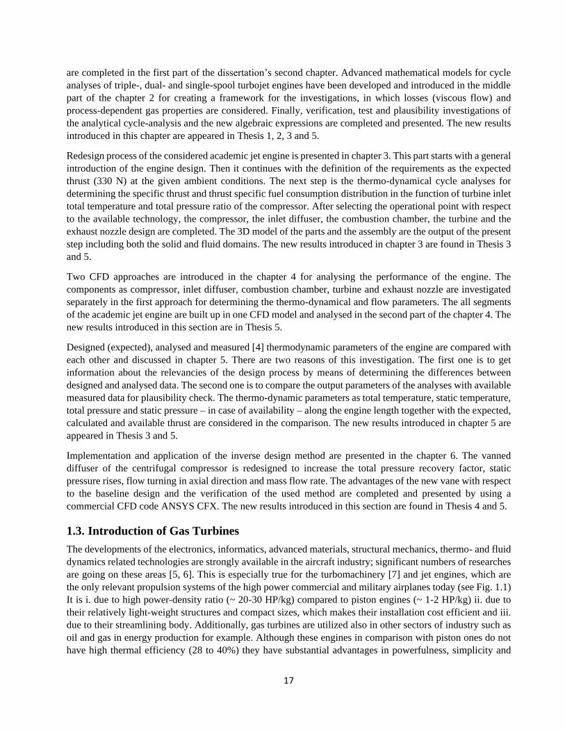
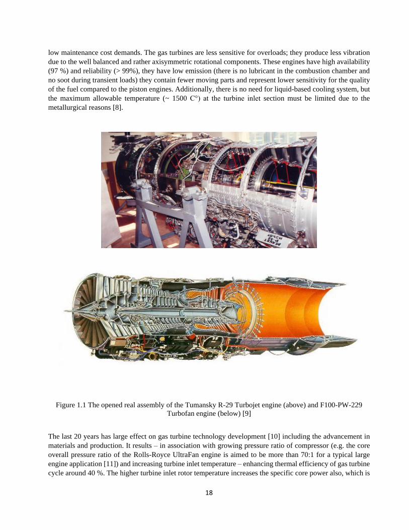
are going on these areas [5, 6]. This is especially true for the turbomachinery [7] and jet engines, which are

the only relevant propulsion systems of the high power commercial and military airplanes today (see Fig. 1.1)

It is i. due to high power-density ratio (~ 20-30 HP/kg) compared to piston engines (~ 1-2 HP/kg) ii. due to

their relatively light-weight structures and compact sizes, which makes their installation cost efficient and iii.

due to their streamlining body. Additionally, gas turbines are utilized also in other sectors of industry such as

oil and gas in energy production for example. Although these engines in comparison with piston ones do not

have high thermal efficiency (28 to 40%) they have substantial advantages in powerfulness, simplicity and

18

low maintenance cost demands. The gas turbines are less sensitive for overloads; they produce less vibration

due to the well balanced and rather axisymmetric rotational components. These engines have high availability

(97 %) and reliability (> 99%), they have low emission (there is no lubricant in the combustion chamber and

no soot during transient loads) they contain fewer moving parts and represent lower sensitivity for the quality

of the fuel compared to the piston engines. Additionally, there is no need for liquid-based cooling system, but

the maximum allowable temperature (~ 1500 C°) at the turbine inlet section must be limited due to the

metallurgical reasons [8].

Figure 1.1 The opened real assembly of the Tumansky R-29 Turbojet engine (above) and F100-PW-229

Turbofan engine (below) [9]

The last 20 years has large effect on gas turbine technology development [10] including the advancement in

materials and production. It results – in association with growing pressure ratio of compressor (e.g. the core

overall pressure ratio of the Rolls-Royce UltraFan engine is aimed to be more than 70:1 for a typical large

engine application [11]) and increasing turbine inlet temperature – enhancing thermal efficiency of gas turbine

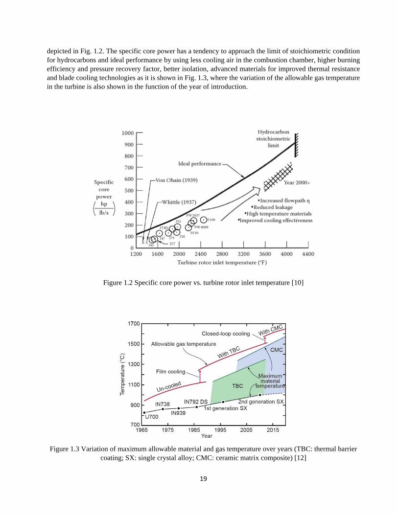
cycle around 40 %. The higher turbine inlet rotor temperature increases the specific core power also, which is

19

depicted in Fig. 1.2. The specific core power has a tendency to approach the limit of stoichiometric condition

for hydrocarbons and ideal performance by using less cooling air in the combustion chamber, higher burning

efficiency and pressure recovery factor, better isolation, advanced materials for improved thermal resistance

and blade cooling technologies as it is shown in Fig. 1.3, where the variation of the allowable gas temperature

in the turbine is also shown in the function of the year of introduction.

Figure 1.2 Specific core power vs. turbine rotor inlet temperature [10]

Figure 1.3 Variation of maximum allowable material and gas temperature over years (TBC: thermal barrier

coating; SX: single crystal alloy; CMC: ceramic matrix composite) [12]

20

The gas turbines are frequently used as aero engines. Beside high reliability and high performance, satisfying

operations all over the flight envelope are the key specification of their design. According to the expectation

for the gas turbines, the consideration of acceptable thrust/weight ratio is essential also.

It can be summarised that improved pressure ratio of compressor and the temperature of turbine beside

decreasing the losses and increasing the efficiencies are considered in the design and development processes

of the gas turbines to have the expected output performance together with increasing the thrust/weight ratio.

21

2. Mathematical Model Development for Thermo-Dynamic Cycle Analysis and

Optimization of Turbojet Engines

The extensive need and the wide-range application of gas turbines-based propulsion systems at different

configurations and operational conditions are observable today. It leads the manufacturers and experts to come

up with more and more effective ways of design and development by means of using several mathematical

models with the optimum form and choice of the most suitable methods. This approach, so called “virtual or

digital prototyping”, can significantly reduce design cost in the development processes. In order to response

to the arisen expectations, following the first chapter about general introduction, the aim of the present chapter

is to give overview about

i. the available thermo-dynamical models on analyses, design and optimisation of gas turbines with especial

care on jet engines by the scientific literature,

ii. derivation novel algebraic equation for

a. determining the critical pressure in choked flow condition at converging nozzle with considering

losses and process-dependent gas properties,

b. calculating the optimum total pressure ratio of the compressor pertaining at maximum thrust for

single spool turbojet engine at chocked and unchocked nozzle flow conditions with considering

losses and process-dependent gas properties,

iii. mathematical model development for thermo-dynamic cycle analysis of triple-, dual- and single-spool

turbojet engines with verification a. for the sake of the highest-level coverage in conjunction with different

types of engines, b. for having accurate model for the analyses and c. for having basic platform for

investigating the new equations and finally

iv. analysing, testing and verifying the new expression for optimum compressor total pressure ratio

introduced in point ii.

The governing equations of the advanced model developments for cycle analysis are the mass, energy balance

and thermo-dynamical process-equations with viscous flow assumption. The temperature and component mass

fraction dependent gas properties are calculated by iteration cycles in case of functional dependencies. Triple-

, dual- and single-spool jet engines, with the available structural and operational condition, are considered for

the model development and analyses in order to cover the widest range of the possible applications. The

unknown input parameters as efficiencies (mechanical, isentropic of fan, compressor and turbine units, burning

and exhaust nozzle), the pressure recovery rates (in the inlet diffuser, combustion chamber and afterburner or

turbine exhaust pipe), the power reduction rate of the auxiliary systems, the bleed air ratio for technological

reasons, the air income ratio due to blade cooling, the total pressure ratio of the intermediate pressure

compressor and fan, and the total temperature in the afterburner, if they are considered in the specific cases,

are determined by constraint nonlinear optimization. The goal function of the optimization is to minimize the

difference between the calculated and available thrust and thrust specific fuel consumption if they are given

in the datasheet of the engines found in [3].

2.1. Introduction

Beside the technical characteristics of the gas turbines today, still certain amounts of potentials are available

for improving their efficiencies, power and emissions. Although the experiences and the know-how of the gas

turbine manufacturers are increasing continuously, the suitable application of different mathematical models

and processes can significantly contribute to decrease the cost, time and capacity in the early phase of gas

22

turbine design and developments. Many scientific publications are subjected to the thermodynamic-based

simulation approaches, which confirm also the need for creating more accurate calculation methods.

Homaifar et al. [13] presented an application of genetic algorithms to the system optimization of turbofan

engines. The goal was to optimize the thrust per unit mass flow rate and overall efficiency in the function of

Mach number, compressor pressure ratio, fan pressure ratio and bypass ratio. Genetic algorithms were used in

this article because they were able to quickly optimize the objective functions involving sub functions of

multivariate. Although the model used here to represent a turbofan engine is a relatively simple one, the

procedure would be the same with a more elaborate model. Results of assorted runs fixed with experimental

and single parameter optimization results. Chocked condition was not considered, and the air and gas

properties were constant or averaged at the given sections of the engine based on the used reference.

Guha [14] determined the optimum fan pressure ratio for separate-stream as well as mixed-stream bypass

engines by both numerical and analytical ways. The optimum fan pressure ratio was shown to be

predominantly a function of the specific thrust and a weak function of the bypass ratio. The gas properties

were constant in the expression of optimum fan pressure ratio for separate-stream bypass engines at real flow

condition.

Silva and his co-workers [15] presented an evolutionary approach called the StudGA which is an optimization

design method. The purpose of their work was to optimize the performance of the gas turbine in terms of

minimizing fuel consumption at nominal thrust output, maximize the thrust at the same fuel consumption and

minimizing turbine blade temperature.

Al-Hamdan et.al [16] worked on the modelling and simulation of a gas turbine for power generation. A

computer program has been developed and introduced for the simulating gas turbine components by means of

satisfying the matching conditions between them analytically. The matching conditions can be analysed for

design and off-design operational modes. This research can also help in designing an efficient control system

for the gas turbine engine of an application including being a part of power generation plant.

Henriksson et.al [17] developed a model-based thrust estimation for turbofan engines. Two different model-

based thrust estimation filters were applied to a low bypass ratio turbofan engine. The two estimators were

based on a simple gross thrust model and on a thermodynamic semi-transient model, respectively. The filter

parameter estimation as well as the corresponding validation of parameters was based on the use of the “leave

one out cross validation” technique.

Turan [18] in 2012 investigated the design parameters on a small gas turbine by using the exergetic and

energetic approaches. These parameters included the pressure ratio of compressor and turbine inlet

temperature. The results demonstrated that with increasing the turbine inlet temperature is being accompanied

in decreasing exergy efficiency in the investigated operating range. On the other hand, increasing the pressure

ratio of compressor along with increase in flight Mach number resulted in an increasing exergy efficiency of

the engine. It was declared that studying the effect of investigated parameters indicates how much

improvement is possible for the small turbojet engine to achieve better energy and exergy consumption.

Khaliq et.al [19] presented a thermodynamic methodology for performance evaluation of combustion gas

turbine cogeneration system with reheat. The effects of process steam pressure and pinch point temperature

used in the design of heat recovery steam generator and reheat on energetic and exergetic efficiencies have

been investigated. Based on the results, the present method is useful in selection and comparison of combined

energy production systems from thermodynamic performance point of view.

23

Sanjay [20] investigated the effect of variation of thermodynamic cycle parameters on rational efficiency and

component-wise non-dimensionalized exergy destruction of a basic gas turbine-based gas-steam combined

cycle. It was shown that the rational efficiency is higher in case of higher turbine inlet temperature. The sum

of exergy destruction of all components of the combined cycle plant was lower at higher value of compressor

pressure ratio. Also, exergy destruction was minimized with the adoption of multi-pressure-reheat steam

generator configuration.

Atashkari et.al [21] applied multi-objective genetic algorithms for Pareto approach optimization of

thermodynamic cycle of ideal turbojet engines. A new diversity preserving algorithm was proposed to enhance

the performance of multi-objective evolutionary algorithms with more than two objective functions. Beside

the advancement of the new algorithm, it was shown that some interesting and important relationships among

optimal objective functions and decision variables involved in the thermodynamic cycle of turbojet engines

can be discovered consequently. It was also demonstrated that the results of four-objective optimization can

include those of two-objective optimization and, therefore, provide more choices for optimal design of

thermodynamic cycle of ideal turbojet engines.

In 2001 Lazzaretto et.al [22] presented a model for gas turbine design and off-design. The problem due to the

missing information about stage-by-stage performance were overcome by constructing artificial machine maps

through appropriate scaling techniques applied to generalized maps taken from the literature and validating

them with test measurement data from real plants. The results of the simulations were used for neural network

training: problems associated with the construction and use of neural networks was discussed and their

capability as a tool for predicting machine performance was analysed.

Mattingly [23] published a detailed theoretical review about the rocket and gas turbine propulsion. There is a

description also in that literature how the thermo-dynamical cycles determine the mean characteristic of the

jet engines. The author presented a closed-form equation for the optimum compressor pressure ratio at

maximum specific thrust at ideal (inviscid) flow condition. The effects of temperature and fuel to air ratio

were not considered in parameters describe the gas properties.

As the above-mentioned scientific literatures use simplifications e.g.: - where it is relevant - excluding the

effect of chocked, real (viscous) flow condition at converging nozzle and some of them consider gas properties

without applying local temperature and fuel to air ratio, it also confirms the need for developing physically

advanced, more accurate mathematical models, calculations, equations and optimizations.

2.2. Novel Closed-Form Expression for Critical Pressure and Optimum Pressure Ratios

of Turbojet Engines

New equations have been introduced in the present subchapter for the optimum pressure ratio pertaining at

maximum specific thrust for single spool turbojet engine

i. for unchoked and

ii. for the chocked flow conditions.

A novel equation is also derived for the last item (ii.) in order to consider critical pressure for converging

nozzle flow. Closed-form expression means that the unknown parameter is calculated by an analytical equation

directly/explicitly. The optimum pressure ratio and the maximum possible thrust can be calculated by these

equations for turbojet engines immediately, easily and short without using complex, rather long mathematical

calculations.

24

The expressions apply the real (viscous) flow assumptions and the temperature and mass fraction dependencies

of the relevant gas properties.

The derivation of the optimum pressure ratio at thermodynamic conditions with losses and variable gas

properties is based on finding the extreme value of the specific thrust in the function of the compressor pressure

ratio. Hence, as the first step, the expression of the thrust is introduced in Eq. (2.1) [24].

𝑇 = [��9𝑉9 − ��𝑎𝑖𝑟𝑉0] + 𝐴9(𝑝9 − 𝑝0) (2.1)

The mass flow rate at the exhaust nozzle is determined by (2.2) [25].

��9 = ��𝑎𝑖𝑟[(1 − 𝛿𝑡𝑒𝑐ℎ)(1 + 𝑓𝑐𝑐 + 𝑓𝐴)(1 + 𝛿𝑏𝑐)] (2.2)

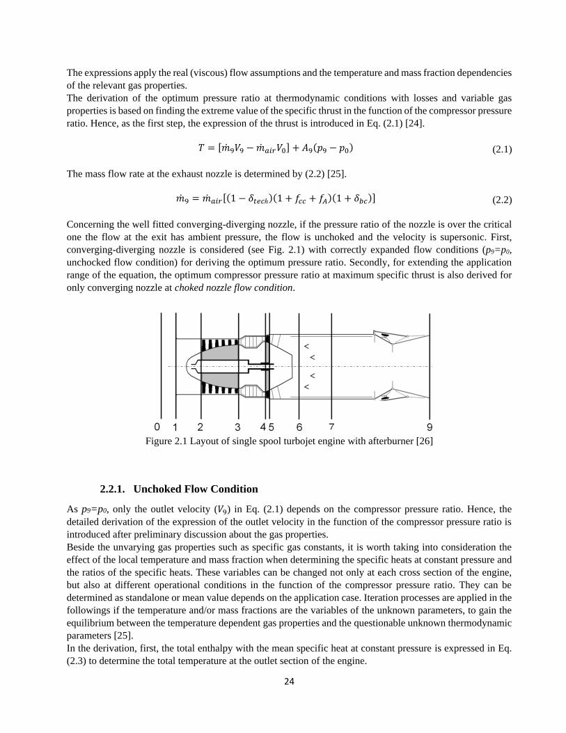
Concerning the well fitted converging-diverging nozzle, if the pressure ratio of the nozzle is over the critical

one the flow at the exit has ambient pressure, the flow is unchoked and the velocity is supersonic. First,

converging-diverging nozzle is considered (see Fig. 2.1) with correctly expanded flow conditions (p9=p0,

unchocked flow condition) for deriving the optimum pressure ratio. Secondly, for extending the application

range of the equation, the optimum compressor pressure ratio at maximum specific thrust is also derived for

only converging nozzle at choked nozzle flow condition.

Figure 2.1 Layout of single spool turbojet engine with afterburner [26]

2.2.1. Unchoked Flow Condition

As p9=p0, only the outlet velocity (𝑉9) in Eq. (2.1) depends on the compressor pressure ratio. Hence, the

detailed derivation of the expression of the outlet velocity in the function of the compressor pressure ratio is

introduced after preliminary discussion about the gas properties.

Beside the unvarying gas properties such as specific gas constants, it is worth taking into consideration the

effect of the local temperature and mass fraction when determining the specific heats at constant pressure and

the ratios of the specific heats. These variables can be changed not only at each cross section of the engine,

but also at different operational conditions in the function of the compressor pressure ratio. They can be

determined as standalone or mean value depends on the application case. Iteration processes are applied in the

followings if the temperature and/or mass fractions are the variables of the unknown parameters, to gain the

equilibrium between the temperature dependent gas properties and the questionable unknown thermodynamic

parameters [25].

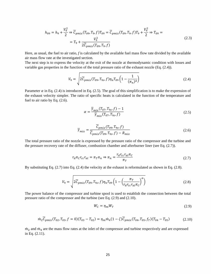
In the derivation, first, the total enthalpy with the mean specific heat at constant pressure is expressed in Eq.

(2.3) to determine the total temperature at the outlet section of the engine.

25

ℎ09 = ℎ9 +𝑉92

2⇒ 𝐶𝑝𝑚𝑖𝑥(𝑇09, 𝑇9, 𝑓)𝑇09 = 𝐶𝑝𝑚𝑖𝑥(𝑇09, 𝑇9, 𝑓)𝑇9 +

𝑉92

2⇒ 𝑇09 =

= 𝑇9 +𝑉92

2𝐶𝑝𝑚𝑖𝑥(𝑇09, 𝑇9, 𝑓)

(2.3)

Here, as usual, the fuel to air ratio, f is calculated by the available fuel mass flow rate divided by the available

air mass flow rate at the investigated section.

The next step is to express the velocity at the exit of the nozzle at thermodynamic condition with losses and

variable gas properties in the function of the total pressure ratio of the exhaust nozzle (Eq. (2.4)).

𝑉9 = √2𝐶𝑝𝑚𝑖𝑥(𝑇09, 𝑇9𝑠, 𝑓)휂𝑛𝑇09 (1 −1

(𝜋𝑛)𝛼) (2.4)

Parameter 𝛼 in Eq. (2.4) is introduced in Eq. (2.5). The goal of this simplification is to make the expression of

the exhaust velocity simpler. The ratio of specific heats is calculated in the function of the temperature and

fuel to air ratio by Eq. (2.6).

𝛼 =𝛾𝑚𝑖𝑥(𝑇07, 𝑇9𝑠 , 𝑓) − 1

𝛾𝑚𝑖𝑥(𝑇07, 𝑇9𝑠 , 𝑓) (2.5)

𝛾𝑚𝑖𝑥 =𝐶𝑝𝑚𝑖𝑥(𝑇09, 𝑇9𝑠 , 𝑓)

𝐶𝑝𝑚𝑖𝑥(𝑇09, 𝑇9𝑠 , 𝑓) − 𝑅𝑚𝑖𝑥 (2.6)

The total pressure ratio of the nozzle is expressed by the pressure ratio of the compressor and the turbine and

the pressure recovery rate of the diffuser, combustion chamber and afterburner liner (see Eq. (2.7)).

𝑟𝑑𝜋𝐶𝑟𝑐𝑐𝑟𝑎𝑙 = 𝜋𝑇𝜋𝑛 ⇒ 𝜋𝑛 =𝑟𝑑𝑟𝑐𝑐𝑟𝑎𝑙𝜋𝐶

𝜋𝑇 (2.7)

By substituting Eq. (2.7) into Eq. (2.4) the velocity at the exhaust is reformulated as shown in Eq. (2.8).

𝑉9 = √2𝐶𝑝𝑚𝑖𝑥(𝑇09, 𝑇9𝑠 , 𝑓)휂𝑛𝑇09 (1 − (𝜋𝑇

𝑟𝑑𝑟𝑐𝑐𝑟𝑎𝑙𝜋𝐶)𝛼

) (2.8)

The power balance of the compressor and turbine spool is used to establish the connection between the total

pressure ratio of the compressor and the turbine (see Eq. (2.9) and (2.10).

𝑊𝐶 = 휂𝑚𝑊𝑇 (2.9)

��2𝐶𝑝𝑚𝑖𝑥(𝑇02, 𝑇03, 𝑓 = 0)(𝑇03 − 𝑇02) = 휂𝑚��4(1 − 휁)𝐶𝑝𝑚𝑖𝑥(𝑇04, 𝑇05, 𝑓𝑇)(𝑇04 − 𝑇05) (2.10)

��2 and ��4 are the mass flow rates at the inlet of the compressor and turbine respectively and are expressed

in Eq. (2.11).

26

��2 = ��𝑎𝑖𝑟, ��4 = ��𝑎𝑖𝑟[(1 − 𝛿𝑡𝑒𝑐ℎ)(1 + 𝑓𝑐𝑐)(1 + 𝛿𝑏𝑐)] (2.11)

Eq. (2.12) is formed by replacing the mass flow rates in Eq. (2.10) by Eq. (2.11) and introducing isentropic

efficiencies and isentropic relationship between the temperatures and pressures.

1

휂𝐶,𝑠𝐶𝑝𝑚𝑖𝑥(𝑇02, 𝑇03, 𝑓 = 0)𝑇02((𝜋𝐶)

𝛽 − 1) =

=휂𝑚휂𝑇,𝑠(1 − 𝛿𝑡𝑒𝑐ℎ)(1 + 𝛿𝑏𝑐)(1 + 𝑓𝑐𝑐)(1 − 𝜉)𝐶𝑝𝑚𝑖𝑥(𝑇04, 𝑇05, 𝑓𝑇)𝑇04 (1 −1

(𝜋𝑇)𝜀)

(2.12)

𝛽 and 휀 in the superscripts represent compact forms of the exponents for the isentropic processes in the

compressor and the turbine respectively (see Eq. (2.13)). They are the function of the temperature and the local

mass fraction of the air and burnt gases.

𝛽 =𝛾𝑚𝑖𝑥(𝑇02,𝑇03𝑠,𝑓=0)−1

𝛾𝑚𝑖𝑥(𝑇02,𝑇03𝑠,𝑓=0), 휀 =

𝛾𝑚𝑖𝑥(𝑇04,𝑇05𝑠,𝑓𝑇)−1

𝛾𝑚𝑖𝑥(𝑇04,𝑇05𝑠,𝑓𝑇) (2.13)

Parameter 𝜙 is introduced to include all the parameters in Eq. (2.12) except for 휀, 𝜋𝑇, 𝜋𝐶 and 𝛽 and it is shown

in Eq. (2.14).

𝜙 =𝐶𝑝𝑚𝑖𝑥(𝑇02𝑇03, 𝑓 = 0)

𝐶𝑝𝑚𝑖𝑥(𝑇04𝑇03, 𝑓𝑐𝑐)

𝑇02𝑇04

1

휂𝑚휂𝐶,𝑠휂𝑇,𝑠(1 − 𝛿𝑡𝑒𝑐ℎ)(1 + 𝛿𝑏𝑐)(1 + 𝑓𝑐𝑐)(1 − 𝜉) (2.14)

Eq. (2.15) is formed by rearranging Eq. (2.12) and expressing the total pressure ratio of the turbine.

𝜋𝑇 = (1 − 𝜙((𝜋𝐶)𝛽 − 1))

(−1⁄ ) (2.15)

The velocity at the exhaust of the nozzle (see Eq. (2.16)) is derived by substituting Eq. (2.15) into Eq. (2.8).

𝑉9 = √2𝐶𝑝𝑚𝑖𝑥(𝑇09, 𝑇9𝑠 , 𝑓)휂𝑛𝑇09 [1 − (1

(1 − 𝜙((𝜋𝐶)𝛽 − 1))

1

𝜋𝐶𝜅

)

𝛼

] (2.16)

κ in Eq. (2.16) represents the multiplication of the pressure recovery rates in the diffuser, in the combustion

chamber and in the afterburner liner (𝜅 = 𝑟𝑑𝑟𝑐𝑐𝑟𝑎𝑙).

Finally, the specific thrust (Eq. (2.17)) is expressed by inserting Eq. (2.16) into Eq. (2.1) at the start and at

unchoked nozzle flow condition.

𝑇

��𝑎𝑖𝑟= [(1 − 𝛿𝑡𝑒𝑐ℎ)(1 + 𝑓𝑐𝑐 + 𝑓𝐴)(1

+ 𝛿𝑏𝑐)]√2𝐶𝑝𝑚𝑖𝑥(𝑇09, 𝑇9𝑠 , 𝑓)휂𝑛𝑇09 [1 − (1

(1 − 𝜙((𝜋𝐶)𝛽 − 1))

1

𝜋𝐶𝜅

)

𝛼

] (2.17)

The objective of the optimization process is to determine the optimum pressure ratio of the compressor, which

pertains at maximum specific thrust. The reason of considering the specific thrust (thrust per unit mass flow

rate of air) is to exclude the effect of compressor pressure ratio on the mass flow rate of air. The condition for

the maximum specific thrust is shown by Eq. (2.18).

27

𝜕 (𝑇

��𝑎𝑖𝑟)

𝜕𝜋𝐶= 0 (2.18)

Two sub steps of the derivation process are shown in the next two equations.

𝜕 (𝑇

��𝑎𝑖𝑟)

𝜕𝜋𝐶

= −1

2

[(1 − 𝛿𝑡𝑒𝑐ℎ)(1 + 𝑓𝑐𝑐 + 𝑓𝐴)(1 + 𝛿𝑏𝑐)] [1

(1 − 𝜙((𝜋𝐶)𝛽 − 1))

1

𝜋𝐶

]

𝛼

⋅

⋅ 𝛼

[

𝜑(𝜋𝐶)𝛽𝛽

(1 − 𝜑(((𝜋𝐶)𝛽 − 1)))

1

(𝜋𝐶)2휀 (1 − 𝜑(((𝜋𝐶)

𝛽 − 1)))

−1

(1 − 𝜑((𝜋𝐶)𝛽 − 1))

1

(𝜋𝐶)2 ]

(1 − 𝜑((𝜋𝐶)𝛽 − 1))

1

(𝜋𝐶)

√1 − [1

(1 − 𝜑((𝜋𝐶)𝛽 − 1))

1

(𝜋𝐶)

]

𝛼

(2.19)

𝜕 (𝑇

��𝑎𝑖𝑟)

𝜕𝜋𝐶=

=1

2

[(1 − 𝛿𝑡𝑒𝑐ℎ)(1 + 𝑓𝑐𝑐 + 𝑓𝐴)(1 + 𝛿𝑏𝑐)] [(1 − 𝜑(𝜋𝐶)

𝛽 + 𝜑)−1

(𝜋𝐶)]

𝛼

𝛼(𝜑(𝜋𝐶)𝛽𝛽 − 휀 + εφ(𝜋𝐶)

𝛽 − εφ)

(𝜋𝐶)√1 − [(1 − 𝜑(𝜋𝐶)

𝛽 + 𝜑)−1

(𝜋𝐶)]

𝛼

휀(−1 + 𝜑(𝜋𝐶)𝛽 − 𝜑)

(2.2

0)

After completing the derivation and performing arrangements and simplifications, the final form of the

optimum pressure ratio is presented in Eq. (2.21).

𝜋𝐶_𝑜𝑝𝑡 = √휀(1 + 𝜙)

𝜙(휀 + 𝛽)

𝛽

(2.21)

2.2.2. Choked Flow Condition at Converging Exhaust Nozzle

Although converging-diverging nozzle is used for single spool turbojet engines (e.g. РД-9Б and АЛ-21Ф3)

designed for high flight speed (over Mach number 1), as it is shown in Fig. 2.1, the extension of the method is

discussed in the present section for increasing the application range of the method for converging type nozzle

at choked flow condition.

28

A similar procedure is applied to evaluate the optimum pressure ratio of the compressor in a choked condition

as it was in the previous subchapter. The velocity at the exit of the converging nozzle is the speed of sound

when it is in a choked condition and it is not a function of the compressor pressure ratio explicitly. However,

beside the exhaust velocity, the exhaust pressure also contributes to generating thrust (see p9 in Eq. (2.1). This

pressure is the critical pressure and can also be expressed in the function of the compressor pressure ratio as it

is shown below. The total pressures at the inlet and at the outlet section of the turbine are calculated by Eq.

(2.22) and (2.23) respectively.

𝑝04 = 𝑟𝑐𝑐𝜋𝐶𝑝02 (2.22)

𝑝05 =𝑝04𝜋𝑇

=𝑟𝑐𝑐𝜋𝐶𝑝02

(1 − 𝜙((𝜋𝐶)𝛽 − 1))

−1

(2.23)

The total pressure at the inlet section of the nozzle (see Eq. (2.24)) is determined by the turbine outlet total

pressure and the total pressure recovery rate of the afterburner liner.

𝑝07 = 𝑟𝑎𝑙𝑝05 =𝑟𝑐𝑐𝑟𝑎𝑙𝜋𝐶𝑝02

(1 − 𝜙((𝜋𝐶)𝛽 − 1))

−1

(2.24)

The total enthalpy and subsequently the total temperature at section “9” is introduced in the next steps (see

Eq. (2.25) and (2.26).

ℎ09 = ℎ9 +𝑉92

2→ 𝐶𝑝𝑚𝑖𝑥(𝑇09, 𝑇9, 𝑓)𝑇09 = 𝐶𝑝𝑚𝑖𝑥(𝑇09, 𝑇9, 𝑓)𝑇9 +

𝑉92

2→ 𝑇09 =

= 𝑇9 +𝑉92

2𝐶𝑝𝑚𝑖𝑥(𝑇09, 𝑇9, 𝑓)

(2.25)

𝑇09 = 𝑇9 +1

𝐶𝑝𝑚𝑖𝑥(𝑇09, 𝑇9, 𝑓)

𝑉92

2

𝑎92

𝑎92 ⇒ 𝑇09 = 𝑇9 +

1

𝐶𝑝𝑚𝑖𝑥(𝑇09, 𝑇9, 𝑓)𝑀92𝛾𝑚𝑖𝑥(𝑇9, 𝑓)𝑅𝑚𝑖𝑥𝑇9

2 (2.26)

The critical condition corresponds to M9=1 and T9=TC, so Eq. (2.26) is reformulated accordingly. The

isentropic static temperature at point “9” is expressed by the equation of isentropic nozzle efficiency and it is

given by Eq. (2.27).

𝑇9𝑠 = 𝑇09 −1

휂𝑛

(𝑇09 − 𝑇𝑐)𝐶𝑝𝑚𝑖𝑥(𝑇09,𝑇𝑐 , 𝑓)

𝐶𝑝𝑚𝑖𝑥(𝑇09,𝑇9𝑠 , 𝑓) (2.27)

The thermodynamic process between point “7” and “9s” is isentropic (see Eq. (2.28)).

𝑝𝑐𝑝07

= (𝑇9𝑠𝑇09

)

𝛾𝑚𝑖𝑥(𝑇09,𝑇9𝑠,𝑓)

𝛾𝑚𝑖𝑥(𝑇09,𝑇9𝑠,𝑓)−1 (2.28)

A new closed-form expression (Eq. (2.29)) is introduced to determine the critical pressure at the exit of the

converging nozzle after substituting the isentropic static temperature in Eq. (2.27), and the total temperature

at nozzle exit in Eq. (2.26) into Eq. (2.28). Here, the dependencies of the temperature variations and fuel to air

ratios in the specific heats at constant pressure and so in the ratios of the specific heats are also considered.

While the critical static pressure at the outlet section of the exhaust system is coupled with the total and static

exit temperatures, iteration cycles are used to determine the unknown thermodynamic parameters. Eq. (2.29)

29

gives higher critical pressure by 9.3 % for the РД-9Б engine than its original form (see Eq. 2.59) with constant

gas data according to the theory of ideal gases (the ratio of specific heats for gas=1.33).

𝑝9 = 𝑝𝑐 = 𝑝07 [1

−1

휂𝑛(1

−2𝐶𝑝𝑚𝑖𝑥(𝑇09,𝑇𝑐 , 𝑓)

2𝐶𝑝𝑚𝑖𝑥(𝑇09,𝑇𝑐 , 𝑓) + 𝛾𝑚𝑖𝑥(𝑇𝑐 , 𝑓)𝑅𝑚𝑖𝑥)𝐶𝑝𝑚𝑖𝑥(𝑇09,𝑇𝑐 , 𝑓)

2𝐶𝑝𝑚𝑖𝑥(𝑇09,𝑇𝑐 , 𝑓)]

𝛾𝑚𝑖𝑥(𝑇09,𝑇9𝑠,𝑓)

𝛾𝑚𝑖𝑥(𝑇09,𝑇9𝑠,𝑓)−1

(2.29)

By substituting Eq. (2.24) in Eq. (2.29) and Eq. (2.29) in Eq. (2.1) the thrust can be expressed as follow:

𝑇 = [��9𝑉9 − ��𝑎𝑖𝑟𝑉0] +

+𝐴9

[

(

𝑝02(𝑟𝑐𝑐𝑟𝑎𝑙𝜋𝐶) (1 − 𝜙((𝜋𝐶)𝛽 − 1))

1

𝜀⋅

⋅ [1 −1

𝜂𝑛(1 −

2𝐶𝑝𝑚𝑖𝑥(𝑇09,𝑇𝑐,𝑓)

2𝐶𝑝𝑚𝑖𝑥(𝑇09,𝑇𝑐,𝑓)+𝛾𝑚𝑖𝑥(𝑇𝑐,𝑓)𝑅𝑚𝑖𝑥)𝐶𝑝𝑚𝑖𝑥(𝑇09,𝑇𝑐,𝑓)

2𝐶𝑝𝑚𝑖𝑥(𝑇09,𝑇𝑐,𝑓)]

𝛾𝑚𝑖𝑥(𝑇09,𝑇9𝑠,𝑓)

𝛾𝑚𝑖𝑥(𝑇09,𝑇9𝑠,𝑓)−1

)

− 𝑝0

]

(2.30)

The determination of the optimum pressure ratio pertaining at maximum thrust in choked converging nozzle

flow conditions begins by completing the derivation presented in Eq. (2.31) and continues with simplifications

shown in Eq. (2.32).

𝜕𝑇

𝜕𝜋𝐶= ((1 − 𝜙(𝜋𝐶)

𝛽 + 𝜙)1

−(1 − 𝜙(𝜋𝐶)

𝛽 + 𝜙)1

𝜙(𝜋𝐶)𝛽𝛽

휀(1 − 𝜙(𝜋𝐶)𝛽 + 𝜙)

) (2.31)

𝜕𝑇

𝜕𝜋𝐶= (

(1 − 𝜙(𝜋𝐶)𝛽 + 𝜙)

1

휀 − (1 − 𝜙(𝜋𝐶)𝛽 + 𝜙)

−−1+

𝜙(𝜋𝐶)𝛽𝛽

휀) (2.32)

Completing the arrangements and simplifications, the final form of the expression for the optimum compressor

total pressure ratio is given by Eq. (2.33).

𝜋𝐶_𝑜𝑝𝑡 = √휀(1 + 𝜙)

𝜙(휀 + 𝛽)

𝛽

(2.33)

Based on Eq. (2.21) and (2.33) the optimum pressure ratios for the convergent-divergent nozzle at correctly

expanded flow conditions (p9=p0 and no shock waves form) and only convergent nozzle at choked flow

conditions are the same. This new closed-form explicit expression involves simplifications, because the gas

properties and unknown variables – including specific heats, efficiencies, pressure recovery rates – and the

incoming mass flow rate of air in case of choked converging nozzle are constant in the derivation process. Due

to the proximity to the operational point, the presented approximation used the same recovery rates,

efficiencies, power reduction rate of the auxiliary systems, bleed air ratio and air income ratio due to the blade

cooling. Concerning these simplifications, further investigations are needed to determine their effects on the

optimum total pressure ratio.

30

Test, verification and the plausibility check of the above-mentioned new equations are found in subchapter

2.4. after subchapter 2.3, which is dedicated for introducing advanced thermo-dynamical model developments

and verifications for triple-, dual- and single-spool turbojet engines due to the widest technical coverage and

relevancies.

2.3. Modell Development for Thermo-Dynamic Cycle Analysis of Turbojet Engines with

Verification and Plausibility Check

Thermodynamic model-development with testing, applications and verifications are introduced in the present

subchapter for triple-, dual- and single-spool turbojet engines for the sake of the highest-level complexity with

respect to the engine configuration. The most complex engine type is the triple-spool one, so it is considered

only in the detailed model developments and description, meanwhile the governing equations for the dual- and

single-spool turbojet engines can easily be deduced from them with considering less power balance equations

according to the available pool number and without by-pass, if it is the case. The calculation approach, the

processes and the determination of the gas parameters are the same in the all three versions.

2.3.1. Triple-Spool Mixed Turbofan Jet Engine

The triple-spool turbofan jet engines are frequently used in commercial and military applications due to their

outstanding normalized range factor and emission at relatively high flight Mach number and at wide

operational range. НК-32 (see Fig. 2.2) and НК-25 mixed turbo jet engines are considered in mathematical

model-development for thermodynamic cycle analysis to test and verify the results first. The Kuznetsov НК-

32 is an afterburning triple-spool low bypass mixed turbofan jet engine, which powers the Tupolev Tu-160

supersonic bomber, and was fitted to the later model Tupolev Tu-144LL supersonic transporter. It is the largest

and most powerful engine ever fitted on a combat aircraft. It produces 245 kN of thrust in maximum

afterburner [27]. The Kuznetsov НК-25 is a turbofan mixed aircraft engine used in the Tupolev Tu-22M

strategic bomber. It can equal the НК-321 engine as one of the most powerful supersonic engines in service

today. It is rated at 245 kN thrust. It was superior to many other engines because of its improved fuel

consumption [28].

Figure 2.2 НК-32 afterburning triple-spool low bypass mixed turbofan jet engine [29]

31

Introduction, general remarks, considerations, derivation of the advanced mathematical model of triple-spool

turbofan jet engine is found in next parts below.

Introduction and General Considerations

Take-off (start) condition (maximum thrust at sea level) with M = 0 is considered in most of the investigated

cases as data belong to that operational mode are available in the technical specification of the engines.

The ambient parameters of pressure and temperature at static sea level conditions are obtained from the ISA

(International Standard Atmosphere) [30]:

- Ambient static pressure: =101325 Pa

- Ambient static temperature: = 288.15 K

A layout with the considered cross sections of a typical triple-spool mixed turbofan jet engine with afterburner

is shown in Fig. 2.3.

The operation of the engine is the following. The ambient air enters the engine at section 1. The operational

fluid suffers from pressure drop in the inlet diffuser, which is between port 1 and 2. The compressed air is

generated from cross section 2 to 3 in the internal (core) section. The compressor unit consists of three main

segments as low, medium and high-pressure components. The low-pressure compressor unit operates as fan

module also and the by-passed air leaves the downstream section of the last fan stage is not directly exhausted,

but it flows in a duct around the engine core and it is mixed with the hot gases leaving the turbine at section 6.

The combustion chamber is located between port 3 and 4 in the internal section, where the heat is generated

by adding fuel to the compressed air and burn develops at reaching activation temperature. The flow stream

with high total enthalpy expands and provides energy to the high, medium and low-pressure turbines in the

internal section, which is transmitted to spool of the high and medium compressor segments and to the fan

respectively. The afterburner for elevating thrust is located between section 6 and 7. The exhaust gases with

unburned oxygen leave the engine across the nozzle (7-9) with losses for producing thrust.

Figure 2.3 Layout of the mixed triple-spool turbofan jet engine with afterburner [26]

32

Regarding the present investigations, real engine specifications are considered for plausibility analysis.

However, based on the available literature [3], there are known and unknown data which can be distinguished.

The known parameters are the incoming air mass flow rate, pressure ratio of the compressor, turbine inlet total

temperature and the length and the diameter of the engine. Except for the last two, these are also considered

as input parameters of the analyses. The unknown parameters are; efficiencies (mechanical, isentropic of

compressor and turbine, burning and exhaust nozzle), losses (total pressure recovery factor of inlet diffuser,

combustion chamber and afterburner or turbine exhaust pipe), power reduction rates of the auxiliary systems,

total pressure ratio of the fan and intermediate pressure compressor, bleed air ratios for technological reasons,

air income ratios due to blade cooling and total temperature at the afterburner. In order to determine these

unknown parameters, constrained nonlinear optimization method is applied with the goal function to minimize

the deviations between the calculated and given thrust and thrust specific fuel consumption.

Beside the unvarying material properties, such as specific gas constants, it is important to take the local

temperature and mass fraction conditions into consideration in determining gas properties, such as, the specific

heat at constant pressure and the ratio of the specific heats. These variables can be changed not only at each

cross section of the engine, but also at different operational conditions belonging to different compressor

pressure ratios. Eq. (2.34) and (2.36) shows the expressions how they are determined as the mean value through

the considered process. Eq. (2.35) and (2.37) presents their standalone value at given temperature and fuel to

air mass flow rates ratio. Iteration processes are applied if the temperature and/or fuel to air ratio is the variable

of the unknown parameter to gain the balance between the temperature and mass fraction dependent material

properties and the determined unknown thermo-dynamical parameter. The block diagram of such type of

iteration process is depicted in Fig. 2.4 for determining the isentropic and real temperatures caused by the

compression process.

𝐶��𝑚𝑖𝑥(𝑇𝑖 , 𝑇𝑖+1, 𝑓) =

1000∑𝑎𝑗 + 𝑓𝑐𝑗

(𝑗 + 1)(𝑓 + 1)[(𝑇𝑖+11000

)𝑗+1

− (𝑇𝑖

1000)𝑗+1

]𝑛𝑗=0

𝑇𝑖+1 − 𝑇𝑖

(2.34)

𝐶𝑝𝑚𝑖𝑥(𝑇, 𝑓) =∑𝑎𝑗 + 𝑓𝑐𝑗

𝑓 + 1(

𝑇

1000)𝑗𝑛

𝑗=0

(2.35)

��𝑚𝑖𝑥 =𝐶��𝑚𝑖𝑥(𝑇𝑖 , 𝑇𝑖+1, 𝑓)

𝐶��𝑚𝑖𝑥(𝑇𝑖 , 𝑇𝑖+1, 𝑓) − 𝑅𝑚𝑖𝑥 (2.36)

𝛾𝑚𝑖𝑥 =𝐶𝑝𝑚𝑖𝑥(𝑇, 𝑓)

𝐶𝑝𝑚𝑖𝑥(𝑇, 𝑓) − 𝑅𝑚𝑖𝑥 (2.37)

The polynomial constants for air and kerosene fuel are 𝑎𝑗 and 𝑐𝑗 according to [1]. The values of the polynomial

constants for the used gases are shown in Table 2.1.

33

Figure 2.4 Iteration cycle including mean specific heat at constant pressure for determining outlet

temperature (i=initial, f=final) at real and adiabatic compression process between stage 1 and 2 (the 𝜅 in the

flow chart is 𝛾 and * means total quantities) [31]

Table 2.1 Polynomial constants used for computing the material properties of gases [1]

𝑎𝑗 Value 𝑐𝑗 Value

𝑎0 1043.797 𝑐0 614.786

𝑎1 -330.6087 𝑐1 6787.993

𝑎2 666.7593 𝑐2 -10128.91

𝑎3 233.4525 𝑐3 9375.566

𝑎4 -1055.395 𝑐4 -4010.937

𝑎5 819.7499 𝑐5 257.6096

𝑎6 -270.54 𝑐6 310.53

𝑎7 33.60668 𝑐7 -67.426468

Mathematical Model of Triple-Spool Mixed Turbofan Engines

The used physical and mathematical approaches and models have been derived and introduced in the present

subchapter.

Regarding to most general aspects, the first step of the analysis is to determine the total temperature and

pressure at the inlet with using static ambient temperature, pressure and flight Mach number by using Eq.

(2.38) and (2.39) [24].

𝑇02 = 𝑇01 = 𝑇00 = 𝑇0(1 +𝛾 − 1

2𝑀2) (2.38)

𝑝01 = 𝑝00 = 𝑝0(1 +𝛾 − 1

2𝑀2)

𝛾𝛾−1 (2.39)

The goal of the favourable intake design is to minimize flow losses by appropriate inlet duct and nose shaping

to enable a pressure recovery factor close to unity. Due to friction of the airflow in contact with the intake wall

and the occasional separation, a loss in total pressure will always be present.

34

The total pressure at fan (or compressor) intake is determined by the total pressure recovery factor of the

intake:

𝑝02 = 𝑝01𝑟𝑑 (2.40)

The total pressure and temperature at the outlet of the fan is expressed as follow:

𝑝02.1 = 𝑝02𝜋𝑓 (2.41)

𝑇02.1 = 𝑇02 +𝐶��𝑚𝑖𝑥(𝑇02, 𝑇02.1𝑠, 𝑓 = 0)(𝑇02.1𝑠 − 𝑇02)

𝐶��𝑚𝑖𝑥(𝑇02, 𝑇02.1, 𝑓 = 0)휂𝑓,𝑠 (2.42)

Similarly, the total pressure and temperature at the outlet of intermediate (medium) pressure compressor is

determined by the next equations:

𝑝02.3 = 𝑝02.1𝜋𝑖𝑝,𝐶 (2.43)

𝑇02.3 = 𝑇02.1 +𝐶��𝑚𝑖𝑥(𝑇02.1, 𝑇02.3𝑠, 𝑓 = 0)(𝑇02.3𝑠 − 𝑇02.1)

𝐶��𝑚𝑖𝑥(𝑇02.1, 𝑇02.3, 𝑓 = 0)휂𝑖𝑝,𝐶,𝑠 (2.44)

The total pressure ratio of the high-pressure compressor is calculated by Eq. (2.45) considering that the overall

total pressure ratio of the compressor and the total pressure ratio of the fan and intermediate compressor is

given.

𝜋ℎ𝑝,𝐶 =𝜋𝑐

𝜋𝑓𝜋𝑖𝑝,𝐶 (2.45)

The total pressure at the outlet of the high-pressure compressor is calculated by the previously determined

total pressure ratio of the high-pressure compressor as follows:

𝑝03 = 𝜋ℎ𝑝,𝐶𝑝02.3 (2.46)

The total temperature at the outlet of the high-pressure compressor is computed by using the isentropic

efficiency of the high-pressure compressor (see Eq. (2.47)). Iteration cycle is used at this stage also, as it is in

the case of low and intermediate pressure compressor units, due to the fact that the specific heat at constant

pressure depends on the total temperature.

𝑇03 = 𝑇02.3 +𝐶��𝑚𝑖𝑥(𝑇02.3, 𝑇03𝑠 , 𝑓 = 0)(𝑇03𝑠 − 𝑇02.3)

𝐶��𝑚𝑖𝑥(𝑇02.3, 𝑇03, 𝑓 = 0)휂ℎ𝑝,𝐶,𝑠 (2.47)

Total pressure recovery factor has been considered because of viscous flow modelling to determine the total

pressure at the outlet of the combustion chamber ( 𝑝04 = 𝑝03𝑟𝑐𝑐). Stagnation energy balance of the combustion

chamber is applied for determining the mass flow rate of the fuel, meanwhile the expected turbine inlet total

temperature is fixed due to the given technological level. Eq. (2.48) includes five terms (from left to right) as

1. stagnation enthalpy of the incoming pure air into the combustion chamber, 2. stagnation enthalpy of the

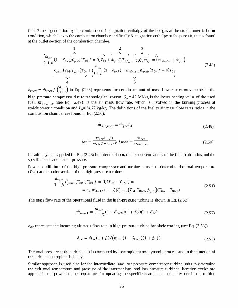
35

fuel, 3. heat generation by the combustion, 4. stagnation enthalpy of the hot gas at the stoichiometric burnt

condition, which leaves the combustion chamber and finally 5. stagnation enthalpy of the pure air, that is found

at the outlet section of the combustion chamber.

��𝑎𝑖𝑟

1 + 𝛽(1 − 𝛿𝑡𝑒𝑐ℎ)𝐶𝑝𝑚𝑖𝑥(𝑇03, 𝑓 = 0)𝑇03 + ��𝑓𝑐𝑐

𝐶𝑓𝑇0,𝑓𝑐𝑐+ 휂

𝑏𝑄𝑅��𝑓𝑐𝑐

= (��𝑎𝑖𝑟,𝑠𝑡,𝑐𝑐 + ��𝑓𝑐𝑐)

𝐶𝑝𝑚𝑖𝑥(𝑇04, 𝑓𝑠𝑡,𝑐𝑐)𝑇04 + (��𝑎𝑖𝑟

1 + 𝛽(1 − 𝛿𝑡𝑒𝑐ℎ) − ��𝑎𝑖𝑟,𝑠𝑡,𝑐𝑐)𝐶𝑝𝑚𝑖𝑥(𝑇04, 𝑓 = 0)𝑇04

(2.48)

𝛿𝑡𝑒𝑐ℎ = ��𝑡𝑒𝑐ℎ/ (��𝑎𝑖𝑟

1+𝛽) in Eq. (2.48) represents the certain amount of mass flow rate re-movements in the

high-pressure compressor due to technological reason. 𝑄𝑅= 42 MJ/kg is the lower heating value of the used

fuel. ��𝑎𝑖𝑟,𝑠𝑡,𝑐𝑐 (see Eq. (2.49)) is the air mass flow rate, which is involved in the burning process at

stoichiometric condition and 𝐿0=14.72 kg/kg. The definitions of the fuel to air mass flow rates ratios in the

combustion chamber are found in Eq. (2.50).

��𝑎𝑖𝑟,𝑠𝑡,𝑐𝑐 = ��𝑓𝑐𝑐𝐿0 (2.49)

𝑓𝑐𝑐 =��𝑓𝑐𝑐(1+𝛽)

��𝑎𝑖𝑟(1−𝛿𝑡𝑒𝑐ℎ), 𝑓𝑠𝑡,𝑐𝑐 =

��𝑓𝑐𝑐

��𝑎𝑖𝑟,𝑠𝑡,𝑐𝑐 (2.50)

Iteration cycle is applied for Eq. (2.48) in order to elaborate the coherent values of the fuel to air ratios and the

specific heats at constant pressure.

Power equilibrium of the high-pressure compressor and turbine is used to determine the total temperature

(T04.1) at the outlet section of the high-pressure turbine:

��𝑎𝑖𝑟

1 + 𝛽𝐶��𝑚𝑖𝑥(𝑇02.3, 𝑇03, 𝑓 = 0)(𝑇03 − 𝑇02.3) =

= 휂𝑚��4−4.1(1 − 휁)𝐶��𝑚𝑖𝑥(𝑇04, 𝑇04.1, 𝑓ℎ𝑝,𝑇)(𝑇04 − 𝑇04.1) (2.51)

The mass flow rate of the operational fluid in the high-pressure turbine is shown in Eq. (2.52).

��4−4.1 =��𝑎𝑖𝑟

1 + 𝛽(1 − 𝛿𝑡𝑒𝑐ℎ)(1 + 𝑓𝑐𝑐)(1 + 𝛿𝑏𝑐) (2.52)

𝛿𝑏𝑐 represents the incoming air mass flow rate in high-pressure turbine for blade cooling (see Eq. (2.53)).

𝛿𝑏𝑐 = ��𝑏𝑐(1 + 𝛽) (��𝑎𝑖𝑟(1 − 𝛿𝑡𝑒𝑐ℎ)(1 + 𝑓𝑐𝑐))⁄ (2.53)

The total pressure at the turbine exit is computed by isentropic thermodynamic process and in the function of

the turbine isentropic efficiency.

Similar approach is used also for the intermediate- and low-pressure compressor-turbine units to determine

the exit total temperature and pressure of the intermediate- and low-pressure turbines. Iteration cycles are

applied in the power balance equations for updating the specific heats at constant pressure in the turbine

4

1 2

3

5

36

segments too.

The total pressure recovery factor of the bypass liner 2.1-6 and engine core section 5-6 (see Fig. 2.3) is included

in the afterburner liner location corresponds to 6-7, which approximation has negligible effect for the output

of the analyses. This simplification is due to the fact that, as it is already mentioned, there are no available

(measured) or calculated (by CFD for example) data for the pressure recovery factors and so reducing their

numbers makes the parameter fitting simpler and faster.

The by-passed and core flows are mixed at section 6. Although the velocities and the static pressure should be

the same for the flow streams enter in the mixing domain [24], slight difference can be observed. So, mass

flow weighted averaging procedure is applied for determining the common total pressure. The mixing loss is

going to be considered in pressure recovery factor of the afterburner liner. Mass conservation law is used for

calculating the total mass flow rate in section 6. Total enthalpy balance is used for having the total temperature

of the gas mixture as follow:

��𝑏𝑦_𝑝𝑎𝑠𝑠𝐶𝑝𝑎𝑖𝑟(𝑇02.1, 𝑓 = 0)𝑇02.1 + ��5𝐶𝑝𝑚𝑖𝑥(𝑇05, 𝑓5)𝑇05 = ��6𝐶𝑝𝑚𝑖𝑥(𝑇06, 𝑓6)𝑇06 (2.54)

Iteration process is applied here also as the specific heat at constant pressure is the function of the resulted

total temperature. The ��𝑏𝑦_𝑝𝑎𝑠𝑠 is the mass flow rate in the fan section:

��𝑏𝑦_𝑝𝑎𝑠𝑠 =𝛽

1 + 𝛽��𝑎𝑖𝑟 (2.55)

The ��5 is the mass flow rate at the outlet of the high-pressure turbine:

��5 =��𝑎𝑖𝑟

1 + 𝛽[(1 − 𝛿𝑡𝑒𝑐ℎ)(1 + 𝑓)(1 + 𝛿𝑏𝑐)] (2.56)

The ��6 is the mass flow rate after mixing part:

��6 =��𝑎𝑖𝑟

1 + 𝛽[(1 − 𝛿𝑡𝑒𝑐ℎ)(1 + 𝑓)(1 + 𝛿𝑏𝑐) + 𝛽] (2.57)

The afterburner is located between cross section 6. and 7. (see Fig. 2.3). If the afterburner operates, the total

energy balance has been considered for this segment in order to calculate the fuel mass flow rate (��𝑓,𝐴) enters

into the afterburner as it is shown in Eq. (2.58).

��𝑎𝑖𝑟,6 𝐶𝑝𝑚𝑖𝑥(𝑇06, 𝑓 = 0)𝑇06 + ��𝑓,𝐴𝐶𝑓𝑇0,𝑓,𝐴 + 휂𝑏𝑄𝑅��𝑓,𝐴

+ (��𝑎𝑖𝑟,𝑠𝑡,𝑐𝑐 + ��𝑓𝑐𝑐) 𝐶𝑝𝑚𝑖𝑥(𝑇06, 𝑓𝑠𝑡,𝑐𝑐)𝑇0,6

= (��𝑎𝑖𝑟,𝑠𝑡,𝑐𝑐 + ��𝑓𝑐𝑐) 𝐶𝑝𝑚𝑖𝑥(𝑇07, 𝑓𝑠𝑡,𝑐𝑐)𝑇07

+ (��𝑎𝑖𝑟,𝑠𝑡,𝐴 + ��𝑓𝐴) 𝐶𝑝𝑚𝑖𝑥(𝑇07, 𝑓𝑠𝑡,𝐴)𝑇07 + (��𝑎𝑖𝑟,6 − ��𝑎𝑖𝑟,𝑠𝑡,𝐴)𝐶𝑝𝑚𝑖𝑥(𝑇07, 𝑓

= 0)𝑇07

(2.58)

The left side of Eq. (2.58) shows the incoming total enthalpies and energy into the system and the right-hand

side represents the leaving total enthalpies. The first term in Eq. (2.58) is the stagnation enthalpy of pure air,

which is available at section 6. The second and third term is the total enthalpy of the fuel entering afterburner

and heat generated by the combustion respectively. The last term in the left-hand side is the total enthalpy of

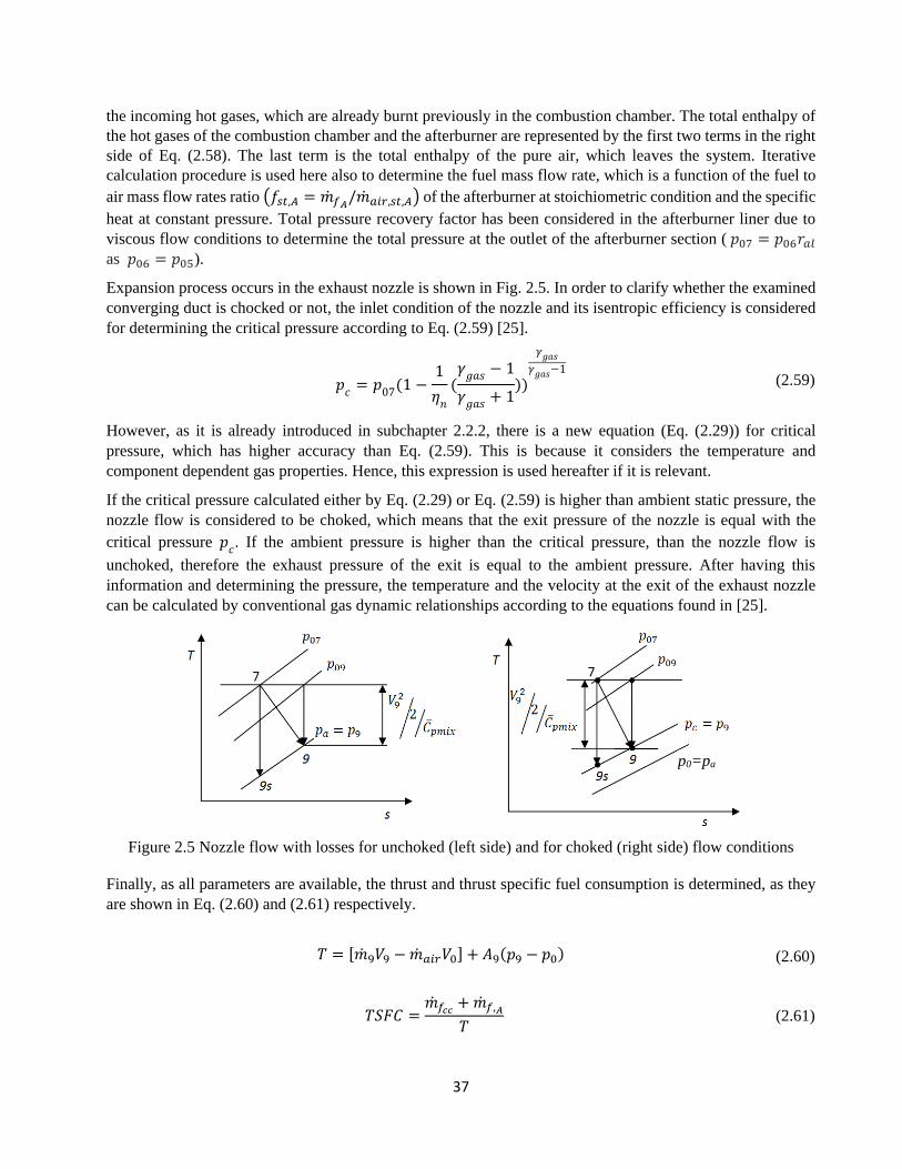
37

the incoming hot gases, which are already burnt previously in the combustion chamber. The total enthalpy of

the hot gases of the combustion chamber and the afterburner are represented by the first two terms in the right

side of Eq. (2.58). The last term is the total enthalpy of the pure air, which leaves the system. Iterative

calculation procedure is used here also to determine the fuel mass flow rate, which is a function of the fuel to

air mass flow rates ratio (𝑓𝑠𝑡,𝐴 = ��𝑓𝐴/��𝑎𝑖𝑟,𝑠𝑡,𝐴) of the afterburner at stoichiometric condition and the specific

heat at constant pressure. Total pressure recovery factor has been considered in the afterburner liner due to

viscous flow conditions to determine the total pressure at the outlet of the afterburner section ( 𝑝07 = 𝑝06𝑟𝑎𝑙 as 𝑝06 = 𝑝05).

Expansion process occurs in the exhaust nozzle is shown in Fig. 2.5. In order to clarify whether the examined

converging duct is chocked or not, the inlet condition of the nozzle and its isentropic efficiency is considered

for determining the critical pressure according to Eq. (2.59) [25].

𝑝𝑐= 𝑝

07(1 −

1

휂𝑛

(𝛾𝑔𝑎𝑠

− 1

𝛾𝑔𝑎𝑠

+ 1))

𝛾𝑔𝑎𝑠𝛾𝑔𝑎𝑠−1

(2.59)

However, as it is already introduced in subchapter 2.2.2, there is a new equation (Eq. (2.29)) for critical

pressure, which has higher accuracy than Eq. (2.59). This is because it considers the temperature and

component dependent gas properties. Hence, this expression is used hereafter if it is relevant.

If the critical pressure calculated either by Eq. (2.29) or Eq. (2.59) is higher than ambient static pressure, the

nozzle flow is considered to be choked, which means that the exit pressure of the nozzle is equal with the

critical pressure 𝑝𝑐. If the ambient pressure is higher than the critical pressure, than the nozzle flow is

unchoked, therefore the exhaust pressure of the exit is equal to the ambient pressure. After having this

information and determining the pressure, the temperature and the velocity at the exit of the exhaust nozzle

can be calculated by conventional gas dynamic relationships according to the equations found in [25].

Figure 2.5 Nozzle flow with losses for unchoked (left side) and for choked (right side) flow conditions

Finally, as all parameters are available, the thrust and thrust specific fuel consumption is determined, as they

are shown in Eq. (2.60) and (2.61) respectively.

𝑇 = [��9𝑉9 − ��𝑎𝑖𝑟𝑉0] + 𝐴9(𝑝9 − 𝑝0) (2.60)

𝑇𝑆𝐹𝐶 =��𝑓𝑐𝑐 + ��𝑓,𝐴

𝑇 (2.61)

p0=pa

38

The mass flow rate leaves the engine is found in Eq. (2.62) [25].

��9 =��𝑎𝑖𝑟

1 + 𝛽[(1 − 𝛿𝑡𝑒𝑐ℎ)(1 + 𝑓𝑐𝑐 + 𝑓𝐴)(1 + 𝛿𝑏𝑐) + 𝛽] (2.62)

Verification of Thermo-dynamic Cycle Analysis for Triple-Spool Mixed Turbofan Engines

First, as it is already mentioned in the first paragraph of the present subchapter (2.3.1), НК-32 and НК-25

triple spool mixed turbofan engines are used as two gas turbines in start (take-off) condition to analyse and

verify the simulation method. The afterburner operates and converging nozzles are considered in both cases.

The available input parameters of the two selected engines are presented in Table 2.4 according to [3].

However, as it was mentioned earlier, there are also several unavailable parameters, which are determined by

parameter identifications. The missing losses (total pressure recovery factor of inlet diffuser, combustion

chamber and afterburner or turbine exhaust pipe), efficiencies (isentropic of the compressor, fan and turbine,

mechanical, burning, and exhaust nozzle) (see them in Table 2.2), power reduction rate of the auxiliary

systems, bleed air ratios for technological reasons, air income ratio due to blade cooling, total pressure ratio

of the fan and intermediate pressure compressor, and last but not least the total temperature of the afterburner

(see them in Table 2.3) are identified by nonlinear constrained optimization. Matlab’s “fmincon” function is

used for that purpose. The constrained minimization is the problem of finding a vector x that is a local

minimum to a scalar function f(x) subject to constraints on the allowable x: min f(x) such that one or more of

the following holds: c(x) ≤ 0, ceq(x) = 0, A·x ≤ b, Aeq·x = beq, l ≤ x ≤ u [32]. “fmincon” function can use

Trust Region Reflective, Active Set, Sequential Quadratic Programming and Interior Point Algorithms [32] to

find the unknown loss and technical parameters mentioned before over the given ranges while the goal function

of the optimisation is to minimize the differences between the calculated and available specific thrust and

thrust specific fuel consumption found in the available technical literature [3]. More information about the

used constrained nonlinear optimization algorithms is found in [32] and [33]. The used ranges for the

constrained optimisation in the present section are shown in Table 2.2 and Table 2.3.

Table 2.2 Considered ranges of the unknown parameters in the constrained optimisation

Pressure recovery rates and efficiencies of the engine components

𝑟𝑑 𝑟𝑐𝑐 𝑟𝑎𝑙 휂𝐶,𝑠 휂𝑓,𝑠 휂𝑇,𝑠 휂𝑚 휂𝑏 휂𝑛

Given ranges for the

constrained optimization

0.88

0.94

0.93

0.97

0.88

0.97

0.81

0.88

0.81

0.88

0.86

0.94

0.98

0.999

0.92

0.98

0.92

0.98

Table 2.3 Applied ranges of the unknown parameters in the constrained optimisation

Power reduction rate for the auxiliary systems (𝝃), bleed air ratio for

technological reasons (𝜹𝒕𝒆𝒄𝒉), air income ratio due to blade cooling (𝜹𝒃𝒄), total pressure ratio of the fan (𝝅𝒇) and intermediate pressure compressor

(𝝅𝒊𝒑,𝑪), and total temperature in the afterburner (𝑻𝟎𝟕)

𝜉 𝛿𝑡𝑒𝑐ℎ 𝛿𝑏𝑐 𝜋𝑓

𝜋𝑖𝑝,𝐶 𝑇07[K]

Given ranges for the

constrained optimization

0.004

0.012

0.02

0.2

0.05

0.12

1.1

2.3

2

4

1700

2200

39

Table 2.5, Table 2.6 and Table 2.7 show the results of the parameter identification. The calculated data are in

the reasonable range therefore they can be accepted.

Table 2.4 Operational data of the НК-32 and НК-25 turbofan engines from the available

specification [3], [27] and [28]

Type of engine The main characteristics of the engine (take-off condition)

𝑇04 [K] 𝜋𝐶 𝛽 ��𝑎𝑖𝑟 [kg/s] T [kN] TSFC [kg/(kNh)]

НК-32 1630 28.4 1.4 290 245 -

НК-25 1600 26 1.44 280.9 245 205.3

The thrust and thrust specific fuel consumption – belong to the parameters found in Table 2.5, Table 2.6 and

Table 2.7 – are shown in Table 2.8. The relative maximal deviation between the given and the calculated data

during the parameter fitting is 0.122 % in case of thrust and 0.195 % at the thrust specific fuel consumption.

Although both engines have the same thrust, the TSFC of НК-32 engine is higher (see Table 2.8) due to the

higher temperature in the combustion chamber and in the afterburner. НК-32 engine has lower total pressure

recovery factor (higher pressure loss) in the combustion chamber (𝑟𝑐𝑐), afterburner liner (𝑟𝑎𝑙) and intake duct

(𝑟𝑑). The НК-32 has lower mechanical, nozzle and burning efficiency beside lower fan and compressor

isentropic efficiencies in comparing with НК-25.

Although more investigations would be needed, the obtained results together with the plausible parameter

identifications and verification show, that the thermodynamic model is suitable for analysing processes of the

triple-spool turbojet engines.

Table 2.5 Identified efficiencies of the НК-32 and НК-25 turbofan engines

Type of

Engine

Mechanical, nozzle, burning and isentropic (high-

pressure turbine, intermediate-pressure turbine, low-

pressure turbine, fan, high-pressure compressor and

intermediate-pressure compressor) efficiencies

휂𝑚 휂𝑛 휂𝑏

휂ℎ𝑝,𝑇,𝑠

휂𝑖𝑝,𝑇,𝑠

휂𝑙𝑝,𝑇,𝑠

휂𝑓,𝑠 휂ℎ𝑝,𝐶,𝑠 휂𝑖𝑝,𝐶,𝑠

НК-32 0.99 0.94 0.94 0.89 0.84 0.83 0.84

НК-25 0.992 0.95 0.97 0.89 0.86 0.87 0.87

Table 2.6 Identified total pressure recovery factors of the investigated turbofan engines

Type of Engine Total pressure recovery factors of comb. chamber

(𝒓𝒄𝒄) afterburner liner (𝒓𝒂𝒍) and intake duct (𝒓𝒅)

𝑟𝑐𝑐 𝑟𝑎𝑙 𝑟𝑑

НК-32 0.95 0.9 0.91

НК-25 0.96 0.94 0.94

40

Table 2.7 Identified parameters of the investigated turbofan engines

Type of

Engine

Total pressure ratio of the fan (𝝅𝒇) and intermediate pressure

compressor (𝝅𝒊𝒑,𝑪), bleed air ratio for technological reasons (𝜹𝒕𝒆𝒄𝒉), air

income ratio due to blade cooling (𝜹𝒃𝒄), power reduction rate for the

auxiliary systems (𝝃) and total temperature in the afterburner (𝑻𝟎𝟕)

𝜋𝑓 𝜋𝑖𝑝,𝐶 𝛿𝑡𝑒𝑐ℎ 𝛿𝑏𝑐 𝜉 𝑇07 [K]

НК-32 2 3 0.16 0.116 0.005 1800

НК-25 2.19 3 0.18 0.0952 0.005 1780

Table 2.8 Comparisons of the available data with the outputs of the parameter identification

Type of

Engine

Available data

(take-off condition)

Outputs of the parameter

identification

(take-off condition)

Relative differences (%)

between the available and

calculated data

T [kN] TSFC

[kg/(kNh)] T [kN] TSFC [kg/(kNh)] T TSFC

НК-32 245 - 245.1 229.4 0.04 -

НК-25 245 205.3 245.3 205.7 0.122 0.195

The thermo-dynamical cycles of the engine processes are found in Fig. 2.6 and 2.7. The red curve-sections (or

lighter and thinner in greyscale) represent the constant pressures in the T-s diagrams (total from points 0-7 and

static at 9). The processes between the engine states denoted by numbers are plotted by thicker black lines.

This visualization effect is the reason of the constant pressure line goes below the process line in case of

pressure decrement just after sections “2.1” and “3”.

Figure 2.6 Thermo-dynamical cycle of the НК-32 turbofan engine with afterburner (the red curve sections

(the lighter thinner ones in greyscale) in the T-s diagrams are the constant pressure curves (total from 0-7 and

static at 9) belong to the shown numbers of the engine cross sections)

41

Figure 2.7 Thermo-dynamical cycle of the НК-25 turbofan engine with afterburner (the red curve sections

(the lighter thinner ones in greyscale) in the T-s diagrams are the constant pressure curves (total from 0-7 and

static at 9) belong to the shown numbers of the engine cross sections)

The analysis of the НК-32 and НК-25 engines are also completed by using the conventional Eq. (2.59) for

determining the critical pressure at the exit of the converging nozzle in case of the same thermo-dynamical

conditions. The effect of the fuel to air mass flow rates ratio and temperature are not considered in the ratio of

specific heats in Eq. (2.59), the flow is supposed to be pure gas with 𝛾𝑔𝑎𝑠=1.33. The results of the calculations

are shown in Table 2.9. The average value of the relative deviations between the resulted and the available

thrust and thrust specific fuel consumption is 0.119 % by using a variant of the new equation (Eq. (2.29)) for

the critical pressure and 3.13 % in case of the conventional equation. The “variant” in the present context

means that the true specific heat is considered (a specific heat belongs to the given temperature and fuel to air

ratio) instead of the average one at the given temperature range in the total enthalpy equation (Eq. 2.25).

Table 2.9 Effect of the conventional and a variant of the new equation for critical pressure on the thrust and

the thrust specific fuel consumption in case of НК-32 and НК-25 turbofan mixed jet engines

Type of

Engine

Relative difference

(a variant of the new equation)

Relative difference (conventional

equation)

T [kN] TSFC [kg/(kNh)] T [kN] TSFC [kg/(kNh)]

НК-32 0.04 % - 3.27 % -

НК-25 0.122 % 0.195 % 2.85 % 3.27 %

2.3.2. Dual-Spool Mixed Turbofan Engine

A simplified layout of a dual-spool mixed turbofan engine is shown in Fig. 2.8. Beside the inlet diffuser (1-2)

and exhaust nozzle (7-9), the gas turbine has combustion chamber (3-4), afterburner (6-7), two shafts, two

compressor- and two turbine-units. The compressor that is closer to the intake is the low-pressure compressor

(fan, in this case) (2-2.1) and it is driven by the low-pressure turbine (4.1-5). The high-pressure compressor

(2.1-3), which is located at the downstream of the fan, is driven by the high-pressure turbine (4-4.1). The

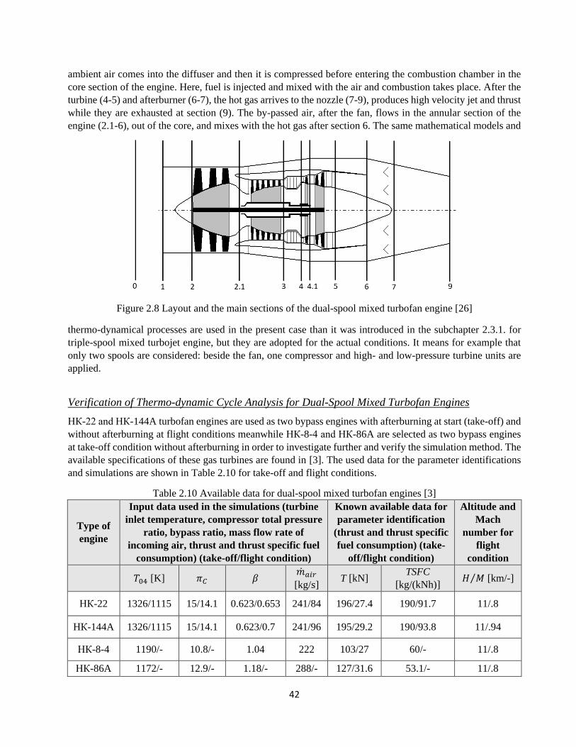
42

ambient air comes into the diffuser and then it is compressed before entering the combustion chamber in the

core section of the engine. Here, fuel is injected and mixed with the air and combustion takes place. After the

turbine (4-5) and afterburner (6-7), the hot gas arrives to the nozzle (7-9), produces high velocity jet and thrust

while they are exhausted at section (9). The by-passed air, after the fan, flows in the annular section of the

engine (2.1-6), out of the core, and mixes with the hot gas after section 6. The same mathematical models and

Figure 2.8 Layout and the main sections of the dual-spool mixed turbofan engine [26]

thermo-dynamical processes are used in the present case than it was introduced in the subchapter 2.3.1. for

triple-spool mixed turbojet engine, but they are adopted for the actual conditions. It means for example that

only two spools are considered: beside the fan, one compressor and high- and low-pressure turbine units are

applied.

Verification of Thermo-dynamic Cycle Analysis for Dual-Spool Mixed Turbofan Engines

НК-22 and НК-144A turbofan engines are used as two bypass engines with afterburning at start (take-off) and

without afterburning at flight conditions meanwhile НК-8-4 and НК-86A are selected as two bypass engines

at take-off condition without afterburning in order to investigate further and verify the simulation method. The

available specifications of these gas turbines are found in [3]. The used data for the parameter identifications

and simulations are shown in Table 2.10 for take-off and flight conditions.

Table 2.10 Available data for dual-spool mixed turbofan engines [3]

Type of

engine

Input data used in the simulations (turbine

inlet temperature, compressor total pressure

ratio, bypass ratio, mass flow rate of

incoming air, thrust and thrust specific fuel

consumption) (take-off/flight condition)

Known available data for

parameter identification

(thrust and thrust specific

fuel consumption) (take-

off/flight condition)

Altitude and

Mach

number for

flight

condition

𝑇04 [K] 𝜋𝐶 𝛽 ��𝑎𝑖𝑟

[kg/s] T [kN]

TSFC

[kg/(kNh)] 𝐻 𝑀⁄ [km/-]

НК-22 1326/1115 15/14.1 0.623/0.653 241/84 196/27.4 190/91.7 11/.8

НК-144A 1326/1115 15/14.1 0.623/0.7 241/96 195/29.2 190/93.8 11/.94

НК-8-4 1190/- 10.8/- 1.04 222 103/27 60/- 11/.8

НК-86A 1172/- 12.9/- 1.18/- 288/- 127/31.6 53.1/- 11/.8

43

The calculation of the unknown variables such as total pressure recovery factors, efficiencies, total pressure

ratios of fan, bleed air ratios for technological reasons, air income ratios due to blade cooling, power reduction

rates for the auxiliary systems and total temperatures of the afterburners are like at the triple-spool turbofan

engines, which is discussed earlier in the subchapter 2.3.1. except for the mentioned differences. Referring to

Table 2.10 as the input data of the analysis, the identified parameters are shown in Table 2.11, 2.12 and 2.13.

Table 2.11 Identified efficiencies of the investigated dual-spool mixed turbofan engines

Type of

engine

Efficiencies (nozzle, mechanical, burning, low pressure turbine isentropic, high

pressure turbine isentropic, fan isentropic and high-pressure compressor

isentropic) of the cycles at take-off/flight condition

휂𝑛 휂𝑚 휂𝑏 휂𝑙𝑝,𝑇,𝑠 휂ℎ𝑝,𝑇,𝑠 휂𝑓,𝑠 휂ℎ𝑝,𝐶,𝑠

НК-22 0.95/0.96 0.99/0.99 0.97/0.97 0.88/0.87 0.89/0.9 0.85/0.85 0.85/0.86

НК-144A 0.95/0.96 0.99/0.99 0.97/0.97 0.88/0.87 0.88/0.89 0.85/0.86 0.86/0.86

НК-8-4 0.95/- 0.99/- 0.96/- 0.89/- 0.87/- 0.85/- 0.86/-

НК-86A 0.95/- 0.995/- 0.95/- 0.89/- 0.87/- 0.85/- 0.86/-

Table 2.12 Identified total pressure recovery factors of the investigated dual-spool mixed turbofan engines

Type of

engine

Total pressure recovery factors of intake duct (𝒓𝒅), combustion

chamber (𝒓𝒄𝒄) and afterburner liner (𝒓𝒂𝒍) (take-off/flight conditions)

𝑟𝑑 𝑟𝑐𝑐 𝑟𝑎𝑙

НК-22 0.89/0.91 0.94/0.96 0.9/0.9

НК-144A 0.89/0.9 0.95/0.95 0.85/0.9

НК-8-4 0.9/- 0.96/- -/-

НК-86A 0.9/- 0.95/- -/-

Table 2.13 Identified parameters of the investigated dual-spool mixed turbofan engines

Type of

engine

Total pressure ratio of the fan (𝝅𝒇), bleed air ratio for technological reasons

(𝜹𝒕𝒆𝒄𝒉), air income ratio due to blade cooling (𝜹𝒃𝒄), power reduction rate for

the auxiliary systems (𝝃) and total temperature of the afterburner (𝑻𝟎𝟕)

(take-off/flight conditions)

𝜋𝑓 𝛿𝑡𝑒𝑐ℎ 𝛿𝑏𝑐 𝜉 𝑇07[K]

НК-22 1.8/2.18 0.18/0.18 0.0713/0.071 0.008/0.007 1750/-

НК-144A 1.4/2.15 0.18/0.18 0.0595/0.0595 0.008/0.001 1750/-

НК-8-4 1.1/- 0.18/- 0.071/- 0.008/- -/-

НК-86A 1.3/- 0.18/- 0.059/- 0.008/- -/-

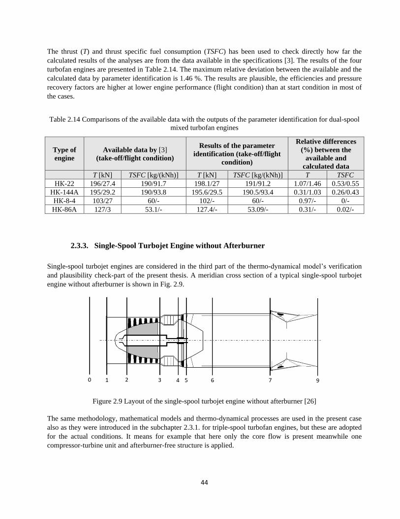
44

The thrust (T) and thrust specific fuel consumption (TSFC) has been used to check directly how far the

calculated results of the analyses are from the data available in the specifications [3]. The results of the four

turbofan engines are presented in Table 2.14. The maximum relative deviation between the available and the

calculated data by parameter identification is 1.46 %. The results are plausible, the efficiencies and pressure

recovery factors are higher at lower engine performance (flight condition) than at start condition in most of

the cases.

Table 2.14 Comparisons of the available data with the outputs of the parameter identification for dual-spool

mixed turbofan engines

Type of

engine

Available data by [3]

(take-off/flight condition)

Results of the parameter

identification (take-off/flight

condition)

Relative differences

(%) between the

available and

calculated data

T [kN] TSFC [kg/(kNh)] T [kN] TSFC [kg/(kNh)] T TSFC

НК-22 196/27.4 190/91.7 198.1/27 191/91.2 1.07/1.46 0.53/0.55

НК-144A 195/29.2 190/93.8 195.6/29.5 190.5/93.4 0.31/1.03 0.26/0.43

НК-8-4 103/27 60/- 102/- 60/- 0.97/- 0/-

НК-86A 127/3 53.1/- 127.4/- 53.09/- 0.31/- 0.02/-

2.3.3. Single-Spool Turbojet Engine without Afterburner

Single-spool turbojet engines are considered in the third part of the thermo-dynamical model’s verification

and plausibility check-part of the present thesis. A meridian cross section of a typical single-spool turbojet

engine without afterburner is shown in Fig. 2.9.

Figure 2.9 Layout of the single-spool turbojet engine without afterburner [26]

The same methodology, mathematical models and thermo-dynamical processes are used in the present case

also as they were introduced in the subchapter 2.3.1. for triple-spool turbofan engines, but these are adopted

for the actual conditions. It means for example that here only the core flow is present meanwhile one

compressor-turbine unit and afterburner-free structure is applied.

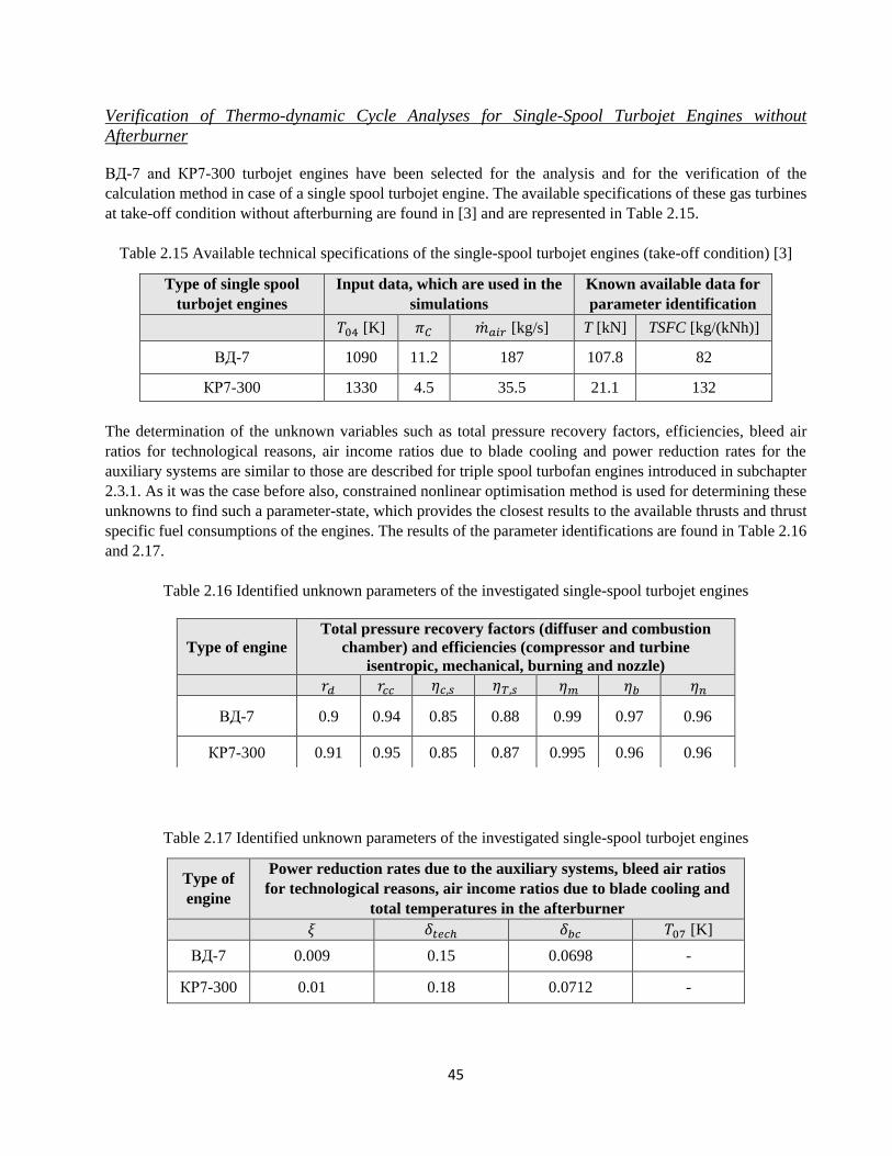
45

Verification of Thermo-dynamic Cycle Analyses for Single-Spool Turbojet Engines without

Afterburner

ВД-7 and КР7-300 turbojet engines have been selected for the analysis and for the verification of the

calculation method in case of a single spool turbojet engine. The available specifications of these gas turbines

at take-off condition without afterburning are found in [3] and are represented in Table 2.15.

Table 2.15 Available technical specifications of the single-spool turbojet engines (take-off condition) [3]

Type of single spool

turbojet engines

Input data, which are used in the

simulations

Known available data for

parameter identification

𝑇04 [K] 𝜋𝐶 ��𝑎𝑖𝑟 [kg/s] T [kN] TSFC [kg/(kNh)]

ВД-7 1090 11.2 187 107.8 82

КР7-300 1330 4.5 35.5 21.1 132

The determination of the unknown variables such as total pressure recovery factors, efficiencies, bleed air

ratios for technological reasons, air income ratios due to blade cooling and power reduction rates for the

auxiliary systems are similar to those are described for triple spool turbofan engines introduced in subchapter

2.3.1. As it was the case before also, constrained nonlinear optimisation method is used for determining these

unknowns to find such a parameter-state, which provides the closest results to the available thrusts and thrust

specific fuel consumptions of the engines. The results of the parameter identifications are found in Table 2.16

and 2.17.

Table 2.16 Identified unknown parameters of the investigated single-spool turbojet engines

Table 2.17 Identified unknown parameters of the investigated single-spool turbojet engines

Type of

engine

Power reduction rates due to the auxiliary systems, bleed air ratios

for technological reasons, air income ratios due to blade cooling and

total temperatures in the afterburner

𝜉 𝛿𝑡𝑒𝑐ℎ 𝛿𝑏𝑐 𝑇07 [K]

ВД-7 0.009 0.15 0.0698 -

КР7-300 0.01 0.18 0.0712 -

Type of engine

Total pressure recovery factors (diffuser and combustion

chamber) and efficiencies (compressor and turbine

isentropic, mechanical, burning and nozzle)

𝑟𝑑 𝑟𝑐𝑐 휂𝑐,𝑠 휂𝑇,𝑠 휂𝑚 휂𝑏 휂𝑛

ВД-7 0.9 0.94 0.85 0.88 0.99 0.97 0.96

КР7-300 0.91 0.95 0.85 0.87 0.995 0.96 0.96

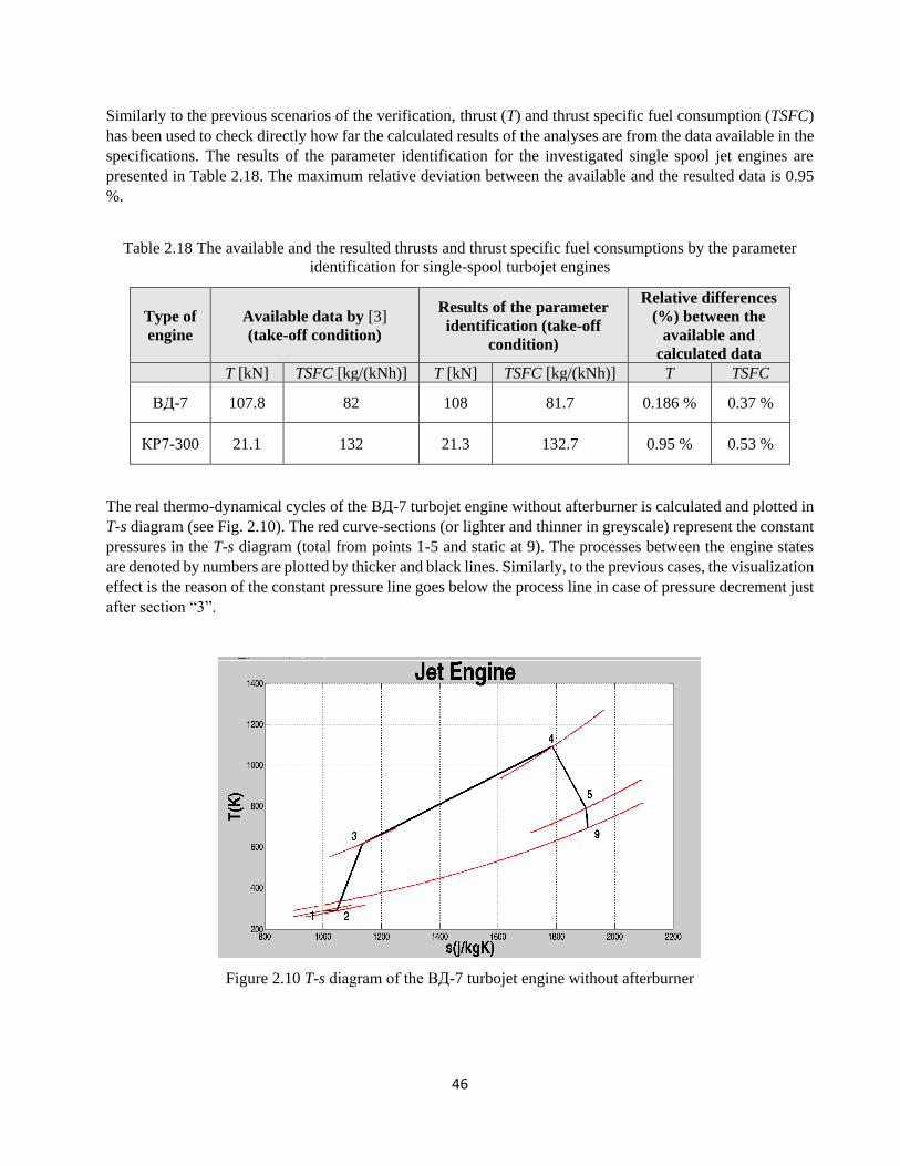
46

Similarly to the previous scenarios of the verification, thrust (T) and thrust specific fuel consumption (TSFC)

has been used to check directly how far the calculated results of the analyses are from the data available in the

specifications. The results of the parameter identification for the investigated single spool jet engines are

presented in Table 2.18. The maximum relative deviation between the available and the resulted data is 0.95

%.

Table 2.18 The available and the resulted thrusts and thrust specific fuel consumptions by the parameter

identification for single-spool turbojet engines

Type of

engine

Available data by [3]

(take-off condition)

Results of the parameter

identification (take-off

condition)

Relative differences

(%) between the

available and

calculated data

T [kN] TSFC [kg/(kNh)] T [kN] TSFC [kg/(kNh)] T TSFC

ВД-7 107.8 82 108 81.7 0.186 % 0.37 %

КР7-300 21.1 132 21.3 132.7 0.95 % 0.53 %

The real thermo-dynamical cycles of the ВД-7 turbojet engine without afterburner is calculated and plotted in

T-s diagram (see Fig. 2.10). The red curve-sections (or lighter and thinner in greyscale) represent the constant

pressures in the T-s diagram (total from points 1-5 and static at 9). The processes between the engine states

are denoted by numbers are plotted by thicker and black lines. Similarly, to the previous cases, the visualization

effect is the reason of the constant pressure line goes below the process line in case of pressure decrement just

after section “3”.

Figure 2.10 T-s diagram of the ВД-7 turbojet engine without afterburner

47

2.4. Verification and Plausibility Check of the New Equation for the Optimum

Compressor Total Pressure Ratio

РД-9Б and АЛ-21Ф3 turbojet engines at take-off condition (maximum thrust at sea level condition) with

afterburning have been considered for further verification of the simulation method and to test the new

equation for the optimum total pressure ratio of the compressor belongs to the maximum specific thrust.

2.4.1. Analysis of Single-Spool Turbojet Engines with Afterburning

A meridian cross section of a typical single spool turbojet engine with afterburner is shown in Fig. 2.11.

Section “0” represents the ambient conditions and “9” is the outlet of the exhaust nozzle. The afterburner is

found between section 6-7. Real flow conditions are considered in the mathematical model of each segment

of the assembly including pressure recovery factors and efficiencies as they are relevant similarly to the

previous cases. Temperature and fuel to air mass flow rates ratio dependencies are considered for specific

heats as it is mentioned in the subchapter 2.3.1.

Figure 2.11 Layout of the single-spool turbojet engine without afterburner [26]

Regarding the ambient conditions, static pressure and temperature at sea level are considered. These data are

obtained from the ISA (International Standard Atmosphere) [30] also: ambient static pressure: 𝑝0=101325 Pa,

ambient static temperature: 𝑇0=288.15 K, meanwhile the flight Mach number: 𝑀 = 0. The reason of this take-

off condition (maximum thrust at sea level) is – as it is already mentioned – that the engine specifications are

available at that operational mode in the technical datasheet of the engines [3].

The calculation methodology is summarized in subchapter 2.3.3 has been used in the present case also

considering afterburning additionally. The mathematical model and the simulation approach of the afterburner

is described in subchapter 2.3.1 for triple-spool mixed turbojet engines that can be used also for single-spool

turbojet propulsion system after the needed adaptations. The known parameters of the engines are presented

in Table 2.19. However, similarly to the previous scenarios, there are also unknown parameters of the engines,

which are shown in Table 2.20. and 2.21. Matlab’s “fmincon” function has been used for constrained nonlinear

optimization to find these non-available parameters. Minimising the differences between the available and

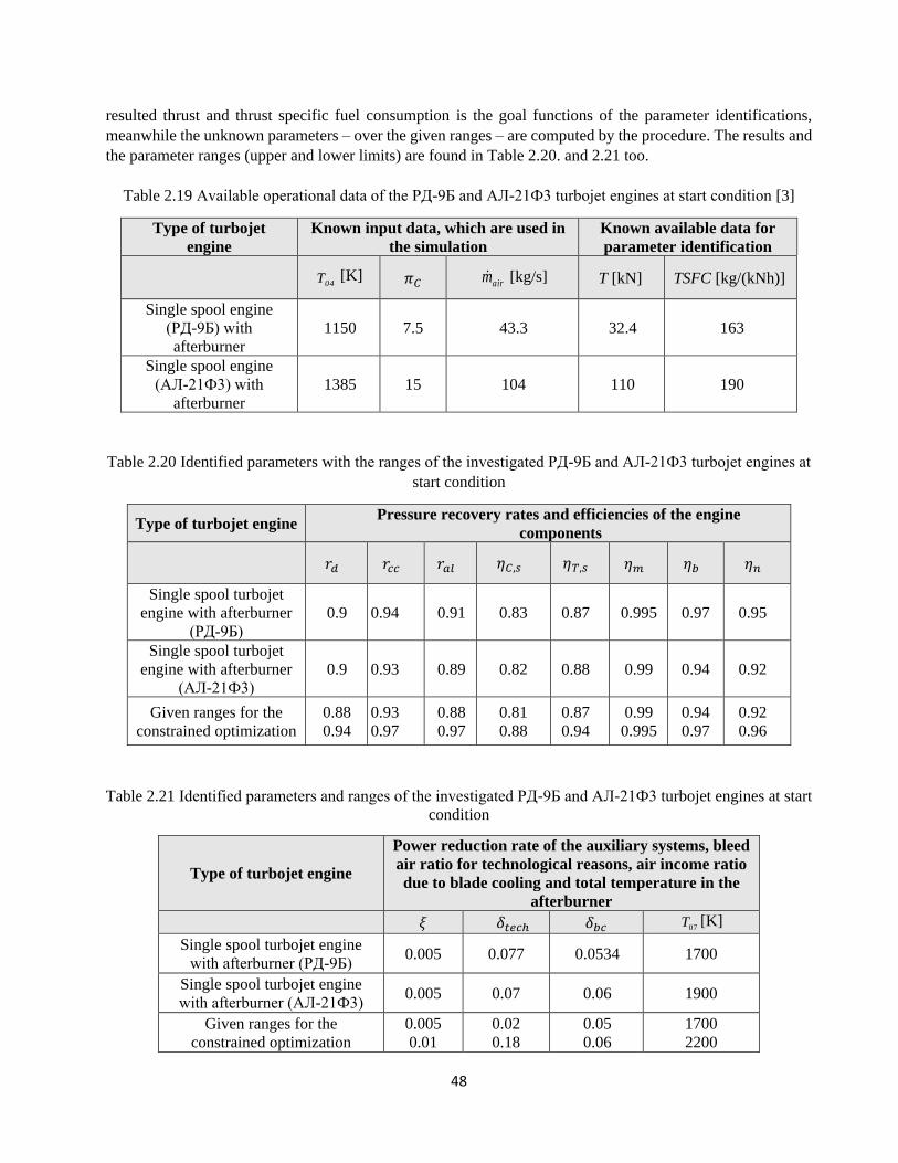
48

resulted thrust and thrust specific fuel consumption is the goal functions of the parameter identifications,

meanwhile the unknown parameters – over the given ranges – are computed by the procedure. The results and

the parameter ranges (upper and lower limits) are found in Table 2.20. and 2.21 too.

Table 2.19 Available operational data of the РД-9Б and АЛ-21Ф3 turbojet engines at start condition [3]

Type of turbojet

engine

Known input data, which are used in

the simulation

Known available data for

parameter identification

04T [K] 𝜋𝐶 airm [kg/s] T [kN] TSFC [kg/(kNh)]

Single spool engine

(РД-9Б) with

afterburner

1150 7.5 43.3 32.4 163

Single spool engine

(АЛ-21Ф3) with

afterburner

1385 15 104 110 190

Table 2.20 Identified parameters with the ranges of the investigated РД-9Б and АЛ-21Ф3 turbojet engines at

start condition

Type of turbojet engine Pressure recovery rates and efficiencies of the engine

components

𝑟𝑑 𝑟𝑐𝑐 𝑟𝑎𝑙 휂𝐶,𝑠 휂𝑇,𝑠 휂𝑚 휂𝑏 휂𝑛

Single spool turbojet

engine with afterburner

(РД-9Б)

0.9 0.94 0.91 0.83 0.87 0.995 0.97 0.95

Single spool turbojet

engine with afterburner

(АЛ-21Ф3)

0.9 0.93 0.89 0.82 0.88 0.99 0.94 0.92

Given ranges for the

constrained optimization

0.88

0.94

0.93

0.97

0.88

0.97

0.81

0.88

0.87

0.94

0.99

0.995

0.94

0.97

0.92

0.96

Table 2.21 Identified parameters and ranges of the investigated РД-9Б and АЛ-21Ф3 turbojet engines at start

condition

Type of turbojet engine

Power reduction rate of the auxiliary systems, bleed

air ratio for technological reasons, air income ratio

due to blade cooling and total temperature in the

afterburner

𝜉 𝛿𝑡𝑒𝑐ℎ 𝛿𝑏𝑐 07T [K]

Single spool turbojet engine

with afterburner (РД-9Б) 0.005 0.077 0.0534 1700

Single spool turbojet engine

with afterburner (АЛ-21Ф3) 0.005 0.07 0.06 1900

Given ranges for the

constrained optimization

0.005

0.01

0.02

0.18

0.05

0.06

1700

2200

49

Table 2.22 shows that the resulted thrust and thrust specific fuel consumption of the optimization is close to

the available data. The highest relative differences between the known and the resulted values in the parameter

fitting is 0.0617 % for the thrust and 0.0245 % for TSFC at РД-9Б engine, while the unknown parameters are

presented in Table 2.20. and 2.21. are within the expected intervals.

Table 2.22 The available and the resulted thrust and thrust specific fuel consumption used in the

optimization for parameter identification

Type of turbojet engine Available data Output of the optimization

T [kN] TSFC [kg/(kNh)] T [kN] TSFC [kg/(kNh)]

Single spool turbojet engine

(РД-9Б) with afterburner 32.4 163 32.42 162.96

Single spool turbojet engine

(АЛ-21Ф3) with afterburner 110 190 110 190

The thermodynamic cycle including real engine processes of the РД-9Б engine in the T-s diagram is plotted

in Fig. 2.12. The red curves (with smaller thickness) represent the constant pressures. The processes between

the engine sections denoted by numbers are shown by thicker lines. This visualization effect is the reason for

the constant pressure lines going below the process line in case of the pressure decrement just after sections

“3” and “5” in this case also.

Figure 2.12 T-s diagram of the РД-9Б turbojet engine with afterburning

2.4.2. Numerical Representation – Verification of the New Equation for Optimum

Total Pressure Ratio of the Compressor

The goal of the present subchapter is to verify the correctness and investigate the accuracy of the new

expression for the optimum compressor total pressure ratio (see Eq. (2.21) and (2.33) in subchapter 2.2).

Hence, a numerical representation of the optimum pressure ratio is completed. In this context, the numerical

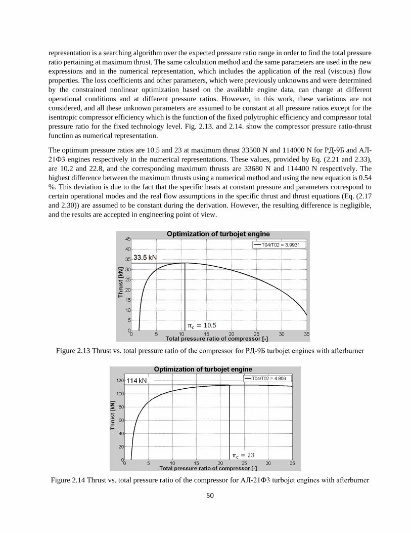
50

representation is a searching algorithm over the expected pressure ratio range in order to find the total pressure

ratio pertaining at maximum thrust. The same calculation method and the same parameters are used in the new

expressions and in the numerical representation, which includes the application of the real (viscous) flow

properties. The loss coefficients and other parameters, which were previously unknowns and were determined

by the constrained nonlinear optimization based on the available engine data, can change at different

operational conditions and at different pressure ratios. However, in this work, these variations are not

considered, and all these unknown parameters are assumed to be constant at all pressure ratios except for the

isentropic compressor efficiency which is the function of the fixed polytrophic efficiency and compressor total

pressure ratio for the fixed technology level. Fig. 2.13. and 2.14. show the compressor pressure ratio-thrust

function as numerical representation.

The optimum pressure ratios are 10.5 and 23 at maximum thrust 33500 N and 114000 N for РД-9Б and АЛ-

21Ф3 engines respectively in the numerical representations. These values, provided by Eq. (2.21 and 2.33),

are 10.2 and 22.8, and the corresponding maximum thrusts are 33680 N and 114400 N respectively. The

highest difference between the maximum thrusts using a numerical method and using the new equation is 0.54

%. This deviation is due to the fact that the specific heats at constant pressure and parameters correspond to

certain operational modes and the real flow assumptions in the specific thrust and thrust equations (Eq. (2.17

and 2.30)) are assumed to be constant during the derivation. However, the resulting difference is negligible,

and the results are accepted in engineering point of view.

Figure 2.13 Thrust vs. total pressure ratio of the compressor for РД-9Б turbojet engines with afterburner

Figure 2.14 Thrust vs. total pressure ratio of the compressor for АЛ-21Ф3 turbojet engines with afterburner

51

The specific thrusts in the function of compressor total pressure ratios for the both engines are shown in case

of correctly expanded converging-diverging nozzle flow conditions and at different T04/T02 ratios in Fig. 2.15

and 2.16. Higher turbine inlet temperature increases the specific thrust and the maximum values of that belong

to higher compressor total pressure ratios. The thrust specific fuel consumption in the function of compressor

total pressure ratio for the both engines are shown in case of correctly expanded flow conditions and at different

T04/T02 ratios in Fig. 2.17. The maximum specific thrust and minimum TSFC belong roughly to the same

compressor total pressure ratio ranges at the both investigated cases.

Figure 2.15 Specific thrust vs. total pressure ratio of the compressor for РД-9Б turbojet engines with

afterburner

Figure 2.16 Specific thrust vs. total pressure ratio of the compressor for АЛ-21Ф3 turbojet engines with

afterburner

Four different test scenarios are investigated to determine the effect of the pressure recovery factors,

efficiencies and parameter dependent specific heats for the thermodynamic cycle, for the optimum pressure

ratio and so for the maximum thrust of a single-spool turbojet engine. The results of this analysis are found in

Table 2.23. The ■ sign in the column of viscous flow conditions means that the pressure recovery factors and

efficiencies are considered in the calculation, meanwhile □ represents that they are not. In case of the real flow

conditions and variable specific heats, which are considered in the Eq. (2.21) and (2.33), the optimum pressure

ratio at the new equation is higher with 40 % and 53.3 % than the pressure ratio given in [3]. It corresponds to

3.39 % and 3.64 % thrust rising for РД-9Б and АЛ-21Ф3 jet engines respectively. In addition, besides keeping

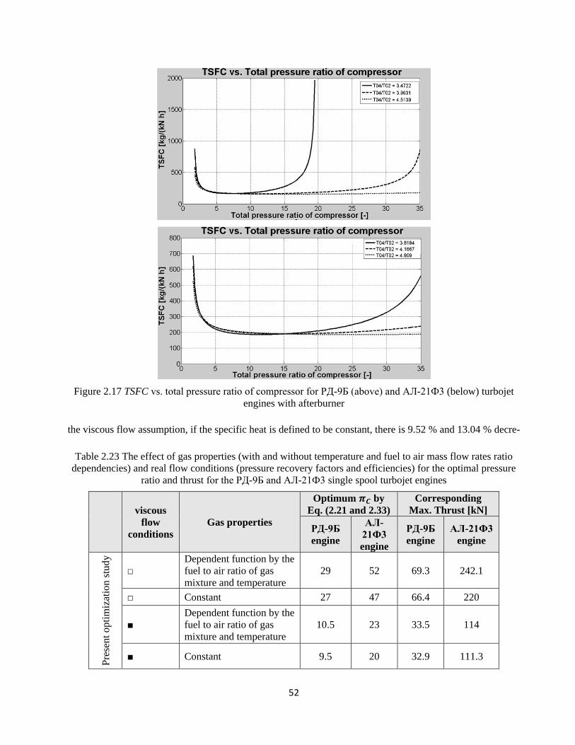
52

Figure 2.17 TSFC vs. total pressure ratio of compressor for РД-9Б (above) and АЛ-21Ф3 (below) turbojet

engines with afterburner

the viscous flow assumption, if the specific heat is defined to be constant, there is 9.52 % and 13.04 % decre-

Table 2.23 The effect of gas properties (with and without temperature and fuel to air mass flow rates ratio

dependencies) and real flow conditions (pressure recovery factors and efficiencies) for the optimal pressure

ratio and thrust for the РД-9Б and АЛ-21Ф3 single spool turbojet engines

viscous

flow

conditions

Gas properties

Optimum 𝝅𝑪 by

Eq. (2.21 and 2.33)

Corresponding

Max. Thrust [kN]

РД-9Б

engine

АЛ-

21Ф3

engine

РД-9Б

engine

АЛ-21Ф3

engine

Pre

sent

opti

miz

atio

n s

tud

y

□

Dependent function by the

fuel to air ratio of gas

mixture and temperature

29 52 69.3 242.1

□ Constant 27 47 66.4 220

■

Dependent function by the

fuel to air ratio of gas

mixture and temperature

10.5 23 33.5 114

■ Constant 9.5 20 32.9 111.3

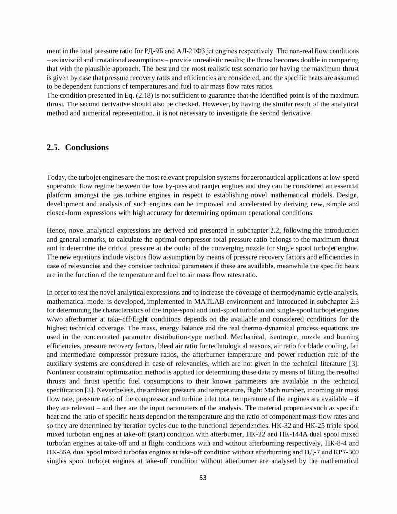
53

ment in the total pressure ratio for РД-9Б and АЛ-21Ф3 jet engines respectively. The non-real flow conditions

– as inviscid and irrotational assumptions – provide unrealistic results; the thrust becomes double in comparing

that with the plausible approach. The best and the most realistic test scenario for having the maximum thrust

is given by case that pressure recovery rates and efficiencies are considered, and the specific heats are assumed

to be dependent functions of temperatures and fuel to air mass flow rates ratios.

The condition presented in Eq. (2.18) is not sufficient to guarantee that the identified point is of the maximum

thrust. The second derivative should also be checked. However, by having the similar result of the analytical

method and numerical representation, it is not necessary to investigate the second derivative.

2.5. Conclusions

Today, the turbojet engines are the most relevant propulsion systems for aeronautical applications at low-speed

supersonic flow regime between the low by-pass and ramjet engines and they can be considered an essential

platform amongst the gas turbine engines in respect to establishing novel mathematical models. Design,

development and analysis of such engines can be improved and accelerated by deriving new, simple and

closed-form expressions with high accuracy for determining optimum operational conditions.

Hence, novel analytical expressions are derived and presented in subchapter 2.2, following the introduction

and general remarks, to calculate the optimal compressor total pressure ratio belongs to the maximum thrust

and to determine the critical pressure at the outlet of the converging nozzle for single spool turbojet engine.

The new equations include viscous flow assumption by means of pressure recovery factors and efficiencies in

case of relevancies and they consider technical parameters if these are available, meanwhile the specific heats

are in the function of the temperature and fuel to air mass flow rates ratio.

In order to test the novel analytical expressions and to increase the coverage of thermodynamic cycle-analysis,

mathematical model is developed, implemented in MATLAB environment and introduced in subchapter 2.3

for determining the characteristics of the triple-spool and dual-spool turbofan and single-spool turbojet engines

w/wo afterburner at take-off/flight conditions depends on the available and considered conditions for the

highest technical coverage. The mass, energy balance and the real thermo-dynamical process-equations are

used in the concentrated parameter distribution-type method. Mechanical, isentropic, nozzle and burning

efficiencies, pressure recovery factors, bleed air ratio for technological reasons, air ratio for blade cooling, fan

and intermediate compressor pressure ratios, the afterburner temperature and power reduction rate of the

auxiliary systems are considered in case of relevancies, which are not given in the technical literature [3].

Nonlinear constraint optimization method is applied for determining these data by means of fitting the resulted

thrusts and thrust specific fuel consumptions to their known parameters are available in the technical

specification [3]. Nevertheless, the ambient pressure and temperature, flight Mach number, incoming air mass

flow rate, pressure ratio of the compressor and turbine inlet total temperature of the engines are available – if

they are relevant – and they are the input parameters of the analysis. The material properties such as specific

heat and the ratio of specific heats depend on the temperature and the ratio of component mass flow rates and

so they are determined by iteration cycles due to the functional dependencies. НК-32 and НК-25 triple spool

mixed turbofan engines at take-off (start) condition with afterburner, НК-22 and НК-144A dual spool mixed

turbofan engines at take-off and at flight conditions with and without afterburning respectively, НК-8-4 and

НК-86A dual spool mixed turbofan engines at take-off condition without afterburning and ВД-7 and КР7-300

singles spool turbojet engines at take-off condition without afterburner are analysed by the mathematical

54

model to be introduced. The resulted thrusts and thrust specific fuel consumptions by parameter fitting and the

available data in [3] are compared with each other. The maximum and the average relative deviation between

them are 1.46 % and 0.645 % for the thrust and 0.55 % and 0.32 % for the thrust specific fuel consumptions

respectively, meanwhile the identified parameters are within the plausible range.

Although the presented results provide feasible and correct technical information about the engines’ operation,

more analyses at different operational conditions together with applications of different types of propulsion

systems should be considered, including validation, to investigate further the accuracy of the developed

mathematical model.

The НК-32 and НК-25 engines have been used for determining the effect of the new equation - calculates the

critical pressure - on the thrust and thrust specific fuel consumption. The results of the parameter identification

for the unknown data show that the average value of the relative deviations between the resulted and the

available thrust and thrust specific fuel consumption is 0.119 % by using a variant of the new equation for the

critical pressure and it is 3.13 % at the conventional equation with constant gas properties (the ratio of specific

heats for gas equals 1.33). The “variant” in the present context means that the true specific heats at constant

pressure and at the given temperatures are considered instead of the averaged one in the total enthalpy equation.

The new equation for determining the critical pressure is tested also for РД-9Б single-spool turbojet engine

with afterburning and at take-off condition. It gives higher critical pressure by 9.3 % than its original form

with constant gas properties.

Finally, testing and verification of the novel analytical equation for the optimum compressor total pressure

ratio is completed and presented in subchapter 2.4. РД-9Б and АЛ-21Ф3 single-spool turbojet engines are

considered for that purpose with afterburning and at take-off condition. First, similarly to the parameter

identification described above, the unknown pressure recovery factors, efficiencies and the missing technical

parameters are determined with MATLAB-based “fmincon” optimization algorithm. The known thrust and

thrust specific fuel consumption are the goal functions of the optimization, which are aimed to be reached by

modifying the unknown parameters over the given ranges. The resulted thrusts and thrust specific fuel

consumptions of the optimization are close to the available data in [3]. Concerning both engines, the highest

relative differences between the known and the resulted values by the parameter fitting is 0.0617 % for the

thrust and 0.0245 % for the TSFC at РД-9Б engine, while the unknown parameters are within the expected

intervals. The plausibility of the new equation for the optimum total pressure ratio is verified by determining

the extreme value of the pressure ratio-thrust functions numerically. The new equation for the optimum

pressure ratio provides 3.39 % and 3.64 % thrust increments for the РД-9Б and АЛ-21Ф3 jet engine

respectively.

The presented modelling process and the new equations provide not only more accurate results for physical

and technical processes but decrease the time for design, development and analysis of turbojet jet engines

beside providing common platform for extending them for other type of engines too.

Based on the summary above in the paragraphs of the conclusions, the developed mathematical model and the

new equations can be used in design and development processes of the engines.

55

3. Redesign of the Academic Turbojet Engine

3.1. Introduction

The small sized gas turbines are widely used for ground-based, vehicular applications, starter engine, APU

(Auxiliary Power Unit) and research jet engine in academic applications due to low weight, easy to move and

relative low cost. Furthermore, the utilization of this kind of engines has increased significantly as they are

also applicable for remote-control airplanes or on unmanned aerial vehicles (UAVs) due to high thrust to

weight ratio [34].

The small gas turbine includes power delivery under 5 MW. Typically, they are consisting of axial and/or

centrifugal compressor, combustion chamber and axial turbine. The centrifugal compressors have several

advantages in compared with axial compressors especially for small gas turbines, at which the flow paths are

smaller and so the boundary layer thickness (δ) is relatively high. The centrifugal compressors are shorter,

simpler and cheaper constructions and the blade numbers per stage is less than in case of axial compressors.

The centrifugal compressors have higher pressure ratio per stage, they can resist better for surge and for impact

of flying object. These types of compressors can fit to systems better with high pressure drop, because of the

more effective energy-transfer. They have favourable isentropic efficiency below 5 kg/s mass flow rate, it is

easier to balance, they are not much sensitive to the sudden variation of mass flow rate in time than the axial

compressors do. The operation and the maintenance of the centrifugal compressor are cheaper; they have low

power consumption at starting phase, higher reliability and longer lifetime [8].

Nowadays the demand for different calculation methods – including both design and analysis – is enhanced;

significant numbers of researches are in progress with applying these approaches in the mechanical

engineering ( [35] and [36]). This is due to fact that high amount of cost, time and capacity can be saved by

using well established and accurate methods and processes based on analytical, empirical, or numerical

solutions. The frontloading product development reconfigures the conventional design processes and several

sampling phases can be omitted by the virtual prototyping.

Moreover, there is another aspect, according to which the modelling and simulation is more important in case

of complex systems as gas turbines for example. The development namely, in general, can be classified by the

two limiting cases based on the delivered number of the products. The lower bound is called project related

development, which means that the effort turns to realize only one product (as a new building, a special ship

or other unique machine for example), meanwhile the upper limit, the product-based developments refer to

the high number, sometimes millions of the products. The project related developments are characterised to

be more costly, there are no sampling phases and there are no tests previously because the first product will

be the final one in general. In contrast with that, the product-based developments involve low cost products in

general and measurements are often the cases in the sampling phases. The schematic about the range between

the project and product related developments are shown in Fig. 3.1. It is clear by the mentioned number of the

products that the jet engines are closer to the project-based developments, so the emphasize in design and

developments are rather based on reliable modelling and simulation, which makes the design and also the

system cost effective and guarantees the safety and reliability.

56

Project related

developments

Product related

developments

Arch Bridge Chain

Bridge, Budapest [37]

Delivered Airbus

A380 till May 2017

[38]

Built Gas Turbine

GE90 high bypass

turbofan aircraft

engines till 2014 [39]

Delivered BA new

generation MB

Actros since 2015

[40]and [41]

Sold Jet Black

iPhone 7iphone since

2007 till 2016 [42]

1 piece 213 pieces 2000 pieces 100000 pieces 1 billion pieces

Figure 3.1 The project and product related developments

In most of the development processes, the available design variants are analysed by different calculation

disciplines and design modifications are made if the characteristics are not matching with the expected

specifications or other constraints are violated. The presented loop is going on till the desired structure is

available. The Fig. 3.2 illustrates the impact of virtual prototyping on the time reduction and effectivity

increment by using simulation driven product development. Of course, not the all design phases can be omitted

by virtual prototyping. Measurements for validation purposes are strongly preferable to have at each design

milestone.

Figure 3.2 The impact of the virtual prototyping

The one of the main goals of the present research is to develop, apply, verify and validate aerodynamic

development procedure for small jet engine corresponds to simulation driven product development.

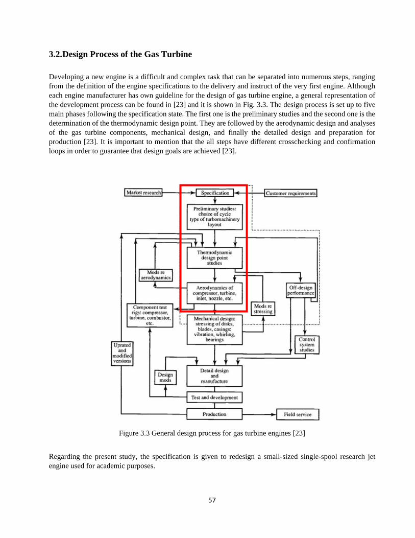
57

3.2. Design Process of the Gas Turbine

Developing a new engine is a difficult and complex task that can be separated into numerous steps, ranging

from the definition of the engine specifications to the delivery and instruct of the very first engine. Although

each engine manufacturer has own guideline for the design of gas turbine engine, a general representation of

the development process can be found in [23] and it is shown in Fig. 3.3. The design process is set up to five

main phases following the specification state. The first one is the preliminary studies and the second one is the

determination of the thermodynamic design point. They are followed by the aerodynamic design and analyses

of the gas turbine components, mechanical design, and finally the detailed design and preparation for

production [23]. It is important to mention that the all steps have different crosschecking and confirmation

loops in order to guarantee that design goals are achieved [23].

Figure 3.3 General design process for gas turbine engines [23]

Regarding the present study, the specification is given to redesign a small-sized single-spool research jet

engine used for academic purposes.

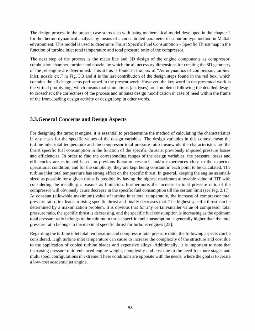
58

The design process in the present case starts also with using mathematical model developed in the chapter 2

for the thermo-dynamical analysis by means of a concentrated parameter distribution type method in Matlab

environment. This model is used to determine Thrust Specific Fuel Consumption – Specific Thrust map in the

function of turbine inlet total temperature and total pressure ratio of the compressor.

The next step of the process is the mean line and 3D design of the engine components as compressor,

combustion chamber, turbine and nozzle, by which the all necessary dimensions for creating the 3D geometry

of the jet engine are determined. This status is found in the box of “Aerodynamics of compressor, turbine,

inlet, nozzle etc.” in Fig. 3.3 and it is the last contribution of the design steps found in the red box, which

contains the all design steps performed in the present work. However, the key word in the presented work is

the virtual prototyping, which means that simulations (analyses) are completed following the detailed design

to crosscheck the correctness of the process and initiates design modification in case of need within the frame

of the front-loading design activity or design loop in other words.

3.3. General Concerns and Design Aspects

For designing the turbojet engine, it is essential to predetermine the method of calculating the characteristics

in any cases for the specific values of the design variables. The design variables in this context mean the

turbine inlet total temperature and the compressor total pressure ratio meanwhile the characteristics are the

thrust specific fuel consumption in the function of the specific thrust at previously imposed pressure losses

and efficiencies. In order to find the corresponding ranges of the design variables, the pressure losses and

efficiencies are estimated based on previous literature research and/or experiences close to the expected

operational condition, and for the simplicity, they are kept being constant in each point to be calculated. The

turbine inlet total temperature has strong effect on the specific thrust. In general, keeping the engine as small-

sized as possible for a given thrust is possible by having the highest maximum allowable value of TIT with

considering the metallurgic reasons as limitation. Furthermore, the increase in total pressure ratio of the

compressor will obviously cause decrease in the specific fuel consumption till the certain limit (see Fig. 2.17).

At constant (allowable maximum) value of turbine inlet total temperature, the increase of compressor total

pressure ratio first leads to rising specific thrust and finally decreases that. The highest specific thrust can be

determined by a maximization problem. It is obvious that for any certain/smaller value of compressor total

pressure ratio, the specific thrust is decreasing, and the specific fuel consumption is increasing as the optimum

total pressure ratio belongs to the minimum thrust specific fuel consumption is generally higher than the total

pressure ratio belongs to the maximal specific thrust for turbojet engines [23].

Regarding the turbine inlet total temperature and compressor total pressure ratio, the following aspects can be

considered. High turbine inlet temperature can cause to increase the complexity of the structure and cost due

to the application of cooled turbine blades and expensive alloys. Additionally, it is important to note that

increasing pressure ratio enhanced engine weight, complexity and cost due to the need for more stages and

multi spool configurations in extreme. These conditions are opposite with the needs, where the goal is to create

a low-cost academic jet engine.

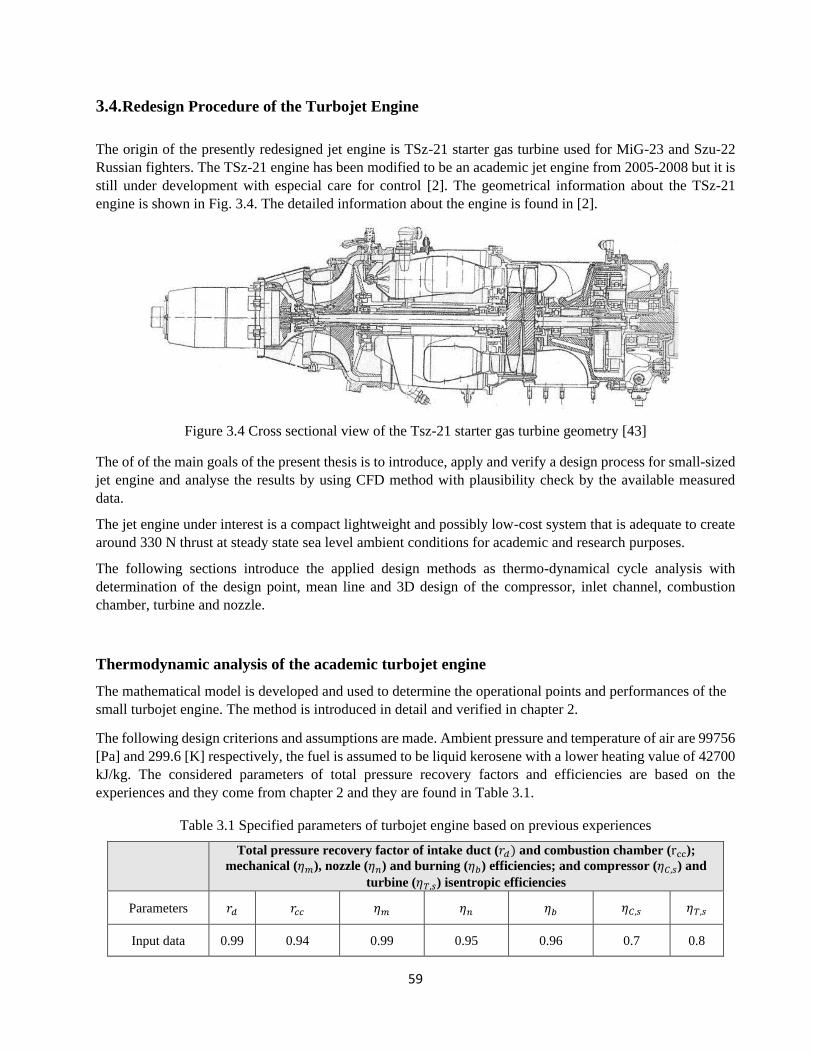
59

3.4. Redesign Procedure of the Turbojet Engine

The origin of the presently redesigned jet engine is TSz-21 starter gas turbine used for MiG-23 and Szu-22

Russian fighters. The TSz-21 engine has been modified to be an academic jet engine from 2005-2008 but it is

still under development with especial care for control [2]. The geometrical information about the TSz-21

engine is shown in Fig. 3.4. The detailed information about the engine is found in [2].

Figure 3.4 Cross sectional view of the Tsz-21 starter gas turbine geometry [43]

The of of the main goals of the present thesis is to introduce, apply and verify a design process for small-sized

jet engine and analyse the results by using CFD method with plausibility check by the available measured

data.

The jet engine under interest is a compact lightweight and possibly low-cost system that is adequate to create

around 330 N thrust at steady state sea level ambient conditions for academic and research purposes.

The following sections introduce the applied design methods as thermo-dynamical cycle analysis with

determination of the design point, mean line and 3D design of the compressor, inlet channel, combustion

chamber, turbine and nozzle.

Thermodynamic analysis of the academic turbojet engine

The mathematical model is developed and used to determine the operational points and performances of the

small turbojet engine. The method is introduced in detail and verified in chapter 2.

The following design criterions and assumptions are made. Ambient pressure and temperature of air are 99756

[Pa] and 299.6 [K] respectively, the fuel is assumed to be liquid kerosene with a lower heating value of 42700

kJ/kg. The considered parameters of total pressure recovery factors and efficiencies are based on the

experiences and they come from chapter 2 and they are found in Table 3.1.

Table 3.1 Specified parameters of turbojet engine based on previous experiences

Total pressure recovery factor of intake duct (𝑟𝑑) and combustion chamber (rcc);

mechanical (휂𝑚), nozzle (휂𝑛) and burning (휂𝑏) efficiencies; and compressor (휂𝐶,𝑠) and

turbine (휂𝑇,𝑠) isentropic efficiencies

Parameters 𝑟𝑑 𝑟𝑐𝑐 휂𝑚 휂𝑛 휂𝑏 휂𝐶,𝑠 휂𝑇,𝑠

Input data 0.99 0.94 0.99 0.95 0.96 0.7 0.8

60

The next step is to determine the expected design point of the jet engine. Hence, first, the performance map of

the gas turbine has been created, where the thrust specific fuel consumption values are plotted in the function

of the specific thrust, turbine inlet total temperature and total pressure ratio of the compressor. By this way,

the effect of compressor pressure ratio on air mass flow rate is excluded; the variation in compressor pressure

ratio does not change the mass flow rate across the engine at the same temperature. The outputs of the cycle

analyses are used to determine the specific thrust (Eq. (3.1)) and thrust specific fuel consumption (Eq. (3.2))

[1]:

𝑇𝑠 = (1 + 𝑓𝑐𝑐)𝑉9 − 𝑉0 +(1 + 𝑓𝑐𝑐)

𝜌9𝑉9(𝑝9 − 𝑝0) (3.1)

𝑇𝑆𝐹𝐶 =𝑓𝑐𝑐𝑇𝑠

(3.2)

The subscripts are based on the numbering shown in Fig. 2.9.

The performance map of the engine is shown in Fig. 3.5. For designing the jet engine, the basic thermo-

dynamic parameters to be determined are the compressor total pressure ratio (πC) and turbine inlet temperature

(T04).

Figure 3.5 Performance characteristics of the academic jet engine

A total pressure ratio 2.5 is selected in the present case to be a reasonable compromise within the investigated

range. As to achieve higher pressure ratio, it is required to consider advanced aerodynamic developments for

the compressor, higher dimension, performance and state of the art production technology, which cannot be

afforded by university application in the recent conditions. 1000 K turbine inlet total temperature is selected

with considering that there is limited access for using high-tech cooling technology and advanced materials

for the turbine blades.

Selected

point

61

The specific thrust is 327 Ns/kg (9.08E-5 Nh/g) at this point. So, by having the expected and the specific thrust

of the academic jet engine, the mass flow rate of the incoming air is determined by the following way:

��𝑎𝑖𝑟 =𝑇

𝑇𝑠=

330 𝑁

327 𝑁/(𝑘𝑔/𝑠)= 1.009

𝑘𝑔

𝑠≈ 1

𝑘𝑔

𝑠 (3.3)

The mass flow rate of the fuel is 0.019 kg/s by Eq. (3.4) in the design point as the thrust specific fuel

consumption is 209 g/Nh.

𝑇𝑆𝐹𝐶 =��𝑓

𝑇 (3.4)

The real thermo-dynamical cycle of the engine in T-s diagram is plotted in Fig. 3.6. The red curves (with

smaller thickness) represent the constant pressures. The processes between the engine states denoted by

numbers are plotted by thicker lines. This visualization effect is the reason of constant pressure lines goes

below the process line in case of pressure decrement just after section “3”.

The thermodynamic parameters at the engine sections are shown in the Table 3.2

Figure 3.6 The T-s diagram of the academic jet engine

Table 3.2 Total pressure and temperature resulted by the thermodynamic cycle analysis.

Parameters Ambient

conditions

Inlet of the

compressor (outlet

of the diffuser)

Inlet of the

combustion

chamber

Inlet of

the

turbine

Inlet

of the

nozzle

Exit of the nozzle

Total

pressure [Pa] 99756 98758 246896 232082 125722

124240

(static one: 99756)

Total

temperature

[K]

299.6 299.6 427.68 1000 887.12 887.12

(static one: 840.1)

0 2

3

4

5

9

62

3D design of the academic turbojet engine

After completing the thermodynamic analysis based on the required design specifications, the next step is to

determine the geometrical sizes of the basic engine components as inlet diffuser, compressor, combustion

chamber, turbine and exhaust nozzle [1]. As these designs are based on well established methods, the details

of the component-designs are shown in Appendix A.

3.5. Conclusions

The aerodynamic redesign of a small academic jet engine has been introduced in the present part of the thesis.

The considered engine was a starter gas turbine originally, which has been used for MiG-23 and Szu-22

Russian fighters. The engine was reconstructed to be a propulsion system by Dr. Beneda and Dr. Pásztor [2].

The present redesign process starts with the cycle analysis to determine the main thermodynamic parameters

at the expected 330 N thrust at stationary (start) condition. The thermodynamic parameters are determined

with viscous flow assumption and location dependent material properties in order to calculate the specific

thrust and thrust specific fuel consumption. After making decision about operational point and having the

states of the thermo-dynamical cycle, mean line design of the centrifugal compressor and axial turbine are

completed. Following the 3D extension of the blades and the determination of the blade angles, chords,

spacings, blade numbers and profiles, the 3D CAD models are prepared. Beside the compressor and turbine,

the 3D models of the intake channel, combustion chamber and exhaust nozzle are also created. The main

design criteria of these last three structures are to fit their geometrical sizes to the compressor and turbine and

provide minimum pressure recovery factors. Moreover, the combustion chamber additionally should have high

burning efficiency. The calculated thrust is 333.1 N, which is in line with the design specification. The

aerodynamic design process of the components of the academic jet engine is introduced in Appendix A in

detail.

The CFD analyses for crosschecking the correctness and the accuracy of the design are presented in chapter

4. CFD models with separated components and with complete assembly, as two approaches, have been used

for that purpose.

The quantitative results of the i. thermodynamic design, ii. mean line design, iii. separated CFD analysis, iv.

full model CFD analysis and v. the available measured data are shown and discussed in the chapter 5.

63

4. CFD Analysis of the Redesigned Academic Jet Engine

In the last decades, the benefit of CFD has been used in the design process more than before. Using that

computational technology, numerous measurements can be replaced or reduced significantly, and so cost,

capacity and time of developments can be saved. Many activities are available in that field [44, 45, 46]. The

parameterization of the geometry provides higher reproducibility and flexibility in the model generation. The

wide range of the visualization techniques get insight into the origin of the problem much deeper as ever was.

Consistency, stability and convergence characteristics of the different numerical methods have been

investigated and proved. The accuracy of the available methods allows designers to turn more effort on the

new fields of the engineering practice called virtual prototyping, which is going to be the keyword of the next

decades.

ANSYS CFX has been used for CFD analyses in the present work. The ANSYS CFX software is a state of the

art, high-performance and general-purpose fluid dynamics program that has been applied to solve a wide-

range of continuum-based fluid flow problems for over 25 years. The core feature of the ANSYS CFX is its

advanced solver technology, the key to achieve reliable and accurate solutions quickly and robustly. The

modern, highly parallelized solver is the foundation for an abundant choice of physical models to capture

virtually any type of phenomena related to fluid flow. The solver and its many physical models are wrapped

in a modern, intuitive and flexible GUI and user environment with extensive capabilities for customization

and automation using session files, scripting and a powerful expression language [47] [48].

More information about the used CFD software is found in the Appendix B.

The all components of the academic jet engine are available in 3D CAD format till the end of the design

process described in the previous chapter. The next step of the investigation is to crosscheck how the all

components working separately and together, how their operation fulfil the design criterions and how their

parameters fit to the parameters come from the design. Hence, 3D CFD simulations are prepared and

completed.

Solid Edge software has been used for making the 3D models based on the geometry output described in

chapter 3. Then Boolean operation is used to create flow fields from the solid structures. The solid domains

are subtracted from the reasonable oversized volumes to get the flow field for the compressor, for the

combustion chamber, for the turbine and for the nozzle. The 3D geometry of the assembly in wireframe model

is shown in Fig. 4.1.

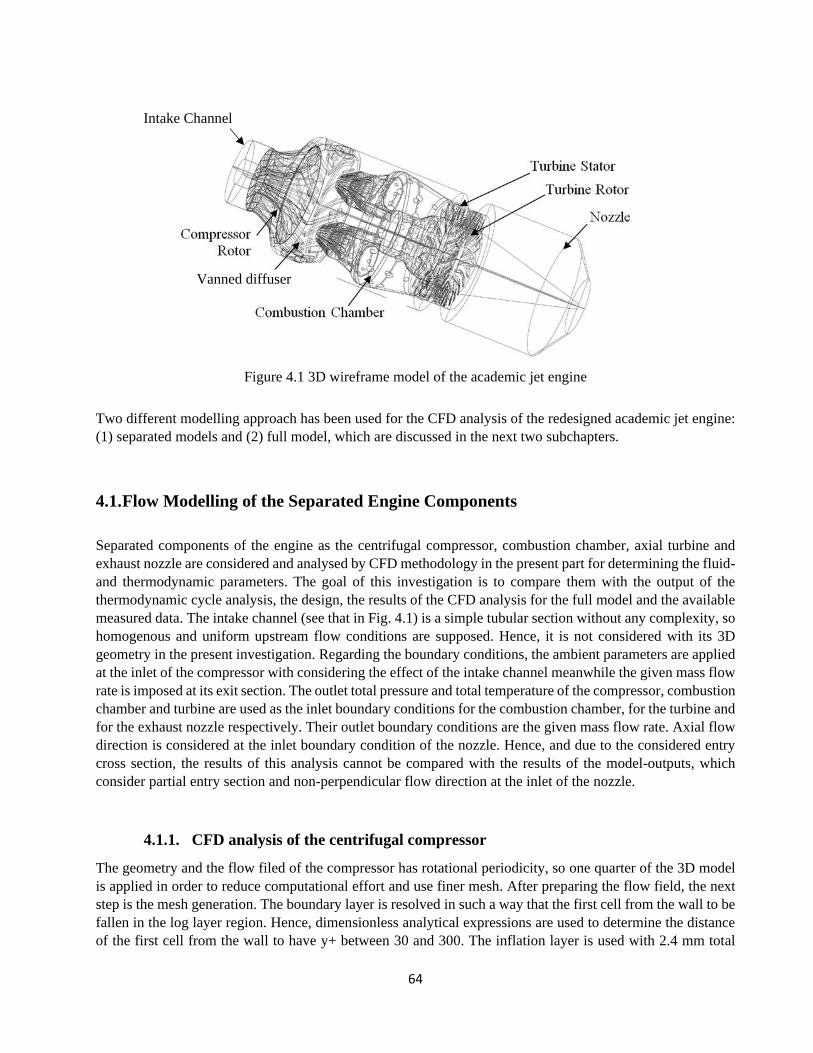
64

Figure 4.1 3D wireframe model of the academic jet engine

Two different modelling approach has been used for the CFD analysis of the redesigned academic jet engine:

(1) separated models and (2) full model, which are discussed in the next two subchapters.

4.1. Flow Modelling of the Separated Engine Components

Separated components of the engine as the centrifugal compressor, combustion chamber, axial turbine and

exhaust nozzle are considered and analysed by CFD methodology in the present part for determining the fluid-

and thermodynamic parameters. The goal of this investigation is to compare them with the output of the

thermodynamic cycle analysis, the design, the results of the CFD analysis for the full model and the available

measured data. The intake channel (see that in Fig. 4.1) is a simple tubular section without any complexity, so

homogenous and uniform upstream flow conditions are supposed. Hence, it is not considered with its 3D

geometry in the present investigation. Regarding the boundary conditions, the ambient parameters are applied

at the inlet of the compressor with considering the effect of the intake channel meanwhile the given mass flow

rate is imposed at its exit section. The outlet total pressure and total temperature of the compressor, combustion

chamber and turbine are used as the inlet boundary conditions for the combustion chamber, for the turbine and

for the exhaust nozzle respectively. Their outlet boundary conditions are the given mass flow rate. Axial flow

direction is considered at the inlet boundary condition of the nozzle. Hence, and due to the considered entry

cross section, the results of this analysis cannot be compared with the results of the model-outputs, which

consider partial entry section and non-perpendicular flow direction at the inlet of the nozzle.

4.1.1. CFD analysis of the centrifugal compressor

The geometry and the flow filed of the compressor has rotational periodicity, so one quarter of the 3D model

is applied in order to reduce computational effort and use finer mesh. After preparing the flow field, the next

step is the mesh generation. The boundary layer is resolved in such a way that the first cell from the wall to be

fallen in the log layer region. Hence, dimensionless analytical expressions are used to determine the distance

of the first cell from the wall to have y+ between 30 and 300. The inflation layer is used with 2.4 mm total

Vanned diffuser

Intake Channel

65

thickness and 1.2 growth rate on the blade wall of the rotor and stator. The inflation layer is built up from 5

layers. Although the hex-dominant elements give better resolution due to the discretization method at grid

aligned flow conditions, tetrahedron elements have been used due to the complexity of the geometry. The final

mesh is built up from 3471912 elements and it contains 986800 nodes (see Fig. 4.2.).

Figure 4.2 The final mesh of the centrifugal compressor passage (left) with the cut section of the rotor blade

(right, top) and the stator vanes (right, bottom) meshing

Steady state continuum mechanics-based flow simulation is completed in ANSYS CFX software. 3D,

compressible, turbulent and viscous air flow is considered. The operational fluid is assumed to be ideal gas.

SST turbulence model is applied due to their advanced physical capabilities described in Appendix B.

subchapter B.2. Frozen rotor interface has been used for rotor-stator interaction. Constant 43000 RPM is

defined for the flow field of the impeller with no slip boundary condition for the relative velocity at the walls.

Counter rotating wall option is set at the shroud section of the rotating flow field. Total pressure and total

temperature at the inlet and mass flow rate at the outlet of the compressor unit have been defined as boundary

condition. The heat transfer coefficient 8 W/(m2 K) corresponds to the stationer ambient air with 299.6 K

temperature on the outer walls is applied for considering free convection, meanwhile adiabatic condition is

imposed at the inner-side walls [49]. Table 4.1 shows the exact value of the boundary conditions, which are

used in the simulations and Fig. 4.3 provides an overview about the locations of the used boundary conditions

(excluding the solid walls).

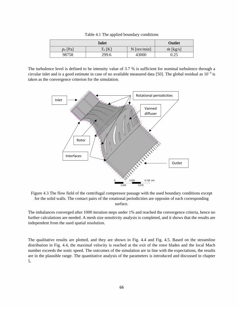
66

Table 4.1 The applied boundary conditions

Inlet Outlet

p0 [Pa] T0 [K] N [rev/min] �� [kg/s]

98758 299.6 43000 0.25

The turbulence level is defined to be intensity value of 3.7 % is sufficient for nominal turbulence through a

circular inlet and is a good estimate in case of no available measured data [50]. The global residual as 10−4 is

taken as the convergence criterion for the simulation.

Figure 4.3 The flow field of the centrifugal compressor passage with the used boundary conditions except

for the solid walls. The contact pairs of the rotational periodicities are opposite of each corresponding

surface.

The imbalances converged after 1000 iteration steps under 1% and reached the convergence criteria, hence no

further calculations are needed. A mesh size sensitivity analysis is completed, and it shows that the results are

independent from the used spatial resolution.

The qualitative results are plotted, and they are shown in Fig. 4.4 and Fig. 4.5. Based on the streamline

distribution in Fig. 4.4, the maximal velocity is reached at the exit of the rotor blades and the local Mach

number exceeds the sonic speed. The outcomes of the simulation are in line with the expectations, the results

are in the plausible range. The quantitative analysis of the parameters is introduced and discussed in chapter

5.

Inlet

Outlet

Rotational periodicities

Interfaces

Rotor

Vanned

diffuser

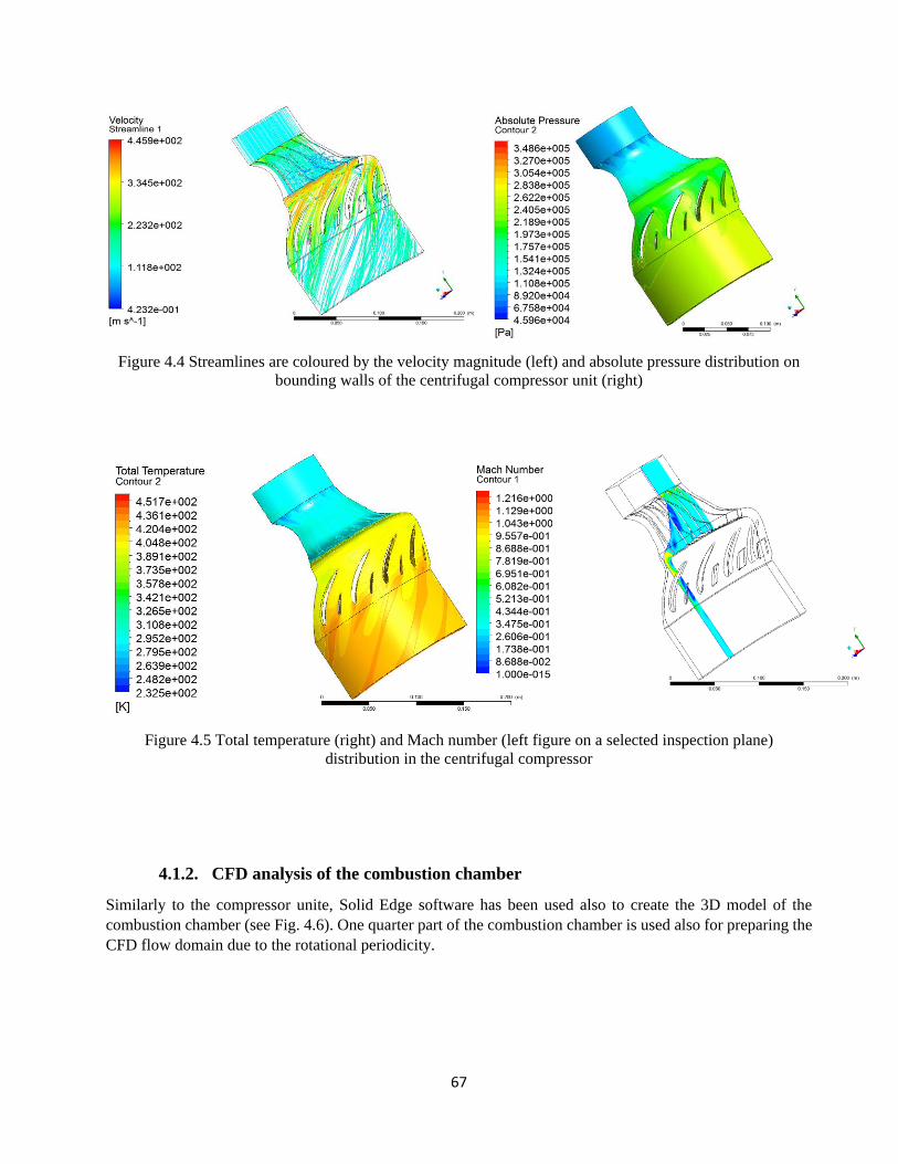
67

Figure 4.4 Streamlines are coloured by the velocity magnitude (left) and absolute pressure distribution on

bounding walls of the centrifugal compressor unit (right)

Figure 4.5 Total temperature (right) and Mach number (left figure on a selected inspection plane)

distribution in the centrifugal compressor

4.1.2. CFD analysis of the combustion chamber

Similarly to the compressor unite, Solid Edge software has been used also to create the 3D model of the

combustion chamber (see Fig. 4.6). One quarter part of the combustion chamber is used also for preparing the

CFD flow domain due to the rotational periodicity.

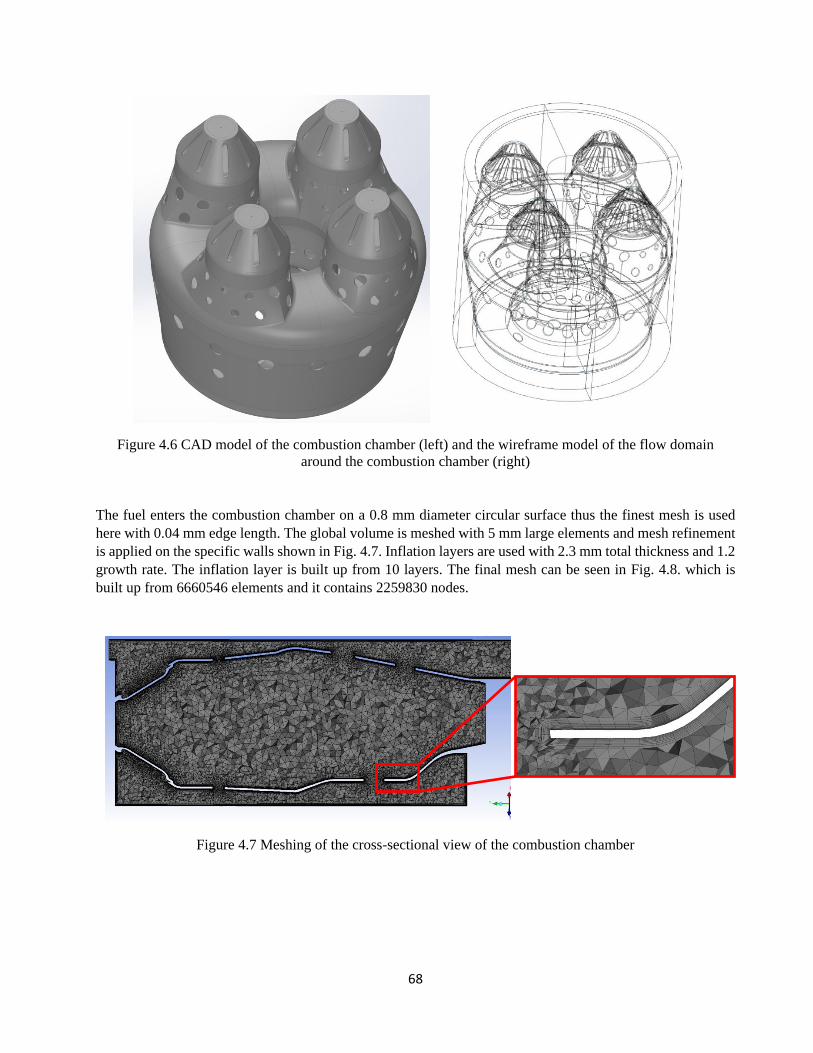
68

Figure 4.6 CAD model of the combustion chamber (left) and the wireframe model of the flow domain

around the combustion chamber (right)

The fuel enters the combustion chamber on a 0.8 mm diameter circular surface thus the finest mesh is used

here with 0.04 mm edge length. The global volume is meshed with 5 mm large elements and mesh refinement

is applied on the specific walls shown in Fig. 4.7. Inflation layers are used with 2.3 mm total thickness and 1.2

growth rate. The inflation layer is built up from 10 layers. The final mesh can be seen in Fig. 4.8. which is

built up from 6660546 elements and it contains 2259830 nodes.

Figure 4.7 Meshing of the cross-sectional view of the combustion chamber

69

Figure 4.8 Final mesh of the combustion chamber

The fluid dynamic phenomena are turbulent, and they are combined with heat transfer processes and the

reaction kinetics in the combustion chamber. So, beside the basic governing equations as mass-, momentum-

and energy conservation laws, supplementary equations are needed to be solved numerically. The standard k-

epsilon turbulence model and P-1 radiation model is used in this analysis. Regarding the combustion, non-

premixed combustion modelling with the PDF-mixture fraction model is applied. In the non-premixed

combustion, the fuel and oxidizer enter separately in the reaction zone. The PDF Flamelet combustion model

is considered, it can handle chemical reactions by means of going through in a non-premixed turbulent fluid

flow in a short time frame. The generated Flame let library for Jet A is large, since it includes all the possible

species that can exist in the Jet-A combustion. Simulations with this library take much computational time and

computer resources, even the required time to load this library at the beginning of each simulation. In order to

save time, the spices of the library are reduced to H, O2, OH, O, H2, H2O, CO, CO2, n-C10H22, TMB-C9H12 and

N2 [51]. Table 4.2. represents the list of applied models to be used in this simulation with especial care for the

combustion modelling.

Table 4.2 The applied methods and settings for modelling processes in the combustion chamber

Advection scheme High resolution

Turbulence model discretization scheme High resolution

Turbulence model K-Epsilon

Liquid phase Lagrangian Particle Tracking

Primary breakup Blob Method

Drag Force Schiller-Naumann

Heat transfer Ranz-Marshall

Combustion PDF Flamelet

Thermal radiation model P-1

Fig. 4.9 provides an overview about the boundary conditions (excluding the solid walls), which has been

considered in the simulation of the combustion and Table 4.3 shows their exact value.

Table 4.3 The applied boundary conditions for combustion chamber

Inlet air Inlet fuel Outlet

p0 [Pa] T0 [K] V [m/s] T0 [K] ��𝑓𝑢𝑒𝑙 [kg/s] ��[kg/s]

267175.2 419.5 12 299.6 0.00475 0.25

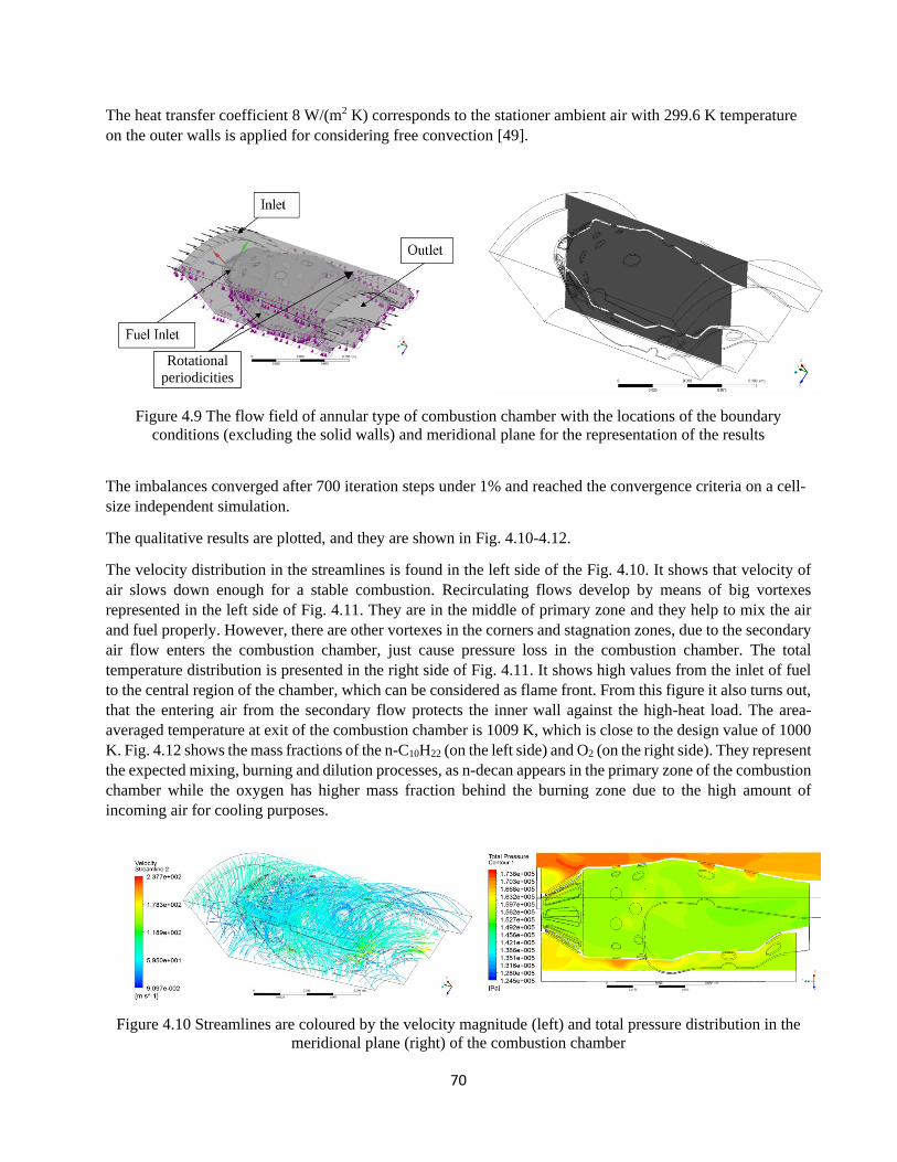
70

The heat transfer coefficient 8 W/(m2 K) corresponds to the stationer ambient air with 299.6 K temperature

on the outer walls is applied for considering free convection [49].

Figure 4.9 The flow field of annular type of combustion chamber with the locations of the boundary

conditions (excluding the solid walls) and meridional plane for the representation of the results

The imbalances converged after 700 iteration steps under 1% and reached the convergence criteria on a cell-

size independent simulation.

The qualitative results are plotted, and they are shown in Fig. 4.10-4.12.

The velocity distribution in the streamlines is found in the left side of the Fig. 4.10. It shows that velocity of

air slows down enough for a stable combustion. Recirculating flows develop by means of big vortexes

represented in the left side of Fig. 4.11. They are in the middle of primary zone and they help to mix the air

and fuel properly. However, there are other vortexes in the corners and stagnation zones, due to the secondary

air flow enters the combustion chamber, just cause pressure loss in the combustion chamber. The total

temperature distribution is presented in the right side of Fig. 4.11. It shows high values from the inlet of fuel

to the central region of the chamber, which can be considered as flame front. From this figure it also turns out,

that the entering air from the secondary flow protects the inner wall against the high-heat load. The area-

averaged temperature at exit of the combustion chamber is 1009 K, which is close to the design value of 1000

K. Fig. 4.12 shows the mass fractions of the n-C10H22 (on the left side) and O2 (on the right side). They represent

the expected mixing, burning and dilution processes, as n-decan appears in the primary zone of the combustion

chamber while the oxygen has higher mass fraction behind the burning zone due to the high amount of

incoming air for cooling purposes.

Figure 4.10 Streamlines are coloured by the velocity magnitude (left) and total pressure distribution in the

meridional plane (right) of the combustion chamber

Rotational

periodicities

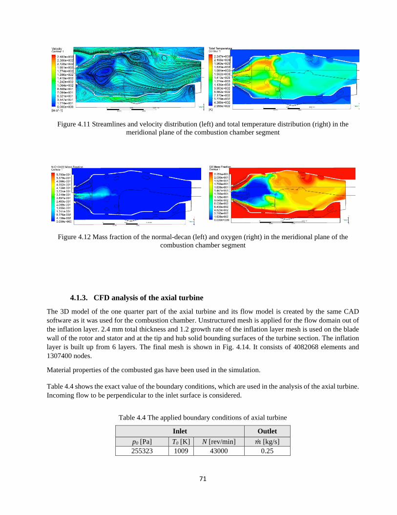
71

Figure 4.11 Streamlines and velocity distribution (left) and total temperature distribution (right) in the

meridional plane of the combustion chamber segment

Figure 4.12 Mass fraction of the normal-decan (left) and oxygen (right) in the meridional plane of the

combustion chamber segment

4.1.3. CFD analysis of the axial turbine

The 3D model of the one quarter part of the axial turbine and its flow model is created by the same CAD

software as it was used for the combustion chamber. Unstructured mesh is applied for the flow domain out of

the inflation layer. 2.4 mm total thickness and 1.2 growth rate of the inflation layer mesh is used on the blade

wall of the rotor and stator and at the tip and hub solid bounding surfaces of the turbine section. The inflation

layer is built up from 6 layers. The final mesh is shown in Fig. 4.14. It consists of 4082068 elements and

1307400 nodes.

Material properties of the combusted gas have been used in the simulation.

Table 4.4 shows the exact value of the boundary conditions, which are used in the analysis of the axial turbine.

Incoming flow to be perpendicular to the inlet surface is considered.

Table 4.4 The applied boundary conditions of axial turbine

Inlet Outlet

p0 [Pa] T0 [K] N [rev/min] �� [kg/s]

255323 1009 43000 0.25

72

Figure 4.13 The final mesh of the axial turbine (top left) with cut section through the vanes (top right,

bottom left and bottom right) including the inflation layer

Fig. 4.14 provides an overview about the flow fields, interfaces and boundary conditions (except for the solid

walls and periodic surfaces), which have been used in the simulation.

Figure 4.14 The flow fields, interfaces and the locations of the boundary conditions (except for the solid

walls and periodic surfaces) of the axial turbine

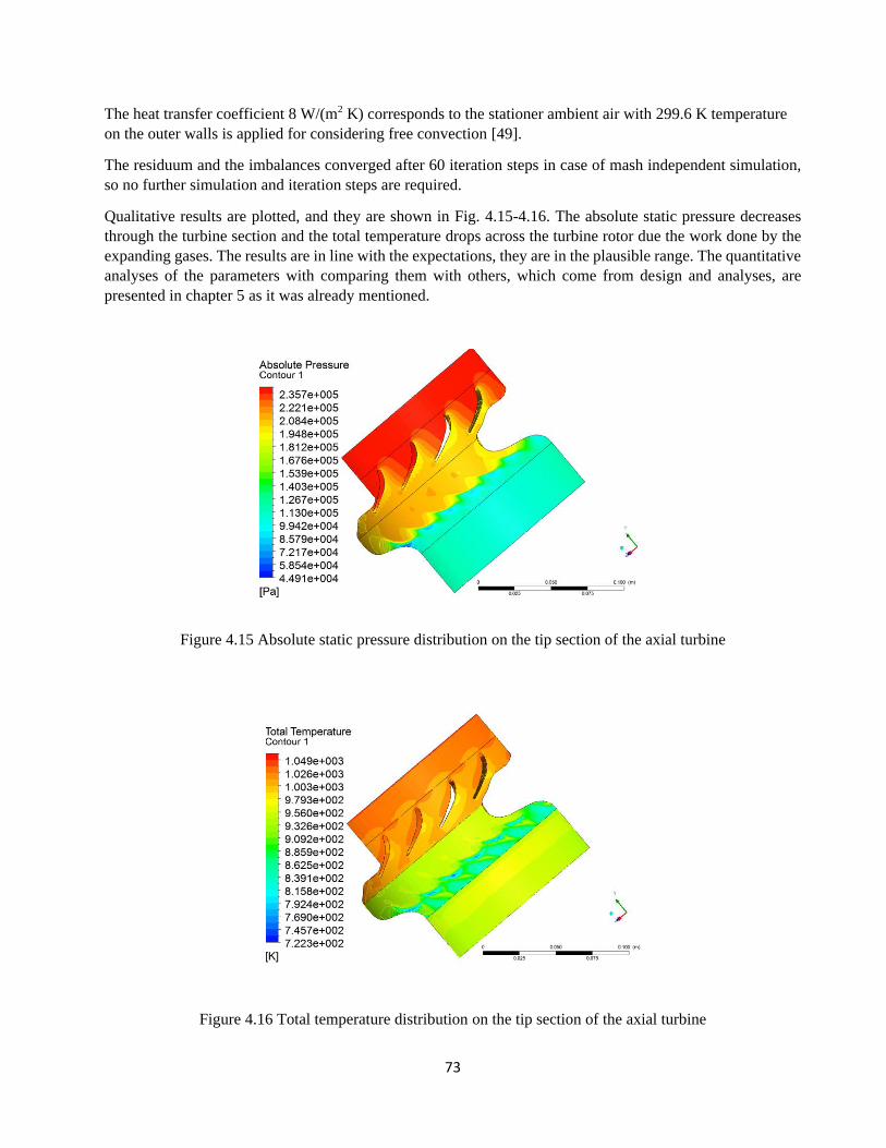
73

The heat transfer coefficient 8 W/(m2 K) corresponds to the stationer ambient air with 299.6 K temperature

on the outer walls is applied for considering free convection [49].

The residuum and the imbalances converged after 60 iteration steps in case of mash independent simulation,

so no further simulation and iteration steps are required.

Qualitative results are plotted, and they are shown in Fig. 4.15-4.16. The absolute static pressure decreases

through the turbine section and the total temperature drops across the turbine rotor due the work done by the

expanding gases. The results are in line with the expectations, they are in the plausible range. The quantitative

analyses of the parameters with comparing them with others, which come from design and analyses, are

presented in chapter 5 as it was already mentioned.

Figure 4.15 Absolute static pressure distribution on the tip section of the axial turbine

Figure 4.16 Total temperature distribution on the tip section of the axial turbine

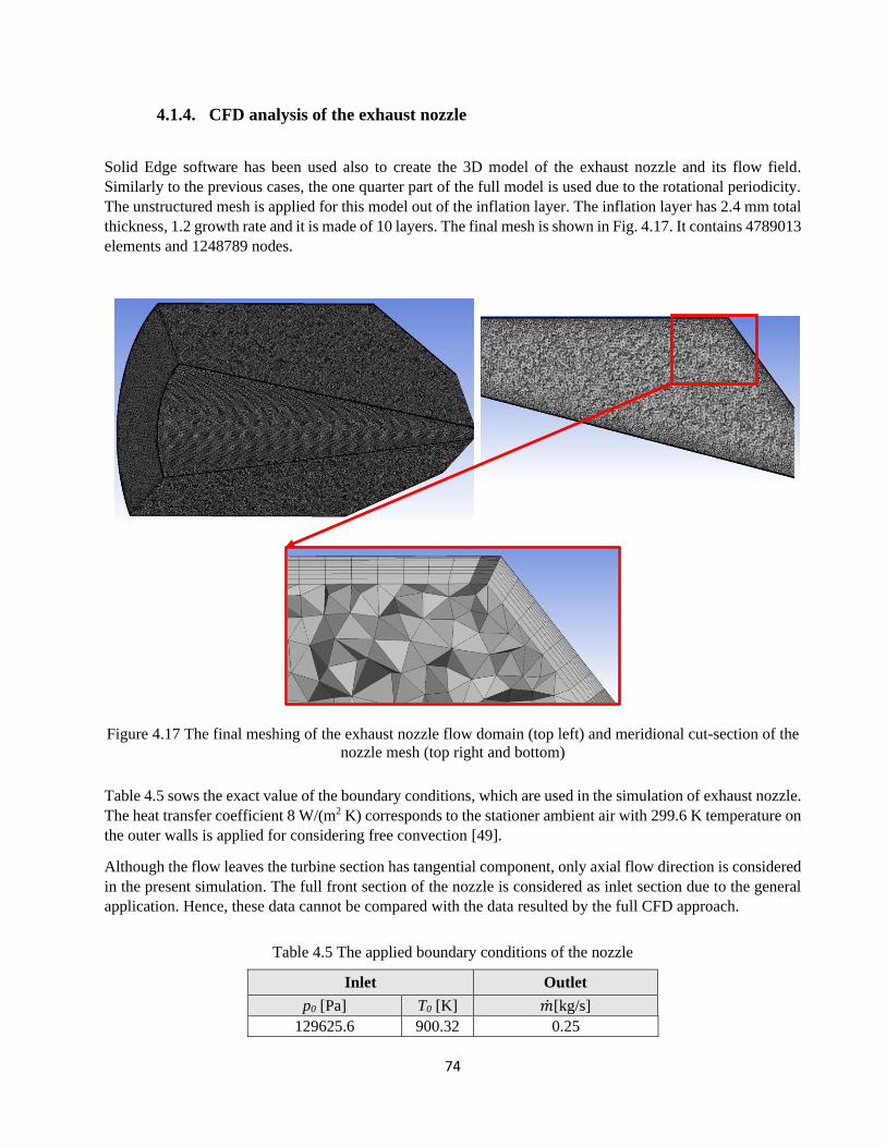
74

4.1.4. CFD analysis of the exhaust nozzle

Solid Edge software has been used also to create the 3D model of the exhaust nozzle and its flow field.

Similarly to the previous cases, the one quarter part of the full model is used due to the rotational periodicity.

The unstructured mesh is applied for this model out of the inflation layer. The inflation layer has 2.4 mm total

thickness, 1.2 growth rate and it is made of 10 layers. The final mesh is shown in Fig. 4.17. It contains 4789013

elements and 1248789 nodes.

Figure 4.17 The final meshing of the exhaust nozzle flow domain (top left) and meridional cut-section of the

nozzle mesh (top right and bottom)

Table 4.5 sows the exact value of the boundary conditions, which are used in the simulation of exhaust nozzle.

The heat transfer coefficient 8 W/(m2 K) corresponds to the stationer ambient air with 299.6 K temperature on

the outer walls is applied for considering free convection [49].

Although the flow leaves the turbine section has tangential component, only axial flow direction is considered

in the present simulation. The full front section of the nozzle is considered as inlet section due to the general

application. Hence, these data cannot be compared with the data resulted by the full CFD approach.

Table 4.5 The applied boundary conditions of the nozzle

Inlet Outlet

p0 [Pa] T0 [K] ��[kg/s]

129625.6 900.32 0.25

75

Fig. 4.18 provides an overview about the boundary conditions, which has been used in the simulation.

Figure 4.18 Flow field of the exhaust nozzle with the used boundary conditions (left) and the cut section for

displaying the results (right)

The residuum and imbalances are converged after 15 iteration steps. The results are mesh independent.

The qualitative outcomes of the simulation are shown in Fig. 4.19 and 4.20. The static pressure and temperature

reduce, and the velocity increases during the expansion process. The results are plausible, the parameters are

in the expected ranges.

Figure 4.19 Streamlines are coloured by the velocity magnitude in the flow domain (left) and absolute static

pressure distribution in the cut section of the nozzle (right)

Periodic

Solid

walls

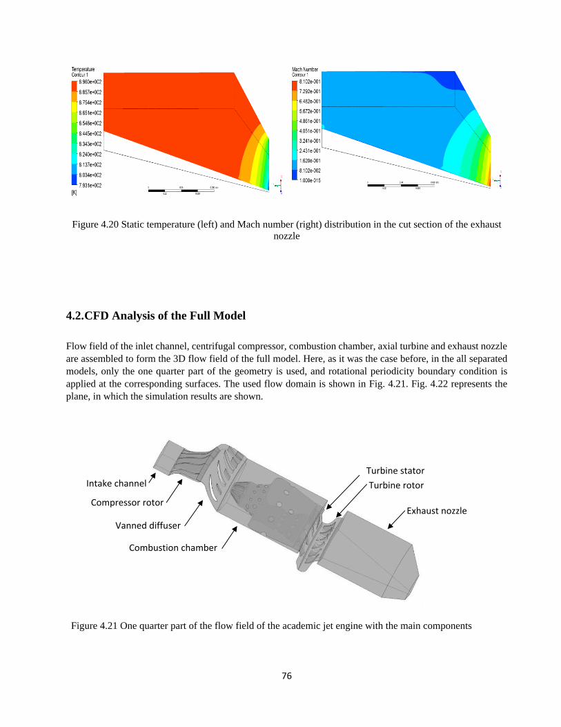
76

Figure 4.20 Static temperature (left) and Mach number (right) distribution in the cut section of the exhaust

nozzle

4.2. CFD Analysis of the Full Model

Flow field of the inlet channel, centrifugal compressor, combustion chamber, axial turbine and exhaust nozzle

are assembled to form the 3D flow field of the full model. Here, as it was the case before, in the all separated

models, only the one quarter part of the geometry is used, and rotational periodicity boundary condition is

applied at the corresponding surfaces. The used flow domain is shown in Fig. 4.21. Fig. 4.22 represents the

plane, in which the simulation results are shown.

Figure 4.21 One quarter part of the flow field of the academic jet engine with the main components

Exhaust nozzle

Turbine rotor

Turbine stator

Combustion chamber

Intake channel

channel Compressor rotor

Vanned diffuser

77

Figure 4.22 Flow field of a quarter academic jet engine by wire frame and the meridional plane for showing

the results

The numerical mesh is designed to apply local mesh refinement at the high gradient flow conditions and to

guarantee the completeness of y+ to be 30-300. The expectation is that results should be mesh independent by

maximum 5 % allowing differences in the thrust. The final mesh is built up from 4799728 elements and it

contains 2067312 nodes. The final mesh configuration is shown in Fig. 4.23.

Figure 4.23 The final mesh for the one quarter flow field of the academic jet engine

The material properties of the incoming air as ideal gas are γ = 1.4 and R = 287.058 J/(kg K). The reference

pressure of the domains is 99756 Pa. The ambient air enters in the jet engine and the hot gases expand in the

environments. Hence 99756 Pa total pressure and 299.6 K total temperature with normal flow direction into

the inlet surface of the intake flow channel is defined as inlet boundary condition. 99756 Pa static pressure is

defined as outlet boundary condition. 43000 RPM rotational speed is defined for the rotating flow domain of

the compressor and turbine. Table 4.6 shows the used boundary conditions.

The list of applied models for the combustion chamber is found in Table 4.2.

Fig. 4.24 provides an overview about the type and the location of the used boundary conditions.

The heat transfer coefficient is 8 W/(m2 K) corresponding to the stationer ambient air with 299.6 K temperature

on the outer walls is applied for considering the free convection [49].

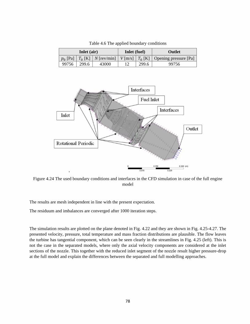
78

Table 4.6 The applied boundary conditions

Inlet (air) Inlet (fuel) Outlet

𝑝0 [Pa] 𝑇0 [K] N [rev/min] V [m/s] 𝑇0 [K] Opening pressure [Pa]

99756 299.6 43000 12 299.6 99756

Figure 4.24 The used boundary conditions and interfaces in the CFD simulation in case of the full engine

model

The results are mesh independent in line with the present expectation.

The residuum and imbalances are converged after 1000 iteration steps.

The simulation results are plotted on the plane denoted in Fig. 4.22 and they are shown in Fig. 4.25-4.27. The

presented velocity, pressure, total temperature and mass fraction distributions are plausible. The flow leaves

the turbine has tangential component, which can be seen clearly in the streamlines in Fig. 4.25 (left). This is

not the case in the separated models, where only the axial velocity components are considered at the inlet

sections of the nozzle. This together with the reduced inlet segment of the nozzle result higher pressure-drop

at the full model and explain the differences between the separated and full modelling approaches.

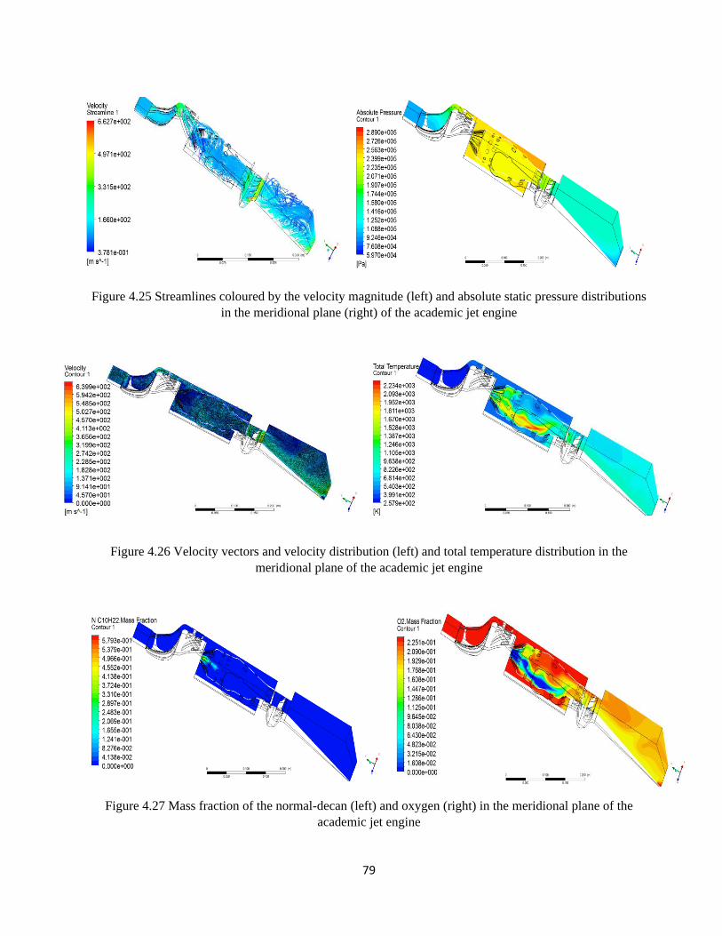
79

Figure 4.25 Streamlines coloured by the velocity magnitude (left) and absolute static pressure distributions

in the meridional plane (right) of the academic jet engine

Figure 4.26 Velocity vectors and velocity distribution (left) and total temperature distribution in the

meridional plane of the academic jet engine

Figure 4.27 Mass fraction of the normal-decan (left) and oxygen (right) in the meridional plane of the

academic jet engine

80

4.3. Conclusions

The goal of the present chapter of the thesis is to complete CFD analyses for the separated and for the full

models of the academic jet engine under investigation. The outcomes of these computations can be used to

determine and evaluate the accuracy of the analysis, design and to compare them with the available measured

data. The qualitative results of the analyses are plausible, and the two CFD approaches (for separated and full

models) provide parameters in the same ranges except for the exhaust nozzle, where the tangential flow

components are not considered and its entire inlet surface is applied as inlet boundary condition in case of the

separated modelling approach.

The quantitative results of the i. thermodynamic design, ii. mean line design, iii. separated and iv. full CFD

analyses and v. measurement are shown and discuss in the next chapter, in the chapter 5 in detail.

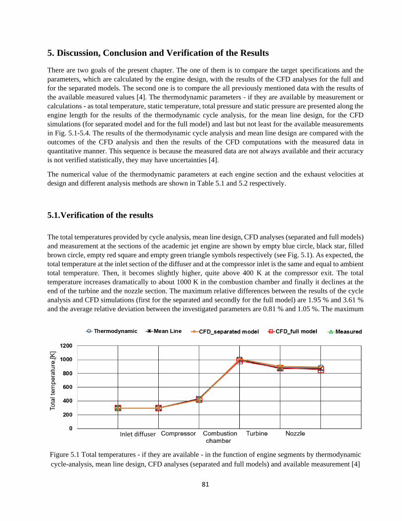
81

5. Discussion, Conclusion and Verification of the Results

There are two goals of the present chapter. The one of them is to compare the target specifications and the

parameters, which are calculated by the engine design, with the results of the CFD analyses for the full and

for the separated models. The second one is to compare the all previously mentioned data with the results of

the available measured values [4]. The thermodynamic parameters - if they are available by measurement or

calculations - as total temperature, static temperature, total pressure and static pressure are presented along the

engine length for the results of the thermodynamic cycle analysis, for the mean line design, for the CFD

simulations (for separated model and for the full model) and last but not least for the available measurements

in Fig. 5.1-5.4. The results of the thermodynamic cycle analysis and mean line design are compared with the

outcomes of the CFD analysis and then the results of the CFD computations with the measured data in

quantitative manner. This sequence is because the measured data are not always available and their accuracy

is not verified statistically, they may have uncertainties [4].

The numerical value of the thermodynamic parameters at each engine section and the exhaust velocities at

design and different analysis methods are shown in Table 5.1 and 5.2 respectively.

5.1. Verification of the results

The total temperatures provided by cycle analysis, mean line design, CFD analyses (separated and full models)

and measurement at the sections of the academic jet engine are shown by empty blue circle, black star, filled

brown circle, empty red square and empty green triangle symbols respectively (see Fig. 5.1). As expected, the

total temperature at the inlet section of the diffuser and at the compressor inlet is the same and equal to ambient

total temperature. Then, it becomes slightly higher, quite above 400 K at the compressor exit. The total

temperature increases dramatically to about 1000 K in the combustion chamber and finally it declines at the

end of the turbine and the nozzle section. The maximum relative differences between the results of the cycle

analysis and CFD simulations (first for the separated and secondly for the full model) are 1.95 % and 3.61 %

and the average relative deviation between the investigated parameters are 0.81 % and 1.05 %. The maximum

Figure 5.1 Total temperatures - if they are available - in the function of engine segments by thermodynamic

cycle-analysis, mean line design, CFD analyses (separated and full models) and available measurement [4]

Inlet diffuser

82

relative differences between the mean line design and CFD data (first for the separated and secondly for the

full model) are 4.10 % and 2.22 % meanwhile the average relative deviations between the investigated

parameters are 1.75 % and 1.13 %. Concerning the CFD (first the separated and secondly the full model) and

measured total temperatures, the maximum relative deviations between them are 1.26 % and 3.04 % and the

average relative deviation between their values are 0.61 % and 1.98 %, respectively.

Fig. 5.2 shows the calculated and measured static temperatures in the function of the engine length similarly

than it was mentioned in the previous paragraph except for the data from the thermodynamic cycle analysis,

because only the total quantities are considered in it omitting the nozzle exit. The calculated mean line design

and CFD results match well with each other similarly than it was before at the total temperature. The maximum

relative difference between the outputs of the mean line design and CFD simulations (first for the separated

and secondly for the full model) are 4.58 % and 3.04% and the average relative deviation between the

investigated values are 1.59 % and 1.56 %. The highest relative differences between the available measured

and CFD data (first for the separated and secondly for the full model) are 4.25 % and 3.89 % meanwhile the

average relative deviations between the investigated static temperatures are 3.03 % and 2.11 %. The separated

CFD model gives the highest static temperature at the inlet of the nozzle (see Fig. 5.2). This is caused by the

low Mach number and so the low flow speed, which is the consequence of the inlet and outlet boundary

conditions. Namely the flow has higher inlet area at the nozzle, and it is imposed to be perpendicular to the

inlet surface of the nozzle, which provides low axial velocity corresponds to the inlet total pressure, total

temperature and exit mass flow rate. However, in the other cases, beside the axial velocity, there is a tangential

component of the flow also together with smaller inlet cross section of the nozzle, which results higher absolute

velocity. This higher absolute velocity provides less static temperature and pressure at the same or similar total

temperature and pressure respectively. Hence, due to the used boundary conditions, the results of the separated

CFD model in case of the nozzle cannot be reasonably compared directly with the parameters provided by the

other approaches.

Figure 5.2 Static temperatures - if they are available - in the function of the engine segments by mean line

design, CFD analyses (separated and full models) and available measurement [4]

The total pressure at the compressor inlet is 99756 Pa. It is boosted by the compressor to around 250 kPa

before the combustion chamber (see Fig. 5.3). Afterwards, it expands to the atmospheric pressure in three

Inlet diffuser

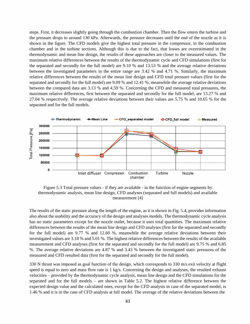
83

steps. First, it decreases slightly going through the combustion chamber. Then the flow enters the turbine and

the pressure drops to around 130 kPa. Afterwards, the pressure decreases until the end of the nozzle as it is

shown in the figure. The CFD models give the highest total pressure in the compressor, in the combustion

chamber and in the turbine sections. Although this is due to the fact, that losses are overestimated in the

thermodynamic and mean line design, the results of these approaches are closer to the measured values. The

maximum relative differences between the results of the thermodynamic cycle and CFD simulations (first for

the separated and secondly for the full model) are 9.10 % and 13.53 % and the average relative deviations

between the investigated parameters in the entire range are 3.42 % and 4.71 %. Similarly, the maximum

relative differences between the results of the mean line design and CFD total pressure values (first for the

separated and secondly for the full model) are 9.09 % and 12.41 %, meanwhile the average relative deviations

between the compared data are 3.13 % and 4.59 %. Concerning the CFD and measured total pressures, the

maximum relative differences, first between the separated and secondly for the full model, are 13.27 % and

27.04 % respectively. The average relative deviations between their values are 5.75 % and 10.65 % for the

separated and for the full models.

Figure 5.3 Total pressure values - if they are available - in the function of engine segments by

thermodynamic analysis, mean line design, CFD analyses (separated and full models) and available

measurement [4]

The results of the static pressure along the length of the engine, as it is shown in Fig. 5.4, provides information

also about the usability and the accuracy of the design and analyses models. The thermodynamic cycle analysis

has no static parameters except for the nozzle outlet, because it uses total quantities. The maximum relative

differences between the results of the mean line design and CFD analyses (first for the separated and secondly

for the full model) are 9.77 % and 12.60 %, meanwhile the average relative deviations between their

investigated values are 3.18 % and 5.01 %. The highest relative differences between the results of the available

measurement and CFD analyses (first for the separated and secondly for the full model) are 9.75 % and 6.85

%. The average relative deviations are 4.87 % and 3.43 % between the investigated static pressures of the

measured and CFD resulted data (first for the separated and secondly for the full model).

330 N thrust was imposed as goal function of the design, which corresponds to 330 m/s exit velocity at flight

speed is equal to zero and mass flow rate is 1 kg/s. Concerning the design and analyses, the resulted exhaust

velocities – provided by the thermodynamic cycle analysis, mean line design and the CFD simulations for the

separated and for the full models – are shown in Table 5.2. The highest relative difference between the

expected design value and the calculated ones, except for the CFD analysis in case of the separated model, is

1.46 % and it is in the case of CFD analysis at full model. The average of the relative deviations between the

Inlet diffuser

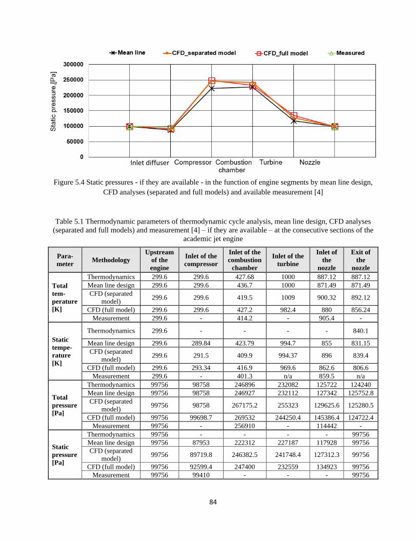
84

Figure 5.4 Static pressures - if they are available - in the function of engine segments by mean line design,

CFD analyses (separated and full models) and available measurement [4]

Table 5.1 Thermodynamic parameters of thermodynamic cycle analysis, mean line design, CFD analyses

(separated and full models) and measurement [4] – if they are available – at the consecutive sections of the

academic jet engine

Para-

meter Methodology

Upstream

of the

engine

Inlet of the

compressor

Inlet of the

combustion

chamber

Inlet of the

turbine

Inlet of

the

nozzle

Exit of

the

nozzle

Total

tem-

perature

[K]

Thermodynamics 299.6 299.6 427.68 1000 887.12 887.12

Mean line design 299.6 299.6 436.7 1000 871.49 871.49

CFD (separated

model) 299.6 299.6 419.5 1009 900.32 892.12

CFD (full model) 299.6 299.6 427.2 982.4 880 856.24

Measurement 299.6 - 414.2 - 905.4 -

Static

tempe-

rature

[K]

Thermodynamics 299.6 - - - - 840.1

Mean line design 299.6 289.84 423.79 994.7 855 831.15

CFD (separated

model) 299.6 291.5 409.9 994.37 896 839.4

CFD (full model) 299.6 293.34 416.9 969.6 862.6 806.6

Measurement 299.6 - 401.3 n/a 859.5 n/a

Total

pressure

[Pa]

Thermodynamics 99756 98758 246896 232082 125722 124240

Mean line design 99756 98758 246927 232112 127342 125752.8

CFD (separated

model) 99756 98758 267175.2 255323 129625.6 125280.5

CFD (full model) 99756 99698.7 269532 244250.4 145386.4 124722.4

Measurement 99756 - 256910 - 114442 -

Static

pressure

[Pa]

Thermodynamics 99756 - - - - 99756

Mean line design 99756 87953 222312 227187 117928 99756

CFD (separated

model) 99756 89719.8 246382.5 241748.4 127312.3 99756

CFD (full model) 99756 92599.4 247400 232559 134923 99756

Measurement 99756 99410 - - - 99756

Inlet diffuser

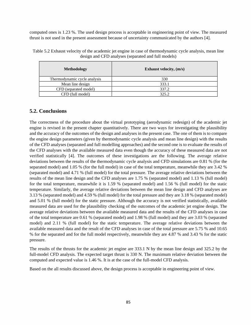
85

computed ones is 1.23 %. The used design process is acceptable in engineering point of view. The measured

thrust is not used in the present assessment because of uncertainty communicated by the authors [4].

Table 5.2 Exhaust velocity of the academic jet engine in case of thermodynamic cycle analysis, mean line

design and CFD analyses (separated and full models)

Methodology Exhaust velocity, (m/s)

Thermodynamic cycle analysis 330

Mean line design 333.1

CFD (separated model) 337.2

CFD (full model) 325.2

5.2. Conclusions

The correctness of the procedure about the virtual prototyping (aerodynamic redesign) of the academic jet

engine is revised in the present chapter quantitatively. There are two ways for investigating the plausibility

and the accuracy of the outcomes of the design and analyses in the present case. The one of them is to compare

the engine design parameters (given by thermodynamic cycle analysis and mean line design) with the results

of the CFD analyses (separated and full modelling approaches) and the second one is to evaluate the results of

the CFD analyses with the available measured data even though the accuracy of these measured data are not

verified statistically [4]. The outcomes of these investigations are the following. The average relative

deviations between the results of the thermodynamic cycle analysis and CFD simulations are 0.81 % (for the

separated model) and 1.05 % (for the full model) in case of the total temperature, meanwhile they are 3.42 %

(separated model) and 4.71 % (full model) for the total pressure. The average relative deviations between the

results of the mean line design and the CFD analyses are 1.75 % (separated model) and 1.13 % (full model)

for the total temperature, meanwhile it is 1.59 % (separated model) and 1.56 % (full model) for the static

temperature. Similarly, the average relative deviations between the mean line design and CFD analyses are

3.13 % (separated model) and 4.59 % (full model) for the total pressure and they are 3.18 % (separated model)

and 5.01 % (full model) for the static pressure. Although the accuracy is not verified statistically, available

measured data are used for the plausibility checking of the outcomes of the academic jet engine design. The

average relative deviations between the available measured data and the results of the CFD analyses in case

of the total temperature are 0.61 % (separated model) and 1.98 % (full model) and they are 3.03 % (separated

model) and 2.11 % (full model) for the static temperature. The average relative deviations between the

available measured data and the result of the CFD analyses in case of the total pressure are 5.75 % and 10.65

% for the separated and for the full model respectively, meanwhile they are 4.87 % and 3.43 % for the static

pressure.

The results of the thrusts for the academic jet engine are 333.1 N by the mean line design and 325.2 by the

full-model CFD analysis. The expected target thrust is 330 N. The maximum relative deviation between the

computed and expected value is 1.46 %. It is at the case of the full-model CFD analysis.

Based on the all results discussed above, the design process is acceptable in engineering point of view.

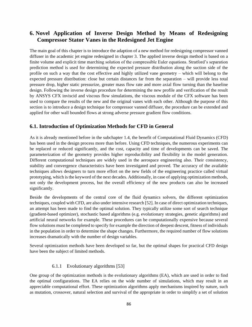
86

6. Novel Application of Inverse Design Method by Means of Redesigning

Compressor Stator Vanes in the Redesigned Jet Engine

The main goal of this chapter is to introduce the adaption of a new method for redesigning compressor vanned

diffuser in the academic jet engine redesigned in chapter 3. The applied inverse design method is based on a

finite volume and explicit time marching solution of the compressible Euler equations. Stratford’s separation

prediction method is used for determining the expected pressure distribution along the suction side of the

profile on such a way that the cost effective and highly utilized vane geometry – which will belong to the

expected pressure distribution: close but certain distances far from the separation – will provide less total

pressure drop, higher static pressurize, greater mass flow rate and more axial flow turning than the baseline

design. Following the inverse design procedure for determining the new profile and verification of the result

by ANSYS CFX inviscid and viscous flow simulations, the viscous module of the CFX software has been

used to compare the results of the new and the original vanes with each other. Although the purpose of this

section is to introduce a design technique for compressor vanned diffuser, the procedure can be extended and

applied for other wall bounded flows at strong adverse pressure gradient flow conditions.

6.1. Introduction of Optimization Methods for CFD in General

As it is already mentioned before in the subchapter 1.4, the benefit of Computational Fluid Dynamics (CFD)

has been used in the design process more than before. Using CFD techniques, the numerous experiments can

be replaced or reduced significantly, and the cost, capacity and time of developments can be saved. The

parameterization of the geometry provides higher reproducibility and flexibility in the model generation.

Different computational techniques are widely used in the aerospace engineering also. Their consistency,

stability and convergence characteristics have been investigated and proved. The accuracy of the available

techniques allows designers to turn more effort on the new fields of the engineering practice called virtual

prototyping, which is the keyword of the next decades. Additionally, in case of applying optimization methods,

not only the development process, but the overall efficiency of the new products can also be increased

significantly.

Beside the developments of the central core of the fluid dynamics solvers, the different optimization

techniques, coupled with CFD, are also under intensive research [52]. In case of direct optimization techniques,

an attempt has been made to find the optimal solution. They typically utilize some sort of search technique

(gradient-based optimizer), stochastic based algorithms (e.g. evolutionary strategies, genetic algorithms) and

artificial neural networks for example. These procedures can be computationally expensive because several

flow solutions must be completed to specify for example the direction of deepest descent, fitness of individuals

in the population in order to determine the shape changes. Furthermore, the required number of flow solutions

increases dramatically with the number of design variables.

Several optimization methods have been developed so far, but the optimal shapes for practical CFD design

have been the subject of limited methods.

6.1.1 Evolutionary algorithms [53]

One group of the optimization methods is the evolutionary algorithms (EA), which are used in order to find

the optimal configurations. The EA relies on the wide number of simulations, which may result in an

appreciable computational effort. These optimization algorithms apply mechanisms inspired by nature, such

as mutation, crossover, natural selection and survival of the appropriate in order to simplify a set of solution

87

candidates by using repeated analyses. The most important idea for evolution algorithms is to find the optimal

solution by using the analogy to estimate the theory. Evolutionary algorithms can be coupled with CFD

methods. The basic cycle of evolutionary algorithms is depicted in Fig. 6.1.

Figure 6.1 The basic cycle of evolutionary algorithms [53]

If the final criterion is satisfied, the evolution stops. Otherwise, the algorithm continues with next cycle. The

group of genetic algorithms (GA) is a part of the group of evolutionary algorithms. The GA proceeds to

initialize a function of solutions haphazardly, and then refine it through several applications of mutation,

crossover, inversion and selection operators. Crossover and mutation are identified as essential genetic

operators. This formation process is repeated until an ending condition has been reached. There are many

disadvantages of the use of genetic algorithms as compared to the other optimization algorithms:

1. One single function evaluation may need many hours of complete simulation. Then optimization

methods cannot work with this type of problem because it is a very expensive fitness function evaluation.

Thus, it is required to use an approximated fitness that is computationally efficient.

2. In many problems, GAs may have a trend to converge to local optima rather than the global optimum of

the problem. GAs is unacquainted with the abnegation of short-term capability in order to get longer-

term capability.

3. If the capability measure is only a single right/wrong criterion then GAs cannot be adopted to solve the

problem and there is no way to converge on the solution. In this case a random search can solve the

problem fast as a GA.

4. For certain optimization problems and problem cases other optimization algorithms may find better

solutions than genetic algorithms (given the same computational capacity).

6.1.2 Genetic programming [53]

The goal of genetic programming (GP) is to determine the connection between the inputs and output before

the simulation. The aim of this process is to find system operator that connects the given input and response,

as sketched in Fig. 6.2. Meanwhile the GA determines the set of input data which, when transformed by a

known system dynamics algorithm, most closely matches a set of known output data, the GP determines the

system dynamics algorithm, which most closely transforms a set of known input data into a set of known

output data. The GA/GP applied to problems in many different disciplines: engineering design (e.g.: air foil

88

optimization, control system tuning, artificial vision systems), financial forecasting and biological system

modelling.

Figure 6.2 Relation between input and output [53]

6.1.3 Simulated annealing [53]

The starting point is an analogy with the thermodynamics of equilibrium. Condensed matter consists of a very

large number of molecules, whose energy is described by the Boltzmann probability distribution: P(E) = exp(-

E/kT), where E is the energy of the configuration, T the temperature and k the Boltzmann constant. The

simulated annealing (SA) is a multi-dimensional optimization technique based on following local gradients to

a minima/maximum. The SA requires the user to choose some optimization parameters (e.g. transition

probability function, transition step size) meanwhile GA requires less explicit input by the user. The GA may

be less efficient than SA for well-behaved optimization problems but may be better suited to complex

parameter spaces.

6.1.4 Evolutionary programming [53]

Evolutionary Programming (EP) was used first in 1960’s in order to use simulated evolution as a learning

process aiming to generate artificial intelligence. Currently, evolutionary programming is a wide evolutionary

computing dialect with no fixed structure or (representation), in contrast with some of the other dialects. It is

becoming harder to distinguish between evolutionary strategies. Some of its original variants are quite similar

to the later genetic programming, except that the program structure is fixed and its numerical parameters are

allowed to evolve. Different from genetic algorithm, evolutionary programming mimics the evolution of

species not the genes, so in evolutionary programming emphasize the linking of species behaviour. The

evolutionary programming emphasize is on the behaviour evolution of species and establishes the behaviour

chain between parent and offspring, that is to say, the good offspring can be existed and not consider its parent.

So, in evolutionary programming the fitness value is applied to select offspring.

6.1.5 Learning classifier system [53]

A Learning Classifier System, or LCS, is an automatic learning system with close links to genetic algorithms.

Learning classifier systems can be divided into two types depending on when the genetic algorithm acts. One

of them is the Pittsburgh-type LCS which has a well-known set up of rules, where the genetic algorithm

recombines and copy the best of these rule sets. In a Michigan-style LCS there is only a single well-known

rule and the algorithm's action focuses on selecting the best classifiers within that rule set. Michigan-style

LCSs have two main types of fitness definitions, strength-based and accuracy-based. The term "learning

classifier system" most often refers to Michigan-style LCSs.

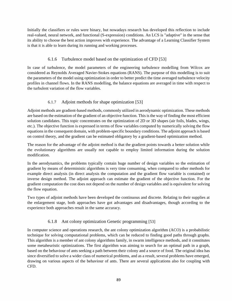
89

Initially the classifiers or rules were binary, but nowadays research has developed this reflection to include

real-valued, neural network, and functional (S-expression) conditions. An LCS is "adaptive" in the sense that

its ability to choose the best action improves with experience. The advantage of a Learning Classifier System

is that it is able to learn during its running and working processes.

6.1.6 Turbulence model based on the optimization of CFD [53]

In case of turbulence, the model parameters of the engineering turbulence modelling from Wilcox are

considered as Reynolds Averaged Navier-Stokes equations (RANS). The purpose of this modelling is to suit

the parameters of the model using optimization in order to better predict the time averaged turbulence velocity

profiles in channel flows. In the RANS modelling, the balance equations are averaged in time with respect to

the turbulent variation of the flow variables.

6.1.7 Adjoint methods for shape optimization [53]

Adjoint methods are gradient-based methods, commonly utilized in aerodynamic optimization. These methods

are based on the estimation of the gradient of an objective function. This is the way of finding the most efficient

solution candidates. This topic concentrates on the optimization of 2D or 3D shapes (air foils, blades, wings,

etc.). The objective function is expressed in terms of flow variables computed by numerically solving the flow

equations in the consequent domain, with problem-specific boundary conditions. The adjoint approach is based

on control theory, and the gradient can be estimated obligatory by a gradient-based optimization method.

The reason for the advantage of the adjoint method is that the gradient points towards a better solution while

the evolutionary algorithms are usually not capable to employ limited information during the solution

modification.

In the aerodynamics, the problems typically contain huge number of design variables so the estimation of

gradient by means of deterministic algorithms is very time consuming, when compared to other methods for

example direct analysis (in direct analysis the computation and the gradient flow variable is contained) or

inverse design method. The adjoint approach can estimate the gradient of the objective function. For the

gradient computation the cost does not depend on the number of design variables and is equivalent for solving

the flow equation.

Two types of adjoint methods have been developed the continuous and discrete. Relating to their supplies at

the enlargement stage, both approaches have got advantages and disadvantages, though according to the

experience both approaches result in the same accuracy.

6.1.8 Ant colony optimization Genetic programming [53]

In computer science and operations research, the ant colony optimization algorithm (ACO) is a probabilistic

technique for solving computational problems, which can be reduced to finding good paths through graphs.

This algorithm is a member of ant colony algorithms family, in swarm intelligence methods, and it constitutes

some metaheuristic optimizations. The first algorithm was aiming to search for an optimal path in a graph,

based on the behaviour of ants seeking a path between their colony and a source of food. The original idea has

since diversified to solve a wider class of numerical problems, and as a result, several problems have emerged,

drawing on various aspects of the behaviour of ants. There are several applications also for coupling with

CFD.

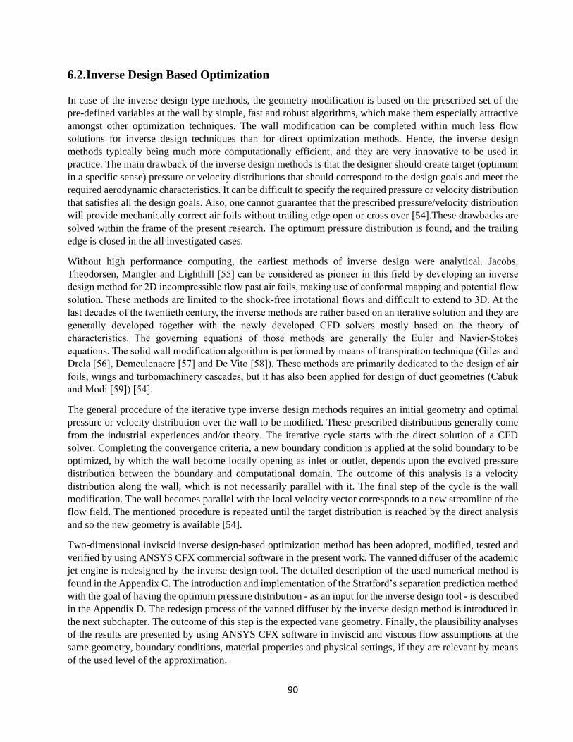
90

6.2. Inverse Design Based Optimization

In case of the inverse design-type methods, the geometry modification is based on the prescribed set of the

pre-defined variables at the wall by simple, fast and robust algorithms, which make them especially attractive

amongst other optimization techniques. The wall modification can be completed within much less flow

solutions for inverse design techniques than for direct optimization methods. Hence, the inverse design

methods typically being much more computationally efficient, and they are very innovative to be used in

practice. The main drawback of the inverse design methods is that the designer should create target (optimum

in a specific sense) pressure or velocity distributions that should correspond to the design goals and meet the

required aerodynamic characteristics. It can be difficult to specify the required pressure or velocity distribution

that satisfies all the design goals. Also, one cannot guarantee that the prescribed pressure/velocity distribution

will provide mechanically correct air foils without trailing edge open or cross over [54].These drawbacks are

solved within the frame of the present research. The optimum pressure distribution is found, and the trailing

edge is closed in the all investigated cases.

Without high performance computing, the earliest methods of inverse design were analytical. Jacobs,

Theodorsen, Mangler and Lighthill [55] can be considered as pioneer in this field by developing an inverse

design method for 2D incompressible flow past air foils, making use of conformal mapping and potential flow

solution. These methods are limited to the shock-free irrotational flows and difficult to extend to 3D. At the

last decades of the twentieth century, the inverse methods are rather based on an iterative solution and they are

generally developed together with the newly developed CFD solvers mostly based on the theory of

characteristics. The governing equations of those methods are generally the Euler and Navier-Stokes

equations. The solid wall modification algorithm is performed by means of transpiration technique (Giles and

Drela [56], Demeulenaere [57] and De Vito [58]). These methods are primarily dedicated to the design of air

foils, wings and turbomachinery cascades, but it has also been applied for design of duct geometries (Cabuk

and Modi [59]) [54].

The general procedure of the iterative type inverse design methods requires an initial geometry and optimal

pressure or velocity distribution over the wall to be modified. These prescribed distributions generally come

from the industrial experiences and/or theory. The iterative cycle starts with the direct solution of a CFD

solver. Completing the convergence criteria, a new boundary condition is applied at the solid boundary to be

optimized, by which the wall become locally opening as inlet or outlet, depends upon the evolved pressure

distribution between the boundary and computational domain. The outcome of this analysis is a velocity

distribution along the wall, which is not necessarily parallel with it. The final step of the cycle is the wall

modification. The wall becomes parallel with the local velocity vector corresponds to a new streamline of the

flow field. The mentioned procedure is repeated until the target distribution is reached by the direct analysis

and so the new geometry is available [54].

Two-dimensional inviscid inverse design-based optimization method has been adopted, modified, tested and

verified by using ANSYS CFX commercial software in the present work. The vanned diffuser of the academic

jet engine is redesigned by the inverse design tool. The detailed description of the used numerical method is

found in the Appendix C. The introduction and implementation of the Stratford’s separation prediction method

with the goal of having the optimum pressure distribution - as an input for the inverse design tool - is described

in the Appendix D. The redesign process of the vanned diffuser by the inverse design method is introduced in

the next subchapter. The outcome of this step is the expected vane geometry. Finally, the plausibility analyses

of the results are presented by using ANSYS CFX software in inviscid and viscous flow assumptions at the

same geometry, boundary conditions, material properties and physical settings, if they are relevant by means

of the used level of the approximation.

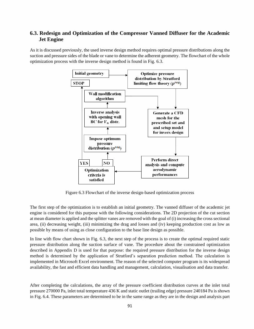
91

6.3. Redesign and Optimization of the Compressor Vanned Diffuser for the Academic

Jet Engine

As it is discussed previously, the used inverse design method requires optimal pressure distributions along the

suction and pressure sides of the blade or vane to determine the adherent geometry. The flowchart of the whole

optimization process with the inverse design method is found in Fig. 6.3.

Figure 6.3 Flowchart of the inverse design-based optimization process

The first step of the optimization is to establish an initial geometry. The vanned diffuser of the academic jet

engine is considered for this purpose with the following considerations. The 2D projection of the cut section

at mean diameter is applied and the splitter vanes are removed with the goal of (i) increasing the cross sectional

area, (ii) decreasing weight, (iii) minimizing the drag and losses and (iv) keeping production cost as low as

possible by means of using as close configuration to the base line design as possible.

In line with flow chart shown in Fig. 6.3, the next step of the process is to create the optimal required static

pressure distribution along the suction surface of vane. The procedure about the constrained optimization

described in Appendix D is used for that purpose: the required pressure distribution for the inverse design

method is determined by the application of Stratford’s separation prediction method. The calculation is

implemented in Microsoft Excel environment. The reason of the selected computer program is its widespread

availability, the fast and efficient data handling and management, calculation, visualisation and data transfer.

After completing the calculations, the array of the pressure coefficient distribution curves at the inlet total

pressure 270000 Pa, inlet total temperature 436 K and static outlet (trailing edge) pressure 240184 Pa is shown

in Fig. 6.4. These parameters are determined to be in the same range as they are in the design and analysis part

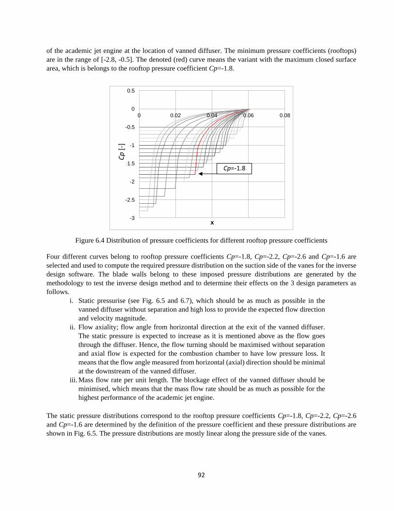
92

of the academic jet engine at the location of vanned diffuser. The minimum pressure coefficients (rooftops)

are in the range of [-2.8, -0.5]. The denoted (red) curve means the variant with the maximum closed surface

area, which is belongs to the rooftop pressure coefficient Cp=-1.8.

Figure 6.4 Distribution of pressure coefficients for different rooftop pressure coefficients

Four different curves belong to rooftop pressure coefficients Cp=-1.8, Cp=-2.2, Cp=-2.6 and Cp=-1.6 are

selected and used to compute the required pressure distribution on the suction side of the vanes for the inverse

design software. The blade walls belong to these imposed pressure distributions are generated by the

methodology to test the inverse design method and to determine their effects on the 3 design parameters as

follows.

i. Static pressurise (see Fig. 6.5 and 6.7), which should be as much as possible in the

vanned diffuser without separation and high loss to provide the expected flow direction

and velocity magnitude.

ii. Flow axiality; flow angle from horizontal direction at the exit of the vanned diffuser.

The static pressure is expected to increase as it is mentioned above as the flow goes

through the diffuser. Hence, the flow turning should be maximised without separation

and axial flow is expected for the combustion chamber to have low pressure loss. It

means that the flow angle measured from horizontal (axial) direction should be minimal

at the downstream of the vanned diffuser.

iii. Mass flow rate per unit length. The blockage effect of the vanned diffuser should be

minimised, which means that the mass flow rate should be as much as possible for the

highest performance of the academic jet engine.

The static pressure distributions correspond to the rooftop pressure coefficients Cp=-1.8, Cp=-2.2, Cp=-2.6

and Cp=-1.6 are determined by the definition of the pressure coefficient and these pressure distributions are

shown in Fig. 6.5. The pressure distributions are mostly linear along the pressure side of the vanes.

-3

-2.5

-2

-1.5

-1

-0.5

0

0.5

0 0.02 0.04 0.06 0.08C

p [-]

x

Cp=-1.8

Cp

[-]

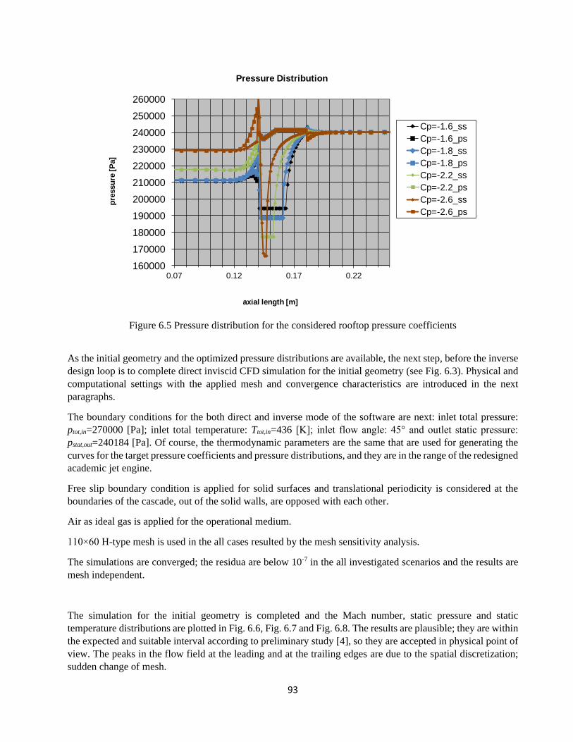
93

Figure 6.5 Pressure distribution for the considered rooftop pressure coefficients

As the initial geometry and the optimized pressure distributions are available, the next step, before the inverse

design loop is to complete direct inviscid CFD simulation for the initial geometry (see Fig. 6.3). Physical and

computational settings with the applied mesh and convergence characteristics are introduced in the next

paragraphs.

The boundary conditions for the both direct and inverse mode of the software are next: inlet total pressure:

ptot,in=270000 [Pa]; inlet total temperature: Ttot,in=436 [K]; inlet flow angle: 45° and outlet static pressure:

pstat,out=240184 [Pa]. Of course, the thermodynamic parameters are the same that are used for generating the

curves for the target pressure coefficients and pressure distributions, and they are in the range of the redesigned

academic jet engine.

Free slip boundary condition is applied for solid surfaces and translational periodicity is considered at the

boundaries of the cascade, out of the solid walls, are opposed with each other.

Air as ideal gas is applied for the operational medium.

110×60 H-type mesh is used in the all cases resulted by the mesh sensitivity analysis.

The simulations are converged; the residua are below 10-7 in the all investigated scenarios and the results are

mesh independent.

The simulation for the initial geometry is completed and the Mach number, static pressure and static

temperature distributions are plotted in Fig. 6.6, Fig. 6.7 and Fig. 6.8. The results are plausible; they are within

the expected and suitable interval according to preliminary study [4], so they are accepted in physical point of

view. The peaks in the flow field at the leading and at the trailing edges are due to the spatial discretization;

sudden change of mesh.

160000

170000

180000

190000

200000

210000

220000

230000

240000

250000

260000

0.07 0.12 0.17 0.22

pre

ssu

re [

Pa]

axial length [m]

Pressure Distribution

Cp=-1.6_ss

Cp=-1.6_ps

Cp=-1.8_ss

Cp=-1.8_ps

Cp=-2.2_ss

Cp=-2.2_ps

Cp=-2.6_ss

Cp=-2.6_ps

94

Figure 6.6 Mach number [-] distribution in case of initial geometry [m]

Figure 6.7 Static pressure [Pa] distribution in case of initial geometry [m]

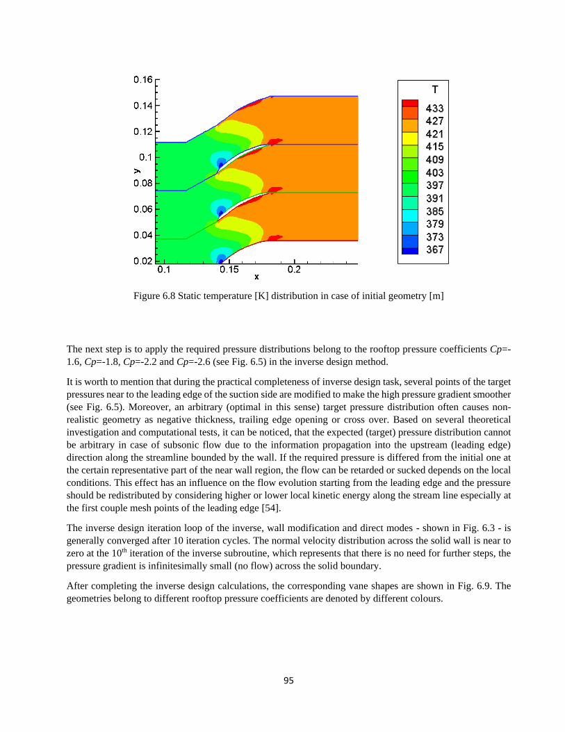
95

Figure 6.8 Static temperature [K] distribution in case of initial geometry [m]

The next step is to apply the required pressure distributions belong to the rooftop pressure coefficients Cp=-

1.6, Cp=-1.8, Cp=-2.2 and Cp=-2.6 (see Fig. 6.5) in the inverse design method.

It is worth to mention that during the practical completeness of inverse design task, several points of the target

pressures near to the leading edge of the suction side are modified to make the high pressure gradient smoother

(see Fig. 6.5). Moreover, an arbitrary (optimal in this sense) target pressure distribution often causes non-

realistic geometry as negative thickness, trailing edge opening or cross over. Based on several theoretical

investigation and computational tests, it can be noticed, that the expected (target) pressure distribution cannot

be arbitrary in case of subsonic flow due to the information propagation into the upstream (leading edge)

direction along the streamline bounded by the wall. If the required pressure is differed from the initial one at

the certain representative part of the near wall region, the flow can be retarded or sucked depends on the local

conditions. This effect has an influence on the flow evolution starting from the leading edge and the pressure

should be redistributed by considering higher or lower local kinetic energy along the stream line especially at

the first couple mesh points of the leading edge [54].

The inverse design iteration loop of the inverse, wall modification and direct modes - shown in Fig. 6.3 - is

generally converged after 10 iteration cycles. The normal velocity distribution across the solid wall is near to

zero at the 10th iteration of the inverse subroutine, which represents that there is no need for further steps, the

pressure gradient is infinitesimally small (no flow) across the solid boundary.

After completing the inverse design calculations, the corresponding vane shapes are shown in Fig. 6.9. The

geometries belong to different rooftop pressure coefficients are denoted by different colours.

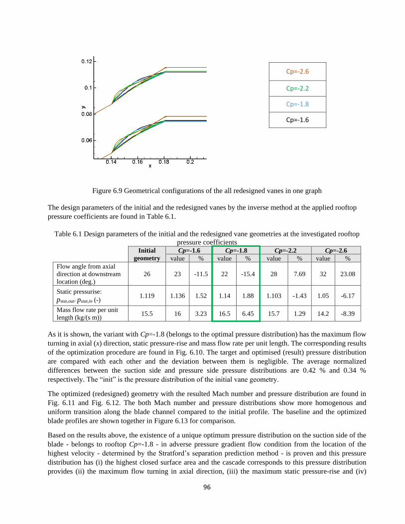
96

Figure 6.9 Geometrical configurations of the all redesigned vanes in one graph

The design parameters of the initial and the redesigned vanes by the inverse method at the applied rooftop

pressure coefficients are found in Table 6.1.

Table 6.1 Design parameters of the initial and the redesigned vane geometries at the investigated rooftop

pressure coefficients

Initial

geometry

Cp=-1.6 Cp=-1.8 Cp=-2.2 Cp=-2.6

value % value % value % value %

Flow angle from axial

direction at downstream

location (deg.)

26 23 -11.5 22 -15.4 28 7.69 32 23.08

Static pressurise:

pstat,out/ pstat,in (-) 1.119 1.136 1.52 1.14 1.88 1.103 -1.43 1.05 -6.17

Mass flow rate per unit

length (kg/(s m)) 15.5 16 3.23 16.5 6.45 15.7 1.29 14.2 -8.39

As it is shown, the variant with Cp=-1.8 (belongs to the optimal pressure distribution) has the maximum flow

turning in axial (x) direction, static pressure-rise and mass flow rate per unit length. The corresponding results

of the optimization procedure are found in Fig. 6.10. The target and optimised (result) pressure distribution

are compared with each other and the deviation between them is negligible. The average normalized

differences between the suction side and pressure side pressure distributions are 0.42 % and 0.34 %

respectively. The “init” is the pressure distribution of the initial vane geometry.

The optimized (redesigned) geometry with the resulted Mach number and pressure distribution are found in

Fig. 6.11 and Fig. 6.12. The both Mach number and pressure distributions show more homogenous and

uniform transition along the blade channel compared to the initial profile. The baseline and the optimized

blade profiles are shown together in Figure 6.13 for comparison.

Based on the results above, the existence of a unique optimum pressure distribution on the suction side of the

blade - belongs to rooftop Cp=-1.8 - in adverse pressure gradient flow condition from the location of the

highest velocity - determined by the Stratford’s separation prediction method - is proven and this pressure

distribution has (i) the highest closed surface area and the cascade corresponds to this pressure distribution

provides (ii) the maximum flow turning in axial direction, (iii) the maximum static pressure-rise and (iv)

Cp=-2.6

Cp=-2.2

Cp=-1.8

Cp=-1.6

97

maximum mass flow rate per unit length, (v) beside close, but certain distance far from the separation. The all

parameters are improved by 7.9 % in average. This pressure distribution is going to be used in the next chapter

of the present work for the verification of the results.

Figure 6.10 Comparison of the initial, target (at rooftop Cp=-1.8) and the resulted static pressure

distributions along the suction and pressure side of the profile (ss: suction side, ps: pressure side)

Figure 6.11 Mach number [-] distribution in case of redesigned (optimal) vane geometry [m] (at rooftop

Cp=-1.8)

160000

170000

180000

190000

200000

210000

220000

230000

240000

250000

260000

0.07 0.12 0.17 0.22

pre

ssu

re [

Pa]

axial length [m]

Pressure Distribution

init_ss

init_ps

target_ss

target_ps

result_ss

result_ps

Leading

edge zone

Trailing

edge zone

98

Figure 6.12 Static pressure [Pa] distribution in case of redesigned (optimal) vane geometry [m] (at rooftop

Cp=-1.8)

Figure 6.13 Vane configurations in case of baseline (black) and redesigned (optimal at rooftop Cp=-1.8)

(red) variants

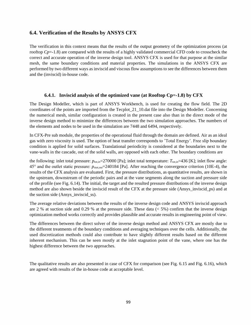
99

6.4. Verification of the Results by ANSYS CFX

The verification in this context means that the results of the output geometry of the optimization process (at

rooftop Cp=-1.8) are compared with the results of a highly validated commercial CFD code to crosscheck the

correct and accurate operation of the inverse design tool. ANSYS CFX is used for that purpose at the similar

mesh, the same boundary conditions and material properties. The simulations in the ANSYS CFX are

performed by two different ways as inviscid and viscous flow assumptions to see the differences between them

and the (inviscid) in-house code.

6.4.1. Inviscid analysis of the optimized vane (at Rooftop Cp=-1.8) by CFX

The Design Modeller, which is part of ANSYS Workbench, is used for creating the flow field. The 2D

coordinates of the points are imported from the Tecplot_21_10.dat file into the Design Modeller. Concerning

the numerical mesh, similar configuration is created in the present case also than in the direct mode of the

inverse design method to minimize the differences between the two simulation approaches. The numbers of

the elements and nodes to be used in the simulation are 7448 and 6494, respectively.

In CFX-Pre sub module, the properties of the operational fluid through the domain are defined. Air as an ideal

gas with zero viscosity is used. The option of heat transfer corresponds to ’Total Energy’. Free slip boundary

condition is applied for solid surfaces. Translational periodicity is considered at the boundaries next to the

vane-walls in the cascade, out of the solid walls, are opposed with each other. The boundary conditions are

the following: inlet total pressure: ptot,in=270000 [Pa]; inlet total temperature: Ttot,in=436 [K]; inlet flow angle:

45° and the outlet static pressure: pstat,out=240184 [Pa]. After reaching the convergence criterion (10E-4), the

results of the CFX analysis are evaluated. First, the pressure distributions, as quantitative results, are shown in

the upstream, downstream of the periodic pairs and at the vane segments along the suction and pressure side

of the profile (see Fig. 6.14). The initial, the target and the resulted pressure distributions of the inverse design

method are also shown beside the inviscid result of the CFX at the pressure side (Ansys_inviscid_ps) and at

the suction side (Ansys_inviscid_ss).

The average relative deviations between the results of the inverse design code and ANSYS inviscid approach

are 2 % at suction side and 0.29 % at the pressure side. These data (< 5%) confirm that the inverse design

optimization method works correctly and provides plausible and accurate results in engineering point of view.

The differences between the direct solver of the inverse design method and ANSYS CFX are mostly due to

the different treatments of the boundary conditions and averaging techniques over the cells. Additionally, the

used discretization methods could also contribute to have slightly different results based on the different

inherent mechanism. This can be seen mostly at the inlet stagnation point of the vane, where one has the

highest difference between the two approaches.

The qualitative results are also presented in case of CFX for comparison (see Fig. 6.15 and Fig. 6.16), which

are agreed with results of the in-house code at acceptable level.

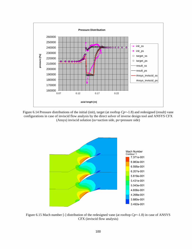
100

Figure 6.14 Pressure distributions of the initial (init), target (at rooftop Cp=-1.8) and redesigned (result) vane

configurations in case of inviscid flow analysis by the direct solver of inverse design tool and ANSYS CFX

(Ansys) inviscid solution (ss=suction side, ps=pressure side)

Figure 6.15 Mach number [-] distribution of the redesigned vane (at rooftop Cp=-1.8) in case of ANSYS

CFX (inviscid flow analysis)

160000

170000

180000

190000

200000

210000

220000

230000

240000

250000

260000

0.07 0.12 0.17 0.22

pre

ssu

re [

Pa]

axial length [m]

Pressure Distribution

init_ss

init_ps

target_ss

target_ps

result_ss

result_ps

Ansys_inviscid_ss

Ansys_inviscid_ps

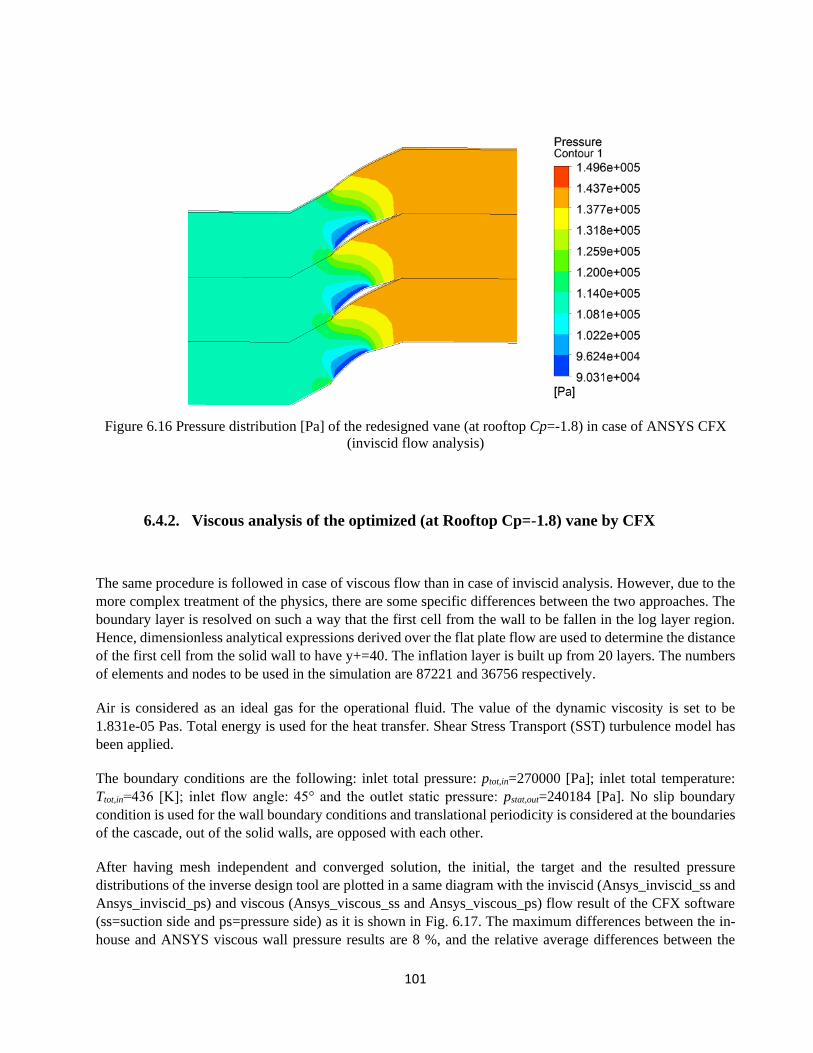
101

Figure 6.16 Pressure distribution [Pa] of the redesigned vane (at rooftop Cp=-1.8) in case of ANSYS CFX

(inviscid flow analysis)

6.4.2. Viscous analysis of the optimized (at Rooftop Cp=-1.8) vane by CFX

The same procedure is followed in case of viscous flow than in case of inviscid analysis. However, due to the

more complex treatment of the physics, there are some specific differences between the two approaches. The

boundary layer is resolved on such a way that the first cell from the wall to be fallen in the log layer region.

Hence, dimensionless analytical expressions derived over the flat plate flow are used to determine the distance

of the first cell from the solid wall to have y+=40. The inflation layer is built up from 20 layers. The numbers

of elements and nodes to be used in the simulation are 87221 and 36756 respectively.

Air is considered as an ideal gas for the operational fluid. The value of the dynamic viscosity is set to be

1.831e-05 Pas. Total energy is used for the heat transfer. Shear Stress Transport (SST) turbulence model has

been applied.

The boundary conditions are the following: inlet total pressure: ptot,in=270000 [Pa]; inlet total temperature:

Ttot,in=436 [K]; inlet flow angle: 45° and the outlet static pressure: pstat,out=240184 [Pa]. No slip boundary

condition is used for the wall boundary conditions and translational periodicity is considered at the boundaries

of the cascade, out of the solid walls, are opposed with each other.

After having mesh independent and converged solution, the initial, the target and the resulted pressure

distributions of the inverse design tool are plotted in a same diagram with the inviscid (Ansys_inviscid_ss and

Ansys_inviscid_ps) and viscous (Ansys_viscous_ss and Ansys_viscous_ps) flow result of the CFX software

(ss=suction side and ps=pressure side) as it is shown in Fig. 6.17. The maximum differences between the in-

house and ANSYS viscous wall pressure results are 8 %, and the relative average differences between the

102

results of the direct mode of the in-house code and Ansys viscous flow analysis are 3.04 % on the suction side

and 0.3 % at pressure side. The highest difference is arisen around the leading-edge stagnation point, similarly

to the inviscid flow analyses discussed in the previous subchapter.

The qualitative results are also presented in case of viscous CFX simulations for comparison. The relative

static and total pressure distributions are plotted in Fig. 6.18 and Fig. 6.19 respectively. These distributions

are in line with the results of the CFX inviscid analysis and with the results of the direct solver of the inverse

design method.

Both, the viscous and inviscid analyses confirm that the adopted and applied inverse design optimization

method provides plausible and accurate results for the presented case, which is acceptable in engineering point

of view as the average difference between the different approaches is less than 5 % at the investigated

quantitative results. Hence, the introduced inverse design-based optimization method - after further sensitivity

analyses and validations by measurements - can be used in design and developments in the other field of the

engineering science, too.

Figure 6.17 Pressure distributions of the initial (init), target and redesigned (result) vane configurations in

case of inviscid flow analyses by the direct mode of the in-house invers design code and inviscid and viscous

flow analyses by the ANSYS CFX (Ansys) (ss=suction side, ps=pressure side)

160000

170000

180000

190000

200000

210000

220000

230000

240000

250000

260000

0.07 0.12 0.17 0.22

pre

ssu

re [

Pa]

axial length [m]

Pressure Distribution

init_ss

init_ps

target_ss

target_ps

result_ss

result_ps

Ansys_inviscid_ss

Ansys_inviscid_ps

Ansys_viscous_ss

Ansys_viscous_ps

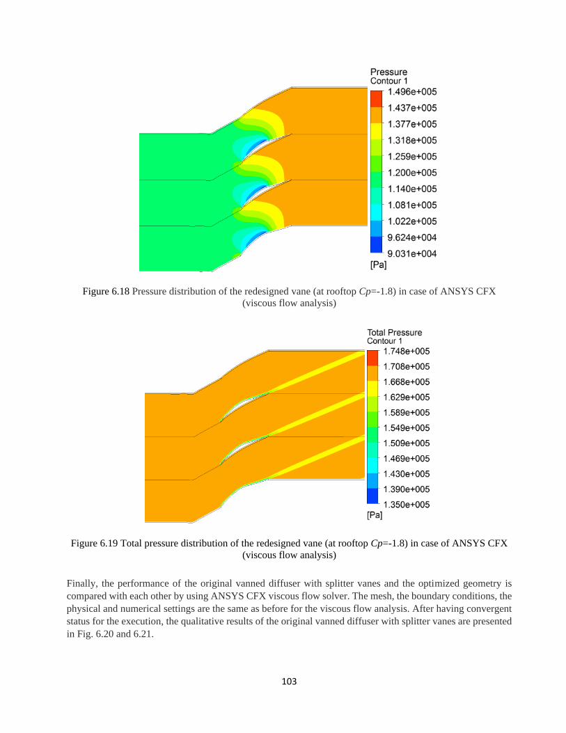
103

Figure 6.18 Pressure distribution of the redesigned vane (at rooftop Cp=-1.8) in case of ANSYS CFX

(viscous flow analysis)

Figure 6.19 Total pressure distribution of the redesigned vane (at rooftop Cp=-1.8) in case of ANSYS CFX

(viscous flow analysis)

Finally, the performance of the original vanned diffuser with splitter vanes and the optimized geometry is

compared with each other by using ANSYS CFX viscous flow solver. The mesh, the boundary conditions, the

physical and numerical settings are the same as before for the viscous flow analysis. After having convergent

status for the execution, the qualitative results of the original vanned diffuser with splitter vanes are presented

in Fig. 6.20 and 6.21.

104

Figure 6.20 Pressure distribution of the baseline vanned diffuser in case of ANSYS CFX (viscous flow

analysis)

Figure 6.21 Total pressure distribution of the baseline vanned diffuser in case of ANSYS CFX (viscous flow

analysis)

Following the qualitative results, the quantitative comparison is completed between the original (baseline)

geometry with splitter vanes and the optimized geometry (at rooftop Cp=-1.8) in order to evaluate the

relevancies of the design. The total pressure recovery factor, the static pressurize, the flow turning in axial

direction and the mass flow rate are shown in the Table 6.2.

105

Table 6.2 Improvements of design parameters with respect to the baseline design

Baseline

configuration

Optimized vanned

diffuser Improvements

Total pressure recovery

factor (-) 0.96 0.99 3.13%

Static pressure-rise (-) 1.1 1.12 1.81%

Flow angle from

horizontal at downstream

(degrees)

26 22 -15.38%

Mass flow rate per unit

length (kg/(m s)) 15.5 16 3.2%

It is shown that the newly redesigned optimum vane configuration provides better performance than the

original vane configuration in the all investigated design parameters. The average relative improvements are

5.88 %.

The combination of the optimum pressure distribution by means of the maximum closed surface area created

by Stratford’s separation prediction method and the presented inverse design method provides a suitable tool

for determining the best design variant at given operational condition for vanned diffuser of centrifugal

compressors.

6.5. Conclusions

The adoption and the new application of the inversed design optimization method have been completed in

the present research for redesigning the vanned diffuser in an academic jet engine with verification. The goal

function of the optimization is to keep the (i) original geometrical configuration and dimensions as much as

possible, meanwhile (ii) the maximum flow turning (the maximum blade loading and so the maximal closed

area of pressure distribution around the vane), (iii) the maximum static pressurize, (iv) the maximum mass

flow rate and (v) the maximal pressure recovery factor are expected on such a way that (vi) the flow stream to

be close but certain distance far from the separation.

Compressible Euler equations are considered as governing equations in the used academic code and a

specific finite volume method has been applied to solve the system of the nonlinear partial differential

equations. Stratford’s separation prediction method has been used to determine and then select the optimum

pressure distribution at given boundary conditions along the suction side in adverse pressure gradient flow

condition.

The outcomes of the recent investigations are the following:

(i) The initial geometry for the inverse design tool is determined to 1. increase the cross-sectional area,

2. decrease the weight, 3. minimize the drag and losses and 4. keep production cost as low as

possible, so

a. the splitter vanes are removed and

b. only the longer vanes are kept and used as initial geometry.

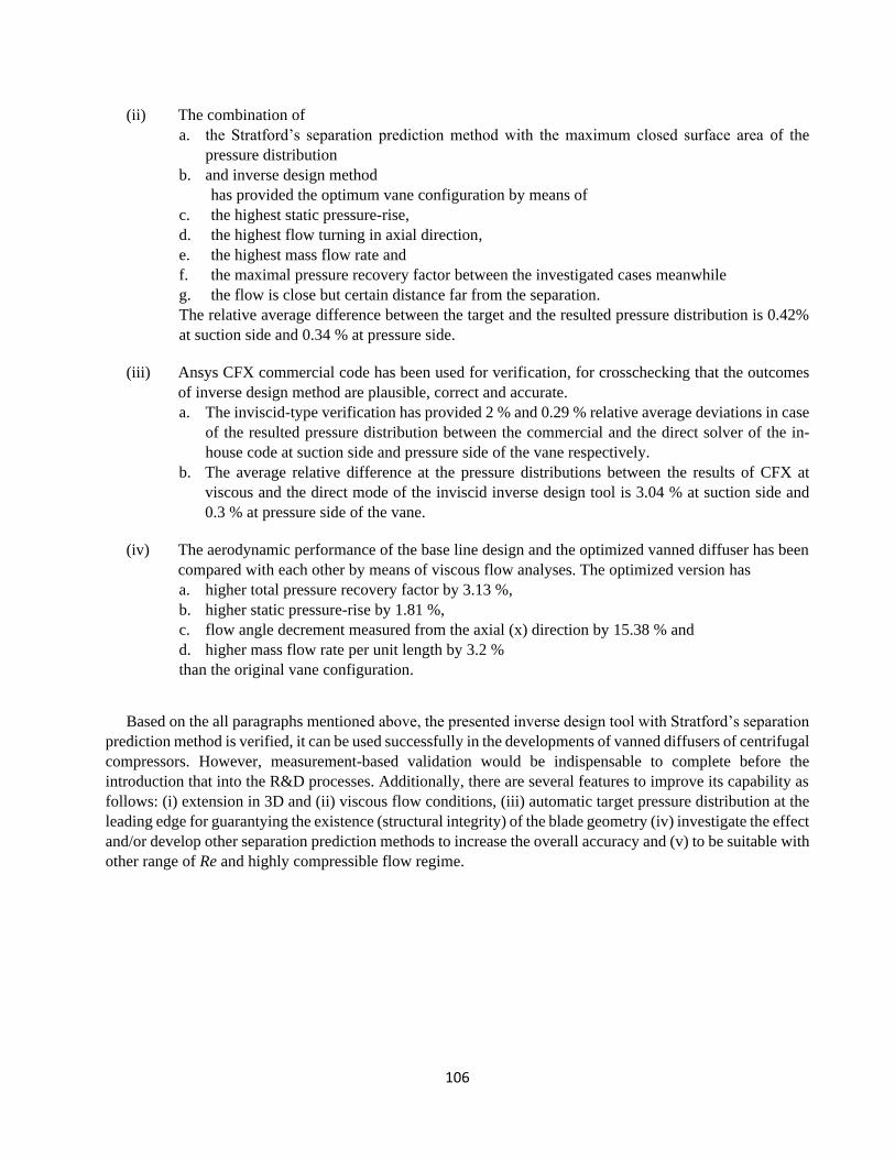
106

(ii) The combination of

a. the Stratford’s separation prediction method with the maximum closed surface area of the

pressure distribution

b. and inverse design method

has provided the optimum vane configuration by means of

c. the highest static pressure-rise,

d. the highest flow turning in axial direction,

e. the highest mass flow rate and

f. the maximal pressure recovery factor between the investigated cases meanwhile

g. the flow is close but certain distance far from the separation.

The relative average difference between the target and the resulted pressure distribution is 0.42%

at suction side and 0.34 % at pressure side.

(iii) Ansys CFX commercial code has been used for verification, for crosschecking that the outcomes

of inverse design method are plausible, correct and accurate.

a. The inviscid-type verification has provided 2 % and 0.29 % relative average deviations in case

of the resulted pressure distribution between the commercial and the direct solver of the in-

house code at suction side and pressure side of the vane respectively.

b. The average relative difference at the pressure distributions between the results of CFX at

viscous and the direct mode of the inviscid inverse design tool is 3.04 % at suction side and

0.3 % at pressure side of the vane.

(iv) The aerodynamic performance of the base line design and the optimized vanned diffuser has been

compared with each other by means of viscous flow analyses. The optimized version has

a. higher total pressure recovery factor by 3.13 %,

b. higher static pressure-rise by 1.81 %,

c. flow angle decrement measured from the axial (x) direction by 15.38 % and

d. higher mass flow rate per unit length by 3.2 %

than the original vane configuration.

Based on the all paragraphs mentioned above, the presented inverse design tool with Stratford’s separation

prediction method is verified, it can be used successfully in the developments of vanned diffusers of centrifugal

compressors. However, measurement-based validation would be indispensable to complete before the

introduction that into the R&D processes. Additionally, there are several features to improve its capability as

follows: (i) extension in 3D and (ii) viscous flow conditions, (iii) automatic target pressure distribution at the

leading edge for guarantying the existence (structural integrity) of the blade geometry (iv) investigate the effect

and/or develop other separation prediction methods to increase the overall accuracy and (v) to be suitable with

other range of Re and highly compressible flow regime.

107

7. Conclusions

Aero- and thermodynamic redesign and analyses of the TSz-21 academic jet engine is completed in the present

thesis. The origin of the single spool engine is a starter gas turbine, which was used originally for MiG-23 and

Szu-22 Russian fighters. This engine has been modified to be an academic jet propulsion system by Dr. Beneda

and Dr. Pásztor from 2005-2008 and it is still under development with especial care for control systems [2].

The virtual prototyping of the jet engine components consists of four different steps in the present case as

follows:

1. Thermo-dynamic cycle analysis for determining the design (operational) point,

2. Mean line and 3D design of the engine for having geometrical sizes and CAD models,

3. Computational Fluid Dynamics (CFD) analysis for verification of the design and plausibility check by

the available data and

4. Inverse design of the vanned diffuser.

Thermo-dynamic cycle analysis for determining the design (operational) point

The redesign process starts with thermodynamic cycle analysis for determining the expected operational

condition. Hence, first, improved mathematical models have been developed for cycle analysis, for

determining the critical pressure at converging nozzle and for determining the optimum total pressure ratio of

the compressor belongs to the maximum thrust. These models are based on the mass and energy balance, they

consider viscous flow conditions meanwhile the specific heats at constant pressure and the ratios of specific

heats depend on the total temperature and fuel to air mass flow rates ratio. The model for cycle analysis is

adapted for triple-, dual- and single-spool turbojet engines for the shake of the complexity and the expression

for the optimum total pressure ratio is developed for single spool turbojet engines.

НК-32 and НК-25 triple spool mixed turbofan engines at take-off (start) condition with afterburner, НК-22

and НК-144A dual spool mixed turbofan engines at take-off and at flight conditions with and without

afterburning respectively, НК-8-4 and НК-86A dual spool mixed turbofan engines at take-off condition

without afterburning and ВД-7 and КР7-300 singles spool turbojet engines at take-off condition without

afterburner are considered for verification and plausibility check of the thermodynamic cycle analysis.

Constrained nonlinear optimisation is applied at these cases for determining the unknown parameters as

efficiencies, losses, power reduction rates of the auxiliary systems, bleed air ratios for technological reasons,

air income ratios due to blade cooling and total temperatures in the afterburner (if it is the case) by means of

having parameter-state, which provides the closest results to the available thrusts [3] and thrust specific fuel

consumptions. The maximum and the average relative deviations between the resulted and available thrusts

and thrust specific fuel consumptions are 1.46 % and 0.645 % (for the thrusts) and 0.55 % and 0.32 % (for the

thrust specific fuel consumptions) respectively, meanwhile the identified parameters are within the plausible

range.

НК-32 and НК-25 engines have been used for determining the effect of the new equation - calculates the

critical pressure - on the thrust and thrust specific fuel consumption. The results of the parameter identification

for the unknown data show that the average value of the relative deviations between the resulted and the

available thrusts and thrust specific fuel consumptions is 0.119 % by using a variant of the new equation for

the critical pressure and it is 3.13 % at the conventional equation with constant gas properties (the ratio of

specific heats for gas equals 1.33). The “variant” in the present context means that the true specific heat is

considered instead of the average one at the given temperature range in the total enthalpy equation. The new

equation for determining the critical pressure is tested also for РД-9Б single-spool turbojet engine with

108

afterburning and at take-off condition. It gives higher critical pressure by 9.3 % than its original form with

constant gas properties.

Finally, the last section in the thermodynamic cycle-analyses is the test and the verification of the novel

analytical equation for the optimum compressor total pressure ratio. РД-9Б and АЛ-21Ф3 single-spool turbojet

engines are considered for that purpose with afterburning and at take-off condition. First, similarly to the

parameter identification described above, the unknown pressure recovery factors, efficiencies and the missing

technical parameters are determined by constraint optimisation. Concerning the both engines, the highest

relative differences between the known and the resulted thrusts and thrust specific fuel consumptions are

0.0617 % and 0.0245 % respectively for the TSFC at РД-9Б engine, while the unknown parameters are within

the expected intervals. The plausibility of the new equation for the optimum total pressure ratio is verified by

determining the extreme value of the pressure ratio-thrust functions numerically. The new equation for the

optimum pressure ratio provides 3.39 % and 3.64 % thrust increments for the РД-9Б and АЛ-21Ф3 jet engine

respectively.

Based on the intensive verification and plausibility check, the developed mathematical model and the new

equations are suitable. So, they are used for determining the operational point of the academic jet engine,

which belongs to expected thrust 330 N at start and sea level conditions.

Mean line and 3D design of the engine for the geometrical sizes and CAD models

After making decision about operational point and having the states of the thermo-dynamical cycle, mean line

design of the centrifugal compressor and axial turbine are completed. The design processes for the compressor

and turbine are based on the standard procedure found in [60] and [1] respectively. Constant nozzle outlet

angle blade twisting method is used due to favourable production cost. Following the 3D extension of the and

the determination of the blade angles, chords, spacings, blade numbers and profiles, the 3D CAD models are

prepared. Beside the turbine, the 3D models of the compressor, inlet channel, combustion chamber and exhaust

nozzle are also created. The main design criteria of these last three structures are to fit their geometrical sizes

to the compressor and turbine and provide minimum pressure recovery factors. The combustion chamber

additionally has high burning efficiency. The calculated thrust is 333.1 N in the mean line design, which is in

line with the design specification. As the 3D models of the structures are available, the preparations of the

flow fields are also completed.

CFD analysis for verification of the design and plausibility check by the available data

CFD analyses are performed and introduced in the next steps of the present work by means of separated and

full components as two different approaches for crosschecking the correctness and the plausibility of the results

of the design. The qualitative results of these simulations are plausible, the thermodynamic parameters are in

the same intervals. Concerning the quantitative results, there are two ways for investigating the plausibility

and the accuracy of the outcomes of the design and the analyses in the present case. The one of them is to

compare the engine design parameters (given by thermodynamic cycle analysis and mean line design) with

the results of the CFD analyses (separated and full modelling approaches) and the second one is to evaluate

the results of the CFD analyses with the available measured data even though the accuracy of these measured

data are not verified statistically [4]. The outputs of these investigations are the following. The average relative

deviations between the results of the thermodynamic cycle analysis and CFD simulations are 0.81 % (for the

separated model) and 1.05 % (for the full model) in case of the total temperature, meanwhile they are 3.42 %

(separated model) and 4.71 % (full model) for the total pressure. The average relative deviations between the

results of the mean line design and the CFD analyses are 1.75 % (separated model) and 1.13 % (full model)

109

for the total temperature, meanwhile it is 1.59 % (separated model) and 1.56 % (full model) for the static

temperature. Similarly, the average relative deviations between the mean line design and CFD analyses are

3.13 % (separated model) and 4.59 % (full model) for the total pressure and they are 3.18 % (separated model)

and 5.01 % (full model) for the static pressure. Although the accuracy is not verified statistically, available

measured data are used for the plausibility checking of the outcomes of the academic jet engine design. The

average relative deviations between the available measured data and the results of the CFD analyses in case

of the total temperature are 0.61 % (separated model) and 1.98 % (full model) and they are 3.03 % (separated

model) and 2.11 % (full model) for the static temperature. The average relative deviations between the

available measured data and the result of the CFD analyses in case of the total pressure are 5.75 % and 10.65

% for the separated and for the full model respectively, meanwhile they are 4.87 % and 3.43 % for the static

pressure.

The results of the thrusts for the academic jet engine are 333.1 N by the mean line design and 325.2 by the

full-model CFD analysis. The expected target thrust is 330 N. The maximum relative deviation between the

computed and expected value is 1.46 %. It is at the case of the full-model CFD analysis.

Based on the discussed results above, the presented methodology till that section by means of virtual

prototyping of the academic jet engine components is suitable, the provided results are acceptable in

engineering point of view.

Inverse design of the vanned diffuser

Inverse design optimization technology is adopted and developed in the last part of the present research for

redesigning the vanned diffuser in the academic jet engine with verification. Compressible Euler equations are

considered as governing equations in the used academic code and a specific finite volume method has been

applied to solve the system of the nonlinear partial differential equations. Stratford’s separation prediction

method has been used to determine and then select the optimum pressure distribution at given boundary

conditions along the suction side of the vane in adverse pressure gradient flow condition.

The outcomes of the inverse design optimisation are the following:

(i) The initial geometry for the inverse design tool is determined to 1. increase the cross-sectional area,

2. decrease the weight, 3. minimize the drag and losses and 4. keep production cost as low as

possible, so

a. the splitter vanes are removed and

b. only the longer vanes are kept and used as initial geometry.

(ii) The combination of

a. the Stratford’s separation prediction method with the maximum closed surface area of the

pressure distribution

b. and inverse design method

has provided the optimum vane configuration by means of

c. the highest static pressure-rise,

d. the highest flow turning in axial direction,

e. the highest mass flow rate and

f. the maximal pressure recovery factor between the investigated cases meanwhile

g. the flow is close but certain distance far from the separation.

The relative average difference between the target and the resulted pressure distribution is 0.42 %

at suction side and 0.34 % at pressure side.

110

(iii) Ansys CFX commercial code has been used for verification, for crosschecking that the outcomes

of inverse design method are plausible, correct and accurate.

a. The inviscid-type verification has provided 2 % and 0.29 % relative average deviations in case

of the resulted pressure distribution between the commercial and the direct solver of the in-

house code at suction side and pressure side of the vane respectively.

b. The average relative difference at the pressure distributions between the results of CFX at

viscous and the direct mode of the inviscid inverse design tool is 3.04 % at suction side and

0.3 % at pressure side of the vane.

(iv) The aerodynamic performance of the base line design and the optimized vanned diffuser has been

compared with each other by means of viscous flow analyses. The optimized version has

a. higher total pressure recovery factor by 3.13 %,

b. higher static pressure-rise by 1.81 %,

c. flow angle decrement measured from the axial (x) direction by 15.38 % and

d. higher mass flow rate per unit length by 3.2 %

than the original vane configuration.

Based on the results mentioned above, the presented inverse design tool with Stratford’s separation prediction

method is verified, it can be used successfully in the developments of vanned diffusers of centrifugal

compressors. However, measurement-based validation would be indispensable to complete before the

introduction that into the R&D processes.

111

8. List and Summary of the Thesis

Advanced aerodynamic design process has been developed and applied for a turbojet engine with especial care

i. for deriving new equations and procedures to increase the accuracy of thermo-dynamic cycle analyses and

ii. for introducing inverse design methodology for redesign vanned diffuser in order to optimize design

specifications. Jet engines with available technical parameters in the open literature are used for the verification

and plausibility check of the thermodynamic models, meanwhile an in-house academic turbo jet engine has

been considered for design, design-verification and plausibility check.

Thesis 1:

The accuracy of the critical pressure at the exit of the converging nozzle of jet engines is increased by

considering specific heats at constant pressure and ratios of specific heats are the functions of temperatures

and fuel to air mass flow rates ratio. Hence, the following equation has to be used for determining critical

static pressure at the outlet of the converging nozzle:

𝒑𝑪 = 𝒑𝟎𝟕 [𝟏 −𝟏

𝜼𝒏(𝟏 −

𝟐𝑪𝒑𝒎𝒊𝒙(𝑻𝟎𝟗,𝑻𝑪,𝒇)

𝟐𝑪𝒑𝒎𝒊𝒙(𝑻𝟎𝟗,𝑻𝑪,𝒇)+𝜸𝒎𝒊𝒙(𝑻𝑪,𝒇)𝑹𝒎𝒊𝒙)𝑪𝒑𝒎𝒊𝒙(𝑻𝟎𝟗,𝑻𝑪,𝒇)

𝟐𝑪𝒑𝒎𝒊𝒙(𝑻𝟎𝟗,𝑻𝑪,𝒇)]

𝜸𝒎𝒊𝒙(𝑻𝟎𝟗,𝑻𝟗𝒔,𝒇)

𝜸𝒎𝒊𝒙(𝑻𝟎𝟗,𝑻𝟗𝒔,𝒇)−𝟏

, (8.1)

where 𝒑𝟎𝟕 is the total pressure [Pa] at the upstream of the nozzle, 𝜼𝒏 is the isentropic efficiency of the nozzle

[-], 𝑪𝒑𝒎𝒊𝒙 is the average specific heat [J/(kg K)], 𝑻𝟎 and 𝑻 is the total and static temperatures respectively

[K], 𝒇 is the fuel to air mass flow rates ratio [-], 𝑹𝒎𝒊𝒙 is the specific gas constant of the gas mixture [J/(kg

K)], 𝜸𝒎𝒊𝒙 is the average ratio of the specific heats [-] and “C” in subscript means critical. The standalone

parameters are valid at the given nozzle sections meanwhile the averaged ones are at the given temperature

ranges and fuel to air ratios.

The Eq. (8.1) gives higher critical pressure by 9.3 % for the РД-9Б single spool turbojet engine than its original

form shown by Eq. (8.2) with constant gas parameters (the ratio of specific heats for the gas is 1.33).

𝑝𝐶 = 𝑝07 (1 −1

𝜂𝑛(𝛾𝑔𝑎𝑠−1

𝛾𝑔𝑎𝑠+1)

𝛾𝑔𝑎𝑠

𝛾𝑔𝑎𝑠−1) (8.2)

The thermodynamic analyses of the НК-32 and НК-25 triple spool jet engines are also completed including

the determination of the critical pressure at the exit of the converging nozzle by using a variant of (8.1) and

(8.2). The average deviation between the resulted (by the parameter fitting) and the available thrust and thrust

specific fuel consumption [3] is 0.119 % by using a variant of (8.1) and 3.13 % at the conventional equation

(8.2) at the same other conditions. The “variant” in the present context means that the true specific heats at

constant pressure and at the given temperatures are considered instead of the averaged one in the total enthalpy

equation.

Related publications: [117, 118 and 121]

Thesis 2:

The accuracy of the optimum total pressure ratio of the turbojet engines pertaining at maximum specific thrust

is improved by applying frictional (viscous) flow assumptions beside the temperature and mass fraction

dependencies of the relevant properties of the gas mixture. Therefore, the following expression has to be used

for determining the optimum total pressure ratio of turbojet engines at maximum specific thrust:

𝝅𝑪_𝒐𝒑𝒕 = √𝜺(𝟏+𝝓)

𝝓(𝜺+𝜷)

𝜷

, (8.3)

112

where

𝜷 =𝜸𝒎𝒊𝒙(𝑻𝟎𝟐,𝑻𝟎𝟑𝒔,𝒇=𝟎)−𝟏

𝜸𝒎𝒊𝒙(𝑻𝟎𝟐,𝑻𝟎𝟑𝒔,𝒇=𝟎), (8.4)

𝜺 =𝜸𝒎𝒊𝒙(𝑻𝟎𝟒,𝑻𝟎𝟓𝒔,𝒇𝑻)−𝟏

𝜸𝒎𝒊𝒙(𝑻𝟎𝟒,𝑻𝟎𝟓𝒔,𝒇𝑻), (8.5)

𝝓 =𝑪𝒑𝒎𝒊𝒙(𝑻𝟎𝟐𝑻𝟎𝟑,𝒇=𝟎)

𝑪𝒑𝒎𝒊𝒙(𝑻𝟎𝟒𝑻𝟎𝟑,𝒇𝒄𝒄)

𝑻𝟎𝟐

𝑻𝟎𝟒

𝟏

𝜼𝒎𝜼𝑪,𝒔𝜼𝑻,𝒔(𝟏−𝜹𝒕𝒆𝒄𝒉)(𝟏+𝜹𝒃𝒄)(𝟏+𝒇𝒄𝒄)(𝟏−𝝃), (8.6)

𝜸𝒎𝒊𝒙 is the average ratio of the specific heats of gas mixture [-], 𝑻𝟎 is the total temperature [K], 𝒇 is the fuel

to air mass flow rates ratio [-] (cc: combustion chamber), 𝑪𝒑𝒎𝒊𝒙 is the average specific heat at constant

pressure for the gas mixture [J/(kg K)], 𝜼 is the efficiency [-] (s: isentropic, m: mechanical, T: turbine and C:

compressor), 𝛿𝑡𝑒𝑐ℎ is the bleed air ratio for technological reasons [-], 𝜹𝒃𝒄 is the ratio of the incoming air

due to blade cooling [-] and 𝝃 is the power reduction rate of the auxiliary systems [-]. The standalone

parameters are valid at the specified engine sections meanwhile the averaged ones are at the given

temperature ranges and fuel to air ratios.

In case of viscous (frictional) flow conditions and variable specific heats, which are included in Eq. (8.3), the

calculated optimum total pressure ratio is higher by 40 % and 53.3 % for the РД-9Б and АЛ-21Ф3 jet engines

respectively than their total pressure ratios found in the technical specification [3]. These newly calculated

optimum total pressure ratios correspond to 3.39 % and 3.64 % thrust increments consistently. In addition,

besides keeping the viscous flow assumption, if the specific heats (and so the ratios of specific heats) are

defined to be constant, there are 9.52 % and 13.04 % decrements in the total pressure ratios for РД-9Б and

АЛ-21Ф3 jet engines respectively.

Related publication: [117]

Thesis 3:

The thermo-dynamical model for design and analysis jet engines including single-, dual-, and triple spool

configurations has to be established by the following way:

i. Mass and energy balance have to be applied,

ii. Frictional (viscous) flow assumption has to be considered in the processes of the thermo-dynamical

cycles,

iii. The specific heats and the ratio of specific heats are the functions of the temperature and the fuel

to air mass flow rates ratios. Iteration cycles have to be used for evaluating the temperatures and

component mass fractions if they are the variables of the gas parameters.

iv. The non-available technical data as efficiencies (e.g.: mechanical, isentropic of fan, compressor

and turbine, burning and exhaust nozzle), total pressure recovery factors (e.g.: inlet diffuser,

combustion chamber and afterburner or turbine exhaust pipe), total pressure ratio of the fan and

intermediate pressure compressor, power reduction rate of the auxiliary systems, bleed air ratio for

technological reasons, air income ratio due to blade cooling and total temperature of the

afterburner, if these are relevant – have to be determined either by

a) well known and established (practical) experiences,

b) measurements,

c) simulations (e.g.: CFD simulations for efficiencies and total pressure recovery factors) and

d) parameter identification, in which the goal function of the optimization is to minimize the

differences between the calculated and available thrust and thrust specific fuel consumption.

113

v. Equation (8.1) has to be used for determining critical static pressure at the exit of the converging

nozzle.

vi. Equation (8.3) has to be used for determining the optimum compressor total pressure ratio at

maximum specific thrust for turbojet engines.

4 single spool (at one operational condition), 4 dual spool (two is at two and two is at one operational

conditions) and 2 triple spool (at one operational condition) jet engines are analysed by the mathematical

models introduced in the present thesis. The resulted thrusts and thrust specific fuel consumptions by constraint

nonlinear optimisation - in order to find the unknown parameters – are compared with available data in [3] for

verification. The maximum and the average relative deviation between them are 1.46 % and 0.645 % for the

thrust and 0.55 % and 0.32 % for the thrust specific fuel consumptions respectively, meanwhile the identified

parameters are within the plausible range.

Related publications: [117-119, 121, 122, 125 and 126]

Thesis 4:

The combination of the Stratford’s separation prediction method – for providing the maximum closed

surface area of the pressure distribution – and inviscid inverse design method – for creating the blade

geometry belongs to this pressure distribution – have to be used in design, re-design and developments of

vanned diffusers in centrifugal compressor units for providing the optimum vane configurations by means

of having:

i. the minimal design changes with respect to the baseline configuration, if it is applicable, and in the

present case:

a. the splitter vanes are removed, and

b. only the vanes with higher chord-length are kept and used as initial geometry for the inverse

design method,

ii. the maximum static pressure-rise,

iii. the highest flow turning in axial direction,

iv. the largest mass flow rate

v. and the greatest total pressure recovery factor (ptotal_downstream/ptotal_upstream),

meanwhile the flow is close but certain safe distance far from the separation as it is guaranteed by the

Stratford’s separation prediction method.

Regarding the redesigned (optimized) blade configuration, the average relative difference of the pressure

distributions between the results of the CFX at viscous flow condition and the inviscid in-house code is 3.04

% at suction side and 0.3 % at pressure side.

The aerodynamic performance of the base line design and the optimized vanned diffuser has been compared

with each other by means of viscous flow analyses. The optimized version has

i. higher total pressure recovery factor by 3.13 %,

ii. higher static pressure-rise by 1.81 %,

iii. flow angle decrement measured from the axial (x) direction by 15.38 %, and

iv. higher mass flow rate per unit length by 3.2 %

than the original vane configuration has. 2D planar approach has been considered in the present methodology.

Related publications: [119, 120 and 123]

Thesis 5:

The following process has to be used for aerodynamic design of jet engines:

i. thermo-dynamic cycle analyses according to Thesis 1. 2. and 3. for determining the design

(operational) point,

114

ii. establishment of the main geometrical sizes and the necessary RPM, if they are relevant [1],

iii. mean line and 3D design with geometry preparation and CAD modelling,

iv. CFD analyses for verification of the design and plausibility check by the available data and

v. inverse design of the solid walls, vanned diffuser in the present case according to Thesis 4.

After completing the aerodynamic redesign of the academic jet engine in line with the above defined process,

excluding the last steps, the conclusions are next. The average relative deviation – using data at engine unit

sections – between the results of the thermodynamic cycle analysis and the CFD analysis in case of the full

model is 1.05 % for the total temperature and it is 4.71 % for the total pressure. The average relative deviation

between the results of the mean line design and CFD analysis in case of the full model also is 1.13 % for the

total temperature and it is 1.56 % for the static temperature. Similarly, it is 4.59 % for the total pressure and it

is 5.01 % for the static pressure. Although its accuracy is not verified statistically, available measured data [4]

is used for plausibility checking of the computed results. The average relative deviation between the available

measured data and the results of the CFD analysis in case of full model is 1.98 % for the total temperature and

it is 2.11 % for the static temperature. Similarly, it is 10.56 % for the total pressure and it is 3.43 % for the

static pressure. The thrust of the academic jet engine is 333.1 N by the mean line design and 325.2 by the full-

model CFD analysis. The expected target thrust is 330 N. The maximum relative deviation between these

computed and the expected value is 1.46 % and it is at the full-model CFD analysis.

Related publications: [117-128]

Berlin, 31. 12. 2020.

………………………………………..

Foroozan Zare

115

Bibliography

[1] Sánta, I., Tervezési Segédlet - Gázturbinás Repülőgép Hajtóművek (Design Guide Line - Aircraft Engines with

Gas Turbines), Budapest: BME Vasúti Járművek, Repülőgépek és Hajók Tanszék (BME, Department of

Aeronautics, Naval Architecture and Railway Vehicles), 2008.

[2] Beneda, K., Pásztor, E., “A TKT-1 Kisméretű, Oktatási és Kutatási Célú Gázturbinás Sugárhajtómű Első Tíz

Éve (The First Ten Years of the TKT-1 Small-Sized Academic and Research Turbo Jet Engine),”

Repüléstudományi Közlemények (Aeronautical Science Bulletins - online scientific journal), vol. 3, pp. 117-132,

2015.

[3] Кулагин, В.В., Tеория расчёт и проектирование авиационных двигателей и энергетических установок,

Книга 1, 2, ISBN 5-217-03269-3, Moscow: Mockba, Maшиноcтроeние, 2005.

[4] Pallag, N., “A TKT-1 gázturbinás sugárhajtómű áramlástani vizsgálata (Numerical Analysis of Flow Conditions

in TKT-1 Jet Engine), MSc Thesis,” Budapest University of Technology and Economics, Budapest, 2013.

[5] Gáti, B., Drouin, A., “Open Source Autopilot for Academic Research-The Paparazzi System,” in IEEE,

Washington, DC, USA, 2013.

[6] Voskuilj, M., Rohács, D., Rohács, J., Schoustra, R-J.,, “Preliminary Evaluation of the Environmental Impact

Related to Take-off and Landings Supported with Ground-Based (MAGLEV) Power,” Journal of Aerospace

Operations, vol. 2, no. 3-4, pp. 161-180, 2013.

[7] Beneda, K., Rohács, J., “Dynamic Model of Variable Inducer Shroud Bleed for Centrifugal Compressor Surge

Suppression,” International Review of Aerospace Engineering, vol. 6(3), pp. 163-173, 2013.

[8] Beneda, K., Simongáti, Gy., Veress, Á.,, Járművek hő- és áramlástechnikai berendezései I. (Turbomachinery

and Heat Engines in Vehicles I.), Budapest: Typotex Kiadó, URL:

https://www.tankonyvtar.hu/hu/tartalom/tamop412A/0018_Jarmuvek_ho-

_es_aramlastechnikai_berendezesei_1/adatok.html [Accessed: 02.10.2019.], 2014.

[9] [Online]. Available: http://www.leteckemotory.cz/motory/r-29b/r-29b-300_rez.jpg and

http://www.leteckemotory.cz/motory/f100/. [Accessed 02. 10. 2019.].

[10] Koff, B., “Spanning the Globe with Jet Propulsion,” American Institute of Aeronautics & Astronautics, no.

https://doi.org/10.2514/6.1991-2987, 2012.

[11] Rolls-Royce, “Civil Aerospace, Future product, UltraFan,” Rolls-Royce, [Online]. Available: https://www.rolls-

royce.com/products-and-services/civil-aerospace/future-products.aspx#section-overview. [Accessed 31 12

2020].

[12] Han, P., “Additive Design and Manufacturing of Jet Engine Parts,” Engineering, vol. 3, no. 5, pp. 648-652,

2017.

[13] Homaifar, A., Lai, Y. H., McCormick, E., “System Optimization of Turbofan Engines Using Genetic

Algorithms,” Applied Mathematical Modelling, vol. 18, no. 2, pp. 72-83, 1994.

[14] Guha, A., “Optimum Fan Pressure Ratio for Bypass Engines with Separate or Mixed Exhaust Streams,” Journal

of Propulsion and Power, vol. 17, no. 5, pp. 1117-1122, 2001.

116

[15] Silva, V.V.R., Khatib, W., Fleming, P.J., “Performance Optimization of Gas Turbine Engine,” Engineering

Aplications of Artificial Intelligence, vol. 18, no. 5, pp. 575-583, 2005.

[16] Al-Hamdan, Q., Ebaid, M., “Modeling and Simulation of a Gas Turbine Engine for Power Generation,” Journal

of Engineering for Gas Turbine and Power, vol. 128, no. 2, 2006.

[17] Henriksson, M., Grönstedt, T., Breitholtz, C., “Model-Based on-Board Turbofan Thrust Estimation,” Journal of

Control Engineering Practice, vol. 19, no. 6, pp. 602-610, 2011.

[18] Turan, O., “Exergetic Effects of Some Design Parameters on the Small Turbojet Engine for Unmanned Air

Vehicle Applications,” Energy, vol. 46, no. 1, pp. 51-61, 2012.

[19] Khaliq, A., Kaushik, S.C., “Thermodynamic Performance Evaluation of Combustion Gas Turbine Cogeneration

System with Reheat,” Applied Thermal Engineering, vol. 24, no. 13, pp. 1785-1795, 2004.

[20] Sanjay, “Investigation of Effect of Variation of Cycle Parameters on Thermodynamic Performance of Gas-

Steam Combined Cycle,” Energy, vol. 36, no. 1, pp. 157-167, 2010.

[21] Atashkari, K., Nariman-Zadeh, N., Pilechi, A., Jamali, A., Yao, X., “Thermodynamic Pareto Optimization of

Turbojet Engines Using Multi-Objective Genetic Algorithms,” International Journal of Thermal Science, vol.

44, no. 11, pp. 1061-1071, 2005.

[22] Lazzaretto, A., Toffolo, A., “Analytical and Neural Network Models for Gas Turbine Design and Off-Design

Simulation,” International Journal of Thermodynamics, vol. 4, pp. 173-182, 2001.

[23] Mattingly, J. D., Elements of Propulsion: Gas Turbines and Rockets, 1801 Alexander Bell Drive, Reston,

Virginia 20191-4344: American Institute of Aeronautics and Astronautics, Inc., 2006.

[24] El-Sayed, A. F., Aircraft Propulsion and Gas Turbine Engines, United States of America: Taylor & Francis

Group, LLC, ISBN 9781466595163, 2008.

[25] Sánta, I., Repülőgép Hajtóművek Elmélete I. (Theory of Aircraft Engines I.) (Gázturbinás Hajtóművek (Engines

with Gas Turbines)), Budapest: BME, Department of Aeronautics, Naval Architecture and Railway Vehicles,

lecture note, 2008.

[26] Kurzke, J., “The GasTurb Program - Commercial Computer Program, GasTurb12,” [Online]. Available:

http://www.gasturb.de. [Accessed 03 03 2016].

[27] Kuznetsov, “Wikipedia,” Kuznetsov Design Bureau, [Online]. Available:

https://en.wikipedia.org/wiki/Kuznetsov_NK-32. [Accessed 17. 11. 2019.].

[28] Kuznetsov, “Wikipedia,” Kuznetsov Design Bureau, [Online]. Available:

https://en.wikipedia.org/wiki/Kuznetsov_NK-25. [Accessed 17. 11. 2019.].

[29] Russian Aviation, “Russian Aviaton (News),” Kuznetsov, [Online]. Available:

https://www.ruaviation.com/news/2016/8/15/6454/?h. [Accessed 17. 11. 2019.].

[30] I. 2. International Organization for Standardization, “International Standard Atmosphere,” Wikipedia, 1975.

[Online]. Available: https://en.wikipedia.org/wiki/International_Standard_Atmosphere. [Accessed 02 02 2020].

[31] Beneda, K., “Development of Active Surge Control Devices for Centrifugal Compressors, PhD Thesis,” BME,

Department of Aeronautics, Naval Architecture and Railway Vehicles, Budapest, 2013.

117

[32] MathWorks, “MATLAB, Constrained Nonlinear Optimization Algorithms,” MathWorks, Inc., [Online].

Available: https://uk.mathworks.com/help/optim/ug/constrained-nonlinear-optimization-

algorithms.html#brnox0o. [Accessed 28 12 2020].

[33] Mathworks, “Matlab R2017b Documentation (Optimization Toolbox; "fmincon" function),” 2017. [Online].

Available: https://uk.mathworks.com/help/optim/ug/fmincon.html. [Accessed 30 09 2017].

[34] Chu, H. H., Hsiao-Wei, C., “Aerospace Technology Development – Small Gas-Turbine development,” ROC:

Aerospace Development Planning, pp. 4-22, 1996.

[35] Beneda, K., “Dynamic Nonlinear Mathematical Model of Active Compressor Surge Control Devices,” in

Proceedings of the 11th Mini Conference on Vehicle System Dynamics, Identification and Anomalies (VSDIA),

Budapest, 2008.

[36] Hargitai, C., “Effect of Parameters of Inland Vessel Semi Empirical Motion Equations on Transient Motion

Phenomena,” in in Proceedings of the TVL: Second Scientific Workshop on Transport, Vehicle and Logistics

organized by the PhD Schools of the Faculty of transporation engineering and vehicle engineering, Budapest,

2012.

[37] “The bridges of Budapest,” [Online]. Available: http://www.bridgesofbudapest.com/bridge/chain_bridge.

[Accessed 24 06 2017].

[38] “Airbus A380,” Wikipedia, [Online]. Available: https://en.wikipedia.org/wiki/Airbus_A380. [Accessed 24 06

2017].

[39] [Online]. Available: https://en.wikipedia.org/wiki/General_Electric_GE90. [Accessed 24. 06. 2017.].

[40] Mercedes-Benz, “Mercedes-Benz Actros,” Mercedes-Benz, [Online]. Available:

http://media.daimler.com/marsMediaSite/en/instance/ko/Mercedes-Benz-Actros.xhtml?oid=9904742. [Accessed

24. 06. 2017.].

[41] [Online]. Available: http://behindthewheel.com.au/next-gen-mercedes-benz-actros-launched-australia/2017-

mercedes-benz-actros. [Accessed 24. 06. 2017.].

[42] [Online]. Available: https://en.wikipedia.org/wiki/IPhones. [Accessed 24. 06. 2017.].

[43] “Re/872. Az 55 típusú hajtómű műszaki üzembentartási szakutasítás 2. könyv. (Operational and maintenance

manual of engine Type 55, second book),” Honvédelmi Minisztérium (Ministry of National Defense ), 1980.

[44] Beneda, K., “CFD Simulation of Blade Load Distribution Control as Active Centrifugal Compressor Surge

Suppression,” ACTA AVIONICA, vol. 15, no. 25, pp. 13-20, 2013.

[45] Beneda, K., “Numerical Simulation of MEMS-based Blade Load Distribution Control in Centrifugal

Compressor Surge Suppression,” in ICNPAA 2012 Congress: Mathematical Problems in Engineering,

Aerospace and Sciences, Vienna, Austria, 2012.

[46] Nagy, A., Rohács, J., Régert, T., “Investigation on the Effect of Hydrodynamic MEMS on Airfoil,” in 26th

International Congress of the Aeronautical Sciences (ICAS), Optimage Ltd., Anchorage, USA, 2008.

[47] swMATH, “ANSYS-CFX,” swMATH - an Information Service for Mathematical Software, [Online].

Available: http://swmath.org/software/6391. [Accessed 30. 12. 2020.].

118

[48] ANSYS, ANSYS CFX-Solver Theory Guide, Release 14.5, Southpointe, 275 Technology Drive, Canonsburg, PA

15317, 2012.

[49] Robert Bosch GmbH, Automotive Handbook, John Wiley & Sons, 2018.

[50] ANSYS Inc., “CFX Inlet Turbulence Conditions,” Introduction to ANSYS CFX, Lecture 07 - Turbulence, CFX-

Intro_14.0_L07_Turbulence .pdf , 2013.

[51] Khayamyan, S., Flow Field in a Gas Turbine Burner, MSc Thesis, Lulea, Sweden: Lulea University of

Technology, http://www.diva-portal.org/smash/get/diva2:1017888/FULLTEXT01.pdf, 2010 [Accessed:

23.10.2019].

[52] Thévenin, D. Janiga,G., Optimization and Computational Fluid Dynamics, Hardcover, Berlin: Springer, 2008.

[53] Weise, T., Global Optimization Algorithms - Theory and Application, ebook: http://www.it-weise.de/, 2011.

[54] Veress, Á., Felföldi, A., Gausz, T., Palkovics, L., “Coupled Problem of the Inverse Design and Constraint

Optimization,” Applied Mathematics and Computation, vol. 219 , no. 13, pp. 7115-7126, 2013.

[55] Lighthill, M.J., “A new Method of Two-dimensional Aerodynamic Design,” in Aeronautical Research Council,

London,, 1945.

[56] Giles, M. B., Drela, M., “Two-Dimensional Transonic Aerodynamic Design Method,” Journal of AIAA, vol. 25,

no. 9, pp. 1199-1206, 1987.

[57] Demeulenaere, A., “An Euler/Navier-Stokes Inverse Method for Compressor and Turbine Blade Design,” Von

Kármán Institute for Fluid Dynamics, Inverse Design and Optimisation Methods, 1997.

[58] De Vito, L., Van den Braembussche, R. A. , Deconinck, H., “A Novel Two-dimensional Viscous Inverse Design

Method for Turbomachinery Blading,” in International Gas Turbine and Aeroengine Congress and Exhibition,

Amsterdam, PAYS-BAS, 03/06/2002.

[59] Cabuk, H., Modi, V., “Optimum Plane Diffusers In Laminar Flow,” Journal of Fluid Mechanics, vol. 237, pp.

373-393, 1992.

[60] Japikse, D., Centrifugal Compressor Design and Performance, Wilder, Vermont: Concepts ETI, Inc. Printed in

the United States of America by Thomson-Shore, Inc., 1996.

[61] Andronenko, S., Stiharu, I., Packirisamy, M., Moustapha, H. Dionne, P., “The Use of Microelectromechanical

Systems for Surge Detection in Gas Turbine Engines,” in Proceedings of the 2005 International Conference on

MEMS, NANO and Smart Systems (ICMENS’05), 2005.

[62] Шустов, И. Г., Двигатели 1944-2000: авиационные, ракетные, морские, промышленные.

Илюстрированный каталог авиадвигателей с их характеристиками, описанием, АКС-Конверсалт, 2000.

[63] Ailer, P., “Kisteljesítményű gázturbina modellezése és nemlineáris irányítása, PhD értekezés (Modelling and

Nonlinear Control of a Low-Power Gas Turbine, PhD thesis),” BME Repülőgépek és Hajók Tanszék (BME

Department of Aircraft and Ships), Budapest, 2002.

[64] Al-Hamdan, Q. Z., Ebaid, M. S. Y., “Modeling and Simulation of a Gas Turbine Engine for Power Generation,”

ASME Journal of Engineering for Gas Turbines and Power, vol. 128, no. 2, pp. 302-311, April 2006.

119

[65] Bartolini, G., Muntoni, A., Pisano, A., and Usai, E., “Compressor Surge Active Control via Throttle and CCV

Actuators. A Second-Order Sliding-Mode Approach,” in International Workshop on Variable Structure Systems,

Antalya, Turkey, 2008.

[66] Schleer, M. W., “Flow Structure and Stability of a Turbocharger Centrifugal Compressor,” PhD Dissertation,

Eidgenössischen Technische Hochschule, Zürich, 2006.

[67] Yoon, S. Y., Lin, Z., Goyne, C., Allaire, P. E., “An Enhanced Greitzer Compressor Model Including Pipeline

Dynamics and Surge,” ASME Journal of Vibration and Acoustics, vol. 133, no. 5, October 2011.

[68] Boinov, K. O., Lomonova, E. A., Vandenput, A. J. A., Tyagunov, A., “Surge Control of the Electrically Driven

Centrifugal Compressor,” vol. 42, no. 6, pp. 1523-1531, 2006.

[69] Ferrari, M. L., Pascenti, M., Magistri, L., Massardo, A. F., “Hybrid System Test Rig: Start-up and Shutdown

Physical Emulation,” ASME Journal of Fuel Cell Science and Technology, vol. 7, no. 2: 021005, 2010.

[70] Veress, Á., “Axial Compressors (Aircraft Engines II., lecture note at BME University),” Budapest University of

Technology and Economics (BME), Department of Aeronautics, Naval Architecture and Railway Vehicles,

Budapest, 2018.

[71] Boyce, M. P., “Principles of Operation and Performance Estimation of Centrifugal Compressors,” Proceedings

of the 22nd Turbomachinery Symposium, pp. 161-177, 1993.

[72] “Turbine Engines of the World. In: Flight International Weekly,” 10 January 1974. [Online]. Available:

http://www.flightglobal.com/pdfarchive/view/1974/1974%20-%200043.html. [Accessed 15 02 2013].

[73] Ballal, D. R., Zelina, J., “Progress in Aero Engine Technology (1939 – 2003),” [Online]. Available:

http://soliton.ae.gatech.edu/ people/jseitzma/classes/ae4451/AeroEngineTechnology1939_2003AE4451.pdf.

[Accessed 15 03 2013].

[74] [Online]. Available: Sources:

https://www.reddit.com/r/ThingsCutInHalfPorn/comments/et58le/lycoming_alf_502/ and

http://www.seattleturbine.com/index2.shtml, both are accessed on 13.09.2020.

[75] Bauer, P., Bokor, J., “Infinite Horizon LQ Optimal Output Tracking – From Development to Real Flight Tests,”

in In Proc. of 12th IEEE International Symposium on Computational Intelligence and Informatics, Budapest,

November 2, 2011.

[76] Gáti, B., “Unmanned Aerial Systems for Educational Purpose,” in 13th Mini Conference on Vehicle System

Dynamics, Identification and Anomalies, Budapest, 2012.

[77] Szabolcsi, R., “UAV automatikus repülésszabályozó rendszer számítógépes tervezése (Computational Design of

UAV's Automatic Flight Control System),” Hadmérnök (Military Engineer), vol. 1, pp. 222-237, March 2012.

[78] Koncz, M. T., “Automatikus irányítású célrepülőgépek pályatervezése (Flight Path Design of Targeted Aircraft

with Automatic Control),” in Új évezred, új technológia – Gripenek a magyar légierőben, Szolnoki

Repüléstudományi Konferencia (Grippens are in the Hungarian Air Force, Conference on Aeronautical

Sciences in Szolnok), Szolnok, 2006.

[79] Helvoirt, van, J., “Centrifugal compressor surge: modeling and identification for control, PhD Thesis,

https://doi.org/10.6100/IR629084,” Technische Universiteit Eindhoven, 2007.

120

[80] Eckert, B., Schnell, E., Axial- und Radialkompressoren: Anwendung, Theorie, Berechnung, Berlin: Springer,

1980.

[81] Csató, J., “Előperdítés hatása turbófeltöltő centrifugálkompresszorának karakterisztikájára (Effect of prerotation

on the characteristics of centrifugal compressor in turbocharger),” BME Közlekedésmérnöki Kar (Budapest

University of Technology and Economics, Faculty of Transportation Engineering), Budapest, 1994.

[82] Veress, Á., “Centrifugal Compressors (Aircraft Engines II., lecture note at BME University),” Budapest

University of Technology and Economics (BME), Department of Aeronautics, Naval Architecture and Railway

Vehicles, Budapest, 2013.

[83] Osborne, C., Runstadler, P. W., Dodd Stacy, W., “Aerodynamic and Mechanical Design of an 8:1 Pressure

Ratio Centrifugal Compressor,” NASA Lewis Research Center, Clevaland, 1975.

[84] Rolls-Royce, The Jet Engine, Hoboken, United States: John Wiley and Sons Ltd., 2015.

[85] ANSYS, “ANSYS CFX-Solver Modeling Guide, Release 14.5,” ANSYS, Inc., Southpointe 275 Technology

Drive Canonsburg, PA 15317, ansysinfo@ansys.com, http://www.ansys.com, October 2012.

[86] Lentini, J. J., Scientific Protocols for Fire Investigation, New York: CRC Press, Taylor and Francis Group,

2013.

[87] Montgomery, J. H., Crompton, T. R., Environmental Chemicals Desk Reference, New York: CRC Press, Taylor

and Francis Group, 2017.

[88] Chen, L., Gao, K., Zhang, C., Lang, W., “Advanced Biofuels: Chapter 2 - Alternative Fuels for IC Engines and

Jet Engines and Comparison of Their Gaseous and Particulate Matter Emissions,” Woodhead Publishing Series

in Energy, 2019.

[89] Cyrus, B. M. H., “The Historical Evolution of Turbomachinery,” in Proceding of the 29 Turbomachinery

Symposium, Mee Industries Inc,, Monrovia, california, 2000.

[90] Masanori, Y., Junichiro, M., Keizo, T., Eisaku, I., Satoshi, H., “Development of 1600°C - Class High-Efficiency

Gas Turbine for Power Generation Applying J-Type Technology,” Mitsubishi Heavy Industries Technical

Review, vol. 50, no. 3, 2013.

[91] Nageswara, R. M., Advances in Gas Turbine Technology, Materials for gas turbines - An Overview, India: VIT

University, 2011.

[92] Gorla, R. S. R., Khan, A., A., Turbomachinery - Design and Theory, Karachi, Pakistan: Marcel Dekker, 2003.

[93] Tournier,J. Michel. El-Genk, S.Mohamed., “Axial flow, multi-stage turbine and compressor models,” Energy

Conversion and Management, no. 51, pp. 16-29, 29 September 2009.

[94] Da Lio, L., Manente, G., Lazzaretto, A., “New efficiency charts for the optimum design of axial flow turbines,”

Energy, no. 77, pp. 447-459, 2014.

[95] Moustapha, H., Zelesky, M.F., Baines, N.C., Japikse, D., Axial and Radial Turbines, 3nd ed., Concepts ETI,

Inc., 2003.

[96] Beneda, K., Repülőgép-hajtóművek elmélete 2. (Theory of Aircraft Engines II.), Budapest: Akadémiai Kiadó,

2018.

121

[97] Sánta, I., “Repülőgép Hajtóművek Tervezése - Axiális Kompresszorok Aero- Termodinamikai Számítása

(Design of Aircraft Engines - Aero- and Thermodynamic Calculations of Axial Compressors),” Budapest

University of Technology and Economics, Department of Aeronautics Naval Architecture and Railway

Vehicles, Budapest, 2009.

[98] Menter, F. R., “Two-Equation Eddy-Viscosity Turbulence Models for Engineering Applications,” AIAA

Journal, vol. 32, no. 8, p. 1598–1605, 1994.

[99] “SST k-omega model,” CFD Online, 28 02 2011. [Online]. Available: http://www.cfd-online.com/Wiki/SST_k-

omega_model. [Accessed 11 10 2019].

[100] Menter, F. R., “Zonal Two Equation k-ω Turbulence Models for Aerodynamic Flows,” AIAA Paper, Vols. 93-

2906, 1993.

[101] Stiesch, G., Modeling Engine Spray and Combustion Processes, Berlin Heidelberg: Springer-Verlag, ISBN 978-

3-642-05629-1, 2003.

[102] Herrmann, M., “Modeling Primary Breakup: A Three-Dimensional Eulerian Level Set/Vortex Sheet Method for

Two-Phase Interface Dynamics,” Center for Turbulence Research, Annual Research Briefs, pp. 185-196, 2003.

[103] Edwards, J. T., “Reference Jet Fuels for Combustion Testing,” in 55th AIAA Aerospace Sciences Meeting,

Session: Alternate Aviation Fuels I, Grapevine, Texas, 2017.

[104] Bacchi, R., D., A. , “Best Practice Guidelines for Combustion Modeling (ANSYS),” [Online]. Available:

http://www.esss.com.br/events/ansys2013/brazil/pdf/24_5_1450.pdf. [Accessed 23 10 2019].

[105] Marchello, M., “A Three Dimensional High Resolution Compressible Flow Solver,” PhD thesis, Catholic

University of Leuven, 1992.

[106] Roe, P.L., “Approximate Riemann Solvers, Parameter Vectors, and Difference Schemes,” Journal of

Computational Physics, vol. 43, pp. 357-372, 1981.

[107] Yee, H.C., “A class of high-resolution explicit and implicit shock-capturing methods,” NASA TM-101088,

1989.

[108] Hirsch, C., Numerical Computation of Internal and External Flows, vol. II, John Wiley & Sons, 1990.

[109] Lefebvre, M., Antwerp, T.S., “Arts Numerical Aero-thermal Prediction of Laminar/Turbulent Flows in a Two-

dimensional High Pressure Turbine Linear Cascade,” in Second European Conference on Turbomachinery -

Fluid Dynamics and Thermodynamic, Belgium, 1997.

[110] Laney, C. B., Computational Gas dynamics, Cambridge University Press, ISBN-13: 978-0521625586, 1998.

[111] Stein, E., Borst, R. Hughes, T, Finite volume methods,foundation and analysis, L. c. Edited by John Wiley &

Sons, Ed., 2004.

[112] Kuzmin, D., Möller, M. , “Algebraic Flux Correction II. Compressible Euler Equations,” Springer, pp. 207-250,

1990.

[113] Smith, A. M. O., “High-Lift Aerodynamics,” Journal of Aircraft, vol. 12, no. 6, pp. 501-530, 1975.

[114] Stratford, B. S., “The Prediction of Separation of the Turbulent Boundary Layer,” Journal of Fluid Mechanics,

vol. 5, pp. 1-16, 1959.

122

[115] Molnár, D., “Investigation of Inverse Design Utilization for Static Pressurize of a Cascade,” Budapest university

of technology and economics, Budapest, 2016.

[116] Ochkov, V. F. , “Теплотехника и теплоэнергетика,” National Research University Moscow Power

Engineering Institute (Technical University), Dept. Theoretical basics of thermal engineering, 27 06 2016.

[Online]. Available: http://twt.mpei.ac.ru/TTHB/2/KiSyShe/eng/Chapter1/1-6-Concept-of-heat-capacity.html.

[Accessed 01 02 2020].

Author’s Publications

[117] Zare, F., Veress, Á., “Novel Closed-Form Equation for Critical Pressure and Optimum Pressure Ratio

for Turbojet Engines,” International Journal of Turbo & Jet-Engines, IF: 0.733, Q3, (2019/2020),

accepted for publication, https://www.degruyter.com/view/j/tjj.ahead-of-print/tjj-2019-0039/tjj-2019-

0039.xml, published online: 2019-11-30, DOI: https://doi.org/10.1515/tjj-2019-0039, 2019.

[118] Zare, F., Veress, Á., “Derivation and Application of a New Equation for Design and Analysis of Triple

Spool Mixed Turbofan Jet Engines with Verification,” Acta Polytechnica Hungarica, IF: 0.745, Q2

(2016), vol. 13, No. 6, 2016 pp. 147-162, http://www.uni-obuda.hu/journal/Zare_Veress_70.pdf, 2016.

[119] Zare, F., Veress, Á., “Preliminary Introduction to Virtual Prototyping of Jet Engine Components by

Means of Aerodynamic Design,” Repüléstudományi Közlemények, on-line tudományos folyóirat

(Aeronautical Science Bulletins - online scientific journal), number: XXIX. vol.: 2017/3., pp. 141-148,

2017.

[120] Zare, F., Veress, Á., “Plausibility Check of the Inverse Design and Optimization Method for Cascade

Flow by Means of ANSYS CFX Software,” Repüléstudományi Közlemények, on-line tudományos

folyóirat (Aeronautical Science Bulletins - online scientific journal), number: XXVII., vol.: 2015/2.,

HU ISSN 1789-770X, pp. 182-206. 2015.

[121] Zare, F., Veress, Á., “Development and Verification of an Improved Thermo-Dynamical Model for

Single Spool Jet Engines,” Repüléstudományi Közlemények, on-line tudományos folyóirat

(Aeronautical Science Bulletins - online scientific journal), number: XXVI. vol.: 2014/2., pp. 539-551.

2014

[122] Zare, F., Veress, Á., “Aerodynamic Redesign and Analysis of Gas Turbine Components - Virtual

prototyping of Jet engine,” XIX. Magyar Repüléstudományi Napok 2017. (XIX. Hungarian Days of

Aeronautical Sciences 2017.) 15-16. November 2017. HungaroControl (Hungarian Air Navigation

Services Pte. Ltd. Co. 1185. Budapest Igló u. 33-35.) Repüléstudományi Közlemények, on-line

tudományos folyóirat (Aeronautical Science Bulletins - online scientific journal), number: XXIX., vol.:

2017/2., pp. 309-330. 2017.

[123] Zare, F., Veress, Á., “Novel Application of Inverse Design Method by Means of Redesigning

Compressor Stator Vanes in a Research Jet Engine,” in the Proceedings of 15th mini Conference on

Vehicle System Dynamics, Identification and Anomalies, Budapest, 7-9. November 2016, ISBN 978-

963-313-266-1, pp. 261-280. 2016.

123

[124] Zare, F., Veress, Á., “Numerical Modelling and Simulation of a Centrifugal Compressor Passage with

Plausibility Check,” 14th mini Conference on Vehicle System Dynamics, Identification and Anomalies,

Budapest, November. 10-12, 2014, Conference Proceedings, ISBN 978-963-313-186-2, pp. 367-378.

2014.

[125] Zare, F., Veress, Á., “Mathematical Model Development and Thermo-dynamical Cycle Analyses of a

Dual Spool no By-pass and a Dual Spool Mixed Turbofan Engine,” International Conference on

Innovative Technologies, IN-TECH 2013, Budapest, 10. - 12. 09. 2013, ISBN 978-953-6326-88-4, pp.

41-44, 2013.

[126] Zare, F., Veress, Á., Beneda, K., “Simplified Mathematical Model for a Single Spool and no Bypass Jet

Engines,” Repüléstudományi Konferencia (Conference on Aeronautical Sciences) 11.04.2013., Szolnok,

Hungary, Repüléstudományi Közlemények (Aeronautical Science Bulletins - online scientific journal),

number: XXV., vol.: 2013/2 (special issue), HU ISSN 1789-770X, pp. 39-52, 2013.

[127] Bicsák, Gy., Zare, F., Veress, Á., “Gázturbina égésfolyamatának vizsgálata különböző égésmodellekkel

(Analysing of Combustion Processes in Gas Turbine with Using Different Combustion Models),” Jövő

Járműve folyóirat (Journal of Future Vehicles), HU ISSN 1788-2699, vol.: 2012-3/4, pp. 46-51, 2012.

[128] Bicsák, Gy., Zare, F., Veress, Á., “Numerical Modelling of Heat Transfer Processes in the Solar Taurus

T60 Gas Turbine Combustion Chamber,” VSDIA 2012 Conference (13th MINI Conference on Vehicle

System Dynamics, Identification and Anomalies), Budapest, November 5-7, 2012, Conference

Proceedings, ISBN 978-963-313-102-2, pp. 555-574. 2012.

124

APPENDIX A – Aerodynamic Redesign of

the Academic Jet Engine’s Components

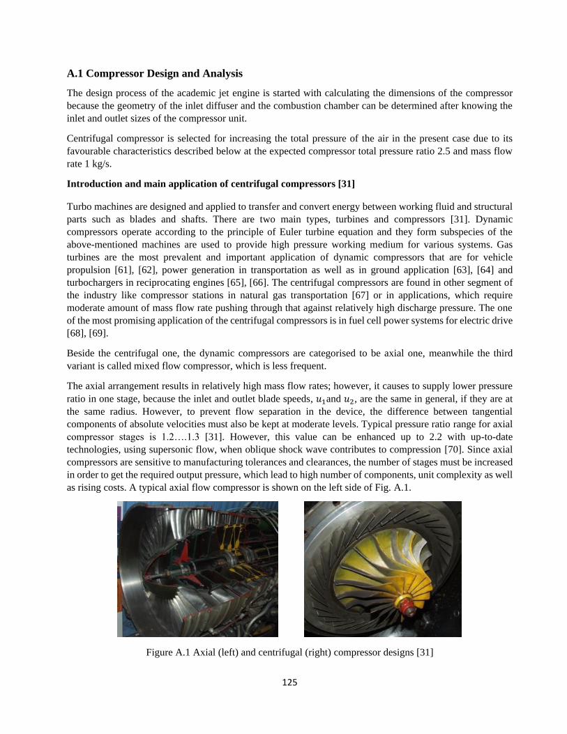
125

A.1 Compressor Design and Analysis

The design process of the academic jet engine is started with calculating the dimensions of the compressor

because the geometry of the inlet diffuser and the combustion chamber can be determined after knowing the

inlet and outlet sizes of the compressor unit.

Centrifugal compressor is selected for increasing the total pressure of the air in the present case due to its

favourable characteristics described below at the expected compressor total pressure ratio 2.5 and mass flow

rate 1 kg/s.

Introduction and main application of centrifugal compressors [31]

Turbo machines are designed and applied to transfer and convert energy between working fluid and structural

parts such as blades and shafts. There are two main types, turbines and compressors [31]. Dynamic

compressors operate according to the principle of Euler turbine equation and they form subspecies of the

above-mentioned machines are used to provide high pressure working medium for various systems. Gas

turbines are the most prevalent and important application of dynamic compressors that are for vehicle

propulsion [61], [62], power generation in transportation as well as in ground application [63], [64] and

turbochargers in reciprocating engines [65], [66]. The centrifugal compressors are found in other segment of

the industry like compressor stations in natural gas transportation [67] or in applications, which require

moderate amount of mass flow rate pushing through that against relatively high discharge pressure. The one

of the most promising application of the centrifugal compressors is in fuel cell power systems for electric drive

[68], [69].

Beside the centrifugal one, the dynamic compressors are categorised to be axial one, meanwhile the third

variant is called mixed flow compressor, which is less frequent.

The axial arrangement results in relatively high mass flow rates; however, it causes to supply lower pressure

ratio in one stage, because the inlet and outlet blade speeds, 𝑢1and 𝑢2, are the same in general, if they are at

the same radius. However, to prevent flow separation in the device, the difference between tangential

components of absolute velocities must also be kept at moderate levels. Typical pressure ratio range for axial

compressor stages is 1.2….1.3 [31]. However, this value can be enhanced up to 2.2 with up-to-date

technologies, using supersonic flow, when oblique shock wave contributes to compression [70]. Since axial

compressors are sensitive to manufacturing tolerances and clearances, the number of stages must be increased

in order to get the required output pressure, which lead to high number of components, unit complexity as well

as rising costs. A typical axial flow compressor is shown on the left side of Fig. A.1.

Figure A.1 Axial (left) and centrifugal (right) compressor designs [31]

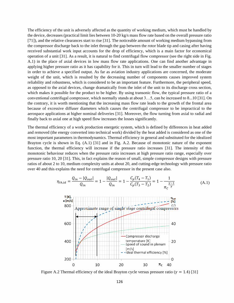
126

The efficiency of the unit is adversely affected as the quantity of working medium, which must be handled by

the device, decreases (practical limit lies between 10-20 kg/s mass flow rate based on the overall pressure ratio

[71]), and the relative clearances start to rise [31]. The noticeable amount of working medium bypassing from

the compressor discharge back to the inlet through the gap between the rotor blade tip and casing after having

received substantial work input accounts for the drop of efficiency, which is a main factor for economical

operation of a unit [31]. As a result, it is natural to find centrifugal flow compressor (see the right side in Fig.

A.1) in the place of axial devices in low mass flow rate applications. One can find another advantage in

applying higher pressure ratio as it has capability for it. This in turn will lead to the smaller number of stages

in order to achieve a specified output. As far as aviation industry applications are concerned, the moderate

weight of the unit, which is resulted by the decreasing number of components causes improved system

reliability and robustness, which is considered to be an important feature. Furthermore, the peripheral speed,

as opposed to the axial devices, change dramatically from the inlet of the unit to its discharge cross section,

which makes it possible for the product to be higher. By using transonic flow, the typical pressure ratio of a

conventional centrifugal compressor, which normally stands at about 3…5, can be increased to 8...10 [31]. On

the contrary, it is worth mentioning that the increasing mass flow rate leads to the growth of the frontal area

because of excessive diffuser diameters which causes the centrifugal compressor to be impractical to the

aerospace applications at higher nominal deliveries [31]. Moreover, the flow turning from axial to radial and

finally back to axial one at high speed flow increases the losses significantly.

The thermal efficiency of a work production energetic system, which is defined by differences in heat added

and removed (the energy converted into technical work) divided by the heat added is considered as one of the

most important parameters in thermodynamics. Thermal efficiency in general and substituted for the idealized

Brayton cycle is shown in Eq. (A.1) [31] and in Fig. A.2. Because of monotonic nature of the exponent

function, the thermal efficiency will increase if the pressure ratio increases [31]. The intensity of this

monotonic behaviour reduces when the pressure ratio increases at high pressure ratio range, especially over

pressure ratio 10, 20 [31]. This, in fact explains the reason of small, simple compressor designs with pressure

ratios of about 2 to 10, medium complexity units at about 20, and cutting-edge technology with pressure ratio

over 40 and this explains the need for centrifugal compressor in the present case also.

휂𝑡ℎ,𝑖𝑑 =𝑄𝑖𝑛 − |𝑄𝑜𝑢𝑡|

𝑄𝑖𝑛= 1 −

|𝑄𝑜𝑢𝑡|

𝑄𝑖𝑛= 1 −

𝐶𝑝(𝑇4 − 𝑇1)

𝐶𝑝(𝑇3 − 𝑇2)= 1 −

1

𝜋𝐶

𝛾−1𝛾

(A.1)

Figure A.2 Thermal efficiency of the ideal Brayton cycle versus pressure ratio (𝛾 = 1.4) [31]

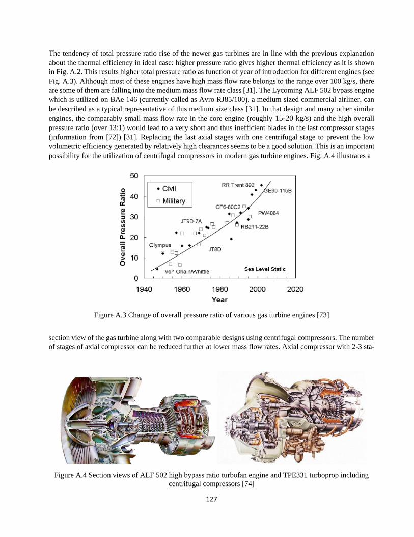
127

The tendency of total pressure ratio rise of the newer gas turbines are in line with the previous explanation

about the thermal efficiency in ideal case: higher pressure ratio gives higher thermal efficiency as it is shown

in Fig. A.2. This results higher total pressure ratio as function of year of introduction for different engines (see

Fig. A.3). Although most of these engines have high mass flow rate belongs to the range over 100 kg/s, there

are some of them are falling into the medium mass flow rate class [31]. The Lycoming ALF 502 bypass engine

which is utilized on BAe 146 (currently called as Avro RJ85/100), a medium sized commercial airliner, can

be described as a typical representative of this medium size class [31]. In that design and many other similar

engines, the comparably small mass flow rate in the core engine (roughly 15-20 kg/s) and the high overall

pressure ratio (over 13:1) would lead to a very short and thus inefficient blades in the last compressor stages

(information from [72]) [31]. Replacing the last axial stages with one centrifugal stage to prevent the low

volumetric efficiency generated by relatively high clearances seems to be a good solution. This is an important

possibility for the utilization of centrifugal compressors in modern gas turbine engines. Fig. A.4 illustrates a

Figure A.3 Change of overall pressure ratio of various gas turbine engines [73]

section view of the gas turbine along with two comparable designs using centrifugal compressors. The number

of stages of axial compressor can be reduced further at lower mass flow rates. Axial compressor with 2-3 sta-

Figure A.4 Section views of ALF 502 high bypass ratio turbofan engine and TPE331 turboprop including

centrifugal compressors [74]

128

ges are used in the lower range of medium sized airlines (e.g. Bombardier Dash 8 Q400), in which the nominal

mass flow rate of the gas turbine is about 10 kg/s [31]. The other solution – instead of applying 2-3 stages

axial compressor – is using double stage centrifugal compressor (see TPE331 engine in Fig. A.4).

A single stage centrifugal compressor, which uses transonic inlet flow regime in most of the cases can be

found in mini or micro gas turbines, such as auxiliary power units (APU’s) and engines of unmanned aerial

vehicles (UAV’s).

The one of the most actual application fields of the centrifugal compressor is in the engine of UAVs, for which

a flexible platform is under development to be able to fulfil both civil and military purposes. Noticeable results

have been obtained regarding the optimal tracking of the vehicle [75], application for educational purpose [76]

or utilization in the field of military intelligence services [77] and target drone for practice-firing [78].

Although these applications may not be in a tight relationship with the main issue of the current subchapter, it

has been emphasized because they are often equipped with turbojet engines in which, due to their performance

needs, just centrifugal compressors are affordable [31].

Operation principle of centrifugal compressors [31]

Both axial and centrifugal compressor types work on the same basic principle; one stage of a compressor is

composed of a rotor and a stator. The compression process takes place as fluid momentum change in the rotor

followed by diffusion in the stator to convert kinetic energy into static pressure [79]. The designation stator in

the case of centrifugal compressors can stand for a vaneless or a vanned diffuser and a volute. The section

view of a centrifugal compressor is depicted in Fig. A.5.

Figure A.5 Front view [79] and a meridional section [31] of centrifugal compressor

The energy transfer, which is done by the impeller, can be demonstrated by the Euler’s turbine equation that

can be derived from the impulse moment equation:

𝑀 = �� (𝑟2𝑐2𝑢 − 𝑟1𝑐1𝑢) (A.2)

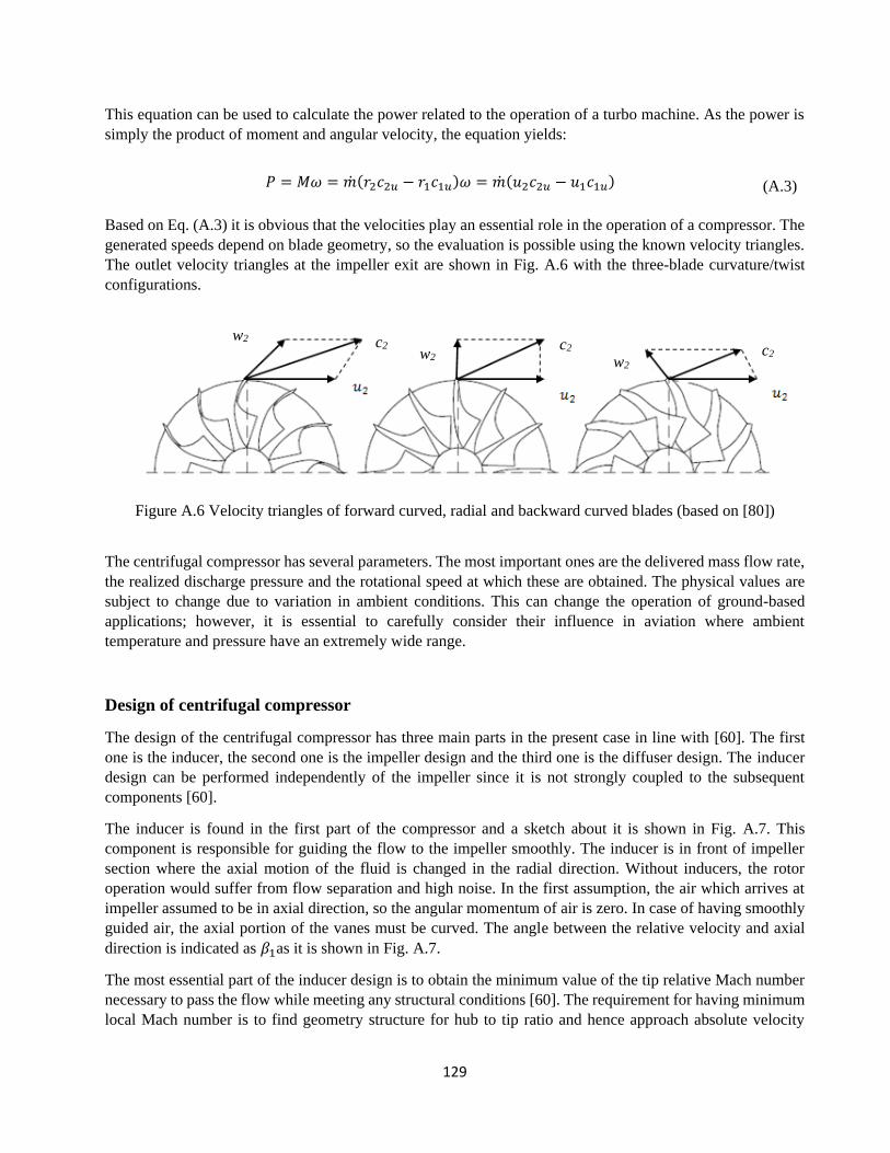
129

This equation can be used to calculate the power related to the operation of a turbo machine. As the power is

simply the product of moment and angular velocity, the equation yields:

𝑃 = 𝑀𝜔 = ��(𝑟2𝑐2𝑢 − 𝑟1𝑐1𝑢)𝜔 = ��(𝑢2𝑐2𝑢 − 𝑢1𝑐1𝑢) (A.3)

Based on Eq. (A.3) it is obvious that the velocities play an essential role in the operation of a compressor. The

generated speeds depend on blade geometry, so the evaluation is possible using the known velocity triangles.

The outlet velocity triangles at the impeller exit are shown in Fig. A.6 with the three-blade curvature/twist

configurations.

Figure A.6 Velocity triangles of forward curved, radial and backward curved blades (based on [80])

The centrifugal compressor has several parameters. The most important ones are the delivered mass flow rate,

the realized discharge pressure and the rotational speed at which these are obtained. The physical values are

subject to change due to variation in ambient conditions. This can change the operation of ground-based

applications; however, it is essential to carefully consider their influence in aviation where ambient

temperature and pressure have an extremely wide range.

Design of centrifugal compressor

The design of the centrifugal compressor has three main parts in the present case in line with [60]. The first

one is the inducer, the second one is the impeller design and the third one is the diffuser design. The inducer

design can be performed independently of the impeller since it is not strongly coupled to the subsequent

components [60].

The inducer is found in the first part of the compressor and a sketch about it is shown in Fig. A.7. This

component is responsible for guiding the flow to the impeller smoothly. The inducer is in front of impeller

section where the axial motion of the fluid is changed in the radial direction. Without inducers, the rotor

operation would suffer from flow separation and high noise. In the first assumption, the air which arrives at

impeller assumed to be in axial direction, so the angular momentum of air is zero. In case of having smoothly

guided air, the axial portion of the vanes must be curved. The angle between the relative velocity and axial

direction is indicated as 𝛽1as it is shown in Fig. A.7.

The most essential part of the inducer design is to obtain the minimum value of the tip relative Mach number

necessary to pass the flow while meeting any structural conditions [60]. The requirement for having minimum

local Mach number is to find geometry structure for hub to tip ratio and hence approach absolute velocity

w2

w2 w2

c2 c2 c2

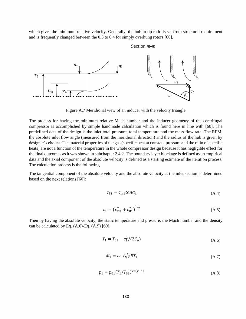
130

which gives the minimum relative velocity. Generally, the hub to tip ratio is set from structural requirement

and is frequently changed between the 0.3 to 0.4 for simply overhung rotors [60].

Section m-m

Figure A.7 Meridional view of an inducer with the velocity triangle

The process for having the minimum relative Mach number and the inducer geometry of the centrifugal

compressor is accomplished by simple handmade calculation which is found here in line with [60]. The

predefined data of the design is the inlet total pressure, total temperature and the mass flow rate. The RPM,

the absolute inlet flow angle (measured from the meridional direction) and the radius of the hub is given by

designer’s choice. The material properties of the gas (specific heat at constant pressure and the ratio of specific

heats) are not a function of the temperature in the whole compressor design because it has negligible effect for

the final outcomes as it was shown in subchapter 2.4.2. The boundary layer blockage is defined as an empirical

data and the axial component of the absolute velocity is defined as a starting estimate of the iteration process.

The calculation process is the following.

The tangential component of the absolute velocity and the absolute velocity at the inlet section is determined

based on the next relations [60]:

𝑐𝜃1 = 𝑐𝑚1𝑡𝑎𝑛𝛼1 (A.4)

𝑐1 = (𝑐𝑚12 + 𝑐θ1

2 )12⁄ (A.5)

Then by having the absolute velocity, the static temperature and pressure, the Mach number and the density

can be calculated by Eq. (A.6)-Eq. (A.9) [60].

𝑇1 = 𝑇01 − 𝑐12/(2𝐶𝑝) (A.6)

𝑀1 = 𝑐1 /√𝛾𝑅𝑇1 (A.7)

𝑝1 = 𝑝01(𝑇1 𝑇01⁄ )𝛾 (𝛾−1)⁄ (A.8)

𝑟𝑡

𝑟𝑚 𝑟ℎ

𝑚 𝑚

u1

c1

w1 β1

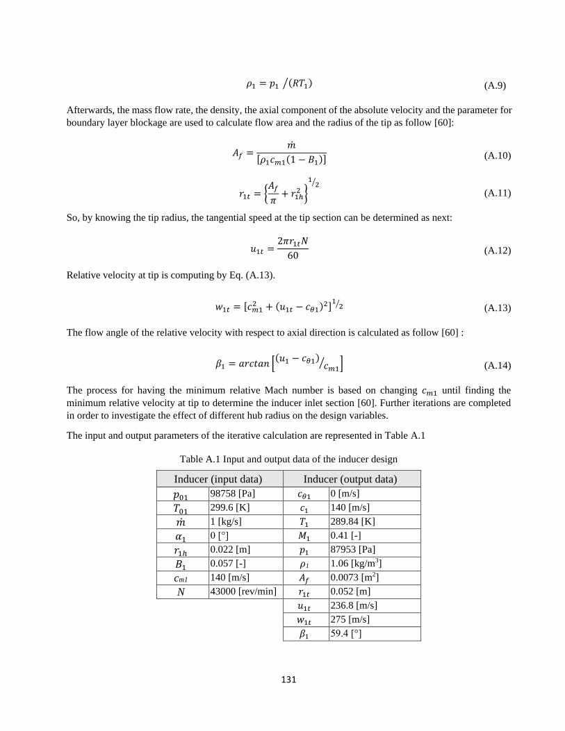
131

𝜌1 = 𝑝1 (𝑅𝑇1)⁄ (A.9)

Afterwards, the mass flow rate, the density, the axial component of the absolute velocity and the parameter for

boundary layer blockage are used to calculate flow area and the radius of the tip as follow [60]:

𝐴𝑓 =��

[𝜌1𝑐𝑚1(1 − 𝐵1)] (A.10)

𝑟1𝑡 = {𝐴𝑓

𝜋+ 𝑟1ℎ

2 }

12⁄

(A.11)

So, by knowing the tip radius, the tangential speed at the tip section can be determined as next:

𝑢1𝑡 =2𝜋𝑟1𝑡𝑁

60 (A.12)

Relative velocity at tip is computing by Eq. (A.13).

𝑤1𝑡 = [𝑐𝑚12 + (𝑢1𝑡 − 𝑐𝜃1)

2]12⁄ (A.13)

The flow angle of the relative velocity with respect to axial direction is calculated as follow [60] :

𝛽1 = 𝑎𝑟𝑐𝑡𝑎𝑛 [(𝑢1 − 𝑐𝜃1)

𝑐𝑚1⁄ ] (A.14)

The process for having the minimum relative Mach number is based on changing 𝑐𝑚1 until finding the

minimum relative velocity at tip to determine the inducer inlet section [60]. Further iterations are completed

in order to investigate the effect of different hub radius on the design variables.

The input and output parameters of the iterative calculation are represented in Table A.1

Table A.1 Input and output data of the inducer design

Inducer (input data) Inducer (output data)

𝑝01 98758 [Pa] 𝑐𝜃1 0 [m/s]

𝑇01 299.6 [K] 𝑐1 140 [m/s]

�� 1 [kg/s] 𝑇1 289.84 [K]

𝛼1 0 [°] 𝑀1 0.41 [-]

𝑟1ℎ 0.022 [m] 𝑝1 87953 [Pa]

𝐵1 0.057 [-] 𝜌1 1.06 [kg/m3]

cm1 140 [m/s] 𝐴𝑓 0.0073 [m2]

N 43000 [rev/min] 𝑟1𝑡 0.052 [m]

𝑢1𝑡 236.8 [m/s]

𝑤1𝑡 275 [m/s]

𝛽1 59.4 [°]

132

Impeller design is the next step of the centrifugal compressor design process by means of calculating the

impeller diameter and depth, flow state and velocity triangle at impeller tip [60]. The calculation process

applies parameters provided by the inducer design also: the absolute inlet velocity and its flow angle comes

from the inducer design. The predefined data of the design is the inlet total pressure and total temperature,

mass flow rate and total pressure ratio of the compressor stage, meanwhile the rotor efficiency, pressure

recovery coefficient and slip factor are given as empirical data. The axial component and the flow angle of the

absolute velocity at the inlet section, the RPM, the number of vanes, the swirl factor at the mean section of the

impeller exit and the relative flow angle measured from radial direction at the outlet section of the impeller

are given by the designer’s choice.

The slip factor is introduced in the present paragraph before discussing the used equations and iteration process

in detail. The tangential component of the absolute velocity at the impeller discharge depends on the outlet

angle of the blade [31]. Ideally, one can assume that the flow direction is tangential to the blade surface at the

exit of the impeller. However, in reality, due to the Coriolis force in the rotating frame of reference, the flow

direction changes, so there is a certain difference between ideal and real flow directions. Hence, slip factor 𝜎

is introduced, which is the ratio of tangential component of the absolute velocity under real and ideal conditions

at the exit of the impeller [81]. Therefore, tangential component of the real outlet absolute velocity is obtained

by multiplying the slip factor with the tangential component of the absolute velocity, which is purely based on

the blade geometry. There are several ways to define the slip factor based on countless researches, which have

come up with various formulas, utilizing different input parameters. In this case the slip factor is determined

by Stanitz formula as follow [80]:

𝜎 = 1 −2

𝑧 (A.15)

where z is the number of vanes.

The iteration process for the impeller design starts with selecting an isentropic efficiency for the compressor

stage (휂𝑠,𝑠𝑡𝑎𝑔𝑒) and recalculating that till the resulted total pressure ratio of the compressor unit is equal with

the already specified input data (2.5 in the present case) meanwhile the outlet diameter and the width of the

impeller-exit are the resulted geometrical parameters. The next step is the determination of the specific total

enthalpy change by Eq. (A.16) based on the available data [60].

𝛥ℎ0𝑠 =𝛾𝑅𝑇01𝛾 − 1

(𝑝𝑟_𝑠𝑡𝑎𝑔𝑒(𝛾−1

𝛾⁄ )− 1) (A.16)

As the value of the stage efficiency is assumed, total specific shaft work is determined [60]:

𝑊𝑋 = 𝛥ℎ0 =𝛥ℎ0𝑠휂𝑠,𝑠𝑡𝑎𝑔𝑒

(A.17)

The total outlet temperature at meridional blade section is given by Eq. (A.18) [60].

𝑇02𝑚 = 𝑇01 + 𝛥ℎ0𝛾 − 1

𝛾𝑅 (A.18)

Although impeller configurations with backward turning blade-end has the highest total pressure ratio, the

highest efficiency and wider operational range at the given conditions [82], radial blade-end configuration is

selected due to the moderate total pressure ratio, structural robustness and favourable cost [82]. Hence, the

133

tangential velocity component of the absolute velocity equals to the peripheral speed in ideal case. Therefore,

the peripheral speed is calculated by using slip factor and the Euler’s turbine equation as follow [60]:

𝑢2 = [(𝑢1𝑐𝜃1 +𝑊𝑥)

𝜎⁄ ]

12⁄

, (A.19)

where 𝑐𝜃1 = 𝑐𝑚1𝑡𝑎𝑛𝛼1 is the tangential component of the absolute velocity.

As the value of the rotational speed is given like input data, the outlet diameter of the impeller is given by Eq.

(A.20).

𝐷2 =𝑢2

𝜋𝑁⁄ (A.20)

So, the tangential and axial (meridional) component of the absolute velocity at the mean section of the blade

exit is determined by the following equations [60]:

𝑐𝜃2𝑚 = 𝜎𝑢2 (A.21)

𝑐𝑚2𝑚 = 𝑐𝜃2𝑚/𝜆2𝑚 (A.22)

The tangent of the absolute flow angle (angle between the meridional and peripheral components of the

absolute velocity) at the vane exit is equal with the swirl factor (𝜆2𝑚) [83].

The static temperature at the vane exit is calculated by Eq. (A.23) [60].

𝑇2𝑚 = 𝑇02𝑚 −𝛾 − 1

2𝛾𝑅(𝑐𝜃2𝑚

2 + 𝑐𝑚2𝑚2 ) (A.23)

The rotor (isentropic) efficiency is given by an empirical parameter, so the total pressure ratio of the impeller

is the following [60]:

𝑝02𝑚𝑝01

= [(𝛾 − 1

𝛾𝑅𝑇01𝑊𝑋휂𝑠,𝑟𝑜𝑡𝑜𝑟) + 1]

𝛾𝛾−1⁄

(A.24)

The static pressure is determined by using the next equation to calculate the density at the meridian section of

the impeller exit [60]:

𝑝2𝑚 = 𝑝02𝑚 (𝑇02𝑚𝑇2𝑚

)

𝛾𝛾−1⁄

⁄ (A.25)

𝜌2𝑚 =𝑝2𝑚

(𝑅𝑇2𝑚) (A.26)

The required cross-sectional area for the flow is computed by Eq. (A.27).

𝐴2𝑚 = ��(𝜌2𝑚𝑐𝑚2𝑚)⁄ (A.27)

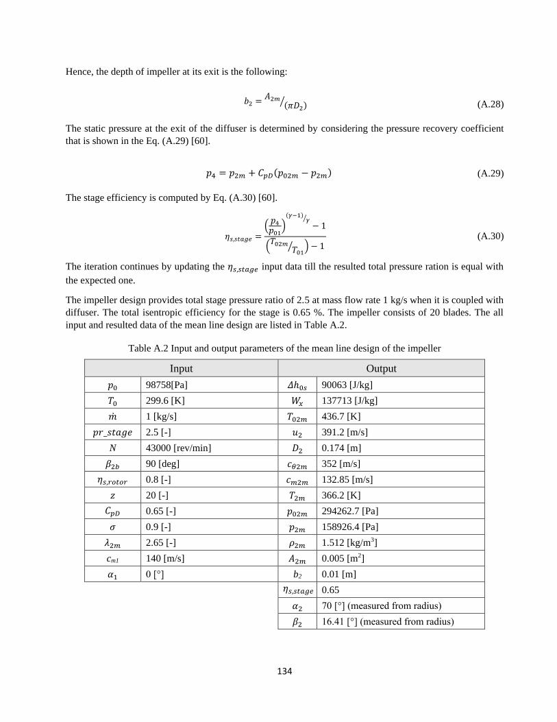
134

Hence, the depth of impeller at its exit is the following:

𝑏2 =𝐴2𝑚

(𝜋𝐷2)⁄ (A.28)

The static pressure at the exit of the diffuser is determined by considering the pressure recovery coefficient

that is shown in the Eq. (A.29) [60].

𝑝4 = 𝑝2𝑚 + 𝐶𝑝𝐷(𝑝02𝑚 − 𝑝2𝑚) (A.29)

The stage efficiency is computed by Eq. (A.30) [60].

휂𝑠,𝑠𝑡𝑎𝑔𝑒 =(𝑝4𝑝01

)

(𝛾−1)𝛾⁄

− 1

(𝑇02𝑚

𝑇01⁄ ) − 1

(A.30)

The iteration continues by updating the 휂𝑠,𝑠𝑡𝑎𝑔𝑒 input data till the resulted total pressure ration is equal with

the expected one.

The impeller design provides total stage pressure ratio of 2.5 at mass flow rate 1 kg/s when it is coupled with

diffuser. The total isentropic efficiency for the stage is 0.65 %. The impeller consists of 20 blades. The all

input and resulted data of the mean line design are listed in Table A.2.

Table A.2 Input and output parameters of the mean line design of the impeller

Input Output

𝑝0 98758[Pa] 𝛥ℎ0𝑠 90063 [J/kg]

𝑇0 299.6 [K] 𝑊𝑥 137713 [J/kg]

�� 1 [kg/s] 𝑇02𝑚 436.7 [K]

𝑝𝑟_𝑠𝑡𝑎𝑔𝑒 2.5 [-] 𝑢2 391.2 [m/s]

N 43000 [rev/min] 𝐷2 0.174 [m]

𝛽2𝑏 90 [deg] 𝑐𝜃2𝑚 352 [m/s]

휂𝑠,𝑟𝑜𝑡𝑜𝑟 0.8 [-] 𝑐𝑚2𝑚 132.85 [m/s]

𝑧 20 [-] 𝑇2𝑚 366.2 [K]

𝐶𝑝𝐷 0.65 [-] 𝑝02𝑚 294262.7 [Pa]

𝜎 0.9 [-] 𝑝2𝑚 158926.4 [Pa]

𝜆2𝑚 2.65 [-] 𝜌2𝑚 1.512 [kg/m3]

cm1 140 [m/s] 𝐴2𝑚 0.005 [m2]

𝛼1 0 [°] b2 0.01 [m]

휂𝑠,𝑠𝑡𝑎𝑔𝑒 0.65

𝛼2 70 [°] (measured from radius)

𝛽2 16.41 [°] (measured from radius)

135

The impeller connects to the diffuser. The last step of the compressor unit design is to determine the flow

characteristics and the geometry of the diffuser. The section 2-3 corresponds to the vaneless meanwhile the

section 3-4 represents the vanned diffuser. The input for the calculation is the outlet thermodynamic state of

the impeller together with the loss coefficient (𝐾2𝑚−3) of the vaneless diffuser, the pressure recovery

coefficient (𝐶𝑝3−4) of the vanned diffuser and the Mach number (𝑀3).

As the total temperature at the impeller exit is equal with total temperature in the diffuser:

𝑇03 = 𝑇02𝑚 (A.31)

the static temperature is determined with gas dynamic equations as follow [60]:

𝑇3 =𝑇03

1 +𝛾 − 12

𝑀32

(A.32)

Taking into consideration the pressure loss between the impeller exit and vaneless diffuser outlet, the total

pressure can be determined at section 3 [60]:

𝑝03 = 𝑝02𝑚 − 𝐾2𝑚−3(𝑝02𝑚 − 𝑝2𝑚) (A.33)

Static pressure, density and velocity at the exit of the vaneless diffuser are calculated by the Eqs. (A.34)-(A.36)

[60].

𝑝3 = 𝑝03 (𝑇3

𝑇03⁄ )

𝛾(𝛾−1)⁄

(A.34)

𝜌3 =𝑝3

𝑅𝑇3⁄ (A.35)

𝑐3 = 𝑀3√𝛾𝑅𝑇3 (A.36)

The cross-sectional area of the vaneless diffuser is computed by the following equation:

𝐴3 =��

𝜌3(𝑐3cos (atan (𝑐𝜃2𝑚/𝑐𝑚2𝑚))) (A.37)

It is supposed in Eq. (A.37) that the angular momentum is not changed significantly with respect to the section

2 and normal velocity to the area is considered. The total pressure at the exit of the vanned diffuser is computed

by Eq. (A.38).

𝑝04 = 𝑟03−04 𝑝03 (A.38)

𝑟03−04 total pressure recovery rate is considered for pressure loss in the vanned diffuser due to the strong

adverse pressure gradient.

136

The combustion chamber is the next unit of the engine after the compressor. Hence, the flow should be guided

to turn from rather radial to axial direction in the vaneless diffuser. This requires a curved axisymmetric flow

channel here, ended by increased hub and shroud radiuses (see Fig. A.8). The thickness of the flow channel

after the curved section is set 10 mm, which results higher cross-sectional area than it is at the exit of the

impeller at about 23 %. However, there are vanes in section 3-4, which reduce the trough-flow area.

The all input and output data of the diffuser design is shown in Table A.3.

Table A.3 Input and output parameters of the diffuser-design

Input Output

T03 436.7 [K] T3 403.3 [K]

K2m-3 0.166 p03 271797 [pa]

M3 0.643 p3 205817 [pa]

𝑟 03−04 0.91 𝜌3 1.78 [kg/m3]

𝑐3 258.85 [m/s]

A3 0.006154 [m2]

p04 246927 [Pa]

The meridional view with the sections of the compressor flow domain, main dimensions and the proportionally

scaled velocity triangles at the inlet and outlet of the impeller are shown in the Fig. A.8 and A.9 respectively.

All thermodynamic parameters and geometrical sizes are available after the mean line design of the compressor

at the design condition. The next step of the development is to create the 3D model of the assembly for the

analysis and continue the design – after the inlet nozzle – with the next part of the engine, which is the

combustion chamber.

Figure A.8 Meridional view of the centrifugal compressor flow domain with the sections (1-4) and

main dimensions (the dimensions are in [mm])

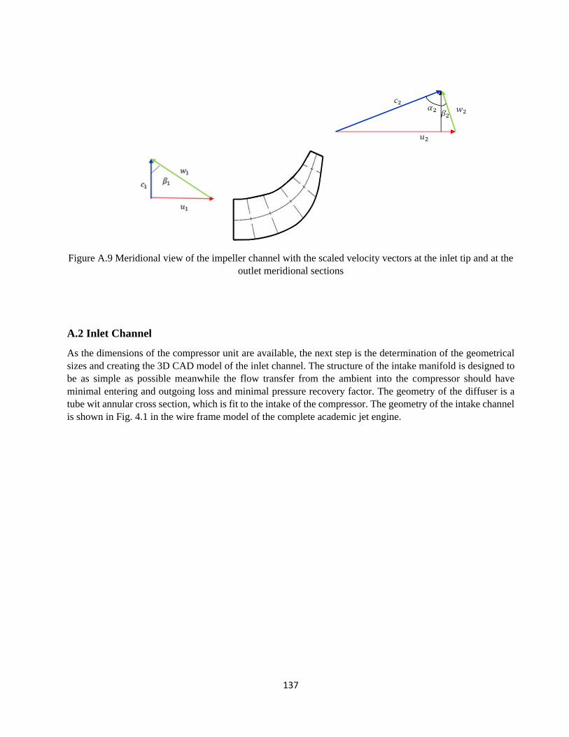
137

Figure A.9 Meridional view of the impeller channel with the scaled velocity vectors at the inlet tip and at the

outlet meridional sections

A.2 Inlet Channel

As the dimensions of the compressor unit are available, the next step is the determination of the geometrical

sizes and creating the 3D CAD model of the inlet channel. The structure of the intake manifold is designed to

be as simple as possible meanwhile the flow transfer from the ambient into the compressor should have

minimal entering and outgoing loss and minimal pressure recovery factor. The geometry of the diffuser is a

tube wit annular cross section, which is fit to the intake of the compressor. The geometry of the intake channel

is shown in Fig. 4.1 in the wire frame model of the complete academic jet engine.

138

A.3 Design Aspects of the Combustion Chamber

The combustion chamber has the challenging task of burning certain amount of fuel that is supplied through

the fuel burners with wide range of volume of air. The air leaving the compressor goes through the combustors,

expanding and accelerating to give a smooth stream of uniformly heated gas at all conditions required by the

turbine. The fuel is burned almost stoichiometrically with only 25 to 35 percent of total air entering [84] in

general and it is 28 % in the present case (��𝑓𝑐𝑐 = 0.019 𝑘𝑔

𝑠, 𝐿0 = 14.72

kg

kg⇒ ��𝑎𝑖𝑟,𝑠𝑡,𝑐𝑐 = ��𝑓𝑐𝑐𝐿0 = 0.2797

𝑘𝑔

𝑠)

in order to keep the turbine inlet temperature down to permissible limits. As a result, combustion must be

completed without causing high pressure loss and taking into consideration the huge heat release for the limited

space existing. In providing adequate turbulence and mixing, a total pressure loss changing from about 2 to 9

percent of the air pressure at which it goes through the chamber [84]. It is 6 % based on the inlet total pressure

at the combustion chamber in this case by the thermo-dynamical analysis.

For many years the combustion has had less capability to theoretical treatment in comparison with other parts

of the gas turbine and any development software involved some trial and error. With high cycle temperature

of modern gas turbine, mechanical design stays complex task and need for improvement of technical

development is obvious. Concerning the industrial gas turbines they have a certain range of usable types of

fuel amongst them natural gas is included frequently beside the liquid based hydrocarbons [84].

Combustion chambers can be distinguished based on their structure. Regarding flow direction, reverse-flow

and one-directional flow combustion chambers exist.

The reverse-flow combustion chambers have the advantage of obtaining shorter gas turbine design, because

the flow path is shortened by half in one direction as the combustor is located to sit on perimeter of the

compressor and turbine. Thus, this design does not require so improved shaft materials and bearing design

compared to the one-directional flow combustion chambers. Due to this, the reverse-flow combustion

chambers are basically applied on older gas turbines, however, where a short and compact design is required,

this combustion chamber is still applied nowadays. As a disadvantage, reverse-flow combustion chambers

have high pressure losses compared to one-directional chambers. Furthermore, due to the noticeable cross

section, reverse-flow combustion chamber produces high aerodynamic drag, thus they are very rarely used in

aircraft propulsion systems.

Although gas turbines, which are applied with one-directional flow combustion chambers are longer, hence

better shaft materials and improved bearing designs are required, due to the lower cross section and better total

pressure recovery factor and burning efficiency; they are more widespread in aviation industry.

Regarding the one-directional flow combustion chambers, there are three main types of the structure can be

distinguished. They are the multiple can, can-annular and the annular type combustion chambers. All the three

kinds of combustors have the recirculation, burning and dilution zone. First, fuel is partially burned in the

recirculation zone. But there is some fuel, which is not completely burned, so the remainder of fuel is

completely burned in the burning zone. The hot gas is then mixed in the dilution zone with the cooling air and

provides a suitable inlet temperature for the turbine section. One part of the cooling air works on the principle

of film cooling, it separates hot working fluid from the walls of the combustor; hence higher operating

temperatures can be allowed. Furthermore, appropriate application of cooling air contributes to flame

stabilization and more even mixture distribution while proceeding to the turbine inlet cross section [84].

The combustion chamber design is a complex and challenging task in small gas-turbine engines due to the size

limitation by means of couplings the compressor and turbine, typically constructive limitations on shaft length

and diameter. These requirements have focused also in the present case to highlight the annular combustion

chamber, as it is used today mostly. This kind of chamber is ideal because of “clean” aero-dynamic layout

results in a compact unit and better characteristics than other combustor types. The annular combustor has the

benefit of being able to use smaller cross section, achieves smaller pressure loss if compared with can-type

one [84]. The other advantages of this kind combustor that the limited space available is used more effectively,

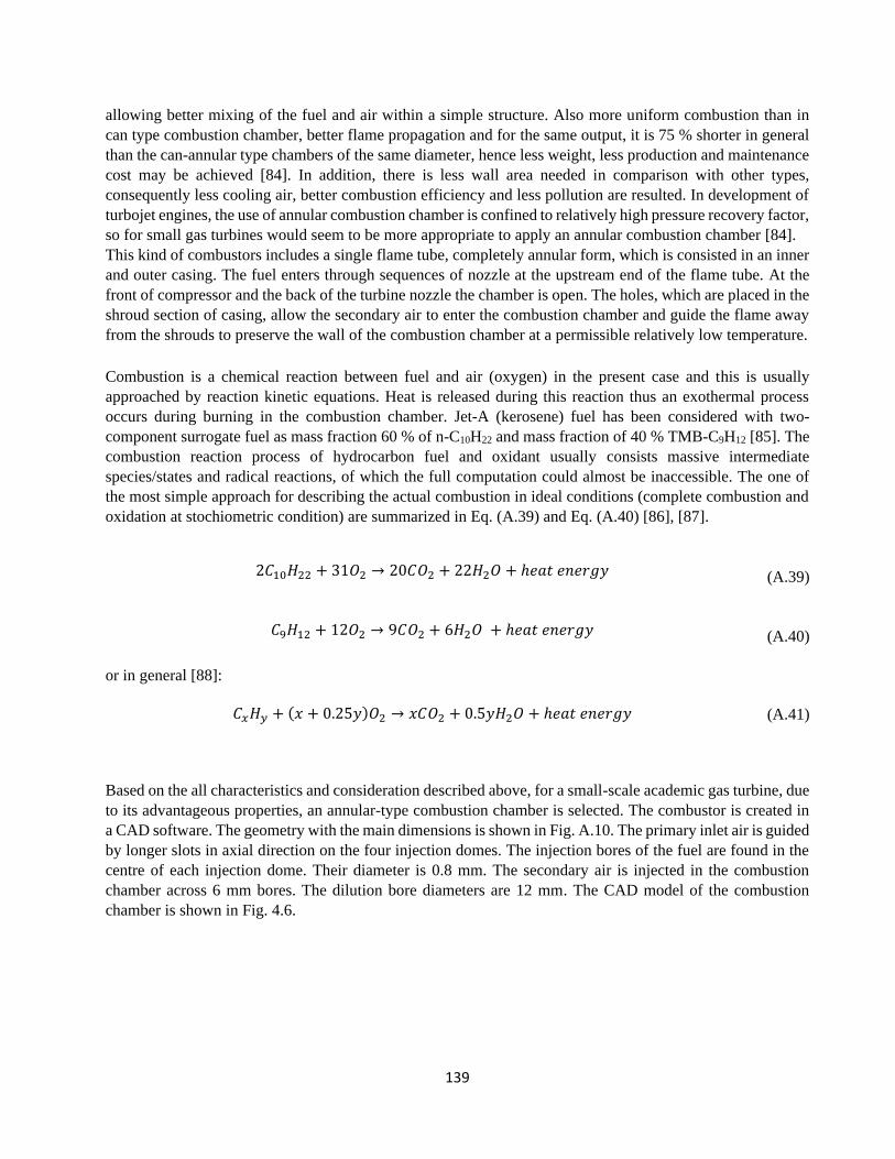
139

allowing better mixing of the fuel and air within a simple structure. Also more uniform combustion than in

can type combustion chamber, better flame propagation and for the same output, it is 75 % shorter in general

than the can-annular type chambers of the same diameter, hence less weight, less production and maintenance

cost may be achieved [84]. In addition, there is less wall area needed in comparison with other types,

consequently less cooling air, better combustion efficiency and less pollution are resulted. In development of

turbojet engines, the use of annular combustion chamber is confined to relatively high pressure recovery factor,

so for small gas turbines would seem to be more appropriate to apply an annular combustion chamber [84].

This kind of combustors includes a single flame tube, completely annular form, which is consisted in an inner

and outer casing. The fuel enters through sequences of nozzle at the upstream end of the flame tube. At the

front of compressor and the back of the turbine nozzle the chamber is open. The holes, which are placed in the

shroud section of casing, allow the secondary air to enter the combustion chamber and guide the flame away

from the shrouds to preserve the wall of the combustion chamber at a permissible relatively low temperature.

Combustion is a chemical reaction between fuel and air (oxygen) in the present case and this is usually

approached by reaction kinetic equations. Heat is released during this reaction thus an exothermal process

occurs during burning in the combustion chamber. Jet-A (kerosene) fuel has been considered with two-

component surrogate fuel as mass fraction 60 % of n-C10H22 and mass fraction of 40 % TMB-C9H12 [85]. The

combustion reaction process of hydrocarbon fuel and oxidant usually consists massive intermediate

species/states and radical reactions, of which the full computation could almost be inaccessible. The one of

the most simple approach for describing the actual combustion in ideal conditions (complete combustion and

oxidation at stochiometric condition) are summarized in Eq. (A.39) and Eq. (A.40) [86], [87].

2𝐶10𝐻22 + 31𝑂2 → 20𝐶𝑂2 + 22𝐻2𝑂 + ℎ𝑒𝑎𝑡 𝑒𝑛𝑒𝑟𝑔𝑦 (A.39)

𝐶9𝐻12 + 12𝑂2 → 9𝐶𝑂2 + 6𝐻2𝑂 + ℎ𝑒𝑎𝑡 𝑒𝑛𝑒𝑟𝑔𝑦 (A.40)

or in general [88]:

𝐶𝑥𝐻𝑦 + (𝑥 + 0.25𝑦)𝑂2 → 𝑥𝐶𝑂2 + 0.5𝑦𝐻2𝑂 + ℎ𝑒𝑎𝑡 𝑒𝑛𝑒𝑟𝑔𝑦 (A.41)

Based on the all characteristics and consideration described above, for a small-scale academic gas turbine, due

to its advantageous properties, an annular-type combustion chamber is selected. The combustor is created in

a CAD software. The geometry with the main dimensions is shown in Fig. A.10. The primary inlet air is guided

by longer slots in axial direction on the four injection domes. The injection bores of the fuel are found in the

centre of each injection dome. Their diameter is 0.8 mm. The secondary air is injected in the combustion

chamber across 6 mm bores. The dilution bore diameters are 12 mm. The CAD model of the combustion

chamber is shown in Fig. 4.6.

140

Figure A.10 Geometry of the annular type combustion chamber with the main sizes (the dimensions are in

[mm])

A.4 Turbine Design

Introduction:

Turbines are essential part of turbo-machinery devices, which are used to convert the potential and kinetic

energy of the working fluid into mechanical energy. There is a wide range of use of turbines in the different

segments of industry, providing a reliable, efficient energy conversion method for rotating machines. The first

application of the modern turbine technology can be deducted to the late 18th century where steam was used

as the working fluid to drive turbine blades. Remarkable contributors to steam turbine development were Carl

Gustav De Laval and Sir Charles Parsons. Despite De Laval was involved in developing the convergent-

divergent nozzle - nowadays the so-called Laval nozzle - he also designed a steam turbine in 1870, which had

an impeller speed of 30 000 rpm and a performance of 150 kW. The appearance of turbines was very different

from nowadays steam turbines; however, the concept of blade design is almost identical what we call today as

an impulse turbine blade design. As developments proceeded, Sir Charles Parsons came up with at that time,

revolutionary multiple stage steam turbines. The blades were designed to form a so-called reaction turbine. As

Sir Parsons continued his developments, by 1893, his multiple stage designs were producing first 25 000 kW,

then 50 000 kW. As technology improvement and turbine developments continued, steam turbines were used

in more and more fields of industry. First, accompanied with the appropriate reduction gears, steam turbines

were driving pumps, then became a standard device to create electricity, and essential in maritime application.

A good evidence of naval application is the propulsion system of the 70 000 horsepower Mauretania and

Lusitania [89].

Although the first patent for gas turbines was released in 1791 by John Barber, due to insufficient efficiency

levels which originated from manufacturing reasons, researchers had to wait until the early 20th century to

create the first working gas turbine. From the aspect of the turbine, at the time, metallurgical development

141

made it only possible to achieve turbine inlet temperatures of only 400 °C. The very first gas turbines were

developed for industrial application. As it is briefly mentioned above, the turbine uses the energy of the

working fluid to rotate the shaft which it is mounted on, thus the higher the turbine inlet temperature, the more

work the turbine can produce. The manufacturing and metallurgical developments between the world wars

made it possible to achieve turbine inlet temperatures of 775°C [89]. In this aspect, one of the pioneers in

turbine development was the Junkers Jumo 004 engine in 1937. The turbine blades of Jumo variant 004A were

solid, while variant 004B were made of hollow Cromandur alloy. Approximately thirty years later, in the late

1960s aviation industry achieved a turbine inlet temperature of 1010°C in the JT9D-7 gas turbine, which

powered the Boeing 747-100. The almost 300°C increment of turbine inlet temperature was made possible by

the new turbine blade materials, the introduction of superalloys, and by the turbine blade cooling system also.

Since the Jumo 004 gas turbine, roughly 100°C increment of turbine inlet temperatures was achieved in each

decade until early 2010. Thus, the latest gas turbines in the aviation industry, such as the Rolls Royce Trent

1000 (powering the Airbus A380), the GE NX (powering the Boeing 787) can operate with turbine inlet

temperatures around 1500 °C. Most recent developments, such as the Mitsubishi M501J industrial gas turbine

with an advanced turbine blade barrier coating and cooling system, achieves a turbine inlet temperature of

1600 °C [90].

In the aviation industry, besides blade cooling, metallurgical developments and material sciences made it

possible to attain such high turbine inlet temperature as previously mentioned. In turbine blade construction,

wide range of materials are used, one of them are superalloys. Superalloys are high performance alloys, which

are capable of withstanding high temperatures, high stresses and often highly oxidizing atmospheres. First in

the material development of turbine blades, the emphasis was based on to apply materials that have high

temperature tensile strength. As operating temperatures increased, the priority became to find superalloys, that

are characterized by favourable creeping properties and favourable low and high cycle fatigue. Consequently,

the superalloys used in turbine blade construction are mainly cast Nickel based alloys, where also noticeable

amount of Chromium is added to resist corrosion. Another achievement in turbine material research was the

introduction of directionally solidified (DS) castings. Blades created with DS technology, can bear higher

temperatures as without this technology, the grain boundaries in the alloy had better quality, than

conventionally casted alloys. Turbine blades are also produced from single crystals, which have better

temperature and stress withstanding capabilities than directionally solidified castings, as the crystal structure

is uniform, because grain boundaries are eliminated. Turbine blade coating is also an efficient method of

allowing higher turbine inlet temperatures. The advantage of applying blade coating is to reduce blade

oxidation and keep the blade as heat resistant as possible, while the original favourable mechanical properties

of the blade is still present. Thermal barrier coatings (TBC) are one of the most efficient coating methods. The

operating temperatures of TBC coated blades may be about 150 °C above the original operating temperature

of the superalloy [91]. TBC is usually multi-layer coatings, as a corrosion protective layer is also sublimated

under the TBC upper layer. Besides thermal barrier coating, diffusion and overlay coatings are applied in

turbine blade development [91].

Parallel with the improvements on material and production process including heat- and surface treatment,

turbine blade cooling also increases the maximum achievable turbine inlet temperature. Blade cooling started

to develop in the 1950s where besides air; water was also used for turbine cooling. However due to its weight

and complicated application, only air, which is withdrawn from the compressor stages is used for turbine blade

cooling. As turbine temperatures increased and technology developed hollow turbine blades were introduced,

into which cooling air was supplied from the compressor stages. The cooling air flowing out from the blade

also creates an insulation film between the turbine blade and the hot working fluid.

142

As previously indicated, turbines use the kinetic energy of the usually high temperature working medium to

produce shaft power, which drives a compressor in aviation gas turbine applications. There are two main types

of turbines in the aspect of flow direction: axial (see Fig. 3.16) and radial turbines. In the axial turbine, the

working fluid flows through the turbine parallel to the shaft, while entering one or more stages. Axial turbines

are more suitable for higher mass flow rates (approximately at and above 1 kg/s), usually applied in machines

that have approximately 15-20 cm nominal diameter or more. Compared to radial turbines, the blade cooling

can be realized easier and more efficiently, hence higher turbine inlet temperatures are achievable. A typical

single stage axial flow turbine is shown in Fig. A.11. Radial turbines are rotary machines, where the hot

working fluid enters the impeller in a perpendicular direction to the shaft and exits in axial direction. Radial

turbines are more compact devices than axial turbines, and at same working medium conditions are capable to

produce more shaft power than an axial turbine, as expansion ratio is higher. Choosing between the two types

of turbines indicated previously are highly dependent on the type application; however, it can be said that

radial turbines can attain better efficiencies at small mass flow rates than axial turbines. Consequently, radial

turbines are applied in small gas turbines, or as a part of a turbocharger in vehicles where approximately 700

°C exhaust gas drives the device, thus no cooling is required. Due to small sizes, in some cases, contrary to

axial turbines, radial turbines are designed without nozzle vanes, to keep friction losses as low as possible.

Comparing radial and axial turbines, multiplying stages is more demanding in case of radial ones than axial

ones. Furthermore, due to the lower appropriate mass flow rates for radial turbines, the impeller size rarely

exceeds a diameter of 20 cm, while axial turbines in industrial applications can be designed with diameters

greater than 2 m.

Figure A.11 Axial flow turbine rotors (Courtesy Rolls-Royce) [92]

The conversion of kinetic energy to mechanical energy in turbines can be divided into two types, impulse and

reaction turbines. In the impulse turbines the working fluid accelerates only between the stator vanes while

decreasing the pressure and the direction of flow changes from axial to nearly radial. Then the fluid changes

direction on the rotor blades, creating a torque on the shaft and gets rather axial direction at the end of the

blades. In case of an impulse turbine stage, apart from losses, the pressure does not change on the rotor blades,

while the absolute speed of the flow decreases compared to the stator outlet cross section meanwhile the

relative velocity remains constant as the cross section between two blades is not changed. In the turbine blade

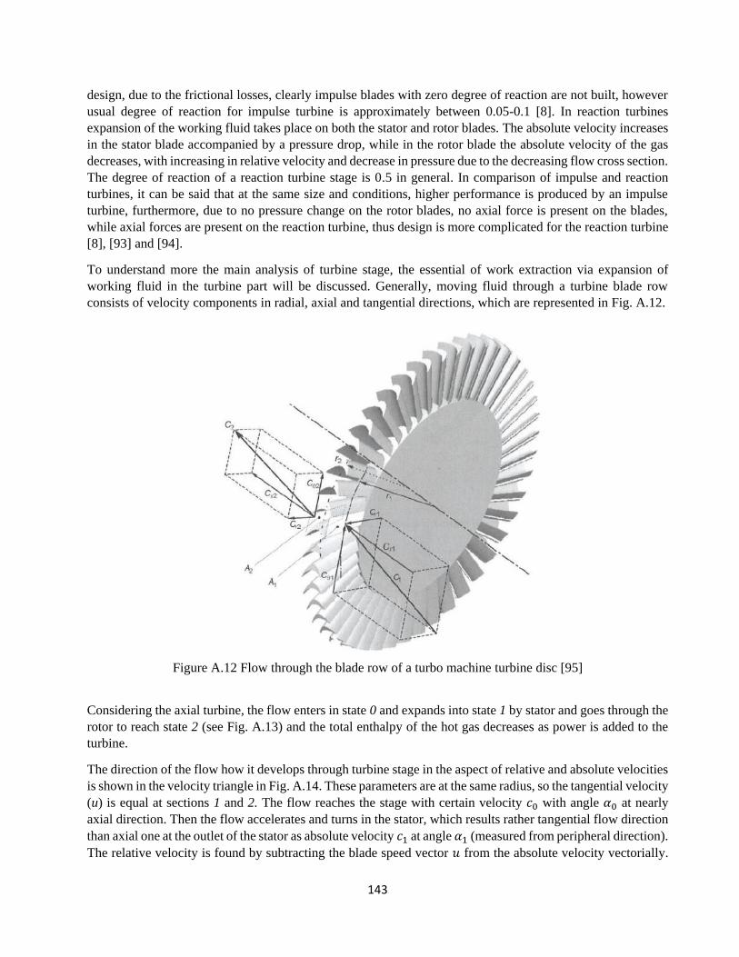
143

design, due to the frictional losses, clearly impulse blades with zero degree of reaction are not built, however

usual degree of reaction for impulse turbine is approximately between 0.05-0.1 [8]. In reaction turbines

expansion of the working fluid takes place on both the stator and rotor blades. The absolute velocity increases

in the stator blade accompanied by a pressure drop, while in the rotor blade the absolute velocity of the gas

decreases, with increasing in relative velocity and decrease in pressure due to the decreasing flow cross section.

The degree of reaction of a reaction turbine stage is 0.5 in general. In comparison of impulse and reaction

turbines, it can be said that at the same size and conditions, higher performance is produced by an impulse

turbine, furthermore, due to no pressure change on the rotor blades, no axial force is present on the blades,

while axial forces are present on the reaction turbine, thus design is more complicated for the reaction turbine

[8], [93] and [94].

To understand more the main analysis of turbine stage, the essential of work extraction via expansion of

working fluid in the turbine part will be discussed. Generally, moving fluid through a turbine blade row

consists of velocity components in radial, axial and tangential directions, which are represented in Fig. A.12.

Figure A.12 Flow through the blade row of a turbo machine turbine disc [95]

Considering the axial turbine, the flow enters in state 0 and expands into state 1 by stator and goes through the

rotor to reach state 2 (see Fig. A.13) and the total enthalpy of the hot gas decreases as power is added to the

turbine.

The direction of the flow how it develops through turbine stage in the aspect of relative and absolute velocities

is shown in the velocity triangle in Fig. A.14. These parameters are at the same radius, so the tangential velocity

(u) is equal at sections 1 and 2. The flow reaches the stage with certain velocity 𝑐0 with angle 𝛼0 at nearly

axial direction. Then the flow accelerates and turns in the stator, which results rather tangential flow direction

than axial one at the outlet of the stator as absolute velocity 𝑐1 at angle 𝛼1 (measured from peripheral direction).

The relative velocity is found by subtracting the blade speed vector 𝑢 from the absolute velocity vectorially.

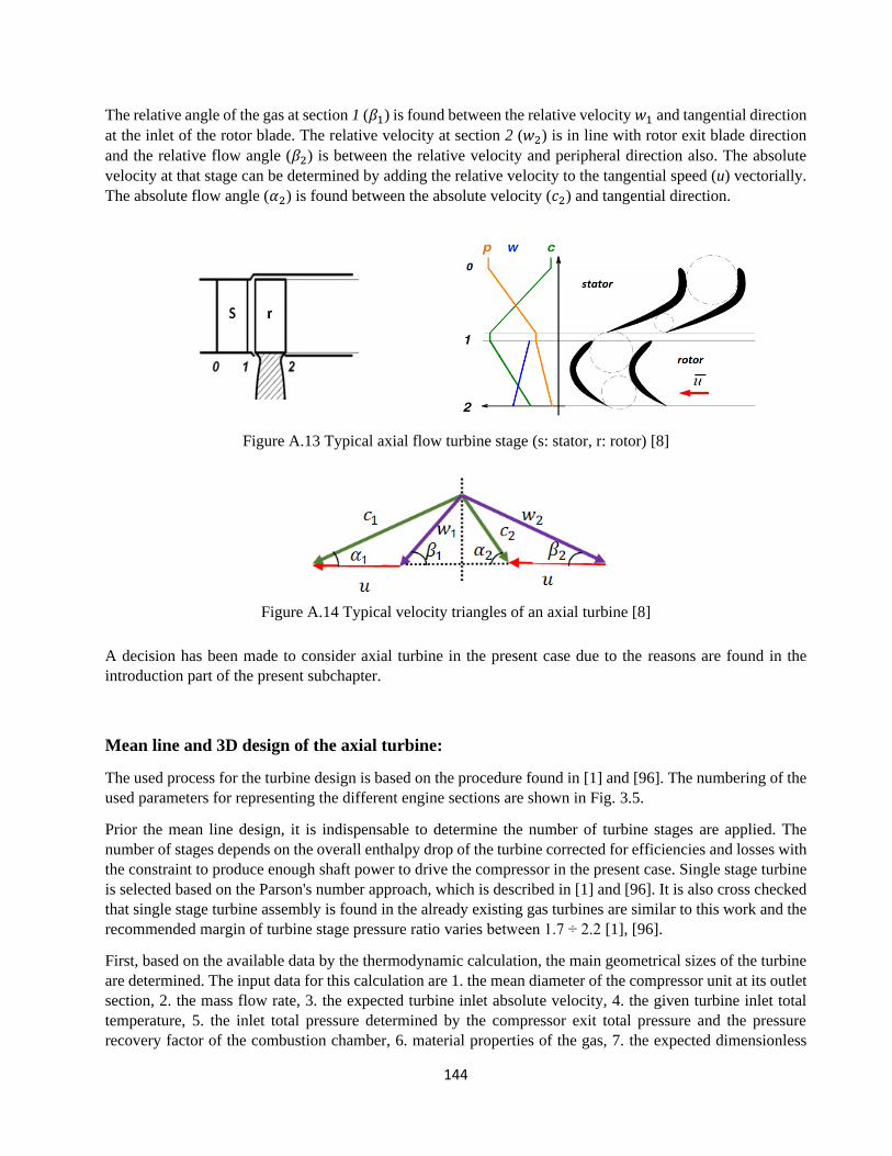
144

The relative angle of the gas at section 1 (𝛽1) is found between the relative velocity 𝑤1 and tangential direction

at the inlet of the rotor blade. The relative velocity at section 2 (𝑤2) is in line with rotor exit blade direction

and the relative flow angle (𝛽2) is between the relative velocity and peripheral direction also. The absolute

velocity at that stage can be determined by adding the relative velocity to the tangential speed (u) vectorially.

The absolute flow angle (𝛼2) is found between the absolute velocity (𝑐2) and tangential direction.

Figure A.13 Typical axial flow turbine stage (s: stator, r: rotor) [8]

Figure A.14 Typical velocity triangles of an axial turbine [8]

A decision has been made to consider axial turbine in the present case due to the reasons are found in the

introduction part of the present subchapter.

Mean line and 3D design of the axial turbine:

The used process for the turbine design is based on the procedure found in [1] and [96]. The numbering of the

used parameters for representing the different engine sections are shown in Fig. 3.5.

Prior the mean line design, it is indispensable to determine the number of turbine stages are applied. The

number of stages depends on the overall enthalpy drop of the turbine corrected for efficiencies and losses with

the constraint to produce enough shaft power to drive the compressor in the present case. Single stage turbine

is selected based on the Parson's number approach, which is described in [1] and [96]. It is also cross checked

that single stage turbine assembly is found in the already existing gas turbines are similar to this work and the

recommended margin of turbine stage pressure ratio varies between 1.7 ÷ 2.2 [1], [96].

First, based on the available data by the thermodynamic calculation, the main geometrical sizes of the turbine

are determined. The input data for this calculation are 1. the mean diameter of the compressor unit at its outlet

section, 2. the mass flow rate, 3. the expected turbine inlet absolute velocity, 4. the given turbine inlet total

temperature, 5. the inlet total pressure determined by the compressor exit total pressure and the pressure

recovery factor of the combustion chamber, 6. material properties of the gas, 7. the expected dimensionless

145

speed at the exit of the turbine, 8 total specific enthalpy drop, 9. isentropic turbine efficiency and 10. the exit

total temperature and pressure. The material properties of the gas (specific heat at constant pressure and the

ratio of specific heats) are constants, they are not a function of the temperature and the mass fraction of the

material components because it has negligible effect for the final outcomes as it was shown in subchapter

2.4.2. The main outputs of the calculation are the static pressure, temperature, density, velocity, cross section,

diameter (inner and outer) and the blade height at the inlet and outlet section of the turbine. The calculation in

detail is the following. First, the static temperature, static pressure, density and the cross section of the inlet

section are determined by Eq. (A.42)-Eq. (A.45) [1].

𝑇4 = 𝑇04 −𝑐42

2𝑐𝑝,𝑔𝑎𝑠 (A.42)

𝑝4 = 𝑝04 (𝑇4𝑇04

)𝛾𝑔𝑎𝑠 (𝛾𝑔𝑎𝑠−1)⁄

(A.43)

𝜌4 =𝑝4

𝑅𝑔𝑎𝑠𝑇4

(A.44)

𝐴4 =��4

𝑐4𝜌4 (A.45)

The direction of the velocity 𝑐4 is supposed to be axial, it has no tangential component. The next step is the

determination of the mean diameter with especial care for the low centrifugal force, the blade height and the

hub and tip diameters at constant mean diameter design choice for the turbine unit due to the streamline flow

path and low production cost. The calculation is shown in the following equations [1]:

𝐷4𝑚 = 0.68 𝐷3𝑚 (A.46)

𝑙4 =𝐴4

𝜋𝐷4𝑚 (A.47)

𝐷4ℎ = 𝐷4𝑚 − 𝑙4 (A.48)

𝐷4𝑡 = 𝐷4𝑚 + 𝑙4 (A.49)

Determination of the static thermodynamic parameters and the main geometrical sizes of the turbine exit is

show in Eq. (A.50)-Eq. (A.59) [1].

𝑐5𝑐𝑟𝑖𝑡 = √2𝛾𝑔𝑎𝑠

𝛾𝑔𝑎𝑠 + 1𝑅𝑔𝑎𝑠𝑇05 (A.50)

𝑐5 = 𝜆5𝑐5𝑐𝑟𝑖𝑡 = 𝑐5𝑎 (A.51)

146

𝑇5 = 𝑇05 −𝑐52

2𝑐𝑝,𝑔𝑎𝑠 (A.52)

𝑝5 = 𝑝05 (𝑇5𝑇05

)𝛾𝑔𝑎𝑠 (𝛾𝑔𝑎𝑠−1)⁄

(A.53)

𝜌5 =𝑝5

𝑅𝑔𝑎𝑠𝑇5

(A.54)

𝐴5 =��5

𝑐5𝜌5 (A.55)

𝐷5𝑚 = 𝐷4𝑚 (A.56)

𝑙5 =𝐴5

𝜋𝐷5𝑚 (A.57)

𝐷5ℎ = 𝐷5𝑚 − 𝑙5 (A.58)

𝐷5𝑡 = 𝐷5𝑚 + 𝑙5 (A.59)

The total temperature and pressure at the exit of the turbine are pre-calculated from the total specific enthalpy

drop and the isentropic efficiency of the turbine. ��4 = ��5 as there is no blade cooling considered. The

summary of the all input data and the resulted parameters are shown in Table A.4.

The second main part of the turbine design is the determination of the unknown thermodynamic, aerodynamic

and flow parameters together with the velocity triangles at the mean line of each section (0, 1 and 2) of the

turbine stage. The input and the output data for this calculation are shown in the Table A.5.

The computation starts with quantifying the exit pressure of turbine by the inlet total temperature and pressure

and the adiabatic enthalpy drop of the stage with supposing an ideal adiabatic expansion till the same pressure

as it is in the real turbine process. Hence, first the critical isentropic velocity at the inlet of the turbine stage is

determined [1], [96]:

𝑐𝑠,𝑐𝑟𝑖𝑡 = √2𝛾𝑔𝑎𝑠

𝛾𝑔𝑎𝑠 + 1𝑅𝑔𝑎𝑠𝑇00 (A.60)

The available velocity by the isentropic energy change is calculated by Eq. (A.61) [1], [96].

𝑐𝑠 = √2∆ℎ0𝑠, where ∆ℎ0𝑠 = 𝑐𝑝𝑔𝑎𝑠𝑇00(1 −1

(𝑝00𝑝2

)

𝛾𝑔𝑎𝑠−1

𝛾𝑔𝑎𝑠

) (A.61)

147

Table A.4 Input and output parameters of the mean line design of the turbine for determining its main inlet

and exit geometrical sizes

Input Output

𝐷3𝑚 0.2 [m] 𝑐4𝑐𝑟𝑖𝑡 568.26 [m/s]

��4 1 [kg/s] 𝑇4 994.69 [K]

𝑐4 110 [m/s] 𝑝4 227187 [Pa]

𝑇04 1000 [K] 𝜚4 0.81 [kg/m3]

𝑝04 232111.85 [Pa] 𝐴4 0.01 [m2]

𝛾𝑔𝑎𝑠 1.33 [-] 𝐷4𝑚 0.13 [m]

𝑅𝑔𝑎𝑠 282.86 [J/kg/K] 𝑙4 0.027 [m]

𝜆4 0.36 [-] 𝐷4ℎ 0.103 [m]

∆ℎ𝑇0 137713 [J/kg] 𝐷4𝑡 0.157 [m]

휂𝑠𝑇 0.87 𝑐5𝑐𝑟𝑖𝑡 532.83 [m/s]

𝑇05 879.2 [K] 𝑐5 191.82 [m/s]

𝑝05 127070.3 [Pa] 𝑇5 863.06 [K]

𝑝5 117928.14 [Pa]

𝜚5 0.48 [kg/m3]

𝐴5 0.01 [m2]

𝑙5 0.027 [m]

𝐷5𝑚 0.13 [m]

𝐷5ℎ 0.103 [m]

𝐷5𝑡 0.157 [m]

The dimensionless speed at the turbine outlet cross section is expressed as follow [1]:

𝜆𝑠 =𝑐𝑠

𝑐𝑠,𝑐𝑟𝑖𝑡

(A.62)

The static pressure at the outlet of the stage can then be computed with the help of dimensionless gas dynamic

equation [1]:

𝑇2𝑇00

= (𝑝2𝑝00

)

𝛾𝑔𝑎𝑠−1

𝛾𝑔𝑎𝑠 (A.63)

1 −𝛾𝑔𝑎𝑠 − 1

𝛾𝑔𝑎𝑠 + 1𝜆𝑠2 = (

𝑝2𝑝00

)

𝛾𝑔𝑎𝑠−1

𝛾𝑔𝑎𝑠 (A.64)

𝑝2 = (1 −𝛾𝑔𝑎𝑠 − 1

𝛾𝑔𝑎𝑠 + 1𝜆𝑠2)

𝛾𝑔𝑎𝑠𝛾𝑔𝑎𝑠−1

𝑝00 (A.65)

148

The degree of reaction is determined to be 0.2 to be closer to the impulse-type turbine in order to utilize its

advantages discussed in the introduction part of subchapter of Appendix A.4. Then the enthalpy drop of the

stator and rotor can be determined by the following ways (the s and r in the subscripts indicate the stator and

rotor respectively) [1]:

∆ℎ𝑠,𝑠 = (1 − 𝑟𝑜)∆ℎ𝑜𝑠 (A.66)

∆ℎ𝑠,𝑟 = 𝑟𝑜∆ℎ𝑜𝑠 (A.67)

The total enthalpy drop across the stator turns to increase the velocity. So, the theoretical absolute velocity at

the exit of the stator is given by Eq. (A.68) [1].

𝑐1,𝑡ℎ = √2∆ℎ𝑠,𝑠 (A.68)

However, due to the fluid dynamic losses, this velocity is less in the reality. The speed coefficient is used to

determine the real velocity at the exit of the stator [1]:

𝑐1 = 𝜑𝑠𝑐1,𝑡ℎ (A.69)

Then, the static temperature at this section can be calculated by the Eq. (A.70) [1].

𝑇1 = 𝑇00 −𝑐12

2𝑐𝑝,𝑔𝑎𝑠 (A.70)

The critical speed and the theoretical dimensionless speed at the stator exit are computed by Eq. (A.71) and

Eq. (A.72) respectively [1].

𝑐1,𝑐𝑟𝑖𝑡 = √2𝛾𝑔𝑎𝑠

𝛾𝑔𝑎𝑠 + 1𝑅𝑔𝑎𝑠𝑇00 (A.71)

𝜆1,𝑡ℎ =𝑐1,𝑡ℎ𝑐1,𝑐𝑟𝑖𝑡

(A.72)

The static pressure at the outlet of the stator can be determined in the function of the inlet total pressure,

theoretical dimensionless speed and ratio of specific heats [1]:

𝑝1 = (1 −𝛾𝑔𝑎𝑠 − 1

𝛾𝑔𝑎𝑠 + 1𝜆1,𝑡ℎ2 )

𝛾𝑔𝑎𝑠𝛾𝑔𝑎𝑠−1

𝑝00 (A.73)

The flow angle of the absolute velocity (measured from tangential direction) at the stator outlet section is given

by Eq. (A.74) [1], [96].

𝛼1 = 𝑎𝑟𝑐𝑠𝑖𝑛��√𝑇00

𝛽𝑝00A1𝜑𝑠𝑞(𝜆1,𝑡ℎ)휀1 (A.74)

149

Typically, the gas dynamic constant is 𝛽 = 0.0396 and 휀1 is a factor considers the flow cross section, which

is affected (reduced) by the blades. It needs to be taken into account when the blades are shorter than 12 mm

[1]. The 𝑞(𝜆1,𝑡ℎ) is the dimensionless mass flow rate [1]:

𝑞(𝜆1,𝑡ℎ) = (𝛾𝑔𝑎𝑠 + 1

2)

1𝛾𝑔𝑎𝑠−1

𝜆1,𝑡ℎ (1 −𝛾𝑔𝑎𝑠 − 1

𝛾𝑔𝑎𝑠 + 1𝜆1,𝑡ℎ2 )

1𝛾𝑔𝑎𝑠−1

(A.75)

The relative velocity at the rotor inlet section is computed from the known components of the velocity triangle

as [1], [96]:

𝑤1 = √𝑐12 + 𝑢1

2 − 2𝑐1𝑢1𝑐𝑜𝑠𝛼1 (A.76)

The tangential velocity (𝑢1 ) is determined by the diameter (radius) at the mean line and RPM (angular speed).

The incoming flow angle of the relative velocity measured from tangential direction is given by Eq. (A.77)

[1], [96].

𝛽1 = 𝑎𝑟𝑐𝑠𝑖𝑛𝑐1𝑠𝑖𝑛𝛼1𝑤1

(A.77)

In the relative frame of reference, the relative total temperature at the rotor inlet is calculated as follow [1],

[96]:

𝑇0𝑤1 = 𝑇1 +𝑤12

2𝑐𝑝,𝑔𝑎𝑠 (A.78)

and it is constant in the rotor segment. So one can write [1], [96]:

𝑇0𝑤1 = 𝑇0𝑤2 ⇒ 𝐶𝑝,𝑔𝑎𝑠𝑇1 +𝑤12

2= 𝐶𝑝,𝑔𝑎𝑠𝑇2 +

𝑤22

2 (A.79)

The relative velocity at the outlet section of the rotor is determined by Eq. (A.80) [1], [96].

𝑤2 = 𝜑𝑟√𝑤12 + 2∆ℎ𝑠,𝑟 (A.80)

where 𝜑𝑟 is the speed coefficient of the rotor for considering the losses. The relative critical speed and the

dimensionless speed at the rotor exit are computed as follow [1], [96]:

𝑤2,𝑐𝑟𝑖𝑡 = √2𝛾𝑔𝑎𝑠

𝛾𝑔𝑎𝑠 + 1𝑅𝑔𝑎𝑠𝑇0𝑤2 (A.81)

𝜆𝑤2 =𝑤2

𝑤2,𝑐𝑟𝑖𝑡

(A.82)

The total pressure in the relative frame of reference can be calculated as the p2 static pressure is known [1],

[96]:

150

𝑝0𝑤2 = (1 −𝛾𝑔𝑎𝑠 − 1

𝛾𝑔𝑎𝑠 + 1𝜆𝑤22 )

−𝛾𝑔𝑎𝑠

𝛾𝑔𝑎𝑠−1

𝑝2 (A.83)

The outlet static temperature is determined by the temperature ratio in terms of gas dynamic function (see Eq.

(A.84) [1], [96]).

𝑇2 = (1 −𝛾𝑔𝑎𝑠 − 1

𝛾𝑔𝑎𝑠 + 1𝜆𝑤22 )𝑇0𝑤2 (A.84)

The flow angle of the relative velocity measured from tangential direction is given by Eq. (A.85) [1], [96].

𝛽2 = 𝑎𝑟𝑐𝑠𝑖𝑛��√𝑇0𝑤1

𝛽𝑝0𝑤2A2𝜑𝑟𝑞(𝜆𝑤2) 2, (A.85)

where the 𝑞(𝜆𝑤2) is the dimensionless mass flow rate [1]:

𝑞(𝜆𝑤2) = (𝛾𝑔𝑎𝑠 + 1

2)

1𝛾𝑔𝑎𝑠−1

𝜆𝑤2 (1 −𝛾𝑔𝑎𝑠 − 1

𝛾𝑔𝑎𝑠 + 1𝜆𝑤22 )

1𝛾𝑔𝑎𝑠−1

(A.86)

The outlet absolute velocity is calculated by the cosine theorem [1], [96]:

𝑐2 = √𝑤22 + 𝑢2

2 − 2𝑤2𝑢2𝑐𝑜𝑠𝛽2 (A.87)

as the tangential velocity is computed similarly to the same speed but at the inlet section of the rotor. The flow

angle of the absolute velocity measured from the tangential direction is shown by Eq. (A.88) [1], [96].

𝛼2 = 𝑎𝑟𝑐𝑠𝑖𝑛𝑤2𝑠𝑖𝑛𝛽2

𝑐2 (A.88)

Concerning the total temperature, the critical velocity, the dimensionless speed and the total pressure at the

exit of the rotor, they are determined by Eq. (A.89)-Eq. (A.92) [1], [96].

𝑇02 = 𝑇2 +𝑐22

2𝑐𝑝,𝑔𝑎𝑠 (A.89)

𝑐2,𝑐𝑟𝑖𝑡 = √2𝛾𝑔𝑎𝑠

𝛾𝑔𝑎𝑠 + 1𝑅𝑔𝑎𝑠𝑇02 (A.90)

𝜆2 =𝑐2

𝑐2,𝑐𝑟𝑖𝑡

(A.91)

𝑝02 = (1 −𝛾𝑔𝑎𝑠 − 1

𝛾𝑔𝑎𝑠 + 1𝜆22)

−𝛾𝑔𝑎𝑠

𝛾𝑔𝑎𝑠−1

𝑝2 (A.92)

The input and the output parameters of the mean line design of the turbine are shown in Table A.5.

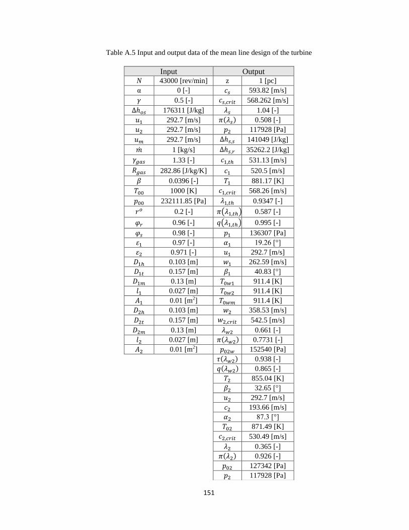
151

Table A.5 Input and output data of the mean line design of the turbine

Input Output N 43000 [rev/min] z 1 [pc]

α 0 [-] 𝑐𝑠 593.82 [m/s]

𝛾 0.5 [-] 𝑐𝑠,𝑐𝑟𝑖𝑡 568.262 [m/s]

∆ℎ𝑜𝑠 176311 [J/kg] 𝜆𝑠 1.04 [-]

𝑢1 292.7 [m/s] 𝜋(𝜆𝑠) 0.508 [-]

𝑢2 292.7 [m/s] 𝑝2 117928 [Pa]

𝑢𝑚 292.7 [m/s] ∆ℎ𝑠,𝑠 141049 [J/kg]

�� 1 [kg/s] ∆ℎ𝑠,𝑟 35262.2 [J/kg]

𝛾𝑔𝑎𝑠 1.33 [-] 𝑐1,𝑡ℎ 531.13 [m/s]

𝑅𝑔𝑎𝑠 282.86 [J/kg/K] 𝑐1 520.5 [m/s]

𝛽 0.0396 [-] 𝑇1 881.17 [K]

𝑇00 1000 [K] 𝑐1,𝑐𝑟𝑖𝑡 568.26 [m/s]

𝑝00 232111.85 [Pa] 𝜆1,𝑡ℎ 0.9347 [-]

𝑟𝑜 0.2 [-] 𝜋(𝜆1,𝑡ℎ) 0.587 [-]

𝜑𝑟 0.96 [-] 𝑞(𝜆1,𝑡ℎ) 0.995 [-]

𝜑𝑠 0.98 [-] 𝑝1 136307 [Pa]

휀1 0.97 [-] 𝛼1 19.26 [°]

휀2 0.971 [-] 𝑢1 292.7 [m/s]

𝐷1ℎ 0.103 [m] 𝑤1 262.59 [m/s]

𝐷1𝑡 0.157 [m] 𝛽1 40.83 [°]

𝐷1𝑚 0.13 [m] 𝑇0𝑤1 911.4 [K]

𝑙1 0.027 [m] 𝑇0𝑤2 911.4 [K]

𝐴1 0.01 [m2] 𝑇0𝑤𝑚 911.4 [K]

𝐷2ℎ 0.103 [m] 𝑤2 358.53 [m/s]

𝐷2𝑡 0.157 [m] 𝑤2,𝑐𝑟𝑖𝑡 542.5 [m/s]

𝐷2𝑚 0.13 [m] 𝜆𝑤2 0.661 [-]

𝑙2 0.027 [m] 𝜋(𝜆𝑤2) 0.7731 [-]

𝐴2 0.01 [m2] 𝑝02𝑤 152540 [Pa]

𝜏(𝜆𝑤2) 0.938 [-]

𝑞(𝜆𝑤2) 0.865 [-]

𝑇2 855.04 [K]

𝛽2 32.65 [°]

𝑢2 292.7 [m/s]

𝑐2 193.66 [m/s]

𝛼2 87.3 [°]

𝑇02 871.49 [K]

𝑐2,𝑐𝑟𝑖𝑡 530.49 [m/s]

𝜆2 0.365 [-]

𝜋(𝜆2) 0.926 [-]

𝑝02 127342 [Pa]

𝑝2 117928 [Pa]

152

The 3D extension of the blade design by means of blade twisting is the next step in the aerodynamic design of

the turbine stage. So, the velocity vectors at the hub and tip sections are determined in the present paragraph.

The ISRE (Isentropic Radial Equilibrium Equation) is used as governing equation for that purpose [70]:

𝑑ℎ0𝑑𝑟

= 𝑐𝑎𝑑𝑐𝑎𝑑𝑟

+ 𝑐𝑤𝑑𝑐𝑤𝑑𝑟

+𝑐𝑤2

𝑟 (A.93)

Eq. (A.93) includes that the effect of the inertial (centrifugal) force due to the high-speed rotation is balanced

by the pressure force for the flow in radial direction. Furthermore, the entropy-variation in the radial direction

is supposed to be zero. Constant blade loading provides uniform energy decrease in the spanwise direction of

the turbine blades, so the enthalpy change of the flow in the function of radius is zero also. This is considered

in Eq. (A.94).

0 = 𝑐𝑎𝑑𝑐𝑎𝑑𝑟

+ 𝑐𝑤𝑑𝑐𝑤𝑑𝑟

+𝑐𝑤2

𝑟 (A.94)

Constant nozzle outlet angle (𝛼1 = 𝑐𝑜𝑛𝑠𝑡.) blade twisting method is used in the present case due to the

favourable production cost. The axial and tangential velocity components of the absolute velocity along the

radius is determined from Eq. (A.94). The detailed derivations of the final expressions are presented hereafter.

Using trigonometric relation, the tangent of the absolute flow angle at the inlet section of the rotor is given by

Eq. (A.95) [70].

𝑡𝑔𝛼1 =𝑐1𝑎𝑐1𝑤

(A.95)

The 𝛼1 is measured from tangential direction. Furthermore, the partial derivatives can be constituted in radial

direction [70]:

𝑑𝑐1𝑎𝑑𝑟

=𝑑𝑐1𝑤𝑑𝑟

𝑡𝑔𝛼1 (A.96)

Thus, using Eq. (A.95) and Eq. (A.96), Eq. (A.94) can be rewritten as follow:

0 = 𝑐1𝑤𝑡𝑔2𝛼1

𝑑𝑐1𝑤𝑑𝑟

+ 𝑐1𝑤𝑑𝑐1𝑤𝑑𝑟

+𝑐1𝑤2

𝑟 (A.97)

or after rearrangements:

0 = (1 + 𝑡𝑔2𝛼1 )𝑑𝑐1𝑤𝑑𝑟

+𝑐1𝑤𝑟

(A.98)

The final form of the differential equation before its analytical solution is given Eq. (A.99) [70].

1

𝑐𝑜𝑠2𝛼1

𝑑𝑐1𝑤𝑑𝑟

= −𝑐1𝑤𝑟

(A.99)

153

The solution of Eq. (A.99) is the following [70]:

𝑐1𝑤𝑟cos2 𝛼1 = 𝑐𝑜𝑛𝑠𝑡. (A.100)

and because 𝑐1𝑎

𝑐1𝑤= 𝑡𝑔𝛼1 and it is constant:

𝑐1𝑎𝑟cos2 𝛼1 = 𝑐𝑜𝑛𝑠𝑡. (A.101)

Based on the fact that the total enthalpy reduction along the radius is constant and the inlet and outlet section

is on the same radius, the Euler's turbine equation gives [70]:

𝑢(𝑐1𝑤 − 𝑐2𝑤) = 𝑢𝑚(𝑐1𝑤𝑚 − 𝑐2𝑤𝑚), 𝑟(𝑐1𝑤 − 𝑐2𝑤) = 𝑟𝑚(𝑐1𝑤𝑚 − 𝑐2𝑤𝑚) (A.102)

The tangential velocity component of the absolute velocity at the outlet of the rotor and at given r radius can

be expressed from Eq. (A.102) and it is shown in Eq. (A.103) [70], [97].

𝑐2𝑤 =𝑐1𝑤𝑚

𝑅cos2 𝛼1

−(𝑐1𝑤𝑚 − 𝑐2𝑤𝑚)

𝑅 (A.103)

Here, the equalities 𝑐1𝑤 =𝑐1𝑤𝑚

𝑅𝑐𝑜𝑠2 𝛼1

and 𝑅 = 𝑟/𝑟𝑚 are considered. As 𝑐2𝑤 is known, 𝑐2𝑎 can be calculated by

integrating Eq. (A.94) for the outlet cross section (cross section 2) between 1 and R and using Eq. (A.103)

[97]:

𝑐2𝑎 = √𝑐2𝑎𝑚2 + 4𝑐1𝑤𝑚

2 (1

𝑅𝑐𝑜𝑠2 𝛼1

− 1) 𝑠𝑖𝑛2 𝛼1 𝑐𝑜𝑠2 𝛼1 − 2𝑐1𝑤𝑚

2

(A.104)

√(1 −𝑐2𝑤𝑚𝑐1𝑤𝑚

)(1 + 𝑐𝑜𝑠2 𝛼1)(1

𝑅1+𝑐𝑜𝑠2 𝛼1

− 1) 𝑠𝑖𝑛2 𝛼1

As the absolute velocity components at the rotor outlet are determined, the flow angles, the absolute and

relative velocities are calculated as follows:

𝛼2 = 𝑎𝑟𝑐𝑡𝑎𝑛 (𝑐2𝑎𝑐2𝑤

) (A.105)

𝑐2 = √𝑐2𝑎2 + 𝑐2𝑤

2 (A.106)

𝑤2 = √𝑐22 + 𝑢2

2 − 2𝑐2𝑢2𝑐𝑜𝑠𝛼2 (A.107)

𝛽2 = arcsin (𝑐2𝑎𝑤2)

(A.108)

154

The final outcomes for the velocity triangles at hub, mean and tip section are shown in Table A.6.

Table A.6 Components and angles (measured from the tangential direction) of the velocity triangles in the

turbine at hub, mean and tip sections

The absolute Mach number at the exit and at the hub section of the turbine stator is higher than 1, so the flow

is deviated due to the expansion in the obliquely cut blade nozzle section. Hence, the new absolute flow angle

is computed (see Eq. (A.109) [1], [96]) and considered hereafter.

Following the 3D extension of the mean line design by means of blade twisting, the next step of the turbine,

particularly the turbine blade design is the determination of the blade chord, pitch and the number of blades.

The chord is computed by the length of the blade and the blade aspect ratio (l/c) as it is shown in Eq. (A.110)

[1].

The 𝑙

𝑐= 0.73 and 1.17 has been defined in the present case for the stator and rotor blade respectively and l is

0.027 m for both. The optimum ratios of the blade spacing to chord length in the function of the flow angles

are shown in Fig. A.15. As these flow angles are known, the value of t/c can be determined. It results 0.7 for

Data Hub section Mean section Tip section

r [m] 0.0515 0.065 0.0785

R [m] 0.7923 1 1.2077

𝑢1[m/s] 231.9 292.7 353.48

𝑢2 [m/s] 231.9 292.7 353.48

𝑐1 [m/s] 640.52 520.5 439.93

𝑐1𝑎 [m/s] 211.2821 171.7 145.12

𝑐1𝑢 [m/s] 604.667 491.37 415.3

𝑐2 [m/s] 72.08 193.66 229.021

𝑐2𝑎 [m/s] 71.22 193.445 228.46

𝑐2𝑢 [m/s] -11.04 9.162 16.027

𝑤1 [m/s] 376.787 269.59 189.985

𝑤2 [m/s] 290.516 343.235 358.8

𝛼1 [°] 19.26 19.26 19.26

𝛼2 [°] -81.188 87.288 85.987

𝛽1 [°] 34.1 40.8 49.8

𝛽2 [°] 14.19 34.3 39.55

𝛼1,𝑛𝑒𝑤 = 𝑎𝑟𝑐𝑠𝑖𝑛 (𝑠𝑖𝑛(𝛼1,𝑜𝑟𝑖𝑔𝑖𝑛𝑎𝑙)

𝑞(𝜆1))=23.9° where 𝜆1 =

𝑐1

𝑐1,𝑐𝑟𝑖𝑡 (A.109)

𝑐 =𝑙

(𝑙𝑐)

(A.110)

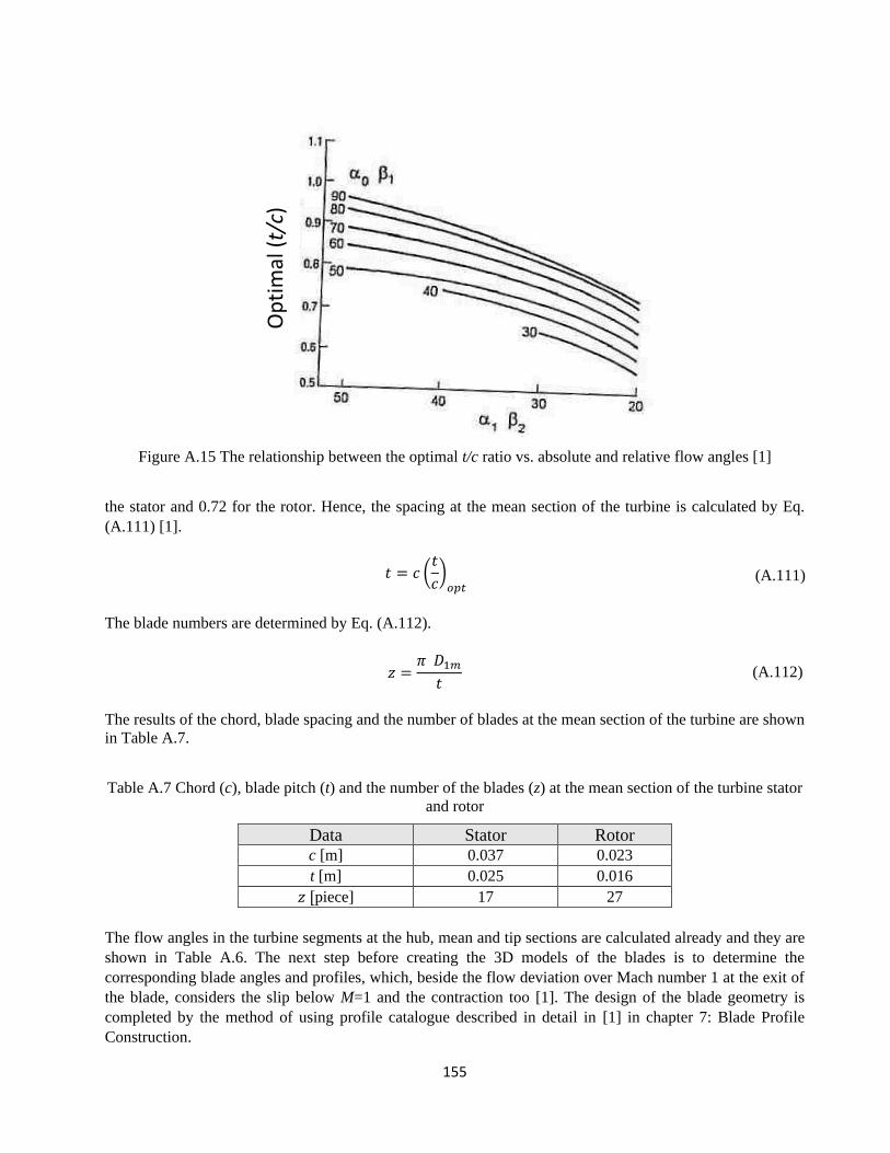
155

Figure A.15 The relationship between the optimal t/c ratio vs. absolute and relative flow angles [1]

the stator and 0.72 for the rotor. Hence, the spacing at the mean section of the turbine is calculated by Eq.

(A.111) [1].

𝑡 = 𝑐 (𝑡

𝑐)𝑜𝑝𝑡

(A.111)

The blade numbers are determined by Eq. (A.112).

𝑧 =𝜋 𝐷1𝑚𝑡

(A.112)

The results of the chord, blade spacing and the number of blades at the mean section of the turbine are shown

in Table A.7.

Table A.7 Chord (c), blade pitch (t) and the number of the blades (z) at the mean section of the turbine stator

and rotor

The flow angles in the turbine segments at the hub, mean and tip sections are calculated already and they are

shown in Table A.6. The next step before creating the 3D models of the blades is to determine the

corresponding blade angles and profiles, which, beside the flow deviation over Mach number 1 at the exit of

the blade, considers the slip below M=1 and the contraction too [1]. The design of the blade geometry is

completed by the method of using profile catalogue described in detail in [1] in chapter 7: Blade Profile

Construction.

Data Stator Rotor c [m] 0.037 0.023

t [m] 0.025 0.016

𝑧 [piece] 17 27

Op

tim

al (

t/c)

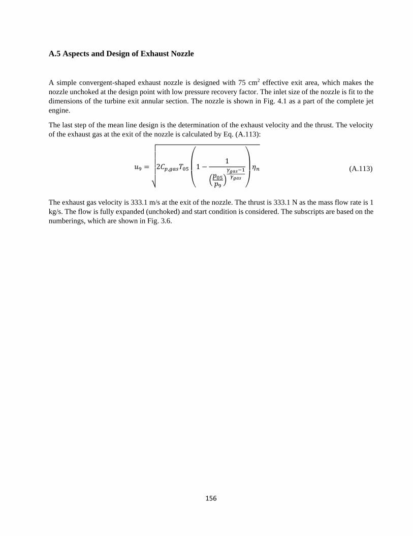
156

A.5 Aspects and Design of Exhaust Nozzle

A simple convergent-shaped exhaust nozzle is designed with 75 cm2 effective exit area, which makes the

nozzle unchoked at the design point with low pressure recovery factor. The inlet size of the nozzle is fit to the

dimensions of the turbine exit annular section. The nozzle is shown in Fig. 4.1 as a part of the complete jet

engine.

The last step of the mean line design is the determination of the exhaust velocity and the thrust. The velocity

of the exhaust gas at the exit of the nozzle is calculated by Eq. (A.113):

𝑢9 =

√

2𝐶𝑝,𝑔𝑎𝑠𝑇05

(

1 −

1

(𝑝05𝑝9)

𝛾𝑔𝑎𝑠−1

𝛾𝑔𝑎𝑠

)

휂𝑛 (A.113)

The exhaust gas velocity is 333.1 m/s at the exit of the nozzle. The thrust is 333.1 N as the mass flow rate is 1

kg/s. The flow is fully expanded (unchoked) and start condition is considered. The subscripts are based on the

numberings, which are shown in Fig. 3.6.

157

APPENDIX B - Introduction of the Used

CFD Methodology by Means of ANSYS CFX

158

B.1 Governing Equation

The basics of the used commercial CFD technology for computing the flow characteristics of the redesigned

academic jet engine are the continuity, momentum and energy conservation laws. These equations are the most

suitable mathematical expressions in flow complexity point of view, and they form the system of the nonlinear

partial differential equations.

The mass conservation law is the following [48]:

𝜕𝜌

𝜕𝑡+ 𝛻 ∙ (𝜌 𝑼) = 0 (B.1)

The moment equation is expressed [48]:

𝜕(𝜌 𝑼)

𝜕𝑡+ 𝛻 ∙ (𝜌 𝑼 x 𝑼) = − 𝛻𝑝 + 𝛻 ∙ 𝜏 + 𝑺𝑴 (B.2)

where the stress tensor, 𝝉, is related to strain rate [48]:

𝜏 = µ(𝛻𝑼 + (𝛻𝑼)𝑇 −2

3𝛿𝛻𝑼) (B.3)

The conservation of the specific total enthalpy is next [48]:

𝜕(𝜌 ℎ𝑡𝑜𝑡)

𝜕𝑡−𝜕𝑝

𝜕𝑡+ 𝛻 ∙ (𝜌𝑼ℎ𝑡𝑜𝑡) = 𝛻 ∙ (𝜆 𝛻𝑇) + 𝛻 ∙ (𝑼 ∙ 𝜏) + 𝑼 ∙ 𝑺𝑴 + 𝑺𝑬 (B.4)

where ℎ𝑡𝑜𝑡 is related to the static h(T, p) enthalpy by [48]:

ℎ𝑡𝑜𝑡 = ℎ +1

2𝑼2 (B.5)

The term 𝛻 ∙ (𝑼 ∙ 𝜏) represents the work due to viscous stresses and is called the viscous work term. This

models the internal heating by viscosity in the fluid and is considered in the present case. The term 𝑼 ∙ 𝑺𝑴 is

the work due to external momentum sources and is currently neglected [48].

These equations above are used in Reynolds averaged manner and turbulence modelling (see the next

subchapter) is considered to closure the system of the nonlinear partial differential equations following the

Boussinesq approximation. The reason why this methodology is used, that this approach is the most suitable

from the accuracy and computational effort point of view in general and in rather complex engineering

problems (compressible flow with high turbulence intensity at strong adverse pressure gradient conditions)

and at complex geometry.

B.2 Turbulence Modelling [48]

Turbulence occurs when the inertia forces in the fluid become significant compared to viscous forces and is

characterized by high Reynolds number. It consists of fluctuations in the flow field in time and space. The

turbulence is a complex process, mainly because it is three dimensional, non-isotropic, unsteady and consists

of many scales. It can have a significant effect on the characteristics of the flow.

159

In principle, the considered governing equations (including conservation of momentum, which are also called

Navier-Stokes1 equations) describe both laminar and turbulent flows without the need for additional

information. However, turbulent flows at high Reynolds numbers span a large length and time scales and

would generally involve length scales much smaller than the smallest finite volume mesh, which can be

practically used in a numerical analysis. The Direct Numerical Simulation (DNS) of these flows around the

complex geometry would require computing power, which are many orders of magnitude higher than the

available in the foreseeable future.

Turbulence models expect to modify the original unsteady Navier-Stokes equations by the introduction of the

averaged and fluctuating quantities to produce the Reynolds Averaged Navier-Stokes (RANS) equations.

These equations are going to be solved for the mean flow quantities, while the turbulence effects are modelled

without a need for resolving the turbulent fluctuations. All scales of the turbulence field are being modelled.

Turbulence models based on the RANS equations are known as statistical turbulence models due to the

statistical averaging procedure employed to obtain the equations.

The k-ω based SST turbulence model accounts for the transport of the turbulent shear stress and gives highly

accurate predictions of the onset and the amount of flow separation under adverse pressure gradients [98]. The

SST model uses a k-ω formulation in the inner parts of the boundary layer that makes the model directly usable

all the way down to the wall through the viscous sub-layer, hence the SST model can be used as a Low-Re

turbulence model without any extra damping functions. The SST formulation also switches to k-ε behaviour

in the free-stream and thereby avoids the common k-ω problem, that the model is too sensitive to the inlet

free-stream turbulence properties [99]. The SST model takes the transport of the shear stress into account; it

modifies the turbulence eddy-viscosity function. The model is based on Bradshaw's assumption that the

principal shear stress is proportional to the turbulent kinetic energy. The model improves the accuracy of

prediction of flows with strong adverse pressure gradients and pressure-induced boundary layer separation.

Thus, the SST model is used in this work. More detailed information about turbulence model is found in [98],

[99] and [100].

B.3 Spray Breakup Models for Combustion

The combustion chamber is the mechanical component of the gas turbine where the heat is added to the system.

The combustion develops in the combustion chamber. The fuel enters the combustion chamber in continuous

liquid phase and then becomes dispersed one. Following the disintegration of the liquid continuous phase into

the dispersed phase, the resulting droplet system is called spray. So, the spray breakup models for combustion

are introduced in the present subchapter.

The breakup of liquid stream happens in the atomizer. Various atomizer types, based on their energy that is

converted into the fluid to achieve atomization, can be realized, such as pressure atomizer - where the energy

of the liquid is utilized -, rotational atomizer - where the mechanical energy utilized - and further types such

as pneumatic based, electrical and acoustic can be distinguished for example.

As gas turbine engines are considered, the most used atomizer is the pressure type one. In the pressure

atomizer, pressurized liquid passes through a narrow channel before injected into the gas stream or passed

onto swirlers. Although the pressure type atomizer is the most widespread in the industry, it has some

1 Claude-Louis Navier and George Gabriel Stokes described the motion of the fluid flow in 1822 and in 1845

respectively.

160

disadvantages, as it is suitable only for low mass flow rates, relatively coarse droplet sizes can be achieved

and of course there is a need to pressurize the liquid [51].

The one of the most challenging parts of flow modelling is the breakup treatment of the liquid fuel in the

combustion chamber. During the atomization process, the liquefied continuous phase fuel is dispersed to

droplets to mix with air as much as possible. The purpose of atomization is to increase the area of the liquid;

thus, the molecules are surrounded by more oxygen, which contributes to a more efficient combustion. On the

other hand, better heat and momentum transfer is realized. Atomization process happens due to different types

of forces within the liquid and gas, such as cavitation forces, forces due to turbulence and external aerodynamic

forces resulting from the interaction of the two phases [51].

Multiphase flow

The examined process of fluid disintegration as two different state mediums are present needs to be considered

as a multiphase flow phenomenon occurs. Multiphase flow can be modelled by two different ways: the

Eulerian or the Lagrangian model. The Eulerian two-fluid model treats the dispersed phase as a continuous

phase and different formulations are applied based on the mixed phases, such as gas-fluid or gas-solid mixture.

In this model particle-particle forces are modelled, and also coupling of the two phases are represented by a

pressure force, gravity force, interaction force and viscous force, which act on the two phases in the two-fluid

model for a laminar case. The Lagrangian model is based on solving the equations of motion - second law of

Newton - to determine the position and velocity of each particle. Solving and storing the state of each particle

requires high computational capacity. Thus, the Lagrangian model is rather suitable for applications where

relatively small numbers of particles are present and/or the collisions of particles are rare. There are three level

of coupling between the fluid phase and dispersed phase based on assumptions made to reduce complexity of

the problem and they include different levels of physical detail. If it is considered that just the fluid phase

affects the dispersed phase and dispersed phase does not affect the fluid phase, there is one-way coupling

between phases. When it is assumed that both phases affect each other, there is two-way coupling between

phases. The most realistic model is four-way coupling, where besides the two phases affecting each other the

particles also interact and affect each other as well [51]. Regarding the spray-type breakup model, which is

implemented in CFX and can be applied for fuel injection systems, particle transport modelling is used. It is a

type of multiphase model, where particulates are tracked through the flow in a Lagrangian way, rather than

being modelled as an extra Eulerian phase. The full particulate phase is modelled by just a sample of individual

particles. The tracking is carried out by forming a set of ordinary differential equations in time for each particle,

consisting of equations for position, velocity, temperature, and masses of species. These equations are then

integrated using a simple integration method to calculate the behaviour of the particles as they traverse the

flow domain [48].

The atomization process can be divided into more steps till the combustion. First the injected liquid starts to

breakup into larger structures, then, after the first interactions between liquid and gas, both large and small

structures evolve. This stage of atomization is called primary breakup (see Fig. B.1) [101]. After this, during

the secondary breakup, droplets disintegrate into finer drops [102], and finally evaporate. Including these steps,

the spray combustion process can be divided into six parts: primary breakup, secondary breakup, droplet

motion, droplet evaporation, mixing and combustion. Fuel droplets travel through the combustor with an initial

velocity that they have after injector and they live until they evaporate totally. The evaporated fuel mixes with

air and this mixture starts to burn when its temperature reaches the ignition temperature and fuel/air mixture

ratio is within the flammability.

161

Figure B.1 Breakup of a liquid jet [102]

The primary breakup happens at the stage when the liquid state fuel first leaves the injector and enters the

combustion chamber. In the combustion chamber, the continuous liquid breaks up into smaller particles, but

still rather coarse droplets are present. The process of the primary breakup is highly dependent on the initial

particle size, initial particle velocity, speed of liquid jet and initial spray angle at the outlet of the fuel nozzle.

Based on the nozzle geometry, primary breakup model can be categorized into three types in ANSYS CFX.

The simplest method is achieved by the Blob model. This method assumes that in the moment when particles

exit the nozzle, the diameter of particles equal the diameter of the nozzle bore, from which the liquid jet comes

(see Fig. B.2). The velocity of the particles is then retrieved according to the conservation of mass (see Eq.

(B.6)). 𝐴𝑛𝑜𝑧𝑧𝑙𝑒 is the cross section of the nozzle and ��𝑛𝑜𝑧𝑧𝑙𝑒 is the mass flow through injector in Eq. (B.6)

[48]. The Blob method is the default injection approach in ANSYS CFX, does not require additional settings,

however it has constraints such as possible turbulence, cavitation in the nozzle are not considered. In this

approach all particles leaving injector are of spherical shape and with uniform size of the injector nozzle's

diameter (B.7) [48], [101]. The injector must have a sharp corner at the end where the liquid enters the

chamber. This sharp corner plays an important role since it helps the liquid to turn into smaller parts.

Figure B.2 Blob method [48]

𝐷𝑝 = 𝐷𝑁𝑜𝑧𝑧𝑙𝑒 (B.7)

𝑈𝑃,𝑖𝑛𝑖𝑡𝑖𝑎𝑙(𝑡) =��𝑛𝑜𝑧𝑧𝑙𝑒

𝐴𝑛𝑜𝑧𝑧𝑙𝑒𝜌𝑃 (B.6)

162

Enhanced Blob method is based on the previous method; thus, it also assumes that atomization process need

not be resolved in detail. However, in opposition to the Blob method, it takes into consideration the possible

cavitation in the nozzle. This model is capable to determine whether there is a possibility for cavitation by

comparing the static pressure at the “vena contracta” to the vapor pressure [48]. The ANSYS CFX also utilizes

a liquid contraction coefficient in the nozzle to determine the jet velocity in the nozzle. Once “vena contracta”

pressure is higher than vapor pressure, no cavitation occurs, and the model is simplified into the Blob model.

If cavitation occur the Enhanced Blob method determines the effective injection velocity and particle diameter.

Besides Blob and Enhanced Blob methods also Linearized Instability Sheet Atomization model and

Turbulence Induced Atomization is available in ANSYS CFX to model the primary breakup [48]. The

characteristics of the previously mentioned primary breakup models are that they present average information

(liquid velocity, turbulence, location and distribution of gas zones, etc.) about the disintegration, thus quasi

one-dimensional data is shown instead of a spectrum of data. Primary breakup injection is only available for

cone type injection and only if the nozzle cross section data is greater than 0 [48].

After primary breakup process, coarse liquid particles disintegrate into finer droplets before they evaporate.

This stage is called the secondary breakup of the liquid. Different mechanisms, such as turbulence, implosion

of cavitation and external aerodynamic forces act on the liquid jet in this stage [48]. Based on the ratio of these

parameters, the secondary breakup characteristics vary. For the description of the vast variety of secondary

breakups, dimensionless numbers, such as the Ohnesorge and Weber numbers are used. Ohnesorge number

indicates the ratio of viscous and surface tension in the liquid by involving only drop properties. On the other

hand, Weber number indicates the ratio between the inertia forces and the surface tension forces in the liquid.

Surface tension coefficient of fuel droplets are considered with value of 0.027 N/m [103]. Dependent on the

size of Weber number, in increasing order, the following breakup regimes occur: vibrational breakup, bag

breakup, bag-and-stamen breakup, sheet stripping and catastrophic breakup [48]. Vibrational breakup occurs

when particles can oscillate around their natural frequencies and disintegrate due to the forces present. This

type of breakup is relatively long. Bag-and-stamen break up occurs via a formation of a rim and a bag in the

liquid before disintegrating into fine droplets and evaporating. During sheet stripping, a sheet of liquid is

formed, and the fine droplets detach from the edges of the sheet.

ANSYS CFX uses a statistical modelling for secondary breakup, where droplets breakup into child droplets,

and during this their quantity increases while their size decreases [48]. During this process the total particle

mass remains constant. The statistical models available in ANSYS CFX for breakup are mentioned briefly in

the followings. Reitz and Diwakar Breakup model distinguishes between bag breakup and stripping breakup

and applies them accordingly when the related Weber number is achieved. Schmehl breakup model besides

monitoring the Weber number uses experimental results in determining the breakup time and droplet

deformation. In this model, depending on the Weber number, three droplet breakup scenarios are possible.

The Taylor Analogy Breakup (TAB) model assumes that the droplet distortion is a one-dimensional forced,

damped harmonic oscillation system, like a spring-damper system. The droplet deformation is expressed in a

dimensionless quantity. When the forces exerted on the droplet exceed unity, the particle disintegrates. In other

words, the disintegration in this model occurs, when the distorted particle radius becomes smaller than half of

the equilibrium particle radius. The Enhanced Taylor Analogy Breakup (ETAB) model works on the same

principle as TAB model, however it also takes into consideration that the rate of child droplet generation is

proportional to the child droplets [48]. The ETAB model estimates more accurately the penetration depth,

cross-sectional droplet size distribution than the TAB model, where it is usually underestimated. Finally, the

Cascade Atomization Breakup (CAB) model is a further development of the ETAB model as it uses additional

equations to determine the child droplet sizes more accurately, furthermore it can consider catastrophic

breakup as well [48].

163

Considering propagation of liquid particles after being injected into the gas stream, drag plays an essential

role. Many particles drag models assume a spherical shape during breakup process, however in reality, shape

of particles can vary in a vast range. Thus, ANSYS CFX provides dynamic modelling of particle drag by

changing drag coefficient, based on the distortion of the shape. As distortion of the particles are involved,

dynamic drag model can only be applied for TAB, ETAB and CAB break up models. Two dynamic drag

modelling methods are available in ANSYS CFX, Liu - where drag coefficient varies linearly between sphere

and disk shape - and Schmehl - which operates similarly for Liu's, however it can be only applied in Schmehl

breakup model [48].

As liquid-liquid, liquid-gas particles interact with each other during breakup heat transfer and mass transfer

must also be mentioned. Droplet heat transfer can occur by convective, latent or radiative heat transfer [48].

B.4 Combustion

Combustion process consists of reactions between multiple components, specifically between fuel - which can

be anything that conserves its energy until released by chemical reaction - and oxidizer. JET-A (kerosene) as

fuel and oxygen content of the air as oxidizer have been applied in the present analyses of the redesigned

academic jet engine. Following the breaking up process of the liquid fuel, multi component flow should be

considered with Eulerian approach for cost effective numerical treatment of the combustion. The formulation

used for multicomponent flows in ANSYS CFX is used here with considering source/sink term due to chemical

reactions [48]. Dealing with multi component flow in the applied software assumes that components are mixed

in a molecular level that they share the same mean velocity, pressure and temperature field. In multi component

flow terminology, pure substance is used for materials that comprise from only one kind of molecule and have

specified properties. When a pure substance is used as a part of a multi component fluid, it is called a

component of that fluid. Furthermore, ideal mixture is used for mixtures where properties of the mixture can

be calculated directly from the properties of the component and their proportion in the mixture. In studying

combustion, flame characteristics, such as propagation, flame front and occurrence of component mixing are

considered. Flame is the part of combustion, where the released chemical energy from the hot gases emit

energy in a visible spectrum. The flame front or reaction zone is a small region where chemical reactions take

place. Flames can also be categorized regarding where the oxidizer meets the fuel. Based on this, premixed,

partially premixed and non-premixed flames can be distinguished. In many industrial combustion devices,

pure non-premixed combustion is less present than premixed or partly premixed combustion [48].

As the combustion process are briefly initiated above, the characteristics of the most dominant models

available in ANSYS CFX are described: i. Eddy Dissipation Model (EDM), ii. Finite Rate Chemistry (FRC)

Model iii. EDM/FRC Model iv. Flamelet Model, v. Burning Velocity Model (BVM), and vi. Extended

Coherent Flame Model (ECFM) [48].

The EDM is based on that the chemical reaction of the combustion is relatively fast compared to the transport

processes in the flow. In practice, it means that once the fuel and the oxidizer become mixed at molecular

level, the combustion process instantaneously occurs. The time of mixing highly depends on the eddies of the

flow, thus on the turbulent kinetic energy and its dissipation. This concept of reaction control is applicable in

many industrial combustion problems where reaction rates are fast compared to reactant mixing rates [48].

The EDM model is best applied in turbulent conditions, has a robust performance, suitable for premixed,

partially premixed and non-premixed combustions [104]. As a downside, EDM can produce unrealistic results

as there is no kinetic control of the reaction process; however, it is handled by product limiters [51]. FRC

model enables the computation of reaction rates described by the molecular interactions between the

components in the fluid [48]. This model is suitable for situations where the chemical time scale of the process

164

has a great influence on combustion, furthermore it is applicable for both laminar and turbulent flow

conditions. EDM and FRC model can be combined, where both the mixing times and reaction rates are

computed, and the minimum is utilized out of them [51]. This model is usually advisable for combustion

processes where one part of the flow is limited by kinetics and the other part is limited by turbulent mixing.

Flamelet model assumes that the combustion occurs in thin sheets with stoichiometric inner structures, which

are called flamelets. The turbulent flame itself is built up by the flamelets, which are embedded in the flow

field. The flamelet concept can be used for non-premixed combustion describes the interaction of chemistry

with turbulence in the limit of fast reaction [48]. The advantage of the flamelet model is that detailed

information is retrieved about the molecular transport processes and about the elementary kinetic reactions by

solving only two scalar equations in case of turbulent flow. However, as it is already mentioned, the model is

performed by assuming fast reactions, and is applicable in only two-feed systems such as fuel and oxidizer

and requires chemistry library as input. Flamelet libraries provide information about mean species of mass

fractions as a function of mean mixture fraction, variance of mixture fraction and scalar dissipation rates. Fluid

properties, such as density and temperatures are computed from the mean composition of the fluid as in the

EDM model. Concerning combustion of the analysed academic jet engine, as a non-premixed, turbulent and

fast combustion is realized, Probability Density Function (PDF)-mixture fraction based flamelet model is used

in the present thesis. The next model is the BVM, which is suitable for premixed or partially premixed

combustion and it can be split into two independent parts [48]:

• Model for the progress of the global reaction: Burning Velocity Model (BVM), also called Turbulent

Flame Closure (TFC) [48].

• Model for the composition of the reacted and non-reacted fractions of the fluid: Laminar Flamelet with

PDF [48].

The mass fractions in the non-reacted fraction of the fluid are obtained by linear blending of fuel and oxidizer

compositions. The species mass fractions in the burned fraction of the fluid are computed by applying the

flamelet model [48]. ECFM shares the framework for premixed or partially premixed combustion with the

BVM. The transport equations are solved for mean mixture fraction, variance of mixture fraction and for either

reaction progress or weighted reaction progress [48].

B.5 Numerical Method

The considered governing equations has no general closed form solution in the most complex form over

arbitrary kind and size of flow domains. However, in the consideration of increasing expectations arisen from

the industry and the high-level evolution of the computer technology, the different numerical methods have

been developed and implemented in the complex framework of CFD programs as it is the case also at ANSYS

CFX.

ANSYS CFX uses an element-based finite volume method, which involves discretizing the spatial domain

using a mesh. The mesh is used to construct finite volumes, which are used to conserve relevant quantities

such as mass, momentum, energy and other relevant transport properties [48].

Many discrete approximations developed for CFD are based on series expansion approximations of continuous

functions (such as the Taylor series). The order accuracy of the approximation is determined by the exponent

on the mesh spacing or time step factor of the largest term in the truncated part of the series expansion, which

is the first term excluded from the approximation. Increasing the order-accuracy of an approximation generally

implies that errors are reduced more quickly with mesh or time step size refinement. Unfortunately, in addition

to increasing the computational load, high-order approximations are also generally less robust (that is, less

165

numerically stable) than their low-order counterparts. ANSYS CFX uses second order accurate

approximations as much as possible [48]. Detailed information about discretization in CFX are found in [48].

The used commercial code applies a co-located (non-staggered) grid layout such that the control volumes are

identical for all transport equations. However, according to Pantankar, naïve co-located methods lead to a

decoupled (checkerboard) pressure field. Rhie and Chow proposed an alternative discretization for the mass

flows to avoid the decoupling, and this discretization was modified by Majumdar to remove the dependence

of the steady-state solution on the time step. A similar strategy is adopted in ANSYS CFX [48].

ANSYS CFX uses a coupled solver, which solves the hydrodynamic equations (for u, v, w, p) as a single

system. This solution approach uses a fully implicit discretization of the equations at any given time step. For

steady state problems, the time-step behaves like an ‘acceleration parameter’, to guide the approximate

solutions in a physically based manner to a steady-state solution. This reduces the number of iterations required

for convergence to a steady state, or to calculate the solution for each time step in a time-dependent analysis

[48].

ANSYS CFX applies an algebraic multigrid accelerated Incomplete Lower Upper (ILU) factorization

technique for solving the discrete system of the linearized equations. It is an iterative solver whereby the exact

solution of the equations is approached during several iterations. It applies a series of coarse meshes in order

that the longer wavelength errors disappear from the computational domain as close short as the shorter

wavelength errors do [48]. ANSYS CFX uses an implementation of the above-mentioned Algebraic Multigrid

called Additive Correction method. This approach is ideally suited to the CFX-Solver implementation because,

it takes advantage of the fact that the discrete equations are representative of the balance of conserved

quantities over a control volume. The coarse mesh equations can be created by merging the original control

volumes to create larger [48].

More detailed information and the theoretical background about the used CFD program can be found in [48].

166

APPENDIX C - Numerical Algorithm of 2D

Inhouse Inviscid Flow Solver [54]

167

C.1 Governing Equations

Due to the aeronautical application with the assumption of non-viscous flow, the conservative form of the

unsteady 2D Euler equations has been used as governing equations for compressible and rotational flow

modelling, which are given in Cartesian coordinate system by Eq. (C.1) [105] in 𝛬 (x,y) [54],

𝜕𝑼

𝜕𝑡+𝜕𝑭(𝑼)

𝜕𝑥+𝜕𝑮(𝑼)

𝜕𝑦= 0 (C.1)

where x, y Є R and t Є R+. The conservative variables and convective fluxes are given by Eq. (C.2),

𝑼 = (

𝜌𝜌𝑢𝜌𝑣𝜌𝐸

), 𝑭(𝑼) = (

𝜌𝑢

𝜌𝑢2 + 𝑝𝜌𝑢𝑣𝜌𝑢ℎ0

), 𝑮(𝑼) = (

𝜌𝑣𝜌𝑣𝑢

𝜌𝑣2 + 𝑝𝜌𝑣ℎ0

) (C.2)

Here, 𝜌 is the density, 𝑢 and 𝑣 are the Cartesian components of velocity and 𝑝 is the static pressure. The

specific total energy and specific total enthalpy are the following [54]:

𝐸 =1

𝛾−1

𝑝

𝜌+

𝑢2+𝑣2

2 , ℎ0 =

𝛾

𝛾−1

𝑝

𝜌+

𝑢2+𝑣2

2 (C.3)

The 𝛾 is the ratio of specific heats.

C.2 Finite Volume Discretization Method

Integrating system of Eqs. (C.1) over a control surface 𝛺, which is bounded by interface 𝛤, and applying the

Gauss divergence theorem gives [105]:

𝜕

𝜕𝑡∬ 𝑈𝑑𝛺𝛺

+ ∫ ����𝛤

𝑑𝛤 = 0, (C.4)

where �� = (𝑛𝑥 , 𝑛𝑦) is the local outward pointing unit normal vector of the cell boundary, �� = 𝐹𝑒𝑥 + 𝐺𝑒𝑦 and

���� is given by

𝐻𝑛 = ���� = (

𝜌𝑉𝑛𝜌𝑢𝑉𝑛 + 𝑝𝑛𝑥𝜌𝑣𝑉𝑛 + 𝑝𝑛𝑦𝜌𝑉𝑛ℎ0

), (C.5)

where

𝑉𝑛 = ���� = (𝑢𝑒𝑥 + 𝑣𝑒𝑦)(𝑛𝑥𝑒𝑥 + 𝑛𝑦𝑒𝑦) (C.6)

Finite volume method has been applied for the discretization. The second integral in Eq. (C.4) is replaced by

summation over the all boundaries 𝑁𝑏 of the control surface 𝛺𝑗. Eq. (C.4) can be written in the following semi-

discrete form for the point, 𝑗:

168

𝑑

𝑑𝑡𝑈𝑗 = −

1

𝛺𝑗∑[𝐻𝑛]𝑗,𝑘

𝑁𝑏

𝑘=1

𝛤𝑗,𝑘 = ℜ𝑗 (C.7)

where [𝐻𝑛]𝑗,𝑘 is the total inviscid flux normal to the cell boundary at cell face boundary k and 𝑈𝑗 is the vector

of conservative variables in Eqs. (C.2). In present case, in 2D, 𝛺𝑗 is the area of the finite surface and 𝛤𝑗,𝑘 is the

length of a cell boundary number 𝑘 of 𝛺𝑗 [54]. In case of upstream differencing (or upwind) schemes, the

quantity [𝐻𝑛]𝑗,𝑘 are characterized by a flux function ��𝑛, which takes into account the sign of the Jacobian

matrices, or in other words the relevant propagation directions between the left (L) and right (R) states (sides)

of the cell boundary [105]:

��𝑛(𝑈𝐿 , 𝑈𝑅) (C.8)

The ��𝑛(𝑈𝐿 , 𝑈𝑅) can be evaluated by linear wave decomposition where an unique average state (which is

denoted by a hat) of the left and right states exist [106]:

��𝑛(𝑈𝐿 , 𝑈𝑅) =

1

2{𝐻𝑛(𝑈

𝐿) + 𝐻𝑛(𝑈𝑅) −|��𝑛(𝑈

𝐿 , 𝑈𝑅)|(𝑈𝑅 − 𝑈𝐿)} (C.9)

For ideal gas, Roe has shown that the matrix ��𝑛 is equal to the Jacobian 𝐷𝑛 [106] when expressed as a function

of the variables of ��, ��, ��, and ℎ0, which are weighted variables of the square root of density [54]. Detailed

information about the Roe’s method of the approximate Riemann solver is found in [106]. The method of Roe

is highly non-dissipative and closely linked to the concept of characteristic transport. It is one of the most

powerful linear Riemann solvers due to the excellent discontinuity-capturing property including shear waves

[54]. However, it is well-known that flux function mentioned above can produce non-physical expansion

shocks that violate the entropy condition [54]. This can be avoided, by modifying the modulus of the

eigenvalues for the non-linear fields and method of Yee [107] is used at the present case [54].

Monotone Upstream Schemes for Conservation Laws (MUSCL) approach is implemented for higher order

spatial extension by which, the piece-wise constant distribution of the initial variables over the cell can be

replaced by a piecewise linear or quadratic one. The mathematical deduction starts with the introduction of

Taylor series expansion around point i [54]:

( ) ( ) ( ) ( )32

2

2

2

1xxx

x

Uxx

x

UUxU ixixi ii

+−

+−

+= (C.10)

The x spatial direction corresponds to local curvilinear coordinate in each direction. After discretization and

integration of Eq. (C.10) yields:

(𝑈𝑅 =)��𝑖+

1

2

𝑅 = 𝑈𝑖+1 −1

4[(1 − 𝜅)𝛥

𝑖+3

2

+ (1 + 𝜅)𝛥𝑖+

1

2

] and

(𝑈𝐿 =)��𝑖+12

𝐿 = 𝑈𝑖 +1

4[(1 − 𝜅)𝛥

𝑖−12+ (1 + 𝜅)𝛥

𝑖+12]

(C.11)

169

where 𝛥𝑖−

1

2

= 𝑈𝑖 − 𝑈𝑖−1, 𝛥𝑖+

1

2

= 𝑈𝑖+1 − 𝑈𝑖, 𝛥𝑖+32

= 𝑈𝑖+2 − 𝑈𝑖+1 and the new left and right states next to the

cell boundary 𝑖 +1

2 (between points i and i+1) are denoted by 𝑈𝐿 and 𝑈𝑅 . The 𝜅 = 1 3⁄ in Eq. (C.11)

corresponds to the third order accurate space discretization in one dimensional problem [105]. The spurious

oscillations (wiggles) can occur with high order spatial discretization schemes due to shocks, discontinuities

or sharp changes in the solution domain. Hence, in this case, Mulder limiter is implemented in the high

resolution schemes for monotonicity preserving [105]:

(𝑈𝑅 =)��𝑖+

1

2

𝑅 = 𝑈𝑖+1 −1

4𝜓𝑅 [(1 − 𝜅𝜓𝑅)𝛥

𝑖+3

2

+ (1 + 𝜅𝜓𝑅)𝛥𝑖+

1

2

] and (C.12)

(𝑈𝐿 =)��𝑖+12

𝐿 = 𝑈𝑖 +1

4𝜓𝐿 [(1 − 𝜅𝜓𝐿)𝛥

𝑖−12+ (1 + 𝜅𝜓𝐿)𝛥

𝑖+12] (C.13)

where

𝜓𝑅 =2𝛥

𝑖+12𝛥𝑖+32+

𝛥𝑖+12

2 +𝛥𝑖+32

2 +, 𝜓𝐿 =

2𝛥𝑖−12𝛥𝑖+12+

𝛥𝑖−12

2 +𝛥𝑖+12

2 + and 10−7 ≤ 휀 ≤ 10−5 (C.14)

A widely used class of non-linear multi-stage time integration techniques is given by the Runge-Kutta (RK)

schemes. They are usually designed to obtain higher order temporal accuracy with minimum computational

storage and the large stability range with the specific coefficients, even though it has been often used for steady

state calculations as herein. The 4 stages RK method (RK4) is used to solve the time derivatives of the

conservative variables in Eq. (C.7) [105]:

𝑈0 = 𝑈𝑛

𝑈𝑘 = 𝑈0 + 𝛼𝑘𝛥𝑡ℜ(𝑈𝑘−1),

𝑈𝑛+1 = 𝑈𝑚𝑘 = 1, . . . , 4 (C.15)

where 𝛼1 =1

8, 𝛼2 = 0.306, 𝛼3 = 0.587, 𝛼4 = 1 [108], n is the previous time step and n+1 is the next time

step. The RK4 index is denoted by k and it runs from 1 to m with its maximum value of 4. Due to the steady

state assumption, the time accuracy is not required; hence the RK4 coefficients are applied to have high

stability and smoothing properties of the upwind scheme with MUSCL reconstruction. In order to optimize

the time step behind the stability criterion, the local time stepping has been used for every cells 𝑗 as follows

[109]:

𝛥𝑡𝑗 =𝛺𝑗𝜈

∑ (|𝑉𝑛| + 𝑎)𝑗,𝑘𝑁𝑏𝑘=1 𝛤𝑗,𝑘

(C.16)

where 𝛺𝑗 is the area of the finite surface j, 𝜈 is the Courant number, 𝛤𝑗,𝑘 is the length of the cell boundary 𝑘 of

𝛺𝑗, 𝑉𝑛 is the cell face normal velocity and a is the sound speed. Detailed description of the finite volume

discretization and the analysis of numerical methods are found in [110] and [111].

C.3 Boundary Conditions

The numerical treatment of the boundary conditions strongly influences not only the convergence properties

but the accuracy of the results in solving partial differential equations. The hyperbolic system that consists of

Ne partial differential equations, Np ≤ Ne physical boundary conditions (PBC) and Nn = Ne − Np numerical

boundary conditions (NBC) are necessary to be prescribed [112]. The former must secure the existence and

170

uniqueness of the exact solution, while the latter are supposed to ensure that various perturbations generated

in the interior of the computational domain leave it without being reflected at the boundaries [108]. Hence, a

proper combination of PBC and NBC must be imposed by means of some extra calculations.

The characteristic form of the governing equations in outward cell face normal direction yields a sequence of

decoupled convection equations as follows [110]:

𝜕𝑊𝑛(1)

𝜕𝑡+ 𝑉𝑛

𝜕𝑊𝑛(1)

𝜕𝑛= 0

𝜕𝑊𝑛(2)

𝜕𝑡+ 𝑉𝑛

𝜕𝑊𝑛(2)

𝜕𝑛= 0

𝜕𝑊𝑛(3)

𝜕𝑡+ (𝑉𝑛 + 𝑎)

𝜕𝑊𝑛(3)

𝜕𝑛= 0

𝜕𝑊𝑛(4)

𝜕𝑡+ (𝑉𝑛 − 𝑎)

𝜕𝑊𝑛(4)

𝜕𝑛= 0

(C.17)

Where n is the unit normal direction to the cell face, Vn is the scalar product of vector �� and �� , a is the sound

speed and Wn is the characteristic variables or Riemann invariants. These invariants are transported along the

characteristic curves at the respective speeds. The direction of wave propagation (Vn, Vn, Vn+a, Vn-a) depends

not only on the sign of the velocity Vn but also on the local speed of sound a. At the boundary, the number of

PBC to be imposed equals the number of negative eigenvalues, which correspond to the incoming

characteristics from the outside (boundary) to the computational domain. The need for NBCs comes from the

fact that the actual problem to be solved is formulated in terms of the conservative variables rather than

Riemann invariants. Therefore, it is impossible to impose the Dirichlet boundary conditions in the usual way.

It is common practice to recover the boundary values by changing to the characteristic variables, evaluating

the incoming Riemann invariants from the PBCs and extrapolating the outgoing ones from the interior of the

computational domain [112].

Regarding the specific and detailed description of the inlet, outlet, solid wall, opening and translational

periodic boundary conditions, in theoretical manner, they are found in [54].

C.4 Wall Modification Algorithm

While the incoming and out coming velocity distribution is given at the solid wall, based on the inverse mode

of the analysis by using so called opening boundary condition, the last step of the iterative design cycle is the

modification of the geometry. The new position of the solid boundary coordinates is calculated by setting the

wall parallel to the local velocity vector:

𝛥𝑦𝑖(𝑥𝑖) = ∑ (𝑣𝑘𝑢𝑘𝛥𝑥𝑘)

𝑖

𝑘=𝐿𝑒

(C.18)

where 𝑢 and 𝑣 are the Cartesian component of the velocity vector. The wall modification starts from the

leading edge or inlet stagnation point till the trailing edge or the outlet stagnation point and completed in

vertical directions (see Fig. C.1).

171

Figure C.1 Schematic view of the wall modification process based on the local velocity vector [54]

172

APPENDIX D - Constrained Optimization

[54]

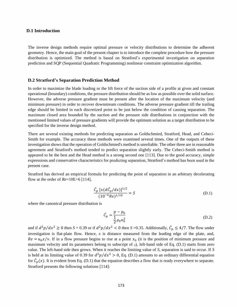
173

D.1 Introduction

The inverse design methods require optimal pressure or velocity distributions to determine the adherent

geometry. Hence, the main goal of the present chapter is to introduce the complete procedure how the pressure

distribution is optimized. The method is based on Stratford’s experimental investigation on separation

prediction and SQP (Sequential Quadratic Programming) nonlinear constraint optimization algorithm.

D.2 Stratford’s Separation Prediction Method

In order to maximize the blade loading or the lift force of the suction side of a profile at given and constant

operational (boundary) conditions, the pressure distribution should be as low as possible over the solid surface.

However, the adverse pressure gradient must be present after the location of the maximum velocity (and

minimum pressure) in order to recover downstream conditions. The adverse pressure gradient till the trailing

edge should be limited in each discretized point to be just below the condition of causing separation. The

maximum closed area bounded by the suction and the pressure side distributions in conjunction with the

mentioned limited values of pressure gradients will provide the optimum solution as a target distribution to be

specified for the inverse design method.

There are several existing methods for predicting separation as Goldschmied, Stratford, Head, and Cebeci-

Smith for example. The accuracy these methods were examined several times. One of the outputs of these

investigation shows that the operation of Goldschmied's method is unreliable. The other three are in reasonable

agreement and Stratford's method tended to predict separation slightly early. The Cebeci-Smith method is

appeared to be the best and the Head method is a strong second one [113]. Due to the good accuracy, simple

expressions and conservative characteristics for predicting separation, Stratford’s method has been used in the

present case.

Stratford has derived an empirical formula for predicting the point of separation in an arbitrary decelerating

flow at the order of Re=10E+6 [114],

��𝑝 [𝑥(𝑑��𝑝/𝑑𝑥)]1/2

(10−6𝑅𝑒)1/10= 𝑆 (D.1)

where the canonical pressure distribution is

��𝑝 =𝑝 − 𝑝012𝜌0𝑢0

2

(D.2)

and if 𝑑2𝑝 𝑑𝑥2⁄ ≥ 0 then S = 0.39 or if 𝑑2𝑝 𝑑𝑥2⁄ < 0 then S =0.35. Additionally, ��𝑝 ≤ 4/7. The flow under

investigation is flat-plate flow. Hence, x is distance measured from the leading edge of the plate, and,

𝑅𝑒 =𝑢0𝑥 𝜈⁄ . If in a flow pressure begins to rise at a point 𝑥0 (it is the position of minimum pressure and

maximum velocity and its parameters belong to subscript of 0), left-hand side of Eq. (D.1) starts from zero

value. The left-hand side then grows. When it reaches the limiting value of S, separation is said to occur. If S

is held at its limiting value of 0.39 for 𝑑2𝑝 𝑑𝑥2⁄ > 0, Eq. (D.1) amounts to an ordinary differential equation

for ��𝑝(𝑥). It is evident from Eq. (D.1) that the equation describes a flow that is ready everywhere to separate.

Stratford presents the following solutions [114]:

174

��𝑝 = 0.645 {0.435𝑅𝑒01/5

[(𝑥 𝑥0⁄ )1 5⁄ − 1]}2/𝑛

𝑓𝑜𝑟 ��𝑝 ≤ (𝑛 − 2) (𝑛 + 1)⁄ and (D.3)

��𝑝 = 1 −𝑎

[(𝑥 𝑥0⁄ ) + 𝑏]1 2⁄𝑓𝑜𝑟 ��𝑝 ≥ (𝑛 − 2) (𝑛 + 1)⁄ (D.4)

Figure D.1 Stratford limiting flows at two values of unit Reynolds number [113]

In that two-part solution (see Fig. D.1), 𝑥0 is the start of pressure rise, 𝑅𝑒0 =𝑢0𝑥0 𝜈⁄ , x is the distance

measured from the very start of the flow, which begins as flat-plate, turbulent flow. The number n is a constant

that Stratford finds to be about 6. The quantities a and b are arbitrary constants used in matching values and

slopes in the two equations at the joining point, ��𝑝 ≥ (𝑛 − 2) (𝑛 + 1)⁄ . Eq. (D.3) describes the beginning of

the flow and Eq. (D.4) the final part. The flow is an equilibrium flow that always has the same margin, if any,

against separation. More information about Stratford’s separation prediction method is found in [113], [114]

and [115].

D.3 Constrained Optimization of Stratford’s Limiting Pressure Distribution

The method presented above is used for determining the pressure distribution at maximum blade loading and

at the limit of separation on the suction side for given boundary conditions:

ℵ (��𝑝(𝑥)) = ℑ (𝐶𝑝(𝑥)) = ∮𝐶𝑝(𝑥)𝑑𝑥 = ∮𝑝 − 𝑝∞

12𝜌∞𝑢∞

2𝑑𝑥 = ∮

𝑝 − 𝑝∞

0.5𝛾𝑝∞𝑀∞2𝑑𝑥

(D.5)

where p is the static pressure at the given location and the other primitive variables correspond to inlet

condition denoted by ∞. The connection between ��𝑝(𝑥) and 𝐶𝑝(𝑥) is given by:

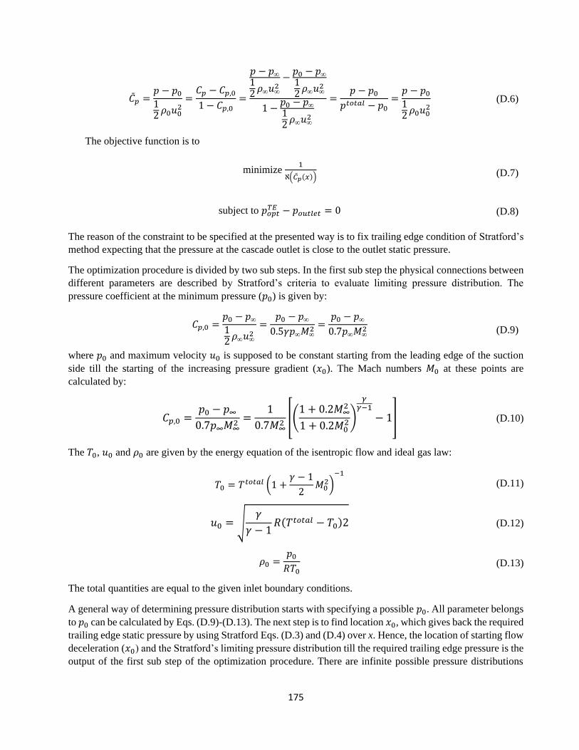
175

��𝑝 =𝑝 − 𝑝012𝜌0𝑢0

2=𝐶𝑝 − 𝐶𝑝,0

1 − 𝐶𝑝,0=

𝑝 − 𝑝∞

12𝜌∞𝑢∞

2−𝑝0 − 𝑝∞

12𝜌∞𝑢∞

2

1 −𝑝0 − 𝑝∞

12𝜌∞𝑢∞

2

=𝑝 − 𝑝0

𝑝𝑡𝑜𝑡𝑎𝑙 − 𝑝0=𝑝 − 𝑝012𝜌0𝑢0

2 (D.6)

The objective function is to

minimize 1

ℵ(��𝑝(𝑥)) (D.7)

subject to 𝑝𝑜𝑝𝑡𝑇𝐸 − 𝑝𝑜𝑢𝑡𝑙𝑒𝑡 = 0 (D.8)

The reason of the constraint to be specified at the presented way is to fix trailing edge condition of Stratford’s

method expecting that the pressure at the cascade outlet is close to the outlet static pressure.

The optimization procedure is divided by two sub steps. In the first sub step the physical connections between

different parameters are described by Stratford’s criteria to evaluate limiting pressure distribution. The

pressure coefficient at the minimum pressure (𝑝0) is given by:

𝐶𝑝,0 =𝑝0 − 𝑝∞

12𝜌∞𝑢∞

2=

𝑝0 − 𝑝∞

0.5𝛾𝑝∞𝑀∞2=𝑝0 − 𝑝∞

0.7𝑝∞𝑀∞2

(D.9)

where 𝑝0 and maximum velocity 𝑢0 is supposed to be constant starting from the leading edge of the suction

side till the starting of the increasing pressure gradient (𝑥0). The Mach numbers 𝑀0 at these points are

calculated by:

𝐶𝑝,0 =𝑝0 − 𝑝∞0.7𝑝∞𝑀∞

2=

1

0.7𝑀∞2[(1 + 0.2𝑀∞

2

1 + 0.2𝑀02)

𝛾𝛾−1

− 1] (D.10)

The 𝑇0, 𝑢0 and 𝜌0 are given by the energy equation of the isentropic flow and ideal gas law:

𝑇0 = 𝑇𝑡𝑜𝑡𝑎𝑙 (1 +𝛾 − 1

2𝑀02)

−1

(D.11)

𝑢0 = √𝛾

𝛾 − 1𝑅(𝑇𝑡𝑜𝑡𝑎𝑙 − 𝑇0)2 (D.12)

𝜌0 =𝑝0𝑅𝑇0

(D.13)

The total quantities are equal to the given inlet boundary conditions.

A general way of determining pressure distribution starts with specifying a possible 𝑝0. All parameter belongs

to 𝑝0 can be calculated by Eqs. (D.9)-(D.13). The next step is to find location 𝑥0, which gives back the required

trailing edge static pressure by using Stratford Eqs. (D.3) and (D.4) over x. Hence, the location of starting flow

deceleration (𝑥0) and the Stratford’s limiting pressure distribution till the required trailing edge pressure is the

output of the first sub step of the optimization procedure. There are infinite possible pressure distributions

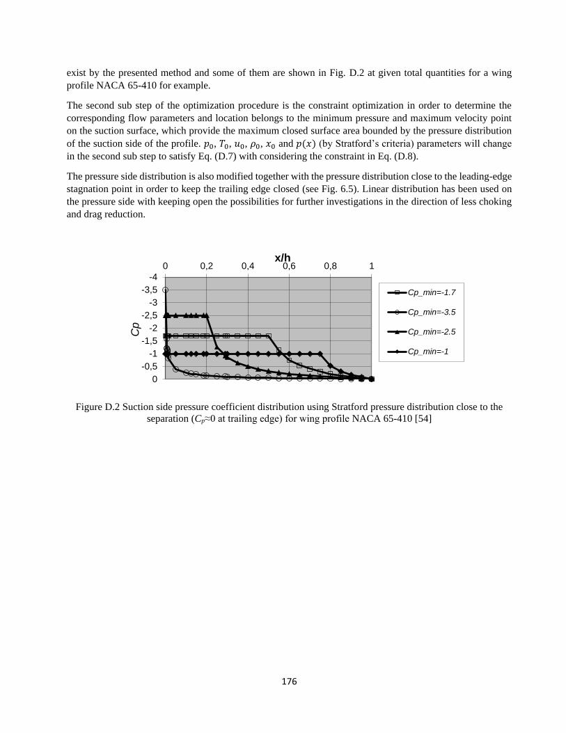
176

exist by the presented method and some of them are shown in Fig. D.2 at given total quantities for a wing

profile NACA 65-410 for example.

The second sub step of the optimization procedure is the constraint optimization in order to determine the

corresponding flow parameters and location belongs to the minimum pressure and maximum velocity point

on the suction surface, which provide the maximum closed surface area bounded by the pressure distribution

of the suction side of the profile. 𝑝0, 𝑇0, 𝑢0, 𝜌0, 𝑥0 and 𝑝(𝑥) (by Stratford’s criteria) parameters will change

in the second sub step to satisfy Eq. (D.7) with considering the constraint in Eq. (D.8).

The pressure side distribution is also modified together with the pressure distribution close to the leading-edge

stagnation point in order to keep the trailing edge closed (see Fig. 6.5). Linear distribution has been used on

the pressure side with keeping open the possibilities for further investigations in the direction of less choking

and drag reduction.

Figure D.2 Suction side pressure coefficient distribution using Stratford pressure distribution close to the

separation (Cp≈0 at trailing edge) for wing profile NACA 65-410 [54]

-4

-3,5

-3

-2,5

-2

-1,5

-1

-0,5

0

0 0,2 0,4 0,6 0,8 1

Cp

x/h

Cp_min=-1.7

Cp_min=-3.5

Cp_min=-2.5

Cp_min=-1