Business School

Managing Financial Resources

(Finance & Financial

Management)

COURSE ASSINGMEMENT

Student Name: Said Al Said

Student ID:

Centre: Qatar1

Assignment Layout

This report is structured to fulfil to the requirements

of Finance and Financial Management assignment. The

assignment contains four questions. Each question will

be attempted separately and sections will be labelled

(whenever applicable). All tables and figures are

tagged. Reference to these tables and figures is

available within the text.

Said Al Said

Qatar

2

QUESTION 1: Capital Expenditure Decisions

and Investment Criteria – Saron plc.

ObjectiveThe objective of this case is to evaluate a proposal to

invest in a new product. Therefore, we used a model of

NPV, IRR and Payback period to predict if this product is

worthy or not.

Assumptions

3

There are some assumptions we considered through the

analysis.

1. R& D expenses of £1,600,000 are a sun cost. They

already incurred and capitalized as an assets.

2. Advertising and marketing expenses started at year0

and ended with zero at year 6.

3. In profit and loss statement the equipment is

depreciated of £800,000 yearly for the tax purposes

on a straight-line basis over 10 years. It is not

cash flow item.

4. The space available in the company’s existing

factories already been accounted so cannot be

utilized for any other purpose and hence no

opportunity cost.

5. The total direct production cost is £25/ unit, the

actual cost of material alone is assumed to be £15/

unites and labour cost is £10/ unit.

6. Overheads are allocated and not incremental to the

project.

7. Tax rate and discounted rate are constant across

time.

8. Finished goods inventory valuation is done on the

basis of raw material cost and labour cost.

9. no incidental effects on sales, cost for existing

projects (no cannibalization)

4

We are assuming a mythical “no inflation” scenario such

that all costs and even the selling price remains fixed

throughout the period of analysis.

Computation ProcessThe computation of the investment’s net present value,

internal rate of return, and payback are available in

Table 1.

Findings & ImplicationsBased on our scenario the NPV works out to £ 3,559,037.

The IRR is 22% above the rate of returned on investment

and payback period is 3.8887 years. Looking especially at

the NPV, the company would find the project to be

worthwhile for its pursuits. In other word, the capital

outlay will be covered, the interest rate will be covered

and a surplus generated.

5

Table 1: Computations of net present value, internal rate of return, and payback

Change in P& LYr.0 Yr.1 Yr.2 Yr.3 Yr.4 Yr.5 Yr.6

Sales Volume 250,000 500,000

500,000

500,000

500,000

300,000

SalesPrice/unit 40

40

40

40

40

40

Revenue 10,000,000 20,000,000

20,000,000

20,000,000

20,000,000 12,000,000

New Equipment/ dep (800,000) (800,000)

(800,000)

(800,000)

(800,000)

(800,000)

Book Value 8,000,000 7,200,000

6,400,000

5,600,000

4,800,000

4,000,000

3,200,000

New Equipment sales             1,500,000

Profit on Sale of new Equipment

(1,700,000)

2nd Equipment opportunity cost

(200,000)

2nd Equipment sale 50,000

Advt expenses (1,800,000) (500,000)

(500,000)

(500,000)

(500,000)

(500,000)

-

Labour costs (2,500,000) (5,000,000)

(5,000,000)

(5,000,000)

(5,000,000)

(3,000,000)

Raw Material & component costs (3,750,000)

(7,500,000)

(7,500,000)

(7,500,000)

(7,500,000)

(4,500,000)

Fixed costss (500,000) (500,000)

(500,000)

(500,000)

(500,000)

(500,000)

Profit before tax (2,000,000) 1,950,000

5,700,000

5,700,000

5,700,000

5,700,000

1,550,000

Tax thereon (40%) (780,000)

6

800,000 (2,280,000) (2,280,000)(2,280,000) (2,280,000) (620,000)

Change Cash flow statement

Yr.0 Yr.1 Yr.2 Yr.3 Yr.4 Yr.5 Yr.6

Revenue 10,000,000 20,000,000

20,000,000

20,000,000

20,000,000 12,000,000

Purchase of New Equipment

(8,000,000)

Sale of equipment 1,500,000

2nd Equipment opportunity cost

(200,000)

2nd Equipment sale 50,000

Advt expenses (1,800,000) (500,000)

(500,000)

(500,000)

(500,000)

(500,000)

-

Labour costs (2,500,000) (5,000,000)

(5,000,000)

(5,000,000)

(5,000,000)

(3,000,000)

Raw Material & component costs (3,750,000)

(7,500,000)

(7,500,000)

(7,500,000)

(7,500,000)

(4,500,000)

Fixed costss (500,000)

7

(500,000) (500,000) (500,000) (500,000) (500,000)W/C calculationStocks of finished product

1,250,000 2,500,000

2,500,000

2,500,000

2,500,000

1,500,000

-

Stock of raw materials and componenets

937,500 1,875,000

1,875,000

1,875,000

1,875,000

1,125,000

-

Total inventory/ WC 2,187,500 4,375,000

4,375,000

4,375,000

4,375,000

2,625,000

-

Funds blocked/ Change in WC

(2,187,500) (2,187,500)

-

-

-

1,750,000

2,625,000

Taxes 800,000 (780,000)

(2,280,000)

(2,280,000)

(2,280,000)

(2,280,000)

(620,000)

Net Cash Flow

(11,387,500) (217,500)

4,220,000

4,220,000

4,220,000

5,970,000

7,555,000

Rate of return 14% 14% 14% 14% 14% 14%PVF 1.0000 0.8772 0.7695 0.6750 0.5921 0.5194 0.4556

Discounted Cash Flows

(11,387,500) (190,791)

3,247,290

2,848,500

2,498,662

3,100,818

3,442,058

NPV 3,559,037

IRR 22.0%Payback period 3.8887Discounted Payback period

4 to 5 years

8

Sensitivity AnalysisSensitivity analysis is a powerful tool that is commonly

used to assess the robustness of the results obtained by

examination of ‘what-if’ scenarios. As such, it involves

identifying all components of a model (e.g. price,

volumes, raw material expenses, labour cost) that would

have a material impact on cash flows and end value (NPV,

IRR). Once these parameters are obtained, sensitivity

analysis examines how changes in these parameters would

change the output result. Table 2 illustrates the

sensitivity analysis that is carried out for this

problem.

Table 2: Sensitivity AnalysisBaseCase

BaseCase

NPV NPV IRR IRR

10% Reduction in price3,559,037

-362,515

22% 13.2%

10% Reduction in volumes3,559,037

2,288,603

22% 19.4%

10% Increase in rawmaterial expenses

3,559,037

2,088,455

22% 18.7%

10% Increase in wages3,559,037

2,578,649

22% 19.8%

n this problem, it is given that the sale price for the

product is £40/ unit so a reduction of 10% in price (36

instead of 40) will decrease NPV to -362,515. Also, a

result of reduce of 10% in volume (y1=225,000 y2=450,000,

y3=450,000, y4=450,000, y5=450,000 , y6=270,000) NPV

reduces from +3,559,037 to +2,288,60. The value of NPV

will also reduce if we increase the expenses of raw

9

material and labour of by10%. Therefore, the NPV seems to

be most sensitive to change in price, volumes, raw

material expenses, labour cost.

QUESTION 2: Share Valuation – Tonddo plc.

Company Value & AssumptionsThe objective of this part is to determine the value of

the company (Tonddu Plc). The computation table is

illustrated in Table 3.

Table 3: Computation of Company Value

Earnings, E

Retention

ratio,b

Rate ofinv, k

Rateof

return, r

Investment,

I=(E*B)

Dividend,

D=(E-I)ΔE=K X I

g = k X b=ΔE/E NPV

Yr.1 120 70% 50% 10% 84 36 42 35.00% 336

Yr.2 162 50% 35% 10% 81 81 28.35 17.50% 202.5

Yr.3 190.35 40% 20% 10% 76.14 114.21 15.228 8.00% 76.14

10

Yr.4 205.578 25% 10% 10% 51.3945

154.1835 5.13945 2.50% 0

The dividend is at year 1 when the rate of return is 50%

the dividend is £36m however, at year 4 when the rate of

return is 10% the dividend is £154.1835, this shows that

whenever the rate of return is low the dividend value is

high. The company expected to invest 70% of its earning

when the rate of the return is 50%, the company has

achieved a £84m retention on year 1, however, the company

expected that this 70% will fall to 50% by year 2, when

the rate of return was 35% which reflects an increase in

the earnings, as it was £120m in year 1, it becomes £162m

in year 2. However, the retention value is decreased by

£3m from year 1. At year 4 when the rate of return is 10%

and the retention ration is 25% the dividend is

£154.1835m and earnings is £205.578m.

Dividends valuation model is not providing an appropriate

basis for the valuation of growth share, V0=D1/r-g, where

r>g, Vo=n*P0; D1=n*d1 and n=total number of shares

outstanding. It is difficult for a firm to grow at a

faster rate than the economy in long term. This model

assumes that the earnings from existing investments

remain unchanged over time. In addition to that a

constant fraction of earning is retained every year, the

rate of return on investment is constant over time, and

cash flows generated by new investment are perpetuities.

The value of share price in year 3 is computed as 11

P3 = D4/(r-g)

= 154.1835/(0.1-0.025)= £2055.78

The value of the company is, then, computed by

substituting the values of P3, D (from the table), and r

(which is given). The resulted initial value of the

company V0 is, therefore, £1730.015. Detailed of the

computation is illustrated below.

V0 = D1/(1+r)+D2/(1+r)^2+ D3/(1+r)^3+P3/(1+r)^3 = 36/(1.1)+81/(1.1)^2+114.21/(1.1)^3+2055.78/(1.1)^3 =1730.015.

The earning based valuation module focuses on the earning

power of the assets of the company and its anticipated

investment. It is focusing on the value of the company

rather than the value of shares. The value of the firm is

given by:

V0 = Value of Current Assets+ Value of GrowthOpportunities, PVGO

12

Rate ofreturn, r

Dividend,D=(E-I)

g = k X b=ΔE/E

Yr.1 36Yr.2 81Yr.3 114.21Yr.4 10% 154.1835 2.50%

This analysis assumes that as the level of earnings

grows over time as a result of investments the level

future investment could also grow if the retention ratio

remains constant. In this illustration the rate of

returned on investment is fall to 10% in year 4 and the

level of retention is decreased to 51.39. By substituting

the E,NPV in the formula we got the value of the company

is =£1730.015

V0 =

E1/r+NPV1/(1+r)^2+ NPV2/(1+r)^3+NPV3/(1+r)^3 =120/0.1+336/(1.1)+ 202.5/(1.1)^2+76.14/(1.1)^3 =1730.015

Company Value & AssumptionsThe ratio of price per share to earnings per share is

commonly known price-earning ratio (P/E ratio).

Generally speaking, high values of P/E ratio of a firm

implies higher earning growth in future when compared

with companies with how values. On the contrary, low

value of P/E ratio indicates a ‘vote of no confidence’ by

the market or it might suggest a sleeper that the market

has over looked. The P/E ratio is commonly compared with

previous year price-earning ratio performance or

benchmarked with other companies’ ratios in the same

industry and/or market. The differences in P/E ratios

across firms are influenced by the expected growth13

Earnings,E

Rate ofreturn, r NPV

Yr.1 120 336Yr.2 202.5Yr.3 76.14Yr.4 10% 0

opportunities, which a subjective view of the analysts.

The use of P/E ratio has been subject to some

limitations. These are summarized as:

1. The accounting earnings are influenced by arbitrary

accounting rules (e.g. use of historical cost in

depreciation and inventory valuation), which tends

to under-represent true economic values of historic

cost depreciation and inventory cost in times of

high inflation. This is due to the fact that,

during inflation, the replacement cost of both goods

and capital equipment will rise with the general

level of prices. As such, the P/E ratios tend to be

lower when inflation is higher, indicating ‘lower

quality’ of market assessment. Thus, a version of

earnings management that became common in the 1990s

was to report ‘pro forma earnings’ measures which

are computed ignoring certain expenses such as,

restructuring charges, stock-option expenses, or

write-down of assts from continuing operations.

2. Another limitation is related to the business cycle.

Earnings are defined as being net of economic

depreciation, that is, the maximum flow of income

that the firm could pay out without depleting its

productive capacity. However, reported earnings are

computed according to generally accepted accounting

principles and need not correspond to economic

earning.

14

Therefore, the relationship between P/E and growth is not

perfect although P/E multiple does tract growth

opportunities. In fact, there is no way to say P/E

ration is overly high or low without referring to the

company’s long run growth prospects, as well as to

current earnings per share relative to the long-run trend

line.

Efficient Market TheoryThere has been a debate of whether the Efficient Market

Theory is responsible for the current financial global

crisis. The Efficient Market Hypothesis states that the

prices of securities reflect all know information that

impact their value, but it doesn’t claim the market price

is always right. This implies that the market prices

mostly incorrect and it is not that easy to tell whether

these prices are too high or low.

I believe that the theory is only a ‘theoretical

considerations’, and requires human judgement before its

executions in our lives. The execution of the theory

requires a clear understanding of the situation it is

applied on. Lack of understanding the market and

evaluating its various components would definitely lead

to undesired consequences. In his article in Wall Street

Journal, Siegel (Oct 2009) emphasizes “ .. this does not mean

15

the EMH- Efficient Market Hypothesis - can be used as an excuse

by the CEOs of the failed financial firms or by the regulators who did not see

the risks that subprime mortgage-backed securities posed to the financial

stability of the economy. Regulators wrongly believed that financial firms

were offsetting their credit risks, while the banks and credit rating agencies

were fooled by faulty models that underestimated the risk in real estate”.

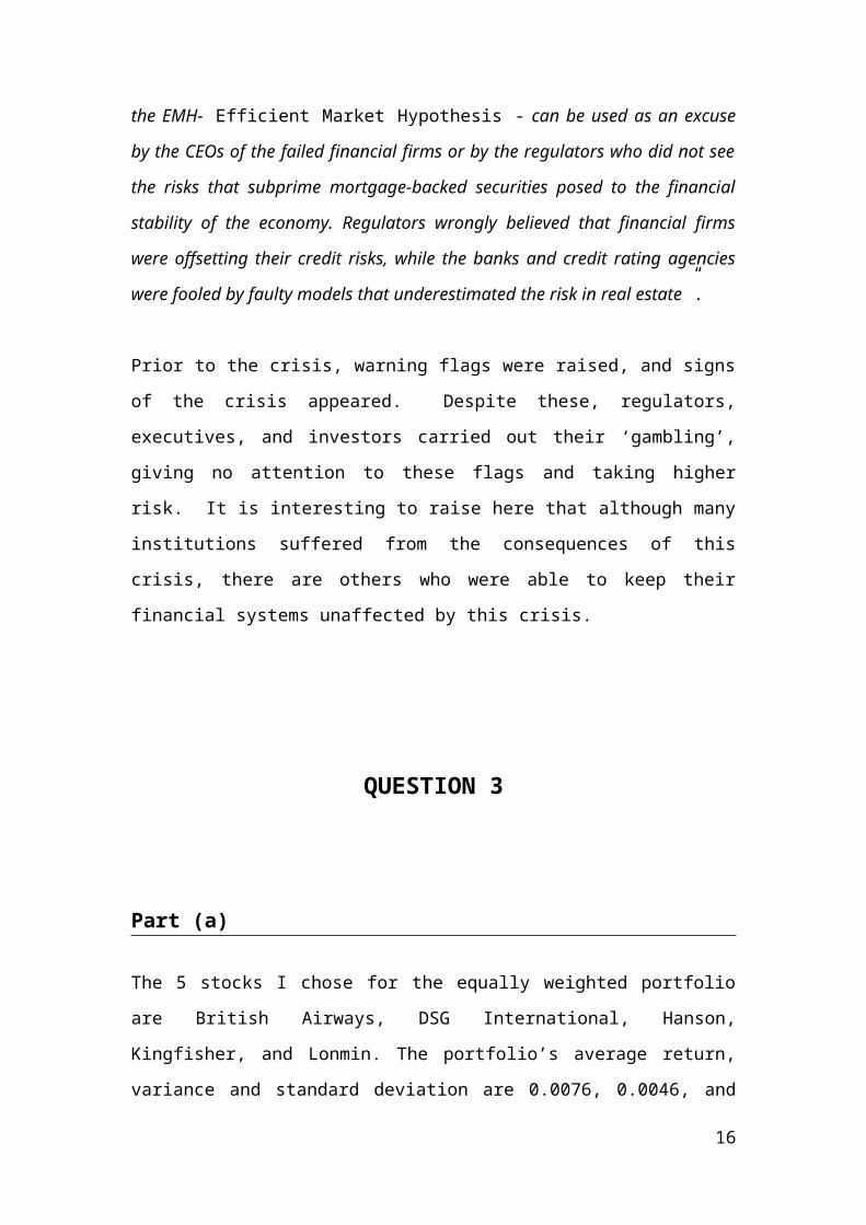
Prior to the crisis, warning flags were raised, and signs

of the crisis appeared. Despite these, regulators,

executives, and investors carried out their ‘gambling’,

giving no attention to these flags and taking higher

risk. It is interesting to raise here that although many

institutions suffered from the consequences of this

crisis, there are others who were able to keep their

financial systems unaffected by this crisis.

QUESTION 3

Part (a)

The 5 stocks I chose for the equally weighted portfolio

are British Airways, DSG International, Hanson,

Kingfisher, and Lonmin. The portfolio’s average return,

variance and standard deviation are 0.0076, 0.0046, and

16

0.0677 respectively. In other words, the average

portfolio return of the equally weighted portfolio over

132 months is 0.76% and the standard deviation is 6.77%.

The individual average returns, variances and standard

deviations are available in Table 4.

Table 4: Individual and Portfolio Average Returns,

Variances and SDs

BA DSGInt.Han.

KingFisher Lonmin Portforlio

AverageReturn 0.0016 0.0122 0.0063 0.0056 0.0126 0.0076Variance 0.0166 0.0107 0.0068 0.0078 0.0089 0.0046StandardDev. 0.1289 0.1034 0.0823 0.0881 0.0944 0.0677

After we calculate portfolio risk, we get the same value

of average returns variance and standard deviation for

the 5 securities. The computations are illustrated in the

table below. The average variance of the portfolio is

0.46%, and the individual variances of each security are

clustered uniformly around, indicating no extreme (very

high or vey low) variances. The standard deviation tells

about the risk in the portfolio. British Airways has

higher risk than other securities as it has the highest

standard deviation.

17

SECURITIES VARIANCES Portfolio. VAR1 0.01662 0.0107 1/N*AV.VAR3 0.0068 0.0020 0.00204 0.0078 (1 - 1/N)* AV.COV5 0.0089 0.0026 0.0026SUM 0.0508 SUM = 0.0046

AVERAGE 0.0102 VAR (R) 0.0046SD[R] 0.0677

Then, the covariance between each pair of securities in

the portfolio is computed. Table 4 illustrates the

covariance values. The average covariance is

approximated to be 0.0032. The relationship between the

pairs of securities has, to some extend, similar

strength, ranging from 0.0011 (pair 2 and 3) to 0.0046

(pair 1 and 3; pair 1 and 4). All relationships are

positive, indicating that the returns of all securities

move together.

Table 4: Covariance Values of Each Pair of Securities

Pair Covariance1 and 2 0.00441and 3 0.00461and 4 0.00461and 5 0.00382 and 3 0.00112 and 4 0.0034

2 and 5 0.00163 and 4 0.00323 and 5 0.00294 and 5 0.0023

18

SUM 0.0320AVERAGE CO-VAR 0.003196

To compute the standard deviation of the portfolio given

the covariance, we use the following equation:

Assuming that all securities have equally likely weights,

the computed standard deviation of the portfolio is found

to be 0.2391. This value is much greater than that

obtained above.

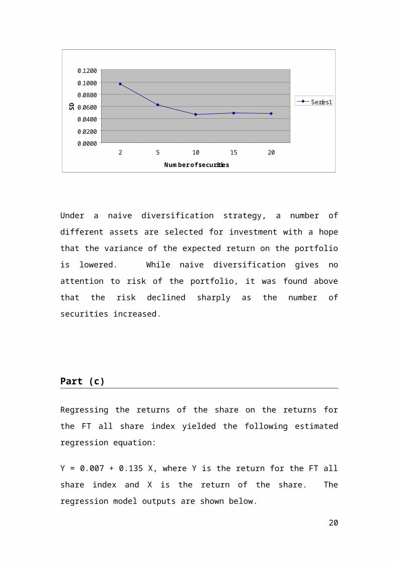
Part (b)

By choosing portfolio which consists between 2 to 20

randomly chosen securities, the risk of each of these

portfolios is calculated on the basis of standard

division. It is found that the risk declined sharply as

the number of securities increased. The below figure

explain the relation.

Number of securities SD

2 0.09645 0.062810 0.046315 0.049020 0.0479

19

0.00000.02000.04000.06000.08000.10000.1200

2 5 10 15 20Num ber of securities

SD

Series1

Risk of Equally W eighted Portfolio

Under a naive diversification strategy, a number of

different assets are selected for investment with a hope

that the variance of the expected return on the portfolio

is lowered. While naive diversification gives no

attention to risk of the portfolio, it was found above

that the risk declined sharply as the number of

securities increased.

Part (c)

Regressing the returns of the share on the returns for

the FT all share index yielded the following estimated

regression equation:

Y = 0.007 + 0.135 X, where Y is the return for the FT all

share index and X is the return of the share. The

regression model outputs are shown below.

20

  CoefficientsStandard

Error t Stat P-valueLower95%

Upper95%

Lower95.0%

Upper95.0%

Intercept 0.006608

0.003186

2.074289

0.040026

0.000306 0.01291

0.000306 0.01291

X Variable1 0.135471

0.030927

4.380402

2.42E-05

0.074286

0.196655

0.074286

0.196655

The regression model is highly significant (p-value is

less than 0.05). The R-square is 12.9%, indicating that

only 12.9% of the variation in the return of the FT all

share index is explained by the regression model.

The coefficient (beta) of the independent variable tells,

statistically, about the amount of change in the

dependent variable for any unit increase in the

independent variable. In investment, it expresses the

stock risk (volatility) - the degree to which its price

fluctuates in relation to the overall market. In our

example, beta is found to be 0.135, indicating that this

company has a volatility less than the market.

In statistics, beta is computed as the sum of the product

of deviation from the mean of both the dependent and

independent variables divided by the sum of the square

deviation from the mean of the independent variable. In

21

Regression Statistics

Multiple R0.3586

3

R Square0.1286

16Adjusted R Square

0.121913

Standard Error

0.036543

Observations 132

investment, beta is computed by dividing the covariance

of the return on a security with the return on the market

by the variance of the market return. It is also the

correlation coefficient multiplied by the ratio of

individual security risk to market risk. This implies

that when the security has the same risk as the market,

beta is the correlation coefficient. Also, when the

security has greater risk than that of the market, beta

is greater and vice versa. In practice, betas are

regularly calculated by several agencies (e.g. The Risk

Measurement Service (RMS) in London Business School).

However, users should be caution when using beta. Beta

is computed based on historical data and it is not

necessary predict the future beta. Moreover, the amount

of risk that beta takes into account is limited to

systematic risk only. In other words, beta does not

consider all the risk that a firm alone faces.

22

QUESTION 4

Part (a)

From investor prospective:

1- At share price , S < 64 loss = -9.752- At share price , S = 73.756 loss = 0 (break even)

3- At share price , S > 73.756 profit situation

profit diagram for an investor

23

From writer prospective:

4- At share price , S > 64 loss5- At share price , S = 73.756 loss = 0 (break even)

6- At share price , S < 73.756 profit =9.75

Profit diagram for a writer volatility

24

C=-9.75

X=64

X+C=73.7564

Profit

Loss

Share Price

C=9.75 X=64 X+C=73.

7564

Profit

Loss

Share Price

The options market is always a Zero sum game, in that the

combined profits of the options writer and options

investor net out to zero. So the trader who hopes to

speculate successfully must be planning for someone

else’s losses to provide his or her profits. Thus the

options market is a very competitive with profits coming

only at the expense of another trader. In the above

example this is clearly evident. At each stock price

level, the combined losses/gain for the long and opposing

short position all net out to zero.

Part (a)

The March CALL is trading for the highest price. This is

because of reasons that the chances of volatility of

price increases with increasing time frame. The longer

the time period until the expiry date the greater the

scope for price changes in the underlying share. While

the risk of decreasing price of the share is adequately

covered in case of a CALL option, the benefit for the

price increase will be fully available to the investor in

the CALL. As the writer of CALL of the CALL covers the

risk of increasing price for the longer duration in case

of the MAR CALL as compared to DEC or JAN CALLS, he price

the MAR CALL the highest. For similar reasons the

investor is willing to pay higher for the MAR CALL. This

25

can be generalized. The CALL for the longest duration

will always be priced the highest.

Part (c)Astraddle is an option combination in which the buyer

purchases a call and put option on the same underlying

good with the same exercise price and time to maturity.

The seller takes the opposing position (i.e. selling a

call and put option on the same underlying good). An

investor in a straddle will benefit in case of higher

volatility or higher price changes, in either direction,

is the underlying security. For a profit to be made based

on MAR CALLS and PUTS, the price has to fall below the

exercise price by the cost of the put and the call (i.e

go below 45.5 before end MAR) or rise above the exercise

price by the same amount (i.e go above 82.5 before end

MAR

26

REFRENCES

Bide, A, Kane, A. and Marcus, A. (2009), Investments, 8th

Ed., McGraw Hill, New York.

Pike, R. And Neale, B. (2003), Corporate Finance and Investment:

Decisions and Strategies, Prentice Hall, UK.

Siegel, J. (Oct 27, 2009), “Efficient market theory and

the crisis”, The Wall Street Journal. Accessed on 15/2/2010

through {

27

Profit

Breakeven Points

Loss

Call

Put

45.5=BEP

9.75=price of a call

8.75= price of a put

18.5=price of straddle

82.5=BEP

http://online.wsj.com/article/SB1000142405274870357360457

4491261905165886.html}.

28